Ground Moving Target Indication Using Monopulse SAR for

Multimode Fire Control AESA RADAR

Vandana AR*, Abid Hussain VA*, Suchith Rajagopal*,Vinod Kumar Jaysaval*, Ramesha A*, Ashok Kumar* *Scientist, LRDE, F-Radar, CV Raman Nagar, Bangalore

vandana_ar@rediffmail.com Abstract

Ground moving target indication with a monopulse system makes it possible to measure an accurate individual radial velocity component of moving targets via special processing techniques. The presented method requires the focused data from the sum and difference monopulse channels and is based upon amplitude deviations in the doppler monopulse ratios due to object movement. The presented algorithm is validated using the Multimode Fire control X band AESA Radar simulated data for Air to ground mode. The advantage is its higher resolution and detectability of endo clutter target velocities.

Tools used: Matlab 2010a Keywords: Monopulse, SAR, Radar, GMTI, DPCA, ATI, STAP

INTRODUCTION

Ground moving target indication (GMTI) has been a

widely explored field of interest ever since. Techniques for detection, position correction, refocusing, and velocity measurements of moving targets include the use of single as well as multichannel SAR data giving a good overview of some of them including multilooking, Displaced Phase Center Antenna (DPCA) processing, Along Track Inteferometry (ATI), monopulse processing, and signal filtering by Space Time Adaptive Processing (STAP).

Monopulse processing for GMTI is often used tantamount to ATI in SAR community. This paper would like to make a distinction in that ATI refers to interferometry and the direct comparison of two or more received data records while monopulse or ∑Δ processing is a general term often used for monopulse tracking radar systems and always specified through a sum data signal and one or more isochronous difference data signals.

MONOPULSE GMTI

Monopulse processing uses the ratio between Sum and Difference channels signal and is used in GMTI techniques. Assume the sum channel signal as ∑ = |∑| ejφ∑

and the difference signal as Δ = |Δ| ejφΔ

and the Monopulse ratios as

MPR = Δ / ∑ = (|Δ| / |∑|) e j(φΔ-φ∑) In the proposed Monopulse Radar GMTI processing,

Azimuth FFT will be done on both the sum channel and the Azimuth channel. Amplitude threshold is applied on the Azimuth FFT to filter the clutter returns. MonoPulse Ratio (MPR) without phase factor is calculated for the data after clutter rejection. Another MPR with phase factor is calculated for the data after clutter

rejection. Comparing both the monopulse ratio with phase factor based on the monopulse threshold which is calculated using the monopulse ratio without phase factor. Calculate the position shift for the targets. Now azimuth IFFT followed by target extraction is carried out.

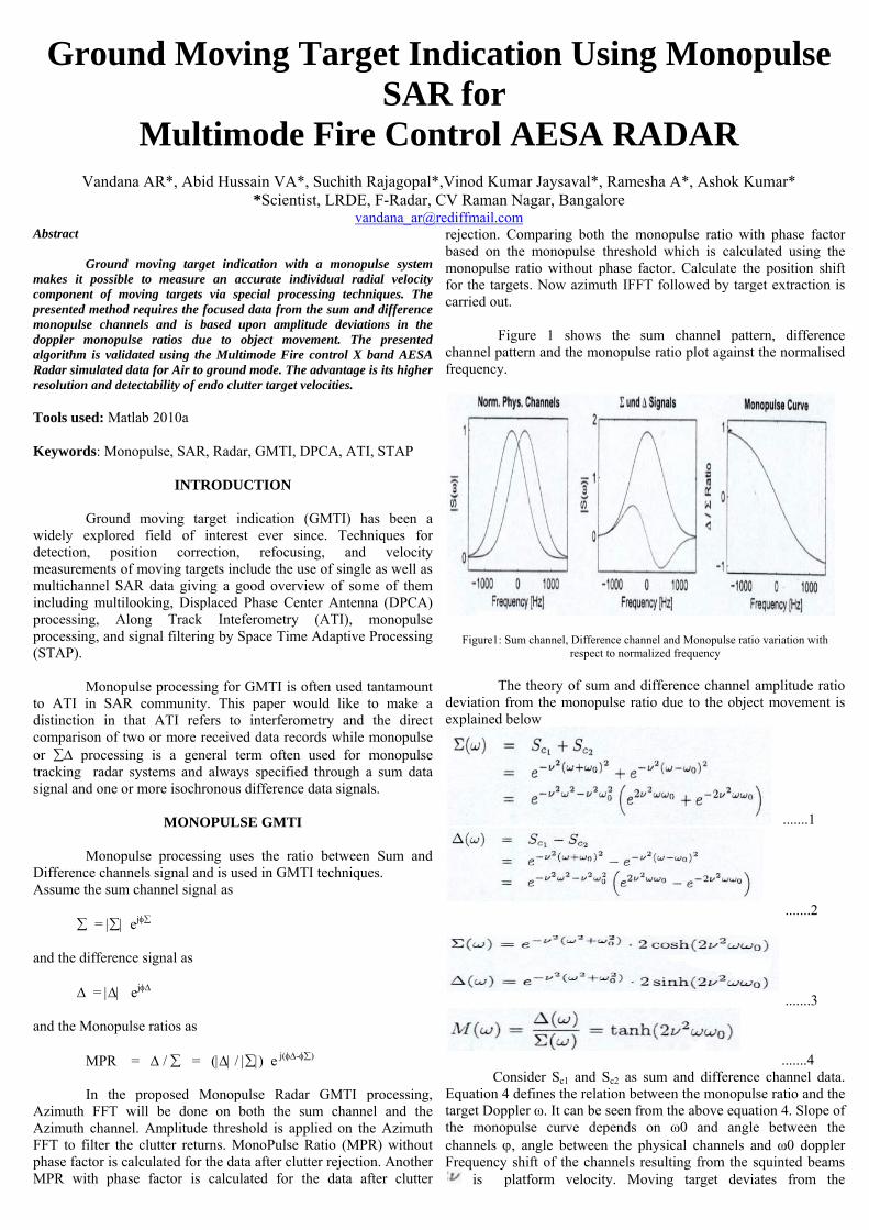
Figure 1 shows the sum channel pattern, difference

channel pattern and the monopulse ratio plot against the normalised frequency.

Figure1: Sum channel, Difference channel and Monopulse ratio variation with respect to normalized frequency

The theory of sum and difference channel amplitude ratio deviation from the monopulse ratio due to the object movement is explained below

.......1

.......2

.......3

.......4 Consider Sc1 and Sc2 as sum and difference channel data. Equation 4 defines the relation between the monopulse ratio and the target Doppler ω. It can be seen from the above equation 4. Slope of the monopulse curve depends on ω0 and angle between the channels ϕ, angle between the physical channels and ω0 doppler Frequency shift of the channels resulting from the squinted beams

is platform velocity. Moving target deviates from the

monopulse curve of the static scene with magnitude of deviation depending on the target’s velocity component.

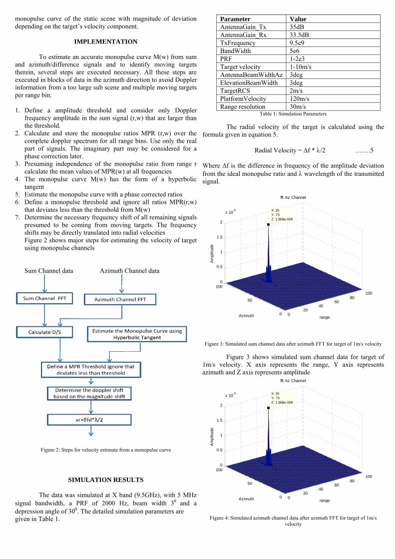
IMPLEMENTATION

To estimate an accurate monopulse curve M(w) from sum and azimuth/difference signals and to identify moving targets therein, several steps are executed necessary. All these steps are executed in blocks of data in the azimuth direction to avoid Doppler information from a too large sub scene and multiple moving targets per range bin.

1. Define a amplitude threshold and consider only Doppler

frequency amplitude in the sum signal (r,w) that are larger than the threshold.

2. Calculate and store the monopulse ratios MPR (r,w) over the complete doppler spectrum for all range bins. Use only the real part of signals. The imaginary part may be considered for a phase correction later.

3. Presuming independence of the monopulse ratio from range r calculate the mean values of MPR(w) at all frequencies

4. The monopulse curve M(w) has the form of a hyperbolic tangent

5. Estimate the monopulse curve with a phase corrected ratios 6. Define a monopulse threshold and ignore all ratios MPR(r,w)

that deviates less than the threshold from M(w) 7. Determine the necessary frequency shift of all remaining signals

presumed to be coming from moving targets. The frequency shifts may be directly translated into radial velocities Figure 2 shows major steps for estimating the velocity of target using monopulse channels Sum Channel data Azimuth Channel data

Figure 2: Steps for velocity estimate from a monopulse curve

SIMULATION RESULTS The data was simulated at X band (9.5GHz), with 5 MHz signal bandwidth, a PRF of 2000 Hz, beam width 3θ and a depression angle of 30θ. The detailed simulation parameters are given in Table 1.

Parameter Value AntennaGain_Tx 35dB AntennaGain_Rx 33.5dB TxFrequency 9.5e9 BandWidth 5e6 PRF 1-2e3 Target velocity 1-10m/s AntennaBeamWidthAz 3deg ElevationBeamWidth 3deg TargetRCS 2m/s PlatformVelocity 120m/s Range resolution 30m/s

Table 1: Simulation Parameters

The radial velocity of the target is calculated using the formula given in equation 5.

Radial Velocity = Δf * λ/2 …….5

Where Δf is the difference in frequency of the amplitude deviation from the ideal monopulse ratio and λ wavelength of the transmitted signal.

Figure 3: Simulated sum channel data after azimuth FFT for target of 1m/s velocity

Figure 3 shows simulated sum channel data for target of

1m/s velocity. X axis represents the range, Y axis represents azimuth and Z axis represents amplitude

Figure 4: Simulated azimuth channel data after azimuth FFT for target of 1m/s velocity

020

4060

80100

0

50

1000

0.5

1

1.5

2

x 10-9

range

fft Az Channel

X: 35Y: 73Z: 1.968e-009

Azimuth

Am

plitu

de

020

4060

80100

0

50

1000

0.5

1

1.5

2

x 10-9

range

fft Az Channel

X: 35Y: 73Z: 1.968e-009

Azimuth

Am

plitu

de

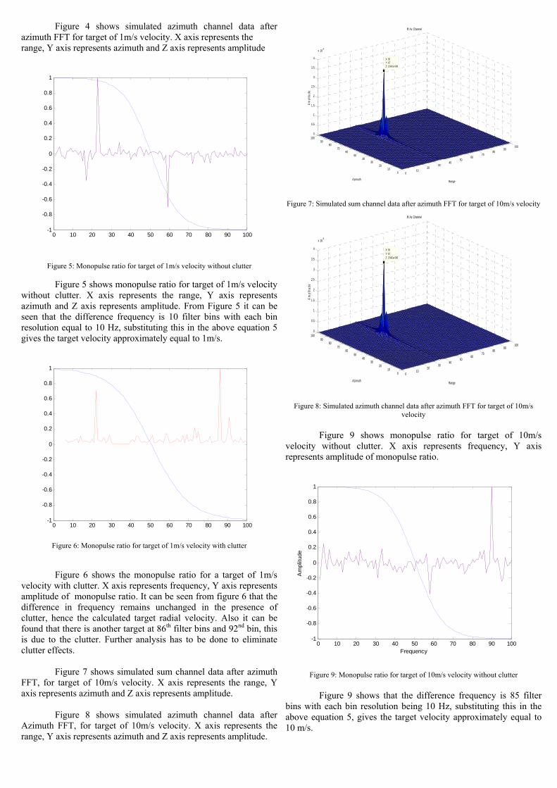
Figure 4 shows simulated azimuth channel data after azimuth FFT for target of 1m/s velocity. X axis represents the range, Y axis represents azimuth and Z axis represents amplitude

Figure 5: Monopulse ratio for target of 1m/s velocity without clutter

Figure 5 shows monopulse ratio for target of 1m/s velocity without clutter. X axis represents the range, Y axis represents azimuth and Z axis represents amplitude. From Figure 5 it can be seen that the difference frequency is 10 filter bins with each bin resolution equal to 10 Hz, substituting this in the above equation 5 gives the target velocity approximately equal to 1m/s.

Figure 6: Monopulse ratio for target of 1m/s velocity with clutter

Figure 6 shows the monopulse ratio for a target of 1m/s velocity with clutter. X axis represents frequency, Y axis represents amplitude of monopulse ratio. It can be seen from figure 6 that the difference in frequency remains unchanged in the presence of clutter, hence the calculated target radial velocity. Also it can be found that there is another target at 86th filter bins and 92nd bin, this is due to the clutter. Further analysis has to be done to eliminate clutter effects.

Figure 7 shows simulated sum channel data after azimuth

FFT, for target of 10m/s velocity. X axis represents the range, Y axis represents azimuth and Z axis represents amplitude.

Figure 8 shows simulated azimuth channel data after

Azimuth FFT, for target of 10m/s velocity. X axis represents the range, Y axis represents azimuth and Z axis represents amplitude.

Figure 7: Simulated sum channel data after azimuth FFT for target of 10m/s velocity

Figure 8: Simulated azimuth channel data after azimuth FFT for target of 10m/s velocity

Figure 9 shows monopulse ratio for target of 10m/s

velocity without clutter. X axis represents frequency, Y axis represents amplitude of monopulse ratio.

Figure 9: Monopulse ratio for target of 10m/s velocity without clutter Figure 9 shows that the difference frequency is 85 filter

bins with each bin resolution being 10 Hz, substituting this in the above equation 5, gives the target velocity approximately equal to 10 m/s.

0 10 20 30 40 50 60 70 80 90 100-1

-0.8

-0.6

-0.4

-0.2

0

0.2

0.4

0.6

0.8

1

0 10 20 30 40 50 60 70 80 90 100-1

-0.8

-0.6

-0.4

-0.2

0

0.2

0.4

0.6

0.8

1

010

2030

4050

6070

8090

100

010

2030

4050

6070

8090

1000

0.5

1

1.5

2

2.5

3

3.5

4

x 10-6

Range

fft Az Channel

X: 35Y: 67Z: 3.542e-006

Azimuth

Am

plitu

de

010

2030

4050

6070

8090

100

010

2030

4050

6070

8090

1000

0.5

1

1.5

2

2.5

3

3.5

4

x 10-6

Range

fft Az Channel

X: 35Y: 67Z: 3.542e-006

Azimuth

Am

plitu

de

0 10 20 30 40 50 60 70 80 90 100-1

-0.8

-0.6

-0.4

-0.2

0

0.2

0.4

0.6

0.8

1

Frequency

Am

plitu

de

Figure 10: Monopulse ratio for target of 10m/s velocity with clutter

Figure 10 shows monopulse ratio for target of 10m/s

velocity. X axis represents frequency, Y axis represents amplitude of monopulse ratio. It can be seen from figure 10 that the difference frequency due to the amplitude variation is unaffected due to the presence of clutter. It can also be seen that there in another target velocity at 96th bin due to clutter which can be eliminated by using the clutter reduction techniques.

CONCLUSION AND FUTURE WORK

Advantage with this algorithm is that the target radial

velocity is accurate and endo clutter target radial velocity can also be detected. The algorithm has to be verified for different clutter scenarios and different target RCS under different mode of radar operation with different SCR. The algorithm to be studied for detecting two targets present in same range bin. The algorithm can be explored for other monopulse radar systems. The algorithms can be explored with different clutter reduction schemes.

ACKNOWLEDGMENT

Authors would like to thank to Divisional Officer Shri SS

Nagaraj Sc G, all senior and junior colleagues for their support and encouragement for this work

REFERENCES

[1] Juan J. Martinez - Espla, Tomas Martinez - Marin, and Jaun M Lopez- Sanchez, senior Member IEEE –“ A Practical filter Approach for InSAR Phase Filtering and Unwrapping”, IEEE Transaction on geo science and remote sensing vol 47,No 4, April 2009. [2] P J Fielding BAE Systemss, Scotland GMTI Performance Estimation for Airborne E - Scan Employing DPCA Motion Compensation, published by IEE savoy Place, London WC2R 0BL, UK [3] Li Xiao - ming, Luo Ding, Qiu Chao-yang, Li Chunsheng “ Adaptive Generalised DPCA Algorithm for Clutter Suppression in Airborne Radar System” IEEE 2011 [4] George R Legters, Satellite Beach , Joseph R Guerei, Arlington “Physics Based Airborne GMTI Radar Signal Processing” IEEE, 2004 [5] Shen Chiu Space – Base Radar Group, Radar Systems Section, Defence R&D Canada-Ottawa “Clutter Effects on Ground Moving Targets Velocity Estimation with SAR Along Track Interferometry” IEEE 2003 [6] Maurice Ruegg, student Member , IEEE, Erich Meier, and Daniel Nuesch, Member, IEEE “ Capabilities of Dual Frequency Millimeter Wave SAR with Monopulse Processing for Ground Moving target Indication” IEEE 2007

BIODATA OF AUTHORS

0 10 20 30 40 50 60 70 80 90 100-1

-0.8

-0.6

-0.4

-0.2

0

0.2

0.4

0.6

0.8

1

frequency

Am

plitu

de