Embed Size (px)
Citation preview

________________________________________________________________________ Pokorny, Connie. 2007. Groundwater Mapping: Defining the Shallow Aquifer System for the Barrington Area Council of Governments. Volume 9, Papers in Resource Analysis. 18 pp. Saint Mary’s University of Minnesota Central Services Press. Winona, MN, Retrieved (date) from http://www.gis.smumn.edu
Groundwater Mapping: Defining the Shallow Aquifer System for the Barrington Area Council of Governments Connie L. Pokorny ¹³׳²׳ ¹Department of Resource Analysis Saint Mary’s University of Minnesota, Winona, MN 55987; ²The Barrington Area Council of Governments, Barrington, IL 60010; ³KOT Environmental Consulting, Racine, WI 53402 Keywords: GIS, Groundwater, Water Well Database, Aquifer, 3D Modeling, Stratigraphy, Basal Aquifer, Bedrock, 3D Analyst, Standardization, Spatial Analyst Abstract Groundwater is vital to the Barrington Area as it is the only feasible source of drinking water. The Barrington Area Council of Governments (BACOG) is a regional planning agency with jurisdiction over an approximately seventy-three square mile area, with its center located approximately thirty-five miles northwest of Chicago. It consists of seven suburban municipalities, and two townships. Population growth and development, recent droughts, declining quality and quantity of deep aquifer water, and the lack of other sources of water have increased the need for a greater understanding of the shallow aquifer. Regional maps of shallow aquifers in Illinois exist at the state-wide level, but are not as detailed as local government officials and planners would like. Existing maps show general trends in bedrock geology and drift thickness, but very little variation for regional planning purposes at the county and municipal level. Detailed subsurface maps can be very expensive and time consuming to create as they might require the drilling of new boreholes to generate more precise subsurface information. Using public water well records provided by the Illinois State Geological Survey and GIS, a method of data standardization was developed in order to make raw water well data more usable for map-making procedures. Once the data was classified, maps and a 3D model were created based on statistical averages of hydrologic conditions at over 24,000 points in the BACOG study area. The products developed with this method bridge the gap between the generalized regional state maps, and the current unavailability of more detailed subsurface maps. This method is useful to local governments since it provides a closer look at groundwater resources, and in a reasonable and relatively inexpensive time-frame. Introduction Population growth and local development commonly create conflicting demands on available groundwater resources (Logan et al., 2001). Groundwater is often the only available or economically viable high quality potable water source for domestic use. In the Great Lakes
Region, less than 2 percent of the land area of the four states is depicted on glacial geologic maps that contain sufficient detail to provide data for making informed decisions (Berg et al., 1999). In the BACOG area, residents are completely dependent on groundwater. This paper will describe a new method used to define and map the shallow aquifer system using public data

and GIS techniques. Although state agencies are charged with development of groundwater resource information, it is either currently not available or it is not available at the level of detail desired by stakeholders. This practical approach is for urban and regional planning purposes using a mass of water well data and statistical averages. Considering current growth trends and the fact that numerous area municipalities may have to abandon their deep wells due to the depletion of draw-downs at unsustainable levels and quality concerns, characterization of the shallow aquifer system is a vital step in furthering the Barrington area’s groundwater planning and sustainability research.
This paper will discuss data development for this project, the creation of several maps, and a 3D model of the subsurface. A bedrock topography and depth to bedrock map, and a map depicting the thickness of aquifer materials in contact with the bedrock surface were produced using GIS. Additionally a 3D model was developed using the Spatial Analyst extension, and ArcScene.
It is important to note that the final products created from this data will exceed the bounds of this project. The data will be useful in creating a wide variety of maps for the BACOG area in the future. For this reason, the discussion of data development is a critical part of this research project. Study Area The study area goes beyond the limits of the BACOG planning area. The study area is approximately 600 square miles and is in the shape of a square (Figure 1). It has the Village of Barrington at its
center, and includes a very large portion of suburban Chicago and large portions of four of the most densely populated counties in Illinois: Lake, Cook, McHenry, and Kane Counties. Data Sources Groundwater Data The main data source for this project is the ISGS public water well database. The ISGS provided historical well log information and locations for approximately 24,000 water wells that exist within the study area. Over 106,000 stratum records are associated with the 24,000 well point locations. The stratum records contain geological materials information and the depths at which the materials occur, which is essential to assigning the hydrologic units which are the basis of this groundwater mapping project. Surface Elevation The ISGS water well data includes a field for the surface elevation of each well. However, this field was left blank for a very large portion of the wells in the database. Surface elevation is a required variable for this project. 10 meter Digital Elevation Models (DEM’s) from the United States Geological Survey (USGS) were used to obtain surface elevations for the wells that did not contain sufficient elevation data. Base Data The Barrington Area Geographic Information System (BAGIS) was used to provide administrative and landmark information. Where
2

3
§̈ ¦90§̈ ¦29
0
§̈ ¦94
US
HW
Y 14
Route
59
Route 31
Ro
ute
22
US
HW
Y 2
0
Rou
te 6
2
Ro
ute
68
Ro
ute
176
Ro
ute
120
Lak
e C
oo
k R
oad
Bac
og B
ound
ary
Larg
e S
tudy
Are
a
Inte
rsta
te
US
Hig
hway
Sta
te R
oute
Wat
er W
ell P
oint
sBS
t Are
Wel
lL
oca
tio
n
AC
OG
u
dy a
& Po
int s
Sour
can
d G
e
nie
L. P
okor
ny
ctob
er, 2
006
es o
f the
dat
a ar
e th
e B
arrin
gton
Are
a G
eogr
aphi
c In
form
atio
n Sy
stem
(BA
GIS
5)
Lake
, Coo
k, K
ane
and
McH
enry
Cou
ntie
s. W
ell d
ata
is fr
om th
e Ill
inoi
s Sta
te
olog
ical
Sur
vey.
Con O
Fig
ure
1: T
he a
bove
map
dep
icts
the
proj
ect s
tudy
are
a in
Nor
thea
ster
n Ill
inoi
s. T
he g
reen
dot
s re
pres
ent d
ata
poin
ts th
at w
ere
used
to in
terp
olat
e su
rfac
es fo
r th
is p
roje
ct.
²0
36
1.5
Mile
s

BAGIS was not sufficient for the entire study area, shapefiles for major roads and interstates provided by the Illinois Department of Natural Resources were obtained. Shapefiles of the Fox and Des Plaines Rivers have been digitized using portions of BAGIS data and DEM’s from the USGS as a guide. Data Development The inconsistencies in geologic materials reporting create difficulties for cartographers, GIS professionals, and scientists because a particular geologic unit may be described differently by different drillers; each driller has a unique style of data recording and interpretation. Since water well databases generally are historic or archival, most digital databases were created from paper records. An additional source of error in water well databases results from the manual entry of hardcopy information into electronic format (Abbey et al., 2001).
In order to make thematic maps in GIS, classification systems are necessary. In the case of water well databases, classification of materials is a time consuming challenge. However, for the practical assessment of hydraulic conditions to become cheaper, simpler, and faster than current methods classification of materials is a required as a first step. The following paragraphs are a description of the approach used to standardize the database and classify geological materials into aquifer, aquitard, aquiclude and bedrock units. It is important to note that operations were repeated many times in order to achieve standardization. Once all operations were complete, a portion of the records had to be examined individually in order
to best categorize them. Some records had to be changed to “null” if the original description did not have enough information, was too vague, or did not have any information at all. The first step to standardization was familiarization with the data. This was accomplished by creating a summary table of the field that contained the original geologic description. Over 15,000 unique terms (out of 106,000 records) were found. For querying and mapping purposes, it was essential to reduce that number to less than 1000, as all of the descriptions would then fall into four categories: aquifer, aquitard, aquiclude, or bedrock.
Summary tables were created periodically to monitor the development of the classification technique, and to identify patterns and the most frequently occurring geologic materials in the database. A list of categorical terms, extraneous descriptors, and rules concerning punctuation and adjectives were created using the summary table. Thomsen (2004) suggests methods for assigning average hydraulic conductivity values to geological descriptions. Since hydraulic conductivity is a measurable numerical characteristic of soil material, it was used to define the stratum of the shallow aquifer system so that it would be easier to classify the materials for mapping purposes and to perform interpolations based on the distribution of the well points.
In using average hydraulic conductivity values, the actual values are not as important as the degree of separation provided between the various particles and mixtures of particles. When used consistently, average hydraulic conductivity values provide an excellent mathematical and computer
4

friendly approach to the separation of materials by their ability to transmit water.
This approach is not meant to be used to estimate the actual hydraulic conductivity of materials mapped, but provide a means of determining the relative locations of hydrogeologic units for planning purposes (Thomsen et al., 2006). Table 1 lists the average hydraulic conductivity for the basic soil types present in most shallow aquifer systems (Sanders, 1998). Table 1. Average Hydraulic Conductivity (K) of Soil Materials.
Soil Material Average Log10 K (cm/sec)
Clay -7.5 Silt -5
Sand -3 Gravel 1
Cobbles 3 Boulders 3
The terms (Soil Material) listed
in the above table are the components that became the basis of categories used to simplify the water well database. Three new fields were added to the database: new_description, k, and unit. The original description was simplified to reflect its basic composition using the above table, assigned a hydraulic conductivity, and unit: bedrock, aquifer, aquitard, or aquifer. Since many stratum descriptions consist of more than just one of the soil materials in Table 1, rules concerning the proportion of each material were also created. For instance, a stratum could be composed of equal parts sand and gravel, or forty percent sand and sixty percent gravel. Many descriptions were composed of up to five different materials. All of this variability was
taken into account, and hydraulic conductivity was assigned based on the proportion of each material found in the geologic description.
Given the nature of the original descriptions, rules also needed to be created for punctuation. Commas, symbols, dashes, all needed to be viewed as indicators of a proportion of a material. This also required subjectivity, since not all punctuation has the same meaning to each driller. Generally, it was assumed that commas signified an equal proportion of each material in the description. For instance “sand, gravel” would signify “sand and gravel.”
Conversely, if there was no punctuation between two materials, it was interpreted to mean that the second term carried a greater significance than the first. For example, “clay sand” became “clayey sand,” that meant it is composed of forty percent clay and sixty percent sand. All of the final descriptions in the database are some combination soil materials defined in Table 1, with two exceptions. One exception was broken or weathered bedrock, which was described as weathered rock and was classified as an aquifer unit. The second exception was hard bedrock materials which were not assigned a hydraulic conductivity but were simply assigned to the bedrock unit.
A combination of the “find and replace” tool, the field calculator, and SQL queries were used to define and classify the 15,000 unique descriptions to approximately 650. For example, “blue clay,” “coarse clay,” and “yellowish fine clay” all have a hydraulic conductivity of -7.5. Therefore, they were all listed as “clay” in the “new_description” field. Adjectives such as color and texture
5

were removed from the description, greatly reducing the number of unique identifiers. Misspellings were corrected, and punctuation, though taken into account for proportion purposes, was eliminated to streamline querying procedures.
Once the new descriptions were in place, the field calculator was used to calculate hydraulic conductivity for each of the 650 standardized descriptors, depending on proportions of each material defined in the soil description. A hydraulic unit was then assigned to each stratum. The bedrock units were also coded at this time, but not in the same way the aquifer units were coded. Bedrock was not described by hydraulic conductivity.
Bedrock consists of materials like limestone, shale, and sandstone and was assigned to a unit by querying the new description field for bedrock terms. Table 2 lists the units and the corresponding range of hydraulic conductivity (Thomsen et al., 2004).
Table 2. Ranges of K Values and Associated Aquifer Units.
Unit Numerical Range
of Log10 K Values Aquifer -3.0 and greater Aquitard -5.0 to -3.01 Aquiclude -7.5 to -5.01 Once the aquifer units had been derived from the old materials description, the water well data development was considered complete. Most or all subsequent data analysis will directly use the ‘unit’ field or the field holding the average hydraulic conductivity. Surface Elevation and Depth
In order to obtain surface elevations, and derive the elevation of the base and top of stratigraphic layers, more data was needed. USGS DEM’s were loaded into ArcMap where they were projected to overlay correctly with the water well data. The study area is comprised of 20 quadrangles. With the exception of one quad, all of the DEM’s are of 10 meter accuracy. Only a 30 meter DEM was available for the Wauconda quadrangle. Using a spatial join, new elevations were attached to each of the water well points. Surface elevations are essential to producing all of the maps for this project. Different data sources will have nuances that make a spatial overlay prone to error. Since this project requires the overlay of two different data sources, the potential for error must be understood by the map reader, and stakeholders who will use the information generated in this project. 10 meter DEM’s should be assumed to be very accurate since the USGS cannot use information that does not meet certain standards. However, even a small vertical or horizontal error in one layer, when overlain with another small error in a different layer, can exaggerate or diminish actual conditions.
In this project, the ISGS water well locations present another possible source of error. While most wells have been placed as accurately as possible, it is important to note that this historical database was once completely reliant on the Public Land Surveying System to describe well locations. Many point locations represent the center of the smallest legal description of a property and not the exact location of the well (ISGS, 2007).
However, in recent years many of the locations have been updated with
6

GPS, or technicians have used aerial photos to place the wells in more accurate positions. Since this project is regional in focus, the error is considered acceptable, yet the map products should be viewed with possible error in mind. Subsurface map products from this data should not be taken literally at specific locations, such as a small backyard. However, the maps are representative of the general area conditions.
Methods Overview The following sections describe the creation of new groundwater maps using the standardized water well data. Bedrock topography, and preliminary aquifer thickness maps were produced. In addition, a 3-D model of the entire study area was created. Interpolation The dilemma of how to interpolate surfaces in the Barrington area was a difficult question. Software concerns, map accuracy, and replication by future staff and agencies were the most significant themes. A method that was accessible, standard, and simple enough to be passed on to future users was a major concern.
The ordinary kriging method in spatial analyst was used to interpolate all new maps, with a variable search radius of 10560 feet (2 miles) with a minimum of 3 points, with a cell size of 500 feet. The point value was changed to be higher but there was no significant difference in the maps, the most important factor was the search radius. A search radius of 2 miles was chosen so that outlying well points were still
included, but the distance was also enforced as a maximum since the closer two points are together the more likely they are to be similar. The cell size of 500 feet was chosen because it was realistic concerning the input data. A smaller cell size would have jeopardized the accuracy of the interpolated surfaces.
The drift aquifer maps used for the 3D model required a different set of rules and methods. These maps will likely be produced only once every 5 or 10 years by a GIS professional. These stack maps are comprised of many raster maps, at different depths. Since a different amount of points were used to create each layer, the search radius was adjusted each time an interpolation was created. The drift aquifer maps were also created using the kriging method in Spatial Analyst and have a cell size of 100 meters.
Bedrock Mapping Methods In order to obtain the bedrock elevation, or topography, the entire database was queried for the bedrock unit, and then exported as a shapefile. Secondly, the first instance of bedrock at each point was obtained by joining the bedrock database back to the original file that contained only the well ID numbers and general well information. The database that contained the stratum information is in sequential order from the top elevation to the bottom elevation; when it is joined back to the well ID file, only the first instance remains. This process created a new database containing only the first instance of the bedrock, if there were a record associated with that well ID.
The wells that did not have any bedrock stratum were removed from the file. Finally, using the field calculator,
7

the topography of the bedrock was determined by subtracting the depth of the bedrock from the surface elevation at each well point. The database records were visually checked to confirm that the bedrock database was correct; erroneous records were then removed. Errors included such mistakes as an incorrect unit description (some records which contained broken rock instead of solid rock were eliminated), and records containing errors in the reporting of stratum depths were also removed (some contained zeros).
A total of 10,051 points were used in the interpolation of the bedrock topography map. The resulting raster was classified into 5 ranges, and mapped (Figure 2). Depth to Bedrock Depth to bedrock was derived almost exactly the same way bedrock topography was derived. The field calculator was used to subtract the derived bedrock elevation from the surface elevation. The result was interpolated, classified into intervals, and then mapped. This map relied upon the same dataset as the bedrock topography map.
However, the depth to bedrock map is a better portrayal of the bedrock topography in relation to the surface elevation, which is very useful for urban planning purposes. The depth to bedrock map may also be called a drift thickness map, and may be more meaningful to different map readers depending on how they interpret the title (Figure 3). Preliminary Basal Aquifer Thickness Mapping Methods
The most productive region in terms of water production within the shallow aquifer system is the region located directly above the bedrock. This region is composed of weathered and broken bedrock and combinations of sand and gravel and is referred to as the basal aquifer. This water-bearing unit is the most extensive in the BACOG study area and is present everywhere except for small portions of the area (Thomsen et al., 2004).
The process to isolate the basal aquifer in the database is more complicated than the bedrock querying process. Since the unit is described as the aquifer unit lying directly on top of the bedrock, the base is relatively simple to define by querying for all aquifer materials and then joining the results to the bedrock topography database. The top of the basal unit is difficult to define for two reasons.
The first, is that even after all of the stratum have been classified into units and given a hydraulic conductivity, there may be several of the same kind of unit lying directly on top of one another. Thus, difficulties exist to estimate a thickness for the unit without first grouping the basal aquifer units together. For instance, a layer of cobbles may be sitting on top of a layer of broken limestone. Both are considered aquifer materials, but are separate records in the database even though they are lying one on top of the other at the same well location. It was necessary to find a way to group layers together in order to create a thickness map.
Second, some scientists carry a strict view that the basal aquifer unit consists only of aquifer materials that satisfy a certain description, such as broken limestone or weathered bedrock.
8

9
§̈ ¦90§̈ ¦29
0
§̈ ¦94
US
HW
Y 14
Route
59
Route 31
Rou
te 2
2
US
HW
Y 2
0
Rou
te 6
2
Rou
te 6
8
Rou
te 1
76
Rou
te 1
20
Lake
Coo
k R
oad
Leg
end
area
_clip
_new
1_U
nion
Bac
og B
ound
ary
Inte
rsta
te
US
Hig
hway
Sta
te R
oute
701
- 75
0
651
- 70
0
601
- 65
0
551
- 60
0
500
- 55
0
BA
CO
G A
rea
Bed
rS
uTo
po
gro
ckrf
ace
aph
y
Sour
cean
d La
Geo
l
odel
(DEM
) ind
icat
es o
f the
bed
rock
sur
face
e IS
GS
was
gene
raliz
edy
cont
rol a
nd q
uerie
d dr
ock
surfa
ce
surfa
ce, A
rcG
ISio
n an
d th
e kr
igin
ger
e us
ed
Apr
il, 2
006
cil o
f Gov
ernm
ents
y - A
pril,
200
6s o
f the
dat
a ar
e th
e B
arrin
gton
Are
a G
eogr
aphi
c In
form
atio
n Sy
stem
(BA
GIS
5)
ke, C
ook,
Kan
e an
d M
cHen
ry C
ount
ies.
Wel
l dat
a is
from
the
Illin
ois S
tate
og
ical
Sur
vey.
This
Dig
ital E
leva
tion
Mth
e es
timat
ed e
leva
tion
Wel
l poi
nt d
ata
from
than
d ex
amin
ed fo
r qua
litto
isol
ate
the
be
To in
terp
olat
e th
is
Spat
ial A
naly
st E
xten
sm
etho
d w
Map
cre
ated
:Ba
rring
ton
Area
Cou
n
Con
nie
Pok
orn
03
61.
5M
iles
²
Larg
e S
tudy
Are
a
Fig
ure
2 : T
he a
bove
map
dep
icts
the
bedr
ock
surf
ace
elev
atio
n in
the
stud
y ar
ea.

10
§̈ ¦90§̈ ¦29
0
§̈ ¦94
US
HW
Y 14
Route
59
Route 31
Rou
te 2
2
US
HW
Y 2
0
Rou
te 6
2
Rou
te 6
8
Rou
te 1
76
Rou
te 1
20
Lake
Coo
k R
oad
Bac
og B
ound
ary
Inte
rsta
te
US
Hig
hway
Sta
te R
oute
25 -
50
50 -
100
100
- 15
0
150
- 20
0
200
- 25
0
250
- 30
0
BA
CO
G
Dep
tB
edr
Are
a
h t
oo
ck
S and
Geo
logi
cal S
urve
y.
odel
(DEM
) ind
icat
es th
e be
droc
k su
rface
SGS
was
gen
eral
ized
con
trol a
nd q
uerie
d to
ro
ck s
urfa
ce
surfa
ce, A
rcG
ISio
n an
d th
e kr
iggi
ngre
use
d
Apr
il, 2
006
cil o
f Gov
ernm
ents
Pok
orny
2
006
ourc
es o
f the
dat
a ar
e th
e B
arrin
gton
Are
a G
eogr
aphi
c In
form
atio
n Sy
stem
(BA
GIS
5)
Lake
, Coo
k, K
ane
and
McH
enry
Cou
ntie
s. W
ell d
ata
is fr
om th
e Ill
inoi
s Sta
te
This
Dig
ital E
leva
tion
Mth
e es
timat
ed d
epth
to
Wel
l poi
nt d
ata
from
the
Ian
d ex
amin
ed fo
r qua
lityiso
late
the
bed
To in
terp
olat
e th
is
Spat
ial A
naly
st E
xten
sm
etho
d w
e
Map
cre
ated
:Ba
rring
ton
Area
Cou
n
Con
nie
L. A
pril,
²
Larg
e S
tudy
Are
a
Fig
ure
3: T
he a
bove
map
sho
ws
the
appr
oxim
ate
dept
h to
the
bedr
ock,
mea
sure
d fr
om th
e gr
ound
sur
face
in U
S fe
et.
Mile
s0
2.5
5

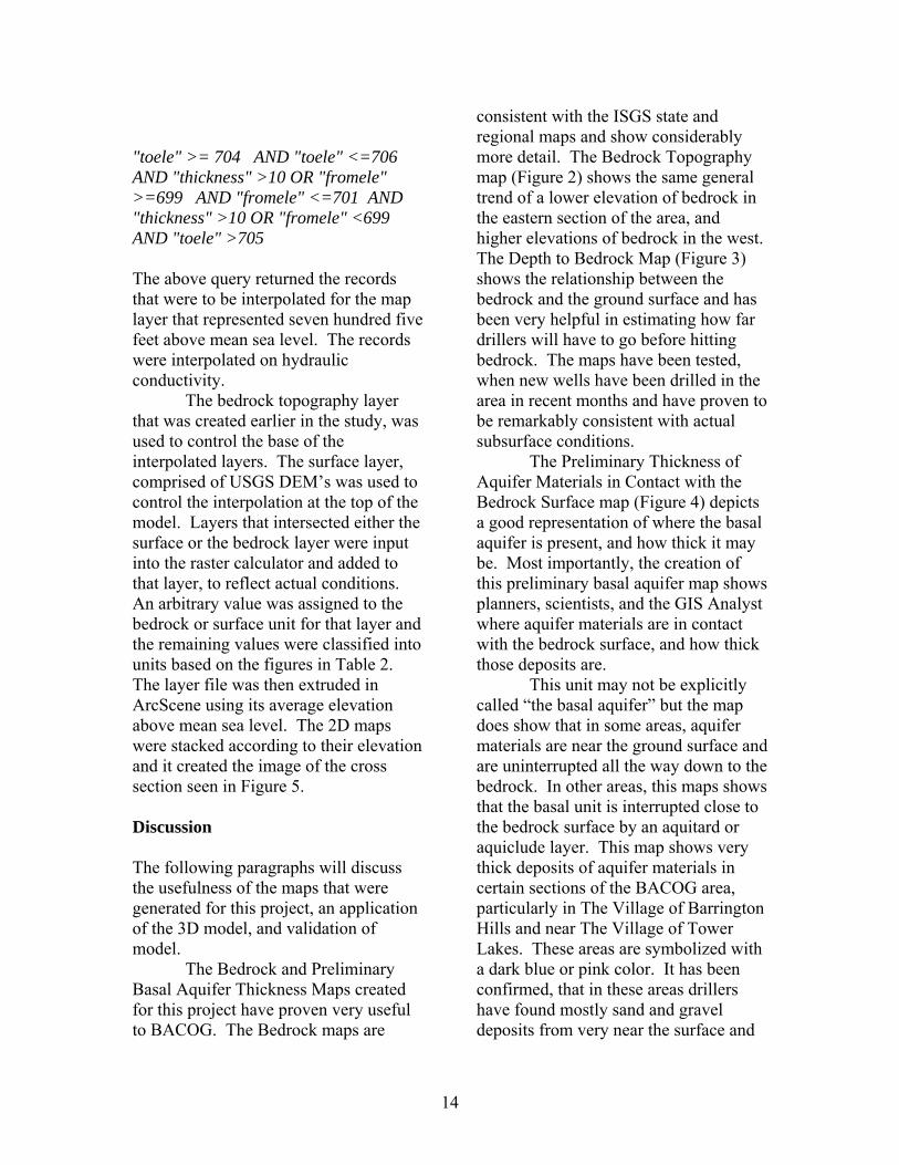
The basal unit is too difficult to delineate using the public water well database. Many of the wells only contain the description “sand and gravel” where it is lying on top of the bedrock. In a great proportion of wells, a layer of broken limestone sits atop bedrock, and atop of it a layer of sand and gravel, or cobbles. The top of the aquifer materials were delineated for thickness mapping, rather than delineating a basal surface based on strict definitions of the term, and because so many well logs contained a very general description of materials on top of the bedrock. In order to group layers to create the thickness map in Figure 4, the field calculator was used to find where aquifer units were lying on top of one another. First, aquifer units were queried out of the database. They were then joined to the database containing the base points. Where the points matched, a calculation was completed to determine if there was any space between the aquifer units. Where there was none, that layer was added to the thickness at that point. This process was repeated a total of 11 times to account for each instance where aquifer units were lying on top of one another.
The thickness was finally determined by subtracting the top of the bedrock from the highest aquifer strata at each point. Data points in the bedrock database that did not have aquifer material present, were given a negative value, to represent that an aquitard or aquiclude was present at the bedrock surface. 10,051 data points were used to to interpolate the preliminary thickness of aquifer units in contact with the bedrock surface map. Of those data points, 6, 120 points represented aquifer materials.
Drift Aquifers Creation of the drift aquifer cross section required different methods, and more specialized operations. Drift aquifers in the BACOG area can be described as the aquifers that reside in the glacial drift materials above the shallow bedrock unit. This may include the basal aquifer unit, and any aquifer above it. Drift aquifers are characterized by being highly variable over a distance and depth.
Several methods were considered for modeling the drift aquifer units. Initially, the methods described for isolating the basal unit were going to be employed for the drift aquifers. The mapping and querying would be more controlled by breaking the study area into pieces based on surface elevation, or a grid to limit false relationships. However, it was decided that would not eliminate enough of the error involved with this type of highly variable data. Instead, a method relying on the recorded depths of each stratum was developed. This method allowed for more control over interpolation, and it also lent itself better to 3D modeling.
The cross sections in Figure 5 are the result of querying the aquifer, aquitard and aquiclude units out of the database at 5-foot intervals and interpolating the results of each query to create a single layer to represent the average elevation represented by the records that were selected. The query to isolate the 5-foot intervals depended on the top elevation of each stratum in the database, and its individual calculated thickness.
The following query is an example of one of the basic queries used to create each 5-foot layer.
11

²
BA
CO
G A
rea
Pre
limin
ary
Th
ickn
ess
of
Aq
uif
er M
ater
ials
in
Co
nta
ct
wit
h t
he
Bed
rock
Su
rfac
e
Bas
al A
quife
r no
t pre
sent
area
_clip
_new
1_U
nion
§̈ ¦90§̈ ¦29
0
§̈ ¦94
US
HW
Y 14
Route
59
Route 31
Rou
te 2
2
US
HW
Y 2
0
Rou
te 6
2
Rou
te 6
8
Rou
te 1
76
Rou
te 1
20
Lake
Coo
k R
oad
Leg
end
Bac
og B
ound
ary
Inte
rsta
te
US
Hig
hway
Sta
te R
oute
0 -
10
11 -
20
21 -
40
41 -
60
61 -
80
81 -
100
101
- 12
0
121
- 14
0
03
61.
5M
iles
Sour
ces o
f the
dat
a ar
e th
e B
arrin
gton
Are
a G
eogr
aphi
c In
form
atio
n Sy
stem
(BA
GIS
5)
and
Lake
, Coo
k, K
ane
and
McH
enry
Cou
ntie
s. W
ell d
ata
is fr
om th
e Ill
inoi
s Sta
te
Geo
logi
cal S
urve
y.
This
Dig
ital E
leva
tion
Mod
el (D
EM)
indi
cate
sthe
est
imat
ed B
asal
Aqu
ifer
Thic
knes
s
Wel
l poi
nt d
ata
from
the
ISG
S wa
s ge
nera
lized
and
exam
ined
for
qual
ity c
ontro
l and
que
ried
toiso
late
the
the
bedr
ock
surfa
ce a
nd a
quife
r mat
eria
ls
To in
terp
olat
e th
is s
urfa
ce, A
rcG
ISSp
atia
l Ana
lyst
Ext
ensio
n an
d th
e kr
igin
gm
etho
d w
ere
used
Con
nie
Pok
orny
- O
ctob
er 2
006
Larg
e S
tudy
Are
a
Fig
ure
4: T
he a
bove
map
dep
icts
the
aqui
fer
mat
eria
ls in
con
tact
with
the
bedr
ock
surf
ace.
12

13
BA
CO
G A
rea
ss on
sC
roS
ecti
Con
nie
L. P
okor
ny -
Feb
ruar
y, 2
007
Larg
e S
tudy
Are
a
Fig
uT
he re
5: T
he a
bove
figu
res
are
repr
esen
tatio
ns o
f the
stu
dy a
rea
from
the
bedr
ock
to th
e su
rfac
e.
figur
es w
ere
crea
ted
by s
tack
ing
laye
rs a
t fiv
e-fo
ot in
terv
als.
No
rth
Ed
ge
So
uth
Ed
ge
Eas
t E
dg
eW
est
Ed
ge
Thes
e C
ross
Sec
tion'
s aq
uife
r un
its a
t the
ed
BA
CO
G s
tudy
ar
Wel
l poi
nt d
ata
from
the
ISG
S
and
exam
ined
for
qual
ity c
ontr
ode
pth
and
hydr
ocon
duct
To in
terp
olat
e th
is s
urf
Spa
tial A
naly
st E
xten
sion
m
etho
d w
ere
used
.
show
the
ge's
of t
heea
.
was
gen
eral
ized
l and
que
ried
for
ivity
.
ace,
Arc
GIS
and
the
krig
ing
Aqu
iclu
deA
quita
rd
Aqu
ifer
Bed
rock
Sur
face
s of t
he d
ata
are
the
Bar
ringt
on A
rea
Geo
grap
hic
Info
rmat
ion
Syst
em (B
AG
IS 5
) La
ke, C
ook,
Kan
e an
d M
cHen
ry C
ount
ies.
Wel
l dat
a is
from
the
Illin
ois S
tate
ic
al S
urve
y.
Sour
cean
d G
eolo
g
"toele" >= 704 AND "toele" <=706 AND "thickness" >10 OR "fromele" >=699 AND "fromele" <=701 AND "thickness" >10 OR "fromele" <699 AND "toele" >705 The above query returned the records that were to be interpolated for the map layer that represented seven hundred five feet above mean sea level. The records were interpolated on hydraulic conductivity. The bedrock topography layer that was created earlier in the study, was used to control the base of the interpolated layers. The surface layer, comprised of USGS DEM’s was used to control the interpolation at the top of the model. Layers that intersected either the surface or the bedrock layer were input into the raster calculator and added to that layer, to reflect actual conditions. An arbitrary value was assigned to the bedrock or surface unit for that layer and the remaining values were classified into units based on the figures in Table 2. The layer file was then extruded in ArcScene using its average elevation above mean sea level. The 2D maps were stacked according to their elevation and it created the image of the cross section seen in Figure 5. Discussion The following paragraphs will discuss the usefulness of the maps that were generated for this project, an application of the 3D model, and validation of model. The Bedrock and Preliminary Basal Aquifer Thickness Maps created for this project have proven very useful to BACOG. The Bedrock maps are
consistent with the ISGS state and regional maps and show considerably more detail. The Bedrock Topography map (Figure 2) shows the same general trend of a lower elevation of bedrock in the eastern section of the area, and higher elevations of bedrock in the west. The Depth to Bedrock Map (Figure 3) shows the relationship between the bedrock and the ground surface and has been very helpful in estimating how far drillers will have to go before hitting bedrock. The maps have been tested, when new wells have been drilled in the area in recent months and have proven to be remarkably consistent with actual subsurface conditions.
The Preliminary Thickness of Aquifer Materials in Contact with the Bedrock Surface map (Figure 4) depicts a good representation of where the basal aquifer is present, and how thick it may be. Most importantly, the creation of this preliminary basal aquifer map shows planners, scientists, and the GIS Analyst where aquifer materials are in contact with the bedrock surface, and how thick those deposits are.
This unit may not be explicitly called “the basal aquifer” but the map does show that in some areas, aquifer materials are near the ground surface and are uninterrupted all the way down to the bedrock. In other areas, this maps shows that the basal unit is interrupted close to the bedrock surface by an aquitard or aquiclude layer. This map shows very thick deposits of aquifer materials in certain sections of the BACOG area, particularly in The Village of Barrington Hills and near The Village of Tower Lakes. These areas are symbolized with a dark blue or pink color. It has been confirmed, that in these areas drillers have found mostly sand and gravel deposits from very near the surface and
14

all the way to the bedrock. The results are consistent with actual conditions in known areas and even reveal patterns that were not apparent before this study. It has been decided that this map is not for public consumption though, as what it communicates may be very confusing for the lay reader. This map was shown at a meeting among Stakeholders in the BACOG area and people did draw inaccurate conclusions from looking at it. Application of the Stratigraphic Model The 3D Model has proven to be extremely useful to BACOG. The model can be rotated, and the layers can be peeled away so the information can be viewed as it changes at each depth. The model can be clipped to a smaller location so that multiple cross sections are possible, and a smaller area is also easier to rotate and view. Additionally, points can be overlaid at any horizontal location and extruded so that it is possible to use the model for planning new well locations, and to plan areas that need to be protected for conservation purposes.
Various surface layers and interpolated subsurface layers can be overlain on the model to increase the understanding of the area and its relation to the subsurface. Figure 6a and 6b show the model from the top and from the side. The layers were clipped to focus on The Village of Barrington municipal boundaries, which is in orange.
In addition, the water level was interpolated using available data in the water well records and then inserted into the model. The surface was symbolized realistically by the USGS DEM and the
upper layers of the model were turned off. The area was clipped to highlight a specific area and several points were created to signify possible new well locations.
Figure 6a. Clipped Section of 3D Model.
Figure 6b. South Side View of Clipped Section.
nits
ved, so
ate odel for The
illage of Barrington.
The information in the model canalso be simplified so that only the uconsisting of aquifer materials are symbolized. The aquitard and aquiclude unit’s color information was remowhen it was viewed in 3D it was possible to see how the aquifer units are connected and their estimated geometry. The images in Figure 7a and 7b illustrthis application of the mV
15

Figure 7a. 3D Model with aquitard and aquiclude color information removed. The light blue color represents aquifer materials, the pink layer is the interpolated water level, the dark blue color is the bedrock surface, the orange line is the Village Boundary, overlain on the transparent green surface. The yellow point symbolizes a current municipal well, extruded to the bedrock.
Figure 7b. South Side View of 3D model with color information removed. Preliminary Validation of the Stratigraphic Model The recent ISGS mapping initiative included the drilling of several boreholes in the BACOG area. The logs of these boreholes were provided to BACOG and were used to conduct a preliminary validation of the BACOG stratigraphic model. Logs of 13 boreholes were provided. Figure 9 illustrates a close up of the sub-area and shows the location of the ISGS boreholes in relation to the neighboring water wells. The ISGS boreholes were located on the BACOG stratigraphic model.
Figure 9. Location of ISGS validation wells (pink) in relation to all of the data points (blue) used to create the stratigraphic model. The gray polygon represents the large study area, as seen in Figure 1. A virtual borehole was drilled by recording the type of material encountered in each five-foot layer until bedrock was reached. Since the objective of the water resource initiative was to map the distribution of aquifer materials in the study area, a comparison between the occurrences of aquifer materials in the boreholes was made. Evaluation criteria included: depth to bedrock, depth to the aquifer(s), and thickness of aquifer(s) and the differences are recorded (Table 1). The total error was divided by the depth of the borehole and multiplied by 100 to arrive at the percent error. The comparison resulted in an average accuracy of 63 percent. Accuracy ranged from 46 to 80 percent 95 percent of the time. Conclusions A greater understanding of groundwater resources in Northeastern Illinois is currently in great demand. The resource is not only necessary for residents who depend on it, but it must be studied in order for planners and decision makers
16

to decide if it is a sustainable supply for current and future residents. The techniques described in this paper and the resulting maps are one attempt to meet the demand for a better understanding of the area’s water resources. The maps are a very good representation of baseline conditions in the area and support further research in water quality and sustainability by BACOG. Great care was taken to ensure and improve the accuracy of existing data, and data that was obviously erroneous was not used. A great number of water well points were used to create averages for the maps in this research project. The belief is that these averages and resulting maps are the best currently available to support local stakeholders interested in subsurface conditions for planning purposes. The data development associated with this method is a time consuming process, as it is with almost any GIS project. However, once the data is in place a wide variety of subsurface mapping information becomes available. In addition to the maps in this research paper, many more have been developed or are currently being developed for BACOG. Many communities could possibly benefit by following the model described in this paper. Furthermore, GIS methods for mapping groundwater information would be greatly simplified or improved, if standards were mandated so that well drillers and scientists alike would be able to code well log information in a way that would be more easily queried by computers. Acknowledgements I would like to thank Dr. Kurt Thomsen for his input and knowledge, the ISGS for answering difficult questions and
providing the use of their water well database. Thanks to Janet Agnoletti for her continued support of groundwater research at BACOG and her understanding of regional issues. Thanks to all BACOG staff and member governments for their financial contributions that made this project possible. Thanks to the Resource Analysis Department at Saint Mary’s University of Minnesota for their involvement in the development of this research paper. References Abbey, D. G., Carnegie, A., & Harvey,
D. J. M. 2001. Using Public Water Well Records to Generate Model Input Data: Overcoming Challenges. Waterloo Hydrogeologic Inc.
Berg, R., Bleur, N., Berwyn, J., Jones, K., Kincare, K., Pavey, R., & Stone, B. 1999. Mapping the Glacial Geology of the Central Great Lakes Region in Three Dimensions – A model for State-Federal Cooperation. U.S. Geological Survey Open-File Report 99-349.
Illinois State Geological Survey. 2007. How Well Locations are Described in Illinois. Online. Internet. <http://www.isgs.uiuc.edu/maps-data- pub/wwdb/locate.shtml> Logan, C., Russell, H. A. J., & Sharpe,
D. R. 2001. Regional Three-Dimensional Stratigraphic Modeling of the Oak Ridges Moraine Area, Southern Ontario. Geological Survey of Canada: Current Research, 2001-D1.
Sanders, L. L. 1998. A Manual of Field Hydrogeology. Prentice Hall, Upper Saddle River, NJ. Thomsen, K. O., Pokorny, C., &
Agnoletti, J. 2004. Groundwater
17

18
Resource Planning - Defining the Shallow Aquifer System. Proceedings of the 26th Annual ESRI User’s Conference, San Diego, CA August 2006.