Group actions on trees and dendrons

B. H. BowditchFaculty of Mathematical Studies, University of Southampton,

Highfield, Southampton SO17 1BJ, Great Britain.bhb@maths.soton.ac.uk

0. Introduction.

The main objective of this paper will be to describe how certain results concerningisometric actions on R-trees can be generalised to a wider class of treelike structures.This enables us to analyse convergence actions on dendrons, and hence on more generalcontinua, via the results of [Bo1]. The main applications we have in mind are to boundariesof hyperbolic and relatively hyperbolic groups. For example, in the case of a one-endedhyperbolic group, we shall see that the existence of a global cut point gives a splittingof the group over a two ended subgroup (Corollary 5). Pursuing these ideas further, onecan prove the non-existence of global cut points for strongly accessible hyperbolic groups[Bo5], and indeed for hyperbolic groups in general [Sw]. Reset in a general dynamicalcontext, one can use these methods to show, for example, that every global cut point inthe limit set of a geometrically finite group is a parabolic fixed point [Bo6]. These resultshave implications for the algebraic structure of such groups. Some of these are discussedin [Bo3].

The methods of this paper are essentially elementary and self-contained (except ofcourse for the references to what have now become standard results in the theory of R-treeactions). A different approach has been described by Levitt [L2], which gives a generalisa-tion of the central result (Theorem 0.1) to non-nesting actions on R-trees. Levitt’s workmakes use of ideas from the theory of codimension-1 foliations (in particular the result ofSacksteder [St]). This seems a more natural result, though our version of Theorem 0.1suffices for the applications we have in mind at present. There are many further questionsconcerning the relationship between actions on R-trees and dendrons, which seem worthyof further investigation. Some of these are described in [Bo2].

The notion of an R-tree was formulated in [MoS]. It can be given a number of equiv-alent definitions. For example, it can be defined simply as a path-metric space whichcontains no embedded circle. For more discussion of R-trees, see, for example, [Sh,P2].There is a powerful machinery for studying isometric group actions onR-trees, due to Rips,and generalised by Bestvina and Feighn [BeF] and Gaboriau, Levitt and Paulin [GaLP1].In most applications, such actions arise from some kind of degeneration of a hyperbolicmetric, so that the R-trees obtained come already equipped with a natural metric. How-ever, there are potential applications, as we shall describe, where one obtains, a-priori,only an action by homeomorphism with certain dynamical properties.

To deal with this situation, one might attempt either to generalise the Rips machineryto cover such cases, or one might attempt to construct a genuine R-tree starting with amore general action. It is the latter course that is followed in this paper (and that of Levitt

1

Trees and dendrons

[L2]).

Let’s begin by giving more precise definitions of the objects we are working with:

Definition : A real tree, T , is a hausdorff topological space which is uniquely arc con-nected, and locally arc connected.

More precisely, if x, y ∈ T , then there is a unique interval, [x, y] connecting x to y. (Here“interval” means a subset homeomorphic to a closed real interval.) Moreover, given anyneighbourhood, U , of x, there is another neighbourhood, V , of x, such that if y ∈ V , then[x, y] ⊆ U . We shall define a dendron to be a compact real tree.

We shall say that a metric, d, on T , is monotone if given x, y, z ∈ T with z ∈ [x, y],then d(x, z) ≤ d(x, y). We shall say that d is convex , if for all such x, y, z, we haved(x, y) = d(x, z) + d(z, y). Clearly, any convex metric is monotone.

An equivalent definition of an R-tree is thus a real tree, together with a continuousconvex metric. (We specify continuous, with respect to the real tree topology, since weshall later be obliged to consider discontinuous metrics.) We also have the more generalnotion:

Definition : A monotone tree consists of a real tree, together with a continuous monotonemetric.

A result of Mayer and Oversteegen [MaO] tells us that that any metrisable real treeadmits the structure of an R-tree (i.e. a continuous convex metric). However the R-treemetric arising from this construction is not in any way canonical, and it’s not clear howthis procedure could be generalised to give R tree metrics which are invariant under somegroup action — even starting from an invariant metric. Here we shall use a differentconstruction, which gives a somewhat weaker result, but which is equivariant.

Suppose Γ acts by homeomorphism on the real tree T . Given x ∈ T , write Γ(x) =ΓT (x) = {g ∈ Γ | gx = x}. We say the action is parabolic if there is a point x ∈ Twith Γ(x) = Γ. (This is frequently termed “trivial” in the literature. We use the term“parabolic” for consistency with the terminology of convergence actions.) If x, y ∈ T aredistinct, we write Γ(A) (or ΓT (A)) for the pointwise stabiliser of the interval A = [x, y].Thus, Γ(A) = Γ(x)∩Γ(y). A subgroup of the form Γ(A) is referred to as an edge stabiliser ,or if we need to be more specific, a T -edge stabiliser . A sequence of subgroups (Gi)i∈N isreferred to as a chain of T -edge stabilisers if there is a sequence of non-trivial intervals,(Ai)i∈N, such that Gi = Γ(Ai) and Ai+1 ⊆ Ai for all i, and such that

⋂i∈N

Ai consistsof a single point. Thus, (Gi)i∈N is an ascending chain of subgroups. The action of Γ inT is said to be stable if every chain of edge stabilisers is eventually constant. The resultsconcerning actions on R-trees already alluded to, refer to non-parabolic stable isometricactions, usually with some conditions imposed on the types of groups that can arise asedge stabilisers.

Here we shall show that much of this theory can be generalised, as least as far asisometric actions on monotone trees. Specifically, we show:

2

Trees and dendrons

Theorem 0.1 : Suppose Γ is a finitely presented group, which admits a non-parabolicisometric action on a monotone tree, T . Then Γ also admits a non-parabolic isometricaction on an R-tree, Σ, such that each Σ-edge stabiliser is contained in a T -edge stabiliser.Moreover, if (Gi)i∈N is a chain of Σ-edge stabilisers, then there is a chain of T -edgestabilisers, (Hi)i∈N, such that Gi ≤ Hi for all i ∈ N.

In many cases of interest, the stability of the action on T will imply the stability of theaction on Σ. Suppose, for example, that each subgroup of Γ which fixes an interval of T(i.e. any subgroup of any T -edge stabiliser) is finitely generated. Then, if the action of Γon T is stable, then so is the action on Σ. This additional assumption is likely to hold formost plausible applications, where the T -edge stabilisers are constrained to be reasonablynice subgroups. Of particular interest here is the case where all T -edge stabilisers areassumed to finite.

Now, a consequence of the results of [BeF], is that a finitely presented group which actsisometrically, stably and non-parabolically on an R-tree with finite edge stabilises mustbe virtually abelian or split over a finite or two-ended subgroup. (Note that “two-ended”is the same as “virtually cyclic”.) Applying Theorem 0.1, we thus obtain the same resultfor monotone trees:

Corollary 0.2 : Suppose Γ is a finitely presented group, which acts isometrically, stably,non-parabolically, and with finite edge-stabilisers, on a monotone tree. Then, either Γ isvirtually abelian, or it splits over a finite or two-ended subgroup.

In the case where Γ is virtually abelian, it must fix some subtree of T , homeomorphicto the real line. This case is of no particular interest to us here.

A principal application of this result concerns discrete convergence actions on non-trivial dendrons. (Recall that a “dendron” is a compact real tree. The term “non-trivial”simply means that it is not a point. The notion of a “discrete convergence” action wasdefined in [GeM]. For further discussion, see [T] or [Bo4]. Putting results of [Bo2] togetherwith Corollary 0.2, we obtain:

Theorem 0.3 : Suppose Γ is a finitely presented infinite group, such that any as-cending chain of finite subgroups eventually stabilises. Suppose that Γ admits a discreteconvergence action on a dendron. Then, Γ splits over a finite or two-ended subgroup.

(It’s not clear that the assumption on chains of finite subgroups is necessary. It is alsoprobable that the result holds for finitely generated groups.)

This result in turn has applications to the boundaries of certain hyperbolic groups.Suppose that Γ is a one-ended word hyperbolic group (in the sense of Gromov [Gr]). Then,Γ is finitely presented, has a bound on the orders of finite subgroups, and does not splitover any finite subgroup. Moreover the boundary, ∂Γ, is connected and hence a continuum— a connected, compact, hausdorff topological space. (See [GhH]). It was conjectured in[BeM] that such a case, ∂Γ must be locally connected. They showed that if ∂Γ is notlocally connected, then it must contain a global cut point. (A converse was obtained in

3

Trees and dendrons

[Bo3].) Moreover, it was shown in [Bo2] that if ∂Γ contains a global cut, then it admitsa Γ-invariant quotient which is a non-trivial (separable and hence metrisable) dendron.Now, Γ acts as a convergence group on this dendron, and so we obtain:

Corollary 0.4 : If Γ is a one-ended hyperbolic group with a global cut point in itsboundary, then Γ splits over a two-ended subgroup.

In fact, Swarup [Sw] showed how one can adapt these ideas to prove the cut pointconjecture in general. This result can be generalised to a dynamical context [Bo6], whichalso has applications to limit sets of geometrically finite kleinian groups (and groups actingon pinched hadamard manifolds). One can obtain most of the results of the present paperwithout explicit use of these refinements.

Now, if we assume that ∂Γ has no global cut point, then it’s locally connected (by[BeM]) so we can bring the results of [Bo3] into play. In particular, we obtain:

Theorem 0.5 : A one-ended non-fuchsian hyperbolic group splits over a two-endedsubgroup if and only if its boundary contains a cut point.

Here “cut point” should be interpreted as either local or global. A local cut point may bedefined as a point x ∈ ∂Γ such that ∂Γ \ {x} has more than one end. A fuchsian groupis one which contains a finite index subgroup which is the fundamental group of a closedsurface. (The case of fuchsian groups can be explicitly described, see for example [Bo3].)

The importance of splitting over over two-ended subgroups is well-known, see, forexample [P1,Se]. The set of such splittings determines the structure of the outer automor-phism group. In particular, if a one-ended hyperbolic group has infinite outer automor-phism group, then it splits over a two-ended subgroup. We say that a one-ended hyperbolicgroup is strongly rigid if there is no such splitting. We see that, modulo fuchsian groups,strong rigidity of a one-ended hyperbolic group can be recognised from the topology of theboundary. In particular, we see:

Corollary 0.6 : For non-fuchsian one-ended hyperbolic groups, strong rigidity is ageometric property.

Here “geometric” means “quasiisometry invariant”. We refer to [Bo3] for more details.We can give a refinement of Theorem 0.1 as described in Section 7. Thus, ifH1, . . . , Hn

are finitely presented subgroups of Γ which act parabolically on T , then they can beassumed to act parabolically also on Σ. This leads to refinements of Corollary 0.2 andTheorem 0.3 which find application in [Bo6].

We make a few observations about Theorem 0.1, and generalisations. First we needanother definition:

Definition : Suppose that g is a homeomorphism of a real tree, T . We say that g isnon-nesting if, given any compact interval, A ⊆ T such that either A ⊆ gA or gA ⊆ A,then gA = A.

4

Trees and dendrons

We say that a group of homeomorphisms is non-nesting if every element is.

Non-nesting homeomorphisms have many of the features of isometries of R-trees, forexample, they can be classified into types, as described later. (Note that any isometry ofa monotone tree is necessarily non-nesting.) Levitt [L2] has generalised Theorem 0.1 tothe case of non-nesting actions on a real tree. This generalisation is remarkable in thatthe dynamics of the original action might not resemble that of an isometric action. Forexample, the tree might contain wandering intervals, in which case action would certainlynot be topologically conjugate to an isometric action. Note that, in proving Theorem 0.3,this result would enable us to bypass the construction of the monotone metric (see Section6).

We remark that Levitt does not obtain explicitly our result about chains of edgestabilisers, and hence the preservation of stability in the case of finitely generated edgestabilisers. It’s possible that a careful analysis of Levitt’s construction would yield this.In any case, for the applications which interest us here (where edge stabilisers are finite,and there is no infinite torsion subgroup) stability is automatic.

Levitt’s construction proceeds by translating the problem into the language of one-dimensional pseudogroups, and appealing to some of the results developed in the theory ofcodimension-one foliations in this context. In particular a theorem of Sacksteder [Sa] givesmethods for finding invariant Borel measures on pseudogroups. One then constructs anR-tree from such a measure. Here, we shall phrase everything in terms of pseudometricsrather than measures.

We suspect that Theorem 0.1 remains true if “finitely presented” is replaced by“finitely generated”. Perhaps the argument presented here can be made to work in thatgenerality, using “normal covers”, as described, for example in [LP], though we have notworked out the details.

One might also ask when an action of a (finitely presented) group on a real treeis conjugate to an action on an R-tree. Here “conjugate” might mean “topologicallyconjugate”, or probably more naturally “conjugate under a pretree isomorphism” (seebelow). One certainly needs stronger constraints on the dynamics than just the non-nestinghypothesis. Perhaps the existence of an invariant monotone metric would be sufficient. Inparticular, one might ask if this is true of the monotone tree arising from a convergenceaction on a metrisable dendron, as constructed in [Bo2]. On the other hand, going in theopposite direction, from an R-tree action to an action on a dendron, can be describedfairly easily in terms of a compactification process. Of course one needs a constraint onthe R-tree action for it to give rise to a convergence action. This is discussed in [Bo2].In general, the relationship between R-trees and dendrons seems subtle, and worthy offurther investigation.

We remark that the topology on the real tree is not directly relevant to anything wedo. All we really need is the relation of “betweenness”, which we can regard as determininga preferred class of subsets of the set T , namely the closed intervals. One can write downexplicit axioms for such a structure, which in [Bo2] is referred to as a “real pretree” (seealso [W] and [AN]). This structure is weaker than that of a topology, in that differentreal tree topologies might give rise to the same pretree structure. It would probably be

5

Trees and dendrons

more natural to phrase everything in terms of isomorphisms of real pretrees, rather thanhomeomorphisms of real trees. However the extra generality is spurious, since it can beshown that every real pretree admits a certain canonical topology as a real tree (one whichadmits a hausdorff compactification).

The principal tools we shall use are foliations on 2-complexes. We shall use the term“track complex” for such an object, since our formulation is analogous to the tracks ofDunwoody [D]. However, they are essentially the same as foliated 2-complexes discussedin [LP]. A track complex (or foliated 2-complex as in [LP]) essentially consists of a locallyfinite 2-dimensional simplicial complex, together with a partition into leaves, in such away that the set of leaves meets any given simplex in one of specific number of patterns.They are closely related to the band complexes of [BeF], and everything we do could berephrased in these terms, or indeed in terms of pseudogroups. However, since we shall notbe applying the Rips machinery directly, we prefer to use this intuitively simpler picture.

The idea of the proof of Theorem 0.1 is roughly as follows. Suppose Γ is a finitelypresented group which acts on a real tree T . By taking a “resolution” of such an action (cf.[BeF]), we construct a track complex based on a finite 2-dimensional simplicial complex,K, with Γ ≡ π1(K). An invariant continuous monotone metric on K induces a kindof “transverse” metric on K. By a compactness argument, we use this to construct atransverse convex pseudometric. This gives rise to a genuine path-pseudometric on theuniversal cover, K, which we proceed to show is “0-hyperbolic”. The R-tree, Σ, thusarises as the hausdorffification of K. We finally have to verify the statements about edgestabilisers and non-parabolicity of the action.

I am indebted to Mladen Bestvina and Gilbert Levitt who suggested to me that resultsof this nature should be possible. It was Gilbert Levitt, who put me on to the article bySacksteder, which partly inspired the arguments of this paper, even if I don’t apply theseresults directly. Most of this paper was prepared while visiting the Universitat Zurich,at the invitation of Viktor Schroeder. It was revised somewhat while I was visiting theUniversity of Melbourne at the invitation of Walter Neumann and Craig Hodgson. I wouldlike to thank both institutions for their hospitality.

1. Pseudometrics.

In this section, we make some elementary observations about pseudometrics.

Let M be a hausdorff topological space. A pseudometric on M is a function d :M ×M −→ [0,∞) satisfying d(x, x) = 0, d(x, y) = d(y, x) and d(x, y) ≤ d(x, z) + d(z, y)for all x, y, z ∈M . It is a metric if d(x, y) = 0 implies x = y. Note that we do not assumethat d is continuous, unless explicitly stated.

Suppose d is a continuous pseudometric on M . We may define the rectifiable length,lengthd β ∈ [0,∞] of any continuous path, β, in M , in the usual way. We say that d is apath-pseudometric if given any x, y ∈M , and any ǫ > 0, there is a path β inM , joining x toy with lengthd β ≤ d(x, y)+ǫ. Note that path-pseudometrics are assumed to be continuous.By a geodesic in M joining x to y, we mean a path, β, with lengthd β = d(x, y).

6

Trees and dendrons

Given a continuous pseudometric space, (M, d), we define an equivalence relation, ∼,on M by x ∼ y if d(x, y) = 0. Thus, d descends to a continuous metric on the quotient,M/∼, which we shall also denote by d. We call M/∼ the hausdorffification of M . Notethat if d is a path-pseudometric on M , then the metric on the quotient is a path-metric.

We shall say that a path-pseudometric is 0-hyperbolic if, given any x, y, z, w ∈M , thelargest two of the three quantities, d(x, y)+ d(z, w), d(x, z) + d(y, w) and d(x, w)+ d(y, z)are equal. Note that an R-tree can be defined as a 0-hyperbolic path-metric space. (Theequivalence of this with the usual definition is shown, for example, in [Bo1], where theformulation of hyperbolicity we have used is referred to as “H1”. In fact, as noted in[Sho], any 0-hyperbolic connected metric space is an R-tree.) In particular, we see that in0-hyperbolic path-metric space, every pair of points can be joined by a geodesic. This neednot be true in a 0-hyperbolic path-pseudometric space. Note that the hausdorffification ofa 0-hyperbolic path-pseudometric space is an R-tree.

We shall be particularly interested in pseudometrics on intervals, or disjoint unionsof intervals. Let I = [0, 1] be the unit interval in R. We say that a pseudometric, d, on Iis monotone, in whenever x < y < z, we have d(x, y) ≤ d(x, z) and d(y, z) ≤ d(x, y). Wesay that d is convex if whenever x < y < z, we have d(x, z) = d(x, y) + d(y, z). Clearly aconvex pseudometric is monotone. In any case, let l(I, d) = d(0, 1). Clearly, a monotonepseudometric, d, is identically 0 if and only if l(I, d) = 0.

Let V (I) = (I×{−,+})\{(0,−), (1,+)}. We think of V (I) as the set of unit tangentvectors to I. Thus, (x,+) is the vector based at x pointing towards 1. Suppose that d is amonotone pseudometric on I. For x ∈ [0, 1) we define µd(x,+) = inf{d(x, y) | y > x}. Wesimilarly define µd(x,−) for x ∈ (0, 1]. This gives a map µd : V (I) −→ [0,∞). We refer tov ∈ V (I) as an atom if µd(v) > 0. Thus, a monotone pseudometric is continuous if andonly if there are no atoms.

Suppose that d is convex pseudometric. If x < y ∈ I, then we see easily that µd(x,+)+µd(y,−) ≤ d(x, y). Thus, if 0 = x0 < x1 < · · · < xm = 1, we see that

∑mi=0(µd(xi,−) +

µd(xi,+)) ≤∑m

i=1 d(xi, xi−1) = d(0, 1) = l(I, d) (with the convention that µd(0,−) =µd(1,+) = 0). Thus,

∑v∈V (I) µd(v) ≤ l(I, d) < ∞. (In particular, there are at most

countably many atoms.)We may apply exactly the same discussion to a finite set of disjoint intervals, J =

I1 ⊔ I2 ⊔ · · · ⊔ In. Here the pseudometric is assumed to be defined on P (J) =⊔n

i=1 I2i .

We say that d is monotone (convex) if d|I2i is monotone (convex) on Ii for each i. Letl(J, d) =

∑ni=1 l(Ii, d|I

2i ). Note that d is identically zero of and only if l(J, d) = 0. We say

that d is normalised if l(J, d) = 1.Let M(J) be the set of normalised monotone pseudometrics on J . We can embed

M(J) in the Tychonoff cube [0, 1]P (J), by taking the (x, y)-coordinate of d to be d(x, y).Now each of the relations defining a monotone pseudometric is closed, and so M(J) is aclosed subset of [0, 1]P (J). Thus, with the subspace topology, M(J) is compact.

We define V (J) =⊔n

i=1 V (Ii). Given a monotone pseudometric d, we may defineµd : V (J) −→ [0,∞) as before. As in the case of a single interval, we note

Lemma 1.1 : If d is a monotone pseudometric on J , then∑

v∈V (J) µd(v) <∞. ♦

We finally make a few remarks about convex pseudometrics. Suppose d is a non-zero

7

Trees and dendrons

continuous convex pseudometric on a closed interval I. Let q : I −→ I ′ be the quotientmap to the hausdorffification I ′. Thus, I ′ is also an interval, and d is a continuous convexmetric on I ′. Thus, (I ′, d) is isometric to a closed real interval. The pullback of Lebesguemeasure on I ′ gives us an atomless regular Borel measure on I. The measure of anysubinterval of I is thus the same as its d-length. We write supp d for the support of thismeasure. Now, q collapses each of an (at most) countable set of disjoint closed intervals toa point, and is injective on the complement of the union of these intervals. These intervalsare precisely the closures of the components of the complement of supp d.

2. Foliations on 2-complexes.

In this section, we discuss foliations on 2-complexes. Variations of these ideas havebeen studied by several authors in relation to R-trees. The theory has been recently de-veloped formally by Levitt and Paulin in [LP]. Here we shall use the term “track complex”for a foliated 2-complex. Our formulation differs slightly from that given in [LP], thoughfor all practical purposes, it amounts to the same thing.

We shall be interested in certain “transverse” structures to these foliations, which wephrase in terms of pseudometrics. Thus, an atomless transverse regular Borel measure, asdescribed in [LP] translates to a continuous convex pseudometric. We shall not want toassume that the measure has full support, as has typically been done elsewhere. However,the relevant arguments would seem to generalise without problems.

One of the main aims of this section is to describe how transverse pseudometrics giverise to R-trees. In the context of pseudogroups (or “systems of isometries”), this hasbeen examined by several authors, see, in particular, [L1,GaLP2]. It is also described forfoliated 2-complexes in [LP], refering to this earlier work. For completeness, we include analternative, direct argument here.

We begin with some definitions.Let M be a connected locally finite simplicial 2-complex. (In this paper, the term

“complex” is always taken to mean “simplicial complex”.) We refer to the 1-simplices ofM as edges of M , and 0-simplices as vertices . Let F be a partition of M is a disjointconnected subsets. Given a simplex, σ, of M , a stratum of σ is defined to be a connectedcomponent of the intersection of σ with an element of F .

We say that F is a track foliation of M if the following hold:

(1) If σ is an edge of M , then the set of strata in σ either consists of just one element,namely σ itself, or else consists of the set of all points of σ.

(2) If σ is a 2-simplex of M , then each stratum of σ is topologically a point, a closedinterval, or a closed disc. Moreover the set of strata forms, up to homeomorphism relativeto the set of vertices, one of the four patterns, (A)–(D), given by Figure 1 (see below).

(3) Each stratum of a 2-simplex intersects each face of that simplex in a stratum of thatface.

(If we imagine a 2-simplex, σ, as an equilateral triangle, then up to homeomorphisms,the patterns can be described as follows. In picture (A), there is a single stratum, namelyσ itself. In picture (B), the strata consist of all lines parallel to one edge, together with the

8

Trees and dendrons

vertex opposite that edge. In picture (C), the strata consist of all lines perpendicular toone edge, together with the two endpoints of that edge. In picture (D), one statum is thetriangular convex hull of the midpoints of the three edges. The remaining strata are linesparallel to one of the edges of this hull, together with all three vertices of the simplex.)

We refer to an edge of M as essential if each stratum is a point. If σ is a 2-simplex,a singular stratum, is either one which contains a vertex, or one which intersects all three1-dimensional faces. (Thus all strata which are topologically discs are singular.) A pointon an essential edge is singular if it is a vertex, or if it lies in a singular stratum of anincident face. Thus, the set of singular points in each edge is finite.

Without loss of generality, we can assume that each stratum of a 2-simplex is a point,a euclidean arc, or bounded by euclidean arcs.

Definition : A track complex , (M,F), consists of a locally finite simplicial complex, M ,together with a track foliation, F , on M . An element of F is referred to as a leaf of thefoliation. A leaf is singular if it contains a singular stratum.

Note that a leaf itself has the structure of a locally finite 2-complex. A non-singular leafis a locally finite 1-complex.

Note that we can recover a track foliation from the set of strata in each leaf as follows.Define a relation on M , by saying that two points are related if they lie in the samestratum of some simplex. Take the equivalence relation on M generated by this relation.The equivalence classes are precisely the the leaves of the foliation. Note that for thisto work, we need only that the set of strata satisfies axioms (1)–(3) above. We can thusdefine a track foliation by describing the set of strata, and so it can be thought of as reallya “local” structure.

Now any subcomplex of M inherits a structure as a track complex. More generally, ifL is a connected locally finite 2-complex, and f : L −→M is a simplicial map, we can pullback the track foliation to L. (Note that if f collapses a 2-simplex, σ, to an edge, thenthe pattern induced on σ will be of type (B) or type (A), depending in whether of not theedge is essential.) Clearly, f maps each leaf in L into a leaf in M .

Another point to note is that we can find arbitrarily fine simplicial subdivisions ofM which admit track foliations with precisely the same set of leaves. We refer to such asubdivision as a foliated subdivision. The Simplicial Approximation Theorem now tells usthat, up to small homotopy, every continuous map of simplicial 2-complex into M can beassumed to be simplicial.

The definition of a foliation given in [LP] is essenially the same, except that they onlyallow for pictures (B) and (C). Since our complex is locally finite, we can clearly eliminatepicture (D) after subdivision. (This may be more natural for our purposes, though onemight imagine contexts in which it might be useful to allow it, for example to study thespace of foliations on a fixed complex.) One could also collapse down the union of all thesimplices of type (A) without doing much damage, though it is technically convenient toallow the possibility here.

Here are some more definitions:

9

Trees and dendrons

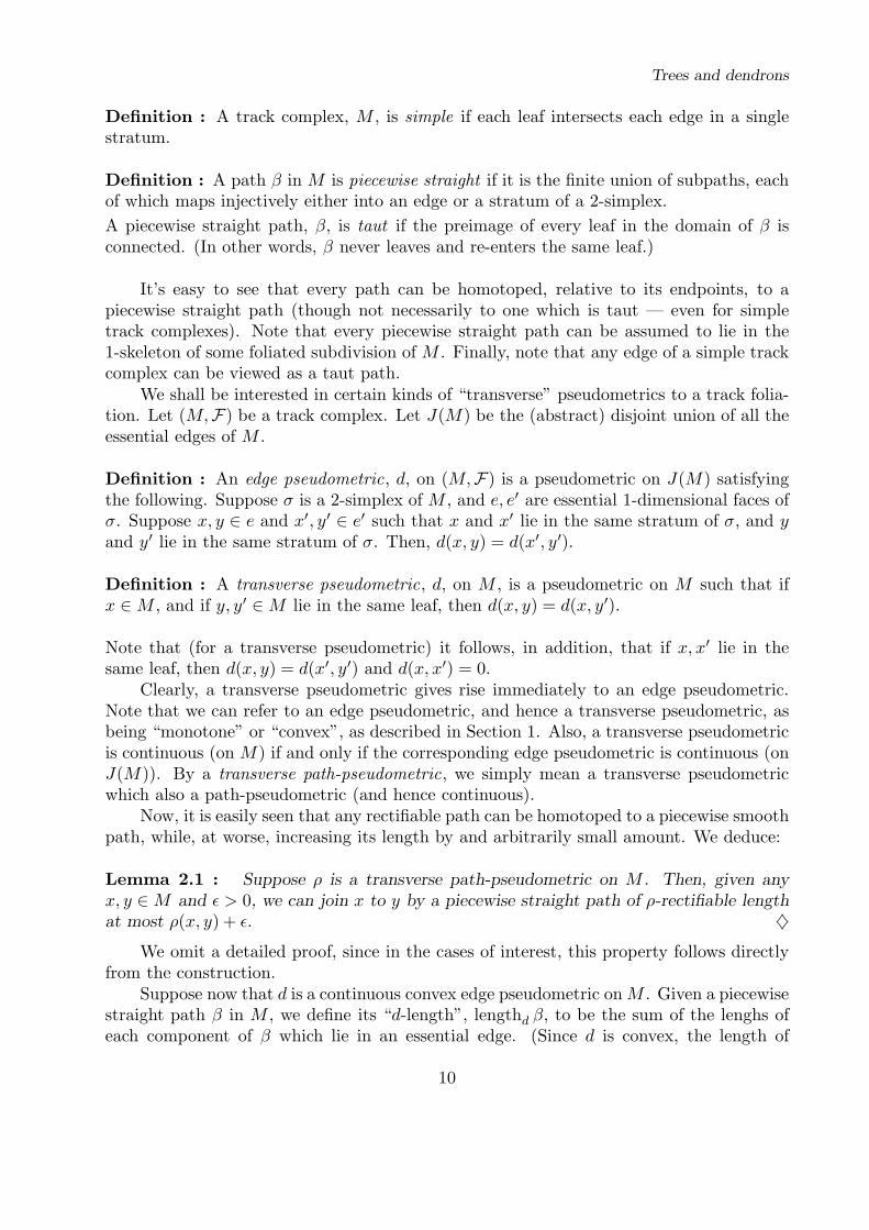
Definition : A track complex, M , is simple if each leaf intersects each edge in a singlestratum.

Definition : A path β in M is piecewise straight if it is the finite union of subpaths, eachof which maps injectively either into an edge or a stratum of a 2-simplex.

A piecewise straight path, β, is taut if the preimage of every leaf in the domain of β isconnected. (In other words, β never leaves and re-enters the same leaf.)

It’s easy to see that every path can be homotoped, relative to its endpoints, to apiecewise straight path (though not necessarily to one which is taut — even for simpletrack complexes). Note that every piecewise straight path can be assumed to lie in the1-skeleton of some foliated subdivision of M . Finally, note that any edge of a simple trackcomplex can be viewed as a taut path.

We shall be interested in certain kinds of “transverse” pseudometrics to a track folia-tion. Let (M,F) be a track complex. Let J(M) be the (abstract) disjoint union of all theessential edges of M .

Definition : An edge pseudometric, d, on (M,F) is a pseudometric on J(M) satisfyingthe following. Suppose σ is a 2-simplex of M , and e, e′ are essential 1-dimensional faces ofσ. Suppose x, y ∈ e and x′, y′ ∈ e′ such that x and x′ lie in the same stratum of σ, and yand y′ lie in the same stratum of σ. Then, d(x, y) = d(x′, y′).

Definition : A transverse pseudometric, d, on M , is a pseudometric on M such that ifx ∈M , and if y, y′ ∈M lie in the same leaf, then d(x, y) = d(x, y′).

Note that (for a transverse pseudometric) it follows, in addition, that if x, x′ lie in thesame leaf, then d(x, y) = d(x′, y′) and d(x, x′) = 0.

Clearly, a transverse pseudometric gives rise immediately to an edge pseudometric.Note that we can refer to an edge pseudometric, and hence a transverse pseudometric, asbeing “monotone” or “convex”, as described in Section 1. Also, a transverse pseudometricis continuous (on M) if and only if the corresponding edge pseudometric is continuous (onJ(M)). By a transverse path-pseudometric, we simply mean a transverse pseudometricwhich also a path-pseudometric (and hence continuous).

Now, it is easily seen that any rectifiable path can be homotoped to a piecewise smoothpath, while, at worse, increasing its length by and arbitrarily small amount. We deduce:

Lemma 2.1 : Suppose ρ is a transverse path-pseudometric on M . Then, given anyx, y ∈M and ǫ > 0, we can join x to y by a piecewise straight path of ρ-rectifiable lengthat most ρ(x, y) + ǫ. ♦

We omit a detailed proof, since in the cases of interest, this property follows directlyfrom the construction.

Suppose now that d is a continuous convex edge pseudometric onM . Given a piecewisestraight path β in M , we define its “d-length”, lengthd β, to be the sum of the lenghs ofeach component of β which lie in an essential edge. (Since d is convex, the length of

10

Trees and dendrons

such a component is just the distance between its endpoints. Note that there is no clashof notation if d happens to be the restriction of a transverse pseudometric, since theremaining parts of β is automatically have zero length.) Given x, y ∈M , we define ρ(x, y)to be inf{lengthd β}, as β ranges over all piecewise straight paths joining x to y.

Lemma 2.2 : ρ is a transverse path-pseudometric on M .

Proof : The fact that ρ is a transverse pseudometric is essentially trivial. Also, since d isconvex, it’s clear that ρ ≤ d on each edge. Since d is assumed to be continuous, it followsthat ρ is continuous on each edge, and hence on M .

Suppose β is a piecewise smooth path. Now the ρ-length of each component of β in astratum of a 2-simplex is 0 (since ρ is identically zero on each leaf). Moreover, since ρ ≤ d,we see that the ρ-rectifiable length is at most the d-length on each essential edge. Thus,lengthρ β ≤ lengthd β. But now, by definition, if x, y ∈M and ǫ > 0, we can join x to y bya piecewise straight path β, with lengthd β ≤ ǫ. This shows that ρ is a path-pseudometric.

♦

Note that we have, in fact, verified the conclusion of Lemma 2.1, for a path-pseudometricarising in this way. We refer to ρ as the “induced transverse path-pseudometric”.

Given any track complex, (M,F), we can view the leaf space F as a topological spacewith the quotient topology from M . Viewed in this way, we shall write it as F (M). Notethat the transverse pseudometric gives rise to a pseudometric on F (M), which we shallalso denote by ρ. In general, F (M) will not be hausdorff. However, in certain cases, weget a nice space. Of special interest is the following situation.

Suppose that M is finite, and (M,F) is simple. In this case, each leaf is compact,and there are only finitely many singular leaves. If the remove all the singular leaves,each component of the complement is topologically of the form G×R, where G is a finite1-complex. Moreover, the leaves have the form G × {x} for x ∈ R. We conclude that, inthis case, F (M) is a finite 1-complex. We shall write p : M −→ F (M) for the quotientmap. Of particular interest is the case where M is topologically a disc:

Lemma 2.3 : Suppose (D,F) is a simple track complex on the topological disc, D.Then F (D) is a finite tree.

Proof : Note that any non-singular leaf in D is an arc connecting two points of theboundary, ∂D. Suppose e is an edge of F (D) with endpoints x and y, and let z be anyinterior point. Now, p−1z is an arc in D which must locally, and hence globally, separateany point in p−1x from any point in p−1y. Thus, z separates x from y in F (M). Thus, ecannot lie in any embedded circle in F (M). ♦

Corollary 2.4 : Suppose that ρ is a transverse path-pseudometric on D. Then ρ is0-hyperbolic.

11

Trees and dendrons

Proof : Now ρ induces a pseudometric on F (D), which is also a path-pseudometric.It’s easily verified that any path-pseudometric on a (finite) tree must be 0-hyperbolic. Itfollows that ρ is also 0-hyperbolic on D. ♦

We now move on to consider a more general situation. We aim to show:

Proposition 2.5 : Suppose that (M,F) is a simply connected simple track complex, andthat d is a continuous convex edge pseudometric on M . Let ρ be the induced transversepath-pseudometric. Then ρ is 0-hyperbolic, and induces the original metric, d, on eachedge of M .

¿From this we see immediately that:

Corollary 2.6 : The hausdorffification of (M, ρ) is an R-tree. ♦

A similar result, in the context of pseudogroups, is given in [GiS]. This is also discussedin [L1]. A proof along similar lines to the one we give here can be found in [P2].

We begin by showing:

Lemma 2.7 : Suppose β is a taut piecewise straight path in M connecting points x andy. Then lengthd β = ρ(x, y).

Proof : By the definition of ρ, we have ρ(x, y) ≤ lengthd β. Suppose that ρ(x, y) <lengthd β. Let ǫ = lengthd β − ρ(x, y). By the definition of ρ, there is a piecewise straightpath, β′ joining y to x with lengthd β

′ < ρ(x, y) + ǫ = lengthd β. Now, γ = β ∪ β′ is aloop in M . After subdivision, we can suppose that γ lies in the 1-skeleton of M . (Notethat simplicity is preserved under subdivision.) Since M is simply connected, we can finda triangulation of the disc D, and a simplicial map f : D −→ M such that f |∂D = γ.We can now pull back the track foliation and edge pseudometric to D. Clearly D is alsosimple. Let λ be the transverse path-pseudometric on D induced by this edge metric. Notethat any piecewise smooth path in D maps under f to a piecewise smooth path in M . Wesee that f is distance non-increasing from (D, λ) to (M, ρ).

Now, let α and α′ be, respectively, the pullbacks of the paths β and β′. Thus ∂D = α∪α′. Now, lengthd α = lengthd β and lengthd α

′ = lengthd β′, and so lengthd α

′ < lengthd α.Also, α is an taut path in D.

Let p : D −→ F (D) be the projection to leaf space, F (D). Thus, λ also gives apath-pseudometric on F (D). By Lemma 2.3, F (D) is a finite tree. Since α is taut, it mapsto an interval in F (D). Moreover, the projection of α to F (D) is injective on the union ofsegments lying in essential edges of M . Since F (D) is a tree, we see that the projection ofthe path α′ to F (D) must contain the projection of α. ¿From this, we arrive easily at thecontradiction that lengthd α ≤ lengthd α

′. ♦

Now, as observed earlier, we must have ρ ≤ d on each edge of M . Thus, we see thatρ(x, y) ≤ lengthρ β ≤ lengthd β = ρ(x, y), and so these quantities are all equal. Thus, β isa ρ-geodesic.

12

Trees and dendrons

In the particular case where β is a segment of an edge of M , we have (by convexityof d, that lengthd β = d(x, y). Since all edges are taut (by simplicity), we deduce thatρ(x, y) = d(x, y). This shows that ρ induces the original edge metric, d.

To prove Proposition 2.5, it remains to show:

Lemma 2.8 : ρ is 0-hyperbolic.

Proof : If not, then there are points, y1, y2, y3, y4 ∈ M such that the largest two ofthe three quantities, ρ(yi, yj) + ρ(yk, yl) with {i, j, k, l} = {1, 2, 3, 4} are distinct. Thus,without loss of generality, we can assume that

max{ρ(y1, y2) + ρ(y3, y4), ρ(y2, y3) + ρ(y4, y1)} < ρ(y1, y3) + ρ(y2, y4)− 2ǫ

for some ǫ > 0.Let βi piecewise straight path joining yi to yi+1 inM with lengthd βi ≤ ρ(yi, yi+1)+ǫ.

Let γ be the loop β1 ∪ β2 ∪ β3 ∪ β4. After subdivision, we can suppose that γ lies in the1-skeleton of M . Let f : D −→ M and λ be as in the proof of Lemma 2.7. Thus f isdistance non-increasing from (D, λ) to (M, ρ). Let xi be the preimage of yi and αi be thepullback of βi to D. Thus, ∂D = α1 ∪ α2 ∪ α3 ∪ α4. Note that ρ(yi, yj) ≤ λ(xi, xj). Inparticular,

ρ(y1, y3) + ρ(y2, y4) ≤ λ(x1, x3) + λ(x2, x4).

Also λ(xi, xi+1) ≤ lengthd αi = lengthd βi ≤ ρ(xi, xi+1). Putting this back in the earlierinequality for ρ, we find that

max{λ(x1, x2) + λ(x3, x4), λ(x2, x3) + λ(x4, x1)} < λ(x1, x3) + λ(x2, x4).

This contradicts the fact that (D, λ) is 0-hyperbolic (Corollary 2.4). ♦

This proves Proposition 2.5.

3. From convex pseudometrics to R-trees.

A the end of Section 2, we described how a continuous convex edge pseudometric in asimply connected simple track complex gives rise to an R-tree. In this section we considerthe case where there is a group action which respects this construction. We explain how torecognise edge stabilisers in the complex, and give a criterion for the action to be minimal.

Suppose that K is a finite track complex.

Definition : A subset, Q, of K is elementary it is a union of leaves, and intersects everyedge of K in a closed connected set (possible empty).

It follows that Q is itself closed. Note that ∂Q meets every edge in a finite set (at mosttwo points). We see that ∂Q is intrinsically a 1-complex and lies inside a finite union ofleaves. Thus each component of ∂Q lies inside a single leaf.

13

Trees and dendrons

Definition : We say that K is efficient if it does not contain a proper elementary subsetwhich carries all the fundamental group.

Suppose now that K is a finite track complex. Let Γ = π1(K), and let K be theuniversal cover of K. Let π : K −→ K be the quotient map. We can pull back thefoliation on K to give a Γ-invariant track foliation on K. We shall assume that K issimple.

Suppose that K carries a continuous convex edge-pseudometric, d. We can pull thisback to one on K, which we also denote by d. Let ρ be the induced transverse path-pseudometric on K, so that ρ agrees with d on every edge (Proposition 2.5). Let Σ bethe hausdorffification of (K, ρ). We also denote the induced metric on Σ by ρ. Thus, byCorollary 2.6, (Σ, ρ) is an R-tree. We write ψ : K −→ Σ for the projection map. Sincethe construction is Γ-invariant, we see that Σ admits an isometric action by Γ.

Note that this is precisely the contruction given in by Levitt and Paulin [LP], exceptthat they assume that d is an edge-metric. They describe actions arising in this way as“geometric”, and also characterise geometric actions as ones which are not strong limits.We note that the proof of Theorem 2.5 of [LP] should work under our weaker hypothesesto show that the actions we obtain are also geometric.

Proposition 3.1 : IfK is efficient, then Σ contains no proper closed Γ-invariant subtree.

Proof : Suppose that S ⊆ Σ is a closed proper Γ-invariant subtree. Let Q = ψ−1S ⊆ K.Thus, Q is a closed Γ-invariant set. Let Q = π(Q) ⊆ K. Thus, Q is closed, and a union ofleaves.

Suppose e is an edge of K. By Proposition 2.5, we know that the path-pseudometric ρrestricted to e agrees with the original convex metric d defining ρ. Suppose that x, y ∈ e∩Q,and z ∈ [x, y] ⊆ e. By convexity, we have ρ(x, y) = ρ(x, z) + ρ(z, y) and so, projecting toΣ, we have ρ(ψx, ψy) = ρ(ψx, ψz) + ρ(ψz, ψy). Thus, ψz ∈ [ψx, ψy] ⊆ S, and so z ∈ Q.This shows that e ∩ Q is convex. Projecting to K, we see that Q also meets every edge ina convex set, and so Q is elementary.

Now, the set of singular points, R(e) on each edge e of K is finite. Suppose that e∩ Qis a proper non-empty subinterval of e. Let ǫ(e) = ρ(e∩Q, R(e)\Q). (This is defined, sinceevery vertex is a singular point, and so R(e) \ Q is non-empty.) We must have ǫ(e) > 0.(For if x ∈ e∩ Q and y ∈ e \ Q, we have ρ(x, y) > 0, otherwise ψx = ψy, contradicting thedefinition of Q as ψ−1S.) Let ǫ = min{ǫ(e)} as e ranges over all edges of Q. Thus ǫ > 0(since K = K/Γ is a finite complex). Now, it’s easy to see that any piecewise straightpath connecting two distinct components, Q1 and Q2, of Q must have d-length at least ǫ.Thus ρ(Q1, Q2) ≥ ǫ. If Q1 = ψ(Q1) and Q2 = ψ(Q2), then ρ(Q1, Q2) ≥ ǫ. But now S is adisjoint union of sets of this form. Since S is connected, we see that there can only be onesuch set. In other words, Q is connected. It follows that Q carries all of the fundamentalgroup if K, contradicting the hypothesis that K is efficient. ♦

Note that it was shown in [LP] that the minimal subtree of a geometric action isnecessarily closed. Thus, given the observation preceeding Proposition 3.1, it follows thatthe action on Σ is, in fact, minimal.

14

Trees and dendrons

We next want to consider edge stabilisers in Σ.

Suppose that e is an edge of K, and that x, y ∈ e are distinct points. Let β be theinterval [x, y], and write int β for its interior , i.e. the open interval (x, y). Suppose thatβ is length-minimal in the sense that there does not exist a proper subinterval β′ ⊆ βwith lengthd β

′ = lengthd β. It follows that x, y ∈ supp d, where supp d is the support ofd as described at the end of Section 1. It also follows that ρ(x, y) = d(x, y) > 0, and soψx 6= ψy. Let Γ(ψβ) = Γ(ψx) ∩ Γ(ψy) be the stabiliser of the interval ψβ in Σ.

Given a point z ∈ K, write L(z) for the leaf containing z.

Lemma 3.2 : Suppose that β is a length-minimal subinterval of an edge of K. Ifz ∈ int β ∩ supp d, then Γ(ψβ) preserves setwise the leaf L(z).

In fact, if K as the “non-nesting” property (see Section 4), then the conclusion is truefor all z ∈ int β.

Proof : Let ǫ = min{d(x, z), d(y, z)}. ¿From the length-minimality assumption on β itfollows that ǫ > 0. Suppose g ∈ Γ(ψβ). Since g ∈ Γ(ψx) we have g(ψx) = ψx and soρ(x, ψx) = 0. Thus, we can join x to gx by a piecewise straight path, α, with lengthd α < ǫ.Similarly, we can join y to gy by a piecewise straight path α′ with lengthd α

′ < ǫ. Writex′ = gx, y′ = gy, z′ = gz and β′ = gβ. Thus, the paths β, α, β′, α′ form a piecewisesmooth loop γ, which, after subdivision of K, can be assumed to lie in the 1-skeleton. (Itmay no longer be the case that β lies inside a single edge, but that is unimportant in whatfollows.)

Let f : D −→ K, and λ be as in the proof of Lemma 2.7. Thus, f : (D, λ) −→ (K, ρ)is distance non-increasing. Let, p : D −→ F (D) be the projection to the leaf space of D,which, by Lemma 2.3, is a finite tree. Note that λ descends to a pseudometric, λ on F (D),also denoted by λ. Now, the map ψ◦f : (D, λ) −→ (Σ, ρ) collapses each leaf ofD to a point,and so gives rise to a continuous, distance non-increasing map q : (F (D), λ) −→ (Σ, ρ).

Now, the loop γ can be lifted to ∂D and then projected back down to F (D). Wewrite h for the map thus defined. (Strictly speaking h is defined on the domain of γ.)Now, h|β and h|β′ are homeomorphisms onto the arcs hβ and hβ′ in F (D). Moreover,λ(hx, hz) = ρ(x, z) ≥ ǫ. Similarly, λ(hy, hz) ≥ ǫ, λ(hx′, hz′) ≥ ǫ and λ(hy′, hz′) ≥ ǫ. Also,we have lengthλ hα = lengthd α < ǫ. Similarly, lengthλ hα

′ < ǫ. Now, the paths hβ, hα,hβ′ and hα′ form a loop cyclically connecting the points hx, hy, hy′, hx′, hx. Now, sinceF (D) is a tree, it follows easily that hz, hz′ ∈ hβ ∩ hβ′.

Now, q(hz′) = ψ(z′) = ψ(gz) = g(ψz) = ψz = q(hz). Also q|hβ and q|hβ′ areprecisely the hausdorffification maps to ψβ and ψβ′. It follows that λ(hz, hz′) = 0. Ifz does not lies in any of the closed intervals of hβ which get collapsed to a point underthe hausdorffification, then if follows that hz = hz′ = h(gz). On the other hand, sincez ∈ supp d, we can always find some w ∈ int b arbitrarily close to z which does not lie inany such interval. (Note that supp d does not contain any isolated points.) In this case wededuce, by the same argument, hw = h(gw). It follows, by continuity, that we again havehz = h(gz).

But now, this means that the preimages of z and gz in D lie in the same leaf of D, and

15

Trees and dendrons

so z and gz lie in the same leaf of K. This shows that L(z) = L(gz) = gL(z) as required.♦

To relate this to edge stabilisers more generally, we note:

Lemma 3.3 : Suppose that a, b ∈ Σ are distinct points. Then, there is an edge e of K,and points x, y ∈ e, such that ψx = a, ψy ∈ (a, b], and [x, y] is length-minimal.

Proof : Choose any z ∈ ψ−1a and w ∈ ψ−1b. Join z to w by a piecewise straight pathα. Now, since Σ is a tree, [a, b] ⊆ ψα, and so there must be a segment, α′, of α lying insome essential edge e of K, with [a, c] ⊆ ψα′ for some c ∈ (a, b]. Now, let [x, y] ⊆ α′ bethe minimal interval such that ψx = a and ψy = c. ♦

It follows that for any edge stabliser, G ≤ Γ, we can find a set of G-invariant leavesin the manner described by Lemma 3.2.

4. From monotone metrics to convex pseudometrics.

In this section, we show how to obtain convex edge pseudometrics on a finite trackcomplex, starting with a monotone edge metric. We start with a few definitions.

Suppose (K,F) is a finite track complex. Let J = J(K) be the (abstract) disjointunion of all the essential edges of K. If L is a leaf of K, we can view the intersectionof L with the union of the essential edges of K, as an equivalence class in J , where theequivalence relation may be defined as follows. If e, e′ are essential edges in a 2-simplex,σ of K, and x ∈ e and x′ ∈ e′, then we write x ≈ x′ if x and x′ lie in the same stratumof σ. The equivalence relation in question is that generated by all the relations ≈ for all2-simplexes of K. We refer to this equivalence relation as the pushing relation. Thus wesay that one point can be “pushed to” another if they are equivalent under this relation.

The point of making this observation, is that we can generalise the idea to subintervalsof J . Thus, again if e, e′, σ are as above, and α, α′ are respectively subintervals of e ande′, then we write α ≈ α′ if there is a homeomorphism of α onto α′ such that each point ofα gets mapped to a point of α′ in the same stratum of σ. Again, the “pushing relation”is the equivalence relation on the set of all subintervals of J generated by the relations ≈for all simplices of K.

Finally, we can also define a pushing relation on the set, V (J), of unit tangent vectorsto J . Thus, if v, v′ ∈ V (J), then v can be pushed to v′ if and only if there are (non-trivial) closed intervals, α, α′ ⊆ J , such that α can be pushed onto α′, and v and v′ arerespectively the initial tangent vectors of α and α′. (Thus the basepoint of v is pushedonto the basepoint of v′.)

In all cases, we refer to equivalence classes under the pushing relation as orbits .

Definition : We say that (K,F) is non-nesting if there is no subinterval of J which canbe pushed onto a proper subinterval of itself.

Note that if K admits a monotone edge metric, then it is necessarily non-nesting.

16

Trees and dendrons

The theorem of Levitt [L2] can be reinterpreted as asserting that if (K,F) is non-nesting, then it admits a non-zero continuous convex edge pseudometric. Here, we shallprove the weaker result:

Proposition 4.1 : If (K,F) admits a non-zero continuous monotone edge metric, thenit also admits a non-zero continuous convex edge pseudometric.

In fact, we could replace “metric” by “pseudometric” in the hypothesis, provided weassume, in addition, that (K,F) is non-nesting. This is all we essentially use in the proof.Note also that the term “non-zero” in the hypothesis is redundant, unless the whole of Kconsists of a single leaf.

Recall, from Section 1, that M(J) is the compact space of normalised monotonepseudometrics on J . Let E(K) be the subset of edge pseudometrics on K. Since theproperty of being an edge metric is given by a set of closed relations, we see that E(K) isa closed subset of M(J). Thus, E(K) is compact. The hypotheses of the proposition tellus that E(K) is non-empty.

Proof : Choose any d ∈ E(K). Given any ǫ > 0, we define another metric on J as follows.Suppose that e is a component of J , with linear order <. Suppose x, y ∈ e with x < y.By an “ǫ-sequence” from x to y, we mean a finite sequence, t = (ti)

mi=0, of points of e

such that x = t0 < t1 < · · · < tm = y and d(ti−1, ti) ≤ ǫ for all i ∈ {1, . . . , m}. Letλ(t) =

∑mi=1 d(ti−1, ti), and let dǫ(x, y) = inf{λ(t)} as t ranges over all ǫ-sequences from x

to y. We perform this construction on each component of J .

Now, it’s simple a exercise to verify that dǫ is a monotone metric on J . Moreover, ifx, y, z lie in some component, e, with x < y < z, then dǫ(x, y) + dǫ(y, z) ≤ dǫ(x, z) + ǫ.Also, dǫ ≥ d, and so l(J, dǫ) ≥ l(J, d) = 1. Let ρǫ = dǫ/l(J, dǫ). Since the construction wasnatural, we see that ρǫ is an edge metric, and so ρǫ ∈ E(K).

Let ρ ∈ E(K) be an accumulation point of the set {ρ1/n | n ∈ N}. We claim thatρ is convex. To see this, let e be any component of J , and suppose that x, y, z ∈ ewith x < y < z. Choose any η > 0. ¿From the definition of the topology, we canfind a neighbourhood, U , of ρ in E(K), such that for all ρ′ ∈ U , we have max{|ρ(x) −ρ′(x)|, |ρ(y)− ρ′(y)|, |ρ(z)− ρ′(z)|} < η. Now, for some n > 1/η, we have ρ1/n ∈ U . Now,ρ1/n(x, y) + ρ1/n(y, z)− ρ1/n(x, z) ≤ 1/n < η, and so ρ(x, y) + ρ(y, z) ≤ ρ(x, z) + 4η. Theclaim now follows by letting η tend to 0, and noting that x, y, z were arbitrary.

Now, if ρ is continuous, we are done. We are thus left to consider the case where thereis some atom, i.e., some vector v0 ∈ V (J), with µρ(v0) > 0. (Recall the definitions fromSection 1.) Let W ⊆ V (J) be the orbit of v0 (under the pushing relation). Now, for eachv ∈W , we have µρ(v) = µρ(v0) and so it follows from Lemma 1.1 that W is finite.

Given v ∈ V (J), let x(v) be the basepoint of v. Let F ⊆ J be the union of {x(v) |v ∈ W} and the set of all singular points of J . Thus, F is finite. Given v ∈ W , leth(v) = min{d(x(v), y)} as y ranges over the set of all points of F \ {x(v)} which lie inthe same edge as x, and are such that v points towards y. Let h = min{h(v) | v ∈ W}.Thus h > 0. Given any v ∈ W , let a(v) and b(v) be the points in the same edge asx(v) such that v point towards both a(v) and b(v), and such that d(x(v), a(v)) = h/5 and

17

Trees and dendrons

d(x(v), b(v)) = 2h/5. (Such points exist, since vertices are considered as singular points.)Let β(v) be the interval [a(v), b(v)]. Thus, β(v) ∩ F = ∅, and β(v) ∩ β(w) = ∅ if v 6= w.Also, since there are no singular points in any of the half-open intervals (x(v), b(v)], wesee easily that {β(v) | v ∈ W} is precisely the orbit of a single interval. (Note that weonly really need the non-nesting property to construct the intervals β(v) from the orbit ofvectors, W . However, the construction is more succinctly expressed in terms of an edgemetric.)

Finally, we obtain a non-zero continuous convex edge pseudometric by choosing anysuch pseudometric on one of the intervals β(v) and transporting to all the other suchintervals using the pushing operation. ♦

In fact, for applications, the last paragraph of the proof is superfluous. The finite orbitof intervals immediately gives us a splitting of the group; so it’s a bit pointless to contructa pseudometric, only to recover another splitting subsequently. However, the observationsaves us having to deal with this as a special case.

5. From monotone trees to monotone metrics.

In fact we shall deal generally with non-nesting actions on real trees. We show howthese give rise to finite track complexes in the case of finitely presented groups. We canalways arrange that such a complex be efficient. If the group acts by isometry on amonotone tree, then we can pull back the metric to obtain a continuous edge metric onthe complex. First we make a few general observations.

Let T be a real tree. Recall from the introduction that a homeomorphism, g, of T is“non-nesting” if neither g nor g−1 maps any closed interval of T into a proper subinterval ofitself. (Here we use the term “closed interval” to mean a set of the form [x, y] for x, y ∈ T .)We say that a non-nesting homeomorphism, g, is loxodromic if there is a g-invariant closedsubset, β ⊆ T , which is homeomorphic to the real line, and on which g has no fixed point.(Thus β/〈g〉 is a circle.) It’s easily seen that in this case g has no fixed points in T , andthat the axis β is unique. Moreover, all powers of g are also loxodromic. Conversely, wehave:

Lemma 5.1 : If g is a non-nesting homeomorphism of T with no fixed point, then g isloxodromic.

Proof : (Sketch) Choose any x ∈ T , and consider the combinatorial possibilities for thefinite tree, τ , spanned by the points {x, gx, g2x, g3x}, i.e. τ =

⋃i,j∈{0,1,2,3}[g

ix, gjx]. (We

do not know a-priori that these four points are distinct.) If all the intervals, [gix, gjx]intersect pairwise, then they must all meet at a point, and this point would have to befixed by g. Now, it’s fairly easy to rule out the possibility that [x, g3x] ∩ [gx, g2x] = ∅. If[x, g2x] ∩ [gx, g3x] = ∅, then the interval [x, gx] ∩ [g2x, g3x] would have to contain a fixedpoint of g. Finally, if [x, gx] ∩ [g2x, g3x] = ∅, let α = [x, g2x] ∩ [gx, g3x]. In this case,⋃

i∈Zgiα is a loxodromic axis. ♦

18

Trees and dendrons

On the other hand, if g is non-nesting and has a fixed point, then the fixed point set,fix g must be a closed subtree of T .

We say that a group, Γ, of homeomorphisms is non-nesting if every element is. It isnon-parabolic if there is no point fixed by the whole of Γ.

Lemma 5.2 : Suppose that Γ is a finitely generated group with a non-parabolic non-nesting action on a real tree, T . Suppose Γ0 is a finite symmetric system of generators forΓ (i.e. if g ∈ Γ0, then g−1 ∈ Γ0). Then there is a point x ∈ T , and elements g, h ∈ Γ0,such that x lies in the open interval (gx, hx).

Proof : If Γ0 contains a loxodromic element, g, choose any point x in the axis of g. Thus,x ∈ (gx, g−1x). So, suppose that for all g ∈ Γ0, fix g 6= ∅. Now an analogue of Helly’stheorem for trees tells us that any finite set of pairwise intersecting closed subtrees of areal tree must have non-empty intersection. Now, since the action of Γ is assumed to benon-parabolic, we have

⋂g∈Γ0

fix g = ∅. Thus, there exist g, h ∈ Γ0 with fix g ∩ fix h = ∅.Now there is a (unique) closed interval in T , meeting both fix g and fixh in a single point.Choose any x in the interior of this interval. It is easily verified that x ∈ (gx, hx) asrequired. ♦

We remark that it’s easy to see that a non-parabolic non-nesting action must containa loxodromic element. (Consider the product gh, where fix g ∩ fixh = ∅.) Thus, if we wereto allow ourselves to change the generating set, we could always take h = g−1 in the aboveresult.

We now want to obtain track complexes from real trees. This will be done using“resolutions” as in [BeF].

Definition : Suppose T is a real tree, and (M,F) is a track complex. A resolving mapis a continuous map φ : M −→ T such that every leaf of M gets mapped to a point of T ,and such that φ is injective on each essential edge of M .

Note that it follows that M is necessarily simple.

We can construct resolving maps as follows. Let P be the set of vertices ofM . Supposewe are given any map φ : P −→ T . Suppose e is an edge of M , with endpoints x, y ∈ P .We extend φ to e by mapping e to [φx, φy], either homeomorphically (if φx 6= φy) or bycollapsing it to a point (if φx = φy). This gives a map of the 1-skeleton of M into T .Suppose now that σ is a 2-simplex of M . We have φ already defined on ∂σ, and φ(∂σ)must be a point, an interval, or a tripod. Now, it’s easily seen that we can extend φ over σ,in such a way that the set of preimages of points in σ conforms to one of the patterns (A)–(D) in the definition of a track complex (Section 2). Calling each preimage a “stratum”of σ, we obtain a simple track foliation on M , so that the map φ :M −→ T is a resolvingmap.

Suppose now that T admits non-nesting action of a finitely presented group Γ. Let Kbe a finite 2-complex with π1(K) = Γ. Let K be the universal cover of K.

19

Trees and dendrons

Definition : A resolution of the action of Γ on T consists of a track foliation on Ktogether with a Γ-equivariant resolving map φ : K −→ T .

A resolution is efficient if the track foliation on K is efficient (as defined in Section 3).

Now it’s easy to see that we can construct a resolution for any Γ-action, starting withany 2-complex K with π1(K) = Γ. First, choose any Γ-equivariant map of the vertices ofK into T , and then extend over K, in the manner described above, taking care to do soequivariantly. The track complex thus defined on K is necessarily simple, and descends toone on K.

The following gives a condition under which the resolution is efficient:

Lemma 5.3 : Suppose that T admits a non-nesting action by the group Γ. Supposethat φ : K −→ T is a resolution of this action. Suppose that each vertex, a, of K liesin the interior of a path, β, consisting of a sequence, e0, . . . , en, of edges of K such thate1, . . . , en−1 are non-essential, and such that φa ∈ (φb, φc), where b and c are the endpointsof β. Then, φ is efficient.

Proof : Suppose, to the contrary, that Q is a proper elementary subset of K which carriesall of the fundamental group Γ. Since Q meets every edge of K in a connected set, itcannot contain all vertices of K. Let R be a component of K \ Q, and let V (R) be theset of vertices of K lying in R. We can suppose that V (R) 6= ∅. Note that R cannot lieinside a leaf of K (since Q is a union of leaves) and so must contain an open interval ofsome essential edge. Let G be the subgroup of Γ carried by R.

Now ∂R is a finite 1-complex in K, which lies inside ∂Q. Some neighbourhood of ∂Rin K retracts onto ∂R. Thus, by the Van Kampen Theorem, we see that ∂R is connectedand carries all of G. Let R be a lift of R to K. We see that its boundary, ∂R, is connected.It follows that ∂R lies in a leaf of K, and so φ(∂R) is a single point, say y, in T . Since R isG-invariant, we see that y is fixed by G. Let S = φ(R). Thus, S is a G-invariant subtreeof T containing the point y. Since R contains an open interval of some essential edge, wesee that S 6= {y}.

Let V (R) be the set of vertices of K which lie in R. We claim that there is somea ∈ V (R) such that φa is terminal in S and not equal to y. For if not, given thatV (R)/G ≡ V (R) is finite, we could find p ∈ V (R) and g ∈ G such that φp ∈ (y, φ(gp)).But now, [y, φp] is a proper subset of [y, φ(gp)] = g[y, φp], contrary to the non-nestinghypothesis. This proves the claim.

Now, given a, let β, e0, . . . , en and b, c ∈ K be as given by the hypotheses. (Thus band c are endpoints, respectively of the edges e0 and en.) Now, e1, . . . , en−1 all lie in a leafof K, and so all project under φ to the point φa ∈ S \ {y}. By hypothesis, φa ∈ (φb, φc),and so without loss of generality, we have φa ∈ (y, φb). It follows that y /∈ [φa, φb] = φ(e0).Thus, ∂R ∩ e0 = ∅ and so e0 ⊆ R. Thus, b ∈ V (R) and so φb ∈ S. This contradicts thefact that φa is terminal in S. ♦

Proposition 5.4 : Suppose T admits a non-nesting action of a finitely presented groupΓ. Then the action admits an efficient resolution.

20

Trees and dendrons

Proof : Let K by any finite 2-complex, with π1(K) = Γ. If Γ acts parabolically, then (forwhat it’s worth) we get a an efficient resolution by mapping all of K to any Γ-invariantpoint of T . So, we can assume that the action is non-parabolic.

Let τ be a maximal simplicial subtree of the 1-skeleton ofK. Relative to any basepointin τ , any directed edge K gives rise to a (possibly trivial) element of π1(K) = Γ. Thus,any undirected edge gives rise to a pair of the form {g, g−1} ⊆ Γ. Let Γ0 be the set ofelements of Γ arising in this way. Thus, Γ0 is a finite symmetric generating set for Γ. ByLemma 5.2, we can find a point x ∈ T , such that x ∈ (gx, hx) for some g, h ∈ Γ0.

Let τ be a lift of τ to K. Let P be the set of all vertices of K. We define a mapφ : P −→ T by sending every point of P∩τ to x, and mapping the rest of P Γ-equivariantly.As discussed above, this gives rise to a resolution φ : K −→ T . Note that τ lies inside aleaf of K, and so τ lies in a leaf of K. We claim that this resolution is efficient.

To see this, we verify the hypotheses of Lemma 5.3. Let a be any vertex of K, which wecan assume to lie in τ . Let g, h ∈ Γ0 be the elements given by Lemma 5.2. By construction,there are edges e and e′ of K which connect τ respectively to gτ and hτ . We connect eand e′ by a path in τ to give a path β connecting a point b ∈ gτ to a point c ∈ hτ . Now,φb = gx and φc = hx, and so φa ∈ (φb, φc) as required. ♦

We noted in the introduction, that any isometric action in a monotone tree is non-nesting. We can pull back the metric on T to get a Γ-invariant continuous monotone edgemetric on K. This descends to an edge metric on K. The only way for an edge metric tobe identically zero is for it to be defined on an empty set. In other words, all edges areinessential, and so K conists of a single leaf. In this case the action of Γ would have to beparabolic. In summary, for a non-parabolic action on a monotone tree, we get a non-zerocontinuous monotone edge metric on K. Moreover, we can assume K to be efficient, andK to be simple.

6. Proofs and applications.

In this section, we complete the proof of Theorem 0.1, and describe in more detailsome of the applications outlined in the introduction.

Proof of Theorem 0.1 : Suppose, then, that Γ is a finitely presented group, witha non-trivial isometric action on a monotone tree, (T, d). Let K be a finite 2-complexwith π1(K) = Γ. By Proposition 5.4, there exists an efficient resolution, φ : K −→ T .As described at the end of Section 5, we can pull back the metric to obtain a non-zerocontinuous monotone edge metric on K. By Proposition 4.1, K also admits a non-zerocontinuous convex edge pseudometric. We lift this pseudometric to K, and let ρ be theinduced transverse path-pseudometric on K. Since K is simple and simply connected,Corollary 2.6 tells us that the hausdorffification, (Σ, ρ) of (K, ρ) is an R-tree. Since ρis non-zero, Σ in non-trivial, i.e. not a point. Since the whole construction has been Γ-invariant, we get an isometric action of Γ on Σ. Since K is efficient, Proposition 3.1 tells usthat Σ has no proper closed invariant subtree. In particular, the action on Σ is non-trivial.Let ψ be the quotient map to Σ. In summary, we have two Γ-equivariant maps of K to

21

Trees and dendrons

trees, namely φ : K −→ T and ψ : K −→ Σ.It remains to verify the statements about edge stabilisers. Suppose, then, that G ⊆ Γ

is a Σ-edge stabiliser. In other words, there are distinct points, a, b ∈ Σ, such thatG = ΓΣ([a, b]). Now, by Lemma 3.3, there is an edge e of K, and points, x, y ∈ e, withψx = a, ψy ∈ (a, b], and such that [x, y] is length-minimal in e with respect to the metricρ. Note that G ⊆ ΓΣ(ψ[x, y]). Now, since ψx 6= ψy, e is essential, and so, since φ is aresolving map, φ|e is injective. In particular, φx 6= φy, and φ maps [x, y] homeomorphicallyonto [φx, φy] = φ[x, y]. Let H be the T -edge stabiliser ΓT (φ[x, y]).

Suppose g ∈ Γ(ψ[x, y]), and w ∈ (φx, φy). Now, w = φz for some z ∈ (x, y). Since Kis non-nesting, using Lemma 3.2, and the subsequent observation, we see that g preservessetwise the leaf L(z) passing through z. In other words, L(gz) = L(z), and so φ(gz) = φ(z).It follows that gw = w. This shows that g fixes pointwise the open interval (φx, φy), andso, by continuity, also the closed interval [φx, φy]. It follows that G ⊆ ΓΣ(ψ[x, y]) ⊆ΓT (φ[x, y]) = H.

We have shown that every Σ-edge stabiliser in Γ is contained in a T -edge stabiliser.It remains to worry about chains of edge stabilisers.

Suppose, then, that (Gi)i∈N is a chain of Σ-edge stabilisers. In other words, thereis a decreasing sequence of closed intervals (Ai)i∈N of Σ, with

⋂i∈N

Ai a singleton, {a},and Gi = ΓΣ(Ai) for all i. We can find some point, b ∈ A0, such that (a, b] ∩ Ai 6= ∅for all i. By Lemma 3.3, there is some edge, e of K, and points x, y0 ∈ e with ψx = a,ψy0 ∈ (a, b] and such that [x, y0] is length-minimal with respect to the metric ρ. Letb0 = ψy0. We now, choose points, bi inductively, so that bi ∈ Ai and bi+1 ∈ (a, bi]. Thus,[a, bi] ⊆ Ai and so Gi ⊆ ΓΣ([a, bi]). For each i > 0, let yi be the point of (x, y0] ⊆ e closestto x (i.e. with [x, yi] minimal) subject to ψyi = bi. Thus, it’s easily seen that [x, yi] islength-minimal with respect to ρ. Moreover, yi+1 ∈ [x, yi] for all i. Now, e is essential, andso φ|e is injective. Thus, we get a decreasing chain, φ[x, yi], of non-trivial intervals of T .Let Hi be the T -edge stabiliser ΓT (φ[x, yi]). Now, as the previous argument, we obtain,Gi ⊆ ΓΣ(ψ[x, yi]) ⊆ ΓT (φ[x, yi]) = Hi. Finally, note that ρ(x, yi) must tend to 0. Sinceeach [x, yi] is edge-minimal, we see easily that

⋂i∈N

[x, yi] = {x}. Thus the intersection ofthe intervals φ[x, yi] is just a point, {φx}. We thus have that (Hi)i∈N is a chain of T -edgestabilisers in the sense defined in the introduction. ♦

Suppose that every subgroup of Γ which fixes a non-trivial interval of T is finitelygenerated. Suppose also that the action on T is stable. Given a chain, (Gi)i∈N, of Σ-edgestabiliser, let (Hi)i∈N be the chain of T -edge stabilisers given by the theorem. Since theaction on T is stable, we see that H =

⋃i∈N

Hi is a T -edge stabiliser. Now,⋃

i∈NGi ⊆ H

is subgroup of a T -edge stabiliser, and so, by hypothesis, is finitely generated. It followsthat the sequence (Gi)i∈N must stabilise. This shows that the action on Σ is also stable.

The observation of the last paragraph applies to most actions of interest, where theedge stabililisers are constrained to lie in some class of reasonably nice groups, for examplefinitely generated virtually abelian groups. In particular, if all the edge stabilisers arefinite, then Theorem 9.5 of [BeF] tells us that Γ is either virtually abelian or splits over afinite or two-ended subgroup. This gives us Corollary 0.2.

Suppose Γ is a finitely generated infinite virtually abelian group acting by isometrieson a real tree, with finite kernel (for example if the edge stabilisers are finite). Let Γ′

22

Trees and dendrons

be a free abelian subgroup of finite index in Γ. Now every non-trivial element of Γ′ isloxodromic, and all the loxodromic axes coincide. In fact, this axis will be Γ-invariant, sowe get an action of Γ on the real line. Now if this action preserves a mononote metric (orany continuous metric), then it’s not too hard to see that it will be topologically conjugateto a linear action. All we need to observe here, is that if Γ is not virtually cyclic, thenthe action on this line cannot be properly discontinuous. In particular, we can find aninfinite sequence of distinct elements, (gi)i∈N, and a non-trivial interval, A, such that giAconverges on a non-trivial interval.

We are now ready to prove Theorem 0.3. We should first note that there is no loss ofgenerality in assuming that the dendron is metrisable. (Since Γ is countable, the smallestsubcontinuum containing any Γ-orbit will be a Γ-invariant separable dendron, and hencemetrisable). The only likely applications are to metrisable dendrons anyway.

The first part of the argument (the construction of the monotone tree) was describedin detail in [Bo2], so we only outline the procedure here.

Proof of Theorem 0.3 : Suppose that Γ is a finitely presented infinite group acting onthe metrisable dendron P , with the hypotheses of Theorem 0.3. A theorem of Bing/Moisetells us that P admits a continuous convex metric, δ. (This also follows from [MaO].) Let Tbe the connected subset of P consisting of the set of non-terminal points. Given x, y ∈ T ,let d(x, y) = max{δ(gx, gy) | g ∈ Γ}. ¿From the convergence property of the action, thismaximum is necessarily attained. (In fact, for each r > 0, the set of γ ∈ Γ such thatδ(γx, γy) ≥ r is finite. For otherwise, we could find points a, b ∈ P , and a sequence (γi)iin Γ such that γi|P \ {a} converges locally uniformly to b, and with δ(γix, γiy) boundedaway from 0. Since [x, y] lies in the interior of a larger interval in P , it is easy to deducethat both sequences (γix)i and (γiy)i must tend to b, giving us a contradiction.) It is alsoeasily seen that d is a monotone metric on T , and so (T, d) is a monotone tree. Since theconstruction is natural, we see that the action of Γ on T is isometric. (For further details,see [Bo2]).

Now, again from the convergence property, we see easily that edge stabilisers have tobe finite. The hypothesis about chains of finite subgroups now tells us that the action onT is stable. Corollary 0.2 now tells us that Γ is either virtually abelian of splits over afinite or two-ended subgroup.

Suppose Γ were virtually abelian but not virtually cyclic. Then the observation aboutconvergence of intervals made immediately before the proof is easily seen to contradict theconvergence property of the action.

Finally, note that any virtually cyclic group splits over a finite subgroup. ♦

More details of the applications of this result to hyperbolic groups, as outlined in theintroduction, can be found in [Bo2] and [Bo3].

7. A refinement of the main theorem.

In this section, we briefly describe a relative version of Theorem 0.1, which findsapplication in [Bo6]. Specifically, we show:

23

Trees and dendrons

Theorem 7.1 : Suppose that Γ is a finitely presented group, and that H1, . . . , Hn arefinitely presented subgroups. Suppose that Γ admits a non-parabolic isometric action on amonotone tree, T , such that the actions of each of the groups Hi is parabolic. Then Γ alsoadmits an isometric action on an R-tree, Σ, with the properties described by Theorem 0.1,and such that the action of each of the groups Hi on Σ is parabolic.

We note that, using [BeF], we get a refinement of Corollary 0.2, which tells us that, inthis case, (assuming that Γ is not virtually abelian) the splitting can be chosen such thateach of the groups Hi is conjugate into one of the vertex groups. This also carries over toconvergence actions on dendrons, given a refinement of Theorem 0.3. More discussion ofthis is given in [Bo6]. (In this context, we should note that the fixed point of a parabolicelement acting on a dendron cannot be terminal, and so the induced isometry on themonotone tree, as constructed in [Bo2], is also parabolic.)

Before giving the proof of Theorem 7.1, we make a few preliminary observations.Suppose that Γ is a group of non-nesting homeomorphisms of a real tree, T . SupposeS ⊆ T is a Γ-invariant subtree. If H ≤ Γ is parabolic on T , then it’s parabolic on S. (Notethat each x ∈ T determines a unique y ∈ S with the property that [x, y] ∩ S = {y}. Ifx is fixed by H, then so is y.) Thus, without loss of generality, we can assume that theΓ-action on T is minimal. It follows that every point of T lies in some loxodromic axis.(Note that the union of all the loxodromic axes is non-empty and connected, and hencean invariant subtree — this is a standard argument for R-trees.)

Proof of Theorem 7.1 : We need a variation of the construction of Proposition 5.4.

As observed above, we can suppose that the action of Γ on T is minimal. Let xi be afixed point of Hi in T . Let γi ∈ Γ be a loxodromic whose axis contains xi. In particular, wehave xi ∈ (γ−1

i xi, γixi). For each i, we construct a finite simplicial 2-complexes, Li ⊆ Ki,with fundamental groups Hi and Γ respectively. In fact, we choose a basepoint, pi ∈ Li

such that the inclusion of pointed complexes (Li, pi) into (Ki, pi) induces the inclusionof Hi into Γ. We construct a maximal tree in the 1-skeleton of Li, and extend it to amaximal tree, τi, in the 1-skeleton of Ki. Thus, each directed edge of Ki not in τi givesus an element of Γ. Note that, if this edge lies in Li, then the corresponding element of Γlies in Hi. We can assume (by enlarging Ki if necessary) that at least one edge of Ki givesus the element γi ∈ Γ.

We now construct a finite simplicial 2-complex K, with base point p, such thatπ1(K, p) = Γ. We can assume that K contains disjoint copies of each of the complexes Ki.We can also assume that there is a tree, τ , in the 1-skeleton of K, containing the pointp, and such that τ ∩Ki = {pi}. We thus get homomorphisms from π1(Ki, pi) to π1(K, a)which we can assume to be the identity on Γ. Now, τ ∪

⋃ni=1 τi is a tree, which we extend

to a maximal tree, σ, in the 1-skeleton of K. We can find disjoint subtrees, σ1, . . . , σn, ofσ such that τi ⊆ σi and

⋃ni=1 σi contains all the vertices of K.

Now let σ be a lift of σ to K. Let σi be the lift of σi which is contained in σ. Wedefine a Γ-equivariant resolving map, φ : K −→ T by sending each σi to the point xi.Thus, if Li is the lift of Li meeting σi, then φ(Li) = {xi}. We see that Li lies inside singleleaf of K.

24

Trees and dendrons

We next verify the hypothesis of Lemma 5.3. Suppose that a is any vertex of K, whichwe can suppose lies in some σi. ¿From the construction, we can find edges, e and e′ of K,which connect σi respectively to γ−1

i σi and γiσi. Let α be any path in σi containing a, andconnecting the points e∩ σi and e

′ ∩ σi. Let β be the path e∪α∪ e′. Now, φ(a) = xi, andthe endpoints of β get mapped respectively to γ−1

i xi and γixi. Now, xi ∈ (γ−1i xi, γixi),

so the hypotheses of Lemma 5.3 are satisfied. It follows that φ is efficient.

Now, let Σ be the R-tree constructed as in the proof of Theorem 0.1. This admits anatural isometric action of the group Γ. Since each Li lies inside a leaf of K, we see thatall the subgroups Hi are parabolic on Σ. ♦

As mentioned earlier, this gives us refinements of Corollary 0.2 and Theorem 0.3. Formore details and applications, see [Bo6].

References.

[AN] S.A.Adeleke, P.M.Neumann, Relations related to betweenness: their structure andautomorphisms : to appear in Mem. Amer. Math. Soc.

[BeF] M.Bestvina, M.Feighn, Stable actions of groups on real trees : Invent. Math. 121(1995) 287–321.

[BeM] M.Bestvina, G.Mess, The boundary of negatively curved groups : J. Amer. Math.Soc. 4 (1991) 469–481.

[Bo1] B.H.Bowditch, Notes on Gromov’s hyperbolicity criterion for path-metric spaces, :in “Group theory from a geometrical viewpoint” (ed. E.Ghys, A.Haefliger, A.Verjovsky),World Scientific (1991) 64–167.

[Bo2] B.H.Bowditch, Treelike structures arising from continua and convergence groups :preprint, Southampton (1995).

[Bo3] B.H.Bowditch, Cut points and canonical splittings of hyperbolic groups : preprint,Southampton (1995).

[Bo4] B.H.Bowditch, Convergence groups and configuration spaces : to appear in “Grouptheory down under” (ed. J.Cossey, C.F.Miller, W.D.Neumann, M.Shapiro), de Gruyter.

[Bo5] B.H.Bowditch, Boundaries of strongly accessible hyperbolic groups : preprint, Mel-bourne (1996).

[Bo6] B.H.Bowditch, Connectedness properties of limit sets : preprint, Melbourne (1996).

[D] M.J.Dunwoody, The accessibility of finitely presented groups : Invent. Math. 81 (1985)449–457.

[GaLP1] D.Gaboriau, G.Levitt, F.Paulin, Pseudogroups of isometries of R and Rips’ the-orem on free actions on R-trees : Israel J. Math. 87 (1994) 403–428.

[GaLP2] D.Gaboriau, G.Levitt, F.Paulin, Pseudogroups of isometries of R: reconstructionof free actions on R-trees : Ergod. Th. & Dynam. Sys. 15 (1995) 633-652.

25

Trees and dendrons

[GeM] F.W.Gehring, G.J.Martin, Discrete quasiconformal groups I : Proc. London Math.Soc. 55 (1987) 331–358.

[GhH] E.Ghys, P.de la Harpe, Sur les groupes hyperboliques d’apres Mikhael Gromov :Progress in Maths. 83, Birkhauser (1990).

[GiS] H.Gillet, P.Shalen, Dendrology of groups in low Q-ranks : J. Differential Geom. 32(1990) 605–712.

[Gr] M.Gromov, Hyperbolic groups : in “Essays in Group Theory” (ed. S.M.Gersten)M.S.R.I. Publications No. 8, Springer-Verlag (1987) 75–263.

[L1] G.Levitt, Constructing free actions on R-trees : Duke. Math. J. 69 (1993) 615–633.

[L2] G.Levitt, Non-nesting actions on real trees : to appear in Bull. London. Math. Soc.

[LP] G.Levitt, F.Paulin, Geometric group actions on trees : Amer. J. Math. 119 (1997)83–102.

[MaO] J.C.Mayer, L.G.Oversteegen, A topological characterization of R-trees : Trans.Amer. Math. Soc. 320 (1990) 395–415.

[MoS] J.Morgan, P.B.Shalen, Valuations, trees, and degenerations of hyperbolic structures,I : Ann. Math. 120 (1984) 401–476.

[P1] F.Paulin, Outer automorphisms of hyperbolic groups and small actions R-trees : in“Arborial group theory” (ed. R.C.Alperin) M.S.R.I. Publications No. 19, Spinger-Verlag(1991) 331–343.

[P2] F.Paulin, Degenerescences algebriques de representations hyperboliques : preprint.

[P3] F.Paulin, Actions de groupes sur les arbres : Seminaire Bourbaki, Expose 808, AsterisqueNo. 241, Societe Mathematique de France (1997) 97–138.

[Sa] R.Sacksteder, Foliations and pseudogroups : Amer. J. Math. 87 (1965) 79–102.

[Se] Z.Sela, Structure and rigidity in (Gromov) hyperbolic groups and discrete groups inrank 1 Lie groups II : preprint, Princeton.

[Sh] P.B.Shalen, Dendrology and its applications : in “Group theory from a geometricalviewpoint” (ed. E.Ghys, A.Haefliger, A.Verjovsky), World Scientific (1991) 543–616.

[Sw] G.A.Swarup, On the cut point conjecture : Electron. Res. Announc. Amer. Math. Soc.2 (1996) 98–100.

[T] P.Tukia, Convergence groups and Gromov’s hyperbolic metric spaces : New Zealand J.Math. 23 (1994) 157-187.

[W] L.E.Ward, Axioms for cutpoints : in “General topology and modern analysis”, Pro-ceedings, University of California, Riverside (ed. L.F.McAuley, M.M.Rao) Academic Press(1980) 327–336.

26