Group problem solutions

1. (a)

(b)

P(X2 =k X1 =j,X0 =i)

=P(X2 =k X0 =i)P(X1 =j X0 =i)

≠P(X2 = k X1 = j,X0 = l)

= P(X2 = k X0 = l)P(X1 = j X0 = l)

P(Y3 =(k,i) Y2 =(j,i),Y1 =(l,i))

=P(X3 =k X0 =i)P(X2 =j X0 =i)P(X1 =l X0 =i)

P(X2 =j X0 =i)P(X1 =l X0 =i)

=P(X3 =k X0 =i)

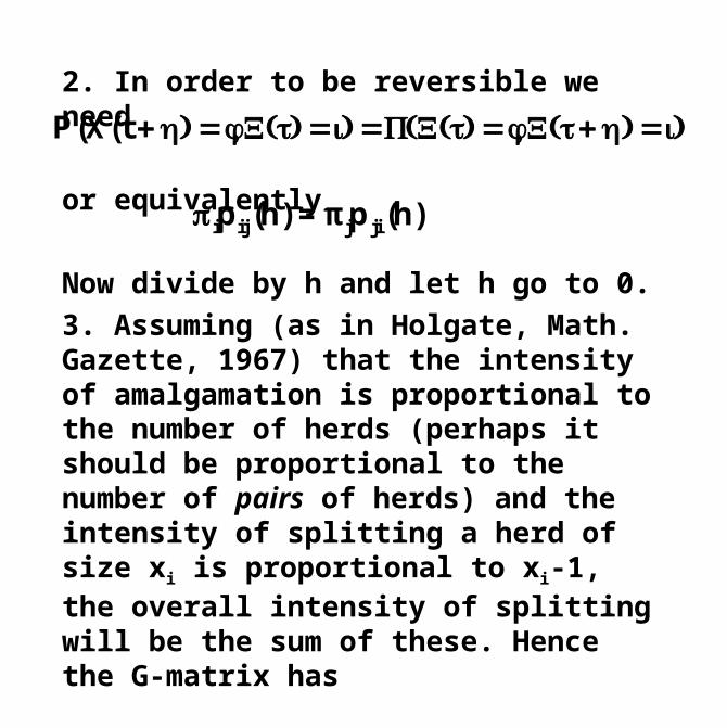
2. In order to be reversible we need

or equivalently

Now divide by h and let h go to 0.

3. Assuming (as in Holgate, Math. Gazette, 1967) that the intensity of amalgamation is proportional to the number of herds (perhaps it should be proportional to the number of pairs of herds) and the intensity of splitting a herd of size xi is proportional to xi-1, the overall intensity of splitting will be the sum of these. Hence the G-matrix has

P(X(t +h) =j,X(t) =i) =P(X(t) =j,X(t+h) =i)

π ipij (h) = πjp ji (h)

so the equations for the stationary distribution are (using Holgate’s model)

whence the stationary distribution is 1+Bin(K-1,).

gi,i+1 = (xj −1)j=1

i

∑ =(K −i)

gi,i−1 =(i−1) (or i(i−1) / 2)

π2 = π1

λ

μ(K − 1)

πk = π1

K − 1

k − 1

⎛⎝⎜

⎞⎠⎟

λ

μ

⎛⎝⎜

⎞⎠⎟

K−1

Brown’s motion

Richard Brown (1773-1858)Scottish botanistFirst systematic description of Australian faunaNamed the cell nucleusObserved irregular pollen motion in liquid (first described by Ingenhousz in 1784)

Observed motion

Interpretation

The basic unit of living matter (molecule)

Same motion with dust particles (or carbon on oil)

Ongoing motion in closed box “forever”

Explained by: fluctuating temperature due to heating by incident light; electrical forces; temperature difference in the liquid.

Delsaux (1877): impact of molecules of liquid on immersed particles–lots of small bumps

Einstein’s contribution

1905: Annus mirabilis1. Photoelectric effect2. Special relativity3. E=mc2

4. “On the Motion —Required by the Molecular Kinetic Theory of Heat— of Small Particles Suspended in a Stationary Liquid”

Some physics

Two forces act on suspended particles:

osmotic pressure (tendency towards equal concentration)

diffusion (particles hit by heat-induced movement of liquid molecules)

If q(x) is the density of particles per unit volume, the osmotic force is

(R gas constant, T abs temp, N Avogadro’s number)

This force causes flux

−RT

N′q (x)

−RT

6πrNη′q (x)

More physics

The flux due to diffusion with diffusion coefficient D is

These two fluxes must be equal in equilibrium, so

If we know D and r we can compute N (which was not known in 1905).

−D ′q (x)

D =RT

6πrNη

Einstein’s stochastic model

Over a short time period , a particle is displaced by a random quantity Y. It should have mean 0 in equilibrium. Assume for simplicity with probability 1/2 each. Let x be a point. Only particles in (x-y,x) can pass x from left to right in a time interval . Only half of those particles will in fact move from left to right, i.e. about

particles.

Similarly, about particles move from right to left.

Y =±y

12 q(x −y

2 )y12 q(x + y

2 )y

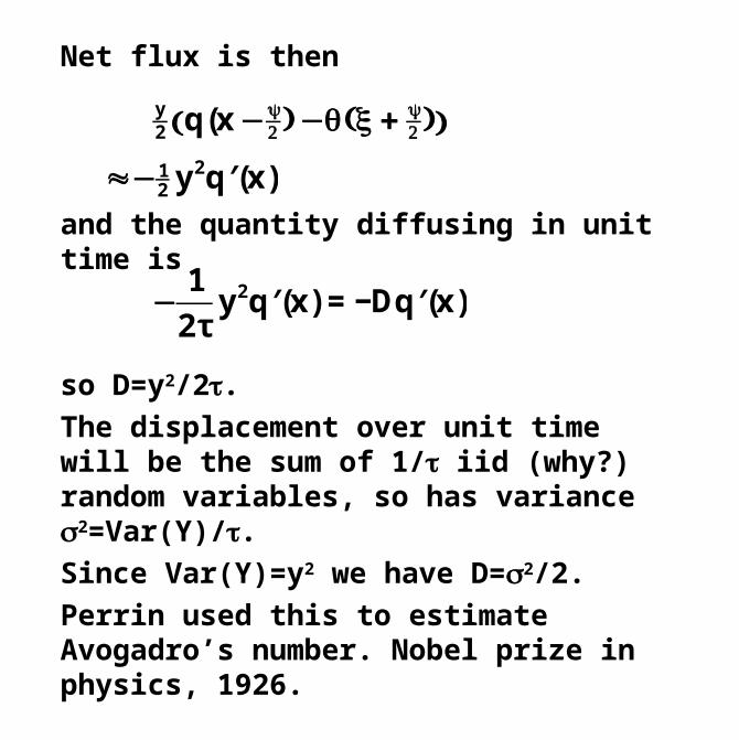
Net flux is then

and the quantity diffusing in unit time is

so D=y2/2. The displacement over unit time will be the sum of 1/ iid (why?) random variables, so has variance 2=Var(Y)/. Since Var(Y)=y2 we have D=2/2.

Perrin used this to estimate Avogadro’s number. Nobel prize in physics, 1926.

y2 q(x −y

2 ) −q(x+y2 )( )

≈−12 y2 ′q (x)

−1

2τy2 ′q (x) = −D ′q (x)

The distribution of Brownian motion

A particle starting at the origin jumps Y units in time . The pgf of Y is

In time t, the particle takes t/independent steps. The total displacement has pgf

with mean 0 and variance ty2/. In order to have the variance converge to 2t we need y=1/2. Then

Esy = 12 s

y + 12 s

−y

X(t) = Yii=1

t/ ∑EsX(t) = 1

2 sy + 1

2 s−y( )

t/

EsX(t) = 12 s

+ 12 s

− ( )

t/

An excursion

Let X~N(2). Then

E(eθX ) = eθx∫ φx−

⎛⎝⎜

⎞⎠⎟dx

= eθ(uσ+μ)∫ φ(u)du

=eθμ

2πeθuσe− 1

2u2

du∫

=eθμ

2πe− 1

2(u−θσ)2

e12θ2σ2

du∫

=eθμ+ 12θ2σ2

Let s=eθ. This yields the moment generating function. We get

Exponentiating back we get the mgf for a N(0,2t)-random variable.

One can use this type of limit to calculate the forward equation for the process, which turns out to be the heat equation.

logEeθX(t) =tlog 1

2 eθ + 1

2 e−θ

( )

=tlog 1+

θ222

+O(3 / 2 )⎛

⎝⎜⎞

⎠⎟

=θ2σ2t

2+ O( τ )

A general definition

A Brownian motion process is a stochastic process having:

(1) Independent increments

(2) Stationary increments

(3) Continuity: for any 0limΔt↓0

P(X(t+ Δt) −X(t) ≥) =o(Δt)

Some Brownian motion process paths

Properties of Brownian motion process

X(t)~N(t,2t)

Continuous paths

Finite squared variation

Not bounded variation

Not differentiable paths

Derivative of location is velocity, so for small time intervals this is not defined (not a very accurate model!)

Is it Markov?

More realistic assumption

Stationarity is the probability counterpart to conservation of momentum (mass x velocity)

Instead of independent increments of location, we could consider independent increments of momentum

Velocity change in particle would be twice the speed of the molecule times the ratio of molecule to particle mass

The Ornstein-Uhlenbeck approach

Let U(t) be the velocity of a particle. Langevin’s equation says

where K*(t) is a stochastic process with mean zero and very quickly decreasing covariance (collisions from independent molecules)

Divide through by m to get =*/m and K(t)=K*(t)/m. Multiply by exp(t), so

mdU(t)

dt=−∗U(t) +K∗(t)

d

dtetU(t)( ) =etK (t)

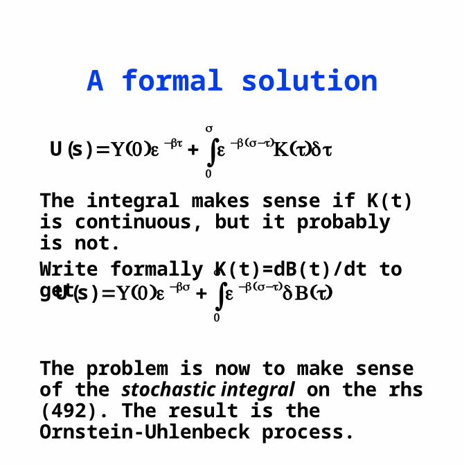
A formal solution

The integral makes sense if K(t) is continuous, but it probably is not. Write formally K(t)=dB(t)/dt to get

The problem is now to make sense of the stochastic integral on the rhs (492). The result is the Ornstein-Uhlenbeck process.

U(s) =U(0)e−t + e−(s−t)K (t)dt0

s

∫

U(s) =U(0)e−s + e−(s−t)dB(t)0

s

∫

Properties of the O-U process

It is the only stationary Gaussian Markov process in continuous time and space.

U(t) ~ N E(U(0))e−s ,2 (1−e−2s )

2⎛

⎝⎜⎞

⎠⎟

The displacement

is another Gaussian process with mean X(0) and variance

For large t this behaves like a constant times t, as Einstein found, but for small t this behaves like t2. It has a derivative (velocity). Why?

X(t) =X(0) +1−e−t

U(0) +

1−e−(t−v)

dB(v)∫

2 e−βt − 1+ βt

β2