GROUP SCHEDULING IN CELLULAR NETWORKS A THESIS IN

GROUP SCHEDULING IN CELLULAR NETWORKS

A THESIS IN

Electrical Engineering

Presented to the Faculty of the University

of Missouri—Kansas City in partial fulfillment of

the requirements for the degree

MASTER OF SCIENCE

by

Rajesh Kumar Srirambhatla

B.E., Osmania University, Hyderabad, India, 2008

Kansas City, Missouri

2012

©2012

RAJESH KUMAR SRIRAMBHATLA

ALL RIGHTS RESERVED

iii

GROUP SCHEDULING IN CELLULAR NETWORKS

Rajesh kumar Srirambhatla, Candidate for the Master of Science Degree

University of Missouri—Kansas City, 2012

ABSTRACT

With the ever increasing number of users and the usage of data in cellular

networks, meeting the expectations is a very difficult challenge. To add to the

difficulties, the available resources are very limited, so proper management of

these resources is very much needed. Scheduling is a key component and having a

scheduling scheme which can meet the Qos requirements such as Throughput,

Fairness and Delay is important.

A new dimension to scheduling known as Group Scheduling has been

designed in this project. Common scheduling schemes, which include Maximum

Carrier to Interference, Round Robin, Proportional Fair and Modified Largest

Weighted Delay First, have been studied and analyzed.

In a network where the users are divided into a number of groups, such as

Public Safety which has Fire, Health and Police, the Group Scheduling scheme is

designed to find the right balance between Throughput and Fairness. It allocates

the resources to the best available group and the best available user inside that

iv

particular group based on a contention mechanism which takes into account the

location of the user and the fast varying channel conditions for that user. The

Proportional Fair scheme has been used as the basis for this Group Scheduling

scheme and results have been simulated to show that it performs better than the

other scheduling schemes studied for this project. Also, the scheme has been

shown to be highly reliable.

v

APPROVAL PAGE

The faculty listed below, appointed by the Dean of the School of

Computing and Engineering have examined a thesis titled “ Group Scheduling in

Cellular Networks”, presented by Rajesh kumar Srirambhatla, candidate for the

master of Electrical Engineering degree, and certify that in their opinion it is

worthy of acceptance.

Supervisory Committee

Dr. Cory Beard, Ph.D.

Department of Computer Science and Electrical Engineering

Dr. Deep Medhi, Ph.D.


Dr. Ken Mitchell, Ph.D.


vi

CONTENTS

ABSTRACT ................................................................................................... iii

LIST OF ILLUSTRATIONS ......................................................................... ix

LIST OF TABLES.......................................................................................... xi

ACKNOWLEDGEMENTS .......................................................................... xii

Chapter

1. INTRODUCTION ................................................................................. 1

1.1 OFDMA ................................................................................................ 1

1.2 Importance of Scheduling in Cellular Networks .................................. 2

1.3 Project Proposal ..................................................................................... 4

2. BACKGROUND ........................................................................... …... 6

2.1 Evolution of Cellular Networks ............................................................ 6

2.2 Fading ................................................................................................... 7

2.3 Scheduling Schemes ............................................................................. 9

2.4 Public Safety ....................................................................................... 11

vii

2.5 Related Work ...................................................................................... 12

3. CODE IMPLEMENTATION .............................................................. 15

3.1 Introduction to Matlab ......................................................................... 15

3.2 Code Description ................................................................................. 15

3.3 Assumptions ........................................................................................ 19

4. RESULTS AND ANALYSIS .............................................................. 21

4.1 Individual Scheduling Schemes ......................................................... 21

4.1.1 Max C/I ............................................................................................... 21

4.1.2 Proportional Fairness Scheme ............................................................ 23

4.1.3 Modified Largest Weighed Delay First .............................................. 24

4.1.4 Round Robin ...................................................................................... 25

4.2 Comparison of Group Scheduling with Round Robin and PF ............ 26

4.3 Reliability of the Group Scheduling Scheme ....................................... 29

4.3.1 Increase the Number of Users .............................................................. 30

4.3.2 Users of One Group in Good Channel Conditions ............................... 32

viii

4.3.3 Groups of Different Sizes ................................................................... 34

4.3.4 Increase the Number of Groups ........................................................... 36

4.4 Tunable PF Metric ................................................................................. 37

5. CONCLUSION AND FUTURE SCOPE .................................................. 43

5.1 Conclusion .............................................................................................. 43

5.2 Future Scope ........................................................................................... 44

REFERENCES ............................................................................................ 45

VITA ............................................................................................................. 48

ix

ILLUSTRATIONS

Figure Page

1. Plot for actual SNR of each User1 ............................................................................... 21

2. Plot for location SNR of each user ............................................................................... 21

3. Plot for time slots of each user with max C/I ............................................................... 22

4. Plot for time slots of each user with PF ........................................................................ 23

5. Plot for throughput of each user with PF ..................................................................... 23

6. Plot for time slots of each user with MLWDF ............................................................ 24

7. Plot for average delay of each user with MLWDF ...................................................... 24

8. Plot for time slots of each user with Round Robin....................................................... 25

9. Plot for time slots of each group with Round Robin .................................................. 26

10. Plot for throughput of each group with Round Robin .................................................. 27

11. Plot for time slots of each group with PF ..................................................................... 28

12. Plot for throughput of each group with PF ................................................................... 28

13. Plot for time slots of each group with 20 Users each ................................................... 30

14. Plot for Group throughput with PF ............................................................................... 31

15. Plot for location SNR of each user in both the groups ................................................ 32

16. Plot for time slots of each group with different channel conditions ........................... 33

17. Plot for group throughput with different channel conditions ....................................... 33

18. Plot for time slots of each group with a different number of users .............................. 34

19. Plot for group throughput with a different number of users ........................................ 35

x

20. Plot for time slots with an increase in the number of groups ...................................... 36

21. Plot for group throughput with an increase in the number of groups .......................... 36

22. Plot for throughput for different combinations of tunable PF metric .......................... 40

23. Plot for Group1 time slots with the tunable PF metric ................................................. 40

24. Plot for Group1 worst case user time slots with the tunable PF metric ....................... 41

xi

TABLES

Table Page

1. Simulation results for Tunable PF metric ………………………………………..38

xii

ACKNOWLEDGEMENTS

I would like to take this opportunity to express my deep gratitude to my

advisor and mentor Dr. Cory Beard for all his guidance during the project. I thank

him for all the encouragement he had given me to finish the project successfully. I

appreciate his valuable time and his useful critiques.

I would also like to extend my thanks to Dr. Deep Medhi and Dr. Ken

Mitchell for serving as members of my thesis committee.

I would like to thank my parents MR.S.Ravinder and MRS.Vidya Ravinder

for their love and support.

Also, I would like to thank University of Missouri – Kansas City for giving

me this wonderful opportunity.

1

CHAPTER 1

INTRODUCTION

Data usage has become very predominant in cellular networks. Almost all

data applications such as VoIP, banking and online gaming are now available on

smart phones. With limited spectral resources, it is becoming extremely difficult

for the cellular operators to satisfy the data needs of users. The primary objective

of the operator is to make an efficient use of the limited spectrum while ensuring

certain QoS parameters such as throughput, fairness and delay. In order to meet

these requirements, a wide range of new techniques have been introduced. These

include

OFDMA (Orthogonal Frequency Division Multiple Access)

Multi User MIMO

Beamforming

1.1 Orthogonal Frequency Division Multiple Access

Orthogonal frequency division multiple access is the technology that is

being used in LTE and Wimax to get higher data rates over traditional Time

Division Multiple Access (TDMA) and Code Division Multiple Access (CDMA).

It is based on a multiplexing scheme that divides the bandwidth into multiple

closely spaced sub carriers which are orthogonal to each other thus avoiding

2

interference among the adjacent sub carriers. In this scheme, the available

bandwidth is divided both in time and frequency. In LTE, resources allocated to

users are in units of Resource Block which is a combination of OFDM symbols in

the time domain and sub carriers in the frequency domain. The other notable

advantages of OFDMA are its ability to reduce the impact of multipath fading and

Inter symbol Interference. ‘The main advantages of OFDMA are scalability and

robust nature towards multi-path fading’[11]. It uses parallel transmission of flows

with long symbol times to overcome multipath.

1.2 Importance of Scheduling in Cellular Networks

The distribution of the radio resources in a cellular network is done by the

base station based on a scheduling scheme. With the number of mobile users and

the demand for higher data rates increasing every day, it is important to have a

scheduling scheme which can meet the Quality of Service (QoS) requirements.

These include

Throughput

Fairness

Delay

3

Meeting the downlink QoS is largely dependent on the scheduling

mechanism deployed at the base station. The scheduling schemes that have been

studied for this project are

Maximum Carrier to Interference ratio

Proportional Fair

Modified Largest Weighed Delay First

Round Robin

Opportunistic scheduling schemes such as maximum carrier to interference

ratio assign the resources to the user with the best channel condition and therefore

maximizing the throughput. With these scheduling schemes, fairness is not taken

into consideration. On the other hand, there are scheduling schemes such as round

robin and proportional fair which treat the users fairly but in this process do not

achieve maximum throughput since the users at the edge of the cell are also given

an equal amount of resources. We could see that based on the scheduling

mechanism used at the base station there could be a tradeoff between throughput

and fairness. Hence, having a scheduling scheme that could find the right balance

among the QoS metrics is extremely important.

4

1.3 Project Proposal

A new dimension to scheduling known as group Scheduling has been

proposed in this project. This scheduling scheme is designed for a network where

the users are classified into groups such as public safety. The main objective of

this scheme is to meet the QoS requirements at the group level and also at the user

level. In our simulation, resources are allocated by the base station in time slots of

1ms windows. The group scheduling scheme is a two stage process. In the first

stage, the base station chooses which one of the groups is to be given the time slot

at any instant in time based on a metric which is a derived from the proportional

fair scheduling metric. In the second stage, a particular user inside the chosen

group is given the time slot based on different scheduling schemes which include

maximum carrier to interference ratio, proportional fair and round robin. Results

have been simulated and analyzed to show that proportional fair scheme performs

better than round robin at the group stage.

Reliability is one of the key features of the scheduler at the base station. It is

a necessity that a scheduling scheme is highly reliable and delivers the goods

under any conditions. To meet this requirement, different environments have been

simulated for this project that include

increase in the number of users

increase in the number of groups

5

different channel conditions for the users in different groups

groups of different sizes

Results have been simulated for the above conditions to prove that the proposed

group scheduling scheme is highly reliable.

In addition to the group scheduling scheme, a new metric known as tunable

proportional fair metric has been proposed in this project. This metric is a

compromise between the Max C/I and the Proportional Fair schemes. Further

research is required to find an optimal solution for the tunable PF metric.

6

CHAPTER2

BACKGROUND

2.1 Evolution of Cellular Networks

Around 1985, the first generation of cellular systems (1G) focused on

analog systems which were voice only with no data. The critical problem in 1G

was capacity. The main requirement was to increase it. These requirements

brought several new technologies: TDMA, GSM, and CDMA. The promise was to

significantly increase the efficiency of cellular telephone systems and to allow a

greater number of simultaneous conversations.

Between 1992 and 2000, 2G was developed. It supported voice, SMS, WAP

and 30-40Kbps of data. In 2001, 2.5G GPRS/1XRTT was introduced, improving

data rates up to 100-200Kbps. By 2003, evolution into 3.0G-3.5G

(UMTS/CDMA2000, HSDPA/HSUPA, 1xEVDO/Rev.A,B) provided advanced

services such as video streaming, video conference, high speed packet data up to

1-5Mbps.

More recently around 2010, 4G LTE has proposed and promised up to 100

Mbps data transfer. If you notice, through cellular network evolution, the focus

has been mainly on user satisfaction such as throughput and fairness. Data rate and

data related services became of prime importance from the end user standpoint.

7

2.2 Fading

Fading is one of the key difficulties in wireless communications. The signal

from the base station can reach the user in a number of different paths caused due

to reflection, diffraction and scattering. These are also known as multi path

components (MPC). Each MPC has its own length of travel and also direction

from the base station to the mobile user which results in a different phase shift. So,

when all these MPC’s add up at the mobile user with different phase shifts, they

could either make the signal strength at the receiver better or worse. This

phenomenon of the deviation of the signal strength in wireless communications is

known as fading.

Fading can be broadly classified into two types

large scale fading

small scale fading

Large scale fading as the name suggests is the attenuation of the signal

considered over large distances. For this project, the Okamura-Hata model is

considered to demonstrate large scale fading. This model is commonly used on

many real-world measurements. The key factors in this model are :

frequency which ranges from 150MHz to 1500MHz

height of the Base Station which ranges from 30m to 200m

height of the Mobile User which ranges from 1m to 10m

8

the distance from the Base Station which ranges from 1km to 20km

the environment is a small/medium sized city

The formula used to calculate the path loss using Okamura-Hata is:

( ) ( ) ( ( )) ( )

( ( ) ) ( )

Where

Lp is the Path loss in dB

Fc is the frequency in MHz

Hb is the height of the base station in meters (m)

Hm is the height of the mobile station in meters (m)

d is the distance between the base station and the mobile station in kilometers (km)

Small scale is the deviation of the signal strength considered over very small

distances. The profile of the multi path components which includes the phase shift

could vary due to very small movements of the mobile user as small as 10cm

which results in varying signal strength at the user. Rayleigh fading has been used

to demonstrate small scale fading in this project. Rayleigh fading is best suited to

sub-urban and urban areas where having a line of sight communication between

the base station and the mobile user is very difficult because of all of the tall

buildings in between and also in places where the originating signal from the base

station takes multiple paths because of reflection and scattering from different

objects.

9

2.3 Scheduling Schemes

‘Packet scheduling mechanisms play an important role on how to distribute

radio resources among a number of users taking into account channel conditions

and QoS requirements’ [4]. There is a trade off in spectral efficiency and fairness

which is mainly based on scheduling. Some scheduling schemes are specifically

designed to maximize the spectral efficiency, some are for fairness, and there are

others which try to find a right balance between these two. All of these kinds are

studied for this project and explained in the later sections.

Scheduling schemes can be broadly classified into two types:

channel aware scheduling schemes

channel unaware scheduling schemes

Channel Aware Scheduling schemes take the channel conditions into

account. Channel conditions include the effects of large scale and small scale

fading which is a result of factors which include

channel fluctuations

user mobility

multipath effect

These scheduling schemes exploit the varying channel conditions to meet

certain QoS parameters such as throughput, fairness etc.

10

Some of the channel aware scheduling studied for this project are Max C/I,

Proportional Fairness and Modified Largest Weighed Delay First (MLWDF).

Max C/I, where C/I is the carrier to interference ratio, serves the user with

the best channel condition in every time slot. This maximizes the overall

throughput of the system. The disadvantage of using this scheme is that it does not

treat the users fairly. There is a possibility that the user with poor channel

conditions will not be given any bandwidth.

The Proportional Fair scheme, also abbreviated as PF, chooses the user with

the best PF metric. The PF metric is defined as the throughput achieved by the

user in the current time slot divided by the average throughput of that user. The

PF scheme achieves high throughput while ensuring fairness among all the users.

PF scheme exploits multi-user diversity by giving the time slot to the user who can

make the best use of the channel at that instant. The formula used in Proportional

fair scheme to choose a particular user is

[7]

Where Ri is the rate achievable by user I and Ai is the average rate of user i.

The main function of the Modified Largest Weighted Delay First scheme is

to give larger priority to the user with the largest waiting time in the given time

slot. In this scheme delay is also taken as the QoS metric. The metric used in this

scheme is the same as the PF metric times a factor of delay which makes a user

much higher priority as it nears the deadline. ‘Modified Largest Weighted Delay

11

First is throughput optimal, namely it ensures that the queues are stable as long as

the vector of average arrival rates is within the system maximum stability region’

[9]. The formula used to choose a particular user in this scheme is

( (

) (

))

Where pi is a constant, Wi is actual waiting time and Di is the deadline.

Round Robin (RR) is the channel unaware scheduling scheme studied in this

project. The Round Robin scheme polls the Users one after the other sequentially.

It does not take the channel conditions into account. It is an absolutely fair scheme

where all the users are treated the same. As it does not take the fast varying

channel conditions into account, the Throughput is very low. ‘The Round Robin

method is considerably simpler than earlier strategies to achieve global fairness’

[10].

2.4 Public Safety

Public safety is one of the key sectors and it plays an important role in our

day to day life. The key objective of public safety groups which includes fire,

health and police is to respond to the emergency situations as soon as possible.

Communication plays a vital role in this aspect. Quality of service which includes

guaranteed throughput and fairness is very important in public safety

communications. The scheduling scheme proposed in this project emphasizes on

this aspect. ‘The lack of interoperability between emergency response departments

12

were not fully appreciated until recent crisis highlighted the importance of

coordinated operations on a broad scale’ [2]. This objective has been taken care of

by the group scheduling developed in this project which unifies all the three

departments in a single system and maintains the right balance while sharing the

resources. ‘In an envisioned future, public safety communications use the same

technologies as the consumer market, allowing cost reductions and improved data

service capabilities’ [3]. These technologies include EVDO, HSPA and LTE.

Since, the spectrum allocated for public safety is very limited, it is very important

to use it very effectively while meeting the objectives. Reliability is one of the key

factors for any means of communications and it is very important for public safety

communications. The Group scheduling scheme developed in this project ensures

that it is reliable under different conditions.

2.5 Related Work

There has been a lot of research and effort been put into scheduling in

wireless and cellular networks. With the users and data usage increasing rapidly

and the available resources such as spectrum being very limited, the main focus

would be on spectral efficiency and fairness. Here are a few papers which talk

about different methods how scheduling can effectively be used.

13

In paper [11], different scheduling mechanisms are studied that can be

implemented in mobile Wimax networks to allocate resources to meet the QoS

requirements such as delay, and throughput. These scheduling schemes include

round robin and proportional fair.

In paper [5], the authors present the fair throughput scheduling model. This

scheme allocates the resources to the user with the least average throughput in the

past interval of time. It is also shown that using the fair throughput scheduling

model, equal amount of resources will be allocated to all the users in the longer

term.

In paper [4], an analysis of various scheduling schemes in LTE cellular

networks is presented. It provides an overview of the key issues in the allocation

of resources in LTE networks. The paper also presents the challenges of using a

more complex scheduling algorithm for example modified largest weighted delay

first which yields a better result in terms of QoS compared to a less complex round

robin method. The authors present a thorough understanding of the resource

sharing problem in LTE networks.

Scheduling proves to be one of the most challenging areas in wireless

networks and lot of research has been put into this aspect. The concept of group

scheduling is new, however, and is discussed in this project to add a new

dimension to it which could be more prominent in areas like public safety

14

communications. The proposed group scheduling scheme has good scope in it to

attract the researchers to come up with even better results.

15

CHAPTER 3

CODE IMPLEMENTATION

3.1 Introduction to MATLAB

MATLAB has been used as the programming tool to write and simulate the

code for this project. MATLAB or also known as matrix laboratory is a

programming tool which has been developed by Mathworks. MATLAB is widely

used in academic and research projects. MATLAB has hundreds of inbuilt

functions which can be used to develop codes and also to plot the data. MATLAB

is a user friendly tool which is the main reason for using it for this project.

3.2 Code Description

A group scheduling scheme to optimize fairness and throughput has been

designed in matlab for this project. Below is the description of the code

implemented for this project:

a total number of 20 users are divided into two groups

each user is placed at a certain distance(in km) from the base station

distancefromBS=[8 5 4 10 2 6 7 9 12 11 5.5 2.3 3.4 8 9.5 10.5 7 5 6

13];

based on the distance from the base station, location SNR is calculated for

each user using the Okamura-Hata model.

16

SNR: Signal to Noise Ratio is the ratio of the Signal power to the Noise

power. The higher the ratio, the better is the quality of the signal.

Okamura-Hata model: This model has been used in this project to emulate

large scale fading. Fading in wireless communications is the deviation of

the signal strength over a period of time. It is broadly classified into large

scale and Small scale fading. Large scale fading observed over long

distances. The following is the code used for large scale fading:

for j=1:N Fc=950; Hb=60; Hm=5; EIRP=30; Gm=0; a= ((1.1*log10(Fc)-0.7)*Hm)-(1.56*log10(Fc)-0.8); A = 69.55+26.16*log10(Fc)-13.82*log10(Hb)-a; B = 44.9-6.55*log10(Hb); C = 0; L = A+B*log10(distancefromBS(j))+C; Pr = EIRP-L+Gm; Pn = -174+10*log10(200e3); % Pn = -174+10*log10(950e6); SNR = Pr-Pn; locationSNR(j)=SNR; end

The main factor in large scale fading is the distance at which the user is

from the base station. The greater the distance, the lower would be the

Location SNR.

After calculating each user’s Location SNR using large scale fading,

Actual SNR for each user is calculated and it is based on location SNR

plus small scale fading. The Rayleigh fading model has been used in this

17

project to emulate small scale fading. Small scale fading is caused due the

multiple contributions of the signal coming in different directions which is

a result of reflection, scattering and diffraction. A combination of all these

factors results in the deviation of the received signal strength even when

the user moves by a fraction of the wavelength. Rayliegh fading is

simulated using Clarke’s model [16]

Figure 3.1 Plot for the ActualSNR of User1 for 40 time slots

once the actual SNR has been calculated for each user, the downlink

throughput for that user will be mapped based on the code and table below:

if (actualSNR(j)>SNRclasses(1)) actualthroughput(j) = DLthroughput(1); else for k=1:length(SNRclasses)-1 if (actualSNR(j)<=SNRclasses(k)) &

(actualSNR(j)>SNRclasses(k+1)) actualthroughput(j) = DLthroughput(k+1); end end end if (actualSNR(j)<SNRclasses(length(SNRclasses)))

-35

-30

-25

-20

-15

-10

-5

0

5

10

15

ActualSNR for User1

ActualSNR

18

actualthroughput(j) = 0; end

This table is used to map SNR to throughput. Different modulation

schemes can be used for different throughput. This table comes from

Wimax documents [17]

SNRclasses= [24.4 22.7 18.2 16.4 11.2 9.4 6.4]; DLthroughput=[14.26 12.6 9.5 6.34 4.75 3.17 1.41];

The next step is to decide which one of the groups is given the

instantaneous time slot. The proportional fair scheme has been used for

this. PF metric for all the users is calculated for each time slot. The top

three users with best PF metric in each group are chosen and added up to

get the final metric for each group. The group with the best final metric is

given the time slot.

PFmetric1 = sort(PFmetric(1:N/2),'descend'); PFmetric2=sort(PFmetric(N/2+1:N),'descend'); Finalmetric1 = PFmetric1(1)+PFmetric1(2)+PFmetric1(3); Finalmetric2 = PFmetric2(1)+PFmetric2(2)+PFmetric2(3);

G = max(Finalmetric1,Finalmetric2);

once the group has been decided, the next step is to choose a particular user

inside that group which is based on the scheduling scheme used inside the

group. Four kinds of scheduling schemes have been used inside the Group

for this project.

Max C/I

[Ydummy,I]=max(actualthroughput(:,1:N));

19

Round robin

Proportional fair

PFmetric =

actualthroughput./(pastthroughput./(i*timeslot));

Modified Weighed Largest Delay First

deadlinemetric=((timestamp-(Qgroup1-

packetdeadline))./packetdeadline).*actualthroughput1./(p

astthroughput1/(i*timeslot));

The last step in the code is to calculate the group throughput which is

summing up the user throughput selected for that group and also the total

throughput, which is the addition of both the groups’ throughputs. In

addition to this, time slots that have been given to a particular user and also

to the group are also calculated.

timeslots(I) = timeslots(I)+1; Group1throughput=Group1throughput+actualthroughput(I)*timeslot;

Group2throughput=Group2throughput+actualthroughput(I)*timeslot;

Totalthroughput = Group1throughput+Group2throughput;

The code designed for this project is a bit complex since it involves

computing all the above calculations for every 1ms window.

3.3 Assumptions

There have been some assumptions made for this project. They are listed

below

users have traffic inflow all the time (greedy sources)

20

scheduling is only limited to downlink and this project does not cover

uplink

this simulation model does not include the effect of shadowing

the fading model used in this project is more suited for sub-urban areas

the distance between the user and the base station was chosen at random,

but then has been maintained the same for all the simulations to have

consistency across all the results

21

CHAPTER4

RESULTS AND ANALYSIS

4.1 Individual Scheduling Schemes

In this section, we see the performance of the individual schemes studied for

this project. There are 20 users distributed around the base station.

4.1.1 Max C/I

Figure 4.1 Plot for the location SNR of each user

0

5

10

15

20

25

30

1 2 3 4 5 6 7 8 9 10 11 12 13 14 15 16 17 18 19 20

Loca

tio

n S

NR

User

Plot of user vs location SNR

22

Figure 4.2 Plot for the time slots given to each user with Max C/I

From Figure 4.1 and 4.2, we can see that user 5, who has the best location

SNR, has the maximum number of time slots. Users who have a very low location

SNR did not get a considerable number of time slots. Some of them received zero

time slots. Max C/I takes the channel conditions of each user into account and

choose the user with the best conditions. The total throughput with Max C/I is

13.78Mbps.

0

1000

2000

3000

4000

5000

6000

7000

8000

1 2 3 4 5 6 7 8 9 10 11 12 13 14 15 16 17 18 19 20

Tim

e s

lots

User

Plot of user vs time slots

23

4.1.2 Proportional Fairness Scheme

Figure 4.3 Plot for time slots of each user with PF

Figure 4.4 Plot for throughput of each user with PF

From the Figure 4.3, we can see that the minimum number of slots that a user has

is 422 and the maximum is 569, which is very fair compared to Max C/I. Also, it

0

100

200

300

400

500

600

1 2 3 4 5 6 7 8 9 10 11 12 13 14 15 16 17 18 19 20

Tim

e s

lots

User


0

0.2

0.4

0.6

0.8

1

1 2 3 4 5 6 7 8 9 10 11 12 13 14 15 16 17 18 19 20

Thro

ugh

pu

t(M

bp

s)

User

Plot of user vs throughput

24

can be seen that all the users have a fair share of slots but with a drop in total

throughput from 13.78 for max C/I to 7.88Mbps.

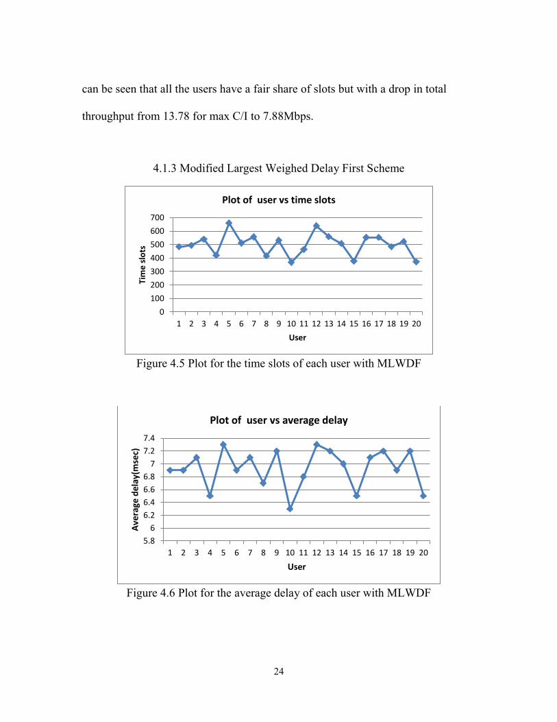
4.1.3 Modified Largest Weighed Delay First Scheme

Figure 4.5 Plot for the time slots of each user with MLWDF

Figure 4.6 Plot for the average delay of each user with MLWDF

0

100

200

300

400

500

600

700

1 2 3 4 5 6 7 8 9 10 11 12 13 14 15 16 17 18 19 20

Tim

e s

lots

User


5.8

6

6.2

6.4

6.6

6.8

7

7.2

7.4

1 2 3 4 5 6 7 8 9 10 11 12 13 14 15 16 17 18 19 20

Ave

rage

del

ay(m

sec)

User

Plot of user vs average delay

25

From the above figures, we can see that the average delay for each user is

around 7ms with the given packet deadline of 10ms. All the users had the same

packet deadline. Also, every user got a fair share of the time slots. The total

throughput with MLWDF is 7.66Mbps which is slightly less than the PF scheme

(7.66 compared to 7.88Mbps).

4.1.4 Round Robin Scheme

Figure 4.7 Plot for time slots of each user with Round Robin

From the figure above, it can be seen that with Round Robin all the users

got equal number of time slots. The total throughput with this scheme is 3.75Mbps

which is considerably low. When compared to the PF scheme, fairness is a bit

better but the total throughput drops by close to 50% from 7.88 Mbps to 3.75

Mbps, which makes PF a much better choice.

0

100

200

300

400

500

600

1 2 3 4 5 6 7 8 9 10 11 12 13 14 15 16 17 18 19 20

Tim

e sl

ots

User


26

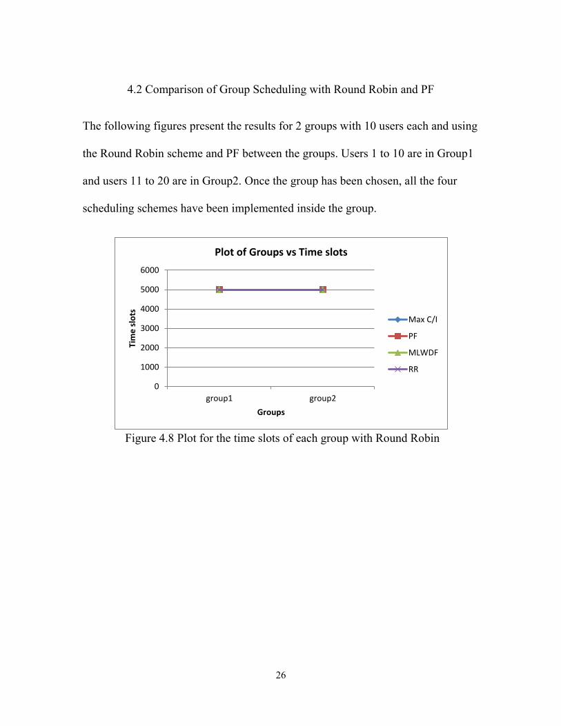
4.2 Comparison of Group Scheduling with Round Robin and PF

The following figures present the results for 2 groups with 10 users each and using

the Round Robin scheme and PF between the groups. Users 1 to 10 are in Group1

and users 11 to 20 are in Group2. Once the group has been chosen, all the four

scheduling schemes have been implemented inside the group.

Figure 4.8 Plot for the time slots of each group with Round Robin

0

1000

2000

3000

4000

5000

6000

group1 group2

Tim

e s

lots

Groups

Plot of Groups vs Time slots

Max C/I

PF

MLWDF

RR

27

Figure 4.9 Plot for the throughput of each group with round robin

Below is the total throughput of the system with round robin between the

groups

with max C/I inside the group it is 12.64Mbps

with round robin inside the group it is 3.74 Mbps

with proportional fair inside the group it is 7.57 Mbps

with MLWDF inside the group it is 7.37 Mbps

0

1

2

3

4

5

6

7

group1 group2

Thro

ugh

pu

t(M

bp

s)

Groups

Plot of Groups vs Throughput

Max C/I

PF

MLWDF

RR

28

Figure 4.10 Plot for the time slots of each group with PF

Note how the scheduling scheme inside the group affects the choice of

groups.

Figure 4.11 Plot for the throughput of each group with PF

Below is the total throughput of the system with PF between the groups

with max C/I inside the group it is 12.64Mbps

0

1000

2000

3000

4000

5000

6000

group1 group2

Tim

e s

lots

Groups


Max C/I

PF

MLWDF

RR

0

1

2

3

4

5

6

7

8

group1 group2

Thro

ugh

pu

t(M

bp

s)

Groups


Max C/I

PF

MLWDF

RR

29




From the above numbers, it can be seen that there is an increase in

throughput in each of the groups and also the total throughput when using

Proportional Fairness scheme between the groups as compared to using Round

Robin. Also, there is not much difference in the time slots for each of the groups

using both the schemes. This implies that both the schemes are being fair to the

groups. PF takes the channel conditions and round robin does not. Taking all these

things into consideration, we come to a conclusion that using PF yields better

results as compared to using round robin between the groups.

To summarize the group scheduling mechanism, proportional fairness will

be used in the first stage to decide the group and in the second stage, all the four

scheduling schemes discussed in the project are used to choose a particular user

inside the group.

4.3 Reliability of the Group Scheduling Scheme

To prove the reliability of this group scheduling mechanism with PF between

the groups, different conditions have been taken into considerations that include

increase the number of Users

30

have users in one group in better conditions as compared to the other group

have groups with different sizes

increase the number of Groups.

4.3.1 Increase the Number of Users

For this scenario, the number of users has been increased to 40 and they are

split into two groups of 20 Users each. The following figures present the results

for this test case.

Figure 4.12 Plot for the times slots of each group of 20 users with PF

0

1000

2000

3000

4000

5000

6000

7000

group1 group2

Tim

e s

lots

Groups


Max C/I

PF

MLWDF

RR

31

Figure 4.13 Plot for the Group Throughput with PF

Below are the total throughputs for this scenario

with max C/I inside the group it is 13.81 Mbps




From the above figures, it can be seen though the number of users has

increased to 40, time slots assigned to both the groups has been very consistent.

Also, there has been an increase in the total throughput with all the schemes as

compared to having 20 users. Note also that Max C/I inside the group still causes

unequal allocations.

0

1

2

3

4

5

6

7

8

9

group1 group2

Thro

ugh

pu

t(M

bp

s)

Groups


Max C/I

PF

MLWDF

RR

32

4.3.2 Users of One Group in Good Channel Conditions Compared to the Other

For this condition, users in group 1 are located close to the base station

which results in high location SNR as compared to the users in group 2 located far

away which results in very poor location SNR. The following figures present the

results on how the PF scheme performs for this particular scenario.

Figure 4.14 Plot for the location SNR of the users in both the groups

0

5

10

15

20

25

30

1 2 3 4 5 6 7 8 9 10

Loca

tio

n S

NR

User

Plot of User vs Location SNR

Group1

Group2

33

Figure 4.15 Plot for time slots of each group with different channel conditions

Figure 4.16 Plot for the group throughput with PF under different channel

conditions

0

1000

2000

3000

4000

5000

6000

7000

8000

9000

10000

group1 group2

Tim

e s

lots

Groups


Max C/I

PF

MLWDF

RR

0

2

4

6

8

10

12

14

group1 group2

Thro

ugh

pu

t(M

bp

s)

Groups


Max C/I

PF

MLWDF

RR

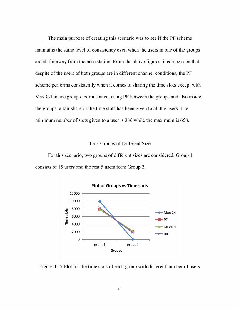
34

The main purpose of creating this scenario was to see if the PF scheme

maintains the same level of consistency even when the users in one of the groups

are all far away from the base station. From the above figures, it can be seen that

despite of the users of both groups are in different channel conditions, the PF

scheme performs consistently when it comes to sharing the time slots except with

Max C/I inside groups. For instance, using PF between the groups and also inside

the groups, a fair share of the time slots has been given to all the users. The

minimum number of slots given to a user is 386 while the maximum is 658.

4.3.3 Groups of Different Size

For this scenario, two groups of different sizes are considered. Group 1

consists of 15 users and the rest 5 users form Group 2.

Figure 4.17 Plot for the time slots of each group with different number of users

0

2000

4000

6000

8000

10000

12000

group1 group2

Tim

e s

lots

Groups


Max C/I

PF

MLWDF

RR

35

Figure 4.18 Plot for the group throughput with different number of users

This condition is studied to ensure that PF scheme performs consistently

even when the group sizes are different. From the results above, it could be seen

that the time slots assigned to each of the groups is consistent with the ratio of the

number of users inside the groups. For instance, using PF scheme inside the group

the number of slots for Group1 is 7831 and for Group2, it is 2169 which is

consistent with what one would expect (7500 to 2500). This means that with more

users, the proportion of time the top 3 PF metrics per group are proportional to the

number of users.

0

2

4

6

8

10

12

14

16

group1 group2

Thro

ugh

pu

t(M

bp

s)

Groups


Max C/I

PF

MLWDF

RR

36

4.3.4 Increase the Number of Groups

For this simulation, the number of groups has been increased from 2 to 4.

So, each group has a total of 5 users.

Figure 4.19 Plot for the time slots with increase in the number of groups

Figure 4.20 Plot for group throughput with increase in the number of

groups

0

1000

2000

3000

4000

5000

group1 group2 group3 group4

Tim

e s

lots

Groups


Max C/I

PF

MLWDF

RR

0

1

2

3

4

5

6

group1 group2 group3 group4

Thro

ugh

pu

t(M

bp

s)

Groups


Max C/I

PF

MLWDF

RR

37

The number of time slots that each of the four groups is close to 2500 which

is really good, except for Max C/I. These results prove that PF scheme works the

same way even though the number of groups has been increased.

All the above scenarios show that group scheduling scheme with

proportional fairness between the groups works consistent under different

conditions proving the reliability of the scheme.

4.4 Tunable PF Metric

Tunable PF metric is a compromise between the Max C/I and the

proportional fairness schemes. The metric used to decide the user in Max C/I only

takes instantaneous data rate of the user into consideration where as in PF scheme,

instantaneous data rate as well as the average throughput of the user are

considered. Max C/I gives us the best throughput possible where as PF ensures

fairness among the users in terms of resource allocation while taking channel

conditions into account.

Metric used for Max C/I = Instantaneous data rate of the user

PF metric = Instantaneous data rate of the user/ Average throughput of the user

If we carefully analyze both the metrics, PF metric is the same as Max C/I

divided by the average throughput. Tunable PF metric is a solution to find the

38

right balance between Max C/I and PF such that the fairness among the users is

still maintained while increasing the overall throughput of the system.

( )

Tunable PF Metric = Instantaneous data rate of the user/ {X + (1-X)* Average

throughput of the user}

In the above equation, if X =0 it becomes PF metric and if X=1 makes it the

metric for Max C/I. For this project, we have used tunable PF metric both between

the groups and also inside the groups. Simulations have been done for different

combinations of the tunable PF metric between and inside the group. The table

below presents the results

Table 4.1 Simulation results for tunable PF metric

Combination

ID

Tunable

PF metric

inside the

group

Tunable

PF metric

between

the groups

Throughput(

Mbps)

Group1 time

slots

Worst case user

Group1

Worst case

user Group2

1 1*AT 1*AT 7.86 4986 423 420

2 1*AT 0.9*AT 7.89 4926 401 406

3 1*AT 0.8*AT 7.92 4821 344 420

4 1*AT 0.7*AT 8 4786 322 379

5 1*AT 0.6*AT 8 4705 326 355

6 1*AT 0.5*AT 7.98 4580 297 320

7 0.95*AT 1*AT 8.08 4998 362 354

8 0.95*AT 0.9*AT 8.15 4887 351 374

9 0.95*AT 0.8*AT 8.22 4853 330 357

10 0.95*AT 0.7*AT 8.17 4750 307 381

11 0.95*AT 0.6*AT 8.18 4696 299 345

12 0.95*AT 0.5*AT 8.2 4562 290 343

13 0.9*AT 1*AT 8.3 5019 352 310

14 0.9*AT 0.9*AT 8.4 4893 319 310

39

Combination

ID

Tunable

PF metric

inside the

group

Tunable

PF metric

between

the groups

Throughput(

Mbps)

Group1 time

slots

Worst case user

Group1

Worst case

user Group2

15 0.9*AT 0.8*AT 8.44 4851 315 310

16 0.9*AT 0.7*AT 8.45 4727 281 313

17 0.9*AT 0.6*AT 8.45 4593 266 327

18 0.9*AT 0.5*AT 8.44 4588 242 318

19 0.85*AT 1*AT 8.58 4983 288 235

20 0.85*AT 0.9*AT 8.60 4945 264 239

21 0.85*AT 0.8*AT 8.68 4842 260 247

22 0.85*AT 0.7*AT 8.78 4729 233 235

23 0.85*AT 0.6*AT 8.74 4659 237 262

24 0.85*AT 0.5*AT 8.78 4569 195 243

25 0.8*AT 1*AT 8.74 4918 211 232

26 0.8*AT 0.9*AT 8.86 4878 186 221

27 0.8*AT 0.8*AT 8.95 4815 176 182

28 0.8*AT 0.7*AT 9 4757 181 161

29 0.8*AT 0.6*AT 9.06 4644 175 192

30 0.8*AT 0.5*AT 9.08 4552 182 199

31 0.75*AT 1*AT 8.9 4962 213 226

32 0.75*AT 0.9*AT 9.11 4876 156 195

33 0.75*AT 0.8*AT 9.14 4735 149 187

34 0.75*AT 0.7*AT 9.26 4734 131 143

35 0.75*AT 0.6*AT 9.34 4604 98 143

36 0.75*AT 0.5*AT 9.33 4556 144 104

37 0.7*AT 1*AT 9.16 4949 189 154

38 0.7*AT 0.9*AT 9.25 4911 178 175

39 0.7*AT 0.8*AT 9.43 4727 102 174

40 0.7*AT 0.7*AT 9.5 4656 129 157

41 0.7*AT 0.6*AT 9.51 4604 111 149

42 0.7*AT 0.5*AT 9.58 4459 86 116

In the above table, AT stands for actual throughput and the tunable PF

metric only shows the denominator portion of the actual metric.

40

1*AT is the same as the original PF metric and 0.95*AT is the same as 0.05

+ 0.95*AT

Figure 4.21 Plot for throughput for different combinations of the tunable PF metric

Figure 4.22 Plot for combination ID and group1 time slots

7

7.5

8

8.5

9

9.5

10

0 10 20 30 40 50

Thro

ugh

pu

t(M

bp

s)

Combination ID

Plot of combinations vs throughput

4400

4500

4600

4700

4800

4900

5000

5100

0 10 20 30 40 50

tim

e s

lots

combination ID

plot of cominations vs group1 time slots

41

Figure 4.23 Plot for combination ID and the time slots for the worst case user in

group1

For the above simulations, 2 groups with 10 users each have been used.

From the above table and the figures, it could be seen that as we move from PF to

Max C/I there is an increase in throughput. There is a 22% increase in throughput

when using original PF metric both inside and between the groups (Throughput =

7.86) compared to when using 0.3+0.7*AT inside the group and 0.5+0.5*AT

between the groups (Throughput = 9.58) which is a considerable increase.

However the worst case in second case gets only 86 time slots.

The number of slots assigned to group1 goes down as we move from

proportional fairness to Max C/I. Careful observation of the results show that as

we move from PF scheme to Max C/I, the slots are taken from the users in poor

0

100

200

300

400

500

0 10 20 30 40 50

tim

e s

lots

combination ID

Plot for combinations vs worst case user group1 time slots

42

channel conditions, who are far away from the Base station and given to the users

who are in good conditions.

The best condition for the above results seems to be to use 0.15 + 0.85*AT

inside the group and use 0.3 + 0.7*AT between the groups. This condition yields

close to 12% increase in the total throughput, the slots assigned to Group1 is 4729

which is about only a 2.5% drop from ideal condition. Also, the slots assigned to

the Worst case User is 233 in group1 and 235 in group2 which is still a fair

amount of slots as compared to having nothing in case of Max C/I. Worst case

user for these simulations means the user who has the least amount of time slots in

a particular group.

43

CHAPTER 5

CONCLUSION AND FUTURE SCOPE

5.1 Conclusion

Meeting the demands of the users such as high data rates, fairness and low

latency is important and extremely difficult to achieve. There are a lot of

technologies such as MIMO, adaptive modulation and coding that can be used to

meet this requirements and scheduling is one among them. To have a scheduling

scheme that can make the best use of the available resources is vitally important

for a cellular network.

Group scheduling adds a new dimension to the traditional scheduler by

dividing the users into groups and meeting the QoS requirements such as

throughput and fairness at the group level and also at the user level. Proportional

fair has been chosen to decide between the groups and we have seen that it

performs better than the round robin scheme. At the user level, different

scheduling schemes have been used which meet different objectives. Max C/I

achieves the maximum overall throughput while round robin is perfectly fair. The

Proportional fair scheme finds a balance between throughput and fairness by

taking into account user’s past average throughput. Modified largest weighed

delay first scheme accomplishes the user latency requirement. Results have been

simulated to show the reliability of the group scheduling under different

44

conditions. The Tunable PF metric has also been proposed in this project and

results show that it could be used to increase the overall throughput of the system

by maintaining the aspect of fairness.

To conclude, the proposed group scheduling scheme meets the requirements

of the public safety groups by dividing the resources fairly and effectively between

the groups and also inside the group at the user level.

5.2 Future Scope

Future work that can be done based on this project includes

finding the optimal solution for the tunable PF metric

adding the aspect of Multi user MIMO and beamforming

design a group scheduling scheme that can guarantee a certain throughput

across all the groups while maintaining fairness

group scheduling in the uplink

scheduling subcarriers for OFDMA in LTE.

45

REFERENCE LIST

[1] Guangliang, Z., Lian, S. Research on Scheduling Models of Emergency

Resource. Intelligent Computation on Technology and Automation, Fourth

International Conference on, June 2011,pp.1110-1113.

[2] Miller, L., J.Haas, Z. Public Safety. Guest Editorial, IEEE Communications

Magazine, January 2006, pp.28-29.

[3] Rolf, B., Bruin, P., Eman, J., Folke, M., Hannu, H., Naslund, M., Stalnacke,

M., Synnergren, P. Public Safety Communication using Commercial Cellular

Technology. Next Generation Mobile Applications, Services, and

Technologies, Second International Conference on, September 2008, pp.291-

296.

[4] Capozzi, F., Piro, G., Grieco, L.A., Boggia, G., Camarda, P. Downlink Packet

Scheduling in LTE Cellular Networks: Key Design Issues and a Survey. IEEE

Communications Surveys & Tutorials, May 2012, pp.1-23.

[5] Ferneke, A., Klien, A., Wegmann, B., Dietrich, K. Analysis of Cellular

Mobile Networks Using Fair Throughput Scheduling. IEEE, 2012, pp.2945-

2949.

[6] Ratan, J., Holla, A., Sadakale, R., Jeyakumar, A., Performance of LTE

Downlink Scheduling Algorithm with Load. IEEE, 2011, pp.278-281.

46

[7] Bu, T., Li, L., Ramjee, R. Generalised Proportional Fair Scheduling in Third

Generation Wireless Data Networks. Computer Communications Proceedings,

25th

IEEE conference on, INFOCOM, April 2006, pp.1-12.

[8] Andrews, M., Kumaran, K., Ramanan, K., Stoylar, A., Whiting, P.,

Vijaykumar, R. Providing quality of service over a shared wireless link.

Communications Magazine, IEEE, Vol. 39,issue. 2,Feb 2001, pp.150-154.

[9] Andrews, M., Kumaran, K., Ramanan, K., Stoylar, A., Whiting, P.,

Vijaykumar, R. Scheduling in a Queuing System with Asynchronously

Varying Service Rates. Probability in the Engineering and Informational

Sciences, Vol.18, Issue.2, April 2004, pp.191-217.

[10] Hanne, E.L., Round-robin Scheduling for Max- Min Fairness in Data

Networks. Selected areas in Communications, IEEE Journal on, Vol.9, Issue.7,

September 1991,pp.1024-1039.

[11] Hujun, Y., Saivash, A., OFDMA: A Broadband Wireless Access

Technology. Sarnoff Symposium, IEEE, March 2006, pp.1-4.

[12] Spencer, Q.H., Peel, C.B., Swindlehurst, A.L., Haardt, M., An Introduction

to the Multi user MIMO Downlink. Communications Magazine, IEEE, Vol.42,

Issue.10,October 2004, pp.60-67.

47

[13] So-In, C., Jain, R., Tamimi, A.-K. Scheduling in IEEE 802.16e Mobile

WiMAX Networks: Key Issues and a Survey. Selected Areas in

Communications, IEEE Journal on, vol.27, no.2, February 2009, pp.156-171.

[14] Kwan, R., Leung, C., A Survey of Scheduling and Interference Migitation

in LTE. Research Article, May 2010, pp.1-10.

[15] Molisch, A.F., Wireless Communications. John Wiley & Sons, May 2007.

[16] Rappaport, T., Wireless Communications: Principles and Practice. Second

Edition, Prentice Hall, 2002.

[17] Shah, K., Thesis on Throughput Enhancement using Wireless Mesh

Networks. University of Missouri Kansas City, March 2008.

48

VITA

Rajesh kumar Srirambhatla was born on August 23th, 1987 in Manthani,

India. He attended St.Joseph’s Convent High School, Hyderabad and finished the

high school in 2004. He received his Bachelor degree in Electronics and

Communications Engineering from M.V.S.R Engineering College, Hyderabad,

India in 2008.

In 2009, he was admitted into the Master of Science in Electrical

Engineering department at University of Missouri Kansas City, Kansas City, MO.

He was awarded the Dean’s scholarship award for this program. He is expecting to

graduate in December 2012.

Upon the completion of the degree, he plans to work as a Network Engineer

in the future.

Documents

GROUP SCHEDULING IN CELLULAR NETWORKS A THESIS IN