Embed Size (px)
Citation preview

UNIVERSITA CA’ FOSCARI DI VENEZIA
SCUOLA DOTTORALE DI ATENEO — GRADUATE SCHOOL
VENETO GRADUATE SCHOOL OF ECONOMICS AND MANAGEMENT
Dottorato di Ricerca in Economia, Ciclo XXVII
Anno di Discussione: 2015
GROUP STRUCTURE AND COLLECTIVE BEHAVIOR
SETTORE SCIENTIFICO DISCIPLINARE DI AFFERENZA: SECS-P/01, SECS-S/06
Tesi di Dottorato di SHILEI WANG, Matricola 955949
Coordinatore del Dottorato Tutore del Dottorando
Michele Bernasconi Michele Bernasconi

A dissertation submitted to the Graduate School of Ca’ Foscari University of Venice,and the Veneto Graduate School of Economics and Management of the Universitiesof Ca’ Foscari, Padua, and Verona in partial fulfillment of the requirements for thedegree of Doctor of Philosophy in Economics.

To nothing, the mother of anything

Preface
The present dissertation is the outcome of studies on group structure and itseffects on collective behavior. Its underlying concern is that individual behaviors donot merely depend on self-interested motives, but group structure should be equallyimportant, as if, in some extreme situations, individual intentions even did not takeany effect at all. Although the main topic of the dissertation should be well-defined,different chapters might still seem diverse for some readers. However, I wish peoplewould not ask for its completeness and consistency as much as a book.
The first part of the dissertation including Chapter 1 and 2 investigates groupstructures in a more mathematical sense. Chapter 1 studies a time-dependent groupwhich can be formalized as a dynamical system, and in particular, discusses itsdynamics, stability, chaos, and some other properties in great detail. Chapter 2studies a preference-dependent group whose welfare states can be characterized bysome aggregation rule, and develops a number of assertions on its separable andadditive representations. The second part containing Chapter 3 and 4 is devoted tostudies on concrete groups which emerge institutionally from our society, viz., thecentralized limit order market with its roots in equity markets, and the hierarchicalgovernment network with its roots in political systems and organizations.
Some reported results in this dissertation have already been published, althoughthey entailed minor revisions to maintain a higher typographical quality. Concretely,Section 3 and 4 of Chapter 1 were once integrated into an independent article, andpublished as a preprint on arXiv; Chapter 3 was published as a preprint on arXiv,and later as a research paper in the journal Algorithmic Finance (Wang [66]).
It might be noted that these chapter headings are shortened so as to reflect themain “objects” of the studies. To be more precise, each chapter had ever longertitle when being prepared initially, that is, “On the iterative nature of economicdynamics” for Chapter 1, “On the axiom of separability” for Chapter 2, “Dynamicaltrading mechanism in limit order markets” for Chapter 3, and “A theory of localpublic good provision in distributed political systems” and “Complex interactions inlarge government networks” for Chapter 4.
In the period of preparing this dissertation, there are people I am deeply indebtedto, and some I even did not realize clearly at this stage. For this reason, I hesitate
iii

iv Preface
to write all their names here. But people who naturally own something never claimthat fact, do they? It surely applies here, and would help me do this usually difficulttask in a preface.
Venice, November 2014 S. Wang
Contents
Preface iii
Chapter 1. On Dynamics and Chaos 11. Introduction 12. Dynamical System 53. Iterated Function System 134. Application 21
Chapter 2. On Separability 271. Introduction 272. Axiomatic Systems 293. Thomsen Condition 324. Necessary Condition 37
Chapter 3. Trading in Limit Order Market 411. Introduction 412. Atomic Trading Scheme 433. Iterated Trading Process 534. Controlled Trading System 635. Final Remarks 70
Chapter 4. Collective Decision on Political Network 731. Introduction 732. Basic Definitions 763. Local Provision 854. Hierarchical Interaction 895. Coordinated Interaction 986. Complex Interaction 1117. Final Remarks 122
Bibliography 125
Index 129
v

CHAPTER 1
On Dynamics and Chaos
We begin with a treatment of dynamical system, as an abstract representationof time-dependent group.
1. Introduction
1.1. Determinism and Chaos. In economic science, studies are framed a lotby the philosophy of determinism, or more precisely, by causal determinism in termsof Laplace’s demon. For instance, economists describe individuals as rational agents,whose choices and social behaviors are determined by a set of fixed economic laws;the motion of an economic system is either totally determined by a representativeagent, or deterministic as well by the belief that the economic system would beessentially rational in the whole. The only indeterminacy is usually described by thevague concept randomness, and people try to add it to the economic system so as tohave a more general sense of determinism.
In this consideration, if there is a cause c, there will definitely be an effect e,simply as there exists a deterministic causal law L. But D. Hume argued that thiskind of determinacy is effective only up to empirical induction. Again, suppose c isa cause, and one observes that c always leads to an effect e in the past, then onenormally infers that c causes e, i.e., there naıvely exists a causal law L, such thatc causes e if and only if L is the causal law linking c and e. Unfortunately, ourobservations happen always in finite times, so the causal law L will not be logicallytrue, but approximately or even empirically true. From this perspective, the causalitywhich is so important in the philosophy of determinism should be thought of to bea metaphysical principle.
However, even if one had the logically true laws in a system, the outcomes mightstill not be deterministic. Suppose one has a set of fixed causal laws denoted byL again in a system, and there is a cause or an initial condition c, then by L onepredicts that there will be a result e = L(c). It might be noted that the cause ccan be known and realized only as a measurable cause m(c), which is approximatelyclose to the true c, but there is no reason that m(c) ≡ c. Then one will predict aresult L
(m(c)
), which could be totally different from the true result e = L(c), as the
error between L(m(c)
)and L(c) may not be linearly proportional to the difference
1

2 On Dynamics and Chaos
between m(c) and c. Consequently, the deterministic nature of a system may notgenerate fully predictable happenings in the future, or we can say a slight piece ofimprecise measurability in a system could eventually make the system unpredictableat all.
Such a somewhat peculiar fact was realized first by H. Poincare when he studiedthe three-body problem in the 1890s. As he wrote in the book “Science and Method”(Poincare [52], p. 68):
But it is not always so; it may happen that small differences in theinitial conditions produce very great ones in the final phenomena.A small error in the former will produce an enormous error in thelatter. Prediction becomes impossible, and we have the fortuitousphenomenon.
We can notice that this kind of (dynamical) instability in a system does not comefrom any stochastic or random factors, but from small measurable errors enlargedby certain deterministic laws. Such an unpredictable property of a system is calleddeterministic chaos , or simply just chaos .
Moreover, when one says there is a system with deterministic laws, it means thatone holds a belief that she has a full knowledge of that system as it exists, andconsistently also the chaotic properties it might have. When such a belief is neitherperfect nor absent, one should be aware that her knowledge of the system is onlypartial. One then introduces the randomness in order to smooth the relation betweenher belief and the truth, in consequence, the pseudo-chaos as is mixed by chaos andrandomness would conceptually emerge.
Suppose noises as a special form of randomness can be introduced intentionallyinto a chaotic system, so that only the laws of the system would be affected, butits states remain unchanged. Under some restricted assumptions, that system withnoises could then be characterized by a certain stochastic process, for instance, aniterated random function system might be equivalent to some Markov chain, as willbe discussed in Section 3.2 of this chapter. On the other hand, if introduced noisesonly affect the states in a chaotic system, but do not modify its laws, then the basicdeterministic skeleton could be thought of to be stable as if the noises had not beenintroduced. To a certain extent, it seems however impossible to separate noises fromchaos or vice versa, because noises entering at different times would adhere to thestates and also evolve according to the laws of the system.
1.2. Order in Chaotic System. The order in a system can be attached tosome basic properties of existent mathematical objects in that system, where theexistence of an object means that it can be defined. For instance,
(i) a function should be differentiable on its domain;
Introduction 3
(ii) the time domain, normally Z or R, should be transitive, otherwise thedynamics driven by iteration would be impossible;
(iii) the state transition function ϕt(x), which maps the initial state x into thestate ϕt(x) at t, should satisfy
ϕs(ϕt(x)) = ϕs+t(x), or ϕs ◦ ϕt = ϕs+t,
so that the state transition operator preserves the additive structure of thetime domain.
Many well-defined systems can be thought of having an appropriate order inthe above sense, because the laws that govern these systems are fairly normal inmathematical terms. However, with respect to the stability of these systems or theirpossible states after evolving for a sufficiently long time, there could still exist somemathematical objects not having a nice order, especially when the laws are nonlinearand can not be properly linearized.
Let us consider a system which has a set of fixed laws L, a state space X, anda time domain T such that the time t can be forward to s > t, or backward tor < t. The set of states A ⊆ X in the system is called an attractor , if A is invariantunder L with forward iteration, or L(A) = A, and there exists a neighborhood of A,N(A) such that all state in N(A) will converge to some state in A under L after asufficiently long time, and moreover, any proper subset of A has no such properties.The essential property of the attractor A and its neighboring trajectories in N(A)is stability. For any two close enough states x, y ∈ N(A), the stability of A requiresthat these two iterated forward motions should be uniformly close to each other.Yet such property can not be satisfied by a lot of systems, and in these hence so-called unstable systems, the attractors will very likely demonstrate bizarre geometricrepresentations. Such attractors are called strange attractors , or notably fractals aswas coined by Mandelbrot [41, 42]. Nevertheless, there is still no necessary relationbetween instability and fractals, as some stable systems could also have fractals, andmeanwhile, some unstable systems could have normal attractors (cf., Milnor [45]).
That being stated, unstable systems can yet preserve an order which is partlyindicated in some nice properties of their fractals. For instance,
(i) fractals fully embedded in the n-dimensional Euclidean space can have aHausdorff-Besicovitch dimension between n − 1 and n for n ≥ 1, e.g., theKoch curve has a dimension log 4/ log 3 ≈ 1.262 in the Euclidean plane;
(ii) fractals are continuous and nowhere differentiable;(iii) most fractals are self-similar, and their scaled parts always have similar
structures to the wholes.
1.3. Chaos in Social System. Unlike mathematically-defined systems, socialsystems, such as social groups, social networks, and organized markets, are complex
4 On Dynamics and Chaos
by nature. In general, the governing laws for a social system can not be directlyderived by aggregation of the laws for its agents, even if one could have a perfectknowledge of the social system. What’s more, repeated interactions among manyagents, learning to adapt their strategies, and self-organization pattern formationsin a large social system will make its laws evolve themselves, and therefore agents’knowledge may not necessarily match the laws time by time. As a social system isnow investigated from a complex perspective, its properties such like self-adaptationand self-regulation would turn out to be evidently important, and its different scalesmay show a disordered structure or even random pattern. If the disordered structurerooted in different scales could be ideally removed, then the relation between thewhole social system and its parts would be stable, and thus the complex socialsystem could be refined to a chaotic social system. The finer chaotic social systemshould be more easily represented by some mathematically-defined system, in caseits social attributes could be formalized to some extent1.
Example 1.1. The cobweb theorem was first studied by Leontief [37], Kaldor[31], and Ezekiel [17] in the 1930s, when they investigated the interactive dynamicsof price and quantity in a single market. Let (pt, qt) denote the pair of price andquantity in a market at time t. Suppose the market is controlled by the demand lawD and the supply law S in a delayed way, that is,
pt = D(qt), qt+1 = S(pt),
then pt+1 = D(S(pt)
), or pt+1 = C(pt) for C = D ◦ S.
Assume C takes the form of Logistic map, then
(1.1) pt+1 = rpt(1− pt) (r > 0).
Suppose the price is normalized so that it is in the real interval [0, 1]. Notice thatpt(1 − pt) ≤ 1/4 for all pt ∈ [0, 1], so we need r ∈ (0, 4] to ensure that pt is alwaysin [0, 1]. If r ∈ (0, 1], pt will converge to 0 and the good in the market will be freein the long term. If r ∈ (1, 3], pt will converge to either 0 or some stable price in(0, 1). However, if r ∈ (3, 4], the market will have bifurcations. The cardinality ofits attractor can be 2n(r), where n(r) ∈ N is a function of r. Once n(r) is sufficientlylarge, the attractor would be almost dense on [0, 1], and hence the market would bechaotic.
Example 1.2. The price dynamics in a speculative market was first studied byBachelier [3]. One now knows that the fair price process is actually a martingale,
1There are many literatures on complex and chaotic social system in such fields of research likesystems biology, swarm intelligence, and social psychology. Since our studies in this chapter willfocus on economic and financial systems, they are not cited here, though some are quite insightful.Besides, the author should acknowledge one reviewer of this dissertation for suggesting literatureson dynamic psychological system.
Dynamical System 5
so that there is no further arbitrage opportunity on the market at any time. Inpractice, it was initially assumed that the underlying price P (t) moves approximatelyas a Brownian motion, i.e., P (t + dt) − P (t) is Gaussian with the mean 0 and the
volatility√dt. Later on, Osborne [50] showed that P (t) should follow a geometric
Brownian motion, i.e., log(P (t)
)is a Brownian motion.
As one may know, a Brownian motion is almost surely continuous and nowheredifferentiable, and thus its possible realization is essentially a fractal. Suppose thereis a dynamical system with a price space R and a time domain [0,+∞), which has anattractor R, then its price dynamics is a priori chaotic. A motion of the system canthen be represented by a realization p(t) of the stochastic process P (t). Clearly, p(t)should have some scaling properties, and might maintain a thick tail and a persistentlong-memory volatility, as are constantly observed in real financial markets (see forexample, Mandelbrot [40], and Calvet and Fisher [11]).
Recall that a Brownian motion B(t) must be invariant under any scaling, that’s
to say, B(λt) =√λB(t) for all λ > 0. A quite natural generalization for B(t) is the
fractional Brownian motion Bh(t) for h ∈ (0, 1), as was proposed by Mandelbrot andVan Ness [43], such that Bh(λt) = λhBh(t), and hence its volatility is equal to th.Another helpful consideration is to replace the real time t by a trading time τ(t),which potentially has different values at different real times.
In case h = 1/2 and τ(t) = t, one then has the Brownian motion B(t). In general,one would have a compound stochastic process Bh
(τ(t)
), which can hopefully serve
as a bridge connecting randomness to chaos, with a fair ability to catch the patternsin the price dynamics.
2. Dynamical System
2.1. General Definition. Throughout this chapter, we will use R+ and R− tomean the nonnegative and nonpositive real numbers, and use Z+ and Z− to meanthe nonnegative and nonpositive integers. For any sets X and Y , X × Y denotestheir Cartesian product. The closure of a set X is denoted by cl(X). I denotes anindex set, whose cardinality is at least 2 and at most ℵ0.
Let X be a metric space with the metric d : X ×X → R+, or simply let X be asubset of the n-dimensional Euclidean space. We call X a state space. Let T be asubset of R. If (T,+) is a semigroup, i.e., (r + s) + t = r + (s+ t) for all r, s, t ∈ T ,then we say T is a time domain. Usually, it can be R, Z, R+, or any interval in R.
The abstract definitions of continuous dynamical system can be found in thebooks by Bhatia and Szego [8], Krabs and Pickl [33], and Teschl [61]. We shallmake the definition of general dynamical system in a similar way.
Definition. A dynamical system on X is a triplet (X,T, ϕ), which is governedby the function ϕ : X × T → X with the properties:

6 On Dynamics and Chaos
(i) ϕ(x, t0) = x for all x ∈ X and any initial time t0 ∈ T ,(ii) ϕ(ϕ(x, s), t) = ϕ(x, t+ s) for all x ∈ X and all s, t ∈ T .
The function ϕ in a dynamical system (X,T, ϕ) is called a flow . For any givenstate x ∈ X we define a motion ϕx : T → X passing through x as ϕx(t) = ϕ(x, t),and for any t ∈ T we define a transition ϕt : X → X between the states at t0 and tas ϕt(x) = ϕ(x, t). Note that
ϕ(ϕ(x, s), t) = ϕ(ϕs(x), t) = ϕt(ϕs(x)),
and also ϕ(x, t+ s) = ϕt+s(x), thus ϕt ◦ϕs = ϕt+s by property (ii) of the function ϕin the above definition, and hence ϕ is a homomorphism between (T,+) and (X, ◦).
Suppose T = R, then the motion ϕx(t) passing through x at the initial time t0 is acontinuous function of t. We hence call the dynamical system a continuous dynamicalsystem, and replace ϕx(t) by x(t). As for the transition function ϕt(x), since T isnow dense, we adopt its differential term as a measure for its movement. We thusdefine x = ∂ϕt(x)/∂t = g(x, t), with the initial condition x(t0) = ϕ(x(t0), t0) = x0.Consequently, a continuous dynamical system can also be defined by an ordinarydifferential equation x = g(x, t) with x(t0) = x0.
Let W be an open subset of X × T , and (x0, t0) ∈ W . If g(x, t) is continuous onW , then by the Peano existence theorem, there exists at least one solution to makesuch a dynamical system work at a time domain [t0, t1] ⊆ T , where t1 > t0, or thereis at least one function y : [t0, t1] → X, such that y(t) = g(y(t), t) and y(t0) = x0.Moreover, if g(x, t) is Lipschitz continuous in x, i.e., there is a piecewise continuousfunction `(t) such that for all t ∈ T and all x, y ∈ X,
(1.2) d(g(x, t)− g(y, t)
)≤ `(t)d(x, y),
then by the Picard existence theorem, the solution y(t) is also unique.Suppose T = Z, then the motion ϕx(t) will be discrete, as it has values only at
dispersed times. We hence call that system a discrete dynamical system, and replaceϕx(t) by xt. As for the transition rule, we take t0 = 0, and define
f(x) = ϕ1(x) = ϕ(x, 1),
then by the fact that ϕt ◦ ϕs = ϕt+s, we have ϕt(x) = f t(x) for all t ∈ Z+. Here, f t
is defined by the recursion f t = f ◦f t−1 with f 0 = idX , where t ∈ N and idX denotesthe identity function on X. If t ∈ Z−, then −t ∈ Z+. Note that
ϕ−t(ϕt(x)
)= ϕ−t
(ϕ(x, t)
)= ϕ
(ϕ(x, t),−t
)= ϕ(x, 0) = x,
so ϕt is the inverse function of ϕ−t, and hence
ϕt = (ϕ−t)−1 = (f−t)−1 = (f−1)−t = f t,
which yields that ϕt = f t for all t ∈ Z. The dynamics driven by ϕt is called forwardfor t ∈ Z+, and backward for t ∈ Z−.
Dynamical System 7
Notice that a discrete dynamical system can be completely determined by thetransition rule f : X → X between two consecutive time points. We then have themotion xt = f t(x), where t0 = 0 and x0 = ϕ(x0, 0) = x, and usually f is assumed tobe continuous.
2.2. Basic Properties. In this subsection, we will use the notation x〈t〉 in somedefinitions to denote a generic motion ϕx(t), which can be either continuous as x(t),or discrete as xt.
Definition. For all deterministic x, the trajectory passing through x is the setof states γ(x) = {x〈t〉 : t ∈ T}.
Since T can be partitioned into T+ = T ∩ R+ and T− = T ∩ R−, γ(x) can alsobe partitioned into two semi-trajectories,
γ+(x) = {x〈t〉 : t ∈ T+}, γ−(x) = {x〈t〉 : t ∈ T−},
such that γ+(x) ∪ γ−(x) = γ(x) and γ+(x) ∩ γ−(x) ⊇ {x}.If γ(x) = {x}, x is called an equilibrium state. In terms of motion, if x is an
equilibrium state, then ϕx(t) = x〈t〉 = x for all t ∈ T . If a dynamical system startsfrom a state not in equilibrium, say y, then its trajectory γ(y) can not contain anyequilibrium state in a finite time. We can prove this claim by contradiction. Supposean equilibrium state x enters into γ(y) at a time t, which means ϕy(t) = x, thenϕt(y) = x, and thus ϕ−t(x) = y = ϕx(−t). But by the definition of equilibrium state,we should have ϕx(t) = x for all t ∈ T , a contradiction. Therefore, the motion ϕx(t)in a dynamical system either remains at the initial state x, or evolves forever.
Definition. A set of states S ⊆ X is invariant , if ϕt(S) = S for all t ∈ T .
Alternatively, we say S as a subset of X is invariant if γ(x) ⊆ S for all x ∈ S. Andthese two definitions are actually equivalent. To see this fact, suppose ϕt(S) = S,then for all x ∈ S we have ϕt(x) ∈ S for all t ∈ T , so ϕx(t) ∈ S for all t, and henceγ(x) ⊆ S for all x ∈ S. On the other hand, suppose γ(x) ⊆ S for all x ∈ S, butϕt(S) 6= S, then there is at least one pair (y, t) for y ∈ S with ϕt(y) /∈ S, whichhence implies that γ(y) * S, a contradiction.
Suppose S is an invariant set of states, and y /∈ S, then γ(y) will not move intoS in a finite time, otherwise y should be contained in S. This fact is very similar tothe reachability of an equilibrium state, but if we notice that an invariant set itselfis an equilibrium set of states, it should be not surprising. Note that any singleton{x} with an equilibrium state x is invariant, so if S is invariant, then S ∪ {x} willbe invariant again. It is thus essential to identify the kernel of an invariant set S,which should be minimal. And in general, an invariant set S is called minimal , if Shas no proper subset that is again invariant.

8 On Dynamics and Chaos
It can be shown that any bounded invariant set must have a kernel. In a discretedynamical system, any invariant set has finite or countably infinite states, thus wecan always find its minimally invariant kernel by backward induction. In a continuousdynamical system with a state space X ⊆ Rn, any invariant set should be closed andhence compact because of its boundedness, thus by Zorn’s Lemma it’s not hard tosee that its minimally invariant kernel also exists.
Definition. A motion ϕx(t) passing through x is called periodic, if there existssome s 6= 0 such that ϕx(t+ s) = ϕx(t) for all t ∈ T .
If a motion ϕx(t) is periodic, then the state x is called periodic as well, and itstrajectory γ(x) is called a limit cycle. The minimal s 6= 0 satisfying ϕx(t+s) = ϕx(t)for all t ∈ T is called the period of the motion ϕx(t). In particular, if the periodof ϕx(t) is close enough to 0, then x will be nearly an equilibrium state, and if itsperiod tends to be infinite, then the motion will be almost nonperiodic.
Definition. A state y is called an ω-limit state, if there is a sequence (ti, i ∈ I)where ti ∈ T for all i ∈ I, such that limti↑+∞ x〈ti〉 = y, and similarly, a state z iscalled an α-limit state, if limti↓−∞ x〈ti〉 = z.
The set of all the ω-limit states for a state x is called an ω-limit set , and we useω(x) to denote it. The set of all the α-limit states for a state x is called an α-limitset , and we use α(x) to denote it.
Any ω-limit set must be invariant. To show this assertion, consider ω(x), thenfor all y ∈ ω(x) there must be a sequence (ti, i ∈ I) such that limti↑+∞ x〈ti〉 = y,and thus for all s ∈ T we have limti↑+∞ ϕs(ϕti(x)) = ϕs(y), which directly yields thatlimti↑+∞ x〈ti + s〉 = ϕs(y). Since (ti + s, i ∈ I) is again a sequence in T , we haveϕs(y) ∈ ω(x) for all s ∈ T , and hence γ(y) ⊆ ω(x) for all y ∈ ω(x), which impliesω(x) is invariant by definition.
Also, we can define these two limit sets by means of the notion semi-trajectory.In a continuous dynamical system with T = R, an ω-limit set ω(x) can be definedto be
ω(x) =⋂t∈T
cl(γ+(x(t))
)=
⋂y∈γ(x)
cl(γ+(y)
),
and an α-limit set α(x) can be defined to be
α(x) =⋂
y∈γ(x)
cl(γ−(y)
).
If the motion ϕx(t) passing through x is periodic, then ω(x) = α(x) = γ(x), andω(x) and α(x) are thus both limit cycles. The reason that ω(x) and α(x) are identicalwhen the motion ϕx(t) is periodic is quite direct, that is, any state y ∈ γ(x) can be

Dynamical System 9
reached with infinite times, and hence is essentially a limit state. On the other hand,if γ(x) = ω(x) = α(x), then either ϕx(t) is periodic, or x is an equilibrium state.
Let’s now consider a continuous dynamical system (X,T, ϕ) on the Euclideanplane. The following theorem on the possibilities of ω(x) can be stated:
Theorem 1.1 (Poincare-Bendixson). In a planar dynamical system with an openstate space X ⊆ R2, a time domain R and an ODEs transition rule x = g(x), whereg : X → X is of class C1, if ω(x) 6= ∅ is compact and contains no equilibrium state,then ω(x) is a closed limit cycle.
Proof. Let y ∈ ω(x), then ω(y) 6= ∅ and ω(y) ⊆ ω(x). Assume z ∈ ω(y), thenalso z ∈ ω(x), and hence z is not an equilibrium state. Consider a Poincare section Jpassing through z, then on R2, J is a transversal segment to g, and it always exists asz is not an equilibrium state. y(t) will cross J with infinite times. Consider a sequence(ti, i ∈ I) in R, such that y(ti) ∈ J for all i ∈ I and limti↑+∞ y(ti) = z, where thePoincare map y(ti) = ϕ(y, ti) is ordered, and hence the sequence
(y(ti), i ∈ I
)along
J must be monotonic. Note that ω(x) is invariant, and y ∈ ω(x), so y(ti) ∈ ω(x) forall ti ∈ R. Hence y(ti) ∈ J ∩ ω(x).
We now show J ∩ ω(x) can not have more than one state. Suppose it has twodifferent states, say z1 and z2, then there must exist two different sequences x(ri)and x(si) converging to z1 and z2, respectively, where x(ri) and x(si) are orderedintersections of x(t) and J . But we can only have one monotonic sequence x(ti) alongJ , because all the subsequences of any monotonic sequence should have a same limit.Thus z1 must be equal to z2, a contradiction. Consequently, J ∩ ω(x) is either ∅ ora singleton.
Since z ∈ J ∩ ω(x), it must be J ∩ ω(x) = {z}, and thus y(ti) = z for all ti ∈ R.It hence suggests that γ(y) should be periodic, and γ(y) ⊆ ω(x). For all w ∈ γ(y),there always exists a Poincare section J ′ passing through w, and also a sequencex(ti) which converges to w. By the same arguments as above, we can directly haveJ ′ ∩ γ(y) = {w}, and hence γ(y) ⊇ ω(x). Recall that γ(y) ⊆ ω(x), so ω(x) = γ(y)must be a limit cycle, which completes the proof. �
Suppose now ω(x) contains equilibrium states. If ω(x) contains only equilibriumstates, then it must be a singleton with one equilibrium state, otherwise we wouldhave a connected limit set with isolated states. If ω(x) contains both equilibriumand non-equilibrium states, then for all non-equilibrium state y ∈ ω(x), ω(y) mustbe a singleton having one of the equilibrium states in ω(x).
In general, if ω(x) 6= ∅ is compact and contains finite states, then ω(x) can be
(i) ω(x) = {y}, where y is an equilibrium state;(ii) ω(x) is a limit cycle, and contains no equilibrium state;

10 On Dynamics and Chaos
(iii) ω(x) = {y1, y2, . . . , ym} ∪ γ(z1) ∪ γ(z2) ∪ · · · ∪ γ(zn), in which yi is anequilibrium state for all i ∈ {1, 2, . . . ,m}, and γ(zj) is a trajectory for allj ∈ {1, 2, . . . , n}, such that either ω(zj) or α(zj), or both are singletonshave an equilibrium state in {y1, y2, . . . , ym}.
However, if a dynamical system has a state space X ⊆ Rn for n ≥ 3, its long-termbehavior of trajectory will then begin to be quite hard to characterize.
2.3. Stability and Local Behavior. In this subsection, we focus on continuousdynamical systems, and introduce a number of concepts about stability, so that wecan use them to investigate local behaviors in a dynamical system.
The δ-neighborhood of a set S in the metric space (X, d) is defined by
N(S, δ) = {x ∈ X : d(x, S) < δ},where d(x, S) = infy∈S d(x, y). If S is occasionally a singleton, say S = {s}, we willthen have N(s, δ) = {x ∈ X : d(x, s) < δ}.
Definition. A set of states S ⊆ X is called weakly stable, if γ(x) is compact forall x ∈ S.
Once the state space X is weakly stable in a dynamical system, the system itselfwill be called weakly stable. If X ⊆ Rn, and x belongs to some weakly stable set,then the motion ϕx(t) should be bounded.
Definition. A closed set A ⊆ X is called an attractor , if it has the followingproperties:
(i) there is a set B(A) ⊆ X, such that ∅ 6= ω(x) ⊆ A for all x ∈ B(A),(ii) there is a δ > 0 such that the δ-neighborhood of A is a subset of B(A), i.e.,
N(A, δ) ⊆ B(A),(iii) there is no proper subset of A satisfying property (i) and (ii).
Here, the set B(A) is called a basin of the attractor A. If we replace property (i)and (ii) by a weaker statement that there is a δ > 0 such that ω(x) ∩ A 6= ∅ for allx ∈ N(A, δ), then A will be called a weak attractor .
Definition. An attractor A ⊆ X is called Lyapunov stable, if for all ε > 0 thereis a δ > 0, such that γ+(x) ⊆ N(A, ε) for all x ∈ N(A, δ).
Lyapunov stability states that any state in a δ-neighborhood of A will convergeto some state in a corresponding ε-neighborhood of A. If there is some state in Awhich converges to a state not in A, we then shall say A is unstable. More precisely,A is called unstable, if there is a state x /∈ A such that α(x)∩A 6= ∅. Clearly, even ifA is Lyapunov stable, there still could be some x /∈ A such that α(x) ∩N(A, ε) 6= ∅for ε > 0, and hence the ε-neighborhood of A is unstable. For this reason, we mayneed a stronger concept of stability:

Dynamical System 11
Definition. An attractor A ⊆ X is called asymptotically stable, if A is Lyapunovstable, and there is a ξ > 0, such that α(x) ∩ A = ∅ for all x ∈ N(A, ξ) \ A.
In particular, suppose {x} is an attractor in some dynamical system, then thereshould be a basin B(x) such that ω(y) = {x} for all y ∈ B(x). Lyapunov stabilityrequires that the trajectory of any state in an ε-neighborhood of {x} should stayclose enough to x, while asymptotic stability requires that γ+(x) = {x}. If x isthe unique equilibrium state in the dynamical system, and {x} is an asymptoticallystable attractor, then ω(y) = {x} and α(y) ∩ {x} = ∅ for all y ∈ B(x) \ {x}.
Let’s now consider a dynamical system (X,T, ϕ) with a state space X ⊆ Rn andan ODEs transition rule x = g(x), where g : X → X is of class C1.
A state x ∈ X is called Lyapunov stable, if for all neighborhood N(x, ε), there isa neighborhood N(x, δ) ⊆ N(x, ε), such that y(t) ∈ N(x, ε) for all y ∈ N(x, δ) andall t ∈ T .
A state x ∈ X is called asymptotically stable, if it is Lyapunov stable, and thereis a neighborhood N(x, ξ), such that limt ↑+∞ d(x, y(t)) = 0 for all y ∈ N(x, ξ).
A state x ∈ X is called exponentially stable, if there is a neighborhood N(x, ε)and two constants k, λ > 0, such that when t tends to be sufficiently large, for ally ∈ N(x, ε),
(1.3) d(x, y(t)) ≤ ke−λtd(x, y).
If x is an equilibrium state in the dynamical system (X,T, ϕ), then the motionx(t) around x can be approximated by its linearization. Let x(t) = x + µ(t), whereµ(t) is a small perturbation, then
µ = g(x+ µ) ≈ g(x) +Dg(x)µ,
with g(x) = 0. We therefore have a linear dynamical system
(1.4) µ = Dg(x)µ,
which is determined by the Jacobian Dg(x). If all the eigenvalues of Dg(x) havenegative real parts, then d(µ(t), 0) will exponentially converge to 0 when t goes to+∞. It thus suggests that the equilibrium state x should be exponentially stable,and surely Lyapunov stable.
2.4. Chaos. A quite popular definition of chaos is given by Devaney [16], whichstates that a dynamical system is chaotic if
(i) its dynamics sensitively depends on the initial state,(ii) it is topologically transitive,
(iii) its periodic states are dense in the state space.
However, these three conditions are actually not completely independent of eachother, as we might notice that condition (ii) and (iii) can imply condition (i) in a

12 On Dynamics and Chaos
discrete dynamical system (cf., Banks et al. [4]). It thus seems natural to removeone likely unnecessary condition in the above definition. Notice that some dynamicalsystems can be in disorder, even if they have no periodic state at all. In considerationof this fact, we remove condition (iii), and give the following definition.
Definition. A dynamical system (X,T, ϕ) is called chaotic if
(i) for all x ∈ X and ε > 0, there is a δ > 0 such that d(ϕt(x), ϕt(y)
)> ε for
all y ∈ N(x, δ) at some t ∈ T ,(ii) for all open S1, S2 ⊆ X, there is some t ∈ T such that ϕt(S1) ∩ S2 6= ∅,
where ϕt(S1) = {ϕt(x) : x ∈ S1}.
The chaotic property can be preserved for all topologically conjugate dynamicalsystems, that’s to say, a dynamical system is chaotic if and only if its topologicallyconjugation is chaotic. Suppose two dynamical systems (X1, T1, ϕ) and (X2, T2, ψ)are topologically conjugate, then their transition functions
ϕt : X1 → X1, and ψt : X2 → X2
should satisfy
(1.5) ϕt = φ−1 ◦ ψt ◦ φ,
where φ : X1 → X2. Assume X1 and X2 are both compact, then (X1, T1, ϕ) is chaoticshould directly imply (X2, T2, ψ) is chaotic too, and vice versa.
The sensitivity to the initial state in a chaotic dynamical system can be measuredby the Lyapunov exponent. To some extent, the Lyapunov exponent is determinedby the exponential rate of deviation caused by a small perturbation to the initialstate. Evidently, it does not directly rely on the transition function and the motion,but on the vector field of the transition and motion. For instance, in a dynamicalsystem with an ODEs transition rule x = g(x), the Lyapunov exponent at a statex ∈ X can be obtained by the Jacobian Dg(x).
Generally, in a dynamical system (X,T, ϕ), the Lyapunov exponent at a statex ∈ X is defined by
(1.6) χ(x) = lim supt ↑+∞
log d(x(t), 0)
t,
where x(t) is the motion ϕx(t) mapping T into X. Moreover,
Definition. A function χ : X → R ∪ {−∞} is called the Lyapunov exponent if
(i) χ(λx) = χ(x) for all x ∈ X and all λ ∈ R \ {0},(ii) χ(x+ y) ≤ max{χ(x), χ(y)} for all x, y ∈ X,
(iii) χ(0) = −∞.

Iterated Function System 13
3. Iterated Function System
3.1. Discrete Dynamical System. As discussed in Section 2.1 of this chapter,the transition rule in a discrete dynamical system can be completely determined byone mapping defined on its state space. Let’s now suppose the state space X is ametric space with a metric d, and the time domain T is Z.
Definition. A discrete dynamical system on X is a pair (X, f) with xn+1 =f(xn) for all xn, xn+1 ∈ X and all n ∈ Z, where f : X → X is of class C0.
The trajectory passing through a state x ∈ X is
γ(x) = {fn(x) : n ∈ Z},
and its positive and negative semi-trajectories are
γ+(x) = {fn(x) : n ∈ Z+}, γ−(x) = {fn(x) : n ∈ Z−}.
Evidently, the positive semi-trajectory γ+(x) also represents the motion starting fromthe state x.
A state x is an equilibrium state, if γ(x) = {x}, or f(x) = x. A set of statesS ⊆ X is invariant if f(S) = S. Recall that any nonempty ω-limit set should beinvariant, and thus here, we have f
(ω(x)
)= ω(x) for all ω(x) 6= ∅.
A set of states A ⊆ X is an attractor, if there is a neighborhood N(A, ε) suchthat f(N(A, ε)) ⊆ N(A, ε), and
ω(N(A, ε)
)=⋂n∈Z+
fn(N(A, ε)
)= A,
but no proper subset of A has such properties.A state x (and also the motion γ+(x)) is periodic, if there is a k ∈ Z+ such that
fk(x) = x, and the minimal k ∈ Z+ satisfying fk(x) = x is the period of γ+(x). Ifthe period of γ+(x) is 1, then f(x) = x, and thus x is actually an equilibrium state.If the period of γ+(x) is p < +∞, then
(1.7) γ+(x) = {x, f(x), . . . , f p(x)}.
A state x is called finally periodic, if there is an m ∈ Z+ such that fn(x) is aperiodic state for all n ≥ m, or equivalently stating, there is some p ∈ Z+ such thatfn+p(x) = fn(x) for all n ≥ m. A state x is called asymptotically periodic, if thereis a y ∈ X such that
(1.8) limn ↑+∞
d(fn(x), fn(y)
)= 0.
If the state space X ⊆ R and it is compact, we will have the following theorem:

14 On Dynamics and Chaos
Theorem 1.2 (Li-Yorke). Suppose X is an interval in R, and f : X → X is ofclass C0. If there exists a motion of period 3 in (X, f), viz., there are three distinctstates x, y, z ∈ X such that f(x) = y, f(y) = z, and f(z) = x, then there is somemotion of period n in (X, f) for all n ∈ N.
Proof. Let <S denote Sarkovskii’s order on N, then we have
3 <S 5 <S 7 <S · · · <S 2n <S 2n−1 <S · · · <S 22 <S 2 <S 1.
By Sarkovskii’s theorem, if (X, f) has a motion of period m, then it must have somemotion of period m′ with m <S m
′. Since 3 <S n for all n 6= 3, and there is a motionof period 3 in (X, f), the statement will thus directly follow. �
As defined in Section 2.4 of this chapter, a dynamical system is chaotic if itsdynamics sensitively depends on the initial state, and its states are transitive. Forthe moment, a discrete dynamical system (X, f) is called chaotic if it satisfies
(i) for all x ∈ X and any ε > 0, there is a δ > 0 such that d(fn(x), fn(y)
)> ε
for all y ∈ N(x, δ) and some n ∈ Z+,(ii) for all S1, S2 ⊆ X, there is an n ∈ Z+ such that fn(S1) ∩ S2 6= ∅.
In particular, when X ⊆ R is compact, and f is of class C0, an alternativedefinition of chaos can be proposed in the sense of Li and Yorke [38].
Definition. A discrete dynamical system (X, f) is nonperiodically chaotic, ifthere is an uncountable set S ⊆ X such that
(i) lim supn ↑+∞ d(fn(x), fn(y)
)> 0 for all distinct x, y ∈ S,
(ii) lim infn ↑+∞ d(fn(x), fn(y)
)= 0 for all distinct x, y ∈ S,
(iii) for all z ∈ X periodic, lim supn ↑+∞ d(fn(x), fn(z)
)> 0 for all x ∈ S.
It might be noticed that nonperiodic chaos is a slightly weaker concept thanchaos itself. That’s to say, if a discrete dynamical system on X ⊆ R is chaotic,then it must be nonperiodically chaotic as well; but if a discrete dynamical systemis nonperiodically chaotic, it may not be chaotic.
The reason behind such an assertion is constructive. If (X, f) is nonperiodicallychaotic, then there is at most one asymptotically periodic state in S. Now supposea state u ∈ X is not asymptotically periodic, then ω(u) should have infinitely manystates. Let V ⊆ ω(u) be the (minimally invariant) kernel of ω(u), and suppose thereis some v ∈ X such that V = ω(v), which hence again contains infinitely manystates. Let U = X \ V , then fn(V ) ∩ U = ∅ for all n ∈ Z+, and therefore V and Uare not transitive, which then implies (X, f) is not chaotic.
3.2. Iterated Function System. Let’s now consider a collection of contractivefunctions defined on the state space X with a metric d. Here, a function f : X → X

Iterated Function System 15
is called contractive, if there is a λ ∈ (0, 1) such that d(f(x), f(y)
)≤ λd(x, y) for all
x, y ∈ X.Let IN denote an index set with N elements for N ≥ 2 finite. Let
F = {fi : i ∈ IN},where fi : X → X is contractive and of class C0 for all i ∈ IN .
Definition. The pair (X,F ) is called an iterated function system, if (X, fi) isa discrete dynamical system for all i ∈ IN .
Suppose X is compact, and let Q(X) denote the collection of all the nonemptycompact subsets of X. Then Q(X) with the Hausdorff metric dH is a compact metricspace, where the Hausdorff metric dH on Q(X) can be defined by the metric d onX, i.e., for all U, V ∈ Q(X),
(1.9) dH(U, V ) = supu∈U, v∈V
{d(u, V ), d(v, U)},
in which d(u, V ) = infv∈V d(u, v) and d(v, U) = infu∈U d(v, u).Define a mapping H : Q(X)→ Q(X), such that for all B ∈ Q(X),
(1.10) H(B) =⋃i∈IN
fi(B).
Here, H is called the Hutchinson operator . Moreover, define Hn by the recursionHn = H ◦ Hn−1 with H0 = idQ(X), where n ∈ Z and idQ(X) denotes the identitymapping on Q(X).
Definition. A ∈ Q(X) is called an attractor of (X,F ), if there is a neighborhoodN(A, ε) ∈ Q(X) such that
H(N(A, ε)
)⊆ N(A, ε),
⋂n∈Z+
Hn(N(A, ε)
)= A,
and no proper subset of A in Q(X) has such properties.
Theorem 1.3. (X,F ) has a unique attractor A with H(A) = A.
Proof. For all fi ∈ F , there is a λi ∈ (0, 1) such that for all x, y ∈ X,
d(fi(x), fi(y)
)≤ λid(x, y).
Let λ = maxi∈IN λi, then λ ∈ (0, 1) as well. Note that for all U, V ∈ Q(X) we have
dH(H(U), H(V )
)≤ sup
i∈INdH(fi(U), fi(V )
)≤ sup
i∈INλidH(U, V ) ≤ λdH(U, V ),
thus by the Banach fixed point theorem, there is a unique A ∈ Q(X) such thatH(A) = A, and limn ↑+∞H
n(B) = A for all B ∈ Q(X). And clearly, there exists aneighborhood N(A, ε) ∈ Q(X) serving as a basin of A.

16 On Dynamics and Chaos
We then show that any B 6= A in Q(X) can not be an attractor of (X,F ), whichwould imply A is the unique attractor of (X,F ), and thus completes our proof. First,any B ⊃ A can not be an attractor of (X,F ), as for all ε > 0,⋂
n∈Z+
Hn(N(B, ε)
)⊆ A ⊂ B.
Next, any B ⊂ A also can not be an attractor of (X,F ), otherwise we would have
limn ↑+∞
Hn(N(B, ε)
)= B ⊂ A,
a contradiction. �
Now consider the space IωN , and for all µ ∈ IωN write
µ = (µn, n ∈ N) = (µ1, µ2, . . . , µω),
where µn ∈ IN for all n ∈ N. The Baire metric between all µ, υ ∈ IωN is
dB(µ, υ) = 2−m,
where m = min{n ∈ N : µn 6= υn}. Clearly, (IωN , dB) is a compact metric space. Let’sdefine a mapping C : IωN ×Q(X)→ Q(X), such that for all µ ∈ IωN and S ∈ Q(X),
(1.11) C(µ, S) =⋂n∈N
fµω ◦ · · · ◦ fµn+1 ◦ fµn(S).
Note in addition that the motion of any state x ∈ S can be expressed as
(1.12) γ+(x) = {fµn ◦ · · · fµ2 ◦ fµ1(x) : n ∈ N}.
Suppose B(A) = N(A, ε) for some ε > 0 is a basin of the attractor A, then forall S ⊆ B(A) and µ ∈ IωN , we have C(µ, S) ⊆ A, and hence we can write
(1.13) C(IωN , B(A)
)= A.
It therefore suggests that the attractor A of (X,F ) could be practically attained byall the ω-permutations of the transition rules in F .
Suppose there is some probability measure on IωN , and in particular, we shallassume it is stationary, so that it can be fully characterized by a discrete probabilitymeasure on IN . Let π : IN → [0, 1] denote such a probability measure, which satisfies∑
i∈IN π(i) = 1. Thus at any time a function fi stands out in F with a probabilityπ(i) for all i ∈ IN .
Definition. The triplet (X,F, π) is called an iterated random function system.
Let σn be a random variable, such that Prob(σn = i) = π(i) for all i ∈ IN . Thetransition function at a time n ∈ Z can thus be denoted by a randomly indexed

Iterated Function System 17
function fσn . Let a random variable Zn denote the stochastic state in the system(X,F, π) at the time n ∈ Z, then we have
(1.14) Zn+1 = fσn+1(Zn).
Suppose the initial time is 0, and the initial state is x ∈ X, then the randommotion can be written as
Γ+(x) = {Zn : n ∈ Z+},in which Z0 = x, Z1 = fσ1(x), and Zn = fσn(Zn−1) for all n ≥ 2. Note that thestochastic process (Zn, n ∈ N) is a Markov chain, and it is equivalent to the iteratedrandom function system (X,F, π). Suppose Zn = z, then Prob(Zn+1 ∈ S) for someS ⊆ X takes the value
(1.15) P (z, S) =∑i∈IN
π(i)1S(fi(z)
),
where
1S(x) =
{1 if x ∈ S0 if x /∈ S
When S is a Borel subset of X, there should be an invariant probability measureρ, such that
(1.16) ρ(S) =
∫X
P (z, S)dρ(z) =∑i∈IN
π(i)ρ(f−1i (S)
).
Here, ρ is called a π-balanced measure for (X,F, π), as was proposed by Barnsleyand Demko [5].
Let R(ρ) denote the support of ρ, then R(ρ) = {x ∈ X : ρ(x) 6= 0} and hence
(1.17) R(ρ) =⋃i∈IN
fi(R(ρ)
)= H
(R(ρ)
).
By Theorem 1.3, it directly appears that R(ρ) = A, and therefore the support of aπ-balanced measure for (X,F, π) is exactly the unique attractor A of (X,F ) for allπ. As a result, we can see that the attractor A of (X,F ) can also be attained by arandom ω-permutation of the transition rules in F .
Example 1.3. Let’s assume X = [0, 1], I2 = {a, b}, π(a) = π(b) = 0.5, andF = {fa, fb} with
fa : x 7→ x/3, fb : x 7→ x/3 + 2/3.
The iterated random function system (X,F, π) is clearly equivalent to the followingautoregressive process,
(1.18) Zn+1 = Zn/3 + εn+1 (n ∈ Z+),
18 On Dynamics and Chaos
where Z0 is deterministic, and for all n ∈ N,
Prob(εn = 0) = Prob(εn = 2/3) = 0.5.
The iterated function system (X,F ) has a unique attractor A as a Cantor ternaryset, that is,
(1.19) A ={∑n∈N
xn/3n : (xn, n ∈ N) ∈ {0, 2}ω
}.
Let
Bk ={∑n≥k
xn/3n : (xn, n ≥ k) ∈ {0, 2}ω
}(k ∈ N),
then B1 = A and B2 = A/3, and thus
fa(A) = B2, fb(A) = B2 + 2/3,
which yield fa(A)∪ fb(A) = B1. Recall that H = fa ∪ fb is the Hutchinson operatorfor (X,F ), we can thus write H(A) = A.
In practice, the attractor A can be realized by a random motion with any initialstate x ∈ [0, 1] in (X,F, π). There are two cases to consider.
If x ∈ A, then Γ+(x) = A almost surely. If x /∈ A, then there should be a finitesequence (x1, x2, . . . , xk) ∈ {0, 2}k, such that
x =k∑
n=1
xn/3n + rk(x),
where rk(x) ≤ 1/3k. Clearly, rk(x) will tend to be 0 when k goes to infinity. Now
we have Z1 = x/3 + ε1 = Y1 + rk(x)/3, where Y1 =∑k
n=1 xn/3n+1 + ε1 ∈ A, and in
general, Zm = Ym + rk(x)/3m, where Ym ∈ A and rk(x)/3m ≤ 1/3m+k. Evidently,there should be an ` such that Z` ∈ A, which suggests Γ+(Z`) = A almost surely.
3.3. Strange Attractor. The notion strange attractor first appeared in a paperon turbulence by Ruelle and Takens [56], but it was not precisely defined. A formaldefinition later was made by Ruelle [55], according to which, however, any attractorof a chaotic dynamical system would be strange. With further restrictions, we shallsay an attractor of a dynamical system is strange if the dynamical system is chaotic,and it is a fractal.
Definition. A set is called a fractal , if its Hausdorff-Besicovitch dimension isgreater than its topological dimension.
For all set Z ⊆ X, where X is a metric space with some metric, its topologicaldimension dimL(Z) should be in N ∪ {−1, 0,+∞}. In particular, if Z = ∅, thendimL(Z) = −1; if Z is discrete, then dimL(Z) = 0. In general, if all z ∈ Z can be

Iterated Function System 19
contained in at most n + 1 open sets in any open cover of Z, then dimL(Z) = n; ifthere is no such a finite n, then dimL(Z) = +∞.
Let Hd(Z) denote the d-dimensional Hausdorff measure of Z for d ≥ 0, then theHausdorff-Besicovitch dimension of Z, denoted by dimH(Z), can be defined by
dimH(Z) = inf{d : Hd(Z) = 0} = sup{d : Hd(Z) = +∞}.In practice, a more useful notion that can be used to describe the dimension of a
fractal is the box-counting dimension. The lower and upper box-counting dimensionsof a set Z ⊆ X are defined to be
dimB(Z) = lim infε ↓ 0
log n(Z, ε)
log(1/ε), dimB(Z) = lim sup
ε ↓ 0
log n(Z, ε)
log(1/ε),
where n(Z, ε) denotes the minimal number of sets required for an open ε-cover of Z.If X is an Euclidean space, and ε is close to 0, we would have
n(Z, ε) ≈ λ(1/ε)d,
where λ > 0 and d ≥ 0.If dimB(Z) = dimB(Z), the box-counting dimension of Z is said to exist, and can
be defined asdimB(Z) = dimB(Z) = dimB(Z).
In general, it holds that
dimH(Z) ≤ dimB(Z) ≤ dimB(Z),
and hence we have dimH(Z) ≤ dimB(Z) if dimB(Z) exists.Let’s return back to the iterated function system (X,F ), and assume X ⊆ Rn.
With regards its unique attractor A, we have dimH(A) = dimB(A), and when A isstrange, by definition we should have
dimB(A) = dimH(A) > dimL(A).
Suppose all fi ∈ F is affine, and moreover, all distinct fi(A) and fj(A) do notoverlap, that’s to say, there is an open set D ⊆ A, such that fi(D)∩fj(D) = ∅ for alldistinct i, j, and
⋃i∈IN fi(D) ⊆ D. Then dimB(A) = dimH(A) is the unique solution
of the following equation,
(1.20)∑i∈IN
λdi = 1,
where λi ∈ (0, 1) is the Lipschitz constant of fi for all i ∈ IN .A quite intuitive verification of (1.20) is as follows. Note that A =
⋃i∈IN fi(A),
and all distinct fi(A) and fj(A) do not overlap, thus we have
n(A, ε) =∑i∈IN
n(fi(A), ε
).

20 On Dynamics and Chaos
By scaling fi(A) and ε by λi simultaneously, we should see n(fi(A), ε
)= n(A, ε/λi),
and therefore
n(A, ε) =∑i∈IN
n(A, ε/λi).
Since n(A, ε) ≈ λ(1/ε)d, we then have (1/ε)d =∑
i∈IN (λi/ε)d for ε close to 0, which
directly yields the equation (1.20).
Example 1.4. Let X = [0, 1], and pick c ∈ (2,+∞). We remove the interval(1/c, 1− 1/c) from [0, 1] to have
C1 = [0, 1/c] ∪ [1− 1/c, 1].
We then remove some middle parts from [0, 1/c] and [1− 1/c, 1] to have
C2 = [0, 1/c2] ∪ [1/c− 1/c2, 1/c] ∪ [1− 1/c, 1− 1/c+ 1/c2] ∪ [1− 1/c2, 1].
In general, Cn+1 = Cn/c∪(Cn/c+ (1− 1/c)
)for all n ∈ N. When n goes to infinity,
we obtain the Cantor set
(1.21) C ={∑n∈N
xn/cn : (xn, n ∈ N) ∈ {0, c− 1}ω
},
which is the attractor of (X,F ) for F = {x/c, x/c+ (1− 1/c)}.Let ε = 1/cn for some n ∈ N, then n(C, ε) = 2n, because we need at least 2n
pairwise disjoint intervals for an open ε-cover of C. It thus appears that
dimB(C) = limn ↑+∞
log 2n/ log cn = log 2/ log c.
Since c ∈ (2,+∞), we have dimB(C) ∈ (0, 1). Notice that (X,F ) is an iterated affinefunction system, in which these two Lipschitz constants are both 1/c, so dimB(C) isthe unique solution of the equation
(1/c)d + (1/c)d = 1,
which also yields dimB(C) = log 2/ log c.As for a Cantor ternary set that appeared in Example 1.3, its dimension is equal
to log 2/ log 3 ≈ 0.631 for c = 3.
Example 1.5 (De Rham [13]). Let X ⊆ C be a triangle with vertices 0, a, and1, such that |a| < 1 and |1− a| < 1. Suppose F = {f1, f2} with
f1(z) = az, f2(z) = (1− a)z + a,
where z denotes the complex conjugate of z. (X,F ) is thus an iterated affine functionsystem on the complex (Gaussian) plane.

Application 21
Suppose a = 1/2 + i√
3/6, then X is equilateral, and the attractor of (X,F ) isthe Koch curve K. Note that |a| = |1− a| = 1/
√3, so these two Lipschitz constants
are both 1/√
3. The dimension of K is the unique solution of the equation
(1/√
3)d + (1/√
3)d = 1,
which directly yields dimB(K) = 2 log 2/ log 3 ≈ 1.262.Suppose |a− 1/2| = 1/2, e.g., a = 1/2 + i/2, then the attractor of (X,F ) turns
out to be the Peano curve P . Since these two Lipschitz constants are now both 1/√
2,the dimension of P is the unique solution of the equation (1/
√2)d + (1/
√2)d = 1,
and thus dimB(P ) = 2.
4. Application
4.1. Random Utility. Consider a generic agent w in a large group W , andsuppose w has a preference relation by nature. Let X denote a decision state spacefor the group W , and let & be a weak order on X such that
(i) either x & y or y & x for all x, y ∈ X,(ii) x & y and y & z implies x & z for all x, y, z ∈ X.
So & can serve as a rational preference relation for w. In particular, we shall assumethat there is a utility function u : X → R such that for all x, y ∈ X,
x & y ⇐⇒ u(x) ≥ u(y).
Let P(X) be the power set of X. A mapping C : P(X) → P(X) is called a choicefunction if ∅ 6= C(Y ) ⊆ Y for all nonempty Y ∈ P(X).
If y ∈ C(Y ) for some y ∈ Y , and meanwhile, u(y) ≥ u(x) for all x ∈ Y , wesay the choice made by w matches to her preference relation. It should be notedthat there are two implicit assumptions under this statement, i.e., the choices madeby w can be perfectly observed, and w can perfectly identify and also intentionallyapply her preference relation. However, it seems that empirical verifications wouldbe unable to simultaneously support these two intertwined assumptions. The reasonis that observations about the choices made by w are reasonable only if w does makeher choices complying with her preference relation, and on the other hand, the truepreference relation of w can be thought of as identifiable only if observations abouther choices are perfect.
To overcome such difficulties in empirical verifications of consistency of choice andpreference, we have to set one assumption ad hoc true, so that we could verify theother one. To begin with, if the preference relation of w is supposed to be perfectlyidentifiable and intentionally applied by w herself, then it will become possible to inferit from observations about her choices with some confidence level. This approachappeared in a study on stochastic utility model estimation by Manski [44].

22 On Dynamics and Chaos
Let v : X → R denote a utility function consistent with observations about thechoices made by w. And we shall say v(x) is the observed utility if a choice x ∈ Xhas been observed. It thus appears to us that
(1.22) u(x) = v(x) + ε(x),
where ε(x) denotes a “noise” function that might be independently distributed forall x ∈ X. In particular, the choice x can be assumed to be characterized by nindependently observed attributes, J(x) ∈ Rn, thus v(x) admits a linearly parametricmodel v(x) = β′J(x) for β ∈ Rn. In consequence, we have
(1.22′) u(x) = β′J(x) + ε(x),
in which the estimation β is determined by the observed data J(x) for x ∈ S, whereS ⊆ X is a certain sample.
On the other hand, if the choices made by w are supposed to be perfectly observed,then we could discuss her identification of the true preference relation. In practice,the true preference relation might be only partially identified by w, but it shouldnot be totally vague to her, even if she had an extremely limited cognitive ability.Suppose w has a collection of observable utility functions, which can represent heridentified preference relations in different situations, and all these utility functionshave an identical kernel as her invariant knowledge of her true preference relation.
Let IN be a finite index set with |IN | = N ≥ 2, and let vi : X → R be a utilityfunction of w for all i ∈ IN . Suppose u : X → R is the kernel utility function of all vifor i ∈ IN . Let Xu = u(X), then Xu ⊆ R. And for all i ∈ IN , there is a contractivefunction fi : Xu → Xu such that vi = fi ◦ u, or vi(x) = fi
(u(x)
)for all x ∈ X.
Clearly, {vi : i ∈ IN} on the domain X is now equivalent to F = {fi : i ∈ IN} on thedomain Xu.
Suppose w makes her choices along the time domain Z+ in such a way that ateach time t ∈ N, she picks a function fi ∈ F to form her utility function
(1.23) ut = fi ◦ ut−1,
where ut−1 is her utility function at the time t−1. More concretely, at the initial time0, the utility function of w is set as her kernel utility function, i.e., u0(x) = u(x), andat the time 1, her utility function is u1(x) = fi
(u(x)
)for some i ∈ IN . In general, at
any time t ∈ N, her utility function is ut(x) = fi(ut−1(x)
)for some i ∈ IN . Here, the
sequence of utility functions (ut(x), t ∈ Z+) can be considered as a general extensionof a normal discounted utility function series, and in terms of time preference, weactually generalize (&, t ∈ Z+) to (&t, t ∈ Z+), where &t varies across time.
For the moment, we should notice that (ut(x), t ∈ Z+) is completely determinedby the iterated function system (Xu, F ). By Theorem 1.3, we directly see (Xu, F )

Application 23
has a unique attractor, say A ⊆ Xu, such that A =⋃i∈IN fi(A). It thus suggests
that some kernel utilities in A could be reached by w in the long term.Let π denote a probability measure on IN , then an iterated random function
system (Xu, F, π) will emerge. By (1.14), we obtain
(1.24) Ut+1(x) = fσt+1
(Ut(x)
)(t ∈ Z+),
where U0(x) = u(x), and Ut(x) denotes the random utility function at any t ∈ N.If fi(x) = ρix for all i ∈ IN , where ρi ∈ (0, 1) and ρi 6= ρj for all distinct i, j ∈ IN ,
then (1.24) will be
(1.24′) Ut+1(x) = ξt+1Ut(x) (t ∈ Z+),
where Prob(ξt = ρi) = π(i) for all i ∈ In and all t ∈ N. Thus at any time t ∈ N, therandom utility function of w is
Ut(x) =( t∏n=1
ξn
)u(x) = exp
( t∑n=1
log ξn
)u(x) = exp
(−
t∑n=1
log(1/ξn))u(x).
Let δt =∑t
n=1 log(1/ξn), then the random utility function of w at t ∈ N can bewritten as
(1.25) Ut(x) = e−δtu(x).
When t goes to infinity, δt will approach infinity, and thus Ut(x) will approach zeroalmost surely for all choice x.
If fi(x) = ρx + ri for all i ∈ IN , where ρ ∈ (0, 1), ri > 0, and ri 6= rj for alldistinct i, j ∈ IN , then (1.24) will be
(1.24′′) Ut+1(x) = ρUt(x) + θt+1 (t ∈ Z+),
in which once more Prob(θt = ri) = π(i) for all i ∈ IN and all t ∈ N. At any timet ∈ N, the random utility function of w is
(1.26) Ut(x) = ρtu(x) +t∑
n=1
ρt−nθn.
Note that ρtu(x) will vanish when t goes to infinity, but the remaining part will notconverge almost surely, as a new piece of randomness θt will emerge at each time t.
4.2. Stochastic Growth. Consider an economy with a production functionY = F (K,L), where Y , K, and L denote the total production, the capital input,and the labor supply in the economy, respectively. Let y = Y/L and k = K/L, andsuppose F (K,L) is a homogeneous function of degree 1, then Y/L = F (K/L, 1).
24 On Dynamics and Chaos
Define f(k) = F (K/L, 1), thus the production technology of a generic agent w inthat economy can be represented by
(1.27) y = f(k) (k ∈ R+).
As typically assumed, f(k) should satisfy that for all k ∈ R+,
f ′(k) > 0, f ′′(k) < 0,
and the following Inada conditions (which are usually named after K. Inada, but alsopartly attributed to H. Uzawa [64]),
limk ↓ 0
f ′(k) = +∞, limk ↑+∞
f ′(k) = 0.
Let’s now introduce a stochastic factor ξ into the economy, so that the productiontechnology of w can be expressed as
(1.28) y = f(k, ξ) (k ∈ R+).
In case k and ξ are separable, we could consider two fundamental cases, i.e., ξ is anadditive shock to f(k), and ξ is a multiplicative shock to f(k). Similar to the studiesby Mitra, Montrucchio, and Privileggi [46], and Mitra and Privileggi [47], we shallfocus on the latter case, and rewrite the technology (1.28) as
(1.28′) y = ξf(k) (k ∈ R+),
where ξ > 0 is a random variable. In practice, we can assume that the support ofξ is {λi : i ∈ IN}, where IN is a finite index set with |IN | = N ≥ 2, and there is aprobability measure π on IN , such that Prob(ξ = λi) = π(i) for all i ∈ IN .
In addition, the consumption and investment which are both necessary parts ofa sustainable economy, are denoted by C and E, thus we should have Y = C + E.Let c = C/L and e = E/L, then the income identity for w is y = c+ e. Suppose theeconomy functions on the time domain Z+, so that the economic variables all becometime-dependent, i.e., yt, kt, ct, et, ξt for t ∈ Z+, then the economy can be representedby the following system,
yt = ξtf(kt)
yt = ct + et
kt+1 = et
in which k0 6= 0 is the initial capital input, and ξt, ξt′ are independent for all distinctt, t′ ∈ Z+.
Suppose w has a stationary utility function in her consumption c, u(c) such thatu′(c) > 0 and u′′(c) < 0 for all c ∈ R+, and limc ↓ 0 u
′(c) = +∞, then it clearly appearsthat ct > 0 at any time t ∈ Z+. Assume the time preference of w can be characterizedby a regular discounting ρ ∈ (0, 1), then her additive utilities from a deterministicconsumption flow (c0, c1, . . . , ct) for t ∈ Z+, can be written as
∑tn=0 ρ
nu(cn).
Application 25
The steady growth path of the economy is thus determined by the equilibrium ofthe decision-making process for w, that is, w maximizes
(1.29) E0
∑t∈Z+
ρtu(ct),
subject to ct = ξtf(kt) − kt+1 for all t ∈ Z+ with k0 > 0 initially given. Here, Et
denotes the expectation operator at a time t ∈ Z+.Recall that an optimal consumption flow (ct, t ∈ Z+) should satisfy the following
Euler equation,
(1.30) u′(ct) = ρEt
(ξt+1f
′(kt+1)u′(ct+1)
).
Since kt+1 = yt − ct, (1.30) is equivalent to
(1.30′) u′(ct) = ρf ′(yt − ct) Et
(ξt+1u
′(ct+1)),
there should exist a real function ϕ(y) such that ct = ϕ(yt) for all ct in the optimalconsumption flow, which yields kt+1 = yt − ϕ(yt), and thus
yt+1 = ξt+1f(kt+1) = ξt+1f(yt − ϕ(yt)
).
Let ψ(y) = f(y − ϕ(y)
), then we have the following stochastic growth process,
(1.31) yt+1 = ξt+1ψ(yt) (t ∈ Z+).
Let XY ⊆ R+ be an invariant support set for yt driven by the process (1.31), so thatyt ∈ XY at any t ∈ Z+. Define gi(y) = λiψ(y) for all y ∈ XY . Let G = {gi : i ∈ IN},then the stochastic growth sequence (yt, t ∈ Z+) as is determined by (1.31) shouldbe equivalent to the iterated random function system (XY , G, π).
Corresponding to the optimal consumption flow, the following optimal capitalflow would directly come out,
(1.32) kt+1 = yt − ϕ(yt) = ξtf(kt)− ϕ(ξtf(kt)
),
which can also be supposed to admit an invariant support set XK ⊆ R+. Define
mi(k) = λif(k)− ϕ(λif(k)
),
and let M = {mi : i ∈ IN}, then we have another iterated random function system(XK ,M, π), which in a sense is conjugate to the above one (XY , G, π).
Example 1.6. Assume IN = {a, b}, f(k) = 3√k, and u(c) = log c. Let’s suppose
(ξt, t ∈ Z+) is a Bernoulli process with
Prob(ξt = λa) = q, Prob(ξt = λb) = 1− q,where q ∈ (0, 1), and
1/λ2a < λb < 1 < λa < 1/λb.

26 On Dynamics and Chaos
It thus suggests that the shock is either positive or negative, while the negative shockwould not make the economy vanish as λbλ
2a > 1, and the positive shock would not
make it too expansive as λaλb < 1.In the optimal consumption flow (ct, t ∈ Z+), we might see that ct = (1−ρ/3)yt,
which yields ϕ(yt) = (1− ρ/3)yt, and thus the optimal capital flow is determined bythe formula
kt+1 = ρyt/3 = ρξt3√kt/3.
Let κt = log kt for all t ∈ Z+, then we have
(1.33) κt+1 = κt/3 + log ξt + log(ρ/3),
which should have an invariant support interval [α, β].We now have two affine functions,
`a(κ) = κ/3 +(
log λa + log(ρ/3)), `b(κ) = κ/3 +
(log λb + log ρ/3)
).
Let Λ = {`a, `b}, then ([α, β],Λ) is an iterated function system. Notice that
β/3 +(
log λa + log(ρ/3))
= β, α/3 +(
log λb + log(ρ/3))
= α,
so log λa + log(ρ/3) = 2β/3 and log λb + log(ρ/3) = 2α/3, and thus `a(κ) and `b(κ)can be also written as
`a(κ) = κ/3 + 2β/3, `b(κ) = κ/3 + 2α/3,
where β > α because of λa > λb. Let z = (κ − α)/(β − α), then Λ on [α, β] can betransformed into a pair of functions defined on [0, 1], i.e.,
Z = {z/3, z/3 + 2/3}.It therefore appears that ([α, β],Λ) is equivalent to the iterated function system
([0, 1], Z). By Example 1.3, we know that the unique attractor of ([0, 1], Z) is theCantor ternary set, and therefore the attractor of ([α, β],Λ) should be also a Cantorset, which then conveys that the dynamics of the optimal stochastic growth in theeconomy should be essentially chaotic.
CHAPTER 2
On Separability
In the last chapter, we studied a generic time-dependent group whose structurecan be characterized by a dynamical system. However, the collective behavior in sucha group was implicitly assumed to exist independently of its single agents, as if thegroup itself were an intentional individual. In this chapter, we shall take a differentperspective to investigate collective behavior in some structured group. In particular,the structure of a group is assumed to be characterized by the preference relations ofits agents, so that such a group is preference-dependent, and its collective behaviorwould now not naturally emerge, but be determined by some embedded aggregationrule.
Here, we will focus on the aggregation rule to investigate how collective behaviorof a preference-dependent group could be derived from individual behaviors. For thereason of simplicity, we will study preference relations defined on a multi-dimensionaldomain (as a peculiarly simplified representation of group), but not mention at timesthat our study has been rooted in group.
1. Introduction
Consider a general domain Σ, on which a rational preference relation can bedefined. Suppose Σ can be formalized as a product set,
Σ =n∏i=1
Xi (n ∈ N).
Example 2.1. Let Σ = X1 ×X2 × · · · ×Xn, where Xi ⊆ R for all i, and n ∈ N.σ ∈ Σ can be a bundle of n different commodities, or an array of n independentstimulus variables affecting a certain attribute of an observable object.
Let Σ = X × X, where X is a set of sure prospects, then any (x1, x2) ∈ Σ canrepresent an uncertain prospect of being x1 and x2 with some allocated probabilities.
Let Σ = X × T , where X is a set of events, and T is a time domain, then any(x, t) ∈ Σ denotes a realization x at a specific time t ∈ T .
Let Σ = X ×Q, where X ⊆ R+ and Q ⊆ [0, 1], then any (x, q) ∈ Σ can representsuch a gambling that a gambler wins x and loses
√x with probability q and 1 − q,
respectively.
27

28 On Separability
We will then study rational preferences on such product sets, and in particular,be interested in such properties as separability and additivity per se in their utility(value) representations. Such investigations can be found in the books by Fishburn[19, Chapter 4 & 5], Krantz et al. [34, Chapter 6 & 7], Roberts [54, Chapter 5],and Wakker [65, Chapter II & III], as well as the contributions by Gorman [26],Debreu [14], Luce and Tukey [39], Fishburn [20], Karni and Safra [32], Bouyssouand Marchant [10], and many other authors.
A utility function u : Σ → R is called an additive conjoint representation of apreference relation on Σ =
∏ni=1Xi, if for all (x1, x2, . . . , xn) ∈ Σ,
(2.1) u(x1, x2, . . . , xn) =n∑i=1
ui(xi),
where ui : Xi → R for all i. A preference relation that admits an additive conjointrepresentation is then called additively separable or just additive.
More generally, a utility function u : Σ → R is called a separable representationof a preference relation on Σ =
∏ni=1Xi, if there is a function v : Rn → R, such that
for all (x1, x2, . . . , xn) ∈ Σ,
(2.2) u(x1, x2, . . . , xn) = v(u1(x1), u2(x2), . . . , un(xn)
),
where ui : Xi → R for all i. The aggregation operator v in a separable utility functionis called a separability rule. As a special case, the summation operator in an additiveutility function is an additive separability rule. We shall call a preference relationthat admits a separable representation generally separable or just separable.
The structure of this chapter is arranged as follows. Section 2 aims to connectthe existing studies to our proposed investigations. Four distinct axiomatic systems,which are respectively based on the solvability, the Thomsen condition, the doublecancellation condition, and the stationarity, are constructed so that they can allsufficiently generate additive preference structures, with differential capabilities yet.
In Section 3, the Thomsen condition on the plane is studied from the perspectiveof web geometry. We first make a more intuitive definition for the Thomsen conditionby employing a transformation operator in the web-covered plane. We next show acritical lemma stating that a preference relation satisfies the Thomsen condition ifand only if its corresponding 3-web on the plane is hexagonal.
In Section 4, we could then show that the Thomsen condition is also a necessarycondition for the additivity of a preference structure on a general domain. And finally,we state a theorem to provide an identification rule to check whether a separablepreference structure is actually additive.
Axiomatic Systems 29
2. Axiomatic Systems
In this section, we will summarize some developed axiomatic systems that cansufficiently ensure separable preference structures. Before we state these results, wehave to make some formal definitions.
Let & denote a binary relation on the product set Σ =∏n
i=1Xi. & is called
(i) reflexive, if σ & σ for all σ ∈ Σ,(ii) transitive, if σ1 & σ2 and σ2 & σ3 imply σ1 & σ3 for all σ1, σ2, σ3 ∈ Σ,(iii) complete, if either σ1 & σ2 or σ2 & σ1 for all σ1, σ2 ∈ Σ.
A preference relation & on Σ is essentially a binary relation on the same Σ.
Definition. A preference relation & on a domain Σ is rational , if it is reflexive,transitive, and complete.
If Σ is countable, or Σ is uncountable but & is dense on it, there should be anisomorphism u : Σ→ R such that & on Σ can be preserved by ≥ on R, or in termsof utility theory, there is an equivalent utility function u : Σ→ R, such that σ1 & σ2if and only if u(σ1) ≥ u(σ2) for all σ1, σ2 ∈ Σ.
Suppose & is a rational preference on Σ =∏n
i=1Xi. If σ1 & σ2 as well as σ2 & σ1,we shall write σ1 ∼ σ2, where ∼ is called the indifference relation corresponding to &.Let &i denote the rational preference on Xi induced from & on Σ, and let &−i denotethe rational preference on
∏j 6=iXj induced from & on Σ, where i ∈ {1, 2, . . . , n}. For
all σ = (x1, x2, . . . , xn) in Σ, one can also write σ = (xi, x−i) for all i ∈ {1, 2, . . . , n},where x−i denotes the tuple of all the ordered elements in σ except xi.
Definition. A preference relation & on Σ is independent , if (xi, x−i) & (yi, x−i)is equivalent to xi &i yi for all i ∈ {1, 2, . . . , n}.
Definition. A preference relation & on Σ is solvable, if (xi, x−i) & σ & (yi, x−i)implies there exists a zi ∈ Xi such that (zi, x−i) ∼ σ for all i ∈ {1, 2, . . . , n}.
We can then construct a somewhat restricted axiomatic system for an additivepreference structure,
Theorem 2.1. If a preference relation & is rational, independent, and solvableon Σ =
∏ni=1Xi, then it is additive, and admits an additive conjoint representation.
Sketch of Proof. By the independence condition, (xi, x−i) & (yi, x−i) if andonly if xi &i yi for all i. Since & is solvable on Σ, &i is dense on Xi. Thus there existsa utility function ui : Xi → R representing &i. By the solvability condition, each xiis essential, so for all σ ∈ Σ, we can have (xi, x−i) & σ & (xi, y−i). Then we can finda z−i such that σ ∼ (xi, z−i) by applying the solvability condition n − 1 times. Sothere also exists a function u−i :
∏j 6=iXj → R representing &−i. We hence obtain 2n
functions, u1, u2, . . . , un, and u−1, u−2, . . . , u−n. Note that u−i must be composed of

30 On Separability
all the uj’s for j 6= i, otherwise some xj’s would not be essential. The utility functionu : Σ → R representing & is thus determined by n functions, u1, u2, . . . , un. Noticethat the role of ui in u−j and that of uj in u−i is inverse to each other for all i 6= j,but the function form of u is constant, thus we must have ui + uj in u. It thereforecomes to us that u =
∑ni=1 ui, which completes the proof. �
Note that the condition of solvability is a rather strong axiom of separability, asany factor can be separated from the other n− 1 factors. Debreu [14] presented anaxiomatic system with a weaker separability condition for preference relations on atwo-dimensional domain. To follow this tradition and also to simplify our analysis,we will focus on two-dimensional domains in the remaining parts of this chapter.
Let Σ = X1 ×X2, where X1 and X2 are general topologically connected spaces,as was similarly assumed by Debreu [14].
Definition. A preference relation & on X1×X2 satisfies the Thomsen condition,if (x1, y2) ∼ (y1, x2) and (y1, z2) ∼ (z1, y2) imply (x1, z2) ∼ (z1, x2) for all x1, y1, z1 ∈X1 and x2, y2, z2 ∈ X2.
If a preference relation & on X1 ×X2 is rational, independent, and satisfies theThomsen condition, then it must have an additive structure, and could be representedby a certain additive utility function. Fishburn [19] generalized the two-dimensionaldomain in Debreu’s axiomatic system to an n-dimensional domain for n ≥ 2 finite,on which the general Thomsen condition can be defined by the relation betweeneach pair of factors (see Theorem 5.5 in Fishburn [19], pp. 71–76). As a graphicillustration, Figure 2.1 shows a preference relation satisfying the Thomsen conditionon the real plane R2.
Definition. A preference relation & on X1×X2 satisfies the double cancellationcondition, if (x1, y2) & (y1, x2) and (y1, z2) & (z1, y2) imply (x1, z2) & (z1, x2) for allx1, y1, z1 ∈ X1 and x2, y2, z2 ∈ X2.
Luce and Tukey [39] proposed a similar axiomatic system to Debreu’s, in whichthe Thomsen condition is replaced by the double cancellation condition. The doublecancellation condition is slightly stronger than the Thomsen condition, but againweaker than the solvability condition. So the range of preference relations that canbe captured by the axiomatic system in Theorem 2.1 is smaller than that proposedby Luce and Tukey, and even much smaller than that proposed by Debreu.
As a special case of Debreu’s axiomatic system, Fishburn and Rubinstein [21]stated an axiomatic system on the domain X × T , where X ⊆ R, and T is the timedomain, either discrete as Z or dense on R. According to Debreu’s theorem, if thetime preference & on X × T is rational, independent, and satisfies the Thomsencondition, there should be an additive conjoint representation µ : X × T → R, such

Axiomatic Systems 31
X1
X2
x1 y1 z1
x2
y2
z2
Figure 2.1.
that for all (x, t) ∈ X × T ,
(2.3) µ(x, t) = ν(x) + %(t),
where ν : X → R and % : T → R.Recall that an ordinal utility representation must be invariant to any positively
monotonic transformation, thus we can have another equivalent utility representationu(x, t) = exp
(µ(x, t)
), such that for all (x, t) ∈ X × T ,
(2.4) u(x, t) = ρ(t)v(x),
where ρ = exp(%) and v = exp(ν).
Definition. A time preference & on X×T is stationary , if (x, t) ∼ (y, s) implies(x, t+ τ) ∼ (y, s+ τ) for all x, y ∈ X and all t, s, t+ τ, s+ τ ∈ T .
Notice that the stationarity condition means that the induced preference &t onthe time dimension (as a naıve time preference) is linear and independent of thedimension x, so it is much stronger than the solvability condition.
As shown by Fishburn and Rubinstein [21], if the time preference & on X × Tis rational, independent, and stationary, the additive utility representation will bequasi-linear, viz., %(t) = αt for α < 0. Thus µ(x, t) = ν(x) + αt. Let β = eα, thenρ(t) = exp(αt) = βt, where β ∈ (0, 1), and hence the following exponentially scaledutility representation stands out:
(2.4′) u(x, t) = βtv(x).

32 On Separability
Here, β is the discounting that measures the impatience of the time preference.In sum, four axiomatic systems that are sufficient for additive representation of a
preference relation on product sets have been presented, viz., these ones based on thestationarity condition, the solvability condition, the double cancellation condition,and the Thomsen condition, respectively. Among them, the Thomsen condition isthe weakest one, while the stationarity condition is the strongest one. Once we planto study the necessary condition for the additivity and separability of preferencerelations on product sets, we should first study the Thomsen condition. In case theThomsen condition is not necessary for an additive or separable preference structure,then all the other stronger ones could not be, either.
3. Thomsen Condition
In this section, we want to reconstruct the Thomsen condition by the theory ofweb geometry. We will again consider a two-dimensional domain Σ = X1×X2, whereX1 and X2 are now general metric spaces.
Assume there always exists a diffeomorphism f : Σ → R2 transforming Σ to anaffine domain Σ′ = X × Y of the plane R2. Under the diffeomorphism f , any point(x1, x2) ∈ Σ is mapped uniquely to a corresponding point (x, y) = f(x1, x2) in Σ′,and also any smooth curve in Σ is transformed into a corresponding smooth curvein Σ′. A preference relation & on Σ is again a preference relation on Σ′, as σ1 & σ2if and only if f(σ1) & f(σ2) for all σ1, σ2 ∈ Σ, where f(σ1), f(σ2) ∈ Σ′.1 Therefore,the Thomsen condition is satisfied by & on the domain Σ, if and only if it can besatisfied by the same preference relation on the affine domain Σ′.
In Σ′ = X × Y , through a given point (x, y) there exist infinitely many smoothcurves, each of which can be determined by a mapping g : Σ′ → R, such that g(x, y)is a constant for all (x, y) on a same curve. Thus any mapping g : Σ′ → R actuallydetermines a family of smooth curves on Σ′. Let γ denote a regular family of smoothcurves on Σ′. Suppose the collection of all the regular families of smooth curves onΣ′ can be expressed as
Γ(Σ′) = {γi : i ∈ I},where I denotes an index set. The mapping that determines the family γi ∈ Γ(Σ′)is denoted by gi : Σ′ → R for all i ∈ I. We thus have an equivalent collection ofmappings {gi : i ∈ I}, in other words, Γ(Σ′) ' {gi : i ∈ I}.
Definition. {γ1, γ2, γ3} is called a 3-web on Σ′, if γ1, γ2, γ3 ∈ Γ(Σ′).
1It means that an agent’s preference relation as her subjective knowledge over Σ is shaped afterher knowledge on the domain Σ and a generic transformation rule f on such a domain. So herpreference relation can be kept over the domain Σ′ = f(Σ).

Thomsen Condition 33
Since γi is solely determined by the mapping gi(x, y) for all i ∈ I, we can alsouse {g1, g2, g3} to denote a 3-web {γ1, γ2, γ3}.
Example 2.2. Suppose
g1(x, y) = x+ y, g2(x, y) = x− y, g3(x, y) = xy,
then {x+ y, x− y, xy} is a 3-web on X × Y .Suppose
gi(x, y) = x+ aiy (i = 1, 2, 3),
where a1 6= a2 6= a3 6= a1, then {x+a1y, x+a2y, x+a3y} is a linear 3-web on X×Y ,in which all the curves are lines.
A 3-web {γ1, γ2, γ3} is called complete, if
(i) there exists only one curve in the family γi passing any point σ ∈ Σ′,(ii) any two distinct curves in the same family γi are disjoint,(iii) any curve in a family γi has only one intersection with any curve in another
family γj, for i, j ∈ {1, 2, 3} distinct.
Note that in a complete 3-web {γ1, γ2, γ3}, there exist exactly three different curvespassing a given point in Σ′.
Now suppose there are three curves Li ∈ γi for i = 1, 2, 3 in a complete 3-web{γ1, γ2, γ3}, such that L1 ∩L2 ∩L3 = {σ}. For any point σ′ 6= σ on the curve Li, wedefine a rule,
(2.5) pij : Li → Lj,
such that a curve in γk passes both σ′ and pij(σ′) for all distinct i, j, k ∈ {1, 2, 3}.
Notice that pij = p−1ji , so pij ◦ pji is an identity function on Li for all j 6= i.Although pki ◦ pjk ◦ pij and pji ◦ pkj ◦ pik will both return back to a point in Li,
they are not necessarily identical.For instance, if we start from a point σ1 ∈ L1, then
p12(σ1) = σ2 ∈ L2, p23(σ2) = σ3 ∈ L3, p31(σ3) = σ4 ∈ L1,
p12(σ4) = σ5 ∈ L2, p23(σ5) = σ6 ∈ L3, p31(σ6) = σ7 ∈ L1.
We shall call the region shaped by the points σ1, σ2, σ3, σ4, σ5, σ6, σ7 a sequentiallyconstructed hexagon. If σ7 = σ1, such a hexagon is then called closed . In effect, wecan see if p31 ◦ p23 ◦ p12 = p21 ◦ p32 ◦ p13, then
p31 ◦ p23 ◦ p12 ◦ p31 ◦ p23 ◦ p12 = p31 ◦ p23 ◦ p12 ◦ (p21 ◦ p32 ◦ p13)−1
will be an identify function, and thus any sequentially constructed hexagon will beclosed. The next Figure 2.2 shows a closed sequentially constructed hexagon on theplane which is embedded with a linear 3-web.

34 On Separability
L2
L3
L1
σ
σ1
σ2
σ3
σ4
σ5
σ6
σ7
Figure 2.2.
Definition. A 3-web on Σ′ is called hexagonal , if any sequentially constructedhexagon in Σ′ is closed.
Thomsen [62] proved that a planar 3-web is hexagonal if and only if it is equivalentto some linear 3-web on the plane. The Thomsen condition for a preference relationis proposed, largely because it is rather hard to geometrically identify equivalenceconditions between different 3-webs before we know their algebraic representations.
Lemma 2.2. Assume a preference relation & on Σ′ has a utility representationu : Σ′ → R. & on Σ′ satisfies the Thomsen condition, if and only if the 3-web{x, y, u(x, y)} on Σ′ is hexagonal.
Let {x, y, w(x, y)} be a complete 3-web on Σ′ = X×Y , where w : Σ′ → R. Definea transformation operator ./, such that for all (x1, y1) and (x2, y2) in Σ′,
(2.6) (x1, y1) ./ (x2, y2) = (x1, y2),
where x1, x2 ∈ X and y1, y2 ∈ Y . Note that (x1, y2) and (x1, y1) are on a same curvex = x1 in the family x, and (x1, y2) and (x2, y2) are on a same curve y = y2 in thefamily y, then we can set rules so that (x1, y1) on a curve in the family y movesto (x1, y2) on a curve in the family w(x, y), and moves to (x2, y2) on a curve in thefamily x. Thus (x1, y1), (x1, y2), and (x2, y2) will be consecutive in a sequentiallyconstructed hexagon on {x, y, w(x, y)}.

Thomsen Condition 35
Proof of Lemma 2.2. We have three regular families of smooth curves,
g1(x, y) = x, g2(x, y) = y, g3(x, y) = u(x, y),
where x and y are coordinate bases of Σ′, and u(x, y) is determined by the preferencerelation & on Σ′, thus {x, y, u(x, y)} is a complete 3-web on Σ′.
If {x, y, u(x, y)} on Σ′ is hexagonal, then we need to show that (x1, y2) ∼ (x2, y1)and (x2, y3) ∼ (x3, y2) can sufficiently imply (x1, y3) ∼ (x3, y1) for all x1, x2, x3 ∈ Xand all y1, y2, y3 ∈ Y . Note that
(x1, y2) ./ (x2, y3) = (x1, y3), (x2, y3) ∼ (x3, y2),
and also
(x3, y2) ./ (x2, y1) = (x3, y1), (x2, y1) ∼ (x1, y2).
Thus the two sequences of consecutive points (x1, y2), (x1, y3), (x2, y3), and (x3, y2),as well as (x3, y2), (x3, y1), (x2, y1), and (x1, y2) are in certain sequentially constructedhexagons. Since {x, y, u(x, y)} is hexagonal, those two sequences should form a closedhexagon in Σ′. Since (x2, y3) ∼ (x3, y2) and (x2, y1) ∼ (x1, y2), both pairs of pointsshould be on same curves in the family u(x, y). Thus the remaining two points,(x1, y3) and (x3, y1), must be also on a same curve in u(x, y), as any closed hexagonis shaped by 3 curves in x, 3 curves in y, and 3 curves in u(x, y). It now appears that(x1, y3) ∼ (x3, y1), and thus the Thomsen condition is satisfied by & on Σ′, whichcompletes the proof of the sufficient part.
If & satisfies the Thomsen condition on Σ′, then
(x1, y2) ∼ (x2, y1), (x2, y3) ∼ (x3, y2), (x1, y3) ∼ (x3, y1),
for all x1, x2, x3 ∈ X and all y1, y2, y3 ∈ Y . We again have
(x1, y2) ./ (x2, y3) = (x1, y3), (x3, y2) ./ (x2, y1) = (x3, y1).
So the sequence of (x1, y2), (x1, y3), and (x2, y3), and also that of (x3, y2), (x3, y1),and (x2, y1) are on sequentially constructed hexagons.
Note that (x2, y1) and (x3, y1) are on a same curve in y, and (x2, y1) and (x1, y2)are on a same curve in u(x, y), so (x3, y1), (x2, y1), and (x1, y2) are consecutive pointsin a sequentially constructed hexagon. Similarly, (x2, y3), (x3, y2), and (x3, y1) are ina sequentially constructed hexagon as well. Thus the sequence of the seven points
(x1, y2), (x1, y3), (x2, y3), (x3, y2), (x3, y1), (x2, y1), (x1, y2)
form a closed sequentially constructed hexagon. Since x1, x2, x3 and y1, y2, y3 are allpicked arbitrarily, the 3-web {x, y, u(x, y)} must be hexagonal, which completes theproof of the necessary part. �

36 On Separability
By applying the transformation operator ./ on Σ′, we can have a more intuitiveillustration of the Thomsen condition.
Let σ1 = (x1, y2), σ2 = (x2, y1), σ3 = (x2, y3), and σ4 = (x3, y2). So σ1 and σ4 areon the same curve y = y2 in the family y, and σ2 and σ3 are on the same curve x = x2in the family x. A preference relation & on Σ′ satisfies the Thomsen condition, ifσ1 ∼ σ2 and σ3 ∼ σ4 imply
σ1 ./ σ3 ∼ σ4 ./ σ2,
where σ1 ./ σ3 = (x1, y3) and σ4 ./ σ2 = (x3, y1). Its graphic illustration has beenshown in Figure 2.3.
X
Y
x1 x2 x3
y1
y2
y3
σ1
σ2
σ3
σ4
σ1 ./ σ3
σ4 ./ σ2
Figure 2.3.
Note that
σ3 ./ σ1 = σ2 ./ σ4 = (x2, y2),
and in addition,
σ1 ./ σ4 = σ1, σ3 ./ σ2 = σ2, σ4 ./ σ1 = σ4, σ2 ./ σ3 = σ3.
Let δ ∈ {σ1, σ2} and δ′ ∈ {σ1, σ2} \ {δ}. Let κ ∈ {σ3, σ4} and κ′ ∈ {σ3, σ4} \ {κ}.We therefore have a more general invariant relation between those two indifferencesets {σ1, σ2} and {σ3, σ4}: for all δ and κ,
(2.7) δ ./ κ ∼ κ′ ./ δ′,
by which the specific implication of the Thomsen condition can be clearly included.

Necessary Condition 37
4. Necessary Condition
The main result of this section is that the Thomsen condition on a general domainΣ = X1 × X2, which is equivalent to Σ′ ⊆ R2 through a diffeomorphism, is alsonecessary for a preference structure on Σ being additive. Thus a rational preferenceis additive on Σ can be totally captured by a pair of axioms, viz., the independencecondition and the Thomsen condition.
Theorem 2.3. If a preference relation & on Σ′ = X × Y is additive, then &must satisfy the Thomsen condition.
Note that any 3-web {γ1, γ2, γ3} ' {x, y, u(x, y)} on Σ′ can represent a certainclass of rational preferences on Σ′, where u : X×Y → R serves as the utility functionrepresenting the family of indifference curves γ3. A 3-web {x, y, u(x, y)} is hexagonal,if and only if its curvature is zero (cf., Akivis and Goldberg [1], p. 207). Recall thatthe curvature of the 3-web {x, y, u(x, y)} can be defined as
(2.8) k(u) = − 1
uxuy
∂2
∂x∂ylog(ux/uy),
where ux = ∂u/∂x and uy = ∂u/∂y.If u(x, y) is additive, i.e., u(x, y) = u1(x) + u2(y), then
ux/uy = u′1(x)/u′2(y),
where u′1 = du1/dx and u′2 = du2/dy, and thus its curvature k(u) = 0. However, ifu(x, y) is just in general separable, i.e., u(x, y) = v
(u1(x), u2(y)
), where v : R2 → R,
k(u) will not be necessarily zero. For instance, consider
(2.9) u(x, y) = u1(x) + log(u1(x) + u2(y)
),
in which ux/uy = (u1 + u2 + 1)u′1/u′2, then clearly, its curvature
(2.10) k(u) =(u1 + u2)
2
(u1 + u2 + 1)36= 0.
Proof of Theorem 2.3. By the definition of additive preference relation, &on Σ′ = X × Y admits at least one additive conjoint representation. Let u(x, y) =u1(x)+u2(y) be such a utility representation, then {x, y, u1(x)+u2(y)} is a 3-web onΣ′. Define a mapping g that maps any (x, y) ∈ Σ′ to
(u1(x), u2(y)
), then it appears
that g is bijective. Let the image of g be Σ∗ = Z1 ×Z2. We then have an equivalent3-web {z1, z2, z1 + z2} on Z1 ×Z2. The linear 3-web {z1, z2, z1 + z2} is hexagonal, sois {x, y, u1(x) + u2(y)} on Σ′. By Lemma 2.2, & satisfies the Thomsen condition onΣ′, which hence completes the proof. �

38 On Separability
Corollary 2.4. If a preference relation & is additive on a domain Σ whichcould be transformed to an affine domain Σ′ ⊆ R2 by some diffeomorphism, then &satisfies the Thomsen condition.
Proof. Suppose there exists a diffeomorphism f : Σ→ R2, which transforms Σto Σ′ = X ×Y . The preference relation & will be again additive on Σ′. By Theorem2.3, & satisfies the Thomsen condition on Σ′, thus & also satisfies the Thomsencondition on Σ, as f is bijective between Σ and Σ′. �
As a result, if a rational preference relation & is independent on a general domainΣ = X1×X2, the Thomsen condition is not only sufficient but also necessary for itsadditive structure. By the discussion above based on the curvature, we should seethat the Thomsen condition on Σ′ is too strong for its separability. However, therestill exists some general relation between the separability and the Thomsen condition.In effect, we will next show that a separable preference structure is additive if andonly if its separability rule can represent an additive preference structure on a propersubset of R2.
Theorem 2.5. A separable preference relation & on Σ = X1 × X2 with someseparability rule v : R2 → R is additive, if and only if v can represent a preferencerelation on u1(X1) × u2(X2) satisfying the Thomsen condition, where ui : Xi → Rfor i = 1, 2.
Proof. If v : R2 → R can represent a preference relation &′ on the domain Σ′ =u1(X1)× u2(X2) satisfying the Thomsen condition, then by Debreu’s theorem [14],&′ must be additive on Σ′. Thus &′ on Σ′ admits an additive conjoint representation,v1(x) + v2(y) for all (x, y) ∈ Σ′, where vi : ui(Xi)→ R for i = 1, 2. There then mustbe a positively monotonic function g : R → R, such that v(x, y) = g
(v1(x) + v2(y)
)can also represent &′ on Σ′ for all (x, y) ∈ Σ′.
Note that for all x = u1(x1) and y = u2(x2), we have the utility representationfor &,
g(v1 ◦ u1(x1) + v2 ◦ u2(x2)
)= v(u1(x1), u2(x2)),
where (x1, x2) ∈ Σ. Scaling v(u1(x1), u2(x2)) by the positively monotonic functiong−1, we obtain another utility representation for &,
u(x1, x2) = v1 ◦ u1(x1) + v2 ◦ u2(x2),which suggests that & is actually additive on Σ.
On the other hand, if & is separable on Σ with a separability rule v, then &should admit the specific utility representation u(x1, x2) = v
(u1(x1), u2(x2)
), where
(x1, x2) ∈ X1×X2. Suppose v is not additive on Σ′ = u1(X1)×u2(X2), then v(x, y),where (x, y) ∈ Σ′, can not be any function like v1(x) + v2(y) up to all positivelymonotonic transformation. But it would imply & on Σ can not admit any utility

Necessary Condition 39
function like v1 ◦ u1(x1) + v2 ◦ u2(x2) up to all positively monotonic transformation,which means& can not be additive, a contradiction. Therefore, v must be additive onu1(X1)× u2(X2), and by Theorem 2.3, it should satisfy the Thomsen condition. �
Example 2.3. Consider the Cobb-Douglas utility function u(x1, x2) = xα1xβ2 on
the domain Σ = R+ × R+, where α, β ∈ (0, 1). It can be equivalently expressed as
(2.11) u(x1, x2) = exp(α log x1 + β log x2),
where (x1, x2) ∈ Σ. Note that exp(x+ y) is additive on Σ′ = log(X1)× log(X2), as itis equivalent to x+ y on Σ′ by the positively monotonic transformation “log”. Thus,the Cobb-Douglas utility function represents an additive preference relation on Σ.Evidently, we know it is equivalent to the utility function α log x1 + β log x2.
Example 2.4. Consider a utility function
(2.12) u(x1, x2) = min{αu1(x1), βu2(x2)}on a general domain Σ = X1 ×X2, where α, β 6= 0, and ui : Xi → R for i = 1, 2. Itis a representation of the Leontief class of utility functions. We can observe that uis separable with a separability rule “min”. However, it is not additive, as min{x, y}can not be additive on u1(X1)× u2(X2).


CHAPTER 3
Trading in Limit Order Market
We now move to study some concrete structured group, which usually exists as aninstitution in human society, either designed consciously or emerging spontaneously.For instance, a large group of traders has a structure characterized by the financialmarket shaped by such a group, and a group of governments has its essential structurecharacterized by a political network with hierarchical connections.
In this chapter, we shall study a specific equity market, the limit order market,and investigate its price formation and dynamics as the performance of its collectivebehavior. In the next chapter, the study will then be devoted to political network.
1. Introduction
This chapter1 aims to investigate and understand the price dynamics in a genericlimit order market, in which the best quotes, as well as the induced spread and mid-price, are evidently important information carriers for both traders and analysts.Early studies of prices formation in these financial markets mainly concentrated ontheir economic natures, for instance, Demsetz [15] considered the bid-ask spread as amarkup “paid for predictable immediacy of exchange in organized markets” (Demsetz[15], p. 36), and regarded it as an important source in transaction costs. However,more recent studies started to explore the dynamics and evolutions appearing inthese financial markets, partly because people might realize that understanding theprocesses and dynamics seems very likely more important and more useful thanmerely explaining the equilibrium states. And such a tendency seems to be necessaryas well, since the real financial markets created a few catastrophes in the past century,say in particular, the crash of October 1929, and the crash of October 1987 (cf.,Sornette [60], pp. 5–7 & 12–15). The present investigations will also follow such atransformation and, as we have put at the very beginning, study trading processesin the limit order market.
Most modern stock exchanges adopt electronic order-driven platforms, in whichlimit order books operate to match demand with supply, and shape value for time and
1The author would like to acknowledge P. Z. Maymin, P. Pellizzari, M. Tolotti, and the reviewersof the journal Algorithmic Finance for their comments at different stages when writing and revisingthis chapter.
41
42 Trading in Limit Order Market
liquidity. They surely provide opportunities to obtain stylized empirical observationsof the limit order market. There are plenty of investigations published in past fewyears. For instance, Lehmann and Modest [36] studied the trading mechanism andthe liquidity in the Tokyo Stock Exchange, Biais, Hillion, and Spatt [9] studied thelimit order book and the order flow in the Paris Bourse, Harris and Hasbrouck [29]measured the performance of the SuperDOT traders in the NYSE, and Al-Suhaibaniand Kryzanowski [2] analyzed the order book and the order flow in the Saudi StockExchange.
As for theoretical understandings of the limit order market, the approaches of theexisting studies might be roughly separated into two distinct categories, fortunately,which would also supply concrete cases in that methodological transformation aswe mentioned before. Namely, one is to explain the performance of a limit ordermarket and its stable states by modeling the behavior of traders in equilibrium.While the other is to consider the limit order market as a “super-trader” in order toeither explain or predict its behavior statistically. The first category understands thestrategic behavior of traders and generates testable implications by capturing someattributes of traders, for instance, being informed versus being uninformed as usedby Kyle [35], and also Glosten and Milgrom [25], time preference used by Parlour[51], and patience versus impatience used by Foucault, Kadan, and Kandel [22].The second category analyzes the limit order market by assuming there exist a fewstatistical laws for the dynamics or processes in the market. It is somewhat able tocatch certain profiles of the market, say notably, fat tails of the price distribution,concavity of the price impact function, and the scaling law of spread to orders (seeSmith et al. [59], and Farmer, Patelli, and Zovko [18]).
Here, we will take an intermediary position between these two quite differentmethodologies. That’s to say, we not only agree that the performance of a limitorder market and its evolution can be determined by the behavior of rational tradersinvolved in the market, but also keep in mind that statistical mechanics could befairly important in its dynamics and process. For this reason, we would supposethere is a large population of traders in a limit order market, and assume each traderin the population is rational, in the sense that her behavior is always strategicallyoptimal in any game-theoretic framework. In practice, we assume that a rationaltrading decision in a very short time interval, as a quasi-static equilibrium, can berepresented in terms of conformity with the optimal price distribution of the orderbook, which has a fine meaning of collective rationality. Evidently, the notions ofindividual rationality and collective rationality are thus supposed to be determinedinterchangeably.
In general, we will study how individual traders affect the price dynamics inthe limit order market, how different trading blocks influence the stability of themarket, how a piece of randomness in a trading system can stochastically enhance

Atomic Trading Scheme 43
its systemic stability, and why the market would evolve more predictably, in casewe can control certain factors of the market. In brief, it aims to clarify a dynamicaltrading mechanism in the limit order market.
The writing is organized as follows. The first section is a general introductionto the literature, the methodology, the structure, and some awaiting questions. Andthe last section is mixed of a summary and some additional remarks on instabilityand stochastic stability.
In Section 2, we first construct a basic modeling framework, and introduce atomictrading schemes as the necessary knowledge for traders in the limit order market.We then develop the switching laws for appearances of different types of traders, andshow that the market capacities of accepting limit-type and market-type traders canbe measured by floor functions of the log-scaled spread, and similarly the capacitiesof accepting buy-type and sell-type traders can be measured by floor functions of thelog-scaled mid-price. These results are critical to the upcoming probabilistic settingof a random trading process.
In Section 3, we first study deterministic trading processes in a dynamical tradingsystem from a combinatorial perspective. We recognize sufficient conditions for itsgeneral instability, and identify the necessary condition for its stability — any tradingprocess should contain at least one reducible trading block. We next study stochastictrading processes with some certain probabilistic structures. We practically introducetwo fundamental concepts — kernel region and buffering region — and show thatthe dynamical trading system will be stochastically stable in the kernel region, if itskernel region is moderately large and its buffering region is nonempty.
In Section 4, we would check the robustness of stochastic stability for a regularuncontrolled trading system, by setting its kernel region controlled to have somerestricted properties. We show that the controlled dynamical trading system couldbe still stochastically stable, even if either its range of the spread or its range of themid-price is extremely small. And thus, in a general sense, the stochastic stabilityof a regular trading system is robust.
2. Atomic Trading Scheme
2.1. Preliminary Framework. Consider a generic order-driven market with alarge population of traders, whose attributes can be characterized by their tradingdirections and demands for the liquidity. As usual, the trading direction is eitherbuying or selling initiation, while the liquidity demand determines the type of asubmitted order, namely either a limit order or a market order.
The group of traders can thus be partitioned into four pairwise disjoint subgroups,each of which includes homogeneous traders, according to these two kinds of binaryclassification. It then appears that we have only four different types of traders:

44 Trading in Limit Order Market
(i) a buyer submitting a limit order,(ii) a buyer submitting a market order,
(iii) a seller submitting a limit order,(iv) a seller submitting a market order.
Let σ(1), σ(2), σ(3), and σ(4) denote these four types, where σ : i 7→ σ(i) is a normalpermutation function defined on {1, 2, 3, 4}. Let the type space be Σ4, then
Σ4 = {σ(1), σ(2), σ(3), σ(4)}.
Evidently, any trader in the population must be of a unique type in Σ4.Assume that the depth of the limit order book is equal to the trading volume of
any new order, thus a new transaction will either clear a limit order or add a moreattractive limit order on the market, once there do not exist queued and hiddenorders. So traders of any type in Σ4 must affect the limit order book. We thereforecall such traders marginal traders , in the sense that the (best) quotes will be definitelyupdated by their submitted orders.
Let the best bid, best ask, bid-ask spread, and mid-price in an order book be b,a, s, and m. The (best) bid-ask pair is denoted by (b, a) or w. Note that s = a− band m = (b+ a)/2. More generally, we define a spread function
s : w 7→ s(w),
such that s(w) = a− b, and define a mid-price function
m : w 7→ m(w),
such that m(w) = (b+ a)/2, where w = (b, a).Let the time domain be Z. At each time t ∈ Z, the time-dependent bid-ask pair
will be denoted by (bt, at) or wt. Once the time t is in the future, we introduce a two-dimensional random variable Dt to represent that unrealized bid-ask pair (Bt, At),where Bt and At are stochastic versions of bt and at, respectively. Here, the normalnotions of volatility and unpredictability could apply to Bt, At, and even Dt.
Observe that there typically exists a tick size as the minimal change of prices inthe market. Let τ > 0 denote it, then we have s > 0, and moreover, s ≥ τ . Here,we shall set a stricter condition for the lower bound of the bid-ask spread, that’s tosay, there is a lower bound s > τ , such that s ≥ s at any time.
Naturally, there also exists an upper bound of the best ask a, in virtue of thelimited value of any security for all trader. Let a denote it. Besides that, note thatb ≥ 0, otherwise there would be no demand in the market, as the inverse of even thebest bid would exist as a part of the ask side of the market. As a result, the bid-askpair (b, a) should be located within a compact domain W ⊂ R2, which is defined byb ≥ 0, a ≤ a, and a − b ≥ s. In the b-a plane, W can be geometrically represented

Atomic Trading Scheme 45
by a triangle, whose vertices are (0, s), (0, a), and (a − s, a), which has been shownin Figure 3.1.
b
a
0
s
a
a− s
W
Figure 3.1.
Suppose that the ordered quotes on both sides of the order book are naıvelydistributed over [0, b] and [a, a]. In addition, we assume that the difference betweenadjacent quotes on the same side of the order book should be proportional to thebid-ask spread. This assumption as an empirical fact was found and statisticallytested by Biais, Hillion, and Spatt [9] using data from the Paris Bourse, and alsosupported by Al-Suhaibani and Kryzanowski [2] with evidence from the Saudi StockExchange. Furthermore, we set the difference of adjacent quotes equal to α(a−b) onthe ask side of the book, and β(a−b) on the bid side of the book, where α, β ∈ (0, 1).
The upper quote next to the best ask a is thus equal to a+ = a + α(a− b), andthe lower quote next to the best bid is equal to b− = b− β(a− b). Let’s assume theratio 〈β, 1, α〉 of the differences between these four consecutive prices b−, b, a, a+ inthe order book (see Figure 3.2) is an indicator of optimal information aggregation ormarket efficiency in a very short time interval. That’s to say, prices, which conformto such a ratio, suggest that the market should be in a quasi-static equilibrium, sothat there is no profitable perturbation that could emerge in that short time interval.In practice, the values of α and β can be roughly set as 1/2, which was proposed byBiais, Hillion, and Spatt [9].

46 Trading in Limit Order Market
0 b− b a a+ a
β 1 α
Figure 3.2.
2.2. Evolution of Bid-Ask Pair. Suppose that a marginal trader gets to themarket at the time t, just after the bid-ask pair (bt, at) forms, thus she has all theinformation on the market, at and before the time t. Her trading decision at t canbe denoted by a price, say pt. If she submits a limit order, then bt < pt < at, whileif she submits a market order, we have either pt ≥ at or pt ≤ bt. If she is a buyer,then pt ≤ at, while if she is a seller, then pt ≥ bt. Recall that we have assumed theorder book’s depth at the quotes is equal to the trading volume of any new order.So a market order will definitely clear one of the two limit orders at the best quotes,and the cleared previous limit order will be replaced by a less attractive one. And alimit order will surely lower the bid-ask spread, and improve one of the best quotes.
Type σ(1). If the marginal trader is a buyer and submits a limit order, then thebest bid bt+1 at the time t + 1 will be pt = bt + ρ, where ρ > 0, and the best askat+1 at the time t+ 1 will remain unchanged. Suppose the marginal trader’s decisionprocess can be described by her maximizing the utility function of pt or equivalentlyρ, say u(pt) = u(ρ + bt), where u is concave in ρ. By the requirement of rationality,we have ρ∗ ∈ argmaxρ u(pt), subject to ρ∗ > 0 and at − bt − ρ∗ ≥ s. According toour assumption on the optimal structure of the limit order book in a very short timeinterval around t, ρ∗ should comply with the ratio 〈β, 1〉 on the bid side, which henceimplies
(3.1) ρ∗ = β(at − bt − ρ∗),so ρ∗ = β
1+β(at − bt). Thus bt+1 = 1
1+βbt + β
1+βat, and at+1 = at. Or wt+1 = wtS1,
where
S1 =
(1
1+β0
β1+β
1
),
and wt+1 is the realization of the random variable Dt+1.After this trade of limit order on the bid side, the spread st = at−bt and mid-price
mt = (bt + at)/2 will be updated respectively to
st+1 =1
1 + βst, mt+1 = mt +
β
2(1 + β)st.
Note that st+1 ≥ s, so st ≥ (1 + β)s. The marginal trader is of type σ(1), only ifst ≥ (1 + β)s. And if she is of type σ(1), she will choose an optimal improvementρ∗ ≥ βs.

Atomic Trading Scheme 47
Type σ(2). If the marginal trader is again a buyer, but now she submits a marketorder hitting at, then the best ask at+1 at the next period will be at + α(at − bt),and the best bid bt+1 will remain same as bt. Here, her decision process is overlaidwith the principle of price-time priority employed in the limit order market. So herdecision set is the singleton {at}, which then implies that pt = at. Consequently, wehave bt+1 = bt and at+1 = −αbt + (1 + α)at. Or wt+1 = wtS2, where
S2 =
(1 −α0 1 + α
).
After this trade of market order on the bid side, the new spread and mid-pricewill be
st+1 = (1 + α)st, mt+1 = mt +α
2st.
Note that st+1 ≤ a, so st ≤ a/(1 + α). The marginal trader is of type σ(2), only ifst ≤ a/(1 + α).
Type σ(3). If the marginal trader is a seller, and she submits a limit order, thenthe best ask at+1 at the time t + 1 will be at − θ, where θ > 0, and the best bidbt+1 at the time t + 1 will remain same as bt. Similar to the type σ(1), this typeof marginal trader’s decision process can be described as maximizing her utilityv(pt) = v(−θ + at), where v is convex in θ. Her decision will admit the optimalchoice θ∗ ∈ argmaxθ v(pt), subject to θ∗ > 0 and at− θ∗− bt ≥ s. By the assumptionthat the optimal ratio 〈1, α〉 on the ask side represents the quasi-static equilibriumaround the time t in the market, we have
(3.2) θ∗ = α(at − θ∗ − bt),
so θ∗ = α1+α
(at − bt). Thus bt+1 = bt, and at+1 = α1+α
bt + 11+α
at. Or more concisely,wt+1 = wtS3, where
S3 =
(1 α
1+α
0 11+α
).
After this trade of limit order on the ask side, the spread and mid-price will beupdated to
st+1 =1
1 + αst, mt+1 = mt −
α
2(1 + α)st.
Similar to the type σ(1), we have st ≥ (1 + α)s, since st+1 can not be less than s.The marginal trader is of type σ(3), only if st ≥ (1 +α)s. And if she is of type σ(3),she will choose an optimal improvement θ∗ ≥ αs.

48 Trading in Limit Order Market
Type σ(4). If the marginal trader is a seller and submits a market order hittingbt, then the best bid bt+1 at the time t + 1 will be bt − β(at − bt), and the bestask at+1 will remain unchanged as at. Her decision is restricted to choosing pt tomaximize her utility subject to pt ∈ {bt}, so the optimal choice is pt = bt. We havebt+1 = (1 + β)bt − βat and at+1 = at. Or wt+1 = wtS4, where
S4 =
(1 + β 0−β 1
).
After this trade of market order on the ask side, we will have
st+1 = (1 + β)st, mt+1 = mt −β
2st.
Similar to the type σ(2), we should have st ≤ a/(1 + β). And only if st ≤ a/(1 + β),the marginal trader could be of type σ(4).
Type Space. Observe that any spread s can increase to (1 + α)s or (1 + β)s,and decrease to s/(1 + α) or s/(1 + β) after a new order, so the maximal differencegenerated by α and β could be |α − β|s. Since a � s in most normal limit ordermarkets, and both α and β are roughly close to 1/2, |α−β|s will be extremely smallin regard to a − s. Therefore, we can, without loss of generality, assume α = β toset |α − β|s exactly equal to 0. The ratio of 〈β, 1, α〉 will then be replaced by thesimpler one, 〈α, 1, α〉.
Consider an arbitrary initial bid-ask pair (b, a). If a marginal trader of type σ(1)comes to the market, the bid-ask pair in the next period will be (b+, a), where b+ > b.If the marginal trader is of type σ(2), it will be (b, a+), where a+ > a. If the marginaltrader is of type σ(3), it will be (b, a−), where a− < a. Finally, if the marginal traderis of type σ(4), it will be (b−, a), where b− < b. Note that
b+ − b = a− a− =α
1 + αs, a− b+ = a− − b =
s
1 + α,
and also
a+ − a = b− b− = αs, a+ − b = a− b− = (1 + α)s.
The types σ(2) and σ(4) will cause a greater bid-ask spread than s, namely (1 +α)s,while the types σ(1) and σ(3) will cause a smaller bid-ask spread than s, namelys/(1+α). In fact, σ(2) and σ(4) are both market-type, while σ(1) and σ(3) are bothlimit-type (see Figure 3.3).
By similar computations as above, we can obtain
a+ b+ = 2m+α
1 + αs, a+ + b = 2m+ αs,
and also
a− + b = 2m− α
1 + αs, a+ b− = 2m− αs.

Atomic Trading Scheme 49
The types σ(1) and σ(2) will generate a new mid-price greater than m, while thetypes σ(3) and σ(4) will generate a new mid-price smaller than m. We clearly seethat σ(1) and σ(2) are both buy-type, while σ(3) and σ(4) are both sell-type (seeagain Figure 3.3).
(b, a) (b+, a)
(b, a+)
(b, a−)
(b−, a)
Limit
Market Buy
Sell
σ(1)
σ(2)
σ(3)
σ(4)
Figure 3.3.
2.3. Capacity and Switching Law. From the discussions on trading decisionsof different marginal traders, we can see how the bid-ask spread and mid-price developin an iterative way. Notice that a limit order will change the bid-ask spread from sto s/(1 + α), while a market order will change it from s to (1 + α)s. It appears thatany s will converge to infinity after sufficiently many market orders, and any s willconverge to zero after infinitely many limit orders. Recall that s should be boundedwithin the interval [s, a] (a line a = b + s should pass W , see Figure 3.1), so whens is too close to its bounds, the market should have stability incentives to make sbounce away against them. The mid-price m has a similar internal stability scheme,as m should be bounded within the interval [s/2, a− s/2] (a line a+ b = 2m shouldpass W , see also Figure 3.1). Quite intuitively, we shall say such internal stabilityschemes originate in some hidden “gravitational forces” in the market, in the sensethat they can control the appearances of different types of orders, and determinetheir switching possibilities.

50 Trading in Limit Order Market
We should admit that the force related to the bid-ask spread and that relatedto the mid-price should have different actions on the market, but similar analyticalnatures. In consideration of such facts, we will mainly study the force related to thebid-ask spread, and yet we will directly state similar results on the force related tothe mid-price at the end of this subsection.
To investigate the gravitational force for the bid-ask spread, we first concentrateon such spreads that are very close to either s or a, so that we could easily see itsworking principles.
If the spread is sufficiently great, the hidden force will attract limit-type traders,σ(1) and σ(3), and repel market-type traders, σ(2) and σ(4), but of course doesn’tnecessarily reject them until the spread is close enough to the upper bound a.
On the other hand, if the bid-ask spread is extremely small, then such a hiddenforce will attract market-type traders and repel limit-type traders, and it will rejectlimit-type traders once the spread is close enough to s.
Formally stating, the market with a spread s only accepts traders of type σ(2)and type σ(4), if
s ≤ s < (1 + α)s.
Suppose there exists a nonempty interval ((1 − γ)a, a], where 0 < γ < 1 and(1− γ)(1 + α) ≤ 12, or equivalently,
α/(1 + α) ≤ γ < 1,
under which the market will never accept any more market-type trader. Thus themarket with a spread s only accepts traders of type σ(1) and type σ(3), if
(1− γ)a < s ≤ a.
In the remaining interval,
(1 + α)s ≤ s ≤ (1− γ)a,
the market can accept traders of any type in Σ4. In fact, [s, a] is now partitionedinto three pairwise disjoint intervals, as shown in Figure 3.4.
sτ s (1 + α)s (1− γ)a a
σ(2)/σ(4) σ(1)/σ(3)
Figure 3.4.
2This inequality gives a necessary condition for a zero-capacity of accepting market-type traders.If we assume (1− γ)(1 + α) = 1, although we could have less parameters, there would be also lessroom for interesting analysis.

Atomic Trading Scheme 51
We then establish a result stating that the capacity of accepting limit-type tradersin the limit order market can be measured by a function of the bid-ask spread.
Proposition 3.1. The maximal number of limit-type traders that can be acceptedcontinuously by a limit order market with a spread s, is determined by the function
(3.3) z(s) =
⌊log s− log s
log(1 + α)
⌋.
Proof. Define a sequence of consecutive intervals,
[(1 + α)is, (1 + α)i+1s),
for i ∈ {0, 1, . . . , n}, and
n = max{i ∈ Z : (1 + α)i ≤ a} − 1.
For all s ∈ [s, (1 + α)n+1s), there is a unique j(s) ∈ {0, 1, . . . , n}, such that
s ∈ [(1 + α)j(s)s, (1 + α)j(s)+1s).
We want to show that z(s) = j(s) by induction. If j(s) = 0, then s ∈ [s, (1+α)s),and the limit order market will reject limit-type orders, so z(s) = 0. Assume z(s) =j(s) for all j(s) ≤ k, and consider j(s) = k+1 such that s ∈ [(1+α)k+1s, (1+α)k+2s).After a marginal trader of type σ(1) or type σ(3) comes to the market, s will beupdated to s′ = s/(1 + α) ∈ [(1 + α)ks, (1 + α)k+1s). By the assumption, we knowz(s′) = k, so z(s) = z(s′) + 1 = k + 1 = j(s).
If s ∈ [(1+α)n+1s, a], then s ∈ [(1+α)n+1s, (1+α)n+2s), as (1+α)n+2s > a. Herej(s) = n + 1, so we have z(s) = n + 1 = j(s) by induction, simply as z(s′) = j(s′)for all j(s′) = n.
Therefore, z(s) satisfies
(1 + α)z(s)s ≤ s < (1 + α)z(s)+1s,
and thus we have
z(s) ≤ log s− log s
log(1 + α)< z(s) + 1,
which exactly defines the floor function. �
We can thus state that there is an exponential law of the bid-ask spread s to themarket’s capacity of accepting limit-type traders n,
(3.4) s = (1 + α)ns,
where n ∈ [z(s), z(s) + 1).To a certain extent, the appearance probability of a new limit-type trader should
be simply determined by its capacity of accepting limit-type traders. Since thecapacity is a function of the spread, that probability should be also a function of the

52 Trading in Limit Order Market
spread. Let f : [s, a] → [0, 1] be such a function3. Since the log-scaled spread hasbeen used to measure the capacity, f(s) is actually a function of log s, and moreover,we suppose f(s) is positively linear in log s. Thus we could define f(s) more preciselyin the following way. If s ∈ [(1 + α)s, (1− γ)a], then
(3.5) f(s) = k1 log s+ k2,
where k1 ≥ 0 and k2 are constants depending on s, a, α, γ. If s ∈ [s, (1 + α)s), thenf(s) = 0. And if s ∈ ((1− γ)a, a], then f(s) = 1.
Similar to Proposition 3.1, a result on the capacity of accepting market-typetraders in the market can be proposed, and yet its proof will not be provided, as itslogic is nearly the same as that of Proposition 3.1.
Proposition 3.2. The maximal number of market-type traders which can beaccepted continuously by a limit order market with a spread s, is determined by thefunction
(3.6) y(s) =
⌊log((1− γ)a)− log s
log(1 + α)+ 1
⌋+,
where bxc+ = max{bxc, 0}.
Evidently, there is also an exponential law of the bid-ask spread s to the market’scapacity of accepting market-type traders n,
(3.7) s ∝ (1 + α)−na,
where n ∈ [y(s), y(s) + 1).The appearance probability function g : [s, a]→ [0, 1], which assigns a probability
of a new market-type trader appearing in the market to any spread s, can be definedas a negatively linear function of log s. Concretely, if s ∈ [(1 + α)s, (1− γ)a], then
(3.8) g(s) = k3 log s+ k4,
where k3 ≤ 0 and k4 are again constants determined by s, a, α, γ. If s ∈ ((1−γ)a, a],then g(s) = 0. And if s ∈ [s, (1 + α)s), then g(s) = 1.
Note that, in any case, a new trader appearing in the market is either limit-typeor market-type, that’s to say, we have f(s) + g(s) = 1 for all s. Intuitively, theprobabilities f(s) as well as g(s) at any s can be thought of to be a measure ofswitching possibility between the limit-type and market-type traders in the market.We can thus rigorously state such a switching law between limit type and markettype as follows:
3Note that f(s) is not a probability measure over the spread domain [s, a], as we are notconsidering the uncertainty in the spread, but the uncertainty in the appearance of different typesof traders at any deterministic spread s.

Iterated Trading Process 53
(i) If s ∈ [s, (1 + α)s), the probability of switching from limit type to markettype is 1, and that of switching from market type to limit type is 0.
(ii) If s ∈ ((1− γ)a, a], the probability of switching from market type to limittype is 1, and that of switching from limit type to market type is 0.
(iii) If s ∈ [(1 + α)s, (1 − γ)a], the probability of switching from limit typeto market type is decreasing according to g(s), while the probability ofswitching from market type to limit type is increasing according to f(s).
As for the mid-price as the counterpart of the spread, we can also develop, througha highly similar reasoning process, the switching law between buy type (i.e., typeσ(1) and σ(2)) and sell type (i.e., type σ(3) and σ(4)). Once again, we partition themid-price domain [s/2, a− s/2] into three pairwise disjoint intervals,
[s/2, (1 + δ)s/2), [(1 + δ)s/2, (1− ε)(a− s/2)], ((1− ε)(a− s/2), a− s/2],
where δ > 0 and δ/(1 + δ) ≤ ε < 1, as we need initially assume 0 < ε < 1 and(1 + δ)(1− ε) ≤ 1. In short, we shall directly state that switching law between buytype and sell type as follows:
(i) If m ∈ [s/2, (1 + δ)s/2), sell type will switch to buy type for sure.(ii) If m ∈ ((1− ε)(a− s/2), a− s/2], buy type will switch to sell type for sure.(iii) In the remaining domain of m, the probability of switching from buy type
to sell type is increasing with logm, and that of switching from sell type tobuy type is decreasing with logm.
3. Iterated Trading Process
3.1. Sequential Trading. Define four linear functions mapping W to itself,
fi(w) = wSi (i ∈ {1, 2, 3, 4}),where S1, S2, S3, S4 are 2×2 matrices as defined in Section 2.2 of this chapter. Recallthat β in S1 and S4 are now replaced by α. Let F be the collection of these fourfunctions, then F = {f1, f2, f3, f4}.
For each i ∈ {1, 2, 3, 4}, and all given w ∈ W , define a convex set
Li(w) = {λw + (1− λ)wSi : 0 ≤ λ ≤ 1}.Notice that Li(w) is actually the line segment between w and wSi in the b-a plane.More precisely, we redefine fi(w) to be
fi(w) ∈{ {wSi} if wSi ∈ WLi(w) ∩ ∂W if wSi /∈ W
where ∂W denotes the boundary of the closed domain W . Since both {wSi} andLi(w) ∩ ∂W are singletons, fi(w) will take either the value of wSi or the uniqueelement in Li(w) ∩ ∂W , hence it is essentially a well-defined function.

54 Trading in Limit Order Market
We should notice that the domain W will then have an absorbing barrier, in sucha sense that the dynamics induced by any fi ∈ F will be always bounded withinW . To state the sharp distinction between a state absorbed on ∂W and a state inW \ ∂W , we shall propose two useful notions to describe the states in ∂W . If thestate of a limit order market is first absorbed on ∂W at a time t, we say the marketis unstable before the time t, and it is in a crash or catastrophe at and after the timet.
Definition. The pair (W, fi) is called a trading system generated by the traderof type σ(i) for all i ∈ {1, 2, 3, 4}.
Each trading system (W, fi) for i ∈ {1, 2, 3, 4} can create a certain dynamics ofbid-ask pairs in the domain W . For any initial state w ∈ W , the bid-ask pair in thetrading system (W, fi) will eventually hit the point wi ∈ ∂W , where
w1 = (a− s, a), w2 = (b, a), w3 = (b, b+ s), w4 = (0, a).
These generic states are also shown geometrically in the b-a plane (see Figure 3.5).
b
a
0
s
a
a− s
w w1
w2
w3
w4
Figure 3.5.
Proposition 3.3. If a fixed-type marginal trader repeatedly comes to a limitorder market, then the market starting from any initial state in W is unstable.

Iterated Trading Process 55
Proof. Consider any initial state w = (b, a) in W . After n forward periods withthe marginal trader of type σ(1), the bid-ask pair will be wSn1 , which will convergeto (a, a), if n goes to infinity. But in the trading system (W, f1), the bid-ask pairshould always stay in W , thus the last bid-ask pair remaining in the trading systemis (a − s, a) ∈ ∂W . It means that the trading system will monotonically move to acrash, and hence it is unstable. Similar arguments can be made for the other threetypes, and they will complete the proof. �
In Proposition 3.3, we actually consider a countably infinite sequence of marginaltraders with a constant type, {q, q, . . . } for all q ∈ Σ4. It appears to us that thetrading system involved with {q, q, . . . }must be unstable. In general, we can considera countably infinite sequence of marginal traders with variable types, {qt, t ∈ Z},where qt ∈ Σ4 for all t ∈ Z, and investigate the stability of the trading systeminvolved with {qt, t ∈ Z}. Evidently, the set of all such {qt, t ∈ Z} can be denotedby Σω
4 .If the type of marginal trader at a time t is qt = σ(i), the atomic trading scheme
functioning at that time will be fi for all i ∈ {1, 2, 3, 4}. Thus the permutationfunction σ can relate the functioning scheme fi ∈ F to the marginal trader of typeσ(i) ∈ Σ4.
Definition. The triplet (W,F, σ) is called a dynamical trading system or aniterated trading system.
Since (W, fi) is a discrete dynamical system for all fi ∈ F , (W,F ) is essentiallyan iterated function system. In the definition of dynamical trading system, σ isintroduced additionally so as to determine the functioning schemes in (W,F ) for allsequence of marginal traders in Σω
4 . Recall that F has a parameter α ∈ (0, 1), so thedynamical trading system (W,F, σ) depends on α as well.
First of all, we are interested in identifying certain trading blocks in a sequenceof traders that will never change the state of the dynamical trading system (W,F, σ).Notice that S1S4 = I and S2S3 = I for all α ∈ (0, 1), where I denotes the identitymatrix of order 2, thus {σ(1), σ(4)}, {σ(4), σ(1)}, {σ(2), σ(3)}, and {σ(3), σ(2)} areall such trading blocks for all α ∈ (0, 1).
Definition. A periodic block is a consecutive trading block that will not changeany bid-ask pair in a specific dynamical trading system.
Notice that any combination of periodic blocks is again periodic. For instance,
{σ(1), σ(4), σ(2), σ(3)}
is a periodic block for all α ∈ (0, 1), as {σ(1), σ(4)} and {σ(2), σ(3)} are both generalperiodic blocks. So we need to catch the invariant part of a periodic block.

56 Trading in Limit Order Market
Definition. A periodic block is called minimal , if it has no proper subtuplethat is again a periodic block.
Any periodic block can be reduced into a series of minimal ones. Note that aperiodic block C is either minimal or not. If C is minimal, it is equivalent to itself.If C is not minimal, we can always find a proper subtuple C ′ ⊂ C such that bothC ′ and C \ C ′ are still periodic blocks. We can eventually have a series of minimalperiodic blocks by applying this process recursively.
Example 3.1. If α ∈ (0, 1), the periodic block
{σ(1), σ(2), σ(3), σ(4)}has two minimal ones, {σ(2), σ(3)} and {σ(1), σ(4)}, while the minimal periodicblocks of
{σ(4), σ(1), σ(1), σ(4), σ(4), σ(1)}are {σ(1), σ(4)} and double {σ(4), σ(1)}.
If α = 1/2, the consecutive trading block
{σ(2), σ(1), σ(2), σ(1), σ(3), σ(4), σ(3), σ(4), σ(3), σ(4)}is periodic, and it is also minimal.
If α = 1/3,
{σ(1), σ(2), σ(1), σ(2), σ(1), σ(2), σ(1), σ(2), σ(4), σ(3), σ(4), σ(3), σ(4), σ(3)}is a minimal periodic block.
Lemma 3.4. The number of marginal traders in any minimal periodic block isfinite and even.
Proof. Consider a minimal periodic block C, and assume the number of tradersin C is infinite. Then C must pass infinite bid-ask pairs. If not, we suppose C passesfinite bid-ask pairs. Since the number of traders in C is infinite, there must exist aclosed route, such that a related subset of C is a periodic block, which contradictsthat C is minimal.
Assume the initial condition of C is w ∈ W with a bid-ask spread s. Note that scan be updated into either (1+α)s or s/(1+α), so any bid-ask pair on the trajectorywill have a spread in the set
Sw ={
(1 + α)is : −N1 ≤ i ≤ N2 and i ∈ Z},
where N1, N2 ∈ Z+ are finite, as W is bounded. Let the bid-ask pair wr be thefirst state with a spread r on the trajectory starting from w for all r ∈ Sw, wherewr = w if r = s. wr will be updated to wr ± (αr/(1 + α), αr/(1 + α)) by theblock {σ(1), σ(2)} or {σ(3), σ(4)}, and to wr ± (αr, αr) by the block {σ(2), σ(1)} or

Iterated Trading Process 57
{σ(4), σ(3)}. So at the constant-spread line a− b = r, all the possible states on thetrajectory have the form
wr + k1(αr, αr) + k2
( α
1 + αr,
α
1 + αr)
= wr +(k1α +
k2α
1 + α, k1α +
k2α
1 + α
)r,
where k1, k2 ∈ Z and they are finite, as W is bounded. Since α, k1, k2 are finite, allthe possible states with a given spread r on the trajectory are finite, and hence allthe states in W starting from w are finite. So C can not pass infinite bid-ask pairs,which implies the number of marginal traders in C must be finite.
Suppose C has 2n+ 1 traders, where n ∈ Z+, and assume it will pass x differentbid-ask pairs, the collection of which is denoted by the set P . By Proposition 3.3,any trader of type σ(i) will definitely update the bid-ask pair in a trading system(W, fi), so 1 < x <∞. Let P be the set of nodes in a graph, so any trader in C willlink two different nodes in P . Since there are 2n+ 1 traders, we have 2n+ 1 links inthis graph. But if there exists a directed circle, such that the bid-ask pair after thisblock will not be changed, then the number of links of any node in P should be even.So the total links in this graph should be even, which contradicts that the numberof links is 2n+ 1. Therefore, a block with 2n+ 1 traders can not be periodic, whichcompletes the proof. �
Note that we can have an equivalent reduced sequence of traders by identifyingand then removing (minimal) periodic blocks iteratively in any sequence of traders,as we just delete some closed routes of bid-ask pairs, which will not change thedynamics in the dynamical trading system as a whole.
Definition. A sequence of marginal traders is called irreducible, if it containsno minimal periodic block.
Proposition 3.5. A limit order market that accepts any irreducible sequence oftraders is unstable.
Proof. Note that a market functioning for infinite periods must contain severalminimal periodic blocks, otherwise it is a minimal periodic block with infinite traders,which contradicts Lemma 3.4. Since any irreducible sequence of marginal traderscontains no minimal periodic block, the number of marginal traders in any irreduciblesequence must be finite, otherwise we have a market functioning for infinite periodshas no minimal periodic block. If the number of marginal traders in a sequence isfinite, then the market must function only for finite periods. So the bid-ask pair inthe market must be absorbed on ∂W , and hence the market will be in a crash, whichimplies that the market must be unstable. �
It is clear that any market functioning for infinite periods will never accept anirreducible sequence of marginal traders. Or we can say the sequence of marginal

58 Trading in Limit Order Market
traders in a stable market should be infinite and reducible, so that we can alwaysfind some minimal periodic blocks that stay in the market for finite periods.
A similar concept to periodic block is the well-known notion of hedge, as therole of risk sharing through assets diversification has a counterpart here, namely,instability sharing through orders grouping in the limit order market. Our resultsuggests that periodic blocks as the “hedging” units in a limit order market shouldbe necessary for its dynamic stability.
3.2. Stochastic Trading. So far, we have studied a dynamical trading systemfrom a combinatorial perspective. In effect, we consider all possible permutation ofcountably infinite marginal traders, which form the space Σω
4 . We find two generalcategories of sequences of marginal traders in Σω
4 , which can sufficiently cause anunstable limit order market. That’s to say, the sequence of marginal traders witha constant type, as stated in Proposition 3.3, and any irreducible sequence thatcontains no minimal periodic block, as stated in Proposition 3.5. In addition, if wemight realize that a sequence of marginal traders with a constant type is certainlyirreducible, Proposition 3.3 would then become a natural corollary of Proposition 3.5at this stage.
In this subsection, we will take a different perspective to study sequential tradingprocesses in the limit order market. We assume there is a certain probability structureover the space Σω
4 , and hence the dynamics of bid-ask pairs in the dynamical tradingsystem (W,F, σ) is random. Not surprisingly, the related limit order market wouldbe stochastically stable, in the sense that the random trajectory in (W,F, σ) wouldnot be absorbed on ∂W almost surely, in other words, the market would not be in acrash almost surely.
Assume the appearance probability of any type in Σ4 at any state w ∈ W isstationary, i.e., independent of the time. Define a function
π : W → [0, 1]4,
such that, at any state w ∈ W , π(w) is the 4-tuple of the appearance probabilitiesof type σ(1), type σ(2), type σ(3), and type σ(4), or
π(w) =(π1(w), π2(w), π3(w), π4(w)
),
with∑4
i=1 πi(w) = 1, where πi(w) denotes the appearance probability of type σ(i)at the state w.
We can therefore have four aggregated appearance probability functions, whichcan be directly induced from the original π(w), and they are
(i) the market-type appearance probability function πM(w) = π2(w) + π4(w),(ii) the limit-type appearance probability function πL(w) = π1(w) + π3(w),
(iii) the buy-type appearance probability function πB(w) = π1(w) + π2(w),

Iterated Trading Process 59
(iv) the sell-type appearance probability function πS(w) = π3(w) + π4(w).
Here, we have πM(w) + πL(w) = 1 and also πB(w) + πS(w) = 1 for all w ∈ W .Note that the value of πL(w) only depends on the spread of w, and moreover,
πL(w) = f(s(w)
), where f : [s, a]→ [0, 1] was defined in Section 2.3 of this chapter.
Similarly, the value of πB(w) only depends on the mid-price of w, and specifically,we let πB(w) = h
(m(w)
), where h : [s/2, a− s/2]→ [0, 1].
Recall that f(s) is an increasing function of log s, so πL(w) is increasing withlog s(w), and πM(w) is decreasing with log s(w). Moreover, if w belongs to theregion
WM = {w : s ≤ s(w) < (1 + α)s},we have πM(w) = 1 and πL(w) = 0. If w belongs to the region
WL = {w : (1− γ)a < s(w) ≤ a},we have πL(w) = 1 and πM(w) = 0. Here, 0 < α < 1 and α/(1 + α) ≤ γ < 1.
Notice that h(m) is a decreasing function of logm, so πB(w) is decreasing withlogm(w), and πS(w) is increasing with logm(w). Moreover, if w belongs to theregion
WB = {w : s/2 ≤ m(w) < (1 + δ)s/2},we have πB(w) = 1 and πS(w) = 0. If w belongs to the region
WS = {w : (1− ε)(a− s/2) < m(w) ≤ a− s/2},we have πS(w) = 1 and πB(w) = 0. Here, 0 < δ < 1 and δ/(1 + δ) ≤ ε < 1.
Definition. The buffering region of W is the largest nonclosed subset H ⊂ Wwith the property that
∏x∈{L,M,B,S} πx(w) = 0 for all w ∈ H.
At any state w ∈ H, there exists at least an x ∈ {L,M,B, S} such that πx(w) =0. Since πL + πM = πB + πS = 1, there also exists at least a y ∈ {L,M,B, S}such that πy(w) = 1 at the state w. So we can have at most two elements, sayx1 ∈ {L,M} and x2 ∈ {B, S}, such that πx1(w) = πx2(w) = 0, and πy(w) = 1 fory /∈ {x1, x2}.
Definition. The kernel region of W is the largest closed subset K ⊆ W withthe property that πx(w) 6= 0 for all x ∈ {L,M,B, S} and for all w ∈ K.
Note that for all w ∈ K we also have πx(w) 6= 1 for all x ∈ {L,M,B, S}, asthere exists a unique y such that πx(w) = 1− πy(w), where πy(w) 6= 0.
In general, we have K = W \H and K ∩H = ∅. Thus we have a bipartition ofthe domain W , as K ∪ H = W and K ∩ H = ∅. Since K is defined to be closed,and H is defined to be nonclosed, H may be empty, but H 6= W , and hence K isalways nonempty. If K = W , then H = ∅. If K = {w}, for some w ∈ W certain,then H = W \ {w}.
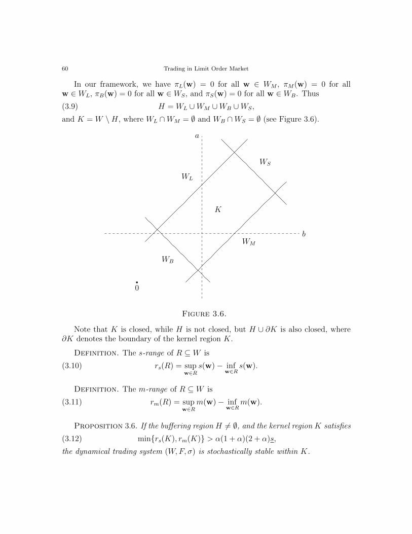
60 Trading in Limit Order Market
In our framework, we have πL(w) = 0 for all w ∈ WM , πM(w) = 0 for allw ∈ WL, πB(w) = 0 for all w ∈ WS, and πS(w) = 0 for all w ∈ WB. Thus
(3.9) H = WL ∪WM ∪WB ∪WS,
and K = W \H, where WL ∩WM = ∅ and WB ∩WS = ∅ (see Figure 3.6).
b
a
0
WB
WS
WL
WM
K
Figure 3.6.
Note that K is closed, while H is not closed, but H ∪ ∂K is also closed, where∂K denotes the boundary of the kernel region K.
Definition. The s-range of R ⊆ W is
(3.10) rs(R) = supw∈R
s(w)− infw∈R
s(w).
Definition. The m-range of R ⊆ W is
(3.11) rm(R) = supw∈R
m(w)− infw∈R
m(w).
Proposition 3.6. If the buffering region H 6= ∅, and the kernel region K satisfies
(3.12) min{rs(K), rm(K)} > α(1 + α)(2 + α)s,
the dynamical trading system (W,F, σ) is stochastically stable within K.
Iterated Trading Process 61
Proof. For any trajectory starting from a bid-ask pair w ∈ W , all the possiblestates in W are finite, as shown in the proof of Lemma 3.4. The set of all the possiblestates for any initial state w can be denoted by a corresponding lattice Λ(w). Letthe neighborhood of any v ∈ Λ(w) be
N(v) = {vS1,vS2,vS3,vS4} ∩W.
Observe that Λ(w) is globally defined on W = K∪H, so there exist states v ∈ Λ(w)near ∂K, such that N(v) ∩H 6= ∅ and N(v) ∩K 6= ∅.
Note that the spread s(v) of the state v can be updated to either s(v)/(1 +α) or(1 + α)s(v), and its mid-price m(v) can be updated to maximally m(v) + αs(v)/2and minimally m(v)− αs(v)/2, so
rs(N(v)) =α(2 + α)
1 + αs(v), rm(N(v)) = αs(v).
Suppose s(v)/(1 +α) ≥ (1 +α)s, where (1 +α)s is the lower bound of the spread inK, so we have
rs(N(v)) ≥ α(1 + α)(2 + α)s, rm(N(v)) ≥ α(1 + α)2s,
and hence
rs(K) > infv∈K
rs(N(v)), rm(K) > infv∈K
rm(N(v)).
So for any initial state w ∈ W , there exists at least a v ∈ Λ(w) ∩ K such thatN(v) ⊂ K.
Note that W = K ∪H, and both K and H are nonempty, so both H and K areproper subsets of W . Suppose w ∈ H. We know H = WL∪WM ∪WB ∪WS, so thereexists at least an x ∈ {L,M,B, S} such that w ∈ Wx. Note that πx(v) = 1 for allv ∈ Wx, thus w will move towards K along a continuous flow in Λ(w) ∩ H. Sincethe number of states in Λ(w)∩H is finite, w will move into the closed kernel regionK after finite periods. If the market is stochastically stable within K once w ∈ K,the market will function for infinite periods, and hence it is also stochastically stablewith the initial state w ∈ H. Thus we only need to show the trading system isstochastically stable for any initial state w ∈ K. Let p(w) denote the probabilitythat bid-ask pairs stay in H with an initial state w. We need to show that p(w) = 0for all w ∈ K.
Suppose w ∈ K, then we have two possibilities, N(w) ⊂ K, and N(w)∩H 6= ∅.If N(w) ∩ H 6= ∅, then N(w) ∩ K 6= ∅, otherwise w ∈ H. There exist somex ∈ {L,M,B, S}, such that πx(v) = 0 for all v ∈ N(w)∩H, and πx(v) = εx ∈ [0, 1]for all v ∈ N(w) ∩K. πx(v) 6= 1 for all v ∈ K and all x ∈ {L,M,B, S}, otherwisethere must exist a y ∈ {L,M,B, S} such that πy(v) = 1 − πx(v) = 0, which thenimplies v ∈ H, a contradiction. Hence εx 6= 1 for all x ∈ {L,M,B, S}.

62 Trading in Limit Order Market
If w moves to v ∈ N(w) ∩ H with a probability εx, it will return back tov′ ∈ N(v) ∩ K with probability 1 in the next period, where N(v′) ∩ H 6= ∅ asv ∈ N(v′). If w moves to v ∈ N(w)∩K with a probability 1−εx, it can stay withinΛ(w) ∩ K with k(w) consecutive periods, and then move into a state v′ such thatN(v′) ∩H 6= ∅. Recall that, for all w ∈ K, we have
{v ∈ Λ(w) ∩K : N(v) ⊂ K} 6= ∅,so k(w) ≥ 0. Then we have
p(w) = limT ↑∞
εxp(w)(
1− 2
T
)+ (1− εx)p(w)
(1− k(w) + 1
T
),
where 0 ≤ k(w) ≤ T − 1. When k(w) = T − 1,
p(w) = limT ↑∞
εxp(w)(
1− 2
T
)= εxp(w),
which generates (1 − εx)p(w) = 0. Since 1 − εx 6= 0, p(w) = 0 for all w ∈ K withN(w) ∩H 6= ∅.
If w ∈ K and N(w) ⊂ K, its trajectory can either achieve a state w′ ∈ Λ(w)∩Ksuch that N(w′)∩H 6= ∅ after h(w) periods, where h(w) ≥ 1, or never move to sucha state w′ and thus stay within K for ever. Note that p(w′) = 0, if w′ ∈ K andN(w′) ∩H 6= ∅. So p(w) ≤ p(w′) = 0, but p(w) ≥ 0, hence p(w) = 0 for all w ∈ Kwith N(w) ⊂ K.
As a result, p(w) = 0 if w ∈ K, and thus p(w) = 0 for all w ∈ W . So thedynamical trading system is stable within K almost surely. �
Since (bt, at) will stay within K almost surely, the random trajectories of bt andat will also stay within bounded intervals. Note that
(3.13) (1 + α)s ≤ st ≤ rs(K) + (1 + α)s,
and
(3.14) (1 + δ)s/2 ≤ mt ≤ rm(K) + (1 + δ)s/2,
almost surely for all t ∈ Z, so we almost surely have
(3.15) at ≤ rm(K) + rs(K)/2 + (2 + α + δ)s/2 < rm(K) + rs(K)/2 + 2s,
and
(3.16) bt ≤ rm(K) + (2 + α + δ)s/2 < rm(K) + 2s,
where α, δ ∈ (0, 1), so (2 + α + δ)/2 < 2.The upper bounds of bt and at both have interesting implications on the roles of
s-range and m-range in the limit order market. The upper bound of the best bid btin the market is solely determined by the m-range of the kernel region K, rather than

Controlled Trading System 63
any property of the whole domain W . The upper bound of the best ask at is alsoonly related to the kernel region K, and yet it is determined by both the m-rangeand the s-range of K. Notice that the lower bounds of bt and at are both close to 2s,so the bid-range in the market is approximately equal to rm(K), and the ask-rangeis roughly rm(K) + rs(K)/2. Evidently, the ask side of the limit order book shouldbe more volatile than its bid side, in case that the range of a price is a meaningfulindicator of its volatility.
4. Controlled Trading System
In this section, we assume again H 6= ∅, but either the s-range or the m-rangeof K will be less than α(1 + α)(2 + α)s. So the condition on the kernel region inProposition 3.6 is no longer satisfied. We would like to check whether a randomtrajectory of bid-ask pairs can maintain the property of stochastic stability withincertain bounded domains.
Let U1 = WL∪WM . Since K 6= ∅, we have WL∩WM = ∅ and W \U1 6= ∅. DefineU2 = W \ U1, so W = U1 ∪ U2 and U1 ∩ U2 = ∅.
Similarly, let V1 = WB∪WS, again W \V1 6= ∅. Define V2 = W \V1, so W = V1∪V2and V1 ∩ V2 = ∅.
Note that K = U2 ∩ V2 and H = U1 ∪ V1. Also observe that rs(K) = rs(U2) andrm(K) = rm(V2).
4.1. Controlled Spread Dynamics. By the condition WL∩WM = ∅, we havers(U2) ≥ 0, so (1 + α)s ≤ (1− γ)a, or
s/a ≤ 1− γ1 + α
.
At the same time, we assume that the s-range of U2 is sufficiently small, namely,rs(U2) < α(1 + α)s, so
(1− γ)a− (1 + α)s < α(1 + α)s,
which implies that s/a has a lower bound,
s/a >1− γ
(1 + α)2.
Intuitively, the upper bound of the s-range of U2 gives such a sufficient conditionthat any type of marginal trader will definitely update any w ∈ U2 to some w′ ∈ U1.
In brief, if 0 ≤ rs(U2) < α(1+α)s, the domain W will have the following property,
(3.17)1− γ
(1 + α)2< s/a ≤ 1− γ
1 + α.

64 Trading in Limit Order Market
Once the above inequality is satisfied by the domain W , we have U2 6= ∅, and
U2 = {w : (1 + α)s ≤ s(w) ≤ (1− γ)a},where s(w) is the spread function. Let the boundary of U2 be ∂U2, then
∂U2 = {w : s(w) = (1 + α)s} ∪ {w : s(w) = (1− γ)a}.
Proposition 3.7. If the buffering region H = U1 ∪ V1 is nonempty, and thekernel region K = U2 ∩ V2 satisfies
0 ≤ rs(U2) < α(1 + α)s, rm(V2) > α(1 + α)(2 + α)s,
the dynamical trading system (W,F, σ) is stochastically stable within the region
{w : s ≤ s(w) < (1 + α)3s} ∩ V2.
Proof. Since U2 6= ∅ and its s-range is less than α(1 + α)s, we obtain
(1 + α)s ≤ (1− γ)a < (1 + α)2s.
Note thatminw∈U2
s(w) = (1 + α)s, maxw∈U2
s(w) = (1− γ)a,
so we have
s ≤ (1− γ)a
(1 + α)< (1 + α)s = min
w∈U2
s(w),
and also(1 + α)2s > (1− γ)a = max
w∈U2
s(w).
Since any initial state w ∈ H will definitely move into K after finite periods, weonly need to show the statement is true when the initial state w ∈ K. Considerany initial state w ∈ U2 ∩ V2, we have (1 + α)s ≤ s(w) ≤ (1 − γ)a. Note thatπL(w) > 0 and πM(w) > 0 for all w ∈ K, so πi(w) 6= 0 for all w ∈ K and alli ∈ {1, 2, 3, 4}. Suppose w is updated to v = wS1 by a marginal trader of type σ(1),s(v) = s(w)/(1 + α), which is greater than s and less than (1− γ)a/(1 + α). Since(1 − γ)a/(1 + α) < minw∈U2 s(w), we should have v ∈ WM , and hence πM(v) = 1.The trader in the next period will be market-type, namely, either type σ(4) or typeσ(2). If she is of type σ(4), v will then become wS1S4 = w, since {σ(1), σ(4)} is aminimal periodic block. If she is of type σ(2), v will become v′ = wS1S2, where
S1S2 =
(1
1+α0
α1+α
1
)(1 −α0 1 + α
)=
1
1 + α
(1 −αα 1 + 2α
),
so s(v′) = s(w). Thus after two periods, w will return back to itself or move to astate with the same spread as itself.
If w is updated to v = wS2 by a marginal trader of type σ(2), then v ∈ WL. Soin the next period, there will come either type-σ(3) trader or type-σ(1) trader. The

Controlled Trading System 65
type-σ(3) trader will update v to wS2S3 = w, as {σ(2), σ(3)} is a minimal periodicblock. The type-σ(1) trader will update v to wS2S1 that has the same spread as w.If w is updated to wS3 by a marginal trader of type σ(3), wS3 will then be updatedeither to wS3S2 = w, or to wS3S4 that have the same spread as w. Finally, if wis updated to wS4 by a marginal trader of type σ(4), wS4 will then move either towS4S1 = w, or to wS4S3 such that s(wS4S3) = s(w).
Therefore, any initial state w ∈ U2 ∩V2 will be updated to a state with the samespread as itself after two consecutive periods. Note that the dynamics in (W,F, σ)is repeatedly composed of those two-period dynamical blocks, thus the spread thatcan be achieved in such a dynamical trading system will be greater than or equal to
minw∈U2
s(w)/(1 + α) = s,
and less than or equal to
(1 + α) maxw∈U2
s(w) < (1 + α)3s,
as maxw∈U2 s(w) < (1 + α)2s.So the trajectory of bid-ask pairs starting from any initial state w ∈ W will be
bounded in the region {w : s ≤ s(w) < (1 + α)3s} ∩ V2 almost surely. �
If 0 ≤ rs(U2) < α(1 + α)s, there exists a unique exponent l ∈ [1, 2), such that
(3.18) s/a =1− γ
(1 + α)l.
Note that the upper bound of the bid-ask spread in W is a, so (1 + α)3s should beno greater than a, or equivalently,
s/a ≤ 1
(1 + α)3.
Thus we need (1− γ)(1 + α)h ≤ 1, where h = 3− l, so h ∈ (1, 2]. It appears to be aslightly stricter requirement than (1− γ)(1 +α) ≤ 1 that we have used before, since(1 + α)h > 1 + α for h > 1.
Recall that U2 = {w : (1 + α)s ≤ s(w) ≤ (1− γ)a}, we thus have two nonemptyregions in U1, which will contain buffering overflows,
{w : s ≤ s(w) < (1 + α)s}, {w : (1− γ)a < s(w) < (1 + α)3s}.
Evidently, the trajectory of bid-ask pairs will not stay exactly within the kernelregion K = U2 ∩ V2, but within K and parts of the buffering region U1 ∩ V2 in H.
As we can see from the proof of Proposition 3.7, there are in fact eight possibletwo-period dynamical blocks for all w ∈ U2 ∩ V2. Half of them are minimal periodicblocks, so the bid-ask pair driven by each of them will return back to w. While the

66 Trading in Limit Order Market
remaining ones will update w to w′ 6= w, with s(w′) = s(w) (see Figure 3.7, wheres(w) is replaced simply by s).
w
s
(1 + α)s
s/(1 + α)
Figure 3.7.
If w′ 6= w, the distance (in the b-a plane) between w and w′ is√
2α
1 + αs(w) or
√2αs(w),
and the absolute difference between m(w) and m(w′) is
α
1 + αs(w) or αs(w).
The possible trajectories in the dynamical trading system (W,F, σ) are nowconsecutive combinations of those eight two-period dynamical blocks. Recall thats(w) ∈ [(1 + α)s, (1− γ)a] for all w ∈ U2 ∩ V2. The trajectory starting from w willbe bounded within the region
{v : s(w)/(1 + α) ≤ s(v) ≤ (1 + α)s(w)},
where
(1 + α)s ∈ (s(w)/(1 + α), s(w)], (1− γ)a ∈ [s(w), (1 + α)s(w)).

Controlled Trading System 67
So the region containing buffering overflows are
{v : s(w)/(1 + α) ≤ s(v) < (1 + α)s}, {v : (1− γ)a < s(v) ≤ (1 + α)s(w)},
where s(w)/(1+α) ≥ s and (1 +α)s(w) < (1+α)3s. We shall show two trajectoriesstarting from w with seven periods on the b-a plane in the following Figure 3.8,where s = s(w).
w
s
(1 + α)s
s/(1 + α)
∂U2
∂U2
Figure 3.8.
4.2. Controlled Mid-Price Dynamics. If the m-range of V2, rather than thes-range of U2, is sufficiently small, we may establish a similar result to Proposition3.7. Assume 0 ≤ rm(V2) < α(1 + α)s/2. By the condition rm(V2) ≥ 0, we haveV2 6= ∅ and WB ∩WS = ∅, so (1 + δ)s/2 ≤ (1− ε)(a− s/2), or
s/2
a− s/2≤ 1− ε
1 + δ,
where δ ∈ (0, 1) and ε ∈ [δ/(1 + δ), 1). On the other hand, if rm(V2) < α(1 + α)s/2,then
(1− ε)(a− s/2)− (1 + δ)s/2 < α(1 + α)s/2,

68 Trading in Limit Order Market
which implies
s/2
a− s/2>
1− ε1 + δ + α(1 + α)
.
As a result, if 0 ≤ rm(V2) < α(1 + α)s/2, the domain W will have the followingproperty,
(3.19)1− ε
1 + δ + α(1 + α)<
s/2
a− s/2≤ 1− ε
1 + δ.
Under that condition, we have a nonempty V2,
V2 = {w : (1 + δ)s/2 ≤ m(w) ≤ (1− ε)(a− s/2)}.
Let the boundary of V2 be ∂V2, then
∂V2 = {w : m(w) = (1 + δ)s/2} ∪ {w : m(w) = (1− ε)(a− s/2)}.
The lower bound in the condition (3.19) is a sufficient condition for the existenceof dynamical two-period switching blocks, by which any state in V2 ∩ U2 can returnback into V2 ∩ U2 after two periods. To confirm this claim, we only need to showthat any state w in ∂V2∩U2 at a time t will be updated to some w′ ∈ V1 at the timet+ 1. Note that
maxv∈V2
m(v) = (1− ε)(a− s/2), minv∈V2
m(v) = (1 + δ)s/2,
and they can be achieved by the states in ∂V2.Consider a generic state w ∈ ∂V2 ∩ U2 with m(w) = maxv∈V2 m(v). A buy-type
trader will induce a greater mid-price, which means that the next state will be in V1.A sell-type trader can generate a new mid-price,
m(w)− α
2s(w) or m(w)− α
2(1 + α)s(w).
A sufficient condition for the new state will be in V1 is that the greatest mid-priceshould be less than minv∈V2 m(v), that’s to say,
(3.20) maxv∈V2
m(v)− α
2(1 + α)minw∈∂V2
s(w) < minv∈V2
m(v).
Note that s(w)/(1+α) ≥ (1+α)s for all w ∈ V2∩U2, so minw∈∂V2 s(w) = (1+α)2s.Then we obtain
(1− ε)(a− s/2)− α(1 + α)s/2 < (1 + δ)s/2,
which is exactly equivalent to the condition rm(V2) < α(1 + α)s/2.

Controlled Trading System 69
Now if w ∈ ∂V2 ∩U2 with m(w) = minv∈V2 m(v), a sell-type trader will induce asmaller mid-price, and hence the next state must be in V1. While the new mid-pricegenerated by a buy-type trader can be
m(w) +α
2s(w) or m(w) +
α
2(1 + α)s(w).
A sufficient condition ensuring the new state will be in V1 is that the smallestmid-price should be greater than maxv∈V2 m(v), that’s to say,
(3.21) minv∈V2
m(v) +α
2(1 + α)minw∈∂V2
s(w) > maxv∈V2
m(v),
which is again equivalent to rm(V2) < α(1 + α)s/2.
Proposition 3.8. If the buffering region H = V1 ∪ U1 is nonempty, and thekernel region K = V2 ∩ U2 satisfies
0 ≤ rm(V2) < α(1 + α)s/2, rs(U2) > α(1 + α)(2 + α)s,
the dynamical trading system (W,F, σ) is stochastically stable within the region
{w : m ≤ m(w) < m} ∩ U2,
where m and m are constants in the trading system.
The proof of Proposition 3.8 is roughly similar to that of Proposition 3.7, and thusnot provided here. Once again, its trajectory of bid-ask pairs will not be boundedwithin the kernel region K = V2∩U2, but within K and parts of the buffering regionV1∩U2, so that the trading system can contain certain buffering overflows to supportits stability. In the limit, each state on the trajectory will be either in K = V2 ∩ U2
or in the buffering region V1 ∩ U2 with equal probability.Since the updating process of the mid-price also depends on the spread of the
states on the trajectory, the buffering region used to hold the buffering overflows isquite wide. We can see that the m-range of the region {w : m < m(w) < m} ∩ U2
is very large, by virtue of
m = (1 + δ)s/2− α(1− γ)a/2, m = (1− ε)(a− s/2) + α(1− γ)a/2,
where (1− γ)a = maxw∈U2 s(w). In fact, its m-range is equal to
(3.22) m−m = rm(V2) + α(1− γ)a,
which is greater than or equal to α(1− γ)a, and less than α(1− γ)a+ α(1 + α)s/2.So m−m = O(a). On the other hand, in Proposition 3.7, the s-range of the region
{w : s ≤ s(w) < (1 + α)3s} ∩ V2is only ((1 + α)3 − 1)s = O(s), where O(s)� O(a).

70 Trading in Limit Order Market
Proposition 3.7 and 3.8 collectively produce interesting observations about thevolatilities of the mid-price and the bid-ask spread on a limit order market. If thespread s in the kernel region K = U2 ∩ V2 is required to be ex ante stable, then therandom trajectory in the dynamical trading system will be bounded within a certainregion with a sufficiently small s-range. However, if the mid-price m in K is requiredto be ex ante stable, the random trajectory can not remain in a certain region witha small m-range.
Suppose again the range of a time-dependent price can be thought of to be anindicator of its volatility. Let us adopt an artificial concept of “disorder” to describethe origins of price volatility, and yet we leave such an introduced concept in itsobscurity. Moreover, imagine the disorder in a trading system could be classifiedinto one intrinsic part and another external part (which are evidently similar to theterms of “self-generated disorder” and “quenched disorder” in physics), such thatthe intrinsic disorder has an ex ante controllable nature, while the external disorderhas an ex ante uncontrollable nature, and hence carries a high volume of potentialinformation in the trading system. In practice, more intrinsic disorder should makea price in the trading system less unpredictable, while more external disorder couldmake the price more unpredictable. And thus a price volatility that can be partiallycharacterized by its unpredictability should be lower if the disorder is rather intrinsic,and higher if that is rather external.
Quite directly, we say that the disorder in the bid-ask spread is mainly intrinsicor self-generated, as we find that the bid-ask spread has an ex ante controllablenature. On the other hand, most of the disorder in the mid-price should be externalor quenched, since we show that the mid-price has an ex ante uncontrollable nature.For this reason, we conclude that the volatility of the bid-ask spread should be lowerthan that of the mid-price in the dynamical trading system.
5. Final Remarks
In our studies, we take a dynamical perspective to investigate the microstructureof the limit order market. A limit order market is theoretically thought of to bea dynamical trading system, in which sequential trading processes are determinedby either deterministic or probabilistic switches between different types of traders(represented by their optimal trading decisions in a very short time interval). Inour analysis, the perfect information usually required to model traders’ strategicbehavior is loosened to the knowledge of the so-called atomic trading schemes. Wethus set less assumptions for traders and the market, and yet still obtain a powerfulability to understand and even predict the order flow and the order book evolution ina generic limit order market. Some interesting and hopefully insightful conclusionshave developed, for instance, the best ask is more volatile than the best bid, the

Final Remarks 71
mid-price is more volatile than the spread, and the best ask seems to have moredeterminants than the best bid.
To close this chapter, we would like to make some concluding remarks on these twocritical notions appearing in our main results — general instability in a deterministictrading system, and stochastic stability in a stochastic trading system.
The stability of a deterministic trading system means that there should existsome bid-ask pairs such that certain trading blocks can generate convergent limitcycles attracted to them. We show that a necessary condition for general stability ofthe trading system is the trading block must be reducible, so that they can generateperiodic bid-ask pair dynamics. Thus the notion of general instability implies thatthere is no stable bid-ask pair in the trading system, and it happens if the tradingblock is irreducible.
Once the trading block in the dynamical trading system stochastically emergesfrom Σω
4 with a certain stationary probability measure, the trading system will not beunstable for sure. One intuitive reason is that a countably infinite random tradingblock will be reducible almost surely. Therefore, we state that the bid-ask pairdynamics will be bounded within the domain W for sure, which gives meanings tostochastic stability of the dynamical trading system. More strictly, we show thatthe domain that serves for stochastic stability is only a proper subset of W , whichis defined as its kernel region. However, in the meantime, the buffering region of Wstill has a positive role for stochastic stability, as it occasionally holds states on thebid-ask pair trajectory.
Finally, it might be worth figuring out one practical application of the notionsof kernel region and buffering region. They could be used to measure the risk ofsystemic instability in a real market. Say, the market would have a high risk ofsystemic instability, if its state moves into the buffering region, while the risk ofsystemic instability should be acceptable with a certain confidence level, if the statestays in the kernel region.


CHAPTER 4
Collective Decision on Political Network
In this chapter, we shall study a group of governments structured as a genericpolitical network, and investigate collective decision-making process thereof withcertain economic meanings conveyed by the local public good provision.
Although the political network seems like a rather specific group structure bynature, we still formalize it in a general sense, so that we could add a third abstraction“relation-dependent group” to the former two, “time-dependent group” as studiedin Chapter 1, and “preference-dependent group” as studied in Chapter 2.
1. Introduction
This chapter aims to explore and solve the optimal provision problem raised inthe economic theory of public good provision. In a study of public expenditureon collective consumption by Samuelson [57], he claimed that there does not existany “decentralized pricing system can serve to determine optimally these levels ofcollective consumption” (Samuelson [57], p. 388). However, that impossibility resultdepends on that the public expenditure can only be manipulated by the centralgovernment in an economy, and the economy relies exclusively on market mechanism.In the meanwhile, Samuelson equally admitted that the optimal decisions of collectiveconsumption would exist, in case sufficient knowledge and ethical welfare functionfor the economy could be obtained. As he wrote in the article “The pure theory ofpublic expenditure” (Samuelson [57], p. 389):
The failure of market catallactics in no way denies the followingtruth: given sufficient knowledge the optimal decisions can alwaysbe found by scanning over all the attainable states of the world andselecting the one which according to the postulated ethical welfarefunction is best. The solution “exists”; the problem is how to“find” it.
Tiebout [63] took a different perspective to frame such a public expenditureproblem. He introduced the notion of local expenditure, and then developed a simplemodel which can yield a solution for optimal (local) public expenditure. Since themechanism in Tiebout’s model is purely political, and also the optimality in his
73

74 Collective Decision on Political Network
model is kept to local levels, the solution proposed by Tiebout in effect has a ratherdifferent nature to that of Samuelson.
In the present chapter, we shall take a perspective that combines the approachesof Samuelson and Tiebout to study the public good provision problem, so that wecould propose some solutions to the optimal provision problem. With this respect,the mechanism to determine the optimal public good provisions will then have botheconomic and political natures, and the attained optimality will be not only local butalso global. To achieve these objectives, we first introduce a political system into atypical economy, such that it has a group of economic planners (local governments)forming a government network, it has a distribution rule of political powers over thegovernment network, and it has a collection of pairwise disjoint districts, populatedby fixed citizens and administered by distinct local governments. After that, wepropose a formal definition to the local public good in the economy, and give economicmeanings to decision-making processes and corresponding games appearing in thepolitical system.
A well-studied topic related to this study is comparative economic performancesunder different governance structures. Most studies suggest that the decentralizedpublic good provision scheme should be more efficient than the centralized provisionscheme owing to various economic reasons. For example, the dominant efficiencyof the decentralized scheme comes from its adaptation to local consumer-voters(Tiebout [63]); the decentralization theorem dominates citizen-oriented decision-making processes (Oates [48, 49]); the decentralized scheme promotes the emergenceand maintenance of an efficient market (Weingast [67]); the decentralized schemepreserves market incentives (Qian and Weingast [53]). Even if we do not develop anormative principle to compare decentralized and centralized governance structures,we do obtain, under a set of restricted assumptions, a same efficiency judgementon the decentralized and centralized public good provision schemes to the popularlyaccepted one.
What’s more, this chapter might also contribute partly to studies on a number ofother topics. To wit, positive applications of the concept authority in organizationsand partnerships, e.g., the authority relationship in employment contracts (Simon[58]), and the optimal authority allocation in complex partnerships (Francesconiand Muthoo [23]); social network game and communication, e.g., information (as apublic good) acquisition and communication structure on social networks (Galeottiand Goyal [24]); private provision of public good and market institution design,e.g., truthful revelation mechanism that can admit Pareto optima (Groves and Loeb[27]), and noncooperative solution with a neutral property of income redistribution(Bergstrom, Blume, and Varian [7]).
The writing of the present chapter shall be organized as follows. This section isa general introduction, while the last section provides some additional remarks.

Introduction 75
In Section 2, we give formal definitions to related economic and political objects inthe political system. Concretely, a government network is defined to be a graph thatadmits a hierarchical structure in whole. By introducing an authority allocation ruleto the government network, we can then accordingly define centralized, autonomous,and decentralized governance structures. Besides, a local public good is characterizedby its partial provision capacity (viz., the ability of benefit exclusion) with regards itsprovision district, and thus it will be defined as a two-dimensional economic objectand measured by its provision level and provision capacity.
In Section 3, each government in the political system will be simplified to be apolitical agency with a utilitarian welfare function. We could then show two basicpropositions on optimal local public good provision states under the centralized anddecentralized provision schemes. These arguments will also become our fundamentalknowledge prepared for the studies in the next three sections, which constitute themost significant parts of this chapter.
Section 4 and 5 will be devoted to extensive studies of the H-form game andM-form game, respectively. Roughly speaking, an H-form game is another word ofa negotiation game with “hierarchical interactions”, and an M-form game can berepresented by a collection of parallel negotiation games which are connected by anoncooperative game with “coordinated interactions”. In Section 4, we show thatany Pareto efficient solution to an H-form game is determined by two hierarchicallyconsecutive governments, which therefore have the greatest enforceable authoritiesin the political system. Moreover, the utilitarian solution of an H-form game canbe characterized by some polynomial in the political discounting. In Section 5, wemainly study “degenerate” and “analytic” M-form games under the assumption thatthe provision cost function is separable. The solution to a degenerate M-form gameis actually such a strategic equilibrium that is determined by a system of marginalconditions. Although the (utilitarian) solution to an analytic M-form game does notdirectly have computational properties, we still propose an interval representation,and develop a number of propositions on its bounds.
In Section 6, the more general mixed-form game (usually with great complexity)will be discussed. We define a mixed-form game in such a way that we could have acomplete classification of games on a compact government network, viz., any gameon a compact government network must be in one of the following three classes —H-form game, analytic M-form game, and mixed-form game. Since any incompactgovernment network could be reduced to a compact one by identifying and removingits authority gaps, we actually have developed a full knowledge of games on anygovernment network. After defining the indicator matrix for a compact governmentnetwork, we clarify the equivalence relations among the three mathematical objects,that is, graph, game, and matrix. Lastly, we propose a pragmatic solution concept

76 Collective Decision on Political Network
to the mixed-form game, which hopefully can help capture complex interactions ina complex political system.
2. Basic Definitions
2.1. Government Network. Consider a group of n governments
N = {r0, r1, r2, . . . , rn−1},
in which r0 is the central government , while r1, r2, . . . , rn−1 are all local governments .Let c = r0, then we can also write
N = {c, r1, r2, . . . , rn−1}.
Let I = {0, 1, . . . , n − 1} be the index set of N . Define a mapping f : I × I →{0, 1}, and let fij = f(i, j) for all i, j ∈ I. Then we have a graph (N, f), whosestructure is determined by the n× n matrix (fij). We shall say that
(i) (N, f) has no loop, if fii = 0 for all i ∈ I.(ii) (N, f) is undirected , if fij = fji for all i, j ∈ I.
(iii) ri1ri2 · · · ril is an l-cycle in (N, f), if fi1i2 = fi2i3 = · · · = fili1 = 1, wherel ≥ 3 and i1, i2, . . . , il are distinct.
(iv) (N, f) is acyclic, if it does not have any l-cycle for 3 ≤ l ≤ n.
Definition. (N, f) is called a government network , if it is undirected, acyclic,and without loops.
For all government ri, rj ∈ N , the distance (that is, the number of edges on theshortest path) between them is denoted by dij. Define the hierarchical level of agovernment ri ∈ N to be the value of di0. Let d00 = 0, and di0 = ∞ if there doesnot exist any path between ri and c. Thus di0 ∈ {0, 1, . . . , n− 1,∞} for all ri ∈ N .If (N, f) is connected, di0 6=∞ for all ri ∈ N .
There are two fundamental connected government networks which can be definedas follows:
(i) If there is a unique ri such that di0 = k for all k ∈ {0, 1, . . . , n− 1}, we say(N, f) is an H-form government network or government line.
(ii) If di0 = 1 for all ri 6= c, we say (N, f) is an M-form government network orgovernment star .
Evidently, any connected government network (N, f) has a collection of blocks, eachof which is an H-form or M-form government network.
On a government network (N, f), the group of level-k governments is
Nk = {ri ∈ N : di0 = k},

Basic Definitions 77
where k ∈ {0, 1, . . . , n−1,∞}. Note that N0 = {c}, and N∞ contains all the isolatedgovernments which do not connect with the central government c. Clearly, N \N∞is the connected part of N . If (N, f) is connected, then N∞ = ∅.
Let the group of the directly subordinate governments to ri ∈ N be Di, then
Di = {rj ∈ N : dij = 1 and dj0 ≥ di0}.
Note that D0 = N1. If ri ∈ Nk, then Di ⊆ Nk+1, where k ≤ n − 2. As for anyri, rj ∈ N∞ with dij = 1, by definition we have both rj ∈ Di and ri ∈ Dj, andthus we shall say all the governments in N∞ have identical roles on the hierarchicalstructure of (N, f).
Let the group of all the subordinate governments to ri ∈ N be Di, then
Di = {rj ∈ N : 0 < dij <∞ and dj0 ≥ di0}.
Note that {c} ∪ D0 = N \ N∞, and Di ⊇ Di for all ri ∈ N . If ri ∈ N∞, then Di iseither empty or the connected block (in N∞) to ri.
Let the group of bottom governments be Nb, then
Nb = {ri /∈ N∞ : Di = ∅}.
If (N, f) is connected, we can write Nb = {ri ∈ N : Di = ∅}. Note that Di = ∅ forall ri ∈ Nb.
Example 4.1. Let N = {c, r1, r2, . . . , r12}, and define a graph (N, f) as shownin Figure 4.1. Observe that (N, f) is a connected government network. We have
N0 = {c}, N1 = {r1, r2, r3, r4}, N2 = {r5, r6, r7, r8, r9, r10}, N3 = {r11, r12}.
Notice that D0 = N1, D2 = {r5}, D3 = {r6, r7, r8}, D4 = {r9, r10}, and D10 ={r11, r12}. Since Di = ∅ for all ri /∈ {c, r2, r3, r4, r10}, we have
Nb = {r1, r5, r6, r7, r8, r9, r11, r12}.
Finally, we have Di = Di for all ri /∈ {c, r4}, while
D0 = {r1, r2, . . . , r12}, D4 = {r9, r10, r11, r12}.
Example 4.2. Let N = {c, r1, r2, r3, r4, r5}, and define an H-form governmentnetwork (N, f) as shown in Figure 4.2. Observe that N0 = {c}, and Ni = {ri} forall i ∈ {1, 2, 3, 4, 5}. Note that for all i ∈ {0, 1, 2, 3, 4},
Di = {ri+1}, Di = {ri+1, ri+2, . . . , r5},
while Nb = N5 = {r5}.

78 Collective Decision on Political Network
c
r1
r2 r3
r4
r5
r6
r7
r8
r9
r10
r11
r12
Figure 4.1.
c r1 r2 r3 r4 r5
Figure 4.2.
Example 4.3. Let N = {c, r1, r2, . . . , r6}, and define an M-form governmentnetwork (N, f) as shown in Figure 4.3. Observe that
N0 = {c}, N1 = {r1, r2, r3, r4, r5, r6}.

Basic Definitions 79
Note that D0 = N1, D0 = D0, and Nb = N1; in effect, they are all generic for anyM-form government network.
cr1
r2 r3
r4
r5r6
Figure 4.3.
2.2. Governance Structure. In order to make formal definitions and developidentification principles for different governance structures, we need a prerequisitenotion, authority. That’s because the governance arrangements would not set upstable institutional regulations for collective actions in the political system, unless thedistributed authorities have been clarified. Here, we shall interpret the authority asthe power to make favorable decisions in a decision-making process, and any decision-making process ought to be designed to decide actions for a certain government onthe government network.
If a decision-making process aims to decide actions for ri /∈ N∞, the authorityin that process will be shared by a group of governments that participate in theprocess, such that it is a connected block, and it contains ri and governments withhierarchical levels lower than that of ri. In particular, we are interested in the finestgroup of participating governments which minimizes the ex ante transaction costs,though the ex post negotiation is assumed to be Coasian. Let Li denote such a uniquegroup, then
(4.1) Li = {rj ∈ N : ri ∈ Dj} ∪ {ri},
which actually represents a path connecting ri to c.If a decision-making process aims to decide actions for ri ∈ N∞, we then directly
set Li = {ri}, by virtue of all the governments in N∞ having identical roles on thehierarchical structure of (N, f) (cf., the notion of directly subordinate government).

80 Collective Decision on Political Network
Properly speaking, any decision-making process in the political system could thenbe represented by its participating government path in (N, f). For example, withregards a decision-making process deciding actions for a level-k government, ri ∈ Nk
for k 6=∞, we can write
Li = {c, ri1 , ri2 , . . . , rik−1, ri},
where rix ∈ Nx for all x ∈ {1, 2, . . . , k − 1}. Let the authority shared by rix be γxfor all x, and the authorities shared by c and ri be γc and γk, respectively. Supposethe absolute authority for any decision-making process in the political system isnormalized to 1, and its distributed parts to distinct governments are homogeneous.It then appears that
(4.2) γc +k∑x=1
γx = 1,
where γx ∈ [0, 1] for all x ∈ {c, 1, 2, . . . , k}.In general, distributed authorities might not be normally homogeneous in the
decision-making process, so there should be a nonlinear authority allocation rule,say Γ, such that
(4.3) Γ(γc, γ1, γ2, . . . , γk) = 1.
However, in the present studies, we will simply assume Γ is linearly additive, anduse γ to denote such an authority allocation rule.
Definition. The governance structure of (N, f) is called centralized , if N∞ = ∅and γc = 1 for all decision-making process in (N, f).
Once (N, f) has a centralized governance structure, it must be connected, andthe authority will be exclusively allocated to the central government c, so that allthe local governments are confined to the monolithic authority.
Definition. The governance structure of (N, f) is called autonomous , if N∞ =N \ {c}.
Once (N, f) has an autonomous governance structure, all the local governmentsshould be on the∞-level, and hence isolated from c. Moreover, any decision-makingprocess aiming to decide actions for ri 6= c has Li = {ri} and thus γi = 1, whichtherefore means that each government in N∞ has full sovereignty of its own.
Definition. The governance structure of (N, f) is decentralized , if it is neithercentralized nor autonomous.
If (N, f) has a decentralized governance structure, two cases could be classifiedas follows:
Basic Definitions 81
(i) N∞ 6= ∅, and N \ ({c} ∪N∞) 6= ∅.(ii) N∞ = ∅, but there exists at least one decision-making process with the
group Li, such that γc 6= 1.
In case (i), (N, f) is disconnected, and there exists at least one local governmentri ∈ N∞ with γi = 1 for the decision-making process deciding its own actions. Incase (ii), (N, f) is connected, and there exists at least one local government in Liwith γi 6= 0 for the decision-making process represented by Li. Thus in any casethe authority will be always allocated to at least one local government, when (N, f)adopts a decentralized governance structure. In addition, it might be noted thatthe governance structure of a connected government network is either centralized ordecentralized.
Let’s consider a decision-making process in (N, f) with a decentralized governancestructure, and suppose it can be represented by the path
Li = {c, ri1 , ri2 , . . . , rik},
where rix ∈ Nx for all x ∈ {1, 2, . . . , k}. If the authority is allocated solely to theuppermost-level government rik in Li, then the decision-making process is calledpurely decentralized .
Definition. A decentralized governance structure of (N, f) is called pure, if alldecision-making process in (N, f) is purely decentralized.
Notice that any decision-making process aiming to decide actions for ri ∈ N∞ isnaıvely a purely decentralized one, as its participating group is Li = {ri}. Thus it’ssufficient to just use the verification that all decision-making process in N \ N∞ ispurely decentralized.
As a further remark on all these above definitions, we would like to commenton the stability of a governance structure which would be implicitly adopted in ourinvestigations. Although the formation process of a governance structure could have afew complex features (see e.g., Wibbels [68]), the structure, once it had been shaped,will be assumed to be stable for a sufficiently long time. Thus such a statement thata political system adopts a certain governance structure means that the structureitself is exogenous and will be stable at least in our reasoning framework.
2.3. Local Public Good. Let R denote the region collectively administered bythe government network (N, f). Each element s ∈ R denotes a place in the regionR, and each subset S ⊆ R denotes a district of R. Suppose there is a topology, i.e.,a collection of subsets of R, such that for every two distinct places s and s′ in R,there exist two disjoint districts S and S ′ of R satisfying s ∈ S and s′ ∈ S ′. Thetopology on R is actually Hausdorff, and the region R described as above is thus aHausdorff space.
82 Collective Decision on Political Network
Let |Nk| denote the number of level-k governments for all k ∈ {0, 1, . . . , n−1,∞},then
n−1∑k=0
|Nk|+ |N∞| = n,
where |N0| = 1 always. If (N, f) is connected, then we have |N∞| = 0. If (N, f)has an autonomous governance structure, then |N∞| = n − 1, and |Nk| = 0 for allk /∈ {0,∞}.
Let the district directly administered by ri ∈ N be Ri. On each hierarchical levelk with Nk 6= ∅, there are |Nk| governments sharing the control rights over the district⋃ri∈Nk
Ri, where Ri ∩Rj = ∅ for all distinct ri, rj. It is direct to see that⋃ri∈Nb∪N∞
Ri = R.
If (N, f) is connected, we have⋃ri∈Nb
Ri = R, which thus means all the bottomgovernments make a partition of R.
With regards a level-k government ri ∈ Nk having a nonempty Di ⊆ Nk+1, wehave a partition of Ri,
Ri =⋃rj∈Di
Rj,
where Rj ∩ Rj′ = ∅ for all distinct rj, rj′ . The district Ri administered by ri thuscontains |Di| (no greater than |Nk+1|) disjoint districts, which are administered bythe governments in Di, separately. In particular, in a connected (N, f), the centralgovernment c administers the whole region R which is also fully administered by allthe level-1 governments in N1, by virtue of R =
⋃ri∈N1
Ri for D0 = N1.Let the population of the region R be P . Define a mapping
P : S 7→ P (S),
so that it generates a population P (S) ⊆ P for all district S ⊆ R. Since thepopulation of a district is an invariant representation for the district, the mappingshould satisfy
(i) P (∅) = ∅ and P (R) = P ,(ii) P (S) ⊆ P (T ) if S ⊆ T ,
(iii) P (S ∪ T ) = P (S) ∪ P (T ) for all S, T ⊆ R.
Let P (Ri) = Pi for all ri ∈ N , then each district Ri has a population Pi. It can beclaimed that Pi 6= ∅ for all ri ∈ N , because there is no reason to place a governmentfor a district without citizen, and hence without decision-making process. When(N, f) is connected, we have
⋃ri∈Nb
Pi = P , where Pi ∩ Pj = ∅ for all distinct ri, rj.

Basic Definitions 83
Definition. A public good G is called local , if there exist nonempty districtsS, T ⊂ R, such that P (S) can consume G but P (T ) is excluded from the benefits ofG.
A pure (or global) public good can be defined by such properties as “jointnessof supply” and “impossibility of exclusion” (see Hardin [28], p. 17). Our definitionof local public good generalizes the assumption about the exclusion ability, in sucha way that the partial exclusion impossibility replaces the absolute one adopted inthe definition of public good.
By means of the definition of local public good, we are able to bridge the gapbetween private good and public good, and think of private good and pure publicgood as two special cases of regular local public good. In fact, if G is provided tocover the region R, and no citizen in P is excluded from its benefits, then G is clearlya pure public good. On the other hand, if G is provided to cover a (virtual) districtS with a single citizen, and all the population P except that citizen living in S canbe excluded from its benefits, then G is actually a typical private good. In general,G is a regular local public good if it is neither private nor purely public; here, “local”means it partially excludes a proper and nonempty subset of P from its benefits.
To treat the definition of local public good analytically, we gauge the provisionability of a local public good using a measure of analytic sets of the Hausdorff spaceR, which is in essence a capacity monotone of order 2 in Choquet’s [12] term. Let℘(R) denote the power set of R, and define a mapping λ : ℘(R)→ [0, 1] such that
(i) λ(∅) = 0 and λ(R) = 1,(ii) λ(S) ≤ λ(T ) if S ⊆ T ,
(iii) λ(S ∪ T ) + λ(S ∩ T ) ≥ λ(S) + λ(T ) for all S, T ⊆ R.
If λ satisfies property (iii), it is called superadditive. It can be noted that for anysuperadditive λ, λ(S ∪ T ) ≥ λ(S) + λ(T ) for all disjoint S, T ⊆ R.
The capacity λ as a measure of provision ability is assumed to be superadditiverather than subadditive, because a local public good provided to S ∪ T seems toneed a less exclusion ability than that needed by two local public goods, which areprovided to S and T , separately.
The provision state of a local public good G can thus be characterized by the pair(g, S), where g ∈ R+ denotes the provision level, and S ⊆ R denotes the provisiondistrict. Since a district S can now be measured by its provision capacity λS = λ(S),the provision state of G can be equivalently characterized by the real pair (g, λS),where λS ∈ [0, 1]. We shall see that
(i) If g = 0, G is in fact not provided at all.(ii) If g > 0 and λS = 1, then G is actually a pure public good.

84 Collective Decision on Political Network
(iii) If g > 0 and λS = 01, then G turns out to be a private good.(iv) If g > 0 and λS ∈ (0, 1), then G is a regular local public good which
partially excludes P \ P (S) from its benefits.
Suppose the local public good provision is implemented by the governments inNb∪N∞ (i.e., either bottom or isolated), and all the implementing governments havea same real provision cost function2 M(g, λ), where (g, λ) ∈ R+× [0, 1] measures theprovision state. Once the real pair (g, λ) is replaced with its initial pair (g, S),the provision cost function should then be written as M(g, λ(S)), or M(g, λS) forλS = λ(S).
Moreover, we shall assume
Mg ≥ 0, Mλ ≥ 0, Mgg ≥ 0, Mλλ ≥ 0,
where all these inequalities will be strict if g > 0 and λ > 0. It thus directly suggeststhat M(g, λ) is convex in both g and λ. Additionally, to get rid of such an optimalprovision state as (∞, λ) or (g, 1), that is, an infinite provision level or a perfectprovision capacity, we ought to set the following boundary conditions,
Mg(0, λ) = 0, Mg(∞, λ) =∞, Mλ(g, 0) = 0, Mλ(g, 1) ≤ ∞.
Example 4.4. Consider M(g, λ) = ϕ(g) + ψ(λ), where ϕ(g) and ψ(λ) are bothconvex functions. Assume ϕ′(0) = 0, ϕ′(∞) = ∞, ψ′(0) = 0, and ψ′(1) ≤ ∞, thenM(g, λ) is clearly a provision cost function. Note that Mgλ = 0. For example, letϕ(g) = β1g
2 and ψ(λ) = β2 exp(λ2) for β1, β2 > 0, then the provision cost functionis written in the form
(4.4) M(g, λ) = β1g2 + β2 exp(λ2).
Example 4.5. Consider M(g, λ) = ϕ(g)ψ(λ), where ϕ(g) and ψ(λ) are both realand convex. Assume ϕ′(0) = ψ′(0) = 0 and ψ′(1) ≤ ϕ′(∞) = ∞. In this case, wehave Mgλ = ϕ′(g)ψ′(λ) which is normally nonzero. For example, let ϕ(g) = β1g
2/2and ψ(λ) = β2λ
2/2 for β1, β2 > 0, then
(4.5) M(g, λ) = β(λg)2/4,
where β = β1β2. Note that Mgλ = βλg ≥ 0.
1More precisely, we should write λS = o(1), as λS is an infinitesimal quantity but should notbe equal to zero.
2It implicitly implies the technology for providing the local public good is identical for all theimplementing governments. On a connected government network with a hierarchical (or vertical)structure, it is evidently true by the fact that the diffusion of a technology could be thought of tobe immediate, for example, its spread from the level k to the level k+ 1, or from the level k to thelevel 0 and then directly to the level k − 1, where 1 ≤ k ≤ n− 2.

Local Provision 85
3. Local Provision
3.1. Political Agency. A government ri ∈ N in the political system will beconsidered as a governmental agent of the population Pi living in its administereddistrict Ri. Since we have already set up the economic context in the political system,viz., local public good provision, a decision-making process that aims to decide theprovision state for ri should exclusively have economic natures. After clarifyingthe political aggregation law on Pi adopted by ri, we will perceive, at the end ofthis subsection, that ri is actually thought of as an economic agent which thereforereplaces the initial governmental one.
Suppose the population P of the region R can be partitioned into a collection ofdisjoint groups according to a combination of social attributes of the citizens, suchas age, profession, income, and so on. Let J denote a finite index set such that
P =⋃j∈J
Pj,
where |J | � |P |. Each population Pi of the district Ri will then also be partitionedinto a collection of groups {Pi ∩ Pj : j ∈ J}. Let P j
i = Pi ∩ Pj for all j ∈ J , then
Pi =⋃j∈J P
ji for all ri ∈ N . Notice that Pc = P , and hence P j
c = Pj for all j ∈ J .Assume each government ri ∈ N adopts a political aggregation law on Pi in order
to generate a unique citizen pji ∈ Pji as a representative of P j
i for all j with P ji 6= ∅.
Let P ri denote the committee of all the representatives of Pi, then
P ri = {pji ∈ P
ji : j ∈ J and P j
i 6= ∅}.
In case ri happens to be the central government c, we will take the notation P r
instead of P rc , and pj instead of pjc.
Recall that we claim Pi 6= ∅ for all ri ∈ N , so any ri has at least one nonemptyP ji , and thus P r
i 6= ∅ for all ri ∈ N . Evidently, 1 ≤ |P ri | ≤ |J | for all ri ∈ N , and
|P r| = |J |. Once |P ri | = |J |, we simply set P r
i = P r, so that the political aggregationlaws of ri and c should in principle generate a same representative committee.
Suppose every citizen in P ji has a rational preference for the local public good, in
the sense that the representative pji ∈ Pji has a utility function of local public good
provision state in Ri,
(4.6) vji (g, S) =
{uji (g) if pji ∈ P (S)
0 if pji /∈ P (S)
where P (S) is the population of the district S, and uji (g) is a concave utility function.
If P ri = P r, we use the notations vj(g, S) and uj(g) to replace vji (g, S) and uji (g),
respectively. As usual, we assume u′j(0) =∞ and u′j(∞) = 0, so that any pj should

86 Collective Decision on Political Network
require a nonzero and finite provision level to have a reasonable marginal utilitybalancing her satiable wants.
Each government ri is supposed to take a normative utilitarianism perspectivetowards its committee P r
i . In particular, the welfare of ri is assumed to be equal tothe weighted average of its representatives’ utilities, in other words, it is determinedby the societal utility function of the committee P r
i which admits a functional formas was proposed by Harsanyi [30]. Consequently, the welfare function of ri can bewritten as
(4.7) Vi(g, S) =∑pji∈P r
i
αjivji (g, S),
where αji ∈ (0, 1) for all pji , and∑
pji∈P riαji = 1. Let
(4.8) Ui(g) =∑pji∈P r
i
αjiuji (g).
If P (S) ⊇ Pi or S ⊇ Ri, we will definitely have Vi(g, S) = Ui(g). Note that Vi(g, S) ≤Ui(g) for all g ≥ 0 and all S ⊆ R.
In case P ri = P r, we will use the notations αj, V (g, S), and U(g) instead of αji ,
Vi(g, S), and Ui(g), simply as the committee of ri now coincides with that of c. Sowe will have
V (g, S) =∑pj∈P r
αjvj(g, S), U(g) =∑pj∈P r
αjuj(g).
As a result, a government ri ∈ Nb ∪N∞, which implements provision actions toprovide the local public good, will have an objective function of the provision state(g, S),
(4.9) Πi(g, S) = Vi(g, S)−M(g, λ(S)).
If S ⊇ Ri and P ri = P r, the above objective function (4.9) will become a uniform
one,
(4.9′) Πi(g, S) = U(g)−M(g, λ(S)).
However, the objective function of a government ri /∈ Nb∪N∞ can not be specifiedby a general functional form at this moment, because its (shared, but not direct)provision cost function should depend on the structure of (N, f).
3.2. Optimal Provision State. The main goal of this subsection is to showtwo propositions on optimal states of the local public good provision in a governmentnetwork when its governance structure is centralized or purely decentralized. Witheither governance structure, the authority for any decision-making process will be
Local Provision 87
absolutely allocated to a single government, that is, either the central government cif centralized, or a government in Nb ∪N∞ if purely decentralized.
Proposition 4.1. If ri ∈ Nb has γi = 1 in the local public good provisiondecision-making process for ri, the provision district decision will be exactly Ri.
Proof. Let the decision on the local public good provision state for ri be (g, S),where g ≥ 0 and S ⊆ R. We first show S ⊇ Ri. Suppose not, we would have S ⊂ Ri
and thus Ri \ S 6= ∅. But then P (Ri \ S) 6= ∅, otherwise the administered district ofri would be S rather than Ri. In the meantime, we should see P (S) = Pi, otherwisethe population in Ri \ S would be attracted to the provision district S. It thereforeappears that P (Ri \ S) = Pi \ P (S) = ∅, a contradiction.
Now that S ⊇ Ri, we have Vi(g, S) = Ui(g). Let λ = λ(S), then the objectivefunction of ri can be written as
Πi(g, S) = Ui(g)−M(g, λ).
If γi = 1 in the provision decision-making process for ri, its decision should directlymaximize Πi(g, S). Recall that U ′i(0) =∞ and Mg(0, λ) = 0, thus (∂Πi/∂g)(0, S) =∞ which implies the provision level decision g > 0. Since Mλ ≥ 0, ∂Πi/∂λ = −Mλ ≤0, where the inequality will be strict if λ 6= 0. By S ⊇ Ri we have λ = λ(S) ≥ λ(Ri),and hence Πi(g, S) ≤ Πi(g,Ri). Moreover, Πi(g, S) < Πi(g,Ri) if S ⊃ Ri for λ(Ri) 6=0. Consequently, the provision district decision S = Ri, which then completes theproof. �
A direct corollary of Proposition 4.1 is that the provision district decision for anyri ∈ N∞ must be Ri. The reason is that the group of participating governments inthe provision decision-making process for ri is the singleton Li = {ri}, in which rishould naturally have the absolute authority and hence γi = 1.
It comes to be realized that any government ri ∈ Nb ∪ N∞ with γi = 1 in thedecision-making process for ri will make a provision decision (g,Ri), or (g, λi) forλi = λ(Ri). Clearly, the objective function of ri ∈ Nb ∪N∞ is now written as a realfunction in g,
(4.10) Λi(g) = Πi(g,Ri) = Ui(g)−M(g, λi).
Since U ′i(0) =∞, Mg(0, λi) = 0, U ′i(∞) = 0, and Mg(∞, λi) =∞, we have
Λ′i(0) =∞, Λ′i(∞) = −∞.
Recall also that U ′′i ≤ 0 and Mgg ≥ 0, so Λ′i(g) should be monotonic in g, and thusthere exists a unique gi ∈ (0,∞) such that Λ′i(gi) = 0, or equivalently,
(4.11) U ′i(gi) = Mg(gi, λi).
88 Collective Decision on Political Network
So far, we could arrive at a significant conclusion that the unique equilibriumprovision states in (N, f) with a pure decentralized governance structure can bedescribed by the collection {
(gi, Ri) : ri ∈ Nb ∪N∞},
where⋃ri∈Nb∪N∞ Ri = R and gi ∈ (0,∞) for all ri. In this respect, such a systematic
provision arrangement is called the decentralized provision scheme.If a government network takes a centralized governance structure, then the central
government c has the absolute authority (i.e., γc = 1) in any provision decision-making process for ri ∈ Nb. In practice, c makes a provision decision for eachri ∈ Nb, and each ri ∈ Nb will then implement provision actions according to thedecision approved by c. Suppose c decides a uniform provision level for all ri ∈ Nb,and perfectly identifies provision costs as if c itself implemented provision actions inthe whole region R, then c would have an objective function of provision state (g, S),
(4.12) Πc(g, S) = V (g, S)−M(g, λ(S)).
The provision decision procedure behind (4.12) is called the centralized provisionscheme.
Proposition 4.2. In a connected government network (N, f) the decentralizedprovision scheme is more efficient than the centralized provision scheme, if P r
i = P r
for all ri ∈ Nb and Mgλ = 0.
Proof. By similar arguments developed in the proof of Proposition 4.1, theprovision district decision under the centralized provision scheme is R which has acapacity λ(R) = 1. c thus has the objective function Πc(g,R) = U(g) −M(g, 1) asper (4.12), so the provision decision is (gc, R) such that U ′(gc) = Mg(gc, 1).
Since P ri = P r for all ri ∈ Nb, we have Ui(g) = U(g) for all ri ∈ Nb. The provision
decision for ri ∈ Nb under the decentralized provision scheme is (gi, Ri) such thatU ′(gi) = Mg(gi, λ(Ri)) as per (4.11), where
⋃ri∈Nb
Ri = R. By Mgλ = 0 we shouldsee
U ′(gi) = Mg(gi, λ(Ri)) = Mg(gi, 1),
and thus gi = gc for all ri ∈ Nb. Recall that the capacity λ is superadditive, so∑ri∈Nb
λ(Ri) ≤ λ( ⋃ri∈Nb
Ri
)= λ(R) = 1.
By virtue of Mλ ≥ 0 and Mλλ ≥ 0,∑ri∈Nb
M(gi, λ(Ri)) =∑ri∈Nb
M(gc, λ(Ri)) ≤M(gc,∑ri∈Nb
λ(Ri))≤M(gc, 1).
Hierarchical Interaction 89
It is now evident that these two provision schemes yield a same social welfareU(gc), but different provision costs. The judgement on their efficiencies should thenbe direct to derive. �
In addition, at the equilibrium provision state (gi, Ri) the following comparativestatics can be acquired:
(4.13)dgidλi
=Mgλ(gi, λi)
U ′′(gi)−Mgg(gi, λi),
where λi = λ(Ri). In Proposition 4.2, we assume Mgλ = 0 to have dgi/dλi = 0, sothat gi = gc for all ri ∈ Nb. If Mgλ < 0, then dgi/dλi > 0 and hence gc > gi for allri ∈ Nb, which means the local public good will be over-provided and require muchmore provision costs under the centralized provision scheme. On the other hand,if Mgλ > 0, then dgi/dλi < 0 and hence gi > gc for all ri ∈ Nb, which means thelocal public good will be over-provided under the decentralized provision scheme.However, the efficiency judgement on these two provision schemes when Mgλ 6= 0seems unlikely in general.
4. Hierarchical Interaction
We now advance to study collective decision-making processes on a governmentnetwork in which at least two governments share the authority. A collective decision-making process is clearly much more complicated than what we studied in the last“preparation” section, in which only one government has the authority and provisiondecisions are always kept to the local administration. As we have mentioned in thevery beginning, two quite fundamental connected government network will be studiedin the present chapter, viz., the H-form government line and the M-form governmentstar. This section will be devoted to a formal study of the H-form government lineand games emerging on it, while the next section will investigate in detail the M-formgovernment star and its associated games. Properly speaking, we shall call a gameemerging on an H-form government line an H-form game, and similarly, a game onan M-form government star can be named as an M-form game.
4.1. H-form Game. Recall that N = {c, r1, r2, . . . , rn−1}, where c = r0 andI = {0, 1, . . . , n − 1} denotes the index set of N . Suppose (N, f) is an H-formgovernment line, then |Ni| = 1 for all i ∈ I. Without loss of generality, we assumeNi = {ri} for all i ∈ I, so that Di = {ri+1} for all i ∈ I \ {n− 1}, and Dn−1 = ∅, andhence Nb = {rn−1}. Evidently, an H-form government line is actually a chain with asimple and complete order over N , for this reason, we shall simply use N to denoteit. Besides, we should notice that Ri = R and Pi = P for all ri ∈ N in the H-formgovernment line N .

90 Collective Decision on Political Network
If any decision-making process in the political system is intentionally designedto decide the local public good provision for the bottom government rn−1 which inpractice implements provision actions thereafter the decision, there will be a uniquedecision-making process with a group of participating governments Ln−1 = N . Theauthority for that decision-making process is distributed over N , such that ri hasan authority γi, and
∑ri∈N γi = 1. Clearly, there is at least one government with
a nonzero authority, and possibly γi 6= 0 for all ri ∈ N . If γc = 1, the governancestructure of N will be centralized; if γn−1 = 1, its governance structure will bepurely decentralized; if there are at least two governments with nonzero authorities,its governance structure will be decentralized but impure.
Let rt and rb be the lowermost-level government and uppermost-level governmentamong the governments with nonzero authorities in N , then the indices t, b can bedefined by
t = min{i ∈ I : γi 6= 0}, b = max{i ∈ I : γi 6= 0},where 0 ≤ t ≤ b ≤ n − 1. Once t = b, the authority will be solely allocated to theunique government rt = rb. If t 6= b, there should be at least two governments withnonzero authorities.
Definition. If there is a government rm in the H-form government line N suchthat γm = 0 for t < m < b, N is then said to have an authority gap.
Notice that if t 6= 0 and b 6= n − 1, all government rm for 0 ≤ m < t andb < m ≤ n − 1 will have no authority at all, however, they do not shape anyauthority gap in N by the above definition. In a much stricter sense, we shall say Nhas no authority gaps , if γi 6= 0 for all 0 ≤ i ≤ n− 1.
More generally, we say a government network (N, f) has an authority gap ona path, if there is a government on the path (as a local H-form government line)satisfying the above definition. And we say (N, f) has no authority gaps, if theauthority for any decision-making process which aims to decide actions for some ri,will be allocated to all the governments in Li.
To simplify our analysis, we shall claim that an authority gap does not affectnegotiations or interactions in the H-form government line N at all. Now supposeN has some authority gaps (between rt and rb), then the participating group in thecollective decision-making process must have at least two governments with nonzeroauthorities, and some “active” governments in the group are not connected directlybut through certain intermediary “inactive” governments which in this case havezero authorities. Since the decision-making process does not depend on any privateinformation of the intermediary governments situated in authority gaps, informationtransmission over N should be naıvely equivalent to transmissions over just the groupof these governments with nonzero authorities. Consequently, a game on the H-formN should be completely determined by a certain authority allocation rule γ, and

Hierarchical Interaction 91
two games on N would have a similar structure if the numbers of nonzero-authoritygovernments of these two games are same. It then appears to us that there are intotal n classes of game structure on N , and each can be characterized by the fact thatthe authority for the collective decision-making process is shared by k consecutivegovernments for k ∈ {1, 2, . . . , n}.
If there is a single government ri ∈ N with γi = 1, then the provision districtdecision will be R with a capacity λ(R) = 1. So the objective function of ri is writtenas Ui(g)−M(g, 1), whether the provision scheme is decentralized or centralized, andthe provision level decision is gi such that for all g ≥ 0,
Ui(gi)−M(gi, 1) ≥ Ui(g)−M(g, 1),
where Ui = U , as Pi = P and hence P ri = P r. By the marginal condition (4.11), gi
should be the unique solution of the following equation,
U ′(g)−Mg(g, 1) = 0.
The provision decision of ri will be the pair (gi, R), where gi = gn−1 for all ri ∈ N .However, if the provision decision of ri 6= rn−1 is not simply determined through thedecentralized or centralized provision scheme, it is very likely that gi 6= gn−1.
If there are at least two governments with nonzero authorities, the collectivedecision-making process will turn out to be a negotiation game, in which governmentsbargain to reach agreement on the local public good provision decision, and thebargaining power of each government is assumed to be equal to its allocated authority.
Suppose k consecutive governments in N share the authority for the negotiationgame, where 2 ≤ k ≤ n. There are n− k + 1 possible combinations,
{ri, ri+1, . . . , ri+k−1} for i ∈ {0, 1, . . . , n− k}.
Since they are all in a same class of game structure, we can focus on the specific one,to which the bottom government rn−1 always belongs, that is,
{rn−k, rn−k+1, . . . , rn−1}.
It comes out to be an H-form government line as well, and clearly equivalent to{c, r1, r2, . . . , rk−1}, in which γi 6= 0 for all ri. By taking a different notation, we cantherefore directly concentrate on the H-form government lineN = {c, r1, r2, . . . , rn−1}for n ≥ 2, in which γi 6= 0 for all ri.
4.2. Negotiation Game. Note that Pn−1 = P and hence P rn−1 = P r, then the
welfare function of the bottom government rn−1 can be written in the form
V (g, S) =∑pj∈P r
αjvj(g, S),
92 Collective Decision on Political Network
where αj ∈ (0, 1) for all pj, and∑
pj∈P r αj = 1. Since rn−1 is the only government
that really implements local public good provision actions in the political system,its (direct) provision cost function ought to be M(g, λ(S)). Finally, we obtain itsobjective function,
(4.14) Πn−1(g, S) = V (g, S)−M(g, λ(S)).
Recall that Di = {ri+1} for all ri 6= rn−1. Assume each government ri 6= rn−1 hassuch an objective function that is a convex combination of its own welfare functionand the objective function of its directly subordinate government ri+1. Since P r
i = P r
for all ri, the welfare function of ri is also V (g, S). The objective function of ri cantherefore be expressed as
(4.15) Πi(g, S) = (1− δ)V (g, S) + δΠi+1(g, S),
where 0 ≤ i ≤ n− 2 and δ ∈ [0, 1].Here, the constant δ is called the political discounting in the political system,
in the sense that any government can only partially identify the welfare states ofits directly subordinate governments. If δ = 1, then Πi(g, S) = Πi+1(g, S), andthus all the governments in N would have a same objective function Πn−1(g, S). Ifδ = 0, then Πi(g, S) = V (g, S) for all ri 6= rn−1, which thus means all the nonbottomgovernments would directly take the welfare function V (g, S) as their own objectivefunctions. In most discussions, a regular political discounting will be assumed inadvance however, in order to keep δ ∈ (0, 1).
According to the recursive formula (4.15) and the initial condition (4.14), we canobtain
(4.16) Πi(g, S) = V (g, S)− δn−1−iM(g, λ(S)),
where 0 ≤ i ≤ n− 1. In particular, the objective function of the central governmentc now takes the form
Πc(g, S) = V (g, S)− δn−1M(g, λ(S)).
Despite none of the governments has the absolute authority, the provision districtdecision of the negotiation game should be R, as all the governments unanimouslyagree on that (cf., arguments in the proof of Proposition 4.1). The welfare functionV (g,R) then becomes
U(g) =∑pj∈P r
αjuj(g),
and the provision cost function of rn−1 becomes M(g, 1). The objective function ofeach ri ∈ N can thus be rewritten as
(4.16′) Πi(g,R) = U(g)− δn−1−iM(g, 1).

Hierarchical Interaction 93
The status quo provision level of each ri denoted by gi can be directly thought of asthe provision state maximizing its objective function Πi(g,R). It is clear that gi isthe unique provision level that satisfies the following marginal condition,
(4.17) U ′(gi) = δn−1−iMg(gi, 1).
In case the political discounting δ is irregular, i.e., δ ∈ {0, 1}, the status quoprovision level would either be trivial or not make sense in the political system. Inmore detail, if δ = 1, we would have gi = gn−1 for all ri 6= rn−1, yet the negotiationgame would then have no reason to exist; if δ = 0, we would have gi = ∞ for allri 6= rn−1, but it were clearly impossible for them to stand as the status quo. Thisgives us another reason to set δ ∈ (0, 1) so as to keep the political discounting regular.
If δ ∈ (0, 1), it then finely appears that gi 6= gi+1 for all 0 ≤ i ≤ n − 2. So foreach ri 6= rn−1, there exist two provision levels between gi and gi+1, say gı and gısuch that
U ′(gi)− U ′(gi+1) = U ′′(gı)(gi − gi+1),
Mg(gi, 1)−Mg(gi+1, 1) = Mgg(gı, 1)(gi − gi+1).
By the formula (4.17), U ′(gi) and U ′(gi+1) can be substituted in terms of Mg(gi, 1)and Mg(gi+1, 1), thus
gi − gi+1 =(δ − 1)δn−2−iMg(gi, 1)
U ′′(gı)− δn−2−iMgg(gı, 1).
Since U ′′ < 0, Mgg > 0, and Mg > 0 for all positive provision level, gi − gi+1 > 0,and therefore gi > gi+1 for all 0 ≤ i ≤ n− 2, which then yields
gc > g1 > g2 > · · · > gn−2 > gn−1 > 0.
Lemma 4.3. Any Pareto efficient bargaining solution to the negotiation game onN must be a convex combination of gi+1 and gi for some 0 ≤ i ≤ n− 2.
Proof. Note that all Πi(g,R) is concave in g, and achieves its maximum at gi, soany provision level g > gc or g < gn−1 is clearly not Pareto efficient. Thus any Paretoefficient bargaining solution to the negotiation game should be a convex combinationof gn−1 and gc. Since all the n status quo provision levels gc, g1, g2, . . . , gn−1 arepairwise distinct, the interval (gi+1, gi) for 0 ≤ i ≤ n− 2 is dense.
A Pareto efficient bargaining solution is therefore either equal to such a status quoprovision level as gi, or located in such an interval as (gi+1, gi). In either case, there isa constant εi ∈ [0, 1] such that this bargaining solution is equal to (1− εi)gi+1 + εigi,where 0 ≤ i ≤ n− 2 fixed, which then completes the proof. �
No matter which Pareto efficient bargaining solution concept we take, by Lemma4.3, there is always an interval [gi+1, gi] for some 0 ≤ i ≤ n − 2, which can serve as

94 Collective Decision on Political Network
the negotiation set for the game. It helps us notice that a negotiation game withmore than two government players can be in practice reduced to an equivalent onewith just two government players, in case we could identify its ad hoc negotiationset. The basic but rather critical feature of a negotiation game thus lies in politicalinteractions between each pair of consecutive governments in N . In consideration ofthis fact, we shall first study in detail the negotiation game that appears on {c, r1}.
4.3. Utilitarian Solution. Let’s now take the utilitarian bargaining solutionconcept for the two-government negotiation game on {c, r1}. The solution to thatnegotiation game can be captured by a procedure that c and r1 jointly minimizethe weighted average of their welfare losses with respect to their status quo welfarestates, where a status quo welfare state is determined by its corresponding status quoprovision level, and the weighting factor of a government is equal to its correspondingallocated authority.
The status quo provision levels of c and r1 are gc and g1 with gc > g1 > 0, andaccording to (4.17) for n = 2 here, they should satisfy
U ′(gc) = δMg(gc, 1), U ′(g1) = Mg(g1, 1).
These two status quo states can be denoted by Π∗c = Πc(gc, R) and Π∗1 = Π1(g1, R).In addition, the authority allocation rule γ over {c, r1} delivers γc and γ1 to c andr1, where γc, γ1 > 0 and γc + γ1 = 1.
The collective strategy space of the negotiation game between c and r1 is in effectthe Pareto efficient negotiation set [g1, gc]. Let gu denote the utilitarian bargainingsolution to that negotiation game, then it should be the argument
(4.18) ming∈[g1,gc]
γc(Π∗c − Πc(g,R)
)+ γ1
(Π∗1 − Π1(g,R)
),
or equivalently,
(4.18′) maxg∈[g1,gc]
γcΠc(g,R) + γ1Π1(g,R).
Proposition 4.4. gu = (1 − ε)g1 + εgc, in which ε ∈ (0, 1) and moreover, εincreases when γcδ + γ1 decreases.
Proof. Recall that
Πc(g,R) = U(g)− δM(g, 1), Π1(g,R) = U(g)−M(g, 1).
gu is then the argument
(4.18′′) maxg∈[g1,gc]
U(g)− (γcδ + γ1)M(g, 1),
and thus gu satisfies the following marginal condition,
(4.19) U ′(gu) = (γcδ + γ1)Mg(gu, 1).

Hierarchical Interaction 95
Since δ ∈ (0, 1), γc, γ1 > 0 and γc + γ1 = 1, we have
δMg(gu, 1) < U ′(gu) < Mg(g
u, 1).
Notice that
U ′(gc) = δMg(gc, 1), U ′(g1) = Mg(g1, 1),
so gu 6= gc, g1, simply as U ′′ < 0 and Mgg > 0 at all g > 0.Since a utilitarian bargaining solution is Pareto efficient, by Lemma 4.3, gu must
be a convex combination of g1 and gc. Thus there exists a unique constant ε ∈ (0, 1)such that
gu = (1− ε)g1 + εgc,
which yields dgu/dε = gc − g1 > 0. By (4.19), it is not hard to see that
dgu
d(γcδ + γ1)=
Mg(gu, 1)
U ′′(gu)− (γcδ + γ1)Mgg(gu, 1)< 0,
which then completes the proof. �
Let us return back to the two-government negotiation game, as if Proposition4.4 had not been developed to characterize its utilitarian solution. Alternatively, weshall propose an intuitive method to find such a solution.
Note that at any g ∈ [g1, gc], the marginal welfare states of c and r1 are
U ′(g)− δMg(g, 1) ≥ 0, U ′(g)−Mg(g, 1) ≤ 0,
whose difference is equal to (1−δ)Mg(g, 1). Any collective strategy g will divide thatdifference into two parts to be shared by c and r1 separately. Define a “parameter”function
β : [g1, gc]→ [0, 1],
such that at any g the ratio of the part shared by c to the remaining part sharedby r1 is exactly β(g) to 1 − β(g). By (4.18), gu is the equilibrium if and only ifβ(gu) = γ1 and 1− β(gu) = γc. In other words,
U ′(gu)− δMg(gu, 1) = γ1(1− δ)Mg(g
u, 1),
U ′(gu)−Mg(gu, 1) = −γc(1− δ)Mg(g
u, 1),
in fact, both of which are equivalent to the marginal condition (4.19). The followingFigure 4.4 gives a graphic illustration of this method.
With regards some negotiation game emerging on the H-form government line Nwith n ≥ 3 governments, thought Lemma 4.3 is a quite useful statement, finding thecritical ri should be very likely hard. However, if we consider a general n-governmentnegotiation game simply as a “linear” extension of a 2-government negotiation game,we could still have a few interesting results which might be unexpected at this stage.

96 Collective Decision on Political Network
gg1 gcgu
γ1
γc
U ′(g)− δMg(g, 1)
U ′(g)−Mg(g, 1)
c
r1
Figure 4.4.
Directly, we shall say that the utilitarian bargaining solution to the n-governmentnegotiation game on N = {c, r1, r2, . . . , rn−1} is gu ∈ [gn−1, gc], which maximizes
(4.20) γcΠc(g,R) +n−1∑i=1
γiΠi(g,R),
where γi > 0 for all i, and γc +∑n−1
i=1 γi = 1. Equivalently, gu should then maximize
(4.21) U(g)− h(δ, γ)M(g, 1),
where h(δ, γ) is a polynomial in δ of degree n− 1, that is,
(4.22) h(δ, γ) = γcδn−1 + γ1δ
n−2 + · · ·+ γn−2δ + γn−1.
Let’s define the characteristic of h(δ, γ) as
(4.23) χ = logδ h(δ, γ).
Note that δn−1 < h(δ, γ) < 1 for all authority allocation rule γ, thus 0 < χ < n− 1,and hence 0 ≤ bχc ≤ n − 2 as bχc = max{z ∈ Z : z ≤ χ}. Next, let’s define theconjugate value of bχc (with respect to n− 2) as
(4.24) χ∗ = n− 2− bχc.
It is clear that 0 ≤ χ∗ ≤ n− 2.
Proposition 4.5. gu is a convex combination of gχ∗+1 and gχ∗.

Hierarchical Interaction 97
Proof. Since bχc ≤ χ < bχc+ 1, we have n− 2− χ∗ ≤ χ < n− 1− χ∗. By thedefinition of χ, we have h(δ, γ) = δχ, thus
δn−1−χ∗< h(δ, γ) ≤ δn−2−χ
∗.
By (4.17), there are two consecutive governments rχ∗ and rχ∗+1, whose status quoprovision levels are gχ∗ and gχ∗+1 such that
U ′(gχ∗) = δn−1−χ∗Mg(gχ∗ , 1), U ′(gχ∗+1) = δn−2−χ
∗Mg(gχ∗+1, 1).
In the meantime, by (4.21), gu should satisfy
(4.25) U ′(gu) = h(δ, γ)Mg(gu, 1).
Let Z(g) = U ′(g)/Mg(g, 1), then Z(g) is a decreasing function of g, as U ′′(g) < 0and Mgg(g, 1) > 0 at all g > 0. Note that
Z(gu) = h(δ, γ); Z(gχ∗) = δn−1−χ∗, Z(gχ∗+1) = δn−2−χ
∗,
which yield
Z(gχ∗) < Z(gu) ≤ Z(gχ∗+1),
thus gχ∗+1 ≤ gu < gχ∗ , which completes the proof. �
By Proposition 4.5, it could be concluded that the 2-government negotiationgame on {rχ∗ , rχ∗+1} stands out to be a reasonable approximation for the originaln-government negotiation game on N . Thus χ∗ appears to be a meaningful indicatorfor the focal hierarchical level of a long H-form government line, and these twogovernments on the hierarchical levels χ∗ and χ∗ + 1 evidently have the greatest(enforceable) authorities in the political system.
Example 4.6. Assume uj(g) = log(g + 1) and αj = 1/|J | for all pj ∈ P r, where|J | = |P r|, thus
U(g) = log(g + 1), U ′(g) = 1/(g + 1).
Assume M(g, λ) = (λg)2/2, then
M(g, 1) = g2/2, Mg(g, 1) = g.
In the H-form government line {c, r1}, set γc = 0.4, γ1 = 0.6, and δ = 0.5. Bysolving the following two equations,
1/(g + 1) = 0.5g, 1/(g + 1) = g,
we obtain gc = 1 and g1 = (√
5 − 1)/2 ≈ 0.618. The utilitarian solution to thenegotiation game on {c, r1} is gu > 0 such that
1/(gu + 1) = 0.8gu,
which yields gu = (√
6− 1)/2 ≈ 0.725.

98 Collective Decision on Political Network
Let gu = (1− ε)g1 + εgc, then
ε =gu − g1gc − g1
=
√6−√
5
3−√
5≈ 0.28.
When γcδ + γ1 decreases, or equivalently γc(1 − δ) increases, ε and gu will bothincrease, which means gu gets closer to gc.
Example 4.7. In the H-form government line {c, r1, r2, r3, r4}, set γi = 0.2 forall i, and δ = 0.8. We have h(δ, γ) = 1− 0.85, thus
χ = log0.8(1− 0.85) ≈ 1.78,
and hence χ∗ = 3 − b1.78c = 2. By Proposition 4.5, we see that the utilitariansolution of the 5-government negotiation game which is denoted by gu, must be aconvex combination of g3 and g2. In effect, it does happen that g3 < gu < g2, whichthus suggests r2 and r3 have the most powerful authorities in the political system.
Suppose again U ′(g) = 1/(g + 1) and Mg(g, 1) = g, then we should have
1/(g3 + 1) = 0.8g3, 1/(g2 + 1) = 0.82g2,
which yield g3 = (√
6− 1)/2 ≈ 0.725 and g2 = (√
29− 2)/4 ≈ 0.846. Meanwhile, gu
satisfies1/(gu + 1) = (1− 0.85)gu,
which shows gu = (√
14601/2101 − 1)/2 ≈ 0.818. It seems that r2 plays a morepowerful role than r3 in the negotiation game, as we might observe that gu is muchcloser to g2 than to g3.
5. Coordinated Interaction
5.1. M-form Game. Suppose now (N, f) is an M-form government star, thenthere are only two hierarchical levels, the level 0 and level 1, and N = N0∪N1, whereN0 = {c} and N1 = N \ {c}. Notice that D0 = N1 and Di = ∅ for all ri ∈ N1, thusNb = N1 = N \ {c}. Similar to the case of H-form government line, we shall alsouse N to directly denote an M-form (N, f) by virtue of its simple structure. Notethat, related to an M-form government star, the region R is partitioned into n − 1pairwise disjoint districts, i.e., Ri for all ri ∈ N1, each of which holds a populationP (Ri) = Pi, and is administered by a bottom government ri ∈ N1 which is also localhere.
In an H-form government line, all the governments have a common committee ofrepresentatives, viz., P r
i = P r for all ri ∈ N , because Pi = P for all ri ∈ N . But foran M-form government star, P r
i is not necessarily identical to P r, simply as now Piis only a proper subgroup of P . Recall that P r = {pj ∈ Pj : j ∈ J} and |P r| = |J |.Since P r
i 6= ∅ and highly likely P ri ⊆ P r for all ri ∈ N1, any P r
i could be one of
Coordinated Interaction 99
the nonempty subgroups of P r, and thus it has 2|J | − 1 possible combinations. Thenumber of composite arrangements of those n− 1 committees for N1 is thus equal to(2|J | − 1)n−1. In case |J | is designed to be equal to |N1| in the political system, thatis, |J | = n− 1, then that value would be
(2n−1 − 1)n−1 ≈ 2(n−1)2 .
Evidently, it grows exponentially fast with n, and it will become rather great foreven n > 5.
In spite of the existence of enormous possible committee arrangements due tovarious population distributions over R, two crucial and yet quite specific cases couldbe imaged:
(i) any Pj for j ∈ J is naıvely distributed over R, so that P ri = P r for all
ri ∈ N ;(ii) any Pj for j ∈ J is distributed over one district Ri, and any Ri for ri ∈ N1
holds only one population Pj, so that P r = {p1, p2, . . . , pn−1} and P ri = {pi}
for all ri ∈ N1.
In case (i), |P ri | = |P r| = |J | for all ri ∈ N1; in case (ii), |J | is designed to be equal
to n− 1, so that |P r| = n− 1, and |P ri | = 1 for all ri ∈ N1.
Suppose a single decision-making process inN is again designed to decide the localpublic good provision for one certain bottom government, and moreover, distinctdecision-making processes do not have any overlapping procedure, then there shouldbe n−1 distinct collective decision-making processes in the political system for |Nb| =n − 1. With regards a specific decision-making process that aims to decide actionsfor some ri ∈ Nb, there is a group of participating governments, i.e., Li = {c, ri},and an authority distribution over Li. It is noteworthy that a local government inN1 is merely involved in one decision-making process, and the central governmentc is involved in all the n − 1 decision-making processes. It then turns to be clearthat there are in total n− 1 distinct authority distributions over Li = {c, ri} for allri ∈ N1, which on the whole constitute the authority rule γ in the political system.
Let the authority allocated to ri ∈ N1 be γi, then the central government c shouldbe allocated all the remaining authorities which can be ordered as an (n− 1)-tuple,
Γc = (1− γ1, 1− γ2, . . . , 1− γn−1),where 1−γi is the authority allocated to c concerning the decision-making process forri ∈ N1. Note that γi ∈ [0, 1] for all ri ∈ N1, and Γc ∈ [0, 1]n−1. If Γc = (1, 1, . . . , 1),or γi = 0 for all ri ∈ N1, N will have a centralized governance structure; if Γc =(0, 0, . . . , 0), or γi = 1 for all ri ∈ N1, N will have a pure decentralized governancestructure.
An isolated collective decision-making process for some ri ∈ N1 stands out to bea negotiation game on the H-form government line Li = {c, ri}, and interactions in
100 Collective Decision on Political Network
N1, in view of that it can be separated from N0 = {c}, appear to be a noncooperativegame, in which local public good provision is dominated by free-rider inertia. In aquite practical sense, the M-form game N can then be thought of as a collectionof n normal games, viz., n − 1 two-government negotiation games on {c, ri} for allri ∈ N1, and one noncooperative game on N1. Note that the appearances of thesen− 1 negotiation games and the noncooperative game on N1 is fairly determined byΓc. For example, if Γc = (0, 0, . . . , 0), there will be no negotiation games, but onlythe noncooperative game on N1; if Γc = (1, 1, . . . , 1), all the n normal games willdisappear, and hence the M-form game will degenerate into a decision situation forthe central government c.
What’s more, two main (and nearly complete) classes of M-form game can bediscerned by means of Γc, so that M-form games in either class would have a similaranalytical structure. They are
(i) Γc ∈ {0, 1}n−1, so that each decision-making process allocates its absoluteauthority to one single government, either central or local, and we call itthe degenerate class;
(ii) Γc ∈ (0, 1)n−1, so that each decision-making process allocates its nonzeroauthorities to the central government and a local government, and we callit the analytic3 class.
Let (gi, Si) denote the local provision state decided by the negotiation game on{c, ri} for all ri ∈ N1. Let (gc, Sc) denote the global provision state identifiable tothe central government c. We shall assume gc is equal to the weighted average ofthese n−1 local provision levels, where the weighting factor of gi is set as its relativeprovision capacity µi = λ(Si)/
∑rj∈N1
λ(Sj), thus
(4.26) gc =∑ri∈N1
µigi.
It is direct that Sc =⋃ri∈N1
Si, as there ought to be no difficulty in provision districtidentifications.
Depending on all (variable) local provision state (gi, Si) for ri ∈ N1, the welfarefunction of the local government ri ∈ N1 takes the form Vi(gi, Sc ∩ Ri), which willbe Ui(gi) if Sc ∩ Ri = Ri. And the welfare function of the central government cis V (gc, Sc), which will be U(gc) if Sc = R. In particular, we assume V (gc, Sc) islinear in gc, and the welfare state V (gi, Sc) of c is equivalent to the welfare state
3Here, we use the term “analytic class” rather than directly “nondegenerate class” as is thenegation of degenerate class, because this class only contains some nondegenerate M-form games,though most of them.
Coordinated Interaction 101
Vi(gi, Sc ∩Ri) of ri, it therefore follows that
(4.27) V (gc, Sc) =∑ri∈N1
µiV (gi, Sc) =∑ri∈N1
µiVi(gi, Sc ∩Ri).
If Sc = R, we have V (gc, Sc) = U(gc) and Vi(gi, Sc ∩Ri) = Ui(gi), and thus
(4.28) U(gc) =∑ri∈N1
µiUi(gi).
It might be emphasized that the relevant provision district to the welfare functionof ri is in effect Sc ∩ Ri rather than Si. Clearly, Si ⊆ Sc ∩ Ri. In case Si ⊂ Sc ∩ Ri,there must be some other local governments with provisions to cover parts of thedistrict Ri \Si, and the population in Ri who can benefit from the local public goodis P (Sc ∩Ri) which satisfies
P (Si) ⊂ P (Sc ∩Ri) ⊆ Pi.
Although the local public good provisions in Ri \ Si could then be very likely variedand different from gi, the identifiable provision level entering the welfare function of riis simply its own provision level gi, because the utility functions of its representativesshould basically reflect the provision level of ri.
The objective function of the local government ri ∈ N1 can now be expressed as
(4.29) Πi(gi, Sc) = Vi(gi, Sc ∩Ri)−M(gi, λ(Si)).
The objective function of the central government c is again assumed to be a convexcombination of its own welfare function and the objective functions of its directlysubordinate governments in D0 = N1. It can thus be written as
(4.30) Πc(gc, Sc) = (1− δ)V (gc, Sc) + δ∑ri∈N1
µiΠi(gi, Sc),
where δ ∈ (0, 1) is a regular political discounting. By the condition (4.27), we have∑ri∈N1
µiΠi(gi, Sc) = V (gc, Sc)−∑ri∈N1
µiM(gi, λ(Si)),
and therefore we reach the function
(4.31) Πc(gc, Sc) = V (gc, Sc)− δ∑ri∈N1
µiM(gi, λ(Si)).
Note that the condition (4.27) is sufficient for c having an objective function like(4.31), and yet it is surely not necessary. In the remaining discussion of this section,we shall directly use (4.31), but not require that V be a convex combination of all Vifor ri ∈ N1. To put it clearer, (4.31) will be supposed to be independent of (4.27),so that V and Vi’s could have the potential to take forms freely.
102 Collective Decision on Political Network
5.2. Degenerate Game. Suppose Γc ∈ {0, 1}n−1, then the M-form game on Nwill be degenerate. In this subsection, we shall develop three formal assertions on itssolutions.
Proposition 4.6. If Γc = (1, 1, . . . , 1) and Mgλ = 0, the solution of the M-formgame will be the provision decision (gcc, R) such that U ′(gcc) = δMg(g
cc, 1).
Proof. If Γc = (1, 1, . . . , 1), the M-form game will degenerate into a decisionsituation for the central government c, and its solution should then maximize theobjective function of c. Let (gci , S
ci ) denote the provision state for ri ∈ N1 decided
by c, then gcc =∑
ri∈N1µig
ci . Since Sci = Ri for all ri ∈ N1 (cf., Proposition 4.1),
Scc =⋃ri∈N1
Sci = R. The objective function of c defined by (4.31) will then berewritten as a real function in gc,
(4.31′) Λc(gc) = Πc(gc, R) = U(gc)− δ∑ri∈N1
µiM(gi, λ(Ri)),
where gc =∑
ri∈N1µigi.
It is clear that all gci for ri ∈ N1 should satisfy
dΛc(gcc)/dgi = µiU
′(gcc)− δµiMg(gci , λ(Ri)) = 0,
where µi > 0 as λ(Ri) > 0, so it follows that
U ′(gcc) = δMg(gci , λ(Ri)).
Since Mgλ = 0, it clearly happens that Mg(gci , λ(Ri)) = Mg(g
ci , 1), and thus we have
the following marginal condition for all ri,
(4.32) U ′(gcc) = δMg(gci , 1).
Recall that Mgg > 0 and U ′′ < 0 at all positive provision level, then gci is unique andalso constant for all ri ∈ N1. So gci = gcc for all ri ∈ N1, and hence the provision statefor all ri ∈ N1 is (gcc, Ri), which means the provision decision of c is (gcc, R) such thatU ′(gcc) = δMg(g
cc, 1). �
If Mgλ 6= 0, it still be true that Scc =⋃ri∈N1
Sci = R, however, it now couldhappen that Sci 6= Ri for some ri ∈ N1. The provision state (gci , S
ci ) for ri ∈ N1
satisfies
(4.33) U ′(gcc) = δMg(gci , λ(Sci )).
Two artificial decision procedures without great computing complexity could beimagined. First, suppose c decides gci = gcc for all ri ∈ N1, then λ(Sci ) must beconstant, which implies these n − 1 provision districts should be fairly divided4.
4Here, the fairness means that each Sci has a same provision capacity, say λc. Since the provision
capacity is superadditive, we must have λc ≤ 1/(n− 1).
Coordinated Interaction 103
Next, suppose c decides Sci = Ri for all ri ∈ N1, then for all distinct ri, rj, thefollowing relation should hold,
(4.34) (gci − gcj)(λ(Ri)− λ(Rj)
)Mgλ ≤ 0.
In other words, if Mgλ < 0, then gci ≥ gcj for λ(Ri) ≥ λ(Rj), and if Mgλ > 0, thengci ≥ gcj for λ(Ri) ≤ λ(Rj).
Proposition 4.7. If Γc = (0, 0, . . . , 0), the solution of the M-form game will bethe strategic equilibrium (gri , Ri) for all ri ∈ N1, such that U ′i(g
ri ) = Mg(g
ri , λ(Ri)).
Proof. If Γc = (0, 0, . . . , 0), the M-form game will plainly degenerate into anoncooperative game on N1, and its solution should then be the strategic equilibriumof that noncooperative game, which can be denoted by the collection{
(gri , Sri ) : ri ∈ N1
}.
Note that Sri ∩ Srj = ∅ for all distinct ri, rj, otherwise some local government wouldhave incentives to decrease its provision capacity. Meanwhile, Sri ⊇ Ri for all ri ∈ N1
(cf., Proposition 4.1), so Sri = Ri for all ri ∈ N1, and hence⋃ri∈N1
Sri = R. gri forall ri ∈ N1 will then be the optimal provision level in an isolated decision situationfor ri, to wit gri maximizes Πi(gi, R). Recall that
Πi(gi, R) = Ui(gi)−M(gi, λ(Ri)),
so gri is the unique provision level satisfying
(4.35) U ′i(gri ) = Mg(g
ri , λ(Ri)),
which completes the proof. �
Define
N c1 = {ri ∈ N1 : γi = 0}, N r
1 = {ri ∈ N1 : γi = 1}.It should be evident that N c
1 and N r1 form a bipartition of N1. If Γc = (1, 1, . . . , 1),
then γi = 0 for all ri ∈ N1, and hence N r1 = ∅. If Γc = (0, 0, . . . , 0), we will have
N c1 = ∅. We shall next consider such a general tuple Γc that N c
1 and N r1 could be
both nonempty.
Corollary 4.8. If Γc ∈ {0, 1}n−1 and Mgλ = 0, the solution of the M-formgame will be (gdi , Ri) for all ri ∈ N1, such that U ′i(g
di ) = Mg(g
di , 1) for all ri ∈ N r
1 ,and U ′(gdc ) = δMg(g
di , 1) for all ri ∈ N c
1 .
Proof. If Γc = (1, 1, . . . , 1), then N c1 = N1, and Proposition 4.6 shows that
gdi = gdc = gcc such that U ′(gcc) = δMg(gcc, 1) for all ri ∈ N1. If Γc = (0, 0, . . . , 0), then
N r1 = N1, and Proposition 4.7 with the condition Mgλ = 0 shows that gdi = gri such
that U ′i(gri ) = Mg(g
ri , 1) for all ri ∈ N1.

104 Collective Decision on Political Network
With regards all the other Γc ∈ {0, 1}n−1, we have N c1 6= ∅ and N r
1 6= ∅. TheM-form game will degenerate into a noncooperative game on N r
1 , and a decisionsituation concerning N c
1 for c. By Proposition 4.7 with the condition Mgλ = 0, theprovision decision concerning N r
1 will be (gdi , Ri) such that U ′i(gdi ) = Mg(g
di , 1) for all
ri ∈ N r1 . By Proposition 4.6, the provision decision concerning N c
1 will be (gdi , Ri)such that U ′(gdc ) = δMg(g
di , 1) for all ri ∈ N c
1 , where gdc =∑
ri∈N1µig
di . �
Let gc and gr denote the average provision levels in N c1 and N r
1 , respectively.Note that gdi = gc for all ri ∈ N c
1 , and gr =∑
ri∈Nr1µig
di /∑
ri∈Nr1µi, then it follows
that
(4.36) gdc =∑ri∈N1
µigdi =
∑ri∈Nc
1
µi · gc +∑ri∈Nr
1
µi · gr,
which means that gdc is a convex combination of gc and gr.It might be noticed that gcc is also a convex combination of gc and gr. To show
this fact, suppose gdc ≤ gcc, then U ′(gcc) ≤ U ′(gdc ), and thus the following relationholds,
δMg(gcc, 1) = U ′(gcc) ≤ U ′(gdc ) = δMg(g
di , 1) = δMg(g
c, 1),
which clearly implies gcc ≤ gc. It then follows that gdc ≤ gc, and hence gdc ≥ gr
according to (4.36). In consequence, it appears to us that
gr ≤ gdc ≤ gcc ≤ gc.
On the other hand, if gdc ≥ gcc, we will have gcc ≥ gc, and hence
gr ≥ gdc ≥ gcc ≥ gc.
Observe that the order on the 3-tuple (gr, gdc , gc) has a bifurcation at gcc, viz., it would
change from “≤” to its inverse “≥” when gdc moves from the left of gcc to its right ina real line.
5.3. Analytic Game. If Γc ∈ (0, 1)n−1, the M-form games on N will be clearlynondegenerate and of the analytic class. We shall assume Mgλ = 0 throughout thissubsection, except the examples thereafter our theoretical investigations.
As we have so far developed, an analytic M-form game can be decomposed ofn− 1 negotiation games on Li = {c, ri} for all ri ∈ N1 and one noncooperative gameon N1. When Mgλ = 0 as is assumed above, the decisions on provision capacityand provision level are in effect separable, as Mg is independent of λ and also Mλ isindependent of g. Thus the equilibrium arrangement of provision capacities in thenoncooperative game on N1 should comply with the administration regions, that’sto say, a local government ri ∈ N1 will set its optimal provision district exactly as itsadministration region Ri. In this respect, the arrangement of provision levels in thenoncooperative game on N1 will be reduced to n− 1 decision situations without any

Coordinated Interaction 105
strategic interaction, therefore it should be sufficient to only consider the remainingn−1 “parallel” two-government negotiation games. As usual, the utilitarian solutionconcept will be adopted for any negotiation game, thus the solution to the analyticM-form game will have utilitarian meanings per se, and for this reason, we shall usethe term utilitarian solution when referring to it.
Let the collection of these n − 1 provision states{
(gui , Sui ) : ri ∈ N1
}denote
the utilitarian solution to the analytic M-form game, then guc =∑
ri∈N1µig
ui and
Suc =⋃ri∈N1
Sui . It is direct by the above treatment of the M-form game, thatSui = Ri for all ri ∈ N1, which then yields Suc = R. Recall that the followingconditions for gcc and gri where ri ∈ N1 always holds:
U ′(gcc) = δMg(gcc, 1), U ′i(g
ri ) = Mg(g
ri , 1).
Proposition 4.9. Suppose U(g) and δUi(g) have no crossing point on the plane,then
max{gui , guc } ≥ min{gri , gcc}, min{gui , guc } ≤ max{gri , gcc}.
Proof. The coordinated decision problem delivered by the negotiation game on{c, ri} is
maxgi>0
γiΠi(gi, R) + (1− γi)Πc(gc, R),
or equivalently,
maxgi>0
γi(Ui(gi)−M(gi, λi)
)+ (1− γi)
(U(gc)− δ
∑rj∈N1
µjM(gj, λj)),
where λi = λ(Ri) for all ri. gui should then satisfy
γi(U ′i(g
ui )−Mg(g
ui , λi)
)+ µi(1− γi)
(U ′(guc )− δMg(g
ui , λi)
)= 0,
which directly yields the following marginal condition,
(4.37) γiU′i(g
ui ) + µi(1− γi)U ′(guc ) =
(γi + δµi(1− γi)
)Mg(g
ui , 1),
where Mg(gui , 1) = Mg(g
ui , λi) as Mgλ = 0, and δ, γi, µi(1− γi) > 0.
First, suppose gui ≤ guc , then
U ′(gui ) ≥ U ′(guc ); U ′i(guc ) ≤ U ′i(g
ui ), Mg(g
ui , 1) ≤Mg(g
uc , 1).
Thus there is a system of inequalities,
γiU′i(g
ui ) + µi(1− γi)U ′(gui ) ≥
(γi + δµi(1− γi)
)Mg(g
ui , 1)(4.38)
γiU′i(g
uc ) + µi(1− γi)U ′(guc ) ≤
(γi + δµi(1− γi)
)Mg(g
uc , 1)(4.39)
Since U(g) and δUi(g) have no crossing point, either U(g) ≥ δUi(g) or U(g) ≤δUi(g) for all g ≥ 0. If U(g) ≥ δUi(g), then U ′(g) ≥ δU ′i(g) and thus U ′i(g
cc) ≤
Mg(gcc, 1), but U ′i(g
ri ) = Mg(g
ri , 1). Notice that Zi(g) = U ′i(g)/Mg(g, 1) is decreasing

106 Collective Decision on Political Network
with g, so gcc ≥ gri . By (4.38), U ′(gui ) ≥ δMg(gui , 1), and hence gui ≤ gcc; by (4.39),
U ′i(guc ) ≤Mg(g
uc , 1), and hence guc ≥ gri . It then comes to us that
guc ≥ gri , gui ≤ gcc.
If U(g) ≤ δUi(g), then gcc ≤ gri . By (4.38), U ′i(gui ) ≥Mg(g
ui , 1), and hence gui ≤ gri ;
by (4.39), U ′(guc ) ≤ δMg(guc , 1), and hence guc ≥ gcc. We thus have
guc ≥ gcc, gui ≤ gri .
Next, suppose gui ≥ guc , then
U ′(gui ) ≤ U ′(guc ); U ′i(guc ) ≥ U ′i(g
ui ), Mg(g
ui , 1) ≥Mg(g
uc , 1).
Thus there is another system of inequalities,
γiU′i(g
ui ) + µi(1− γi)U ′(gui ) ≤
(γi + δµi(1− γi)
)Mg(g
ui , 1)(4.40)
γiU′i(g
uc ) + µi(1− γi)U ′(guc ) ≥
(γi + δµi(1− γi)
)Mg(g
uc , 1)(4.41)
If U(g) ≥ δUi(g), we have gcc ≥ gri . By (4.40), U ′i(gui ) ≤ Mg(g
ui , 1), and hence
gui ≥ gri ; by (4.41), U ′(guc ) ≥ δMg(guc , 1), and hence guc ≤ gcc. So
gui ≥ gri , guc ≤ gcc.
If U(g) ≤ δUi(g), we have gcc ≤ gri . By (4.40), U ′(gui ) ≤ δMg(gui , 1), and hence
gui ≥ gcc; by (4.41), U ′i(guc ) ≥Mg(g
uc , 1), and hence guc ≤ gri . Thus
gui ≥ gcc, guc ≤ gri .
It is clear that the above classification about the pairs (gui , guc ) and (gri , g
cc) is
complete, thus the assertion is proven. �
If max{gui , guc } ≥ min{gri , gcc}, it must be true that max{gri , gcc} ≥ min{gui , guc },and vice versa. It hence shows that the real interval bounded by gui and guc and thereal interval bounded by gri and gcc always have a nonempty intersection. To havea graphical impression, we can consider one of the four possibilities, gui ≥ guc andgri ≥ gcc. In the following diagram (see Figure 4.5), we set the interval [gcc, g
ri ] fixed
on the real line, and show three generic cases of [guc , gui ] which have different relative
positions to [gcc, gri ].
gcc gri
Figure 4.5.

Coordinated Interaction 107
Moreover, if there exists some ri ∈ N1 such that gui = guc , then max{gui , guc } =min{gui , guc }, and thus guc (and also that gui ) must be located between gri and gcc, thatis,
(4.42) min{gri , gcc} ≤ guc ≤ max{gri , gcc}.However, in many cases we may find that gui 6= guc for all ri ∈ N1. Since guc =∑
ri∈N1µig
ui , there must exist at least two distinct local governments ri and rj, such
that gui < guc < guj . It thus appears that
guc = min{guj , guc } ≤ max{grj , gcc},and meanwhile,
guc = max{gui , guc } ≥ min{gri , gcc}.Without loss of generality, we assume the sequence (gri , ri ∈ N1) could be ordered
as
gr1 ≥ gr2 ≥ · · · ≥ grn−1 > 0.
It then follows that
max{grj , gcc} ≤ max{gr1, gcc}, min{gri , gcc} ≥ min{grn−1, gcc},and therefore the following assertion has been proven:
Corollary 4.10.
(4.43) min{grn−1, gcc} ≤ guc ≤ max{gr1, gcc}
In a quite ethical sense, U(g) should be neither greater nor smaller than allδUi(g) for ri ∈ N1, viz., the central government should neither overestimate norunderestimate all local government’s politically discounted welfare state. Due tothat presumption, there must be two local governments in N1, say again ri and rj,such that δUi(g) ≤ U(g) ≤ δUj(g) for all g ≥ 0. In other words, it should alwayscome out that gri ≤ gcc ≤ grj (cf., the proof of Proposition 4.9), and furthermore,grn−1 ≤ gcc ≤ gr1, which thus gives (4.43) a finer expression,
(4.43′) grn−1 ≤ guc ≤ gr1.
Surprising as it might seem, the global provision level guc in the analytic M-formgame is always confined by the lower and upper bounds of local provision levelsdecided through the decentralized provision scheme. As for a specific Γc, there mustbe some 1 ≤ i ≤ n− 2 such that gri+1 ≤ guc ≤ gri , which thus means, as we have longbeen familiar, that guc is a convex combination of gri+1 and gri .
Corollary 4.11. If min{guc , gcc} ≤ gri ≤ max{guc , gcc}, then
(4.44) (gui − gri )(guc − gcc) ≤ 0.

108 Collective Decision on Political Network
Proof. Suppose guc ≤ gcc, then guc ≤ gri ≤ gcc. By Proposition 4.9, we have
max{gui , guc } ≥ min{gri , gcc} = gri ≥ guc ,
thus gui ≥ guc , and hence max{gui , guc } = gui which yields gui ≥ gri .On the other hand, suppose guc ≥ gcc, then gcc ≤ gri ≤ guc . By Proposition 4.9, we
have
min{gui , guc } ≤ max{gri , gcc} = gri ≤ guc ,
thus gui ≤ guc , and hence min{gui , guc } = gui which yields gui ≤ gri . �
Suppose there are nearly infinite local governments in N1, then the index set Ishould be dense almost as Z+. Let’s use a bounded interval I on the real line torepresent I, then gui and gri will be some almost continuous functions of i defined onI. Note that gri is determinate, while gui is indeterminate but depends on the valueΓc. Just as we have assumed above, gri can be similarly thought of to be decreasingwith i. Then by Corollary 4.11, there is a subinterval of I,
Im ={i ∈ I : min{guc , gcc} ≤ gri ≤ max{guc , gcc}
},
such that gui is always bounded by gri which could serve as its floor or ceiling. Figure4.6 shows such two opposite cases, in which we simply set gri linear, and gui partlylinear with only one cusp to gri .
gcc
gucgri
gui(i) guc ≤ gcc
gcc
guc
gri
gui
(ii) guc ≥ gcc
Figure 4.6.
Once γi is designed to be sufficiently close to 1 for all i /∈ Im, gui would be nearlyequal to gri for all i /∈ Im. In consequence, if guc ≤ gcc, then guc ≥ grc as gui ≥ gri for alli ∈ Im (see case (i) in Figure 4.6); if guc ≥ gcc, then guc ≤ grc as gui ≤ gri for all i ∈ Im(see case (ii) in Figure 4.6). Hence
(4.45) min{grc , gcc} ≤ guc ≤ max{grc , gcc},and immediately, we can see there might exist some Γc ∈ (0, 1)n−1 with γi ↑ 1 for alli /∈ Im, such that guc is a certain convex combination of grc and gcc.

Coordinated Interaction 109
To close this section, we shall propose two computational examples, in which thecommittee arrangement is described as either one of the two specific cases as wasimagined at the beginning of this section.
Example 4.8. Consider the case that P ri = P r for all ri ∈ N1, then Ui(g) = U(g)
for all ri ∈ N1. If Γc = (1, 1, . . . , 1), the equilibrium provision states of the degenerateM-form game will be (gci , S
ci ) for all ri ∈ N1, such that
U ′(gcc) = δMg(gci , λ
ci), Mλ(g
ci , λ
ci) = Mλ(g
cj , λ
cj),
where λci = λ(Sci ) for all ri, and ri, rj are distinct. If Γc = (0, 0, . . . , 0), the equilibriumprovision states will be (gri , Ri) for all ri ∈ N1, such that U ′(gri ) = Mg(g
ri , λ(Ri)).
Let N = {c, r1, r2}, and assume
U(g) = log(g + 1), M(g, λ) = (λg)2,
then the marginal utility and marginal provision cost functions take the forms
U ′(g) = 1/(g + 1), Mg(g, λ) = 2λ2g.
It should be noted that Mgλ = 4λg 6= 0 for all g, λ > 0. Suppose λ(R1) = 1/2 andλ(R2) = 1/4, so µ1 = 2/3 and µ2 = 1/3, and hence gc = (2g1 + g2)/3. Besides, setδ = 0.5 arbitrarily.
If Γc = (1, 1), then we should have λc1 = λc2 and gc1 = gc2. Suppose the twofairly divided regions for r1 and r2 both have a provision capacity 1/3, that is,λc1 = λc2 = 1/3, then gc1, g
c2 should be the positive solution of the equation
1/(g + 1) = g/9,
which yields gc1 = gc2 = (√
37 − 1)/2 ≈ 2.541, and hence gcc ≈ 2.541. Observe thatλc1 < λ(R1) and λc2 > λ(R2), thus there is a nonempty ∆ ⊂ R1 such that Sc1 = R1 \∆and Sc2 = R2 ∪∆.
If Γc = (0, 0), then Sr1 = R1 and Sr2 = R2. gr1 and gr2 then satisfy the following
two marginal conditions,
1/(gr1 + 1) = gr1/2, 1/(gr2 + 1) = gr2/8,
which yield gr1 = 1 and gr2 = (√
33 − 1)/2 ≈ 2.372, and hence grc = (√
33 + 3)/6 ≈1.457.
Now keep all the above assumptions unaltered except M(g, λ). Let’s assumeM(g, λ) is separable such that Mgλ = 0 for all g, λ, for example, M(g, λ) = g2/2 +ψ(λ), and thus Mg(g, λ) = g. It is clear that gc1 = gc2 = gcc and gr1 = gr2 = grc , whichshould satisfy
1/(gcc + 1) = gcc/2, 1/(grc + 1) = grc ,
so gcc = 1 and grc = (√
5− 1)/2 ≈ 0.618.

110 Collective Decision on Political Network
If Γc ∈ (0, 1)2, for example, Γc = (1/3, 2/3) which says γ1 = 2/3 and γ2 = 1/3.By (4.37), there is a system of equations
(4.46)
{6/(1 + g1) + 2/(1 + gc) = 7g1
3/(1 + g2) + 2/(1 + gc) = 4g2
which yields gu1 ≈ 0.679 and gu2 ≈ 0.729, and hence guc ≈ 0.696. Note that
grc < guc < gcc; gu1 > gr1, gu2 > gr2.
Example 4.9. Consider the case that P ri = {pi} for all ri ∈ N1, and P r =
{p1, p2, . . . , pn−1}, then we should have Ui(g) = ui(g) for all ri ∈ N1, and U(g) =∑n−1i=1 αiui(g), where αi ∈ (0, 1) and
∑n−1i=1 αi = 1.
Let N = {c, r1, r2}, so N1 = {r1, r2}. Assume
u1(g) = 2 log(g + 1), u2(g) = log(g + 1)/2,
and set α1 = 1/3 and α2 = 2/3, then
U(g) = log(g + 1).
Assume M(g, λ) = g2/2 +ψ(λ) so that Mgλ(g, λ) = 0 for all g, λ, then Mg(g, λ) = g.Let λ(R1) = 1/2 and λ(R2) = 1/4, then µ1 = 2/3 and µ2 = 1/3, and hence gc =(2g1 + g2)/3. Set once again δ = 0.5.
Clearly, gc1 = gc2 = gcc, and they should satisfy
1/(gcc + 1) = gcc/2,
which yields gcc = 1. With regards gr1 and gr2, they are the solutions of the followingtwo equations,
2/(g1 + 1) = g1, 1/(g2 + 1) = 2g2,
which yield gr1 = 1 and gr2 = (√
3−1)/2 ≈ 0.366, and hence grc = (√
3+3)/6 ≈ 0.789.As for Γc ∈ (0, 1)2, we can take for example Γc = (1/3, 2/3) which says γ1 = 2/3
and γ2 = 1/3. By (4.37), there is a system of equations
(4.47)
{12/(1 + g1) + 2/(1 + gc) = 7g1
3/(1 + g2) + 4/(1 + gc) = 8g2
which yields gu1 ≈ 1.008 and gu2 ≈ 0.518, and hence guc ≈ 0.845.Observe that grc < guc < gcc and gr2 < guc < gr1. Notice also that gu1 > gr1 and
gu2 > gr2, it thus follows that
gr2 < gu2 < grc < guc < gr1 = gcc < gu1 .
It is not hard to see that
[gu2 , guc ] ∩ [gr2, g
cc] = [gu2 , g
uc ] 6= ∅, [guc , g
u1 ] ∩ [gr1, g
cc] = {gcc} 6= ∅,

Complex Interaction 111
which both comply with Proposition 4.9, and that gu1 > gr1 for guc < gr1 ≤ gcc shouldcomply with Corollary 4.11.
6. Complex Interaction
When one studies dynamics and processes on a network carrying randomness,the disorder of the network very often leads to the emergence of complexity (seefor example, Barrat, Barthelemy, and Vespignani [6]). In this respect, the notioncomplexity which is usually associated with nonlinear dynamics seems to be closelyrelated with time and randomness, and thus a complex network means that itsbehavior or any performance that could be investigated and gauged should essentiallyshow complicated and sometimes even chaotic dynamics. In this section, we willhowever take a different perspective towards complexity, that’s to say, it could alsoexist in a static and deterministic government network, particularly when the numberof governments is extremely great.
6.1. Mixed-form Game. Recall that any isolated government in (N, f) onlyparticipates in the decision-making process deciding actions for itself, so it’s sufficientto just consider the connected part of (N, f). Also, any government in an authoritygap does not participate in any decision-making process, and even more, holds noinformation relevant to any decision-making process, thus a government network canbe reduced to an equivalent one that has no authority gaps, in which the authorityallocation rule should cover all the governments concerning at least one decision-making process5.
We shall thus focus on government networks that are not only physically connected(i.e., with no isolated governments), but also politically connected (i.e., with noauthority gaps).
Definition. A government network (N, f) with an authority allocation rule γis called compact , if N∞ = ∅ and it has no authority gap under γ.
The compactness of a government network implies its physical connectedness andpolitical connectedness. Note that the governance structure of a compact governmentnetwork must be decentralized, and yet not purely decentralized.
Consider a (physically) connected government network (N, f), then N∞ = ∅ andNb 6= ∅. Recall that |N | = n and c /∈ Nb, so 1 ≤ |Nb| ≤ n − 1. If |Nb| = 1, then(N, f) is an H-form government network, and if |Nb| = n − 1, then it is an M-form
5Here, a government ri is in an authority gap means that there exist some governments withnonzero authorities on both higher and lower hierarchical levels than that of ri. On the other hand,there being no authority gaps, however conveys a much stronger condition, that is, any participatinggroup Li in (N, f) for a certain decision-making process has no zero-authority government.

112 Collective Decision on Political Network
government network. If 2 ≤ |Nb| ≤ n−2, we shall say it is a mixed-form governmentnetwork .
Definition. A game emerging from a compact mixed-form government networkis called a mixed-form game.
The definition of mixed-form game appears to need much stronger conditionsthan the former terms, H-form game and M-form game, as we do not require anH-form or M-form game should happen on a compact H-form government line orcompact M-form government star. However, we can still focus on the H-form gameson a compact H-form government line, as authority gaps in a government line couldbe omitted without loss of generality. Also, we can point up the analytic M-formgames which must be on a compact M-form government star, though the degenerateM-form games should happen on a politically disconnected and hence incompact M-form government star. Consequently, the game emerging on a compact governmentnetwork must be one of the three possibilities: H-form game, analytic M-form game,and more generally, mixed-form game. Without generating any confusion, we willplainly use the group of government players N to denote a certain game on (N, f).
Recall that the group of directly subordinate governments to any ri ∈ N isdenoted by Di. In a mixed-form government network, we have Di 6= ∅ for all ri /∈ Nb.
Definition. {ri} ∪Di in a mixed-form game N is called a simple game for allri /∈ Nb.
In particular, if |Di| = 1, we call {ri}∪Di a simple H-form game, and if |Di| ≥ 2,we call it a simple M-form game. Since there are n−|Nb| governments not in Nb, thenumber of simple games in N is exactly equal to n−|Nb|, where 2 ≤ n−|Nb| ≤ n−2,as 2 ≤ |Nb| ≤ n− 2 for a mixed-form government network.
Notice that, in a simple game {ri} ∪ Di, the government ri is a lower-level oneto all government in Di, on the other hand, each government in Di is an upper-levelone to ri. Here, an upper-level government to ri means it is further to c than ri,while a lower-level government to ri means it is closer to c than ri.
Lemma 4.12. Any government player ri in a mixed-form game N is engaged ineither one simple game or two distinct simple games.
Proof. We first show that any government player in N should be engaged in atleast one simple game. Suppose not, and there is a government ri not engaged in anysimple game, then we must have Di = ∅, and hence ri ∈ Nb. So there is a lower-levelgovernment to ri, say rj such that ri ∈ Dj, otherwise ri = c would contradict ri ∈ Nb.It hence appears that Dj 6= ∅ and rj /∈ Nb, thus {rj} ∪Dj must be a simple game.But ri is then engaged in the simple game {rj} ∪Dj, a contradiction.
We next show that any government player can not be engaged in more than twodistinct simple games, which would complete the proof. Suppose not, and there is a
Complex Interaction 113
government ri engaged in more than two distinct simple games. Notice that ri has aunique Di, so there is at most one simple game {ri}∪Di, in which ri is on the lowerlevel. Then there should be at least two distinct simple games, in which ri is on theupper level, for instance, {rj}∪Dj and {rj′}∪Dj′ , where j 6= j′, and ri ∈ Dj as wellas ri ∈ Dj′ .
Since (N, f) as a mixed-form government network must be (physically) connected,there exist two paths,
Lj = {c, r, . . . , r, rj}, Lj′ = {c, r′ , . . . , r′ , rj′},
where |Lj|, |Lj′ | ≥ 2, and thus
fj = · · · = f0 = 1, f0′ = · · · = f′j′ = 1.
Since ri ∈ Dj and ri ∈ Dj′ , we have fij = fj′i = 1. Immediately, there would be anl-cycle in (N, f) for l ≥ 4, i.e., rirj · · · c · · · rj′ , as
fij = fj = · · · = f0 = f0′ = · · · = f′j′ = fj′i = 1.
But (N, f) is defined to be acyclic, a contradiction. �
In a mixed-form government network (N, f), there should be |Nb| distinct pathsconnecting the central government to the bottom governments, i.e., Li = {c, . . . , ri}for all ri ∈ Nb, where |Li| ≥ 2. Note that the central government c is always onthe lowermost level 0 in any path Li, while each bottom government ri ∈ Nb ison the uppermost level |Li| − 1 in the path Li. It plainly implies that merely thegovernments in {c}∪Nb are engaged in one simple game, and hence by Lemma 4.12,all the other governments which are neither central nor bottom, should be engagedin exactly two distinct simple games.
Recall that the group of all the subordinate governments to any ri ∈ N is denotedby Di. Properly stating, any Di should be completely determined by all path Lj forrj ∈ Nb, such that ri ∈ Lj, and more precisely, for all ri ∈ N ,
(4.48) Di =⋃Lj3 ri
Lj \⋂Lj3 ri
Lj.
Directly, we can hence verify that D0 = N \ {c}, and Di = ∅ for all ri ∈ Nb.
Definition. {ri}∪Di in a mixed-form game N is called an induced subgame forall ri /∈ Nb.
If ri = c, the induced subgame will then be {c} ∪ D0 = N , which is actually themixed-form game N itself. If Di ⊆ Nb for some ri, then we must have Di = Di, andhence the induced subgame {ri} ∪ Di is also a simple game. If Di 6= Di, or henceDi ⊃ Di for some ri, we shall call the induced subgame {ri} ∪ Di nonsimple.

114 Collective Decision on Political Network
Lemma 4.13. Any nonsimple induced subgame {ri} ∪ Di can be hierarchicallydecomposed as a simple game {ri}∪Di and a collection of induced subgames {rj}∪Djfor all rj ∈ Di.
Proof. Suppose {ri} ∪ Di is a nonsimple induced subgame of N , then we musthave ri /∈ Nb and Di ⊃ Di, and of course, Di 6= ∅. Notice that {ri} and Di form asimple game {ri}∪Di, and there is still a nonempty group of government players notengaged in the simple game, i.e., Di \Di, which is the group of all the governmentssubordinate to some government in Di. We thus have
Di \Di =⋃rj∈Di
Dj,
and as a result of that, each rj ∈ Di serves as a government hub connecting theinduced subgame {rj} ∪Dj to the simple game {ri} ∪Di, which then completes ourproof. �
Proposition 4.14. A mixed-form game N can be hierarchically decomposed asn− |Nb| simple games.
Proof. Note that N = {c} ∪ D0 is an induced subgame itself, and it is clearlynonsimple, otherwise N would be an analytic M-form game. By Lemma 4.13, N canbe hierarchically decomposed as a simple game {c}∪D0, or equivalently {c}∪N1 asD0 = N1, and a collection of induced subgames {ri} ∪ Di for all ri ∈ N1. Note thatDi ⊇ Di for all ri ∈ N1, so either Di = Di, or Di ⊃ Di for each ri ∈ N1. If Di = Di
for some ri ∈ N1, the induced subgame {ri} ∪ Di is actually simple, and hence thehierarchical decomposition stops there.
If Di ⊃ Di for some ri ∈ N1, the induced subgame {ri} ∪ Di is nonsimple, andagain by Lemma 4.13, it can be hierarchically decomposed as a simple game {ri}∪Di
and a collection of induced subgames {rj} ∪ Dj for all rj ∈ Di. Notice that ri isnow engaged in two distinct simple games, i.e., {c} ∪N1 and {ri} ∪Di. By Lemma4.12, any government can be engaged in at most two distinct simple games, so thehierarchical decomposition process at any ri ∈ N1 should be complete.
In general, the hierarchical decomposition process is complete and would continueuntil it reaches all government rj with Dj = Dj, or {rj} ∪ Dj is simple. Evidently,Dj = Dj happens only if Dj ⊆ Nb. Therefore, the hierarchical decomposition processpasses through all the governments except these bottom ones, and hence we will have1 + 2(n− |Nb| − 1) simple games, among which n− |Nb| − 1 ones are duplicated. Itfinally shows that the number of distinct simple games emerging in the hierarchicaldecomposition of the mixed-form game N should be equal to
1 + 2(n− |Nb| − 1)− (n− |Nb| − 1) = n− |Nb|,

Complex Interaction 115
which then completes the proof. �
We should admit that the hierarchical decomposition of a mixed-form game is arather artificial and yet quite useful notion. A complex mixed-form game could thenhave a separable structure with fair simplicity, as any simple game in a mixed-formgame is either H-form or analytic M-form.
Example 4.10. Consider a small mixed-form game on the government networkas defined in Figure 4.1, in which n = 13 and |Nb| = 8. Such a mixed-form game canbe hierarchically decomposed as the following 5 simple games,
{c, r1, r2, r3, r4}, {r2, r5}, {r3, r6, r7, r8}, {r4, r9, r10}, {r10, r11, r12}.
Note that {r2, r5}, {r3, r6, r7, r8}, and {r10, r11, r12} are also induced subgames,as we have
D2 = D2 = {r5}, D3 = D3 = {r6, r7, r8}, D10 = D10 = {r11, r12}.
Observe that {r4, r9, r10} and {r10, r11, r12} are the outcomes of the hierarchicaldecomposition of the (nonsimple) induced subgame {r4, r9, r10, r11, r12}.
6.2. Political Structure. As we have frequently written, any decision-makingprocess in (N, f) is in practice designed towards local public good provision decisionsfor some bottom government in Nb, and distinct decision-making processes have nooverlapping procedures. In that sense, there should be |Nb| distinct decision-makingprocesses in total, and the authority allocation rule γ is then entirely determined by|Nb| authority distributions over such path as Lj for all rj ∈ Nb.
Suppose each ri ∈ N would be allocated with an authority γji concerning the
decision-making process aiming to decide provision actions for rj ∈ Nb, then γji ∈[0, 1), or more precisely, γji could be either 0 for ri /∈ Lj, or within (0, 1) for ri ∈ Lj.Let
Γi = (γji , rj ∈ Nb),
thus Γi is an |Nb|-tuple. Let zi denote the number of nonzero entries in Γi. Since(N, f) is compact and hence politically connected, we have 1 ≤ zi ≤ |Nb| for all ri.
For example, for any rj ∈ Nb, we have rj ∈ Lj with γjj 6= 0, and rj /∈ L for allr ∈ Nb \ {rj} and hence γj = 0, thus zj = 1 for all rj ∈ Nb. As for c, we have
c ∈ Lj for all rj ∈ Nb and hence γj0 6= 0, thus z0 = |Nb|. Moreover, the authoritydistribution over a path Lj = {c, . . . , rj} for some rj ∈ Nb should satisfy
(4.49) γj0 + γjj +∑
ri /∈Nb∪{c}
γji = 1,
where γj0, γjj 6= 0.

116 Collective Decision on Political Network
We now have an |Nb| × n matrix
Q =(ΓT0 ,Γ
T1 , . . . ,Γ
Tn−1),
where ΓTi denotes the transpose of Γi for all ri. Recall that I = {0, 1, . . . , n − 1} is
the index set of N , we then define a permutation rule σ : I → I, such that
(i) σ(i) ∈ {i ∈ I : ri ∈ N \Nb} for all 0 ≤ i ≤ n− |Nb| − 1,(ii) σ(i) ∈ {i ∈ I : ri ∈ Nb} for all n− |Nb| ≤ i ≤ n− 1,(iii) σ(i) < σ(j), if 0 ≤ i < j ≤ n− |Nb| − 1 or n− |Nb| ≤ i < j ≤ n− 1.
Intuitively saying, σ allows us to rearrange Q in such a way that any government inN \Nb will be placed before all the governments in Nb, and governments in N \Nb
and Nb will both keep their original orders. Let
(4.50) Qσ =(ΓTσ(0),Γ
Tσ(1), . . . ,Γ
Tσ(n−1)
).
And we shall partition Qσ into a pair of submatrices, Qσ = (Qσa , Q
σb ), such that
Qσa =
(ΓTσ(0),Γ
Tσ(1), . . . ,Γ
Tσ(n−|Nb|−1)
),
Qσb =
(ΓTσ(n−|Nb|),Γ
Tσ(n−|Nb|+1), . . . ,Γ
Tσ(n−1)
).
Clearly, Qσa is an |Nb|×(n−|Nb|) matrix, and Qσ
b is an invertible |Nb|×|Nb| diagonalmatrix.
Let dΓie = (dγji e, rj ∈ Nb), where dγji e = min{x ∈ Z : x ≥ γji }. Define theceiling of Q to be
(4.51) dQe =(dΓ0eT, dΓ1eT, . . . , dΓn−1eT
).
Since γji ∈ [0, 1), we have dγji e ∈ {0, 1}, and in particular, dγji e = 1 if γji ∈ (0, 1),
and dγji e = 0 if γji = 0. Note that zi now also counts the number of entries equal to1 in |Γie.
Notice that dQeσ = dQσe. Let Q∗ = dQσe and Q∗a = dQσae. We thus have
(4.52) Q∗ =(dQσ
ae, dQσb e)
=(Q∗a, I|Nb|
),
where I|Nb| is the identity matrix of order |Nb|. Evidently, Q∗a has all the informationabout γ carried by Q∗, and thus we could use it to replace Q∗.
Definition. Q∗a is called the indicator matrix of the compact (N, f).
Q∗a contains all the column vectors dΓieT for ri /∈ Nb, and the (i + 1)-th columnof Q∗a for 0 ≤ i ≤ n − |Nb| − 1 is fixed by dΓσ(i)eT, or inversely stating, each dΓieTfor ri /∈ Nb is placed as the (σ−1(i) + 1)-th column of Q∗a.
If (N, f) is H-form, then |Nb| = 1, and hence Q∗a is an (n − 1)-dimensional rowvector. Since zi = 1 for all ri ∈ N , we have Q∗a = (1, 1, . . . , 1). If (N, f) is M-form,then |Nb| = n − 1, and hence Q∗a is an (n − 1)-dimensional column vector. Noticethat z0 = n− 1, so Q∗a = (1, 1, . . . , 1)T.

Complex Interaction 117
If (N, f) is mixed-form, then 2 ≤ |Nb| ≤ n − 2, and Q∗a is an |Nb| × (n − |Nb|)matrix. Note that z0 = |Nb|, and 1 ≤ zi ≤ |Nb| for all ri /∈ Nb ∪ {c}, Q∗a should thussatisfy
(4.53) n− 1 ≤∑ri /∈Nb
zi ≤ |Nb|(n− |Nb|).
Example 4.11. We can consider the mixed-form game on (N, f) as defined inFigure 4.1 once more. The permutation rule σ is defined by σ(0) = 0, σ(4) = 10,σ(5) = 1, and
σ(i) =
i+ 1 if i = 1, 2, 3
i− 1 if i = 6, 7, 8, 9, 10
i if i = 11, 12
Since n = 13 and |Nb| = 8, Q∗a is an 8× 5 matrix, and moreover,
Q∗a =
1 0 0 0 01 1 0 0 01 0 1 0 01 0 1 0 01 0 1 0 01 0 0 1 01 0 0 1 11 0 0 1 1
The (i+1)-th column of Q∗a corresponds to the government rσ(i) for all 0 ≤ i ≤ 4,
that’s to say, these 5 ordered columns of Q∗a are determined by c, r2, r3, r4, and r10,respectively. Observe that z0 = 8, z2 = 1, z3 = z4 = 3, and z10 = 2, thus there are17 entries in Q∗a with the value 1.
Let Nai denote the group of governments in Nb with entries equal to 1 in the
σ−1(i)-th column of Q∗a corresponding to ri ∈ N \ Nb. Let Laj denote the group of
governments in N \Nb with entries equal to 1 in the (σ−1(j)−N + |Nb|+ 1)-th rowof Q∗a corresponding to rj ∈ Nb. Thus for each ri ∈ N \Nb, we have
(4.54) Nai = {rj ∈ Nb : dγji e = 1},
and in particular, Na0 = Nb. Note that Na
i 6= ∅ for all ri ∈ N \Nb, as |Nai | = zi ≥ 1.
And for each rj ∈ Nb, we have
(4.55) Laj = {ri /∈ Nb : dγji e = 1}.
Note that c ∈ Laj and Laj ∪ {rj} = Lj for all rj ∈ Nb.
Lemma 4.15. The following two dual statements hold for all Q∗a:

118 Collective Decision on Political Network
(i) If Nai ∩Na
i′ 6= ∅, then either Nai ⊆ Na
i′ or Nai′ ⊆ Na
i ;(ii) If Laj ∩ Laj′ ⊃ {c}, then either Laj ⊆ Laj′ or Laj′ ⊆ Laj .
Proof. Suppose Nai ∩ Na
i′ 6= ∅, but neither Nai ⊆ Na
i′ nor Nai′ ⊆ Na
i . ThenNai \Na
i′ 6= ∅ and also Nai′ \Na
i 6= ∅, thus there should be at least two distinct bottomgovernments, rj and rj′ , such that rj ∈ Na
i but rj /∈ Nai′ , and rj′ ∈ Na
i′ but rj′ /∈ Nai .
Let Lj ∩Lj′ = Lı, so Lı ⊇ {c}. If ri ∈ Lı, then Di ⊇ Dı. Since rj′ ∈ Dı, we then haverj′ ∈ Di, and hence rj′ ∈ Na
i , a contradiction. If ri′ ∈ Lı, we would have rj ∈ Nai′ ,
again a contradiction. Thus ri, ri′ /∈ Lı. Since Nai ∩ Na
i′ 6= ∅, there is at least onebottom government r ∈ Nb, such that r ∈ Na
i and r ∈ Nai′ . But then the path L
would have two distinct representations,
Lı ∪ {. . . , ri, . . . , r}, Lı ∪ {. . . , ri′ , . . . , r},
and evidently, that fact contradicts L should be unique. Therefore, Nai must be
either a subset or a superset of Nai′ , which completes the proof of statement (i).
Since rj ∈ Nai if and only if ri ∈ Laj for all ri /∈ Nb and rj ∈ Nb, the proof of
statement (ii) is direct. �
Proposition 4.16. The rank of Q∗a is equal to the number of governments thatdirectly connect with some bottom government.
Proof. Let’s partition Nb into two disjoint groups, N cb and N r
b , such that Laj ={c} for all rj ∈ N c
b , and Laj ⊃ {c} for all rj ∈ N rb . The rows of Q∗a corresponding to
N cb are thus all (1, 0, 0, . . . , 0), while the row of Q∗a corresponding to some rj ∈ N r
b
can be written as
(1, 0, 0, . . . , 0) + qj,
where qj 6= (0, 0, . . . , 0). It should be direct that (1, 0, 0, . . . , 0) is linearly independentto all the rows corresponding to N r
b .Consider rj, rj′ ∈ N r
b with Laj ∩ Laj′ = {c}, then the rows that correspond torj and rj′ must be linearly independent, as qj 6= qj′ . Consider rj, rj′ ∈ N r
b withLaj ∩ Laj′ ⊃ {c}, then by statement (ii) of Lemma 4.15, either Laj ⊆ Laj′ or Laj′ ⊆ Laj ,and hence the rows corresponding to rj and rj′ are again linearly independent. Inany case, if the rows corresponding to rj and rj′ are not same, they then must belinearly independent.
In sum, the rows corresponding to all distinct rj, rj′ ∈ Nb are linearly dependent,if and only if they are exactly same. Consequently, the rank of Q∗a is equal to thenumber of distinct, and hence linearly independent, rows in Q∗a. Note that the rowscorresponding to rj and rj′ are same, if and only if Laj = Laj′ , in other words,
Lj \ {rj} = Lj′ \ {rj′},

Complex Interaction 119
which means rj and rj′ connect to a same government. Thus the rank of Q∗a is equalto the number of distinct governments next to the bottom governments in all Lj forrj ∈ Nb, which completes the proof. �
The objects of mixed-form game N and indicator matrix Q∗a are both derivedfrom a compact government network (N, f). In fact, when the compact governmentnetwork (N, f) is mixed-form, i.e., 2 ≤ |Nb| ≤ n− 2, the game is a mixed-form one.Since the authority allocation rule γ in a compact government network fully coversall Lj for rj ∈ Nb, Q
∗a as a Boolean matrix is effectively determined by the network
structure of (N, f), which can be characterized by all value dγji e for ri /∈ Nb andrj ∈ Nb. In addition, we should see that the mixed-form game N can be derivedfrom the indicator matrix Q∗a by means of Na
i and Laj for ri /∈ Nb and rj ∈ Nb, andvice versa. It thus suggests that Q∗a should have some invariants with respect to itscorresponding mixed-form game N , and Proposition 4.16 does show that the rank ofQ∗a is such an invariant.
The following diagram (see Figure 4.7) briefly presents these relations among thethree mathematical objects, i.e., the graph (N, f), the game N , and the matrix Q∗a.
(N, f)2≤|Nb|≤n−2
//
dγji e
��
N==
Nai , L
aj
}}Q∗a
Figure 4.7.
Without any more formal arguments, we can make some observations about themixed-form game N based on the indicator matrix Q∗a. First of all, for all ri 6= c(and not in Nb), if there is no ri′ 6= ri, c with Na
i′ ⊆ Nai , then
Nai = Di = Di,
and hence {ri} ∪Nai is a simple game.
Next, for all ri /∈ Nb, if there are governments ri1 , ri2 , . . . , ril , such that Naı ⊆ Na
i
for all ı ∈ {i1, i2, . . . , il}, and there is no other government ri′ with Nai′ ⊆ Na
i , then
(4.56) Di = {ri1 , ri2 , . . . , ril} ∪Nai ,
and thus
{ri1 , ri2 , . . . , ril , ri} ∪Nai = {ri} ∪ Di

120 Collective Decision on Political Network
is an induced subgame. In case {ri1 , ri2 , . . . , ril} 6= ∅, such an induced subgame wouldbe nonsimple.
Last but not least, by statement (i) of Lemma 4.15, Nb can be partitioned intopairwise disjoint nonempty groups of governments, say,
Naı , Na
i1, Na
i2, . . . , Na
il,
such that for all ri 6= c, Nai ⊆ Na
ı for some ı ∈ {i1, i2, . . . , il}, and
(4.57) Naı =
{rj ∈ Nb : Laj = {c}
}.
In a mixed-form government network, rı can not be c, as Na0 = Nb but Na
ı ⊂ Nb,and can not be any other ri 6= c either, as Na
i ∩ Naı = ∅ for all ri 6= c. It therefore
implies that rı does not really exist, and for that reason, we shall call rı an imaginarygovernment .
It might be noted that Naı = N c
b (cf., the proof of Proposition 4.16), and
(4.58) Naı ∪ {ri1 , ri2 , . . . , ril} = D0 = N1.
In particular, if Naı = ∅, then N1 will contain no bottom government, and hence
N1 ∩ Nb = ∅; if Naı = Nb, the partition of Nb will then become trivial, and hence
N1 = Nb, which means the mixed-form game N would degenerate into an analyticM-form one.
6.3. Pragmatic Solution. In this subsection, we are about to propose onesolution to the mixed-form game N on a large compact government network (N, f).To deal with the complexity of the game, we shall impose a simplified reasoningstructure on the game, so that its solution could emerge in a rather natural way.Even though the imposed reasoning structure might have some satisfying features,we are still unable to predict that complex interactions in a real government networkshould generate the same outcome just as we propose.
Let’s introduce a small time interval into our modelling framework, and assumethe mixed-form game would then exist on that time interval. Hence the mixed-formgame would be essentially dynamic, and by Proposition 4.14, the mixed-form gameN could be hierarchically decomposed as n − |Nb| simple games, which can now beviewed as existing at distinct time points of the time interval. In case a simple gamecould be represented by its solution, or more generally, its (integrated) objectivefunction, then the simple game itself would turn out to be an integrated governmentwith a certain common objective characterized by its solution. Suppose a simplegame on an upper hierarchical level should also appear relatively earlier in the timeinterval, as it is closer to the bottom governments which implement provision actionsin the political system. The mixed-form game will thus become an updating process,which goes through all the n− |Nb| simple games from Nb to {c}.
Complex Interaction 121
Let k denote the uppermost hierarchical level of (N, f). Since (N, f) is compact,and hence physically connected, we have 2 ≤ k ≤ n− |Nb|, where 2 ≤ |Nb| ≤ n− 2.To see this fact, suppose k = 1, then there were n− |Nb| ≥ 2 central governments, acontradiction; suppose k = n − |Nb| + 1, then there were at most n − k = |Nb| − 1bottom governments, simply as there were at least k governments not in Nb, againa contradiction.
Each government in N should be on a certain hierarchical level l for 0 ≤ l ≤ k,and directly, N can thus be partitioned into the following k + 1 pairwise disjointgroups,
N0, N1, N2, . . . , Nk,
where N0 = {c} and Nk ⊆ Nb.Let N l
b denote the group of bottom governments on the hierarchical level l for1 ≤ l ≤ k, then we have
(4.59) N lb = {rj ∈ Nb : rj ∈ Nl},
where Nkb = Nk, and N l
b ⊂ Nl for all 1 ≤ l ≤ k − 1.It thus appears that Nb can be partitioned into k pairwise disjoint groups,
N1b , N2
b , . . . , Nkb .
Notice that N lb can be equally expressed as
(4.59′) N lb = {rj ∈ Nb : |Laj | = l},
thus we have N1b = N c
b and Nb \N1b = N r
b (cf., the proof of Proposition 4.16), whichyield
N rb = N2
b ∪N3b ∪ · · · ∪Nk
b .
The group of the directly subordinate governments to Nl \ N lb is now another
perspective to interpret the group of governments on the next hierarchical level l+ 1for all 1 ≤ l ≤ k − 1. Accordingly, the following recursive relation between Nl andNl+1 can be derived,
(4.60) Nl+1 =⋃
ri∈Nl\N lb
Di,
where 1 ≤ l ≤ k − 1 and for l = 0 we have N1 = D0.By (4.60), we should see the updating process has k time steps, and the τ -th
time step for 1 ≤ τ ≤ k, will be occupied with such a collection of simple games thatNk+1−τ is exactly the group of all their upper-level government players. Let ε[τ, τ+1)denote the τ -th time step, then the introduced short time interval is ε[1, k+1), whereε > 0 is close enough to 0. The timing representation of the updating process is shownin the following diagram (see Figure 4.8), in which ε[1, k + 1) is uniformly scaled by1/ε for transparency.
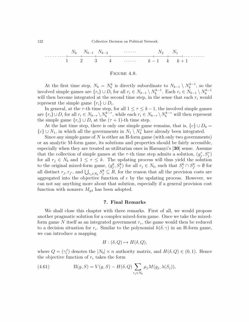
122 Collective Decision on Political Network
1 2 3 4 k − 1 k k + 1
Nk Nk−1 Nk−2 N2 N1. . . . . .
. . . . . .
Figure 4.8.
At the first time step, Nk = Nkb is directly subordinate to Nk−1 \ Nk−1
b , so theinvolved simple games are {ri} ∪Di for all ri ∈ Nk−1 \Nk−1
b . Each ri ∈ Nk−1 \Nk−1b
will then become integrated at the second time step, in the sense that each ri wouldrepresent the simple game {ri} ∪Di.
In general, at the τ -th time step, for all 1 ≤ τ ≤ k−1, the involved simple gamesare {ri}∪Di for all ri ∈ Nk−τ \Nk−τ
b , while each ri ∈ Nk−τ \Nk−τb will then represent
the simple game {ri} ∪Di at the (τ + 1)-th time step.At the last time step, there is only one simple game remains, that is, {c} ∪D0 =
{c} ∪N1, in which all the governments in N1 \N1b have already been integrated.
Since any simple game of N is either an H-form game (with only two governments)or an analytic M-form game, its solutions and properties should be fairly accessible,especially when they are treated as utilitarian ones in Harsanyi’s [30] sense. Assumethat the collection of simple games at the τ -th time step admits a solution, (gτj , S
τj )
for all rj ∈ Nb and 1 ≤ τ ≤ k. The updating process will thus yield the solutionto the original mixed-form game, (gkj , S
kj ) for all rj ∈ Nb, such that Skj ∩ Skj′ = ∅ for
all distinct rj, rj′ , and⋃rj∈Nb
Skj ⊆ R, for the reason that all the provision costs are
aggregated into the objective function of c by the updating process. However, wecan not say anything more about that solution, especially if a general provision costfunction with nonzero Mgλ has been adopted.
7. Final Remarks
We shall close this chapter with three remarks. First of all, we would proposeanother pragmatic solution for a complex mixed-form game. Once we take the mixed-form game N itself as an integrated government rc, the game would then be reducedto a decision situation for rc. Similar to the polynomial h(δ, γ) in an H-form game,we can introduce a mapping
H : (δ,Q) 7→ H(δ,Q),
where Q = (γji ) denotes the |Nb| × n authority matrix, and H(δ,Q) ∈ (0, 1). Hencethe objective function of rc takes the form
(4.61) Π(g, S) = V (g, S)−H(δ,Q)∑rj∈Nb
µjM(gj, λ(Sj)),

Final Remarks 123
where g =∑
rj∈Nbµjgj and S =
⋃rj∈Nb
Sj. Clearly, the solution to the game N is
the collection of (gcj , Scj ) for all rj ∈ Nb which jointly maximize Π(g, S).
Secondly, it should be stressed that the roles of communication and informationsharing in the games were intentionally neglected. In fact, we have assumed that anyauthority gap in a government network does not affect any decision-making processand hence the entire game. However, governments in some authority gap, thoughtwith no authority at all, might still play nontrivial roles in some collective decision-making process, especially when they serve as hubs connecting governments withenforceable political powers.
Last but not least, the authority allocation rule in a political system has been setas fixed in our studies. Nevertheless, it seems fairly natural that different politicalsystems should adopt different authority allocation rules according to their differentnormative initiations per se. For example, if a political system is supposed to relyon economic efficiency and direct democracy more seriously, then more authoritiesshould be distributed to the bottom governments. If a political system has developeda rather dominant tendency towards justice, then more authorities might be betterallocated to such governments that have greatest enforceable political powers. Aswas demonstrated in an H-form government line, they should be the governments onthe hierarchical levels χ∗ and χ∗ + 1, where χ∗ is defined to be the conjugate valueof blogδ h(δ, γ)c. Overall, it seems quite hard to determine and even to design anappropriate authority allocation rule for a specific political system.


Bibliography
1. M. A. Akivis and V. V. Goldberg, Algebraic aspects of web geometry, Comment. Math. Univ.Carolin. 41 (2000), no. 2, 205–236.
2. M. Al-Suhaibani and L. Kryzanowski, An exploratory analysis of the order book, and order flowand execution on the Saudi Stock Market, J. Bank. Finance 24 (2000), no. 8, 1323–1357.
3. L. Bachelier, Theorie de la speculation, Ann. Sci. Ec. Norm. Super. 3 (1900), no. 17, 21–86.4. J. Banks, J. Brooks, G. Cairns, G. Davis, and P. Stacey, On Devaney’s definition of chaos,
Amer. Math. Mon. 99 (1992), no. 4, 332–334.5. M. F. Barnsley and S. Demko, Iterated function systems and the global construction of fractals,
Proc. R. Soc. Lond. A 399 (1985), no. 1817, 243–275.6. A. Barrat, M. Barthelemy, and A. Vespignani, Dynamical processes on complex networks, Cam-
bridge University Press, New York, 2008.7. T. Bergstrom, L. Blume, and H. Varian, On the private provision of public goods, J. Public
Econ. 29 (1986), no. 1, 25–49.8. N. P. Bhatia and G. P. Szego, Dynamical systems: Stability theory and applications, Lect. Notes
Math., vol. 35, Springer-Verlag, Berlin, 1967.9. B. Biais, P. Hillion, and C. Spatt, An empirical analysis of the limit order book and the order
flow in the Paris Bourse, J. Finance 50 (1995), no. 5, 1655–1689.10. D. Bouyssou and T. Marchant, Additive conjoint measurement with ordered categories, Eur. J.
Oper. Res. 203 (2010), no. 1, 195–204.11. L. Calvet and A. Fisher, Multifractality in asset returns: theory and evidence, Rev. Econ. Stat.
84 (2002), no. 3, 381–406.12. G. Choquet, Theory of capacities, Ann. Inst. Fourier 5 (1954), 131–295.13. G. de Rham, On some curves defined by functional equations, Classics on Fractals (G. A. Edgar,
ed.), Westview Press, Boulder, CO, 2004, pp. 285–297.14. G. Debreu, Topological methods in cardinal utility theory, Mathematical Methods in the Social
Sciences (K. J. Arrow, S. Karlin, and P. Suppes, eds.), Stanford University Press, Stanford,CA, 1960, pp. 16–26.
15. H. Demsetz, The cost of transacting, Q. J. Econ. 82 (1968), no. 1, 33–53.16. R. L. Devaney, An introduction to chaotic dynamical systems, Benjamin Cummings, Menlo
Park, CA, 1986.17. M. Ezekiel, The cobweb theorem, Q. J. Econ. 52 (1938), no. 2, 255–280.18. J. D. Farmer, P. Patelli, and I. I. Zovko, The predictive power of zero intelligence in financial
markets, Proc. Natl. Acad. Sci. USA 102 (2005), no. 6, 2254–2259.19. P. C. Fishburn, Utility theory for decision making, John Wiley & Sons, New York, 1970.20. , Nontransitive additive conjoint measurement, J. Math. Psychol. 35 (1991), no. 1, 1–40.21. P. C. Fishburn and A. Rubinstein, Time preference, Int. Econ. Rev. 23 (1982), no. 3, 677–694.
125

126 Bibliography
22. T. Foucault, O. Kadan, and E. Kandel, Limit order book as a market for liquidity, Rev. Financ.Stud. 18 (2005), no. 4, 1171–1217.
23. M. Francesconi and A. Muthoo, Control rights in complex partnership, J. Eur. Econ. Assoc. 9(2011), no. 3, 551–589.
24. A. Galeotti and S. Goyal, The law of the few, Am. Econ. Rev. 100 (2010), no. 4, 1468–1492.25. L. R. Glosten and P. R. Milgrom, Bid, ask and transaction prices in a specialist market with
heterogeneously informed traders, J. Financ. Econ. 14 (1985), no. 1, 71–100.26. W. M. Gorman, Separable utility and aggregation, Econometrica 27 (1959), no. 3, 469–481.27. T. Groves and M. Loeb, Incentives and public inputs, J. Public Econ. 4 (1975), no. 3, 211–226.28. R. Hardin, Collective action, John Hopkins University Press, Baltimore, MA, 1982.29. L. Harris and J. Hasbrouck, Market vs. limit orders: the SuperDOT evidence on order submis-
sion strategy, J. Financ. Quant. Anal. 31 (1996), no. 2, 213–231.30. J. C. Harsanyi, Cardinal welfare, individual ethics, and interpersonal comparisons of utility, J.
Polit. Econ. 63 (1955), no. 4, 309–321.31. N. Kaldor, A classificatory note on the determinateness of equilibrium, Rev. Econ. Stud. 1
(1934), no. 2, 122–136.32. E. Karni and Z. Safra, The hexagon condition and additive representation for two dimensions:
An algebraic approach, J. Math. Psychol. 42 (1998), no. 4, 393–399.33. W. Krabs and S. Pickl, Dynamical systems: Stability, controllability and chaotic behavior,
Springer-Verlag, Berlin, 2010.34. D. H. Krantz, R. D. Luce, P. Suppes, and A. Tversky, Foundations of measurement, vol. I:
Additive and polynomial representations, Academic Press, New York, 1971.35. A. S. Kyle, Continuous auctions and insider trading, Econometrica 53 (1985), no. 6, 1315–1335.36. B. N. Lehmann and D. M. Modest, Trading and liquidity on the Tokyo Stock Exchange: a bird’s
eye view, J. Finance 49 (1994), no. 3, 951–984.37. W. Leontief, Delayed adjustment of supply and partial equilibrium, J. Econ. 5 (1934), no. 5,
670–676.38. T.-Y. Li and J. A. Yorke, Period three implies chaos, Amer. Math. Mon. 82 (1975), no. 10,
985–992.39. R. D. Luce and J. W. Tukey, Simultaneous conjoint measurement: a new type of fundamental
measurement, J. Math. Psychol. 1 (1964), no. 1, 1–27.40. B. B. Mandelbrot, The variation of certain speculative prices, J. Bus. 36 (1963), no. 4, 394–419.41. , Les objets fractals: forme, hasard et dimension, Flammarion, Paris, 1975.42. , The fractal geometry of nature, W. H. Freeman and Company, New York, 1982.43. B. B. Mandelbrot and J. W. van Ness, Fractional Brownian motions, fractional noises and
applications, SIAM Rev. 10 (1968), no. 4, 422–437.44. C. F. Manski, Maximum score estimation of the stochastic utility model of choice, J. Econom.
3 (1975), no. 3, 205–228.45. J. Milnor, On the concept of attractor, Comm. Math. Phys. 99 (1985), no. 2, 177–195.46. T. Mitra, L. Montrucchio, and F. Privileggi, The nature of the steady state in models of optimal
growth under uncertainty, Econ. Theory 23 (2004), no. 1, 39–71.47. T. Mitra and F. Privileggi, On Lipschitz continuity of the iterated function system in a stochastic
optimal growth model, J. Math. Econ. 45 (2009), no. 1–2, 185–198.48. W. E. Oates, Fiscal federalism, Harcourt Brace Jovanovich, New York, 1972.49. , An essay on fiscal federalism, J. Econ. Lit. 37 (1999), no. 3, 1120–1149.50. M. F. M. Osborne, Brownian motion in the stock market, Oper. Res. 7 (1959), no. 2, 145–173.

127
51. C. A. Parlour, Price dynamics in limit order markets, Rev. Financ. Stud. 11 (1998), no. 4,789–816.
52. H. Poincare, Science and method, (F. Maitland trans.), Thomas Nelson & Sons, London, 1914.53. Y. Qian and B. R. Weingast, Federalism as a commitment to preserving market incentives, J.
Econ. Perspect. 11 (1997), no. 4, 83–92.54. F. S. Roberts, Measurement theory: With applications to decisionmaking, utility, and the social
sciences, Addison-Wesley, Reading, MA, 1979.55. D. Ruelle, Strange attractors, Math. Intell. 2 (1980), no. 3, 126–137.56. D. Ruelle and F. Takens, On the nature of turbulence, Comm. Math. Phys. 20 (1971), no. 3,
167–192.57. P. A. Samuelson, The pure theory of public expenditure, Rev. Econ. Stat. 36 (1954), no. 4,
387–389.58. H. A. Simon, A formal theory of the employment relationship, Econometrica 19 (1951), no. 3,
293–305.59. E. Smith, J. D. Farmer, L. Gillemot, and S. Krishnamurthy, Statistical theory of the continuous
double auction, Quant. Finance 3 (2003), no. 6, 481–514.60. D. Sornette, Why stock markets crash: Critical events in complex financial systems, Princeton
University Press, Princeton, NJ, 2003.61. G. Teschl, Ordinary differential equations and dynamical systems, Grad. Stud. Math., vol. 140,
Amer. Math. Soc., Providence, RI, 2012.62. G. Thomsen, Un teoreme topologico sulle schiere di curve e una caratterizzazione geometrica
delle superficie isotermo-asintotiche, Boll. Un. Mat. Ital. Bologna 6 (1927), 80–85.63. C. M. Tiebout, A pure theory of local expenditure, J. Polit. Econ. 64 (1956), no. 5, 416–424.64. H. Uzawa, On a two-sector model of economic growth, Rev. Econ. Stud. 29 (1961), no. 1, 40–47.65. P. P. Wakker, Additive representations of preferences: A new foundation of decision analysis,
Kluwer Academic Publishers, Dordrecht, 1989.66. S. Wang, Dynamical trading mechanisms in limit order markets, Algorithm. Finance 2 (2013),
no. 3–4, 213–231.67. B. R. Weingast, The economic role of political institutions: market-preserving federalism and
economic development, J. Law Econ. Organ. 11 (1995), no. 1, 1–31.68. E. Wibbels, Decentralized governance, constitution formation, and redistribution, Constitut.
Polit. Econ. 16 (2005), no. 2, 161–188.


Index
3-web, 32Complete, 33Curvature, 37Hexagonal, 34
π-balanced measure, 17
Attractor, 3, 10, 13, 15Asymptotically stable, 11Basin, 10Lyapunov stable, 10Strange attractor, 3, 18Unstable, 10Weak attractor, 10
Authority, 79, 99, 115Authority allocation rule, 80Authority gap, 90Indicator matrix, 116
Brownian motion, 5Fractional, 5Geometric, 5
Chaos, 2, 11, 12, 14Nonperiodic, 14
Choice function, 21Cobweb theorem, 4Complexity, 4, 111
Decision-making process, 79, 99Purely decentralized, 81
Disorder, 70, 111External, 70Intrinsic, 70
Dynamical system, 5Continuous dynamical system, 6
Discrete dynamical system, 6, 13, 55Flow, 6Linear dynamical system, 11Motion, 6Planar dynamical system, 9State space, 5Time domain, 5Trajectory, 7, 13Transition, 6
Euler equation, 25Exponential law, 51, 52
Fractal, 3, 18Cantor set, 20Koch curve, 3, 21Peano curve, 21
Governance structure, 80Autonomous, 80Centralized, 80Decentralized, 80
Pure, 81Government network, 76
Bottom government, 77Central government, 76Compact, 111
Physically connected, 111Politically connected, 111
Directly subordinate government, 77, 112H-form, 76Hierarchical level, 76Imaginary government, 120Isolated government, 77Local government, 76
129

130 Index
M-form, 76Mixed-form, 112Path, 80Subordinate government, 77, 113
H-form government line, 76, 89Focal hierarchical level, 97H-form game, 89Negotiation game, 94Pareto efficient solution, 93Utilitarian solution, 94
Hutchinson operator, 15
Inada condition, 24Iterated function system, 15, 55
Iterated affine function system, 20Iterated random function system, 16
Limit order market, 44Appearance probability, 52, 59Bid-ask pair, 44Limit order, 46Limit order book, 45Marginal trader, 44Market capacity, 51, 52Market order, 47Mid-price, 44Mid-price function, 44Spread, 44Spread function, 44Switching law, 52, 53Tick size, 44
Local public good, 83Centralized provision scheme, 88Decentralized provision scheme, 88Provision capacity, 83
Superadditive, 83Provision cost function, 84
Lyapunov exponent, 12
M-form government star, 76, 89Interval solution, 106M-form game, 89
Analytic, 100, 104Degenerate, 100, 102
Mixed-form government network, 112Hierarchical decomposition, 114
Indicator matrix, 116Induced subgame, 113
Nonsimple, 113Mixed-form game, 112Pragmatic solution, 120Simple game, 112
Poincare-Bendixson theorem, 9Political discounting, 92
Regular, 92Preference relation, 21, 29
Additive, 28, 37Double cancellation condition, 30Independent, 29Indifference, 29Induced, 29Rational, 29Separable, 28Solvable, 29Stationary, 31Thomsen condition, 30Time preference, 22, 24, 31
Sarkovskii’s theorem, 14Stateα-limit, 8ω-limit, 8Asymptotically stable, 11Attractor, 10, 13Equilibrium, 7, 13Exponentially stable, 11Invariant, 7, 13Limit cycle, 8Lyapunov stable, 11Periodic, 8, 13
Asymptotic, 13Final, 13
Weakly stable, 10
Thomsen condition, 30, 32, 36, 37Trading block, 55
Consecutive, 55Irreducible, 57Periodic, 55
Minimal, 56Trading system, 54m-range, 60

131
s-range, 60Ask-range, 63Bid-range, 63Buffering region, 59, 71Catastrophe, 54Controlled trading system, 63Crash, 54Dynamical trading system, 55Instability sharing, 58Iterated trading system, 55Kernel region, 59, 71Stochastic stability, 61, 64, 69, 71Systemic instability, 71Trading block, 55Unstable, 54
Transformation operator, 34
Utility function, 21, 29Additive, 28Cobb-Douglas, 39Harsanyi, 86Leontief, 39Random, 23Separable, 28
Volatility, 5, 63, 70


Estratto per riassunto della tesi di dottorato
Studente Shilei WangMatricola 955949Dottorato EconomiaCiclo XXVIITitolo della tesi Group Structure and Collective Behavior
Abstract:
The present dissertation consists of four chapters, which are loosely connected bythe abstract relation between group structure and collective behavior. Three mainabstractions of group structure are proposed, viz., time-dependent group which canbe characterized by dynamical system, preference-dependent group that depends onaggregation of individual preferences, and relation-dependent group which is knownas network.
In this respect, some interesting problems are investigated so as to demonstrate theeffects of group structure on collective behavior. In detail, Chapter 1 studies suchproperties as dynamics, chaos, and stability in a typical time-dependent group, whichalso lays some solid foundations for the studies in the other three chapters. Chapter2 investigates separable and additive aggregation rules in a preference-dependentgroup, with the aim of developing algebraic-geometric principles to efficiently identifyadditive aggregation rules. In particular, the Thomsen condition has been revisitedand shown to be a both sufficient and necessary requirement for an aggregation rulebeing additive on a quite general two-dimensional domain.
Chapter 3 can be thought of as an application of time-dependent group in equitymarkets, in which quotation formation and dynamics are discussed in great detail.Some significant assertions on stability and stochastic stability are developed bymeans of market conditions. Chapter 4 relies on collective decision-making processon a government network to show how decisions are contingent on different networkstructures, which can be classified as H-form government line, M-form governmentstar, and more general mixed-form network.
JEL Classification. C69, C79, D69, D79, G19
2000 Mathematics Subject Classification. 91B15, 91B16, 91B18, 91B55, 91G99
Firma dello studente
Shilei Wang