Embed Size (px)
Citation preview
Growth and Development in
an Empirical Dual Economy Model
Markus Eberhardta,b∗ Francis Tealb,c
a St Catherine’s College, Oxfordb Centre for the Study of African Economies,
Department of Economics, University of Oxfordc Institute for the Study of Labor, Bonn (IZA)
Draft paper: 24th February 2010
Abstract:
The empirical literature on cross-country growth and development commonly employs aggre-gate economy data such as the Penn World Table Heston, Summers, and Aten (2009) toestimate homogeneous production function or convergence regression models. Against thebackground of a dual economy framework this paper investigates the potential sources of biaswhen aggregate economy data is adopted instead of sectoral data. Furthermore we investigatethe evidence for various sources of growth arising in the dual economy literature. Followingappropriate empirical specification and testing we estimate production functions in agricultureand manufacturing for a large panel of developing and developed countries (1963-1992, Crego,Larson, Butzer, & Mundlak, 1998). Our focus is on recent panel time series methods whichcan accommodate technology heterogeneity, variable time-series properties and the breakdownof the standard cross-section independence assumption in panels. We investigate the potentialfor bias in the production parameter coefficients due to aggregation of sectors and empiricalmisspecification. Finally we test the significance of the potential sources of growth identifiedin our discussion of the dual economy model.
Keywords: dual economy model, production function, common factor modelJEL classification: C33, O13
∗Financial support from the UK Economic and Social Research Council [grant numbers PTA-031-2004-00345and PTA-026-27-2048] is gratefully acknowledged by the first author. Correspondence: Centre for the Studyof African Economies (CSAE), Department of Economics, Manor Road Building, Oxford OX1 3UQ, UK; Email:[email protected]
AN EMPIRICAL DUAL ECONOMY MODEL 1
1. INTRODUCTION
“If we ask ‘why do they [undeveloped economies] save so little’, the truthful answer is not‘because they are so poor’ . . . The truthful answer is ‘because their capitalist sector is sosmall’ (remembering that ‘capitalist’ here does not mean private capitalist, but would applyequally to state capitalist).” Lewis (1954, p.159)
In the early literature on developing countries a distinction was made between the processes of eco-nomic development and of economic growth. Economic development was seen to be a process ofstructural transformation by which in Lewis’ frequently cited phrase an economy which was “previ-ously saving and investing 4 or 5 percent of its national income or less, converts itself into an economywhere voluntary savings is running at about 12 to 15 percent of national income” (Lewis, 1954, p.155).An acceleration in the investment rate was only one part of this process of structural transformation;of equal importance was the process by which an economy moved from a dependence on subsistenceagriculture to one where an industrial modern sector absorbed an increasing proportion of the labourforce (Jorgensen, 1961; Kaldor, 1966; Kindleberger, 1967; Kuznets, 1961; Leibenstein, 1957; Ranis &Fei, 1961; Robinson, 1971). In contrast to these models of “development for backward economies”(Jorgensen, 1961, p.309), where duality between the modern and traditional sectors was a key featureof the model, was the analysis of economic growth in developed economies.1 Here the processes offactor accumulation and technical progress occur in an economy which is already ’developed’, in thesense that it has a modern industrial sector and agriculture has ceased to be a major part of theeconomy (e.g. Solow, 1956, 1957; Swan, 1956; Cass, 1965).
A common feature across these literatures on both economic development and growth was the useof closed economy models. The basic models put forward by Lewis and by Solow-Swan were closedeconomy models in which structural transformation and growth occurred within economies.2 Howeverit was soon realised that these were not the most appropriate models for economies which were smallin geographical area and open to the world economy in the sense that their influence on the prices oftheir products was minimal. As noted by Lucas (1988), the theory of trade as developed by Ricardoand Heckscher-Ohlin implies that trade can have “a level effect, analogous to the one-time shiftingupward in production possibilities, [but] not a growth effect” (12) on income. The strong correlationapparent in the data between income growth and trade led to much new work on the theory of howtrade may impact growth (e.g. Grossman & Helpman, 1991; Rivera-Batiz & Romer, 1991; Aghion &Howitt, 1992; Matsuyama, 1992), one key mechanism being via improvement in technical progress,another being externalities. In fact much of the empirical work on this topic (Coe, Helpman, & Hoff-maister, 1997; Frankel & Romer, 1999; Rodriguez & Rodrik, 2001; Greenaway, Morgan, & Wright,2002; Dollar & Kraay, 2002, 2004) used reduced form models and side-stepped the theoretical issuesas to exactly why more open economies might grow faster.
Much of the early growth modelling work proceeded without close connection to observed data. Themodels were in Solow’s classic exposition of growth theory inspired by stylised ‘Kaldor’ facts (Kaldor,1957). As Solow (1970, p.2) notes, “[t]here is no doubt that they are stylized, though it is possible toquestion whether they are facts.” The dual economy models of structural transformation used case
1A note on nomenclature: we refer to ‘duality’ or ‘dual economy models’ as representing economies with two stylisedsectors of production (agriculture and manufacturing), while ‘dualism’ refers to wage or marginal labour product differ-ences between sectors. Total Factor Productivity (TFP) is referred to as technology or technology levels, TFP growth astechnical/technological progress. We use productivity to refer to income/output per worker, and commonly make thisclear by referring to ‘labour productivity’ in contrast to productivity referring to TFP levels.
2This is in one sense not surprising as the major ‘development’ question of the 1930s still influencing these authors’thinking was the experiment in the Soviet Union to industrialise in autarky in the space of a decade. This aside, thelargest economy in the world – the United States – occupying as it does an entire continent was one in which externaltrade certainly did not seem the major agent in the growth process.
AN EMPIRICAL DUAL ECONOMY MODEL 2
studies (e.g. Paauw & Fei, 1973) and facts at least as stylised as those in the Solow-Swan growthcontext. Empirical studies employed a vast array of explanatory variables of growth, while method-ological, statistical, and conceptual difficulties on top of sample heterogeneity made it difficult todraw reliable conclusions from the existing literature (Levine & Renelt, 1991). The key papers whichbrought modelling and data together were the contributions of Barro (1991) and Mankiw, Romer,and Weil (1992), which initiated a major revival in the Solow-Swan model and effectively merged theconcerns of economic development with those of growth.3
The literature begun in the early 1990s has yielded a large array of models in which there has beenincreasing interaction between the theory and the empirics (see discussion in Aghion & Howitt, 1998;Durlauf & Quah, 1999; Easterly, 2002; Durlauf, Johnson, & Temple, 2005). It remains true that theempirical analysis continues to be dominated by the empirical version of the aggregate Solow-Swanmodel (Temple, 2005) with much of the empirical debate focusing on the roles of factor accumula-tion versus technical progress (Young, 1995; Chen, 1997; Klenow & Rodriguez-Clare, 1997a, 1997b;Easterly & Levine, 2001; Lipsey & Carlaw, 2001; Baier, Dwyer, & Tamura, 2006). While there issome new theoretical and empirical work using a dual economy model (e.g. Vollrath, 2009a, 2009b,2009c), this is largely absent from textbooks on economic growth and has not been the central focus ofattention for most of the empirical analyses (Temple, 2005). A primary reason for the focus has beenthe availability of data. The Penn World Table (PWT) dataset — most recently (Heston et al., 2009)— and the Barro-Lee data on human capital (Barro & Lee, 1993, 2001) have supplied macro-datawhich ensure that the aggregate Solow-Swan model can be readily estimated. In recent years therehas however been a development of datasets that allow a closer matching between the dual economymodels and the data (Larson, Butzer, Mundlak, & Crego, 2000), which this paper will exploit to throwlight on several of the empirical issues that have been central to the analysis of the sources of growth.
Cross-country growth regressions represent one of the most active fields of empirical analysis withinapplied development economics, however the viability of this empirical approach has been seriouslyquestioned over the past decade and at present these methods are deeply unfashionable. We haveargued elsewhere that much can be learned from cross-country empirics provided the empirical setupallows for greater flexibility in the estimation equation and recognises the salient data properties ofmacro panel datasets (Eberhardt & Teal, 2010). Methods developed in the emerging panel time seriesliterature (Bai & Ng, 2002, 2004; Coakley, Fuertes, & Smith, 2006; Pesaran, 2006; Bai, 2009) cango further in providing robust estimation and inference for nonstationary panel data where variableseries may be correlated across countries and where common shocks are likely to impact all countriesin the sample, albeit to a different extent.
This paper, providing empirical analysis of panel data for developing and developed economies, setsout to address three main objectives: (i) rather than using a calibrated dual economy model forquantitative analysis we provide empirical estimates for technology coefficients in sectoral productionfunctions. This allows for the integration of recent developments in the literature on applied paneldata econometrics, including the insights of the emerging panel time series literature. (ii) We estimatea stylised aggregate production function model from agriculture and manufacturing data, and compareresults with those from disaggregated regressions. This will allow us to judge whether neglecting adual economy structure leads to bias in the empirical technology coefficients. (iii) In the light of theresults from our sectoral production function estimations we assess the relative sources of growth in adual economy model: TFP growth and level differences across sectors, and marginal factor dualism.
3The addition of human capital to the Solow model in Mankiw et al. (1992) “leads to quantitative predictions thatlook consistent with the data” (Temple, 2005, p.436).
AN EMPIRICAL DUAL ECONOMY MODEL 3
The remainder of this paper is organised as follows: Section 2 reviews the existing literature andprovides an encompassing conceptual framework for the analysis of dual economy effects at the macrolevel. In the following section we then introduce an empirical specification of our dual economy frame-work, discuss the data and briefly review the empirical methods and estimators employed. Section4 reports and discusses empirical findings and we then investigate suggested sources of growth anddevelopment empirically in Section 5. Section 6 summarizes and concludes.
2. GROWTH AND DEVELOPMENT
The literature on dual economy models is surprisingly large, given the relatively limited impact thisapproach has had in entering textbooks on economic growth theory and analysis, and economics ‘or-thodoxy’ in general. With the availability of sectoral data for a cross-section of countries limiteduntil recently, some of the existing work in this area is built on models relatively disjoint from theformulation of empirically testable questions, while other studies have focused on very specific detailsof the growth and development process which are then ‘tested’ using simulation or calibrated mod-els. As a result many of the dual economy models, given their complexity and data requirements,do not suit themselves for empirical testing. In this section we present a theoretical dual economymodel based on the existing literature, however focussed on providing as general and encompassing atreatment as possible whilst formulating an empirically testable model. Findings from previous workusing accounting exercises and a small number of sectoral production function estimations suggest anumber of potential sources of growth in a dual economy framework which we review below.
In the next section an empirically testable model of the open dual economy will be set out. In section2.2 the potential sources of growth in such models will be outlined and the empirical evidence forthe importance of duality in the growth process reviewed. Section 2.3 concludes this part of thepaper.
2.1 A model of an open dual economy
The early literature on structural change did not pursue formal modelling of the small open dualeconomy setup, but limited itself to a conceptual understanding of the link between structural changeand potential growth in a closed economy. Lewis (1954), Kaldor (1966), Kindleberger (1967) andRanis and Fei (1961), for instance, all emphasize the potential for surplus labour in agriculture to actas a major driver for structural change via the migration of labour into the emerging manufactur-ing sector. In their analyses elastic labour supply enables economic growth by keeping wages in themodern sector low and preserving industrial peace (Temple, 2001; Temin, 2002; Barbier & Rauscher,2007). A somewhat more complex analysis suggests that agricultural income and food supply con-straints should be the focus of analysis, since they represent barriers to structural change and thusdevelopment (Jorgensen, 1961). Openness to trade, however, somewhat relaxes these constraints. Asnoted in the introduction, modelling structural change and growth in a closed economy model is notdeemed appropriate to model the development process in small open economies.
The supply side of a small, open dual economy model can be represented by two sectors, assumed tobe agriculture (‘traditional sector’) and manufacturing (‘modern sector’), producing distinct goods. Itis posited that these two types of production are geographically distinct, the former present in ruralareas and the latter in urban areas. Their respective technologies are assumed Cobb-Douglas but
AN EMPIRICAL DUAL ECONOMY MODEL 4
unrestricted with regard to returns to scale4
Ya,t = Aa,t F (Ka,t, La,t, Na,t) = Aa,tKαa,t, L
βa,t, N
γa,t α, β, γ < 1 (1)
Ym,t = Am,tG(Km,t, Lm,t) = Am,tKφm,t, L
ψm,t φ, ψ < 1 (2)
Aj,t = Aj,0 exp(λjt) for j = a,m (3)
where A represents disembodied technical efficiency of production (TFP),5 K is physical, reproduciblecapital, and L is labour (either raw labour or adjusted for human capital differences) for both agri-cultural and manufacturing sectors a and m.6 Capital and labour are stock variables which can beaccumulated infinitely, but are subject to diminishing returns. N is non-reproducible capital (assumedto be arable land and other forms of capital), and only enters the agricultural production function.We drop the time subscript for ease of exposition.
In the most general specification TFP growth rates λj and TFP levels Aj,0 are allowed to differ acrosssectors, countries, and in case of TFP growth across time. When a country’s manufacturing sectorenjoys higher TFP growth than its agricultural sector, this implies ceteris paribus higher output growthin manufactured goods, and (deflated by sector share in total output sa, sm) higher aggregate outputgrowth g.
g = Y /Y = Z/Z[+ηL/L+ µK/K
]= Z/Z = saAa/Aa + smAm/Am (4)
Allowing TFP growth λj to vary over time allows for a more realistic dynamic evolvement of thesectoral technology level than a constant TFP growth rate. Given differential TFP levels betweensectors, say Aa < Am, structural transformation in the form of labour migration to manufacturingwould result in a temporary level effect on output. Unlike in the TFP growth case this would not changethe perpetual growth trajectory of the economy.7 Persistent and significant TFP level differencesbetween sectors signal the presence of barriers to technology acquisition or some other form of frictionin the low-TFP sector, while TFP level differences across countries signal frictions on the country-level (Caselli, 2005; Restuccia, Yang, & Zhu, 2008). We assume that the economy is open to trade inproducts but closed to cross-country factor migration such that
Y = Ya + pYm (5)
where the price of the agricultural good Ya is the numeraire and p provides the relative price ofmanufactures, exogenously determined by the world price. We restrict discussion to incompletelyspecialised economies, i.e. both sectors have positive output. We assume full capital employment
K = Ka +Km (6)
with capital perfectly mobile between the two sectors leading to rental rate equalisation
ra = MPKa = Aa∂F/∂Ka = αYaKa
rm = MPKm = pAm∂G/∂Km = pφYmKm
rm = ra (7)
4Our model specification is guided by Temple (2005) and Corden and Findlay (1975).5We see this as a ‘catch-all’ for disembodied levels of productive efficiency and technology as well as characteristics
such as taxation, regulation, climate, soil conditions etc., following Gollin, Parente, and Rogerson (2002).6Note that agricultural and rural labour should not be taken as homogeneous, but we can assume a setup that
allows us to keep the model as it is laid out above, without losing the appeal of this notion (Temple, 2005): using ourspecification, we assume human capital to be embodied partly within capital and partly within the technical progressterm . Human capital data in Timmer (2000) taken from Chai (1995) would halve the number of countries in ourmanufacturing dataset since only developing nations are discussed. A UNESCO dataset discussed in Cordoba and Ripoll(2009) contains only a handful of observations across time and countries. Due to reasons of limited space in this paperthe option to experiment with these datasets was not pursued.
7Nevertheless, TFP levels “capture the differences in long-run economic performance that are most directly relevantto welfare” (Hall & Jones, 1999, p.85).
AN EMPIRICAL DUAL ECONOMY MODEL 5
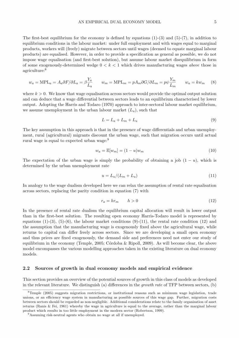
The first-best equilibrium for the economy is defined by equations (1)-(3) and (5)-(7), in addition toequilibrium conditions in the labour market: under full employment and with wages equal to marginalproducts, workers will (freely) migrate between sectors until wages (deemed to equate marginal labourproducts) are equalised. However, in order to provide a specification as general as possible, we do notimpose wage equalisation (and first-best solution), but assume labour market disequilibrium in formof some exogenously-determined wedge 0 < k < 1 which drives manufacturing wages above those inagriculture:8
wa = MPLa = Aa∂F/∂La = βYaLa
wm = MPLm = pAm∂G/∂Lm = pψYmLm
wa = kwm (8)
where k > 0. We know that wage equalisation across sectors would provide the optimal output solutionand can deduce that a wage differential between sectors leads to an equilibrium characterised by loweroutput. Adopting the Harris and Todaro (1970) approach to inter-sectoral labour market equilibrium,we assume unemployment in the urban labour market (Lu), such that
L = La + Lm + Lu (9)
The key assumption in this approach is that in the presence of wage differentials and urban unemploy-ment, rural (agricultural) migrants discount the urban wage, such that migration occurs until actualrural wage is equal to expected urban wage:9
wa = E[wm] = (1− u)wm (10)
The expectation of the urban wage is simply the probability of obtaining a job (1 − u), which isdetermined by the urban unemployment rate
u = Lu/(Lm + Lu) (11)
In analogy to the wage dualism developed here we can relax the assumption of rental rate equalisationacross sectors, replacing the parity condition in equation (7) with
ra = hrm h > 0 (12)
In the presence of rental rate dualism the equilibrium capital allocation will result in lower outputthan in the first-best solution. The resulting open economy Harris-Todaro model is represented byequations (1)-(3), (5)-(6), the labour market conditions (9)-(11), the rental rate condition (12) andthe assumption that the manufacturing wage is exogenously fixed above the agricultural wage, whilereturns to capital can differ freely across sectors. Since we are developing a small open economyand thus prices are fixed exogenously, the demand side and preferences need not enter our study ofequilibrium in the economy (Temple, 2005; Cordoba & Ripoll, 2009). As will become clear, the abovemodel encompasses the various modelling approaches taken in the existing literature on dual economymodels.
2.2 Sources of growth in dual economy models and empirical evidence
This section provides an overview of the potential sources of growth in this class of models as developedin the relevant literature. We distinguish (a) differences in the growth rate of TFP between sectors, (b)
8Temple (2005) suggests migration restrictions, or institutional reasons such as minimum wage legislation, tradeunions, or an efficiency wage system in manufacturing as possible sources of this wage gap. Further, migration costsbetween sectors should be regarded as non-negligible. Additional considerations relate to the family organisation of assetreturns (Ranis & Fei, 1961) whereby the wage in agriculture is equal to the average, rather than the marginal labourproduct which results in too little employment in the modern sector (Robertson, 1999).
9Assuming risk-neutral agents who obtain no wage at all if unemployed.
AN EMPIRICAL DUAL ECONOMY MODEL 6
differences in the level of TFP between sectors, and (c) marginal factor product dualism. Respectivemodelling approaches, empirical specifications and estimation methods are presented in the following,along with the most important findings.
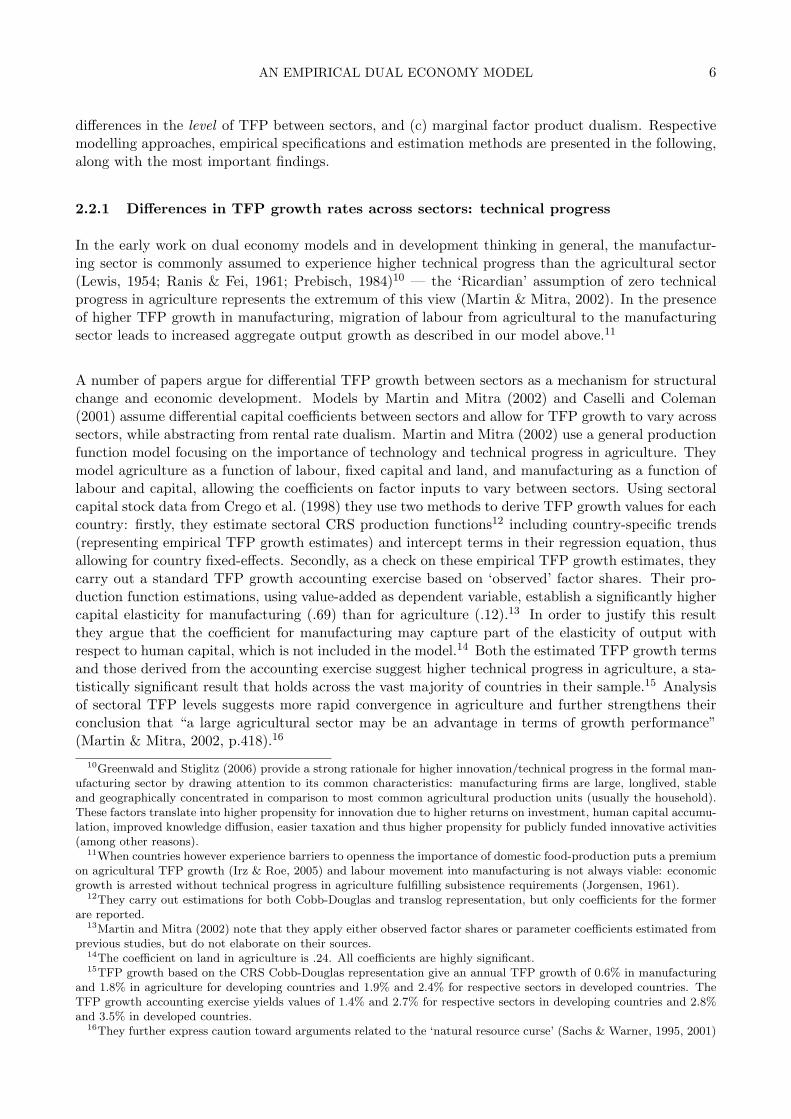
2.2.1 Differences in TFP growth rates across sectors: technical progress
In the early work on dual economy models and in development thinking in general, the manufactur-ing sector is commonly assumed to experience higher technical progress than the agricultural sector(Lewis, 1954; Ranis & Fei, 1961; Prebisch, 1984)10 — the ‘Ricardian’ assumption of zero technicalprogress in agriculture represents the extremum of this view (Martin & Mitra, 2002). In the presenceof higher TFP growth in manufacturing, migration of labour from agricultural to the manufacturingsector leads to increased aggregate output growth as described in our model above.11
A number of papers argue for differential TFP growth between sectors as a mechanism for structuralchange and economic development. Models by Martin and Mitra (2002) and Caselli and Coleman(2001) assume differential capital coefficients between sectors and allow for TFP growth to vary acrosssectors, while abstracting from rental rate dualism. Martin and Mitra (2002) use a general productionfunction model focusing on the importance of technology and technical progress in agriculture. Theymodel agriculture as a function of labour, fixed capital and land, and manufacturing as a function oflabour and capital, allowing the coefficients on factor inputs to vary between sectors. Using sectoralcapital stock data from Crego et al. (1998) they use two methods to derive TFP growth values for eachcountry: firstly, they estimate sectoral CRS production functions12 including country-specific trends(representing empirical TFP growth estimates) and intercept terms in their regression equation, thusallowing for country fixed-effects. Secondly, as a check on these empirical TFP growth estimates, theycarry out a standard TFP growth accounting exercise based on ‘observed’ factor shares. Their pro-duction function estimations, using value-added as dependent variable, establish a significantly highercapital elasticity for manufacturing (.69) than for agriculture (.12).13 In order to justify this resultthey argue that the coefficient for manufacturing may capture part of the elasticity of output withrespect to human capital, which is not included in the model.14 Both the estimated TFP growth termsand those derived from the accounting exercise suggest higher technical progress in agriculture, a sta-tistically significant result that holds across the vast majority of countries in their sample.15 Analysisof sectoral TFP levels suggests more rapid convergence in agriculture and further strengthens theirconclusion that “a large agricultural sector may be an advantage in terms of growth performance”(Martin & Mitra, 2002, p.418).16
10Greenwald and Stiglitz (2006) provide a strong rationale for higher innovation/technical progress in the formal man-ufacturing sector by drawing attention to its common characteristics: manufacturing firms are large, longlived, stableand geographically concentrated in comparison to most common agricultural production units (usually the household).These factors translate into higher propensity for innovation due to higher returns on investment, human capital accumu-lation, improved knowledge diffusion, easier taxation and thus higher propensity for publicly funded innovative activities(among other reasons).
11When countries however experience barriers to openness the importance of domestic food-production puts a premiumon agricultural TFP growth (Irz & Roe, 2005) and labour movement into manufacturing is not always viable: economicgrowth is arrested without technical progress in agriculture fulfilling subsistence requirements (Jorgensen, 1961).
12They carry out estimations for both Cobb-Douglas and translog representation, but only coefficients for the formerare reported.
13Martin and Mitra (2002) note that they apply either observed factor shares or parameter coefficients estimated fromprevious studies, but do not elaborate on their sources.
14The coefficient on land in agriculture is .24. All coefficients are highly significant.15TFP growth based on the CRS Cobb-Douglas representation give an annual TFP growth of 0.6% in manufacturing
and 1.8% in agriculture for developing countries and 1.9% and 2.4% for respective sectors in developed countries. TheTFP growth accounting exercise yields values of 1.4% and 2.7% for respective sectors in developing countries and 2.8%and 3.5% in developed countries.
16They further express caution toward arguments related to the ‘natural resource curse’ (Sachs & Warner, 1995, 2001)
AN EMPIRICAL DUAL ECONOMY MODEL 7
The model by Caselli and Coleman (2001) imposes relatively faster TFP growth in agriculture, lessthan unit income elasticity in demand for agricultural goods, and a fall in the cost of non-agriculturalsector skills acquisition to explain the link between structural change and regional convergence withinthe U.S. from 1880-1980. In their model both manufacturing and agricultural production functionscontain land, labour and capital as factor inputs, while TFP levels are identical across regions inmanufacturing but differ in agriculture, such that agriculture is only profitable in the South. Initialincome levels are explained by the prevalence of agriculture across states. They calibrate this modelwith differential capital coefficients for the two sectors and an initial TFP growth rate for agriculturedouble that for manufacturing. The assumption of declining education costs is crucial for a good fit ofthe model’s predictions with historical experience. As their simulation shows, productivity increasesin agriculture allow for a reduction in the sector’s employment, accompanied by a rise in nationwiderelative agricultural wages.
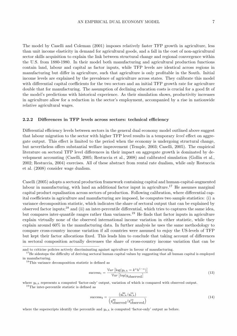
2.2.2 Differences in TFP levels across sectors: technical efficiency
Differential efficiency levels between sectors in the general dual economy model outlined above suggestthat labour migration to the sector with higher TFP level results in a temporary level effect on aggre-gate output. This effect is limited to the period when the economy is undergoing structural change,but nevertheless offers substantial welfare improvement (Temple, 2003; Caselli, 2005). The empiricalliterature on sectoral TFP level differences in their impact on aggregate growth is dominated by de-velopment accounting (Caselli, 2005; Restuccia et al., 2008) and calibrated simulation (Gollin et al.,2002; Restuccia, 2004) exercises. All of these abstract from rental rate dualism, while only Restucciaet al. (2008) consider wage dualism.
Caselli (2005) adopts a sectoral production framework containing capital and human-capital-augmentedlabour in manufacturing, with land an additional factor input in agriculture.17 He assumes marginalcapital product equalisation across sectors of production. Following calibration, where differential cap-ital coefficients in agriculture and manufacturing are imposed, he computes two sample statistics: (i) avariance decomposition statistic, which indicates the share of sectoral output that can be explained byobserved factor inputs;18 and (ii) an inter-percentile differential, which tries to captures the same idea,but compares inter-quantile ranges rather than variances.19 He finds that factor inputs in agricultureexplain virtually none of the observed international income variation in either statistic, while theyexplain around 60% in the manufacturing data. In further analysis he uses the same methodology tocompare cross-country income variation if all countries were assumed to enjoy the US-levels of TFPbut kept their factor allocations fixed. This leads him to conclude that taking account of differencesin sectoral composition actually decreases the share of cross-country income variation that can be
and to criticise policies actively discriminating against agriculture in favour of manufacturing.17He sidesteps the difficulty of deriving sectoral human capital values by suggesting that all human capital is employed
in manufacturing.18This variance decomposition statistic is defined as
success1 =Var
[log(yk,h = kαh1−α)
]Var
[log(yobserved
] (13)
where yk,h represents a computed ‘factor-only’ output, variation of which is compared with observed output.19The inter-percentile statistic is defined as
success2 =
(y90k,h/y10
k,h
)(y90
observed/y10
observed
) (14)
where the superscripts identify the percentile and yk,h is computed ‘factor-only’ output as before.
AN EMPIRICAL DUAL ECONOMY MODEL 8
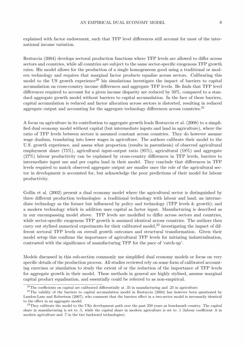
explained with factor endowment, such that TFP level differences still account for most of the inter-national income variation.
Restuccia (2004) develops sectoral production functions where TFP levels are allowed to differ acrosssectors and countries, while all countries are subject to the same sector-specific exogenous TFP growthrates. His model allows for the production of a single homogeneous good using a traditional or mod-ern technology and requires that marginal factor products equalise across sectors. Calibrating thismodel to the US growth experience20 his simulations investigate the impact of barriers to capitalaccumulation on cross-country income differences and aggregate TFP levels. He finds that TFP leveldifferences required to account for a given income disparity are reduced by 50%, compared to a stan-dard aggregate growth model without barriers to capital accumulation. In the face of these barriers,capital accumulation is reduced and factor allocation across sectors is distorted, resulting in reducedaggregate output and accounting for the aggregate technology differences across countries.21
A focus on agriculture in its contribution to aggregate growth leads Restuccia et al. (2008) to a simpli-fied dual economy model without capital (but intermediate inputs and land in agriculture), where theratio of TFP levels between sectors is assumed constant across countries. They do however assumewage dualism, translating into lower wages in agriculture. The authors calibrate their model to theU.S. growth experience, and assess what proportion (results in parenthesis) of observed agriculturalemployment share (75%), agricultural input-output ratio (95%), agricultural (18%) and aggregate(27%) labour productivity can be explained by cross-country differences in TFP levels, barriers tointermediate input use and per capita land in their model. They conclude that differences in TFPlevels required to match observed aggregate output are smaller once the role of the agricultural sec-tor in development is accounted for, but acknowledge the poor predictions of their model for labourproductivity.
Gollin et al. (2002) present a dual economy model where the agricultural sector is distinguished bythree different production technologies: a traditional technology with labour and land; an interme-diate technology as the former but influenced by policy and technology (TFP levels & growth); anda modern technology which in addition uses capital as factor input. Manufacturing is described asin our encompassing model above. TFP levels are modelled to differ across sectors and countries,while sector-specific exogenous TFP growth is assumed identical across countries. The authors thencarry out stylised numerical experiments for their calibrated model,22 investigating the impact of dif-ferent sectoral TFP levels on overall growth outcomes and structural transformation. Given theirmodel setup this confirms the importance of agricultural TFP levels for initiating industrialisation,contrasted with the significance of manufacturing TFP for the pace of ‘catch-up’.
Models discussed in this sub-section commonly use simplified dual economy models or focus on veryspecific details of the production process. All studies reviewed rely on some form of calibrated account-ing exercises or simulation to study the extent of or the reduction of the importance of TFP levelsfor aggregate growth in their model. These methods in general are highly stylised, assume marginalcapital product equalisation, and essentially could be referred to as non-empirical.
20The coefficients on capital are calibrated differentially at .35 in manufacturing and .25 in agriculture.21The validity of the barriers to capital accumulation model in Restuccia (2004) has however been questioned by
Landon-Lane and Robertson (2007), who comment that the barriers effect in a two-sector model is necessarily identicalto the effect in an aggregate model.
22They calibrate the model to the UKs development path over the past 250 years as benchmark country. The capitalshare in manufacturing is set to .5, while the capital share in modern agriculture is set to .1 (labour coefficient .6 inmodern agriculture and .7 in the two backward technologies).
AN EMPIRICAL DUAL ECONOMY MODEL 9
2.2.3 Productivity differences between sectors: marginal factor product dualism
A large number of theoretical studies explore the dual economy model assuming marginal productequality across sectors (e.g. Matsuyama, 1992; Echevarria, 1997; Kongsamut, Rebelo, & Xie, 2001;Laitner, 2000).23 As noted above, in the presence of wage and/or rental rate dualism the equilib-rium output will be lower than in the undistorted first-best equilibrium. Resolution of the factorprice dualism allows for movement toward the first-best equilibrium with positive effects for aggregateoutput (Temple, 2005), while the presence of a persistent marginal productivity gap between sectorsmay explain the importance of structural change for economic development (Robinson, 1971; Feder,1986; Vollrath, 2009c). The following studies integrate sectoral marginal product differences for labour(MPL), and in some cases also for capital (MPK), in an open dual economy model. Empirical analysisis by cross-country regression (Robinson, 1971; Feder, 1986; Dowrick & Gemmell, 1991; Temple &Woßmann, 2006) and/or accounting exercise (Temple, 2004; Vollrath, 2009c).
Robinson (1971) extends a cross-country growth regression model to account for structural change(and foreign capital inflows). His dual economy setup allows for sectoral marginal factor productdualism but abstracts from technical progress and land in the production functions. Apart from termsfor labour growth and investment ratio his static regression model includes two terms measuring thegrowth contribution of factor transfers between sectors with differential marginal factor products.24
When estimated using pooled OLS for a short panel of LDC observations the structural change termfor labour is significant, while that for capital is found only marginally significant.
Similarly, Feder (1986) develops a dual economy disequilibrium model with factor inputs capital andlabour, which allows for differential MPL and MPK across sectors, and tests their importance fordevelopment in static, period-averaged cross-country growth regressions.25 Disembodied TFP levelsor growth are not included in the model.26 Estimation results for a sample of semi-industrialised coun-tries suggest significant differences in marginal factor products in favour of manufacturing. Moreover,the ratio of MPL between the two sectors is suggested to the same as that of MPK. The disequilib-rium regression model is found to explain variation in growth rates better than an aggregate growthmodel,27 and the author concludes that his findings provide evidence for sectoral MP differences as asource of faster growth in countries pursuing industrialisation.28
The model by Vollrath (2009c) adopts sectoral production functions similar to our own encompassingmodel, explicitly accounting for land, allowing for marginal factor product dualism and for TFP levelsto differ across sectors. In addition he integrates sectoral human capital derived from Timmer (2002),29
capital stock data for agriculture and manufacturing is taken from the Crego et al. (1998) dataset.30
He imposes differential capital coefficients in agriculture and manufacturing (following Caselli, 2005)23Note that all of these model a closed economy – with the exception of Matsuyama (1992) who models both a closed
and open economy. Robertson (1999) considers wage dualism in a simple extension to his closed economy model.24Note that this setup assumes identical marginal factor product differential between sectors across all countries.25He averages all variables for the period of observation (1964-73) and runs a cross-section OLS regression (n = 30).
The semi-industrialised countries are chosen as they represent a relatively homogenous group. Again the ratios of sectoralmarginal factor products are implicitly assumed identical across countries.
26The author does however note that externalities such as agglomeration effects or benefits from training and on-the-joblearning are likely to accrue in the manufacturing/modern sector.
27Results for a separate sample of LDCs are inconclusive this may reflect the high levels of country homogeneity (MPratios) the model imposes on the data.
28Holding labour in both sectors constant, the estimation results suggest that transfer of capital worth the equivalentof 1% of GDP from the non-manufacturing to the manufacturing sector would yield an increase in GDP of around 0.5%– a sizeable increase for simply shifting capital between sectors.
29See comments on this dataset in our discussion of the encompassing theoretical model in footnote 3.30The sample includes 48 developing and developed countries at five intervals between 1970 and 1990 (n = 206).
AN EMPIRICAL DUAL ECONOMY MODEL 10
and then calculates MPL and MPK ratios between sectors: results suggest considerable marginalfactor product dualism. Sectoral TFP levels are then backed out from the respective production func-tions.31 Results from the development accounting exercise suggest that the substantial factor marketinefficiencies identified32 are instrumental in explaining aggregate income variation across countries,and that sectoral TFP-levels “appear to have almost no impact on the relative incomes of rich andpoor countries” (Vollrath, 2009c, p.29).33 Further analysis suggests that developing countries withsignificant factor market distortions even tend to have higher levels of manufacturing TFP than de-veloped countries with competitive markets. The implication that factor inputs drive output are indirect contrast to Caselli (2005), but Vollrath (2009c) proposes that the latter’s results derive fromhis treatment of physical and human capital data.34
The model by Dowrick and Gemmell (1991) allows for marginal labour product differentials and dif-ferences in TFP growth rates across sectors and countries.35 Marginal capital product equalisationacross sectors is assumed, based on earlier analysis by the authors. Sectoral TFP growth is specifiedas a linear function of exogenous sectoral TFP growth, relative sectoral labour productivity (againstbenchmark country), and for agricultural TFP growth also the labour productivity ratio of agricul-ture over industry (country-specific).36 They estimate this model (with capital and labour as factorinputs) for two period-averaged cross-sections of rich and middle-income countries, and separately fora single averaged cross-section of a more diverse set of countries, allowing for structural breaks bylevel of development.37 For the former dataset, they conclude that the degree of labour market dise-quilibrium is proportional to the level of development.38 Further, they identify substantial differencesin TFP growth across sectors, pointing to TFP level convergence in manufacturing and a mixture ofconvergence and divergence at difference stages in agriculture.39 For the latter dataset, they find thatindustrial TFP growth in the poorest countries is far below that of rich and middle-income countries,leaving the former’s technology levels to fall further and further behind. In agriculture they identifytechnology ‘catch-up’ for the poorest countries, confirming the differential TFP growth rates in thisexpanded sample.40 Poor countries have fallen further behind rich and middle-income countries inaggregate growth terms due to the small contribution of their agricultural sector to aggregate GDP(only about 30%).
31Vollrath (2009c) uses the agricultural and manufacturing capital stock data from Crego et al. (1998), rather thantransformed values as suggested by Martin and Mitra (2002) or in present study. Note that the use of the original Cregoet al. (1998) capital data was rejected by Martin and Mitra (2002) on conceptual grounds.
32His industry/agriculture marginal labour product ratios sample average is 4.22 (st.dev. 3.17), for marginal capitalratios the sample mean is 3.98 (st.dev. 5.15).
33Development accounting analysis by Cordoba and Ripoll (2009) similarly concludes that the source of the sectoralwage gap determines the contribution of TFP variation to cross-country income per worker. The importance of TFPis reduced if particularly low human capital in agriculture, home production or rural-urban living cost differentials areassumed, whereas it increases in contribution if high human capital in manufacturing is taken as the source of the wagegap.
34Vollrath (2009c, p.326) suggests that Caselli (2005)’s finding of dominance of TFP level differences to explain cross-country income differences is due to “the way he was forced to deal with physical and human capital allocations acrosssectors.”.
35They use the ratio of average factor productivities in the two sectors as proxy for the marginal differentials.36Their empirical model is thus an extension of Feder (1986) allowing for more flexibility in the MP differences and
containing additional terms deriving from their TFP growth specification.37These breaks group the data along almost identical lines as the ‘rich’ & ‘upper middle-income’, ‘lower middle-income’
and ‘poor’ used by the World Bank.38Tests for labour market equilibrium and identical degree of disequilibrium across countries are rejected.39Through their modelling specification they can identify the importance of TFP growth and levels in industry for
the development process, since in-country there are spillovers to the technologically backward agricultural sector, whileacross countries they find evidence of industrial catch-up (at least for middle-income countries).
40Note that their estimation results also suggest differential marginal capital products between the group of rich &middle-income countries and the poor countries.
AN EMPIRICAL DUAL ECONOMY MODEL 11
Research conducted by Jon Temple investigates the relationship between wage dualism and cross-country TFP growth differences using calibrated models as well as regression analysis. Temple (2004)develops a model which we have taken as foundation for our own encompassing framework describedabove, but abstracts from land in agriculture and does not consider marginal capital product dual-ism. Due to his specification and assumptions, output gains from eradicating wage dualism translateone-to-one into TFP level gains. His calibration exercise for Sub-Saharan Africa, East Asia and LatinAmerica uses technology parameters derived from the data41 and assumes a manufacturing wage pre-mium of 40%. The purpose of the exercise is to assess how a reallocation of labour between sectors(equivalent to the elimination of wage dualism and urban unemployment) will influence aggregateoutput in a typical country within each region. Temple finds relatively modest aggregate outputimprovement following the elimination of these labour market distortions. Sectoral composition ofemployment and output however changes significantly. Thus while tying labour market distortionclosely to potential failure to industrialise, this study finds only modest effects on aggregate outputgrowth upon eradication of wage dualism.42
Temple and Woßmann (2006) also analyse the impact of wage differentials on aggregate output growth.They derive an empirical model where terms for wage differential and speed of adjustment in disequi-librium are additional regressors to sectoral TFP growth terms. This empirical specification allowsthem to test for their hypothesis that the growth bonus of structural change increases with the extentof wage dualism. They do not account for the possibility of sectoral marginal capital product differ-ences and abstract from land as factor input. Their empirical analysis comprises a TFP accountingexercise using calculated TFP growth rates from existing studies, and static period-averaged growthregressions a la Mankiw et al. (1992) extended by the two structural change terms.43 The formerconcludes that structural change in their specification can explain a significant share of cross-countryvariation in aggregate TFP growth rates. Their growth regressions have higher explanatory powerthan the Mankiw et al. (1992) specification and yield jointly significant structural change terms, thusproviding some evidence for convexity of the structural change-growth relationship.
The above studies attempt to quantify the impact of factor price dualism on aggregate output or TFPgrowth. The early models by Robinson (1971) and Feder (1986) incorporate variables for marginalproduct differentials in growth regressions to estimate the contribution of structural change. Thishowever assumes identical differentials across the sample of countries. Further, these studies abstractfrom disembodied technology in their framework, while their static growth regression frameworks,like those in Dowrick and Gemmell (1991) and Temple and Woßmann (2006), make no attempts atintegrating dynamics or exploiting the panel dimension of the data. While the theoretical model inVollrath (2009c) is sufficiently general, he does not consider estimating production functions,44 as hismain focus is to query the methodology leading Caselli (2005) to conclude that TFP-level differencesare of fundamental importance for cross-country income variation. Like in the stylised calibrationexercise by Temple (2004), development accounting and TFP growth accounting force the data intoa rigid mould rather than allowing it to reveal statistical significance in a well-specified estimation-based framework. Finally, Temple and Woßmann (2006) and Temple (2004) only consider the impactof wage dualism.
41Based on the assumption of a CRS Cobb-Douglas production function and free factor mobility the labour elasticityis derived as a function of aggregate labour share in output, and employment and output shares in agriculture. Templeassumes a value of .5 across all countries for the former and derives labour coefficients for Sub-Saharan Africa (.8 inagriculture, .2 in manufacturing), East Asia (.93, .27) and Latin America (.83, .36).
42Rather than making an educated guess about the wage differential they infer it from observed labour migrationpropensity. This is simply the proportional change in the agricultural employment share, assuming that in the absenceof migration labour forces in the two sectors would grow at the same rate.
43They adopt the human capital augmented Solow model from Mankiw et al. (1992).44This is despite his use of the Crego et al. (1998) dataset, which was not available to authors of some of the other
studies reviewed here.
AN EMPIRICAL DUAL ECONOMY MODEL 12
In conclusion, marginal factor product differentials may play an important role in explaining barriersto structural transformation, and cross-country variation in economic performance. The identificationof wage dualism across sectors can highlight the importance of labour market functioning for aggregateeconomy output. Significant differences in marginal capital product across sectors and a systematiclink of these differences to level of development would suggest a growth engine that explains theimportance of structural transformation for economic development.
2.3 Summary
In this section we developed a simple open dual economy model which encompasses the existingmodels in the literature and provides a general framework for empirical testing. Following detaileddiscussion of empirical implementation, Section 4 will provide sectoral production function regressionsbased on this framework. The present section also reviewed possible sources of growth in a dualeconomy model and provided an insight into the empirical and accounting results previously obtained.Note that all models reviewed use differential output elasticities on capital in the two stylised sectors(either imposed or derived as empirical estimates). As various empirical studies have suggested, vastdifferences in aggregate TFP levels and economic growth may simply be an artefact of not accountingfor sectoral composition or marginal factor product dualism. The three major potential sources ofeconomic growth in a dual economy model — technology level differences, differential TFP growthand marginal factor product dualism — will be analysed in detail in Section 5.
3. AN EMPIRICAL MODEL OF A DUAL ECONOMY
In seeking to understand processes of growth at the macro-level, empirical work has focused primarilyon an aggregate production specification (see surveys in Barro & Sala-i-Martin, 1995; Aghion & Howitt,1998; Temple, 1999; Aghion & Durlauf, 2005). While duality has featured prominently in theoreticaldevelopments there has been only a very limited matching of this theory to empirical models. Thisdisjunction between theory and testing has reflected in large part the availability of data. In thispaper we employ a large-scale cross-country dataset made publicly available by the World Bank in2003 (henceforth Crego et al (1998), although the data is also described in detail in Larson et al., 2000)which allows us to specify manufacturing and agricultural production functions and thus provides amacro-model of a dual economy that can be compared with the single sector models dominating theempirical literature. In the following we first present a general empirical specification for our sector-specific analysis of agriculture and manufacturing. Next we review a number of empirical estimators,focusing in particular on those arising from the recent panel time series literature, before we brieflydiscuss the data.
3.1 Empirical specification
The analysis of growth and development using cross-country data is still dominated by variants onthe ‘convergence equation’ introduced by Mankiw et al. (1992), where variables are averaged over theentire time-horizon and estimation is carried out in a single cross-country regression (Durlauf et al.,2005). The multiple short-comings of this approach have been discussed elsewhere in great detail, mostrecently in Eberhardt and Teal (2010). The latter also point to a number of modelling concerns we willaddress in our empirical analysis, namely parameter heterogeneity, cross-section dependence and vari-able time-series properties. Briefly, the notion that equilibrium relationships may differ fundamentallyacross countries (perhaps at different stages of development) is a familiar one, both in the theoretical(Murphy, Shleifer, & Vishny, 1989; Azariadis & Drazen, 1990; Durlauf, 1993; Banerjee & Newman,
AN EMPIRICAL DUAL ECONOMY MODEL 13
1993) and empirical literatures (Durlauf, Kourtellos, & Minkin, 2001; Basturk, Paap, & Dijk, 2008;Kourtellos, Stengos, & Tan, 2008; Cavalcanti, Mohaddes, & Raissi, 2009) on cross-country growth.In contrast, the notion of cross-section correlation, hypothesised to arise from common global shocksand/or local spillover effects, and concerns about variable nonstationarity have received little attentionin the mainstream growth empirics literature. This is despite the rapid developments in econometricstheory over recent years (Bai & Ng, 2004; Andrews, 2005; Pesaran, 2006, 2007; Kapetanios, Pesaran,& Yamagata, 2009; Bai, 2009; Bai, Kao, & Ng, 2009), particularly in panel time series econometrics.In the context of cross-country growth and development analysis, the potential for cross-section de-pendency is particularly salient, given the interconnectedness of countries through history, geographyand trade relations. Besides a number of spatial econometric approaches, where the nature of thespatial association is imposed by the econometrician (Conley & Ligon, 2002; Ertur & Koch, 2007),only a limited number of applied papers have concerned themselves with these matters (Eberhardt &Teal, 2008; Cavalcanti et al., 2009; Costantini & Destefanis, 2009).
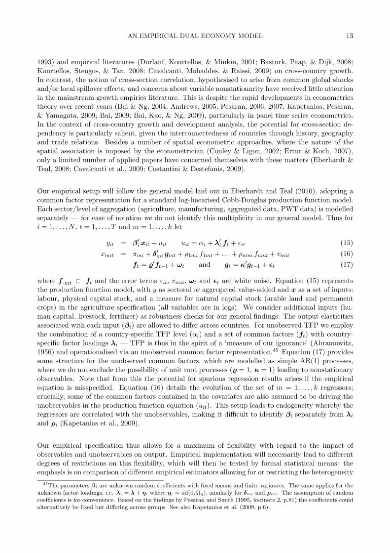
Our empirical setup will follow the general model laid out in Eberhardt and Teal (2010), adopting acommon factor representation for a standard log-linearised Cobb-Douglas production function model.Each sector/level of aggregation (agriculture, manufacturing, aggregated data, PWT data) is modelledseparately — for ease of notation we do not identify this multiplicity in our general model. Thus fori = 1, . . . , N , t = 1, . . . , T and m = 1, . . . , k let
yit = β′i xit + uit uit = αi + λ′i ft + εit (15)xmit = πmi + δ′mi gmt + ρ1mi f1mt + . . .+ ρnmi fnmt + vmit (16)
ft = %′ft−1 + ωt and gt = κ′gt−1 + εt (17)
where f ·mt ⊂ ft and the error terms εit, vmit, ωt and εt are white noise. Equation (15) representsthe production function model, with y as sectoral or aggregated value-added and x as a set of inputs:labour, physical capital stock, and a measure for natural capital stock (arable land and permanentcrops) in the agriculture specification (all variables are in logs). We consider additional inputs (hu-man capital, livestock, fertilizer) as robustness checks for our general findings. The output elasticitiesassociated with each input (βi) are allowed to differ across countries. For unobserved TFP we employthe combination of a country-specific TFP level (αi) and a set of common factors (ft) with country-specific factor loadings λi — TFP is thus in the spirit of a ‘measure of our ignorance’ (Abramowitz,1956) and operationalised via an unobserved common factor representation.45 Equation (17) providessome structure for the unobserved common factors, which are modelled as simple AR(1) processes,where we do not exclude the possibility of unit root processes (% = 1, κ = 1) leading to nonstationaryobservables. Note that from this the potential for spurious regression results arises if the empiricalequation is misspecified. Equation (16) details the evolution of the set of m = 1, . . . , k regressors;crucially, some of the common factors contained in the covariates are also assumed to be driving theunobservables in the production function equation (uit). This setup leads to endogeneity whereby theregressors are correlated with the unobservables, making it difficult to identify βi separately from λiand ρi (Kapetanios et al., 2009).
Our empirical specification thus allows for a maximum of flexibility with regard to the impact ofobservables and unobservables on output. Empirical implementation will necessarily lead to differentdegrees of restrictions on this flexibility, which will then be tested by formal statistical means: theemphasis is on comparison of different empirical estimators allowing for or restricting the heterogeneity
45The parameters βi are unknown random coefficients with fixed means and finite variances. The same applies for theunknown factor loadings, i.e. λi = λ + ηi where ηi ∼ iid(0, Ωη), similarly for δmi and ρmi. The assumption of randomcoefficients is for convenience. Based on the findings by Pesaran and Smith (1995, footnote 2, p.81) the coefficients couldalternatively be fixed but differing across groups. See also Kapetanios et al. (2009, p.6).
AN EMPIRICAL DUAL ECONOMY MODEL 14
in observables and unobservables outlined above. A conceptual justification for the pervasive characterof unobserved common factors is provided by the nature of macro-economic variables in a globalisedworld. In our mind latent forces drive all of the variables in our model, and their presence makes itdifficult to argue for the validity of traditional approaches to causal interpretation of cross-countrygrowth analyses. For instance, instrumental variable estimation in standard cross-section growthregressions (Clemens & Bazzi, 2009, p.2) or (Arellano & Bond, 1991)-type lag-instrumentation inpooled panel models (Pesaran & Smith, 1995; Lee, Pesaran, & Smith, 1997) are both invalid in theface of common factors and/or heterogeneous equilibrium relationships. We now introduce a novelestimation approach developed by Pesaran (2006) which allows us to bypass these issues by adoptingpanel time series methods for estimation and inference.
3.2 Empirical implementation
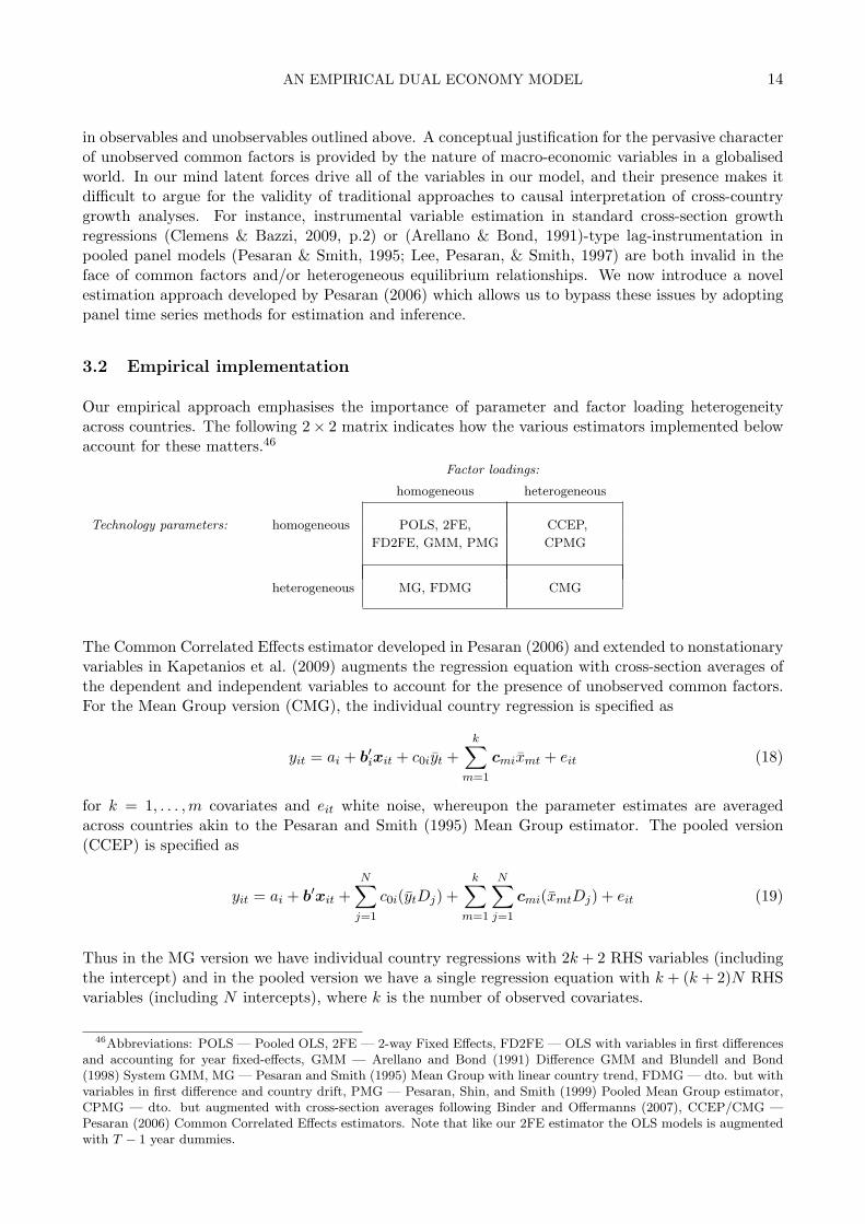
Our empirical approach emphasises the importance of parameter and factor loading heterogeneityacross countries. The following 2× 2 matrix indicates how the various estimators implemented belowaccount for these matters.46
Factor loadings:
homogeneous heterogeneous
Technology parameters: homogeneous POLS, 2FE, CCEP,
FD2FE, GMM, PMG CPMG
heterogeneous MG, FDMG CMG
The Common Correlated Effects estimator developed in Pesaran (2006) and extended to nonstationaryvariables in Kapetanios et al. (2009) augments the regression equation with cross-section averages ofthe dependent and independent variables to account for the presence of unobserved common factors.For the Mean Group version (CMG), the individual country regression is specified as
yit = ai + b′ixit + c0iyt +k∑
m=1
cmixmt + eit (18)
for k = 1, . . . ,m covariates and eit white noise, whereupon the parameter estimates are averagedacross countries akin to the Pesaran and Smith (1995) Mean Group estimator. The pooled version(CCEP) is specified as
yit = ai + b′xit +N∑j=1
c0i(ytDj) +k∑
m=1
N∑j=1
cmi(xmtDj) + eit (19)
Thus in the MG version we have individual country regressions with 2k + 2 RHS variables (includingthe intercept) and in the pooled version we have a single regression equation with k + (k + 2)N RHSvariables (including N intercepts), where k is the number of observed covariates.
46Abbreviations: POLS — Pooled OLS, 2FE — 2-way Fixed Effects, FD2FE — OLS with variables in first differencesand accounting for year fixed-effects, GMM — Arellano and Bond (1991) Difference GMM and Blundell and Bond(1998) System GMM, MG — Pesaran and Smith (1995) Mean Group with linear country trend, FDMG — dto. but withvariables in first difference and country drift, PMG — Pesaran, Shin, and Smith (1999) Pooled Mean Group estimator,CPMG — dto. but augmented with cross-section averages following Binder and Offermanns (2007), CCEP/CMG —Pesaran (2006) Common Correlated Effects estimators. Note that like our 2FE estimator the OLS models is augmentedwith T − 1 year dummies.
AN EMPIRICAL DUAL ECONOMY MODEL 15
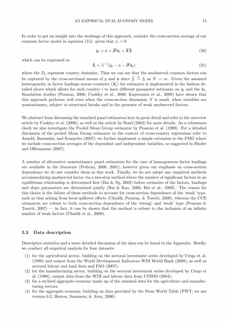
In order to get an insight into the workings of this approach, consider the cross-section average of ourcommon factor model in equation (15): given that εt = 0
yt = α+ β′xt + λ′ft (20)
which can be expressed asft = λ−1(yt − α− β′xt) (21)
where the Dj represent country dummies. Thus we can see that the unobserved common factors canbe captured by the cross-sectional means of y and x since ft
p→ ft as N → ∞. Given the assumedheterogeneity in factor loadings across countries (λ′i) the estimator is implemented in the fashion de-tailed above which allows for each country i to have different parameter estimates on yt and the xt.Simulation studies (Pesaran, 2006; Coakley et al., 2006; Kapetanios et al., 2009) have shown thatthis approach performs well even when the cross-section dimension N is small, when variables arenonstationary, subject to structural breaks and in the presence of weak unobserved factors.
We abstract from discussing the standard panel estimators here in great detail and refer to the overviewarticle by Coakley et al. (2006), as well as the article by Bond (2002) for more details. As a robustnesscheck we also investigate the Pooled Mean Group estimator by Pesaran et al. (1999). For a detaileddiscussion of the pooled Mean Group estimator in the context of cross-country regressions refer toArnold, Bassanini, and Scarpetta (2007); we further implement a simple extension to the PMG wherewe include cross-section averages of the dependent and independent variables, as suggested in Binderand Offermanns (2007).
A number of alternative nonstationary panel estimators for the case of homogeneous factor loadingsare available in the literature (Pedroni, 2000, 2001), however given our emphasis on cross-sectiondependence we do not consider them in this work. Finally, we do not adopt any empirical methodsaccommodating unobserved factor via a two-step method where the number of significant factors in anequilibrium relationship is determined first (Bai & Ng, 2002) before estimates of the factors, loadingsand slope parameters are determined jointly (Bai & Kao, 2006; Bai et al., 2009). The reason forthis choice is the failure of these methods to account for cross-section dependence of the ‘weak’ type,such as that arising from local spillover effects (Chudik, Pesaran, & Tosetti, 2009), whereas the CCEestimators are robust to both cross-section dependence of the ‘strong’ and ‘weak’ type (Pesaran &Tosetti, 2007) — in fact, it can be shown that the method is robust to the inclusion of an infinitenumber of weak factors (Chudik et al., 2009).
3.3 Data description
Descriptive statistics and a more detailed discussion of the data can be found in the Appendix. Briefly,we conduct all empirical analysis for four datasets:
(1) for the agricultural sector, building on the sectoral investment series developed by Crego et al.(1998) and output from the World Development Indicators WDI World Bank (2008), as well assectoral labour and land data and FAO (2007);
(2) for the manufacturing sector, building on the sectoral investment series developed by Crego etal. (1998), output data from the WDI and labour data from UNIDO (2004);
(3) for a stylised aggregate economy made up of the summed data for the agriculture and manufac-turing sectors;
(4) for the aggregate economy, building on data provided by the Penn World Table (PWT; we useversion 6.2, Heston, Summers, & Aten, 2006).
AN EMPIRICAL DUAL ECONOMY MODEL 16
The capital stocks in the agriculture, manufacturing and PWT samples are constructed from in-vestment data following the perpetual inventory method (see Klenow & Rodriguez-Clare, 1997b, fordetails), for the aggregated sample we simple added up sectoral capital stock for agriculture and man-ufacturing. Comparison across sectors and with the stylised aggregate sector is possible due to theefforts by Crego et al. (1998) in providing sectoral investment data for agriculture and manufacturing.All monetary values in the sectoral and aggregated datasets are transformed into US$ 1990 values(in the capital stock case this transformation is applied to the investment data before the capitalstocks are constructed), following the suggestions in Martin and Mitra (2002). Given concerns thatthe stylised aggregate economy data may not represent a good proxy for aggregate economy data wehave adopted the PWT data, which measures monetary values in International $ PPP, as a benchmarkfor comparison — despite a number of vocal critics (Johnson, Larson, Papageorgiou, & Subramanian,2009) the latter is without doubt the most popular macro dataset for cross-country empirical analysis.We are of course aware that the difference in deflation between our sectoral and aggregated data onthe one hand and PWT on the other makes them conceptually very different measures of growth anddevelopment: the former emphasise tradable goods production whereas the latter puts equal empha-sis on tradable and non-tradable goods and services. However, we believe that these differences arecomparatively unimportant for estimation and inference in comparison to the distortions introducedby neglecting the sectoral makeup and technology heterogeneity of economies at very different stagesof economic development.
Our sample is an unbalanced panel for 1963 to 1992 made up of 41 developing and developed countrieswith a total of 928 observations (average T = 22.6) — our desired aim to compare estimates acrossthe four datasets requires us to we match the same sample, thus reducing the number of observationsto the smallest common denominator. A detailed description of the sample is available in Table A-I,descriptive statistics in Table A-II are provided for each of the four samples (both tables can be foundin the appendix).
Note that in our production function regressions we adopt a very common trick whereby the outputand non-labour input variables are all expressed in ‘per worker’ terms (all variables in logs). If thelabour variable is added to this its estimated parameter coefficient provides a simple test for constantreturns to scale: if insignificant the relationship is subject to constant returns, if positive (negative)significant the relationship is suggested to be subject to increasing (decreasing) returns. In addition,this setup allows for easy imposition of constant returns by simply dropping the labour variable fromthe regression equation. Variable tests for stationarity and cross-section dependence are thereforecarried out for the variables entering the regression equations, namely output, capital, land (all in logsof per worker terms) and labour (in logs).
4. EMPIRICAL RESULTS
Preliminary data analysis (unit root and cross-section dependence tests) have been confined to thetechnical appendix of the paper. We adopt the Pesaran (2007) CIPS panel unit root test whichassumes a single unobserved common factor. This is clearly restrictive, however given the data re-strictions (unbalanced panel, relatively short) we were unable to implement the newer CIPSM versionof this test (Pesaran, Smith, & Yamagata, 2009) which allows for multiple common factors. Results(see Table TA-1) strongly suggest that variables in levels for all four datasets are nonstationary. Addi-tional analysis of variables in first difference further suggests that our measure for agricultural labourmay in fact be I(2) — this is almost definitely the outcome of variable construction: FAO (2007) dataon economically active population in agriculture (and for that matter for all the other labour-relatedmeasures) are not evaluated annually, but at 5- or 10-year intervals.
AN EMPIRICAL DUAL ECONOMY MODEL 17
In the following we discuss the empirical results from sectoral production function regressions foragriculture and manufacturing respectively, first assuming technology parameter homogeneity (Section4.1) and then allowing for differential technology across countries (Section 4.2).
4.1 Pooled models
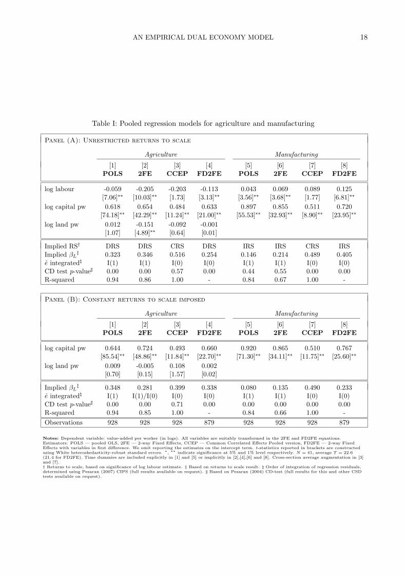
Table I presents the empirical results for agriculture and manufacturing, Panel A for unrestrictedreturns to scale and Panel B for the specification with CRS imposed. Beginning with agriculture,the empirical estimates for the models neglecting cross-section dependence are quite similar, withthe capital coefficient around .63 and statistically significant decreasing returns to scale. Diagnostictests indicate that the residuals in these models are cross-sectionally dependent, and that the levelsmodels (POLS, 2FE) have nonstationary residuals and thus may represent spurious regressions. Itis important to point out that in the presence of nonstationary residuals the t-statistics in the levelsmodels are invalid (Kao, 1999). The CCEP model yields cross-sectionally independent and stationaryresiduals, a capital coefficient of around .5 and insignificant land coefficient. Imposition of CRS doesnot change these results substantially, with the exception of the 2FE estimates, where the land variable(previously negative and significant) is now insignificant and the capital coefficient has been inflated.
In the manufacturing data the models ignoring cross-section dependence yield increasing returns toscale and capital coefficients in excess of .85 for POLS and 2FE while the FD model yields .7. Whileresiduals for the former two models again display nonstationarity the CD tests now suggest that theyare cross-sectionally independent. Surprisingly the CCEP model, with a capital coefficient of around.5 (like in agriculture) does not pass the cross-section correlation test. Following imposition of CRSall models reject cross-section independence, while parameter estimates are more or less identical tothose in the unrestricted models.
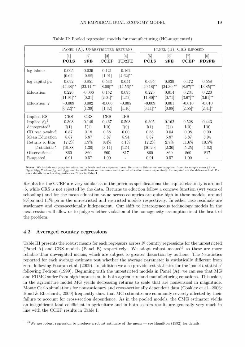
Based on these pooled regression results, the diagnostic tests seem to favour the CCEP results inthe agriculture data, whereas in the manufacturing data no estimator seems without concern. For theagriculture sample we conducted a number of robustness checks, including further covariates (livestockper worker, fertilizer per worker) in the pooled regression framework. Results (available on request)did not change from those presented above, with the CCEP estimator emerging as the most reliableempirical model.47 The CCEP therefore remains our estimator of choice for the pooled agriculturedata. For manufacturing, we conducted robustness checks including human capital in the estimationequation (linear & squared terms)48 — as a result a number of countries drop out of our sample (CRI,IRN, KOR, MDG) which now contains n = 860 observations (N = 37). Results for unconstrainedand CRS regressions are presented in Table II.
47In some more detail: The specification including livestock and fertilizer (both in log of per worker terms) could notreject CRS. The CRS specification yielded a capital coefficient of .383 [t = 5.64] which is lower than the comparableelasticity presented in Table I (.493) but the two estimates are still contained in each other’s 95% confidence intervals;residual diagnostics indicate stationary and cross-sectionally independent resiudals. The livestock coefficient of .097[t = 3.70] seems to capture the difference.
48We follow convention and pick the average years of schooling in the population as a proxy for Human Capital stock.We assume that the aggregate economy data for schooling developed by Barro and Lee (2001) which is available in 5-yearintervals. Simple interpolation to obtain annual data (as is done here) is not ideal, however the evolution of this variableover time is commonly very stable (linear), s.t. we do not feel that linear interpolation creates additional issues.
AN EMPIRICAL DUAL ECONOMY MODEL 18
Table I: Pooled regression models for agriculture and manufacturing
Panel (A): Unrestricted returns to scale
Agriculture Manufacturing
[1] [2] [3] [4] [5] [6] [7] [8]POLS 2FE CCEP FD2FE POLS 2FE CCEP FD2FE
log labour -0.059 -0.205 -0.203 -0.113 0.043 0.069 0.089 0.125[7.06]∗∗ [10.03]∗∗ [1.73] [3.13]∗∗ [3.56]∗∗ [3.68]∗∗ [1.77] [6.81]∗∗
log capital pw 0.618 0.654 0.484 0.633 0.897 0.855 0.511 0.720[74.18]∗∗ [42.29]∗∗ [11.24]∗∗ [21.00]∗∗ [55.53]∗∗ [32.93]∗∗ [8.90]∗∗ [23.95]∗∗
log land pw 0.012 -0.151 -0.092 -0.001[1.07] [4.89]∗∗ [0.64] [0.01]
Implied RS† DRS DRS CRS DRS IRS IRS CRS IRSImplied βL
‡ 0.323 0.346 0.516 0.254 0.146 0.214 0.489 0.405e integrated\ I(1) I(1) I(0) I(0) I(1) I(1) I(0) I(0)CD test p-value] 0.00 0.00 0.57 0.00 0.44 0.55 0.00 0.00R-squared 0.94 0.86 1.00 - 0.84 0.67 1.00 -
Panel (B): Constant returns to scale imposed
Agriculture Manufacturing
[1] [2] [3] [4] [5] [6] [7] [8]POLS 2FE CCEP FD2FE POLS 2FE CCEP FD2FE
log capital pw 0.644 0.724 0.493 0.660 0.920 0.865 0.510 0.767[85.54]∗∗ [48.86]∗∗ [11.84]∗∗ [22.70]∗∗ [71.30]∗∗ [34.11]∗∗ [11.75]∗∗ [25.60]∗∗
log land pw 0.009 -0.005 0.108 0.002[0.70] [0.15] [1.57] [0.02]
Implied βL‡ 0.348 0.281 0.399 0.338 0.080 0.135 0.490 0.233
e integrated\ I(1) I(1)/I(0) I(0) I(0) I(1) I(1) I(0) I(0)CD test p-value] 0.00 0.00 0.71 0.00 0.00 0.00 0.00 0.00R-squared 0.94 0.85 1.00 - 0.84 0.66 1.00 -Observations 928 928 928 879 928 928 928 879
Notes: Dependent variable: value-added per worker (in logs). All variables are suitably transformed in the 2FE and FD2FE equations.Estimators: POLS — pooled OLS, 2FE — 2-way Fixed Effects, CCEP — Common Correlated Effects Pooled version, FD2FE — 2-way FixedEffects with variables in first difference. We omit reporting the estimates on the intercept term. t-statistics reported in brackets are constructedusing White heteroskedasticity-robust standard errors. ∗, ∗∗ indicate significance at 5% and 1% level respectively. N = 41, average T = 22.6(21.4 for FD2FE). Time dummies are included explicitly in [1] and [5] or implicitly in [2],[4],[6] and [8]. Cross-section average augmentation in [3]and [7].† Returns to scale, based on significance of log labour estimate. ‡ Based on returns to scale result. \ Order of integration of regression residuals,determined using Pesaran (2007) CIPS (full results available on request). ] Based on Pesaran (2004) CD-test (full results for this and other CSDtests available on request).
AN EMPIRICAL DUAL ECONOMY MODEL 19
Table II: Pooled regression models for manufacturing (HC-augmented)
Panel (A): Unrestricted returns Panel (B): CRS imposed
[1] [2] [3] [4] [5] [6] [7] [8]POLS 2FE CCEP FD2FE POLS 2FE CCEP FD2FE
log labour 0.005 0.029 0.121 0.162[0.62] [0.88] [1.91] [4.62]∗∗
log capital pw 0.692 0.851 0.533 0.654 0.695 0.839 0.472 0.558[44.38]∗∗ [22.14]∗∗ [8.00]∗∗ [14.56]∗∗ [49.18]∗∗ [24.30]∗∗ [8.87]∗∗ [13.85]**
Education 0.226 -0.006 0.152 0.095 0.226 0.014 0.234 0.220[11.91]∗∗ [0.21] [2.04]∗ [1.53] [11.80]∗∗ [0.71] [3.67]∗∗ [3.91]∗∗
Educationˆ2 -0.009 0.002 -0.006 -0.005 -0.009 0.001 -0.010 -0.010[6.22]∗∗ [1.39] [1.32] [1.10] [6.11]∗∗ [0.98] [2.55]∗ [2.41]∗
Implied RS† CRS CRS CRS IRSImplied βL
‡ 0.308 0.149 0.467 0.508 0.305 0.162 0.528 0.443e integrated\ I(1) I(1) I(0) I(0) I(1) I(1) I(0) I(0)CD test p-value] 0.87 0.18 0.58 0.00 0.88 0.04 0.08 0.00Mean Education 5.87 5.87 5.87 5.94 5.87 5.87 5.87 5.94Returns to Edu 12.2% 1.9% 8.4% 4.1% 12.2% 2.7% 11.6% 10.5%
[t-statistic][ [19.88] [1.30] [3.11] [1.54] [20.20] [2.30] [5.25] [4.62]Observations 860 860 860 817 860 860 860 817R-squared 0.91 0.57 1.00 - 0.91 0.57 1.00 -
Notes: We include our proxy for education in levels and as a squared term. Returns to Education are computed from the sample mean (E) asβE + 2βE2E where βE and βE2 are the coefficients on the levels and squared education terms respectively. [ computed via the delta-method. Formore details on other diagnostics see Notes in Table I.
Results for the CCEP are very similar as in the previous specifications: the capital elasticity is around.5, while CRS is not rejected by the data. Returns to eduction follow a concave function (wrt years ofschooling) and for the mean education value across countries are quite high in these models, around8%pa and 11% pa in the unrestricted and restricted models respectively. In either case residuals arestationary and cross-sectionally independent. Our shift to heterogeneous technology models in thenext session will allow us to judge whether violation of the homogeneity assumption is at the heart ofthe problem.
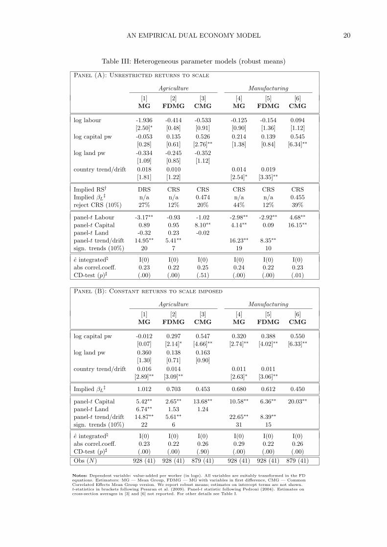
4.2 Averaged country regressions
Table III presents the robust means for each regressors acrossN country regressions for the unrestricted(Panel A) and CRS models (Panel B) respectively. We adopt robust means49 as these are morereliable than unweighted means, which are subject to greater distortion by outliers. The t-statisticsreported for each average estimate test whether the average parameter is statistically different fromzero, following Pesaran et al. (2009). In addition we also provide test statistics for the ‘panel t-statistic’following Pedroni (1999). Beginning with the unrestricted models in Panel (A), we can see that MGand FDMG suffer from high imprecision in both agriculture and manufacturing equations. This aside,in the agriculture model MG yields decreasing returns to scale that are nonsensical in magnitude.Monte Carlo simulations for nonstationary and cross-sectionally dependent data (Coakley et al., 2006;Bond & Eberhardt, 2009) frequently show that MG estimates are commonly severely affected by theirfailure to account for cross-section dependence. As in the pooled models, the CMG estimator yieldsan insignificant land coefficient in agriculture and in both sectors results are generally very much inline with the CCEP results in Table I.
49We use robust regression to produce a robust estimate of the mean — see Hamilton (1992) for details.
AN EMPIRICAL DUAL ECONOMY MODEL 20
Table III: Heterogeneous parameter models (robust means)
Panel (A): Unrestricted returns to scale
Agriculture Manufacturing
[1] [2] [3] [4] [5] [6]MG FDMG CMG MG FDMG CMG
log labour -1.936 -0.414 -0.533 -0.125 -0.154 0.094[2.50]∗ [0.48] [0.91] [0.90] [1.36] [1.12]
log capital pw -0.053 0.135 0.526 0.214 0.139 0.545[0.28] [0.61] [2.76]∗∗ [1.38] [0.84] [6.34]∗∗
log land pw -0.334 -0.245 -0.352[1.09] [0.85] [1.12]
country trend/drift 0.018 0.010 0.014 0.019[1.81] [1.22] [2.54]∗ [3.35]∗∗
Implied RS† DRS CRS CRS CRS CRS CRSImplied βL
‡ n/a n/a 0.474 n/a n/a 0.455reject CRS (10%) 27% 12% 20% 44% 12% 39%
panel-t Labour -3.17∗∗ -0.93 -1.02 -2.98∗∗ -2.92∗∗ 4.68∗∗
panel-t Capital 0.89 0.95 8.10∗∗ 4.14∗∗ 0.09 16.15∗∗
panel-t Land -0.32 0.23 -0.02panel-t trend/drift 14.95∗∗ 5.41∗∗ 16.23∗∗ 8.35∗∗
sign. trends (10%) 20 7 19 10
e integrated\ I(0) I(0) I(0) I(0) I(0) I(0)abs correl.coeff. 0.23 0.22 0.25 0.24 0.22 0.23CD-test (p)] (.00) (.00) (.51) (.00) (.00) (.01)
Panel (B): Constant returns to scale imposed
Agriculture Manufacturing
[1] [2] [3] [4] [5] [6]MG FDMG CMG MG FDMG CMG
log capital pw -0.012 0.297 0.547 0.320 0.388 0.550[0.07] [2.14]∗ [4.66]∗∗ [2.74]∗∗ [4.02]∗∗ [6.33]∗∗
log land pw 0.360 0.138 0.163[1.30] [0.71] [0.90]
country trend/drift 0.016 0.014 0.011 0.011[2.89]∗∗ [3.09]∗∗ [2.63]∗ [3.06]∗∗
Implied βL‡ 1.012 0.703 0.453 0.680 0.612 0.450
panel-t Capital 5.42∗∗ 2.65∗∗ 13.68∗∗ 10.58∗∗ 6.36∗∗ 20.03∗∗
panel-t Land 6.74∗∗ 1.53 1.24panel-t trend/drift 14.87∗∗ 5.61∗∗ 22.65∗∗ 8.39∗∗
sign. trends (10%) 22 6 31 15
e integrated\ I(0) I(0) I(0) I(0) I(0) I(0)abs correl.coeff. 0.23 0.22 0.26 0.29 0.22 0.26CD-test (p)] (.00) (.00) (.90) (.00) (.00) (.00)Obs (N) 928 (41) 928 (41) 879 (41) 928 (41) 928 (41) 879 (41)
Notes: Dependent variable: value-added per worker (in logs). All variables are suitably transformed in the FDequations. Estimators: MG — Mean Group, FDMG — MG with variables in first difference, CMG — CommonCorrelated Effects Mean Group version. We report robust means; estimates on intercept terms are not shown.t-statistics in brackets following Pesaran et al. (2009). Panel-t statistic following Pedroni (2004). Estimates oncross-section averages in [3] and [6] not reported. For other details see Table I.
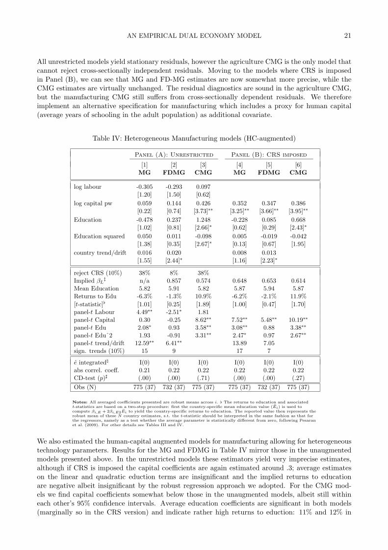
AN EMPIRICAL DUAL ECONOMY MODEL 21
All unrestricted models yield stationary residuals, however the agriculture CMG is the only model thatcannot reject cross-sectionally independent residuals. Moving to the models where CRS is imposedin Panel (B), we can see that MG and FD-MG estimates are now somewhat more precise, while theCMG estimates are virtually unchanged. The residual diagnostics are sound in the agriculture CMG,but the manufacturing CMG still suffers from cross-sectionally dependent residuals. We thereforeimplement an alternative specification for manufacturing which includes a proxy for human capital(average years of schooling in the adult population) as additional covariate.
Table IV: Heterogeneous Manufacturing models (HC-augmented)
Panel (A): Unrestricted Panel (B): CRS imposed
[1] [2] [3] [4] [5] [6]MG FDMG CMG MG FDMG CMG
log labour -0.305 -0.293 0.097[1.20] [1.50] [0.62]
log capital pw 0.059 0.144 0.426 0.352 0.347 0.386[0.22] [0.74] [3.73]∗∗ [3.25]∗∗ [3.66]∗∗ [3.95]∗∗
Education -0.478 0.237 1.248 -0.228 0.085 0.668[1.02] [0.81] [2.66]∗ [0.62] [0.29] [2.43]∗
Education squared 0.050 0.011 -0.098 0.005 -0.019 -0.042[1.38] [0.35] [2.67]∗ [0.13] [0.67] [1.95]
country trend/drift 0.016 0.020 0.008 0.013[1.55] [2.44]∗ [1.16] [2.23]∗
reject CRS (10%) 38% 8% 38%Implied βL
‡ n/a 0.857 0.574 0.648 0.653 0.614Mean Education 5.82 5.91 5.82 5.87 5.94 5.87Returns to Edu -6.3% -1.3% 10.9% -6.2% -2.1% 11.9%[t-statistic][ [1.01] [0.25] [1.89] [1.00] [0.47] [1.70]panel-t Labour 4.49∗∗ -2.51∗ 1.81panel-t Capital 0.30 -0.25 8.62∗∗ 7.52∗∗ 5.48∗∗ 10.19∗∗
panel-t Edu 2.08∗ 0.93 3.58∗∗ 3.08∗∗ 0.88 3.38∗∗
panel-t Eduˆ2 1.93 -0.91 3.31∗∗ 2.47∗ 0.97 2.67∗∗
panel-t trend/drift 12.59∗∗ 6.41∗∗ 13.89 7.05sign. trends (10%) 15 9 17 7
e integrated\ I(0) I(0) I(0) I(0) I(0) I(0)abs correl. coeff. 0.21 0.22 0.22 0.22 0.22 0.22CD-test (p)] (.00) (.00) (.71) (.00) (.00) (.27)Obs (N) 775 (37) 732 (37) 775 (37) 775 (37) 732 (37) 775 (37)
Notes: All averaged coefficients presented are robust means across i. [ The returns to education and associatedt-statistics are based on a two-step procedure: first the country-specific mean education value (Ei) is used tocompute βi,E + 2βi,E2Ei to yield the country-specific returns to education. The reported value then represents therobust mean of these N country estimates, s.t. the t-statistic should be interpreted in the same fashion as that forthe regressors, namely as a test whether the average parameter is statistically different from zero, following Pesaranet al. (2009). For other details see Tables III and IV.
We also estimated the human-capital augmented models for manufacturing allowing for heterogeneoustechnology parameters. Results for the MG and FDMG in Table IV mirror those in the unaugmentedmodels presented above. In the unrestricted models these estimators yield very imprecise estimates,although if CRS is imposed the capital coefficients are again estimated around .3; average estimateson the linear and quadratic eduction terms are insignificant and the implied returns to educationare negative albeit insignificant by the robust regression approach we adopted. For the CMG mod-els we find capital coefficients somewhat below those in the unaugmented models, albeit still withineach other’s 95% confidence intervals. Average education coefficients are significant in both models(marginally so in the CRS version) and indicate rather high returns to eduction: 11% and 12% in
AN EMPIRICAL DUAL ECONOMY MODEL 22
the unrestricted and CRS model respectively. This merits two comments: firstly, we might argue forthe validity of this high estimate given that the manufacturing sector is arguably the more dynamicsector in comparison to agriculture, which builds on innovation and R&D, thus relying on knowledge-accumulation which is heavily linked to human capital. Secondly, adopting country-wide educationdata as a proxy for manufacturing may severely distort the results we present here — firm-level data(Baptist & Teal, 2008) on Ghana and Korea in the late 1990s for instance indicates that average workereduction (crudely measured in years of schooling) does not differ substantially between these countries.
5. DUALITY AND THE DETERMINANTS OF GROWTH
In this section we will return to the themes developed in Section 2 and ask how the dual economymodel can contribute to our understanding of the sources of economic growth. In a first attempt ofdoing so we will investigate whether the assumption of an aggregate production function yields biasedresults. To the best of our knowledge this is the first paper to consider this issue empirically, en-abled by pioneering work of Crego et al. (1998) in providing comparable investment and capital stockmeasures for Agriculture and Manufacturing. In the following section we will lay out how productionfunction estimation based on aggregate data leads to biased results in the capital coefficient. Section5.2 then turns to the debate of growth determinants, investigating in turn TFP growth rates, TFPlevels and marginal factor product dualism.
5.1 Aggregation bias
Our empirical results in Section 4 suggested fairly similar pooled and averaged capital coefficients formanufacturing and agriculture across the various empirical models. This might lead one to suggestthat carrying out cross-country growth empirics may best be conducted taking the aggregate econ-omy, and thus the Penn World Table (PWT) data (Heston et al., 2009), as the basic unit of analysis.Our empirical approach emphasised the importance of unobserved heterogeneity across countries, butour analysis refrained from testing technology parameter differences across sectors with any formalmethods — our justification is that in our most flexible specification (CMG) the individual country-estimates are not reliable (Pedroni, 2007) and should not be the basis for comparison. In this sectionwe will instead provide practical evidence that the use of an aggregate production function will lead toseriously biased estimates of the capital coefficient. We carry out this analysis by creating a stylised‘aggregated economy’ from our data on agriculture and manufacturing. Since it might be suggestedthat results could be severely distorted by the overly simplistic nature of our inquiry, we compareresults with those from a matched sample of data from the PWT.
We begin with the pooled models in Table V. Across all specifications the estimated capital coefficientsin the aggregated data far exceed those derived from the respective agriculture and manufacturingsamples in Table I. Furthermore, the patterns in the aggregated data are replicated one-to-one in thePWT data, which also yields excessively high capital coefficients across all models. All models sufferfrom cross-sectional dependence in the residuals, while there are also indications that the residuals inthe CCEP model for the aggregated data are nonstationary (those in the two other levels specificationsare always nonstationary). We also investigated the impact of human capital (proxied via averageyears of schooling attained in the population over 15 years of age) in these aggregate economy datamodels, but as Table TA-IV in the Technical Appendix reveals the basic bias remains.
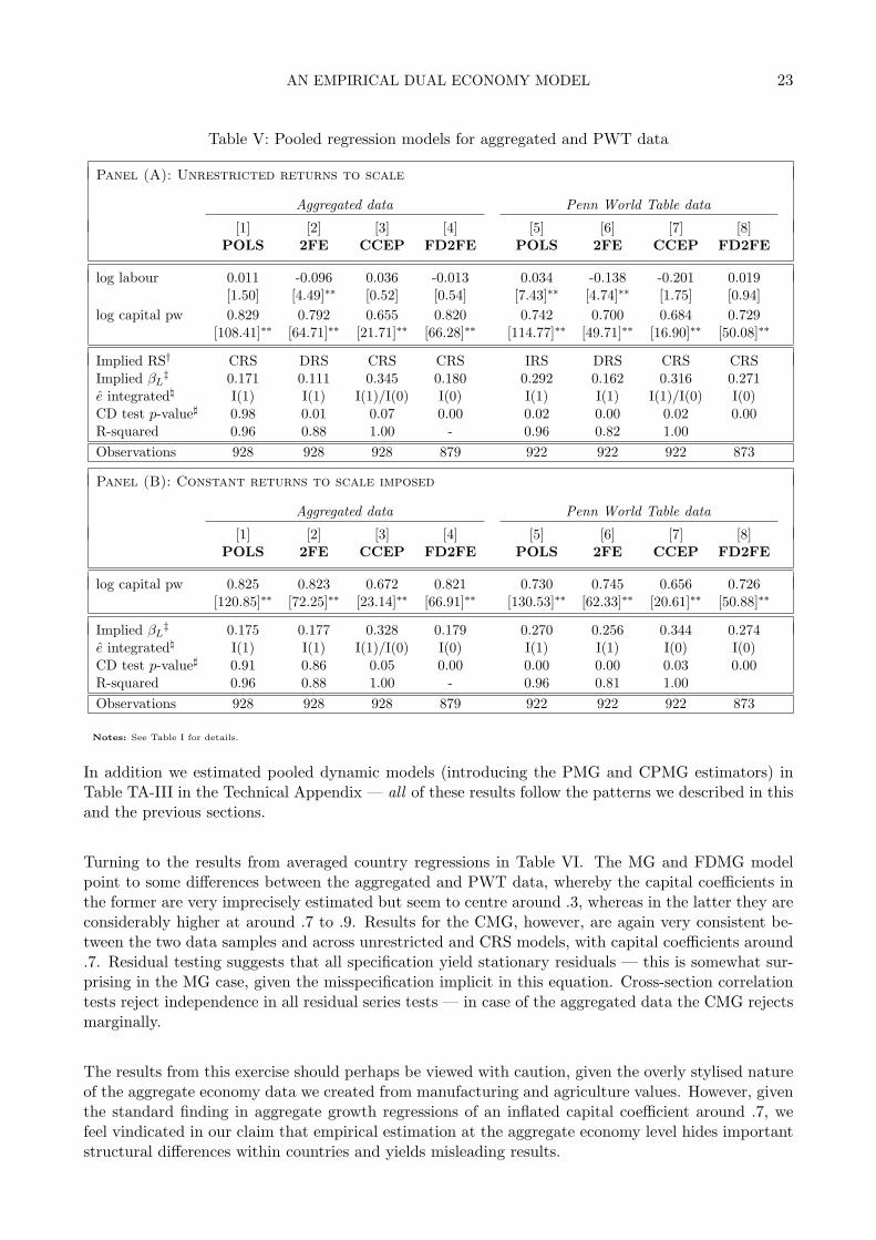
AN EMPIRICAL DUAL ECONOMY MODEL 23
Table V: Pooled regression models for aggregated and PWT data
Panel (A): Unrestricted returns to scale
Aggregated data Penn World Table data
[1] [2] [3] [4] [5] [6] [7] [8]POLS 2FE CCEP FD2FE POLS 2FE CCEP FD2FE
log labour 0.011 -0.096 0.036 -0.013 0.034 -0.138 -0.201 0.019[1.50] [4.49]∗∗ [0.52] [0.54] [7.43]∗∗ [4.74]∗∗ [1.75] [0.94]
log capital pw 0.829 0.792 0.655 0.820 0.742 0.700 0.684 0.729[108.41]∗∗ [64.71]∗∗ [21.71]∗∗ [66.28]∗∗ [114.77]∗∗ [49.71]∗∗ [16.90]∗∗ [50.08]∗∗
Implied RS† CRS DRS CRS CRS IRS DRS CRS CRSImplied βL
‡ 0.171 0.111 0.345 0.180 0.292 0.162 0.316 0.271e integrated\ I(1) I(1) I(1)/I(0) I(0) I(1) I(1) I(1)/I(0) I(0)CD test p-value] 0.98 0.01 0.07 0.00 0.02 0.00 0.02 0.00R-squared 0.96 0.88 1.00 - 0.96 0.82 1.00Observations 928 928 928 879 922 922 922 873
Panel (B): Constant returns to scale imposed
Aggregated data Penn World Table data
[1] [2] [3] [4] [5] [6] [7] [8]POLS 2FE CCEP FD2FE POLS 2FE CCEP FD2FE
log capital pw 0.825 0.823 0.672 0.821 0.730 0.745 0.656 0.726[120.85]∗∗ [72.25]∗∗ [23.14]∗∗ [66.91]∗∗ [130.53]∗∗ [62.33]∗∗ [20.61]∗∗ [50.88]∗∗
Implied βL‡ 0.175 0.177 0.328 0.179 0.270 0.256 0.344 0.274
e integrated\ I(1) I(1) I(1)/I(0) I(0) I(1) I(1) I(0) I(0)CD test p-value] 0.91 0.86 0.05 0.00 0.00 0.00 0.03 0.00R-squared 0.96 0.88 1.00 - 0.96 0.81 1.00Observations 928 928 928 879 922 922 922 873
Notes: See Table I for details.
In addition we estimated pooled dynamic models (introducing the PMG and CPMG estimators) inTable TA-III in the Technical Appendix — all of these results follow the patterns we described in thisand the previous sections.
Turning to the results from averaged country regressions in Table VI. The MG and FDMG modelpoint to some differences between the aggregated and PWT data, whereby the capital coefficients inthe former are very imprecisely estimated but seem to centre around .3, whereas in the latter they areconsiderably higher at around .7 to .9. Results for the CMG, however, are again very consistent be-tween the two data samples and across unrestricted and CRS models, with capital coefficients around.7. Residual testing suggests that all specification yield stationary residuals — this is somewhat sur-prising in the MG case, given the misspecification implicit in this equation. Cross-section correlationtests reject independence in all residual series tests — in case of the aggregated data the CMG rejectsmarginally.
The results from this exercise should perhaps be viewed with caution, given the overly stylised natureof the aggregate economy data we created from manufacturing and agriculture values. However, giventhe standard finding in aggregate growth regressions of an inflated capital coefficient around .7, wefeel vindicated in our claim that empirical estimation at the aggregate economy level hides importantstructural differences within countries and yields misleading results.
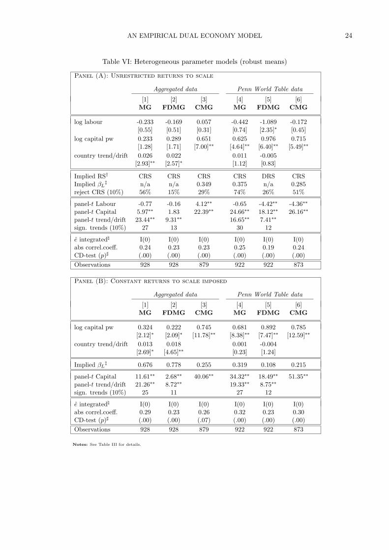
AN EMPIRICAL DUAL ECONOMY MODEL 24
Table VI: Heterogeneous parameter models (robust means)
Panel (A): Unrestricted returns to scale
Aggregated data Penn World Table data
[1] [2] [3] [4] [5] [6]MG FDMG CMG MG FDMG CMG
log labour -0.233 -0.169 0.057 -0.442 -1.089 -0.172[0.55] [0.51] [0.31] [0.74] [2.35]∗ [0.45]
log capital pw 0.233 0.289 0.651 0.625 0.976 0.715[1.28] [1.71] [7.00]∗∗ [4.64]∗∗ [6.40]∗∗ [5.49]∗∗
country trend/drift 0.026 0.022 0.011 -0.005[2.93]∗∗ [2.57]∗ [1.12] [0.83]
Implied RS† CRS CRS CRS CRS DRS CRSImplied βL
‡ n/a n/a 0.349 0.375 n/a 0.285reject CRS (10%) 56% 15% 29% 74% 26% 51%
panel-t Labour -0.77 -0.16 4.12∗∗ -0.65 -4.42∗∗ -4.36∗∗
panel-t Capital 5.97∗∗ 1.83 22.39∗∗ 24.66∗∗ 18.12∗∗ 26.16∗∗
panel-t trend/drift 23.44∗∗ 9.31∗∗ 16.65∗∗ 7.41∗∗
sign. trends (10%) 27 13 30 12
e integrated\ I(0) I(0) I(0) I(0) I(0) I(0)abs correl.coeff. 0.24 0.23 0.23 0.25 0.19 0.24CD-test (p)] (.00) (.00) (.00) (.00) (.00) (.00)Observations 928 928 879 922 922 873
Panel (B): Constant returns to scale imposed
Aggregated data Penn World Table data
[1] [2] [3] [4] [5] [6]MG FDMG CMG MG FDMG CMG
log capital pw 0.324 0.222 0.745 0.681 0.892 0.785[2.12]∗ [2.09]∗ [11.78]∗∗ [8.38]∗∗ [7.47]∗∗ [12.59]∗∗
country trend/drift 0.013 0.018 0.001 -0.004[2.69]∗ [4.65]∗∗ [0.23] [1.24]
Implied βL‡ 0.676 0.778 0.255 0.319 0.108 0.215
panel-t Capital 11.61∗∗ 2.68∗∗ 40.06∗∗ 34.32∗∗ 18.49∗∗ 51.35∗∗
panel-t trend/drift 21.26∗∗ 8.72∗∗ 19.33∗∗ 8.75∗∗
sign. trends (10%) 25 11 27 12
e integrated\ I(0) I(0) I(0) I(0) I(0) I(0)abs correl.coeff. 0.29 0.23 0.26 0.32 0.23 0.30CD-test (p)] (.00) (.00) (.07) (.00) (.00) (.00)Observations 928 928 879 922 922 873
Notes: See Table III for details.
AN EMPIRICAL DUAL ECONOMY MODEL 25
5.2 The Sources of Growth. . . Revisited
Our review of the literature in Section 2 discussed three potential sources of economic growth in a dualeconomy model — differential TFP growth, technology level differences and marginal factor productdualism. We now investigate the empirical evidence for the relative importance of these three potentialsources of growth in our panel dataset.
5.2.1 TFP growth differences as a potential source of aggregate growth
Technical progress in form of TFP growth in aggregate growth accounting exercises has frequentlybeen hailed as the dominant source of growth in empirical studies (Easterly & Levine, 2001; Klenow& Rodriguez-Clare, 1997a). As the discussion in Section 2 showed this can equally apply for sector-specific analysis. Since Cobb-Douglas production estimations and growth accounting are essentiallyidentical approaches (Chen, 1997) the unobserved common factors in our regression-based model cancapture the sectoral TFP growth values (Bond, Leblebicioglu, & Schiantarelli, 2007; Durlauf et al.,2005).
Table TA-VI in the Technical Appendix provides country-level growth estimates — in this and thefollowing analysis we present results for the CCEP and CMG estimators in the specification withCRS imposed, where in the agriculture equations we always include land per worker. For comparativepurposes we also present results for the 2FE estimator which we have seen is severely biased. TFPgrowth is constructed from the data in two steps: first we impose the estimated output elasticities withrespect to observable inputs on the data, accounting for the white noise error component, thus
ˆTFPit = yit − β′iXit − eit (22)
where βi are the technology parameter estimates (homogeneous in the 2FE and CCEP case), Xit
represents the factor inputs and eit is the 2FE, CCEP or CMG regression residual from the regressionresults presented in the previous section. In a second step we simply compute annual TFP growth asthe first difference of this TFP series.50 Note that the consideration related to the correct TFP-levelestimation (see below) need not concern us for TFP growth, since the growth rate estimates are unaf-fected by the issues about heterogeneity faced in the TFP level estimation case.
We find that the average sector-specific TFP growth rate for the entire sample (robust mean estimates)differs considerably between the 2FE estimates on one hand and the CMG and CCEP estimates onthe other — note however that the difference is only statistically significant in the manufacturing case.In agriculture the 2FE growth rate of around half a percent per annum is roughly doubled in the twoCCE estimates, whereas in manufacturing the mean estimate for the CCEP and CMG estimators arefive and three times that of the 2FE, which yields less than a fifth of a percent per annum. Turningto the question of whether TFP growth in agriculture exceeds that in manufacturing we can see thatin line with the results in Martin and Mitra (2002)51 the two-way fixed effects estimator suggests thatthis is the case in 33 out of 41 countries. In contrast, once we account for cross-section dependencewe find that only around half of the countries in our sample have higher TFP growth in agriculture(21 for CCEP, 23 for CMG).
50In practice we do not rely on annual estimates for TFP growth but construct average growth rate using the first andlast observed TFP-level estimates.
51“A comparison of the two sector shows that agriculture generally had faster TFP growth than manufacturing”(Martin & Mitra, 2002, p.411).
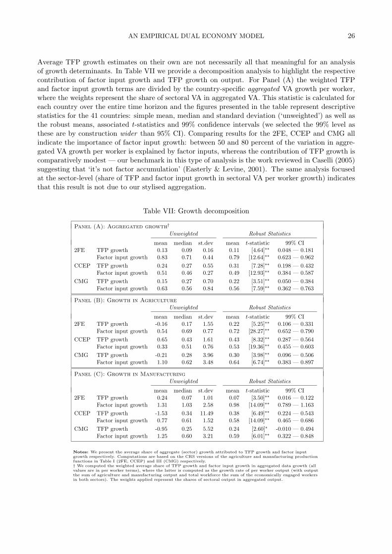
AN EMPIRICAL DUAL ECONOMY MODEL 26
Average TFP growth estimates on their own are not necessarily all that meaningful for an analysisof growth determinants. In Table VII we provide a decomposition analysis to highlight the respectivecontribution of factor input growth and TFP growth on output. For Panel (A) the weighted TFPand factor input growth terms are divided by the country-specific aggregated VA growth per worker,where the weights represent the share of sectoral VA in aggregated VA. This statistic is calculated foreach country over the entire time horizon and the figures presented in the table represent descriptivestatistics for the 41 countries: simple mean, median and standard deviation (‘unweighted’) as well asthe robust means, associated t-statistics and 99% confidence intervals (we selected the 99% level asthese are by construction wider than 95% CI). Comparing results for the 2FE, CCEP and CMG allindicate the importance of factor input growth: between 50 and 80 percent of the variation in aggre-gated VA growth per worker is explained by factor inputs, whereas the contribution of TFP growth iscomparatively modest — our benchmark in this type of analysis is the work reviewed in Caselli (2005)suggesting that ‘it’s not factor accumulation’ (Easterly & Levine, 2001). The same analysis focusedat the sector-level (share of TFP and factor input growth in sectoral VA per worker growth) indicatesthat this result is not due to our stylised aggregation.
Table VII: Growth decomposition
Panel (A): Aggregated growth†
Unweighted Robust Statistics
mean median st.dev mean t-statistic 99% CI2FE TFP growth 0.13 0.09 0.16 0.11 [4.64]∗∗ 0.048 — 0.181
Factor input growth 0.83 0.71 0.44 0.79 [12.64]∗∗ 0.623 — 0.962CCEP TFP growth 0.24 0.27 0.55 0.31 [7.28]∗∗ 0.198 — 0.432
Factor input growth 0.51 0.46 0.27 0.49 [12.93]∗∗ 0.384 — 0.587CMG TFP growth 0.15 0.27 0.70 0.22 [3.51]∗∗ 0.050 — 0.384
Factor input growth 0.63 0.56 0.84 0.56 [7.59]∗∗ 0.362 — 0.763
Panel (B): Growth in AgricultureUnweighted Robust Statistics
mean median st.dev mean t-statistic 99% CI2FE TFP growth -0.16 0.17 1.55 0.22 [5.25]∗∗ 0.106 — 0.331
Factor input growth 0.54 0.69 0.77 0.72 [28.27]∗∗ 0.652 — 0.790CCEP TFP growth 0.65 0.43 1.61 0.43 [8.32]∗∗ 0.287 — 0.564
Factor input growth 0.33 0.51 0.76 0.53 [19.36]∗∗ 0.455 — 0.603CMG TFP growth -0.21 0.28 3.96 0.30 [3.98]∗∗ 0.096 — 0.506
Factor input growth 1.10 0.62 3.48 0.64 [6.74]∗∗ 0.383 — 0.897
Panel (C): Growth in ManufacturingUnweighted Robust Statistics
mean median st.dev mean t-statistic 99% CI2FE TFP growth 0.24 0.07 1.01 0.07 [3.50]∗∗ 0.016 — 0.122
Factor input growth 1.31 1.03 2.58 0.98 [14.09]∗∗ 0.789 — 1.163CCEP TFP growth -1.53 0.34 11.49 0.38 [6.49]∗∗ 0.224 — 0.543
Factor input growth 0.77 0.61 1.52 0.58 [14.09]∗∗ 0.465 — 0.686CMG TFP growth -0.95 0.25 5.52 0.24 [2.60]∗ -0.010 — 0.494
Factor input growth 1.25 0.60 3.21 0.59 [6.01]∗∗ 0.322 — 0.848
Notes: We present the average share of aggregate (sector) growth attributed to TFP growth and factor inputgrowth respectively. Computations are based on the CRS versions of the agriculture and manufacturing productionfunctions in Table I (2FE, CCEP) and III (CMG) respectively.† We computed the weighted average share of TFP growth and factor input growth in aggregated data growth (allvalues are in per worker terms), where the latter is computed as the growth rate of per worker output (with outputthe sum of agriculture and manufacturing output and total workforce the sum of the economically engaged workersin both sectors). The weights applied represent the shares of sectoral output in aggregated output.
AN EMPIRICAL DUAL ECONOMY MODEL 27
5.2.2 TFP level differences as a potential source of aggregate growth
Rather than differential technical progress, differential technology (TFP) levels between sectors havebeen suggested as the source of growth variation across countries (Caselli, 2005). TFP levels “capturethe differences in long-run economic performance that are most directly relevant to welfare” (Hall &Jones, 1999, p.85).
From the preferred country regressions we can obtain estimates for the intercept, technology param-eters, and common trend (year dummy) coefficients or the parameters on the cross-section averagesfor the CCEP and CMG specification respectively. One may be tempted to view the coefficients onthe intercepts as TFP level estimates, just like in the pooled fixed effects case. However, in Eberhardtand Teal (2009) we develop in detail that once technology parameters in the production function areallowed to differ across countries the regression intercept can no longer be interpreted as a TFP-levelestimate, since the ceteris paribus assumption no longer holds. In the same paper we suggested analternative measure for TFP-level which is robust to parameter heterogeneity. We suggest to use thelocus of the first capital stock observation along the trajectory of the regression line (in output-capitalstock space — both in per worker terms).52 In the 2FE specification this adjusted base-year TFP-levelis defined as
ai + β log(K/L)0,i (23)
where log(K/L)0,i is the country-(sector)-specific base-year value for capital per worker (in logs), βrepresents the (country-specific) capital coefficient and ai is the coefficient for the intercept.
For the CCE estimators we need to change this approach to extracting the unobserved common factors(multiplied by the heterogeneous factor loadings) using the technology parameter estimates βi (β forCCEP) and CCE regression residuals eit
yit − βi log(K/L)0,i − eit (24)
In our results we will contrast the adjusted TFP level estimates derived from this approach with astandard practice in the literature, where the TFP level differences are captured by the fixed effects:these represent the relative TFP level of each country compared with that of the omitted benchmarkcountry. If we use the empirically equivalent Least Squares Dummy Variable (LSDV) estimator, weare able to select the benchmark country to be omitted (here: the United States) and can read offthe country-specific relative TFP-level from the country dummy coefficients ηij . As we work with anequation in logs we obtain each country’s relative TFP level from the country dummy as(
TFPiTFPUS
)j
= exp(ηij) (25)
since the implicit coefficient on the omitted benchmark country is zero (i.e. unity in the non-logarithmic transformation: exp(0) = 1). We present the outcome of this exercise in Table VIIIunder the 2FE (LSDV) entry. For all other models we mimic the same relative TFP level statistic byexpressing each country’s TFP level with reference to that of the US.
As can be seen the conventional 2FE (LSDV) approach leads to a vast range of TFP levels in agri-culture, from 41% to 279% of the US-level. In comparison the adjusted TFP levels for 2FE, CCEPand CMG all yield a range between around 40% and 100% (thus the US has highest agricultural TFP
52In the agriculture sector this computation is adjusted to take the impact of land per worker into account. We presentthe manufacturing case for simplicity.
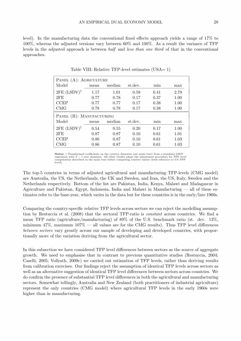
AN EMPIRICAL DUAL ECONOMY MODEL 28
level). In the manufacturing data the conventional fixed effects approach yields a range of 17% to100%, whereas the adjusted versions vary between 60% and 100%. As a result the variance of TFPlevels in the adjusted approach is between half and less than one third of that in the conventionalapproaches.
Table VIII: Relative TFP-level estimates (USA= 1)
Panel (A): AgricultureModel mean median st.dev. min max
2FE (LSDV)† 1.17 1.01 0.59 0.41 2.792FE 0.77 0.78 0.17 0.37 1.00CCEP 0.77 0.77 0.17 0.38 1.00CMG 0.78 0.78 0.17 0.38 1.00
Panel (B): ManufacturingModel mean median st.dev. min max
2FE (LSDV)† 0.54 0.55 0.20 0.17 1.002FE 0.87 0.87 0.10 0.61 1.01CCEP 0.86 0.87 0.10 0.61 1.03CMG 0.86 0.87 0.10 0.61 1.03
Notes: † Transformed coefficients on the country dummies (see main text) from a standard LSDVregression with T − 1 year dummies. All other results adopt the adjustment procedure for TFP levelcomputation described in the main text before computing relative values (with reference to US TFPlevel).
The top-5 countries in terms of adjusted agricultural and manufacturing TFP-levels (CMG model)are Australia, the US, the Netherlands, the UK and Sweden, and Iran, the US, Italy, Sweden and theNetherlands respectively. Bottom of the list are Pakistan, India, Kenya, Malawi and Madagascar inAgriculture and Pakistan, Egypt, Indonesia, India and Malawi in Manufacturing — all of these es-timates refer to the base-year, which varies in the data but for these countries is in the early/late 1960s.
Comparing the country-specific relative TFP levels across sectors we can reject the modelling assump-tion by Restuccia et al. (2008) that the sectoral TFP-ratio is constant across countries. We find amean TFP ratio (agriculture/manufacturing) of 89% of the U.S. benchmark ratio (st. dev. 13%,minimum 47%, maximum 107% — all values are for the CMG results). Thus TFP level differencesbetween sectors vary greatly across our sample of developing and developed countries, with propor-tionally more of the variation deriving from the agricultural sector.
In this subsection we have considered TFP level differences between sectors as the source of aggregategrowth. We need to emphasise that in contrast to previous quantitative studies (Restuccia, 2004;Caselli, 2005; Vollrath, 2009c) we carried out estimation of TFP levels, rather than deriving resultsfrom calibration exercises. Our findings reject the assumption of identical TFP levels across sectors aswell as an alternative suggestion of identical TFP level differences between sectors across countries. Wedo confirm the presence of substantial TFP level differences in both the agricultural and manufacturingsectors. Somewhat tellingly, Australia and New Zealand (both practitioners of industrial agriculture)represent the only countries (CMG model) where agricultural TFP levels in the early 1960s werehigher than in manufacturing.
AN EMPIRICAL DUAL ECONOMY MODEL 29
5.2.3 Sectoral productivity differences: wage and rental rate dualism
Following the estimation of sectoral production functions and the analysis of TFP differences acrosscountries we now want to compute marginal labour products (MPL) and marginal capital products(MPK) from the estimates we obtained. For a generic CRS Cobb-Douglas production function sectoralMPL and MPK are derived as follows (for i = 1, . . . , N and j = a, m)
Yij = AijKαijij L
1−αijij (26)
MPLij = (1− αij)AijKαijij L
−αijij = (1− αij)Aij(K/L)αjij (27)
MPKij = αijAijKαij−1ij L
1−αijij = αijAij(K/L)αij−1
ij (28)
Equations (27) and (28) show that marginal factor products can differ across sectors j and countriesi because of
(i) differences in TFP-levels (A) across sectors and countries,(ii) differences in factor proportions (K/L) across sectors and countries,
(iii) differences in the output elasticity with respect to capital (α) across sectors, or(iv) differences in output elasticity with respect to capital across sectors and across countries.
In the following we compute the sectoral marginal factor products to investigate wage and rentalrate dualism. Initially we hold the factor proportions (K/L) constant across countries and sectors(employing the U.S. mean period value in the aggregated data) to investigate what evidence thereis for dualism in marginal factor products, given that countries are assumed to use the same factorproportions but differ in efficiency levels. In all cases we take robust means from CMG regressions(either at the sector or the aggregated data level) as the basis for the capital coefficient.
Panel (A) in Table IX presents our findings for the scenario where countries are endowed with identicalcapital-labour ratio and only vary in their efficiency (TFP) levels — in the Technical Appendix, TableTA-VII we also present re-scaled results with reference to US marginal factor product (USA= 100).Results suggest that MPL in agriculture exceeds that in manufacturing in all but 3 countries, whereasfor the MPK the reverse is obtain.
In Panel (B) we allow for heterogeneous capital-labour ratios, which are now allowed to differ bycountry and sector — we use country-sector-specific averages over the sample period in this and thefollowing results. The variation in relative MPL and MPK immediately shoots up in both sectors,with the standard deviations between two and four times as large as in the previous results. Panel (C)adds sector-specific capital coefficients (albeit it common across countries), where we adopt the robustmean from our sector regressions. Standard deviations settle somewhat and the range of relativeMPLs is reduced; the same obtains in the MPK estimates. In both cases (Panel (B) and (C)) themanufacturing sector has higher MPL than the agriculture sector in most countries, but this is onlythe case for around one-third of the MPK estimates. In our final scenario in Panel (D), where inaddition we allow for capital coefficients to differ across countries53 the results for both MPK andMPL in either sector display the largest standard deviations.
53We cannot rely on country-specific capital parameter estimates and therefore divide the sample into three groups,representing ‘low’, ‘intermediate’ and ‘high’ output elasticities with respect to capital, based on the magnitude of thecoefficient estimates. See Table footnote for more details.
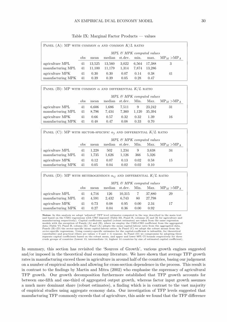
AN EMPIRICAL DUAL ECONOMY MODEL 30
Table IX: Marginal Factor Products — values
Panel (A): MP with common α and common K/L ratio
MPL & MPK computed valuesobs mean median st.dev. min. max. MPM >MPA
agriculture MPL 41 13,525 13,560 3,022 6,564 17,388 3manufacturing MPL 41 11,100 11,179 1,314 7,874 13,286agriculture MPK 41 0.30 0.30 0.07 0.14 0.38 41manufacturing MPK 41 0.39 0.39 0.05 0.28 0.47
Panel (B): MP with common α and differential K/L ratio
MPL & MPK computed valuesobs mean median st.dev. Min. Max. MPM >MPA
agriculture MPL 41 6,606 1,686 7,511 9 23,242 31manufacturing MPL 41 8,796 7,434 7,360 1,120 35,394agriculture MPK 41 0.66 0.57 0.32 0.32 1.39 16manufacturing MPK 41 0.48 0.47 0.08 0.33 0.70
Panel (C): MP with sector-specific αj and differential K/L ratio
MPL & MPK computed valuesobs mean median st.dev. Min. Max. MPM >MPA
agriculture MPL 41 1,228 502 1,234 9 3,638 34manufacturing MPL 41 1,735 1,626 1,126 366 5,326agriculture MPK 41 0.12 0.07 0.13 0.02 0.58 15manufacturing MPK 41 0.05 0.04 0.02 0.02 0.10
Panel (D): MP with heterogeneous αij and differential K/L ratio
MPL & MPK computed valuesobs mean median st.dev. Min. Max. MPM >MPA
agriculture MPL 41 4,716 126 10,315 7 37,880 29manufacturing MPL 41 4,591 2,432 6,743 80 27,798agriculture MPK 41 0.73 0.08 0.95 0.00 2.34 17manufacturing MPK 41 0.27 0.04 0.36 0.00 0.92
Notes: In this analysis we adopt ‘adjusted’ TFP level estimates computed in the way described in the main textand based on the CMG regressions with CRS imposed (Table III, Panel B, columns [3] and [6] for agriculture andmanufacturing respectively). Capital coefficients applied (robust estimates) are taken from the same regressionmodels with the exception of Panels (A) and (B), where we employ the CMG-CRS coefficient from the aggregateddata (Table VI, Panel B, column [3]). Panel (A) adopts the mean capital-labour ratio from the aggregated data,Panels (B)-(D) the sector-specific mean capital-labour ratios. In Panel (C) we adopt the robust means from thesector-specific regressions. Using country-specific estimates for the capital-coefficient is infeasible, for theoretical(unreliable) and practical (there are values < 0 and > 1) reasons. In Panel (D) we compromise by adopting threeseparate capital coefficients based on the robust mean, and upper and lower 99% CI bounds respectively for threecrude groups of countries (lowest 13, intermediate 14, highest 14 countries by size of estimated capital coefficient).
In summary, this section has revisited the ‘Sources of Growth’, various growth engines suggestedand/or imposed in the theoretical dual economy literature. We have shown that average TFP growthrates in manufacturing exceed those in agriculture in around half of the countries, basing our judgementon a number of empirical models and allowing for cross-section dependence in the process. This result isin contrast to the findings by Martin and Mitra (2002) who emphasise the supremacy of agriculturalTFP growth. Our growth decomposition furthermore established that TFP growth accounts forbetween one-fifth and one-third of aggregated output growth, whereas factor input growth assumesa much more dominant share (robust estimates), a finding which is in contrast to the vast majorityof empirical studies using aggregate economy data. Our investigation of TFP levels suggested thatmanufacturing TFP commonly exceeds that of agriculture, this aside we found that the TFP difference
AN EMPIRICAL DUAL ECONOMY MODEL 31
between these two sectors is by no means constant across countries. Finally, our analysis of marginalfactor products across countries revealed that the assumption of country-specific factor intensities aswell as heterogeneous technology parameters led to variation most in line with that observed in theoutput data.
6. CONCLUSIONS
In this paper we have developed a general framework for dual economy models and used some uniquepanel data for agriculture and manufacturing to estimate sector-level and aggregated production func-tions. Our conceptual development built on the theoretical contributions by Temple (2005) and Cordenand Findlay (1975) and our overview of the literature highlighted a number of ‘sources of growth’ hy-pothesised in the dual economy literature. Our empirical analysis emphasised the contribution of therecent panel time-series econometric literature, which suggests to adopt unobserved common factorsto deal with the cross-sectional dependence commonly found in macro panel data. In addition wetook the nonstationarity of observable and unobservable factor inputs into account and emphasisedthe importance of parameter heterogeneity — across countries as well as sectors.
We draw the following conclusions from our first, crude attempt at highlighting the importance of struc-tural makeup and change in the empirical analysis of cross-country growth and development:
(i) Empirical analysis of growth and development at the cross-country level — most commonlyconducted using the Penn World Tables (Heston et al., 2009) — gains considerably from theseparate consideration of modern and traditional sectors that make up the economy. Our anal-ysis of agriculture and manufacturing versus a stylised aggregated economy suggests that thelatter yields severely distorted empirical results. Across multiple empirical specifications andestimators we could show that the capital coefficient for aggregated data far exceeds that ob-tained from separate sector regressions. Analysis of PWT data in parallel with the aggregateddata suggested that this finding is not an artefact of our stylised empirical setup. To the best ofour knowledge this is the first time that these matters are investigated empirically at this levelof aggregation. Our analysis was enabled by the unique data on agricultural and manufacturinginvestment and capital stock developed by Crego et al. (1998) — a dataset which deserves fargreater attention than it presently receives.54
(ii) Following empirical estimation, our analysis of the ‘sources of growth’ suggested in the literaturerevealed that in contrast to previous findings the TFP growth rate in agriculture is not consis-tently larger than that in manufacturing — indeed in at least half of our countries the reverseis the case.
(iii) Conducting a growth decomposition exercise based on our empirical estimates of TFP growth,we suggest that aggregated output growth is to large parts explained by the variation in factorinput growth, a finding in contrast to much of the growth accounting literature reviewed inCaselli (2005). This result obtains both at the sector level, as well as the stylised aggregatedlevel of the economy.
(iv) Investigation of TFP levels revealed that manufacturing TFP commonly exceeds that of agri-culture. Furthermore, we found little evidence for the suggestion that the sectoral difference inTFP levels is constant across countries.
(v) Our analysis of marginal factor products across countries revealed that the assumption ofcountry-specific factor intensities as well as heterogeneous technology parameters led to vari-ation most in line with that observed in the output data.
54Don Larson and collaborators have more recently developed an updated version of this dataset (1967-2003), albeitlimited to 30 developing and developed countries. In future work we plan to use this new version and a matchedmanufacturing dataset to investigate the robustness of our results.
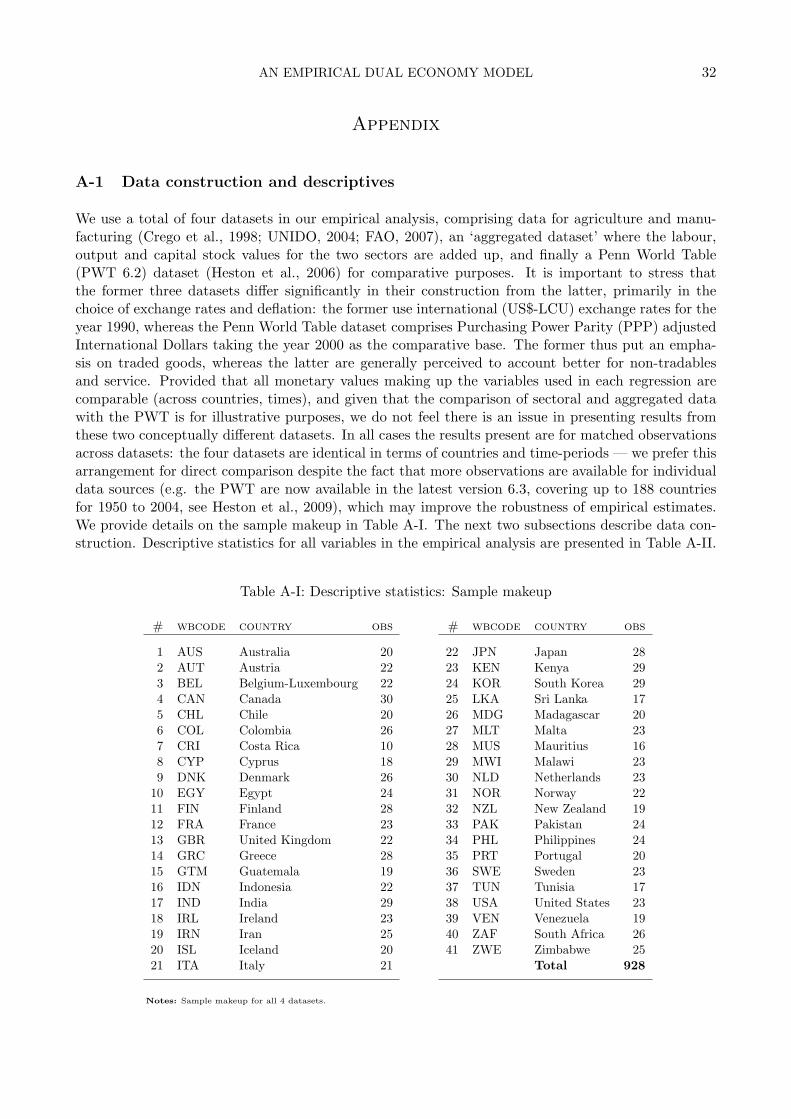
AN EMPIRICAL DUAL ECONOMY MODEL 32
Appendix
A-1 Data construction and descriptives
We use a total of four datasets in our empirical analysis, comprising data for agriculture and manu-facturing (Crego et al., 1998; UNIDO, 2004; FAO, 2007), an ‘aggregated dataset’ where the labour,output and capital stock values for the two sectors are added up, and finally a Penn World Table(PWT 6.2) dataset (Heston et al., 2006) for comparative purposes. It is important to stress thatthe former three datasets differ significantly in their construction from the latter, primarily in thechoice of exchange rates and deflation: the former use international (US$-LCU) exchange rates for theyear 1990, whereas the Penn World Table dataset comprises Purchasing Power Parity (PPP) adjustedInternational Dollars taking the year 2000 as the comparative base. The former thus put an empha-sis on traded goods, whereas the latter are generally perceived to account better for non-tradablesand service. Provided that all monetary values making up the variables used in each regression arecomparable (across countries, times), and given that the comparison of sectoral and aggregated datawith the PWT is for illustrative purposes, we do not feel there is an issue in presenting results fromthese two conceptually different datasets. In all cases the results present are for matched observationsacross datasets: the four datasets are identical in terms of countries and time-periods — we prefer thisarrangement for direct comparison despite the fact that more observations are available for individualdata sources (e.g. the PWT are now available in the latest version 6.3, covering up to 188 countriesfor 1950 to 2004, see Heston et al., 2009), which may improve the robustness of empirical estimates.We provide details on the sample makeup in Table A-I. The next two subsections describe data con-struction. Descriptive statistics for all variables in the empirical analysis are presented in Table A-II.
Table A-I: Descriptive statistics: Sample makeup
# wbcode country obs # wbcode country obs
1 AUS Australia 20 22 JPN Japan 282 AUT Austria 22 23 KEN Kenya 293 BEL Belgium-Luxembourg 22 24 KOR South Korea 294 CAN Canada 30 25 LKA Sri Lanka 175 CHL Chile 20 26 MDG Madagascar 206 COL Colombia 26 27 MLT Malta 237 CRI Costa Rica 10 28 MUS Mauritius 168 CYP Cyprus 18 29 MWI Malawi 239 DNK Denmark 26 30 NLD Netherlands 23
10 EGY Egypt 24 31 NOR Norway 2211 FIN Finland 28 32 NZL New Zealand 1912 FRA France 23 33 PAK Pakistan 2413 GBR United Kingdom 22 34 PHL Philippines 2414 GRC Greece 28 35 PRT Portugal 2015 GTM Guatemala 19 36 SWE Sweden 2316 IDN Indonesia 22 37 TUN Tunisia 1717 IND India 29 38 USA United States 2318 IRL Ireland 23 39 VEN Venezuela 1919 IRN Iran 25 40 ZAF South Africa 2620 ISL Iceland 20 41 ZWE Zimbabwe 2521 ITA Italy 21 Total 928
Notes: Sample makeup for all 4 datasets.
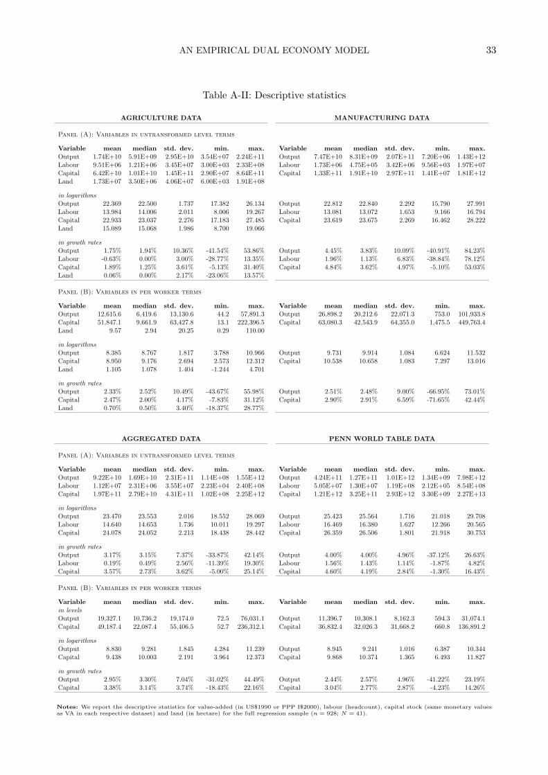
AN EMPIRICAL DUAL ECONOMY MODEL 33
Table A-II: Descriptive statistics
AGRICULTURE DATA MANUFACTURING DATA
Panel (A): Variables in untransformed level terms
Variable mean median std. dev. min. max. Variable mean median std. dev. min. max.Output 1.74E+10 5.91E+09 2.95E+10 3.54E+07 2.24E+11 Output 7.47E+10 8.31E+09 2.07E+11 7.20E+06 1.43E+12Labour 9.51E+06 1.21E+06 3.45E+07 3.00E+03 2.33E+08 Labour 1.73E+06 4.75E+05 3.42E+06 9.56E+03 1.97E+07Capital 6.42E+10 1.01E+10 1.45E+11 2.90E+07 8.64E+11 Capital 1.33E+11 1.91E+10 2.97E+11 1.41E+07 1.81E+12Land 1.73E+07 3.50E+06 4.06E+07 6.00E+03 1.91E+08
in logarithmsOutput 22.369 22.500 1.737 17.382 26.134 Output 22.812 22.840 2.292 15.790 27.991Labour 13.984 14.006 2.011 8.006 19.267 Labour 13.081 13.072 1.653 9.166 16.794Capital 22.933 23.037 2.276 17.183 27.485 Capital 23.619 23.675 2.269 16.462 28.222Land 15.089 15.068 1.986 8.700 19.066
in growth ratesOutput 1.75% 1.94% 10.36% -41.54% 53.86% Output 4.45% 3.83% 10.09% -40.91% 84.23%Labour -0.63% 0.00% 3.00% -28.77% 13.35% Labour 1.96% 1.13% 6.83% -38.84% 78.12%Capital 1.89% 1.25% 3.61% -5.13% 31.40% Capital 4.84% 3.62% 4.97% -5.10% 53.03%Land 0.06% 0.00% 2.17% -23.06% 13.57%
Panel (B): Variables in per worker terms
Variable mean median std. dev. min. max. Variable mean median std. dev. min. max.Output 12,615.6 6,419.6 13,130.6 44.2 57,891.3 Output 26,898.2 20,212.6 22,071.3 753.0 101,933.8Capital 51,847.1 9,661.9 63,427.8 13.1 222,396.5 Capital 63,080.3 42,543.9 64,355.0 1,475.5 449,763.4Land 9.57 2.94 20.25 0.29 110.00
in logarithmsOutput 8.385 8.767 1.817 3.788 10.966 Output 9.731 9.914 1.084 6.624 11.532Capital 8.950 9.176 2.694 2.573 12.312 Capital 10.538 10.658 1.083 7.297 13.016Land 1.105 1.078 1.404 -1.244 4.701
in growth ratesOutput 2.33% 2.52% 10.49% -43.67% 55.98% Output 2.51% 2.48% 9.00% -66.95% 73.01%Capital 2.47% 2.00% 4.17% -7.83% 31.12% Capital 2.90% 2.91% 6.59% -71.65% 42.44%Land 0.70% 0.50% 3.40% -18.37% 28.77%
AGGREGATED DATA PENN WORLD TABLE DATA
Panel (A): Variables in untransformed level terms
Variable mean median std. dev. min. max. Variable mean median std. dev. min. max.Output 9.22E+10 1.69E+10 2.31E+11 1.14E+08 1.55E+12 Output 4.24E+11 1.27E+11 1.01E+12 1.34E+09 7.98E+12Labour 1.12E+07 2.31E+06 3.55E+07 2.23E+04 2.40E+08 Labour 5.05E+07 1.30E+07 1.19E+08 2.12E+05 8.54E+08Capital 1.97E+11 2.79E+10 4.31E+11 1.02E+08 2.25E+12 Capital 1.21E+12 3.25E+11 2.93E+12 3.30E+09 2.27E+13
in logarithmsOutput 23.470 23.553 2.016 18.552 28.069 Output 25.423 25.564 1.716 21.018 29.708Labour 14.640 14.653 1.736 10.011 19.297 Labour 16.469 16.380 1.627 12.266 20.565Capital 24.078 24.052 2.213 18.438 28.442 Capital 26.359 26.506 1.801 21.918 30.753
in growth ratesOutput 3.17% 3.15% 7.37% -33.87% 42.14% Output 4.00% 4.00% 4.96% -37.12% 26.63%Labour 0.19% 0.49% 2.56% -11.39% 19.30% Labour 1.56% 1.43% 1.14% -1.87% 4.82%Capital 3.57% 2.73% 3.62% -5.00% 25.14% Capital 4.60% 4.19% 2.84% -1.30% 16.43%
Panel (B): Variables in per worker terms
Variable mean median std. dev. min. max. Variable mean median std. dev. min. max.in levelsOutput 19,327.1 10,736.2 19,174.0 72.5 76,031.1 Output 11,396.7 10,308.1 8,162.3 594.3 31,074.1Capital 49,187.4 22,087.4 55,406.5 52.7 236,312.1 Capital 36,832.4 32,026.3 31,668.2 660.8 136,891.2
in logarithmsOutput 8.830 9.281 1.845 4.284 11.239 Output 8.945 9.241 1.016 6.387 10.344Capital 9.438 10.003 2.191 3.964 12.373 Capital 9.868 10.374 1.365 6.493 11.827
in growth ratesOutput 2.95% 3.30% 7.04% -31.02% 44.49% Output 2.44% 2.57% 4.96% -41.22% 23.19%Capital 3.38% 3.14% 3.74% -18.43% 22.16% Capital 3.04% 2.77% 2.87% -4.23% 14.26%
Notes: We report the descriptive statistics for value-added (in US$1990 or PPP I$2000), labour (headcount), capital stock (same monetary valuesas VA in each respective dataset) and land (in hectare) for the full regression sample (n = 928; N = 41).
AN EMPIRICAL DUAL ECONOMY MODEL 34
A-1.1 Sectoral and aggregated data
Investment data Data for agricultural and manufacturing investment (AgSEInv, MfgSEInv) inconstant 1990 LCU, the US$-LCU exchange rate (Ex Rate, see comment below) as well as sector-specific deflators (AgDef, TotDef) were taken from Crego et al. (1998).55 Note that Crego et al.(1998) also provide capital stock data, which they produced through their own calculations from theinvestment data. Following Martin and Mitra (2002) we believe the use of a single year exchange rateis preferrable to the use of annual ones in the construction of real output (see next paragraph) andcapital stock (see below).
Output data For manufacturing we use data on aggregate GDP in current LCU and the share ofGDP in manufacturing from the World Bank World Development Indicators (WDI) (World Bank,2008). For agriculture we use agricultural value-added in current LCU from the same source. Weprefer the latter over the share of GDP in agriculture for data coverage reasons (in theory they shouldbe the same, but they are not). The two sectoral value-added series are then deflated using the Cregoet al. (1998) sectoral deflator for agriculture and the total economy deflator for manufacturing, beforewe use the 1990 US$-LCU exchange rates to make them comparable across countries.
Note that the currencies used in the Crego et al. (1998) data differ from those applied in the WDIdata for a number of European countries due to the adoption of the Euro: for the latter we thereforeneed to use an alternative 1990 US$-LCU exchange rate for these economies.56
Labour data For agriculture we adopt the variable ‘economically active population in agriculture’from the FAO’s PopSTAT (FAO, 2007). Manufacturing labour is taken from UNIDO’s INDSTATUNIDO (2004).
Additional data The land variable is taken from ResourceSTAT and represents arable and perma-nent crop land (originally in 1000 hectare) (FAO, 2007). The livestock variable is constructed fromthe data for asses (donkeys), buffalos, camels, cattle, chickens, ducks, horses, mules, pigs, sheep &goats and turkeys in the ‘Live animals’ section of ProdSTAT. Following convention we use the belowformula to convert the numbers for individual animal species into the livestock variable:
livestock = 1.1∗camels + buffalos + horses + mules + 0.8∗cattle + 0.8∗asses+0.2∗pigs + 0.1∗(sheep+goats) + 0.01∗(chickens+ducks+turkeys)
The fertilizer variable is taken from the ‘Fertilizers archive’ of ResourceSTAT and represents agricul-tural fertilizer consumed in metric tons, which includes ‘crude’ and ‘manufactured’ fertilizers.
Capital stock We construct capital stock in agriculture and manufacturing by applying the perpet-ual inventory method described in detail in Klenow and Rodriguez-Clare (1997b) using the investmentdata from Crego et al. (1998), which is transformed into US$ by application of the 1990 US$-LCUexchange rate. For the construction of sectoral base year capital stock we employ average sectorvalue-added growth rates gj (using the deflated sectoral value-added data described above), the av-erage sectoral investment to value-added ratio (I/Y )j and an assumed depreciation rate of 5% to
55Data is available in excel format on the World Bank website at http://go.worldbank.org/FS3FXW7461. All datadiscussed in this appendix are linked at http://sites.google.com/site/medevecon/devecondata.
56In detail, we apply exchange rates of 1.210246384 for AUT, 1.207133927 for BEL, 1.55504706 for FIN, 1.204635181for FRA, 2.149653527 for GRC, 1.302645017 for IRL, 1.616114954 for ITA, 1.210203555 for NLD and 1.406350856 forPRT. See Table A-I for country codes.
AN EMPIRICAL DUAL ECONOMY MODEL 35
construct (K
Y
)0j
=IYj
gj + 0.05
for sector j. This ratio is then multiplied by sectoral value-added in the base year to yield K0j . Notethat the method deviates from that discussed in Klenow and Rodriguez-Clare (1997b) as they useper capita GDP in their computations and therefore need to account for population growth in theconstruction of the base year capital stock.
Aggregated data We combine the agriculture and manufacturing data to produce a stylised ‘ag-gregate economy’: for labour we simply add up the headcount, for the monetary representations ofoutput and capital stock we can do so as well. We are afforded this ability to simply add up variablesfor the two sectors by the efforts Crego et al. (1998), who have built the first large panel datasetproviding data on investment in agriculture for a long timespan.
A-1.2 Penn World Table data
As a means of comparison we also provide production function estimates using data from PWT ver-sion 6.2. We adopt Real per capita GDP in International $ Laspeyeres (rgdpl) as measure for outputand construct capital stock using investment data (derived from Investment Share in Real GDP, ki,and the output variable, rgdpl) in the perpetual inventory method described above, adopting again5% depreciation (this time we need to use the data on population from PWT, pop, to compute theaverage annual population growth rate).
REFERENCES
Abramowitz, M. (1956). Resource and output trend in the United States since 1870. American Economic Review , 46 (2),5-23.
Aghion, P., & Durlauf, S. (Eds.). (2005). Handbook of economic growth (Vol. 1) (No. 1). Elsevier.Aghion, P., & Howitt, P. (1992). A model of growth through creative destruction. Econometrica, 60 (2), 323-51.Aghion, P., & Howitt, P. (1998). Endogenous Growth Theory. Cambridge, Mass.: MIT Press.Andrews, D. W. K. (2005). Cross-Section Regression with Common Shocks. Econometrica, 73 (5), 1551-1585.Arellano, M., & Bond, S. (1991). Some tests of specification for panel data. Review of Economic Studies, 58 (2), 277-297.Arnold, J., Bassanini, A., & Scarpetta, S. (2007). Solow or Lucas?: Testing Growth Models Using Panel Data from
OECD Countries (OECD Economics Department Working Papers No. 592).Azariadis, C., & Drazen, A. (1990). Threshold externalities in economic development. Quarterly Journal of Economics,
105 (2), 501-26.Bai, J. (2009). Panel Data Models with Interactive Fixed Effects. Econometrica, 77 (4), 1229-1279.Bai, J., & Kao, C. (2006). On the estimation and inference of a panel cointegration model with cross-sectional dependence.
In B. H. Baltagi (Ed.), Panel data econometrics: Theoretical contributions and empirical applications. Amsterdam:Elsevier Science.
Bai, J., Kao, C., & Ng, S. (2009). Panel cointegration with global stochastic trends. Journal of Econometrics, 149 (1),82-99.
Bai, J., & Ng, S. (2002). Determining the Number of Factors in Approximate Factor Models. Econometrica, 70 (1),191-221.
Bai, J., & Ng, S. (2004). A PANIC attack on unit roots and cointegration. Econometrica, 72 , 191-221.Baier, S. L., Dwyer, G. P., & Tamura, R. (2006). How important are capital and total factor productivity for economic
growth? Economic Enquiry , 44 (1), 23-49.Banerjee, A. V., & Newman, A. F. (1993). Occupational Choice and the Process of Development. Journal of Political
Economy , 101 (2), 274-98.Baptist, S., & Teal, F. (2008). Why do South Korean firms produce so much more output per worker than Ghanaian
ones? (CSAE working paper, WPS/2008-10)
AN EMPIRICAL DUAL ECONOMY MODEL 36
Barbier, E. B., & Rauscher, M. (2007). Trade and development in a labor surplus economy. The B.E. Journal ofEconomic Analysis & Policy , 7 (1).
Barro, R. J. (1991). Economic growth in a cross-section of countries. Quarterly Journal of Economics, 106 (2), 407-443.Barro, R. J., & Lee, J.-W. (1993). International comparisons of educational attainment. Journal of Monetary Economics,
32 (3), 363-394.Barro, R. J., & Lee, J.-W. (2001). International data on educational attainment: Updates and implications. Oxford
Economic Papers, 53 (3), 541-63.Barro, R. J., & Sala-i-Martin, J. (1995). Economic growth. New York: MacGraw-Hill.Basturk, N., Paap, R., & Dijk, D. van. (2008). Structural differences in economic growth. (Tinbergen Institute Discussion
Paper 2008-085/4)Binder, M., & Offermanns, C. J. (2007). International investment positions and exchange rate dynamics: a dynamic
panel analysis (Discussion Paper Series 1: Economic Studies Nos. 2007,23). Deutsche Bundesbank, ResearchCentre.
Blundell, R., & Bond, S. (1998). Initial conditions and moment restrictions in dynamic panel data models. Journal ofEconometrics, 87 (1), 115-143.
Bond, S. (2002). Dynamic panel data models: a guide to micro data methods and practice. Portuguese EconomicJournal , 1 (2), 141-162.
Bond, S., & Eberhardt, M. (2009). Cross-section dependence in nonstationary panel models: a novel estimator. (Paperprepared for the Nordic Econometrics Meeting in Lund, Sweden, October 29-31)
Bond, S., Leblebicioglu, A., & Schiantarelli, F. (2007). Capital Accumulation and Growth: A New Look at the EmpiricalEvidence. (unpublished, updated version of 2004 paper)
Caselli, F. (2005). Accounting for Cross-Country Income Differences. In P. Aghion & S. Durlauf (Eds.), Handbook ofEconomic Growth (Vol. 1, p. 679-741). Elsevier.
Caselli, F., & Coleman, W. J. (2001). The U.S. Structural Transformation and Regional Convergence: A Reinterpretation.Journal of Political Economy , 109 (3), 584-616.
Cass, D. (1965). Optimum growth in an aggregative model of capital accumulation. Review of Economic Studies, 32 (3),233-240.
Cavalcanti, T., Mohaddes, K., & Raissi, M. (2009). Growth, development and natural resources: New evidence using aheterogeneous panel analysis (Cambridge Working Papers in Economics (CWPE) No. 0946). (November 2009)
Chen, E. K. (1997). The Total Factor Productivity debate: Determinants of economic growth in East Asia. Asian-PacificEconomic Literature, 11 (1), 18-38.
Chudik, A., Pesaran, M. H., & Tosetti, E. (2009). Weak and Strong Cross Section Dependence and Estimation of LargePanels (Cambridge Working Papers in Economics (CWPE) No. 0924). (June 2009)
Clemens, M., & Bazzi, S. (2009). Blunt Instruments: On Establishing the Causes of Economic Growth (Working PapersNo. 171).
Coakley, J., Fuertes, A. M., & Smith, R. (2006). Unobserved heterogeneity in panel time series models. ComputationalStatistics & Data Analysis, 50 (9), 2361-2380.
Coe, D. T., Helpman, E., & Hoffmaister, A. W. (1997). North-South R&D spillovers. Economic Journal , 107 (440),134-49.
Conley, T., & Ligon, E. (2002). Economic Distance and Long-run Growth. Journal of Economic Growth, 7 (2), 157-187.Corden, W. M., & Findlay, R. (1975). Urban unemployment, intersectoral capital mobility, and development policy.
Economica, 42 , 59-78.Cordoba, J. C., & Ripoll, M. (2009). Agriculture and aggregation. Economics Letters, 105 (1), 110-112.Costantini, M., & Destefanis, S. (2009). Cointegration analysis for cross-sectionally dependent panels: The case of
regional production functions. Economic Modelling , 26 (2), 320-327.Crego, A., Larson, D., Butzer, R., & Mundlak, Y. (1998). A new database on investment and capital for agriculture and
manufacturing (Policy Research Working Paper Series No. 2013).Dollar, D., & Kraay, A. (2002). Growth is good for the poor. Journal of Economic Growth, 7 (3), 195-225.Dollar, D., & Kraay, A. (2004). Trade, growth, and poverty. Economic Journal , 114 (493), F22-F49.Dowrick, S., & Gemmell, N. (1991). Industrialisation, Catching Up and Economic Growth: A Comparative Study across
the World’s Capitalist Economies. Economic Journal , 101 (405), 263-75.Durlauf, S. N. (1993). Nonergodic economic growth. Review of Economic Studies, 60 (2), 349-66.Durlauf, S. N., Johnson, P. A., & Temple, J. R. (2005). Growth econometrics. In P. Aghion & S. Durlauf (Eds.),
Handbook of Economic Growth (Vol. 1, p. 555-677). Elsevier.Durlauf, S. N., Kourtellos, A., & Minkin, A. (2001). The local Solow growth model. European Economic Review , 45 (4-6),
928-940.Durlauf, S. N., & Quah, D. T. (1999). The new empirics of economic growth. In J. B. Taylor & M. Woodford (Eds.),
Handbook of Macroeconomics (Vol. 1, p. 235-308). Elsevier.Easterly, W. (2002). The Elusive Quest for Growth - Economists’ Adventures and Misadventures in the Tropics. Cam-
bridge, Mass.: MIT Press.Easterly, W., & Levine, R. (2001). It’s not factor accumulation: Stylised facts and growth models. World Bank Economic
Review , 15 (2), 177-219.
AN EMPIRICAL DUAL ECONOMY MODEL 37
Eberhardt, M., & Teal, F. (2008). Modeling Technology and Technological Change in Manufacturing: How do CountriesDiffer? [CSAE Working Paper, WPS/2008-12].
Eberhardt, M., & Teal, F. (2009). Analysing heterogeneity in global manufacturing production [unpublished workingpaper].
Eberhardt, M., & Teal, F. (2010). Econometrics for Grumblers: A New Look at the Literature on Cross-Country GrowthEmpirics. Journal of Economic Surveys. (forthcoming)
Echevarria, C. (1997). Changes in sectoral composition associated with economic growth. International EconomicReview , 38 (2), 431-52.
Ertur, C., & Koch, W. (2007). Growth, technological interdependence and spatial externalities: theory and evidence.Journal of Applied Econometrics, 22 (6), 1033-1062.
FAO. (2007). FAOSTAT [Online database, Rome: FAO]. (Accessed July 2007)Feder, G. (1986). Growth in Semi-Industrial Countries: A Statistical Analysis. In H. Chenery, S. Robinson, & M. Syrquin
(Eds.), Industrialization and Growth — A Comparative Study (p. 263-282). Oxford University Press.Frankel, J. A., & Romer, D. (1999). Does trade cause growth? American Economic Review , 89 (3), 379-399.Gollin, D., Parente, S., & Rogerson, R. (2002). The Role of Agriculture in Development. American Economic Review ,
92 (2), 160-164.Greenaway, D., Morgan, W., & Wright, P. (2002). Trade liberalisation and growth in developing countries. Journal of
Development Economics, 67 (1), 229-244.Greenwald, B., & Stiglitz, J. E. (2006). Helping infant economies grow: Foundations of trade policies for developing
countries. American Economic Review , 96 (2), 141-146.Grossman, G. M., & Helpman, E. (1991). Innovation and growth in the global economy. Cambridge, Mass: MIT Press.Hall, R. E., & Jones, C. I. (1999). Why do some countries produce so much more output per worker than others?
Quarterly Journal of Economics, 114 (1), 83-116.Hamilton, L. C. (1992). How robust is robust regression? Stata Technical Bulletin, 1 (2).Harris, J. R., & Todaro, M. P. (1970, March). Migration, unemployment & development: A two-sector analysis. American
Economic Review , 60 (1), 126-42.Heston, A., Summers, R., & Aten, B. (2006). Penn World Table version 6.2. (Center for International Comparisons of
Production, Income and Prices at the University of Pennsylvania)Heston, A., Summers, R., & Aten, B. (2009). Penn World Table version 6.3. (Center for International Comparisons of
Production, Income and Prices at the University of Pennsylvania)Irz, X., & Roe, T. (2005). Seeds of growth? agricultural productivity and the transitional dynamics of the ramsey model.
European Review of Agricultural Economics, 32 (2), 143-165.Johnson, S., Larson, W., Papageorgiou, C., & Subramanian, A. (2009). Is Newer Better? Penn World Table Revisions
and Their Impact on Growth Estimates (NBER Working Papers No. 15455). National Bureau of EconomicResearch, Inc.
Jorgensen, D. W. (1961). The development of a dual economy. Economic Journal , 72 , 309-334.Kaldor, N. (1957). A model of economic growth. Economic Journal , 67 , 591-624.Kaldor, N. (1966). Causes of the Slow Rate of Economic Growth in the United Kingdom. Cambridge University Press.Kao, C. (1999). Spurious regression and residual-based tests for cointegration in panel data. Journal of Econometrics,
65 (1), 9-15.Kapetanios, G., Pesaran, M. H., & Yamagata, T. (2009). Panels with Nonstationary Multifactor Error Structures.
(unpublished working paper, July 2009, updated version of IZA Discussion Paper #2243)Kindleberger, C. P. (1967). Europe’s post-war growth: the role of labor supply. Cambridge, Mass.: Harvard University
Press.Klenow, P. J., & Rodriguez-Clare, A. (1997a). Economic growth: A review essay. Journal of Monetary Economics,
40 (3), 597-617.Klenow, P. J., & Rodriguez-Clare, A. (1997b). The neoclassical revival in growth economics: Has it gone too far? NBER
Macroeconomics Annual , 12 , 73-103.Kongsamut, P., Rebelo, S., & Xie, D. (2001). Beyond balanced growth. Review of Economic Studies, 68 (4), 869-82.Kourtellos, A., Stengos, T., & Tan, C. M. (2008). THRET: Threshold Regression with Endogenous Threshold Variables
(University of Cyprus Working Papers in Economics No. 3-2008).Kuznets, S. (1961). Economic growth and the contribution of agriculture: notes on measurement. International Journal
of Agrarian Affairs, 3 (1), 56-75.Laitner, J. (2000). Structural change and economic growth. Review of Economic Studies, 67 (3), 545-61.Landon-Lane, J. S., & Robertson, P. E. (2007). Reassessing the impact of barriers to capital accumulation on international
income differences. International Economic Review , 48 (1), 147-154.Larson, D. F., Butzer, R., Mundlak, Y., & Crego, A. (2000). A cross-country database for sector investment and capital.
World Bank Economic Review , 14 (2), 371-391.Lee, K., Pesaran, M. H., & Smith, R. (1997). Growth and convergence in a multi-country empirical stochastic Solow
model. Journal of Applied Econometrics, 12 (4), 357-92.Leibenstein, H. (1957). Economic backwardness and economic growth. NY: Wiley.Levine, R., & Renelt, D. (1991). Cross-country studies of growth and policy - methodological, conceptual and statistical
problems. (World Bank WPS# 608)
AN EMPIRICAL DUAL ECONOMY MODEL 38
Lewis, W. A. (1954). Economic development with unlimited supplies of labour. The Manchester School , 22 , 139-191.Lipsey, R. G., & Carlaw, K. I. (2001). What does Total Factor Productivity measure? (Unpublished manuscript)Lucas, R. J. (1988). On the mechanics of economic development. Journal of Monetary Economics, 22 (1), 3-42.Mankiw, G., Romer, D., & Weil, D. N. (1992). A Contribution to the Empirics of Economic Growth. Quarterly Journal
of Economics, 107 (2), 407-437.Martin, W., & Mitra, D. (2002). Productivity Growth and Convergence in Agriculture versus Manufacturing. Economic
Development and Cultural Change, 49 (2), 403-422.Matsuyama, K. (1992). Agricultural productivity, comparative advantage, and economic growth. Journal of Economic
Theory , 58 (2), 317-334.Moscone, F., & Tosetti, E. (2009). A Review And Comparison Of Tests Of Cross-Section Independence In Panels.
Journal of Economic Surveys, 23 (3), 528-561.Murphy, K. M., Shleifer, A., & Vishny, R. W. (1989). Industrialization and the Big Push. Journal of Political Economy ,
97 (5), 1003-26.Paauw, D. S., & Fei, J. C. (1973). The Transition in Open Dualistic Economies — Theory and Southeast Asian
Experience. New Haven, CN: Yale University Press.Pedroni, P. (1999). Critical values for cointegration tests in heterogeneous panels with multiple regressors. Oxford
Bulletin of Economics and Statistics, 61 (Special Issue), 653-670.Pedroni, P. (2000). Fully modified OLS for heterogeneous cointegrated panels. In B. H. Baltagi (Ed.), Nonstationary
panels, cointegration in panels and dynamic panels. Amsterdam: Elsevier.Pedroni, P. (2001). Purchasing power parity tests in cointegrated panels. The Review of Economics and Statistics,
83 (4), 727-731.Pedroni, P. (2004). Panel Cointegration: Asymptotic and Finite Sample Properties of Pooled Time Series Tests with an
Application to the PPP Hypothesis. Econometric Theory , 20 (3), 597-625.Pedroni, P. (2007). Social capital, barriers to production and capital shares: implications for the importance of parameter
heterogeneity from a nonstationary panel approach. Journal of Applied Econometrics, 22 (2), 429-451.Pesaran, M. H. (2004). General diagnostic tests for cross section dependence in panels. (IZA Discussion Paper No. 1240
and CESifo Working Paper No. 1229)Pesaran, M. H. (2006). Estimation and inference in large heterogeneous panels with a multifactor error structure.
Econometrica, 74 (4), 967-1012.Pesaran, M. H. (2007). A simple panel unit root test in the presence of cross-section dependence. Journal of Applied
Econometrics, 22 (2), 265-312.Pesaran, M. H., Shin, Y., & Smith, R. (1999). Pooled mean group estimation of dynamic heterogeneous panels. Journal
of the American Statistical Association, 94 , 289-326.Pesaran, M. H., & Smith, R. (1995). Estimating long-run relationships from dynamic heterogeneous panels. Journal of
Econometrics, 68 (1), 79-113.Pesaran, M. H., Smith, V., & Yamagata, T. (2009). Panel unit root tests in the presence of a multifactor error structure.
(unpublished working paper, September 2009)Pesaran, M. H., & Tosetti, E. (2007). Large panels with common factors and spatial correlations. (IZA Discussion Papers
No. 3032)Prebisch, R. (1984). Pioneers in development. In G. Meier & D. Seers (Eds.), (chap. Five Stages in my Thinking on
Economic Development). Oxford University Press.Ranis, G., & Fei, J. (1961). A theory of economic development. American Economic Review , 51 (4), 533-556.Restuccia, D. (2004). Barriers to Capital Accumulation and Aggregate Total Factor Productivity. International Economic
Review , 45 (1), 225-238.Restuccia, D., Yang, D. T., & Zhu, X. (2008). Agriculture and Aggregate Productivity: A Quantitative Cross-Country
Analysis. Journal of Monetary Economics, 55 (2), 234-250.Rivera-Batiz, L. A., & Romer, P. M. (1991). Economic integration and endogenous growth. The Quarterly Journal of
Economics, 106 (2), 531-55.Robertson, P. E. (1999). Economic growth and the return to capital in developing economies. Oxford Economic Papers,
51 (4), 577-94.Robinson, S. (1971). Sources of growth in less developed countries: A cross-section study. Quarterly Journal of
Economics, 85 (3), 391-408.Rodriguez, F., & Rodrik, D. (2001, March). Trade policy and economic growth: A skeptic’s guide to the cross-national
evidence. In Nber macroeconomics annual 2000, volume 15 (p. 261-338). National Bureau of Economic Research,Inc.
Sachs, J. D., & Warner, A. (1995). Natural resource abundance and economic growth (NBER Working Papers No. 5398).Sachs, J. D., & Warner, A. M. (2001). The curse of natural resources. European Economic Review , 45 (4-6), 827-838.Solow, R. M. (1956). A contribution to the theory of economic growth. Quarterly Journal of Economics, 70 (1), 65-94.Solow, R. M. (1957). Technical change and the aggregate production function. Review of Economics and Statistics,
39 (3), 312-20.Solow, R. M. (1970). Growth theory: an exposition. Oxford: Oxford University Press.Swan, T. W. (1956). Economic growth and capital accumulation. Economic Record , 32 (2), 334-61.Temin, P. (2002). The golden age of european growth reconsidered. European Review of Economic History , 6 (01), 3-22.
AN EMPIRICAL DUAL ECONOMY MODEL 39
Temple, J. (1999). The new growth evidence. Journal of Economic Literature, 37 (1), 112-156.Temple, J. (2001). Structural change and europe’s golden age (CEPR Discussion Papers No. 2861). C.E.P.R. Discussion
Papers.Temple, J. (2003). The long-run implications of growth theories. Journal of Economic Surveys, 17 (3), 497-510.Temple, J. (2004, May). Dualism and Aggregate Productivity (CEPR Discussion Papers No. 4387).Temple, J. (2005). Dual economy models: A primer for growth economists. The Manchester School , 73 (4), 435-478.Temple, J., & Woßmann, L. (2006). Dualism and cross-country growth regressions. Journal of Economic Growth, 11 (3),
187-228.Timmer, C. P. (2002). Agriculture and economic development. In B. L. Gardner & G. C. Rausser (Eds.), Handbook of
Agricultural Economics (Vol. 2, p. 1487-1546). Elsevier.UNIDO. (2004). UNIDO Industrial Statistics 2004 [Online database, Vienna: UNIDO].Vollrath, D. (2009a). The Agricultural Basis of Comparative Development. (Paper presented at the North Eastern
Universities Development Conference, Boston, November 2009)Vollrath, D. (2009b). The dual economy in long-run development. Journal of Economic Growth, 14 (4), 287-312.Vollrath, D. (2009c). How important are dual economy effects for aggregate productivity? Journal of Development
Economics, 88 (2), 325-334.World Bank. (2008). World Development Indicators. Database.Young, A. (1995). The tyranny of numbers: confronting the statistical realities of the East Asian growth experience.
Quarterly Journal of Economics, 110 (3), 641-680.

AN EMPIRICAL DUAL ECONOMY MODEL i
TECHNICAL APPENDIX
TA-1 Time-series properties of the data
Table TA-I: Second generation panel unit root tests
Panel (A): Agriculture data
Variables in levels Variables in growth rates
log VA pw log Labour log Cap pw VA pw Labour Cap pwlags Ztbar (p) Ztbar (p) Ztbar (p) lags Ztbar (p) Ztbar (p) Ztbar (p)
0 -0.662 (.25) 7.869 (1.00) 7.182 (1.00) 0 -16.230 (.00) -2.829 (.00) -1.550 (.06)1 -0.326 (.37) 5.392 (1.00) 3.871 (1.00) 1 -9.960 (.00) 3.394 (1.00) -0.359 (.36)2 2.911 (1.00) 7.550 (1.00) 5.490 (1.00) 2 -4.970 (.00) 5.639 (1.00) 4.161 (1.00)3 4.817 (1.00) 9.859 (1.00) 5.417 (1.00) 3 -1.474 (.07) 6.238 (1.00) 5.171 (1.00)4 7.301 (1.00) 9.686 (1.00) 6.865 (1.00) 4 3.869 (1.00) 9.043 (1.00) 9.442 (1.00)
Land pw Land pwlags Ztbar (p) lags Ztbar (p)
0 9.432 (1.00) 0 -9.704 (.00)1 7.223 (1.00) 1 -3.433 (.00)2 6.069 (1.00) 2 1.324 (.91)3 3.266 (1.00) 3 3.132 (1.00)4 5.339 (1.00) 4 6.584 (1.00)
Panel (B): manufacturing data
Variables in levels Variables in growth rates
log VA pw log Labour log Cap pw VA pw Labour Cap pwlags Ztbar (p) Ztbar (p) Ztbar (p) lags Ztbar (p) Ztbar (p) Ztbar (p)
0 0.903 (.82) 2.539 (.99) 1.668 (.95) 0 -18.029 (.00) -11.824 (.00) -9.259 (.00)1 2.631 (1.00) 1.971 (.98) 0.667 (.75) 1 -8.603 (.00) -6.586 (.00) -4.928 (.00)2 2.513 (.99) 4.240 (1.00) 2.060 (.98) 2 -3.585 (.00) -3.700 (.00) -2.263 (.01)3 4.022 (1.00) 4.066 (1.00) 3.240 (1.00) 3 -1.059 (.14) -0.176 (.43) 0.847 (.80)4 9.332 (1.00) 7.207 (1.00) 6.194 (1.00) 4 2.134 (.98) 4.982 (1.00) 4.511 (1.00)
Panel (C): Aggregated data
Variables in levels Variables in growth rates
log VA pw log Labour log Cap pw VA pw Labour Cap pwlags Ztbar (p) Ztbar (p) Ztbar (p) lags Ztbar (p) Ztbar (p) Ztbar (p)
0 2.558 (.99) 6.950 (1.00) 5.920 (1.00) 0 -15.283 (.00) -5.625 (.00) -4.489 (.00)1 3.112 (1.00) 4.292 (1.00) 3.668 (1.00) 1 -8.185 (.00) -2.324 (.01) -1.073 (.14)2 5.190 (1.00) 4.906 (1.00) 4.177 (1.00) 2 -3.429 (.00) 0.035 (.51) 1.154 (.88)3 5.361 (1.00) 5.131 (1.00) 4.307 (1.00) 3 -0.640 (.26) 2.637 (1.00) 3.472 (1.00)4 7.108 (1.00) 8.155 (1.00) 8.252 (1.00) 4 2.569 (.99) 5.652 (1.00) 6.452 (1.00)
Panel (D): Penn World Table data
Variables in levels Variables in growth rates
log VA pw log Labour log Cap pw VA pw Labour Cap pwlags Ztbar (p) Ztbar (p) Ztbar (p) lags Ztbar (p) Ztbar (p) Ztbar (p)
0 4.544 (1.00) -1.069 (.14) 2.802 (1.00) 0 -14.287 (.00) 0.711 (.76) -4.690 (.00)1 6.126 (1.00) 7.647 (1.00) 6.097 (1.00) 1 -6.603 (.00) -1.977 (.02) -2.437 (.01)2 6.581 (1.00) 7.215 (1.00) 7.215 (1.00) 2 -4.112 (.00) 1.784 (.96) -1.801 (.04)3 7.772 (1.00) 6.475 (1.00) 7.576 (1.00) 3 -1.050 (.15) 2.205 (.99) -0.468 (.32)4 7.578 (1.00) 7.484 (1.00) 8.950 (1.00) 4 4.229 (1.00) 3.884 (1.00) 3.656 (1.00)
Notes: We report test statistics and p-values for the Pesaran (2007) CIPS panel unit root test of the variables in our four datasets. Inall cases we use N = 41, n = 928 for the levels data.
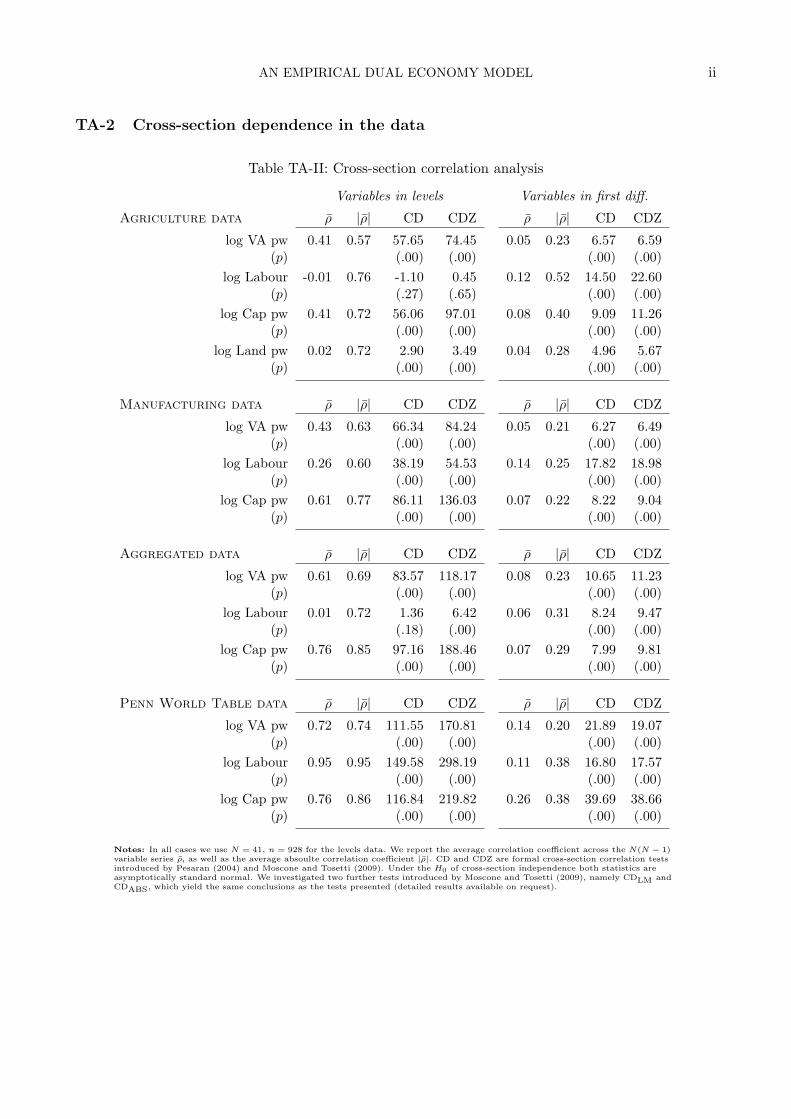
AN EMPIRICAL DUAL ECONOMY MODEL ii
TA-2 Cross-section dependence in the data
Table TA-II: Cross-section correlation analysis
Variables in levels Variables in first diff.
Agriculture data ρ |ρ| CD CDZ ρ |ρ| CD CDZ
log VA pw 0.41 0.57 57.65 74.45 0.05 0.23 6.57 6.59(p) (.00) (.00) (.00) (.00)
log Labour -0.01 0.76 -1.10 0.45 0.12 0.52 14.50 22.60(p) (.27) (.65) (.00) (.00)
log Cap pw 0.41 0.72 56.06 97.01 0.08 0.40 9.09 11.26(p) (.00) (.00) (.00) (.00)
log Land pw 0.02 0.72 2.90 3.49 0.04 0.28 4.96 5.67(p) (.00) (.00) (.00) (.00)
Manufacturing data ρ |ρ| CD CDZ ρ |ρ| CD CDZ
log VA pw 0.43 0.63 66.34 84.24 0.05 0.21 6.27 6.49(p) (.00) (.00) (.00) (.00)
log Labour 0.26 0.60 38.19 54.53 0.14 0.25 17.82 18.98(p) (.00) (.00) (.00) (.00)
log Cap pw 0.61 0.77 86.11 136.03 0.07 0.22 8.22 9.04(p) (.00) (.00) (.00) (.00)
Aggregated data ρ |ρ| CD CDZ ρ |ρ| CD CDZ
log VA pw 0.61 0.69 83.57 118.17 0.08 0.23 10.65 11.23(p) (.00) (.00) (.00) (.00)
log Labour 0.01 0.72 1.36 6.42 0.06 0.31 8.24 9.47(p) (.18) (.00) (.00) (.00)
log Cap pw 0.76 0.85 97.16 188.46 0.07 0.29 7.99 9.81(p) (.00) (.00) (.00) (.00)
Penn World Table data ρ |ρ| CD CDZ ρ |ρ| CD CDZ
log VA pw 0.72 0.74 111.55 170.81 0.14 0.20 21.89 19.07(p) (.00) (.00) (.00) (.00)
log Labour 0.95 0.95 149.58 298.19 0.11 0.38 16.80 17.57(p) (.00) (.00) (.00) (.00)
log Cap pw 0.76 0.86 116.84 219.82 0.26 0.38 39.69 38.66(p) (.00) (.00) (.00) (.00)
Notes: In all cases we use N = 41, n = 928 for the levels data. We report the average correlation coefficient across the N(N − 1)variable series ρ, as well as the average absoulte correlation coefficient |ρ|. CD and CDZ are formal cross-section correlation testsintroduced by Pesaran (2004) and Moscone and Tosetti (2009). Under the H0 of cross-section independence both statistics areasymptotically standard normal. We investigated two further tests introduced by Moscone and Tosetti (2009), namely CDLM andCDABS, which yield the same conclusions as the tests presented (detailed results available on request).
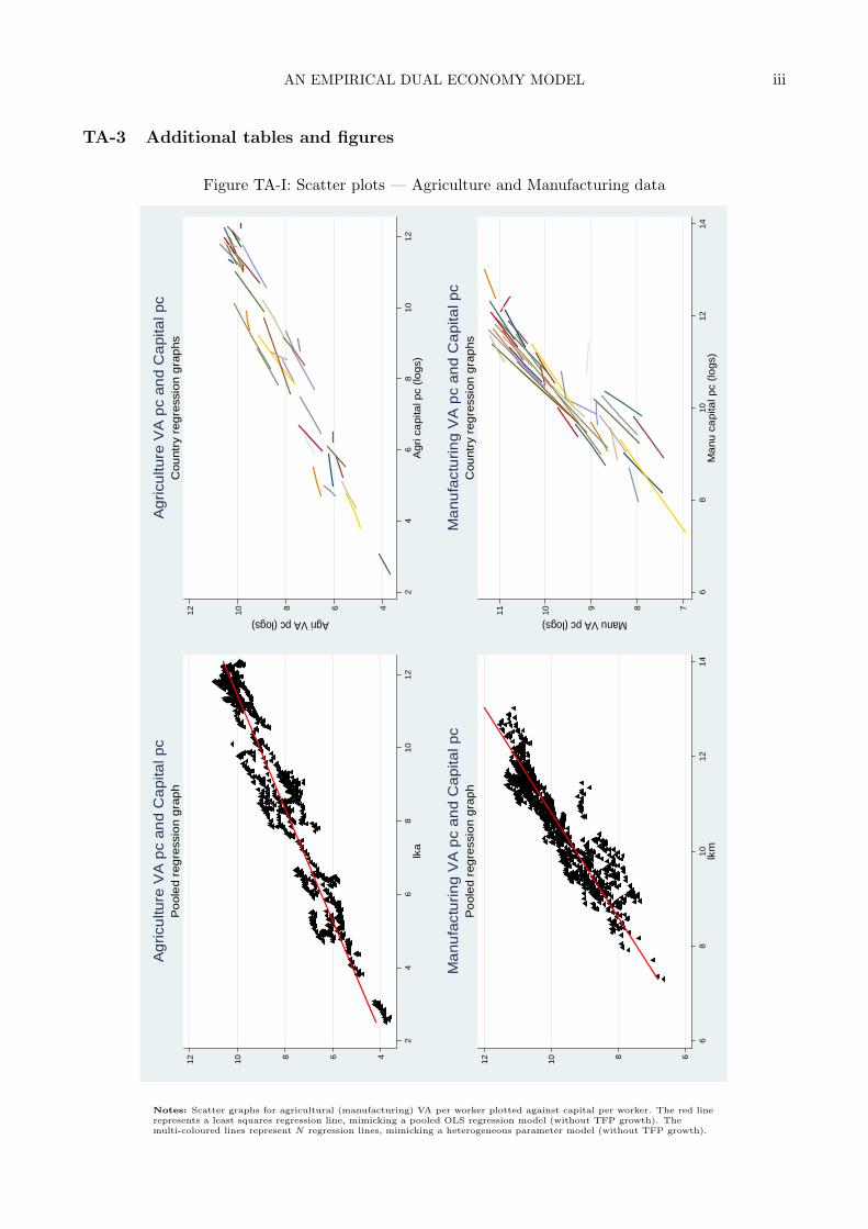
AN EMPIRICAL DUAL ECONOMY MODEL iii
TA-3 Additional tables and figures
Figure TA-I: Scatter plots — Agriculture and Manufacturing data
681012
68
1012
14lk
m
Poo
led
regr
essi
on g
raph
Man
ufac
turin
g V
A p
c an
d C
apita
l pc
4681012
24
68
1012
lka
Poo
led
regr
essi
on g
raph
Agr
icul
ture
VA
pc
and
Cap
ital p
c
4681012 Agri VA pc (logs)
24
68
1012
Agr
i cap
ital p
c (lo
gs)
Cou
ntry
reg
ress
ion
grap
hsA
gric
ultu
re V
A p
c an
d C
apita
l pc
7891011 Manu VA pc (logs)
68
1012
14M
anu
capi
tal p
c (lo
gs)
Cou
ntry
reg
ress
ion
grap
hsM
anuf
actu
ring
VA
pc
and
Cap
ital p
c
Notes: Scatter graphs for agricultural (manufacturing) VA per worker plotted against capital per worker. The red linerepresents a least squares regression line, mimicking a pooled OLS regression model (without TFP growth). Themulti-coloured lines represent N regression lines, mimicking a heterogeneous parameter model (without TFP growth).
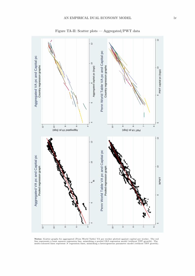
AN EMPIRICAL DUAL ECONOMY MODEL iv
Figure TA-II: Scatter plots — Aggregated/PWT data
4681012
46
810
12lk
Poo
led
regr
essi
on g
raph
Agg
rega
ted
VA
pc
and
Cap
ital p
c
4681012 Aggregated VA pc (logs)
46
810
12A
ggre
gate
d ca
pita
l pc
(logs
)
Cou
ntry
reg
ress
ion
grap
hsA
ggre
gate
d V
A p
c an
d C
apita
l pc
678910
68
1012
lkP
WT
Poo
led
regr
essi
on g
raph
Pen
n W
orld
Tab
le V
A p
c an
d C
apita
l pc
678910 PWT VA pc (logs)
68
1012
PW
T c
apita
l pc
(logs
)
Cou
ntry
reg
ress
ion
grap
hsP
enn
Wor
ld T
able
VA
pc
and
Cap
ital p
c
Notes: Scatter graphs for aggregated (Penn World Table) VA per worker plotted against capital per worker. The redline represents a least squares regression line, mimicking a pooled OLS regression model (without TFP growth). Themulti-coloured lines represent N regression lines, mimicking a heterogeneous parameter model (without TFP growth).
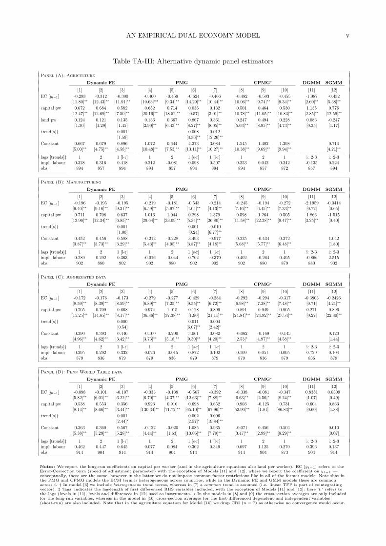
AN EMPIRICAL DUAL ECONOMY MODEL v
Table TA-III: Alternative dynamic panel estimators
Panel (A): Agriculture
Dynamic FE PMG CPMG? DGMM SGMM
[1] [2] [3] [4] [5] [6] [7] [8] [9] [10] [11] [12]EC [yt−1] -0.293 -0.312 -0.300 -0.460 -0.459 -0.624 -0.466 -0.482 -0.503 -0.455 -1.087 -0.432
[11.80]∗∗ [12.43]∗∗ [11.91]∗∗ [10.63]** [9.34]∗∗ [14.29]∗∗ [10.44]∗∗ [10.06]∗∗ [9.74]∗∗ [9.34]∗∗ [2.60]∗∗ [5.38]∗∗
capital pw 0.672 0.684 0.582 0.652 0.714 0.036 0.132 0.501 0.464 0.530 1.135 0.776[12.47]∗∗ [12.69]∗∗ [7.50]∗∗ [20.16]∗∗ [18.52]∗∗ [0.57] [3.01]∗∗ [10.78]∗∗ [11.05]∗∗ [10.83]∗∗ [2.85]∗∗ [12.59]∗∗
land pw 0.124 0.121 0.135 0.136 0.367 0.867 0.361 0.247 0.494 0.228 0.083 -0.247[1.30] [1.29] [1.45] [2.90]∗∗ [6.43]∗∗ [8.27]∗∗ [8.05]∗∗ [5.03]∗∗ [8.95]∗∗ [4.73]∗∗ [0.35] [1.17]
trend(s)† 0.001 0.008 0.012[1.59] [3.36]∗∗ [12.26]∗∗
Constant 0.667 0.679 0.896 1.072 0.644 4.273 3.084 1.545 1.402 1.298 0.714[5.03]∗∗ [4.75]∗∗ [4.58]∗∗ [10.48]∗∗ [7.53]∗∗ [13.11]∗∗ [10.27]∗∗ [10.38]∗∗ [9.69]∗∗ [9.94]∗∗ [4.21]∗∗
lags [trends]‡ 1 2 1 [l-r] 1 2 1 [s-r] 1 [l-r] 1 2 1 i: 2-3 i: 2-3impl. labour 0.328 0.316 0.418 0.212 -0.081 0.098 0.507 0.253 0.042 0.242 -0.135 0.224obs 894 857 894 894 857 894 894 894 857 872 857 894
Panel (B): Manufacturing
Dynamic FE PMG CPMG? DGMM SGMM
[1] [2] [3] [4] [5] [6] [7] [8] [9] [10] [11] [12]EC [yt−1] -0.196 -0.195 -0.195 -0.219 -0.181 -0.543 -0.214 -0.245 -0.194 -0.272 -2.1959 -0.0414
[9.40]∗∗ [9.16]∗∗ [9.31]∗∗ [6.59]∗∗ [5.97]∗∗ [4.04]∗∗ [4.13]∗∗ [7.16]∗∗ [6.45]∗∗ [7.33]∗∗ [0.72] [0.65]capital pw 0.711 0.708 0.637 1.016 1.044 0.298 1.379 0.598 1.264 0.505 1.866 -1.515
[12.96]∗∗ [12.34]∗∗ [6.85]∗∗ [29.64]∗∗ [33.09]∗∗ [5.34]∗∗ [26.80]∗∗ [11.58]∗∗ [22.28]∗∗ [9.47]∗∗ [3.25]∗∗ [0.40]trend(s)† 0.001 0.001 -0.010
[1.00] [0.24] [6.77]∗∗
Constant 0.452 0.456 0.588 -0.212 -0.228 3.493 -0.977 0.225 -0.434 0.372 1.042[3.87]∗∗ [3.73]∗∗ [3.29]∗∗ [5.43]∗∗ [4.95]∗∗ [3.87]∗∗ [4.18]∗∗ [5.68]∗∗ [5.77]∗∗ [6.48]∗∗ [1.80]
lags [trends]‡ 1 2 1 [l-r] 1 2 1 [s-r] 1 [l-r] 1 2 1 i: 2-3 i: 2-3impl. labour 0.289 0.292 0.363 -0.016 -0.044 0.702 -0.379 0.402 -0.264 0.495 -0.866 2.515obs 902 880 902 902 880 902 902 902 880 879 880 902
Panel (C): Aggregated data
Dynamic FE PMG CPMG? DGMM SGMM
[1] [2] [3] [4] [5] [6] [7] [8] [9] [10] [11] [12]EC [yt−1] -0.172 -0.176 -0.173 -0.279 -0.277 -0.429 -0.284 -0.292 -0.294 -0.317 -0.3803 -0.2426
[8.59]∗∗ [8.39]∗∗ [8.59]∗∗ [6.89]∗∗ [7.25]∗∗ [9.55]∗∗ [6.72]∗∗ [6.98]∗∗ [7.38]∗∗ [7.48]∗∗ [0.71] [4.21]∗∗
capital pw 0.705 0.709 0.668 0.974 1.015 0.128 0.899 0.891 0.949 0.905 0.271 0.896[15.25]∗∗ [14.65]∗∗ [8.17]∗∗ [36.86]∗∗ [37.38]∗∗ [1.90] [21.11]∗∗ [24.84]** [24.92]∗∗ [27.54]∗∗ [0.27] [22.80]∗∗
trend(s)† 0.000 0.011 0.004[0.54] [6.07]∗∗ [2.42]∗
Constant 0.390 0.393 0.446 -0.100 -0.200 3.061 0.082 -0.062 -0.169 -0.145 0.120[4.96]∗∗ [4.62]∗∗ [3.42]∗∗ [3.73]∗∗ [5.18]∗∗ [9.30]∗∗ [4.20]∗∗ [2.53]∗ [4.97]∗∗ [4.58]∗∗ [1.44]
lags [trends]‡ 1 2 1 [l-r] 1 2 1 [s-r] 1 [l-r] 1 2 1 i: 2-3 i: 2-3impl. labour 0.295 0.292 0.332 0.026 -0.015 0.872 0.102 0.109 0.051 0.095 0.729 0.104obs 879 836 879 879 836 879 879 879 836 879 836 879
Panel (D): Penn World Table data
Dynamic FE PMG CPMG? DGMM SGMM
[1] [2] [3] [4] [5] [6] [7] [8] [9] [10] [11] [12]EC [yt−1] -0.098 -0.101 -0.107 -0.333 -0.138 -0.567 -0.392 -0.338 -0.081 -0.347 0.8351 0.0309
[5.82]∗∗ [6.01]∗∗ [6.22]∗∗ [6.70]∗∗ [4.37]∗∗ [12.63]∗∗ [7.88]∗∗ [6.63]∗∗ [2.56]∗ [8.24]∗∗ [1.07] [0.49]capital pw 0.538 0.553 0.356 0.923 0.916 0.698 0.652 0.903 -0.125 0.731 0.604 0.863
[8.14]∗∗ [8.66]∗∗ [3.44]∗∗ [130.34]∗∗ [71.72]∗∗ [65.10]∗∗ [67.96]∗∗ [52.90]∗∗ [1.81] [86.83]∗∗ [0.60] [1.88]trend(s)† 0.001 0.002 0.006
[2.44]∗ [2.57]∗ [19.84]∗∗
Constant 0.363 0.360 0.567 -0.122 -0.020 1.085 0.935 -0.071 0.456 0.504 0.010[5.38]∗∗ [5.29]∗∗ [5.28]∗∗ [4.44]∗∗ [1.63] [13.05]∗∗ [7.79]∗∗ [3.47]∗∗ [2.99]∗∗ [8.29]∗∗ [0.07]
lags [trends]‡ 1 2 1 [l-r] 1 2 1 [s-r] 1 [l-r] 1 2 1 i: 2-3 i: 2-3impl. labour 0.462 0.447 0.645 0.077 0.084 0.302 0.349 0.097 1.125 0.270 0.396 0.137obs 914 904 914 914 904 914 914 904 873 904 914
Notes: We report the long-run coefficients on capital per worker (and in the agriculture equations also land per worker). EC [yt−1] refers to theError-Correction term (speed of adjustment parameter) with the exception of Models [11] and [12], where we report the coefficient on yt−1 —conceptually, these are the same, however in the latter we do not impose common factor restrictions like in all of the former models. Note that inthe PMG and CPMG models the ECM term is heterogeneous across countries, while in the Dynamic FE and GMM models these are commonacross i. † In model [6] we include heterogeneous trend terms, whereas in [7] a common trend is assumed (i.e. linear TFP is part of cointegratingvector). ‡ ‘lags’ indicates the lag-length of first differenced RHS variables included, with the exception of Models [11] and [12]: here ‘i:’ refers tothe lags (levels in [11], levels and differences in [12] used as instruments. ? In the models in [8] and [9] the cross-section averages are only includedfor the long-run variables, whereas in the model in [10] cross-section averages for the first-differenced dependent and independent variables(short-run) are also included. Note that in the agriculture equation for Model [10] we drop CRI (n = 7) as otherwise no convergence would occur.
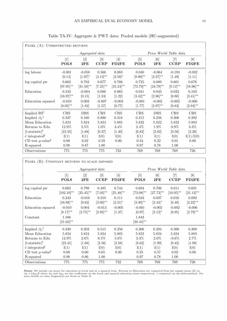
AN EMPIRICAL DUAL ECONOMY MODEL vi
Table TA-IV: Aggregate & PWT data: Pooled models (HC-augmented)
Panel (A): Unrestricted returns
Aggregated data Penn World Table data
[1] [2] [3] [4] [5] [6] [7] [8]POLS 2FE CCEP FD2FE POLS 2FE CCEP FD2FE
log labour -0.001 -0.058 0.566 0.083 0.040 -0.064 -0.193 -0.032[0.14] [1.97]∗ [4.13]∗∗ [2.50]∗ [8.99]∗∗ [3.27]∗∗ [1.49] [1.11]
log capital pw 0.662 0.782 0.677 0.766 0.725 0.680 0.601 0.676[97.95]∗∗ [31.50]∗∗ [7.25]∗∗ [25.24]∗∗ [72.79]∗∗ [24.79]∗∗ [9.12]∗∗ [18.96]∗∗
Education 0.243 -0.004 0.086 0.065 0.041 0.043 0.032 0.103[16.97]∗∗ [0.15] [1.24] [1.22] [3.42]∗∗ [2.86]∗∗ [0.80] [3.41]∗∗
Education squared -0.010 0.003 -0.007 -0.003 -0.001 -0.002 -0.002 -0.006[8.05]∗∗ [1.82] [1.57] [0.77] [1.77] [2.97]∗∗ [0.83] [2.94]∗∗
Implied RS† CRS DRS CRS CRS CRS DRS CRS CRSImplied βL
‡ 0.337 0.160 0.890 0.318 0.315 0.256 0.206 0.292Mean Education 5.824 5.824 5.824 5.885 5.822 5.822 5.822 5.883Returns to Edu 12.9% 2.5% 1.0% 3.4% 2.4% 1.9% 0.9% 3.3%[t-statistic][ [22.35] [1.68] [0.37] [1.40] [6.82] [2.02] [0.56] [2.26]e integrated\ I(1) I(1) I(0) I(0) I(1) I(1) I(0) I(1)/I(0)CD test p-value] 0.00 0.02 0.59 0.00 0.34 0.22 0.01 0.00R-squared 0.98 0.87 1.00 - 0.97 0.78 1.00 -Observations 775 775 775 732 769 769 769 726
Panel (B): Constant returns to scale imposed
Aggregated data Penn World Table data
[1] [2] [3] [4] [5] [6] [7] [8]POLS 2FE CCEP FD2FE POLS 2FE CCEP FD2FE
log capital pw 0.662 0.798 0.485 0.744 0.694 0.706 0.611 0.691[102.10]∗∗ [35.45]∗∗ [7.03]∗∗ [25.48]∗∗ [73.08]∗∗ [27.73]∗∗ [10.05]∗∗ [21.13]∗∗
Education 0.243 -0.016 0.210 0.111 0.043 0.037 0.016 0.092[16.98]∗∗ [0.62] [3.00]∗∗ [2.21]∗ [3.30]∗∗ [2.44]∗ [0.48] [3.22]∗∗
Education squared -0.010 0.004 -0.013 -0.005 -0.001 -0.002 -0.002 -0.006[8.17]∗∗ [2.75]∗∗ [2.92]∗∗ [1.37] [0.97] [2.12]∗ [0.95] [2.79]∗∗
Constant 1.586 1.843[21.62]∗∗ [20.44]∗∗
Implied βL‡ 0.338 0.203 0.515 0.256 0.306 0.294 0.390 0.309
Mean Education 5.824 5.824 5.824 5.885 5.822 5.824 5.824 5.883Returns to Edu 12.9% 2.6% 6.5% 5.8% 3.3% 2.0% -0.6% 2.7%[t-statistic][ [22.41] [1.68] [2.56] [2.56] [8.62] [1.99] [0.42] [1.98]e integrated\ I(1) I(1) I(0) I(0) I(1) I(1) I(0) I(0)CD test p-value] 0.00 0.00 0.65 0.00 0.25 0.57 0.02 0.00R-squared 0.98 0.86 1.00 0.97 0.78 1.00Observations 775 775 775 732 769 769 769 726
Notes: We include our proxy for education in levels and as a squared term. Returns to Education are computed from the sample mean (E) asβE + 2βE2E where βE and βE2 are the coefficients on the levels and squared education terms respectively. [ computed via the delta-method. Formore details on other diagnostics see Notes in Table II.
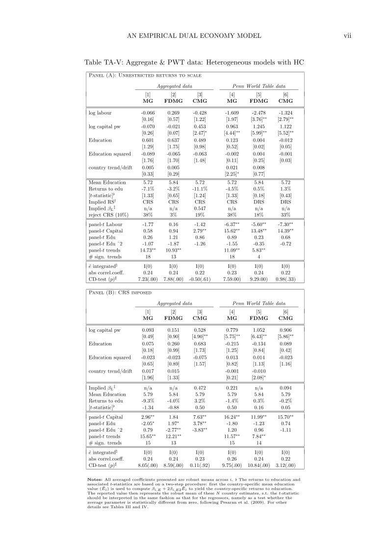
AN EMPIRICAL DUAL ECONOMY MODEL vii
Table TA-V: Aggregate & PWT data: Heterogeneous models with HC
Panel (A): Unrestricted returns to scale
Aggregated data Penn World Table data
[1] [2] [3] [4] [5] [6]MG FDMG CMG MG FDMG CMG
log labour -0.066 0.269 -0.428 -1.609 -2.478 -1.324[0.16] [0.57] [1.22] [1.97] [3.76]∗∗ [2.79]∗∗
log capital pw -0.070 -0.021 0.453 0.963 1.245 1.122[0.26] [0.07] [2.47]∗ [4.44]∗∗ [5.99]∗∗ [5.52]∗∗
Education 0.601 0.637 0.489 0.123 0.004 -0.012[1.29] [1.75] [0.98] [0.52] [0.02] [0.05]
Education squared -0.089 -0.065 -0.063 -0.002 0.004 -0.001[1.76] [1.70] [1.48] [0.11] [0.25] [0.03]
country trend/drift 0.005 0.005 0.021 0.008[0.33] [0.29] [2.25]∗ [0.77]
Mean Education 5.72 5.84 5.72 5.72 5.84 5.72Returns to edu -7.1% -3.2% -11.1% -4.5% 0.5% 1.3%[t-statistic][ [1.33] [0.65] [1.24] [1.33] [0.18] [0.43]Implied RS† CRS CRS CRS CRS DRS DRSImplied βL
‡ n/a n/a 0.547 n/a n/a n/areject CRS (10%) 38% 3% 19% 38% 18% 33%
panel-t Labour -1.77 0.16 -1.42 -6.37∗∗ -5.60∗∗ -7.30∗∗
panel-t Capital 0.58 0.94 2.79∗∗ 15.62∗∗ 13.48∗∗ 14.39∗∗
panel-t Edu 0.26 1.21 0.86 0.89 0.23 0.68panel-t Edu ˆ2 -1.07 -1.87 -1.26 -1.55 -0.35 -0.72panel-t trends 14.73∗∗ 10.93∗∗ 11.09∗∗ 5.83∗∗
# sign. trends 18 13 18 4
e integrated\ I(0) I(0) I(0) I(0) I(0) I(0)abs correl.coeff. 0.24 0.24 0.22 0.23 0.24 0.22CD-test (p)] 7.23(.00) 7.88(.00) -0.50(.61) 7.59.00) 9.29.00) 0.98(.33)
Panel (B): CRS imposed
Aggregated data Penn World Table data
[1] [2] [3] [4] [5] [6]MG FDMG CMG MG FDMG CMG
log capital pw 0.093 0.151 0.528 0.779 1.052 0.906[0.49] [0.90] [4.90]∗∗ [5.75]∗∗ [6.43]∗∗ [5.86]∗∗
Education 0.075 0.260 0.683 -0.215 -0.134 0.089[0.18] [0.99] [1.73] [1.25] [0.84] [0.42]
Education squared -0.023 -0.023 -0.075 0.013 0.014 -0.023[0.65] [0.89] [1.57] [0.82] [1.13] [1.16]
country trend/drift 0.017 0.015 -0.001 -0.010[1.96] [1.33] [0.21] [2.08]∗
Implied βL‡ n/a n/a 0.472 0.221 n/a 0.094
Mean Education 5.79 5.84 5.79 5.79 5.84 5.79Returns to edu -9.3% -4.0% 3.2% -1.4% 0.3% -0.2%[t-statistic][ -1.34 -0.88 0.50 0.50 0.16 0.05
panel-t Capital 2.96∗∗ 1.84 7.63∗∗ 16.24∗∗ 11.99∗∗ 15.70∗∗
panel-t Edu -2.05∗ 1.97∗ 3.78∗∗ -1.80 -1.23 0.74panel-t Edu ˆ2 0.79 -2.77∗∗ -3.83∗∗ 1.20 0.96 -1.11panel-t trends 15.65∗∗ 12.21∗∗ 11.57∗∗ 7.84∗∗
# sign. trends 15 13 15 14
e integrated\ I(0) I(0) I(0) I(0) I(0) I(0)abs correl.coeff. 0.24 0.24 0.23 0.26 0.24 0.22CD-test (p)] 8.05(.00) 8.59(.00) 0.11(.92) 9.75(.00) 10.84(.00) 3.12(.00)
Notes: All averaged coefficients presented are robust means across i. [ The returns to education andassociated t-statistics are based on a two-step procedure: first the country-specific mean educationvalue (Ei) is used to compute βi,E + 2βi,E2Ei to yield the country-specific returns to education.The reported value then represents the robust mean of these N country estimates, s.t. the t-statisticshould be interpreted in the same fashion as that for the regressors, namely as a test whether theaverage parameter is statistically different from zero, following Pesaran et al. (2009). For otherdetails see Tables III and IV.
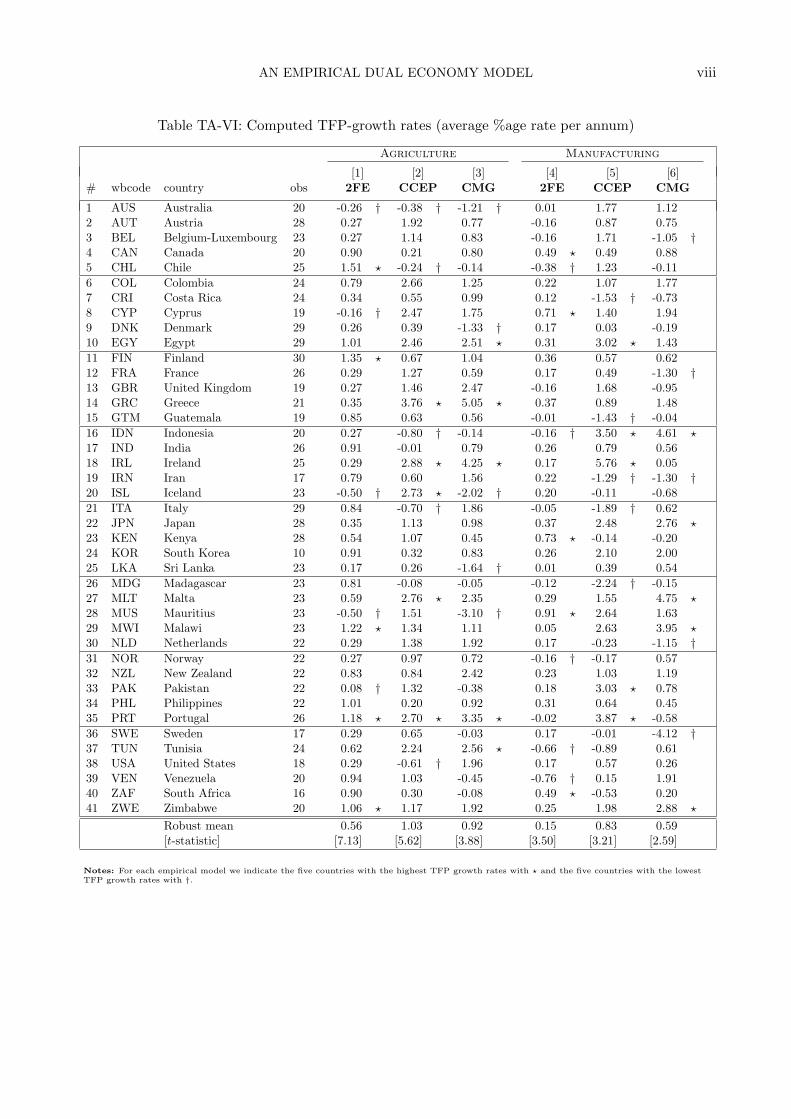
AN EMPIRICAL DUAL ECONOMY MODEL viii
Table TA-VI: Computed TFP-growth rates (average %age rate per annum)
Agriculture Manufacturing
[1] [2] [3] [4] [5] [6]# wbcode country obs 2FE CCEP CMG 2FE CCEP CMG
1 AUS Australia 20 -0.26 † -0.38 † -1.21 † 0.01 1.77 1.122 AUT Austria 28 0.27 1.92 0.77 -0.16 0.87 0.753 BEL Belgium-Luxembourg 23 0.27 1.14 0.83 -0.16 1.71 -1.05 †4 CAN Canada 20 0.90 0.21 0.80 0.49 ? 0.49 0.885 CHL Chile 25 1.51 ? -0.24 † -0.14 -0.38 † 1.23 -0.116 COL Colombia 24 0.79 2.66 1.25 0.22 1.07 1.777 CRI Costa Rica 24 0.34 0.55 0.99 0.12 -1.53 † -0.738 CYP Cyprus 19 -0.16 † 2.47 1.75 0.71 ? 1.40 1.949 DNK Denmark 29 0.26 0.39 -1.33 † 0.17 0.03 -0.1910 EGY Egypt 29 1.01 2.46 2.51 ? 0.31 3.02 ? 1.4311 FIN Finland 30 1.35 ? 0.67 1.04 0.36 0.57 0.6212 FRA France 26 0.29 1.27 0.59 0.17 0.49 -1.30 †13 GBR United Kingdom 19 0.27 1.46 2.47 -0.16 1.68 -0.9514 GRC Greece 21 0.35 3.76 ? 5.05 ? 0.37 0.89 1.4815 GTM Guatemala 19 0.85 0.63 0.56 -0.01 -1.43 † -0.0416 IDN Indonesia 20 0.27 -0.80 † -0.14 -0.16 † 3.50 ? 4.61 ?17 IND India 26 0.91 -0.01 0.79 0.26 0.79 0.5618 IRL Ireland 25 0.29 2.88 ? 4.25 ? 0.17 5.76 ? 0.0519 IRN Iran 17 0.79 0.60 1.56 0.22 -1.29 † -1.30 †20 ISL Iceland 23 -0.50 † 2.73 ? -2.02 † 0.20 -0.11 -0.6821 ITA Italy 29 0.84 -0.70 † 1.86 -0.05 -1.89 † 0.6222 JPN Japan 28 0.35 1.13 0.98 0.37 2.48 2.76 ?23 KEN Kenya 28 0.54 1.07 0.45 0.73 ? -0.14 -0.2024 KOR South Korea 10 0.91 0.32 0.83 0.26 2.10 2.0025 LKA Sri Lanka 23 0.17 0.26 -1.64 † 0.01 0.39 0.5426 MDG Madagascar 23 0.81 -0.08 -0.05 -0.12 -2.24 † -0.1527 MLT Malta 23 0.59 2.76 ? 2.35 0.29 1.55 4.75 ?28 MUS Mauritius 23 -0.50 † 1.51 -3.10 † 0.91 ? 2.64 1.6329 MWI Malawi 23 1.22 ? 1.34 1.11 0.05 2.63 3.95 ?30 NLD Netherlands 22 0.29 1.38 1.92 0.17 -0.23 -1.15 †31 NOR Norway 22 0.27 0.97 0.72 -0.16 † -0.17 0.5732 NZL New Zealand 22 0.83 0.84 2.42 0.23 1.03 1.1933 PAK Pakistan 22 0.08 † 1.32 -0.38 0.18 3.03 ? 0.7834 PHL Philippines 22 1.01 0.20 0.92 0.31 0.64 0.4535 PRT Portugal 26 1.18 ? 2.70 ? 3.35 ? -0.02 3.87 ? -0.5836 SWE Sweden 17 0.29 0.65 -0.03 0.17 -0.01 -4.12 †37 TUN Tunisia 24 0.62 2.24 2.56 ? -0.66 † -0.89 0.6138 USA United States 18 0.29 -0.61 † 1.96 0.17 0.57 0.2639 VEN Venezuela 20 0.94 1.03 -0.45 -0.76 † 0.15 1.9140 ZAF South Africa 16 0.90 0.30 -0.08 0.49 ? -0.53 0.2041 ZWE Zimbabwe 20 1.06 ? 1.17 1.92 0.25 1.98 2.88 ?
Robust mean 0.56 1.03 0.92 0.15 0.83 0.59[t-statistic] [7.13] [5.62] [3.88] [3.50] [3.21] [2.59]
Notes: For each empirical model we indicate the five countries with the highest TFP growth rates with ? and the five countries with the lowestTFP growth rates with †.
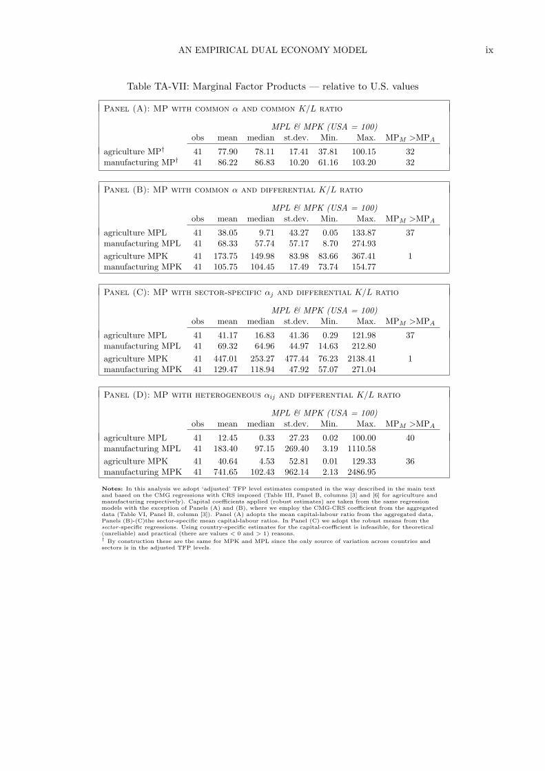
AN EMPIRICAL DUAL ECONOMY MODEL ix
Table TA-VII: Marginal Factor Products — relative to U.S. values
Panel (A): MP with common α and common K/L ratio
MPL & MPK (USA = 100)obs mean median st.dev. Min. Max. MPM >MPA
agriculture MP† 41 77.90 78.11 17.41 37.81 100.15 32manufacturing MP† 41 86.22 86.83 10.20 61.16 103.20 32
Panel (B): MP with common α and differential K/L ratio
MPL & MPK (USA = 100)obs mean median st.dev. Min. Max. MPM >MPA
agriculture MPL 41 38.05 9.71 43.27 0.05 133.87 37manufacturing MPL 41 68.33 57.74 57.17 8.70 274.93agriculture MPK 41 173.75 149.98 83.98 83.66 367.41 1manufacturing MPK 41 105.75 104.45 17.49 73.74 154.77
Panel (C): MP with sector-specific αj and differential K/L ratio
MPL & MPK (USA = 100)obs mean median st.dev. Min. Max. MPM >MPA
agriculture MPL 41 41.17 16.83 41.36 0.29 121.98 37manufacturing MPL 41 69.32 64.96 44.97 14.63 212.80agriculture MPK 41 447.01 253.27 477.44 76.23 2138.41 1manufacturing MPK 41 129.47 118.94 47.92 57.07 271.04
Panel (D): MP with heterogeneous αij and differential K/L ratio
MPL & MPK (USA = 100)obs mean median st.dev. Min. Max. MPM >MPA
agriculture MPL 41 12.45 0.33 27.23 0.02 100.00 40manufacturing MPL 41 183.40 97.15 269.40 3.19 1110.58agriculture MPK 41 40.64 4.53 52.81 0.01 129.33 36manufacturing MPK 41 741.65 102.43 962.14 2.13 2486.95
Notes: In this analysis we adopt ‘adjusted’ TFP level estimates computed in the way described in the main textand based on the CMG regressions with CRS imposed (Table III, Panel B, columns [3] and [6] for agriculture andmanufacturing respectively). Capital coefficients applied (robust estimates) are taken from the same regressionmodels with the exception of Panels (A) and (B), where we employ the CMG-CRS coefficient from the aggregateddata (Table VI, Panel B, column [3]). Panel (A) adopts the mean capital-labour ratio from the aggregated data,Panels (B)-(C)the sector-specific mean capital-labour ratios. In Panel (C) we adopt the robust means from thesector-specific regressions. Using country-specific estimates for the capital-coefficient is infeasible, for theoretical(unreliable) and practical (there are values < 0 and > 1) reasons.† By construction these are the same for MPK and MPL since the only source of variation across countries andsectors is in the adjusted TFP levels.


![Hogeschool van Amsterdam Instituut voor Interactieve Media PROPEDEUSE ONDERNEMEN College 2 [06-02-07] Peter Buis Lori de Paauw](https://img.pdfslide.net/doc/110x75/5551a0f04979591f3c8ba9ec/hogeschool-van-amsterdam-instituut-voor-interactieve-media-propedeuse-ondernemen-college-2-06-02-07-peter-buis-lori-de-paauw.jpg)

![College 6 [22-05-07] Peter Buis Lori de Paauw](https://img.pdfslide.net/doc/110x75/5681428b550346895daeb732/college-6-22-05-07-peter-buis-lori-de-paauw.jpg)