GRUPO DE GEOFÍSICA MATEMÁTICA Y ... - mmc.geofisica.unam.mxmmc.geofisica.unam.mx/mmc/ReportesInternos/MEMORIA06.pdf · grupo de . geofÍsica matemÁtica y computacional . memoria

GRUPO DE

GEOFÍSICA MATEMÁTICA Y COMPUTACIONAL

MEMORIA Nº 6

MÉXICO 2014

MEMORIAS GGMC INSTITUTO DE GEOFÍSICA UNAM

ii

MIEMBROS DEL GGMC

Dr. Ismael Herrera Revilla [email protected]

Dr. Luis Miguel de la Cruz Salas

[email protected]

Dr. Guillermo Hernández García [email protected]

Dra. Graciela Herrera Zamarrón

[email protected]

Dr. Norberto Vera Guzmán [email protected]

Dr. Álvaro Alberto Aldama Rodríguez

[email protected]

Depto. Recursos Naturales Instituto de Geofísica

UNAM

Publicado y distribuido por:

Grupo de Geofísica Matemática y Computacional

GGMC

Apartado Postal: 22-220 CP. 14000

Unidad de Apoyo Editorial

[email protected]

mailto:[email protected]





iii

Four General Purposes Massively Parallel DDM Algorithms By

Ismael Herrera and Alberto Rosas-Medina

del 2012

GRUPO DE

GEOFÍSICA MATEMÁTICA Y COMPUTACIONAL

GGMC

iv

CONTENTS

Abstract

1. INTRODUCTION 1

2. OVERVIEW OF THE DVS FRAMEWORK 4

3. THE ORIGINAL PROBLEM AND THE ORIGINAL NODES 6

4. DERIVED-NODES 8

5. THE “DERIVED VECTOR-SPACE (DVS)” 10

6. THE GENERAL PROBLEM WITH CONSTRAINTS 14

7. THE DVS-ALGORITHMS WITH CONSTRAINTS 15

8. NUMERICAL PROCEDURES 16

8.1- COMMENTS ON THE DVS NUMERICAL PROCEDURES 17

8.2- APPLICATION OF S 18

8.3- APPLICATION OF S -1 19

8.4- APPLICATION OF a 20

9. NUMERICAL RESULTS 21

10. CONCLUSIONS 24

REFERENCES 25

v

GGMC

Four General Purposes Massively Parallel DDM Algorithms By

Ismael Herrera and Alberto Rosas-Medina Instituto de Geofísica

Universidad Nacional Autónoma de México (UNAM) Apdo. Postal 22-220, México, D.F. 14000

Email: [email protected]

Abstract Parallel computers available nowadays require massively parallel software. DDMs are the approach to this problem; they seek algorithms capable of constructing the global solution by solving local problems, in each partition subdomain, exclusively. At present, however, competitive algorithms need to incorporate constraints, such as continuity on primal-nodes. This poses an additional challenge, which has been difficult to overcome. This paper is devoted to discuss four general-purposes preconditioned algorithms with constraints in which such a goal is achieved. Each one of them can be applied to symmetric, non-symmetric and indefinite problems, and here it is shown that they have update numerical efficiency and the global solution is obtained by solving local

Keywords: Massively-parallel algorithms; parallel-computers; non-overlapping DDM; DDM with constraints; BDDC; FETI-DP

problems, exclusively. Furthermore, the outstanding uniformity of the formulas from which they derive yields clear advantages for code development; for example, the construction of very robust codes. The new algorithms have been derived in the realm of the DVS-framework, recently introduced. Two of them are the DVS versions of BDDC and FETI-DP, respectively, which in this manner have been extended to non-symmetric and indefinite matrices. The originality of the other two is more complete, since we have not identified in the literature algorithms with clear similarities to them.

Equation Section 1

1.- INTRODUCTION Mathematical models of many systems of interest, including very important

continuous systems of Engineering and Science, lead to a great variety of partial

differential equations whose solution methods are based on the computational

processing of large-scale algebraic systems. Furthermore, the incredible expansion

experienced by the existing computational hardware and software has made

amenable to effective treatment problems of an ever increasing diversity and

complexity, posed by engineering and scientific applications.

Parallel computing is outstanding among the new computational tools, especially at

present when further increases in hardware speed apparently have reached


Ismael Herrera and Alberto Rosas Medina

2

insurmountable barriers. Therefore, the emergence of parallel computing during

the last twenty or thirty years, prompted on the part of the computational-modeling

community a continued and systematic effort with the purpose of harnessing it for

the endeavor of solving partial differential equations [1]. Very early after such an

effort began, it was recognized that domain decomposition methods (DDM) were

the most effective technique for applying parallel computing to the solution of

partial differential equations, since such an approach drastically simplifies the

coordination of the many processors that carry out the different tasks and also

reduces very much the requirements of information-transmission between them. At

the beginning much attention was given to overlapping domain decomposition

methods, but soon it was realized that iterative substructuring methods in non-

overlapping partitions, known as non-overlapping DDM, were more effective [2].

Hence, domain decomposition methods (DDM) have been developed mainly as a

tool for applying parallel computers to the solution of partial differential equations

and to this end non-overlapping DDM formulations split the domain of definition of

the partial differential equation at hand, or system of such equations, into many

subdomains with the intention of developing procedures that permit “solving the

global problem by exclusively solving problems separately defined in each one of

the partition subdomains, frequently called: local problems”. The basic idea is to

assign to each subdomain a different processor capable of solving the

corresponding local problem. However, at present it is recognized that competitive

algorithms need to incorporate constraints, such as continuity on primal-nodes [2-

6]. This poses an additional challenge for developing 100% parallelizable

algorithms, which has been difficult to overcome; indeed, up to now the most

effective DDM-algorithms do not fully achieve the above-stated goal [7] of “solving

the global problem by exclusively solving local

problems”.

The present paper is devoted to discussing four general non-overlapping DDM-

algorithms recently introduced and summarized in [8], which are referred to as

preconditioned DVS-algorithms with constraints. They are applicable to a wide

Four General Purposes Massively Parallel DDM Algorithms.

3 Memorias GMMC 2012 - 7

range of matrices that stem from the discretization of partial differential equations;

such matrices may be symmetric-definite, indefinite or non-symmetric. In the

present paper we show that each one of these algorithms enjoys the following

properties:

I. Possesses update numerical efficiency. Here, by update numerical

efficiency it is meant that their efficiency is at least as good that of the best

domain decompositions formulations existing today. Comparisons of

numerical performances were made with BDDC and FETI-DP [2-6]; and

II. “The global solution is obtained by exclusively solving local problems”.

The algorithms here discussed are formulated in the realm of the derived-vector

space (DVS) framework, which was recently introduced by I. Herrera and

coworkers [8-13]. The DVS, in the sense here used, was explained in [8]; the

reader is referred to [8-10] for the basic developments of this approach and to [11-

13] for background material on which the DVS-framework was built. The

developments to be presented are based on the extensive work on DDM done

during the last twenty years or so by many authors (see, for example [1,2]), albeit

what is special of our approach is the use of the DVS-framework, in which our

developments are set.

In this respect, we point out that two algorithms of the set of preconditioned DVS-

algorithms to be discussed are the DVS-versions of two well-known, very efficient

non-overlapping DDM approaches: the balancing domain decomposition with

constraints (BDDC) and the dual-primal finite-element tearing and interconnecting

(FETI-DP) methods, respectively [14]. The balancing domain decomposition

method was originally introduced by Mandel [15,16] and more recently modified by

Dohrmann who introduced constraints in its formulation [3,4], while the original

finite-element tearing and interconnecting method was introduced by Farhat [17,18]

and later modified by the introduction of a dual-primal approach [19-21]. It should

be mentioned that the BDDC and FETI-DP methods were originally developed for


4

definite (positive definite) symmetric problems, although certain number of

applications to non-symmetric and indefinite matrices have been made (see, for

example, [6, 22-25]). On the other hand, the algorithms derived from the DVS-

versions of BDDC and FETI-DP are applicable to non-symmetric matrices

independently of the particular problem considered. As for the other two

preconditioned DVS-algorithms, their novelty is more complete, since they do not

correspond to any DDM previously reported in the literature [8].

Equation Section 2

2.- OVERVIEW OF THE DVS FRAMEWORK The ‘derived vector space framework (DVS-framework)’ starts with the system of

linear equations that is obtained after the partial differential equation, or system of

such equations, has been discretized; this system of discrete equations is referred

to as the ‘original problem’. Independently of the discretization method used, it is

assumed that a set of nodes and a domain-partition have been introduced and that

both the nodes and the partition-subdomains have been numbered. Generally,

some of these original-nodes belong to more than one partition-subdomain (Fig.1).

For the formulation of non-overlapping domain decomposition methods it would be

better if each node would belong to one and only one partition-subdomain, and a

new set of nodes – the derived-nodes- that enjoy this property is introduced. This

new set of nodes is obtained by dividing each original-node in as many pieces as

required to obtain a set with the desired property (Fig.2). Then, each derived-node

is identified by means of an ordered-pair of numbers: the label of the original-node,

it comes from, followed by the partition-subdomain label, it belongs to. A ‘derived-

vector’ is simply defined to be any real-valued function1

1 For the treatment of systems of equations, vector-valued functions are considered, instead

defined in the whole set of

derived-nodes; the set of all derived-vectors constitutes a linear space: the

‘derived-vector space (DVS)’. The ‘Euclidean inner-product’, for each pair of

derived-vectors, is defined to be the product of their components summed over all

the derived-nodes. The DVS constitutes a finite-dimensional Hilbert-space, with



Figure 1. The ‘original nodes’

Figure 2. The ‘derived nodes’ respect to the Euclidean inner-product. A new problem, which is equivalent to the

original problem, is defined in the derived-vector space. Of course, the matrix of

Γ1Ω 2Ω

3Ω 4Ω

1 2 3 4 5

76 8

2521 22

9 10

11 12 13 14 15

16 17 18 19 20

23 24

1ΩΓ

2Ω

3Ω 4Ω

( )1,1 ( )2,1 ( )3,1 ( )3, 2 ( )4, 2( )5, 2

( )21, 3 ( )22, 3 ( )23, 3 ( )23, 4 ( )24, 4 ( )25, 4

( )13,1 ( )13,2

( )13,3 ( )13,4

( )6,1( )7,1

( )8,1

( )11,1 ( )12,1

( )8,2 ( )9,2 ( )10,2

( )14,2 ( )15,2

( )11,3 ( )12,3 ( )14,4 ( )15,4

( )16,3 ( )17,3 ( )18,3 ( )18,4 ( )19,4 ( )20,4


6

this new problem is different to the original-matrix, which is only defined in the

original-vector space, and the theory supplies a formula for deriving it [8]. From

there on, in the DVS framework, all the work is done in the derived-vector space

and one never goes back to the original vector-space. In a systematic manner, this

framework led to the construction of the following preconditioned DVS-algorithms:

DVS-primal formulation #1, DVS-dual formulation #1, DVS-primal formulation #2

and DVS-dual formulation #2. However, the DVS-primal formulation #1 and DVS-

dual formulation #1 were later identified as DVS-versions of BDDC and FETI-DP,

respectively. With this adjustment in nomenclature, in [8] they were summarized as

it is indicated next. Thereby, it should be mentioned that standard versions of

BDDC and FETI-DP were originally formulated for definite-symmetric matrices

(positive-definite or negative-definite) [3,4,14-20]; thus, their extension to non-

symmetric and indefinite matrices is one of the achievements of the DVS-

framework.

The Four General Preconditioned Algorithms with Constraints that will be

studied in this paper are:

a).- The DVS-version of BDDC;

b).-The DVS-version of FETI-DP;

c).- DVS-primal formulation #2;

d).- DVS-dual formulation #2.

All these algorithms are preconditioned and are formulated in vector-spaces

subjected to constraints; so, they are preconditioned and constrained algorithms as

their titles indicate.

Equation Section 3

3.- THE ORIGINAL PROBLEM AND THE ORIGINAL NODES It will be assumed that the system of linear algebraic equations:

Au f=

(3.1)

is the result that has been obtained after the (linear) partial differential equation, or

system of such equations has been discretized. Eq.(3.1) will be referred to as the

‘original problem’ and, as said before, it will be the starting point of our discussions.



The DVS-framework is an axiomatic approach; so, its developments are based on

a set of assumptions fulfilled by the linear system of Eq.(3.1). In this system of

equations the ‘original matrix’ A

, and the ‘original vectors’ u and f

are:

( ) ( ) ( ) 1,...,ij j jA A , u u , f f with i, j n≡ ≡ ≡ =

(3.2)

Here, n is the number of ‘original nodes’ occurring in the original discretization of

the problem. Let Ω be the domain of definition of the continuous problem, before

discretization. Then, it is assumed that the family 1,..., EΩ Ω of sub-domains of Ω

constitutes a non-overlapping domain decomposition of Ω ; i.e., the relations

1

E

and α β αα=

Ω ∩Ω =∅ Ω⊂ Ω

(3.3)

are satisfied. Here, αΩ stands for the closure of αΩ . Furthermore, it is assumed

that the two sets of numbers:

ˆ ˆ1,..., 1,...,n and EΝ ≡ Ε ≡ (3.4)

label the original nodes and the partition-subdomains, respectively. The notation

ˆ αΝ , 1,..., Eα = , will be used for the subset of original-nodes that pertain to αΩ .

Original nodes will be classified into ‘internal’ and ‘interface-nodes’: a node is

internal if it belongs to only one partition-subdomain closure and it is an interface-

node, when it belongs to more than one. Furthermore, for the development of

domain decomposition methods with restrictions it will be necessary to choose a

subset of interface-nodes: the set of primal nodes.

We define:

• ˆ ˆΙΝ ⊂ Ν as the set of internal-nodes;

• ˆ ˆΓΝ ⊂ Ν as the set of interface-nodes;

• ˆ ˆπΝ ⊂ Ν as the set of primal-nodes2

2 In order to mimic standard notations, we should have used

; and

Π instead of the low-case π . However, the modified definitions here given yield some convenient algebraic properties.


8

• ˆ ˆ ˆ ˆπ∆ Γ ΓΝ ≡ Ν − Ν ⊂ Ν as the set of dual-nodes.

For the time being, the set ˆ ˆπ ΓΝ ⊂ Ν may be any, depending on the specific

problem treated3

ˆ ˆ,Ι ΓΝ Ν

. Each one of the following two families of node-subsets is disjoint:

and ˆ ˆ ˆ, ,πΙ ∆Ν Ν Ν . Furthermore, these node subsets fulfill the relations:

ˆ ˆ ˆ ˆ ˆ ˆ ˆ ˆ ˆ and π πΙ Γ Ι ∆ Γ ∆Ν = Ν ∪Ν = Ν ∪Ν ∪Ν Ν = Ν ∪Ν (3.5)

Using the notations thus far introduced, the following assumption is adopted:

AXIOM 1.- “Let the indices î α∈Ν and ˆj β∈Ν be internal original-nodes, then:

0,ijA whenever α β= ≠

(3.6)”

The real-valued functions defined in ˆ 1,..., nΝ = constitute a linear vector-space

that will be denoted by W and referred to as the ‘original vector-space’. When

u W∈ , we write ( )iu u i≡ for the value of u at any original-node î∈Ν . As said

before, we use the notation ( )1,..., nu u u≡ for the original-vectors. Thereby, we

observe the duality of interpretation: original-vectors can also be thought as real-

valued functions defined in the finite-set ˆ 1,...,nΝ ≡ .

Equation Section 4

4.- DERIVED-NODES As said before, when a non-overlapping partition is introduced some of the nodes

used in the discretization belong to more than one partition-subdomain. To

overcome this inconvenient feature in the DVS-framework, besides the original-

nodes, another set of nodes is introduced, called the ´derived nodes’. The general

developments are better understood, through a simple example that we explain

first.

3 Extensive research has been carried out to establish criteria for the choice of ˆ

πΝ , which will not be discussed here.



Consider the set of twenty five nodes of a “non-overlapping” domain

decomposition, which consists of four subdomains, as shown in Fig.1. Thus, we

have a set of nodes and a set of subdomains, which are numbered using of the

index-sets: ˆ 1,..., 25Ν ≡ and ˆ 1, 2,3, 4Ε ≡ , respectively. Then, the sets of nodes

corresponding to such a non-overlapping domain decomposition is actually

overlapping

, since the four subsets

1 2

3 4

ˆ ˆ1, 2,3,6,7,8,11,12,13 3,4,5,8,9,10,13,14,15ˆ ˆ11,12,13,16,17,18,21,22,23 13,14,15,18,19,20,23,24,25

Ν ≡ Ν ≡

Ν ≡ Ν ≡ (4.1)

are not disjoint (see, Fig.1). Indeed, for example:

1 2ˆ ˆ 3,8,13Ν ∩Ν = (4.2)

In order to obtain a “truly” non-overlapping decomposition, we replace the set of

‘original nodes’ by another set: the set of ‘derived nodes’; a ‘derived node’ is

defined to be a pair of numbers: ( ),p α , where p corresponds a node that belongs

to αΩ . In symbols: a ‘derived node’ is a pair of numbers ( ),p α such that ˆp α∈Ν .

We denote by Χ the set of derived nodes; we observe that the total number of

derived-nodes is 36 while that of original-nodes is 25. Then, we define αΧ as the

set of derived-nodes that can be written as ( ),p α , where α is kept fixed. Taking α

successively as 1, 2 , 3 and 4 , we obtain the family of four subsets,

1 2 3 4, , ,Χ Χ Χ Χ , which is a truly disjoint decomposition of Χ , in the sense that

(see, Fig.2):

4

1

, and when α α β

α

α β=

Χ = Χ Χ ∩Χ =∅ ≠

(4.3)

Of course, the cardinality (i.e., the number of members) of each one of these

subsets is 36 4 equal to 9 .

The above discussion had the sole purpose of motivating the more general and

formal developments that follow. So, now we go back to the general case

introduced in Section 3, in which the sets of node-indexes and subdomain-indexes


10

are ˆ 1,..., nΝ = and ˆ 1,..., EΕ = , respectively, and define a ‘derived-node’ to be

any pair of numbers, ( ),p α , such that ˆp α∈Ν . Then, the total set of derived-nodes,

is given by:

( ) ˆ ˆ,p & p αα αΧ ≡ ∈Ε ∈Ν (4.4)

When ( ),p α ∈Χ , ( ),p α is said to be a ‘descendant’ of ˆp∈Ν . Given any ˆp∈Ν ,

the full set of descendants of p is given by

( ) ( ) ( ) , ,p p pα αΖ ≡ ∈Χ (4.5)

The ‘multiplicity’, ( )m p , of any original-node ˆp N∈ is defined to be the cardinality

of ( )pΖ .

In order to avoid too many repetitions in the developments that follow, where we

deal extensively with derived-nodes, the notation ( ),p α is reserved for pairs such

that ( ),p α ∈Χ ; i.e., such that ˆp α∈Ν . Some subsets of Χ are defined next:

( ) ( ) ˆ ˆ, ,p p and p pα αΙ ΓΙ ≡ ∈Ν Γ ≡ ∈Ν (4.6)

( ) ( ) ˆ ˆ, ,p p and p pππ α α ∆≡ ∈Ν ∆ ≡ ∈Ν (4.7)

With each 1,..., Eα = , we associate a unique ‘local subset of derived-nodes’:

( ) ,pα αΧ ≡ (4.8)

The family of subsets 1 ,..., EΧ Χ , is a truly disjoint decomposition Χ of , the whole

set of derived-nodes, in the sense that:

1

,E

and when α α β

α

α β=

Χ = Χ Χ ∩Χ =∅ ≠

(4.9)

Equation Section 5

5.- THE “DERIVED VECTOR-SPACE (DVS)”

Firstly, we recall from Section 3 the definition of the vector space W . Then, for

each 1,..., Eα = , we define the vector-subspace W Wα⊂ , which is constituted by



the vectors that have the property that, for each î α∉Ν , its i - component vanishes.

With this notation, the ‘product-space’ W , is defined by

1

1

...E E

W W W Wα

α =

≡ = × ×∏ (5.1)

As explained in Section 2, the ‘original problem’ of Eq.(2.4) is a problem formulated

in the original vector-space W and in the developments that follow we transform

this problem into one that is formulated in the product-space W , which is a space

of discontinuous functions.

By a ‘derived-vector’ we mean a real-valued function4

Χ

defined in the set of derived-

nodes, . The set of derived-vectors constitute a linear space, which will be

referred to as the ‘derived-vector space’. Corresponding to each local subset of

derived-nodes, αΧ , there is a ‘local subspace of derived-vectors’, W Wα ⊂ , which

is defined by the condition that vectors of W α vanish at every derived-node that

does not belong to αΧ . A formal manner of stating this definition is

• u W Wα∈ ⊂ , if and only if, ( ), 0u p β = whenever β α≠

An important difference between the subspaces W α and Wα

should be observed:

W Wα ⊂ , while W Wα⊄ . In particular,

1 ... EW W W= ⊕ ⊕ (5.2)

In words: the space W is the direct sum of the family of subspaces 1,..., EW W .

Using Eq.(5.2), it is straightforward to establish a bijection (actually, an

isomorphism) between the derived-vector space and the product-space.

1

E

Wα

α =∏ .

For every pair of vectors, u W∈ and w W∈ , the ‘Euclidean inner product’ is

defined to be

4 For the treatment of systems of equations, such as those of linear elasticity, such functions are vector-valued.


12

( ) ( )( ),

, ,p

u w u p w pα

α α∈Χ

= ∑ (5.3)

In applications of the theory to systems of equations, when ( ),u p α itself is a

vector, Eq.(5.3) is replaced by

( ) ( )( ),

, ,p

u w u p w pα

α α∈Χ

= ∑ (5.4)

Here, u w means the inner product of the vectors involved. An important property

is that the derived-vector space, W , constitutes a finite dimensional Hilbert-space

with respect to the Euclidean inner product. We observe that this definition of the

Euclidean inner product is independent of the original matrix A

, which can be non-

symmetric or indefinite.

The natural injection, :R W W→ , of W into W , is defined by the condition that, for

every u W∈ , one has

( )( ) ( ) ( ), ,Ru p u p , pα α= ∀ ∈Χ (5.5)

A derived-vector, u , is said to be ‘continuous’ when ( ),u p α is independent of α ,

whenever ( ),p α ∈Χ . The subset of W , of continuous vectors, constitutes a linear

subspace that is denoted by 12W . It can be seen that :R W W→ defines a bijection

of W in 12W ; thus we write

112:R W W− → for the inverse of R , when restricted to

12W .

The subspace 11W W⊂ is defined to be the orthogonal complement of 12W , with

respect to the Euclidean inner-product. In this manner the space W is

decomposed into two orthogonal complementary subspaces: 11W W⊂ and

12W W⊂ . They fulfill

11 12W W W= ⊕ (5.6)



The derived-vectors that belong to 11W W⊂ will be said to be ‘zero-average

vectors’. Two matrices :a W W→ and :j W W→ are introduced; they are the

projections operators, with respect to the Euclidean inner-product, on 12W and 11W ,

respectively. The first one will be referred to as the ‘average operator’ and the

second one will be the ‘jump operator’, respectively. We observe that in view of

Eq.(5.6), every derived-vector, u W∈ , can be written in unique manner as the sum

of a zero-average vector plus a continuous vector (we could say: a zero-jump

vector); indeed:

11 11

11 1212 12

u ju Wu u u with

u au W

≡ ∈= + ≡ ∈

(5.7)

The vectors ju and au are said to be the ‘jump’ and the ‘average’ of u ,

respectively.

The following linear subspaces of W will be used in the sequel and are defined by

imposing some restrictions. The subspace rW W⊂ is the ‘restricted subspace’.

Vectors of

• IW vanish at every derived-node that is not an internal node;

• WΓ vanish at every derived-node that is not an interface node;

• Wπ vanish at every derived-node that is not a primal node; and

• W∆ vanish at every derived-node that is not a dual node.

Furthermore, it assumed that

• rrW W a W WπΙ ∆≡ + + ;

• rW W a WπΠ Ι≡ + .

Here, ra stands for the projection operator on rW . Thus far, only dual-primal

restrictions have been implemented. In that case,

• rW W aW WπΙ ∆≡ + + ;


14

• W W aWπΠ Ι≡ + .

We observe that each one of the following families of subspaces are linearly

independent:

, , , ,W W , W W W , W WπΙ Γ Ι ∆ Π ∆

And also that

rW W W W W W and W W WπΙ Γ Ι ∆ Π ∆= + = + + = + (5.8)

The above definition of rW is appropriate when considering dual-primal

formulations; other kinds of restrictions require changing the term aWπ by ra Wπ ,

where ra is a projection on the restricted subspace.

Equation Section 6

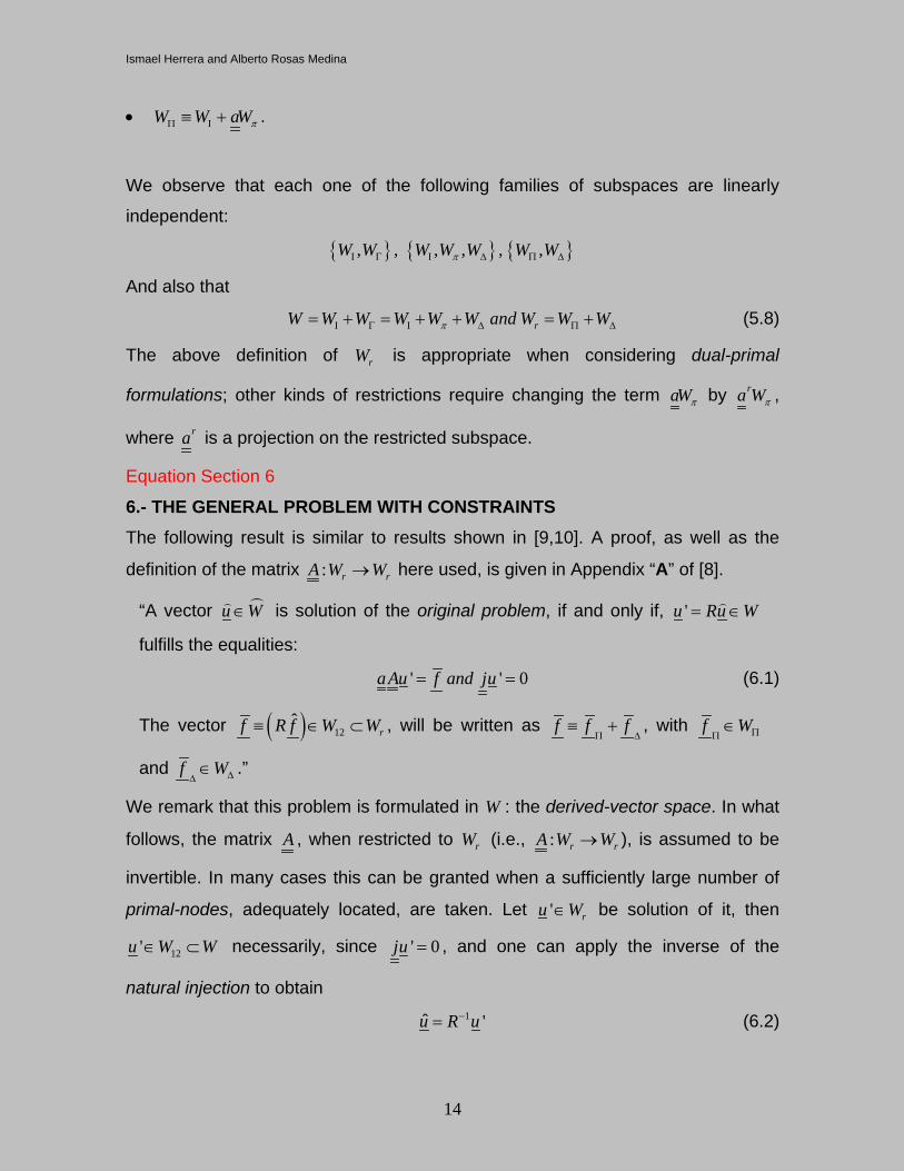
6.- THE GENERAL PROBLEM WITH CONSTRAINTS The following result is similar to results shown in [9,10]. A proof, as well as the

definition of the matrix : r rA W W→ here used, is given in Appendix “A” of [8].

“A vector u W∈ is solution of the original problem, if and only if, 'u Ru W= ∈

fulfills the equalities:

' ' 0aAu f and ju= = (6.1)

The vector ( ) 12ˆ

rf R f W W≡ ∈ ⊂ , will be written as f f fΠ ∆

≡ + , with f WΠΠ∈

and f W∆∆∈ .”

We remark that this problem is formulated in W : the derived-vector space. In what

follows, the matrix A , when restricted to rW (i.e., : r rA W W→ ), is assumed to be

invertible. In many cases this can be granted when a sufficiently large number of

primal-nodes, adequately located, are taken. Let ' ru W∈ be solution of it, then

12'u W W∈ ⊂ necessarily, since ' 0ju = , and one can apply the inverse of the

natural injection to obtain

1ˆ 'u R u−= (6.2)



Thereby, we observe that the mapping 1R− is only defined when 'u is a continuous

vector. Due to this fact, Eq.(6.2) is not adequate for numerical applications, in

which 'u is only evaluated in an approximate manner and, therefore, usually will

not be continuous; i.e., Eq.(6.2) cannot be applied to such a 'u . For its numerical

application, it is better to replace Eq. (6.2) by

1 'u R au−= (6.3)

This replacement is very convenient, since 'au is the continuous vector closest to

'u (here, ‘closest’ is with respect to the Euclidean distance). Finally, we notice that

in all the algorithms to be presented all the operations are carried out in the

derived-vectors space, since the problem of Eq.(6.1) is formulated in W ; in

particular, we will never return to the original vector space, W , except at the end

when we apply Eq.(6.3).

Equation Section 7

7.- THE DVS-ALGORITHMS WITH CONSTRAINTS

The matrix A of Eq.(6.1), can be written as (see [8,9]):

A A

AA AΠΠ Π∆

∆Π ∆∆

=

(7.1)

Using this notation, we define the ‘Schur-complement matrix with constraints’, by

1S A A A A−

∆∆ ∆Π ΠΠ Π∆≡ − (7.2)

Furthermore, in what follows:

( ) ( )1f R f A A R f−

∆ ∆Π ΠΠ∆ Π≡ −

(7.3)

7.1- THE DVS VERSION OF THE BDDC ALGORITHM

The DVS-BDDC algorithm is [8]: “Find u W∆ ∆∈ such that

1 1 0aS aSu aS f and ju− −∆ ∆∆= = (7.4)”

Once u W∆ ∆∈ has been obtained, u W∈

solution of Eq.(3.1) is given by


16

( ) ( ) 1 ~1~1u R a A A u A R f−∆ΠΠ Π∆ ΠΠ Π

= Ι − +

(7.5)

7.2- THE DVS VERSION OF FETI-DP ALGORITHM

The DVS-FETI-DP algorithm is [ ]: “Given f aW∆∆∈ , find Wλ ∆∈ such that

1 1 0jS jS jS jS f and aλ λ− −

∆= = (7.6)”

Once jWλ ∆∈ has been obtained, u aW∆∆ ∈ is given by:

( )1u aS f λ−∆ ∆= − (7.7)

Then, Eq.(7.5) can be applied to obtain u W∈

solution of Eq. (3.1).

7.3- THE DVS PRIMAL-ALGORITHM #2

This algorithm consists in searching for a function W∆ ∆∈v , which fulfills

1 1 1 0S jS j S jS jS f and aS− − −∆ ∆∆= =v v (7.8)”

Once 1S jSW−∆ ∆∈v has been obtained, then

( )1u a S f−∆∆ ∆

= −v (7.9)

and Eq.(7.5) can be applied to obtain u W∈


7.4- THE DVS DUAL-ALGORITHM #2

This algorithm consists in searching for a function Wµ ∆∈ , which fulfills

1 1 1 1 0SaS a SaS aS jS f and jSµ µ− − − −

∆= = (7.10)

Once 1SaS Wµ −∆∈ has been obtained, u aW∆∆ ∈ is given by:

( )1u aS f µ−∆ ∆= + (7.11)

and Eq.(7.5) can be applied to obtain u W∈


Equation Section 8 8.- NUMERICAL PROCEDURES



The numerical experiments were carried out with each one of the four

preconditioned DVS-algorithms with constraints enumerated in Section 7; they are:

1 1 0;aS aSu aS f and ju DVS - BDDC− −∆ ∆∆= = (8.1)

1 1 0;jS jS jS jS f and a DVS - FETI - DPλ λ− −

∆= = (8.2)

1 1 1 0;S jS j S jS jS f and aS DVS - PRIMAL - 2− − −∆ ∆∆= =v v (8.3)

and

1 1 1 1 0;SaS a SaS aS jS f and jS DVS - DUAL - 2µ µ− − − −

∆= = (8.4)

8.1- COMMENTS ON THE DVS NUMERICAL PROCEDURES

The outstanding uniformity of the formulas given in Eqs.(8.1) to (8.4) yields clear

advantages for code development, especially when such codes are built using

object-oriented programming techniques. Such advantages include:

I. The construction of very robust codes. This is an advantage of the DVS-

algorithms, which stems from the fact the definitions of such algorithms

exclusively depend on the discretized system of equations (which will be

referred to as the original problem) that is obtained by discretization of the

partial differential equations considered, but that is otherwise independent of

the problem that motivated it. In this manner, for example, essentially the

same code was applied to treat 2-D and 3-D problems; indeed, only the part

defining the geometry had to be changed, and that was a very small part of

it; II. The codes may use of different local solvers, which can be direct or iterative

solvers; III. Minimal modifications are required for transforming sequential codes into

parallel ones; and IV. Such formulas also permit to develop codes in which “the global-problem-

solution is obtained by exclusively solving local problems”.


18

This last property must be highlighted, because it makes the DVS-algorithms very

suitable as a tool to be used in the construction of massively-parallelized software,

which is needed for efficiently programming the most powerful parallel computers

available at present. Thus, procedures for constructing codes possessing Property

IV are outlined and analyzed next.

All the DVS-algorithms of Eqs.(8.1) to (8.4) are iterative and can be implemented

with recourse to Conjugate Gradient Method (CGM), when the matrix is definite

and symmetric, or some other iterative procedure such as GMRES, when that is

not the case. At each iteration step, one has to compute the action on a derived-

vector of one of the following matrices: 1aS aS− , 1jS jS − , 1S jS j− or 1SaS a− ,

depending on the DVS-algorithm that is applied. Such matrices in turn are different

permutations of the matrices S , 1S − , a and j . Thus, to implement any of the

preconditioned DVS-algorithms, one only needs to separately develop codes

capable of computing the action of one of the matrices S , 1S − , a or j on an

arbitrary vector of W , the derived-vector-space. Therefore, next we separately

explain how to compute the application of each one of the matrices S and 1S − . As

for a and j , as it will be seen, their application requires exchange of information

between derived-nodes that are descendants of the same original-node.and that is

a very simple operation for which such exchange of information is minimal.

8.2- APPLICATION OF S

From Eq.(7.2), we recall the definition of the matrix S :

1S A A A A−

∆∆ ∆Π ΠΠ Π∆≡ − (8.5)



In order to evaluate the action of S on any derived-vector, we need to successively

evaluate the action of the following matrices AΠ∆

, ~1AΠΠ

, A∆Π

and A∆∆

. Nothing

special is required except for ~1AΠΠ

, which is explained next.

We have

t t r

r t r t r

A A A A aA

A A a A a A aπ π

π ππ π ππ

ΙΙ Ι ΙΙ Ι

ΠΠΙ Ι

≡ =

(8.6)

Let w W∈ , be an arbitrary derived-vector, and write

1A w−

ΠΠ≡v (8.7)

Then, ( )Wπ π∈v is characterized by

( ) ~1 0A w A A w , subjected to jππ πππ π πσ ΙΠΠ Ι ΙΙ

= − =v v (8.8)

and can obtained iteratively. Here,

( ) ~1A A A A Aππ ππ π πσ

ΠΠ Ι ΙΙ Ι≡ − (8.9)

and, with aπ as the projection-matrix into ( )rW π ,

j aπ π≡ Ι − (8.10)

We observe that the computation in parallel of the action of 1A−

ΙΙ is straightforward

because

( ) 11

1

E

A Aα

α

−−

ΙΙ ΙΙ=

= ∑ (8.11)

Once ( )rWπ π∈v has been obtained, to derive Ιv one can apply:

( )1A w A ππ

−Ι ΙΙΙ Ι= −v v (8.12)

This completes the evaluation of S .

8.3- APPLICATION OF S -1


20

We define

Σ ≡ Ι ∪ ∆ (8.13)

A property that is relevant for the following discussion is:

( ) ( )rW WΣ = Σ (8.14)

Therefore, the matrix 1A− can be written as:

( ) ( )( ) ( )

( ) ( )( ) ( )

1 11 1

1

1 1 1 1

A AA AA

A A A Aπ

π ππ

− −− −

− ΣΣ ΣΠΠ Π∆

− − − −

∆Π ∆∆ Σ

= =

(8.15)

Then, :S W W∆ ∆→ fulfills

( )1 1S A− −

∆∆= (8.16)

For any w W∈ , let us write

1A w−≡v (8.17)

Then, πv fulfills

( ) ( ) 10t rA w A A w , subjected to jπ πππ π π

σ−

ΣΣ ΣΣ= − =v v (8.18)

Here, r rj a≡ Ι − , where the matrix ra is the projection operator on rW , while

( ) ( ) 1tA A A A Aππ ππ π πσ

−

Σ ΣΣ Σ≡ − (8.19)

Furthermore, we observe that

( ) ( )1 1

1

EtA Aα

α

− −

ΣΣ ΣΣ=

= ∑ (8.20)

Eq.(8.18) is solved iteratively. Once πv has been obtained, we apply:

( ) ( )1tA w A ππ

−

Σ ΣΣΣ Σ= −v v (8.21)

This procedure permits obtaining 1A w− in general; however, what we need only is

( )1A w−

∆∆. We observe that

( ) ( )1 1A w A w− −∆∆∆ ∆

= (8.22)



The vector 1A w−∆ can be obtained by the general procedure presented above.

Thus, take w w W W∆∆≡ ∈ ⊂ and

1A w−∆≡v (8.23)

Therefore,

( ) ( )1 1t t t rA A A A aπ ππ π

− −

Ι ∆ Σ ΣΣ Σ ΣΣ Σ+ = = − = −v v v v v (8.24)

Using Eq.(8.20), these operations can be fully parallelized. However, the detailed

discussion of such procedures will be presented separately [ ].

8.4- APPLICATION OF a AND j .

We use the notation

( )( )( ), ,i ja a α β= (8.25)

Then [10]:

( )( ) ( ) ( ) ( ), ,1 ,iji ja i and j

m iα β δ α β= ∀ ∈Ζ ∀ ∈Ζ (8.26)

While

j a= Ι − (8.27)

Therefore,

,jw w aw for every w W= − ∈ (8.28)

As for the right hand-sides of Eqs.(7.4), (7.6), (7.8) and (7.10), all they can be

obtained by successively applying to f∆ some of the operators that have already

been discussed. Recalling Eq.(7.3), we have

( ) ( )1f R f A A R f−

∆ ∆Π ΠΠ∆ Π≡ −

(8.29)

The computation of R f

does present any difficulty and the evaluation of the

actions of 1A−

ΠΠ and A

∆Π were already analyzed.


22

Equation Section 9 9- NUMERICAL RESULTS

All the partial differential equations treated had the form:

( )

2

1

( ) ( )

,d

i ii

a u b u cu f x xu g x x

α β=

− ∇ + ⋅∇ + = ∈Ω= ∈∂Ω

Ω =∏

(9.1)

where , 0a c > are constants, while 1 dim( ,..., )b b b= is a constant vector and

dim 2,3= . The family of subdomains 1,..., EΩ Ω is assumed to be a partition of the

set 1,..., dΩ ≡ of original nodes (this count does not include the nodes that lie on

the external boundary). In the applications we present, n is equal to the number of

degrees of freedom (dof) of the original problem; we use linear functions and only

one of them is associated with each original node. As for the original problems

treated, they have the standard form of Eq.(3.1):

A u f⋅ =

(9.2)

They were obtained by discretization of three different differential equations, in two

and three dimensions, of the above boundary value problem with 1a = . Choosing

0b = symmetric matrices were obtained, which correspond to the choices 1c =

and to 0c = , respectively; in this latter case, the differential operator treated is the

Laplacian. The choices ( )1,1b = and ( )1,1,1b = , with 0c = , yield non-symmetric

matrices.

As for the right-hand side, the following choices were made:

• For the Laplacian operator

( ) ( )( ) ( ) ( )

sin sin

sin sin sin

f n x n y , in 2D

f n x n y n z , in 3 D

π π

π π π

≡

≡ (9.3)

• Other differential operators

( ) ( ) ( ) ( )

2 2

3 2 2

exp 1

exp 2

f xy x y , in 2D

f xyz yz xyz x y z , in 3D

≡ − −

≡ + + + (9.4)



Discretization was accomplished using central finite differences, but streamline

artificial viscosity was incorporated in the treatment when 0b ≠ . The DQGMRES

algorithm [33] was implemented for the iterative solution of the non-symmetric

problems. The restrictions used were continuity on the primal nodes. The

numerical results that were obtained are reported in six tables that follow. Tables 1

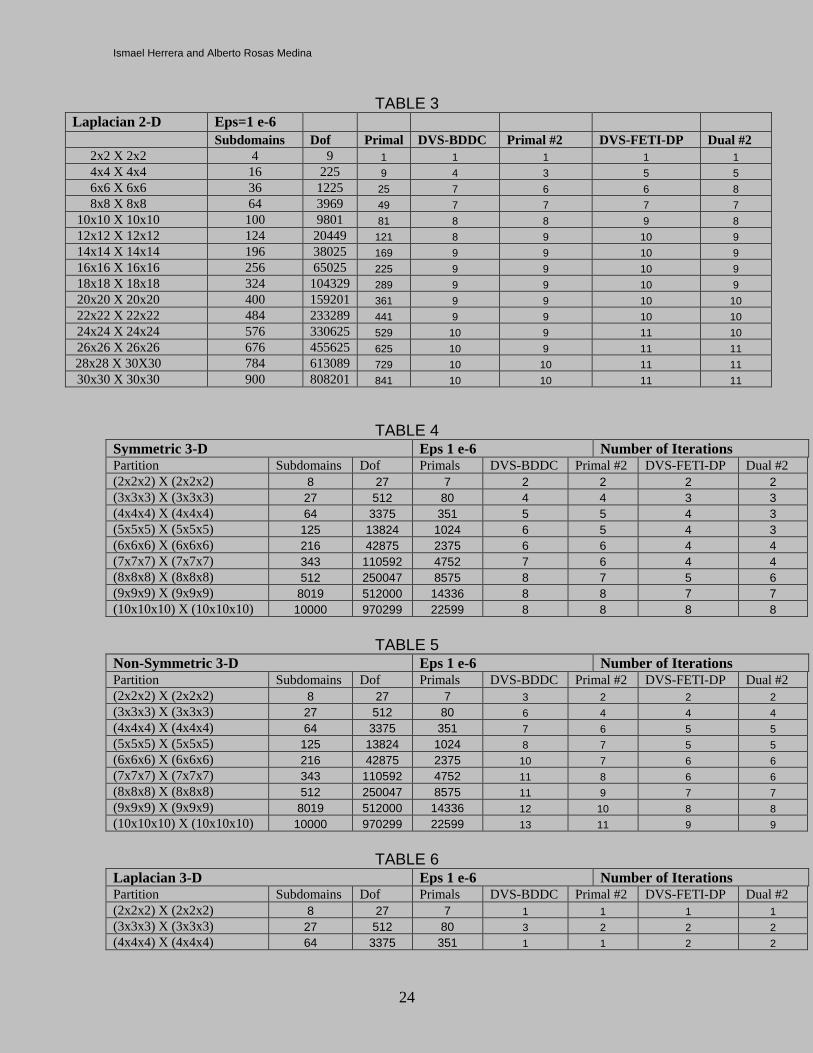
to 3 refer to 2D problems while Tables 4 to 6 to 3D problems.

TABLE 1 Symmetric 2-D Eps=1 e-6 Subdomains Dof Primal DVS-BDDC Primal #2 DVS-FETI-DP Dual #2

2x2 X 2x2 4 9 1 2 1 2 1 4x4 X 4x4 16 225 9 7 7 6 5 6x6 X 6x6 36 1225 25 9 9 7 6 8x8 X 8x8 64 3969 49 10 10 9 7

10x10 X 10x10 100 9801 81 11 11 10 8 12x12 X 12x12 124 20449 121 12 11 13 9 14x14 X 14x14 196 38025 169 12 12 13 12 16x16 X 16x16 256 65025 225 13 12 14 12 18x18 X 18x18 324 104329 289 13 13 15 13 20x20 X 20x20 400 159201 361 13 13 15 14 22x22 X 22x22 484 233289 441 13 14 15 16 24x24 X 24x24 576 330625 529 14 14 15 15 26x26 X 26x26 676 455625 625 14 14 15 15 28x28 X 30X30 784 613089 729 14 14 15 15 30x30 X 30x30 900 808201 841 15 14 15 15

TABLE 2

Non-Symmetric 2-D Eps=1 e-6 Subdomains Dof Primal DVS-BDDC Primal #2 DVS-FETI-DP Dual #2

2x2 X 2x2 4 9 1 2 1 2 1 4x4 X 4x4 16 225 9 8 6 6 6 6x6 X 6x6 36 1225 25 10 8 8 7 8x8 X 8x8 64 3969 49 12 10 9 9



24

TABLE 3 Laplacian 2-D Eps=1 e-6 Subdomains Dof Primal DVS-BDDC Primal #2 DVS-FETI-DP Dual #2

2x2 X 2x2 4 9 1 1 1 1 1 4x4 X 4x4 16 225 9 4 3 5 5 6x6 X 6x6 36 1225 25 7 6 6 8 8x8 X 8x8 64 3969 49 7 7 7 7


TABLE 4 Symmetric 3-D Eps 1 e-6 Number of Iterations Partition Subdomains Dof Primals DVS-BDDC Primal #2 DVS-FETI-DP Dual #2 (2x2x2) X (2x2x2) 8 27 7 2 2 2 2 (3x3x3) X (3x3x3) 27 512 80 4 4 3 3 (4x4x4) X (4x4x4) 64 3375 351 5 5 4 3 (5x5x5) X (5x5x5) 125 13824 1024 6 5 4 3 (6x6x6) X (6x6x6) 216 42875 2375 6 6 4 4 (7x7x7) X (7x7x7) 343 110592 4752 7 6 4 4 (8x8x8) X (8x8x8) 512 250047 8575 8 7 5 6 (9x9x9) X (9x9x9) 8019 512000 14336 8 8 7 7 (10x10x10) X (10x10x10) 10000 970299 22599 8 8 8 8

TABLE 5 Non-Symmetric 3-D Eps 1 e-6 Number of Iterations Partition Subdomains Dof Primals DVS-BDDC Primal #2 DVS-FETI-DP Dual #2 (2x2x2) X (2x2x2) 8 27 7 3 2 2 2 (3x3x3) X (3x3x3) 27 512 80 6 4 4 4 (4x4x4) X (4x4x4) 64 3375 351 7 6 5 5 (5x5x5) X (5x5x5) 125 13824 1024 8 7 5 5 (6x6x6) X (6x6x6) 216 42875 2375 10 7 6 6 (7x7x7) X (7x7x7) 343 110592 4752 11 8 6 6 (8x8x8) X (8x8x8) 512 250047 8575 11 9 7 7 (9x9x9) X (9x9x9) 8019 512000 14336 12 10 8 8 (10x10x10) X (10x10x10) 10000 970299 22599 13 11 9 9

TABLE 6

Laplacian 3-D Eps 1 e-6 Number of Iterations Partition Subdomains Dof Primals DVS-BDDC Primal #2 DVS-FETI-DP Dual #2 (2x2x2) X (2x2x2) 8 27 7 1 1 1 1 (3x3x3) X (3x3x3) 27 512 80 3 2 2 2 (4x4x4) X (4x4x4) 64 3375 351 1 1 2 2



(5x5x5) X (5x5x5) 125 13824 1024 5 4 5 4 (6x6x6) X (6x6x6) 216 42875 2375 6 6 5 6 (7x7x7) X (7x7x7) 343 110592 4752 6 6 6 6 (8x8x8) X (8x8x8) 512 250047 8575 7 7 8 8 (9x9x9) X (9x9x9) 8019 512000 14336 8 9 9 9 (10x10x10) X (10x10x10) 10000 970299 22599 10 10 10 10

Equation Section 10

10.- CONCLUSIONS In this article, numerical tests were carried out for each one of the preconditioned

DVS-algorithms with constraints [8]:

a).- The DVS-version of BDDC, Eq.(8.1);

b).-The DVS-version of FETI-DP, Eq.(8.2);

c).- DVS-primal formulation #2, Eq.(8.3);

d).- DVS-dual formulation #2, Eq.(8.4).

Each one of these algorithms is applicable to symmetric-definite, indefinite and

non-symmetric problems [8].

In the sequence of numerical experiments that was carried out all they have

exhibited equivalent efficiencies. Furthermore, in two previous paper [9,10] the

DVS-versions of BDDC and FETI-DP, were compared with standard versions

BDDC and FETI-DP and it was shown that they are, at least, as efficient as them.

Thus, the results of the present paper indicate that each one of the four

preconditioned DVS-algorithms here discussed has efficiency comparable with the

best non-overlapping DDM available at present. Thus, another important

conclusion of this paper is that the four preconditioned DVS-algorithms with

constraints studied in this paper numerically have update efficiency. This fact,

together with their excellent parallelization properties indicate that they are very

suitable as a tool to be used in the construction of massively-parallelized software

that is needed for efficiently programming the most powerful parallel computers

available at present.

REFERENCES


26

1. DDM Organization, Proceedings of 20 International Conferences on Domain Decomposition Methods. www.ddm.org, 1988-2009.

2. Toselli A. and O. Widlund, Domain decomposition methods- Algorithms and Theory, Springer Series in Computational Mathematics, Springer-Verlag, Berlin, 2005, 450p.

3. Dohrmann C.R., A preconditioner for substructuring based on constrained energy minimization. SIAM J. Sci. Comput. 25(1):246-258, 2003.

4. Mandel J. and C. R. Dohrmann, Convergence of a balancing domain decomposition by constraints and energy minimization, Numer. Linear Algebra Appl., 10(7):639-659, 2003.

5. Mandel J., Dohrmann C.R. and Tezaur R., An algebraic theory for primal and dual substructuring methods by constraints, Appl. Numer. Math., 54: 167-193, 2005.

6. Da Conceição, D. T. Jr., Balancing domain decomposition preconditioners for non-symmetric problems, Instituto Nacional de Matemática Pura e Aplicada, Agencia Nacional do Petróleo PRH-32, Rio de Janeiro, May. 9, 2006.

7. Widlund O., Personal communication, 2010. 8. Herrera, I., Carrillo-Ledesma A. & Rosas-Medina Alberto “A Brief Overview of

Non-overlapping Domain Decomposition Methods”, Geofisica Internacional, Vol. 50(4), pp 445-463, 2011.

9. Herrera, I. & Yates R. A. The Multipliers-Free Dual Primal Domain Decomposition Methods for Nonsymmetric Matrices NUMER. METH. PART D. E. 2009, DOI 10.1002/Num. 20581, (Published on line April 28, 2010).

10. Herrera, I. & Yates R. A. The Multipliers-free Domain Decomposition Methods NUMER. METH. PART D. E. 26: 874-905 July 2010, DOI 10.1002/num. 20462. (Published on line Jan 28, 2009)

11. Herrera I. and R. Yates “Unified Multipliers-Free Theory of Dual-Primal Domain Decomposition Methods. NUMER. METH. PART D. E. Eq. 25:552-581, May 2009, (Published on line May 13, 08) DOI 10.1002/num. 20359.

12. Herrera, I. “New Formulation of Iterative Substructuring Methods without Lagrange Multipliers: Neumann-Neumann and FETI”, NUMER METH PART D E 24(3) pp 845-878, 2008 (Published on line Sep 17, 2007) DOI 10.1002 NO. 20293.

13. Herrera, I. “Theory of Differential Equations in Discontinuous Piecewise-Defined-Functions

14. Brenner S. and Sung L. BDDC and FETI-DP without matrices or vectors Comput. Methods Appl. Mech. Engrg. 196(8): 1429-1435. 2007.

”, NUMER METH PART D E, 23(3), pp 597-639, 2007 DOI 10.1002 NO. 20182.

15. Mandel J. Balancing domain decomposition, Commun. Numer. Methods Engrg. 1(1993) 233-241.

16. Mandel J. and Brezina M. Balancing domain decomposition for problems with large jumps in coefficients. Math. Comput. 65, pp 1387-1401, 1996.

17. Farhat Ch., and Roux F. A method of finite element tearing and interconnecting and its parallel solution algorithm. Internat. J. Numer. Methods Engrg. 32:1205-1227, 1991.

18. Mandel J. and Tezaur R. Convergence of a substructuring method with Lagrange multipliers. Numer. Math 73(4): 473-487, 1996

http://www.ddm.org/



19. Farhat C., Lessoinne M. LeTallec P., Pierson K. and Rixen D. FETI-DP a dual-primal unified FETI method, Part I: A faster alternative to the two-level FETI method. Int. J. Numer. Methods Engrg. 50, pp 1523-1544, 2001.

20. Farhat C., Lessoinne M. and Pierson K. A scalable dual-primal domain decomposition method, Numer. Linear Algebra Appl. 7, pp 687-714, 2000.

21. Mandel J. and Tezaur R., On the convergence of a dual-primal substructuring method, SIAM J. Sci. Comput., 25, pp 246-258, 2001.

22. Cai, X-C. & Widlund, O.B., Domain Decomposition Algorithms for Indefinite Elliptic Problems, SIAM J. Sci. Stat. Comput. 1992, Vol. 13 pp. 243-258

23. Farhat C., and Li J. An iterative domain decomposition method for the solution of a class of indefinite problems in computational structural dynamics. ELSEVIER Science Direct Applied Numerical Math. 54 pp 150-166. 2005.

24. Li J. and Tu X. Convergence analysis of a Balancing Domain Decomposition method for solving a class of indefinite linear systems. Numer. Linear Algebra Appl. 2009; 16:745–773

25. Tu X. and Li J., A Balancing Domain Decomposition method by constraints for advection-diffusion problems. www.ddm.org/DD18/

http://www.ddm.org/DD18/

Documents

GRUPO DE GEOFÍSICA MATEMÁTICA Y ... - mmc.geofisica.unam.mxmmc.geofisica.unam.mx/mmc/ReportesInternos/MEMORIA06.pdf · grupo de . geofÍsica matemÁtica y computacional . memoria