1

Optimization and application of GPU calculations in material science

Grzegorz Korpała, Rudolf Kawalla

Grzegorz.Korpala@imf.tu-frieberg.de

Institut of Metallforming, Technische Universität Bergakademie Freiberg

Bernhard-von-Cotta-Str.4 D-09599 Freiberg (Saxony, Germany)

1. Introduction

Nowadays, many phenomena are described numerically. The data generated assist

when designing technology, when estimating the safety of components or enable

improved understanding of physical effects such as diffusion or heat transfer. The

methods that have been predominantly used up until now are the Finite Difference

Method (FDM) and the Finite Element Method (FEM). Both are different in the

mathematical description. The FEM gives good calculation accuracy and speed with

a lower number of elements. As shown in fig. 1 schematically FDM 1 and 2 (with a

low and high number of nodes) demonstrate lower calculation accuracy than FEM.

The only opportunity for improving accuracy is to further refine the node density on

FDM. However, this means a longer calculation time, more calculation steps and a

greater quantity of data to transfer. However, one advantage of FDM is the simple

application of individual physical phenomena.

fig. 1: Schematic illustration of results in accordance with different calculation methods

Simple parallelisation of calculations in FDM yields potential for acceleration. Use of

GPU architecture allows for additional acceleration. A faster Video RAM as well as a

shared memory installed in the graphics processor and corresponding storage

management are not always fully utilised. Commercial programs use either

combination 1 or 2 (fig. 2) due to the original source code. All combinations differ

from each other not just in construction, but also in terms of calculation speed. This is

strongly dependent on the data transfer paths. Modification of the source code

makes it possible to apply combinations 3, 4 or 5 into FDM, where combinations 4

and 5 are the fastest possible variants. Variants 3, 4, and 5 can, due to the special

2

GPU architecture, calculate several sections of the parent lattice at once, otherwise

known as blocks, in a special process (Tariq, 2011) (see fig. 3).

These are defined, per block, by block size, shared memory and registry size. Within

the block, the executed processes have the capacity to communicate with each other

via the shared memory (Woolley, 2013). The processes also have direct access to

the parent lattice that is fed into the global memory and finds space in the video

RAM.

Combination 1 RAM- Processing-RAM

Combination 2 RAM- Processing-RAM

Combination 3

RAM-VRAM-Processing-VRAM-RAM Combination 4

VRAM-Processing-VRAM Combination 5

VRAM-S. Memory-Processing-VRAM fig. 2: Schematic illustration of data transfer in the computer with the use of different processing units

fig. 3: Parent lattice and block (data structure)

3

A comparison of speeds of different types of memory can be seen in table 1. The

fastest L1 cache and shared memory should be used the most according to the table,

as the transfer speed of these is larger by several factors. When a few of a block's

processes access the same memory address then it is better to first store these in

the shared memory and then allow these to be called up from the processes at higher

speed (Sanders, et al., 2010). When calculating with classic CPU a large proportion

of the calculation time is used for storing data to the data carrier (HDD or SSD).

Despite saving on several hard drives (via Raid) this problem has still not been

solved. The only method appears to be writing the data to the hard drive in the

background parallel to the calculation. However, this requires a great deal of RAM for

intermediate storage of the data. Complete storage of data from 4 Titan graphics

processors (6GB video RAM) requires RAM capacity of 48 GB, which can be

implemented in most systems.

table 1 Reading and writing speeds of different memory types (Woolley, 2013)

Used in Combination:

Unit Memory Type: Mem. Speed 1 2 3 4 5

CPU SSD (reference) 550 MB/s RAM 18 GB/s

GPU

Video RAM (Titan GTX) 288 GB/s L1 - Cache ~2.5 TB/s Shared Memory ~2.5 TB/s

In order to determine the influence of calculation concepts (fig. 2) on calculation time,

a simple equation (1 was applied with different methods and with different data

quantities (Grid Size) in Mathematica®:

𝑦𝑖 = √(((𝑎𝑖 + 𝑏𝑖)

2+ 2) ∗ 10 + 3)

3

+ 10, (1)

where 𝑦𝑖, a𝑖 and b𝑖 tables are with a specified size. For compiling Mathematica® uses

a C compiler from Microsoft Visual Studio® for combinations 1 and 2 and a NVCC

compiler for combinations 3 and 4. Calculation procedure 5 could not be verified in

this example as the use of shared memory is not advantageous in this calculation.

The measured, absolute times for the simple calculation can be found in fig. 4. It can

be clearly seen that a reduction in calculation time is expected due to the use of rapid

data transfer. Combination 5 should be even faster, as the data transfer from video

RAM to GPU is accelerated via shared memory. This combination is used in further

calculations.

4

fig. 4: Calculation times for different combinations of data processing depending on data size

2. Optimisation potential with GPU - complex calculations:

An algorithm is used for calculating complex physical phenomena in which the Finite

Difference Method is used in accordance with Wilkins (Wilkins, 1998) and Patankar

(Patankar, 1980). The whole concept was newly programmed using combination 5,

the fastest available one. When working on the compilation of sub-routines, various

block sizes and registry sizes were tested to gain the fastest possible acceleration.

To test the efficiency the function (Wilkins, 1998) used for calculating the acceleration

vectors was selected as an example in this case. It was surprisingly established that

the compilation with the largest possible number of blocks (the largest number of

threads running simultaneously) did not yield the shortest calculation times. It goes

without saying that attention was paid to the highest level of occupancy for the GPU

(the CUDA Occupancy Calculator was used). It must be pointed out that the data

transfer from VRAM and the number of threads are the main influential factors.

Dependency of the calculation time on the theoretical block size can be seen in fig. 5.

The theoretical block size can be found from the third root of the number of

processes in the block. Various lengths, widths and depths of the block are

considered and the fastest variant is taken for a theoretical length. Compilation with

small block sizes, as expected, resulted in longer calculation times. The best

compilation in this case is a block size of 4x4x4 and a registry size of 160. The

fastest variant requires just 0.058 seconds to calculate the new acceleration vectors

for 1,000,000 elements. The slowest example needed 0.174 seconds, which was

three times the calculation time.

5

fig. 5: Calculation time for 1,000,000 elements for movement in 3D

Further calculations were also carried out (see appendix) such as the stress state,

diffusion or heat transport which were also transferred in their entirety to the GPU

without large data volumes via PCIe 3.0 Bus. The CPU is responsible for issuing

commands and storing data on the hard drive. Controlling of graphics cards

(calculation) and saving data take place simultaneously. 4 graphics Geforce cards

Titan GTX were used in test, each with a Kepler processor architecture and 6 GB of

storage capacity. 8 processes were also carried out in the CPU simultaneously: 4 for

controlling GPUs and 4 for saving the data. The schematic illustration of the process

for two processes running simultaneously can be seen in fig. 6

fig. 6: Calculation algorithm of the new program and resources used

After optimisation calculation times were established to be 15% shorter. The

calculation times (Fig. 7) were established for the complete procedure within fig. 6

with storage of data on HDD. The maximum size of the lattice is approx. 12,000,000

elements per graphics card. The times were noticeably shorter after optimisation in

all lattice sizes.

6

Fig. 7: Comparison of calculation times depending on the number of elements before and after optimisation.

3. Application of GPU calculations in material science

In the calculations system the mathematical description of diffusion depending on

chemical analysis (Mujahid, et al., 1992), of heat transfer (Patankar, 1980), of

stresses, strains and flows (Wilkins, 1998) was also programmed. The algorithm is

structured for universal use and changing the source codes is possible without

problems and without help from third parties. The calculations should help make the

complex micro-structure development in the material easier to understand. The

interpretation of the results of the numerical simulation is an additional support for the

experimental investigations and aids clarification of the results that cannot be directly

explained. Local conditions such as the chemical analysis, stress state or

temperature provide the necessary information for modelling the energy contributions

when converting or recrystallizing.

7

3.1. Example 1

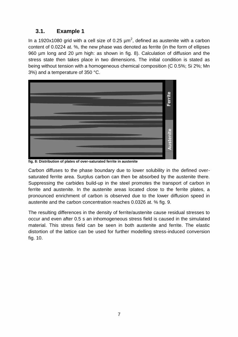
In a 1920x1080 grid with a cell size of 0.25 µm2, defined as austenite with a carbon

content of 0.0224 at. %, the new phase was denoted as ferrite (in the form of ellipses

960 µm long and 20 µm high: as shown in fig. 8). Calculation of diffusion and the

stress state then takes place in two dimensions. The initial condition is stated as

being without tension with a homogeneous chemical composition (C 0.5%; Si 2%; Mn

3%) and a temperature of 350 °C.

fig. 8: Distribution of plates of over-saturated ferrite in austenite

Carbon diffuses to the phase boundary due to lower solubility in the defined over-

saturated ferrite area. Surplus carbon can then be absorbed by the austenite there.

Suppressing the carbides build-up in the steel promotes the transport of carbon in

ferrite and austenite. In the austenite areas located close to the ferrite plates, a

pronounced enrichment of carbon is observed due to the lower diffusion speed in

austenite and the carbon concentration reaches 0.0326 at. % fig. 9.

The resulting differences in the density of ferrite/austenite cause residual stresses to

occur and even after 0.5 s an inhomogeneous stress field is caused in the simulated

material. This stress field can be seen in both austenite and ferrite. The elastic

distortion of the lattice can be used for further modelling stress-induced conversion

fig. 10.

8

fig. 9: Carbon distribution of concentration in at. % after 350 min.

fig. 10: Stress field in accordance with von Mises in GPa after 0.5 s

3.2. Example 2

A random generator is often necessary for modelling phenomena which take place in

material. With the aid of CUDA, these can run very efficiently. In principle a seed is

generated for every block and then made available for every process via conversion.

The efficiency of such a generator is introduced here. Each process in the calculation

carries out 18 random draws of a natural number from 0 to 999999. No shared

memory is used here so that no additional calculations are carried out. Small, yet

relevant differences in calculation times are established depending on block size with

this approach. The largest possible grid size is 7003, which is limited by the 6 GB of

the video RAM. The measured times for the calculation can be found in fig. 11.

9

fig. 11: Necessary time for generating random numbers for different lattice sizes

3.3. Example 3

The calculation used in example 1 can also map more complicated 3D systems. This

includes the forming simulation with texture-dependent yield stress, which is shown in

equation 2 as a model. The yield stress is modelled via two equations and brought

together via a parameter 𝛾. The cosine of the smallest angle between the direction of

the greatest shear stress and the sliding direction serves as this parameter 𝛾 here.

𝑌 = 𝑌𝑇 ∙ 𝛾 + 𝑌𝑇 ∙ (1 − 𝛾);

𝑌𝑇 = 0.35 ∙ (1 + 4 ∗ 𝜖𝑒)0,35 ∙ 𝑝; 𝑌𝑆 = 0.31 ∙ (1 + 4 ∗ 𝜖𝑒)0,3 ∙ 𝑝;

𝑝 = 1 + 3 ∙ 𝑃 ∙ √𝑉3

;

𝑌𝑇- flow stress model from tensile test,

𝑌𝑠- flow stress model from torsion test, 𝜖𝑒- effective strain,

𝑃- pressure,

𝑉- relative volume, 𝛾 - equal to cosines of angle between direction maximum shear stress and

nearest slip direction

(2)

The parallel length of the model probes was 18 mm, the width was 10 mm and the

thickness was 1 mm. 4,000,000 volumes were used. The nodes at the beginning and

end of the length were fixed in direction y and z and pulled in direction x with a speed

of 1 m/s.

Depending on the grain, texture-dependent lines were shown via the stress field

described in accordance with von Mises, along which incremental deformation took

place. Depending on the grain, which had a random orientation, the lines were

developed differently. In the final step the directions of the grains rotate to the same

10

shear direction and form a necking in an angle of approximately 45 degrees to the x-

axis fig. 12.

fig. 12: Results of simulation, stress field in accordance with von Mises

a. in the elastic area at the beginning of the rupturing process b. in the plastic area during the rupturing attempt c. in the plastic area at the end of the rupturing attempt

11

4. Summary

With continued developments in graphics processors it is expected that the potential

in the algorithms shown in this publication will continue to grow. The algorithms used

are based on the Finite Differences Method and are only limited by the size of the

available video RAM. The principles of FDM are adhered to and the calculation

algorithm was newly developed for the graphics processors. Storage of the

calculation in the graphics card only becomes advantageous if transportation of the

data via PCIe BUS is minimised. In complex functions, the use of shared memory

speeds up calculations. For this purpose, the compilation of sub-routines using

shared memory with different block sizes should be tested. New models of yield

stress give the option of taking dependency of shear stress and texture into account,

which can be used to describe the damage mechanisms.

Reference

Mujahid, S. A. and Bhadeshia, H. K. D. H. 1992. Partitioning of carbon from

supersaturated ferrite plates. Acta Metallurgica. 1992, Vol. 40, pp. 389-396.

Patankar, Suhas V. 1980. Numerical Heat Transfer and Fluid Flow. New York :

Hemisphere publishing corporation, 1980.

Sanders, Janson and Kandrot, Edward. 2010. CUDA by Example. 2010. 978-0-13-

138768-3.

Tariq, Sarah. 2011. An Introduction to GPU Computing and CUDA Architecture.

https://de.scribd.com/doc/61664546/NVIDIA-02-BasicsOfCUDA. 2011.

Wilkins, Mark L. 1998. Computer Simulation of Dynamic Phenomena. Livermore :

Lawrance Livermore National Laboratory, 1998.

Woolley, Cliff. 2013. GPU Optimization Fundamentals. https://www.olcf.ornl.gov/wp-

content/uploads/2013/02/GPU_Opt_Fund-CW1.pdf. 2013.