Embed Size (px)
Citation preview
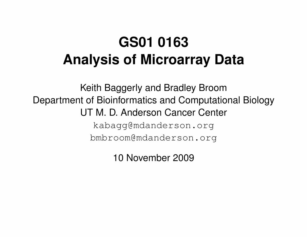
GS01 0163Analysis of Microarray Data
Keith Baggerly and Bradley BroomDepartment of Bioinformatics and Computational Biology
UT M. D. Anderson Cancer [email protected]@mdanderson.org
10 November 2009
INTRODUCTION TO MICROARRAYS 1
Lecture 21: Gene Set Enrichment Analysis
• Gene Set Enrichment Analysis
c© Copyright 2004–2009, KR. Coombes, KA. Baggerly, and BM. Broom GS01 0163: ANALYSIS OF MICROARRAY DATA
INTRODUCTION TO MICROARRAYS 2
Night Sky
Go to a remote location (preferably in the SouthernHemisphere) late at night when the weather is clear and lookup.
What do you see?
c© Copyright 2004–2009, KR. Coombes, KA. Baggerly, and BM. Broom GS01 0163: ANALYSIS OF MICROARRAY DATA
INTRODUCTION TO MICROARRAYS 3
Gene Set Enrichment Analysis (GSEA)
Last week, we saw that we can use known information aboutgene functions and gene relationships to help understand thebiology behind a list of differentially expressed genes:
• Derive a list of significantly differentially expressed genes,while controlling for false discovery,
• Determine pathways containing (many of) the genesconcerned,
• Gain biological insight . . .
Will this algorithm find all significantly affected pathways?
c© Copyright 2004–2009, KR. Coombes, KA. Baggerly, and BM. Broom GS01 0163: ANALYSIS OF MICROARRAY DATA

INTRODUCTION TO MICROARRAYS 4
Overview of GSEA
Detecting modest changes in gene expression datasets ishard, due to:
• the large number of variables,
• the high variability between samples, and
• the limited number of samples.
The goal of GSEA is to detect modest but coordinatedchanges in prespecified sets of related genes.
Such a set might include all the genes in a specific pathway,for instance.
c© Copyright 2004–2009, KR. Coombes, KA. Baggerly, and BM. Broom GS01 0163: ANALYSIS OF MICROARRAY DATA
INTRODUCTION TO MICROARRAYS 5
GSEA Publications
Mootha et al., Nature Genetics 34, 267–273 (2003)
Subramanian et al., PNAS 102(43), 15545–15550 (2005).
The description of GSEA changed between the two papers.We follow the second formulation.
c© Copyright 2004–2009, KR. Coombes, KA. Baggerly, and BM. Broom GS01 0163: ANALYSIS OF MICROARRAY DATA

INTRODUCTION TO MICROARRAYS 6
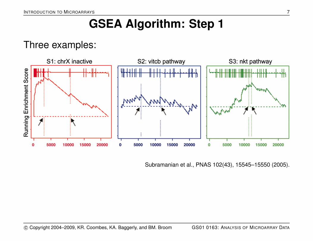
GSEA Algorithm: Step 1
Calculate an Enrichment Score:
• Rank genes by their expression difference
• Compute cumulative sum over ranked genes:
• Increase sum when gene in set, decrease it otherwise.• Magnitude of increment depends on correlation of gene
with phenotype.
• Record the maximum deviation from zero as theenrichment score
c© Copyright 2004–2009, KR. Coombes, KA. Baggerly, and BM. Broom GS01 0163: ANALYSIS OF MICROARRAY DATA
INTRODUCTION TO MICROARRAYS 7
GSEA Algorithm: Step 1
Three examples:
Subramanian et al., PNAS 102(43), 15545–15550 (2005).
c© Copyright 2004–2009, KR. Coombes, KA. Baggerly, and BM. Broom GS01 0163: ANALYSIS OF MICROARRAY DATA
INTRODUCTION TO MICROARRAYS 8
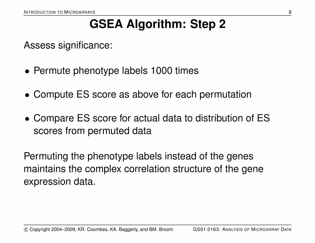
GSEA Algorithm: Step 2
Assess significance:
• Permute phenotype labels 1000 times
• Compute ES score as above for each permutation
• Compare ES score for actual data to distribution of ESscores from permuted data
Permuting the phenotype labels instead of the genesmaintains the complex correlation structure of the geneexpression data.
c© Copyright 2004–2009, KR. Coombes, KA. Baggerly, and BM. Broom GS01 0163: ANALYSIS OF MICROARRAY DATA
INTRODUCTION TO MICROARRAYS 9
GSEA Algorithm: Step 3
Adjustment for multiple hypothesis testing:
• Normalize the ES accounting for size of each gene set,yielding normalized enrichment score (NES)
• Control proportion of false positives by calculating FDRcorresponding to each NES, by comparing tails of theobserved and null distibutions for the NES.
c© Copyright 2004–2009, KR. Coombes, KA. Baggerly, and BM. Broom GS01 0163: ANALYSIS OF MICROARRAY DATA
INTRODUCTION TO MICROARRAYS 10
GSEA Algorithm: Step 4
The original method used equal weights for each gene.
The revised method weighted genes according to theircorrelation with phenotype.
This may cause an asymmetric distribution of ES scores ifthere is a big difference in the number of genes highlycorrelated to each phenotype.
Consequently, the above algorithm is performed twice: onefor the positively scoring gene sets and once for thenegatively scoring gene sets.
c© Copyright 2004–2009, KR. Coombes, KA. Baggerly, and BM. Broom GS01 0163: ANALYSIS OF MICROARRAY DATA

INTRODUCTION TO MICROARRAYS 11
Schematic overview of GSEA
Subramanian et al., PNAS 102(43), 15545–15550 (2005).
c© Copyright 2004–2009, KR. Coombes, KA. Baggerly, and BM. Broom GS01 0163: ANALYSIS OF MICROARRAY DATA
INTRODUCTION TO MICROARRAYS 12
GSEA Availability
GSEA is available from their websitehttp://www.broadinstitute.org/gsea/ .
GSEA is available as both a Java program and an R script.Because we like scripts, we’ll use the R version.
The same site provides several existing gene sets, including
• positional gene sets,
• curated gene sets,
• motif gene sets,
• computational gene sets,
• and gene ontology gene sets.
c© Copyright 2004–2009, KR. Coombes, KA. Baggerly, and BM. Broom GS01 0163: ANALYSIS OF MICROARRAY DATA
INTRODUCTION TO MICROARRAYS 13
What you need
Download the R source code (GSEA.1.0.R), and the geneset databases (.gmt files).
To analyze experimental data, you will need to create two textfiles:
• a sample phenotype file (.cls), and
• an gene expression file (.gct).
c© Copyright 2004–2009, KR. Coombes, KA. Baggerly, and BM. Broom GS01 0163: ANALYSIS OF MICROARRAY DATA
INTRODUCTION TO MICROARRAYS 14
Gene Set Database File
A geneset database (.gmt) file is a tab separated text filecontaining one geneset per line.
The first column is the gene set name.
The second column is a brief description of the gene set.
The remaining columns contain the names of the genes inthe gene set. Notes:
• there are many trailing empty columns,
• there are many genes with names like 8-Sep,
• suggesting whoever developed the “database” used Excel.
c© Copyright 2004–2009, KR. Coombes, KA. Baggerly, and BM. Broom GS01 0163: ANALYSIS OF MICROARRAY DATA
INTRODUCTION TO MICROARRAYS 15
Sample Phenotype File
A sample phenotype (.cls) file is a text file containing threelines.
The first line contains three numbers separated by spaces.The first number is the number of samples. The second andthird numbers are the constants 2 and 1, respectively.
The second line begins with # and is followed by a spaceseparated list of “long” phenotype names.
The third line consists of a space separated list of “short”phenotype labels for each of the samples in the geneexpression file, in the same order they occur there.
• You’ll get nonsense if these two orders ever get out of sync.
c© Copyright 2004–2009, KR. Coombes, KA. Baggerly, and BM. Broom GS01 0163: ANALYSIS OF MICROARRAY DATA
INTRODUCTION TO MICROARRAYS 16
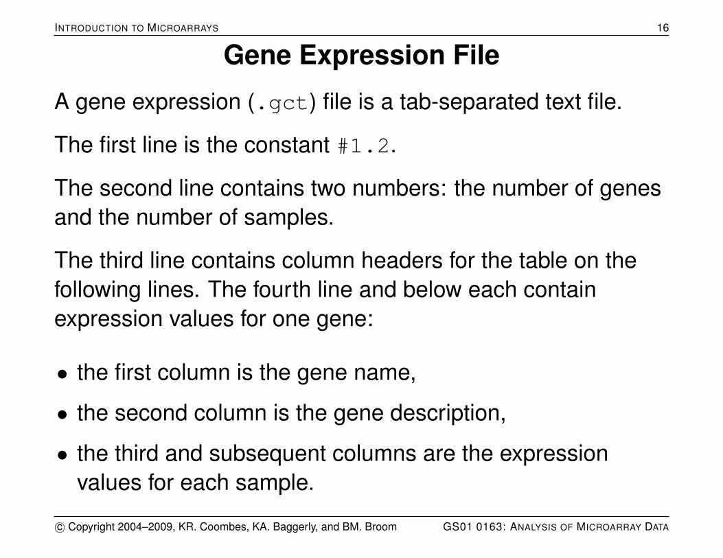
Gene Expression File
A gene expression (.gct) file is a tab-separated text file.
The first line is the constant #1.2.
The second line contains two numbers: the number of genesand the number of samples.
The third line contains column headers for the table on thefollowing lines. The fourth line and below each containexpression values for one gene:
• the first column is the gene name,
• the second column is the gene description,
• the third and subsequent columns are the expressionvalues for each sample.
c© Copyright 2004–2009, KR. Coombes, KA. Baggerly, and BM. Broom GS01 0163: ANALYSIS OF MICROARRAY DATA
INTRODUCTION TO MICROARRAYS 17
Notes:
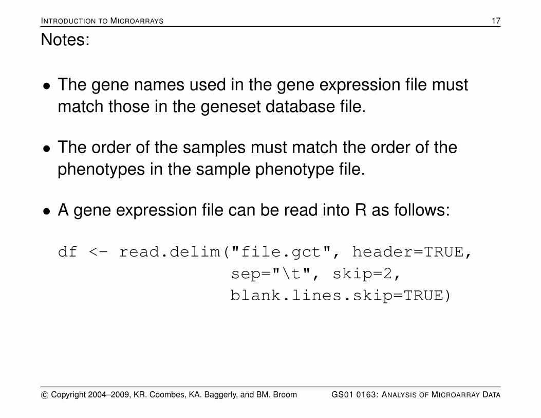
• The gene names used in the gene expression file mustmatch those in the geneset database file.
• The order of the samples must match the order of thephenotypes in the sample phenotype file.
• A gene expression file can be read into R as follows:
df <- read.delim("file.gct", header=TRUE,sep="\t", skip=2,blank.lines.skip=TRUE)
c© Copyright 2004–2009, KR. Coombes, KA. Baggerly, and BM. Broom GS01 0163: ANALYSIS OF MICROARRAY DATA
INTRODUCTION TO MICROARRAYS 18
Running GSEA
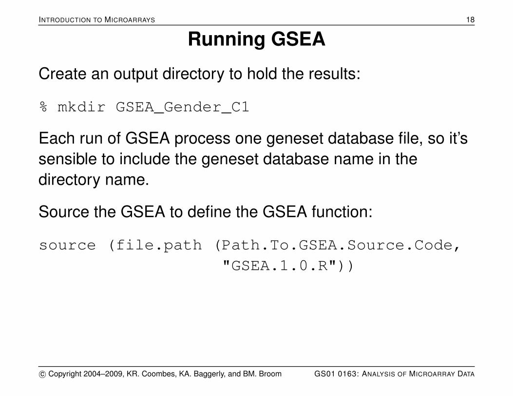
Create an output directory to hold the results:
% mkdir GSEA_Gender_C1
Each run of GSEA process one geneset database file, so it’ssensible to include the geneset database name in thedirectory name.
Source the GSEA to define the GSEA function:
source (file.path (Path.To.GSEA.Source.Code,"GSEA.1.0.R"))
c© Copyright 2004–2009, KR. Coombes, KA. Baggerly, and BM. Broom GS01 0163: ANALYSIS OF MICROARRAY DATA

INTRODUCTION TO MICROARRAYS 19
Call GSEA:
GSEA(# Input/Output Files :-------------------------------------------input.ds = "Datasets/Gender.gct",input.cls = "Datasets/Gender.cls",gs.db = "GeneSetDatabases/C1.gmt",output.directory = "GSEA_Gender_C1/",
# Program parameters :-----------------------------------------doc.string = "Gender_C1",non.interactive.run = FALSE,reshuffling.type = "sample.labels",nperm = 1000,weighted.score.type = 1,nom.p.val.threshold = -1,
c© Copyright 2004–2009, KR. Coombes, KA. Baggerly, and BM. Broom GS01 0163: ANALYSIS OF MICROARRAY DATA
INTRODUCTION TO MICROARRAYS 20
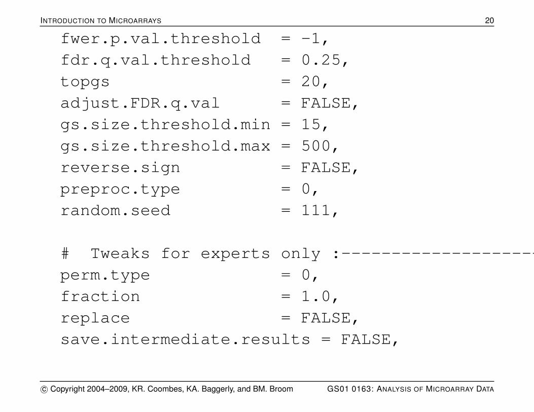
fwer.p.val.threshold = -1,fdr.q.val.threshold = 0.25,topgs = 20,adjust.FDR.q.val = FALSE,gs.size.threshold.min = 15,gs.size.threshold.max = 500,reverse.sign = FALSE,preproc.type = 0,random.seed = 111,
# Tweaks for experts only :-----------------------------------------perm.type = 0,fraction = 1.0,replace = FALSE,save.intermediate.results = FALSE,
c© Copyright 2004–2009, KR. Coombes, KA. Baggerly, and BM. Broom GS01 0163: ANALYSIS OF MICROARRAY DATA

INTRODUCTION TO MICROARRAYS 21
OLD.GSEA = FALSE,use.fast.enrichment.routine = TRUE
)
c© Copyright 2004–2009, KR. Coombes, KA. Baggerly, and BM. Broom GS01 0163: ANALYSIS OF MICROARRAY DATA
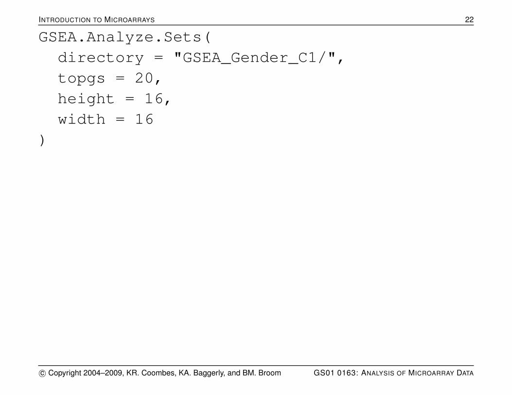
INTRODUCTION TO MICROARRAYS 22
GSEA.Analyze.Sets(directory = "GSEA_Gender_C1/",topgs = 20,height = 16,width = 16
)
c© Copyright 2004–2009, KR. Coombes, KA. Baggerly, and BM. Broom GS01 0163: ANALYSIS OF MICROARRAY DATA
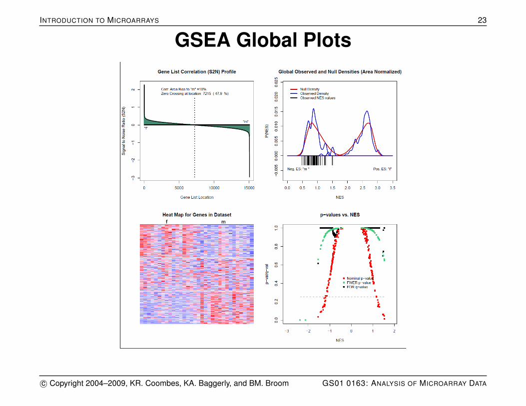
INTRODUCTION TO MICROARRAYS 23
GSEA Global Plots
c© Copyright 2004–2009, KR. Coombes, KA. Baggerly, and BM. Broom GS01 0163: ANALYSIS OF MICROARRAY DATA
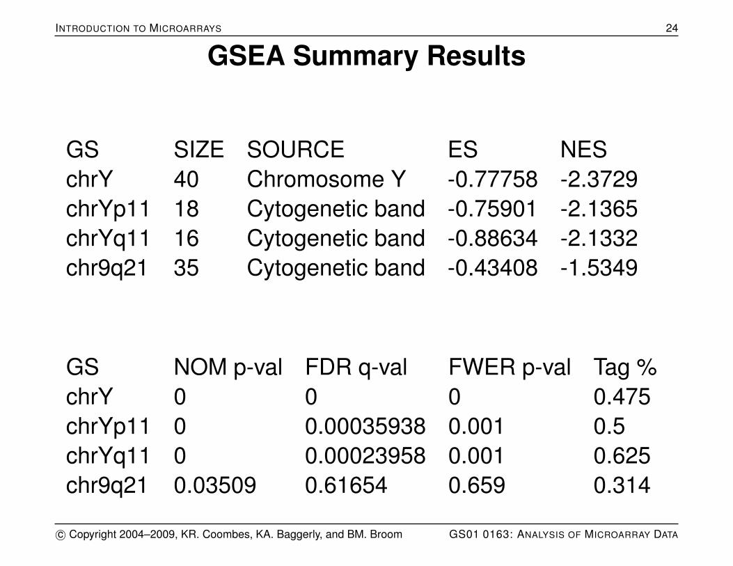
INTRODUCTION TO MICROARRAYS 24
GSEA Summary Results
GS SIZE SOURCE ES NESchrY 40 Chromosome Y -0.77758 -2.3729chrYp11 18 Cytogenetic band -0.75901 -2.1365chrYq11 16 Cytogenetic band -0.88634 -2.1332chr9q21 35 Cytogenetic band -0.43408 -1.5349
GS NOM p-val FDR q-val FWER p-val Tag %chrY 0 0 0 0.475chrYp11 0 0.00035938 0.001 0.5chrYq11 0 0.00023958 0.001 0.625chr9q21 0.03509 0.61654 0.659 0.314
c© Copyright 2004–2009, KR. Coombes, KA. Baggerly, and BM. Broom GS01 0163: ANALYSIS OF MICROARRAY DATA
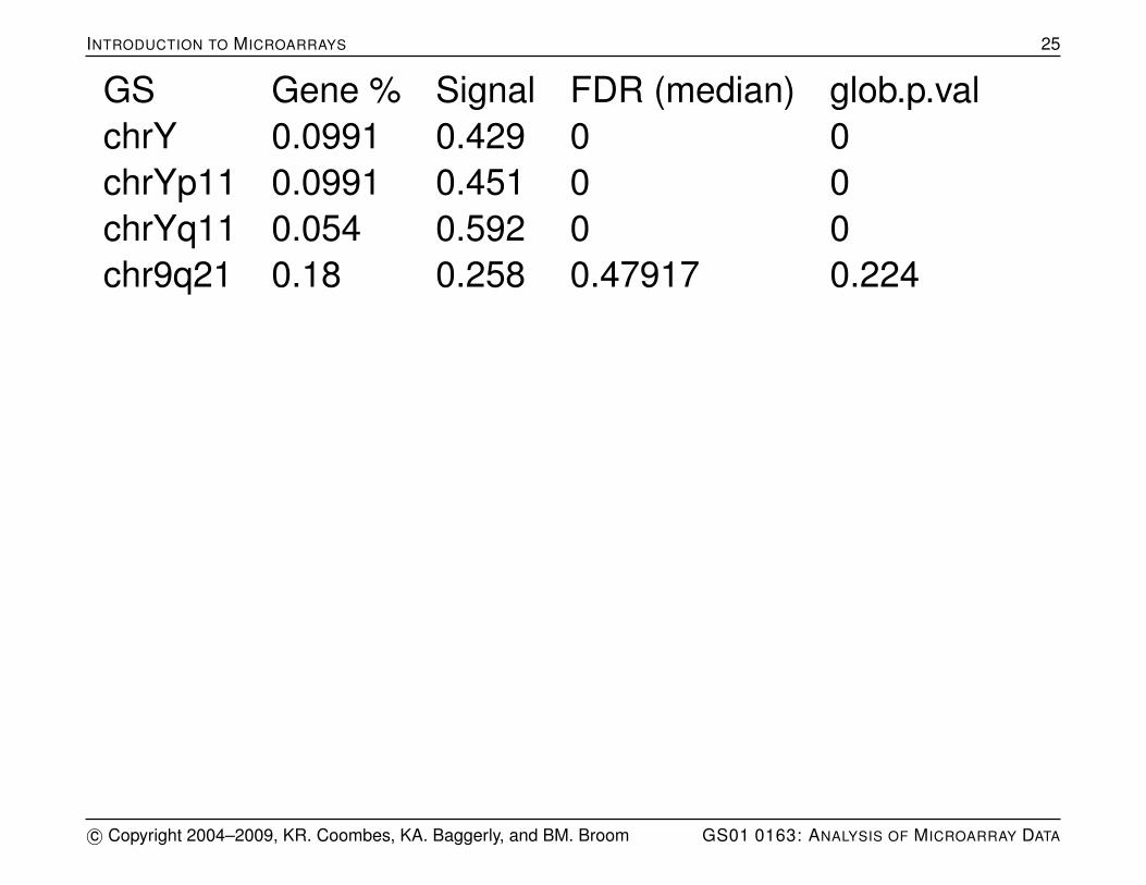
INTRODUCTION TO MICROARRAYS 25
GS Gene % Signal FDR (median) glob.p.valchrY 0.0991 0.429 0 0chrYp11 0.0991 0.451 0 0chrYq11 0.054 0.592 0 0chr9q21 0.18 0.258 0.47917 0.224
c© Copyright 2004–2009, KR. Coombes, KA. Baggerly, and BM. Broom GS01 0163: ANALYSIS OF MICROARRAY DATA
INTRODUCTION TO MICROARRAYS 26
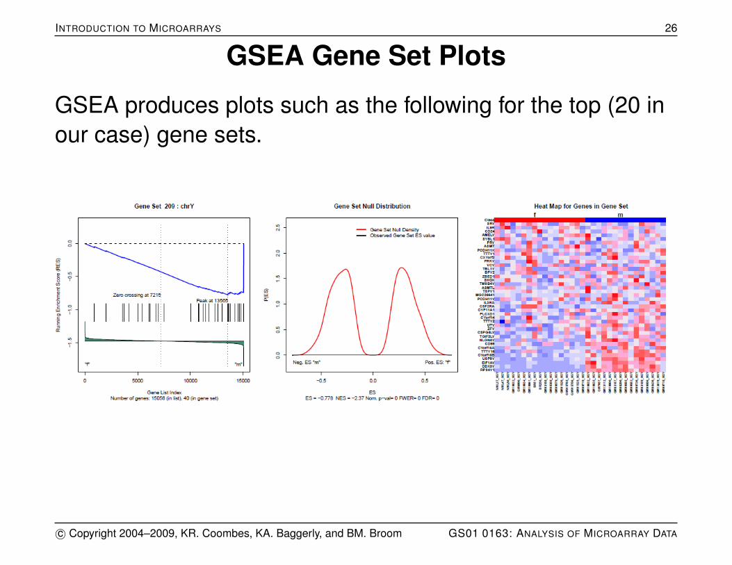
GSEA Gene Set Plots
GSEA produces plots such as the following for the top (20 inour case) gene sets.
c© Copyright 2004–2009, KR. Coombes, KA. Baggerly, and BM. Broom GS01 0163: ANALYSIS OF MICROARRAY DATA

INTRODUCTION TO MICROARRAYS 27
GSEA Gene Set Report# GENE LIST LOC S2N RES CORE ENRICHMENT1 RPS4Y1 15056 -2.94 -6.85e-17 YES2 DDX3Y 15055 -1.84 -0.167 YES3 EIF1AY 15053 -1.71 -0.272 YES4 USP9Y 15052 -1.52 -0.369 YES5 CYorf15B 15051 -0.993 -0.456 YES6 TTTY15 15050 -0.805 -0.512 YES7 CYorf15A 15046 -0.705 -0.558 YES8 CD99 15045 -0.703 -0.598 YES
33 PCDH11X 6105 0.0294 -0.357 NO34 ASMT 5407 0.05 -0.312 NO35 PRY 5037 0.0614 -0.29 NO36 SYBL1 4175 0.089 -0.236 NO37 AMELY 3720 0.105 -0.211 NO38 CD24 3543 0.112 -0.205 NO39 IL9R 2009 0.175 -0.11 NO40 SRY 904 0.248 -0.046 NO
c© Copyright 2004–2009, KR. Coombes, KA. Baggerly, and BM. Broom GS01 0163: ANALYSIS OF MICROARRAY DATA
INTRODUCTION TO MICROARRAYS 28
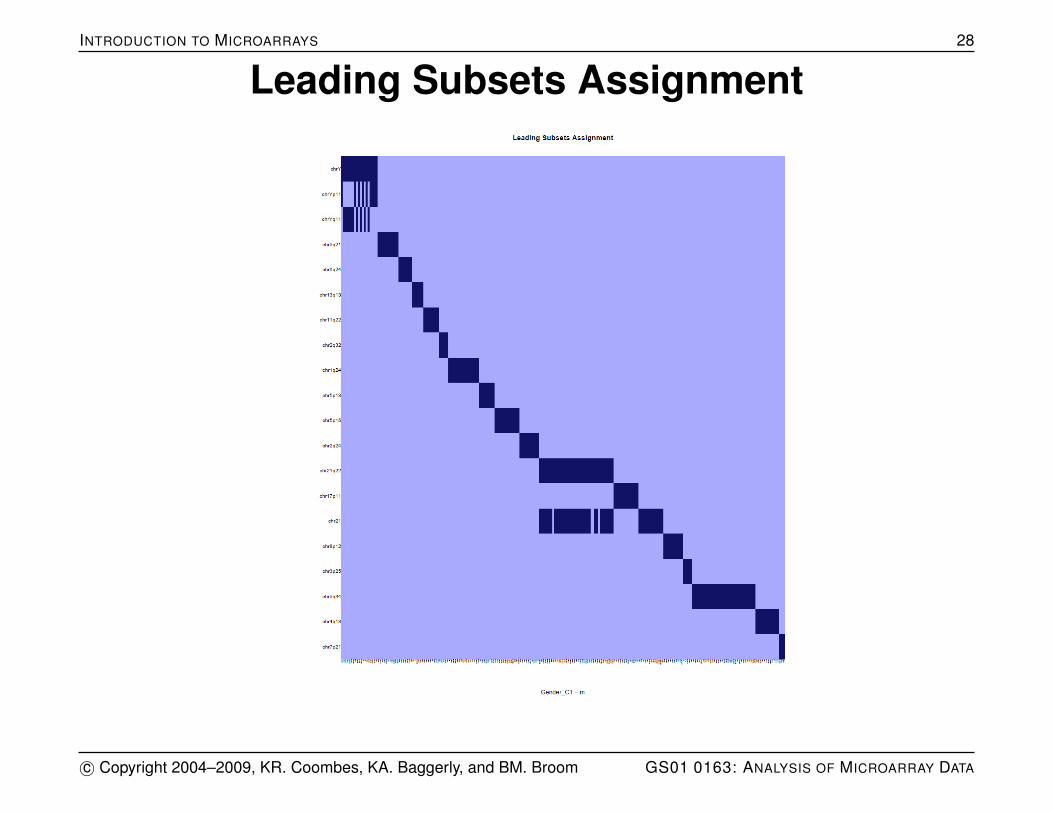
Leading Subsets Assignment
c© Copyright 2004–2009, KR. Coombes, KA. Baggerly, and BM. Broom GS01 0163: ANALYSIS OF MICROARRAY DATA
INTRODUCTION TO MICROARRAYS 29
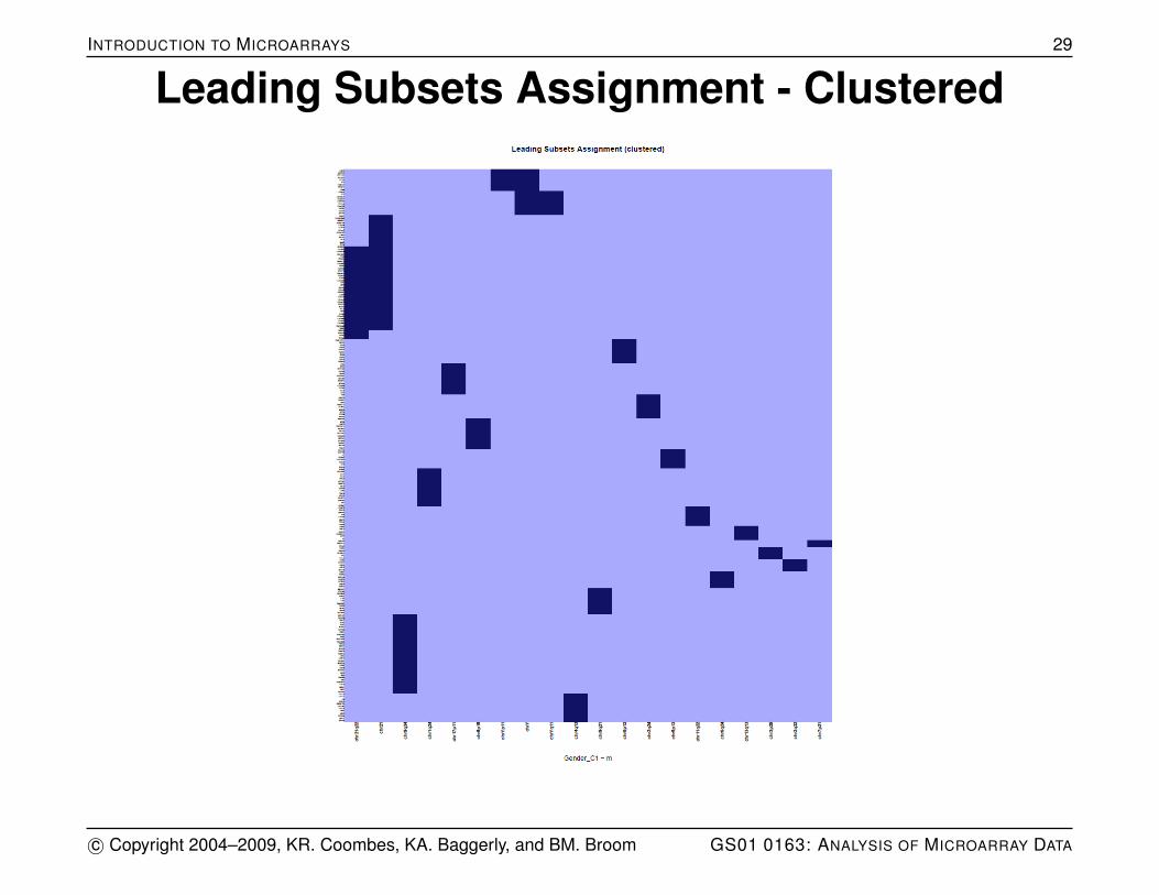
Leading Subsets Assignment - Clustered
c© Copyright 2004–2009, KR. Coombes, KA. Baggerly, and BM. Broom GS01 0163: ANALYSIS OF MICROARRAY DATA
INTRODUCTION TO MICROARRAYS 30
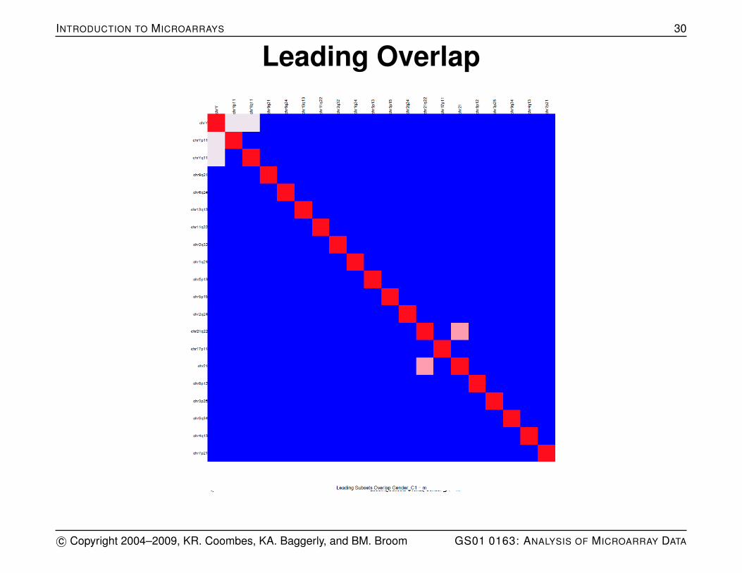
Leading Overlap
c© Copyright 2004–2009, KR. Coombes, KA. Baggerly, and BM. Broom GS01 0163: ANALYSIS OF MICROARRAY DATA
INTRODUCTION TO MICROARRAYS 31
Defining New Genesets
You aren’t limited to using the predefined gene sets.
Indeed, it might be hard to use the existing gene setstogether with new data types.
In addition to using sources similar to those used to generatethe predefined gene sets, it might be fruitful to use thesignificant genes found in one analysis as the basis of ageneset.
GSEA facilitates this by create a geneset database file(.gmt) file containing a geneset of the leading genes found inthe top genesets.
c© Copyright 2004–2009, KR. Coombes, KA. Baggerly, and BM. Broom GS01 0163: ANALYSIS OF MICROARRAY DATA