Embed Size (px)
Citation preview

1
GSA Data Repository 2018138
Levy et al., 2018, Mechanics of fault reactivation before, during, and after the 2015 eruption of
Axial Seamount: Geology, https://doi.org/10.1130/G39978.1.
DATA AND METHODS 1
Earthquake Location and Magnitude Procedures 2
Earthquakes were identified and located using data from seven three-component seismic stations 3
deployed as part of the Ocean Observatories Initiative (OOI) Cabled Array (Kelley et al, 2014). 4
An STA/LTA algorithm operating on a band-passed (750 Hz) vertical channel waveform was 5
used to detect P-wave arrivals that were associated to form an initial set of hypocenters. S-waves 6
were then identified using a kurtosis algorithm (e.g., Baillard et al., 2014) applied to the vector 7
sum of horizontal components. Detections of whale calls and other in-water sources were 8
excluded based on the coherence between the seismic waveforms and co-located hydrophone 9
sensors. The remaining P- and S-wave detections were associated to form a catalog of 41,522 10
hypocenters, which were then located using a 1-D velocity model derived from multi-channel 11
seismic studies (Arnulf et al., 2014) and the generalized earthquake-location (GENLOC) 12
package (Pavlis et al., 2004). The earthquake hypocenters were relocated using the double-13
difference algorithm hypoDD (Waldhauser and Ellsworth, 2000). A final catalog of 19,049 14
earthquakes, each with at least nine defining phases, was derived from processing differential 15

2
arrival times using an 18-step iterative conjugate gradient method with the parameters listed in 16
Table DR1. The median hypocenter location change after relocation is 230 m and the mean of 17
the residuals is 0.029s. Median relative location uncertainty was estimated to be 47 m in the 18
horizontal and 103 m in the vertical direction. 19
Microearthquake moments (Mo) were determined in the frequency domain from P and S 20
arrivals (Brune, 1970): 21
22
where is the crustal density at the hypocenter (2700 kg/m3), v is the average seismic velocity 23
for P (5.09 km/s) or S (2.78 km/s) waves (Arnulf et al., 2014),, r is the slant range from the 24
earthquake hypocenter to the station, K is the free-surface correction taken to be 1.5 and 1.7 for P 25
and S waves, and R is the radiation function assumed to be 0.42 and 0.59 for P or S waves, 26
respectively (Toomey et al., 1985; Weekly et al., 2013). Ωo is the low frequency level of the 27
amplitude spectrum calculated using a Boatwright (1980) model of the form: 28
29
The quality factor (Q), corner frequency (fc) and Ω0 are found simultaneously using a non-linear 30
least squares procedure, and the spectral amplitudes Ω(f) are obtained using a multi-taper (7) 31
approach with a time-bandwidth product of 4. Moment magnitudes (Mw) were estimate from the 32
seismic moments in Nm as (Hanks and Kanamori, 1979): 33
Mw= 2/3 log10(Mo) – 6 34
35
Mo4v3r
o
RK
( f )
oe( ft/Q)
[1( f / fc)4 ]1/2

3
Table DR1. HypoDD Parameters 36
Parameters used in the hypoDD hypocenter relocation process. The max distance between linked 37
pairs and residual threshold became progressively smaller as iterations progressed through the 38
relocation routine in order to minimize and remove outliers. 39
Iterations P weight S weight Max link
separation (km)
Factor multiplied by the
standard deviation of
the residuals
Damping
1‐6 1 0.5 3 8 240
7‐12 1 0.5 2 7 240
13‐18 1 0.5 1 6 240
40
41
Composite Focal Mechanisms 42
Composite focal mechanisms are commonly used to decrease solution uncertainty when the 43
number of recording stations is limited and/or the signal-to-noise ratio of the arrivals is low (e.g., 44
Waldhauser and Tolstoy, 2011). Cross-correlating the vertical channel waveforms recorded on 45
station AXEC1 identified groups of similar earthquakes. A correlation window of 1.4 s was used 46
starting 0.1 sec before the P wave arrival in order to capture both the P- and S-wave energy. 47
Event clusters were defined based on similarity between waveforms (Fig. DR1) using a 48
hierarchical approach with a correlation coefficient cutoff of 0.7. These data were subset to select 49
clusters with earthquakes spanning a limited time range, resulting in a set of 100 clusters that 50
each contain between 3 and 9 earthquakes. The clusters were then used to track the evolution of 51
fault slip through time. The median time spanned by events within an individual composite is 52
29.3 days; however, this varied based on the event rate throughout the volcanic cycle (22.0 days 53
pre-eruption, 1.2 days during the eruption, and 138.0 days post-eruption) (Fig. DR2). The 54
average horizontal radius of the events within a composite cluster is 212 m. 55

4
P-wave polarities were reviewed by the author for the suite of 501 origins belonging to 56
the composite groups (Levy, 2017). S/P amplitude data were measured in the 3-20 Hz frequency 57
band using the vector sum of the peak amplitudes on each of the three channels, following the 58
procedure of Yang et al. (2012). Focal mechanism solutions were found using HASH 59
(Hardebeck & Shearer, 2002). The best solution was found at the average cluster location, but a 60
set of acceptable focal mechanisms was calculated using an allowed polarity misfit of 10%, an 61
epicenter uncertainty of 50 m, a vertical uncertainty of 100 m, and small variations in the 62
velocity model. The preferred focal mechanism was then found by averaging the acceptable focal 63
mechanisms after the removal of outliers. 64
Solutions run with and without S/P information returned similar nodal plane geometries; 65
however, when the amplitude ratio data were included the average nodal plane uncertainty 66
(NPU) decreased from 38 to 21 and the number of A and B quality (Hardebeck & Shearer, 67
2002) solutions increased from 25 to 81. To further assess the sensitivity of the solution to 68
uncertainty in focal depth, focal mechanism parameters were analyzed for a range of depths 69
between 0.7 and 2.0 km, in 0.1 km increments. The median nodal plane rotation is <24 across 70
this depth range, with fault plane uncertainty typically minimized near the mean centroid depth 71
of earthquakes within the cluster. 72
The mean strike and dip of the inferred fault planes (taken to be the outward dipping 73
nodal plane returned for each solution) were estimated using the vector statistics package of 74
Jones (2005); uncertainty in the mean was found using the 95th percentile of the chi-squared 75
distribution. For the entire dataset the vector mean strike and dip is 34513 and 702, 76
respectively. The strike and dip vector means were also calculated during the identifiable phases 77

5
of the volcanic cycle and were found to be 33321/674 (strike/dip for pre-eruption), 78
33815/695 (syn-eruption), and 00727/754 (post-eruption). 79
Analysis of Bottom Pressure Data 80
Bottom-pressure recorder (BPR) data were averaged over 1-minuate intervals and corrected for 81
tides by subtracting the predicted pressure change associated with ocean tides, as estimated using 82
the OSU tidal model (Egbert et al., 1994) implemented within SPOTL (Agnew, 2012). Pressure 83
was converted to water column height assuming a density of 1030 kg/m3. A least-squares linear 84
regression was used to estimate the inflation rates during different phases of the eruption (Fig 85
DR3). 86
Seismic Moments and Cumulative Slip Estimates 87
The seismic moment for each earthquake was found using the median of the individual P and S 88
wave attenuation-corrected spectral amplitudes. The average slip (d) calculation along the 89
eastern ring fault is estimated from the sum of the scalar seismic moments: Mo=μAd. The shear 90
modulus (μ) was taken to be 1-4 GPa, appropriate for fractured basalt in the upper crust 91
(Gudmundsson, 2016), and the area (A) is estimated based on the along-strike (3.0 km) and 92
down-dip (1.75 km) dimensions of the seismically active eastern margin of the caldera. 93
Assuming a 1-4 GPa range of shear modulus, the cumulative slip along the eastern portion of the 94
ring fault was estimated to be 8-30 cm in the three months prior to the eruption, 44-175 cm over 95
the ~1-month period during the eruption, and <0.5 cm over the 19-month period post eruption. 96
These estimates were then related to the differential vertical motion between BPR stations 97
AXCC1 and AXEC2 to constrain the relative coupling between the eastern fault system and the 98
geodetic uplift. 99

6
REFERENCES FOR DATA REPOSITORY 100
Agnew, D. C., 2012, SPOTL: Some Programs for Ocean-Tide Loading, SIO Technical Report, 101
Scripps Institution of Oceanography, http://escholarship.org/uc/item/954322pg. 102
Baillard, C., Crawford, W. C., Ballu, V., Hibert, C., and Mangeney, A., 2014, An automatic 103
kurtosis-based P and S-phase picker designed for local seismic networks. Bulletin 104
Seismological Society of America, v. 104, no.1, p. 394–409 doi:10.1785/0120120347 105
Boatwright J., 1980, A spectral theory for circular seismic sources: simple estimates of source 106
dimension, dynamic stress drop and radiated energy. Bulletin Seismological Society 107
America 70, 1–27 108
Brune, J. N., 1970, Tectonic stress and the spectra of seismic shear waves from earthquakes, 109
Journal of Geophysical Research 75, 4997–5009 110
Egbert, G. D., A. F. Bennett, and M. G. G. Foreman, 1994, TOPEX/POSEIDON tides estimated 111
using a global inverse model, Journal of Geophysical Research., v. 99, no. 24, p. 24,821–112
24,852. 113
Gudmundsson et al., 2016, Gradual caldera collapse at Bárdarbunga volcano, Iceland, regulated 114
by lateral magma outflow, Science 353, doi:10.1126/science.aaf8988 115
Hanks, T. C., and Kanamori, H., 1979, Moment magnitude scale, Journal of Geophysical 116
Research, 84, 2348–2350 117
Hardebeck, J. L., and Shearer, P. M., 2002, A new method for determining first-motion focal 118
mechanisms. Bulletin Seismological Society of America, v. 92, no. 6, p. 2264–2276. 119
doi:10.1785/0120010200 120
Hardebeck, J. L., and Shearer, P. M., 2003, Using S/P amplitude ratios to constrain the focal 121
mechanisms of small earthquakes. Bulletin of the Seismological Society of America, v. 93, 122
no. 6 p. 2434–2444. doi:10.1785/0120020236 123
Jones, T. A., 2005, MATLAB functions to analyze directional (azimuthal) data-I: Single-Sample 124
inference. Computers and Geosciences, v. 36, no. 4, p. 520–525. 125
doi:10.1016/j.cageo.2009.07.011 126
Levy, S., Bohnenstiehl D.R., Wegmann, K., Byrne, P., 2017, Ring Fault Mechanics Surrounding 127
the 2015 Eruption of Axial Seamount, [Master’s thesis] Raleigh, North Carolina State 128
University, North Carolina. 129
Pavlis, G. L., F. L. Vernon, D. Harvey, and D. Quinlan, 2004, The generalized earthquake 130
location (GENLOC) package: A modern earthquake location library, Computers in 131
Geosciences, 30, 1079-1091. 132
Toomey, D. R., Solomon, S. C., Purdy, G. M. and Murray, M. H., 1985, Microearthquakes 133
beneath the median valley of the Mid-Atlantic Ridge near 23N: Hypocenters and focal 134
mechanisms, Journal of Geophysical Research, 90, 5443–5458. 135

7
Waldhauser, F., and Ellsworth, W. L., 2000, A Double-difference Earthquake location algorithm: 136
Method and application to the Northern Hayward Fault, California. Bulletin of the 137
Seismological Society of America, v. 90, no. 6, p. 1353–1368. doi:10.1785/0120000006 138
Waldhauser, F., and Tolstoy, M., 2011, Seismogenic structure and processes associated with 139
magma inflation and hydrothermal circulation beneath the East Pacific Rise at 950’N. 140
Geochemistry, Geophysics, Geosystems, v. 12, no. 9, p. 1-18. doi:10.1029/2011GC003568 141
Weekly, R. T., Wilcock, W. S. D., Hooft, E. E. E., Toomey, D. R., McGill, P. R., and Stakes, D. 142
S., 2013, Termination of a 6 year ridge-spreading event observed using a seafloor seismic 143
network on the Endeavour Segment, Juan de Fuca Ridge. Geochemistry, Geophysics, 144
Geosystems, v. 14, no. 5, p. 1375–1398. doi:10.1002/ggge.20105 145
Wilcock, W. S. D., Tolstoy, M., Waldhauser, F., Gracia, C., Tan, Y. J., Bohnenstiehl, D. R., 146
Caplan-Auerbach, J., Dziak, R.P, Arnulf, A.F., and Mann, E. M., 2016, Seismic Constraints 147
on caldera dynamics from the 2015 Axial Seamount eruption. Science, v. 354, no. 6318, p. 148
1395-1399. doi:10.1126/science.aah5563 149
Yang, W., Hauksson, E., and Shearer, P. M., 2012, Computing a large refined catalog of focal 150
mechanisms for southern California (1981-2010): Temporal stability of the style of faulting. 151
Bulletin of the Seismological Society of America, v. 102, no. 3, p. 1179–1194. 152
doi:10.1785/0120110311 153
154
155

8
FIGURE CAPTIONS: 156
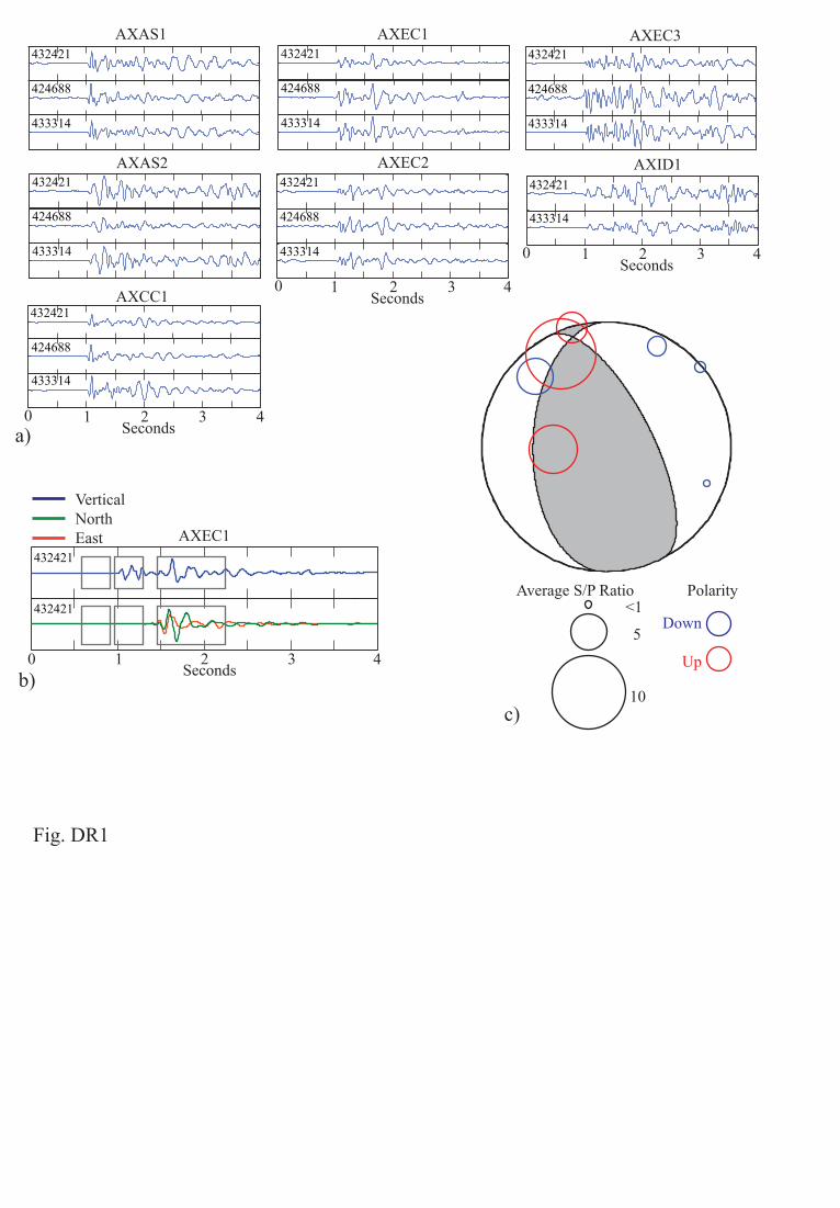
Figure DR1. a) Vertical channel waveforms for similar events in the cluster, used to generate a 157
composite focal mechanism. b) Vertical and the horizontal waveforms for a single arrival shown 158
with windows (boxes) used to estimate the noise, P-arrival, and the S-arrival amplitudes. c) 159
Composite focal mechanism with red and blue indicating upward and downward polarity, 160
respectively, and the size of the circle scaled to represent the S/P amplitude. 161
162
Figure DR2. Graph showing the length of time spanned by events in each composite focal 163
mechanism cluster. The y-axis represents the cluster numbered from 0 to 100. Each horizontal 164
line begins and ends at the times of the earliest and latest earthquake in a cluster. Background 165
shading denotes phases of volcanic inflation and deflation. 166
167
Figure DR3. Time series of elevation data from BPR stations (a) AXCC1, (b) AXEC2 and (c) 168
AXID1 processed to remove tidal variations. Slopes indicating inflation rates are shown by 169
dashed black lines. Background shading denotes phases of volcanic inflation and deflation. 170
AXAS1
AXAS2
AXCC1
AXEC1
AXEC2
AXEC3
AXID1
432421
433314
424688
432421
433314
424688
432421
433314
424688
432421
433314
424688
432421
433314
424688
432421
433314
424688
432421
433314
<1
5
10
Down
Up
Average S/P Ratio Polarity
AXEC1
432421
0 1 2 3
432421
432421
0 1 2 3 4Seconds
0 1 2 3 4Seconds
0 1 2 3 4Seconds
Seconds4
VerticalNorthEast
a)
b)
c)
Fig. DR1

Jan’15 Mar May Jul Sep Nov Jan Mar May Jul Sep Nov Jan’170
10
20
30
40
50
60
70
80
90
100Co
mpo
site
Foc
al M
echa
nism
Clu
ster
#
Eruption
Slower Ination Rate
Post-Eruption Pre-eruption Post-eruption
Date (MMM-YY)
Fig. DR2

Slower Ination RateEruption
40.7cm/yr
91.6 cm/yr
60.9 cm/yr
20.2 cm/year42.6 cm/year
30.3 cm/year
Dec’14 Feb Apr Jun Aug Oct Dec Feb Apr Jun Aug Oct Dec’160
1
2
3
21.1 cm/year
28.9 cm/year15.4 cm/year
Dec’14 Feb Apr Jun Aug Oct Dec Feb Apr Jun Aug Oct Dec’160
1
2
3
Dec’14 Feb Apr Jun Aug Oct Dec Feb Apr Jun Aug Oct Dec’160
1
2
3
AXCC1
AXEC2
AXID1
Chan
ge in
ele
vatio
n (m
)Ch
ange
in e
leva
tion
(m)
Chan
ge in
ele
vatio
n (m
)
a)
b)
c)
Fig. DR3