-GSI Methodology- Utilizing the Gonadosomatic Index (GSI) for Hatchery Evaluation

and Monitoring, as refined by USFWS/MCFWCO

(The document formerly known as ‘NAD Sampling Protocols)

Katy Pfannenstein

Mid-Columbia Fish and Wildlife Conservation Office

US Fish and Wildlife Service

January 2019

The purpose of this document is to describe the methodology on how to assess early maturation rates in juvenile male salmonids at hatchery facilities by using the Gonadosomatic Index (GSI). These methodologies were refined through three years of sampling at three Mid-Columbia River hatcheries (Leavenworth, Entiat, and Winthrop National Fish Hatcheries) with four salmonid stocks (both spring and summer Chinook Salmon, as well as steelhead). For full results of the three year study, please see Pfannenstein and Cooper, 2019. This documents outlines the supplies needed for sampling, step-by-step dissection instructions with color photographs, and data summarization and analysis suggestions. The appendix includes sample R-Studio code for determining the GSI threshold (the graphical separation point between the immature and mature males). For questions about the GSI methodology presented in this document, please contact Matt Cooper, USFWS Hatchery Evaluation Supervisor, at matt_cooper@fws.gov or 509-548-2992.

GSI Supplies List [Bracketed numbers are minimum numbers needed for one crew, 4-6 people, for 300 fish]

Daily consumables:

o Data sheets: Length/weight sheet AND gonad weight sheet (Rite in the Rain)

o Paper number tabs (Rite in the Rain) o Paper towels (brown single fold, ~100/pack) o Absorbent lab paper to cover work surfaces

(roll) o Garbage bags

General:

o [5] Clipboards o [5] Mechanical pencils + lead o [2] Tables o [4] Chairs o [4] Buckets to raise table (small white) o [2] 5 gallon buckets for fish o [2] aerators o [2] Power strips o [2] Extension cords o Duct tape o Large scissors o Sharpie o Extra batteries (9 volt + AA) o Camera/iPad

Length and weight station:

o Tricane Methanesulfonate (MS 222) o [1] Tub for fish o [1] Dip net o [1] PIT tag (PIT) scanner + [1] stand o [4] large sponges + [2] cookie trays o [1] Scale for weights + [1] smolt weight pan o [1] Length board

Dissecting station:

o [1 or 2] Micro scale (minimum power 0.001 g) + power cords

o [4] Scissors + [4] tweezers o [2] Buckets for garbage (5 gallon) o S/M/L glove boxes o Weigh boats for scales o Portable lights

Vendors Used VWR - Absorbent lab paper with Leak-proof Barrier 20”x300’ (VWR) Fischer Scientific - Scissors/Forceps Item #: 08-935, 08-940, 08-875, 08-880 (straight scissors and curved forceps preferred by most samplers, but not all) Ohaus - Micro scale Adventurer Pro Model: AV264C NOTE: The mention of trade names or commercial products in this document does not constitute endorsement or recommendation for use by the federal government.

GSI Sampling How-To

1. Prepare two different data sheets: one with fish ID, fork length, weight, smolt index (0-4), PIT #, and the other with fish ID, sex (M/F), maturation (0-3), gonad weight. Each fish will have an individual fish ID number, which will be matched up during data entry. Pre-make and cut ID labels in advance. Measure fish body weight to the nearest 0.1 g and gonad weight to 0.0001 g.

2. Collect fish from hatchery ponds. Random sample? Keep different ponds separate? CWT? PIT? If possible, collect fish before samplers arrive to increase efficiency. Standard sample size is 300 fish from each stock (Larson et al. 2004).

3. Set up two stations: a fish length/weight measuring station with two staff and a dissecting station where each dissector gets their own data sheet and clip board. Note the length/weight station is at standing height.

4. Kill fish with a lethal dose of MS-222 just prior to sampling to maintain accurate weight and smolt index

characteristics. Smolt Index: 0. Unknown (not shown), 1. Parr, dark marks (bottom fish), 2. Transitional, faded marks (middle fish), 3. Smolt, silver, no marks (top fish), 4. Milting (not shown).

5. Set out 15-20 fish at a time in a row on the sponges. Add number tags to fish. Assess smolt index while all fish are in the line. Obtain weights and lengths, place on paper towel and pass to the dissecting crew.

6. Fish dissection: Cut open belly from vent (shallow incision), next cut behind gill, open fish and gently remove

guts to expose air bladder. Both male and female gonads are located on the top/edge of the air bladder (orange arrow on mature male below).

7. Female identification: 1. Ovary forms a point and then narrows to oviduct – thread like (green arrow) 2. Ovary is angular, has ridge (blue arrow), 3. Granulated (orange arrow), 4. Color (red arrow) is not a good indicator as it can vary from pink to white. The bottom two images show additional variations in size and shape of ovaries.

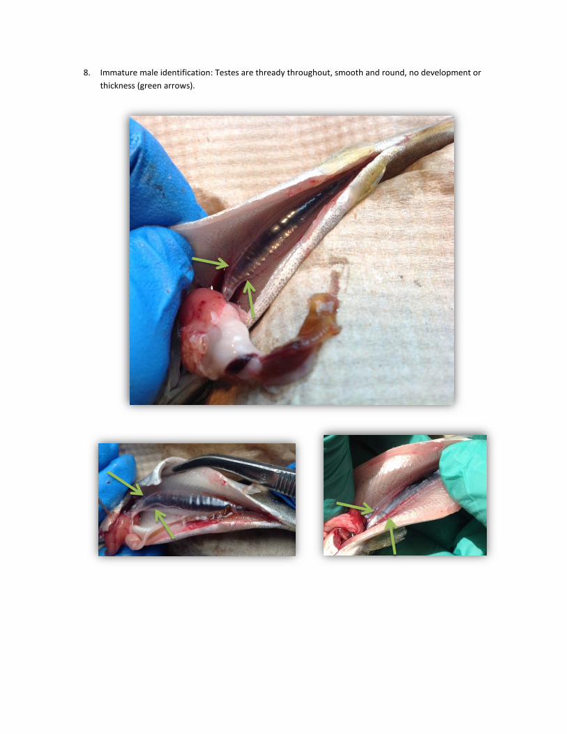
8. Immature male identification: Testes are thready throughout, smooth and round, no development or thickness (green arrows).

9. Mature male identification: Testes thicken, become white/translucent, smooth, tapers to tail.

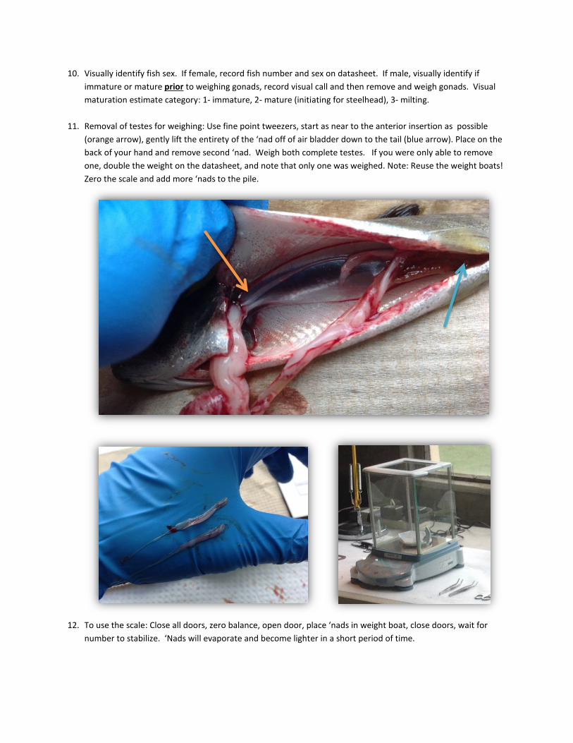
10. Visually identify fish sex. If female, record fish number and sex on datasheet. If male, visually identify if immature or mature prior to weighing gonads, record visual call and then remove and weigh gonads. Visual maturation estimate category: 1- immature, 2- mature (initiating for steelhead), 3- milting.

11. Removal of testes for weighing: Use fine point tweezers, start as near to the anterior insertion as possible (orange arrow), gently lift the entirety of the ‘nad off of air bladder down to the tail (blue arrow). Place on the back of your hand and remove second ‘nad. Weigh both complete testes. If you were only able to remove one, double the weight on the datasheet, and note that only one was weighed. Note: Reuse the weight boats! Zero the scale and add more ‘nads to the pile.

12. To use the scale: Close all doors, zero balance, open door, place ‘nads in weight boat, close doors, wait for

number to stabilize. ‘Nads will evaporate and become lighter in a short period of time.

13. Enjoy all the ‘nad jokes you can handle and interagency mingling!

NAD Data Summarization and Analysis Methods

• Enter data and QA/QC work, make sure to include specific banks/raceways. • Calculate Gonadosomatic Index (GSI = (gonad weight (g) / fish weight (g)) *100). • Calculate Condition Factor (K=(105)* fish weight (g) /length3 (mm)). • Calculate the Log10(GSI) and graph the frequencies in a histogram to visually see the bimodal pattern of

the immature and mature males. Use this graph to determine the GSI threshold (orange arrow) that separates immature (left mode) and mature males (right mode). This can be done in excel or R-Studio. R-Studio uses a mixture model to identify the bi-modality of the data. R code provided in appendix.

• From the GSI threshold, calculate the counts, percentages, average length, weight, and condition factor for immature and mature males.

• In a summary table, for both males and females, include gender counts, percentages, and average length, weight and condition factors. For males, summarize visual counts for immature and mature fish and the percentage of mature fish. Summarize GSI counts and percent for immature and mature fish and list the average length, weigh and condition factor for each group. Make sure to note what GSI threshold was used.

• Perform additional statistics as desired (Were the raceways different? Feed differences? Circular tanks vs. raceways, differences between years, etc). Normality, chi-squared goodness of fit, t-test, anova, etc.

Mature Males

Immature Males

‘NAD Sampling Notes and Suggestions

• Print off more data sheets and number tab sets than you think you need. • Have two people or fewer per dissection scale; the more people using the scale, the more awkward it is. • Best to weigh all male gonads, otherwise there is a gap in the data and the bimodal pattern is difficult to

assess. • After three years of sampling a facility, if there are similar results annually and a large visual difference

between the immature and mature males, experienced samplers may be able to solely assess maturation visually.

• Steelhead that were expressing milt were assigned a maturation level of 3, and were counted, but not weighed. Milting males were not included in the GSI graphs for assessing bimodality.

• Thank you to everyone who participated in the 2016-2018 ‘NAD sampling: USFWS, WDFW, Chelan PUD, Douglas PUD and Grant PUD!

References Harstad, D. L., D. A. Larsen, and B. R. Beckman. 2014. Variation in minijack rate among hatchery populations of Columbia River basin Chinook salmon. Transactions of the American Fisheries Society 143:768-778. Larsen, D. A., B. R. Beckman, K. A. Cooper, D. Barrett, M. Johnston, P. Swanson, and W. W. Dickhoff. 2004. Assessment of high rates of precocious male maturation in a spring Chinook salmon supplementation hatchery program. Transactions of the American Fisheries Society 133:98–120. Pfannenstein, K. and M. Cooper. 2019. Utilizing the Gondosomatic Index (GSI) to Assess the Early Maturation Rates of Juvenile Males at Three Mid-Columbia River National Fish Hatcheries for Spring and Summer Chinook Salmon (Oncorhynchus tshawytscha) and steelhead (Oncorhynchus mykiss). US Fish and Wildlife Service, Leavenworth, Washington.

Appendix – Sample R Code #################################################### #################################################### ## WNFH SCS 3 year summary ## file: WNFHSCS.csv ## 14 columns, 4951 rows ## ## Columns: ## 1-Facility, 2- BY, 3- Species, 4- Sex, ## 5- Length, 6- Weight, 7- VisualMat, 8- GonadWt, 9- K, ## 10- GSI, 11- log10GSI, 12- GSI_Mat, 13- Smolt Index ## ## Rows: ## (1:300) BY14 ## (301:600) BY15 ## (601:900) BY16 ## ## male14 <- WNFHSCS[5:157, c("log10GSI")] ## male15 <- WNFHSCS[304:453, c("log10GSI")] ## male16 <- WNFHSCS[601:744, c("log10GSI")] #################################################### #################################################### # Load the appropriate packages: tools, install packages, CRAN, package install.packages("crandatapkgs") library(mixtools) library(Hmisc) #import dataset attach(WNFHSCS) #################################################### # WNFH SCS Mixture Model #################################################### op=par(mfrow=c(1,1)) male14 <- WNFHSCS[5:145, c("log10GSI")] #view data in basic histogram model=normalmixEM(male14) plot(model, whichplots = 2, breaks=20) #determine cutoff index.lower <- which.min(model$mu) find.cutoff <- function(proba=0.5, i=index.lower) { f <- function(x) {

proba - (model$lambda[i]*dnorm(x, model$mu[i], model$sigma[i]) / (model$lambda[1]*dnorm(x, model$mu[1], model$sigma[1]) + model$lambda[2]*dnorm(x, model$mu[2], model$sigma[2]))) } return(uniroot(f=f, lower=-2, upper=2)$root) # -2,2 may work 0,3 may work } cutoff <- c(find.cutoff(proba=0.5)) h <- hist(male14,ylim=c(0,50),breaks=20, main = "BY14") xfit <- seq(-2.6,1,length=100) yfit1 <- model$lambda[1]*dnorm(xfit,mean=model$mu[1],sd=model$sigma[1]) yfit2 <- model$lambda[2]*dnorm(xfit,mean=model$mu[2],sd=model$sigma[2]) yfit1 <- yfit1*diff(h$mids[1:2])*length(male14) yfit2 <- yfit2*diff(h$mids[1:2])*length(male14) v1 = seq(-2.7,0.2, length=30) v2 = c(-2.7, -2.6, -2.5, -2.4, -2.3, -2.2, -2.1, -2.0, -1.9, -1.8, -1.7, -1.6, -1.5, -1.4, -1.3, -1.2, -1.1, -1.0, -0.9, -0.8, -0.7, -0.6, -0.5, -0.4, -0.3, -0.2, -0.1, 0, 0.1, 0.2) #plot pretty graph hist(male14, breaks = 20, density = 20, col = "purple", xaxt="n", xlab = "Log10 GSI", ylim = c(0, 30), main = "WNFH BY14 SCS") lines(xfit, yfit1, col="red", lwd=2) lines(xfit, yfit2, col="blue", lwd=2) axis(side = 1, at = v1, labels = v2, cex.axis=.75, las=2) abline(v=cutoff, col="green", lty=2, lwd=2) text(-0.35,25, paste("Maturation Threshold", "\n =", round(10^(cutoff), 2),"GSI")) text(-0.35, 12, "Maturation Rate= 9.2%") #################################################### # 2014-2016 WNFH SCS Male Fork Length Vs Maturation #################################################### op=par(mfrow=c(2,2)) male14 <- WNFHSCS[5:157, c("GSI_Mat", "Length")] attach(male14) mature<-male14[which (GSI_Mat=="2"), ] immature<-male14[(GSI_Mat=="1"), ] bins<- c(75, 80, 85, 90, 95, 100, 105, 110, 115, 120, 125, 130,135, 140,145, 150, 155, 160, 165, 170, 175, 180, 185, 190) hist(immature$Length, breaks=bins, col="darkblue", ylim=c(0,45), main = "Males BY14", xlab = "Fork Length (mm)", xaxt="n") hist(mature$Length, breaks=bins, col = "lightblue", ylim=c(0,25), add=TRUE)

legend("topright", c("Immature", "Mature"), col = c("darkblue", "lightblue"), pch= 15, bty = "n") axis(side=1, at = c(75, 80, 85, 90, 95, 100, 105, 110, 115, 120, 125, 130, 135, 140, 145, 150, 155, 160, 165, 170, 175, 180, 185, 190), labels = NULL, las=2) #################################################### # 2014-2016 WNFH SCS All Fork Length Vs Maturation #################################################### ## (1:300) BY14 all_FL14 <- WNFHSCS[1:300, c("GSI_Mat", "Length")] attach(all_FL14) mature<-all_FL14[which (GSI_Mat=="2"), ] bins<- c(75, 80, 85, 90, 95, 100, 105, 110, 115, 120, 125, 130,135, 140,145, 150, 155, 160, 165, 170, 175, 180, 185, 190) hist(all_FL14$Length, breaks=bins, col="forestgreen", ylim=c(0,80), main = "All Fish BY14", xlab = "Fork Length (mm)", xaxt="n") hist(mature$Length, breaks=bins, col = "gold", ylim=c(0,25), add=TRUE) legend("topright", c("All Fish", "Mature Males"), col = c("forestgreen", "gold"), pch= 15, bty = "n") axis(side=1, at = c(75, 80, 85, 90, 95, 100, 105, 110, 115, 120, 125, 130, 135, 140, 145, 150, 155, 160, 165, 170, 175, 180, 185, 190), labels = NULL, las=2) text(170, 25, "9.2%", cex = 2) text(170, 35, "Male Mat. Rate", cex = .75) ##