Embed Size (px)
Citation preview

GRAPH THEORY NOTESOF NEW YORK
Editors:John W. KennedyLouis V. Quintas
The Metropolitan New York Section of
LIX
(2010)
Graph Theory Notes of New York
Graph Theory Notes of New York
publishes short contributions andresearch articles in graph theory, its related fields, and its applications.
Founding Editors: John W. Kennedy (Queens College, CUNY)
Louis V. Quintas (Pace University)
Editorial Address: Graph Theory Notes of New York
Mathematics Department
Queens College, CUNY
Kissina Boulevard
Flushing, NY 11367, U.S.A.
Associate Editors: Krystyna T. Bali
ƒ
ska (Technical University of Pozna
ƒ
, POLAND)
Ivan Gutman (University of Kragujevac,YUGOSLAVIA)
Linda Lesniak (Drew University, New Jersey and Western Michigan University)
Peter J. Slater (University of Alabama at Huntsville, Alabama)
Editorial Board: Brian R. Alspach (University of Newcastle, AUSTRALIA)
Peter R. Christopher (Worcester Polytechnic Institute, Massachusetts)
Edward J. Farrell (University of the West Indies, TRINIDAD)
Ralucca M. Gera (Naval Postgraduate School, California)
Michael Kazlow (Pace University, New York)
Irene Sciriha (University of Malta, MALTA)
Ronald Skurnick (Nassau Community College, New York)
Richard Steinberg (London School of Economics, ENGLAND, U.K.)
Christina M.D. Zamfirescu (Hunter College, CUNY, New York)
Published by: The Metropolitan New York Section of the
Mathematical Association of America
<http://www.maa.org/metrony>
Composit:
K-M Research
50 Sudbury Lane
Westbury, NY 11590, U.S.A.
ISSN 1040-8118
Information for contributors can be found on the inside back cover.

Metropolitan New York Section
GRAPH THEORY NOTES
OF NEW YORK
LIX
(2010)
This issue includes papers presented at
Graph Theory Day 59
held at
Department of Mathematics and Center for Excellence in Mathematics and Science
Southern Connecticut State University
New Haven, Connecticut
Saturday, May 8, 2010
Graph Theory Notes of New York LIX The Mathematical Association of America (2010)
CONTENTS
Introductory Remarks [GTN LIX: 5
Graph Theory Day 59 6
:1] The upper Steiner number of a graph; A.P. Santhakumaran and J. John 9
:2] On graph pebbling numbers and Graham’s conjecture; D.S. Herscovici 15
:3] Canonical consistency of signed line structures; D. Sinha and P. Garg 22
:4] Enumeration of Hamilton cycles and triangles in Euler totient Cayley graphs; B. Maheswari and L. Madhavi 28
:5] On fractional efficient dominating sets of graphs; K.R. Kumar and G. MacGillivray 32
[GTN LIX] Key-Word Index 42
Graph Theory Notes of New York LIX (2010) 5
INTRODUCTORY REMARKS
We are pleased to announce an enhancement to the editorial structure of
Graph Theory Notes of New York
with the appointment of the following Associate Editors:
Krystyna T. Bali
ƒ
ska (Technical University of Pozna
ƒ
, POLAND)Ivan Gutman (University of Kragujevac, YUGOSLAVIA)Linda Lesniak (Drew University and Western Michigan University, U.S.A)Peter J. Slater (University of Alabama at Huntsville, U.S.A)
We appreciate their contributions while they were members of our Editorial Board and look forward toworking with them in their new role.
We move ahead in many ways, but somethings remain the same. We continue to ask for your support of theMathematical Association of America (MAA) Graph Theory Fund. This is part of the sponsorship for
GraphTheory Notes
and Graph Theory Days provided by the Metropolitan New York Section (METRO-NY) ofthe MAA. Contributions are welcome and can be sent to either of the Editors at their institutional addresswith the contribution payable to the ”MAA Graph Theory Fund”.
Another ongoing need is that of hosts for Graph Theory Days. Although not trivial, this is a very manage-able task that provides a great service to the graph theory community and promotion for the host institutions.In May 2010 a successful Graph Theory Day 59 was hosted by Southern Connecticut State University, NewHaven, Connecticut.
All efforts to keep our field of Graph Theory the exciting activity that it is are important. Thus, we call ongraph theory enthusiasts to consider submitting an article to
Graph Theory Notes of New York
, contributingto the MAA Graph Theory Fund, and hosting a Graph Theory Day at their institution.
Thank you.
JWK/LVQNew York
November 2010

6 Graph Theory Notes of New York LIX (2010)
GRAPH THEORY DAY 59
Organizing Committee
Graph Theory Day 59 was sponsored by The Metropolitan New York Section of The Mathematical Associ-ation of America. The event was hosted by the Department of Mathematics and Center for Excellence inMathematics and Science, Southern Connecticut State University, New Haven, Connecticut. Conferencehosts Joseph E. Fields and Val Pinciu introduced the featured speakers. John W. Kennedy and Louis V.Quintas chaired the contributed talks session.
The featured presentations at Graph Theory Day 59 were:
Path Covering of Faulty Hypercubes
Ivan Gotchev Department of Mathematical SciencesCentral Connecticut State UniversityNew Britain, Connecticut, U.S.A.
On Graph Pebbling Numbers and Graham's Conjecture
David Herscovici [See this issue page 15]Department of Computer Science and Digital DesignQuinnipiac UniversityHamden, Connecticut, U.S.A.
Participants at Graph Theory Day 59
Armen R. Baderian Department of MAT/CSC/ITENassau Community CollegeGarden City, NY [email protected]
Laura Baker Department of MathematicsSouthern Connecticut State University501 Crescent StreetNew Haven, CT 06515
Cameron Bishop Department of MathematicsSouthern Connecticut State University501 Crescent StreetNew Haven, CT 06515
Eric Blatchley Department of MathematicsSouthern Connecticut State University501 Crescent StreetNew Haven, CT 06515
Len Brin Department of MathematicsSouthern Connecticut State University501 Crescent StreetNew Haven, CT [email protected]
Susan Buccino Department of MathematicsSouthern Connecticut State University501 Crescent StreetNew Haven, CT 06515
Joseph E. Fields and Val Pinciu (Southern Connecticut State University)
John W. Kennedy (Queens College, CUNY), Louis V. Quintas (Pace University)
Graph Theory Notes of New York LIX (2010) 7
Nikki Butcaris Department of MathematicsSouthern Connecticut State University501 Crescent StreetNew Haven, CT 06515
Nelson Castañeda Department of Mathematical SciencesCentral Connecticut State University1615 Stanley StreetNew Britain, CT [email protected]
Mike Daven Division of Mathematics and Information TechnologyMount Saint Mary College330 Powell AvenueNewburgh, NY [email protected]
Nick Deschene Department of MathematicsSouthern Connecticut State University501 Crescent StreetNew Haven, CT 06515
Edgar G. DuCasse Mathematics DepartmentPace UniversityOne Pace PlazaNew York, NY [email protected]
Joseph Edward Fields Department of MathematicsSouthern Connecticut State University501 Crescent StreetNew Haven, CT [email protected]
Allison Generoso Department of MathematicsSouthern Connecticut State University501 Crescent StreetNew Haven, CT 06515
Ross Gingrich Department of MathematicsSouthern Connecticut State University501 Crescent StreetNew Haven, CT 06515 [email protected]
Michael Golinski Department of MathematicsSouthern Connecticut State University501 Crescent StreetNew Haven, CT 06515
Ivan Gotchev Department of Mathematical SciencesCentral Connecticut State University1615 Stanley StreetNew Britain, CT 06050 [email protected]
Patricia Hand Department of MathematicsSouthern Connecticut State University501 Crescent StreetNew Haven, CT 06515
David Herscovici Department of Computer Science and Digital DesignQuinnipiac University275 Mount Carmel Avenue, CL-AC1Hamden, CT 06518 [email protected]
Leeling Ho Flextrade System Inc.1533 Jasmine AvenueNew Hyde Park, NY 11040 [email protected]

8 Graph Theory Notes of New York LIX (2010)
Joseph Jahr Department of MathematicsSouthern Connecticut State University501 Crescent StreetNew Haven, CT 06515
Caroline Janson Department of MathematicsSouthern Connecticut State University501 Crescent StreetNew Haven, CT 06515
Zachary Kudiak Mathematics DepartmentUniversity of Rhode IslandKingston, RI [email protected]
Dennis Manderino Pace University2151 East 12th StreetBrooklyn, NY 11229-4103 [email protected]
Amy Morrissey Department of MathematicsSouthern Connecticut State University501 Crescent StreetNew Haven, CT 06515
Val Pinciu Department of MathematicsSouthern Connecticut State University501 Crescent StreetNew Haven, CT 06515 [email protected]
Louis V. Quintas Department of MathematicsPace UniversityOne Pace PlazaNew York, NY 10038 [email protected]
Dan Radil Department of MathematicsSouthern Connecticut State University501 Crescent StreetNew Haven, CT 06515
Kathleen Rondinone Department of MathematicsSouthern Connecticut State University501 Crescent StreetNew Haven, CT 06515 [email protected]
Martha Saleski Department of MathematicsSouthern Connecticut State University501 Crescent StreetNew Haven, CT 06515
Pat Schwanfelder Department of MathematicsSouthern Connecticut State University501 Crescent StreetNew Haven, CT 06515
Marianne Uus Department of MathematicsSouthern Connecticut State University501 Crescent StreetNew Haven, CT 06515
Max H. Wentworth Central Connecticut State University225 Huntington Road, P.O. Box 200Scotland, CT [email protected]
Graph Theory Notes of New York LIX, 9–14 (2010)The Mathematical Association of America.
[GTN LIX:1] THE UPPER STEINER NUMBER OF A GRAPH
Anandhapalpu P. Santhakumaran
1
and Johnson John
2
1
Research Department of MathematicsSt. Xavier’s CollegePalayamkottai - 627 002, INDIA<[email protected]>
2
Department of MathematicsGovernment College of EngineeringTirunelveli - 627 007, INDIA<[email protected]>
Abstract
For a connected graph of order at least 2 and a nonempty set
W
of vertices in
G
, theSteiner distance is the minimum size of a connected subgraph of
G
containing
W
. Each suchsubgraph is a tree and is called a Steiner
W
-tree. A set is called a Steiner set of
G
if every ver-tex of
G
is contained in a Steiner
W
-tree of
G
. The Steiner number of
G
is the minimum cardi-nality of its Steiner sets and any Steiner set of cardinality is a minimum Steiner set of
G
. ASteiner set
W
in a connected graph
G
is called a minimal Steiner set if no proper subset of
W
is aSteiner set of
G
. The upper Steiner number of
G
is the maximum cardinality of a minimalSteiner set of
G
. The upper Steiner numbers of certain classes of graphs are determined. Graphs
G
oforder
p
with are characterized. It is shown that for positive integers
r
,
d
, and, with , there exists a connected graph
G
of radius
r
, diameter
d
, and upper Steinernumber
l
. It is also shown that for every two integers
a
and
b
such that , there exists a con-nected graph
G
with and .
1. Introduction
By a graph , we mean a finite, undirected, connected graph with no loop or multiple edge. Theorder and size of
G
are denoted by
p
and
q
respectively. For basic graph theoretic terminology, we refer to
[1][2]
. For vertices
x
and
y
in a connected graph
G
, the
distance
is the length of a shortest
x
—
y
pathin
G
. It is known that the distance is a metric on the vertex set of
G
. An
x
—
y
path of length is calledan
x
—
y
geodesic
. For a vertex
v
of
G
, the
eccentricity
is the distance between
v
and a vertex farthest from
v
. The minimum eccentricity among the vertices of
G
is the
radius
, , and the maximum eccentricity isthe
diameter
, , of
G
. For a nonempty set
W
of vertices in a connected graph
G
, the
Steiner distance
of
W
is the minimum size of a connected subgraph of
G
containing
W
. Necessarily, each such subgraphis a tree and is called a
Steiner tree
with respect to
W
or a Steiner
W
-tree. It is noted that when. The set of all vertices of
G
that lie on some Steiner
W
-tree is denoted by . If ,then
W
is called a
Steiner set
for
G
. A Steiner set of minimum cardinality is a minimum Steiner set or simplya
s
-set of
G
and this cardinality is the
Steiner number
, , of
G
. The Steiner number of a graph was intro-duced and studied in
[3]
. When , every Steiner
W
-tree in G is a
u—v
geodesic. Also, isequal to the set of all vertices lying in
u—v
geodesics, inclusive of
u and v. Hence, Steiner trees, Steiner sets,and Steiner numbers can be considered as extensions of geodesic concepts.
G V E,( )=d W( )
W V⊆s G( )
s G( )
s+ G( )
s+ G( ) p or p 1–=l 2≥ r d 2r≤<
2 a b≤ ≤s G( ) a= s+ G( ) b=
G V E,( )=
d x y,( )d x y,( )
e v( )rad G( )
diam G( )d W( )
d W( ) d u v,( )=W u v,{ }= S W( ) S W( ) V=
s G( )w u v,{ }= S W( )

10 Graph Theory Notes of New York LIX (2010)
For the graph G shown in Figure 1,
,
, and
are the only three s-sets of G, so that .
Two Steiner W1 trees in the graph G of Figure 1 are shown in Figure 2.
For a cut vertex v in a connected graph G and a component H of , the subgraph H and the vertex v,together with all edges joining v to is called a branch of G at v. An end block of G is a block containingexactly one cut vertex of G. Thus, every end block is a branch of G. A vertex v is an extreme vertex of a graphG if the subgraph induced by the neighbors of v is a complete graph. Throughout the following G denotes aconnected graph with at least two vertices.
The following theorems are used in the sequel.
Theorem 1.1 [3]: Each extreme vertex of a graph G belongs to every Steiner set of G. Inparticular, each end vertex of G belongs to every Steiner set of G. �
Theorem 1.2 [3]: Every non-trivial tree with exactly k end vertices has Steiner number k.�
Theorem 1.3 [3]: For a connected graph G, if and only if . �
Theorem 1.4 [3]: Let G be a connected graph of order .Then if and only if G contains a cut vertex of degree . �
2. The Upper Steiner Number of a Graph
Definition 2.1: A Steiner set W in a connected graph G is called a minimal Steiner set if noproper subset of W is a Steiner set of G. The upper Steiner number of G is the max-imum cardinality of a minimal Steiner set of G. �
Example 2.2: For the graph G shown in Figure 3 (left), and are theonly two s-sets, so that . Also, is a minimal Steiner set of G. It is easily ver-ified that no 5-element subset of V is a minimal Steiner set, hence, .
Figure 1: Graph G
W1 v1 v4 v5, ,{ }=
W2 v2 v4 v7, ,{ }=
W3 v3 v5 v7, ,{ }=
s G( ) 3=
Figure 2: Two Steiner W1 trees in graph G.
G v–V H( )
s G( ) p= G K p≅
p 3≥s G( ) p 1–= p 1–
s+ G( )
W1 v1 v3 v4, ,{ }= W2 v1 v3 v5, ,{ }=s G( ) 3= W v2 v4 v5 v6, , ,{ }=
s+ G( ) 4=
Figure 3:

A.P. Santhakumaran and J. John: The upper Steiner number of a graph 11
For the graph G shown in Figure 3 (right), , , , and are minimum Steiner sets of G so that .
Also , , , ,and are minimal Steiner sets of G, so that . It is easily verified that no6-element subset and no 7-element subset of V is a minimal Steiner set of G, and thus .
Remark 2.3: Every minimum Steiner set of G is a minimal Steiner set of G, but the converse is not true. Forthe graph G shown in Figure 3 (left), is a minimal Steiner set but not a minimumSteiner set of G.
Theorem 2.4: For a connected graph G of order p, .
Proof: Since any Steiner set needs at least two vertices, . Let W be a minimum Steiner set of G, sothat . Since W is also a minimal Steiner set of G, it is clear that . Since G isa connected graph of order at least two, it contains a spanning tree and thus V is always a Steiner set for G.Hence, . Thus, . �
Remark 2.5: By Theorem 1.2, for any non-trivial tree T, the set of all end vertices of T is the unique minimumSteiner set of T and thus . It follows from Theorem 1.3 that for the complete graphK2 and that for the complete graph Kp ( ). Thus, the bounds in Theorem 2.4 are sharp.
Also, for the graph shown in Figure 2 (left), and so that strict inequality can hold inTheorem 2.4.
Theorem 2.6: For a connected graph G of order p, if and only if .
Proof: Let . Then V is the unique minimal Steiner set of G. Since no proper subset of V is a Steinerset, it is clear that V is the unique minimum Steiner set of G and hence . The converse follows fromTheorem 2.4. �
Corollary 2.7: For a connected graph G of order p, the following statements are equivalent:(1) ,(2) , and(3) ( ).
Proof: The statement follows from Theorem 1.3 and Theorem 2.6. �
Theorem 2.8: Let G be a connected graph with v a cut vertex of G and let W be a Steiner set of G. Then every component of contains an element of W.
Proof: Let v be a cut vertex of G and W a Steiner set of G. Suppose that there exists a component, say G1 of such that G1 contains no vertex of W. By Theorem 1.1, W contains all the extreme vertices of G and it
follows that G1 does not contain any extreme vertex of G. Thus, G1 contains at least one edge, say xy. Sinceevery Steiner W-tree T must have its end vertices in W and v is a cut vertex of G, it is clear that vertices x andy do not lie on any Steiner W-tree of G. This contradicts that W is a Steiner set of G. �
Corollary 2.9: If v is a cut vertex of a connected graph G and W is a Steiner set of G,then v lies in every Steiner W-tree of G. �
Corollary 2.10: Let G be a connected graph with cut vertices and let W be a Steiner set of G. Then, every branch of G contains an element of W. �
Corollary 2.11: If G is a connected graph with end blocks, then . �
Theorem 2.12: No cut vertex of a connected graph G belongs to any minimal Steiner set of G.
Proof: Suppose that there exists a minimal Steiner set W that contains a cut vertex v of G. Let G1, G2, …, Gr( ) be the components of . By Theorem 2.8, each component Gi ( ) contains an elementof W. We claim that is also a Steiner set of G. Since v is a cut vertex of G, by Corollary 2.9,each Steiner W-tree contains v. Now, since , it follows that each Steiner W-tree is also a Steiner W′-treeof G. Thus, W is a Steiner set of G such that , which is a contradiction to W is a minimal Steiner setof G. Hence, the theorem. �
S1 v1 v4 v5, ,{ }= S2 v1 v2 v5, ,{ }= S3 v2 v5 v6, ,{ }=S4 v2 v3 v6, ,{ }= s G( ) 3=
W1 v3 v4 v7 v8, , ,{ }= W2 v1 v,3
v5 v6, ,{ }= W3 v3 v2 v4 v6, , ,{ }= W4 v2 v3 v5 v7 v8, , , ,{ }=W5 v2 v4 v5 v7 v8, , , ,{ }= s+ G( ) 5≥
s+ G( ) 5=
W v2 v4 v5 v6, , ,{ }=
2 s G( ) s+ G( ) p≤ ≤ ≤s G( ) 2≥
s G( ) W= s+ G( ) W≥ s G( )=
s+ G( ) p≤ 2 s G( ) s+ G( ) p≤ ≤ ≤
s T( ) s+ T( )= s G( ) 2=s+ G( ) p= p 2≥
s G( ) 3= s+ G( ) 4=
s G( ) p= s+ G( ) p=
s+ G( ) p=s G( ) p=
s G( ) p=s+ G( ) p=G K p≅ p 2≥
G v–
G v–
k 2≥ s+ G( ) k≥
r 2≥ G v– i 1 … r, ,=W′ W v{ }–=
v W′∉W′ W⊆

12 Graph Theory Notes of New York LIX (2010)
Corollary 2.13: For any tree T with k end vertices, .
Proof: This follows from Theorems 1.1 and 2.12. �
Theorem 2.14: For a complete bipartite graph ,
(1) if .
(2) if and .
(3) if .
Proof: Statements (1) and (2) follow from Corollary 2.13.
To prove statement (3), first assume that . Let and be abipartition of . Let . We prove that W is a minimal Steiner set of G.
Any Steiner W-tree T is a star centered at each xi ( with yj ( ) as the end vertices of T. Hence,every vertex of G lies on a Steiner W- tree, so that W is a Steiner set of G. Let . Then there exists avertex such that . Since every Steiner W ′-tree is a star centered at xi ( ) whose endvertices are elements of W′, the vertex yj does not lie on any Steiner W ′-tree and thus W′ is not a Steiner setof G. This shows that W is a minimal Steiner set of G. Hence, . It can be proved similarly that
is also a minimal (in fact, minimum) Steiner set of G.
Let S be any minimal Steiner set of G such that . Hence, S is neither contained in X nor in Y. Fur-thermore, since X and Y are (minimal) Steiner sets of G, it follows that S contains neither X nor Y. Hence, thereexist vertices ( ) and ( ) such that and . Because the subgraphinduced by S is connected, it follows that any Steiner S-tree contains only the vertices of S. Thus, vertices xiand yj do not lie on any Steiner S-tree of G, so that S is not a Steiner set of G, which is a contradiction. Thus,any minimal Steiner set of G contains at most n elements, and hence, . Consequently, .For , it can be proved similarly that . �
Theorem 2.15: If G is a connected, non-complete graph of order p, with no cut vertex,then .
Proof: Suppose that . Then . If , then from Corollary 2.7 G iscomplete, which is a contradiction. Therefore, . Let v be a vertex of G such that is a minimal Steiner set of G. Since v is not a cut vertex of G, then is connected. Hence, S is not a Steinerset of G, which is a contradiction. Thus, . �
Remark 2.16: The bound in Theorem 2.15 is sharp. For a complete bipartite graph ( ), it followsfrom Theorem 2.14 that .
Theorem 2.17: For a connected graph G, if and only if .
Proof: Let . Then it follows from Theorem 2.4 that . If , thenby Theorem 2.6, , which is a contradiction. Hence, . Conversely, let
. Then it follows from Corollary 2.7 that G is a non-complete graph. Hence, by Theorem 2.15,G contains a cut vertex, say v. Since , it follows from Theorem 2.12 that is theunique minimal Steiner set of G. Since every minimum Steiner set is also a minimal Steiner set of G, we seethat . �
Theorem 2.18: Let G be a connected graph of order . Then the following statementsare equivalent:(1) .(2) .(3) G contains a cut vertex of degree .
Proof: This follows from Theorems 1.4 and 2.17. �
3. Realization Results
For every connected graph, . Ostrand [4] showed that every two positive inte-gers a and b, with are realizable as the radius and diameter, respectively, of some connected graph.Ostrand’s theorem can be extended so that the upper Steiner number can also be prescribed, when .
s T( ) s+ T( ) k= =
Km n,s+ Km n,( ) 2= m n 1= =
s+ Km n,( ) n= n 2≥ m 1=
s+ Km n,( ) max m n,{ }= m n, 2≥
m n< X x1 x2 … xm, , ,{ }= Y y1 y2 … yn, , ,{ }=G Km n,≅ W Y=
1 i m≤ ≤ 1 j n≤ ≤W ′ W⊂
y j W∈ y j W ′∉ 1 i m≤ ≤
s+ G( ) n≥W X=
S n 1+≥
xi X∈ 1 i m≤ ≤ y j Y∈ 1 j n≤ ≤ xi S∉ y j S∉
s+ G( ) n≤ s+ G( ) n=m n= s+ G( ) m n= =
s+ G( ) p 2–≤s+ G( ) p 1–≥ s+ G( ) p 1– or p= s+ G( ) p=
s+ G( ) p 1–= S V v{ }–=S⟨ ⟩
s+ G( ) p 2–≤K2 n, n 2≥
s+ K2 n,( ) n=
s G( ) p 1–= s+ G( ) p 1–=
s G( ) p 1–= s+ G( ) p or p 1–= s+ G( ) p=s G( ) p= s+ G( ) p 1–=
s+ G( ) p 1–=s+ G( ) p 1–= S S v{ }–=
s G( ) p 1–=
p 3≥
s G( ) p 1–=s+ G( ) p 1–=
p 1–
rad G( ) diam G( ) 2rad G( )≤ ≤a b 2a≤ ≤
a b 2a≤ ≤

A.P. Santhakumaran and J. John: The upper Steiner number of a graph 13
Theorem 3.1: For positive integers r, d, and , with , their exists a connectedgraph G with , , and .
Proof: When , let . Then and, by Corollary 2.13, .
Now, let . We construct a graph G with the desired property as follows. Let : bea cycle of order 2r and let : be a path of order . Let H be the graphobtained from and by identifying v1 in with u0 in . Now, add new ver-tices to H and join each vertex wi ( ) to the vertex , and also join thevertices vr and to obtain the graph G as illustrated in Figure 4.
Then and . Let be the set of all extremevertices of G. By Theorem 1.1, W is a subset of every Steiner set of G. It is clear that W is a Steiner set of Gand it follows that W is the unique minimal Steiner set of G so that . �
In view of Theorem 2.4, the following theorem gives a realization for the Steiner number and the upperSteiner number of a graph.
Theorem 3.2: For positive integers a and b, with , there exists a connected graph G such that and .
Proof: If , let . Then, by Corollary 2.13, . If , let .Let and be the bipartition of G. Any Steiner X-tree T of G is a star cen-tered at each yj ( ) with x1 and x2 as end vertices of T and so X is a Steiner set of G. Since ,it follows that X is a minimum Steiner set, so that . Also, by Theorem 2.14, .
If , let G be the graph, illustrated in Figure 5, obtainedfrom the path P on three vertices u1, u2, u3, by adding the newvertices and , and joining eachvi ( ) with u1 and u3, and also joining each wi( ) with u1 and u2.
Let be the set of extreme vertices of G.Let S be any Steiner set of G. Then by Theorem 1.1, . It is clearthat W is not a Steiner set of G. Also, it is easily verified that
, where , is not a Steiner set of G. It is clear that is a Steiner set of G and so .
Now, let . Then it is clear that Tis a Steiner set of G. We show that T is a minimal Steiner set of G. LetT′ be any proper subset of T. Then there exists at least one vertex, say
such that .
If for some i ( ), then by Theorem 1.1, T is not aSteiner set of G. If for some j ( ), then thevertex vj does not lie on any Steiner T′-tree of G. Similarly, if ,then the vertices u2 and u3 do not lie on any Steiner T′-tree of G. ThusT′ is not a Steiner set of G. Hence, T is a minimal Steiner set of G, sothat .
Now, we show that there is no minimal Steiner set X of G with . Since G has vertices andT is a Steiner set of G with cardinality b, it follows that V is not a minimal Steiner set of G. Suppose that thereexists a minimal Steiner set X such that . Now, if , then it is clear that u3 is not containedin any Steiner X-tree and so X is not a Steiner set of G, which is a contradiction. If , then, since T is a
l 2≥ r d 2r≤ ≤rad G( ) r= diam G( ) d= s+ G( ) l=
r 1= G K1 l,≅ d 2= s+ G( ) l=
r 2≥ C2r v1 v2 … v2r v1, , , ,Pd r– 1+ u0 u1 u2 … ud r–, , , , d r– 1+
C2r Pd r– 1+ C2r Pd r– 1+ l 2–( )w1 w2 … wl 2–, , , 1 i l 2–≤ ≤ ud r– 1–
vr 2+
Figure 4:
rad G( ) r= diam G( ) d= W vr 1+ w1 w2 … wl 2– ud r–, , , , ,{ }=
s+ G( ) l=
2 a b≤ ≤s G( ) a= s+ G( ) b=
a b= G K1 a,≅ s G( ) s+ G( ) a= = 2 a b<= G K2 b,≅X x1 x2,{ }= Y y1 y2 … yn, , ,{ }=
1 j n≤ ≤ X 2=s G( ) 2 a= = s+ G( ) b=
Figure 5:
2 a b< <
v1 v2 … vb a– 1+, , , w1 w2 … wa 2–, , ,1 i b a– 1+≤ ≤
1 i a 2–≤ ≤W w1 w2 … wa 2–, , ,{ }=
W S⊆
W v{ }∪ v W∉W u1 u3,{ }∪ s G( ) a=
T W v1 v2 … vb a– 1+ u3, , , ,{ }∪=
u T∈ u T′∉u wi= 1 i a 2–≤ ≤
u v j= 1 j b a– 1+≤ ≤u u3=
s+ G( ) T≥ b=
X b 1+≥ b 2+
X b 1+= u3 X∉u3 X∈

14 Graph Theory Notes of New York LIX (2010)
Steiner set of cardinality b and X is minimal, there exists exactly one vertex vi ( ) such that. It is now clear that vi is not contained in any Steiner X-tree, and therefore, X is not a Steiner set of G,
which is a contradiction. Thus, there is no minimal Steiner set X of G with . Hence, .�
Remark 3.3: The graph G shown in Figure 5 contains precisely two minimal Steiner sets, viz:
and .
Hence, this example shows that there is no intermediate value theorem for minimal Steiner sets. That is, if kis an integer such that , then there need not exist a minimal Steiner set of cardinality k in G.
Using the structure of the graph G constructed in the proof of Theorem 3.2, we can obtain a graph Gn of ordern with and for all . This suggests the following theorem.
Theorem 3.4: There is an infinite sequence of connected graphs Gn of order such that , , and .
Proof:
Let Gn be the graph, illustrated in Figure 6, obtained from the path P: of length 2, by adding the new vertices v1, v2, , and
w1, and joining each vi ( ) with u1 and u3, and also joiningw1 with u1 and u2.
Let and . It is clear fromthe proof of Theorem 3.2 that the graph Gn contains precisely twominimal Steiner sets, namely
and ,
so that and .
Hence, the result follows. �
References [1] F. Harary; Graph Theory, Addison–Wesley (1969).
[2] F. Buckley and F. Harary; Distance in Graphs, Addison–Wesley, Redwood City (1990).
[3] G. Chartrand, F. Harary, and P. Zhang; The Steiner number of a graph, Discrete Mathematics, 242, 41–54 (2002).
[4] A. Ostrand; Graphs with specified radius and diameter, Discrete Mathematics, 4, 71–75 (1973).
Received: March 9, 2010
1 i b a– 1+≤ ≤vi X∉
X b 1+≥ s+ G( ) b=
W u1 u3,{ }∪ T W v1 v2 …vb a– 1+ u3, , ,{ }∪=
s G( ) k s+ G( )< <
s Gn( ) 3= s+ Gn( ) n 1–= n 5≥
Gn{ } n 5≥s Gn( ) 3= s+ Gn( ) n 1–= s Gn( ) n⁄
n ∞→lim 0= s+ Gn( ) n⁄
n ∞→lim 1=
Figure 6:
u1 u2 u3, , vn 3–1 i n 3–≤ ≤
W w1{ }= T w1 v1 v2 … vn 3– u3, , , , ,{ }=
w1 u1 u3, ,{ } w1 v1 v2 … vn 3– u3, , , , ,{ }
s Gn( ) 3= s+ Gn( ) n 1–=
Graph Theory Notes of New York LIX, 15–21 (2010)The Mathematical Association of America.
[GTN LIX:2] ON GRAPH PEBBLING NUMBERS AND GRAHAM’S CONJECTURE
David S. HerscoviciDepartment of Mathematics and Computer ScienceCL-AC3Quinnipiac University275 Mount Carmel AvenueHamden, Connecticut 06518, U.S.A.<[email protected]>
AbstractWe investigate various results concerning pebbling numbers and optimal pebbling numbers of a con-nected graph. We imagine discrete pebbles placed on the vertices of a graph. We allow pebblingmoves in which two pebbles are removed from some vertex, and one pebble is added to an adjacentvertex. The pebbling number of a graph is the smallest number of pebbles required to ensure that nomatter how they are originally placed, we can reach every vertex by a sequence of pebbling moves.The optimal pebbling number of a graph is the smallest number of pebbles for which some placementallows us to reach every vertex. We also discuss Graham’s conjecture, which asserts that the pebblingnumber of a Cartesian product is at most the product of the pebbling numbers of the graphs in thatproduct.
1. Basic Notions
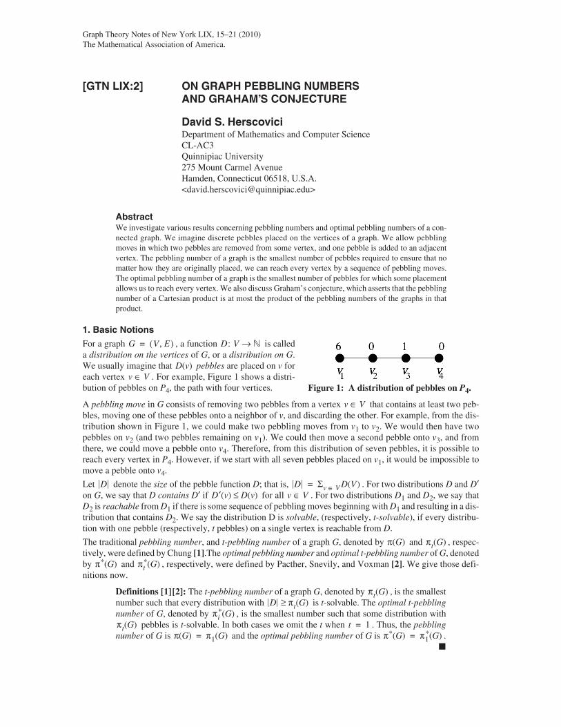
For a graph , a function is calleda distribution on the vertices of G, or a distribution on G.We usually imagine that pebbles are placed on v foreach vertex . For example, Figure 1 shows a distri-bution of pebbles on P4, the path with four vertices.
A pebbling move in G consists of removing two pebbles from a vertex that contains at least two peb-bles, moving one of these pebbles onto a neighbor of v, and discarding the other. For example, from the dis-tribution shown in Figure 1, we could make two pebbling moves from v1 to v2. We would then have twopebbles on v2 (and two pebbles remaining on v1). We could then move a second pebble onto v3, and fromthere, we could move a pebble onto v4. Therefore, from this distribution of seven pebbles, it is possible toreach every vertex in P4. However, if we start with all seven pebbles placed on v1, it would be impossible tomove a pebble onto v4.
Let denote the size of the pebble function D; that is, . For two distributions D and D′on G, we say that D contains D′ if for all . For two distributions D1 and D2, we say thatD2 is reachable from D1 if there is some sequence of pebbling moves beginning with D1 and resulting in a dis-tribution that contains D2. We say the distribution D is solvable, (respectively, t-solvable), if every distribu-tion with one pebble (respectively, t pebbles) on a single vertex is reachable from D.
The traditional pebbling number, and t-pebbling number of a graph G, denoted by and , respec-tively, were defined by Chung [1].The optimal pebbling number and optimal t-pebbling number of G, denotedby and , respectively, were defined by Pacther, Snevily, and Voxman [2]. We give those defi-nitions now.
Definitions [1][2]: The t-pebbling number of a graph G, denoted by , is the smallestnumber such that every distribution with is t-solvable. The optimal t-pebblingnumber of G, denoted by , is the smallest number such that some distribution with
pebbles is t-solvable. In both cases we omit the t when . Thus, the pebblingnumber of G is and the optimal pebbling number of G is .
�
Figure 1: A distribution of pebbles on P4.
G V E,( )= D: V �→
D v( )v V∈
v V∈
D D Σv V∈ D V( )=D′ v( ) D v( )≤ v V∈
π G( ) πt G( )
π* G( ) πt* G( )
πt G( )D πt G( )≥
πi* G( )
πt G( ) t 1=π G( ) π1 G( )= π* G( ) π1
* G( )=

16 Graph Theory Notes of New York LIX (2010)
We leave the reader to verify that and . Note the following basic result.
Proposition 1.1: For any graph G with n vertices and diameter , and .
Proof: Placing one pebble on every vertex creates a solvable distribution, thus . Placing one pebbleon every vertex except for some vertex v creates an unsolvable distribution with pebbles: v is unreach-able because no move is possible. Therefore, . Similarly, placing pebbles on any vertex v cre-ates a solvable distribution, but if the distance from v to w is , placing pebbles on v gives adistribution from which w is unreachable. Therefore, . �
2. Graham’s Conjecture
Graham’s conjecture asserts a bound on the pebbling number of the Cartesian product of two graphs.
Definition: If and are two graphs, their Cartesian product isthe graph with vertex set:
and whose edge set is:
. �
To provide examples, Figure 2 shows a graph G together with the products and , where Knrepresents the complete graph on n vertices. We also write Gd for the graph , the product ofd copies of G.
Chung [1] attributed the following conjecture to Graham.
Conjecture 2.1 (Graham’s Conjecture): For graphs G and G′, .�
Conjecture 2.2 is a generalization of Conjecture 2.1.
Conjecture 2.2: For any multiset of graphs ,
. �
Conjectures 2.1 and 2.2 appear very difficult to resolve in general, but they have been proved for some spe-cific graphs.
Theorem 2.3 [1][3][4]: For a multiset of graphs , if every Gi is a com-plete graph, a tree, or a cycle, and at most two of the Gi are 5-cycles, then Conjecture 2.2holds. That is, . �
π P4( ) 8= π* P4( ) 3=
D G( ) π* G( ) n π G( )≤ ≤π* G( ) 2D G( ) π G( )≤ ≤
π* G( ) n≤n 1–
π G( ) n≥ 2D G( )
D G( ) 2D G( ) 1–π* G( ) 2D G( ) π G( )≤ ≤
G V E,( )= G′ V′ E′,( )=G G′×
V G G′×( ) V V′× x x′,( ) : x V∈ x′ V′∈,{ }= =
E G G′×( ) x x′,( ) y x′,( ),( ) : x y,( ) E∈{ } x x′,( ) x y′,( ),( ) : x′ y′,( ) E′∈{ }∪=
G K2× G K3×G G …× G××
Figure 2: Cartesian products.
π G G′×( ) π G( )π G′( )≤
G1 G2 … Gk, , ,{ }
π G1 G2× …× Gk×( ) π G1( )π G2( )…π Gk( )≤
G1 G2 … Gk, , ,{ }
π G1 G2× …× Gk×( ) π G1( )π G2( )…π Gk( )≤

D.S. Herscovici: On graph pebbling numbers and Graham’s conjecture 17
Cartesian products involving C5 turn out to be difficult to work with. It is known (from [5]) that and , but it has turned out to be difficult to verify the following conjecture, due to Chung[1].
Conjecture 2.4 [1]: and . �
3. Two-Pebbling Properties
It is natural to ask at this point whether it is possible to say anything at all, in general, about Graham’s con-jecture. For example, it is easy to see that for any positive integer n. Is it possible to guarantee that
for any graph G? The answer, in general, is no, but we can guarantee this for any graphthat satisfies one of two possible two-pebbling properties.
To motivate a description of these properties, we ask how might we prove inductively that. Assume that . Further assume the inductive hypothesis that when (the base case is trivial). Suppose we have an arbitrary distribution
of pebbles on . We may assume, without loss of generality, that the target vertex is for some . Suppose we try to transfer pebbles onto the vertices of the form ,with . Denote these vertices by . We transfer as many pebbles as possiblefrom each to . Unfortunately, if has an odd number of pebbles, we must leave a pebblebehind.
These ideas motivate the following notation: given a distribution with , letpi be the number of pebbles on and let ri be the number of vertices in with an oddnumber of pebbles. Then, by transferring pebbles from each to , we can ensure a total of
pebbles on . If it is not possible to reach thetarget from there, it must be the case that . Sincewe started with pebbles on the graph, this would mean that or equivalently, . From these distributions, we try to move two pebbles onto . If wesucceed, we could then move a pebble onto , as desired. The two-pebbling properties are designed toallow this approach to succeed when the first strategy fails. Chung [1] first defined the two-pebbling propertyand Wang [6] defined the odd two-pebbling property.
Definitions [1][6]: Given a distribution of pebbles on the vertices of a graph G, let, let q be the number of occupied vertices in G, and let r be the number of vertices
with an odd number of pebbles. We say G satisfies the two-pebbling property if it is possibleto move two pebbles to any vertex of G by a sequence of pebbling moves whenever
. We say G satisfies the odd two-pebbling property if it is possible to movetwo pebbles to any vertex of G by a sequence of pebbling moves whenever .
�
The previous argument shows that if G satisfies the odd two-pebbling property, then satisfies Gra-ham’s conjecture, . Theorem 3.1 offers a few more examples of productsthat satisfy Graham’s conjecture.
Theorem 3.1: If G satisfies the odd two-pebbling property, then provided H is a complete graph, a complete bipartite graph, a tree, or an even cycle graph.
�
Note that if G satisfies the two-pebbling property, it automatically satisfies the odd two-pebbling property: if, then . Therefore, if G satisfies the two-pebbling property, two pebbles
can be moved to any vertex. The following conjecture asserts the converse.
Conjecture 3.2: G satisfies the two-pebbling property if and only if it satisfies the odd two-pebbling property. �
Many graphs satisfy at least the odd two-pebbling property.
Theorem 3.3 [1]–[3]: G satisfies the odd two-pebbling property if the diameter of G is atmost two (e.g., complete graphs and complete bipartite graphs), or if G is a tree or a cycle.
�
π C5( ) 5=π C5 C5×( ) 25=
π C5 C5× C5×( ) 125= π C5d( ) 5d=
π Kn( ) n=π G Kn×( ) nπ G( )≤
π G Kn×( ) nπ G( )≤ V Kn( ) v1 v2 … vn, , ,{ }=π G Km×( ) mπ G( )≤ m n< n 1=
nπ G( ) G Kn× x0 v1,( )x0 V G( )∈ n 1–( )π G( ) x vi,( )
i n 1–≤ V G( ) v1 v2 … vn 1–, , ,{ }×x vn,( ) x v1,( ) x vn,( )
D: V G Kn×( ) �→ D nπ G( )=V G( ) vi{ }× V G( ) vi{ }×
x vn,( ) x v1,( )p1 p2 … pn 1– pn rn–( ) 2⁄+ + + + V G( ) v1 v2 … vn 1–, , ,{ }×
x0 v1,( ) p1 p2 … pn 1– pn rn–( ) 2⁄+ + + + n 1–( )π G( )<p1 p2 … pn+ + + nπ G( )= pn rn+( ) 2⁄ π G( )>pn rn+ 2π G( )> x0 vn,( )
x0 v1,( )
p D=
p q+ 2π G( )>p r+ 2π G( )>
G Kn×π G Kn×( ) π G( )π Kn( )≤ nπ G( )=
π G H×( ) π G( )π H( )≤
p r+ 2π G( )> p q p r 2π G( )>+≥+

18 Graph Theory Notes of New York LIX (2010)
A natural question to ask is whether any graph does not satisfythese properties. We call such a graph a Lemke graph, in honor ofPaul Lemke who discovered the example L shown in Figure 3. Ittakes some effort, but one can verify that . However,for the given distribution, we have and , buttwo pebbles cannot be moved to v. Lemke graphs are thought tobe the most likely candidates for counterexamples to Graham’sconjecture. It would be interesting to verify the following conjec-ture.
Conjecture 3.4: If L is the Lemke graph shown in Figure 3, then . �
4. A Generalization of Graham’s Conjecture
We can generalize what we allow as the target distributions, with-out insisting that all pebbles have to be on the same vertex. Thisgives us more general versions of pebbling numbers.
Definitions: If D is any distribution of pebbles on the vertices of the graph G, we say thedistribution D′ is D-solvable if it is possible to go from D′ to a distribution that contains Dby a sequence of pebbling moves. We then define as the smallest number such thatevery distribution of pebbles on G is D′-solvable. Similarly, if S is a set of distri-butions of pebbles on G, we define as the smallest number such that every distri-bution of pebbles on G is D-solvable for every . We also define tobe the smallest number such that some distribution of pebbles on G is D-solvablefor every . �
In particular, if we define as the set of distributions with t pebbles on a single vertex, then = and . For a single distribution D, is not interesting; since D isD-solvable, and trivially .
To generalize Graham’s conjecture, we generalize products to work with sets of distributions.
Definitions: Given distributions and on the vertices ofgraphs G and H, respectively, we define as the distribution on
given by .If SG and SH are sets of distributions on G and H, respectively, we define as theset of distributions on given by . �
Figure 4 illustrates an example of the product of a distribution on the graph G from Figure 2 and a distributionon K2.
Figure 3: The Lemke graph L.
π L( ) 8=p 13= q r 5= =
π L L×( ) 64=
π G D,( )π G D,( )
π G S,( )π G S,( ) D S∈ π* G S,( )
π G S,( )D S∈
St G( ) π G St G( ),( )πt G( ) π* G St G( ),( ) πt
* G( )= πt* G( )
π* G D,( ) D=
DG: V G( ) �→ DH : V H( ) �→DG DH⋅ : V G H×( ) �→
G H× DG DH⋅( ) v w,( )( ) DG v( )DH w( )=SG SH⋅
G H× SG SH⋅ DG DH⋅ : DG SG∈ DH SH∈,{ }=
Figure 4: An example of product distribution.
D.S. Herscovici: On graph pebbling numbers and Graham’s conjecture 19
We can now generalize Conjecture 2.1 as follows:
Conjecture 4.1: For any graphs G and H, and any sets of distributions SG and SH on thevertices of G and H, respectively,
. �
Note that if and , then , hence with this choice of distri-butions, we obtain Graham’s conjecture precisely.
Obviously, Conjecture 4.1 is very difficult for regular pebbling. However, the analog for optimal pebblingfollows relatively easily from the following nontrivial observations.
Observations: If we are able to get from the distribution to D1 in G by a sequence of pebbling moves andwe can get from to D2 in H, then we can get from to to in by asequence of pebbling moves. In particular, if we can get from DG to every distribution in SG, and we can getfrom DH to every distribution in SH, then we can get from to every distribution in .
Since , Theorem 4.2 follows from the above observations. This theorem generalizesa result from Shiue [7] that .
Theorem 4.2 [8]: For any graphs G and H, and any sets of distributions SG and SH on thevertices of G and H, respectively, then . �
Thus, for optimal pebbling, an analog of Graham’s conjecture holds in a very general setting.
5. Some Solvable Distributions
In this section, we construct solvable distributions for hypercubes and for Cartesian products of C5. Theseare not optimal distributions, at least not for large products, but they are better then previously knowndistributions.
5.1. Solvable Distributions on Hypercubes
Write Qd for the d-dimensional hypercube, , and label the vertices of Qd by bitstrings. Given a vertex and a bit , let be the vertex in obtained by appending b to the bitstring for v.
Moews [9] proved the following theorem, which gives the best known bound on the optimal pebbling numberof hypercubes.
Theorem 5.1 [9]: for some constant k. �
Moews proof, however, was probabilistic; he did not construct explicit distributions. It also does not tell usanything when d is small. The best previously constructed distributions are given in the following theorem,obtained by Pachter, Snevily, and Voxman [2].
Theorem 5.2 [2]: If , then putting 2k pebbles each on the vertices and gives a solvable distribution on Qd. If , then putting pebbles on and putting 2k pebbles on gives a solvable distribution on Qd. �
We call the distributions in Theorem 5.2 antipodal distributions, and write Ad for the antipodal distribution onQd. The number of pebbles required by Ad is in . We inductively extend the antipodaldistributions to produce solvable distributions with fewer pebbles by using the following definition:
Definition: Let be a distribution of pebbles on Qd, and for each ,let . Then construct a distribution as follows:
• If , let .
• If , let .
• If , let and .
We write for the distribution on obtained by applying this constructionm times. �
Note that in each case, we can put pi pebbles on for each . In particular, if D is solvable inQd, then is solvable in . Note further that if each pi is sufficiently large. Unfortu-nately, this requirement that pi must be sufficiently large limits our ability to repeatedly improve the bound by
π G H× SG SH⋅,( ) π G SG,( )π H SH,( )≤
SG S1 G( )= SH S1 H( )= SG SH⋅ S1 G H×( )=
D1′D2′ D1′ D2′⋅ D1′ D2⋅ D1 D2⋅ G H×
DG DH⋅ SG SH⋅DG DH⋅ DG DH=
πst* G H×( ) πs
* G( )πt* H( )≤
π* G H× SG SH⋅,( ) π* G SG,( )π* H SH,( )≤
Qd K2d≅
v Qd∈ b 0 1,{ }∈ v b⋅ Qd 1+
π* Qd( ) 43---⎝ ⎠
⎛ ⎞ d O dlog( )+∈ O 4
3---
ddk
⎝ ⎠⎛ ⎞=
d 2k= 00…011…1 d 2k 1+= 2k 1+00…0 11…1
Θ 2n( ) Θ 1.4142n( )≈
D: V Qd( ) �→ vi V Qd( )∈pi D vi( )= ρ D( ): V Qd 1+( ) �→
pi 3k= ρ D( )( ) vi 0⋅( ) ρ D( )( ) vi 1⋅( ) 2k= =
pi 3k 1+= ρ D( )( ) vi 0⋅( ) ρ D( )( ) vi 1⋅( ) 2k 1+= =
pi 3k 2+= ρ D( )( ) vi 0⋅( ) 2k 2+= ρ D( )( ) vi 1⋅( ) 2k 1+=
pm D( ) Qd m+
vi b⋅ b 0 1,{ }∈ρ D( ) Qd 1+ ρ D( ) 4
3--- D≈
20 Graph Theory Notes of New York LIX (2010)
a factor of 4/3, but if we start with a sufficiently large antipodal distribution, a careful analysis, conducted in[8] gives the following result.
Theorem 5.3 [8]: Given an integer d, let
, and let .
Then the distribution on satisfies
. �
5.2. Solvable Distributions on
Moews [9] generalized Theorem 5.1 to apply to all graphs. In particular, applying it to C5 gives the followingtheorem:
Theorem 5.4 [9]: for some constant k. �
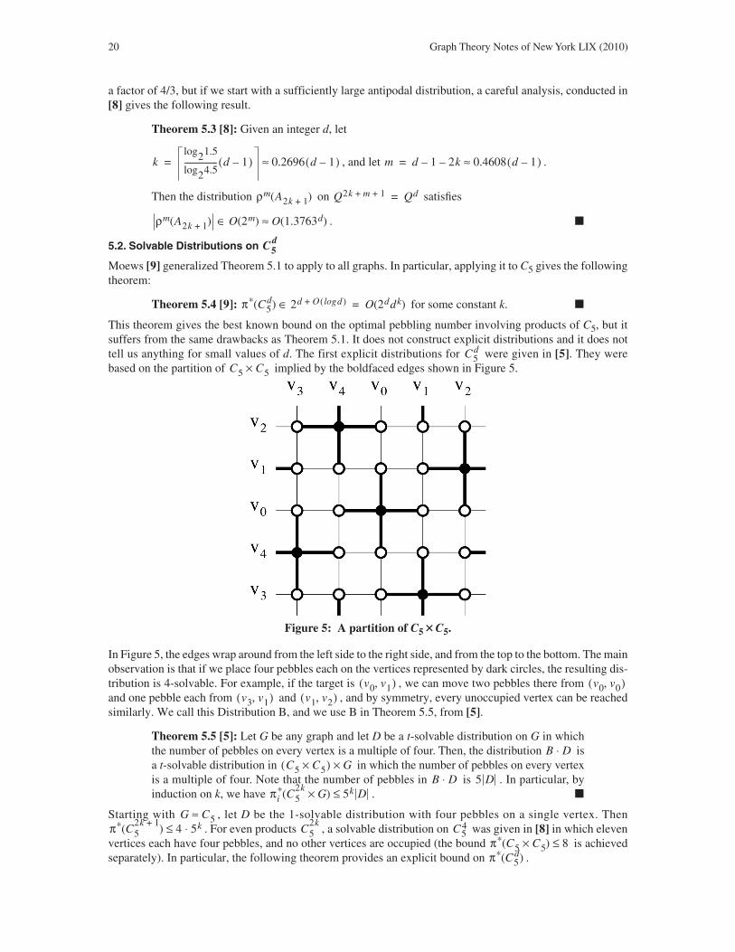
This theorem gives the best known bound on the optimal pebbling number involving products of C5, but itsuffers from the same drawbacks as Theorem 5.1. It does not construct explicit distributions and it does nottell us anything for small values of d. The first explicit distributions for were given in [5]. They werebased on the partition of implied by the boldfaced edges shown in Figure 5.
In Figure 5, the edges wrap around from the left side to the right side, and from the top to the bottom. The mainobservation is that if we place four pebbles each on the vertices represented by dark circles, the resulting dis-tribution is 4-solvable. For example, if the target is , we can move two pebbles there from and one pebble each from and , and by symmetry, every unoccupied vertex can be reachedsimilarly. We call this Distribution B, and we use B in Theorem 5.5, from [5].
Theorem 5.5 [5]: Let G be any graph and let D be a t-solvable distribution on G in whichthe number of pebbles on every vertex is a multiple of four. Then, the distribution isa t-solvable distribution in in which the number of pebbles on every vertexis a multiple of four. Note that the number of pebbles in is . In particular, byinduction on k, we have . �
Starting with , let D be the 1-solvable distribution with four pebbles on a single vertex. Then. For even products , a solvable distribution on was given in [8] in which eleven
vertices each have four pebbles, and no other vertices are occupied (the bound is achievedseparately). In particular, the following theorem provides an explicit bound on .
klog21.5
log24.5------------------ d 1–( ) 0.2696 d 1–( )≈= m d 1– 2k– 0.4608 d 1–( )≈=
ρm A2k 1+( ) Q2k m 1+ + Qd=
ρm A2k 1+( ) O 2m( ) O 1.3763d( )≈∈
C5d
π* C5d( ) 2d O dlog( )+∈ O 2ddk( )=
C5d
C5 C5×
Figure 5: A partition of C5�C5.
v0 v1,( ) v0 v0,( )v3 v1,( ) v1 v2,( )
B D⋅C5 C5×( ) G×
B D⋅ 5 Dπi
* C52k
G×( ) 5k D≤
G C5≈π* C5
2k 1+( ) 4 5k⋅≤ C5
2kC5
4
π* C5 C5×( ) 8≤π* C5
d( )
D.S. Herscovici: On graph pebbling numbers and Graham’s conjecture 21
Theorem 5.6 [8]: and . Thus, for all
. �
References [1] F.R.K. Chung; Pebbling in hypercubes, SIAM J. Discrete Math., 2(4), 467–472 (1989).
[2] L. Pachter, H.S. Snevily, and B. Voxman; On pebbling graphs, Congr. Numer., 107, 65–80 (1995).
[3] D. Moews; Pebbling graphs, J. Combin. Theory Ser. B, 55, 244–252 (1992).
[4] D.S. Herscovici; Graham’s pebbling conjecture on products of many cycles, Discrete Mathematics, 308, 6501–6512(2008).
[5] D.S. Herscovici and A.W. Higgins; The pebbling number of , Discrete Mathematics, 187(1–3), 123–135(1998).
[6] S.S. Wang; Pebbling and Graham’s conjecture, Discrete Math., 226(1–3), 431–438 (2001).
[7] C.-L. Shiue; Optimally Pebbling Graphs, Ph.D. Dissertation, Department of Applied Mathematics, National ChiaoTung University, Hsin chu, Taiwan (1999).
[8] D.S. Herscovici, B.D. Hester, and G.H. Hurlbert; Optimal pebbling in products of graphs. Preprint (2010).
[9] D. Moews; Optimally pebbling hypercubes and powers, Discrete Mathematics, 190, 271–276 (1998).
Received: June 3, 2010
π* C52k 1+
( ) 4 5k⋅≤ π* C52k
( ) 4425------ 5k( )≤ d 1≥
π* C5d
( ) 4
5------- 5d 2/( ) O 5d( )∈≤
C5 C5×

Graph Theory Notes of New York LIX, 22–27 (2010)The Mathematical Association of America.
[GTN LIX:3] CANONICAL CONSISTENCY OF SIGNED LINE STRUCTURES
Deepa Sinha and Pravin GargCentre for Mathematical SciencesBanasthali UniversityBanasthali-304022Rajasthan, INDIA<deepa [email protected]><[email protected]>
AbstractA marked signed graph is an ordered pair , where is a sigraph and
is a function from the vertex set of Su into the set , called a mark-ing of S. A cycle Z in Sμ is said to be consistent if it contains an even number of negatively markedvertices. A sigraph S is consistent if every cycle in S is consistent. In particular, σ induces a uniquemarking defined by , where Ev is the set of edges incident on v in S, and iscalled the canonical marking of S. In this paper, we characterize canonically consistent line sigraphsand canonically consistent ×-line sigraphs, the latter being a variation of the standard notion of a linesigraph.
1. Introduction
A signed graph (or sigraph) is an ordered pair , where is a graph, called the under-lying graph of S and is a function from the edge set E of Su into the set called the sig-nature of S. Let and . The elements of
and are called positive and negative edges of S, respectively. For standard terminology andnotation in graph theory see Harary [1] and West [2]. For sigraphs see Zaslavsky [3][4]. Throughout thispaper graphs are finite with no loop or multiple edge.
A sigraph S is called regular if the number of positive edges, , incident on a vertex v in S and the numberof negative edges, incident on v, are the same for all vertices in S, with and not necessarilyequal. The numbers and are called the positive and negative degrees of v in S, respectively. Fora regular sigraph S, the degree of S is the pair .
The edge degree of an edge ej in a sigraph S is the total number of edges adjacent to ej in S. The positive(negative) edge degree, ( ) of edge ej in S is the total number of positive (negative) edges adja-cent to ej. The negation of a sigraph S is a sigraph obtained from S by negating the sign of every edgeof S. Thus, to obtain , change the sign of every edge of S to its opposite.
An alternating sequence of vertices and edges of S, beginning and terminating with vertices, in which all thevertices are distinct, is called a path in S. The length of a path is defined to be the number of edges containedin the path. A path containing precisely n edges, is called an n-path. If all the edges in a path are negative, thenthe path is called an all-negative path. A negative section (see [5]) of a subsigraph S′ of a sigraph S is a max-imal edge-induced connected subsigraph in S consisting of only the negative edges of S. The length of a neg-ative section is the number of negative edges it contains.
For a sigraph S, Behzad and Chartrand [6] defined its line sigraph as the sigraph in which the edges ofS are represented by vertices with two vertices adjacent in whenever the corresponding edges in S sharea common vertex. An edge ef in is defined to be negative whenever both e and f are negative edges inS. In [7][8], the authors introduced a variation of the standard notion for the line sigraph of a givensigraph S: is a sigraph defined on the line graph of the graph Su by assigning to each edge ef of
the product of signs of the adjacent edges e and f of S. is called the ×-line sigraph of S.
Sμ S μ,( )= S Su σ,{ }=μ: V Su( ) + –,{ }→ V Su( ) + –,{ }
μσ μσ v( ) Πe j Ev∈ σ e j( )=
S Su σ,( )= Su V E,( )=σ: E + –,{ }→ + –,{ }
E+ S( ) e E S( ) : ∈ σ e( ) +={ }= E– S( ) e E S( ) : ∈ σ e( ) –={ }=E+ S( ) E– S( )
d+ v( )d– v( ) d+ v( ) d– v( )
d+ v( ) d– v( )d+ v( ) d– v( ),( )
de e j( )de
+ e j( ) de– e j( )
η S( )η S( )
L S( )L S( )
L S( )L S( )
L× S( ) L Su( )L Su( ) L× S( )

D. Sinha and P. Garg: Canonical consistency of signed line structures 23
A sigraph is -marked if there exists a sigraph , a bijection →, a binary relation R on , and a marking of satisfying the following
compatibility conditions:
(1) ,
(2) , .
Furthermore, S1 is -consistent if the following condition is satisfied:
(3) , for every cycle Z in S1.
The case when R is defined by the condition is treated in Sinha [9] in a study ofsigned graph equations involving signed line graphs. In this particular case, the terms -marked and
-consistent will be simplified to S2-marked and S2-consistent, respectively. In particular, σ inducesa unique marking , called the canonical marking of S, defined by
where Ev is the set of edges incident on v in S.
If every vertex of a sigraph S is canonically marked, then a cycle Z in S is said to be canonically consistent ifZ has an even number of negatively marked vertices. A sigraph S is said to be canonically consistent if everycycle in S is canonically consistent.
2. Canonically Consistent Line Sigraphs
Beineke and Harary [10][11] were the first to pose the problem of characterizing consistent marked graphs.This question was subsequently settled by Acharya [12][13] and by Hoede [14]. Acharya and Sinha obtainedS-consistency of line sigraphs in [9][15]. In this section, we obtain a characterization of canonically consis-tent line sigraphs.
The following theorem by Hoede plays an important role in solving this problem.
Theorem 1 [14]: A marked graph is consistent if and only if for any spanning tree T ofG all fundamental cycles with respect to T are consistent and all common paths of pairs ofthese fundamental cycles have end vertices carrying the same marks. �
Theorem 2: The line sigraph of a sigraph is canonically consistent ifand only if the following conditions hold in S:
(1) The number of negative edges of odd negative edge degree is even(a) for every cycle Z in S, and(b) for the edges incident at v with such that v does not lie on any cycle Z in S;
(2) If and are edges incident at v with lying on the cycle Z,then the numbers of all-negative 2-paths from ei and ej have the same parity and the number of all-negative 2-paths from ek is even;
(3) If , then for all negative edges ej incident at v, .
Proof: Necessity Suppose is canonically consistent, then every cycle Z′ in is canonically consis-tent. Thus, Z′ must have an even number of negatively marked vertices. Let be a cyclein S. By definition of , is a cycle in . Clearly, a positive edge and a negative edgeof even negative edge degree in Z will result in positively marked vertices in Z′ but a negative edge of oddnegative edge degree in Z will create a negatively marked vertex in Z′. Since Z′ has an even number of neg-atively marked vertices, this means that the number of negative edges of odd negative edge degree is even.Thus, (1a) follows.
Next, let . Suppose v does not lie on any cycle Z in S and that the edges are incident at v.Since these three edges form a triangle in and is canonically consistent, the number of negativeedges of odd negative edge degree amongst them must be even. Thus, (1b) follows.
S1 S1u σ1,( )= S2 R,( ) S2 S2
u σ2,( )= ϕ: E S2( )V S1
u( ) E S2( ) μ: V S1
u( ) +1 –1,{ }→ S1
u
uv E S1u
( )∈ ϕ 1– u( ) ϕ 1– v( ),{ } R∈⇔
μ u( ) μ v( ),{ } σ ϕ 1– u( )( ) σ ϕ 1– v( )( ),{ }= uv E S1u
( )∈∀
S2 R,( )
μ v( )v V Z( )∈∏ 1=
ϕ 1– u( ) ϕ 1– v( )∩ ∅=S2 R,( )
S2 R,( )μσ
μσ v( ) σ e j( )e j Ev∈∏ ,=
Gμ
L S( ) S Su σ,( )=
d v( ) 3=
d v( ) 3= ei e j ek, , ei e j,
d v( ) 3> de–
e j( ) 0 (mod 2)≡L S( ) L S( )
Z v1e1…vnenv1=L S( ) Z′ e1e2…ene1= L S( )
d v( ) 3= ei e j ek, ,L S( ) L S( )

24 Graph Theory Notes of New York LIX (2010)
Now, let and suppose that are edges incident at v with ei and ej lying on the cycle Z. Bydefinition of , the edge in is in the cycles Z′ and Z′′ created, respectively, from the vertex ofdegree three and the cycle Z. Because is canonically consistent, using Theorem 1, we obtain
(1) .
Assume that the numbers of all-negative 2-paths from ei and ej have opposite parity. Then ei and ej are oppo-sitely marked vertices in , a contradiction to equation (1). However, if and Z′ is canon-ically consistent, then ek must be a positively marked vertex in Z′. Consequently, the number of all-negative2-paths from ek is even and (2) follows.
Now, let v be a vertex in S such that and let ej be a negative edge incident at v. Suppose that, then is odd. Then an odd number of negative edges are adjacent to ej in S and
because of the canonical marking, ej is a negatively marked vertex in . Thus, this will form an inconsis-tent cycle in , a contradiction to the assumption that is canonically consistent. Therefore,
for all negative edges ej incident at v, and (3) follows.
Sufficiency Suppose Conditions (1), (2), and (3) hold for a sigraph S. We show that is canonically con-sistent,; that is, every cycle Z′ in must have an even number of negatively marked vertices. Let Z′ be acycle in corresponding to the cycle Z in S. By Condition (1a), Z contains an even number of negativeedges of odd negative edge degree, so by the definition of , Z′ contains an even number of negativelymarked vertices. Now let , with v not lying on any cycle Z in S, and suppose edges are inci-dent at v. Clearly, by the definition of , there is a cycle Z′ due to the three edges incident at v. By Con-dition (1b), there is an even number of negative edges of odd negative edge degree incident at v. This meansthat the cycle Z′ contains either two or zero negatively marked vertices.
Now, let and let be edges incident at v, where ei and ej lying on the cycle Z in S. By thedefinition of , the edge in is common to the cycles Z′ and Z′′ created by the three edges inci-dent at v and the cycle Z. Now, by Condition (2), the number of all-negative 2-paths from ei and ej have thesame parity, this means that
,
and again, by Condition (2),
.
Consequently, Z′ contains an even number of negatively marked vertices, by Condition (1a), Z′′ contains aneven number of negatively marked vertices, and using Theorem 1, the cycle formed by the symmetric differ-ence of Z′ and Z′′ also contains an even number of negatively marked vertices.
By condition (3), all the vertices of cycles in due to vertices of degree greater than three in S are posi-tively marked. Hence the theorem. �
Theorem 3: If for every negative edge ej in a sigraph S, ,then the line sigraph of S is canonically consistent.
Proof: Since only negative edges in S generate negatively marked vertices in , forevery negative edge ej in S. This implies that an even number of negative edges is adjacent to every negativeedge in S, and hence, by definition of , every vertex in is marked positively. Thus is canoni-cally consistent. �
Corollary 4: If a sigraph S has all-negative sections of length at most one, then the line sigraph of S is canonically consistent. �
Corollary 5: Theorem 3 and Corollary 4 provide sufficient conditions for a line sigraph of S to be canonically consistent. �
Corollary 6: The line sigraph of a regular sigraph S is canonically consistent. �
Corollary 7: If for every positive edge ej in a sigraph S, then the line sigraph of is canonically consistent. �
d v( ) 3= ei e j ek, ,L S( ) eie j L S( )
L S( )
μσ ei( ) μσ e j( )=
L S( ) μσ ei( ) μσ e j( )=
d v( ) 3>de
–e j( ) 1 (mod 2)≡ de
–e j( )
L S( )L S( ) L S( )
de–
e j( ) 0 (mod 2)≡L S( )
L S( )L S( )
L S( )d v( ) 3= ei e j ek, ,
L S( )
d v( ) 3= ei e j ek, ,L S( ) eie j L S( )
μσ ei( ) μσ e j( )=
μσ ek( ) +=
L S( )
de–
e j( ) 0 (mod 2)≡L S( )
L S( ) de–
e j( ) 0 (mod 2)≡
L S( ) L S( ) L S( )
L S( )
L S( )
L S( )
de–
e j( ) 0 (mod 2)≡L μ S( )( ) μ S( )

D. Sinha and P. Garg: Canonical consistency of signed line structures 25
3. Canonically Consistent �-Line Sigraphs
In this section, we obtain a characterization of canonically consistent ×-line sigraphs.
Theorem 8: The ×-line sigraph of a sigraph is canonically consistent if and only if the following conditions hold in S:
(1) For every cycle Z in S, the number of negative edges of odd edge degree is even;
(2) If , then for all ej incident at v,(a) if , and(b) if ;
(3) If and are edges incident at v with ei and ej lying on the cycle Z having , , and ; and ( ),
( ), and ( ) are edges adjacent to ei, ej, and ek,respectively, then
(a) , and
(b) ;
(4) If and v does not lie on any cycle Z in S, then the edges ei, ej, and ek incident at v satisfy Conditions (3a) and (3b).
Proof: Necessity Suppose is canonically consistent, then every cycle Z′ in is canonically con-sistent. This means that Z′ must have an even number of negatively marked vertices. Let be a cycle in S. By definition of , is a cycle in . Let for each edgeej, . Since
(2) ,
where and are edges not contained in Z.
If lj is even, then is also even. Thus the right hand side of Equation (2) is always positive irrespectiveof the signs of edges of the cycle Z. If ej is positive, then again the right hand side of Equation (2) is positive.Thus, let be the negative edges of odd edge degree and be the positive ornegative edges of even edge degree. Then,
(3) .
Since is canonically consistent, the right hand side of Equation (3) must be positive but the factor
is positive, so the factor is also positive.
Since is odd and ej is a negative edge for , then k must be even and (1) follows.
Now, let v be a vertex in S such that and let ej be a positive edge incident at v. If ,then is odd so that an odd number of negative edges are adjacent to ej in S. Then, because of the canon-ical marking, ej is a negatively marked vertex in . This creates an inconsistent cycle in , a contra-diction to the assumption that is canonically consistent. Therefore,
if .
Hence, (2a) follows.
L× S( ) S Su σ,( )=
d v( ) 3>de
–e j( ) 0 (mod 2)≡ σ e j( ) +=
de+
e j( ) 0 (mod 2)≡ σ e j( ) –=
d v( ) 3= ei e j ek, ,de ei( ) l= de e j( ) m= de ek( ) n= eip
p 1 2 … l, , ,=e jq
q 1 2 … m, , ,= ekrr 1 2 … n, , ,=
σ ei( )( )lσ eip( )
p 1=
l∏ σ e j( )( )mσ e jq( )
q 1=
m∏=
σ ek( )( )nσ ekr( )
r 1=
n∏ +=
d v( ) 3=
L× S( ) L× S( )Z v1e1…vnenv1=
L× S( ) Z′ e1e2…ene1= L× S( ) de e j( ) l j=j 1 2 … n, , ,=
μ e j( )
j 1=
n
∏ σ e j( )( )l j 2+
j 1=
n
∏ σ e j′( )( )2
i 1=
h
∏=
h l jj 1=n∑( ) 2⁄ n–= e1′ e2′ … eh′, , ,
l j 2+
e1 e2 … ek, , , ek 1+ ek 2+ … en, , ,
μ e j( )
j 1=
n
∏ σ e j( )( )l j 2+
j 1=
k
∏ σ e j( )( )l j 2+
j k 1+=
n
∏ σ e j′( )( )2
i 1=
h
∏=
L× S( )
σ e j( )( )l j 2+
j k 1+=
n
∏ σ e j′( )( )2
i 1=
h
∏
σ e j( )( )l j 2+
j 1=
k∏l j 2+ j 1 2 … k, , ,=
d v( ) 3> de–
e j( ) 1 (mod 2)≡de
–e j( )
L× S( ) L× S( )L× S( )
de+
e j( ) 0 (mod 2)≡ σ e j( ) –=

26 Graph Theory Notes of New York LIX (2010)
Now suppose and let edges ej, ej, and ek be incident at v, with ei and ej lying on a cycle Z. Let, , and . By the definition of , the edge in is common to
the cycles Z′ and Z′′ respectively created the vertex of degree three and the cycle Z. Since is canonicallyconsistent, and using Theorem 1, we obtain
(4) .
Then
(5) .
Similarly,
(6) .
From (4), (5), and (6), we obtain
.
Thus, (3a) follows.
Next, since Z′ is a cycle in resulting from the edges ei, ej, and ek, and , then
,
otherwise we have an inconsistent cycle Z′ in . Thus, (3b) follows.
Now let , where v does not lie on any cycle Z in S, and let edges ei, ej, ek be incident at v. Since thesethree edges form a triangle in , Condition (3a) and (3b) must be satisfied by edges ei, ej, and ek, other-wise, there is a contradiction to the assumption. Hence, (4) follows.
Sufficiency Suppose conditions (1), (2), (3), and (4) hold for a sigraph S. We show that is canonicallyconsistent; that is, every cycle Z′ in has an even number of negatively marked vertices. Let Z′ be a cyclein corresponding to the cycle Z in S. By condition (1), Z contains even number of negative edges of oddedge degree. Using Equation (3), Z′ contains an even number of negatively marked vertices. By condition (2),any cycle in resulting from a vertex of degree greater than three in S contains an even number of neg-atively marked vertices.
Now suppose and let ei, ej, and ek be edges incident at v with ei and ej lying on the cycle Z, with, e , and . By the definition of , the edge in is common
to the cycles Z′ and Z′′ respectively created by the three edges incident at v and the cycle Z. By Condition (3a), and by Condition (3b), . Consequently, Z′ contains an even number of nega-
tively marked vertices. By Condition (1), Z′′ contains an even number of negatively marked vertices. Thus,using Theorem 1, the cycle formed by the symmetric difference of Z′ and Z′′ also contains an even number ofnegatively marked vertices.
Now let where v does not lie on a cycle and suppose the edges ei, ej, and ek are incident at v. Clearly,by definition of there is a cycle Z′ due to the three edges incident at v. By Condition (4), the edges ei,ej, and ek satisfy Conditions (3a) and (3b). Thus, the cycle Z′ contains two or zero negatively marked vertices.Hence the theorem. �
d v( ) 3=de ei( ) l= de e j( ) m= de ek( ) n= L× S( ) eie j L× S( )
L× S( )
μσ ei( ) μσ e j( )=
μσ ei( ) σ eieip( )
p 1=
l
∏ σ ei( )( )lσ eip( )
p 1=
l
∏= =
μσ e j( ) σ e j( )( )mσ e jq( )
q 1=
m
∏=
σ ei( )( )lσ eip( )
p 1=
l
∏ σ e j( )( )mσ e jq( )
q 1=
m
∏=
L× S( ) μσ ei( ) μσ e j( )=
μσ ek( ) σ ek( )( )nσ ekr( )
r 1=
n
∏ += =
L× S( )
d v( ) 3=L× S( )
L× S( )L× S( )
L× S( )
L× S( )
d v( ) 3=de ei( ) l= de e j( ) m= de ek( ) n= L× S( ) eie j L× S( )
μσ ei( ) μσ e j( )= μσ ek( ) +=
d v( ) 3=L× S( )

D. Sinha and P. Garg: Canonical consistency of signed line structures 27
Theorem 9: If for every edge ej in a sigraph S,
(1) if and
(2) if ,
then the ×-line sigraph of S is canonically consistent.
Proof: If ej is positive edge in S, then by condition (1), an even number of negative edges is adjacent to ej inS. This implies that ej is a positively marked vertex in . If ej is a negative edge in S, then by condition(2) there is an even number of positive edges adjacent to ej in S. This means that ej is a positively marked ver-tex in . Thus is canonically consistent. �
Remark 10: Theorem 9 provides a sufficient condition for a ×-line sigraph of a sigraph S to be canon-ically consistent.
Corollary 11: The ×-line sigraph of a regular sigraph S is canonically consistent. �
Theorem 12: If the ×-line sigraph is canonically consistent for a sigraph S, then is also canonically consistent. �
4. Conclusion
In this paper, we obtained the characterization of canonically consistent line sigraphs and canonically consis-tent ×-line sigraphs. We have also derived various sufficient conditions for a line sigraph and a ×-line sigraphto be canonically consistent.
References [1] F. Harary; Graph Theory, Addison-Wesley, Reading (1969).
[2] D.B. West; Introduction to Graph Theory, Prentice-Hall of India (1996).
[3] T. Zaslavsky; A mathematical bibliography of signed and gain graphs and allied areas, VIII Edition, Electronic J.Combinatorics, #DS8(2009), Dynamic Surveys, 233 pp.
[4] T. Zaslavsky; Glossary of signed and gain graphs and allied areas, II Edition, Electronic J. Combinatorics,#DS9(1998).
[5] M.K. Gill and G.A. Patwardhan; Switching-invariant two-path sigraphs, Discrete Math., 61, 189–196 (1986).
[6] M. Behzad and G.T. Chartrand; Line coloring of signed graphs, Element der Mathematik, 24(3), 49–52 (1969).
[7] M. Acharya; ×-line sigraph of a sigraph, J. Combin. Math. Combin. Comp., 69, 103–111 (2009).
[8] M.K. Gill; Contribution to some Topics in Graph Theory and Its Applications, Ph.D. Thesis, Indian Institute of Tech-nology, Bombay (1983).
[9] D. Sinha; New Frontiers in the Theory of Signed Graphs, Ph.D. Thesis, University of Delhi, Faculty of Technology(2005).
[10] L.W. Beineke and F. Harary; Consistency in marked graphs, J. Math. Psychol., 18(3), 260–269 (1978).
[11] L.W. Beineke and F. Harary; Consistent graphs with signed points, Riv. Math. per. Sci. Econom. Sociol., 1, 81–88(1978).
[12] B.D. Acharya; A characterization of consistent marked graphs, National Academy Science Letters, India, 6(12), 431–440 (1983).
[13] B.D. Acharya; Some further properties of consistent marked graphs, Indian J. of Pure Appl. Math., 15(8), 837–842(1984).
[14] C. Hoede; A characterization of consistent marked graphs, J. Graph Theory, 16(1), 17–23 (1992).
[15] B.D. Acharya, M. Acharya, and D. Sinha; Characterization of a signed graph whose signed line graph is s-consistent,Bull. Malays. Math. Sci. Soc., (2), 32(3), 335–341 (2009).
Received: October 19, 2010Revised: January 5, 2011
de–
e j( ) 0 (mod 2)≡ σ e j( ) +=
de+
e j( ) 0 (mod 2)≡ σ e j( ) –=
L× S( )
L× S( )
L× S( ) L× S( )
L× S( )
L× S( )
L× S( )L× η S( )( )
Graph Theory Notes of New York LIX, 28–31 (2010)The Mathematical Association of America.
[GTN LIX:4] ENUMERATION OF HAMILTON CYCLES AND TRIANGLES IN EULER TOTIENT CAYLEY GRAPHS
Bommireddy Maheswari1 and Levaku Madhavi21Department of MathematicsSri Padmavati Mahila UniversityTirupati – 517 502, Andhra Pradesh, INDIA<[email protected]>
2Department of Applied MathematicsYogi Vemana UniversityKadapa, A.P., INDIA<[email protected]>
AbstractHamilton cycles are cycles of largest length and triangles are cycles of smallest length in a graph. Inthis paper the number of Hamilton cycles and triangles in a class of Cayley graphs associated with theEuler totient function , for integer , are determined.
1. Introduction
Berrizbeitia and Giudici [1][2] and Dejter and Giudici [3] studied the cycle structure of Cayley graphs asso-ciated with certain arithmetic functions. In this paper we determine the number of Hamilton cycles and trian-gles in a class of Cayley graphs associated with the Euler totient function . The enumeration of Hamiltoncycles and triangles in quadratic residue Cayley graphs is presented elsewhere [4].
Let be a group. A subset S of X is called a symmetric subset provided that for all , . Thegraph G with vertex set X and edge set is called the Cayley graph of X corre-sponding to the symmetric set S. We denote this graph by . Clearly, is an undirected graphthat contains no loop if the identity element e of X is deleted from S. It is easy to see that the Cayley graph
is -regular and that the size of is .
2. Euler Totient Cayley Graph and Its Properties
For positive integer n, let be the set of equivalence classes modulo n. Then is an Abelian group of order n, where ⊕ denotes addition modulo n. Let S denote the set of all pos-
itive integers that are less than n and relatively prime to n. Then, , the Euler totient function. It iseasy to see that S is a symmetric subset of the group ; and that is a multiplicative subgroupwith order of the semigroup , where , and � denotes multiplication modulo n.
Definition 2.1: For positive integer n, let be the additive group of integersmodulo n and let S be the set of all positive integers less than n and relatively prime to n.The Euler totient Cayley graph is defined as the graph whose vertex set is
and whose edge set is . �
Because the graph is the Cayley graph of the group associated with the symmetric set S,the following lemma is immediate.
Lemma 2.2: The graph is -regular. Moreover, the size of is . �
Lemma 2.3: The graph is Hamiltonian, and hence, it is connected.
Proof: Let s be an element of S. Then and s is relatively prime to n. Hence, s is a generator of for. Consequently, are all distinct and . For ,
. Thus, for each r, , there is an edge connecting and . Conse-quently, contains the Hamilton cycle . Thus is Hamiltonian, andthus, is a connected graph. �
φ n( ) n 1≥
φ n( )
X �,( ) s S∈ s 1– S∈gh : g 1– h S∈ or hg 1– S∈{ }
G X S,( ) G X S,( )
G X S,( ) S G X S,( ) X S 2⁄
�n 0 1 2 … n 1–, , , ,{ }=�n ⊕,( )
S φ n( )=�n ⊕,( ) S �,( )
φ n( ) �n* �,( ) �n
* �n 0{ }–=
�n ⊕,( )
G �n Φ,( )�n 0 1 … n 1–, , ,{ }= xy : x y– S∈ or y x– S∈{ }
G �n Φ,( ) �n ⊕,( )
G �n Φ,( ) φ n( )G �n Φ,( ) nφ n( ) 2⁄
G �n Φ,( )
0 s n< <�n ⊕,( ) s 2s … n 1–( )s, , , s 2s … ns, , ,{ } �n= 1 r n< <r 1+( )s rs– s S∈= 1 r n≤ ≤ r 1+( )s rs
G �n Φ,( ) 0 s 2s … ns 0=, , , ,( ) G �n Φ,( )

B. Maheswari and L. Madhavi: Enumeration of Hamilton cycles and triangles in Euler totient Cayley graphs 29
Definition 2.4: For , the cycle is called the Hamiltoncycle corresponding to the element s in S. �
Lemma 2.5: For , the graph is Eulerian.
Proof: The graph is -regular. By Theorem 2.5(e) of [5], is even for . Thus, thedegree of each vertex in is even so that is Eulerian. �
Theorem 2.6: If n is even, then the graph is bipartite.
Proof: We show that has no odd cycle. To see this, let be a cycle in .Then are edges in , so that for . Since n is even,
and are both odd for . That is, one of and is even and the other is oddfor , and the same is true for and . Thus, alternate in parity. This shows thathalf of are even and the other half are odd. Consequently, their number (r) is even. It follows thatthe cycle is an even cycle. Hence, has no odd cycle, so that [6] the graph
is bipartite. �
Corollary 2.7: If n is even, then has no triangle.
Proof: By Theorem 2.6, if n is even, then has no odd cycle. Hence, has no triangle.�
3. Enumeration of Disjoint Hamilton Cycles
Lemma 3.1: For any , the Hamilton cycles associated with s and with are the same.
Proof: Let s be an element of S. Then, by Lemma 2.3, the graph has a Hamilton cycle:
.
In the Abelian group , for . Hence, for any r, ,
.
Thus the cycle is the same as Cs. �
Lemma 3.2: For , , and , the Hamilton cycles Cs and Ct are edge disjoint.
Proof: Let such that and . Then the Hamilton cycles Cs and Ct are
, and .
By Lemma 3.1,
We claim that the Hamilton cycles Cs and Ct are edge disjoint. Suppose that Cs and Ct are not edge disjoint.Then there exists an edge in Ct such that either
or
for some or .
However, implies that and , which is a contradic-tion. Similarly, implies that and =
, which is also a contradiction. Therefore, the Hamilton cycles Cs and Ct are edge disjoint.�
s S∈ Cs 0 s 2s … ns 0=, , , ,( )=
n 3≥ G �n Φ,( )
G �n Φ,( ) φ n( ) φ n( ) n 3≥G �n Φ,( ) G �n Φ,( )
G �n Φ,( )
G �n Φ,( ) i1 i2 … ir i1, , , ,( ) G �n Φ,( )i1i2 i2i3 … iri1, , , G �n Φ,( ) is is 1+– S∈ 1 s r 1–≤ ≤
is is 1+– ir i1– 1 s r 1–≤ ≤ is is 1+1 s r 1–≤ ≤ i1 ir i1 i2 … ir i1, , , ,
i1 i2 … ir, , ,i1 i2 … ir i1, , , ,( ) G �n Φ,( )
G �n Φ,( )
G �n Φ,( )
G �n Φ,( ) G �n Φ,( )
s S∈ n s–
G �n Φ,( )
Cs 0 s 2s … n 2–( )s n 1–( )s ns 0=, , , , , ,( )=
�n ⊕,( ) nt 0= 1 t n≤ ≤ 0 r n≤ ≤
n r–( )s ns rs– 0 rs– rn rs– r n s–( )= = = =
Cn s– 0 n s–( ) 2 n s–( ) … n 1–( ) n s–( ) 0, , , , ,( )=
s t, S∈ t s≠ t n s–≠
s t, S∈ t s≠ t n s–≠
Cs 0 s 2s … n 1–( )s ns 0=, , , , ,( )= Ct 0 t 2t … n 1–( )t nt 0=, , , , ,( )=
Cs 0 s 2s … n 1–( )s ns 0=, , , , ,( )=
0 n s–( ) 2 n s–( ) … n 1–( ) n s–( ) n n s–( ) 0=, , , , ,( ) Cn s– .= =
it i 1+( )t,( )
it i 1+( )t,( ) js j 1+( )s,( )= it i 1+( )t,( ) k n s–( ) k 1+( ) n s–( ),( )=
0 j n 1–≤ ≤ 0 k n 1–≤ ≤
it i 1+( )t,( ) js j 1+( )s,( )= it js= i 1+( )t j 1+( )s=it i 1+( )t,( ) k n s–( ) k 1+( ) n s–( ),( )= it k n s–( )= i 1+( )t
k 1+( ) n s–( )
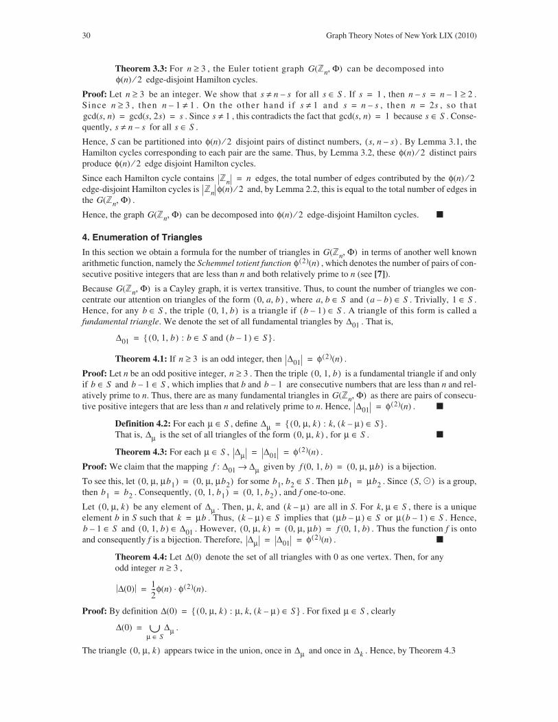
30 Graph Theory Notes of New York LIX (2010)
Theorem 3.3: For , the Euler totient graph can be decomposed into edge-disjoint Hamilton cycles.
Proof: Let be an integer. We show that for all . If , then .Since , then . On the other hand i f and , then , so that
. Since , this contradicts the fact that because . Conse-quently, for all .
Hence, S can be partitioned into disjoint pairs of distinct numbers, . By Lemma 3.1, theHamilton cycles corresponding to each pair are the same. Thus, by Lemma 3.2, these distinct pairsproduce edge disjoint Hamilton cycles.
Since each Hamilton cycle contains edges, the total number of edges contributed by the edge-disjoint Hamilton cycles is and, by Lemma 2.2, this is equal to the total number of edges inthe .
Hence, the graph can be decomposed into edge-disjoint Hamilton cycles. �
4. Enumeration of Triangles
In this section we obtain a formula for the number of triangles in in terms of another well knownarithmetic function, namely the Schemmel totient function , which denotes the number of pairs of con-secutive positive integers that are less than n and both relatively prime to n (see [7]).
Because is a Cayley graph, it is vertex transitive. Thus, to count the number of triangles we con-centrate our attention on triangles of the form , where and . Trivially, .Hence, for any , the triple is a triangle if . A triangle of this form is called afundamental triangle. We denote the set of all fundamental triangles by . That is,
Theorem 4.1: If is an odd integer, then .
Proof: Let n be an odd positive integer, . Then the triple is a fundamental triangle if and onlyif and , which implies that b and are consecutive numbers that are less than n and rel-atively prime to n. Thus, there are as many fundamental triangles in as there are pairs of consecu-tive positive integers that are less than n and relatively prime to n. Hence, . �
Definition 4.2: For each , define That is, is the set of all triangles of the form , for . �
Theorem 4.3: For each , .
Proof: We claim that the mapping given by is a bijection.
To see this, let for some . Then . Since is a group,then . Consequently, , and f one-to-one.
Let be any element of . Then, μ, k, and are all in S. For , there is a uniqueelement b in S such that . Thus, implies that or . Hence,
and . However, . Thus the function f is ontoand consequently f is a bijection. Therefore, . �
Theorem 4.4: Let denote the set of all triangles with 0 as one vertex. Then, for anyodd integer ,
Proof: By definition . For fixed , clearly
.
The triangle appears twice in the union, once in and once in . Hence, by Theorem 4.3
n 3≥ G �n Φ,( )φ n( ) 2⁄
n 3≥ s n s–≠ s S∈ s 1= n s– n 1– 2≥=n 3≥ n 1– 1≠ s 1≠ s n s–= n 2s=
gcd s n,( ) gcd s 2s,( ) s= = s 1≠ gcd s n,( ) 1= s S∈s n s–≠ s S∈
φ n( ) 2⁄ s n s–,( )φ n( ) 2⁄
φ n( ) 2⁄�n n= φ n( ) 2⁄
�n φ n( ) 2⁄G �n Φ,( )
G �n Φ,( ) φ n( ) 2⁄
G �n Φ,( )φ 2( ) n( )
G �n Φ,( )0 a b, ,( ) a b, S∈ a b–( ) S∈ 1 S∈
b S∈ 0 1 b, ,( ) b 1–( ) S∈Δ01
Δ01 0 1 b, ,( ) : b S and b 1–( ) S∈∈{ }.=
n 3≥ Δ01 φ 2( ) n( )=
n 3≥ 0 1 b, ,( )b S∈ b 1– S∈ b 1–
G �n Φ,( )Δ01 φ 2( ) n( )=
μ S∈ Δμ 0 μ k, ,( ) : k k μ–( ), S∈{ }.=Δμ 0 μ k, ,( ) μ S∈
μ S∈ Δμ Δ01 φ 2( ) n( )= =
f : Δ01 Δμ→ f 0 1 b, ,( ) 0 μ μb, ,( )=
0 μ μb1, ,( ) 0 μ μb2, ,( )= b1 b2, S∈ μb1 μb2= S �,( )b1 b2= 0 1 b1, ,( ) 0 1 b2, ,( )=
0 μ k, ,( ) Δμ k μ–( ) k μ, S∈k μb= k μ–( ) S∈ μb μ–( ) S∈ μ b 1–( ) S∈
b 1– S∈ 0 1 b, ,( ) Δ01∈ 0 μ k, ,( ) 0 μ μb, ,( ) f 0 1 b, ,( )= =Δμ Δ01 φ 2( ) n( )= =
Δ 0( )n 3≥
Δ 0( ) 12---φ n( ) φ 2( ) n( ).⋅=
Δ 0( ) 0 μ k, ,( ) : μ k k μ–( ), , S∈{ }= μ S∈
Δ 0( ) Δμμ S∈∪=
0 μ k, ,( ) Δμ Δk

B. Maheswari and L. Madhavi: Enumeration of Hamilton cycles and triangles in Euler totient Cayley graphs 31
�
Theorem 4.5: For any integer the total number of triangles in is given by
Proof: If n is even, then by Corollary 2.7, . Thus, let n be an odd positive integer. is ver-tex transitive and -regular. Thus, the same number of triangles passes through each vertex and this num-ber is . Therefore, because has order n, the total number of triangles in is
.
However, each triangle in is counted three times (once for each of its three vertices). Thus, thenumber of distinct triangles in is given by
�
References
[1] P. Berrizbeitia and R.E. Giudici; Counting pure k-cycles in sequences of Cayley graphs, Discrete Math., 149, 11–18(1996).
[2] P. Berrizbeitia and R.E. Giudici; On cycles in the sequence of unitary Cayley graphs. Reporte Techico No. 01-95,Universidad Simon Bolivar, Dpto. de Mathematicas, Caracas, Venezuela (1995).
[3] I. Dejter and R.E. Giudici; On unitary Cayley graphs, JCMCC, 18, 121–124 (1995).
[4] L. Madhavi and B. Maheswari; Enumeration of Hamilton cycles and triangles in quadratic residue Cayley graphs,Chamchuri J. Math., 1(1), 95–103 (2009).
[5] T.M. Apostol; Introduction to Analytic Number Theory, Springer International, Student Edition (1989).
[6] J.A. Bondy and U.S.R. Murty; Graph Theory with Applications, Macmillan, London (1976).
[7] E. Dickson; History of Theory of Numbers, Vol. 1, Chelsea Publishing Company (1952).
Received: July 25, 2008Revised: July 14, 2009
Δ 0( ) 12--- Δμ
μ S∈∑=
12--- φ 2( ) n( )
μ S∈∑=
12---φ 2( ) n( ) S⋅ 1
2---φ n( ) φ 2( ) n( ).⋅= =
n 3≥ T Φ( )G �n Φ,( )
T Φ( )0 if n is even16---nφ n( )φ 2( ) n( ) if n is odd.⎩
⎨⎧
=
T Φ( ) 0= G �n Φ,( )φ n( )
12---φ n( )φ 2( ) n( ) G �n Φ,( ) G �n Φ,( )
12---nφ n( )φ 2( ) n( )
G �n Φ,( )T Φ( ) G �n Φ,( )
T Φ( )0 if n is even16---nφ n( )φ 2( ) n( ) if n is odd.⎩
⎨⎧
=

Graph Theory Notes of New York LIX, 32–41 (2010)The Mathematical Association of America.
[GTN LIX:5] ON FRACTIONAL EFFICIENT DOMINATING SETS OF GRAPHS
K. Reji Kumar1 and Gary MacGillivray21Department of MathematicsN.S.S. College, Pandalam - 689 501, INDIA<[email protected]>
2Department of Mathematics and StatisticsUniversity of Victoria, BC, CANADA<[email protected]>
AbstractA dominating function or a fractional dominating set of a graph is a function
such that for all , the sum of the function values over the closed neighborhoodof v is at least one. A minimal dominating function or a fractional minimal dominating set f is a frac-tional dominating set such that f is not a fractional dominating set if for any the value of can be decreased. A function f is called a fractional independent set if , for everyvertex v with . An independent function f is called a maximal fractional independent set, if
for every with . A set is a perfect dominating set if forevery vertex , . A perfect dominating set S is minimal, if no proper subsetof S is a perfect dominating set. We define the fractional version of minimal perfect dominating setand make a comparative study of various subsets of the fractional minimal dominating sets of a graph.
1. Introduction
In this paper represents an undirected graph with no loop or multiple edge. For graph theoreticterms that are not defined here refer to West [1]. In this section we discuss basic definitions and results. A sub-set D of the vertex set of a graph G, is called a dominating set if for any ,where is the closed neighborhood of vertex v. A dominating set D is a minimal dominating set, if noproper subset of D is a dominating set. More than one thousand research papers have been published onapproximately one hundred variations of domination in graphs. Almost all versions of dominating sets andtheir properties, are discussed by Haynes, Slater, and Hedetniemi in [2]. Another text by the same authors [3],discusses almost all advanced topics in this area and contains many comprehensive survey articles. The frac-tional version of a dominating set is popularly known as a dominating function of a graph and isdefined as a function such that
for all . A minimal dominating function is a dominating function f such that f is not a dominating func-tion if for any the value of is decreased. In this paper, we call these functions fractional domi-nating sets and fractional minimal dominating sets, respectively. For any dominating function of G,
.
The boundary of f denoted by Bf is
.
The positive set of f, denoted by Pf is . For any two subsets A and B of V, we say that Adominates B (denoted by ) if each vertex in is adjacent to some vertex in A. The fractional dom-inating number of a graph G, denoted by
G V E,( )=f : V 0 1,[ ]→ v V∈
v V∈ f v( )Σx N v[ ]∈ f x( ) 1=
f v( ) 0>Σx N v[ ]∈ f x( ) 1≥ v V∈ f v( ) 0= S V⊆
v V S–∈ N v( ) S∩ 1=
G V E,( )=
V G( ) N v[ ] D∩ ∅≠ v V D–∈N v[ ]
G V E,( )f : V 0 1,[ ]→
f x( )x N v[ ]∈
∑ 1≥
v V∈v V∈ f v( )
f : V 0 1,[ ]→
f N v[ ]( ) f x( )x N v[ ]∈
∑=
v V∈ : f x( )x N v[ ]∈
∑ 1=⎩ ⎭⎨ ⎬⎧ ⎫
v V∈ : f v( ) 0>{ }A B→ B A–

K.R. Kumar and G. MacGillivray: On fractional efficient dominating sets of graphs 33
The set of all fractional minimal dominating sets of a graph G is denoted by . The following theoremprovides a way to identify fractional minimal dominating sets of a given graph.
Theorem 1.1 [4]: A fractional dominating set f of a graph G is a fractional minimal dominating set if and only if . �
A convex combination of two fractional minimal dominating sets f and g of G is , where. Because any convex combination of two fractional dominating sets is a fractional dominating set,
the set of all fractional dominating sets is a convex set. However, it is evident from the following theorem thatthe convex combination of two fractional minimal dominating sets need not always be a fractional minimaldominating set. The next theorem offers a necessary and sufficient condition for a convex combination of twofractional minimal dominating sets to be minimal.
Theorem 1.2 [4]: A convex combination of two fractional minimal dominating sets f and gis minimal if and only if . �
In this context Cockayne et al. [4] introduced the concept of a universal fractional minimal dominating set. Afractional minimal dominating set of G is called a universal fractional minimal dominating set if and only ifits convex combination with any other fractional minimal dominating set is minimal.
Theorem 1.3 [4]:
1. If the fractional minimal dominating set g satisfies and if for any fractional minimal dominating set f, Bf dominates V, then g is a universal fractional minimal dominating set.
2. If g is a universal fractional minimal dominating set, then Bg dominates V. �
To continue with our characterization of universal fractional minimal dominating sets we require the follow-ing definitions.
Definitions: A vertex is said to absorb the vertex , and u is said to be absorbedby v, if . In this case, v is called an absorbing vertex and u is called anabsorbed vertex.
Let A = { : v is an absorbing vertex} and Ω = { : u is an absorbed vertex}. Avertex w of a graph G is said to be f-sharp, where f is an fractional minimal dominating setof G, if . Furthermore, w is said to be sharp if w is f-sharp, for some frac-tional minimal dominating set f of G. �
Lemma 1.4 [4]: Let f be an fractional minimal dominating set of G and let w be an f-sharpvertex. Then1. If with a vertex absorbed by v, then ;2. ; and3. . �
Theorem 1.5 [5]: The fractional minimal dominating set g of a graph is auniversal fractional minimal dominating set if and only if1. and2. for each sharp vertex w of G. �
Theorem 1.2 can be extended to a finite number of fractional minimal dominating sets. Thus, we obtain thefollowing generalization.
Theorem 1.6 [6]: A convex combination of n fractional minimal dominating sets is minimal if and only if .
�
The fact that the set of fractional dominating sets is convex and some fractional dominating sets cannot beexpressed as a convex combination of two or more fractional dominating sets motivates the definition of basic
γ f G( ) min f x( )x V∈∑ : f is a fractional mimimal dominating set of G
⎩ ⎭⎨ ⎬⎧ ⎫
.=
FD G( )
B f P f→hλ λf 1 λ–( )g+=
0 λ 1< <
B f Bg∩ P f Pg∪→
Bg V=
v V∈ u v≠N u[ ] N v[ ]⊂
v V∈ u V∈
B f N w[ ]∩ A⊆
v B f N w[ ]∩∈ u Ω A–∈ w N u[ ]∉w B f∉f w( ) 0=
G V E,( )=
V A– Bg⊆g w( ) 0=
f 1 f 2 … f n, , , B f 1B f 2
… B f n∩ ∩ ∩ P f 1
P f 2… P f n
∪ ∪ ∪→

34 Graph Theory Notes of New York LIX (2010)
fractional dominating sets and basic fractional minimal dominating sets [6]. A fractional minimal dominatingset is called a basic fractional minimal dominating set if it cannot be expressed as a proper convex combina-tion of two distinct fractional minimal dominating sets. Kumar et al. [7] presented a necessary and sufficientcondition for a fractional minimal dominating set to be a basic fractional minimal dominating set. Based onthis condition they developed an algorithm to determine whether a given fractional minimal dominating setis basic.
Theorem 1.7 [7]: Let f be a fractional minimal dominating set. The function f is a basicfractional minimal dominating set if and only if there does not exist a fractional minimaldominating set g such that and . �
Theorem 1.8 [7]: Let f be a fractional minimal dominating set of a graph with and . Let
be an matrix defined by
Consider the system of linear equations
(1) , for .
Then the function f is a basic fractional minimal dominating set if and only ifEquation (1) has only a trivial solution. �
Corollary 1.9 [7]: If for all , then the fractional minimal dominating set f of G is a basic fractional minimal dominating set. �
A set is called an independent set of a graph G, if no pair of vertices of S is adjacent in G. A maximalindependent set of G is an independent set S such that there does not exist another independent set S′ that prop-erly contains S. In [6] Kumar suggested a definition for the fractional versions of both independent sets andmaximal independent sets.
A function is called a fractional independent set if for every vertex v with ,. A fractional independent set f is called a maximal fractional independent set if for every
with , . The set of all maximal fractional independent sets is denoted byFI. We observe that if S is (a maximal) an independent set in G, then is (a maximal) a fractional inde-pendent set.
Theorem 1.10 [8]: A function f is a fractional independent set if and only if . �
A convex combination of two maximal fractional independent sets f and g is defined by ,where . A characterization of convex maximal fractional independent sets is provided by the nextresult.
Lemma 1.11 [8]: A convex combination of two maximal fractional independent sets f and g is a maximal fractional independent set if and only if . �
A maximal fractional independent set f is said to be a basic maximal fractional independent set if there do notexist two maximal fractional independent sets f and g, and , such that . Thecharacteristic function of a single vertex subset of is a basic maximal fractional independent set of Kn,the complete graph of order n.
Theorem 1.12 [8]: A maximal fractional independent set f of G is basic if and only if thereis no other maximal fractional independent set g such that and . �
A maximal fractional independent set f is said to be a universal maximal fractional independent set, if a con-vex combination of f with any other maximal fractional independent set is a maximal fractional independentset. The set of all universal maximal fractional independent sets is denoted by FUI.
B f Bg= P f Pg=
G V E,( )=B f v1 v2 … vm, , ,{ }= P f u V∈ : 0 f u( ) 1< <{ } u1 u2 … un, , ,{ }= =
A aij( )= m n×
aij
1 if v j is adjacent to u j or v j u j=
0 otherwise.⎩⎨⎧
=
aijx jj
∑ 0= 1 i m≤ ≤
f v( ) 0 1,[ ]∈ v V∈
S V⊆
f : V 0 1,[ ]→ f v( ) 0>Σx N v[ ]∈ f x( ) 1=v V∈ f v( ) 0= Σx N v[ ]∈ f x( ) 1≥
f χS=
P f B f⊆
hλ λf 1 λ–( )g+=0 λ 1< <
P f Pg∪ B f Bg∩⊆
λ 0 1,( )∈ h λf 1 λ–( )g+=V Kn( )
B f Bg= P f Pg=
K.R. Kumar and G. MacGillivray: On fractional efficient dominating sets of graphs 35
Lemma 1.13 [8]: If f is a universal maximal fractional independent set of a graph G,then . �
Corollary 1.14 [8]: If f is a universal maximal fractional independent set of G, then
,
where the intersection is taken over all maximal fractional independent sets of G. �
A characterization of graphs that have a universal maximal fractional independent set is provided in [8].
Theorem 1.15 [8]: A graph G has a universal maximal fractional independent set if andonly if there exists a unique partition of V into sets that induce maximal cliques. �
The graphs that admit a universal maximal fractional independent set can be constructed from a disjoint unionof t cliques (possibly of different sizes), . For each i, , select a non-empty subset
and any subset of edges joining vertices in
The graph induced by these edges admits a universal maximal fractional independent set.
2. Minimal Fractional Perfect Dominating Sets and Fractional Efficient Dominating Sets
A set is called a perfect dominating set if, for every vertex , . Yen and Lee[9] proved that, given a positive integer k, the problem of deciding if a graph G has a perfect dominating setof cardinality at most k is NP-complete. A fractional perfect dominating set of G is defined to be a function
such that if and if . A fractional perfect dom-inating set is a minimal fractional perfect dominating set if it is a fractional minimal dominating set.
Theorem 2.1: A fractional perfect dominating set f is minimal, if and only if .�
A convex combination of two fractional perfect dominating sets f and g, is always a frac-tional perfect dominating set. Thus, the set of all fractional perfect dominating sets is a convex set. However,as the following theorem states, a convex combination of two minimal fractional perfect dominating sets maynot be minimal. A minimal fractional perfect dominating set is a universal minimal fractional perfect domi-nating set if its convex combination with any other minimal fractional perfect dominating set is minimal. Thecondition for minimality of a convex combination is given in the following result, which shows that the set ofall minimal fractional perfect dominating sets is not in general convex.
Theorem 2.2: A convex combination of two minimal fractional perfect dominating sets fand g is minimal, if and only if . �
Theorem 2.3: If f is an minimal fractional perfect dominating set of G, then .
Proof: Since f is minimal, . By definition of fractional perfect dominating set, if , then. Hence, . �
Theorem 2.4: If a graph G has an minimal fractional perfect dominating set f with, then f is a universal minimal fractional perfect dominating set.
Proof: Let g be any minimal fractional perfect dominating set of G. Then and since ,. Thus, the convex combination f and g is an minimal fractional perfect dom-
inating set. Hence, f is a universal minimal fractional perfect dominating set. �
A minimal fractional perfect dominating set of a graph G is a basic minimal fractional perfect dominating setif it cannot be expressed as a convex combination of two or more minimal fractional perfect dominating sets.The following results reveal the relationship between the set of all basic fractional minimal dominating setsand the set of all basic minimal fractional perfect dominating sets of a graph.
B f V=
P f Bgg
∩
G1 G2 … Gt, , , 1 i t≤ ≤Xi V Gi( )⊆
Xii 1=
t
∪ .
S V⊆ v V S–∈ N v( ) S∩ 1=
f : V 0 1,[ ]→ f N v[ ]( ) 1≥ f v( ) 0> f N v[ ]( ) 1= f v( ) 0=
B f P f→
hλ λf 1 λ–( )g+=
B f Bg∩ P f Pg∪→
B f V G( )→
B f P f→ f v( ) 0=f N v[ ]( ) 1= B f V P f–( )→
B f V G( )=
Bg V→ B f V G( )=B f Bg∩ V Bg∩ Bg V→= =
36 Graph Theory Notes of New York LIX (2010)
Theorem 2.5: If a basic fractional minimal dominating set f of a graph G is a minimal per-fect dominating set, then it is a basic minimal fractional perfect dominating set.
Proof: Suppose, f is not a basic minimal fractional perfect dominating set. Then , where and each fi is a minimal fractional perfect dominating set. This shows that f is a convex combina-
tion of two or more fractional minimal dominating sets, which is a contradiction. �
Theorem 2.6: If f is a basic minimal fractional perfect dominating set, then f is a basic fractional minimal dominating set.
Proof: Let f be a basic minimal fractional perfect dominating set and suppose that it is not a basic fractionalminimal dominating set. Then there exist fractional minimal dominating sets such that
, where . The boundary and the positive set of f are and ,respectively. Thus, there exist infinitely many fractional minimal dominating sets whose boundary andpositive sets are same as that of f. Hence, these fractional minimal dominating sets are minimal fractionalperfect dominating sets. We can select two minimal fractional perfect dominating sets g1 and g2 such that
. Therefore, f can be expressed as a convex combination of at least two minimal frac-tional perfect dominating sets, a contradiction. �
Lemma 2.7: If a minimal fractional perfect dominating set h is a convex combination oftwo fractional minimal dominating sets f and g and f is not an minimal fractional perfectdominating set, then there exists some such that and .
Proof: Since f is not a minimal fractional perfect dominating set, there exists such that and. Thus, . Now suppose . Since h is a minimal fractional perfect dominating set, v
must be an element of Bh, which is a contradiction. �
If, for a graph G, there exists a set of basic minimal fractional perfect dominating sets, say, such that every minimal fractional perfect dominating set of the graph is a convex
combination of a subset of B, then the set of all minimal fractional perfect dominating sets is closed. The nextresult discusses the possibility of the set of all minimal fractional perfect dominating sets being closed.
Lemma 2.8: If there exists a minimal fractional perfect dominating set h, of a graph G suchthat if h can be expressed as a convex combination of a set of fractional minimal dominatingsets that are not all minimal fractional perfect dominating sets, then the set of all minimalfractional perfect dominating sets of G is not a closed set.
Proof: Let the minimal fractional perfect dominating set h be a convex combination of a set of fractional min-imal dominating sets say such that f1 is not a minimal fractional perfect dominating set. If
, let . The function g is a minimal fractional perfect dominating set. Define asequence of real numbers such that . Let . Since each hj is a convexcombinations of fis, it is a minimal fractional perfect dominating set. Furthermore, and f1 is not inthe set of all minimal fractional perfect dominating sets. Consequently, the set is not closed. �
Next we discuss an example of a graph whose set of minimal fractional perfect dominating sets is open.
Example: Let , where . Let the vertex set of G be . Consider thefunctions f1 and f2 defined by , , , and for . f1and f2 are the only two basic fractional minimal dominating sets and all other fractional minimal dominatingsets are convex combinations of these two basic fractional minimal dominating sets. Furthermore, all frac-tional minimal dominating sets except f2 are minimal fractional dominating sets of G. Hence, the set of allminimal fractional perfect dominating sets of G is not closed.
Theorem 2.9: Let g be a fractional minimal dominating set of a graph G such that is g-sharp. Then g is not a universal minimal fractional perfect dominating set.
Proof: Let g be a fractional minimal dominating set of a graph G such that is g-sharp. Suppose thatg is a universal minimal fractional perfect dominating set. Then, by definition of minimal fractional perfectdominating set, all with must be in Bg. Thus, by Lemma 1.4, and , whichis a contradiction. �
f Σiλi f i=Σiλi 1=
f 1 f 2 … f r, , ,f Σiλi f i= Σiλi 1= B f ∩iB f i
= P f ∩iP f i=
f λg1 1 λ–( )g2+=
v V∈ f v( ) 0= h v( ) 0>
v V∈ f v( ) 0=v B f∉ v Bh∉ h v( ) 0=
B f 1 f 2 … f r, , ,{ }=
f 1 f 2 … f r, , ,{ }h Σiλi f i= g Σi 2≥ λi f i=
λ1 j( ) λ1 j 1→ h j λ1 j f 1 1 λ1 j–( )g+=h j f 1→
G K1 n,= n 2≥ V G( ) v v1 v2 … vn, , , ,{ }=f 1 v( ) 1= f 1 vi( ) 0= f 2 v( ) 0= f 2 vi( ) 1= i 1 2 … n, , ,=
w V G( )∈
w V G( )∈
v V∈ g v( ) 0= g w( ) 0= w Bg∉

K.R. Kumar and G. MacGillivray: On fractional efficient dominating sets of graphs 37
According to the definition given by Bang et al. [10][11], a dominating set S of G is called an efficient dom-inating set of G if the closed neighborhood of every vertex in V has exactly one vertex of S. Equivalently, Sis an efficient dominating set if S dominates G and the distance between any two elements of S is at least three.Grinstead and Slater [12] introduced the idea of fractional efficient domination. A fractional efficient domi-nating set of a graph is a dominating function such that forall . If f is a fractional efficient dominating set, then . Thus, every fractional efficientdominating set of a graph G is a fractional minimal dominating set. Grinstead and Slater [12] also proved that,if f is a fractional efficient dominating set of G, then . It is interesting to note thatthe conditions for minimal fractional perfect dominating set and the conditions for maximal fractional inde-pendent set together give the conditions for fractional efficient dominating set. A fractional efficient domi-nating set f of G is a positive fractional efficient dominating set if . For convenience, denote the setof all fractional efficient dominating sets of G by . Additionally, let and denote theset of all minimal fractional perfect dominating sets and the set of all positive fractional efficient dominatingsets, respectively. Then . We note the following:
Observation 2.10: The set of all positive fractional efficient dominating sets and the set of all maximal frac-tional independent sets are subsets of the set of all fractional minimal dominating sets.
Observation 2.11: If a function is both a positive fractional efficient dominating set and a maximal fractionalindependent set, then it is a fractional efficient dominating set.
Observation 2.12: If f is a universal maximal fractional independent set of G, then f is a fractional efficientdominating set.
These observations are summarized in the following figure.
A convex combination of two fractional efficient dominating sets f and g is minimal if and only if → . Naturally, there exists a fractional efficient dominating set that cannot be expressed as a convexcombination of two or more fractional efficient dominating sets. Such functions are basic fractional efficientdominating sets. The next result characterizes basic fractional efficient dominating sets of a graph.
Theorem 2.13: A fractional efficient dominating set f of a graph G is a basic fractionalefficient dominating set if and only if there exists no other fractional efficient dominatingset g such that .
Proof: Let f be a basic fractional efficient dominating set and suppose there exists an fractional efficient dom-inating set g with the property . Because f and g are maximal fractional independent sets, then byTheorem 1.12, f is not a basic maximal fractional independent set. Consequently, there exists a set of maximalfractional independent sets such that , , and . Since
, then for all i, and hence, for all i. Thus, each fi is a fractional efficient domi-nating set. This contradicts the fact that f is a basic fractional efficient dominating set.
Conversely, suppose there is no fractional efficient dominating set g such that and , andthat f is not a basic fractional efficient dominating set. Then, by definition of basic fractional efficient domi-nating set, there exists a set of fractional efficient dominating sets such that
, where and . Furthermore, and . SinceNow for , and are fractional efficient dominating sets with and .This is a contradiction.
�
G V E,( )= f : V 0 1,[ ]→ Σx N v[ ]∈ f x( ) 1=v V∈ B f V P f→=
γ G( ) f Σx V∈ f x( )= =
P f V=FE G( ) FPE G( ) FMP G( )
FPE G( ) FMP G( )∩ FE G( )=
Figure
B f Bg∩P f Pg∪
P f Pg=
P f Pg=
f 1 f 2 … f r, , ,{ } f Σiλi f i= B f ∩iB f i= P f ∪iP f i
=B f V= B f i
V= P f iB f i
⊆
B f Bg= P f Pg=
f 1 f 2 … f r, , ,{ }f hλ1
Σiλi f i= = Σiλi 1= 0 λi 1< < B f ∩iB f i= P f ∪iP f i
=λ11 λ12≠ hλ11
hλ12Bhλ1i
B f= Phλ1i
P f=

38 Graph Theory Notes of New York LIX (2010)
Theorem 2.14: Every fractional efficient dominating set of G is a maximal fractional independent set.
Proof: If f is a fractional efficient dominating set of G, then and . Thus, , andhence, f is an maximal fractional independent set of G. �
A convex combination of two fractional efficient dominating sets (positive fractional efficient dominatingsets) f and g of a graph G is a function , where . A positive fractional efficientdominating set f is a basic positive fractional efficient dominating set if it is not a convex combination of twoor more positive fractional efficient dominating sets. Let f be a fractional efficient dominating set of G. Wedefine
and .
Lemma 2.15: If f is a positive fractional efficient dominating set of G, then
1. , and
2. .
Proof: The first statement follows from the definition of positive fractional efficient dominating set.
To prove Statement 2, suppose that f is a positive fractional efficient dominating set of G and .Because f is a fractional minimal dominating set, . Let . Since and , there exists such that . This contradicts the premise .
�
Theorem 2.16: If a graph G has a basic positive fractional efficient dominating set, then Ghas no other positive fractional efficient dominating set.
Proof: Suppose a graph G has a basic positive fractional efficient dominating set f and another positive frac-tional efficient dominating set g. Since and , the systems of equations corre-sponding to f and g are the same. Thus, by Theorem 1.7, we obtain a system of equations that hassimultaneously a unique solution and infinitely many solutions, a contradiction. �
Corollary 2.17: If a graph G has two positive fractional efficient dominating sets, then Ghas no basic positive fractional efficient dominating set. �
Theorem 2.18: The set of all fractional efficient dominating sets and the set of all positivefractional efficient dominating sets of a graph G are convex.
Proof: Let f and g be two fractional efficient dominating sets of a graph G and let be theirconvex combination. Then, . Consequently, h is an fractional efficient dominating set.
Similarly, let f and g be two positive fractional efficient dominating sets of G and let h be their convex com-bination. Then, h is a fractional efficient dominating set. Furthermore, . Hence, h is apositive fractional efficient dominating set. �
Theorem 2.19: Let G be a graph such that . Then is a closedsubset of .
Proof: By Theorem 2.18, is a convex set. First, we show that if a fractional efficient dominating set
f of G is a convex combination of a set of fractional minimal dominating sets, say , then fi isa fractional efficient dominating set for all i.
We know that for all i. Thus, for all i, and hence, each fi is a fractionalefficient dominating set. The rest of the proof follows easily. �
Now we prove that if is not a singleton set, then is an open set. For this we need the fol-lowing definitions from [6]. Let f and g be two fractional minimal dominating sets of a graph G, with
and . Let i be any real number and let . Clearly and .Now, let S be the subset of the set of real numbers � defined by
In general, hi is not a fractional dominating set because hi becomes negative for large values of i.
B f V= P f V⊆ P f B f⊆
h λf 1 λ–( )g+= 0 λ 1< <
C0 f( ) v V∈ : f v( ) 0={ }= C1 f( ) v V∈ : f v( ) 1={ }=
C0 f( ) ∅=
C1 f( ) ∅=
x C1 f( )∈B f N x( )∩( ) ∅≠ y B f N x( )∩∈ N y( ) 2≥
x N y( )∈ z N y( )∈ f z( ) 0= C0 f( ) ∅=
B f Bg V= = P f Pg V= =
h λf 1 λ–( )g+=Bh B f Bg∩ V= =
Ph P f Pg∪ V= =
FE G( ) ∅≠ FE G( )FD G( )
FE G( )
f 1 f 2 … f r, , ,{ }
V B f ∩iB f iB f i
⊆= = B f iV=
FPE G( ) FPE G( )
B f Bg= P f Pg= hi 1 i+( )g if–= h0 g= h 1– f=
S i : i �∈ hi is a fractional dominating set such that BhiBg= and Phi
Pg=,{ }.=
K.R. Kumar and G. MacGillivray: On fractional efficient dominating sets of graphs 39
Lemma 2.20 [6]: If , then hi is a fractional minimal dominating set of G. �
Lemma 2.21 [6]: S is a bounded open interval of �. �
It may be noted that for any hi, where is a convex combination of two fractional minimal dominatingsets hk and hl, where , the set is an open set.
Theorem 2.22: Let G be a graph such that contains at least two elements. Then, is an open subset of .
Proof: First, we claim that if f and g are two partial fractional efficient dominating sets of a graph G, then any, , is a positive fractional efficient dominating set. For all , hi is a fractional
minimal dominating set. Additionally, and . Thus, hi is a positive fractionalefficient dominating set. Now, by the remark given above, any hi, where , is a convex combination oftwo positive fractional efficient dominating sets hk and hl, where . Hence, for every positive fractionalefficient dominating set f, there exists an open subset of . �
Proposition 2.23: If a graph G contains two vertices u and v such that , then for all , where f is any fractional efficient dominatingset of G.
Proof: Let f be a fractional efficient dominating set of G. Then, by definition of fractional efficient dominat-ing set, . Also, = = 1. Hence, for all . �
Corollary 2.24: If a graph G contains two vertices u and v such that , then G has no positive fractional efficient dominating set f with . �
Theorem 2.25: A positive fractional efficient dominating set f of a graph G is a universalmaximal fractional independent set, if and only if the set of all maximal fractional indepen-dent sets and the set of all fractional efficient dominating sets are equal.
Proof: Suppose that a positive fractional efficient dominating set f of G is a universal maximal fractionalindependent set. Then, by Corollary 1.14, , where the intersection is taken over all maximalfractional independent sets of G. Thus, for any maximal fractional independent set, g, of G. Hence,g is an fractional efficient dominating set.
Conversely, suppose that any maximal fractional independent set, g, is an fractional efficient dominating setof G. Then, . If f and g are two different maximal fractional independent sets of G, then
. Thus, any convex combination of f and g is a maximal fractional independent set.Consequently, is a convex set.
In other words, the set of all maximal fractional independent sets and the set of all universal maximal frac-tional independent sets are equal. Since, , it follows that . �
Theorem 2.26: Every fractional efficient dominating set of a graph G is a universalminimal fractional perfect dominating set of G.
Proof: Let f be a fractional efficient dominating set of G. Then . Let g be any minimal fractional per-fect dominating set of G. Then Bg dominates V and . Consider h, a convex combination of f andg. Then and Bg dominates V. Thus, h is a fractional minimal dominating set. Since
and , h is a minimal fractional perfectdominating set. This shows that f is a universal minimal fractional perfect dominating set. �
There are many classes of graphs having at least one fractional efficient dominating set. The following con-struction is useful for a class of graphs that have no fractional efficient dominating set. Let H be a graph con-taining a vertex v such that there exist three vertices u1, u2, and w such that , , for
, and , and . Let F be the class of all graphs having the aboveproperty. In the next theorem, we prove that the graphs in F have no fractional efficient dominating set.
i S∈
i S∈l k, S∈ hi : i S∈{ }
FPE G( )FPE G( ) FD G( )
hi 1 i+( )g if–= i S∈ i S∈Bhi
Bg V= = PhiPg V= =
i S∈l k, S∈
FPE G( )
N u[ ] N v[ ]⊂f x( ) 0= x N v[ ] N u[ ]–( )∈
f N v[ ]( ) f N u[ ]( ) 1= = f N v[ ]( ) f N u[ ]( ) Σx N v[ ] N u[ ]–( )∈ f x( )+ f x( ) 0=x N v[ ] N u[ ]–( )∈
N u[ ] N v[ ]⊂B f P f V= =
P f V ∩gBg⊆=Bg V=
Bg V=P f Pg∪ B f Bg∩⊆ V=
FI G( )
FPE G( ) FI G( )⊆ FPE G( ) FUI G( )⊆
B f V=V Pg– Bg⊆
Bh B f Bg∩ Bg= =V Ph– V Pg–( ) V P f–( )∩= V Ph–( ) V Pg–( ) Bg⊆ ⊆ Bh=
N ui[ ] 2≥ N ui[ ] N v[ ]⊆i 1 2,= N u1[ ] N u2[ ]∩ v{ }= N w( ) N v( )⊆

40 Graph Theory Notes of New York LIX (2010)
Theorem 2.27: If , then G has no fractional efficient dominating set.
Proof: Let and let be a vertex such that there exist vertices u1, u2, and w satisfying theconditions given above. Suppose that f is a fractional efficient dominating set of G. We claim that .By definition of F, and . If , then for some x ∈
, where . Thus, , which contradicts thefact that f is a fractional efficient dominating set. Consequently, for all and since
, . Because there is a vertex that is adjacent to both v and w, then for some , a contradiction. �
The classes of graphs that admit universal maximal fractional independent sets are known. By Theorem 2.25,the set of all graphs G, such that must be a subset of this class.
Theorem 2.28: Let G be a graph. Then if and only if G is a disjointunion of t disjoint cliques (possibly of different orders).
Proof: By Theorem 1.15 a graph G has a universal maximal fractional independent set if and only if thereexists a unique partition of V into sets that induces maximal cliques. If G belongs to this class and is notthe disjoint union of t disjoint cliques, there exist two vertices u and v such that . Thus, byTheorem 2.27, G cannot have any positive fractional efficient dominating set. Hence, .Proof of the converse is straightforward. �
3. Conclusion and Open Questions
Theorem 2.9 gives a sufficient condition for the set of all minimal fractional perfect dominating sets to be aproper subset of the set of all minimal fractional dominating sets. Whether this condition is necessary, is aninteresting question for further investigation. If a universal minimal fractional dominating set f is a minimalfractional perfect dominating set, then f is a universal minimal fractional perfect dominating set. Whether anygraph has a universal minimal fractional perfect dominating set that is not a universal minimal fractional dom-inating set is still unknown. If a graph G has a universal minimal fractional perfect dominating set does itguarantee the existence of a positive fractional efficient dominating set? Similarly, does the existence of apositive fractional efficient dominating set imply the existence of a universal minimal fractional perfect dom-inating set? Having characterized the graphs such that (see Theorem 2.28) is it possible tocharacterize those graphs having at least one fractional efficient dominating set as well as those graphs havingno fractional minimal dominating set other than fractional efficient dominating set?
4. Acknowledgements
Part of this research was completed when the first author visited the Department of Mathematics and Statis-tics, University of Victoria, BC, Canada with the financial support of the Department of Science and Tech-nology, India as a BOYSCAST fellow. He expresses his gratitude for all facilities provided and support givenby the Department of Mathematics and Statistics, University of Victoria.
References
[1] D.B. West; Graph Theory: An Introductory Course, Prentice Hall, New York (2002).
[2] T.W. Haynes, S.T. Hedetniemi, and P.J. Slater; Fundamentals of Domination in Graphs, Marcel Dekker, New York(1998).
[3] T.W. Haynes, S.T. Hedetniemi, and P.J. Slater; Domination in Graphs—Advanced Topics, Marcel Dekker, New York(1998).
[4] E.J. Cockayne, G. Fricke, S.T. Hedetniemi, and C.M. Mynhardt; Properties of minimal dominating functions ofgraphs, ARS Combinatoria., 41, 107–115 (1995).
[5] E.J. Cockayne, G. MacGillivray, and C.M. Mynhardt; Convexity of minimal dominating functions and universals ingraphs, Bull. Inst. Combin. Appl., 5, 37–48 (1992).
[6] K.R. Kumar; Studies in Graph Theory—Dominating Functions, Ph.D. Thesis, Manonmaniam Sundaranar University,Tirunelveli, India (2004).
[7] K.R. Kumar and S. Arumugam; Basic minimal dominating functions, Utilitas Mathematica, 77, 235–247 (2008).
G F∈G F∈ v V G( )∈
f v( ) 1=N u1[ ] N u2[ ]∩ v{ }= N u1[ ] 2≥ f v( ) 1< f x( ) 0>
N vi[ ] v{ }–( ) i 1 2,= f N v[ ]( ) f N u1[ ]( ) f N u2[ ]( ) f v( )–+ 1>=f x( ) 0= x v( )∈
f N w[ ]( ) 1= f w( ) 1= x N v( )∈f N x[ ]( ) 1> x N v( )∈
FE G( ) FI G( )=
FE G( ) FI G( )=G1 G2 … Gt, , ,
N u[ ] N v[ ]⊂FE G( ) FI G( )=
FE G( ) FI G( )=
K.R. Kumar and G. MacGillivray: On fractional efficient dominating sets of graphs 41
[8] K.R. Kumar, S. Arumugam, and G. MacGillivray; On maximal fractional independent sets in graphs, ARS Combina-toria, 87, 205–212 (2008).
[9] C.C. Yen and R.C.T. Lee; The weighted perfect dominating problem, Inform. Process. Lett., 35(6), 295–299 (1990).
[10] D.W Bang, A.E Barkauskas, and P. J. Slater; Disjoint dominating sets in trees, Sandia Laboratories Report, SAND78-1087J (1978).
[11] D.W. Bang, A.E. Barkauskas, and P. J. Slater; Efficient dominating sets in graphs, Applications of Discrete Mathe-matics, SIAM, Philandalphia, 189–199 (1988).
[12] D.L. Grinstead and P.J. Slater; Fractional domination and fractional packing graphs, Congr Numer., 71, 153–172(1990).
Received: November 3, 2009Revised: March 4, 2011

Graph Theory Notes of New York LIX The Mathematical Association of America (2010)
Aabsorb, vertex, 33all-negative path, 22antipodal distribution, 19
Bbasic
fractional minimal dominating set, 34maximal fractional independent set, 34minimal fractional perfect dominating set, 35
block, end, 10boundary, dominating function, 32branch, 10
CCartesian product, 16Cayley graph, 28
Euler totient, 28closed neighborhood, 32combination, convex, 33convex combination, 33cycle, Hamilton, 29
Ddegree
edge, 22negative, 22positive, 22
diameter, 9distance, 9
Steiner, 9distribution
antipodal, 19containment, 15reachable, 15solvable, 15vertex, 15
dominates, 32dominating function, 32
boundary, 32minimal, 32positive set, 32
dominating number, fractional, 32dominating set, 32
basic fractional minimal, 34efficient, 37fractional, 32
efficient, 37minimal, 32perfect, 35perfect minimal, 35
minimal, 32perfect, 35positive fractional efficient, 37universal fractional minimal, 33
Eeccentricity, 9edge
degree, 22negative, 22positive, 22
efficient dominating set, 37fractional, 37positive fractional, 37
end block, 10Euler totient
Cayley graph, 28function, 28
extreme vertex, 10
Ffractional
dominatingnumber, 32set, 32
efficient dominating set, 37positive, 37
independent set, 34basic maximal, 34maximal, 34
minimal dominating set, 32universal, 33
perfect dominating set, 35basic minimal, 35minimal, 35
functiondominating, 32Euler totient, 28minimal dominating, 32Schemmel totient, 30
fundamental triangle, 30
Ggeodesic, 9
HHamilton cycle, 29hypercube, 19
Iindependent set, 34
fractional, 34basic maximal, 34universal maximal, 34
maximal, 34maximal fractional, 34
LLemke graph, 18length
negative section, 22path, 22
line sigraph, 22
Mmaximal
fractional independent set, 34basic, 34universal, 34
independent set, 34
KEY-WORD INDEX
Graph Theory Notes of New York LIX (2010) 43
minimal
dominating function, 32
dominating set, 32
basic fractional, 34
fractional perfect dominating set, 35
basic, 35
Steiner set, 10
N
negation of sigraph, 22
negative
degree, 22
edge, 22
section, 22
length, 22
neighborhood, closed, 32
number
fractional dominating, 32
pebbling, 15, 15optimal, 15, 15
Steiner, 9t-pebbling, 15
optimal, 15upper Steiner, 10
O
odd two-pebbling property, 17
optimal
pebbling number, 15, 15t-pebbling number, 15
P
path, 22
all-negative, 22
length, 22
pebbles, 15
pebbling
move, 15
number, 15, 15optimal, 15, 15
property, 17
perfect dominating set, 35
basic minimal fractional, 35
fractional, 35
minimal fractional, 35
positive
degree, 22
edge, 22
fractional efficient dominating set, 37
set, dominating function, 32
product, Cartesian, 16
R
radius, 9regular sigraph, 22
S
Schemmel totient function, 30
section, negative, 22
sharp vertex, 33
signature, 22
signed graph (sigraph), 22
sigraph, 22
line, 22
negation, 22
regular, 22
size of pebble function, 15
Steiner
distance, 9number, 9
upper, 10
set, 9minimal, 10
tree, 9subset, symmetric, 28
symmetric subset, 28
T
totient function
Euler, 28
Scemmel, 30
t-pebbling number, 15
optimal, 15
tree, Steiner, 9triangle, fundamental, 30
two-pebbling property, 17
odd, 17
U
underlying graph, 22
universal
fractional minimal dominating set, 33
maximal fractional independent set, 34
upper Steiner number, 10
V
vertex
absorption, 33
distribution, 15
extreme, 10
sharp, 33

Graph Theory Notes of New York LIX The Mathematical Association of America (2010)
Subscription Request and Address Update Form
Please update/add the following information to the distribution list for future issues of
Graph Theory Notes of New York.
My/library mailing information is as follows:
Individual/Library Name:
Mailing Address:
Attention of (if Library):
Telephone Number:
e-mail address:
Date: Please check if this is an address update: ■
Please check if you are currently a member of the Mathematical Association of America ■
____________________________________________________
RETURN FORM TO: The Editors, Graph Theory Notes of New York:
Graph Theory Notes of New YorkMathematics DepartmentQueens College, CUNYKissena BoulevardFlushing, NY 11367, U.S.A.
For further informatione-mail: [email protected]
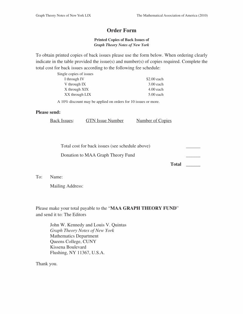
Graph Theory Notes of New York LIX The Mathematical Association of America (2010)
Order Form
Printed Copies of Back Issues ofGraph Theory Notes of New York
To obtain printed copies of back issues please use the form below. When ordering clearlyindicate in the table provided the issue(s) and number(s) of copies required. Complete thetotal cost for back issues according to the following fee schedule:
Single copies of issues I through IV $2.00 eachV through IX 3.00 eachX through XIX 4.00 eachXX through LIX 5.00 each
A 10% discount may be applied on orders for 10 issues or more.
Please send:
Back Issues: GTN Issue Number Number of Copies
Total cost for back issues (see schedule above) ______
Donation to MAA Graph Theory Fund ______
Total ______
To: Name:
Mailing Address:
Please make your total payable to the “MAA GRAPH THEORY FUND”and send it to: The Editors
John W. Kennedy and Louis V. QuintasGraph Theory Notes of New YorkMathematics DepartmentQueens College, CUNYKissena BoulevardFlushing, NY 11367, U.S.A.
Thank you.
Graph Theory Notes of New York
Instructions for Contributors
Articles published in Graph Theory Notes of New York are of the following types:
(1) Short contributions, surveys, and research articles in graph theory, related fields, and applications.
(2) Graph theory problems (clean or dirty), partial solutions to problems.
(3) Information about availability of graph theory information such as, preprints and technical reports.
(4) Developments on articles in previous Graph Theory Notes of New York.
Graph Theory Notes of New York is intended to provide for informal exchange of ideas within the graphtheory community. Thus, a good selection of references should be included in each submission.
Please submit contributions to the Editors following the format of a recent issue.
All manuscripts submitted to Graph Theory Notes of New York are refereed. Acceptance is the responsi-bility of the Editors. Accepted articles will not necessarily be published in the order they are received butwith the objective of balancing the content of each issue with respect to diversity of topics and authors.
Preferred articles should be concise, self-contained with respect to definitions, provide adequate back-ground to the subject matter. In general, proofs should be in outline form rather than detailed. Papers con-taining open problems or partial solutions are especially welcome.
Excessive use of figures is discouraged. If used, art work must be submitted in camera ready form (goodquality ink drawings or 1200 dpi laser printer output are acceptable). Text used as items contained in theart work should be in Times Roman and variables used should be italicized. Please note that figures maybe subjected to considerable size reduction and this should be allowed for when preparing the originals.
Electronic submissions are welcome but must be accompanied by a printed copy of the manuscript.
Material from articles published in Graph Theory Notes of New York may be reproduced in publicationselsewhere provided proper acknowledgement is given, for example, by citing the original article.


![Gtn [nº 4] Paris](https://img.pdfslide.net/doc/110x75/579071b91a28ab6874a371c7/gtn-no-4-paris.jpg)
![Gtn [nº 7] - Istanbul](https://img.pdfslide.net/doc/110x75/5790754f1a28ab6874b3f99e/gtn-no-7-istanbul.jpg)
![Gtn [nº 8] Barcelona](https://img.pdfslide.net/doc/110x75/5790765d1a28ab6874b8eaef/gtn-no-8-barcelona.jpg)


![GRAPH THEORY NOTES OF NEW YORK LV - GTN Home …gtn.kazlow.info/GTN55.pdf · Graph Theory Notes of New York LV New York Academy of Sciences ... M.B. Kattimani 25:4] ... 1533 Jasmine](https://img.pdfslide.net/doc/110x75/5ad53b647f8b9a48398d55dc/graph-theory-notes-of-new-york-lv-gtn-home-gtn-theory-notes-of-new-york-lv.jpg)