Department of Economics and Finance

Working Paper No. 11-06

http://www.brunel.ac.uk/about/acad/sss/depts/economics

Econ

omic

s an

d Fi

nanc

e W

orki

ng P

aper

Ser

ies

Guglielmo Maria Caporale and Luis A. Gil-Alana

Infant Mortality Rates: Time Trends and Fractional Integration

April 2011

INFANT MORTALITY RATES: TIME TRENDS AND FRACTIONAL INTEGRATION

Guglielmo Maria Caporalea Brunel University, London, UK

Luis A. Gil-Alanab University of Navarra, Pamplona, Spain

April 2011

Abstract

This paper examines the time trends in infant mortality rates in a number of countries in

the 20th century. Rather than imposing that the error term is a stationary I(0) process,

we allow for the possibility of fractional integration and hence for a much greater

degree of flexibility in the dynamic specification of the series. Indeed, once the linear

trend is removed, all series appear to be I(d) with d > 0 rather than I(0), implying long-

range dependence. As expected, the time trend coefficients are significantly negative,

although of a different magnitude from to those obtained assuming I(0) disturbances.

Keywords: Infant mortality rates; time trends; fractional integration JEL Classification: C22, I12

a Corresponding author: Professor Guglielmo Maria Caporale, Centre for Empirical Finance, Brunel University, West London, UB8 3PH, UK. Tel.: +44 (0)1895 266713. Fax: +44 (0)1895 269770. Email: Guglielmo-Maria.Caporale@brunel.ac.uk b The second-named author gratefully acknowledges financial support from the Ministerio de Ciencia y Tecnología (ECO2008-03035 ECON Y FINANZAS, Spain) and from a PIUNA Project of the University of Navarra.

1

1. Introduction

The issue of modelling trends in infant mortality rates (IMR) is still a controversial one.

Obviously the IMR cannot keep declining linearly forever, since at some point it would

reach the value 0 and it can never be negative. For this reason the logarithm

transformation has been widely used implying an exponential decay (as in the seminal

paper by Preston, 1975). The implication is a much faster decline than would be implied

by a linear process. Whether or not IMRs have declined exponentially, and the

statistical adequacy of a log transformation, have been examined in a recent study by

Bishai and Opuni (2009). Using maximum likelihood methods, they show that only in

the case of the US is the decline exponential, whilst in the other 17 countries included in

their sample the best fit is obtained when IMR is linear in time. Moreover, imposing a

log transform can lead to biased estimates of the relationship between IMR and GDP

per capita. More recently, some papers have taken a growth regression approach to

modelling IMR, finding that only primary school enrolment and vaccination rates for

infants are significant factors driving it (see Younger, 2001).

However, even when imposing a log-transformation of the data the regression

errors in a model with a linear trend are usually assumed to be I(0), a rather strong

assumption rarely verified in empirical studies. For the purpose of the present paper, an

I(0) process is defined as a covariance stationary process with a spectral density

function that is positive and finite at the zero frequency. This includes standard models

in time series analysis such as white noises, stationary ARs, MAs, stationary ARMAs,

etc. If there is strong evidence that the series is not stationary I(0) the standard approach

is then to take first differences based on the assumption that the series is I(1). However,

in recent years, fractional integration or I(d) models have become plausible alternatives

to the two standard (I(0) and I(1)) specifications.

2

In this paper we consider linear trends in the log-IMR series; however, we argue

that a crucial issue in this context is the specification of the error term. In particular,

instead of imposing that the error is stationary I(0) (or nonstationary I(1) in some cases)

we allow for the possibility that the detrended series is I(d), where d can be any real

value. This is a more general model which includes the above two as particular cases of

interest.

The outline of the paper is as follows. Section 2 briefly presents the statistical

model including time trends and fractional integration. Section 3 describes the data and

the main empirical results, while Section 4 offers some concluding remarks.

2. Time trends and fractional integration

The standard statistical way of modelling time trends is to assume a linear function of

time as in the following equation:

,...,2,1, =++= txty tt βα (1)

where yt is the observed time series (in our case, IMR), and xt is the deviation term that

is assumed to be relatively stable across time. The parameter β measures the average

change in yt per time period. In the case of the IMR series, we should expect a

significantly negative value for β, which measures the average yearly reduction in the

mortality rate. However, as mentioned in the introduction, in order to make valid

statistical inference about β it is crucial to determine correctly the structure of the

deviation term. For example, if xt is a random variable independently drawn from a

Gaussian distribution with zero mean and constant variance, the OLS estimates can be

efficiently calculated, and inference is possible based on the F and t statistics (see, e.g.

Hamilton, 1994, Chapter 16, and Draper and Smith, 1998). On the other hand, the

3

detrended data may display some degree of dependence. Such behaviour can be

captured by different models. One of the most widely used is the AutoRegressive

process of order 1, AR(1), defined as

,...,2,1,1 =+= − txx ttt ερ (2)

with | ρ | < 1 and white noise εt. This model has been widely employed in the literature

because of its relation with the stochastic first-order differential equation. One can use

the Prais-Wisten (1954) transformation in order to obtain a t-statistic, which converges

in distribution to a N(0, 1) random variable. However, as noted by authors such as Park

and Mitchell (1980) and Woodward and Gray (1993), significant size distortions appear

in the test statistic when the AR coefficient in (2) is close to 1. On the other hand, if one

believes that the detrended series is nonstationary, one can set ρ in (2) equal to 1, and

the process is then said to be integrated of order 1 (and denoted as xt ~ I(1)). Then, xt is

nonstationary, and the statistical inference should be based on its first differences, xt –

xt-1, which are stationary. Combining now (1) and (2) (with ρ = 1) the model becomes:

,...,2,1,)1( =+=− tyL tt εβ (3)

and one can construct another t-statistic for β.

From the comments above it is clear that it is important to determine if the

detrended process xt is stationary I(0) (even allowing for weak (ARMA)-

autocorrelation) or nonstationary I(1). However, it may also be I(d) where d is a number

between 0 and 1 or even above 1. This is the hypothesis examined in this study, noting

that different estimates for the time trend may be obtained depending on the

assumptions made about the order of integration in the detrended series.

A time series {xt, t = 1, 2, ..., } is said to be I(d) if it can be represented as:

...,,2,1,)1( ==− tuxL ttd (4)

4

and ut is I(0). These processes (with d > 0) were introduced by Granger (1980, 1981),

Granger and Joyeux (1980) and Hosking (1981) and since then have been widely

employed to describe the behaviour of many economic time series (Diebold and

Rudebusch, 1989; Sowell, 1992; Gil-Alana and Robinson, 1997; etc.).1

It can be showed that the polynomial on the left hand side in (1) can be

expressed in terms of its Binomial expansion such that, for all real d,

,...2

)1(1)1()1( 2

0−

−+−=−∑ ⎟⎟

⎠

⎞⎜⎜⎝

⎛=−

∞

=LddLdL

jd

L jj

j

d

implying that the higher is the value of d, the higher is the degree of association

between observations distant in time. Thus, the parameter d plays a crucial role in

determining the degree of persistence of the series. If d = 0 in (4), clearly xt = ut, the

process is short memory, and it may be weakly (ARMA) autocorrelated with the

autocorrelations decaying at an exponential rate. If d belongs to the interval (0, 0.5), xt

is still covariance stationary although the autocorrelations will take a longer time to

disappear than in the previous case of I(0) behaviour; if d belongs to [0.5, 1) the process

is no longer covariance stationary but it is still mean reverting in the sense that shocks

will tend to disappear in the long run. Finally, if d ≥ 1, xt is nonstationary and not mean

reverting.

Throughout this paper we estimate d in (1) and (4) using the Whittle function in

the frequency domain (Dahlhaus, 1989) along with a testing Lagrange Multiplier (LM)

procedure developed by Robinson (1994) that basically consists in testing the null

hypothesis:

,: oo ddH = (5)

1 See Robinson (2003), Doukham et al. (2003) and Gil-Alana and Hualde (2009) for recent reviews of I(d) models.

5

in (1) and (4) for any real value do. This method has several advantages compared with

other approaches: it tests any real value d, thus encompassing stationary (d < 0.5) and

nonstationary (d ≥ 0.5) hypotheses, unlike other procedures that require first

differencing prior to the estimation of d. Moreover, the limit distribution is standard

normal unlike most unit root methods which are based on non-standard critical values.

Finally, this method is the most efficient one in the Pitman sense against local

departures from the null. As in other standard large-sample testing situations, Wald and

LR test statistics against fractional alternatives have the same null and limit theory as

the LM test of Robinson (1994). Lobato and Velasco (2007) essentially employed such

a Wald testing procedure, and, although this and other recent methods such as the one

developed by Demetrescu, Kuzin and Hassler (2008) have been shown to be robust with

respect to even unconditional heteroscedasticity (Kew and Harris, 2009), they require an

efficient estimate of d, and therefore the LM test of Robinson (1994) seems

computationally more attractive.2

In the following section we show that the detrended series of the log-IMR data

are in fact I(d) with d statistically significantly different from zero. That means that the

standard approach of estimating a linear trend using the log-transformed data and the

OLS-GLS methods may lead to incorrect inferences about the time trends in the

mortality rates.

3. Data and empirical results

We use data obtained from the Human Mortality Database, at the University of

California, Berkeley. They are mortality rates for infants less than 1 year old, in the

following countries: Australia, Austria, Belgium, Bulgaria, Canada, Czeck Republic,

2 Other parametric estimation approaches (Sowell, 1992; Beran, 1995) were also employed for the empirical analysis producing very similar results to those obtained using the method of Robinson (1994).

6

Denmark, Finland, France, Hungary, Iceland, Ireland, Italy, Japan, The Netherlands,

New Zeeland, Norway, Portugal, Slovakia, Spain, Sweden, Switzerland, U.K., and

U.S.A..

[Insert Table 1 about here]

We report in Table 1 the sample period for each country, along with the

mortality rates in two years that are far apart, namely 1950 and 2006, in order to analyse

the reduction in the rates over time. It can be seen that the biggest fall occurs in the case

of countries such as Slovakia, Portugal and Bulgaria that were relatively

underdeveloped at the beginning of the sample and have undertaken significant reforms

in the following period and experienced relatively high economic growth.

In all cases we estimate the time trends in the log-transformed data, assuming

that the detrended series are I(d) where d can be any real number, thus including also

integer degrees of differentiation. In other words, the specified model is:

,...,2,1,)1(,)(log ==−++= tuxLxty ttd

tt βα (6)

with white noise ut. Although autocorrelation in ut could also be allowed for, given the

fact that the number of observations is less than 100 in most cases), autocorrelation is

likely to be well described by the fractional polynomial in (6).

[Insert Table 2 about here]

Table 2 displays the estimates of d in (6) along with the 95% confidence interval

of the non-rejection values of d using Robinson’s (1994) approach. We disaggregate the

results in male, female and total infant (<1) mortality rates. All the orders of integration

are significantly greater than 0 and in many cases significantly different from 1.

Therefore, the use of standard methods based on integer degrees of differentiation may

produce invalid estimates of the time trend coefficients.

7

As for the aggregate series, there is a single country (Iceland) with a value of d

below 0.5 implying stationary behaviour. In another eleven countries (New Zealand,

Australia, Hungary, Switzerland, The Netherlands, Denmark, Finland, Portugal,

Sweden, France and Norway) the estimated value of d is significantly below 1, implying

that the unit root null hypothesis is rejected and therefore mean reversion occurs.

Finally, there is another group of eleven countries (Ireland, Austria, UK, Canada, Spain,

Japan, Slovakia, Bulgaria, Belgium, Italy and the US) where the unit root null

hypothesis (i.e. d = 1) cannot be rejected at the 5% level, and one country, the Czech

Republic, with an estimated value of d strictly above 1 (d = 1.213), the unit root null

being rejected in this case in favour of d > 1.

When disaggregating the data by sex no significant differences are found, at

least with respect to the degree of persistence. Specifically, for females, evidence of

mean reversion (i.e., d < 1) is observed in sixteen countries (New Zealand, Iceland,

Ireland, Australia, Hungar, Switzerland, Austria, Portugal, The Netherlands, Denmark,

Norway, Belgium, Finland, Sweden, UK and France), and the same is found for males

with the exceptions of Belgium and the UK where the unit root null cannot be rejected.

It is also noteworthy that the explosive behaviour in the Czech Republic is mainly due

to females since the unit root null cannot be rejected in this country for males.

[Insert Table 3 about here]

Table 3 reports for each series the estimated time trend coefficients. All of them

are significantly negative. Focusing first on the aggregate series, we notice that the

biggest coefficients (in absolute value) of the time trends are estimated for the Czech

Republic (-0.06337) followed by Japan (-0.05855), Portugal (-0.05515), Austria (-

0.05306) and Slovakia (-0.05066), while the lowest values occur for the US (-0.02922),

8

the Netherlands (-0.02621), Norway (-0.02308), Denmark (-0.02296) and Sweden (-

0.01717).

Given the different sample sizes and in order to make more meaningful

comparisons between countries, in what follows we use the same sample period (1950 –

2006) for all countries. The results for the estimated values of d are presented in Table

4, while the time trends coefficients are displayed in Table 5.

[Insert Table 4 about here]

In the case of the aggregate series, the results vary substantially from one series

to another. In Iceland the series may be I(0); there are nine countries with evidence of

mean-reverting behaviour (d < 1): the Netherlands, New Zealand, Finland, Sweden,

Denmark, Hungary, Austria, Australia and Portugal; the unit root null (d = 1) cannot be

rejected in Belgium, Ireland, Switzerland, Bulgaria, Slovakia, the UK and Canada; and

evidence of d > 1 is obtained for the Czech Republic and the US. Once more we do not

find significant differences between results for males and females.

[Insert Table 5 about here]

The estimated time trend coefficients for the time period 1950 - 2006 are

displayed in Table 5. For the aggregate series, the highest values (in absolute values) are

those for Portugal (-0.06230), the Czech Republic (-0.06074), Spain (-0.05521), Japan

(-0.05476), Italy (-0.05312) and Austria (-0.05201), while the lowest values are those

for Norway (-0.02308), the US (-0.02389) and Iceland (-0.03031). Similarly, for

females and males, the highest values are those for Portugal, the Czech Republic, Japan

and Spain and the lowest ones those for the US and Norway.

[Insert Table 6 about here]

In Table 6 we compare the estimates of the time trends under the assumption

that the detrended series are I(d) and I(0) for the aggregate data. There are substantial

9

differences in some cases. In sixteen countries (Iceland, Japan, Sweden, Norway,

Portugal, Italy, Austria, Spain, Ireland, Denmark, Switzerland, Australia, Canada, the

UK, New Zealand and the US) the time trend coefficient is over-estimated when

wrongly imposing the I(0) specification for the error term. On the other hand in eight

countries ((Finland, Czech Republic, France, Belgium, The Netherlands, Hungary and

Slovakia) the values of the time trend are under-estimated with I(0) errors. The biggest

differences are found in the cases of the Czech Republic (-0.06074 with I(d) errors and -

0.04120 with I(0) errors), Iceland (-0.03031 with I(d) errors and -0.04410 with I(0)

ones) and Norway (-0.02308 with I(d) errors and -0.03693 with I(0) errors).

4. Conclusions

In this paper we have estimated the time trend coefficients for Infant Mortality Rates

(IMR, infants less than 1 year) in 24 countries, based on the log-transformed data and

using I(d) specifications of the error term. This is a general model that includes the

standard cases of I(0) stationarity and I(1) nonstationarity as special cases of interest.

The fact that the order of integration may be fractional allows for a greater degree of

flexibility in the dynamic specification of the series. The results indicate that in all the

countries examined the order of integration in the detrended series are I(d) with d

strictly positive, and significantly different from zero, implying that the series display

long memory behaviour. This suggests that the estimation of the time trend coefficients

based on standard I(0) errors may produce invalid results because of the

misspecification of the order of differentiation.

As for the orders of integration, we find that there is one country (Iceland) with

an estimated value of d in the interval (0, 0.5) implying stationary behaviour. For a

group of eleven countries ((New Zealand, Australia, Hungary, Switzerland, The

10

Netherlands, Denmark, Finland, Portugal, Sweden, France and Norway) the values of d

are in the interval [0.5, 1), implying nonstationarity but mean reverting behaviour. For

the remaining countries the differencing parameter is equal to or higher than 1. In

general we do not observe significant differences between males and females in terms

of the degree of dependence. With respect to the time trend coefficients, the most

significant ones are those corresponding to the Czech Republic, Japan, Portugal, Austria

and Slovakia, while the lowest values are those for the US, the Netherlands, Norway,

Denmark and Sweden, more developed countries to start with and therefore with lower

reductions in the mortality rates.

11

References

Bishai, D. and M. Opuni (2009) Are infant mortality rate declines exponential? The

general pattern of 20th century infant mortality decline, Population Health Metrics, 7,

13, 1-8.

Dahlhaus. R., (1989), “Efficient parameter estimation for self-similar processes”,

Annals of Statistics 17, 1749-1766.

Demetrescu, M., V. Kuzin and U. Hassler (2008) Long memory testing in the time

domain, Econometric Theory 24, 176-215.

Diebold, F.X., and G.D. Rudebusch (1989). “Long memory and persistence in

aggregate output”, Journal of Monetary Economics 24, 189-209.

Doukham, P., G. Oppenheim and M.S. Taqqu (2003), Long range dependence. Theory

and Application, Boston, US.

Draper, N.R. and H. Smith (1998) Applied Regression Analysis, Third Edition, John

Wiley & Sons, 706 pp.

Gil-Alana, L.A. and J. Hualde (2009) Fractional integration and cointegration. An

overview with an empirical application. The Palgrave Handbook of Applied

Econometrics, Volume 2. Edited by Terence C. Mills and Kerry Patterson, MacMillan

Publishers, pp. 434-472.

Gil-Alana, L.A. and Robinson, P.M. (1997) Testing of unit roots and other

nonstationary hypotheses in macroeconomic time series, Journal of Econometrics 80,

241-268.

Granger, C.W.J. (1980) “Long memory relationships and the aggregation of dynamic

models.” Journal of Econometrics 14, 227-238.

Granger, C.W.J. (1981). “Some properties of time series data and their use in

econometric model specification.” Journal of Econometrics 16, 121-130.

12

Granger, C.W.J. and R. Joyeux, (1980). “An introduction to long memory time series

and fractionally differencing,” Journal of Time Series Analysis 1, 15-29.

Hamilton, J.D. (1994) “Time Series Analysis”, Princeton University Press.

Hosking, J.R.M. (1981). “Fractional differencing.” Biometrika 68, 168-176.

Kew, H. and D. Harris (2009) Heteroskedasticity robust testing for a fractional unit root,

Econometric Theory 25, 1734-1753.

Lobato, I. and C. Velasco (2007) Efficient Wald tests for fractional unit roots,

Econometrica 75, 575-589.

Park, R.E. and B.M. Mitchell (1980) Estimating the autocorrelated error model with

trended data, Journal of Econometrics 13, 185-201.

Prais, S.J. and C.B. Winsten (1954) Trend estimators and serial correlation, Cowles

Commission Monograph, No. 23, New Haven CT, Yale University Press.

Preston, S.H. (1975) The changing relation between mortality and the level of economic

development, Population Studies, 29, 231-248.

Robinson, P.M. (1994), “Efficient tests of nonstationary hypotheses”, Journal of the

American Statistical Association, 89, 1420-1437.

Robinson, P.M. (2003), Time series with long memory, P.M. Robinson, eds. Oxford,

Oxford University Press.

Sowell, F. (1992) Modelling long run behaviour with the fractional ARIMA model,

Journal of Monetary Economics 29, 277-302.

Woodward, W.A. and H.L. Gray (1993) Distinguishing between deterministic and

random trends in time series data, Computers Science and Statistics, Proceedings of the

25th Symposium on the Interface.

13

Younger, S.D. (2001) Cross-country determinants of declines in infant mortality: a

growth regression approach?, Cornell University, Food and Nutrition Policy

Programme, mimeo.

14

Figure 1: Time series plots Australia Austria

0

0,02

0,04

0,06

0,08

1921 20070

0,02

0,04

0,06

0,08

0,1

1947 2008

Belgium Bulgaria

0

0,04

0,08

0,12

0,16

1919 20070

0,05

0,1

0,15

0,2

1947 2009 Canada Czech Republic

0

0,04

0,08

0,12

0,16

1921 20070

0,02

0,04

0,06

0,08

1950 2008

Denmark Finland

0

0,1

0,2

0,3

1835 20080

0,05

0,1

0,15

0,2

0,25

1878 2008

(cont.)

15

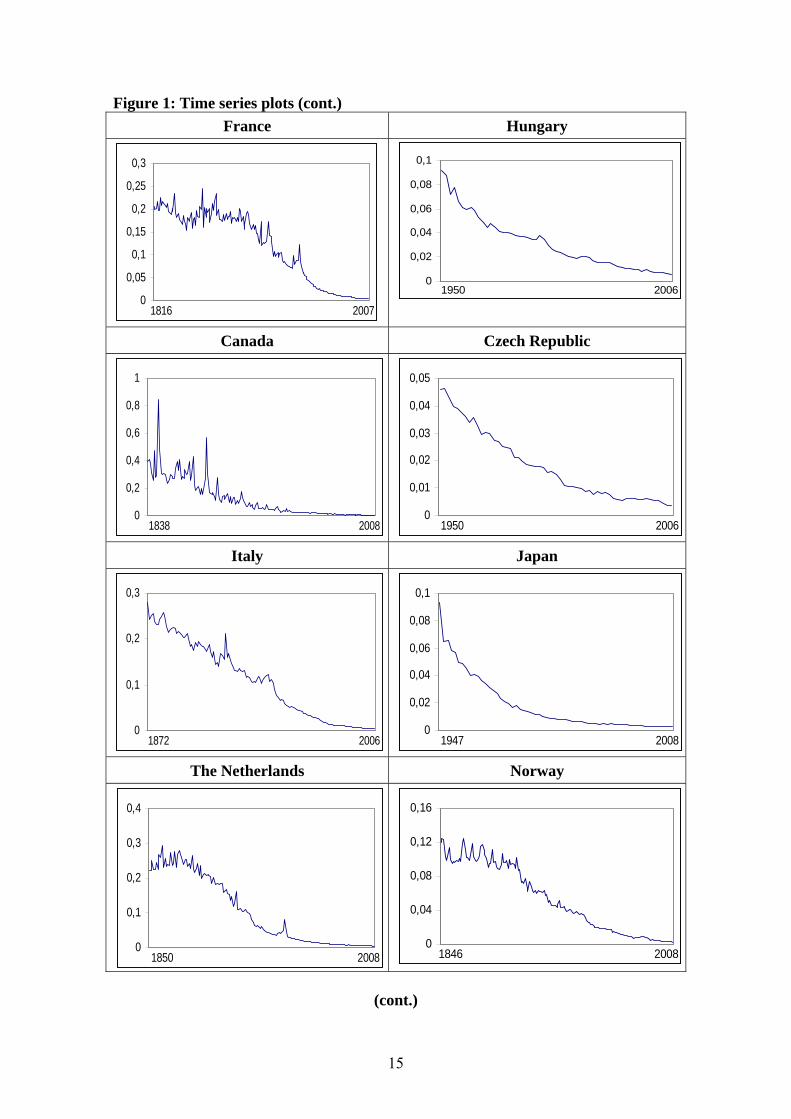
Figure 1: Time series plots (cont.) France Hungary

0

0,05

0,1

0,15

0,2

0,25

0,3

1816 2007

0

0,02

0,04

0,06

0,08

0,1

1950 2006

Canada Czech Republic

0

0,2

0,4

0,6

0,8

1

1838 20080

0,01

0,02

0,03

0,04

0,05

1950 2006

Italy Japan

0

0,1

0,2

0,3

1872 20060

0,02

0,04

0,06

0,08

0,1

1947 2008

The Netherlands Norway

0

0,1

0,2

0,3

0,4

1850 20080

0,04

0,08

0,12

0,16

1846 2008

(cont.)

16

Figure 1: Time series plots (cont.) New Zealand Czech Republic

0

0,01

0,02

0,03

0,04

1948 20080

0,05

0,1

0,15

0,2

1940 2009

Spain Slovakia

0

0,05

0,1

0,15

0,2

0,25

1908 20060

0,04

0,08

0,12

0,16

1950 2008

Sweden Switzerland

0

0,1

0,2

0,3

0,4

1751 20070

0,05

0,1

0,15

0,2

0,25

0,3

1876 2007

UK US

0

0,02

0,04

0,06

0,08

0,1

1922 20090

0,02

0,04

0,06

0,08

1933 2007

17

Table 1: Sample period and reduction in IMR by country Country Time period 1950 2006 Reduction

ICELAND 1838 - 2008 0.022790 (2) 0.001372 (1) 0.021418 (21)

JAPAN 1947 - 2008 0.058245 (15) 0.002693 (2) 0.055552 (9)

SWEDEN 1751 - 2007 0.020851 (1) 0.002857 (3) 0.017994 (24)

FINLAND 1878 - 2008 0.043277 (12) 0.002874 (4) 0.040403 (13)

NORWAY 1846 - 2008 0.025948 (5) 0.003196 (5) 0.022752 (20)

PORTUGAL 1940 - 2009 0.104441 (21) 0.003260 (6) 0.101181 (2)

CZECH REP. 1950 - 2008 0.067921 (17) 0.003380 (7) 0.064541 (6)

ITALY 1872 - 2006 0.066113 (16) 0.003468 (8) 0.062645 (8)

AUSTRIA 1947 - 2008 0.068012 (18) 0.003604 (9) 0.064408 (7)

SPAIN 1908 - 2006 0.077807 (18) 0.003681 (10) 0.074126 (5)

FRANCE 1816 - 2007 0.053602 (13) 0.003716 (11) 0.049886 (11)

IRELAND 1950 - 2006 0.045980 (13) 0.003800 (12) 0.042180 (12)

DENMARK 1835 - 2008 0.031315 (8) 0.003853 (13) 0.027462 (16)

BELGIUM 1919 - 2007 0.055066 (14) 0.004072 (14) 0.050994 (10)

NETHERLANDS 1850 - 2008 0.025320 (3) 0.004411 (15) 0.020909 (22)

SWITZERLAND 1876 - 2007 0.032827 (10) 0.004462 (16) 0.028365 (15)

AUSTRALIA 1921 – 2007 0.025426 (4) 0.004696 (17) 0.020730 (23)

CANADA 1921 - 2007 0.042973 (11) 0.005058 (18) 0.037915 (14)

UK 1922 - 2009 0.030922 (7) 0.005090 (19) 0.025832 (17)

NEW ZEALAND 1948 - 2008 0.028433 (6) 0.005172 (20) 0.023261 (19)

HUNGARY 1950 - 2006 0.091480 (19) 0.005841 (20) 0.085639 (4)

SLOVAKIA 1950 - 2008 0.118871 (22) 0.006585 (21) 0.112286 (1)

US 1933 - 2007 0.032468 (9) 0.006813 (22) 0.025655 (18)

BULGARIA 1947 - 2009 0.103598 (20) 0.010355 (23) 0.093243 (3)

18

Table 2: Estimates of d for each series and 95% confidence bands Country Female Male Total

ICELAND 0.410 (0.342, 0.504) 0.370 (0.314, 0.446) 0.431 (0.367, 0.519)

JAPAN 0.946 (0.854, 1.074) 0.921 (0.812, 1.075) 0.953 (0.851, 1.096)

SWEDEN 0.828 (0.791, 0.875) 0.870 (0.833, 0.918) 0.863 (0.826, 0.910)

FINLAND 0.813 (0.751, 0.901) 0.811 (0.752, 0.893) 0.850 (0.789, 0.937)

NORWAY 0.801 (0.746, 0.875) 0.866 (0.809, 0.944) 0.903 (0.842, 0.987)

PORTUGAL 0.739 (0.658, 0.848) 0.846 (0.754, 0.979) 0.862 (0.772, 0.988)

CZECH REP. 1.134 (1.004, 1.309) 1.106 (0.973, 1.282) 1.213 (1.079, 1.389)

ITALY 0.967 (0.914, 1.038) 0.964 (0.913, 1.032) 0.977 (0.922, 1.044)

AUSTRIA 0.727 (0.504, 0.998) 0.738 (0.565, 0.961) 0.816 (0.647, 1.027)

SPAIN 0.938 (0.859, 1.047) 0.932 (0.854, 1.041) 0.945 (0.866, 1.055)

FRANCE 0.853 (0.813, 0.904) 0.878 (0.837, 0.932) 0.868 (0.827, 0.920)

IRELAND 0.418 (0.284, 0.610) 0.552 (0.353, 0.833) 0.761 (0.558, 1.039)

DENMARK 0.798 (0.751, 0.861) 0.834 (0.786, 0.898) 0.847 (0.798, 0.913)

BELGIUM 0.813 (0.704, 0.971) 0.959 (0.819, 1.178) 0.972 (0.838, 1.181)

NETHERLANDS 0.788 (0.725, 0.872) 0.801 (0.738, 0.883) 0.807 (0.744, 0.891)

SWITZERLAND 0.681 (0.606, 0.781) 0.744 (0.669, 0.847) 0.768 (0.692, 0.869)

AUSTRALIA 0.578 (0.474, 0.722) 0.724 (0.613, 0.885) 0.695 (0.585, 0.852)

CANADA 0.929 (0.819, 1.084) 0.886 (0.777, 1.032) 0.929 (0.819, 1.079)

UK 0.830 (0.716, 0.978) 0.881 (0.755, 1.049) 0.881 (0.760, 1.042)

NEW ZEALAND 0.281 (0.145, 0.481) 0.627 (0.486, 0.824) 0.548 (0.412, 0.743)

HUNGARY 0.657 (0.463, 0.920) 0.727 (0.561, 0.977) 0.741 (0.560, 0.999)

SLOVAKIA 0.845 (0.703, 1.013) 0.964 (0.829, 1.136) 0.956 (0.829, 1.126)

US 1.031 (0.896, 1.214) 1.061 (0.927, 1.239) 1.059 (0.925, 1.241)

BULGARIA 0.884 (0.790, 1.012) 0.937 (0.837, 1.079) 0.956 (0.859, 1.094)

19

Table 3: Estimates of the time trend along with the t-values Country Female Male Total

ICELAND -0.03125 (-16.71) -0.03006 (-19.34) -0.03031 (-17.44)

JAPAN -0.05812 (-9.09) -0.05880 (-10.58) -0.05855 (-9.57)

SWEDEN -0.01697 (-6.96) -0.01711 (-6.27) -0.01717 (-6.47)

FINLAND -0.03391 (-8.66) -0.03282 (-8.59) -0.03333 (-8.07)

NORWAY -0.02321 (-7.75) -0.02251 (-6.68) -0.02308 (-6.13)

PORTUGAL -0.05673 (-12.69) -0.05450 (-8.97) -0.05515 (-9.30)

CZECH REP. -0.05992 (-3.37) -0.05696 (-3.44) -0.06337 (-3.04)

ITALY -0.03314 (-6.24) -0.03220 (-6.21) -0.03265 (-6.06)

AUSTRIA -0.05372 (-17.03) -0.05283 (-13.68) -0.05306 (-13.46)

SPAIN -0.04036 (-6.16) -0.03963 (-6.13) -0.03988 (-6.01)

FRANCE -0.02114 (-5.51) -0.02064 (-5.08) -0.02086 (-5.27)

IRELAND -0.04283 (-24.34) -0.04470 (-18.81) -0.04398 (-12.80)

DENMARK -0.02293 (-7.68) -0.02295 (-7.08) -0.02296 (-6.91)

BELGIUM -0.04061 (-10.33) -0.03958 (-6.33) -0.03976 (-6.41)

NETHERLANDS -0.02633 (-8.12) -0.02617 (-7.90) -0.02621 (-7.78)

SWITZERLAND -0.03181 (-19.83) -003220 (-17.11) -0.03194 (-16.46)

AUSTRALIA -0.03105 (-21.84) -0.03192 (-15.07) -0.03152 (-16.59)

CANADA -0.03669 (-9.08) -0.03821 (-11.49) -0.03735 (-9.79)

UK -0.03319 (-10.77) -0.03372 (-9.37) -0.03341 (-9.39)

NEW ZEALAND -0.03142 (-24.17) -0.03088 (-13.75) -0.03095 (-17.64)

HUNGARY -0.04704 (-16.14) -0.04767 (-14.44) -0.04761 (-13.94)

SLOVAKIA -0.05013 (-5.45) -0.05009 (-4.29) -00.0566 (-4.45)

US -0.02920 (-7.13) -0.02944 (-6.52) -0.02922 (-6.60)

BULGARIA -0.04423 (-5.60) -0.04265 (-4.96) -0.04350 (-4.91)

20

Table 4: Estimates of d and the 95% confidence interval for the time period 1950-2006 Country Female Male Total

ICELAND 0.072 (-0.093, 0.311) 0.008 (-0.133, 0.201) 0.093 (-0.064, 0.352)

JAPAN 1.023 (0.939, 1.135) 0.981 (0.888, 1.108) 1.041 (0.952, 1.163)

SWEDEN 0.386 (0.215, 0.623) 0.622 (0.431, 0.905) 0.602 (0.422, 0.857)

FINLAND 0.447 (0.319, 0.636) 0.477 (0.356, 0.653) 0.580 (0.457, 0.762)

NORWAY 0.560 (0.401, 0.762) 0.749 (0.573, 0.983) 0.897 (0.723, 1.117)

PORTUGAL 0.737 (0.643, 0.859) 0.808 (0.713, 0.933) 0.843 (0.751, 0.963)

CZECH REP. 1.133 (1.003, 1.304) 1.087 (0.959, 1.255) 1.195 (1.066, 1.366)

ITALY 0.779 (0.637, 0.982) 0.808 (0.678, 0.994) 0.887 (0.745, 1.102)

AUSTRIA 0.618 (0.409, 1.020) 0.675 (0.503, 0.913) 0.745 (0.568, 0.998)

SPAIN 0.799 (0.679, 0.963) 0.807 (0.689, 0.963) 0.845 (0.728, 1.002)

FRANCE 0.849 (0.708, 1.046) 0.857 (0.676, 1.137) 0.906 (0.732, 1.161)

IRELAND 0.418 (0.284, 0.610) 0.552 (0.353, 0.833) 0.761 (0.558, 1.039)

DENMARK 0.524 (0.399, 0.8702) 0.562 (0.415, 0.765) 0.709 (0.557, 0.930)

BELGIUM 0.303 (0.044, 0.641) 0.623 (0.396, 0.958) 0.680 (0.405, 1.084)

NETHERLANDS 0.435 (0.313, 0.604) 0.413 (0.289, 0.576) 0.510 (0.387, 0.678)

SWITZERLAND 0.596 (0.460, 0.793) 0.684 (0.530, 0.901) 0.821 (0.664, 1.046)

AUSTRALIA 0.651 (0.539, 0.795) 0.759 (0.644, 0.910) 0.756 (0.644, 0.903)

CANADA 1.027 (0.909, 1.205) 1.070 (0.946, 1.260) 1.121 (0.997, 1.322)

UK 0.891 (0.751, 1.083) 1.058 (0.891, 1.301) 1.107 (0.942, 1.344)

NEW ZEALAND 0.281 (0.142, 0.484) 0.626 (0.467, 0.858) 0.538 (0.398, 0.745)

HUNGARY 0.657 (0.463, 0.920) 0.727 (0.561, 0.977) 0.741 (0.560, 0.999)

SLOVAKIA 0.842 (0.697, 1.016) 0.964 (0.827, 1.142) 0.959 (0.824, 1.131)

US 1.279 (1.107, 1.558) 1.327 (1.178, 1.555) 1.356 (1.192, 1.629)

BULGARIA 0.870 (0.769, 1.019) 0.959 (0.838, 1.134) 0.952 (0.843, 1.111)

21

Table 5: Estimates of the time trend along with the t-values for the time period 1950-2006 Country Female Male Total

ICELAND -0.03125 (-16.71) -0.03006 (-19.34) -0.03031 (-17.44)

JAPAN -0.05480 (-8.60) -0.05499 (-10.07) -0.05476 (-8.83)

SWEDEN -0.03609 (-22.77) -0.03722 (-15.84) -0.03655 (-17.75)

FINLAND -0.04718 (-29.72) -0.04774 (-22.11) -0.04784 (-20.79)

NORWAY -0.02321 (-7.75) -0.02251 (-6.68) -0.02308 (-6.13)

PORTUGAL -0.06336 (-12.68) -0.06142 (-10.47) -0.06230 (-10.44)

CZECH REP. -0.05969 (-3.27) -0.05457 (-3.46) -0.06074 (-3.05)

ITALY -0.05391 (-21.10) -0.05289 (-16.89) -0.05312 (-15.28)

AUSTRIA -0.05140 (-22.21) -0.05242 (-16.02) -0.05201 (-16.33)

SPAIN -0.05542 (-18.28) -0.05479 (-15.50) -0.05521 (-15.54)

FRANCE -0.04777 (-6.73) -0.04811 (-14.40) -0.04784 (-13.64)

IRELAND -0.04283 (-24.34) -0.04470 (-18.81) -0.04398 (-12.80)

DENMARK -0.03641 (-14.54) -0.03816 (-16.28) -0.03633 (-8.11)

BELGIUM -0.04672 (-47.53) -0.04760 (-24.19) -0.04718 (-23.11)

NETHERLANDS -0.03097 (-24.04) -0.03171 (-33.10) -0.03145 (-26.80)

SWITZERLAND -0.03682 (-14.40) -0.03757 (-13.01) -0.03630 (-9.49)

AUSTRALIA -0.03122 (-13.40) -0.03114 (-9.74) -0.03106 (-10.39)

CANADA -0.03719 (-6.04) -0.03853 (-6.19) -0.03765 (-5.35)

UK -0.03199 (-9.50) -0.03255 (-6.13) -0.03149 (-5.42)

NEW ZEALAND -0.03191 (-22.86) -0.03125 (-12.91) -0.03160 (-17.39)

HUNGARY -0.04704 (-16.14) -0.04767 (-14.44) -0.04761 (-13.94)

SLOVAKIA -0.05019 (-5.29) -0.05044 (-4.17) -0.05094 (-4.28)

US -0.02451 (-3.14) -0.02483 (-2.88) -0.02389 (-2.62)

BULGARIA -0.03971 (-4.93) -0.04221 (-4.35) -0.04090 (-4.43)

22

Table 6: Comparisons of the time trends with I(d) and I(0) errors

Country I(d) errors I(0) errors

ICELAND -0.03031 (-17.44) -0.04410 (-35.671)

JAPAN -0.05476 (-8.83) -0.05665 (-45.453)

SWEDEN -0.03655 (-17.75) -0.03734 (-61.240)

FINLAND -0.04784 (-20.79) -0.04683 (-58.562)

NORWAY -0.02308 (-6.13) -0.03693 (-41.299)

PORTUGAL -0.06230 (-10.44) -0.06674 (-46.333)

CZECH REP. -0.06074 (-3.05) -0.04120 (-22.958)

ITALY -0.05312 (-15.28) -0.05579 (-87.880)

AUSTRIA -0.05201 (-16.33) -0.05246 (-74.349)

SPAIN -0.05521 (-15.54) -0.05842 (-78.515)

FRANCE -0.04784 (-13.64) -0.04781 (-92.968)

IRELAND -0.04398 (-12.80) -0.04417 (-63.834)

DENMARK -0.03633 (-8.11) -0.03764 (-47.218)

BELGIUM -0.04718 (-23.11) -0.04671 (-103.571)

NETHERLANDS -0.03145 (-26.80) -0.03102 (-69.381)

SWITZERLAND -0.03630 (-9.49) -0.03906 (-53.003)

AUSTRALIA -0.03106 (-10.39) -0.03383 (-42.943)

CANADA -0.03765 (-5.35) -0.04313 (-49.501)

UK -0.03149 (-5.42) -0.03557 (-59.553)

NEW ZEALAND -0.03160 (-17.39) -0.03261 (-48.550)

HUNGARY -0.04761 (-13.94) -0.04509 (-59.855)

SLOVAKIA -0.05094 (-4.28) -0.03983 (-25.694)

US -0.02389 (-2.62) -0.03215 (-57.956)

BULGARIA -0.04090 (-4.43) -0.03666 (-20.385)