Guidance and Trajectory Following ofan Autonomous Vision-Guided Micro

QuadRotor

Sofia Isabel Batista Fernandes

Dissertação para obtenção do Grau de Mestre em

Engenharia Aeroespacial

Júri

Presidente: Professor Fernando J. P. LauOrientador: Professor Afzal SulemanVogal: Professor Agostinho R. A. da Fonseca

Janeiro de 2011

Acknowledgments

I would like to thank my thesis advisors, without whom this work wouldn’t have beenpossible. To Pini Gurfil, who received me at the Technion and guided my practical andlaboratory work there, and to Afzal Suleman, who directed the course of the thesis.

Also I would like to thank Yuval, Sergey, Aram, Yair and all the people from theTechnion’s ISL for their help during the course of my work there and even afterwards.

To my family and friends, specially to my closest family, I express my deepest ap-preciation. You are motivating and inspirational and took my intercalated absences andhumours with an everlasting smile.

And a final note to my Israeli friends for having turned my life in a foreign countryinto a cherished memory.

A todos muito obrigada.

Yeager broke the barrier of sound with two broken ribs;Beethoven wrote brilliant symphonies while being deaf;

How far can we go?

i

Abstract

The present thesis documents the dynamics modelling and control design developmentfor an autonomous micro-quadrotor that will be vision-guided. Linear models were de-termined for Roll, Pitch, Yaw and Altitude and PID controllers for attitude and positionwere designed and tested.

The system identification software CIFER® was used to determine the frequencydomain models from the previously recorded time-domain flight data. The flight testswere conducted with a human pilot flying the QuadRotor remotely.

Matlab® and Simulink® were used for the development and simulation of the PIDattitude, position and altitude controllers.

A testbed was built for tests with the QuadRotor platform. The realtime controllerswere implemented in Matlab code. A C++ program was developed to handle the com-munications, close the loop with the QuadRotor platform and manage the experiments.

Successful attitude tests were conducted and the results are presented.

Keywords: micro-Quadrotor, MAV, linear control, attitude control, PID, dynamics mod-elling

ii

Resumo

A presente tese documenta o processo de desenvolvimento de um modelo dinâmico ealgoritmos de controlo para um micro-quadrotor que virá a ser guiado por visão. Modeloslineares foram determinados para o Rolamento, Picada, Guinada e Altitude e contro-ladores PID foram desenvolvidos e testados para a atitude.

O software de identificação de sistemas CIFER® foi usado para determinar os modelosem frequência a partir de dados de voos previamente recolhidos. Os ensaios em voo foramconduzidos com recurso a um piloto humano, pilotando remotamente o QuadRotor.

Matlab® e Simulink® foram usados no desenvolvimento e simulação dos controladoresPID para atitude, posição e altitude.

Uma plataforma de testes foi construída para o QuadRotor. Os controladores emtempo real foram implementados em código Matlab. Um programa em C++ foi desen-volvido para gerir as comunicações, fechar o loop com a plataforma física do QuadRotor,bem como fazer a gestão de toda o o software e hardware durante os testes.

São apresentados resultados de testes ao controlo de attitude.

Keywords: micro-Quadrotor, MAV, controlo linear, controlo de atitude, PID, modelaçãodinâmica

iii

Contents

Acknowledgments i

Abstract ii

Resumo iii

List of Figures vii

List of Symbols ix

Abbreviations xi

1 Introduction 11.1 Definition of MAV . . . . . . . . . . . . . . . . . . . . . . . . . . . . . . . 11.2 Motivation . . . . . . . . . . . . . . . . . . . . . . . . . . . . . . . . . . . . 2

1.2.1 Design Challenges and Wind Limitations . . . . . . . . . . . . . . . 31.2.2 Why a QuadRotor . . . . . . . . . . . . . . . . . . . . . . . . . . . 3

1.3 Context and Other Aproaches / Related Projects . . . . . . . . . . . . . . 61.4 The ISL micro-quadrotor project . . . . . . . . . . . . . . . . . . . . . . . 8

1.4.1 The project’s goals . . . . . . . . . . . . . . . . . . . . . . . . . . . 81.4.2 The quadrotor platform . . . . . . . . . . . . . . . . . . . . . . . . 81.4.3 The XSens unit . . . . . . . . . . . . . . . . . . . . . . . . . . . . . 11

1.5 Thesis Objective . . . . . . . . . . . . . . . . . . . . . . . . . . . . . . . . 111.6 Thesis Layout . . . . . . . . . . . . . . . . . . . . . . . . . . . . . . . . . . 12

2 Dynamics Modelling 142.1 System Identification using CIFER® . . . . . . . . . . . . . . . . . . . . . 15

2.1.1 Introduction to CIFER® . . . . . . . . . . . . . . . . . . . . . . . . 152.1.2 Data acquisition . . . . . . . . . . . . . . . . . . . . . . . . . . . . . 162.1.3 Data handling: software overview and user’s perspective . . . . . . 182.1.4 Data handling: the CZT . . . . . . . . . . . . . . . . . . . . . . . . 20

iv

2.1.5 CIFER® Results . . . . . . . . . . . . . . . . . . . . . . . . . . . . 222.2 Position Model . . . . . . . . . . . . . . . . . . . . . . . . . . . . . . . . . 24

2.2.1 Vertical Position Model . . . . . . . . . . . . . . . . . . . . . . . . . 27

3 Attitude PID Control 283.1 Introduction . . . . . . . . . . . . . . . . . . . . . . . . . . . . . . . . . . . 28

3.1.1 Design Specifications . . . . . . . . . . . . . . . . . . . . . . . . . . 303.1.2 Digital PID Control . . . . . . . . . . . . . . . . . . . . . . . . . . . 30

3.2 Yaw Control . . . . . . . . . . . . . . . . . . . . . . . . . . . . . . . . . . . 323.2.1 Yaw fine tunning and simulation results . . . . . . . . . . . . . . . 353.2.2 Yaw Stability analysis . . . . . . . . . . . . . . . . . . . . . . . . . 37

3.3 Pitch Control . . . . . . . . . . . . . . . . . . . . . . . . . . . . . . . . . . 373.3.1 Pitch fine tunning and simulation results . . . . . . . . . . . . . . . 413.3.2 Pitch Stability analysis . . . . . . . . . . . . . . . . . . . . . . . . . 42

3.4 Roll Control . . . . . . . . . . . . . . . . . . . . . . . . . . . . . . . . . . . 433.4.1 Roll fine tunning and simulation results . . . . . . . . . . . . . . . . 463.4.2 Roll Stability Analysis . . . . . . . . . . . . . . . . . . . . . . . . . 47

4 Position Control 494.1 Backstepping algorithm . . . . . . . . . . . . . . . . . . . . . . . . . . . . . 494.2 Horizontal Position Control . . . . . . . . . . . . . . . . . . . . . . . . . . 50

4.2.1 Simulation and fine tunning/ New controller . . . . . . . . . . . . . 504.2.2 Y position control . . . . . . . . . . . . . . . . . . . . . . . . . . . . 54

4.3 Vertical Position Control . . . . . . . . . . . . . . . . . . . . . . . . . . . . 57

5 Implementation and Test Results 615.1 Communication Strategy . . . . . . . . . . . . . . . . . . . . . . . . . . . . 615.2 Development of the Realtime Controller for Attitude . . . . . . . . . . . . 63

5.2.1 Finite Difference Weighted Average Derivative . . . . . . . . . . . . 645.2.2 Realtime Matlab Code . . . . . . . . . . . . . . . . . . . . . . . . . 65

5.3 Test Results and Future Work . . . . . . . . . . . . . . . . . . . . . . . . . 67

6 Concluding Remarks 71

Bibliography 73

Appendix A 77

Appendix B 78

v

Appendix C 86

vi

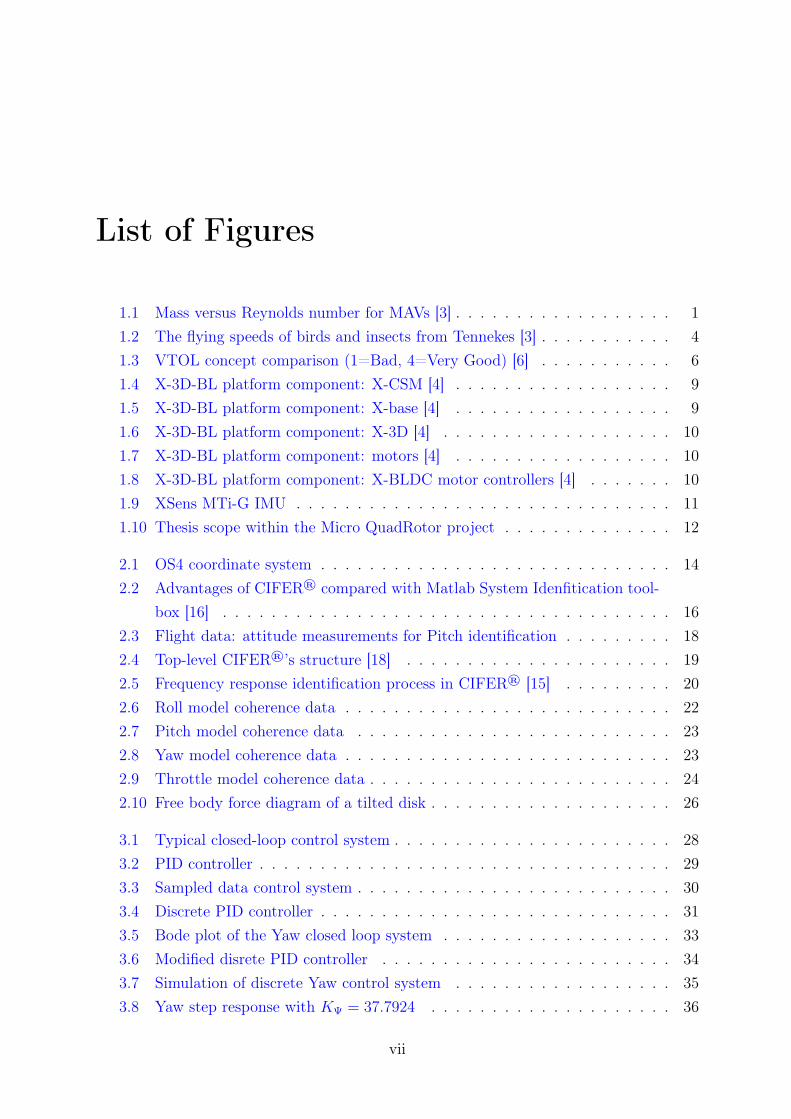
List of Figures

1.1 Mass versus Reynolds number for MAVs [3] . . . . . . . . . . . . . . . . . . 11.2 The flying speeds of birds and insects from Tennekes [3] . . . . . . . . . . . 41.3 VTOL concept comparison (1=Bad, 4=Very Good) [6] . . . . . . . . . . . 61.4 X-3D-BL platform component: X-CSM [4] . . . . . . . . . . . . . . . . . . 91.5 X-3D-BL platform component: X-base [4] . . . . . . . . . . . . . . . . . . 91.6 X-3D-BL platform component: X-3D [4] . . . . . . . . . . . . . . . . . . . 101.7 X-3D-BL platform component: motors [4] . . . . . . . . . . . . . . . . . . 101.8 X-3D-BL platform component: X-BLDC motor controllers [4] . . . . . . . 101.9 XSens MTi-G IMU . . . . . . . . . . . . . . . . . . . . . . . . . . . . . . . 111.10 Thesis scope within the Micro QuadRotor project . . . . . . . . . . . . . . 12

2.1 OS4 coordinate system . . . . . . . . . . . . . . . . . . . . . . . . . . . . . 142.2 Advantages of CIFER® compared with Matlab System Idenfitication tool-

box [16] . . . . . . . . . . . . . . . . . . . . . . . . . . . . . . . . . . . . . 162.3 Flight data: attitude measurements for Pitch identification . . . . . . . . . 182.4 Top-level CIFER®’s structure [18] . . . . . . . . . . . . . . . . . . . . . . 192.5 Frequency response identification process in CIFER® [15] . . . . . . . . . 202.6 Roll model coherence data . . . . . . . . . . . . . . . . . . . . . . . . . . . 222.7 Pitch model coherence data . . . . . . . . . . . . . . . . . . . . . . . . . . 232.8 Yaw model coherence data . . . . . . . . . . . . . . . . . . . . . . . . . . . 232.9 Throttle model coherence data . . . . . . . . . . . . . . . . . . . . . . . . . 242.10 Free body force diagram of a tilted disk . . . . . . . . . . . . . . . . . . . . 26

3.1 Typical closed-loop control system . . . . . . . . . . . . . . . . . . . . . . . 283.2 PID controller . . . . . . . . . . . . . . . . . . . . . . . . . . . . . . . . . . 293.3 Sampled data control system . . . . . . . . . . . . . . . . . . . . . . . . . . 303.4 Discrete PID controller . . . . . . . . . . . . . . . . . . . . . . . . . . . . . 313.5 Bode plot of the Yaw closed loop system . . . . . . . . . . . . . . . . . . . 333.6 Modified disrete PID controller . . . . . . . . . . . . . . . . . . . . . . . . 343.7 Simulation of discrete Yaw control system . . . . . . . . . . . . . . . . . . 353.8 Yaw step response with KΨ = 37.7924 . . . . . . . . . . . . . . . . . . . . 36

vii

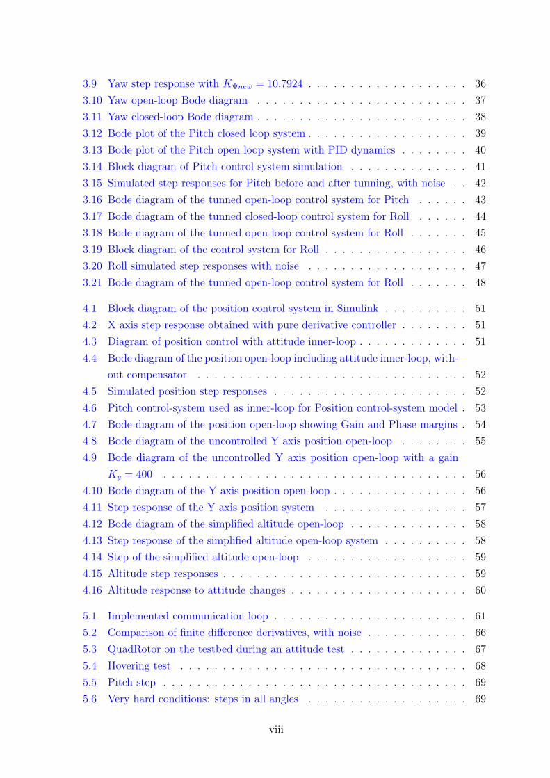
3.9 Yaw step response with KΨnew = 10.7924 . . . . . . . . . . . . . . . . . . . 363.10 Yaw open-loop Bode diagram . . . . . . . . . . . . . . . . . . . . . . . . . 373.11 Yaw closed-loop Bode diagram . . . . . . . . . . . . . . . . . . . . . . . . . 383.12 Bode plot of the Pitch closed loop system . . . . . . . . . . . . . . . . . . . 393.13 Bode plot of the Pitch open loop system with PID dynamics . . . . . . . . 403.14 Block diagram of Pitch control system simulation . . . . . . . . . . . . . . 413.15 Simulated step responses for Pitch before and after tunning, with noise . . 423.16 Bode diagram of the tunned open-loop control system for Pitch . . . . . . 433.17 Bode diagram of the tunned closed-loop control system for Roll . . . . . . 443.18 Bode diagram of the tunned open-loop control system for Roll . . . . . . . 453.19 Block diagram of the control system for Roll . . . . . . . . . . . . . . . . . 463.20 Roll simulated step responses with noise . . . . . . . . . . . . . . . . . . . 473.21 Bode diagram of the tunned open-loop control system for Roll . . . . . . . 48

4.1 Block diagram of the position control system in Simulink . . . . . . . . . . 514.2 X axis step response obtained with pure derivative controller . . . . . . . . 514.3 Diagram of position control with attitude inner-loop . . . . . . . . . . . . . 514.4 Bode diagram of the position open-loop including attitude inner-loop, with-

out compensator . . . . . . . . . . . . . . . . . . . . . . . . . . . . . . . . 524.5 Simulated position step responses . . . . . . . . . . . . . . . . . . . . . . . 524.6 Pitch control-system used as inner-loop for Position control-system model . 534.7 Bode diagram of the position open-loop showing Gain and Phase margins . 544.8 Bode diagram of the uncontrolled Y axis position open-loop . . . . . . . . 554.9 Bode diagram of the uncontrolled Y axis position open-loop with a gain

Ky = 400 . . . . . . . . . . . . . . . . . . . . . . . . . . . . . . . . . . . . 564.10 Bode diagram of the Y axis position open-loop . . . . . . . . . . . . . . . . 564.11 Step response of the Y axis position system . . . . . . . . . . . . . . . . . 574.12 Bode diagram of the simplified altitude open-loop . . . . . . . . . . . . . . 584.13 Step response of the simplified altitude open-loop system . . . . . . . . . . 584.14 Step of the simplified altitude open-loop . . . . . . . . . . . . . . . . . . . 594.15 Altitude step responses . . . . . . . . . . . . . . . . . . . . . . . . . . . . . 594.16 Altitude response to attitude changes . . . . . . . . . . . . . . . . . . . . . 60

5.1 Implemented communication loop . . . . . . . . . . . . . . . . . . . . . . . 615.2 Comparison of finite difference derivatives, with noise . . . . . . . . . . . . 665.3 QuadRotor on the testbed during an attitude test . . . . . . . . . . . . . . 675.4 Hovering test . . . . . . . . . . . . . . . . . . . . . . . . . . . . . . . . . . 685.5 Pitch step . . . . . . . . . . . . . . . . . . . . . . . . . . . . . . . . . . . . 695.6 Very hard conditions: steps in all angles . . . . . . . . . . . . . . . . . . . 69

viii

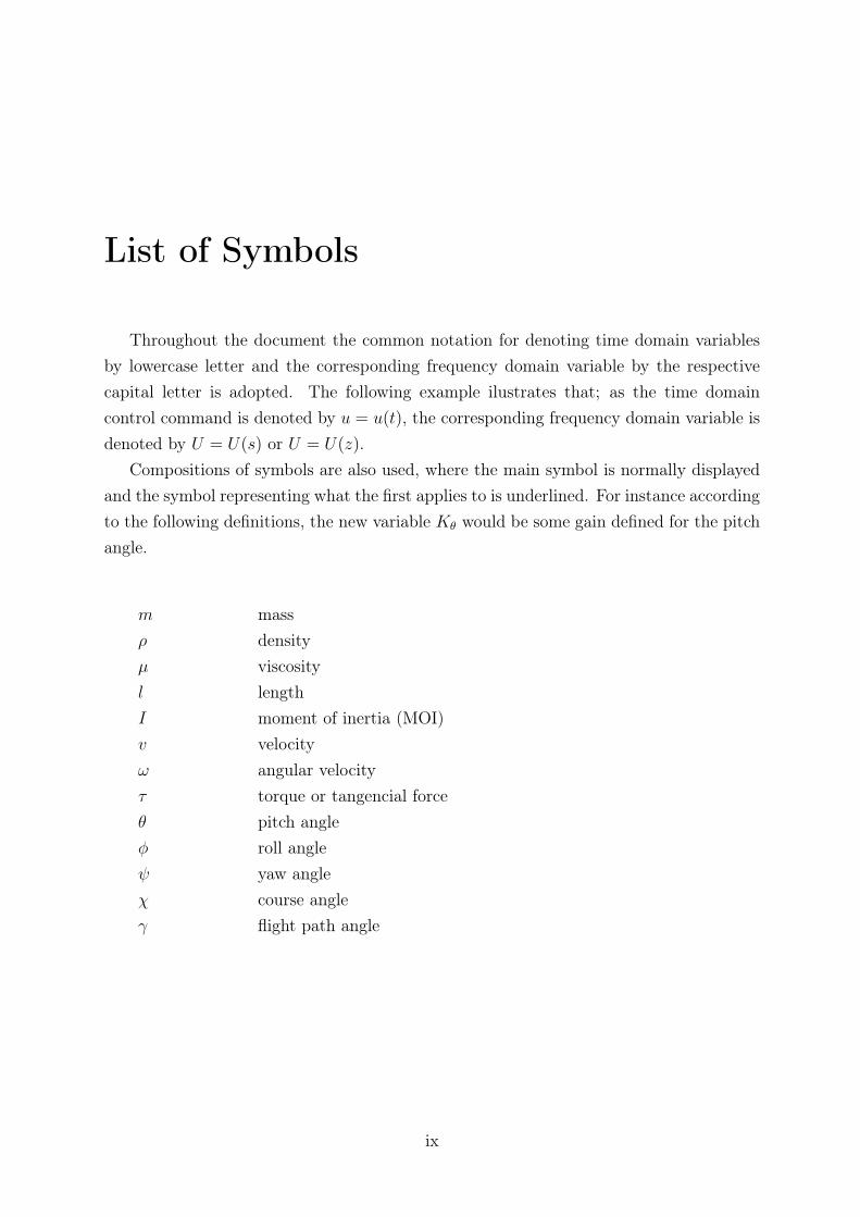
List of Symbols

Throughout the document the common notation for denoting time domain variablesby lowercase letter and the corresponding frequency domain variable by the respectivecapital letter is adopted. The following example ilustrates that; as the time domaincontrol command is denoted by u = u(t), the corresponding frequency domain variable isdenoted by U = U(s) or U = U(z).

Compositions of symbols are also used, where the main symbol is normally displayedand the symbol representing what the first applies to is underlined. For instance accordingto the following definitions, the new variable Kθ would be some gain defined for the pitchangle.

m massρ densityµ viscosityl lengthI moment of inertia (MOI)v velocityω angular velocityτ torque or tangencial forceθ pitch angleφ roll angleψ yaw angleχ course angleγ flight path angle

ix

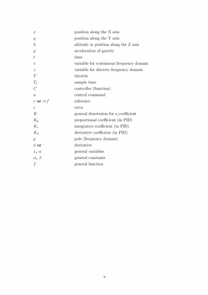
x position along the X axisy position along the Y axish altitude or position along the Z axisg acceleration of gravityt times variable for continuous frequency domainz variable for discrete frequency domainT throttleTs sample timeC controller (function)u control commandr or ref referencee errorK general denotation for a coefficientKp proportional coefficient (in PID)Ki integrative coefficient (in PID)Kd derivative coefficient (in PID)p pole (frequency domain)d or ˙ derivativex, α general variablesα, β general constantsf general function

x

Abbreviations

AHRS Attitude and Heading Reference SystemAI Artificial IntelligenceCIFER CIFER® softwareCZT Chirp-Z TransformFFT Fast Fourier TransformGM Gain MarginGPS Global Positioning SystemIMU Inertial Measurement UnitIB Integral BacksteppingISL Intelligent Systems LaboratoryMAV Micro Aerial VehicleMEMS Micro-Electro-Mechanical SystemsMFR Miniature Flying RobotMOI Moment Of InertiaNAV Nano Aerial VehiclePID Proportional Integrative Derivative (controller)PM Phase MarginRTWT RealTime Windows TargetSISO Single-Input Single-OutputSSE Steady State ErrorTF Transfer FunctionUAV Unmanned Air VehicleVTOL Vertical Take-Off and Landing

xi

Chapter 1

Introduction

1.1 Definition of MAV

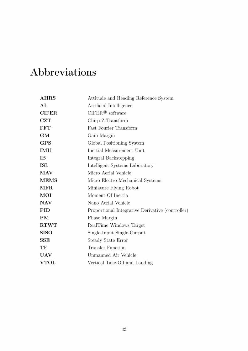
Micro Aerial Vehicles (MAV) can be considered a sub-class of uninhabited air vehicles(UAVs). They are small, lightweight aircraft characterized by small vehicle size (O10cm),low flight speed (O10m/s) and low Reynolds number (O10, 000− 100, 000). [1] [2]

Figure 1.1 shows where MAVs lay on the mass versus Reynolds number plot for flightvehicles / animals.

Figure 1.1: Mass versus Reynolds number for MAVs [3]

MAVs are used mostly to perform reconnaissance, surveillance, and inspection mis-sions. Such missions can occur in a variety of environments. For example, lengthy re-conflights across a desert or hovering above a foreign building to collect target information.

1

Oftentimes the specifics of the mission dictate the MAV platform configuration. If verticaltakeoff or hovering is required, then rotary-wing aircraft, such as a quad-rotors or ductedfans, are most optimal. However, if endurance is a priority, then a fixed-wing body typewill most likely be selected. [2]

MAVs and NAVs (Nano Aerial Vehicles) are the most maneuverable man-made flightvehicles. They are useful to the extent that they are agile in flight. Due to their lightweight, low Reynolds numbers and low air loading, they are also potentially the mostsensitive to disturbances such as wind gusts in complex flight environments. Hence, theMAV design problem – and the challenges in the underlying sciences – is how to enablehigh agility, and how to do so efficiently and robustly. [1] [4] [5]

Section 1.2 elaborates on the motivations for MAV development and choice of config-uration.

1.2 Motivation

The desire to develop MAVs is fueled by the need for increased situational awareness(especially in urban environments), remote sensing capability, "over the hill" reconnais-sance, precision payload delivery, and aid in rescue missions. [1]

Miniature aerial vehicles (MAVs) have attracted major research interest during thelast decade. Recent advances in low power processors, miniature sensors and controltheory have contributed to system miniaturization and creation of new application fields.Miniature flying robots (MFR) offer major advantages when used for aerial surveillancein complex or cluttered environments like office buildings and commercial centers. Whenthere is a need to acquire intelligence in hostile or dangerous environments such as caves,forests, or urban areas, rather than risking human life, back-packable, bird-sized aircraft,equipped with a wireless camera, can be rapidly deployed to gather reconnaissance in suchenvironments. However, they first must be designed to fly in tight, cluttered terrain. [6]

MFRs may assist in search and rescue missions after earthquakes, explosions and othernatural disasters, that make reconnaissance, surveillance and search-and-rescue missionscan be difficult and dangerous to accomplish: Runways may be crippled thus denyingconventional aircraft in the area from taking off. Also the time required to schedulea satellite fly-by may delay first response efforts. As such, backpackable aerial robotscapable of flying in narrow spaces, fit through small openings and collapsed buildings,maneuver around pillars and destroyed wall structures can provide real-time situationalawareness without risking human lives. [2] [6] [7]

2

1.2.1 Design Challenges and Wind Limitations

Micro air vehicles (MAVs) pose unique challenges for autonomous controlled flight.MAVs are extremely small in size (∼ 15cm), slow in speed (∼ 10m/s), and light inweight (∼ 100gm). Additionally, their small size gives rise to low Reynolds number(∼ 50, 000) flight regimes where aerodynamic separation and unsteadiness are known tooccur. The result is that MAVs are sensitive to small changes in flight conditions andatmospheric disturbances (i.e., wind gusts). Furthermore, some classes of MAVs tend tohave a high degree of structural flexibility due to packaging or aerodynamic considerations.For this class of MAV, aero-structural interaction is dominant which leads to changes inthe vehicle’s mass properties, aerodynamic coefficients, and stability derivatives. All thesefactors need to be considered in autonomous flight control development for MAVs. [1]

Military and the larger commercial aircraft can generally fly in all but the most extremewind conditions (e.g., cyclonic), but as the size and mass of the aircraft reduce, the abilityto maintain control and satisfactory forward motion reduces for any given wind condition.[3]

Figure 1.2 shows a summary of flying speeds indicating the wind conditions thatdifferent animals and aircraft can fly in.

Atmospheric winds present a considerable challenge to insects and birds, with thespeed at which they curtail flying set by their capability to negotiate a desired flight pathand/or strength limitations on their wings. [3]

Regarding MAVs, their low Reynolds number, very light weight and low wing loadplace them in the same wind range as small birds, as in Figure 1.1.

1.2.2 Why a QuadRotor

As widely known, when compared with other aerial vehicles, VTOL vehicle systemshave specific characteristics like flying in very low altitudes and being able to hover thatmake them suitable for applications that may be impossible to complete using fixed-wingvehicles. [6]

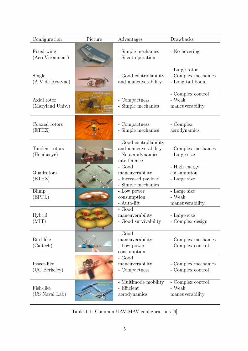
Different configurations of MAVs commonly used both for research purposes and inindustry are shown in Table 1.1 along with related advantages and drawbacks. This tableoffers a pictorial comparison that may be used when a new design is proposed.

Further, Figure 1.3 presents a short and not exhaustive comparison between differentVTOL vehicle concepts. It may be observed from Figure 1.3 that the quadrotor and thecoaxial helicopter are among the best configurations if used as MFRs.

Quadrotors offer VTOL capability and also the ability to fly along a designated pathwith any designated yaw angle attitude. This is a major advantage in surveillance missionsbecause it allows for the cameras to look in a chosen direction during flight, almost

3

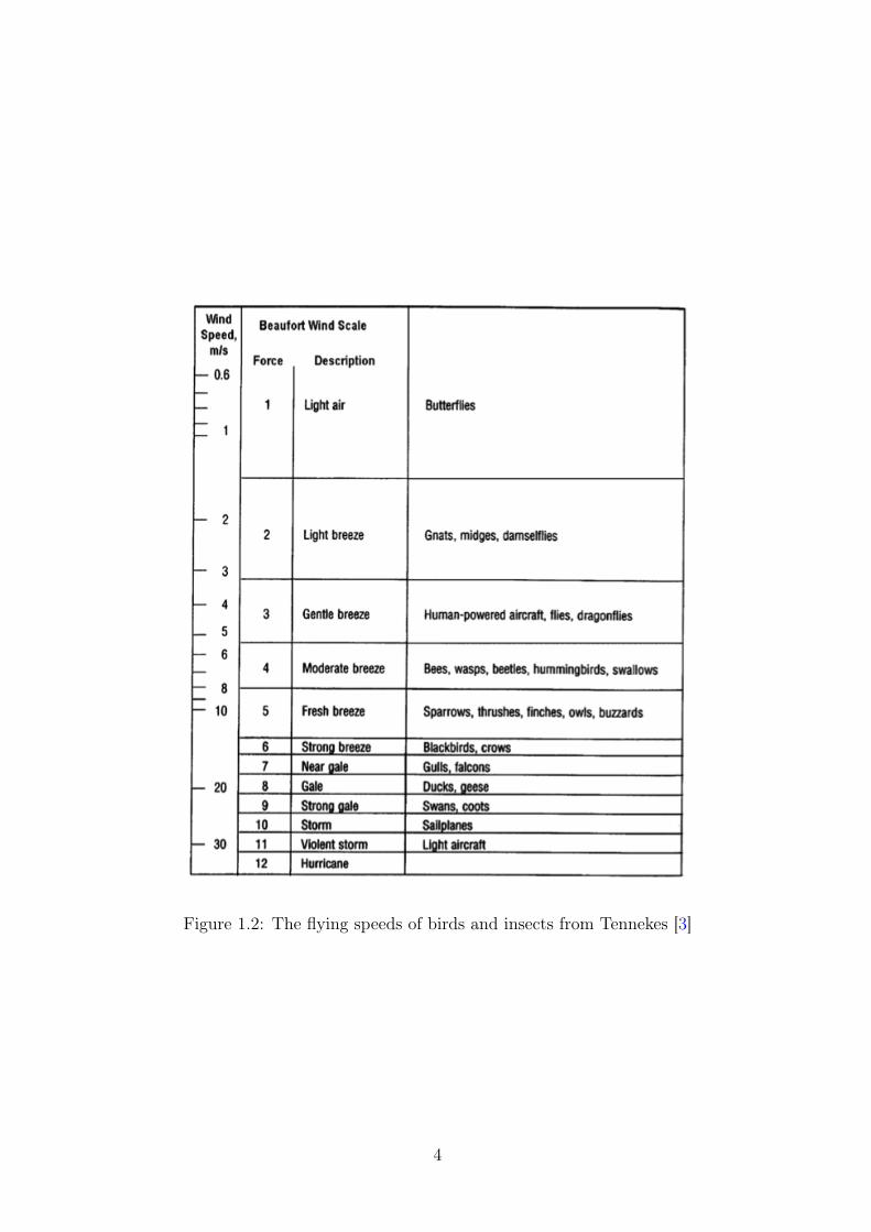
Figure 1.2: The flying speeds of birds and insects from Tennekes [3]

4

Configuration Picture Advantages Drawbacks

Fixed-wing - Simple mechanics - No hovering(AeroVironment) - Silent operation

- Large rotorSingle - Good controllability - Complex mechanics(A.V de Rostyne) and maneuverability - Long tail boom

- Complex controlAxial rotor - Compactness - Weak(Maryland Univ.) - Simple mechanics maneuverability

Coaxial rotors - Compactness - Complex(ETHZ) - Simple mechanics aerodynamics

- Good controllabilityTandem rotors and maneuverability - Complex mechanics(Heudiasyc) - No aerodynamics - Large size

interference- Good - High energy

Quadrotors maneuverability consumption(ETHZ) - Increased payload - Large size

- Simple mechanicsBlimp - Low power - Large size(EPFL) consumption - Weak

- Auto-lift maneuverability- Good

Hybrid maneuverability - Large size(MIT) - Good survivability - Complex design

- GoodBird-like maneuverability - Complex mechanics(Caltech) - Low power - Complex control

consumption- Good

Insect-like maneuverability - Complex mechanics(UC Berkeley) - Compactness - Complex control

- Multimode mobility - Complex controlFish-like - Efficient - Weak(US Naval Lab) aerodynamics maneuverability

Table 1.1: Common UAV-MAV configurations [6]

5

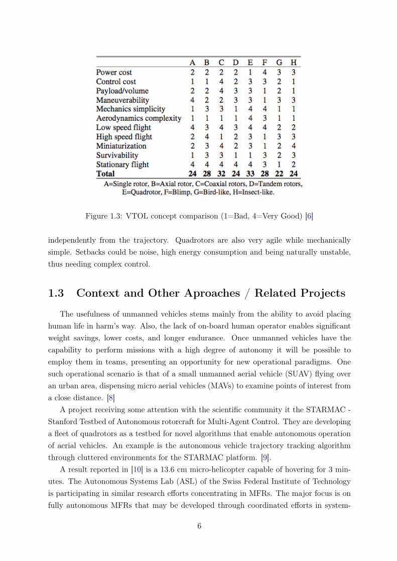
Figure 1.3: VTOL concept comparison (1=Bad, 4=Very Good) [6]

independently from the trajectory. Quadrotors are also very agile while mechanicallysimple. Setbacks could be noise, high energy consumption and being naturally unstable,thus needing complex control.

1.3 Context and Other Aproaches / Related Projects

The usefulness of unmanned vehicles stems mainly from the ability to avoid placinghuman life in harm’s way. Also, the lack of on-board human operator enables significantweight savings, lower costs, and longer endurance. Once unmanned vehicles have thecapability to perform missions with a high degree of autonomy it will be possible toemploy them in teams, presenting an opportunity for new operational paradigms. Onesuch operational scenario is that of a small unmanned aerial vehicle (SUAV) flying overan urban area, dispensing micro aerial vehicles (MAVs) to examine points of interest froma close distance. [8]

A project receiving some attention with the scientific community it the STARMAC -Stanford Testbed of Autonomous rotorcraft for Multi-Agent Control. They are developinga fleet of quadrotors as a testbed for novel algorithms that enable autonomous operationof aerial vehicles. An example is the autonomous vehicle trajectory tracking algorithmthrough cluttered environments for the STARMAC platform. [9].

A result reported in [10] is a 13.6 cm micro-helicopter capable of hovering for 3 min-utes. The Autonomous Systems Lab (ASL) of the Swiss Federal Institute of Technologyis participating in similar research efforts concentrating in MFRs. The major focus is onfully autonomous MFRs that may be developed through coordinated efforts in system-

6

level optimization, design and control. The approach that is followed is to design vehicleswith optimized mechanics and innovative control techniques. The goal is to keep on minia-turizing the MFR in every redesign step, following the latest technological advancements.[6]

Many research groups are developing aerial robots for security and rescue operations.But no mater whether a system is designed to inspect the outside of a building or searchfor casualties in a disaster, its goal is to fly sensors into a difficult to-get-to site and sendback information to a remote operator. [11]

A completely different approach from the quadrotors is passive morphing, that pro-poses high structural flexibility as a way to address the problem of sensitivity to windand gusts. In this manner, the energy of the wind and gusts can be absorbed by theairframe to help minimize the gross movement of the vehicle. This passive response to adisturbance may allow improved flight performance of a MAV. This approach also studiespossible aerodynamic advantages associated with flexible wings which may help improveMAV flight characteristics. [1]

Another branch of MAV research is centered about the development of an additionalflight modality enabling fixed-wing MAVs to supplement existing endurance superioritywith hovering capabilities. This secondary flight mode can also be used to avoid imminentcollisions by quickly transitioning from cruise to hover flight. [2]

In this kind of aircraft, even though hovering may be possible, it’s harder to keep andnot as stable as with rotorcrafts.

There have been several attempts to use vision guidance for control purposes on ro-torcraft, such as the work conducted by Altug and Taylor into the use of a ground basedtracking camera to control the pose of a quadrotor and a stable response was obtained.The work involved using a camera directly beneath the base of the quadrotor which lookedat 4 dots on the 4 rotor head bases. Since the size of these dots was a known variable,it was then possible to calculate the distance above the ground of each rotor and as suchfind the current Euler angles of the craft and the overall height. This information wasthen used to actuate control commands on the vehicle to reach a desired state. The in-evitable problem with this work was that the stability of the system was dependent uponthe quadrotor maintaining its position roughly above the fixed ground camera and workon allowing the ground camera to translate is planned. [12] [13]

Intensive investigation is being made worldwide on this subject, including in theproject that the present work is part of. The subject of vision sensoring is still a greatchallenge due to the huge ammounts of information to be handled, as well as the difficultyto extract features and distances from a raw image.

On the other hand the MAV flight mechanics challenge consists of generating sufficientcontrol power to maneuver, negotiate gusts while keeping sensors on target and remain

7

controllable in ground effect or in the presence of other obstacles. Indoors the challenge isto precisely maintain path and orientation in confined spaces, and cluttered/complex en-vironments; to “perch” and perform related maneuvers of precision landing and to achieveall of these with minimal onboard energy storage, with low-resolution air data sensorsand with limited onboard computational resources.

Even though research on MAV’s started quite recently, there is great motivation toovercome the problems faced. Many projects worldwide are addressing the MAV subject,following a variety of approaches. Only a few projects were named here, with the purposeof giving a general notion about the several areas of open research on the MAV subject.

1.4 The ISL micro-quadrotor project

1.4.1 The project’s goals

The ISL’s QuadRotor project aims to develop a fully autonomous micro-quadrotorthat uses cameras as auxiliary position and attitude sensors as well as for video recordingpurposes. The use of vision as an additional sensor is beneficial when flying in closeproximity to the ground, or in an inner city environment, as well as ease in carrying outautonomous landings.

In this manner the necessary accuracy of the Inertial Measurement Unit (IMU) isreduced, allowing for a cheap platform. Low prices would enable a larger disseminationof this kind of products. Light weight is also a goal.

Artificial Intelligence (AI) is emlpoyed to develop algorithms for automatic real-timeonboard computation of optimal trajectories according to user-input path-points, andobstacle avoidance.

The ISL’s QuadRotor will be robust for indoor as well as outdoor flight, for which aGPS receiver is implemented as auxiliary position sensor.

1.4.2 The quadrotor platform

The ISL’s quadrotor platform was bought from the german company Ascending Tech-nologies. The model is named X-3D-BL and is a hobby line platform. It is sold as a kitto be assembled by the costumer.

The main components of the X-3D-BL platform are:

X-3D - The sensor board;

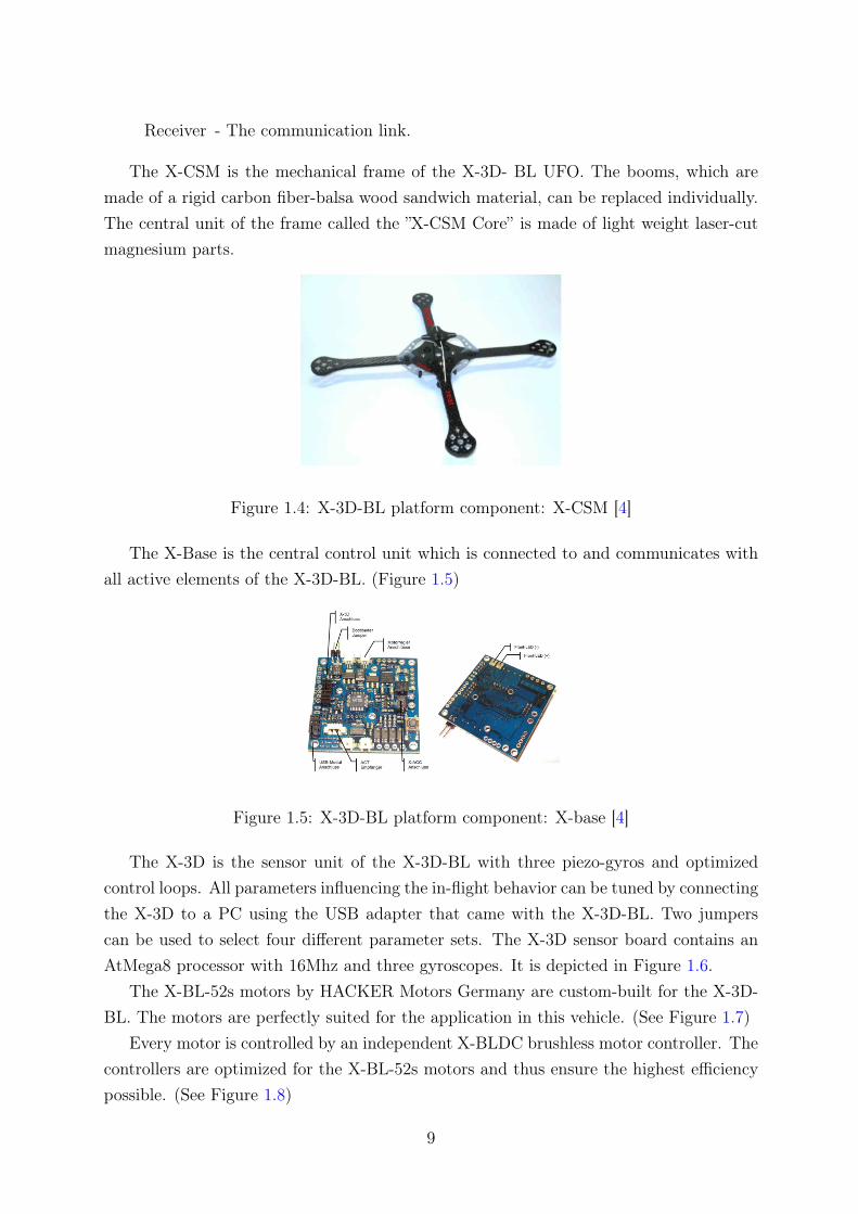
X-Base - The baseboard. Power and signal processing;

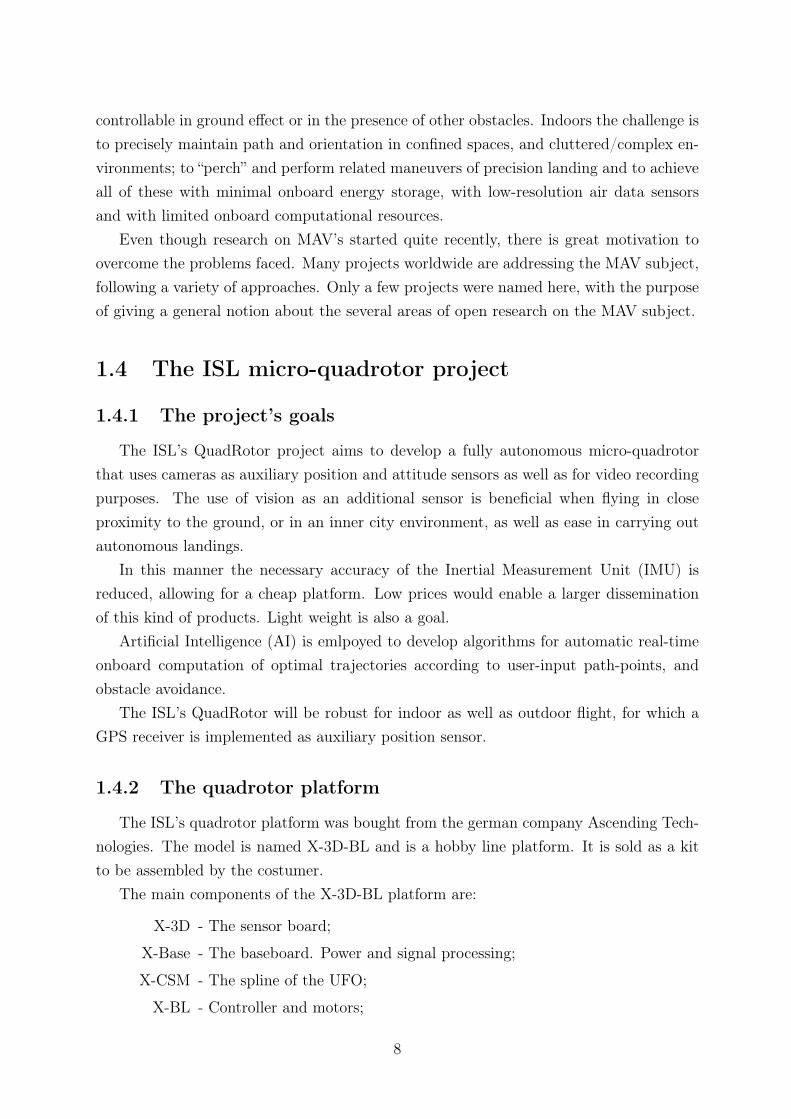
X-CSM - The spline of the UFO;

X-BL - Controller and motors;

8

Receiver - The communication link.

The X-CSM is the mechanical frame of the X-3D- BL UFO. The booms, which aremade of a rigid carbon fiber-balsa wood sandwich material, can be replaced individually.The central unit of the frame called the ”X-CSM Core” is made of light weight laser-cutmagnesium parts.

Figure 1.4: X-3D-BL platform component: X-CSM [4]

The X-Base is the central control unit which is connected to and communicates withall active elements of the X-3D-BL. (Figure 1.5)

Figure 1.5: X-3D-BL platform component: X-base [4]

The X-3D is the sensor unit of the X-3D-BL with three piezo-gyros and optimizedcontrol loops. All parameters influencing the in-flight behavior can be tuned by connectingthe X-3D to a PC using the USB adapter that came with the X-3D-BL. Two jumperscan be used to select four different parameter sets. The X-3D sensor board contains anAtMega8 processor with 16Mhz and three gyroscopes. It is depicted in Figure 1.6.

The X-BL-52s motors by HACKER Motors Germany are custom-built for the X-3D-BL. The motors are perfectly suited for the application in this vehicle. (See Figure 1.7)

Every motor is controlled by an independent X-BLDC brushless motor controller. Thecontrollers are optimized for the X-BL-52s motors and thus ensure the highest efficiencypossible. (See Figure 1.8)

9

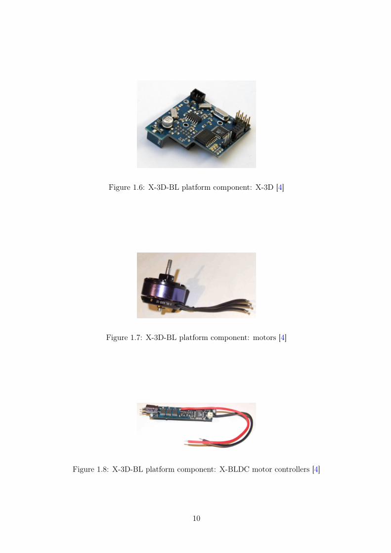
Figure 1.6: X-3D-BL platform component: X-3D [4]

Figure 1.7: X-3D-BL platform component: motors [4]

Figure 1.8: X-3D-BL platform component: X-BLDC motor controllers [4]

10

The following Table 1.2 summarizes some global characteristics of the X-3D-BL plat-form.

Flight Performance General and Technical DataCruise Speed 36 km/h Chassis design HummingbirdMax. Speed 50 km/h Dimensions (cm) 40x40x10Min. Speed 0 km/h Weight incl. battery (g) 500Launch Type VTOL Number of Propellers 4Usual Operating Altitude 50 m Propeller Size (inches) 8Max. Flight Time 20 min Battery Type LiPo11.1V

2100 mAhMax. Payload 200 g Flight Time, Max. Payload 10-12 min

Table 1.2: Global characteristics of the X-3D-BL platform [4]

1.4.3 The XSens unit

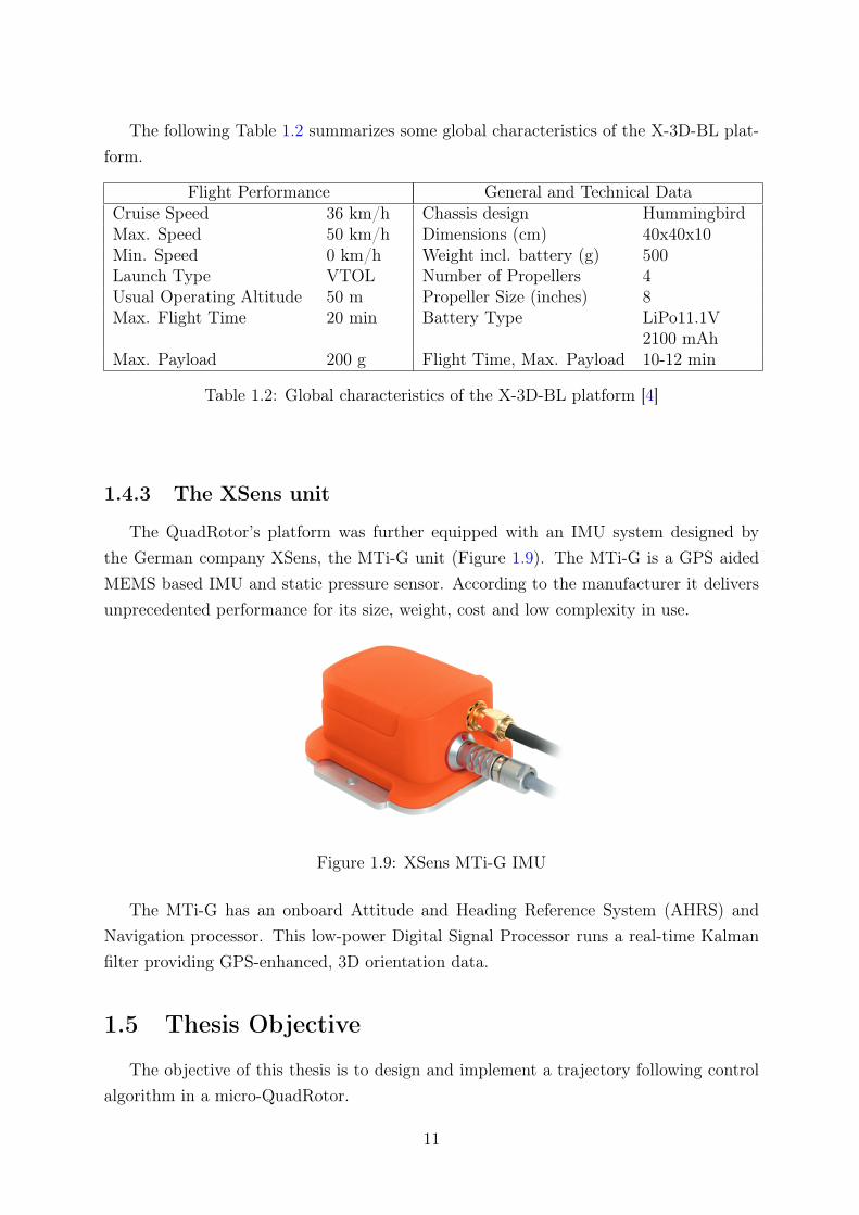
The QuadRotor’s platform was further equipped with an IMU system designed bythe German company XSens, the MTi-G unit (Figure 1.9). The MTi-G is a GPS aidedMEMS based IMU and static pressure sensor. According to the manufacturer it deliversunprecedented performance for its size, weight, cost and low complexity in use.

Figure 1.9: XSens MTi-G IMU

The MTi-G has an onboard Attitude and Heading Reference System (AHRS) andNavigation processor. This low-power Digital Signal Processor runs a real-time Kalmanfilter providing GPS-enhanced, 3D orientation data.

1.5 Thesis Objective

The objective of this thesis is to design and implement a trajectory following controlalgorithm in a micro-QuadRotor.

11

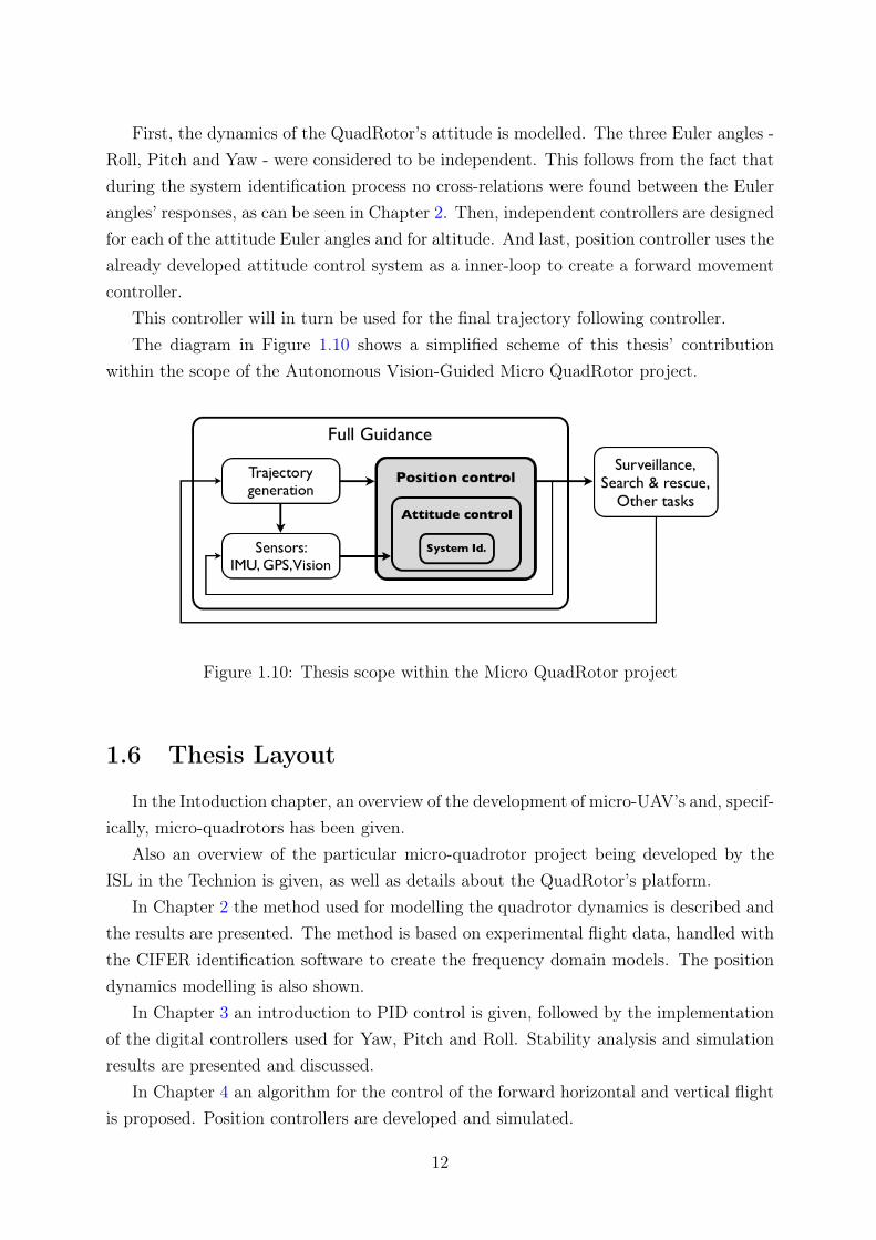
First, the dynamics of the QuadRotor’s attitude is modelled. The three Euler angles -Roll, Pitch and Yaw - were considered to be independent. This follows from the fact thatduring the system identification process no cross-relations were found between the Eulerangles’ responses, as can be seen in Chapter 2. Then, independent controllers are designedfor each of the attitude Euler angles and for altitude. And last, position controller uses thealready developed attitude control system as a inner-loop to create a forward movementcontroller.

This controller will in turn be used for the final trajectory following controller.The diagram in Figure 1.10 shows a simplified scheme of this thesis’ contribution

within the scope of the Autonomous Vision-Guided Micro QuadRotor project.

Figure 1.10: Thesis scope within the Micro QuadRotor project

1.6 Thesis Layout

In the Intoduction chapter, an overview of the development of micro-UAV’s and, specif-ically, micro-quadrotors has been given.

Also an overview of the particular micro-quadrotor project being developed by theISL in the Technion is given, as well as details about the QuadRotor’s platform.

In Chapter 2 the method used for modelling the quadrotor dynamics is described andthe results are presented. The method is based on experimental flight data, handled withthe CIFER identification software to create the frequency domain models. The positiondynamics modelling is also shown.

In Chapter 3 an introduction to PID control is given, followed by the implementationof the digital controllers used for Yaw, Pitch and Roll. Stability analysis and simulationresults are presented and discussed.

In Chapter 4 an algorithm for the control of the forward horizontal and vertical flightis proposed. Position controllers are developed and simulated.

12

In Chapter 5 the implementation efforts are described, including the realtime softwaredevelopment. Experimental test results are also presented and discussed.

In Chapter 6, some conclusions are drawn and suggestions for future work are pre-sented.

13

Chapter 2

Dynamics Modelling

The dynamics of a rigid body subject to external forces applied to the center of massand expressed in the body-fixed reference frame in Newton-Euler formalism are:

�mI3×3 0

0 I

��V

ω

�+

�ω ×mV

ω × Iω

�=

�F

τ

�(2.1)

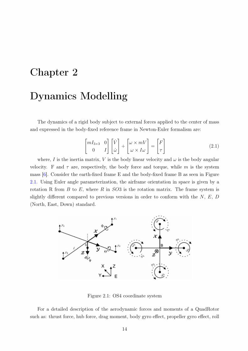
where, I is the inertia matrix, V is the body linear velocity and ω is the body angularvelocity. F and τ are, respectively, the body force and torque, while m is the systemmass [6]. Consider the earth-fixed frame E and the body-fixed frame B as seen in Figure2.1. Using Euler angle parameterization, the airframe orientation in space is given by arotation R from B to E, where R in SO3 is the rotation matrix. The frame system isslightly different compared to previous versions in order to conform with the N , E, D(North, East, Down) standard.

Figure 2.1: OS4 coordinate system

For a detailed description of the aerodynamic forces and moments of a QuadRotorsuch as: thrust force, hub force, drag moment, body gyro effect, propeller gyro effect, roll

14

actuators action, hub moments and rotor dynamics, please refer to [6] or [14] for example.

2.1 System Identification using CIFER®

Regarding the determination of the QuadRotor’s platform attitude dynamics, twomain methods were available: algebraic deduction of a theoretical model or system iden-tification using flight measurements. The later was chosen for four reasons:

1. The system would be very difficult to accurately describe due to the complexity ofthe QuadRotor platform and the fact that it was acquired as a final product andthen altered to support the payload and instruments.

2. Following the flight measurements plus numerical system identification path wassimple because the platform was already flying controlled remotely by a humanpilot and with instruments onboard.

3. Recording flight measurements of attitude, position, accelerations and velocitiesand afterwards using a system identification software like CIFER® should producea more reliable result than trying to physically model such a complex structure asthis QuadRotor platform.

4. A theoretical description here would be possible only as a simple and rough model,while CIFER® software produces accurate dynamic models. This is of major im-portance because, as can be seen in Chapters 3 and 4, the Attitude control is thecore of the control system.

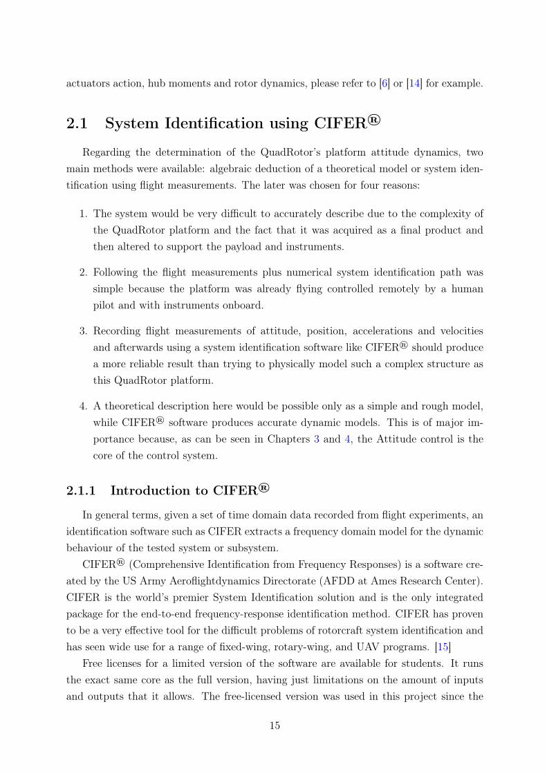
2.1.1 Introduction to CIFER®

In general terms, given a set of time domain data recorded from flight experiments, anidentification software such as CIFER extracts a frequency domain model for the dynamicbehaviour of the tested system or subsystem.

CIFER® (Comprehensive Identification from Frequency Responses) is a software cre-ated by the US Army Aeroflightdynamics Directorate (AFDD at Ames Research Center).CIFER is the world’s premier System Identification solution and is the only integratedpackage for the end-to-end frequency-response identification method. CIFER has provento be a very effective tool for the difficult problems of rotorcraft system identification andhas seen wide use for a range of fixed-wing, rotary-wing, and UAV programs. [15]

Free licenses for a limited version of the software are available for students. It runsthe exact same core as the full version, having just limitations on the amount of inputsand outputs that it allows. The free-licensed version was used in this project since the

15

limitations did not prove to be a problem for the application in hand. It should be noticedthat the CIFER version used runs its graphical interface on Matlab®, which was alreadyinstalled on the machines since it is the main software used for the design of the controlalgorithms in this project.

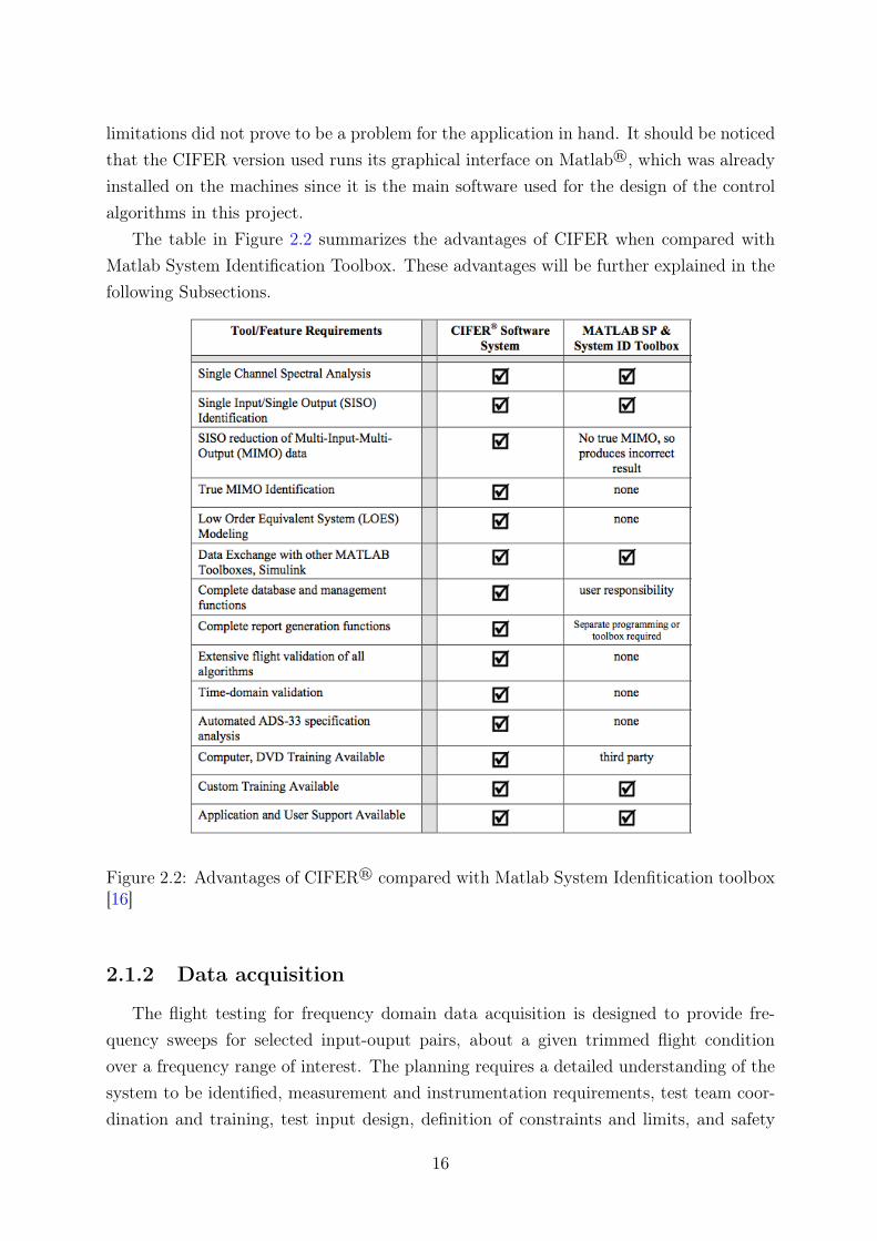
The table in Figure 2.2 summarizes the advantages of CIFER when compared withMatlab System Identification Toolbox. These advantages will be further explained in thefollowing Subsections.

Figure 2.2: Advantages of CIFER® compared with Matlab System Idenfitication toolbox[16]

2.1.2 Data acquisition

The flight testing for frequency domain data acquisition is designed to provide fre-quency sweeps for selected input-ouput pairs, about a given trimmed flight conditionover a frequency range of interest. The planning requires a detailed understanding of thesystem to be identified, measurement and instrumentation requirements, test team coor-dination and training, test input design, definition of constraints and limits, and safety

16

considerations. The previous information on the QuadRotor’s platform dynamics, gainedby searching literature about similar aircrafts, reading the platform’s users manual andpiloting it is of key importance for the definition of which relations to search for in anidentifcation process. [17]

Even though the final goal for the present case is position control of the platform, onlythe attitude inner-loop (see Chapter 3) and the altitude responses were identified. Nodetailed information on rotors, servos or other sub-systems was of interest because thedesired models should regard the system as a whole. Having in mind these identificationobjectives, the recorded quantities were the measurements from the XSens unit as well asthe pilot inputs.

The angle rate measurements were used for attitude (Roll, Pitch and Yaw) togetherwith the respective commands from the remote control (pilot input). For altitude, thealtitude rate measurement was used with the throttle command (T) (see Equation 2.2).

φ(s)

Uφ(s)= TFφ(s) (2.2a)

θ(s)

Uθ(s)= TFθ(s) (2.2b)

ψ(s)

Uψ(s)= TFψ(s) (2.2c)

Z(s)

T (s)= TFZ(s) (2.2d)

Inertial measurements can be instrumented with an inertial system package with itsassociated internal filtering and processing. It is essential for accurate identification thatthe sensor, filtering and data acquisition system characteristics be well understood. [17]The IMU used here is the XSens unit described in Chapter 1.

One of the strengths of frequency domain testing is that the associated data reductionis not dependent on the input shape. It is not necessary for the frequency sweep input tobe a sinusoid. In fact, piloted inputs typically have a richer frequency content than a puresine wave, which enhances the results quality. Automated computer-generated sweeps arenot desired for most applications. [17]

The set of test inputs needed for frequency domain analysis consists of piloted fre-quency sweeps, doublets or pulses. The sweeps are used to generate the frequency re-sponse database, and the doublets and pulses are used for time domain verification ofresulting models. For the frequency sweep, the pilot produces a sinusoidal input abouta reference trim condition, beginning at very low frequency and progressively increasing

17

the frequency of inputs. For most flying qualities a desired cutoff frequency of 2Hz is rec-ommended. The total record length should be 3-4 times the maximum period of interest.Two pulses should be made for the purpose of generating independent time histories formodel verification.

Since the results’ frequency domain analysis are only appropriate for dynamics in theneighborhood of the trim condition tested and the open-loop response was desired, theflight conditions were forward and hover flight with all augmentation systems disabled.Frequency domain flight testing requires same weather conditions as vehicle performancetesting. [17]

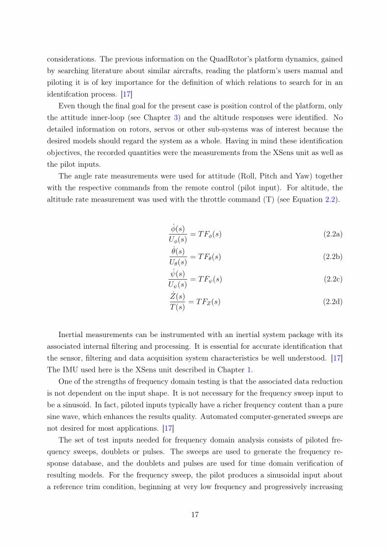
Figure 2.3 shows the recorded attitude angles measured in a flight test for Pitchdynamics identification.

Figure 2.3: Flight data: attitude measurements for Pitch identification

The data acquisition and test planning was conducted by the Technion’s ISL personnel,including aerodynamics enginner and pilot.

2.1.3 Data handling: software overview and user’s perspective

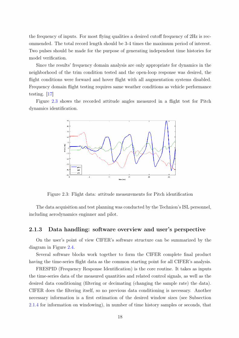
On the user’s point of view CIFER’s software structure can be summarized by thediagram in Figure 2.4.

Several software blocks work together to form the CIFER complete final producthaving the time-series flight data as the common starting point for all CIFER’s analysis.

FRESPID (Frequency Response Identification) is the core routine. It takes as inputsthe time-series data of the measured quantities and related control signals, as well as thedesired data conditioning (filtering or decimating (changing the sample rate) the data).CIFER does the filtering itself, so no previous data conditioning is necessary. Anothernecessary information is a first estimation of the desired window sizes (see Subsection2.1.4 for information on windowing), in number of time history samples or seconds, that

18

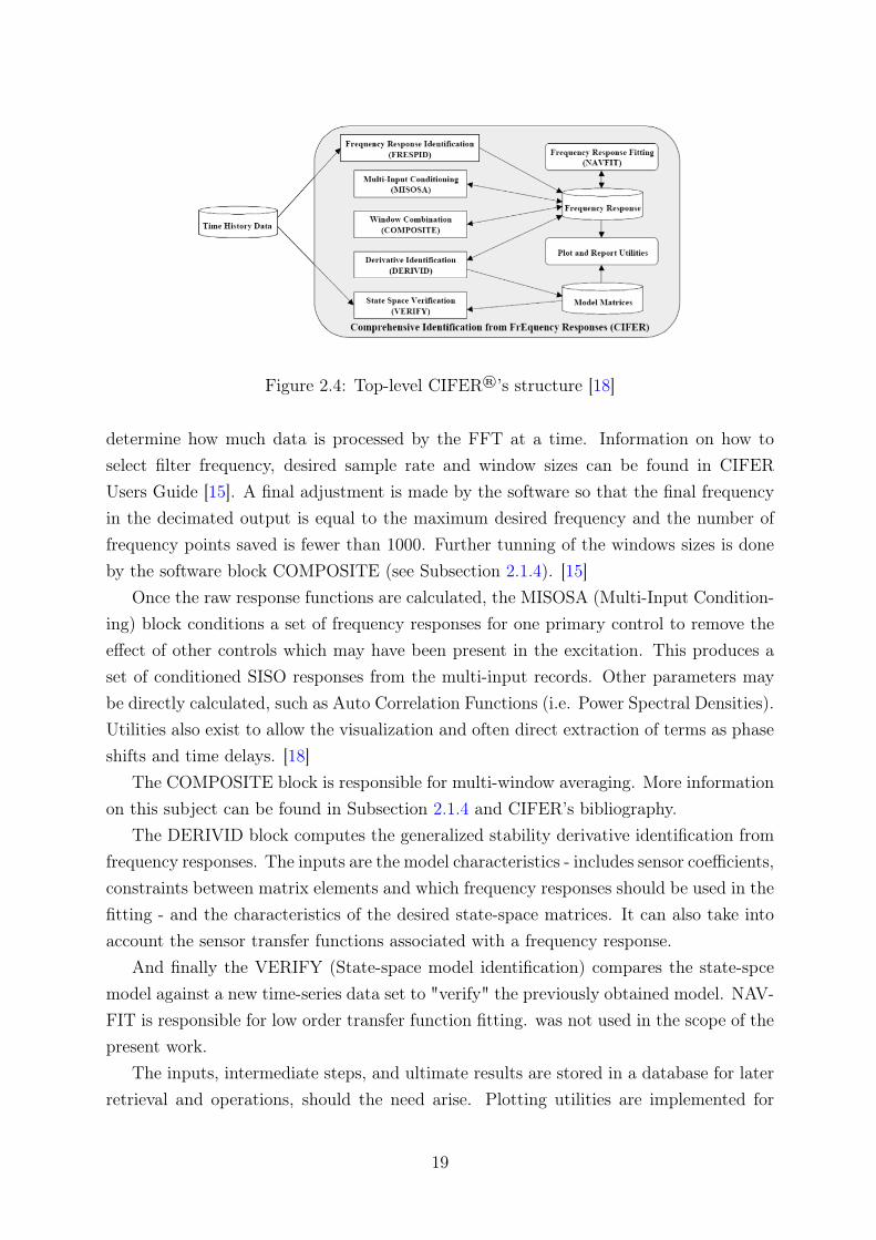
Figure 2.4: Top-level CIFER®’s structure [18]

determine how much data is processed by the FFT at a time. Information on how toselect filter frequency, desired sample rate and window sizes can be found in CIFERUsers Guide [15]. A final adjustment is made by the software so that the final frequencyin the decimated output is equal to the maximum desired frequency and the number offrequency points saved is fewer than 1000. Further tunning of the windows sizes is doneby the software block COMPOSITE (see Subsection 2.1.4). [15]

Once the raw response functions are calculated, the MISOSA (Multi-Input Condition-ing) block conditions a set of frequency responses for one primary control to remove theeffect of other controls which may have been present in the excitation. This produces aset of conditioned SISO responses from the multi-input records. Other parameters maybe directly calculated, such as Auto Correlation Functions (i.e. Power Spectral Densities).Utilities also exist to allow the visualization and often direct extraction of terms as phaseshifts and time delays. [18]

The COMPOSITE block is responsible for multi-window averaging. More informationon this subject can be found in Subsection 2.1.4 and CIFER’s bibliography.

The DERIVID block computes the generalized stability derivative identification fromfrequency responses. The inputs are the model characteristics - includes sensor coefficients,constraints between matrix elements and which frequency responses should be used in thefitting - and the characteristics of the desired state-space matrices. It can also take intoaccount the sensor transfer functions associated with a frequency response.

And finally the VERIFY (State-space model identification) compares the state-spcemodel against a new time-series data set to "verify" the previously obtained model. NAV-FIT is responsible for low order transfer function fitting. was not used in the scope of thepresent work.

The inputs, intermediate steps, and ultimate results are stored in a database for laterretrieval and operations, should the need arise. Plotting utilities are implemented for

19

visualization of these results [18]. There’s also a set of utilities to further analyse theresults. [15]

The last three software blocks - DERIVID, VERIFY and NAVFIT - were not used inthe scope of the present work.

2.1.4 Data handling: the CZT

CIFER® receives the response features as well as the original or filtered waveformsand uses these data to perform spectral analysis and a variety of specialized behaviorextractions. The block-diagram in Figure 2.5 shows the algorithm structure for systemidentification in CIFER®.

Figure 2.5: Frequency response identification process in CIFER® [15]

CIFER® begins with some checks of each sample on the integrity of the data, to findthose cases where data corruption has occurred but is not self-evident.

Next, FRESPID uses a flexible form of the fast Fourier transform (FFT) that wasdeveloped in CIFER® facility, known as the Chirp-Z transform (CZT), to condition thefrequency responses. The CZT is not subject to the restriction that the number of timehistory samples (L) and the number of frequency points (N) be equal (however, thecondition that N≤L must be met) which results in a finer frequency resolution for agiven window size. Another key advantage of the CZT is that there is no restrictionthat N be a power of 2; for the CZT only N+L must be a power of 2. Finally, there isno need to calculate over the entire Nyquist frequency range; the CZT determines theFFT over any frequency range. This combination yields the condition that there is muchgreater flexibility in selection of sample rate, window length, and frequency resolution – a

20

necessary criterion to support CIFER® capability for automatic sliding window processingand optimization, in the COMPOSITE routine. [17] [18]

In summary, the capabilities of the CZT allow the extraction of high-resolution spectrain a narrow frequency band and an increase in the identified dynamic range, especiallyat the low-frequency end [17]. Furthermore this is accomplished with simultaneouslymore accurate results (because CIFER® can interactively narrow the range of interest)at greatly reduced computational cost (because only the needed points are calculated).[18]

WindowingA phenomenon exists in Fourier analysis where erroneous frequency content appears

as sidelobes to the Fourier frequency of interest. This phenomenon is commonly referredto as "leakage", and since the analysis objective is to separate the effects of differentfrequencies on a system, leakage contaminates the results. A technique to reduce leakageis by "windowing" or "tapering" the data. [17]

In simple terms, the "windows" refer to subrecords of the FFT total time history record(or multiple concatenated records) and are sized to optimize the quality of the spectralidentification. The frequency content of the window is limited by the window length, inthat the lowest frequency possible in the window is that frequency with a period the sizeof the window. On the other hand, the more windows that a particular time history isdivided into, the lower the random error in the result because of averaging. For a givenrecord length, smaller windows yield more averaging and lower spectral variance. Thus,the selection of window length involves a compromise between a high number of averagesand adequate low-frequency signal content. [17]

Like other Fourier analysis implementations, CIFER® provides for dividing signalsamples into overlapping time intervals, called windows. It is well recognized that largerwindows give better accuracy at lower frequencies while smaller windows improve accuracyin higher frequencies. The calculation, interpretation, and management of these windowsis typically a manual and very time/attention-intensive task. However, because the CZTremoves many restrictions on windowing choices, CIFER® implements in COMPOSITEfunction a unique windowing algorithm that generates various combinations, selects thebest results using an embedded coherence and error function calculation, and integratesthe optimal combination automatically. [18]

Despite the tapered window approach, sidelobe noise will still exist in the result. Win-dow overlapping can further improve the results. If each successive window, or subrecord,of a concatenated multiple frequency sweep data set is overlapped by as much as 50%, thespectral bias and variance can be reduced and the results will be significantly improved.

As discussed previously, the selection of a single window size is a compromise betweenhaving a low frequency content (larger windows) and having a low random error (smaller

21

windows). The CIFER® computational system identification tool (ref 3) includes anadditional facility called COMPOSITE that takes the results from repeated conditioningof data using different window sizes, and combines the auto- and cross- spectral densityestimates (discussed in the next section) using a non-linear, least-squares optimization.The COMPOSITE routine will combine the low frequency content of the large windowsand the low random error of the smaller windows, resulting in improved spectral densityestimates over a wide frequency range. [17]

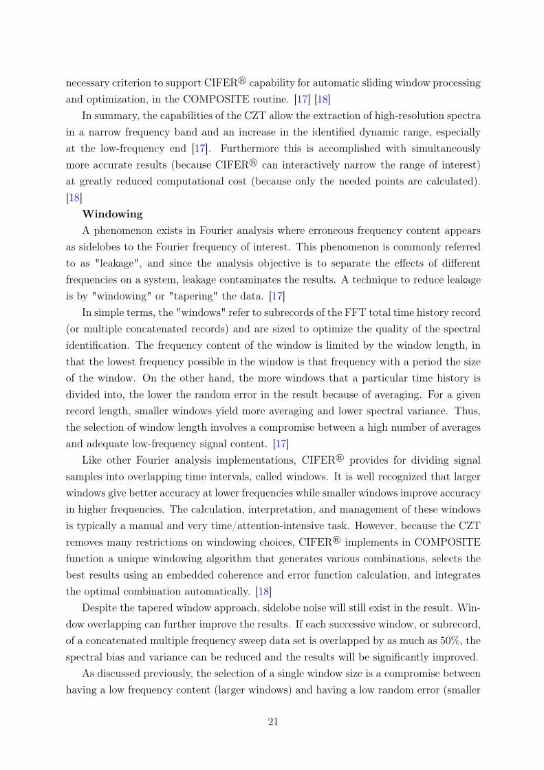
2.1.5 CIFER® Results

In this section, the transfer functions obtained with CIFER to model the QuadRotor’sattitude dynamics as well as the altitude are presentend together with the respectivecoherence data.

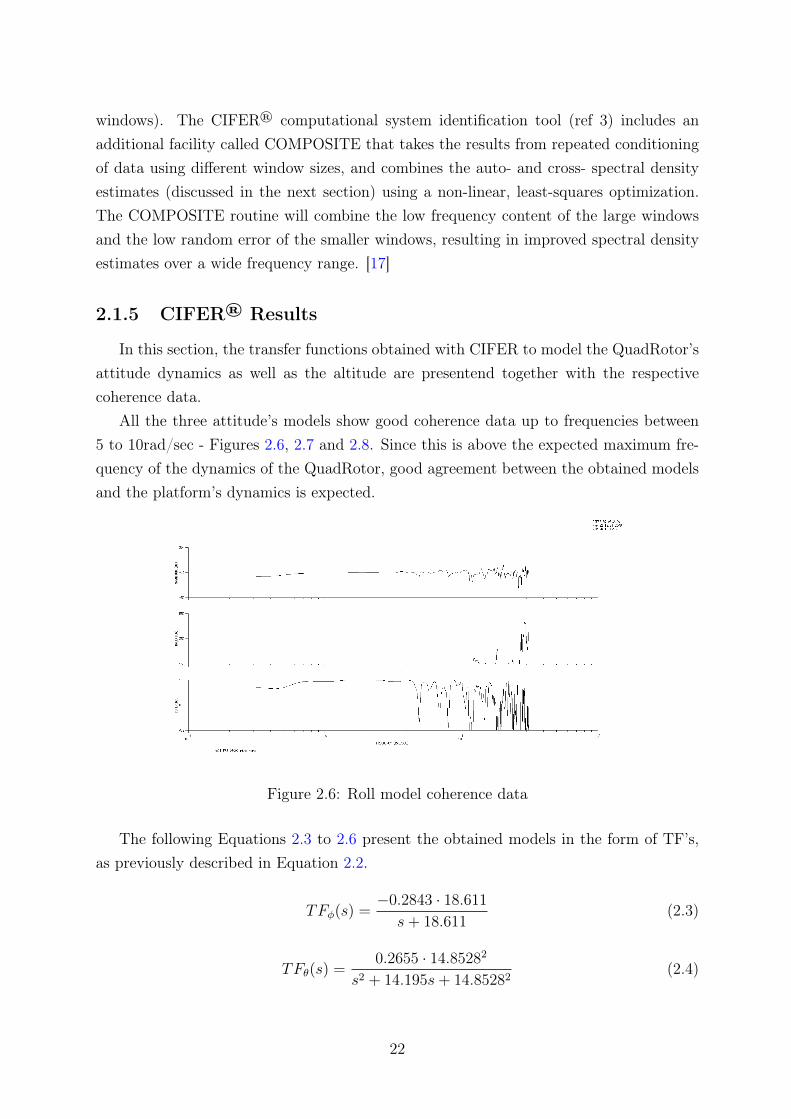
All the three attitude’s models show good coherence data up to frequencies between5 to 10rad/sec - Figures 2.6, 2.7 and 2.8. Since this is above the expected maximum fre-quency of the dynamics of the QuadRotor, good agreement between the obtained modelsand the platform’s dynamics is expected.

Figure 2.6: Roll model coherence data

The following Equations 2.3 to 2.6 present the obtained models in the form of TF’s,as previously described in Equation 2.2.

TFφ(s) =−0.2843 · 18.611

s+ 18.611(2.3)

TFθ(s) =0.2655 · 14.85282

s2 + 14.195s+ 14.85282(2.4)

22

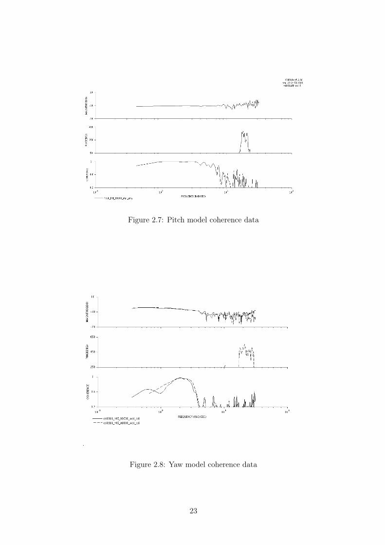
Figure 2.7: Pitch model coherence data

Figure 2.8: Yaw model coherence data

23

TFψ(s) =0.377568 · 3.51842

s2 + 2 · 0.5006 · 3.5184s+ 3.51842(2.5)

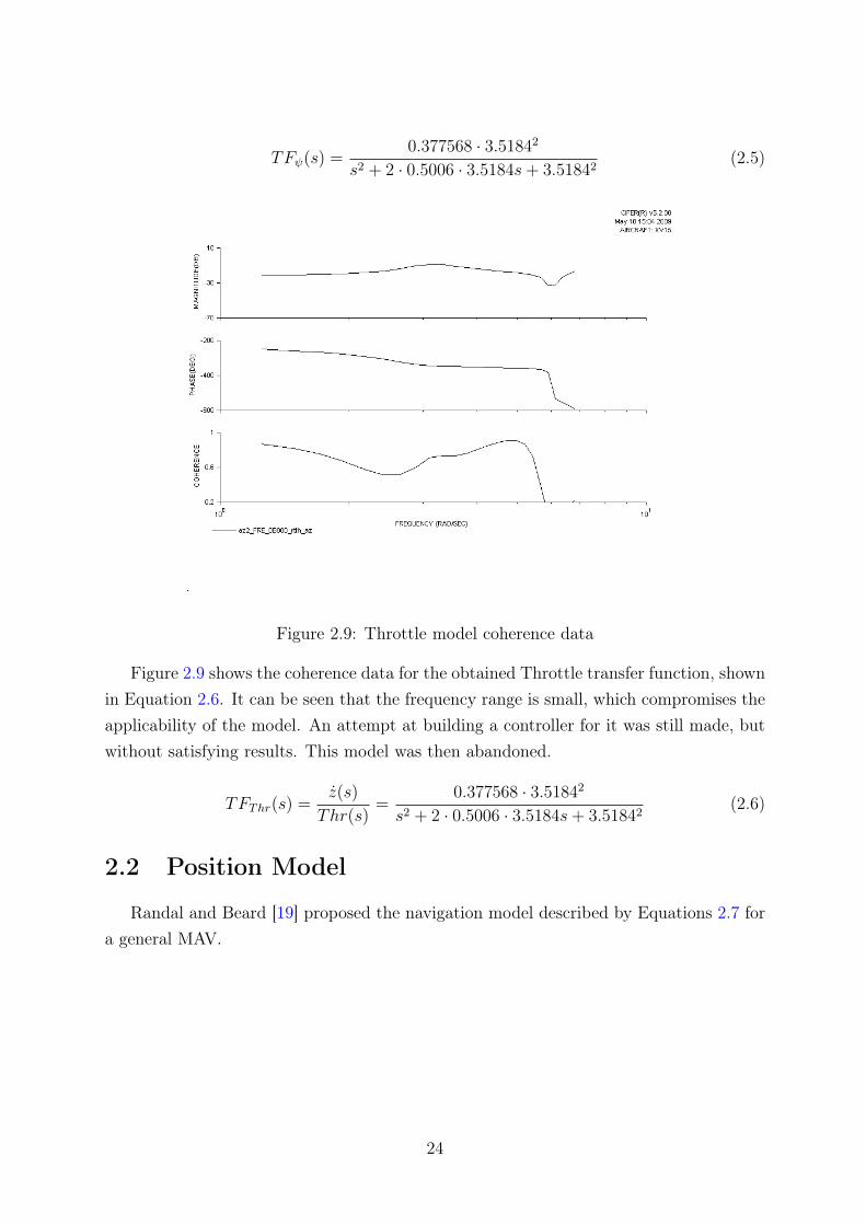
Figure 2.9: Throttle model coherence data

Figure 2.9 shows the coherence data for the obtained Throttle transfer function, shownin Equation 2.6. It can be seen that the frequency range is small, which compromises theapplicability of the model. An attempt at building a controller for it was still made, butwithout satisfying results. This model was then abandoned.

TFThr(s) =z(s)

Thr(s)=

0.377568 · 3.51842

s2 + 2 · 0.5006 · 3.5184s+ 3.51842(2.6)

2.2 Position Model

Randal and Beard [19] proposed the navigation model described by Equations 2.7 fora general MAV.

24

pn = V cos(χ)cos(γ)

pe = V sin(χ)cos(γ)

h = V sin(γ)

χ =g

Vtan(φ)

φ = u1

γ = u2

(2.7)

where pn and pe are the North and East position of the MAV, h is the altitude, V isthe groundspeed, χ is the course angle, γ is the flight path angle, etc.

According to [20], the following set of definitions is used in the present subsection.• local reference airframe �G = {G,Eg

1 , Eg

2 , Eg

3} is attached to the center of mass G;• inertial reference frame �O = {O,Ex, Ey, Ez}, where Ez is upwards and its unit

vector is eZ ;• ξ = (x, y, z) is the position of G wrt �O;• rotation of the rigid body R : �G → �O, where R is orthogonal;• Euler angles η = (ϕ, θ,ψ);• Position of G wrt �O is OG = (x, y, z)T ;• acceleration of G is d2OG

dt2= γG|�O

.Applying the first Newton equation of mechanics, we obtain the compact expression

of the translational motion in Equation 2.8.

mγG|�O= −mgeZ +RϕθψTu (2.8)

where the lift (collective) force u is the sum of four [rotor lift] forces. Drag forces andgyroscopic due to motors effects will be not considered in this work.

The form of the rotation matrix used in Equation 2.8 is as follows (Equation 2.9).

Rϕθψ =

cos(θ)cos(ψ) sin(ψ)cos(θ) −sin(θ)

cos(ψ)sin(θ)sin(ϕ)− sin(ψ)cos(ϕ) sin(θ)sin(ψ)sin(ϕ) + cos(ψ)cos(ϕ) cos(θ)sin(ϕ)

cos(ψ)sin(θ)cos(ϕ) + sin(ψ)sin(ϕ) sin(θ)sin(ψ)cos(ϕ)− cos(ψ)sin(ϕ) cos(θ)cos(ϕ)

(2.9)Substituting u into 2.8, we obtain 2.10.

mγG|�O= −mgeZ + TRϕθψT e3 (2.10)

where the scalar T =�4

i=1 kiω2i

represents the system input [throttle].In short, the difference between Equations 2.8 e 2.10 is that u ∼ Te3.

25

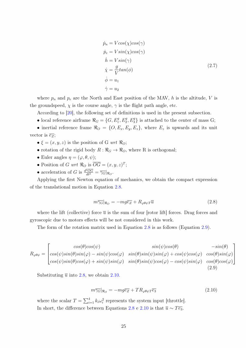
Equations 2.10 e 2.8 can be detailed as in Equation 2.11, where the Euler anglesrepresent the platform’s orientation with respect to the frame �O and T represents thethrottle, associated with the lift force.

mx = −Tsin(θ)

my = Tcos(θ)sin(ϕ)

mz = Tcos(θ)cos(ϕ)−mg

(2.11)

Assuming that (θ,ϕ) ≈ (0, 0), Equation 2.11 can be linearized to:

mx = −T θ

my = Tϕ

mz = T −mg

(2.12)

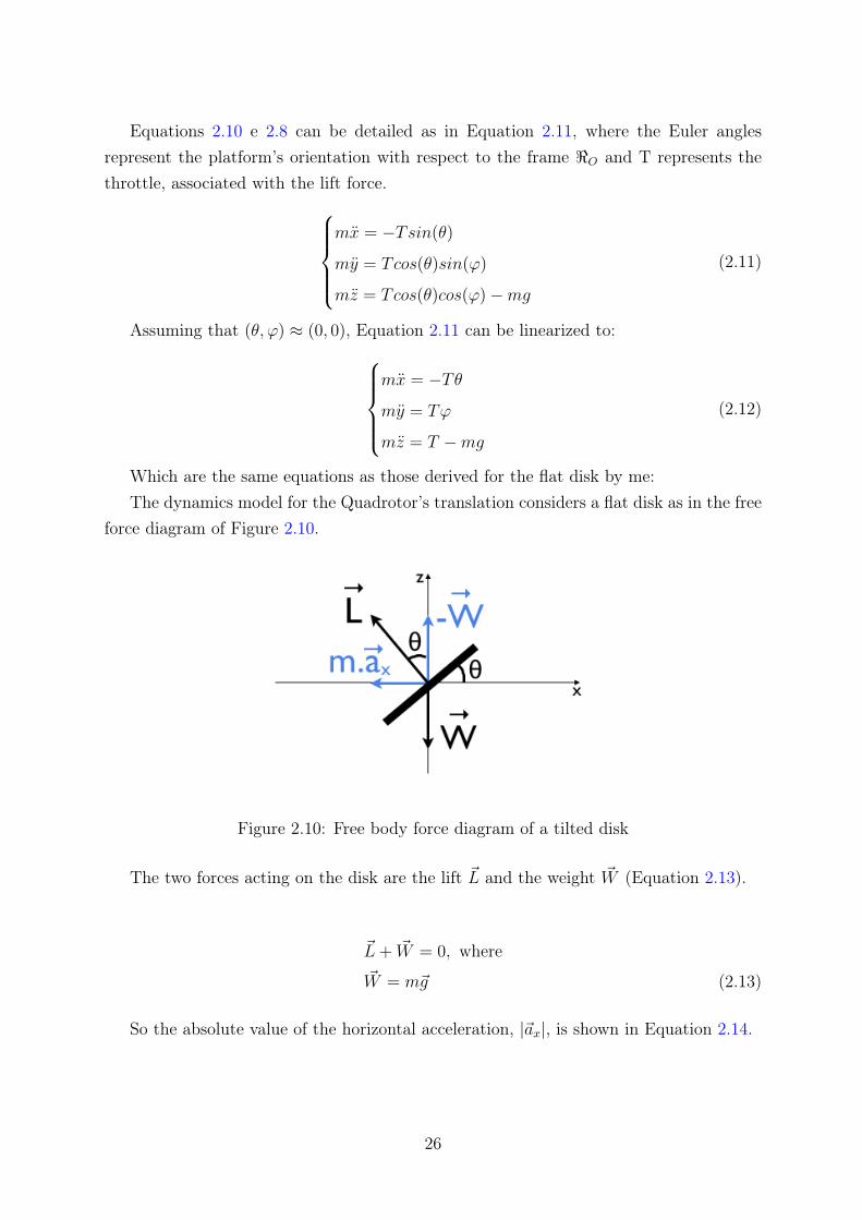
Which are the same equations as those derived for the flat disk by me:The dynamics model for the Quadrotor’s translation considers a flat disk as in the free

force diagram of Figure 2.10.

Figure 2.10: Free body force diagram of a tilted disk

The two forces acting on the disk are the lift �L and the weight �W (Equation 2.13).

�L+ �W = 0, where

�W = m�g (2.13)

So the absolute value of the horizontal acceleration, |�ax|, is shown in Equation 2.14.

26

m|�g| = |�L|cos(θ)

m|�ax| = |�L|sin(θ)⇒ |�ax| = g tan(θ) (2.14)

Having in mind that tan(x) ≈ x for |x| � 1, we get the final model in Equation 2.15.

x =d2x

dt≈ −gθ, |θ| � 1 (2.15)

This model already relates the horizontal position of the platform with its attitude,namely the position along the X axis with the Pitch angle.

From this model a Transfer Function can be obtained, Equation 4.1.

X(s)

θ(s)= −g

1

s2(2.16)

2.2.1 Vertical Position Model

For the first simulations of altitude control, a very simple model was used, in accor-dance with Bouabdallah’s book [6]. The model is shown in Equation 2.17.

h(t) =dh

dt= −g + cos(φ)cos(θ)

T (t)

m(2.17)

where h is the altitude measurement using the ground as reference, T is the platform’sthrottle and also the control signal and g is the gravity acceleration.

This is a non-linear model that was linearized for small pitch and roll angles, as follows.

h(t) =T (t)

m− g, (θ,φ) ≤ 10◦ (2.18)

Since it’s not possible to extract a transfer function for the model as it is, even afterlinearization, a change of variables was applied to Equation 2.17. So, having Tn(t) =

T (t)/m− g, the model from Equation 2.18 becomes a basic derivative, in Equation 2.19.

h(t) = Tn(t), Tn(t) =T (t)

m− g (2.19)

The resulting transfer functions in the frequency domain and the result of its’ dis-cretization with a sample time Ts = 0.04s are shown below.

H

Tn

(s) =1

s=⇒

H

Tn

(z) =0.04

z − 1(2.20)

27

Chapter 3

Attitude PID Control

In a quadrotor the attitude angles together with throttle are used to control all the air-ship’s movement. The translation movement control using the attitude angles is discussedin Chapter 4.

In this chapter PID controllers are developed, implemented and tested for each of theEuler Angles: Yaw, Pitch and Roll.

3.1 Introduction

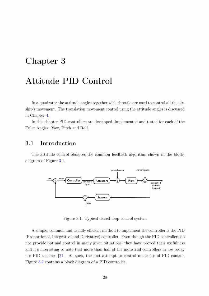
The attitude control observes the common feedback algorithm shown in the block-diagram of Figure 3.1.

Figure 3.1: Typical closed-loop control system

A simple, common and usually efficient method to implement the controller is the PID(Proportional, Integrative and Derivative) controller. Even though the PID controllers donot provide optimal control in many given situations, they have proved their usefulnessand it’s interesting to note that more than half of the industrial controllers in use todayuse PID schemes [21]. As such, the first attempt to control made use of PID control.Figure 3.2 contains a block diagram of a PID controller.

28

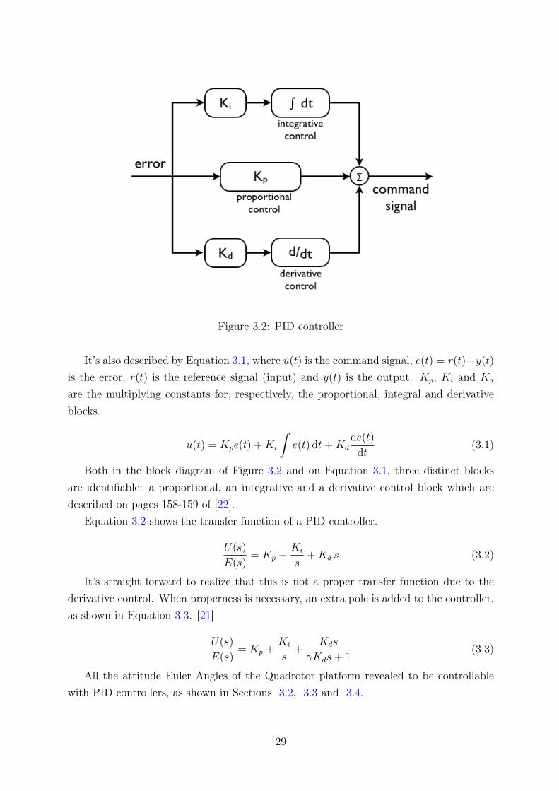
Figure 3.2: PID controller

It’s also described by Equation 3.1, where u(t) is the command signal, e(t) = r(t)−y(t)

is the error, r(t) is the reference signal (input) and y(t) is the output. Kp, Ki and Kd

are the multiplying constants for, respectively, the proportional, integral and derivativeblocks.

u(t) = Kpe(t) +Ki

�e(t) dt+Kd

de(t)

dt(3.1)

Both in the block diagram of Figure 3.2 and on Equation 3.1, three distinct blocksare identifiable: a proportional, an integrative and a derivative control block which aredescribed on pages 158-159 of [22].

Equation 3.2 shows the transfer function of a PID controller.

U(s)

E(s)= Kp +

Ki

s+Kd s (3.2)

It’s straight forward to realize that this is not a proper transfer function due to thederivative control. When properness is necessary, an extra pole is added to the controller,as shown in Equation 3.3. [21]

U(s)

E(s)= Kp +

Ki

s+

Kds

γKds+ 1(3.3)

All the attitude Euler Angles of the Quadrotor platform revealed to be controllablewith PID controllers, as shown in Sections 3.2, 3.3 and 3.4.

29

3.1.1 Design Specifications

The attitude Euler angles of the controlled Quadrotor platform must meet the followingdesign specifications:

• gain margin ≥ 10dB;

• phase margin � 60 deg;

• settling time should be minimal;

• steady-state error � 0 (type one system [23] [24] ).

• peak overshoot should be below 10%

3.1.2 Digital PID Control

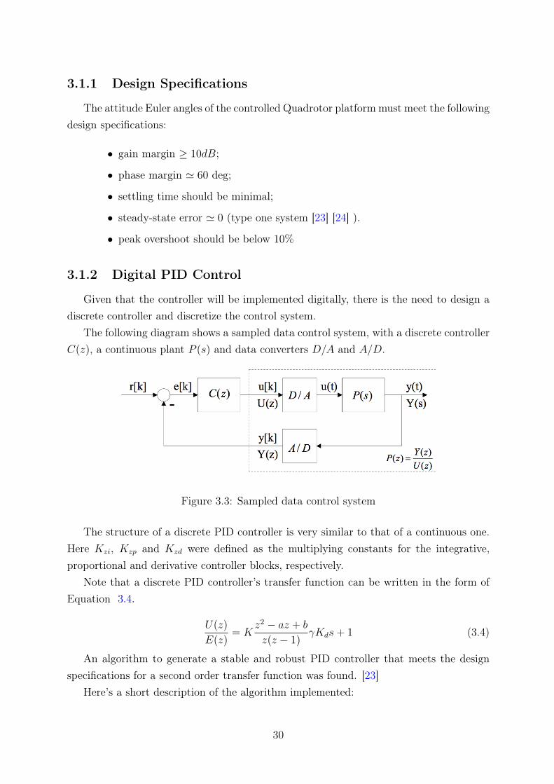
Given that the controller will be implemented digitally, there is the need to design adiscrete controller and discretize the control system.

The following diagram shows a sampled data control system, with a discrete controllerC(z), a continuous plant P (s) and data converters D/A and A/D.

Figure 3.3: Sampled data control system

The structure of a discrete PID controller is very similar to that of a continuous one.Here Kzi, Kzp and Kzd were defined as the multiplying constants for the integrative,proportional and derivative controller blocks, respectively.

Note that a discrete PID controller’s transfer function can be written in the form ofEquation 3.4.

U(z)

E(z)= K

z2 − az + b

z(z − 1)γKds+ 1 (3.4)

An algorithm to generate a stable and robust PID controller that meets the designspecifications for a second order transfer function was found. [23]

Here’s a short description of the algorithm implemented:

30

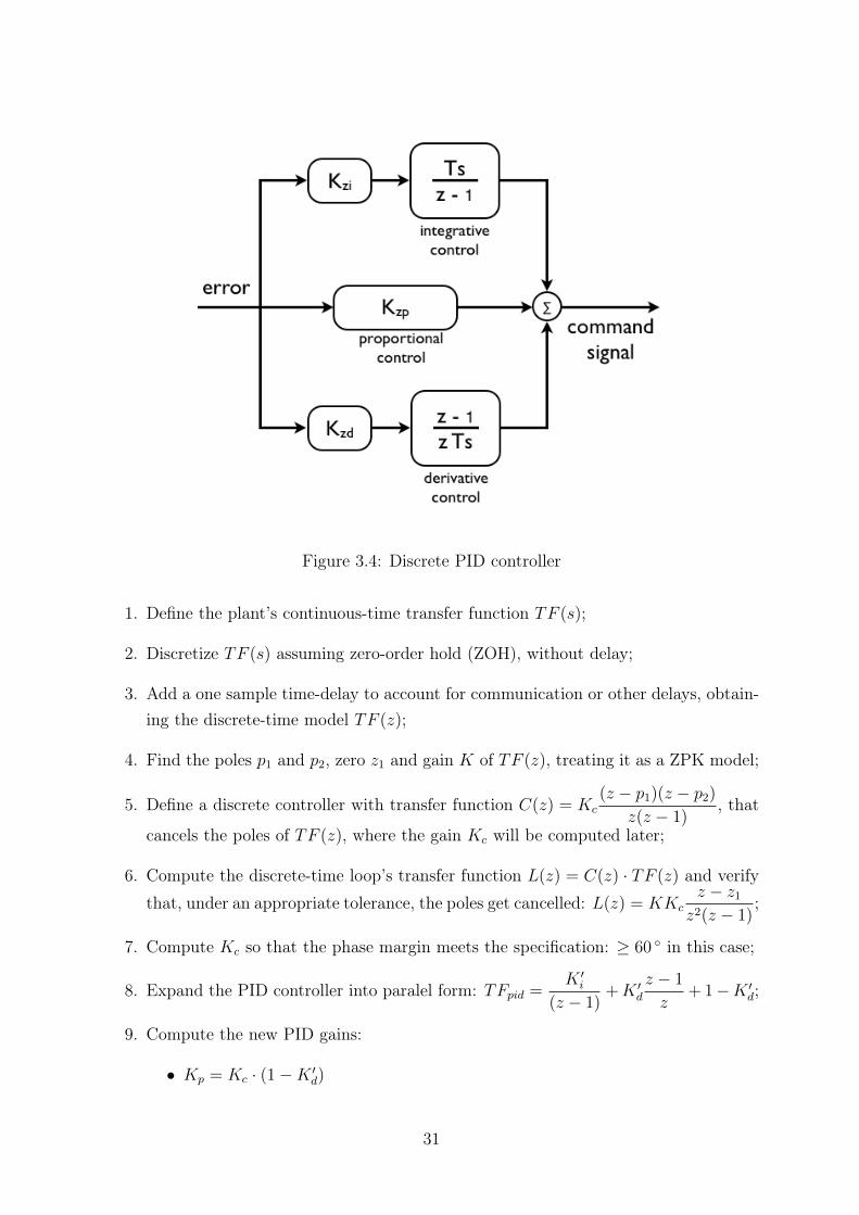
Figure 3.4: Discrete PID controller

1. Define the plant’s continuous-time transfer function TF (s);

2. Discretize TF (s) assuming zero-order hold (ZOH), without delay;

3. Add a one sample time-delay to account for communication or other delays, obtain-ing the discrete-time model TF (z);

4. Find the poles p1 and p2, zero z1 and gain K of TF (z), treating it as a ZPK model;

5. Define a discrete controller with transfer function C(z) = Kc

(z − p1)(z − p2)

z(z − 1), that

cancels the poles of TF (z), where the gain Kc will be computed later;

6. Compute the discrete-time loop’s transfer function L(z) = C(z) · TF (z) and verifythat, under an appropriate tolerance, the poles get cancelled: L(z) = KKc

z − z1z2(z − 1)

;

7. Compute Kc so that the phase margin meets the specification: ≥ 60 ◦ in this case;

8. Expand the PID controller into paralel form: TFpid =K �

i

(z − 1)+K �

d

z − 1

z+ 1−K �

d;

9. Compute the new PID gains:

• Kp = Kc · (1−K �d)

31

• Ki = Kc ·K �

i

Ts• Kd = Kc ·K �

d· Ts, where Ts is the sampling period.

10. Verify the system’s behaviour and check the specifications and performance param-eters using Bode plots as well as Simulink or other tools.

3.2 Yaw Control

The transfer function obtained for Yaw in Chapter 2 is shown in Equations 2.5 and3.5.

TFΨ =0.377568 · 3.51842

s2 + 2 · 0.5006 · 3.5184s+ 3.51842(3.5)

To create a PID controller for Yaw angle, the algorithm described in Subsection 3.1.2was followed. First, Matlab function c2d was used to discretize the transfer function. Theresulting discrete transfer function can be found in Equation 3.6.

TFΨz =0.003564z + 0.0034

z2 − 1.85z + 0.8686(3.6)

To this transfer function was added a unit time delay to account for the processingand communication times. The zeros and poles of the resulting transfer function wereretrieved using the Matlab function zpkdata, which also returns the global gain for thezero-pole-gain form of the transfer function. The poles, zeros and gain can be found inTable 3.1.

Zeros Poles Gain

−0.9541 0.9251± 0.1133i 0.0036

Table 3.1: Zeros, poles and gain of the discrete Yaw TF with delay

After creating the closed loop discrete transfer function in the manner described inSubsection 3.1.2 and cancelling the zero-pole pairs with 0.001 tolerance, the transferfunction of Equation 3.7 was obtained.

TFΨcl =TFΨz · TFΨc

1 + TFΨz · TFΨc

= 0.13468z + 0.9541

z2(z − 1)(3.7)

32

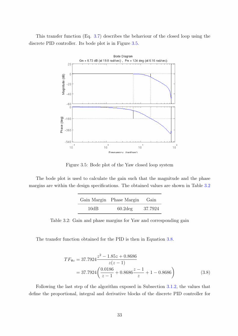
This transfer function (Eq. 3.7) describes the behaviour of the closed loop using thediscrete PID controller. Its bode plot is in Figure 3.5.

Figure 3.5: Bode plot of the Yaw closed loop system

The bode plot is used to calculate the gain such that the magnitude and the phasemargins are within the design specifications. The obtained values are shown in Table 3.2

Gain Margin Phase Margin Gain

10dB 60.2deg 37.7924

Table 3.2: Gain and phase margins for Yaw and corresponding gain

The transfer function obtained for the PID is then in Equation 3.8.

TFΨc = 37.7924z2 − 1.85z + 0.8686

z(z − 1)

= 37.7924

�0.0186

z − 1+ 0.8686

z − 1

z+ 1− 0.8686

�(3.8)

Following the last step of the algorithm exposed in Subsection 3.1.2, the values thatdefine the proportional, integral and derivative blocks of the discrete PID controller for

33

Yaw are obtained. These simple calculations are shown in Equation 3.9.

KpΨz = 37.7924(1− 0.8686) = 4.96592 (3.9a)

KiΨz = 37.7924 · 0.0186/Ts = 17.5735 (3.9b)

KdΨz = 37.7924 · 0.8686 · Ts = 1.31306, (3.9c)

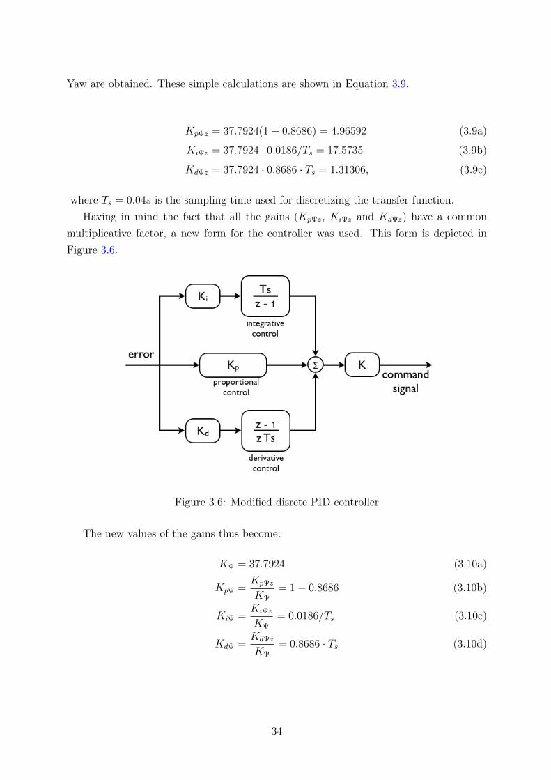
where Ts = 0.04s is the sampling time used for discretizing the transfer function.Having in mind the fact that all the gains (KpΨz, KiΨz and KdΨz) have a common

multiplicative factor, a new form for the controller was used. This form is depicted inFigure 3.6.

Figure 3.6: Modified disrete PID controller

The new values of the gains thus become:

KΨ = 37.7924 (3.10a)

KpΨ =KpΨz

KΨ= 1− 0.8686 (3.10b)

KiΨ =KiΨz

KΨ= 0.0186/Ts (3.10c)

KdΨ =KdΨz

KΨ= 0.8686 · Ts (3.10d)

34

3.2.1 Yaw fine tunning and simulation results

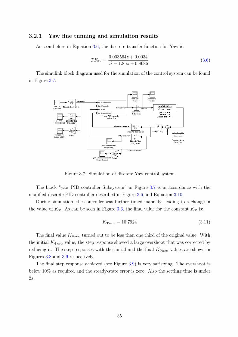
As seen before in Equation 3.6, the discrete transfer function for Yaw is:

TFΨz =0.003564z + 0.0034

z2 − 1.85z + 0.8686(3.6)

The simulink block diagram used for the simulation of the control system can be foundin Figure 3.7.

Figure 3.7: Simulation of discrete Yaw control system

The block "yaw PID controller Subsystem" in Figure 3.7 is in accordance with themodified discrete PID controller described in Figure 3.6 and Equation 3.10.

During simulation, the controller was further tuned manualy, leading to a change inthe value of KΨ. As can be seen in Figure 3.6, the final value for the constant KΨ is:

KΨnew = 10.7924 (3.11)

The final value KΨnew turned out to be less than one third of the original value. Withthe initial KΨnew value, the step response showed a large overshoot that was corrected byreducing it. The step responses with the initial and the final KΨnew values are shown inFigures 3.8 and 3.9 respectively.

The final step response achieved (see Figure 3.9) is very satisfying. The overshoot isbelow 10% as required and the steady-state error is zero. Also the settling time is under2s.

35

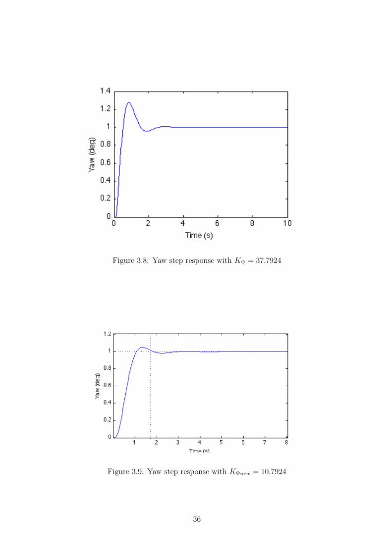
Figure 3.8: Yaw step response with KΨ = 37.7924

Figure 3.9: Yaw step response with KΨnew = 10.7924

36

3.2.2 Yaw Stability analysis

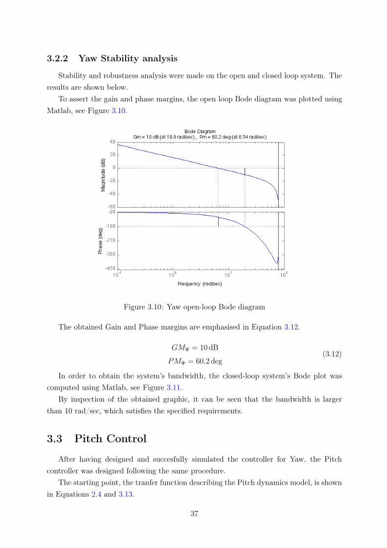
Stability and robustness analysis were made on the open and closed loop system. Theresults are shown below.

To assert the gain and phase margins, the open loop Bode diagram was plotted usingMatlab, see Figure 3.10.

Figure 3.10: Yaw open-loop Bode diagram

The obtained Gain and Phase margins are emphasised in Equation 3.12.

GMΨ = 10 dB

PMΨ = 60.2 deg(3.12)

In order to obtain the system’s bandwidth, the closed-loop system’s Bode plot wascomputed using Matlab, see Figure 3.11.

By inspection of the obtained graphic, it can be seen that the bandwidth is largerthan 10 rad/sec, which satisfies the specified requirements.

3.3 Pitch Control

After having designed and succesfully simulated the controller for Yaw, the Pitchcontroller was designed following the same procedure.

The starting point, the tranfer function describing the Pitch dynamics model, is shownin Equations 2.4 and 3.13.

37

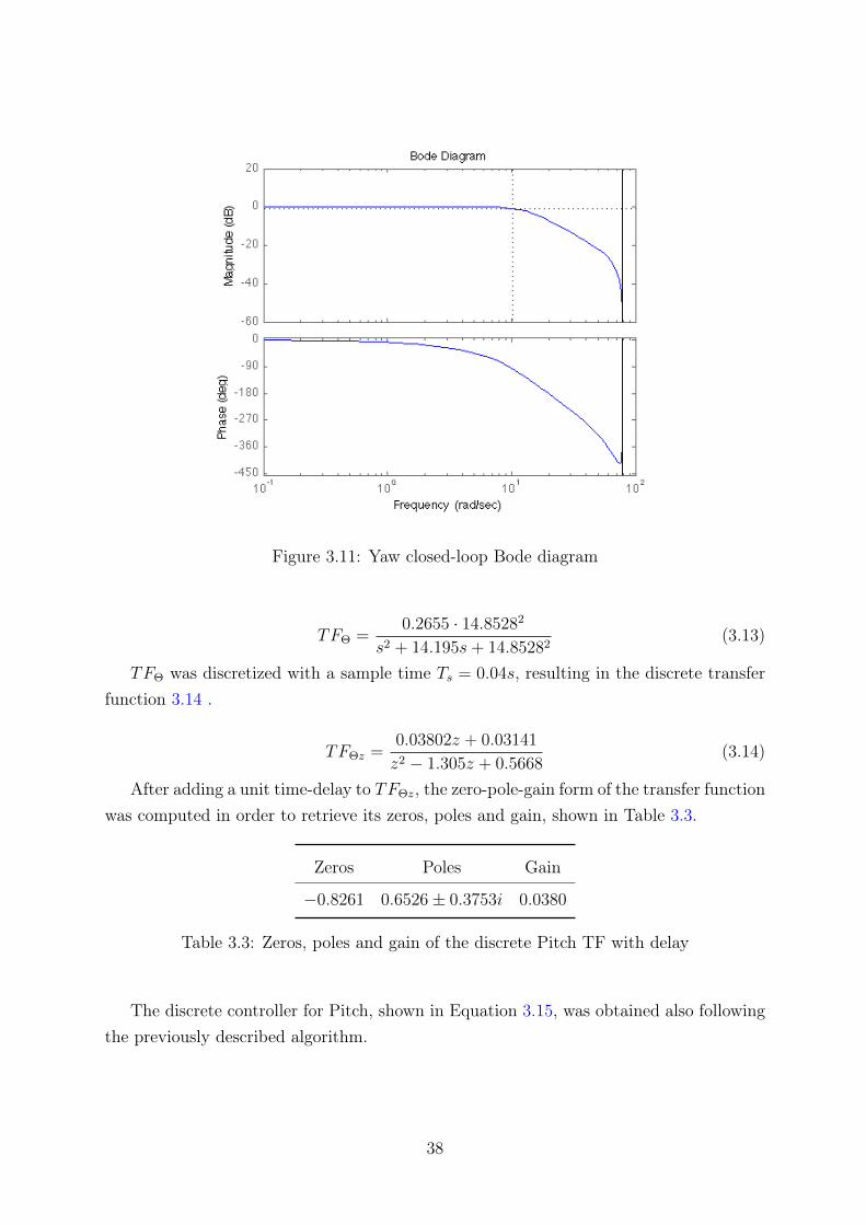
Figure 3.11: Yaw closed-loop Bode diagram

TFΘ =0.2655 · 14.85282

s2 + 14.195s+ 14.85282(3.13)

TFΘ was discretized with a sample time Ts = 0.04s, resulting in the discrete transferfunction 3.14 .

TFΘz =0.03802z + 0.03141

z2 − 1.305z + 0.5668(3.14)

After adding a unit time-delay to TFΘz, the zero-pole-gain form of the transfer functionwas computed in order to retrieve its zeros, poles and gain, shown in Table 3.3.

Zeros Poles Gain

−0.8261 0.6526± 0.3753i 0.0380

Table 3.3: Zeros, poles and gain of the discrete Pitch TF with delay

The discrete controller for Pitch, shown in Equation 3.15, was obtained also followingthe previously described algorithm.

38

TFΘc = KΘc

z2 − 1.305z + 0.5668

z(z − 1)

= KΘc

�0.2618

z − 1+ 0.5668

z − 1

z+ 1− 0.5668

�,

KΘc = 3.8680 (3.15)

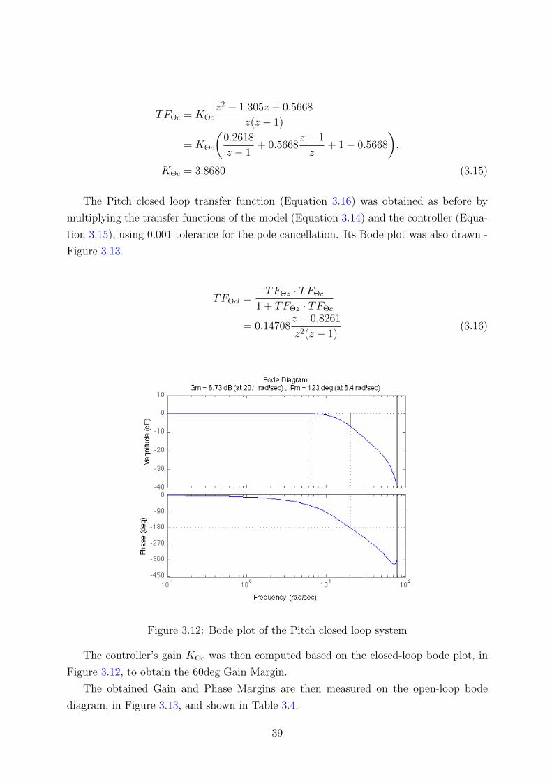
The Pitch closed loop transfer function (Equation 3.16) was obtained as before bymultiplying the transfer functions of the model (Equation 3.14) and the controller (Equa-tion 3.15), using 0.001 tolerance for the pole cancellation. Its Bode plot was also drawn -Figure 3.13.

TFΘcl =TFΘz · TFΘc

1 + TFΘz · TFΘc

= 0.14708z + 0.8261

z2(z − 1)(3.16)

Figure 3.12: Bode plot of the Pitch closed loop system

The controller’s gain KΘc was then computed based on the closed-loop bode plot, inFigure 3.12, to obtain the 60deg Gain Margin.

The obtained Gain and Phase Margins are then measured on the open-loop bodediagram, in Figure 3.13, and shown in Table 3.4.

39

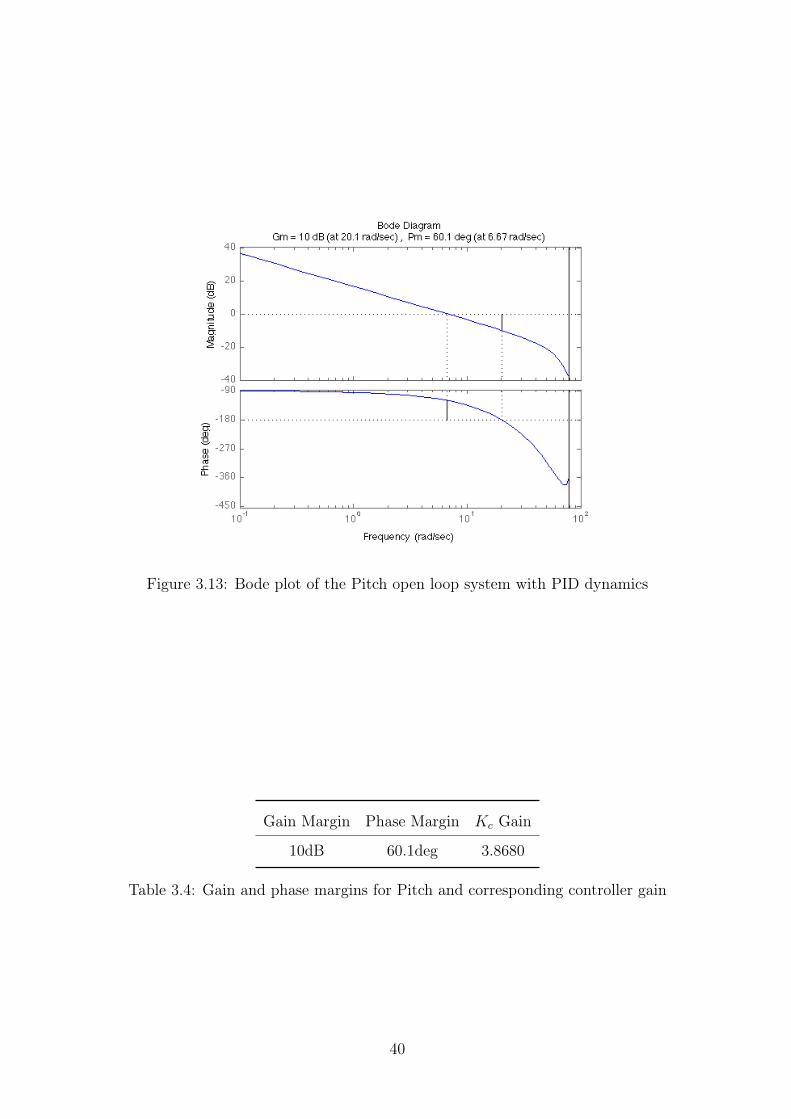
Figure 3.13: Bode plot of the Pitch open loop system with PID dynamics

Gain Margin Phase Margin Kc Gain

10dB 60.1deg 3.8680

Table 3.4: Gain and phase margins for Pitch and corresponding controller gain

40

At last, the obtained controller was put into the form of a PID and the new controllergains were computed, using a sample time Ts = 0.04s. The resulting PID controller isshown in Figure 3.6 and the corresponding gains are shown in Equation 3.17.

KΘ = 3.8680 (3.17a)

KpΘ =KpΘz

KΘ= 1− 0.5668 = 0.4332 (3.17b)

KiΘ =KiΘz

KΘ= 0.2618/Ts = 6.5450 (3.17c)

KdΘ =KdΘz

KΘ= 0.5668 · Ts = 0.0227 (3.17d)

3.3.1 Pitch fine tunning and simulation results

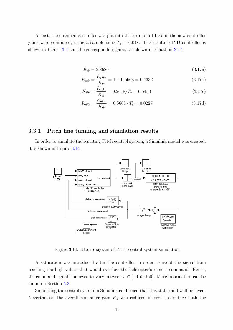
In order to simulate the resulting Pitch control system, a Simulink model was created.It is shown in Figure 3.14.

Figure 3.14: Block diagram of Pitch control system simulation

A saturation was introduced after the controller in order to avoid the signal fromreaching too high values that would overflow the helicopter’s remote command. Hence,the command signal is allowed to vary between u ∈ [−150; 150]. More information can befound on Section 5.3.

Simulating the control system in Simulink confirmed that it is stable and well behaved.Nevertheless, the overall controller gain Kθ was reduced in order to reduce both the

41

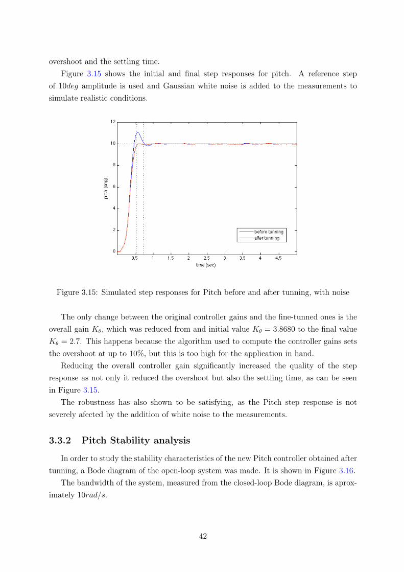
overshoot and the settling time.Figure 3.15 shows the initial and final step responses for pitch. A reference step

of 10deg amplitude is used and Gaussian white noise is added to the measurements tosimulate realistic conditions.

Figure 3.15: Simulated step responses for Pitch before and after tunning, with noise

The only change between the original controller gains and the fine-tunned ones is theoverall gain Kθ, which was reduced from and initial value Kθ = 3.8680 to the final valueKθ = 2.7. This happens because the algorithm used to compute the controller gains setsthe overshoot at up to 10%, but this is too high for the application in hand.

Reducing the overall controller gain significantly increased the quality of the stepresponse as not only it reduced the overshoot but also the settling time, as can be seenin Figure 3.15.

The robustness has also shown to be satisfying, as the Pitch step response is notseverely afected by the addition of white noise to the measurements.

3.3.2 Pitch Stability analysis

In order to study the stability characteristics of the new Pitch controller obtained aftertunning, a Bode diagram of the open-loop system was made. It is shown in Figure 3.16.

The bandwidth of the system, measured from the closed-loop Bode diagram, is aprox-imately 10rad/s.

42

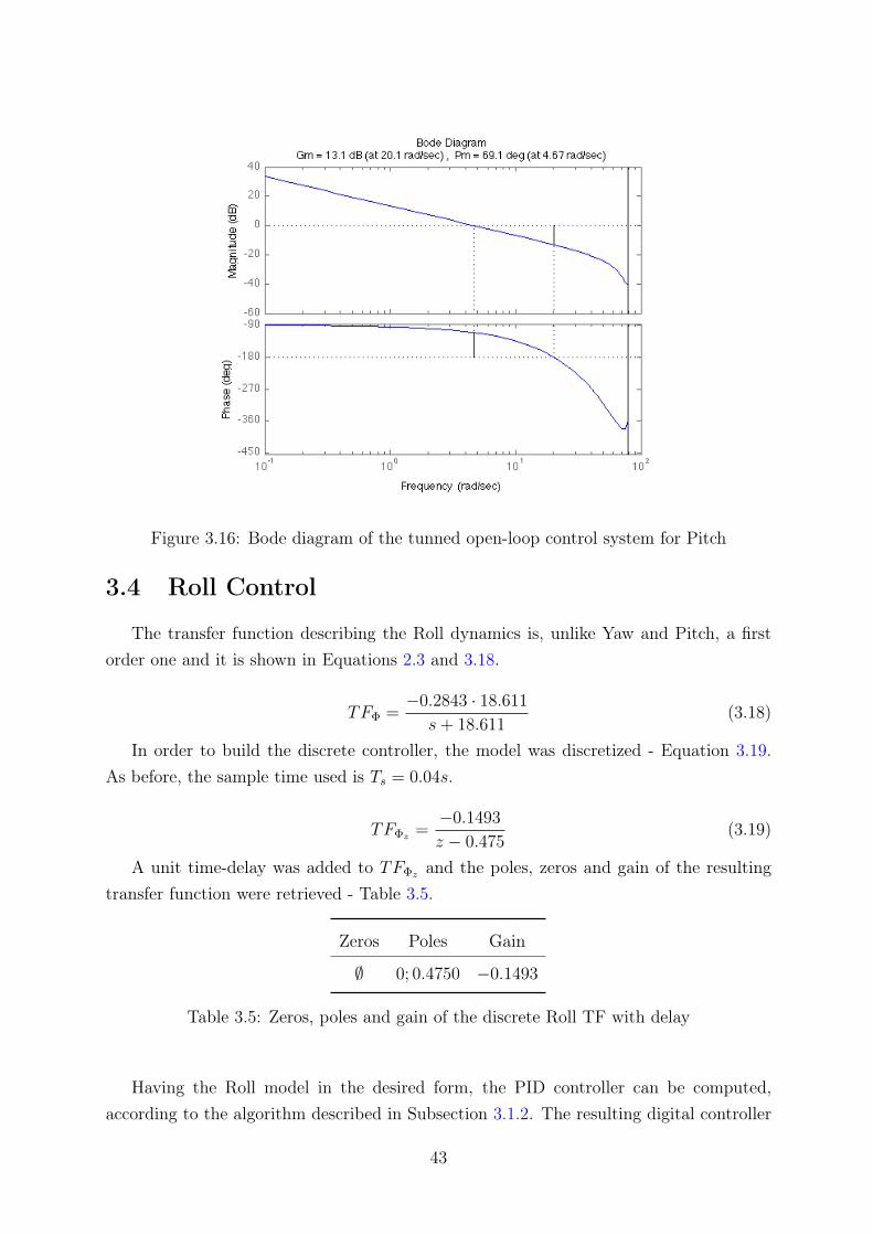
Figure 3.16: Bode diagram of the tunned open-loop control system for Pitch

3.4 Roll Control

The transfer function describing the Roll dynamics is, unlike Yaw and Pitch, a firstorder one and it is shown in Equations 2.3 and 3.18.

TFΦ =−0.2843 · 18.611

s+ 18.611(3.18)

In order to build the discrete controller, the model was discretized - Equation 3.19.As before, the sample time used is Ts = 0.04s.

TFΦz=

−0.1493

z − 0.475(3.19)

A unit time-delay was added to TFΦzand the poles, zeros and gain of the resulting

transfer function were retrieved - Table 3.5.

Zeros Poles Gain

∅ 0; 0.4750 −0.1493

Table 3.5: Zeros, poles and gain of the discrete Roll TF with delay

Having the Roll model in the desired form, the PID controller can be computed,according to the algorithm described in Subsection 3.1.2. The resulting digital controller

43

is shown in Equation 3.20.

TFΦc = KΦc

z − 0.475

z(z − 1)

= KΦc

�0.525

z − 1+ 0.475

z − 1

z− 0.475

�, (3.20)

KΦc = −1

The closed-loop transfer function was computed following the same procedure as beforeand is shown in Equation 3.21.

TFΦcl =TFΦz · TFΦc

1 + TFΦz · TFΦc

=0.14926

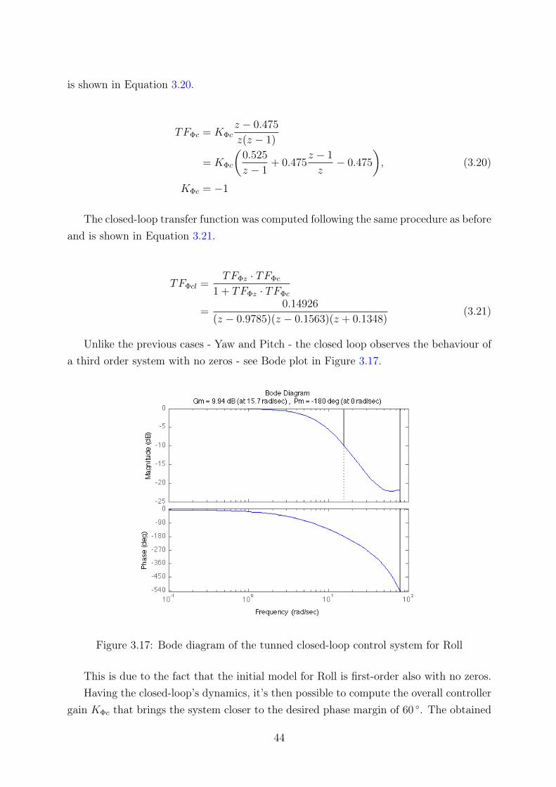
(z − 0.9785)(z − 0.1563)(z + 0.1348)(3.21)

Unlike the previous cases - Yaw and Pitch - the closed loop observes the behaviour ofa third order system with no zeros - see Bode plot in Figure 3.17.

Figure 3.17: Bode diagram of the tunned closed-loop control system for Roll

This is due to the fact that the initial model for Roll is first-order also with no zeros.Having the closed-loop’s dynamics, it’s then possible to compute the overall controller

gain KΦc that brings the system closer to the desired phase margin of 60 ◦. The obtained

44

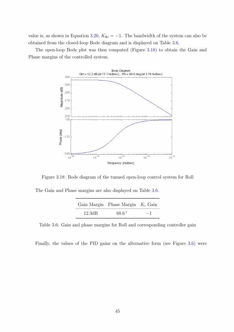
value is, as shown in Equation 3.20, KΦc = −1. The bandwidth of the system can also beobtained from the closed-loop Bode diagram and is displayed on Table 3.6.

The open-loop Bode plot was then computed (Figure 3.18) to obtain the Gain andPhase margins of the controlled system.

Figure 3.18: Bode diagram of the tunned open-loop control system for Roll

The Gain and Phase margins are also displayed on Table 3.6.

Gain Margin Phase Margin Kc Gain

12.3dB 68.6 ◦ −1

Table 3.6: Gain and phase margins for Roll and corresponding controller gain

Finally, the values of the PID gains on the alternative form (see Figure 3.6) were

45

computed and are displayed in Equation 3.22.

KΦ = −1 (3.22a)

KpΦ =KpΦz

KΦ= −0.475 (3.22b)

KiΦ =KiΦz

KΦ= 0.525/Ts = 13.1250 (3.22c)

KdΦ =KdΦz

KΦ= 0.475 · Ts = 0.0190 (3.22d)

The negative Kp value is due to the fact that the roll model is first order.

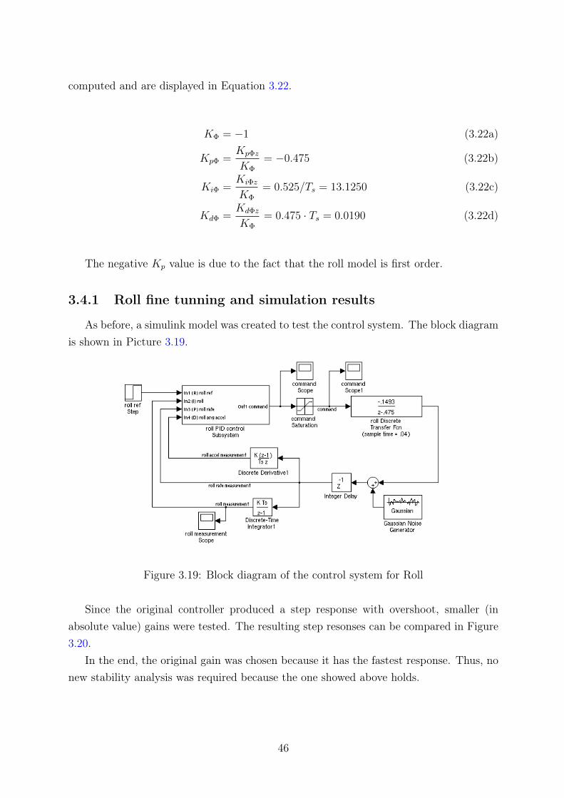
3.4.1 Roll fine tunning and simulation results

As before, a simulink model was created to test the control system. The block diagramis shown in Picture 3.19.

Figure 3.19: Block diagram of the control system for Roll

Since the original controller produced a step response with overshoot, smaller (inabsolute value) gains were tested. The resulting step resonses can be compared in Figure3.20.

In the end, the original gain was chosen because it has the fastest response. Thus, nonew stability analysis was required because the one showed above holds.

46

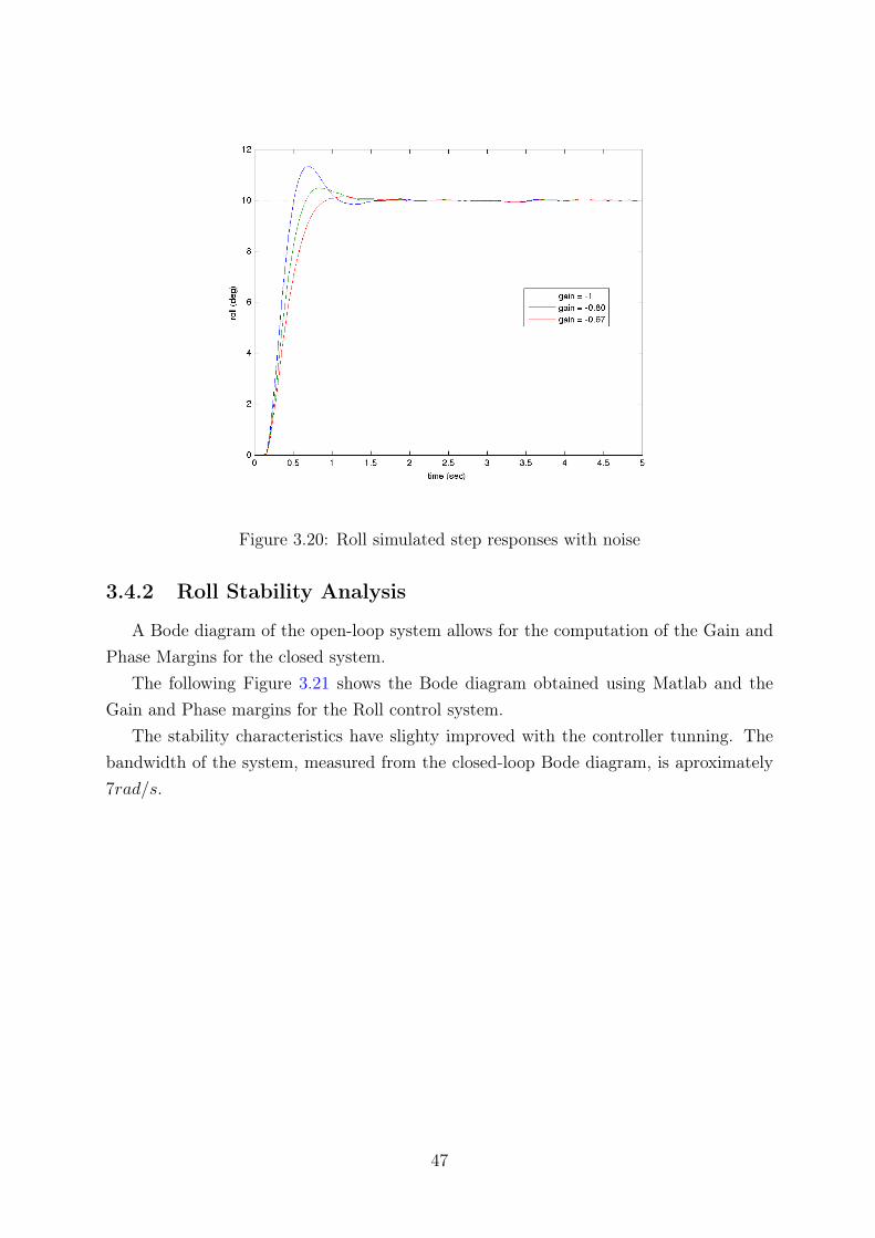
Figure 3.20: Roll simulated step responses with noise

3.4.2 Roll Stability Analysis

A Bode diagram of the open-loop system allows for the computation of the Gain andPhase Margins for the closed system.

The following Figure 3.21 shows the Bode diagram obtained using Matlab and theGain and Phase margins for the Roll control system.

The stability characteristics have slighty improved with the controller tunning. Thebandwidth of the system, measured from the closed-loop Bode diagram, is aproximately7rad/s.

47

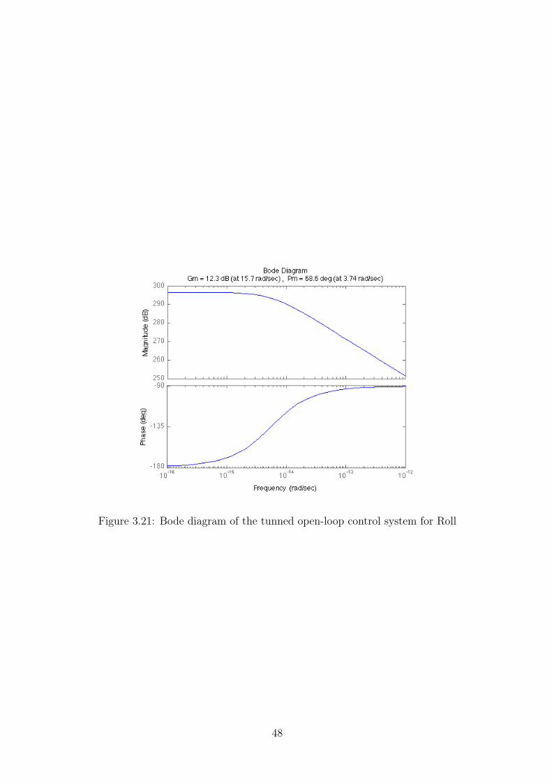
Figure 3.21: Bode diagram of the tunned open-loop control system for Roll

48

Chapter 4

Position Control

With an attitude controller of sufficient bandwidth defined, it is possible to develop apath tracker that generates attitude reference commands, ignoring the fast dynamics ofthe attitude angles. [9]

Position control is currently implemented using a PID controller design which actuatesthe vehicle’s roll and pitch as control inputs. Tilting the vehicle in any direction causes acomponent of the thrust vector to point in that direction, so commanding pitch and roll isdirectly analogous to commanding accelerations in the X-Y plane. However, the currentcontrol implementation has little ability to reject disturbances from wind and translationalvelocity effects. For this scale aircraft, even mild winds can cause disturbances. There issignifant coupling between the velocity and the attitude dynamics, so assuming that freestream velocity and attitude control are decoupled is a key weakness of this approach.[14]

4.1 Backstepping algorithm

With the goal of improving the designed attitude controllers and design the positioncontrol, an attempt to design a non-linear Integrative Backstepping algorithm based on[6] was made.

For that purpose, a non-linear model development was considered and the momentsof inertia (MOI) around the QuadRotor’s platform’s principal axis were measured.

The measurement of the MOI’s entailed the design and construction of a dedicatedinstrument.

The backstepping algorithm and the non-linear model were abandoned since theachieved results were not satisfying. Nevertheless, the attempt at developing it helpedgaining some extra insight about the system, which eventually brought about some im-provements to the already developed algorithms.

49

4.2 Horizontal Position Control

As derived in Chapter 2, Equation 4.1 models the dynamics of the horizontal positionalong the x axis, having the attitude Pitch angle as input.

X(s)

θ(s)= −g

1

s2(4.1)

With the purpose of controlling this double integrator with no zeros, the same algo-rithm that was used for the attitude controllers (see Section 3.1.2) was followed.

The ZOH transfer function for Equation 4.1 is:

X(z)

θ(z)= −g

0.0008(z + 1)

(z − 1)2(4.2)

The controller obtained by cancelling the poles of the TF in Equation 4.2 turns outto be a pure derivative, as shown in Equation 4.3.

C(z) = Kc

(z − 1)2

z(z − 1)= Kc

(z − 1)

z(4.3)

It is though known that a derivative controller introduces sensitivity to noise andprovides no guarantee regarding SSE.

It is also well known that this approach is only a rough attempt at controlling position,since the dynamics is being extremely simplified, ignoring aerodynamic effects and otherdynamics. Even though, some litterature [25] as shown that these simple models may bea good start, allowing for comparatively good results.

4.2.1 Simulation and fine tunning/ New controller

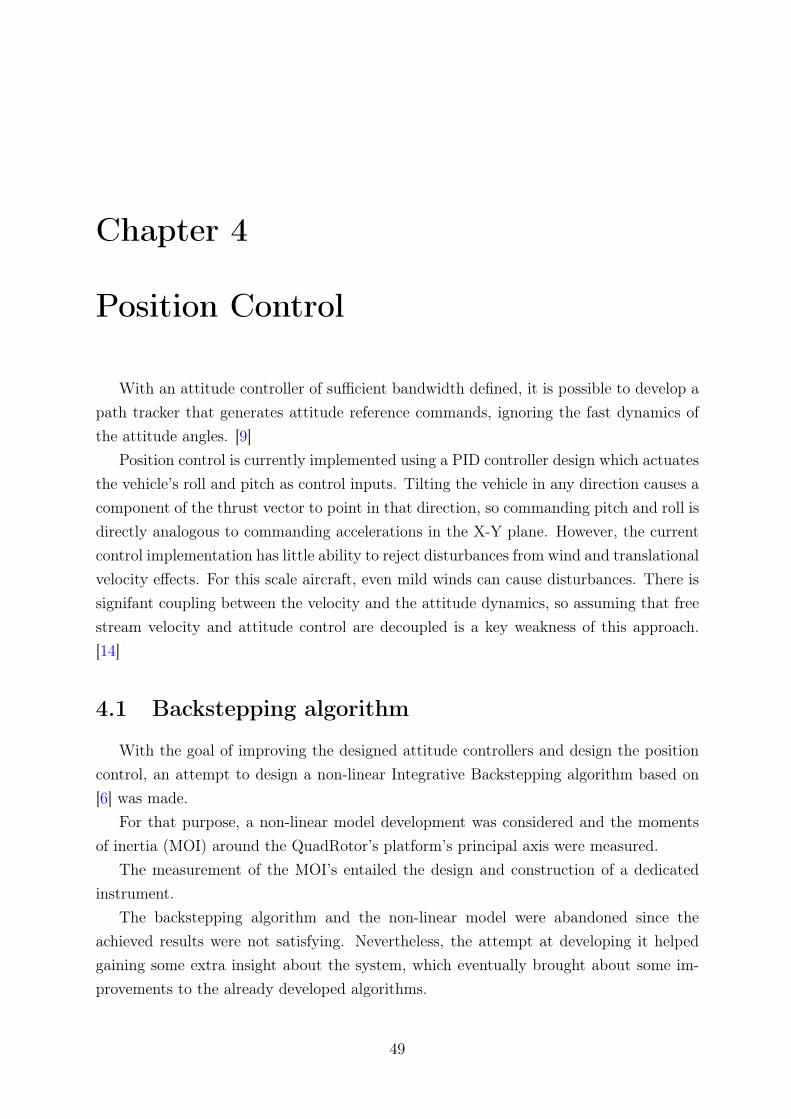
The pure derivative controller obtained with the PID algorithm was simulated in thesimulink model shown in Figure 4.1.

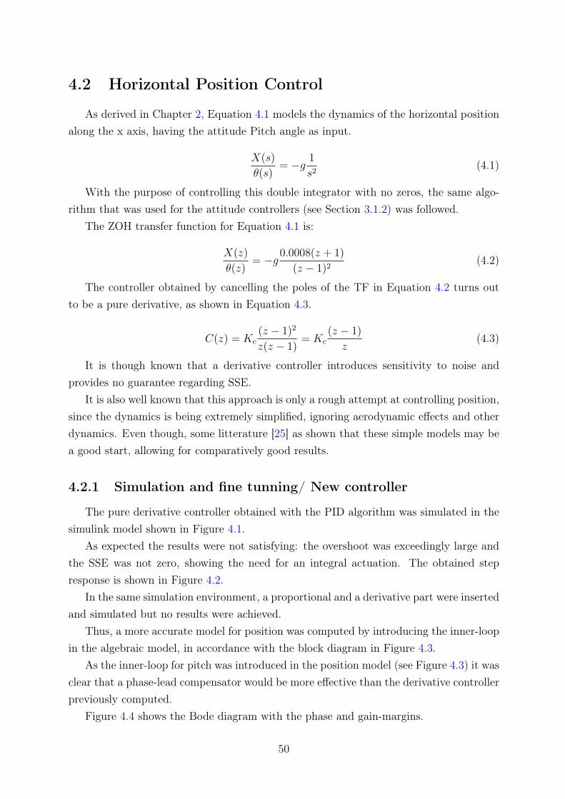
As expected the results were not satisfying: the overshoot was exceedingly large andthe SSE was not zero, showing the need for an integral actuation. The obtained stepresponse is shown in Figure 4.2.

In the same simulation environment, a proportional and a derivative part were insertedand simulated but no results were achieved.

Thus, a more accurate model for position was computed by introducing the inner-loopin the algebraic model, in accordance with the block diagram in Figure 4.3.

As the inner-loop for pitch was introduced in the position model (see Figure 4.3) it wasclear that a phase-lead compensator would be more effective than the derivative controllerpreviously computed.

Figure 4.4 shows the Bode diagram with the phase and gain-margins.

50

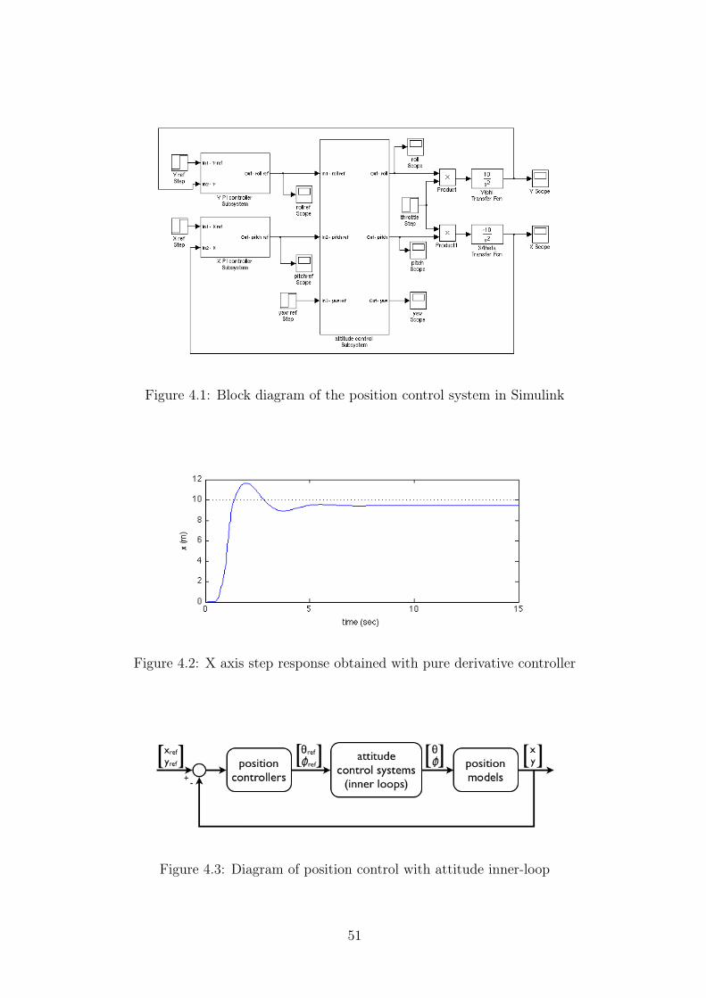
Figure 4.1: Block diagram of the position control system in Simulink

Figure 4.2: X axis step response obtained with pure derivative controller

Figure 4.3: Diagram of position control with attitude inner-loop

51

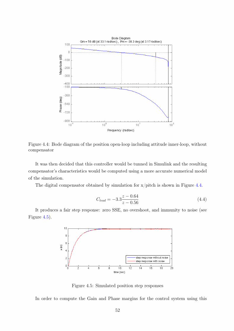
Figure 4.4: Bode diagram of the position open-loop including attitude inner-loop, withoutcompensator

It was then decided that this controller would be tunned in Simulink and the resultingcompensator’s characteristics would be computed using a more accurate numerical modelof the simulation.

The digital compensator obtained by simulation for x/pitch is shown in Figure 4.4.

Clead = −3.3z − 0.64

z − 0.56(4.4)

It produces a fair step response: zero SSE, no overshoot, and immunity to noise (seeFigure 4.5).

Figure 4.5: Simulated position step responses

In order to compute the Gain and Phase margins for the control system using this

52

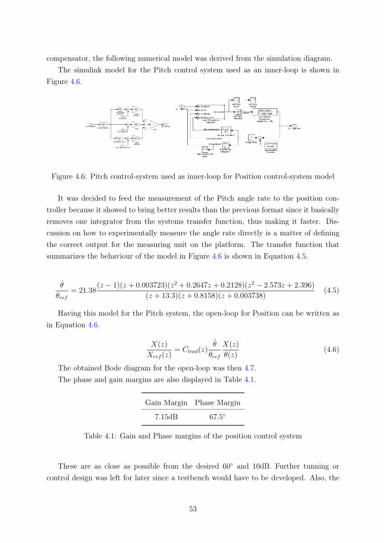
compensator, the following numerical model was derived from the simulation diagram.The simulink model for the Pitch control system used as an inner-loop is shown in

Figure 4.6.

Figure 4.6: Pitch control-system used as inner-loop for Position control-system model

It was decided to feed the measurement of the Pitch angle rate to the position con-troller because it showed to bring better results than the previous format since it basicallyremoves one integrator from the systems transfer function, thus making it faster. Dis-cussion on how to experimentally measure the angle rate directly is a matter of definingthe correct output for the measuring unit on the platform. The transfer function thatsummarizes the behaviour of the model in Figure 4.6 is shown in Equation 4.5.

θ

θref= 21.38

(z − 1)(z + 0.003723)(z2 + 0.2647z + 0.2128)(z2 − 2.573z + 2.396)

(z + 13.3)(z + 0.8158)(z + 0.003738)(4.5)

Having this model for the Pitch system, the open-loop for Position can be written asin Equation 4.6.

X(z)

Xref (z)= Clead(z)

θ

θref

X(z)

θ(z)(4.6)

The obtained Bode diagram for the open-loop was then 4.7.The phase and gain margins are also displayed in Table 4.1.

Gain Margin Phase Margin

7.15dB 67.5◦

Table 4.1: Gain and Phase margins of the position control system

These are as close as possible from the desired 60◦ and 10dB. Further tunning orcontrol design was left for later since a testbench would have to be developed. Also, the

53

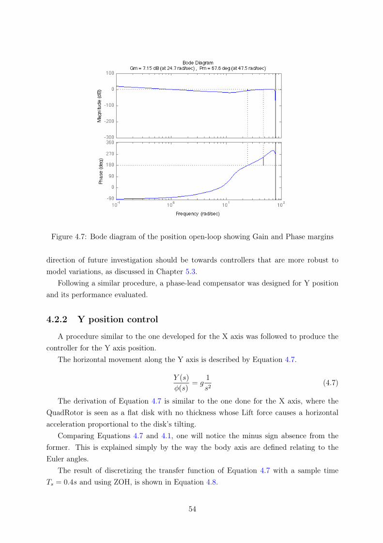
Figure 4.7: Bode diagram of the position open-loop showing Gain and Phase margins

direction of future investigation should be towards controllers that are more robust tomodel variations, as discussed in Chapter 5.3.

Following a similar procedure, a phase-lead compensator was designed for Y positionand its performance evaluated.

4.2.2 Y position control

A procedure similar to the one developed for the X axis was followed to produce thecontroller for the Y axis position.

The horizontal movement along the Y axis is described by Equation 4.7.

Y (s)

φ(s)= g

1

s2(4.7)

The derivation of Equation 4.7 is similar to the one done for the X axis, where theQuadRotor is seen as a flat disk with no thickness whose Lift force causes a horizontalacceleration proportional to the disk’s tilting.

Comparing Equations 4.7 and 4.1, one will notice the minus sign absence from theformer. This is explained simply by the way the body axis are defined relating to theEuler angles.

The result of discretizing the transfer function of Equation 4.7 with a sample timeTs = 0.4s and using ZOH, is shown in Equation 4.8.

54

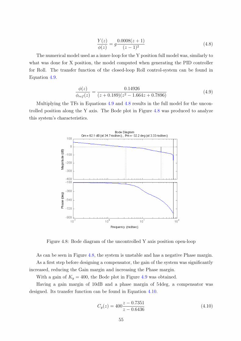
Y (z)

φ(z)= g

0.0008(z + 1)

(z − 1)2(4.8)

The numerical model used as a inner-loop for the Y position full model was, similarly towhat was done for X position, the model computed when generating the PID controllerfor Roll. The transfer function of the closed-loop Roll control-system can be found inEquation 4.9.

φ(z)

φref (z)=

0.14926

(z + 0.189)(z2 − 1.664z + 0.7896)(4.9)

Multiplying the TFs in Equations 4.9 and 4.8 results in the full model for the uncon-trolled position along the Y axis. The Bode plot in Figure 4.8 was produced to analyzethis system’s characteristics.

Figure 4.8: Bode diagram of the uncontrolled Y axis position open-loop

As can be seen in Figure 4.8, the system is unstable and has a negative Phase margin.As a first step before designing a compensator, the gain of the system was significantly

increased, reducing the Gain margin and increasing the Phase margin.With a gain of Ky = 400, the Bode plot in Figure 4.9 was obtained.Having a gain margin of 10dB and a phase margin of 54deg, a compensator was

designed. Its transfer function can be found in Equation 4.10.

Cy(z) = 400z − 0.7351

z − 0.6436(4.10)

55

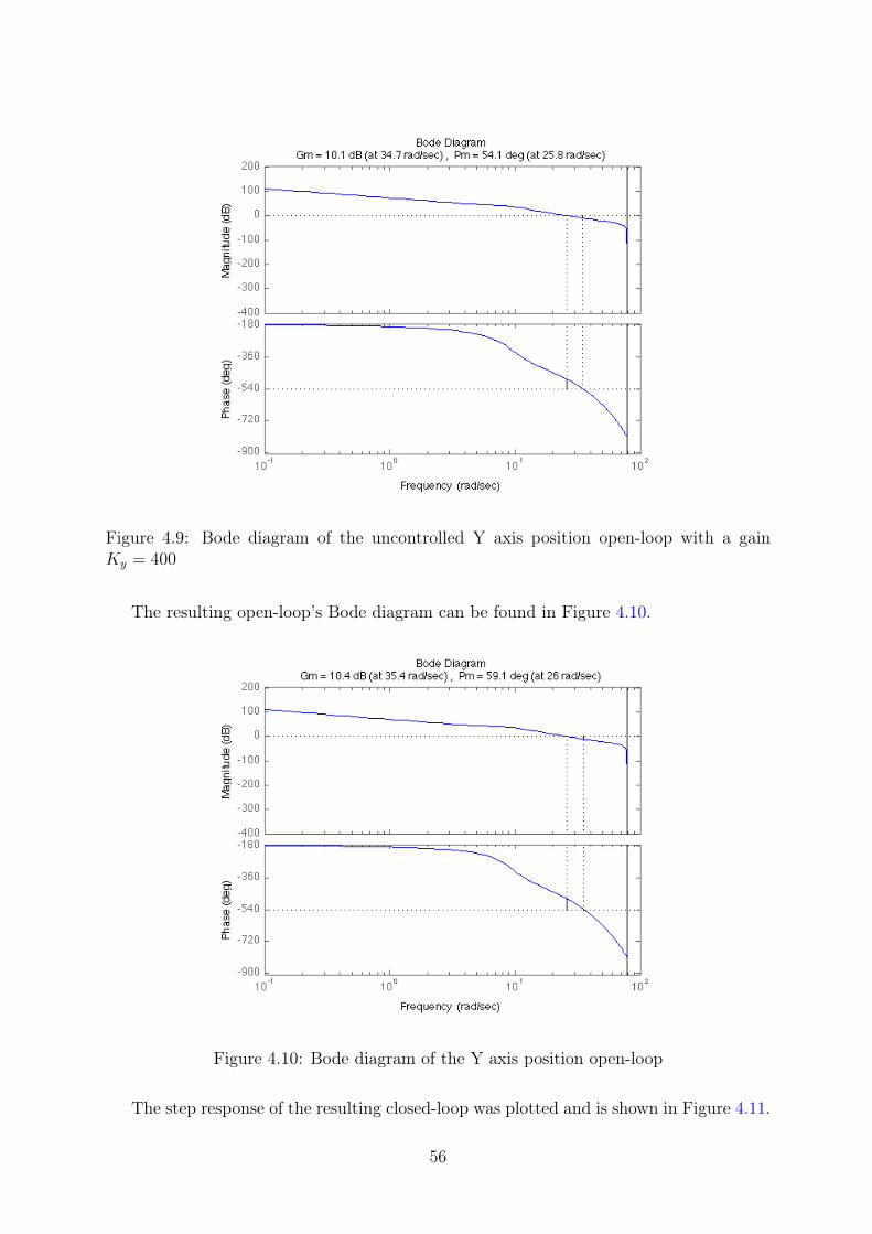
Figure 4.9: Bode diagram of the uncontrolled Y axis position open-loop with a gainKy = 400

The resulting open-loop’s Bode diagram can be found in Figure 4.10.

Figure 4.10: Bode diagram of the Y axis position open-loop

The step response of the resulting closed-loop was plotted and is shown in Figure 4.11.

56

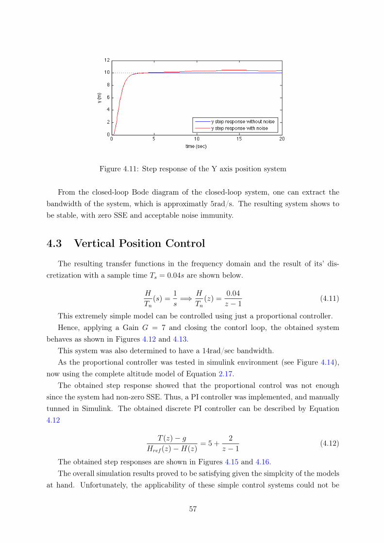
Figure 4.11: Step response of the Y axis position system

From the closed-loop Bode diagram of the closed-loop system, one can extract thebandwidth of the system, which is approximatly 5rad/s. The resulting system shows tobe stable, with zero SSE and acceptable noise immunity.

4.3 Vertical Position Control

The resulting transfer functions in the frequency domain and the result of its’ dis-cretization with a sample time Ts = 0.04s are shown below.

H

Tn

(s) =1

s=⇒

H

Tn

(z) =0.04

z − 1(4.11)

This extremely simple model can be controlled using just a proportional controller.Hence, applying a Gain G = 7 and closing the contorl loop, the obtained system

behaves as shown in Figures 4.12 and 4.13.This system was also determined to have a 14rad/sec bandwidth.As the proportional controller was tested in simulink environment (see Figure 4.14),

now using the complete altitude model of Equation 2.17.The obtained step response showed that the proportional control was not enough

since the system had non-zero SSE. Thus, a PI controller was implemented, and manuallytunned in Simulink. The obtained discrete PI controller can be described by Equation4.12

T (z)− g

Href (z)−H(z)= 5 +

2

z − 1(4.12)

The obtained step responses are shown in Figures 4.15 and 4.16.The overall simulation results proved to be satisfying given the simplcity of the models

at hand. Unfortunately, the applicability of these simple control systems could not be

57

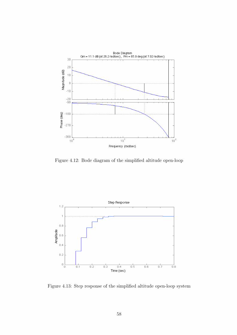
Figure 4.12: Bode diagram of the simplified altitude open-loop

Figure 4.13: Step response of the simplified altitude open-loop system

58

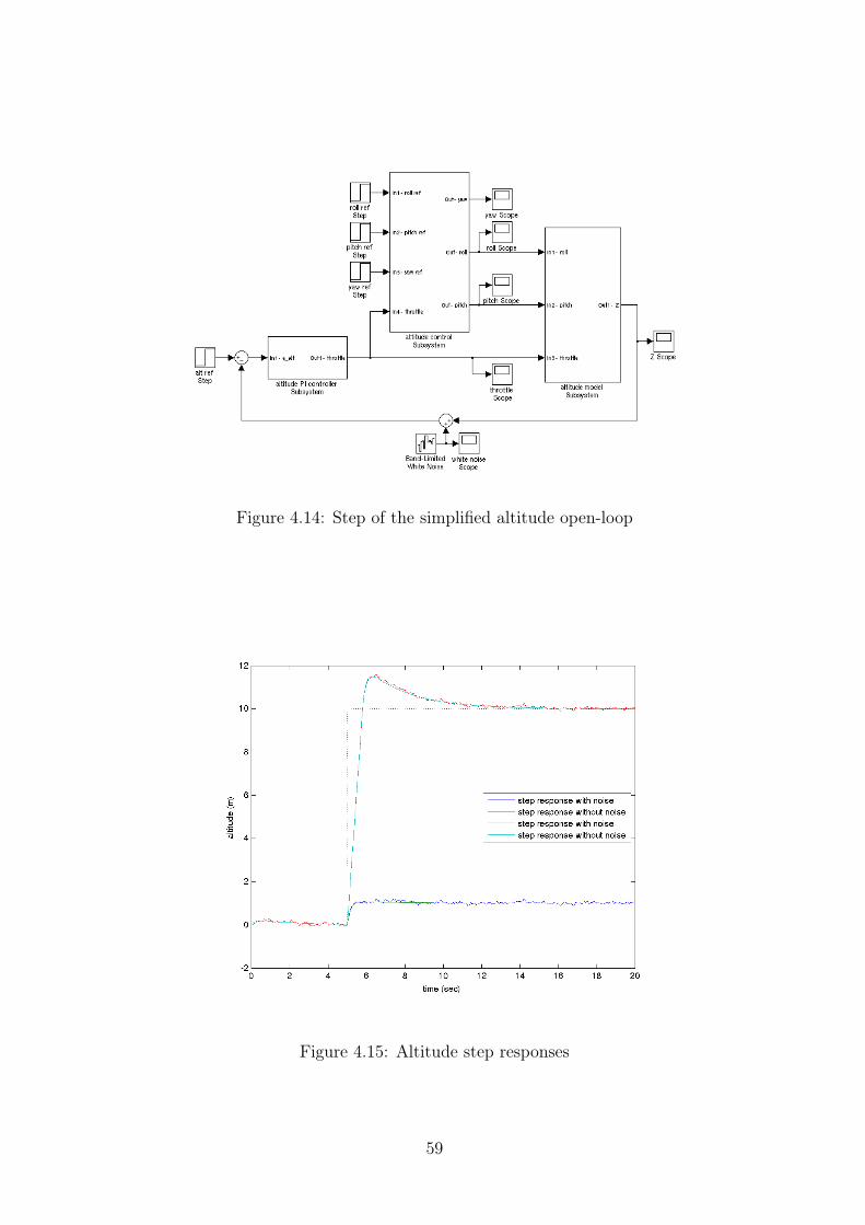
Figure 4.14: Step of the simplified altitude open-loop

Figure 4.15: Altitude step responses

59

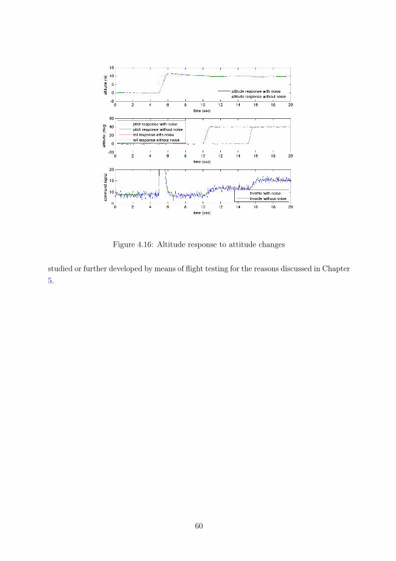
Figure 4.16: Altitude response to attitude changes

studied or further developed by means of flight testing for the reasons discussed in Chapter5.

60

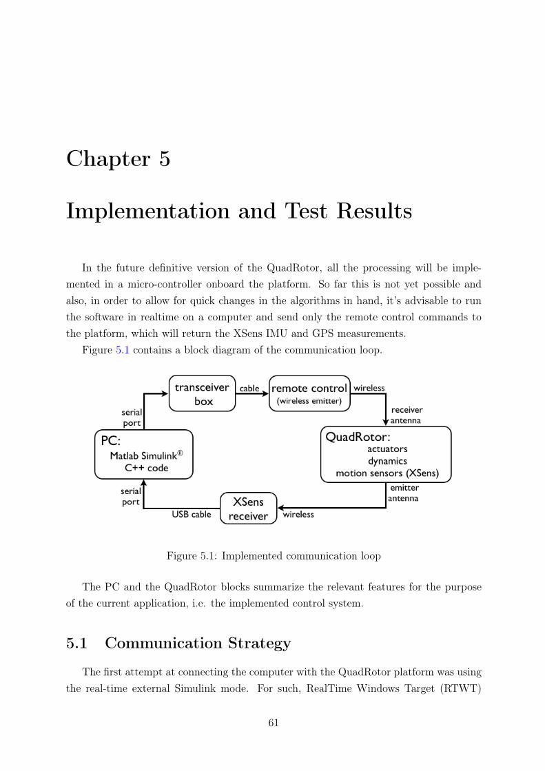
Chapter 5

Implementation and Test Results

In the future definitive version of the QuadRotor, all the processing will be imple-mented in a micro-controller onboard the platform. So far this is not yet possible andalso, in order to allow for quick changes in the algorithms in hand, it’s advisable to runthe software in realtime on a computer and send only the remote control commands tothe platform, which will return the XSens IMU and GPS measurements.

Figure 5.1 contains a block diagram of the communication loop.

Figure 5.1: Implemented communication loop

The PC and the QuadRotor blocks summarize the relevant features for the purposeof the current application, i.e. the implemented control system.

5.1 Communication Strategy

The first attempt at connecting the computer with the QuadRotor platform was usingthe real-time external Simulink mode. For such, RealTime Windows Target (RTWT)

61

toolbox was installed on the PC and several methods using built-in serial communicationblocks were tried.

Two important shortcomings arose from this strategy:

1. The transceiver box is not commercial, but has rather been developed at ISL;

2. The XSens company doesn’t provide Simulink compatibility, which was neededfor the receiver.

Hence, the needed tools for RTWT to deal with both the transceiver box and the XSensreceiver would have to be developed by us. This was neither time nor effort-feasible, butmostly it didn’t provide certainty as to wether it would be a successful strategy.

Since a lower level code was needed, the final decision was to use C++ to manage allthe serial port communication. Matlab code would still be used in realtime mode, butinstead of RTWT or another serialport communication tool using Simulink in realtime,an external C++ realtime code would manage the entire process and call the Matlabfunctions.

The main reasons for choosing C++ language instead of Matlab or any another lan-guage to manage the serial port communications are the following:

• Familiarity with the C++ language, in particular for handling serial port com-munication;

• Existance of known reliable C++ functions to handle the serial port;

• XSens support with code examples that served as a beginning to write thecommunication with the XSens receiver;

• Easy accessing of low level code to implement the data exchange protocol withthe transceiver box.

This strategy brings new advantages and setbacks, being the most important:

Advantage The process is closer to what will be the definitive method in the sensethat the control algorithms are discretized and in realtime form;

Advantage Less computational power is required: realtime algorithms are computa-tionally more efficient than running Simulink;

Setback It’s harder to monitor the experiments while they are running;

Setback The realtime code has to be developped and then directly changed every-time the algorithms need adjustments.

The C++ program was built from scratch, having in mind the data exchange protocolbetween the box and the serial port, that can be found in Appendix A.

62

It is important to notice that with this new way of managing the serial ports, all theexperiment is now managed by the C++ program from the point of view of the computer.It is in this software that the experiment duration defined, and it is this software thatcalls the Matlab function where the control algorithm is implemented.

The C++ program code can be found in Appendix B.

5.2 Development of the Realtime Controller for Atti-tude

Until this point, two stages were completed in the development of the PID controllersfor attitude :

1. Design of a PID controller C(s) able to control the process (Chapter 3);

2. Translation of the controller’s TF C(s) into block diagram form (Figure 3.2)and simulation in Simulink.

In order to adapt the designed algorithms to the C++ code developed, there is theneed to create a time-step based algorithm to compute the PID’s output - the controlcommand - in each time step.

In the time domain, the PID controllers for attitude can be generally described byEquation 5.1.

u(t) = Kpe(t) +Ki

�e(t) dt+Kd

de(t)

dt, (5.1)

where e(t) is now defined as e(t) = αref (t)− αmeasured(t) and α stands for Roll, Pitchor Yaw, measured in degree. The new definition arises from a practical issue: even thoughthe model’s TFs are defined in terms of angle rates, it’s more handy to define the referencesignals in terms of the angles, measured in deg.

As such, Equation 5.1 immediately entails Equation 5.2.

u(t) = Ki · e(t) +Kp · e(t) +Kd · e(t) (5.2)

Hence, there is no need to compute any integrals; only derivatives. For this purpose,a discrete real-time finite difference formula was created in order to compute the valuesof the derivatives of the real measured angles in each time-step, in a causal manner andwith low sensitivity to noise.

63

5.2.1 Finite Difference Weighted Average Derivative

To obtain an explicit way of computing the discrete derivative in the time domain, afinite difference expression was developed.

The start point was the widely known definition of the derivative of a function, shownin Equation 5.3.

x�(t0) =dx

dt

���t0

= limh→0

x(t0 + h)− x(t0)

h(5.3)

Discretizing Equation 5.3 is simply replacing the limit limh→0 with a certain valueh = Ts � 1. Hence the discrete derivative becomes the forward difference (by Euler’smethod [26]) in Equation 5.4:

dx

dt

���t0

≈x(t0 + Ts)− x(t0)

Ts

(5.4)

This is not a causal process, thus it cannot be implemented. To solve this problemthe backward difference (Equation 5.5) is used instead.

dx

dt

���t0

≈x(t0)− x(t0 − Ts)

Ts

(5.5)

The main issue related to this alternative approximation is that it introduces an extratime-delay. This cannot be avoided though, because the derivative must be causal.

A known issue with implementing derivatives is their sensitivity to noise. In orderto reduce it, a new expression to compute the backward difference was developed, usingolder samples. This introduces an even bigger delay, but it was necessary since simulationsusing the finite difference in Equation 5.5 showed a signal to noise ratio that was too low.

A way to design an average weighted derivative is to consider the weighted averagebetween the regular finite difference (Equation 5.5) and what it would become if thesample time would double, as shown in Equation 5.6.

dx

dt

���t0

≈ αx(t0)− x(t0 − Ts)

Ts

+ βx(t0)− x(t0 − 2Ts)

2Ts

(5.6)

whereα + β = 1 (5.7)

The condition in Equation 5.7 is necessary for Equation 5.6 to describe a weightedaverage, and thus, by linearity, a derivative of x(t) at instant t0.

The most common implementation of this kind of derivative, achieved with the finitedifference method, is shown in Equation 5.8 and approximates f �(x) up to a term of orderh2. This can be proven by expanding the above expression in Taylor series, or by usingthe calculus of finite differences. [27]

64

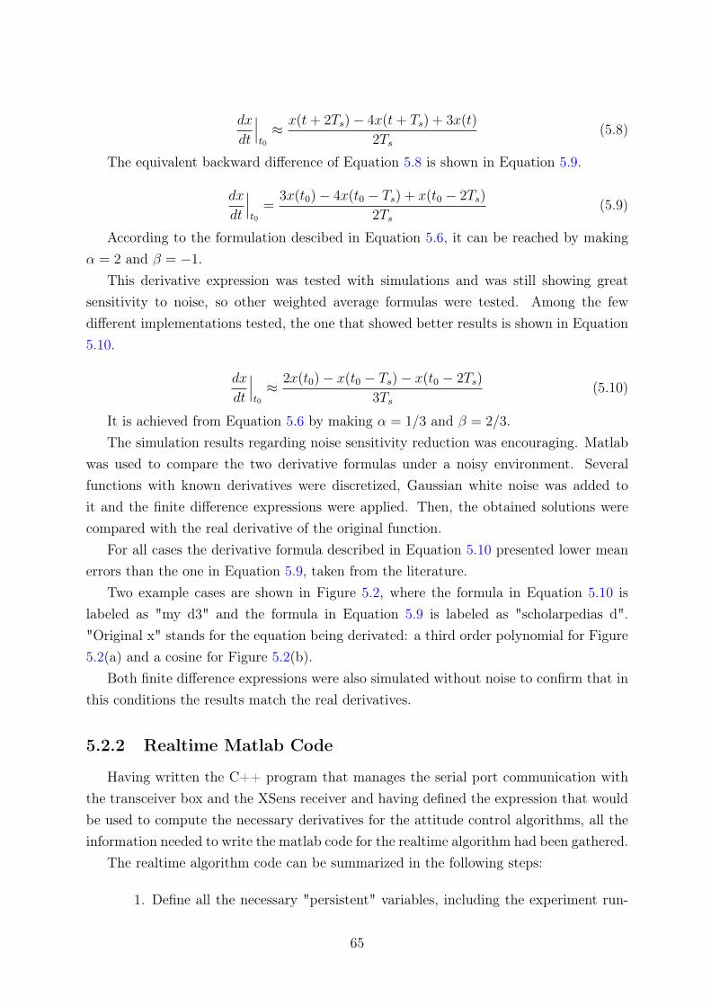
dx

dt

���t0

≈x(t+ 2Ts)− 4x(t+ Ts) + 3x(t)

2Ts

(5.8)

The equivalent backward difference of Equation 5.8 is shown in Equation 5.9.

dx

dt

���t0

=3x(t0)− 4x(t0 − Ts) + x(t0 − 2Ts)

2Ts

(5.9)

According to the formulation descibed in Equation 5.6, it can be reached by makingα = 2 and β = −1.

This derivative expression was tested with simulations and was still showing greatsensitivity to noise, so other weighted average formulas were tested. Among the fewdifferent implementations tested, the one that showed better results is shown in Equation5.10.

dx

dt

���t0

≈2x(t0)− x(t0 − Ts)− x(t0 − 2Ts)

3Ts

(5.10)

It is achieved from Equation 5.6 by making α = 1/3 and β = 2/3.The simulation results regarding noise sensitivity reduction was encouraging. Matlab

was used to compare the two derivative formulas under a noisy environment. Severalfunctions with known derivatives were discretized, Gaussian white noise was added toit and the finite difference expressions were applied. Then, the obtained solutions werecompared with the real derivative of the original function.

For all cases the derivative formula described in Equation 5.10 presented lower meanerrors than the one in Equation 5.9, taken from the literature.

Two example cases are shown in Figure 5.2, where the formula in Equation 5.10 islabeled as "my d3" and the formula in Equation 5.9 is labeled as "scholarpedias d"."Original x" stands for the equation being derivated: a third order polynomial for Figure5.2(a) and a cosine for Figure 5.2(b).

Both finite difference expressions were also simulated without noise to confirm that inthis conditions the results match the real derivatives.

5.2.2 Realtime Matlab Code

Having written the C++ program that manages the serial port communication withthe transceiver box and the XSens receiver and having defined the expression that wouldbe used to compute the necessary derivatives for the attitude control algorithms, all theinformation needed to write the matlab code for the realtime algorithm had been gathered.

The realtime algorithm code can be summarized in the following steps:

1. Define all the necessary "persistent" variables, including the experiment run-

65

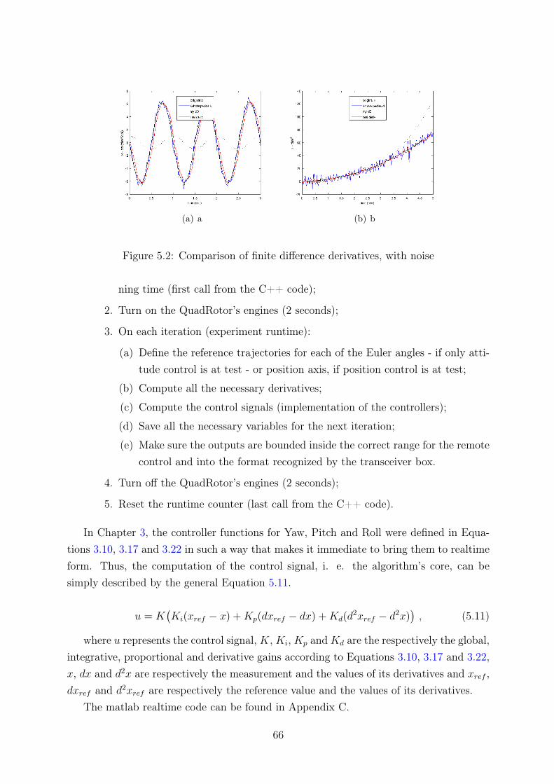
(a) a (b) b

Figure 5.2: Comparison of finite difference derivatives, with noise

ning time (first call from the C++ code);

2. Turn on the QuadRotor’s engines (2 seconds);

3. On each iteration (experiment runtime):

(a) Define the reference trajectories for each of the Euler angles - if only atti-tude control is at test - or position axis, if position control is at test;

(b) Compute all the necessary derivatives;

(c) Compute the control signals (implementation of the controllers);

(d) Save all the necessary variables for the next iteration;

(e) Make sure the outputs are bounded inside the correct range for the remotecontrol and into the format recognized by the transceiver box.

4. Turn off the QuadRotor’s engines (2 seconds);

5. Reset the runtime counter (last call from the C++ code).

In Chapter 3, the controller functions for Yaw, Pitch and Roll were defined in Equa-tions 3.10, 3.17 and 3.22 in such a way that makes it immediate to bring them to realtimeform. Thus, the computation of the control signal, i. e. the algorithm’s core, can besimply described by the general Equation 5.11.

u = K�Ki(xref − x) +Kp(dxref − dx) +Kd(d

2xref − d2x)�, (5.11)

where u represents the control signal, K, Ki, Kp and Kd are the respectively the global,integrative, proportional and derivative gains according to Equations 3.10, 3.17 and 3.22,x, dx and d2x are respectively the measurement and the values of its derivatives and xref ,dxref and d2xref are respectively the reference value and the values of its derivatives.

The matlab realtime code can be found in Appendix C.

66

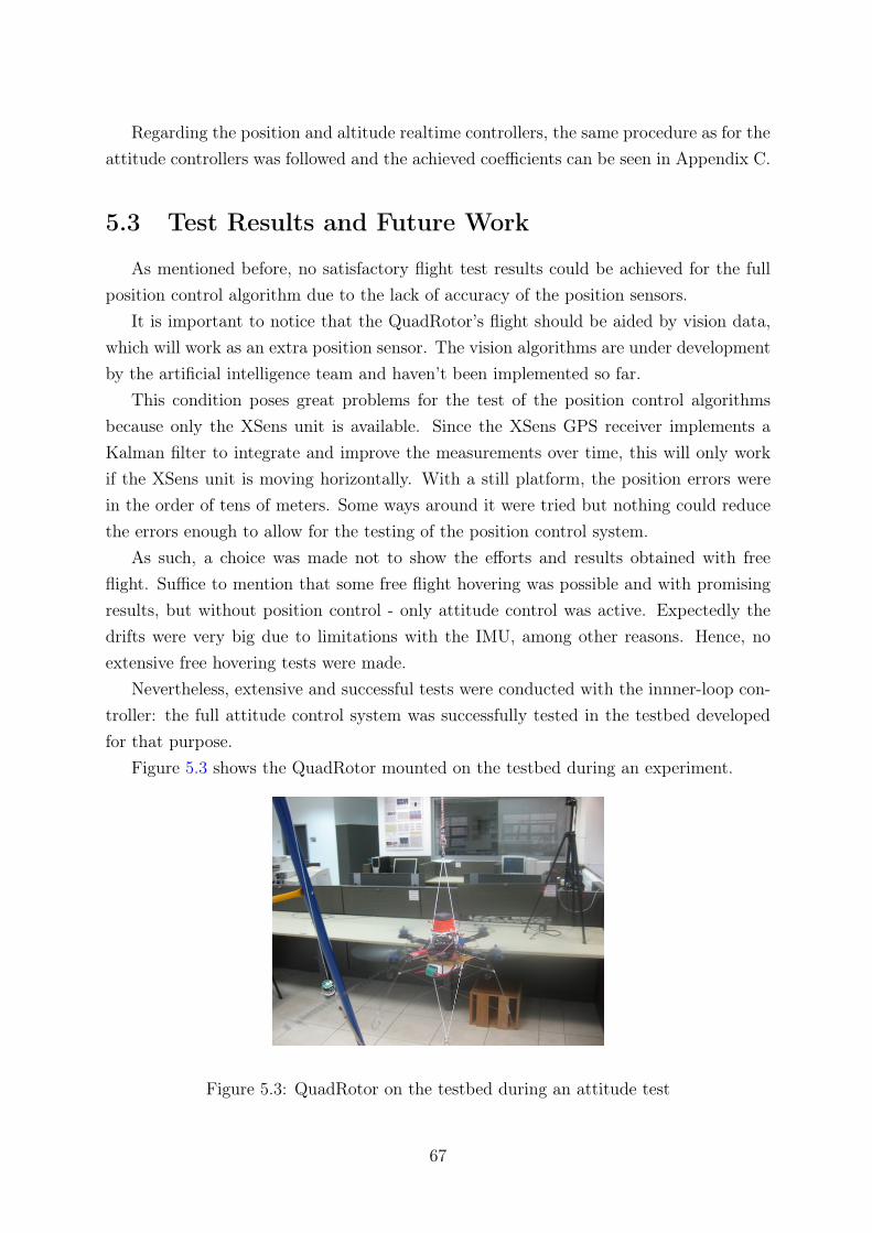
Regarding the position and altitude realtime controllers, the same procedure as for theattitude controllers was followed and the achieved coefficients can be seen in Appendix C.

5.3 Test Results and Future Work

As mentioned before, no satisfactory flight test results could be achieved for the fullposition control algorithm due to the lack of accuracy of the position sensors.

It is important to notice that the QuadRotor’s flight should be aided by vision data,which will work as an extra position sensor. The vision algorithms are under developmentby the artificial intelligence team and haven’t been implemented so far.

This condition poses great problems for the test of the position control algorithmsbecause only the XSens unit is available. Since the XSens GPS receiver implements aKalman filter to integrate and improve the measurements over time, this will only workif the XSens unit is moving horizontally. With a still platform, the position errors werein the order of tens of meters. Some ways around it were tried but nothing could reducethe errors enough to allow for the testing of the position control system.

As such, a choice was made not to show the efforts and results obtained with freeflight. Suffice to mention that some free flight hovering was possible and with promisingresults, but without position control - only attitude control was active. Expectedly thedrifts were very big due to limitations with the IMU, among other reasons. Hence, noextensive free hovering tests were made.

Nevertheless, extensive and successful tests were conducted with the innner-loop con-troller: the full attitude control system was successfully tested in the testbed developedfor that purpose.

Figure 5.3 shows the QuadRotor mounted on the testbed during an experiment.

Figure 5.3: QuadRotor on the testbed during an attitude test

67

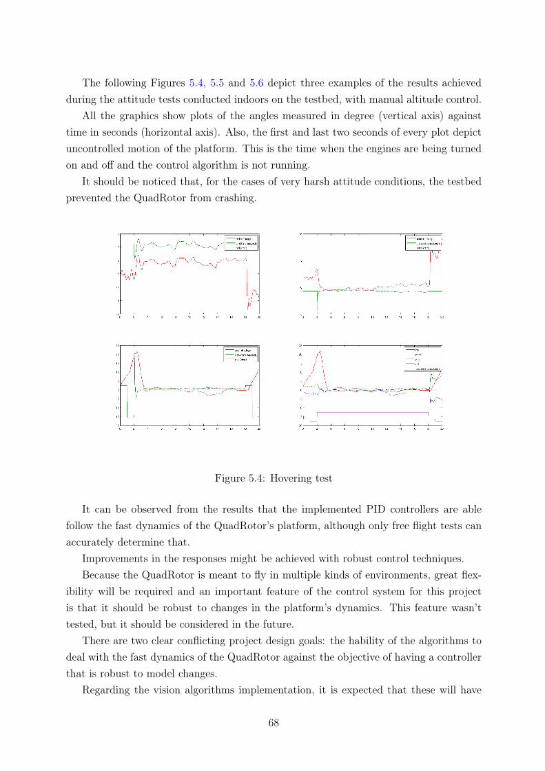
The following Figures 5.4, 5.5 and 5.6 depict three examples of the results achievedduring the attitude tests conducted indoors on the testbed, with manual altitude control.

All the graphics show plots of the angles measured in degree (vertical axis) againsttime in seconds (horizontal axis). Also, the first and last two seconds of every plot depictuncontrolled motion of the platform. This is the time when the engines are being turnedon and off and the control algorithm is not running.

It should be noticed that, for the cases of very harsh attitude conditions, the testbedprevented the QuadRotor from crashing.

Figure 5.4: Hovering test

It can be observed from the results that the implemented PID controllers are ablefollow the fast dynamics of the QuadRotor’s platform, although only free flight tests canaccurately determine that.

Improvements in the responses might be achieved with robust control techniques.Because the QuadRotor is meant to fly in multiple kinds of environments, great flex-

ibility will be required and an important feature of the control system for this projectis that it should be robust to changes in the platform’s dynamics. This feature wasn’ttested, but it should be considered in the future.

There are two clear conflicting project design goals: the hability of the algorithms todeal with the fast dynamics of the QuadRotor against the objective of having a controllerthat is robust to model changes.

Regarding the vision algorithms implementation, it is expected that these will have

68

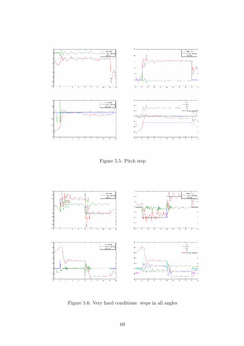
Figure 5.5: Pitch step

Figure 5.6: Very hard conditions: steps in all angles

69

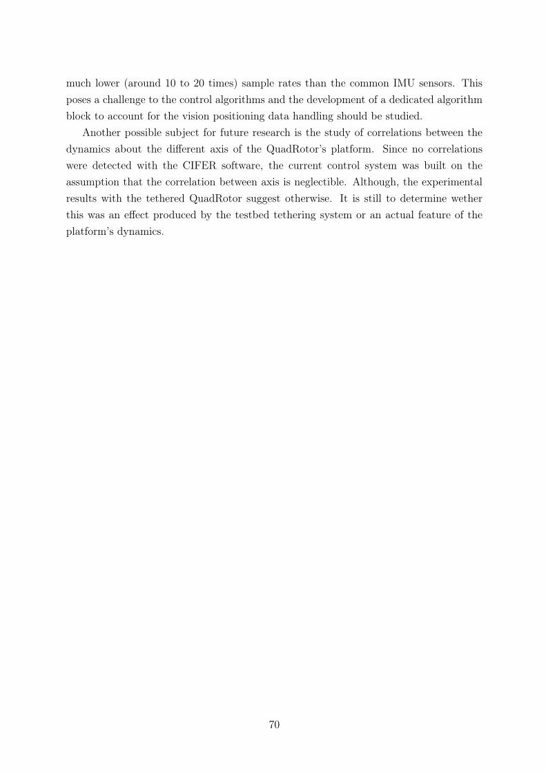
much lower (around 10 to 20 times) sample rates than the common IMU sensors. Thisposes a challenge to the control algorithms and the development of a dedicated algorithmblock to account for the vision positioning data handling should be studied.

Another possible subject for future research is the study of correlations between thedynamics about the different axis of the QuadRotor’s platform. Since no correlationswere detected with the CIFER software, the current control system was built on theassumption that the correlation between axis is neglectible. Although, the experimentalresults with the tethered QuadRotor suggest otherwise. It is still to determine wetherthis was an effect produced by the testbed tethering system or an actual feature of theplatform’s dynamics.

70

Chapter 6

Concluding Remarks

Throughout the course of this thesis, a dynamics model for the attitude and altitudeof the QuadRotor was determined, using the CIFER identification software. A set ofPID controllers for attitude was developed. A testbed was built and successful tests wereconducted on the platform. Also simple models were determined for position and altitudedynamics and controllers were developed.

More might have been done, but given the difficulties and setbacks that are alwaysfaced when dealing with pratical projects, the results are quite satisfying.

Using the linear uncorrelated models and PID controllers for attitude, the first suc-cessful test results with automatic control were obtained for this QuadRotor platform.

The attitude controllers were able to follow the fast dynamics of the QuadRotor. Forthe tests on tethered platform, hover with errors below 2deg on all attitude angles - Roll,Pitch and Yaw - during the 20second long tethered flight tests was achieved.

Harsh conditions with simultaneous steps on all the attitude angles were also testedwit satisfying results. Even if the response shows oscillations, it does stabilize.

Despite the CIFER results, where no axis correlations could be found, careful anal-ysis of flight data under these simultaneous steps conditions suggests that there may benon-neglectible aerodynamic effects causing correlations between axis. These correlationscould have been masked during the flight tests by the action of the trained pilot in sucha way that they don’t appear in the recorded flight data.

These hypothesis should be further analysed and tested in the future. If cross-axiscorrelations are to be found, the controllers should be adapted accordingly.

Another theme for possible study in the future is the optimization of the algorithmsalgready developed. This applies both for the altitude and for the position and altitudealgorithms.

Regarding the position and altitude models and controllers developed, much work canbe done as soon as a test platform that allows for its test is ready. Such simple controlalgorithms are but a start and can certainly be improved in many ways. The choice of

71

trying to actually control the position and altitude using such simple models turns tothe goal of control robustness with respect to changes in the platforms’ dynamics, butimprovement of the models could also be a way to go.

Regarding the attitude controllers, optimal control methods could be employed havingin mind the robustness to dynamics changes as well.

Although the results in tethered flight were satisfying, which leads to the possibilityof already being able to hover in a free flight situation, this could not be conclusivelytested. As such, even though the attained results point in that direction, the controllersdeveloped are not proved to be effective. As a next step, a testbed that allows for freeflight hover tests should be developed and free hovering should be tested. Naturally,without the outter loop of position control, the platform will drift away from its positionbut a stability test can be conducted anyway. Further in time, once the vision algorithmsare implemented and vision can be used as the extra position sensor, the full controlsystem can be tested.

On a last remark, it is interesting to notice that once again it was made evident thatthe PID controller, while being so simple and easy to implement, is still a very reliabletool, proving to be robust in the real world environment.

Several approaches were studied and abandoned during the course of this thesis’ workand eventually, in the several different areas - attitude, altitude and position control - thePID controllers were the only to reach implementation fase, even with satisfying results,as was the case of the attitude controllers for Roll, Pitch and Yaw

For the altitude transfer function obtained with CIFER, an optimal LQR controllerwas designed. Eventually it was dropped due to the fact that the model was not accurateenough, so it didn’t reach the test phase and it wasn’t documented in this thesis. It isonly mentioned here as an additional point on why only PID’s were documented.

Also another advanced algorithm was studied, the Integral Backstepping non-linearcontroller. There were several problems with this attempt, including difficulties withthe dynamic modelling. Only the development of a full accurate model of the platformcould have been another thesis, but this was not the case and so it was not feasible toimplement such an approach. Again, it isn’t documented here because no solid resultscould be achieved with it.

72

Bibliography

[1] K. Stewart, G. Abate, and J. Evers. Flight mechanics and control issues for microair vehicles. In AIAA Atmospheric Flight Mechanics Conference and Exhibit. AIAA,Keystone, Colorado, USA August 2006.

[2] W. E. Green and P. Y. Oh. A mav that flies like an airplane and hovers like a heli-copter. Proceedings of the 2005 IEEE/ASME International Conference on AdvancedIntelligent Mechatronics, Monterey, California, USA, July 2005.

[3] S. Watkins, J. Milbank, B. J. Loxton, and W. H. Melbourne. Atmospheric windsand their implications for microair vehicles. AIAA Journal, November 2006.

[4] Ascending Technologies GmbH. X-3D-BL User’s Manual, Germany, 2009.

[5] M. Ol, G. Parker, G. Abate, and J. Evers. Flight controls and performance chal-lenges for mavs in complex environmnents. AIAA Guidance, Navigation and ControlConference and Exhibit, Honolulu, Hawaii, USA, August 2008.

[6] S. Bouabdallah and R. Siegwart. Advances in Unmanned Aerial Vehicles, chapter 6 -Design and Control of a Miniature Quadrotor, pages 171–210. Springer, Netherlands,2007.

[7] W. E. Green, P. Y. Oh, and S. Yoon. An acquisition and distribution system for sit-uational awareness. Proceedings of IMECE’03 2003 ASME International MechanicalEngineering Congress, Washington D.C., USA, November 2003.

[8] T. Shima, S. J. Rasmussen, and D. Gross. Assigning micro uavs to task tours inan urban terrain. AIAA Guidance, Navigation, and Control Conference and Exhibit,Keystone, Colorado, USA, August 2006.

[9] G. M. Hoffman, S. L. Waslander, and C. J. Tomlin. Quadrotor helicopter trajectorytracking control. In AIAA Guidance, Navigation and Control Conference and Exhibit.American Institute of Aeronautics and Astronautics, August 2008.

73

[10] W. Wang, G. Song, K. Nonami, M. Hirata, and O. Miyazawa. Autonomous controlfor micro-flying robot and small wireless helicopter. In IEEE/RSJ InternationalConference on Intelligent Robots and Systems, Beijing, China, 2006. IEEE/RSJ.

[11] P. J. McKerrow and D. Ratner. The design of a tethered aerial robot. IEEE Inter-national Conference on Robotics and Automation, Roma, Italy, April 2007.

[12] C. G. Jones, J. J. Heyder-Bruckner, T. S. Richardson, and C. D. Jones. Vision-based control for unmanned rotorcraft. AIAA Guidance, Navigation, and ControlConference and Exhibit, Keystone, Colorado, USA, August 2006.

[13] J. Buchli, editor. Mobile Robots - Moving Intelligence. Advanced Robotic SystemsInternational and pro literatur Verlag, 2006.

[14] G. M. Hoffman, H. Huang, S. L. Waslander, and C. J. Tomlin. Quadrotor helicopterflight dynamics and control: Theory and experiment. In AIAA Guidance, Navi-gation and Control Conference and Exhibit. American Institute of Aeronautics andAstronautics, August 2007.

[15] CIFER® User’s Guide, student version 5.2.00 edition, 2009.

[16] M. Tischler. A Case for System Identification Using CIFER. NASA, 2006.

[17] M. B. T. Jeffrey N. Williams, Johnie A. Ham. Flight Test Manual - RotorcraftFrequency Domain Flight Testing. U.S. Army Test and Evaluation Command, U.S.Army Aviation Technical Test Center - Airworthiness Qualification Test Directorate,September 1995.

[18] M. Tischler, CIFER® Background and Application, 2006.

[19] R. W. Beard. A class of flight trajectories for tracking ground targets with micro airvehicles. In 2007 Mediterranean Conference on Control and Automation. IEEE, July2007.

[20] L. Beji and A. Abichou. Streamlined rotors mini rotorcraft: Trajectory generationand tracking. International Journal of Control, Automation and Systems, 3(1):87–99,March 2005.

[21] K. Ogata. Modern Control Engineering. Prentice Hall International, Inc., 3rd edition,1997.

[22] G. C. Goodwin, S. F. Graebe, and M. E. Salgado. Control System Design. Univer-sidad Técnica Federico Santa María, 2000.

74

[23] A. B. J. Hetthéssy, R. Bars. Discrete PID Control. Budapest University of Technologyand Economics, 2004.

[24] J. Kamman. Me 360 control systems - system type and steady-state error. WesternMichigan University, 2010.

[25] K. Hazawa, J. Shin, D. Fujiwara, K. Igarashi, D. Fernando, and K. Nonami. Au-tonomous flight control of hobby-class small unmanned helicopter - trajectory fol-lowing control by using preview control considering heading direction. In IEEE/RSJInternational Conference on Intelligent Robots and Systems, Sendai, Japan, Septem-ber 2004. IEEE.

[26] K. Astrom and B. Wittenmark. Computer Controlled Systems. Prentice Hall Inter-national, Inc., 1997.

[27] S.D. Conte, C. Boor. Elementary Numerical Analysis - An Algorithmic Approach.McGraw-Hill, 3rd edition, 1980.

[28] S.-K. Bae, H. C. Hwang, K.-J. Yoon, and N.-S. Goo. Development of small flyingrobot with rotary wing and autonomous control system. Proceedings of the 2007IEEE International Conference on Robotics and Biometrics, December 2007.

[29] Y. Bestaoui. On-line reference trajcetory definition with joint torque and velocityconstraints. The International Journal of Robotics Research, 11(75), 2002.

[30] S. Bouabdallah, A. Noth, and R. Siegwart. Pid vs lq control techniques applied toan indoor micro quadrotor. In IEEE/RSJ International Conference on IntelligentRobots and Systems, Sendai, Japan, 2004.

[31] S. Bouabdallah and R. Siegwart. Backstepping and sliding-mode techniques appliedto an indoor micro quadrotor. In IEEE International Conference on Robotics andAutomation, Barcelona, Spain, 2005.

[32] C. E. Crede. Determining moment of inertia. 1948.

[33] W. E. Green and P. Y. Oh. Autonomous hovering of a fixed-wing micro air vehicle.Proceedings of the 2006 IEEE International Conference on Robotics and Automation,May 2006.

[34] M. E. Greene and V. Trent. Software algorithms in air data attitude heading referencesystems. Aircraft Engineering and Aerospace Technology, 75(5):470–476, 2003.

[35] H. Kwakernaak and R. Sivan. Linear Optimal Control Systems. John Whiley & Sons,Inc., 1972.

75

[36] S. Lasic and G. Torzo. Torsion pendulum: A mechanical nonlinear oscillator. Pro-ceeding Int. GIREP Sem., Udine, 2-6, September, 2001.

[37] J. McLean, G. Parker, and N. Seal. Basic control for four rotor autonomous aerialagent. ISORA (International Symposium on Operations Research and Its Applica-tions), 2008.

[38] D. Poinsot, C. Bérard, R. Krashanitsa, and S. Shkarayev. Investigation of flightdynamics and automatic controls for hovering micro air vehicles. AIAA Guidance,Navigation and Control Conference, August 2008.

76

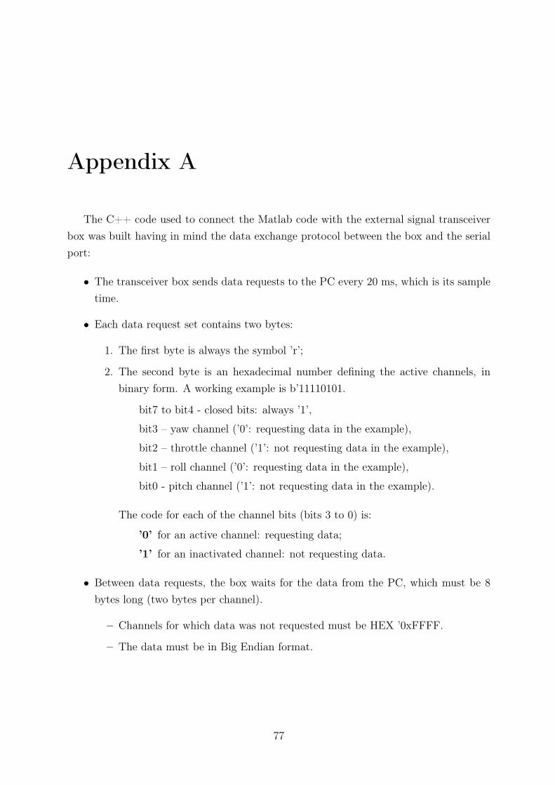
Appendix A

The C++ code used to connect the Matlab code with the external signal transceiverbox was built having in mind the data exchange protocol between the box and the serialport:

• The transceiver box sends data requests to the PC every 20 ms, which is its sampletime.

• Each data request set contains two bytes:

1. The first byte is always the symbol ’r’;

2. The second byte is an hexadecimal number defining the active channels, inbinary form. A working example is b’11110101.

bit7 to bit4 - closed bits: always ’1’,

bit3 – yaw channel (’0’: requesting data in the example),

bit2 – throttle channel (’1’: not requesting data in the example),

bit1 – roll channel (’0’: requesting data in the example),

bit0 - pitch channel (’1’: not requesting data in the example).

The code for each of the channel bits (bits 3 to 0) is:

’0’ for an active channel: requesting data;

’1’ for an inactivated channel: not requesting data.

• Between data requests, the box waits for the data from the PC, which must be 8bytes long (two bytes per channel).

– Channels for which data was not requested must be HEX ’0xFFFF.

– The data must be in Big Endian format.

77

Appendix B

In this Appendix, the C++ program code developed to manage the serial port com-munications and call the control algorithms developed is listed.

This code was developed by Yair Atzmon at the Technion - Israel Institute of Tech-nology, during the year 2009.

#include "mex . h" // a l l MATLAB C in t e r f a c e programs need t h i s at the beg inning

#include <s td i o . h> // Needed fo r p r i n t f e t c

#include <s t r i n g . h>#include <objbase . h> // Needed fo r COM fun c t i o n a l i t y

#include <tchar . h>#include <conio . h> // inc luded fo r _getch and _kbhit

#include <windows . h>#include <time . h>#include "XsensCMT. h"

//∗∗∗∗∗∗∗∗∗∗∗∗∗∗∗∗∗∗∗∗∗∗∗

// d e f i n i t i o n s

//∗∗∗∗∗∗∗∗∗∗∗∗∗∗∗∗∗∗∗∗∗∗∗

// d e f i n i t i o n s f o r xsense

#define KEY "32 df f −5da5b−b9a5d−61a5e"#define SAMPLE_FREQUENCY 25#define MODE (CMT_OUTPUTMODE_POSITION | CMT_OUTPUTMODE_VELOCITY | CMT_OUTPUTMODE_ORIENT)

// the dev i ce outputs both c a l i b r a t e d data and o r i en t a t i on

#define SETTINGS (CMT_OUTPUTSETTINGS_ORIENTMODE_EULER |CMT_OUTPUTSETTINGS_TIMESTAMP_SAMPLECNT) // the dev i ce outputs o r i en t a t i on in eu l e r

format and a l s o timestamp

#define XSENSE_BAUDRATE 57600

// d e f i n i t i o n s f o r remote con t ro l com port

#define COMPORT "Com4"#define REMOTE_CONTROL_BAUDRATE 115200

// genera l

#define NUM_OF_ITERATIONS 1000 // processData .m i s c a l l e d once every 2 i t e r a t i o n s

// t h i s macro t e s t s f o r an error on xsense and e x i t s the program with a message i f t he re

was one

#define EXIT_ON_ERROR( res , comment ) i f ( r e s != XRV_OK) { mexPrintf ( "Error %d occurred inxsense func t i on : " comment " : %s \n" , res , cmtGetResultText ( r e s ) ) ; return ; }

78

//∗∗∗∗∗∗∗∗∗∗∗∗∗∗∗∗∗∗∗∗∗∗∗∗

// de c l a r a t i on s

//∗∗∗∗∗∗∗∗∗∗∗∗∗∗∗∗∗∗∗∗∗∗∗∗

// se tup func t i on fo r xsense

void setupXsense (void ) ;

// se tup func t i on fo r remote con t ro l com port

void setupCom(void ) ;

// v a r i a b l e s used when c a l l i n g e x t e rna l matlab func t i on s

mxArray ∗ inputArray [ 1 2 ] ;mxArray ∗outputArray [ 4 ] ;

// xsense g l o b a l v a r i a b l e s

long i n s t anc e = −1; // o b j e c t to i n t e r f a c e the Xsense module

unsigned short mtCount = 0 ; // num of sensors connected

CmtDeviceId dev i c e Id s [ 2 5 6 ] ; // dev i ce IDs

// remote con t ro l com g l o b a l v a r i a b l e s

HANDLE m_hCom; // handle to com port

//∗∗∗∗∗∗∗∗∗∗∗∗∗∗∗∗∗∗∗∗∗∗∗∗∗∗∗∗∗∗∗∗∗∗∗∗∗∗

// Remote con t ro l com port f unc t i on s

//∗∗∗∗∗∗∗∗∗∗∗∗∗∗∗∗∗∗∗∗∗∗∗∗∗∗∗∗∗∗∗∗∗∗∗∗∗∗

// s e t s e r i a l communication fo r remote con t ro l

void setupCom(void ){

bool m_bPortReady ;char m_sComPort [ 2 0 ] ;DCB m_dcb ;COMMTIMEOUTS m_CommTimeouts ;

s t r cpy (m_sComPort ,COMPORT) ;m_hCom = CreateF i l e (m_sComPort ,

GENERIC_READ | GENERIC_WRITE,0 , // e x c l u s i v e access

NULL, // no s e cu r i t y

OPEN_EXISTING,0 , // no over lapped I /O

NULL) ; // nu l l templa te

i f (m_hCom == INVALID_HANDLE_VALUE){

mexErrMsgTxt ( "can ’ t c r e a t e f i l e f o r s e r i a l port " ) ;return ;

}

79

m_bPortReady = SetupComm(m_hCom, 128 , 128) ; // s e t b u f f e r s i z e s

// i n i t i a l i z e comm parameters

m_bPortReady = GetCommState (m_hCom, &m_dcb) ;m_dcb . BaudRate = REMOTE_CONTROL_BAUDRATE;m_dcb . ByteSize = 8 ;m_dcb . Par i ty = NOPARITY;m_dcb . StopBits = ONESTOPBIT;m_dcb . fAbortOnError = TRUE;

m_bPortReady = SetCommState (m_hCom, &m_dcb) ;

// s e t t imeouts

m_bPortReady = GetCommTimeouts (m_hCom, &m_CommTimeouts) ;

m_CommTimeouts . ReadIntervalTimeout = MAXWORD; // 50;

m_CommTimeouts . ReadTotalTimeoutConstant = 0 ; // 50;

m_CommTimeouts . ReadTotalTimeoutMult ipl ier = 0 ; // 10;

m_CommTimeouts . WriteTotalTimeoutConstant = 0 ; //50

m_CommTimeouts . WriteTota lTimeoutMult ip l ier = 0 ; // 10;

m_bPortReady = SetCommTimeouts (m_hCom, &m_CommTimeouts) ;}

//∗∗∗∗∗∗∗∗∗∗∗∗∗∗∗∗∗∗∗∗∗∗∗∗∗∗∗∗∗∗∗∗∗∗∗∗∗∗

// Xsense func t i on s

//∗∗∗∗∗∗∗∗∗∗∗∗∗∗∗∗∗∗∗∗∗∗∗∗∗∗∗∗∗∗∗∗∗∗∗∗∗∗

void setupXsense (void ){

XsensResultValue r e s ;CmtPortInfo po r t In f o [ 2 5 6 ] ;unsigned long portCount = 0 ;unsigned short sampleFreq = SAMPLE_FREQUENCY;CmtOutputMode mode = MODE;CmtOutputSettings s e t t i n g s = SETTINGS;

// crea t e the Xsens CMT ins tance to handle the sensor ( s )

char ser ia lNumber [ 2 4 ] = KEY;

in s t anc e = cmtCreateInstance ( ser ia lNumber ) ;i f ( i n s t ance != −1)

mexPrintf ( "CMT ins tance c rea ted \n\n" ) ;else {

mexPrintf ( "Creat ion o f CMT ins tance f a i l e d , probably because o f an i n v a l i d s e r i a lnumber\n" ) ;

return ;}

// Checks a v a i l a b l e COM por t s and scans f o r MotionTrackers

mexPrintf ( "Scanning f o r connected Xsens dev i c e s . . . " ) ;r e s = cmtScanPorts ( por t In fo , &portCount , 0) ;EXIT_ON_ERROR( res , " cmtScanPorts " ) ;mexPrintf ( "done\n" ) ;

80

i f ( portCount == 0) {mexPrintf ( "No MotionTrackers found\n\n" ) ;return ;

}

for ( int i = 0 ; i < ( int ) portCount ; i++) {mexPrintf ( "Using COM port %d at %d baud\n\n" ,

( long ) po r t In f o [ i ] . m_portNr , po r t In f o [ i ] . m_baudrate ) ;}

mexPrintf ( "Opening por t s . . . " ) ;//open the por t which the dev i ce i s connected to and connect at the dev i ce ’ s baudrate

.

for ( int p = 0 ; p < ( int ) portCount ; p++){r e s = cmtOpenPort ( ins tance , po r t In f o [ p ] . m_portNr , po r t In f o [ p ] . m_baudrate ) ;EXIT_ON_ERROR( res , "cmtOpenPort" ) ;

}mexPrintf ( "done\n\n" ) ;

// ge t the Mt sensor count .

mexPrintf ( " Ret r i ev ing MotionTracker count ( exc lud ing attached Xbus Master ( s ) ) \n" ) ;r e s = cmtGetMtCount ( ins tance ,&mtCount ) ;EXIT_ON_ERROR( res , "cmtGetMtCount" ) ;mexPrintf ( "MotionTracker count : %i \n\n" ,mtCount ) ;

// r e t r i e v e the dev i ce IDs

mexPrintf ( " Ret r i ev ing MotionTrackers dev i c e ID( s ) \n" ) ;for (unsigned int j = 0 ; j < mtCount ; j++ ) {

r e s = cmtGetMtDeviceId ( ins tance , &dev i c e Id s [ j ] , j ) ;EXIT_ON_ERROR( res , " cmtGetDeviceId" ) ;mexPrintf ( "Device ID at index %i : %08x\n" , j , ( long ) d ev i c e Id s [ j ] ) ;

}

// s e t baudrate

int newBaudRate = XSENSE_BAUDRATE;mexPrintf ( " Set baudrate to %d" , newBaudRate ) ;for (unsigned int j = 0 ; j < mtCount ; j++ ) {

r e s = cmtSetBaudrate ( ins tance , XSENSE_BAUDRATE, dev i c e Id s [ j ] ) ;EXIT_ON_ERROR( res , " cmtSetBaudrate" ) ;

}

// make sure t ha t we ge t the f r e s h e s t data

mexPrintf ( "\ nSet t ing queue mode so that we always get the l a t e s t data\n\n" ) ;r e s = cmtSetQueueMode ( ins tance ,CMT_QM_LAST) ;EXIT_ON_ERROR( res , "cmtSetQueueMode" ) ;

// Set user s e t t i n g s in MTi/MTx

// Assumes i n i t i a l i z e d g l o b a l MTComm c l a s s

// s e t sensor to con f i g sa t e

r e s = cmtGotoConfig ( i n s t anc e ) ;EXIT_ON_ERROR( res , "cmtGotoConfig" ) ;

// s e t the dev i ce output mode fo r the dev i ce ( s )

81

mexPrintf ( " Conf igur ing mode s e l e c t i o n ( eu l e r , po s i t i on , v e l o c i t y . . . ) \n" ) ;for ( int i =0; i < mtCount ; i++) {

i f ( cmtIdIsMtig ( dev i c e Id s [ i ] ) ) {r e s = cmtSetDeviceMode ( ins tance , mode , s e t t i n g s , sampleFreq , d ev i c e Id s [ i ] ) ;

} else {r e s = cmtSetDeviceMode ( ins tance , mode & 0xFF0F , s e t t i n g s , sampleFreq ,

d ev i c e Id s [ i ] ) ;}EXIT_ON_ERROR( res , " setDeviceMode" ) ;

}

// s t a r t r e c e i v i n g data

mexPrintf ( " s t a r t measuring ! \ n\n" ) ;r e s = cmtGotoMeasurement ( i n s t ance ) ;EXIT_ON_ERROR( res , "cmtGotoMeasurement\n\n" ) ;

// Wait f o r f i r s t data item ( s ) to a r r i v e . In product ion code , you would use a

c a l l b a c k func t ion in s t ead ( see cmtSetCal lbackFunct ion )

Sleep (20) ;}

void mexFunction ( int nlhs , mxArray ∗ plhs [ ] , int nrhs , const mxArray ∗prhs [ ] ){

unsigned char noData [ 2 ] = {255 ,255} ; // used to send unrequested channels

// unsigned char t h r o t t l e S t a r t S t opEng in e s [ 2 ] = {3 ,17};

// unsigned char yawStartStopEngines [ 2 ] = {2 ,178};

// unsigned shor t t h r o t t l eEng in e = 785;

// unsigned shor t yawEngine = 690;

// time_t startTime , endTime ;

// doub le difTime ;

// xsense v a r i a b l e s

XsensResultValue r e s = XRV_OK;unsigned short sdata ; // sample counter

CmtVector pos i t ion_data ; // s t r u c t s to ho ld po s i t i on data

CmtVector ve loc i ty_data ; // s t r u c t s to ho ld v e l o c i t y data

CmtEuler euler_data ; // s t r u c t s to ho ld eu l e r data

// remote con t ro l com port v a r i a b l e s

BOOL bWriteRC ;BOOL bReadRC ;DWORD iBytesWritten ;DWORD iBytesRead ;char sBu f f e r [ 1 2 8 ] ;unsigned int RCB;unsigned int i sP i t c h ;unsigned int i s R o l l ;unsigned int i sTh r o t t l e ;unsigned int isYaw ;

// b u f f e r s to save da ta t during run time fo r debugging

double i nputBuf f e r [NUM_OF_ITERATIONS ] [ 9 ] ;unsigned short outputBuf fer [NUM_OF_ITERATIONS ] [ 4 ] ;

82

// crea t e input and output array to i n t e r f a c e matlab func t i on s

for ( int i = 0 ; i <= 11 ; i++)inputArray [ i ] = mxCreateNumericMatrix (1 , 1 ,mxDOUBLE_CLASS, mxREAL ) ;

for ( int i = 0 ; i <= 3 ; i++)outputArray [ i ] = mxCreateNumericMatrix (1 , 1 ,mxINT16_CLASS, mxREAL ) ;

// c a l l se tup func t i on fo r xsense

setupXsense ( ) ;// c a l l se tup func t i on fo r remote con t ro l com port

setupCom ( ) ;

//∗∗∗∗∗∗∗∗∗∗∗∗∗∗∗∗∗∗∗∗∗∗∗∗∗∗∗∗∗∗∗∗∗∗∗∗∗∗∗∗∗∗∗∗∗∗∗∗∗∗∗

// s t a r t operat ion

// read and wr i t e from sensor and remote con t ro l

//∗∗∗∗∗∗∗∗∗∗∗∗∗∗∗∗∗∗∗∗∗∗∗∗∗∗∗∗∗∗∗∗∗∗∗∗∗∗∗∗∗∗∗∗∗∗∗∗∗∗∗

// send s t a r t engine parameters

int counter = 0 ;while ( counter < NUM_OF_ITERATIONS){

//∗∗∗∗∗∗∗∗∗∗∗∗∗∗∗∗∗∗∗∗∗∗∗∗∗∗∗∗∗∗∗∗∗∗

// read from remote con t ro l f i r s t

//∗∗∗∗∗∗∗∗∗∗∗∗∗∗∗∗∗∗∗∗∗∗∗∗∗∗∗∗∗∗∗∗∗∗

sBu f f e r [ 0 ] = 0 ; // anything but ’ r ’

while ( sBu f f e r [ 0 ] != ’ r ’ ) // synchronize to ’ r ’

bReadRC = ReadFile (m_hCom, &sBuf fe r , 1 , &iBytesRead , NULL) ;

// now ge t the ac tua l r e que s t

bReadRC = ReadFile (m_hCom, &sBu f f e r [ 1 ] , 1 , &iBytesRead , NULL) ;

RCB = sBu f f e r [ 1 ] ; // the by te ho ld ing the dev i ce r eque s t

i sP i t c h = RCB & 1 ;i sR o l l = RCB & 2 ;i sTh r o t t l e = RCB & 4 ;isYaw = RCB & 8 ;

//∗∗∗∗∗∗∗∗∗∗∗∗∗∗∗∗∗∗∗∗∗∗∗∗∗∗∗

// read from xsense

//∗∗∗∗∗∗∗∗∗∗∗∗∗∗∗∗∗∗∗∗∗∗∗∗∗∗∗

// ge t the bundle o f data

r e s = cmtGetNextDataBundle ( i n s t ance ) ;

// ge t sample count

r e s = cmtDataGetSampleCounter ( ins tance , &sdata , d ev i c e Id s [ 0 ] ,NULL) ;

// ge t po s i t i on data

r e s = cmtDataGetPositionLLA ( ins tance , &posit ion_data , d ev i c e Id s [ 0 ] ) ;// mexPrintf ("\n\n\n%6.1 f \ t%6.1 f \ t%6.1 f \n" , pos i t ion_data .m_data [ 0 ] , pos i t ion_data .

m_data [ 1 ] , pos i t ion_data .m_data [ 2 ] ) ;

// ge t v e l o c i t y data

r e s = cmtDataGetVelocity ( ins tance , &veloc i ty_data , d ev i c e Id s [ 0 ] ) ;// mexPrintf ("\n\n\n%6.1 f \ t%6.1 f \ t%6.1 f \n" , ve l oc i t y_da ta .m_data [ 0 ] , ve l oc i t y_da ta .

83

m_data [ 1 ] , ve l oc i t y_da ta .m_data [ 2 ] ) ;

// ge t eu l e r

r e s = cmtDataGetOriEuler ( ins tance , &euler_data , d ev i c e Id s [ 0 ] ) ;// mexPrintf ("\n\n\n%6.1 f \ t%6.1 f \ t%6.1 f \n" , euler_data . m_roll , euler_data . m_pitch ,

euler_data .m_yaw) ;

// process data in e x t e rna l matlab func t i on

// f i r s t s e t l a t e s t xsense data as input

∗(double∗)mxGetPr( inputArray [ 0 ] ) = pos i t ion_data . m_data [ 0 ] ;∗(double∗)mxGetPr( inputArray [ 1 ] ) = pos i t ion_data . m_data [ 1 ] ;∗(double∗)mxGetPr( inputArray [ 2 ] ) = pos i t ion_data . m_data [ 2 ] ;∗(double∗)mxGetPr( inputArray [ 3 ] ) = ve loc i ty_data . m_data [ 0 ] ;∗(double∗)mxGetPr( inputArray [ 4 ] ) = ve loc i ty_data . m_data [ 1 ] ;∗(double∗)mxGetPr( inputArray [ 5 ] ) = ve loc i ty_data . m_data [ 2 ] ;∗(double∗)mxGetPr( inputArray [ 6 ] ) = euler_data . m_roll ;∗(double∗)mxGetPr( inputArray [ 7 ] ) = euler_data . m_pitch ;∗(double∗)mxGetPr( inputArray [ 8 ] ) = euler_data .m_yaw;

// c a l l e x t e rna l func t i on

i f ( counter & 1)mexCallMATLAB(4 , outputArray , 9 , inputArray , " processData " ) ;

// wr i t e to remote con t ro l the output a f t e r proces s ing

// the f i r s t 50 and l a s t 50 i t e r a t i o n s are devoted to s t a r t and s top engines

bWriteRC = WriteFi l e (m_hCom, i sP i t c h ? noData : (unsigned char∗)mxGetPr(outputArray [ 0 ] ) ,2 ,& iBytesWritten ,NULL) ;

bWriteRC = WriteFi l e (m_hCom, i sR o l l ? noData : (unsigned char∗)mxGetPr(outputArray [ 1 ] ) ,2 ,& iBytesWritten ,NULL) ;

// i f ( ( counter > START_STOP_ENGINE_ITERATIONS) && ( counter < (NUM_OF_ITERATIONS−START_STOP_ENGINE_ITERATIONS) ) )

// {

bWriteRC = WriteFi l e (m_hCom, i sTh r o t t l e ? noData : (unsigned char∗)mxGetPr(outputArray [ 2 ] ) ,2 ,& iBytesWritten ,NULL) ;

bWriteRC = WriteFi l e (m_hCom, isYaw ? noData : (unsigned char∗)mxGetPr(outputArray [ 3 ] ) ,2 ,& iBytesWritten ,NULL) ;

// }

// e l s e

// {

// mexPrintf ("\n%d" , counter ) ;

// bWriteRC = WriteFi le (m_hCom, th ro t t l eS t a r tS t opEng ine s ,2 ,& iBytesWrit ten ,NULL) ;

// bWriteRC = WriteFi le (m_hCom, yawStartStopEngines ,2 ,& iBytesWritten ,NULL) ;

// bWriteRC = WriteFi le (m_hCom, &thro t t l eEng ine ,2 ,& iBytesWrit ten ,NULL) ;

// bWriteRC = WriteFi le (m_hCom, &yawEngine ,2 ,& iBytesWritten ,NULL) ;

// }

// save input and output in b u f f e r s f o r debugging

i nputBuf f e r [ counter ] [ 0 ] = ∗(double∗)mxGetPr( inputArray [ 0 ] ) ;i nputBuf f e r [ counter ] [ 1 ] = ∗(double∗)mxGetPr( inputArray [ 1 ] ) ;i nputBuf f e r [ counter ] [ 2 ] = ∗(double∗)mxGetPr( inputArray [ 2 ] ) ;i nputBuf f e r [ counter ] [ 3 ] = ∗(double∗)mxGetPr( inputArray [ 3 ] ) ;i nputBuf f e r [ counter ] [ 4 ] = ∗(double∗)mxGetPr( inputArray [ 4 ] ) ;i nputBuf f e r [ counter ] [ 5 ] = ∗(double∗)mxGetPr( inputArray [ 5 ] ) ;i nputBuf f e r [ counter ] [ 6 ] = ∗(double∗)mxGetPr( inputArray [ 6 ] ) ;i nputBuf f e r [ counter ] [ 7 ] = ∗(double∗)mxGetPr( inputArray [ 7 ] ) ;i nputBuf f e r [ counter ] [ 8 ] = ∗(double∗)mxGetPr( inputArray [ 8 ] ) ;

84

outputBuf fer [ counter ] [ 0 ] = ∗(unsigned short ∗)mxGetPr( outputArray [ 0 ] ) ;outputBuf fer [ counter ] [ 1 ] = ∗(unsigned short ∗)mxGetPr( outputArray [ 1 ] ) ;outputBuf fer [ counter ] [ 2 ] = ∗(unsigned short ∗)mxGetPr( outputArray [ 2 ] ) ;outputBuf fer [ counter ] [ 3 ] = ∗(unsigned short ∗)mxGetPr( outputArray [ 3 ] ) ;

counter += 1 ;}

// c l o s e the handle to com port o f remote con t ro l

CloseHandle (m_hCom) ;// c l o s e com port o f xsense

i f ( i n s t ance != −1){

// Close any open COM por t s

cmtClose ( i n s t ance ) ;cmtDestroyInstance ( i n s t ance ) ;

}

//∗∗∗∗∗∗∗∗∗∗∗∗∗∗∗∗∗∗∗∗∗∗∗∗∗∗∗∗∗∗∗∗∗∗∗∗∗∗∗∗∗∗∗∗∗∗∗∗∗∗∗∗∗∗∗∗

// p r in t b u f f e r s and sav ing in f i l e s f o r debugging

//∗∗∗∗∗∗∗∗∗∗∗∗∗∗∗∗∗∗∗∗∗∗∗∗∗∗∗∗∗∗∗∗∗∗∗∗∗∗∗∗∗∗∗∗∗∗∗∗∗∗∗∗∗∗∗∗

FILE ∗ fp ;fp = fopen ( "runTimeData . txt " , "w+" ) ;i f ( fp == NULL)

mexPrintf ( "\nThere was a problem opening the f i l e to wr i t e runtime data" ) ;else{

for ( int i = 0 ; i < NUM_OF_ITERATIONS; i++){

// mexPrintf ("\n\ninput %d : %6.2 f \ t%6.2 f \ t%6.2 f \ t%6.2 f \ t%6.2 f \ t%6.2 f \ t%6.2 f \ t

%6.2 f \ t%6.2 f \ t%6.2 f \ t%6.2 f \ t%6.2 f " , i ,

// inpu tBu f f e r [ i ] [ 0 ] , inpu tBu f f e r [ i ] [ 1 ] , inpu tBu f f e r [ i ] [ 2 ] , inpu tBu f f e r [ i

] [ 3 ] ,

// inpu tBu f f e r [ i ] [ 4 ] , inpu tBu f f e r [ i ] [ 5 ] , inpu tBu f f e r [ i ] [ 6 ] , inpu tBu f f e r [ i

] [ 7 ] ,

// inpu tBu f f e r [ i ] [ 8 ] ) ;

// mexPrintf ("\ noutput %d : %d %d %d %d" , i , ou tpu tBuf f er [ i ] [ 0 ] , ou tpu tBuf f er [ i

] [ 1 ] , ou tpu tBuf f er [ i ] [ 2 ] , ou tpu tBuf f er [ i ] [ 3 ] ) ;

f p r i n t f ( fp , "\n\ t%d\ t%6.9 f \ t%6.9 f \ t%6.4 f \ t%6.4 f \ t%6.4 f \ t%6.4 f \ t%6.2 f \ t%6.2 f \ t%6.2 f " , i ,

i nputBuf f e r [ i ] [ 0 ] , i nputBuf f e r [ i ] [ 1 ] , i nputBuf f e r [ i ] [ 2 ] , i nputBuf f e r [ i] [ 3 ] ,

i nputBuf f e r [ i ] [ 4 ] , i nputBuf f e r [ i ] [ 5 ] , i nputBuf f e r [ i ] [ 6 ] , i nputBuf f e r [ i] [ 7 ] ,

i nputBuf f e r [ i ] [ 8 ] ) ;f p r i n t f ( fp , "\ t%d\ t%d\ t%d\ t%d" , outputBuf fer [ i ] [ 0 ] , outputBuf fer [ i ] [ 1 ] ,

outputBuf fer [ i ] [ 2 ] , outputBuf fer [ i ] [ 3 ] ) ;}f c l o s e ( fp ) ;

}mexPrintf ( "\nEnd o f program .\ n" ) ;}

85

Appendix C

In this Appendix, the Matlab code developed for the realtime control algorithms developed is listed.

f unc t i on [ u_pitch , u_rol l , u_thrott le , u_yaw ] = processData ( long , l a t , a l t , vx , vy , vz , r o l l , p i tch, yaw)

Ts = 0.04 ; % sample time ( sec ) −> i f Ts i s changed , then a l l the c on t r o l law has tobe r e c a l c u l a t e d

nr_ca l l s = 500 ; % runtime = nr_ca l l s ∗Ts% Note : for each c a l l o f this funct ion , the s e r i a l P o r t . cpp func t i on% was c a l l e d twice

p e r s i s t e n t counter phi0 theta0 c s i 0 a l t 0 vx_p vx_p2 xref_p xref_p2 xref_dp xref_dp2 vy_pvy_p2 yref_p yref_p2 yref_dp yref_dp2 ro l l_p rol l_p2 rol l_dp rol l_dp2 r o l l r e f_pro l l r e f_p2 ro l l r e f_dp ro l l r e f_dp2 pitch_p pitch_p2 pitch_dp pitch_dp2 pitchre f_ppitchre f_p2 pitchre f_dp pitchref_dp2 yaw_p yaw_p2 yaw_dp yaw_dp2 yawref_dp yawref_dp2yawref_p yawref_p2 z in tp z r e f i n t p ; % (p stands for prev ious and d stands for

d e r i v a t i v e )i f isempty ( counter )

counter = 0 ;phi0 = 0 ;theta0 = 0 ;c s i 0 = 0 ;a l t 0 = 0 ;

endcounter = counter + 1 ;

% measure and averag ing the a t t i t ud e and a l t i t u d e d r i f t si f and( counter > 10 , counter < 31) %Ts=.04 => f i r s t 2 sec

phi0 = phi0 + r o l l ; %i n t e g r a ltheta0 = theta0 + pi t ch ;c s i 0 = c s i 0 + yaw ;a l t 0 = a l t 0 + a l t ;

endi f counter == 32 %average

phi0 = phi0 /20 ;theta0 = theta0 /20 ;c s i 0 = c s i 0 /20 ;a l t 0 = a l t 0 /20 ;

end

%−−−−−−−−−−−−−−−−−−−−−−−−−−−−−−−−−−−−−−−−−−−−−−−−−−−−−−−−−−−−i f and( counter >= 2/Ts , counter <= nr_cal l s −2/Ts)%works from counter = 2/Ts to counter = nr_cal l s −2/Ts

86

% s h i f t a t t i t ud e and a l t i t u d e accord ing to the computed d r i f t averager o l l = r o l l − phi0 ;p i t ch = pi t ch − theta0 ;yaw = yaw − c s i 0 ;z = a l t − a l t 0 ;

% t r a n s l a t e ( long , l a t ) to (x , y )% see ’ experiment r e s u l t s /long_lat_to_km . txt ’ or http : //en . w ik iped ia . org/wik i /

Longitude

x = ( long − 32 .7775) ∗96 . 400 ; % x and y in meters ( aprox . )y = ( l a t − 35 .02175) ∗110 . 000 ;

%c r ea t e r e f e r e n c e s% r o l l , p i t ch and yaw are in degree s% x and y are in aprox . meters% z i s in metersi f counter < nr_ca l l s /2

r o l l r e f = 0 ;p i t c h r e f = 0 ;yawref = 0 ;x r e f = 0 ;y r e f = 0 ;z r e f = 1 ;

elser o l l r e f = 0 ;p i t c h r e f = 0 ;yawref = 0 ;x r e f = 0 ;y r e f = 0 ;z r e f = 1 ;

end

% % X po s i t i o n con t r o l a lgor i thm% % given c e r t a i n x r e f and x , d e f i n e s the cor respond ing p i t c h r e f% %i n i t i a l i z a t i o n ( should only produce e f f e c t the f i r s t time the func t i on i s% %ca l l e d )% i f isempty ( xref_p )% vx_p = vx ;% vx_p2 = vx ;% xref_p = xr e f ;% xref_p2 = xr e f ;% xref_dp = 0 ;% xref_dp2 = 0 ;% end%% %genera t i on o f nece s sa ry s i g n a l s% % this i s the new d e r i v a t i v e introduced at 17Dec ’ 09% vx_d = (2∗vx − vx_p − vx_p2) /(3∗Ts) ;% xref_d = (2∗ x r e f − xref_p − xref_p2 ) /(3∗Ts) ;% xref_2d = (2∗ xref_d − xref_dp − xref_dp2 ) /(3∗Ts) ;%% %PID algor i thm% xi = ( x r e f − x ) ∗ . 4 ; % Ki ;% xk = ( xref_d − vx ) ∗3 ; % Kk;% xd = ( xref_2d − vx_d) ∗ . 4 ; % Kd;% p i t c h r e f = ( x i + xk + xd ) ∗(−1) ;%/12) ; % Kf ;%% % saving the inputs f o r next c a l l ’ s d e r i v a t i o n s

87

% vx_p2 = vx_p ;% vx_p = vx ;% xref_p2 = xref_p ;% xref_p = xr e f ;% xref_dp2 = xref_d ;% xref_dp = xref_d ;%% %s i g n a l c ond i t i on ing% l im i t = 45 ;% i f p i t c h r e f < − l im i t% p i t c h r e f = − l im i t ;% e l s e i f p i t c h r e f > l im i t% p i t c h r e f = l im i t ;% end%% % Y po s i t i o n con t r o l a lgor i thm% % given c e r t a i n y r e f and y , d e f i n e s the cor respond ing r o l l r e f% %i n i t i a l i z a t i o n ( should only produce e f f e c t the f i r s t time the func t i on i s% %ca l l e d )% i f isempty ( yref_p )% vy_p = vy ;% vy_p2 = vy ;% yref_p = yr e f ;% yref_p2 = yr e f ;% yref_dp = 0 ;% yref_dp2 = 0 ;% end%% %genera t i on o f nece s sa ry s i g n a l s% % this i s the new d e r i v a t i v e introduced at 17Dec ’ 09% vy_d = (2∗vy − vy_p − vy_p2) /(3∗Ts) ;% yref_d = (2∗ y r e f − yref_p − yref_p2 ) /(3∗Ts) ;% yref_2d = (2∗ yref_d − yref_dp − yref_dp2 ) /(3∗Ts) ;%% %PID algor i thm% xi = ( y r e f − y ) ∗ . 6 ; % Ki ;% xk = ( yref_d − vy ) ∗2 ; % Kk;% xd = ( yref_2d − vy_d) ∗ . 5 ; % Kd;% r o l l r e f = ( x i + xk + xd ) ;%∗(1/9) ; % Kf ;%% % saving the inputs f o r next c a l l ’ s d e r i v a t i o n s% vy_p2 = vy_p ;% vy_p = vy ;% yref_p2 = yref_p ;% yref_p = yr e f ;% yref_dp2 = yref_d ;% yref_dp = yref_d ;%% %s i g n a l c ond i t i on ing% l im i t = 45 ;% i f r o l l r e f < − l im i t% r o l l r e f = − l im i t ;% e l s e i f r o l l r e f > l im i t% r o l l r e f = l im i t ;% end

%r o l l c on t r o l a lgor i thm

88

% %r o l l i s the cur rent r o l l ang le measurement ( in degree s )% %r e f i s the r e f e r e n c e value for r o l l for the same in s t an t ( in degree s )% %u_rol l i s the command s i g n a l for the remote , i t s the ouput

%i n i t i a l i z a t i o n ( should only produce e f f e c t the f i r s t time the func t i on i s%c a l l e d )i f isempty ( r o l l r e f_p )

ro l l_p = r o l l ;ro l l_dp = 0 ;r o l l r e f_p = r o l l r e f ;r o l l r e f_dp = 0 ;ro l l_p2 = r o l l ;ro l l_dp2 = 0 ;r o l l r e f_p2 = r o l l r e f ;r o l l r e f_dp2 = 0 ;

end

%genera t i on o f nece s sa ry s i g n a l s% this i s the new d e r i v a t i v e introduced at 17Dec ’ 09

ro l l_d = (2∗ r o l l − ro l l_p − ro l l_p2 ) /(3∗Ts) ;ro l l_2d = (2∗ ro l l_d − rol l_dp − rol l_dp2 ) /(3∗Ts) ;r o l l r e f_d = (2∗ r o l l r e f − r o l l r e f_p − r o l l r e f_p2 ) /(3∗Ts) ;r o l l r e f_2d = (2∗ r o l l r e f_d − r o l l r e f_dp − r o l l r e f_dp2 ) /(3∗Ts) ;

%PID algor i thmx i = ( r o l l r e f − r o l l ) ∗13 . 1250 ; % Ki = . 5 2 5 / . 0 4 ;xk = ( r o l l r e f_d − ro l l_d ) ∗(−0.475) ; % Kk = −.475 ;xd = ( ro l l r e f_2d − ro l l_2d ) ∗0 . 0190 ; % Kd = . 4 7 5 ∗ . 0 4 ;u_ro l l = ( x i + xk + xd) ∗(−1) ; % Kf ;

% sav ing the inputs f o r next c a l l ’ s d e r i v a t i o n sro l l_p2 = rol l_p ;rol l_dp2 = rol l_dp ;r o l l r e f_p2 = ro l l r e f_p ;ro l l r e f_dp2 = ro l l r e f_dp ;ro l l_p = r o l l ;ro l l_dp = rol l_d ;r o l l r e f_p = r o l l r e f ;r o l l r e f_dp = ro l l r e f_d ;

%s i g n a l c ond i t i on ingl im i t = 250 ;i f u_rol l < − l im i t

u_ro l l = − l im i t ;e l s e i f u_ro l l > l im i t

u_ro l l = l im i t ;end

%pi t ch con t r o l a lgor i thm% func t i on u_pitch = pi tch_contro l ( pitch , p i t ch_re f )% %pi tch i s the cur rent p i t ch ang le measurement ( in degree s )% %r e f i s the r e f e r e n c e value for p i t ch for the same in s t an t ( in degree s )

%i n i t i a l i z a t i o n ( should only produce e f f e c t the f i r s t time the func t i on i s%c a l l e d )i f isempty ( p i tchre f_p )

pitch_p = pi t ch ;

89

pitch_dp = 0 ;p i tchre f_p = p i t c h r e f ;p i tchre f_dp = 0 ;pitch_p2 = pi t ch ;pitch_dp2 = 0 ;p i tchre f_p2 = p i t c h r e f ;p itchre f_dp2 = 0 ;

end

%genera t i on o f nece s sa ry s i g n a l s% this i s the new d e r i v a t i v e introduced at 17Dec ’ 09

pitch_d = (2∗ p i t ch − pitch_p − pitch_p2 ) /(3∗Ts) ;pitch_2d = (2∗ pitch_d − pitch_dp − pitch_dp2 ) /(3∗Ts) ;p i tchre f_d = (2∗ p i t c h r e f − pitchre f_p − pitchre f_p2 ) /(3∗Ts) ;p i tchre f_2d = (2∗ pitchre f_d − pitchref_dp − pitchref_dp2 ) /(3∗Ts) ;

%PID algor i thmx i = ( p i t c h r e f − p i t ch ) ∗6 . 5 4 ; % Ki = . 2 6 1 6 / . 0 4 ;xk = ( pi tchre f_d − pitch_d ) ∗0 . 4324 ; % Kk = 1 − . 5676 ;xd = ( pitchre f_2d − pitch_2d ) ∗0 . 0227 ; % Kd = . 5 6 7 6 ∗ . 0 4 ;u_pitch = ( x i + xk + xd) ;%∗3 .8651 ; % Kf ;

% sav ing the inputs f o r next c a l l ’ s d e r i v a t i o n spitch_p2 = pitch_p ;pitch_dp2 = pitch_dp ;p i tchre f_p2 = pitchre f_p ;pitchre f_dp2 = pitchref_dp ;pitch_p = pi t ch ;pitch_dp = pitch_d ;p i tchre f_p = p i t c h r e f ;p i tchre f_dp = pitchre f_d ;

%s i g n a l c ond i t i on ingl im i t = 150 ;i f u_pitch < − l im i t

u_pitch = − l im i t ;e l s e i f u_pitch > l im i t

u_pitch = l im i t ;end

%yaw con t r o l a lgor i thm%func t i on u_yaw = yaw_control (yaw , yaw_ref )%p i t ch i s the cur rent p i t ch ang le measurement ( in degree s )%r e f i s the r e f e r e n c e value for p i t ch for the same in s t an t ( in degree s )

%i n i t i a l i z a t i o n ( should only have e f f e c t the f i r s t time the func t i on i s c a l l e d )i f isempty ( yawref_dp )

yaw_p = yaw ;yaw_dp = 0 ;yawref_p = yawref ;yawref_dp = 0 ;yaw_p2 = yaw ;yaw_dp2 = 0 ;yawref_p2 = yawref ;yawref_dp2 = 0 ;

end

90

%genera t i on o f nece s sa ry s i g n a l s ( d e r i v a t i v e s )% this i s the new d e r i v a t i v e introduced at 17Dec ’ 09

yaw_d = (2∗yaw − yaw_p − yaw_p2) /(3∗Ts) ;yaw_2d = (2∗yaw_d − yaw_dp − yaw_dp2) /(3∗Ts) ;yawref_d = (2∗ yawref − yawref_p − yawref_p2 ) /(3∗Ts) ;yawref_2d = (2∗ yawref_d − yawref_dp − yawref_dp2 ) /(3∗Ts) ;

%PID algor i thmx i = ( yawref − yaw) ∗0 . 4 65 ; % Ki = . 0 1 8 6 / . 0 4 ;xk = ( yawref_d − yaw_d) ∗0 . 1314 ; % Kk = 1 − . 8 6 8 6 ;xd = ( yawref_2d − yaw_2d) ∗0 . 0347 ; % Kd = . 8 6 8 6 ∗ . 0 4 ;u_yaw = ( x i + xk + xd ) ∗10 . 7924 ; % Kf ;

% sav ing the inputs f o r next c a l l ’ s d e r i v a t i o n syaw_p2 = yaw_p ;yaw_dp2 = yaw_dp ;yawref_p2 = yawref_p ;yawref_dp2 = yawref_dp ;yaw_p = yaw ;yaw_dp = yaw_d ;yawref_p = yawref ;yawref_dp = yawref_d ;

%s i g n a l c ond i t i on ingl im i t = 500 ;i f u_yaw < − l im i t

u_yaw = − l im i t ;e l s e i f u_yaw > l im i t

u_yaw = l im i t ;end

% a l t i t u d e con t r o l a lgor i thm% %z i s the cur rent a l t i t u d e measurement ( in meters above sphero id ?)% %r e f i s the r e f e r e n c e value for z for the same in s t an t ( in meters above sphero id ?)% %th r o t t l e i s the command s i g n a l for the remote , i t s the ouput

%i n i t i a l i z a t i o n ( should only produce e f f e c t the f i r s t time the func t i on i s c a l l e d )i f isempty ( z in tp )

% zp = z ;% zp2 = z ;% z r e f p = z r e f ;% z r e fp2 = z r e f ;

z in tp = 0 ;z r e f i n t p = 0 ;

end

%genera t i on o f nece s sa ry s i g n a l s% this i s the new d e r i v a t i v e introduced at 17Dec ’ 09

% zd = (2∗ z − zp − zp2 ) /(3∗Ts) ; % = vz ;% z r e f d = (2∗ z r e f − z r e f p − z r e fp2 ) /(3∗Ts) ;

z i n t = z in tp + z∗Ts ;z r e f i n t = z r e f i n t p + z r e f ∗Ts ;

%PI a lgor i thmx i = ( z r e f i n t − z i n t ) ∗2 ; % or 3xk = ( z r e f − z ) ∗4 ; % or 3xd = 0 ; % ( z r e f d − vz ) ∗0 ;

91

t h r o t t l e = ( x i + xk + xd ) + 9 . 9 8 ; % 9.98 i s the g rav i ty

% sav ing the inputs f o r next c a l l ’ s d e r i v a t i o n s% zp2 = zp ;% zp = z ;% zr e fp2 = z r e f p ;% z r e f p = z r e f ;

z in tp = z i n t ;z r e f i n t p = z r e f i n t ;

%s i g n a l c ond i t i on ingl im i t = 20 ;i f t h r o t t l e > l im i t

t h r o t t l e = l im i t ;e l s e i f t h r o t t l e < 0

t h r o t t l e = 0 ;end

%outputs

% u_rol l = uint16 (1010) ; %from 701 to 1346 , middle i s 1010i f u_rol l < 0

u_rol l = uint16 (1010 + u_rol l ∗1 .236) ;else

u_rol l = uint16 (1010 + u_rol l ∗1 .344) ;end

% u_pitch = uint16 (1012) ; %from 685 to 1354 , middle i s 1012i f u_pitch < 0

u_pitch = uint16 (1012 + u_pitch ∗2 .18 ) ;else

u_pitch = uint16 (1012 + u_pitch ∗2 .28 ) ;end

% u_yaw = uint16 (1015) ; %from 690 to 1366 , middle i s 1015i f u_yaw < 0

u_yaw = uint16 (1012 + u_yaw∗ . 6 5 ) ;else

u_yaw = uint16 (1012 + u_yaw∗ . 702 ) ;end

% u_thrott l e = uint16 (900) ; % from 785 (700 for eng ine s t a r t / stop ) to 1239 , middle i s1002u_thrott l e = uint16 (900 + t h r o t t l e ∗15) ;

end

%−−−−−−−−−−−−−−−−−−−−−−−−−−−−−−−−−−−−−−−−−−−−−−−−−−−−−−−−−−−%s t a r t and stop the h e l i c o p t e r ’ s eng ine s ( t h i s b lock o f code i s always the same )i f or ( counter < 1/Ts , and ( counter > nr_cal l s −2/Ts , counter < nr_cal l s −1/Ts) )

u_thrott l e = uint16 (750) ; %prepare f o r s t a r t / stop (1 sec )u_yaw = uint16 (1050) ;u_pitch = uint16 (1012) ;u_ro l l = uint16 (1010) ;

e l s e i f or ( counter < 2/Ts , and ( counter >= nr_cal l s −1/Ts , counter < nr_ca l l s ) )u_thrott l e = uint16 (700) ; % s t a r t / stop (2 s e c s /1 sec )u_yaw = uint16 (690) ;u_pitch = uint16 (1012) ;u_ro l l = uint16 (1010) ;

e l s e i f counter == nr_ca l l s % f i n i s h the program

92

u_thrott l e = uint16 (750) ;u_yaw = uint16 (1050) ;u_pitch = uint16 (1012) ;u_ro l l = uint16 (1010) ;counter = 0 ; % r e s e t the counter

end

i f counter == 1di sp ( ’ S t a r t i ng eng ine s . ’ ) ;

e l s e i f counter == nr_cal l s −2/Tsd i sp ( ’ Stopping eng ine s . ’ ) ;

end

end

93