Embed Size (px)
Citation preview

GUIDANCE MANUAL FOR ENVIRONMENTAL SITE
CHARACTERIZATION IN SUPPORT OF ENVIRONMENTAL AND HUMAN HEALTH RISK
ASSESSMENT
VOLUME 1 GUIDANCE MANUAL
PN 1551 ISBN 978-1-77202-026-7 PDF
© Canadian Council of Ministers of the Environment, 2016

Volume 1: Guidance Manual i
PREFACE This manual is one of a series of volumes dedicated to providing guidance on environmental site characterization in support of environmental and human health risk assessment at contaminated sites. Canadian Council of Ministers of the Environment (CCME) initiated the National Contaminated Sites Remediation Program (NCSRP), a five year program (1989-1995), to develop a consistent national approach for the assessment and remediation of Canada’s contaminated sites, and specifically to clean up high-risk orphan contaminated sites. As part of providing national tools for site characterization, the NCSRP released the Guidance Manual on Sampling, Analysis, and Data Management for Contaminated Sites (Volume I: Main Report, and Volume II: Analytical Method Summaries) in 1993, and the Subsurface Assessment Handbook for Contaminated Sites in 1994. The purpose of this document, and related volumes, is to provide a replacement of the 1993 sampling and analytical guidance. This work is being done by the Soil Quality Guidelines Task Group, which was established by CCME to develop Canadian Soil Quality Guidelines and to continue providing national guidance on contaminated sites after sunsetting of the NCSRP.
The goal of the environmental site characterization guidance is to provide Canadians with a consistent approach to sampling and analyzing complex environmental matrices, such that the data obtained will be representative and of known quality. The guidance provides a summary of key elements that should be performed, and reported, during site investigations. The guidance also recommends sample handling and storage requirements, analytical methods, and method specific quality control and assurance procedures to ensure that the results of laboratory analyses are reported for Canadian Environmental Quality Guidelines with sufficient quality upon which to base decisions.
The environmental site characterization guidance consists of four volumes:
Volume 1: Guidance Manual [this document] Volume 2: Checklists Volume 3: Suggested Operating Procedures Volume 4: Analytical Methods Methods and any reference to specific sampling equipment provided in this guidance are provided for information purposes only. CCME does not warrant the use of any of these methods or equipment. The responsibility for selection and use lies solely with the user.

Volume 1: Guidance Manual ii
ACKNOWLEDGEMENTS
The primary authors of the four volume Site Characterization guidance were: Dr. Ian Hers, Mr. Guy Patrick, Dr. Reidar Zapf-Gilje (Golder Associates Ltd) for volume 1 (chapters 1-8), volume 2, and volume 3, and SOPs 1-6; Ms. Miranda Henning, Ms. Andrea Fogg, Ms. Katrina Leigh (Environ International Corp.) for volume 1 (chapters 9-11) and sections of chapter 4, media specific material in volume 2, volume 3, and SOPs 7-17; Barry Loescher, with the assistance of Elizabeth Walsh, (Maxxam Analytics) volume 4.
Golder, Environ and Maxxam provided assistance in addressing public review comments. The four volumes were extensively reviewed by members of the CCME Soil Quality Guidelines Task Group, and colleagues within their respective jurisdictions.
CCME would like to thank reviewers who provided feedback during the public review process. The contribution of time and expertise of all participants is gratefully acknowledged.

Volume 1: Guidance Manual iii
TABLE OF CONTENTS
1 INTRODUCTION ..................................................................................................... 1
Background and Purpose ........................................................................................ 1 1.1 Intended Audience and Guidance Application .......................................................... 1 1.2 Scope ...................................................................................................................... 1 1.3 Guidance Outline ..................................................................................................... 2 1.4
2 CONTAMINATED SITE INVESTIGATION AND MANAGEMENT PROCESS ............................................................................................................... 6
Integrated Risk Management Process for Contaminated Sites ................................ 6 2.1 Site Characterization Process .................................................................................. 6 2.2
2.2.1 Phased Investigation Approach .......................................................................... 7 2.2.2 Data Quality as a Central Theme to the Site Characterization
Process .............................................................................................................. 7 Development of a Conceptual Site Model ................................................................ 8 2.3 Define the Project Background and Goals ............................................................. 12 2.4 Establish the Investigation Objectives .................................................................... 13 2.5 Prepare a Sampling and Analysis Plan .................................................................. 14 2.6
2.6.1 Review of Existing Data ................................................................................... 14 2.6.2 Pre-mobilization Tasks ..................................................................................... 14 2.6.3 Sampling Media, Data Types and Investigation Tools ...................................... 15 2.6.4 Sampling Rationale and Design ....................................................................... 16 2.6.5 Sampling and Analysis Methods and Quality Assurance Project Plan .............. 18
Conduct the Field Investigation Program – Conventional Phased 2.7Approach and Expedited Site Assessment Process ............................................... 19
Validate and Interpret Data .................................................................................... 21 2.8 Resources and Weblinks ....................................................................................... 23 2.9
References ............................................................................................................ 23 2.103 QUALITY ASSURANCE/QUALITY CONTROL ................................................... 25
Quality Assurance Project Plan .............................................................................. 25 3.1 Data Quality Indicators .......................................................................................... 27 3.2 Quality Control ....................................................................................................... 28 3.3
3.3.1 Quality Control Checks and Samples ............................................................... 28 3.3.2 Recommended Minimum Frequency of Quality Control Samples ..................... 29
Data Quality Targets .............................................................................................. 29 3.43.4.1 Duplicate Samples ........................................................................................... 30
Reporting of QA/QC ............................................................................................... 31 3.5 References ............................................................................................................ 31 3.6
4 CONCEPTUAL SITE MODEL FOR CONTAMINATED SITES............................ 32 Contamination Sources and Types ........................................................................ 33 4.1

Volume 1: Guidance Manual iv
4.1.1 Overview .......................................................................................................... 33 4.1.2 Common Types of Contamination .................................................................... 33 4.1.3 Non-Point Sources of Contamination ............................................................... 34 4.1.4 Emergent or Less Common Chemicals ............................................................ 37
Conceptual Site Model for LNAPL and DNAPL Characterization ........................... 37 4.2 Conceptual Site Model for Groundwater Characterization ...................................... 39 4.3
4.3.1 Partitioning ....................................................................................................... 40 4.3.2 Unsaturated Zone Chemical Transport ............................................................ 41 4.3.3 Groundwater Contaminant Transport ............................................................... 42 4.3.4 Considerations for Fractured Bedrock .............................................................. 44 4.3.5 Considerations for Permafrost .......................................................................... 45
Conceptual Site Model for Soil Characterization .................................................... 45 4.4 Conceptual Site Model for Soil Vapour .................................................................. 49 4.5
4.5.1 Contamination Sources .................................................................................... 50 4.5.2 Chemical Transfer to Vapour Phase (Volatilization) ......................................... 51 4.5.3 Vadose Zone Fate and Transport Processes ................................................... 53 4.5.4 Near-Building Processes for Soil Vapour Intrusion ........................................... 55 4.5.5 Summary ......................................................................................................... 55 4.5.6 Conceptual Site Scenarios for Vapour Intrusion ............................................... 56 4.5.7 Resources, References and Links ................................................................... 64
Conceptual Site Model for Surface Water Characterization ................................... 64 4.64.6.1 Study Area and Reference Area Identification .................................................. 66
Conceptual Site Model for Sediment Characterization ........................................... 68 4.7 Conceptual Site Model for Biological Characterization ........................................... 71 4.8 References ............................................................................................................ 73 4.9
5 SOIL CHARACTERIZATION GUIDANCE ........................................................... 76 Context, Purpose and Scope ................................................................................. 76 5.1 Conceptual Site Model for Soil Characterization .................................................... 77 5.2 Soil Sampling Design ............................................................................................. 78 5.3
5.3.1 Representative Sampling Challenges .............................................................. 79 5.3.2 Sampling Design Strategies ............................................................................. 81 5.3.3 Statistical Methods for Sampling Design .......................................................... 85 5.3.4 Discrete and Composite Samples .................................................................... 88
Investigation Soil Sampling Methods ..................................................................... 89 5.4 Field Analytical Methods ........................................................................................ 92 5.5
5.5.1 Headspace Vapour Tests ................................................................................. 93 5.5.2 Colourimetric Tests .......................................................................................... 94 5.5.3 Immunoassay Tests ......................................................................................... 94 5.5.4 X-ray fluorescence (XRF) ................................................................................. 96
Field Preservation of Soil Samples for VOC Analysis ............................................ 97 5.6 Methods for Data Interpretation ............................................................................. 98 5.7

Volume 1: Guidance Manual v
5.7.1 Statistical Data Analysis for Soil Characterization ............................................ 99 5.7.2 Non-Detect Values ......................................................................................... 101 5.7.3 Statistical Approach to Characterizing Contaminated Soil .............................. 101
Data Presentation and Reporting ......................................................................... 102 5.8 Resources and Weblinks ..................................................................................... 102 5.9
References .......................................................................................................... 104 5.106 GROUNDWATER CHARACTERIZATION GUIDANCE .................................... 110
Purpose, Background and Need .......................................................................... 110 6.16.1.1 Obtaining Representative Samples from the Well .......................................... 111 6.1.2 Non-Aqueous Phase Liquids (NAPLs) ........................................................... 115
Conceptual Site Models for Groundwater Characterization .................................. 115 6.2 Approach and Sampling Design ........................................................................... 116 6.3
6.3.1 Intrusive Field Program for Groundwater Characterization ............................. 117 6.3.2 Addressing the Issue of Scale ........................................................................ 118 6.3.3 Acquiring Groundwater Quality Information .................................................... 119 6.3.4 Available Technologies .................................................................................. 120 6.3.5 Direct-Push Technologies for Groundwater Characterization ......................... 122
Acquiring Hydrogeologic Information ................................................................... 125 6.46.4.1 Groundwater Flow Direction ........................................................................... 125 6.4.2 Groundwater Velocity ..................................................................................... 126
Monitoring and Monitoring Networks .................................................................... 128 6.56.5.1 Well Screen Length and Well Completion Intervals ........................................ 128 6.5.2 Horizontal Spacing of Data Points .................................................................. 131 6.5.3 Vertical Spacing of Data Points ...................................................................... 134
Field and Laboratory Data Acquisition ................................................................. 134 6.66.6.1 Well Development .......................................................................................... 135 6.6.2 Well Purging and Sampling ............................................................................ 135 6.6.3 Field Laboratories .......................................................................................... 138 6.6.4 Special Considerations .................................................................................. 138 6.6.5 Selection of Analytical Tests .......................................................................... 140 6.6.6 Data Validation and Quality Assurance/Quality Control .................................. 140
Well Abandonment .............................................................................................. 141 6.7 Data Assessment and Interpretation .................................................................... 141 6.8
6.8.1 Conceptual Site Model Development ............................................................. 141 6.8.2 Data Presentation and Reporting ................................................................... 142 6.8.3 Modelling Issues ............................................................................................ 143
References .......................................................................................................... 144 6.97 SOIL VAPOUR GUIDANCE................................................................................ 145
Context, Purpose and Scope ............................................................................... 145 7.1 Conceptual Site Model for Soil Vapour Characterization ...................................... 146 7.2 Study Objectives .................................................................................................. 146 7.3

Volume 1: Guidance Manual vi
Soil Vapour Sampling Approach and Design ....................................................... 147 7.47.4.1 Overview of Sampling Strategy ...................................................................... 147 7.4.2 Soil Vapour Sampling Locations in Relation to Conceptual Site Model .......... 148 7.4.3 Recommendations for Soil Vapour Sampling Locations ................................. 152 7.4.4 When to Sample and Sampling Frequency .................................................... 154 7.4.5 Biodegradation Assessment for Aerobically Degrading Hydrocarbons ........... 155
Soil Vapour Probe Construction and Installation .................................................. 156 7.57.5.1 Probes Installed in Boreholes......................................................................... 156 7.5.2 Probes Installed Using Direct Push Technology ............................................. 158 7.5.3 Driven Probes ................................................................................................ 158 7.5.4 Use of Water Table Monitoring Wells as Soil Vapour Probes ......................... 159 7.5.5 Subslab Soil Vapour Probes .......................................................................... 160 7.5.6 Probe Materials .............................................................................................. 160 7.5.7 Decontamination of Sampling Materials and Equipment ................................ 161
Soil Vapour Sampling Procedures ....................................................................... 161 7.67.6.1 Soil Vapour Probe Development and Equilibration ......................................... 162 7.6.2 Flow and Vacuum (Probe Performance) Check ............................................. 162 7.6.3 Leak Testing of Probes and Sampling Trains ................................................. 162 7.6.4 Sampling Container or Device........................................................................ 163 7.6.5 Sample Probe Purging and Sampling ............................................................ 164
Soil Vapour Analysis ............................................................................................ 167 7.77.7.1 Selection of Method ....................................................................................... 167 7.7.2 Field Detectors ............................................................................................... 168 7.7.3 Field Laboratory Analysis ............................................................................... 170 7.7.4 Fixed Laboratory Analysis .............................................................................. 171 7.7.5 Quality Assurance / Quality Control Considerations ....................................... 175
Soil and Groundwater Characterization ............................................................... 178 7.87.8.1 Groundwater Data .......................................................................................... 178 7.8.2 Soil Data ........................................................................................................ 179
Ancillary Data ...................................................................................................... 180 7.9 Data Interpretation and Analysis .......................................................................... 182 7.10
7.10.1 Data Organization and Reporting ................................................................... 182 7.10.2 Data Quality Analysis ..................................................................................... 183 7.10.3 Data Consistency Analysis ............................................................................. 184 7.10.4 Further Evaluation .......................................................................................... 184
Resources and Weblinks ..................................................................................... 185 7.11 References .......................................................................................................... 185 7.12
8 INDOOR AIR QUALITY TESTING FOR EVALUATION OF SOIL VAPOUR INTRUSION ........................................................................................ 193
Context, Purpose and Scope ............................................................................... 193 8.1 Conceptual Site Model for Indoor Air ................................................................... 194 8.2

Volume 1: Guidance Manual vii
8.2.1 Background Indoor Air Concentrations ........................................................... 195 8.2.2 Building Foundation Construction .................................................................. 196 8.2.3 Building Ventilation ........................................................................................ 196 8.2.4 Building Pressures and Weather Conditions .................................................. 197 8.2.5 Mixing of Vapours Inside Building .................................................................. 198 8.2.6 Vapour Depletion Mechanisms ...................................................................... 199
Development of Indoor Air Quality Study Approach and Design .......................... 199 8.38.3.1 Define Study Objectives ................................................................................. 199 8.3.2 Identify Target Compounds ............................................................................ 200 8.3.3 Develop Communications Program ................................................................ 200 8.3.4 Conduct Pre-Sampling Building Survey ......................................................... 200 8.3.5 Conduct Preliminary Screening ...................................................................... 201 8.3.6 Identify Immediate Health or Safety Concerns ............................................... 201 8.3.7 Define Number and Locations of Indoor and Outdoor Air Samples ................ 202 8.3.8 Define Sampling Duration .............................................................................. 202 8.3.9 Define Sampling Frequency ........................................................................... 203 8.3.10 Preparing the Building for Sampling and Conditions during Sampling ............ 203
Indoor Air Analytical Methods .............................................................................. 204 8.48.4.1 Air Analysis Using USEPA Methods TO-15 and TO-17 .................................. 205 8.4.2 Air Analysis using Passive Diffusive Badge Samplers .................................... 205
Data Interpretation and Analysis .......................................................................... 207 8.58.5.1 Data Organization and Reporting ................................................................... 207 8.5.2 Data Quality Evaluation.................................................................................. 208 8.5.3 Methods for Discerning Contributions of Background from Indoor
Sources ......................................................................................................... 208 Resources and Weblinks ..................................................................................... 214 8.6 References .......................................................................................................... 214 8.7
9 SURFACE WATER CHARACTERIZATION GUIDANCE .................................. 220 Context, Purpose, Scope ..................................................................................... 220 9.1 Conceptual Site Model for Surface Water Characterization ................................. 221 9.2 Study Approach and Design for Surface Water Characterization ......................... 224 9.3
9.3.1 Goals and Objectives ..................................................................................... 224 9.3.2 Data Quality Objectives.................................................................................. 225 9.3.3 Overview of Sampling Designs ...................................................................... 226 9.3.4 Quality Assurance/Quality Control ................................................................. 235
Sampling Equipment for Surface Water Characterization .................................... 237 9.49.4.1 General Considerations ................................................................................. 237 9.4.2 Contact Materials ........................................................................................... 238 9.4.3 Discrete Sampling Equipment ........................................................................ 239 9.4.4 Composite Sampling Equipment .................................................................... 242 9.4.5 Equipment for Sampling Ice and Surface Water Underneath Ice .................... 243

Volume 1: Guidance Manual viii
Sample Preservation and Storage ....................................................................... 244 9.5 Data Analysis for Surface Water Characterization ............................................... 244 9.6 Resources and Weblinks ..................................................................................... 245 9.7 References .......................................................................................................... 247 9.8
10 SEDIMENT CHARACTERIZATION GUIDANCE ............................................... 249 Context, Purpose, and Scope .............................................................................. 249 10.1 Conceptual Site Model for Sediment Characterization ......................................... 250 10.2 Study Approach and Design for Sediment Characterization ................................. 251 10.3
10.3.1 Goals and Objectives ..................................................................................... 251 10.3.2 Data Quality Objectives.................................................................................. 252 10.3.3 Sediment Sampling Design Considerations ................................................... 253
General Sample Collection, Handling, and Analytical Considerations .................. 261 10.410.4.1 Contact Materials ........................................................................................... 261 10.4.2 Sample Types ................................................................................................ 262 10.4.3 Sample Handling............................................................................................ 262 10.4.4 Sample Volume, Preservation, and Storage ................................................... 264 10.4.5 Considerations for the analysis of sediment samples ..................................... 264
Quality Assurance and Quality Control Considerations ........................................ 266 10.5 Sediment Sampling Methodology and Equipment ................................................ 267 10.6
10.6.1 General Methodology ..................................................................................... 268 10.6.2 Sediment Sampling Equipment Types ........................................................... 268
Sediment Porewater Collection and Extraction Methodology ............................... 272 10.710.7.1 In Situ Porewater Collection Methods ............................................................ 273 10.7.2 Ex Situ Porewater Extraction Methods ........................................................... 274
Data Analysis for Sediment Characterization ....................................................... 274 10.8 Resources and Weblinks ..................................................................................... 275 10.9
References .......................................................................................................... 276 10.1011 BIOLOGICAL CHARACTERIZATION GUIDANCE ........................................... 289
Context, Purpose, Scope ..................................................................................... 289 11.1 Conceptual Site Model for Biological Characterization ......................................... 292 11.2 Study Approach and Design for Biological Characterization ................................ 295 11.3
11.3.1 Goals and Objectives ..................................................................................... 295 11.3.2 Data Quality Objectives.................................................................................. 296 11.3.3 Biological Sampling Design Considerations ................................................... 297 11.3.4 Sample Specific Considerations ..................................................................... 302 11.3.5 Quality Assurance/Quality Control ................................................................. 303
Biota Sampling and Survey Methods ................................................................... 305 11.411.4.1 Terrestrial and Aquatic Plants ........................................................................ 305 11.4.2 Terrestrial Invertebrates ................................................................................. 307 11.4.3 Aquatic Invertebrates ..................................................................................... 309 11.4.4 Fish ................................................................................................................ 314

Volume 1: Guidance Manual ix
11.4.5 Small Mammals ............................................................................................. 317 11.4.6 Storage .......................................................................................................... 319
Data Analysis for Biological Characterization ....................................................... 319 11.5 Resources and Weblinks ..................................................................................... 321 11.6 References .......................................................................................................... 325 11.7
12 ACRONYMS ........................................................................................................ 329 LIST OF APPENDICES Appendix 5-1: Confirmation of Remediation Soil Sampling........................................107 Appendix 7-1: Selected Laboratory Analytical Methods .............................................189 Appendix 7-2: Methods for Hydrocarbon Fractions .....................................................191 Appendix 8-1: Compilation of Indoor Air Quality Data from Canadian
Studies ...........................................................................................................................218 Appendix 10-1: Advantages and Disadvantages of Sediment and
Porewater Sampling Equipment .............................................................................281 LIST OF TABLES
Table 2-1: Conceptual Site Model Component Checklist ...................................................... 10 Table 2-2: Potential Data Requirements for Exposure Pathway Modelling ........................ 16 Table 2-3: Spatial and Temporal Variability Between Different Media .............................. 18 Table 3-1: Components of a Quality Assurance Project Plan ............................................... 26 Table 3-2: Description of Primary Data Quality Indicators .................................................. 27 Table 4-1: Contaminants Commonly Associated with Various Activities
(adapted from Health Canada PQRA Guidance, 2007) .............................................. 35 Table 5-1: Description of Common Soil Sampling Methods .................................................. 90 Table 6-1: Types of Groundwater Quality Information ...................................................... 121 Table 7-1: Comparison of Soil Vapour Measurement Locations ........................................ 149 Table 7-2: Soil Gas Sample Collection Containers and Devices .......................................... 165 Table 7-3: Summary of Common Soil Vapour Sampling and Analysis
Methods .......................................................................................................................... 169 Table 8-1: Dominant Sources of VOCs in Residential Indoor Air ....................................... 195 Table 8-2: Lines of Evidence for Evaluating Contribution of Background
Indoor Air Sources ........................................................................................................ 209

Volume 1: Guidance Manual x
LIST OF FIGURES Figure 1-1: Site Characterization Process and Guidance Outline ............................................4 Figure 2-1: Integrated Risk Management Process ....................................................................6 Figure 2-2: Conceptual Site Model – Risk Focus .....................................................................11 Figure 2-3: Conceptual Site Model – Hydrogeological Focus .................................................11 Figure 2-4: Conceptual Exposure Model for Residential Scenario ........................................12 Figure 4-1: Groundwater Pathway Conceptual Model ...........................................................40 Figure 4-2: Conceptual Water Balance Model .........................................................................42 Figure 4-3: Distribution of Continuous and Discontinuous Permafrost in Canada .............46 Figure 4-4: Generalized Conceptual Site Model for Soil .........................................................48 Figure 4-5: Example of a Conceptual Site Model for Vapour Intrusion into a
Residential Building (from USEPA, 2002).....................................................................50 Figure 4-6: Fresh Water Lens ....................................................................................................56 Figure 4-7: Interface Plume Development ................................................................................57 Figure 4-8: Falling Water Table ................................................................................................58 Figure 4-9: Lateral Diffusion and Preferential Pathways .......................................................59 Figure 4-10: Conceptual Model for Aerobic Biodegradation .................................................61 Figure 4-11: Stack and Wind Effect on Depressurisation (NPL = neutral pressure
line) ....................................................................................................................................62 Figure 4-12: Generalized Conceptual Site Model for Surface Water ....................................65 Figure 4-13: Generalized Conceptual Site Model for Sediment Characterization ................70 Figure 4-14: Generalized Conceptual Site Model for Biological Characterization ...............72 Figure 5-1: Process for Defining Study Boundaries ................................................................80 Figure 5-2: Some Common Two-Dimensional Sampling Designs ..........................................81 Figure 5-3: Required Sample Grid Spacing Corresponding to Acceptable
Probability (β) of Not Finding Contamination Hot-spot. .............................................86 Figure 5-4: Stockpile Characterization Guidance .................................................................109 Figure 6-1: A. Pumping Well and Monitoring Well Completed in Multi-layered
Aquifer. B. Varying Concentrations in Multi-layered System ..................................112 Figure 6-2: Non-Aqueous Phase Liquids LNAPL Conceptual Model ..................................113 Figure 6-3: A. Plan showing elevation contours of potentiometric surface across a
site. B and C. Plan showing contours of cis-1,2-dichloroethene in groundwater. ..................................................................................................................133
Figure 7-1: Soil Vapour Sampling Locations and Vertical Profile Concept .......................148 Figure 7-2: Results of 3-D Oxygen-Limited Soil Vapour Transport Modelling for
High Concentration Source (Cg = 100 mg/L) and Moderate Concentration Source (Cg=20 mg/L) Hydrocarbon contours normalized to the vapour source concentration are shown on the left and oxygen contours normalized to the atmospheric concentration are shown on the right (from Abreu and Johnson, 2005). ...............................................................................................................150
Figure 7-3: Lateral Transect Concept.....................................................................................154 Figure 7-4: USEPA (2004) Recommended Subslab Soil Gas Probe.....................................160 Figure 8-1: Framework for IAQ Sampling and Analysis Program ......................................194 Figure 8-2: Subslab Vapour to Indoor Air Attenuation Factors for
Trichloroethylene – USEPA and Health Canada Database. ......................................210

Volume 1: Guidance Manual xi
Figure 8-3: Tri-Linear Plot Comparing Soil Vapour and Indoor Air from Petroleum Contaminated Site. ......................................................................................211
Figure 9-1: Simple Random Sampling Design ........................................................................226 Figure 9-2: Illustration of Riverine Sampling Design ............................................................227 Figure 9-3: Lake Stratification ................................................................................................233 Figure 9-4: A. van Dorn Bottle Sampler. B. Kemmerer Sampler. C. Rosette
Sampler containing Niskin Bottles. ..............................................................................240 Figure 9-5: Automatic Water Sampler ....................................................................................241 Figure 10-1: Overview of the Sediment Sampling Design Process .......................................253 Figure 10-2: Glove Box ..............................................................................................................263 Figure 10-3: Small Ekman .......................................................................................................269 Figure 10-4: Petite Ponar ..........................................................................................................270 Figure 10-5: van Veen ................................................................................................................270 Figure 10-6: Gravity Corer .......................................................................................................270 Figure 10-7: Box Corer ..............................................................................................................270 Figure 10-8: PistonCorer……………………………...……………………………….……..271 Figure 10-9 Vibracore……………………………………………………………..…………271 Figure 10-10: McNeil Sampler ..................................................................................................272 Figure 10-11: Sediment Peepers ...............................................................................................273 Figure 11-1: Minnow trap .........................................................................................................310 Figure 11-2: D-Frame Dip net ..................................................................................................310 Figure 11-3: Plankton Net .........................................................................................................310 Figure 11-4: Sieve bucket ..........................................................................................................310 Figure 11-5: Fyke net .................................................................................................................315 Figure 11-6: Seine net ................................................................................................................315 Figure 11-7: Electrofishing ........................................................................................................315 Figure 11-8: Havahart trap .......................................................................................................318 Figure 11-9: Sherman trap ........................................................................................................318

Chapter 1: Introduction
Volume 1: Guidance Manual 1
1 INTRODUCTION
Background and Purpose 1.1
This document provides a guidance manual for environmental site characterization in support of environmental and human health risk assessment at contaminated sites. It is intended to support the Canadian Council of Ministers of the Environment to provide national guidance, training and advice with regard to environmental and human health risk assessments. This guidance document describes the site characterization process and methods to obtain environmental data required for input to environmental and human health risk assessments at contaminated sites.
There are thousands of contaminated sites across Canada with widely varying characteristics for geologic and hydrogeologic settings, contamination types and distributions, contamination transport pathways, and exposure pathways and receptors. This guidance addresses the need for a comprehensive “road-map” for assessment of sites using approaches and methods that represent the current state-of-the-science and that will lead to appropriate data collection for risk assessment purposes. In this context, the primary purpose of this guidance is to describe the approach and methods for acquiring representative data that should be considered when undertaking site characterization programs at contaminated sites.
Intended Audience and Guidance Application 1.2
The intended audiences for this guidance are contaminated site managers and the contracted consultants, including risk assessors and project managers who are responsible for carrying out the review of assessment reports and practitioners who are responsible for implementing investigation programs at contaminated sites. This guidance may also be useful for other key participants and stakeholders in the contaminated site management process.
Scope 1.3
This guidance manual consists of four volumes: Volume 1: Guidance Manual, Volume 2: Checklists, Volume 3: Suggested Operating Procedures, and Volume 4: Analytical Methods. The scope of the guidance addresses the overall contaminated sites management process, the development of a conceptual site model (CSM) and collection and analysis of soil, groundwater, soil vapour, indoor air, surface water, sediment and biota. A key focus of this guidance is the CSM and representative sampling since many investigation programs at contaminated sites can fall short of their objectives if the data obtained are not representative, and are subsequently relied upon inappropriately for the assessment of risk and/or remediation design. Methods for sample collection and analysis as well as quality assurance and quality control (QA/QC) considerations are also key aspects of this guidance.
The guidance is, by intent, prescriptive in identifying minimum requirements or specific methods on key issues that warrant prescription; however, alternate methods may be acceptable where there is a supporting rationale for such methods. On issues where there is no clear consensus on methods or where different approaches may yield acceptable results, the guidance describes

Chapter 1: Introduction
Volume 1: Guidance Manual 2
factors that should be considered when designing an environmental site characterization program.
While the focus of the guidance is to improve the quality of data used to support risk assessment, it provides approaches and methods that are highly relevant and useful in the contaminated site assessment process. This guidance is based on the knowledge and experience of the authors and peer reviewers, as well as much of the latest available technical data and information. Nevertheless, this guidance is not intended to represent the definitive resource for application at all sites or situations, nor can it address all questions and issues that may arise during the contaminated site assessment process. New developments are expected in the future that could require updating of this guidance.
The guidance document includes a listing of selected tools, software and other resources, which may be found at the end of most chapters for reference purposes. For software, the focus has been on identifying programs that are free or low-cost. The identification of specific software and other tools should not be construed as an endorsement by Canadian Council of Ministers of the Environment; the determination of the usefulness and applicability of these tools is the responsibility of the user.
Guidance Outline 1.4
Volume 1: Guidance Manual: Following this chapter, the guidance is divided into ten subject areas:
Chapter 2 Contaminated Sites Management and Investigation Process. This chapter presents an overview of the steps to successfully investigate a site; these comprise the development of a conceptual site model (CSM), defining the project background, goals and investigation objectives, the preparation of a sampling plan, and validation and interpretation of data.
Chapter 3 Quality Assurance / Quality Control. This chapter describes the key elements of a quality assurance / quality control (QA/QC) plan, and data quality indicators and checks that should be assessed as part of a contaminated site investigation program.
Chapter 4 Conceptual Site Model for Contaminated Sites. This chapter provides the background needed for the design of investigation programs and interpretation of data, and describes the key elements of the contaminated sites conceptual site model, contamination sources and types, and fate and transport processes.
Chapter 5 Soil Characterization Guidance. This chapter describes the process and considerations for collection of representative and valid data for characterization of soil quality. Sampling design and statistical considerations, sampling methods and field analytical methods are discussed.

Chapter 1: Introduction
Volume 1: Guidance Manual 3
Chapter 6 Groundwater Characterization Guidance. This chapter describes the process and considerations for obtaining representative groundwater quality data. The issues for groundwater quality assessments, recommended approach and methods, and supporting data and analysis needed for groundwater characterization are discussed.
Chapter 7 Soil Vapour Characterization Guidance. This chapter describes the soil vapour investigation approach and design process, soil vapour probe installation and sampling, soil vapour analysis, and data interpretation.
Chapter 8 Indoor Air Characterization Guidance. This chapter describes the process for indoor air testing, including preparatory steps, sampling design and methods, analytical considerations, and ancillary data that may be useful when evaluating soil vapour intrusion.
Chapter 9 Surface Water Characterization Guidance. This chapter describes the process and options for obtaining representative surface water data under various conditions. It focuses on sampling design and methods.
Chapter 10 Sediment Characterization Guidance. This chapter describes the process and options for obtaining representative sediment data under various conditions. It focuses on sampling design and methods.
Chapter 11 Biological Characterization Guidance. This chapter describes methods of obtaining representative samples of biological tissue from a variety of plants and animals, in support of both human health and ecological risk assessments.
The site characterization process and Volume 1 guidance document outline are provided in Figure 1-1.

Chapter 1: Introduction
Volume 1: Guidance Manual 4
Figure 1-1: Site Characterization Process and Guidance Outline
1. Develop Conceptual Site Model (Chapters 2, 4)
2. Define Project Background and Goals (Chapter 2)
3. Establish Investigation Objectives (Chapters 2, 5, 6, 7, 8, 9, 10, 11)
4. Prepare Sampling and Analysis Plan (Chapters 2, 5, 6, 7, 8, 9, 10, 11)
Review Existing Data Pre - mobilization Tasks
Define Data Needs and Tools Sampling Design
Sampling and Analysis Methods Quality Assurance Project Plan
5. Conduct Field Investigation
6. Validate and Interpret Data (Chapters 2, 5, 6, 7, 8, 9, 10, 11)
Qua
lity
Ass
uran
ce/Q
ualit
y C
ontr
ol
(Cha
pter
s 3,
5, 6
, 7, 8
, 9, 1
0, 1
1)
Soil (ch. 5); Groundwater (ch. 6); Soil Vapour (ch. 7); Indoor Air (ch 8.); Surface Water (ch. 9); Sediment (ch. 10); Biota (ch. 11)

Chapter 1: Introduction
Volume 1: Guidance Manual 5
Volume 2: Checklists: Intent is to facilitate a concise compilation of key information on the site, and to facilitate a review of the key elements of an Environmental Site Assessment to assess the completeness and to identify data gaps that may exist.
Volume 3: Suggested Operating Procedures: Provides more detailed sampling guidance than Volume 1 for selected aspects of the site investigation process, as follows:
• SOP #1: Borehole Drilling and Installation of Monitoring Wells (in overburden)
• SOP #2: Soil Sampling
• SOP #3: Low-Flow Groundwater Sampling
• SOP #4: Soil Gas Probe Installation
• SOP #5: Soil Gas Sampling
• SOP #6: Soil Gas Probe Leak Tests
• SOP #7: Collection of In Situ Water Quality Measurements
• SOP #8: Near-Surface Water Discrete Samples by Direct Dip
• SOP #9: Surface Water Discrete Samples with Mechanical Collection Devices
• SOP #10: Collection of Surface and Subsurface Sediment
• SOP #11: Collection of Sediment Core Samples
• SOP #12: Collection of Porewater Samples
• SOP #13: Plant Sampling
• SOP #14: Terrestrial Invertebrate Sampling
• SOP #15: Benthic Invertebrate Collection and Processing
• SOP #16: Fish Sampling
• SOP #17: Small Mammal Sampling
Volume 4: Analytical Methods: Volume 4 is presented for sample handling and storage requirements, analytical methods and method specific quality control and assurance procedures for laboratories. The information is provided to ensure that appropriate samples are submitted to laboratories, the samples are analyzed with the appropriate methods, and that the results of laboratory analyses are reported with sufficient quality for comparison with Canadian Environmental Quality Guidelines.

Chapter 2: Investigation and Management Process
Volume 1: Guidance Manual 6
2 CONTAMINATED SITE INVESTIGATION AND MANAGEMENT PROCESS
Integrated Risk Management Process for Contaminated Sites 2.1
The integrated risk management process for contaminated sites is illustrated in Figure 2-1. The three core components to this process are (i) investigation and remediation, (ii) risk management and (iii) human health and ecological risk assessment: the focus of this guidance is site characterization, which is one part of the investigation and remediation process. A fundamental concept of critical importance is that the investigation process should be integrated with the process of risk assessment and risk management and that sampling and analysis decisions should result in adequate characterization of the site that satisfy risk assessment needs and support risk management decisions. It is also important that this planning be started early in the site characterization process.
Figure 2-1: Integrated Risk Management Process
Site Characterization Process 2.2
Site characterization is a scientific process that involves careful planning and implementation of the following steps (Figure 1-1):
1. Develop a Conceptual Site Model (CSM); 2. Define the Project Background and Goals; 3. Establish the Investigation Objectives; 4. Prepare a Sampling and Analysis Plan; 5. Conduct the Field Investigation Program; and, 6. Validate and Interpret the Data.

Chapter 2: Investigation and Management Process
Volume 1: Guidance Manual 7
The site characterization process can be viewed as a scientific hypothesis, based on historical and current land use, which is continually updated and modified as new information is obtained. The above elements should be incorporated in a written proposal and/or project work plan. The steps are described in Sections 2.3 to 2.8.
2.2.1 Phased Investigation Approach
The site characterization process is often implemented in phases. Different terminology is used to describe these phases, but more important are the underlying concepts. The first phase, often referred to as a Phase I Environmental Site Assessment (ESA) or Preliminary Site Investigation (PSI), involves an evaluation of historical and current land use, a site reconnaissance and other information gathering techniques to assess the potential for site contamination. Typically, a Phase I ESA does not include a sampling and analysis component. The outcome of the Phase I ESA should be the identification of areas of potential environmental concern (APECs) and associated contaminants of potential concern (COPCs). Guidance on performing Phase I ESAs is provided in ASTM (2005) and CSA (2001).
Subsequent intrusive phases of investigation are often referred to as a Phase II ESA, designed to investigate whether contamination is present or absent (e.g., rule out the presence of elevated COPCs in relevant media), and a Phase III ESA, designed to delineate contamination and provide information required for risk assessment and remediation planning. Guidance on performing Phase II ESAs is provided in ASTM (2013) and CSA (2012).
2.2.2 Data Quality as a Central Theme to the Site Characterization Process
Fundamental to the site characterization process is data quality that enables goals and objectives for site characterization to be met. Data quality should be viewed in the broadest sense in that it is influenced by all facets of the site characterization process. These facets should range from the initial development of a conceptual site model as well as identification of goals and objectives, to more detailed planning phases of the project involving sampling design and determination of appropriate methods. This broad planning is sometimes referred to as the “data quality objective process”, which describes the overall planning process for contaminated site investigation in the context of activities that lead to acceptable data quality (USEPA, 2006).
More specifically, data quality can be viewed as the composite features or characteristics that bear upon the ability to fulfill project goals and objectives based on the intended use of the data. Data quality is much more than analytical accuracy or precision and involves all aspects of the site characterization process, including selection of sample locations, numbers of samples, when to sample, sampling methods, analytical parameters, sample handling, and analytical methods. A key concept is that the goal of the investigation should be to obtain representative data that enables informed decisions to be made. The collection of non-representative samples will produce misleading or meaningless data, even if the analytical quality for those samples was near-perfect.
Obtaining representative data is closely linked to the sampling design, which involves consideration of the scale and frequency at which samples are analyzed. It is important that

Chapter 2: Investigation and Management Process
Volume 1: Guidance Manual 8
Definition of Conceptual Site Model
A conceptual site model or CSM is a visual represent-ation and written description of the relationships between the physical, chemical, and biological processes of the site and the human and environmental receptors.
uncertainty be controlled to tolerable limits through a sampling design compatible with the goals of the risk assessment. The sources of uncertainty in data should be understood, and effectively communicated to the risk assessor. The importance of representative sampling is emphasized throughout this guidance given the inherent variability in site conditions that exists at contaminated sites.
Development of a Conceptual Site Model 2.3
The following discussion is an overview of the development of a conceptual site model (CSM). more detailed in–depth discussion is provided in Chapter 4.
The first step of the site characterization process is the development of a CSM. A CSM is a visual representation and narrative description of the physical, chemical, and biological processes occurring, or that have occurred, at a site. The CSM should be able to tell the story of how the site became contaminated, how the contamination was and is transported, where the contamination will ultimately end up, and whom it may affect. A well-developed CSM provides decision makers with an effective tool that helps to organize, communicate, and interpret existing data, while also identifying areas where additional data are required. The CSM should be considered dynamic in nature and continuously updated and shared as new information becomes available (USEPA, 2002a; 1996).
A CSM should provide information on the sources, types and extent of the contamination, its release and transport mechanisms, possible subsurface migration pathways, as well as potential receptors and the routes of exposure. As warranted, information on the current and future land use and community concerns should be incorporated into the CSM. The specific elements of the CSM may include:
• An overview of historical, current, and planned future land uses;
• A detailed description of the site and its physical setting that is used to form hypotheses about the release and ultimate fate of contamination at the site;
• Sources of contamination at the site, the potential chemicals of concern, and the media (soil, groundwater, surface water, sediments, soil vapour, indoor and outdoor air, country foods, or biota) that may be affected;
• The distribution of chemicals within each medium including information on the concentration, mass and/or flux;
• How contaminants may be migrating from the source(s), the media and pathways through which migration and exposure of potential human or ecological receptors could occur, and

Chapter 2: Investigation and Management Process
Volume 1: Guidance Manual 9
information needed to interpret contaminant migration such as geology, hydrogeology, hydrology and possible preferential pathways;
• Information on climate and meteorological conditions that may influence contamination distribution and migration;
• Where relevant, information pertinent to soil vapour intrusion into buildings including construction features of buildings (e.g., size, age, foundation depth and type, presence of foundation cracks, entry points for utilities), building heating, ventilation and air conditioning (HVAC) design and operation, and subsurface utility corridors; and,
• Information on human and ecological receptors and activity patterns at the site or at areas impacted by the site.
An overview checklist of the components of the conceptual site model is provided in Table 2-1. The CSM for contaminated sites is further described in Chapter 4 and additional details relevant to different media being sampled are provided in subsequent chapters.
For the development of the CSM, it is helpful to prepare plans and cross sections (two-dimensional), and to at least conceptually, consider the three-dimensional contaminant distribution at a site. An example of a risk-focused CSM is shown in Figure 2-2 while a hydrogeological-focused CSM is shown in Figure 2-3. The CSM should show sufficient details and when possible, be drawn to scale, to realistically portray the characteristics of the site (see examples in Chapter 6).
A risk-focused CSM may also be referred to as a conceptual exposure model (CEM); an example of this type of CSM, developed to delineate exposure pathways from source to receptors in a risk assessment, is shown in Figure 2-4.

Chapter 2: Investigation and Management Process
Volume 1: Guidance Manual 10
Table 2-1: Conceptual Site Model Component Checklist
Site description
� Location, legal description and size � Topography � Climate � Buildings and surface structures (e.g. parking lot) � Subsurface utilities � Vegetation
� Surface water (lakes, rivers, streams, wetlands) � Surface water drainage
Land use description
� Current land use � Proposed land use � Land use history
Regional processes
� Geology � Hydrogeology � Hydrology � Meteorology
Site investigations, contaminant characteristics and migration
� Results of previous site investigations � Contaminants of concern � Contaminant sources � Contaminant variability in time and space (at larger and smaller scales) � Contaminant fate and transport � Preferential pathways � Building characteristics and meteorology (soil vapour intrusion pathway)
Potential exposure pathways and receptors
� Exposure pathways � Habitat description � Receptor characteristics and activity patterns
Summary
� Potential or known areas of environmental concern (APEC or AEC) � Contaminants of potential concern (COPC) � Data gaps and data needs

Chapter 2: Investigation and Management Process
Volume 1: Guidance Manual 11
Figure 2-2: Conceptual Site Model – Risk Focus (from USEPA, 2003b)
Figure 2-3: Conceptual Site Model – Hydrogeological Focus
Bedrock
Silt
Gravelly Sand
DirectionGroundwaterFlow
DissolvedPlume
MonitoringWell
Silt
DNAPL
Concentration Profile

Chapter 2: Investigation and Management Process
Volume 1: Guidance Manual 12
Figure 2-4: Conceptual Exposure Model for Residential Scenario
Define the Project Background and Goals 2.4
The initial planning phase of the site characterization process consists of defining the project from a broad overview perspective through development of a problem statement and identification of project requirements, data users, types of decisions that need to be made, and project goals.
The first step in defining the project is a concise statement of the problem or potential problem based on available information. An example for a petroleum hydrocarbon-contaminated site is as follows: “A preliminary site investigation has indicated contamination, consisting of gasoline- and diesel-range hydrocarbons, in soil and groundwater at a commercial site with two former underground storage tanks. The extent of contamination has not been delineated and off-site migration has not been assessed.”
Next, it is important to summarize relevant background information to provide the context needed for the site characterization planning process, including:
• definition of the site (size, property boundaries, etc);
• identification of past, current and planned future site uses;
• identification of applicable regulatory requirements including applicability of federal, provincial and/or municipal legislation to the site;
ContaminantSource
Contaminant Release
Mechanisms
Environmental Transport &
Residency Media
Exposure Routes Receptors
VolatilizationVolatilizationSubsurface SoilSubsurface Soil
Soil VapourSoil Vapour
Potential exposure pathway Indoor AirIndoor Air Inhalation of Volatiles
Inhalation of Volatiles
Adult & ChildResident
Adult & ChildResident
LeachingLeaching GroundwaterGroundwater
SoilSoil
ProduceProduce
IngestionIngestion
Surface SoilSurface Soil
Dermal UptakeDermal Uptake

Chapter 2: Investigation and Management Process
Volume 1: Guidance Manual 13
• constraints that could influence the site characterization process including those relating to financial aspects, schedule, and/or site access; and,
• stakeholders and types of decisions to be made.
The project definition should clearly indicate if the site investigation is intended to support a regulatory permit or approval, a project application under the Canadian Environmental Assessment Act, or whether the site investigation requires regulatory approval, as may be required for sites divested from federal ownership.
This phase of the project should end with the project goal that summarizes the main purpose of the investigation. An example for detailed site investigation, where a preliminary site investigation indicated contamination was limited to metals contamination in soil, is “The goal of the investigation is to provide data needed for human health risk assessment, which is delineation of the vertical and lateral extent of metals contamination, data on the contaminant distribution and relevant statistics, and supporting data on soil properties.”
The initial planning phase of the project will also involve assembling a team to perform the work. Often a multi-disciplinary team comprised of individuals with expertise in hydrogeology, environmental sampling and analysis, human health and/or ecological risk assessment, and statistics is assembled to complete risk assessments.
Establish the Investigation Objectives 2.5
The third step in the site characterization process is to establish the investigation objectives, which are more detailed and specific than project goals. For many sites, the following broad investigation objectives will be applicable to the site characterization process:
• Characterize the types of contaminants present at the site; • Develop an understanding of site geology and hydrogeology; • Delineate the extent and distribution (vertical and lateral) of contamination; • Characterize the actual and potential migration of contaminants; and, • Obtain data to identify and assess the actual and potential adverse effects to public health and
the environment.
Investigation objectives should be as specific as possible. While the above general objectives are helpful, there may also be specific objectives that the investigation should accomplish and that should be identified as part of the investigation planning process. Specific objectives generally
Investigation Focus and Data Needs The site characterization process is influenced by the investigation focus and decisions that will be made based on the data, which include a:
• Risk focus;
• Compliance focus;
• Remediation focus;
• Legal focus.
There will be varying data needs depending on the investigation focus.

Chapter 2: Investigation and Management Process
Volume 1: Guidance Manual 14
fall within two categories: decision and estimation problems. Examples of both are provided below.
Decision Problems Estimation Problems Does the concentration of a contaminant in
groundwater exceed regulatory criteria? What is the rate of contaminant migration and
travel time to a receptor within an aquifer? Does the concentration of a contaminant in
surface or near-surface soil to a specified depth pose a human health risk?
Is the free-phase dense non-aqueous phase liquid (DNAPL) at a site mobile?
Is the concentration of a contaminant in groundwater in a specified hydrogeological unit
significantly above background levels?
What is the temporal variation in soil vapour concentrations near a building?
Prepare a Sampling and Analysis Plan 2.6
The fourth step of the site characterization process is to develop a sampling and analysis plan. The sampling and analysis plan should flow from the available site information, the conceptual site model, and investigation objectives. The sampling and analysis plan should include the following elements:
• Review of Existing Data; • Pre-mobilization Tasks; • Sampling Media, Data Types and Investigation Tools; • Sampling Design; and • Sampling and Analysis Methods and Quality Assurance Project Plan. The scope of the sampling plan will vary depending on the project. The above elements of the sampling and analysis plan are described below.
2.6.1 Review of Existing Data
A critical review of available existing data is an essential first step for all projects. The data review is used to develop the CSM and guide the scoping of investigation programs. The review should be thorough and include an assessment of the reliability and usefulness of the data for the purposes of the current project. The review should clearly state which data have been relied upon. A review checklist for evaluating existing reports is provided in Volume 2 of this guidance.
2.6.2 Pre-mobilization Tasks
The pre-mobilization tasks include preparation of a project health and safety plan (HSP) and locating above-ground and below-ground utilities and structures that could affect or be affected by an intrusive investigation program.
The preparation and implementation of a project specific HSP is a critical part of the site characterization process to ensure that sampling activities are conducted in a manner that will not

Chapter 2: Investigation and Management Process
Volume 1: Guidance Manual 15
compromise the health and safety of site workers, by-standers, or others. Use of existing site information and data should be considered in the development of the HSP. Sufficient reference material exists in the literature for developing HSPs, therefore development of HSPs is not further discussed as part of this guidance.
2.6.3 Sampling Media, Data Types and Investigation Tools
Site characterization for risk assessment may include sampling of several different media including soil, sediment, groundwater, soil vapour, indoor air, outdoor air, biota, surface water, indoor dust, and outdoor dust. The media addressed by this guidance are soil, groundwater, soil vapour and indoor air vapour, sediment, surface water, and biota.
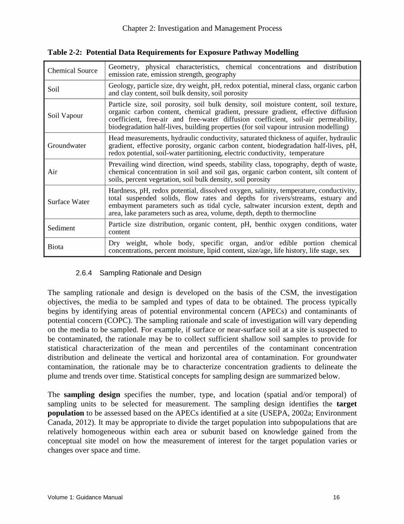
The different types of data that may be needed for risk assessment, in addition to chemical concentrations in each media, are summarized in Table 2-2. Several different types of data may be needed for site characterization purposes including:
• Chemical concentration data, which may be on a mass per unit weight or volume basis;
• Contaminant mass flux data (i.e., mass per unit area per time), which is the rate at which contaminants migrate within a unit area; and,
• Physical properties, which may include, but are not limited to hydraulic conductivity, permeability, moisture content and grain size.
• Leachability of contaminants.
There is a broad range of site investigation tools available to the site assessor. The site characterization planning process will often include an assessment of whether non- or less-intrusive field methods are warranted as part of a field investigation program. A geophysical survey can be a useful tool for inference of different geological structures and units and buried structures (i.e., utilities, tanks, drums), and is often performed prior to the intrusive component of the investigation to help identify proposed sample locations and potential safety hazards. An emerging use of environmental geophysics is the use of surface geophysics to identify possible contamination zones. The use of specific environmental applications involving downhole sensors (i.e., in conjunction with direct push technologies) are described in Chapter 6. A soil vapour survey is a less invasive method that can also be used to infer areas of contamination and optimize subsequent stages of the investigation. Approaches and methods for conducting soil vapour surveys are described in detail in Chapter 7. The intrusive methods selected will depend on investigation objectives, sampling media and data needs, and site specific conditions.
Chapter 2: Investigation and Management Process
Volume 1: Guidance Manual 16
Table 2-2: Potential Data Requirements for Exposure Pathway Modelling
Chemical Source Geometry, physical characteristics, chemical concentrations and distribution emission rate, emission strength, geography
Soil Geology, particle size, dry weight, pH, redox potential, mineral class, organic carbon and clay content, soil bulk density, soil porosity
Soil Vapour Particle size, soil porosity, soil bulk density, soil moisture content, soil texture, organic carbon content, chemical gradient, pressure gradient, effective diffusion coefficient, free-air and free-water diffusion coefficient, soil-air permeability, biodegradation half-lives, building properties (for soil vapour intrusion modelling)
Groundwater Head measurements, hydraulic conductivity, saturated thickness of aquifer, hydraulic gradient, effective porosity, organic carbon content, biodegradation half-lives, pH, redox potential, soil-water partitioning, electric conductivity, temperature
Air Prevailing wind direction, wind speeds, stability class, topography, depth of waste, chemical concentration in soil and soil gas, organic carbon content, silt content of soils, percent vegetation, soil bulk density, soil porosity
Surface Water Hardness, pH, redox potential, dissolved oxygen, salinity, temperature, conductivity, total suspended solids, flow rates and depths for rivers/streams, estuary and embayment parameters such as tidal cycle, saltwater incursion extent, depth and area, lake parameters such as area, volume, depth, depth to thermocline
Sediment Particle size distribution, organic content, pH, benthic oxygen conditions, water content
Biota Dry weight, whole body, specific organ, and/or edible portion chemical concentrations, percent moisture, lipid content, size/age, life history, life stage, sex
2.6.4 Sampling Rationale and Design
The sampling rationale and design is developed on the basis of the CSM, the investigation objectives, the media to be sampled and types of data to be obtained. The process typically begins by identifying areas of potential environmental concern (APECs) and contaminants of potential concern (COPC). The sampling rationale and scale of investigation will vary depending on the media to be sampled. For example, if surface or near-surface soil at a site is suspected to be contaminated, the rationale may be to collect sufficient shallow soil samples to provide for statistical characterization of the mean and percentiles of the contaminant concentration distribution and delineate the vertical and horizontal area of contamination. For groundwater contamination, the rationale may be to characterize concentration gradients to delineate the plume and trends over time. Statistical concepts for sampling design are summarized below.
The sampling design specifies the number, type, and location (spatial and/or temporal) of sampling units to be selected for measurement. The sampling design identifies the target population to be assessed based on the APECs identified at a site (USEPA, 2002a; Environment Canada, 2012). It may be appropriate to divide the target population into subpopulations that are relatively homogeneous within each area or subunit based on knowledge gained from the conceptual site model on how the measurement of interest for the target population varies or changes over space and time.

Chapter 2: Investigation and Management Process
Volume 1: Guidance Manual 17
The sampled population is that part of the target population that is accessible and available for sampling. For example, the target population may be defined as a soil layer, and the sampled population may be the portion of the site not covered by a building. If there are differences between the target and sampled population, the site assessor must determine whether such differences will significantly affect the conclusions drawn from the data.
A sampling unit for continuous media such as soil, groundwater, soil vapour and air is defined as some area, volume, or mass that may be selected from the target population. For soil it could represent all individual 0.3 m long core samples collected from a particular soil unit; for indoor air it could represent a 6-litre composite sample collected from an individual room.
The spatial and temporal constraints and boundaries are important considerations for development of the sampling plan. The spatial boundaries for the target population applicable to decision-making and estimation should be unambiguously defined using spatial data (e.g., latitude, longitude, elevation) or physical reference points (e.g., property boundary, fence line, and stream). In some cases it may be appropriate to define a specific subunit (e.g., soil or stratigraphic unit) as the spatial boundary for the sampling plan.
The time unit that data will represent should also be defined. Conditions may vary over time due to weather patterns, fluctuations in the water table or operation or activity patterns (e.g., indoor air). The timescales for weather related variation can range from hourly to seasonal changes in conditions. The site assessor should determine when and over which period conditions are favourable for collection of representative samples. For example, if based on the conceptual site model the groundwater concentrations are expected to vary seasonally, it may be appropriate to obtain samples on a quarterly or twice yearly basis. Similarly, if diel fluctuations of indoor air concentrations are expected, 24-hour composite samples may be appropriate. The rationale for the time unit should be documented in the report.
Specific objectives of the risk assessment should be incorporated into the sampling design where applicable. For example, if the objective is to assess potential risk through direct exposure to soil contaminants (i.e., ingestion, dermal absorption, inhalation of suspended particular matter), it may be appropriate to define a "surface" soil layer of specified thickness as the unit of interest. The precise definition of surface soil will vary from site to site, depending on actual land use, regulatory definitions, and the risk assessment assumptions, and may be represented by depths ranging from ≤5 cm to 1.5 m. CCME (2006) defines surface soil as the interval from “grade” to 1.5 m below grade. The CCME (2006) definition should generally be used as a starting point to define surface versus subsurface soils, but this definition may be adjusted when supported through shallow soil testing data and on a site-specific basis. For human health risk assessment, the surface layer of soil that will contribute to the majority of incidental exposures will typically be ≤5 cm, provided that the soils are not subject to gardening, tilling, excavation, etc. For typical residential land use, people may dig > 5 cm for gardens, etc. Therefore, the depth of the surface “layer” identified for the subject site must be clearly defined, and the site characterization data must relate clearly to the definition of surface soil. It must be noted that this does not imply that 5 cm of clean soil is considered an adequate surface cover layer for purposes of risk management.

Chapter 2: Investigation and Management Process
Volume 1: Guidance Manual 18
The sampling rationale and design should also consider the particle size range of soil as a factor to control in sampling (Health Canada, 2010). The grain size fraction on which the chemical analysis is conducted depends on the objectives of the risk assessment and will affect:
• Contaminant distribution within soil; and
• Bioavailability (through dermal, oral, and inhalation pathways).
For input into the development of a sampling strategy and design, it is important to recognize the broad differences in spatial and temporal variability between different media, as reflected in Table 2-3.
There are several different types of sampling designs (e.g., random, stratified, grid sampling) that can be used in the evaluation of sites. Some of these designs are based on statistical constructs. Different sampling designs are described in detail in the chapter on soil characterization (Chapter 5).
Table 2-3: Spatial and Temporal Variability Between Different Media
Media Temporal Variability Spatial Variability
Soil Negligible High
Groundwater Low to Moderate May depend on flow rate and
tidal influences
Low to Moderate Groundwater plumes tend to disperse, although there may be steep concentration gradients at
plume boundaries
Soil Vapour Moderate Increases closer to ground
surface and buildings
Moderate to High Especially when there is geologic variability
and/or bioattenuation
Surface Water Moderate to High Depends on type of surface water, stratification, mixing
Sediment Moderate, with rapid changes following sediment
disturbance
Moderate to high Variability in grain size and organic carbon
content influence spatial distribution
Biota Moderate, depending on life history and life stage of
species investigated
Moderate, depending on mobility of species investigated
2.6.5 Sampling and Analysis Methods and Quality Assurance Project Plan
Sampling and analysis methods and procedures for quality assurance are to varying degrees media specific. The purpose of this section is to provide an overview of common elements and concepts that should be considered when developing a quality assurance project plan. More detailed guidance on quality assurance and quality control measures are provided in Chapter 3 while media specific sampling guidance is provided in Chapters 5 through 11.

Chapter 2: Investigation and Management Process
Volume 1: Guidance Manual 19
Quality assurance is an integrated system of management activities involving planning, quality control, quality assessment, and implementation of quality improvement to ensure that project requirements and expectations of data users are met. Quality control comprises technical measures to assess the effect of errors or variability in sampling and analysis. It may also include specification of
acceptance criteria for the data and corrective actions to be taken when they are exceeded.
While data quality is influenced by the entire site characterization process, a quality assurance project plan typically focuses on certification and training requirements, sampling methods, analytical protocols, quality control checks and data management procedures (USEPA, 2002b). It is important to recognize that there are many sources or reasons for there to be variability in data ranging from heterogeneity in the concentrations (or property) being measured, methods for sampling, storage and handling, laboratory handling and preparation of samples, and laboratory analysis. While analyses of quality control samples are valuable for evaluation of precision and accuracy, uncertainty is increased when there is significant small-scale variability within samples. It is important to recognize that only a very small mass of sample (usually 1 to 10 grams dependant on the test) is typically analyzed.
A key concept is that data quality and acceptance criteria are often expressed in terms of data quality indicators (DQI). The familiar PARCC parameters represent the five principal DQIs, which are Precision, Accuracy (used in this context to denote bias), Representativeness, Comparability, and Completeness. The ability of the analytical method to detect the analytes of interest at the required concentration (e.g., detection limits) may also be included as a principal DQI. The components of a quality assurance project plan, definition of DQI indictors, data quality targets and quality control checks and procedures are described in greater detail in Chapter 3.
Conduct the Field Investigation Program – Conventional Phased Approach and 2.7Expedited Site Assessment Process
Field investigation programs are often phased over time by first defining minimal, targeted information needs using the CSM, acquiring new data, updating the CSM, and then re-defining new information needs, where necessary, to satisfy the investigation objectives. Several phases of investigation may be necessary before the investigation objectives are finally satisfied. While the intent of phasing may be to avoid unnecessary drilling and sampling, the approach can lead to lengthy delays in the characterization process that ultimately may result in increased expenditures.
Over the past decade, new paradigms have been introduced to expedite or streamline the site characterization process and to provide data that are more effective for decision-making purposes relative to conventional site investigation methods. This new approach is often referred to as expedited site assessments or the Triad Approach (http://www.triadcentral.org/tech/) to site
Quality Assurance / Quality Control
Quality assurance / quality control is a key part of the site characterization process. Quality assurance is a system of management activities to ensure project requirements are met while quality control is technical measures to assess quality aspects.

Chapter 2: Investigation and Management Process
Volume 1: Guidance Manual 20
characterization, which involves integration of three key elements – systematic planning, dynamic work strategies, and real-time measurement technologies (Crumbling, 2004; ITRC, 2003; USEPA, 2003a,b).
The conventional approach to investigation typically involves the use of standard investigation tools (e.g., boreholes, monitoring wells) and collection of media samples for analysis by a fixed laboratory. An expedited site investigation or Triad Approach use field analytical methods to more rapidly collect data and increase the amount of useful information collected, and lower the overall cost of data collection and site characterization. Through the use of dynamic work plans and near real-time or real-time data collection and flexible contingency-based decision-making, there may be an opportunity to obtain better data in a more efficient manner that will more thoroughly describe site conditions.
The three principle components of the Triad Approach are summarized below:
• Systematic Planning. The systematic planning process is critical to the success of an expedited field investigation program. It involves the development of a CSM, a good understanding of the goals and objectives of the investigation, identification of roles and responsibilities of team members and development of a framework to support on-site decision-making, and identification of data quality requirements. While planning is important for any investigation, for expedited site assessments it is particularly important since field investigations will tend to evolve rapidly as they progress.
• Dynamic Work Strategies. The flexibility to change or adapt to information generated by real-time measurement technologies is key to dynamic work plans. The important decision points and logic should be identified together with contingent actions that may be required as the site investigation proceeds. Defined communication strategies are important for dynamic work strategies. Adequate resources should be allocated to data handling and interpretation to enable appropriate decisions to be made.
• Real-Time Measurement Technologies. Over the past decade there have been significant advancements in data collection technologies and measurement systems. A range of field analytical methods have been developed from rapid screening methods to on-site laboratories that provide nearly all the capabilities of a fixed laboratory, thus providing near real-time concentrations. The use of Global Positioning Systems provides for reasonably accurate determination of spatial locations. Through direct push technologies, there is the ability to rapidly collect multiple samples and provide concentration profiles. There is also an array of sensors that can be deployed with direct push technologies to help detect and delineate contamination zones. These new technological advances are important to the implementation of the Triad approach, and are discussed in subsequent chapters of this guidance.
A key concept is that the Triad Approach emphasizes managing decision uncertainty, rather than simply analytical uncertainty. For example, the Triad Approach recognizes that it may be more useful to obtain larger quantities of less precise data to characterize site conditions compared to a smaller quantity of more analytically precise data.

Chapter 2: Investigation and Management Process
Volume 1: Guidance Manual 21
There are several requirements for successful implementation of a Triad Approach. There should be concurrence from regulators and stakeholders on data collection methods. It makes little sense to embark on a field investigation where data obtained will not meet minimum requirements. Likewise, there should be adequate quality control and assurance measures in-place. The team conducting the work should be sufficiently experienced to make appropriate field decisions. There should be flexible contract provisions to facilitate the work.
Validate and Interpret Data 2.8
The sixth step of the site characterization process is the validation and interpretation of data. The data validation step involves review of whether the general objectives of the site investigation have been met, whether the quality assurance and quality control (QA/QC) results are within acceptable limits, and other checks to verify data and completeness. The PARCC parameters (Precision, Accuracy, Representativeness, Comparability, and Completeness) should be evaluated to determine whether performance and acceptance criteria have been met. A checklist for data validation is provided below:
Are the data complete and based on the sampling and analysis plan?
Is the documentation complete including field data records, test pit, borehole and monitoring well logs, analytical laboratory reports, and all other supporting documentation?
Have all test holes and sampling locations been clearly indicated on scaled drawings?
Have the QA/QC data been reviewed and are they within acceptable limits? Are re-tests or verification tests required? Can the data be relied upon?
Have apparent outliers been evaluated and addressed?
Has the data been checked for possible transcription and manipulation errors?
Have all APECs been adequately assessed for all COPCs?
Have the investigation objectives been met, including all data required for risk assessment purposes?
Has available previous work that can be reliably used been synthesized in the data interpretation?
Have the sampling design objectives been met? Based on the updated conceptual site model, has sufficient sampling been completed at the site based on the study boundaries and APECs and populations identified?
Do the results make sense relative to the conceptual site model and hypothesis for site contamination?
Have the correct criteria or standards been used for all relevant media?
Has off-site migration of contamination been identified?
Is further assessment required to delineate the horizontal and/or vertical extent of contamination at a site?

Chapter 2: Investigation and Management Process
Volume 1: Guidance Manual 22
The data interpretation will be specific to the type and quantity of data collected, the media being sampled and other project-specific considerations. Broadly applicable guidance and principles for data interpretation are provided below while additional considerations pertinent to the media under assessment (soil, groundwater, soil vapour, surface water, sediment, and biota) are addressed in the subsequent chapters.
Exploratory data analysis should be completed through techniques that provide information on trends, correlations and other patterns. Several exploratory data views are listed below:
• Data posting to show concentration patterns in plan view and cross section; • Frequency tables; • Histograms; • Cumulative frequency plots; • Correlation plots; and, • Contouring.
If the site is likely to proceed to human health risk assessment (HHRA) or Ecological Risk Assessment (ERA), summary statistics should be calculated to describe each data set (e.g., number of samples, minimum, maximum, arithmetic mean, standard deviation, coefficient of variation, percentiles of the distribution). For this purpose, the data must be grouped into logical groupings that reflect study boundaries, the CSM, and areas of potential concern. To the extent possible, the data should represent a single population, although in some cases, statistical analyses may be needed to determine appropriate groupings of data and possible outliers.
Summary statistics can be used in describing a set of observations (set of samples collected and corresponding concentration data). For further statistical analysis and to draw conclusions about the population from which the data set is collected, inferential statistics can be used. Inferential statistics involves a set of assumptions to model the underlying population from which the samples are collected and analysed. For example, environmental data sets are often skewed and follow an approximate log-normal distribution. Data sets should be carefully evaluated as to their underlying distribution since the use of conventional statistical parameters such as the arithmetic mean and standard deviation based on the assumption of a normal distribution may result in biased estimates (Gilbert, 1987). Inferential statistics can be divided into parametric and non-parametric statistics depending on the degree of model assumptions and number of parameters used to describe the model. In parametric statistics, a finite number of parameters are used to describe an underlying distribution to which the data is assumed to belong (e.g. normal distribution described by two parameters: mean and variance). On the other hand, there are cases where the data cannot reasonably or easily be described by parametric statistics. In such cases, it is better to describe such data using non-parametric statistics. In non-parametric statistics, no assumptions are made about the data belonging to a particular distribution. Further guidance on statistical evaluation of soil data is provided in Chapter 5. Although high concentration values may appear to be anomalous, great care must be taken when considering whether to remove apparent outliers from a data set; such data may represent hot-spots that comprise a separate population. Outliers should not be discarded without a thorough and documented examination and understanding of the circumstances that created them.

Chapter 2: Investigation and Management Process
Volume 1: Guidance Manual 23
Resources and Weblinks 2.9
U.S. Environmental Protection Agency: The USEPA has extensive resources available on their Hazardous Waste Clean-up Information (CLU-IN) website. General publications and training course on site assessment and remediation can be found at http://www.clu-in.org/courses/. The USEPA Technology Innovation program has a website specific to characterization and monitoring technologies http://cluin.org/char1_edu.cfm and a monthly newsletter (subscribe at http://www.epa.gov/tio/techdrct/). Information on the USEPA Superfund program and links to an extensive document library can be found at http://www.epa.gov/superfund/about.htm. Guidance specific to investigation and clean-up of Brownfield’s sites can be found at http://www.epa.gov/swerosps/bf/.
Conceptual Site Models: An example of a complete CSM including diagrams prepared for soil screening purposes can be found in Attachment A of the Soil Screening Guidance: User’s Guide (USEPA, 1996). http://www.epa.gov/superfund/health/conmedia/soil/pdfs/attacha.pdf
Conceptual Exposure Models: A software application, the “Site Conceptual Exposure Model Builder” that can generate conceptual exposure model (CEM) diagrams, but that also helps understand site data and fate and transport mechanisms has been developed by the U.S. Department of Energy.
References 2.10
American Society for Testing and Materials Standards (ASTM) E1527-13 (2013). Standard Practice for Environmental Site Assessments: Phase 1 Environmental Site Assessment Process. ASTM International, 47 pages.
American Society for Testing and Materials Standards (ASTM) E1903-11 (2011) Standard Guide for Environmental Site Assessments: Phase II Environmental Site Assessment Process, ASTM International, 21 pages.
Canadian Council of Ministers of the Environment (CCME), 2006. A Protocol for the Derivation of Environmental and Human Health Soil Quality Guidelines. PN 1332.
CAN/CSA-Z768-01. 2012. Phase 1 Environmental Site Assessment. Canadian Standards Association. Toronto, Ontario.
CAN/CSA-Z769-00. 2013. Phase II Environmental Site Assessment. Canadian Standards Association. Toronto, Ontario.
Crumbling, D.M. 2004. The Triad Approach to Managing the Uncertainty in Environmental Data. White paper prepared for United States Environmental Protection Agency. March 25.
Environment Canada. 2012. Guidance Document on the Sampling and Preparation of Contaminated Soil for Use in Biological Testing. EPS 1/RM/53. Science and Technology Branch.
Gilbert, R.O. 1987. Statistical Methods for Environmental Pollution Monitoring. Van Nostrand Reinhold Company, New York, NY. 320 pp.
Health Canada. 2010. Federal Contaminated Site Risk Assessment in Canada Part V: Guidance on Complex Human Health Detailed Quantitative Risk Assessment for Chemicals (DQRACHEM). Contaminated Sites Division, Safe Environments Directorate, Health Canada, Ottawa.
Hers, I., and R. Zapf-Gilje. 1991. The Use of Statistics for Interpretation of Soil Contamination at the Former Expo '86 Site. Preprints, 44th Canadian Geotechnical Conference, Calgary.

Chapter 2: Investigation and Management Process
Volume 1: Guidance Manual 24
Interstate Technology & Regulatory Council (ITRC). 2003. Technical and Regulatory Guidance for the Triad Approach: A New Paradigm for Environmental Project Management, Prepared by Sampling, Characterization and Monitoring Team, December.
Starks, T. H. 1986. Determination of Support in Soil Sampling. Mathematical Geology, Vol. 18, No. 6, pp. 529-537.
U.S. Environmental Protection Agency. 1996. Soil Screening Guidance: User’s Guide. United States Office of Solid Waste and Publication 9355.4-23. Washington, DC, July.
U.S. Environmental Protection Agency. 2002a. Guidance on Choosing a Sampling Design for Environmental Data Collection for Use in Developing a Quality Assurance Project Plan. Washington, DC 20460. Report EPA QA/G-5S, December.
U.S. Environmental Protection Agency. 2002b. Guidance for Quality Assurance Project Plans. Washington, DC, Report EPA/240/R-02/009, December.
U.S. Environmental Protection Agency. 2003a. Using Dynamic Field Activities for On-Site Decision Making: A Guide for Project Managers. Office of Solid Waste and Emergency Response U.S. Environmental Protection Agency Washington, DC 20460, OSWER Report No. 9200.1-40 EPA/540/R-03/002, May.
U.S. Environmental Protection Agency. 2003b. Using the Triad Approach to Streamline Brownfield’s Site Assessment and Cleanup – Brownfield’s Technology Primer Series. Office of Solid Waste and Emergency Response Brownfield’s Technology Support Center Washington, DC 20460, June.
U.S. Environmental Protection Agency. 2006. Guidance on Systematic Planning Using the Data Quality Objectives Process EPA QA/G-4. Office of Environmental Information Washington, DC 20460, Report EPA/240/B-06/001, February.

Chapter 3: QA / QC
Volume 1: Guidance Manual 25
3 QUALITY ASSURANCE/QUALITY CONTROL
The goal of representative sampling is to collect samples which will yield results that accurately characterize site conditions. The goal of quality assurance and quality control (QA/QC) is to limit errors and bias in sampling and analysis through integrated implementation of management, assessment and control measures, thus facilitating generation of data that are useful for their intended purpose. This section begins with a description of the quality assurance project plan components, which is an important planning phase that helps ensure acceptable data quality. Next, data quality indicators and targets are discussed, followed by specific data quality control checks and procedures.
Quality Assurance Project Plan 3.1
The quality assurance project plan (QAPP) is an integral part of a sampling and analysis plan. The QAPP identifies all aspects of the site characterization program that may influence data quality. The components of a QAPP are summarized in Table 3-1. Many aspects of the QAPP are media and method specific and relevant protocols should be consulted for details (USEPA, 2002).
The QAPP should include consideration of laboratory accreditation and analytical protocols. Laboratories should be accredited to the international standard "ANS/ISO/IEC 17025 General Requirements for the Competence of Testing and Calibration Laboratories". An accredited laboratory will have a "scope of accreditation" that lists the matrix, method and parameters for which a laboratory has been accredited (many laboratories also conduct analyses that are not on their scope of accreditation meaning they are not accredited for those tests). There are three recognized agencies in Canada granting accreditation to environmental testing laboratories: (i) the Canadian Association for Laboratory Accreditation Inc. (CALA: in June 2008 Canadian Association for Environmental Analytical Laboratories [CAEAL] changed its name to CALA), (ii) Standards Council of Canada (SCC), and (iii) the MDDELCC (in Québec). Standardised methods are typically used for analysis of many chemical parameters. A comprehensive list of references is included in Volume 4.
There are also mandated protocols for certain compounds under certain programs (e.g., the F1 to F4 fractions as defined in the Canada Wide Standards for Petroleum Hydrocarbons in Soil (CCME, 2008)) and within each Province or Territory, there are varying requirements for sampling and analysis that should be followed, as applicable.

Chapter 3: QA / QC
Volume 1: Guidance Manual 26
Table 3-1: Components of a Quality Assurance Project Plan
Certification and Training • Required certifications for analytical laboratory • Required certifications and specialized training required by field staff (e.g., health safety, equipment
operation, sampling methods) Sampling Methods • Sampling plan • Sampling methodology and equipment • Equipment decontamination procedures Field Equipment • Instrument type and model specification • Calibration requirements and documentation • Instrument inspection and maintenance requirements • Operator training required • Calibration and inspection Sample Handling, Custody and Analysis • Analytical protocol • Sample containers • Field preservation • Holding times • Sample 0storage requirements (e.g., packing, type, temperature) • Chain-of-custody, use consistent labeling and nomenclature on chain-of-custody and sample
containers • Data quality targets (e.g., detection limits, precision, accuracy) • Field quality control samples (e.g., duplicates, trip blanks, field blanks) • Laboratory quality control samples (e.g., duplicates, method blanks, surrogate and matrix spikes,
standard or certified reference materials) • Frequency of quality control samples tested • Other performance assessment measures (e.g., audits, inter-laboratory testing) • Analytical testing turn-around time Documentation and Record Keeping • Identification of field computer hardware and software • Field documentation requirements (e.g., list logs, forms, photographic records) • Procedures for storage and archiving field data • Procedures for data transfer from the analytical laboratory • Applicable procedures for data security Data Validation • Checking for transcription and manipulation errors • Review of PARCC parameters • Review of data quality indicators relative to data quality targets and acceptance criteria for analytical
methods

Chapter 3: QA / QC
Volume 1: Guidance Manual 27
Data Quality Indicators 3.2
Performance and acceptance criteria for data are often expressed in terms of data quality indicators (DQI) (Table 3-2). The familiar PARCC parameters are considered to consist of five principal DQIs that are precision, accuracy (used in this context to denote bias), representativeness, comparability, and completeness. Selectivity may also be included as a principal DQI. Selectivity describes what analytes the technique can quantitate and discriminate from other target analytes or from similar-behaving, but non-target, substances. Mass spectrometric methods would generally provide for greater selectivity in unequivocal identification of a compound compared to flame ionization and other non specific detectors. Selectivity may be important when using screening tests such as immunoassay tests for environmental contaminants where test kit reagents frequently cross-react with structurally similar compounds and therefore provide for results that may be biased high.
Table 3-2: Description of Primary Data Quality Indicators
DQI Definition and Quantification Methods
Precision The measure of agreement between repeated measurements of the same parameter measured under identical or similar conditions. Quantified as the relative percent difference (RPD): RPD (%) = (C1-C2) / [ (C1+C2)/2 ] * 100
Repeated analyses on the same sample by the laboratory: Measures sample preparation and analytical method variability. Split a sample in the field and analyze both samples: Measures sampling splitting, handling procedures and laboratory-derived variability. Collect co-located samples and analyze both samples: Measures local scale variability, sample acquisition, handling and laboratory variability.
Bias The degree to which there is a systematic error in one direction from a true value. %Bias = %Recovery – 100 %Bias = ( C – Cstandard ) / Cstandard
Use reference materials or analyze spiked matrix samples.
Accuracy The overall agreement of a measurement to a known value; includes random error (precision) and systematic error (bias).
Analyze a reference material or re-analyze a sample to which a material of known concentration has been added; usually expressed either as percent recovery or as a percent bias.
Represen-tativeness
The degree to which data represent the population under investigation with respect to the decision to be made.
Evaluate whether samples collected and measurements made appropriately reflect the characteristic being measured or studied.
Comparability Describes whether different data sets can be considered equivalent based on a common goal.
Compare sample collection and handling, analytical protocols, detection limits, and QC results (e.g., recovery, comparison to certified reference materials) for different data sets.
Completeness Describes the degree to which valid data are Compare number of valid measurements

Chapter 3: QA / QC
Volume 1: Guidance Manual 28
DQI Definition and Quantification Methods generated. (samples collected or samples analyzed)
with project specific quality objectives. Sensitivity Describes the lowest concentration, or
increment of concentration, that the technique is able to detect or quantitate with a certain level of confidence.
Determine the minimum concentration or attribute that can be measured by a method (method detection limit) or by a laboratory (quantitation limit).
Quality Control 3.3
Quality control comprises technical activities that are used to measure or assess the effect of errors or variability in sampling and analysis. It may also include specification of acceptance criteria for the data and corrective actions to be taken when they are exceeded. Quality control includes checks performed to evaluate laboratory analytical quality, checks designed to assess the combined influence of field sampling and laboratory analysis, and checks to specifically evaluate the potential for cross contamination during sampling and sample handling.
3.3.1 Quality Control Checks and Samples
The main laboratory quality control activities and check samples are as follows:
• Calibration of instruments; tuning of mass spectrometers.
• Method blanks, where a clean sample is processed simultaneously with and under the same conditions (i.e., using the same reagents and solvents) as the samples being analyzed; used to confirm whether the instrument, reagents and solvents used are contaminant free.
• Laboratory duplicates, where two samples obtained from the sample container are analyzed; used to evaluate laboratory precision.
• Surrogate spike samples, where a known mass of compound not found in nature (e.g., deuterated compounds such as toluene-d8) but that has similar characteristics to the analyzed compounds is added to a sample at a known concentration; used to assess the recovery efficiency.
• Matrix spike samples, where a known mass of target analyte is added to a matrix sample with known concentrations; used to evaluate the influence of the matrix on a method’s recovery efficiency.
• Standard or certified reference materials, a reference material where the content or concentration has been established to a very high level of certainty (usually by a national regulatory agency); used to assess accuracy.
The main field quality control checks are as follows:

Chapter 3: QA / QC
Volume 1: Guidance Manual 29
• Field duplicates, where split samples or co-located samples obtained in the field using the same sampling procedure are submitted to the laboratory “blind”; used to assess sampling and analysis precision.
• Trip blanks, where a clean sample of the matrix being analyzed is transported to and from the site unopened using the same container as the samples analyzed; used to assess whether cross-contamination occurred during sample transport and storage.
• Equipment blanks, prepared in the field, where for example, contaminant-free water (distilled-deionized) or air is passed through a sampling device (e.g., pump and tubing); used to assess equipment decontamination procedures.
• Field blanks, which can consist of a clean sample (e.g., distilled-deionized water) where the sample container is exposed to sampling conditions (i.e., cap removed) or where an ambient air sample is obtained; used to check for artifacts introduced by background conditions.
Field control checks should be completed early in the site investigation process so that adjustments can be made, when warranted.
3.3.2 Recommended Minimum Frequency of Quality Control Samples
The recommended minimum frequency for testing of laboratory duplicate samples is 1 in 20 samples and 1 in 10 samples for field duplicates; for smaller programs where less than twenty, or ten, samples are analyzed, consideration should nevertheless be given to analysis of a duplicate sample. The samples submitted for duplicate analysis should have sufficiently high levels of contamination (if possible) so that there is the ability to evaluate precision. For other quality control samples, it is recommended that one check sample be analysed per batch (up to 20 samples per batch).
Data Quality Targets 3.4
The previous sections described the data quality indicators used to evaluate precision and accuracy and the specific quality control checks that are performed to evaluate data quality. As part of the quality assurance project plan, it is also important to establish data quality targets or to recognize method precision and accuracy that can be achieved based on the analytical method and matrix being tested.
Target acceptance criteria for all QC samples (method blanks, lab control samples, matrix spikes, duplicates, surrogates (organic tests)) for all analytical methods used in support of the Canadian Environmental Quality Guidelines (CEQG) are found in Section 5 of Volume 4.
Typically, laboratories adopt or establish their own acceptance criteria that are to varying degrees based on performance requirements in the applicable analytical protocols (e.g., USEPA SW-846). As a general rule, the allowable tolerances for soil are greater than for groundwater due to variability introduced by the matrix. Similarly, for semi-volatiles, the ranges for acceptable recoveries are slightly higher than for volatiles.

Chapter 3: QA / QC
Volume 1: Guidance Manual 30
The data quality targets should be compared to analytical method performance specifications. The laboratory reporting limit (LRL) is a basic data quality requirement, and ideally the target is set at a minimum of 5X to 10X less than the regulatory criteria. An example data quality target for a project might read as follows: “The measurement method selected for the project must be able to detect the presence of compounds X, Y, and Z in groundwater at a quantitation limit of 1 ug/L with a recovery range (relative to certified reference materials) of 70 to 130 percent and a precision, as quantified by the RPD, of less than 20 percent”.
3.4.1 Duplicate Samples
Sampling programs should include both analyses of laboratory and field duplicate samples. The acceptance criteria will depend on the analytical protocol and media, but guidelines are provided below for common analytes (extractable hydrocarbons, metals, and volatile and semi-volatile organic chemicals).
For laboratory duplicates of groundwater, typical RPDs for inorganic parameters are less than 20 percent. For soil there is greater matrix variability; therefore, somewhat higher acceptable RPDs on the order of 30 percent are reasonable.
For field duplicates, there is added variability introduced by matrix variability and sampling and handling procedures. Quantifying acceptable precision is a matter of judgement, but assuming the field and laboratory error are similar in magnitude, acceptance criteria twice those given above would result (i.e., RPD of 40 percent for groundwater and 60 percent for soil). Note that since organics tests are “whole bottle” analysis, all duplicates for organic tests are of necessity field duplicates.
Near to the detection limit, acceptance criteria are relaxed, for example, within 5X of the LRL, a criterion that may be used is that the difference between the duplicate concentrations should be less than 2X the LRL. When the acceptance criteria are exceeded, the sampling procedures should be reviewed and the soil or groundwater matrix examined. The importance of reduced precision becomes more important when concentrations straddle or are near regulatory guidelines.
Detection Limits
While there are many different definitions for detection limits, the primary definitions that may be relevant to practitioners are:
Method detection limit (MDL): The minimum concentration of an analyte that can be measured and reported with 99% confidence to be greater than zero for a given matrix and specific method.
Limit of Quantification (LOQ): The lowest concentration of an analyte that can be reliably measured within specified limits of precision and accuracy during routine operating conditions, as opposed to being detected (USEPA, 2002; Gibbons and Coleman, 2001).
Practical Quantification Limit (PQL): May be similarly defined as the LOQ, the reporting limits in the method, or otherwise defined.
Laboratory reporting limit (LRL): The lowest concentration of an analyte reported within a reasonable degree of accuracy and precision, ideally synonymous with the LOQ or PQL. The LRL is typically 3-10 times the MDL (some Guidelines are so low that the LRL is equal to the MDL in order to report to the guideline).
The uncertainty in concentrations increases near to the detection limit. Some laboratories may also report concentrations detected below the LRL (“J-flagged” results); however, these concentrations should be considered an estimate. Detection limits may be raised due to the matrix effects or sample dilution.
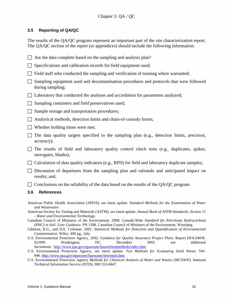
Chapter 3: QA / QC
Volume 1: Guidance Manual 31
Reporting of QA/QC 3.5
The results of the QA/QC program represent an important part of the site characterization report. The QA/QC section of the report (or appendices) should include the following information:
Are the data complete based on the sampling and analysis plan?
Specifications and calibration records for field equipment used;
Field staff who conducted the sampling and verification of training where warranted;
Sampling equipment used and decontamination procedures and protocols that were followed during sampling;
Laboratory that conducted the analyses and accredation for parameters analyzed;
Sampling containers and field preservatives used;
Sample storage and transportation procedures;
Analytical methods, detection limits and chain-of-custody forms;
Whether holding times were met;
The data quality targets specified in the sampling plan (e.g., detection limits, precision, accuracy);
The results of field and laboratory quality control check tests (e.g., duplicates, spikes, surrogates, blanks);
Calculation of data quality indicators (e.g., RPD) for field and laboratory duplicate samples;
Discussion of departures from the sampling plan and rationale and anticipated impact on results; and,
Conclusions on the reliability of the data based on the results of the QA/QC program.
References 3.6
American Public Health Association (APHA), see latest update. Standard Methods for the Examination of Water and Wastewater.
American Society for Testing and Materials (ASTM), see latest update. Annual Book of ASTM Standards, Section 11 - Water and Environmental Technology.
Canadian Council of Ministers of the Environment. 2008. Canada-Wide Standard for Petroleum Hydrocarbons (PHC) in Soil: User Guidance. PN 1398. Canadian Council of Ministers of the Environment, Winnipeg.
Gibbons, R.G., and D.E. Coleman. 2001. Statistical Methods for Detection and Quantification of Environmental Contamination. Wiley, 400 pg., July.
U.S. Environmental Protection Agency. 2002. Guidance for Quality Assurance Project Plans. Report EPA/240/R-02/009. Washington, DC, December 2002. see additional documents: http://www.epa.gov/epawaste/hazard/testmethods/index.htm
U.S. Environmental Protection Agency, see latest update. Test Methods for Evaluating Solid Waste; SW-846. http://www.epa.gov/epaoswer/hazwaste/test/main.htm
U.S. Environmental Protection Agency Methods for Chemical Analysis of Water and Wastes (MCAWW). National Technical Information Service (NTIS), 800 553-6847.

Chapter 4: Site Model for Contaminated Sites
Volume 1: Guidance Manual 32
Definition of Conceptual Site Model
A conceptual site model or CSM is a visual represent-ation and written description of the relationships between the physical, chemical, and biological processes of the site and the human and environmental receptors.
4 CONCEPTUAL SITE MODEL FOR CONTAMINATED SITES
As described in Chapter 2, a conceptual site model (CSM) provides a narrative and/or graphical representation of the contamination sources and physical, chemical, and biological processes occurring, or that have occurred, at a contaminated site. Development of a site-specific CSM is a critical first step in the process of characterizing the nature and extent of COPCs present at a study area. The CSM serves many purposes. It allows visualization and compartmentalization of study area-related COPCs. It facilitates understanding of potential routes of exposure and the fate and transport processes that may alter the form and location of a COPC in the environment, and it serves as a guide to the design of the sampling program. The CSM also forms the basis for understanding which COPCs may be present on-site, and provides ready visualization of important fate and transport mechanisms. Finally, the CSM provides project personnel and decision makers with a tool to understand and communicate potential exposures.
Both Table 2-1 and Volume 2 of this guidance list general elements to consider when developing a site-specific CSM. As discussed above, a CSM should, at a minimum, consider: 1) the migration and exposure pathways of the site; 2) the physical processes of the site; 3) the chemical properties of the potentially affected media; 4) the attributes and behaviours of the ecological receptors (e.g., preferred habitat, foraging behaviour, dietary preferences); and 5) the presence and behaviour of human receptors (e.g., fishing and consumption practices, accessibility for children, presence of workers) (see Chapter 9). It is important to recognize that CSMs are dynamic (USEPA, 1996; 2002) and subject to change as additional study area information is obtained.
The purpose of this chapter is to describe important factors to consider in developing a CSM prior to the site investigation. This chapter is divided into the following parts: (1) a discussion of the sources and types of chemicals that may be found at contaminated sites, and (2) the development of CSM for the following contaminated media: groundwater, soil, soil vapour, LNAPL and DNAPL, surface water, sediment, and biota. Depending upon site conditions, a CSM for a particular site may need to include detailed consideration of only groundwater or soil, or it may include consideration of all of these media. Therefore, each environmental medium is treated separately below, but it is important to understand and consider interactions among media prior to planning a site investigation.
The complexity and importance of fate and transport mechanisms differ among media, and the varying levels of detail presented for each medium reflect these differences. The discussions on groundwater and soil vapour, in particular, are limited to an overview of key processes and issues. They are not intended to provide the theoretical background needed to understand the complex chemical fate and transport processes, since this information is readily available elsewhere (e.g., Fetter, 2004; Domenico and Schwartz, 1998; Zheng and Bennett, 1995).

Chapter 4: Site Model for Contaminated Sites
Volume 1: Guidance Manual 33
Contamination Sources and Types 4.1
4.1.1 Overview
There are a broad range of sources of environmental contamination; such sources can be broadly categorized as point sources and non-point sources. Leaking fuel storage tanks, accidental spills at industrial sites, waste disposal areas, and landfills are examples of point sources of contamination; in contrast, the infiltration of water containing fertilizer applied to farmland or salt from road run-off represent non-point sources of contamination. COPCs may be synthetic organic compounds, inorganic chemicals, naturally occurring elements (e.g., arsenic or radionuclides), microbiological contaminants, or nutrients from agricultural sources.
Many contaminants may biodegrade under natural conditions. Some breakdown or daughter products are innocuous (e.g., water, carbon dioxide), whereas some contaminants degrade to products that are more toxic and mobile than the source contaminant (e.g., vinyl chloride). Identification of COPCs should include consideration of potential breakdown products.
4.1.2 Common Types of Contamination
Common types and sources of contamination include petroleum hydrocarbon compounds (fuel products, lubricants, oil), polycyclic aromatic hydrocarbons (creosote, coal-tar), chlorinated solvents (degreasers, dry cleaners), non-chlorinated solvents (mineral spirits, naphthas), chlorophenols (wood preservatives), polychlorinated biphenyls (electrical equipment, hydraulic oil) and metals (mine waste dumps, wood treatment, metal plating). Table 4-1 lists land uses and activities that are commonly associated with contamination from various types or classes of chemicals.
Since sources and types of contaminants can be highly variable and complex, the information listed in Table 4-1 should only be used as a guide. Site assessors should conduct their own assessment of the potential for site activities to cause contamination and COPCs. For site investigation planning, it is important to understand contamination sources and the types and properties of chemicals that may be present. Several common types of contamination are described below to illustrate the range of chemical composition and properties that should be considered. This discussion, however, is not intended to be exhaustive.
Petroleum hydrocarbon contamination is found at many sites with leaking above-ground or underground fuel storage tanks or distribution lines (e.g., gas stations, bulk plants, refineries or other fuel-handling facilities). Petroleum products can range from light distillate (e.g., gasoline), light to middle distillate (e.g., kerosene, Jet A, Jet B), middle distillate (e.g., diesel, Fuel Oil No. 2) to heavy distillate products (e.g., Fuel Oil No. 6).
Fuel additives should be considered when investigating petroleum hydrocarbon contamination. Historically, some gasoline included additives such as tetra-ethyl lead and, less commonly, ethylene dibromide and 1,2-dichloroethane (Falta et al., 2005). More recently, fuel oxygenates such as methyl tert-butyl ether (MTBE), tertiary-butyl alcohol (TBA) (a fuel oxygenate and also a breakdown product of MTBE), tert-amyl methyl ether (TAME) and ethanol have been added to

Chapter 4: Site Model for Contaminated Sites
Volume 1: Guidance Manual 34
fuels. Anti-soot and anti-corrosion agents containing metals such as iron, manganese, and chromium may be present in diesel fuels.
There are important physical, chemical and biological properties associated with additives. For example, MTBE is a relatively soluble compound and less amenable to biodegradation than benzene, ethylbenzene, toluene, and xylenes (BTEX). Higher quantities of ethanol may result in mobilization of residual NAPL and enhanced solubility of BTEX.
Coal tar contamination is often found at former manufactured gas plant (MGP) sites historically used for the production of gas (for heating and illumination purposes) through the coal-gasification process. Creosote, which is a common wood preservative, is a distillation product of coal tar with a somewhat narrower range of compounds than coal tar. Both coal tar and creosote are composed of complex mixtures of polycyclic aromatic hydrocarbons (PAHs), typically representing about 85 percent of the compounds present, with lesser quantities of alkyl-PAHs, monocyclic aromatic hydrocarbons (MAHs), tar acids and phenolics (e.g., cresols, phenols), tar bases and nitrogen (N)-heterocyclics (e.g., quinolines, carbozoles), sulphur (S)-heterocyclics (e.g., thiophenes), oxygen (O)-heterocyclics (e.g., dibenzofurans), and aromatic amines (e.g., anilines). Inorganic (e.g., cyanide) and metals contamination may also be associated with coal tar wastes. The PAHs present in coal tar and creosote vary significantly in terms of their physical-chemical properties (e.g., solubility, volatility, partitioning coefficients).
Sources of chlorinated solvent contamination include dry cleaners, maintenance shops, semi-conductor manufacturers or other industrial applications where solvents are used as degreasers. Common chlorinated solvents include tetrachloroethylene (PCE), often referred to as perchloroethylene or PERC, which is a contaminant found at many dry cleaner sites across Canada, and trichloroethylene (TCE), which is often used as a degreaser. Chemicals such as PCE and TCE degrade to lesser chlorinated compounds such as cis- and trans-1,2-dichloroethylene, 1,1-dichloroethylene, vinyl chloride and ethene. The degradation of more highly chlorinated solvents (PCE and TCE) is primarily through reductive dechlorination, an anaerobic process. The site assessor should be aware of the potential reactions and daughter products for the chlorinated solvents being investigated. Important properties include density (chlorinated solvents are denser than water; see Section 4.2) and biotransformation (rates are highly variable and dependent on the compound and biogeochemical conditions, e.g., Wiedemeier et al., 1999).
4.1.3 Non-Point Sources of Contamination
A comprehensive study of the quality of groundwater in Canada reviewed data on groundwater contamination by nitrate, pesticides, and bacteria. The study concluded that nitrate levels in groundwater are a continuing concern in Canada and that bacterial contamination of groundwater is also observed; particularly in areas where large quantities of manure are applied (Agriculture and Agri-Food Canada, 2000). Agriculture is the primary source of nitrates, particularly in areas with intensive farming or high-density livestock operations.

Chapter 4: Site Model for Contaminated Sites
Volume 1: Guidance Manual 35
Table 4-1: Contaminants Commonly Associated with Various Activities (adapted from Health Canada PQRA Guidance, 2007)
Note: Acromyms follow table Industrial Facility/Operation Potential Contaminants
Abandoned Laboratory/Chemical Facilities
Metals, cyanide, ACM, pH changes, VOCs, PAHs, PCBs, solvents, site-specific chemicals used, stored or manufactured on-site
Adhesives Manufacturing and Storage Variable depending on type; water-based, solvent-based, epoxy resin based, natural adhesives (e.g., rubber), solvents, PHCs, isocyanate or cyanocrylates
Agricultural Operations Pesticides, metals (as components of pesticides), microbiologicals, nitrates
Airstrips/Hangars Operations PHCs, BTEX, PAHs, ethylene glycol, VOCs (notably degreasing solvents), metals
Antifreeze bulk storage or recycling Glycols Ash from Incinerators or other Thermal Facilities
Metals, pH change, PAHs, PCBs, dioxins/furans (depending on feedstock)
Asbestos Mining, Milling, Wholesale Bulk Storage or Shipping ACM
Automotive Repair, Maintenance, Autobody Shops
Metals (notably aluminum, cadmium, chromium, lead, mercury), VOCs, PHCs, BTEX, PAHs, acetone, carbon tetrachloride, PCE and degradation products, TCE and degradation products, ethylene glycol, CFCs, pH changes
Battery Recycling, Disposal Metals (notably arsenic, cadmium, chromium, copper, lead, mercury, nickel, zinc), pH changes
Coal Gasification Plants/Coal Tar Sites PAHs, BTEX, cyanide, phenols, ammonia, metals (notably aluminum, chromium, iron, lead, nickel), pH changes
Drum and Barrel Recycling Cyanide, pH changes, pesticides, PHCs, BTEX, PAHs, solvents
Dry Cleaning PCE and degradation products, some new dry cleaners used hydrocarbon based cleaners
Dye Facilities PAHs, benzene, toluene, metals (notably cadmium, chromium, copper, lead, mercury, nickel, zinc), anilines, amines, quinolines, pH changes
Electrical Equipment/Transformers PCBs, PHCs (mineral oils), possibly PAH and metals Explosives or Ammunition Manufacturing Metals, nitrates
Electroplating Metals (notably cadmium, chromium, copper, nickel, zinc), cyanide, TCE and degradation products, TCA, pH changes
Electronic/Computer Equipment Manufacturing Solvents, TCE, TCA and degradation products, PHCs, metals
Fertilizer Manufacturing and Storage Nitrate, chloride, sulphur, metals Fire Training Areas PHCs, PAHs, VOCs (notably, solvents), lead, MTBE, PFOS, PFOA
Fire Retardant Manufacturing Metals (notably antimony and brominated compounds such polybrominated diphenyl ether), PFOS, PFOA
Firing Range PAHs, metals (notably arsenic, antimony, lead), possible ordnance (see “ordnance sites”), herbicides
Foundries and Scrap Metal Smelting Metals
Glass Manufacturing Metals (notably arsenic, cobalt, thorium, uranium and zinc), radioactive material, PHCs, BTEX, PAHs
Ink Manufacturing PHCs, BTEX, metals
Landfills Metals (including iron, mercury, lead, zinc), PHCs, BTEX, PAHs, VOCs, phenols, cyanide, PCBs, PCDDs/DFs, pesticides, gases (including methane, carbon dioxide)
Machine Maintenance Shops, Metal Fabrication Metals, VOCs, TCE and degradation products
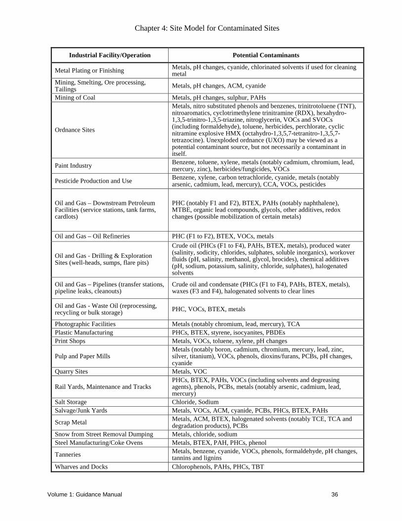
Chapter 4: Site Model for Contaminated Sites
Volume 1: Guidance Manual 36
Industrial Facility/Operation Potential Contaminants
Metal Plating or Finishing Metals, pH changes, cyanide, chlorinated solvents if used for cleaning metal
Mining, Smelting, Ore processing, Tailings Metals, pH changes, ACM, cyanide
Mining of Coal Metals, pH changes, sulphur, PAHs
Ordnance Sites
Metals, nitro substituted phenols and benzenes, trinitrotoluene (TNT), nitroaromatics, cyclotrimethylene trinitramine (RDX), hexahydro-1,3,5-trinitro-1,3,5-triazine, nitroglycerin, VOCs and SVOCs (including formaldehyde), toluene, herbicides, perchlorate, cyclic nitramine explosive HMX (octahydro-1,3,5,7-tetranitro-1,3,5,7-tetrazocine). Unexploded ordnance (UXO) may be viewed as a potential contaminant source, but not necessarily a contaminant in itself.
Paint Industry Benzene, toluene, xylene, metals (notably cadmium, chromium, lead, mercury, zinc), herbicides/fungicides, VOCs
Pesticide Production and Use Benzene, xylene, carbon tetrachloride, cyanide, metals (notably arsenic, cadmium, lead, mercury), CCA, VOCs, pesticides
Oil and Gas – Downstream Petroleum Facilities (service stations, tank farms, cardlots)
PHC (notably F1 and F2), BTEX, PAHs (notably naphthalene), MTBE, organic lead compounds, glycols, other additives, redox changes (possible mobilization of certain metals)
Oil and Gas – Oil Refineries PHC (F1 to F2), BTEX, VOCs, metals
Oil and Gas - Drilling & Exploration Sites (well-heads, sumps, flare pits)
Crude oil (PHCs (F1 to F4), PAHs, BTEX, metals), produced water (salinity, sodicity, chlorides, sulphates, soluble inorganics), workover fluids (pH, salinity, methanol, glycol, brocides), chemical additives (pH, sodium, potassium, salinity, chloride, sulphates), halogenated solvents
Oil and Gas – Pipelines (transfer stations, pipeline leaks, cleanouts)
Crude oil and condensate (PHCs (F1 to F4), PAHs, BTEX, metals), waxes (F3 and F4), halogenated solvents to clear lines
Oil and Gas - Waste Oil (reprocessing, recycling or bulk storage) PHC, VOCs, BTEX, metals
Photographic Facilities Metals (notably chromium, lead, mercury), TCA Plastic Manufacturing PHCs, BTEX, styrene, isocyanites, PBDEs Print Shops Metals, VOCs, toluene, xylene, pH changes
Pulp and Paper Mills Metals (notably boron, cadmium, chromium, mercury, lead, zinc, silver, titanium), VOCs, phenols, dioxins/furans, PCBs, pH changes, cyanide
Quarry Sites Metals, VOC
Rail Yards, Maintenance and Tracks PHCs, BTEX, PAHs, VOCs (including solvents and degreasing agents), phenols, PCBs, metals (notably arsenic, cadmium, lead, mercury)
Salt Storage Chloride, Sodium Salvage/Junk Yards Metals, VOCs, ACM, cyanide, PCBs, PHCs, BTEX, PAHs
Scrap Metal Metals, ACM, BTEX, halogenated solvents (notably TCE, TCA and degradation products), PCBs
Snow from Street Removal Dumping Metals, chloride, sodium Steel Manufacturing/Coke Ovens Metals, BTEX, PAH, PHCs, phenol
Tanneries Metals, benzene, cyanide, VOCs, phenols, formaldehyde, pH changes, tannins and lignins
Wharves and Docks Chlorophenols, PAHs, PHCs, TBT

Chapter 4: Site Model for Contaminated Sites
Volume 1: Guidance Manual 37
Industrial Facility/Operation Potential Contaminants
Wood Treating/Preservation Chlorophenols, phenols, PAHs, PHCs, BTEX, metals (CCA) ACM = asbestos containing material; BTEX = benzene, toluene, ethylbenzene, xylenes; CCA = chromated copper arsenate, a compound that contains arsenic, chromium and copper; CFCs = chlorofluorocarbons; F1 to F4 = Petroleum Hydrocarbon Fractions as defined in CCME (2008); MTBE = methyl tertiary butyl ether; PAHs = polycyclic aromatic hydrocarbons; PBDE = polybrominated diphenyl ethers; PCBs = polychlorinated biphenyls; PCDDs/PCDFs = polychlorinated dibenzodioxins/furans; PCE = tetrachloroethylene; PFOA = perflorooctanoic acid; PFOS = perflourooctane sulphonate; PHCs = petroleum hydrocarbons compounds; SVOCs = semi-volatile organic compounds; TBT = tributyltin; TCA = trichloroethane; TCE = trichloroethylene; UXO = unexploded ordnance; VOCs = volatile organic compounds
4.1.4 Emergent or Less Common Chemicals
There are a number of emergent or less common chemicals in environmental media that are receiving increased attention, such as: 1,4 dioxane, perchlorate, nitrosodimethylamine (NDMA), perfluorooctane sulphonate (PFOS), and 1,2,3-trichloropropane (Exhibit 4-1). While information on the identification and significance of chemicals lacking Canadian Environmental Quality Guidelines may be limited, the site assessor should be aware that assessment of all COPCs is warranted. CCME recommends that the proponent assess background concentrations, and review criteria from other jurisdictions. The proponent is also encouraged to contact the appropriate regulatory authority to discuss their proposed approach. Further evaluation of chemicals lacking regulatory guidelines, if present, would normally occur as part of a site specific risk assessment.
The analytical methods described in Volume 4, can be applied to the analysis of these and other emerging contaminats.
Conceptual Site Model for LNAPL and DNAPL Characterization 4.2
The objectives of this subsection are to: 1) provide an understanding of how a CSM is used in the evaluation of non-aqueous phase liquids (NAPLs); 2) identify the fate and transport mechanisms that influence movement of NAPLs through the environment; and 3) discuss the unique characteristics of NAPLs that should be considered when developing a CSM for site characterization.
NAPLs are liquids that exist as a separate, immiscible phase when in contact with water. The differences in the physical and chemical properties between water and NAPL result in a physical interface between the liquids that prevents the two fluids from mixing. NAPLs are typically classified as either light (i.e., LNAPLs) with densities less than that of water, or dense (i.e., DNAPLs) with densities greater than that of water. Common LNAPLs include petroleum products such as gasoline, diesel, jet fuel and lubricants. Common DNAPLs include creosote, coal tar and chlorinated solvents such as TCE and PCE.
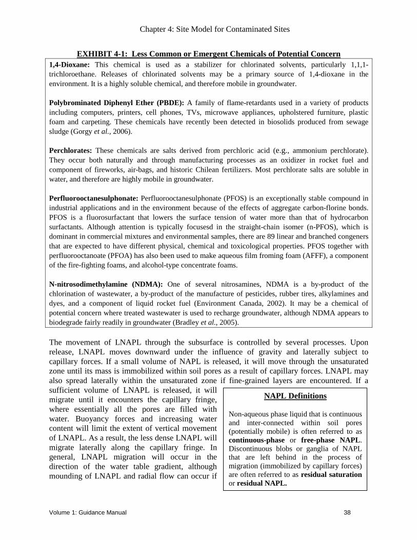
Chapter 4: Site Model for Contaminated Sites
Volume 1: Guidance Manual 38
EXHIBIT 4-1: Less Common or Emergent Chemicals of Potential Concern 1,4-Dioxane: This chemical is used as a stabilizer for chlorinated solvents, particularly 1,1,1-trichloroethane. Releases of chlorinated solvents may be a primary source of 1,4-dioxane in the environment. It is a highly soluble chemical, and therefore mobile in groundwater.
Polybrominated Diphenyl Ether (PBDE): A family of flame-retardants used in a variety of products including computers, printers, cell phones, TVs, microwave appliances, upholstered furniture, plastic foam and carpeting. These chemicals have recently been detected in biosolids produced from sewage sludge (Gorgy et al., 2006).
Perchlorates: These chemicals are salts derived from perchloric acid (e.g., ammonium perchlorate). They occur both naturally and through manufacturing processes as an oxidizer in rocket fuel and component of fireworks, air-bags, and historic Chilean fertilizers. Most perchlorate salts are soluble in water, and therefore are highly mobile in groundwater.
Perfluorooctanesulphonate: Perfluorooctanesulphonate (PFOS) is an exceptionally stable compound in industrial applications and in the environment because of the effects of aggregate carbon-florine bonds. PFOS is a fluorosurfactant that lowers the surface tension of water more than that of hydrocarbon surfactants. Although attention is typically focusesd in the straight-chain isomer (n-PFOS), which is dominant in commercial mixtures and environmental samples, there are 89 linear and branched congeners that are expected to have different physical, chemical and toxicological properties. PFOS together with perfluorooctanoate (PFOA) has also been used to make aqueous film froming foam (AFFF), a component of the fire-fighting foams, and alcohol-type concentrate foams.
N-nitrosodimethylamine (NDMA): One of several nitrosamines, NDMA is a by-product of the chlorination of wastewater, a by-product of the manufacture of pesticides, rubber tires, alkylamines and dyes, and a component of liquid rocket fuel (Environment Canada, 2002). It may be a chemical of potential concern where treated wastewater is used to recharge groundwater, although NDMA appears to biodegrade fairly readily in groundwater (Bradley et al., 2005).
The movement of LNAPL through the subsurface is controlled by several processes. Upon release, LNAPL moves downward under the influence of gravity and laterally subject to capillary forces. If a small volume of NAPL is released, it will move through the unsaturated zone until its mass is immobilized within soil pores as a result of capillary forces. LNAPL may also spread laterally within the unsaturated zone if fine-grained layers are encountered. If a sufficient volume of LNAPL is released, it will migrate until it encounters the capillary fringe, where essentially all the pores are filled with water. Buoyancy forces and increasing water content will limit the extent of vertical movement of LNAPL. As a result, the less dense LNAPL will migrate laterally along the capillary fringe. In general, LNAPL migration will occur in the direction of the water table gradient, although mounding of LNAPL and radial flow can occur if
NAPL Definitions
Non-aqueous phase liquid that is continuous and inter-connected within soil pores (potentially mobile) is often referred to as continuous-phase or free-phase NAPL. Discontinuous blobs or ganglia of NAPL that are left behind in the process of migration (immobilized by capillary forces) are often referred to as residual saturation or residual NAPL.

Chapter 4: Site Model for Contaminated Sites
Volume 1: Guidance Manual 39
the rate of LNAPL movement from the surface is greater than the lateral migration.
The movement of DNAPL is similar to LNAPL through the unsaturated zone; however, since DNAPL is denser than water, it can often be found below the water table. For DNAPL, capillary forces, which are a function of both the properties of the DNAPL and soil, have a critical effect on the subsurface DNAPL distribution. When finer-grained soil deposits (i.e., clay or silt) are encountered, the DNAPL may migrate along the top of these deposits and may form pools or puddles. However, DNAPL penetration may sometimes occur where the aquitards are non-uniform or not continuous (e.g., there may be “windows” in the aquitard allowing DNAPL passage) or where preferential pathways (e.g., vertical fractures or root holes within tills or clays) are present.
The site assessor should recognize several key implications for LNAPL and DNAPL contamination. Both LNAPL and DNAPL zones are often long-term sources of dissolved contaminant plumes in groundwater, and often require delineation prior to remediation. While appropriate investigation techniques for both forms of contamination are essential, investigation for DNAPL is challenging since DNAPL source zones and migration pathways can be difficult to detect. For DNAPL, an indirect approach is often used to assess whether DNAPL may be present. Specifically, dissolved chemical concentrations measured in a groundwater well are compared to the theoretical solubility limit of the chemical. A commonly-adopted threshold for the possible presence of DNAPL is a dissolved concentration that exceeds 1 percent of its theoretical effective solubility (i.e., “1% rule-of-thumb”). Another key consideration is the stability of LNAPL or DNAPL zones. This too may be challenging to determine, since their movement may be slow and subtle changes in hydrogeological conditions may cause re-mobilization. SABCS (2006a) provides a detailed evaluation of LNAPL mobility.
Conceptual Site Model for Groundwater Characterization 4.3
The objectives of this subsection are to: 1) provide an understanding of how a CSM is used to identify the likely location of COPCs at a study area where groundwater is an environmental medium of interest; and 2) identify the fate and transport mechanisms important to COPCs in groundwater and ways in which exposure to COPCs in groundwater may occur.
An example of a CSM for the groundwater pathway is shown in Figure 4-1. The following sections present an overview of fate and transport processes pertinent to this model. For evaluation of the groundwater pathway, it is important to characterize the fate and transport processes along the transport pathway from contamination source to receptor. Contaminants dissolved in soil-water will migrate with infiltrating water toward the water table. Below the water table, infiltrating water will migrate by advection, dispersion, and diffusion, mixing with flowing groundwater. Mixing will be enhanced by groundwater level fluctuations. If there is clean water recharge along the flowpath, the contaminant plume may “dive” as it migrates from the source area. Contaminants will migrate, to varying degrees, in the direction of groundwater flow and may come into contact with human receptors via use of well water, discharge to surface water bodies or ecological receptors through the discharge to surface water bodies.

Chapter 4: Site Model for Contaminated Sites
Volume 1: Guidance Manual 40
Figure 4-1: Groundwater Pathway Conceptual Model
4.3.1 Partitioning
Chemicals sorbed to soil particles or present as NAPL will partition to varying degrees into soil-water present within the unsaturated zone. For non-ionic organic compounds, there are well-established partitioning models based on linear equilibrium partitioning between the contaminant in the aqueous phase and absorbed within organic carbon (i.e., when no NAPL is present). These models are described in greater detail in Section 4.5.2. For metals, the processes that influence partitioning are much more complex and include ion complexation, surface complexation and precipitation. Concentrations of metals in solution, pH, organic carbon content and hydrous iron oxide content are all important factors for metals partitioning.
When NAPL composed of a single chemical is present, the solubility of the chemical represents the maximum possible dissolved-phase concentration that can be expected in groundwater. However, for a mixture of chemicals, the aqueous solubility of an individual chemical will be less than its pure (“textbook”) solubility. Its solubility in the mixture will be approximately proportionate to the product of its mole fraction in the liquid and its activity coefficient:
Ciw = γi Xi Si [4.1]
where Ciw is the aqueous concentration (mg/L), γ i is the activity coefficient (dimensionless), Xi is the mole fraction (dimensionless) and Si is the pure-chemical solubility (mg/L). In most cases,

Chapter 4: Site Model for Contaminated Sites
Volume 1: Guidance Manual 41
the activity coefficient can be assumed to be equal to unity for mixtures of organic chemicals. Corrections are required for chemicals such as naphthalene, which are normally solids, but exist as liquids in mixtures such as diesel and creosote (Schwarzenbach et al., 2003).
4.3.2 Unsaturated Zone Chemical Transport
The fate and transport of water-phase chemicals within the unsaturated zone (often termed the vadose zone) depends on advection, dispersion, diffusion, sorption, degradation or decay and volatilization. Advection is the bulk movement of water under a hydraulic head gradient, whereas diffusion is the process involving the transfer of chemicals from a higher to lower chemical potential by random molecular motion (Robinson and Stokes, 1959). The sorption of dissolved chemicals in soil-water to organic carbon or mineral surfaces will result in the retardation in the bulk movement of chemicals in soil-water.
For common organic chemicals like benzene, toluene, ethylbenzene and xylenes, biodegradation has been demonstrated in groundwater under both aerobic and anaerobic conditions. Similar reaction kinetics would be expected in the unsaturated zone, except possibly under very dry conditions. Volatilization may be an important mechanism for mass loss for volatile chemicals in the vadose zone. Mechanical dispersion in the unsaturated zone has not been as extensively researched as saturated zone dispersion, although there are field-scale experiments where a longitudinal dispersivity of greater than 10 cm has been measured (Charbonneau and Daniel, 1993). onceptually, transverse dispersion within the unsaturated zone could be highly variable, depending on the potential for fingering or spreading based on horizontal layering of soil.
For unsaturated groundwater transport, the amount of water that infiltrates through the sub-surface via advection has a direct impact on the quantity of chemical mass that is transported in the aqueous phase toward groundwater. The atmospheric and near-surface processes that influence infiltration may be characterized by a water balance model that describes the fundamental components of the surface hydrology for precipitation, snow melt, run-off, potential evaporation, actual soil evaporation, plant uptake and transpiration, changes in shallow soil moisture, and net infiltration or percolation (Figure 4-2). The prediction of infiltration requires adequate characterization of surface hydrology, as well as forces and processes that lead to the upward and downward movement of water (and water vapour) at the ground surface and atmospheric boundary.
As in saturated aquifers, the downward flow of water through the unsaturated zone (advection) is impeded by the solid grains. Unlike saturated flow, however, the interactions between air, water, and the soil matrix lead to capillary effects. Capillary forces affect the moisture state within the vadose zone as well as the rate that water moves (i.e., hydraulic conductivity).

Chapter 4: Site Model for Contaminated Sites
Volume 1: Guidance Manual 42
Figure 4-2: Conceptual Water Balance Model
4.3.3 Groundwater Contaminant Transport
The fate and transport of chemicals within the saturated zone are dependent on processes similar to those associated with unsaturated zone transport, including advection, dispersion, diffusion, sorption, degradation or decay, and volatilization. For non-ionic organic compounds, there are well established partitioning models based on linear equilibrium partitioning between the contaminant in the aqueous phase and absorbed within organic carbon. Significant attenuation of dissolved plumes composed of petroleum hydrocarbon compounds occurs through both aerobic and anaerobic biodegradation (Wiedemeier et al., 1999). Advection and dispersion have a significant influence on the transport of dissolved chemicals in relatively permeable soils, whereas the importance of other transport mechanisms increases for moderate and low permeability soils.
Groundwater will move in response to differences in hydraulic head, which are due to differences in potential energy arising from the pressure and elevation of groundwater. On a regional scale, groundwater flows from recharge zones in the uplands, where recharge from precipitation occurs, towards discharge zones in the low lying areas, forming springs and
Precipitation
RunoffEvaporation
Cover
Soil
Transpiration
∆ StorageInfiltration
Percolation
Recharge
Groundwater Flow Concepts Groundwater scientists have defined a number of useful hydrogeological concepts for purposes of understanding groundwater movement. There are two basic types of subsurface medium in which groundwater flows; porous media and fractured media. Porous media consist of aggregates of individual particles such as silt, sand or gravel. Fractured media can consist of soil (e.g., clay) or bedrock where groundwater moves primarily through fractures, cracks or other openings. Aquifers are defined as geologic deposits that are relatively permeable (sometimes defined on the basis of groundwater yield in economic quantities) whereas aquitards are relatively impermeable units. An unconfined aquifer is bounded by the water table while a confined aquifer lies beneath an aquitard.

Chapter 4: Site Model for Contaminated Sites
Volume 1: Guidance Manual 43
discharging to creeks, rivers, lakes, wetlands, and the ocean. In the discharge zones, hydraulic heads measured at depth can be above the ground surface, which results in flowing artesian conditions (i.e., the water level in the well rises above the ground surface and the well flows). On regional and local scales, groundwater flow occurs from the locations where the hydraulic head is high towards lower head regions, with energy loss along the flow line. The energy loss is proportional to the hydraulic conductivity (K), which is the ability of soil to transmit water and depends on the properties of both the soil and the fluid. The porosity, pore-size and pore continuity are important properties affecting hydraulic conductivity. Darcy’s Law governs the groundwater flow and is expressed as:
q = -K*dh/dl [4.2]
where q is the specific discharge [(L3/L2)/T] and dh (L) is the difference in hydraulic head over a distance dl (L). Specific discharge is also known as Darcy flux or Darcy velocity. Specific discharge, or the volume of groundwater moving across a unit cross-sectional area, should not be confused with groundwater velocity v (L/T):
v = q/ne [4.3]
where ne is effective porosity (-) of the soil.
Hydraulic conductivity can vary over several orders-of-magnitude over relatively short distances in the subsurface. For example, in a hydrostratigraphic sequence where coarse sand unit pinches out against a silt unit, the change in hydraulic conductivity could vary from 10-3 m/s in sand to 10-7 m/s in silt. As the groundwater velocity is proportional to hydraulic conductivity, this could result in a four orders-of-magnitude change in velocity between these units. In addition, the groundwater velocity typically varies within individual hydrostratigraphic units due to heterogeneity of subsurface media, although these changes are typically less than one order-of-magnitude.
Dispersion effectively results in the dilution of contamination during plume migration, and is usually of much greater significance in the longitudinal direction than in directions transverse to flow. The degree of dispersion is “scale-dependent,” meaning that the larger the region occupied by a contaminant plume, the larger will be the significance of dispersion. Dispersion is also dependent on the heterogeneity of the aquifer. As a consequence of these factors, it is a relatively difficult variable to measure in the field, and is more commonly estimated based on empirical information obtained from the literature.
With the exception of chloride and similar chemicals, which are not affected by sorption, dissolved chemicals in groundwater typically move through the subsurface at velocities that are less than the groundwater velocity. Contaminant velocity vc (L/T) is defined as:
vc = v / R [4.4]

Chapter 4: Site Model for Contaminated Sites
Volume 1: Guidance Manual 44
where R is a retardation factor that accounts for the affects of sorption on the contaminant movement. For most contaminants, the retardation factor is higher for soils rich in organic matter than for mostly mineral soils. The organic matter content in soil samples is typically expressed as fraction of organic carbon foc (-).
4.3.4 Considerations for Fractured Bedrock
The properties of fractured bedrock can vary widely, ranging from granitic bedrock with small fractures to limestone deposits where there are openings enlarged by dissolution, commonly referred to as karst deposits. In most bedrock aquifers, groundwater primarily migrates through discontinuities (fractures and joints) in the rock matrix. Flow can also occur in the rock matrix in the presence of significant secondary porosity (e.g., in vuggy limestone). Groundwater velocity can be rapid and the influence of pumping may be seen over large areas, which has potential implications for well-head protection of groundwater drinking water supplies (Crowe et al., 2003).
Groundwater flow in fractured bedrock is complex and knowledge and techniques for characterizing groundwater flow and chemical transport in porous media cannot easily be applied to fractured rock. Two traditional approaches have been used to conceptualise groundwater flow in fractured bedrock are: (i) the non-continuum approach (i.e., discrete fracture network or DFN) and (ii) the continuum approach (i.e., equivalent porous medium or EPM), as described in NRC (1996) and summarized below. DFN models may be applied when individual fractures or groups of fractures significantly influence groundwater flow and solute transport. The modelling of flow and transport through a DFN approach is highly complex and assumes that fluid flow can be predicted from knowledge of the fracture geometry and data on the hydraulic properties of individual fractures. As there is always uncertainty in geometry and properties of fracture networks, DFN models rely heavily on statistical concepts for predictions. Under the EPM approach, the individual fractures are not explicitly treated in the model. Instead, at the scale of interest, hydraulic properties represent the volume-averaged behaviour of many fractures. Similar concepts as applied to porous media may be used to model contaminant transport under the EPM, but these predictions are only valid if it is possible to define a reasonable averaging volume.
The groundwater flow in individual fractures may be described by a Cubic Law, where hydraulic conductivity of a fracture is a function of its aperture. For a set of planar fractures, a porous-media equivalent hydraulic conductivity can be estimated when there is information on the fracture density or spacing (Snow, 1968).
The site characterization methods subsequently described in this guidance are, to varying degrees, applicable to fractured bedrock settings, particularly if bedrock can be represented using a EPM approach, depending on site conditions. Specialists in this area should be consulted for further guidance, where warranted.
Chapter 4: Site Model for Contaminated Sites
Volume 1: Guidance Manual 45
4.3.5 Considerations for Permafrost
Much of the three northern territories in Canada, as well as some parts of the northern regions of the provinces, are covered with either continuous or discontinuous permafrost (Figure 4-3). A common definition for permafrost is ground (soil or rock) that remains at or below 0oC for two or more years (NRC, 1988). Where permafrost is present, there are four phases present in the subsurface consisting of ice, water, air and soil. Permafrost does not typically underlie lakes and rivers, which are typically underlain by taliks.
Particularly in discontinuous permafrost, the groundwater flow regime can be extremely complex and is controlled by ice saturation, discrete fractures and channels and is often seasonally dependent. On a local scale, the seasonal development of an active layer can provide permeable pathways for subsurface movement of water and contaminants. The top of the permafrost may also have a saturated zone referred to as supra-permafrost groundwater. The ice content in permafrost can vary widely; therefore, one should not assume that permafrost represents a barrier to contaminant migration. Dry permafrost refers to soil or bedrock where the temperature remains below 0oC but most of the pore space is free of ice.
Characterization of groundwater flow and contaminant transport in permafrost can be highly complex. In addition to conventional methods, specialised techniques may be used to characterize permafrost zones including geophysical techniques such as ground penetrating radar, direct current (DC) resistivity and thermal-pulse flow meters. Further discussion on methods for characterization of contamination in permafrost is beyond the scope of this guidance; specialists in this area should be consulted, where warranted.
Conceptual Site Model for Soil Characterization 4.4
The objectives of this subsection are to: 1) provide an understanding of how a CSM is used to identify the likely location of COPCs in soil at study areas where soil is an environmental medium of interest; and 2) identify the fate and transport mechanisms important to COPCs in soil and ways in which exposure to COPCs in soil may occur.
As discussed above, there are a broad range of sources of soil contamination including both point sources and non-point sources. Leaking fuel storage tanks, accidental spills at industrial sites, and waste disposal areas such as burn pits, lagoons, and landfills are examples of point sources of contamination that may result in soil contamination. Salt from road runoff, runoff of water containing fertilizer applied to farmland, and deposition of contaminated sediments or soils carried during flood events represent non-point sources of contamination.
For the purposes of risk assessment, it is essential that all sources of soil contamination and the inferred distribution of contaminants in soil be understood, in order to assess potential exposure pathways.
Several factors differentiate soil from other media with respect to site characterization requirements (see Table 2-3). For example, soil contamination is often highly variable over relatively small distances. Whereas organic chemicals in groundwater tend to form plumes in a

Chapter 4: Site Model for Contaminated Sites
Volume 1: Guidance Manual 46
relatively predictable manner, soil contamination may be discontinuous and dispersed depending on the contamination source. Temporal changes in soil concentrations tend to be slow and generally inconsequential; therefore, temporal considerations tend not to be important for soil contamination1.
Figure 4-3: Distribution of Continuous and Discontinuous Permafrost in Canada (from Atlas of Canada, 6th Edition, Natural Resources Canada http://geogratis.gc.ca/api/en/nrcan-rncan/ess-sst/dc7107c0-8893-11e0-aa10-6cf049291510.html)
1 In situations with substantial erosion potential (long, steep, and unvegetated slopes, loosely aggregated soils, lack of snow cover, etc), temporal changes in the soil contaminant distribution could occur. In addition to reviewing field erosion indicators and site meteorological data, the Universal Soil Loss Equation (USLE) or the Wind Erosion Equation (WEQ) may be used to gain an understanding of the erosion potential at a site. Deposition patterns of eroded materials are highly variable; following major erosive events re-sampling of site soils may be needed to maintain an up-to-date CSM.
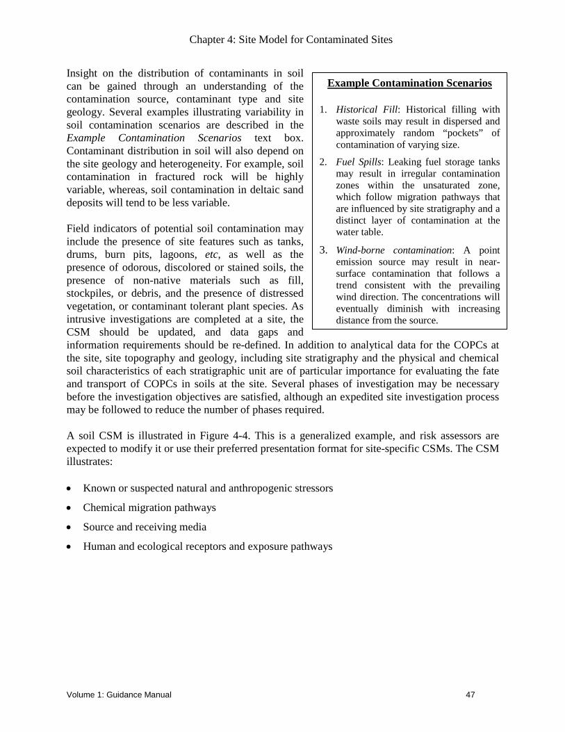
Chapter 4: Site Model for Contaminated Sites
Volume 1: Guidance Manual 47
Insight on the distribution of contaminants in soil can be gained through an understanding of the contamination source, contaminant type and site geology. Several examples illustrating variability in soil contamination scenarios are described in the Example Contamination Scenarios text box. Contaminant distribution in soil will also depend on the site geology and heterogeneity. For example, soil contamination in fractured rock will be highly variable, whereas, soil contamination in deltaic sand deposits will tend to be less variable.
Field indicators of potential soil contamination may include the presence of site features such as tanks, drums, burn pits, lagoons, etc, as well as the presence of odorous, discolored or stained soils, the presence of non-native materials such as fill, stockpiles, or debris, and the presence of distressed vegetation, or contaminant tolerant plant species. As intrusive investigations are completed at a site, the CSM should be updated, and data gaps and information requirements should be re-defined. In addition to analytical data for the COPCs at the site, site topography and geology, including site stratigraphy and the physical and chemical soil characteristics of each stratigraphic unit are of particular importance for evaluating the fate and transport of COPCs in soils at the site. Several phases of investigation may be necessary before the investigation objectives are satisfied, although an expedited site investigation process may be followed to reduce the number of phases required.
A soil CSM is illustrated in Figure 4-4. This is a generalized example, and risk assessors are expected to modify it or use their preferred presentation format for site-specific CSMs. The CSM illustrates:
• Known or suspected natural and anthropogenic stressors
• Chemical migration pathways
• Source and receiving media
• Human and ecological receptors and exposure pathways
Example Contamination Scenarios
1. Historical Fill: Historical filling with waste soils may result in dispersed and approximately random “pockets” of contamination of varying size.
2. Fuel Spills: Leaking fuel storage tanks may result in irregular contamination zones within the unsaturated zone, which follow migration pathways that are influenced by site stratigraphy and a distinct layer of contamination at the water table.
3. Wind-borne contamination: A point emission source may result in near- surface contamination that follows a trend consistent with the prevailing wind direction. The concentrations will eventually diminish with increasing distance from the source.

Chapter 4: Site Model for Contaminated Sites
Volume 1: Guidance Manual 48
Figure 4-4: Generalized Conceptual Site Model for Soil
Fate and transport of soil contaminants, and subsequent exposure to these contaminants, can occur through the following mechanisms:
• In-situ soil containing COPCs. Direct soil contact and soil ingestion by humans can occur, especially if the contaminated soils are present in areas of human activity (e.g. residential areas with gardens, playgrounds, etc). Ecological receptors that ingest or live in close contact with soil (e.g. soil invertebrates and other burrowing animals) may also be directly exposed via direct contact and ingestion. Some ecological receptors may also be exposed to soil COPCs via ingestion of prey items (e.g., soil invertebrates, small mammals) that have accumulated soil COPCs in their tissue.
• Plant uptake of COPCs in soil. Plants have the ability to extract and assimilate some metals and other compounds from the soil. Human and ecological receptors may be exposed to the soil COPCs through the consumption of crops and plants grown in contaminated soils.

Chapter 4: Site Model for Contaminated Sites
Volume 1: Guidance Manual 49
• Dust formation of soils containing COPCs. Dry, unvegetated, loosely aggregated soils can be prone to dust formation, especially in combination with wind or mechanical agitation (tilling, heavy traffic, etc). Soil COPCs in airborne dust can be inhaled by human and ecological receptors.
• Surface erosion and runoff of soil containing COPCs. Rain events or floods can erode soil (and soil COPCs) and carry soil particles down slope and/or into surface water bodies where ecological and human receptors may be exposed to COPCs. Once velocities decrease, entrained soil particles will settle out and become part of the sediment. More details regarding the fate and transport of sediment COPCs can be found in Section 4.7.
• Partitioning of soil COPCs into soil vapour phase (volatilization). Volatilized soil contaminants can be inhaled by human or ecological receptors. Vapour intrusion is of particular concern in certain situations. More details regarding the fate and transport of soil vapour can be found in Section 4.5.
• Partitioning of soil COPCs into pore- or groundwater (leaching). Leached soil contaminants can impact drinking water sources, or other water bodies, exposing ecological receptors, which may ultimately be consumed by humans. More details regarding the fate and transport of leached COPCs can be found in Sections 4.2 and 4.3.
Conceptual Site Model for Soil Vapour 4.5
The objectives of this subsection are to: 1) provide an understanding of how a CSM is used to identify study areas and COPCs for which soil vapour intrusion is likely to be a concern; and 2) identify the fate and transport mechanisms that affect soil vapour intrusion.
An example of a CSM for the vapour intrusion pathway is shown in Figure 4-5. In developing a CSM depicting the soil vapour pathway, it is particularly important to consider the fate and transport processes along the transport pathway from contamination source to receptor. Where there are volatile or semivolatile contaminants within the unsaturated zone, partitioning to the vapour phase will occur. Methane, carbon dioxide, and other gases may also be generated through biological decomposition of organic compounds. Soil vapour migrates away from source zones and, depending on site conditions, may migrate toward and into buildings. Within buildings, mixing and dilution of vapours will occur as a result of ventilation and air movement. The following sections present an overview of fate and transport processes pertinent to this model, followed by specific models of interest for vapour intrusion (Section 4.5.6). A conceptual site model checklist is provided in Volume 2.

Chapter 4: Site Model for Contaminated Sites
Volume 1: Guidance Manual 50
Figure 4-5: Example of a Conceptual Site Model for Vapour Intrusion into a Residential Building (from USEPA, 2002)
4.5.1 Contamination Sources
Common COPCs for soil vapour intrusion include a range of organic chemicals, including petroleum hydrocarbons from fuel products, coal tar or creosote, and chlorinated solvents.
Petroleum hydrocarbons are mixtures of hundreds of compounds and are associated with fuels, such as gasoline, jet fuel and diesel. While risk assessments often focus on benzene, toluene, ethylbenzene and xylenes (BTEX), and polycyclic aromatic hydrocarbons (PAHs), these compounds represent only a small fraction of hydrocarbon vapours and other compounds of interest may be present, including hexane, decane, trimethylbenzenes and naphthalene, depending on the fuel type. Typically, analytical tests for hydrocarbon vapours will also include hydrocarbon fractions based on carbon chain length (e.g., F1 and F2 as defined in CCME (2008)) and aromatic and aliphatic fractions.
Coal tar, frequently associated with former manufactured gas plants (MGP), and creosote, frequently associated with wood preservation, have similar organic COPCs composed of monocyclic aromatic hydrocarbons, such as BTEX, and PAHs. There is significant variation in

Chapter 4: Site Model for Contaminated Sites
Volume 1: Guidance Manual 51
the volatility and mobility of PAH compounds ranging from naphthalene, considered a semivolatile, to five- and six-ring PAHs, which are essentially non-volatile. While some of the heavier PAH compounds are identified as COPCs for the vapour intrusion pathway based on conservative screening approaches (e.g., Health Canada and USEPA vapour intrusion guidance), their vapour concentrations are relatively low and organic carbon partitioning coefficients (Koc) tend to be high. As a consequence, the mobility of heavier molecular weight PAHs via soil vapour transport is limited and, for practical purposes, is not of potential concern for vapour intrusion. Similar considerations apply to other heavier molecular weight organic chemicals with similar properties.
Common chlorinated solvents include tetrachloroethylene or perchloroethylene (PCE), trichloroethylene (TCE) and 1,1,1-trichloroethane (TCA), and associated breakdown products of biodegradation or abiotic transformation (e.g., cis- and trans-1,2-dichloroethylene (cis-1,2-DCE), 1,1-dichloroethylene (1,1-DCE) and vinyl chloride). Chloroform is also commonly detected in soil vapour, and is in some cases associated with anthropogenic sources (e.g., leaking water mains) or natural sources. Most chlorinated solvents are relatively mobile and persistent within the unsaturated zone due to their relatively low solubility, high volatility and their resistance to degradation under aerobic conditions.
Depending on the form present, mercury may also pose a potential vapour inhalation risk, since elemental mercury has a high vapour pressure.
Soil gases such as methane, carbon dioxide and, in some cases, hydrogen sulphide, may be generated as by-products of the anaerobic decomposition of organic chemicals such as petroleum fuels, waste material (e.g., refuse) and/or native organic matter (e.g., peat). The presence of these gases may represent a potential safety hazard through explosion or asphyxiation. Methane is explosive in the range of 5 to 15 percent by volume in air. Gas produced by microbiological activity may generate pressure gradients that enhance subsurface vapour migration through advection. Another source of pressure-driven gas is leaking natural gas lines. The CSM subsequently described in this chapter does not address assessment of sites where there is potential for significant pressure-driven gas flow.
4.5.2 Chemical Transfer to Vapour Phase (Volatilization)
Chemical transfer to the vapour phase may occur through partitioning of NAPL present above the water table into soil gas (“vapourisation”) or partitioning of dissolved chemicals in soil-water above the water table into soil gas (“volatilization”). NAPL is referred to as a primary source of vapours, while a dissolved phase plume is referred to as a secondary source. Soil contamination within the unsaturated zone also represents a potential source of vapours.
The distribution of NAPL relative to the water table will have a large influence on its potential to volatilise and migrate to indoor air. If NAPL is situated below the water table, then volatilization will be relatively limited since, as subsequently discussed in this chapter, the mass transport through groundwater is relatively slow due to the low diffusion rate in water, and since vertical dispersion tends to be limited.

Chapter 4: Site Model for Contaminated Sites
Volume 1: Guidance Manual 52
For a secondary source where chemicals are present only as a dissolved phase in groundwater, their distribution below the water table will also determine their potential to volatilize. If volatile chemicals are present near the surface of the water table, volatilization will readily occur. In contrast, if there is a layer of uncontaminated groundwater above contaminated water, then the rate of volatilization will decrease.
Equilibrium partitioning models are typically used to estimate the distribution of chemicals between different phases. Where NAPL is present above the water table, a two-phase model based on the vapour pressure of the chemical is used to estimate the soil vapour concentration. Raoult’s Law is used to account for partitioning for a multi-component mixture of chemicals, which is a function of the mole fraction and vapour pressure, as follows:
𝐶𝐶𝑣𝑣 = 1000𝑀𝑀𝑊𝑊𝑋𝑋𝑉𝑉𝑃𝑃𝑅𝑅𝑅𝑅
[4.5]
where Cv is the soil vapour concentration (mg/m3), MW is the molecular weight (g/mole), X is the mole fraction (dimensionless), VP is the vapour pressure (atm), R is the gas constant (m3-atm/K-mole), and T is the temperature (K).
For dissolved chemicals in groundwater, the Henry’s Law constant is typically used to estimate the vapour concentration in equilibrium with water, as follows:
𝐶𝐶𝑣𝑣 = 1000𝐶𝐶𝑔𝑔𝐻𝐻′ [4.6]
where Cg is the groundwater concentration (mg/L) and H’ is the dimensionless Henry’s Law constant. Since it is not possible to obtain a soil gas sample at the water table (i.e., due to the capillary transition zone), the measured soil vapour concentration should be lower than that predicted using the Henry’s Law constant. This is because there will be attenuation of chemical concentrations by diffusion (and possibly biodegradation) within the capillary fringe and transition zone between the water table and region where there are continuous gas-filled soil pores. Attenuation within the capillary zone has implications for soil vapour intrusion modelling and comparison of measured and predicted soil vapour concentrations.
Where there is soil contamination, but no NAPL, a three phase model for partitioning between sorbed, aqueous, and vapour phases can be used to estimate the soil vapour concentration, as follows:
𝐶𝐶𝑡𝑡 = 𝐶𝐶𝑤𝑤 �𝐾𝐾𝑑𝑑 + �θ𝑤𝑤 + θ𝑎𝑎𝐻𝐻′
𝜌𝜌𝑏𝑏�� 𝑤𝑤ℎ𝑒𝑒𝑒𝑒𝑒𝑒 𝐾𝐾𝑑𝑑 = 𝐾𝐾𝑜𝑜𝑜𝑜𝑓𝑓𝑜𝑜𝑜𝑜 [4.7]
where Ct is the total soil concentration (mg/kg), Cw is the soil-water concentration (mg/L), Koc is the organic carbon-water partition coefficient (L/kg), foc is the fraction organic carbon (dimensionless), θw is the water-filled porosity (dimensionless), θa is the air-filled porosity (dimensionless), H’ is the Henry’s Law constant (dimensionless) and ρb is the bulk dry density (kg/L). If, under equilibrium, the three phases become saturated by the chemical, then the

Chapter 4: Site Model for Contaminated Sites
Volume 1: Guidance Manual 53
remainder of the chemical will be in its pure form (i.e., NAPL). Guidance on calculation of the soil saturation (“Csat”) concentration for NAPL is provided in USEPA (1996).
For non-ionizing organic chemicals, a linear equilibrium partitioning model is widely used to predict absorption of organics into native organic carbon. Studies have shown that the sorption of organics by soils is highly correlated with the foc (e.g., Chiou et al., 1979; Hassett et al., 1980; Hassett and Banwart, 1989), provided the foc is above a critical level. USEPA (1996) suggests that when foc is below about 0.001, adsorption to inorganic mineral surfaces becomes important. While soil partitioning models are well established, the accuracy of such models to predict soil vapour concentrations is poor. Therefore, it is generally not advisable to estimate soil vapour concentrations from soil concentration data. Instead, soil vapour concentrations should be predicted from groundwater data using Henry’s Law constant (when appropriate) or they should be measured directly.
4.5.3 Vadose Zone Fate and Transport Processes
Fate and transport processes in the vadose zone that influence the movement of chemicals from a contamination source toward a building include: diffusion, advection, dispersion, partitioning between soil, water and gas phases, and biodegradation reactions. Several of the fate and transport processes that influence soil vapour intrusion were illustrated in Figure 4-5. In this example, volatilization is occurring just above the top of the capillary fringe to create soil vapours. These vapours are subsequently transported upwards toward the ground surface via diffusion. loser to the building advective soil gas transport may be the dominant process if the building is depressurized relative to atmospheric pressure. The rate of volatilization at the contamination source is controlled by the mass flux rate for chemical migration away from the source. In turn, the mass flux rate will vary temporally as a result of fluctuations in moisture content, temperature, elevation of the water table, and other factors.
Diffusion Diffusion is the movement of molecules from an area of higher concentration to an area of lower concentration, as influenced by their kinetic energy. The rate that a chemical will diffuse is a function of the concentration difference (gradient) and the compound- and temperature-dependent diffusion coefficient. The mass flux, J (M/L2-T), is calculated by Fick’s Law, as follows:
𝐽𝐽 = −𝐷𝐷eff 𝜕𝜕𝜕𝜕𝑣𝑣𝜕𝜕𝜕𝜕
[4.8]
Where Deff is the effective diffusion coefficient (L2/T), C is the vapour concentration (mass/volume of gas) and Z is the distance over which the concentration change is measured (L). The diffusive flux is less in soil than in a gas-filled volume as a result of the tortuosity or non-linear migration path for diffusing gas species. Mathematically, this is expressed as the effective diffusion coefficient, typically estimated from the Millington-Quirk relationship (1961):
𝐷𝐷𝑒𝑒𝑒𝑒𝑒𝑒 = 𝐷𝐷𝑎𝑎𝜃𝜃𝑎𝑎3.33
𝜃𝜃2+ 𝐷𝐷𝑤𝑤
𝐻𝐻′𝜃𝜃𝑤𝑤3.33
𝜃𝜃2 [4.9]

Chapter 4: Site Model for Contaminated Sites
Volume 1: Guidance Manual 54
Diffusion coefficients in air (Da, L2/T) are about four orders-of-magnitude higher than in water (Dw, L2/T); therefore, diffusion is much faster through the air-filled soil pores, than through water-filled soil pores, and the second term in equation 4.9 tends not be important, except under nearly saturated conditions or for compounds with very low Henry’s Law constant (i.e., dimensionless H’ less than 0.001). When contamination is limited to dissolved chemicals in groundwater, diffusion through the capillary fringe is often the rate-limiting process because the moisture content in the capillary fringe is high, and may even be completely saturated. The thickness of the capillary fringe increases with decreasing soil grain size. Diffusion rates may also be highly sensitive to the presence of fine-grained, high moisture content soil layers within the vadose zone. There may also be a “rain-shadow” below a building with locally drier soils beneath the building (although drains and gutters may influence the soil moisture distribution).
Sorption As soil vapours migrate away from contamination source zones, the transport of soil vapours will be retarded due to sorption to the soil matrix and transfer of chemicals into soil water. Soils with higher native organic carbon will tend to have a greater sorption capacity. While partitioning into soil water will occur rapidly, biodegradation of some chemicals may occur simultaneously, thereby reducing the concentration in soil water. This process allows for the continuous partitioning of the chemical into the soil water, thus reducing the concentration in the vapour phase.
Biodegradation Different organic compounds will biodegrade at different rates, and with varying oxygen demands. For example, the aerobic biodegradation of volatile petroleum hydrocarbons in the vadose zone (e.g., BTEX) has been demonstrated through many investigations (Ostendorf and Campbell, 1991; Ririe et al., 1998; Roggemans et al., 2002; Hers et al., 2000; Hers et al., 2002; Davis et al., 2009; Patterson and Davis, 2009). Several of these studies indicate orders-of-magnitude bioattenuation of hydrocarbon vapour concentrations over relatively small distances within the vadose zone. Since chlorinated solvents (e.g., PCE and TCE) primarily degrade under anaerobic conditions through reductive dechlorination (Wiedemeier et al., 1999), biotransformation of these compounds will usually be limited due to the presence of oxygen within the unsaturated zone. There is evidence of aerobic biodegradation of vinyl chloride.
Vadose Zone Advection Gas-phase advective transport can occur as a result of fluctuations in atmospheric pressure (e.g., barometric pumping), water movement, water table fluctuations, and density gradients due to composition and temperature variations (soil gas advection due to building depressurization is discussed in Section 4.5.4). For most geologic environments, diffusion is the dominant vadose zone transport process; however, soil gas advection can be important where there is high permeability, relatively deep unsaturated zone deposits (i.e., tens of metres deep) and/or methanogenesis is significant. A modeling study by Choi and Smith (2005) found that pressure-driven advective flux increased for deep, drier, permeable deposits; nevertheless, for all combinations of scenarios, diffusive flux was at least one order-of-magnitude greater than

Chapter 4: Site Model for Contaminated Sites
Volume 1: Guidance Manual 55
advective flux. Where there are relatively high soil gas advection rates, dispersion may also be important. Dispersion is a mixing process that is caused by small-scale variations in air velocities in soil. The effects of these velocity variations are similar to the effects of diffusion (Auer, 1996).
4.5.4 Near-Building Processes for Soil Vapour Intrusion
The primary process for soil vapour intrusion into buildings is typically soil gas advection, although vapour migration will also occur as a result of diffusion through the building foundation. Model sensitivity analyses suggest that soil gas advection will be the dominant mechanism when the building depressurization (relative to ambient air) is greater than about 1 Pascal (Hers et al., 2003; Johnson, 2005), which will be exceeded at many residential buildings.
Soil gas advection can occur through untrapped floor drains, edge cracks at the building wall and floor slab interface (shown in Figure 4-5), unsealed entry points for utilities, expansion joints and other cracks and openings, if present. Field research programs that include pressure data for soil adjacent to the residential building foundation indicate that most of the soil gas flow occurs within 1 to 2 m of the foundation (Garbesi et al, 1993; Hers et al., 2002). Therefore, the properties of the backfill surrounding the foundation and the bedding associated with nearby utility corridors are important factors affecting advection. Field measurements and model simulations indicate that, for most sites, the permeability of soil near the building controls the rate of soil gas flow, to a greater extent than does the permeability of the building foundation.
Depressurization of the building airspace relative to the ambient (outdoor) air pressure can be caused by a number of factors including temperature differences between indoor and outdoor air (i.e., “stack effect”), wind-loading and operation of the building heating, ventilation and air-conditioning (HVAC) systems. The operation of HVAC systems can cause a building to be depressurized through insufficient combustion air for furnaces or unbalanced heating and ventilation systems where the exhaust air flow rate exceeds the intake flow rate. Commercial buildings may be either positively or negatively pressurized, depending on HVAC system design, operation and environmental conditions. Diffusion through the building foundation will readily occur through cracks and openings in the foundation. Diffusion rates through intact building materials are relatively low, but will depend somewhat on material type (e.g., poured concrete slab, concrete block wall). Plastic moisture vapour barriers placed during the construction of slabs may reduce diffusion to some degree, but will have little effect on reducing advection, since significant soil gas flows can occur through small openings.
4.5.5 Summary
Diffusion is the dominant process for soil vapour transport in many geologic settings, although aerobic biodegradation of hydrocarbon vapours can be an important mechanism for vapour attenuation. Advective soil gas processes may be dominant closer to a building. Soil vapour intrusion is influenced by building characteristics, geologic setting and anthropogenic features. There can be significant temporal variation in soil vapour intrusion due to environmental and building related conditions. Long-term transient effects may be important if there is depletion of the contamination source through volatilization, leaching and/or biodegradation.

Chapter 4: Site Model for Contaminated Sites
Volume 1: Guidance Manual 56
4.5.6 Conceptual Site Scenarios for Vapour Intrusion
Fresh Water Lens
For chemicals present only in groundwater (i.e., dissolved phase sources), their distribution below the water table will determine their potential to volatilize and migrate to indoor air. If volatile chemicals are present near the surface of the water table, volatilization will readily occur. In contrast, if there is a layer of uncontaminated groundwater above contaminated water, then the rate of volatilization will decrease since mass transport is controlled by diffusion and dispersion in groundwater. At some sites in wetter areas, the layer of clean water has been observed to increase in thickness with increasing down-gradient distance from a contamination source (i.e., “fresh water lens formation”) (Figure 4-6). Water table fluctuations and upward vertical gradients may prevent the formation of a fresh water lens. The implication for sampling is that wells with short screens at the water table or groundwater profiling methods should be considered.
Figure 4-6: Fresh Water Lens
Fresh-water lens (non-contaminated groundwater)
infiltration
Precipitation
Capillary Transition Zone
NAPL Source

Chapter 4: Site Model for Contaminated Sites
Volume 1: Guidance Manual 57
Vapour Diffusion Fluctuatingwater table
Mass transfer between groundwater andvadose zone
NAPL Source
Interface Plume Development
If vapours are diffusing from contamination in the unsaturated zone, they will partition into groundwater (Figure 4-7). In combination with water table fluctuations, this process can result in an interface zone groundwater plume, which is a shallow plume located within the capillary fringe and groundwater just below the water table (Rivett, 1995). Both lateral and vertical flow and solute transport occur within the capillary fringe (Silliman et al., 2002), which contrasts with the common conceptualization of primarily downward vertical fluid flow through the unsaturated zone, with a transition to fully three-dimensional flow only below the water table. Volatilization from an interface plume may be significant.
Figure 4-7: Interface Plume Development
Falling Water Table
If there is a significant water table decline, higher levels of dissolved contamination or NAPL may become exposed to soil gas (Figure 4-8). As a result, volatilization rates may increase. In addition, the beneficial effect of a fresh water lens may be lost if there is a significant drought and the water table drops by a distance larger than the thickness of the fresh water lens. Long-term water level data should be reviewed to assess the potential significance of water table fluctuations on volatilization rates and to inform decisions about when to sample soil gas. For soil vapour sampling programs, the implication is that seasonal data should be considered when the water table is dropping.

Chapter 4: Site Model for Contaminated Sites
Volume 1: Guidance Manual 58
Figure 4-8: Falling Water Table
Lateral Soil Vapour Diffusion
Organic chemicals released near the ground surface may result in a contamination source in the unsaturated zone, which can potentially diffuse laterally toward adjacent buildings (Figure 4-9). For unsaturated zone sources, vapour diffusion in all directions will occur, which tends to result in a rapid decline in soil vapour concentrations with increasing lateral distance from the source, particularly for smaller contamination sources. The presence of anthropogenic features, such as paved surfaces, concrete slabs and fine-grained fill materials can reduce soil vapour flux to the atmosphere and may promote lateral diffusion of soil vapour. There will also tend to be more lateral diffusion than vertical diffusion, due to depositional history and soil layering, although the effect for most soils is relatively minor.
For the Health Canada vapour intrusion guidance (Health Canada, 2010), buildings more than 30 m from contamination were excluded from the screening process partly based on modelling studies that included lateral diffusion and which indicated a significant decline in predicted vapour concentrations over this distance (Mendoza, 1995; Abreu, 2005; Lowell and Eklund, 2004). A semi-logarithmic chart of concentration versus log of distance may help estimate the distance where soil vapour concentrations fall below levels of potential concern.
Falling water table
Capillary Transition ZoneNAPL Source

Chapter 4: Site Model for Contaminated Sites
Volume 1: Guidance Manual 59
Capillary Transition Zone
NAPL Source
Preferential Pathways
The presence of preferential pathways, such as utility conduits with granular backfill, which intersect a contamination source and connect to the building, may result in enhanced soil vapour intrusion. Since most buildings have subsurface utility penetrations, their presence alone is not typically of concern. Of relevance are pathways that facilitate enhanced movement of soil vapour toward and into a building. VOCs will readily partition into air when contaminated groundwater is in contact with sumps or drain tiles, which is a scenario that should be investigated for indoor air quality.
Figure 4-9: Lateral Diffusion and Preferential Pathways
Transient Soil Vapour Migration
After a spill has occurred, sorption into native organic carbon will initially cause concentrations to be transient, as soil vapour migrates from the source. With time, an approximate steady state vapour profile will develop after sorption sites are filled (assuming no biodegradation). There are also transient effects through partitioning into soil moisture, which may be significant for soluble chemicals such as MTBE. The time for a steady state profile to develop will depend on chemical and soil properties and the thickness of the uncontaminated soil layer. The time for steady state conditions can be estimated through an analytical solution for one-dimensional steady-state diffusion and sorption based on linear partitioning into native organic carbon. For example, based on solutions to this equation provided by Johnson et al. (1998), for TCE, the approximate time required for a steady state diffusion profile to develop would be approximately 0.5 years, for a depth to contamination of 3 m, and 5.7 years, for a depth to contamination of 10 m. The time to steady state may have implications for design of soil gas sampling programs (i.e., sampling location and when to sample).

Chapter 4: Site Model for Contaminated Sites
Volume 1: Guidance Manual 60
Hydrocarbon Vapour Biodegradation
Many petroleum-based hydrocarbons are readily degraded to carbon dioxide (CO2) in the presence of oxygen (O2) and ubiquitous soil microbes. Oxygen is supplied by the atmosphere through diffusion, barometric and diel pumping, and infiltrating water containing dissolved oxygen. Aerobic biodegradation of petroleum hydrocarbons is a rapid process and often occurs over relatively thin layers within the subsurface (Figure 4-10). Aerobic biodegradation is typically primarily controlled by oxygen levels; other potentially important factors include the presence of requisite microbes, moisture content, availability of nutrients and pH. Since anaerobic biodegradation of hydrocarbons may also occur in oxygen-depleted zones, methane (CH4) may be generated. Methane will also undergo aerobic biodegradation, so its presence represents an addition demand on oxygen within the subsurface environment. Higher methane generation rates have been observed for gasoline containing ethanol (Golder Assoc., 2013, and references therein). Significant bioattenuation of hydrocarbon vapours will occur when the downward flux of oxygen is sufficient to satisfy the requirements for aerobic biodegradation. Where the hydrocarbon flux exceeds the oxygen supply, for example, below a building, an anaerobic zone (sometimes referred to as an “oxygen shadow”) may develop.
The key factors affecting biodegradation are source concentrations (“strength”) and distance separating the source and building. The size and depth of the building may also be important depending on whether oxygen can readily penetrate through the foundation or whether most oxygen replenishment is from beside the building. Barometric pumping may also increase oxygen transfer to below the building. Sites with shallow and high levels of contamination with larger buildings or paved surfaces beside buildings conceptually present the greatest potential for an oxygen shadow to develop. Natural soil respiration in soil with high organic carbon content can also result in depletion of oxygen.
Chlorinated solvents also can be biodegraded, but the process tends to occur under anaerobic conditions (except for vinyl chloride) and is much slower than the aerobic degradation of BTEX.
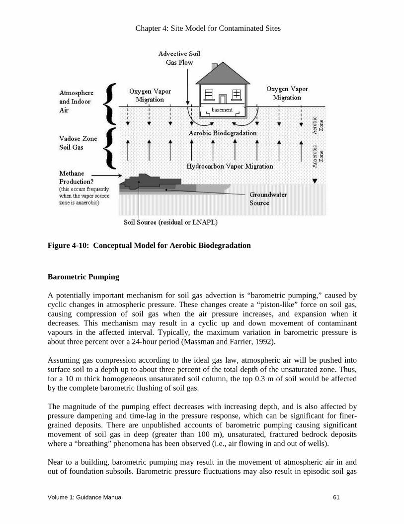
Chapter 4: Site Model for Contaminated Sites
Volume 1: Guidance Manual 61
Figure 4-10: Conceptual Model for Aerobic Biodegradation
Barometric Pumping
A potentially important mechanism for soil gas advection is “barometric pumping,” caused by cyclic changes in atmospheric pressure. These changes create a “piston-like” force on soil gas, causing compression of soil gas when the air pressure increases, and expansion when it decreases. This mechanism may result in a cyclic up and down movement of contaminant vapours in the affected interval. Typically, the maximum variation in barometric pressure is about three percent over a 24-hour period (Massman and Farrier, 1992).
Assuming gas compression according to the ideal gas law, atmospheric air will be pushed into surface soil to a depth up to about three percent of the total depth of the unsaturated zone. Thus, for a 10 m thick homogeneous unsaturated soil column, the top 0.3 m of soil would be affected by the complete barometric flushing of soil gas.
The magnitude of the pumping effect decreases with increasing depth, and is also affected by pressure dampening and time-lag in the pressure response, which can be significant for finer-grained deposits. There are unpublished accounts of barometric pumping causing significant movement of soil gas in deep (greater than 100 m), unsaturated, fractured bedrock deposits where a “breathing” phenomena has been observed (i.e., air flowing in and out of wells).
Near to a building, barometric pumping may result in the movement of atmospheric air in and out of foundation subsoils. Barometric pressure fluctuations may also result in episodic soil gas

Chapter 4: Site Model for Contaminated Sites
Volume 1: Guidance Manual 62
intrusion. If there is a low permeability surface seal adjacent to buildings, cross-foundation slab pressure gradients may be generated when the barometric pressure decreases. One study reported measured transient cross-slab differential pressures of up to 500 Pascals (Adomait and Fugler, 1997).
Stack and Wind Effect
The heating of a building, either by furnace, radiator, or other sources (i.e., sunlight on the roof) creates a “stack effect” as warm air rises in the building (Figure 4-11). This causes an outward air pressure in upper storeys and inward air pressure near the base of the building. Warm air that escapes is replaced by air infiltrating through doors and windows and soil gas migrating through the foundation. The magnitude of the depressurization at the base of the building is proportional to the height of the building, although tall buildings are designed with features to minimize cross-floor leakage of air and excessive depressurization.
Figure 4-11: Stack and Wind Effect on Depressurisation (NPL = neutral pressure line)
Elevator shafts may represent a preferential pathway both for soil gas intrusion at the base of the building (a drain is often present in the elevator pit) and for upward movement of air within the building. The force of wind on the side of a building will cause a positive pressure on the windward side of the building and a negative pressure on the lee side thus potentially resulting in a depressurised building.
Foundation Construction
Conceptually, different types of foundation construction could lead to different processes for soil vapour intrusion. For example, higher soil gas advection rates would be expected for houses with basements, due to higher depressurization and larger subsurface foundation surface area for intrusion. For houses with crawlspace foundations, the degree to which the crawlspace is ventilated by outside air and the influence of cross-floor mixing and leakage between the

Chapter 4: Site Model for Contaminated Sites
Volume 1: Guidance Manual 63
crawlspace and main floor could affect soil vapour intrusion rates. In cold climate areas, crawlspaces are more likely to be well sealed to reduce the influx of cold air into the house. Buildings with earthen floors are especially prone to vapour intrusion for chlorinated solvent chemicals, since there is a large surface area for migration of soil vapour into the overlying structure. For petroleum hydrocarbons, earthen floors are conducive to aerobic biodegradation because of efficient transfer of oxygen to subsurface, potentially counteracting the absence of diffusive barrier represented by the concrete foundation. Openings around utilities and a perimeter crack, often observed at the interface between the foundation wall and floor slab, also represent potentially significant entry routes for soil gas migration.
Although working hypotheses have been developed, the influence of foundation type on soil vapour intrusion is still poorly understood. However, there are empirical data indicating that soil vapour intrusion can be significant for several different types of building foundations including basements, crawlspaces and slab-on-grade construction. The importance of the foundation for vapour intrusion may depend on the distance from the contamination source to the building. For larger distances, the foundation may have little effect on vapour intrusion rate. For smaller distances or where contamination is close to or in direct contact with the building (e.g., sumps, wet basements), the foundation properties will tend to be significant.
Condominiums or commercial buildings may have one or more levels of below-grade parking. Since ventilation rates are high for parking garages, there will tend to be greater dilution of vapours that may migrate into the garage than for other building types.
Temporal and Seasonal Considerations
Temporal factors influencing soil vapour intrusion are complex. Higher building depressurization and soil gas intrusion rates would be expected during the heating season. Winter frost or higher soil moisture in near surface soils may limit the surface flux of volatiles to the atmosphere. As a consequence, the migration of soil vapour toward drier soils below the building may be enhanced. In some cases, intensive snowmelt or rain and wetting fronts can induce advective movement of soil gas, which may, in turn, cause nonequilibrium mass transfer of the contaminants between the water and the gas phases (Cho et al., 1993).
Surface soils with high moisture content may also reduce migration of atmospheric oxygen into soil, which may reduce aerobic biodegradation of hydrocarbon vapours. An off-setting factor is that during summer, near surface ground temperatures may be higher leading to slightly higher volatilization rates, since the Henry’s Law Constant is temperature dependent. The amplitude in seasonal temperature variation decreases with increasing depth below ground surface, and at many sites, temperature effects will be insignificant.
The influence of seasonal factors on building ventilation, which dilutes vapours, is difficult to predict. While natural ventilation through open doors or windows may be reduced in winter, there may be increased air exchange through building depressurization and operation of a furnace. There can also be significant short-term variability unrelated to seasonal factors caused by diel temperature fluctuations, occupant use (e.g., opening windows and doors), wind, and

Chapter 4: Site Model for Contaminated Sites
Volume 1: Guidance Manual 64
Common Mechanisms of Chemical Release to Surface Water
1. Point source surface and subsurface drainages and runoff from land-based disposal or storage sites
2. Nonpoint source runoff (i.e., overland flow) from urban, construction, logging, and agricultural areas
3. Inputs from unknown sources in tributary streams and wet weather conveyances
4. Continuous and intermittent effluent discharges (process and storm water)
5. Groundwater discharge to surface water
6. Atmospheric deposition
barometric pressure variations. On balance, the above factors suggest that in Canada, soil vapour intrusion would tend to be greatest during winter months based on climatic conditions.
Buildings and Tanks as Soil Vapour Sources
While the usual paradigm for soil vapour transport is upward migration from a contamination source located at or near the water table, if there is a surface contamination source, vapours will migrate in all directions, including downwards. Indoor air that is affected by contamination sources within a building may affect subsurface vapour concentrations if the building is positively pressurized (McHugh et al., 2006). In this case, air will move downwards through the foundation. Once below the building, vapours could diffuse away from the building, thus creating a zone of impacted soil vapour. While it would be rare for buildings to have a significant effect on subsurface soil vapour concentrations, a dry cleaner is one possible example of where this could occur. Leaking underground storage tanks also represent potential soil vapour sources.
4.5.7 Resources, References and Links
The USEPA has developed a number of on-line assessment tools for groundwater and soil vapour that include, for example, calculators for determining the groundwater hydraulic gradient, retardation factors for solute transport, plume diving, diffusion coefficients, Johnson and Ettinger alpha calculator and unit conversions. (http://www.epa.gov/athens/onsite/)
Conceptual Site Model for Surface 4.6Water Characterization
The objectives of this subsection are to: 1) provide an understanding of how a CSM is used to identify the likely location of COPCs at a specific study area where surface water is an environmental medium of interest; 2) identify the aquatic fate and transport mechanisms important to those COPCs; and 3) determine human and ecological receptors potentially exposed to COPCs in surface water and, hence, guide surface water sampling design.
If COPCs with widely varying physical and chemical properties are present on-site, information related to their solubility, octanol/water partition coefficient, Henry’s Law constants, etc. will aid in defining key transport and fate processes (e.g., evaporation, sorption) and sinks (i.e., depositories). If migration pathways are likely to be influenced by weather, climatic and meteorological data may enhance the CSM.

Chapter 4: Site Model for Contaminated Sites
Volume 1: Guidance Manual 65
Common and important sources of COPCs in surface waters at contaminated sites are listed in the Common Mechanisms of Chemical Release to Surface Water text box. Less obvious sources of COPCs, such as aerial transport and deposition, should not be overlooked, particularly for mercury and other trace contaminants for which atmospheric deposition is a key route of entry to surface water.
A surface water CSM is illustrated in Figure 4-12. Risk assessors are expected to modify this example or use their preferred presentation format for site-specific CSMs. The CSM depicted here is consistent with USEPA guidance (USEPA, 1995; 1996; 2000a; 2002) in that it illustrates:
• Known or suspected natural and anthropogenic stressors
• Chemical migration pathways
• Source and receiving media
• Human and ecological receptors.
• Potential reference sites.
Figure 4-12: Generalized Conceptual Site Model for Surface Water

Chapter 4: Site Model for Contaminated Sites
Volume 1: Guidance Manual 66
In addition, the narrative discussion accompanying any visual illustration of a CSM may detail study area impairment and likely causes, nature and extent of stressors (i.e., concentration, duration, spatial variability, temporal variability), and biogeochemical processes that may alter the bioavailability and toxicity of COPCs.
Several fate and transport processes are particularly important to consider when developing a CSM for surface water. Sources of contaminants in surface water include both point sources (e.g., leaking fuel storage tanks or accidental spills at industrial sites) and non-point sources (e.g., salt from road or parking lot run-off). Surface water is a unique medium in that surface water is rarely remediated; rather, inputs from other media are mitigated (e.g., control or remediation of contaminated groundwater that discharges to surface water, or remediation of contaminated sediment if sediment is the source of contaminants in surface water). It is important, therefore, to understand potential sources of COPCs in surface water, and the fate and transport processes that affect movement of COPCs in surface water. Potential sources (e.g., effluent, groundwater, sediment, and/or surface soil) should be considered during early stages to help inform the CSM and direct characterization efforts to the portion of the surface water body most likely to be affected. If groundwater discharging to surface water is suspected, it is helpful to identify areas or zones of likely or known groundwater discharge. Sorption/desorption characteristics of COPC, oxidation-reduction changes within the system, and volatilization of contaminants released to surface water are important processes to consider. If partitioning of COPCs from sediment is a concern, consideration of the physical characteristics of the sediment (e.g., organic carbon content) and potential movements of surface water (e.g., currents, tides, waves, flood events) is important in the development of the CSM. If bioaccumulative chemicals are present, uptake by biological organisms, and subsequent ingestion by human or ecological receptors, is also important to consider. Additional discussion of CSMs for biological characterization is provided in Section 4.8.
CSMs for study areas with significant surface water may warrant consideration of water body specific factors, such as lake thermal stratification, salinity barriers and stratification in estuaries, tides, seasonal flow and droughts, and storm flow in streams. CSMs for such study areas may also address COPC-specific considerations, such as batch or pulsed discharges of industrial effluents, peak flow discharge of municipal effluents, wet season seepage from landfills and buried wastes and the effect of tidal fluctuation (i.e., tidal pumping) on groundwater-surface water interactions in the coastal zone. Consideration of these factors will help focus sampling priorities during the study design phase. In addition, the narrative and/or pictorial CSMs for individual sites should acknowledge and discuss reference sites to which conditions at the contaminated site will be compared in the risk assessment.
4.6.1 Study Area and Reference Area Identification
CSMs for study areas with significant surface water may also consider one or more reference areas, as well as the natural and land use factors in the area that might influence surface water resources or provide a source of COPCs that might not originate at the study area.

Chapter 4: Site Model for Contaminated Sites
Volume 1: Guidance Manual 67
A study area refers to the body of water to be monitored and/or assessed, as well as adjacent areas (land or water) that might either affect the local conditions or be affected by releases from the investigated site (USEPA, 2001a). It is important to clearly define the boundaries of the study area, as the size of this area dictates the breadth and scope of the project and greatly influences the surface water sampling design. The study area should encompass the entire zone of impact associated with the site including wave, tide, and current activity, and should be large enough to allow the characterization of the severity of the impacts, in reference to an unimpacted or reference area (MOEE, 1996). However, if the study area is very large, as is typically the case for industrial harbours and marine systems, it can be subdivided into smaller areas to facilitate and focus site investigation activities; division of a study area into multiple sub-areas (exposure units or exposure areas) can also aid future site management decisions. Often in larger marine systems, the boundaries of the study area cannot be clearly defined until after initial sampling has delineated the site-related impact. In this case, the study area is operationally defined by taking into account potential site-related COPC movement in surface water due to wave, tide, and current activity and is much larger than the “final” study area. Chapter 5 (including Figure 5-1) further describes the process for defining a study area’s boundaries.2
A reference area is an unimpacted or relatively unimpacted area with physical and biological attributes similar to those of the study area, but for the release of site-related chemicals. Because of the practical difficulty in locating an ideal reference area, it is often necessary to select locations with COPC concentrations that are equivalent to regional background concentrations.
It is often advisable to select more than one reference area to represent the range of background conditions and/or the range of the site physical and biological characteristics, and to allow for more meaningful statistical comparisons. Evaluation of two or more reference areas will allow for a more accurate representation of true reference conditions. If only one reference area is identified, it is imperative to acknowledge the assumptions and limitations of this comparison (i.e., the assumption that this area is reasonably representative of other reference areas, and that multiple samples collected from this single reference area are pseudo-replicates rather than truly independent samples).
The selection criteria for reference areas should be defined a priori and may include (e.g., Apitz et al., 2002):
• Physical nature of soil or sediment (e.g., grain size, organic carbon content);
• Flow dynamics (e.g., fast vs. slow or no flow, flashiness, stream order);
• Chemical composition (e.g., contributions from road runoff, atmospheric deposition, naturally-occurring inorganic chemicals);
• Habitat type (specific aquatic or wetland habitats);
• Biological composition (e.g., benthic invertebrate communities:
2 Although the medium in this figure is soil, the process is similar for both terrestrial and aquatic investigations

Chapter 4: Site Model for Contaminated Sites
Volume 1: Guidance Manual 68
• Geomorphology (e.g., braided, meandering, channelized streams);
• Wetland classification (e.g., bog, fen, swamp, marsh, shallow water);
• Oceanographic conditions (e.g., currents);
• Tidal conditions (ebb vs. flood tide); and
• Proximity to the study area.
In lotic (flowing) systems, suitable reference areas are often located immediately upstream of the study area, beyond the influence of the site. In lentic (static) systems, a suitable water body or multiple waterbodies within the same watershed, but outside of the area of impact, should be targeted.
Comparisons between the study area and the reference areas are one means of determining the potential effects of site-related COPCs. Reference areas can help to differentiate off-site vs. site-related contributions of COPCs. Furthermore, reference areas provide a measure of background concentrations of chemicals, particularly those that may have a natural or anthropogenic, but not site-related, source (e.g., pesticide applications, road runoff, and atmospheric deposition) (Gandesbury and Hetzel, 1997). For example, if an ecological risk
assessment documented fish mortality in a pond that was affected by both site-related chemical releases and acid precipitation, concurrent evaluation of one or more reference ponds would be critical to understanding whether the chemical releases and/or the acid precipitation caused the observed fish mortality. As a second example, if a human health risk assessment predicted that risks from fish ingestion were unacceptable due to mercury in fish tissue, it would be important to accurately characterize the ambient (including anthropogenic but not site-related) mercury concentrations, in order to help ensure that risk management decisions will effectively mitigate risks.
Conceptual Site Model for Sediment Characterization 4.7
The objectives of this subsection are to: 1) provide an understanding of how a CSM is used to identify the likely location of COPCs at a specific study area where sediment is of interest; 2) identify aquatic fate and transport mechanisms for COPCs, and 3) to determine human and ecological receptors potentially exposed. The CSM will help guide sediment sampling design. It is often useful to develop more than one CSM for a given site, each highlighting different aspects, such as separate CSMs for human health and ecological processes or for different habitat types (e.g., wetland and stream areas or upland and aquatic habitats). A generalized CSM for a contaminated sediment site is shown in Figure 4-13. Risk assessors are expected to modify this example or use their preferred presentation format for site-specific CSMs. In addition, the narrative and/or pictorial CSMs for individual sites should acknowledge and discuss reference sites to which conditions at the contaminated site will be compared in the risk assessment.
Natural Background: Representative, naturally occurring concentrations of chemicals in the environment, primarily reflecting natural geologic variations.
Ambient Background: Representative concentrations of chemicals in the environment reflecting natural and regional anthropogenic (not site-related) sources of chemicals.
Chapter 4: Site Model for Contaminated Sites
Volume 1: Guidance Manual 69
Chemical types, sources, fate and transport, exposure pathways, and potential receptors are important considerations for sediment characterization. Section 4.1 provides a detailed summary of the types of chemicals associated with various anthropogenic and natural activities. Sources of sediment contamination are grouped as “point sources” and “nonpoint sources,” where the former are discrete and defined discharge points (e.g., outfall pipes, oil spills, and other direct releases) and the latter are diffuse (e.g., overland runoff, atmospheric deposition). Water plays a significant role in the fate and transport of sediment-associated chemicals. Surface water runoff, floods, groundwater upwelling, and water movements (e.g., currents, tides, waves) can suspend and redistribute sediment. Contaminated sediment can also serve as a source of chemicals to water, as natural and anthropogenic disturbances release chemicals associated with sediment particles or porewater into the water column. Other factors that influence transport of sediment and sediment-associated chemicals include:
• Bank erosion
• Instream erosion and accretion
• Bioturbation
• Uptake through the food chain
• Development or navigational dredging
• Propeller wash
• Currents and tides
• Ship or other groundings (e.g. log booms)
• Ice scour
• Surface water intakes and discharges
• Remedial activities

Chapter 4: Site Model for Contaminated Sites
Volume 1: Guidance Manual 70
Figure 4-13: Generalized Conceptual Site Model for Sediment Characterization
Sampling data and mathematical modelling may be helpful in predicting transport and fate of sediment and sediment-associated chemicals (USEPA, 2005a).
Many site-specific factors also influence the potential for exposure to and subsequent risk from sediment-associated chemicals. For example, sediment physicochemical properties, such as sediment particle size, organic matter content and composition, reduction-oxidation (redox) potential, and pH, dictate the amount and type of chemical(s) that may be present and bioavailable in sediment (see Sections 10.3.3 and 10.4.5 for additional discussion; Wenning et al., 2002; USEPA, 2007a). In addition, the adsorption of chemicals to sediment particles (and out of the water phase) is determined by the chemical-specific organic carbon partition coefficient (Koc), while the affinity of chemicals to bind with lipids is determined by the chemical-specific octanol-water partition coefficient (Kow). Consideration of these physical and chemical-specific properties, including volatility, are important in the development of the CSM and the determination of potential exposure pathways.
Examples of potential human receptors that may be exposed directly (e.g., incidental ingestion, dermal contact) or indirectly (i.e., through the food chain) to sediment-associated chemicals

Chapter 4: Site Model for Contaminated Sites
Volume 1: Guidance Manual 71
include recreational and subsistence harvesters of biota (i.e. fish shellfish and aquatic plants), people involved in recreational activities, such as, swimming, wading, walking and playing along the beach, and workers. Examples of pathways for human health exposure to sediment-associated chemicals include: fish/seafood ingestion, dermal contact, and incidental ingestion of sediment. Inhalation of volatile organic compounds (VOCs) and particulate matter derived from sediment tend to be minor or negligible pathways for human exposure to sediment-associated chemicals because: 1) air contaminants are readily diluted outdoors; and 2) the water that overlies sediment mitigates the generation of dust. However, sediment exposed at low tide or seasonal low water can be distributed by wind and be a source of inhalation concern. Exposure to sediment-associated chemicals could also occur if sediments are used to amend a garden.
For ecological risk assessments, valued ecosystem components (VECs) often include epibenthic and infaunal invertebrates, fish, birds, and mammals. Examples of pathways for ecological exposure include: diet, incidental ingestion, direct uptake from contact with the porewater or the water column, water consumption, dermal contact, and gill transfer. However, dermal contact tends to be a negligible exposure route for most avian and mammalian VECs, because contact is inhibited by the feathers, scales, and fur that cover most of the skin. Inhalation also tends to be a negligible exposure route for VECs for the same reasons discussed above for human receptors. However, inhalation and, to a lesser extent, dermal exposure may be significant pathways for benthic species exposed to sediment porewater (Fuchsman et al., 2001; Smith et al., 1996). For example, water ventilation may be a significant pathway, as large quantities of water pass through the gills, and equilibrium between body tissue and the medium occurs rapidly (de Voogt et al., 1991; USEPA, 2000a).
Conceptual Site Model for Biological Characterization 4.8
The purposes of this subsection are to: 1) provide an understanding of how a CSM is used to identify conditions where biological sampling is warranted; 2) identify the fate and transport mechanisms important to movement of COPCs into biological tissue; 3) identify types of target COPCs most commonly considered in biological sampling; and 4) describe types of biological sampling that are commonly pertinent to human and ecological risk assessment. Each of these objectives is important in guiding the design of biological sampling programs.
The biological pathways depicted in the CSM in Figure 4-14 are generally consistent with USEPA (1995; 1996; 2000; 2002a) guidance. This CSM is provided as a generalized example; risk assessors are expected to modify it or use their preferred presentation format for site-specific CSMs. Development of a site-specific CSM is useful in determining if biological sampling is warranted, and in identifying the appropriate type of biological sampling needed to characterize risk. One of the primary fate and transport mechanisms of greatest interest for biological organisms is the movement of a COPC from abiotic media (e.g., soil, sediment, or water) into biotic media (i.e., biological tissue). This is most commonly referred to as bioconcentration.
COPCs most commonly evaluated in biological sampling are bioaccumulative compounds, including organochlorine pesticides such as dichlorodiphenyltrichloroethane (DDT) and dieldrin, as well as polychlorinated biphenyls (PCBs), dioxins and furans, lead, and methylmercury. Other

Chapter 4: Site Model for Contaminated Sites
Volume 1: Guidance Manual 72
Figure 4-14: Generalized Conceptual Site Model for Biological Characterization
COPCs may be targeted, particularly if screening-level desk-top food chain calculations suggest that they may pose a risk to human or ecological receptors.
Such chemicals are taken up by biota from other media, including prey, surface water, sediment, air and soil. Exposure pathways through which biota may contact COPCs include ingestion of prey, sediment, soil and water, dermal contact with sediment, soil and water, gill exchange with water, and inhalation of air. Of these many pathways, prey ingestion often dominates all other pathways, particularly for bioaccumulative chemicals.
Fish and aquatic and benthic invertebrates are common receptor groups targeted for biological sampling in aquatic systems. Terrestrial invertebrates (e.g., earthworm) and small mammals (e.g., mice, shrew) are generally the most common target species for characterizing ecological risks in terrestrial systems. Common game species (e.g., gamebirds and deer) and/or plants also may be sampled to characterize human health and/or ecological risks
In general, species targeted for biological sampling are selected based on feasibility (e.g., presence, ease of capture, permissibility, available tools) and relevance to the risk questions

Chapter 4: Site Model for Contaminated Sites
Volume 1: Guidance Manual 73
posed by the risk assessment. Sampled species may reflect the selected VECs and/or the preferred dietary items of those VECs and human receptors. In addition, the narrative and/or pictorial CSMs for individual sites should acknowledge and discuss reference sites to which conditions at the contaminated site will be compared in the risk assessment, as well as the natural and/or land use factors in the area that might influence natural resources or provide a source of a chemical that might not originate at the study area. For example, in agricultural watersheds, nutrients (phosphorus and nitrogen), silt, pesticides and herbicides may impair water bodies and/or be sources of chemicals. Failure to recognize the influence of such conditions could lead to erroneous conclusions regarding the cause(s) of any impairment and/or misdirect the study design.
References 4.9
Abreu, L. 2005. A Transient Three Dimensional Numerical Model To Simulate Vapor Intrusion Into Buildings. A Dissertation Presented in Partial Fulfillment of the Requirements for the Degree Doctor of Philosophy, Arizona State University, May 2005.
Adomait, M., and D. Fugler. 1997. A Method to Evaluate Vapour Influx into Houses. Presented at AWMA 90th Meeting, June 8 to 13, Toronto, Ontario, Canada.
Agriculture and Agri-Food Canada, 2000. The health of our water - toward sustainable agriculture in Canada. Edited by D.R. Coote and L.J. Gregorich. Publication 2020/E.
Anderson, M. R., R. L. Johnson, and J. F. Pankow. 1992. Dissolution of dense chlorinated solvents into ground water: 1. Dissolution from a well-defined residual source. Ground Water 30(2), pp. 250-256.
Auer, L.H., N.D. Rosenberg,, K.H. Birdsell, and E.M. Whitney. 1996. The effects of barometric pumping on contaminant transport. J. Contaminant Hydrology. 24:145-166.
Bradley, P.M., S.A. Carr, R.B. Baird and F.H. Chapelle. 2005. Biodegradation of N-nitrosodimethylamine in soil from a water reclamation facility. Bioremediation Journal, 9(2): 115-120.
Canadian Council of Ministers of the Environment. 2008. Canada-Wide Standard for Petroleum Hydrocarbon (PHC) in Soil: Scientific Rationale. January 2008. PN 1399. Canadian Council of Ministers of the Environment, Winnipeg.
Charbeneau, R.J., and D.E. Daniel. 1993. Contaminant Transport in Unsaturated Zone (Chapter 15). In Handbook of Hydrology. David Maidment, Editor in Chief. McGraw Hill, New York.
Choi, J.W., and J. A. Smith. 2005. Geoenvironmental Factors Affecting Organic Vapor Advection and Diffusion Fluxes from the Unsaturated Zone to the Atmosphere under Natural Conditions. Environmental Engineering Science Volume 22, Number 1, 2005.
Chiou, C.T., L.J. Peters and V.H. Freed. 1979. A physical concept of soil-water equilibrium for non-ionic organic compounds. Science 206: 831-832.
Cho, H.J., P.R. Jaffe, and J.A. Smith. 1993. Simulating the volatilization of solvents in unsaturated soils during laboratory and field infiltration experiments. Water Resources Research, 29(10): 3329-3342.
Crowe, A.S., K.A. Schaefer, A. Kohut, S.G. Shikaze and C.J. Ptacek. 2003. Groundwater Quality. Canadian Council of Ministers of the Environment, Winnipeg.. CCME Linking Water Science to Policy Workshop Series, Report No. 2, 52 p.
Davis, G.B., B.M. Patterson and M.G. Trefry. 2009. Evidence for instantaneous oxygen-limited biodegradation of petroleum hydrocarbon vapors in the subsurface. Groundwater Monitoring and Remediation. 29(1): 126–137.
Domenico, P.A., and F.W. Schwartz. 1998. Physical and Chemical Hydrogeology. 2nd Edition. John Wiley and Sons, Inc.

Chapter 4: Site Model for Contaminated Sites
Volume 1: Guidance Manual 74
Environment Canada. 2001. Assessment Report - N-Nitrosodimethylamine. http://www.hc-sc.gc.ca/ewh-semt/pubs/contaminants/psl2-lsp2/nitrosodimethylamine/index-eng.php
Falta, R.W., B. Bulsara, J.L. Henderson and R.A. Mayer. 2005. Leaded-Gasoline Additives Still Contaminate Groundwater. Environ. Sci. and Technol., 39(18): 379A-384A.
Fetter, C.W. 2004. Applied Hydrogeology. Prentice Hall.
Garbesi, K., R.G. Sextro, W.J. Fisk, M.P. Modera and K.L. Revzan. 1993. Soil-Gas Entry into an Experimental Basement: Model Measurement Comparisons and Seasonal Effects. Environ. Sci. Technol. 27(3): 466-473.
Government of Canada. 2003. Canadian Framework for Collaboration on Groundwater, at p. 1.
Gorgy, T.A., L. Li and J. Grace. 2006. Fate and Transport of Polybrominated Biphenyl Ethers from Biosolids. ISSMGE 5th International Conference on Environmental Geotechnics, Cardiff, Wales.
Hassett, J.J. and W.L. Banwart. 1989. The sorption of nonpolar organics by soils and sediments. In: Reactions and movement of organic chemicals in soils. Sawney, B.L., and K. Brown, eds. SSSA Spec. Publ. 22. Soil Science Society of America Inc., Madison, WI.
Hassett, J.J., J.C. Means, W.L. Banwart and S.G. Wood. 1980. Sorption properties of sediments and energy-related pollutants. EPA-600/3-80-041. U.S. Environmental Protection Agency, Washington, DC.
Health Canada. 2007. Federal Contaminated Site Risk Assessment in Canada Part I: Guidance on Human Health Preliminary Quantitative Risk Assessment (PQRA). Contaminated Sites Division, Safe Environments Directorate, Health Canada, Ottawa.
Health Canada. 2010. Federal Contaminated Site Risk Assessment in Canada, Part VII: Guidance for Soil Vapour Intrusion Assessment at Contaminated Sites. Contaminated Sites Division, Safe Environments Directorate, Health Canada, Ottawa.
Hers, I., Zapf-Gilje, R., P.C. Johnson, and L. Li. 2003. Evaluation of the Johnson and Ettinger Model for Prediction of Indoor Air Quality. Ground Water Monitoring and Remediation, 23(2): 119-133.
Hers, I., J. Atwater, L. Li and R. Zapf-Gilje. 2000. Evaluation of vadose zone biodegradation of BTX vapours. Journal of Contaminant Hydrology, 46: 233-264.
Hers, I., D. Evans, R. Zapf-Gilje, and L. Li. 2002. Comparison, Validation and Use of Models for Predicting Indoor Air Quality from Soil and Groundwater Contamination. Journal of Soil and Sediment Contamination, 11(4): 491-527.
Johnson, P.C. 2005. Identification of application-specific critical inputs for the 1991 Johnson and Ettinger vapor intrusion algorithm. Groundwater Monitoring & Remediation, 25(1): 63-78.
Johnson, P.C., W. Kemblowski and R.L. Johnson. 1998. Assessing the Significance of Subsurface Contaminant Vapour Migration to Enclosed Spaces – site specific alternatives to generic estimates. API Publication.
Golder Associates Ltd. 2013. Investigation of Risks & Hazards of Methane Production from Environmental Releases of Motor fuel Ethanol and Ethanol-Gasoline Mixtures to the Soil & Groundwater Environment. API-Golder-UBC Ethanol Study, Submitted to American Petroleum Institute, Soil/Groundwater Technical Group, May 27, 2013.
Lowell, P.S. and B. Eklund. 2004. VOC Emission Fluxes as a Function of Lateral Distance from the Source. Environmental Progress. 23(1): 52-58
Massman, J., and D.F. Farrier. 1992. Effects of Atmospheric Pressures on Gas Transport in the Vadose Zone. Water Resources Research 28: 777-791.
McHugh, T., P.C. De Blanc and R.J. Pokluda. 2006. Indoor Air as a Source of VOC Contamination in Shallow Soils Below Buildings. Journal of Soil & Sediment Contamination, 15: 103-122.
Mendoza, C.A. 1995. Conceptual Models and Effective Transport Parameters for Long-term Vapour Transport in Heterogeneous Unsaturated Media. Presented at: Solutions ’95 IAH International Congress XXVI, June 5-9, 1995, Edmonton, Alberta.

Chapter 4: Site Model for Contaminated Sites
Volume 1: Guidance Manual 75
Millington, R.J. and J.M. Quirk. 1961. Permeability of porous solids. Transactions of the Farady Society, 57: 1200-1207.
National Research Council of Canada. 1988. Glossary of Permafrost and Related Ground-ice Terms. Technical Memorandum No. 142. Associate Committee on Geotechnical Research. Permafrost Subcommittee, Ottawa.
National Research Council (US). 1996. Rock Fractures and Fluid Flow: Contemporary Understanding and Applications. Committee of Fracture Characterization and Fluid Flow, U.S. National Committee for Rock Mechanics. National Academy Press, Washington, D.C.
Ostendorf, D.W. and D.H. Campbell. 1991. Biodegradation of hydrocarbon vapours in the unsaturated zone. Water Resources Research. 27(4): 453-462.
Patterson, B.M., and G.B. Davis. 2009. Quantification of vapor intrusion pathways into a slab-on-ground building under varying environmental conditions. Environmental Science and Technology. 43(3): 650–656.
Park, H.S. and C. San Juan. 2000. A Method for Assessing Leaching Potential for Petroleum Hydrocarbons Release Sites. Soil and Sediment Contamination, 9(6): 611-632.
Ririe, T., R. Sweeney, S. Daughery, and P. Peuron. 1998. A Vapour Transport Model That is Consistent with Field and Laboratory Data. In Proceedings: Petroleum Hydrocarbons and Organic Chemicals in Ground Water: Prevention, Detection, and Remediation Conference. Ground Water Association Publishing, Houston, TX: 299-308.
Robinson, R.A., and R.H. Stokes. 1959. Electrolyte solutions. Butterworths, London.
Roggemans, S., C.L. Bruce, and P.C. Johnson. 2002. Vadose Zone Natural Attenuation of Hydrocarbon Vapors: An Empirical Assessment of Soil Gas Vertical Profile Data. American Petroleum Institute Technical Report.
Rivett, M.O. 1995. Soil-gas signatures from volatile chlorinated solvents: Borden field experiments. Ground Water 33(1): 84-98.
Schwartz, W., and H. Zhang. 2002. Fundamentals of Ground Water. 1st ed. John Wiley & Sons. 592pp.
Schwarzenbach, R.P, P.M. Gschwend and D.M. Imboden. 2003. Environmental Organic Chemistry. John Wiley and Sons, Inc.
Science Advisory Board for Contaminated Sites (SABCS) (of British Columbia). 2006a. Approaches and Methods for Evaluation of Light Non Aqueous Phase Liquid Mobility. Report prepared by Golder Associates Ltd. (Hers, I., G. Patrick and M. Mailloux).
Science Advisory Board for Contaminated Sites (SABCS) (of British Columbia). 2006b. Approaches and Methods for Evaluation of Unsaturated Zone Contaminant Transport processes and Effects on Groundwater. Report prepared by Golder Associates Ltd (Hers, I., and D. Fredlund).
Silliman, S.E., B. Berkowitz, J. Simunek and M.Th. van Genuchten. 2002. Fluid flow and chemical migration within the capillary fringe. Ground Water 40(1): 76–84.
Snow, D.T. 1968. Rock fracture spacings, openings and porosities. J. Soil Mech. Found. Div. Proc. Am. Soc. Civil Eng. 94: 73–91.
United States Environmental Protection Agency (USEPA). 1996. Soil Screening Guidance: Technical Background Document, EPA/540/R95/128. Available at http://www.epa.gov/superfund/resources/soil/toc.htm
United States Environmental Protection Agency (USEPA). 2002. Draft Guidance for Evaluating the Vapor Intrusion to Indoor Air Pathway from Groundwater and Soils (Subsurface Vapour Intrusion Guidance). Office of Solid Waste and Emergency Response.
Wiedemeier, T.H., H.S. Rafai, J.T. Wilson and C.J. Newell, 1999. Natural Attenuation of Fuels and Chlorinated Solvents in the Subsurface. John Wiley and Sons, Inc., 617 pg.
Zheng, C., and G.D. Bennett. 1995. Applied Contaminant Transport Modeling Theory and Practice. Van Nostrand Reinhold.

Chapter 5: Soil Characterization
Volume 1: Guidance Manual 76
5 SOIL CHARACTERIZATION GUIDANCE
Context, Purpose and Scope 5.1
Soil is the main medium where contamination resides (source) and from where contaminants partition into groundwater and soil vapour. Understanding the presence, extent and characteristics of contamination in soil is therefore critical for understanding the ultimate fate and potential impact of the contamination on human and ecological receptors. For example, the measurement of chemical concentrations in soil may be required to evaluate potential human exposure through direct exposure pathways such as ingestion and dermal contact. The characterization of soil may also be required to evaluate the potential effect of contamination in soil on other media such as groundwater, soil vapour, indoor air and ambient air.
The primary purpose of this soil investigation guidance is to describe the approach and methods for acquiring representative data (Exhibit 5-1). Obtaining representative data is closely linked to the sampling design, which involves consideration of the scale at which samples are analyzed.
The sources of uncertainty in data should be understood, and effectively communicated to the risk assessor. Uncertainties may include those due to the variability in the contaminant distribution, those introduced through the sampling design, and methods used for sampling and analysis. As subsequently described in this chapter, uncertainty is reduced through the development of a conceptual site model that is updated as new information is obtained, an appropriate soil sampling strategy and design, and through statistical techniques to assist in sampling design and data interpretation.
The characterization of soil at contaminated sites should follow the characterization process described in Chapter 2, as outlined in the above text box. This guidance does not address laboratory analytical protocols since details are found in Volume 4. While the focus of this chapter is intrusive soil sampling, indirect methods such as geophysical techniques can be used to help to identify potential contamination zones and provide stratigraphic information. Guidance on confirmation of remediation sampling is provided in Appendix 5-1.
Additional guidance that is more specific to boreal forest, taiga and tundra, and cryosolic soils, as well as stony/shallow or organic and wetland soils can be found in Environment Canada’s Guidance Document on the Sampling and Preparation of Contaminated Soil for Use in Biological Testing (Environment Canada, 2012).
Soil Characterization
This chapter describes the planning, process and methods for soil characterization. The key elements and their corresponding sections in the chapter are:
• Conceptual site model development (5.2),
• Sampling design considerations and statistical methods (5.3),
• Soil sampling methods, soil description and field analytical methods (5.4 to 5.6), and
• Methods for data interpretation (5.7).
Related tools are the Soil Sampling Checklists in Volume 2, and Suggested Operating Procedure for Soil Sampling (SOP #2) in Volume 3.

Chapter 5: Soil Characterization
Volume 1: Guidance Manual 77
Conceptual Site Model for Soil Characterization 5.2
As discussed in Chapter 2, the first step of the site characterization process is the development of a conceptual site model (CSM), which through review of background information brings together information on historical, physical, chemical and biological components of the site characterization that will define a problem. For the purposes of risk assessment, it is essential that all sources of soil contamination and the inferred distribution of contaminants in soil be understood in order to assess potential exposure pathways.
There are considerations that make soil, as a media, different than groundwater or soil vapour, with respect to site characterization requirements (see Table 2-3). Of critical importance is that contamination in soil is often highly variable over relatively small distances. Whereas organic chemicals in groundwater tend to form plumes in a relatively predictable manner, soil contamination may be discontinuous and dispersed depending on the contamination source. Except for substances that are volatile or highly soluble, temporal changes in soil concentrations tend to be slow and generally inconsequential; therefore, temporal considerations tend not to be important for soil contamination.
Insight on the distribution of contaminants in soil can be gained through an understanding of the contamination source, contaminant type and site geology. Several examples illustrating the variability in contamination scenarios are described in the Example Contamination Scenarios text box. The contaminant distribution in soil will also depend on the site geology and heterogeneity. For example, soil contamination in fractured rock will be highly variable, whereas, soil contamination in deltaic sand deposits will tend to be less variable.
EXHIBIT 5-1: Characteristics of Representative Data
Representative soil data has the following characteristics:
1. Soil sampling locations must be selected based on a good understanding of past site activities and geological and hydrogeological conditions.
2. Samples must be collected using acceptable methods.
3. The chemical analyses must include all known and potential contaminants of concern determined through a detailed review of the site history.
4. The data must be validated and interpreted appropriately.
5. The uncertainty in the data must be described and preferably quantified.
A common flaw when using site investigation data in risk assessment is a reliance on tabulated results where data are non-representative. A validated result for an appropriate contaminant from a soil sample collected from the wrong location, may result in a risk assessment that is not representative of the site.

Chapter 5: Soil Characterization
Volume 1: Guidance Manual 78
The elements or components of the CSM should follow those listed in Table 2-1. Of particular importance for characterization of soil is information on filling at the site and soil layering. As intrusive investigations are completed at a site, the CSM should be updated, and data gaps and information requirements should be re-defined. Several phases of investigation may be necessary before the investigation objectives are finally satisfied, although as described in Chapter 2, an expedited site investigation process may be followed to reduce the number of phases required.
Soil Sampling Design 5.3
The sampling design describes the number of samples, and where and when samples should be collected. The goal of the sampling design is to provide representative data that are defensible for their intended use and decisions to be made. Representativeness may be considered as the degree to which data accurately and precisely represents the relevant characteristics of the target soil. As a general rule, the representativeness of a sampling program increases and the uncertainty decreases as the number of samples analyzed increases.
The objectives of soil sampling design can vary widely. Typically, the objectives for environmental soil sampling programs include:
• To characterize the nature and extent of contamination at a site;
• To support a decision about whether contamination concentrations exceed regulatory criteria, background concentrations, or a threshold of unacceptable risk;
• To estimate the mean or percentiles of contaminant concentrations in target soil (i.e., to use inferential statistics to quantitatively describe the population from which the data is collected), with a certain level of confidence;
• To determine whether the contaminant concentrations in two soil units can be considered to fall within the same population
Sampling Design Objectives for Risk Assessment
The site investigator, with input from the risk assessor, should develop sampling objectives that are consistent with the goals of the risk assessment. The objectives may be broad, for example, “determine whether metals concentrations in soil exceed a risk-based screening level”, or highly specific to the data needs and scale of interest for the risk assessment, for example “provide statistical estimates (upper confidence limit of the mean and 90th percentile) of the metals concentrations in upper 0.5 m of soil for evaluation of the direct contact pathway, and provide data on the fraction of organic carbon and grain size distribution”.
Example Contamination Scenarios
1. Historical Fill: Historical filling with waste soils may result in dispersed and approximately random “pockets” of contamination of varying size.
2. Fuel Spills: Leaking fuel storage tanks may result in irregular contamination zones within the unsaturated zone, which follow migration pathways that are influenced by site stratigraphy and a distinct layer of contamination at the water table.
3. Wind-borne contamination: A point emission source may result in near- surface contamination that follows a trend consistent with the prevailing wind direction. The concentrations will eventually diminish with increasing distance from the source.

Chapter 5: Soil Characterization
Volume 1: Guidance Manual 79
or not (i.e., whether the measured concentrations of the two units are similar or different for a given level of confidence);
• To identify possible “hot spots” (areas having high levels of contamination), and;
• To delineate hot-spots or areas where concentrations exceed regulatory criteria or thresholds of concern.
The efficient use of time, money and human resources are also important considerations for sampling design. A good design should meet the needs of the study with a minimum expenditure of resources.
A complete sampling design indicates the number of samples and identifies the geographic locations where these samples will be collected and the time points when samples will be collected. Along with this information, a complete sampling design will also include an explanation and justification for the number and the locations of the samples.
5.3.1 Representative Sampling Challenges
There are a number of challenges for the design of representative soil sampling and analysis programs. The soil concentrations at sites often exhibit a high degree of spatial variability and concentration distributions are typically skewed (e.g., lognormal) (Ott, 1990; Ott, 1995). Only a small volume and mass of soil is tested from a site. For example, for many chemical parameters, only five to ten grams of soil are subsampled from a 60mL to 250mL jar and analyzed. For many sites, this means decisions for site assessment and remediation are made on the basis of chemical analysis limited to a few hundred grams of soil. Relative to the total mass and volume of soil that could be analyzed, the quantity analyzed is miniscule.
The sampling representativeness can be improved through appropriate sample design for a site and careful field observations. The use of statistical methods or tools for data analysis can also help guide the sampling design and provide insight on the variability in contaminant concentrations at a site. Another approach for increasing sample representativeness may be to increase the density of samples analyzed. The analysis of a larger number of samples using less precise field analytical methods, compared to a smaller number of samples using more rigorous analytical methods, may be warranted for some sites
.
Influence of Sample Volume on Concentration Variability
A study reported by Gilbert and Doctor (1985) illustrates the influence of sample size on concentration variability and representativeness. Different volume subsamples, obtained from a five kilogram soil sample, were analyzed for metals content. The results below indicate the range in concentrations increased as the mass of the subsample analyzed decreased (average concentration of 1.92 ppm).
Subsample volume
(g)
Range of results for 20 individual subsamples
(ppm) 1 1.01-8.00 10 2.36-3.43 50 1.55-2.46 100 1.70-2.30
Adapted from Gilbert and Doctor (1985)

Chapter 5: Soil Characterization
Volume 1: Guidance Manual 80
Figure 5-1: Process for Defining Study Boundaries

Chapter 5: Soil Characterization
Volume 1: Guidance Manual 81
5.3.2 Sampling Design Strategies
An important part of the sampling design process is defining the geographical boundaries, the population of interest and dividing the site into strata based on distinct characteristics. The sampling design may also depend on whether there is surface or sub-surface contamination. An example of this process is shown in Figure 5-1. Depending on the sampling objectives, a probabilistic or non-probabilistic approach to soil sampling may be adopted (Environment Canada, 2012; USEPA, 2002). Several common probabilistic sampling designs that can be employed are shown in Figure 5-2. Knowledge of site history, visual inspections, and professional judgement is recommended for all sampling design strategies.
Figure 5-2: Some Common Two-Dimensional Sampling Designs
5.3.2.1 Non-probabilistic Sampling Non-probabilistic sampling, also referred to as targeted, convenience, or judgemental sampling (Environment Canada, 2012), is the subjective selection of sampling locations at a site based on historical information, visual inspection and best professional judgement. It is commonly used to screen sites for the presence or absence of a contaminant or to identify the contaminants present
Nested Random Sampling

Chapter 5: Soil Characterization
Volume 1: Guidance Manual 82
in areas likely having the highest concentrations (i.e., worst-case conditions); in both cases often only a small number of samples are collected and reliable site information exists. It is also typically the default sampling design in emergency situations when the goal is to quickly obtain data. This approach is selected when the sampling objective does not require statistical inference about the target soil (or underlying population) from which the samples are collected. A common example is the investigation of a known release from, for example, a former fuel-storage tank, which would initially involve sampling of soil and groundwater in the source area.
5.3.2.2 Probabilistic Sampling Probabilistic sampling is used when the sampling objectives for investigation and/or risk assessment require quantitative description of the contaminant concentrations in the target soil (i.e., the underlying population from which the samples are collected). For details on the use of inferential statictics for data interpretation, refer to Section 5.7. Probabilistic sampling strategies are more difficult and may require assistance of a statistician (Environment Canada, 2012). Examples of probabilistic sampling strategies are provided below.
Cluster Sampling
Cluster sampling is where samples are selected based on observations, site history or other rationale and each cluster is measured independently of one another. This approach is often conducted in areas of potential environmental concern in the early stages of site assessment to determine whether further assessment is warranted. Cluster sampling may not be representative of the whole population because samples would not have been selected at random, which would increase the sample error and potentially lead to bias in statistical calculations.
Random Sampling
Random sampling is where the sampling units are selected using random numbers. There is equal probability of selection of all possible units within defined boundaries of the area of concern. Random sampling has two primary limitations: (i) because all sampling points have an equal chance of being selected, sampling locations are not evenly dispersed across the site and therefore sample location coverage may be poor, unless a very large number of samples are taken, and (ii) random sampling ignores prior information or professional knowledge in the sampling process. Since random sampling is relatively inefficient, it is rarely used for characterising soil contamination.
Nested Random Sampling
Nested random sampling involves taking samples (primary units) using the simple random sampling technique and then taking aliquots of those samples (Figure 5-2). Nested random sampling allows for a lower error than cluster sampling, yet higher error than simple random sampling.

Chapter 5: Soil Characterization
Volume 1: Guidance Manual 83
Stratified Sampling
Stratified sampling relies on historical information, screening and prior analytical results to divide the sampling area into smaller areas called strata. Each stratus is more homogeneous than the site is as a whole. Strata can be defined based on various factors, including: historical site use and APECs, soil type, depth, contaminant concentration levels and knowledge on expected contaminant migration patterns for different media (e.g., groundwater, soil vapour, wind).
Systematic Grid Sampling
Systematic grid sampling involves subdividing the area of concern by using a square, rectangular or triangular grid and collecting samples from the nodes (i.e., intersections of the grid lines). The origin and orientation of the grid can be based on random selection. Systematic grid sampling is often used to delineate the extent of contamination and may be used to define contaminant concentration gradients. This design is also a practical method for designating sample locations and provides for uniform coverage of a site.
A potential shortcoming of grid sampling is the possibility of bias when there are cyclical patterns to contamination where the grid spacing is a multiple of the period to the concentration cycles. While this scenario is highly unlikely, if this is a potential concern, a different grid spacing for a portion of the site may be superimposed over the larger grid to assess this hypothesis.
Systematic grid sampling is commonly used over larger areas where contamination is dispersed and where there is a need to provide for sufficient sample coverage. Guidelines for sample spacing are provided in Figure 5-3 and Exhibit 5-2. Contamination scenarios where systematic sampling may be appropriate include fill deposits, surface contamination from airborne deposits or other surface deposition. When the initial starting point to the grid is randomly selected, systematic grid sampling is a probability-based method that may be used to derive statistical inferences. Grid sampling may also be used to delineate concentration gradients and trends.
Transect Sampling
Transect sampling is a special case of systematic grid sampling where certain specific spatial characteristics of the contamination are targeted. It is a valid approach where contamination is inferred to exhibit strong trends along a linear profile. Contamination examples where transect sampling may be used are airborne deposits that would preferentially occur along the prevalent wind directions in relation to an emissions source (e.g., smokestack), contamination derived from vehicles along a roadway, and soil along the base of a ditch. Since the concentration trends for each of the above scenarios will vary in a predictable manner, transects with appropriately spaced sampling locations can be used to effectively characterize linear trends.

Chapter 5: Soil Characterization
Volume 1: Guidance Manual 84
Summary of Sampling Design Considerations
Typically, the three most prevalent sampling designs for early stages of an investigation of potential soil contamination are non-probabilistic (or judgemental) sampling, systematic grid sampling and transect sampling. Often a combination of the above approaches is used.
The detailed investigation sampling design will depend on the current CSM, including results of the preliminary sampling, statistical analysis (where relevant), site specific geology, contaminants of concerns or potential concern, location of potential contaminant source, release and transport mechanism. During the detailed stages of an investigation, contamination delineation (in situ) sampling is often employed to define the limits of contamination previously identified at a site. Such sampling should consider both the vertical and lateral distribution of contaminants. The lateral sampling design may depend on the size of the contamination area. For smaller hot-spots, several step-out samples evenly spaced in a radial pattern (i.e., spokes of a wheel) are typically used for delineation purposes. Sampling may also be guided by real-time measurement technologies, as appropriate.
EXHIBIT 5-2: Guidance on Sample Spacing
The lateral sample spacing will depend on the characterization objectives, sampling design and, where applicable, statistical objectives. While it is not possible to prescribe sample spacings applicable to every site, provided below are recommended sample spacing considered reasonable for most sites:
Characterization Stage Investigation Objective Recommended Grid
Spacing
Phase II environmental site assessment
Investigate larger areas of suspected contamination
25 m to 50 m1
Phase III environmental site assessment
Investigate areas of known contamination with systematic grid approach
5 m to 20 m
Contamination delin-eation sampling
Delineation of localised contamination hot-spots
Step-outs in 3 to 4 directions at 5 m to 10 m spacing2
1 For large fill sites, with consistent sample observations, a smaller number of samples may adequately represent site soils. Reports should provide justification for reduced sampling frequency.
2 The spacing is dependent on the contamination level. A 5 m spacing should be used for concentrations that are greater than 10X the regulatory criteria. A larger spacing may be used for lower contamination levels.
Chapter 5: Soil Characterization
Volume 1: Guidance Manual 85
If the data analysis indicates a dispersed contamination scenario that is part of a single population, further systematic grid sampling may be warranted on a closer spaced grid to improve the level of confidence in the data. The statistical analysis described in Section 5.7 should be performed to determine whether this approach is valid.
For comparison purposes, reference background samples should also be collected away from the source of contamination (Rencz et al., 2011). Useful guidance on local background reference sites is provided in BC Ministry of Environment Technical Guidance 16 (BC MOE, 2005a).
Guidelines on sample spacing for Phase I and II ESAs are provided in Exhibit 5-2. Consideration should be given to the defined depth for surface soil as applicable to the site use for risk assessment as discussed in Section 2.6.4.
In accordance with the sampling objectives and considerations for risk assessment, the appropriate soil particle size fraction should be used for chemical analysis as discussed in Section 2.6.4.
To assist the reviewer, a checklist for items that should be included in the sampling design workplan is listed below:
� The physical location of each sample.
� The type of sampling design selected and rationale for each sampling location.
� Supporting statistical analyses.
� The approximate spacing between samples.
� The type of sample (e.g., discrete or composite).
� Parameters for chemical analysis.
� Volume of sample required (consult the laboratory).
� A description or reference to specific sampling protocol.
� Any deviation from recommended sample spacing provided above together with supporting rationale.
5.3.3 Statistical Methods for Sampling Design
Three different statistical methods or tools that can be used for sampling design purposes are described below. Statistical methods for interpretation of data are described in Section 5.7.
Search Sampling
Search sampling utilizes a systematic grid sampling approach to search for areas where contaminants exceed applicable criteria. The number of samples and the grid spacing are determined on the basis of the acceptable level of error (i.e., the chance of missing a hot spot). Search sampling requires that assumptions be made about the size, shape, and depth of the hot

Chapter 5: Soil Characterization
Volume 1: Guidance Manual 86
spots. The smaller and/or narrower the hot spots are, the smaller the grid spacing must be in order to locate them. Also, the smaller the acceptable error of missing hot spots is, the smaller the grid spacing must be. This, in effect, means collecting more samples. Once a grid spacing has been selected, the probability of locating an elliptically-shaped hot spot can be estimated from Figure 5-3. Conversely, if the acceptable probability of missing a hot spot is specified, then the size of the hot spot which can be located at that probability level can be determined.
Figure 5-3: Required Sample Grid Spacing Corresponding to Acceptable Probability (β) of Not Finding Contamination Hot-spot. G = grid spacing, L = half the length of long axis of an elliptical contamination source (radius if circle), S = length short axis/long axis contamination source (equal to 1 for a circular source) (from Gilbert, 1987). Minimum Sample Number for Statistical Hypothesis Testing
The sampling objective may require the use of statistical hypothesis testing. For example, the mean concentration of a contaminant concentration in target soil (i.e., the population from which soil is collected) should not exceed a regulatory criteria, or site versus background comparisons.
Search Sampling Grid Spacing Example
A historical review suggests the presence of buried waste on a site but the location is unknown. The waste area is assumed to be approximately circular in shape (S = 1) with a radius of 5 m (L = 5 m). The desired probability of not finding this hot-spot is 0.05. From Fig. 5-3, L/G is equal to 0.58. Therefore, the desired grid spacing is 8.6 m.

Chapter 5: Soil Characterization
Volume 1: Guidance Manual 87
Hypothesis testing and types of decision errors are described in more detail in Section 5.7.1. In general terms, the probability of a false positive decision is represented by α, and the probability of a false negative decision is represented by β. Based on these definitions, the probabilities of avoiding false positive and false negative decision errors are referred to as the confidence level (1-α) and the statistical power (1-β), respectively. For example, if the hypothesis testing is based on the null hypothesis that contaminant concentrations at a site under remediation do not meet regulatory standards but the null hypothesis is rejected, statistical power is the probability of correctly identifying that the site has been successfully remediated (i.e., concentrations are below the standard). Statistical power depends on number of measurements, standard deviation, and confidence level of the test (1-α).
Sample size formulas for different hypothesis tests are provided in USEPA (2002) and are available in statistical software tools such as ProUCL (USEPA, 2013a,b). The minimum number of samples required to achieve a specified confidence level at a defined minimum detectable difference (i.e., precision) may be estimated as shown in the Example of Statistically-Based Estimate Minimum Sample Number text box. Additionally, Appendix C of Environment Canada (2012) provides examples for calculating sample numbers for various sampling strategy case studies.
Geostatistical Methods
For some contaminated sites, the sampling design objectives include the use of geostatistical methods to quantify spatial dependences and/or to contour concentration data. Geostatistical methods can be used to estimate the area of contamination and therefore to direct more precise sampling if needed or can be used to estimate exposure concentrations.
Evaluating spatial dependence may be needed if statistical methods used in data interpretation assume independent data that are not spatially correlated (see Section 5.7.3). When there is a spatial dependence, concentrations of nearby samples will change less dramatically than those for samples spaced farther apart. If there is a significant spatial dependence relative to the sample grid spacing employed, sampling following a systematic grid design will produce biased estimates of the mean if they are not adjusted for the degree of spatial continuity (USEPA, 2002).
In simple terms, geostatistical analysis for contouring concentration data involves a two-step process. First, the spatial dependence in data is quantified through the use of a variogram or semi-variogram. The variogram is a plot of the variance of paired sample measurements as a
Example of Statistically-Based Estimate Minimum Sample Number
Lead contamination is associated with refinery sludge deposited at a site. The contamination is believed to be approximately randomly distributed within the fill. The desired confidence level (1-α) and power (1-β) are 95 and 80 percent, respectively. The standard deviation is estimated to range from 250 to 500 mg/kg, considered a reasonable range for a well-characterized site with reasonably uniform contamination. The applicable regulatory criterion for lead is 500 mg/kg. The minimum detectable difference is assumed to be 100 mg/kg. The minimum number of samples (using Wilcoxon Signed Rank Test) to fulfill the specified range in standard deviation, confidence level and power is between 47 and 181. This example illustrates the large number of samples that may be required to meet statistically-based criteria.

Chapter 5: Soil Characterization
Volume 1: Guidance Manual 88
function of the distance between samples. When there is little distance between points, the variability between points will be small. As the distance between points increases, the difference or variability between points increases. A variogram model is fit to the empirical data based on the observed relationship. From the empirical data and variogram model, the distance over which there is a spatial correlation in the data is determined. The second step of the geostatistical analysis is kriging, which involves estimating chemical concentrations for grid points or blocks in the area of concern as determined from the variogram model. The estimated point concentrations may then be contoured. Environment Canada’s Guidance Document on the Sampling and Preparation of Contaminated Soil for Use in Biological Testing (Environment Canada, 2012) provides a more detailed discussion on the selection and construction of a variogram, and data interpolation through kriging,
It is difficult a-priori to determine whether site contamination is amenable to a geostatistical approach and to determine the appropriate sample spacing. In some cases, an iterative approach may be followed where an initial grid spacing is chosen and data are analyzed using geostatistical methods. If there appears to be a weak spatial correlation that could potentially be improved through additional sampling, such sampling could be completed if the objective is to satisfy a geostatistical approach. Another option may be to initially employ a coarse grid with finer grid superimposed over a portion of the site to determine whether further sampling is warranted.
5.3.4 Discrete and Composite Samples
For the purposes of this document, discrete and composite samples are defined as follows.
A discrete sample is;
A sample obtained from a single sampling point or location, and is considered normally as being taken from a single use of the sampling tool used to obtain the sample.
A composite sample is:
A sample obtained by combining a number of discrete samples into one homogenized sample in order to represent the average concentrations of the area and volume of material over which the combined discrete samples were taken.
Soil is inherently variable spatially, with many elements displaying significant variability over distances as short as one metre, even in natural conditions. For characterization of contaminated sites, use of only discrete sampling can result in missing this short range variability and thereby making assumptions regarding the representativeness of the samples that are inaccurate and unsupportable. To achieve reasonably representative sampling using only discrete sampling, very large numbers of samples can often be required, which is often impractical. It therefore is often practical to combine a number of discrete samples into one composite that represents the area of concern. Care must be taken in the use of composite samples for characterizing contaminated sites such that important information is not lost in the compositing process, that meaningful areas of high concentration that should be identified are not averaged out by areas of low

Chapter 5: Soil Characterization
Volume 1: Guidance Manual 89
concentration, and that the composite sample is representative of the area being sampled and fulfills the objectives of the sampling program. A composite sample must be confined to a single soil unit and contamination zone, should be taken over a limited area and depth relevant to the sampling objectives, and generally should not straddle the interface between the unsaturated and saturated zone. Where this is not done (e.g. in some cases, defined sampling objectives and a fluctuating water table may make sampling across the interface unavoidable), the sampler should have a strong understanding of the rationale for, and implications of, sampling across the interface for the particular site specific situation.
The text box at right gives the requirements for an acceptable composite sample. For samples to be analyzed for volatile compounds, a discrete sample should be obtained from a single point. Unless all of the above requirements are met, the use of composite samples for in situ characterization is typically not recommended due to potential limitations caused by concentration heterogeneity and non-representative sampling caused by blending of soil with differing contamination properties. Additionally, consult jurisdictional authorities to determine the maximum allowable volume/size/area (or time for air or water samples) deemed appropriate for composite sampling, and whether adjustment of regulatory criteria (e.g. regulatory criteria ÷ number of discrete subsamples) is necessary when comparing composite samples to regulatory criteria.
Investigation Soil Sampling Methods 5.4
The two basic methods for investigation (in situ) soil sampling are excavation of test pits and drilling of boreholes. Test pits can be excavated by hand to shallow depths or by machine to deeper depths. Samples may be collected from the walls of the test pit when they are shallow and it is safe to do so in accordance with the project specific health and safety plan and as mandated by applicable regulatory agencies. An advantage of test pits is that more soil is exposed to the sampler enabling better visual inspection of soil horizons and possible contamination zones and collection of larger volume soil samples. The disadvantages of test pits are greater disturbance and depth limitations.
When boreholes are drilled, there are a number of methods for obtaining soil samples depending on the drilling method used. The preference for environmental investigations is methods that provide for continuous or near-continuous soil cores with a small to moderate degree of disturbance. Applicable methods meeting these criteria are roto-sonic or direct push (e.g.,
Requirements for use of composite sampling
A composite soil sample should meet all of the following requirements:
1. Collected from a single soil unit and contamination unit at one location.
2. Spatial extent over which discrete samples are collected is dependent upon sampling objectives.
3. From ground surface to 1.5 m depth, obtained over a maximum 0.5 m vertical interval; below 1.5 m depth, obtained over a maximum 1 m interval.
4. Not collected across the interface between the unsaturated and saturated zones.
5. Not made up of a mixture of contaminated and non-contaminated material as determined from field observations and tests.

Chapter 5: Soil Characterization
Volume 1: Guidance Manual 90
Table 5-1: Description of Common Soil Sampling Methods
Method Description Comments Roto-sonic Vibrating and rotating
core barrel provides for continuous soil core (typically 100 mm diameter).
• Continuous soil core possible • Can obtain sample from significant
depths and from dense soils • May heat up soil core (potential loss of
volatiles) • Provides slightly disturbed soil samples
with some fines migrating to the outer core edge
Geoprobe Vibrating core barrel provides for continuous soil core (typically 38 mm diameter).
• Continuous soil core possible • Depth limitations, also not possible to
obtain samples for very dense or coarse soils
Split Spoon Hollow stem augers are drilled to desired depth, split spoon sampler driven into soil (typically 0.45 m long, 38 mm diameter).
• Common technique • Sample recovery may be poor for certain
soil types (e.g., unconsolidated sands) • Moderately disturbed soil sample
Auger Obtain samples directly from auger flights removed from borehole.
• Quick method • Poor method for environmental sampling • Cross contamination may occur due to
smearing and sloughing of soil into open borehole
• Sample depth somewhat inaccurate • Sample recovery may be poor for certain
soil types (e.g., unconsolidated sands) • Disadvantages increase with increasing
depth • Not appropriate for sampling volatiles in
soil Shelby Tube Thin-walled tube with a
tapered cutting head pushed into soil.
• Typically used for geotechnical investigations, but may also be used to obtain samples for chemical analysis
• Undisturbed sample • Only applicable for soft soils
Air Rotary cyclone
Soil cuttings obtained at surface from cyclone.
• Highly disturbed sample • The sample depth cannot be controlled
and is inaccurate • Poor method for environmental sampling • Not appropriate for sampling volatiles in
soil

Chapter 5: Soil Characterization
Volume 1: Guidance Manual 91
GeoprobeTM) methods or split spoon samples taken at a relatively high frequency. The least preferred methods are those where the soil sample is highly disturbed (e.g., samples obtained from the cyclone of an air rotary drill rig). The common soil sampling methods associated with drilling boreholes are summarized in Table 5-1.
The field description of soils is an important component of an investigation program. These descriptions, which are prepared at the time of sampling, are vital in that they provide a basis for identifying possible contamination, selection of samples for field screening and laboratory analysis, and interpretation of chemical testing results. There are numerous soil classification systems including those based on engineering properties (used by geotechnical engineers) such as the one described in the Canadian Foundation Engineering Manual (Canadian Geotechnical Society, 2006) and the Unified Soil Classification System (ASTM, 2006) (used predominantly in the US), and those based on soil genesis and morphology such as the Canadian System of Soil Classification (Agriculture and Agri-Food Canada, 1998) and the US Department of Agriculture taxonomy-based soil classification system. One method should be chosen, communicated to and understood by field personnel, documented and followed.
For environmental investigations, geotechnical soil classification systems are typically modified for soil classification and description. Geotechnical soil classifications divide soils into coarse- and fine-grained; coarse-grained soils (sand, gravel and cobbles) are subdivided by the grain size distribution whereas fine-grained soils (silt and clay) are typically classified through their plasticity. A basic geotechnical engineering soil description will include compactness for coarse-grained soils, consistency for fine-grained soils, and in-situ moisture content, colour and soil type for both coarse- and fine-grained soils. Other features that are often described are soil fabric or structure, particle shape, grading, weathering and bedding features. When known, the geological stratigraphic name of the unit (e.g., “Ottawa formation”) can also be provided. For fine-grained soils, there are several field tests (dilatency, toughness, plasticity and dry strength) that provide additional information on soil properties and the clay and silt content. The preference of this guidance is a hybrid system consisting of the geotechnical system described in Canadian Geotechnical Society (2006) combined with the environmental descriptors below
A checklist for description of soil for environmental investigations is provided below:
� Moisture Content: the soil moisture should be described as dry, damp, moist, or wet.
� Colour: qualitative description of colour or determined with the use of a colour chart (e.g., Munsell).
� Mottles: blotches or spots of contrasting colour interspersed with the dominant soil colour.
� Soil composition: this is the relative amounts of boulders, cobbles, sand, silts and clays in a soil.
� Particle shape: shape of individual soil particles.
� Structure or Fabric: shape of the natural soil aggregates including bedding orientation and thickness, occurrence of joints and fissures, voids, plant roots and root holes.

Chapter 5: Soil Characterization
Volume 1: Guidance Manual 92
� Debris: examples are woodwaste, metal, ash, paint flakes, clinker and asbestos; the type and approximate percentage of debris within the soil horizon should be noted.
� Odour: to the extent possible describe the type of odour (e.g., diesel-like, sweet, pungent) and strength (faint, moderate, strong).
� Staining: describe the colour and intensity of staining where there is evidence for discolouration caused by contamination.
� Fuels or Solvents: presence of visible oil, gasoline, solvents or other organic liquids.
� Compactness or consistency (optional): soil strength (coarse-grained) or degree of resistance to breaking or crushing (fine-grained).
� Horizon thickness: layers of soil with distinct changes of the above features.
Field Analytical Methods 5.5
There is an emerging suite of field analytical methods that can be used to evaluate chemical concentrations in soil at contaminated sites. The field methods range from relatively simple screening tests, such as headspace vapour tests and colourimetric tests, to relatively sophisticated analyses, where equipment that provides for low-level analyses using techniques such as atomic adsorption spectrometry (AAP) or gas chromatography/mass spectrometry (GC/MS) is deployed in the field. Over the past decade, there have been significant developments in the area of sensors including x-ray fluorescence, biosensors and electrochemical detectors for metals analyses, and ultraviolet (UV) fluorescence, laser-induced fluorescence and spectrometry for organic analyses (USEPA Technology Innovation Program: Site Characterization and Monitoring Webpage http://www.epa.gov/superfund/remedytech/char.htm; Reible and Demnerova, 2002).
The objective of this section of the guidance is to describe four relatively common field techniques used for assessment of soil contamination, which are headspace vapour, colourimetric and immunoassay tests for organic compounds and x-ray fluorescence (XRF) for metals. Headspace vapour tests for VOC are the simplest field test but provide for the lowest level of quantification, whereas, colourimetric, immunoassay and XRF techniques (metals) provide for a higher level of quantification.
The potential advantages of these field analytical methods include near real-time results and potentially lower costs. Field analytical methods may be effective for follow-up phases of a site characterization program when a higher sampling density, but less precise data, is desired and acceptable, or during the site remediation phase where near real-time results can facilitate more timely and effective decision-making.
The potential disadvantages of field analytical methods include regulatory and stakeholder acceptance. An initial study involving a comparison of field methods and laboratory testing results using site samples is often required to verify the performance of the field method. The verification testing should be conducted on a sample set of sufficient size to draw statistical inferences, which generally will consist of at least 15 to 25 samples. It may also be important to

Chapter 5: Soil Characterization
Volume 1: Guidance Manual 93
conduct verification testing as a first stage pilot test and to then conduct periodic checks during the course of a field program.
Some field analytic methods require a reasonably high level of training for field personnel. It is essential that the training, quality control and testing procedures for field analytical testing be thoroughly documented.
5.5.1 Headspace Vapour Tests
Field headspace testing using detectors that measure organic vapours is a common method of screening soil samples for volatile or semi-volatile organic compounds. The procedure involves collecting a soil sample, placing it in an air-tight container (glass jar or polyethylene bag) and then analyzing the headspace vapour using a portable analytical instrument. The headspace is the air-filled part of the sample (i.e., the container is only partially filled with soil).
The recommended test procedure is as follows:
1. Fill a clean 250 to 500 ml jar half-way; a larger jar is preferred when the sampling method provides for sufficient soil.
2. Seal the jar using two sheets of aluminum foil.
3. Shake the sample jar for about ten seconds.
4. Wait between 15 and 30 minutes to allow chemicals in soil to volatilise into the headspace. If ambient temperatures are below 0oC, place the samples in a heated building or vehicle.
5. Puncture the seal with the probe tip and record the maximum vapour concentration measured using a field detector.
6. The headspace vapour test results should be recorded on the borehole or test pit logs.
Headspace vapour tests can be performed using either photoionisation detector (PID) with 10.2 eV or higher energy lamp, flame ionisation detector (FID) or explosimeter. For headspace vapour tests, a PID or FID may be preferred due to typically lower detection limits that can be achieved. Care must be taken when using PIDs since a positive bias may result due to moist air and/or dust being drawn into the instrument. FIDs are not sensitive to water vapour, but require a hydrogen source to operate. When using hydrogen gas, applicable regulatory requirements for transportation and storage must be followed. The instrument characteristics should be understood and instruments calibrated daily (or more frequently) in accordance with the manufacturers specifications prior to use. Typically, PIDs are calibrated using a 50 ppm or 100 ppm span gas (e.g., isobutylene). In cases where elevated VOC concentrations in ambient air could affect the calibration process, zero gas (certified clean air) must be used for “zeroing” the instrument. It is also good practice to regularly analyze a field blank consisting of moist clean soil placed in a jar that is tested using the above procedure.
The advantage of field headspace testing is that it is a simple, rapid and low cost technique. The field headspace results can be used to help select samples for analytical testing. The

Chapter 5: Soil Characterization
Volume 1: Guidance Manual 94
disadvantages include that it is non-quantitative and only provides a relative indication of potential volatile or semi-volatile compound concentrations for similar soil types and contamination. Although the test is simple, it is essential that standardised procedures are consistently used and that the test methods be documented (i.e., size of jar, soil volume, equilibration time, temperature).
5.5.2 Colourimetric Tests
Method Description
Colourimetric tests refer to chemical reaction-based indicators that are used to produce compound reactions to individual compounds, or classes of compounds. Colourimetry is generally performed by mixing reagents in specified amounts with the soil sample to be tested and observing the color change in the slurry solution. The intensity of the color change is an indicator of the concentration of the chemical of interest. The color change is either observed visually through comparison with colour charts or electronically with a hand held colorimeter. Colourimetric test kits have been developed for total petroleum hydrocarbons, total PAHs and certain explosive contaminants. There are USEPA SW-846 methods for RDX and HMX in soil (Method 8510) and trinitrotoluene in soil (Method 8515) (USEPA, 1996).
Application
Since the detection limits are generally in the low ppm range, these field test kits are primarily used as a semi-quantitative screening tool for site characterization or to guide site remediation. The advantages of colourimetric tests are that they are relatively simple to perform and provide for near real-time results. The disadvantages with colourimetric tests include higher detection limits (depending on the kit) and possible interference by other co-contaminants, naturally occurring chemicals and organic matter. The site-specific method performance should be evaluated through comparisons between colourimetric test results and laboratory analytical results.
5.5.3 Immunoassay Tests
Method Description
Immunoassay field kits are a rapid screening tool that provide for qualitative or semi-quantitative results for specific compounds or groups of compounds. Immunoassay tests are designed to detect specific chemicals by measuring the chemicals’ response to specific antibodies. The antibodies are developed to be specific to individual compounds such as individual pesticides or chlorophenols (e.g., pentachlorophenol) or compound groups such as PAHs, PCBs or petroleum hydrocarbons. The antibodies do not respond to dissimilar substances; however, there may be cross sensitivities to compounds with similar properties. Functionally, the test is usually performed by adding a sample to a test tube coated with antibodies. A chemical reagent is then added to the test tube that reacts with enzymes released by the antibodies. The colour change in an extracted solution in response to the enzymes is related to the specific contaminant

Chapter 5: Soil Characterization
Volume 1: Guidance Manual 95
concentration. Quantification is either determined through visual inspection or through use of a spectrophotometer.
Many immunoassay test kits have undergone significant validation (USEPA technology verification (ETV) program) and are USEPA SW-846 Methods (4000 series). There are SW-846 method immunoassay kits for the following analytes:
Analyte SW-846 Method Pentachlorophenol (PCP) 4010A 2,4 Dichlorophenoxy Acetic Acid in soil 4015 Polychlorinated Biphenyls (PCBs) in soil 4020 Total Petroleum Hydrocarbons (TPH) in soil 4030 Polynuclear Aromatic Hydrocarbons (PAH) in soil 4035 Carcinogenic PAH in soil 4035 Toxaphene in soil 4040 Chlordane in soil 4041 DDT in soil 4042 Trinitrotoluene (TNT) in water and soil 4050 Hexahydro-1,3,5-Trinitro-1,3,5-Triazinc (RDX) in water and soil 4051 Triazene in water 4670 If properly utilized, some immunoassay tests allow for analysis of specific organics to sub-parts per million (ppm) levels in soil and sub-parts per billion (ppb) levels in water.
Applicability
The advantages of immunoassay tests are near real-time results (typically less than a 30 minute test), relatively low cost, and ability to rapidly screen a large number of samples. They are most commonly used during follow-up phases of a site characterization program when a higher sampling density is warranted or during the site remediation phase (e.g., to guide an excavation program).
The disadvantages of immunoassay tests are that the technology is not compound specific for organic chemicals such as PAHs and PCBs, and for compound specific tests for pesticides there may be cross-sensitivities to similar compounds that cause false positives. For this reason, the types of contaminants present at a site and the concentration ranges must be reasonably well known to determine if immunoassay tests are appropriate. The detection limits for immunoassay tests for some compounds are similar to conventional laboratory analyses (e.g., 0.1 to 1 ppm for PCBs for some test kits) while for other compounds are higher than laboratory detection limits. The immunoassay test process can also be sensitive to the type of matrix. For example, the test may not work well in clay soils when contaminants are strongly bound to clay particles. Immunoassay tests, although relatively simple, do require that the operator conducting the tests be adequately trained and the tests must be carefully performed to ensure accurate and repeatable results. The training, testing and quality control procedures should be documented.
Chapter 5: Soil Characterization
Volume 1: Guidance Manual 96
5.5.4 X-ray fluorescence (XRF)
Method Description
X-ray fluorescence (XRF) is a rapid screening tool that is used to determine concentrations of major and trace elements in soil. The principle behind this process is simple: when an X-ray emission from a radioactive source strikes an atom in the sample, energy is absorbed by the atom. If the energy is high enough, electrons will be displaced with the result being an x-ray with energy unique to the elements present. The x-ray emitted is detected by a fluorescence detector, which can either be a wavelength dispersive spectrometer, where the photons are separated by diffraction on a single crystal before being detected, or energy dispersive spectrometers (EDX or EDS), where the detector allows the determination of the energy of the photon when it is detected. The XRF technology is limited to certain trace and major elements. Although a range of trace and major elements can be simultaneously detected, there are potential cross sensitivities or interferences that may influence the accuracy and precision of the method.
Specific methodology has been developed by USEPA (Method 6200) to guide XRF analysis. Technology verification studies indicate the performance of XRF is variable depending on the element, matrix and instrument (USEPA, 2006b; USEPA, 2004). The detection limits generally range between 5 ppm and 500 ppm. For some elements, verification studies indicate precision and accuracy for certain XRF instruments are similar to that obtained by atomic absorption spectrometry (AAS) laboratory analysis (USEPA, 2006b). Over the past decade, advances in detector technology have improved detection limits and precision and speed of analyses using hand-held XRF detectors.
Applicability
The advantages of XRF include real-time results, when used in scanning mode on surface soil, or near real-time results when soil samples are collected and analyzed (i.e., less than 20 minutes per test) and typically lower cost than laboratory methods. The sample preparation requirements for XRF testing are relatively minimal and consist of drying and pulverising of the sample. The XRF technique is non-destructive so selected samples can be sent to the laboratory for verification analysis. XRF is most commonly used during the follow-up phase of a site characterization program when contaminants of potential concern have been identified and when a higher sampling density is desired. Investigation scenarios where XRF may be employed include surface trace and major elements contamination associated with airborne deposits, paint flakes containing lead, or trace and major element contamination associated with mining or mineral-processing wastes.
The disadvantages of XRF include higher detection limits than laboratory analyses and possible cross-sensitivities for certain trace and major elements. The soil matrix and moisture can influence results, although this can be improved through drying, sieving and milling or pulverising the sample. It is generally advisable to perform a pilot test where split samples are analyzed using XRF and laboratory methods. Persons using some XRF detectors must have appropriate certification and training for radiation-emitting equipment. It is also necessary to calibrate each unit for specific soil and/or sediment matrix. This step is usually carried out in

Chapter 5: Soil Characterization
Volume 1: Guidance Manual 97
preliminary detailed but small scale studies of a site of interest, where limited number of soil or sediment samples are collected and analyzed by laboratory based analytical methods (atomic absorption) and then those results are used to calibrate the field based XRF unit.
Field Preservation of Soil Samples for VOC Analysis 5.6
Traditional collection of bulk soil samples for VOC analysis involves filling small glass jars (50-100 ml), using a spatula type scoop, to the top with no voids or headspaces and then closing jars with a septum sealed screw cap. Samples are immediately cooled to ~ 4°C and stored up to 14 days.
Since the establishment of generic guidelines and analytical methods for VOC determination in the early 1990's, scientific evidence has shown that the failure to use proper methods to preserve soil samples during sample collection and storage can result in substantial losses of VOC content of 90% or more, and consequently, substantial underestimating of concentrations (i.e. biased low) (Minnich et al., 1997; Ball et al., 1997; USEPA, 1997; Hewitt, 1999; Sorini et al., 2002). Losses are primarily due to volatilization and biodegradation. To counteract VOC losses, especially for low concentrations of VOCs, USEPA methods now require use of field preservation methods that include methanol or sodium bisulphate (NaHSO4), or hermetically sealed samplers. Most US states and Ontario have followed suit.
Because of this, the Ontario Ministry of the Environment and Climate Change has endorsed field preservation and this is also the recommended procedure in Volume 4. Field preservation as per USEPA Method 5035 and 5035A, using pre-weighed vials containing methanol, is the preferred option provided the Laboratory Reporting Limits meet the CEQGs for VOCs. If the CEQG value can’t be achieved either pre-weighed vials containing aqueous sodium bisulphate or hermetically sealed vials are used. Jurisdictions in Canada should be contacted to see if field preservation methods for reducing losses of volatiles are recommended, such as using methanol or freezing of soil samples destined for VOC analysis.
US EPA Method 5035 and 5035A describe field equipment, sample collection, preservation, and storage advice for field preservation techniques which involves using an acceptable sample collection device (e.g.
coring tool) to collect a 5 g sample and extruding it into a pre-weighed Volatile Organic Analysis (VOA) vial containing acidified (with sodium bisulphate) organic-free reagent water for collection of low concentration VOC samples (0.05 to 200 μg/kg), or purge–and-trap grade methanol for collection of high concentration VOCs (> 200 μg/kg). Potential disadvantages of the acidification process are, the production of acetone, acidification may result in the loss of certain VOCs (e.g. 2-chloroethylvinyl ether), and certain soils may effervesce. As a result, USEPA method 5035A describes alternate collection methods (without acidification) of low concentration VOC samples using either “empty vial” techniques or VOA vials containing reagent water only, or use of an hermetically sealed sampler. In the latter preservation-free method, extrusion (within 48 hours of collection) occurs in the laboratory into a VOA vial containing either methanol, or sodium bisulphate or as preservation for later VOC analysis.

Chapter 5: Soil Characterization
Volume 1: Guidance Manual 98
When collecting soil samples not using the traditional bulk soil collection approach, an additional sample is required for moisture content determination.
Holding times are 14 days for methanol or NaHSO4 preserved sample cooled to ≤ 10°C (in transit), and 48 hours when a hermetic sampler is used as a transport device, and cooled to ≤ 10°C (in transit). Freezing has also been identified as a possible preservation technique but has not been fully validated. Deviations from standard protocols should be identified together with supporting rationale. Volume 4 of this guidance describes appropriate sample handling and storage for VOCs in soil, as well as, recognized methods for sample introduction and analysis.
For more guidance on the collection, preservation, and storage of soil VOC samples, consult Method 5035A Appendix A, and the American Society for Testing and Materials (ASTM) Method 4547-98 “Standard Guide for Sampling Wastes and Soil for Volatile Organic Compounds”. Although these documents discuss some traditional approaches, their focus is on providing guidance on newer sample collection and preservation methods including methanol, NaHSO4, and freezing (in Method 5035A; “ASTM D 4547-98 and Method 5035 briefly mention freezing, but do not endorse it because data were not available at the time of their publication to support preservation by freezing”).
Numerous other regulatory agencies have also adopted protocols for field preservation (New Jersey Department of Environmental Protection, 1997; Massachusetts Department of Environmental Protection, 1999; California Regional Water Quality Control Board, 1999). Videos of methanol preservation and EnCoreTM sampler training (i.e., hermetically sealed coring device) are available at http://vimeo.com/ennovativetech.
Methods for Data Interpretation 5.7
General descriptive techniques may be used to summarize the data and provide data visualization with respect to the temporal and spatial distribution of COPC concentrations in study area. Such techniques generally consist of data compilation (i.e., tabulation and preparation of summary tables), and plotting or graphing data with respect to time, location, key sources of COPC, etc. Simplistic plotting and other visual techniques of data presentation often reveal trends that guide and refine further sampling efforts.
The data quality and consistency should be evaluated to determine whether there are data gaps or quality issues that warrant additional testing. The COPC concentrations will also typically be compared, individually, to risk-based generic (if available) or site-specific criteria. If the laboratory analytical data includes non-detect values, the detection limit (DL) should be used for comparison to the applicable criteria. Methods for dealing with data-sets containing non-detects when performing statistical analysis is described in Section 5.7.2.
Exploratory data views should be completed (Chapter 2) and summary statistics may be calculated for each data set. ProUCL is an example of available statistical software tools that can be used for plotting and analysis of data (USEPA, 2013a,b see Section 5.9). When sufficient data is available for statistical analysis and the dataset represents a single population, a statistical evaluation of soil quality is justified. There are a number of approaches that may be used to

Chapter 5: Soil Characterization
Volume 1: Guidance Manual 99
evaluate population characteristics of a data set including a review of historical information, contaminant migration characteristics, and the statistical techniques described below. Soil that has become contaminated by similar processes and events will likely have contamination concentrations that represent a single population.
Comparison of study area conditions to reference conditions can take two forms: a comparison of individual results to a threshold value, or a statistical test that checks for significant differences between study area and reference area datasets. Threshold tests, based on a tolerance interval or a specific percentile of the reference dataset, are most commonly applied to identify specific locations with elevated concentrations (i.e., to delineate hot spots). A qualified statistician should design and implement statistical analyses based on the project goals and the applicability of the data to the statistical techniques under consideration.
The remainder of section 5.7 focusses on statistical methods to evaluate data populations and distributions, and statistical tests that can help draw conclusions from site data. The appropriate jurisdiction should be contacted for advice on how to proceed in interpreting site data in cases where there is insufficient data (or assumptions invalidated) to perform statistical analysis, or where jurisdictional policy does not support the use of statistics for decision making, for example, jurisdictions may favour a pass/fail method based on individual site samples rather than summary statistics of the whole site for defining what constitutes a contaminated site.
5.7.1 Statistical Data Analysis for Soil Characterization
Frequency Distributions and Histograms: These techniques can be used to evaluate whether there is the potential for multiple populations. For example, a large gap in a frequency distribution plot may indicate separate populations.
Boxplots (or box and whisker plots): These plots are useful for comparing various data sets for the same parameter (e.g., arsenic concentrations from different AEC locations) and for the identification of potential outliers in a given data set. Although high concentration values may appear to be anomalous, great care must be taken when considering whether to remove apparent outliers from a data set. Such data may represent hot-spots that comprise a separate population.
Goodness-of-Fit Tests: Goodness-of-fit tests are used to test whether data follow a specific distribution, or how "good" a specified distribution fits the data. As noted in Section 2.8, environmental data are typically skewed and in many cases are better described by a lognormal or a gamma distribution than a normal distribution. There are also cases where the data cannot be reasonably described by parametric statistics (i.e., non-parametric methods are required). Both formal goodness-of-fit tests and graphical methods such as probability-probability (P-P) or quantile-quantile (Q-Q) plots can be used to evaluate the likelihood of the data belonging to a particular distribution. The ProUCL software package (USEPA, 2013a,b; see Section 5.9) provides goodness-of-fit tests for normal, lognormal, and gamma distributions, as well as Q-Q plots. Probability plots can also be useful in identifying the presence of outliers and multiple populations (i.e., data belonging to more than one population).

Chapter 5: Soil Characterization
Volume 1: Guidance Manual 100
Upper confidence limits: (particularly the 95% upper confidence limit on the mean or 95% UCLM) is frequently required to support risk assessments, as the 95% UCLM is commonly employed as the exposure point concentration. The ProUCL software package (USEPA, 2013a,b; see Section 5.9) provides a single platform to perform a number of UCLM calculations. A certain degree of care is required in the use of ProUCL version 4.0 as described by Helsel and Gilroy (2012 – The Unofficial User’s Guide to ProUCL 4). Some of these issues have been addressed in the new version of ProUCL 5.0 (USEPA, 2013a,b); however, a review of the new version is not yet available.
Hypothesis Testing: Standard statistical tests can be applied to determine significant differences between various sample locations, and between the study area and reference (background) areas. The types of tests applied at contaminated sites can be broadly classified as one-sample (single-site) tests or two-sample (double-site) tests. For a one-sample test, data from a site (mean, median or percentile) are typically compared to regulatory criteria. In the two-sample cases, data from a site are compared with data from another site or background area. In this case, the parameter of interest is usually the difference between the two means, two medians, or two percentiles. Another two-sample scenario is comparison of pre- and post-remediation data.
Hypothesis testing involves consideration of the following decision errors:
• The null hypothesis (baseline condition) is rejected when it is actually true, which is a false rejection (Type I) decision error. The probability of this error occurring is called alpha (α) and is called the hypothesis test’s level of significance.
• The null hypothesis is not rejected when it is actually false, which is a false acceptance (Type II) decision error. The probability that this error will occur is called beta (β). The probability of correctly rejecting the null hypothesis when it is false (1-β) is referred to as the statistical power.
An example is where a mean concentration of a contaminant in soil should not exceed a regulatory criterion. The null hypothesis may be formulated as the true mean concentration is equal to or exceeds the criteria, while the alternative hypothesis is that the true mean is less than the criteria.1 If one concludes that the mean concentration is less than the criteria when the true mean exceeds the criteria, then a Type I error has been committed. If one concludes that the mean concentration exceeds the criteria when the true mean is less than the criteria, then a Type II error has been committed. In this context, a Type I error may result in health risks not being adequately addressed, whereas a Type II error may result in needless remediation and resource expenditure. As described in Section 5.3.3, statistical power (1-β) is the probability of correctly rejecting the null hypothesis (and thereby not commiting a Type II error).
1 Depending on the project objectives, the formulation of hypotheses could be reversed, i.e., the null hypothesis is the true mean concentration is less than or equal to the criteria, and the alternative hypothesis is the true mean concentration exceeds the criteria.

Chapter 5: Soil Characterization
Volume 1: Guidance Manual 101
The same statistical principles that underlie hypothesis tests can be applied to the interpretation of confidence limits of the mean. For example, suppose a one-sided 95% upper confidence limit of the mean exceeds the regulatory criteria. One would conclude that the null hypothesis could not be rejected, and would instead accept that the true mean could exceed the regulatory criteria at the 0.05 significance level.
5.7.2 Non-Detect Values
Soil chemistry data will often include non-detect values. Common methods for analyzing data-sets with non-detect values includes removing the non-detect, or substituting the non-detect with a constant value. Removing non-detect values and basing sample statistics on the remaining data-set results in mean concentrations that are biased high and variances low. The simple substitution method of replacing non-detects with a constant value such as the detection limit (DL), DL/2 or square root of DL/2, can also result in biased estimates of the mean and variance (e.g., Helsel, 2012).
More accurate methods for computed statistics on data that include non-detects are those based on maximum likelihood estimation methods (Cohen, 1959; Cohen, 1961; Helsel, 2005; Helsel, 2012) or those based on computational methods where varying values are assigned to non-detect data based on fitting the data to a probability plot either using graphical methods or regression analysis. This method assumes that the distribution of the data above and below the detection limit is the same. Gilbert (1987) advices against using this method when there is greater than 15 percent non-detects, unless the distribution is known to be log-normal.
Helsel (2005) summarizing a number of studies indicates that the traditional method of replacing the non-detect values with half the detection limit can result in a significant bias when more than 10 percent of data are non-detect values and recommends one of three methods for dealing with non-detect values (i) maximum likelihood estimation, (ii) imputation methods such as robust regression on order statistics (ROS), and (iii) the Kaplan-Meier method. Huston and Juarez-Colunga (2009) describe how the appropriate selection of these methods depends on the sample size, percentage of non-detect values, and whether or not the data can be reasonably described by parametric statistics (see Table 2.1 in Huston and Juarez-Colunga, 2009). An example of an available software tool that can be used for the analysis of datasets with non-detect values is ProUCL and R.
5.7.3 Statistical Approach to Characterizing Contaminated Soil
Some jurisdictions may allow the use of statistics in determining if a site is contaminated. Below is an example of using statistics in soil characterization and should not be construed as prescriptive CCME guidance. Jurisdictions must be consulted for guidance on how they define contamination, which is a key policy component of any contaminated sites framework. As an example, the soil volume is considered to meet regulatory criteria when:
• the data is demonstrably representative of one population; and, for that data set; and,

Chapter 5: Soil Characterization
Volume 1: Guidance Manual 102
• the upper 90th percentile of sample concentrations is less than the criterion concentration; and,
• the upper 95 percent confidence limit (see Section 5.7.1) of the arithmetic mean concentration of the samples is less than the criterion concentration; and,
• no sample within the data-set has a concentration exceeding two times (BC MOE, 2009) or three times (USEPA, 1989a) the criterion concentration.
Data Presentation and Reporting 5.8
Soil characterization reports should include tabulated data on tables and figures as a means to convey relevant information to the reader. Since often soil and groundwater data are presented together, a more detailed description of data presentation format is provided in Chapter 6. Essential items for presentation and reporting of soil data are:
• Tabulate all data including sample location, sample identifier, sample date, sample depth, sampling methods, chemical analysis methods, laboratory detection limits and results of chemical analysis;
• Tabulate field screening and laboratory analysis data to enable side-by-side comparisons; and,
• Provide detailed descriptions of stratigraphy and indicators of potential contamination (e.g., staining, debris) and field screening tests (e.g., headspace tests) on borehole and test pit logs.
It is also often helpful to show soil concentration data on plans to illustrate the spatial distribution in concentrations.
Resources and Weblinks 5.9
Over the last decade a number of software tools, often described as Decision Support Software (DSS), have been developed to support site investigation planning, analysis of data and a structured decision-making process for environmental management decisions. A review by USEPA indicates over 50 different tools have been developed addressing a wide range of decision support areas including site characterization data analysis and visualisation, data worth analysis, option analysis using decision analysis tools, remediation technology selection, human health risk assessment, and economic and cost/benefit analysis. The new software provide capabilities in the area of visually-based development of sampling plans, rapid processing and integration of spatial information and contaminant data as it is obtained, and two- and three-dimensional contouring and visualization of data. The software tools represent varying levels of sophistication in terms of statistical design and analysis methods. Some software tools include a human health risk assessment module where potential exposure and risk associated with measured concentration data can be evaluated. While these tools are potentially useful for assessment and management of contaminated sites, the assumptions and limitations of the statistical models should be understood. Care must be taken to appropriately match the

Chapter 5: Soil Characterization
Volume 1: Guidance Manual 103
capabilities of the tool with the problem under consideration. For some types of software tools (e.g., 3-D visualisation using geostatistical methods), a significant quantity of data is required, which may be infrequently available at contaminated sites.
Spatial Analysis Decision Assistance (SADA): A software program developed by the University of Tennessee Research Corporation for USEPA that integrates a number of tools for data visualization, statistical analysis, decision analysis and human health and ecological risk assessment. The modules that are part of SADA are data exploration: statistical summaries, database query, data screening relative to thresholds; data visualization: two-dimensional slices and three-dimensional volumes; geospatial analysis: tools for measuring spatial correlation among data, interpolation routines including kriging, inverse distance, nearest neighbour and contouring programs; human health risk assessment: estimation of risk following Risk Assessment Guidance for Superfund (RAGS); decision analysis: summarization, visualization, and modelling tools to aid decision making; cost benefit analysis: site-specific cost-benefit curves for given remedial cleanup goal; and secondary sampling: different strategies for determining future sampling locations (http://www.sadaproject.net/).
Field Environmental Decision Support (FIELDS): An ArcView® compatible software program developed by USEPA that combines a geographic information system (GIS) interface, global positioning system (GPS), database and imaging technologies to help process, assess and communicate environmental data. The software includes the capability through global positioning technology and a direct link to the output of supported field detectors (e.g., PIDs and XRFs from certain manufacturers) to plot a two-dimensional display of the data in real-time over an aerial photograph or site map. The data can be processed as it is obtained through programs than enable statistical parameters to be calculated, measurements to be compared to a specified threshold, or contouring of data using a natural neighbour interpolation algorithm. There are also trend analysis windows that show changes in collected data values over time. A human health and ecological module is also available (www.epa.gov/region5fields/).
Visual Sampling Plan (VSP): A software tool designed to assist in sampling plan design for site characterization developed by the U.S. Department of Energy (DOE) Pacific Northwest National Laboratory. VSP is designed to select the number of samples needed to satisfy specified criteria and develop two-dimensional sampling designs that may be overlain on site maps. The tool may be used to construct a sampling grid based on a systematic design or statistically-based designs such as random or stratified random sampling or hot-spot sampling designed to detect a certain size source with a defined probability (i.e., Section 5.3.3). The number of samples can be determined through statistical hypothesis testing to meet defined decision criteria through comparison of mean or percentiles to acceptable threshold values (i.e., Section 5.3.3). A module for in-fill sampling based on largest spacing between samples is also provided. (http://vsp.pnnl.gov/dqo/)
Paraview: Paraview is a visualization, not modelling, program that uses 2-D and 3-D geometric points as input data. Multiple scalar, vector and colour properties can be attached to the points. Data filters are then applied to create sections, contours, extrusions, warping, etc. In addition, datasets can be manipulated using a built-in calculator filter. Colour-mapping and transparency are two of the many effects available. Graphic output can include: animations by viewpoint

Chapter 5: Soil Characterization
Volume 1: Guidance Manual 104
and/or parameters in MPG and AVI formats; screen-capture of still images in JPG and BMP and PNG formats; postscript for very high resolution; and, direct to printer. Data output options include transformed datasets. The program can create ASCII session files that record the current state of model creation, that can be edited by hand, and that are used as scripts in restoring the model at a later time or publishing the model to other users. The development of Paraview is ongoing, at Kitware, Inc. and U.S. national laboratories in Los Alamos, Sandia and Lawrence Livermore. The intent is to create an open-source, scalable, parallel processing and distributed memory program that is freely available. Development is being funded by U.S. Dept. of Energy. (http://www.paraview.org)
Surfer: A commercial program available at relatively low cost, Surfer is a highly capable program for contouring, gridding, surface mapping and other similar analyses, using many different customizable algorithms. Input data is in the format of (X,Y,parameter), from which the program can create labelled and coloured 2-D and 3-D plots of the output as linework and continuous bitmapped images, AutoCAD DXF files and grid files in binary or ASCII format for input to other programs. (http://www.goldensoftware.com/products/surfer)
Voxler: A commercial program available at relatively low cost, Voxler is similar to Paraview in capabilities, although some specific attributes are different. For example, Voxler is more limited in the complexity of the datasets it can handle, while it is much enhanced in most aspects of colour-mapping. Its user interface adheres more closely to the MS Windows standard than Paraview’s. Voxler has been created by the same company that produces Surfer, and can use as input the grid files output by Surfer. Choosing which of the two (Paraview or Voxler) to use for a particular project depends on the input data and on the desired output result. (http://www.goldensoftware.com/products/voxler)
The USEPA Field Analytic Technologies database provides information of latest advances in field methods including technologies such as field gas chromatographic methods, immunoassay test kits, laser-induced fluorescence, X-ray fluorescence, direct push methods, soil and soil gas samples, passive diffusion bags for sampling groundwater. http://clu-in.org/characterization/technologies/
The USEPA ProUCL free software calculates summary statistics, performs goodness-of-fit testing to evaluate whether data follows a normal or log-normal distribution and calculates the upper confidence of the mean using a number of parametric and non-parametric methods. http://www.epa.gov/osp/hstl/tsc/software.htm
References 5.10
Agriculture and Agri-Food Canada Publication. 1998. The Canadian System of Soil Classification. 3rd ed., 187 pp.
American Society for Testing and Materials Standards (ASTM) D2487-06. 2006. Standard Classification of Soils for Engineering Purposes (Unified Soil Classification System). 12 pages.
Ball, W.P., G. Xia, D.P. Durfee, R.D. Wilson, M.J. Brown and D.M. Mackay. 1997. Hot Methanol Extraction for the Analysis of Volatile Organic Chemicals in Surface Core Samples for Dover Air Force Base, Delaware. Winter 1997 Ground Water Monitoring and Remediation, pg. 104-121.

Chapter 5: Soil Characterization
Volume 1: Guidance Manual 105
British Columbia Ministry of Environment. 2005a. Technical Guidance 16 on Contaminated Sites: Soil Sampling Guide for Local Background Reference Sites.
British Columbia Ministry of Environment. 2005b. Technical Guidance 1 on Contaminated Sites: Site Characterization and Confirmation Testing.
British Columbia Ministry of Environment. 2009. Technical Guidance 2 on Contaminated Sites: Statistical Criteria for Characterizing a Volume of Contaminated Material.
Canadian Geotechnical Society. 2006. Canadian Foundation Engineering Manual, . 4th Edition, Bitech Publishers Ltd.
California Regional Water Quality Control Board (CRWQB). 1999. Fact Sheet Underground Storage Tank (US) Program (2/1/99).
Cohen, A.C. 1959. Simplified estimators for the normal distribution when samples are singly censored or truncated. Technometrics, 1: 217-237.
Cohen, A.C. 1961. Tables for maximum likelihood estimates: singly truncated and singly censored samples. Technometrics, 3: 535-541.
Environment Canada. 2012. Guidance Document on the Sampling and Preparation of Contaminated Soil for Use in Biological Testing. EPS 1/RM/53. Science and Technology Branch.
Gilbert, R.O., and P.G. Doctor. 1985. Determining the Number and Size of Soil Aliquots for Assessing Particulate Contaminant Concentrations. Journal of Environmental Quality. Vol. 14: 286-292.
Gilbert, R.O. 1987. Statistical Methods for Environmental Pollution Monitoring. Van Nostrand Reinhold Company, New York, NY. 320 pp.
Hardin, J.W., and R.O. Gilbert. 1993. Comparing Statistical Tests for Detecting Soil Contamination Greater than Background, Report to U.S. Department of Energy. PNL-8989, UC-630, Pacific Northwest Laboratory, Richland, WA.
Helsel, D. 2005. More than Obvious: Better Methods for Interpreting Nondetect Data. Environ. Science and Technol., 39(20): 409A-424A.
Helsel, D. 2012. Statistics for Censored Environmental Data Using Minitab and R, 2nd Edition. Wiley. Hoboken, New Jersey.
Helsel, D.R. and E.J. Gilroy. 2012. The Unofficial Users Guide to ProUCL4. Kindle ebooks.
Hewitt, A.D. 1999. Storage and Preservation of Soil Samples for Volatile Compounds Analysis. Report prepared for US Army Corp of Engineers.
Hirotaka, S., and P. Goovaerts. 2001. Accounting for source location and transport direction into geostatistical prediction of contaminants. Environ. Sci. Technol., 35(24): 4823-4829.
Huston, C., and E. Juarez-Colunga. 2009. Guidelines for Computing Summary Statistics for Data-Sets Containing Non-Detects. Prepared for the Bulkley Valley Research Center with assistance from the B.C. Ministry of Environment, January 19, 2009.
Massachusetts Department of Environmental Protection. 1999. Preservation Techniques for Volatile Organic Compound (VOC) Soil Sample Analyses. Commonwealth of Massachusetts, Report WSC # 99-415.
Minnich, M.M, B.A. Schumacher and J.H. Zimmerman. 1997. Comparison of Soil VOCs Measured by Soil Gas, Heated Headspace, and Methanol Extraction Techniques. J. Soil Contam. 6(2); 187-203.
New Jersey Department of Environmental Protection. 1997. Methanol Preservation/Extraction of Soil Samples: Policy Implementation Guidance. Memorandum from Richard Gimello, Assistant Commissioner, July 1.
Ott, W.R. 1990. A Physical Explanation of the Lognormality of Pollutant Concentrations. J. Air Waste Manag Assoc, 40: 1378.
Ott, W.R. 1995. Environmental Statistics and Data Analysis. Lewis Publishers, Boca Raton, FL.

Chapter 5: Soil Characterization
Volume 1: Guidance Manual 106
Reible, D., and K. Demnerova (Editors). 2002. Innovative Approaches to the On-Site Assessment and Remediation of Contaminated Sites. Kluwer Academic Publishers, Boston.
Rencz, A.N., R.G. Garett, I.M. Kettles, E.C. Grunsky and R.J. McNeil. 2011. Using soil geochemical data to estimate range of background element concentrations for ecological and human-health risk assessments. Geological Survey of Canada, Current Research, no. 2011-9 (22 pp). http://publications.gc.ca/site/eng/390785/publication.html
Sorini, S.S., J.F. Schabron and J.F. Rovani. 2002. Evaluation of VOC Loss from Soil Samples: Extrusion into Empty VOA Vials, Refrigerated Storage and Methanol Injection in Preparation for Volatile Organic Analysis. AEHS Soil, Sediment and Water Magazine of Environmental Assessment and Remediation, April/May Edition.
Steele, M.C. 2003. The Power of Categorical Goodness-of-Fit Statistics. Ph.D. thesis. Griffith University, Australia. https://www120.secure.griffith.edu.au/rch/items/7b676c25-f764-0c98-621d-2f951f3f290e/1/
U.S. Environmental Protection Agency. 2013a. ProUCL Version 5.0.00 Technical Guide. EPA/600/R-07/041. Office of Research and Development. Washington, DC.
U.S. Environmental Protection Agency. 2013b. ProUCL Version 5.0.00 User Guide. EPA/600/R-07/041, Office of Research and Development. Washington, DC.
U.S. Environmental Protection Agency. 2006a. Data Quality Assessment: Statistical Methods for Practitioners EPA QA/G-9S. Washington, DC. Report EPA/24/B-06/003. February.
U.S. Environmental Protection Agency. 2006b. Innovative Technology Verification Report XRF Technologies for Measuring Trace Elements in Soil and Sediment Oxford X-Met 3000TX XRF Analyzer. Washington, DC. Report EPA/540/R-06/008. , February.
U.S. Environmental Protection Agency. 2004. Field Measurement Technology for Mercury in Soil and Sediment, NITON’s XLi/XLt 700 Series X-Ray Fluorescence Analyzers. Office of Research and Development, Washington, D.C. Report EPA/600/R-03/148. May.
U.S. Environmental Protection Agency. 2002. Guidance on Choosing a Sampling Design for Environmental Data Collection for Use in Developing a Quality Assurance Project Plan. Washington, DC. Report EPA QA/G-5S. December.
U.S. Environmental Protection Agency. 1997. Test Methods for Evaluating Solid Waste, No. SW846. Final Update III, Method 5035, June 13.
U.S. Environmental Protection Agency. 1996. Project Summary Field Sampling and Sampling On-Site Analytical Methods for Explosives in Soil. EPA/540/S-97/501. December.
U.S. Environmental Protection Agency. 1994. Methods for Evaluating the Attainments of Cleanup Standards: Volume 3: Reference-Based Standards. EPA/230/R-94-004. Office of Policy, Planning, and Evaluation. (NTIS: PB94-176831).
U.S. Environmental Protection Agency. 1992. Methods for Evaluating the Attainments of Cleanup Standards: Volume 2: Ground Water. EPA/230/R-92/014. Office of Policy, Planning, and Evaluation. (NTIS: PB94-138815).
U.S. Environmental Protection Agency. 1989a. Methods for Evaluating the Attainments of Cleanup Standards: Volume 1: Soils and Solid Media. EPA/230/02-89-042. Office of Policy, Planning, and Evaluation. (NTIS: PB89-234959).
U.S. Environmental Protection Agency. 1989b. Soil Sampling Quality Assurance User’s Guide, 2nd Edition. Report EPA/600/8-89/046. March.

Chapter 5: Soil Characterization
Volume 1: Guidance Manual 107
Appendix 5-1: Confirmation of Remediation Soil Sampling This appendix provides guidance on sampling design for confirmation of remediation where soil contamination has been excavated at a site. The remedial excavation process often will involve the use of screening-level field analytical testing described in Chapter 5; however, at the completion of remediation, confirmatory samples are generally analyzed using laboratory methods to verify whether or not remediation objectives have been met. During the site remediation process, excavated soil is often placed in stockpiles to facilitate segregation and characterization for soil management.
The site remediation process requires consideration of numerous aspects that go beyond the scope of this guidance. The scope of this appendix is limited to confirmatory sampling design for remedial excavation programs and stockpile soil characterization. While specific guidance is provided below on sampling frequency and spacing, as described elsewhere in the guidance, there may be alternate sampling designs that are acceptable and that meet project objectives. Any deviations from the guidance provided in this appendix should be documented and a rationale should be provided.
A 5.1 Sampling Design - Confirmation of Remediation
Following completion of a remedial excavation program, samples from the excavation should be obtained and analyzed to confirm that contamination was removed. The minimum requirements for confirmation of remediation sampling are:
• Discrete samples should be collected from each excavation face (i.e., walls and base);
• For VOCs, one discrete confirmatory sample should be collected and analyzed such that there is at least one sample within a grid based on 10-m increments (5-m increments for hazardous waste). For other substances, a composite sample conforming to the requirements of Section 5.3.4 may be used;
• More closely spaced confirmation sampling may be necessary where there are thin identifiable soil layers that are suspected to be contaminated; and
• Samples should be collected from within a 0.2 m perpendicular distance from the excavation surface.
Depending on the type of contamination, field screening methods may be used to target samples for chemical analysis. Several field screening methods are described in Section 5.5.
If composite samples do not meet the requirements in Section 5.3.4, then the concentration in the composite soil sample should be compared to the applicable regulatory criterion which has been divided by the number of samples the make up the composite sample. It is recommended that all the discrete soil samples be analyzed if the composite concentration exceeds the adjusted regulatory criterion.

Chapter 5: Soil Characterization
Volume 1: Guidance Manual 108
If concentrations in the confirmatory soil samples exceed the regulatory criteria, additional soil should be excavated and the above process should be repeated, unless an alternate approach (e.g., risk management or in situ treatment) is followed.
A 5.2 Sampling Design - Ex situ (Stockpile) Characterization
Stockpile sampling may be used to characterize contaminant levels in soils, excavated at a contaminated site, that are to be disposed of off site or treated. While the details of stockpile sampling will vary depending on project specific objectives and requirements and possible regulatory constraints, the approach for stockpile characterization should follow certain principles, as described below.
Stockpile sampling should not be used as a means to characterize a site; the site should be adequately characterized using in situ sampling.
Soil should be segregated during the excavation process and placed in separate like stockpiles that correspond to the inferred contamination level based on prior knowledge from in situ characterization, field screening and analytical testing, and where applicable, visual and/or olfactory indications of potential contamination. For example, soil at a site could be segregated into three classes consisting of soil most likely to be contaminated, suspected to be contaminated, and likely to be not contaminated.
The stockpile soil volume will depend on the contamination level; typically, a larger stockpile size is acceptable for soil with low levels of contamination while a smaller stockpile is warranted when contamination levels are higher (e.g., hazardous waste). The size may also depend on the contaminant type, toxicity, disposal or treatment costs, or other practical considerations.
The stockpile sampling design will depend on the contaminant characteristics. For sampling purposes, stockpiles are divided into equal-volume cells. For volatile organic contaminants, two co-located discrete samples are obtained from each cell. A field headspace test is conducted on each co-located discrete sample. Samples are selected for laboratory analysis on the basis of the headspace test results and visual/olfactory indications of potential contamination. The analytical testing program is often biased toward samples inferred to have the greatest potential for contamination. For non-volatile contaminants, the typical approach is a sampling progression that begins with collection of multiple small-scale specimens which are combined to form an aliquot; depending on the size of the cell, a single aliquot or combination of aliquots is then used to make one sample intended to represent the properties of the cell. The representative cell sample is then split into two sub-samples and a composite sample is formed, from ½ of the split samples, which is analyzed for the contaminant of concern (a stockpile would typically consist of 5 equal-volume cells).
The sampling locations should provide for uniform sample collection from the soil stockpile. Collection of soil samples from the surface of the stockpile is not acceptable; instead a method that provides for samples within the core of the stockpile should be employed. Care must be exercised to ensure that material of equal parts (equal volumes) be used to make up the aliquots, representative cell samples, or composite samples.

Chapter 5: Soil Characterization
Volume 1: Guidance Manual 109
For analytical characterization of stockpiles, two approaches are recommended depending on the volume of the stockpile. The first approach involves relatively small volume stockpiles ranging from 10 m3 to 50 m3 and the analysis of a composite sample for non-volatile chemicals, and a discrete sample inferred to have the highest contamination levels for volatile chemicals. A 10 m3 stockpile should be used for hazardous waste while up to 50 m3 stockpile may be acceptable for slightly contaminated soil. The analytical results for the composite and discrete samples are directly compared to the regulatory criteria (note; in situ and ex situ characterization treats comparison of composite samples to regulatory criteria differently). The second approach involves larger stockpiles ranging from 50 m3 to 250 m3. Since there is the potential for greater concentration variability for larger stockpiles, a quasi-statistical approach involving analysis of both composite and discrete soil samples is recommended. One possible approach for large volume stockpile sampling is described in BC MOE (2005b). The basic assumption of this stockpile sampling procedure is that all material within a cell volume is sufficiently homogeneous such that one sample can represent the characteristics of the cell volume.
Figure 5-4: Stockpile Characterization Guidance
Scenario Stockpile Size
Sampling Analysis
Small Volume Stockpiles
10 to 50 m3 3 aliquots per cell (discrete) 5 cells per stockpile (2 to 10 m3)
Non-volatiles: Composite Volatiles: Discrete inferred to have highest contamination
Large Volume Stockpiles
50 to 250 m3 3 to 5 aliquots per cell (discrete) 5 cells per stockpile (10 to 50 m3)
Non-volatiles: Composite plus selected discretesa Volatiles : Range of discretes
aFor an example of discrete sample characterization see British Columbia Ministry of Environment, 2005. Technical Guidance 1 on Contaminated Sites: Site Characterization and Confirmation Testing.
Caution should be exercised when stockpile results indicate much lower concentrations than those expected based on in situ testing results. The excavation, segregation and stockpile testing program should be reviewed and modified if there are indications that soil with differing contamination levels is being blended together. Depending on the circumstances, it may be appropriate to manage the soil stockpile on the basis of the in situ test results as opposed to stockpile test results.
Stockpiles should be appropriately managed to limit contaminant pathways. This could include, but is not limited to: application of covers, liners, pads and berms, regular monitoring, and, leachate collection and disposal.

Chapter 6: Groundwater Characterization
Volume 1: Guidance Manual 110
6 GROUNDWATER CHARACTERIZATION GUIDANCE
Purpose, Background and Need 6.1
In Canada, groundwater is a commonly used and valued resource. Protective criteria have been developed for various groundwater uses, including drinking water, irrigation, and livestock watering, as well as criteria to protect aquatic life in water bodies that may receive groundwater. To serve their intended purpose, it is important that groundwater criteria are applied against accurate and reliable groundwater quality data that have been acquired in a manner that represents, as best as practical, the quality of the groundwater source (i.e., the aquifer) and the manner in which the water is extracted (e.g., withdrawals from small domestic wells versus large municipal production wells).
Many groundwater investigation programs at contaminated sites fall short of their objectives because the data obtained are not representative, and are subsequently relied upon inappropriately for the assessment of risks and/or the design of a remedial system. The purpose of this groundwater guidance is to describe the approach and methods for acquiring representative data that should be considered when undertaking site characterization programs at contaminated sites where the information obtained is to be used to evaluate potential human health risk from groundwater consumption or use. Appropriate groundwater characterization may be achieved through the completion of a detailed background information review (as discussed in Chapter 2) and a focused field program that obtains site data at a scale that is compatible with the scale required in order to make decisions on actual risk. The uncertainties in the data set must be understood and tolerable, and communicated effectively to the risk assessor, who may then factor these uncertainties into their own assessment. For purposes of this guidance, emphasis is placed on acquiring representative data at the appropriate scale. In this context, scale is taken to mean the:
a) spatial scale (vertical and horizontal distribution of contaminants in the subsurface) at a site that is compatible with the scale at which groundwater withdrawals occur, yielding concentrations of a contaminant that may be encountered by a receptor (e.g., concentrations in groundwater at the well head of a water supply well),
b) chemical scale, in terms of the range of chemicals of concern to be analysed, including their possible transformation products and their respective LRLs, all of which should be considered in the risk assessment, and
Groundwater Characterization
This chapter describes the planning, process and methods for groundwater characterization. The key elements and their corresponding sections in the chapter are:
• Conceptual site model development (6.2),
• Approach and sampling design (6.3),
• Acquiring hydrogeologic information and monitoring networks (6.4 and 6.5),
• Field and laboratory data acquisition (6.6),
• Well abandonment (6.7), and
• Data assessment, interpretation and presentation (6.8).
Related tools are Suggested Operating Procedures for Borehole Drilling and Monitoring Well Installation (SOP #1) and Low-Flow Groundwater Sampling (SOP #3) in Volume 3.

Chapter 6: Groundwater Characterization
Volume 1: Guidance Manual 111
c) temporal scale that provides certainty, within tolerable limits, of the expected concentrations that may be encountered over time at a receptor.
Temporal scales may include both short-term concentration variations caused, for example, by tidal changes in water-level elevations, seasonal changes in elevation and/or groundwater flow direction, and longer-term trends (e.g., over several years) in chemical or hydrogeological conditions.
6.1.1 Obtaining Representative Samples from the Well
Rigorous and accepted groundwater sampling procedures are available and commonly used by groundwater practitioners to acquire samples that are considered to be representative of actual groundwater conditions (refer to Section 6.6.2 and Volume 2). However, when the hydraulic characteristics of the aquifer and the physical process of water movement from the aquifer to the well screen are closely examined, then it becomes apparent that most groundwater sampling procedures, including those that purport to minimize sampling bias, may yield high quality samples that are not truly representative of the aquifer. Rather, and as discussed further below, the samples are more likely to represent a quasi-average of actual conditions, and the concentrations in the samples can often be biased low because of an averaging effect.
If the concentrations of a particular contaminant were the same throughout the aquifer of interest, then the problem of obtaining representative samples would be greatly simplified; there would be no need to consider the length of a monitoring well screen when designing a monitoring program, provided that the well was completed somewhere within the aquifer. All samples acquired using similar procedures would yield very similar results, with variances mainly attributable to sampling technique, changes occurring during sample storage, transport and handling prior to analysis, and variance introduced by the analytical procedures.
In reality, such variances are often overshadowed by the variance introduced because of the heterogeneous distribution of contaminants within the aquifer. For example, in impacted aquifers, it is common to encounter varying concentrations of contaminants at different depths within the aquifer. Concentrations may vary by orders-of-magnitude over vertical distances of only a few centimetres (e.g., Pitkin et al., 1999; Guilbeault et al., 2005). As illustrated in Figure 6-1, when such variations in concentration are present in the geologic formation adjacent to a length of well screen, then sampling will result in mixing at the well. In heterogeneous aquifers such as the multi-layered system shown, each soil type may carry a different concentration, Ci, of the same dissolved chemical species. When the well is pumped, a sample of the pumped water will represent a quasi-average, CSAMPLE, of the concentrations in each layer.

Chapter 6: Groundwater Characterization
Volume 1: Guidance Manual 112
Figure 6-1: A. Pumping Well and Monitoring Well Completed in Multi-layered Aquifer. B.
Varying Concentrations in Multi-layered System
A.
B.

Chapter 6: Groundwater Characterization
Volume 1: Guidance Manual 113
This effect can be further illustrated for the common situation where petroleum hydrocarbon contaminants migrate vertically downward from a surface or near-surface release. The highest concentrations in groundwater would typically be expected at and very near the water table, with perhaps highest concentrations within a few centimetres of the water table or capillary fringe, and low to non-detectable values a few metres below the water table (Figure 6-2). Single monitoring well screens extending from the water table to some greater depth (perhaps a metre or two below the water table, as is common practice) would tend to dilute these concentrations, and yield average values that would be considerably less than those obtained from wells with shorter screens at the water table. In such situations, a risk assessor may be most interested in groundwater concentrations closest to ground surface, and the consequent vapour concentrations that may evolve from groundwater into soil vapour, and thence into structures such as basements or confined spaces. However, as distance from the source area increases, the dissolved plume may be observed to “dive”, resulting from infiltration of precipitation and groundwater recharge. The degree of dilution caused by the well sampling procedure would need to be factored into an estimate of the near-surface groundwater and soil vapour concentrations.
Figure 6-2: Non-Aqueous Phase Liquids LNAPL Conceptual Model

Chapter 6: Groundwater Characterization
Volume 1: Guidance Manual 114
A further and probably more important complication arises where the aquifer is not homogeneous (i.e., the hydraulic properties of the aquifer are not the same, but vary with location in the aquifer) and is anisotropic (i.e., the hydraulic properties vary depending on the direction in which they are measured). In such aquifers, relatively long monitoring well screens are likely to intercept different zones of higher and lower permeability, some of which may be highly contaminated and some not. Where commonly accepted sampling protocols are applied, the average concentrations obtained at a monitoring well in such a system will be biased towards concentrations in the more permeable zones. At one extreme, even though an aquifer may be highly contaminated, permeable zones that are relatively free of contamination may result in well water samples that contain little of the contaminants. At the other extreme, a relatively clean aquifer with contamination that occurs in one or two thin permeable units may yield high concentrations at the well that do not necessarily represent the overall condition of the aquifer or the water quality that can be expected at a water supply well or in a groundwater discharge zone beneath a stream.
Unfortunately, virtually all aquifers are non-homogenous and exhibit some degree of anisotropy. For example, coarse-grained aquifers formed in the geologic past by fluvial action will virtually always exhibit some degree of horizontal layering, and commonly exhibit hydraulic conductivities that are around five to ten times higher when measured in the horizontal direction than in the vertical direction (Freeze and Cherry, 1979). For fractured rock systems, the degree of anisotropy can be very significant where discrete, water-bearing fractures may only be encountered every few metres along a borehole, and/or faulting and rock partings impose directional trends on groundwater flow.
Once contamination is suspected, then a more technically sound approach, which is addressed in greater detail in this guidance, would consider and resolve the issue of scale and averaging effects in the site characterization. Once the scale of the problem is understood, then an appropriate and reasonable sampling design and strategy can be implemented that is tailored to the needs of the risk assessor, and that is more likely to provide the assessor with a data set that falls within their tolerable limits of uncertainty.
Although some level of heterogeneity and anisotropy will be evidenced in all aquifers, in no case should it be considered acceptable to have the filter pack and screen extend through a confining layer allowing two or more separate aquifers to become connected. Such poor construction methods may cause migration of contaminants from one water-bearing zone to another.
Addressing Data Uncertainty
Given the realities described in this section, it is questionable whether truly representative groundwater data can ever be acquired during a site assessment. Unfortunately, this has often lead to the practice of ignoring the issue entirely, and as a consequence, the risk assessor is often provided with a data set in which the uncertainties associated with heterogeneity and anisotropy are not even mentioned. For purposes of this guidance, practitioners are encouraged to first define the limits of uncertainty that can be tolerated, and then plan the investigation and acquire the site data accordingly. Once a data set is received, the investigator should define the uncertainties in the data, compare the data against the tolerable limits, and conduct further investigation, if necessary, to reduce the uncertainties.

Chapter 6: Groundwater Characterization
Volume 1: Guidance Manual 115
6.1.2 Non-Aqueous Phase Liquids (NAPLs)
In many groundwater investigations, the source(s) of contamination are composed of non-aqueous phase liquids (NAPLs) that were inadvertently released to the subsurface, and then migrated towards and sometimes below the water table. NAPLs that are less dense than water are commonly referred to as LNAPL, and include petroleum hydrocarbon products such as gasoline. NAPLs that are denser than water are commonly referred to as DNAPL, and commonly include halogenated solvents such as the dry cleaning solvent, tetrachloroethylene. Many NAPLs are also volatile and, once embedded in the subsurface, may act as a long-term source of groundwater and soil vapour contamination until removed or otherwise controlled.
Where groundwater contamination is present, it is particularly important that the presence and lateral extent of each subsurface source of the contamination are defined and delineated with confidence. The nature of NAPL flow in the subsurface is rarely simple and not easily predicted (e.g., SABCS, 2006; Cohen and Mercer, 1993). The delineation of NAPL sources should include an assessment of likely primary release locations (e.g., areas of leaks, spills or releases from storage tanks, sumps, liquid transfer lines, etc.) where NAPL may have migrated vertically downward with some lateral spreading, as well as possible secondary source areas. Such secondary source areas may result from migration along preferential pathways such as:
• the migration of NAPL along the backfill of a buried utility with subsequent vertical migration and lateral spreading;
• the migration of NAPL from the utility backfill and into a utility (e.g., into a storm or sanitary sewer), with subsequent migration along the utility to a receptor; and
• the release of NAPL to a storm or sanitary sewer, and subsequent leakage from the buried utility (e.g., leakage out of pipe joints) into the backfill and/or into the surrounding soil.
In all of these cases, the spatial scale of the delineation should be compatible with the scale of the source zone “hot spots” and consequent exposure areas for a receptor (e.g., affected areas beneath or adjacent to floor slabs, basements, etc.). For most cases involving NAPL that has migrated to the water table or to greater depths, the horizontal extent of the plume is typically at least 5 m and the spatial resolution of the data should be at a comparable scale. For example, where NAPL sources as small as 5 m in extent are suspected, borehole and/or monitoring well locations should be separated horizontally at a scale of about 5 m or less to resolve the scale of the NAPL zone and plume width. As cautioned by Pankow and Cherry (1996), where DNAPL may be present, care must be taken to avoid unknowingly penetrating the DNAPL and inadvertently allowing DNAPL to migrate to greater depths in the subsurface.
Conceptual Site Models for Groundwater Characterization 6.2
The approach selected for any site investigation must be tailored to site-specific conditions and constraints, including local subsurface geologic, stratigraphic and hydrogeologic conditions underlying the site and vicinity. As discussed previously (Chapter 4), the various historical, physical, chemical and biological components of the site characterization that will define a

Chapter 6: Groundwater Characterization
Volume 1: Guidance Manual 116
problem must be drawn together into a conceptual site model, or CSM, in order to develop an effective investigation program. Where groundwater characterization is to be undertaken for purposes of risk assessment, it is critical at the planning stage that the CSM comprise a three-dimensional understanding of the physical site setting that spans the depth and breadth of the area to be investigated. The CSM should, among other items, include the physical and hydrogeologic boundaries that define the groundwater flow systems of interest (including recharge and discharge areas, pumping wells, etc.). As well, the CSM should incorporate the locations of potential source zones (their composition, nature, breadth and extent), associated dissolved-phase plumes of contamination that may presently exist, and any pathways for transport to potential receptors including dissolved-phase and vapour-phase plumes that may be expected to develop in the future.
Almost all groundwater investigations will involve an intrusive field program that will typically involve drilling, hydrologic monitoring and groundwater sampling. The types of data and the manner in which the data are acquired for a particular setting will be constrained by factors such as the depth to the water table, soil density and consistency, competence of bedrock where present, and other factors. Consequently, the optimal approaches for data collection (e.g., use of conventional drilling rig technologies versus direct-push technologies) and the best technology to use (e.g., the type of drilling rig, continuous coring versus discrete sampling, depth profiling of soil or groundwater concentrations, surface geophysics, etc.) will likely vary among settings, and among sites falling within similar settings. Depending on the nature of the contamination and the physical setting, non-intrusive assessments, such as electromagnetic geophysical surveys, may also prove invaluable in establishing the extent of contamination, but typically require follow-up intrusive programs to acquire groundwater samples for verification and longer term monitoring.
A broad range of drilling and sampling technologies are available and commonly used in Canada to drill boreholes and install monitoring wells in porous media (e.g., hollow- and solid-stem augers, mud and air rotary, sonic and rotary sonic, etc.) and rock (air rotary with down-hole hammer, “Becker” drills, Odex, wash rotary diamond drills, etc.). A summary of appropriate drilling technologies that can be used for various site-specific conditions is provided in Nielsen (2006, Chapter 5). Local drilling companies can be consulted for information regarding local geological and hydrogeological conditions.
Approach and Sampling Design 6.3
Site characterization usually comprises two stages: 1) a background information review including a site visit, which is used to develop a preliminary site conceptual model (refer to Chapter 4); and 2) an intrusive field program that refines and updates the CSM until the objectives of the characterization are met (i.e., the intrusive program should define the extent of contamination within tolerable limits under current conditions, and provide the data necessary to allow predictive assessments that can address current and probable future risk). In many parts of Canada, especially northern environments, it is important to have a good understanding of site conditions during different seasons (e.g. snow cover, frozen ground, freshet and dry period(s)).

Chapter 6: Groundwater Characterization
Volume 1: Guidance Manual 117
6.3.1 Intrusive Field Program for Groundwater Characterization
In this guidance, data interpretation and updating of the conceptual model are assumed to be on-going throughout each step of the site characterization process. Commonly, the risk assessor requires an estimate of future concentrations of a contaminant in groundwater at a point of impact such as a water supply well, or near a stream where groundwater may discharge. Depending on the level of certainty required, such an exercise will require, at a minimum, that groundwater flow velocities are understood within each of the flow zones where the contamination currently resides. Further effort may be necessary to infer or predict groundwater flow velocities in regions or portions of the aquifer that are located between the contaminant and the nearest receptor. These regions, which will be hydraulically downgradient of the contaminated area, may serve as pathways for contaminant migration in the future.
Additional effort will likely be required to identify the character and nature of each source of contamination in the subsurface (e.g., LNAPL, DNAPL, aqueous liquid, solid waste, etc.), the spatial extent of each of these source zones, the highest concentrations evolving from each zone, and attenuating factors that may act on the contaminant as it migrates hydraulically downgradient towards the potential receptors. Attenuating factors commonly investigated include, for example:
• retardation of contaminant velocity due to partitioning onto soil solids or diffusion into the soil or rock matrix;
• subsurface chemical or biological transformations of the contaminant, resulting in mass losses and decreasing concentration, and/or degradation to other, potentially more toxic and/or more mobile, chemicals; and
• dispersion of the contaminant, which causes highest concentrations to decline with distance from the source.
Retardation and dispersion are discussed in some detail in Chapter 4 of this guidance. Where subsurface chemical or biological transformations are considered to be of potential significance, then effort may be expended on acquiring additional data to assess whether the process is significant and, if so, approximate degradation rates. Geochemical information (e.g., redox conditions), information on possible electron acceptors (e.g., dissolved oxygen, nitrates, sulphate, iron, etc.), and other factors may be acquired and used to assess the current and future conditions. Further discussion of this topic may be found in Wiedemeier et al. (1995) and Johnson et al. (2006).
Groundwater Characterization Approach
For groundwater assessments, investigators should give preference to approaches that will increase the spatial and temporal density, and chemical breadth of useful data and information to be collected, thereby providing a larger three-dimensional data set from which to more thoroughly describe site conditions, better define the scale of the problem, and reduce the possibility that significant issues of concern are missed.

Chapter 6: Groundwater Characterization
Volume 1: Guidance Manual 118
6.3.2 Addressing the Issue of Scale
To adequately address the issue of scale, the project team must first define the tolerable limits of uncertainty for the data set, recognizing that no level of investigation can provide full certainty that all contamination will be encountered and characterized. Minimum sizes of contamination targets (e.g., source zones, plumes) and sampling frequencies should be established in planning the site assessment, with the understanding that smaller target sizes may still be missed.
For purposes of this guidance, default sizes for source zones and plumes have been specified in Exhibit 6-1. These have been set to serve as a guide for the groundwater practitioner, and are not necessarily appropriate for all sites. Accordingly, as each site is unique, variations from these default values are to be expected. However, any deviation from the default values below should be identified, together with supporting rationale and consequent implications on the uncertainty of the acquired data set.
EXHIBIT 6-1: Considerations for Assessment Scale
Spatial Characterization
The site assessment should characterize the three-dimensional spatial scale of chemical concentration variations so that:
• all source zones of significant size (typically 5 m diameter or larger) or volume (typically 5 m3 or larger) at a site are identified with confidence,
• all groundwater plumes of significant size (typically 10 m or longer longitudinally, 5 m or wider laterally, and 0.1 m or thicker vertically) at a site are identified with confidence, and
• the effects of well screen length and dilution at a potential receptor are understood and taken into account in the characterization and risk assessment.
Where the cost of drilling sufficient wells and boreholes to meet these criteria is prohibitive, then the investigator should recognize the added uncertainties of the investigation program, and clearly document such uncertainties in the assessment report (e.g., indicate the minimum plume size that may be identified by the investigation).
Chemical Characterization
The site characterization should include an appropriate range of chemicals and parameters in the analytical program, and at the appropriate detection limits, to address the objectives of the characterization program. The chemical suite should include:
• contaminants of known or potential concern, and their potential transformation products in the subsurface that may pose risk to potential receptors.
In addition, the chemical suite may also include:

Chapter 6: Groundwater Characterization
Volume 1: Guidance Manual 119
• inorganic constituents (more commonly major ions, and less commonly dissolved gases and/or isotopes) that may assist in addressing the hydrogeologic characterization (e.g., groundwater age, mixing zones, recharge and discharge areas , etc.), and
• geochemical and chemical information that will assist in assessing contaminant transport and fate in the subsurface (e.g., redox conditions, soil and dissolved organic carbon content, dissolved oxygen and pH, nutrients, etc.) during migration through the aquifer to the receptor.
Temporal Characterization
The site characterization should obtain a sufficient number of samples over time to:
• establish the magnitude of temporal concentration variations (e.g., seasonal and/or tidal effects) and allow predictions to be made with some level of confidence.
Where seasonal effects may be significant (e.g., where concentrations may vary and are within 50 percent of a critical value), then at least quarterly sampling should be performed over at least one year.
Such an approach necessarily implies that, once contamination is identified or suspected, a significant number of data points must be collected from many locations in order to complete the site characterization program. This approach contrasts with more conventional approaches that are based on the collection of relatively few, laboratory analyzed samples from selected locations. Fortunately, several technologies, developed over the years are currently available and have proven to be cost-effective for acquisition of large data sets. As new sample collection and analysis technologies and techniques emerge, the efficacy and cost-effectiveness for the acquisition of large data sets will continue to improve, thereby reducing uncertainty in site characterization. For example, targeting the presence and extent of source zones at the scale of a few metres or less can be facilitated using soil vapour and/or geophysical surveys as screening approaches, with follow-up verification drilling and sampling. For vertical delineation of contamination, several direct-push technologies are now widely available that can provide continuous or near-continuous vertical profiles of soil chemistry or groundwater quality, resulting in spatial resolution at scales of a few centimetres or less. A summary of some of the more common of these technologies and their attributes and constraints is provided in Table 6-1.
6.3.3 Acquiring Groundwater Quality Information
Field investigations focused on groundwater quality will have several components, depending on investigation objectives and data needs. Virtually all will include the acquisition and chemical analysis of representative groundwater samples, which are most frequently obtained from conventional monitoring wells installed in drilled boreholes at a site. However, groundwater quality data may also be acquired using many other methods, depending on site objectives.
For risk assessment purposes, high-quality samples yielding reliable, precise and accurate chemistry data are often required, or perceived as a requirement, in the site characterization.

Chapter 6: Groundwater Characterization
Volume 1: Guidance Manual 120
However, if the pursuit of quality is undertaken at the expense of resolving the spatial, temporal or chemical scales that define the presence, magnitude and nature of the contamination that may be present, then the effort may be inadequate and even futile, particularly if source zones or plumes are missed.
To satisfy issues of scale, “low” quality data, sometimes referred to as “screening-level” data, can often be used successfully and economically to acquire simple measures of potential contamination over a broad area and/or vertical thickness of soil. Further screening measures may then be used specifically to acquire a relatively large number of data points, providing information on the spatial scale of the contamination. Once the scale of the problem is understood, then high-quality data may be acquired from a few strategic locations for verification and quantification. When employed effectively, this approach can provide a much more detailed understanding of the nature and extent of contamination sources and associated groundwater plumes than sampling programs based only on acquiring high-quality data from a relatively few number of conventional monitoring wells.
6.3.4 Available Technologies
Several technologies are available for groundwater characterization. Types of groundwater quality information are compared and contrasted in Table 6-1 in terms of the quality of the data provided, and the relative resolution of scale that may be achieved by the data. Spatial scales are often best satisfied by technologies that acquire many data points from many locations on a one-time basis (i.e., they provide a “snap-shot” of current conditions). Of these technologies, some are more suited to resolving lateral spatial scales (e.g., mini-piezometers) while others can better resolve vertical scales (e.g., Waterloo Profiler™). Satisfying temporal scales is usually best accomplished by multiple samplings over time from permanent or semi-permanent installations (e.g., conventional monitoring wells). A summary of technologies available for locating and characterizing DNAPL contaminated sites is available in USEPA (2004).
As noted in Table 6-1, in addition to direct methods for groundwater sampling, there are a number of indirect methods available to infer subsurface conditions and groundwater quality, and thereby supplement and/or complement a limited water quality data set. These range, for example, from qualitative, detailed descriptions and logging of field observations during drilling and sampling (e.g., odours, NAPL sheens, colour and staining, etc.), to the more complex methods of vertical profiling using special down-hole tools.
Of the indirect methods, soil profiling (i.e., profiling the soil chemistry along soil cores retrieved from a borehole) is one of several that can provide useful information on the vertical groundwater profile. Analysis of several discrete soil samples along a vertical soil column (common sampling frequencies are one sample analysed for every 0.3 m to 0.6 m of core) can often resolve the vertical distribution of contamination, and thereby address the issue of vertical scale. This, in turn, can provide the technical rationale to avoid the need to install an excessive number of wells during the characterization program. Because soil samples that are obtained from depths below the water table will contain porewater, they also provide an opportunity to roughly estimate groundwater concentrations once soil-water partitioning is taken into account. As described by USEPA (1992) and Feenstra et al. (1991), in addition to the measured soil

Chapter 6: Groundwater Characterization
Volume 1: Guidance Manual 121
concentration, the calculation requires an estimate of the soil organic carbon fraction (foc), as well as the soil-water partitioning coefficient (Kd).
Several indirect methods are also available that make use of certain properties of chemicals in soil or water (e.g., ultraviolet fluorescence of aromatic hydrocarbons), and can provide semi-quantitative, screening-level data with which to target a limited number of groundwater sampling locations.
With each of these indirect methods, the information obtained should be used together with other stratigraphic, hydrogeologic and chemical information, to update the CSM within the context of groundwater contaminant flow and transport.
Table 6-1: Types of Groundwater Quality Information
Sampling Method Relative Data Quality
Relative Resolution of Scale Comment Spatial Temporal Chemical
Direct Methods
Monitoring Wells
Quantitative Poor Good Good Sample represents an average over the well completion interval
Suitable for long-term monitoring to establish trends if if proper inspection and maintenance is provided
In addition to samples, provides hydraulic information (e.g., water levels)
Commonly available technology suitable for most geologic conditions
Mini-piezometers
Quantitative Poor to Good
Good Poor to Good
As above; however, usually limited to shallow water table aquifers. Many piezometers can be deployed to resolve lateral spatial scales
Sample volumes typically small, which can limit range of chemicals analysed
Well Points Quantitative Poor Good Poor to Good
Same as per mini-piezometers
Direct-Push Groundwater Samplers (e.g., Waterloo Profiler)
Quantitative Good Poor Poor to Good
Discrete groundwater samples acquired along vertical profile
Sample volumes typically small, which can limit range of chemicals analysed
Not suitable in dense tills, cobbly soils or bedrock
Indirect Methods
Discrete Soil Samples
Semi- Quantitative
Good Poor Poor to Good
Detection limits usually much higher in soil than groundwater
Porewater concentration must be estimated
Soil sampling technologies are common and available

Chapter 6: Groundwater Characterization
Volume 1: Guidance Manual 122
Sampling Method Relative Data Quality
Relative Resolution of Scale Comment Spatial Temporal Chemical
Passive Diffusion Bags
Quantitative Poor Poor to Good
Poor to Good
Effective for several groundwater constituents, but not for all
Provides an average of concentrations over the period of deployment
Direct Push Profilers (general)
Qualitative to Quantitative
Good Poor Poor Non- or semi-quantitative data need to be correlated with analytical chemistry data for meaningful results
Many are not suitable in dense tills, cobbly soils or bedrock
Membrane Interface Probe (MIP)
Semi- Quantitative
Good Poor Poor to Good
Targets in situ concentrations of volatile organic chemicals (VOCs) in soil along a vertical profile
Laser or Ultraviolet-Induced Fluorescence (LIF /UVIF)
Qualitative to Semi- Quantitative
Good Poor Poor Targets in situ concentrations of susceptible compounds (e.g., fluorescent aromatic and poly-aromatic hydrocarbons) in soil along a vertical profile
Field Observations
Qualitative Poor to Good
Poor to Good
Poor Data should be correlated with analytical chemistry data
Detailed descriptions over continuous sampled intervals (e.g., continuous soil or rock cores) preferable
Geophysics: surface (e.g., electromagnettic), down hole
Qualitative Poor to Good
Good Poor Data should be correlated with hydrostratigraphic and analytical chemistry data
Applicable to most sites, although often subject to interferences (e.g., structures, buried utilities)
6.3.5 Direct-Push Technologies for Groundwater Characterization
Direct-push technologies include a variety of methods to obtain information on subsurface conditions such as soil stratigraphy, engineering properties, and soil and groundwater chemistry. Environmental samples may be acquired using direct-push technologies, or information may be obtained in situ using specialized downhole tools or equipment. A brief summary of some of the more common direct-push technologies currently in use in North America is provided below. A good discussion of range of available direct-push technologies, and the advantages and limitations of the technologies, is provided by Nielsen (2006, Chapter 6). Further information may be found in the referenced materials and links below.

Chapter 6: Groundwater Characterization
Volume 1: Guidance Manual 123
Stratigraphic Profiling Stratigraphic profiling using direct-push technologies was pioneered by the Dutch in the 1930s, with the development of the Dutch Cone to determine bearing capacity of soils in situ. Since that time, cone penetrometer testing (CPT) has evolved into a common technology used in many geotechnical investigations to obtain information on subsurface stratigraphy and engineering soil properties. CPT procedures typically comprise attaching an electronic cone to the tip of a drill string, which is pushed into the subsurface by hydraulic rams mounted on a relatively heavy cone truck. Because the cone displaces soil rather than excavating the soil, no drill cuttings are produced, and therefore there are no soil handling or disposal costs. Electronic data generated by the cone may include soil resistivity (to infer soil moisture content), skin friction (to measure soil cohesive strength), and piezometric head (i.e., hydraulic head). The data are typically acquired at a resolution of a few centimetres or less, yielding a very detailed vertical profile of soil properties and inferred stratigraphy. Depths of 30 m or more may be profiled under favourable soil conditions.
Over the past decade, specialized sampling tools and procedures have been developed to obtain multiple groundwater samples along a vertical profile, and in situ measurements of soil chemical conditions. Common direct-push technologies include the Waterloo Profiler™, laser-induced fluorescence (LIF), membrane interface probes (MIP), and others (e.g., www.clu-in.org/download/remed/542r05007.pdf). A few of these are further discussed below.
Groundwater Profiling
Groundwater profiling gained prominence in the late 1980s and early 1990s with the development of the Waterloo Profiler™ (Pitkin et al., 1999). The Waterloo Profiler™ comprises a steel tip with small-diameter screened ports connected to small-diameter tubing (typically quarter-inch). The tip is fitted to a hollow drill string (e.g., “A” rods), with the tubing running up the hollow centre of the rods to ground surface, where a groundwater sample may be acquired into a vial using a peristaltic pump. During tip advancement, water may be pumped at very low flow rates downhole and into the probe to assist in keeping the screened ports open and silt-free. During a typical application, groundwater samples are obtained at depth intervals of 0.3 m to 0.5 m, providing relatively good resolution of the groundwater profile. The technology can be very useful where the water table is relatively shallow (the use of a peristaltic pump limits the effective depth of the water table to a few metres or less below ground surface), and where small sample sizes are adequate for chemical analysis (e.g., 40 mL samples, although larger sample sizes can be obtained). Caution is advised at highly contaminated sites, where there is some possibility of contaminant dragdown, leading to an overestimate of the thickness of the contaminated zone.
Other technologies are available that can be used to develop groundwater profiles including the Hydropunch sampler (www.state.nj.us/dep/srp/regs/agws/agws_06.htm) which can be deployed using a hollow-stem auger drill rig, and the Geoprobe sampler, which can be deployed from direct-push rigs (www.geoprobe.com).

Chapter 6: Groundwater Characterization
Volume 1: Guidance Manual 124
Laser-Induced Fluorescence
Laser-induced fluorescence (LIF), sometimes referred to as ultraviolet-induced fluorescence (UVIF), is a technology based on variable or fixed wavelength lasers (typically an ultraviolet wavelength). The laser transmits optic pulses into an optic fibre, which runs down a CPT drill string to a 6.4 mm diameter sapphire window that is mounted flush with the probe rod, approximately 0.6 m above a standard CPT cone. The ultraviolet light excites molecules of aromatic hydrocarbons that may be present in soil at the window, and causes them to fluoresce. Emitted light is carried back to a detector at ground surface via a second optic fibre. The spectral intensity of the fluorescence can be directly related to the concentration of the aromatic hydrocarbons present, allowing concentrations to be quantified. In field applications, LIF results are often calibrated in the field by comparison against soil concentrations in samples obtained from an adjacent borehole. Contaminants that can be measured using LIF technology include petroleum hydrocarbons (e.g., gasoline, diesel, and kerosene), coal tars, creosote, and any other liquid containing significant concentrations of aromatic hydrocarbons (e.g., http://www.clu-in.org/characterization/technologies/lif.cfm).
Membrane Interface Probe
The membrane interface probe (MIP) comprises a semi-permeable membrane mounted flush with the side of a cone. After pushing the cone to the desired depth, the membrane is heated to between about 100oC and 125oC, promoting diffusion of VOCs in the soil across the membrane into the probe, where a carrier gas sweeps the inside of the membrane and carries the gas to surface. Detectors at surface record VOC concentrations in the gas, as well as soil electrical conductivity and temperature. VOC concentrations may be measured semi-quantitatively using various detectors such as photoionization detectors (PID), flame ionization detectors (FID) and electron capture detectors (ECD). Quantitative measurements may be made by coupling the system with a GC mass spectrometer.
The MIP has become a relatively common direct-push technology for the in situ quantification of volatile organic compound (VOC) concentrations in soil, and to infer the presence of LNAPL and DNAPL. Measurements are commonly made over short depth intervals (about 0.3 m intervals), providing a vertical profile or log of concentrations with depth. Examples of purveyors of the technology may be found from the following links: http://geoprobe.com/mip-membrane-interface-probe, http://www.zebraenv.net/mip.htm
Other Technologies
A range of tools have been or are currently under development to provide quantitative in situ measurements of specific compounds or groups of compounds. Some examples are discussed by Nielsen (2006, Chapter 6), and are provided below:
• fuel fluorescent detectors for sensing petroleum hydrocarbons;
• CPT-based Raman spectroscopy to detect a variety or compounds including, metals and metals complexes, DNAPLs (e.g., TCE and PCE);

Chapter 6: Groundwater Characterization
Volume 1: Guidance Manual 125
• metals sensors using x-ray diffraction (XRF) or laser-induced breakdown spectroscopy; and,
• explosives sensors to characterize soil containing various nitro-aromatic explosives materials.
Acquiring Hydrogeologic Information 6.4
In addition to satisfying issues of scale related to the presence, distribution and fate of the contaminants, it is imperative that the groundwater characterization program define site-specific hydrogeologic conditions (e.g., the presence, extent and properties of underlying aquifers and aquitards, groundwater flow direction and velocities, etc.). These should be resolved at a scale that is compatible with the size of the contamination sources and associated plumes, and the rate of plume migration and evolution. Stratigraphic conditions should be well-defined over the area where the contamination sources and plumes currently exist, and over the predicted region that they may occupy in the future. Stratigraphic conditions should also be understood in detail within the vertical zone or thickness of soil that is contaminated, with particular emphasis on defining or estimating permeability and permeability contrasts among the various strata and the potential for preferential pathways for contaminants.
Hydrogeologic information is commonly acquired through drilling, well installation, and well monitoring and testing programs. Soil and/or rock core samples are usually obtained and used to describe physical aquifer conditions, and hydraulic tests or measurements are made to acquire hydraulic information about the aquifer. Field tests may range from simple static water-level measurements that can be used to assess the water table or piezometric surface of the aquifer, to more involved aquifer pumping tests that hydraulically stress a region of the aquifer, and thereby allow estimation of local and/or regional-scale hydraulic parameters (e.g., hydraulic conductivity, storativity, etc.). Further information on this topic can be found in various reference texts (e.g., Fetter, 2001; Domenico and Schwartz, 1998; Freeze and Cherry, 1979).
6.4.1 Groundwater Flow Direction
Almost all characterization programs that address groundwater contamination need to clearly identify groundwater flow direction and velocity in each of the flow zones of interest. Commonly, flow direction is established by obtaining groundwater elevations from monitoring wells at several locations within the same aquifer, and posting and contouring the data. Monitoring wells need to be surveyed in order to accurately interpret water levels, piezometric contours and hydraulic gradients. Water levels should be measured over the shortest practicable time frame due to the influence of barometric pumping and that the comparison of water levels over larger time periods between measurments (i.e. days or weeks) should not be used to determine flow directions or hydraulic gradients.
Where the wells are completed with long well screens (e.g., a metre or more in length), and/or at different depths within the aquifer, problems may arise where vertical hydraulic gradients are also present within the aquifer, or when data are used from wells that are installed across more than one aquifer or groundwater flow zone. Because the measured water level in a well actually represents a quasi-average of hydraulic heads encountered across the well completion interval, the resulting contour map may suggest unusual, inexplicable and erroneous patterns of hydraulic

Chapter 6: Groundwater Characterization
Volume 1: Guidance Manual 126
head and groundwater flow. Poor well construction methods may also allow flow between zones, and serve as conduits allowing contaminant migration between the zones.
In addition to the potential problems with long well screens, the presence of LNAPL in a well may also yield erroneous measurements of water elevation. Where significant floating LNAPL is present, the elevation of the LNAPL must be corrected to determine the actual groundwater elevation, to account for the density difference between the LNAPL and groundwater. As discussed by SABCS (2006), the water elevation can be calculated using the relative density of the oil to water (ρro), the elevation of the water-oil interface (Zow, m), and the LNAPL thickness measured in the well (Ho, m). The theoretical water elevation (Zaw, m) in a well containing LNAPL can be estimated as follows:
Zaw = Zow + (ρroHo) [6-1]
It also should be recognized that the thickness of NAPL measured in a monitoring well is commonly greater than the actual NAPL-saturated thickness of the formation. Further discussion of this topic is provided by API (2003).
Identifying and/or avoiding such pitfalls can be facilitated as the field data are acquired by preparing simple two-dimensional stratigraphic cross sections, or two- or three-dimensional visualizations of the field stratigraphic and hydrogeologic information. By undertaking such forms of data assessment and interpretation in the field, and routinely updating the CSM, issues can be identified, and timely and effective field decisions can be made. Once an issue is identified, efforts can be directed towards avoiding cross-communication between flow zones through appropriate design (e.g., using small well screens, targeting well completions to monitor specific depths and/or single flow zones within the aquifer, using alternative characterization approaches, etc.). Where cross-communication is known or suspected to have occurred, consideration should be given to promptly removing the well installation so that present or future cross contamination is avoided.
6.4.2 Groundwater Velocity
Groundwater velocity (velocity at which water is actually moving) estimates are commonly derived using a simple analytical model, which is a modification of the Darcy equation:
v = K * i / n [6-2]
where v is the estimated advective groundwater velocity (also known as average linear porewater velocity), K is the formation hydraulic conductivity, i is the hydraulic gradient, and n is the effective porosity of the aquifer. Of these variables, n typically falls within the range of 0.2 to 0.5 (Freeze and Cherry, 1979) and is rarely measured. The hydraulic gradient, i, is commonly calculated based on simple field measurements of static groundwater levels in monitoring wells. Provided that the flow direction is estimated appropriately, then the contoured data may be used as a reliable estimate of i. The hydraulic conductivity, K, may be estimated by a variety of means, depending on the level of certainty required. Common methods include:

Chapter 6: Groundwater Characterization
Volume 1: Guidance Manual 127
• use of simple “textbook” values, based on descriptions of soil type, with no actual field tests conducted (simplest approach with highest uncertainty);
• use of empirical relationships drawn between soil grain size and hydraulic conductivity (e.g., Hazen method, as described by Freeze and Cherry, 1979, and Fetter, 2001) (unreliable for soil with more than a few percent of fine materials);
• single-well response tests, also referred to as slug tests, which are field tests performed at individual monitoring wells, and provide an indication of local horizontal hydraulic conductivity at the well screen;
• laboratory permeameter tests, conducted on small samples (typically a few centimetres in length) of formation material (many tests may be required to estimate large-scale hydraulic conductivity);
• pumping tests, conducted on individual wells, with water-level drawdowns monitored at other wells (this approach stresses a much larger volume of aquifer than single-well response tests, and commonly provides more useful and reliable information);
• tidal response analyses, whereby changes in water levels caused by tidal action are monitored and used to estimate formation hydraulic conductivity (as with pumping tests, tidal response analyses provide relatively reliable, large-scale estimates of hydraulic conductivity); and,
• tracer tests, whereby the travel time of a groundwater tracer (usually a large inorganic anion such as chloride), is monitored over time and used to directly estimate velocity (usually the most accurate method to estimate velocity).
Each of the variables used to estimate groundwater velocity should be defined with a level of certainty (e.g., plus or minus twenty percent, one hundred percent, order of magnitude, etc.) so that the uncertainty in the velocity estimate, which is usually expressed as a range, can be provided and is sufficiently narrow for decision-making purposes. In calculating groundwater velocities, i and n carry relatively little uncertainty when compared with estimates of K, which commonly vary by factors of two to ten or more within an aquifer, both vertically and laterally. As noted above, the more sophisticated (and usually more costly) methods for estimating K usually provide a higher level of certainty than the simple approaches.
For many site assessments, tightly bounded estimates of groundwater velocity are not necessary, and the investigator may use relatively low-cost approaches to derive an estimate. For example, crude approximations may be appropriate where the distance to the nearest groundwater receptor is several kilometres, and soil conditions are known to be fine-grained and therefore poorly conductive. In such cases, gross estimates of hydraulic conductivity (e.g., textbook values for different soil classes) and measured hydraulic gradients may be all that is necessary to adequately address velocity.

Chapter 6: Groundwater Characterization
Volume 1: Guidance Manual 128
Where greater certainty is desired, such as may occur when the travel time to a receptor is of critical importance, then more sophisticated methods with tighter bounds of uncertainty should be used.
Where the receptor is located some distance hydraulically downgradient of the site, this will also require an assessment of the hydraulic properties of the aquifer (e.g., K and n) through which the contaminants must travel, and the hydraulic gradient. Where the properties are not known or cannot be estimated with reasonable certainty, then in-situ investigation will likely be required.
Monitoring and Monitoring Networks 6.5
While groundwater monitoring is often undertaken to provide a snapshot of current conditions within an aquifer, a network of monitoring points or wells may be established at a site to serve as “sentinel” wells to monitor the progress or confirm the absence of particular contaminants at a location, or to establish temporal trends in plume behaviour. The design of the monitoring wells and the monitoring well network requires careful consideration of the local hydrostratigraphic conditions, and the receptor who may receive and potentially become exposed to the affected groundwater.
6.5.1 Well Screen Length and Well Completion Intervals
Groundwater supply wells in both porous and rock media are commonly designed to extract acceptable quality water at a high sustainable flow rate. Such wells typically have well screens in excess of one metre in length, and may have multiple screened intervals along the well bore, sometimes intercepting multiple aquifer zones. While the wells are designed for maximizing productivity, they may not always intercept all productive zones within a particular aquifer system. Because the groundwater quality from such wells represents an average condition, it is important from a characterization perspective that site characterization data are acquired at a smaller scale than the supply wells, so that any averaging effect is understood. Vertical variations and trends in the spatial distribution of site contamination should be assessed and taken into account in the characterization program.
Effectively, this means that the maximum monitoring interval in wells for site characterization purposes should be, at most, the shortest expected screen length of a water supply well and, preferably, much shorter than the screen length of a water supply well. Further, at least one of the wells in the monitoring network should be placed within the depth interval, and at the most likely location, where highest concentrations occur in the aquifer so that the relevance of any averaging of chemical conditions in the aquifer can be better understood and addressed from a risk perspective.
In absence of a site-specific rationale that establishes the maximum well screen lengths for a monitoring network, the following guidance is provided in Exhibit 6-2:
As part of the rationale used to select screen length for monitoring wells in a site characterization program, the monitored interval should be sufficiently small to resolve the contamination at a vertical scale that allows reasonable predictions of concentrations to be made at a receptor. For

Chapter 6: Groundwater Characterization
Volume 1: Guidance Manual 129
example, where the receptors may be water supply wells of uncertain design, then expected variations in design of the water supply wells, and their variable positions in the aquifer, should be taken into account when predicting future concentrations at the receptors. For purposes of this guidance, the monitoring interval should be, at most, 1.5 m in length. Thus, for example, where supply wells that are potential receptors may have long screens (e.g., several metres in length), site characterization using monitored intervals of 1.5 m or less would be expected to provide data at a scale that would allow reasonable predictions to be made at such receptors. As each site is unique, variations from these default values are to be expected. However, any deviation from the default values should be identified, together with supporting rationale and consequent implications on the uncertainty of the acquired data set.
Advances in the development of direct-push technologies allow for detailed vertical profiling of groundwater chemistry so that acquisition of data over intervals of 0.3 m or less can often be readily achieved. Alternatively, analysis of discrete soil samples using either in situ (e.g., MIP or LIF) or ex situ sampling approaches at closely spaced intervals (e.g., 0.3 m or less) can also be used to effectively establish vertical profiles of relative concentrations in groundwater. Such information may be used together with groundwater chemistry data from conventional monitoring wells, to semi-quantitatively predict the expected groundwater quality that may be obtained from wells with shorter screen lengths, or from wells placed at other locations and/or depths within the aquifer.

Chapter 6: Groundwater Characterization
Volume 1: Guidance Manual 130
EXHIBIT 6-2: Recommended Well Screen Lengths
Maximum Well Screen Length – Initial Phases of Field Investigation
Subsequent to the historical review (i.e., Phase I ESA), the initial phase of field investigation may consider “screening level” approaches to establish the presence of potential or actual contamination in groundwater. Such approaches may include the drilling and logging of a “stratigraphic” borehole, located beyond all zones of potential contamination, to establish site-specific stratigraphic conditions and to identify target intervals for well completions. Efforts to limit the well screen to the affected hydrostratigraphic unit are recommended to prevent the introduction of a pathway to other stratigraphic units. Based on site-specific information, monitored depth intervals in each aquifer during the screening phase may range from a few centimetres to a few metres, recognizing that dilution of constituents is likely to occur for the longer well screens.
Where well completion intervals exceed 1.5 m, chemical data for samples from such wells should not be compared directly with groundwater quality criteria or standards, as dilution is to be expected. Wells with long screen intervals (e.g., well completion intervals exceeding 1.5 m) that are no longer necessary, should be promptly decommissioned to avoid risk of future of cross contamination.
Maximum Well Screen Length – Once Contamination is Suspected or Confirmed
Once contamination is suspected or confirmed, site characterization activities will usually focus on defining the presence and extent of the contamination in an aquifer or vertically separated aquifers. In absence of site-specific information, monitored depth intervals in each aquifer should be less than or equal to 1.5 m,, including the well screen length and filter pack. Preference should be given to much smaller intervals, on the order of 0.3 m or less, so that any expected averaging effect at a receptor such as a water supply well can be established. In aquifers that exceed one to two metres in thickness, multiple wells completed in well nests, or vertical groundwater profiles, should be considered to define conditions over the depth of the aquifer. Where a water table aquifer is monitored for LNAPL or for vapour intrusion assessment purposes, the screen length should not extend beyond a depth of one metre below the seasonal and/or low tide level of the aquifer to ensure that the data is representative of groundwater concentrations near the water table.
Longer well screen intervals may be used in circumstances where reconnaissance sampling remains appropriate or where costs are prohibitive, provided that the risk of cross communication is addressed and minimized. However, in absence of supporting rationale, the chemistry results should not be considered directly comparable to applicable standards or criteria because of dilution effects.
Vertical Profiles
Vertical profiles of groundwater chemistry data are desirable for risk assessment purposes, and should be used to:
• determine the zone of highest groundwater concentrations within the aquifer;
• evaluate the expected averaging effect at a water supply well; and
• provide rationale for longer well screen lengths, once the averaging effect and vertical trends are established.

Chapter 6: Groundwater Characterization
Volume 1: Guidance Manual 131
6.5.2 Horizontal Spacing of Data Points
In the horizontal plane, the spacing of chemistry data points acquired using monitoring wells or other means should be sufficient to resolve the boundary of a contaminant plume at an appropriate scale. As a guide for establishing appropriate scales, it is assumed in this guidance that lateral dispersion of the plume is minimal whereas longitudinal dispersion is significant, and that longitudinal dispersion is both velocity- and scale-dependent. Under these assumptions, the appropriate scale selected to encounter potential plumes and resolve their width should be compatible with the size of contaminant source zone at each AEC. Assuming AECs of at least 5 m in diameter, then lateral well separations of about 5 m are appropriate. The appropriate scale for establishing and monitoring plume length will be highly dependent on groundwater and contaminant velocity, and the size of the plume, and should be established after reasonable estimates for these variables have been determined.
Dispersion is much more significant in the longitudinal direction, and the degree to which the longitudinal extent of contamination is resolved may be influenced by several constraints and data needs. For example, these may include the need to define the presence or absence of contamination at particular property boundaries or potential receptors, or the need to quantify contaminant transport velocities. Velocities that are estimated based on the known extent of the plume emanating from a source, and the initial time of release at the source, can often be used to estimate travel times to the nearest receptor with a relatively high degree of confidence. In such a case, better definition of the extent of the plume is likely to yield a more reliable estimate of velocity.
Figure 6-3 provides an example of a site where data were acquired at an inappropriate scale to resolve the locations and extent of source zones and associated plumes of contamination. Data contours using different interpolation assumptions and the same data set yielded remarkably different interpretations of groundwater chemistry. Much more closely spaced monitoring wells would be necessary at the site to resolve the contamination for purposes of remediation and/or risk management.
In absence of site-specific information on the size of a source zone and the groundwater velocity, guidance is provided in Exhibit 6-3:

Chapter 6: Groundwater Characterization
Volume 1: Guidance Manual 132
EXHIBIT 6-3: Recommended Well Spacing
Minimum Horizontal Separation – Initial Phases of Investigation
In the initial phases of investigation, monitoring well locations should be selected with the intent to intercept highest concentrations of potential contaminants evolving from each potential source zone. However, because groundwater flow direction is unlikely to be established with precision during the initial phases, and the presence and extent of each source zone is probably not known, screening approaches (e.g., wells with long screen intervals, location selection based on geophysics, soil vapour surveys, local topography or bedrock geology) are sometimes appropriate.
The data from screening-level assessments should almost always be viewed with caution, and usually should not be regarded as conclusive with respect to the absence of contamination. For example, subtle differences between actual and assumed groundwater flow direction, and the dilution effects of relatively long well screens, may lead to erroneous conclusions regarding the presence of low but detectable levels of contamination. To circumvent these shortcomings, groundwater flow direction should be established during the initial phases of investigation, and the data used to re-assess the optimum sampling locations with respect to anticipated highest concentrations. Further, groundwater quality data should be considered “preliminary.” Other than the absence (i.e., non-detection) of contaminants of potential concern, or the presence of contaminants at concentrations less than one-tenth of the applicable standard or criteria, further assessment of the groundwater pathway should be conducted.
Minimum Horizontal Separation – Once Contamination is Suspected or Confirmed
Once groundwater contamination is suspected or confirmed, and groundwater flow direction has been established, horizontal separations for wells or similar data points should be on the order of 20 m to 50 m in the longitudinal direction (along the expected direction of groundwater flow) and 10 m to 20 m transverse to flow. Exceptions may occur, for example, where large source zones are known to be present, or where the aquifer is relatively homogeneous and groundwater flow velocities are high. In such cases, site-specific rationale should be provided to justify the well separation distances.
Once the locations and sizes of all source zones of groundwater contamination have been identified, the lateral spacing should be adjusted accordingly. At the final selected scales, the uncertainty associated with “missing” a relatively narrow plume and its consequences on predicted groundwater quality at a supply well should be assessed, documented in the assessment report and communicated to the risk assessor.

Chapter 6: Groundwater Characterization
Volume 1: Guidance Manual 133
Figure 6-3: A. Plan showing elevation contours of potentiometric surface across a site. B and C. Plan showing contours of cis-1,2-dichloroethene in groundwater. Note that both drawings are based on the same data set, but using different interpolation assumptions.
C
B
A

Chapter 6: Groundwater Characterization
Volume 1: Guidance Manual 134
For groundwater characterization programs aimed at defining the extent of source zones that may evolve vapours to the vadose zone, a much smaller scale of resolution, on the order of 5 m or less, is typically necessary in order to resolve the extent of the zone and evaluate risk. Site specific conditions will dictate the most appropriate scale.
Resolution of plume sizes at smaller scales will reduce uncertainty and provide more confidence in predicted concentrations. In addition, or as an alternative, to installing and sampling more monitoring wells, methods to reduce uncertainty may include, but are not limited to:
• use of direct-push technologies, such as MIP or LIF;
• groundwater pumping tests to evaluate and sample larger volumes of aquifer material than can be obtained using single monitoring points (though caution should be emphasized when free-phase is present);
• geophysics to map certain types of plumes (e.g., highly conductive shallow groundwater plumes such as dissolved salts); and,
• soil vapour surveys to more accurately map source zones associated with VOCs such as NAPL.
6.5.3 Vertical Spacing of Data Points
Vertically, a groundwater plume should be resolved to a scale that is compatible with the scale at which the groundwater is used, such as the screen length of a groundwater supply well. However, site characterization also must consider the scale of the stratigraphic layering that is likely present, and the presence and evolution of contaminant plumes as they encounter and migrate through the various strata. In absence of site-specific rationale, data to define and bound the vertical extent and thickness of a plume should be derived from locations that are separated vertically by no more than one metre from the bottom of one well and the top of the next, within each aquifer of interest. Where monitoring wells are used, care must be taken to select a practical small monitored interval, to avoid cross-communication between aquifers, or even between significant stratigraphic layers within the same aquifer.
Field and Laboratory Data Acquisition 6.6
Several types of groundwater information are best acquired in the field rather than by a fixed analytical laboratory, with the proviso that the data are acquired by trained personnel using acceptable procedures and protocols. Important field measurements such as groundwater pH, temperature, dissolved oxygen, redox potential, electric conductivity, and alkalinity should only be taken in the field as they are subject to significant and often rapid changes once the groundwater has been removed from the subsurface. Such data and procedures should be provided in the site assessment report, as they are often critical to the interpretation of site conditions.
These and other measurements that are easily obtained in the field can provide the investigator with useful information to direct the field program. For example, electrical conductance is simply measured with a probe and provides a rapid estimate of total dissolved solids content,

Chapter 6: Groundwater Characterization
Volume 1: Guidance Manual 135
which sometimes serves as an excellent indicator of plume strength, such as with landfill leachate. Total organic vapour concentrations, measured in the head space of an enclosed jar sample of groundwater using an organic vapour meter, can often provide a rapid estimate of total volatile organic chemical concentrations in the water sample. In addition to simple probes, several types of direct measurements of soil or groundwater chemistry can also be obtained using direct push technologies, such as LIF and MIP (see Table 6-1).
6.6.1 Well Development
Where data are to be acquired using samples from monitoring wells, it is important that the well is developed soon after installation, to remove fluids potentially introduced to the well during drilling, and to remove particulates that may have become entrained in the well and filter pack. However, well development should not be performed prior to 24 hours after installation in order to ensure proper hydration of sealant (bentonite) and proper setting of grout. Well development can be achieved in several ways. Some of the more common methods involve a) use of a surge block to flush and move water in and out of the well screen, and then to surface, and b) briefly over-pumping and then resting the well using a submersible pump, and c) air-lifting fluids from the well by injecting air from a compressor through a downhole pipe that discharges the air near the well bottom. Development should be conducted by experienced personnel to avoid compromising the integrity of the well and formation. It is recommended that development water be stored until it can be determined that the water is not out compliance and can be discharged.
6.6.2 Well Purging and Sampling
Following well development, it is unlikely that the monitoring well will be in equilibrium with conditions in the surrounding geologic medium. For example, the sand filter pack between the well and geologic formation will not be in geochemical equilibrium. Gases may have been introduced where drilling methods such as air rotary have been used, and NAPL, if present in the formation, may not have achieved a new static equilibrium with respect to well and pore geometry and hydraulic pressures following drilling. In tight clays, well development may lead to a week or longer delay as the well recharges. To reduce uncertainty in the subsequent monitoring data set, it is common practice to acquire samples at least one week following well development and preferably after two weeks. However, it is recognized that, in some circumstances, near-immediate results are required. For purposes of this guidance, the following practice is recommended.
At the time of sampling, groundwater is usually first removed from the well and field measurements are monitored over time prior to sample collection in a process referred to as purging. Once “stabilized”, the measurements
Resting Time Between Well Development and Sampling
Groundwater sampling from newly installed monitoring wells should be conducted at least one week following well installation and development. Where shorter intervals are desired or required, the data acquired should be considered “preliminary” until a subsequent second sample can be obtained and analysed after one week to confirm or revise the data set. To provide further certainty, particularly where decisions are to be made based on the absence of contamination, at least two samples should be obtained on different dates, separated by at least one month, for analysis of the constituents of concern.

Chapter 6: Groundwater Characterization
Volume 1: Guidance Manual 136
are used to infer that representative groundwater conditions are present, and that a representative groundwater sample for chemical analysis can now be obtained.
The most common practice used to obtain reliable field measurements (e.g., pH, conductivity, temperature and others) involves placement of field probes into a flow-through cell. As groundwater is pumped from a monitoring well through the cell, direct measurements of each variable are then obtained from calibrated instruments attached to the probes. Stabilization of field parameters is likely to be indicative of a quasi-equilibrium condition and subsequent samples may be considered representative of the aquifer. Where a flow-through cell is not used, care must be taken to minimize exposure of the water to the atmosphere prior to measurement. Even a few seconds exposure to the atmosphere may significantly alter readings of variables such as dissolved oxygen.
Conventional purging practice is to remove at least three to five “well volumes” prior to sampling, where a well volume comprises the volume of standing water in the well. Some practitioners include the additional water volume entrained in the sand filter pack in the annulus between the well’s screen and borehole wall. Either approach is usually acceptable, provided that the practice is consistent among wells and different sampling events. Methods used and volumes purged should be reported as part of the site assessment report.
In many site investigations, project objectives often necessitate installation of monitoring wells in relatively low-permeability formations (e.g., clays and silts, or fractured rock). Purging such wells is sometimes difficult, and frequently results in purging the well dry. In such situations, it is recommended that such wells be carefully and slowly purged, with the objective of avoiding dewatering of the well screen (Puls and Barcelona, 1996). The purge water should be monitored for field parameters. Water levels in the well should be recorded at the beginning and end of the purging process, and then be allowed to recover prior to sampling. Where water-level recovery may take several hours to days, it must be recognized that the sampled water is likely to have established partial or full equilibrium with atmospheric conditions, and that a truly representative groundwater sample may not be possible. In particular, volatile organic chemicals may be substantially lower in the sample than the groundwater, and constituents such as metals may be biased low due to precipitation.
Within the context of well averaging that occurs while sampling, as discussed previously (6.1.1), it should be recognized that the stable field measurements (conductivity, temperature, turbidity, and pH) are likely to be indicative of a quasi-equilibrium condition. The groundwater sample obtained following purging will represent a mixture of formation waters that enter the well screen from the various permeable zones encountered at the well screen and/or well filter pack. Uniform purging and sampling techniques serve to stabilize the mixing process, yielding stabilized field measurements.
Once conditions in the well are considered stable, then a variety of acceptable sampling methods are available to acquire the groundwater sample. Several methods are briefly discussed below:
• Conventional Sampling Approaches - Some of the more common sampling methods used to recover groundwater samples include the use of bailers, inertial lift pumps (e.g.,

Chapter 6: Groundwater Characterization
Volume 1: Guidance Manual 137
Waterra™), bladder pumps and downhole submersible electrical pumps. When applied conventionally, the pumps are used to purge the well of at least three to five volumes of water from the well prior to sample collection. Field parameters, as discussed above, are monitored to infer that representative groundwater conditions have been achieved. In low-permeability formations, it may not be possible to remove at least three well volumes of water from the well, thus fewer well volumes, or alternative sampling methods, should be considered, recognizing that the sample may not truly represent groundwater conditions. Once purging is complete, samples are then obtained in sample containers and preserved, if required, prior to transport (usually in a chilled container) to the analytical laboratory for analysis.
• Low-Flow Purging and Sampling – Low-flow purging and sampling refers to procedures that minimize the flow of water through a well screen during pumping, resulting in less disturbance at the well screen and production of a smaller volume of purge water prior to obtaining a stable representative groundwater sample. Common techniques involve setting the tubing or intake of a pump (e.g., peristaltic, bladder, centrifugal, variable speed low-flow electrical submersible) at the well screen and withdrawing formation water at rates of about 100 to 500 mL/minute (Puls and Barcelona, 1996). Withdrawal rates in excess of one litre per minute should be avoided. Water levels are typically monitored during purging, to ensure that minimal formation drawdowns (i.e., about ten centimetres or less is preferred but not mandatory) are achieved. With low-flow sampling, the intake of the sampling device is set at a low velocity to minimize drawdown in the well, thereby minimizing hydraulic stress and disturbance on the well and adjacent geologic formation. Greater stable drawdowns (i.e., greater than ten centimetres) may yield acceptable samples, although the increased hydraulic stress imposed on the formation at the well screen may yield disturbed (e.g., turbid) samples. In situations where the well is completed in a low-permeability formation, it may be necessary to purge at very low flow rates (i.e., less than 100 mL/minute), taking care to avoid dewatering the well screen (Puls and Barcelona, 1996). If dewatering remains a problem, then alternative approaches, such as no-flow or passive sampling described below, should be considered. Where applicable, low-flow sampling of monitoring wells is usually favoured over conventional procedures (e.g., bailers or inertial lift pumps) because minimized disturbance at the well screen during sampling will also minimize volatilization losses and re-suspension of colloidal materials. The procedure also usually reduces the volume and handling of large volumes of purge water. A suggested low-flow sampling procedure is provided in SOP #3.
• No-flow Purging and Sampling - No-flow purging and sampling refers to sampling procedures that negate the need for any purging prior to sample collection. Examples include micro-purging, wherein only the sample tubing of, for example, a peristaltic pump, is purged prior to sample collection, and discrete downhole samples (e.g., Hydrasleeve™, www.hydrasleeve.com; and Snap Sampler™, www.snapsampler.com), wherein a sampling device is submersed downhole, opened and filled at a discrete depth, and returned to surface for chemical analysis. Sampling using such approaches is predicated on the assumption that the natural horizontal groundwater flux across a monitoring well screen is sufficiently high to develop groundwater chemical conditions in the well that are representative of conditions in the adjacent geologic formation. Such an assumption is likely
Chapter 6: Groundwater Characterization
Volume 1: Guidance Manual 138
to be valid in permeable formations (e.g., sands and gravels), but may be invalid in less permeable materials where stagnant water may be present in the well. Where the approach is used, it should be validated for site-specific conditions by comparison with alternative conventional or low-flow procedures. Alternatively, the techniques should be considered to provide screening level information to determine the presence or absence of potential contamination.
• Passive Diffusion Sampling – Passive diffusion sampling refers to a group of sampling devices that are typically composed of elongated semi-permeable membrane bags (often polyethylene plastic), which can be submersed in monitoring wells, allowed to equilibrate, and then withdrawn for chemical analysis. The bag is filled with a liquid (usually distilled water) and inserted to a discrete depth within the well screen of a monitoring well. After allowing a period to achieve chemical equilibrium across the membrane (usually several days), the bag is retrieved and the liquid analysed for the constituents of concern. Single and multi-interval passive diffusion bags are available. Similar to no-purge sampling, passive diffusion bags rely on the assumption that the groundwater in the monitoring well is not stagnant, but rather, represents conditions in the aquifer adjacent to the well screen. Consequently, similar caveats on their use should be applied as those for no-flow sampling. A comparison of discrete sampling devices and passive diffusion bags is provided at the following link: http://el.erdc.usace.army.mil/elpubs/pdf/trel05-14.pdf.
It is recommended that dates for drilling, well development, and sampling be noted in field notes and well logs be submitted with all details.
6.6.3 Field Laboratories
With respect to quantitative groundwater chemistry data, data acquisition in the field by a field laboratory can sometimes be beneficial to the program as it can allow timely decisions to be made as the investigation program proceeds. Changes in chemistry resulting from factors such as mass losses are usually minimized because the groundwater samples are preserved, sealed and refrigerated soon after retrieval. The advantages of a field laboratory are often of more significance for analysis of soil rather than groundwater, because soil samples are much more prone to chemical losses resulting from volatilization and degradation.
6.6.4 Special Considerations
Metals
Where groundwater samples are obtained for quantifying metals concentrations, it is important that the samples be filtered in the field (unless samples are obtained from drinking water wells) during or immediately after retrieval, and prior to preserving the sample (e.g., with nitric acid). Typically a clean 0.45 micron membrane filter is employed but if refinement of the information regarding dissolved metals in groundwater is needed, then other filters sizes (such as a 0.1 micron filter [USEPA, 2007]) could be used. Because aquifers normally act as filters and prevent significant migration of particulates, analysis of samples containing particulates will not represent actual groundwater conditions. Unfiltered samples, when analysed by a laboratory, will

Chapter 6: Groundwater Characterization
Volume 1: Guidance Manual 139
commonly contain elevated metals concentrations because the particulates contain metals and are digested at the laboratory prior to analysis. On the other hand, filtered samples may contain non-representative low metals concentrations if the sample was allowed to sit for some time prior to filtering, allowing dissolved metals to precipitate from the water as a consequence of gas exchange and a rise in redox potential.
NAPLs
Caution should be exercised when drilling, installing and sampling wells suspected to contain NAPL. Many NAPLs are clear and colourless, or are easily missed because they co-dissolve natural organic materials, taking on the same colour as the surrounding medium. If suspected, meticulous care should be taken to avoid cross contamination and drawdown from one water-bearing unit to another. Once the well is installed, monitoring should be conducted to determine NAPL presence. Special probes, such as an interface meter (e.g., http://www.solinst.com/products/level-measurement-devices/122-interface-meter/), may be inserted into the well to verify the presence and thickness of any LNAPL or DNAPL. Alternatively, special bailers and/or oil-finding pastes may be used.
NAPL characterization is usually best achieved by direct sampling and analysis, although assessment of dissolved-phase constituents can often be used successfully to infer NAPL composition. NAPL sampling involves the careful use of special bailers or pumps. It is common among some practitioners to avoid obtaining groundwater samples from wells with detected NAPL, because the NAPL may easily become entrained in the water sample, yielding false high concentrations of constituents. Sometimes false high concentrations are obtained in groundwater samples because the NAPL was not obvious. For example, the NAPL may be missed because it is clear and colourless, or because small entrained blebs of NAPL are masked by a silty, cloudy sample.
Where NAPL is present, it is reasonable to assume that groundwater in contact with the NAPL is at a quasi-equilibrium state, where constituent concentrations in groundwater approach their theoretical effective solubility limits, and no laboratory analysis may be required. For NAPLs with known compositions, such limits may be estimated using reference solubility limits for pure-phase chemicals (e.g., USEPA, 1992).
Volatile Organic Chemicals
VOCs comprise a range of organic chemicals that, as their name implies, are volatile and therefore require special consideration during sampling to avoid mass losses to air. Methods that may entrain air in the sample, such as the rigorous (and improper) use of bailers or inertial lift pumps downhole in a well, may entrain air within the sample and strip out VOCs, and should therefore be avoided. Other methods, such as peristaltic pumps, draw a vacuum on the sample water in the downhole tubing, potentially causing degassing and stripping of VOCs. Sometimes bubbles may be observed in the tubing where significant degassing is occurring. VOC samples retrieved using a peristaltic pump from depth greater than about 3 m should be viewed with caution, and treated as screening-level data in absence of quantitative, comparative tests with other acceptable methods. Further precautions should be taken at ground surface to ensure

Chapter 6: Groundwater Characterization
Volume 1: Guidance Manual 140
minimal or zero contact between the sample and air. Special VOC bailers are available, for example, to assist in minimizing air exposure during transfer to sample containers such as a standard 40 ml glass VOC sampling vial. With such vials, it is important that no air bubbles are entrained in the sample, as mass transfer to the bubble can also compromise the sample concentrations.
6.6.5 Selection of Analytical Tests
The analytical program should focus on resolving the objectives of the characterization program, including the information needs of the risk assessor. As discussed previously in Section 6.3.1, analytical tests should be selected to address not only the known or suspected contaminants of concern at a site (e.g., the chemical constituents initially released to the subsurface), but also the potential contaminants that may form in the subsurface as a consequence of chemical or biological transformation (e.g., vinyl chloride from trichloroethene), or changes in geochemical conditions (e.g., decreasing redox potential, leading to dissolution of metals). For example, increased concentrations of manganese and other metals in groundwater can often result from the geochemical reduction of metals to their more soluble form, as a consequence of biodegradation of organic substrates such as petroleum hydrocarbons.
In addition to analytical tests associated with the contaminants and their transformation, consideration should be given to measurement of other variables, such as the concentrations of major ions (e.g., sodium, calcium, magnesium, chloride, sulphate, bicarbonate and carbonate) and isotopes (e.g., tritium, carbon 13), to the extent that they can assist in defining the subsurface groundwater flow regime or contaminant transport and fate.
6.6.6 Data Validation and Quality Assurance/Quality Control
Data validation and quality assurance/quality control (QA/QC) are discussed elsewhere in this guidance document. In summary, care should be taken to use appropriate and consistent field procedures, and to quantify analytical data using approved methods by an accredited laboratory. Data quality objectives should be established at the beginning of the field program, and the data should be compared against these objectives for completeness of the data set, and to define the approximate level of precision and accuracy for decision-making purposes. Commonly, for groundwater characterization studies at least 10 percent of the samples or one sample per batch, if less than ten are obtained in duplicate for assessment of reproducibility. Field equipment blanks and/or travel blanks may also be acquired and submitted to confirm the presence or absence of cross-contamination during field activities, travel or laboratory analysis. Characterization reports should always include a discussion of QA/QC, including an assessment of sample variance, and the consequent level of uncertainty that should be attached to the more critical variables that may be considered in a subsequent action such as remediation or risk assessment.
In addition to field duplicates, it is good practice to obtain at least two groundwater samples on different days from any monitoring well prior to making decisions based on the chemistry data. Groundwater chemistry may change over time at a particular location as a result, for example, of seasonal changes in flow direction and/or changes to the saturated thickness of the aquifer.

Chapter 6: Groundwater Characterization
Volume 1: Guidance Manual 141
Where a monitoring well is sampled and found not to be contaminated, a second sample should be considered for analysis to provide redundancy in the data prior to well decommissioning. Sampling over more than one season may be appropriate in some cases, but not necessary in many cases. This should be addressed on a case-by-case basis, taking into consideration local hydrogeological conditions.
Well Abandonment 6.7
Monitoring wells that no longer serve their intended purpose, such as wells that may remain at the completion of a site investigation or remedial monitoring program, should be properly abandoned or decommissioned. Neglected wells often become damaged and/or buried, and may provide conduits for potential future contamination (e.g., a surface spill at an industrial site) to enter the subsurface. The objective of a successful well abandonment is to prevent surface infiltration of contaminants to an underlying aquifer, and to prevent cross communication between flow zones intercepted by a well screen and monitored interval. The following guidance is provided for consideration:
1) For wells where the screen and filter pack intervals do not cross communicate between separate groundwater flow zones then, if possible, the well casing should be pulled, and the resulting borehole backfilled from its base using a tremie pipe to deliver a low permeability grout such as bentonite or a cement-bentonite mixture. If the borehole collapses after casing removal or where long well screens cross communicate between flow zones, then the well should be re-drilled and grouted from its base to surface.
2) As an alternative to well removal, the well may be sealed by injecting grout into the well under pressure, with the intent of injecting grout through the well screen and into the surrounding filter pack. Simple placement of grout into the well casing will not necessarily address the filter pack of the well. In some cases, it may be necessary to perforate the casing to allow grout to penetrate the well annulus. In situations where the well completion interval is one metre or less, the issue of hydraulic cross communication by the filter pack will be of less concern, and simple sealing of the casing with bentonite to surface may be appropriate.
Where the well is damaged below grade and cannot be accessed, attempts should be made to drill out the well and then grout the borehole to surface. Caution is advised, however, as attempts to over drill piping such as polyvinyl chloride (PVC) can sometimes result in lateral displacement of the pipe into the sidewall.
Data Assessment and Interpretation 6.8
6.8.1 Conceptual Site Model Development
On-going data assessment and interpretation are critical during the groundwater characterization. Each new piece of information should feed into the CSM, allowing it to develop and evolve. As an ultimate goal, a robust CSM will develop that allows predictions to be made with the confidence necessary for a successful and reliable risk assessment. Understanding current conditions is fundamental to the development of the CSM, and this provides the platform for data

Chapter 6: Groundwater Characterization
Volume 1: Guidance Manual 142
extrapolations and predictions of future conditions, which are most often necessary as part the risk assessment.
The role of the trained practitioner in the acquisition and interpretation of data for groundwater characterization programs cannot be overemphasized. No two sites are the same; each possesses some nuance that requires an element of professional judgement. Regardless of the breadth of the data set, the number of data points obtained, and their spatial and temporal density, there can never be sufficient data to fully address all risks, and consequently there will always be a need to exercise some degree of professional judgement.
6.8.2 Data Presentation and Reporting
Groundwater characterization reports should include summaries of key information in tables and on figures, as a means to convey relevant information to the reader. Much of the regional and local information in a groundwater characterization study, such as the surface topography, water-table surface, stratigraphic conditions, spatial distribution and inferred extent of contamination, and locations of human and/or aquatic receptors, describe physical conditions and spatial relationships that are most effectively portrayed with text and pictorially through plans, cross sections and three-dimensional representations (e.g., fence-diagrams). More innovative approaches to convey site information include slide presentation formats (e.g., Power Point presentations) and three-dimensional visualizations. The data should be presented in a manner that communicates an accurate portrayal of the CSM, and clarifies the rationale used to conduct and complete the characterization. The conclusions of the assessment should be self-evident to the risk assessor based on the results presented and their stated interpretation. The recommended figures and tables for groundwater studies are provided in Exhibit 6-4.
Where data are contoured, the contours represent an interpolation between data points, and are therefore subject to some uncertainty. Areas of obvious uncertainty should be demarcated on contour plots, so that the uncertainty is effectively communicated. Figure 6-3 presents a plan map of a site with posted data, and examples of contouring carried out using different assumptions and bias. The actual subsurface condition may be unknown. In absence of clarifying information on the spatial scale of the sources, and the expected plume size associated with each source (i.e., implying that the time of release, transport velocities and dispersivity are well understood), conservative data interpretations should be made, particularly where potential ecological or health risks are to be addressed.

Chapter 6: Groundwater Characterization
Volume 1: Guidance Manual 143
EXHIBIT 6-4: Guidance for Data Presentation
Figures and/or drawings should include, at a minimum:
• a scaled regional location plan and site plan, showing relevant hydrological, topographical and physiographic features;
• a contour plan of piezometric heads in each aquifer of interest and monitoring periods, with data points posted at measurement locations on each drawing;
• stratigraphic cross sections that are longitudinal and transverse with respect to the known or estimated groundwater flow direction, and that include physical conditions (e.g., stratigraphy, water table, piezometric surface elevations, etc.);
• contours, in plan and cross section, of chemical concentrations that show the specific lateral and vertical distribution of each contaminant of concern in on-site and off-site soil and groundwater;
• sample locations with corresponding analytical results used to develop each figure, that are shown on the figure and in tabular form with reference to applicable criteria; and
• well completion details should be summarised and presented in a table.
6.8.3 Modelling Issues
In developing the CSM, analytical and/or numerical models are often used as tools to better understand the limitations and areas of uncertainty of the current data set, and to predict future conditions. A discussion of models and modelling approaches is provided elsewhere (e.g., Bear et al., 1992). As a rule, most problems in groundwater characterization can be readily framed and often resolved through the use of simple analytical models using, for example, formulas based on Darcy’s Law. Once the data needs have been identified and the tolerable limits of uncertainty have been established, then more complex models may be necessary to address specific issues.
A common pitfall of hydrogeological assessments occurs where relatively complex numerical models are developed and implemented to address problems that are not well defined or constrained, usually because of a lack of sufficient data. As previously discussed, a theme of the present guidance is to address the issue of scale, and the adequacy of the data set in terms of limits of uncertainty that can be tolerated by the risk assessor. Modelling can play a significant role in quantifying the uncertainties of a prediction.
Analytical or numerical models are often used to predict plume evolution and migration. Such predictive efforts usually require a good understanding of the groundwater flow regime, including areas of recharge and discharge and other boundary conditions, as well as a detailed understanding of hydraulic conductivity (K) and hydraulic gradient (i) at all points in the modeled domain. If the uncertainty associated with K is relatively high, then it may not make sense to further define other groundwater transport variables such as dispersivity, retardation or

Chapter 6: Groundwater Characterization
Volume 1: Guidance Manual 144
biotransformation. Scoping calculations using simple models can often be very useful in establishing the weaknesses in the data set, and in defining areas where further efforts should be expended. Uncertainty should be explored and quantified, where possible, using sensitivity analysis.
References 6.9
American Petroleum Institute (API). 2003. Answers to Frequently Asked Questions about Managing Risk at LNAPL Sites. API Soil and Groundwater Research Bulletin Number 18, May.
Bear, J., M.S. Beljin and R. R. Ross. 1992. Ground Water Issue.- Fundamentals of Ground Water Modeling. U.S Environmental Protection Agency, Report EPA/540/S-92/005. April.
Cohen, R.M., and J.W. Mercer. 1993. DNAPL Site Characterization. CRC Press, Boca Raton, Florida. Domenico, P.A., and F.W. Schwartz. 1998. Physical and Chemical Hydrogeology. 2nd Edition. John Wiley and
Sons, New York. Fetter, C.W. 2001. Applied Hydrogeology. 4th Edition. Prentice Hall. Fetter, C.W. 1998. Contaminant Hydrogeology. 2nd Edition. Prentice Hall. Feenstra, S., D.M. Mackay and J.A. Cherry, 1991. Presence of Residual NAPL based on Organic Chemical
Concentrations in Soil Samples. Ground Water Monitoring Review, 11, No. 2, 128-136. Freeze, R.A., and J.A. Cherry. 1979. Groundwater. Prentice Hall. Guilbeault, M., B.L. Parker, and J.A. Cherry, 2005. Mass and Flux Distributions from DNAPL Zones in Sandy
Aquifers. Groundwater, 43, No. 1, 70-86. Johnson, P., P. Lundegard and Z. Liu. 2006. Source Zone Natural Attenuation at Petroleum Hydrocarbon Spill
Sites-I: Site-Specific Assessment Approach. Ground Water Monitoring and Remediation, 26, No. 4: 82-92 Nielsen, D.M. (ed.). 2006. Practical Handbook of Environmental Site Characterization and Ground-Water
Monitoring. 2nd Edition. CRC Press, Taylor & Francis Group (1318 pp). Pankow, J.F., and J.A. Cherry. 1996. Dense Chlorinated Solvents and Other DNAPLs in Groundwater: History,
Behaviour and Remediation. Portland Oregon. Waterloo Press. Pitkin, S.E., J.A. Cherry, R.A. Ingleton and M. Broholm. 1999. Field Demonstrations Using the Waterloo Ground
Water Profiler. Groundwater Monitoring and Remediation, Vol. 19, No. 2. Puls, R.W., and M.J. Barcelona. 1996. Low-Flow (Minimal Drawdown) Groundwater Sampling Procedures.
Ground Water Issue. U.S. Environmental Protection Agency, Report EPA Pub. EPA/540/S-95/504. April. Science Advisory Board for Contaminated Sites in British Columbia (SABCS). 2006. Evaluation of Methods and
Approaches for Evaluation of Light Non-Aqueous Phase Liquid Mobility – Hydrogeological Assessment Tools Project. Submitted to B.C. Ministry of Environment. February.
U.S. Environmental Protection Agency, 2007. Monitored Natural Attenuation of Inorganic Contaminants in Ground Water: Volume 2: assessment for Non-Radionuclides Including Arsenic, Cadmium, Chromium, Copper, Lead, Nickel, Nitrate, Perchlorate, and Selenium. Report EPA Pub. No. EPA 600-R-07-140, October.
U.S. Environmental Protection Agency. 2004. Site Characterization Technologies for DNAPL Investigations. Report EPA 542-R-04-017. September.
U.S. Environmental Protection Agency. 1992. Estimating the Occurrence of DNAPL at Superfund Sites. Report 9355.4-07FS. January.
Wiedemeier T.H., J.T. Wilson, D.H. Kampbell, R.N. Miller andJ. E. Hansen. 1995. Technical Protocol for Implementing Intrinsic Remediation with Long-Term Monitoring for Natural Attenuation of Fuel Contamination Dissolved in Groundwater. Air Force Center for Environmental Excellence, Technology Transfer Division, Brooks AFB, San Antonio, Texas.

Chapter 7: Soil Vapour Characterization
Volume 1: Guidance Manual 145
7 SOIL VAPOUR GUIDANCE
Context, Purpose and Scope 7.1
This chapter describes methodologies for completing site characterization programs at sites where the information obtained is used to evaluate soil vapour intrusion into buildings.1 The focus of this chapter is investigation methods for characterization of soil vapour, since at many sites soil vapour measurements are an important component of a technically defensible assessment of soil vapour intrusion. A brief summary of considerations for sampling and analysis of other media (soil and groundwater) is also provided as well as ancillary information that may assist in the interpretation of soil vapour intrusion data.
Soil vapour data is often preferred for evaluation of the soil vapour intrusion pathway because it provides a direct measure of the contaminant phase that may migrate into indoor air. However, it is critical that an appropriate sampling approach and methodology be followed to obtain representative data. While the context of this chapter is guidance on methodology for evaluation of soil vapour intrusion, the concepts and techniques described are applicable for any site assessment where soil vapour sampling is proposed.
The soil vapour investigation should follow the characterization process described in Chapter 2 (see key elements in above text box). Since soil vapour characterization programs are highly influenced by site specific conditions, project-specific objectives, and potential constraints, it is not possible to provide a standardized template for sampling design and methods. However, the key principles and factors that should be considered in developing a sampling strategy are outlined and a range of methods are described to provide the practitioner with the necessary approaches and tools to investigate this pathway.
1 The guidance in this chapter was developed in parallel with similar guidance on soil vapour for Ontario Ministry of Environment and Climate Change, Alberta Environment, and British Columbia Ministry of Environment. As a result there are common elements to all four guidance documents.
Soil Vapour Characterization
This chapter describes the planning, process and methods for soil vapour characterization. The key elements and their corresponding sections in the chapter are:
• Conceptual site model (7.2),
• Study objectives (7.3),
• Sampling approach and design (7.4),
• Soil vapour probe construction (7.5),
• Soil vapour sampling and analysis procedures (7.6 & 7.7),
• Soil and groundwater characterization (7.8), and
• Data interpretation (7.10).
Related tools are checklists for Review of Environmental Site Characterization Report – Supplemental Information for Soil Vapour Studies and Soil Vapour Intrusion CSM in Volume 2 and Suggested Operating Procedures for Soil Gas Probe Installation (SOP #4), Soil Gas Sampling (SOP #5) and Soil Gas Probe Leak Tracer (SOP #6) in Volume 3.

Chapter 7: Soil Vapour Characterization
Volume 1: Guidance Manual 146
Conceptual Site Model for Soil Vapour Characterization 7.2
As discussed in Chapter 2, the first step of the site characterization process is development of a conceptual site model (CSM), which through review of background information brings together information on historical, physical, chemical and biological components of the site characterization that will define a problem. A key consideration for soil vapour intrusion is that there is often significant spatial and temporal variation in soil vapour concentrations. The theoretical basis for the soil vapour CSM was addressed in detail in Chapter 4.
The relevant information that should be gathered to develop the CSM is outlined in Table 2-1 (general considerations) and soil vapour checklist in Volume 2. While often the focus of the site investigation is subsurface conditions, it is also important to evaluate building conditions for soil vapour intrusion. Information on commercial buildings may be obtained from design drawings and through discussions with mechanical and heating, ventilation and air conditioning (HVAC) engineers. Additionally, if land use may change, the potential influence of future buildings and surface features on soil vapour intrusion should be considered.
As intrusive investigations are completed at a site, the CSM should be updated, and data gaps and information requirements should be re-defined. Several phases of investigation may be necessary before the investigation objectives are finally satisfied, although as described in Chapter 2, an expedited site investigation process may be followed to reduce the number of phases required.
Study Objectives 7.3
The goal of a soil vapour investigation is typically to provide the data needed to evaluate potential risk to occupants of buildings who may be exposed to vapours migrating to indoor air. Specific objectives of the soil vapour investigation may include the following:
• Compare measured soil vapour concentrations to generic or site-specific soil vapour guidelines;
• Provide soil vapour data needed for models used for site-specific risk assessment;
• Evaluate petroleum hydrocarbon vapour biodegradation through collection of soil vapour samples from vertical profiles or lateral transects;
• Evaluate chemical partitioning and attenuation within the capillary fringe through comparison of measured soil vapour concentrations and predicted vapour concentrations from groundwater;
• Evaluate model accuracy (or calibrate models) by comparing measured and predicted soil vapour concentrations along the migration pathway; and,
• Evaluate the influence of background chemical sources on indoor air samples through concurrent collection of subslab vapour and indoor air samples.

Chapter 7: Soil Vapour Characterization
Volume 1: Guidance Manual 147
The study objectives should be well defined prior to developing a sampling plan, as the sampling plan could vary substantially depending on the type of data required and how that data is intended to be used.
Soil Vapour Sampling Approach and Design 7.4
7.4.1 Overview of Sampling Strategy
The initial phase of a soil vapour investigation should generally characterize soil vapour concentrations in close proximity to the known or suspected sources of vapours. This is because soil vapour near a source is least influenced by spatial and temporal variability. For many contamination scenarios, the source consists of NAPL or dissolved constituents at the water table; therefore, deeper samples are required to characterize the soil vapour source.
When initial soil vapour data indicate the potential for unacceptable health risk, subsequent phases may include delineation of soil vapour concentrations (potentially along vertical profiles or lateral transects) and/or testing of subslab vapour and indoor air. Subslab soil vapour testing may be conducted as part of a multiple lines of evidence approach to evaluate the potential for vapour intrusion and/or indoor background sources of VOCs through evaluation of concentration and constituent ratios (see Section 8.5.3). However, as subsequently described, significant variability in subslab vapour concentrations is frequently observed at sites, which can make such evaluations challenging.
A “bottom-up” phased approach described above may not be appropriate when initial site screening using soil and/or groundwater data indicates the potential for significant risk associated with vapour intrusion or when the source of contamination is very close to the building (e.g., sumps, drains). Under these circumstances, the initial investigation phase should generally include indoor air quality testing as a more direct and efficient characterization of potential exposure.
The sampling design includes the specification of the number of probes, their locations, when to sample and frequency of sampling. The design should consider the characteristics of the contamination source, geologic heterogeneity, possible temporal changes in site conditions, and where relevant, anthropogenic features such as utility corridors, particularly where they intersect confining soil layers. Repeat testing of soil vapour over different time periods to capture possible seasonal variations will often be warranted.
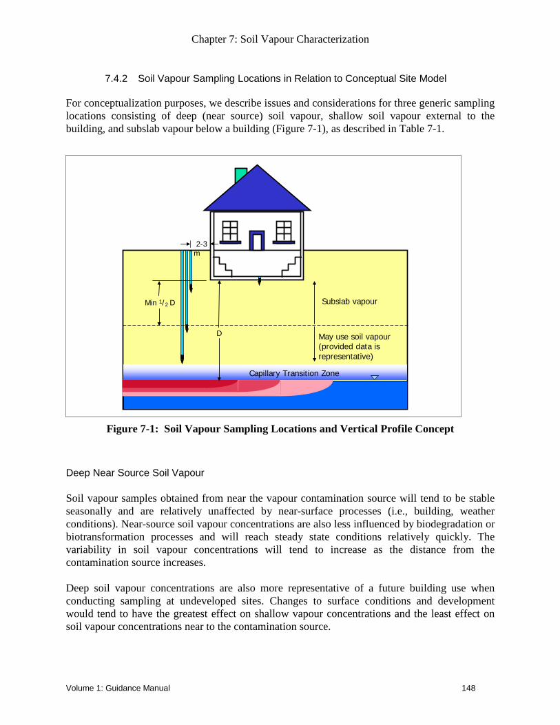
Chapter 7: Soil Vapour Characterization
Volume 1: Guidance Manual 148
7.4.2 Soil Vapour Sampling Locations in Relation to Conceptual Site Model
For conceptualization purposes, we describe issues and considerations for three generic sampling locations consisting of deep (near source) soil vapour, shallow soil vapour external to the building, and subslab vapour below a building (Figure 7-1), as described in Table 7-1.
Figure 7-1: Soil Vapour Sampling Locations and Vertical Profile Concept
Deep Near Source Soil Vapour
Soil vapour samples obtained from near the vapour contamination source will tend to be stable seasonally and are relatively unaffected by near-surface processes (i.e., building, weather conditions). Near-source soil vapour concentrations are also less influenced by biodegradation or biotransformation processes and will reach steady state conditions relatively quickly. The variability in soil vapour concentrations will tend to increase as the distance from the contamination source increases.
Deep soil vapour concentrations are also more representative of a future building use when conducting sampling at undeveloped sites. Changes to surface conditions and development would tend to have the greatest effect on shallow vapour concentrations and the least effect on soil vapour concentrations near to the contamination source.
2-3 m
Min 1/2 D
Capillary Transition Zone
May use soil vapour(provided data is representative)
Subslab vapour
D

Chapter 7: Soil Vapour Characterization
Volume 1: Guidance Manual 149
Table 7-1: Comparison of Soil Vapour Measurement Locations
Type of Soil
Vapour Data
Where Obtained Characteristics Use of Data and Cautions
Deep Near-Source
Soil Vapour
(external)
Near to water table or contamination source in vadose zone, but above capillary fringe. May be practical limitations for drilling where there is deep contamination.
Concentrations reach near-steady state conditions quickly, tend to be stable seasonally and are relatively unaffected by near-surface changes. Least affected by biodegradation. Should represent the highest concentrations of soil vapour.
If deep vapour concentrations are below target levels, soil vapour intrusion unlikely to be of concern. For future development scenario, only deep vapour concentrations should be used.
Shallow Soil
Vapour (external)
Close to the building, but outside peri-foundational area. At shallow depth near to elevation of lowest part of foundation.
Greater spatial and temporal variability than deep vapour data. More likely to be affected by changes in near-surface conditions including barometric pumping, temperature and shallow soil properties. May be affected by bioattenuation depending on chemical. Greater potential for non steady state conditions.
If there is significant bioattenuation beside but not below building, use of shallow soil vapour may result in non-conservative predictions of vapour concentrations in indoor air. Shallow soil vapour concentrations should be lower than deeper near source concentrations.
Subslab Soil
Vapour
Immediately below foundation slab. Central location away from the foundation footings is preferred.
Similar or greater spatial variability than shallow external soil vapour data. May be additionally short-term temporal variability from building pressures and breathing effect (e.g., due to HVAC system, stack effect). Concentrations may be affected by subslab utilities (e.g., drains, sewers) and variable foundation subsoils. Greater potential for non steady state conditions.
Logistical issues associated with sample collection. Subslab sample location may not be representative of the vapour concentrations entering the building. Due diligence is warranted to ensure sampling activities do not cause harm to workers and bystanders and minimize potential disruptions to building activities.
Shallow Soil Vapour (External to Building)
Shallow external soil vapour concentrations are typically more variable than deep near-source vapour concentrations and more likely to be affected by geologic heterogeneity, changes in near-surface conditions such as barometric pressure or temperature fluctuations, surface cover type (e.g., paved versus non-paved surface), and bioattenuation or biotransformation processes.
Bioattenuation is an important process for aerobically biodegradable chemicals (e.g., petroleum hydrocarbon compounds such as BTEX) that should be taken into account when considering

Chapter 7: Soil Vapour Characterization
Volume 1: Guidance Manual 150
where to locate soil vapour probes. Several case studies indicate a large reduction in soil vapour concentrations over small vertical distances due to aerobic biodegradation of hydrocarbon vapours or low diffusion rates through fine-grained soil layers with high moisture content (Davis et al., 2009; Fischer et al., 1996; Hers et al., 2000). There may also be significant lateral concentration gradients over short distances as evidenced by large concentration differences for probes situated on either side of houses (Sanders and Hers, 2006).
A review of empirical data indicates oxygen shadows below small to medium sized buildings at petroleum hydrocarbon contaminated sites are uncommon but have been observed where there is shallow LNAPL contamination with high source vapour concentrations (USEPA, 2013). At sites where there is an oxygen shadow (and potentially drier soils) below the building, shallow external soil vapour samples may be non-representative of conditions below the building. The results of a modelling study by Abreu and Johnson (2005) provide valuable insight on possible vapour concentration patterns for biodegradable contamination below buildings (Figure 7-2). The use of non-representative soil vapour concentrations external to the building could lead to non-conservative predictions of indoor air concentrations.
Figure 7-2: Results of 3-D Oxygen-Limited Soil Vapour Transport Modelling for High Concentration Source (Cg = 100 mg/L) and Moderate Concentration Source (Cg=20 mg/L) Hydrocarbon contours normalized to the vapour source concentration are shown on the left and oxygen contours normalized to the atmospheric concentration are shown on the right (from Abreu and Johnson, 2005).

Chapter 7: Soil Vapour Characterization
Volume 1: Guidance Manual 151
Subslab Soil Vapour
There is typically a high degree of spatial variability in subslab vapour concentrations. Factors that contribute to the variability observed include contamination source variability, geologic heterogeneity, foundation subsoil variability, bioattenuation, subsurface utility corridors and soil gas advection because of building and/or barometric pressure effects. Subslab vapour concentrations may be highest near the centre of a building for a relatively uniform contamination source, and potentially lower near cracks where soil gas is entering the building (e.g., along perimeter wall-base cracks).
Building pressures vary depending on several factors including seasonal temperatures (e.g., stack effect) and HVAC operation. At some buildings, positive pressures and reverse intrusion (extrusion) of air are observed, or there may be cyclic diel variations in building pressures (i.e., positive to negative) leading to exchange between indoor and subslab air. If indoor air contains elevated VOC concentrations, this could confound interpretation of subslab data. The reverse intrusion phenomenon can be evaluated by monitoring the pressure differential across the slab using digital micromanometers.
There are other potential drawbacks associated with subslab sampling that should be recognized. It requires an access agreement from the building owner, and is intrusive in that drilling or coring equipment must be used inside the building and floor coverings may be damaged, which may be disruptive or unpleasant for owners and occupants. It may also be difficult to determine subsurface utility locations below slabs, although geophysical techniques (e.g., ground penetrating radar) can be used for this purpose. Thus, the assessor must weigh the value of the data to be obtained against the potential damages or disruption.
Subslab Soil Vapour Challenges
Studies where multiple samples have been obtained below houses or small commercial buildings often indicate spatial concentration variability of one to two orders-of-magnitude and seasonal temporal variability of up to one order-of-magnitude (Holten et al., 2013; Lutes et al., 2013; Wertz and Festa, 1997). Depending on foundation construction and HVAC operation there may also be short-term concentration variability. There are no simple solutions to obtaining representive subslab vapour data but potential strategies include increased density of sampling, high purge volume (McAlary et al., 2010) recognizing that common methods involve sampling of only a few litres of soil gas, which may be a very small proportion of subslab soil gas volume, and deeper below-building soil vapour sampling when there is reverse air intrusion (extrusion). Subslab sampling costs may not be insignificant, especially if the vapour intrusion assessment includes multiple residences and temporal monitoring is required.

Chapter 7: Soil Vapour Characterization
Volume 1: Guidance Manual 152
Criteria for External Soil Vapour
The recommended soil vapour design for risk assessment is:
1. Sample on at least two sides of building with probes generally to be located within 2 - 3 m of building.
2. Where there is no building, obtain a minimum of two probes per APEC (additional probes may be needed for delineation purposes).
3. Obtain vertical soil vapour concentration profiles at selected locations.
4. The minimum probe depth should be equal to half-way between lowest part of building foundation and contamination source, further constrained as at least 1 m below ground surface.
5. Generally use maximum near-building concentration in risk assessment.
6. Conduct repeat sampling on at least two occasions.
7.4.3 Recommendations for Soil Vapour Sampling Locations
Soil Vapour External to Buildings
The lateral spacing of deep soil vapour probes needed to characterize soil vapour source zones is highly dependent on site conditions and the number and size of buildings where soil vapour intrusion is of potential concern. For large disperse groundwater plumes, a soil vapour probe spacing of several tens of meters may be adequate. For smaller plumes and areas where steep concentration gradients are expected in groundwater, more closely spaced probes are warranted (e.g., 5 m to 15 m, or spacing similar to the size of a house).
When evaluating potential vapour intrusion into a building, typically soil vapour samples from at least two sides of the building should be obtained, unless trends in soil vapour concentrations can be resolved and contoured on a broader scale. One location should be in the direction of the inferred highest soil vapour concentrations based on soil and groundwater data. The soil vapour sampling locations should be relatively close to the building (i.e., within 10 m), but beyond the zone of disturbance and fill located next to a building (generally 1 m to 2 m from the foundation wall). This distance may also depend on whether access agreements can be obtained. When there is contamination below the building, the use of soil vapour profiles at selected locations is recommended, as described above. Lateral transects should also be considered when the contamination source is laterally removed from the building. Deep near-source soil vapour sampling is also recommended for the future building scenario.
Deep, near-source vapour concentrations should be used for risk assessment. The minimum recommended depth is equal to half the distance between the building foundation and contamination source. This depth criterion is, in part, based on the model results of Abreu and Johnson (2005). The depth should generally be further constrained as a minimum of 1 m below the elevation of the foundation slab base and 1 m below ground surface to be beyond the advective zone of influence associated with barometric pumping and building depressurization and of sufficient depth to minimize the potential for atmospheric air to be drawn into the sample. However, with precautions such as plastic ground sheet and careful sealing of the probe verified by a leak test, valid samples from as little as 0.5 m depth can be obtained. A maximum depth of 10 m below the foundation is considered a reasonable upper bound based on practical considerations (e.g., drilling costs).

Chapter 7: Soil Vapour Characterization
Volume 1: Guidance Manual 153
When determining where to locate deep soil vapour probes, it is important to recognize that soil vapour samples cannot be obtained unless there is a continuous interconnected network of gas-filled pores, which is a function of the capillary fringe and transition zone thickness. The height above the water table where the transition to continuous gas-filled pores begins can be approximated using a water retention model (e.g., Van Genuchten model). Using model input parameters from US Soil Conservation Service (SCS) soil texture classifications, the predicted height of this transition point is approximately 17 cm for sand and 38 cm for loam. When a small additional allowance is included for water table fluctuations, these transition height estimates suggest that soil vapour probes should generally be installed 0.5 m to 1 m above the water table. Additional information on modeling of water retention is provided in Golder (2007).
Subslab Vapour Below Buildings
The number and location of subslab soil vapour samples that should be tested will depend on site-specific conditions. For small to moderate sized houses a minimum of two to three subslab samples is recommended. The subslab samples should preferably be located in a central location away from foundation footings but it is recognized that practical considerations (e.g., homeowner access) will often dictate the locations of subslab soil vapour samples. For larger buildings, a greater number of samples are warranted to characterize spatial variability and delineate areas with elevated subslab vapour concentrations. Deeper below building probes are recommended when there is the potential for building air-soil gas exchange.
Lateral Transects and Vertical Profiles
The soil vapour sampling design may employ transects or vertical profiles to characterize spatial variation in concentrations (Figures 7-1 and 7-3). Lateral transects or vertical profiles can provide useful information for more in-depth analysis of the effect of biodegradation or fine-grained soil layers on soil vapour transport. Transect or vertical profile data can increase the level of confidence in the CSM for soil vapour transport and data quality. For example, an increase in vapour concentrations with decreasing depth may suggest that deeper samples are invalid due to an improper sampling method, or that shallow contamination is present within the unsaturated zone.
Lateral transects are generally used when the contamination source is laterally removed from the building. Generally, a minimum of three samples should be used as part of a transect, consisting of soil vapour samples from (i) the edge of contamination source nearest to the building, (ii) the mid-point between the source and building, and (iii) near the edge of the building (API, 2005). When the distance between the contamination source and building is greater than 30 m, additional probes should be considered.
Ancillary Data
Ancillary data to support subslab vapour investigations include building foundation type/condition, foundation subsoils, HVAC system, and utilities. In some cases, chemical, geophysical or tracer testing may be warranted to assess whether utilities represent potential preferential pathways. Measurement of differential pressures between the building/subsoil using sensitive manometers can provide useful data on gradients.

Chapter 7: Soil Vapour Characterization
Volume 1: Guidance Manual 154
Vertical profiles are generally used when the contamination source is below or near to the building. Again, three or more samples should be obtained from (i) just above the contamination source, (ii) mid-point between upper and lower sampling point, and (iii) a sampling point located near the building. The contamination source must be at least 1.5 m below the building foundation for vertical profiles to be effective in resolving vertical concentration trends.
Additional probes are recommended where there are changes in lithology, where changes in concentrations are expected, where the pathway is uncertain, or where the distance between the source and building is sufficiently large. The soil vapour sampling design should also consider the potential implications of subsurface utilities for sampling locations since utilities may represent preferential pathways for soil vapour migration. Caution should always be taken when considering sampling near utilities to ensure the health and safety of workers and bystanders and the integrity of the utility is not compromised.
Figure 7-3: Lateral Transect Concept
7.4.4 When to Sample and Sampling Frequency
Investigation of the soil vapour intrusion pathway will typically require multiple rounds of soil vapour sampling since there can be significant temporal variability in soil vapour concentrations due to changes in source contamination concentrations, seasonal variations in the water table, and conditions for hydrocarbon vapour bioattenuation. For example, if the water table level decreases, soil contamination, which previously was submerged by groundwater, could be exposed to soil gas thus resulting in increased volatilization. For soil vapour samples collected near to a building, there may be weather or building related sources of variability. In general, the sampling frequency should coincide with seasonal patterns for factors affecting soil vapour such
Capillary Transition Zone

Chapter 7: Soil Vapour Characterization
Volume 1: Guidance Manual 155
as the water table elevation (i.e., high and low levels) and precipitation (soil moisture) (i.e., wet and dry season).
Under certain circumstances, one sampling event may be sufficient depending on the results of initial soil vapour testing. For example, if soil vapour concentrations are significantly less (i.e., greater than one to two orders-of-magnitude) than concentrations of potential concern, and if vapour concentrations are unlikely to change significantly over time, one monitoring event may be sufficient. Alternately, if soil vapour concentrations are close to concentrations of potential concern, repeat testing will be warranted.
Soil vapour sampling should be avoided during and after heavy rainfall events since collection of a representative sample is difficult. In addition, infiltration of water into soil can result in negative bias in soil vapour concentrations due to partitioning of vapour into soil moisture and, in some cases, induce advective movement of soil gas. The time for moisture to drain from soil pores will depend on the soil type. Coarse-grained soil (sand or gravel) will drain to field capacity within a few hours (from complete saturation) while fine-grained soil will take longer to drain (Hillel, 1980). Field capacity is the soil water content after water drainage by the force of gravity is mostly complete. Based on drainage data, we recommend that you wait at least one day after a significant rainfall event (defined here as 0.5 cm) for coarse-grained soils (sand or gravel) and several days for fine-grained soils.
The design of a soil vapour sampling program should consider the possible effect of barometric pressure fluctuations. These fluctuations could influence shallow soil vapour concentrations when there are thick coarse-grained unsaturated zones. A conservative approach would be to collect soil vapour samples when the barometric pressure is decreasing. Because it is generally not practical to schedule soil vapour sampling events to target the desired barometric pressure, barometric pressure data for several days before and after sampling should be obtained, when available, and related uncertainty documented in the assessment report. Water table fluctuations caused by tides could result in advective soil gas pumping and should be considered when designing soil vapour sampling programs.
There may be conditions where snow and frost, and snow melt could reduce hydrocarbon fluxes to the surface and oxygen flux to the subsurface, and potentially affect conditions for soil vapour intrusion. However, research on the influence of snow and frost cover at one cold climate site indicated little effect on seasonal soil vapour concentrations (Hers et al., 2013). Consideration should be given to repeat sampling with and without frost or snow cover.
7.4.5 Biodegradation Assessment for Aerobically Degrading Hydrocarbons
Extensive empirical data on petroleum hydrocarbon biodegradation has led to new approaches for risk-based screening of sites based on an exclusion (or inclusion) distance approach, defined as the (vertical) separation distance from the contamination source beyond which the potential for petroleum vapour intrusion can be considered negligible (USEPA, 2013; Lahvis et al., 2013), or bioreduction factors applied to vapour attenuation factors (Health Canada, 2010). In some cases, testing of soil vapour for biodegradation indicators may be warranted to support the above

Chapter 7: Soil Vapour Characterization
Volume 1: Guidance Manual 156
approaches (e.g., when site applicability is uncertain) or to support higher tier modeling through calibration or comparison of measured to model-predicted concentrations.
Key factors affecting oxygen concentrations and aerobic biodegradation of petroleum hydrocarbon vapours include source type (i.e., LNAPL or dissolved source), source size, source vapour concentration, distance to the building from the vapour source, building size, surface cover beside building and processes that enhance oxygen recharge to subsurface (e.g., wind or barometric pumping).
Investigation approaches to evaluate biodegradation include vertical soil vapour profiles (typically three or more samples) below buildings or surface covers of similar properties to a building foundation (e.g., potentially pavement). Soil vapour samples should be tested for the hydrocarbon vapours of potential concern, and for oxygen, carbon dioxide and methane. Nitrogen is also useful as a quality control check and indicator of soil gas advection. Depleted oxygen and elevated carbon dioxide levels are indicators of aerobic biodegradation of hydrocarbons. Elevated methane concentrations are an indicator of anaerobic biodegradation. Analysis of hydrocarbon compounds that are less soluble and potentially less biodegradable than the BTEX compounds (e.g., cyclohexane, 2,2,4-trimethylpentane) may serve as useful tracers for hydrocarbon vapour transport (Sanders and Hers, 2006).
Supporting data for a biodegradation assessment should include evaluation of LNAPL presence through observation at monitoring wells, and collection of soil cores for field indicator tests (e.g., headspace tests using a photoionization detector and dye tests) and laboratory analyses. Testing of soil samples for fraction of organic carbon and physical properties may also be warranted. Collection of a continuous soil core over the zone of potential impact is recommended so that the soil lithology can be examined and representative samples collected.
Soil Vapour Probe Construction and Installation 7.5
Soil vapour probes can be constructed of a variety of materials and installed using several techniques (EPRI, 2005; API; 2005; Atlantic PIRI, 2006). Critical aspects to probe construction include (i) probes should be constructed from materials that are relatively inert and non-sorptive, (ii) techniques should be used to minimize the potential for short-circuiting of atmospheric air to the probe soil vapour collection point, and (iii) the probe should remain sealed between sampling events. The main options for installation of soil vapour probes include:
• Probes installed in boreholes in soil or coreholes through a concrete slab; • Probes installed via direct push technology; and, • Driven probes.
7.5.1 Probes Installed in Boreholes
Permanent probes installed in boreholes are the preferred method. However, multiple options for probes are described below to provide the practitioner with alternatives to accommodate site-specific conditions and constraints (see SOP #4). For all probe types, it is important that subsurface utilities be located prior to installation. Probes Installed in Boreholes
Chapter 7: Soil Vapour Characterization
Volume 1: Guidance Manual 157
Boreholes should be advanced using methods that minimize disturbance and introduction of fluids in the subsurface (e.g., Geoprobe, auger, rotosonic without using fluids). Methods involving introduction of fluids in the subsurface or significant disburbance (e.g., hydrovac holes) should be avoided.
Probes installed in boreholes are constructed in a similar fashion to groundwater monitoring wells; however, there are important differences in design. Generally short screens (0.1 m to 0.3 m length) should be used for probes since typically the objective is to characterize local soil vapour concentrations (i.e., over a small volume). The probe diameter should be kept small (maximum of 25 mm (1 inch) and preferably less) to minimize purge volumes and surface area for adsorption of VOCs on probe surfaces.
Two common probe designs are rigid PVC pipe and “implants” constructed of steel mesh screens connected to flexible tubing. For probes constructed of continuous PVC pipe to ground surface, 19 mm (¾ inch) diameter pipe is recommended. While the slot size for groundwater wells is typically No. 10 slot (0.01 inch), a larger slot size (up to No. 40 slot) may be used for PVC soil vapour probes since there is less potential for the filter pack to intrude into the probe within the unsaturated zone. Commercially-available implants are typically 0.15 m to 0.3 m long, 12.5 mm (½ inch) in diameter, and connected to ground surface using 6 mm (¼ inch) tubing. A potential disadvantage of smaller diameter tubing (i.e., 6 mm or smaller) is frictional losses if pneumatic tests are to be performed (see SOP #5). A threaded cap should be placed over top of the riser pipe and riser pipe segments should be flush-threaded with o-ring seal. No glue should be used for construction of probes.
Coarse sand or fine gravel should be placed surrounding the screened portion of the probe, and a bentonite seal (minimum 0.3 m thick) should be constructed above the screened portion of the probe. Since soil vapour probes are installed in the unsaturated zone where soil moisture may be relatively low, careful consideration should be given to the hydration of the bentonite seal. A competent seal can be constructed through use of dry granular bentonite (16 mesh), as opposed to powder, chips, or pellets, and addition of distilled water to the bentonite during installation. Granular bentonite has a texture much like the sand used for a filter-pack, and so it will settle effectively within the borehole, but hydrates instantaneously. Two or three lifts of granular bentonite and water is usually sufficient to form a competent seal. An effective method of sealing the remainder of the borehole annulus is to use a thick slurry of powdered bentonite and water (“volclay grout”). At some sites, it may be prudent to use distilled water for hydration to avoid compromising soil vapour with volatiles commonly detected in tap water (e.g., chloroform).
If multiple probes are installed in a single borehole, the borehole above and below each probe should be sealed with granular bentonite. After allowing the seal to set overnight, the integrity of the seal should be checked by drawing a vacuum on each probe, and measuring the vacuum at adjacent probes. For a competent seal, a vacuum may still be measured at adjacent probes; however, the vacuum will develop slowly and will be less than that measured at the pumped probe (EPRI, 2005). Soil vapour probes should be completed with an air-tight valve or stopcock at surface to prevent atmospheric air from entering the probe, and protected using a well cover or other similar protective casing for security and weatherproofing. If multi-level probes are used, each probe should be tagged with a permanent label, using no glues or markers. In general, a
Chapter 7: Soil Vapour Characterization
Volume 1: Guidance Manual 158
similar or higher level of care and quality control to that employed for monitoring wells should be followed when installing a soil vapour probe.
Potential advantages of permanent probes installed in boreholes are that temporal variability can be assessed through repeat sampling and there is greater installation flexibility (i.e., deep probes, dense soils). In addition, the filter pack that surrounds the screen provides for more open area for drawing a soil vapour sample than a driven probe. A potential disadvantage of probes installed in boreholes may be access restrictions for drill rigs.
Soil samples should be collected during drilling of boreholes for soil vapour probes. Consideration should be given to testing of soil samples for soil moisture content and grain size distribution and the soil lithology and stratigraphy should be carefully logged. Soil samples should also be evaluated for possible contamination including sources that may be located above the water table (see Section 7.8).
7.5.2 Probes Installed Using Direct Push Technology
Direct-push techniques can be used to install a single soil vapour implant in a borehole. Direct push rods are pushed to the desired depth, and implants are installed post-run after the desired depth is reached by lowering the implant down the hollow rods and attaching it to a detachable anchor drive point. A sand pack and bentonite seal should be installed through the push rods as they are removed to prevent short-circuiting of atmospheric air from ground surface to the sampling point. The position of the filter pack and seal should be confirmed using a tamping rod. Natural collapse of the formation around the probes will not provide a competent seal and should not be relied upon. Direct push equipment can also be used to obtain soil cores prior to probe deployment. Soil data can be useful to target intervals for probe installation.
A potential advantage of using direct push technology to install a probe is that implants can be rapidly installed with minimal disturbance, but care must be taken to construct a competent seal. The presence of gravel or cobbles may hinder or preclude the use of direct-push technology.
7.5.3 Driven Probes
Driven probes in their simplest form are hollow steel rods with an internal diameter typically ranging between 9 mm and 25 mm (sometimes referred to as ground probes). The probes can be driven by hand, or with the aid of direct push equipped vehicles. The rods include a loosely-fitting conical tip that is pushed a short distance further into the formation using an inner rod, once the probe is driven to its desired depth. Several holes may also be drilled near the tip of the probe to increase the open area through which soil vapour is drawn into the probe. A bentonite seal should be placed around the probe at surface. Driven probes are typically temporary installations in that the probe is removed after the sample is obtained.
There is also direct push equipment that enables collection of multiple samples during a single push where soil vapour samples are collected through a screen located within a retractable protective sleeve. New tubing is threaded to the sampling point at each new depth (e.g., Geoprobe Post Run Tubing (PRT) system) or the tubing is permanently attached to the sampling
Chapter 7: Soil Vapour Characterization
Volume 1: Guidance Manual 159
point and thus should only be used for collection of one sample per push (e.g., AMS Retract-a-Tip system). This technology may be useful in characterizing soil vapour concentrations above source contamination zones; however, due to the potential for cross-contamination, it should not be used within or below source contamination zones. A bentonite seal should be placed around the rods at surface.
Driven probes may be advantageous in terms of flexibility of installation and cost. A disadvantage is that driven probes can be difficult to install in coarse-grained or dense soil, especially at greater depths. The probe may also deflect during driving in coarse-grained or dense soils creating pathways for annular leakage. Clogging of retractable screens often occurs in fine-grained soils making it difficult to obtain a sample. For the Geoprobe PRT system it is difficult to leak test the connection between the tubing to the probe. Once installed, it is important not to disturb and move probes to avoid the creation of voids adjacent to probes, which are more likely to become a path of least resistance in low permeability soils.
Driven probes installed vertically using a hydraulic ram or slide hammer without subsequent disburbance and that pass leak tests (SOP #6) are considered acceptable although permanent probes installed in boreholes are preferred. Ground probes are not recommended.
An additional pre-caution that should be considered for shallow probes (less than 1 m deep) of any type is placement of a plastic sheet at ground surface (e.g., 1.5 m by 1.5 m), as recommended by BCCSAP (2009). Such a seal reduces the potential for ambient air intrusion from beyond the immediate seal around the probe.
7.5.4 Use of Water Table Monitoring Wells as Soil Vapour Probes
Soil vapour samples can be obtained from groundwater monitoring wells screened across the water table when the well screen extends above the capillary fringe. Prior to collecting a sample for analysis, the well should be purged by removing several casing volumes of air. For typical well diameters, a purge rate of several litres per minute may be required, and therefore an appropriate sized pump is required for this approach. Since groundwater wells may be vented at surface, an air-tight cap and valve should be used when sampling soil vapour.
Since essentially a composite soil vapour sample is obtained over the length of the well screen above the capillary fringe, data from monitoring wells may not provide the desired vertical discretization. Off-gasing of volatiles from groundwater at the water table surface and from the capillary fringe will influence the soil vapour concentrations to varying degrees. For a thick capillary fringe, the surface area over which volatilization could occur within the well may be significant (approaching 1 m2). For this scenario, the soil vapour concentration measured in a monitoring well may be significantly higher than that measured in a soil vapour probe installed directly above the capillary fringe, meaning that data from wells may be unsuitable for evaluation of concentration attenuation within the capillary transition zone.

Chapter 7: Soil Vapour Characterization
Volume 1: Guidance Manual 160
7.5.5 Subslab Soil Vapour Probes
Prior to drilling or coring through concrete slabs, relevant structural and utility information should be reviewed to evaluate whether drilling or coring could adversely affect the integrity of the building envelope, foundation slab or subsurface utilities, and whether there are any potential health and safety issues with drilling or coring. As warranted, geophysical techniques should be used to identify the location of re-bar within concrete slabs prior to drilling. After drilling the hole and prior to installation of the probe, the hole should be temporarily sealed (e.g., using a rubber stopper) to minimize disturbance to subslab vapour concentrations.
Typically, the objective of subslab soil vapour sampling is to characterize vapour concentrations in foundation subsoils immediately below the slab. Therefore, permanent probes typically consist of stainless steel or brass inserts installed within a corehole that are sealed with concrete grout (USEPA, 2004). The concrete grout should consist of Portland cement, aggregate and water, and should not contain any additives that could contain VOCs. A fast setting, hydrating (swelling) cement may be a good option provided there are no additives that give off VOCs. An alternate design is an expanding packer type probe, which does not require sealing with grout and that is typically used as a temporary probe. Regardless of the probe type used, it is good practice to also place a temporary bentonite seal around the probe during sampling. A subslab probe design by USEPA (2004) is shown in Figure 7-4.
Figure 7-4: USEPA (2004) Recommended Subslab Soil Gas Probe.
7.5.6 Probe Materials
Inert and non-porous materials should be used for soil vapour sampling. While probes constructed of either stainless steel or PVC are acceptable, sorption of VOCs onto PVC occurs (Hers et al., 2004), so sufficient time for probes to equilibriate and adequate purging is required

Chapter 7: Soil Vapour Characterization
Volume 1: Guidance Manual 161
to ensure sorption is not biasing results. For sampling trains, the use of Teflon is recommended. As part of a tubing study, Hayes et al. (2006) report significant sorption and a negative bias in concentrations of naphthalene using Nyla-Flow tubing. Therefore, it should not be used for naphthalene or similar compounds but may be acceptable for lighter molecular weight VOCs. Polyethylene, silicon and tygon tubing are highly sorptive and should not be used. Threaded couplings (e.g., Swagelok) are preferred although tight barbed-fittings (with tubing pushed over at least three barbs) should also provide for a reasonable seal. Glue, tape or other materials that could emit volatiles should not be used as part of probe construction.
7.5.7 Decontamination of Sampling Materials and Equipment
Clean materials and equipment should be used for soil vapour sampling. This can be implemented through decontamination of materials or through the use of new, unused materials. Care should also be taken when handling equipment because sampling equipment could be contaminated by dirty containers, permanent marking pens, hands, vehicle exhaust, etc. The level of decontamination may depend on the objectives of the soil vapour survey and LRLs for analytical testing.
If the soil vapour survey is limited to testing of vapour samples using a field photoionization detector (PID) or flame ionization detector (FID) measuring to part-per-million levels, it may be appropriate to re-use the soil vapour probes, tubing and sampling containers (e.g., gas-bags). However, prior to installing a probe and collecting each sample, a field blank sample comprised of ambient air should be collected through the entire sampling train and tested using the field PID or FID. If concentrations in the field blank are elevated above background ambient levels, the equipment should be cleaned or new equipment should be used.
If the soil vapour survey involves collection of vapour samples for field PID or FID analysis at part-per-billion levels or for laboratory analysis, either new, unused materials should be used, or a rigorous cleaning procedure should be followed together with testing of equipment blanks using certified zero gas.
Temporary steel probes should be decontaminated prior to use at each location. Care should be taken when storing and handling materials and equipment to avoid contamination (e.g., store materials in sealed bags). Sampling and decontamination procedures should be documented as part of the QA/QC program.
Soil Vapour Sampling Procedures 7.6
Soil vapour sampling procedures addressed in this section are soil vapour equilibration, probe performance testing, sampling containers, methods to detect leaks and short-circuiting, and purging and sampling. The methods used should be documented throughout the sampling process. SOP #5 provides additional details on soil vapour sampling procedures. Good overviews of sampling procedures are also provided in NJDEP (2013), ITRC (2007), Atlantic PIRI (2006) and EPRI (2005).

Chapter 7: Soil Vapour Characterization
Volume 1: Guidance Manual 162
7.6.1 Soil Vapour Probe Development and Equilibration
Soil vapour probes should be developed by removing air entrained during installation or allowed to re-equilibrate via diffusion prior to sampling. Development followed by equilibration is also acceptable and may be advantageous for PVC probes to enable sorption to occur. A minimum of three probe volumes of air (including the probe, tubing and air-filled pore volume of the sand pack) should be removed during development. Otherwise, the probe should be allowed to re-equilibrate prior to sampling. The time required for equilibration will depend on the disturbance caused during installation. Recommended minimum equilibration times are: driven probes or where samples are obtained from direct push drive rods that remain in the ground (20 minutes), probes installed in small diameter direct push holes (one day), probes installed in auger holes or rotosonic holes where no air or water is used for drilling (two days). Probes installed using sonic or air rotary drilling where fluids are introduced or in hydrovac holes should be developed by removing air introduced into the formation and then allowed to equilibrate for at least a week. In addition, sequential purging and testing of soil vapour should be conducted to confirm stable concentrations.
7.6.2 Flow and Vacuum (Probe Performance) Check
The performance testing of selected probes should be conducted prior to soil vapour sampling. The objective of the performance test is to verify the flow and vacuum are within acceptable ranges prior to sampling. The test is conducted by withdrawing soil vapour from the probe at the desired flow rate using a pump and measuring the vacuum. If the vacuum exceeds 0.36 psi (10” of water column) a lower flow rate should be used to reduce the vacuum where practical. Soil vapour samples can be obtained at higher vacuums, but a specialised pump may be required. For subslab soil vapour samples, a lower vacuum (less than 1 inch of water) would typically be expected since granular materials are commonly present below foundation slabs. Vacuum and flow measurements should be roughly comparable between sampling events. Higher vacuums inconsistent with known soil conditions can be diagnostic of a water-blocked probe while lower vacuums may indicate a leak in the sampling train. Flow and vacuum measurements may be used to estimate the soil-air permeability using mathematical models for soil gas flow to a point probe (Garbesi et al., 1996) or to a well (Johnson et al., 1990) (see SOP #5).
7.6.3 Leak Testing of Probes and Sampling Trains
A leak test should be conducted at each new soil vapour probe installed and repeated if there are indications that the probe or surface seal has been disturbed. Even if there are no signs of disturbance, it is good practice to check a subset of probes (e.g., 10-20%) for each new monitoring event. The most common leak test of the probe seal and surface valve is to introduce helium beneath a shroud that covers the probe and valve (SOP #6). A soil vapour sample is collected from the probe using a gas-bag and analyzed using a hand-held helium detector that
Equilibration Time for Sand Pack To answer how long does it take for the sand pack to equilibrate with surrounding soil gas, DiGuilio et al. (2006) used a model to calculate equilibration times for different distances and soil water contents. For a 50 mm diameter borehole, the equilibration time plot for the sand pack shows a required time of few minutes to a few hours.

Chapter 7: Soil Vapour Characterization
Volume 1: Guidance Manual 163
provides readings with a range of 0.01% to 100%. Advantages of a helium leak tracer test are that real-time data is obtained and that it is a relatively simple test to perform (i.e., the test can be performed during purging and field testing of gas-bag samples for fixed gases). A disadvantage is that helium is becoming more difficult and costly to obtain. Alternate methods include the use of sulphur hexafluoride as a tracer gas or use of a volatile liquid tracer such as iso-propanol (SOP #6).
The entire sampling train used for collection of samples for field and laboratory analysis should also be checked for leaks. This can be done by conducting a shut-in vacuum or pressure test and monitoring the change in vacuum/pressure over time (SOPs #5 and #6). If pressurized it may be possible to use a soapy-water solution to identify couplings that may be leaking. When canisters are used, it is also possible to collect the canister inside a helium-filled shroud, although this will require use of additional helium and periodic checking and “topping up” of the shroud helium concentration. The laboratory should also be advised of this procedure so that appropriate arrangements can be made for laboratory analysis for helium. A disadvantage of this method is that real-time leak test results are not obtained.
Potential short-circuiting of atmospheric air during sampling can also be indirectly evaluated through careful examination of oxygen and carbon dioxide data. For example, oxygen concentrations are generally depleted in the presence of elevated hydrocarbon vapour concentrations near petroleum sources, so if a soil vapour sample contains moderate to high concentrations of both hydrocarbons and oxygen, atmospheric air may have leaked into the sample (see Section 7.10 for additional discussion).
7.6.4 Sampling Container or Device
Sample collection devices can include evacuated steel canisters, sorbent tubes, glass cylinders and gas-bags (e.g., Tedlar or polyvinylfluoride). The selection of a collection device is influenced by investigation objectives, analytical requirements and LRLs. For field screening using hand-held detectors, soil vapour samples are typically collected using gas-bags. The use of a vacuum chamber (“lung box”) to fill gas-bags avoids passing soil gas through a pump and possible pump contamination that may result. Gas-tight syringes are often used for on-site analysis using mobile laboratories. Soil vapour samples collected for analysis by a fixed laboratory for VOCs should generally be obtained using sorbent tubes or stainless steel (e.g., SummaTM) or glass-lined (e.g., SilcoSteelTM) canisters. Sampling devices are compared in Table 7-2.
Due to a shortage of Tedlar, new plastics for gas-bags are being used, which may not perform as well as Tedlar. Coyne et al. (2009) compared SKC FlexFilm to Tedlar and found that while the concentration of background total VOC concentrations were about three times lower in FlexFilm than Tedlar, greater losses over time were observed for samples in FlexFilm gas-bags. While
Helium Leak Tracer Test For a helium leak tracer test, the Leakage, defined as soil vapour / shroud helium concentration (x100%) should be estimated. The threshold for acceptable Leakage is 2 %. When greater than 2 %, the probe and/or sampling train should be repaired. Note that the presence of methane in soil gas will result in a positive bias in helium concentrations when measured by common field detectors (SABCS, 2011). Ultra-high purity helium of 99.995 % or better is recommended (SOP #6).

Chapter 7: Soil Vapour Characterization
Volume 1: Guidance Manual 164
according to the analytical method (ASTM D1946-90(2011)) gas-bags may be used for fixed gas analysis (e.g., oxygen, carbon dioxide, methane), because of the potential for leakage and limited holding times (Table 7-2), their use is generally not adviseable and instead canisters are recommended. However, some laboratories recommend the use of Tedlar bags over canisters for reduced sulphur analysis because studies indicate the recovery of hydrogen sulphide and certain mercaptans is poor for aged glass-lined canisters (Bontempo and Kao, 2008; Rezendes and Lanna, 2004).
7.6.5 Sample Probe Purging and Sampling
Purging Probe
The purpose of purging is to ensure a representative soil vapour sample is collected by removing stagnant air from the probe and filter pack prior to collecting a sample. Typically, the objective is to obtain a soil vapour sample from the geologic material immediately surrounding the probe.
Cody (2003) evaluated purge volumes on the basis of a differential equation for the sequential and complete mixing of VOCs over each time step within the entire volume under consideration (probe and tubing). On the basis of this equation, the estimated concentration within the probe volume reaches 90 percent of the input concentration after purging about three volumes. For narrow diameter tubing, fewer purge volumes are likely needed to obtain a representative sample due to reduced mixing resulting from more of a “plug flow” phenomena.
As a minimum three probe volumes including air-filled pores in filter pack should be removed prior to soil vapour sample collection. The emerging best practice is to collect a soil vapour sample for analysis after field indicators (organic vapours measured by a PID, oxygen and carbon dioxide) measured in sequential samples (e.g., collected in gas-bags in a vacuum box) have stabilized (e.g., within approximately 10%) or to conduct a purge optimization test on a subset of probes where field readings are taken after the removal of 1, 3 and 10 probe volumes and where the optimal volume corresponds to the purge volume where the highest PID concentration is obtained. Further research on criteria for stability is needed before this approach can be fully adopted.
Over-purging should be avoided when there are shallow probes or the soil-air porosity is low (e.g., fractured deposits) and where atmospheric air intrusion to the probe is possible. While the
Purging and Sampling Summary
1. Allow probe to equilibrate. 2. Check for leaks in sampling equipment. 3. Calculate the dead volume based on the
inner volume of probe and tubing and air-filled pores of the filter pack.
4. Purge three volumes from the probe. 5. A flow rate between 20 ml/min and 200
ml/min should generally be used for purging and sampling, although purge rates of up to 5 L/min are acceptable for large volume probes.
6. Monitor the vacuum during purging; reduce the flow rate if the vacuum exceeds 0.36 psi (10” water).
7. Use direct reading instruments to monitor VOC concentrations as part of sequential purging test.
8. When purging is complete, close the sampling valve and allow the vacuum to dissipate before collecting a sample.

Chapter 7: Soil Vapour Characterization
Volume 1: Guidance Manual 165
Table 7-2: Soil Gas Sample Collection Containers and Devices
Gas-bags (e.g., Tedlar®, SKC Flexfilm)
• Gas-bags are available in a range of volumes; typically a 0.5 to 1 litre gas-bag is used for soil gas sampling.
• Gas-bags should be filled using a vacuum chamber, which avoids possible cross-contamination from pumps and leakage.
• Studies indicate significant leakage of Tedlar® bags over the first 24 to 48 hours after sampling (Wang et al., 1996; Andiro and Butler, 1991).
• Gas-bags are generally not recommended for laboratory analysis, but if used, should be analyzed as quickly as possible. Although reported analytical holding times are up to seven days, analysis of bags within 24 and 48 hours is recommended.
Gas-Tight Syringes
• Gas-tight syringes are used to collect small volume gas samples (typically 5 to 60 ml).
• Gas-tight syringes are typically used for on-site GC analysis. • Gas-tight syringes should be made of inert materials (e.g., stainless
steel and Teflon) and blanks should be run to evaluate possible losses through sorption.
• Samples should be analyzed within a short time (30 minutes) of collection.
Sorbent Tubes • A wide range of sorbent materials are available. Tubes are selected based on the types and concentrations of volatile chemicals expected in soil gas.
• Sorbent tubes are placed in-line between the probe and pump. • Sorbent tube sampling rates are typically 50 to 200 ml/min; the flow
rate supplied by the sampling pump must be accurately determined. • The sampling duration will depend on the expected concentration, flow
rate, chemical type, sorbent and desired detection limit. • For quality control purposes, some sorbent tubes have a “front” and
“back” section, or two tubes are placed in series to evaluate possible chemical breakthrough.
Stainless Steel or Glass-Lined Canisters
• Stainless steel canisters have a passivated (treated to improve the chemical inertness) interior surface. Glass-lined canisters are designed for reactive or polar chemicals.
• Available volumes range from 400 ml to 6 litres. • Canisters are supplied under vacuum. The vacuum is measured prior to
shipping by the laboratory, immediately prior to and after sampling using a gauge, and by the laboratory upon receipt. Significant differences in laboratory and field vacuums (beyond the range of accuracy of the gauge) indicate possible leakage during transit.
• There should be a residual vacuum left in the canisters; otherwise, the sample will not represent the entire planned sampling interval.
• The sampling rate is typically controlled by a flow regulator (either mass flow controller or critical orifice).

Chapter 7: Soil Vapour Characterization
Volume 1: Guidance Manual 166
vacuum should always be allowed to dissipate prior to collection of soil vapour samples for laboratory analysis, an optional wait time (several hours) to address possible disequilibrium may be warranted when purge volumes are large and/or vacuums are very high.
High Purge Volume Sampling
High purge volume (HPV) sampling may be desirable if the intent is to evaluate conditions beyond the immediate proximity of the soil vapour probe. If the approximate permeability and soil gas flow regime is known, a volume-integrated concentration may be obtained (McAlary et al., 2010). Transient vacuum response data may also be used to estimate the leakage of a foundation slab, given certain assumptions are fulfilled for boundary conditions and the contrast in permeability between the fill below the slab and underlying native soil. The HPV approach has potential advantages when obtaining subslab samples below larger buildings, where the volume of a conventional discrete soil gas sample is very small compared to the total volume of gas-filled soil pores. For example, for a 5,000 m2 building, the volume of gas-filled soil pores is 300,000 litres assuming a soil thickness of 0.2 m and gas-filled porosity of 0.3.
The concentration trends over time as measured by direct reading instruments may also provide qualitative information on spatial variability in source concentrations. For example, slowly increasing concentrations could indicate a higher soil vapour concentration zone laterally removed from the probe. Commensurate with HPV sampling is the need for larger pumps, the removal of hundreds or thousands of litres of soil gas and repeat testing over time.
Sampling Flow Rate and Vacuum
The acceptable sampling flow rate will depend on the soil properties (soil-air permeability) and practical considerations relating to sampling device. For evacuated canisters, use of a flow regulator typically results in sampling rates between about 3 and 100 ml/min. For most sorbent tubes, the analytical protocols indicate that the sampling rate should not exceed 200 ml/min.
One study demonstrated that soil vapour concentrations were not sensitive to a flow rate of up to 10 L/min, in samples collected from properly sealed probes screened in moderately permeable materials (McAlary and Creamer, 2006). Conversely, it may not be practical to collect samples at flow rates of 100 ml/min in fine-grained soil (e.g., silts and clays) without imposing an excessive vacuum. The concern with higher flow rates and vacuums is the increased potential for leakage of air into the soil vapour probe and sampling train. High vacuums may enhance the volatilization of the more volatile compounds in a chemical mixture (ITRC, 2007; API, 2005).
For this guidance, a flow rate between 10 ml/min and 200 ml/min and a vacuum that is less than 0.36 PSI (10” of water) is recommended for soil vapour sampling. The vacuum can be readily measured using a T-junction connected to a digital manometer. An optional pre-caution that is considered reasonable to minimize the potential for disequilibrium is a flow rate less than 50 ml/min for collection of samples in fine-grained soils.

Chapter 7: Soil Vapour Characterization
Volume 1: Guidance Manual 167
Sample Collection
Soil vapour samples are typically collected over a relatively short duration (15 minutes to 2 hours) although subslab vapour samples of up to 24-hour duration may be obtained using canisters. Indoor air samples are typically obtained over an 8- to 24-hour period. The soil vapour sampling rate for a 6-litre Summa sample collected over 24 hours is about 3.5 mL/minute to result in a residual vacuum of about 2.45 PSI (5” Hg). Sampling of probes at a site should be completed over a relatively short time period (e.g., within one week) to provide an internally consistent data set (Lahvis, 2002). If any water is drawn in the sample container, re-collect the sample after taking measures to eliminate water.
For subslab soil vapour probes, it may be desirable to collect a subslab vapour sample concurrently with an indoor air sample to enable comparison to indoor air data and to reduce short-term variability. However, given the overall variability in subslab measurements and processes for vapour intrusion, a shorter-duration subslab sample (e.g., 15 to 30 minutes) is considered acceptable and collection of concurrent subslab vapour and indoor air samples is not considered required practice. Precautions should be taken to avoid contamination of indoor air through rapid sealing of foundation holes after drilling and venting of purge gases outdoors. Indoor air and subslab sampling programs should be appropriately scheduled to avoid bias of indoor air results.
Sample Handling and Storage
Soil vapour samples obtained using syringes, gas-bags, canisters or cylinders should not be placed in a chilled cooler for transport since volatiles may condense out the vapour phase at lower temperature (Hartman, 2002). Gas-bags and glass syringes should be placed inside an opaque container immediately after collection to avoid possible photo-oxidation reactions. Samples should not be subjected to excessive heat.
For sorbent tubes, cool storage in sealed containers is recommended where during transport, and storage, the temperature is less than 4oC. Sorbent tubes should be stored in a sealed plastic container containing a bed of activated carbon to minimize the potential for adsorption of ambient VOCs. All soil vapour samples should be transported in separate containers from soil and groundwater samples.
Soil Vapour Analysis 7.7
7.7.1 Selection of Method
Analytical testing methods appropriate for analyzing soil vapour samples are dependent on risk assessment objectives, sampling method and data quality objectives. Soil vapour programs often consist of a combination of field testing of soil vapour samples using hand-held detectors and laboratory analysis of selected soil vapour samples for specific chemicals of potential concern. Since analytical testing is a broad topic, only an overview of the key issues is provided below. Common analytical methods for soil vapour are summarized in Table 7-3, with a detailed list provided in Appendix 7-1.

Chapter 7: Soil Vapour Characterization
Volume 1: Guidance Manual 168
It is important to understand procedures and potential limitations associated with different testing methods. Since soil vapour and air methods are not as well defined as groundwater methods, adequate consultation with the laboratory is essential. The types of information that should be discussed include optimal sampling flow rate and duration, detection limits, laboratory QA/QC requirements and considerations, and the handling and transport of samples. Communication with the laboratory at the early stages ensures that important analytical considerations are taken into account during the development of the sampling plan.
7.7.2 Field Detectors
Field detectors commonly used are photoionization detectors (PID) or flame ionization detectors (FID), combustible gas detectors or explosimeters, and multi-gas detectors for compounds such as oxygen, carbon dioxide and methane, which are important for studies evaluating biodegradation. Photoionization detectors will respond to most organic vapours as well as some inorganic vapours (e.g., hydrogen sulphide, ammonia) depending on the ionization lamp energy. The sensitivity of a PID varies depending on the compound, and moisture can bias readings; therefore care should be taken when conducting soil vapour surveys.
Combustible gas detectors are typically calibrated to methane or hexane in air depending on type of site contamination expected. Filters can be used to mostly eliminate methane, if desired (about 90% for one common combustible gas detector). It is important to document the type of combustible gas detector, calibration gas and mode of operation. Photoionization detectors, which measure hydrocarbon vapour concentrations to ppm, or even ppb levels, are generally more sensitive than combustible gas detectors.
While field detectors are valuable for site screening, the limitations associated with these instruments, including non-specificity to compounds of possible interest and the effect of environmental factors and sampling methods, should be clearly understood (Robbins et al., 1990). For example, infrared detectors for methane are subject to significant positive bias when exposed to gasoline vapours or other light hydrocarbon vapours. Field detectors should generally not be directly connected to sampling probes when taking measurements, and instead samples should be obtained in gas-bags. Photoionization detectors, in particular, are sensitive to variation in the sampling flow rate.
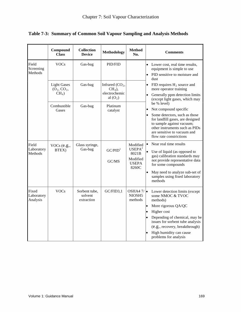
Chapter 7: Soil Vapour Characterization
Volume 1: Guidance Manual 169
Table 7-3: Summary of Common Soil Vapour Sampling and Analysis Methods
Compound Class
Collection Device Methodology Method
No. Comments
Field Screening Methods
VOCs Gas-bag PID/FID • Lower cost, real time results, equipment is simple to use
• PID sensitive to moisture and dust
• FID requires H2 source and more operator training
• Generally ppm detection limits (except light gases, which may be % level)
• Not compound specific • Some detectors, such as those
for landfill gases, are designed to sample against vacuum; other instruments such as PIDs are sensitive to vacuum and flow rate constrictions
Light Gases (O2, CO2,
CH4)
Gas-bag Infrared (CO2, CH4),
electrochemical (O2)
Combustible Gases
Gas-bag Platinum catalyst
Field Laboratory Methods
VOCs (e.g., BTEX)
Glass syringe, Gas-bag
GC/PID1
GC/MS
Modified USEPA2 8021B
Modified USEPA 8260C
• Near real time results
• Use of liquid (as opposed to gas) calibration standards may not provide representative data for some compounds
• May need to analyze sub-set of samples using fixed laboratory methods
Fixed Laboratory Analysis
VOCs Sorbent tube, solvent
extraction
GC/FID3,1 OSHA4 7/ NIOSH5 methods
• Lower detection limits (except some NMOC & TVOC methods)
• More rigorous QA/QC • Higher cost • Depending of chemical, may be
issues for sorbent tube analysis (e.g., recovery, breakthrough)
• High humidity can cause problems for analysis

Chapter 7: Soil Vapour Characterization
Volume 1: Guidance Manual 170
Compound Class
Collection Device Methodology Method
No. Comments
VOCs Sorbent tube, thermal
extraction
GC/MS USEPA TO-17
VOCs Specially–treated
(e.g., Summa) canister
GC/MS USEPA TO-14A /TO-15
PAHs Resin or Polyurethane Foam (PUF)
GC/MS USEPA TO-13A
TVOC & Hydrocarbon
Fractions6
Sorbent tube, solvent
extraction
GC/FID NIOSH 1550
TVOC & Hydrocarbon
Fractions
Canister (Summa or non treated), Gas-
bag
GC/FID (Cryotrap)
USEPA TO-3
NMOC7 Canister or on-line
FID USEPA TO-12
Light Gases (e.g.,O2,
CO2, CH4, CO, H2)
Canister, Gas-bag, Glass
syringe
GC/TCD1 ASTM D1945-03
Notes: 1. GC = gas chromatograph, PID = photoionization detector, FID = flame ionization detector, TCD = thermal conductivity
detector, MS = Mass Selective detector. 2. USEPA = US Environmental Protection Agency. 3. MS, the recommended method, is also used by commercial labs but is not part of the reference method. 4. OSHA = Occupational Safety & Health Administration (USA) 5. NIOSH = National Institute for Occupational Safety and Health (USA) 6. Hydrocarbon fractions can consist of both ranges (e.g., TVOC (C6-10), TVOC (C10-19)) and aromatic and aliphatic
fractions 7. NMOC = non-methane organic compounds
7.7.3 Field Laboratory Analysis
Field laboratory methods are used when a greater degree of precision or component-specific information is required than that provided by a field screening method. The advantages of field laboratory methods are near real-time results, which can be used to modify programs while in progress, and potentially lower costs. Also the ability to collect repeat samples can be an advantage for assessing sampling, temporal, and spatial variability. The disadvantage of field laboratory methods are higher detection limits than fixed laboratory methods based on USEPA TO- protocols (see below). Possible regulatory requirements for soil vapour analytical protocols should also be reviewed when evaluating field laboratory analysis.

Chapter 7: Soil Vapour Characterization
Volume 1: Guidance Manual 171
Field laboratory methods include the use of portable gas chromatographs (GCs) that are brought to the site to analyze grab samples on an on-going basis. Soil gas air is usually collected using gas-tight syringes and is injected into the GC (or purge-and-trap apparatus) for analysis. The portable GC usually analyses data through photo ionization, flame ionization or electron capture detectors (e.g., modified USEPA Method 8021B). The precision of the results can vary depending on the equipment used. Portable mass spectrometers (MS) are also being introduced to the market, which provide greater certainty for compound identification (e.g., modified USEPA Method 8260C). Modified water methods (USEPA Method 8021B and 8260C) can work well for many compounds, but for polar compounds calibration methods may introduce bias, and for heavier molecular weight compounds such as naphthalene recovery tends to be poor (Hayes et al., 2005).
7.7.4 Fixed Laboratory Analysis
For risk assessment studies, low LRLs and more rigorous quality control requirements typically require that soil vapour samples be collected using either active sorbent tubes (i.e., air is drawn through a tube using a pump) or canisters, and quantified by GC/MS methods at fixed laboratory locations. The use of GC/FID analysis is generally not recommended due to non-specificity of detection but may be used in the assessment of CCME F1 and F2 parameters for certain test methods (Appendix 7-2).
Sampling using a sorbent tube is an indirect method of estimating the soil vapour concentration in that the test measures the mass of chemical trapped on the sorbent. The air concentration is estimated by dividing the mass by the total volume of air drawn through the tube. The canister method involves collection of a “whole air” sample enabling direct analysis of the soil vapour sample. Both methods are described in detail below.
Active Sorbent Tube Method
Active sorbent tubes have been used for indoor air quality testing for several decades, but only more recently have air methods been modified for soil vapour. There are complicating factors for soil vapour that should be accounted for including higher humidity (often 100%) and typically much higher analyte concentrations than for indoor air.
Analytical Methods: A key distinguishing factor between methods is whether thermal desorption (e.g., USEPA TO-17) or solvent extraction is used (e.g., modified OSHA 7 or NIOSH 1501 methods). Thermal desorption involves rapidly heating the sorbent to desorb the VOC, while passing an inert carrier gas through the tube. The VOCs are carried by the gas and concentrated on a smaller downstream trap, which usually is cryogenically cooled. For thermal desorption, the whole sample is released from the sorbent during the heated desorption step. While some of the earlier thermal desorption units do not allow for the possibility for replicate analyses, the newer units have the capability of re-collecting a portion of sample during the primary desorption step to allow for re-analysis. Additionally, sample introduction parameters can be modified such that less mass is loaded onto the GC/MS in order to perform sample dilutions. This is important since soil vapour concentrations, as compared to air, can be very high
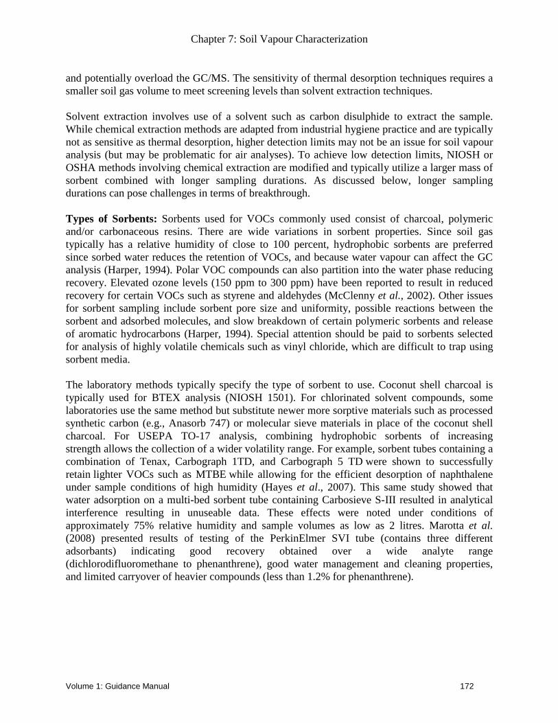
Chapter 7: Soil Vapour Characterization
Volume 1: Guidance Manual 172
and potentially overload the GC/MS. The sensitivity of thermal desorption techniques requires a smaller soil gas volume to meet screening levels than solvent extraction techniques.
Solvent extraction involves use of a solvent such as carbon disulphide to extract the sample. While chemical extraction methods are adapted from industrial hygiene practice and are typically not as sensitive as thermal desorption, higher detection limits may not be an issue for soil vapour analysis (but may be problematic for air analyses). To achieve low detection limits, NIOSH or OSHA methods involving chemical extraction are modified and typically utilize a larger mass of sorbent combined with longer sampling durations. As discussed below, longer sampling durations can pose challenges in terms of breakthrough.
Types of Sorbents: Sorbents used for VOCs commonly used consist of charcoal, polymeric and/or carbonaceous resins. There are wide variations in sorbent properties. Since soil gas typically has a relative humidity of close to 100 percent, hydrophobic sorbents are preferred since sorbed water reduces the retention of VOCs, and because water vapour can affect the GC analysis (Harper, 1994). Polar VOC compounds can also partition into the water phase reducing recovery. Elevated ozone levels (150 ppm to 300 ppm) have been reported to result in reduced recovery for certain VOCs such as styrene and aldehydes (McClenny et al., 2002). Other issues for sorbent sampling include sorbent pore size and uniformity, possible reactions between the sorbent and adsorbed molecules, and slow breakdown of certain polymeric sorbents and release of aromatic hydrocarbons (Harper, 1994). Special attention should be paid to sorbents selected for analysis of highly volatile chemicals such as vinyl chloride, which are difficult to trap using sorbent media.
The laboratory methods typically specify the type of sorbent to use. Coconut shell charcoal is typically used for BTEX analysis (NIOSH 1501). For chlorinated solvent compounds, some laboratories use the same method but substitute newer more sorptive materials such as processed synthetic carbon (e.g., Anasorb 747) or molecular sieve materials in place of the coconut shell charcoal. For USEPA TO-17 analysis, combining hydrophobic sorbents of increasing strength allows the collection of a wider volatility range. For example, sorbent tubes containing a combination of Tenax, Carbograph 1TD, and Carbograph 5 TD were shown to successfully retain lighter VOCs such as MTBE while allowing for the efficient desorption of naphthalene under sample conditions of high humidity (Hayes et al., 2007). This same study showed that water adsorption on a multi-bed sorbent tube containing Carbosieve S-III resulted in analytical interference resulting in unuseable data. These effects were noted under conditions of approximately 75% relative humidity and sample volumes as low as 2 litres. Marotta et al. (2008) presented results of testing of the PerkinElmer SVI tube (contains three different adsorbants) indicating good recovery obtained over a wide analyte range (dichlorodifluoromethane to phenanthrene), good water management and cleaning properties, and limited carryover of heavier compounds (less than 1.2% for phenanthrene).

Chapter 7: Soil Vapour Characterization
Volume 1: Guidance Manual 173
Sorbents used for semi-volatile (PAH) analyses (naphthalene and heavier molecular weight compounds) often consist of Teflon®-impregnated glass fibres followed by a resin (XAD-2) sorbent (NIOSH 5515 or USEPA Method TO-13A). Since trapping of particulates for soil vapour is usually not an objective, typically only the XAD resin sorbent is used for semi-volatile analyses (i.e., polyurethane (PUF) foam is not used).
Sorbent Sampling Volume: The sampling volume should be carefully determined through consideration of the expected VOC concentration and mass, the sorption capacity and required detection limits. When available, the results of field PID analyses of soil vapour should be communicated to the laboratory analyst prior to sorbent sampling to guide selection of a sampling duration and flow rate that would minimize the potential for chemical breakthrough. An option is to collect two samples over different time durations to avoid the possibility of re-sampling.
Pump Flow Rate: Since the concentration is sensitive to the flow rate, pumps must be accurately calibrated and provide a constant flow rate throughout the sampling duration. The pump flow rate must be checked prior to and during sampling, since actual pump flow rates may vary considerably depending on the soil-air permeability and vacuum. A recent study (Golder Associates, 2007, unpublished) found a significant and roughly linear drop in pump flow rate under vacuum conditions induced by soil (e.g., 11% drop in flow at 3.4 inches H20, 40% drop at 9 inches H20 and 93% drop at 16.5 inches H20).
Environmental Conditions: Appropriate measures should be taken to mitigate the effects of high humidity or cold weather when sampling using sorbent tubes, which may not always be practical to avoid. Reducing the air flow rate or sampling with varying volumes of air (using multiple samples) may be a good approach under this circumstance. Further discussion on cold weather considerations is provided in Exhibit 7-1.
Canister Method
Low detection limits can be achieved utilizing canister samples testing in accordance with USEPA Method TO-15 and, in general, the accuracy and precision of analytical results generated are high.
Analytical Methods: The analytical protocols for the Summa method are USEPA TO-14A (non-polar compounds) (USEPA, 1999a) and USEPA TO-15 (polar and non-polar compounds) (USEPA, 1999b). USEPA Method TO-15 is commonly used for soil vapour analyses since there are a number of significant improvements for Method TO-15 compared to TO-14A, including enhanced measures for quality control (e.g., 5-point calibration), specific canister cleaning procedures, better water management procedures and better recovery of polar compounds.
Sampling Volume Calculation
An example sampling volume calculation is provided for sorbent tube analysis for benzene. Assuming a target indoor air concentration of 3 µg/m3, a target detection limit of 30 µg/m3 is obtained (Eq. 7-1 Section 7.7.5). A typical benzene detection limit is 0.1 µg (MS detector), therefore approximately 3.3 litres of soil gas would need to be drawn through the tube (0.1µg/30µg/m3 X 1000 L/m3). At a sampling rate of 100 ml/min, the required sampling duration would be 33 minutes.

Chapter 7: Soil Vapour Characterization
Volume 1: Guidance Manual 174
USEPA Method TO-15 utilizes a gas chromatograph (GC) with a mass spectrometer (MS) as the detector. When the MS is run in full scan mode up to 70 compounds can be readily detected with typical reporting limits between 0.2 to 0.5 parts per billion by volume (ppbV). Analytical methodology considerations are further discussed in Section 8.4.1.
Hardware: Two types of canisters are available: Summa canisters, which are electro-polished steel canisters and Silco canisters, where the steel is coated with an inert fused silica layer. The silcosteel canisters internal surface is intended to be non-reactive with sulphur compounds or compounds that react with metal surfaces (e.g., polar compounds). It is important that the canister hardware be in good condition. For soil vapour sampling, a one-litre canister is typically a sufficient volume.
The flow regulator (mass flow controller or critical orifice) should be appropriately calibrated based on the desired sampling duration and the vacuum before sampling and residual vacuum after sampling should be recorded. Flow regulators are temperature and altitude dependent; therefore, the sampling location should be communicated to the laboratory so that appropriate adjustments can be made.2 A critical orifice is often used for short duration sampling for soil vapour (i.e., up to about two hours), but it does not provide for a uniform flow since the flow rate is a function of the pressure differential. For longer duration sampling (e.g., indoor air sampling), a mass flow controller should be used to provide for a uniform flow rate. Particulate filters consisting of sintered steel with 2 to 7 micron pore sizes or deactivated glass frit are placed before the critical orifice. It is essential that all fittings are tight during sampling.
Equipment Cleaning: The TO methods and hardware were designed to measure low VOC concentrations in ambient air. At some sites (e.g., dry cleaners, UST sites with free-phase NAPL), canisters are subject to soil vapour concentrations that exceed 100,000 to 1,000,000 ug/m3. Experience has shown that there is a significant potential for contaminant carry over in the canister, regulator, filter or inlet tube under these conditions. Therefore, all equipment must be thoroughly cleaned and canister blanks tested. Canisters are typically cleaned by the laboratories by heating the canister and passing humidified zero air under pressure through the canister.
For heavier molecular weight compounds (e.g., trimethylbenzene and naphthalene), sorption onto metal tubing and filter has been shown to result in reduced compound recovery (Entech, 2007). Poor recovery due to sorption and carryover of naphthalene are potentially problematic issues but improved laboratory methods have led to acceptable recovery for naphthalene. However, the analysis of compounds with molecular weights higher than naphthalene is not routinely feasible using the TO-15 method.
Environmental Conditions: For Summa canisters, some water vapour is needed to coat the inside of the surface of the steel to provide for an inert surface. However, similar to sorbent tubes, excessive water can create challenges for sample recovery and cryogenic focusing prior to 2 Laboratories typically conduct performance studies to verify that flow regulators provide for a uniform sampling rate over the sampling duration, within an acceptable tolerance. If warranted, flow rates can be verified in the field using an extra canister using an electronic mass flow meter or rotometer, calibrated for vacuum conditions.

Chapter 7: Soil Vapour Characterization
Volume 1: Guidance Manual 175
analysis, although an alternate method of multiple focusing steps using non-cooled sorbent tubes can reduce problems associated with water vapour.
The barometric pressure at both the sampling and laboratory location should be recorded. When there are significant differences in the elevation at which the sample was obtained and the laboratory, it may be possible to correct for the effect of ambient barometric pressure on the sample concentration (i.e., using Boyle’s Law for an ideal gas).
Selection of Method
The chemical to be measured, detection limit, ease of use, cost, laboratory certification and quality control are factors that should be considered when selecting the soil vapour analysis method. The use of thermal tubes analyzed by Method TO-17 (using an appropriate sorbent) and canisters by Method TO-15 are both considered acceptable methods for a wide range of compounds. Modified OSHA or NIOSH methods may be acceptable for a more limited range of analytes.
The potential advantages with thermal tubes compared to evacuated canisters include that they are easier to clean and provide for better recovery of higher molecular weight compounds (i.e., heavier than naphthalene). The disadvantages include possible breakthrough requiring careful selection of safe sampling volumes, the requirement for a pump, and accurate flow measurements during the sampling process. Under conditions of higher vacuums, pump failure during sampling may be an issue. Leak checking and shut-in vacuum tests are potentially not as straightforward for tubes as for canisters.
The potential advantages of evacuated canisters are a more direct measurement through a whole air sample and easier sample collection. The disadvantages include poor recovery of higher molecular weight compounds, challenges with hardware (e.g., fittings, controllers, gauges) and greater difficulty in cleaning canisters compared to tubes.
7.7.5 Quality Assurance / Quality Control Considerations
Data Quality Objectives
Data quality objectives should be established as part of the sampling plan in conjunction with the overall study objectives. In broad terms, the data quality objective is to ensure that data quality is acceptable and that data can be relied upon for decision-making purposes. Specific objectives may be developed in terms of accuracy, precision, data representativeness, data completeness and detection limits. There may also be specific considerations for cold weather sampling that should be incorporated in the data quality objectives (Exhibit 7-1).

Chapter 7: Soil Vapour Characterization
Volume 1: Guidance Manual 176
The development of a QA/QC plan will help to ensure that the desired data quality is achieved. Standard operating procedures should be used for sampling and analytical procedures, including the use of chain-of-custody records and identifying sampling locations. Systematic data collection and planning helps provide for defensible results and increased credibility.
Detection Limits
For risk assessments, the measured vapour concentrations are often used to predict indoor air concentrations. The required detection limit can be back-calculated using risk-based target indoor air concentrations combined with minimum expected dilution factors between soil vapour and indoor air. A lower bound dilution factor for the soil vapour to indoor air transport pathway
of 30 may be used to estimate the required detection limit. An additional adjustment factor (about 5 to 10X, where possible) should be applied to provide for greater flexibility in data interpretation and since there is increased uncertainty near to the detection limit. The maximum detection limit is calculated as follows:
DLmax = DF * Cair / AF [7-1]
Where DL is the analytical reporting (detection) limit, DF is the dilution factor (30), Cair is the target indoor air concentration, and AF is adjustment factor (5 to 10). As a practical matter, the
EXHIBIT 7-1: Considerations for Cold Weather Sampling
In many regions of Canada, environmental investigations may be completed during periods of relatively cold weather (i.e., freezing temperatures). The soil vapour design should consider the potential effect of cold temperatures, snow and frost. Soil vapour samples from frozen ground are not considered representative and therefore either deeper external vapour samples or samples from below a building where warmer temperatures are expected should be obtained. Pre-cautions should be taken when conducting soil vapour programs during cold weather. Field instruments such as PIDs and FIDs and pumps are not designed to operate when temperatures are below freezing. Field instruments may be kept warm in a heated building or vehicle, with field samples collected and transported in gas-bags. Sampling pumps may be kept warm by storing them in insulated coolers or insulated lunch bags with heat packs. Condensation through cooling of warmer soil gas is rare, but if it occurs, is problematic for sorbent tube and canister analysis. The sample tubing should be closely observed for signs of condensation (e.g., through use of translucent tubing). The tubing should be kept as short as practical and sampling repeated during a different season if condensation is an issue. While the cold temperature performance of sorbent tubes is not well understood, consideration should be given to heating and insulating of sorbent tubes during sampling. Tubes should not be over-heated since sorption efficiency decreases with increasing temperature. For canister sampling, the canister pressure at room temperature will be lower than the field measured pressure when the field temperature is less than room temperature. At cold temperatures, the difference can be significant potentially resulting in the erroneous conclusion that there is a residual vacuum in the canister when none exists. The Ideal Gas Law can be used to adjust the pressure for temperature.

Chapter 7: Soil Vapour Characterization
Volume 1: Guidance Manual 177
LRL may be raised due to matrix interference when concentrations of selected compounds are very high.
Quality Control Samples
The recommended field quality tests for analysis of sorbent tubes are as follows:
• Cleaning and Proofing: Thermal tubes should as a minimum be batch proofed and the usage history of each tube should be recorded by the laboratory to enable tracking of suspected contamination (BC Laboratory Manual, 2009).
• Field duplicates: Should be obtained by collecting distributed volume pairs submitted blind to the laboratory. The minimum frequency is 10 percent of the samples analyzed. When less than 10 samples are analyzed, it is recommended that one field duplicate per sampling event be analyzed.
• Tests for Breakthrough: For tubes that are solvent extracted (e.g., NIOSH methods), the front and back sections of sampling tubes for every sample collected are analyzed separately to evaluate for chemical breakthrough. For thermal desorption tubes, the laboratory should provide data on safe sampling volumes (SSV) that apply to each analyte tested. Testing of two tubes in series is optional (and not required by the USEPA TO-17 method) but is good practice particularly when soil vapour concentrations are elevated and there is uncertainty in the SSV. An alternate approach when there are a range of compounds with widely varying properties and SSV is to collect two distributed tube samples simultaneously but at different flow rates and thus different sampling volumes.
• Field transport blank: Is typically obtained by removing the caps from tubes and leaving them in the sampling environment for a short time (e.g., 5 minutes), and placing caps back on the tube. The sample should be submitted blind to the laboratory.
• Equipment blank: High purity inert gas is drawn through the sampling train and/or probe and analyzed to determine whether the sampling train is clean. Equipment blanks are mandatory if equipment is re-used; optional if new materials are used.
• Field Spikes: Sample tubes spiked with known concentrations of analytes are used to evaluate the recovery of the spiked compound and accuracy of the extraction and analytical procedure. This test is not typically a field test but may be performed by the laboratory.
• Sampling Flow Rate and Time: The flow rate during sampling should be measured and sampling time accurately recorded.
For evacuated canister analysis the following quality control testing is recommended:
• Cleaning and proofing: Canisters and flow controllers should as a minimum be batch proofed and the usage history of each canister should be recorded by the laboratory to enable

Chapter 7: Soil Vapour Characterization
Volume 1: Guidance Manual 178
tracking of suspected contamination (BC Laboratory Manual, 2009). For low-level (sub-ppbV) analysis, individual proofing or “certification” of canisters is recommended.
• Field duplicates: Should be obtained by collecting two canisters using a splitter. It is recommended that a single flow controller be used (i.e., splitter is downstream of the controller).
• Field transport blank: A “blank” canister is filled either in the field with ultra high purity air or nitrogen supplied by the laboratory in a separate canister or by the laboratory upon receipt. The blank canister is handled the same way as other canisters (i.e., vacuum is tested). This is considered an optional test when a higher level of quality assurance is desired, given that other quality control tests are typically performed such as laboratory certification of canisters and testing of the vacuum before and after sampling.
• Equipment blank: High purity inert gas is drawn through the sampling train and/or probe and analyzed to determine whether the sampling train is clean. Equipment blanks are mandatory if equipment is re-used; optional if new materials are used.
• Vacuum Measurements: Should be measured in the field prior to and after sampling and by the laboratory upon receipt of the canister. See Section 7.10 for data quality requirements.
All data should be clearly reported, including blanks, and any suspect results should be flagged. The interpretation of quality control data is discussed in Section 7.10.
Soil and Groundwater Characterization 7.8
Soil and/or groundwater data are important for developing the CSM that is used to guide the development of the soil vapour characterization program. Soil data can be used to evaluate contamination source zones, including possible sources that are located above the water table. Shallow groundwater data and predictions of deep soil vapour concentrations along with measured deep vapour concentrations can be used to evaluate the degree to which volatilization from groundwater and migration through the capillary fringe occurs, or the degree to which it may be inhibited through infiltration or geologic barriers. In some cases, it may not be possible to collect a representative soil vapour sample due to low permeability deposits; therefore, the use of soil and/or groundwater data alone may be required for evaluation of the soil vapour intrusion pathway.
7.8.1 Groundwater Data
Groundwater characterization for evaluation of soil vapour intrusion should provide information on concentrations in groundwater near to the water table. This is because cross-media transfer from groundwater to soil vapour occurs when chemicals in pore-water volatilize into soil gas, which occurs in the capillary transition zone above the water table. Since there can be significant vertical concentration stratification, the use of relatively short monitoring well screens situated across the water table or depth discrete sampling methods such as the GeoprobeTM, Waterloo ProfilerTM or HydropunchTM methods are recommended when evaluating the soil vapour

Chapter 7: Soil Vapour Characterization
Volume 1: Guidance Manual 179
intrusion pathway.3 Depth discrete samples can also be obtained from existing monitoring wells using Passive Diffusive Bag Samplers (Vroblesky and Hyde, 1997; ITRC, 2002). Diffusive Bag Samplers can also be used to measure VOC concentrations in pore-water within the capillary transition zone.
As well screen lengths increase, there is increased blending of groundwater across the screened interval. This may result in either over-estimation or under-estimation of concentrations at the top of the aquifer, depending on the contamination scenario. At locations where LNAPL is present or where there is an interface plume from fluctuating water table and interaction between soil gas and the water table, longer well screens may under predict concentrations near the top of the aquifer. Where there is a fresh-water lens or contamination source below the water table (e.g., DNAPL), longer well screens may over predict concentrations near the top of the aquifer.
Groundwater well installation, well development and purging prior to sampling should be conducted according to current standards of practice. For vapour intrusion assessments, a saturated screen length of 1 to 2 m is recommended. Low flow purging and sampling methods that minimize disturbance, aeration and/or de-gassing of groundwater are recommended (Puls and Barcelona, 1996). Particular attention should be given to groundwater samples collected from submerged screens or wells with long screen intervals. The concentrations from these wells may be of limited value for vapour intrusion assessments.
While the appropriate focus of groundwater investigations for vapour intrusion studies is shallow groundwater quality, in some cases, it may also be important to assess the deeper groundwater quality. This is because contaminants at depth within groundwater systems could pose future vapour intrusion potential for hydrogeologic systems that undergo changes, due to natural seasonal fluctuations of the water table elevation and/or through human activities. The vertical concentration variability can be investigated either through the use of nested wells (at different elevations) or vertical profiling using a Geoprobe or similar groundwater sampling technique as discussed in Chapter 6 of this document.
7.8.2 Soil Data
There are a number of uncertainties associated with use of soil data for evaluation of soil vapour intrusion as a result of losses of volatile contaminants during soil sampling, handling and chemical analysis. Depending on the contaminant type and geologic conditions, there may be significant spatial variation in soil concentrations, which may be difficult to detect based on conventional sampling programs. Finally, there are uncertainties associated with soil partitioning calculations and predicted soil vapour concentrations are sensitive to the partitioning coefficient between water and organic carbon, and the fraction organic content in soil, a parameter that can be difficult to accurately determine. If soil analyses results are to be used for the vapour pathway, it is recommended that the soil samples be field preserved (e.g., using methanol), where possible (e.g., USEPA SW-846 Method 5035a). A multi-functional sampling device (MFSDs), which act
3 Another potential option may be to install small diameter implants (e.g., 15 cm long) at several depths near the water table,
which can be used to sample either soil gas or groundwater depending on water table fluctuations.

Chapter 7: Soil Vapour Characterization
Volume 1: Guidance Manual 180
as a coring tool and airtight storage container, can also be used to collect soil samples for volatile analysis. The storage chamber is completely soil filled with zero headspace and is then capped to form an airtight seal.
Ancillary Data 7.9
The ancillary data below may assist in understanding the vapour intrusion pathway. With appropriate planning, some of this data can be obtained as part of a standard environmental site assessment. For other data, supplementary investigations would typically be required.
Physical Properties: The properties of soil layers of the vadose zone, including soil moisture, bulk density, air- and water-filled porosity and total organic carbon content may be important in evaluating vapour intrusion. Care should be taken to minimize re-distribution of soil moisture or drying of soil during drilling, sampling and storage of samples. Water retention tests on undisturbed samples can provide useful data on the likely range of water-filled porosity that could be expected in soil. Although not commonly performed, consideration can also be given to in situ tests to provide estimates of tortuosity (effective diffusion coefficient) (Johnson et al., 1998; Lahvis et al., 1999) and soil-air permeability (Baehr et al., 1991).
Hydrogeological Properties: The groundwater elevation during sampling and during an appropriate period prior to sampling is important when evaluating the possible seasonal influence on volatilization. The hydraulic conductivity and gradient are fundamental parameters required to evaluate groundwater flow systems.
Meteorological Data: There are an increasing number of weather stations (government, private) for which meteorological data (temperature, barometric pressure, wind speed and direction, relative humidity and precipitation) can be readily down-loaded. If there is a weather station near the site, this meteorological data should be obtained. Portable weather stations are also relatively inexpensive, and barometric pressure can be readily obtained (e.g., BarologgerTM). Barometric pressure and precipitation data for a few days prior to sampling should be obtained to enable trends to be evaluated. Frost and snow cover should be noted. Meteorological data may be useful in interpretation of soil vapour intrusion particularly if there were severe weather conditions during sampling (e.g., rapid change in barometric pressure, strong winds).
Building Pressure Data: Highly sensitive manometers (sensitivity less than 0.00015 psi (1/250” of water)) can be used to measure the differential pressure between the building and outdoor air, and building air and subslab soil vapour. Information on pressure gradients can be useful in assessing soil vapour intrusion potential; for example, soil vapour intrusion potential would
Commerical Building Evaluation
Some commerical buildings are designed to be positively pressurized through operation of HVAC system. Vapour intrusion will be significantly curtailed if the building is sufficiently pressurized (i.e., comparable to 6 Pa to 9 Pa recommended in ASTM (2001)). For such scenarios, an evaluation consisting of review of HVAC design, interview with facilities engineer to review HVAC operation, and series of differential pressure measurements to capture possible seasonal and barometric pressure variations may provide valuable information on pressure gradients and the potential for a complete vapour intrusion pathway (EPRI, 2005).

Chapter 7: Soil Vapour Characterization
Volume 1: Guidance Manual 181
be low if the pressure in the building is higher than in soil below the building. When measuring pressures, consideration must be given to the potential influence of wind and other environmental variables on the measurements. The building pressure data should be plotted against barometric pressure and other weather data to assess whether there are any correlations in the data.
Building Ventilation Tracer Test: Inert tracers such as carbon dioxide can be used to evaluate building ventilation characteristics and to estimate air change rates (ASTM E741-00). The ventilation test involves release of tracer gas (carbon dioxide) within the enclosed space followed by monitoring of the concentration decay over time. The concentration decay rate is used to estimate the air exchange rate. There are also tracer test methods that use sulphur hexafluoride. For commercial buildings, it may be possible to estimate the ventilation rate from HVAC system design. The air exchange rate should be calculated from the make-up volume, and not the total air handling volume.
Tracer Tests: Naturally-occurring radon can be used as a tracer to evaluate sub-slab to indoor air attenuation (McHugh et al., 2008), although results may be somewhat biased by radon emissions from concrete itself or off-gassing from water, if from a groundwater source containing radon. The potential advantages of using radon, compared to analyses for VOCs, are potentially lower analytical costs, there are no common sources of indoor radon (excluding granite counter-tops), and indoor radon concentrations are in most cases above detectable levels (unlike VOCs where bias may be caused by non-detect values). Tracers can also be used to evaluate potential preferential pathways such as sewers. For example, Poll et al. (2010) successfully used a method where they injected nitrogen and hydrogen in the subsurface and identified utility pathways in the building using a portable detecter.
Passive Soil Vapour Samplers: Passive diffusion samplers contain a hydrophobic adsorbent material that collects organic compounds over time. The adsorbed compounds are removed from the adsorbent by thermal desorption or solvent extraction, and typically analyzed using GC/MS methods. The passive soil vapour method provides the mass of vapours adsorbed to the media, but in typical applications cannot reliably be used to estimate soil vapour concentrations. Certain low-uptake rate passive samplers have indicated reasonable comparisons in soil vapour (within factor of two) to active canister (TO-15) results for select compounds excluding subsurface conditions when the starvation effect is significant such as in clays or wet soils (McAlary et al., 2012). Passive soil vapour samples are typically deployed for a few days to weeks, and therefore provide a time-integrated sample. The extended sampling duration also provides for high sensitivity. In the context of soil vapour intrusion studies, passive soil vapour sampling methods could be useful in mapping the location of subsurface plumes and for identifying pathways (in particular when placed in or along utility corridors) for determining locations for permanent probe placement when the CSM is not well understood. Passive diffusive samples can be used to estimate VOC concentrations in air and are described in Chapter 8.
Flux Chamber Test: The surface emission flux rate of volatile chemicals may be measured by placing an open bottom box on top of bare ground or above a crack on a concrete floor (where the box is appropriately sealed to the concrete) and measuring the increase in volatile chemical concentrations in the chamber over time (static test) or measuring concentrations in air extracted

Chapter 7: Soil Vapour Characterization
Volume 1: Guidance Manual 182
at a steady rate from the chamber (dynamic test) (Hartman and Jacobs, 2005). Flux chamber tests are affected by the methodology used and conditions at the time of sampling and are relatively difficult tests to perform. The use or scaling of data for purposes of a vapour intrusion assessment is also not straightforward, although flux chamber tests may be useful when emissions to outdoor air are estimated.
Larger-Scale Tracer and Pneumatic Testing: Several different techniques may be used to estimate soil-air permeability and evaluate soil gas migration pathways. Helium tracers may be released at probes and travel times monitored at a central probe where soil gas is being extracted. Measurements of soil gas flow rates, pressures and vapour concentrations may be used for evaluating contamination source zones and for remediation design.
Tree Coring: Recent studies have shown tree core concentrations of chlorinated solvent chemicals to be related to soil and groundwater concentrations (Burken et al., 2010; Struckoff et al., 2005). This technique could be a useful screening tool at some sites.
Data Interpretation and Analysis 7.10
The procedures for data interpretation and analysis of soil vapour data are described below. A detailed checklist for persons reviewing soil vapour assessment reports is provided in Volume 2.
7.10.1 Data Organization and Reporting
The soil vapour data should be tabulated and plotted to facilitate evaluation and review of data relationships and trends. The following data organization and presentation is recommended:
• Tabulate all data including sample location identifier, sample date, sample depth, sampling methods (including sampling duration and flow rate), chemical analysis methods, laboratory LRLs and results of chemical analysis;
• Tabulate field screening and laboratory analysis data to enable side-by-side comparisons;
• Prepare plan drawings showing soil vapour concentration data that includes pertinent structures (buildings, utilities, paved areas, vegetated areas);
• Compare soil vapour with nearby groundwater concentration data; consider geologic conditions when evaluating variability;
• Prepare vertical profiles of soil vapour concentration data that includes oxygen, carbon dioxide and methane and boring log data where available; and,
• Identify soil vapour target concentrations and background indoor and outdoor air concentrations, where available.

Chapter 7: Soil Vapour Characterization
Volume 1: Guidance Manual 183
7.10.2 Data Quality Analysis
Following receipt of the soil vapour results, the data should be evaluated to determine whether they meet data quality objectives outlined in the sampling plan (Section 7.7.5 and Chapter 3). The data quality checks should include the following:
• Review reported detection limits relative to data quality objectives. In some cases, sample dilution is required, which results in raised detection limits.
• Review canister pressure data upon completion of sampling. The initial vacuum in the canister should be greater than 27 inches Hg (at sea level), otherwise the canister should not be used. After sampling, there should be a residual vacuum left that ideally is between 4 and 6 inches Hg, but should be no more than 10 inches Hg. For short duration soil vapour sampling (i.e., typically less than 2 hours), if there is no vacuum left in the canister at the end of the sampling process, the data is still considered valid (there is no mandatory minimum vacuum requirement in USEPA Method TO-15); however, results should be flagged. For longer duration air sampling (i.e., typically 8 or 24 hours), there should be a vacuum remaining for the sample to be considered valid. See SOP #5 for additional details.
• For sorbent tube analyses, review results of analyses of front and back sections of the tube (or two tubes in series) to evaluate possible chemical breakthrough. Breakthrough can be caused when the adsorptive capacity is exceeded, the air flow through the tube is too high, and chromatographic effects caused by other compounds. If the laboratory considers the first tube saturated, then results are potentially biased and re-sampling should occur. The criterion for evaluating breakthrough is method and chemical dependent but typically is a concentration in the second tube that is greater than 10 to 25 percent of the concentration in the first tube. If the sample media is not saturated, the front and back concentrations should be added together for numerical evaluation.
• Evaluate precision for laboratory and field duplicate or co-located samples as quantified by the relative percent difference (RPD). The acceptable RPD under USEPA Method TO-15 for laboratory duplicate samples from the same canister is 25%. Greater variability would be expected for field duplicates obtained from two canisters. A provisional target RPD for field duplicates is 50% based on the current state of knowledge.
• Review analytical results for blank samples (e.g., field blanks, laboratory blanks and trip blanks) to identify possible issues with the laboratory or field procedures that may have affected the results.
• Recognize that reported concentrations within five times of the quantification limit are typically more uncertain than higher concentration values.

Chapter 7: Soil Vapour Characterization
Volume 1: Guidance Manual 184
7.10.3 Data Consistency Analysis
The results of the soil vapour sampling program should be reviewed in terms of the expected results, based on consistency with the conceptual site model and internal consistency between sampling points. These consistency checks should include the following:
• The soil vapour concentrations should be spatially consistent with the soil and groundwater concentrations, for example, the highest soil vapour concentration should be measured in source contamination areas where soil and groundwater concentrations are also highest.
• The soil vapour concentrations should decrease with increasing distance from a known contamination source.
• The soil vapour concentrations should be consistent with the expected CSM for aerobic and/or anaerobic biodegradation of petroleum hydrocarbons or other degradable organics including natural organics (e.g., organic soil layers). Typically, oxygen concentrations are depleted by a few percent in organic soil layers and to a greater extent near to petroleum hydrocarbon source zones. In contrast, elevated carbon dioxide concentrations are expected near to petroleum hydrocarbon sources (except in rare circumstances when CO2 is removed through interaction with certain types of soils such as high limestone content soils). Oxygen concentrations close to atmospheric levels (20.9 percent) near petroleum hydrocarbon source zones are a strong indicator that the soil gas sample was compromised through short-circuiting or leakage. Closer to ground surface, oxygen concentrations would be expected to increase and carbon dioxide concentrations decrease. If this pattern is not observed, additional contamination sources may be present.
• The relationship between oxygen and carbon dioxide concentrations can be further evaluated through plotting the O2 and CO2 anomaly, where the term “anomaly” refers to the observed concentration of O2 and CO2 after removing the canonical background atmospheric values of these gases according to the following equations: [O2]’=[O2] measured – 20.9460% and [CO2]’=[CO2]measured – 0.0400%. Based on stoichiometric considerations and the organics oxidized, different slopes will be observed, for example, the O2 versus CO2 anomaly data should plot on a 1:1 line for aerobic respiration of natural organic matter, the data should plot on a 2:1 line for respiration of CH4, and somewhere between the 1:1 and 2:1 lines for respiration of petroleum hydrocarbons.
• Soil vapour concentrations should be consistent with expected temporal trends. A priori it may be difficult to predict the effect of temporal factors on soil vapour data; therefore, a database that already includes some temporal data may be required to make this evaluation.
7.10.4 Further Evaluation
The data quality and consistency should be evaluated to determine whether there are data gaps or quality issues that warrant additional soil vapour testing. The soil vapour concentrations will also typically be compared to risk-based generic (if available) or site-specific soil vapour criteria for

Chapter 7: Soil Vapour Characterization
Volume 1: Guidance Manual 185
the vapour intrusion pathway. Depending on the results of this comparison, additional soil vapour characterization and/or indoor air testing may be warranted.
Resources and Weblinks 7.11
Compared to soil and groundwater, there are much fewer state-of-the-art guidance documents and resources available on soil vapour sampling and analysis. Useful information is provided in the following references.
Interstate Technology and Regulatory Council (ITRC). The Vapor Intrusion Pathway: A Practical Guide (VI-1)(January 2007, 173 pages) provides a generalized framework for evaluating the vapour intrusion pathway and describes the various tools available for investigation, data evaluation, and mitigation. The Vapor Intrusion Pathway: Investigative Approaches for Typical Scenarios (VI-2) (January 2007, 52 pages) is a supplement to Vapor Intrusion Pathway: A Practical Guide. The supplement describes applicable approaches for evaluating the vapour intrusion pathway in six typical scenarios. http://www.itrcweb.org/Documents/VI-1.pdf . http://www.itrcweb.org/Documents/VI-1A.pdf
American Petroleum Institute (API). A Practical Strategy for Assessing the Subsurface Vapor-to-Indoor Air Migration Pathway at Petroleum Hydrocarbon Sites (November 2005) includes guidance on soil gas sampling approach, methods and analysis (November, 2005). http://www.api.org/environment-health-and-safety/clean-water/ground-water/vapor-intrusion/vi-publications/assessing-vapor-intrusion
New Jersey Department of Environmental Protection. apour Intrusion Guidance (January, 2013). This guidance includes comprehensive methods for site characterization, including soil gas sampling and analysis. http://www.state.nj.us/dep/srp/guidance/vaporintrusion/vig.htm
California Environmental Protection Agency. Guidance for the Evaluation and Mitigation of Subsurface Vapor Intrusion to Indoor Air (October 2011). Department of Toxic Substances Control. http://www.dtsc.ca.gov/AssessingRisk/upload/Final_VIG_Oct_2011.pdf
References 7.12
Abreu, L., and P.C. Johnson. 2005. Effect of Vapor Source-Building Separation and Building Construction on Soil Vapor Intrusion as Studied with a Three-Dimensional Model. Environ. Sci. Technol., 39, 4550-4561.
American Petroleum Institute (API). 2005. Collecting and Interpreting Soil Gas Samples from the Vadose Zone: A Practical Strategy for Assessing the Subsurface Vapour-to-Indoor-Air Migration Pathway at Petroleum Hydrocarbon Sites. November 2005.
American Society for Testing Materials (ASTM). 2001. Standard E-2121-03 - Standard Practice for Installing Radon Mitigation Systems in Existing Low-Rise Residential Buildings.
American Society for Testing Materials (ASTM). 2000. Standard E-741-00 - Standard Test Method for Determining Air Change in a Single Zone by Means of a Tracer Gas Dilution.

Chapter 7: Soil Vapour Characterization
Volume 1: Guidance Manual 186
Andiro, J.M., and J.W. Butler. 1991. A study of the stability of methanol-fueled vehicle emissions in Tedlar bags. Environ. Sci. Technol. 25: 1644-1646.
Atlantic Partners in RBRC Implementation. 2006. Atlantic Risk-Based Corrective Action Version 2.0 for Petroleum Impacted Sites in Atlantic Canada User Guidance Appendix 9, Guidance for Soil Vapour and Indoor Air Monitoring Assessments. July.mber 2007
Baehr, A.L., and M.F. Hult. 1991. Evaluation of unsaturated zone air permeability through pneumatic tests. Water Resources Research, 27, 2605-2617.
Cody, R. 2003. Soil Vapour Sampling and Analysis: Sources of Random and Systematic Error in the Characterization of Low Level Organohalide Sources. In: USEPA Seminar on Indoor Air Intrusion, January 14-15, 2003. Fairmont Hotel, Dallas, Tx.
Davis, G.B., B.M. Patterson and M.G. Trefry. 2009. Evidence for Instantaneous Oxygen-Limited Biodegradation of Petroleum Hydrocarbon Vapors in the Subsurface. Ground Water Monitoring & Remediation, 29: 126 - 137.
Diguilio, D., C. Paul, R. Cody, R. Willey, S. Clifford, R. Moseley, A. Lee and K. Christensen. 2006. Comparison of Geoprobe PRT and AMS GVP soil-gas sampling systems with dedicated probes in sandy soils at the Raymark Superfund site. USEPA ORD draft report, 6/5/06.
Electric Power Research Institute (EPRI). 2005. Reference Handbook for Site-Specific Assessment of Subsurface Vapor Intrusion in Indoor Air. Palo Alto, California, 1008492.
Entech. 2007. Application Note 902: Improving the Performance of Time Integrating Sampling of TO14 Compounds in Stainless Steel Canisters. Entech Instruments, Inc., Simi Valley, California, Accessed May 7, 2007. Available at http://www.entechinst.com/technical-info/library/improving-to14-time-integrated-sampling/
Fischer, M.L., A.J. Bentley, K.A. Dunkin, A.T. Hodgson, W.W. Nazaroff, R.G. Sextro and J.M. Daisy. 1996. Factors affecting indoor air concentrations of volatile organic compounds at a site of subsurface gasoline contamination. Environ. Sci. Technol. 30: 2948-2957.
Garbesi, K., R.G. Sextro, A.L. Robinson, J.D. Wooley, J.A. Owens and W.W. Nazaroff. 1996. Scale dependence of soil permeability to air: Measurement method and Field Investigation. Water Resources Research, 32(3): 547-560.
Golder Associates Ltd. 2007. Soil Vapour Intrusion Guidance for Screening Level Risk Assessment (SLRA) (Draft). Prepared for Health Canada. November.
Harper, M. 1994. Novel Sorbents for Sampling Organic Vapours. Analyst, January, Vol. 119.
Hartman, B. 2002. How to Collect Reliable Soil-Gas Data for Risk-Based Applications, Part I: Active Soil-Gas Method. LUST Line Bulletin 42. October. http://www.handpmg.com/resources/articles.html
Hayes, H.C., D.J. Benton, S. Grewal and N. Khan. 2005. A Comparison between EPA Compendium Method TO-15 and EPA Method 8260B for VOC Determination in Soil Gas. AWMA Symposium on Air Quality Measurement Methods and Technology, April 19-21, 2005.
Hayes, H.C., D.J. Benton and N. Khan. 2006. Impact of sampling media on soil gas measurements. A&WMA “Vapour Intrusion – The Next Great Environmental Challenge – An Update”, September 13-15, 2006, Los Angeles, CA.
Hayes, H., D.J. Benton, S. Grewal and N. Khan. 2007. Evaluation of Sorbent Methodology for Petroleum-Impacted Site Investigations. Proc. Of AWMA Vapor Intrusion – Learning from the Challenges, September 25-27, Providence, Rhode Island.
Health Canada. 2010. Federal Contaminated Site Risk Assessment in Canada, Part VII: Guidance for Soil Vapour Intrusion Assessment at Contaminated Sites. Cat.: H128-1/11-635E-PDF.

Chapter 7: Soil Vapour Characterization
Volume 1: Guidance Manual 187
Hers, I., J. Atwater, L. Li and R. Zapf-Gilje. 2000. Evaluation of vadose zone biodegradation of BTX vapours. Journal of Contaminant Hydrology, 46, 233-264.
Hillel, D. 1980. Introduction to Soil Physics. Academic Press. New York, NY.
Holton, C., E. Luo, Y. Guo, P. Dahlen, P. Johnson, K. Gorder and E. Dettenmaier. 2013. Multi-Year Monitoring of a House Over a Dilute CHC Plume: Implications for Pathway Assessment Using Indoor Air Sampling and Forced Under-Pressurization Tests. Presentation at AEHS Westcoast Conference, San Diego, March 15-18.
Interstate Technology and Regulatory Council (ITRC). 2002. Technical Decision Analysis for the Potential Use of Passive Diffusion Bag Samplers for Long-Term Monitoring, Prepared by The Interstate Technology and Regulatory Council, Diffusion Sampler Team, May.
Johnson, P.C., Bruce, C., Johnson, R.L., and M. W. Kemblowki. 1998. In situ measurement of effective vapor-phase porous media diffusion coefficients. ES&T, 32, 3405-3409.
Johnson, P.C., C.C. Stanley, M.W. Kemblowski, D.L. Byers, and J.D. Colthart. 1990. A practical approach to the design, operation, and monitoring of in-situ soil venting systems. Ground Water Monit. Rev., 10(2): 159-178.
Kreamer, D. 2001. Field Innovation Forum: Down the Rabbit Hole with Alice – Sucking Soil Gas All the Way. Ground Water Monitoring and Remediation. Fall.
Lahvis, M.A., I. Hers, R. Davis, J. Wright and G.E. DeVaull. 2013. Vapor Intrusion Screening Criteria for Application at Petroleum UST Release Sites. Groundwater Monitoring & Remediation. 33 (2): 53–67.
Lahvis, M.A. 2002. Guidance on Use of Soil-Gas Surveys to Assess Vapour Transport to Indoor Air. Shell Global Solutions (U.S.), Inc., Houston, TX.
Lahvis, M., A. Baehr and A. Baker. 1999. Quantification of aerobic and volatilization rates of gasoline hydrocarbons near the water table under natural attenuation conditions, Water Resources Research, 35, 753-765.
Lutes, C., P. Johnson and R. Truesdale. 2013. Comparison of Sun Devil and Indianapolis Studies. Presentation at AEHS Westcoast Conference, San Diego, March 15-18.
Marcotti, L., M. Snow and S. Varisco. 2008. Optimizing Sampling and Analytical Parameters for Soil Vapour Samples using Automated Thermal Desorption / Gas Chromatography / Mass Spectrometry. PerkinElmer Internal Presentation.
McClenny, W.A., K.D. Oliver, H.H. Jacumin Jr., and E.H. Daughtrey Jr. 2002. Ambient volatile organic compound (VOC) monitoring using solid adsorbants - recent U.S. EPA developments, JEM 4(5): 695 – 705.
McAlary, T., H. Groenevelt, T. Gorecki, S. Seethapathy, D. Crump, P. Sacco, H. Hayes, M. Tuday, B. Schumacher and P.C. Johnson. 2012. Quantitative Passive Diffusive Sampling for Assessing Soil Vapor Intrusion to Indoor Air. Presentation Westcoast AEHS Conference, San Diego, March 20.
McAlary, T., P. Nicholson, L. Yik, D. Bertrand and G. Thrupp. 2010. High Purge Volume Sampling – A New Paradigm for Subslab Soil Gas Monitoring. Ground Water Monitoring and Remediation, 30(2): 73-85.
McHugh, T.E., D.E. Hammond, T. Nickels and B. Hartman. 2008. Use of Radon Measurements for Evaluation of Volatile Organic Compound (VOC) Vapor Intrusion. Environmental Forensics, Vol. 9, pp. 107–114.
Loll, P., P. Larsen and C. Larsen. 2010. Tracking Vapor Intrusion Pathways. Battelle Seventh International Conference on Remediation of Chlorinated and Recalcitrant Compounds.
Puls, R.W. and M.J. Barcelona. 1996. Low-Flow (Minimal Drawdown) Ground-Water Sampling Procedures. Ground Water Issue, EPA/540/S-95/504, April 1996.

Chapter 7: Soil Vapour Characterization
Volume 1: Guidance Manual 188
Robbins, G.A., B.G. Deyo, M.R. Temple, J.D. Stuart and M.J. Lacy. 1990. Soil-Gas Surveying for Subsurface Gasoline Contamination Using Total Organic Vapour Detection Instruments Part I. Theory and Laboratory Experimentation. Groundwater Monitoring and Remediation. Summer.
Sanders, P., and I. Hers. 2006. Vapor Intrusion in Homes over Gasoline-Contaminated Groundwater in Stafford, NJ. Ground Water Monitoring and Remediation, Spring 2006.
Science Advisory Board for Contaminated Sites in British Columbia (SABCS). 2011. Guidance on Site Characterization for Evaluation of Soil Vapour Intrusion into Buildings. Prepared by Golder Associates Ltd. (Dr. Ian Hers, author). May.
United States Environmental Protection Agency (USEPA). 2013. Evaluation Of Empirical Data To Support Soil Vapor Intrusion Screening Criteria For Petroleum Hydrocarbon Compounds (report prepared by Golder Associates and RTI International). January. EPA 510-R-13-001.
United States Environmental Protection Agency (USEPA). 2004. Standard Operating Procedure (SOP) for Installation of Sub-Slab Vapor Probes and Sampling Using EPA Method TO-15 to Support Vapor Intrusion Investigations. Draft. Office of Research and Development, Ada, OK. February 12.
United States Environmental Protection Agency (USEPA). 2002. Draft Guidance for Evaluating the Vapor Intrusion to Indoor Air Pathway from Groundwater and Soils (Subsurface Vapour Intrusion Guidance). Office of Solid Waste and Emergency Response.
U.S. Environmental Protection Agency (USEPA). 1999a. Compendium of Methods for Toxic Air Pollutants, Second Edition, Method TO-14A. Center for Environmental Research Information, Office of Research and Development. Cincinnati, OH.
U.S. Environmental Protection Agency (USEPA). 1999b. Compendium of Methods for Toxic Air Pollutants, Second Edition, Method TO-15. Center for Environmental Research Information, Office of Research and Development. Cincinnati, OH.
Vroblesky, D.A., and W.T. Hyde. 1997. Diffusion samplers as an inexpensive approach to monitoring VOCs in ground water. Ground Water Monitoring and Remediation, Summer 1997, p. 177-184.
Wang, Y., T.S. Raihala, A.P. Jackman and R. St. John. 1996. Use of Tedlar Bags in VOC Testing and Storage: Evidence of Significant VOC Losses. Enviro Science and Technology 30: 3115-3117.
Wertz, B., and T. Festa. 2007. The Patchy Fog Model of Vapor Intrusion. Proc. Of AWMA Conference Vapor Intrusion: Learning from the Challenges, Providence, Rhode Island, Sept. 26-28.

Chapter 7: Soil Vapour Characterization
Volume 1: Guidance Manual 189
Appendix 7-1: Selected Laboratory Analytical Methods Method
No. Type of
Compounds Collection
Device Method Stability Detection Limit2 Reference
TO-1 3 VOC Tenax® solid sorbent
GC/MS or GC/FID 0.02 - 200 ug/m3
(0.01-100 ppbv) USEPA 1999
TO-2 3 VOC Molecular sieve sorbent GC/MS 0.2 - 400 ug/m3
(0.1-200 ppbv) USEPA 1999
TO-3 VOC Canister, Gas-bag (Cryotrap) GC/FID 0.2 - 400 ug/m3
(0.1-200 ppbv) USEPA 1999
TO-9A, 10A SVOC Polyurethane foam (PUF) GC/MS 1 - 20 ug/m3 5
(0.4-2.5 ppbv) USEPA 1999
TO-12 NMOC Canister or on-line FID
200 - 400,000 ug/m3 (100-200,000 ppbvC)
USEPA 1999
TO-13A3 PAH Polyurethane foam (PUF) GC/MS 0.5-500 ug/m3
(0.6 - 600 ppbv) USEPA 1999
TO-14A VOC (nonpolar)
Specially-treated canister
GC/MS 0.4 - 20 ug/m3 (0.2-2.5 ppbv)
USEPA 1999
TO-15 VOC (polar/nonpolar)
Specially-treated canister
GC/MS 30 days 0.4 - 20 ug/m3 (0.2-2.5 ppbv)
USEPA 1999
TO-15A VOC Specially-treated canister
GC/MS/SIM 30 days 0.005 - 0.02 ug/m3
(0.002-0.04 ppbv) USEPA 2000b
TO-173 VOC Single/multi-bed adsorbent
GC/MS, FID 30 days 0.4 - 20 ug/m3
(0.2-2.5 ppbv) USEPA 1999
Modified OSHA 7 VOC
sorbent, solvent extraction
GC/MS, FID 14 days 1 - 20 ug/m3 5
(0.4-2.5 ppbv) OSHA 2000
Modified NIOSH 1550
Hydrocarbon fractions
sorbent, solvent extraction
GC/FID 30 days 4 100 – 400 ug/m3 5 NIOSH 1994
Method 3C N2, O2, CO2, and CH4
Canister GC/TCD 20,000 - 150,000 ug/m3 (10,000 ppbv)
USEPA 2002a
Method 16 H2S Gas-bag, Canister, Glass vials
GC/FPD 100 - 700 ug/m3 (50 ppbv)
USEPA 2002a
8015B* TPH/VOC Gas-bag, Canister, Glass vials
GC/FPD 300 – 3000 ug/m3 (100 - 10,000 ppbv)
USEPA 1998

Chapter 7: Soil Vapour Characterization
Volume 1: Guidance Manual 190
Method No.
Type of Compounds
Collection Device Method Stability Detection Limit2 Reference
8021B* VOC Gas-bag, Canister, Glass vials
GC/PID 4.0 - 60.0 ug/m3 (0.3 ppbv to 30 ppbv)
USEPA 1998
8260C* VOC Gas-bag, Canister, Glass vials
GC/MS 10.0 - 50.0 ug/m3 (0.6 ppbv to 25 ppbv)
USEPA 1998
8270D* SVOC Gas-bag, Canister, Glass vials
GC/MS 1,000 ug/m3 (20,000 ppbv to 100,000 ppbv)
USEPA 1998
D1945-03 (2010)
natural gases and mixtures
Gas-bag, Canister, Glass vials
GC/TCD 800 - 29,000 ug/m3 (10,000 ppbv)
ASTM 2010
D1946-90 (2011)
H2, O2, CO2, CO, CH4, C2H6, and
C2H4
Gas-bag, Canister, Glass vials
GC/TCD 800 - 18,000 ug/m3 (10,000 ppbv)
ASTM 2011
Notes: Adapted from API (2005). 1This is not an exhaustive list. Some methods may be more applicable in certain instances. Other proprietary or unpublished methods may also apply. 2Detection limits are compound specific and can depend upon the sample collection and the nature of the sample. Detection limits shown are for the range of compounds reported by the analytical methods. 3To achieve high sensitivity, the indicated methods utilize a trapping-type sampling method and relation of results to air-borne concentrations may not be possible. 4Taken from NIOSH 1500 “Hydrocarbons, BP 36°-216 °C” and NIOSH 1501 “Hydrocarbons, Aromatic”. 5Based on a sample volume of 50L. Larger volumes can be collected to improve sensitivity. *Soil and water methods adapted to an air matrix. GC/MS = Gas chromatography/mass spectrometry GC/FID = Gas chromatography/flame ionization detector GC/FPD = Gas chromatography/flame photometric detector GC/TCD = Gas chromatography/thermal conductivity detector VOC = Volatile organic compounds PAH = Polycyclic aromatic hydrocarbons NMOC = Non-methane organic compounds SVOC = Semi-volatile organic compounds Hydrocarbon Fractions include TVOC C6-10, TVOC C10-19, CCME CWS-PHC fractions for F1 and F2.

Chapter 7: Soil Vapour Characterization
Volume 1: Guidance Manual 191
Appendix 7-2: Methods for Hydrocarbon Fractions The collection of soil vapour and/or air samples for analysis of hydrocarbon fractions is often required for risk assessments performed in Canada. The hydrocarbon fractions are described in the Canada Wide Standards for Petroleum Hydrocarbon Compounds (CCME, 2008) and consist of the F1 (C6-C10), F2 (C10-C16), F3 (C16-34) and F4 (C34-C50+) fractions, and aliphatic and aromatic subfractions. The aliphatic fractions of interest are C6-C8, C>8-C10, C>10-C12 and C>12-C164. The aromatic fractions of interest are C>7-C85, C>8-C10, C>10-C12 and C>12-C16.
Canisters and Sorbent Tubes by Thermal Desorption Method
When canisters (USEPA TO-15) or thermal tubes (USEPA TO-17) are used, GC/MS analysis must be performed to obtain the aromatic and aliphatic subfractions. When GC/MS is used for analysis of hydrocarbon fractions, differences in MS operation (i.e., full scan versus selective ion mode (SIM)) and the number of and specific ions selected for quantification and calibration will influence the analytical results, which may vary significantly between analytical laboratories depending on the method used. In addition, the way in which non-petroleum hydrocarbons are addressed, and potential sub-tracted from the total concentrations, will affect the results. Although quantitative studies have been limited, it appears that a full scan approach where data is obtained on all or most peaks is a more accurate method of quantification compared to SIM mode and quantification of only a limited number of compounds. Unfortunately, CCME (2001) does not prescribe methods for how GC/MS analysis should be performed since it is a soil method involving fractionation and GC/FID analysis.CCME (2008) defines F1 as the total area summation between the apex of the hexane and decane peaks, and F2 as between the apex of the decane and hexadecane peaks. The BTEX and naphthalene peak areas are removed from the total area summations for each fraction. In the CCME soil procedure the F1 is calibrated against toluene response on the FID and F2 against the average of the nC10, nC16 and nC25 peaks on the FID. In air analysis generally GCMS is used and F1 calculated from the toluene response obtained as a full scan GC/MS peak. The F2 is typically calculated against decane response as a full scan GC/MS peak. This is a slight deviation from CCME (2001), which indicates the average of the nC10, nC16 and nC24 response should be used; however, laboratories find it is difficult to generate and maintain a known vapour concentration of hexadecane. Therefore the response of decane only is often used to calibrate for the F2 fraction. For the aliphatic/aromatic subfractions, one option is identify the peaks as being aromatic or aliphatic and then add full scan peak areas (not area summation) of the aliphatic and aromatic peaks within their respective carbon number ranges. Aliphatic subfractions are quantified against the full mass spectra response of n-hexane; aromatics against toluene. Some laboratories will also subtract non-petroleum hydrocarbon compounds such as siloxanes from the total “hydrocarbon” concentration, if requested.
4 In some cases C>16-C21 is also quantified, although the vapour-phase concentrations within this carbon range tend to be negligible. 5 This fraction is comprised mostly of toluene, ethylbenzene and xylenes (TEX) and therefore is sometimes not quantified

Chapter 7: Soil Vapour Characterization
Volume 1: Guidance Manual 192
While CCME (2001) clearly defines the F1 and F2 fractions, no such guidelines exist for subfractions. This has lead to variable and uncertain definitions, for example, the C6-C8 aliphatic fraction is referenced as either C6-C8 or >C6-C8. The first implies including the n-hexane peak in the area summation. The second implies excluding n-hexane. The n-hexane peak should be included in the analysis considering it has a relatively high toxicity.
Sorbent Tubes that are Solvent Extracted
Sorbent tubes that are extracted with a solvent such as carbon disulphide (i.e., modified industrial hygiene methods) allow fractionation using silica gel columns and analysis using GC/FID methods. One method commonly used by laboratories in Canada involves fractionation of the carbon disulphide extract (i.e., sample) using a micro-silica gel column. After adding the carbon disulphide to the column, the column is successively eluted with pentane and a pentane/dichloromethane (60:40) mixture to collect the aliphatic and aromatic fractions, respectively. Each fraction is analyzed by GC/FID method for quantification. This method does not have the sensitivity that the USEPA TO-15 and TO-17 methods have because only a small fraction of the solvent extract is analyzed.
British Columbia Method
In British Columbia, a single regulatory hydrocarbon fraction VHv (C6-13) has been defined, which includes the sum of those compounds that elute on a 100% polydimethylsiloxane gas chromatographic column between the retention times for n-hexane (nC6) and n-tridecane (nC13) (BC Laboratory Manual, 2009). VHv6-13 encompasses a vapour pressure range of approximately 0.05 – 150 Torr (at 25oC), or a boiling point range of approximately 69°C to 234°C. Volatile Petroleum Hydrocarbons (VPHv), a calculated parameter, is equal to VHv minus the sum of: benzene, ethylbenzene, n-decane, n-hexane, toluene and xylenes. Ambient air or soil gas samples for VHv6-13 are collected using stainless steel canisters, or with appropriate sorbent tubes. VHv(C6-13) is analyzed by GC/FID or by GC/MS in scan mode, and is quantified in two ranges; the nC6 – nC10 range is quantitated against toluene, and the nC10 – nC13 range is quantitated against n-dodecane (nC12), using 3 point (minimum) linear calibrations.
References
Canadian Council of Ministers of the Environment. 2001. Reference Method for Canada-Wide Standard for Petroleum Hydrocarbons (PHC) in Soil – Tier 1 Method. PN 1310. Canadian Council of Ministers of the Environment, Winnipeg.

Chapter 8: Indoor Air & Vapour Intrusion
Volume 1: Guidance Manual 193
8 INDOOR AIR QUALITY TESTING FOR EVALUATION OF SOIL VAPOUR INTRUSION
Context, Purpose and Scope 8.1
This chapter describes methodology for completing indoor air quality (IAQ) testing for evaluation of soil vapour intrusion.1 The testing of IAQ may be warranted when previous phases of an investigation indicate the potential for unacceptable risks from vapour migration into indoor air. The use of IAQ measurements to evaluate potential health risk associated with vapour intrusion is an option for a current exposure scenario (existing building). While indoor air testing can provide a direct measurement of potential inhalation exposure, there are a number of issues that can complicate a risk assessment based on indoor air measurements, and which should be taken into consideration. These issues include background sources of the chemicals of interest and often significant variability observed in indoor vapour concentrations due to building or weather related factors. An IAQ testing program is also a relatively intrusive activity that particularly for a residential or institutional setting requires appropriate communication of program objectives and results.
The basic steps for design of an IAQ program are similar to those described for soil vapour characterization and consist of (1) development of a conceptual site model (CSM), with specific consideration of factors that influence IAQ based on site conditions, (2) development of IAQ study objectives, and (3) preparation of a sampling plan. As indicated for soil vapour characterization, it is not possible to provide a standardized template for IAQ program design, and instead key principles and factors that should be considered in developing a sampling strategy are discussed below. A detailed flow chart of the framework for an IAQ study is provided in Figure 8-1.
Indoor air sampling should be carried out according to an established plan, considering the study objectives and the data quality objectives. However, the plan should be flexible in that if the circumstances change, the plan could be adapted accordingly. In addition, if relevant information is obtained from activities such as the pre-sampling building survey or preliminary screening, the program should be refined to address these changes.
Indoor air quality studies for assessment of soil vapour intrusion typically include some concurrent testing of outdoor air as well as subslab or near building soil vapour testing. Subslab 1 The guidance in this chapter was developed in parallel with similar guidance on soil vapour for Ontario Ministry of Environment and Climate Change, Alberta Environment, and British Columbia Ministry of Environment. As a result there are common elements to all four guidance documents.
Indoor Air Quality (IAQ) Testing
This chapter describes the planning, process and methods for IAQ studies. The key elements and their corresponding sections in the chapter are:
• Conceptual site model (8.2),
• Study objectives (8.3),
• Sampling approach and design (8.3),
• Indoor air analysis (8.4), and
• Data interpretation and analysis (8.5)

Chapter 8: Indoor Air & Vapour Intrusion
Volume 1: Guidance Manual 194
or near building soil vapour samples may be used to identify the contaminants that have the potential to migrate into indoor air. Similarly, outdoor air samples may provide information with respect to the influence of ambient air quality on IAQ. These types of samples may provide additional lines of evidence that are helpful in assessing potential VOC source
Figure 8-1: Framework for IAQ Sampling and Analysis Program
Conceptual Site Model for Indoor Air 8.2
The CSM for soil vapour transport and intrusion into buildings was described in detail in Chapter 4. The purpose of this section is to describe specific aspects of the CSM that could influence indoor air quality (excluding subsurface factors), which are background sources of VOCs in
Define study objectives Identify target compounds Develop communications plan Pre-sampling building survey Conduct preliminary screening
PREPARATORY TASKS
Assess building conditions (integrate above information)
Define number & locations of indoor air samples
Define sampling duration Define sampling frequency Sampling and analytical methods
DEVELOP DETAILED SAMPLING PLAN
Building Preparation Sampling & analysis
PERFORMING THE SAMPLING
DATA INTERPRETATION AND EVALUATION
IMMEDIATE HEALTH OR
SAFETY CONCERNS?
UNDERTAKE MITIGATION
ASSESSMENT OF
EXPOSURE AND RISK
ADDITIONAL SAMPLING NEEDED ? END
YES NO
NO
YES
Data organization & reporting Data quality evaluation Discerning contributions of back-
ground sources

Chapter 8: Indoor Air & Vapour Intrusion
Volume 1: Guidance Manual 195
indoor air, building foundation construction, building ventilation, building depressurization and weather conditions, and vapour depletion processes within buildings.
8.2.1 Background Indoor Air Concentrations
When evaluating the impact of subsurface vapour sources on IAQ, it is paramount that background sources of VOCs in indoor air be considered, since many subsurface contaminants of concern are also common “background” VOCs. Common background sources of VOCs include household products, off-gassing from building products (i.e., carpeting, shower curtains, building insulation, pressed wood products, fabrics), home heating (i.e., heating oil storage, combustion emissions), tobacco smoke, attached garages (i.e., vehicle emissions, stored products), volatilization from water (particularly when heated) as well as through activities occurring in the home or workplace. A list of dominant indoor air sources and associated volatile contaminants is provided in Table 8-1. Due to these and other indoor air sources, contaminant concentrations in indoor air are frequently higher than in outdoor air. Other background sources of contaminants include outdoor sources such as vehicle or industrial air emissions that enter the building through air leakage or ventilation. Compounds present in various consumer products are described in the U.S. Department of Health and Human Services’ household products database http://householdproducts.nlm.nih.gov/.
Table 8-1: Dominant Sources of VOCs in Residential Indoor Air
Source Volatile Organic Contaminant
Latex Paints Benzene, Toluene, TMBs Alkyl Paints PCE, CBs
Carpets Benzene, Toluene, Styrene, TMBs, CBs, Decane Wood Burning Toluene, Xylenes, Styrene, TMBs, Naphthalene
Foam Board CBs Paint Removers Toluene Spray Products Xylenes
Adhesives/Tapes Toluene, Styrene, TCE, Decane Room Deodorizers CBs
Tobacco Smoke Benzene, Toluene, Ethylbenzene, Xylenes, Styrene Gasoline/Driving Benzene, Toluene, Xylenes, Styrene, TMBs
Solvents Toluene, Ethylbenzene, Trichloroethanes Dry Cleaning PCE
Notes: Adapted from Hers et al. (2001) TMBs: Trimethylbenzenes; TCE: Trichloroethylene; PCE: Tetrachloroethylene; CBs: Chlorobenzenes
As a consequence of the large variations in building design, use, and environmental setting, IAQ data is also highly variable. A number of studies have been completed in the United States, but fewer studies have been undertaken in Canada examining background IAQ in residential homes. Appendix 8-2 provides a summary of VOC data from six Canadian studies conducted between

Chapter 8: Indoor Air & Vapour Intrusion
Volume 1: Guidance Manual 196
1991 and 2008 in the provinces of Québec, Ontario and Saskatchewan. These studies demonstrate that background concentrations are highly variable, but also show that a large number of compounds can be expected to be found in residential buildings. Although background IAQ can be expected to vary between buildings, regions and time frames, the data from these and other studies can be used to help interpret the results of IAQ investigations (refer to Section 8.5 for further discussion).
Due to the high potential for detecting VOCs from background sources, particular care must be taken in the collection, review and interpretation of IAQ data. For instance, it is important to minimize the effects of indoor sources through an assessment of building conditions and proper building preparation prior to sampling (Exhibit 8-1), and in certain cases, include sampling to evaluate representative background air concentrations at the site.
8.2.2 Building Foundation Construction
The building foundation construction will influence soil vapour intrusion rates into the building. For example, soil vapour can migrate through relatively small cracks or openings in the foundation or through utility penetrations. Soil vapour intrusion rates may vary depending on type of foundation, which includes basement, slab-on-grade, crawlspace or earthen floor construction. For houses, there is often a perimeter edge crack between the foundation wall and slab for concrete floor slab construction. Compared to houses, construction methods for commercial buildings may be different including some buildings where measures are taken to seal concrete foundations, which would tend to reduce (but perhaps not eliminate) soil vapour intrusion. Utilities represent potential entry points for soil vapour intrusion regardless of building type. Building foundation construction can influence air movement to below a building, which may be important for aerobic biodegradation of petroleum hydrocarbon. For example, there will tend to be more aeration of shallow soil below unlined crawlspaces than concrete foundations.
8.2.3 Building Ventilation
Through building ventilation and exchange with fresh air, soil vapour concentrations are diluted upon mixing with indoor air. Building ventilation or air exchange rates vary depending on climate, construction and season. Standards in Canada and the U.S. both specify minimum ventilation rates for residential dwellings. In Canada, the minimum required outdoor air ventilation rate under the CSA F326-M91 (2010) standard for “Residential Mechanical Ventilation Systems” depends on the number and types of rooms in the house but usually works out to about 0.3 air changes per hour (ACH). In the U.S., the American Society of Heating, Refrigerating and Air-Conditioning Engineers, Inc. (ASHRAE) 62.2-2010 residential standard for whole building ventilation rate is in cfm = floor area/100 + (number of bedrooms + 1) x 7.5 (ASHRAE, 2010a).2 Mechanical ventilation is required to meet minimum ventilation rates in energy-efficient “tight” houses (e.g., “R-2000” or “Energy Star” in Canada). However, mechanical ventilation systems are often operated at less than the design or installed 2 Example: New 2,500 square foot house with 5 bedrooms: Mechanical ventilation rate required = 0.01 x 2500 + 7.5 x (5 + 1) = 70 cfm. The corresponding air change rate is approximately 0.21 ACH for an 8 ft. ceiling. Natural infiltration would increase the air change rate.

Chapter 8: Indoor Air & Vapour Intrusion
Volume 1: Guidance Manual 197
capacity (Figley, 1997; Gusdorf and Hamlin, 1995). For example, energy-efficient houses that have mechanical ventilation supplied through a heat recovery ventilator may have ventilation rates as low as 0.1 ACH (Fellin and Otson, 1996). For commercial buildings, the ASHRAE 62.1-2010 standard minimum ventilation rates depend on occupancy and use (ASHRAE, 2010b). For office space, the corresponding minimum outdoor air change rate for a single-zone is approximately 0.57 ACH3.
A review of approximately 2,800 building ventilation measurements in houses across the U.S. grouped the results according to regions (defined by heating degree-days) and four seasons (Murray and Burmaster, 1995). The average yearly ACH for the four regions ranged from 0.4 to 0.98 h-1. For the north central to eastern part of the US (which most closely approximates most regions in Canada), the average ACH in summer was 0.82 h-1, the average in fall was 0.25 h-1, the average in winter was 0.36 h-1 and the average in spring was 0.44 h-1. In an Ontario study, air exchange rates from 70 houses ranged from 0.06 to 0.77 ACH, with the lowest air exchange occurring in summer in R-2000 houses with closed windows (Walkinshaw, 1987). In a study completed in Saskatchewan and Tilsonburg, Ontario, the average measured air exchange rate from 44 houses was 0.34 ACH (SRC, 1992), while in a study completed in the Greater Toronto area, the average air exchange rate from 44 houses was 0.45 ACH (Otson and Zhu, 1997). In a study of houses in Saskatoon of medium air-tightness, the air change rates measured in 18 houses varied from a low of 0.08 ACH to high of 0.43 ACH, with an average air change rate of 0.2 ACH (CMHC, 1995). It was determined that improved mechanical ventilation systems were required to address low ventilation rates and indoor air quality issues. Gilbert et al. (2008) measured ventilation rates in 96 Québec City houses in winter 2005 using a tracer. The 20th, 40th, 60th and 80th percentiles of the ACHs were 0.11, 0.14, 0.16, and 0.23, respectively. Aubin et al. (2010) presented results of another study of 70 homes in Québec City where the mean ventilation rate for fall/winter of 2008/2009 was 0.26 ACH, while for summer conditions was 0.42 ACH. Additional data on ventilation rates are summarized in Hers et al. (2001).
The USEPA BASE study of one hundred randomly selected commercial buildings, which represented a wide range in construction, found that the 25th, 50th and 75th percentile air change rates were 0.47 h-1, 0.98 h-1 and 2.62 h-1, respectively (NIST, 2004). When conducting a site specific assessment, it may be instructive to obtain information on building ventilation from building HVAC engineers since often design and test information providing data on air flow rates for return and supply air will be available.
8.2.4 Building Pressures and Weather Conditions
Factors that effect building pressures include the indoor and outdoor temperature, number of storeys, degree of air leakage between floors, and presence of chimney, flues, exhaust fans and vents. Building pressures are important to understand (and potentially measure) when assessing sites and designing mitigation systems because of their potentially large influence on vapour intrusion.
3 Assumes minimum ventilation rate equal to 5 CFM/person plus 0.06 CFM/sq.ft., density of 5 persons per 1,000 sq. ft. and 9 ft. ceiling

Chapter 8: Indoor Air & Vapour Intrusion
Volume 1: Guidance Manual 198
Of particular importance is the “stack effect” that may occur during the heating season as a result of hot air rising in a building and leaving near the top of the building (e.g., through a chimney, leaky attic, exhaust vent). This creates a negative pressure within the building, thus drawing outdoor air and soil gas into the building through openings within the lower regions of the building (i.e., doors, windows, cracks and/or the building foundation). Pressure differences during the heating season for houses with basements typically range from 2 to 10 Pa, but may be as high as 15 Pa (Figley, 1997; Hers et al., 2001). Experience monitoring houses in Canada during the heating season indicates that on average basements of houses are depressurized. There is often a diel pattern to pressure data and data scatter may be introduced by the operation of the furnace or environmental variables. During warm weather, variable positive and negative pressures may be observed during the day, but on average, the pressure will be near neutral.
Commercial buildings typically have HVAC systems that bring outside air into the building through filters, blend it with building return air, and thermally condition the air before distributing it throughout the building. Ventilation systems are often designed to vary the proportion of outside air mixing with return air based on energy considerations. The pressure regime in commercial buildings can be relatively complex and will depend on building code requirements, type of building use (office, restaurant, warehouse, etc.), size and height of building, climate, and time of year.
The operation of the HVAC system may result in building depressurization through intake and exhaust systems that are not balanced or through insufficient combustion air. The HVAC system may be designed to provide for positive pressure under most conditions (except in certain parts of the building based on code requirements, i.e., stairwells, food processing areas), but for tall buildings, the stack effect may be sufficient to maintain a negative pressure at ground level during cold weather. Information on weather (e.g., temperature and barometric pressure) and HVAC operations (e.g. ambient pressure in the area of monitoring) should be collected and interpreted as part of the IAQ program.
Wind force may create pressure differentials between upwind and downwind sides of the building, which is another mechanism that causes the building interior to be under pressurized. Changes in barometric pressure as a result of meteorological conditions can also cause pressure differences between the building interior and exterior. These pressure differences may occur at varying temporal scales (hourly to seasonally), but in general, the most significant pressure differences occur under severe winter conditions.
In summary, weather conditions and HVAC operation may have a marked effect on air exchange rates and pressure differences between indoor and outdoor, which can both affect the rates of soil vapour intrusion into buildings and the degree of mixing and dilution within the building structure.
8.2.5 Mixing of Vapours Inside Building
Within the building, contaminants will diffuse as a result of chemical gradients and disperse through air movement. Mixing between building floors will depend on the HVAC system and air leakage between floors. Elevator shafts often include a sump and are not ventilated; they may

Chapter 8: Indoor Air & Vapour Intrusion
Volume 1: Guidance Manual 199
represent points where migration and accumulation of soil vapours could occur. Elevator shafts can also represent conduits for inter-floor migration of vapours.
8.2.6 Vapour Depletion Mechanisms
Chemical or physical mechanisms may result in the removal of vapours from indoor air, in addition to dilution through building ventilation. Since soil vapour intrusion typically occurs over timescales of months to years, the removal of volatiles in air through adsorption onto building materials is unlikely to have a significant long-term effect on indoor vapour concentrations since adsorption sites on building materials will likely be filled over time. Adsorption onto building materials can be reversible (i.e., desorption can occur) and thus should also be considered as a source of volatiles, depending on building conditions. For example, even after soil vapour intrusion is mitigated through a subslab venting system, there may be a period of time over which the chemical of concern is detected in indoor air as a result of desorption from building materials. Chemical transformations due to processes such as photo-oxidation are generally relatively slow processes (i.e., half-lives of days) and biodegradation is unlikely to be an operable process in an indoor environment.
Development of Indoor Air Quality Study Approach and Design 8.3
8.3.1 Define Study Objectives
The study objectives should be well defined prior to developing a sampling plan, as the sampling plan could vary substantially depending on the type of data required and how that data is intended to be used. The primary goal of the indoor air quality study is often to provide data that could be used to evaluate exposure and potential human health risk through inhalation of indoor vapours. To meet this objective, the building conditions and sampling locations should generally reflect typical exposure conditions, as further described below. Samples collected to meet this objective are typically referred to as “exposure” samples.
There may be other specific objectives of the IAQ study that would result in a different sampling strategy. For example, if the goal is to evaluate potential entry points for soil gas into a building, samples may be collected close to cracks or within utility openings. Samples collected to meet this objective are typically referred to as “pathway” samples. If the objective of the IAQ study is to evaluate the potential influence of background sources of indoor air quality relative to subsurface sources, several indoor air samples from different locations within a building may be required. In addition, at the time IAQ sampling is conducted, the building environment may be artificially controlled in order to assist in evaluation of background sources, as described in Section 8.3.10.
The study objectives can also be broadly defined in terms of the phase or level of investigation. An initial preliminary investigation may consist of a limited number of IAQ samples. If the
Types of Indoor Samples Two general types of samples are (1) “exposure point” samples obtained to reflect exposure conditions (i.e., breathing height, near middle or room) and (2) pathway samples obtained to evaluate potential entry points for soil gas into a building (i.e., from cracks or utilities).

Chapter 8: Indoor Air & Vapour Intrusion
Volume 1: Guidance Manual 200
preliminary investigation indicates a potential indoor air quality concern, a detailed investigation may be required consisting of a greater number of samples. Finally, if vapour intrusion mitigation systems are installed, follow-up IAQ monitoring may be required for some period of time.
8.3.2 Identify Target Compounds
The target compounds for the sampling plan are dependant upon the contaminant source under evaluation. Target compounds generally include the primary constituents of the contamination source and potential breakdown products of these constituents. In addition to contaminants of potential concern, other compounds that are present as background constituents and that could be useful as tracers should also be considered.
For an IAQ study designed to evaluate soil vapour intrusion from contaminated soil or groundwater, a screening process based on volatility and toxicity can be used to identify target compounds (Health Canada, 2010). However, depending on the assumptions incorporated in such a process, a relatively broad range of chemicals of concern including semi-volatile chemicals may be identified. SABCS (2011) identifies a slightly different approach for identifying target compounds for vapour intrusion based on toxicity, volatility and mobility and measurement data from laboratory analyses, and from this approach identify naphthalene for aromatic hydrocarbons and tridecane for aliphatic hydrocarbons as threshold compounds of concern for vapour intrusion (i.e., compounds less volatile would not be of concern).
For petroleum hydrocarbons, target compounds also may include petroleum fractions as well as specific chemicals of potential concern. Specific chemicals are often the more potent chemicals associated with the petroleum fraction and include carcinogenic compounds such as benzene.
8.3.3 Develop Communications Program
An important part of the IAQ program is communication with the building occupants and owners and other stakeholders, to keep them informed and involved in the process. This can be done throughout the sampling process, but is especially important in the preparatory stage. Issues to address with building occupants include: why the study is being conducted and what the study objectives are; scheduling the pre-sampling building survey; discussing the types of activities to avoid prior to the sampling events (see Section 8.3.10); scheduling and discussing the sampling that will be conducted; background sources and issues; and communication of the results of the sampling program. Consideration should be given to the development of an access agreement between parties prior to sampling.
8.3.4 Conduct Pre-Sampling Building Survey
Buildings should be inspected prior to and during IAQ testing to assess whether there are potential background sources of chemicals and also to describe building conditions that may influence indoor air concentrations. Building occupants may also be interviewed to derive additional information on factors that may affect IAQ and to determine the building occupancy characteristics. Examples of a pre-sampling building survey, that could be used to direct a

Chapter 8: Indoor Air & Vapour Intrusion
Volume 1: Guidance Manual 201
building inspection and occupant interviews, are included in SABCS (2011) and ITRC (2007). The pre-sampling building survey may be used as a tool to refine the sampling plan and identify any building preparation activities that should be considered prior to sampling. Such activities might include the removal of consumer products and/or other sources of VOCs from the buildings, if possible. Relevant portions of the survey should be reviewed again at the time indoor air sampling is performed. A survey should be completed for each building being investigated.
8.3.5 Conduct Preliminary Screening
In conjunction with the pre-sampling building survey, a preliminary screening of the study building using a portable air monitoring instrument such as a photoionization detector (PID) can provide useful information on background VOC sources in indoor air and combustible gas detectors can be used to identify potentially explosive conditions. When sensitive PIDs are used (low ppbV range), they may also be capable of identifying entry points where soil vapour intrusion is occurring. It is important to note that most direct-measuring instruments measure relative levels of organic compounds as a group and are not capable of identifying specific compounds. Furthermore, for most conventional PIDs/FIDs, the sensitivity of these instruments is often insufficient to detect compounds at levels that may be of concern for human health. Therefore, while they may be a useful tool for identifying indoor VOC sources or targeting sampling locations at some sites, they may not be used to rule out the presence of background contaminants in indoor air.
The PID measurements in some environments may be biased high. For example, condensation on the PID sensor results in a slowly rising false positive response that may reach several hundred ppm (Western Australia Department of Environment, 2005). Microparticles of dust and wood soot absorb moisture more readily than a clean sensor surface exacerbating the effect of moisture; therefore, relevant conditions during sampling should be noted.
There are field portable GC/MS (e.g., HAPSITE) that provide rapid quantification of VOCs to detection limits of approximately 1 µg/m3. This GC/MS was used to identify buildings of potential concern and assist in setting sampling volumes for subsequent sorbent tube analysis (McHugh et al., 2010).
8.3.6 Identify Immediate Health or Safety Concerns
If the building survey or preliminary screening identifies immediate health or safety concerns associated with chemical odours or where occupants exhibit signs of illness due to inhalation of volatiles in indoor air, the environmental health officer (or other responsible authority) should be notified, and building occupants should be evacuated, as appropriate. Further actions should be taken to identify the chemical source and mitigate the hazard, as warranted. There may also be instances where there are safety concerns associated with the accumulation of potentially explosive levels of volatile chemicals or oxygen-deficient conditions inside or near to buildings or confined spaces.

Chapter 8: Indoor Air & Vapour Intrusion
Volume 1: Guidance Manual 202
8.3.7 Define Number and Locations of Indoor and Outdoor Air Samples
The number and locations of indoor air samples will be dictated by several factors. If a preliminary investigation of IAQ is being undertaken, a limited number of samples may be sufficient. If the study objectives require a statistical approach or analysis of results, multiple samples would be required. The building characteristics including size, construction and ventilation patterns will also influence the required number of samples. For example, if the building is a small to moderate sized house with reasonably good ventilation, the indoor air concentrations within the house may be relatively uniform. For this scenario, one sample per floor may be sufficient4. For a larger house, commercial building, or school, where indoor air concentrations may vary in different parts of the building, multiple samples are required to characterize indoor air quality.
For a residence with multiple floors, consideration should be given to collecting at least one sample per floor (per sampling event) to characterize inter-floor variability. Where minimal sampling is conducted for a preliminary assessment, it is generally preferable to target the first level of the building (e.g., basement) since vapour concentrations are expected to be highest in lower regions of the building in instances of soil vapour intrusion. Exposure samples should be collected within the typical breathing zone at a height of approximately 1 m to 1.5 m above the floor, preferably near the centre of the room, which is generally representative of overall room conditions. If there is an attached garage, collection of a sample from this location may provide valuable data on potential background sources.
Outdoor air will influence indoor air quality and may also contain chemicals at concentrations that exceed risk-based concentrations. Therefore, it is good practice to obtain outdoor air samples as part of the IAQ program. The number of samples will be site specific, but several samples obtained from multiple locations may be needed. As part of the outdoor air program, it is also important to identify emission sources such as gasoline stations, major highways, paving operations and remediation systems. It is important to protect outdoor air samplers from the elements (rain or snow) and vandalism.
8.3.8 Define Sampling Duration
The duration for sample collection may depend on the study objectives. The selected sample duration should yield an average concentration of chemicals of potential concern over the expected daily exposure duration. For a residential scenario, it is possible that residents may be present in the home 24 hours per day. Therefore, a 24-hour or longer sample duration is recommended for a residential scenario. For a commercial scenario, a sample duration equivalent to the standard 8-hour commercial exposure duration is recommended. However, longer or shorter sample durations could be selected, if warranted, based on site-specific conditions and site use. When determining the sampling duration, potential limitations in the sampling device should be considered. For example, for sorbent tubes, chemical breakthrough may be an issue 4 Given that the number of indoor air samples is highly influenced by site-specific conditions, no standardized guidance for number of samples has been developed for VOC vapour intrusion. In the radon literature, one indoor air sample per 2,000 square feet is found in several guidance documents (e.g., USEPA, 1993).

Chapter 8: Indoor Air & Vapour Intrusion
Volume 1: Guidance Manual 203
depending primarily on the sampling duration and flow rate. Passive diffusive samplers are better suited to longer sampling periods than active canister or sorbent tube methods.
8.3.9 Define Sampling Frequency
The sampling frequency will depend on study objectives, the nature of the contamination source and variability expected due to factors such as building characteristics, weather conditions and occupancy characteristics during sampling. Since it is not possible to accurately predict concentration variability due to the site specific and complex nature of the processes that contribute to soil vapour intrusion, repeat sampling is generally required to establish concentration variability at a given site. In general, a minimum of two sampling events that capture possible seasonal variability (e.g., winter/summer) are required; however, additional sampling events may be warranted at some sites. During winter, many buildings in Canada are depressurized, which would generally be the most influential factor for vapour intrusion, although other factors such as soil moisture, temperature and water table elevation may also be important, which may be more favourable to higher vapour intrusion during summer. Repeat sampling may also be warranted, for example, if the subsurface source concentrations are changing over time (e.g., mobile groundwater plume).
8.3.10 Preparing the Building for Sampling and Conditions during Sampling
Indoor sources, such as consumer products, combustion sources and new building materials may contribute significantly to the background levels of the target compounds, complicating the interpretation of test results. It is generally desirable to minimize background sources prior and during indoor air sampling when conducting IAQ programs to evaluate soil vapour intrusion.For example, consumer products (e.g., paint removers, solvents, fuel containers) may be removed and combustion sources (e.g., candles, wood stoves) temporarily extinguished prior to sampling. Furthermore, sampling may be delayed to allow elevated VOCs associated with new construction materials, paint or furnishings, or sealing work, to dissipate. A list of measures that should be considered when performing IAQ sampling programs is provided in Exhibit 8-1. It is important that specific instructions be provided to building occupants in advance of the sampling event.
Radon Analogy To provide perspective on sampling duration we note that the generally recommended sampling duration for radon is one week or longer to account for temporal variability (www.epa.gov/radon). Studies of radon provide valuable insight on potential indoor air concentration variability for vapour intrusion. For example, Groves-Kirkby et al. (2006) in a study comparing time-integrated indoor radon sampling for different time scales concluded that natural variability caused many one-week results (compared to three month tests) to be equivocal when compared to action levels, necessitating repetition of the measurement. Continuous radon monitoring indicated roughly diel (i.e. 24-hour) variations up to one order-in-magnitude. Font et al. (2001) found that soil moisture levels caused by precipitation caused variations in indoor radon concentrations. The feasibility and need for longer duration active air sampling for evaluation of vapour intrusion is an area of current research.

Chapter 8: Indoor Air & Vapour Intrusion
Volume 1: Guidance Manual 204
Although not usually part of most vapour intrusion assessments, in some cases, it may be desirable to adjust building HVAC conditions to control conditions for soil vapour intrusion. For example, monitoring of IAQ under conditions of positive and negative building pressure may confirm whether volatiles measured in indoor air are from subsurface or background sources. One way to control building conditions is to either extract or blow in air using a blower or fan. This test may be implemented by replacing a door of a building with custom door of the same size fitted with a blower (i.e., referred to as “blower door test”).
Consideration should be given to obtaining ancillary data (see Section 7.9), such as the differential pressure between the building and outdoor air and meteorological data, to aid in the interpretation of indoor air data. It may also be important to monitor the operation of fans, central vacuum cleaners, or other mechanical devices that could influence ventilation and pressure conditions during indoor air sampling.
Indoor Air Analytical Methods 8.4
The selection of the indoor air analytical method depends on a number of factors, including data quality objectives, risk assessment objectives, detection limits and the contaminants of potential
EXHIBIT 8-1: Preparation of a Building for IAQ Sampling
Summary of measures to be considered and implemented, as appropriate, prior to IAQ sampling: • Remove products that are known significant sources of VOCs, such as fuel containers,
paint, paint removers or solvents at least three days prior to sampling, as is practical1; • Ensure that containers of VOC-containing products are tightly sealed, as is practical; • Combustion sources (e.g., candles, wood stoves) should be extinguished prior to sampling
(preferably 24 hours prior to sampling); • Consideration should be given to delaying sampling to allow elevated VOCs associated
with new construction materials, paint, furnishings and sealing work to dissipate; • After removal or control of known VOC sources, ventilation may be required to help
eliminate residual contaminants. This may be done through operation of the building HVAC system and/or opening of doors, windows, or operation of exhaust fans. It should be completed at least 24 hours prior to sampling; and,
• If electrically powered, HVAC systems (heating and cooling) should generally be operating under normal occupied conditions for at least 24 hours prior to and during the scheduled sampling time (unless the objective is to artificially control building conditions).
Measures to be avoided 24 hours prior to and during sampling: • Storage or use of fuel products, solvents, glues or petroleum-based materials and other
VOC generating materials within building or attached garages; • Operation and storage of automobiles in attached garages; and, • Operation of fireplaces.

Chapter 8: Indoor Air & Vapour Intrusion
Volume 1: Guidance Manual 205
concern. Acceptable indoor air methods consist of analysis of canisters (USEPA TO-15), active sorbent tubes (USEPA TO-17) and passive diffusive samplers. Since the TO-15 and TO-17 analytical protocols were addressed in detail for soil vapour, this section is limited to describing differences in analytical considerations for indoor air, with additional information on passive sampling methods. The laboratory to be used should be accredited by CALA for the method of analysis being used.
The main differences between soil vapour and indoor air sampling are that lower detection limits, larger sample volumes and longer sampling durations are generally required for indoor air testing. The required analytical reporting limit will depend on the compound, but typically is less than 1 ug/m3. For some analytes, the target risk-based indoor air concentration may be below a practically achievable detection limit and/or below typical background levels in indoor or ambient air. The low detection limits require that a high level of care be taken to avoid cross-contamination both by the laboratory (e.g., cleaning of sampling device) and by persons performing the sampling (e.g., handling and storage of sampling device). Whether canisters or sorbent tubes are used, it is important that they are cleaned and certified to the levels at which the analysis will be performed.
8.4.1 Air Analysis Using USEPA Methods TO-15 and TO-17
Successful analysis by USEPA Methods TO-15 and TO-17 require a competent laboratory and skilled analyst. Recommended minimum requirements for TO-15 analysis, some of which go beyond the TO-15 method, include batch proofing, tracking of canister use, initial five-point calibration, and requirement to check the certified standard against a second certified standard. When preparing standards, it is important to use NIST-traceable gas-phase standards within the supplier-specified holding time (typically 14 days). To provide the sensitivity required, collection of a six-litre canister and GC/MS analysis performed in selective ion model (SIM) may be warranted. The specifications for tuning and use of appropriate ions for correct compound identification are important when using SIM for low-level analysis (which also applies to TO-17 analysis). Active sorbent tubes analyzed by Method TO-17 may also be used for indoor air testing but safe sampling volumes (SSV) must be carefully selected. Depending on the SSV and practical lower limit for sampling rate (about 20 ml/min), the collection of multiple samples for a 24-hour period may be required adding complexity and cost to an air sampling program.
8.4.2 Air Analysis using Passive Diffusive Badge Samplers
Passive diffusive samplers are less commonly used in Canada for vapour intrusion assessments than whole-gas or active adsorptive sampling, but they are commonly used in Europe, and interest in passive samplers is increasing. The principle of diffusive sampling is that if the uptake rate is known, the concentration of chemicals can be calculated from the mass adsorbed over a known sampling duration. The uptake rate is a function of the diffusive coefficient, which is compound and sorbent specific, and the geometry of the sampler. The uptake rate may vary over time. Factors that may affect the performance of diffusive samplers include temperature, pressure, humidity, starvation effect (function of face air velocity and uptake rate) and changes in chemical concentrations over the sampling interval. The advantages of passive samplers include

Chapter 8: Indoor Air & Vapour Intrusion
Volume 1: Guidance Manual 206
that they are easy to use, do not require a sampling pump, and may be less costly than other methods. In addition, passive samplers can be deployed for longer periods of time (some studies indicate one to two weeks) to provide time-averaged concentrations, which is advantageous when the goal is to evaluate longer-term human exposures.
Badge-style samplers have been used for decades for evaluation of workplace exposures to VOCs with reporting limits in the parts per million (ppmV) range for samples collected over an 8-hour period where the sorbent is typically charcoal, which is extracted using a solvent (carbon disulphide) and analyzed using GC/FID methods.
In the 1990’s, badge-style samplers began to be used for indoor air quality studies, for example, 3M OVM 3500 badges combined with GC/MS analysis were used for one of the largest studies in Canada (757 houses) (Otson et al., 1993). Through longer sampling durations, detection limits on the order of 1 ug/m3 have been achieved. These badges continue to be used, for example, Bailey et al. (2008) report a good comparison between TCE concentrations measured with OVM 3500 badges and active sorbent tubes (R2 correlation coefficient of 0.99 or higher). Manufacturer-specified limitations with badge type samplers should be recognized. This includes reduced recovery of vinyl chloride, acetone and methyl ethyl ketone when humidity exceeds 50% and the potential need for project specific recovery tests to quantify recovery for contaminant mixtures (3M Bulletin 1028, 2001).
Over the past few years, new types of diffusive samplers have been developed for longer duration, low-level analysis as described below.
1) Passive diffusive badges: Recent advances in badge-style samplers include larger samplers, use of different sorbents (Tenax TA, Chromosorb 106, Anasorb GCB1 (Carbopack B) and Carbopack X), thermal desorption and GC/MS analysis (OSHA, 2003). McClenny et al. (2005) report on the results of a thermal desorption method involving a larger volume SKC Ultra-II sampler filled with Carbotrap C, where compound-specific method detection limits on the order of 0.03 to 0.3 ppbV were reported. At these levels, badge-style samplers can also be used for assessing VOC vapour concentrations at levels protective of long-term exposures. Comparitive testing of the SKC Ultra III for three studies involving side-by-side sampling using the SKC Ultra III and TO-15 canisters obtained over 24 to 72 hour sampling durations indicated a relatively good comparison and average RPDs between the two methods that were 24, 28 and 40 percent, respectively (Air Toxics, 2011).
2) Radiello® samplers: This sampler has a radial symmetry, and is typically filled with a thermally desorbable Carbograph 4 or Carbopack X or activated charcoal for solvent extraction (Bruno et al., 2004). The radial design increases the uptake rate, which improves the sensitivity of the sampler and decreases the sampling duration compared to other passive samplers. The Radiello has been extensively tested for a wide range of compounds, and the experimentally-determined uptake rates have been published, including correlations for the uptake rate as a function of temperature.
3) Automatic Thermal Desorption (ATD) tube samplers. This sampler is similar to thermal tubes used for active sampling, except that the tube is open at one end with absorbant (e.g.

Chapter 8: Indoor Air & Vapour Intrusion
Volume 1: Guidance Manual 207
Tenax TA or Carbograph 1TD) at the other end (Brown, 2000). A concentration gradient is created within the open air of the tube. Given the geometry of this sampler, the uptake rates are lower than for other diffusive samplers.
4) Polydimethylsiloxane (PDMS) membrane samplers (Waterloo membrane sampler): For this sampler, vapour-phase chemicals partition into and diffuse through a PDMS membrane, where there are trapped by a sorbent (typically Anasorb 747) in a small glass vial (Seethapathy et al., 2008). PDMS is used as a GC stationary phase on capillary columns used in gas chromatography and the rate of uptake through the membrane is correlated to the gas chromatographic retention indices of the analytes. Therefore, the diffusion rates can be estimated from the chromatographic retention times of the analytes. Groenevelt et al. (2010) report a good comparison between PDMS sampler and TO-15 results.
There are significant recent developments for passive sampling technology, which show promise for longer sampling durations and low-level analysis (several studies are summarized in SABCS (2011)). Relatively good comparisons have been obtained between passive diffusive sampler and active sorbent (TO-17) and/or canister (TO-15) analyses, although sorbent selection and correction of uptake rates for low face velocities for some studies was shown to be important. In addition, saturation or back diffusion resulted in lower uptake rates for sampling durations longer than one week for some samplers evaluated (i.e., accuracy may be reduced for sampling durations longer than one week).
It is important that passive samplers are validated over the range of face velocities expected in the sampling environment, and that the linear range and uncertainty in the uptake rate for each chemical is provided. For example, Radiello publish upper limits to exposure duration and maximum concentration-time values for which the uptake rate is linear to. The implication of the maximum concentration-time values is that as the air concentration increases, the allowable sampling time decreases.
The use of passive diffusive samplers for low-level analysis is considered an acceptable method but their performance is chemical, sampler and sorbent specific, and affected by environmental/sampling conditions (concentration, wind velocity, temperature and humidity). It is important to work closely with a knowledgeable laboratory to ensure that data quality objectives are met. In some cases, a validation study where passive diffusive samplers are compared to TO-15 canister sample results may be warranted.
Data Interpretation and Analysis 8.5
8.5.1 Data Organization and Reporting
The indoor air quality data should be tabulated and plotted to facilitate evaluation and review of data relationships and trends. The following data organization and presentation is recommended:
• Tabulate all data including sample location identifier, sample date, sample height, sample location within room, sampling methods, chemical analysis methods, laboratory detection limits and results of chemical analysis.

Chapter 8: Indoor Air & Vapour Intrusion
Volume 1: Guidance Manual 208
• Calculate constituent ratios and evaluate trends with respect to (i) indoor air to soil vapour or subslab vapour samples, (ii) first building level to higher level air samples, and (iii) indoor air to outdoor air samples.
• Note building size, foundation conditions, utility penetrations through floor, sumps and drains, attached garages, and stains on floor.
• Note weather conditions and building HVAC conditions during indoor air sampling and qualitatively describe opening of windows and doors, operation of fireplace, furnace and fans.
• Note potential significant indoor sources of VOCs present during sampling.
• Identify target risk-based indoor air concentrations and background indoor and outdoor air concentrations, where available.
8.5.2 Data Quality Evaluation
Following receipt of the indoor air testing results, the data should be evaluated to determine whether they meet data quality objectives outlined in the sampling plan. The data quality analysis for indoor air is similar to soil vapour (Section 7.7.5).
8.5.3 Methods for Discerning Contributions of Background from Indoor Sources
There are a large number of background sources of VOCs including indoor sources such as building materials and consumer products, and outdoor ambient air sources. Since the intent of this guidance is to evaluate impacts to indoor air resulting from soil vapour intrusion, careful consideration must be given to determining which constituents are derived from background sources and which are likely related to the contaminant release or spill. To the extent possible, multiple lines of evidence should be considered when evaluating IAQ data (Table 8-2). By relying on several lines of evidence rather than a single line of evidence, the overall level of uncertainty of the study can be reduced.
Building Survey and Occupant Use
An evaluation of potential background sources should include a building survey where visual inspection of possible indoor sources (e.g., consumer products, chemical storage and connection of house to garage) together with information on occupant use (e.g., cigarette use, hobbies, etc.) is gathered. Available databases should be consulted to link consumer products with their chemical composition, where available.

Chapter 8: Indoor Air & Vapour Intrusion
Volume 1: Guidance Manual 209
Table 8-2: Lines of Evidence for Evaluating Contribution of Background Indoor Air Sources
Factor Suggests Potential for Vapour Intrusion
Suggests Potential for Background Source
Results of Building Survey Chemical with elevated air concentration linked to product in building
Comparison of Subslab and Indoor Air Concentrations
Ratio subslab vapour to indoor air > ~ 10
Ratio subslab vapour to indoor air < ~ 10
Ratio of Indoor to Outdoor Air Concentrations
Close to One
Comparison of Indoor Air Concentrations to Literature Background
Significantly higher than background
Similar to background
Comparison between Constituent Ratios Between Subsurface and Indoor Air
Similar ratios for chemicals with similar properties repeated in multiple buildings
Large differences in ratios for chemicals with similar properties
Marker chemicals Detected in indoor air when no background sources
Building Pressure Manipulation
Significant difference in indoor air concentrations under positive and negative pressure
Similar indoor air concentrations under positive and negative pressure
Tracer Tests Similar attenuation factor for VOC and tracer
Significantly higher attenuation factor for VOC than tracer
Subslab Data
Subslab vapour concentrations may be compared to indoor air concentrations to evaluate whether there is a significant potential for vapour intrusion. Evaluation of empirical data indicates a high percentage (about 95%) of subslab vapour to indoor air attenuation factors are less than 0.02 (this is equal to dilution factor of 50) (USEPA, 2012). A compilation of subslab vapour to indoor air attenuation factors for trichloroethylene for data compiled by USEPA and Health Canada is shown in Figure 8-2.
If the ratio of the subslab vapour to indoor air concentration is less than approximately 10 (the above dilution factor is adjusted downward to reflect data uncertainty), then this is a line of evidence for indoor contaminants not being due to vapour intrusion and for background sources. The strength of this line of evidence increases with the confidence in the subslab vapour data representativeness (e.g., there would be greater confidence in a larger than smaller dataset).
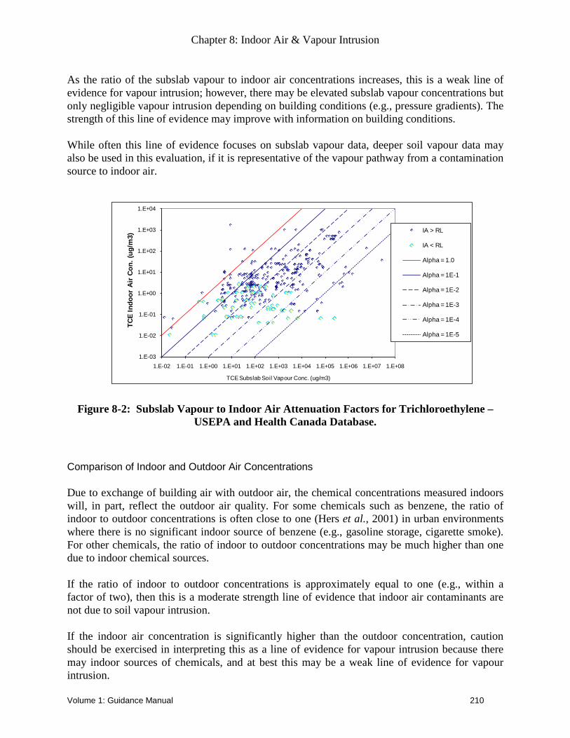
Chapter 8: Indoor Air & Vapour Intrusion
Volume 1: Guidance Manual 210
As the ratio of the subslab vapour to indoor air concentrations increases, this is a weak line of evidence for vapour intrusion; however, there may be elevated subslab vapour concentrations but only negligible vapour intrusion depending on building conditions (e.g., pressure gradients). The strength of this line of evidence may improve with information on building conditions.
While often this line of evidence focuses on subslab vapour data, deeper soil vapour data may also be used in this evaluation, if it is representative of the vapour pathway from a contamination source to indoor air.
Figure 8-2: Subslab Vapour to Indoor Air Attenuation Factors for Trichloroethylene – USEPA and Health Canada Database.
Comparison of Indoor and Outdoor Air Concentrations
Due to exchange of building air with outdoor air, the chemical concentrations measured indoors will, in part, reflect the outdoor air quality. For some chemicals such as benzene, the ratio of indoor to outdoor concentrations is often close to one (Hers et al., 2001) in urban environments where there is no significant indoor source of benzene (e.g., gasoline storage, cigarette smoke). For other chemicals, the ratio of indoor to outdoor concentrations may be much higher than one due to indoor chemical sources.
If the ratio of indoor to outdoor concentrations is approximately equal to one (e.g., within a factor of two), then this is a moderate strength line of evidence that indoor air contaminants are not due to soil vapour intrusion.
If the indoor air concentration is significantly higher than the outdoor concentration, caution should be exercised in interpreting this as a line of evidence for vapour intrusion because there may indoor sources of chemicals, and at best this may be a weak line of evidence for vapour intrusion.
1.E-03
1.E-02
1.E-01
1.E+00
1.E+01
1.E+02
1.E+03
1.E+04
1.E-02 1.E-01 1.E+00 1.E+01 1.E+02 1.E+03 1.E+04 1.E+05 1.E+06 1.E+07 1.E+08
TCE
Indo
or A
ir Co
n. (u
g/m
3)
TCE Subslab Soil Vapour Conc. (ug/m3)
IA > RL
IA < RL
Alpha = 1.0
Alpha = 1E-1
Alpha = 1E-2
Alpha = 1E-3
Alpha = 1E-4
Alpha = 1E-5
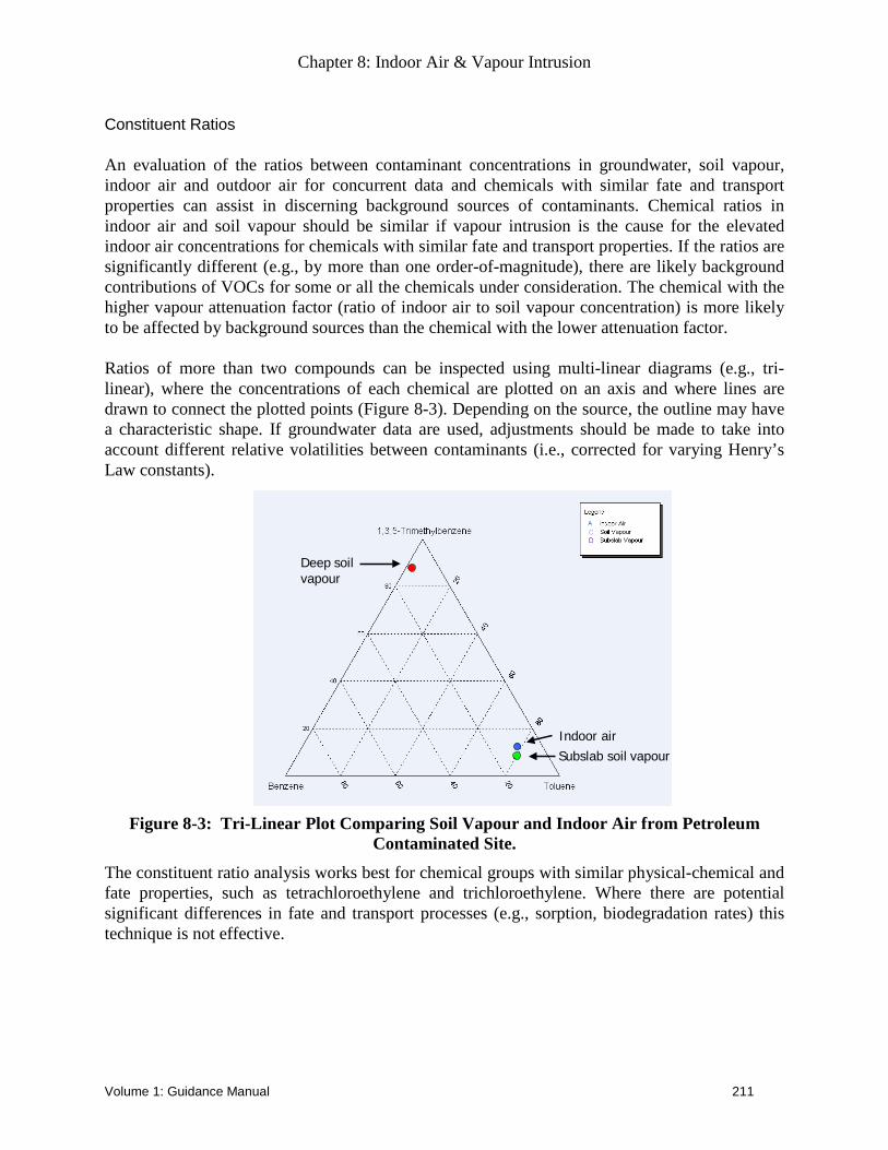
Chapter 8: Indoor Air & Vapour Intrusion
Volume 1: Guidance Manual 211
Constituent Ratios
An evaluation of the ratios between contaminant concentrations in groundwater, soil vapour, indoor air and outdoor air for concurrent data and chemicals with similar fate and transport properties can assist in discerning background sources of contaminants. Chemical ratios in indoor air and soil vapour should be similar if vapour intrusion is the cause for the elevated indoor air concentrations for chemicals with similar fate and transport properties. If the ratios are significantly different (e.g., by more than one order-of-magnitude), there are likely background contributions of VOCs for some or all the chemicals under consideration. The chemical with the higher vapour attenuation factor (ratio of indoor air to soil vapour concentration) is more likely to be affected by background sources than the chemical with the lower attenuation factor.
Ratios of more than two compounds can be inspected using multi-linear diagrams (e.g., tri-linear), where the concentrations of each chemical are plotted on an axis and where lines are drawn to connect the plotted points (Figure 8-3). Depending on the source, the outline may have a characteristic shape. If groundwater data are used, adjustments should be made to take into account different relative volatilities between contaminants (i.e., corrected for varying Henry’s Law constants).
Figure 8-3: Tri-Linear Plot Comparing Soil Vapour and Indoor Air from Petroleum Contaminated Site.
The constituent ratio analysis works best for chemical groups with similar physical-chemical and fate properties, such as tetrachloroethylene and trichloroethylene. Where there are potential significant differences in fate and transport processes (e.g., sorption, biodegradation rates) this technique is not effective.
GOLDER ASSOCI
Deep soil vapour
Subslab soil vapourIndoor air

Chapter 8: Indoor Air & Vapour Intrusion
Volume 1: Guidance Manual 212
Marker Chemicals
Marker chemicals are compounds that are associated with the subsurface contamination, but not background air sources. An example of a marker chemical is 1,1 dichloroethylene (DCE), which is a degradation product of 1,1,1-trichloroethane and trichloroethylene, and which is generally considered not to be present as a background chemical in indoor air. Therefore, detectable levels of 1,1-DCE in indoor air would suggest soil vapour intrusion is occurring (unless from an ambient air source). Marker chemicals, if present, are also useful compounds when evaluating constituent ratios using the method described above.
Spatial Trends
An evaluation of spatial trends may provide insight on differentiating background sources from the contaminants of interest. For instance, VOC concentrations in a basement may be higher than in upper floors. This provides support for a subsurface vapour source, but care must be taken to ensure that the results were not biased by products stored in the basement. Also, testing of “pathway” samples collected near foundation cracks, unsealed utility entry points or other possible preferential transport zones could be compared to samples collected at other parts of the building. Concentrations in pathway samples that are elevated relative to concentrations in samples from other parts of the building may indicate soil vapour intrusion is occurring.
For sites with larger scale impacts with where multiple buildings are tested, it may be possible to compare the spatial trends in subsurface data, if well characterized (e.g., contoured groundwater or soil vapour plume, location of hot spots) and compare this to indoor air concentrations measured in multiple buildings. Caution should be exercised when following this approach depending on the confidence in the subsurface data.
Comparison of Indoor Air Data to Literature Background Concentrations
Indoor air quality data may be compared to published data on indoor air quality from sites that are not impacted by vapour intrusion. Typical background sources and concentrations of VOCs in indoor air were discussed in Section 8.2.1. The site data should be compared to data for buildings of similar type (e.g., single family residence, apartment, commercial).
Comparison of Indoor Air Data to Control Building Survey
IAQ data from buildings above the contaminated area may be compared to IAQ data from nearby “reference” buildings outside the contaminated area. This method requires a sufficient number of buildings to be tested such that statistical comparisons between data sets can be made. There are a number of confounding factors that could contribute to differences in air quality unrelated to soil vapour intrusion. To the extent possible, building construction and occupant usage of the reference buildings should be similar to the buildings of interest. This approach is infrequently used since it is not practical.

Chapter 8: Indoor Air & Vapour Intrusion
Volume 1: Guidance Manual 213
Modification of Building Pressurization
Indoor air quality testing under positive and negative building pressurization can be used to determine whether soil vapour intrusion is occurring and to evaluate the possible influence of background sources on indoor air quality. Indoor air concentrations that are significantly different under positive and negative pressures suggest vapour intrusion is occurring, since typically, soil gas advection caused by building depressurization is the main cause for soil vapour intrusion. Building pressures can be modified through control of the building HVAC system and use of temporary fans or blowers. While modification of building pressurization goes beyond the typical scope of testing for IAQ studies, it could be considered when it is important to distinguish background from possible subsurface vapour sources.
Emerging Methods
Carbon stable isotope analysis (CSIA) is an emerging method for identifying potential vapour sources. Isotopes have a different atomic mass (number of neutrons); one example is carbon 12 and 13. Fractionation may occur when biodegradation or other transformation processes preferentially break down lighter isotopes. McHugh et al. (2010) present preliminary analysis where isotope ratios of TCE were determined by a modified PT-GC-IRMS (purge-and-trap-gas chromatography–isotope ratio mass spectrometry). The results indicated a difference in the carbon isotope ratios for a subsurface and indoor source.
Naturally-occurring radon can be used as a tracer to evaluate sub-slab to indoor air attenuation for VOCs (assuming similar transport properties across the building envelope) through simultaneous measurement of VOCs and radon in indoor air, outdoor air and subslab soil vapour. otential advantages of radon are that there are limited sources of indoor radon (excluding granite counter tops and other decorative stone) and indoor radon concentrations are in most cases above detectable levels (unlike VOCs where bias may be caused by non-detect values).
Comparison of Measurements to Empirical Data and/or Modeling Results
Where there is relatively high confidence in the data and where representative spatially- and temporally-averaged attenuation ratios can be calculated for a building, the internal consistency between measurements and empirical and/or modeling data can be evaluated. A comprehensive statistical analysis of empirical data for non-degrading chemicals is provided in USEPA (2012). A site-specific ratio that exceeds the upper range of the measured empirical database of attenuation factors (for empirical data that has been filtered to remove the influence of background) by a significant degree may suggest a background component. Site-specific modeling may also be performed, for example using the Johnson and Ettinger (1991) model. When there is good quality input data, the modeled and measured values can be expected to agree within about an order-of-magnitude (Hers et al., 2003; Abreu and Johnson, 2005; EPRI, 2005). When using this approach, caution must be taken in that the conceptual site model must be well understood and data adequacy and quality must be high. Comparisons using the Johnson and Ettinger model may not be meaningful if there are conditions that fall outside of the processes included in the Johnson and Ettinger model such as preferential pathways, barometric pumping or biodegradation.

Chapter 8: Indoor Air & Vapour Intrusion
Volume 1: Guidance Manual 214
Resources and Weblinks 8.6
Compared to soil and groundwater, there are much fewer state-of-the-art guidance documents and resources available on indoor air sampling and analysis. Useful information is provided in the following references.
Interstate Technology and Regulatory Council (ITRC). The Vapor Intrusion Pathway: A Practical Guide (VI-1)(January 2007, 173 pages) provides a generalized framework for evaluating the vapour intrusion pathway and describes the various tools available for investigation, data evaluation, and mitigation. The Vapor Intrusion Pathway: Investigative Approaches for Typical Scenarios (VI-2) (January 2007, 52 pages) is a supplement to Vapor Intrusion Pathway: A Practical Guide. The supplement describes applicable approaches for evaluating the vapour intrusion pathway in six typical scenarios. http://www.itrcweb.org/Documents/VI-1.pdf . http://www.itrcweb.org/Documents/VI-1A.pdf
American Petroleum Institute (API). A Practical Strategy for Assessing the Subsurface Vapor-to-Indoor Air Migration Pathway at Petroleum Hydrocarbon Sites (November 2005) includes guidance on soil gas sampling approach, methods and analysis (November, 2005). http://www.api.org/environment-health-and-safety/clean-water/ground-water/vapor-intrusion/vi-publications/assessing-vapor-intrusion
New Jersey Department of Environmental Protection. Vapour Intrusion Guidance (January, 2013). This guidance includes comprehensive methods for site characterization, including soil gas sampling and analysis.
http://www.nj.gov/dep/srp/guidance/vaporintrusion/
Massachusetts Department of Environmental Protection. Indoor Air Sampling and Evaluation Guide (April, 2002). http://www.mass.gov/dep/cleanup/laws/02-430.pdf
References 8.7
Abreu, L., and P.C. Johnson. 2005. Effect of Vapor Source-Building Separation and Building Construction on Soil Vapor Intrusion as Studied with a Three-Dimensional Model. Environ. Sci. Technol., 39, 4550-4561.
Air Toxics. 2011. Ultra III Comparison Studies. February. Accessed April 24, 2014. American Society for Testing Materials (ASTM). 2003. ASTM Standard E-2121. Standard Practice for
Installing Radon Mitigation Systems in Existing Low-Rise Residential Buildings. February 10. American Society of Heating Refrigerating and Air-Conditioning Engineers, Inc. (ASHRAE). 2010a.
ANSI/ASHRAE Standard 62.2-2010a. Ventilation and Acceptable Indoor Air Quality in Low-Rise Residential Buildings.
American Society of Heating Refrigerating and Air-Conditioning Engineers, Inc. (ASHRAE), 2010b. ANSI/ASHRAE Standard 62.1-2010a. Ventilation for Acceptable Indoor Air Quality.
Bailey, S., H. Scobie, P. Fellin and H. Li. 2008. The Use of Passive Sampling Device in a Vapour Intrusion Study. Presentation at AWMA Vapour Intrusion Seminar, Ottawa, Canada, October 28.

Chapter 8: Indoor Air & Vapour Intrusion
Volume 1: Guidance Manual 215
Brown, R. 2000. Monitoring the ambient environment with diffusive samplers: theory and practical considerations. J. Environ. Monit. 2, pp. 1-9.
Bruno, P., M. Caputi, M. Caselli and G. de Gennaro. 2004. Reliability of a BTEX radial diffusive sampler for thermal desorption: field measurements. Atmospheric Environmental, 39(7): 1347-1355.
Colorado Department of Public Health and Environment (DPHE). 2004. Draft Indoor Air Guidance. September.
Davis, C.S., and R. Otson, 1996. Estimation of Emissions of Volatile Organic Compounds (VOCs) from Canadian Residences. Volatile Organic Compounds in the Environment, ASTM STP 1261.
Electric Power Research Institute (EPRI). 2005. Reference Handbook for Site-Specific Assessment of Subsurface Vapor Intrusion in Indoor Air. Palo Alto, California, 1008492.
Figley, D.A. 1997. A Guide for Estimating Indoor Concentrations of Soil Gas Pollutants in Houses. Prepared for CMHC, 1997.
Font, L.L., C. Baixeras, and C. Domingo. 2001. Uncertainty, Variability, and Sensitivity Analysis Applied to the RAGENA Model of Radon Generation, Entry, and Accumulation Indoors. Sci. Total Environ., 272, 25-31.
Gusdorf, J., and T. Hamlin. 1995. Indoor Air Quality and Ventilation Rates in R-2000 Houses. Buildings Group, Residential Programs, Energy Technology Branch. Call-up No. 23440-95-1037. Energy Technology Branch, CANMET, Department of Natural Resources Canada, Ottawa, Ontario (43 pg).
Groenevelt, H., T. McAlary, B. Chadwick and I. Rivera-Duarte. 2010. Quantitative Passive Samplers for Indoor and Outdoor Air Monitoring during Vapour Intrusion Assessments. Poster Battelle Conference Remediation of Chlorinated and Recalitrant Compounds, San Diego, May.
Groves-Kirkby, C.J., A.R. Denman, R.G.M Crockett, P.S. Phillips, A. Woolridge and G.K. Gillmore. 2006. Time-Integrating Radon Gas Measurements in Domestic Premises: Comparison of Short-, Medium and Long-Term Exposures. J. Environ. Radioactivity, 86(1): 92-109.
Hayes, H., D.J. Benton and N. Khan. 2006. The Impact of Sampling Media on Soil Gas Measurements. Proc. Of AWMA Vapor Intrusion – The Next Great Environmental Challenge – An Update, September 13-15, Los Angelos, California.
Hayes, H., D.J. Benton, S. Grewal and N. Khan. 2007. Evaluation of Sorbent Methodology for Petroleum-Impacted Site Investigations. Proc. Of AWMA Vapor Intrusion – Learning from the Challenges, September 25-27, Providence, Rhode Island.
Héroux, M.-È., D. Gauvin, N. Gilbert, M. Guay, G. Dupuis, M. Legris and B. Levesque. 2007. Housing characteristics and indoor concentrations of selected volatile organic compounds (VOCs) in Québec City, Canada. Indoor and Built Environment 17: pp. 128–137.
Hers, I., R. Zapf-Gilje, P.C. Johnson and L. Li. 2003. Evaluation of the Johnson and Ettinger model for prediction of indoor air quality. Ground Water Monitoring and Remediation, Summer 2003.
Hers, I., R. Zapf-Gilje, L. Li and J. Atwater. 2001. The use of indoor air measurements to evaluate exposure and risk from subsurface VOCs. J. Air & Waste Manage. Assoc. 51: 174-185.
Jia, C., S. Batterman and C. Godwin. 2007. Continuous, intermittent and passive sampling of airborne VOCs. J. of Enviro. Monit., 9(11): 1220 -1230.
Johnson, P.C. 2005. Identification of application-specific critical inputs for the 1991 Johnson and Ettinger vapor intrusion algorithm. Groundwater Monitoring & Remediation, 25(1): 63-78.
Johnson, P.C., and R. Ettinger. 1991. Heuristic Model for Predicting the Intrusion Rate of Contaminant Vapours into Buildings. Environmental Science and Technology, 25(8): 1445-1452.

Chapter 8: Indoor Air & Vapour Intrusion
Volume 1: Guidance Manual 216
Lee, K., and M. Yun. 2004. Effect of Face Velocity on Measurement of Passive Samplers. Proc. of American Industrial Hygience Association Conference, May 8-13, 2004, Atlanta, Georgia, USA.
McClenny, W.A., K.D. Oliver, H.H. Jacumin Jr., E.H. Daughtrey and J. Whitaker. 2005. 24-Hour diffusive sampling of toxic VOCs in air onto Carbopack X solid adsorbant followed by thermal desorption GC/MS Analysis – Laboratory studies. Environ. Monit., 7, 248-256.
McHugh, T., K. Gorder, T. Kuder, R. Philip, S. Fiorenza, H. O`Neill and J. Odencrantz. 2010. Use of CSIA to Distinguish Between Vapor Intrusion and Indoor Sources of VOCs. Proc. of AWMA Conference on Vapor Intrusion, Chicago, Illinois, September 29-30.
Murray, D.M. and D.E. Burmaster. 1995. Residential air exchange rates in the United States: empirical and estimated parametric distributions by season and climatic region. Risk Anal. 1995. 15:459-465.
National Institute of Standards and Technology (NIST). 2004. Analysis of Ventilation Data from the U.S. Environmental Protection Agency Building Assessment Survey and Evaluation (BASE) Study. Prepared by Andrew Persily and Josh Gorfain, NISTIR Report 7145.
New Jersey Department of Environmental Protection (NJDEP). 2005. Vapour Intrusion Guidance. October.
Occupational Safety and Health Administration (OHSA). 2003. Performance of SKC Ultra Passive Samplers Containing Carboxen 1016, Carbortap Z, or Chromosorb 106 When Challenged With a Mixture Containing Twenty of OSHA SLTC’s Top Solvent Analytes. Prepared by Warren Hendricks for Organic Methods Evaluation Branch, OSHA Salt Lake Technical Center, Salt Lake City, Utah 84115-1802. February.
Occupational Safety and Health Administration (OHSA). 1998. Determination of the Sampling Rate Variation for SKC 575 Series Passive Samplers. Prepared by Warren Hendricks for Organic Methods Evaluation Branch, OSHA Salt Lake Technical Center, Salt Lake City, Utah 84115-1802. April.
Otson, R., and J. Zhu. 1997. I/O Values for Determination of the Origin of Some Indoor Organic Pollutants. Proc. Air & Waste Management Association’s 90th Annual Meeting and Exhibition, Toronto, Ontario, Canada, June 8 to 13, 1997.
Saskatchewan Research Council (SRC). 1992. Volatile Organic Compound Survey and Summarization of Results. Report I-4800-1-C-92. Prepared for Canada Mortgage and Housing Corporation. April.
Seethapathy, S., T. Górecki and X. Li. 2008. Passive sampling in Environmental Analysis. Journal of Chromatography A, 1184(1-2): 234–253.
Science Advisory Board for Contaminated Sites in British Columbia (SABCS). 2011. Guidance on Site Characterization for Evaluation of Soil Vapour Intrusion into Buildings. Prepared by Golder Associates Ltd. (Dr. Ian Hers, author). May.
SKC. 2006. Measuring sub-ppb levels of VOCs in Indoor Air. Technical Note. Publication 1720, Issue 0611.
Strandberg, B., A. Sunesson, K. Olsson, J. Levin, G. Ljungqvist, M. Sundgren, G, Sallsten and L. Barregard. 2005. Evaluation of two types of diffusive samplers and adsorbents for measuring 1,3-butadience and benzene in air. Atmospheric Environment, 39(22): 4101-1440.
U.S. Environmental Protection Agency. 2012. EPA’s Vapor Intrusion Database: Evaluation and Characterization of Attenuation Factors for Chlorinated Volatile Organic Compounds and Residential Buildings. U.S. Environmental Protection Agency, Washington, DC. Report 530-R-10-002. February.
Walkinshaw, D.S. 1987. Indoor Air Quality in Cold Climates: Hazards and Abatements Measures Summary of an APCA International Speciality Conference. J. Air Pollut. Control Assoc., 36, 235-241.

Chapter 8: Indoor Air & Vapour Intrusion
Volume 1: Guidance Manual 217
Western Australia Department of Environment. 2005. Wagerup 2003 (PID) Ambient Air Sampling Program. June 2005.
3M Technical Data Bulletin. 2000. Organic Vapor Monitor Sampling and Analysis Guide (1028); 3M: St. Paul, MN, 2000. Available at: http://multimedia.3m.com/mws/media/110731O/organic-vapor-monitor-sampling-and-analysis-guide.pdf.
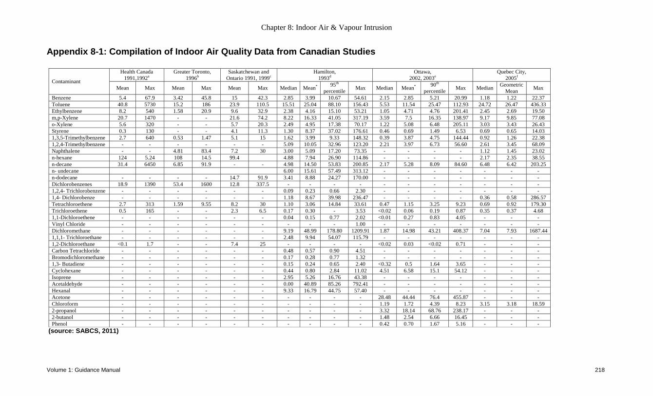
Chapter 8: Indoor Air & Vapour Intrusion
Volume 1: Guidance Manual 218
Contaminant
Health Canada 1991,1992a
Greater Toronto, 1996b
Saskatchewan and Ontario 1991, 1999c
Hamilton, 1993d
Ottawa, 2002, 2003e
Quebec City, 2005f
Mean Max Mean Max Mean Max Median Mean* 95th percentile Max Median Mean* 90th
percentile Max Median Geometric Mean Max
Benzene 5.4 67.9 3.42 45.8 15 42.3 2.85 3.99 10.67 54.61 2.15 2.85 5.21 20.99 1.18 1.22 22.37 Toluene 40.8 5730 15.2 186 23.9 110.5 15.51 25.04 88.10 156.43 5.53 11.54 25.47 112.93 24.72 26.47 436.33 Ethylbenzene 8.2 540 1.58 20.9 9.6 32.9 2.38 4.16 15.10 53.21 1.05 4.71 4.76 201.41 2.45 2.69 19.50 m,p-Xylene 20.7 1470 - - 21.6 74.2 8.22 16.33 41.05 317.19 3.59 7.5 16.35 138.97 9.17 9.85 77.08 o-Xylene 5.6 320 - - 5.7 20.3 2.49 4.95 17.38 70.17 1.22 5.08 6.48 205.11 3.03 3.43 26.43 Styrene 0.3 130 - - 4.1 11.3 1.30 8.37 37.02 176.61 0.46 0.69 1.49 6.53 0.69 0.65 14.03 1,3,5-Trimethylbenzene 2.7 640 0.53 1.47 5.1 15 1.62 3.99 9.33 148.32 0.39 3.87 4.75 144.44 0.92 1.26 22.38 1,2,4-Trimethylbenzene - - - - - - 5.09 10.05 32.96 123.20 2.21 3.97 6.73 56.60 2.61 3.45 68.09 Naphthalene - - 4.81 83.4 7.2 30 3.00 5.09 17.20 73.35 - - - - 1.12 1.45 23.02 n-hexane 124 5.24 108 14.5 99.4 4.88 7.94 26.90 114.86 - - - - 2.17 2.35 38.55 n-decane 31.4 6450 6.85 91.9 - - 4.98 14.50 53.83 200.85 2.17 5.28 8.09 84.60 6.48 6.42 203.25 n- undecane 6.00 15.61 57.49 313.12 - - - - - - - n-dodecane - - - - 14.7 91.9 3.41 8.88 24.27 170.00 - - - - - - - Dichlorobenzenes 18.9 1390 53.4 1600 12.8 337.5 - - - - - - - - - - - 1,2,4- Trichlorobenzene - - - - - - 0.09 0.23 0.66 2.30 - - - - - - - 1,4- Dichlorobenze - - - - - - 1.18 8.67 39.98 236.47 - - - - 0.36 0.58 286.57 Tetrachloroethene 2.7 313 1.59 9.55 8.2 30 1.10 3.06 14.84 33.61 0.47 1.15 3.25 9.23 0.69 0.92 179.30 Trichloroethene 0.5 165 - - 2.3 6.5 0.17 0.30 - 3.53 <0.02 0.06 0.19 0.87 0.35 0.37 4.68 1,1-Dichloroethene - - - - - - 0.04 0.15 0.77 2.02 <0.01 0.27 0.83 4.05 - - - Vinyl Chloride - - - - - - - - - 1.00 - - - - - - - Dichloromethane - - - - - - 9.19 48.99 178.80 1209.91 1.87 14.98 43.21 408.37 7.04 7.93 1687.44 1,1,1- Trichloroethane - - - - - - 2.48 9.94 54.07 115.79 - - - - - - - 1,2-Dichloroethane <0.1 1.7 - - 7.4 25 - - - - <0.02 0.03 <0.02 0.71 - - - Carbon Tetrachloride - - - - - - 0.48 0.57 0.90 4.51 - - - - - - - Bromodichloromethane - - - - - - 0.17 0.28 0.77 1.32 - - - - - - - 1,3- Butadiene - - - - - - 0.15 0.24 0.65 2.40 <0.32 0.5 1.64 3.65 - - - Cyclohexane - - - - - - 0.44 0.80 2.84 11.02 4.51 6.58 15.1 54.12 - - - Isoprene - - - - - - 2.95 5.26 16.76 43.38 - - - - - - - Acetaldehyde - - - - - - 0.00 40.89 85.26 792.41 - - - - - - - Hexanal - - - - - - 9.33 16.79 44.75 57.40 - - - - - - - Acetone - - - - - - - - - - 28.48 44.44 76.4 455.87 - - - Chloroform - - - - - - - - - - 1.19 1.72 4.39 8.23 3.15 3.18 18.59 2-propanol - - - - - - - - - - 3.32 18.14 68.76 238.17 - - - 2-butanol - - - - - - - - - - 1.48 2.54 6.66 16.45 - - - Phenol - - - - - - - - - - 0.42 0.70 1.67 5.16 - - -
Appendix 8-1: Compilation of Indoor Air Quality Data from Canadian Studies
(source: SABCS, 2011)

Chapter 8: Indoor Air & Vapour Intrusion
Volume 1: Guidance Manual 219
Notes: Concentrations in units of µg/m3 *Arithmetic mean
a Davis, C.S. and R. Otson, 1996. Estimation of Emissions of Volatile Organic Compounds (VOCs) from Canadian Residences. Volatile Organic Compounds in the Environment, ASTM STP 1261.
b Otson, R. and J. Zhu. 1997. I/O Values for Determination of the Origin of Some Indoor OrganicPollutants. Proc. of Air & Waste Management Association’s 90th Annual Meeting and Exhibition, Toronto, Ontario, Canada, June 8 to 13, 1997.
c Saskatchewan Research Council (SRC), 1992. Volatile Organic Compound Survey and Summarization of Results. Report I-4800-1-C-92. Prepared for Canada Mortgage and Housing Corporation. April.
d provided by Camilo Martinez, Ontario MoE e Zhu, J., R. Newhook, L. Marbo and C. Chan. 2005. Selected volatile organic compounds in residential air in the city of Ottawa, Canada. Environmental Science & Technology 39: pp. 3964-
3971. f Héroux, M.-È., D. Gauvin, N. Gilbert, M. Guay, G. Dupuis, M. Legris and B. Levesque. 2008. Housing characteristics and indoor concentrations of selected volatile organic compounds
(VOCs) in Québec City, Canada. Indoor and Built Environment 17: pp. 128–137.
Contaminant
Health Canada 1991,1992a
Greater Toronto, 1996b
Saskatchewan and Ontario 1991, 1999c
Hamilton, 1993d
Ottawa, 2002, 2003e
Quebec City, 2005f
Mean Max Mean Max Mean Max Median Mean* 95th percentile Max Median Mean* 90th
percentile Max Median Geometric Mean Max
Carbon disulfide - - - - - - - - - - 0.13 0.34 0.86 3.29 - - - 1-butanol - - - - - - - - - - 0.4 4.25 5.96 139.66 - - - 4-methyl-2-pentanone - - - - - - - - - - 0.16 0.26 0.8 1.40 - - - Acrylonitrile - - - - - - - - - - 0.06 0.27 0.26 8.89 - - - 2-butoxyethanol - - - - - - - - - - <0.28 2.85 7.06 41.44 - - - Methyl methacrylate - - - - - - - - - - <0.01 0.05 0.06 1.12 - - - Methyl tert-butyl ether - - - - - - - - - - <0.05 0.17 <0.05 3.32 - - - Chlorobenzene - - - - - - - - - - <0.01 <0.012 <0.01 0.04 - - - 3,5-dimethylaniline - - - - - - - - - - <1.2 <1.2 <1.2 4.71 - - - 1,2-dichlorobenze - - - - - - - - - - <0.02 <0.02 <0.02 0.11 - - - 1,3-dichlorobenze - - - - - - - - - - 0.15 0.77 1.05 16.19 - - - 2-ethoxyethanol - - - - - - - - - - <0.13 0.43 <0.13 27.14 - - - 2-methoxyethanol - - - - - - - - - - <0.23 <0.23 <0.23 <0.23 - - - 1,2-dichloropropane - - - - - - - - - - <0.04 <0.04 <0.04 <0.04 - - - Ethylene dibromide - - - - - - - - - - <0.02 <0.02 <0.02 <0.02 - - - 1,1,2,2-tetrachloroethane - - - - - - - - - - <0.02 <0.02 <0.02 <0.02 - - -
Cumene - - - - - - - - - - - - - - 0.8 0.88 45.48 α-pinene - - - - - - - - - - - - - - 7.95 9.74 800.68 d-limonene - - - - - - - - - - - - - - 28.54 28.06 329.89 p-cymene - - - - - - - - - - - - - - 1.49 1.55 32.90

Chapter 9: Surface Water Characterization
Volume 1: Guidance Manual 220
9 SURFACE WATER CHARACTERIZATION GUIDANCE
Context, Purpose, Scope 9.1
Surface water is often a critical route of exposure that must be considered in human health and ecological risk assessments.
For example, important and sensitive natural resources such as benthic macroinvertebrates, water column zooplankton, fish, and wildlife depend on surface water for many life-cycle functions. Surface water also provides routes of chemical exposure to humans via drinking water and to recreational swimmers and boaters via incidental surface water ingestion and/or dermal contact. Consideration of potential human health and ecological risks posed by contaminants of potential concern (COPCs) in surface water must also consider fate and transport pathways that may mitigate or exacerbate COPC exposure. For example, changes in surface water hardness (for freshwater), salinity, and pH can increase or decrease the bioavailability of many heavy metals. In addition, sorption of chemicals to solids suspended in surface water can be an important fate process that either decreases chemical bioavailability or enhances deposition of chemicals to sediment, thereby affecting which media are likely to contribute to exposure. The valence state (e.g., hexavalent vs. trivalent chromium), proportion of a chemical in dissolved forms (especially metals), and photoactivation of chemicals such as polycyclic aromatic hydrocarbons (PAHs) can be important considerations in evaluating the risk associated with exposure to chemicals in surface water.
The purposes of this chapter are to:
• Provide a framework that will aid in the collection of valid and representative1 surface water chemical data
• Provide guidance on general factors to consider in sampling surface water and in identifying sources of data uncertainty
• Identify unique sampling considerations for investigators charged with developing and implementing surface water sampling programs to assess human health and ecological risks
1 See Exhibit 5-1 for overview of characteristics of representative data.
Surface Water Sampling Guidance
This chapter describes the planning, process and methods for surface water characterization. The key elements and their corresponding sections in the chapter include:
• Conceptual site model and site reconnaissance (9.2)
• Sampling program design (9.3)
• Sampling equipment (9.4)
• Sample preservation and storage (9.5)
• Data analysis (9.6)
• Resources and weblinks (9.7)
Related tools are the checklists provided in Volume 2, as well as several Suggested Operating Procedures (SOPs) provided in Volume 3.

Chapter 9: Surface Water Characterization
Volume 1: Guidance Manual 221
• Describe quality assurance/quality control (QA/QC) techniques suitable for commonly applied surface water sampling methods
The scope of this chapter is to provide general guidance for sampling surface water in support of study area characterization when conducting human health and ecological risk assessments. Study area characterization may include, for example, chemical analyses, toxicological analyses, and treatability studies using surface water samples. This guidance chapter addresses general sampling design, sampling equipment, and other factors pertaining to sampling water from lakes, ponds, rivers, streams, estuaries, and oceans. It focuses on methods most commonly used in support of risk assessments.
As discussed previously, obtaining representative data is closely linked to the sampling design, which includes consideration of the scale at which samples are analyzed. The sources of uncertainty in data should be understood and effectively communicated to the risk assessor. Uncertainties may include those due to the variability in the chemical distribution, those due to temporal variability, those introduced through the sampling design, and methods used for sampling and analysis. Uncertainty is reduced through development of a conceptual site model (CSM) that is updated as new information is obtained, design and implementation of an appropriate sampling strategy, and use of statistical techniques to assist in sampling design and data interpretation. Most risk assessments describe sources of uncertainty and their effects on overall conclusions in a qualitative narrative and/or summary table. Quantitative methods, such as probabilistic (e.g., Monte Carlo) analyses, can also be employed to characterize uncertainty and variability (see, for example, MOEE, 1996; USEPA 1997a; 1999; Ritter et al., 2000; Warila et al., 2001).
The characterization of surface water at contaminated study areas should follow the characterization process described in Chapter 2. This guidance chapter does not address laboratory analytical protocols since for most COPCs, standardized methods are employed and information on these methods is readily available (see Volume 4 of the guidance). Furthermore, the intent of this chapter is to focus on methods for collecting samples to be used for chemical analyses.
Conceptual Site Model for Surface Water Characterization 9.2
As detailed in Chapter 4 of this guidance document, development of a site-specific CSM is a critical first step in the process of characterizing the nature and extent of COPCs present at a study area. The CSM serves many purposes. It allows visualization and compartmentalization of COPCs, potential exposure routes, and the fate and transport processes that may alter the form and location of a COPC in the aquatic environment. The CSM serves as a guide to the design of the sampling program. Finally, the CSM provides project personnel and decision makers with a tool to understand and communicate potential exposures within a defined study area.
Definition of Surface Water For purposes of this guidance chapter, surface water refers to water that has collected in water bodies on the land surface, rather than beneath it (groundwater). In this context, surface water may include water at the surface and at depth in these water bodies.

Chapter 9: Surface Water Characterization
Volume 1: Guidance Manual 222
If COPCs with widely varying physical and chemical properties are present on-site, information related to their solubility, octanol/water partition coefficient, Henry’s Law constants, etc. will aid in defining key transport and fate processes (e.g., evaporation, sorption) and sinks (i.e., depositories). If migration pathways are likely to be influenced by weather, climatic and meteorological data may enhance the CSM.
Both common and less obvious sources of COPCs in surface water should be considered, particularly for mercury and other trace contaminants for which atmospheric deposition is a key route of entry to surface water.
An example surface water CSM is illustrated in Figure 4-12. Risk assessors are expected to modify it or use their preferred presentation format for site-specific CSMs.
As discussed in Chapter 4, CSMs for study areas with significant surface water may warrant consideration of water body specific factors and COPC-specific considerations to help focus sampling priorities during the study design phase. In addition, the narrative and/or pictorial CSMs for individual sites should acknowledge and discuss reference sites to which conditions at the contaminated site will be compared in the risk assessment.
CSMs for study areas with significant surface water may also consider one or more reference areas. Definition of study area boundaries and selection of appropriate unimpacted or reference areas are important considerations that should be completed as part of the CSM development. A reference area is an unimpacted or relatively unimpacted area with physical and biological attributes similar to those of the study area with the exception of the presence of COPCs. Because of the practical difficulty in locating an ideal reference area, it is often necessary to select locations with COPC concentrations that are equivalent to regional background concentrations.
It is often advisable to select more than one reference area to represent the range of background conditions and/or the range of the site physical and biological characteristics, and to allow for more meaningful statistical comparisons, although in some instances (e.g., locations with unique physical or biological conditions or constrained options for reference areas) reliance on data from a single reference area may be necessary. Additional information regarding selection criteria for reference areas is discussed in Section 4.6.1.
Site Reconnaissance for Surface Water Characterization The primary objective of site reconnaissance is to improve the efficiency and effectiveness of sampling programs through early planning and identification of unique study area conditions that warrant consideration before sampling begins. Both desk top and on-site reconnaissance can be conducted prior to initiation of surface water sampling. Although the initial site reconnaissance can be conducted either prior to or in conjunction with the first sampling event, the former is preferable in that early reconnaissance provides time to obtain any specialized equipment (e.g., four wheel drive vehicles) necessitated by unique study area conditions and to resolve study area access issues (e.g., obtaining access permission, resolving safety issues, confirming small boat access across different tidal stages).

Chapter 9: Surface Water Characterization
Volume 1: Guidance Manual 223
Prior to conducting the site reconnaissance, it is advisable to review background and supporting information and materials, such as:
• Files related to the nature and extent of COPCs present at the study area, historical study area uses, historical manufacturing and disposal practices, and the presence of other infrastructure (e.g., roadways, railways, pipelines, bridges)
• Topographic maps and aerial photographs
• Property boundaries, as well as names, addresses, and phone numbers of abutting land owners
• Physical/chemical information on materials manufactured, stored, or disposed on-site
• Study area drainage maps and relationship of drainage structures to waste storage or disposal areas. Identify wetlands and floodplains
• Locations of effluent discharges (process water and storm water), landfills, and above ground and below ground storage tanks
• Tide data
• Identification of nearby water bodies and information related to seasonal flow and general water quality conditions (pH, suspended solids, salinity etc.)
• Aquatic setting, as it pertains to study design and equipment needs (e.g., wadeable riffle/run/pool stream habitat vs. deep pond or lake, tidally dominated estuary vs. river with unidirectional flow, current and historical flow regime and pattern)
• Presence of federally or provincially endangered species, threatened species or species of special concern, provincial areas of natural or scientific interest, special habitats or “residences” as defined by Canada’s Species at Risk Act (SARA) (i.e., dwelling-place, such as a den, nest or other similar area or place, that is occupied or habitually occupied by one or more individuals during all or part of their life cycles, including breeding, rearing, staging, wintering, feeding or hibernating), , provincially significant wetlands, and other sensitive aquatic communities (e.g., marine protected areas, coldwater fishery).
Key tasks to address during site reconnaissance include:
• Photograph and/or video record study area conditions
• Assess potential sampling locations and identify key surface water features (e.g., riffle and pool areas, eddies, salinity mixing zones) that may influence sampling locations and equipment needs
• Find suitable access points and routes of egress
• Identify safety issues and personal protective equipment
• Confirm routes of exposure identified in the CSM
• Identify factors that may mitigate or exacerbate exposure, as indicated by the CSM

Chapter 9: Surface Water Characterization
Volume 1: Guidance Manual 224
• Evaluate general water quality to confirm or refute information obtained during the desk top review
• Document indicators of disposal activities (e.g., visible drums, stained soil, dead vegetation)
• Identify low tide and high tide lines
• Identify potential reference areas
If any industrial facilities operate at the study area, it may be appropriate to interview facility personnel. For example, current employees may have knowledge of recent construction activities or new discharges not listed in historic files. Historic flow information on streams can be misleading if land uses have changed. Unknown operational conditions related to wastewater treatment processes can also be discerned through employee interviews (e.g., use of wastewater treatment chemicals not listed in background files). Facility employees may also provide information related to historic operating practices, dredging and channelization of local waterbodies, locations of historic outfalls, layout of the storm sewer and floor drain system, and COPCs historically used.
USEPA (1995) and the U.S. Navy (1997) provide additional information related to conducting desk top and on-site reconnaissance. USEPA (1997b) provides a detailed checklist for ecological study area reconnaissance.
Study Approach and Design for Surface Water Characterization 9.3
The purpose of this subsection is to identify key factors to consider when developing an appropriate study design for surface water sampling in support of human health and ecological risk assessments. Establishing a conceptually sound study approach supported by a technically sound study design is critical to proper characterization of COPCs in surface water.
9.3.1 Goals and Objectives
An appropriate surface water sampling program design depends on clear definition of sampling goals and objectives (CCME, 1993). Specifically, the goals and objectives of the sampling program dictate the extent to which sampling must address factors that dictate the form, fate, and effects of COPCs. Initially, project goals can be stated in broad terms, with specificity added as additional information on the most important aspects of a given risk assessment becomes available. The following list of fundamental goals and objectives of sampling programs for study area characterization in support of risk assessment was compiled from earlier chapters of this guidance (2 and 3) and several Canadian and US sources (CCME, 1993; Environment Canada, 2008; USEPA, 1995; U.S. Navy, 1997):
• To provide representative surface water COPC data related to potential human health and ecological risks at the study area; representative data are considered those that accurately reflect study area conditions as they relate to potential exposure to receptors
• To characterize, quantify, and delineate the spatial and temporal nature and extent of COPC concentrations relative to human and ecological exposure pathways

Chapter 9: Surface Water Characterization
Volume 1: Guidance Manual 225
• To assess the presence of COPCs in surface water relevant to migration and exposure pathways identified in the CSM
• To measure the extent to which factors identified in the CSM as potentially altering the form and fate of COPCs actually occur in study area surface water
• To ensure that the data collected will support meaningful conclusions and defensible decisions related to mitigation of any risks due to COPCs in surface water
• To identify, at least on a relative basis, high priority areas of concern that may pose imminent risks to human health and the environment, especially as defined by relevant regulatory statutes
Study objectives can be broad (e.g., to characterize the nature and extent of COPC concentrations at the study area) or highly focused (e.g., to develop statistically valid COPC distribution profiles for all on-site surface water bodies). CCME (1993) suggests differentiating between goals and objectives at the exploratory level and at the monitoring level. Regardless, the fundamental study objectives must be clearly stated if they are to effectively guide the sampling program. If statistical characterization of the data is desired, clear hypotheses must be formulated during the planning stage to guide study design. Quality assurance methods specific to surface water sampling programs are described below. For guidance related to quality management plans and methods related to broader project and program objectives (e.g., continuous quality improvement), see USEPA (2001b).
9.3.2 Data Quality Objectives
This subsection describes the data quality objectives (DQO) process and its role in establishing surface water sampling programs. The DQO process is used to determine if the data collected is the type, quantity, and quality needed to develop a defensible dataset. Various guidance documents and resources are available regarding the DQO process (e.g., USEPA, 2006 and www.triadcentral.org). Establishing concise DQOs is important to defining the specific types of data to be collected. Performance criteria and specific data acceptance and rejection criteria are critical components of the DQO process (e.g., CCME 1993; Chapters 3, 6, and 7 of this document; USEPA, 2006; U.S. Navy, 1997).
Fundamentally, the DQO process consists of seven iterative steps. Each step defines criteria that are used to establish final data collection and study design. The seven steps of the DQO process are (USEPA, 2000b; www.triadcentral.org/mgmt/splan/frame/dqo/index.cfm):
1. Problem statement – State the nature of the problem and develop a CSM and risks to be evaluated
2. Identify study goals, decisions to be supported – Establish how the data will be used to meet previously established study goals and support decision making

Chapter 9: Surface Water Characterization
Volume 1: Guidance Manual 226
Figure 9-1: Simple Random Sampling Design
(Source: USEPA 1995)
3. Identify data needs, inputs – Specifically identify the data and information needed to meet study goals and make critical decisions
4. Define study area boundaries – Specifically identify the medium to be sampled and the spatial and temporal bounds of the sampling program.
5. Design the analytical approach and decision rules – Identify the COPCs and any supporting analyses important to understanding the fate and effects of study area COPCs (e.g., in situ water quality analyses). Specifically address analytical parameters with respect to the forms of COPCs to be measured (e.g., total vs. dissolved components). Develop “if/then” decisions guiding decision makers to identify alternatives
6. Develop performance or acceptance criteria – Specify probability limits for false rejection and false acceptance decision errors
7. Develop and optimize a sampling and analysis plan – Develop a cost-effective sampling and analysis plan meeting study objectives
DQOs can be general, such as, “determine whether target analyte is present on-site at concentrations above water quality guidelines.” DQOs can also be highly specific and quantitative, such as, “determine whether the dissolved form of the target analyte, i.e., that passes through a 0.45 micrometre (µm) filter, in study area surface water samples, is significantly higher (α =0.05) than observed at the reference area.”
9.3.3 Overview of Sampling Designs
Various resources are available to assist in the design of sampling programs (e.g., Maher et al., 1994; USEPA, 1995). Some of the more commonly used general sampling designs are summarized in this subsection, as well as in Section 5.3.2. With the exception of transect sampling (which is more appropriate for use in linear systems such as streams and rivers), the sampling designs described below may be adapted for most types of water bodies, depending on the sources of COPCs. Chapter 5 and USEPA (1995) offer helpful illustrations of these sampling designs.
Random sampling targets random sampling locations, in order to achieve fundamental statistical assumptions (i.e., samples are random and independent). Thus, for random sampling designs, random numbers are used to select sampling locations. For example, a numbered grid may be mapped across (or along the length of) waterbodies to be sampled, with each node assigned a sequential number (Figure 9-1). A pseudorandom number function (e.g., within

Chapter 9: Surface Water Characterization
Volume 1: Guidance Manual 227
Microsoft® Excel) can then be used to randomly select the desired number of samples from the range of numbered nodes on the grid. Random sampling often results in uneven spatial distribution of samples across the study area, an outcome that can be offset by increasing the number of samples collected. Random sampling purposefully avoids making use of available study area information. Consequently, random sampling may be appropriate for characterizing exposure point concentrations for a receptor with broad habitat tolerance or for areas where non-point sources of COPCs are suspected. However, random sampling designs are generally inefficient for purposes of locating hot spots.
As the name suggests, judgemental sampling employs professional judgement based on study area-specific knowledge and past experience. This approach is often used to identify study area hot spots. For example, if there is existing knowledge about chemical releases into a river or along a shoreline from a storm sewer outfall, judgemental sampling could be employed to target the area immediately downstream of that outfall, using stratified, grid, or transect sampling. As a second example, the foraging behaviour of local fish species might be considered to focus a surface water sampling program on areas characterized by that fish species’ preferred habitat. Judgemental sampling often purposefully biases sampling toward suspected contaminated areas, thereby concentrating the number of grids or transects nearest the potential source(s) of COPCs. If the system is flowing, then COPC transport should be considered in sampling location selection.
Stratified sampling (Figure 9-2) uses study area specific information to establish smaller, more targeted sampling locations or periods (i.e., strata). For example, if three different types of habitat are favoured by local fish species, sampling may be stratified by habitat type to ensure consistent representation (i.e., equal numbers of samples) across the three habitat types.
Grid and transect sampling (Figure 9-2) use systematic, pre-established sampling locations. These designs are often useful if non-point sources of COPCs are suspected.
Systematic grid sampling assigns sample locations across the water body by dividing the area into square grid coordinates. Such an approach can be used to document the range of COPC concentrations in study area surface waters. Transect sampling lays out sampling locations across a linear feature, such as a river or stream. For example, surface water samples may be collected from multiple transects along a river, with a specific number of samples collected from each transect (e.g., one from each shore and a third from the thalweg). Depending on the purpose of the study, transects may be placed perpendicular to or parallel with the transport of chemicals.
Figure 9-2: Illustration of Riverine Sampling Design Employing Transects and Sample Stratification
(Source: http http://www.state.nj.us/dep/)
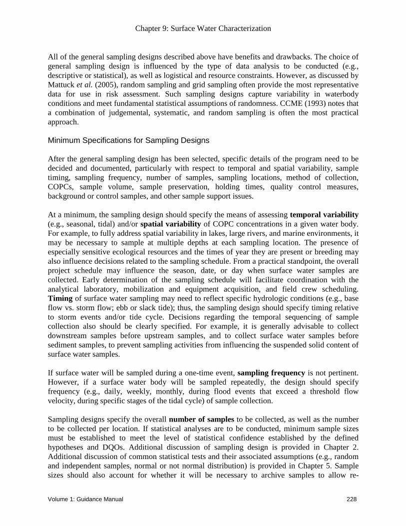
Chapter 9: Surface Water Characterization
Volume 1: Guidance Manual 228
All of the general sampling designs described above have benefits and drawbacks. The choice of general sampling design is influenced by the type of data analysis to be conducted (e.g., descriptive or statistical), as well as logistical and resource constraints. However, as discussed by Mattuck et al. (2005), random sampling and grid sampling often provide the most representative data for use in risk assessment. Such sampling designs capture variability in waterbody conditions and meet fundamental statistical assumptions of randomness. CCME (1993) notes that a combination of judgemental, systematic, and random sampling is often the most practical approach.
Minimum Specifications for Sampling Designs After the general sampling design has been selected, specific details of the program need to be decided and documented, particularly with respect to temporal and spatial variability, sample timing, sampling frequency, number of samples, sampling locations, method of collection, COPCs, sample volume, sample preservation, holding times, quality control measures, background or control samples, and other sample support issues.
At a minimum, the sampling design should specify the means of assessing temporal variability (e.g., seasonal, tidal) and/or spatial variability of COPC concentrations in a given water body. For example, to fully address spatial variability in lakes, large rivers, and marine environments, it may be necessary to sample at multiple depths at each sampling location. The presence of especially sensitive ecological resources and the times of year they are present or breeding may also influence decisions related to the sampling schedule. From a practical standpoint, the overall project schedule may influence the season, date, or day when surface water samples are collected. Early determination of the sampling schedule will facilitate coordination with the analytical laboratory, mobilization and equipment acquisition, and field crew scheduling. Timing of surface water sampling may need to reflect specific hydrologic conditions (e.g., base flow vs. storm flow; ebb or slack tide); thus, the sampling design should specify timing relative to storm events and/or tide cycle. Decisions regarding the temporal sequencing of sample collection also should be clearly specified. For example, it is generally advisable to collect downstream samples before upstream samples, and to collect surface water samples before sediment samples, to prevent sampling activities from influencing the suspended solid content of surface water samples.
If surface water will be sampled during a one-time event, sampling frequency is not pertinent. However, if a surface water body will be sampled repeatedly, the design should specify frequency (e.g., daily, weekly, monthly, during flood events that exceed a threshold flow velocity, during specific stages of the tidal cycle) of sample collection.
Sampling designs specify the overall number of samples to be collected, as well as the number to be collected per location. If statistical analyses are to be conducted, minimum sample sizes must be established to meet the level of statistical confidence established by the defined hypotheses and DQOs. Additional discussion of sampling design is provided in Chapter 2. Additional discussion of common statistical tests and their associated assumptions (e.g., random and independent samples, normal or not normal distribution) is provided in Chapter 5. Sample sizes should also account for whether it will be necessary to archive samples to allow re-

Chapter 9: Surface Water Characterization
Volume 1: Guidance Manual 229
evaluation in the event of questionable data, alternative analytical methods, or the need for additional sample results. The number of samples required to obtain representative data for a water body increases with the heterogeneity of the system. Water quality varies over time (seasonal variations discussed below) and over space (e.g., depth, distance from potential sources or inlets). Overall, the appropriate number of samples depends on the variability of the system being sampled and the goals of the sampling program.
In determining the number of samples needed, statistical power analysis is considered to determine the likelihood that a statistical test will yield a significant result, given that an effect actually exists. Thus, power analysis is linked to and complementary to traditional statistical hypothesis testing. The power of a statistical test is a function of three parameters: 1) the variability associated with the parameter of interest; 2) the magnitude of the minimum detectable difference; and 3) the sample size. Statistical power increases with samples size and the magnitude of the minimum detectable difference and statistical power decreases with increasing variability. Power calculations are typically used either to assess the power of a previously performed statistical test or a priori to estimate the minimum sample size required to detect a minimum difference. A priori tests require an estimate of the variability, either based on professional judgement or based on a pilot data set. Typically, the only parameter under the control of the experimenter is sample size; thus, sample size is often chosen to achieve a specific statistical power. Statistical methods for determining a sufficient number of samples for risk assessment purposes are discussed in detail in Chapter 5 and by Mattuck et al. (2005).
Sampling locations closely relate to the general sampling design, but also consider access to water body(ies) and safety. This aspect of the sampling design is highly variable with respect to spatial and depth considerations. It is also highly site-specific (e.g., source influence, COPC distribution, flow dynamics).
The sampling design specifies methods for collection (discussed further below), as well as the containers to be used for storage and transport. Laboratory pre-cleaned sample containers are required to ensure that samples are not contaminated by residues in the sample containers. The number of analyses to be completed on each sample, as well as the sample volume required for each analytical method and for the required detection limits, will dictate the sample volume and, thus, the sample container sizes. These aspects of the sampling design should be discussed with representatives of the analytical laboratory early in the planning process.
The specific COPCs and their forms dictate many other aspects of the sampling design. For example, COPCs influence the sampling method, containers, volume, and preservation methods. The form of the COPC can influence the equipment used for sampling. For example, if samples are being collected solely to compare surface water concentrations to a benchmark, sample processing should be consistent with the basis for that benchmark (e.g., CCME water quality guidelines are based on total concentrations rather than dissolved). However, dissolved concentrations of COPCs (e.g., metals) are often most relevant for ecological risk assessments. Therefore, field filtering of samples is most often conducted to support dissolved metals analyses. If specific valence states of metals are to be assessed, specific sample preservatives may be necessary and field analysis may be required. See Volume 4, section 3. Depending on the equipment needed and associated logistics, such analyte-specific details may alter sampling

Chapter 9: Surface Water Characterization
Volume 1: Guidance Manual 230
design. Again, these aspects of the sampling design should be discussed with representatives of the analytical laboratory early in the planning process.
The sample volume required for a given analysis depends on the analytical method, which in turn is generally driven by regulatory requirements and the detection limits needed to adequately assess risk. In addition, toxicity tests and treatability studies typically require large sample volumes. Sample volume can influence decisions related to the number of samples collected and sample locations. For example, it may be feasible to collect more samples from less accessible areas for analytes requiring 40 millilitre sample volumes as compared to 1 litre sample volumes.
Depending on the goals of the sample collection and the COPCs, sample preservation may be required upon collection of the sample. Sample preservation prevents degradation of some COPCs (e.g., inorganic and organic nutrients, organic carbon) prior to analysis. Water collected for other purposes (e.g., toxicity testing or treatability studies) may not require preservation. Proper sample preservation controls both chemical and physical inherent properties of the sample. For example, preservation methods can: 1) retard biological action; 2) retard hydrolysis of chemical compounds and complexes; 3) reduce volatility of constituents; and 4) reduce absorption effects. Thus, preservation can reduce the potential for error in analysis of COPCs.
The holding times of COPCs can complicate field logistics and the number of samples that can be collected within a given time period. The availability of next day shipping and/or distance to the analytical laboratory often factor into such considerations. Particularly labile materials (e.g., chlorine) are assessed immediately upon collection, necessitating transport of associated equipment, and often limiting the number of samples that can be collected. Holding times for microbiological parameters can also be of short duration, and parameters such as pH, dissolved oxygen, and oxidation-reduction potential must be assessed in situ.
The sampling design specifies quality control measures to be used to control error and bias, thereby ensuring that the required data quality is obtained. For example, the sampling design should consider the requirement for blanks (most important for trace level COPCs) and matrix spikes to assess COPC recovery from study area media. Section 9.3.4 further discusses quality control practices associated with surface water sampling.
Reference area samples provide a measure of concentrations of chemicals, particularly those that may have a natural or anthropogenic, but non site-related, source (e.g., pesticide applications, road runoff, atmospheric deposition) (Gandesbury and Hetzel, 1997). Reference area samples are collected in an unimpacted or relatively unimpacted area with physical and biological attributes similar to those of the study area (see Section 9.2 for additional discussion of reference areas).
The sampling design also specifies the supporting parameters (e.g., analyses and in situ measurements) needed for data interpretation with respect to COPCs. For example, changes in pH, suspended solids, organic carbon concentration, water hardness (for freshwater) and salinity influence the form of many COPCs. These changes in form can alter the toxicity and fate and transport of chemicals in aquatic systems and must be considered during sample design development and implementation.

Chapter 9: Surface Water Characterization
Volume 1: Guidance Manual 231
Although supporting parameters will vary across sites, depending on historical and on-going site uses, most surface water sampling programs should include an analysis of Standard Surface Water Constituents. Those constituents that have the greatest concentrations and that together exert many chemical controls on the nature of the water. This core group is called the major ions and common field measurements and includes:
• Major cations - H+ (from pH), Ca+2
, Mg+2
, K+, Na
+, NH4
+. H
+ and pH are important because
of direct toxicity to aquatic organisms and they affect the solubility of toxic metals.
• Ions Ca+2, Mg+2, K+, Na+ are important indicators of how the rock and soil in the watershed react with water.
• Major anions – Acid neutralizing capacity (ANC), SO4-2
, NO3- Cl
-. ANC is an important
measure of the lake or stream’s ability to neutralize acid; if its concentration is near 0 then additional acid can easily affect pH and produce toxic conditions. The ions SO4
-2 and NO3
-
are common indicators of acid from manmade or natural sources. Cl- is very useful in
estimating the amount of evapo-transpiration in some watersheds.
• Common field measurements - Water temperature, pH, specific conductance, dissolved oxygen, water level and, if applicable, discharge.
Depending on the stated program objectives, many additional constituents can be added to the major ion/common field measurements. Common additions are:
• Additional nutrients - total P, soluble reactive P, total N.
• Organic chemistry - Total organic carbon (TOC), dissolved organic carbon (DOC),
• Bacteria - total and fecal coliform, fecal streptococci
In addition to selection of constituents, it is important to ensure that the analytical method used for each constituent is appropriate to the aquatic system being sampled.
Detection limits, e.g., Laboratory Reporting Limits, must be well below screening values, guidelines, standards, and the expected minimum concentrations for constituents expected to be present. Some constituents may not be detected, but this absence may need to be documented.
The precision of the method needs to be greater than expected natural variations. As part of program planning, the basis for selecting each method should be discussed. As data are collected, this discussion of methods should be revisited and either confirmed or replaced with a more suitable method.
Differences in the sampling and analytical methods used during different sampling events or at different locations can contribute significant variability in the results. Consistency across methods should be maintained to the extent feasible, in order to minimize variability across

Chapter 9: Surface Water Characterization
Volume 1: Guidance Manual 232
samples or study areas. Such consistency is particularly important if conditions are to be compared across areas.
Additional Considerations
While the previous subsection describes the minimum requirements of sampling designs, a large number of factors will influence each component of the sampling design. This subsection recognizes additional considerations related to sample timing, locations, and type (i.e., composite vs. discrete). With respect to timing, some sampling programs benefit from a phased design. In particular, a first phase of exploratory sampling may be important in confirming the appropriateness of reference areas and/or presence of hot spots, while the second phase is used for the detailed characterization, and a third phase may be useful for additional delineation of a plume or hot spot or investigation of incongruous results.
Additional considerations related to the selection of sampling locations include: spatial distribution of COPCs; bathymetry, sampling depth, and hydrologic connectivity; presence and location of distinct sources; distance required before full mixing occurs downstream of the confluence of streams or chemical sources to surface waters; key in-flow features, such as the presence of marsh channels in estuaries, backwaters, and oxbows in meandering rivers, and wing dams or other structures that may enhance or diminish surface water mixing; sampling logistics; need for and availability of one or more reference areas; and technical tradeoffs. As an example of a technical trade off, it might be recognized that sampling from a bridge has many logistical advantages, but that metals and PAHs are often associated with road runoff. Thus, bridge sampling may not be advisable unless there exists a method to ensure that samples are collected upstream of the influence of road runoff from the bridge. If the bridge overlies a river within the zone of tidal influence, it may not be possible to collect true upstream samples from the bridge. Sampling location considerations in estuaries and tidal zones include: tidal regime, mixing characteristics of freshwater-saltwater transition zones, and the spatial extent of freshwater and saltwater areas. These and other considerations for sampling in saltwater are discussed by National Oceanic and Atmospheric Administration (NOAA, 2005).
A very important added dimension related to sampling locations pertains to sampling surface water at multiple depths. Because of the thermal stratification that occurs in many lakes (Figure 9-3), as well as the salinity stratification that characterizes many estuaries, sampling at multiple water depths may be necessary depending on the goals of the sampling program. If the water body is stratified, collecting water only from the surface will provide no information on the water quality in the bottom layers due to lack of mixing between the layers. For example, in the summer, dissolved oxygen concentrations in surface water tend to be significantly higher than in water below the thermocline (as illustrated in Figure 9-3). Likewise, for deep lakes and open ocean sampling, it may be important to define what constitutes a “surface water” sample, with that definition influenced by factors such as water clarity (i.e., the depth of the photic zone), temperature, salinity, and the extent of vertical upwelling. Broad guidelines are available for general characterization of lake sampling (e.g., Wetzel and Likens, 1991; http://www.glsc.usgs.gov/sites/default/files/product_files/InlandLakesManual.pdf and coastal marine sampling (NOAA, 2005).
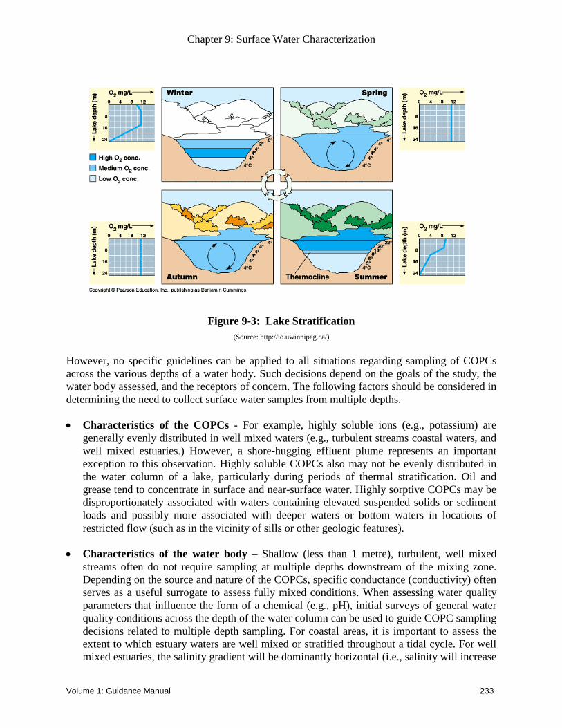
Chapter 9: Surface Water Characterization
Volume 1: Guidance Manual 233
Figure 9-3: Lake Stratification (Source: http://io.uwinnipeg.ca/)
However, no specific guidelines can be applied to all situations regarding sampling of COPCs across the various depths of a water body. Such decisions depend on the goals of the study, the water body assessed, and the receptors of concern. The following factors should be considered in determining the need to collect surface water samples from multiple depths.
• Characteristics of the COPCs - For example, highly soluble ions (e.g., potassium) are generally evenly distributed in well mixed waters (e.g., turbulent streams coastal waters, and well mixed estuaries.) However, a shore-hugging effluent plume represents an important exception to this observation. Highly soluble COPCs also may not be evenly distributed in the water column of a lake, particularly during periods of thermal stratification. Oil and grease tend to concentrate in surface and near-surface water. Highly sorptive COPCs may be disproportionately associated with waters containing elevated suspended solids or sediment loads and possibly more associated with deeper waters or bottom waters in locations of restricted flow (such as in the vicinity of sills or other geologic features).
• Characteristics of the water body – Shallow (less than 1 metre), turbulent, well mixed streams often do not require sampling at multiple depths downstream of the mixing zone. Depending on the source and nature of the COPCs, specific conductance (conductivity) often serves as a useful surrogate to assess fully mixed conditions. When assessing water quality parameters that influence the form of a chemical (e.g., pH), initial surveys of general water quality conditions across the depth of the water column can be used to guide COPC sampling decisions related to multiple depth sampling. For coastal areas, it is important to assess the extent to which estuary waters are well mixed or stratified throughout a tidal cycle. For well mixed estuaries, the salinity gradient will be dominantly horizontal (i.e., salinity will increase

Chapter 9: Surface Water Characterization
Volume 1: Guidance Manual 234
in the downgradient direction), and sampling at multiple depth increments may not be required. For stratified estuaries, the salinity gradient will be both horizontal and vertical (i.e., tidal inflow will restrict freshwater outflow to the surface water), and accurate characterization of chemical distributions will require sampling at multiple water depths.
• Source characteristics – Due to the differences in the hydraulic factors that influence mixing, COPCs associated with side channel discharges and seepage from waste disposal areas have much different mixing and water column profiles than effluents discharged through point source high rate diffusers. For example, discharges via seeps will vary seasonally with variations in precipitation, infiltration, and groundwater flow. The physical characteristics of the source must be considered before deciding whether to conduct sampling throughout the water column.
• Valued ecosystem components (VECs) - If a lake or estuary is stratified, sampling at multiple depths may be necessary to accurately evaluate risks to different receptors. For example, if COPC exposure of open water sportfish drives the risk assessment, sampling should target the photic zone of a stratified water body. Conversely, sampling focused on deep water habitats would support exposure assessment for bottom-dwelling fish or benthic invertebrates. In human health risk assessments, the location of drinking water intakes and recreational areas influence sampling locations.
• Life histories of VECs – The location of sensitive forms of aquatic life (e.g., fish fry in shallow nursery areas) may dictate sampling at different water depths at different seasons.
• Logistical and safety considerations, including appropriate equipment and personnel, are important sampling design considerations, as they may influence both the collection of samples at various depths within the water body and how the samples are collected.
In general, for well mixed estuaries, rivers, and large streams, a depth-integrated sample (discussed in further detail below) is sufficient to characterize COPC concentrations for use in human health and ecological risk assessment. In small streams, a center of stream discrete sample collected at about 60% of depth in an area of maximum turbulence is generally appropriate. In areas where COPCs are not well mixed, exploratory (i.e., phased) sampling with depth and/or along a cross section of the water body can help inform the need to sample at multiple water depths. In the first (exploratory) phase, three to five sampling depths are usually sufficient to characterize COPC concentrations with the potential to vary with depth at a given sample location. In tidally dominated areas, exploratory sampling can be extended to target the range of likely flow and mixing conditions at a given sampling location. Targeted sampling intervals can include spring tide vs. neap tide, high tide vs. low tide, and/or high river flow vs. low river flow conditions. These variables all influence the extent to which the water column at a given sample location can be considered well mixed.
The decision to collect discrete samples vs. composite samples is an important additional consideration for sampling designs, in that distinctly different types of data are obtained with the two types of samples. Additional information related to the advantages and disadvantages of

Chapter 9: Surface Water Characterization
Volume 1: Guidance Manual 235
discrete and composite samples is provided by CCME (1993), USEPA (1995), and MOEE (1996).
Discrete samples provide information for samples collected at specific times and locations. Discrete samples typically require the least amount of equipment, and are therefore usually the simplest and least expensive type of sample to collect. Discrete samples can be collected by direct dipping of sample containers into surface water, or with mechanical devices, such as peristaltic pumps, van Dorn bottles or Niskin bottles. Multiple Niskin bottles can also be deployed on a frame (rosette) that can be programmed to close individual bottles at pre-determined discrete water depths. Depth-integrated discrete samples are collected at predetermined locations in the water column and mixed, or they are collected across the entire water column by mechanical means. The simplicity and cost effectiveness of discrete samples make them appealing in many regards. However, discrete samples do not account for variations in COPC concentrations over time or across locations. Discrete samples are, however, well suited to identify maximum COPC concentrations in judgemental sampling programs.
Composite samples generally consist of a mixture of multiple discrete samples (sampled manually or with automated sampling devices). Composite samples reflect average conditions within the composited area, flow, or time interval. Composite samples are most often timed sequentially (e.g., hourly sample collection before compositing) to allow variance and random distribution, although automated flow-weighted composite sampling devices are available. Continuous pumping of water into a common sample collection vessel is another method of collecting composite samples. Compared to discrete samples, composite samples tend to be more expensive to collect and are logistically more complicated. Composite samples do not identify peak COPC concentrations, and compositing samples may dilute COPC concentrations in individual discrete subsamples. Composite sampling is not advised for obtaining data on volatile or labile compounds (e.g., chlorine).
9.3.4 Quality Assurance/Quality Control
Accounting for the QA/QC samples necessary to support surface water sampling is an important component of study design. Clark (2003) and USEPA (2006) provide guidance in this and related areas. The focus of a QA/QC program for field sampling is usually to document that samples were not compromised as a result of the sampling techniques or equipment used. This goal can be verified through the use of blanks. The most commonly used blanks, their intended purpose, and general procedures for use are summarized below. In general, blanks are used when COPCs are expected to be in the microgram per litre (µg/L) range and below. Blanks also help
IMPORTANT: Never compromise your personal safety or that of a field partner to collect a sample. Always plan ahead to avoid falling and drowning hazards. Always wear appropriate safety gear such as life vests. When working with winches, cables and similar machinery, gloves, hard hats, safety glasses and steel-toed boots are also important safety items. A qualified boat operator should be required for all sampling from a boat. Boat operations should conform to all requirements in federal and provincial laws.

Chapter 9: Surface Water Characterization
Volume 1: Guidance Manual 236
quantify systematic and random error if present as a result of the field and laboratory techniques used.
• Trip Blanks - A trip blank is a laboratory prepared blank (e.g., distilled water) that accompanies sample collection bottles into the field, is not opened in the field, and is returned to the laboratory and analyzed to determine whether sample contamination may have occurred as a result of general sample handling and sample transport techniques.
• Field Blanks - Field blanks are identical to trip blanks except they are opened in the field in sample collection areas and otherwise handled as if they were an environmental sample. Field blanks identify sources of sample contamination related to airborne particles and sample handling techniques.
• Equipment Blanks – Equipment blanks also make use of analyte-free water, but the water contacts sampling equipment to determine whether sampling equipment is a source of sample contamination. For example, distilled water can be added to a clean van Dorn or Kemmerer sample bottle or passed through the sample lines of an automated sampling device, then dispensed into sample bottles and analyzed. Equipment blanks should be collected periodically throughout the sampling program to evaluate the efficiency of the decontamination procedures.
• Filtration blanks are a type of equipment blank that assess the possibility that sample filtration (e.g., for dissolved metals analyses) contaminates samples. The same general process is used for other equipment blanks in that analyte-free water is filtered and analyzed for COPCs to determine whether the filters or filtration apparatus are sources of sample contamination.
Analyte-free water should always be provided by the analytical laboratory conducting the chemical analyses. This practice ensures that water known to be free of the COPCs has been provided and allows efficient determination of sources of sample contamination if observed.
Other commonly used QA/QC methods are designed to assess loss due to sample handling and transport, assess the precision associated with analyses of each COPC, or assess COPC recovery from the sample matrix. The most commonly used QA/QC procedures related to such concerns are summarized below.
• Reference Standards – Reference standards are water samples provided by the laboratory that contain known concentrations of the COPC. They accompany the other field sampling equipment in the field, are not opened in the field, and are returned to the laboratory for analysis. This practice assesses both analyte loss during transport and contamination associated with sample transport and/or general field conditions.
• Duplicate Samples – Duplicate (i.e., two) samples are collected from the same location at the same time using identical sampling techniques. Duplicates are labelled and submitted for analysis under “blind” conditions. The purpose of collecting duplicates is to assess the precision associated with a given chemical analysis. The precision observed is a function of

Chapter 9: Surface Water Characterization
Volume 1: Guidance Manual 237
any true variance in the analyte concentration at a given place and time, sampling variance, and variability associated with the laboratory analysis. Better indications of precision are obtained by collecting replicate (i.e., three or more) samples in identical fashion to the more commonly utilized duplicate sample approach.
• Split Samples – Split samples are duplicate samples collected from a single large volume sample after it has been thoroughly homogenized. The purpose of a split sample is to minimize the variability associated with the analyte in the environment and better assess variability associated with the laboratory analysis of a given COPC. Split samples can be used to assess variability associated with analysis of given analyte by different methods or by different laboratories.
• Matrix Spike/Matrix Spike Duplicate Samples (MS/MSD) – These samples are prepared in the laboratory by adding known amounts of a COPC to subsamples of the waters collected on-site. The primary QA/QC goal is to determine recovery efficiency for a given analyte in the study area water matrix, and identify sources of interference in study area water. MS/MSD analyses can also be used to assess laboratory performance or assess performance of a specific piece of equipment (Clark, 2003).
Sampling Equipment for Surface Water Characterization 9.4
This subsection provides an overview of the general methodologies, advantages, and disadvantages of the most commonly applied surface water sampling techniques used in support of risk assessments. Because the most commonly used surface water sampling techniques and sampling devices can be applied in various habitats, the techniques and equipment discussed herein are organized by general sampling equipment types (e.g., discrete sampling and composite sampling equipment). The following discussion provides examples of the general conditions under which each sampling device is most commonly used. It opens with a brief discussion of general considerations for surface water sampling equipment and contact materials, which is relevant to the full range of sampling equipment options. Other information related to sampling equipment selection (e.g., ease of use and decontamination requirements) can be found in USEPA (1995). For more information refer to Protocols Manual for Water Quality Sampling in Canada (http://www.ccme.ca/files/Resources/water/water_quality/protocols_document_e_final_101.pdf).
9.4.1 General Considerations
Sampling locations must be safe, accessible, and easily located by others using field descriptions and/or Global Positioning System (GPS).
• Sample Collection - The sample containers required vary with the constituents to be sampled and the laboratory contracted for the analysis. For example, acid-washed polyethylene sample containers are typically used for trace metals analysis, while glass sample containers are typically required for analysis of organics. Sometimes, several containers will be required for each sample, with differing processing of each sample container required in the field or at the laboratory. Sample containers must be non-reactive

Chapter 9: Surface Water Characterization
Volume 1: Guidance Manual 238
with the constituents measured from that container and should hold sufficient volume for the laboratory to do all required analyses and have sufficient excess in case a rerun of the archived sample is needed. Powder-free gloves should be worn throughout the sample collection process.
• Filtration - For samples that require filtration prior to analysis, the pore size of the filter is critical in determining what actually is analyzed in filtered samples. A pore size of 0.45 microns is commonly used for many constituents, although other pore sizes may be appropriate depending on the analysis and site characteristics (e.g., the presence of colloidal material). Filtration can be completed in the field (e.g., while on the vessel or shore-side) to prevent degradation of the sample following collection of the sample or in the laboratory to minimize the possibilities for cross-contamination of samples.
• Sample Labelling - Each sample container must have a waterproof label. All information required by the laboratory must be written with waterproof ink. All sample containers should be labelled with the site name as it appears on the laboratory submission form. Sample labels should also specify the date and time of the sample collection, the name of the sample collector, and any other information specified by the laboratory.
• Equipment Decontamination – For efficiency and to reduce field decontamination activities, all sampling equipment should be cleaned and decontaminated at the laboratory or field office before going to the sample site. If possible, a separate set of cleaned and decontaminated equipment should be available for each sampling site. If decontamination is required in the field, decontamination washwater and rinse water can be ‘contaminated’ by the sampling media and by the decontamination products (detergents, etc.) and should be collected and contained for appropriate disposal.
• Sample Handling and Shipment – Sample containers should be placed in clear plastic bags to minimize potential cross-contamination of samples and to protect laboratory personnel. Glass containers should be protected from breakage. All surface water samples should be chilled and stored in coolers or similar containers at ≤ 10°C. Field technicians should record a description of how the samples were packed in the field, preservatives used, and shipping methods.
• Field Notes - Field technicians should record field observations and measurements in a log throughout the sampling program. Either a prepared form or a field notebook can be effective, provided that notes are clear, accurate, legible, and detailed. Information recorded includes: date, time, technicians’ names, ambient temperature, cloud cover, precipitation, approximate wind speed, stage of lake/river, tidal conditions, water flow velocity at the sampling location, GPS coordinates, water depth, any unusual observations, etc.
9.4.2 Contact Materials
It is imperative that contact materials in the sampling equipment (i.e., the composition of the surfaces that come into contact with surface water) not contaminate the surface water samples or otherwise alter sample integrity. For example, plastic sample containers cannot be used to collect
Chapter 9: Surface Water Characterization
Volume 1: Guidance Manual 239
samples to be analyzed for sorptive trace-organic compounds or organic compounds used as plasticizers (e.g., bis(2-ethylhexyl)phthalate). Polyvinyl chloride (PVC) and PVC cemented joints can be a source of chloroform, and various organic compounds such as toluene, acetone, methyl ethyl ketone, and others (CCME, 1993).
In general, samples that contact glass, stainless steel, polypropylene tubing, and Teflon® materials are unlikely to be compromised. However, stainless steel containers can be a source of chromium, nickel, and other metals if prolonged sample contact is allowed. The use of glass or Teflon® sample containers and contact materials is preferable for collection of samples for analysis of organic compounds, while polypropylene plastic is sufficient for collection of samples for heavy metals analyses when samples are immediately acidified upon collection. Plated or painted sampling equipment can contaminate samples. The potential for contamination due to contact materials associated with supporting equipment (e.g., boats) also warrants consideration. For example, oils and other hydrocarbons may compromise samples, if samples are collected from a gas-powered boat. Additional guidance related to proper contact materials for sampling equipment is provided by MOEE (1996), particularly with regard to assessing the temperature stability of sampling equipment. Supporting information related to contaminants associated with various types of sampling equipment and the operation of equipment is provided by CCME (1993).
9.4.3 Discrete Sampling Equipment
Discrete sampling equipment can be quite simple, ranging from the sample container to a bucket to van Dorn or Niskin bottle and Kemmerer samplers. Discrete sampling equipment may require modification to fit study area-specific conditions. For example, buckets or sample containers can be attached to ropes or dip poles to sample hard to reach areas. When fabricating sampling equipment, the same general guidelines related to contact materials, as discussed above, should be considered to protect sample integrity. General guidance is provided by the U.S. Navy (1997) on fabricating discrete sampling equipment, and the use of sampling equipment for specific waste and surface water applications. These include the Wheaton dip sampler for shallow water sampling, and the Bacon bomb sampler for petroleum hydrocarbon sampling. Guidance specific to sampling for volatile organic compounds and extractable organic compounds is also presented in the U.S. Navy (1997) guidance.
The direct-dip technique is a discrete sampling technique conducted by placing the sample container directly under the water surface. It has the advantage of using the laboratory-provided sample container as the collection device, alleviating any concerns that improper contact materials were used during sample collection. This technique also alleviates the need for sample equipment decontamination and is appropriate for sampling all types of water bodies when shallow (less than 0.5 metres) or surface layer water samples are needed. The technique cannot be used for analytes that require preservation using sample containers with preservatives that may be lost during sample collection.
Subsurface samples also can be collected directly into sample containers with modification of the weighted bottle technique (Lind, 1979; U.S. Navy, 1997). Typically, a glass container with stopper and attached release line, or weighted basket with sample container and stopper with

Chapter 9: Surface Water Characterization
Volume 1: Guidance Manual 240
attached release line, are lowered to the desired water depth and the stopper removed by pulling the release line.
Various mechanical sampling devices have long been used to collect subsurface water samples (Lind, 1979). The most common of these are the van Dorn bottle, Kemmerer sampler, and the Niskin bottle (Figure 9-4). These devices collect discrete samples at depths specified by either calibrated ropes affixed to the sampling device or through the use of an automatic electronic firing module that closes discrete bottles at pre-programmed water depths. Although the electronic firing module is most commonly applied to the deployment of multiple bottles on a rosette, Niskin bottles can also be deployed individually or clamped in series onto a hydrographic wire. For discrete deployments of all three sampling devices, bottle closure is triggered by a mechanical messenger that is slid down the rope or wire on which the bottle is
suspended. Many rosette samplers are equipped with multi-parameter probes that provide continuous water quality data (pH, salinity, etc.) during either the rosette downcast or recovery (preferred). Warren (1996) provides a more detailed overview of sampling procedures for rosette style samplers. Additional information can be obtained at http://www.glwi.uwm.edu/education/outreach/cruise/niskin.php.
The van Dorn and Kemmerer samplers are available as plastic or metal sample bottles, whereas the Niskin bottle is available as a plastic bottle. These devices have the advantage of being relatively simple to operate, and are sufficiently rugged to be used in a wide range of sampling conditions. Kemmerer and van Dorn samplers are most often used to collect subsurface samples in lakes and ponds, but can also be applied to calm, deep water habitats of rivers and streams. These sampling bottles are almost always deployed from a boat. They are generally ineffective in fast-water habitats because their depth of deployment cannot be accurately assessed and because it can be difficult to maintain a fixed position in the water column as is required prior to
A B C Figure 9-4: A. van Dorn Bottle Sampler. B. Kemmerer Sampler. C. Rosette
Sampler containing Niskin Bottles. (Photo sources: http://www.pc.gc.ca/, http://www.cnr.vt.edu/, http://www.kc-denmark.dk/public_html/ and http://www.epa.gov/

Chapter 9: Surface Water Characterization
Volume 1: Guidance Manual 241
triggering the sampling device. Niskin bottles are most commonly deployed on a rosette (as shown in Figure 9-4C) and used for oceanographic sampling. Because Niskin bottles can be deployed to significant water depths (1000+ metres), deployment typically requires the use of a hydrographic winch and hydraulic hoist. Strong surface or subsurface currents and/or significant deployment depths can limit the users’ ability to target specific sampling intervals, but do not typically limit deployment of the rosette and bottles. As with all marine sampling equipment, electrical connections and winch components (including the wire) should be protected from corrosion, and all components of the rosette (including the bottles) should be rinsed well with freshwater after recovery.
Commercial devices are also available that allow for autonomous, real-time water quality monitoring and bathymetry mapping. While new technology is being developed to allow some autonomous underwater vehicles (AUVs)2 to collect deep water samples, most AUVs available today do not retrieve samples. Instead, they are fitted with sensors to monitor a range of physical, chemical, and biological parameters. Common measurements include temperature, salinity, dissolved oxygen, turbidity, nutrients, chlorophyll, and pH. These unmanned vehicles were developed as a way to reduce costs by eliminating the need for large ships or crews (http://www.mbari.org/auv/). AUVs are outfitted with GPS systems, so they can be programmed onshore to navigate a specified route and monitor conditions at regular intervals. While each AUV is unique, most can operate at depths of at least 60 metres and some, such as YSI’s EcoMapper can work continuously for up to 10 hours (http://www.ysisystems.com/systemsdetail.php?EcoMapper-1). High costs typically limit the use of AUVs for risk assessment purposes.
Use of automated sampling equipment (Figure 9-5) can improve sampling efficiency if a series of discrete samples must be collected over time (e.g., hourly for 24 hours). Such sampling equipment provides discrete sample vessels into which samples are dispensed at pre-programmed time intervals. The sample vessels must be maintained in a self-contained and fully enclosed sample housing vessel to eliminate sample contamination from airborne chemicals. Depending on the COPC being assessed, automated samplers with sample refrigeration capabilities may be needed.
Depth-integrated samplers are designed to collect water samples throughout the water column to integrate or combine water collected throughout the water transit. In its simplest form, a depth-integrated sample can be collected by lowering a sealed sample container to the bottom of the water body or the base of the desired sampling interval, opening it, and raising it at a constant rate so that the sample is just filled when it reaches the water surface. The most common applications use a plastic sample bottle with a
2 Sometimes referred to as remotely operated vehicles (ROV).
Figure 9-5: Automatic Water Sampler (Photo source: http://www.isco.com/)

Chapter 9: Surface Water Characterization
Volume 1: Guidance Manual 242
specialized nozzle that allows water to enter the sample bottle as the bottle is raised through the water column. The technique is most often applied in wadeable streams and rivers, using a bottle affixed to a stainless steel sampling rod. Alternative techniques include but are not limited to, integrated vertical column tube samplers that can range from one to three litre volume capacities. Equipment manufacturers typically provide instructions as to the rate at which to raise the water sample bottle through a water column based on the depth and velocity of the water being sampled. This technique yields a full sample bottle just as the sampling device reaches the water surface. The technique is generally limited to sampling waters less than five metres deep and generally provides a water sample of one litre or less. Because sample bottles in most commercial sampling devices are plastic, collection of water samples for analysis of sorptive organic compounds is not recommended.
9.4.4 Composite Sampling Equipment
Composite samples can be prepared by manually collecting discrete samples over time or from different locations and mixing them. Any of the discrete sampling equipment discussed above can be used for this purpose. However, it is often most efficient to use an automated sampling device that composites samples collected over time into a common sample vessel. The compatibility of COPCs with the sample collection devices and associated tubing must be confirmed before sampling.
Automated sampling devices typically use electric peristaltic or rotary pumps, although hand-operated diaphragm pumps are not uncommon. Composite sampling can be conducted on an equal time and equal volume basis, or through collection of flow proportionate samples. Various manufacturers provide compatible sampling and flow monitoring devices specifically for this purpose. Various regulatory agencies define composite samples based on minimum time intervals for sampling in a given time period (e.g., at least hourly samples for 24 hours) or minimum numbers of samples in a given time period (e.g., minimum of eight samples collected at equal time intervals over a 24-hour period). Factors to consider in selecting composite sampling equipment and sample collection intervals include:
• Variability in concentrations of COPCs in the surface water to be sampled.
• Variability in the discharge or release source of COPCs.
• Compatibility of any common sample compositing vessels for the COPCs.
• Stability, volatility, and holding time of COPCs – readily volatile and highly degradable COPCs are not amenable to composite sampling techniques because they dissipate during the compositing period. In such cases, discrete samples can be used to augment the composite sample collection technique.
• The need for preservation and refrigeration upon sample collection – generally, samples requiring preservation can be preserved upon transfer into sample bottles, but some analytes (e.g., cyanide, phenolics) require immediate chemical preservation. Immediate sample cooling is necessary for analytes requiring refrigeration or cooling to below a specified temperature (usually 4° Celsius).

Chapter 9: Surface Water Characterization
Volume 1: Guidance Manual 243
• Contact materials in the collection equipment – some automatic samplers use pliable rubber or plastic tubes in conjunction with moving parts. While this practice is necessary in order for automated equipment to function properly, such soft materials may remove sorptive trace-level (µg/L levels and below) chemicals. Pumping large volumes of water to be collected across such contact materials in order to satiate sorption sites can minimize such problems, as can sample line purging prior to collection of each sample. Organic plasticizers are also common sample contaminants in automated collection equipment that makes use of pliable rubber or plastic tubes that contact water being sampled.
• Costs and logistic constraints associated with the composite sampling equipment (e.g., size and weight, power source availability and/or the need for batteries and battery replacement).
9.4.5 Equipment for Sampling Ice and Surface Water Underneath Ice
The optimal strategy for ice-related sampling is a function of the specific program objectives, including whether researchers are specifically targeting ice collection or are intending to drill through the ice to collect a water sample from underneath the floe. For ice sampling, cores can be recovered with instruments ranging from handheld augers to mechanical, electro-mechanical, or thermo-mechanical drills. The choice of instruments is dependent on the length and diameter of the core required. Drilling capabilities can range from several metres (for a handheld auger) to thousands of metres (for thermo-mechanical drills), and are influenced by the characteristics of the ice. Although drilling through ice is facilitated by application of drilling fluids (such as hot water, ethanol, or Freon), it is important to assess the extent to which such fluids could compromise the sample collected. Sample contamination also should be minimized by selecting sampling stations that are upwind from field camps (if in remote locations) or cities and industrial areas (to the extent possible), and by scrupulously cleaning all sampling equipment with appropriate reagents. For example, core barrels and containers used to collect samples for major anion analysis (e.g., Cl-, NO3
-, and/or SO42-) should not be acid washed. Once cores are
recovered and transported to the analytical laboratory, the portion of the core that was in direct contact with the drilling equipment is typically discarded3 and the inner portion of the core is analyzed.
The collection of water samples from underneath ice requires penetration of the ice floe prior to sample recovery. Prior to sampling, the thickness of the ice should be assessed in locations that will support sampling or equipment transport. Relevant data on ice thickness is commonly available from provincial and/or federal agencies. Depending on the thickness of the ice, penetration can involve a simple handheld or mechanical auger, or can require elaborate drilling platforms. Once the ice has been penetrated, standard surface water sampling equipment can be lowered through the drill hole or secured to the perimeter of the hole for sample collection. The diameter of the drilled hole will depend on the size of the sampling equipment required and may range from 1 to 2 centimetres (cm) for a water sampling line to greater than 100 cm. In shallow water areas, care should be taken in penetrating the ice to not disturb bottom sediment.
3 Unless the sample is from a heavily contaminated site, unusable portions of the sample can typically be discarded on-site.

Chapter 9: Surface Water Characterization
Volume 1: Guidance Manual 244
For large-scale oceanographic deployment, Ice Tethered Profilers (ITPs) have been developed for continuous underwater collection of water quality data. The ITP includes a surface instrument package that is secured to an ice floe, a weighted, jacketed wire tether suspended from the surface instrument package, and an instrument package that travels continuously on the tether. The tether length can reach 800 metres, and the instrument package can continuously record and transmit data on station location, water temperature, salinity, dissolved oxygen concentration and chlorophyll-a fluorescence. Details regarding the development and instrumentation of the ITP can be found at: http://www.whoi.edu/page.do?pid=20756.
Sample Preservation and Storage 9.5
Sample integrity is essential in the generation of representative analytical data sets. Proper sample preservation and storage regulates changes in chemical and physical properties of the sample to delay biological changes and hydrolysis of chemical compounds and complexes, and to reduce volatility of constituents and adsorption effects.
Early consultation with the analytical laboratory is recommended to determine required preservation and storage methods to ensure sample representativeness. This practice will aid in the selection of a sampling approach, methodology, and other logistics related to the surface water sampling program design as it pertains to issues concerning the use of non-laboratory applied preservative (e.g., ice and cooling of sample) or unique storage practices (e.g., light sensitivity) of samples.
Clark (2003) and USEPA (2001b; 2002) present detailed information on the recommended preservatives and storage practices for various analytes. For more information refer to Protocols Manual for Water Quality Sampling in Canada (http://www.ccme.ca/files/Resources/water/water_quality/protocols_document_e_final_101.pdf).
Data Analysis for Surface Water Characterization 9.6
The discussion of data analysis techniques provided for soil in Section 5.7 is also suitable for characterization of surface water chemistry data.
This subsection provides a general overview of data analysis techniques suitable for characterization of surface water chemistry data in support of human health and ecological risk assessment. This subsection is not intended to be prescriptive, nor is it intended to provide detailed guidance with respect to statistical evaluations of data. Rather, it describes a widely applicable progression of data analysis practices in support of risk assessments.
General descriptive techniques may be used to summarize the data and provide data visualization with respect to the temporal and spatial distribution of COPC concentrations in study area surface waters. Such techniques generally consist of data compilation (i.e., tabulation and preparation of summary tables), and plotting or graphing data with respect to time, location, key sources of COPC, key water bodies, etc. Simplistic plotting and other visual techniques of data presentation often reveal trends that guide and refine further sampling efforts.

Chapter 9: Surface Water Characterization
Volume 1: Guidance Manual 245
Preliminary data characterization may define fundamental information, such as central tendency (e.g., calculation of mean, median, mode, percentiles) and variability (e.g., range, standard deviation, coefficient of variation, etc.), as the first step to understanding data trends and designing more meaningful statistical evaluations. These initial data characterization steps also provide information for comparison to regulatory concentrations. Calculation of upper confidence limits (particularly the 95% upper confidence limit on the mean or 95% UCLM) is frequently required at this stage to support risk assessments, as the 95% UCLM is commonly employed as the exposure point concentration in risk assessment.
The ProUCL software package (USEPA, 2013a,b) provides a single platform to perform a number of UCLM calculations. Several limitations can be associated with ProUCL, including unreliability of goodness of fit tests, methods for estimating UCLs, and treatment of non-detects. In particular, the specific recommendations for UCLM methods provided by ProUCL can be problematic and controversial. For example, the Chebyshev UCLM is not a traditional UCLM but rather a tolerance interval that may approximate a UCLM. In addition, not all methods allow the use of the Kaplan-Meier estimation method for data sets with non-detects. The use of traditional non-detect data handling methods, such as using one-half of the detection limit for non-detects, can introduce bias in datasets with a frequency of detection of 90% or less (USEPA, 2013a,b). Of the UCLM methods available, the Bias-Corrected Accelerated Bootstrap (BCA) method provides results that are consistent with other methods, allows the use of the Kaplan-Meier adjustment for non-detects, is statistically robust, and does not depend on the underlying data distribution. Thus, the BCA bootstrap method is a widely applicable method and can be used for the majority of datasets.
Standard statistical tests can be applied to determine significant differences between various sample locations, and between the study area and reference areas. Hypothesis testing (e.g., Student’s T test) and analysis of variance (ANOVA) techniques are most often used in support of risk assessments. The choice of statistical test should be based on the underlying assumptions associated with the test (e.g., random and independent samples, or type of distribution). In most cases, nonparametric and multivariate statistics are required, as environmental datasets are rarely normally distributed. Comparison of study area conditions to reference area conditions can take two forms: a comparison of individual results to a threshold value, or a statistical test that checks for a significant difference between study area and reference area datasets. Threshold tests, based on tolerance interval or a specific percentile of the reference area dataset, are most commonly applied to identify specific locations with elevated concentrations (i.e., to delineate hot spots). Because of the complexity of the statistical analyses frequently required to evaluate environmental datasets, a qualified statistician should design and implement statistical analyses based on the project goals and the applicability of the data to the statistical techniques under consideration.
Resources and Weblinks 9.7
Environment and Climate Change Canada, Canada – New Brunswick water/Economy Agreement. Monitoring Surface Water Quality. A Guide for Citizens, Students, and Communities, in Atlantic Canada. http://publications.gc.ca/site/eng/464771/publication.html

Chapter 9: Surface Water Characterization
Volume 1: Guidance Manual 246
Environment and Climate Change Canada technical guidance on how to conduct effluent plume delineation studies. http://www.ec.gc.ca/esee-eem/default.asp?lang=En&n=E93AE5BC-1.
USEPA Region 9 Quality Assurance. Surface Water Field Sampling Procedures. Available at: www.epa.gov/region09/qa/fieldsamp.html
The OZCoasts Australian Online Coastal Information website has a series of questions listed that would be useful in creating a cost efficient sampling program. The web page is titled: How do you design a water quality monitoring program. Available at: http://www.ozcoasts.gov.au/nrm_rpt/mar/info.jsp.
Detailed explanations and photographs of various types of oceanographic sampling equipment can be viewed at the Woods Hole Oceanographic Institution website. Available at: www.whoi.edu/page.do?pid=8415
A list of key elements that technical reviewers would typically be looking for when reviewing DQO process summary reports can be found at the Department of Energy website. Department of Energy Data Quality Objectives Summary of Key Elements to the DQO Process. Available at: http://www.hanford.gov/files.cfm/HASQARD%20Vol%201.pdf
Triad Resource Center website lists a seven-step DQO process that will address the planning cycle for Triad projects. Available at: www.triadcentral.org/mgmt/splan/frame/dqo/index.cfm
Details regarding the Niskin Bottle are presented on the Great Lakes Water Institute webpage. Available at: http://www.glwi.uwm.edu/education/outreach/cruise/niskin.php
Information regarding AUVs can be found on the Monterey Bay Aquarium Research Institute. Available at: http://www.mbari.org/auv/
Specifications for YSI’s commercial AUV, the EcoMapper, can be found at: http://www.ysisystems.com/systemsdetail.php?EcoMapper-1
Information regarding the US DH81 Sampler can be located at the Federal Interagency Sedimentation Project website. US DH 81 Sampler. Available at: http://water.usgs.gov/fisp/products/4107002.html
Laboratory analytical methods available for the analysis of chemical, physical, and biological components of wastewater and other environmental samples required under the U.S. Clean Water Act are published by the USEPA at http://water.epa.gov/scitech/methods/cwa/index.cfm.
The USEPA Forum on Environmental Measurements provides a collection of test methods (i.e., “approved procedures for measuring the presence and concentration of physical and chemical pollutants; evaluating properties, such as toxic properties, of chemical substances; or measuring the effects of substances under various conditions”). http://www2.epa.gov/measurements/collection-methods.

Chapter 9: Surface Water Characterization
Volume 1: Guidance Manual 247
References 9.8
Apitz, S.E. , J.W. Davis, K. Finkelstein, D.L. Hohreiter, R. Hoke, R.H. Jensen, J.M. Jersak, V.J. Kirtay, E.E. Mack, V. Magar, D. Moore, D. Reible, and R. Stahl. 2002. Critical Issues for Contaminated Sediment Management. U.S. Navy, Space and Naval Warfare Systems Center, San Diego, CA, USA. MESO-02-TM-01.
Canadian Council of Ministers of the Environment [CCME]. 1993. Guidance Manual on Sampling, Analysis, and Data Management for Contaminated Sites Volume I: Main Report. PN 1101. CCME National Contaminated Sites Program. December.
Clark, M.J.R. (editor). 2003. British Columbia Field Sampling Manual. Water, Air, and Climate Change Branch. Ministry of Water, Land and Air Protection. Victoria, BC, Canada. 312 pp.
Environment Canada. 2008. Literature Evaluation of Sampling and Analytical Methods in Contaminated Site Characterization. Environment Canada 08-1113-0040. April.
Gandesbury, T., and F. Hetzel. 1997. Ambient Concentrations of Toxic Chemicals in San Francisco Sediments. San Francisco Bay Regional Water Quality Control Board, Oakland, California. http://www.sfei.org.
Lind, O.T. 1979. Handbook of Common Methods in Limnology. The CV Mosby Company. St. Louis, MO. 199 pp.
Maher, W.A., P. Cullen, and R. Norris. 1994. Framework for Designing Sampling Programs. Env. Monit. Assmnt. 30:139-162.
Mattuck, R., R. Blancet, and A.D. Wait. 2005. Data Representativeness for Risk Assessment. Env. Forensics. 6:65-70.
National Oceanic and Atmospheric Administration. 2005. Science Based Restoration Monitoring of Coastal Habitats. Volume Two: Tools for Monitoring Coastal Habitats. G. W. Thayer, T.A. McTigue, R. Salz, D.H. Merkey, F.M. Burrows, and P. Gayaldo (eds.). NOAA Coastal Ocean Program Decision Analysis Series 23. NOAA National Centers for Coastal Ocean Science, Silver Spring, MD, 7.1-7.18.
Ontario Ministry of the Environment and Energy (MOEE). 1996. Guidance on Sampling and Analytical Methods for use at Contaminated Sites in Ontario. Standards Development Branch. December.
Ritter, A.M., J.L. Shaw, W.M. Williams, and K.Z. Travis. 2000. Characterizing Aquatic Ecological Risks from Pesticides Using a Diquat Dibromide Case Study. I. Probabilistic Exposure Estimates. Environmental Toxicology and Chemistry 19(3):749-759.
U.S. Environmental Protection Agency. 1995. Superfund Program Representative Sampling Guidance Volume 5: Water and Sediment Part I – Surface Water and Sediment Interim Final. Office of Emergency and Remedial Response, Office of Solid Waste and Emergency Response. Washington, DC. December.
U.S. Environmental Protection Agency. 1996. Soil Screening Guidance: User’s Guide. United States Office of Solid Waste. Publication 9355.4-23. Washington, DC.
U.S. Environmental Protection Agency. 1997a. Guiding Principles for Monte Carlo Analysis. EPA/630/R-97/001. Risk Assessment Forum, U.S. Environmental Protection Agency, Washington, DC.
U.S. Environmental Protection Agency. 1997b. Superfund Program Representative Sampling Guidance. Volume 3: Biological. Interim Final. Environmental Response Team Center, Office of Emergency and Remedial Response, Office of Solid Waste and Emergency Response. Washington, DC.

Chapter 9: Surface Water Characterization
Volume 1: Guidance Manual 248
U.S. Environmental Protection Agency. 1999. Report of the Workshop on Selecting Input Distributions for Probabilistic Assessments, U.S. Environmental Protection Agency, New York, NY. April 21-22, 1998. EPA/630/R-98/004. Risk Assessment Forum, Washington, DC.
U.S. Environmental Protection Agency. 2000a. Stressor Identification Guidance Document. EPA/822/B-00/025. Office of Water and Office of Research and Development. Washington, DC.
U.S. Environmental Protection Agency. 2000b. Data Quality Objectives Process for Hazardous Waste Site Investigations. EPA QA/G-4HW Final. EPA/600/R-00/007. Office of Environmental Protection. Washington, DC.
U.S. Environmental Protection Agency. 2001a. Risk Assessment Guidance for Superfund: Volume III – Part A, Process for conducting Probabilistic Risk Assessment. EPA 540-R-02-002. Office of Emergency and Remedial Response, Washington, DC.
U.S. Environmental Protection Agency. 2001b. EPA Requirements for Quality Management Plans. EPA/240/B-01/002. Office of Environmental Information. Washington, DC.
U.S. Environmental Protection Agency. 2002. Guidance on Choosing a Sampling Design for Environmental Data Collection for use in Developing a Quality Assurance Project Plan. EPA/240/R-02/009. Washington, DC.
U.S. Environmental Protection Agency. 2006. Guidance on Systematic Planning Using the Data Quality Objectives Process. EPA/240/B-06/011. Office of Environmental Information. Washington, DC.
U.S. Environmental Protection Agency. 2013a. ProUCL Version 5.0 Technical Guide. EPA/600/R-07/041. Office of Research and Development. Washington, DC.
U.S. Environmental Protection Agency. 2013b. ProUCL Version 5.0 User Guide. EPA/600/R-07/041, U.S. Environmental Protection Agency, Washington, DC.
U.S. Navy. (Department of the Navy, USA). 1997. Navy Environmental Compliance Sampling and Field Testing Procedures. NAVSEA T0300-AZ-PRO-010.
Warila, J., S. Batterman, and D.R. Passino-Reader. 2001. A Probabilistic Model for Silver Bioaccumulation in Aquatic Systems and Assessment of Human Health Risks. Environmental Toxicology and Chemistry 20(2):432-441.
Warren, G.J. 1996. Field Sampling Using the Rosette Sampler. USEPA Great Lakes National Program Office. Chicago, IL. May.
Wetzel, R and G. Likens. 1991. Limnological Analyses. Second Ed. Springer-Verlag. New York, New York.

Chapter 10: Sediment Characterization
Volume 1: Guidance Manual 249
10 SEDIMENT CHARACTERIZATION GUIDANCE
Context, Purpose, and Scope 10.1
Sediment provides essential habitats for many invertebrates and fish and supports primary productivity in aquatic systems. Sediment often becomes a repository or sink for many chemicals that partition between the overlying surface water, the interstitial water (i.e., sediment porewater), and the sediment layer. Many contaminants that are detectable in only trace amounts in surface water can bind to organic carbon or minerals and accumulate in sediment, where they may persist for many years. Thus, freshwater, estuarine, and marine organisms can be exposed to contaminants in sediment and can be affected. Consequently, aquatic organisms, wildlife, and humans can be adversely affected by contaminants in sediment via food chain and direct contact exposures. In addition, sediment associated contaminants may compromise uses of aquatic systems through reduction or elimination of species of recreational, commercial, or ecological importance, or cause impairment of the navigational uses of rivers or harbours.
Sediment sampling often presents unique challenges. First, aquatic systems are generally less well understood than terrestrial systems. This difference is at least partially due to limited or restricted accessibility to sediments. Second, sediment is inherently dynamic. Sediment movements caused by natural or anthropogenic forces affect sediment associated contaminant transport and can increase the difficulty of defining the extent of spatial contamination. Third, specialized methods, knowledge and experience are required for collection, analysis, and remediation of sediment. Intermittent streams and other areas may appear to consist of upland soil during a brief site visit (particularly under drought conditions), but may be more appropriately classified as sediment upon closer examination. A general understanding of hydrological fluctuations (e.g., intermittent and ephemeral streams or periodically flooded wetlands) is required in order to accurately identify substrate types and areas to which aquatic organisms could potentially be exposed. The unique physicochemical properties of sediment often dictate the use of particular sampling equipment; handling, transport, and storage protocols; analytical methods; and decontamination strategies. These challenges frequently make investigation of sediment quality more complex than terrestrial investigations, often leading to an increase in opportunities for errors.
Sediment Characterization This chapter describes the planning, process, and methods for sediment characterization. Key considerations and their corresponding sections in the chapter are:
• Conceptual site model (10.2)
• Study approach and design (10.3)
• General sample collection, handling, and analytical considerations (10.4)
• Quality assurance and quality control (10.5)
• Sampling methodology and equipment (10.6)
• Porewater collection and extraction (10.7)
• Data analysis (10.8)
• Resources and weblinks (10.9)
Definition of Sediment For purposes of this guidance chapter, sediment is defined as inorganic sand, silt, clay, other minerals, and organic matter that deposit on the bottom of a water body.

Chapter 10: Sediment Characterization
Volume 1: Guidance Manual 250
The primary purpose of this sediment characterization guidance chapter is to facilitate the collection of high quality, representative data by providing general, consistent methodologies for investigators tasked with developing and implementing sediment sampling programs in support of human health and ecological risk assessments. Sediment sampling can be initiated to satisfy a variety of needs, spanning risk assessment, chemical characterization, biological characterization, source identification, allocation of financial responsibility, emergency response, remedy selection, post-remediation monitoring, and attenuation monitoring. While this chapter focuses on sediment sampling in support of risk assessments, some aspects of the chapter have broader applications. Readers are also referred to the Canada Ontario Agreement (COA) (2008), Fletcher et al. (2008), MacDonald and Ingersoll (2003), and the U.S. Environmental Protection Agency (USEPA) (2005a) for discussions of sediment sampling in support of remedy selection and design.
This sediment characterization guidance chapter provides a framework for development of the general sampling approach and design, the sampling methodology and equipment, the quality assurance and quality control measures (QA/QC), and data analysis considerations for a sediment sampling program. This chapter specifically addresses general sampling design, sampling equipment, and other factors pertaining to sediment sampling in lakes, ponds, wetlands, rivers, streams, estuaries, and oceans.
Given the breadth of this chapter’s scope, it is not intended to provide overly detailed or prescriptive sampling methodologies, information on specific regulatory requirements, or laboratory analytical methods. The information presented in this chapter is based on current information and recommendations from a variety of agencies and is intended to provide a coherent set of recommendations for site investigation personnel.
Conceptual Site Model for Sediment Characterization 10.2
As detailed in Chapter 2 of this guidance document, the conceptual site model (CSM) is an important early tool in the site characterization process, in that it forms the framework for human health and ecological risk assessment activities. The CSM is a dynamic, visual and written representation of the relationships between the physical, chemical, and biological processes of the site and human and ecological receptors and serves as a guide to the design of the sampling program. Chemical types, sources, fate and transport, exposure pathways, and potential receptors are important considerations for sediment characterization. Chapter 4 provides a detailed summary of the types of chemicals associated with various anthropogenic and natural activities. Both “point sources” and “nonpoint sources” of sediment associated contaminants should be considered in development of the CSM for sediment. Surface water may provide a transport mechanism for suspension and redistribution of sediment, and sediment can serve as an ongoing source of contamination to water; therefore these two media are nearly always considered together. Measurement of sediment physicochemical properties (e.g., particle size, and organic carbon content) are required to properly predict transport and fate of sediment and sediment associated contaminants (USEPA, 2005a). (see Sections 10.3.3 and 10.4.5 for additional discussion; Wenning et al., 2002; USEPA, 2007a). Consideration of these contaminant specific properties is important in the development of the CSM, the interpretation of sediment chemistry results, and the determination of potential exposure pathways.

Chapter 10: Sediment Characterization
Volume 1: Guidance Manual 251
As discussed in Chapter 4, a CSM for sediment should, at a minimum, consider: 1) the unique migration and exposure pathways of the site; 2) the physical processes at the site; 3) the physicochemical properties of the sediments; 4) the attributes and behaviours of the ecological receptors (e.g., preferred habitat, foraging behaviour, dietary preferences); and 5) the presence and behaviour of human receptors (e.g., fishing and consumption practices, accessibility for children, presence of workers). A generalized CSM for a contaminated sediment site is shown in Figure 4-13. Risk assessors are expected to modify it or use their preferred presentation format for site-specific CSMs. In addition, the narrative and/or pictorial CSMs for individual sites should acknowledge and discuss reference sites to which conditions at the contaminated site will be compared in the risk assessment.
Study Approach and Design for Sediment Characterization 10.3
Consistent with the overall purpose of this guidance chapter, this section describes a generic sediment quality study’s goals and objectives and provides considerations for sediment sampling design and collection. Of particular interest are factors that influence the generation of high quality, representative sediment quality data in support of human health and ecological risk assessment. The collection of consistent
and representative sediment data facilitates: 1) accurate characterization of the site; 2) comparisons among sites; 3) comparisons to sediment quality guidelines or benchmarks; and 4) informed and effective planning of investigation and remediation activities.
10.3.1 Goals and Objectives
The clear definition of sampling goals and objectives is critical to the approach and design of any successful sediment sampling program. However, the specificity of the goals and objectives largely depends on the amount of site information available, which in turn often depends on the progress of investigative activities for a given site. Preliminary sediment quality investigations typically employ broad study objectives, whereas long-term sediment quality investigations require more focused objectives developed to address specific data gaps. In general terms, the fundamental goals and objectives for the approach and design of sediment sampling programs for site characterization in support of human health and ecological risk assessment are as follows:
• Characterize the nature and spatial extent of contaminants of potential concern (COPCs) as they relate to human and ecological exposure pathways; and
• Ensure that the data collected are valid, representative, and sufficient to yield meaningful conclusions and support decisions related to mitigation of any risks to human health or VECs.
Definition of Representative Data Representative data accurately characterize and represent sediment quality at a given site. Exhibit 5-1, “Characteristics of Representative Data,” provides additional detail.

Chapter 10: Sediment Characterization
Volume 1: Guidance Manual 252
The development of more focused study goals and objectives is discussed in Chapter 2, as well as other guidance (e.g., USEPA, 1995; 2002a; 2005a; MOEE, 1996). Although these goals and objectives are site-specific, some examples are presented below.
• Identify the composition of COPCs, as well as the key chemical and biological processes affecting the fate, transport, and bioavailability of COPCs in the sediment.
• Understand the vertical and horizontal distribution of COPCs in sediment.
• Understand the temporal variability in concentrations of COPCs.
• Understand site-specific processes (e.g., resuspension, transport) affecting the stability of the sediment.
• Refine the CSM by identifying complete or potentially complete human and ecological exposure pathways.
• Determine if there is an imminent or potential threat to human health or the aquatic ecosystem.
• Understand concerns of the public and other stakeholders.
• Determine the need for remedial action, evaluate the available remedial technologies/actions and determine the most suitable remedial action.
• Collect the necessary data for monitoring and evaluating the effectiveness of selected and implemented remedial action.
Adherence to the study’s goals and objectives will aid in designing and implementing the sediment sampling program by clearly focusing site investigations, resulting in accurate, representative, and cost effective sediment quality data on which to base sound decision-making.
10.3.2 Data Quality Objectives
Data quality objectives, or DQOs, support the study’s identified goals and objectives. They are the product of an iterative, flexible process that determines the type, quantity, and quality of data needed to support site-related decisions (USEPA, 2000b; 2006). This strategic planning approach should be implemented prior to the collection of the samples and is an integral part of the sampling design. The DQO process is also closely associated with QA/QC considerations.
DQOs are qualitative and quantitative statements that: 1) clarify the purpose of the sediment quality study; 2) state the level of uncertainty that is acceptable for the data to be
Data Quality Objective (DQO) Process The seven iterative steps of the DQO process are identified below and described in Chapter 9 of this manual.
1. State the problem
2. Identify study goals
3. Identify data needs
4. Define site boundaries
5. Design the analytical approach
6. Develop performance/acceptance criteria
7. Develop a sampling and analysis plan

Chapter 10: Sediment Characterization
Volume 1: Guidance Manual 253
collected; 3) define the most appropriate type of data to collect; and 4) determine the most appropriate methods and conditions under which to collect the data (CCME, 1993a; USEPA, 1995; 1997; 2001; 2006). The successful implementation of the DQO process produces high quality, representative data while promoting efficiency and cost effectiveness by strategically and appropriately focusing the sampling strategy.
10.3.3 Sediment Sampling Design Considerations
Sediment sampling design involves determining sampling locations and the appropriate number of samples to collect for proper site characterization. The study’s overall goals and objectives, as well as DQOs and available funding, guide the sediment sampling design process. Depending on the study area, it may be necessary to develop separate sampling designs for subareas that clearly require different sampling strategies (e.g., pond vs. wetland habitats; riverine vs. estuarine vs. offshore environments; littoral vs. sublittoral). The end result of the design process is typically a sampling and analysis plan that will direct sample collection. An overview of this process is presented in Figure 10-1.
An appropriate sediment sampling design, along with careful field observations, minimizes the numerous challenges associated with the collection of representative sediment samples. Chapter 5 and USEPA (1995; 2000c; 2001) identify several such challenges:
Figure 10-1: Overview of the Sediment Sampling Design Process

Chapter 10: Sediment Characterization
Volume 1: Guidance Manual 254
• Media variability – Variations in the physical and chemical (physicochemical) characteristics of sediment, such as redox potential, particle size, and hydrodynamic regime of the study area (depositional vs. transitional areas).
• Chemical concentration variability – Variations in the spatial or temporal concentrations of COPCs and/or those variables affecting the release of COPCs.
• Collection and preparation variability – Variation in collection of sediment samples, preparation, and shipping methods, resulting in sampling and/or measurement error or bias.
• Analytical variability – Variations in the manner in which samples are stored, prepared, and analyzed by analytical laboratories.
In addition to minimizing these challenges, a proper sampling design will consider geospatial characterization needed to help make remedial decisions. If a sampling plan is designed to identify spatial variability over the scale of interest, geostatistical methods (discussed in Chapter 5) can be used to quantify spatial trends and to contour concentration data.
A common pitfall of site investigations is the collection of too few sediment samples. Regardless of the number of sediment samples collected, it is essential that the data obtained from these samples be of the highest quality. The sediment sampling design process consists of site reconnaissance, the delineation of the study area, the identification of reference area (if required), selection of sediment sampling approaches, selection of sampling stations, and the determination of the number of samples, as described below.
Site Reconnaissance
Site reconnaissance is an important step in the sediment sampling process. Information obtained from both desktop reviews and site visits make sediment sampling programs more efficient and effective by allowing personnel to assess site conditions, evaluate areas of potential contamination, identify ecologically sensitive habitats, evaluate potential hazards associated with sampling, and finalize the sampling and analysis plan (USEPA, 1995). Information obtained from reconnaissance also can be used to inform and refine the CSM (Section 10.2).
General types of information recommended for both a desktop review and on-site visit are described in Chapter 9. Exhibit 10-1 provides examples of the types of information that should be collected during site reconnaissance that are specific to sediment sampling programs. In addition, Volume 2 of this guidance document provides a checklist for ecological site reconnaissance. Following the review of this data/information, information/data gaps must be identified. The sediment sampling design should, at least in part, address these data gaps. If time and budget permit, an on-site reconnaissance immediately prior to sampling may be useful to verify that conditions have not changed (e.g., changes in the drainage patterns [or lack of water], or changes in the accessibility of the sampling points).

Chapter 10: Sediment Characterization
Volume 1: Guidance Manual 255
Study Area and Reference Area Identification
A study area refers to the body of water and the associated sediments to be monitored and/or assessed, as well as the adjacent areas (land or water) that might either affect the local conditions or be affected by releases from the investigated site (USEPA, 2001). It is important to clearly define/delineate the boundaries of the study area, as the size of this area dictates the breadth and scope of the sediment sampling or assessment project and greatly influences the sediment sampling design. The study area should encompass the entire zone of impact associated with the site, including wave, tide, and current activity, and should be large enough to allow the characterization of the severity of the impacts, in reference to an unimpacted or reference area (MOEE, 1996). However, if the study area is very large, as is typically the case for industrial harbours and marine systems, it can be subdivided into smaller areas to facilitate and focus site investigation activities; division of a study area into multiple sub-areas (exposure units or exposure areas) can aid future site management decisions. The smaller areas may be defined by source(s) and/or type(s) of contamination, physical structures or features, or use by humans of the area. Often in larger marine systems, the boundaries of the target study area cannot be clearly defined until after initial sampling has delineated the site-related impact. In this case, the overall study area is operationally defined by taking into account potential site-related COPC movement
Exhibit 10-1: Reconnaissance Information Relevant to Sediment Sampling Projects
• Regional land use patterns
• Site layout and topography
• Site environmental background
• General information on the associated watershed (if relevant)
• Water bodies present (or evidence of previous water bodies)
• Distribution and type of sediment
• Nature of shoreline
• Harbour or shipping channel historical documentation
• Oceanographic conditions
• Potential onshore/offshore sources of contaminants
• Ecological habitats
• Use of the study area for fishing, shellfish harvesting, boating/recreation, and primary contact recreation
• Current and anticipated future use of the water body
• Water depth
• Tides (timing, location, and extent of intertidal zone)
• Access and boat launch locations

Chapter 10: Sediment Characterization
Volume 1: Guidance Manual 256
in sediment due to wave, tide, and current activity and is much larger than the target study area. Figure 5-1 outlines the process for defining a study area’s boundaries1.
A reference area is an unimpacted or relatively unimpacted area with physical and biological attributes similar to those of the study area, but for the release of site-related chemicals. The ideal reference area—which generally does not exist—is a waterbody that is essentially identical to the study area in all respects, except for the release of site-related chemicals. Because of the practical difficulty in locating ideal reference area locations, it is often necessary to select locations with COPC concentrations that are equivalent to regional ambient background concentrations (Environment Canada, 2002a). It is equally important that the reference locations have similar physical and biological properties as the study area. It is almost always advisable to select more than one reference area to represent the range of background conditions and/or the range of the site physical and biological characteristics (USEPA, 2002b), and to allow for more meaningful statistical comparisons. Evaluation of two or more reference areas will allow for more accurate representation of a true reference condition. If only one reference area is identified, it is imperative to acknowledge the assumptions and limitations of this comparison (i.e., the assumption that this area is reasonably representative of other reference areas, and that multiple samples collected from this single reference area are pseudo-replicates rather than truly independent samples). The following factors should be considered as part of the process of selecting reference areas:
• The use of the reference area in interpreting results of any sediment quality study;
• Physical nature of sediment (e.g., grain size, organic carbon content);
• Flow dynamics (e.g., fast vs. slow or no flow, flashiness, stream order);
• Chemical composition (e.g., contributions from road runoff, atmospheric deposition, naturally-occurring inorganic chemicals);
• Geomorphology (e.g., braided, meandering, channelized streams);
• Wetland classification (e.g., bog, fen, swamp, marsh, shallow water);
• Oceanographic conditions (e.g., currents);
• Tidal conditions (ebb vs. flood tide);
• Tidal zone (sublittoral, intertidal, supratidal)
• Circulation depositional patterns;
• Biological composition (e.g., benthic invertebrate communities); and
• Proximity to the study area.
In lotic (flowing) systems, suitable reference areas are often located immediately upstream of the study area, beyond the influence of the site. In lentic (static) systems, a suitable water body(ies) within the same watershed, but outside of the area of impact, should be targeted. 1 Although the medium in this figure is soil, the process is similar for both terrestrial and aquatic investigations.

Chapter 10: Sediment Characterization
Volume 1: Guidance Manual 257
Comparisons between the study area and the reference area(s) provide a means to determine the potential effects of site-related COPCs. Upgradient reference areas in lotic systems can help to identify off-site contributions of COPCs. Furthermore, reference areas provide a measure of background concentrations of chemicals, particularly those that may have a natural or anthropogenic, but non site-related, source (e.g., pesticide applications, road runoff, atmospheric deposition, component of the earth’s crust) (Gandesbury and Hetzel, 1997; USEPA 2002b). For example, if an ecological risk assessment documented fish mortality in a pond that was affected by both site-related chemical releases and acid precipitation, concurrent evaluation of one or more reference ponds would be critical to understanding whether the chemical releases and/or the acid precipitation caused the observed fish mortality. As a second example, if a human health risk assessment predicted that risks to wading children were unacceptable due to arsenic in sediments that could be incidentally ingested, it would be necessary to accurately characterize the naturally-occurring concentrations of arsenic in the sediments, in order to ensure that risk management decisions could be effective in mitigating the risks.
Sediment Sampling Designs
The design of sediment sampling programs can generally be classified into two types: biased and unbiased. In biased (or judgemental) sampling designs, the selection of the locations of the sampling stations is targeted toward the area(s) of concern (e.g., discharge or release points). By definition, biased sampling requires at least some previous knowledge of the distribution of sediment associated contaminants at the site. This type of sampling is useful if: 1) site boundaries are well defined; 2) small numbers of sediment samples will be collected; 3) information is desired for a particular condition or location; 4) the objective of the investigation is to screen an area for the presence of a particular COPC; 5) no statistical analysis of error or bias is required; and/or 6) there are schedule or budget limitations (USEPA, 1995; 2001).
For risk assessment purposes, an unbiased sampling approach is preferred (Mattuck et al., 2005) because it most closely simulates actual exposure patterns for human receptors and VECs. However, occasionally a combination of biased and unbiased sampling designs provides the most representative sampling approach for a study area. In unbiased (or probability) sampling, sample locations are selected randomly, without regard to the physical characteristics of the site. Unbiased sampling provides estimates of chemical variability and meets fundamental statistical assumptions (i.e., measurements are random and independent). In addition to the resources listed in Chapter 5, various other sources that describe and illustrate unbiased sampling approaches are available (e.g., USEPA, 1995; 2000c; 2001; MOEE, 1996). Selected examples of common unbiased sampling approaches are described below. There are numerous variations on these common approaches.
• Simple random – Distribution of sampling locations are random. All sampling locations have an equal probability of selection. Random sampling may result in uneven spatial distribution of sampling stations across the study area, which can be at least partially offset by increasing the number of samples collected.

Chapter 10: Sediment Characterization
Volume 1: Guidance Manual 258
• Systematic – The first sample location is chosen randomly, and all subsequent locations are placed at regular intervals using a square or triangular grid system (e.g., place locations at the nodes or intersections of the grid lines) or along a transect line.
• Stratified – The area to be sampled is divided into non-overlapping strata. The strata are determined based on pre-determined factors such as sediment particle size distribution, different habitat types or point sources of contamination and represent subareas in which different sampling approaches may be employed.
The selection of the appropriate sampling approach for a given type of study is discussed in detail by Gilbert and Pulsipher (2005), MOEE (1996), and USEPA (2000c; 2001). Exhibit 10-2 presents a summary of key considerations in selecting a sampling approach.
Sediment Sampling Locations and Number of Samples
After the approach to sediment sampling is decided, there are many factors to consider in determining the placement of individual sample locations and the number of samples to collect, including:
• Study objectives
• Information from the site reconnaissance
• Known or potential sources (discharge points, outfalls)
• Size of the study area or subarea
• Type of contaminant
• Presence and location of a reference site
• Physicochemical sediment characteristics
• Need for co-located samples (chemistry, toxicity, taxonomy, benthic assessment)
• Habitat types and home range areas for VECs
EXHIBIT 10-2: Key Considerations in the Selection of a Sampling Approach
• What is/are the question(s) (objectives) the study attempts to address?
• Does knowledge exist (including historical data) about COPCs and/or the spatial or temporal distribution of the COPCs?
• Is this a preliminary investigation? Is a phased approach feasible?
• Is/are the source(s) of the COPCs known? Is/are the source(s) point or non-point?
• What is the size of the study area? Is fine spatial resolution required?
• Is one of the study’s objectives to estimate statistical parameters or the population mean?
• Is the cost of analyzing individual samples for selected contaminants high compared to the cost of sampling?

Chapter 10: Sediment Characterization
Volume 1: Guidance Manual 259
• Historic sampling locations
• Statistical issues
• Accessibility
• Budget
If a source of contamination is known or expected, sediment sampling locations may be placed near (e.g., along the shoreline of a diffuse source) or immediately downgradient of the source (e.g., downstream of an outfall). In many cases, a concentration gradient related to the distance from the original source of the contamination is observed, even if the sediment has been affected by hydrodynamic processes (Apitz et al., 2002). To avoid compromising the representativeness of data, the study area may need to be subdivided or more locations added to the sampling program.
Non-ionic polar organic compounds and some metals readily partition from the overlying surface water and sediment porewater to sediment. The characteristics of sediment—such as particle size, origin, organic carbon content, and redox conditions—influence the type and concentration of contaminants present. Compared to coarse-grained sediment particles (sand), fine-grained sediment particles (silt and clay) have a greater overall surface area-to-volume ratio. This characteristic, along with other physicochemical properties, make fine-grained sediments much more chemically and biologically interactive than coarse-grained sediments, often resulting in greater sediment associated contaminant concentrations.
For most sediment quality investigations conducted for risk assessment purposes, sample locations should target areas of depositional, fine-grained sediments. Available sediment mapping surveys and geochemistry data may be useful. In lotic systems, examination of the water body characteristics may indicate the presence of sediment deposits. Stream bends and river meanders, log jams and other natural obstructions, and/or pools or other depressions typically slow water flow and promote accumulation of sediment. In shallow areas, a probing rod (made of steel or other rigid material) can be used to probe the sediment to locate deposits, determine the depth of the deposits, or roughly distinguish between fine-grained and coarse-grained sediment. When selecting sampling locations in marine areas, tidal fluctuations, tidal ranges, and surface and subsurface currents warrant careful consideration. In deeper areas, more advanced, remote sensing methods, such as acoustic survey techniques and side-scan or multi-beam sonar, may be useful (Environment Canada, 1994; USEPA, 2001; Apitz et al., 2002).
Issues of accessibility often affect the selection of sediment sampling locations. If the water is too deep or fast-flowing to safely wade, samples may need to be collected from a boat, the shore, or a bridge. While shoreline or bridge sampling limits the locations that can be sampled, doing so is often more cost effective than sampling from a boat.
Definition of Depositional Area A depositional area is an area where fine-grained sediment (i.e., sediment that is greater than 30 percent silt and clay particles) has accumulated within a water body. Deposition of suspended solids from the water column is a function of the bedload and the water velocity. Therefore, some areas may only be depositional during low flow periods or periods (such as during snow melt) when the waterbody carries elevated suspended solids.

Chapter 10: Sediment Characterization
Volume 1: Guidance Manual 260
Finally, once proposed sediment sampling locations are determined, it is imperative that the locations be properly referenced. Georeferencing allows: 1) precise repeat sampling in the future, if necessary; 2) proper identification on site-related maps; and 3) accurate spatial evaluation of sediment quality. Georeferencing is most accurately conducted using either a Global Positioning System (GPS) or a surveyor. However, even a hand-drawn map can be useful, as long as the location is referenced relative to a permanent or stationary feature (e.g., bridge, culvert). If possible, mark the location (e.g., stakes, flagging, paint) during field sampling and reference the location at a later date using GPS or a surveyor. It is often prudent to wait until sample collection to reference a sampling location. Even if a site reconnaissance is performed prior to sampling, slight adjustments to the actual sampling location are almost always required as the sediment characteristics are assessed or because of changes in the environmental conditions between the reconnaissance and the time of sampling. Occasionally, a proposed sampling location may need to be moved or eliminated. For example, if there is no fine-grained sediment at a proposed location, it is generally preferable to relocate the sample location, rather than collect a non-representative sample.
The number of samples required is influenced by the objectives of the overall program and is often challenging to determine. Most risk-based sediment investigations require a greater number of samples in order to accurately characterize the sediment in question. Statistical methods for determining a sufficient number of samples for risk assessment purposes are discussed in detail in Chapter 5 and by Mattuck et al. (2005) and Environment Canada (2002b). However, in some situations, the number of samples is determined from a compromise between statistical considerations and cost effectiveness.
In determining the number of samples needed, statistical power analysis2 is considered to determine the likelihood that a statistical test will yield a significant result, given that an effect actually exists. Thus, power analysis is linked to and complementary to traditional statistical hypothesis testing. The power of a statistical test is a function of three parameters: 1) the variability associated with the parameter of interest; 2) the magnitude of the minimum detectable difference; and 3) the sample size. Statistical power increases with sample size and the magnitude of the minimum detectable difference; statistical power decreases with increasing variability. Power calculations are typically used either to assess the power of a previously performed statistical test or a priori to estimate the minimum sample size required to detect a minimum difference. A priori tests require an estimate of the variability, either based on professional judgement or based on a pilot data set. Typically, the only parameter under the control of the experimenter is the sample size; thus, sample size is often chosen to achieve a specific statistical power. 2 The power of a statistical test is the probability that the test will reject the null hypothesis when the alternative hypothesis is true. Power analysis can be used to calculate the minimum sample size required to accept the outcome of a statistical test with a particular level of confidence.
Areal Sediment Sample Spacing If the distribution of sediment is relatively:
Homogeneous use widely spaced sampling locations
Heterogeneous use more densely spaced sampling locations (also see Exhibit 5-2)

Chapter 10: Sediment Characterization
Volume 1: Guidance Manual 261
General Sample Collection, Handling, and Analytical Considerations 10.4
This section discusses the general collection and handling of sediment samples, as well as analytical considerations. A selection of equipment types and specific collection methodology are detailed in Section 10.6 and in Volume 3 of this guidance. Additional supporting information for sample collection, handling, and analytical considerations is available in CCME (1993a), Clark (2003), and USEPA (1995; 2001). For more information refer to Section 7 of Protocols Manual for Water Quality Sampling in Canada (http://www.ccme.ca/files/Resources/water/water_quality/protocols_document_e_final_101.pdf)
Differences in the sampling and analytical methods used during different sampling events or at different locations can contribute significant variability in the results. Consistency across methods should be maintained to the extent feasible, in order to minimize variability across samples, sampling events, and study areas. Such consistency is particularly important if conditions are to be compared across areas.
The use of proper sampling and handling techniques maintains the integrity of the samples, thereby preserving the physicochemical properties and allowing an accurate representation of the sediment in question. Inappropriate sample collection procedures can seriously bias the representativeness of a sample (USEPA, 1995). Therefore, sampling personnel and appropriate training are often critical to the success of any sediment sampling program.
10.4.1 Contact Materials
Consideration and care should be given to the type(s) of material that come into contact with the sediment sample during collection (i.e., sampling equipment and containers) in order to prevent, or at least minimize, the potential for chemical artifacts or alteration of sample integrity. For example, plastic sample containers or metal sampling equipment can be sources of trace organic compounds and metals, respectively. Generally, the use of relatively non-reactive material—glass, stainless steel, Teflon®—for sample collection produce samples of acceptable quality. Laboratories typically supply appropriate sample containers that are certified by the laboratory as pre-cleaned. See Section 10.4.4 for more information on appropriate types of sample containers. Proper decontamination and cleaning of sampling equipment between uses is also essential to prevent cross-contamination.
In sediment sample collection and handling, consideration of the COPCs is very important, often dictating all aspects of the sample collection.

Chapter 10: Sediment Characterization
Volume 1: Guidance Manual 262
10.4.2 Sample Types
There are generally two types of sediment samples: discrete and composite samples. Discrete samples are sediment samples that are treated as an individual unit. Depending on the type of equipment used and/or the volume of sediment collected, a subsample of the discrete sample may be collected (e.g., sub-sampling from a Ponar or core, see USEPA [2001]). A composite sample includes several individual discrete samples collected from a small subarea of the study area and from sediment with similar physical characteristics. Discrete samples can be composited in the laboratory. Compositing entails manually or mechanically mixing discrete samples until the sample is homogeneous. A method should be determined to verify the homogeneity of the composite sample (particle size or determination of organic carbon). Samples may be composited horizontally (from the same depth sampled at multiple adjacent areas). Compositing should be limited to a single environmental medium or habitat type over which exposure is expected to be uniform. Samples also may be composited vertically (from the same location but across several depth ranges). In this case, compositing should be limited to a single uniform sediment stratum (e.g., biologically active upper stratum, anoxic lower strata, depths reflecting historical contamination). If sedimentation rates are available they may be useful in determining depth ranges for vertical compositing. The interpretation of data obtained by carrying out compositing of sediment samples needs to be addressed carefully. Both discrete and composite sediment samples may be used for risk assessment purposes (Mattuck et al., 2005).
10.4.3 Sample Handling
Sediment sample handling considerations are discussed by MOEE (1996) and USEPA (1995; 2001), for example, and include:
• Non-sediment material – Non-sediment material (e.g., sticks, rocks, insects, vegetation) should be recorded and carefully removed from the sediment sample prior to placing the sample in the container. This can be accomplished during homogenization. For discrete sampling, careful removal is required to minimize disturbance of the sample.
• Overlying water – Overlying water should be siphoned off, if possible, or carefully decanted from discrete samplers as soon as possible after sample collection and prior to subsampling.
Advantages of Discrete and Composite Sampling
Discrete Sampling:
• Minimizes time and expense for multiple samples
• Minimizes exposure to potentially hazardous chemicals
• Eliminates physicochemical changes during mixing by maintaining sample integrity
• Preserves the variability in the sample of the sediment associated concentration of COPC
Composite Sampling:
• Provides an efficient and cost effective means of characterizing large areas, often useful in initial stages of site investigation
• Provides a good method to obtain a mean concentration

Chapter 10: Sediment Characterization
Volume 1: Guidance Manual 263
Care should be taken to minimize the loss of fine-grained sediment during the process of removing the overlying water. This process will usually be required from bigger sediment samples such as a box corer.
• Homogenization – Certain chemicals and analyses are sensitive to the active mixing required to homogenize a composite sample; samples for such determinations should be subsampled directly from the sampling device, if possible. For example, VOCs will volatilize if the sediment is handled excessively. Sediment subsamples for the determination of parameters of interest that are sensitive to redox conditions, such as acid volatile sulfide (AVS) and simultaneously extracted metals (SEM), should not be subsampled from a composite sample. Even for those parameters of interest that are not typically sensitive to mixing, it is good standard practice to only mix the sample until homogenized—that is, avoid over mixing the sample. The level of mixing should balance effective homogenization (i.e., mixing to evenly distribute any nuggets of concentrated materials, if present) with physically altering the sample. Mixing may even increase segregation of heterogeneous material (Gustavsson et al., 2006). The process of homogenization should be carried out in a laboratory environment and if possible under inert conditions. It will be necessary to have a method for verification of the homogeneity of the composited sample.
• Splitting – Splitting a discrete or composite sediment sample is often performed for QA/QC purposes (see Section 10.5). For discrete samples, containers for split samples should be alternately filled. For composite samples, containers should be filled from the same composite sample. Gerlach et al. (undated) present an evaluation of splitting methods.
• Smearing or cross-contamination – Sediment samples collected from cores are subject to smearing (the transfer of sediment and/or chemicals along the core liner), either as the core is pushed into the sediment or as the sediment is removed from the liner. Samples should be collected from the center of a sediment core, with care taken to avoid the portions of the sediment that have contacted the core liner. This general practice also applies to the collection of subsamples from large sampling device, such as a Ponar.
• Oxygen-free environments – Sediment samples for which oxidation of the sediment is a concern should be processed within an oxygen-free environment (e.g., a glove box, (Figure 10-2) which is an enclosed system, ranging from inflatable plastic bags to larger, more solid structures, allowing external manipulation of the sample within a controlled environment) (Environment Canada, 1994).
• Headspace – Sediment samples that will be analyzed for volatile organic or redox-sensitive compounds, for example, should be placed in the sample container such that no headspace is available. Samples requiring VOC analysis should be extruded directly into preweighed containers containing the appropiate preservative. It may be necessary to
Figure 10-2: Glove Box Source: K. Merritt

Chapter 10: Sediment Characterization
Volume 1: Guidance Manual 264
consider the use of a smaller sample container if limited sample volume is available, as long as sample volume requirements are met for the analytical laboratory.
10.4.4 Sample Volume, Preservation, and Storage
The quantity of sample required for analysis is primarily based on target detection limits, laboratory extraction procedures, and sediment grain size (i.e., coarse-grained sediments may require larger sample volumes) (Gerlach and Nocerino, 2003). Therefore, required volumes of sediment sample vary depending on the type of COPCs to be determined, sediment physicochemical characteristics, and capabilities of the laboratory performing the analyses. In addition, biological assays or bioassays (e.g., toxicity testing, bioaccumulation testing) typically require larger quantities of sediment.
Environment Canada (1994), Clark (2003), MacDonald and Ingersoll (2003), and USEPA (2001; 2002c) present detailed information on the recommended minimum sample volumes, container types, preservation methods, storage temperatures, and hold times for various parameters of interest. All sediment samples for chemical or bioassay analysis should be immediately cooled to ≤ 10°C (while in transit) and stored at > 0 to 6°C (see Volume 4).
10.4.5 Considerations for the analysis of sediment samples
While the presence and concentrations of COPCs are typically defined by the operational history of the study area, bioavailability of those COPCs is often the focus of risk assessment studies. Numerous physicochemical processes (e.g., solubility, oxidation, sorption, precipitation) affect the bioavailability of chemicals in sediment (Apitz et al., 2002). As described in detail by USEPA (2001; 2002d; 2007a), many types of physical and chemical data are useful in supporting the evaluation of chemical bioavailability in sediment, such as:
• Particle size distribution – Sediment particle size, as discussed in Section 10.3.3, affects the type and quantity of a given chemical, thereby influencing the chemical and biological3 characteristics of the sediments.
• Organic carbon – Organic carbon (OC) includes both dissolved organic carbon (DOC) and particulate organic carbon (POC) in the sediments. The presence of organic carbon in
3 Particle size can be an important controlling factor on benthic communities.
Recommendation
Early consultation with the analytical laboratory is recommended to determine required sample volumes, container types, and holding times. This practice will aid in the selection of a sampling approach, methodology, specific sampling equipment, and other logistics related to the sediment sampling program design.
Definition of Bioavailability
Bioavailability is the availability of a chemical for uptake by biological receptors.

Chapter 10: Sediment Characterization
Volume 1: Guidance Manual 265
sediment can determine the bioavailability of some non-ionic organic chemicals (DiToro et al., 1991).
• Water content – The amount of water present in sediment, determined as the moisture content is used in some studies to calculate the total quantity of selected contaminants present in study area.
• AVS-SEM analysis – Measurement of AVS and SEM (cadmium, copper, lead, nickel, silver, and zinc) concentrations in sediments, along with organic carbon, can help to predict the bioavailability of these metals in anaerobic sediments (DiToro et al., 1990; Ankley et al., 1996; USEPA, 2005b).
• Chromium - The toxicity and bioavailability of chromium depend on whether it is present as trivalent or hexavalent chromium. Hexavalent chromium [Cr(VI)] is geochemically unstable in reducing environments where AVS is present, such that AVS and Cr(VI) do not coexist in sediments (USEPA, 2005b; Martello et al., 2007).
• Alkylated polycyclic aromatic hydrocarbons (PAHs) – Measurement of alkylated PAHs, as well as the unsubstituted or parent PAHs, facilitates evaluation of PAHs on a cumulative basis, based on equilibrium partitioning (USEPA, 2003b), thus indicating the potential bioavailability of PAHs in sediment and the likelihood of sediment toxicity.
• Redox potential – Redox potential is a measure of the oxidation-reduction potential of sediments and affects metal speciation, thus affecting metal bioavailability. The determination of this parameter is difficult due to the fact that redox potential is influenced by any changes in the oxidative state of the sediment.
• pH – pH in sediment and sediment porewater controls speciation and equilibration, and thus stability and toxicity, for many chemicals, including sulfides, ammonia, cyanide, and metals.
• Ammonia – The potential toxicity of ammonia is dependent on the whether it exists primarily in the un-ionized (toxic) or the ionized (relatively non-toxic) form. The extent of ionization is determined by pH, temperature, and salinity (in seawater).
• Porewater sulphide – Sulphide affects chemical bioavailability by sequestering many cationic metals via formation of insoluble metal complexes. The sampling of porewater is challenging and if required, should be planned and considered very carefully.
• Porewater salinity and conductivity – Salinity (in marine sediment porewater) is a measure of the mass of dissolved salt in a given mass of solution, whereas conductivity (in freshwater sediment porewater) is a measure of the ability of an aqueous solution to carry an electric current. Both measurements determine the concentration of ions in solution and help to elucidate potential chemical toxicity.
• Bioassays – Bioassays, such as toxicity testing, can indirectly measure chemical bioavailability in sediment or sediment porewater.

Chapter 10: Sediment Characterization
Volume 1: Guidance Manual 266
• Sediment oxygen demand (SOD) – SOD is an in-situ measure of the oxygen consumed by biochemical decomposition of organic matter in stream or lake sediment deposits. SOD can be used to evaluate pollutant source control performance or as a metric (input) for use in water quality models. Analytical methods available for sediment characterization are presented in CCME (1993b), MOEE (1996), USEPA (2003a), in Section 10.9 and Volume 4 of this guidance.
Perhaps equally important as the selection of sediment characterization method(s) is the selection of appropriate analytical detection limits suitable for risk assessment4 and consistent with the study’s goals and objectives. In addition, appropriate sediment preparation (e.g., digestion processes) and sample cleanup procedures should be implemented by the analytical laboratory. If not implemented properly, analytical results may be invalid.
Quality Assurance and Quality Control Considerations 10.5
Adherence to a quality assurance program will help achieve the study’s DQOs and aid in the collection of valid, representative sediment data. Chapter 3 and numerous guidance manuals (e.g., MOEE, 1996; USEPA, 2001; 2006; Clark, 2003; MacDonald and Ingersoll, 2003; CCME, 2011) present considerations for QA/QC, including project organization and responsibilities; equipment and instrument calibration; sample collection, handling, labelling, preservation, transportation, and tracking; decontamination procedures; record keeping and documentation; data reporting; training requirements; performance audits; and corrective action procedures. A few important considerations are discussed below.
• Sample Labelling - All sample containers should be labelled with the sample identification, the date and time of the sample collection, the name of the sample collector, analytes, or other information specified by the laboratory.
• Field notes – It is important that all information (including date, time, personnel present, weather conditions, etc) regarding a sampling event (or any events/activities) be accurately recorded in a field notebook. It is recommended that a high resolution photograph be taken of each sediment sample.
Field QA/QC samples are necessary to monitor both field and laboratory performance, by providing a means of checking the validity of sample results and adherence to precision, accuracy, and representativeness objectives. Typical field QA/QC samples used during sediment collection are described below.
• Field Duplicate Sediment Samples – Field duplicate sediment samples are collected concurrently and from the same location, using identical sampling techniques. Duplicates are labelled and usually submitted for analysis under “blind” conditions. The purpose of collecting duplicate sediment samples is to assess the variability of the concentrations of the sediment associated contaminants or other parameters (such as particle size distribution).
4 For risk assessment purposes, selected detection limits should always be lower than the appropriate criteria.

Chapter 10: Sediment Characterization
Volume 1: Guidance Manual 267
• Split Samples – Split samples are duplicate samples collected from a single sample. The purposes of a split sample are to assess the variability associated with the laboratory analysis of a selected parameter. Split samples can also be used to assess variability associated with analysis of a given contaminant by different methods or by different laboratories. Gerlach et al. (undated) present an evaluation of splitting methods.
Analytical laboratories are required to demonstrate the ability to produce acceptable results by the generation of acceptable QA/QC data. Analytical data are evaluated by the laboratory prior to submittal based on internal reviews of the QA/QC data. Typical laboratory QA/QC samples include laboratory duplicate samples, matrix spike (MS) samples, laboratory method blanks, and laboratory control samples.
Sediment Sampling Methodology and Equipment 10.6
For risk assessment purposes, sediment sampling focuses on the biologically active zone within the upper layers of sediment. Epifauna and megafauna within the sediment mix the upper layers of sediment primarily through feeding and movement (termed bioturbation). The biologically active zone in sediment is then defined by the zone of bioturbation. Therefore, the depth of the biologically active zone varies depending on the types of epifauna and megafauna present. A wide range of depths for biologically active zones have been reported, with 10 centimetres (cm) as the most common value of a review of available studies (Iannuzzi and Standbridge, 2005). However, biologically active zones as deep as 100 cm have been reported in marine environments (MacDonald and Ingersoll, 2003).
Exposure routes for both human and ecological receptors are typically only complete for surface sediments within the biologically active zone. However, deeper sediment characterization may be relevant for selection of remedial action and design or for a situation in which surface sediments could be disturbed (e.g., during remediation, dredging or as a result of ship propeller wash, current or wave action, ice scour, or significant environmental events), thereby exposing receptors to subsurface sediments. Although important for other purposes, subsurface sediment characterization is generally not pertinent to risk assessment and is therefore not the focus of this guidance chapter.
Although real-time technology is available to measure chemical, physical, and/or biological parameters in sediment, such methods are outside of the scope of this chapter. Information on rapid sediment characterization techniques, such as photoionization detectors (PIDs), colorimetric tubes, X-ray or ultra violet (UV) fluorescence spectroscopy, and immunoassays, can be found in Apitz et al. (2002), SPAWAR Systems Center and Battelle (2005), and other sources.
The following subsection discusses general methodology and equipment for collecting representative sediment samples. Specific details and instruction on sediment sample collection are provided in Volume 3 of this guidance, as well as MOEE (1996), U.S. Navy (1997), USEPA (1995; 2001), Clark (2003), and Florida Department of Environmental Protection (2009).

Chapter 10: Sediment Characterization
Volume 1: Guidance Manual 268
10.6.1 General Methodology
In a typical aquatic sampling program, sediment sampling is completed concurrently with surface water sampling. Since one of the most important considerations in both surface water and sediment sampling is the avoidance of sediment resuspension or turbidity, the timing and/or sequence of aquatic sampling is thus critical to the acquisition of representative data. Both surface water monitoring (for general water quality parameters, such as pH, temperature, dissolved oxygen, and turbidity) and surface water sample collection, if necessary, are completed prior to sediment sample collection at each location, while taking care to limit disturbance to the sediment layer. In lotic systems, both surface water and sediment samples should be collected in sequence, moving from downstream to upstream, to minimize potential contamination of downstream locations by sediment resuspension. In marine and estuarine environments, surface and subsurface currents should be considered and tidal activity should be considered in the timing of sampling. In addition, if presence of “hot spots” or areas of elevated chemical concentrations are known or suspected, these areas should be sampled last, if possible, to avoid potential cross-contamination of sampling equipment.
10.6.2 Sediment Sampling Equipment Types
This subsection provides a general discussion of the various types of sediment sampling equipment and the appropriate uses of each equipment type. To aid in the selection of the proper sampling equipment for a given sampling program, the advantages and disadvantages of different types of sediment sampling equipment are discussed in Appendix 10-1.
The two main types of sediment sampling devices suitable for sediment characterization studies are (USEPA, 2001; Environment Canada, 2002c):
• Discrete surface samplers – These samplers are typically used to collect surface sediment (and infauna benthos) for the areal evaluation of sediment characteristics and COPC distributions.
• Core samplers – These samplers are typically used to sample sediment deposits for the vertical evaluation of sediment characteristics and COPC distributions.
Because discrete and core samplers promote the retention of fine-grained sediment and cause minimal disruption to the sediment surface, only discrete and core samplers are recommended for the collection of sediment samples for risk assessment purposes.
Cost-Effective Tip Since the cost of mobilization for sediment sampling is typically relatively high, collect additional samples to archive (e.g., by freezing, if appropriate for the COPC) for potential later analysis if necessary. For example, collect additional intervals from a sediment core or save discrete samples from which subsamples have already been submitted for the determination of selected parameters. If samples are to be frozen, additional space should be maintained in the sampling container to allow for expanstion of the frozen sample without bursting the sampling container. Jurisdictions in Canada should be contacted to see if they accept field preservation or freezing of samples destined for chemical or toxicological analysis.

Chapter 10: Sediment Characterization
Volume 1: Guidance Manual 269
The selection of sediment sampling equipment is based on: 1) study objectives; 2) sample type required; 3) physical location constraints; 4) sample equipment and supporting infrastructure limitations; and 5) other site-specific characteristics. Appendix 10-1 discusses the advantages and disadvantages of various types of sediment sampling equipment to aid in equipment selection.
Discrete Samplers
Discrete samplers can range in complexity from simple hand implements to mechanical devices. If the water depth is wadeable, direct method discrete samplers are preferred. Examples of direct method discrete samplers include manual hand tools (e.g., spoons, scoops, or trowels, which may be used in when sampling exposed sediments or in shallow areas with minimal flow, where loss of fine-grained sediment can be minimized), hand augers, or push tubes (e.g., core liners). If the water is not wadeable, indirect method mechanical discrete samplers are usually required (e.g., box corer, Shipek, Ekman, or Ponar). Most indirect method discrete samplers consist of a set of jaws or a bucket that, when the sampler is lowered and reaches the sediment surface on the bottom of the water body, closes to retain a section of the sediment surface (USEPA, 2001). The small Ekman discrete sampler is portable enough to also be used in wadeable water (Figure 10-3).
In shallow, wadeable water (or in deeper water with the assistance of a diver), a push tube or core liner can be used to directly collect a sediment sample. Push tubes can be made of Teflon®, plastic, or glass and are available in many diameters (USEPA, 2007b). They are useful in soft, uniform sediment from which a relatively undisturbed sediment sample is desired (e.g., for VOC analyses). Sample volume is determined by the diameter of the push tube and the depth to which the tube can be manually inserted into the sediment. One limitation of using push tubes is the retention of sediment during extraction. Sediment retention can be improved by one or a combination of the following techniques: 1) core catchers (a finger-like trap that allows advancement of the core into the sediment, but hinders fallout) can be used; 2) immediately prior to extraction, an end cap can be carefully placed on the bottom of the push tube (this is easier in softer sediment and for more shallow samples, as it requires the sampler to be able to physically reach the bottom of the tube); and 3) prior to extraction, the exposed end of the push tube can be filled with water and an end cap applied to create a vacuum to decrease the potential for fallout.
Shipek, Ekman, box corer, Ponar, van Veen, and Peterson samplers are the most commonly used mechanical discrete samplers for the collection of sediment in deep water. These samplers have the following general characteristics (USEPA, 2001).
• They can be used in a variety of aquatic environments and with a variety of sediment types.
• They range in capacity from 0.5 litres to 75 litres.
Figure 10-3: Small Ekman (photo source: www.rickly.com/devwww /as/images EKMAN.JPG)

Chapter 10: Sediment Characterization
Volume 1: Guidance Manual 270
• Depending on their size and weight and the sediment substrate type, they penetrate to varying depths in the surface sediment.
• Smaller mechanical samplers can be used by hand (see Figure 10-3), a line, or mounted to a boat (Figure 10-4 and 10-5).
Core Samplers
For risk assessment purposes, sediment core samplers can be used to obtain: 1) relatively undisturbed vertical surface sediment samples; 2) sediment samples that are sensitive to redox conditions; and 3) deep sediment profiles for the characterization of historical contribution of COPCs and/or the depth of COPC contamination within the sediment column (USEPA, 2001). Core samplers are available in various designs, lengths, diameters, and sediment volume capacities. Due to the large size of most corers, operation from a boat or platform and equipment with large lifting capacities is typically required. There are three broad categories of sediment core samplers: gravity core, piston core, and vibracore samplers. Gravity corers are used to collect sediment samples to a depth of up to 3 metres whereas piston core and vibracore samplers are used to collect sediment samples to a depth of up to 30 metres, as described below.
Gravity core samplers (Figure 10-6) use the force of gravity to penetrate the sediment. Therefore, in general, the gravity core penetrates deeper into the sediment when the device is heavier and the water depth is sufficient to obtain the necessary velocity. In soft, fine-grained sediment, gravity corers can reach depths to 3 metres (USEPA, 2001). The box core sampler (Figure 10-7) is one of the most commonly used gravity core samplers. When used properly, the box corer can obtain undisturbed sediment samples from the sediment-water interface (i.e., shallow
Figure 10-4: Petite Ponar (photo source:
www.envcoglobal.com/files/728L.jpg)) Figure 10-5: van Veen (photo source USEPA 2001)
Figure 10-6: Gravity Corer
(photo source: T.Wyss)
Figure 10-7: Box Corer (photo source: www.bgs.ac.uk)

Chapter 10: Sediment Characterization
Volume 1: Guidance Manual 271
samples) (CCME, 1993a; USEPA, 2001).
Piston core samplers (Figure 10-8) are used in relatively soft, fine-grained sediment to collect sediment cores up to 30 metres deep (CCME, 1993a). Like gravity core samplers, piston core
samplers fall to the sediment surface under gravitational force. The piston, which is located inside the core barrel, stops at the sediment-water interface to avoid sediment disturbance. As the core barrel continues to penetrate the sediment, the piston creates a vacuum, reducing the core barrel’s resistance into the sediment and filling the void space of the core barrel (CCME, 1993a). This action reduces the likelihood of sample disturbance or compression and allows the sampler to reach relatively deeper sediment depths.
Vibracore samplers (Figure 10-9) use an energy source to operate a mechanical vibrator atop the head of a core barrel (SPAWAR Systems Center and Battelle, 2005). The vibrator applies
high frequency vibrations to the core barrel/tube to displace the sediment and allow the corer to reach up to 10 metres or more in depth (USEPA, 2001). The mechanical vibration facilitates the penetration of very compact or hard sediment. Unlike gravity core samplers, vibracores are lowered to the sediment surface prior to initiating sediment collection.
Other Sediment Samplers
In addition to collecting sediment samples from the sediment surface or deeper depositional areas, sediment—typically fine material—can also be collected within the water column. Since a portion of fine sediment can be lost during collection with most discrete and core samplers (e.g., during decanting, washout during ascent, or disturbance at the sediment interface), it is often important to estimate particle size distributions incorporating suspended sediment. There are several types of suspended sediment samplers (CCME, 1993a; Clark, 2003).
The McNeil sediment sampler is used to “instantaneously” collect an entire portion of a streambed for particle size distribution analysis. The sampler contains a cylinder and an attached basin that stores the collected sediment and trapped fine sediment material (Figure 10-10). Another type of suspended sediment sampler is a sediment trap, which consists of a cylindrical container that is open at the top, filled with gravel, and immersed in the sediment at the sediment-water interface. Once these traps are positioned in the sediment, they are left in place over a prescribed period before retrieval. Sediment traps are most often used to collect sediment particles as they fall to the sediment floor, thus allowing for the determination of sedimentation rates and potential movement of sediments.
Figure 10-8: Piston Corer (photo source: www.kc-denmark.dk)
Figure 10-9: Vibracore (photo source: www.qresources.com.au)

Chapter 10: Sediment Characterization
Volume 1: Guidance Manual 272
Sediment Porewater Collection and Extraction Methodology 10.7
Porewater in surface sediment is generally interconnected with the overlying surface water, groundwater (if present), and sediment. An equilibrium or balance is considered to exist between chemicals adsorbed to sediment and the dissolved (i.e., bioavailable) chemical phases in porewater, although this equilibrium is in constant flux (e.g., via bacterial processes).
Porewater sampling has many advantages and disadvantages, as discussed by USEPA (2002d). The primary advantage of porewater sampling is the potential to identify and quantify the
bioavailable (i.e., dissolved) fraction of sediment-associated chemical(s). This identification assists in the risk assessment process to elucidate potential adverse effects to ecological and human receptors. There are also several important disadvantages of porewater sampling to consider, including:
• Porewater chemistry data are typically not useful in isolation.
• Procedures to isolate porewater from bulk sediment have the potential to alter porewater chemistry.
• It is often difficult to obtain adequate porewater sample volumes necessary for chemical analyses, particularly if low detection limits are required.
• Depending on the grain size of the sediment and the flow regime of the overlying water (i.e., a pond, stream, or tidal location), porewater chemistry can vary temporally.
Isolation of porewater from the sediment can be accomplished using both in situ (directly from the sediment) and ex situ (in the laboratory) methods. It is important to recognize that all porewater isolation processes, either in situ or ex situ, have the potential to alter porewater chemistry in some way. In situ methods are generally preferred, but ex situ methods often offer a suitable alternative, particularly if there are schedule or budget limitations or large sample volume requirements.
Definition of Porewater Sediment porewater is the interstitial water between sediment particles.
Figure 10-10: McNeil Sampler (photo sources: Clark, 2003; http://www.whoi.edu)

Chapter 10: Sediment Characterization
Volume 1: Guidance Manual 273
Typically, fine-grained, uncompacted sediment is most suitable for both in situ and ex situ porewater isolation methods (Carr and Nipper, 2003). To ensure comparability among sampling locations, the same sampling method should be used throughout the study area. Similarly, porewater sampling should be completed at approximately the same sediment depth among the various sampling locations.
The following subsections describe the most common in situ and ex situ porewater isolation methods. Detailed information on these methods can also be found in Carr and Nipper (2003) and USEPA (2001). Appendix 10-1 discusses the advantages and disadvantages of the various types of sediment porewater samplers to aid in the selection of appropriate equipment for a given study.
10.7.1 In Situ Porewater Collection Methods
Compared to ex situ porewater extraction methods, in situ methods are generally less likely to produce artifacts related to collection and processing (USEPA, 2001). On the other hand, in situ methods produce relatively small sample volumes and are generally limited to wadeable areas, unless a diver is used.
In situ porewater samplers include “peepers” and direct suction. These sampling devices are similar, in that they both consist of a small chamber covered with membrane or mesh that is inserted into the surface sediment. A typical membrane or mesh pore size is 0.45 microns, which is smaller than the nominal grain size of clay-sized particles, thereby only allowing dissolved chemicals to pass. Pore size can be adjusted to meet the needs of a particular study.
Peepers are filled with analyte-free water (typically distilled and deionized water) which, when deployed in sediment, equilibrates with the ambient porewater via passive diffusion. Equilibration/deployment time is a function of membrane/mesh pore size, peeper volume, sediment type, COPCs, temperature, and study objectives and ranges from days to weeks (USEPA, 2001). Two to four weeks is a typical deployment period. Peepers can be deployed individually or in arrays (Figure 10-11). Following equilibration with ambient porewater, the peeper is retrieved and the contents of each dialysis cell are recovered for analysis. It is important to note that passive sampling devices, such as peepers, often provide only estimated concentrations that can be influenced based on many variables (e.g., temperature, time range, membrane pore size, etc.) described in this paragraph. Consequently, the confidence level for the analytical results for porewater analyses can vary and should be considered when interpreting results. Details regarding the retrieval of peepers from the sediment, and the recovery of porewater samples from the peeper are presented in Appendix 10-1.
In contrast with peepers, suction devices are not filled with analyte-free water prior to deployment and depend on active suction via a vacuum. Suction directly pulls the porewater
Figure 10-11: Sediment Peepers (photo source: USEPA 2001, soils.ag.uidaho.edu)
Chapter 10: Sediment Characterization
Volume 1: Guidance Manual 274
from the interstitial sediment spaces into the sampling container. A tube attached to the buried container allows retrieval of the porewater sample. Porewater collected with suction devices are more vulnerable to fluctuations in redox conditions than peepers (Carr and Nipper, 2003).
10.7.2 Ex Situ Porewater Extraction Methods
Ex situ porewater collection methods are generally used when: 1) larger sample volumes are required (e.g., toxicity testing, low detection limits); 2) in situ devices are not physically feasible (e.g., water is too deep); or 3) time and/or financial limitations exist (USEPA, 2001). Typically, bulk sediment is collected in the field and sent to an analytical laboratory. At the laboratory, porewater is extracted by centrifugation immediately prior to chemical analysis, in order to maintain the physicochemical properties of the porewater sample throughout transport and storage.
Section 10.6 discusses various sampling techniques used to obtain bulk sediment samples. Considerations for the collection of bulk sediment for subsequent porewater extraction include:
• Larger sample volumes
• Retention of fine-grained sediments
• Minimal sediment/sample disturbance
• Avoidance of excessive surface water
Centrifugation is the most common and generally preferred method of ex situ porewater extraction. Bulk sediment samples are simply rotated at various speeds (up to 10,000 x g), allowing centrifugal forces to separate porewater from sediment particles. Since centrifugation at higher speeds increases the likelihood of chemical artifacts in the porewater sample (USEPA, 2001), the speed should be determined in consultation with the analytical laboratory to ensure consistency with the study’s objectives.
Data Analysis for Sediment Characterization 10.8
This subsection provides a general overview of data analysis techniques suitable for characterization of sediment chemical data to be used in support of human health and ecological risk assessment. Various information on sediment data validation, verification, handling, transmission, evaluation, statistics, interpretation, uncertainties, and reporting are provided in Chapters 2, 5, and 9.7 of this guidance, as well as in numerous other sources (CCME, 1993a; USEPA, 1995; 2002c; 2002d; MOEE, 1996; Fletcher et al., 2008). The discussion of data analysis techniques provided for soil in Section 5.8 is also suitable for characterization of sediment chemistry data. However, there are several sediment data considerations that should be addressed in order to provide meaningful quality sediment data. Sediment data are generally presented on a dry weight basis, which can be calculated, if necessary, from the reported moisture content (Plumb, 1981; USEPA, 1987; Vecchi, 1999). Organic carbon normalization for sediment samples that have corresponding organic carbon data, either on a sample-specific or site-specific basis, facilitates comparisons across results (e.g., among locations within the same study area, between the study area and reference areas, among sites). Organic carbon

Chapter 10: Sediment Characterization
Volume 1: Guidance Manual 275
normalization is accomplished by dividing the chemical concentration by the TOC content (percentage) on a sample-specific or site-specific basis. Some sediment quality benchmarks (SQBs) require sediment data to be adjusted to organic carbon for comparison to the benchmark, or vice versa, e.g., the Ontario Severe Effect Level guidelines for non-polar organics (MOEE, 1993). For the Canadian Sediment Quality Guidelines for toxaphene and nonylphenol and its ethoxylates (NPE), it is recommended that these guidelines be adjusted based on local levels of TOC to obtain site-specific objectives (see NPE factsheet in CCME [1999]). Finally, duplicate sample results are generally averaged, as long as the COPC was detected in both samples. Otherwise, only the detected result is used.
Depending on the study’s goals and objectives, sediment data can be used for many purposes. Typically, chemical concentrations in sediment and porewater are compared to appropriate regulatory SQBs and water quality benchmarks (WQBs), respectively. However, simple comparison to SQBs and WQBs is usually not a reliable means of estimating risk and only determines the need for further evaluation (Wenning et al., 2002; COA, 2008). Methods to evaluate bioavailability and/or potential toxicity of COPCs in sediment are more useful for risk assessment purposes and include the following:
• AVS-SEM, including chromium (USEPA, 2005b)
• Alkylated PAHs (USEPA, 2003b)
• Porewater chemistry data (Di Toro et al., 1991; Ankley et al., 1996; USEPA, 2000d; 2000e; 2000f)
• Reference site data (Apitz et al., 2002)
• Chemical fingerprinting (SPAWAR Systems Center and Battelle, 2005)
Because of the complexity and interrelatedness of most sediment studies, it is prudent to consider multiple lines of evidence in decision-making related to sediment management (Menzie et al., 1996; Wenning et al., 2002; Burton et al., 2002; COA, 2008; Fletcher et al., 2008). The weight of evidence is generally evaluated based on either three or four main lines of evidence: chemistry data, toxicity data, benthic community data, and chemical biomagnification potential. Of these lines of evidence, sediment chemistry data generally are assigned the lowest “weight,” while biological data are assigned the highest weight (COA, 2008).
Resources and Weblinks 10.9
Several resources are available to supplement the information presented in this chapter. In addition, general resources described in Chapter 5 are also applicable to sediment studies.
The Sediment Management Work Group (SMWG) is an ad hoc group of predominantly U.S. industry and government representatives with responsibility for management of sites with contaminated sediments. The SMWG advocates “the use of sound science and risk-based evaluation of contaminated sediment management options.” The website provides links to technical papers and workshops. http://www.smwg.org/

Chapter 10: Sediment Characterization
Volume 1: Guidance Manual 276
The USEPA website offers an extensive list of links to other resources. http://www.epa.gov/superfund/health/conmedia/sediment/links.htm
The Woods Hole Oceanographic Institute, the world’s largest private, non-profit ocean research, engineering, and education organization, provides information on technology to sample and study oceans, including photos and descriptions of sensors and samplers that may also be used in lake and pond systems. http://www.whoi.edu/
Laboratory analytical methods acceptable for the analysis of chemical, physical, and biological components of environmental samples are found in Volume 4 of this guidance which also contains all pertinent references.
The USEPA Forum on Environmental Measurements provides a collection of test methods (i.e., “approved procedures for measuring the presence and concentration of physical and chemical pollutants; evaluating properties, such as toxic properties, of chemical substances; or measuring the effects of substances under various conditions”). http://www2.epa.gov/measurements/collection-methods.
The Interactive Sediment Remedy Assessment Portal (ISRAP), managed by the U.S. Navy Space and Naval Warfare Systems Center in San Diego, California and ENVIRON, is an interactive tool designed to assist in understanding monitoring requirements and tools associated with sediment remediation. The sediment monitoring tools matrix facilitates sediment monitoring program design and optimization. http://www.israp.org/
Guidance on sediment sampling developed by other agencies also provides useful information on the subjects discussed in this chapter (e.g., BC Government, 1997; Ohio EPA, 2001; Washington State Department of Ecology, 1995; Environment Canada, 1994; Fletcher and Fletcher, 2008; MacDonald and Ingersoll, 2003; USEPA, 1995; 2001; 2002a; 2002c).
References 10.10
Ankley, G.T., D.M. Di Toro, D.J. Hansen, and W.J. Berry. 1996. Technical Basis and Proposal for Deriving Sediment Criteria for Metals. Environ. Toxicol. Chem. 15:2056-2066.
Apitz, S.E. , J.W. Davis, K. Finkelstein, D.L. Hohreiter, R. Hoke, R.H. Jensen, J.M. Jersak, V.J. Kirtay, E.E. Mack, V. Magar, D. Moore, D. Reible, and R. Stahl. 2002. Critical Issues for Contaminated Sediment Management. U.S. Navy, Space and Naval Warfare Systems Center, San Diego, CA, USA. MESO-02-TM-01.
BC Government. 1997. Lake and Stream Bottom Sediment Sampling Manual. ISBN: 0-7726-3348-7 Product No.: 7680000550 Reference Number: RIC255.
Burton, G.A., P.M. Chapman, E.P. Smith. 2002. Weight-of-Evidence Approaches for Assessing Ecosystem Impairment. Human Ecol. Risk Assess. 8:1657-1673.
Canada Ontario Agreement. 2008. Canada-Ontario Decision-Making Framework for Assessment of Great Lakes Contaminated Sediment. Prepared by Environment Canada, Ontario Ministry of the Environment, and Golder Associates Ltd. March.

Chapter 10: Sediment Characterization
Volume 1: Guidance Manual 277
Canadian Council of Ministers of the Environment. 1993a. Guidance Manual on Sampling, Analysis, and Data Management for Contaminated Sites Volume I: Main Report. The National Contaminated Sites Remediation Program. December.
Canadian Council of Ministers of the Environment. 1993b. Guidance Manual on Sampling, Analysis, and Data Management for Contaminated Sites Volume II: Analytical Method Summaries. The National Contaminated Sites Remediation Program. December.
Canadian Council of Ministers of the Environment. 1999. Canadian environmental quality guidelines. Canadian Council of Ministers of the Environment, Winnipeg.
Canadian Council of Ministers of the Environment. 2011. Protocols Manual for Water Quality Sampling in Canada.
Carr, R.S., and M. Nipper (eds). 2003. Porewater Toxicity Testing: Biological, Chemical, and Ecological Considerations. Proceedings from the Workshop on Sediment Porewater Testing: Biological, Chemical, and Ecological Considerations, 18-22 March 2000. Society of Environmental Toxicology and Chemistry Press, USA.
Clark, M.J.R. (editor). 2003. British Columbia Field Sampling Manual. Water, Air and Climate Change Branch, Ministry of Water, Land, and Air Protection, Victoria, BC, Canada. 312 pp.
de Voogt, P., B. van Hattum, P. Leonards, J.C. Klamer, and H. Govers. 1991. Bioconcentration of Polycyclic Heteroaromatic Hydrocarbons in the Guppy (Poecilia Reticulate). Aquatic Toxicology 20:169-194.
Di Toro, D.M., J.H. Mahony, D.J. Hansen, K.J. Scott, M.B. Hicks, S.M. Mayr, and M. Redmond. 1990. Toxicity of Cadmium in Sediments: The Role of Acid Volatile Sulfides. Environmental Toxicology and Chemistry 9:1487-1502.
Di Toro, D.M., C.S. Zarba, D.J. Hansen, W.J. Berry, R.C. Swartz, C.E. Cowan, S.P. Pavlou, H.E. Allen, N.A. Thomas, and P.A. Paquin. 1991. Technical Basis for Establishing Sediment Quality Criteria for Nonionic Organic Chemicals Using Equilibrium Partitioning. Environ. Toxicol. Chem. 10:1541-1583.
Environment Canada. 1994. Guidance Document on Collection and Preparation of Sediments for Physicochemical Characterization and Biological Testing. Method Development and Application Section, Environmental Technology Center, Environment Canada. December.
Environment Canada. 2002a. Sediment Sampling Guide for Dredging and Marine Engineering Projects in the St. Lawrence River. Volume I: Planning Guidelines. Environment Canada, Environmental Protection Branch, Québec Region Technological Innovation and Industrial Sectors Section. Report 104 pages.
Environment Canada. 2002b. Metal Mining Guidance Document for Aquatic Environmental Effects Monitoring. Environment Canada, National EEM Office. Report 579 pages. http://www.ec.gc.ca/eem.
Environment Canada. 2002c. Sediment Sampling Guide for Dredging and Marine Engineering Projects in the St. Lawrence River. Volume II: Field Operations Manual. Environment Canada, Environmental Protection Branch, Québec Region Technological Innovation and Industrial Sectors Section. Report 104 pages.
Fletcher, R., P. Welsh, and T. Fletcher. 2008. Guidelines for Identifying, Assessing, and Managing Contaminated Sediments in Ontario: An Integrated Approach. Ontario Ministry of the Environment. May.
Florida Department of Environmental Protection. 2009. Status and Temporal Variability Monitoring Networks Sampling Manual. Watershed Monitoring Section. Tallahassee, Florida. January.

Chapter 10: Sediment Characterization
Volume 1: Guidance Manual 278
Fuchsman, P.C., K.B. Leigh, and T.R. Barber. 2001. Ecological Assessment of PAHs in Fish. Sediments Guidance Compendium. Electric Power Research Institute (EPRI) Technical Report. October.
Gandesbury, T., and F. Hetzel. 1997. Ambient Concentrations of Toxic Chemicals in San Francisco Sediments. San Francisco Bay Regional Water Quality Control Board, Oakland, California. http://www.sfei.org.
Gerlach, R.W., D.E. Dobb, G.A. Raab, and J.M. Nocerino. Undated. Gy Sampling Theory in Environmental Studies 1: Assessing Soil Splitting Protocols. Original Research Article. http://www.epa.gov/esd/cmb/research/gy_jn102.pdf.
Gerlach, R.W., and J.M. Nocerino. 2003. Guidance for Obtaining Representative Laboratory Analytical Subsamples from Particulate Laboratory Samples. Office of Research and Development, U.S. Environmental Protection Agency, Washington, D.C.. EPA 600-R-03-027. November.
Gilbert, R.O., and D.A. Pulsipher. 2005. Role of Sampling Designs in Obtaining Representative Data. Environmental Forensics 6:27-33.
Gustavsson, B., K. Luthbom, and A. Lagerkvist. 2006. Comparison of Analytical Error and Sampling Error for Contaminated Soil. Journal of Hazardous Materials 138(2):252-260.
Iannuzzi, T., and A. Standbridge. 2005. Draft – Literature Review on Biologically Active Zone (BAZ) in Sediments. November 11.
MacDonald, D.D., and C.G. Ingersoll. 2003. A Guidance Manual to Support the Assessment of Contaminated Sediments in Freshwater, Estuarine, and Marine Ecosystems in British Columbia. Volumes I through IV. November.
Martello, L.B., Sorensen, M.T., P.C. Fuchsman, and R.J. Wenning. 2007. Chromium Geochemistry and Bioaccumulation in Sediments from the Lower Hackensack River, New Jersey. Archives of Environmental Contamination and Toxicology, 53:337-350.
Mattuck, R., R. Blanchet, and A.D. Wait. 2005. Data Representativeness for Risk Assessment. Environmental Forensics 6:65-70.
Menzie, C., M.H. Henning, J. Cura, K. Finkelstein, J. Gentile, J. Maughan, D. Mitchell, S. Petron, B. Potocki, S. Svirsky, and P. Tyler. 1996. Special Report of the Massachusetts Weight-of-Evidence Workgroup: A Weight-of Evidence Approach for Evaluating Ecological Risks. Human and Ecological Risk Assessment 2(2):277-304.
Ohio Environmental Protection Agency. 2001. Sediment Sampling Guide and Methodologies. 2nd Edition. Ohio EPA, Division of Surface Water. November.
Ontario Ministry of the Environment and Energy (MOEE). 1993. Guidelines for the Protection and Management of Aquatic Sediment in Ontario. Standards Development Branch.
Ontario Ministry of the Environment and Energy (MOEE). 1996. Guidance on Sampling and Analytical Methods for Use at Contaminated Sites in Ontario. Standards Development Branch. December.
Plumb, R.H.. 1981. Procedures for Handling and Chemical Analysis of Sediment and Water Samples. Environmental Protection Agency/Corps of Engineers Technical Committee on Criteria for Dredged and Fill Material, Contract EPA-4805572010.
Smith, A.A., R.A. New, J.E. Wiles, K.M. Kleinow. 1996. Effect of Varying Sediment Organic Content Upon the Dermal Bioavailability and Disposition of Benzo(a)pyrene in the Catfish, Ictalurus Punctatus. Marine Environmental Research 42:87-91.
SPAWAR Systems Center and Battelle. 2005. Implementation Guide for Assessing and Managing Contaminated Sediment at Navy Facilities. Naval Facilities Engineering Command, Washington, DC. San Diego, CA. UG-2053-ENV.

Chapter 10: Sediment Characterization
Volume 1: Guidance Manual 279
U.S. Environmental Protection Agency. 1987. Quality Assurance/Quality Control (QA/QC) for 301(h) Monitoring Programs: Guidance on Field and Laboratory Methods. U.S. EPA 430/9-86-004.
U.S. Environmental Protection Agency. 1995. Superfund Program Representative Sampling Guidance. Volume 5: Water and Sediment Part 1: Surface Water and Sediment. Interim Final. Office of Emergency and Remedial Response Office of Solid Waste and Emergency Response. December.
U.S. Environmental Protection Agency. 1997. Superfund Program Representative Sampling Guidance. Volume 3: Biological. Interim Final. Environmental Response Team Center, Office of Emergency and Remedial Response, Office of Solid Waste and Emergency Response. Washington, DC. May.
U.S. Environmental Protection Agency. 2000a. Bioaccumulation Testing and Interpretation for the Purpose of Sediment Quality Assessment. EPA/823/R-00/001. Office of Water, Office of Research and Development. Washington, DC.
U.S. Environmental Protection Agency. 2000b. Guidance for the Data Quality Objectives Process. EPA/600/R-96/055. Office of Environmental Information. Washington, DC. August.
U.S. Environmental Protection Agency. 2000c. Guidance for Choosing a Sampling Design for Environmental Data Collection. Use in the Development of a Quality Assurance Plan. Peer Review Draft. Office of Environmental Information. Washington, D.C. EPA QA/G5S. August.
U.S. Environmental Protection Agency. 2000d. Equilibrium-Partitioning Sediment Guidelines (ESGs) for the Protection of Benthic Organisms: Polycyclic Aromatic Hydrocarbon (PAH) Mixtures (Draft). U.S. Environmental Protection Agency, Office of Science and Technology and Office of Research and Development.
U.S. Environmental Protection Agency. 2000e. Equilibrium-Partitioning Sediment Guidelines (ESGs) for the Protection of Benthic Organisms: Metal Mixtures (Cd, Cu, Pb, Ni, Ag, Zn) (Draft). U.S. Environmental Protection Agency, Office of Science and Technology, Office of Research and Development.
U.S. Environmental Protection Agency. 2000f. Equilibrium-Partitioning Sediment Guidelines (ESGs) for the Protection of Benthic Organisms: Nonionic Organics (Draft). U.S. Environmental Protection Agency, Office of Science and Technology, Office of Research and Development.
U.S. Environmental Protection Agency. 2001. Methods for Collection, Storage and Manipulation of Sediments for Chemical and Toxicological Analyses: Technical Manual. EPA-823-B-01-002. Office of Water. Washington, DC. October.
U.S. Environmental Protection Agency. 2002a. A Guidance Manual to Support the Assessment of Contaminated Sediments in Freshwater Ecosystems. Volume I: An Ecosystem-Based Framework for Assessing and Managing Contaminated Sediments. Great Lakes National Program Office. Chicago, Illinois. EPA-905-B02-001-A. December.
U.S. Environmental Protection Agency. 2002b. Guidance for Comparing Background and Chemical Concentrations in Soil to CERCLA Sites. Office of Emergency and Remedial Response, Washington, D.C. EPA-540-R-01-003. September.
U.S. Environmental Protection Agency. 2002c. A Guidance Manual to Support the Assessment of Contaminated Sediments in Freshwater Ecosystems. Volume II: Design and Implementation of Sediment Quality Investigations. Great Lakes National Program Office. Chicago, Illinois. EPA-905-B02-001-A. December.
U.S. Environmental Protection Agency. 2002d. A Guidance Manual to Support the Assessment of Contaminated Sediments in Freshwater Ecosystems. Volume III: Interpretation of the Results of Sediment Quality Investigations. Great Lakes National Program Office. Chicago, Illinois. EPA-905-B02-001-A. December.

Chapter 10: Sediment Characterization
Volume 1: Guidance Manual 280
U.S. Environmental Protection Agency. 2003a. A Compendium of Chemical, Physical and Biological Methods for Assessing and Monitoring the Remediation of Contaminated Sediment Sites. EPA-68-W-99-033. Prepared by Battelle Memorial Institute. February.
U.S. Environmental Protection Agency. 2003b. Procedures for the Derivation of Equilibrium Partitioning Sediment Benchmarks (ESBs) for the Protection of Benthic Organisms: PAH Mixtures. EPA-600-R-02-013. U.S. Environmental Protection Agency, Office of Research and Development, Washington DC.
U.S. Environmental Protection Agency. 2005a. Contaminated Sediment Remediation Guidance for Hazardous Waste Sites. EPA-540-R-05-012. Office of Solid Waste and Emergency Response. Washington, DC. December.
U.S. Environmental Protection Agency. 2005b. Procedures for the Derivation of Equilibrium Partitioning Sediment Benchmarks (ESBs) for the Protection of Benthic Organisms: Metals Mixtures. Office of Research and Development. EPA-600-R-02-00
U.S. Environmental Protection Agency. 2006. Guidance on Systematic Planning Using the Data Quality Objectives Process. EPA/240/B-06/011. Office of Environmental Information. Washington, DC.
U.S. Environmental Protection Agency. 2007a. Framework for Metals Risk Assessment. EPA/120/R-07/001. Office of the Science Advisor, Risk Assessment Forum. Washington, DC. March.
U.S. Environmental Protection Agency. 2007b. USEPA, Region 4, Science and Ecosystem Support Division, Athens, Georgia. SOP#SESDPROC-200-R1.
U.S. Navy (Department of the Navy, USA). 1997. Navy Environmental Compliance Sampling and Field Testing Procedures. NAVSEA T0300-AZ-PRO-010.
Vecchi, M., T.B. Reynoldson, A. Pasteris and G. Bonomi. 1999. Toxicity of Copper-Spiked Sediments to Tubifex tubifex (Oligochaeta, Tubificidae): Comparison of the 28-day reproductive bioassay with an early-life-stage biassay. Environmental Toxicology and Chemistry 18(6):1144-1148.
Washington State Department of Ecology. 1995. Sediment Sampling and Analysis Plan Appendix: Guidance on the Development of Sediment Sampling and Analysis Plans Meeting the Requirements of the Sediment Management Standards. Draft. Prepared by: PTI Environmental Services. Bellevue, Washington.
Wenning, R.J., G.E. Batley, C.G. Ingersoll, and D.W. Moore (eds). 2002. Use of Sediment Quality Guidelines and Related Tools for the Assessment of Contaminated Sediments. Proceedings from the Pellston Workshop, Fairmont, MT.

Chapter 10: Sediment Characterization
Volume 1: Guidance Manual 281
Appendix 10-1: Advantages and Disadvantages of Sediment and Porewater Sampling Equipment Device Medium of
Interest Use Sample
Depth Sample Volume(L)
Advantages Disadvantages
Scoops, Trowels, Spoons, Shovels (Direct Method Grab Samplers)
Sediment Lakes, ponds, streams, wetlands, and estuaries where water depth is shallow and wadeable; surface sediment
0 to 10 cm
≤ 0.25 • Quick and easy to use • Readily available and inexpensive • Easy to decontaminate • Available in a variety of materials • Appropriate for consolidated sediment • Disposability reduces the risk for
cross- contamination • Laboratory scoop is less subject to corrosion or chemical reactions than commercially available garden or
household tools (less risk for sample contamination)
• Disturbs the water/sediment interface and may alter sample integrity
• Fine fraction may be lost • Not efficient in mud or other soft
substrates • Difficult to release secured
undisturbed samples to readily permit subsurface sampling
• Difficult to maneuver sample, particularlyif placing into smaller containers
• Limited by water depth • Small sample size necessitates
repetitive sampling Teflon®, plastic, or glass push tube (3.5 to 7.5 cm inner diameter (ID), < 120 cm long) (Direct Method Grab Samplers)
Sediment Lakes, ponds, streams, wetlands, and estuaries where water depth is shallow and wadeable; surface sediment
0 to 10 cm
0.09 to 0.44 • Preserves layering and permits historical study of sediment deposition
• Minimal risk of contamination • Rapid; samples immediately ready for laboratory shipment • Collects relatively undisturbed
samples, preserving sample integrity • Fine surface sediment retained
• Small sample size necessitates repetitive sampling
• Limited by water depth • Potential for sediment fallout
during extraction

Chapter 10: Sediment Characterization
Volume 1: Guidance Manual 282
Device Medium of Interest
Use Sample Depth
Sample Volume(L)
Advantages Disadvantages
Hand corer with removable Teflon®, plastic, or glass liners (3.5 to 7.5 cm ID, < 120 cm long) (Direct Method Grab Samplers)
sediment Lakes, ponds, streams, wetlands, and estuaries where water depth is shallow and adeable; surface sediment, more consolidated sediment than with push tubes
0 to 10 cm
0.96 to 0.44 • Same advantages as above with push tubes
• Use of handles allows greater ease of penetration of substrate • Easy to use • May have a check valve on top to
prevent washout during retrieval • Appropriate for trace organic
compounds or metals analyses
• Same disadvantages as above • Requires careful handling to
prevent spillage • Requires removal of liners before
repetitive sampling • Barrel and core cutter metal may
contaminate sample
Birge-Eckman, Small (Indirect Method Grab Samplers)
sediment Lakes, ponds, wetlands, estuaries, and marine areas; wadeable and deep water; surface sediment; soft sediment - silt and sand
0 to 10 cm
≤ 3.4 • Handles easily without winch or crane • Can be adapted for shallow water use • Good for soft sediment • Allows subsampling • Can obtain samples of bottom fauna
• Restricted to low current due to light weight
and messenger activation • May exceed target penetration
depth • Subsampling may be restricted by
size of top flaps • Sediment integrity disrupted • Incomplete jaw closure in coarse-
grained sediment or with large debris
• Not suitable for sandy, rocky, and hard bottoms, vegetation-covered bottoms,and streams with high velocities
• Should not be used from a bridge a few feet high because spring mechanism could be damaged
Birge-Eckman, Large (Indirect Method Grab Samplers)
sediment Lakes, ponds, rivers, estuaries, marine areas deep water; soft sediment -silt and sand
0 to 30 cm
≤ 13.3 • Good for soft sediment • Allows subsampling • Can obtain samples of bottom fauna
• Restricted to low current conditions
• Penetration depth can exceed desired level due to weight of sampler
• Heavy; requires winch
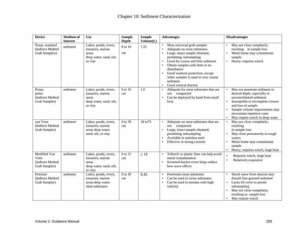
Chapter 10: Sediment Characterization
Volume 1: Guidance Manual 283
Device Medium of Interest
Use Sample Depth
Sample Volume(L)
Advantages Disadvantages
Ponar, standard (Indirect Method Grab Samplers)
sediment Lakes, ponds, rivers, estuaries, marine areas deep water; sand, silt, or clay
0 to 10
cm
7.25 • Most universal grab sampler • Adequate on most substrates • Large, intact sample obtained,
permitting subsampling • Good for coarse and firm sediment • Obtain samples with little or no
disturbance • Good washout protection, except
when sampler is used in very coarse sediment
• Good vertical descent
• May not close completely, resulting in sample loss
• Metal frame may contaminate sample
• Heavy; requires winch
Ponar, petite (Indirect Method Grab Sampler)
sediment Lakes, ponds, rivers, estuaries, marine areas deep water; sand, silt, or clay
0 to 10 cm
1.0 • Adequate for most substrates that are not compacted
• Can be deployed by hand from small boat
• May not penetrate sediment to desired depth, especially in unconsolidated sediment
• Susceptible to incomplete closure and loss of sample
• Sample volume requirements may necessitate repetitive casts
• May require winch in deep water van Veen (Indirect Method Grab Sampler)
sediment Lakes, ponds, rivers, estuaries, marine areas deep water; sand, silt, or clay
0 to 30 cm
18 to75 • Adequate on most substrates that are not compacted
• Large, intact sample obtained, permitting subsampling
• Available in stainless steel • Effective in strong currents
• May not close completely, resulting
in sample loss • May close prematurely in rough
waters • Metal frame may contaminate
sample • Heavy; requires winch, large boat
Modified Van Veen (Indirect Method Grab Sampler)
sediment Lakes, ponds, rivers, estuaries, marine areas deep water; sand, silt, or clay
0 to 15 cm
≤ 18 • Teflon® or plastic liner can help avoid metal contamination • Screened bucket cover helps reduce
bow wave effects
• Requires winch, large boat • Relatively expensive
Petersen (Indirect Method Grab Sampler)
sediment Lakes, ponds, rivers, estuaries, marine areas deep water; most substrates
0 to 30 cm
9.45 • Penetrates most substrates • Can be used in rocky substrates • Can be used in streams with high
velocity
• Shock wave from descent may disturb fine-grained sediment
• Lacks lid cover to permit subsampling
• May not close completely, resulting in sample loss
• May require winch
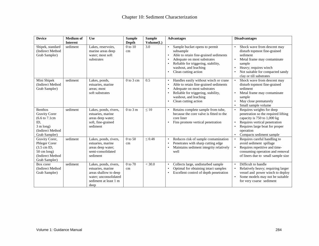
Chapter 10: Sediment Characterization
Volume 1: Guidance Manual 284
Device Medium of Interest
Use Sample Depth
Sample Volume(L)
Advantages Disadvantages
Shipek, standard (Indirect Method Grab Sampler)
sediment Lakes, reservoirs, marine areas deep water; most soft substrates
0 to 10 cm
3.0 • Sample bucket opens to permit subsample
• Able to retain fine-grained sediments • Adequate on most substrates • Reliable for triggering, stability,
washout, and leaching • Clean cutting action
• Shock wave from descent may disturb topmost fine-grained sediment
• Metal frame may contaminate sample
• Heavy; requires winch • Not suitable for compacted sandy
clay or till substrates Mini Shipek (Indirect Method Grab Sampler)
sediment Lakes, ponds, estuaries, marine areas; most soft substrates
0 to 3 cm 0.5 • Handles easily without winch or crane • Able to retain fine-grained sediments • Adequate on most substrates • Reliable for triggering, stability,
washout, and leaching • Clean cutting action
• Shock wave from descent may disturb topmost fine-grained sediment
• Metal frame may contaminate sample
• May close prematurely • Small sample volume
Benthos Gravity Corer (6.6 to 7.1cm ID, 3 m long) (Indirect Method Grab Sampler)
sediment Lakes, ponds, rivers, estuaries, marine areas deep water; soft, fine-grained sediment
0 to 3 m ≤ 10 • Retains complete sample from tube, because the core valve is fitted to the core liner
• Fins promote vertical penetration
• Requires weights for deep penetration so the required lifting capacity is 750 to 1,000 kg
• Requires vertical penetration • Requires large boat for proper
operation • Compacts sediment sample
Gravity Corer, Phleger Corer (3.5 cm ID, 50 cm long) (Indirect Method Grab Sampler)
sediment Lakes, ponds, rivers, estuaries, marine areas deep water; semi-consolidated sediment
0 to 50 cm
≤ 0.48 • Reduces risk of sample contamination • Penetrates with sharp cutting edge • Maintains sediment integrity relatively
well
• Requires careful handling to avoid sediment spillage
• Requires repetitive and time-consuming operation and removal of liners due to small sample size
Box corer (Indirect Method Grab Sampler)
sediment Lakes, ponds, rivers, estuaries, marine areas shallow to deep water; unconsolidated sediment at least 1 m deep
0 to 70 cm
< 30.0 • Collects large, undisturbed sample • Optimal for obtaining intact samples • Excellent control of depth penetration
• Difficult to handle • Relatively heavy; requiring larger
vessel and power winch to deploy • Some models may not be suitable
for very coarse sediment

Chapter 10: Sediment Characterization
Volume 1: Guidance Manual 285
Device Medium of Interest
Use Sample Depth
Sample Volume(L)
Advantages Disadvantages
Piston Corers (Indirect Method Grab Sampler)
sediment Ocean floor and large deep lakes; most substrates
3 to 20 m 5 to 40 • Typically recovers a relatively undisturbed sediment core in deep water
• Samples consolidated sediment
• Requires lifting capacity of > 2,000 kg
• Piston and piston positioning at penetration may fail • Disturbs surface (0 to 0.5 m)
sediment layer • Expensive
Vibracorer (5.0 to 7.5 cm ID) (Indirect Method Grab Sampler)
sediment Continental shelf of oceans, large lakes; sand, silty sand, gravelly sand substrates
3 to 6 m 5.9 to 13.2 • For deep profiles, it effectively samples most substrates with minimum disturbance
• Can be used in over 20 m water depth • Portable models can be operated from
small vessels (e.g., 10 m long) • Samples consolidated sediment
• Labour intensive • Assembly and disassembly might require divers • Disturbs surface (0 to 0.5 m) layer • Special generator may be needed • Heavy models require larger boat
and power winch to deploy

Chapter 10: Sediment Characterization
Volume 1: Guidance Manual 286
Device Medium of Interest
Use Sample Depth
Sample Volume(L)
Advantages Disadvantages
Peeper Porewater Lakes, ponds, wetlands, rivers, estuary, and oceans; shallow or deep water; fine-grained, uncompacted sediment
0.2 to 30cm
≤ 0.25 • Most accurate method • Reduced artifacts due to minimal
disturbance • No laboratory processing • Relatively free of effects from
temperature, oxidation, and pressure • Inexpensive and easy to construct • Some chemical selectivity possible
depending on nature of sample via specific membranes
• Wide range of membrane/mesh pore sizes and internal solutes or substrates available
• Requires deployment by hand (e.g., diver in deeper water)
• Requires weeks to months for equilibration
• Methods not standardized/used infrequently
• Some membranes are subject to fouling
• Must deoxygenate chamber and materials to prevent oxidation effects
• Some chambers only allow small sample volumes
• Care must be used on collection to prevent sample oxidation and/or degassing
• Utility for accurately sampling highly hydrophobic organic compounds is unknown (i.e., sorption of hydrophobic compounds onto sampler or membrane could artificially reduce porewater chemical concentrations
• Labour intensive

Chapter 10: Sediment Characterization
Volume 1: Guidance Manual 287
Device Medium of Interest
Use Sample Depth
Sample Volume(L)
Advantages Disadvantages
Suction Porewater Lakes, ponds, wetlands, streams, and estuary; primarily shallow water fine- to coarse-grained, unconsolidated sediment
0.2 to 30 cm
≤ 0.25 • Reduced artifacts, gradient definition • Rapid collection • No laboratory processing • Closed system which prevents
contamination • Methods include airstone, syringes, probes, and core-type samplers • Operation easy and low-technology • Functions best in highly porous
substrate
• Requires non-standard collection devices
• Small sample volumes • Core airstone method difficult in
some sediment and in deeper water (>1 m)
• Method might require diving for deployment in deeper waters
• Potential for sorption of metals and hydrophobic organic carbons on filter
• Clogging may occur with silt and clay size particles
• Collection of porewater from nontargeted depths (e.g., overlying water) may occur
• Oxidation and degassing of porewater may occur
Squeezing (pneumatic pressure)
Porewater Sediment collection from lakes, ponds, wetlands, rivers, estuary, and oceans; shallow or deep water; fine- grained, unconsolidated sediment
0 to 10 cm
Determined by volume of sediment collected
• Large volumes of porewater are generated
• Operation is easy • Functions with fine, medium, and
coarse particle size sediment
• Hydrophobic organic carbon loss on filter
• May compromise sample integrity • Potential for sample oxidation
and loss of volatile Compounds
Centrifugation Porewater Sediment collection from lakes, ponds, wetlands, rivers, estuary, and oceans; shallow or deep water; fine-grained, unconsolidated sediment
0 to 10 cm
Determined by volume of sediment collected
• Extraction time is brief • Several variables (e.g., duration,
speed) can be varied to optimize operation
• Large volumes of porewater are generated
• Operation is easy • Functions with fine to medium particle size sediment
• Labour intensive (e.g., large volumes of
sediment need to be collected) • Lysis of cells during spinning • Coarser-grained sediment require
larger sample volume or may be impractical • Hydrophobic organic carbon loss
on filter • Degassing may occur • May compromise sample integrity
Chapter 10: Sediment Characterization
Volume 1: Guidance Manual 288
Device Medium of Interest
Use Sample Depth
Sample Volume(L)
Advantages Disadvantages
Sources: USEPA, 1995; 2001; 2002b; Washington State Department of Ecology, 1995; Clark, 1996; Carr and Nipper, 2003; Ohio EPA, 2001.

Chapter 11: Biological Characterization
Volume 1: Guidance Manual 289
11 BIOLOGICAL CHARACTERIZATION GUIDANCE
Context, Purpose, Scope 11.1
This biological characterization chapter addresses general sampling design, sampling equipment, and other factors pertaining to biological sampling in lakes, ponds, wetlands, rivers, streams, estuaries, oceans, and terrestrial habitats.
Biological sampling is typically conducted as part of environmental site characterizations to determine concentrations of contaminants of potential concern (COPCs) in biological tissue for use in human health or ecological risk assessments, or to provide site-specific measures of the diversity and abundance of a biological population or community of valued ecosystem components (VECs).1 Although this chapter is intended to be inclusive of a wide range of organisms and characterization methods, it focuses on the most common sampling methods used to support risk assessments. Thus, because aquatic organisms are more commonly sampled than terrestrial organisms (for risk assessment purposes), this chapter also devotes greater attention to aquatic biota than to terrestrial biota.
Given the breadth of this chapter’s scope, it is not intended to provide overly detailed or prescriptive sampling methodologies, information on specific regulatory requirements, or laboratory analytical protocols. The information presented in this chapter is based on current information and recommendations of a variety of agencies and is intended to provide a coherent set of recommendations for site investigation personnel responsible for implementing the most commonly used field sampling methods.
For the assessment of risks to human health, biological sampling is most often relevant at study areas where the fish ingestion exposure pathway is significant. Biological sampling may also be important in characterizing risks associated with consumption of home-grown vegetables, beef, dairy products, or locally-hunted game. For ecological risk characterization, dietary exposures to bioaccumulative COPCs typically dominate wildlife exposures and potential risks (Moore et al., 1997, 1999) and therefore often warrant special consideration in risk characterizations for carnivorous and piscivorous birds and mammals. Fish tissue chemistry data can be used to evaluate risks to fish themselves, as well as to humans and wildlife that consume fish.
1 Throughout this chapter, “population” is used to refer to a biological population, i.e., a set of organisms of the same group or species that live in the same geographical area, and have the capability of interbreeding. “Population” as used in previous chapters generally refers to a data population (i.e., data set).
Biological Characterization
This chapter describes the planning, process, and methods for biological characterization. The key elements and their corresponding sections in the chapter are:
• Conceptual site model and site reconnaissance (11.2)
• Study approach and design (11.3)
• Biological sampling methods and equipment (11.4)
• Data analysis (11.5)

Chapter 11: Biological Characterization
Volume 1: Guidance Manual 290
The primary purposes of this biological characterization chapter are: 1) to provide guidance on factors to consider in biological sampling for risk assessment data development and 2) to facilitate collection of high quality, useful data by providing consistent methodologies for investigators tasked with developing and implementing biological sampling programs in support of human health and ecological risk assessments.
Biological sampling is most often critical for risk characterization at study areas with bioaccumulative COPCs (e.g., dichlorodiphenyltrichloroethane [DDT], dieldrin, and many other pesticides, as well as polychlorinated biphenyls [PCBs], dioxins and furans [PCDD/Fs], lead, and methylmercury). Exhibit 11-1 presents sources of information for selecting bioaccumulative compounds. Although many of these references focus on bioaccumulative compounds in fish tissue, the compounds identified may also be of concern in terrestrial and other aquatic organisms. Comparable sources identifying bioaccumulative compounds specific to other organisms (e.g., shellfish wildlife, terrestrial invertebrates) were not identified in the available literature, likely reflecting the fact that such organisms are less commonly sampled than fish.
The Persistence and Bioaccumulation Regulations (SOR/2000-107) contained in the Canadian Environmental Protection Act, 1999, set the criteria for determining if a substance is persistent or bioaccumulative under the Act. Under the regulation, a substance is bioaccumulative when its bioaccumulation factor (BAF) is greater than or equal to 5,000; when its bioconcentration factor
EXHIBIT 11-1: Sources of Information for Selecting Bioaccumulative Compounds • The Government of Canada produced an inventory, named the Domestic Substances List
(DSL), of approximately 23,000 substances. Substances on the DSL that were categorized as bioaccumulative may be found at http://www.ec.gc.ca/lcpe-cepa/default.asp?lang=En&n=5F213FA8-1&wsdoc=D031CB30-B31B-D54C-0E46-37E32D526A1F
• 1997 Listing of Fish and Wildlife Consumption Advisories (USEPA, 1997)
• Regional Ambient Fish Tissue Monitoring Program (RAFT) contaminants of concern (provided by USEPA Region 7)
• USEPA. 2000. Guidance for Assessing Chemical Contaminant Data for Use in Fish Advisories Volume 1, Fish Sampling and Analysis, Third Edition, EPA 823-B-00-007
• Persistent Organic Pollutants (POPs) listed in “Substantiation report of the Task Force on POP,” 4th meeting, Den Haag (the Netherlands), February 21-25, 1994
• USEPA and USACE (1998) Inland Testing Manual, Evaluation of Dredged Material Proposed For Discharge in Waters of the U.S. - Testing Manual, February, EPA-823-B-98-O04 (see Tables 9-5 and 9-6 in that document)
• Recommended target analytes in USEPA (1995) Guidance for Assessing Chemical Contaminant Data for Use in Fish Advisories. Volume 1. Fish sampling and analysis. Second edition, EPA 823-R-95-007

Chapter 11: Biological Characterization
Volume 1: Guidance Manual 291
(BCF) is greater than or equal to 5,000; or when the logarithm of its octanol-water partition coefficient is greater than or equal to 52.
The Canadian Council of Ministers of the Environment (CCME) have adopted these same values for determining if a substance is bioaccumulative, as reflected in the CCME Policy Statement for the Management of Toxic Substances, and in the Protocol for the Derivation of Canadian Tissue Residue Guidelines for the Protection of Wildlife that Consume Aquatic Biota (CCME, 1998).
Biological organisms can be exposed to stressors via numerous pathways, depending upon conditions at a particular study area. Exposures to these organisms can also be mitigated via numerous physical and chemical conditions at the study area in ways that are not easily predicted. Thus, biological sampling often provides the most direct and accurate measure of site- 2 BAFs are preferred over BCFs, and when neither BAF nor BCF data exist, the log octanol-water partition coefficient may be used: BAFs and BCFs are considered on a whole-body, wet weight basis.
Terms Used to Describe Accumulation of COPCs in Biota Five terms used to describe the accumulation of COPCs in biota are: • Bioconcentration - the process by which COPCs are directly taken up by terrestrial or
aquatic organisms from a single medium (e.g., soil, water, or sediment). Typically only measured in a laboratory setting.
• Bioaccumulation - the process by which COPCs are taken up by terrestrial and aquatic organisms directly from an environmental medium, as well as diet, at a faster rate than compounds are lost through excretion or metabolism.
• Biomagnification - The process of bioaccumulation by which tissue concentrations of COPCs are passed up through two or more trophic levels so that tissue residue concentrations increase systematically as trophic level increases.
• Bioavailability – The amount of chemical available to the target tissues following exposure. It is usually measured indirectly by comparing concentrations in tissue relative to those in abiotic media, or by measuring parameters in abiotic media known to affect bioavailability (e.g., measuring the organic carbon content or sediment porewater concentrations of sediment, or measuring soil pH or cation exchange capacity in soils. It may also be measured by measuring levels in the bloodstream of an organism, although this is rarely done.
• Bioaccessibility – An analytical technique to estimate bioavailability by performing weak acid, water, or simulated gastric extractions of soil/sediment samples. Bioaccessibility is the estimated fraction of a substance in media that is available for uptake by an organism, whereas bioavailability is a direct measure of what has been adsorbed.
Source: CCME, 2006. The remainder of this chapter generally uses the term “bioaccumulation,” as it reflects exposures from several media.

Chapter 11: Biological Characterization
Volume 1: Guidance Manual 292
specific exposure for VECs. In screening-level risk assessments, biota tissue concentrations can be estimated using literature-based water-to-biota BCFs (typically for fish), sediment-to-biota BAFs, or soil-to-biota BAFs. Direct measurement of COPC concentrations in biota tissue is generally more accurate than extrapolation of biota concentrations based on BCFs or BAFs applied to abiotic media. Therefore, for study areas at which bioaccumulation potential is of concern, collection of biological tissue data is recommended to reduce uncertainty in the human health and/or ecological risk assessment prior to making any risk management or remediation decisions.
While this chapter focuses on collection of biological samples for chemical analysis (i.e., exposure metrics), biological sampling may also be conducted in support of effects metrics (e.g., productivity, community structure). Effects-related metrics are used to assess the impacts of chemical or physical stressors on the environment. A detailed discussion of the multitude of methods for community structure analysis is beyond the scope of this chapter; however, references for additional information are also provided in the appropriate section.
Conceptual Site Model for Biological Characterization 11.2
As detailed in Chapter 4 of this guidance document, development of a CSM is a critical first step in the process of characterizing the nature and extent of COPC concentrations present at a study area. The CSM allows visualization of chemical fate and transport of COPCs in aquatic and terrestrial environments, and serves as a guide to the design of the sampling program. The CSM also provides project personnel and decision makers with a tool for understanding and communicating potential risks at the study area.
As discussed in Chapter 4, one of the primary fate and transport mechanisms of greatest interest for biological organisms is bioaccumulation, and COPCs most commonly evaluated in biological sampling are bioaccumulative compounds (e.g., DDT, PCBs, dioxins and furans, alkylated lead, and methylmercury), although other COPCs may be targeted if preliminary calculations suggest that they may pose a risk to human or ecological receptors.
In general, species targeted for biological sampling are selected based on feasibility and relevance to the risk questions posed by the risk assessment. Sampled species may reflect the selected VECs and/or the preferred dietary items of those VECs and human receptors. Fish, aquatic and terrestrial invertebrates, and small mammals are generally the most common target species, but common game species (e.g., gamebirds and deer) and/or plants also may be sampled to characterize human health and/or ecological risks. A generalized CSM for biological characterization is shown in Figure 4-14. Risk assessors are expected to modify it or use their preferred presentation format for site-specific CSMs. CSMs for individual sites should
Biological Sampling Objectives
Biological sampling is generally conducted for the following reasons:
1. To directly measure bioavailability; 2. To provide site-specific estimates of
exposure to the organisms and their predators;
3. To relate tissue residue levels to concentrations in environmental media (e.g., in soil, sediment, or water) or tissue residue guidelines; and
4. To monitor productivity or community structure.
Chapter 11: Biological Characterization
Volume 1: Guidance Manual 293
acknowledge and discuss reference sites to which conditions at the contaminated site will be compared in the risk assessment.
Site Reconnaissance for Biological Sampling The primary objective of site reconnaissance is to improve the efficiency and effectiveness of sampling programs through early planning and identification of unique study area conditions that warrant consideration before sampling begins. Both desk-top and on-site reconnaissance can be conducted prior to initiation of biological sampling. Although initial on-site reconnaissance can be conducted prior to or in conjunction with the first sampling event, the former is preferable, in that early reconnaissance provides time to obtain any specialized equipment (e.g., four wheel drive vehicles) necessitated by unique study area conditions and to resolve access and safety issues.
Prior to conducting the site reconnaissance, it is advisable to review background and supporting information and materials, such as:
• Files related to the nature and extent of chemicals present on the study area, historical uses of the study area, and historical manufacturing and disposal practices
• Safety issues that may necessitate personal protective equipment (may be revised based on observations during site reconnaissance)
• Topographic maps and aerial photographs to identify the extent of undeveloped areas on or downgradient from the study area that may provide ecological habitat
• Property boundaries, as well as names, addresses, and phone numbers of abutting land owners. Property access needs should be addressed prior to site reconnaissance
• Material Safety Data Sheets (MSDSs) and Workplace Hazardous Materials Information System (WHMIS) information on materials manufactured, stored, or disposed on-site
• Files related to soil hydrogeological properties or other properties that may help determine fate and transport mechanisms
• Drainage maps of the study area and relationship of drainage structures to waste storage or disposal areas; identify wetlands and floodplains
• Locations of effluent discharges (process water and storm water), landfills, and above ground and below ground storage tanks
• Locations and characteristics of nearby water bodies, including general depth, seasonal flow, and water quality conditions that would influence the types of biota that would occur there (i.e., whether the area supports aquatic life). Fish occupy seasonally wetted areas (i.e., ephemeral streams), such that even if they are dry at some times of the year, they are still considered fish habitat and are protected under the Fisheries Act. However, it obviously would be impractical to attempt to sample fish in these habitats during dry seasons. Sampling fish from ephemeral streams would also contribute uncertainty to the subsequent risk

Chapter 11: Biological Characterization
Volume 1: Guidance Manual 294
assessment, as those fish inhabit other water bodies when the stream is dry, and thus could be exposed to contaminants in those other water bodies,
• Aquatic and/or terrestrial setting, as it pertains to study design and equipment needs (e.g., wadeable riffle/run/pool stream habitat vs. deep pond, lake, estuary, coast, open ocean; presence or absence of steep ravines or other barriers)
• Presence of endangered, threatened, or special concern species, special habitats, sensitive sites, significant wetlands, other potential VECs.
Key tasks to address during site reconnaissance include:
• Photograph and/or video record study area conditions
• Acquire geographic positioning system (GPS) coordinates of access points, potential reference area locations
• Assess potential sampling locations and identify key habitat features (e.g., riffle and pool areas, ravines, building structures) and seasonal attributes (e.g., water depth) that may influence sampling locations and equipment needs
• Find suitable access points and routes of egress
• Confirm exposure pathways and routes identified in the CSM
• Identify factors that may mitigate or exacerbate exposure (such as the presence of structures that may preclude biological exposure) as indicated by the CSM
• Evaluate general habitat conditions to confirm or refute information obtained during the desk top review
• Identify potential reference areas
USEPA (1997) provides a detailed checklist for ecological study area reconnaissance.
If the study area is an active facility, it may also be appropriate to interview facility personnel to determine factors unique to the on-site conditions. For example, there may have been historic recreational fishing in water bodies at the study area. Anecdotal observations of wildlife present at the study area may be gathered, although weight given to these observations must be adjusted to take into account reliability of the source.
It is important to obtain information regarding presence of species that are endangered, threatened, or of special concern early in the planning process3. While information may not be available as to whether they are found in a smaller study area, information on their geographic
3 Online sources such as Canada’s Species at Risk Act (SARA) registry (http://www.sararegistry.gc.ca) and comparable provincial registries are readily available sources of this information.

Chapter 11: Biological Characterization
Volume 1: Guidance Manual 295
distribution and habitat requirements is typically available. The potential occurrence of such listed species is important to consider early in the process because:
• If any species are identified, their potential occurrence can be evaluated during the site reconnaissance by comparing habitat present at the site relative to those species’ habitat requirements;
• Potential presence of these species may affect the chosen sampling methods (e.g., use of lethal vs. non-lethal trapping methods); and
• The potential presence of these species may affect the ability to obtain a collection permit for similar species or other species within the same habitat.
Study Approach and Design for Biological Characterization 11.3
The purpose of this subsection is to identify key factors related to developing an appropriate study design for biological characterization sampling in support of ecological and human health risk assessments. Establishing a conceptually sound study approach supported by a technically sound study design is critical to proper characterization of biological tissue concentrations and overall conditions. When designing a program that involves biological sampling, it is also important to obtain any required federal, provincial, or territorial biological collection permits before implementing the sampling program, as the permit requirements may affect the species selected, sampling methods used, and/or timing of the sampling program. Acquiring collection permits early is especially important for areas/sites where a SARA listed species potentially occurs, as there is prohibition against harming, harassing, or killing any individual, and a separate permitting process exists for SARA listed species.
11.3.1 Goals and Objectives
An appropriate biological sampling design depends on clear definition of sampling goals and objectives (CCME, 1993). Initially, project goals can be stated in broad terms, with specificity added as additional information on the most important aspects of a given risk assessment becomes available. Relevant guidance (CCME, 1993; Environment Canada, 2008; USEPA, 1995; Chapters 2 and 3 of this guidance; U.S. Navy, 1997) lists the fundamental goals and objectives of sampling programs for site characterization in support of risk assessment as follows:
• To provide representative chemical data related to potential human health and ecological risks at the study area; representative data are those that accurately reflect study area conditions, as they relate to potential risks to receptors
• To characterize, quantify, and delineate the spatial and temporal nature and extent of chemical concentrations relative to human and ecological exposure pathways
• To assess the presence of COPCs relevant to migration and exposure pathways identified in the CSM
Chapter 11: Biological Characterization
Volume 1: Guidance Manual 296
• To ensure that the data collected are sufficient to yield meaningful conclusions and support defensible decisions related to mitigation of any risks
• To identify, at least on a relative basis, high priority areas of concern that may pose imminent risk to human health and the environment, especially as defined by relevant regulatory statutes.
Study objectives can be broad (e.g., to characterize the nature and extent of chemical concentrations at the study area) or highly focused (e.g., to develop statistically valid chemical distribution profiles). Some guidance suggests use of exploratory level and monitoring level goals and objectives (CCME, 1993). Regardless, the fundamental study objectives must be clearly stated to guide the sampling program. USEPA (1997) and Clark (2003) contain detailed discussions on defining goals and objectives for biological monitoring programs. Examples of goals and objectives that are specific to biological sampling include:
• To understand the temporal variability in abundance or species richness of a benthic community within the study area
• To obtain a site-specific measure of COPCs in biological tissue to generate an accurate characterization of risks to human and ecological receptors
• To evaluate temporal trends in biological tissue concentrations of COPCs prior to or after site remedial measures
If statistical characterization of the data is desired, clear hypotheses must be formulated during the planning stage to guide the study design. Quality assurance methods specific to biological characterization programs are listed below. Chapter 3 and numerous guidance manuals (e.g., MOEE, 1996; USEPA, 2001; 2006; Clark, 2003; MacDonald and Ingersoll, 2003) present considerations for quality assurance/quality control (QA/QC), including project organization and responsibilities; equipment and instrument calibration; sample collection, handling, labelling, preservation, transportation, and tracking; decontamination procedures; record keeping and documentation; data reporting; training requirements; performance audits; and corrective action procedures.
11.3.2 Data Quality Objectives
Once the study goals and objectives have been identified, the data quality objectives (DQO) process is used to determine the type, quantity, and quality of data needed to develop defensible data for use in decision making regarding the nature and extent, as well as potential risks associated with COPCs. Various guidance documents and resources are available regarding the DQO process (e.g., USEPA 2006 and www.triadcentral.org). Establishing concise DQOs is important to defining the specific types of data to be collected. Performance criteria and specific data acceptance and rejection criteria are critical components of the DQO process (e.g., USEPA, 2006; U.S. Navy, 1997). The process is also used in various Canadian sampling programs (e.g., CCME, 1993; Chapters 3, 6, and 7 of this guidance).

Chapter 11: Biological Characterization
Volume 1: Guidance Manual 297
Fundamentally, the DQO process consists of seven iterative steps, which define criteria that are used to establish final data collection and study design. When designing the analytical approach, it is important to identify COPCs and any supporting analyses important to understanding the fate and effects of COPCs (e.g., documentation in the field of sample characteristics such as weight, length, species, gross morphological abnormalities). It is important to identify the specific forms of chemicals to be measured, availability and reliability of analytical methods for those chemicals, and additional parameters to be measured (e.g., percent lipid, percent moisture).
DQOs can be general, such as, “determine whether the COPC is present on-site at concentrations above Canada’s tissue residue guidelines.” DQOs can also be highly specific and quantitative, such as, “determine whether the lipid-normalized COPC concentration in small mammals collected from the study area is significantly higher (α=0.05) than that in samples collected from the reference area.”
11.3.3 Biological Sampling Design Considerations
This subsection describes factors important to proper study design for biological sampling and discusses unique considerations for sampling biota. This subsection also details the technical concerns that warrant consideration in developing a defensible study design. Chemical concentrations in biota can vary both spatially and temporally. Spatial variation may be due to natural variations in substrata or may be reflective of greater isolation from a source of COPCs. Temporal variation in tissue concentrations may be due to an organism’s inactivity during winter months, reproductive status, age, diet, or isolation from a source of COPCs during certain seasons (i.e., organism’s migratory behaviour, seasonal variations in availability of various prey items). Depending upon the mobility of the organism, chemical concentrations may be closely linked or not at all linked to the study area or local conditions. The great variability in biological systems must be properly assessed under the sampling design, in order to obtain representative samples and meaningful data.
General factors to consider in the sampling design for biological conditions include:
• Type, quality, and amount of data needed to achieve study goals and DQOs
• Data representativeness (i.e., data reflecting study area conditions as they relate to human health and ecological risk assessment)
• Quality control measures to be used to control error and bias, thereby ensuring that the required data quality is obtained.
Data Quality Objective (DQO) Process
The seven iterative steps are identified below and described in Chapter 9 of this manual:
1. State the problem
2. Identify study goals
3. Identify data needs
4. Define site boundaries
5. Design the analytical approach
6. Develop performance/acceptance criteria
7. Develop a sampling and analysis plan

Chapter 11: Biological Characterization
Volume 1: Guidance Manual 298
• Expected sampling effort (e.g., area to be sampled for benthos, small mammals, or terrestrial invertebrates) or time per sampling unit (e.g., catch per unit effort for fish sampling, or number of trap-nights for furbearer sampling)
• Data analysis methods, particularly as they relate to required sample sizes
• Types and number of quality control samples (e.g., duplicates)
• Seasonal considerations, as some organisms are more active or are only present at certain times of year. Snow cover and frozen ground or ice may preclude sampling for soil invertebrates or fish species. Benthic invertebrate community structure may vary over the course of the year, due to differences in temperature tolerance and the effect of temperature, light, or other factors on life stage (e.g., hatching/emergence). If there is an annual sampling program in place, it is important to conduct annual sampling events at a consistent time of year to limit temporal variability.
• Organism life history and population dynamics. Migratory species may have increased or reduced exposure to the COPC during critical life stages, or they may be exposed COPCs elsewhere. During a receptor’s life span, its home range may cover an entire basin under investigation, or it may be too broad to characterize exposures to a study area. For example, a crab’s home range may cover an entire basin under investigation, a Coho salmon may use an estuary under investigation for a number of months critical for its development and transition into marine environment, a wintering population of migratory bird may use a certain portion of a basin exclusively for foraging and thus present a higher potential exposure to COPCs. Some species may be facing harvest/population pressure (even if not listed), some long-lived organisms may not be appropriate to sample (i.e., some rockfish live to 80 years and harvesting them for sampling may not be acceptable).
Study Area and Reference Area Identification
A study area refers to the area to be monitored and/or assessed. It is important to clearly define the boundaries of the study area, as the size of this area dictates the breadth and scope of the project and greatly influences the overall sampling design. The study area should encompass the entire zone of impact associated with the site and ideally should be large enough to allow the characterization of the severity of the impacts, in reference to an unimpacted or reference area (MOEE, 1996). However, study areas can be subdivided into smaller areas to facilitate and focus site investigation activities; division of a study area into multiple sub-areas (exposure units or exposure areas) can aid future site management decisions. Boundaries of such exposure areas may be based upon habitat differences (or presence or absence of habitat) within the larger study area. Figure 5-1 outlines the process for defining a study area’s boundaries.4
A reference area is an unimpacted or relatively unimpacted area with physical and biological attributes similar to those of the study area, but for the release of site-related chemicals. Because 4 Although the medium in this figure is soil, the process is similar for both terrestrial and aquatic investigations.
Chapter 11: Biological Characterization
Volume 1: Guidance Manual 299
of the practical difficulty in locating an ideal reference area, it is often necessary to select locations with COPC concentrations that are equivalent to regional background concentrations. It is equally important that the reference areas have similar physical and biological attributes as the study area.
It is usually advisable to select more than one reference area to represent the range of background conditions and/or the range of the site physical and biological characteristics and to allow for more meaningful statistical comparisons. Evaluation of two or more reference areas will allow for a more accurate representation of true reference conditions. If only one reference area is identified, it is imperative to acknowledge the assumptions and limitations of this comparison (i.e., the assumption that this area is a reasonably representative of other reference areas, and that multiple samples collected from this single reference area are pseudo-replicates rather than truly independent samples).
Selection criteria for reference areas should be defined a priori and may include (e.g., Apitz et al., 2002):
• Physical nature of soil or sediment (e.g., grain size, organic carbon content);
• For aquatic systems, flow dynamics (e.g., fast vs. slow or no flow, flashiness, stream order);
• Chemical composition (e.g., contributions from road runoff, atmospheric deposition, naturally-occurring inorganic chemicals);
• Habitat type (specific aquatic, wetland, or terrestrial habitats);
• Biological composition (e.g., benthic invertebrate communities); and
• Proximity to the study area.
In terrestrial systems, suitable reference areas are often located in habitat similar to that of the study area, in locations adjacent to but upgradient or cross-gradient from the study area. In lotic (flowing) aquatic systems, suitable reference areas are often located immediately upstream of the study area, beyond the influence of the site. In lentic (static) aquatic systems, a suitable water body(ies) within the same watershed, but outside of the area of impact, should be targeted.
Comparisons between the study area and the reference areas are one means of determining the potential effects of site-related COPCs. Reference areas can help to differentiate off-site vs. site-related contributions of COPCs. Furthermore, reference areas provide a measure of background concentrations of chemicals, particularly those that may have a natural or anthropogenic, but non site-related, source (e.g., pesticide applications, road runoff, atmospheric deposition) (Gandesbury and Hetzel, 1997). For example, if an ecological risk assessment documented fish mortality in a pond that was affected by both site-related chemical releases and acid precipitation, concurrent evaluation of one or more reference ponds would be critical to understanding whether the chemical releases and/or the acid precipitation caused the observed fish mortality. As a second example, if a human health risk assessment predicted that risks from fish ingestion were unacceptable due to mercury in fish tissue, it would be important to

Chapter 11: Biological Characterization
Volume 1: Guidance Manual 300
accurately characterize the anthropogenic (non-site-related) mercury concentrations, in order to ensure that risk management decisions could effectively mitigate risks.
Biological Sampling Approaches
Approaches to biological sampling can generally be classified into two types: biased and unbiased. Additional discussion of sampling design is provided in Chapter 5.
In biased (or judgemental) sampling, sample stations are targeted toward the area(s) of concern or, in the case of biological sampling, toward areas where the target organism is likely to occur. By definition, biased sampling requires at least some previous knowledge of the site’s chemical distribution or the organism’s likely distribution (USEPA, 1995; 2001). Given the cost of sampling and taxonomy for benthic invertebrate community analysis, sampling and benthic analysis is often done in a tiered manner after potentially impacted and non-impacted areas or sites are identified via chemistry analyses. While an unbiased sampling approach is preferred (Mattuck et al., 2005), sampling for biological organisms is nearly always judgemental sampling, driven by habitat and actual location of the organisms.
In unbiased or probability sampling, sample stations are selected randomly, without regard to the physical characteristics of the study area. While unbiased sampling provides estimates of chemical variability and meets fundamental statistical assumptions (i.e., measurements are random and independent), it is not often possible when sampling for biological organisms. Exceptions would be fish sampling across larger water bodies, or collection of plants from within a garden plot. It is possible to place small mammal traps and pitfall traps for terrestrial invertebrate sampling in a grid or along transects (trap lines) in an unbiased manner, and this may be desirable if abundance, species richness, or other community parameters are of interest. However, if collection of biota for tissue analysis is the overall goal, systematic (i.e., unbiased) placement of traps would likely require a much greater level of effort (trap density) in order to obtain the same sample quantity as from a biased or purposeful sampling layout (i.e., near fallen logs or other areas where use by small mammals is evident).
In stratified sampling, the area to be sampled is divided into non-overlapping strata. The strata are determined based on biological knowledge (i.e., recognition of different habitat types present in the study area) or based on site contaminant-history of the study area (i.e., sources and dispersion patterns of COPCs in abiotic media). The strata represent subareas in which different random or non-random sampling approaches may be employed.
Selection of the sampling approach appropriate for a given type of study is discussed in detail by Gilbert and Pulsipher (2005), MOEE (1996), and USEPA (2001; 2002a).
After the general approach to biological sampling is selected, there are many factors to consider in determining the placement of individual sample locations and the number of samples to collect. One of the key considerations in biological sample design is the incorporation of flexibility into numbers and types of samples collected. The number of samples that should be collected depends on:

Chapter 11: Biological Characterization
Volume 1: Guidance Manual 301
• The distribution pattern of COPCs (homogeneous vs. heterogeneous)
• The desired level of accuracy of the conclusions
• The variance in concentrations
In determining the number of samples needed, statistical power analysis5 is considered to determine the likelihood that a statistical test will yield a significant result, given that an effect actually exists. Thus, power analysis is linked to and complementary to traditional statistical hypothesis testing.
Statistical power may depend on a number of factors. Some of these factors may be particular to a specific testing situation, but at a minimum, power nearly always depends on the following two factors:
• The statistical significance criterion used in the test
• The magnitude of the effect of interest in the population
Power analysis can be used to calculate the minimum sample size required to accept the outcome of a statistical test with a particular level of confidence. It can also be used to calculate the minimum effect size that is likely to be detected in a study using a given sample size.
Given the natural variability in biological systems, it is rarely feasible to collect the number of samples needed to achieve optimal statistical power. Restrictions in overall density or abundance of organisms present at a site and budget and schedule limitations are among the factors that may limit the number of samples collected at a study area. Health Canada (2010) provides additional discussion of sample size requirements for garden vegetables, which range from 3 to 5 plant samples per hot spot, and 10 to 15 (sometimes up to 30) samples per study area. For fish and shellfish, Health Canada (2010) recommends that a minimum of 5 to 10 samples be taken for each target organism. For more detailed assessments, or if remoteness of or access to the study area would make revisiting it infeasible, their recommended minimum sample size is 20 for fish and shellfish. If power analysis methods are being used to calculate sample sizes, Health Canada (2010) suggests using power analysis methods as described by Green (1989) and Environment Canada (1998). Health Canada (2010) acknowledges that collection of 5, 10 or 20 samples of some species may be impractical or impossible, given population density considerations relative to the study area.
Consideration should also be given to stratification of samples based on desired organism size or sizes (i.e., two different fish sizes may be needed to assess risks to two different types of piscivorous VECs) and species availability. If collecting fish, age6, sex, length and weight should
5The power of a statistical test is the probability that the test will reject the null hypothesis when the alternative hypothesis. 6 Because the age of fish is determined in the laboratory, stratification in the field typically focuses on the species and length of fish collected. These attributes can help ensure that representative samples are collected within different strata, in the absence of real-time information on fish age.

Chapter 11: Biological Characterization
Volume 1: Guidance Manual 302
be considered. Older fish may have higher body burdens of bioaccumulative substances, and males may have a higher body burden than females, which may lose a portion of their contaminant load during reproduction. It is often useful to include contingencies in the study design to aid with the inevitable field decisions that frequently must be made, so that those decisions will have a minimal influence on the outcome of the sampling program and risk assessment. Even if habitat suitability and other factors appear to support a targeted species, that species (or size of organism) may not be obtained for a number of reasons (habitat preferences, unusual weather or seasonal conditions, etc.). For example, if the target organisms are shrews, and species being captured in the traps are limited to voles or mice, decisions regarding suitability of the alternate species will be necessary. Similarly, if the target organisms are earthworms, and low density of earthworms is hindering collection of adequate sample volume in a reasonable amount of time, decisions regarding the inclusion of a broader variety of soil organisms will be necessary.
If a contaminant source is known or expected, biological sampling locations may be placed near (e.g., along the shoreline of a diffuse source) or immediately downgradient of the source (e.g., downstream of an outfall). In many cases, arrays or transects spreading outward from the original source of contamination can help define concentration-response gradients. In tidal or marine systems, tidal influence and tidal stage must be considered in identifying biological sampling locations. For example, tidal fluctuations can transport COPCs “upgradient” of the original source.
Because most risk assessments are carried out in order to support risk management decisions (e.g., remediation of sediment, soil, or water), it is often beneficial to collect co-located samples of biotic (e.g., tissue) and abiotic (e.g., soil, sediment, water) media. However, the correlation between concentrations in co-located samples will depend on the home range area of the species sampled, relevant exposure pathways, bioavailability of the COPC, and other factors. If there is poor correlation in concentrations in co-located samples, management actions may not prove biologically beneficial.
11.3.4 Sample Specific Considerations
In addition to the considerations related to designing the sampling program, some specific decisions depend on the types of samples to be collected. Such decisions influence the design of the sampling program and ultimate selection of sampling methods. After development of the CSM and after completion of the site reconnaissance, VECs are identified and goals and objectives determined. This information is used to identify data needs and to help determine the types of biological samples needed to yield meaningful conclusions and support defensible decisions at the study area. Target species for tissue analysis are identified based on the diets of the VECs, study area habitat(s), study objectives, and logistical constraints. Typically, target species or organism types are selected based on the VECs and their prey preferences. Commonly targeted species for biological sampling are soil invertebrates, terrestrial plants, small mammals, aquatic invertebrates, and fish; these are the focus of this guidance chapter. Aquatic plants are targeted less frequently because there are relatively few published studies on aquatic phytotoxicity, and many bioaccumulative chemicals have very low water solubility, rendering them unavailable for plant root uptake (ATSDR, 2007).

Chapter 11: Biological Characterization
Volume 1: Guidance Manual 303
An important consideration in biological sampling relates to sample compositing. Compositing several individual organisms into a single biological sample is often necessary to obtain the mass needed for many chemical analyses and in order to obtain sufficiently low detection limits. When done correctly, composite sampling can mimic exposure conditions encountered by a VEC. For example, compositing a variety of terrestrial invertebrates collected from the foraging range of an invertivorous bird or mammal simulates that VEC’s foraging behaviour. Likewise, compositing multiple small mammals from the foraging range of a carnivorous bird or mammal simulates that VEC’s foraging behaviour, while compositing multiple fish of species and size targeted by a piscivorous bird or mammal simulates that VEC’s dietary preferences. In other cases, it may be appropriate to focus on a particular species and composite several individuals of that species (e.g., when sampling the VEC to characterize tissue concentrations for that VEC within a certain area and the species’ mass is to small to achieve adequate RLs without compositing multiple organisms). When creating composite samples, it is important to document the number and types of different organisms present in the sample and to ensure that the composition of the sample reflects the VEC’s dietary preferences. Differences in the sampling and analytical methods used during different sampling events or at different locations can contribute significant variability in the results. Consistency across methods should be maintained to the extent feasible, in order to minimize variability across samples, sampling events, and study areas. Such consistency is particularly important if conditions are to be compared across areas.
Sample-specific considerations for various community surveys also depend on the types of organisms to be surveyed (e.g., plant, benthos, fish, etc.) and the level of differentiation desired (e.g., taxonomic identification to the family, genus, or species level) or degree of information sought (i.e., overall invertebrate abundance vs. statistical comparisons of richness and diversity). For ecological risk assessments, community surveys are most often performed for benthic organisms. Community surveys for fish, bats, terrestrial invertebrates, plants, and birds are also possible, but are relatively rare for risk assessment purposes. Survey methods for such organisms are not the focus of this guidance document because they are not commonly conducted; however, Section 11.6 contains a number of useful references and web links regarding community survey methods for a variety of species.
11.3.5 Quality Assurance/Quality Control
Accounting for QA/QC samples necessary to support biological tissue sampling is an important component of study design. A detailed sampling and analysis plan can aid the field team in understanding sample locations, numbers of samples to be collected, QA/QC samples needed, labelling protocols, sample handling and preservation, and shipping requirements. Use of an
Important Note – In general, a 20 gram (g) tissue sample is required for analysis of metals (including mercury) and a 200 g sample is required for the analysis of organic compounds. The sample size must also include enough tissue for lipid analysis and any other supplemental analyses, as well as adequate tissue in some samples for QC analyses (matrix spikeoutlined in the sampling plan. Analysis of smaller sample mass is often possible, particularly when the analyte list is small. However, low sample masses may result in elevated LRLs. Always check with the analytical laboratory regarding specific requirements for sample mass.

Chapter 11: Biological Characterization
Volume 1: Guidance Manual 304
accredited laboratory for chemical analysis provides an added degree of confidence in the analytical methods and results.
Numerous materials are available providing guidance in this and related areas (e.g., Clark, 2003; USEPA, 2006). The focus of QA/QC programs in support of field sampling efforts is usually to document that samples were not compromised as a result of the sampling techniques or equipment used. Commonly used QA/QC methods are designed to assess analyte loss due to sample handling and transport, assess the precision associated with analyses of each analyte, assess analyte recovery from the sample matrix, and assess cross-contamination. The most commonly used QA/QC procedures related to such concerns are summarized below.
• Reference Standards – Reference standards are biological tissue samples provided by the laboratory that contain known concentrations of chemicals. They accompany the other field sampling equipment in the field, are not opened in the field, and are returned to the laboratory for analysis. This practice assesses both analyte loss during transport and contamination associated with sample transport and/or general field conditions.
• Duplicate Samples – Duplicate (i.e., two) samples are collected from the same location at the same time using identical sampling techniques. Duplicates are labelled and submitted for analysis under “blind” conditions. The purpose of duplicates is to assess the precision associated with a given chemical analysis. The precision observed in such a case would be a function of sampling variance and variability associated with the laboratory analysis. In the case of biological samples, true duplicate biological samples are rarely possible. In some instances, however, larger organisms can be split bilaterally and treated as duplicates.
• Replicate Samples – In the case of biological samples, field replicate (i.e., three or more) samples collected from the same location at the same time using identical sampling techniques are sometimes used to determine variability associated with heterogeneity within a biological population, rather than a measure of variability in analytical procedures. Replicate samples are commonly used in toxicity tests and bioassays, and less frequently in biological tissue sampling. An example of replicate sampling would be to collect three or more invertebrate tissue samples from the same sampling location to determine the natural variability in COPC concentrations in these types of tissue samples.
• Split Samples – More common than duplicate samples in biological sampling, split samples are duplicate samples collected from a single large volume sample after it has been thoroughly homogenized in the laboratory. The purpose of a split sample is to minimize the variability associated with the analyte in the environment in order to better assess variability associated with the laboratory analysis of a given chemical. Split samples can also be used to assess variability associated with analysis of given analyte by different methods or by different laboratories.
• MS Samples – These samples are prepared in the laboratory by adding known amounts of a chemical to subsamples of the tissue collected on-site. The primary QA/QC goals for MS analyses are to determine recovery efficiency for a given analyte in the tissue matrix and to identify sources of interference in tissue concentrations. Organic analyses of tissue samples

Chapter 11: Biological Characterization
Volume 1: Guidance Manual 305
are frequently subject to matrix interferences, which cause biased analytical results. MS analyses can also be used to assess laboratory performance or assess performance of a specific piece of equipment (Clark, 2003).
Biota Sampling and Survey Methods 11.4
This subsection provides an overview of the general methodologies, advantages, and disadvantages of the most commonly applied biological sampling techniques. The techniques and equipment discussed herein are organized by general biota types (e.g., plants, soil invertebrates, fish, small mammals).
The following discussion provides examples of the general conditions under which various sampling methods are most commonly used for each biota type. Other information related to sampling equipment selection is summarized by USEPA (1995) and Southwood and Henderson (2000). This subsection does not include methods for collection of amphibians, reptiles, birds, bird eggs, blood, or other less frequently sampled biota/tissue types. Additional references that may be helpful for these less-common approaches are provided in Exhibit 11-2.
If samples are being collected for chemical analysis, it is important to maintain sample integrity by proper sample storage materials and methods. Storage in plastic may be preferred if analyzing for metals, whereas storage in foil may be preferred if analyzing for organic chemicals. It is generally advisable to confer with the analytical laboratory for proper collection and storage methods and materials.
11.4.1 Terrestrial and Aquatic Plants
Plant sampling may be conducted to characterize: 1) human health risks associated with consumption of produce; 2) ecological risks to animals that ingest plants; or 3) phytotoxicity. Plant sampling for evaluation of phytotoxicity is only meaningful if data are available that link effects in plants to plant tissue concentrations. Such data are generally quite limited, as phytotoxicity is usually reported as function of soil or surface water concentrations. Aquatic or terrestrial plant sampling may also be conducted as part of a plant community survey, although this is more commonly done for habitat or wetland assessment or restoration purposes, rather than for risk assessment purposes. Phytoplankton surveys may be conducted to characterize conditions within aquatic systems.
The type of plant tissues to be sampled and the sampling method depend upon: 1) the type of COPC (e.g., pesticides vs. metals); 2) the plant tissue expected to retain the highest concentrations of COPCs; 3) the target receptor (e.g., human, VECs, or both; and 4) the foraging habits and food preferences of the VEC. For example, muskrat prefer to eat roots of aquatic herbaceous plants, whereas moose ingest whole portions of aquatic plants. Deer are browsersthat ingest leaves of trees and shrubs, while small mammals target grasses and grains. Some bird species preferentially feed on berries. Humans tend to consume farm-grown produce, rather than native plants. The rationale and assumptions for characterizing exposures to human receptors and VECs should be clearly defined before selecting plant types and portions to be sampled. In

Chapter 11: Biological Characterization
Volume 1: Guidance Manual 306
addition, the CSM should identify chemical transport mechanisms. Thus, if aerial deposition is a dominant transport pathway, it may be more appropriate to sample leaves and fruits, instead of roots. If uptake from soil is expected to be the dominant exposure pathway, sampling roots may be most appropriate. To the extent possible, edible plant portions should be collected in the season that they would normally be harvested by humans or VECs.
In general, for plant sampling in terrestrial or aquatic environments, paired soil/sediment samples should be collected concurrently and analyzed for the same COPCs, as well as total organic carbon, grain size, and possibly soil pH. If the plant sample is being collected for other risk assessment purposes, it may be appropriate to limit the soil or sediment samples to the top 10 centimetres (cm) (often considered to represent the biologically active zone in sediment) or perhaps up to 1 metre (biologically active zone as defined by British Columbia). The root zone for many terrestrial plants, on the other hand, is typically 0.15 metres to 0.30 metres (or greater for woody plants) below ground surface (Health Canada, 2007). In instances where the sole purpose of the soil samples is to represent the soil concentration to which the plant is being
EXHIBIT 11-2: Additional References for Specific Types of Biological Sampling Amphibian/reptiles:
• USGS. 2006. Evaluation of seven aquatic sampling methods for amphibians, paper by Margaret S. Gunzburger, Florida Integrated Science Center, USGS, Gainesville, Florida, Presented at the Joint Meeting of Ichthyologists and Herpetologists the week of July 10, 2006 in New Orleans, Louisiana.
• Corn, P.S. and Bury, R. Bruce. 1990. Sampling methods for terrestrial amphibians and reptiles. USDA Forest Service, Pacific Northwest Research Station, Portland, Oregon. Gen. Tech. Rep. PNW-GTR-256.
• Heyer, W.R., M.A. Donnelly, R.W. McDiarmid, L.C. Hayer, and M.S. Foster (eds.). 1994. Measuring and monitoring biological diversity: standard methods for amphibians. Smithsonian Institution Press, Washington.
• Bury, R. B. and P.S Corn. 1991. Sampling methods for amphibians in streams in the Pacific Northwest. USDA Forest Service, Pacific Northwest Research Station, Portland, Oregon. Gen. Tech. Rep. PNW-GTR-275.
• Guidelines for the Use of Live Amphibians and Reptiles in Field Research http://www.asih.org/files/hacc-final.pdf
Birds:
Guidelines for the Use of Wild Birds in Research http://www.nmnh.si.edu/BIRDNET/guide/
Wildlife:
• Canadian Council on Animal Care, 2003 Guidelines On: The Care And Use Of Wildlife. http://ccac.ca/Documents/Standards/Guidelines/Wildlife.pdf
Chapter 11: Biological Characterization
Volume 1: Guidance Manual 307
exposed, it would be more accurate to collect the sample from the area represented by the root zone of the plant. These decisions should be made earlier in the study design process.
Sampling equipment and methods for various plant types are summarized below. Additional information is provided in the applicable SOP that is included in Volume 3.
When sampling roots, it may be necessary to dig using a trowel or small shovel to loosen soil around the roots before pulling the plant free. In such cases, it is imperative to properly decontaminate sampling equipment before collecting the next sample. In less compacted soils, it is sometimes possible to extract the root of the plant by carefully pulling on the above ground portion of the plant.
If the primary focus of the evaluation is to characterise exposures to VECs, it may be appropriate to gently remove excess soil. Washing or rinsing plant samples generally is not appropriate because few VECs rinse food before eating it. If the primary focus of the evaluation is characterization of human health risks, on the other hand, it is appropriate to wash the sample as is done during food preparation.
When collecting shoots, if possible, use scalpels to cut samples or use scissors or clippers if plant material is too thick. Clean nitrile-type gloves should be worn and be either decontaminated or exchanged for new clean gloves at each sample location to avoid cross-contamination. If tools, such as scalpels, scissors or clippers are used, they should have stainless steel blades and should be decontaminated with mild, non-phosphate detergent and deionised water between samples to avoid cross-contamination. Collection and analysis of decontaminated equipment rinseate samples may be incorporated in to the overall QA/QC processes to document an absence of cross-contamination. Decontamination washwater and rinse water can be ‘contaminated’ by the sampling media and by the decontamination products (detergents etc.) and should be collected and contained for appropriate disposal.
The easiest method for collecting fruits is likely to be by hand. Clean nitrile-type gloves should be worn. It may be easiest to collect whole aquatic plants using a rake. After retrieval, non-target portions of plant (if any) can be removed using clippers or scissors and discarded.
Collection of water column plants (phytoplankton) for tissue analysis is less common for risk assessment purposes and is not addressed further in this guidance. However, references that contain methods for phytoplankton collection have been included in Subsection 11.6, Resources and Web Links.
11.4.2 Terrestrial Invertebrates
Terrestrial invertebrate sampling is primarily conducted to characterize ecological risks to animals that consume invertebrates. Because few studies have been published linking terrestrial invertebrate tissue concentrations to toxicity in invertebrates, terrestrial invertebrate tissue chemistry data are rarely useful for characterizing risks to invertebrates. Occasionally, it may be desirable to perform a terrestrial invertebrate community survey to assess the overall abundance

Chapter 11: Biological Characterization
Volume 1: Guidance Manual 308
and diversity within the terrestrial invertebrate community, although this is not frequently needed for risk assessment purposes.
The types of invertebrates collected depend upon the foraging habits and dietary preferences of the VECs. For most ecological risk assessments, soil-dwelling invertebrates, such as earthworms, are often a target prey item. Because soil-dwelling invertebrates are in constant contact with the soil and ingest large quantities of soil, they are a conservative surrogate for other types of terrestrial invertebrates (i.e., for those that live above ground, such as spiders, beetles, crickets, and grasshoppers). In some cases, however, there may be a need to focus collection on aboveground terrestrial invertebrates. For example, because crickets are an important food item for American kestrels, cricket samples may be targeted if American kestrels are a VEC.
Sampling equipment and methods for collection of terrestrial invertebrates for tissue analysis are summarized below. Additional information is provided in the applicable SOP included in Volume 3.
When collecting soil-dwelling invertebrates for tissue analysis, the easiest and most direct method of collection is soil excavation by shovel, followed by manual collection of individual earthworm or invertebrates from the soil. For collection of aboveground terrestrial invertebrates, pitfall traps may be more effective than hand collection. Use of hand (butterfly) nets may also be useful in some situations.
In general, when sampling terrestrial invertebrates, paired soil samples are collected concurrently and analyzed for the same COPCs targeted in the terrestrial invertebrate sample, as well as total organic carbon, grain size, and possibly soil pH. The soil should be collected from the depth most relevant to the sampled invertebrates. Co-located invertebrate and soil samples may both be composite samples, in order to capture the range of conditions throughout the VEC’s foraging range, while obtaining sufficient sample mass to yield acceptable detection limits.
An additional consideration in collecting soil-dwelling invertebrates is whether to depurate the organisms (i.e., allow their digestive tract to clear) prior to submittal for chemical analysis. Depuration procedures vary, but all involve allowing the organism to excrete waste products in a manner in which the products may not be re-ingested, absorbed, or deposited back onto the organism. Because wildlife do not depurate their invertebrate prey before eating them, depuration may result in underestimation of the VEC’s exposure, unless incidental soil ingestion is also estimated. Similarly, it may be appropriate to gently remove excess soil, but washing or
Essential Information: Minimizing Your Risk Although terrestrial invertebrates such as tarantulas and scorpions are not a concern in the Canadian environment, invertebrates such as millipedes may have toxins for defensive purposes and exposure to such toxins can cause an allergic reaction in people. The presence of potentially toxic invertebrates should be considered while planning a terrestrial invertebrate sampling program. Samplers should be aware of the risk of exposure to such toxins, and care should be taken to avoid direct contact with invertebrates.

Chapter 11: Biological Characterization
Volume 1: Guidance Manual 309
rinsing of terrestrial invertebrate samples generally is not considered appropriate, unless incidental ingestion of soil is accounted for elsewhere.
11.4.3 Aquatic Invertebrates
Two general types of aquatic invertebrate sampling are typically conducted in support of human and ecological risk assessments: aquatic invertebrate tissue sampling and aquatic invertebrate community sampling. Aquatic invertebrate tissue sampling is most frequently used in ecological risk assessments to characterize risks to VECs that ingest invertebrates. Tissue chemistry data for some aquatic invertebrates (e.g., mussels, clams, geoducks, oysters) may also be useful in human health risk assessments. Benthic (sediment-dwelling) invertebrates are in constant contact with the sediment and, therefore, may be considered a conservative surrogate for epibenthic invertebrates (i.e., those living at the sediment surface). They can serve as a conservative surrogate for water column invertebrates, although if water column invertebrates (zooplankton) are the prey items of interest then collection of zooplankton samples from the water column may be appropriate7.
The following subsections describe the most commonly used methods for collecting aquatic invertebrates for tissue analysis and benthic community surveys.
Aquatic Invertebrate Tissue Sampling
The type of invertebrates targeted for tissue sampling depends upon the habitat present and the VECs and human receptors evaluated in the risk assessment. Crayfish are good target organisms in many freshwater habitats because it takes very few individuals to obtain necessary sample mass for most analyses and because they are consumed by common VECs (raccoons, belted kingfishers) and people. Molluscs, such as clams, oysters, geoducks, and mussels, and other macroinvertebrates such as crabs or lobsters are good target organisms for similar reasons. However, depending upon the habitat and VECs or human receptors and exposure pathways at a study area, other aquatic invertebrates may be more appropriate. Epibenthic and water column species, such as odonate larvae or various aquatic beetles, and benthic organisms such as amphipods, serve as prey items for a variety of VECs (e.g., shorebirds).
The samples must be transported within a 24-hour period to minimize breakdown of tissues. No more than 48 hours should transpire between sampling and analysis. If this is not possible due to unforeseen conditions (e.g., transport is not possible), the samples must be frozen as quickly as possible.
Perhaps the two greatest challenges associated with collection of aquatic invertebrates are obtaining adequate sample mass at all desired stations and obtaining comparable samples
7 Collection of water column invertebrates for tissue analysis is less common and is not addressed further in this guidance; references that include methods for zooplankton collection have been included in Section 11.7, Resources and Web Links.

Chapter 11: Biological Characterization
Volume 1: Guidance Manual 310
(samples containing the same types of organisms or ranges of organisms) across stations. The most common methods used to collect invertebrate tissue samples are minnow traps, dip netting, sediment sampling/sieving, and hand digging. These methods are summarized below. The applicable SOP details the deployment of these tools.
• Minnow traps, (Figure 11-1), are cylindrical metal traps typically approximately 45 cm long and 23 cm in diameter. Minnow traps can be used in either fresh or marine water, although types of marine invertebrates collected in this trap would be limited by the small-sized trap entrance (approximately 3 to 4 cm). They are typically deployed by attaching strong line and then placed in water in locations where target prey item is likely to occur (e.g., near rocks, submerged snags and debris). Commercial crab traps are often deployed for larger species.
• D-Frame Dip nets, (Figure 11-2), are mesh nets, often reinforced with canvas around the opening, typically with a long handle. They can be used in any aquatic environment, although they are not used to collect truly benthic (sediment-dwelling) invertebrates. They are effective for collecting epibenthic (those that live on the sediment surface) in shallow environments, as well as water column species in any environment.
• Plankton nets, (Figure 11-3), are tapered nets of various sizes. They can be used in fresh or marine water of any depth. They can be cast by hand or, more commonly, towed behind a boat.
• Additional methods frequently used to collect epibenthic and
water column species include kick nets and Surber or Hess samplers. Kick nets are used in wadeable water, with the sampler or samplers dislodging material upstream of the net using their feet, while holding
the net downstream to catch the drift material. Surber and Hess samplers are framed samplers placed directly on the bottom of the stream. They allow water to pass through and collect debris and organisms of varying size depending upon mesh size used. Both samplers can be used in shallow streams with a range of bottoms from silt to large cobble.
• Sediment sampling and sieving is often used to collect amphipods and other benthic invertebrates in either marine or freshwater. Sediment samples collected using any of the equipment described in Chapter 10 can be subsequently sieved using a sieve bucket, (Figure 11-4), sieves, and/or picked through.
Figure 11-1: Minnow trap (photo source: wildco.com)
Figure 11-2: D-Frame Dip net
(photo source: wildco.com)
Figure 11-3: Plankton Net
(photo source wildco.com)
Figure 11-4: Sieve bucket
(photo source: wildco.com)

Chapter 11: Biological Characterization
Volume 1: Guidance Manual 311
For collection of molluscs, the most efficient collection method is often by hand picking and/or using a clam rake. Hand collection is limited to tidal flats or shallow inlets where tidal flats are exposed at low tide. In shallow areas, identification of target areas is done by visual inspection. Water must be shallow enough to see the bottom, preferably on an outgoing tide. Likely locations are identified by looking for holes in the mud or sand that indicate molluscs have been filtering water. Dark, muddy spots can indicate where the clam filtered seawater and left a “stain” of mud on the surface. Shell tongs, a clam rake with a longer handle, or a shovel may work in dry areas or in shallow water. In deeper marine waters, collection of molluscs can be completed using Ekman, Ponar, van Veen, and Peterson samplers, or box corers (discussed in Chapter 10).
An additional means of collecting bivalve tissue samples is by conducting an in situ caged bivalve study, in which bivalves are exposed over a fixed deployment period. With this method, young bivalves obtained from a known (uncontaminated) source are placed in cages and anchored in place for a period of time (i.e., the deployment period). Exposure duration is critical and may be 30 days or longer, because the organisms must remain in-place long enough to reach an equilibrium with environmental concentrations. As part of the national Environmental Effects Monitoring (EEM) program (http://www.ec.gc.ca/esee-eem/)8, individual researchers have been evaluating the strengths and limitations of caged bivalve studies, although no protocol has yet been published.
Regardless of the method used to collect bivalves, a determination should be made before sampling as to whether to depurate the organisms before submitting them for chemical analysis. If the primary purpose for collecting bivalves is to address risks associated with human consumption, the organisms should be depurated because that is common process during food preparation. The depuration method should simulate common food preparation practices (e.g., rinse in several changes of water, followed by soaking). If the primary purpose is to address risks to ecological VECs, then depuration is not appropriate, because VECs do not depurate their prey before consumption.
Crabs or lobster are additional marine invertebrates that may be collected in association with either human health or ecological risk assessments. Crabs may be caught using dip nets in shallow water, although collection of crab or lobster is typically completed using commercial crab or lobster traps.
Benthic Community Sampling
Benthic community sampling involves collection of organisms that live in sediment to allow taxonomic identification and enumeration. Benthic communities are present in both marine and freshwater, although species vary greatly depending upon salinity and other factors. 8 The EEM program evaluates the effects of effluents from regulated mills and mines on fish, fish habitat and the use of fisheries resources by humans. Effects on fish habitat are assessed by comparing benthic invertebrate communities from a study area to those from a reference area. The monitoring and assessment techniques and indicators used are widely accepted techniques for measuring changes to aquatic ecosystems.

Chapter 11: Biological Characterization
Volume 1: Guidance Manual 312
Benthic community sampling is often conducted in conjunction with sediment sampling for chemical analysis and toxicity testing. Together, these three elements comprise the “sediment quality triad” described by Chapman (1996) and others. As described in the Canada-Ontario Decision-Making Framework for Assessment of Great Lakes Contaminated Sediment (Canada Ontario Agreement [COA], 2008), “Environment Canada initiated a program to develop biological sediment guidelines using sediment toxicity tests and invertebrate community structure. These biological guidelines for assessing contaminated sediment were completed in 1998 and extensively reviewed by external experts (Reynoldson et al., 1998). The assessment process [BEnthic Assessment of SedimenT (the BEAST) Reynoldson and Day, 1998] utilizes benthic invertebrates, as these animals are the most exposed and potentially most sensitive to contaminants associated with sediment.” While Chapman (1996), COA (2008), Reynoldson et al., (1998) and Reynoldson and Day (1998) are focused on freshwater environments, many of the general principals may be applied to estuarine or marine environments, as well. Although the COA was developed specifically for Ontario, the concepts are also applicable to other provinces as well. As part of Canada’s Ecological Monitoring and Assessment Network (http://www.ec.gc.ca/faunescience-wildlifescience/default.asp?lang=En&n=B0D89DF1-1) Pohle and Thomas (undated) have developed monitoring protocols specific to marine benthos.
When considering whether to incorporate benthic community assessment into the study design, one needs to first determine if it is appropriate or realistic to assess the benthic community. As described by COA (2008), “in some situations, benthic community structure assessments are not appropriate or useful in evaluating sediment contaminant effects (e.g., shallow harbours where propeller scour, dredging or other habitat disturbances alter benthic communities independent of any contaminant effects; dynamic flow or tidal regimes that may periodically alter the biological zone as a result of deposition or scour). Benthic community structure is often described in terms of the diversity, abundance, and dominance of different invertebrate species living in or on the sediment. Assessment of the benthic community could include multimetric and/or multivariate analysis (as appropriate) to properly characterize it.”
EXHIBIT 11-3: Benefits of Benthic Invertebrate Community Surveys • Benthic invertebrates are ubiquitous, so they are affected by perturbations in many
different habitats
• Benthic invertebrate communities often contain a relatively large number of species with varying tolerance to pollutants; by considering abundance (numbers), diversity, and pollutant tolerance, a range of responses to stressors may be identified.
• Benthic invertebrates are sedentary, which allows determination of the spatial extent of a perturbation
• Benthic invertebrates are often long-lived, which allows evaluation of temporal changes in abundance and age structure
• Benthic invertebrates integrate conditions temporally, so they reflect conditions over long periods of time

Chapter 11: Biological Characterization
Volume 1: Guidance Manual 313
During study design, numerous factors, such as habitat, substrate type, sediment characteristics, water depth, distance and direction from source, should be considered when determining placement and spacing of benthic community sample locations. As discussed in Section 11.5 (Data Analysis), these factors are important when performing correlation or multivariate analyses to look at relationships between sediment characteristics (such as particle size), COPCs, and resulting benthic communities.
A wide variety of methods may be used to collect aquatic invertebrate community samples, including dip-nets, kick-nets, Surber or Hess samplers, or sediment sampling devices such as Ponar, Eckman or van Veen samplers, or box corers (USEPA, 2002b). During study design, a determination should be made as to whether to limit sampling efforts to strictly benthic organisms, or to conduct a multi-habitat assessment by adding various netting techniques (e.g., dip-nets, kick-nets) or samplers such as Surber or Hess samplers, which will also collect epibenthic and water column invertebrates.
Multi-habitat approaches have been developed to sample major habitats in proportional representation within a sampling area. Such approaches typically target various habitats present in a given station in order to maximize the diversity of the sample. A multi-habitat approach may involve collection of benthic samples using various mechanical sediment samplers (Ponar, van Veen, Ekman) appropriate for the sediment conditions in the study area combined with kick nets or D-frame dip nets. Both types of sampling equipment are available in several different mesh sizes, to accommodate varying conditions and sampling objectives. Multi-habitat approaches are generally most applicable to shallow communities where a variety of hand-held nets and devices can be employed.
The use of artificial substrates may also be considered. One of the most popular artificial substrates is the Hester-Dendy multi-plate sampler, which consists of masonite plates separated by nylon spacers. Some sites in the Atlantic Region use an artificial sampler called BASS (benthic artificial substrate sampler) for benthic sampling. Rock-filled wire baskets or mesh bags are standardized artificial substrates that are used by the Maine Department of Environmental Protection (Davies and Tsomides, 1997) for biological sampling of inland waters. Artificial substrates have a benefit of limiting the influence of habitat and substrate differences. They are deployed for a set period of time and then collected and processed to quantify and identify organisms that have colonized them. However, the abundance and composition of the macroinvertebrate fauna on artificial substrates may differ from those found in natural substrate (Casey and Kendall, 1996). Therefore, the benefits of using artificial substrates instead of direct sampling of the natural substrate should be carefully weighed against their limitations.
Sediment samples collected for invertebrate taxonomic analysis are typically washed using a sieve bucket (500 micron mesh) before samples are fixed, preserved or hand-picked to subsample organisms. Regardless of habitat or collection method, invertebrate samples for taxonomic identification are placed in sample containers and preserved with a chemical preservative (often 70% ethanol or 10% buffered formalin). Sieving should be carried out by people that have experience doing this type of work, since improper sieving methods can lead to loss of invertebrates and result in improper data. Stains such as Rose Bengal are sometimes added to facilitate sorting and counting of organisms. The most common procedure is to fix the

Chapter 11: Biological Characterization
Volume 1: Guidance Manual 314
samples with buffered formalin for not more than three days then preserve the samples in 70% ethanol for storage, sorting and identification. Formalin is not recommended for long-term preservation, especially for smaller invertebrates. Preserved or stained samples should be used for taxonomic analysis only, as the addition of preservative or stain may compromise the sample quality for chemical analysis.
Additional information regarding benthic community sampling methods is provided in the applicable SOP included in Volume 3.
11.4.4 Fish
Two general types of fish sampling are most often conducted in association with human and ecological risk assessment: 1) fish tissue sampling; and 2) fish community sampling. Fish tissue sampling is frequently used in human and ecological risk assessments to characterize exposures to humans and VECs that ingest fish. If published toxicity studies are available that link fish tissue concentrations to effects in the fish, then fish tissue data can also be used to evaluate risks to fish. Fish community sampling is less often used, but may serve as an additional line of evidence in evaluating population-level effects in fish. The methods used for fish tissue sampling and fish community sampling are similar and depend largely upon the habitat present. The choice of sampling method depends primarily on: 1) the type of risk assessment being performed (i.e., ecological or human health); 2) the human receptors and VECs being evaluated; 3) the feeding guild or habitat preferences of the VECs (e.g., bottom feeders vs. water column feeders); and 4) the movements of the target fish species in relation to exposure potential and areas of elevated concentrations of COPCs.
Depending on the human receptors and VECs being evaluated, however, the fish species and sizes targeted may differ substantially across receptors. For example, recreational anglers may purposefully avoid suckers and certain other species that may be of ecological interest. Likewise, raccoons, herons, and kingfishers may target smaller fish than humans would catch and keep. Thus, the fish sampling program must include specific targets unique to the different receptor groups. Certain species of fish (and sizes) will be relevant to both human and ecological receptors (e.g., sportfish), although, the preparation method may differ for human and ecological receptors. In particular, fish samples are typically prepared as fillets for purposes of evaluating human exposures, whereas fish samples are prepared as whole body samples for purposes of evaluating ecological exposures. One method of meeting both objectives with a given fish sample is to extract the fillets, weigh them, submit that sample for analysis, and then weigh and analyze the remainder of the fish (referred to as offal) and submit that sample for analysis. Analytical results can then be used, along with sample weight, to generate a whole body tissue concentration appropriate for use in ecological risk assessment.
Five common methods for fish sampling are summarized below, while the applicable SOP offers additional detail.
• Minnow traps: Minnow traps are cylindrical metal traps typically approximately 45 cm long and 23 cm in diameter. They are appropriate for use when small fish are targeted. They can be used in both marine and freshwater environments, and in fast and slow moving water.

Chapter 11: Biological Characterization
Volume 1: Guidance Manual 315
They can be used in shallow water, provided it is greater than 10 cm deep (depth to trap opening). Minnow traps are easily deployed and require less sampling effort than other methods described below. They are typically deployed by attaching strong line and then placement in water in locations where the target prey item is likely to occur. They can be deployed from shore, boat, bridge, or, in shallow water, by wading.
• Fyke nets: Fyke nets, (Figure 11-5), are long funnel-shaped mesh nets. They can be used in both marine and freshwater environments to catch fish of a wide range of sizes. Sampling using fyke nets is typically conducted in water that is less than 1 m deep. Fyke nets can be somewhat cumbersome to deploy and retrieve, but they require less sampling effort than some other methods.
• Seine nets: A seine net, (Figure 11-6), is a dragging-type net that generally requires two or more people to operate. They are frequently used to target small prey or young fish that may be injured with electrofishing. They can be used in both shallow and deep water in marine and freshwater environments, but should be used when a water body lacks physical barriers or substrates that would compromise use of seine. Smaller handheld seines are most useful in shallow habitats and are typically used by placing a person at either end of the net, and slowly moving it by dragging each end of the net, keeping it in
a cup or bowl shape. Beach seines are a medium-sized net deployed from a small boat to target near-shore fish. Larger, commercial-type seine nets (purse seines) can be deployed from boats for use in deeper lake or marine habitats.
• Electrofishing: Electrofishing, (Figure 11-7), is a method for fish collection in which an electrode is placed in the water and an electric current is emitted, which shocks or stuns fish. Electrofishing can be used in water of any depth, but is typically used only in freshwater environments because the higher water conductivity of marine waters greatly decreases its effectiveness. Because this method shocks all fish present, it is preferred for fish community surveys and tissue sampling when the objective is to capture a representative sample of the species, sizes, and age classes present. Electrofishing may be preferable to seining if safety concerns or physical barriers prevent seining. However, electrofishing requires a trained operator and
Figure 11-5: Fyke net (photo source: glei nrri umn edu)
Figure 11-6: Seine net (photo source: epa.gov)
Figure 11-7: Electrofishing (photo source: epa.gov)

Chapter 11: Biological Characterization
Volume 1: Guidance Manual 316
poses a safety hazard due to electrical current to both the operator(s) and to the aquatic life in the area.
• Rod and Reel: Fishing with a rod and reel can be conducted in any environment, although it may be difficult in areas with dense vegetation or substantial submerged debris. This method may be preferred for human health risk assessments where the objective is to sample fish that would represent exposure to humans from eating recreationally-caught fish. However, because this method is labour intensive, it is used infrequently.
Regardless of the collection method employed, field technicians should record data on each fish’s length, weight, sex, species, and age class (e.g., young of the year or adult). Any fish not retained for chemical analysis or taxonomic identification should be released to the water from which it was collected as soon as possible. Fish collected for subsequent analysis should be sacrificed using a decontaminated utensil (e.g., by inserting an ice pick through the head area). A new utensil will be used for each station. Each fish to be retained should be measured (total length in millimetres) and weighed (total weight in grams). The fish should be individually wrapped in decontaminated aluminum foil (dull side toward the fish), and placed in individually marked plastic bags. If fish are to be analyzed for metals analysis, it may be desirable to omit wrapping in foil. It is always wise to consult with the analytical laboratory for preferred storage method.
Fish that are retained should be handled with decontaminated utensils or decontaminated latex gloves. The samples must be transported within a 24-hour period to minimize breakdown of tissues. No more than 48 hours should transpire between sampling and analysis. If this is not possible due to unforeseen conditions, the samples must be frozen as quickly as possible.
In addition to traditional fish sampling methods described above, non-lethal methods for fish tissue analysis have been developed as part of the EEM requirements of Canada’s Metal Mining Effluent Regulations (Baker et al., 2004; Peterson et al., 2005). Although such methods have not yet been widely applied for risk assessment purposes, non-lethal methodologies for mercury analysis are particularly attractive where destructive sampling methods would be detrimental to fish populations (e.g., where fish density is low).
Baker et al. (2004) demonstrated that small tissue quantities collected with two different types of non-lethal biopsy tools (dermal punch and a Tru-Cut™ biopsy needle) provide accurate and precise estimates of mercury concentration in fish muscle relative to benchmark values from the traditional, fillet-style methods. The authors also found that the dermal punch method did not reduce survival of recaptured northern pike. Tyus et al. (1999) examined survival of rainbow trout and razorback sucker subjected to tissue collection using dermal punches, fin punches or liver punches and found no significant differences in growth or survival in any of the treated fish. The following references provide the most recent guidance on non-lethal fish sampling methods:
• Guidance for Fish Tissue Analysis for Mercury using Non-Lethal Methods for the Metal Mining Environmental Effects Monitoring Program, Final Version, June 2005. http://www.ec.gc.ca/eem/pdf_publications/English/mm_fish_tissue.pdf
Chapter 11: Biological Characterization
Volume 1: Guidance Manual 317
• Baker RF, Blanchfield PJ, Paterson MJ, Flett RJ, and Wesson L. 2004. Evaluation of nonlethal methods for the analysis of mercury in fish tissue. Trans. Am. Fish Soc. 133:568-576.
• Peterson SA, Van Sickle J, Hughes RM, Schacher JA and Echols SF. 2005. A biopsy procedure for determining fillet and predicting whole-fish mercury concentration. Arch. Environ. Contam. Toxicol. 48: 99-107.
• Gray MA, Curry AR, Munkittrick KR. 2002. Non lethal sampling methods for assessing environmental impacts using small bodied sentinel fish species. Water Qual. Res. J. Canada. 37(1) 195-211.
Due to the relatively recent development of this method, and its infrequent use in support of risk assessments, an SOP for non-lethal fish tissue analysis has not been developed for this guidance manual.
11.4.5 Small Mammals
Small mammal sampling may be needed to characterize risks to hawks, owls, fox, weasels, or other wildlife that commonly consume small mammals. If published toxicity studies are available that link small mammal tissue concentrations to effects in the small mammals, then small mammal sampling can also be used to evaluate risks to small mammals. Small mammal trapping also may be conducted to evaluate the age structure, sex ratio, and/or composition of the small mammal community. However, schedule and budget constraints, as well as confounding factors associated with such field studies, lead this practice to be employed only rarely in support of risk assessment.
An important consideration in small mammal collecting and processing is the manner in which the small mammals will be handled, with the goal of providing appropriate safety protection for field sampling personnel. Personnel performing small mammal trapping and specimen collection should be made aware of the risks associated with these tasks and precautions to minimize these risks.
The types of small mammals targeted primarily depend upon the habitat present at the study area and preferred prey of VECs. Targeted small mammals generally include mice, moles, voles, and shrews. Of these, shrews may be most highly exposed to bioaccumulative chemicals because they are primarily vermivorous (worm-eating). However, shrews are venomous and malodorous, two adaptations that reduce their consumption by predators (Whitaker and Hamilton 1998, Cleveland Museum of Natural History 2009).
Mice, moles, and voles eat a variety of plant and invertebrate prey items. Shrews are most often associated with forested or wetland habitats, whereas many voles and moles tend to prefer meadow habitat. There is considerable overlap in habitat use by these organisms; therefore, it is often difficult to predict the species likely to be encountered at a study area. Because some shrews, voles, and moles are endangered or are listed as protected species on either provincial or federal lists, special sampling restrictions or considerations may be required. Their potential

Chapter 11: Biological Characterization
Volume 1: Guidance Manual 318
presence and that of other endangered or listed species should be determined before conducting any sampling to ensure that provincial or federal restrictions or requirements are met.
Even if information is lacking on their potential presence in a smaller study area, there is often information as to their broader geographic distribution and habitat preference.
Sampling equipment and methods for collecting small mammals are summarized below. Additional information is provided in the applicable SOP included in Volume 3. Small mammal samples may be collected using two general methods—live trapping and destructive (lethal) trapping. Live trapping is preferred if: 1) there are any concerns about provincially or federally protected small mammal species that may occur in the area; and 2) the only purpose of trapping is to collect census/community structure
data. A benefit of live trapping is that only individuals of the desired species are kept/destroyed (others can be released). Drawbacks of live sampling are that it is more labour-intensive than lethal trapping, and handling live small mammals may result in increased exposure to potential bites, scratches, and diseases. Most commonly used live trapping methods are Havahart traps or Sherman traps, Figures 11-8 and 11-9, which are rectangular traps with doors that snap shut when a small mammal steps on the trigger inside.
Pitfall traps, which consist of a hole in the ground often with a bucket set into the hole so that the open top is flush with the ground surface, may also be used. Pitfall traps are much more
Essential Information: Minimizing Your Risk
Some small mammals may carry Hantavirus or other diseases that are transmittable to humans. Therefore, special precautions should be taken when handling small mammals. Infected rodents shed viruses such as Hantavirus through urine, droppings, and saliva. Viruses can be transmitted to humans through a process called aeroionisation, which occurs when dried materials contaminated by rodent excreta or saliva are disturbed. Humans can become infected by inhaling infectious aerosols or by touching infected rodent excreta or nesting materials and then touching their eyes, nose, or mouth. Some diseases may be transmitted from a mouse or rat bite. Planning small mammal sampling programs should include consideration of health-protective measures, such as use of air-purifying respirators. Additional information on safety precautions for handling small mammals are described in the standard reference guide produced by The Wildlife Society titled Techniques for Wildlife Investigations and Management (The Wildlife Society 2005). See the SOP for Small Mammal Sampling for more information.
Figure 11-8: Havahart trap (photo source: havahart.com)
Figure 11-9: Sherman trap (photo source: benmeadws.com)

Chapter 11: Biological Characterization
Volume 1: Guidance Manual 319
labour intensive to construct and require greater disturbance of the area. Pitfall traps are often placed in arrays, with drift fences (using silt fencing or other material) to help guide individual organisms into the traps. Additional drawbacks of pitfall traps are that they often catch non-target organisms (frogs, invertebrates).
Lethal trapping is typically conducted using disposable snap traps. These traps are inexpensive and easy to use. Drawbacks to their use are that non-target species may be killed and there may be excessive predation if traps are not checked frequently.
11.4.6 Storage
When collecting biota samples for tissue analysis, field judgements are often necessary due to the unpredictable nature of the type and quantity of organisms that are captured. It often makes sense to hold samples and ship together, after determining which individuals to submit for analysis and/or which individuals to composite together. At locations with access to electricity, a small freezer unit is recommended for sample storage until time of shipment. Individuals can be retained, and decisions regarding the necessity for compositing can be made just prior to shipment to the analytical laboratory, minimizing any confusion or sample handling errors. Frozen samples have the added benefit of ensuring that all organisms are dead prior to processing, and that parasitic organisms do not affect the quality of the sample prior to receipt by the laboratory.
It may be desirable to ship frozen samples on dry ice, particularly when shipped in summer months, to ensure sample quality. One of the drawbacks of using dry ice is that it is more difficult to obtain and handle than wet ice. Dry ice also has special shipping requirements. However, depending upon the time of year and distance/location samples are being shipped, use of dry ice can be advisable to ensure that sample quality is maintained through receipt by the laboratory.
Data Analysis for Biological Characterization 11.5
The discussion of data analysis techniques provided for soil in Section 5.7 is also generally suitable for characterization of biological data. General descriptive techniques may be used to summarize data and provide data visualization with respect to the temporal and spatial distribution of COPC concentrations in biota collected from the study area. Such techniques generally consist of data compilation (i.e., tabulation and preparation of summary tables) and plotting or graphing data with respect to time, location, size, key sources of COPCs, etc. Simplistic plotting (e.g., scatter plots, bar charts, mapping) and other visual techniques of data presentation often reveal trends that guide and refine further sampling efforts. There are several biological tissue data considerations that should be addressed in order to provide meaningful quality tissue data. Lipid normalization for biota samples that have corresponding lipid data, either on a sample-specific or site-specific basis, facilitates comparisons across results (e.g., among locations within the same study area, between the study area and reference areas, among sites). Lipid normalization is accomplished by dividing the chemical concentration by the lipid content (percentage) on a sample-specific or site-specific basis. Biological tissue concentrations are typically reported on a wet weight basis, although dry weight is used occasionally. It is

Chapter 11: Biological Characterization
Volume 1: Guidance Manual 320
important to report the basis (i.e., wet weight, dry weight, lipid-normalized) to allow proper application of the data in risk assessments.
Preliminary data characterization may define fundamental information, such as central tendency (e.g., mean, median, mode, percentiles) and variability (e.g., range, standard deviation, coefficient of variation, etc.), as the first step to understanding data trends and designing more meaningful statistical evaluations. These initial data characterization steps also provide information for comparison to regulatory standards and guidelines. Calculation of upper confidence limits (particularly the 95% upper confidence limit on the mean or 95% UCLM) is frequently required at this stage to support risk assessments, as the 95% UCLM is commonly employed as the exposure point concentration in risk assessment.
The Comprehensive Environmental Toxicity Information System (CETIS; Tidepool Scientific Software, McKinleyville, CA) and ProUCL (USEPA, 2013) are two software platforms that perform a number of UCLM calculations. It should be noted that the specific recommendations for UCLM methods provided by ProUCL can be problematic and controversial. For example, the Chebyshev UCLM is not a traditional UCLM, but rather a tolerance interval that may approximate a UCLM. In addition, not all methods allow the use of the Kaplan Meier estimation method for data sets with non-detects. The use of traditional non-detect data handling methods, such as using one-half of the detection limitLRL for non-detects, can introduce bias in datasets with a frequency of detection of 90% or less (USEPA, 2013). Of the UCLM methods available, the Bias-Corrected Accelerated Bootstrap (BCA) method provides results that are consistent with other methods, allows the use of the Kaplan Myeier adjustment for non-detects, is statistically robust, and does not depend on the underlying data distribution. Thus, the BCA bootstrap method is a widely applicable method and can be used for the majority of datasets.
Standard statistical tests can be applied to determine significant differences among sample locations and between the study area and reference areas. Hypothesis testing (e.g., Student’s T test) and analysis of variance (ANOVA) techniques are most often used in support of risk assessments. The choice of statistical tests should be based on the underlying assumptions associated with the test. For example, if the data are not normally distributed, a non-parametric method should be applied. In most cases, non- parametric and multivariate statistics would most likely be required as environmental datasets are rarely normally distributed.
Comparison of tissue concentrations with soil or sediment concentrations from within the same area may reveal trends that are helpful in identifying remedial options that are most closely linked with any risks associated with biological tissue concentrations.
Significance of slopes and determination of simple correlation coefficients can be used to infer relationships along a gradient of independent variables. For example, biological tissue concentrations can be plotted against the abiotic media concentrations, and slope and correlation coefficients calculated using commercially available spreadsheet programs. This type of analysis can be useful in evaluating relationship between abiotic and biotic media, and in developing risk-based remediation goals.

Chapter 11: Biological Characterization
Volume 1: Guidance Manual 321
In addition to the statistical analysis of chemical data described above and in Section 5.7, additional analyses of biological data, such as multivariate techniques are often applied to benthic community data. Habitat, substrate type and sediment characteristics, in addition to spatial orientation (i.e., distance and direction from source) also can be used to evaluate correlations. The use of multivariate analyses often can be used to look at relationships between sediment characteristics (such as particle size), COPCs, and local benthic communities. Although a discussion of the multivariate techniques used to assess community data is beyond the scope of this chapter, several of the resources and web links included in Section 11.6 contain extensive information on analysis of population and community metrics and data.
Comparison of study area conditions to reference conditions can take two forms: a comparison of individual results to a threshold value, or a statistical test that checks for significant differences between study area and reference area datasets. Threshold tests, based on a tolerance interval or a specific percentile of the reference dataset, are most commonly applied to identify specific locations with elevated concentrations (i.e., to delineate hot spots). A qualified statistician should design and implement statistical analyses based on the project goals and the applicability of the data to the statistical techniques under consideration.
Resources and Weblinks 11.6
Analytical methods for the determination of methylmercury in tissue are found in Volume 4 of this guidance. Analytical methods for the determination of metals and organic analytes are generally the same as those provided in Volume 4 for the analysis of soils and sediments with modification to the sample preparation steps.
A number of software tools have been developed that can be used to help design and implement field sampling programs; these are summarized in Section 5.9 of this guidance manual. There are also a number of resources and websites that contain useful information regarding ecological monitoring and sampling. Several of these resources are summarized below. Web links are provided wherever possible.
General Ecological Monitoring and Sampling. The following references include information for a wide range of ecological monitoring:
• Ecological Monitoring and Assessment Network. Environment and Climate Change Canada’s Ecological Monitoring and Assessment Network website (http://www.ec.gc.ca/faunescience-wildlifescience/default.asp?lang=En&n=B0D89DF1-1) is an excellent resource for identify sampling protocols for particular situations, and for identifying experts in various fields of study. It includes a range of monitoring protocols for freshwater, marine, and terrestrial environments.
• Alberta Biodiversity Monitoring Institute. The Alberta Biodiversity Monitoring Institute includes field protocols for a variety of terrestrial, wetland, and aquatic habitats: http://www.abmi.ca/home/publications.html

Chapter 11: Biological Characterization
Volume 1: Guidance Manual 322
• Revised Protocols for Sampling Algal, Invertebrate, and Fish Communities as Part of the National Water-Quality Assessment Program, U.S. Geological Survey (USGS). 2002. Open-File Report 02-150, Reston, VA. This document presents the protocols used by the USGS to evaluate algal, invertebrate, and fish communities in combination with chemical and physical data to provide an integrated assessment of water quality at local, regional, and national scales: http://pubs.usgs.gov/of/2002/ofr-02-150/
Phytoplankton and Zooplankton Sampling. The following references include a discussion of methods for phytoplankton and zooplankton sampling:
• Findlay, D.L., and Kling, H.J. Protocols For Measuring Biodiversity: Phytoplankton in Freshwater, Department of Fisheries and Oceans, Freshwater Institute, 501 University Crescent, Winnipeg, Manitoba, R3T 2N6, http://www.researchgate.net/publication/264881321_Protocols_for_measuring_biodiversity_phytoplankton_in_freshwater.
• Martin, J.L. Marine Biodiversity Monitoring, Protocol for Monitoring Phytoplankton, A Report By The Marine Biodiversity Monitoring Committee (Atlantic Maritime Ecological Science Cooperative, Huntsman Marine Science Center) To The Ecological Monitoring And Assessment Network Of Environment Canada; Department of Fisheries & Oceans, Biological Station, St. Andrews New Brunswick, Canada E0G 2X0, http://www.biomareweb.org/downloads/mbm.pdf.
• Angradi, T.R. (editor). 2006. Environmental Monitoring and Assessment Program: Great River Ecosystems, Field Operations Manual. EPA/620/R-06/002. U.S. Environmental Protection Agency, Washington, D.C. http://www.epa.gov/emfjulte/greatriver/EMAPGREFOM.pdf
• Paterson, M. Protocols For Measuring Biodiversity: Zooplankton In Fresh Waters, http://www.researchgate.net/profile/Michael_Paterson2/publication/238112958_ZOOPLANKTON_IN_FRESH_WATERS/links/02e7e52d44ef15383c000000.pdf
Terrestrial Invertebrate Sampling. The following references include information regarding methods for surveying terrestrial invertebrate communities:
• British Columbia Ministry of Environment, Lands and Parks. 1998. Inventory Methods for Terrestrial Arthropods, Standards for Components of British Columbia's Biodiversity No. 40, Prepared by Ministry of Environment, Lands and Parks Resources Inventory Branch for the Terrestrial Ecosystems Task Force Resources Inventory Committee, October 19, 1998, Version 2.0 https://www.for.gov.bc.ca/hts/risc/pubs/tebiodiv/terranth/assets/arthropod.pdf
• Anderson, R.S. 1996. Sifting and Berlese protocols. pp. 52-53, in: A.T. Finnamore (editor). The SAGE project, a workshop report on terrestrial arthropod sampling protocols for graminoid ecosystems. Prepared for the Ecological Monitoring Coordinating Office of Environment Canada. EMAN Occasional Paper Series Report 74pp.

Chapter 11: Biological Characterization
Volume 1: Guidance Manual 323
• Biological Survey of Canada. 1994. Terrestrial Arthropod Biodiversity: Planning a Study and Recommended Sampling Techniques - A Brief Prepared by the Biological Survey of Canada (Terrestrial Arthropods) – Ottawa, 1994. Reprint edition 2007. http://biologicalsurvey.ca/public/Bsc/Controller/Page/briefs/planningastudy.pdf
Aquatic Invertebrate Sampling. The following references include information regarding methods for sampling or surveying aquatic invertebrates:
• Estuarine and Coastal Marine Waters: Bioassessment And Biocriteria Technical Guidance. This technical guidance provides an extensive collection of methods and protocols for conducting bioassessments in estuarine and coastal marine waters and the procedures for deriving biocriteria from the results. Several case studies illustrate the bioassessment process and biocriteria derivation procedures. http://water.epa.gov/scitech/swguidance/standards/criteria/aqlife/biocriteria/upload/2009_04_22_biocriteria_States_estuaries_estuaries-2.pdf
• Canadian Aquatic Biomonitoring Network (CABIN) (freshwater). A critical part of CABIN is the establishment of a standard set of protocols and methods for all phases of data collection and processing. Environment and Climate Change Canada has developed CABIN protocols for both wadeable streams and open freshwater. Lab forms and benthic ecology laboratory bench sheets for enumerating organisms are presented. http://ec.gc.ca/rcba-cabin/
• Ontario Benthos Biomonitoring Network Protocol Manual (freshwater). C. Jones, K.M. Somers, B. Craig, and T.B. Reynoldson. 2004. Ontario Benthos Biomonitoring Network Protocol Manual, Version 1.0, May 2004. This manual presents Ontario’s approach for assessing aquatic ecosystem condition using a reference condition approach, in which the benthic community at a study area is compared to the benthic community at a reference location:
• Sample Sorting and Subsampling Protocols for EEM Benthic Invertebrate Community Surveys. This link contains detailed guidance on benthic sample processing methods and subsampling approaches: http://www.ec.gc.ca/esee-eem/default.asp?lang=En&n=F919D331-1.
Fish Sampling and Survey Methods. The following references include information regarding methods for sampling or surveying fish:
• A Review of Fish Sampling Methods Commonly Used in Canadian Freshwater Habitats. DFO. 2006. This report offers additional details on sampling methods in freshwater habitats: http://www.dfo-mpo.gc.ca/Library/324435.pdf
• Illustrated Field Guide for Assessing External and Internal Anomalies in Fish. USGS. 2002. This report presents procedures for documenting external and internal abnormalities as an indication of exposure to physical or chemical stressors. It contains detailed recommendations for field processing, recordkeeping, as well as preservation of tissue

Chapter 11: Biological Characterization
Volume 1: Guidance Manual 324
samples for histopathological exam: http://www.cerc.usgs.gov/pubs/center/pdfDocs/ITR_2002_0007.pdf
• Environmental Effects Monitoring (EEM). EEM is used to evaluate the effects of effluents from regulated mills and mines on fish, fish habitat and the use of fisheries resources by humans. Biological monitoring is conducted on fish by comparing adult fish from a study area to adult fish from a reference area. Effects on fish habitat are assessed by comparing benthic invertebrate communities from a study area to those from a reference area. COPC concentrations in fish tissue are also used assess effects on the use of fisheries resources. The monitoring and assessment techniques and indicators used are widely accepted techniques for measuring changes to aquatic ecosystems: http://www.ec.gc.ca/esee-eem/default.asp?lang=En&n=0AFC00BC-1
Life History Information for Potential Ecological Receptors or Target Species. The following websites contain a vast amount of information, such as species profiles, life history, distribution maps and dietary preferences, that may be useful in evaluating potential ecological receptors or target species:
• Animal Diversity Web. Animal Diversity Web (ADW) is an online database of animal natural history, distribution, classification, and conservation biology at the University of Michigan. This online reference provides access to thousands of species accounts about individual animal species. It is a large searchable encyclopaedia of the natural history of animals. http://animaldiversity.ummz.umich.edu/
• NatureServe. NatureServe is on online database of information on more than 70,000 plants, animals, and ecosystems of the United States and Canada. NatureServe Explorer includes particularly in-depth coverage for rare and endangered species. http://www.natureserve-canada.ca/
• FishBase. FishBase is a comprehensive database of information about fish. As of October 2008, it included descriptions of over 30,000 species, over 260,000 common names in hundreds of languages, over 46,000 pictures, and references to more than 42,000 works in the scientific literature: http://www.fishbase.org/home.htm.
• Birds of North America. The Birds of North America (BNA) database is a comprehensive reference covering the life histories of North America’s breeding birds. Account contents are updated frequently, with contributions from researchers, citizen scientists, and designated reviewers and editors. In addition, BNA Online contains image and video galleries showing plumages, behaviours, habitat, nests and eggs, and more. http://bna.birds.cornell.edu/bna
Handling of Fish and Wildlife in Field Research. The following web links provide additional guidance on the handling of fish, amphibians, reptiles, birds, and wildlife in field research:
• Guidelines for the Use of Fishes in Field Research http://fisheries.org/guide-for-the-use-of-fishes-in-research

Chapter 11: Biological Characterization
Volume 1: Guidance Manual 325
• Guidelines for the Use of Live Amphibians and Reptiles in Field Research http://www.aaalac.org/accreditation/Guidelines_for_Use_of_Live_Amphibians_and_Reptiles.pdf
• Recommendations for the Care of Amphibians and Reptiles in Academic Institutions http://netvet.wustl.edu/species/reptiles/pough.txt
• Guidelines for the Use of Wild Birds in Research http://www.nmnh.si.edu/BIRDNET/guide/index.html
• Canadian Council on Animal Care, 2003 Guidelines on the Care and Use of Wildlife. This comprehensive guide discusses development of wildlife study objectives and planning, including the requirement for permits, and conduct of the various procedures. The guide progresses from the least invasive to the most invasive procedures, and through the various stages of capture, restraint, handling, translocation, release, holding, and euthanasia. A section on human safety considerations is also included. http://ccac.ca/Documents/Standards/Guidelines/Wildlife.pdf
References 11.7
Apitz, S.E., J.W. Davis, K. Finkelstein, D.L. Hohreiter, R. Hoke, R.H. Jensen, J.M. Jersak, V.J. Kirtay, E.E. Mack, V. Magar, D. Moore, D. Reible, and R. Stahl. 2002. Critical Issues for Contaminated Sediment Management. U.S. Navy, Space and Naval Warfare Systems Center, San Diego, CA, USA. MESO-02-TM-01.
ATSDR. 2007. Health Consultation, St. Clair Shores PCBs – Residential Soils, St. Clair Shores, Macomb County, MI. EPA Facility ID MIN000510063, November 27, 2007.
Baker R.F., P.J. Blanchfield, M.J. Paterson, R.J. Flett, and L. Wesson. 2004. Evaluation of Nonlethal Methods for the Analysis of Mercury in Fish Ttissue. Trans. Am. Fish Soc. 133:568-576.
Bury, R. B. and P.S Corn. 1991. Sampling Methods for Amphibians in Streams in the Pacific Northwest. USDA Forest Service, Pacific Northwest Research Station, Portland, Oregon. Gen. Tech. Rep. PNW-GTR-275.
Canada Ontario Agreement. 2008. Canada-Ontario Decision-Making Framework for Assessment of Great Lakes Contaminated Sediment. Prepared by Environment Canada, Ontario Ministry of the Environment, and Golder Associates Ltd. March.
Canadian Council of Ministers of the Environment [CCME]. 1993. Guidance Manual on Sampling, Analysis, and Data Management for Contaminated Sites Volume I: Main Report. PN 1101. CCME National Contaminated Sites Program. December.
Canadian Council of Ministers of the Environment [CCME]. 1998. Protocol for the Derivation of Canadian Tissue Residue Guidelines for the Protection of Wildlife that Consume Aquatic Biota. Canadian Council of Ministers of the Environment, Winnipeg [Reprinted in Canadian environmental quality guidelines, Chapter 8, Canadian Council of Ministers of the Environment, 1999, Winnipeg.]
Canadian Council of Ministers of the Environment [CCME]. 2006. A Protocol for the Derivation of Environmental and Human Health Soil Quality Guidelines (update). Canadian Council of Ministers of the Environment, Winnipeg. 210 pages.
Casey, R.J. and S.A. Kendall. 1996. Comparisons Among Colonization of Artificial Substratum Types and Natural Substratum by Benthic Macroinvertebrates, Journal Hydrobiologia, Vol. 341, No.1, December, 1996.

Chapter 11: Biological Characterization
Volume 1: Guidance Manual 326
Chapman, P.M. 1996. Presentation and Interpretation of Sediment Quality Triad Data. Ecotoxicology 5: 327-339.
Clark, M.J.R. (editor). 2003. British Columbia Field Sampling Manual. Water, Air and Climate Change Branch, Ministry of Water, Land, and Air Protection, Victoria, BC, Canada. 312 pp.
Cleveland Museum of Natural History, 2009. Short-tailed shrew, bar code# 1564. file downloaded 4/10/09 from: http://www.cmnh.org/site/Files/SRCenter/ShortTailedShrew.pdf.
Corn, P.S. and R.B. Bury. 1990. Sampling Methods for Terrestrial Amphibians and Reptiles. USDA Forest Service, Pacific Northwest Research Station, Portland, Oregon. Gen. Tech. Rep. PNW-GTR-256.
Davies, S.P. and L. Tsomides. 1997. Methods for Biological Sampling and Analysis of Maine’s Inland Waters. Maine Department of Environmental Protection, Bureau of Land and Water Quality, Division of Environmental Assessment, DEP-LW107-A97.
Environment Canada. 1998. Pulp and Paper Technical Guidance for Aquatic Environmental Effects Monitoring. EEM/1998/1, Environment Canada, National EEM Office, Science Policy and Environmental quality Branch, Ottawa, ON, Canada.
Environment Canada. 2008. Literature Evaluation of Sampling and Analytical Methods in Contaminated Site Characterisation. Environment Canada 08-1113-0040. April.
Gandesbury, T., and F. Hetzel. 1997. Ambient Concentrations of Toxic Chemicals in San Francisco Sediments. San Francisco Bay Regional Water Quality Control Board, Oakland, California. http://www.sfei.org.
Gilbert, R.O. and D.A. Pulsipher. 2005. Role of Sampling Designs in Obtaining Representative Data. Environmental Forensics 6:27-33.
Gray, M.A., A.R. Curry, and K.R. Munkittrick. 2002. Non-Lethal Sampling Methods for Assessing Environmental Impacts Using Small Bodied Sentinel Fish Species. Water Qual. Res. J. Canada. 37(1) 195-211.
Green, R. H. 1989. Power Analysis and Practical Strategies for Environmental Monitoring. Environ. Res. 50: 195-205.
Health Canada. 2010. Federal Contaminated Site Risk Assessment in Canada: Supplemental Guidance on Human Health Risk Assessment for Country Foods (HHRA Foods). Contaminated Sites Division, Safe Environments Directorate, Health Canada, Ottawa.
Health Canada, & Public Health Agency of Canada August 2009. It's Your Health (IYH): Hantaviruses . ISBN # 978-1-100-13474-1
Heyer, W.R., M.A. Donnelly, R.W. McDiarmid, L.C. Hayer, and M.S. Foster (eds.). 1994. Measuring and Monitoring Biological Diversity: Standard Methods for Amphibians. Smithsonian Institution Press, Washington.
MacDonald, D.D. and C.G. Ingersoll. 2003. A Guidance Manual to Support the Assessment of Contaminated Sediments in Freshwater, Estuarine, and Marine Ecosystems in British Columbia. Volumes I through IV. November.
Mattuck, R., R. Blancet, and A.D. Wait. 2005. Data Representativeness for Risk Assessment. Env. Forensics. 6:65-70.
Moore, D.R.J., R.L. Breton and K. Loyd. 1997. The Effects of Hexachlorobenzene onMmink in the Canadian Environment: An Ecological Risk Assessment. Environ. Toxicol. Chem. 16(5):1042-1050.
Moore, D.R.J., B.E. Sample, G.W. Suter, B.R. Parkhurst, and R.S. Teed. 1999. A Probabilistic Risk Assessment of the Effects of Methylmercury and PCBs on Mink and Kingfishers Along East Fork Poplar Creek, Oak Ridge, Tennessee, USA. Environ. Toxicol. Chem. 18(12):2941-2953.
Ontario Ministry of the Environment and Energy (MOEE). 1996. Guidance on Sampling and Analytical Methods for use at Contaminated Sites in Ontario. Standards Development Branch. December.

Chapter 11: Biological Characterization
Volume 1: Guidance Manual 327
Peterson, S.A., J. Van Sickle, R.M. Hughes, J.A. Schacher and S.F. Echols. 2005. A Biopsy Procedure for Determining Fillet and Predicting Whole-Fish Mercury Concentration. Arch. Environ. Contam. Toxicol. 48: 99-107
Pohle, G.W. and M.L.H. Thomas. Undated. Marine Biodiversity Monitoring, Monitoring Protocol For Marine Benthos: Intertidal And Subtidal Macrofaunaintertidal and Subtidal Macrofauna. A Report By The Marine Biodiversity Monitoring Committee (Atlantic Maritime Ecological Science Cooperative, Huntsman Marine Science Centre) to the Ecological Monitoring and Assessment Network Of Environment Canada.
Reynoldson et al. 1998 (as cited in COA, 2008 – complete citation not available). Reynoldson, T.B. and K.E. Day. 1998. Biological Guidelines for the Assessment of Sediment Quality in
the Laurentian Great Lakes. NWRI Report No. 98-232, Burlington, ON, Canada. Southwood, T.R.E. and P.A. Henderson. 2000. Ecological Methods. 3rd edition. Blackwell Science, July
2000. ISBN: 978-0-632-05477-0. Tyus, H.M., W.C. Starnes, C.A. Karp and J.F. Saunders, III. 1999. Effects of Invasive Tissue Collection
on Rainbow Trout, Razorback and Bonytail Chub. Nor. Am. J Fish. Manage. 19:848-855. USGS. 2006. Evaluation of Seven Aquatic Sampling Methods for Amphibians, paper by Margaret S.
Gunzburger, Florida Integrated Science Center. U.S. Coast Guard, Gainesville, Florida. Presented at the Joint Meeting of Ichthyologists and Herpetologists the week of July 10 in New Orleans, Louisiana.
U.S. Department Of Health & Human Services. Public Health Service Centers for Disease Control and Prevention. 1995. Methods for Trapping and Sampling Small Mammals for Virologic Testing. September.
U.S. Environmental Protection Agency. 1995. QA/QC Guidance for Sampling and Analysis of Sediments, Water, and Tissues for Dredged Materials Evaluations. Chemical Evaluations. Office of Water, Office of Science and Technology, Standards and Applied Sciences Division. Washington, D. C. USEPA 823-B-95-001. April.
U.S. Environmental Protection Agency. 1996. Soil Screening Guidance: User’s Guide. United States Office of Solid Waste. Publication 9355.4-23. Washington, DC.
U.S. Environmental Protection Agency. 1997. Superfund Program Representative Sampling Guidance. Volume 3: Biological. Interim Final. Environmental Response Team Center, Office of Emergency and Remedial Response, Office of Solid Waste and Emergency Response. Washington, DC
U.S. Environmental Protection Agency. 2000. Stressor Identification Guidance Document. EPA/822/B-00/025. Office of Water and Office of Research and Development. Washington, DC.
U.S. Environmental Protection Agency. 2001. EPA Requirements for Quality Management Plans. EPA/240/B-01/002. Office of Environmental Information. Washington, DC.
U.S. Environmental Protection Agency. 2002a. Guidance on Choosing a Sampling Design for Environmental Data Collection for use in Developing a Quality Assurance Project Plan. EPA/240/R-02/009. Washington, DC.
U.S. Environmental Protection Agency. 2002b. EPA LG406 Revision 07, Standard Operating Procedure for Benthic Invertebrate Field Sampling Procedure.
U.S. Environmental Protection Agency. 2006. Guidance on Systematic Planning Using the Data Quality Objectives Process. EPA/240/B-06/011. Office of Environmental Information. Washington, DC.
U.S. Environmental Protection Agency. 2013. EPA, 2013, ProUCL Version 5.0.00 User Guide, EPA/600/R-07/041, Office of Research and Development, Washington, D.C..
U.S. Environmental Protection Agency and U.S. Army Corps of Engineers. 1998. Inland Testing Manual, Evaluation of Dredged Material Proposed For Discharge in Waters of the U.S. - Testing Manual. EPA-823-B-98-O04 (see Tables 9-5 and 9-6 in that document). February.

Chapter 11: Biological Characterization
Volume 1: Guidance Manual 328
U.S. Navy. Department of the Navy, USA. 1997. Navy Environmental Compliance Sampling and Field Testing Procedures. NAVSEA T0300-AZ-PRO-010.
Whitaker, J.O., Jr. and W.J. Hamilton, Jr. 1998. Mammals of the Eastern United States. 3rd ed. Cornell University Press, Ithica, NY, USA.

Chapter 12: Acronyms
Volume 1: Guidance Manual 329
12 ACRONYMS
ACH air change per hour AEC area of environmental concern API American Petroleum Institute APHA American Public Health Association APEC Area of Potential Environmental Concern AST Above Ground Storage Tank ASTM American Society Testing Materials AAP atomic adsorption spectrometry ATSDR US Agency for Toxic Substances and Disease Registry BASE Building Assessment Survey and Evaluation (USEPA) bgs below ground surface BTEX benzene, toluene, ethylbenzene and xylenes CAEAL Canadian Association for Environmental Analytical Laboratories CCV Continuing Calibration Verification CPPI Canadian Petroleum Producers Institute CPT cone penetrometer test CCME Canadian Council of Ministers of the Environment CEQG Canadian Environmental Quality Guidelines CEAA Canadian Environmental Assessment Act CEM conceptual exposure model CH4 Methane CO2 Carbon Dioxide COPC contaminant of potential concern CSM conceptual site model CSA Canadian Standards Association CV coefficient of variation (standard deviation divided by mean), same as relative
standard deviation) CWS-PHC Canadian Wide Standards - Petroleum Hydrocarbon Compounds (CCME
guidance) DQI data quality indicators DNAPL dense non-aqueous phase liquid (more dense than water) DRA detailed risk assessment ECD electron capture detector F2 Petroleum Hydrocarbons in the carbon range of C11-16 (CCME) F3 Petroleum Hydrocarbons in the carbon range of C17-34 (CCME) F4 Petroleum Hydrocarbons in the carbon range of C35+ (CCME) FID flame ionization detector GC/FID gas chromatography/flame ionization detection GC/MS gas chromatography/mass spectrometry HI hazard index (sum of HQs) HQ hazard quotient HVAC heating, ventilation and air conditioning IAQ indoor air quality I.D. inside diameter

Chapter 12: Acronyms
Volume 1: Guidance Manual 330
INAC Indian and Northern Affairs Canada IRIS Integrated Risk Information System J&E Johnson and Ettinger LCS laboratory control sample LIF laser-induced fluorescence LRL laboratory reporting limit LNAPL light non-aqueous phase liquid (less dense than water) MDL Method Detection Limit mg/kg Milligrams per Kilogram mg/L Milligrams per Litre MIP membrane interface probe MNA Monitored Natural Attenuation MTBE Methyl tert-butyl ether NAPL non-aqueous phase liquid NDMA N-nitrosodimethylamine NOAEL No observed adverse effect level PAH Polycyclic Aromatic Hydrocarbons PCE perchloroethylene or tetrachloroethylene Phase I ESA phase one environmental site assessment Phase II ESA phase two environmental site assessment ppm Parts per Million (Equivalent to mg/Kg or mg/L) ppb Parts per Billion (Equivalent to μg/Kg or μg/L) PQL practical quantification limit OSHA Occupational Safety and Health Administration O2 Oxygen PARCC Five principal DQIs consisting of Precision, Accuracy, Representativeness,
Comparability, and Completeness PID photoionization detector PVC polyvinyl chloride QAPP quality assurance project plan QA/QC quality assurance/quality control Qsoil advective soil gas flow rate into building Qbuild building ventilation rate RA risk assessment redox Oxidation Reduction Potential RL reporting limit RPD relative percent difference RSD relative standard deviation (standard deviation divided by mean), same as
coefficient of variation) SABCS Science Advisory Board for Contaminated Sites (British Columbia) SCC Standards Council of Canada SF slope factor SFR single family residence SLRA screening-level risk assessment SOP Suggested Operating Procedure SSD subslab depressurization (vapour intrusion mitigation system)

Chapter 12: Acronyms
Volume 1: Guidance Manual 331
TC tolerable concentration TCE trichloroethene (trichloroethylene) TIC tentatively identified compound TRV toxicity reference value Type 1 error Null hypothesis (baseline condition) is rejected when it is actually true.
Probability of this error occurring is called alpha (α) or level of significance. Type 2 error Null hypothesis is not rejected when it is actually false. Probability that this error
will occur is called beta (β) or statistical power. UR unit risk USEPA United States Environmental Protection Agency USSCS United States Soil Conservation Service (for soil texture classification) UST Underground Storage Tank µg/g Micrograms per Gram (Soil) µg/L Micrograms per Litre (Water) UV ultraviolet VOC volatile organic compound WHO World Health Organization XRF x-ray fluorescence