Guide to AVS interactive demos and tutorials

333333333 3333

AVSTUTORIAL

GUIDE333333333333Release 4May, 1992

Advanced Visual Systems Inc.33333333Part Number: 320-0012-02, Rev B

NOTICE

This document, and the software and other products described or referenced in it, are confidential and proprietaryproducts of Advanced Visual Systems Inc. (AVS Inc.) or its licensors. They are provided under, and are subjectto, the terms and conditions of a written license agreement between AVS Inc. and its customer, and may not betransferred, disclosed or otherwise provided to third parties, unless otherwise permitted by that agreement.

NO REPRESENTATION OR OTHER AFFIRMATION OF FACT CONTAINED IN THIS DOCUMENT,INCLUDING WITHOUT LIMITATION STATEMENTS REGARDING CAPACITY, PERFORMANCE, ORSUITABILITY FOR USE OF SOFTWARE DESCRIBED HEREIN, SHALL BE DEEMED TO BE AWARRANTY BY AVS INC. FOR ANY PURPOSE OR GIVE RISE TO ANY LIABILITY OF AVS INC.WHATSOEVER. AVS INC. MAKES NO WARRANTY OF ANY KIND IN OR WITH REGARD TO THISDOCUMENT, INCLUDING BUT NOT LIMITED TO, THE IMPLIED WARRANTIES OFMERCHANTABILITY AND FITNESS FOR A PARTICULAR PURPOSE.

AVS INC. SHALL NOT BE RESPONSIBLE FOR ANY ERRORS THAT MAY APPEAR IN THISDOCUMENT AND SHALL NOT BE LIABLE FOR ANY DAMAGES, INCLUDING WITHOUT LIMITATIONINCIDENTAL, INDIRECT, SPECIAL OR CONSEQUENTIAL DAMAGES, ARISING OUT OF OR RELATEDTO THIS DOCUMENT OR THE INFORMATION CONTAINED IN IT, EVEN IF AVS INC. HAS BEENADVISED OF THE POSSIBILITY OF SUCH DAMAGES.

The specifications and other information contained in this document for some purposes may not be complete,current or correct, and are subject to change without notice. The reader should consult AVS Inc. for moredetailed and current information.

Copyright 1989, 1990, 1991, 1992Advanced Visual Systems Inc.

All Rights Reserved

AVS is a trademark of Advanced Visual Systems Inc.

STARDENT is a registered trademark of Stardent Computer Inc.IBM is a registered trademark of International Business Machines Corporation.

AIX, AIXwindows, and RISC System/6000 are trademarks of InternationalBusiness Machines Corporation.

DEC and VAX are registered trademarks of Digital Equipment Corporation.NFS was created and developed by, and is a trademark of Sun Microsystems, Inc.

HP is a trademark of Hewlett-Packard.CRAY is a registered trademark of Cray Research, Inc.

Sun Microsystems is a registered trademark of Sun Microsystems, Inc.SPARC is a registered trademark of SPARC International.

SPARCstation is a registered trademark of SPARC International,licensed exclusively to Sun Microsystems, Inc.

OpenWindows, SunOS, XDR, and XGL are trademarks of Sun Microsystems, Inc.UNIX and OPEN LOOK are registered trademarks of UNIX System Laboratories, Inc.

Motif is a trademark of the Open Software Foundation.IRIS and Silicon Graphics are registered trademarks of Silicon Graphics, Inc.

IRIX, IRIS Indigo, IRIS GL, Elan Graphics, and Personal IRIS are trademarks of Silicon Graphics, Inc.Mathematica is a trademark of Wolfram Research, Inc.

X WINDOW SYSTEM is a trademark of MIT.PostScript is a registered trademark of Adobe Systems, Inc.

FLEXlm is a trademark of Highland Software, Inc.

RESTRICTED RIGHTS LEGEND (U.S. Department of Defense Users)

Use, duplication, or disclosure by the Government is subject to restrictions as set forth in subparagraph (c)(1)(ii) ofthe Rights In Technical Data and Computer Software clause at DFARS 252.227–7013.

RESTRICTED RIGHTS NOTICE (U.S. Government Users excluding DoD)

Notwithstanding any other lease or license agreement that may pertain to, or accompany the delivery of thiscomputer software, the rights of the Government regarding its use, reproduction and disclosure are as set forth inthe Commercial Computer Software — Restricted Rights clause at FAR 52.227–19(c)(2).

Advanced Visual Systems Inc.300 Fifth Ave.

Waltham, MA 02154

AVS TUTORIAL GUIDE CONTENTS-1

TABLEOFCONTENTS

1 AVS Demo Suite

Introduction 1-1Overview 1-2

Usage 1-4Demo Control Functions 1-4

Script Completion 1-6The AVS Demo Collection 1-6Adding Your Own Demos 1-8

Demo Directories 1-8Writing an AVS CLI Script 1-9demo_menu File Format 1-9

2 Geometry Viewer Tutorial

Introduction 2-1Session 1: Working with a Single Object 2-1

Reading in an Object 2-2Manipulating an Object 2-4Bounding Box 2-6Precise Transformations 2-7Changing the Properties of an Object 2-8

Hardware/Software Renderers 2-12Properties Continued... 2-13

Changing the Rendering Method 2-13Saving Your Work 2-16Exiting the Geometry Viewer 2-18

Session 2: Working with Lights 2-18The Lighting Panel 2-18Manipulating Lights 2-20Creating Additional Lights 2-21Additional Light Types 2-21

Session 3: Creating Composite Objects 2-22Changing the Current Object 2-23

TABLE OF CONTENTS

CONTENTS-2 AVS TUTORIAL GUIDE

Hierarchy and Property Editing 2-23Saving and Retrieving Properties 2-24Inheritance of Properties 2-24

Session 4: Creating Multiple Views 2-24Creating and Resizing a Window 2-25Relating Cameras to Lights and Objects 2-25Adjusting the Camera Lens 2-26Freezing a View 2-27Saving an Entire Scene 2-27Creating a New Scene 2-27

3 Graph Viewer Tutorial

Introduction 3-1Starting the Graph Viewer 3-1Reading In a File 3-1Setting the Title and Axis Labels 3-3Setting the Axis Display 3-6Choosing Select Plot 3-9Using Write Data 3-10Using Multiple Datasets in a Single Window 3-11Using Datasets in Multiple Windows 3-12Plotting a Single Column of Data 3-13Using Data for Color Control 3-13Generating Data for a Contour Plot 3-14

AVS DEMO SUITE 1-1

CHAPTER 1 AVSDEMOSUITE

Introduction

The AVS Demo Suite is a collection of AVS scripts designed to lead a newuser through all of the subsystems and capabilities of AVS. They are access-ed through an intuitive, push-button mechanism. This push-button mecha-nism can be extended to incorporate new demos. The scripts are designedto be interactive: they will show you something, describe it, and then pauseto give you opportunity to either experiment with AVS in the state estab-lished by the script or continue with the script execution.

There are more than 180 scripts broken down into these categories:

• General AVS: the Network Editor, Viewers, Module demos, and Ani-mation

• Visualization Techniques: Image Processing, Volume Visualization,Fluid Flow, and Cell-based techniques

• Market Areas: Medical Imaging, Earth Resources, Computational FluidDynamics, Mechanical Engineering, and Chemistry

The various ways in which the demo scripts may be used are:

• By the new user of AVS for evaluation and educational purposes. Forthis type of user, the General AVS and Techniques categories will bethe most interesting.

• By users and vendors who want to demonstrate AVS features, either tocolleagues or at trade shows. In this case, the Techniques and Marketsmenus will probably show the proper feature subset.

• By users who want to package their own work (using the AVS scriptingmechanism) and display it using an elegant, system-supported inter-face.

The main operational features of the AVS Demo Suite are:

• More than 180 scripts broken down into structured (hierarchical) cate-gories.

• An intuitive, easy-to-learn, push-button interface.• New, interesting sample data files in /usr/avs/data including: a wire-

frame map of the Eastern United States (geometry/east_us.geom), a CATscan volume of a New England boiled lobster (volume/lobster.dat), eight

Overview

1-2 AVS DEMO SUITE

hourly time steps of a U.S. Environmental Protection Agency pollutiondispersion model (field/radm), and a cell-based shock absorber frame froman automobile model (ucd/shock.inp).

• The ability to abort any script at any time and use AVS at its current state.• Pause or No Pause mode which allows for either an interactive learning

experience or a quick preview of the demos• Auto-Run mode wherein all the demos in a category will automatically

be run back-to-back.• Extensibility allowing users to add their own demos to a constant, sys-

tem-supported mechanism.

Overview

The AVS Demo Suite is found in the AVS Applications sub-menu of the mainmenu panel. Clicking on the AVS Applications button with any mouse but-ton produces a sub-menu as seen in Figure 1-1.

Figure 1-1 AVS Application sub-menu.

Overview

AVS DEMO SUITE 1-3

By clicking on the AVS Demo button:

• a pull-down menu will appear across the top of your display,;• a Network Control Panel will appear on the left side of your display;• and the Demo Script Information panel will appear in the lower right

corner of your display (Figure 1-2).

The AVS Demo pulldown menu that appears when you enter the AVS Demoapplication is the Top Level menubar. This menubar has a title AVS Demo. Itcontains a number of pulldown menus (Figure 1-3). One of these pulldown

menus is labeled Control, while the rest of the pulldown menus representdemo categories. The demo category pulldowns contain topics for demos.

When a topic is selected, the Top Level menubar is replaced with a SecondaryLevel menubar. This Secondary menubar will have the topic as the title on themenubar, and will have a number of pulldown menus similar to those on theTop Level menubar. The pulldown menus on the Secondary Level menubar

Network Control Panel

Pull Down Menu

Demo Script Information Panel

Continue Abort

AVS Demo Demo 2Demo 1Control

Figure 1-2 AVS Demo Application.

Figure 1-3 AVS Demo Top Level menubar.

Overview

1-4 AVS DEMO SUITE

contain names of various demos. Selecting a demo from one of these pull-down menus will run the demo.

When a demo is selected from the Secondary Level menubars, text should ap-pear in the Demo Script Information panel.

Each time new text appears in the Demo Script Information panel, the buttonlabeled Continue on the bottom of the panel will become enabled (the buttonwill become a lighter shade of gray). Clicking with any mouse button on theContinue button the demo will continue to the next text description. In gen-eral, if nothing is happening on your display, and the Continue button is lightgray, click on it to have the demo continue to the next screen.

If at any time you wish to stop a demo that is running, click on the Abort but-ton found on the Demo Script Information panel, and then select anotherscript.

Usage

You interact with the AVS Demo menubar in the way that you would expect:it behaves like most button-across-the-top, pulldown menu interfaces foundin today's software products. Pressing any mouse button calls up the pull-down menu; hold the mouse button down as you move the mouse cursordown the list; release the mouse button over your selection; or roll the mousecursor off the list and release the mouse button to choose nothing. Items onthe Control pulldown menu that cannot be selected will be shaded out whenthey are not appropriate selections. In particular, the Pause/No Pause but-tons on the Control pulldown menus behave in this manner.

The demos that are provided with the AVS Demo application are scripts thatwere created using the AVS CLI scripting mechanism described in the "Com-mand Line Interpreter" chapter of the AVS Developer's Guide. These script filesare ASCII files that are run by the AVS Demo application. They can be foundin the directory tree in /usr/avs/demosuite.

Demo Control Functions

All of the menubars—the Top Level and all of the Secondary Levelmenubars—contain a pulldown menu labeled Control. Regardless of whereyou are in the AVS Demo Suite hierarchy, the Control menu provides a simi-lar function: it controls the modes and execution of the AVS Demo Suite it-self.

The Control pulldown menu contains the following functions: Help, Auto-Run, Pause, No Pause and Return/Exit Demos (Figure 1-4). .

Overview

AVS DEMO SUITE 1-5

HelpPresents a browser with the AVS Demo Help file that contains the on-linehelp for AVS Demo.

Auto-RunAuto-Run runs all of the demos in a particular directory. When Auto-Runis selected from the Top Level menubar, all of the scripts in the AVS DemoSuite will be run one after the other. When Auto-Run is selected from aSecondary Level menubar, all of the scripts that could be selected fromthat menubar will be run, one after the other.

Auto-Run is affected by the Pause state of the Control pulldown menu. IfPause is on, as it is run, each script will pause when a comment isreached, and will wait for you to click on the Demo Script Informationpanel's Continue button. To stop an Auto-Run, click on the Abort buttonfound on the Demo Script Information panel.

PauseSets Pause mode. When this mode is set, the Pause button on the Controlpulldown menu is disabled (grayed out), and the No Pause button on thepulldown is enabled.

When this mode is on, demos will pause occasionally to explain what thedemo is doing. The demo will remain in this paused state until you hit theContinue button on the Demo Script Information panel. Pause is the de-fault mode for the AVS Demo Suite. Note that most of the demos found inthe General AVS/Modules category will not pause during the demo, be-cause most of those scripts do not contain explanatory text.

No PauseSets No Pause mode. When this mode is set, the No Pause button on theControl pulldown menus will be disabled (grayed out), and the Pausebutton on the Control pulldown menus will be enabled. This mode is apreview Demo mode, which will run straight through a selected demowithout waiting for you to read the text presented on the Demo Script In-formation panel.

Figure 1-4 AVS Demo Control Pulldown Menu

Script Completion

1-6 AVS DEMO SUITE

Return/Exit DemosOn the Secondary Level menubars, the selection Return appears in thelast position of the Control menu. When Return is selected, the Second-ary Level menubar will replaced with the Top Level menubar, from whichyou can select another topic. Exit Demos appears on the Top Level Con-trol menu. This selection exits the AVS Demo Suite, and will return you tothe AVS Application menu. You may also exit AVS Demo at any time byclicking the Exit button found at the top right of the Network Controlpanel.

On all of the Secondary Level menubars, each of the pulldown menus (exceptControl’s pulldown menu) contains an item entitled About.... This selectionwill present a Help browser that contains some information about the demosthat can be selected from that pulldown menu. Depending on the category,and the dataset that is used in that category, this also may include a descrip-tion of the dataset used in the demo, and where it came from.

Script Completion

In some of the demo scripts, there are operations that may require some timeto complete. If the Network Control Panel is present, there is a status bar nearthe top of that panel that will tell you which module is running, and give anestimate of completion time of that particular module.

Another way to tell if a demo is still running is by looking at the Demo ScriptInformation panel. If the Continue button is disabled (grayed out) and theAbort button is enabled, then the demo is still running. If both the Continueand the Abort buttons are enabled, the demo is paused waiting for you toclick on the Continue button. If both the Continue button and the Abort but-tons are disabled, then there is no demo currently active.

The AVS Demo Collection

There are more than 180 scripts in the AVS Demo Suite. These exist in a hier-archical format whose structure is described below. The broad categories are:General AVS features, Visualization Techniques, and Markets.

General AVS - Demos about all the AVS subsystems

• Network Editor• Net Editor - building and modifying networks, using macro modules• Layout Editor - changing the appearance of the User Interface• Data Import - getting field data into AVS

• Geometry Viewer• Objects - object transformations and properties• Lights - light source transformations and properties• Cameras - camera and view properties

The AVS Demo Collection

AVS DEMO SUITE 1-7

• SW Renderer - transparency, texture mapping, z-buffer• Graph Viewer

• General - labels, axes, tic marks• 1D Techniques - line plots• 2D Techniques - contour plots

• Image Viewer• Images - image display and transformations• Views - view-based properties• Processing - animation and sub-image processing

• Modules - Individual demos of each AVS module• Data, Filters, Mappers, Renderers

• Animator - The AVS Animator features are demonstrated.Note: the AVS Animator is a separately licensed product. If your sys-tem is not licensed to use the AVS Animator, these scripts will notwork.

Techniques - Scientific visualization broken down into four categories

• Image Processing• Filters - convolutions, local area operations• Lookup Table - contrast stretching, thresholding, clamping, etc.• Miscellaneous - gradient shading, 3D mesh generation

• Volume Visualization• Geometry - interpreting volume data as geometries and interactively

rendering them.• Rendering - using direct volume rendering techniques

• Fluid Flow -hedgehogs, streamlines, particle advection• UCD

• Scalars - single value cell-based visualization techniques• Vectors - fluid flow techniques available for cell-based data

Markets - Case studies from customers

• Medical• CAT Scan - Various visualization techniques applied to a CAT scan of

a New England lobster• Earth Resources

• EPA-RADM - Eight time slices of a U.S. Environmental ProtectionAgency model of pollutant dispersion over the Eastern United States.

• CFD - Output from PLOT3D (NASA Ames), air flowing over a bluntwing, post-processed with AVS.

• Mechanical• Scalars - external surfaces, slices, isosurfaces• Vectors - fluid flow for cell-based data

Adding Your Own Demos

1-8 AVS DEMO SUITE

• Chemistry - Demos of some of the capabilities of the AVS CDK (Chemis-try Developer's Kit).


The AVS Demo Suite, as provided, prefers to live in /usr/avs/demosuite. Thereis an ASCII file, /usr/avs/demosuite/demo_menu, that contains all the informa-tion necessary to create the AVS Demo menubar and load the demos.

There are two ways to modify which demos are shown:

1. Modify the installed /usr/avs/demosuite/demo_menu file to removeexisting demos or add new demos.

2. Provide a new path for the demos.

In order to add demos, you need to know three things:

• the format of the demo directories;• how to write an AVS CLI script;• and the format of the demo_menu file.

These topics are described in the following sections.

Demo Directories

Each collection of demos (which are really AVS CLI scripts) live in their owndirectory. Each directory must contain the following items:

A file called .aboutThis file (normally invisible) contains the ASCII text that is displayedwhenever you use the About... feature of the AVS Demo Suite. .about filestypically contain help information, overview information about the na-ture of this collection of demos, and sometimes information about thedata itself (what it is, where it came from, etc.).

A file called .topics.This file (normally invisible) contains the list of scripts that will be includ-ed in the secondary pulldown menu, and an associated phrase for eachscript. This is why you see entries like Build a Network in the pull downmenu rather than build.scr. Each line in the .topics file looks like:

[script_name.scr] [space] [brief description]

A sample .topics file is:

build.scr Build a Networkmodify.scr Modify a Networkmacro.scr Macro Modules


AVS DEMO SUITE 1-9

CLI scriptsThe collection of AVS CLI scripts that are the individual demos.

Writing an AVS CLI Script

An AVS CLI script is a collection of CLI commands. Typically, these com-mands are interactively captured by starting an AVS session with the com-mand:

script -open filename.scr

and ending the session:

script -close

Each of the scripts in the installed AVS Demo Suite assumes nothing about anAVS state. All start off with the CLI net_clear command. This commandcauses any existing network state information to be cleared out. Essentially, itstarts the scripts with a clean Network Editor slate.

Scripts can contain reads of AVS network files, CLI commands, and so on. Formore information on AVS scripts, please see the section called "Writing CLIScripts" in the "Command Language Interpreter" chapter in the AVS Develop-er's Guide.

The AVS Demo Suite makes extensive use of the script_check command.This causes the script to display relevant textual information in the AVSDemo Information Window as well as pause until the Continue button is hit(when in Pause mode). You are encouraged to make use of this feature inyour own scripts.

demo_menu File Format

AVS uses an internal variable called $DemoPath to find the demo_menu file. Asa default, $DemoPath is set to be /usr/avs/demosuite. If you want to provide adifferent demo_menu file, you can reset the $DemoPath variable using the CLIvar_set command.

For example, let us say that you had a different collection of demos living in /usr/joe_avs/private_demos. There must be two files in this directory: demo_menuand help.txt. (The help.txt file in the $DemoPath directory contains the text thatis displayed when you use the Help feature in the Control pulldown).

1. Start AVS by running: avs -cli

2. Type the following command into the xterm from which you start-ed AVS:avs> var_set DemoPath /usr/joe_avs/private_demos

3. Enter the AVS Demo Suite.


1-10 AVS DEMO SUITE

If, after running private_demos for a while, you want to return to the in-stalled AVS Demo Suite, you would:

1. Exit out of the AVS Demo Suite.2. Type the following command into the CLI:

avs> var_set DemoPath /usr/avs/demosuite

3. Enter the AVS Demo Suite again.

The demo_menu file is an ASCII file that contains the hierarchy of demos as ex-pressed in the following example:

Top { "Level 1 Entry 1" { "Level 2 Entry 1" { "Level 3 Entry 1" directory_where_demos_live "Level 3 Entry 2" directory_where_demos_live } "Level 2 Entry 2" { "Level 3 Entry 1" directory_where_demos_live "Level 3 Entry 2" directory_where_demos_live } } "Level 1 Entry 2" { "Level 2 Entry 1" { "Level 3 Entry 1" directory_where_demos_live } "Level 2 Entry 2" { "Level 3 Entry 1" directory_where_demos_live "Level 3 Entry 2" directory_where_demos_live } }}

All of the "Level 1" entries appear in the Top Level Menu Bar. When you se-lect any one of these, the pulldown menu that appears contains the "Level 2"entries associated with it. If you then select any of the "Level 2" entries, thepulldown menu bar is replaced with the "Level 3" selections indicated.

A few notes about the parsing of the demo_menu file:

• Any name containing spaces must be enclosed with double quotes (").Single word names do not need to be quoted.

• The brackets are necessary and must match. This is how the hierarchy isestablished.

• You may use the AVS variables $DemoPath or $Path in the directory linesto establish demo directory locations.

Here is a fragment of the installed demo_menu file (/usr/avs/demosuite/de-mo_menu):


AVS DEMO SUITE 1-11

Top { "General AVS" { "Network Editor" { "Net Editor" $DemoPath/General/Network/Networks "Layout Editor" $DemoPath/General/Network/Layout "Data Import" $DemoPath/General/Network/ADIA } "Geometry Viewer" { "Objects" $DemoPath/General/Geom/Obj "Lights" $DemoPath/General/Geom/Lights "Cameras" $DemoPath/General/Geom/Cameras "SW Renderer" $DemoPath/General/Geom/SW_Rend } . . .


1-12 AVS DEMO SUITE

GEOMETRY VIEWER TUTORIAL 2-1

CHAPTER 2 GEOMETRYVIEWERTUTORIAL

Introduction

This tutorial walks you through several sessions with the AVS GeometryViewer. We start with the simplest case — working with a single, simpleobject. Then, we move on to creating a "scene" out of more than one object.We add lights to the scene, then add another "camera" (that is, another win-dow to view the same scene from a different angle).

This tutorial uses a "movie studio" metaphor in describing the GeometryViewer. The viewing application really does enable you to accomplishmany of the same tasks as a movie director — you specify objects and com-pose them into scenes; you adjust the lighting; you shoot the scene from oneor more camera angles.

The viewing application itself adopts the movie studio metaphor in itsmenu structure, which includes such choices as Lights, Camera, and Action.

We assume that you (or someone at your site) have installed the Applica-tion Visualization System tape according to the instructions in the AVS re-lease notes, and that you have consulted the release notes for informationon how to start AVS correctly on your type of workstation. If not, you mayhave to address system issues, such as adjusting your PATH variable.

Session 1: Working with a Single Object

To get ready to run AVS, simply sign onto the system, just as you always do.There is no need to change to a special directory first. To start the program,type this command:

avs

Within a couple of seconds, the main AVS menu appears. Select the Geome-try Viewer subsystem. An empty window appears on the screen, along witha control panel along the left edge:

The empty window is the viewing area. Think of it as a "scene" in which noobjects have yet been placed. The control panel has two main areas:


2-2 GEOMETRY VIEWER TUTORIAL

• The Transform Selection area allows you to control the way in which themouse works. At any point during a session, the mouse is in control of anobject, a light, or a camera.

• The Menu Selection area is where you invoke most of AVS’s functions: re-trieving and storing data, specifying colors and lighting, etc.

The menu selection area always displays the following options: .

ObjectsLightsCamerasLabelsAction

Note the red ball that indicates Objects is the current menu selection. Accord-ingly, the lower part of the Menu Selection area shows the various Objectsmenu choices.

Reading in an Object

Let’s bring an object into the work area. You’ll note that the Objects menu se-lection is activated automatically at the beginning of the session. Thus, a vari-ety of object-related options are listed in the menu selection area.

Transform

Selection

Area

Menu

Selection

Area

Work Area

Figure 2-1 Initial Geometry Viewer Screen



Figure 2-2 Transformation and Selection Menus



Click on Read Object.

A new window, the File Browser, pops up, listing the files in the current di-rectory that describe objects AVS can display. At the top of this window is thename of the current directory (initially, data). Click on geometry to enter the di-rectory that contains sample geometry objects. Next, click in the scrollbar un-til the file teapot.geom becomes visible.

Click on teapot.geom.

You can add your own objects to this list, as well; we’ll do that later on. We’llalso explain the File Browser’s file naming conventions, and how to accessdata in other subdirectories.

Note that the File Browser window remains onscreen. This makes it easy foryou to bring several objects into a scene at once. For now, however, the teapotis enough, so click Close at the bottom of this window to remove the FileBrowser from the screen.

Manipulating an Object

Now, let’s move the object around. There are three basic ways to manipulatean object: translation, rotation, and scaling. Using the mouse, you can accom-plish all of these:

Figure 2-3 A Teapot



• Translation: When you place the mouse pointer on the teapot and holddown the right mouse button, you can drag the teapot around the win-dow. You can even move the teapot completely out of sight. If you do,click the Reset choice at the bottom of the Transformation Selection area;this returns an object to its original position, in the middle of the window.So far, you’ve translated the teapot only within a single plane. (It’s the "X-Y plane" or the "Z=0" plane. By default, the positive Z axis comes directlyout of the screen.) To translate the teapot in the third dimension, holddown the Shift key on the keyboard while dragging with the right mousebutton. This may take a little while to get used to. Dragging downward orto the left moves the object closer to you; dragging upward or to the rightmoves it further away.Note: Although you are translating the teapot in the Z=0 plane, it will notappear to change size. This is because the picture is being constructed us-ing a parallel projection algorithm. To see the teapot change size, youmust click on the Cameras button to bring up the camera menu, then clickon Perspective. Return to the Objects menu.Note that you can make the teapot disappear by translating it too close ortoo far away. This is because AVS displays only a finite view volume. As anobject passes though the near or far clipping plane, more and more of theobject disappears. When it is entirely beyond the clipping plane, it van-ishes completely. (If you lose an object, use the Reset button in the Trans-form Selection area to bring it back.)

• Rotation: When you place the mouse pointer on the teapot and hold downthe middle mouse button, you can rotate the teapot in three dimensions.(It always rotates around its own center, rather than around some fixed

SelectObject

Rotate

Translate

Shift = Scale

Shifttranslatein 3rd dimension=

further

closer

further

closer

with

with

down

up

up

down

Figure 2-4 Functions of the Mouse Buttons



point in the scene.) Try it, using the spout as the place where you "grab"the teapot.To understand how this works, imagine that a trackball device is embed-ded in the display screen. The mouse cursor is, in effect, attached to thesurface of this "virtual trackball".

With a little practice, you can get the teapot "rolling", so that it continuesto rotate by itself. To do this, release the middle mouse button while youare still moving the mouse. To stop a spinning object, just click the middlemouse button.

• Scaling: To make the teapot grow or shrink, hold down the Shift key onthe keyboard while dragging with the middle mouse button. Dragging tothe right makes the object larger; dragging to the left makes it smaller.If you make an object too large, all its surfaces fall outside the finite viewvolume, and the object disappears. As before, remember the Reset choice.

In general, you make a menu choice in the control panel by clicking once withany mouse button. You can click anywhere within a menu-choice rectangle —AVS confirms the click.

Bounding Box

The Bounding Box button at the bottom of the Transformation Selectionmenu changes the way that object manipulation works. Click on BoundingBox to turn it on. Now, repeat the mouse button manipulations for transla-tion, rotation, and scaling that you experimented with in the previous section.

When you press a mouse button to transform an object, Bounding Box sur-rounds the object with a wireframe box. As you move the mouse, the wire-frame box moves, but the object does not. Only when you release the mouse

Initial Object Position New Object Position

cursor

AVS window AVS object virtual trackball

Figure 2-5 Rotating an Object with the Virtual Trackball



button at the end of the manipulation is the object re-rendered at its new loca-tion or scale.

Bounding Box is useful when you are using AVS from a less-powerful work-station such as an "X terminal" to reduce the amount of computational effort(and therefore time) required to render objects.

Precise Transformations

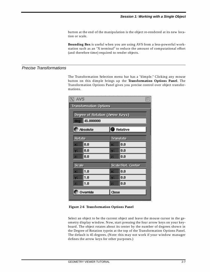
The Transformation Selection menu bar has a "dimple." Clicking any mousebutton on this dimple brings up the Transformation Options Panel. TheTransformation Options Panel gives you precise control over object transfor-mations.

Select an object to be the current object and leave the mouse cursor in the ge-ometry display window. Now, start pressing the four arrow keys on your key-board. The object rotates about its center by the number of degrees shown inthe Degree of Rotation typein at the top of the Transformation Options Panel.The default is 45 degrees. (Note: this may not work if your window managerdefines the arrow keys for other purposes.)

Figure 2-6 Transformation Options Panel



The right/left arrow keys rotate the object about the Y axis, up/down aboutthe X axis, and if you hold a shift key held down while pressing the right/leftarrow keys, the object rotates about the Z axis. You can change the degree ofrotation by moving the mouse cursor into the typein box, deleting 45.0 withCtrl-U, then typing a new rotation value.

The other Transformation Options Panel typeins give you precise control overobject translations either Relative to the object’s current position in space, orto an Absolute location in space. Not all transformations work with all trans-formable objects.

To update the Absolute display, you must click on Relative, then click backon Absolute.

Changing the Properties of an Object

While moving the teapot around the screen, you’ve no doubt noticed variousaspects of its appearance. The entire teapot is a single color, but this color issubtly shaded rather than being uniform. The shading at a particular pointdepends on the shape, and on the angle between the surface and the lightsource. There are specular highlights resulting from a light source located di-rectly in front of the screen.

AVS allows you to control all these aspects of an object’s appearance:

• The apparent color of an object depends on its actual color, but also de-pends on the way the surface reflects light. You can set these "surfaceproperties" (or "material properties") for the teapot by selecting EditProperty under the Object menu selection.The apparent color also depends on the color of the light(s) which illumi-nate the object. We work with lights in the next session of the tutorial.

• The appearance of specular highlights on an object depends both on itssurface properties and on the available light(s). In this session, we’ll ma-nipulate the surface properties only — we defer changing the lighting un-til the next session.

• The degree of realism in an object’s image depends on the rendering meth-od used to draw it. Under the Object menu selection, there are several ren-dering-method choices: Lines, Smooth Lines, Flat, and so on.

Let’s start by changing the surface properties of the teapot. Click on EditProperty to open a window that contains slider controls for various surfaceproperties.

Before we start working with the Edit Property window, remember that AVScan handle multiple objects. When you set about altering the properties of anobject, be sure that you know exactly which object you’re currently workingwith. In our situation, there are actually two slightly different objects:



• The "top-level" object, which hierarchically includes all the objects thatyou’ve read into the scene. At this point, "all the objects" is just the singleteapot.

• The teapot itself, as an individual object.

If you specify a change in the color of the top-level object, it may have no ef-fect on the image. That’s because the teapot itself can have a color, whichoverrides the color setting at the top level. Each object’s color can be either setexplicitly or inherited from its parent object. Explicit settings at lower (morespecific) levels in the hierarchy override settings at higher levels.

Figure 2-7 Edit Property Window



To make sure that the teapot as an individual object is selected, click on theteapot repeatedly with the left mouse button, and watch the Current ObjectIndicator in the Transform Selection area.

Each time you click, you move to a different level in the scene’s object hierar-chy. The label above the Current Object Indicator also helps you to keeptrack:

topIndicates that the top-level object is currently selected

teapot.0Indicates that the teapot as an individual object is currently selected (AVSadds a numeric suffix to help you keep track of objects. If you read in thesame object twice, the instances are assigned two different numeric suffix-es.)

Figure 2-8 Current Object Indicator Showing Top Object

Figure 2-9 Current Object Indicator Showing Child Object



Stop clicking when you are sure that the teapot itself is selected. You maynotice that each time you click, the Edit Property window changes toshow the settings of the current object.

We’ll examine object hierarchy and its implications for attribute setting moreclosely in the third session of this tutorial.

The first six sliders control the surface color of an object. You can specify thecolor in two ways:

• The first three sliders adjust the Red-Green-Blue (RGB) components of thecolor.

• The second three sliders also adjust the color, by specifying its Hue-Satu-ration-Value (HSV) components.

You can use any mouse button to adjust a slider. Just click where you want theslider to move to. (Alternatively, drag the slider from its current location to anew one.)

When you adjust a color-control slider, the teapot’s color changes as soon asyou release the mouse button. Also note that the HSV sliders automaticallyadjust if you change the RGB specification, and vice versa. There’s only onecurrent color, but you can specify it in two different ways.

Below the color-control sliders is a group of reflectance-control sliders.

The first two reflectance-control sliders set the percentage of ambient and dif-fuse light reflected by an object.

• The fraction of ambient (uniform, directionless, background) light thatthe object reflects. Move the slider to the right to make the teapot appearbrighter.

• The fraction of diffuse light (non-ambient light — from directional, point,and spot light sources) that the object reflects diffusely (dependent on theangle between the light source and the surface). As above, moving theslider to the right makes the teapot appear brighter.

Figure 2-10 Material Properties Sliders



You can also control the amount and type of light that actually exists in ascene. This is independent of each object’s ability to reflect the various typesof light. We’ll adjust lighting in the next session.

Three sliders control the appearance of specular highlights on an object. Suchhighlights depend on the angles between the light source, the surface, and theeye. .

• Move the specular slider to the right to make the specular highlight onthe teapot brighter.

• Move the gloss (specular sharpness) slider to the right to increase theglossiness of the highlight.

• AVS constrains the color of specular highlights — move the metal (specu-lar color) slider to vary the color between that of the light source (to theleft) and that of the object (to the right). In our default-lighting situation,the color of the light that produces the specular highlight is white.

The trans slider controls the transparency of the object. Moving this slider tothe left causes the teapot to fade away. Note that as it fades, you can see theback of the teapot through its increasingly transparent surface.

Hardware/Software Renderers

The ability to render objects with transparency is a renderer-dependent feature.AVS has a choice of two renderers: a software renderer and a hardware renderer.The hardware renderer uses the workstation platform’s native graphics li-braries and hardware to draw objects on the screen. The software renderer

Figure 2-11 Teapot with Metallic Surface and Specular Highlights



implements its own graphics model, drawing objects into an X Window Sys-tem image.

In general, the hardware renderer will be faster. However, many worksta-tion’s native graphics facilities do not support rendering features—such astransparency—that are very useful for scientific visualization. You can adjustthe transparency slider, but it will have no effect on the picture. If your hard-ware renderer does not support a rendering feature, you can usually obtain itby first switching to the Cameras menu, then clicking on Software Renderer:

The software renderer may be slower to draw, but it implements more render-ing features than all but the most expensive color graphics workstations. Onsome platforms, such as a simple color X terminal, the software renderer maybe the only renderer available.

Your platform’s AVS release notes should contain a table that lists which ren-dering features are available on your platform.

Properties Continued...

The best way to get the feeling for surface properties is to play with all thesesliders. See how closely you can match the various teapot images.

At any time, you can close the Edit Property window by clicking on Close atthe bottom of the window.

Changing the Rendering Method

Besides being able to control the surface properties of objects, you can controlthe rendering method that AVS uses to create images. Different objects can berendered using different methods. The methods supported will vary fromplatform to platform, and from the hardware renderer to the software render-er. In general, the rendering methods that are not supported will be shadedout..

Click on each of the rendering-method choices, and note the effects on the tea-pot image. The most realistic method offered by AVS is Phong shading. Incombination with specular highlighting, it provides excellent image fidelity.

The following paragraphs describe the differences between the renderingmethods. Several of the methods address the way in which the facets of a sol-id object are colored. A typical object is defined as a collection of tens, hun-dreds, or even thousands of facets (usually triangles).



PointsAn image in which only vertices are plotted; no connections are made be-tween these points. However, AVS does allow you to apply lighting tothese points.

Figure 2-12 Teapot with Clay Surface

Figure 2-13 Teapot with Semi-Transparent Surface



LinesA "wireframe" image, consisting of vertices and lines connecting them.

Smooth LinesA wireframe image in which the lines connecting the vertices are anti-aliases (smoothed). The anti-aliasing process requires extra computation;for complex scenes, there may be a slight performance cost with thismethod vis-a-vis Lines.

No LightingA solid image in which only the color you assign to the object is used.Any lights in the scene are ignored; no shading computations are per-formed.

If an object has colors assigned to each of its vertices, these colors are lin-early interpolated across the facets of the object. For example, a finite ele-ment analysis model might represent stress values as colors for thevarious points in a support beam.

FlatA solid image in which each facet of a polygon is drawn with a single,constant color. This depends on the object’s color, along with the colorand angle of the light(s) shining on the facet. Different facets can have dif-ferent colors.

GouraudA solid image in which each facet of a polygon is shaded (different pixelsare drawn with different colors) using the Gouraud shading algorithm. Inthis algorithm, a color is computed for each vertex that defines a facet.The computation takes into account the color assigned to the vertex (or tothe entire facet), the "vertex normal" vector, and the available light(s).When color values have been computed for all vertices, the values are lin-early interpolated to produce color values for the pixels in the interior ofthe facet.



PhongA solid image in which each facet of a polygon is shaded (different pixelsare drawn with different colors) using the Phong shading algorithm. Thisalgorithm interpolates the vertex normals, rather than the computed ver-tex colors. A separate lighting calculation then takes place for each pixelin the facet, producing greater accuracy at the expense of more computa-tion.

InheritCauses the rendering method of the object’s parent to be used.

Outline GouraudA Gouraud shaded image with a (white lined) wireframe image superim-posed on it.

In some cases, you may notice performance differences among the surface-rendering methods. The following table suggests why these differences exist:

Rendering Method Lighting CalculationsNo lighting noneFlat one per facetGouraud one per vertexPhong one per pixel

Saving Your Work

Continue experimenting with the Edit Property window and the renderingmethods choices until you have a teapot you are proud of. Then, select SaveObject under the Object menu selection. Type in a filename for your teapot inthe popup window that appears. You may need to use New Dir to change toa direcory in which you have write permission. Be sure that the mouse cursoris in the filename entry area before you start typing. Finish by pressing RE-TURN or by clicking the OK box in the popup window. AVS automaticallyadds a .scr filename extension to the name you enter (unless you type the ex-tension yourself).

Figure 2-14 Saving an Object



To verify that your object was saved correctly, follow these steps:

• Select Delete Object to remove the teapot from the scene.• Select Read Object to bring up the File Browser, and click on the filename

you just entered. You may need to scroll the filenames. Scrolling worksthe same way in AVS as it does in the xterm(1) terminal emulator pro-gram: — the right mouse buttons scrolls toward the end of the list; the leftmouse buttons scrolls toward the beginning of the list. Scrolling proceedspage-at-a-time unless the mouse cursor is in the little box at the top (orbottom) of the scroll bar. In that case, scrolling proceeds line-at-a-time.

The teapot should reappear. Notice that any colors, properties, and tranfor-mations that you applied to the teapot are gone. These modifications are partof the Geometry Viewer scene; not the object. To save and retrieve them, youmust save the entire scene using Write Scene under the Cameras menu. Wewill do this later.

Figure 2-15 Scrolling Through the File Browser

Session 2: Working with Lights


Exiting the Geometry Viewer

That’s enough for one session with the Geometry Viewer. To exit the program,select Exit at the very top of the control panel. To exit AVS, select Exit AVS,then click OK in the pop-up window that appears.


In the preceding session, we worked with a single object, changing its posi-tion, its surface properties, and the rendering method used to draw it. In thissession, we’ll leave the object alone and concentrate on another aspect of thescene — the lighting.

First, start AVS and enter the Geometry Viewer as described in Session 1.

Once again, the Object menu selection is chosen automatically. Select ReadObject, and click on the customized teapot object that you created in the pre-ceding session. After you’ve read in the object, close the File Browser window.

To get a feeling for the default lighting, rotate the teapot again. (Use the mid-dle mouse button.) It’s clear from the specular highlights that there is a lightsource located directly in front of the screen. Now, let’s work with that lightsource.

The Lighting Panel

Select the Lights menu selection in the control panel. The various object-relat-ed menu choices disappear and are replaced by lighting-related choices.

The bank of numbers is a lighting panel, which allows you to create and con-trol up to 16 lights. The number (8 or 16) and type of lights (listed below) de-pends upon the renderer being used. Each of the lights may be one of thefollowing types:

• Directional• Bi-Directional• Point• Spot

The last one, AM, is the ambient (non-directional) light for the scene.

Note that the 1 and the AM are illuminated, indicating that light number 1and the ambient light are currently turned on. Below the lighting panel arecontrol/indicator buttons that you can use to turn particular lights on and offand to change the type of each light. Click on the various buttons in the light-ing panel to verify that all lights (except number 16) are initially directional,and all but light number 1 are initially turned off.



At this point, make sure you also select Transform Light in the Transform Se-lection part of the control panel. This causes the mouse to be "attached" to thelights.

As you become more familiar with the Geometry Viewer, you may find it con-venient to "mix-n-match" the transformation selection setting and the menuselection setting. For instance, you might choose the Object menu selection toread new objects, but at the same time choose the Transform Light selectionto move the lights around the new objects. At the beginning, however, we rec-ommend that that you keep the menu selection and the transform selectionsynchronized.

Figure 2-16 The Lights Menu Selection



Manipulating Lights

Just as you have used the middle mouse button to rotate objects, you can nowuse this button to rotate the directional light. Give it a try. The specular high-lights on the teapot give a clear indication that the light direction is, indeed,moving.

To help you work with lighting, there is a Show Lights menu selection. Makethis selection, and an arrow appears in the scene, indicating the direction ofthe light. As you rotate the light, this arrow changes its angle accordingly.

The right mouse button controls translation of the light source parallel to theplane of the display screen, just as it did for objects. (And along with the Shiftkey, it can also control translation perpendicular to the screen.) If you try this,however, you won’t see any change it the lighting. That’s because translatinga directional light source makes no difference. The Spot and Point lights de-scribed below do change the appearance of the object when translated.

Be sure to test the Reset button with the light. As with objects, it returns thelight to its original position (and direction).

Figure 2-17 Using ’Show Lights’



Creating Additional Lights

So far, we’ve been working with just one light. Let’s create another one. Click2 on the lighting panel, then turn the light on by clicking Light On. Assumingthat you still have Show Lights selected, another arrow appears in the scene.

As you switch back and forth between Light number 1 and Light number 2 onthe lighting panel, note that the label above the Current Object Indicator alsochanges, indicating which light is currently under mouse control. As long asTransform Light is the transform selection, the mouse is "attached" to the cur-rently-selected light on the lighting panel.

Try moving and translating both lights, making sure that you can see the ef-fect of each light on the teapot. To facilitate differentiating the lights, trychanging the color of one (or both) of them. At the bottom of the control panelis a miniature set of color controls, just like the ones in the Edit Property win-dow for objects. Moving these sliders controls the color of the currently select-ed light.

Additional Light Types

AVS also supports bi-directional lights and spot lights. Try making light num-ber 2 bi-directional. Note that light number 10 is turned on automatically.That’s because this type of light is actually two directional lights, pointing inopposite directions. When Show Lights is selected, a bi-directional light isrepresented by two arrows.

A spot light is similar to a point light, but has a restricted "cone" of influence.(If a point light is like a naked light bulb, a spot light is like a well-focusedflashlight.) When Show Lights is selected, the symbol for a spot light showsthe cone. The angle of this cone is fixed in AVS — you cannot change it.

Spot and Point lights (if available), display themselves with Show Lights asa single point rather than a directional arrow. The spot light is located at theorigin and may be invisible because it is obscured by the teapot. You cantranslate it outside of the teapot to see it.

Be sure you also work with the ambient light (AM on the lighting panel). Us-ing the mouse won’t make any difference, since ambient light has no positionor direction. But you can change the brightness and the color of this light us-ing the sliders.

That’s all for this session. Note that there is no "Save" menu selection underLights. There is no way to save a particular lighting configuration indepen-dently from the scene in which they exist. In the next session, we’ll save andretrieve an entire scene.

To end the Geometry Viewer session, select Exit at the top of the control pan-el. To exit AVS, select Exit AVS, then click OK to verify your choice.

Session 3: Creating Composite Objects



So far, we have worked with a single object, a teapot, changing its propertiesand changing the way it is lighted. In this session, we explore one of AVS’smore sophisticated capabilities — maintaining hierarchies of objects and at-tributes.

The Geometry Viewer allows you to define complex object hierarchies. For in-stance, a model of a building might feature an office unit, which containsrooms, which contain desks, which have built-in clocks, which have hands.

The viewing application itself does not create multi-level hierarchies in ordi-nary, interactive usage. Each scene you create consists of a top-level object,which is initially empty. Each time you bring an object into the scene usingRead Object, the new object becomes a direct descendant of the top-level ob-ject:

Actually, AVS is capable of handling deeper hierarchies. Some of the suppliedobjects are themselves hierarchical. In addition, you can use the AVS ScriptLanguage to define multi-level object hierarchies. This language is describedin the AVS User’s Guide.

Using the Edit Property window and the rendering-method selections (as wedid in Session 1), you can set the attributes of the top-level object, or of any ofits children. If a child has its attributes set, they override the settings of its par-ent, the top-level object. Alternatively, you can specify that the child is to in-herit the attributes of its parent. You can also save the current state of the EditProperty window in a .prop file, then retrieve the attributes later, applyingthem to the same object (or a different one).

top

teapot.0 jet.2 dodecahedron.3

Figure 2-18 Object Hierarchy



Changing the Current Object

Let’s see how it all works. Start the AVS program and then start the GeometryViewer subsystem, select Read Object, and (once again) click on the custom-ized teapot object that you created in the first session. This time, however,don’t close the File Browser. Instead, select another object to read into thescene: dodec.geom. This is a dodecahedron (a twelve-faced platonic solidwhose principal occurrence in nature is in the form of calendar paper-weights).

The simplest way to explore the object hierarchy is to rotate and translate ob-jects. First, make sure that Transform Object is the current Transform Selec-tion. Now, click the left mouse button at various locations in the window.Watch the current object indicator in the Transform Selection area as you doso:

• Clicking on either the teapot or the dodecahedron makes it the currentobject.

• Clicking on the background makes the top-level object current — this in-cludes both the teapot and the dodecahedron.

Note that the Current Object Indicator always shows the currently selectedobject. In addition, the label above this indicator shows you where you are inthe hierarchy:

top top-level object is currentteapot.1 teapot is currentdodec.3 dodecahedron is current

Verify that a particular object is selected by moving it with the right mousebutton, or rotating it with the middle mouse button. When the top-level objectis selected, the teapot-dodecahedron pair move as a unit.

There are a couple of additional ways to navigate the object hierarchy:

• Clicking on the same object multiple times cycles you through the hierar-chy — the first click selects the object itself (the bottom level); the secondmoves up one level to the parent (in many cases, this is the top-level ob-ject); and so on. Continuing to click after you’ve reached the top level re-turns you to the individual object level.

• Clicking on the current object indicator window cycles through all thesingle and composite objects in the scene.

Try these methods, too, and verify them by moving and rotating the objectyou select.

Hierarchy and Property Editing

Now, let’s explore the way in which you can use hierarchy in editing object at-tributes. Make the teapot the current object. Then select Edit Property under

Session 4: Creating Multiple Views


the Object menu selection. The sliders in the Edit Property window reflect the"customization" you performed on the teapot in the first session. Suppose youwant to these same settings to apply to both the teapot and the dodecahedron.There are two ways to accomplish this:

• Apply the teapot properties directly to the dodecahedron.• Apply the teapot properties to the top-level object, then have both the tea-

pot and the dodecahedron inherit these properties from the top-level ob-ject.

Let’s try both methods.

Saving and Retrieving Properties

Click Save at the bottom of the Edit Property window. Then enter a filenameunder which to save the properties. AVS automatically adds a .prop extensionto the name you type (unless you type the extension yourself).

Now make the dodecahedron the current object by clicking on it with the leftmouse button. The sliders in the Edit Property window change to indicate thecurrent settings for the dodecahedron. Click on Read at the bottom of thiswindow, bringing up the File Browser. Then click on the name of the .prop fileyou just created. This copies the saved properties onto the dodecahedron.

The Geometry Viewer subsystem doesn’t try to keep the properties of the twoobjects synchronized. Both objects have the same color now, but if you changethe color of the teapot, the dodecahedron won’t change too.

Inheritance of Properties

Applying the properties to the top-level object will keep the teapot anddodecahedron synchronized. Make the teapot the current object, then clickInherit at the bottom of the Edit Property window. Do the same for thedodecahedron.

Now select the top-level object (e.g. by clicking with the left mouse button inthe background of the window). Click on Read at the bottom of this windowand, as before, click on the name of the .prop file you created. These savedproperties now pertain to the top-level object and, through inheritance, toboth the teapot and the dodecahedron. If you change the color of the top-levelobject, it affects both objects at the lower level.

That’s all for this session. Exit from the Geometry Viewer and AVS as usual.


In this session, we explore AVS’s ability to show the same scene from differentpoints of view. Continuing the use of the movie studio metaphor, each view isassociated with its own camera. Each camera’s view appears in a separate win-dow, which you can move and resize using any X Window System window



manager. You can change the position of cameras in much the same way asyou change the position of objects and lights. You can also access such fea-tures as depth-cueing and Z-buffering.

Collectively, all the views on a particular collection of objects, along with a setof lights, is called a scene. (Thus far, we’ve been using the term scene moreloosely, referring to a group of objects.) We’ll also see in this session how theGeometry Viewer lets you work with multiple scenes concurrently.

First, recreate the situation of the previous lesson: start AVS and the Geome-try Viewer and read in both the teapot and dodecahedron objects.

Now, bring up the Camera menu selections in the control panel.

Creating and Resizing a Window

Select Create Camera to create a new window that shows the same scene —that is, the same pair of objects. You may want to use the window manager torearrange and/or resize the windows more to your liking.

The initial position of the new camera is the same as the initial position of theoriginal camera, so both views may be the same. The two cameras are inde-pendent, however. To see how this works, click Transform Camera in theTransform Selection area. Now use the right mouse button (with and withoutShift) to change the position of the newly created camera. Also try using themiddle mouse button to rotate the new camera.

It’s easy to move the camera to the other window. As soon as you click (e.g.with the middle mouse button) in the other window, the mouse becomes "at-tached" to that window’s camera.

Relating Cameras to Lights and Objects

To gain a better understanding of how cameras work, try moving the lightand the objects in either window. Remember to change the Transform Selec-tion to Transform Light or Transform Object before you try to manipulatethem with the mouse.

You’ll notice that as you manipulate the light(s) in one window, the lightingalso changes in the other window. That’s because, conceptually, a single scenewith a single set of lights is being viewed in both windows.

Similarly, when you move an object in one window, it also moves in the oth-er—there is one set of objects, being viewed in two different ways.



Adjusting the Camera Lens

Several of the menu selections under Camera allow you to "adjust the lens" ofthe current camera. These adjustments provide access to several features ofthe underlying graphics software:

Figure 2-19 Cameras Menu Selection



• You can switch back and forth between an orthogonal view (the default)and a perspective view. Moving the camera or an object perpendicular tothe screen produces quite different effects, depending on which type ofview is currently selected.

• You can turn on and off the Z-buffering of lines and the depth-cueing oflines and spheres.

• You can turn on and off the display of the X-Y-Z coordinate axes. This canhelp you keep track of the orientation of the object(s) as you work withone or more camera views.

Try each of these adjustments by clicking the menu choices. Keep in mind thateach selection is applied to the current camera (window). You may need toclick in a particular window (with any mouse button) before making theCamera menu choice.

Freezing a View

There may be times when the view provided by one of the cameras is "justright". You can temporarily freeze the image with the Freeze Camera menuselection. You can still manipulate the lights and/or objects in the scene, butthe changes won’t be shown in the frozen window until you unfreeze it byclicking (with any mouse button) in that window’s border.

Saving an Entire Scene

The Save Scene menu selection causes the entire current scene to be saved inthe .scr file. You supply a filename, just as you do when saving objects andEdit Property attributes. The saved scene includes all the objects and their at-tributes, all the lights, and all the cameras/windows that you’ve created forthe scene.

To test this, first save the scene with Save Scene, then delete each of its win-dows with Delete Camera. Now, select Read Scene and click on your scene’sname in the File Browser. All the windows defined for the scene return to thescreen.

Creating a New Scene

The Geometry Viewer lets you create as many windows as you want on thecurrent scene, using Create Camera. You can also create an entirely new scenewith Create Scene. The new scene is an empty window, into which you canread one or more objects, adjust the lighting, and create additional cameras,just as you did with the original scene.



If you have two or more scenes onscreen at the same time, be sure you knowwhich is the current window when you use Create Camera. This function cre-ates a new camera for the scene to which the current window belongs. To getwhat you want, you may need to click in a particular window (using anymouse button) before selecting Create Camera.

GRAPH VIEWER TUTORIAL 3-1

CHAPTER 3 GRAPHVIEWERTUTORIAL

Introduction

This tutorial provides a step-by-step approach to using the AVS GraphViewer. It explains how to read data from a file, how to create a plot titleand labels, and how to save or print the plot. It also discusses using the net-work to obtain data.

Each step has two parts — an action you perform and the explanation ofwhat happens. You should read the explanation before performing the ac-tion so that you know what to expect.

Before starting this tutorial you need to read the "Graph Viewer Subsystem"chapter in the AVS User’s Guide, at least through the section, "Read Data."

Starting the Graph Viewer

To use the Graph Viewer, follow these steps:

1. Start AVS by typing avs and then pressing Return.The AVS program takes several moments to display the menu.You can select menu items in AVS by placing the mouse pointeron the menu item and clicking any mouse button.

2. Select Graph Viewer on the menu.

Reading In a File

The Option Selection menu appears with Read Data already selected toread in a file.

Use the File Type menu to choose the type of file (ASCII, AVS Plot, AVSField or X Image) you want to read. ASCII files are often the output of an-other program, AVS Plot files are plots previously saved, and AVS Fieldfiles are output from another AVS module. The X Image files are used forbackground images.

Begin by reading an ASCII file:

Reading In a File

3-2 GRAPH VIEWER TUTORIAL

1. Select Read ASCII File in the File Type menu. The Data Formatmenu appears for choosing how the Graph Viewer should interpretthe input data.

2. Select Plot as XY Data in the Data Format menu. The default dataformat specifies column one of the input file as the X Axis and col-umn two as the Y Axis. Color Column is set to column zero (no in-put) so it is not used. The default setting for the type of plot isSimple Line.

Figure 3-1 Read Data in the Option Selection Menu

Figure 3-2 Two Column-Linear in the Data Format Menu

Setting the Title and Axis Labels


A File Browser window pops up listing files and directories in thecurrent directory. Near the top of the window the current directoryis displayed (e.g. /usr/avs/data).

3. Select the red graph subdirectory entry to see the listing of availablefiles.When the listing of files appear, select the file growth.dat as theASCII input file. AVS reads the file and the plot appears on yourscreen.

4. Select Close on the File Browser window to remove the File Brows-er.So far you have read in the ASCII file growth.dat which uses col-umns one and two as the XY values for a Line plot.


This sections discusses how to create titles and axis labels.

1. Select Titles, Labels & Legends on the Option Selection menu.This enables you to create or change the plot’s title and axis labels.After you select Titles, Labels & Legends several menus appear.• Label Display menu. Chooses which of the plot labels you are

working on. The default is the Plot Title.• Current Label. Displays the text for the option selected in the

Label Display menu (e.g. the Plot title). If blank, then there isno existing text for the option.

• Label Menu Selection. Chooses either Label Attributes (posi-tion and color) or Font Selection (style and height) for the la-bel. The following figure illustrates this:

2. Place the mouse pointer in the Current Label data area (it willhighlight). If a Title exists, it is displayed in the Current Label dataarea. If no Title exists the data area is blank.

3. Type in a plot Title of your choice and press Return. The typed Titleappears at the top and center of the plot. Center is the default Titleposition.

4. Select Left position to change the Title location. You can change theTitle from Center position to Left or Right or back to Center. Selecteach setting so you can view its effect.

5. Press Edit Label Color. A pop-up appears with color sliderbars.Adjust the colorbar sliders to change the Title color. You can changethe color by placing the mouse pointer on one of the colorbars andclicking any mouse button. The colorbar setting moves to themouse pointer position and the Title changes color. Or, you canhold the mouse button down and drag the pointer to a location —when you release the button the Title changes color.The six colorbar sliders are divided into two sets of three bars. Youcan use one set or the other to adjust color.



The top three colorbar sliders adjust the Red-Green-Blue (RGB)components of the color.The bottom three colorbar sliders adjust the Hue-Saturation-Value(HSV) components of the color.As you adjust the RGB sliders the HSV colorbars change color todisplay the changes. As you adjust the HSV sliders the RGB color-bars change color to display the changes.

6. Select Font Selection in the Label Menu Selection menu. You canchange the font style, attributes and height of the Title. The defaultfont style is Helvetica with a height of 24 points. The next figure il-lustrates this. (Note: fonts may vary from platform to platform.)

Figure 3-3 Label Menu Selection



7. Select New-Century (or any different font) as the Title’s font style.The Title font style changes to the selected font. Select each font toview the results on the Title text.If your PostScript printer does not have the selected font then ituses its default font.

8. Select Bold as an option. The Title text changes to become bold. Se-lect Bold again to remove it as an option. Then select Italic, view itseffect, and reselect to remove its effect. Then select Drop Shadow,view its effect, and reselect to remove its effect.You can also select Bold, Italic and Drop Shadow in combinations.Select Bold with Italic, Bold with Drop Shadow, and so on to viewthe different combination effects.

9. Adjust the Label Height slider to change Title size. You can changethe Title size by placing the mouse pointer on the Label Height slid-er and clicking any mouse button. Or, you can hold the mouse but-ton down and drag the pointer to the size location you want. Whenyou release the button the Title changes size.The numerical value in the Label Height menu indicates relativesize. Note that the actual size displayed depends upon the X-Win-dows font sizes installed for your system. The size printed on Post-Script printers is in actual point size.

10. Select X Axis Label in the Label Display menu. This enables you towork with the X Axis Label and all its attributes (positioning, color-ing, style, height).

Figure 3-4 Font Selection in the Label Menu Selection Area

Setting the Axis Display


11. Place the mouse pointer in the Current Label data area (it willhighlight). If an X Axis Label exists it is displayed in the CurrentLabel data area. If no X Axis Label exists the data area is blank.

12. Type in an X Axis Label of your choice and press Return. The typedX Axis Label appears at the bottom and center of the plot.All of the controls described in Steps 4 through 9 affect the X AxisLabel exactly the same as they did the Title. You can change someor all of the controls (with X Axis Label selected) to view the resultsupon the X Axis Label. Then proceed to the next Step in this tutori-al.

13. Select Y Axis Label in the Label Display menu. This enables you towork with the Y Axis Label and all its attributes (position, color,style, height).

14. Place the mouse pointer in the Current Label data area (it willhighlight). If a Y Axis Label exists, it is displayed in the Current La-bel data area. If no Y Axis Label exists the data area is blank.

15. Type in a Y Axis Label of your choice and press Return. The typedY Axis Label appears at the left side and center of the plot.

16. All of the controls described in Steps 4 through 9 affect the Y AxisLabel exactly the same as they did the X Axis and the Title. You canchange some or all of the controls (with Y Axis Label selected) toview the results upon the Y Axis Label. Then proceed to the nextStep in this tutorial.

17. Select Axis Tic Labels in the Label Display menu. This enables youto work with the Axis Tic Labels and all their attributes (position,color, style, height). (Axis borders and ranges are handled in theAxis Display menu.)Axis Tic Labels are generated automatically and therefore nothingis displayed in the Current Label data area.All of the controls described in Steps 4 through 9 affect the Axis TicLabels exactly the same as they did the X or Y Axis and the Title.You can change some or all of the controls (with Axis Tic Labels se-lected) to view the results upon the Axis Tic Labels.You have now set the Title and Axis Labels for the plot.


Select Axis Display in the Option Selection menu. This enables you to set Xand Y Axis options. The following menus appear:

Border DisplaySets the border on the plot.

Axis SelectionChooses the X or Y Axis for the lower menus.



Figure 3-5 Axis Display in the Option Selection Menu



Axis ScaleSets Linear or Log scaling.

Axis RangeSets axis range between the From and To values.

Axis Tic MarksSets axis tic marks.

1. Select Left & Bottom on the Border Display menu. The border isnow displayed only on the left and bottom sides of the plot.

2. Select Y Axis on the Axis Selection menu. This chooses the Y Axisfor the lower menu operations.If the Y Axis is selected all changes made affect only the Y Axis. Ifthe X Axis is selected all changes made affect only the X Axis.

3. Change the Axis Range for the Y Axis. This menu sets the low andhigh values of the axis range. The default settings are the lowest(From) and highest (To) values of the axis dataset. The Axis Rangevalues do not change their decimal precision immediately. Youneed to select another menu in the Option Selection or Axis Selec-tion menu, to update the values.

4. Place the mouse pointer in the From data area (it will highlight) inthe Axis Range menu. Press Backspace one or more times to deletethe existing entry (or use Ctrl U to clear the field). Type in the value25 and press Return. The Y Axis displays the new range.

5. Place the mouse pointer in the To data area (it will highlight) in theAxis Range menu. Press Backspace to delete the existing entry.Type in the value 75 and press Return. The Y Axis displays the newrange.

6. Return the Y Axis range to the original values by typing in 0 for theFrom data area and 95 for the To data area.

7. Select Outside in the Axis Tic Marks menu. This menu sets the lo-cation of tic marks on the axis. The tic marks move from the insideposition (the default) to the outside position. Select each of themenu choices (None, Inside & Outside) to view the effect upon theaxis tic marks.

8. The number of tic marks displayed between the axis origin and endpoint includes the end point as a tic mark. The axis origin is not in-cluded as a tic mark. For example, four tic marks are on the axis lineand the fifth tic mark is located at the axis end point. Change theNumber of Tics value. This menu sets the number of tic marks dis-played on the axis. Place the mouse pointer in the Number of Ticsdata area (it will highlight). Press Backspace to delete the existingentry (2 is the default value). Type in the value 5 and press Return.The plot axis displays the new number of tic marks.

9. Change the Decimal Precision value. This menu sets the decimalprecision value used in the Axis Range menu and the axis itself.Place the mouse pointer in the Decimal Precision data area (it willhighlight). Press Backspace to delete the existing entry (the defaultis one decimal position). Type in the value 2 and press Return.

Choosing Select Plot


10. Select X Axis on the Axis Selection menu. This chooses the X Axisfor the lower menu options. Repeat steps 3 through 9 in order tomodify the X Axis.

Choosing Select Plot

This section discusses how to select a point within the plot display, choose adataset, change line type, and change plot type.

1. Choose Select Plot in the Option Selection menu. The followingmenus appear:

Figure 3-6 Select Plot Options

Using Write Data


• Display Crosshair. Displays or removes a crosshair at themouse pointer.

• Plot Attributes. Plot type (Simple Line, Area, Scatter, Bar), linethickness line type (Solid, Dash, Dot, Dot-Dash) and color.

2. Move the mouse pointer inside the plot area. The crosshair pro-vides an easy-to-see display of the mouse pointer location withinthe plot area. To remove the crosshair click any mouse button onthe Display Crosshair menu.The Cursor Position (near the bottom) shows your exact locationwithin the plot area. The displayed values are the X Axis (on theleft) and Y Axis (on the right) coordinates.The Selected Point is updated to display the X and Y coordinatevalues of the mouse pointer whenever you click any mouse button.

3. Select the dataset within the plot. Click a mouse button while themouse pointer is on or near the dataset in the plot. The dataset ishighlighted in white to indicate it has been selected. A circle is alsodisplayed at the point within the plot that is closest to the point se-lected.After you have selected a plot, you can delete it with the DeletePlot Dataset menu item. (Do not delete the dataset at this time.)You must select the dataset before you can alter its characteristics(color, plot style).

4. Change the Line Thickness. You can change the line thickness byplacing the mouse pointer in the Line Thickness data area (it willhighlight). Press Backspace to delete the existing entry. Type in thevalue 3 and press Return. The new line thickness is displayed in theplot.

5. Change the Line type. Choose each of the Line types to see whatthey look like. Place the mouse pointer on each of the line types(Dash, Dot, etc.) and click any mouse button to view the result.

6. Change the plot color. You can change the plot color by clicking onthe colorbars (see Step 5 of "Setting The Title & Axis Labels" for de-tails on manipulating colorbars).

7. Change the plot type. You can change the plot type at any time byclicking on the type of plot you want (Area, Scatter, etc.). Note thatcolorbar changes made on a plot type affect only that type and notothers. Select each plot type to see the resulting plot.

Using Write Data

This section describes how to save and print a plot.

1. Select Write Data in the Option Selection menu as illustrated inthe figure, "Write Data in the Option Selection Menu".

2. Select Write AVS Plot Data in the File Type menu. The File Brows-er window pops up. Select the New File button on the File Browser.Type in a new directory to save your plot file (e.g. /home/bob). Now,

Using Multiple Datasets in a Single Window


you can select the New File option at the File Browser window bot-tom and type in the file name graph1 (the filename extension .plt isadded automatically). Or, you can select an existing filename andoverwrite it by clicking on the existing filename.The other menu options are as follows:• Write PostScript. Enables you to save the plot to a file (with the

extension .ps) so that you can print your plot on a PostScriptprinter.

• Write ASCII XY Data. Enables you to save only the data itself.• Write AVS Geometry Data. Enables you to work with the plot

within another AVS module.

You have now saved the plot with Title and Label information from the ASCIIfile growth.dat.

Using Multiple Datasets in a Single Window

This section describes how to display and delete multiple datasets within thesame plot window.

1. Select Read Data in the Option Selection menu.2. Select Read ASCII File in the File Type menu.3. Select Add to Current Plot in the Plot Control menu.

Figure 3-7 Write Data in the Option Selection Menu

Using Datasets in Multiple Windows


4. Select Plot as XY Data in the Data Format menu.5. Set the X Axis Column to column one and the Y Axis Column to

column two. Set Color Column to column zero, indicating it is notused.

6. In the preceding example ("Using Write Data"), you may havesaved your data into a new directory. If you did, you need tochange the directory that the File Browser is currently listing. Selectthe New File button on the File Browser. Type in the directory /usr/avs/data/graph. Now, you can select the file growth2.dat from the FileBrowser window.

7. Choose Select Plot in the Option Selection menu.8. Select growth2.dat. Move the mouse pointer to growth2.dat and click

any mouse button to select the dataset. The dataset highlights inwhite to indicate it has been selected.

9. Delete growth2.dat. Select Delete Plot Dataset to remove growth2.datfrom the plot window. Move the mouse pointer to the Confirm De-lete option and click any mouse button to perform the delete. Thedataset is removed from the plot window.

In this section, you read in the ASCII file growth2.dat into an existing plot win-dow and removed it after comparing it with dataset, growth.dat.

Using Datasets in Multiple Windows

This section of the tutorial describes how to display and delete multiple win-dows.

Currently you should have the ASCII file growth.dat displayed as a line plot ina single window. (If you are using another type of plot you need to change toa line plot for this section. Choose the Select Plot option, click the mousepointer on the plot dataset, and select Simple Line under the Plot Attributesoption.)

1. Select Read Data in the Option Selection menu.2. Select the Create New Plot option in the Plot Control menu. Now,

when you read in a new plot, it goes into a new window.3. Select Read ASCII File in File Type menu.4. Select the Bar plot style. The default plot style is Simple Line.5. The file, growth.dat, automatically appears in the new window as a

bar plot. You can create as many windows as needed and read filesto create plots. You can read the same file and use different plottypes or use different files in each window.

6. Delete plot window two. Selecting the Delete Plot Window optiondeletes the active window (window two in this exercise). AVS doesnot ask for confirmation before deleting. Once a window is deletedit is gone forever.

Plotting a Single Column of Data


7. Delete plot window one. After window two is deleted the red bor-der returns to window one, showing it is the active window. Selectthe Delete Plot Window option to delete it.

You have now created and deleted multiple window plots.

Plotting a Single Column of Data

This section of the tutorial describes how to read in a single column of datafrom a file for a plot.

1. Select Read Data in the Option Selection menu.2. Select Replace Current Plot in the Plot Control menu.3. Select Read ASCII File in File Type menu. The File Browser win-

dow appears.4. Select Plot as Y Data in Data Format menu.5. Set Y Axis Column to 1. The Y Axis is plotted using the selected

data column read from the file. The X Axis is automatically sup-plied. The Graph Viewer counts the number of Y Axis items andsets the X Axis to the same number of items in interval units of 10.The X Axis Intervals can be changed from 10 to any value you need.

6. Select Simple Line as the plot type.7. Select sine.dat file. The data column is read and plotted as the Y

Axis in the plot window.8. Delete the plot window. Select the Delete Plot Window option to

remove the plot window.

You have now read a single column of data as a plot and deleted the plot.

Using Data for Color Control

This section of the tutorial describes how to use a column of data to controlthe coloring of the plot.

1. Select Read Data in the Option Selection menu.2. Select Read ASCII File in the File Type menu.3. Select Plot as XY Data in the Data Format menu.4. Set X Axis Column to column one, Y Axis Column to column two.

This selects the data columns for the plot’s X and Y axis.5. Set Color Column to column three. This chooses data in column

three of the file to control coloring in the plot. The data is used asHue control in a range of 0 - 499 (five hundred values). If a numbergreater than 499 is used it wraps around to the beginning value of0. For example, 500 wraps to 0, 501 wraps to 1, 502 wraps to 2, andso on.

6. Select Area as the type of plot.

Generating Data for a Contour Plot


7. Select growth.dat from the File Browser. The plot is displayed withthe Hue coloring controlled by values in column three of the file.

8. Select Delete Plot Window to remove the plot.

You have now read a file using one column to control color and then deletedthe plot.


This section of the tutorial describes how to display a contour plot. It alsogives an example of using the graph viewer module in a network. In order tounderstand the following instructions, it is assumed that you are familiarwith the use of the Network Editor. If not, see the "Network Editor Sub-system" chapter in the AVS User’s Guide.

You will be constructing the following network:

The basic operations you’ll use to construct this network are the following:

• Scroll the module Palette by putting the mouse in the column title box(e.g. Data Output); then type in the first two or three characters of themodule name you’re looking for. The column scrolls automatically, locat-ing the module. Use the Backspace key to reset to the top of the column.

Figure 3-8 Network with Graph Viewer Module



• You drag icons out of the module palette and into the Workspace with theleft mouse button.

• Connect modules together with the middle mouse button. Where thereare multiple possible pathways, keep the mouse button held down and"follow" the path you want. When it is highlighted, release the mouse but-ton.

• Break module connections with the right mouse button.

Use the following steps to build this network:

1. Select the Close button at the top of the Graph Viewer’s controlpanel. You now see the AVS main menu.

2. Select Network Editor on the menu.3. Drag the read image module from the palette into the workspace.4. Drag the downsize module from the palette into the workspace

and connect the read image module’s output to the downsize mod-ule’s input. Also, change the value on the downsize dial in the con-trol panel from its current setting of 1 to the new setting of 10.

5. Drag the extract scalar module from the palette into the workspaceand connect the downsize module’s output to the extract scalarmodule’s input.

6. Drag the graph viewer module from the palette into the workspaceand connect the extract scalar module’s output to the graph viewermodule’s middle input port.

7. Display the read image module’s file browser by pressing on theread image module’s dimple with the left mouse button.

8. Select the red image subdirectory entry for available files. When thelisting appears, select the file mandrill.x.

9. Wait while the network executes. When it completes firing, displaythe extract scalar module’s control panel by pressing on the extractscalar module’s dimple with the left mouse button.

10. Select the red color channel from the control panel. You’ll see a con-tour plot generated in the graph viewer’s plot window. Now that acontour plot is being displayed, it is possible to look at differentcontour levels for the same data. In order to do this, the graphViewer’s menu must be visible.

11. Go to the Graph Viewer by pressing down and holding the leftmouse button over the Data Viewer’s button. Drag the mousewhile holding the left mouse button down and select the GraphViewer button. The new menu then appears.

12. Select Read AVS Field File in the File Type menu. The File Browserpops up. Do not select a file from this browser.

13. Select Plot as Contour Data in the Data Format menu.14. Select Hue Range in the Color Selection menu.

Color Selection chooses between Monochrome (plotting in a singlecolor only) or Hue Range (different coloring for each value).

15. Contour Level Selection menu chooses between Automatic, ValueRange and User Specified.



• Automatic. Accepts all data values from the lowest to the high-est. The plot displays all data points occurring at the contourlevels. The number of Contour Levels is divided between thelowest and highest value.

• Value Range. Accepts all data values from the specified StartValue to the specified End Value. The number of contour levelsis divided between the Start and End values.

• User Specified. Enables you to specify the contour level datapoints explicitly by value. Select Value Range in the ContourLevel Selection menu. This performs the same way as Auto-matic except that you specify a starting and ending thresholdfor the input file.

16. Type in 10 as the Start Value This allows only values \(>= 10 fromthe file being read.

17. Type in 250 as the End Value. This allows only values \(<= 250from the file to be read.

18. Type in 7 as the number of Contour Levels. This places contour lev-els at the following values: 10, 50, 90, 130, 170, 210 and 250.You have now generated a contour plot by plotting 8 contour levelsbetween the specified Start and End values in the dataset and delet-ed the plot.You can also explicitly specify the values to be plotted by using theUser Specified option in the Contour Level Selection menu.

19. Select User Specified in the Contour Level Selection menu. A win-dow appears prompting you to enter Contour Levels. You can typein values and separate them by typing a space character or a com-ma.

20. Type in the values 20, 135, 245. Press Return or click on the OK inthe window. The plot appears with the specified values.

Figure 3-9 Value Range in the Contour Level Selection Menu



Figure 3-10 User Specified in the Contour Level Selection Menu



Documents

Guide to AVS interactive demos and tutorials