Embed Size (px)
Citation preview

IBM Industry Models and Hadoop workgroup
Guidelines for deploying an IBM Industry Model to Hadoop Version 1.0

1
© Copyright IBM Corporation 2016
Contents 1 Introduction .......................................................................................................................................... 3
1.1 About this document .................................................................................................................... 3
1.2 Intended audience ........................................................................................................................ 3
1.3 Generic focus on Hadoop technology ........................................................................................... 4
2 IBM Industry Models and the overall landscape .................................................................................. 5
2.1 The Big Data landscape ................................................................................................................. 5
2.2 The role of IBM Industry Models and the big data landscape ...................................................... 6
3 Typical scenarios where Hadoop would be used .................................................................................. 8
3.1 Fine grain transaction data ........................................................................................................... 8
3.2 Operational Data Stores .............................................................................................................. 10
3.3 Call center data ........................................................................................................................... 12
3.4 Social media data ........................................................................................................................ 13
3.5 Sensor/instrument data .............................................................................................................. 15
3.6 Geospatial data ........................................................................................................................... 17
4 Typical flow of models deployment to Hadoop .................................................................................. 20
4.1 IBM Industry Model components and a typical Hadoop landscape ........................................... 21
4.2 When to use Hadoop or not ....................................................................................................... 23
5 Considerations for logical to physical modeling for a Hadoop environment ..................................... 25
5.1 Selection of IBM Industry Model components for logical to physical transformations ............. 25
5.1.1 Use Dimensional Models for deployment to Hadoop ........................................................ 26
5.2 Flattening/denormalization of structures in Hadoop ................................................................. 26
5.3 Common de-normalization options ............................................................................................ 28
5.3.1 Vertical reduction of the supertype/subtype hierarchy ..................................................... 29
5.3.2 Reduce or remove the associative entities ......................................................................... 30
5.3.3 Horizontal reduction of entity relationships ....................................................................... 31
5.3.4 Remove the Classification entities (Banking, Retail and Telco only) .................................. 32
5.3.5 De-normalize the Accounting Unit structure (Banking, Retail and Telco only) .................. 32
5.3.6 Examine the equivalent dimensions for de-normalization guidance ................................. 33
5.3.7 Renaming of resulting denormalized structures ................................................................. 34
5.4 Surrogate keys vs business keys ................................................................................................. 35

2
© Copyright IBM Corporation 2016
5.5 Long vs short entity and attribute names ................................................................................... 35
5.6 End-to-end de-normalization example – Social media structures.............................................. 36
6 Considerations regarding of model generated artifacts in Hadoop ................................................... 39
6.1 Example flows across the Hadoop runtime landscape ............................................................... 39
6.2 Security consideration for semi-structured physicalization ....................................................... 40
6.3 Hive v’s HBASE ............................................................................................................................ 41
6.4 Query performance ..................................................................................................................... 41
6.5 ETL considerations ...................................................................................................................... 42
7 Appendix - Advanced techniques for physicalization of the IBM Industry Models with nested
structures utilizing Hive and Parquet/Avro ................................................................................................ 43
7.1 Support for nested structures utilizing ARRAY ........................................................................... 43
7.1.1 Data structure definition ..................................................................................................... 43
7.1.2 Loading sample data ........................................................................................................... 44
7.1.3 Querying ARRAY nested data .............................................................................................. 45
7.2 Support for nested structures utilizing MAP .............................................................................. 47
7.2.1 Creating sample table with MAP based nested structures ................................................. 47
7.2.2 Loading sample data ........................................................................................................... 47
7.2.3 Querying MAP nested data ................................................................................................. 48

3
© Copyright IBM Corporation 2016
1 Introduction One of the traditional objectives of models-based approaches to building data management
infrastructures is the use of such models to enforce the necessary levels of standardization, consistency,
and integrity both of the meaning and of the underlying structures. The emergence of big data means
that organizations are now using a growing collection of different technologies when trying to evolve
their data management or analytics capabilities. In such heterogeneous environments, the need for an
overarching set of business and technical definitions becomes even more important to ensure
consistency of meaning and, where applicable, consistency of structure.
1.1 About this document The broader Hadoop/NoSQL landscape is a growing collection of a range of different technologies and
DB formats. The current version of this document will focus on the use of the IBM Industry Models and
their deployment to the Hive and HBASE areas of the Hadoop landscape. This document will also cover
the supplemental SQL interfaces on top of Hive/HBASE that are provided by IBM and other vendors.
The current version of this document will not cover other Hadoop technologies such as “Document”
databases like Cloudant® or MongoDB, Columnar databases such as DB2® with BLU acceleration or the
many variations of Graph technologies. Future versions of this document might extend to some of these
technologies, depending on the demand from IBM Industry Model customers1.
Also, not included in this document are the considerations for deploying an IBM Industry Models to
other big data technologies (for example, SPARK, Streaming technology, Cloud environments,
Supporting Data Scientists/Advanced Analytics, etc.). Depending on demand, other documents might be
created outlining the considerations for an IBM Industry Model deployment to these technologies.
This document was completed with the assistance and feedback of a number of IBM Industry Models
customers from the Banking, Insurance and Healthcare industries.
1.2 Intended audience This document is intended for use by personnel who are involved in deploying IBM Industry Models on
HBASE/HIVE related Hadoop environments. Data modelers, data architects and Hadoop database
administration staff might find the contents of this document of use.
1 For a broader view of NoSQL Modeling landscape : http://whitepapers.dataversity.net/content50274/

4
© Copyright IBM Corporation 2016
1.3 Generic focus on Hadoop technology
The initial focus of this work focuses on the creation of generic guidelines. Such guidelines and associated patterns should be generally applicable to most types of Hadoop technologies. This is especially relevant given the large range of options open to organizations regarding Hadoop technologies from different vendors. Where explicit Hadoop technologies are referenced, these will be clearly called out in the document.
5
© Copyright IBM Corporation 2016
2 IBM Industry Models and the overall landscape
While this document focuses primarily on the considerations and guidelines for deploying to Hadoop-
based technologies, it might be useful to outline where such technologies fit into the broader big data
landscape. Quite often, the use of the models will not just be exclusively focused on individual
deployments to technologies such as Hadoop, but also with providing an overarching business content
framework across the full landscape.
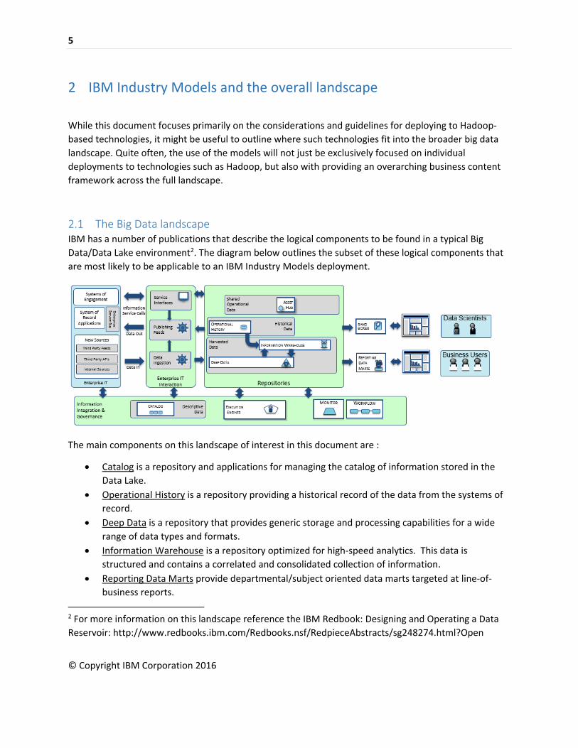
2.1 The Big Data landscape IBM has a number of publications that describe the logical components to be found in a typical Big
Data/Data Lake environment2. The diagram below outlines the subset of these logical components that
are most likely to be applicable to an IBM Industry Models deployment.
The main components on this landscape of interest in this document are :
Catalog is a repository and applications for managing the catalog of information stored in the
Data Lake.
Operational History is a repository providing a historical record of the data from the systems of
record.
Deep Data is a repository that provides generic storage and processing capabilities for a wide
range of data types and formats.
Information Warehouse is a repository optimized for high-speed analytics. This data is
structured and contains a correlated and consolidated collection of information.
Reporting Data Marts provide departmental/subject oriented data marts targeted at line-of-
business reports.
2 For more information on this landscape reference the IBM Redbook: Designing and Operating a Data
Reservoir: http://www.redbooks.ibm.com/Redbooks.nsf/RedpieceAbstracts/sg248274.html?Open

6
© Copyright IBM Corporation 2016
Sandboxes provide a store of information for experimentation, typically by data scientists.
2.2 The role of IBM Industry Models and the big data landscape IBM Industry Models are typically used with the big data landscape in two different but complementary
ways:
The Business Vocabulary provides organizations with the basis on which to define the common business
language and common meaning of the different elements in the landscape.
The Logical and Physical Data Models are design-time artefacts, the output of which are used to define
the commonly used structures across the landscape – where there is a need to enforce structure.
The diagram below provides an overall summary of the main interaction of the different types of IBM
Industry Model component with the typical areas of a big data landscape using Hadoop and more
traditional RDBMS technologies.
In the above diagram, there are the following broad sets of activities:
Mapping of assets to the Business Vocabulary
1. Any relevant assets in the Systems of Record or Systems of Engagement can be mapped to
the overall Business Vocabulary.
2. Any integration-related physical assets (for example, ETL jobs) are mapped to the Business
Vocabulary.

7
© Copyright IBM Corporation 2016
3. All Repository Assets should have mappings to the Business Vocabulary. This should include
assets that were brought in as-is from upstream systems with no attempt to enforce a
standard structure (for example, historical data).
4. Any downstream published data, both data marts as well as certain data scientist Sandboxes
should be mapped to the Business Vocabulary. In the case of the Sandboxes, a decision
might have to be taken in terms of whether such assets have a broader value to the
enterprise beyond the individual data scientist, in which case mapping to the Business
Vocabulary is advisable.
Use of the Business Vocabulary for Search and Discovery
5. The Business Vocabulary should be the basis for any searching or discovery activities that
are carried out by the business users and the data scientists.
Deployment of physical structures from the Logical Models
6. Use the physical Atomic Models to deploy the necessary structures to build out the
traditional Information Warehouse assets.
7. Use the physical Dimensional Models to deploy the necessary structures to build out the
Data Mart layer.
8. Use the physical Dimensional Models to deploy the necessary structures to build out the
Kimball-style Information Warehouse assets.
9. Deploy deep data assets on Hadoop for which there is a need for a specific structure.
10. As required, the physical models might also be used to deploy the data scientist Sandboxes.
Most likely in circumstances where an organization would like to enforce a common set of
structures for their data scientists to use.
8
© Copyright IBM Corporation 2016
3 Typical scenarios where Hadoop would be used
This section describes the typical/sample types of usage scenarios in which Hadoop would be used. As well as describing the typical or assumed business focus of the Scenario, this document will also call out the specific technical focus points of each scenario.
3.1 Fine grain transaction data
Typical use cases of this type of data are where larger amounts of detailed transaction data are required to be stored either to underpin deep analysis of large data sets.
From a technical perspective, the main focus in this scenario is the use of Hadoop to store large volumes of data in an economical way to provide a queryable archive to supplement the traditional RDBMS Information Warehouse.
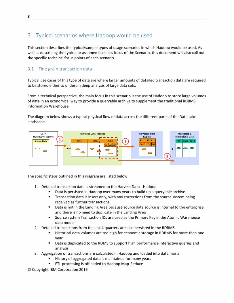
The diagram below shows a typical physical flow of data across the different parts of the Data Lake landscape.
The specific steps outlined in this diagram are listed below:
1. Detailed transaction data is streamed to the Harvest Data - Hadoop Data is persisted in Hadoop over many years to build up a queryable archive Transaction data is insert only, with any corrections from the source system being
received as further transactions Data is not in the Landing Area because source data source is internal to the enterprise
and there is no need to duplicate in the Landing Area Source system Transaction IDs are used as the Primary Key in the Atomic Warehouse
data model 2. Detailed transactions from the last 4 quarters are also persisted in the RDBMS
Historical data volumes are too high for economic storage in RDBMS for more than one year
Data is duplicated to the RDMS to support high performance interactive queries and analysis
3. Aggregation of transactions are calculated in Hadoop and loaded into data marts History of aggregated data is maintained for many years ETL processing is offloaded to Hadoop Map-Reduce

9
© Copyright IBM Corporation 2016
The specific data model constructs used to enable the deployment of fine grain transaction data are a good example of where previously existing structures already in the data models can be used. In this case, there is no new type of information being stored, but it is more a case that a decision has been made to consider using Hadoop as the target repository for storing Transactions, perhaps for cost-of-storage reasons.
The diagram below shows an example from the IBM Banking Data Warehouse of the modeling of the typical aspects of such fine grained Transactions. Similar components are also found in IBM Industry Models for other industries.
In this example the Transaction entity records the details pertaining to the specific transaction with relationships to other relevant elements such as Transaction Document which records any documents associated with the Transaction and Posting Entry.

10
© Copyright IBM Corporation 2016
3.2 Operational Data Stores
This section describes the use of Hadoop as the basis for an organization’s Operational Data Store (ODS). There are traditionally a range of different ODS types. The focus of this document is on two specific types of ODS, what Inmon refers to as Class II and Class IV ODS3.
Class II ODS – This type of ODS is where the transactions that are contained in the ODS are integrated, which means the required level of processing is done on them to achieve the necessary conformity of structure. This type of ODS has a one-way population to the downstream data warehouse.
Class IV ODS – Similar to a Class II, this ODS also had integrated Transactions. However there is an additional process where it also accommodates data coming back from the data warehouse.
From a technical perspective, the ODS scenario is essentially an extension of the previous fine grain Transaction Data scenario. Specifically, this scenario adds the tighter integration of the Harvest Hadoop Data and the associated Harvested RDBMS Data, with certain additional calculated data created in the Information Warehouse being replicated back into the Hadoop ODS.
The diagram below shows a typical physical flow of data across the different parts of the Data Lake landscape.
The diagram above shows the likely flows of data in and out of such a Hadoop ODS. The specific steps
involved are:
1. Detailed transaction data is streamed to the ODS in the Harvest Data - Hadoop
Data is persisted in Hadoop over many years to build up a queryable archive
Transaction data is insert only, with any corrections from the source system being
received as further transactions
3 For example see article entitled “ODS Types“ by Bill Inmon. Information Week, 1st Jan 2000 http://www.information-management.com/issues/20000101/1749-1.html

11
© Copyright IBM Corporation 2016
Data is not in the Landing Area because source data source is internal to the enterprise
and there is no need to duplicate in the Landing Area
Source system Transaction IDs are used as the primary key in the Atomic Warehouse
data model
Key question on the level of structure needed to be enforced in defining the ODS, is
there a need for a common structure for transactions, customer data etc, or is it
sufficient to land the data as is and tag it, and so on.
2. The relevant subset of the detailed data also persisted in the RDBMS
Historical data volumes are too high for economic storage in RDBMS for more than a
specific period (for example, 1 year)
Data is duplicated to RDMS to support high performance interactive queries and
analysis
3. Certain additional data (for example, derived data) to be also placed back in the ODS
For example, derived data or additional new data (for example, scores or ratings)
provided as part of calculation engines
The ETL might take place in batch at a slower frequency to the ODS population
4. As required, data scientists use the ODS as a source for populating their sandboxes
5. Any applications needing more recent operational data or stored data no longer in the data
warehouse access the ODS
Modeling the ODS in Hadoop
A physical model created for an ODS in Hadoop would need to accommodate most of the typical
requirements for building an ODS:
Contains current or near current data
Typically contains atomic data only
Plus the ODS on Hadoop is assumed to have the following additional requirements:
Storage of very large amounts of data
Become a queryable archive
A significant consideration here will be the lower tolerance level of normalized data structures in
Hadoop over that in an RDBMS. In this case it is likely that there might be a need to carefully determine
how to reconcile the need to have a performant ODS on Hadoop with the need to also populate a more
normalized downstream data warehouse.
Performance is one of the key requirements for the ODS, given the velocity of various events’ data that
is often likely to be produced in near-real time and the need to retrieve the data/information in a timely
manner from the ODS. The Atomic Warehouse Model has most of the subject areas and domains that
are likely to be of relevance to an ODS (for example in the Healthcare area: Clinical Orders and Lab
Results). However the constructs such as Anchor, Associations and Array tables often found in the
Atomic Warehouse Model results in an increase in the number of tables, which would in-turn impact the
performance for both loading as well as querying the data. During initial IBM Industry Model projects by
12
© Copyright IBM Corporation 2016
customers deploying ODSs to HDFS, the decision has been to remove such constructs and streamline the
schema with a limited number of required tables, so that it is possible to achieve the performance
targets.
3.3 Call center data
A typical use case of this type of data is the need to import data (often structured and unstructured) from operational call center applications.
From a technical perspective, the call center scenario is focused primarily on the storage of structured and unstructured data such as call audio and transcript files in the Hadoop Harvested area.
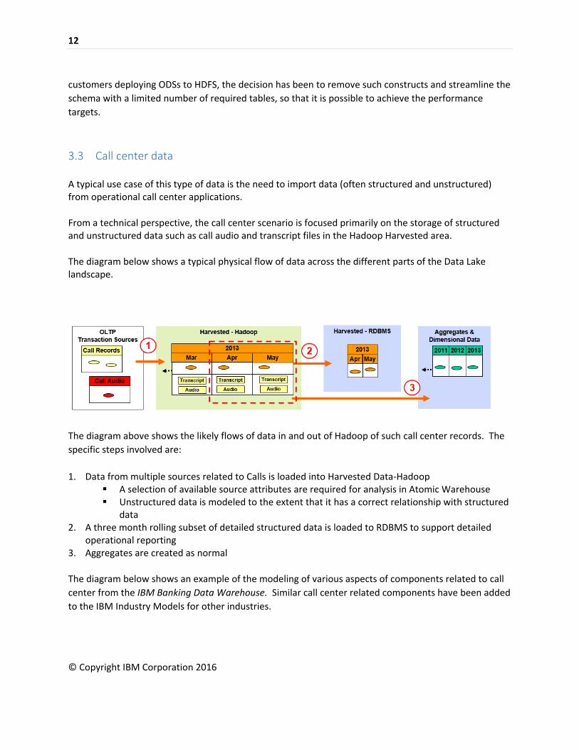
The diagram below shows a typical physical flow of data across the different parts of the Data Lake landscape.
The diagram above shows the likely flows of data in and out of Hadoop of such call center records. The
specific steps involved are:
1. Data from multiple sources related to Calls is loaded into Harvested Data-Hadoop A selection of available source attributes are required for analysis in Atomic Warehouse Unstructured data is modeled to the extent that it has a correct relationship with structured
data 2. A three month rolling subset of detailed structured data is loaded to RDBMS to support detailed
operational reporting 3. Aggregates are created as normal
The diagram below shows an example of the modeling of various aspects of components related to call
center from the IBM Banking Data Warehouse. Similar call center related components have been added
to the IBM Industry Models for other industries.

13
© Copyright IBM Corporation 2016
In this example the Call Audio and associated Text Block entities represent the logical starting point for physical structures that are used to store the transcripts of the call and any additional notes taken by employees.
3.4 Social media data
A typical use cases of such data is the on boarding of Twitter or Facebook data to include in analysis purposes.
From a technical perspective, the key additional component of this scenario is the linkage of often anonymous social personas with existing customers.

14
© Copyright IBM Corporation 2016
The diagram above shows the likely flows of data in and out of Hadoop of such social media data.
The specific steps that are involved are:
1. Very high volume and velocity data from multiple sources is loaded or streamed into the Historical Area
Data is to be combined into related data entities in the Harvested Data (for example, social media postings and social media persona)
2. Standardized detailed social media data is loaded to the Harvested Data -Hadoop Data is validated and standardized to fit the data model, including relationships
between entities Data contains a mixture of primitive and complex data types (image, documents etc.) Source system Transaction IDs are used as the primary key in the Harvested Data area
data model (however SQL-on-Hadoop has non-enforced/informational primary keys that are used to assist the query optimizer.
3. Sentiment Analytics is used to calculate a sentiment analysis for each rating 4. Details data volumes not pragmatic for RDBMS but entities in RDBMS can be inserted or
updated Social Persona details updated in the RDBMS. Analysis tooling that is used to calculate relationship between the Social Persona and
Person records 5. Aggregations of detailed are carried out in Hadoop and loaded into data marts
History of aggregated data is maintained for many years ETL processing is offloaded to Hadoop Map-Reduce
The diagram below shows an example of the modeling of various aspects of social media related elements in IBM Insurance Information Warehouse. Similar such social media components have been added to the IBM Industry Models for other industries.

15
© Copyright IBM Corporation 2016
In this example, the relevant model elements are :
Social Media Text Block – the storage of the contents of a social media posting
Virtual party – relating to the party originating the social media posting
3.5 Sensor/instrument data
Describes the patterns and the possible interaction of model structures using explicit IBM Industry Model examples. Typical use cases of this type of data could include vehicle telematics information from on board automobile sensors or sensors in homes (perhaps as part of a Smarter homes initiative).
From a technical perspective, the focus of this scenario explicitly is around the use of Hadoop to store a range of external heterogeneous data from potentially a number of external sources.
16
© Copyright IBM Corporation 2016
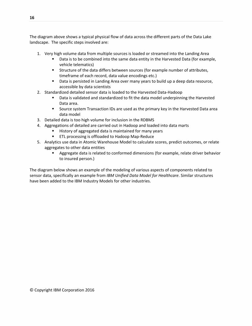
The diagram above shows a typical physical flow of data across the different parts of the Data Lake landscape. The specific steps involved are:
1. Very high volume data from multiple sources is loaded or streamed into the Landing Area Data is to be combined into the same data entity in the Harvested Data (for example,
vehicle telematics) Structure of the data differs between sources (for example number of attributes,
timeframe of each record, data value encodings etc.) Data is persisted in Landing Area over many years to build up a deep data resource,
accessible by data scientists 2. Standardized detailed sensor data is loaded to the Harvested Data-Hadoop
Data is validated and standardized to fit the data model underpinning the Harvested Data area.
Source system Transaction IDs are used as the primary key in the Harvested Data area data model
3. Detailed data is too high volume for inclusion in the RDBMS 4. Aggregations of detailed are carried out in Hadoop and loaded into data marts
History of aggregated data is maintained for many years ETL processing is offloaded to Hadoop Map-Reduce
5. Analytics use data in Atomic Warehouse Model to calculate scores, predict outcomes, or relate aggregates to other data entities
Aggregate data is related to conformed dimensions (for example, relate driver behavior to insured person.)
The diagram below shows an example of the modeling of various aspects of components related to sensor data, specifically an example from IBM Unified Data Model for Healthcare. Similar structures have been added to the IBM Industry Models for other industries.

17
© Copyright IBM Corporation 2016
In this example, the Device Finding (normal results from a Point of Care Device such as a Heart Monitor) or the Device Alert (any emergency alerts from the device) would typically represent the high volume sensor data stored on Hadoop.
3.6 Geospatial data
Typical use cases of this type of data could be the collection of weather data and data from previous storms and floods to enable more precise calculation of insurance risks.
From a technical perspective, the focus of this scenario is on the use of Hadoop to feed the necessary data into the downstream RDBMS to avail of the geospatial features found in many RDBMSs. Equivalent features are currently not found in Hadoop.

18
© Copyright IBM Corporation 2016
The diagram above shows a typical physical flow of data across the different parts of the Data Lake landscape. The specific steps involved are:
1. Different geospatial data is landed from different sources. High likelihood that this data will come in from these sources in different formats (for
example, local weather organizations, international weather sources) Data is persisted in Landing Area over many years to build up a deep data resource,
accessible by data scientists 2. The relevant subset of landed data in the Historical Data area might then be brought into the
data warehouse (Harvested Data RDBMS) For example data that can be uniquely identified and geocoded
3. It is likely that this cleaned up data is stored in RDBMS format as currently there is a more effective and advanced geospatial features library in some RDBMSs than is available in Hadoop. Hence the data is more likely to be move into the RDBMS than stored in a Harvested Hadoop environment.
4. The data might also be transferred into dimensional (either row or column based) for final analysis of for visualization of the results.
The diagram below shows an example from IBM Insurance Information Warehouse of the specific data model constructs used to enable the deployment of geospatial data.

19
© Copyright IBM Corporation 2016
The relevant entities in this example are entities line Area Polygon and Geometric Shape that are used to store the areas at risk and storm paths respectively.

20
© Copyright IBM Corporation 2016
4 Typical flow of models deployment to Hadoop
Before describing in more detail some of the considerations around the deployment of the logical models to Hadoop, it might be useful to describe some possible flows through a typical big data landscape.
The Diagram above describes the overall steps likely to be relevant in the deployment from logical models to physical HDFS structures. These steps are:
1. Modeling carried out on logical model that is identified as a Platform Independent Model (PIM) to reflect the necessary business-specific structures and constraints that are applicable, irrespective of any tooling constraints.
2. The specific subset of the business context to be transformed to Hadoop is copied/recreated into a separate logical model.
3. The introduction of this second logical model to represent the Platform Specific Model(PSM) will depend on the richness of logical to physical functionality in the modeling tool being used. Where such an interim PSM is required, then it is likely that there is a need to carry out specific
21
© Copyright IBM Corporation 2016
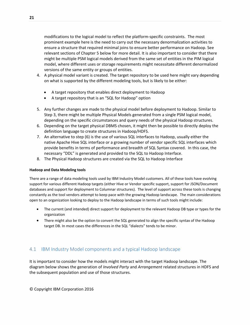
modifications to the logical model to reflect the platform-specific constraints. The most prominent example here is the need to carry out the necessary denormalization activities to ensure a structure that required minimal joins to ensure better performance on Hadoop. See relevant sections of Chapter 5 below for more detail. It is also important to consider that there might be multiple PSM logical models derived from the same set of entities in the PIM logical model, where different uses or storage requirements might necessitate different denormalized versions of the same entity or groups of entities.
4. A physical model variant is created. The target repository to be used here might vary depending on what is supported by the different modeling tools, but is likely to be either:
A target repository that enables direct deployment to Hadoop
A target repository that is an “SQL for Hadoop” option
5. Any further changes are made to the physical model before deployment to Hadoop. Similar to Step 3, there might be multiple Physical Models generated from a single PSM logical model, depending on the specific circumstances and query needs of the physical Hadoop structures.
6. Depending on the target physical DBMS chosen, it might then be possible to directly deploy the definition language to create structures in Hadoop/HDFS.
7. An alternative to step (6) is the use of various SQL interfaces to Hadoop, usually either the native Apache Hive SQL interface or a growing number of vendor specific SQL interfaces which provide benefits in terms of performance and breadth of SQL Syntax covered. In this case, the necessary “DDL” is generated and provided to the SQL to Hadoop Interface.
8. The Physical Hadoop structures are created via the SQL to Hadoop Interface
Hadoop and Data Modeling tools
There are a range of data modeling tools used by IBM Industry Model customers. All of these tools have evolving
support for various different Hadoop targets (either Hive or Vendor specific support, support for JSON/Document
databases and support for deployment to Columnar structures). The level of support across these tools is changing
constantly as the tool vendors attempt to keep pace with the growing Hadoop landscape. The main considerations
open to an organization looking to deploy to the Hadoop landscape in terms of such tools might include:
The current (and intended) direct support for deployment to the relevant Hadoop DB type or types for the
organization
There might also be the option to convert the SQL generated to align the specific syntax of the Hadoop
target DB. In most cases the differences in the SQL “dialects” tends to be minor.
4.1 IBM Industry Model components and a typical Hadoop landscape
It is important to consider how the models might interact with the target Hadoop landscape. The diagram below shows the generation of Involved Party and Arrangement related structures in HDFS and the subsequent population and use of those structures.

22
© Copyright IBM Corporation 2016
In the example in the above diagram the Logical Data Models are de-normalized to define two file structures (Involved Party and Arrangement) to be deployed to HDFS. The source system generates daily extracts for customers, deposits and their relationships. An ETL process ingests the data set into HDFS as Parquet files. Hive defines tables pointing to the Parquet files4. Each sub-folder contains one partition (in the example one version of the data set for a particular date). If the same data set must be reloaded (for instance due to data quality issues with the previous data set) a new sub folder (with different version) is created. Upon completion of the data load the Hive partition is altered to point to the new folder.
In terms of the actual approaches to deploying the structures from the modeling tool into HDFS, there are a number of options, ranging from native Hadoop commands to variants of SQL-based interfaces which enable the use of SQL commands both in terms of the definition of the file structures and subsequently in terms of the querying of the files.
So this results in three possible options for organizations to interact with the HDFS files, specifically:
4 For more information on the use of Avro and Parquet : https://developer.ibm.com/hadoop/blog/2015/11/10/use-parquet-tools-avro-tools-iop-4-1/ http://www.slideshare.net/StampedeCon/choosing-an-hdfs-data-storage-format-avro-vs-parquet-and-more-stampedecon-2015 http://grepalex.com/2014/05/13/parquet-file-format-and-object-model/ http://blog.cloudera.com/blog/2015/03/converting-apache-avro-data-to-parquet-format-in-apache-hadoop/

23
© Copyright IBM Corporation 2016
1. Hive as the Apache Hadoop data warehousing infrastructure. Hive was developed as part of the Apache Hadoop set of tools to provide a data-warehouse style capability on top of HDFS, including a basic SQL interface for the definition and querying of HDFS data. As such this is freely available open source technology
2. Vendor provided SQL interfaces for Hadoop5. This might be one of a number of SQL interfaces supplied by various Vendors. These SQL interfaces typically provide a better coverage of the overall SQL syntax and usually they can deliver a better query performance than the native Hive SQL.
3. Non-SQL Hadoop technology. This might be technology such
as HBASE or the use of Map Reduce technology. This main
challenge here is the need for a specialized skillset.
In fact, organizations can also choose to use a combination of 1
and 2 above on the same datasets. Some users might prefer Hive and some users might prefer a
Vendor provided SQL interface, and both users can work in parallel on the same dataset with their
respective preferred query tools. Another use case is for bulk operations on the entire dataset (e.g.
ETL/ingest – insert-select), some organizations prefer to use Hive rather than a Vendor provided SQL
Interface (hive can actually be faster in this blunt use case).
The choice of query tool over Hbase isn’t as portable/interchangeable in this way as depending on
the agility of schema used in hbase the data may not be suitable for asserting a relational (tabular)
schema over.
4.2 When to use Hadoop or not
Below is an overall set of guidelines regarding the decision of when to use Hadoop or when to use a more traditional RDBMS. There is a fundamental assumption that it is likely that most organizations will require a mixture of both Hadoop and RDBMS technologies.
When to put data in Hadoop and not the RDBMS:
When the volume of data is very large it does not make economic sense to store it in RDBMS for example, the schema of well-structured sensor records might 'fit' into the data warehouse model, but it is not economically or operationally feasible to store it there.
Data is in a raw format for example, text, XML, JSON, binary. You are landing the data and not incurring the high processing cost to transform such data into physical relational structures.
5 For more details on the IBM BigSQL interface to Hadoop: https://developer.ibm.com/hadoop/docs/getting-started/tutorials/big-sql-hadoop-tutorial/ https://developer.ibm.com/hadoop/blog/2014/09/19/big-sql-3-0-file-formats-usage-performance/
SQL interface for Hadoop
Many vendors offer SQL interfaces on Hadoop – IBM BigSQL, MapR, plus Cloudera Impala, Oracle Big Data SQL. Plus there is the possible emergence of standards in this area (https://www.odpi.org/). These capabilities should reduce the need for HDFS-specific knowledge during some physicalization activities.
Another consideration for the use of SQL over Hadoop is the ability to carry out federated queries across Hadoop and traditional RDBMS databases.

24
© Copyright IBM Corporation 2016
It is easy / ‘natural’ to store the data in Hadoop (path of least resistance) for example, JSON document generated from web-based java application.
Data contains data types that are not traditionally held in RDBMS DW for example, audio, scanned documents.
Data is going to be accessed and processed in a 'batch' format by data professionals (data analysts, data scientists, data developers)
Data from a stream source is being landed so it can be mined to develop rules engine algorithms for real-time data analysis for example, next best action
When you have a use for the data! Hadoop should not be seen as place to put data 'we might need some day', especially if there is no obvious current or future use case of business value for the data.
Where some of the components of the data to be stored are in a format that is not able to be specified in ER modeling notation (and by extension defined in a DBMS), for example Composite Types.
When NOT to put data in Hadoop:
When the data is a raw format already existing in enterprise source system for example, call center audio, document management system. Should not duplicate data in this way unless there is a compelling technical or business reason
When then data is frequently updated and referential integrity rules need to be applied - consider the Information Warehouse (RDBMS)
When the data must be queried interactively or with complex joins by business users - consider Information Warehouse (RDBMS) or data mart
When you have concerns about the legal rights to persist the data - consider analyzing in-stream and storing the analysis if appropriate.
Where there is a business need to use specific capabilities in the RDBMS that are not yet present, or are not mature, in the Hadoop technology. An example of this is the superior geospatial features in a number of RDBMSs compared to equivalent capabilities in Hadoop.

25
© Copyright IBM Corporation 2016
5 Considerations for logical to physical modeling for a Hadoop
environment
This chapter is concerned with the set of considerations that are relevant during the specific transformation of a logical data model into a specific physical data model intended for efficient deployment to a Hadoop environment. This chapter will mainly focus on the specific considerations related to the IBM Industry Models for such a Hadoop-focused logical to physical transformation. However, in addition there are a range of other, more general material available that might provide further information and guidance6.
5.1 Selection of IBM Industry Model components for logical to physical transformations As the IBM Industry Models provide a number of different logical data models for each industry it is
necessary to also consider from which of the model components does it make sense to generate a data
model structure for Hadoop.
Across the models for the different industries, there are a number of sub model components,
specifically:
Business Data Model (BDM) – a 3NF model which is intended to capture the full business
content without any design constraints. The BDM exists in the set of models for the Insurance,
Healthcare, and Energy & Utilities industries.
Atomic Warehouse Model (AWM) – typically a 3NF model that incorporates a number of de-normalizations based on observed common usage in that industry. Intended as the starting point for deployments to an Inmon type relational data warehouse. The AWM exists for all industries.
Dimensional Warehouse Model (DWM)– typically would consist of a Kimball-compliant dimensional warehouse consisting of Conformed Dimensions and Mini dimensions, fine grained Transaction Facts, Periodic Snapshot Facts, and Aggregate Facts. The DWM exists for all industries.
The choice of which of these components are the best starting point for a deployment to Hadoop depends on the different industries.
6 There is a good introductory dummies.com article http://www.dummies.com/how-to/content/transitioning-from-an-rdbms-model-to-hbase.html)

26
© Copyright IBM Corporation 2016
Insurance - As the BDM for insurance is a pure conceptual model with very little attribution, the more likely starting point for a Hadoop deployment is from the Atomic Warehouse Model
Healthcare and Energy & Utilities – As the BDM is less normalized than the AWM, in these Industries, this represents the best starting point for Hadoop.
Banking, Retail and Telco – as there is no BDM, then the most likely starting point for a Hadoop deployment is from AWM.
5.1.1 Use Dimensional Models for deployment to Hadoop
It can be noted that in the above diagram, currently all of the deployments to Hadoop are from either the AWM or BDM models and not from the DWM. This is mainly as a result of the limited scope of the experiences and activities of organizations so far when deploying an IBM Industry Model to Hadoop. Essentially there is not enough detailed knowledge of deploying the Dimensional Models to Hadoop to enable a detailed discussion in the current version of this document. This situation is likely to change as organizations do more activities with Dimensional Models in the context of Hadoop in the future. In which case, subsequent versions of this document will be updated accordingly.
One good example of a potential focus for Dimensional, is the suitability of Dimensional Models as a basis to drive out efficient Columnar structures to support very high performance queries.
5.2 Flattening/denormalization of structures in Hadoop
The IBM Industry Data Models (AWM and BDM) are designed to incorporate the necessary flexibility to accommodate the full breadth of the business content and to provide the optimal basis for downstream logical to physical transformations to relational Information Warehouse structures. To that end, these models would typically be quite normalized (in many cases broadly at a third normal form level but with some common de-normalizations). The overall experience with the initial use of normalized structures in

27
© Copyright IBM Corporation 2016
Hadoop indicated that such normalized structures did not perform well, so any logical to physical transformation to Hadoop would require the creation of quite flattened structures. However these performance limitations may be less pronounced when using Vendor supplied SQL interfaces instead of using the underlying Hive SQL.
Unlike the traditional RDBMSs, Hadoop is not designed to work with a large number of normalized data objects while most of the IBM Industry Models were built and rely upon normalized structures. In Hadoop, joins between many tables, although possible in Hive, usually lead to transfer of vast amounts of data over the network and are not performant
At the most fundamental level, there are two ways to de-normalize relational structures:
Horizontal – by adding new records (partially containing duplicated data)
Vertical – by the addition of new columns
While both options are widely used, in general, the first adds significant complexity to the data and the queries and increases the amount of data being stored while the second increases the complexity of each query and implies restrictions on the number of records.
Let’s look at a basic example in order to illustrate the complexity of the de-normalization. The IBM Unified Data Model for Healthcare defines entities “Patient” and “Patient Language” (each Patient has 0, 1 or many Languages) as shown in diagram below.
The options to include the Patient Language in the Patient table are:

28
© Copyright IBM Corporation 2016
a. Vertical De-normalization - move the attributes to the Patient table such as ‘Patient Language 1’, ‘Patient Language 2’, ‘Patient Language X’, which results in a flat structure but a limited number of Patient Language per Patient supported.
b. Horizontal De-normalization - Move the attributes from ‘Patient Language’ to the Patient table and allow many records for the same Patient to be inserted only with different “Patient Language” instances
The former approach not only limits the number of instances of Language for a Patient but also adds complexity to the SQL statements. Whereas the latter approach leads to significant data repetition and makes simple queries such as the number of unique Patients, complex to answer.
In general, a number of separate options can be identified when it comes to carrying out such
denormalization activities on specific areas and structures of the IBM Industry Models. The following
sections describe these different options.
5.3 Common de-normalization options
This section describes a subset of the possible transformation patterns that are commonly applicable to
the IBM Data Models across all industries. It should be remembered that these options are not mutually
exclusive and that it is likely that a combination of these options might be used in any denormalization
of data structures7.
7 In an IBM Industry Model which has the BDM, there is usually a section in the accompanying KnowledgeCenter called “Transformation rules between Business Data Model and Atomic Warehouse Model”. It might also be beneficial to read this section of the relevant KnowledgeCenter.
29
© Copyright IBM Corporation 2016
5.3.1 Vertical reduction of the supertype/subtype hierarchy
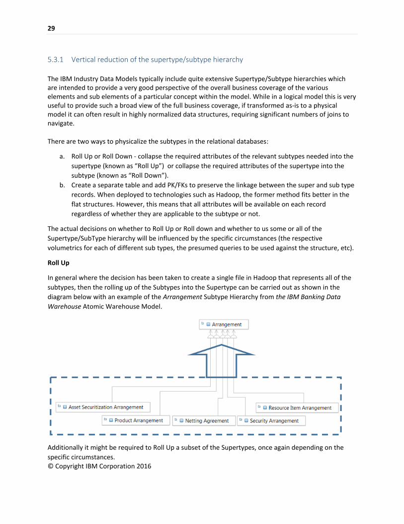
The IBM Industry Data Models typically include quite extensive Supertype/Subtype hierarchies which are intended to provide a very good perspective of the overall business coverage of the various elements and sub elements of a particular concept within the model. While in a logical model this is very useful to provide such a broad view of the full business coverage, if transformed as-is to a physical model it can often result in highly normalized data structures, requiring significant numbers of joins to navigate.
There are two ways to physicalize the subtypes in the relational databases:
a. Roll Up or Roll Down - collapse the required attributes of the relevant subtypes needed into the
supertype (known as “Roll Up”) or collapse the required attributes of the supertype into the
subtype (known as “Roll Down”).
b. Create a separate table and add PK/FKs to preserve the linkage between the super and sub type
records. When deployed to technologies such as Hadoop, the former method fits better in the
flat structures. However, this means that all attributes will be available on each record
regardless of whether they are applicable to the subtype or not.
The actual decisions on whether to Roll Up or Roll down and whether to us some or all of the
Supertype/SubType hierarchy will be influenced by the specific circumstances (the respective
volumetrics for each of different sub types, the presumed queries to be used against the structure, etc).
Roll Up
In general where the decision has been taken to create a single file in Hadoop that represents all of the
subtypes, then the rolling up of the Subtypes into the Supertype can be carried out as shown in the
diagram below with an example of the Arrangement Subtype Hierarchy from the IBM Banking Data
Warehouse Atomic Warehouse Model.
Additionally it might be required to Roll Up a subset of the Supertypes, once again depending on the
specific circumstances.

30
© Copyright IBM Corporation 2016
Roll Down
Alternatively there might be a need to create specific files in Hadoop for one of the Subtypes only, in
which case it might be appropriate to Roll Down the SuperType, so that the more generic attributes of
that Supertype are also included in the created file.
It is likely that such a Roll Down might be carried out a number of times. So in the example in the
diagram above, in addition to a File structure in Hadoop of the Security Arrangement as indicated, a
separate Roll Down of the Supertype might also be done to create a separate Hadoop file for the
Product Arrangement. Once again, the specific circumstances and Business questions to be addressed
will determine which of the Subtypes should be transformed in such a way.
5.3.2 Reduce or remove the associative entities All of the IBM Industry Models make extensive use of the associative entities to describe relationship
between two entities. This is particularly useful as it is Associative Entities that allow a continuous trace
over time of relationships between different entity instances to be recorded in the warehouse.
These relationships might be, for example, the particular values of all Classifications classifying an
Individual at any points in time; the various relationships between any two Arrangements as they
change over time; or the complete historical record of associations between Countries and Currencies.
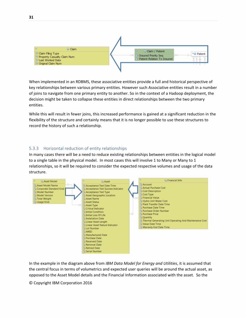
An example of an Associative Entity from IBM Unified Data Model for Healthcare is shown below, which
records the various relationships between Claim and Patient.
31
© Copyright IBM Corporation 2016
When implemented in an RDBMS, these associative entities provide a full and historical perspective of
key relationships between various primary entities. However such Associative entities result in a number
of joins to navigate from one primary entity to another. So in the context of a Hadoop deployment, the
decision might be taken to collapse these entities in direct relationships between the two primary
entities.
While this will result in fewer joins, this increased performance is gained at a significant reduction in the
flexibility of the structure and certainly means that it is no longer possible to use these structures to
record the history of such a relationship.
5.3.3 Horizontal reduction of entity relationships In many cases there will be a need to reduce existing relationships between entities in the logical model
to a single table in the physical model. In most cases this will involve 1 to Many or Many to 1
relationships, so it will be required to consider the expected respective volumes and usage of the data
structure.
In the example in the diagram above from IBM Data Model for Energy and Utilities, it is assumed that
the central focus in terms of volumetrics and expected user queries will be around the actual asset, as
opposed to the Asset Model details and the Financial Information associated with the asset. So the

32
© Copyright IBM Corporation 2016
denormalization will likely be the collapsing of the Asset Model and Financial Info entities into a single
Asset physical table. Separately, there needs to be additional consideration given to whether such
denormalization should be vertical or horizontal.
5.3.4 Remove the Classification entities (Banking, Retail and Telco only) IBM Industry Models for Banking/FM, Retail and Telco make extensive use of Classification entities at
the logical level. The purpose of these entities is to represent a common collection point for simple sets
of codes that are used to classify or codify various aspects of the business (for example Credit Card Type,
Currency Zone.
Even when deploying these models to an RDBMS, the general guidance is not to physicalize what could
be many 100’s of such tables and typically such entities are physicalized into a single Classification
scheme/value look up table. In the case of Hadoop deployments, it might be more preferable to remove
such classifications altogether and assume that such handling of enumerations is carried out as part of
any upstream ETL process.
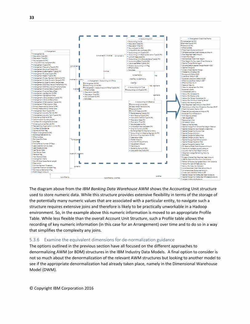
5.3.5 De-normalize the Accounting Unit structure (Banking, Retail and Telco only) One of the key core structures within the models is that of the Accounting Unit. Typically this structure
provides a highly flexible mechanism for the storage of numeric attributes such as balances, totals,
counts, averages, etc. These Accounting Unit structures enable a uniform approach to handling the
storage and history requirements of any numeric (both monetary and non-monetary) values in the
AWM models. Where numerical attributes do occur on entities, the values therein are usually just
derived from Accounting Unit values, and the attributes only exist in order to increase ease of access
and/or visibility of a particular significant data item.
33
© Copyright IBM Corporation 2016
The diagram above from the IBM Banking Data Warehouse AWM shows the Accounting Unit structure
used to store numeric data. While this structure provides extensive flexibility in terms of the storage of
the potentially many numeric values that are associated with a particular entity, to navigate such a
structure requires extensive joins and therefore is likely to be practically unworkable in a Hadoop
environment. So, in the example above this numeric information is moved to an appropriate Profile
Table. While less flexible than the overall Account Unit Structure, such a Profile table allows the
recording of key numeric information (in this case for an Arrangement) over time and to do so in a way
that simplifies the complexity any joins.
5.3.6 Examine the equivalent dimensions for de-normalization guidance The options outlined in the previous section have all focused on the different approaches to
denormalizing AWM (or BDM) structures in the IBM Industry Data Models. A final option to consider is
not so much about the denormalization of the relevant AWM structures but looking to another model to
see if the appropriate denormalization had already taken place, namely in the Dimensional Warehouse
Model (DWM).

34
© Copyright IBM Corporation 2016
In recent releases IBM has focused on the extension of the content in the DWM in many industries and a
lot of that work was denormalizing content from the AWM in the appropriate structures in the DWM. So
it might be worthwhile to examine these DWM structures, in case the de-normalized entities in that
model are a closer match to the specific needs for Hadoop files. Of course, there is likely to be the usual
need for customization in any case.
The Diagram on this page shows a small subset of the highly
denormalized Patient Dimension from IBM Unified Data Model for
Healthcare. This Dimension has incorporated a range of attributes
that would be found in separate entities in the equivalent
AWM/BDM structures.
5.3.7 Renaming of resulting denormalized structures One final denormalization item to consider in conjunction with all of the above options is to examine the
resulting attribute naming. In some cases it might be that the resulting attribute is too generic which
doesn’t result in names that are very user friendly. So, it might be beneficial to examine the names of
the linked business terms to see of there more user-friendly vocabulary-based names that could be used
for otherwise potentially overly generic attribute names.
35
© Copyright IBM Corporation 2016
5.4 Surrogate keys vs business keys While the surrogate keys are fundamental to the implementation of PK/FKs in the relational databases, they are less meaningful to semi-structured data models. It might also prove difficult to generate unique keys across the whole data in Hadoop. Therefore, it is recommended to rely upon business keys and the unique id of the data set (for example, reporting date, source system, version of the data etc). The use of nested structures reduces (although it does not prevent) the risk of duplicated records which is often a problem in the relational world. For instance, in the context of the example of Patient Language in Section 5.2, a duplicated ‘Patient Language’ might result in two records returned from a query with a join statement. In the case of semi-structured implementation, the document still returns one although there might be duplicated rows in some sub elements. It is still possible though to have two different Patient documents which share the same business key (the technology would not prevent it). A separate consideration is regarding the potential denormalization of data structures. If such denormalization takes place, it is recommended to also remove any PK definitions. Otherwise the existence of these PKs could result in the SQL optimizer using this “information” PK to make potentially incorrect assumptions about the data structures. Another consideration here is how to manage the handling of source system ids. One approach could be to define a new Atomic Domain for that technical attribute that could be transformed into the appropriate Hadoop data type such as a MAP. For example, the "Unique Id In Source System" business key for an Arrangement could be populated with (Product,ABCD,Transit,123,Account,4567890) and it would be possible to query any field using Map(Product) for example to return ABCD. There are a number of external blogs and other publications that give examples of some of the considerations: how to create surrogate keys in Hadoop8 , some approaches for the potential enforcement of Surrogate keys in Hadoop9 Finally there are emerging tools such as Cloudera Kudu10 which are created to overcome some of the gaps typically associated with Hadoop/HDFS such as the lack of indexing. However these tools are in their early phases and still proprietary (although Cloudera announced that they will open source the code)
5.5 Long vs short entity and attribute names IBM Industry Models offer a dictionary which maps long to short names (for example Arrangement to AR). This is also inherited from the relational database where the RDBMSs enforced restrictions on the length of the column names. In Hadoop’s world, the restrictions are not as strict as in the RDBMSs and it is up to the organizations to decide whether they still want to shorten the attribute names or to use the full name. The following must be considered:
8 http://www.remay.com.br/blog/hdp-2-2-how-to-create-a-surrogate-key-on-hive/ 9 https://www.linkedin.com/pulse/telecom-big-data-identifying-subscriber-hadoop-qamar-shahbaz-ul-haq 10 https://blog.cloudera.com/blog/2015/09/kudu-new-apache-hadoop-storage-for-fast-analytics-on-fast-data/
36
© Copyright IBM Corporation 2016
Most modern Hadoop file formats (for example AVRO/Parquet) would keep the schema definition only once per file and the remaining content is binary, which means the extra physical space required by the longer names is insignificant
Most modern BI tools will ingest the column names directly from Hive or the Parquet or AVRO schemes, so the users will not have to manually type long names
Short attribute names still make sense if the users of the physicalized data are going to often type the queries manually
In general it is recommended that the original nested schema (for example, XSD) is created using the full names and then simple java programs could be developed to parse the schema, lookup the IBM Industry Model’s dictionary for the short names and create another schema with the shortened names.
5.6 End-to-end de-normalization example – Social media structures.
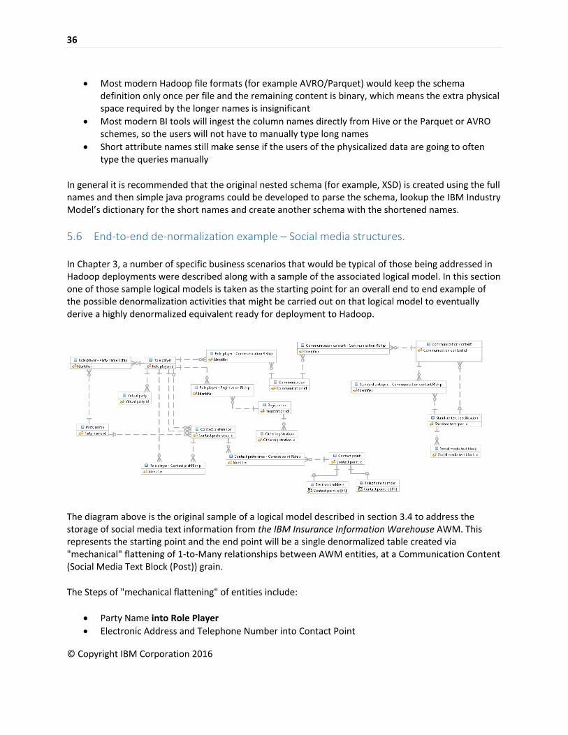
In Chapter 3, a number of specific business scenarios that would be typical of those being addressed in Hadoop deployments were described along with a sample of the associated logical model. In this section one of those sample logical models is taken as the starting point for an overall end to end example of the possible denormalization activities that might be carried out on that logical model to eventually derive a highly denormalized equivalent ready for deployment to Hadoop.
The diagram above is the original sample of a logical model described in section 3.4 to address the storage of social media text information from the IBM Insurance Information Warehouse AWM. This represents the starting point and the end point will be a single denormalized table created via "mechanical" flattening of 1-to-Many relationships between AWM entities, at a Communication Content (Social Media Text Block (Post)) grain.
The Steps of "mechanical flattening" of entities include:
Party Name into Role Player
Electronic Address and Telephone Number into Contact Point

37
© Copyright IBM Corporation 2016
o Contact Point into Contact Preference o Contact Preference into Role Player
Other Registration into Registration o Registration into Role Player
Virtual Party into Role Player
Role Player into Communication
Communication into Communication Content
Social Media Text Block into Standard Text Spec o Standard Text Spec into Communication Content
In terms of the denormalized attribute placement and naming patterns within physical table:
o In general, all attributes from flattened entities are included as initial "mechanical" approach.
There are exceptions – for example, scope of included Contact Point and Registration attributes is limited
Also, "mechanically-included" Attributes can be:
Removed on a case-by-case basis, as desired.
Renamed to use a proper Business Term, if available/defined. o Prefix Attribute Names with Entity and/or "Nature" (Relationship Type) names to clearly
identify "source" of denormalized attributes. o Prefix Names used in this example:
Communication content Social media text block Communication Communication sender (Nature of Role player – Communication Rlship)
Communication sender party name
Communication sender party name
Communication sender user identification (User identification is a Type of "Other Registration", per the AWM.)
Communication sender contact preference
Communication sender telephone number
Communication sender email (Electronic Address.Electronic Type) Communication recipient (Nature of Role player – Communication Rlship)
Communication recipient user identification Social media service provider party name Social media network party name
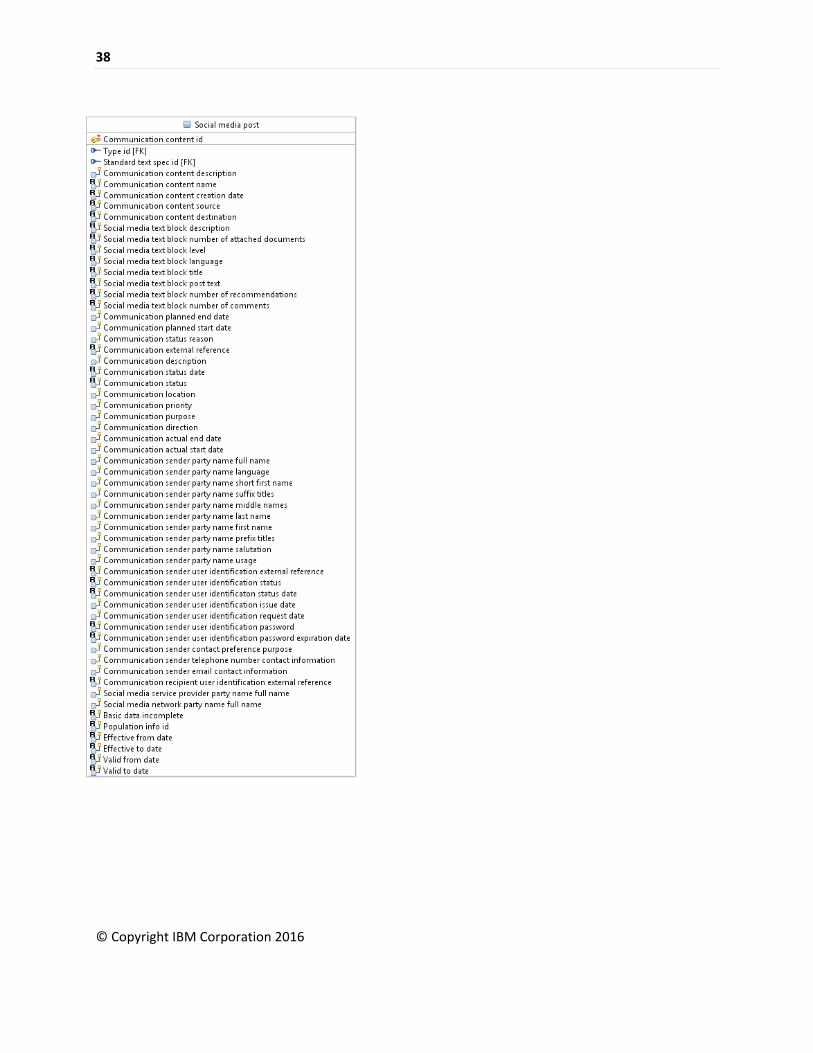
Once all of these de-normalizations have taken place, the entity from which the single physical structure can be generated is shown in the diagram below.
38
© Copyright IBM Corporation 2016

39
© Copyright IBM Corporation 2016
6 Considerations regarding of model generated artifacts in Hadoop
Typically, the details of the physical runtime environment are beyond the scope of IBM Industry Models. However, this chapter outlines some of the broader considerations relating to the customization and use of the physical data model in a Hadoop environment.
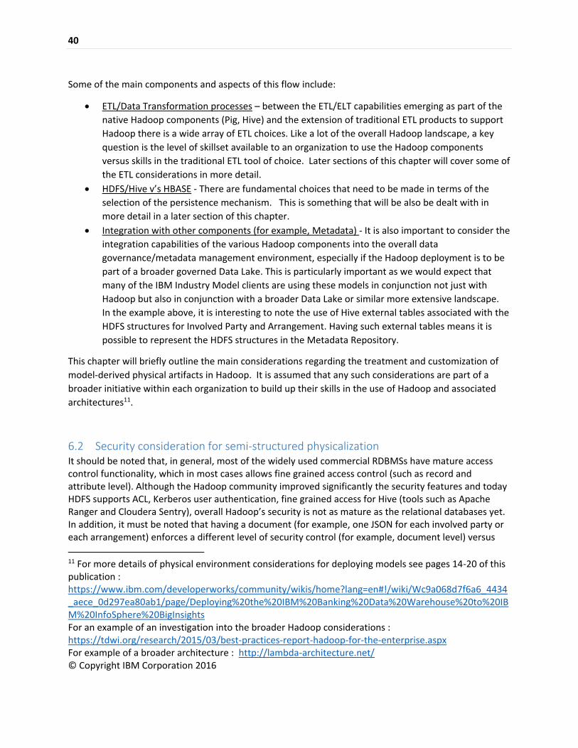
6.1 Example flows across the Hadoop runtime landscape The diagram below shows an example of a possible flow across the Hadoop landscape using IBM
Industry Models derived artifacts.
40
© Copyright IBM Corporation 2016
Some of the main components and aspects of this flow include:
ETL/Data Transformation processes – between the ETL/ELT capabilities emerging as part of the
native Hadoop components (Pig, Hive) and the extension of traditional ETL products to support
Hadoop there is a wide array of ETL choices. Like a lot of the overall Hadoop landscape, a key
question is the level of skillset available to an organization to use the Hadoop components
versus skills in the traditional ETL tool of choice. Later sections of this chapter will cover some of
the ETL considerations in more detail.
HDFS/Hive v’s HBASE - There are fundamental choices that need to be made in terms of the
selection of the persistence mechanism. This is something that will be also be dealt with in
more detail in a later section of this chapter.
Integration with other components (for example, Metadata) - It is also important to consider the
integration capabilities of the various Hadoop components into the overall data
governance/metadata management environment, especially if the Hadoop deployment is to be
part of a broader governed Data Lake. This is particularly important as we would expect that
many of the IBM Industry Model clients are using these models in conjunction not just with
Hadoop but also in conjunction with a broader Data Lake or similar more extensive landscape.
In the example above, it is interesting to note the use of Hive external tables associated with the
HDFS structures for Involved Party and Arrangement. Having such external tables means it is
possible to represent the HDFS structures in the Metadata Repository.
This chapter will briefly outline the main considerations regarding the treatment and customization of
model-derived physical artifacts in Hadoop. It is assumed that any such considerations are part of a
broader initiative within each organization to build up their skills in the use of Hadoop and associated
architectures11.
6.2 Security consideration for semi-structured physicalization It should be noted that, in general, most of the widely used commercial RDBMSs have mature access control functionality, which in most cases allows fine grained access control (such as record and attribute level). Although the Hadoop community improved significantly the security features and today HDFS supports ACL, Kerberos user authentication, fine grained access for Hive (tools such as Apache Ranger and Cloudera Sentry), overall Hadoop’s security is not as mature as the relational databases yet. In addition, it must be noted that having a document (for example, one JSON for each involved party or each arrangement) enforces a different level of security control (for example, document level) versus
11 For more details of physical environment considerations for deploying models see pages 14-20 of this publication : https://www.ibm.com/developerworks/community/wikis/home?lang=en#!/wiki/Wc9a068d7f6a6_4434_aece_0d297ea80ab1/page/Deploying%20the%20IBM%20Banking%20Data%20Warehouse%20to%20IBM%20InfoSphere%20BigInsights For an example of an investigation into the broader Hadoop considerations : https://tdwi.org/research/2015/03/best-practices-report-hadoop-for-the-enterprise.aspx For example of a broader architecture : http://lambda-architecture.net/

41
© Copyright IBM Corporation 2016
attribute level in the relational/structured data. In general, ensuring attribute level security on semi-structured (or unstructured) data is far more difficult than controlling access on structured data. For Hadoop deployment with strong security requirements, it is worth considering Apache Accumulo, which not only supports nested structures but has strong access control capabilities.
6.3 Hive v’s HBASE
Hive and HBASE are two separate capabilities both of which are built on top of Hadoop. Hive is intended for analytical querying of data collected over a period of time. For example, calculate trends, summarize website logs but it can't be used for real time queries. HBASE is intended for real-time querying of big data.
Hive is specifically intended for data warehouse-style operations. It provides a SQL-like language, and hence it is comparatively easy to write batch/Hadoop jobs. While it has support for basic indexes, it is not focused on providing support for real-time activities. An advantage of support of SQL-like language is that it possibly allows business users to write their own jobs if they have some background in SQL. HBASE is a column-oriented datastore which is intended for high performance process on high throughput systems. The main advantage of HBASE over HDFS/Hive is that HBASE it is updateable (but this comes at a cost of flexibility and performance). As HBASE is optimised for large sparse datasets (lots of columns which are only occasionally populated), it stores coordinates, and a timestamp for each HBASE cell which incurs a significant overhead for non-sparse datasets.
Overall, HBASE is not as flexible as HDFS or as performant on batch access, but it does have the advantage of being updateable. Although it should generally be avoided in favour of HDFS, it can be a useful option for managing updates of a very large dimension table which has a known and limited access pattern.
6.4 Query performance
In general, the performance of queries against IBM Industry Model generated artifacts will typically depend on a range of external factors. Organizations are encouraged to carry out the necessary investigations into the most suitable Hadoop query strategy12.
Queries on HBASE are performant on searches over the KEY columns or partial key searches (but keys must be supplied from outer most column inwards). HBASE is fast for key scans, for example select * from customer_names where customer_id (the key) = 50000000 returns subsecond, but substantially slower than HDFS/Hive format for mass scans... , for example select count(1) from customer_names.
12 For a good example of comparative query performances : https://support.sas.com/resources/papers/data-modeling-hadoop.pdf
42
© Copyright IBM Corporation 2016
In other words it is better to do a few random IOs (seeks) than a lot of sequential, but better to do a lot of sequential than a lot of random (seeks), as disk seeks are much slower than sequential access. Therefore, the choice of Key and the order of the columns therein is very important.13
6.5 ETL considerations
In general, there is likely to be a need for an organization to undertake a significant investigation of the ETL strategy necessary for a data management environment that includes Hadoop technology. A key consideration is the review of the Hadoop capabilities of traditional ETL tools versus the ETL capabilities appearing in some of the Hadoop components14.
Initial Load - Loading data to a HBASE table is significantly slower than to HFDS. This is because HBASE is doing a lot more than HDFS (for example, updating KeyValues, setting the most current row or specified timestamps, etc.)
Supports for Updates – Hive now support Updates (and delete) via its Hive ACID updates capability (which is implemented as a form of bucketed merge). It’s limited to ORC tables and it’s not suitable for very frequently updated tables. HBASE has support for Updates and Inserts.
13 The above comparative query times are based on query performance tests carried out by IBM Industry Models team in 2013/2014. These figures are included as general indications of performance differences. The actual performance differences a client is likely to experience will depend on a range of different factors (variant of Hadoop technology used, SQL of queries, volumetrics of the data, partitioning strategy, etc). 14 Example of Apache Hadoop specific ETL features : http://www.ibm.com/developerworks/library/bd-hivetool/
43
© Copyright IBM Corporation 2016
7 Appendix - Advanced techniques for physicalization of the IBM
Industry Models with nested structures utilizing Hive and
Parquet/Avro
This appendix demonstrates a few techniques for flattening of relational structures while keeping the many to one or many to many relationships. This technique benefits from one of the five V-s of big data technologies – the Variety (in particular support for semi-structured data).
All examples here require Hive 0.13.0 or newer (they were developed with CDH 5.5.1 / Hive 1.1.0).
HiveQL supports a few nested constructs, which allow storing many values of a similar type in the same record:
ARRAY (val1, val2…) MAP (key1, val1, key2, val2…)
They are often used in conjunction with STRUCT(val1, val2,…valn) or NAMED_STRUCT(name1,val1,name2,val2…namen,valn).
In this appendix we focus on how to query the data that is already stored in files which support nested structures (in particular Parquet and AVRO). The figures in section 4.1 show some options on how to create those files, but in general, Hive might not be the most optimal way due to performance and complexity considerations. Most ETL tools would be able to write the files straight to HDFS bypassing Hive. As a next step, an external Hive table could be created pointing to those files or a Hive table could be loaded from the content of the files generated by the ETL tool, although duplicating data should be avoided as it increases the data governance requirements and processing time.
For the purpose of the examples in this section, we will load a few sample records using HiveQL utilizing two different approaches.
7.1 Support for nested structures utilizing ARRAY
One of the main entities in BFMDW is the ‘Arrangement’, which is related to few other entities, but for the purpose of this scenario we consider one of the simplest relationships – the ‘Arrangement Alternative Identifier’ to ‘Arrangement’ (m:1).
7.1.1 Data structure definition
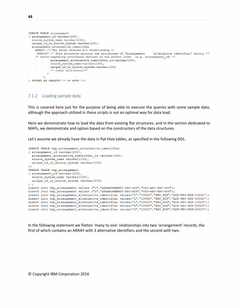
The following script creates a sample arrangement table in Hive, which manages the alternative identifiers (0, 1 or many) into an array:
44
© Copyright IBM Corporation 2016
7.1.2 Loading sample data
This is covered here just for the purpose of being able to execute the queries with some sample data, although the approach utilized in these scripts is not an optimal way for data load.
Here we demonstrate how to load the data from existing flat structures, and in the section dedicated to MAPs, we demonstrate and option based on the constructors of the data structures.
Let’s assume we already have the data in flat Hive tables, as specified in the following DDL:
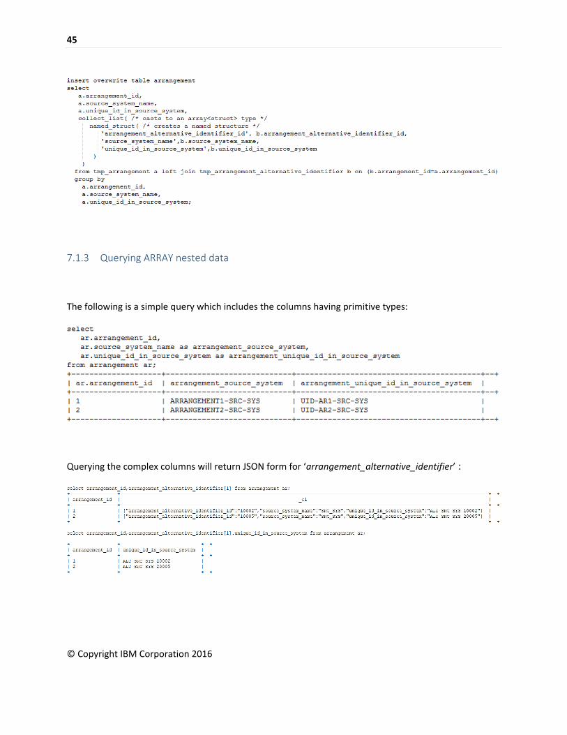
In the following statement we flatten ‘many to one’ relationships into two ‘arrangement’ records, the first of which contains an ARRAY with 3 alternative identifiers and the second with two.
45
© Copyright IBM Corporation 2016
7.1.3 Querying ARRAY nested data
The following is a simple query which includes the columns having primitive types:
Querying the complex columns will return JSON form for ‘arrangement_alternative_identifier’ :

46
© Copyright IBM Corporation 2016
All queries above keep the number of records as of the top level, which is similar to the vertical flattening. To perform a horizontal flattening as might be required by a report, we could use the INLINE function and LATERAL VIEW. This is similar to join between the master record and the nested detailed record (although it is not the same).

47
© Copyright IBM Corporation 2016
7.2 Support for nested structures utilizing MAP
This example is loosely based on the BFMDW ‘Arrangement’, ‘Accounting Unit’ and ‘Accounting Unit Balance’. Each arrangement might have 0, 1 or many Accounting Unit types (different classifications) and further, each Accounting Unit may have 0, 1 or more Accounting Unit Balances (also different classifications).
7.2.1 Creating sample table with MAP based nested structures
7.2.2 Loading sample data
As mentioned above, the data load approach utilized in this example is just for demonstration purposes:
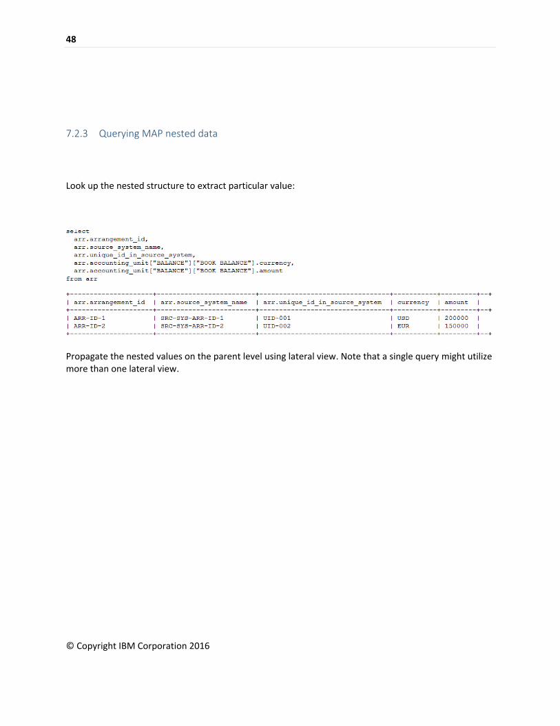
48
© Copyright IBM Corporation 2016
7.2.3 Querying MAP nested data
Look up the nested structure to extract particular value:
Propagate the nested values on the parent level using lateral view. Note that a single query might utilize more than one lateral view.

49
© Copyright IBM Corporation 2016

50
© Copyright IBM Corporation 2016
IMW14872USEN-00