Embed Size (px)
Citation preview
Guidelines for Evaluating Ground-Water Flow Models
By Thomas E. Reilly and Arlen W. Harbaugh
Abstract
Ground-water flow modeling is an important tool fre-quently used in studies of ground-water systems. Reviewers and users of these studies have a need to evaluate the accuracy or reasonableness of the ground-water flow model. This report provides some guidelines and discussion on how to evaluate complex ground-water flow models used in the investigation of ground-water systems. A consistent thread throughout these guidelines is that the objectives of the study must be specified to allow the adequacy of the model to be evaluated.
Introduction
The simulation of ground-water flow systems using com-puter models is standard practice in the field of hydrology. Models are used for a variety of purposes that include educa-tion, hydrologic investigation, water management, and legal determination of responsibility. In the most general terms, a model is a simplified representation of the appearance or oper-ation of a real object or system. Ground-water flow models rep-resent the operation of a real ground-water system with mathe-matical equations solved by a computer program. A difficulty that faces all individuals attempting to use the results of a model is the development of an understanding of the strengths and lim-itations of a model analysis without having to reproduce the entire analysis.
The primary purpose of this report is to help users of reports that document ground-water flow models evaluate the adequacy or appropriateness of a model. A secondary purpose for this report is to provide for model developers a guide to the information that should be included in model documentation. The information in this report is mainly qualitative. It reflects the views developed by the authors on the basis of over 50 years combined experience with ground-water modeling. The authors have used models, reviewed modeling studies and reports, pro-vided modeling advice, taught modeling courses, and devel-oped computer model programs.
It is important to distinguish among three terms we use to discuss the modeling process: conceptual model, computer
model program, and model. A “conceptual model” is the hydrologist’s concept of a ground-water system. A “computer model program” is a computer program that solves ground-water equations. Computer model programs are general pur-pose in that they can be used to simulate a variety of specific systems by varying input data. A “model” is the application of a computer model program to simulate a specific system. Thus, a model incorporates the model program and all of the input data required to represent a ground-water system. The modeler attempts to incorporate what he or she believes to be the most important aspects of the conceptual model into a model so that the model will provide useful information about the system.
The information provided in this report is generally rele-vant to all types of ground-water flow model programs; how-ever, the examples cited throughout the report use the model program MODFLOW (Harbaugh and others, 2000).
This report reviews the important aspects of simulating a ground-water flow system using a computer model program and explains the ramifications of various design decisions. An important part of the information necessary for evaluating a model is the intended use of a model, because it is impossible to develop a model that will fulfill all purposes. Further, the intended use must be specific as opposed to general. For exam-ple, saying that a model will be used to evaluate water-management alternatives is inadequate. Specific information about the alternatives to be considered also would be necessary. Thus, a consistent thread throughout this report is the need to consider the purpose of a model when evaluating the appropri-ateness of the model.
Appropriateness of the Computer Model Program
Many computer model programs are available for simulat-ing ground-water systems. Each computer model program can be characterized by the mathematical method used to represent ground-water equations (Konikow and Reilly, 1999), assump-tions, and the range of simulation capabilities. For example, the mathematical method in MODFLOW is finite difference in space and time, with backward difference for time. Major
2 Guidelines for Evaluating Ground-Water Flow Models
assumptions are (1) confined three-dimensional flow with water-table approximations, and (2) principal directions of hydraulic conductivity are aligned with the coordinate axes. A variety of hydrologic capabilities are included, for example, the simulation of wells, rivers, recharge, and ground-water evapo-transpiration. There also are simple analytical models that assume homogeneous conditions for one or two dimensions that can be used to solve some problems. The tool or computer model program used can be as simple or as complex as required for the problem, but the method, assumptions, and capabilities must be evaluated to assure that the tool is appropriate and can provide scientifically defensible results.
Questions to be answered in the evaluation of the appropri-ateness of the modeling program are:
1. Are the objectives of the study clearly stated?
2. Is the mathematical method used in the computer model program appropriate to address the problem?
3. Does the numerical or analytical model selected for use simulate the important physical processes needed to adequately represent the system?
Different Modeling Approaches to Address a Problem
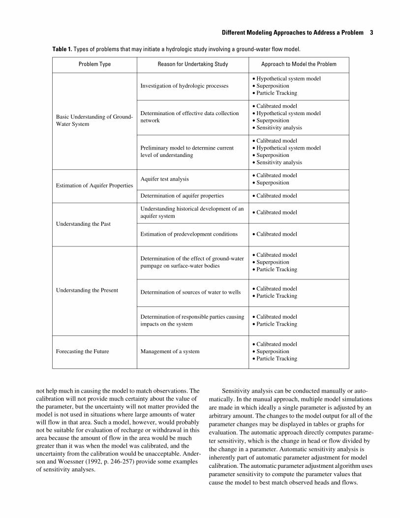
A general-purpose computer model program such as MODFLOW can be used in many ways to address a problem as illustrated in table 1. Approaches to a problem that are com-monly used are: calibrated model, hypothetical system model, sensitivity analysis, superposition, and particle tracking. Fre-quently, several approaches are combined to address a problem.
A Calibrated Model
A model that is “calibrated” is required to address many hydrologic problems. Model calibration in its most limited meaning is the modification of model input data for the purpose of making the model more closely match observed heads and flows. Adjustment of parameters can be done manually or auto-matically by using nonlinear regression statistical techniques. In the broader meaning of model calibration, parameter adjust-ment is only one aspect of model calibration. Key aspects of the model, such as the conceptualization of the flow system, that influence the capability of the model to meet the problem objec-tives also are evaluated and adjusted as needed during calibra-tion. For example, it may be noticed that some of the parameters that result in the best match to observations are not reasonable based on other knowledge of their values. This may indicate that there is a conceptualization problem with the model. Thus, the closeness of fit between the simulated and observed condi-tions, and the extent to which important aspects of the simula-tion are incorporated in the model are both important in evalu-ating how well a model is calibrated. In practice, calibration is
conducted differently by each investigator; some examples that discuss calibrated models are Luckey and others (1986), Buxton and Smolensky (1999), and Anderson and Woessner (1992, section 8.3 and 8.4).
The amount of effort that is required in calibrating a ground-water flow model is dependent upon the intended use of the model (that is, the objective of the investigation). Most mod-els of specific ground-water systems that are used to estimate aquifer properties, understand the past, understand the present, or to forecast the future are calibrated by matching observed heads and flows. Determining if the calibration is sufficient for the intended use of the model is very important in evaluating whether the model has been constructed appropriately. (See later section for more on evaluating the adequacy of model calibration.)
A Hypothetical Model
A hypothetical model is a model of an idealized or repre-sentative system as opposed to a model of a specific system. In an attempt to understand the basic operation of a ground-water system, the determination of whether to develop a model of a hypothetical idealized system or a model of an actual system greatly affects the amount of data needed to construct the model. Hypothetical models are not calibrated, but input data are frequently adjusted during model development to make the model fit the idealized system or to test how the model responds. The utility of hypothetical models is that the system can be defined exactly and the cause and effect processes under investigation can be clearly identified with minimal cost. The input data needed to define the hypothetical system can be as simple or as complex as required to investigate the processes of interest. No effort is required to collect and interpret data from an actual ground-water system and no uncertainty exists in the ability of the model to represent the system, which results in substantial cost savings compared to making a model of a spe-cific system. Hypothetical models have been used to examine various processes that affect or are affected by ground-water flow, for example: boundary conditions (Franke and Reilly, 1987), contributing areas to wells (Morrissey, 1989; Reilly and Pollock, 1993), and model calibration (Hill and others, 1998).
Sensitivity Analysis
Sensitivity analysis is the evaluation of model input parameters to see how much they affect model outputs, which are heads and flows. The relative effect of the parameters helps to provide fundamental understanding of the simulated system. Sensitivity analysis also is inherently part of model calibration. The most sensitive parameters will be the most important parameters for causing the model to match observed values. For example, an area in which the model is insensitive to hydraulic conductivity generally indicates an area where there is rela-tively little water flowing. If the model is being calibrated, then changing the value of hydraulic conductivity in this area will
Different Modeling Approaches to Address a Problem 3
Table 1. Types of problems that may initiate a hydrologic study involving a ground-water flow model.
Problem Type Reason for Undertaking Study Approach to Model the Problem
Basic Understanding of Ground-Water System
Investigation of hydrologic processes• Hypothetical system model• Superposition• Particle Tracking
Determination of effective data collection network
• Calibrated model• Hypothetical system model• Superposition• Sensitivity analysis
Preliminary model to determine current level of understanding
• Calibrated model• Hypothetical system model• Superposition• Sensitivity analysis
Estimation of Aquifer PropertiesAquifer test analysis
• Calibrated model• Superposition
Determination of aquifer properties • Calibrated model
Understanding the Past
Understanding historical development of an aquifer system
• Calibrated model
Estimation of predevelopment conditions • Calibrated model
Understanding the Present
Determination of the effect of ground-water pumpage on surface-water bodies
• Calibrated model• Superposition• Particle Tracking
Determination of sources of water to wells• Calibrated model• Particle Tracking
Determination of responsible parties causing impacts on the system
• Calibrated model• Particle Tracking
Forecasting the Future Management of a system• Calibrated model• Superposition• Particle Tracking
not help much in causing the model to match observations. The calibration will not provide much certainty about the value of the parameter, but the uncertainty will not matter provided the model is not used in situations where large amounts of water will flow in that area. Such a model, however, would probably not be suitable for evaluation of recharge or withdrawal in this area because the amount of flow in the area would be much greater than it was when the model was calibrated, and the uncertainty from the calibration would be unacceptable. Ander-son and Woessner (1992, p. 246-257) provide some examples of sensitivity analyses.
Sensitivity analysis can be conducted manually or auto-matically. In the manual approach, multiple model simulations are made in which ideally a single parameter is adjusted by an arbitrary amount. The changes to the model output for all of the parameter changes may be displayed in tables or graphs for evaluation. The automatic approach directly computes parame-ter sensitivity, which is the change in head or flow divided by the change in a parameter. Automatic sensitivity analysis is inherently part of automatic parameter adjustment for model calibration. The automatic parameter adjustment algorithm uses parameter sensitivity to compute the parameter values that cause the model to best match observed heads and flows.
4 Guidelines for Evaluating Ground-Water Flow Models
Superposition
Superposition (Reilly and others, 1987) is a modeling approach that is useful in saving time and effort and eliminating uncertainty in some model evaluations. Models that are designed to use superposition evaluate only changes in stress and changes in responses. Most aquifer tests that analyze draw-down use superposition. Only the change in heads (the draw-down) and change in flows are analyzed, which assumes the response of the system is only due to the stress imposed and is not due to other processes in the system. The absolute value of the head and a quantification of the actual regional flows are not needed. In the past, superposition was frequently used with ana-log model analysis of ground-water systems because electrical simulation of areal stresses and boundary conditions was extremely difficult. As modern numerical computer models made simulation of all stress conditions easier, superposition was used less frequently in areal models. If the problem to be solved involves only the evaluation of a change due to some change in stress, however, the application of superposition can greatly simplify the data needs for model development. Super-position is strictly applicable to linear problems only, that is, constant saturated thickness and linear boundary conditions. If the system is relatively linear, however, for example the satu-rated thickness does not change by a significant portion (no absolute guidance can be given, but some investigators have used a 10 percent change in thickness as a rule of thumb), super-position can still provide reasonably accurate answers. Cur-rently, superposition is used primarily in the simulation of aqui-fer tests, in that only changes due to the imposed change in stress (that is, the well discharge) are simulated and zero draw-downs are specified as the initial and boundary conditions; example simulations are presented in Prince and Schneider (1989) and McAda (2001).
Particle Tracking
Particle tracking (Pollock, 1989) is the determination of the path a particle will take through a three-dimensional ground-water flow system. The determination of the paths of water in the flow system aids in conceptualizing and quantify-ing the sources of water in a modeled system. For example, Buxton and others (1991) used particle-tracking analysis to determine recharge areas on Long Island, New York, and Mod-ica and others (1997) made use of particle tracking in the con-text of a ground-water flow model to understand the patterns and age distribution of ground-water flow to streams of the Atlantic Coastal Plain. Although particle tracking is useful in determining advective transport, this report does not address the use of models to determine transport of chemicals, but rather refers to the approach of using particle tracking to understand the flow system.
Spatial and Temporal Approaches
In addition to the overall modeling approaches discussed above, many model programs can be used in one, two, or three dimensions, and they can be applied as transient or steady state. The simplification of the model domain to one or two dimen-sions, either in plan view or cross section, is used to minimize the cost of constructing a model. The simplification of the sys-tem to one or two dimensions, however, must be consistent with the flow field under investigation and consistent with the objec-tives of the study. Consistent with the flow field, means that there is no or negligible flow orthogonal to the line or plane of the one- or two-dimensional system being simulated.
Steady-state models are used widely, although true steady-state conditions do not exist in natural systems. All natural sys-tems fluctuate in response to climatic variations that can be sea-sonal, annual, decadal or longer. In steady-state models, an assumption is made that a system can be represented by a state of dynamic equilibrium or an approximate equilibrium condi-tion. If the objectives of the investigation do not require infor-mation on the time it takes for a system to respond to new stresses or the response of the system between periods of rela-tive equilibrium, then simulation of the system as a steady-state system may be a reasonable approach. However, if the system is not at a period of equilibrium or approximate equilibrium dur-ing the periods of interest, then a transient analysis is required.
Questions to be answered in the evaluation of the appropri-ateness of the modeling approach to analyze the problem are:
1. Is the overall approach (calibrated model, hypothetical system model, sensitivity analysis, superposition, and particle tracking) for using simulation in addressing the objectives clearly stated and appropriate?
2. If the analysis is not three dimensional, is the representation of the system using one or two dimensions appropriate to meet the objectives of the study and justified in the report?
3. If the model is steady state, is adequate information provided to justify that the system is reasonably close to a steady-state condition?
Models of ground-water systems may be very different in their level of complexity. Whether the model design and approach are appropriate for the problem being investigated must be evaluated. This evaluation requires a clear statement of the problem to be investigated and the modeling approach. A further requirement is an understanding of the model design. The remainder of this report focuses on specific aspects of model design that should be examined in determining the worth of a particular model. These aspects are: discretization and rep-resentation of the hydrogeologic framework, boundary condi-tions, initial conditions, accuracy of the numerical solution, and accuracy of calibration for the intended use of the model.
Discretization and Representation of the Hydrogeologic Framework 5
Discretization and Representation of the Hydrogeologic Framework
A fundamental aspect of numerical models is the represen-tation of the real world by discrete volumes of material. The volumes are called cells in the finite-difference method, and the volumes are called elements in the finite-element method. The accuracy of the model is limited by the size of the discrete vol-umes. Further, for transient models, time is represented by dis-crete increments of time called time steps in most model pro-grams. The size of the time steps also has an impact on the accuracy of a model. The issue of the size of the discrete vol-umes and time steps is discussed for the finite-difference method.
Cell Size
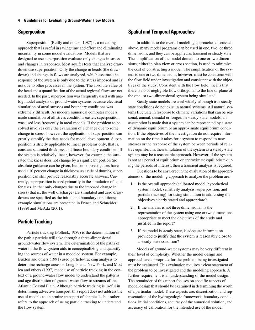
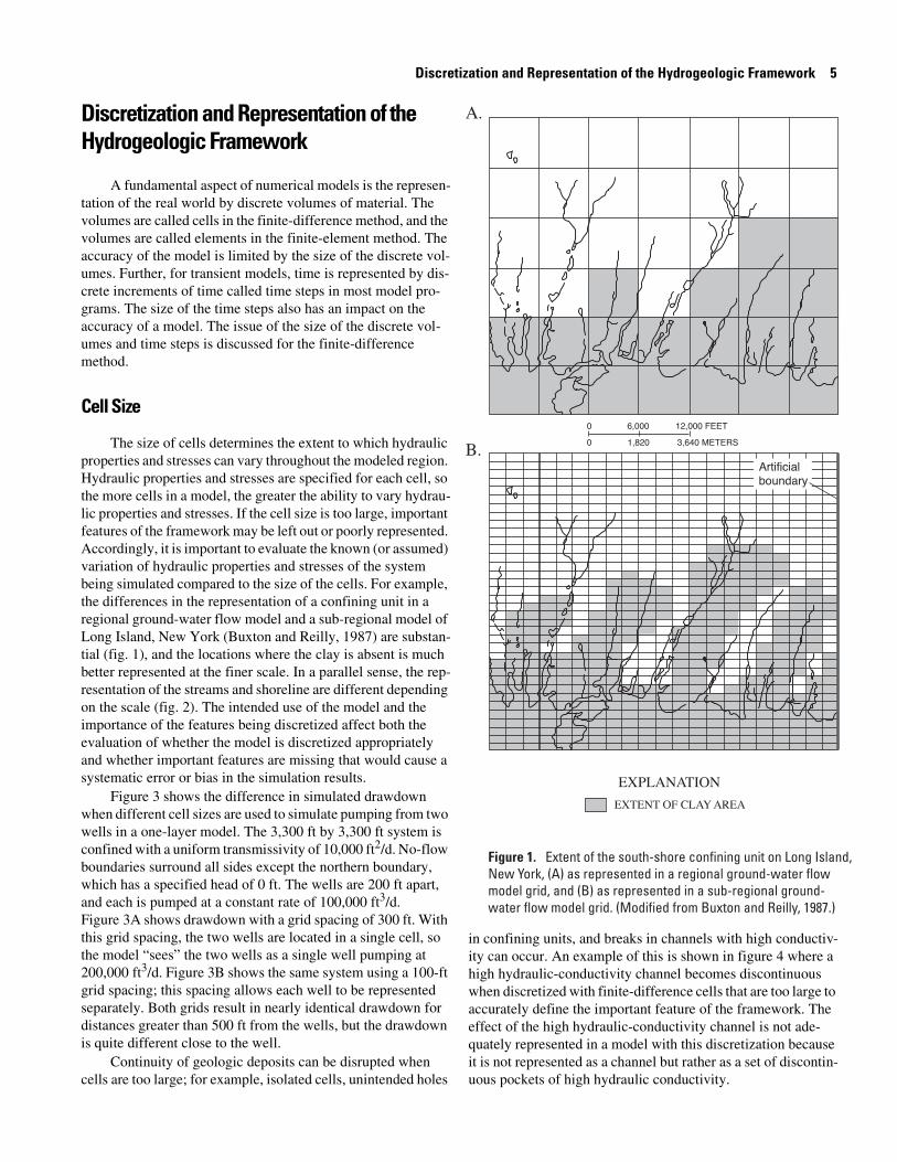
The size of cells determines the extent to which hydraulic properties and stresses can vary throughout the modeled region. Hydraulic properties and stresses are specified for each cell, so the more cells in a model, the greater the ability to vary hydrau-lic properties and stresses. If the cell size is too large, important features of the framework may be left out or poorly represented. Accordingly, it is important to evaluate the known (or assumed) variation of hydraulic properties and stresses of the system being simulated compared to the size of the cells. For example, the differences in the representation of a confining unit in a regional ground-water flow model and a sub-regional model of Long Island, New York (Buxton and Reilly, 1987) are substan-tial (fig. 1), and the locations where the clay is absent is much better represented at the finer scale. In a parallel sense, the rep-resentation of the streams and shoreline are different depending on the scale (fig. 2). The intended use of the model and the importance of the features being discretized affect both the evaluation of whether the model is discretized appropriately and whether important features are missing that would cause a systematic error or bias in the simulation results.
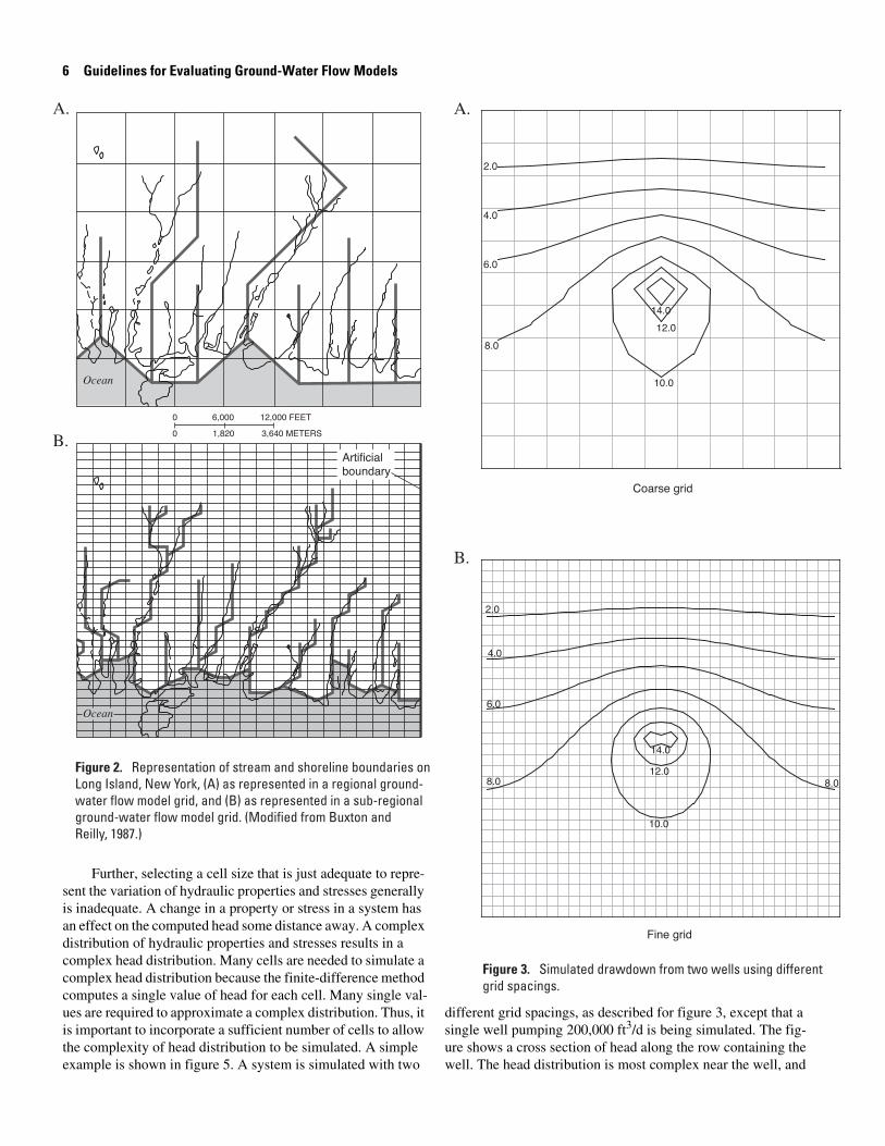
Figure 3 shows the difference in simulated drawdown when different cell sizes are used to simulate pumping from two wells in a one-layer model. The 3,300 ft by 3,300 ft system is confined with a uniform transmissivity of 10,000 ft2/d. No-flow boundaries surround all sides except the northern boundary, which has a specified head of 0 ft. The wells are 200 ft apart, and each is pumped at a constant rate of 100,000 ft3/d. Figure 3A shows drawdown with a grid spacing of 300 ft. With this grid spacing, the two wells are located in a single cell, so the model “sees” the two wells as a single well pumping at 200,000 ft3/d. Figure 3B shows the same system using a 100-ft grid spacing; this spacing allows each well to be represented separately. Both grids result in nearly identical drawdown for distances greater than 500 ft from the wells, but the drawdown is quite different close to the well.
Continuity of geologic deposits can be disrupted when cells are too large; for example, isolated cells, unintended holes
in confining units, and breaks in channels with high conductiv-ity can occur. An example of this is shown in figure 4 where a high hydraulic-conductivity channel becomes discontinuous when discretized with finite-difference cells that are too large to accurately define the important feature of the framework. The effect of the high hydraulic-conductivity channel is not ade-quately represented in a model with this discretization because it is not represented as a channel but rather as a set of discontin-uous pockets of high hydraulic conductivity.
6 Guidelines for Evaluating Ground-Water Flow Models
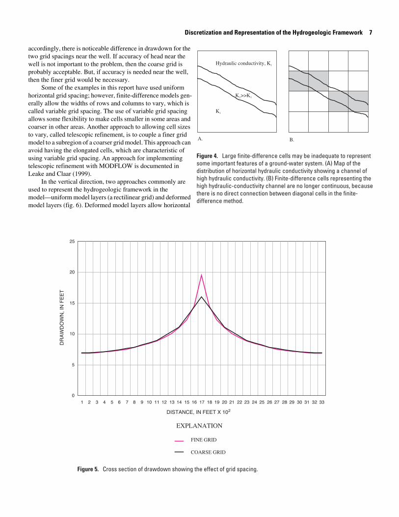
Further, selecting a cell size that is just adequate to repre-sent the variation of hydraulic properties and stresses generally is inadequate. A change in a property or stress in a system has an effect on the computed head some distance away. A complex distribution of hydraulic properties and stresses results in a complex head distribution. Many cells are needed to simulate a complex head distribution because the finite-difference method computes a single value of head for each cell. Many single val-ues are required to approximate a complex distribution. Thus, it is important to incorporate a sufficient number of cells to allow the complexity of head distribution to be simulated. A simple example is shown in figure 5. A system is simulated with two
different grid spacings, as described for figure 3, except that a single well pumping 200,000 ft3/d is being simulated. The fig-ure shows a cross section of head along the row containing the well. The head distribution is most complex near the well, and
Discretization and Representation of the Hydrogeologic Framework 7
accordingly, there is noticeable difference in drawdown for the two grid spacings near the well. If accuracy of head near the well is not important to the problem, then the coarse grid is probably acceptable. But, if accuracy is needed near the well, then the finer grid would be necessary.
Some of the examples in this report have used uniform horizontal grid spacing; however, finite-difference models gen-erally allow the widths of rows and columns to vary, which is called variable grid spacing. The use of variable grid spacing allows some flexibility to make cells smaller in some areas and coarser in other areas. Another approach to allowing cell sizes to vary, called telescopic refinement, is to couple a finer grid model to a subregion of a coarser grid model. This approach can avoid having the elongated cells, which are characteristic of using variable grid spacing. An approach for implementing telescopic refinement with MODFLOW is documented in Leake and Claar (1999).
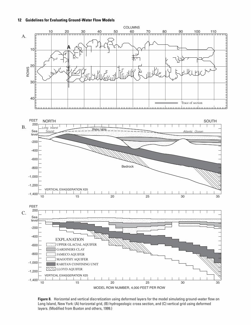
In the vertical direction, two approaches commonly are used to represent the hydrogeologic framework in the model—uniform model layers (a rectilinear grid) and deformed model layers (fig. 6). Deformed model layers allow horizontal
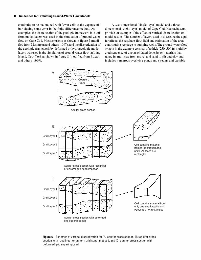
8 Guidelines for Evaluating Ground-Water Flow Models
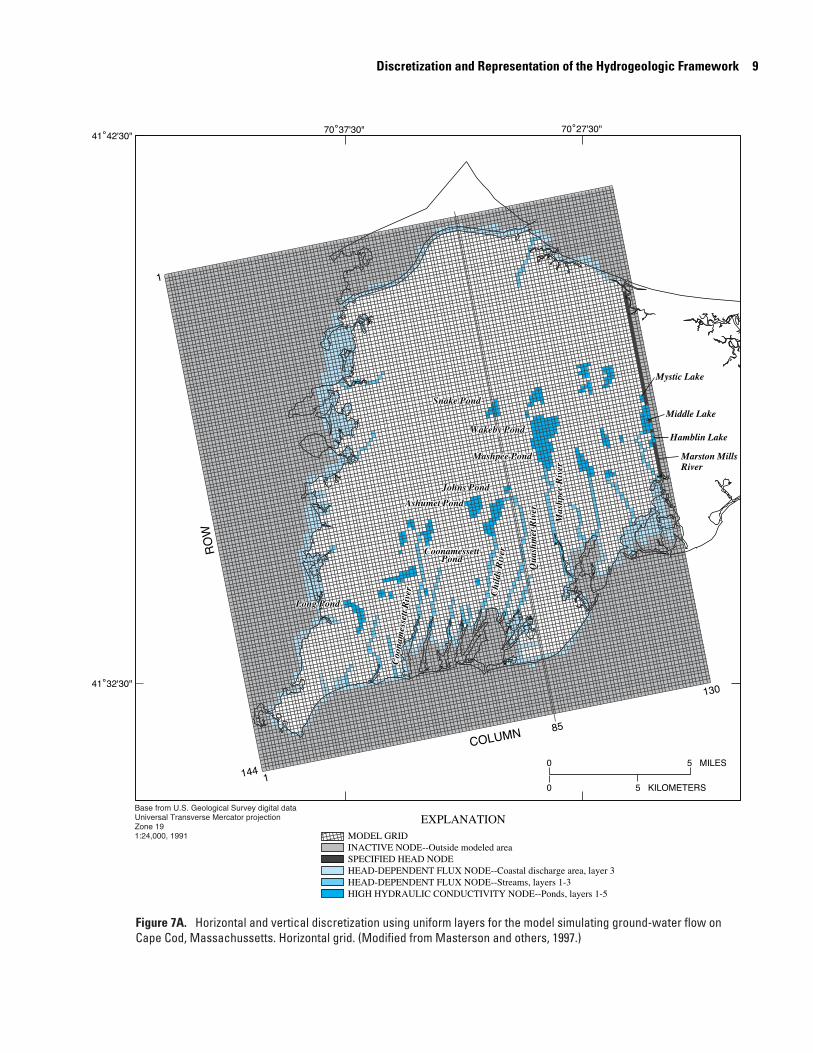
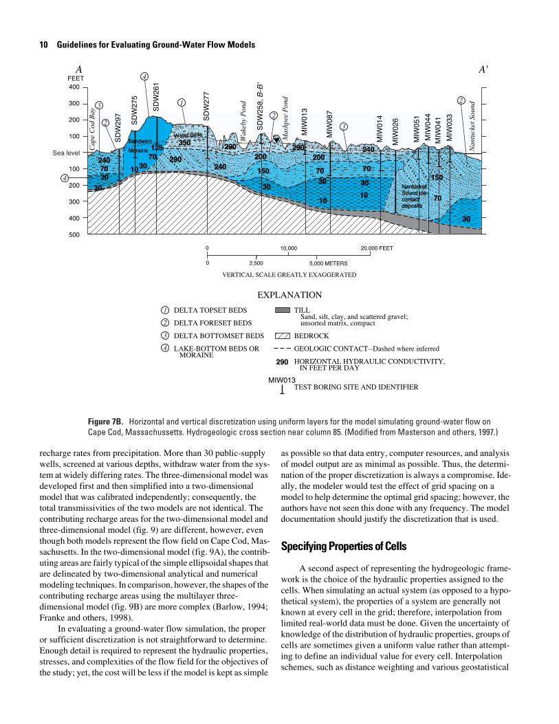
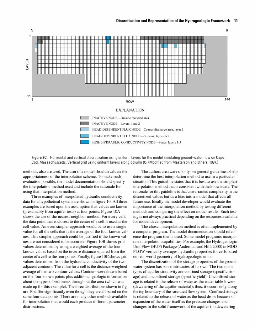
continuity to be maintained with fewer cells at the expense of introducing some error in the finite-difference method. As examples, the discretization of the geologic framework into uni-form model layers was used in the simulation of ground-water flow on Cape Cod, Massachusetts as shown in figure 7 (modi-fied from Masterson and others, 1997), and the discretization of the geologic framework by deformed or hydrogeologic model layers was used in the simulation of ground-water flow on Long Island, New York as shown in figure 8 (modified from Buxton and others, 1999).
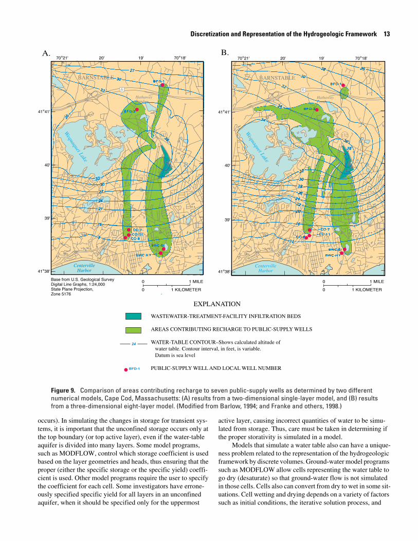
A two-dimensional (single-layer) model and a three-dimensional (eight-layer) model of Cape Cod, Massachusetts, provide an example of the effect of vertical discretization on model results. The number of layers used to discretize the aqui-fer affects the resultant flow field and estimation of the area contributing recharge to pumping wells. The ground-water flow system in the example consists of a thick (250–500 ft) multilay-ered sequence of unconsolidated deposits or materials that range in grain size from gravel and sand to silt and clay and includes numerous overlying ponds and streams and variable
Discretization and Representation of the Hydrogeologic Framework 9
10 Guidelines for Evaluating Ground-Water Flow Models
recharge rates from precipitation. More than 30 public-supply wells, screened at various depths, withdraw water from the sys-tem at widely differing rates. The three-dimensional model was developed first and then simplified into a two-dimensional model that was calibrated independently; consequently, the total transmissivities of the two models are not identical. The contributing recharge areas for the two-dimensional model and three-dimensional model (fig. 9) are different, however, even though both models represent the flow field on Cape Cod, Mas-sachusetts. In the two-dimensional model (fig. 9A), the contrib-uting areas are fairly typical of the simple ellipsoidal shapes that are delineated by two-dimensional analytical and numerical modeling techniques. In comparison, however, the shapes of the contributing recharge areas using the multilayer three-dimensional model (fig. 9B) are more complex (Barlow, 1994; Franke and others, 1998).
In evaluating a ground-water flow simulation, the proper or sufficient discretization is not straightforward to determine. Enough detail is required to represent the hydraulic properties, stresses, and complexities of the flow field for the objectives of the study; yet, the cost will be less if the model is kept as simple
as possible so that data entry, computer resources, and analysis of model output are as minimal as possible. Thus, the determi-nation of the proper discretization is always a compromise. Ide-ally, the modeler would test the effect of grid spacing on a model to help determine the optimal grid spacing; however, the authors have not seen this done with any frequency. The model documentation should justify the discretization that is used.
Specifying Properties of Cells
A second aspect of representing the hydrogeologic frame-work is the choice of the hydraulic properties assigned to the cells. When simulating an actual system (as opposed to a hypo-thetical system), the properties of a system are generally not known at every cell in the grid; therefore, interpolation from limited real-world data must be done. Given the uncertainty of knowledge of the distribution of hydraulic properties, groups of cells are sometimes given a uniform value rather than attempt-ing to define an individual value for every cell. Interpolation schemes, such as distance weighting and various geostatistical
Discretization and Representation of the Hydrogeologic Framework 11
methods, also are used. The user of a model should evaluate the appropriateness of the interpolation scheme. To make such evaluation possible, the model documentation should specify the interpolation method used and include the rationale for using that interpolation method.
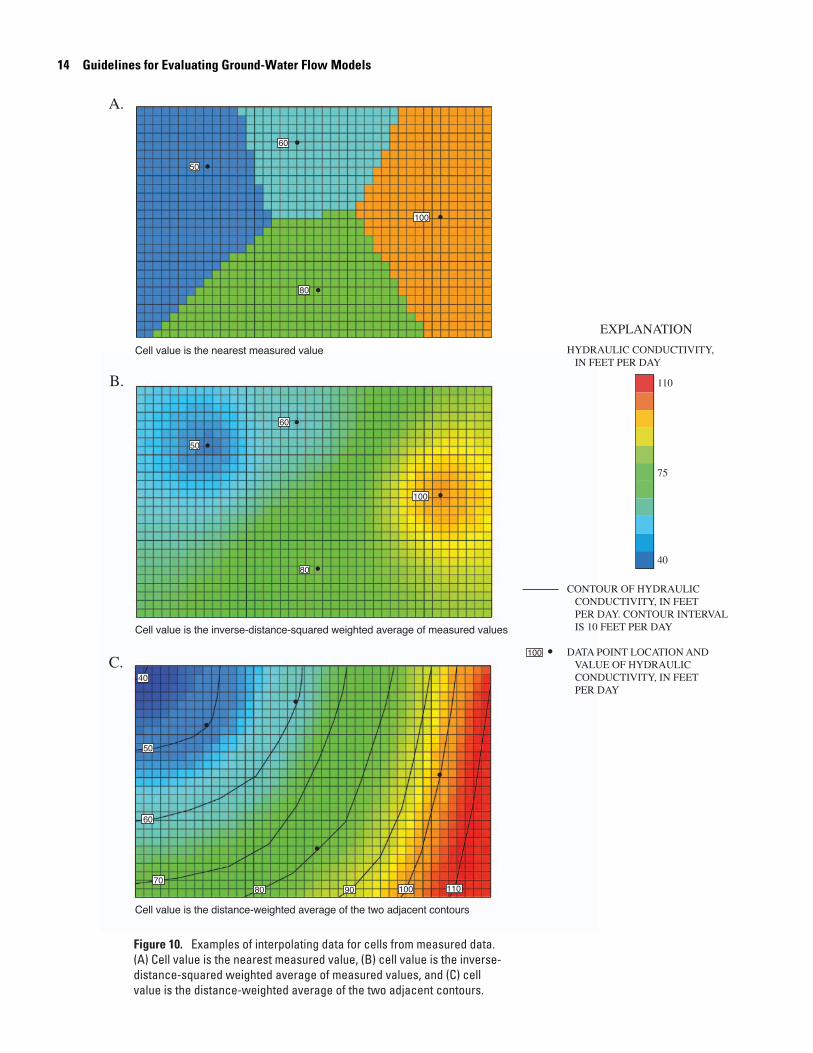
Three examples of interpolated hydraulic conductivity data for a hypothetical system are shown in figure 10. All three examples are based upon the assumption that values are known (presumably from aquifer tests) at four points. Figure 10A shows the use of the nearest-neighbor method. For every cell, the data point that is closest to the center of a cell is used as the cell value. An even simpler approach would be to use a single value for all the cells that is the average of the four known val-ues. This simpler approach could be justified if the known val-ues are not considered to be accurate. Figure 10B shows grid values determined by using a weighted average of the four known values based on the inverse distance squared from the center of a cell to the four points. Finally, figure 10C shows grid values determined from the hydraulic conductivity of the two adjacent contours. The value for a cell is the distance-weighted average of the two contour values. Contours were drawn based on the four known points plus additional geologic information about the types of sediments throughout the area (which was made up for this example). The three distributions shown in fig-ure 10 differ significantly even though they are all based on the same four data points. There are many other methods available for interpolation that would each produce different parameter distributions.
The authors are aware of only one general guideline to help determine the best interpolation method to use in a particular situation. This guideline states that it is best to use the simplest interpolation method that is consistent with the known data. The rationale for this guideline is that unwarranted complexity in the discretized values builds a bias into a model that affects all future use. Ideally the model developer would evaluate the importance of the interpolation method by testing different methods and comparing the effect on model results. Such test-ing is not always practical depending on the resources available for model development.
The chosen interpolation method is often implemented by a computer program. The model documentation should refer-ence the program that is used. Some model programs incorpo-rate interpolation capabilities. For example, the Hydrogeologic-Unit Flow (HUF) Package (Anderman and Hill, 2000) in MOD-FLOW vertically averages hydraulic properties for cells based on real-world geometry of hydrogeologic units.
The discretization of the storage properties of the ground-water system has some intricacies of its own. The two main types of aquifer storativity are confined storage (specific stor-age) and unconfined storage (specific yield). Unconfined stor-age is related to the release of water as the water table lowers (dewatering of the aquifer material); thus, it occurs only along the top boundary of the saturated flow system. Confined storage is related to the release of water as the head drops because of expansion of the water itself as the pressure changes and changes in the solid framework of the aquifer (no dewatering
12 Guidelines for Evaluating Ground-Water Flow Models
Discretization and Representation of the Hydrogeologic Framework 13
occurs). In simulating the changes in storage for transient sys-tems, it is important that the unconfined storage occurs only at the top boundary (or top active layer), even if the water-table aquifer is divided into many layers. Some model programs, such as MODFLOW, control which storage coefficient is used based on the layer geometries and heads, thus ensuring that the proper (either the specific storage or the specific yield) coeffi-cient is used. Other model programs require the user to specify the coefficient for each cell. Some investigators have errone-ously specified specific yield for all layers in an unconfined aquifer, when it should be specified only for the uppermost
active layer, causing incorrect quantities of water to be simu-lated from storage. Thus, care must be taken in determining if the proper storativity is simulated in a model.
Models that simulate a water table also can have a unique-ness problem related to the representation of the hydrogeologic framework by discrete volumes. Ground-water model programs such as MODFLOW allow cells representing the water table to go dry (desaturate) so that ground-water flow is not simulated in those cells. Cells also can convert from dry to wet in some sit-uations. Cell wetting and drying depends on a variety of factors such as initial conditions, the iterative solution process, and
14 Guidelines for Evaluating Ground-Water Flow Models
Discretization and Representation of the Hydrogeologic Framework 15
user-specified options to control wetting and drying. By varying these factors, it is possible to change the number of dry cells, and thus the head will vary. Careful evaluation is required to detect the potential for nonuniqueness and reject solutions that are unreasonable.
To avoid solver convergence problems that sometimes occur when cells can convert between wet and dry, some inves-tigators have resorted to specifying cells representing the water table as having a constant saturated thickness. It is important to evaluate the extent to which this has been done and the degree to which the thickness represented by the simulated heads var-ies from the assumed specified thickness. For steady-state mod-els, the following process can be repeated until the simulated saturated thickness is reasonably close to the specified saturated thickness:
1. Run the model.
2. Compare the simulated saturated thickness (head minus bottom elevation) to the specified saturated thickness.
3. Adjust the specified saturated thickness to match the simulated thickness.
For transient models, the changes in saturated thickness throughout the simulation can be compared to the specified sat-urated thickness to insure that the change is small compared to the total saturated thickness.
Time Steps
Transient models simulate the impact of stresses over time. In MODFLOW, time is divided into time steps, and head is computed at the end of each time step. Many time steps are required to simulate a complex distribution of head over time. This is similar to the need for many cells to represent the spatial distribution of head. It is important to incorporate enough time steps to allow the temporal complexity of head distribution to be simulated.
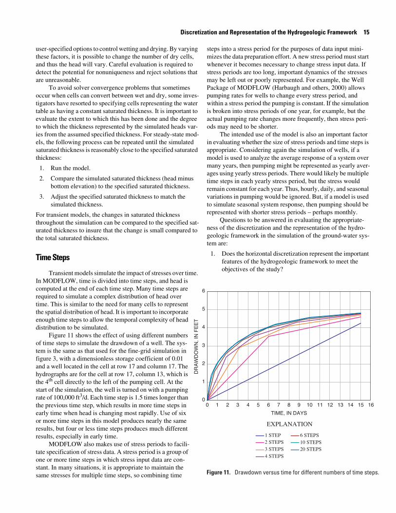
Figure 11 shows the effect of using different numbers of time steps to simulate the drawdown of a well. The sys-tem is the same as that used for the fine-grid simulation in figure 3, with a dimensionless storage coefficient of 0.01 and a well located in the cell at row 17 and column 17. The hydrographs are for the cell at row 17, column 13, which is the 4th cell directly to the left of the pumping cell. At the start of the simulation, the well is turned on with a pumping rate of 100,000 ft3/d. Each time step is 1.5 times longer than the previous time step, which results in more time steps in early time when head is changing most rapidly. Use of six or more time steps in this model produces nearly the same results, but four or less time steps produces much different results, especially in early time.
MODFLOW also makes use of stress periods to facili-tate specification of stress data. A stress period is a group of one or more time steps in which stress input data are con-stant. In many situations, it is appropriate to maintain the same stresses for multiple time steps, so combining time
steps into a stress period for the purposes of data input mini-mizes the data preparation effort. A new stress period must start whenever it becomes necessary to change stress input data. If stress periods are too long, important dynamics of the stresses may be left out or poorly represented. For example, the Well Package of MODFLOW (Harbaugh and others, 2000) allows pumping rates for wells to change every stress period, and within a stress period the pumping is constant. If the simulation is broken into stress periods of one year, for example, but the actual pumping rate changes more frequently, then stress peri-ods may need to be shorter.
The intended use of the model is also an important factor in evaluating whether the size of stress periods and time steps is appropriate. Considering again the simulation of wells, if a model is used to analyze the average response of a system over many years, then pumping might be represented as yearly aver-ages using yearly stress periods. There would likely be multiple time steps in each yearly stress period, but the stress would remain constant for each year. Thus, hourly, daily, and seasonal variations in pumping would be ignored. But, if a model is used to simulate seasonal system response, then pumping should be represented with shorter stress periods – perhaps monthly.
Questions to be answered in evaluating the appropriate-ness of the discretization and the representation of the hydro-geologic framework in the simulation of the ground-water sys-tem are:
1. Does the horizontal discretization represent the important features of the hydrogeologic framework to meet the objectives of the study?
16 Guidelines for Evaluating Ground-Water Flow Models
2. Are the physical boundaries represented appropriately in space by the discretized representation?
3. Is the horizontal discretization appropriate to represent the degree of complexity in the aquifer properties and head distribution (flow system)?
4. Does the vertical discretization adequately represent the vertical connectivity and transmitting properties of the hydrogeologic framework to meet the objectives of the study? Does the method of vertical discretization, either a rectilinear grid or deformed grid, introduce any bias into the representation of the hydrogeologic framework?
5. Is the method of assigning parameter values to individual cells explicitly explained? Is the method appropriate for the objectives of the study and the geologic environment?
6. If the ground-water system is transient, then is the specification of storage coefficients appropriate?
7. If the ground-water system is unconfined in some areas, then is the treatment of changes in saturated thickness and the potential for cells to go dry explained and appropriate? If cells have gone dry, does the resultant solution seem appropriate?
8. Is the time discretization fine enough to represent the degree of complexity in stresses and head distribution over time?
The evaluation of the proper or sufficient discretization of the hydrogeologic framework of a ground-water flow simula-tion is not straightforward to determine. The continuity of deposits and the reasonableness of the specification of values for each cell in light of the depositional environment of the hydrogeologic framework must be considered. As always, the objectives of the study also determine which features must be represented in the model and the level of detail required to ade-quately represent their effect on the flow system.
Representation of Boundary Conditions
Boundary conditions are a key component of the concep-tualization of a ground-water system. The topic of boundary conditions in the simulation of ground-water flow systems has been discussed in Franke and others (1987) and Reilly (2001).
As discussed in Reilly (2001), computer simulations of ground-water flow systems numerically evaluate the mathemat-ical equation governing the flow of fluids through porous media. This equation is a second-order partial differential equa-tion with head as the dependent variable. In order to determine a unique solution of such a mathematical problem, it is neces-sary to specify boundary conditions around the flow domain for head (the dependent variable) or its derivatives (Collins, 1961). These mathematical problems are referred to as boundary-value problems. Thus, a requirement for the solution of the mathemat-ical equation that describes ground-water flow is that boundary conditions must be prescribed over the boundary of the domain.
Boundary conditions also represent any flow or head con-straints within the flow domain. For example, recharge from percolation of precipitation, river interaction, and pumping from wells are simulated as boundary conditions. Three types of boundary conditions—specified head, specified flow, and head-dependent flow—are commonly specified in mathematical analyses of ground-water flow systems. The values of head (the dependent function) in the flow domain must satisfy the pre-assigned boundary conditions to be a valid solution.
In solving a ground-water flow problem, however, the boundary conditions are not simply mathematical constraints; they generally represent the sources and sinks of water within the system. Furthermore, their selection is critical to the devel-opment of an accurate model (Franke and others, 1987). Not only is the location of the boundaries important, but also their numerical or mathematical representation in the model. This is because many physical features that are hydrologic boundaries can be mathematically represented in more than one way. The determination of an appropriate mathematical representation of a boundary condition is dependent upon the objectives of the study. For example, if the objective of a model study is to under-stand the present and no estimate of future conditions is planned, then local surface-water bodies may be simulated as known constant-head boundaries; however, if the model is intended to forecast the response of the system to additional withdrawals that may affect the stage of the surface-water bod-ies, then a constant head is not appropriate and a more complex boundary is required. A model of a particular area developed for one study with a particular set of objectives may not necessarily be appropriate for another study in the same area, but with dif-ferent objectives. All of these aspects of boundary conditions must be considered in evaluating the strengths and weaknesses of a ground-water flow model.
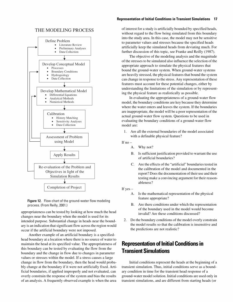
In the ground-water flow modeling process (fig. 12), boundary conditions have an important influence on the areal extent of the model. Ideally in developing a conceptual model, the extent of the model is expanded outward from the area of concern both vertically and horizontally so that the physical extent coincides with physical features of the ground-water sys-tem that can be represented as boundaries. The effect of these boundaries on heads and flows must then be conceptualized, and the best or most appropriate mathematical representation of this effect is selected for use in the model.
When physical hydrologic features that can be used as boundary conditions are far from the area of interest, artificial boundaries are sometimes used. The use of an artificial bound-ary should be evaluated carefully to determine whether its use would cause unacceptable errors in the model. For example, a no-flow boundary might be specified along an approximated flow line at the edge of a modeled area even though the aquifer extends beyond the modeled area. The rationale might be that the artificial boundary is positioned far enough from the area of interest that whatever is simulated in the area of interest would not cause significant flow across that area of the system. The rationale for artificial boundaries can generally be tested using the model. In the example of an artificial no-flow boundary, the
Representation of Initial Conditions in Transient Simulations 17
appropriateness can be tested by looking at how much the head changes near the boundary when the model is used for its intended purpose. Substantial change in heads near the bound-ary is an indication that significant flow across the region would occur if the artificial boundary were not imposed.
Another example of an artificial boundary is a specified-head boundary at a location where there is no source of water to maintain the head at its specified value. The appropriateness of this boundary can be tested by evaluating the flow from the boundary and the change in flow due to changes in parameter values or stresses within the model. If a stress causes a large change in flow from the boundary, then the head would proba-bly change at the boundary if it were not artificially fixed. Arti-ficial boundaries, if applied improperly and not evaluated, can overly constrain the response of the system and bias the results of an analysis. A frequently observed example is when the area
of interest for a study is artificially bounded by specified heads, without regard to the flow being simulated from this boundary into the study area. In this case, the model may not be sensitive to parameter values and stresses because the specified heads artificially keep the simulated heads from deviating much. For further discussion of this topic, see Franke and Reilly (1987).
The objective of the modeling analysis and the magnitude of the stresses to be simulated also influence the selection of the appropriate approach to simulate the physical features that bound the ground-water system. When ground-water systems are heavily stressed, the physical features that bound the system can change in response to the stress. Any representation of these features must account for these potential changes, either by understanding the limitations of the simulation or by represent-ing the physical feature as realistically as possible.
In evaluating the appropriateness of a ground-water flow model, the boundary conditions are key because they determine where the water enters and leaves the system. If the boundaries are inappropriate, the model will be a poor representation of the actual ground-water flow system. Questions to be used in evaluating the boundary conditions of a ground-water flow model are:
1. Are all the external boundaries of the model associated with a definable physical feature?
If no –A. Why not?
B. Is sufficient justification provided to warrant the use of artificial boundaries?
C. Are the effects of the “artificial” boundaries tested in the calibration of the model and documented in the report? Does the documentation of their use and their testing make a convincing argument for their reason-ableness?
If yes –A. Is the mathematical representation of the physical
feature appropriate?
B. Are there conditions under which the representation of the boundary used in the model would become invalid? Are these conditions discussed?
2. Do the boundary conditions of the model overly constrain the model results so that the calibration is insensitive and the predictions are not realistic?
Representation of Initial Conditions in Transient Simulations
Initial conditions represent the heads at the beginning of a transient simulation. Thus, initial conditions serve as a bound-ary condition in time for the transient head response of a ground-water model solution. Initial conditions are used only in transient simulations, and are different from starting heads (or
18 Guidelines for Evaluating Ground-Water Flow Models
the initial guess) in steady state solutions. In steady-state solu-tions, the starting heads can and do affect the efficiency of the matrix solution, but the final correct solution should not be affected by different starting heads. In transient solutions, how-ever, the initial conditions are the heads from which the model calculates changes in the system due to the stresses applied. Thus, the response of the system is directly related to the initial conditions used in the simulation.
The changes in head that occur in the transient model due to any applied stress will be a combination of the effect of the change in stress on the system and any adjustments in heads as a result of errors in the initial head configuration (the initial con-ditions). Adjustments in heads resulting from errors in the ini-tial head configuration do not reflect changes that would occur in the actual system, but rather occur because the heads speci-fied as the initial condition are not a valid solution to the numer-ical model. Because errors in the initial head conditions cause changes in head over time during the simulation, it is best to begin all transient simulations with a head distribution that is a valid solution for the model. This ensures that there are no dis-crepancies (or errors) between the specified initial conditions and a valid head solution for the model.
For simulations that start from a period when the aquifer system was in a steady-state equilibrium, the development of appropriate initial conditions is straightforward. A simulation of the steady-state period should be made. The results of this simulation should then be used as the initial conditions for the transient simulation.
Sometimes, however, it is not possible to start a simulation from a point in time where the aquifer was in steady-state equi-librium. This condition could occur if the simulation is intended to simulate seasonal or other cyclic conditions where the system is never at steady state, or in instances where there is a period of unknown stress that cannot be reproduced accurately, or when it is not feasible to simulate the entire period of record from a time of steady state because of time and money constraints. Under these conditions, it is important that the initial conditions used do not bias the results for the period of interest. Some rules of thumb for the evaluation of the appropriateness of the initial conditions in these non-ideal situations are to evaluate the time constant of the system under investigation and to test the effect of different initial conditions on the results of the model.
The time constant for a ground-water system is derived from a dimensionless form of the ground-water flow equation and is defined as (Domenico and Schwartz, 1998, p. 73):
,
where T is the time constant (T), Ss is the specific storage of a confined aquifer (L-1), L is a characteristic length of the system (L), and K is the hydraulic conductivity (LT-1). The effect of any transient condition will not be observable if the time after the condition occurs is significantly larger than the time constant for the aquifer (T) (Domenico and Schwartz, 1998). Thus, the effect of a poor or erroneous initial condition (assuming the rest
of the model including boundary conditions is correct) should not be observable in model results that are for periods of time significantly larger than the time constant for the aquifer. The time constant is developed from the ground-water flow equa-tion for a confined system with homogeneous hydraulic con-ductivity. Thus, its application in actual systems is not always exact. The appropriate characteristic length (L) of the system is usually chosen to represent the distance between major bound-aries. The specific storage (Ss) represents the compressible stor-age characteristics of the system; however, an equivalent storativity for unconfined aquifers could be calculated as the specific yield (Sy) divided by the thickness (b) of the uncon-fined aquifer. For unconfined aquifers, an approximate time constant would be:
.
The determination of the importance and duration of effects of erroneous or imperfect initial conditions can also be accomplished by testing the effect of different initial conditions on the model under study. This test is accomplished by simulat-ing the same system with the stresses and different initial con-ditions. When the simulations for all the different initial condi-tions produce the same result, then one can assume the influence of the inaccurate initial conditions is negligible at all following time periods.
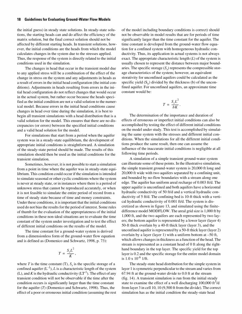
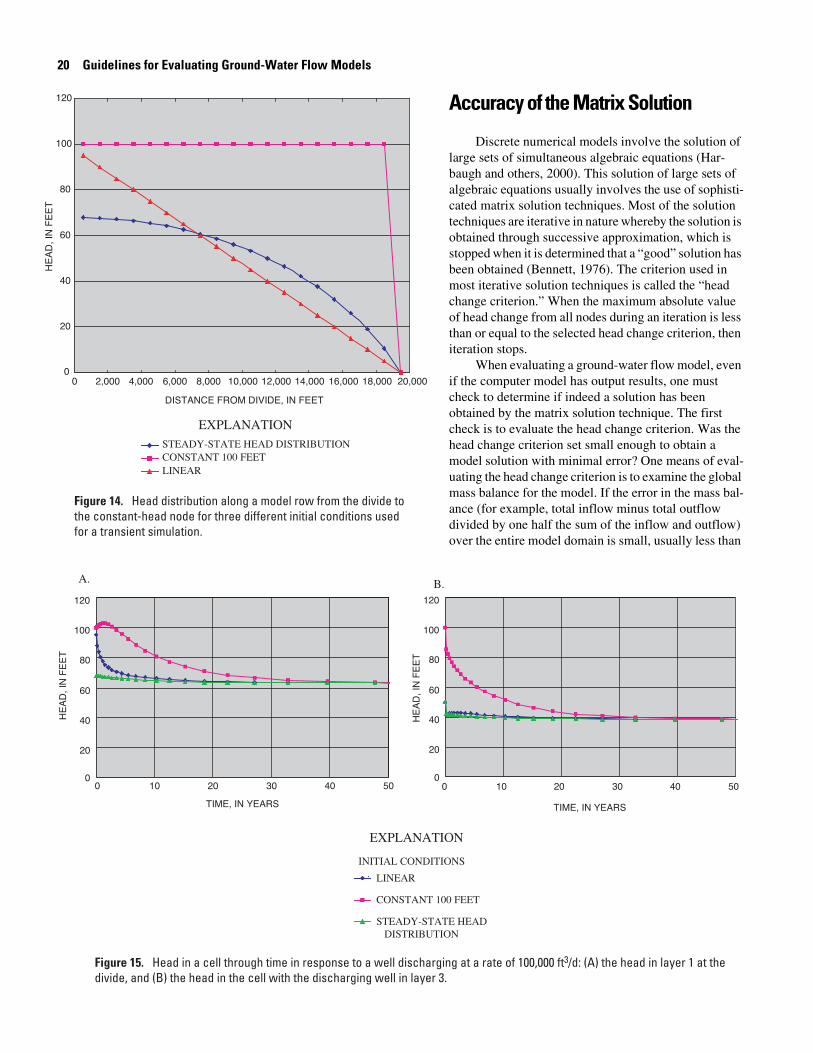
A simulation of a simple transient ground-water system can illustrate some of these points. In the illustrative simulation, the simple transient ground-water system is 20,000 ft long and 20,000 ft wide with two aquifers separated by a confining unit, and bounded by no-flow boundaries with a stream along one edge. The aquifer has uniform areal recharge of 0.003 ft/d. The upper aquifer is unconfined and both aquifers have a horizontal hydraulic conductivity of 50 ft/d and a vertical hydraulic con-ductivity of 5 ft/d. The confining bed is 10-ft thick with a verti-cal hydraulic conductivity of 0.001 ft/d. The system is dis-cretized as shown in figure 13, and simulated using the finite-difference model MODFLOW. The areal grid size is 1,000 ft by 1,000 ft, and the two aquifers are each represented by two lay-ers; the bottom aquifer is represented by a lower layer (layer 4) 50-ft thick overlain by a 40-ft thick layer (layer 3), and the unconfined aquifer is represented by a 50-ft thick layer (layer 2) overlain by a layer (layer 1) with a uniform bottom at –50 ft, which allows changes in thickness as a function of the head. The stream is represented as a constant head of 0 ft along the right-hand boundary in the top layer. The specific yield for the top layer is 0.2 and the specific storage for the entire model domain is 1.0 x 10⁻⁶ 1/ft.
The steady-state head distribution for the simple system in layer 1 is symmetric perpendicular to the stream and varies from 67.94 ft at the ground-water divide to 0.0 ft at the stream (fig. 14). A transient simulation is run from the initial steady state to examine the effect of a well discharging 100,000 ft3/d from layer 3 in cell 10, 10 (9,500 ft from the divide). The correct simulation has as the initial condition the steady-state head
TSsL
2
K----------=
TSyL
2
bK-----------=
Representation of Initial Conditions in Transient Simulations 19
distribution before the well began discharging; the response of the system through time is shown at the divide in layer 1 (fig. 15A) and at the cell containing the well in layer 3 (fig. 15B). The effect of inaccurate initial conditions can be observed in the response of the aquifer at these same locations. Two different initial conditions, as shown on figure 14, are used to test the response of the system to inaccurate initial condi-tions. These two other conditions are a uniform head of 100 ft everywhere (all layers), except at the stream, and a linearly changing initial head ranging from 95 ft to 0 ft at the stream. The response of the system over time in response to the pump-ing well compared to the correct response that used the steady-state head distribution is shown in figure 15 for a cell in layer 1 at the divide and for the cell containing the well in layer 3. The time constant can also be calculated for this system, although some approximations must be made to estimate a saturated thickness. If the saturated thickness of the unconfined aquifer is assumed to be 100 ft (the thickness at the stream), then the time constant is calculated as:
.
As shown in figure 15, the curves for the two inaccurate initial conditions do not approach the correct transient response until about 20 to 40 years after the start of pumping. Thus, inaccurate initial conditions can cause errors for a significant time period in transient sim-ulations.
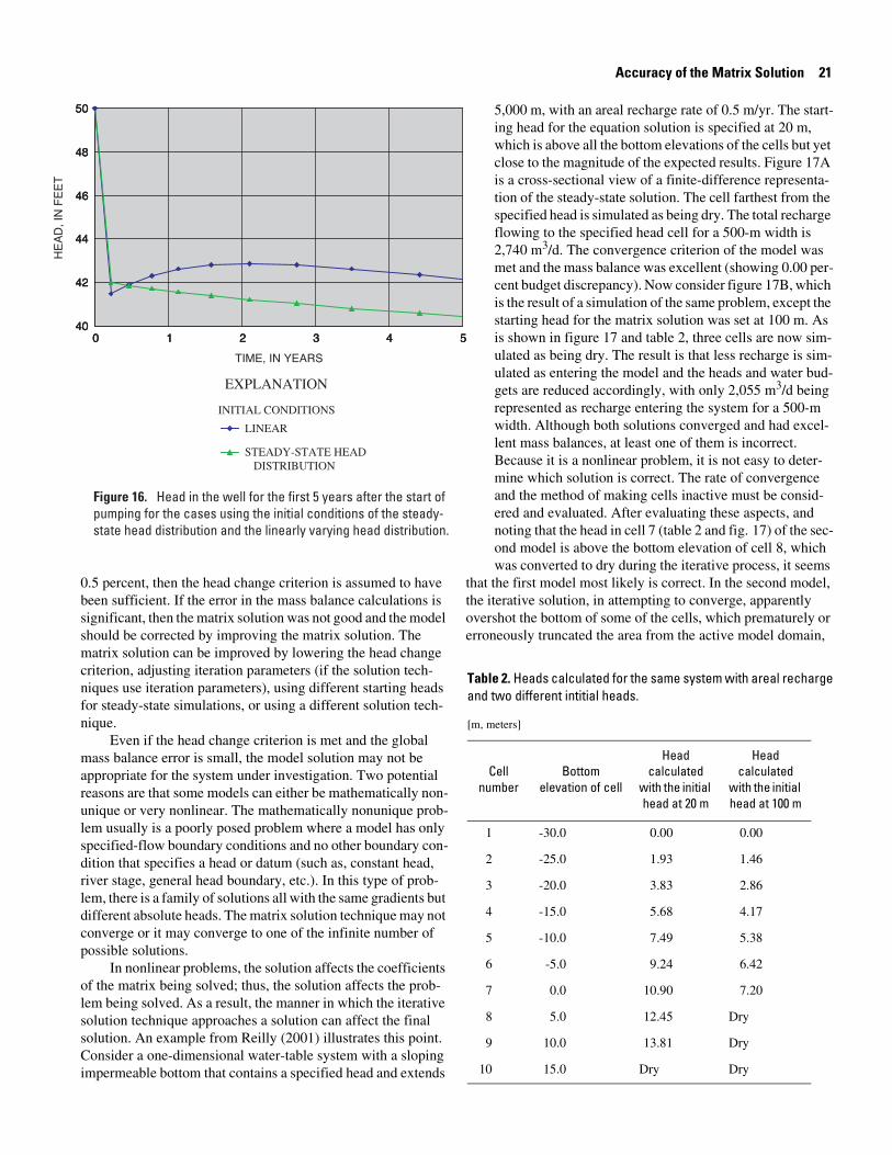
Examination of the simulated response through time from 0-5 years in the finite-difference cell containing the well illustrates some interesting points. The correct response of the system is simulated for the case with the steady-state heads as the initial conditions (fig. 16); the initial value for the head is 50.09 ft in the cell containing the well. The case with the linearly varying heads as initial conditions has the initial value for the cell containing the well equal to 50.0 ft, which is almost the same as the cor-rect steady-state value. Even though the ini-tial conditions in the individual cell are almost the same, the response is different, because the initial conditions over the entire model domain affect the head response. The response of the system with the linearly varying initial conditions is obviously in error because the response of the system shows an increase in head after the first time step in response to pumping, which is not physically reasonable.
Questions to be used in evaluating the initial conditions of a ground-water flow model are:
1. Does the transient model simulation start from a steady-state condition?
If yes –A. Were the initial conditions generated from a steady-
state simulation of the period of equilibrium, which is the preferred method?
B. If the initial conditions were not generated from a steady-state simulation of the period of equilibrium, then is there a compelling reason why they were not generated, or are the initial conditions invalid?
If no –A. Was it possible to select a period of equilibrium to
start the simulation and make the determination of initial conditions more straightforward? If it is possi-ble, then the model should have simulated the tran-sient period from the period of equilibrium.
B. If it was not possible to select a period of equilibrium to start the simulation, then what was the justifica-tion for selecting the starting time and the initial con-ditions for the simulation? How was it shown that the initial conditions used did not bias the result of the simulation?
T0.2 20 000ft,( )2
100.ft 50 ft/d( )------------------------------------- 1.6 104× days = 44 years= =
20 Guidelines for Evaluating Ground-Water Flow Models
Accuracy of the Matrix Solution
Discrete numerical models involve the solution of large sets of simultaneous algebraic equations (Har-baugh and others, 2000). This solution of large sets of algebraic equations usually involves the use of sophisti-cated matrix solution techniques. Most of the solution techniques are iterative in nature whereby the solution is obtained through successive approximation, which is stopped when it is determined that a “good” solution has been obtained (Bennett, 1976). The criterion used in most iterative solution techniques is called the “head change criterion.” When the maximum absolute value of head change from all nodes during an iteration is less than or equal to the selected head change criterion, then iteration stops.
When evaluating a ground-water flow model, even if the computer model has output results, one must check to determine if indeed a solution has been obtained by the matrix solution technique. The first check is to evaluate the head change criterion. Was the head change criterion set small enough to obtain a model solution with minimal error? One means of eval-uating the head change criterion is to examine the global mass balance for the model. If the error in the mass bal-ance (for example, total inflow minus total outflow divided by one half the sum of the inflow and outflow) over the entire model domain is small, usually less than
Accuracy of the Matrix Solution 21
0.5 percent, then the head change criterion is assumed to have been sufficient. If the error in the mass balance calculations is significant, then the matrix solution was not good and the model should be corrected by improving the matrix solution. The matrix solution can be improved by lowering the head change criterion, adjusting iteration parameters (if the solution tech-niques use iteration parameters), using different starting heads for steady-state simulations, or using a different solution tech-nique.
Even if the head change criterion is met and the global mass balance error is small, the model solution may not be appropriate for the system under investigation. Two potential reasons are that some models can either be mathematically non-unique or very nonlinear. The mathematically nonunique prob-lem usually is a poorly posed problem where a model has only specified-flow boundary conditions and no other boundary con-dition that specifies a head or datum (such as, constant head, river stage, general head boundary, etc.). In this type of prob-lem, there is a family of solutions all with the same gradients but different absolute heads. The matrix solution technique may not converge or it may converge to one of the infinite number of possible solutions.
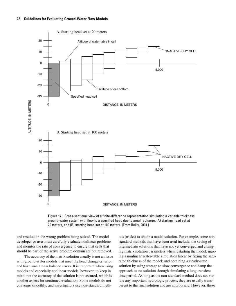
In nonlinear problems, the solution affects the coefficients of the matrix being solved; thus, the solution affects the prob-lem being solved. As a result, the manner in which the iterative solution technique approaches a solution can affect the final solution. An example from Reilly (2001) illustrates this point. Consider a one-dimensional water-table system with a sloping impermeable bottom that contains a specified head and extends
5,000 m, with an areal recharge rate of 0.5 m/yr. The start-ing head for the equation solution is specified at 20 m, which is above all the bottom elevations of the cells but yet close to the magnitude of the expected results. Figure 17A is a cross-sectional view of a finite-difference representa-tion of the steady-state solution. The cell farthest from the specified head is simulated as being dry. The total recharge flowing to the specified head cell for a 500-m width is 2,740 m3/d. The convergence criterion of the model was met and the mass balance was excellent (showing 0.00 per-cent budget discrepancy). Now consider figure 17B, which is the result of a simulation of the same problem, except the starting head for the matrix solution was set at 100 m. As is shown in figure 17 and table 2, three cells are now sim-ulated as being dry. The result is that less recharge is sim-ulated as entering the model and the heads and water bud-gets are reduced accordingly, with only 2,055 m3/d being represented as recharge entering the system for a 500-m width. Although both solutions converged and had excel-lent mass balances, at least one of them is incorrect. Because it is a nonlinear problem, it is not easy to deter-mine which solution is correct. The rate of convergence and the method of making cells inactive must be consid-ered and evaluated. After evaluating these aspects, and noting that the head in cell 7 (table 2 and fig. 17) of the sec-ond model is above the bottom elevation of cell 8, which was converted to dry during the iterative process, it seems
that the first model most likely is correct. In the second model, the iterative solution, in attempting to converge, apparently overshot the bottom of some of the cells, which prematurely or erroneously truncated the area from the active model domain,
Table 2. Heads calculated for the same system with areal recharge and two different intitial heads.
[m, meters]
Cell number
Bottom elevation of cell
Head calculated
with the initial head at 20 m
Head calculated
with the initial head at 100 m
1 -30.0 0.00 0.00
2 -25.0 1.93 1.46
3 -20.0 3.83 2.86
4 -15.0 5.68 4.17
5 -10.0 7.49 5.38
6 -5.0 9.24 6.42
7 0.0 10.90 7.20
8 5.0 12.45 Dry
9 10.0 13.81 Dry
10 15.0 Dry Dry
22 Guidelines for Evaluating Ground-Water Flow Models
and resulted in the wrong problem being solved. The model developer or user must carefully evaluate nonlinear problems and monitor the rate of convergence to ensure that cells that should be part of the active problem domain are not removed.
The accuracy of the matrix solution usually is not an issue with ground-water models that meet the head change criterion and have small mass balance errors. It is important when using models and especially nonlinear models, however, to keep in mind that the accuracy of the solution is not assured, which is another aspect for continued evaluation. Some models do not converge smoothly, and investigators use non-standard meth-
ods (tricks) to obtain a model solution. For example, some non-standard methods that have been used include: the saving of intermediate solutions that have not yet converged and chang-ing matrix solution parameters when restarting the model; mak-ing a nonlinear water-table simulation linear by fixing the satu-rated thickness of the model; and obtaining a steady-state solution by using storage to slow convergence and damp the approach to the solution through simulating a long transient time period. As long as the non-standard method does not vio-late any important hydrologic process, they are usually trans-parent to the final solution and are appropriate. However, these
Adequacy of Calibration for Intended Use of Model Results 23
non-standard techniques should be evaluated to determine whether they cause potential errors to be introduced to the model solution.
Questions to be addressed when evaluating the adequacy of the matrix solution in the simulation of a ground-water sys-tem are:
1. Is the ground-water system and set of matrix equations linear or nonlinear?
If linear –A. Was the head change criterion met and was it suffi-
ciently small to obtain an acceptable (that is, less than 0.05 percent error) global mass balance?
If nonlinear –A. Was a nonlinear matrix solution technique used?
B. Was the head change criterion met and was it suffi-ciently small to obtain an acceptable (that is, less than 0.05 percent error) global mass balance?
C. Did the nonlinear terms, such as cells going dry or drains turning off, behave smoothly during the itera-tion process? Or were there large oscillations that would indicate a potential for convergence to an incorrect solution?
D. Were any “tricks” used to smooth convergence, such as setting saturated thickness as a constant in water-table simulations, and are the assumptions used in defining these artificially constrained features rea-sonable for the solution obtained?
2. Does the solution seem reasonable for the problem posed? If it is not and there are no input data errors, then another matrix solution technique should be tried to determine whether it is a matrix-solution issue or some other problem.
Adequacy of Calibration for Intended Use of Model Results
As discussed previously, not all objectives of using a ground-water model require calibration. For models that require calibration, however, an evaluation of the adequacy of the cali-bration is another difficult task. There are different quantitative measures that investigators use to show the accuracy of the cal-ibration of a ground-water flow model. Some of these are: the mean error, the mean absolute error, and the root mean squared error (Anderson and Woessner, 1992). The areal distribution of residuals (differences between measured and simulated values) also is important to determine whether some areas of the model are biased either too high or too low. The difficulty that arises, however, is how to determine what is good enough.
As stated previously, key aspects of the model, such as the conceptualization of the flow system, that influence the appro-priateness of the model to address the problem objectives, are
often not considered during calibration by many investigators; their focus is on the quantitative measures of goodness of fit. However, the appropriateness of the conceptualization of the ground-water system and processes should always be evaluated during calibration. Thus, the method of calibration, the close-ness of fit between the simulated and observed conditions, and the extent to which important aspects of the simulation were considered during the calibration process are all important in evaluating the appropriateness of the model to address the prob-lem objectives.
Freyberg (1988) reported on a class exercise where differ-ent models were calibrated by students using the same model and identical sets of data. Freyberg’s observations of the exer-cise showed that “success in prediction was unrelated to success in matching observed heads under premodification conditions.” He concluded, “good calibration did not lead to good predic-tion.” This is not to imply that matching heads is unimportant, only that there are other factors that need to be considered in determining the “goodness” of a model. Put in terms of logic, a good match between calculated and observed heads and flow is a necessary condition for a reasonable model, but it is not suffi-cient. The conceptual model and the mathematical representa-tion of all the important processes must also be appropriate for the model to accurately represent the system under investiga-tion. Thus, a model that matches heads and flows well must also be evaluated to determine if it is a reasonable representation of the system under study. As stated by Bredehoeft (2003), “A wrong conceptual model invariably leads to poor predictions, no matter how well the model is fit to the data.”
Thus, the evaluation of the adequacy of the calibration of a model should be based more on the insight of the investigators and the appropriateness of the conceptual model rather than the exact value of the various measures of goodness of fit. For example, it would be possible to specify every cell in a model that had an observation associated with it as a specified head cell in the model. This would produce a perfect match between simulated and observed heads, however, it is conceptually unreasonable to simulate random cells as specified heads that could serve as sources and sinks of water. Thus, although the measures of calibration might make it appear to be a well-calibrated model, in effect the violation of a reasonable concep-tual model makes it a poor model. A model developed accord-ing to a well-argued conceptual model with minor adjustments, in our opinion, is generally superior to a model that has a smaller discrepancy between simulated and observed heads because of unjustified manipulation of the parameter values. A reasonable representation of the conceptual model and sources of water is more important than blindly minimizing the discrep-ancy between simulated and observed heads.
Models can be calibrated by trial and error or by automatic parameter estimation techniques, such as nonlinear regression to minimize some measure of goodness of fit between the sim-ulated and observed values. A key concept in automatic param-eter estimation methods is that a limited set of parameters used in the model is designated to be automatically adjusted. These parameters usually are identified for specific regions (or zones)
24 Guidelines for Evaluating Ground-Water Flow Models
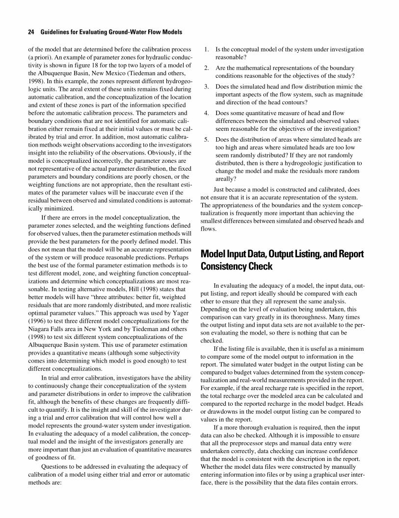
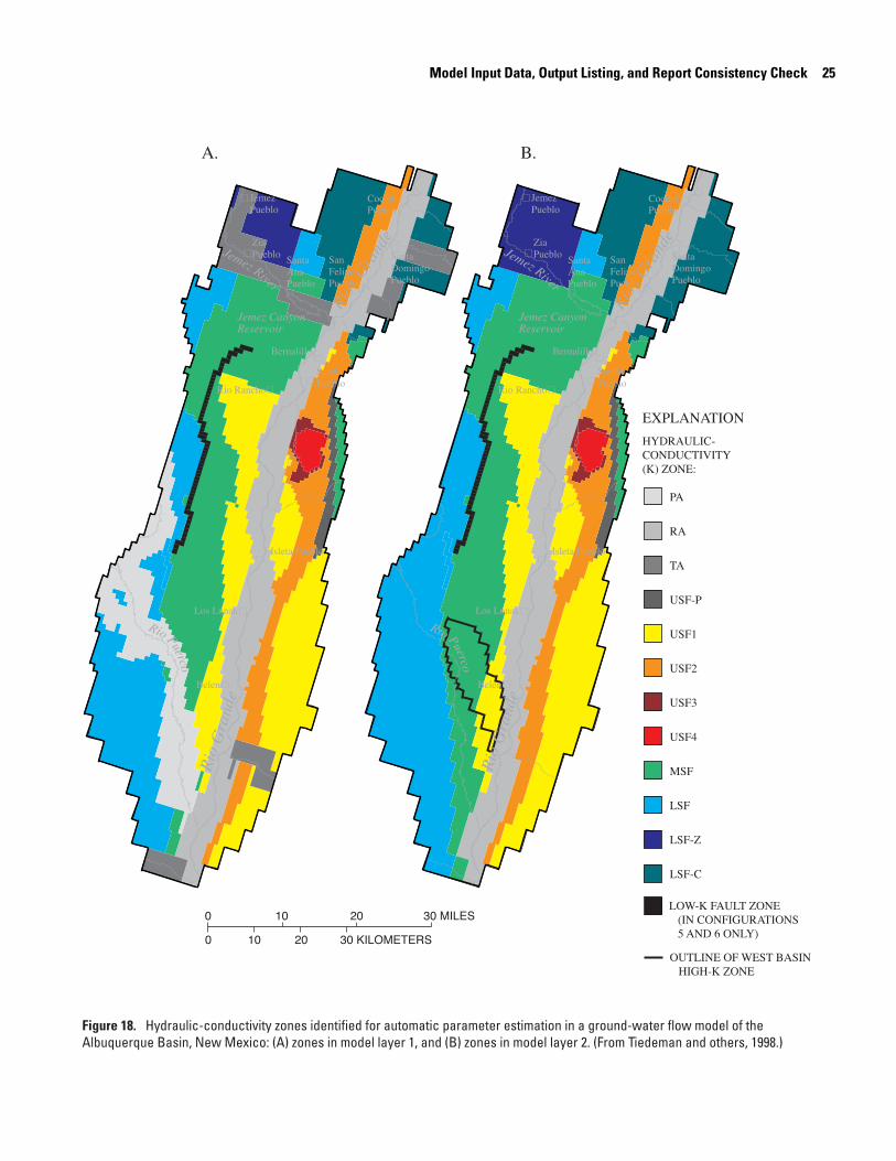
of the model that are determined before the calibration process (a priori). An example of parameter zones for hydraulic conduc-tivity is shown in figure 18 for the top two layers of a model of the Albuquerque Basin, New Mexico (Tiedeman and others, 1998). In this example, the zones represent different hydrogeo-logic units. The areal extent of these units remains fixed during automatic calibration, and the conceptualization of the location and extent of these zones is part of the information specified before the automatic calibration process. The parameters and boundary conditions that are not identified for automatic cali-bration either remain fixed at their initial values or must be cal-ibrated by trial and error. In addition, most automatic calibra-tion methods weight observations according to the investigators insight into the reliability of the observations. Obviously, if the model is conceptualized incorrectly, the parameter zones are not representative of the actual parameter distribution, the fixed parameters and boundary conditions are poorly chosen, or the weighting functions are not appropriate, then the resultant esti-mates of the parameter values will be inaccurate even if the residual between observed and simulated conditions is automat-ically minimized.
If there are errors in the model conceptualization, the parameter zones selected, and the weighting functions defined for observed values, then the parameter estimation methods will provide the best parameters for the poorly defined model. This does not mean that the model will be an accurate representation of the system or will produce reasonable predictions. Perhaps the best use of the formal parameter estimation methods is to test different model, zone, and weighting function conceptual-izations and determine which conceptualizations are most rea-sonable. In testing alternative models, Hill (1998) states that better models will have “three attributes: better fit, weighted residuals that are more randomly distributed, and more realistic optimal parameter values.” This approach was used by Yager (1996) to test three different model conceptualizations for the Niagara Falls area in New York and by Tiedeman and others (1998) to test six different system conceptualizations of the Albuquerque Basin system. This use of parameter estimation provides a quantitative means (although some subjectivity comes into determining which model is good enough) to test different conceptualizations.
In trial and error calibration, investigators have the ability to continuously change their conceptualization of the system and parameter distributions in order to improve the calibration fit, although the benefits of these changes are frequently diffi-cult to quantify. It is the insight and skill of the investigator dur-ing a trial and error calibration that will control how well a model represents the ground-water system under investigation. In evaluating the adequacy of a model calibration, the concep-tual model and the insight of the investigators generally are more important than just an evaluation of quantitative measures of goodness of fit.
Questions to be addressed in evaluating the adequacy of calibration of a model using either trial and error or automatic methods are:
1. Is the conceptual model of the system under investigation reasonable?
2. Are the mathematical representations of the boundary conditions reasonable for the objectives of the study?
3. Does the simulated head and flow distribution mimic the important aspects of the flow system, such as magnitude and direction of the head contours?
4. Does some quantitative measure of head and flow differences between the simulated and observed values seem reasonable for the objectives of the investigation?
5. Does the distribution of areas where simulated heads are too high and areas where simulated heads are too low seem randomly distributed? If they are not randomly distributed, then is there a hydrogeologic justification to change the model and make the residuals more random areally?
Just because a model is constructed and calibrated, does not ensure that it is an accurate representation of the system. The appropriateness of the boundaries and the system concep-tualization is frequently more important than achieving the smallest differences between simulated and observed heads and flows.
Model Input Data, Output Listing, and Report Consistency Check
In evaluating the adequacy of a model, the input data, out-put listing, and report ideally should be compared with each other to ensure that they all represent the same analysis. Depending on the level of evaluation being undertaken, this comparison can vary greatly in its thoroughness. Many times the output listing and input data sets are not available to the per-son evaluating the model, so there is nothing that can be checked.
If the listing file is available, then it is useful as a minimum to compare some of the model output to information in the report. The simulated water budget in the output listing can be compared to budget values determined from the system concep-tualization and real-world measurements provided in the report. For example, if the areal recharge rate is specified in the report, the total recharge over the modeled area can be calculated and compared to the reported recharge in the model budget. Heads or drawdowns in the model output listing can be compared to values in the report.
If a more thorough evaluation is required, then the input data can also be checked. Although it is impossible to ensure that all the preprocessor steps and manual data entry were undertaken correctly, data checking can increase confidence that the model is consistent with the description in the report. Whether the model data files were constructed by manually entering information into files or by using a graphical user inter-face, there is the possibility that the data files contain errors.
Model Input Data, Output Listing, and Report Consistency Check 25
26 Guidelines for Evaluating Ground-Water Flow Models
Examples of possible errors are: numbers scaled improperly, inconsistent data, data entered into incorrect fields, data assigned to incorrect cells, typographical errors, and many oth-ers. An example of inconsistent data is the use of inconsistent time or space units for different parts of the data. For example, pumping might be entered in cubic feet per second (ft3/s) and hydraulic conductivity in feet per day (ft/d). An example of data assigned to incorrect cells is the specification of stress data, for example pumping wells located in inactive cells.
The extent to which the input data can be checked depends on the size of the model, available resources, and how the data were entered. Typical models vary in size from several thou-sand cells to over a hundred thousand cells. There are multiple data values per cell, so it is impractical to check every input value in even the smaller models. Thus, data scanning is a better term to describe the data-checking process. If data files are available, then they can be checked or scanned directly. If the output listing is available and if this listing contains an echo of the input data, then usually it is easier to examine the output list-ing than the input files. Also, seeing the data in the output listing provides added confirmation that the data files have been prop-erly read by the model program.
Some checks that can be considered are:
1. Do the model water-budget quantities seem appropriate for the values described for the actual system in the report?
2. Are the input data the same as those described in the report?
3. Are data values consistent and assigned to appropriate cells?
Checking the information that is read directly by the model increases confidence that the simulation is indeed a solution to the problem described. The level of evaluation required deter-mines the thoroughness of the consistency check that should be undertaken.
Model Reporting and Archiving
Because models are embodiments of scientific hypotheses, a clear and complete documentation of the model development is required for individuals to understand the hypotheses, to understand the methods used to represent the actual system with a mathematical counterpart, and to determine if the model is sufficiently accurate for the objectives of the investigation. As stated in U.S. Geological Survey Office of Ground Water Tech-nical Memorandum 96.04 (see appendix), there is no rigid checklist or recipe for reporting on the use of simulation in a ground-water study. The appropriate level of documentation will vary depending on the study objectives and the complexity of the simulations. A valuable result of the ground-water mod-eling effort is the insight gained by the investigator during the modeling process about the functioning of the flow system. This
understanding of the flow system gained during the modeling process can be an important product of the study and should be appropriately discussed and documented in the modeling report.
The general structure of a well-constructed report describ-ing simulation is much the same as that for any investigative study. It should present (1) the objectives of the study, (2) a description of the work that was done, (3) logical arguments to convince the reader that the methods and analyses used in the study are valid, and (4) results and conclusions.
Ten specific topics that should be addressed in reports that describe studies in which simulation is used are listed and explained in U.S. Geological Survey Office of Ground Water Technical Memorandum 96.04 to aid individuals in document-ing their model studies. These 10 topics are:
1. Describe the purpose of the study and the role that simula-tion plays in addressing that purpose.
2. Describe the hydrologic system under investigation.
3. Describe the mathematical methods used and their appropriateness to the problem being solved.
4. Describe the hydrogeologic character of the boundary conditions used in the simulation of the system.
5. If the method of simulation involves discretizing the system (finite-difference and finite-element methods for example), describe and justify the discretized network used.
6. Describe the aquifer system properties that are modeled.
7. Describe all the stresses modeled such as pumpage, evapotranspiration from ground water, recharge from infiltration, river stage changes, leakage from other aquifers, and source concentrations in transport models.
8. For transient models, describe the initial conditions that are used in the simulations.
9. If a model is calibrated, present the calibration criteria, procedure, and results.
10. Discuss the limitations of the model’s representation of the actual system and the impact those limitations have on the results and conclusions presented in the report.
Once the study is finished, it is always useful to organize and archive the model files. The purpose of the archive is to ensure that the results are reproducible in the future either by the model developer or other interested parties. Thus, the archive should reference any published reports on the model and pro-vide enough explanation in a text “readme” file for the model to be used by others. The archival of the model provides good sci-entific practice and reproducibility of results.
Summary 27
Summary
Ground-water models are designed and built to meet spe-cific objectives. Models must be critically evaluated to ensure that there are no data input errors and that the conceptual model does indeed accurately represent the actual ground-water sys-tem sufficiently to meet the objectives of the study. The items to be evaluated are: the appropriateness of the model program, the discretization and representation of the geologic framework, the representation of the boundary conditions, the representa-tion of the initial conditions, and the accuracy of the matrix solution.
Ground-water flow models attempt to reproduce, or simu-late, the operation of a real ground-water system using a math-ematical counterpart (a mathematical model). Thus, the evalua-tion of the model is intended to ensure that the model program and numerical representation of the important aspects of the system are sufficient to meet the objectives of the study. The guidelines presented in this report raise some of the important aspects of model evaluation.
Acknowledgments
The technical review and improvement of the report by William Alley, James Bartolino, William Cunningham, and Keith Prince are gratefully acknowledged. Sandra Cooper pro-vided editorial review and assistance. The final report and illus-trations were prepared by E.G. Baker and K.A. Waltenbaugh, and J.E. Banton, respectively.
References
Anderman, E.R., and Hill, M.C., 2000, MODFLOW-2000, the U.S. Geological Survey Modular Ground-Water Model—Documentation of the hydrogeologic-unit flow (HUF) package: U.S. Geological Survey Open-File Report 00-342, 89 p.
Anderson, M.P., and Woessner, W.W., 1992, Applied Ground-water Modeling—Simulation of flow and advective trans-port: Academic Press, Inc., San Diego, Calif., 381 p.
Barlow, P.M., 1994, Two- and three-dimensional pathline analysis of contributing areas to public-supply wells of Cape Cod, Massachusetts: Ground Water, v. 32, no. 3, p. 399–410.
Bennett, G.D., 1976, Introduction to ground-water hydrau-lics—A programmed text for self-instruction: Techniques of Water-Resources Investigations of the United States Geolog-ical Survey, Book 3, Chapter B2, 172 p.
Bredehoeft, J.D., 2003, From models to performance assess-ment: The conceptualization problem: Ground Water, v. 41, no. 5, p. 571-577.
Buxton, H.T., and Reilly, T.E., 1987, A technique for analysis of ground-water systems at regional and subregional scales,
applied on Long Island, New York: U.S. Geological Survey Water-Supply Paper 2310, p. 129-142.
Buxton, H.T., Reilly, T.E., Pollock, D.W., and Smolensky, D.A., 1991, Particle tracking analysis of recharge areas on Long Island, New York: Ground Water, v. 29, no. 1, p. 63-71.
Buxton, H.T., and Smolensky, D.A., 1999, Simulation of the effects of development of the ground-water flow system of Long Island, New York: U.S. Geological Survey Water-Resources Investigations Report 98-4069, 57 p.
Buxton, H.T., Smolensky, D.A., and Shernoff, P.K., 1999, Fea-sibility of using ground water as a supplemental supply for Brooklyn and Queens, New York: U.S. Geological Survey Water-Resources Investigations Report 98-4070, 33 p.
Collins, R.E., 1961, Flow of fluids through porous materials: Reinhold Publishing Corp., N.Y., 270 p.
Domenico, P.A., and Schwartz, F.W., 1998, Physical and Chemical Hydrogeology (Second Edition): John Wiley and Sons, New York, N.Y., 506 p.
Franke, O.L., and Reilly, T.E., 1987, The effects of boundary conditions on the steady-state response of three hypothetical ground-water systems—Results and implications of numeri-cal experiments: U.S. Geological Survey Water-Supply Paper 2315, 19 p.
Franke, O.L., Reilly, T.E., and Bennett, G.D., 1987, Definition of boundary and initial conditions in the analysis of saturated ground-water flow systems—An introduction: U.S. Geolog-ical Survey Techniques of Water-Resources Investigations 3-B5, 15 p.
Franke, O.L., Reilly, T.E., Pollock, D.W., and LaBaugh, J.W., 1998, Estimating areas contributing recharge to wells—Les-sons from previous studies: U.S. Geological Survey Circular 1174, 14 p. (Third printing, 1999.)
Freyberg, David L., 1988, An exercise in ground-water model calibration and prediction: Ground Water, v. 26, no. 3, p. 350-360.
Harbaugh, A.W., Banta, E.R., Hill, M.C., and McDonald, M.G., 2000, MODFLOW-2000, The U.S. Geological Survey Mod-ular Ground-Water Model—User guide to modularization concepts and the ground-water flow process: U.S. Geological Survey Open-File Report 00-92, 121 p.
Hill, M.C., 1998, Methods and guidelines for effective model calibration: U.S. Geological Survey Water-Resources Inves-tigations Report 98-4005, 90 p.
Hill, M.C., Cooley, R.L., and Pollock, D.W., 1998, A controlled experiment in ground-water flow model calibration: Ground Water, v. 36, no. 3, p. 520-535.
Konikow, L.F., and Reilly, T.E., 1999, Groundwater modeling: in Delleur, J.W. (ed.), The handbook of groundwater engi-neering: CRC Press, Boca Raton, Fla., 40 p.
Leake, S.A., and Claar, D.V., 1999, Procedures and computer programs for telescopic mesh refinement using MODFLOW: U.S. Geological Survey Open-File Report 99-238, 53 p.
Luckey, R.R., Gutentag, E.D., Heimes, F.J., and Weeks, J.B., 1986, Digital simulation of ground-water flow in the High Plains aquifer in parts of Colorado, Kansas, Nebraska, New
28 Guidelines for Evaluating Ground-Water Flow Models
Mexico, Oklahoma, South Dakota, Texas, and Wyoming: U.S. Geological Survey Professional Paper 1400-D, 57 p.
Masterson, J.P., Walter, D.A., and Savoie, Jennifer, 1997, Use of particle tracking to improve numerical model calibration and to analyze ground-water flow and contaminant migra-tion, Massachusetts Military Reservation, western Cape Cod, Massachusetts: U.S. Geological Survey Water-Supply Paper 2482, 50 p.
McAda, D.P., 2001, Simulation of a long-term aquifer test con-ducted near the Rio Grande, Albuquerque, New Mexico: U.S. Geological Survey Water-Resources Investigations Report 99-4260, 66 p.
McDonald, M.G., and Harbaugh, A.W., 1988, A modular three-dimensional finite-difference ground-water flow model: Techniques of Water-Resources Investigations of the United States Geological Survey, Book 6, Chapter A1, 586 p.
Modica, Edward, Reilly, T.E., and Pollock, D.W., 1997, Pat-terns and age distribution of ground-water flow to streams: Ground Water, v. 35, no. 3, p. 523-537.
Morrissey, D.J., 1989, Estimation of the recharge area contrib-uting water to a pumped well in a glacial-drift, river-valley aquifer: U.S. Geological Survey Water-Supply Paper 2338, 41 p.
Pollock, D.W., 1989, Documentation of computer programs to compute and display pathlines using results from the U.S. Geological Survey modular three-dimensional finite-
difference ground-water flow model: U.S. Geological Survey Open-File Report 89-381, 188 p.
Prince, K.R., and Schneider, B.J., 1989, Estimation of hydraulic characteristics of the Upper Glacial and Magothy aquifers at East Meadow, New York, by use of aquifer tests: U.S. Geo-logical Survey Water-Resources Investigations Report 87-4211, 43 p.
Reilly, T.E., 2001, System and boundary conceptualization in ground-water flow simulation: U.S. Geological Survey Tech-niques of Water-Resources Investigations, Book 3, Chapter B8, 26 p.
Reilly, T.E., Franke, O.L., and Bennett, G.D., 1987, The princi-ple of superposition and its application in ground-water hydraulics: U.S. Geological Survey Techniques of Water-Resources Investigations 3-B6, 28 p.
Reilly, T.E., and Pollock, D.W., 1993, Factors affecting areas contributing recharge to wells in shallow aquifers: U.S. Geo-logical Survey Water-Supply Paper 2412, 21 p.
Tiedeman, C.R., Kernodle, J.M., and McAda, D.P., 1998, Application of nonlinear-regression methods to a ground-water flow model of the Albuquerque Basin, New Mexico: U.S. Geological Survey Water-Resources Investigations Report 98-4172, 90 p.
Yager, R.M., 1996, Simulated three-dimensional ground-water flow in the Lockport Group, a fractured-dolomite aquifer near Niagara Falls, New York: U.S. Geological Survey Water-Supply Paper 2487, 42 p.
Appendix 29
Appendix
April 24, 1996
OFFICE OF GROUND WATER TECHNICAL MEMORAN-DUM NO. 96.04
Subject: PUBLICATIONS—Policy on documenting the use of ground-water simulation in project reports
It has been more than two decades since Ground Water Branch Technical Memorandum No. 75.11 was released on the subject of documenting the use of ground-water simulation in project reports. Because of the time lapse, changes in modeling techniques, and the frequency of problems found when reports are reviewed, a revisit to policy on this subject is appropriate.
There is no rigid checklist or recipe for reporting on the use of simulation in a ground-water study. The appropriate level of documentation will vary depending on the project objectives and the complexity of the simulations. The general structure of a well-constructed report describing simulation is much the same as that for any investigative study. It should present (1) the objectives of the study, (2) a description of the work that was done, (3) logical arguments to convince the reader that the methods and analyses used in the study are valid, and (4) results and conclusions.
Specific topics that should be addressed in reports that describe studies in which simulation is used include the follow-ing.
1. Describe the purpose of the study and the role that simula-tion plays in addressing that purpose. The objective of the simulation must be clearly stated. The model should be represented as a tool to help solve specific problems or answer specific questions rather than as an end product.
2. Describe the hydrologic system under investigation. The extent, nature of boundaries, transmitting properties, storage properties, sources of water, discharge mechanisms and other relevant components of the ground-water system should be described as known or conceptualized. Usually this can be accomplished in part by referencing previous works, but major relevant system characteristics should be summarized in the report that describes the simulation.
3. Describe the mathematical methods used and their appropriateness to the problem being solved. In most cases, a reference to a readily available publication will be sufficient to document mathematical details; however, it will usually be desirable to briefly summarize the methods that are used. For a well-documented computer program, this will often require
only a paragraph or two. If a documented computer program is modified such that computed values are affected, the modifications should be documented and evidence that the modifications are correct should be supplied.
4. Describe the hydrogeologic character of the boundary conditions used in the simulation of the system. In many cases, the model boundaries are placed where the aquifer terminates against relatively impermeable rocks or is intersected by a perennial stream whose head variation in time and space is known. In other cases, the aquifer may be so extensive relative to the area of interest that the modeled area may need to extend beyond the project area to accurately simulate the natural boundaries of the aquifer system. If the modeled area is arbitrarily truncated at some distance from the area of interest, it should be shown that the selection of the arbitrary boundary condition does not materially affect the ability of the model to simulate the system for the purposes of the study. Internal boundaries such as streams, lakes, and pinchouts of important hydrogeologic zones should be identified and their representation in the model should be described in the report. A clear, convincing argument of the appropriateness of the boundary conditions used in the model to represent the actual system should be made for the entire bounding surface of the modeled volume or cross section, as well as for any internal boundaries.
5. If the method of simulation involves discretizing the system (finite-difference and finite-element methods for example), describe and justify the discretized network used. The spacing and distribution of the blocks, elements, or subregions should reflect, in part, the spatial variability of the hydraulic parameters and the location of boundaries (for example streams, lakes, bed pinchouts), human-made features (for example wells and dams), and stresses. In most cases, a map showing the discretized network superimposed on the study area is required. Vertical discretization should be described and/or shown on illustrations. The manner in which time is discretized for transient models also should be described. If a steady-state model is used to simulate an average or approximate steady-state condition, discuss the errors that could be introduced in the study results as a consequence of using a steady-state model.
6. Describe the aquifer system properties that are modeled. Explain whatever inferences are made from field data and previous studies as to the spatial variation of hydraulic properties of aquifers and confining beds and how discretized values are computed throughout the simulated area. During model calibration (see item 9), modeled values are often changed; the final aquifer
30 Guidelines for Evaluating Ground-Water Flow Models
system properties that are modeled should be described in the report. This can be through maps or descriptions in the text. Lists of model arrays do not generally provide much understanding of the model and accordingly should not be included in the report unless it is expected that readers will want to repeat the simulations. If lists of arrays are included, they should usually be provided on electronic media. Note that Office of Ground Water Technical Memorandum No. 93.01 describes the separate requirement for archiving the complete model data sets used in ground-water projects.
7. Describe all the stresses modeled such as pumpage, evapotranspiration from ground water, recharge from infiltration, river stage changes, leakage from other aquifers, and source concentrations in transport models. The relations between observed and modeled stresses should be described. For example, it usually is desirable to provide a representative sample of actual pumping histories and the corresponding modeled pumping histories, although such information would not necessarily be provided for every pumped well. The manner in which stresses are averaged within the discretized time and space scheme should also be described. If a steady-state model is used to simulate an average or approximate steady-state condition, describe how the average stresses representing this system are calculated.
8. For transient models, describe the initial conditions that are used in the simulations. Ideally, a transient simulation will start from a steady-state condition, and the steady-state initial conditions will be generated by a steady-state simulation using the same model. In this case, the steady-state simulation must use the same hydraulic and stress parameters that are used in the transient simulation, except that the transient stresses are removed. In situations where it is not possible to start a transient model from a simulated steady-state condition, it is necessary to describe how the initial conditions were derived. It is also important to estimate the error in the derived values and the possible impact on the model results.
9. If a model is calibrated, present the calibration criteria, procedure, and results. Describe the source of the observed data to which model results are compared. Explain the appropriateness of using these data for model comparisons and the rationale for any adjustments made to actual observations when making the comparisons. For example, when steady-state models are used to simulate an approximate steady-state condition, it is important to explain to what extent the observations that have been made at specific points in time correspond to the approximate steady-state
condition being simulated. Give a representative sample of the actual comparisons used for calibration, and show the locations of the observation points on maps. When the number of observations is extensive, locations of representative points can be shown. It is important to report and use as many types of data as possible for calibration. For example, in a flow model, both head and flow observations are desirable for use in calibration.
10. Discuss the limitations of the model’s representation of the actual system and the impact those limitations have on the results and conclusions presented in the report. Evaluating the sensitivity of the computed model responses to changes in parameter values that reflect plausible parameter uncertainty helps to assess the model reliability. If the model is to be used to make specific projections, it is useful to estimate the impacts of the uncertainty of parameter values on the projections. In calibrated models, a concern is nonuniqueness, which is the extent to which other combinations of parameter values or configurations may result in an equally good fit to the observed data. Discuss the extent to which nonuniqueness may affect the use of the model in the study.
In summary, a report describing a study in which simula-tion is used should address the above topics; however, there is considerable flexibility in the form of such a report. The report should describe the purpose of the simulation and convince the reader that the use of simulation is credible. The report should further describe the system being simulated, the methods of simulation, and the data that are used.
William M. AlleyChief, Office of Ground Water
Distribution: A, B, S, FO, PO
This memorandum supersedes Ground Water Branch Technical Memorandum No. 75.11