" ".... NSWCDDIMP-g2/43 j

AD-A251 781

GUIDELINES FOR THE SELECTION OFWEIGHTING FUNCTIONS FORH-INFINITY CONTROL

BY JOHN E. BIBEL AND D. STEPHEN MALYEVACWEAPONS SYSTEMS DEPARTMENT

JAWARY IDTI

APpovd for public reles*; distribution is unlimited.

1< NAVAL SURFACE WARFARE CENTERDAHLGREN DIVISIONDahlgren. Virginia 2244o1-000

92-1637992 6 22 01 ]6 lllillllllllIfIlllll

NSWCDD/MP-92/43

GUIDELINES FOR THE SELECTION OFWEIGHTING FUNCTIONS FOR

H-INFINITY CONTROL

BY JOHN E. BIBEL AND D. STEPHEN MALYEVACWEAPONS SYSTEMS DEPARTMENT

JANUARY 1992

Approved for public release; distribution is unlimited.

NAVAL SURFACE WARFARE CENTERDAHLGREN DIVISION

Dahlgren, Virginia 22448-5000

NSWCDD/MP-92/43

FOREWORD

This report discusses general engineering guidelines for the design of weightingfunctions in H-Infinity (Hoo) Control. The Ho Control method is one approach torobust control that has been receiving much attention recently in the controlscommunity. The Aeromechanics Branch (G23) has been examining H. control andother robust control methods and their application to naval weapon systems (e.g.,missile flight control and high-performance/high-precision pointing and trackingsystems). The material presented herein is introductory in nature and, hopefully,provides useful information to the control system design engineer.

This work was supported by the Naval Surface Warfare Center, Dahlgren Divi-sion (NSWCDD) Independent Research (II program.

The authors wish to thank E. J. Ohlmeyer for his contributions and review of thisreport. This document has been reviewed by Dr. T. J. Rice, Head, AeromechanicsBranch.

Approved by:

D. L. BRU 0N HaMissile Systems Division

Aooession popINTIS QRA&IDTIC TABUnannounced 0Justification

ByDistribution,Availability CodesIAvll ail ond -

Dist SP0,oisli/ii I ' .. .

NSWCDD/MP-92/43

ABSTRACT

This report provides insight into the selection of H-Infinity (H.) Control weight-ing functions that help shape the performance and robustness characteristics ofsystems designed using the H. and p-Synthesis Control methods. Backgroundmaterial regarding sensitivity functions, loopshaping, and H. Control is followed bya discussion of general engineering guidelines for the design of H. Control weightingfunctions. In addition, unresolved design issues and alternatives are presented.Thus, this report presents practical rules-of-thumb and identifies issues and alterna-tives in the design of weighting functions for Ho Control.

iii/iv

NSWCDD/MP-92/43

CONTENTS

Page

INTRODUCTION ................................................................... 1

BACKGROUN D .................................................................... 1FEEDBACK CONTROL SYSTEMS AND LOOPSHAPING CONTROL DESIGN ....... 2H, CONTROL AND WEIGHTING FUNCTIONS ................................... 6MISSILE AUTOPILOT DESIGN EXAMPLE ....................................... 11

GENERAL GUIDELINES FOR WEIGHT SELECTION ................................. 12

PROBLEM-DEPENDENT ISSUES ................................................... 15

SUMMARY AND CONCLUSIONS .................................................... 17

REFERENCES ...................................................................... 17

DISTRIBUTION .................................................................... (1)

v/vi

NSWCDD/MP-92/43

INTRODUCTION

During the past decade, there have been many theoretical advances in the field ofRobust Control', and, in particular, H-Infinity (I-.) Control. A breakthrough in the solutionof the H. Control problem in 1988 led to the development of computationally feasiblealgorithms for finding H. optimal controllers. Since then, analytical applications of H.Control and /L-Synthesis (an iterative design technique that combines Structured SingularValue, ;, analysis with I-. Control synthesis) to real-world problems"' have demonstrated thepotential of these techniques.

One of the key steps in the H. Control design approach is the formulation of inputand output weighting functions. These weighting functions are utilized to normalize theinputs and outputs and reflect the spatial and frequency dependency of the inputdisturbances and the performance specifications of the output (error) variables.Unfortunately, little work has been performed on finding reliable methods of selecting theseweighting functions.

This document provides insight into useful guidelines for selecting the input andoutput weighting functions utilized in H. Control designs. This report is organized in thefollowing manner. First, a brief description of feedback control systems, loopshaping, andbackground on H. Control weighting functions is presented. Second, general guidelines onformulating these weighting functions are given. Third, some of the remaining problem-dependent issues regarding the control weights are discussed. A summary concludes thisreport.

BACKGROUND

We begin with an introductory level discussion of some of the technical backgroundto the I. Control weighting selection problem. This section includes a description offeedback control systems, loopshaping design concepts, and the definition of the I Controlweight selection problem; it concludes with a missile autopilot example to further illustratethese concepts.

NSWCDDIMP-92/43

FEEDBACK CONTROL SYSTEMS AND LOOPSHAPING CONTROL DESIGN

We begin this section with a definition of control system terminology. The conceptsof loopshaping to meet classical types of design criteria are then presented.

A general control system is pictured in Figure 1. This system could represent eithera scalar (Single-Input SIngle-Output, SISO) system or a multivariable (Multiple-InputMultiple-Output, MIMO) system with scalar or vector input and output signals (asappropriate) and either scalar or matrix transfer function system blocks (as appropriate).We assume that the system can be modeled as a linear time-invariant (LTI) system ofdifferential equations. In Figure 1, G(s) represents the model of the physical plant to becontrolled and K(s) denotes the controller. The inputs to the system are r(s), referencecommand signals; d(s), disturbance inputs; and n(s), measurement sensor noise. The outputvariables are given by y(s). In addition, we may also be interested in monitoring the errorsignals, e(s), and the control signals, u(s).

d(s)K~s) +G~s s)'. y(s)

n(s)

FIGURE 1. CONTROL SYSTEM DIAGRAM

Algebraically, the output y(s) can be related to the three inputs as

y(s) = [I + G(s)K(s)] -1 {G(s)K(s)r(s) + d(s) - G(s)K(s)n(s)} (1)

where I is the identity matrix. Likewise, the error and the control signals can be expressed,respectively, by

e(s) = [I + G(s)K(s)] - 1{r(s) - d(s) -n(s)} (2)

2

NSWCDD/MP-92/43

u(s) = [I + K(s) G(s) ]- K(s) {r(s) - d(s) - n(s)} (3)

Definition of some common terminology follows:

L(s) = G(s) K(s) = loop transfer matrixF. = [I + G(s) K(s)] = (output) return difference transfer matrixS(s) = [I + G(s) K(s)] 1 = (output) sensitivity function matrixT(s) = [I + G(s) K(s)]- G(s)K(s) = (output) closed-loop transfer function matrix

Note that the closed-loop transfer function matrix, T(s), relates the output of the system,y(s), to the input reference signal, r(s). It also specifies how the output y(s) is affected bythe noise, n(s). The sensitivity function, S(s), describes the output, y(s), as a function of thedisturbance input, d(s). It also defines the response of the tracking error e(s) to thereference input r(s). Thus to summarize, S(s) = y(s)/d(s) = e(s)/r(s) and T(s) = y(s)/r(s)

- -y(s)/n(s). From the definitions of S(s) and T(s), we find that

S(s) + T(s) = 1 (4)

Thus, T(s) is also referred to as the complementary sensitivity function matrix. Equation (4)is an important relationship that prescribes a limit on achievable performance.

In addition to the requirement for stability, other properties that the feedback controlsystem should exhibit include

- Command Following. For good command following, we require the output to trackthe input reference signals. To accomplish this, we desire that y(s) - r(s) and thate(s) - 0. For these to be true, we require that Tjo) - I and Soj) - 0, respectively.To achieve this, the loop transfer, Lco), should be large; i.e., G(jo)Koj) > 1.

- Disturbance Rejection. For good disturbance rejection, the disturbance inputsshould have a negligible effect upon the output y(s). Thus, we require that S(jO) -

0. As before, this translates into the need for a large loop gain, G(fr)K(j) > 1, inthe frequency range of the disturbances.

- Sensor Noise Attenuation. In this case, we desire that the sensor noise inputs havea small effect upon the system outputs. For this to happen, we would like T(jo) tobe small, especially in the frequency range that the noise is concentrated. As a result,the loop gain should also be small in the appropriate frequency range, GOjW)KO()cl.

* Control Sensitivity Minimization. Here, we desire to keep the control inputs small,so as to not saturate the servomechanism or amplify noise and disturbance signalsmixed in the control signal. For this to happen, we would like [I + K(s)G(s)]'K(s)to be near zero. In a SISO sense, then we desire

3

NSWCDD/MP-92/43

K(j) - T(jo) 0 (5)1 +K(j)G(j) - G(j6)

So for the SISO case, to minimize the control sensitivity, we would like to keep thecomplementary sensitivity small.

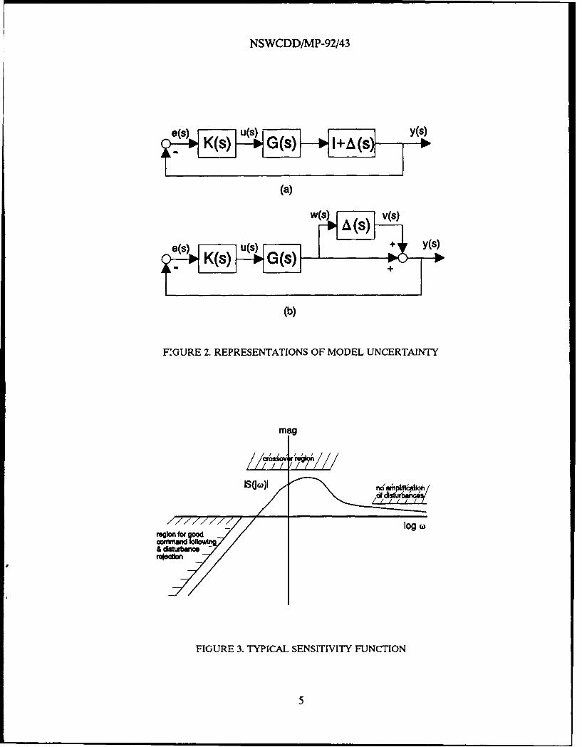
• Robustness to Modeling Errors. We recall that G(s) represents a linear model ofthe true physical system. However, this model cannot represent the real systemperfectly and, thus, contains modeling errors (or model uncertainties); e.g., high-frequency unmodeled dynamics. If we represent the plant model uncertainty asmultiplicative uncertainty at the plant output, the true model of the system is

GO _(s) = [I + A(s)]G(s) (6)

where A(s) denotes a stable transfer function matrix representation of theuncertainties. To examine the sole effect of the uncertainties, assume that r(s) = d(s)= n(s) = 0. The system can then be configured as shown in Figure 2(a). Pulling outthe A(s) into a separate block, the system is then represented by Figure 2(b). If theloop is broken on either side of the uncertainty A(s), the loop properties from theinput v(s) to output w(s) are given by

w(s) = -G(s)K(s)[I + G(s)K(s)]- v(s) (7)

So, to reduce the sensitivity of the system to modeling errors at the plant output, wedesire to keep the quantity Gow)KUo)[I + Go w)K(jw)]' small in the frequency rangeof the expected model uncertainties. To accomplish this, the loop gain should besmall, (i.e., Goj)KO(j) 1). In the SISO case, this simplifies to keeping T(j) and,therefore, Low) small in the appropriate frequency range.

To summarize, for good command following and disturbance rejection, we would liketo keep S small; to remain insensitive to sensor noise and modeling errors (at the plantoutput) and to reduce control sensitivity, we desire to keep T small. However, we cannotkeep both S and T small over the whole frequency range because of the S + T = Iconstraint. Thus, we must determine some tradeoff between the sensitivity andcomplementary sensitivity functions.

Usually, reference signals and disturbances occur at low frequencies, while sensornoise and modeling errors (e.g., high frequency unmodeled dynamics) are concentrated athigh frequencies. The tradeoff, in a SISO sense, is to make I SOjw) I small at low frequenciesand I T(j)I small at high frequencies. For example, a Bode plot of a typical sensitivityfunction is illustrated in Figure 3.

4

NSWCDDIMP-92/43

e(s) u(s) y(s)

's K(s) G(s) 1+A&(s)

(a)

(b)

E.GURE 2. REPRESENTATIONS OF MODEL UNCERTAINTY

log 0A

& istutbanos

FIGURE 3. TYPICAL SENSITIVITY FUNCTION

5

NSWCDD/MP-92/43

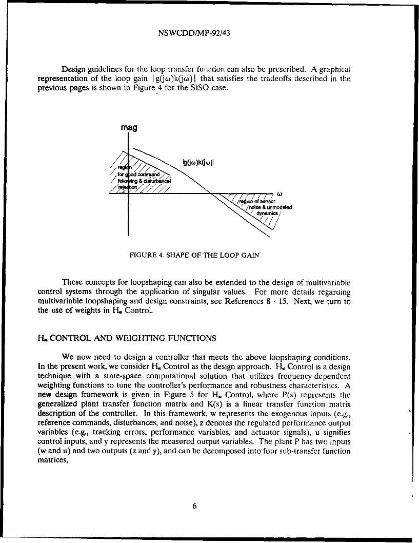
Design guidelines for the loop transfer function can also be prescribed. A graphicalrepresentation of the loop gain I gjo)k(jo) that satisfies the tradeoffs described in theprevious pages is shown in Figure 4 for the SISO case.

mag

/for wr00 nd,

/9 /noise & unmodeled,, d yn/ mcs

FIGURE 4. SHAPE OF THE LOOP GAIN

These concepts for loopshaping can also be extended to the design of multivariablecontrol systems through the application of singular values. For more details regardingmultivariable loopshaping and design constraints, see References 8 - 15. Next, we turn tothe use of weights in H. Control.

I- CONTROL AND WEIGHTING FUNCTIONS

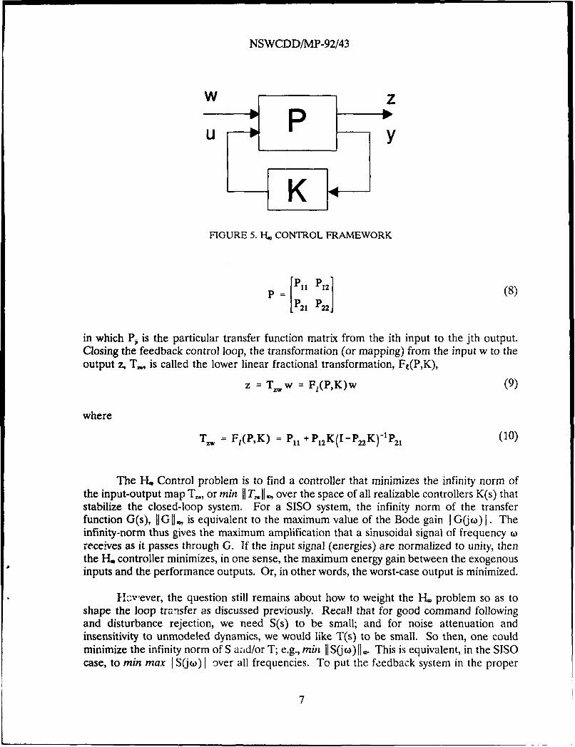
We now need to design a controller that meets the above loopshaping conditions.In the present work, we consider H. Control as the design approach. H. Control is a designtechnique with a state-space computational solution that utilizes frequency-dependentweighting functions to tune the controller's performance and robustness characteristics. Anew design framework is given in Figure 5 for H. Control, where P(s) represents thegeneralized plant transfer function matrix and K(s) is a linear transfer function matrixdescription of the controller. In this framework, w represents the exogenous inputs (e.g.,reference commands, disturbances, and noise), z denotes the regulated performance outputvariables (e.g., tracking errors, performance variables, and actuator signals), u signifiescontrol inputs, and y represents the measured output variables. The plant P has two inputs(w and u) and two outputs (z and y), and can be decomposed into four sub-transfer functionmatrices,

6

NSWCDD/MP-92/43

w zPU Y

KFIGURE 5. H. CONTROL FRAMEWORK

P ~:1)12]I (8)

in which Pji is the particular transfer function matrix from the ith input to the jth output.Closing the feedback control loop, the transformation (or mapping) from the input w to theoutput z, T, is called the lower linear fractional transformation, Ft(P,K),

z = T.,,w = F,(P,K)w (9)

where

T..., = F,(PK) = P11 +P12K(I-P2K)-'P 2, (10)

The I-L Control problem is to find a controller that minimizes the infinity norm ofthe input-output map T,, or min 1 T,,,, 11 , over the space of all realizable controllers K(s) thatstabilize the closed-loop system. For a SISO system, the infinity norm of the transferfunction G(s), 11G 11, is equivalent to the maximum value of the Bode gain I G(j0) j. Theinfinity-norm thus gives the maximum amplification that a sinusoidal signal of frequency Wreceives as it passes through G. If the input signal (energies) are normalized to unity, thenthe H, controller minimizes, in one sense, the maximum energy gain between the exogenousinputs and the performance outputs. Or, in other words, the worst-case output is minimized.

Hzvever, the question still remains about how to weight the HL, problem so as toshape the loop transfer as discussed previously. Recall that for good command followingand disturbance rejection, we need S(s) to be small; and for noise attenuation andinsensitivity to unmodeled dynamics, we would like T(s) to be small. So then, one couldminimize the infinity norm of S and/or T; e.g., min 1IIk So)I11. This is equivalent, in the SISOcase, to min max I S(jo) I over all frequencies. To put the feedback system in the proper

7

NSWCDD/MP-92/43

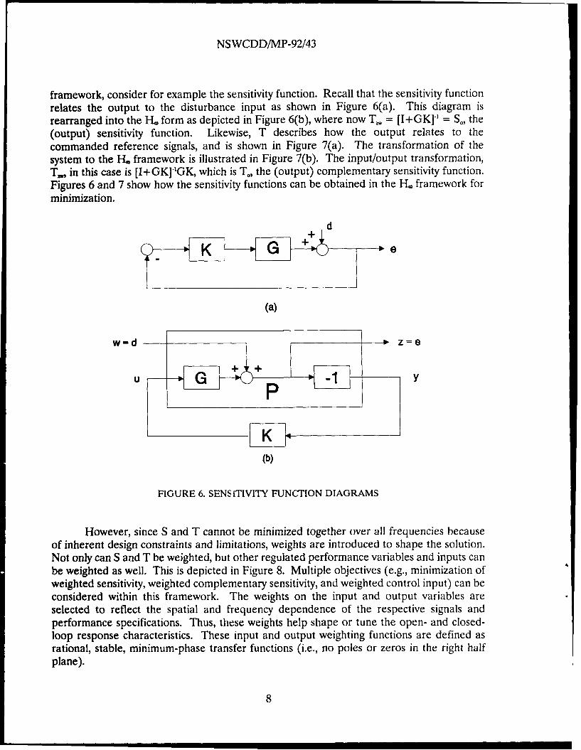
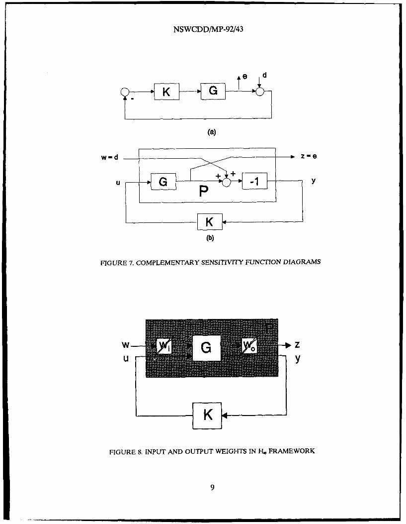
framework, consider for example the sensitivity function. Recall that the sensitivity functionrelates the output to the disturbance input as shown in Figure 6(a). This diagram isrearranged into the H. form as depicted in Figure 6(b), where now T, = [I+GK]2 = S", the(output) sensitivity function. Likewise, T describes how the output relates to thecommanded reference signals, and is shown in Figure 7(a). The transformation of thesystem to the H. framework is illustrated in Figure 7(b). The input/output transformation,T, in this case is [I+GK]1 GK, which is T., the (output) complementary sensitivity function.Figures 6 and 7 show how the sensitivity functions can be obtained in the H, framework forminimization.

d

K e

(a)

w-d o. z=e

P

(b)

FIGURE 6. SENSITIVITY FUNCTION DIAGRAMS

However, since S and T cannot be minimized together over all frequencies becauseof inherent design constraints and limitations, weights are introduced to shape the solution.Not only can S and T be weighted, but other regulated performance variables and inputs canbe weighted as well. This is depicted in Figure 8. Multiple objectives (e.g., minimization ofweighted sensitivity, weighted complementary sensitivity, and weighted control input) can beconsidered within this framework. The weights on the input and output variables areselected to reflect the spatial and frequency dependence of the respective signals andperformance specifications. Thus, these weights help shape or tune the open- and closed-loop response characteristics. These input and output weighting functions are defined asrational, stable, minimum-phase transfer functions (i.e., no poles or zeros in the right halfplane).

8

NSWCDD/MP-92/43

K G te

(a)

(b)

FIGURE 7. COMPLEMENTARY SENSITIVITY FUNCTION DIAGRAMS

K .

FIGURE 8. INPUT AND OUTPUT WEIGHTS IN H, FRAMEWORK

9

NSWCDD/MP-92/43

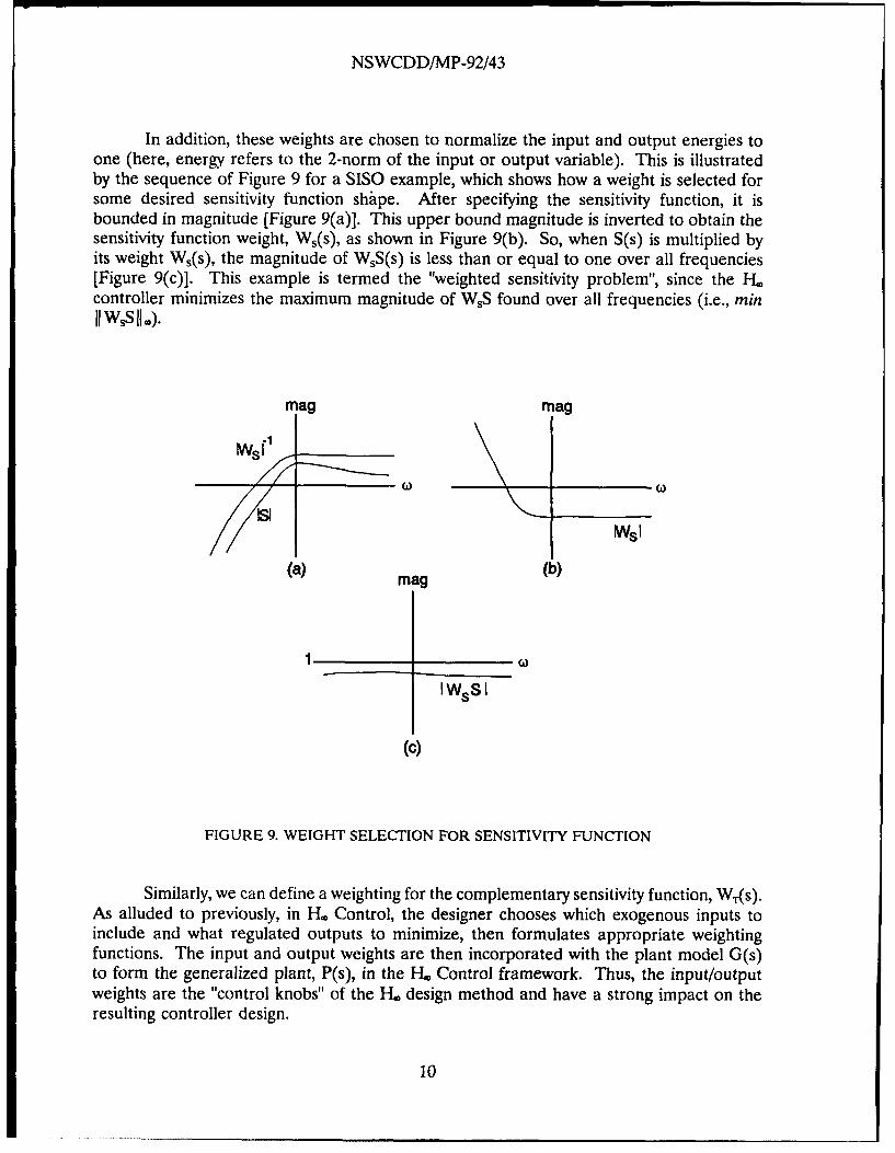
In addition, these weights are chosen to normalize the input and output energies toone (here, energy refers to the 2-norm of the input or output variable). This is illustratedby the sequence of Figure 9 for a SISO example, which shows how a weight is selected forsome desired sensitivity function shape. After specifying the sensitivity function, it isbounded in magnitude [Figure 9(a)]. This upper bound magnitude is inverted to obtain thesensitivity function weight, Ws(s), as shown in Figure 9(b). So, when S(s) is multiplied byits weight Ws(s), the magnitude of WsS(s) is less than or equal to one over all frequencies[Figure 9(c)]. This example is termed the "weighted sensitivity problem", since the H.controller minimizes the maximum magnitude of WsS found over all frequencies (i.e., minIWsS A,).

ag mag

wsI

(a) mag (b)

1WS

(c)

FIGURE 9. WEIGHT SELECTION FOR SENSITIVITY FUNCTION

Similarly, we can define a weighting for the complementary sensitivity function, WT(s).As alluded to previously, in H. Control, the designer chooses which exogenous inputs toinclude and what regulated outputs to minimize, then formulates appropriate weightingfunctions. The input and output weights are then incorporated with the plant model G(s)to form the generalized plant, P(s), in the H. Control framework. Thus, the input/outputweights are the "control knobs" of the H. design method and have a strong impact on theresulting controller design.

10

NSWCDD/MP-92/43

MISSILE AUTOPILOT DESIGN EXAMPLE

To further illustrate these concepts, we present an example of setting up a missileautopilot design in the I-. design framework. This example will be drawn upon throughoutthis report.

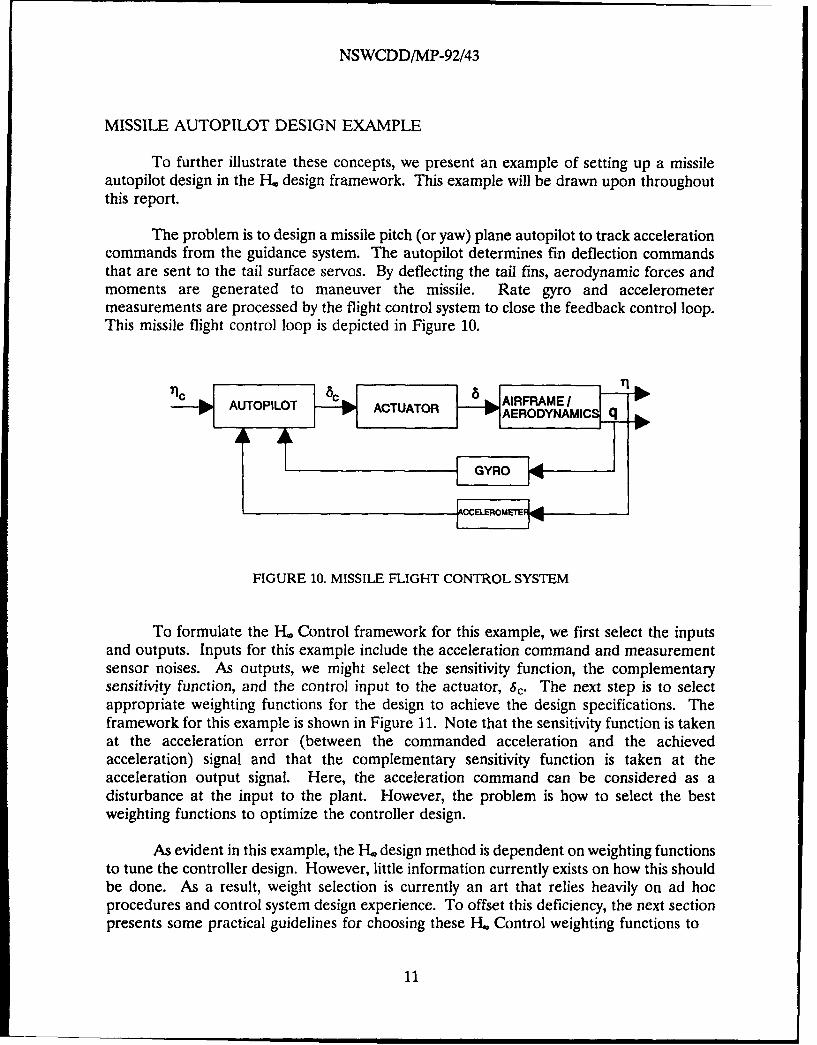
The problem is to design a missile pitch (or yaw) plane autopilot to track accelerationcommands from the guidance system. The autopilot determines fin deflection commandsthat are sent to the tail surface servos. By deflecting the tail fins, aerodynamic forces andmoments are generated to maneuver the missile. Rate gyro and accelerometermeasurements are processed by the flight control system to close the feedback control loop.This missile flight control loop is depicted in Figure 10.

L-pAUTOPILOTJ- ACTUATOR 8 AERODAMIC q'

FIGURE 10. MISSILE FLIGHT CONTROL SYSTEM

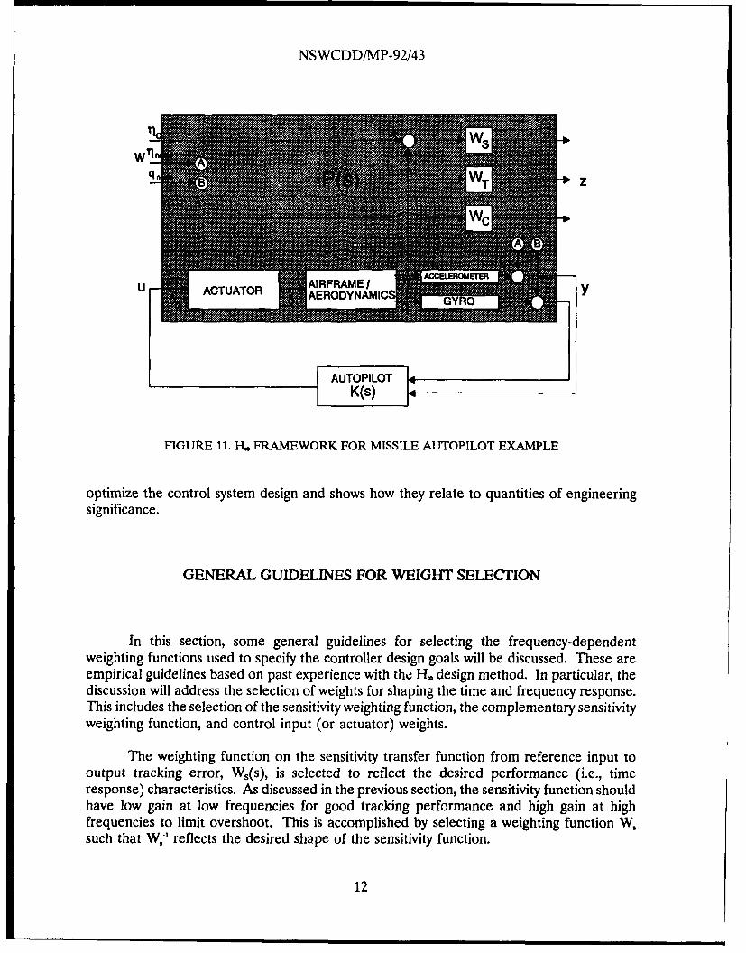
To formulate the I-L Control framework for this example, we first select the inputsand outputs. Inputs for this example include the acceleration command and measurementsensor noises. As outputs, we might select the sensitivity function, the complementarysensitivity function, and the control input to the actuator, 6 c. The next step is to selectappropriate weighting functions for the design to achieve the design specifications. Theframework for this example is shown in Figure 11. Note that the sensitivity function is takenat the acceleration error (between the commanded acceleration and the achievedacceleration) signal and that the complementary sensitivity function is taken at theacceleration output signal. Here, the acceleration command can be considered as adisturbance at the input to the plant. However, the problem is how to select the bestweighting functions to optimize the controller design.

As evident in this example, the H. design method is dependent on weighting functionsto tune the controller design. However, little information currently exists on how this shouldbe done. As a result, weight selection is currently an art that relies heavily on ad hocprocedures and control system design experience. To offset this deficiency, the next sectionpresents some practical guidelines for choosing these H. Control weighting functions to

11

NSWCDD/MP-92/43

qr "W ZTz

ACCELEROMEI"ER

U ACTUATOR AERODYNAMI Y

FIGURE 11. IH, FRAMEWORK FOR MISSILE AUTOPILOT EXAMPLE

optimize the control system design and shows how they relate to quantities of engineeringsignificance.

GENERAL GUIDELINES FOR WEIGHT SELECTION

In this section, some general guidelines for selecting the frequency-dependentweighting functions used to specify the controller design goals will be discussed. These areempirical guidelines based on past experience with the I-. design method. In particular, thediscussion will address the selection of weights for shaping the time and frequency response.This includes the selection of the sensitivity weighting function, the complementary sensitivityweighting function, and control input (or actuator) weights.

The weighting function on the sensitivity transfer function from reference input tooutput tracking error, Ws(s), is selected to reflect the desired performance (i.e., timeresponse) characteristics. As discussed in the previous section, the sensitivity function shouldhave low gain at low frequencies for good tracking performance and high gain at highfrequencies to limit overshoot. This is accomplished by selecting a weighting function W,such that W1- reflects the desired shape of the sensitivity function.

12

NSWCDD/MP-92/43

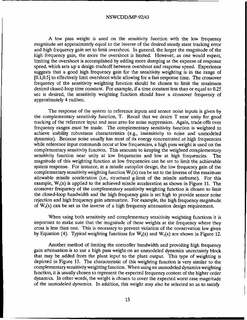
A low pass weight is used on the sensitivity function with the low frequencymagnitude set approximately equal to the inverse of the desired steady state tracking errorand high frequency gain set to limit overshoot. In general, the larger the magnitude of thehigh frequency gain, the more the overshoot is limited. However, as one would expect,limiting the overshoot is accomplished by adding more damping at the expense of responsespeed, which sets up a design tradeoff between overshoot and response speed. Experiencesuggests that a good high frequency gain for the sensitivity weighting is in the range of[0.1,0.5] to effectively limit overshoot while allowing for a fast response time. The crossoverfrequency of the sensitivity weighting function should be chosen to limit the maximumdesired closed-loop time constant. For example, if a time constant less than or equal to 0.25sec is desired, the sensitivity weighting function should have a crossover frequency ofapproximately 4 rad/sec.

The response of the system to reference inputs and sensor noise inputs is given bythe complementary sensitivity function, T. Recall that we desire T near unity for goodtracking of the reference input and near zero for noise suppression. Again, trade-offs overfrequency ranges must be made. The complementary sensitivity function is weighted toachieve stability robustness characteristics (e.g., insensitivity to noise and unmodeleddynamics). Because noise usually has most of its energy concentrated at high frequencieswhile reference input commands occur at low frequencies, a high pass weight is used on thecomplementary sensitivity function. This amounts to keeping the weighted complementarysensitivity function near unity at low frequencies and low at high frequencies. Themagnitude of this weighting function at low frequencies can be set to limit the achievablesystem response. For instance, in a missile autopilot design, the low frequency gain of thecomplementary sensitivity weighting function WT(s) can be set to the inverse of the maximumallowable missile acceleration (i.e., structural g-limit of the missile airframe). For thisexample, WT(s) is applied to the achieved missile acceleration as shown in Figure 11. Thecrossover frequency of the complementary sensitivity weighting function is chosen to limitthe closed-loop bandwidth and the high frequency gain is set high to provide sensor noiserejection and high frequency gain attenuation. For example, the high frequency magnitudeof WT(s) can be set as the inverse of a high frequency attenuation design requirement.

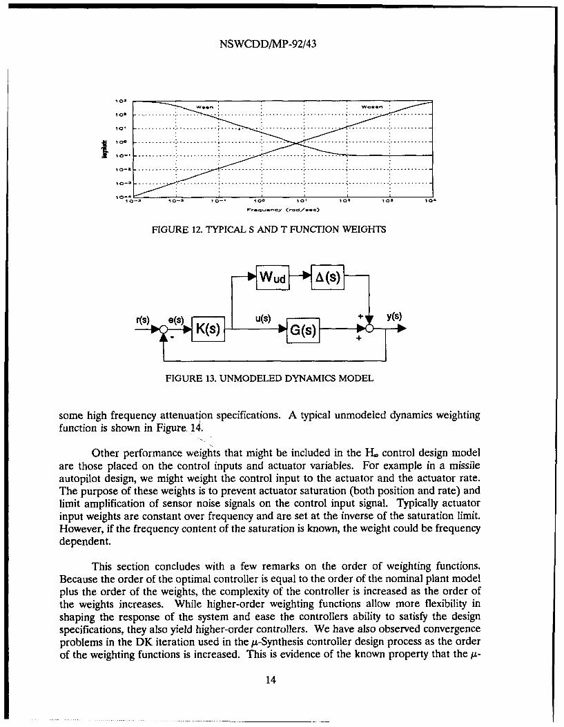
When using both sensitivity and complementary sensitivity weighting functions it isimportant to make sure that the magnitude of these weights at the frequency where theycross is less than one. This is necessary to prevent violation of the conservation law givenby Equation (4). Typical weighting functions for Ws(s) and WT(s) are shown in Figure 12.

Another method of limiting the controller bandwidth and providing high frequencygain attenuation is to use a high pass weight on an unmodeled dynamics uncertainty blockthat may be added from the plant input to the plant output. This type of weighting isdepicted in Figure 13. The characteristic of this weighting function is very similar to thecomplementary sensitivity weighting function. When using an unmodeled dynamics weightingfunction, it is usually chosen to represent the expected frequency content of the higher orderdynamics. In other words, the weight is chosen to cover the expected worst case magnitudeof the unmodeled dynamics. In addition, this weight may also be selected so as to satisfy

13

NSWCDD/MP-92/43

1 03

We W.0-

I.

10- -- - ao--- 1 -. ....... . .. 10

FIGURE 12. TYPICAL S AND T FUNCTION WEIGHTS

FIGURE 13. UNMODELED DYNAMICS MODEL

some high frequency attenuation specifications. A typical unmodeled dynamics weightingfunction is shown in Figure 14.

Other performance weighats that might be included in the H. control design model

are those placed on the control inputs and actuator variables. For example in a missileautopilot design, we might weight the control input to the actuator and the actuator rate.The purpose of these weights is to prevent actuator saturation (both position and rate) andlimit amplification of sensor noise signals on the control input signal. Typically actuatorinput weights are constant over frequency and are set at the inverse of the saturation limit.However, if the frequency content of the saturation is known, the weight could be frequencydependent.

This section concludes with a few remarks on the order of weighting functions.Because the order of the optimal controller is equal to the order of the nominal plant modelplus the order of the weights, the complexity of the controller is increased as the order ofthe weights increases. While higher-order weighting functions allow more flexibility inshaping the response of the system and ease the controllers ability to satisfy the designspecifications, they also yield higher-order controllers. We have also observed convergenceproblems in the DK iteration used in the p-Synthesis controller design process as the orderof the weighting functions is increased. This is evidence of the known property that the /.-

14

NSWCDD/MP-92/43

10210 , . . . . . . ... . . . . . . . . . .. . . . . ... . . . . .

. . . . . .. . ..-- - - - - -

10fl . .. . .. .. . .. . .. ....... ..

0-............ ............ ............ ................ ....... .......... ............

10-3 . . .. .. . . . .

10-- 10-2 10-1 100 10, 10' 103 10

FIGURE 14. EXAMPLE OF UNMODELED DYNAMICS WEIGHT

Synthesis DK iterations are not globally convex, which means that A-Synthesis is not alwaysguaranteed to converge to an improved solution. Our experience suggests that the order ofthe weights should be kept reasonably low to reduce the order of the resulting optimalcompensator and avoid potential convergence problems in the DK iterations.

PROBLEM-DEPENDENT ISSUES

While the guidelines discussed above in general apply for all controller designs,several issues regarding the proper selection of performance weights that we have found tobe problem-dependent follow:

Performance vs Stability/Robustness Tradeoffs and Weight Interaction. Theprimary tradeoff the designer must make in selecting the weighting functions isbetween performance and stability robustness characteristics. For example, increasingthe high frequency magnitude of output weights to add extra robustness to highfrequency unmodeled dynamics usually detracts from the desired output timeresponse characteristics (e.g., slower time response). This is due in part to thelimitation expressed by Equation (4) as well as other limitations. These type oftradeoffs are common to all control design methods. For A-synthesis, these tradeoffsare complicated by the interaction effects of the uncertainty weights with the inputdisturbance and output error weighting functions. The effects of the weightinteractions are complex and nonlinear and vary from problem to problem.

- Fine-Tuning of the Time (_onstant. An example of the above tradeoffs is isolationof the effects of interactions between sensitivity and complementary sensitivity weightson the overall system time constant. With the addition of the complementary

15

NSWCDD/MP-92/43

sensitivity weight, the relationship between the sensitivity weighting function crossoverpoint and closed-loop system time constant seems to be problem-dependent. Thequestion of where to exactly cross Ws and W, and at what magnitude requiresthoughtful consideration.

. Convergence Problems with High-Order Weights. In some cases, nonconvexbehavior in the DK iteration has been observed when using high order weightingfunctions. We have found this to be problem-dependent to some degree; but, ingeneral, we find that low-order weights are better all around. In addition, the fit ofthe D-scales in the DK iteration process may also have an influence on theconvergence behavior, especially if the D-scale fits are of high-order and haveextreme discontinuities. Using D-scale fits with extreme discontinuities and peaks ineffect adds lightly damped modes to the design model.

. Approach to High Frequency Weighting. Several issues concerning weightingfunctions that have most of their energy concentrated at high frequencies have beenidentified. In general, they relate to the best approach for handling the highfrequency loopshaping. These can be summarized as follows: If an unmodeleddynamics weight is used, what, if any, benefit is there to also weighting thecomplementary sensitivity function? There may be cases where a complementarysensitivity weight will be required to meet specific design goals or vice versa for anunmodeled dynamics weight. For some problems, a multiplicative uncertainty weightfor high frequency attenuation can be used at the plant input in place of theunmodeled dynamics weight and/or the complementary sensitivity weight.

• Issues Regarding the Performance Block. Consider robust performance analysisusing the structured singular value. The performance block can be thought of as afictitious unstructured uncertainty block that relates the regulated performanceoutputs to the exogenous (or disturbance) inputs. Certain trade-offs betweenperformance and robustness must be considered when specifying the performanceoutput weights. The point at which performance can be over specified will dependon the uncertainty description of the system. The size of the performance block willalso be a factor in the ability to achieve lower structured singular values, A. Becausethe performance block is treated as a full block, interactions between each componentof the full block will effect the design. For instance, including the actuator and highfrequency attenuation elements in the full block will give higher A-values than if thesewere treated as individual uncertainties included in the diagonal uncertainty Au block.However, if they are included in the full block, the number of D-scales that must befit (and hence the order of the controller) will be reduced. Thus, if you can getrobust performance with the larger full block, then this approach can be used tospeed up the design and keep the order of the controller down by reducing thenumber of uncertainties in the design model. Again, whether or not this can be donedepends on the particular problem.

16

NSWCDD/MP-92/43

The main purpose of the above discussion is to make the designer aware of thealternatives when selecting weighting functions to specify design goals and the potentialpitfalls that should be avoided. It is important to realize that the optimum weightingstrategies in L control and 4-Synthesis are problem-dependent and require engineeringjudgement. However, the guidelines suggested previously can help speed up the formulationof these weighting strategies.

SUMMARY AND CONCLUSIONS

In this report, we discussed the selection of weighting functions in H. Control.Sensitivity functions were defined and loopshaping design concepts were presented. Afterdescribing how the design weights serve as important "tuning knobs" in H. Control,guidelines were given on how these weights can be selected and how they relate to systemcharacteristics. This was followed by a discussion of advanced problem dependent issues yetto be resolved regarding the general weight selection process.

This report provides the H. Control system designer with practical rules-of-thumb fordesigning weighting functions to shape the response characteristics of the system and alsopoints out other options available to the designer and their impact on the design. Throughthe use of the guidelines presented herein, the -I. Control design process should be morestreamlined and, thus, result in savings in development time and cost of new control systems.

REFERENCES

1. Dorato, Peter, "A Historical Review of Robust Control," IEEE Control SystemsMagazine, April 1987.

2. Ohlmeyer, E.J., Robust Control Theory: Current Status and Future Trends, NAVSWCMP 90-385, Naval Surface Warfare Center, Dahlgren, VA, June 1990.

3. Doyle, J.C., Glover, K., Khargonekar, P.P. and Francis, B.A., "State-Space Solutionsto Standard H2 and H, Control Problems," Proceedings of 1988 American ControlConference, Atlanta, GA, June 1988.

4. Chiang, R.Y., Safonov, M.G. and Tekawy, J.A., "H' Flight Control Design with LargeParametric Robustness," Proceedings of l99OAmerican Control Conference, San Diego,CA, May 1990.

17

NSWCDD/MP-92/43

5. Balas, G.J. and Doyle, J.C., "On the Caltech Experimental Large Space Structure,"Proceedings of the 1988 American Control Conference, Atlanta, GA, June 1988.

6. Bibel, J. and Stalford, H., Mu-Synthesis Autopilot Design for a Flexible Missile, AIAA91-0586, 29th Aerospace Sciences Meeting, Reno, NV, January 1991.

7. Bibel, John E. and Stalford, Harold L., An Improved Gain-Stabilized Mu-ControllerFor a Flexible Missile, AIAA-92-0206, 30th Aerospace Sciences Meeting, Reno, NV,January 1992.

8. Grimble, M.J. and Biss, D., "Selection of Optimal Control Weighting Functions toAchieve Good H, Robust Designs," Proceedings of IEE International ConferenceControl 88, Conference Publication No. 285, April 1988.

9. Wall, J.E., Doyle, J.C. and Harvey, C.A., "Tradeoffs in the Design of MultivariableFeedback Systems," Proceedings of 18th Annual Allerton Conference onCommunication, Control and Computing, Monticello, IL, October 1980.

10. Doyle, J.C. and Stein, G., "Multivariable Feedback Design: Concepts for aClassical/Modern Synthesis," IEEE Transactions on Automatic Control, Vol. AC-26,February 1981.

11. Safonov, M.G., Laub, A.J. and Hartmann, G.L., "Feedback Properties ofMultivariable Systems: The Role and Use of the Return Difference Matrix," IEEETransactions on Automatic Control, Vol. AC-26, February 1981.

12. Stein, Gunter, Lecture Notes on Limitations on Achievable Performance of FeedbackSystems, Computer-Aided Multivariable Control System Design Short Course, MIT,Cambridge, MA, August 1989.

13. Freudenberg, J.S. and Looze, D.P., Frequency Domain Properties of Scalar andMultivariable Feedback Systems, Lecture Notes in Control and Information Sciences,#104, Springer-Verlag, Heidelberg, Germany, 1988.

14. Maciejowski, J.M., Multivariable Feedback Design, Addison-Wesley PublishingCompany, Wokingham, England, 1989.

15. Doyle, John C., Francis, Bruce A. and Tannenbaum, Allen R., Feedback ControlTheory, Macmillan Publishing Company, New York, NY, 1992.

18

NSWCDD/MP-92/43

DISTRIBUTION

Copies Copies

DEFENSE TECHNICAL ATTN 3915 R KLABUNDE 1INFORMATION CENTER 2 NAVAL AIR WARFARE CENTERCAMERON STATION CHINA LAKE CA 93555-6001ALEXANDRIA VA 22304-6145

ATTN CODE EC/BC J BURL 1ATTN GIFT AND EXCHANGE DIV 4 NAVAL POSTGRADUATE SCHOOLLIBRARY OF CONGRESS MONTEREY CA 93943-5000WASHINGTON DC 20540

ATTN J CLOUTIER IATTN M Z 4-89 S CHAN 1 AIR FORCE ARMAMENTGENERAL DYNAMICS DIRECTORATEAIR DEFENSE SYSTEMS DIV EGLIN AFB FL 32542POMONA FACILITYPO BOX 2507 ATTN LCDR D KRUEGER IPOMONA CA 91769-2507 593 B MICHELSON RD

MONTEREY CA 93040ATTN T PEPITONE1

AEROSPACE TECHNOLOGY COPO BOX 1809 Internal Distribution:DAHLGREN VA 22448-5000

E231 3AMTN H STALFORD 1 E232 2GEORGIA INST OF TECH E261 (Hall) 1SCHOOL OF AEROSPACE ENG E32 (GIDEP) 1ATLANTA GA 30332 F 1

F20 1ATTN F LUTZE 1 F30 1

E. CLIFF 1 F40 1VIRGINIA POLYTECHNIC F44 1INSTITUTE AND STATE UNIV F44 (Carr) 1DEPT OF AEROSPACE AND G 1OCEAN ENGINEERING G06 1BLACKSBURG VA 24061 G07 1

G10 1ATTN F GARRETT 1 Gl (Lucas) 1

D SCHMIDT 1 G13 (Strother) 1ARIZONA STATE UNIV G20 1SCHOOL OF MECH AND AERO ENG G205 1TEMPE AZ 83287-6106 G21 1

G23 1ATTN PROF D J COLLINS G23 (Bibel) 15NAVAL POSTGRADUATE SCHOOL G23 (Chadwick) 1DEPT OF AERONAUTICS G23 (Chisholm) 1MONTEREY CA 93940 G23 (Drake) 1

(1

NSWCDD/MP-92/43

Copies Copies

G23 (Hanger) 1 N 1G23 (Hardy) 1 N04 (Gaston) 1G23 (Hymer) 1 N07 1G23 (Jones) 1 N20 1G23 (Kiser) 1 N24 1G23 (Malyevac) 15 N24 (Addair) 1G23 (Ohlmeyer) 10 N30 1G23 (Phillips) 1 N35 (Boyer) 1G23 (Rowles) 1 N35 (Fennemore) 1G23 (Weisel) 1 N35 (Taft) 1G30 1 N40 1G31 1 N41 1G31 (Adams) 1 N41 (Hartman) 1G33 1 N41 (Tallant) 1G33 (Fraysse) 1 R04 1G33 (Hagan) IG33 (Nichols) 1G40 1G40 (Rucky) 1G42 1G43 1G43 (Graff) 1G43 (Palmer) 1G70 1G71 (Blair) 1G71 (Gray) 1G71 (Murray) 1G72 (W Smith) 1J 1J10 1J30 1J31 1'33 1K 1K10 1K12 (Rogers) 1K13 1K13 (Lawton) 1K40 1K404 (Alexander) 1K44 (Brnado) 1K" (Chen) 1

(2)

REPORT DOCUMENTATION PAGE Form ApprovedR R DOMB No. 0704.0188

Public repoting burden for this collection of information is esimated to average I hour per response. including the time for reviewing instructiOns. searching existing data sources.gathering and rmintaining the data needed and completing and reviewing the collection of information Send omments regarding this burden estimate or any other aspect of thiscollection of information. including suggestions for reducing this burden, to Washington Headquarters Servces. .irectoate for Information Operations and Reports, 1215 JeffersonDavs Highway, Suite 1204, Arlington. VA 222024302. and to the Oflice of Management and Budget. Paperwork Reduction Project (0704 0188), Washington. DC 20503

1. AGENCY USE ONLY (Leave blank) 2. REPORT DATE 3. REPORT TYPE AND DATES COVERED

January 1992 I4. TITLE AND SUBTITLE 5. FUNDING NUMBERS

Guidei.nes for the Selection of Weighting Functions for H-Infinity Control

6. AUTHOR(S)

John E. Bibel and D. Stephen Malyevac

7. PERFORMING ORGANIZATION NAME(S) AND ADDRESS(ES) S. PERFORMING ORGANIZATIONREPORT NUMBER

Naval Surface Warfare Center NSWCDD/MP-92/43Dahlgren Division (G23)Dahlgren, VA 22448-5000

9. SPONSORING/MONITORING AGENCY NAME(S) AND 10. SPONSORING/MONITORINGAGENCY REPORT NUMBER

11. SUPPLEMENTARY NOTES

12a. DISTRIBUTIONIAVAILABILITY 12b. DISTRIBUTION CODE

Approved for public release; distribution is unlimited.

13. ABSTRACT (Maximum 200 words)

This report provides insight into the selection of H-Infinity (H-) Control weighting functions that helpshape the performance and robustness characteristics of systems designed using the H. and p-SynthesisControl methods. Background material regarding sensitivity functions, loopshaping, and.H. Control isfollowed by a discussion of general engineering guidelines for the design of H. Control weighting functions.In addition, unresolved design issues and alternatives are presented. Thus, this report presents practicalrules-of-thumb and identifies issues and alternatives in the design of weighting functions for H. Control.

14. SUBJECT TERMS 15. NUMBER OF PAGES

Robust Control H-Infinity (H.) Control 27

Weighting Functions Mu-Synthesis 16. PRICE CODE

17. SECURITY CLASSIFICATION 16. SECURITY CLASSIFICATION 19. SECURITY CLASSIFICATION 20. LIMITATION OF ABSTRACT

OF REPORT OF THIS PAGE OF ABSTRACT

UNCLASSIFIED UNCLASSIFIED UNCLASSIFIED

NSN 7S40-01280-S5SOO S . d- fU ,I 2: R fk.. 2 89)P f.. -d b fy ANSI Sid ZII t

GENERAL INSTRUCTIONS FOR COMPLETING SF 298

The Report Documentation Page (RDP) is used in announcing and cataloging reports. It is important thatthis information be consistent with the rest of the report, particularly the cover and its title page.Instructions for filling in each block of the form follow. It is important to stay within the lines to meetoptical scanning requirements.

Block 1. Agency Use Only (Leave blank). Block 12a. Distribution/Availability Statement.Denotes public availability or limitations. Cite any

Block 2. Report Date. Full publication date including availability to the public. Enter additional limitationsday, month, and year, if available (e.g. 1 Jan 88). Must or special markings in all capitals (e.g. NOFORN, REL,cite at least the year. ITAR).

Block 3. Type of Report and Dates Covered. Statewhether report is interim, final, etc. If applicable, enter DOD - See DoDD 5230.24, "Distributioninclusive report dates (e.g. 10 Jun 87 - 30 Jun 88). Statements on Technical Documents."

DOE - See authorities.Block 4. Title and Subtitle. A title is taken from the NASA - See Handbook NHB 2200.2part of the report that provides the most meaningful NTIS - Leave blankand complete information. When a report is preparedin more than one volume, repeat the primary title, addvolume number, and include subtitle for the specific Block 12b. Distribution Code.volume. On classified documents enter the titleclassification in parentheses.

DOD - Leave blank.Block S. Funding Numbers. To include contract and DOE - Enter DOE distribution categories fromgrant numbers; may include program element the Standard Distribution fornumber(s), project number(s), task number(s), and Unclassified Scientific and Technicalwork unit number(s). Use the following labels: Reports.

NASA - Leave blank.C - Contract PR - Project NTIS - Leave blank.G - Grant TA - TaskPE - Program WU - Work Unit Block 13. Abstract. Include a brief (Maximum 200

Element Accession No. words) factual summary of the most significantinformation contained in the report.

BLOCK 6. Author(s). Name(s) of person(s) responsiblefor writing the report, performing the research, or Block 14. Subiect Terms. Keywords or phrasescredited with the content of the report. If editor or identifying major subjects in the report.compiler, this should follow the names).

Block 15. Number of Pages. Enter the total numberBlock 7. Performing Organization Name(s) and of pages.address(es). Self-explanatory.

Block 16. Price Code. Enter appropriate price codeBlock 8. Performing Organization Report Number. (NTIS only)Enter the unique alphanumeric report number(s)assigned by the organization performing the report. Block 17.-19. Security Classifications. Self-

explanatory. Enter U.S. Security Classification inBlock 9. Sponsoring/Monitoring Agency Name(s) and accordance with U.S. Security Regulations (i.e.,Address(es). Self-explanatory. UNCLASSIFIED). If form contains classified

information, stamp classification on the top andBlock 10. Sponsoring/Monitoring Agency Report bottom of this page.Number. (If Known)

Block 20. Limitation of Abstract. This block must beBlock 11. Supplementary Notes. Enter information not completed to assign a limitation to the abstract.included elsewhere such as: Prepared in cooperation Enter either UL (unlimited or SAR (same as report).with...; Trans. of...; To be published in.... When a An entry in this block is necessary if the abstract is toreport is revised, include a statement whether the new be limited. If blank, the abstract is assumed to bereport supersedes or supplements the older report. unlimited.

Standard Form 298 Back (Rev 2-89)