Embed Size (px)
Citation preview

ARCHITECTURE EFFECTS ON THE BULK AND SHEAR RHEOLOGY AND
PVT BEHAVIOR OF POLYMERS
by
Jiaxi Guo, B. Eng.
A DISSERTATION
IN
CHEMICAL ENGINEERING
Submitted to the Graduate Faculty
of Texas Tech University
in Partial Fulfillment of
the Degree of
DOCTOR OF PHILOSOPHY
Approved by
Sindee L. Simon
Chairperson of the Committee
Gregory B. McKenna
Ronald Hedden
Edward Quitevis
Shiren Wang
Accepted
Peggy Gordon Miller
Dean of the Graduate School
August, 2011

Copyright 2011, Jiaxi Guo

Texas Tech University, Jiaxi Guo, August 2011
ii
ACKNOWLEDGEMENTS
"It is much better to teach a person how to fish, rather than simply giving
him/her a fish." This is a very old saying in my country which I had heard since I was
young, but I had never fully understood the underlying meanings of the simple
aphorism until I became a graduate student of Professor Sindee Simon. Professor
Simon always taught me to use critical thinking to review others’ work and use my
own words and ideas to write down what I have learnt. To me, she is not only my
thesis advisor, but also my mentor.
I would like to thank Professor Gregory McKenna for his very helpful and
enlightening suggestions for my research. I also appreciate Professor Ronald Hedden
and Professor Edward Quitevis for taking the time to serve on my committee.
I also want to thank Dr. Paul O'Connell who helped me considerably with the
instrument. I would like to convey my thanks to Dr. Yan Meng for teaching me how to
operate the dilatometer, to Dr. Wei Zheng for teaching me how to operate the
rheometer, to Miao Hu, for helping me in the dynamic shear measurements, to Dr.
Yung Koh, Siyang Gao, Fatema Bengum, Haoyu Zhao, Maitri Vaddey, Yanfei Li, and
Xiguang Li for their suggestions and help, and to Kim Zinsmeyer for helping me
making the mold and machining the samples.
Finally, I want to express my gratitude to my brother and my parents for their
support and understanding of my leaving home so far away for so many years.

Texas Tech University, Jiaxi Guo, August 2011
iii
TABLE OF CONTENTS
ACKNOWLEDGEMENTS .............................................................................................................. ii
ABSTRACT ................................................................................................................................... vii
LIST OF TABLES ........................................................................................................................... ix
LIST OF FIGURES .......................................................................................................................... x
1.0 INTRODUCTION ................................................................................................................... 1
2.0 BACKGROUND ..................................................................................................................... 6
2.1 Pressure-Volume-Temperature Behavior of Polymers ..................................................... 6
2.1.1 Pressure-Volume-Temperature Measurements ...................................................... 6
2.1.2 Tait Equation of State ............................................................................................ 7
2.1.3 Pressure-Dependent Glass Transition Temperature (Tg) ....................................... 8
2.2 Linear Viscoelastic Shear and Bulk Responses of Polymers ......................................... 10
2.2.1 Viscoelastic Behavior .......................................................................................... 10
2.2.2 Linear Viscoelasticity .......................................................................................... 10
2.2.3 Shear Response in Polymers ............................................................................... 11
2.2.4 Bulk Response in Polymers ................................................................................ 14
2.2.4.1 Definition of Bulk Response .................................................................... 14
2.2.4.2 Bulk Response Measurement ................................................................... 15
2.2.4.3 Residual Stress Development ................................................................... 16
2.2.4.4 Comparison between Bulk and Shear Responses in Polymers ................ 16
2.3 Shift Factors and Relaxation Times in Polymers ........................................................... 18

Texas Tech University, Jiaxi Guo, August 2011
iv
2.3.1 Time Temperature Superposition Principle ......................................................... 18
2.3.2 Williams-Landel-Ferry and Vogel-Fulcher-Tammann-Hesse Functions ............. 19
2.3.3 Macedo and Litovitz Model ................................................................................ 20
2.3.4 Thermodynamic Scaling ..................................................................................... 21
REFERENCES ....................................................................................................................... 23
3.0 EXPERIMENTAL METHODOLOGY ................................................................................. 39
3.1 Materials ........................................................................................................................ 39
3.1.1 Polycyanurates .................................................................................................... 39
3.1.2 Three-Arm Star Polystyrene ............................................................................... 40
3.2 Dilatometric Measurements ........................................................................................... 41
3.2.1 Dilatometer ......................................................................................................... 41
3.2.2 Dilatometric Measurements for Polycyanurate Networks .................................. 42
3.2.2.1 Pressure-Volume-Temperature (PVT) Behavior Measurements .............. 42
3.2.2.2 Pressure Relaxation Measurements ......................................................... 43
3.2.2.3 Swell Tests ............................................................................................. 44
3.2.3 Dilatometer Measurement for Star Polystyrene .................................................. 45
3.2.3.1 Isobaric Temperature Scan ....................................................................... 45
3.2.3.2 Pressure Relaxation Measurements ......................................................... 45
3.2.3.3 Swell Test ................................................................................................. 46
3.3 Dynamic Shear Stress Measurement and Retardation Time Spectra Calculation .......... 47
3.3.1 Dynamic Shear Stress Measurements for Star Polystyrene ................................ 47
3.3.3 Retardation Time Spectra Calculation ................................................................ 48

Texas Tech University, Jiaxi Guo, August 2011
v
REFERENCES ....................................................................................................................... 49
4.0 EFFECT OF CROSSLINK DENSITY ON THE PRESSURE RELAXATION RESPONSE
OF POLYCYANURATE NETWORKS ......................................................................................... 56
4.1 Introduction .................................................................................................................... 56
4.2 Results............................................................................................................................ 59
4.3 Discussion ...................................................................................................................... 63
4.4 Conclusions .................................................................................................................... 66
REFERENCES ....................................................................................................................... 68
5.0 PRESSURE-VOLUME-TEMPERATURE BEHAVIOR OF TWO POLYCYANURATE
NETWORKS .................................................................................................................................. 81
5.1 Introduction .................................................................................................................. 81
5.2 Results............................................................................................................................ 83
5.3 Discussion ...................................................................................................................... 89
5.4 Conclusions .................................................................................................................... 92
REFERENCES ....................................................................................................................... 94
6.0 BULK AND SHEAR RHEOLOGY OF A THREE-ARM STAR POLYSTYRENE ........... 110
6.1 Introduction .................................................................................................................. 110
6.2 Results.......................................................................................................................... 111
6.2.1 PVT Behavior ................................................................................................... 111
6.2.2 Viscoelastic Bulk Modulus ............................................................................... 114
6.2.3 Dynamic Shear Relaxation Measurements ....................................................... 116
6.2.4 Comparisons between Bulk and Shear Responses ............................................ 117

Texas Tech University, Jiaxi Guo, August 2011
vi
6.3 Discussion .................................................................................................................... 119
6.4 Conclusions .................................................................................................................. 121
REFERENCES ..................................................................................................................... 123
7.0 THERMODYNAMIC SCALING OF POLYMER DYNAMICS VERSUS T – Tg SCALING
...................................................................................................................................................... 143
7.1 Introduction .................................................................................................................. 143
7.2 Results.......................................................................................................................... 146
7.3 Discussion .................................................................................................................... 152
7.4 Conclusions .................................................................................................................. 156
REFERENCES ..................................................................................................................... 158
8.0 CONCLUSIONS ................................................................................................................. 174
9.0 FUTURE WORK ................................................................................................................. 176
9.1 Pressure Dependent Structure Recovery ...................................................................... 176
9.2 Effects of β Relaxation on Viscoelastic Bulk Modulus ............................................... 177
9.4 Viscoelastic Bulk Modulus for Epoxy/POSS............................................................... 178
REFERENCES ..................................................................................................................... 179

Texas Tech University, Jiaxi Guo, August 2011
vii
ABSTRACT
The viscoelastic bulk modulus [K(t)] plays an important role in residual stress
development during polymer and composite processing and application, and in
developing relationships among the four fundamental material functions, bulk
modulus, shear modulus, Young’s modulus, and Poisson’s ratio. In addition, the
origins of viscoelastic bulk and shear moduli are still unresolved. However, while the
viscoelastic shear modulus has been widely studied, only a handful of investigations
can be found in the literature concerning the viscoelastic bulk response. In order to
investigate the viscoelastic bulk modulus, pressure relaxation responses were
measured in a custom-built pressurizable dilatometer capable of making K(t) and
pressure-volume-temperature (PVT) behavior measurements.
The architectural effects on the bulk and shear relaxation responses of two
polycyanurate networks have been studied and suggest that the shift factors used to
construct the reduced curves are identical in the liquid states. Furthermore,
comparisons of retardation time spectra indicates that bulk and shear responses have
similar underlying molecular mechanisms at short times since the slopes are similar
for the spectra; however, long-time mechanisms that are available to the shear are not
available to the bulk. In addition, the architectures are found to have negligible effects
on the bulk response; on the other hand, the relaxation/retardation time distributions
for the shear are observed to increase with decreasing the crosslink density.
The architecture effects were also studied on the bulk and shear responses for

Texas Tech University, Jiaxi Guo, August 2011
viii
linear and star shape polystyrenes. The shift factors are also found to be identical for
the bulk and shear responses of the two polymers in the liquid state; moreover, by
comparing the bulk and shear retardation time spectra, shear deformations are found
to have long-time mechanisms that are not available for the bulk.
The pressure-volume-temperature (PVT) behavior of the thermosetting networks
is studied to investigate the pressure-dependent glass transition temperature (Tg) and
the architecture effects on the PVT behavior. The results show that although the Tg
values are different, the two networks have similar values of dTg/dP. By comparing
the PVT data calculated from Tait equation with best fits to the experimental data for
the two networks, the most important variable governing the PVT behavior of the
thermosetting materials is found to be the glass transition temperature, which strongly
depends on crosslink density.
Finally, the temperature- and pressure-dependent shift factors which are related
to the relaxation times are reduced using a thermodynamic scaling, where τ=
ƒ(T-1
V-γ), and compared the results to the T – Tg scaling, where τ = ƒ(T – Tg). The
thermodynamic scaling law successfully reduces the data for all of the samples;
however, polymers with similar structures, but with different Tg and PVT behavior,
i.e., the two polycyanurates, cannot be superposed unless the scaling law is
normalized by TgVgγ. On the other hand, the T – Tg scaling successfully reduced the
polymers having similar microstructures.

Texas Tech University, Jiaxi Guo, August 2011
ix
LIST OF TABLES
Table 2.1 Bulk modulus for several small molecules and polymers at 1 atmospheric pressure .. 31
Table 3.1 Physical properties for the star and linear polystyrenes. .............................................. 50
Table 3.2 Tg of the two polycyanurate networks ......................................................................... 51
Table 4.1 KWW parameters for pressure relaxation master curves of two polycyanurate
networks .......................................................................................................................................... 71
Table 5.1 Tait parameters for polycyanurate samples in the rubbery (equilibrium) and glassy
states ............................................................................................................................................... 98
Table 5.2 KWW fitting parameters for viscoelastic bulk modulus, pressure relaxation response,
and cohesive energy density (CED) for the polycyanurate samples ............................................... 99
Table 6.1 Tait parameters for star polystyrene and linear polystyrene in the liquid and glassy
states. ............................................................................................................................................ 127
Table 6.2 KWW fitting parameters for pressure relaxation response and viscoelastic bulk
modulus of star polystyrene and linear polystyrene measured at different pressures. .................. 128
Table 7.1 Thermodynamic scaling exponent (γ) for TVγ scaling. .............................................. 162
Table 7.2 Comparison of mean squared deviation, χ2 × 10
2, for different scaling methods. ..... 163
Table 7.3 Parameters for the pressure-dependent coefficient of thermal expansion in the liquid
state αl in Eqn (7.7)....................................................................................................................... 164
Texas Tech University, Jiaxi Guo, August 2011
x
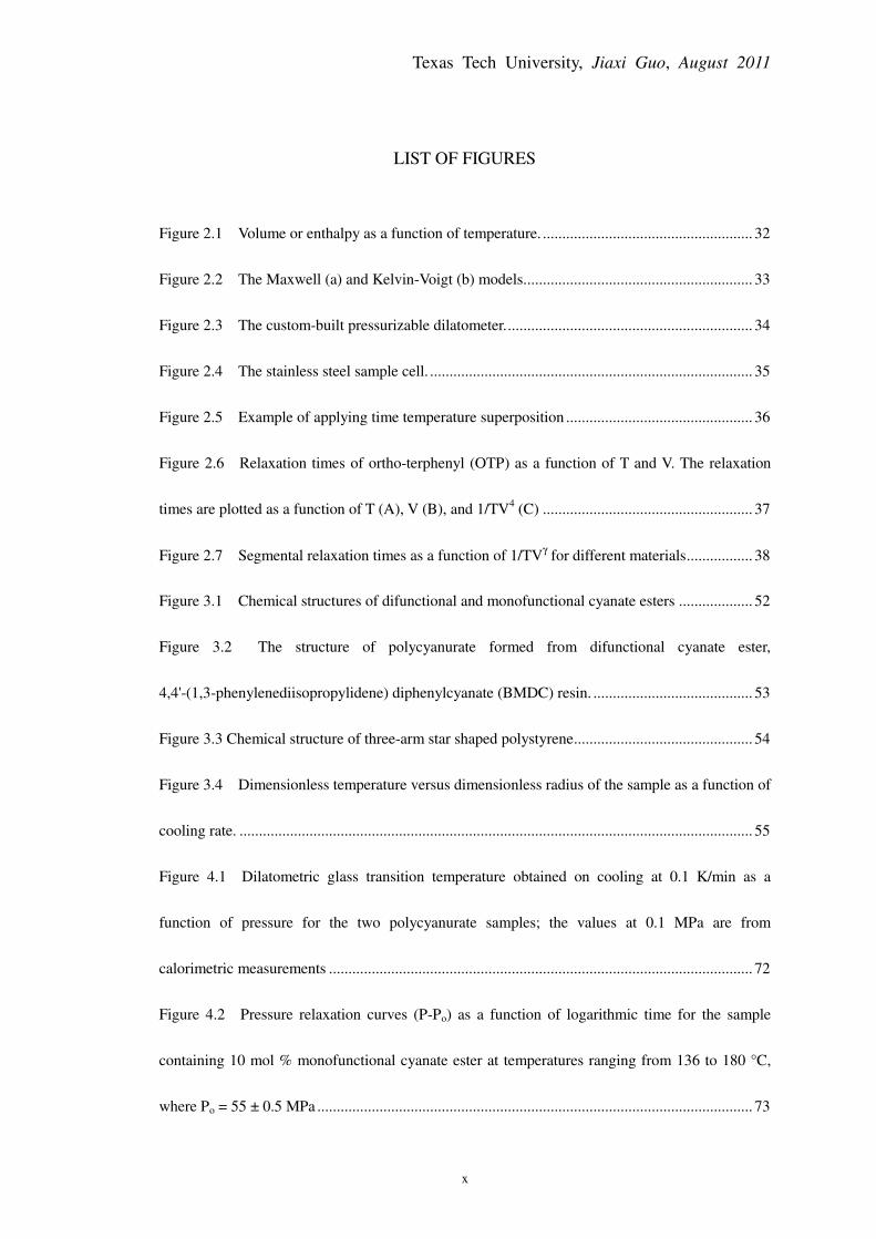
LIST OF FIGURES
Figure 2.1 Volume or enthalpy as a function of temperature. ...................................................... 32
Figure 2.2 The Maxwell (a) and Kelvin-Voigt (b) models. .......................................................... 33
Figure 2.3 The custom-built pressurizable dilatometer. ............................................................... 34
Figure 2.4 The stainless steel sample cell. ................................................................................... 35
Figure 2.5 Example of applying time temperature superposition ................................................ 36
Figure 2.6 Relaxation times of ortho-terphenyl (OTP) as a function of T and V. The relaxation
times are plotted as a function of T (A), V (B), and 1/TV4 (C) ...................................................... 37
Figure 2.7 Segmental relaxation times as a function of 1/TVγ for different materials ................. 38
Figure 3.1 Chemical structures of difunctional and monofunctional cyanate esters ................... 52
Figure 3.2 The structure of polycyanurate formed from difunctional cyanate ester,
4,4'-(1,3-phenylenediisopropylidene) diphenylcyanate (BMDC) resin. ......................................... 53
Figure 3.3 Chemical structure of three-arm star shaped polystyrene .............................................. 54
Figure 3.4 Dimensionless temperature versus dimensionless radius of the sample as a function of
cooling rate. .................................................................................................................................... 55
Figure 4.1 Dilatometric glass transition temperature obtained on cooling at 0.1 K/min as a
function of pressure for the two polycyanurate samples; the values at 0.1 MPa are from
calorimetric measurements ............................................................................................................. 72
Figure 4.2 Pressure relaxation curves (P-Po) as a function of logarithmic time for the sample
containing 10 mol % monofunctional cyanate ester at temperatures ranging from 136 to 180 °C,
where Po = 55 ± 0.5 MPa ................................................................................................................ 73

Texas Tech University, Jiaxi Guo, August 2011
xi
Figure 4.3 Pressure relaxation curves (P-Po) as a function of logarithmic time for the sample
containing 30 mol % monofunctional cyanate ester at temperatures ranging from 91 to 140 °C,
where Po = 55 ± 0.5 MPa ................................................................................................................ 74
Figure 4.4 Pressure relaxation curves as a function of time after application of vertical shifts for
the material containing 10 mol % monofunctional cyanate ester at temperatures ranging from 136
to 180 °C ......................................................................................................................................... 75
Figure 4.5 Pressure relaxation curves as a function of time after application of vertical shifts for
the material containing 30 mol % monofunctional cyanate ester at temperatures ranging from 91 to
140 °C ............................................................................................................................................. 76
Figure 4.6 Comparison of pressure relaxation master curves fitted with KWW function for the
two polycyanurate networks ........................................................................................................... 77
Figure 4.7 Vertical shift factors as a function of the temperature departure from the glass
transition temperature, T-Tg, for the two polycyanurate samples. .................................................. 78
Figure 4.8 Comparison of horizontal shift factors for the bulk response (filled symbols) with
those for the shear response from Li and Simon [34] (open symbols) ........................................... 79
Figure 4.9 Comparison of the bulk retardation time spectra (solid lines) and shear retardation
time spectra (dashed lines) for the sample containing 10 mol % monofunctional cyanate ester (red)
and that containing 30 mol % monofunctional cyanate ester (blue) ............................................... 80
Figure 5.1 Specific volume as a function of temperature at three pressures for the sample
containing 10 mol % monofunctional cyanate ester ..................................................................... 100
Figure 5.2 Specific volume as a function of temperature at five pressures for the sample
containing 30 mol % monofunctional cyanate ester ..................................................................... 101

Texas Tech University, Jiaxi Guo, August 2011
xii
Figure 5.3 Specific volume as a function of pressure for the sample containing 10 mol %
monofunctional cyanate ester ....................................................................................................... 102
Figure 5.4 Specific volume as a function of pressure for the sample containing 30 mol %
monofunctional cyanate ester ....................................................................................................... 103
Figure 5.5 Thermal expansion coefficients for the samples containing 10 mol % and 30 mol %
monofunctional cyanate ester as a function of pressure in both rubbery (filled symbols) and glassy
(open symbols) states, respectively .............................................................................................. 104
Figure 5.6 The instantaneous bulk moduli for the two polycyanurate networks as a function of
pressure measured from isothermal pressure scans at the temperatures indicated ....................... 105
Figure 5.7 The thermal pressure coefficient as a function of pressure for the polycyanurate
networks calculated from the product of the thermal expansion coefficient (Figure 5.5) and the
bulk modulus (Figure 5.6, by interpolation) ................................................................................. 106
Figure 5.8 Time-dependent viscoelastic bulk modulus in the vicinity of α-relaxation calculated
from previous pressure relaxation studies [22] for the two polycyanurate samples ..................... 107
Figure 5.9 Specific volume in both the rubbery and glassy states minus the volume at Tg (V -
VTg) as a function of the temperature departure from Tg [T – Tg(P)] at 0.1, 30 and 60 MPa for the
samples containing 10 mol % monocyanate ester (solid lines) and 30 mol % (dashed lines) ...... 108
Figure 5.10 Comparison of specific volume as a function of temperature at ambient pressure for
the samples containing 10 mol % (red curve) and 30 mol % (blue curve) monofunctional cyanate
ester, respectively .......................................................................................................................... 109
Figure 6.1 Specific volume as a function of temperature at four pressures for star polystyrene.
The data point at 0.1 MPa and 25.3 °C was obtained by density measurement ........................... 129

Texas Tech University, Jiaxi Guo, August 2011
xiii
Figure 6.2 Specific volume as a function of pressure for the star polystyrene measured at 60, 120,
and 130 °C. The solid lines are calculated from the Tait equation for data at 120 and 130 °C in the
liquid state. .................................................................................................................................... 130
Figure 6.3 The instantaneous bulk modulus for the star polystyrene as a function of pressure
obtained at 60, 120, and 130 °C based on the isothermal pressure scan shown in Figure 6.2 ...... 131
Figure 6.4 Glass transition temperatures (Tg) of star polystyrene as a function of pressure
obtained at cooling rate of 0.1 K/min ........................................................................................... 132
Figure 6.5 Pressure relaxation curves [P(t) – Po] as a function of logarithmic time for star
polystyrene carried out at 36 MPa ................................................................................................ 133
Figure 6.6 Pressure relaxation curves [P(t) – Po] as a function of logarithmic time for star
polystyrene carried out at 55 MPa ................................................................................................ 134
Figure 6.7 Pressure relaxation curves as a function of time after application of vertical shifts for
star polystyrene at temperatures ranging from 70 to 123 °C at 36 MPa ....................................... 135
Figure 6.8 Pressure relaxation curves as a function of time after application of vertical shifts for
star polystyrene at temperatures ranging from 81 to 133.5 °C at 55 MPa .................................... 136
Figure 6.9 Comparison of viscoelastic bulk modulus fitted with KWW function for the star and
linear [30] polystyrenes measured at pressures as indicated ......................................................... 137
Figure 6.10 Dynamic shear storage modulus (G') as a function of frequency for the star
polystyrene at temperature ranging from 95 to 170 °C ................................................................. 138
Figure 6.11 Dynamic shear loss modulus (G") as a function of frequency for the star polystyrene
at temperature ranging from 95 to 170 °C .................................................................................... 139
Figure 6.12 Phase angle (tanδ) obtained at different temperatures ranging from 95 to 170 °C for
Texas Tech University, Jiaxi Guo, August 2011
xiv
and shifted to form a master curve by applying time-temperature superposition. The inset shows
Cole-Cole plot for the data obtained at temperatures ranging from 110 to 120 °C. ..................... 140
Figure 6.13 Logarithm of horizontal shift factors obtained from the pressure relaxation studies
and shear dynamic measurements for the star polystyrene with their counterparts for the linear
polystyrenes from creep compliance measurements of Agarwal [25], and pressure relaxation
measurements of Meng and Simon [17], and the dynamic shear measurements of Cavaille et al.
[26]................................................................................................................................................ 141
Figure 6.14 Comparison of the bulk and shear retardation time spectra for the star polystyrene.
Spectra for linear polystyrenes [17, 25, 26] are calculated from data in the literature. The bulk
retardation time spectra are calculated from the KWW function fit to the viscoelastic bulk
modulus. ....................................................................................................................................... 142
Figure 7.1 Temperature- and pressure-dependent normalized relaxation times [log(τ/τTg)] as a
function of 1/TVγ for six polymers. The data are obtained at the pressures indicated on the right
hand side of the figure .................................................................................................................. 165
Figure 7.2 Temperature- and pressure-dependent normalized relaxation times [log(τ/τTg)] as a
function of TgVgγ/TV
γ and T – Tg for the linear and star polystyrenes ......................................... 166
Figure 7.3 Temperature- and pressure-dependent normalized relaxation times [log(τ/τTg)] as a
function of TgVgγ/TV
γ and T – Tg for the polycyanurate networks ............................................... 167
Figure 7.4 Temperature- and pressure-dependent normalized relaxation times [log(τ/τTg)] as a
function of TgVgγ/TV
γ and T – Tg for PVAc .................................................................................. 168
Figure 7.5 Temperature- and pressure-dependent normalized relaxation times [log(τ/τTg)] as a
function of TgVgγ/TV
γ and T – Tg for PVC ................................................................................... 169

Texas Tech University, Jiaxi Guo, August 2011
xv
Figure 7.6 Temperature- and pressure-dependent normalized relaxation times [log(τ/τTg)] as a
function of (T – Tg)(1/Tg(P) + γαl) for polystyrenes ..................................................................... 170
Figure 7.7 Temperature- and pressure-dependent normalized relaxation times [log(τ/τTg)] as a
function of (T – Tg)(1/Tg(P) + γαl) for polycyanurates ................................................................. 171
Figure 7.8 Temperature- and pressure-dependent normalized relaxation times [log(τ/τTg)] as a
function of (T – Tg)(1/Tg(P) + γαl) for PVAc ................................................................................ 172
Figure 7.9 Temperature- and pressure-dependent normalized relaxation times [log(τ/τTg)] as a
function of (T – Tg)(1/Tg(P) + γαl) for PVC ................................................................................. 173

Texas Tech University, Jiaxi Guo, August 2011
1
CHAPTER 1
INTRODUCTION
The viscoelastic bulk modulus [K(t)] has not been widely studied, although it
plays important roles in the development of isotropic residual stresses in polymer
composites application and processing, as well as in the theoretical aspects of polymer
physics. Leaderman [1] has proposed that bulk and shear deformations have different
underlying mechanisms: the former arises from intra-molecular relaxation, while the
latter originates from inter-molecular/segmental relaxations. This hypothesis has been
backed up by several studies [2-8] examining the breadth of the relaxation distribution,
the activation energy of the shift factors, and the time scales where relaxation occurs
for the bulk and shear responses. On the other hand, other studies also show that the
two deformations have identical shift factors [9-12] or share similar relaxation
mechanisms at short times [10, 12]. The motivation of the work is to study the
viscoelastic bulk modulus not only for providing experimental data to the field, but
for further investigating the debates with respect to the origins of bulk and shear
responses.
The dissertation consists nine chapters. Chapter 2 provides general background
for pressure-volume-temperature measurements, viscoelastic bulk and shear responses,
and the temperature dependence of relaxation times in glass-forming polymers.
Chapter 3 describes the experimental methodology. Chapters 4-7 are journal
manuscripts where each chapter consists of one journal article. The journal articles

Texas Tech University, Jiaxi Guo, August 2011
2
have been modified for the dissertation.
Chapter 4 deals with the effects of crosslink density on the viscoelastic bulk
responses of two polycyanurate networks. The article has been published in the
Journal of Polymer Science, Part B: Polymer Physics [13]. The chapter describes the
experimental pressure relaxation data measured by a custom-built dilatometer [14], as
well as the results of comparisons of the shift factors of bulk and shear deformations
[15], and of the retardation time spectra calculated from these responses.
Chapter 5 deals with the pressure-volume-temperature (PVT) behavior of two
polycyanurate networks. The article has been published in the Journal of Polymer
Science, Part B: Polymer Physics [16]. This chapter provides PVT data for the two
materials, the instantaneous bulk modulus as a function of both temperature and
pressure, the pressure expansion coefficient (γ) that is a product of thermal expansion
coefficient (α) and bulk modulus (K). The effects of crosslink density on the PVT
behavior and the viscoelastic bulk modulus are extensively discussed.
Chapter 6 deals with the bulk and shear rheology of a three-arm star-shaped
polystyrene. The article is in the final stages of preparation [17]. The shift factors and
retardation time spectra obtained from the bulk and shear responses of the star
polystyrene are compared to those from linear polystyrene [12]. The architectural
effects on the viscoelastic bulk and shear responses are discussed based on the
experimental results.
Chapter 7 deals with a TVγ thermodynamic scaling proposed in the literature
[18-20] used in the present study to reduce the temperature- and pressure-dependent
Texas Tech University, Jiaxi Guo, August 2011
3
shift factors. This chapter focuses on the comparisons between the TVγ
thermodynamic scaling and the T – Tg scaling in reducing the temperature- and
pressure-dependent relaxation times for six polymers. The article has been submitted
to the Journal of Chemical Physics [21].
Finally, Chapter 8 concludes the work in the dissertation, and Chapter 9 provides
some suggestions for the future work.

Texas Tech University, Jiaxi Guo, August 2011
4
References
1. H. Leaderman, in "Rheology," F. R. Eirich, Ed., Academic, New York, Vol. 2,
1958.
2. S. B. Sane, W. G. Knauss, Mech. Time-Depend. Mater. 5, 293-324, 2001.
3. T. H. Deng and W. G. Knauss, Mech. Time-Depend. Mater. 1, 33-49, 1997.
4. R. Kono, J. Phys. Soc. Japan 15, 718-725, 1960.
5. R. Kono, H. Yoshizaki, Jap. J. Appl. Phys. 12 (3), 445-457, 1973.
6. N. W. Tschoegl, The Phenomenological Theory of Linear Viscoelastic Behavior,
Springer-Verlag, Berlin, 1989.
7. R. J. Crowson, R. G. C. Arridge, Polymer, 20, 737-746, 1979.
8. A. F. Yee, M. T. Takemori, J. Polym. Sci. Polym. Phys. Ed. 20, 205-224, 1982.
9. R. S. Marvin, R. Aldrich, H. S. Sack, J. Appl. Phys. 25 (10), 1213-1218, 1954.
10. C. A. Bero, D. J. Plazek, J. Polym. Sci. Part B: Polym. Phys. 29, 39-47, 1991.
11. D. J. O'Brien, N. R. Sottos, S. R. White, Experimental Mechanics, 47, 237-249,
2007.
12. Y. Meng, S. L. Simon, J. Polym. Sci. Part B: Polym. Phys. 45, 3375-3385, 2007.
13. J. X. Guo, S. L. Simon, J. Polym. Sci. Part B, Polym. Phys., 47, 2477-2486,
2009.
14. Y. Meng, P. Bernazzani, P. O’Connell, G. B. McKenna, S. L. Simon, Rev. Sci.
Instrum. 80, 053903–1-9, 2009.
15. Q. X. Li, S. L. Simon, Macromolecules 40, 2246-2256, 2007.
16. J. X. Guo, S. L. Simon, J. Polym. Sci. Part B: Polym. Phys. 48, 2509-2517, 2010.

Texas Tech University, Jiaxi Guo, August 2011
5
17. J. X. Guo, S. L. Simon, "Bulk and Shear Rheology of a Symmetric Three-Arm
Star Polystyrene," in Preparation, 2011.
18. G. Tarjus, D. Kivelson, S. Mossa, C. Alba-Simionesco, J. Chem. Phys. 120,
6135-6141, 2004.
19. C. Dreyfus, A. Aouadi, J. Gapinski, M. Matos-Lopes, W. Steffen, A. Patkowski,
R. M. Pick, Phys. Rev. E 68, 011204–1-11, 2003.
20. R. Casalini, C. M. Roland, Phys. Rev. E 69, 062501–1-3, 2004.
21. J.X. Guo, S. L. Simon, "Thermodynamic Scaling of Polymer Dynamics versus
Shifting by T – Tg," Submitted to J. Chem. Phys. 2011.
Texas Tech University, Jiaxi Guo, August 2011
6
CHAPTER 2
BACKGROUND
2.1 Pressure-Volume-Temperature Behavior of Polymers
2.1.1 Pressure-Volume-Temperature Measurements
The specific volume of polymeric materials as a function of pressure and
temperature plays a key role in the fields of both polymer physics and plastics
engineering and has been considerably investigated since the 1940s [1-38]. With
respect to polymer physics, the pressure-volume-temperature (PVT) behavior is a
fundamental property of a given material and reflects underlying structure and forces.
On the other hand, from the plastic engineering point of view, the study of the specific
volume as a function of pressure and temperature can be used to optimize the
processing conditions for both thermosetting and thermoplastic materials and to
predict volume shrinkage after molding.
Two methods have been applied to measure the PVT behavior of polymeric
materials: piston-die and confining fluid measurements. In the piston-die method, the
sample is located in a die and pressurized by a piston to obtain the data of specific
volume as a function of pressure or temperature [1-10]. The advantage of this
approach is the volume change of the sample can be directly obtained from the
displacement of the piston. However, this method suffers from two main
disadvantages: the pressure is not hydrostatic when the sample is solidified due to

Texas Tech University, Jiaxi Guo, August 2011
7
vitrification or crystallization, and leakage between the die and the piston may occur
[20, 36, 37, 39]. For the former problem, Zoller and coworkers [39] analyzed the
stress and volume change of polymers in the piston-die technique, and suggested that
only can this method give an accurate measurement when the shear modulus of the
sample is much smaller than its bulk modulus.
On the other hand, in the confining fluid method, the sample is submerged in a
sample cell containing fluid, in which the fluid can be mercury, water, or silicone oil
that is chemically inert [20-36, 40]. During the measurement, the pressure is truly
hydrostatic in both liquid and solid states for polymer samples and moreover, the
leakage problem can be avoided by this method. The volume change in this method
involves both the sample and the fluid, giving a relative volume change for the sample.
The absolute specific volume of the sample can be calculated from the difference of
the total volume change and the fluid volume change. The problem of this method is
that potential interaction may occur between the sample and the fluid, or the sample
may absorb the surrounding fluid, leading to an unacceptable result. Therefore, an
appropriate confined fluid should be selected and swell tests must be made to ensure
that no adverse effects of the fluid occur during the experiment.
2.1.2 Tait Equation of State
For polymeric materials in the equilibrium state, the specific volume only
depends on the applied pressure and temperature. The so-called Tait [41] equation is

Texas Tech University, Jiaxi Guo, August 2011
8
found to be accurate to fit the specific volume as a function of pressure and
temperature in the liquid state. The Tait equation can be expressed as
−+−=
)exp(1ln1),0(V),(V
1TBB
PCTTP
o
(2.1)
where C, Bo and B1 are Tait parameters varied with different materials. C is generally
set to 0.0894 [42]. In the liquid state, the specific volume at zero pressure can be fit
with a polynomial function
2
21
1),0(V
TaTaaT
o ++= (2.2)
The Tait equation is also used to describe PVT data for solid samples, although in this
case, the fit is only valid for the particular solidification path used to obtain the data.
In the solid state, the equation for specific volume as a function of temperature at zero
pressure is generally taken [34]
)exp(
1),0(V
1TaaT
o −= (2.3)
In both Eqns 2.2 and 2.3, ao, a1, and a2 are material dependent constants. Parameters
for Tait equation and V (0, T) are available for a large number of polymers [43].
2.1.3 Pressure-Dependent Glass Transition Temperature (Tg)
For glass-forming materials, glass transition behavior is observed when the
material cools from the liquid (equilibrium) state (high temperature) to the glassy state
(relatively low temperature). Figure 2.1 shows a typical glass-forming process on
cooling. As indicated in Figure 2.1, the glass transition behavior occurs when the

Texas Tech University, Jiaxi Guo, August 2011
9
slope of the volume (V) or enthalpy (H) as a function of temperature changes, and the
glass transition temperature (Tg) is defined by the intercept of the liquid and glassy
lines.
The glass transition occurs because during cooling, the relaxation time (τ) of the
liquid increases significantly, and at some point, the relaxation time is longer than the
time scale of cooling so that the material does not have enough time to maintain
equilibrium density, leading to deviation from the liquid (equilibrium) line to the
glassy (non-equilibrium) line [44]. Therefore, the glass transition is a kinetic behavior
and depends strongly on the cooling rate. As indicated in Figure 2.1, Tg obtained from
q1 (Tg1) is higher than that from q2 (Tg2) for q1 > q2, where q is cooling rate.
In general, Tg can be measured by differential scanning calorimetry (DSC) or
dilatometry. Moreover, Tg can only be determined during cooling [45] by its definition.
In the present study, Tg is measured as a function of pressure using a custom-built
dilatometer [40] at a cooling rate 0.1 K/min. The pressure-dependent Tg has been
reviewed [46] and has been found to increase with increasing pressure. This behavior
is understandable since the specific volume decreases with increasing pressure at a
given temperature, resulting in a reduced mobility or a longer relaxation time.
The relationship between Tg and pressure is linear at relatively low pressures,
whereas the slope is observed to decrease at high pressures. In the limit of low
pressure, the slope of Tg as a function of pressure, dTg/dP, has been found to range
from 0.1 to 0.4 K/MPa [46-47] for a majority of polymers. In wider range of pressure,
Tg as a function of pressure can be described by an empirical equation suggested by

Texas Tech University, Jiaxi Guo, August 2011
10
Anderson and Anderson [48]
b
g Pa
bcPT
/1
1)(
+= (2.4)
where a, b, and c are fitting parameters.
2.2 Linear Viscoelastic Shear and Bulk Responses of Polymers
2.2.1 Viscoelastic Behavior
For a viscous liquid, stress after deformation is a function of strain rate, whereas
for an elastic material, stress is a function of strain. Viscous behavior can be
represented by a dashpot model; on the other hand, elastic behavior can be
represented by an elastic spring model [49]. The viscoelastic response in its simplest
form is the combination of the behavior of the dashpot and the elastic spring.
The dashpot and elastic spring can be either connected in series or in parallel as
shown in Figure 2.2, where the former is referred to as the Maxwell model (2.2a), and
the latter is referred to the Kelvin-Voigt model (2.2b). In general, the Maxwell model
is used to describe the relaxation behavior, whereas the Kelvin-Voigt model is used to
describe the creep behavior for the polymers, although the former one can also
describe the creep functions.
2.2.2 Linear Viscoelasticity
Polymers are viscoelastic materials in that the stress is a function of both applied
strain and rate of strain. In the dissertation, only linear viscoelasticity is considered,

Texas Tech University, Jiaxi Guo, August 2011
11
where the stress is linearly proportional to the strain, i.e., "double the strain, double
the stress [50]." The linear viscoelastic properties can only be obtained when the
applied strain is small and the rate of strain is low [49].
Four linear viscoelastic functions, the shear modulus G (or shear compliance J),
bulk modulus K (or bulk compliance B), Young’s modulus E (or Young’s compliance
D) and Poisson’s ratio ν, are essential to describe the deformations of the materials
and to analyze and design reliable engineering structures. In general, only two of the
four functions are needed to obtain since the other two can be calculated [51, 52] by
the relationship given by
)](21[3
)()(
t
tEtK
ν−= (2.5)
and
)](1[2
)()(
t
tEtG
ν+= (2.6)
where K(t), E(t), G(t), and ν(t) are time-dependent bulk modulus, shear modulus,
Young’s modulus, and Poisson’s ratio, respectively. However, to obtain bulk modulus
or Poisson’s ratio, high accuracies of the other two functions are required [51, 52],
making the relationships in Eqns 2.5 and 2.6 not always useful.
2.2.3 Shear Response in Polymers
In general, the shear response in polymers can be obtained by two different types
of experiments, relaxation and creep. In the relaxation measurement, the viscoelastic

Texas Tech University, Jiaxi Guo, August 2011
12
shear modulus, G(t), is carried out as a function of time-dependent stress [σ(t)] with a
constant strain (γo)
o
ttG
γ
σ )()( = (2.7)
On the other hand, in the creep experiment, the viscoelastic shear compliance, J(t), is
measured as a function of time-dependent strain [γ(t)] with a constant stress (σo)
o
ttJ
σ
γ )()( = (2.8)
It has been mentioned above that the relaxation measurement can be described
by the Maxwell model. For a series of Maxwell elements, the shear modulus can also
be obtained by
∑=
−+=n
i
t
ieieGGtG
1
/)(
τ (2.9)
where Gi and τi are the ith element modulus and characteristic relaxation time, and Ge
is equilibrium modulus. On the other hand, the viscoelastic creep behavior can be
described by a group of Voigt elements, and the series compliance is given by
o
n
i
t
ig teJJtJ i ηλ/)1()(
1
/ +−+= ∑=
− (2.10)
where Ji and λi are the ith element compliance and characteristic retardation time, Jg is
the compliance at t = 0 s, and ηo is the terminal viscosity. Assuming that the
relaxation/retardation time is continuous, the viscoelastic response can be described
by a relaxation (H) or retardation (L) time spectra [49], and the shear relaxation
modulus in Eqn 2.9 can be rewritten as
∫∞
∞−
−+= ττ ln)( /dHeGtG
t
e (2.11)

Texas Tech University, Jiaxi Guo, August 2011
13
Similarly, the shear compliance is given by
∫∞
∞−
− +−+= o
t
g tdeLJtJ ηττ /ln)1()( / (2.12)
On the other hand, the relaxation and retardation time spectra can be calculated from
the shear modulus and compliance by the secondary approximations of Schwarzl and
Staverman [53] given by
( )τ
τ2
2
2
ln
)(
)ln(
)()(
=
+−=t
td
tGd
td
tdGH (2.13)
and
( )λ
λ2
2
2
ln
)(
)ln(
)()(
=
−=t
td
tJd
td
tdJL (2.14)
Other relationships between the functions are fully reviewed by Ferry [49].
In addition, the shear response can also be studied by dynamic measurements,
where the frequency-dependent shear response is measured for a given sinusoidally
oscillating strain as a function of phase angle (δ). In this measurement, the shear
modulus or compliance is complex given by
*
*"'*
γ
σ=+= iGGG (2.15)
and
*
*"'*
σ
γ=−= iJJJ (2.16)
where G' and G" are storage and loss moduli, J' and J" are storage and loss
compliances, σ* and γ* are complex stress and strain, respectively. Mathematically,
the storage and loss moduli/compliances are related to the viscoelastic shear
modulus/compliance or other shear functions. Therefore, only knowledge of one
function is needed to obtain others [49].

Texas Tech University, Jiaxi Guo, August 2011
14
2.2.4 Bulk Response in Polymers
2.2.4.1 Definition of Bulk Response
The bulk response is defined for a material undergoing isotropic compression or
expansion, in which the stress is the hydrostatic pressure (P) and the strain is the
volumetric strain (εv = ∆Vo/V). By the definition, for time-independent response at a
given temperature, the bulk modulus [K(T)] is defined by
TVo
PTK
ε
∆−=)( (2.17)
and the bulk compliance [B(T)] is defined by
T
Vo
PTB
∆−=
ε)( (2.18)
Table 2.1 has shown the bulk modulus at a given temperature as indicated and
atmospheric pressure for several small molecules and polymers from the literature [43,
54-59].
For time-dependent bulk response, the viscoelastic bulk modulus at constant
temperature, K(t)T is obtained measuring the pressure as a function of time [∆P(t)] at
constant volumetric strain (εVo) given by
TVo
T
tPtK
ε
)()(
∆−= (2.19)
whereas the bulk compliance at constant temperature [B(t)T] is obtained measuring
the volumetric strain as a function of time [εV(t)] at constant pressure (∆P) and is
given by

Texas Tech University, Jiaxi Guo, August 2011
15
T
VT
P
ttB
∆−=
)()(
ε (2.20)
2.2.4.2 Bulk Response Measurement
Unlike the shear response that has been widely studied in the literature, the
viscoelastic bulk modulus has been rarely investigated due to long term temperature
stability is needed, which has not been commercialized. So far, only a handful of
studies concerning the viscoelastic bulk measurements can be found in the literature
[60-69]. More recently, Drs. Meng, Bernazzani and coworkers in our laboratory have
developed a pressurizable dilatometer [40] to measure the bulk response. The
instrument can be operated at temperatures ranging from 35 to 230 °C, and at
pressures up to 250 MPa; the oil bath used to maintain the temperature of the sample
has temperature stability greater than 0.01 °C; the average absolute error in volume in
the measurement is better than 5.4×10⁻⁴
cm3. A schematic description of the
instrument has been shown in Figure 2.3 which is taken from Ref. 40, where the
sample is loaded in the sample cell as shown in Figure 2.4 (also from Ref. 40). Using
this instrument, previous researches in our laboratory have measured the viscoelastic
bulk response for linear polystyrene [40, 70]. Here, this technique is used to measure
a three-arm star polystyrene [71], and two polycyanurate networks having different
crosslink density [72, 73]. The results of the star polystyrene and the two
polycyanurates will be shown in the dissertation as Chapters 4-6.

Texas Tech University, Jiaxi Guo, August 2011
16
2.2.4.3 Residual Stress Development
Thermosetting materials have a wide application in the fields of electronic and
aerospace composite industries due to their low cost, light weight and high
mechanical performance [74-76]. However, the residual stresses buildup in the
composites limits the application. The build-up of residual stresses is due to cure
shrinkage of the thermosetting materials (cure stresses) and thermal stresses arising
from the difference between the thermal expansion coefficients (α) for the thermoset
and the substrate. The thermal stresses are found [76-78] to be more dominant.
Two types of residual stress, uniaxial and isotropic stresses, are induced by the
mismatch. The isotropic residual thermal stress (σiso) can be calculated from the
product of thermal expansion coefficient (α) and the temperature-dependent bulk
modulus [K(T)] as a function of temperature given by
∫=∆2
1
)(T
Tiso dTTKασ (2.21)
For time- and temperature-dependent behavior, the isotropic residual thermal stress
σiso(T, t) is a function of both viscoelastic bulk modulus K(t) and rate of temperature
change (q = dT/dt) [79]
dtqTttKTtt
tiiso
i∫ −−=∆ ),(),( ασ (2.22)
2.2.4.4 Comparison between Bulk and Shear Responses in Polymers
The origins of bulk and shear responses in polymers have been debated for years.
Leaderman [80] has suggested that the bulk deformation arises from intra-molecular

Texas Tech University, Jiaxi Guo, August 2011
17
relaxation, whereas the shear is originated from inter-molecular or inter-segmental
relaxation. This hypothesis has subsequently been backed up by several studies [52,
70-73, 81, 82] finding differences in bulk and shear responses. The relaxation
distribution for the shear response has been found to be broader than that for the bulk
[70, 81, 82]. Moreover, the bulk relaxation was found to occur at short times than the
shear relaxation [70-72]. Finally, the activation energies obtained from the shift
factors for reducing the shear and bulk relaxation responses are found to be higher for
the bulk [72, 73].
On the other hand, the shift factors were found to be the same in the studies of
polyisobutylene [83], epoxy materials [84, 85], linear and star polystyrene [70, 71],
and two polycyanurate networks [72, 86]. Furthermore, Bero and Plazek [84] further
compared the two relaxations based on the retardation time spectra and found that the
two spectra have similar slopes at short times, whereas shear relaxation has long-time
underlying mechanisms that are not available for the bulk. However, only relative
values for the bulk spectra were obtained by Bero and Plazek [84]. By measuring the
viscoelastic bulk modulus, absolute values for the bulk retardation time spectra can be
obtained in our laboratory. One aim in the dissertation is to obtain the retardation time
spectra from the viscoelastic bulk modulus and compare it to that for the shear in
order to resolve the debate concerning the origins of bulk and shear deformations.

Texas Tech University, Jiaxi Guo, August 2011
18
2.3 Shift Factors and Relaxation Times in Polymers
2.3.1 Time Temperature Superposition Principle
For polymers, the mechanical properties at a given temperature are
time-dependent. In order to obtain a response for a given property over the entire time
window, the measurement has to be taken over many decades, which is very difficult
to achieve in the laboratory. To solve this problem, the time temperature superposition
(TTS) principle was suggested [49]. The idea of TTS is that mechanical response
curves measured at high temperatures can provide long-time response, whereas those
at low temperatures can provide short-time response. All of the curves can be shifted
to a reference temperature (To) to form a reduced curve which gives the response over
the entire time window. One example of applying TTS to form a reduced curve is
shown in Figure 2.5 which is taken from Meng’s thesis [87].
The factor used to the shift the curves is termed "shift factor (aT).” At given
temperature, aT can be related to the relaxation time (τ) by
o
TTa
τ
τ= (2.23)
where τT and τo are relaxation times at T and To, respectively. In some cases, a small
temperature shift, bT, may be needed to account for the temperature-dependent
modulus or compliance.
TTS can only hold for materials whose chemical and physical structures are
independent of temperature. In addition, if effects of terminal flow and/or β relaxation
are strong in the temperature ranging of interest, the TTS also fails. Plazek [88] has

Texas Tech University, Jiaxi Guo, August 2011
19
reviewed the failure in TTS principle in polymers.
2.3.2 Williams-Landel-Ferry and Vogel-Fulcher-Tammann-Hesse Functions
At given pressure, the shift factor (aT) is a function of temperature. In general,
below Tg, aT follows Arrhenius behavior; on the other hand, at temperatures ranging
from Tg to Tg + 100 K, aT can be described by the Williams-Landel-Ferry (WLF)
function [89] given by
)(
)(log
2
1
o
oT
TTC
TTCa
−+
−−= (2.24)
where C1 and C2 are material-dependent constants, and generally To = Tg. Based on
the WLF function, a T – Tg scaling has been applied [90] where shift factors or
relaxation times are plotted as a function of T – Tg, and the results showed that data
obtained at different pressures and temperatures can be superposed to form a reduced
curve.
The relaxation time (τ) at a given pressure at temperature ranging from Tg to Tg +
100 K is also often described by the Vogel-Fulcher-Tammann-Hesse [91] (VFTH)
function
−=
∞
∞TT
Bexpττ (2.25)
where τ∞, B, and T∞ are material-dependent constants. Since aT and τ are related to
each other, the WLF and VFTH are equivalent [45] with
2
21303.2
CTT
CCB
o −=
=
∞
(2.26)

Texas Tech University, Jiaxi Guo, August 2011
20
The WLF and VFTH can be derived either from Doolittle’s free volume theory [92]
( )
−=
f
f
V
VVBAexpη (2.27)
where A and B are constants, and Vf is the free volume, η is viscosity that is related to
τ, or from Adam-Gibbs configuration entropy model [93]
=
c
oTS
Cexpττ (2.28)
where τo and C are constants, Sc is the configuration entropy.
The WLF and VFT give excellent descriptions to segmental relaxation times (τ)
at temperatures ranging from Tg to Tg + 100 K, but they fail to describe τ at T > Tg +
100 K or T < Tg. For shift factors at temperatures below Tg, Arrhenius behavior is
often observed even though in some cases, the samples [94-98] were aged to reach
their equilibrium densities.
2.3.3 Macedo and Litovitz Model
Macedo and Litovitz [99] developed a model to describe the relaxation times as a
function of T and V combining the rate theory of Eyring [100] with the free volume
concept of Cohen and Turnbull [101]. The function is given by
+=
RT
E
v
vA v
f
oo
*exp
γτ (2.29)
where Ao is constant, γ is a factor equals to 1/2 to 1, Ev* is the volume activation
energy. Since free volume is a function of T – To, Eqn 2.29 can be rewritten

Texas Tech University, Jiaxi Guo, August 2011
21
+
−=
RT
E
TTA v
o
o
*
)('
1exp
ατ (2.30)
where gl ααα −=' is the difference of thermal expansion coefficient between glassy
and liquid states. For those liquids where Ev*/RT << vo/vf, the relaxation times follow
WLF/VFTH behavior; at low T where vo/vf << Ev*/RT, Arrhenius behavior for the
relaxation times can be observed; at T >> To, i.e., T > Tg + 100 K, where 1/α’(T-To) ≈
1/α’T, and Ev* = Ep
* – R/α', one can obtain
=
−+=
+=
RT
EA
RT
EE
RT
EA
TRT
EA
p
o
vpvo
vo
*exp
***exp
'
1*exp
ατ (2.31)
where Ep* is the pressure activation energy. Again, at T >> To, the relaxation times
follow Arrhenius behavior with a different activation energy.
2.3.4 Thermodynamic Scaling
Liquid dynamic has been found [102-104] to be well described by a
thermodynamic coupling parameter Г, where Г ∝ V-1
T-1/4
for soft sphere liquids
having only Lennad-Jones repulsive force [105]. The finding was backed up by
experimental data of ortho-terphenyl (OTP) liquids measured by neutron scattering
[106, 107]. Alba-Simionesco and coworkers [108-110], as well as Dreyfus and
coworkers [111, 112] also found that the relaxation times or viscosities of OTP can be
reduced to form a single curve when the data are scaled by ρT-1/4
(or T-1
V-4
) as shown
in Figure 2.6 which is from Ref. 105. Tarjus et al. [109] further proposed that the
relaxation times can be described by a complex function: τ = ƒ(TVγ), where γ is a

Texas Tech University, Jiaxi Guo, August 2011
22
material-dependent constant. Roland and coworker [47, 113-115] meanwhile
independently proposed the TVγ scaling and found that the values of γ ranging from
0.13 to 8.5. Figure 2.7, which is from Ref. 47, shows the success of TVγ scaling in
reducing relaxation times for a wide range of complex liquids. As one of the aims in
the dissertation, the TVγ scaling will be compared to the T – Tg scaling in reducing the
temperature- and pressure-dependent relaxation times.

Texas Tech University, Jiaxi Guo, August 2011
23
REFERENCES
1. R. S. Spencer, G. D. Gilmore, J. Appl. Phys, 20, 502-506, 1949.
2. S. Matsuoka, B. Maxwell, J. Polym. Sci. 32, 131-159, 1958.
3. G. N. Foster, R. G. Griskey, J. Sci. Instrum. 41, 759-767, 1964.
4. R. W. Warfield, Polym. Eng. Sci. April, 176-180, 1966.
5. A. Rudin, K. K. Chee, J. H. Shaw, J. Polym. Sci. Part C, No. 30, 415-427, 1970.
6. U. Leute, W. Dollhopf, E. Liska, Colloid Polym. Sci., 254, 237-246, 1976.
7. G. Menges, P. Thienel, Polym. Eng. Sci., 17, 758-763, 1977.
8. A. Lundin, R. G. Ross, G. Backstrom, High Temp.-High Press., 26, 477-496,
1994.
9. S. Chakravorty, Polym. Test., 21, 313-317, 2002.
10. M. H. E. Van der Beek, G. W. M. Peters, Intern. Polym. Process. 20, 111-120,
2005.
11. L. A. Wood, N. Bekkedahl, R. E. Gibson, J. Chem. Phys., 13, 475-477, 1945.
12. W. Parks, R. B. Richards, Trans. Faraday Soc., 45, 203-211, 1949.
13. N. Bekkedahl, National Bureau of Standards Research Paper RP 2016, 42,
145-156, 1949.
14. R. A. Orwoll, P. J. Flory, J. Am. Chem. Sco. 20, 6814-6822, 1967.
15. S. S. Rogers, L. Mandelkern, J. Phys. Chem., 61, 985-991, 1957.
16. J. E. McKinney, M. Goldstein, J. Res. Natl. Bur. Stand., A. Phys. Chem., 78A,
331-353, 1974.

Texas Tech University, Jiaxi Guo, August 2011
24
17. H. J. Oels, G. Rehage, Macromolecules, 10, 1036-1043, 1977.
18. J. W. Barlow, Polym. Eng. Sci., 18, 238-245, 1978.
19. E. L. Rodriguez, J. Polym. Sci., Part B: Polym. Phys., 26, 459-462, 1988.
20. Y. Sato, Y. Yamasaki, S. Takishima, H. Masuoka, J. Appl. Polym. Sci., 66,
141-150, 1997.
21. V. S. Nanda, R. Simha, J. Chem. Phys., 41, 3870-3878, 1964.
22. R. A. Haldon, R. Simha, J. Appl. Phys., 39, 1890-1899, 1968.
23. A. Quach, R. Simha, J. Appl. Phys., 42, 4592-4606, 1971.
24. P. S. Wilson, R. Simha, Macromolecules, 6, 902-908, 1973.
25. A. Quach, P. S. Wilson, R. Simha, J. Macromol. Sci. – Phys., B9 (3), 533-550,
1974.
26. O. Olabisi, R. Simha, Macromolecules 8, 206-210, 1975.
27. P. Zoller, P. Bolli, V. Pahud, H. Ackermann, Rev. Sci. Instrum. 47, 948-952,
1976.
28. P. Zoller, J. Appl. Polym. Sci., 21, 3129-3137, 1977.
29. P. Zoller, J. Polym. Sci.: Polym. Phys. Ed., 16, 1261-1275, 1978.
30. P. Zoller, J. Appl. Polym. Sci., 22, 633-641, 1978.
31. P. Zoller, J. Appl. Polym. Sci., 23, 1051-1056, 1979.
32. P. Zoller, J. Appl. Polym. Sci., 23, 1057-1061, 1979.
33. P. Zoller, P. Bolli, J. Macromol. Sci. – Phys., B18 (3), 555-568, 1980.
34. P. Zoller, H. H. Hoehn, J. Polym. Sci., Polym. Phys. Ed., 20, 1385-1397, 1982.
35. H. W. Starkweather, JR., G. A. Jones, P. Zoller, J. Polym. Sci.: Part B: Polym.

Texas Tech University, Jiaxi Guo, August 2011
25
Phys., 26, 257-266, 1988.
36. P. Zoller, Y. A. Fakhreddine, Thermo. Acta, 238, 397-415, 1994.
37. H. Zuidema, G. W. M. Peters, H. E. H. Meijer, J. Appl. Polym. Sci., 82,
1170-1186, 2001.
38. K. D. Pae, S. K. Bhateja, J. Macromol. Sci. – Revs. Macromol. Chem., C13 (1),
1-75, 1975.
39. M. Lei, C. G. Reid, P. Zoller, Polymer, 29, 1784-1788, 1988.
40. Y. Meng, P. Bernazzani, P. A. O'Connell, G. B. McKenna, S. L. Simon, Rev. Sci.
Instrum.. 80, 053903–1-9, 2009.
41. J. H. Dymond, R. Malhotra, Int. J. Thermophys., 9, 941-951, 1988.
42. P. Zoller, In Encyclopedia of Materials Science & Engineering, M. B. Bever, Ed.
Vol 6, Programon Press, Oxford, 1986.
43. R. A. Orwoll, In Physical Properties of Polymers Handbook, Chapter 7, Ed., J. E.
Mark, American Institute of Physics, Woodbury, New York, 1996.
44. G. B. McKenna, "Comprehensive Polymer Science," Vol. 2, Polymer Properties,
Ed. By C. Booth and C. Price, Pergamno, Oxford (1989) pp 311-362.
45. D. J. Plazek, K. L. Ngai, In Physical Properties of Polymers Handbook, Chapter
12, Ed., J. E. Mark, American Institute of Physics, Woodbury, New York (1996).
46. V. F. Skorodumov, Y. K. Godovskii, Polym. Sci. 35, 562-574, 1993.
47. C. M. Roland, S. Hensel-Bielowka, M. Paluch, R. Casalini, Rep. Prog. Phys. 68,
1405, 2005.
48. S. P. Anderson, O. Anderson, Macromolecules 31, 2999-3006, 1998.

Texas Tech University, Jiaxi Guo, August 2011
26
49. J. D. Ferry, In Viscoelastic Properties of Polymers, 3rd ed.; Wiley: New York,
1980.
50. G. B. McKenna, "Viscoelasticity," In Encyclopedia of Polymer Science and
Technology, 4, 533-625, 2002.
51. S. B. Sane, W. G. Knauss, Mech. Time-Depend. Mater. 5, 325-343, 2001.
52. A. F. Yee, M. T. Takemori, J. Polym. Sci. Polym. Phys. Ed. 20, 205-224, 1982.
53. F. Schwarzl, A. J. Staverman, Appl. Sci. Res. 4, 127-141, 1953.
54. A. T. J. HAYWARD, J. Phys. D: Appl. Phys. 4, 951-955, 1971.
55. R. Kiyama, H. Teranishi, K. Inoue, Rev. Phys. Chem. Japan 23, 20-28, 1953.
56. F. J. Millero, R. W. Curry, W. Drost-Hansen, J. Chem. Eng. Data 14, 422-425,
1969.
57. P. W. Bridgman, Proceedings of American Academy of Arts and Sciences 67,
1-27, 1932.
58. V. D. Kiselev, A. V. Bolotov, A. Satonin, I. Shakirova, H. A. Kashaeva, A. I.
Konovalov, J. Phys. Chem. B 112, 6674-6682, 2008.
59. V. D. Kiselev, Mendeleev Commun. 20, 119-121, 2010.
60. S. B. Sane, W. G. Knauss, Mech. Time-Depend. Mater. 5, 293-324, 2001.
61. T. H. Deng and W. G. Knauss, Mech. Time-Depend. Mater. 1, 33-49, 1997.
62. R. Kono, J. Phys. Soc. Japan 15, 718-725, 1960.
63. R. J. Crowson, R. G. C. Arridge, Polymer, 20, 737-746, 1979.
64. R. S. Marvin, R. Aldrich, H. S. Sack, J. Appl. Phys. 25 (10), 1213-1218, 1954.
65. J. E. McKinney, S. Edelman, R. S. Marvin, J. Appl. Phys. 27, 425-430, 1956.

Texas Tech University, Jiaxi Guo, August 2011
27
66. J. E. McKinney, H. V. Belcher, J. Res. Nat. Bur. Stand. A Phys. Chem. 67, 43-53,
1963.
67. J. E. McKinney, H. V. Belcher, R. S. Marvin, J. Rheol. 4, 347-362, 1960.
68. G. Rehage, G. Goldbach, Berichte der Bunsengesellschaft 70 (9/10), 1144-1148,
1966.
69. G. Goldbach, G. Rehage, Rheol. Acta 6, 30, 1967.
70. D. J. O'Brien, N. R. Sottos, S. R. White, 47, 237-249, 2007.
71. J. X. Guo, S. L. Simon, "Bulk and Shear Rheology of a Symmetric Three-Arm
Star Polystyrene," in Preparation, 2011.
72. J. X. Guo, S. L. Simon, J. Polym. Sci. Part B, Polym. Phys., 47, 2477-2486,
2009.
73. J. X. Guo, S. L. Simon, J. Polym. Sci. Part B: Polym. Phys. 48, 2509-2517, 2010.
74. G. Hu, J. E. Luan, S. Chew, Journal of Electronic Packaging, 131, 011010, 1-6,
2009.
75. M. Molyneux, Composites, 14, 87-91, 1983.
76. M. Shimbo, M. Ochi, K. Arai, Journal of Coating Technology, 56, 45-51, 1984.
77. H. B. Wang, Y. G. Yang, H. H. Yu, W. M. Sun, Y. H. Zhang, H. W. Zhou, Polym.
Eng. Sci. 35, 1695-1898, 1995.
78. A. R. Plepys, R. J. Farris, Polymer, 31, 1932-1936, 1990.
79. M. Alcoutlabi, G. B. McKenna, S. L. Simon, J. of Appl. Polym. Sci. 88, 227-244,
2003.
80. H. Leaderman, in "Rheology", F. R. Eirich, Ed., Academic, New York, Vol. 2,
Texas Tech University, Jiaxi Guo, August 2011
28
1958.
81. R. Kono, H. Yoshizaki, Jap. J. Appl. Phys. 12 (3), 445-457, 1973.
82. N. W. Tschoegl, "The Phenomenological Theory of Linear Viscoelastic
Behavior," Springer-Verlag, Berlin, 1989.
83. R. S. Marvin, R. Aldrich, H. S. Sack, J. Appl. Phys. 25 (10), 1213-1218, 1954.
84. C. A. Bero, D. J. Plazek, J. Polym. Sci. Part B: Polym. Phys. 29, 39-47, 1991.
85. D. J. O'Brien, N. R. Sottos, S. R. White, Experimental Mechanics, 47, 237-249,
2007.
86. Q. X. Li, S. L. Simon, Macromolecules 40, 2246-2256, 2007.
87. Y. Meng, "The Bulk Modulus of Polystyrene and Cure of Thermosetting Resins,"
Ph.D. Thesis, Texas Tech University, 2008.
88. D. J. Plazek, J. Rheol. 40, 987-1014, 1996.
89. M. L. Williams, R. F. Landel, J. D. Ferry, J. Am. Chem. Soc. 77, 3701-3707,
1955.
90. J.X. Guo, S. L. Simon, "Thermodynamic Scaling of Polymer Dynamics versus
Shifting by T – Tg," Submitted to J. Chem. Phys. 2011.
91. H. Vogel, Phys. Z. 22, 645, 1921; G. S. Fulcher, J. Am. Ceram. Soc. 8, 339, 1925;
G. Tammann, G. Hesse, Z. Anorg. Allg. Chem. 156, 245, 1926.
92. A. K. Doolittle, J. Appl. Phys. 22, 1471-1475, 1951.
93. G. Adam, J. H. Gibbs, J. Chem. Phys. 43, 139-146, 1965.
94. P. A. O’Connell, G. B. McKenna, J. Chem. Phys. 110, 11054-11060, 1999.
95. I. Echeverria, P. L. Kolek, D. J. Plazek, S. L. Simon, J. Non-Crystal. Solid 324,

Texas Tech University, Jiaxi Guo, August 2011
29
242-55, 2003.
96. S. L. Simon, J. W. Sobieski, D. J. Plazek, 42, 2555-2567, 2001.
97. Q. X. Li, S. L. Simon, Polymer, 47, 4781-4788, 2006.
98. X. Shi, A. Mandanici, G. B. McKenna, J. Chem. Phys. 123, 174507-1-12, 2005.
99. P. B. Macedo, T. A. Litovitz, J. Chem. Phys. 42, 245-256, 1965.
100. S. Glasstone, K. J. Laidler, H. Eyring, The Theory of Rate Processes,
McGraw-Hill Book Company, Inc., New York and London, 1941.
101. M. H. Cohen, D. Turnbull, J. Chem. Phys. 31, 1164-1169, 1959.
102. J. P. Hansen, I. R. McDonald, Theory of Simply Liquids, 2nd Edition, Academic
Press Inc. (London) Ltd., 1986.
103. B. Bernu, J. P. Hansen, Y. Hiwatari, G. Pastore, Phys. Rev. A 36, 4891-4903,
1987.
104. M. Nauroth, W. Kob, Phys. Rev. E 55, 657-667, 1997.
105. D. Chandler, J. D. Weeks, H. C. Andersen, Science 220, 787-794, 1983.
106. A. Tolle, H. Schober, J. Wuttke, O. G. Randl, F. Fujara, Phys. Rev. Lett. 80,
2374-2377, 1998.
107. A. Tolle, Rep. Prog. Phys. 64, 1473-1532, 2001.
108. G. Tarjus, D. Kivelson, S. Mossa, C. Alba-Simionesco, J. Chem. Phys. 120,
6135-6141, 2004.
109. C. Alba-Simionesco, A. Cailliaux, A. Alegria, G. Tarjus, Europhys. Lett. 68 (1),
58-64, 2004.
110. C. Alba-Simionesco, G. Tarjus, J. Non-Crystal. Solids 352, 4888-4894, 2006.

Texas Tech University, Jiaxi Guo, August 2011
30
111. C. Dreyfus, A. Aouadi, J. Gapinski, M. Matos-Lopes, W. Steffen, A. Patkowski,
R. M. Pick, Phys. Rev. E 68, 011204–1-11, 2003.
112. C. Dreyfus, A. Le Grand, J. Gapinski, W. Steffen, A. Patkowski, Eur. Phys. J. B
42, 309-319, 2004.
113. R. Casalini, C. M. Roland, Phys. Rev. E 69, 062501–1-3, 2004.
114. R. Casalini, C. M. Roland, Colloid. Polym. Sci. 283, 107-110, 2004.
115. R. Casalini, S. Capaccioli, C. M. Roland, J. Phys. Chem. B 110, 11491-11495,
2006.

Texas Tech University, Jiaxi Guo, August 2011
31
Table 2.1 Bulk modulus for several small molecules and polymers at 1 atmospheric
pressure
T (°C) K (GPa)
natural rubber, cured 20 1.94
polyisobutylene 20 2.08
poly(methyl methacrylate) 20 3.77
polystyrene 20 3.58
poly(vinyl acetate) 20 3.33
poly(vinyl chloride) 20 4.00
mercury 20 25.05
[(CH3)2SiO]4 20 0.64
water 20 2.15
ethylene glycol 0 2.38
glycerin 0 5.10
glycerol 25 4.33
benzene 25 1.04
toluene 25 1.12
m-toluidine 25 2.46

Texas Tech University, Jiaxi Guo, August 2011
32
Figure 2.1 Volume or enthalpy as a function of temperature.
Tg2 T
H or V Liquid state
Glassy state
q1
Tg1
q2
q1 > q2

Texas Tech University, Jiaxi Guo, August 2011
33
(a)
(b)
Figure 2.2 The Maxwell (a) and Kelvin-Voigt (b) models.

Texas Tech University, Jiaxi Guo, August 2011
34
Figure 2.3 The custom-built pressurizable dilatometer. From Figure 1 of Ref. 40.
Pressure sensing unit
Computer
Stepper
motor
Thermocouple
Pressure Gauge
Valve
Precision oil Bath
Sample cell assembly
Sample
Pressure generation unit
LVDT
DAQ
Piston
Pressure sensing unit
Computer
Stepper
motor
Thermocouple
Pressure Gauge
Valve
Precision oil Bath
Sample cell assembly
Sample
Pressure generation unit
LVDT
DAQ
Piston

Texas Tech University, Jiaxi Guo, August 2011
35
Figure 2.4 The stainless steel sample cell. From Figure 2 of Ref. 40.
Upper fitting
Nipple
End cap
Upper fitting
Nipple
End cap

Texas Tech University, Jiaxi Guo, August 2011
36
Figure 2.5 Example of applying time temperature superposition. From Figure 2.5 in
Meng’s thesis [87].
9
6
T decreases
0 4 8 -4
log (G/Pa)
log (t/s)

Texas Tech University, Jiaxi Guo, August 2011
37
Figure 2.6 Relaxation times of ortho-terphenyl (OTP) as a function of T and V. The
relaxation times are plotted as a function of T (A), V (B), and 1/TV4 (C). From Figure
11 of Ref. 111.

Texas Tech University, Jiaxi Guo, August 2011
38
Figure 2.7 Segmental relaxation times as a function of 1/TVγ for different materials.
The γ value for each material is indicated in the figure. From Figure 17 of Ref. 47.

Texas Tech University, Jiaxi Guo, August 2011
39
CHAPTER 3
EXPERIMENTAL METHODOLOGY
3.1 Materials
3.1.1 Polycyanurates
Two fully cured cyanate ester/polycyanurate thermosetting samples with
different crosslink densities were investigated. A difunctional cyanate ester,
4,4'-(1,3-phenylenediisopropylidene) diphenylcyanate (BMDC) resin is cured with
either 10 mol % or 30 mol % (xMono = 0.1 or 0.3) monofunctional cyanate ester,
4-cumylphenol cyanate ester, to give networks having crosslink densities of 1.60
mol/L and 0.68 mol/L, respectively, based on measurements of the rubbery modulus
[1]. The molecular structures of difunctional and monofunctional cyanate esters are
shown in Figure 3.1; the monomers react via trimerization of the cyanate ester groups
to form cyanurate rings as shown in Figure 3.2. The formulations were fully cured at
180°C for 18 hours and were cooled to room temperature overnight in the oven. The
calorimetric glass transition temperatures for the two formulations are 148.5 ± 0.5 °C
and 109.3 ± 1.2 °C, respectively, as measured by differential scanning calorimetry
(DSC) at a heating rate of 10 K/min after 10 K/min cooling rate; in this work, the
fictive temperature is evaluated from DSC heating scans and is reported as the
calorimetric Tg. The specific volumes for the samples were measured to be 0.876 ±
0.003 cm3/g and 0.873 ± 0.002 cm
3/g at ambient conditions, respectively. The highest

Texas Tech University, Jiaxi Guo, August 2011
40
crosslink density sample (xMono = 0.0) measured in the previous work of Li and Simon
[1] could not be measured here because its higher Tg necessitated pressure relaxation
experiments above ~ 210 - 220 °C, where degradation was observed; the sample from
our previous work with the lowest crosslink density was used, as well as that with the
highest crosslink density upon which can be used to perform the experiments.
3.1.2 Three-Arm Star Polystyrene
A symmetric three-arm star polystyrene with weight average molecular weight
(Mw) 117.5 kg/mol for each arm (Polymer Source, Inc) was studied here. The
chemical structure of the sample is shown in Figure 3.3. The polydispersity index
(PDI) of the sample is 1.07. The density was measured to be 1.05 g/cm3 at 21.2 °C
and 1 atm. The physical parameters for the star polystyrene are shown in Table 1. Also
shown are those for the linear samples [2, 3] that will be used as comparisons to the
star sample. The glass transition temperature (Tg) of star polystyrene is 94.5 °C
measured by differential scanning calorimetry (DSC) at 10 K/min heating rate after
cooled at 0.1 K/min. For pressurizable dilatometry experiments, the sample was
molded at 170 °C and annealed at 115 °C under vacuum condition and was machined
to a rod shape with diameter 4.0 mm; for the shear rheology experiments, the sample
was molded in the rheometer at 170 °C.

Texas Tech University, Jiaxi Guo, August 2011
41
3.2 Dilatometric Measurements
3.2.1 Dilatometer
The dilatometric glass transition temperature and the pressure relaxation
response were measured using a self-built pressurizable dilatometer. The instrument
and its performance are described in detail elsewhere [4]; here, the instrument is
briefly described for the sake of completeness. The samples, having masses of 1.5356
g and 1.5253 g for the 10 and 30 % monofunctional cyanate ester samples,
respectively, and having 0.82 g for the star polystyrene, were loaded in a sample cell
surrounded by about 5 g of fluorinated synthetic oil (Krytox GPL107 from DuPontTM
).
The oil is chemically inert and stable between -30 and 288 °C. The sample cell is
stainless steel 316 with an inner diameter of 4.8 mm, a length of 10 cm, and a volume
of approximately 2.0 cm3. The sample cell is submerged in a Hart Scientific oil bath
which maintains temperature with a standard deviation of ± 0.2 K over the course of
several days; the accuracy of the temperature measurement is better than 0.1 K. The
system is pressurized by a piston controlled by a stepper motor and the position of the
piston is measured by a linear variable differential transducer (LVDT). A Laboratory
Virtual Instrumentation Engineering Workbench (LabVIEW) program controls the
stepper motor through the stepper motor controller and collects the pressure,
temperature, and LVDT voltage values.

Texas Tech University, Jiaxi Guo, August 2011
42
3.2.2 Dilatometric Measurements for Polycyanurate Networks
3.2.2.1 Pressure-Volume-Temperature (PVT) Behavior Measurements
For the polycyanurate networks, isobaric cooling experiments were performed
from approximately 20 to 30 K above Tg(P) to 30 K below Tg(P) at 0.1 K/min for
pressures ranging from 40 to 170 MPa. The pressure-dependent Tg [Tg(P)] is obtained
from the intersection of the extrapolated glass and liquid lines based on the LVDT
voltage versus temperature plot. At the 0.1 K/min cooling rate used, the temperature
gradient in the sample is calculated [5] to be less than 0.01 K. Figure 3.4 shows
dimensionless temperature (T/Touter) versus dimensionless radius (r/router) of the
sample as a function of cooling rate. As indicated, the temperature gradient in the
sample decreases proportionally with decreasing cooling rate. The measurements are
performed at 0.1 K/min as a compromise between the time to do experiments and the
error in temperature.
Isothermal pressure scans were carried out at temperatures of 60, 163.5, and
180 °C for the sample containing 10 mol % monofunctional cyanate ester, and at 60
and 160 °C for the 30 mol % sample. Measurements were performed by increasing
pressure using volume steps of 100,000 steps of the stepper motor, which yields an
increase of pressure of approximately 6 to 10 MPa at 60 °C and 10 to 14 MPa at the
higher temperatures. The sample was held 15 minutes for the sake of instrument
stability before each data point was taken. The instantaneous bulk modulus (K) in the
rubbery and glassy states is calculated from this data from its definition

Texas Tech University, Jiaxi Guo, August 2011
43
TV
PVK
∂
∂−= (3.1)
after fitting the isothermal volume versus pressure to a power-law equation
cPb
aV
×+=
1000, (3.2)
where a, b and c are fitting parameters.
3.2.2.2 Pressure Relaxation Measurements
Isothermal pressure relaxation experiments were also performed after volume
jumps from an initial pressure (Po) of 55 ± 0.5 MPa at temperatures ranging from
approximately 20 K above Tg(P) to 30 K below Tg(P) for the polycyanurate networks.
The volume jump was 150,000 steps of the stepper motor, which resulted in
volumetric strains of less than 0.4 % in the region of the glassy response and less than
0.6 % in the region of the rubbery response; the results are expected to be in the linear
viscoelastic range. The samples were heated to 180 °C and held for at least four hours
to reach equilibrium density and, then were cooled down to the test temperature at 0.1
K/min. For runs made at temperatures below Tg(P) + 4 K, Struik's protocol [6] was
applied, i.e., the testing time was limited to 1/10 of the aging time, to ensure that there
is no effect of physical aging on the pressure relaxation experiment. Aging times were
generally 6 - 7 days, although for measurements deep in the glassy state, some aging
times were as short as 2 days. The pressure relaxation response is measured as a
function of time. In this work, only the pressure relaxation data after 102.5
seconds are

Texas Tech University, Jiaxi Guo, August 2011
44
reported due to the electronic transient response and the transition period resulting
from adiabatic heating caused by the volume jump.
The time-dependent bulk moduli [K(t)] in the vicinity of α-relaxation are
determined from pressure relaxation measurements, where K(t) is given by
TOV
tPVtK
∆
∆−=
)()( (3.3)
and ∆P(t) is the pressure relaxation response as a function of time and ∆Vo is the step
change in volume applied.
3.2.2.3 Swell Tests
To ensure that the samples are not adversely affected by the surrounding
fluorinated synthetic oil, Tg measurements were made both dilatometrically and
calorimetrically before and after the pressure relaxation studies. Swell tests were also
performed at ambient temperature and pressure for a period of eleven months; in
addition to weight measurements which indicate less than 0.38 % weight gain, the
calorimetric Tg before and after swelling was measured. The Tg results are shown in
Table 2. As indicated, for the sample containing 10 mol % monofunctional cyanate
ester, the dilatometric Tg at 34.2 MPa before the pressure relaxation studies was 152.4
± 1.2 °C based on three runs, and the value was 151.9 °C five months later after all of
the measurements were complete. For the sample containing 30 mol %
monofunctional cyanate ester, the dilatometric Tg at 55.2 MPa was 115.1 ± 1.4 °C
based on four runs, and the value was 114.4 °C after the pressure relaxation studies

Texas Tech University, Jiaxi Guo, August 2011
45
were complete. The changes of the calorimetric Tg after the pressure relaxation studies
and after the swell tests for both materials show no systematic trends. The results
indicate that the sample is little changed, if at all, over the course of the studies. This
is also corroborated by the reproducibility of repeat pressure relaxation runs (shown
later in Chapter 4).
3.2.3 Dilatometer Measurement for Star Polystyrene
3.2.3.1 Isobaric Temperature Scan
For the star polystyrene, isobaric temperature scans were performed from 20 to
30 K above Tg(P) to 30 K below Tg(P) at a cooling rate of 0.1 K/min at pressures
ranging from 28 to 83 MPa. Again, a slow cooling rate of 0.1 K/min was used to
minimize temperature gradients in the sample and the pressure-dependent Tg [Tg(P)]
is also obtained from the intersection of the extrapolated glass and liquid lines based
on the LVDT voltage versus temperature plot.
3.2.3.2 Pressure Relaxation Measurements
Isothermal pressure relaxation curves were measured after volume jumps at two
starting pressures, Po = 24 ± 0.2 MPa and 41 ± 0.2 MPa, for various temperatures in
the vicinity of Tg(P) for the star polystyrene. The volume jump was 200,000 steps of
the stepper motor, which resulted in volumetric strains of less than 0.55 % in the

Texas Tech University, Jiaxi Guo, August 2011
46
region of the glassy response and less than 0.70 % in the region of the rubbery
response; the results are expected to be in the linear viscoelastic range. The sample
was heated to Tg(P) + 15 °C for the measurements performed at 36 MPa, and to Tg(P)
+ 20 °C for the measurements made at 55 MPa. The sample was held for at least four
hours at this temperature to reach equilibrium density and, then was cooled down to
the test temperature at 0.1 K/min. For runs made at temperatures below Tg(P) + 7 K,
Struik's protocol [6] was also applied. Aging times were 3 days for the pressure
relaxation measurements at 36 MPa, and were 7 days for the measurements at 55 MPa.
The pressure relaxation response is measured as a function of time. Again, only the
pressure relaxation data after 102.5
seconds are reported.
3.2.3.3 Swell Test
In previous PVT and pressure relaxation experiment on a linear polystyrene [2],
the sample was shown to not be adversely affected by the surrounding fluorinated
synthetic oil by swell test and Tg measurements before and after the experiment. In
present study for the star polystyrene, Tg at 41.4 MPa was 110.4 ± 0.9 °C based on
three runs at the very first beginning of the experiment, and was 110.7 °C 8 months
later after all of the measurements were complete. In addition, repeated pressure
relaxation runs were also measured (shown later in the results) and showed good
reproducibility, further indicating that the sample has not been adversely affected by
the confining fluid.
Texas Tech University, Jiaxi Guo, August 2011
47
3.3 Dynamic Shear Stress Measurement and Retardation Time Spectra
Calculation
3.3.1 Dynamic Shear Stress Measurements for Star Polystyrene
The shear dynamic modulus for the star polystyrene was measured using a
commercial rheometer (Anton Paar, MCR 501) with 8 mm parallel plate platens. The
dynamic studies were performed at frequencies ranging from 0.0006 to 100 rad/s. The
testing temperatures for the shear measurements ranged from 95 to 170 °C. The
sample was molded in the rheometer at 170 °C. For measurements at temperatures
above 110 °C, the sample was held at least 15 min to remove the thermal history; for
those at temperature ≤ 110 °C, Struik’s protocol [6] was also used to minimize effects
of physical aging. Aging times were approximately 120 min. In the glassy state, the
initial strain was set to be 0.05%; whereas in the rubber state, the value was 5%.
Instrument compliance has been corrected for the shear dynamic data following
the method of Schroter et al. [7]:
instrsammeas KKK
111**
+= , (3.4)
and
h
RGK
2
4π= , (3.5)
where K*meas is the measured complex torsional stiffness, K
*sam is the actual complex
torsional stiffness for the sample, Kinstr is the instrument torsional stiffness and is 6.4 ×
Texas Tech University, Jiaxi Guo, August 2011
48
10-3
rad/Nm in the present study, G is shear modulus, R is the radius of the platen, and
h is the gap between upper and lower platens.
3.3.3 Retardation Time Spectra Calculation
The retardation time spectrum from the shear response was calculated from the
interrelations between the relaxation and retardation time spectra [8], with the
relaxation spectra calculated using Tschoegl's second-order approximation [9] from
the storage shear relaxation modulus. The retardation time spectrum for the bulk
response was also calculated from the second approximation by Schwarzl and
Staverman [10] based on the data of the bulk compliance. The
Kohlrausch-Williams-Watts (KWW) [11, 12] fits to the data, rather than the raw data
itself, were used to calculate the first and second derivatives for the bulk responses in
order to reduce the effect of noise on the results.

Texas Tech University, Jiaxi Guo, August 2011
49
REFERENCES
1. Q. X. Li, S. L. Simon, Macromolecules 40, 2246-2256, 2007.
2. Y. Meng, S. L. Simon, J. Polym. Sci. Part B: Polym. Phys. 45, 3375-3385, 2007.
3. J. Y. Cavaille, C. Jourdan, J. Perez, L. Monnerie, G. P. Johari, J. Polym. Sci.: Part
B: Polym. Phys. 25, 1235-1251, 1987.
4. Y. Meng, P. Bernazzani, P. O’Connell, G. B. McKenna, S. L. Simon, Rev. Sci.
Instrum. 80, 053903–1-9, 2009.
5. S. L. Simon, Macromolecules 30, 4056-4063, 1997.
6. L. C. E. Struik, In Physical Aging in Amorphous Polymers and Other Materials,
Elsevier: Amsterdam, 1978.
7. K. Schroter, S. A. Hutcheson, X. Shi, A. Mandanici, G. B. McKenna, J. Chem.
Phys. 125, 214507-1-4, 2006.
8. J. D. Ferry, In Viscoelastic Properties of Polymers, 3rd ed.; Wiley: New York,
1980.
9. N. W. Tschoegl, Rheol. Acta. 10, 582, 1971.
10. F. Schwarzl, A. J. Staverman, Appl. Sci. Res. 4, 127-141, 1953.
11. R. Kohlrausch, Pogg. Ann. Phys. 12, 393-399, 1847.
12. G. Williams, D. C. Watts, Trans. Faraday Soc. 66, 80-85, 1970.

Texas Tech University, Jiaxi Guo, August 2011
50
Table 3.1 Physical properties for the star and linear polystyrenes.
Polymer arms ρ (g/cm3) Mw,a (kg/mol)
b Mw,bb(kg/mol)
b PDI Tg
c (°C)
Star PS 3 1.05 120.5 241 1.07 98.2 ± 1.7
Linear PSa 1.05 221 2.38 99 ± 0.2
Linear PSd 109.8 1.12 95.8 ± 1
a. The physical parameters for Linear PS are obtained from ref. 12.
b. Mw,a and Mw,bb are arm and backbone weight average molecular weights
for the polystyrenes, respectively.
c. Tg for star PS and Linear PS [2] were measured by DSC at 10 K/min
heating rate after cooled at 10 K/min. Both data were obtained at
atmospheric pressure.
d. The linear PS data are from Cavaille et al. [3], where Tg was obtained at 5
K/min heating rate by DuPont thermal analyzer model 910.

Texas Tech University, Jiaxi Guo, August 2011
51
Table 3.2 Tg of the two polycyanurate networks*
xMono
Dilatometric Tg
(q = 0.1 K/min)
Calorimetric Tg
(q = 0.1 K/min)
Calorimetric Tg
(q = 10 K/min)
Initially After pressure relaxation studies
Initially After swell tests
After pressure relaxation studies
Initially After pressure relaxation studies
0.1 152.4 ± 1.2 151.9 144.6 ± 1.4 144.9 ± 0.3 143.6 ± 0.3 148.5 ± 0.5 149.7 ± 0.2
0.3 115.1 ± 1.4 114.4 99.9 ± 0.3 102.5 ± 0.6 98.4 ± 0.7 109.3 ± 1.2 108.7 ± 1.3
* The dilatometric Tg was measured at 34.2 and 55.2 MPa for samples containing
10 and 30 mol % monofunctional cyanate ester, respectively. The calorimetric Tg was
measured using DSC at atmospheric pressure and values reported are the average of
three runs made on the same sample on heating at 10 K/min after cooling at the rate q
indicated.

Texas Tech University, Jiaxi Guo, August 2011
52
Figure 3.1 Chemical structures of difunctional and monofunctional cyanate esters.
The materials homopolymerize by trimerization of the cyanate ester group.

Figure 3.2 The structure of polycyanurate formed from difunctional cyanate ester,
4,4'-(1,3-phenylenediisopropylidene) diphenylcyanate (BMDC) resin.
Texas Tech University, Jiaxi Guo,
53
The structure of polycyanurate formed from difunctional cyanate ester,
phenylenediisopropylidene) diphenylcyanate (BMDC) resin.
August 2011
The structure of polycyanurate formed from difunctional cyanate ester,

Texas Tech University, Jiaxi Guo, August 2011
54
Figure 3.3 Chemical structure of three-arm star shaped polystyrene

Texas Tech University, Jiaxi Guo, August 2011
55
Figure 3.4 Dimensionless temperature versus dimensionless radius of the sample as
a function of cooling rate

Texas Tech University, Jiaxi Guo, August 2011
56
CHAPTER 4
EFFECT OF CROSSLINK DENSITY ON THE PRESSURE RELAXATION
RESPONSE OF POLYCYANURATE NETWORKS
4.1 Introduction
The relationship between the viscoelastic bulk and shear moduli has been debated
for the last fifty years. Leaderman [1] initially hypothesized that the bulk modulus
arises from intramolecular relaxations and that the shear modulus arises from
intermolecular or intersegmental relaxations. This idea, that the bulk and shear
responses have different molecular origins, is backed up by several experimental
observations, namely, that the bulk relaxation response occurs at shorter time scales or
higher temperatures than the shear response, [2-4] has a narrower relaxation time
distribution than the shear response, [2,5] and is independent of molecular weight [5].
Calculations by Tschoegl [6]
show similar differences in time scale and spectral width.
With respect to spectral width, however, Deng and Knauss observed that the transition
width for the shear and bulk compliances of poly(vinyl acetate) were similar although
spectra were not explicitly calculated. [3] In addition to differences in time scale,
spectral width, and molecular weight dependence, the apparent activation energy for
the bulk response has been found to be higher than that for the shear response. [4, 7]
Yee and Takemori [8] comprehensively review early work concerning this debate; in
addition, they concluded that the bulk and shear responses differed in molecular

Texas Tech University, Jiaxi Guo, August 2011
57
origin based on their studies of PMMA in the region of the beta-relaxation.
On the other side of the controversy, Marvin et al. [9] found that the shift factors
for reducing the shear relaxation response of polyisobutylene could be used to
satisfactorily reduce the bulk response, and based on this, they concluded that the two
responses have a similar underlying molecular mechanism. Bero and Plazek, [10] as
well as White and coworkers, [11] also found that the shift factors for the bulk and
shear responses were the same, both for epoxy materials. Bero and Plazek [10] further
compared the retardation time spectra from volume relaxation experiments made in
the linear or near-linear regime (yielding a normalized bulk modulus) with shear creep
compliance experiments and found that the results were consistent with the two
responses having same underlying mechanisms at short times. A recent study from our
laboratory [12] further demonstrated quantitative agreement of the retardation time
spectra for the bulk and shear responses of a polystyrene at short times, while at
longer times, the chain mechanisms available to the shear response were not available
to the bulk response.
This latter point, that chain modes are unavailable to the bulk response has also
been pointed out by Markovitz and by Berry and Plazek [13, 14]. In fact, much of the
apparent controversy concerning the origin of the bulk and shear responses may arise
from this detail. Given that the shear response has considerably more modes available,
it will occur over a broader time or temperature window. Hence, comparisons of the
timescales at the midpoint of the bulk and shear dispersions (or of temperatures at
dynamic loss maxima, for example) may result in erroneous conclusions concerning

Texas Tech University, Jiaxi Guo, August 2011
58
the origin of the two relaxations. Furthermore it has been argued that comparison of
the retardation time spectra rather than comparison of the viscoelastic or dynamic
moduli gives more insight into underlying molecular mechanisms [15, 16].
The effect of crosslink density on the viscoelastic shear response of crosslinked
rubbers is well understood: with increasing crosslink density, the rubbery modulus
increases and long-time mechanisms are lost; in addition, the viscoelastic response
can be reduced by time-crosslink density superposition [17-21]. Similar behavior is
expected for thermosetting resins, and time-crosslink density or time-Tg superposition
has been found to be valid both for describing the physical aging response and the
evolution of the shear modulus during cure [22, 23].
The effect of crosslink density on the bulk response, on the other hand, has not
been studied, in spite of its importance for estimating the thermal stress of
thermosetting materials during curing [24-27]. One reason for this is that the
viscoelastic bulk modulus is difficult to measure due to the small volume changes
involved [28] coupled with the lack of commercial instruments with adequate
temperature control. For this reason, only a handful of studies of the time-dependent
bulk response can be found in the literature [2-4, 7, 9, 12, 29-33].
In order to provide data on the viscoelastic bulk response as a function of
crosslink density and to resolve the controversy concerning whether the bulk and
shear responses arise from the same underlying molecular mechanisms, pressure
relaxation measurements were performed for two polycyanurate samples with
different crosslink densities and compare the results to the shear response data

Texas Tech University, Jiaxi Guo, August 2011
59
obtained on similar samples by Li and Simon [34]. This chapter is organized as
follows. First, results for the pressure-dependent Tg is presented, followed with the
pressure relaxation response measurements, and the bulk retardation time spectra as a
function of crosslink density. Finally, the retardation time spectra of the bulk are
compared to those for the shear response.
4.2 Results
The dilatometric glass transition temperature as a function of pressure obtained
on cooling at 0.1 K/min is shown in Figure 4.1. The glass transition temperature
increases with increasing pressure, with dTg/dP = 0.33 K/MPa and 0.34 K/MPa for the
samples containing 10 mol % and 30 mol % monofunctional cyanate ester,
respectively. The results are consistent with the calorimetric glass transition
temperature at atmospheric pressure performed on heating at 10 K/min after cooling
at 0.1 K/min using DSC.
Pressure relaxation curves were measured as a function of logarithmic time in the
vicinity of Tg(P), as shown in Figures 4.2 and 4.3 for the two materials. The
measurements were performed from 136 to 180 °C and from 91 to 140 °C, for the
samples containing 10 mol % and 30 mol % monofunctional cyanate ester,
respectively. The y-axis in Figures 4.2 and 4.3 is the pressure difference P(t) – Po,
which is related to the viscoelastic bulk modulus: at the highest temperature and
longest times, the rubbery response is obtained; whereas at the lowest temperatures,
Texas Tech University, Jiaxi Guo, August 2011
60
the glassy response is observed; and in the vicinity of Tg(P), pressure relaxation is
observed. The repeat runs which are designated by open and filled symbols of the
same color show good reproducibility, and this also corroborates the earlier statement
that the samples experience negligible changes in Tg through the course of the
experimental work.
The pressure relaxation responses can be reduced to form master curves after
application of vertical and horizontal shifts. The vertical shifts account for the
temperature dependence of the bulk modulus in the glassy and rubbery states, whereas
the horizontal shifts depend on the temperature-dependent relaxation times. The data
after the application of the vertical shifts are shown on the left hand side in Figures
4.4 and 4.5 for the two materials. The reduced curves after the application of
time-temperature superposition are shown on the right hand sides of the two figures.
Both master curves use Tg(P) as the reference temperature, where P is taken midway
through the dispersion (i.e., P ≈ 67 MPa); Tg(P) = 167 and 120 °C, respectively, for
the two networks.
Comparison of the two pressure relaxation master curves is shown in Figure 4.6.
The reference temperature for both curves is Tg(P). Although the magnitude of the
pressure relaxation master curves is different, the dispersion shape and the time scale
are similar. The pressure relaxation master curves are fitted with the
Kohlrausch-Williams-Watts (KWW) [35, 36] expression,
−−+−=−
β
τ
tPPPPPtP rgoro exp)()()( , (4.1)
where Pg and Pr are the glassy and rubbery pressure relaxation response values, τ is

Texas Tech University, Jiaxi Guo, August 2011
61
the average relaxation time for the networks, β is the Kohlrausch stretching exponent.
The values of the fitting parameters are shown in Table 4.1. As indicated in the table,
the value of β is 0.275 for both of the samples, which is near the value of 1/3 that is
considered to be the slope of short-time Andrade creep region [37].
The vertical shift factors (aB) as a function of temperature departure from Tg are
plotted logarithmically versus T – Tg in Figure 4.7. The vertical shift factors increase
linearly with increasing temperature, independent of pressure and crosslink density.
Moreover, the vertical shift factor is derived from the ratio of the bulk modulus at the
reference temperature to the bulk modulus at the test temperature; therefore, the
increase of the vertical shift factors with increasing temperature indicates that the
modulus decreases with increasing temperature, as is experimentally observed. The
horizontal shift factors from the bulk pressure relaxation responses are logarithmically
plotted as a function of T – Tg in Figure 4.8, and are also compared to their
counterparts from the shear response [34]. (The data from the shear were originally
referenced to the 10 K/min Tg; in Figure 4.8, Tg is taken to be the 0.1 K/min Tg in
order to properly compare all of the data.) The horizontal shift factors agree well with
each other for the bulk and shear responses consistent with the interpretation that
these two viscoelastic properties for the polycyanurate networks have the same
underlying molecular mechanisms. In addition, the shift factors have the same
dependence on the temperature departure from Tg, independent of the effect of
crosslink density. The data below Tg follow an Arrhenius temperature dependence
because the measurements were not performed at equilibrium density. On the other
Texas Tech University, Jiaxi Guo, August 2011
62
hand, the data above Tg are well fit by the Williams-Landell-Ferry expression with the
"universal" parameters [38].
The retardation time spectra are plotted as a function of relaxation time in Figure
4.9. The results demonstrate that the retardation time spectra from the bulk response
are independent of crosslink density, indicating the local nature of the underlying
molecular motions. Also, shown in Figure 4.9 are the retardation time spectra from the
shear responses measured at atmospheric pressure, which show a narrowing with
increasing crosslink density, consistent with the literature [17-20]. In order to compare
the bulk and shear retardation time spectra, one should note that the bulk
measurements were carried out at ~ 67 MPa rather than at atmospheric pressure,
leading to a suppression of the retardation time spectrum (a decrease in the absolute
magnitude) for the bulk response relative to the shear response at short times. In
previous work [12], pressure relaxation for polystyrene was measured in two pressure
ranges and the results showed that although the slope in the short-time region did not
seem to be affected by pressure, the absolute magnitude of the retardation time
spectrum decreased 0.014 ± 0.002 decades per MPa. The depression of the bulk
retardation time spectra here, relative to the shear spectra, is of similar magnitude at
0.021 decade per MPa. Consequently, if the effect of pressure is taken into
consideration, the bulk and shear retardation time spectra are nearly identical in slope
and magnitude at short times, indicating that the molecular mechanisms underlying
the two responses are also the same at short times. However, the long-time chain
mechanisms that are available to the shear response are not available for the bulk

Texas Tech University, Jiaxi Guo, August 2011
63
response.
4.3 Discussion
One finding in this study is that both shear and bulk horizontal shift factors have
the same dependence on T-Tg. Although this is consistent with several other works in
the literature, [9-12] three studies have concluded that the bulk and shear shift factors
differ [2, 3, 7]. However, in one of these latter studies, Sane and Knauss [2] point out
that in both of the works from their laboratory, the shift factors for bulk and shear are
"on average, very similar with respect to slope and magnitude." Only at the two
highest temperatures are discrepancies noted, and these discrepancies are in opposite
directions for the two materials studied: for poly(vinyl acetate), the bulk shift factors
fall below the shear shift factors at the highest temperatures, [3] whereas for
poly(methyl methacrylate), the opposite trend is observed [2]. In the case of the
comparison made by Crowson and Arridge, [7] the bulk and shear shift factors are
also very similar in slope and magnitude, with deviations, in their case occurring only
at the lowest two temperatures measured. One possible reason for the observed
deviation in Crowson and Arridge's data is that the experimental procedures for bulk
and shear measurements differed with the samples being held twice as long at each
temperature for the shear measurements; hence, the degree of physical aging at
temperatures below Tg differed, perhaps resulting in the differences in the shift factors
observed at low temperatures. However, in present study, the degree of aging also

Texas Tech University, Jiaxi Guo, August 2011
64
differs with the shear samples having been aged only eight minutes, compared to
several days for the bulk measurements, and systematic discrepancies at lower
temperatures is observed although the temperature range of the shear measurements,
especially for the lowest crosslink density sample, is limited below Tg. It should also
be noted that in none of the early work [7, 9], nor in the work of Knauss and
coworkers [2, 3], was Struik's protocol [38] applied; however, although not using
Struik's protocol calls into question the shape of the reduced curve and the meaning of
the shift factors, the fact that some researchers [9] found similar shift factors without
applying the protocol indicates that this is most likely not the reason for the
discrepancy. Rather, it is suggested that the primary differences in the works cited
arise from differences in data interpretation, with the three works reporting
differences in the bulk and shear shift factors [2, 3, 7] relying heavily on limited data
points at one end of the temperature range or the other for their interpretation.
Another important conclusion from this work is that the comparison between the
bulk and shear retardation time spectra indicates that the underlying molecular
mechanisms for both are similar at short times although the long-time chain
mechanisms available to the shear response are unavailable for the bulk response.
This conclusion is in agreement with the other two works, by Bero and Plazek [10]
and by Meng and Simon, [12] in which retardation time spectra for the bulk and shear
responses were compared. Although the conclusion is inconsistent with Leaderman's
suggestion [1] that bulk and shear responses arise from different underlying molecular
mechanisms, it is consistent with the majority of the literature [2, 4-6, 10, 12], as

Texas Tech University, Jiaxi Guo, August 2011
65
pointed out in the introduction: the bulk response is generally found to be narrower
than the shear response and to occur at shorter times scales (i.e., the midpoint of the
bulk and shear dispersions are shifted in time), similar to the results here. However,
without comparison of the retardation time spectra, these observations were often
previously interpreted, incorrectly to indicate differences in the molecular origin of
the two responses. One should note that Deng and Knauss [3] reported that the
transition widths for the dynamic bulk and shear compliances of poly(vinyl acetate)
are similar, but this is not the general finding in the literature; in addition, Deng and
Knauss find that their bulk response is twice as wide as that measured by McKinney
and Belcher's [30] and the explanation for the discrepancy is unclear.
Another key finding of the present work is that the crosslink density has
negligible effect on the pressure relaxation response for the two polycyanurate
networks studied, with the shape and position of the pressure relaxation master curves
being the same when Tg is taken to be the reference temperature. The horizontal and
vertical shift factors also show the same temperature dependence when plotted as a
function of T - Tg. Moreover, the retardation time spectra for the bulk response are
independent of crosslink density. Previous studies [17-21] indicated that crosslink
density influences the viscoelastic properties only at long times, as can be observed in
the shear retardation time spectrum which narrows with increasing crosslink density.
However, since the long-time mechanisms are unavailable for the bulk response, this
behavior cannot be observed for the bulk. Consistent with the interpretation is the
early finding of Kono and Hoshizaki [5] that the bulk modulus is also independent of

Texas Tech University, Jiaxi Guo, August 2011
66
molecular weight.
4.4 Conclusions
The effect of crosslink density on the pressure relaxation of polycyanurate
networks was studied using a pressurizable dilatometer in this work. The
pressure-dependent glass transition temperature was measured as a function of
pressure from 40 to 170 MPa and was found to increase with increasing pressure at
0.33 K/MPa and 0.34 K/MPa for the samples containing 10 mol % and 30 mol %
monofunctional cyanate ester, respectively. Isothermal pressure relaxation
measurements were carried out at different temperatures in the vicinity of Tg(P) as a
function of time. Pressure relaxation reduced curves are constructed using
time-temperature superposition, and the temperature dependence of horizontal and
vertical shift factors are plotted as a function of temperature departure from Tg (T -
Tg). The shift factors have similar temperature dependence on T - Tg, independent of
crosslink density. The shape of the master curves for the samples are also independent
of crosslink density and fit well to the KWW expression with β = 0.275. The
horizontal shift factors are compared to those obtained from the shear, and the results
show that bulk and shear shift factors have the same dependence on the temperature.
The retardation time spectra were also compared to the counterparts from the shear
response and found that the spectra had similar slope and magnitude at short times
after accounting for the effect of pressure; this result indicates that the underlying

Texas Tech University, Jiaxi Guo, August 2011
67
molecular mechanisms for the bulk and shear responses are similar at short times.
However, because the long-time mechanisms are unavailable to the bulk response, the
retardation time spectra for the bulk is independent of crosslink density, whereas the
retardation time spectra for the shear response narrow with increasing crosslink
density.

Texas Tech University, Jiaxi Guo, August 2011
68
REFERENCES
1. H. Leaderman, in "Rheology", F. R. Eirich, Ed., Academic, New York, Vol. 2,
1958.
2. S. B. Sane, W. G. Knauss, Mech. Time-Depend. Mater. 5, 293-324, 2001.
3. T. H. Deng and W. G. Knauss, Mech. Time-Depend. Mater. 1, 33-49, 1997.
4. R. Kono, J. Phys. Soc. Japan 15, 718-725, 1960.
5. R. Kono, H. Yoshizaki, Jap. J. Appl. Phys. 12 (3), 445-457, 1973.
6. N. W. Tschoegl, "The Phenomenological Theory of Linear Viscoelastic
Behavior," Springer-Verlag, Berlin, 1989.
7. R. J. Crowson, R. G. C. Arridge, Polymer, 20, 737-746, 1979.
8. A. F. Yee, M. T. Takemori, J. Polym. Sci. Polym. Phys. Ed. 20, 205-224, 1982.
9. R. S. Marvin, R. Aldrich, H. S. Sack, J. Appl. Phys. 25 (10), 1213-1218, 1954.
10. C. A. Bero, D. J. Plazek, J. Polym. Sci. Part B: Polym. Phys. 29, 39-47, 1991.
11. D. J. O'Brien, N. R. Sottos, S. R. White, Experimental Mechanics, 47, 237-249,
2007.
12. Y. Meng, S. L. Simon, J. Polym. Sci. Part B: Polym. Phys. 45, 3375-3385, 2007.
13. Markovitz, H. In Linear Viscoelasticity an Introduction, Text for course 09-746,
Carnegie-Mellon University, 1978 and 1980; Chapter 2.
14. Berry, G. C.; Plazek, D. J. In Glass: Science and Technology; Edited by Uhlmann
D. R. and Kreidl, N.J., Academic Press, Inc.: Orlando, FL, 1986; Volume 3,
Chapter 6.

Texas Tech University, Jiaxi Guo, August 2011
69
15. D. J. Plazek and I. C. Chay, J. Polym. Sci. Part B: Polym. Phys. 29, 17-29, 1991.
16. D. J. Plazek, J. Rheol. 36 (8), 1671-1690, 1992.
17. J. D. Ferry, In Viscoelastic Properties of Polymers, 3rd ed.; Wiley: New York,
1980.
18. R. Chasset, P. Thirion, in Proceedings International Conference on Physics of
Noncrystalline Solids, Ed. Prins, J. A. (North-Holland, Amsterdam) pp. 345 -
359, 1965.
19. D. J. Plazek, J. Polym. Sci. Part A-2 4, 745-763, 1966.
20. R. H. Valentine, J. D. Ferry, T. Homma, K. Nimomiya, J. Polym. Sci. Part A-2 6,
479-492, 1968.
21. R. J. Arenz, J. Polym. Sci. Polym. Phys. Ed. 12, 131-143, 1974.
22. A. Lee and G. B. McKenna, Polymer 29, 1812-1817, 1988.
23. S. L. Simon, G. B. McKenna, O. Sindt, J. Appl. Polym. Sci. 76,495-508, 2000.
24. R. S. Chambers, R. R. Lanasse, T. R. Guess, D. J. Plazek, C. Bero, Vol 1,
Proceedings of the Joint ASME/ISME Advances in Electronic Packaging, Ed., W.
T. Chen, H. Abe, Book No G0660A, 537-542, 1992.
25. A. R. Plepys and R. J. Farris, Polymer 31, 1932-1936, 1990.
26. D. Adolf, R. Chambers, Polymer 38, 5481-5481, 1997.
27. P. Prasatya, G. B. McKenna, S. L. Simon, J. Compos. Mater. 35, 826-847, 2001.
28. N. W. Tschoegl, W. G. Knauss and I. Emri, Mech. Time-Depend. Mater. 6, 53-99,
2002.
29. J. E. McKinney, S. Edelman, R. S. Marvin, J. Appl. Phys. 27, 425-430, 1956.

Texas Tech University, Jiaxi Guo, August 2011
70
30. J. E. McKinney, H. V. Belcher, J. Res. Nat. Bur. Stand. A Phys. Chem. 67, 43-53,
1963.
31. J. E. McKinney, H. V. Belcher, R. S. Marvin, Trans. Soc. Rheol. 4, 347-362,
1960.
32. G. Rehage, G. Goldbach, Berichte der Bunsengesellschaft 70 (9/10), 1144-1148,
1966.
33. G. Goldbach, G. Rehage, Rheol. Acta 6, 30-53, 1967.
34. Q. X. Li, S. L. Simon, Macromolecules 40, 2246-2256, 2007.
35. R. Kohlrausch, Pogg. Ann. Phys. 12, 393-399, 1847.
36. G. Williams, D. C. Watts, Trans. Faraday Soc. 66, 80-85, 1970.
37. D. J. Plazek, J. Colloid. Sci. 15, 50-75, 1960.
38. M. L. Williams, R. F. Landel, J. D. Ferry, J. Am. Chem. Soc. 77, 3701-3707,
1955.
39. L. C. E. Struik, In Physical Aging in Amorphous Polymers and Other Materials,
Elsevier: Amsterdam, 1978.
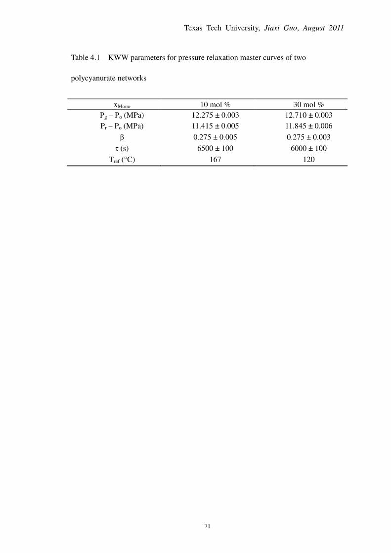
Texas Tech University, Jiaxi Guo, August 2011
71
Table 4.1 KWW parameters for pressure relaxation master curves of two
polycyanurate networks
xMono 10 mol % 30 mol %
Pg – Po (MPa) 12.275 ± 0.003 12.710 ± 0.003
Pr – Po (MPa) 11.415 ± 0.005 11.845 ± 0.006
β 0.275 ± 0.005 0.275 ± 0.003
τ (s) 6500 ± 100 6000 ± 100
Tref (°C) 167 120
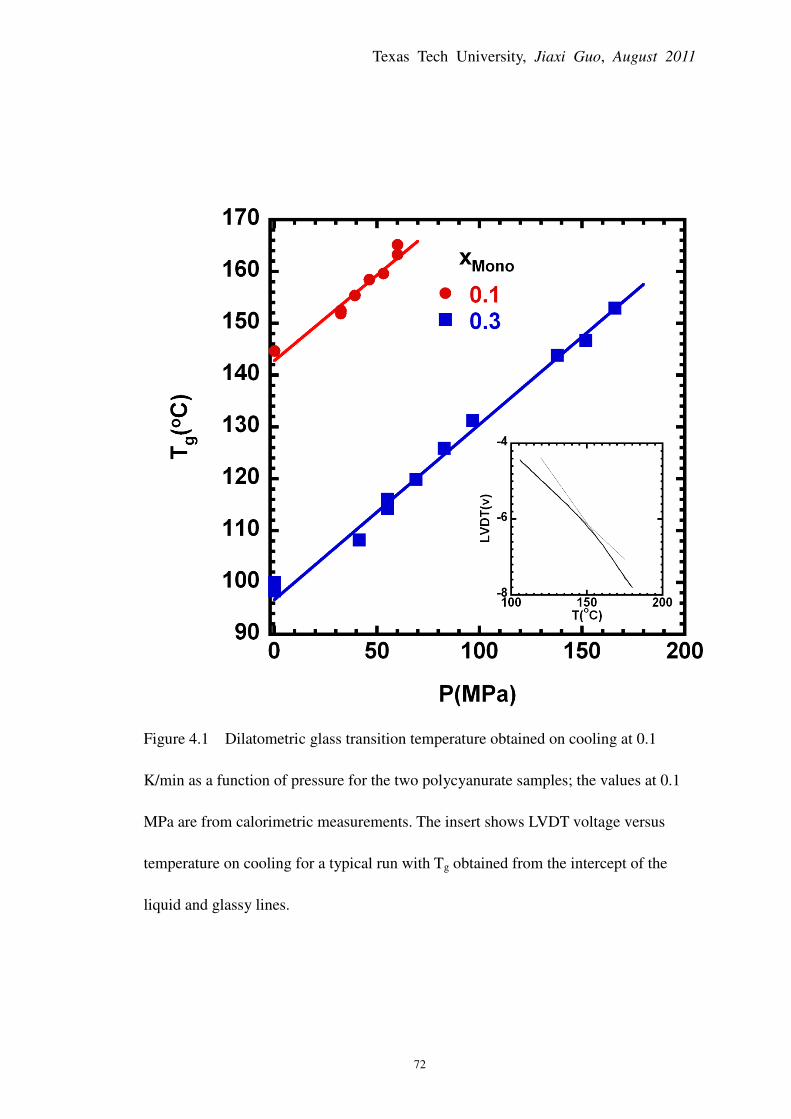
Texas Tech University, Jiaxi Guo, August 2011
72
Figure 4.1 Dilatometric glass transition temperature obtained on cooling at 0.1
K/min as a function of pressure for the two polycyanurate samples; the values at 0.1
MPa are from calorimetric measurements. The insert shows LVDT voltage versus
temperature on cooling for a typical run with Tg obtained from the intercept of the
liquid and glassy lines.

Texas Tech University, Jiaxi Guo, August 2011
73
Figure 4.2 Pressure relaxation curves (P-Po) as a function of logarithmic time for the
sample containing 10 mol % monofunctional cyanate ester at temperatures ranging
from 136 to 180 °C, where Po = 55 ± 0.5 MPa. Two pressure relaxation runs are
shown at 136, 160, 170 and 173.5 °C, one as filled circles and the other as open
circles. Only a fraction of data is shown for clarity. View in color for the best clarity.

Texas Tech University, Jiaxi Guo, August 2011
74
Figure 4.3 Pressure relaxation curves (P-Po) as a function of logarithmic time for the
sample containing 30 mol % monofunctional cyanate ester at temperatures ranging
from 91 to 140 °C, where Po = 55 ± 0.5 MPa. Two pressure relaxation runs are shown
at 120 and 140 °C, one as filled circles and the other as open circles. Only a fraction
of data is shown for clarity. View in color for best clarity.

Texas Tech University, Jiaxi Guo, August 2011
75
Figure 4.4 Pressure relaxation curves as a function of time after application of
vertical shifts for the material containing 10 mol % monofunctional cyanate ester at
temperatures ranging from 136 to 180 °C. The reduced curve on the right is obtained
by time temperature superposition. View in color for best clarity.

Texas Tech University, Jiaxi Guo, August 2011
76
Figure 4.5 Pressure relaxation curves as a function of time after application of
vertical shifts for the material containing 30 mol % monofunctional cyanate ester at
temperatures ranging from 91 to 140 °C. The reduced curve on the right is obtained
by time temperature superposition. View in color for best clarity.

Texas Tech University, Jiaxi Guo, August 2011
77
Figure 4.6 Comparison of pressure relaxation master curves fitted with KWW
function for the two polycyanurate networks. The sample containing 10 mol %
monofunctional cyanate ester uses the left y-axis and has a reference temperature of
167 °C, whereas the sample containing 30 mol % monofunctional cyanate ester uses
the right y-axis and has a reference temperature of 120 °C. View in color for best
clarity.

Texas Tech University, Jiaxi Guo, August 2011
78
Figure 4.7 Vertical shift factors as a function of the temperature departure from the
glass transition temperature, T-Tg, for the two polycyanurate samples.

Texas Tech University, Jiaxi Guo, August 2011
79
Figure 4.8 Comparison of horizontal shift factors for the bulk response (filled
symbols) with those for the shear response from Li and Simon [34] (open symbols).
The shift factors are plotted as a function of the temperature departure from T-Tg.
Data above Tg are fitted with the universal WLF equation, and below Tg are fitted with
the Arrhenius function.

Texas Tech University, Jiaxi Guo, August 2011
80
Figure 4.9 Comparison of the bulk retardation time spectra (solid lines) and shear
retardation time spectra (dashed lines) for the sample containing 10 mol %
monofunctional cyanate ester (red) and that containing 30 mol % monofunctional
cyanate ester (blue). View in color for best clarity.

Texas Tech University, Jiaxi Guo, August 2011
81
CHAPTER 5
PRESSURE-VOLUME-TEMPERATURE BEHAVIOR OF TWO
POLYCYANURATE NETWORKS
5.1 Introduction
The specific volume and viscoelastic shear response of thermosetting polymers as
a function of crosslink density have been well studied [1-21]. The crosslink density
can be varied by changing reactant stoichiometry, epoxy or hardener molecular weight,
amount of monofunctional reactant, or amount of accelerator [1-11], as well as by
controlling the reaction extent [12-20]. The specific volume at room temperature,
V(RT), has been experimentally observed to increase [1-4, 10, 12] or decrease [5, 6,
11] with increasing crosslink density, or to show a minimum [13-18] as the reaction
extent increases. In general, for a given network, V(RT) depends on the relative
volume shrinkage during cure and during cooling from the cure temperature to room
temperature [13]. During cure, shrinkage increases with increasing conversion or
crosslink density; on the other hand, during cooling, the magnitude of volume
shrinkage depends on the Tg of the network in that the higher the Tg, the lower the
volume shrinkage because the coefficient of the thermal expansion (α) in the rubbery
state is much greater than that in the glassy state. Moreover, Tg is enhanced by
increasing conversion or crosslink density in thermosetting networks. Therefore,
whether or not the specific volume at room temperature for a network system

Texas Tech University, Jiaxi Guo, August 2011
82
increases with increasing crosslink density depends on the competition between
volume shrinkage during cure and cooling, and hence the seemingly discrepant results
in the literature [1-18] can be explained. For example, V(RT) in an epoxy resin system
[5] was observed to decrease with increasing crosslink density because volume
shrinkage during cure dominates due to the relatively low values of Tg for the samples,
which ranged from 45 to 78 °C. On the other hand, the minimum in V(RT) with
increasing conversion [12-18] in high-Tg systems can also be understood: volume
shrinkage induced by cure dominates before gelation because of the relatively low Tg
values, whereas that induced by cooling dominates after gelation as Tg increases
nonlinearly with increasing crosslink density.
The effect of increasing conversion or crosslink density on the viscoelastic shear
modulus is also well understood. The magnitude of the shear rubbery plateau modulus
increases with increasing crosslink density as described by the theory of rubber
elasticity [18-21]. In addition, as the crosslink density increases, the molecular weight
between crosslinks decreases, leading to a narrowing of the dispersion in compliance
space [10, 17-19, 22]. On the other hand, the viscoelastic bulk modulus (K) of the
thermosetting networks as a function of crosslink density has not been well studied
although the bulk modulus is an important parameter for estimating the isotropic
residual stresses that develop in the thermosetting materials during cure and cooling.
These stresses may lead to early failure and reduction of lifetimes [23-29] and are
directly related to the thermal pressure coefficient (γ), which is the product of the
thermal expansion coefficient (α) and the bulk modulus (K).

Texas Tech University, Jiaxi Guo, August 2011
83
Polycyanurates are an important class of thermosetting materials whose properties
include high glass transition temperatures, low cost, and good mechanical
performance [30-33].
In this Chapter, the PVT behavior of two polycyanurate networks having different
crosslink densities will be determined, and from this data, the coefficients of thermal
expansion, bulk moduli, and the thermal pressure coefficients will be extracted. The
influence of crosslink density on the PVT properties and the viscoelastic bulk moduli
of these materials will then be discussed.
5.2 Results
Isobaric temperature scans at various pressures are shown in Figures 5.1 and 5.2,
where volume is plotted versus temperature for the polycyanurate samples containing
10 and 30 mol % monofunctional cyanate ester, respectively. Also shown on each plot
is the volume measured independently at ambient pressure and temperature, as well as
the values of the pressure dependent glass transition temperatures [Tg(P)]. Two
measurements were performed at 32.4 and 55.2 MPa for the two samples, respectively,
and are shown in the same color using open and filled symbols; the repeat runs
indicate good reproducibility of the data.
The PVT data can be described by Tait equation [34]
−+−=
)exp(1ln1),0(V),(V
1TBB
PCTTP
o
(5.1)
where C, Bo, and B1 are material-dependent constants, in which C is generally taken

Texas Tech University, Jiaxi Guo, August 2011
84
to be 0.0894 [35]. In the equilibrium liquid or rubbery state, the specific volume at
zero pressure, V(0, T), can be fit with a polynomial function of temperature
2
21
1),0(V
TaTaaT
o ++= (5.2)
whereas in the solid state, the equation for specific volume at zero pressure can be
described as [36]
)exp(
1),0(V
1TaaT
o −= (5.3)
The parameters of the Tait equation used to fit the experimental data are shown
in Table 5.1, with centigrade temperature used in the equations. The average absolute
errors between experimental points in the rubbery state and the Tait equation is 0.0006
cm3/g and 0.0003 cm
3/g for the samples containing 10 and 30 mol % monofunctional
cyanate esters, respectively; the average absolute errors in glassy state are 0.0004
cm3/g and 0.0007 cm
3/g, respectively.
Isothermal pressure scans were performed to obtain specific volume as a function
of pressure, and the data obtained in the rubbery states were also fit to the Tait
equation with the same parameters as were used to describe the isobaric cooling runs.
The results are shown in Figures 5.3 and 5.4 for the two samples, respectively.
Repeat pressure scans were performed at 60 °C, as well as at 160 °C for the sample
containing 30 mol % monocyanate ester; the repeat runs show good reproducibility of
the data. The Tait equation used to fit the glassy isobaric V(T) data is not shown here
because the pressure dependence of the glass V(T) lines differs from the isothermal
pressure dependence. This difference is well understood [21] and arises from the fact

Texas Tech University, Jiaxi Guo, August 2011
85
that the placement of the glass lines shown in Figures 5.1 and 5.2 depends on the
pressure-dependent glass transition temperatures and the volumes at Tg, such that the
placement with respect to pressure does not reflect the pressure dependence of the
volume when pressure is changed after the glass is formed. In addition, the glass PVT
surfaces obtained isothermally and isobarically differ as pointed out by McKenna and
coworkers [37].
The thermal expansion coefficients (PT
V
V
∂
∂=
1α ), are calculated from the
isobaric cooling runs as a function of pressure for the two polycyanurate samples.
Although the thermal expansion coefficient is a weak function of temperature in
glassy or rubbery states, here only one value of α is reported, calculated over
temperatures ranging from ~ Tg + 15 °C to Tg + 35 °C in the rubbery state and from ~
Tg – 35 °C to Tg – 15 °C in the glassy state. The results are shown in Figure 5.5. Also
shown in the figure are the predictions from the Tait equation. As expected, the
thermal expansion coefficients decrease with increasing pressure in both rubbery and
glassy states for the samples containing 10 and 30 mol % monofunctional cyanate
ester, respectively. In the rubbery state, the coefficient of thermal expansion is found
to be independent of the crosslink density within the error of the measurements (~
10 %) although the Tait equation fits indicate a slight increase with increasing
crosslink density; in the literature [2, 4], the value of α in the rubbery state decreases
with increasing crosslink density in epoxy-amine systems. In the glassy state, the
experimental values of the thermal expansion coefficient are also independent of
crosslink density within the error of the measurements (8.7 %, and 0.3 % for the 0.1

Texas Tech University, Jiaxi Guo, August 2011
86
and 0.3 mol % monofunctional samples, respectively) with the Tait equation fits also
indicating an increase in α with increasing crosslink density in the glassy state. In
other works, the value of α in the glassy state has been observed to either increase [2,
4], decrease [12], or show no systematic change [7, 38] with increasing the crosslink
density in epoxy-amine and cyanate ester systems.
The instantaneous rubbery bulk modulus was calculated from the isothermal
pressure scans as a function of pressure at 163.5 and 180 °C for the samples
containing 10 mol % monofunctional cyanate ester, and at 160 °C for the sample
containing 30 mol % monofunctional cyanate ester; glassy values were determined at
60 °C for both polycyanurate samples. The data are shown in Figure 5.6. Also shown
are the instantaneous rubbery bulk moduli obtained from Tait equation, which
underestimates the moduli by 13.4 ± 0.5 % and 10.9 ± 1.3 % for the two samples,
respectively. Both rubbery and glassy instantaneous bulk moduli show a similar
pressure-dependence, increasing with increasing pressure. A previous study [39] on a
linear polystyrene sample found that the instantaneous bulk modulus showed weaker
pressure dependence in the rubbery state than in the glassy state. However, the present
work is consistent with Rehage and Breuer [40] who investigated the PVT behavior
on a polystyrene sample and found that the bulk moduli in the liquid and glassy states
showed a similar dependence on pressure.
The thermal pressure coefficient (γ = αK) is also examined as a function of
pressure at 60 and 163.5 °C for the sample containing 10 mol % monofunctional
cyanate ester, and at 60 and 160 °C for the sample containing 30 mol %

Texas Tech University, Jiaxi Guo, August 2011
87
monofunctional cyanate ester. The results are reported in Figure 5.7. Also shown are
the rubbery thermal pressure coefficients calculated from Tait equation fits for the two
samples, which again underestimate the experimental values by 16.2 ± 0.5 % and 8.0
± 2.7 %, respectively. Although there is considerable scatter in the results, the rubbery
state γ values are statistically larger than the glassy state values, consistent with other
reports in the literature [28, 29] and in contrast to the assumption which has been
made in modeling stress development in thermosetting materials [24-26] that γ is a
constant (αK = αrKr = αgKg). The effect of crosslink density is less clear; the
experimental thermal pressure coefficients in the rubbery state appear to be higher for
the higher crosslink density sample, whereas the opposite appears to be the case for
the prediction from Tait equation. The student t-test [41] confirms that within a 90 %
probability, γ in the rubbery state is higher for the more highly crosslinked sample.
Moreover, statistics also confirm that γ increases with increasing pressure for the 0.3
mol % sample in the rubbery state.
The viscoelastic bulk modulus [K(t)] in the vicinity of the α-relaxation is
calculated from the pressure relaxation reduced curves presented previously [22] and
is plotted as a function of logarithmic time on the left hand side of Figure 5.8, for
reference temperatures of Tg(P) = 167 and 120 °C for the samples containing 10 and
30 mol % monocyanate ester, respectively. Both sets of data were obtained at ~ 67
MPa and show very similar magnitudes and widths for the dispersion although the
absolute values of the moduli at Tg(P) are higher for the sample with lower crosslink
density; it is important to note that this differs from the data shown in Figure 5.6

Texas Tech University, Jiaxi Guo, August 2011
88
where at any given temperature, the higher crosslink density sample shows a higher
modulus because of its higher Tg value. On the right hand side of Figure 5.8, the
master curve for the sample containing 30 mol % monocyanate ester is shifted
downward by 0.3 GPa. The two master curves appear to superpose, indicating that
time-crosslink density superposition [12, 19, 20, 42-45] holds for the polycyanurate
network.
To better quantify the shape of the bulk relaxation, the time-dependent bulk
moduli data are fit to the Kohlrausch-Williams-Watts (KWW) equation [46, 47]
−−+=
β
τ
tKKKtK rgr exp)()( (5.4)
where Kr is rubbery bulk modulus, Kg is glassy bulk modulus, τ is the average
relaxation time for the networks, and β is the Kohlrausch stretching exponent. A
similar equation was used previously [22] to fit the pressure relaxation responses, P(t),
from which K(t) is derived. The values of the parameters are reported in Table 5.2.
Also shown in Table 5.2 are those parameters obtained from the pressure relaxation
response. The values of β obtained for fitting K(t) are 0.22 and 0.21 for the samples
containing 10 and 30 mol % monofunctional cyanate ester, respectively, as tabulated
in Table 5.2. The values differ from the value of 0.28, which was obtained from the
pressure relaxation response. Similarly, the values of τ in the KWW fit differ
significantly from the counterparts for the pressure relaxation responses. To
understand these differences, it should be noted that the pressure relaxation curves not
only result from the response of the sample, but also include a contribution from the
surrounding fluorinated synthetic oil, whereas the time-dependent bulk modulus

Texas Tech University, Jiaxi Guo, August 2011
89
presented here removes the volume change of the surrounding oil, with the result that
the spectra narrows and shifts to shorter times.
5.3 Discussion
One goal in the study is to investigate the effect of crosslink density on the PVT
behavior of the polycyanurate networks. In order to further examine this influence, the
specific volume in both the rubbery and glassy states minus that at Tg (i.e., V - VTg) is
plotted in Figure 5.9 as a function of T – Tg(P) at 0.1, 30, and 60 MPa based on the
Tait equation fits for the two polycyanurate samples. Given the similarity of the
thermal expansion coefficients, at any given pressure, V – VTg shows a similar
dependence on temperature when plotted as the distance from Tg, indicating that to a
reasonable approximation, the shifted PVT data are independent of crosslink density.
Hence, the most important variable governing the PVT behavior for these materials is
the glass transition temperature which strongly depends on crosslink density. This is
further demonstrated in Figure 5.10 where the specific volume is plotted as a function
of temperature at ambient pressure for the two samples based on the Tait equation fits.
As shown in the figure, the volume for the high-crosslink density sample containing
0.1 mol % monofunctional cyanate ester in the equilibrium rubbery state at 180 °C is
lower than that for the low-crosslink density sample. This is expected because the two
samples have very similar chemical composition but the sample with 0.1 mol %
monofunctional cyanate ester has increased crosslink density and fewer dangling ends

Texas Tech University, Jiaxi Guo, August 2011
90
resulting in higher Tg, lower free volume (or configurational entropy), and hence, a
lower volume in the equilibrium state. However, due to its considerably higher Tg, the
more highly crosslinked sample experiences less shrinkage on cooling to room
temperature such that similar volumes for the two samples are observed at room
temperature. Thus, the volume at room temperature as a function of crosslink density
in present system results from the competition between the volume changes induced
by changes in crosslink density (in the equilibrium state) and those induced by
cooling in an analogy to volume at room temperature as a function of conversion
being a result of the competition between the volume shrinkage induced by changes in
conversion during cure and those induced by cooling as pointed by Pang and Gillham
[8].
The influence of the crosslink density on the viscoelastic bulk modulus has also
been examined in the present study. As was discussed, the viscoelastic bulk moduli at
Tref = Tg(P) for the two samples with different crosslink densities are similar in terms
of placement and dispersion indicating the validity of time-crosslink density
superposition [12, 19, 20, 42-45]. The retardation time spectra of samples have been
shown in the previous study [22] and similarly indicate that the bulk response at Tg is
independent of the crosslink density. However, the limiting moduli at Tg and the
absolute values of the moduli at a given temperature and pressure depend on crosslink
density. Given that the cohesive energy density (CED) has been directly related to the
value of the glassy bulk modulus [48, 49], the cohesive energy density of the two
polycyanurate samples is estimated using the group contribution method [50]. The

Texas Tech University, Jiaxi Guo, August 2011
91
values of CED are 354 and 400 MPa, for the samples containing 10 mol % and 30
mol % monofunctional cyanate ester, respectively. The corresponding ratios of the
glassy bulk modulus to CED (Kg/CED) are found to be 15.8 and 15.1, as shown in
Table 2, when using Kg values at 67 MPa and T = Tg(P). On the other hand, using Kg
values at 60 °C and extrapolating to ambient pressure (from Figure 5.6), Kg/CED =
16.4 ± 1.6 and 13.6 ± 2.6 are obtained, respectively. In either case, the results are
consistent with the glassy bulk modulus being proportional to the cohesive energy
density, independent of crosslink density. Morel et al. [48] and Bellenger et al. [49]
investigated the relation between the bulk modulus and the cohesive energy density
for cross-linked epoxide-amine systems and styrene cross-linked vinylesters using
ultrasonic measurements at ambient temperature and pressure, and they found that Kg
can be effectively described as a function of cohesive energy density, with
CEDKg )111( ±= (8)
Although the values in present study are consistent with the relationship proposed
between the glassy bulk modulus and the cohesive energy density, the proportionality
constant is somewhat larger for the polycyanurates studied here than that proposed
previously [48, 49].
The thermal pressure that a three-dimensionally constrained resin will experience
during a temperature change can be estimated from the value of the thermal pressure
coefficient: P = ∫T
To
dTγ . This equation assumes no viscoelastic relaxation during
excursions through Tg and that the material is stress-free at To, often assumed to be
the cure temperature or Tg; neither assumption is strictly valid [27, 28]. The values of

Texas Tech University, Jiaxi Guo, August 2011
92
the thermal pressure coefficients estimated in this work for the cyanate ester resins are
relatively high, ranging from 1.0 to 1.6 MPa/K, depending on the crosslink density,
pressure, and state of the material, but they are consistent with the thermal pressure
coefficients for high-Tg polymers and thermosets in the literature, with glassy values
reported [28] to range from 0.4 to 1.0 MPa/K at ambient pressure. Given a thermal
stress coefficient of 1.0 MPa/K, thermal pressures will quickly, within 20 to 50 K of
the stress-free temperature, lead to premature failure for isochorically constrained
resins; this has been experimentally confirmed [29] and indicates the need to either
design structures where the high-Tg resin is not isochorically constrained or to
develop additives that lower the thermal stress coefficient [51].
5.4 Conclusions
The specific volume of two polycyanurate samples was measured as a function of
pressure and temperature using a custom-built dilatometer, and the experimental data
obtained are well described by the Tait equation. The volume at room temperature as a
function of crosslink density is explained by a competition between volume changes
induced by crosslinking and those induced by cooling; the latter increase with
increasing crosslinking whereas the former decrease. From the experimental PVT data,
the coefficient of the thermal expansion (α), the instantaneous bulk modulus (K), and
the thermal pressure coefficient (γ) are calculated. The extracted data show that α
depends little on the crosslink density, but the instantaneous K increases with

Texas Tech University, Jiaxi Guo, August 2011
93
increasing crosslink density, leading to γ increasing as the crosslink density increases.
The values of the thermal pressure coefficients are relatively high, ranging from 1.0 to
1.6 MPa K-1
, indicating a need to design structures in which the resin is not
isochorically constrained or for additives to reduce its value. The viscoelastic bulk
modulus in the vicinity of α-relaxation at a pressure of ~ 67 MPa and temperature
Tg(P) is calculated from pressure relaxation measurements performed earlier; the
dispersion width and breadth are found to be independent of crosslink density
although the absolute values of the limiting moduli at Tg(P) decrease with increasing
crosslink density. The glassy bulk modulus (Kg) appears to be proportional to the
cohesive energy density (CED), consistent with the literature.

Texas Tech University, Jiaxi Guo, August 2011
94
REFERENCES
1. N. Shito, J. Polym. Sci.: Part C, 23, 569-582, 1968.
2. M. Ogata, N. Kinjo, T. Kawata, J. Appl. Polym. Sci., 48, 583-601, 1993.
3. Y. G. Won, J. Galy, J. P. Pascault, J. Verdu, Polymer, 32, 79-83, 1991.
4. V. B. Gupta, C. Brahatheeswaran, Polymer, 32, 1875-1884, 1991.
5. O. Georjon, J. Galy, Polymer, 39, 339-345, 1998.
6. T. D. Chang, S. H. Carr, J. O. Brittain, Polym. Eng. Sci., 22, 1213-1220, 1982.
7. M. Blanco, J. A. Ramos, S. Goyanes, G. Rubiolo, W. Salgueiro, A. Somoza, I.
Mondragon, J. Polym. Sci,: Part B: Polym. Phys., 47, 1240-1252, 2009.
8. K. P. Pang, J. K. Gillham, J. Appl. Polym. Sci., 37, 1969-1991, 1989.
9. R. A. Venditti, J. K. Gillham, Y. C. Jean, Y. Luo, J. Coat. Technol., 67, 47-56,
1995.
10. C. Jordan, J. Galy, J. P. Pascault, J. Appl. Polym. Sci., 46, 859-871, 1992.
11. V. Bellenger, W. Dhaoui, E. Morel, J. Verdu, J. Appl. Polym. Sci., 35, 563-571,
1988.
12. D. J. Plazek, I. C. Choy, J. Polym. Sci.: Part B: Polym. Phys., 27, 307-324, 1989.
13. A. W. Snow, J. P. Armistead, PMSE, ACS Fall Meeting, Washington, D. C., 71,
819-820, 1994.
14. X. R. Wang, V. J. Foltz, Polymer, 47, 5090-5096, 2006.
15. M. T. Aronhime, X. Peng, J. K. Gillham, J. Appl. Polym. Sci., 32, 3589-3626,
1986.

Texas Tech University, Jiaxi Guo, August 2011
95
16. X. R. Wang, J. Appl. Polym. Sci., 64, 69-75, 1997.
17. A. Tcharkhtchi, E. Gouin, J. Verdu, J. Polym. Sci.: Part B: Polym. Phys., 38,
537-543, 2000.
18. I. C. Choy, D. J. Plazek, J. Polym. Sci., Part B: Polym. Phys., 24, 1303-1320,
1986.
19. D. J. Plazek, I. C. Chay, J. Polym. Sci., Part B: Polym. Phys., 29, 17-29, 1991.
20. Q. X. Li, S. L. Simon, Macromolecules, 40, 2246-2256, 2007.
21. J. D. Ferry, In Viscoelastic Properties of Polymers, 3rd ed.; Wiley: New York,
1980.
22. J. X. Guo, S. L. Simon, J. Polym. Sci. Part B, Polym. Phys., 47, 2477-2486,
2009.
23. P. J. Withers, H. K. D. H. Bhadeshia, Mater. Sci. and Technol., 17, 355-365,
2001.
24. D. Adolf, J. E. Martin, J. Compos. Mater., 30, 13-34, 1996.
25. D. Adolf, R. Chambers, Polymer, 38, 5481-5492, 1997.
26. D. B. Adolf, J. E. Martin, R. S. Chambers, S. N. Burchett, T. R. Guess, J. Mater.
Res., 13, 530-550, 1998.
27. P. Prasatya, G. B. McKenna, S. L. Simon, J. Compos. Mater., 35, 826-848, 2001.
28. M. Alcoutlabi, G. B. McKenna, S. L. Simon, J. Appl. Polym. Sci., 88, 227-244,
2003.
29. M. Merzlyakov, G. B. McKenna, S. L. Simon, Composite: Par A 37, 585-591,
2006.

Texas Tech University, Jiaxi Guo, August 2011
96
30. I. Hamerton, "Introduction to Cyanate Ester Resins", In Chemistry and
Technology of Cyanate Ester Resins, Ed., I. Hamerton, Blackie Academic and
Professional, Glasgow, 1994.
31. D. A. Shimp, J. R. Christenson, S. J. Ising, In 3rd Int. SAMPE Elec. Mater. Proc.,
Los Angeles, CA, 1989.
32. R. B. Graver, "Cyanate Esters - High Performance Resins", In The Development
of High Performance Polymers, Ed., R. B. Seymour, G. S. Kirshenbaum,
Elsevier, New York and Amsterdam, 1986.
33. C. P. R. Nair, D Mathew, K. N. Ninan, Adv. Polym. Sci., 155, 1-99, 2001.
34. J. H. Dymond, R. Malhotra, Int. J. Thermophys., 9, 941-951, 1988.
35. R. A. Orwoll, In Physical Properties of Polymers Handbook, Chapter 7, Ed., J. E.
Mark, American Institute of Physics, Woodbury, New York, 1996.
36. P. Zoller, H. H. Hoehn, J. Polym. Sci., Polym. Phys. Ed., 20, 1385-1397, 1982.
37. D. M. Colucci, G. B. McKenna, J. J. Filliben, A. Lee, D. B. Curliss, K. B.
Bowman, J. D. Russell, J. Polym. Sci.: Part B: Polym. Phys., 35, 1561-1573,
1997.
38. J. L. Halary, High Perform. Polym. 12, 141-153, 2000.
39. Y. Meng, P. Bernazzani, P. A. O'Connell, G. B. McKenna, S. L. Simon, Rev. Sci.
Instrum. 80, 053903-1-9, 2009.
40. G. Rehage, H. Breuer, J. Polym. Sci. Part C, 16, 2299-2312, 1967.
41. F. J. Gravetter, L. B. Wallnau, In Essentials of Statistics for the Behavioral
Sciences, 6th Ed., Thomson Wadsworth, CA, 2008.

Texas Tech University, Jiaxi Guo, August 2011
97
42. D. J. Plazek, J. Polym. Sci.: Part A-2, 4, 745-763, 1966.
43. P. Thirion, R. Chasset, Pure Appl. Chem., 23, 183-199, 1970.
44. R. J. Arenz, J. Polym. Sci.: Polym. Phys. Ed., 12, 131-143, 1974.
45. A. Lee, G. B. McKenna, Polymer, 29, 1812 -1817, 1988.
46. R. Kohlrausch, Pogg. Ann. Phys. 12, 393-399, 1847.
47. G. Williams, D. C. Watts, Trans. Faraday Soc. 66, 80-85, 1970.
48. E. Morel, V. Bellenger, M. Bocquet, J. Verdu, J. Mater. Sci., 24, 69-75, 1989.
49. V. Bellenger, J. Verdu, M. Ganem, B. Mortaigne, Polym. Polym. Compos., 2,
9-16, 1994.
50. D.W. Van Krevelen, In Properties of Polymers, 3rd ed., Elsevier: Amsterdam,
1990.
51. K. Z. Win, T. Karim, Q. X. Li, S. L. Simon, G. B. McKenna, J. Appl. Polym. Sci.,
116, 142-146, 2010.

Texas Tech University, Jiaxi Guo, August 2011
98
Table 5.1 Tait parameters for polycyanurate samples in the rubbery (equilibrium)
and glassy states
xMono = 0.1 xMono = 0.3
Rubbery State Glassy State Rubbery State Glassy State
ao (gcm-3
) 1.191 1.146 1.183 1.149
a1 (10-4
gcm-3o
C-1
) -5.21 ... -5.60 ...
a1 (10-4o
C-1
) ... 2.10 ... 1.94
a2 (10-6
gcm-3o
C-2
) -0.250 ... -0.250 ...
Bo (MPa) 298 314 305 348
B1 (oC
-1) 0.00336 0.00185 0.00374 0.00121
C 0.0894 0.0894 0.0894 0.0894

Table 5.2 KWW fitting parameters for viscoelastic bulk modulus, p
relaxation response, and cohesive energy density (CED) for the polycyanurate
samples
Bulk Modulus
Kg, 67MPa (GPa) 5.60 ± 0.
Kr, 67MPa (GPa) 2.58 ±
β 0.220 ± 0.00
τ (s) 1200
CED(MPa)
Kg, 67MPa/CED*
* In the CED calculation, three (
value of by adding the value for
All parameters are obtained from Fedors' table [
Texas Tech University, Jiaxi Guo,
99
parameters for viscoelastic bulk modulus, pressure
relaxation response, and cohesive energy density (CED) for the polycyanurate
xMono = 0.1 xMono = 0.3
Bulk Modulus Pressure
Relaxation
Bulk Modulus
± 0.04 … 6.05 ± 0.03
± 0.01 … 2.85 ± 0.01
± 0.005 0.275 ± 0.005 0.210 ± 0.003
1200 ± 80 6500 ± 100 1200 ± 40
354 400
15.8 ± 0.1 15.1 ± 0.1
CED calculation, three (−C≡N) groups are used to calculate the
by adding the value for an aromatic ring and three double bonds.
All parameters are obtained from Fedors' table [50].
August 2011
ressure
relaxation response, and cohesive energy density (CED) for the polycyanurate
= 0.3
Pressure
Relaxation …
…
0.275 ± 0.003
6000 ± 100
400
± 0.1
are used to calculate the group
aromatic ring and three double bonds.

Texas Tech University, Jiaxi Guo, August 2011
100
Figure 5.1 Specific volume as a function of temperature at three pressures for the
sample containing 10 mol % monofunctional cyanate ester. The data point at 0.1 MPa
and at ambient temperature was obtained by density measurement. Two measurements
were performed at 32.4 MPa and are shown as open and filled green symbols. The
solid lines are the best fit of Tait equations to data in both rubbery and glassy states;
the dashed line is the pressure-dependent glass transition temperature (Tg(P)). Only a
fraction of data is shown. View in color for the best clarity.

Texas Tech University, Jiaxi Guo, August 2011
101
Figure 5.2 Specific volume as a function of temperature at five pressures for the
sample containing 30 mol % monofunctional cyanate ester. The data point at 0.1 MPa
and at ambient temperature was obtained by density measurement. Two measurements
were performed at 55.2 MPa and are shown as open and filled green symbols. The
solid lines are the best fit of Tait equations to data in both rubbery and glassy states;
the dashed line is the pressure-dependent glass transition temperature (Tg(P)). Only a
fraction of data is shown. View in color for the best clarity.

Texas Tech University, Jiaxi Guo, August 2011
102
Figure 5.3 Specific volume as a function of pressure for the sample containing 10
mol % monofunctional cyanate ester. Two runs were carried out at 60 °C as indicated
by filled and open red symbols. The solid lines are calculated from the Tait equation
for data at 180 and 163.5 °C in the rubbery state only.

Texas Tech University, Jiaxi Guo, August 2011
103
Figure 5.4 Specific volume as a function of pressure for the sample containing 30
mol % monofunctional cyanate ester. Two runs were carried out at 60 °C, and three
measurements were performed at 160 °C as indicated by the different symbols. The
solid line is calculated from the Tait equation fits for the 160°C data in the rubbery
state only.

Texas Tech University, Jiaxi Guo, August 2011
104
Figure 5.5 Thermal expansion coefficients for the samples containing 10 mol % and
30 mol % monofunctional cyanate ester as a function of pressure in both rubbery
(filled symbols) and glassy (open symbols) states, respectively. The solid and dashed
lines are the Tait equation predictions for the samples containing 10 and 30 mol %
monofunctional cyanate ester, respectively.

Texas Tech University, Jiaxi Guo, August 2011
105
Figure 5.6 The instantaneous bulk moduli for the two polycyanurate networks as a
function of pressure measured from isothermal pressure scans at the temperatures
indicated. The data for the sample containing 10 mol % monofunctional cyanate ester
with two separate runs at 60 °C are shown in open red triangles, and with one run at
163.5 and 180 °C are shown in filled red and brown triangles, respectively; the data
for the sample containing 30 mol % monofunctional cyanate ester with two separate
runs at 60 °C are shown in open blue triangles, and with three separate runs at 160 °C
are shown in filled blue triangles and squares. The red and brown solid lines are the
instantaneous bulk modulus at 163.5 and 180 °C from the Tait equation for the xMono =
0.1 sample; and the blue solid line is the instantaneous bulk modulus at 160 °C for the
xMono = 0.3 sample. View in color for the best clarity.

Texas Tech University, Jiaxi Guo, August 2011
106
Figure 5.7 The thermal pressure coefficient as a function of pressure for the
polycyanurate networks calculated from the product of the thermal expansion
coefficient (Figure 5.5) and the bulk modulus (Figure 5.6, by interpolation). The filled
circles and triangles are calculated from the data at 163.5 and 160 °C for the samples
containing 10 and 30 mol % monofunctional cyanate ester, respectively; the open
circles and triangles are calculated at 60 °C for the two samples. The solid and dashed
lines are the Tait equation predictions for the rubbery states for the samples containing
10 and 30 mol % monofunctional cyanate ester, respectively.

Texas Tech University, Jiaxi Guo, August 2011
107
Figure 5.8 Time-dependent viscoelastic bulk modulus in the vicinity of α-relaxation
calculated from previous pressure relaxation studies [22] for the two polycyanurate
samples. The pressure relaxation studies were carried out at pressures ranging from
66.3 MPa to 68.0 MPa; the reference temperatures are the Tgs at 67 MPa, 167 and
120 °C for the materials containing 10 and 30 mol % monofunctional cyanate ester,
respectively. On the right hand side of the figure, the master curve for the more
loosely crosslinked sample is shifted downward by 0.3 GPa to show time-crosslink
density superposition of the two master curves.

Texas Tech University, Jiaxi Guo, August 2011
108
Figure 5.9 Specific volume in both the rubbery and glassy states minus the volume
at Tg (V - VTg) as a function of the temperature departure from Tg [T – Tg(P)] at 0.1,
30 and 60 MPa for the samples containing 10 mol % monocyanate ester (solid lines)
and 30 mol % (dashed lines). The results are calculated from the Tait equation fits.
View in color for best clarity.

Texas Tech University, Jiaxi Guo, August 2011
109
Figure 5.10 Comparison of specific volume as a function of temperature at ambient
pressure for the samples containing 10 mol % (red curve) and 30 mol % (blue curve)
monofunctional cyanate ester, respectively. The data points are obtained at ambient
temperature and pressure, and the lines are calculated from the Tait equation fits.

Texas Tech University, Jiaxi Guo, August 2011
110
CHAPTER 6
BULK AND SHEAR RHEOLOGY OF A THREE-ARM STAR
POLYSTYRENE
6.1 Introduction
The effects of star-shaped structures on the shear rheological properties of the
polymers have been widely investigated due to their unique architectures [1-11]. It has
been proposed [1, 2] that the molecular weight of the branch (Mb) should be at least
twice of the entanglement molecular weight (Me) in order to influence the rheological
properties. The viscosity (η) of star-branched polymers has been found [3] to be lower
than of linear samples at low molecular weights; whereas, η for the star increases
greater than for the linear and has been observed to be higher than that for the linear at
Mb/Me ≥ 0.5 [3, 4]. In addition, the relaxation time for star-shaped polymers in the
terminal region has been found [2, 5-7] to increase with increasing Mb.
Time-temperature superposition (TTS) has also been found to fail for star-shaped
polyethylene [8] and polyisoprene [9], although it is valid for their linear samples. On
the other hand, TTS principle can be applied to both linear and star-shaped
poly(ethylene-alt-propylene) [2] and polyisobutylene [10].
The bulk rheological properties of star-shaped polymers have never been studied,
and furthermore, only a handful of studies can be found of polymers reported in the
literature [12-23] due to difficulties in experimental measurements in which long-term

Texas Tech University, Jiaxi Guo, August 2011
111
stability of temperature control is required. To further examine the hypothesis by
Leaderman [24] that bulk and shear responses arise from different underlying
molecular relaxations as described in the introduction of Chapter 4, as well as to
investigate the effects of long-chain branches on the viscoelastic bulk modulus, bulk
and shear rheological measurements for a symmetric three-arm star polystyrene were
performed using a custom-built pressurizable dilatometer and a commercial rheometer,
respectively.
The chapter is organized as follows. First the results of the
pressure-volume-temperature (PVT) data and the pressure-dependent glass transition
temperature [Tg(P)] are presented. Then the pressure relaxation curves and their
corresponding viscoelastic bulk moduli, as well as the dynamic shear measurement
results are shown. The bulk and shear horizontal shift factors are compared to the
counterparts for linear polystyrene samples [17, 25, 26]. Finally, the retardation time
spectra for the bulk and shear relaxations, as well as those for the linear data are
compared, followed by a discussion and conclusions.
6.2 Results
6.2.1 PVT Behavior
The isobaric specific volume for the star polystyrene as a function of temperature
was obtained at pressures ranging from 27.6 to 82.7 MPa as shown in Figure 6.1. The
isobaric scans were performed on cooling at 0.1 K/min. Also shown are the volume

Texas Tech University, Jiaxi Guo, August 2011
112
measured at atmospheric pressure and 25.3 °C and the pressure-dependent glass
transition temperatures [Tg(P)]. Three measurements were made at 41.4 MPa and are
shown in the same color with different symbols; the repeat runs indicate good
reproducibility of the data.
The pressure-volume-temperature (PVT) data in Figure 6.1 are fitted to the Tait
equation [27] given by
−+−=
)exp(1ln1),0(V),(V
1TBB
PCTTP
o
(6.1)
where C, Bo and B1 are material-dependent constants, and C is taken to be 0.0894 [28].
In the liquid state, the specific volume at zero pressure [V(0,T)] can be described by a
polynomial function of temperature
2
21
1),0(V
TaTaaT
o ++= (6.2)
whereas in the glassy state, V(0,T) is described by a exponential function of
temperature [29]
)exp(
1),0(V
1TaaT
o −= (6.3)
The parameters of the Tait equation for the star polystyrene are shown in Table 6.1.
Also shown are the Tait parameters for the linear polystyrene [30] whose physical
properties are demonstrated in Table 3.1. As indicated in the table, the star polystyrene
shows similar PVT behavior to the linear polystyrene [30] having similar molecular
weight on the backbone.
The isothermal specific volume as a function of pressure was also performed at
60, 120 and 130 °C and is shown in Figure 6.2. As shown in the figure, the data in the

Texas Tech University, Jiaxi Guo, August 2011
113
liquid states are fit to the Tait equation with the same parameters used for describing
the isobaric data, whereas in the glassy state, the Tait function is not shown because
the isothermal glass has different glass-forming history from the isobaric glass [31].
The instantaneous bulk modulus at 60, 120 and 130 °C are then calculated from the
isothermal volume as a function of pressure by fitting the data in power law as
described in the experimental methodology chapter (Chapter 3) and the results are
shown in Figure 6.3. Also shown are the bulk moduli as a function of pressure at 120
and 130 °C estimated from Tait equation with parameters fit to the isobaric PVT data.
As indicated in the figure, the Tait equation slightly underestimates the instantaneous
bulk modulus in the liquid state, consistent with the previous results in the two
polycyanurate networks [32].
The glass transition temperatures for star polystyrene are plotted as a function of
pressure in Figure 6.4. Tg at each pressure is taken as the intersection of the liquid and
glassy lines as shown in Figure 6.1. As indicated, Tg increases with increasing
pressure with dTg/dP = 0.38 ± 0.02 K/MPa for the star polystyrene. Also shown are
comparisons of the star polystyrene data to the Tgs the linear polystyrenes [17] with
physical properties shown in Table 3.1. As shown in Figure 6.4, Tgs for the star
polystyrene are similar to those for the linear sample by Meng and Simon [17].
However, the value of dTg/dP, which is 0.30 ± 0.02 K/MPa for the linear polystyrene,
is slightly lower than that for the star sample.

Texas Tech University, Jiaxi Guo, August 2011
114
6.2.2 Viscoelastic Bulk Modulus
Isothermal pressure relaxation curves [P(t) – Po] were obtained as a function of
logarithmic time for the star polystyrene at 36 and 55 MPa, and are shown in Figures
6.5 and 6.6, respectively. The measurements were carried out in the vicinity of Tg(P)
after volume jumps for the two pressure ranges: at 36 MPa, the relaxation curves were
measured at temperatures ranging from 70 to 123.5 °C; at 55 MPa, the measurements
were carried out at temperature ranging from 81 to 133.5 °C. The pressure relaxation
curves, shown as P(t) – Po in the figures, are directly related to the viscoelastic bulk
modulus: at low temperatures, the glassy response is obtained; in the vicinity of Tg(P),
pressure relaxation is observed; and at high temperatures or long times, the rubbery
response is obtained. Repeat runs made after eight months and designated by filled
and unfilled symbols with the same color show good reproducibility. The noise at
long times is attributed to the temperature fluctuations where the magnitude of the
noise suggests that the temperature stability is better than 0.05 K.
The pressure relaxation curves obtained at different temperatures are superposed
to form a master curve after applying vertical and horizontal shift factors at 36 and 55
MPa, respectively. The vertical shift factors account for the temperature dependent
bulk modulus, and the horizontal shift factors account for the temperature dependent
relaxation time. The results are shown in Figures 6.7 and 6.8 for the relaxation curves
at 36 and 55 MPa, respectively. The master curves after the application of
time-temperature superposition are shown on the right-hand sides of the two figures.
Both master curves are shifted to Tref = Tg(P), where P is taken midway through the

Texas Tech University, Jiaxi Guo, August 2011
115
dispersion; Tg(P) = 108.5 °C and 113.5 °C at 36 and 55 MPa, respectively.
The viscoelastic bulk modulus [K(t)] is calculated from the pressure relaxation
response using the definition given by,
ToV
tPVtK
∆
∆−=
)()( , (6.4)
where ∆P(t) = P(t) – Po, is the pressure relaxation response as a function of time and
∆Vo is the step change in volume applied. The viscoelastic bulk moduli at 36 MPa and
55 MPa for the star polystyrene are plotted as a function of logarithmic time and are
compared to those for the linear polystyrene [17] measured at 42 and 76 MPa. The
results are shown in Figure 6.9, where the reference temperature for each curve is
Tg(P). As shown in the figure, the magnitudes of the dispersions and the relaxation
distribution on the time scale for the bulk modulus obtained at different pressures are
similar for star and linear polystyrenes. To further quantitatively compare the
viscoelastic bulk moduli for the star and linear polystyrene, the data are fit to the
KWW [33, 34] function given by,
−−+=
β
τ
tKKKtK rgr exp)()( , (6.5)
where Kr is rubbery bulk modulus, Kg is glassy bulk modulus, τ is the average
relaxation time, and β is the Kohlrausch stretching exponent. The KWW parameters
for the bulk modulus are shown in Table 6.2. As shown in the table, the values of Kg
and Kr are similar for the star and linear polystyrenes, whereas the β values are higher
for the star polystyrene, suggesting a narrower relaxation time distribution.

Texas Tech University, Jiaxi Guo, August 2011
116
6.2.3 Dynamic Shear Relaxation Measurements
The storage (G') and loss (G") moduli as a function of frequency for the star
polystyrene are shown in Figures 6.10 and 6.11, with the reduced curves shown on the
right-hand sides of the figures. Both reduced curves are obtained at reference
temperature Tref = 101 °C. For the storage modulus, at low temperatures or high
frequencies, the glassy response is observed; as temperature increases or frequency
decreases, the relaxation response is observed; at high temperatures, the rubbery
response occurs, followed by terminal flow. On the other hand, the loss modulus goes
through two peaks as the temperature increases through Tg and terminal regions,
respectively. Also shown in Figures 6.10 and 6.11 are literature data [26] of G' and G"
for a linear polystyrene having a molecular weight and PDI similar to each arm of the
star sample, as was shown in Table 3.2. As indicated in the figure, the storage and loss
moduli of the star polystyrene show similar behavior to the linear sample before
viscous flow occurs; however, the star sample obviously has a longer rubbery plateau
due to its higher overall molecular weight.
The reduced curves shown in Figures 6.10 and 6.11 were obtained by applying
horizontal shift factors obtained by first reducing tangent phase angle (tan δ), and then
by applying small vertical shifts as needed. The advantage of reducing tanδ first is
that no vertical shifts are needed because the temperature dependences in G' and G"
cancel out.
The reduced tanδ is plotted as a function of frequency in Figure 6.10. As
indicated, the tan δ data are not satisfactorily reduced for temperatures ranging from

Texas Tech University, Jiaxi Guo, August 2011
117
110 to 120 °C, suggesting failure of time-temperature superposition (TTS). Also
shown in the inset of Figure 6.12 is the Cole-Cole plot proposed by Dealy and Larson
[35] for examining the validity of TTS where G" versus G' are shown at temperatures
ranging from 110 to 120 °C, and plotting in this way suggests no significant
deviations from reduction. The fact that the storage and loss moduli are also
satisfactorily reduced indicates that only a slight failure in TTS occurs in the glass
transition region. It might be expected that TTS does not strictly hold for polystyrene
as Plazek [36, 37] showed failure of TTS for the linear samples by creep experiments,
although in that case, the failure originates from differences in the activation energies
for the segmental and terminal relaxations.
6.2.4 Comparisons between Bulk and Shear Responses
The logarithmic horizontal shift factors for the bulk and shear responses of the
star polystyrene are plotted as a function of T – Tg(P) in Figure 6.13, where the values
of Tg are indicated in the figure. The shift factors for measurements on the linear
polystyrenes are also shown in Figure 6.13 and are taken from literature [17, 25, 26].
In the liquid state, all of the bulk and shear shift factors for the samples measured at
different pressures superpose as a function of T – Tg(P), where Tg(P) accounts for Tg
changing not only with pressure, but also with structure, consistent to the previous
findings for the two polycyanurate networks having different crosslink densities [18].
The shift factors in the liquid state can be described by the Williams-Landel-Ferry [38]

Texas Tech University, Jiaxi Guo, August 2011
118
equation given by
)]([
)]([log
2
1
PTTC
PTTC
g
g
Tg −+
−−=
τ
τ (6.6)
where C1 and C2 are material-dependent constants, where C1 = 18.2 ± 0.5 and C2 =
42.8 ± 2.1 K by fitting to all the shift factors in the liquid state. On the other hand, in
the glassy state, the shift factors are slightly lower for the star polystyrene than those
for linear polystyrene from Meng and Simon [17], which may due to the fact that the
star polystyrene were only aged for 3 days at 36 MPa and 7 days at 55 MPa, whereas
the linear polystyrene were aged for 7-10 days prior to the pressure relaxation
experiments.
The retardation time spectra of the viscoelastic bulk and shear responses for the
star polystyrene and two linear polystyrenes [16, 25, 26] are plotted in Figure 6.14.
All three materials, the star polystyrene and two linear samples, have similar shear
retardation time spectra in the short-time region which is referred as the Andrade
creep regime [39], where log L(λ) varies with log λ with a slope of approximately 1/3.
The bulk retardation time spectra in the Andrade regime have similar slopes to the
shear spectra, but they are approximately one order of magnitude lower in absolute
value. The indication is that only a small fraction of the Andrade mechanisms
available for the shear response are effective in the bulk response or that the
contribution of the modes is much weaker to the bulk response than that for the shear.
The shear response is observed to have long-time mechanisms, whereas for the
bulk, the retardation time spectra are cut off at short times, consistent with the results
for thermosetting networks [18, 40]. In addition, the shear retardation time

Texas Tech University, Jiaxi Guo, August 2011
119
distribution is found to increase with increasing molecular weight for the polystyrenes.
This result is consistent with Plazek and coworkers [37, 41, 42] who measured
recoverable compliances of several linear polystyrenes having different molecular
weights, and suggested that the distance between two peaks in the shear retardation
time spectrum reflecting the length of the rubbery plateau increases with increasing
number of entanglements, i.e., n = Mw/Me.
6.3 Discussion
Above Tg, the shift factors obtained by bulk and shear measurements for the star
and linear polystyrenes can be reduced by plotting as a function of T – Tg(P). The
result is consistent with the literature where shift factors for polystyrenes with
different molecular weights [43], polybutadienes with different architectures [44], and
two polycyanurate networks having different crosslink densities [18, 45] can be
reduced plotting as a function of 1/T-To, or T – Tg (or To). This behavior is
understandable since the local chemical structure either for the polystyrenes or for the
polybutadienes or between the crosslinks in the polycyanurates are the same. The
success of reducing the shift factors implies that the relaxation times near the
α-relaxation region are dominated by the local segmental relaxations. On the other
hand, this finding is in contrast to Roland and Casalini [46] where the relaxation times
for the polystyrenes with different molecular weights studied by dielectric
measurements cannot be reduced as a function of T – Tg, where Tg is taken at τ = 100

Texas Tech University, Jiaxi Guo, August 2011
120
s. However, the ability to reduce the data appears to depend strongly on the value of
Tg chosen with changes of only 1 to 3 degree making the data superpose; it should be
noted in this regard that polystyrene of different molecular weights were reduced
using Vogel equation with very similar (Tg - T∞) values (28.6 ± 1.9 K) by Simon et al.
[43].
The retardation time spectra for the bulk and shear responses of star and linear
polystyrenes are compared and the results indicate that the bulk and shear retardation
time spectra have similar slopes at short times, but the mechanisms that available for
the shear spectra at long times are unavailable for the bulk in the star polystyrene,
consistent with earlier observations [17, 18, 40]. In addition, the magnitudes of the
bulk retardation time spectra are found to be lower than those for the shear. In
previous publications [17, 18], the differences were ascribed to pressure effects,
because the shear measurements were carried out at atmospheric pressure; whereas
the bulk responses were performed at higher pressure. However, in the linear
polystyrene study [17], the retardation time spectra for the bulk were calculated from
the pressure relaxation responses which are induced not only by the sample, but also
by the confined fluid. On the other hand, the bulk retardation time spectra for the
polycyanurate networks [18] were calculated from the viscoelastic bulk moduli, but
only one test pressure was carried out for both the samples. In both case, conclusions
were made that the viscoelastic bulk and shear responses have similar underlying
molecular mechanisms at short times. However, in the present study, the magnitudes
for the bulk spectra are independent of pressure for both the star and linear

Texas Tech University, Jiaxi Guo, August 2011
121
polystyrenes when the viscoelastic bulk moduli is used to calculate the retardation
time spectra. This finding indicates that the bulk and shear responses are different at
short times, although they have similar slopes in the retardation time spectra. The
higher magnitude in shear retardation time spectra indicates that the shear relaxation
response arises from a greater number of Andrade short-time relaxation modes or that
the contribution of each mode to the response is greater for the shear deformation.
6.4 Conclusions
The bulk and shear rheological properties for a three-arm star polystyrene have
been investigated using a self-built pressurizable dilatometer and a commercial
rheometer. The results are compared to the counterparts for two linear polystyrene
samples having similar weight average molecular weight for each arm. The
pressure-dependent glass transition temperature [Tg(P)] were obtained based on the
pressure-volume-temperature (PVT) measurements where isobaric cooling runs were
performed at 0.1 K/min cooling rate. Tg(P) were found to increase with increasing
pressure at dTg(P)/dP = 0.38 ± 0.02 K/MPa, slightly higher than that for the linear
polystyrene. Isothermal pressure relaxation measurements were made at temperatures
in the vicinity of Tg(P) at 36 and 55 MPa, respectively, and reduced curves were
constructed by time-temperature superposition. The bulk moduli are compared to
those for the linear sample and the results show that the β value in KWW are higher
for the star polystyrene, indicating a narrower relaxation time distribution. Similarly,
the dynamic shear storage and loss moduli of the star polystyrene were measured at

Texas Tech University, Jiaxi Guo, August 2011
122
temperatures ranging from 95 to 170 °C, and shifted to form reduced curves. Above
Tg, the horizontal shift factors (aT) of the bulk and shear responses for the star and
linear polystyrenes are the same within experimental error when plotted as a function
of T – Tg(P). In addition, the retardation time spectra for the bulk and shear responses
of the star and linear polystyrenes indicate that the bulk and shear spectra have similar
slopes at short times, but the bulk response shows a lower magnitude, indicating that
the shear response may arise from more Andrade creep modes at short times or the
contribution of these modes to the shear response may be greater. The bulk response
cuts out when chain modes star to dominate the shear response, indicating that the
long-time mechanisms available for the shear response are not available for the bulk
relaxation.

Texas Tech University, Jiaxi Guo, August 2011
123
REFERENCES
1. E. A. Jordan, A. M. Donald, L. J. Fetters, J. Klein, ACS Polym. Prepr. 30, 63-66,
1989.
2. C. B. Gell, W. W. Graessley, V. Efstratiadis, M. Pitsikalis, N. Hadjichristidis, J.
Polym. Sci. Part B: Polym. Phys. 35, 1943-1954, 1997.
3. L. J. Fetters, A. D. Kiss, D. S. Pearson, G. F. Quack, F. J. Vitus, Macromolecules
26, 647-654, 1993.
4. V. R. Raju, H. Rachapudy, W. W. Graessley, J. Polym. Sci.: Polym. Phys. Ed. 17,
1223-1235, 1979.
5. S. G. Hatzikiriakos, M. Kapnistos, D. Vlassopoulos, C. Chevillard, H. H. Winter,
J. Roovers, Rheol. Acta 39, 38-43, 2000.
6. D. Pearson, S. J. Mueller, L. J. Fetters, N. Hadjichristidis, J. Polym. Sci.: Polym.
Phys. Ed. 21, 2287-2298, 1983.
7. P. M. Wood-Adams, J. M. Dealy, A. W. deGroot, O. D. Redwine,
Macromolecules 33, 7489-7499, 2000.
8. P. Wood-Adams, S. Costeux, Macromolecules 34, 6281-6290, 2001.
9. C. A. Bero, C. M. Roland, Macromolecules 29, 1562-1568, 1996.
10. P. G. Santangelo, C. M. Roland, J. E. Puskas, Macromolecules 32, 1972-1977,
1999.
11. J. M. Carella, J. T. Gotro, W. W. Graessley, Macromolecules 19, 659-667, 1986.
12. S. B. Sane, W. G. Knauss, Mech. Time-Depend. Mater. 5, 293-324, 2001.

Texas Tech University, Jiaxi Guo, August 2011
124
13. T. H. Deng and W. G. Knauss, Mech. Time-Depend. Mater. 1, 33-49, 1997.
14. R. Kono, J. Phys. Soc. Japan 15, 718-725, 1960.
15. R. J. Crowson, R. G. C. Arridge, Polymer, 20, 737-746, 1979.
16. R. S. Marvin, R. Aldrich, H. S. Sack, J. Appl. Phys. 25, 1213-1218, 1954.
17. Y. Meng, S. L. Simon, J. Polym. Sci. Part B: Polym. Phys. 45, 3375-3385, 2007.
18. J. X. Guo, S. L. Simon, J. Polym. Sci. Part B: Polym. Phys. 47, 2477-2486, 2009.
19. J. E. McKinney, S. Edelman, R. S. Marvin, J. Appl. Phys. 27, 425-430, 1956.
20. J. E. McKinney, H. V. Belcher, R. S. Marvin, Trans. Soc. Rheol. 4, 347-362,
1960.
21. J. E. McKinney, H. V. Belcher, J. Res. Nat. Bur. Stand. A Phys. Chem. 67, 43-53,
1963.
22. G. Rehage, G. Goldbach, Berichte der Bunsengesellschaft 70, 1144-1148, 1966.
23. G. Goldbach, G. Rehage, Rheol. Acta 6, 30-53, 1967.
24. H. Leaderman, in "Rheology", F. R. Eirich, Ed., Academic, New York, Vol. 2,
1958.
25. P. K. Agarwal, Creep and Creep Recovery Behavior of Commercial Polystyrene
and Low Density Polyethylenes, Ph.D. Thesis, University of Pittsburgh:
Pittsburgh, PA, 1975.
26. J. Y. Cavaille, C. Jourdan, J. Perez, L. Monnerie, G. P. Johari, J. Polym. Sci.: Part
B: Polym. Phys. 25, 1235-1251, 1987.
27. J. H. Dymond, R. Malhotra, Int. J. Thermophys. 9, 941-951, 1988.
28. R. A. Orwoll, In Physical Properties of Polymers Handbook, Chapter 7, Ed., J. E.

Texas Tech University, Jiaxi Guo, August 2011
125
Mark, American Institute of Physics, Woodbury, New York, 1996.
29. P. Zoller, H. H. Hoehn, J. Polym. Sci., Polym. Phys. Ed. 20, 1385-1397, 1982.
30. Y. Meng, P. Bernazzani, P. O’Connell, G. B. McKenna, S. L. Simon, Rev. Sci.
Instrum. 80, 053903-1-9, 2009.
31. D. M. Colucci, G. B. McKenna, J. J. Filliben, A. Lee, D. B. Curliss, K. B.
Bowman, J. D. Russell, J. Polym. Sci.: Part B: Polym. Phys., 35, 1561-1573,
1997.
32. J. X. Guo, S. L. Simon, J. Polym. Sci.: Part B: Polym. Phys., 48, 2509-2517,
2010.
33. R. Kohlrausch, Pogg. Ann. Phys. 12, 393-399, 1847.
34. G. Williams, D. C. Watts, Trans. Faraday Soc. 66, 80-85, 1970.
35. J. M. Dealy, R. G. Larson, Structure and Rheology of Molten Polymers: From
Structure to Flow Behavior and Back Again, Hanser Gardner Publications,
Cincinnati, 2006.
36. D. J. Plazek, J. Phys. Chem. 69, 3480-3487, 1965.
37. D. J. Plazek, V. M. O’Rourke, J. Polym. Sci.: Part A-2 9, 209-243, 1971.
38. M. L. Williams, R. F. Landel, J. D. Ferry, J. Am. Chem. Soc. 77, 3701-3707,
1955.
39. D. J. Plazek, J. Colloid. Sci. 15, 50-75, 1960.
40. C. A. Bero, D. J. Plazek, J. Polym. Sci. Part B: Polym. Phys. 29, 39-47, 1991.
41. D. J. Plazek, J. Rheol. 40, 987-1014, 1996.
42. D. J. Plazek, I. Echeverria, J. Rheol. 44, 831-841, 2000.

Texas Tech University, Jiaxi Guo, August 2011
126
43. S. L. Simon, J. W. Sobieski, D. J. Plazek, Polymer 42, 2555-2567, 2001.
44. J. M. Carella, W. W. Graessley, L. J. Fetters, Macromolecules 17, 2775-2786,
1984.
45. Q. X. Li, S. L. Simon, Macromolecules 40, 2246-2256, 2007.
46. C. M. Roland, R. Casalini, J. Chem. Phys. 119, 1838-1842, 2003.

Texas Tech University, Jiaxi Guo, August 2011
127
Table 6.1 Tait parameters for star polystyrene and linear polystyrene in the liquid
and glassy states.
Star PS Linear PS [30]
Liquid State Glassy State Liquid State Glassy State
ao (gcm-3
) 1.077 1.053 1.077 1.052
a1 (10-4
gcm-3
°C -1
) -5.00 n/a -4.99 n/a
a1 (10-4
°C -1
) n/a 2.5 n/a 2.37
a2 (10-7
gcm-3
°C -2
) -2.3 n/a -2.08 n/a
Bo (MPa) 233 235 217 209
B1 (°C -1
) 0.0035 0.00135 0.0035 0.001
C 0.0894 0.0894 0.0894 0.0894

Texas Tech University, Jiaxi Guo, August 2011
128
Table 6.2 KWW fitting parameters for pressure relaxation response and viscoelastic
bulk modulus of star polystyrene and linear polystyrene measured at different
pressures.
Star PS Linear PS [30]
P (MPa) 36 55 42 76
Kg (GPa) 3.48 ± 0.006 3.58 ± 0.006 3.34 ± 0.003 3.48 ± 0.002
Kr (GPa) 2.14 ± 0.004 2.30 ± 0.002 1.97 ± 0.003 2.22 ± 0.002
β 0.331 ± 0.004 0.346 ± 0.004 0.241 ± 0.001 0.266 ± 0.001
τ (s) 852 ± 19 1169 ± 23 1056 ± 16 1432 ± 15
Tref (°C) 108.5 113.5 107.5 117.0

Texas Tech University, Jiaxi Guo, August 2011
129
Figure 6.1 Specific volume as a function of temperature at four pressures for star
polystyrene. The data point at 0.1 MPa and 25.3 °C was obtained by density
measurement. Three measurements were performed at 41.4 MPa and are shown in
different symbols with the same color. The solid lines are the best fit of Tait equations
to the data in both liquid and glassy states; the dashed line is the pressure-dependent
glass transition temperature [Tg(P)]. Only a fraction of data is shown. View in color
for the best clarity.

Texas Tech University, Jiaxi Guo, August 2011
130
Figure 6.2 Specific volume as a function of pressure for the star polystyrene
measured at 60, 120, and 130 °C. The solid lines are calculated from the Tait equation
for data at 120 and 130 °C in the liquid state.

Texas Tech University, Jiaxi Guo, August 2011
131
Figure 6.3 The instantaneous bulk modulus for the star polystyrene as a function of
pressure obtained at 60, 120, and 130 °C based on the isothermal pressure scan shown
in Figure 6.2. The solid lines are calculated from Tait equation in the liquid state at
120 and 130 °C.

Texas Tech University, Jiaxi Guo, August 2011
132
Figure 6.4 Glass transition temperatures (Tg) of star polystyrene as a function of
pressure obtained at cooling rate of 0.1 K/min. Also shown are pressure-dependent
Tgs for the linear polystyrene measured by Meng and Simon [17]. Tgs for the star
polystyrene are obtained from isobaric cooling measurements shown in Figure 6.1 by
the intersection of the liquid and glassy lines.

Texas Tech University, Jiaxi Guo, August 2011
133
Figure 6.5 Pressure relaxation curves [P(t) – Po] as a function of logarithmic time
for star polystyrene carried out at 36 MPa. The relaxation curves were measured at
temperature in the vicinity of 108.5 °C. Two pressure relaxation runs are shown at 90,
110, and 117 °C, one as filled circles and the other as open circles. Only a fraction of
data is shown for clarity. View in color for the best clarity.

Texas Tech University, Jiaxi Guo, August 2011
134
Figure 6.6 Pressure relaxation curves [P(t) – Po] as a function of logarithmic time
for star polystyrene carried out at 55 MPa. The relaxation curves were measured at
temperature in the vicinity of 113.5 °C at 55 MPa as indicated in the figures. Two
pressure relaxation runs are shown at 106.5, 120, 123.5 and 133.5 °C at 55 MPa, one
as filled circles and the other as open circles. Only a fraction of data is shown for
clarity. View in color for the best clarity.

Texas Tech University, Jiaxi Guo, August 2011
135
Figure 6.7 Pressure relaxation curves as a function of time after application of
vertical shifts for star polystyrene at temperatures ranging from 70 to 123 °C at 36
MPa. The reduced curve on the right of each figure is obtained by time temperature
superposition. View in color for best clarity.

Texas Tech University, Jiaxi Guo, August 2011
136
Figure 6.8 Pressure relaxation curves as a function of time after application of
vertical shifts for star polystyrene at temperatures ranging from 81 to 133.5 °C at 55
MPa. The reduced curve on the right of each figure is obtained by time temperature
superposition. View in color for best clarity.

Texas Tech University, Jiaxi Guo, August 2011
137
Figure 6.9 Comparison of viscoelastic bulk modulus fitted with KWW function for
the star and linear [30] polystyrenes measured at pressures as indicated. The star
polystyrene measured at 36 MPa uses the left y-axis and with reference temperature
108.5 °C, and that measured at 55 MPa uses the right y-axis with reference
temperature 113.5 °C. The linear polystyrene measured at 42 MPa uses the left side of
the outside y-axis with reference temperature 107.5 °C, and that measured at 76 MPa
uses the right side of the outside y-axis with reference temperature 117 °C. View in
color for best clarity.

Texas Tech University, Jiaxi Guo, August 2011
138
Figure 6.10 Dynamic shear storage modulus (G') as a function of frequency for the
star polystyrene at temperature ranging from 95 to 170 °C. The master curve at Tref =
101°C obtained from time-temperature superposition are shown on the right of the
figure. Also shown is literature G' as solid line for a linear polystyrene [26] at Tref =
94.3 °C; the dashed line is extrapolated.

Figure 6.11 Dynamic shear loss modulus
polystyrene at temperature ranging from 95 to 170 °C. The master curve at T
101°C obtained from time-
figure. Also shown is literature
94.3 °C; the dashed line is extrapolated.
Texas Tech University, Jiaxi Guo,
139
shear loss modulus (G") as a function of frequency for the star
polystyrene at temperature ranging from 95 to 170 °C. The master curve at T
-temperature superposition are shown on the right of the
figure. Also shown is literature G" as solid line for a linear polystyrene [26
; the dashed line is extrapolated.
August 2011
as a function of frequency for the star
polystyrene at temperature ranging from 95 to 170 °C. The master curve at Tref =
wn on the right of the
26] at Tref =

Texas Tech University, Jiaxi Guo, August 2011
140
Figure 6.12 Phase angle (tanδ) obtained at different temperatures ranging from 95 to
170 °C for and shifted to form a master curve by applying time-temperature
superposition. The inset shows Cole-Cole plot for the data obtained at temperatures
ranging from 110 to 120 °C.

Texas Tech University, Jiaxi Guo, August 2011
141
Figure 6.13 Logarithm of horizontal shift factors obtained from the pressure
relaxation studies and shear dynamic measurements for the star polystyrene with their
counterparts for the linear polystyrenes from creep compliance measurements of
Agarwal [25], and pressure relaxation measurements of Meng and Simon [17], and
the dynamic shear measurements of Cavaille et al. [26]. The data above Tg are fitted
to the WLF equation.

Texas Tech University, Jiaxi Guo, August 2011
142
Figure 6.14 Comparison of the bulk and shear retardation time spectra for the star
polystyrene. Spectra for linear polystyrenes [17, 25, 26] are calculated from data in
the literature. The bulk retardation time spectra are calculated from the KWW
function fit to the viscoelastic bulk modulus. The dashed portion of the spectrum from
Ref. 26 is calculated from the extrapolated data Figures 6.10 and 6.11.

Texas Tech University, Jiaxi Guo, August 2011
143
CHAPTER 7
THERMODYNAMIC SCALING OF POLYMER DYNAMICS VERSUS T – Tg
SCALING
7.1 Introduction
The segmental relaxation times of complex liquids depend on both temperature
(T) and volume (V) [1-15]. In early work, Macedo and Litovitz [1] proposed a model
accounting for the independent affects of T and V on the relaxation time combining
the rate theory of Eyring [16] with the free volume concept of Cohen and Turnbull
[17]; the model has been found to well describe experimental data [1, 18-20]. More
recently, theoretical work by Hansen and coworkers [2-3], as well as by Nauroth and
Kob [4], found that liquid dynamics can be described by a thermodynamic coupling
parameter Г, where Г∝V-1
T-1/4
for soft sphere liquids having only Lennard-Jones
repulsive forces. This finding has subsequently been confirmed by experimental data
of ortho-terphenyl (OTP) liquids measured by neutron scattering [5-6].
Alba-Simionesco and coworkers [7-9], as well as Dreyfus and coworkers [10-11] also
found that the relaxation times or viscosities of OTP can be reduced to form a single
curve when the data are scaled by ρT-1/4
(or T-1
V-4
). More generally, Tarjus et al. [7]
first proposed that the Г∝ργ/T (or 1/TV
γ), taking γ as a material-dependent constant.
Roland and coworkers [12-15] independently proposed the TVγ scaling and applied
this to a wide range of glass-forming and polymer liquids obtaining γ values ranging
Texas Tech University, Jiaxi Guo, August 2011
144
from 0.13 to 8.5. Other studies also found that the thermodynamic scaling law holds
for small molecules and polymeric glass forming liquids [8, 11, 21-24]. However, the
scaling does not hold for some H-bonded liquids [25-26] where liquid structure
changes with pressure and temperature.
In contrast to thermodynamic scaling, relaxation times are often reduced by
plotting as a function of the temperature departure from the glass transition
temperature (Tg), i.e., as a function of T – Tg based on the Williams-Landel-Ferry
(WLF) function [27] given by
)(
)(loglog
2
1
g
g
Tg
TTTC
TTCa
−+
−−==
τ
τ, (7.1)
or by plotting versus 1/(T-To) based on the Vogel [28]-Fulcher [29]-Tammann-Hesse
[30] (VFTH) function given by
−=
o
oTT
Bexpττ , (7.2)
where C1, C2, τo, B, and To are material-dependent constants. The WLF and VFTH
functions are equivalent [31] and both can be derived from either the free volume [32,
33] or the configuration entropy [34] considerations. The idea underlying T - Tg
scaling is that dynamics are similar at Tg and that changes in dynamics from that
corresponding state depend only on the temperature departure from Tg and the
concomitant change in some underlying property, e.g., free volume or configurational
entropy. In our previous studies [35, 36], the viscoelastic shift factors for a linear and
a star polystyrene, as well as for two polycyanurate networks having different
crosslink densities, were superposed by plotting as a function of T – Tg. Shift factors
Texas Tech University, Jiaxi Guo, August 2011
145
for shear measurements [36-38] made at atmospheric pressure were found to
superpose with those obtained from viscoelastic bulk modulus measurements [35, 36,
39] made at pressures up to 80 MPa by recognizing that Tg is a function of pressure
and plotting versus T – Tg(P). The results indicated that the relaxation times for
materials of similar microstructure could be reduced by simply accounting for the
changes in Tg with pressure and/or polymer architecture. A similar idea was used in
modeling the viscoelastic response of a thermoset during cure with Tg take as a
function of conversion in that case [40].
In the present study, the TVγ thermodynamic scaling is compared to the T – Tg
scaling for six materials, a three-arm star polystyrene (PS), a linear polystyrene, two
polycyanurate networks (PCy0.1 and PCy0.3) having different crosslink densities, a
poly(vinyl acetate) (PVAc) and a poly(vinyl chloride) (PVC). The temperature- and
pressure-dependent viscoelastic relaxation times and the pressure-volume-temperature
(PVT) data for the two polystyrenes and two polycyanurate networks are from
Agarwal’s shear data for linear polystyrene [37] and from our laboratory [35, 36, 38,
39, 41, 42]; for these four materials, the shift factor log aT was obtained by
time-temperature superposition of data. For polystyrene, it is well known that the
segmental and terminal relaxation times have different temperature dependences [43,
44], and for this reason, the data are only used in the region of the segmental
relaxation, from Tg to Tg + 50 K; for the crosslinked polycyanurates, all of the data is
in the segmental relaxation regime. The relaxation times for the PVAc and PVC are
obtained from dielectric measurements of Heinrich and Stoll [45] and the PVT data

Texas Tech University, Jiaxi Guo, August 2011
146
for the PVAc and PVC are from Zoller and Walsh [46]. In addition to testing the two
scaling methods, the theoretical relationship between TVγ and T – Tg scaling is further
examined. Based on the relationship, a new modified T – Tg scaling is developed,
which does not require absolute volume but gives fits similar to the TVγ scaling for
the case where T – Tg scaling is inadequate.
7.2 Results
The temperature- and pressure-dependent normalized relaxation times [log(τ/τTg)]
for the six polymers investigated are plotted as a function of 1/TVγ in Figure 7.1. For
the polystyrene and polycyanurate data sets, the shift factor log aT = log(τ/τTg) is taken
to be zero at the dilatometric Tg as obtained at 0.1 K/min cooling, whereas for PVAc
and PVC, Tg is defined as the temperature at which the maximum in the dielectric loss
occurs at 0.01 Hz (100 s ). For PVAc, we only use the data at temperatures up to 413.2
K because those at higher temperatures were questioned by Roland and Casalini [47].
As indicated in the figure, the temperature-dependent relaxation times for each sample
obtained at different pressures are shown to be well superposed to construct a single
curve by the TVγ scaling. In addition, the reduced data are described by a WLF-type
equation given by
)(
)(log
*
2
*
1
γγ
γγ
τ
τ
gg
gg
Tg VTTVC
VTTVC
−+
−−=
(7.3)
where C1* and C2
* are constants. This equation is derived from a VFTH form
function proposed by Schwartz et al. [24]. Roland and coworkers proposed [48, 49] a

Texas Tech University, Jiaxi Guo, August 2011
147
different function based on the model of Avramov and Milchev (AM) [50]:
=
φ
γττ
TV
AVT o exp),( (7.4)
where τo, A, and φ are constants. The solid lines in Figure 7.1 show the fits of the
WLF function [Eqn (7.3)] and the dashed lines show the fits of the AM functions [Eqn
(7.4)] using the same values of γ as in Eqn (7.3). As indicated in the figure, both
functions give essentially the same excellent descriptions of the data for the star and
linear polystyrenes and the two polycyanurate networks; however, for PVAc and PVC,
the AM model shows deviations from the data at the highest temperatures, and the
WLF-type fit is significantly better. It should be noted that even when γ is optimized
for the AM model, the WLF function is still a better fit to the data in the case PVAc
and PVC.
The scaling exponent γ, shown in Table 7.1, is obtained from the best fit of Eqn
(7.3) to the data for each sample. Also shown in Table 7.1 are the literature data for γ.
As indicated in the table, the value of γ for linear polystyrene is 2.27 ± 0.08, in good
agreement with Roland et al. [14] who obtained γ = 2.5. For PVAc, the fitting gives γ
of 2.49 ± 0.03, in good agreement with Roland et al. [14] who obtained 2.6 fitting the
same relaxation time data using different PVT data and with Schwartz et al. [24] who
obtained 2.2 ± 0.05 fitting another set of dielectric relaxation time data and using
different PVT data, but these values differ from that of Alba-Simionesco et al. [8] who
obtained γ = 1.4 for another set of dielectric relaxation time data and using different
PVT data; we note that the deviation in the γ value obtained by Alba-Simionesco et al.
is not attributable to differences in the PVT data sets used since those used by

Texas Tech University, Jiaxi Guo, August 2011
148
Alba-Simionesco et al. and Roland et al. [14] are similar. For PVC, γ in the present
study is 1.57 ± 0.03, different from Schwartz et al. [24] who obtained γ = 0.85 ± 0.05;
in this case, the difference in γ is ascribed to a larger compressibility [-(∂lnV/∂P)T] in
the PVT data obtained by Schwartz et al. [24] compared to that of Zoller and Walsh
[45] used in the present work. However, in spite of the differences in the γ values
obtained for PVAc and PVC in the literature, the TVγ scaling gives excellent
superposition for all of the data, suggesting that differences in either the relaxation
time or PVT data do not necessarily lead to failure of TVγ thermodynamic scaling
because such differences (either arising from different samples or from systematic
errors) can be compensated for by changes in γ.
In addition to obtaining γ by fitting data, its value can also be directly obtained
from experimental PVT data using the slope of logTg versus logVg assuming Tg is an
iso-τ event [51, 52]. The values of γ obtained from PVT data are also shown in Table
7.1. As indicated, for PCy0.1, PVAc, and PVC, the values of γ obtained from best fit
are the same as those obtained from the PVT behavior within experimental errors;
however, for the linear and star polystyrenes, and for PCy0.3, the best fit values are
approximately 20 % smaller than those obtained from the Tg-Vg relationship. The
finding that PVT data generally yield higher values of γ is also observed by Roland
and coworkers [51, 52].
As shown in Figure 7.1, the relaxation times for the two polystyrenes are
superposed due to the Tg and PVT behavior are similar, whereas for the two
polycyanurate networks, the data do not superpose using only the TVγ scaling because

Texas Tech University, Jiaxi Guo, August 2011
149
of differences in their Tg and PVT behavior. To account for changes of Tg and Vg with
architecture, a normalized scaling TgVgγ/TV
γ was applied to reduce the relaxation
times. Such a normalized scaling was first used by Roland and coworkers [12] in an
analogy to Angell's fragility plot [52]; here, the scaling is normalized in order to
reduce the relaxation times for materials with similar architectures.
The normalized TgVgγ/TV
γ scaling results are shown as the lower curve in Figure
7.2 for the polystyrenes. As demonstrated, the relaxation times for the linear and star
polystyrenes are superposed by plotting as a function of TgVgγ/TV
γ. Also shown as the
upper curve in Figure 7.2 is the T – Tg scaling where the relaxation times are plotted
as a function of Tg – T in order to more easily compare the two scaling laws. The data
also superpose well when plotted as a function of T – Tg. Similarly, for the two
polycyanurate networks, the data can be superposed by both the TgVgγ/TV
γ scaling
shown as the lower curve in Figure 7.3, and the T – Tg scaling shown as the upper
curve in the same figure. In Figure 7.4, the relaxation times of PVAc can be well
superposed by TgVgγ/TV
γ for pressures from 0.1 to 400 MPa as indicated by the lower
curve; however, the T – Tg scaling of the PVAc data (upper curve) shows systematic
deviations as pressure increases. In Figure 7.5, the relaxation times for PVC at
pressures up to 350 MPa can be well superposed by both the TgVgγ/TV
γ scaling (lower
curve) and the T – Tg scaling (upper curve).
The relaxation times as a function of TgVgγ/TV
γ in Figures 7.2 – 7.5 are
described by Eqn (7.3) normalized by constant TgVgγ, whereas the data as a function
of T – Tg can be fit by the WLF function given by

Texas Tech University, Jiaxi Guo, August 2011
150
( )( )g
g
Tg TTC
TTC
−+
−−=
2
1log
τ
τ, (7.5)
where C1 and C2 are constants, and Tg is a function of pressure. Table 7.2 shows the
values of the mean squared deviation (χ2) for the two types of scaling based on the fits
shown in Figures 7.2 – 7.5. For PVAc, the thermodynamic scaling is superior, whereas
for the three other types of materials, the two scalings are comparable with T – Tg
being slightly better. The similarity of the two scalings shown in Figures 7.2 – 7.5
indicates that an underlying relationship between TgVgγ/TV
γ and T – Tg may exist.
To investigate this relationship, the normalized thermodynamic scaling is
revisited, first assuming that V in the liquid state at a given pressure is a linear
function of T:
)(1 gl
g
TT
VV
−−=
α (7.6)
whereP
ldT
Vd ln=α is thermal expansion coefficient in the liquid state, and Vg and Tg
are the glass transition volume and temperature at a given pressure, respectively.
The thermodynamic scaling parameter TgVgγ/TV
γ can therefore be rewritten as:
γ
γ
γ
α
α
)](1[1
)](1[
1
gl
g
g
gl
ggg
TTT
TT
TTT
T
V
V
T
T
−−
−+=
−−=
− (7.7)
Applying Taylor approximations:
( ) ...)(!2
)1(//1)(/11
...)(!2
)1()(1...1
222
22
2
−−
−+++−+−=
−−
−+−−
−
−+
−−=
glglgglg
glgl
g
g
g
ggg
TTTTTTT
TTTTT
TT
T
TT
TV
VT
αγγ
γαγα
αγγ
γαγ
γ

Texas Tech University, Jiaxi Guo, August 2011
151
(7.8)
Eqn 7.8 indicates that at a given pressure, TVγ scaling is equivalent and uniquely
related to T – Tg scaling through three material constants: Tg, γ and αl. However, Tg
increases and αl decreases with increasing pressure, and the initial slope relating to
the two scaling parameters decreases, showing that there is no unique relationship
independent of pressure between the two scaling laws. This might be expected
because a recent study [24] also showed that there is no one-to-one relationship
between thermodynamic scaling and the Adam-Gibbs configuration entropy model
[34], the latter of which can be related to the T –Tg scaling.
Truncation of the Taylor expansion after one term suggests a new modified T –
Tg scaling: (T – Tg)(1/Tg +γαl). This expression only contains Tg(P), αl(P), and γ, and
thus, is easier to apply than the TVγ scaling which requires absolute volume. Using
the values of γ obtained from the TVγ scaling, the relaxation times are scaled by the
modified T – Tg for the six materials in Figures 7.6-7.9. The pressure-dependent αl
used in the modified scaling was calculated by an empirical function [24] fit to the
experimental data [36, 41, 42, 46],
−−−= =
o
PllP
PA exp10,αα (7.9)
where αl,P=0 is the liquid thermal expansion coefficient at zero pressure, and A and Po
are fitting parameters, all shown in Table 7.3. The results in Figures 7.6 – 7.9 show
that in all cases, the relaxation times can be superposed to form a single curve for
each material using the modified T – Tg scaling, (T – Tg)(1/Tg +γαl). Moreover, for the
two polycyanurate networks, the relaxation times superpose.

Texas Tech University, Jiaxi Guo, August 2011
152
In order to quantify the superposition, reduced curves are fit as shown in Figures
7.6-7.9 to a modified WLF/VFTH equation
( )( )( )( )
lgg
lgg
Tg TTTC
TTTC
γα
γα
τ
τ
+−+
+−−=
/1
/1log
*
4
*
3 (7.10)
where C3* and C4
* are constants, and Tg and αl are functions of pressure. The mean
squared deviations (χ2) for the fits of the modified scaling function are shown in Table
7.2. Comparing the values of χ2 for the three scaling laws, the T – Tg scaling gives the
best superposition in the case of polystyrene and polycyanurate families; the
TgVgγ/TV
γ thermodynamic scaling yields the best in PVAc; and the modified T – Tg
scaling gives the best in the case of PVC. However, even in the case of PVAc where
thermodynamic scaling gives the best superposition, the modified T – Tg scaling is
nearly identical. More importantly, the modified T – Tg scaling only requires the
pressure-dependent Tg and the liquid thermal expansion coefficient (αl), but not
knowledge of absolute volume.
7.3 Discussion
T – Tg scaling is found to well reduce the temperature- and pressure-dependent
relaxation times of five of the six polymers examined, indicating that for these
materials, the temperature dependence of the segmental relaxation times at constant
pressure are approximately independent of pressure. Mathematically,
ln τ(T, P) = ln τg +∂ ln τ
∂T
P
T − Tg (P) (7.11)

Texas Tech University, Jiaxi Guo, August 2011
153
where relaxation time at Tg, τg, is assumed to be independent of pressure. In this
context, the failure of T – Tg scaling in PVAc arises from the fact that the derivative
∂ln τ
∂T
P,T=Tg+c
evaluated a given distance c from Tg depends strongly on pressure.
This is not necessarily surprising, since for example, simple free volume or
configurational entropy arguments suggest that the derivative depends on the thermal
expansion coefficient for the free volume, ∆αf, or on the temperature dependence of
the configurational entropy, ∆Cpc; these quantities are often related to the
experimentally observed change in the thermal expansion coefficient at Tg, ∆α, or to
the change in heat capacity at Tg, ∆Cp, both of which change with pressure.
Interestingly, PVAc has the largest pressure dependence of ∆α for the six materials
examined here, with ∆α decreasing by 53 % for a pressure change from 0.1 to 100
MPa, [46] whereas the other materials show changes that range from 18 % for PVC
[46] to 39 % for star PS [36] over the same pressure range. The derivative
∂ ln τ
∂T
P,T=Tg
when evaluated at Tg is also related to the isobaric fragility m, defined
by Angell [54]. Huang and McKenna [55] evaluated the pressure dependence of the
isobaric fragility for several polymers and found that for some, m was independent of
pressure, whereas for others, it was not, implying that T-Tg scaling would work for
some and not for others. One should note that their results differ from those in the
present study (with PVC showing the strongest pressure dependence, PS showing a
weaker dependence and PVAc showing none) presumably because different data sets
were used for their analysis.
Texas Tech University, Jiaxi Guo, August 2011
154
Given the relationship between thermodynamic TVγ scaling and T–Tg scaling, it
should be clear that they cannot both be correct. Although both thermodynamic
scaling and T–Tg scaling are phenomenological, both can also be explained
theoretically, via the relationship to the entropy [48] or to an activated energy barrier
[9] in the case of TVγ scaling and via the relationship with free volume or
configurational entropy in the case T–Tg scaling (assuming ∆αf or ∆Cpc are
independent of pressure). However, the ansatz underlying the derivations, e.g., that
the relaxation time is directly related to some thermodynamic property is unproven.
The thermodynamic scaling implies that temperature and volume independently
contribute to the relaxation time. On the other hand, the T–Tg scaling indicates that
the derivative ∂ln τ
∂T
P,T=Tg+c
evaluated at T = Tg + c is independent of pressure
which implies that there is an underlying property which changes with the
temperature departure from Tg(P) that determines the relaxation time, rather than the
relaxation time depending independently on T and V.
It is important to note that although the T – Tg scaling has been applied to
isobaric data in the present work, it is not limited in this respect. For example, in the
case of isothermal data, temperature is constant but Tg changes with pressure such that
T – Tg(P) will change along a given isotherm. In the case of isochoric measurements,
both temperature and pressure change simultaneously along an isochore; hence,
changes in both temperature and Tg(P) must be determined in order to determine the
change in the term T – Tg(P) along a given isochore. Interestingly, from the standpoint
of thermodynamic scaling, isobaric measurements are problematic to interpret

Texas Tech University, Jiaxi Guo, August 2011
155
because changes in both temperature and volume contribute to the relaxation
dynamics along an isobar; however, from the standpoint of T – Tg scaling, isochoric
measurements are similarly problematic because changes in both temperature and Tg
contribute to the relaxation dynamics along an isochore.
With respect to the scaling result itself, given that the two scalings both give
excellent superposition to the segmental relaxation times of the polymers, one obvious
advantage for T – Tg scaling is that the only parameter needed is Tg, which can be
determined from the same measurements as those used to obtained τ. However,
knowledge of the PVT behavior is required for the TVγ scaling. In addition to the
difficulties associated with obtaining the PVT behavior, systematic errors can be
introduced when the same samples are not used for the PVT and relaxation time data.
Systematic errors in the PVT data also seem to lead to deviations in the values of γ
with higher compressibilities giving lower values of γ [56]. The value of γ in the TVγ
scaling is a measure of the relative sensitivity of the liquid dynamics to temperature
and volume [12-15]: when γ is zero, the segmental relaxation times are purely
temperature-dependent; when γ is very large, the temperature-dependence of the
relaxation times is insignificant compared to the volume dependence. The strong
dependence of γ on errors in the PVT measurements makes assigning meaning to its
absolute value problematic.
The T – Tg scaling also shows advantage over the TVγ thermodynamic scaling in
reducing the materials having similar microstructure but with different Tg and PVT
behavior, i.e., the two polycyanurate networks having different crosslink densities.

Texas Tech University, Jiaxi Guo, August 2011
156
The latter scaling fails to superpose the relaxation times for the two polymers having
similar microstructure unless the scaling parameter is normalized by TgVgγ to account
for the changes in Tg and PVT behavior with changing polymer architecture. However,
in T – Tg scaling, architectural effects on liquid dynamics can simply be accounted for
by plotting the relaxation times versus the temperature departure from Tg, i.e., versus
T – Tg. The success of T – Tg scaling for materials of similar architecture is
understandable: the relaxation times investigated arise from the local segmental
relaxations and the repeat units in the two polycyanurate networks are similar;
moreover, the value of Tg at a given pressure and molecular weight is influenced by
the architecture; therefore, when plotting the relaxation times as a function of T – Tg,
the effect of architecture is successfully accounted for.
7.4 Conclusions
The TVγ thermodynamic scaling law has been compared to the T – Tg scaling in
reducing the temperature- and pressure-dependent relaxation times for six polymers,
star and linear polystyrenes, two polycyanurate networks with different crosslink
densities, poly(vinyl acetate) and poly(vinyl chloride). The results show that in all
cases, the relaxation times for each polymer can be superposed to a reduced curve by
the TVγ scaling; however, polymers having similar microstructures but with different
Tg and PVT behavior, i.e., the two polycyanurate networks, do not superpose unless
the scaling parameter is normalized by TgVgγ to account for changes in PVT behaviors

Texas Tech University, Jiaxi Guo, August 2011
157
and Tg with architecture. Comparison of the TVγ and T – Tg scalings shows that the T
– Tg scaling gives the best superposition in the case of polystyrene and polycyanurate
families; the TgVgγ/TV
γ thermodynamic scaling yields the best results for PVAc with a
new modified T – Tg scaling nearly as good; and the new modified T – Tg scaling
gives the best results for PVC. A mathematical relationship between TVγ and T – Tg is
derived which shows that the relationship between the two scalings depends on
pressure; hence, the two scalings are not equivalent except for isobaric measurements.
However, an obvious advantage of T – Tg scaling is that it does not require the
absolute volume.

Texas Tech University, Jiaxi Guo, August 2011
158
REFERENCES
1. P. B. Macedo, T. A. Litovitz, J. Chem. Phys. 42, 245-256, 1965.
2. J. P. Hansen, I. R. McDonald, Theory of Simply Liquids, 2nd Edition, Academic
Press Inc. (London) Ltd., 1986.
3. B. Bernu, J. P. Hansen, Y. Hiwatari, G. Pastore, Phys. Rev. A 36, 4891-4903,
1987.
4. M. Nauroth, W. Kob, Phys. Rev. E 55, 657-667, 1997.
5. A. Tolle, H. Schober, J. Wuttke, O. G. Randl, F. Fujara, Phys. Rev. Lett. 80,
2374-2377, 1998.
6. A. Tolle, Rep. Prog. Phys. 64, 1473-1532, 2001.
7. G. Tarjus, D. Kivelson, S. Mossa, C. Alba-Simionesco, J. Chem. Phys. 120,
6135-6141, 2004.
8. C. Alba-Simionesco, A. Cailliaux, A. Alegria, G. Tarjus, Europhys. Lett. 68 (1),
58-64, 2004.
9. C. Alba-Simionesco, G. Tarjus, J. Non-Crystal. Solids 352, 4888-4894, 2006.
10. C. Dreyfus, A. Aouadi, J. Gapinski, M. Matos-Lopes, W. Steffen, A. Patkowski,
R. M. Pick, Phys. Rev. E 68, 011204–1-11, 2003.
11. C. Dreyfus, A. Le Grand, J. Gapinski, W. Steffen, A. Patkowski, Eur. Phys. J. B
42, 309-319, 2004.
12. R. Casalini, C. M. Roland, Phys. Rev. E 69, 062501–1-3, 2004.
13. R. Casalini, C. M. Roland, Colloid. Polym. Sci. 283, 107-110, 2004.
Texas Tech University, Jiaxi Guo, August 2011
159
14. C. M. Roland, S. Hensel-Bielowka, M. Paluch, R. Casalini, Rep. Prog. Phys. 68,
1405-1478, 2005.
15. R. Casalini, S. Capaccioli, C. M. Roland, J. Phys. Chem. B 11491-11495, 2006.
16. S. Glasstone, K. J. Laidler, H. Eyring, The Theory of Rate Processes,
McGraw-Hill Book Company, Inc., New York and London, 1941.
17. M. H. Cohen, D. Turnbull, J. Chem. Phys. 31, 1164-1169, 1959.
18. K. E. Gubbins, M. J. Tham, AIChE J. 15, 264-271, 1969.
19. F. P. Ricci, M. A. Ricci, D. Rocca, IL Nuovo Cimento 28 B, 287-303, 1975.
20. M. Rodriguez, M. Galan, Chem. Eng. J. 60, 117-121, 1995.
21. A Reiser, G. Kasper, S. Hunklinger, Phys. Rev. B 72, 094204-1-7 2005.
22. Z. Wojnarowska, M. Paluch, A. Grzybowski, K. Adrjanowicz, K. Grzybowska, K.
Kaminski, P. Wlodarczyk, J. Pionteck, J. Chem. Phys. 131, 104505-1-14, 2009.
23. A. Grzybowski, S. Haracz, M. Paluch, K. Grzybowska, J. Phys. Chem. B 114,
11544-1-3, 2010.
24. G. A. Schwartz, J. Colmenero, A. Alegria, Macromolecules 39, 3931-3938, 2006.
25. C. M. Roland, S. Bair, R. Casalini, J. Chem. Phys. 125, 124508-1-8, 2006.
26. M. Paluch, K. Grzybowska, A. Grzybowski, J. Phys.: Condens. Matter. 19,
205117-1-12, 2007.
27. M. L. Williams, R. F. Landel, J. D. Ferry, J. Am. Chem. Soc. 77, 3701-3707,
1955.
28. H. Vogel, Phys. Z. 22, 645, 1921.
29. G. S. Fulcher, J. Am. Ceram. Soc. 8, 339, 1925.

Texas Tech University, Jiaxi Guo, August 2011
160
30. G. Tammann, G. Hesse, Z. Anorg. Allg. Chem. 156, 245, 1926.
31. D. J. Plazek, K. L. Ngai, In Physical Properties of Polymers Handbook, Chapter
12, Ed., J. E. Mark, American Institute of Physics, Woodbury, New York (1996).
32. A. K. Doolittle, J. Appl. Phys. 22, 1471-1475, 1951.
33. J. D. Ferry, In Viscoelastic Properties of Polymers, 3rd ed.; Wiley: New York
1980.
34. G. Adam, J. H. Gibbs, J. Chem. Phys. 43, 139-146, 1965.
35. J. X. Guo, S. L. Simon, J. Polym. Sci. Part B, Polym. Phys. 47, 2477-2486, 2009.
36. J. X. Guo, S. L. Simon, "Bulk and Shear Rheology of a Symmetric Three-Arm
Star Polystyrene," in Preparation, 2011.
37. P. K. Agarwal, Creep and Creep Recovery Behavior of Commercial Polystyrenes
and Low Density Polyethylenes. Ph.D. Thesis. University of Pittsburgh:
Pittsburgh, PA, 1975.
38. Q. X. Li, S. L. Simon, Macromolecules 40, 2246-2256, 2007.
39. Y. Meng, S. L. Simon, J. Polym. Sci. Part B, Polym. Phys. 45, 3375-3385, 2007.
40. S. L. Simon, G. B. McKenna, O. Sindt, J. Appl. Polym. Sci. 76, 495-508, 2000.
41. Y. Meng, P. Bernazzani, P. A. O'Connell, G. B. McKenna, S. L. Simon, Rev. Sci.
Instrum. 80, 053903–1-9, 2009.
42. J. X. Guo, S. L. Simon, J. Polym. Sci. Part B, Polym. Phys. 48, 2509-2517, 2010.
43. D. J. Plazek, J. Phys. Chem. 69, 3480-3487, 1965.
44. S. L. Simon, J. W. Sobieski, D. J. Plazek, Polymer 42, 2555-2567, 2001.
45. W. Heinrich, B. Stoll, Colloid Polym. Sci. 263, 873-878, 1985.

Texas Tech University, Jiaxi Guo, August 2011
161
46. P. Zoller, D. J. Walsh, Standard Pressure-Volume-Temperature Data for Polymers,
Technomic Publishing Company, Inc., Lancaster, PA. 1995.
47. C. M. Roland, R. Casalini, Macromolecules 36, 1361-1367, 2003.
48. R. Casalini, U. Mohanty, C. M. Roland, J. Chem. Phys. 125, 014505-1-9, 2006.
49. R. Casalini, C. M. Roland, J. Non-Cryst. Solids 353, 3936-3939, 2007.
50. I. Avramov, A. Milchev, J. Non-Cryst. Solids 104, 253-260, 1988.
51. C. M. Roland, R. Casalini, J. Non-Cryst. Solids 251, 2581-2587, 2005.
52. C. M. Roland, J. L. Feldman, R. Casalini, J. Non-Cryst. Solids 352, 4895-4899,
2006.
53. C. A. Angell, in "Relaxations in Complex Systems," K. L. Ngai and G. B. Wright,
Eds., pp. 3 – 11, National Technical Information Service, Springfield, VA, 1984.
54. R. Böhmer and C. A. Angell, Phys. Rev. B 45, 10091-10094, 1992.
55. D. H. Huang, D. M. Colucci, G. B. McKenna, J. of Chem. Phys. 116, 3925-3934,
2002.
56. A. Grzybowski, M. Paluch, K. Grzybowska, Phys. Rev. E 82, 013501-1-3, 2010.

Texas Tech University, Jiaxi Guo, August 2011
162
Table 7.1 Thermodynamic scaling exponent (γ) for TVγ scaling.
Polymer γbest fit γliterature γPVT
linear PS 2.27 ± 0.08 2.5a 2.62 ± 0.19
star PS 2.79 ± 0.22 3.75 ± 0.32
PCy0.1 2.80 ± 0.17
2.92 ± 0.42
PCy0.3 3.88 ± 0.27 4.62 ± 0.25
PVAc 2.49 ± 0.03 2.6a; 1.4
b; 2.2 ± 0.05
c 2.53 ± 0.02
PVC 1.57 ± 0.03 0.85 ± 0.05c 1.63 ± 0.08
a Reference 14
b Reference 8
c Reference 24

Texas Tech University, Jiaxi Guo, August 2011
163
Table 7.2 Comparison of mean squared deviation, χ2 × 10
2, for different scaling
methods.
Polymers polystyrenes polycyanurates PVAc PVC
TgVgγ/TV
γa 11.0 8.7 0.7 6.8
T – Tgb
8.9 5.1 4.9 5.3
(T – Tg)(1/Tg +γαl)c 10.3 9.0 0.9 5.1
a Based on fit to Eqn (7.3)
b Based on fit to Eqn (7.5)
c Based on fit to Eqn (7.10)

Texas Tech University, Jiaxi Guo, August 2011
164
Table 7.3 Parameters for the pressure-dependent coefficient of thermal expansion in
the liquid state αl in Eqn (7.9).
Polymers 104αl,o (K-1
) 104A (K
-1) Po (MPa)
linear PS 5.37 2.37 ± 0.05 175 ± 5
star PS 5.59 ± 0.06 3.45 ± 0.04 200 ± 21
Pcy,0.1 5.56 ± 0.58 3.67 ± 0.25 222 ± 19
Pcy,0.3 5.54 ± 0.06 2.64 ± 0.04 211 ± 5
PVAc 7.41 3.60 ± 0.02 106 ± 8
PVC 6.29 3.00 ± 0.04 178 ± 5

Texas Tech University, Jiaxi Guo, August 2011
165
Figure 7.1 Temperature- and pressure-dependent normalized relaxation times
[log(τ/τTg)] as a function of 1/TVγ for six polymers. The data are obtained at the
pressures indicated on the right hand side of the figure. The solid lines are calculated
from Eqn 7.3; the dashed lines are calculated from Eqn 7.4.

Texas Tech University, Jiaxi Guo, August 2011
166
Figure 7.2 Temperature- and pressure-dependent normalized relaxation times
[log(τ/τTg)] as a function of TgVgγ/TV
γ and T – Tg for the linear and star polystyrenes.
The lower data relate to the lower and right axes and the upper data relate to the upper
and left axes. The solid lines for TgVgγ/TV
γ and T – Tg scaling laws are calculated
from Eqns 7.3 and 7.5, respectively.

Texas Tech University, Jiaxi Guo, August 2011
167
Figure 7.3 Temperature- and pressure-dependent normalized relaxation times
[log(τ/τTg)] as a function of TgVgγ/TV
γ and T – Tg for the polycyanurate networks. The
lower data relate to the lower and right axes and the upper data relate to the upper and
left axes. The solid lines for TgVgγ/TV
γ and T – Tg scaling laws are calculated from
Eqns 7.3 and 7.5, respectively.
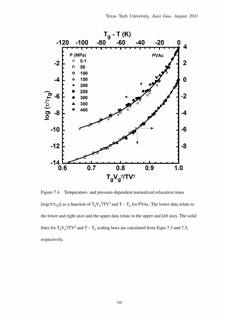
Texas Tech University, Jiaxi Guo, August 2011
168
Figure 7.4 Temperature- and pressure-dependent normalized relaxation times
[log(τ/τTg)] as a function of TgVgγ/TV
γ and T – Tg for PVAc. The lower data relate to
the lower and right axes and the upper data relate to the upper and left axes. The solid
lines for TgVgγ/TV
γ and T – Tg scaling laws are calculated from Eqns 7.3 and 7.5,
respectively.

Texas Tech University, Jiaxi Guo, August 2011
169
Figure 7.5 Temperature- and pressure-dependent normalized relaxation times
[log(τ/τTg)] as a function of TgVgγ/TV
γ and T – Tg for PVC. The lower data relate to
the lower and right axes and the upper data relate to the upper and left axes. The solid
lines for TgVgγ/TV
γ and T – Tg scaling laws are calculated from Eqns 7.3 and 7.5,
respectively.

Texas Tech University, Jiaxi Guo, August 2011
170
Figure 7.6 Temperature- and pressure-dependent normalized relaxation times
[log(τ/τTg)] as a function of (T – Tg)(1/Tg(P) + γαl) for polystyrenes. The solid lines
are calculated from Eqn. 7.10.

Texas Tech University, Jiaxi Guo, August 2011
171
Figure 7.7 Temperature- and pressure-dependent normalized relaxation times
[log(τ/τTg)] as a function of (T – Tg)(1/Tg(P) + γαl) for polycyanurates. The solid lines
are calculated from Eqn. 7.10.

Texas Tech University, Jiaxi Guo, August 2011
172
Figure 7.8 Temperature- and pressure-dependent normalized relaxation times
[log(τ/τTg)] as a function of (T – Tg)(1/Tg(P) + γαl) for PVAc. The solid lines are
calculated from Eqn. 7.10.

Texas Tech University, Jiaxi Guo, August 2011
173
Figure 7.9 Temperature- and pressure-dependent normalized relaxation times
[log(τ/τTg)] as a function of (T – Tg)(1/Tg(P) + γαl) for PVC. The solid lines are
calculated from Eqn. 7.10.

Texas Tech University, Jiaxi Guo, August 2011
174
CHAPTER 8
CONCLUSIONS
The dissertation describes architectural effects on the viscoelastic bulk and shear
responses and pressure-volume-temperature (PVT) behavior for polycyanurate
networks having different crosslink densities and a three-arm star polystyrene using a
custom-built dilatometer and a commercial rheometer. In addition, the shift factors for
reducing the bulk and shear master curves, coupled with the PVT data, are used to
compare TVγ thermodynamic scaling for complex liquids to T – Tg scaling.
For polycyanurate networks, the breadth of the shear retardation time spectra is
found to increase with decreasing crosslink density, whereas the bulk spectra are
identical for the two materials when referenced to Tg. For the polystyrenes, the shear
retardation time spectra become narrower with decreasing molecular weight. In
addition, comparing the bulk and shear retardation time spectra, the two show similar
slopes at short times, but the magnitude of the spectra for the bulk response is lower
than that for the shear, indicating more local Andrade creep modes are involved in the
shear deformation at short times or the contribution of these modes is greater for the
shear response. In addition, at long times, the chain mechanisms that are available to
the shear are not available to the bulk response.
The effects of crosslink density on the PVT behavior of thermosetting materials
were also studied using the two polycyanurate networks. The results show that the
major effect of crosslink density is the change in Tg that dominates the volumetric

Texas Tech University, Jiaxi Guo, August 2011
175
response. In addition, the thermal pressure coefficient (γ) is calculated from the
instantaneous bulk modulus (K) and the thermal expansion coefficient (α) and is
found to range from 1.0 to 1.6 MPa K-1
. The glassy bulk modulus (Kg) appears to be
proportional to the cohesive energy density (CED), consistent with the literature.
Finally, the TVγ thermodynamic scaling was compared to the T – Tg scaling for
reducing the relaxation times of six materials: star and linear polystyrenes, two
polycyanurate networks, poly(vinyl acetate), and poly(vinyl chloride). The results
indicate that in all cases, the TVγ scaling successfully reduced the relaxation times for
each polymer; however, the samples having similar microstructures but with different
Tg and PVT behavior, i.e., the two polycyanurates, cannot be reduced unless the
scaling is normalized by TgVgγ. On the other hand, the T – Tg scaling gives excellent
results for the polystyrene and the polycyanurate families where the samples have
similar structures. A simple theoretical relationship between TVγ and T – Tg scalings
is established and a modified T – Tg scaling is proposed which works as well as the
TVγ scaling in cases where T – Tg scaling fails. Importantly, neither T – Tg scaling or
the new modified scaling requires absolute volume.

Texas Tech University, Jiaxi Guo, August 2011
176
CHAPTER 9
FUTURE WORK
9.1 Pressure Dependent Structure Recovery
Conventional structure recovery experiments are carried out at constant pressure
using temperature jumps [1]. In conventional measurements, asymmetry of approach
and memory effects are observed and found to be a function of both aging
temperature and aging time. The behaviors can be well described by the
Tool−Narayanaswamy−Moynihan (TNM) [2-4] model or the
Kovacs-Aklonis-Hutchinson-Ramos model (KAHR) model [5], where the relaxation
time of the polymers is a function of temperature (T) and structure [δ, where δ = (V –
V∞/ V∞)] or fictive temperature (Tf). However, the pressure dependence of structure
recovery has not been widely studied.
In isothermal pressure dependent structure recovery experiments, the volume can
be measured as a function of structural recovery and for the memory effect after
pressure jump, instead of temperature jumps. In this case, the behavior is expected to
be described by the modified TNM or KAHR model, where the relaxation time (τ) is
a function of pressure (P) and structure or fictive pressure (Pf). Such experiments were
performed by Tribone et al. [6] for a polystyrene sample and qualitative similarities
with temperature jumps were found, but no memory effects have been performed. In
addition, the quantitative equivalence of Tf and Pf discussed by Davies and Jones [7]
will be tested. The activation energy (∆h*), the relaxation time distribution factor (β)

Texas Tech University, Jiaxi Guo, August 2011
177
and the non-linearity parameter (x) can also be studied as a function of pressure.
9.2 Effects of ββββ Relaxation on Viscoelastic Bulk Modulus
The bulk response has been found to be dominated by local motions of the
materials with no chain modes contribution to the bulk response based on previous
works from Bero and Plazek, and in our laboratory [8-12] and reported in Chanters 4 -
6. However, the influence of the β relaxation, which arises from side-chain relaxations
and occurs at shorter times or lower temperature, on the bulk response is unknown.
The effect of β relaxation in bulk modulus is important not only for
understanding the underlying mechanisms of the bulk response, but also for
understanding isotropic residual stress development at low temperatures where the β
relaxation may be dominant. For example, the β relaxation has been found to occur in
an epoxy at approximately – 80 °C, and the shear modulus showed a transition in the
vicinity of this temperature due to the β relaxation [13]. This is important for
predicting the thermal residual stress for cryogenic fuel tank applications that operates
at temperature as low as – 180 °C.
Poly(methyl methacrylate) (PMMA) and poly(ethyl methacrylate) (PEMA) that
have strong β relaxation can be used to examine β-relaxation effects on the bulk
response. In fact, Sane and Knauss [14] has measured dynamic bulk compliances, but
noise in their data is too prominent to determine β relaxation effects. One may expect
that if strong β relaxation occurs, this may lead to failure of time-temperature
Texas Tech University, Jiaxi Guo, August 2011
178
superposition. Moreover, in the retardation time spectra, the bulk response may show
two peaks before it is cut out.
9.4 Viscoelastic Bulk Modulus for Epoxy/POSS
Epoxy resins are low cost, light weight, and high mechanical performance
materials [15-17], and thus they are widely applied in electronic or aerospace
composite industries. However, thermal residual stress may build up in the materials
and may cause premature failure. One idea [13, 18] to reduce the residual stress is to
incorporate into the epoxy particles that have both organic and inorganic character, i.e.,
polyhedral oligomeric silsesquioxane (POSS).
The shear response of epoxy/POSS has been studied [13] as a function of POSS
concentration, where the POSS is found to be helpful for reducing the product of
shear modulus and linear thermal expansion coefficient (αl). In addition, the POSS is
also found to reduce the thermal pressure coefficient (γ) that is a product of bulk
modulus (K) and volumetric thermal expansion coefficient (αV). However, the bulk
viscoelastic behavior has not been studied for POSS-filled epoxy.

Texas Tech University, Jiaxi Guo, August 2011
179
REFERENCES
1. A. J. Kovacs, Fortschr. Hochpolym.-Forsch. 3, 394, 1964.
2. A. W. Tool, J. Am. Ceram. Soc. 29, 240, 1946.
3. O. S. Narayanaswamy, J. Am. Ceram. Soc. 54, 491-498, 1971.
4. C. T. Moynihan, P.B. Macedo, C. T. Montrose, P.K. Gupta, M. A. DeBolt, J. F.
Dill, B. E. Dom, P. W. Drake, A. J. Easteal, P. B. Elterman, R. P. Moeller, H.
Sasabe, J. A. Wilder, Am. N. Y. Acad. Sci. 279, 15-35, 1976.
5. A. Kovacs, J. J. Aklonis, J. M. Hutchinson, A. R. Ramos, J. Polym. Sci., Polym.
Phys. Ed. 17, 1097-1162, 1979.
6. J. J. Tribone, J. M. O’Reilly, J. Greener, J. Polym. Sci.: Part B: Polym. Phys 27,
837-857, 1989.
7. R. O. Davies, G. O. Jones, Adv. Phys. 2, 371-409, 1953.
8. C. A. Bero, D. J. Plazek, J. Polym. Sci. Part B: Polym. Phys. 29, 39-47, 1991.
9. Y. Meng, S. L. Simon, J. Polym. Sci. Part B, Polym. Phys. 45, 3375-3385, 2007.
10. J. X. Guo, S. L. Simon, J. Polym. Sci. Part B, Polym. Phys. 47, 2477-2486, 2009.
11. J. X. Guo, S. L. Simon, "Bulk and Shear Rheology of a Symmetric Three-Arm
Star Polystyrene," in Preparation, 2011.
12. S. B. Sane, W. G. Knauss, Mech. Time-Depend. Mater. 5, 293-324, 2001.
13. Q. X. Li, S. A. Hutcheson, G. B. McKenna, S. L. Simon, J. Polym. Sci.: Part B:
Polym. Phys. 46, 2719-2732, 2008.
14. G. Hu, J. E. Luan, S. Chew, Journal of Electronic Packaging 131, 011010-1-6,
Texas Tech University, Jiaxi Guo, August 2011
180
2009.
15. M. Molyneux, Composites, 14, 87-91, 1983.
16. M. Shimbo, M. Ochi, K. Arai, J. Coat. Technol. 56, 45-51, 1984.
17. K. Z. Win, T. Karim, Q. Li, S. L. Simon, G. B. McKenna, J. Appl. Polym. Sci.
116, 142-146, 2009.


![View Article Online ChemComm - Xiamen University · Xiaobo Qu*[a], Tianyu Qiu[a], Di Guo[b], Hengfa Lu[a], Jiaxi Ying[a], Ming Shen[c], Bingwen Hu[c], Vladislav Orekhov[d], and Zhong](https://img.pdfslide.net/doc/110x75/5fbac280afd5c7577578c107/view-article-online-chemcomm-xiamen-university-xiaobo-qua-tianyu-qiua-di.jpg)