Embed Size (px)
Citation preview
This article has been accepted for inclusion in a future issue of this journal. Content is final as presented, with the exception of pagination.
IEEE TRANSACTIONS ON CYBERNETICS 1
H∞ Scaled Consensus for MASs With Mixed TimeDelays and Disturbances via Observer-Based
Output FeedbackShiming Chen , Zheng Zhang, and Yuanshi Zheng
Abstract—In this article, the H∞ scaled consensus controlproblem for multiagent systems in the presence of external dis-turbances and mixed time delays in both input and Lipschitznonlinearity is investigated. First, a state observer is introducedfor each agent based on the output information of the agent.Then, a scaled consensus protocol is proposed via a truncatedpredictor output-feedback method, which can deal with the inputdelay. The integral terms with the mixed time delays that arecontained in the transformed systems are analyzed by using theLyapunov–Krasovskii functionals method, and sufficient condi-tions are obtained to achieve scaled consensus with guaranteedH∞ performance. An iterative procedure is utilized to calcu-late the linear matrix inequality. By this, the feedback gain andobserver gain are then designed. Finally, a simulation example isprovided to illustrate the effectiveness of the theoretical results.
Index Terms—H∞ scaled consensus, disturbances, multiagentsystems (MASs), observer, output feedback, time delays.
I. INTRODUCTION
COOPERATIVE control of multiagent systems (MASs)has been widely used in many fields due to its poten-
tial applications in mobile robotics, unmanned aerial vehi-cles, complex network control, and digital core [1], [2]. Inthe last few years, complete consensus problems have beenextensively studied for various MASs, such as first/second-order systems [3]–[5]; high-order systems [6]; general lin-ear systems [7]–[10]; nonlinear systems [11], [12]; hybridsystems [13], [14]; and so on.
However, in many fields of engineering applications, suchas webpage ranking, water distribution systems, and closedqueuing, the requirement that all agents states converge to aconsistent value cannot meet human needs. So far, many stud-ies on the other new kinds of consensus have been carriedout, just like group consensus [15], bipartite consensus [16],and scaled consensus [17]. In particular, the scaled consensus
Manuscript received January 20, 2020; revised April 6, 2020; acceptedJune 4, 2020. This article was recommended by Associate Editor L. Zhang.(Corresponding author: Zheng Zhang.)
Shiming Chen and Zheng Zhang are with the School of Electrical andAutomation Engineering, East China Jiaotong University, Nanchang 330013,China (e-mail: [email protected]; [email protected]).
Yuanshi Zheng is with the School of Mechano-ElectronicEngineering, Xidian University, Xi’an 710071, China (e-mail:[email protected]).
Color versions of one or more of the figures in this article are availableonline at http://ieeexplore.ieee.org.
Digital Object Identifier 10.1109/TCYB.2020.3001643
is more attractive and less conservative. The scaled consensuswas first introduced in [17] which means that all agents’ statesin a network reach specified ratios instead of approaching aconsistent value. In addition, scaled consensus can possess thesame group and bipartite consensus behaviors via employingsuitable scaled values. In recent years, scaled consensus prob-lems were analyzed in [18] and [19]. These papers focused onthe scaled consensus of the first/second-order linear MASs.However, due to the challenges of solving scaled consen-sus problems for systems with unideal network factors, it isnontrivial to investigate MASs with time delays and uncer-tainty. Scaled consensus problems of MASs with time-varyingdelays or external disturbances were addressed in [20]–[22],respectively.
With the development of studies on MASs, time delayscaused by agents are diverse and the existence of them maydegrade system performance and even destroy the stabil-ity of the system. Most real MASs contain inherent statedelays, which physically come from calculation or measure-ment. The other source of delay is the input delay that isrelated to the computational time and execution time of eachagent. For input delay, a predictor-based method has beencommonly utilized to deal with it. Various predictor-basedapproaches [23]–[25] can be utilized to deal with the controlproblems of input delayed systems. One of the predictor-basedmethods, known as the truncated prediction feedback, is toignore the troublesome integral part and only to use the expo-nential of the system matrix as the prediction [26]. For theMASs with input delay, truncated prediction feedback controlis utilized to achieve consensus in [26]–[29]. For the timedelays existing in nonlinear dynamics, a Lyapunov controlapproach is utilized to reach consensus [21], [30], [31]. Butthese papers focused purely on the first/second-order nonlinearsystem.
Moreover, external disturbances cannot be avoided in theworks above. There are mainly two approaches to deal withthese situations. One way is the stochastic analysis approachand the other is the robust H∞ control approach. By means ofstochastic analysis, some sufficient conditions were derived toachieve mean-square consensus [32], [33]. Another method tothe disturbance problems is the robust H∞ control, which wasalso utilized to solve H∞ consensus problems with guaranteedH∞ performance [34]–[38]. Therefore, it has been attract-ing more academic focuses. However, few works have takeninto account both time delays and persistent disturbances,
2168-2267 c© 2020 IEEE. Personal use is permitted, but republication/redistribution requires IEEE permission.See https://www.ieee.org/publications/rights/index.html for more information.
Authorized licensed use limited to: XIDIAN UNIVERSITY. Downloaded on July 02,2020 at 03:30:54 UTC from IEEE Xplore. Restrictions apply.
This article has been accepted for inclusion in a future issue of this journal. Content is final as presented, with the exception of pagination.
2 IEEE TRANSACTIONS ON CYBERNETICS
which are the two key factors in affecting the stability andperformance of the MASs.
In many practical control systems, the states of agentsare often not accessible, where only output information isavailable. Using the output information of agents, there aregenerally two basic output-feedback types: 1) the static outputfeedback and 2) the dynamic output feedback. The con-troller with static output-feedback consensus protocols islimited [39], [40]. Thus, it is more realistic to design observersthat generate the system-state estimation online, that is, designa dynamic output-feedback controller. Therefore, the observer-based dynamic output-feedback control has attracted muchattention (see [22], [41], [42], etc.). But the systems in thesepapers did not take both the mixed time delays and externaldisturbances into consideration.
This article investigates the distributed controller designproblems such that the outputs of agents can reach scaled con-sensus with that of the leader. The main contributions of thisarticle are two-fold. First, based on each agent’s output, a localobserver is constructed. By using an observer-based truncatedprediction method, the scaled consensus control protocols aredesigned, which include complete consensus, group consensus,and bipartite consensus as special cases. Second, the consid-ered MASs contain the mix delays and scaled ratios whichleads to the coupling among input delay, delays in nonlineardynamics, and scaled ratios for the system. Several extra inte-gral terms are produced, and the Lyapunov function also needsto be rescaled.
II. PRELIMINARIES
In this section, we recall the algebraic graph theory, someuseful lemmas, and model formulation, which will be used inthe following section.
A. Notations
Let Rp×q be the p × q-dimensional matrices. IN rep-resents the identity matrix of N. 1N = [1, . . . , 1]T ∈RN . diag{�1,�2, . . . ,�N} represents a diagonal matrix and�1,�2, . . . ,�N are diagonal elements. BT represents thetranspose of a matrix B. λmax(L) (λmin(L)) represents the max-imum (minimum) eigenvalue of L. R > 0 indicates that R isa positive-definite matrix. ‖ · ‖ and ‖ · ‖F denote the 2-normand Frobenius norm of a matrix, respectively. A−1 denotes theinverse of the matrix A, and the notation ⊗ is the Kroneckerproduct.
B. Graph Theory
Let G′ = (V ′, E′, A′) be a directed graph of a set of nodesV ′ = {1, 2, . . . , N}, E′ ⊆ V ′ × V ′ is a set of directed edges,and (j, i) ∈ E′ means that agent i can receive information fromagent j. A′ = [a′
ij] ∈ RN×N , a′ij ≥ 0 represents the adjacency
matrix associated with a′ij = 1 if (j, i) ∈ E′ and a′
ij = 0otherwise. The set of neighbors of the node is denoted byNi = {j ∈ V ′ : (j, i) ∈ E′}. If there is a node called root suchthat there exists a directed path from this node to any othernodes, then the graph is said to contain a directed spanningtree. The degree matrix is defined as D′ = diag{d′
1, . . . , d′N},
where d′i = ∑
j∈Nia′
ij. The Laplacian matrix L′ is denoted asL′ = D′ − A′ = [l′ij] ∈ RN×N .
C. Some Useful Lemmas
Assumption 1: The communication topology G1 contains adirected spanning tree with the leader as the root.
Lemma 1 [43]: Under Assumption 1, if the leader’s statesare available to one or multiple followers, then L1 = L′ +B′ isan irreducible diagonally dominant M-matrix and, hence, non-singular. There exists a diagonal matrix � = diag{ε1, . . . , εN}with εi > 0, i = 1, . . . , N, such that
�L1 + LT1 �
�= L1 ≥ ρ0IN
where B′ = diag{a′10, . . . , a′
N0} is the leader adjacency matrixand a′
i0 > 0 if there is an information exchange between leaderand agent i; otherwise, a′
i0 = 0. ρ0 is the minimum eigenvalueof the matrix L1. � can be computed as ε = [ε1, . . . , εN]T =(LT
1 )−11N .Assumption 2: The communication topology G′ contains a
directed spanning tree.Lemma 2 [44]: Under Assumption 2, the Laplacian matrix
L has a simple zero eigenvalue with the associated right eigen-vector 1N , and all nonzero eigenvalues have positive real parts.
Furthermore, there exists a unique vector δ�= [δ1, . . . , δN]T
with∑N
i=1 δi = 1 and δi > 0, ∀i = 1, . . . , N such thatδTL′ = 0.
Lemma 3 [45]: By Lemma 2, there exists an invertiblematrix U, with its first column U1 = 1N and the first rowof U−1, U−1
(1) = ςT, such that
U−1L′U = J
with J being a block-diagonal matrix in the real Jordan form
J = diag{0, J1, . . . , Jc, Jc+1, . . . , Jd}where Jk ∈ Rmk for k = 1, . . . , c are the Jordan blocks for realeigenvalues λk > 0 with the multiplicity mk in the form
Jk =
⎡
⎢⎢⎢⎢⎢⎣
λk 1λk 1
. . .. . .
λk 1λk
⎤
⎥⎥⎥⎥⎥⎦
and Jk ∈ R2mk for k = c + 1, . . . , d are the Jordan blocks forconjugate eigenvalues αk ± jβk, αk > 0, and βk > 0, with themultiplicity mk in the form
Jk =
⎡
⎢⎢⎢⎢⎢⎣
μ(αk, βk) I2
μ(αk, βk) I2. . .
. . .
μ(αk, βk) I2
μ(αk, βk)
⎤
⎥⎥⎥⎥⎥⎦
with I2 the identity matrix in R2×2 and
μ(αk, βk) =[
αk βk
−βk αk
]
∈ R2×2.
Authorized licensed use limited to: XIDIAN UNIVERSITY. Downloaded on July 02,2020 at 03:30:54 UTC from IEEE Xplore. Restrictions apply.
This article has been accepted for inclusion in a future issue of this journal. Content is final as presented, with the exception of pagination.
CHEN et al.: H∞ SCALED CONSENSUS FOR MASs WITH MIXED TIME DELAYS AND DISTURBANCES 3
Lemma 4 [46]: Suppose that W ∈ RN×N is a symmetricpositive-definite matrix and W1 ∈ RN×N is symmetric. Then,for any vector x ∈ RN , the following inequality holds:
λmin
(W−1W1
)xTWx ≤ xTW1x ≤ λmax
(W−1W1
)xTWx.
Lemma 5 [47]: For any constant matrix U ∈ Rn×n, U > 0,scalars b > a, and vector function z : [a, b] → Rn, thefollowing inequality is well defined, then:(∫ b
az(s)ds
)T
U
(∫ b
az(s)ds
)
≤ (b − a)
∫ b
azT(s)Uz(s)ds.
Lemma 6 [48]: For a positive-definite matrix P, the follow-ing identity holds:
eATtPeAt − eαtP = −eαt∫ t
0eατ eATτ PeAτ dτ
where α ≥ 0 is a scalar and R = −ATP − PA + αP.Furthermore, if R is positive definite, ∀t > 0
eATtPeAt ≤ eαtP.
Lemma 7 [49]: For any given x, y ∈ Rn, we have
2xTPQy ≤ xTPSPTx + yTQTS−1Qy
where S > 0, P, and Q have appropriate dimensions.
D. Model Formulation
Suppose that the general nonlinear MAS consists of oneleader and N followers, the dynamics of the followers aredescribed by
⎧⎨
⎩
xi(t) = Axi(t) + Bui(t − τ1) + Ddi(t)+ Ef (xi(t), xi(t − τ2), t)
yi(t) = Cxi(t), i ∈ 1, . . . , N(1)
where xi(t) ∈ Rn, ui(t) ∈ Rm, and yi(t) ∈ Rp are the state, controlinput, and measurement output of agent i, respectively. τ1 > 0is the input delay. τ2 > 0 denotes the unknown time-varyingdelays in the nonlinear dynamics, which physically comesfrom calculation or measurement. di(t) ∈ Lq
2[0,∞) denotesthe external disturbance. A ∈ Rn×n, B ∈ Rn×m, C ∈ Rp×n,D ∈ Rn×q, and E ∈ Rn×n are constant matrices with (A, B)
being controllable and (A, C) being observable. f : Rn × Rn ×[0,+∞) → Rn is a continuously differentiable vector-valuedfunction satisfying the following Lipschitz condition:
‖ϑ1f (e1, e2, t) − ϑ2f (c1, c2, t)‖ ≤2∑
i=1
ρi‖ϑ1ei − ϑ2ci‖ (2)
where ρ1, ρ2, ϑ1, ϑ2 > 0 ∀ei, ci ∈ Rn, i ∈ {1, 2}, t ≥ 0.The virtual leader’s dynamics is denoted by
{x0(t) = Ax0(t) + Ef (x0(t), x0(t − τ2), t)y0(t) = Cx0(t).
(3)
To achieve scaled consensus tracking and leaderless scaledconsensus with a guaranteed H∞ performance, we combinethe leader’s state to define the performance variable zi(t) and z(t), respectively
zi(t) = xi(t) − 1
βix0(t) (4)
zi(t) = βixi(t) −
N∑
j=1
δjβjxj(t). (5)
Definition 1: Given a positive scalar γ , the H∞ scaled con-sensus tracking and leaderless scaled consensus are achieved,respectively, if the following two conditions are met.
1) The MASs (1) and (3) can reach scaled consensus track-ing and leaderless scaled consensus if, when di(t) = 0,the states of agents satisfy limt→∞ ‖βixi(t) − x0(t)‖ = 0and limt→∞ ‖βixi(t) − βjxj(t)‖ = 0 for all initial condi-tions, respectively, where the scaled values βi and βj arenonzero constants, i, j = 1, 2, . . . , N.
2) Under the zero initial condition, the performance vari-ables z(t) and
z(t), respectively, satisfy
J =∫ ∞
0
(zT(t)z(t) − γ 2dT(t)d(t)
)dt < 0 (6)
J =∫ ∞
0
( z
T(t)
z(t) − γ 2dT(t)d(t)
)dt < 0 (7)
where z(t) = [zT1 (t), . . . , zT
N(t)]T, z(t) =
[ z
T1 (t), . . . ,
z
TN(t)]T and d(t) = [dT
1 (t), . . . , dTN(t)]T.
Remark 1: This article considers the scaled consensus ofgeneral nonlinear MASs, where the complete consensus, groupconsensus, and bipartite consensus can be regarded as the spe-cific cases of the scaled consensus by selecting suitable scaledvalues βi, i = 1, . . . , N.
Remark 2: In [18], [21], and [26]–[31], the consensus prob-lems with communication delays, input delays, or delaysin nonlinear dynamics are considered. Note that contraryto [18], [21], and [26]–[31], the scaled consensus problem forMASs in the presence of input delay τ1 and time-varyingdelays τ2 in nonlinear dynamics is addressed. This input delayτ1 may also represent some communication delays in thenetwork system. Thus, the system is more general than theone studied in [18], [21], and [26]–[31]. The research on thissystem might be more meaningful.
III. H∞ SCALED CONSENSUS TRACKING CONTROL
ANALYSIS
In this section, the distributed H∞ scaled consensus trackingcontrol problem for MASs in the presence of external distur-bances and mixed time delays in both input and Lipschitznonlinearity is to be studied.
A. Scaled Consensus Tracking Protocol Design viaObserver-Based Output Feedback
The observer based on output information is constructed as⎧⎪⎪⎨
⎪⎪⎩
˙xi(t) = Axi(t) + Bui(t − τ1) + Ddi(t)+ Ef
(xi(t), xi(t − τ2), t
)− F(yi(t) − Cxi(t)
)
˙x0(t) = Ax0(t) + Ef(x0(t), x0(t − τ2), t
)
− F(y0(t) − Cx0(t)
)(8)
where xi(t) and x0(t) are the estimations of the follower’s statexi(t) and the leader’s state x0(t), respectively, and F ∈ Rn×p isthe observer gain matrix to be designed later. The estimationerror is defined by zi(t) = zi(t) − zi(t) with zi(t) = xi(t) −(1/βi)x0(t).
Authorized licensed use limited to: XIDIAN UNIVERSITY. Downloaded on July 02,2020 at 03:30:54 UTC from IEEE Xplore. Restrictions apply.
This article has been accepted for inclusion in a future issue of this journal. Content is final as presented, with the exception of pagination.
4 IEEE TRANSACTIONS ON CYBERNETICS
To describe the equation in a more convenient way, letfiτ2 = f (xi(t), xi(t − τ2), t), f0τ2 = f (x0(t), x0(t − τ2), t),fiτ2 = f (xi(t), xi(t − τ2), t), and f0τ2 = f (x0(t), x0(t − τ2), t).Combining (1), (3), and (8), we obtain the derivative of zi(t)and zi(t), respectively
zi(t) = Azi(t) + Bui(t − τ1) + Ddi(t) + E
(
fiτ2 − 1
βif0τ2
)
(9)
˙zi(t) = (A + FC)zi(t) + E
(
fiτ2 − 1
βif0τ2
)
− E
(
fiτ2 − 1
βif0τ2
)
. (10)
From the scaled tracking error dynamics (9), we have
zi(t) = eAτ1 zi(t − τ1) +∫ t
t−τ1
eA(t−h)
×[
Bui(h − τ1) + Ddi(h) + E
(
fiτ2 − 1
βif0τ2
)]
dh (11)
where the first term eAτ1 zi(t − τ1) is a truncated predictor ofthe state zi based on zi(t − τ1).
By using the observer-based truncated predictor output-feedback method, the following scaled consensus trackingprotocol is considered:
ui(t) = KeAτ1
⎡
⎣N∑
j=1
a′ij
(
xi(t) − βj
βixj(t)
)
+ a′i0
(
xi(t) − 1
βix0(t)
)⎤
⎦
= KeAτ1
N∑
j=1
lβij
(
xj(t) − 1
βix0(t)
)
= KeAτ1
N∑
j=1
lβij(zi(t) + zi(t)) (12)
where K ∈ Rm×n is the control gain matrix to be designedlater, and lβij = (βj/βi)l1ij, i, j = 1, . . . , N, and l1ij is the elementof matrix L1.
Substituting the scaled consensus tracking protocol (12) into(9) and using (11), we have
zβii (t) = Azβi
i (t) + BKeAτ1
N∑
j=1
l1ijzβjj (t − τ1)
+ βiDdi(t) + E(βifiτ2 − f0τ2
)+ BK
×N∑
j=1
l1ij
{
zβjj (t) −
∫ t
t−τ1
eA(t−h)[βjBuj(h − τ1)
+ βjDdj(h) + E(βjfjτ2 − f0τ2
)]dh
}
(13)
where zβii (t) = βizi(t) and zβi
i (t) = βizi(t).Let zβ(t) = [β1zT
1 (t), . . . , βNzTN(t)]T, zβ(t) =
[β1zT1 (t), . . . , βNzT
N(t)]T, d(t) = [dT1 (t), . . . , dT
N(t)]T,fτ2 = [f T
1τ2, . . . , f T
Nτ2]T, and β = diag{β1, β2, . . . , βN}.
Then, together with (12) again, (13) can be written in acompact matrix form as follows:
zβ(t) = (IN ⊗ A + L1 ⊗ BK)zβ(t) +6∑
v=1
�v + � (14)
where
�v = (L1 ⊗ BK)�v, v = 1, 2, 3, 4
�1 = −∫ t
t−τ1
(L1 ⊗ eA(t−h)BKeAτ1
)zβ(h − τ1)dh
�2 = −∫ t
t−τ1
(L1 ⊗ eA(t−h)BKeAτ1
)zβ(h − τ1)dh
�3 = −∫ t
t−τ1
(β ⊗ eA(t−h)D
)d(h)dh
�4 = −∫ t
t−τ1
(IN ⊗ eA(t−h)E
)[(β ⊗ In)fτ2 − f0τ2 · 1Nn
]dh
�5 =(
L1 ⊗ BKeAτ1)
zβ(t − τ1)
�6 = (IN ⊗ E)[(β ⊗ In)fτ2 − f0τ2 · 1Nn
]
� = (β ⊗ D)d(t).
B. Scaled Consensus Tracking Analysis
In this section, sufficient conditions on scaled consensustracking for MASs (1) and (3) via the observer-based output-feedback controller (12) are presented.
Theorem 1: For the general nonlinear MASs (1) and (3) withinherent delayed nonlinear dynamic, external disturbance, andinput delay, the H∞ scaled consensus tracking can be achievedby the observer (8) with F = −R−1CT and the controller (12)with K = −BTS, if there exist a positive-definite matrix Q, Rand constants ι > 0, ι1 > 0, and ωv > 0, v = 1, . . . , 6 suchthat
SBBTBBTS ≤ ι2In (15)
AT + A < ι1In (16)⎡
⎣
∏11 IN ⊗ Q IN ⊗ D
IN ⊗ Q∏
22 0IN ⊗ DT 0
∏33
⎤
⎦ < 0 (17)
[∐11 RE
ETR −2In
]
< 0 (18)
where Q = S−1, σ = (ρ0/εmin), εmin = min{ε1, . . . , εN},εmax = max{ε1, . . . , εN}, �−1 = diag{ε−1
1 , . . . , ε−1N }, ρ0,
and εi, i = 1, . . . , N, are defined in Lemma 1. β2min =
min{β21 , β2
2 , . . . , β2N}, β−1 = diag{β−1
1 , . . . , β−1N }, and βi, i =
1, . . . , N are scaled ratios of each agent
∏
11
= � ⊗[
AQ + QAT − σBBT +(
6∑
v=1
ωv
)
In
]
∏
22
= −[
γ1εmax
ω1eτ1 + εmax
(ρ2
1 + ρ22
)
×(
γ4
ω4eτ1 + γ6
ω6+ 6
β2minεmax
)]−1
�−1 ⊗ In − INn
Authorized licensed use limited to: XIDIAN UNIVERSITY. Downloaded on July 02,2020 at 03:30:54 UTC from IEEE Xplore. Restrictions apply.
This article has been accepted for inclusion in a future issue of this journal. Content is final as presented, with the exception of pagination.
CHEN et al.: H∞ SCALED CONSENSUS FOR MASs WITH MIXED TIME DELAYS AND DISTURBANCES 5
τ1 is input delay and∏
33 = ([(γ3εmax)/ω3]eτ1 −γ 2)(�−1β−1)2 ⊗ Iq, γ is a guaranteed H∞ performancewhich is defined in (27).
∐11 = RA + ATR − 2CTC +
(4ρ21 + 4ρ2
2 + 1)In + εmax([γ2/ω2]eτ1 + [γ5/ω5])In
γ1 = η1
∥∥∥L2
1
∥∥∥
2, η1 = τ1ι
4e2ι1τ1
γ2 = η2
∥∥∥L2
1
∥∥∥
2, η2 = τ1ι
4β2maxe2ι1τ1
γ3 = η3‖D‖2‖L1‖2, η3 = τ1ι2β2
maxeι1τ1
γ4 = η4‖E‖2‖L1‖2, η4 = 2τ1ι2eι1τ1
γ5 = η5‖L1‖2, η5 = ι2β2maxeι1τ1
γ6 = 2‖E‖2. (19)
Proof: To start the consensus analysis, we try aLyapunov function candidate V0(t) = ∑N
i=1 zTi (t)Rzi(t) +
(zβ(t))T(� ⊗ S)zβ(t).Taking the derivative of V0(t) along (10) and (14), we have
V0(t) =N∑
i=1
{
zTi (t)
[R(A + FC) + (A + FC)TR
]zi(t) + 2zT
i (t)
× RE
[(
fiτ2 − 1
βif0τ2
)
−(
fiτ2 − 1
βif0τ2
)]}
+ (zβ(t)
)T[� ⊗ (
SA + ATS)]
zβ(t)
+ (zβ(t)
)T[(�L1 + LT
1 �)⊗ SBK
]zβ(t)
+ 2(zβ(t)
)T(� ⊗ S)
(6∑
v=1
�v + �
)
. (20)
Under (2), it is not difficult to obtain thatN∑
i=1
−2zTi (t)RE
(
fiτ2 − 1
βif0τ2
)
≤ −N∑
i=1
2zTi (t)RE[ρ1zi(t) + ρ2zi(t − τ2)]
≤N∑
i=1
{zT
i (t)REETRzi(t) + [ρ1zi(t) + ρ2zi(t − τ2)]T
× [ρ1zi(t) + ρ2zi(t − τ2)]}
≤N∑
i=1
[zT
i (t)REETRzi(t) + 2ρ21 zT
i (t)zi(t)
+ 2ρ22 zT
i (t − τ2)zi(t − τ2)]
(21)
and with a similar analysis, by the definition of zi(t), one hasN∑
i=1
2zTi (t)RE
(
fiτ2 − 1
βif0τ2
)
≤N∑
i=1
2zTi (t)RE
[ρ1(zi(t) + zi(t)) + ρ2(zi(t) + zi(t))
]
≤N∑
i=1
[zT
i (t)REETRzi(t) + 4ρ21 zT
i (t)zi(t) + 4ρ21 zT
i (t)zi(t)
+ 4ρ22 zT
i (t − τ2)zi(t − τ2) + 4ρ22 zT
i (t − τ2)zi(t − τ2)].
(22)
Based on Lemma 7, substituting (21), (22), K = −BTS, andF = −R−1CT into (20), it has
V0(t) ≤N∑
i=1
[zT
i (t)(
RA + ATR − 2CTC + 2REETR + 4ρ21 In
)
× zi(t) + 6ρ22 zT
i (t − τ2)zi(t − τ2)
+ 6ρ21 zT
i (t)zi(t) + 4ρ22 zT
i (t − τ2)zi(t − τ2)]
+ (zβ(t)
)T[� ⊗ (
SA + ATS − σSBBTS)]
zβ(t)
+6∑
v=1
ωv(zβ(t)
)T(� ⊗ S2
)zβ(t)
+6∑
v=1
1
ωv�T
v (� ⊗ In)�v + 2(zβ(t)
)T(� ⊗ S)� (23)
where the inequality has used the fact that �L1 + LT1 � =
L1 ≥ ρ0IN . ωv, v = 1, . . . , 6, are any positive real numbersand σ = (ρ0/εmin).
The following lemma gives the bounds of ‖�v‖2, v =1, . . . , 6. It will be used to prove Theorem 1 and its proofis given in the Appendix.
Lemma 8: The bounds on ‖�v‖2, v = 1, . . . , 6, can beestablished as∥∥�1
∥∥2 ≤ γ1
∫ t
t−τ1
(zβ(h − τ1)
)Tzβ(h − τ1)dh
∥∥�2
∥∥2 ≤ γ2
∫ t
t−τ1
zT(h − τ1)z(h − τ1)dh
∥∥�3
∥∥2 ≤ γ3
∫ t
t−τ1
dT(h)d(h)dh
∥∥�4
∥∥2 ≤ γ4ρ
21
∫ t
t−τ1
(zβ(h)
)Tzβ(h)dh
∥∥�5
∥∥2 ≤ γ5zT(t − τ1)z(t − τ1)
∥∥�6
∥∥2 ≤ γ6ρ
21
(zβ(t)
)Tzβ(t) + γ6ρ
22
(zβ(t − τ2)
)Tzβ(t − τ2)
(24)
if conditions (15) and (16) are satisfied, z(t) =[zT
1 (t), . . . , zTN(t)]T and γv, v = 1, . . . , 6 are given in
(19).For the first four integral terms and the latter two delayed
terms shown in (24), and the delayed terms shown in (23), weconsider the following Krasovskii functions, respectively:
�1 = eτ1
∫ t
t−τ1
(zβ(h)
)Tzβ(h)dh
+ eτ1
∫ t
t−τ1
eh−t(zβ(h − τ1))T
zβ(h − τ1)dh
�2 = eτ1
∫ t
t−τ1
zT(h)z(h)dh
+ eτ1
∫ t
t−τ1
eh−t zT(h − τ1)z(h − τ1)dh
�3 = eτ1
∫ t
t−τ1
eh−tdT(h)d(h)dh
�4 = eτ1
∫ t
t−τ1
eh−t(zβ(h))T
zβ(h)dh
Authorized licensed use limited to: XIDIAN UNIVERSITY. Downloaded on July 02,2020 at 03:30:54 UTC from IEEE Xplore. Restrictions apply.
This article has been accepted for inclusion in a future issue of this journal. Content is final as presented, with the exception of pagination.
6 IEEE TRANSACTIONS ON CYBERNETICS
�5 = eτ1
∫ t
t−τ1
eh−t(zβ(h))T
zβ(h)dh
+ eτ1
∫ t
t−τ1
eh−t(zβ(h − τ2))T
zβ(h − τ2)dh
�6 =∫ t
t−τ1
zT(h)z(h)dh
�7 =∫ t
t−τ2
(zβ(h)
)Tzβ(h)dh
�8 =∫ t
t−τ2
zT(h)z(h)dh.
A direct evaluation gives that
�1 ≤ −∫ t
t−τ1
(zβ(h − τ1)
)Tzβ(h − τ1)dh + eτ1
(zβ(t)
)Tzβ(t)
�2 ≤ −∫ t
t−τ1
zT(h − τ1)z(h − τ1)dh + eτ1 zT(t)z(t)
�3 ≤ −∫ t
t−τ1
dT(h)d(h)dh + eτ1 dT(t)d(t)
�4 ≤ −∫ t
t−τ1
(zβ(h − τ2)
)Tzβ(h − τ2)dh + eτ1
(zβ(t)
)Tzβ(t)
�5 ≤ −∫ t
t−τ1
(zβ(h)
)Tzβ(h)dh + eτ1
(zβ(t)
)Tzβ(t)
�6 = zT(t)z(t) − zT(t − τ1)z(t − τ1)
�7 = (zβ(t)
)Tzβ(t) − (
zβ(t − τ2))T
zβ(t − τ2)
�8 = zT(t)z(t) − zT(t − τ2)z(t − τ2). (25)
Let
V(t) = V0(t) +3∑
v=1
γv
ωvεmax�v + γ4
ω4εmax
(ρ2
1�4 + ρ22�5
)
+ γ5
ω5εmax�6 +
(γ6
ω6εmax + 6
β2min
)
ρ22�7 + 4ρ2
2�8.
From (25), taking the time derivative of V(t), we obtain that
V(t) ≤N∑
i=1
{
zTi (t)
[
RA + ATR − 2CTC + 2REETR + 4(ρ2
1 + ρ22
)In
+(
γ2
ω2eτ1 + γ5
ω5
)
εmaxIn
]
zi(t)
}
+ (zβ(t)
)T[
� ⊗ (SA + ATS − σSBBTS
)+ γ1
ω1εmaxeτ1 In
+(
γ4
ω4eτ1 + γ6
ω6+ 6
βmin2 εmax
)
× εmax
(ρ2
1 + ρ22
)In
]
zβ(t)
+ 2(zβ(t)
)T(� ⊗ S)� +
6∑
v=1
ωv(zβ(t)
)T(� ⊗ S2
)zβ(t)
+ γ3
ω3εmaxeτ1 dT(t)d(t)
= eT(t)�e(t) + 2(zβ(t)
)T(� ⊗ S)� + γ3
ω3εmaxeτ1 dT(t)d(t)
(26)
where
e(t) =[ (
zβ(t))T
zT(t)]T
� =[
� ⊗ �11 0Nn×Nn
0Nn×Nn IN ⊗ �22
]
�11 = SA + ATS − σSBBTS + S26∑
v=1
ωv + γ1εmax
ω1eτ1 In
+ εmax
(ρ2
1 + ρ22
)(
γ4
ω4eτ1 + γ6
ω6+ 6
β2minεmax
)
In
and �22 = RA + ATR − 2CTC + 2REETR + 4(ρ21 + ρ2
2)In +([γ2/ω2]eτ1 + [γ5/ω5])εmaxIn.
We define
J =∫ ∞
0
(eT(t)e(t) − γ 2dT(t)d(t)
)dt. (27)
Substituting (26) into (27) and based on the assumption of thezero initial condition of system (1) and (3), we can obtain
J =∫ ∞
0
(eT(t)eT(t) − γ 2dT(t)d(t) + V(t)
)dt − V(∞)
≤∫ ∞
0
[
eT(t)(� + I2Nn)e(t) +(
γ3
ω3εmaxeτ1 − γ 2
)
× dT(t)d(t)+2eT(t)�1d(t)
]
dt
= [eT(t), dT(t)
]�
[e(t)d(t)
]
(28)
where �1 =[
�β ⊗ SD0Nn×Nm
]
and � =[
� + I2Nn �1
�T1
(γ3ω3
εmaxeτ1 − γ 2)
INm
]
.
It is easy to verify that � is negative definite and thus J < 0.By the Schur complement lemma, we know that � is negativedefinite if the following inequalities hold:
γ3εmax
ω3eτ1 − γ 2 < 0 (29)
� ⊗[
SA + ATS − σSBBTS + S26∑
v=1
ωv + γ1εmax
ω1eτ1 In
+ εmax
(ρ2
1 + ρ22
)(
γ4
ω4eτ1 + γ6
ω6+ 6
β2minεmax
)
In
]
+ INn
−(
γ3εmax
ω3eτ1 − γ 2
)−1
(�β)2 ⊗ SDDTS < 0 (30)
RA + ATR − 2CTC + 2REETR +(
4ρ21 + 4ρ2
2 + 1)
In
+ εmax
(γ2
ω2eτ1 + γ5
ω5
)
In < 0. (31)
Let Q = S−1, thus (30) is equivalent to
� ⊗{
AQ + QAT − σBBT +(
6∑
v=1
ωv
)
In
+[
γ1εmax
ω1eτ1 + εmax
(ρ2
1 + ρ22
)
Authorized licensed use limited to: XIDIAN UNIVERSITY. Downloaded on July 02,2020 at 03:30:54 UTC from IEEE Xplore. Restrictions apply.
This article has been accepted for inclusion in a future issue of this journal. Content is final as presented, with the exception of pagination.
CHEN et al.: H∞ SCALED CONSENSUS FOR MASs WITH MIXED TIME DELAYS AND DISTURBANCES 7
×(
γ4
ω4eτ1 + γ6
ω6+ 6
β2minεmax
)]
}
+ IN ⊗ QQ −(
γ3εmax
ω3eτ1 − γ 2
)−1
(�β)2 ⊗ DDT < 0. (32)
By using the Schur complement lemma, we can obtainthat the conditions (29), (32), and (31) are equivalent to theconditions specified in (17) and (18), respectively.
If di(t) = 0, it follows that V(t) ≤ eT(t)�e(t). By conditions(17) and (18), we can obtain � < 0, thus limt→∞ V(t) = 0,which indicates that limt→∞ ‖βixi(t) − x0(t)‖ = 0. Thatmeans the agents reach a scaled consensus tracking exponen-tially, which satisfies condition 1).
By conditions (15)–(18), we have � < 0, in which J < 0.That is,
∫∞0 ‖e(t)‖2dt < γ 2
∫∞0 ‖d(t)‖2dt. Due to e(t) =
[(zβ(t))T
zT(t)]T, thus∫∞
0 ‖zβ(t)‖2dt < γ 2
∫∞0 ‖d(t)‖2dt,
which satisfies (6) in condition 2). Therefore, the H∞ scaledconsensus tracking problem is achieved and the proof isfinished.
Remark 3: Note that in dynamics (14) and (24), there arecouplings between input delay τ1 and time-varying delays τ2in nonlinear dynamics, the Lyapunov–Krasovskii functionalsmethod is utilized to analyze the couplings.
Remark 4: Theorem 1 gives stability conditions (15)–(18)which involve nonlinear matrix inequalities. Traditional LMIsolvers cannot be adopted to find a feasible solution for thesenonlinear matrix inequalities. Instead, we can use the similariterative approach to find a feasible solution (ι, ι1, S, R) of(15)–(18), which was developed in [50].
Remark 5: In many practical control systems, the states ofagents are often not accessible, where only output informationare available. Compared with the existing observers [28], forthe MASs with persistent disturbances and mixed delays in thisarticle, H∞ control approach has been utilized based on out-put feedback. This method provides a guaranteed performanceindex in the sense of L2 gain and it is more realistic andreasonable via observer-based output feedback.
Remark 6: If the system (1) and (3) has only one agent,then it reduces to the general nonlinear system with inherentdelayed nonlinear dynamics, external disturbances, and inputdelay. In this article, the proposed methods can cover partialresults in [27]. Actually, due to distributed coordinated con-trol is important in many areas, H∞ control approach in adistributed framework has more significance in the practicalapplications.
Remark 7: In this article, the H∞ scaled consensus problemis solved in the continuous-time domain, and it is not easy tohandle the problem of our system in the presence of sampling.If the sampled data are taken into account, the system willbe more intricate and the theoretical analysis will be moredifficult. One of our future research topics is to extend theanalysis of this article to the consensus control for MASs inthe presence of sampling, which is still an open problem tobe solved.
IV. H∞ LEADERLESS SCALED CONSENSUS
CONTROL ANALYSIS
In this section, we extend the results to the H∞ leader-less scaled consensus problem in the presence of external
disturbances and mixed time delays in both input and Lipschitznonlinearity. Consider that the general nonlinear MAS consistsof N agents, the dynamics of the agents are described by (1).
A. Leaderless Scaled Consensus Protocol Design viaObserver-Based Output Feedback
For the MAS (1), we have
xi(t) = eAτ1 xi(t − τ1) +∫ t
t−τ1
eA(t−h)
× [Bui(h − τ1) + Ddi(h) + Efiτ2
]dh (33)
where the first term eAτ1 xi(t − τ1) is a truncated predictor ofthe state xi based on xi(t − τ1).
The following scaled consensus protocol is considered:
ui(t) = KeAτ1
N∑
j=1
a′ij
(
xi(t) − βj
βixj(t)
)
= KeAτ1
N∑
j=1
lβ′
ij xj(t) (34)
where K ∈ Rm×n is the control gain matrix to be designedlater. lβ
′ij = (βj/βi)l′ij, i, j = 1, . . . , N, l′ij is the element of
matrix L′. xi(t) is the estimation of the state xi(t). Then, astate observer is constructed as
˙xi(t) = Axi(t) + Bui(t − τ1) + Ddi(t) + Efiτ2
− F(yi(t) − Cxi(t)
). (35)
The estimation error is defined by xi(t) = xi(t)−xi(t). Thus,taking the time derivative of xi(t) along (1) and (35) gives
˙xi(t) = (A + FC)xi(t) + E(
fiτ2 − fiτ2
). (36)
Let xβ(t) = [β1xT1 (t), . . . , βNxT
N(t)]T and xβ(t) =[β1xT
1 (t), . . . , βNxTN(t)]T. In the same way that substitute the
scaled consensus protocol (34) into (1) and using (33), wehave
xβ(t) = (IN ⊗ A + L′ ⊗ BK
)xβ(t) +
6∑
v=1
�v + � (37)
where
�v = (L′ ⊗ BK
)�v, v = 1, 2, 3, 4
�1 = −∫ t
t−τ1
(L′ ⊗ eA(t−h)BKeAτ1
)xβ(h − τ1)dh
�2 = −∫ t
t−τ1
(L′ ⊗ eA(t−h)BKeAτ1
)xβ(h − τ1)dh,
�3 = −∫ t
t−τ1
(β ⊗ eA(t−h)D
)d(h)dh
�4 = −∫ t
t−τ1
(β ⊗ eA(t−h)E
)fτ2 dh
�5 =(
L′ ⊗ BKeAτ1)
xβ(t − τ1)
�6 = (β ⊗ E)fτ2
� = (β ⊗ D)d(t).
Authorized licensed use limited to: XIDIAN UNIVERSITY. Downloaded on July 02,2020 at 03:30:54 UTC from IEEE Xplore. Restrictions apply.
This article has been accepted for inclusion in a future issue of this journal. Content is final as presented, with the exception of pagination.
8 IEEE TRANSACTIONS ON CYBERNETICS
Using the vector δ in Lemma 2, let z(t) =
[ z
T1 (t), . . . ,
z
TN(t)]T, then we obtain
z(t) = (H ⊗ In)x
β(t)
where zi(t) is defined in (5), and H = IN − 1NδT. Then, it
follows that limt→∞ zi(t) = 0 if and only if limt→∞ β1x1(t) =
limt→∞ β2x2(t) = · · · = limt→∞ βNxN(t). Therefore, the lead-erless scaled consensus of MAS (1) under the protocol (34) isachieved if limt→∞
zi(t) = 0.Let ζ(t)
�= [ζT1 (t), . . . , ζT
N (t)]T = (U−1 ⊗ In) z(t). U is
defined in Lemma 3. By the definitions of δ and H, it is easyto see that ζ1(t) = (δTH ⊗ In)xβ(t) = 0.
Due to HL′ = L′H = L′. Then, we have
ζ (t) = (IN ⊗ A + J ⊗ BK)ζ(t) +6∑
v=1
�v +
� (38)
where
�v = (U−1L′ ⊗ BK)�v, v = 1, . . . , 4,
�5 =(U−1L′ ⊗ BKeAτ1)xβ(t − τ1),
�6 = (U−1Hβ ⊗ E)fτ2 , and
� = (U−1Hβ ⊗ D)d(t).
B. Leaderless Scaled Consensus Analysis
In this section, sufficient conditions on leaderless scaledconsensus for MASs (1) via the observer-based output-feedback controller (34) is presented.
Theorem 2: For the general nonlinear MASs (1) withmixed delays and external disturbances, the H∞ leaderlessscaled consensus can be achieved by the observer (35) withF = −R−1CT and the controller (34) with K = −BTS, ifthere exist a positive-definite matrix Q, R and constants
ι > 0, ι 1 > 0, and ωv > 0, v = 1, . . . , 6 such that
SBBTBBTS ≤ ι
2In (39)
AT + A < ι 1In (40)
⎡
⎢⎢⎣
∏11 IN ⊗ Q IN ⊗ D
IN ⊗ Q ∏
22 0
IN ⊗ DT 0 ∏
33
⎤
⎥⎥⎦ < 0 (41)
[ ∐
11 REETR −2In
]
< 0 (42)
where
Q = S−1
κ = max{λmax(UTU
), 1}
∏
22= −
(γ1
ω1eτ1 + γ4
ω4
(ρ2
1 + ρ22
)eτ1 + γ6
ω6ρ2
2 + κ
)−1
INn
∏
33=(
γ3
ω3eτ1 − γ 2
)(
U−1Hβ(
U−1Hβ)T)−1
⊗ Iq
and ∐
11= RA + ATR − 2CTC +
(ρ2
1 + ρ22
)In
+(
γ2
ω2eτ1 + γ5
ω5
)
β2maxIn + κIn.
∏11 specified in one of the following two cases.
1) If the eigenvalues of the Laplacian matrix L′ are distinct, ∏
11 = IN ⊗ [AQ + QAT − 2 σBBT + (
∑6v=1 ωv)In].
2) If the eigenvalues of the Laplacian matrix
L′ have multiple eigenvalues, ∏
11 = IN ⊗[AQ + QAT − 2(
σ − 1)BBT + (
∑6v=1 ωv)In]
γ1 = η1
∥∥∥U−1
∥∥∥
2∥∥L′∥∥2
F
∥∥A′∥∥2
F‖U‖2F, η1 = 4Nτ1
ι
4e2
ι 1τ1
γ2 = η2
∥∥∥U−1L′2
∥∥∥
2, η2 = τ1
ι
4e2
ι 1τ1
γ3 = η3
∥∥∥U−1
∥∥∥
2‖D‖2∥∥L′∥∥2
F, η3 = τ1 ι
2β2
maxe ι 1τ1
γ4 = η4‖E‖2∥∥∥U−1
∥∥∥
2∥∥A′∥∥2
F‖U‖2F
η4 = 4(N + 1)τ1 ι
2e
ι 1τ1
γ5 = η5
∥∥∥U−1L′
∥∥∥
2, η5 =
ι2e
ι 1τ1
γ6 = η6‖E‖2∥∥∥U−1
∥∥∥
2‖U‖2F η6 = 4(N + 1). (43)
Proof: To start the consensus analysis, we try aLyapunov function candidate V0(t) = ∑N
i=1 xTi (t)Rxi(t) +
∑Ni=2 ζT
i (t)Sζi(t).In view of (36) and (38), similar to Theorem 1 and for the
convenience of presentation, we recall from [45] the followingtwo cases on V0(t).
1) If the eigenvalues of the Laplacian matrix L′ are distinct,we have
V0(t) ≤N∑
i=1
[xT
i (t)(
RA + ATR − 2CTC + 2REETR + ρ21 In
)
× xi(t) + ρ22 xT
i (t − τ2)xi(t − τ2)]
+N∑
i=2
ζTi (t)
(
SA + ATS − 2 σSBBTS +
6∑
v=1
ωvSS
)
× ζi(t) +6∑
v=1
1
ωv
∥∥∥
�v
∥∥∥
2 + 2ζ T(t)(IN ⊗ S)
� (44)
where ωv, v = 1, . . . , 6, are any positive real numbersand σ = min{λ1, λ2, . . . , λc, αc+1, αc+2, . . . , αd}.
2) If the eigenvalues of the Laplacian matrix L′ havemultiple eigenvalues, V0(t) satisfies
V0(t) ≤N∑
i=1
[xT
i (t)(
RA + ATR − 2CTC + 2REETR + ρ21 In
)
× xi(t) + ρ22 xT
i (t − τ2)xi(t − τ2)]
+N∑
i=2
ζTi (t)
×(
SA + ATS − 2(
σ − 1
)SBBTS +
6∑
v=1
ωvSS
)
× ζi(t) +6∑
v=1
1
ωv
∥∥∥
�v
∥∥∥
2 + 2ζ T(t)(IN ⊗ S)
�. (45)
Similar to Lemma 8, the following lemma gives the
bounds of ‖
�v‖2, v = 1, . . . , 6. It will be used to proveTheorem 2 and its proof is given in the Appendix.
Authorized licensed use limited to: XIDIAN UNIVERSITY. Downloaded on July 02,2020 at 03:30:54 UTC from IEEE Xplore. Restrictions apply.
This article has been accepted for inclusion in a future issue of this journal. Content is final as presented, with the exception of pagination.
CHEN et al.: H∞ SCALED CONSENSUS FOR MASs WITH MIXED TIME DELAYS AND DISTURBANCES 9
Lemma 9: If conditions (39) and (40) are satisfied, thebounds on ‖
�v‖2, v = 1, . . . , 6, can be established as∥∥∥
�1
∥∥∥
2 ≤ γ1
∫ t
t−τ1
ζT(h − τ1)ζ (h − τ1)dh
∥∥∥
�2
∥∥∥
2 ≤ γ2
∫ t
t−τ1
(xβ(h − τ1)
)Txβ(h − τ1)dh
∥∥∥
�3
∥∥∥
2 ≤ γ3
∫ t
t−τ1
dT(h)d(h)dh
∥∥∥
�4
∥∥∥
2 ≤ γ4ρ21
∫ t
t−τ1
ζT(h)ζ (h)dh
+ γ4ρ22
∫ t
t−τ1
ζT(h − τ2)ζ (h − τ2)dh
∥∥∥
�5
∥∥∥
2 ≤ γ5(xβ(t − τ1)
)Txβ(t − τ1)
∥∥∥
�6
∥∥∥
2 ≤ γ6ρ21ζT(t)ζ (t) + γ6ρ
22ζT(t − τ2)ζ (t − τ2). (46)
Similarly, to mitigate the effects of these upper bounds, weconsider the following Krasovskii functions, respectively:
�1 = eτ1
∫ t
t−τ1
ζT(h)ζ(h)dh
+ eτ1
∫ t
t−τ1
eh−tζT(h − τ1)ζ(h − τ1)dh
�2 = eτ1
∫ t
t−τ1
(xβ(h)
)Txβ(h)dh
+ eτ1
∫ t
t−τ1
eh−t(xβ(h − τ1))T
xβ(h − τ1)dh
�3 = eτ1
∫ t
t−τ1
eh−tdT(h)d(h)dh
�4 = eτ1
∫ t
t−τ1
eh−tζT(h)ζ(h)dh
�5 = eτ1
∫ t
t−τ2
ζT(h)ζ(h)dh
+ eτ1
∫ t
t−τ1
eh−tζT(h − τ2)ζ(h − τ2)dh
�6 =∫ t
t−τ1
(xβ(h)
)Txβ(h)dh
�7 =∫ t
t−τ2
ζT(h)ζ(h)dh
�8 =∫ t
t−τ2
xT(h)x(h)dh.
A direct evaluation gives that
�1 ≤ −∫ t
t−τ1
ζT(h − τ1)ζ (h − τ1)dh + eτ1ζT(t)ζ (t)
�2 ≤ −∫ t
t−τ1
(xβ(h − τ1)
)Txβ(h − τ1)dh
+ eτ1(xβ(t)
)Txβ(t)
�3 ≤ −∫ t
t−τ1
dT(h)d(h)dh + eτ1 dT(t)d(t)
�4 ≤ −∫ t
t−τ1
ζT(h)ζ (h)dh + eτ1ζT(t)ζ (t)
�5 ≤ −∫ t
t−τ1
ζT(h − τ2)ζ (h − τ2)dh + eτ1ζT(t)ζ (t)
�6 = (xβ(t)
)Txβ(t) − (
xβ(t − τ1))T
xβ(t − τ1)
�7 = ζT(t)ζ (t) − ζT(t − τ2)ζ (t − τ2)
�8 = xT(t)x(t) − xT(t − τ2)x(t − τ2). (47)
Let
V(t) = V0(t) +3∑
v=1
γv
ωv
�v + γ4
ω4
(ρ2
1
�4 + ρ22
�5
)+ γ5
ω5
�6
+ γ6
ω6ρ2
2
�7 + ρ22
�8. (48)
From (44) and (47), if the eigenvalues of the Laplacianmatrix L′ are distinct, we obtain that
V(t) ≤N∑
i=1
{
xTi (t)
[
RA + ATR − 2CTC + 2REETR +(ρ2
1 + ρ22
)
× In +(
γ2
ω2eτ1 + γ5
ω5
)
β2maxIn
]
xi(t)
}
+N∑
i=2
ζTi (t)
(
SA + ATS − 2 σSBBTS + S2
6∑
v=1
ωv + γ1
ω1
× eτ1 In + γ4
ω4
(ρ2
1 + ρ22
)eτ1 In + γ6
ω6ρ2
2 In
)
× ζi(t) + 2ζT(t)(IN ⊗ S)
� + γ3
ω3eτ1 dT(t)d(t)
= eT(t)
�e(t) + 2ζT(t)(IN ⊗ S)
� + γ3
ω3eτ1 dT(t)d(t) (49)
where
e(t) = [ζT(t) xT(t)
]T
� =[
IN ⊗
�11 0Nn×Nn
0Nn×Nn IN ⊗
�22
]
�11 = SA + ATS − 2σSBBTS + S26∑
v=1
ωv + γ1
ω1eτ1 In
+ γ4
ω4
(ρ2
1 + ρ22
)eτ1 In + γ6
ω6ρ2
2 In
and
�22 = RA + ATR − 2CTC + 2REETR +(ρ2
1 + ρ22
)In
+(
γ2
ω2eτ1 + γ5
ω5
)
β2maxIn.
If the eigenvalues of the Laplacian matrix L′ have multiple
eigenvalues,
�11 = SA+ATS−2(σ −1)SBBTS+S2 ∑6v=1 ωv+
(γ1/ω1)eτ1 In + (γ4/ω4)(ρ21 + ρ2
2)eτ1 In + (γ6/ω6)ρ22 In.
Let e(t) =
[ z
T(t) xT(t)
]T. Since
z(t) = (U ⊗ In)ζ(t),
one has e(t) = [ ζT(t)(UT ⊗ In) xT(t) ]T.
It follows that e
T(t)
e(t) ≤ κeT(t)e(t) with κ =
max{λmax(UTU), 1}.We define
J =∫ ∞
0
( e
T(t)
e(t) − γ 2dT(t)d(t)
)dt. (50)
Authorized licensed use limited to: XIDIAN UNIVERSITY. Downloaded on July 02,2020 at 03:30:54 UTC from IEEE Xplore. Restrictions apply.
This article has been accepted for inclusion in a future issue of this journal. Content is final as presented, with the exception of pagination.
10 IEEE TRANSACTIONS ON CYBERNETICS
Similar to Theorem 1, under the zero initial condition, wehave
J =∫ ∞
0
( e
T(t)
e(t) − γ 2dT(t)d(t) + V(t)
)dt − V(∞)
≤∫ ∞
0
[
eT(t)(κI2Nn +
�)
e(t) +(
γ3
ω3eτ1 − γ 2
)
dT(t)d(t)
+ 2eT(t)
�1d(t)
]
dt
= [eT(t) dT(t)
]
�
[e(t)d(t)
]
(51)
where
�1 =[
U−1Hβ ⊗ SD0Nn×Nm
]
and
� =⎡
⎣κI2Nn +
�
�1
�T
1
(γ3ω3
eτ1 − γ 2)
INm
⎤
⎦.
It is easy to verify that
� is negative definite and thus J < 0.
By the Schur complement lemma, we know that
� is negativedefinite if the following inequalities hold:
γ3
ω3eτ1 − γ 2 < 0 (52)
RA + ATR − 2CTC + 2REETR +(ρ2
1 + ρ22
)In
+(
γ2
ω2eτ1 + γ5
ω5
)
β2maxIn + κIn < 0 (53)
IN ⊗[
AQ + QAT − 2 σBBT +
(6∑
v=1
ωv
)
In
+(
γ1
ω1eτ1 + γ4
ω4
(ρ2
1 + ρ22
)eτ1 + γ6
ω6ρ2
2 + κ
)
]
+(
γ 2 − γ3
ω3eτ1
)−1
· U−1Hβ(
U−1Hβ)T ⊗ DDT < 0
(54a)
for case 1), and
IN ⊗[
AQ + QAT − 2( σ − 1)BBT +
(6∑
v=1
ωv
)
In
+(
γ1
ω1eτ1 + γ4
ω4
(ρ2
1 + ρ22
)eτ1 + γ6
ω6ρ2
2 + κ
)
]
+(
γ 2 − γ3
ω3eτ1
)−1
U−1Hβ(
U−1Hβ)T ⊗ DDT < 0 (54b)
for case 2).By using the Schur complement lemma, we can obtain
that the conditions (52)–(54) are equivalent to the conditionsspecified in (41) and (42), respectively.
By conditions (39)–(42), we have
� < 0, in which
J < 0. That is,∫∞
0 ‖ e(t)‖2
dt < γ 2∫∞
0 ‖d(t)‖2dt. Due to e(t) = [
zT(t) xT(t) ]T, thus
∫∞0 ‖
z(t)‖2dt < γ 2
∫∞0 ‖d(t)‖2dt,
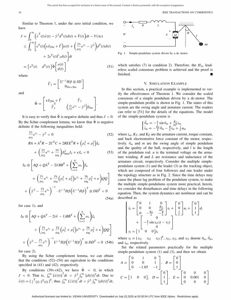
Fig. 1. Simple-pendulum system driven by a dc motor.
which satisfies (7) in condition 2). Therefore, the H∞ lead-erless scaled consensus problem is achieved and the proof isfinished.
V. SIMULATION EXAMPLE
In this section, a practical example is implemented to ver-ify the effectiveness of Theorem 1. We consider the scaledconsensus of a simple pendulum driven by a dc-motor. Thesimple-pendulum profile is shown in Fig. 1. The states of thissystem are the swing angle and armature current. The readerscan refer to [51] for the details of the equations. The modelof the simple-pendulum system is
{θm = − g
l sin θm + KTml2
imim = −KE
L θm − RL im + 1
L um
where im, KT , and KE are the armature current, torque constant,and back electromotive force constant of the motor, respec-tively. θm and m are the swing angle of simple pendulumand the quality of the ball, respectively, and l is the lengthof the pendulum rod. u is the terminal voltage on the arma-ture winding. R and L are resistance and inductance of thearmature circuit, respectively. Consider the multiple simple-pendulum system (1) and the leader (3) as the tracking object,which are composed of four followers and one leader underthe topology structure as in Fig. 2. Since the time delays maycause the phase lag problem of the pendulum system, to makethe multiple simple-pendulums system more practical, herein,we consider the disturbances and time delays in the followingequation. Then, the system dynamics are nonlinear and can bedescribed as
⎧⎪⎪⎪⎪⎪⎪⎪⎪⎨
⎪⎪⎪⎪⎪⎪⎪⎪⎩
xi =⎡
⎣0 1 00 0 KT
ml2
0 −KEL −R
L
⎤
⎦xi +⎡
⎣001L
⎤
⎦ui +⎡
⎣011
⎤
⎦di
+⎡
⎣0
− gl sin xi1(t − τ2)
0
⎤
⎦
yi = [1 0 0
]xi
where xi = [ xi1 xi2 xi3 ]T, xi1, xi2, and xi3 denote θm, θm,and im, respectively.
Set the related parameters practically for the multiplesimple-pendulum system (1) and (3), and then we obtain
A =⎡
⎣0 1 00 0 10 −1.65 −1
⎤
⎦, B =⎡
⎣001
⎤
⎦
C = [1 0 0
], D =
⎡
⎣011
⎤
⎦, E =⎡
⎣0 0 00 0.001 00 0 0
⎤
⎦.
Authorized licensed use limited to: XIDIAN UNIVERSITY. Downloaded on July 02,2020 at 03:30:54 UTC from IEEE Xplore. Restrictions apply.
This article has been accepted for inclusion in a future issue of this journal. Content is final as presented, with the exception of pagination.
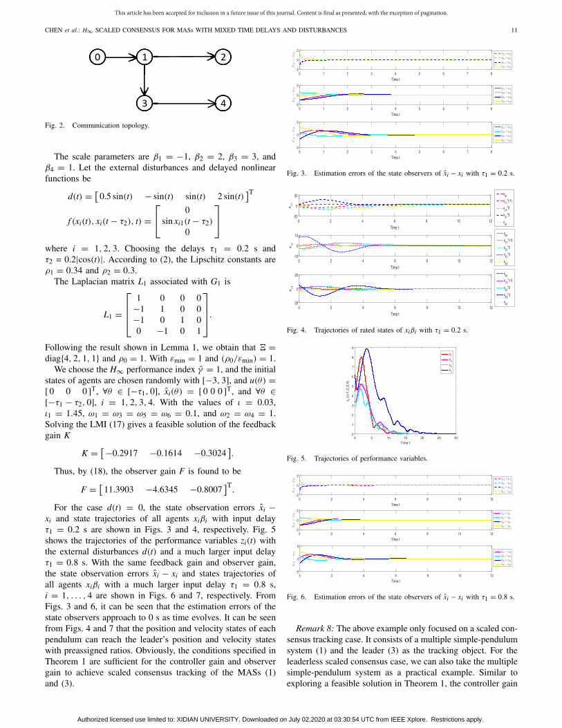
CHEN et al.: H∞ SCALED CONSENSUS FOR MASs WITH MIXED TIME DELAYS AND DISTURBANCES 11
Fig. 2. Communication topology.
The scale parameters are β1 = −1, β2 = 2, β3 = 3, andβ4 = 1. Let the external disturbances and delayed nonlinearfunctions be
d(t) = [0.5 sin(t) − sin(t) sin(t) 2 sin(t)
]T
f (xi(t), xi(t − τ2), t) =⎡
⎣0
sin xi1(t − τ2)
0
⎤
⎦
where i = 1, 2, 3. Choosing the delays τ1 = 0.2 s andτ2 = 0.2|cos(t)|. According to (2), the Lipschitz constants areρ1 = 0.34 and ρ2 = 0.3.
The Laplacian matrix L1 associated with G1 is
L1 =
⎡
⎢⎢⎣
1 0 0 0−1 1 0 0−1 0 1 00 −1 0 1
⎤
⎥⎥⎦.
Following the result shown in Lemma 1, we obtain that � =diag{4, 2, 1, 1} and ρ0 = 1. With εmin = 1 and (ρ0/εmin) = 1.
We choose the H∞ performance index γ = 1, and the initialstates of agents are chosen randomly with [−3, 3], and u(θ) =[ 0 0 0 ]T, ∀θ ∈ [−τ1, 0], xi(θ) = [ 0 0 0 ]T, and ∀θ ∈[−τ1 − τ2, 0], i = 1, 2, 3, 4. With the values of ι = 0.03,ι1 = 1.45, ω1 = ω3 = ω5 = ω6 = 0.1, and ω2 = ω4 = 1.Solving the LMI (17) gives a feasible solution of the feedbackgain K
K = [−0.2917 −0.1614 −0.3024].
Thus, by (18), the observer gain F is found to be
F = [11.3903 −4.6345 −0.8007
]T.
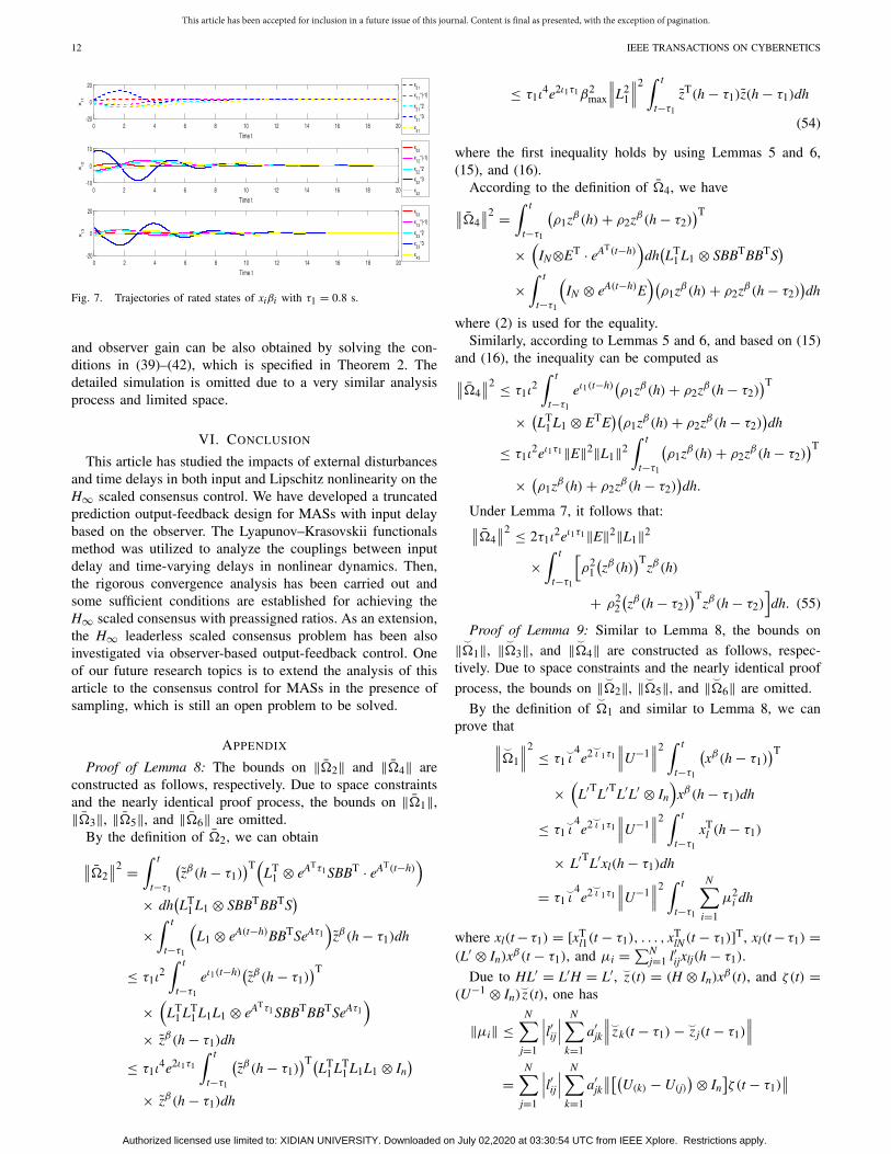
For the case d(t) = 0, the state observation errors xi −xi and state trajectories of all agents xiβi with input delayτ1 = 0.2 s are shown in Figs. 3 and 4, respectively. Fig. 5shows the trajectories of the performance variables zi(t) withthe external disturbances d(t) and a much larger input delayτ1 = 0.8 s. With the same feedback gain and observer gain,the state observation errors xi − xi and states trajectories ofall agents xiβi with a much larger input delay τ1 = 0.8 s,i = 1, . . . , 4 are shown in Figs. 6 and 7, respectively. FromFigs. 3 and 6, it can be seen that the estimation errors of thestate observers approach to 0 s as time evolves. It can be seenfrom Figs. 4 and 7 that the position and velocity states of eachpendulum can reach the leader’s position and velocity stateswith preassigned ratios. Obviously, the conditions specified inTheorem 1 are sufficient for the controller gain and observergain to achieve scaled consensus tracking of the MASs (1)and (3).
Fig. 3. Estimation errors of the state observers of xi − xi with τ1 = 0.2 s.
Fig. 4. Trajectories of rated states of xiβi with τ1 = 0.2 s.
Fig. 5. Trajectories of performance variables.
Fig. 6. Estimation errors of the state observers of xi − xi with τ1 = 0.8 s.
Remark 8: The above example only focused on a scaled con-sensus tracking case. It consists of a multiple simple-pendulumsystem (1) and the leader (3) as the tracking object. For theleaderless scaled consensus case, we can also take the multiplesimple-pendulum system as a practical example. Similar toexploring a feasible solution in Theorem 1, the controller gain
Authorized licensed use limited to: XIDIAN UNIVERSITY. Downloaded on July 02,2020 at 03:30:54 UTC from IEEE Xplore. Restrictions apply.
This article has been accepted for inclusion in a future issue of this journal. Content is final as presented, with the exception of pagination.
12 IEEE TRANSACTIONS ON CYBERNETICS
Fig. 7. Trajectories of rated states of xiβi with τ1 = 0.8 s.
and observer gain can be also obtained by solving the con-ditions in (39)–(42), which is specified in Theorem 2. Thedetailed simulation is omitted due to a very similar analysisprocess and limited space.
VI. CONCLUSION
This article has studied the impacts of external disturbancesand time delays in both input and Lipschitz nonlinearity on theH∞ scaled consensus control. We have developed a truncatedprediction output-feedback design for MASs with input delaybased on the observer. The Lyapunov–Krasovskii functionalsmethod was utilized to analyze the couplings between inputdelay and time-varying delays in nonlinear dynamics. Then,the rigorous convergence analysis has been carried out andsome sufficient conditions are established for achieving theH∞ scaled consensus with preassigned ratios. As an extension,the H∞ leaderless scaled consensus problem has been alsoinvestigated via observer-based output-feedback control. Oneof our future research topics is to extend the analysis of thisarticle to the consensus control for MASs in the presence ofsampling, which is still an open problem to be solved.
APPENDIX
Proof of Lemma 8: The bounds on ‖�2‖ and ‖�4‖ areconstructed as follows, respectively. Due to space constraintsand the nearly identical proof process, the bounds on ‖�1‖,‖�3‖, ‖�5‖, and ‖�6‖ are omitted.
By the definition of �2, we can obtain
∥∥�2
∥∥2 =
∫ t
t−τ1
(zβ(h − τ1)
)T(
LT1 ⊗ eATτ1 SBBT · eAT(t−h)
)
× dh(LT
1 L1 ⊗ SBBTBBTS)
×∫ t
t−τ1
(L1 ⊗ eA(t−h)BBTSeAτ1
)zβ(h − τ1)dh
≤ τ1ι2∫ t
t−τ1
eι1(t−h)(zβ(h − τ1)
)T
×(
LT1 LT
1 L1L1 ⊗ eATτ1 SBBTBBTSeAτ1)
× zβ(h − τ1)dh
≤ τ1ι4e2ι1τ1
∫ t
t−τ1
(zβ(h − τ1)
)T(LT
1 LT1 L1L1 ⊗ In
)
× zβ(h − τ1)dh
≤ τ1ι4e2ι1τ1β2
max
∥∥∥L2
1
∥∥∥
2∫ t
t−τ1
zT(h − τ1)z(h − τ1)dh
(54)
where the first inequality holds by using Lemmas 5 and 6,(15), and (16).
According to the definition of �4, we have∥∥�4
∥∥2 =
∫ t
t−τ1
(ρ1zβ(h) + ρ2zβ(h − τ2)
)T
×(
IN⊗ET · eAT(t−h))
dh(LT
1 L1 ⊗ SBBTBBTS)
×∫ t
t−τ1
(IN ⊗ eA(t−h)E
)(ρ1zβ(h) + ρ2zβ(h − τ2)
)dh
where (2) is used for the equality.Similarly, according to Lemmas 5 and 6, and based on (15)
and (16), the inequality can be computed as∥∥�4
∥∥2 ≤ τ1ι
2∫ t
t−τ1
eι1(t−h)(ρ1zβ(h) + ρ2zβ(h − τ2)
)T
× (LT
1 L1 ⊗ ETE)(
ρ1zβ(h) + ρ2zβ(h − τ2))dh
≤ τ1ι2eι1τ1‖E‖2‖L1‖2
∫ t
t−τ1
(ρ1zβ(h) + ρ2zβ(h − τ2)
)T
× (ρ1zβ(h) + ρ2zβ(h − τ2)
)dh.
Under Lemma 7, it follows that:∥∥�4
∥∥2 ≤ 2τ1ι
2eι1τ1‖E‖2‖L1‖2
×∫ t
t−τ1
[ρ2
1
(zβ(h)
)Tzβ(h)
+ ρ22
(zβ(h − τ2)
)Tzβ(h − τ2)
]dh. (55)
Proof of Lemma 9: Similar to Lemma 8, the bounds on‖
�1‖, ‖
�3‖, and ‖
�4‖ are constructed as follows, respec-tively. Due to space constraints and the nearly identical proof
process, the bounds on ‖
�2‖, ‖
�5‖, and ‖
�6‖ are omitted.
By the definition of
�1 and similar to Lemma 8, we canprove that
∥∥∥
�1
∥∥∥
2 ≤ τ1 ι
4e2
ι 1τ1
∥∥∥U−1
∥∥∥
2∫ t
t−τ1
(xβ(h − τ1)
)T
×(
L′TL′TL′L′ ⊗ In
)xβ(h − τ1)dh
≤ τ1 ι
4e2
ι 1τ1
∥∥∥U−1
∥∥∥
2∫ t
t−τ1
xTl (h − τ1)
× L′TL′xl(h − τ1)dh
= τ1 ι
4e2
ι 1τ1
∥∥∥U−1
∥∥∥
2∫ t
t−τ1
N∑
i=1
μ2i dh
where xl(t − τ1) = [xTl1(t − τ1), . . . , xT
lN(t − τ1)]T, xl(t − τ1) =(L′ ⊗ In)xβ(t − τ1), and μi = ∑N
j=1 l′ijxlj(h − τ1).
Due to HL′ = L′H = L′, z(t) = (H ⊗ In)xβ(t), and ζ(t) =
(U−1 ⊗ In) z(t), one has
‖μi‖ ≤N∑
j=1
∣∣∣l′ij∣∣∣
N∑
k=1
a′jk
∥∥∥
zk(t − τ1) −
zj(t − τ1)
∥∥∥
=N∑
j=1
∣∣∣l′ij∣∣∣
N∑
k=1
a′jk
∥∥[(
U(k) − U(j))⊗ In
]ζ (t − τ1)
∥∥
Authorized licensed use limited to: XIDIAN UNIVERSITY. Downloaded on July 02,2020 at 03:30:54 UTC from IEEE Xplore. Restrictions apply.
This article has been accepted for inclusion in a future issue of this journal. Content is final as presented, with the exception of pagination.
CHEN et al.: H∞ SCALED CONSENSUS FOR MASs WITH MIXED TIME DELAYS AND DISTURBANCES 13
≤N∑
j=1
∣∣∣l′ij∣∣∣
N∑
k=1
a′jk
[(∥∥U(k)
∥∥+ ∥
∥U(j)∥∥)‖ζ (t − τ1)‖
]
≤N∑
j=1
(∣∣∣l′ij∣∣∣∥∥∥a′
j
∥∥∥
2+ √
N∣∣∣l′ij∣∣∣∥∥∥a′
j
∥∥∥
2
)‖U‖F‖ζ (t − τ1)‖
≤ 2√
N∥∥l′i∥∥
2
∥∥A′∥∥
F‖U‖F‖ζ (t − τ1)‖where a′
j is the ith row of A′, l′i is the ith row of L′, and U(k)
and U(j) are the kth and jth rows of U, respectively.
Then, substituting ‖μi‖ into ‖
�1‖2, we can obtain∥∥∥
�1
∥∥∥
2 ≤ 4Nτ1 ι
4e2
ι 1τ1
∥∥∥U−1
∥∥∥
2∥∥L′∥∥2
F
∥∥A′∥∥2
F‖U‖2F
×∫ t
t−τ1
ζT(h − τ1)ζ (h − τ1)dh. (56)
Similarly, according to the definition of
�3, we have∥∥∥
�3
∥∥∥
2 ≤ τ1 ι
2e
ι 1τ1
∥∥∥U−1
∥∥∥
2‖D‖2∫ t
t−τ1
dT(h)
×(βL′TL′β ⊗ In
)d(h)dh
≤ τ1 ι
2e
ι 1τ1
∥∥∥U−1
∥∥∥
2‖D‖2∫ t
t−τ1
dTl (h)dl(h)dh
= τ1 ι
2e
ι 1τ1
∥∥∥U−1
∥∥∥
2‖D‖2∫ t
t−τ1
N∑
i=1
‖dli(h)‖2dh
where dl(t) = [dTl1(t), . . . , dT
lN(t)]T and dl(t) = (L′β ⊗ In)d(t).Since ‖dli(t)‖2 = ‖∑N
j=1 βjl′ijdj(t)‖2 ≤ β2max‖l′i‖2‖d(t)‖2.
Then, substituting ‖dli(t)‖2 into ‖
�3‖2, we have∥∥∥
�3
∥∥∥
2 ≤ τ1 ι
2β2
maxe ι 1τ1
∥∥∥U−1
∥∥∥
2‖D‖2∥∥L′∥∥2
F
×∫ t
t−τ1
dT(h)d(h)dh. (57)
Similarly, by the definition of
�4, we have∥∥∥
�4
∥∥∥
2 ≤ τ1 ι
2e
ι 1τ1‖E‖2
∥∥∥U−1
∥∥∥
2∫ t
t−τ1
f Tτ2
×(βL′TL′β ⊗ In
)fτ2 dh
= τ1 ι
2e
ι 1τ1‖E‖2
∥∥∥U−1
∥∥∥
2∫ t
t−τ1
N∑
i=1
‖fli‖2dh
where fl = [f Tl1, . . . , f T
lN]T and fl = (L′β ⊗ In)fτ2 .Based on (5),
zi(t) = βixi(t) − ∑Nj=1 δjβjxj(t) and ζ(t) =
(U−1 ⊗ In) z(t), then one has
‖fli‖ =N∑
j=1
a′ij
∥∥βifiτ2 − βjfjτ2
∥∥
≤N∑
j=1
a′ij
∥∥∥ρ1
( zi(t) −
zj(t))
+ ρ2
( zi(t − τ2) −
z j(t − τ2))∥∥∥
≤N∑
j=1
a′ij
[(∥∥U(i)
∥∥+ ∥
∥U(j)∥∥)(ρ1‖ζ (t)‖ + ρ2‖ζ (t − τ2)‖)
]
≤(√
N∥∥a′
i
∥∥∥∥U(i)
∥∥+ ∥
∥a′i
∥∥‖U‖F
)
× (ρ1‖ζ (t)‖ + ρ2‖ζ (t − τ2)‖).Thus
N∑
i=1
‖fli‖2 ≤ 4(ρ2
1‖ζ(t)‖2 + ρ22‖ζ(t − τ2)‖2
)
×N∑
i=1
∥∥a′
i
∥∥2(
N‖Ui‖2 + ‖U‖2F
)
≤ 4(N + 1)∥∥A′∥∥2
F‖U‖2F
×(ρ2
1‖ζ(t)‖2 + ρ22‖ζ(t − τ2)‖2
).
Then, substituting∑N
i=1 ‖fli‖2 into ‖
�4‖2, we can obtain∥∥∥
�4
∥∥∥
2 ≤ 4(N + 1)τ1 ι
2e
ι 1τ1‖E‖2
∥∥∥U−1
∥∥∥
2∥∥A′∥∥2
F
× ‖U‖2F
[
ρ21
∫ t
t−τ1
ζT(h)ζ (h)dh
+ ρ22
∫ t
t−τ1
ζT(h − τ2)ζ (h − τ2)dh
]
. (58)
REFERENCES
[1] W. Lin, X. Li, Z. Yang, and J. Wang, “Construction of dual pore 3-Ddigital cores with a hybrid method combined with physical experimentmethod and numerical reconstruction method,” Transp. Porous Media,vol. 120, no. 1, pp. 227–238, 2017.
[2] W. Lin et al., “Multiscale digital porous rock reconstruction using tem-plate matching,” Water Resources Res., vol. 55, no. 8, pp. 6911–6922,2019, doi: 10.1029/2019WR025219.
[3] H. Su, Y. Liu, and Z. Zeng, “Second-order consensus for multi-agent systems via intermittent sampled position data control,”IEEE Trans. Cybern., vol. 50, no. 5, pp. 2063–2072, May 2020,doi: 10.1109/TCYB.2018.2879327.
[4] Y. Zheng, Q. Zhao, J. Ma, and L. Wang, “Second-order consensus ofhybrid multi-agent systems,” Syst. Control Lett., vol. 125, pp. 51–58,Mar. 2019.
[5] S. Chen, H. Pei, Q. Lai, and H. Yan, “Multi-target tracking controlfor coupled heterogeneous inertial agents systems based on flockingbehavior,” IEEE Trans. Syst., Man, Cybern., Syst., vol. 49, no. 12,pp. 2605–2611, Dec. 2019.
[6] Z. Qiu, L. Xie, and Y. Hong, “Quantized leaderless and leader-followingconsensus of high-order multi-agent systems with limited data rate,”IEEE Trans. Autom. Control, vol. 61, no. 9, pp. 2432–2447, Sep. 2016.
[7] H. Su, H. Wu, and J. Lam, “Positive edge-consensus for nodal networksvia output feedback,” IEEE Trans. Autom. Control, vol. 64, no. 3,pp. 1244–1249, Mar. 2019.
[8] S. Chen, J. Guan, Y. Gao, and H. Yan, “Observer-based event-triggeredtracking consensus of non-ideal general linear multi-agent systems,” J.Franklin Inst., vol. 356, no. 17, pp. 10355–10367, 2019.
[9] Z. Meng, T. Yang, D. V. Dimarogonas, and K. H. Johansson,“Coordinated output regulation of heterogeneous linear systems underswitching topologies,” Automatic, vol. 53, pp. 362–368, Mar. 2015.
[10] D. Yang, W. Ren, X. Liu, and W. Chen, “Decentralized event-triggeredconsensus for linear multi-agent systems under general directed graphs,”Automatic, vol. 69, pp. 242–249, Jul. 2016.
[11] H. Su, Y. Ye, Y. Qiu, Y. Cao, and M. Z. Q. Chen, “Semi-global out-put consensus for discrete-time switching networked systems subjectto input saturation and external disturbances,” IEEE Trans. Cybern.,vol. 49, no. 11, pp. 3934–3945, Nov. 2019.
[12] H. Yan, C. Hu, H. Zhang, H. R. Karimi, X. Jiang, and M. Liu, “H∞output tracking control for networked systems with adaptively adjustedevent-triggered scheme,” IEEE Trans. Syst., Man, Cybern., Syst., vol. 49,no. 10, pp. 2050–2058, Oct. 2019.
[13] J. Ma, M. Ye, Y. Zheng, and Y. Zhu, “Consensus analysis ofhybrid multi-agent systems: A game-theoretic approach,” Int. J. RobustNonlinear Control, vol. 29, no. 6, pp. 1840–1853, 2019.
[14] Y. Zheng, J. Ma, and L. Wang, “Consensus of hybrid multi-agentsystems,” IEEE Trans. Neural Netw. Learn. Syst., vol. 29, no. 4,pp. 1359–1365, Apr. 2018.
Authorized licensed use limited to: XIDIAN UNIVERSITY. Downloaded on July 02,2020 at 03:30:54 UTC from IEEE Xplore. Restrictions apply.
This article has been accepted for inclusion in a future issue of this journal. Content is final as presented, with the exception of pagination.
14 IEEE TRANSACTIONS ON CYBERNETICS
[15] Y. Zheng and L. Wang, “A novel group consensus protocol forheterogeneous multi-agent systems,” Int. J. Control, vol. 88, no. 11,pp. 2347–2353, 2015.
[16] Y. Zhu, S. Li, J. Ma, and Y. Zheng, “Bipartite consensus in networksof agents with antagonistic interactions and quantization,” IEEE Trans.Circuits Syst. II, Exp. Briefs, vol. 65, no. 12, pp. 2012–2016, Dec. 2018.
[17] S. Roy, “Scaled consensus,” Automatica, vol. 51, pp. 259–262,Jan. 2015.
[18] J. Yu and Y. Shi, “Scaled group consensus in multiagent systems withfirst/second-order continuous dynamics,” IEEE Trans. Cybern., vol. 48,no. 8, pp. 2259–2271, Aug. 2018.
[19] Z. Zhang, S. Chen, and Y. Zheng, “Leader-following scaled consensusof second-order multi-agent systems under directed topologies,” Int. J.Syst. Sci., vol. 50, no. 14, pp. 2604–2615, 2019.
[20] C. Liu, “Scaled consensus seeking in multiple non-identical linearautonomous agents,” ISA Trans., vol. 71, no. 1, pp. 68–75, 2017.
[21] Z. Zhang, S. Chen, and H. Su, “Scaled consensus of second-order non-linear multi-agent systems with time-varying delays via aperiodicallyintermittent control,” IEEE Trans. Cybern., early access, Jan. 9, 2019,doi: 10.1109/TCYB.2018.2883793.
[22] L. Zhao, Y. Jia, J. Yu, and J. Du, “H∞ sliding mode based scaled con-sensus control for linear multi-agent systems with disturbances,” Appl.Math. Comput., vol. 292, pp. 375–389, Jan. 2017.
[23] W. Kwon and A. Pearson, “Feedback stabilization of linear systemswith delayed control,” IEEE Trans. Autom. Control, vol. AC-25, no. 2,pp. 266–269, Apr. 1980.
[24] A. Manitius and A. Olbrot, “Finite spectrum assignment problem forsystems with delays,” IEEE Trans. Autom. Control, vol. AC-24, no. 2,pp. 541–552, Aug. 1979.
[25] Z. Artstein, “Linear systems with delayed controls: A reduction,” IEEETrans. Autom. Control, vol. AC-27, no. 4, pp. 869–879, Aug. 1982.
[26] B. Zhou and Z. Lin, “Consensus of high-order multi-agent systemswith large input and communication delays,” Automatica, vol. 50, no. 2,pp. 452–464, 2014.
[27] Z. Zuo, Z. Lin, and Z. Ding, “Truncated prediction output feedbackcontrol of a class of Lipschitz nonlinear systems with input delay,”IEEE Trans. Circuits Syst. II, Exp. Briefs, vol. 63, no. 8, pp. 788–792,Aug. 2016.
[28] C. Wang, Z. Zuo, Z. Lin, and Z. Ding, “A truncated predictionapproach to consensus control of Lipschitz nonlinear multiagent systemswith input delay,” IEEE Trans. Control Netw. Syst., vol. 4, no. 4,pp. 716–724, Dec. 2017.
[29] H. Chu, L. Gao, D. Yue, and C. Dou, “Consensus of Lipschitz non-linear multiagent systems with input delay via observer-based truncatedprediction feedback,” IEEE Trans. Syst., Man, Cybern., Syst., vol. 4,no. 4, pp. 716–724, Dec. 2017, doi: 10.1109/TSMC.2018.2883954.
[30] G. Wen, Z. Duan, W. Yu, and G. Chen, “Consensus of second-ordermulti-agent systems with delayed nonlinear dynamics and intermittentcommunications,” Int. J. Control, vol. 86, no. 2, pp. 322–331, 2013.
[31] Z. Yu, H. Jiang, C. Hu, and X. Fan, “Consensus of second-ordermulti-agent systems with delayed nonlinear dynamics and aperiod-ically intermittent communications,” Int. J. Control, vol. 90, no. 5,pp. 909–922, 2017.
[32] X. Zong, T. Li, and J. Zhang, “Consensus conditions of continuous-time multi-agent systems with additive and multiplicative measurementnoises,” SIAM J. Control Optim., vol. 56, no. 1, pp. 19–52, 2018.
[33] L. Cheng, Z.-G. Hou, and M. Tan, “A mean-square consensus proto-col for linear multi-agent systems with communication noises and fixedtopologies,” IEEE Trans. Autom. Control, vol. 59, no. 1, pp. 261–267,Jan. 2014.
[34] L. Yang and Y. Jia, “H∞ consensus control for multi-agent systems withlinear coupling dynamics and communication delays,” Int. J. Syst. Sci.,vol. 43, no. 1, pp. 50–62, 2012.
[35] Z. Li, Z. Duan, and G. Chen, “On H∞ and H2 performance regions ofmulti-agent systems,” Automatica, vol. 47, no. 4, pp. 793–803, 2011.
[36] J. Wang, Z. Duan, Z. Li, and G. Wen, “Distributed H∞ and H2 con-sensus control in directed networks,” IET Control Theory Appl., vol. 8,no. 3, pp. 193–201, 2013.
[37] I. Saboori and K. Khorasani, “H∞ consensus achievement of multi-agent systems with directed and switching topology networks,” IEEETrans. Autom. Control, vol. 59, no. 11, pp. 3104–3109, Nov. 2014.
[38] G. Wen, G. Hu, W. Yu, and G. Chen, “Distributed H∞ consensus ofhigher order multiagent systems with switching topologies,” IEEE Trans.Circuits Syst. II, Exp. Briefs, vol. 61, no. 5, pp. 359–363, May 2014.
[39] J. Xi, Z. Shi, and Y. Zhong, “Output consensus analysis and design forhigh-order linear swarm systems: Partial stability method,” Automatica,vol. 48, pp. 2335–2343, Sep. 2012.
[40] Y. Jiang, H. Wang, and S. Wang, “Distributed H∞ consensus controlfor nonlinear multi-agent systems under switching topologies via relativeoutput feedback,” Neural Comput. Appl., vol. 31, no. 1, pp. 1–9, 2019.
[41] L. Zhang, Z. Ning, and W. Zheng, “Observer-based control forpiecewise-affine systems with both input and output quantization,” IEEETrans. Autom. Control, vol. 62, no. 1, pp. 5858–5865, Nov. 2017.
[42] Z. Ning, L. Zhang, and W. X. Zheng, “Observer-based stabiliza-tion of nonhomogeneous semi-Markov jump linear systems withmode-switching delays,” IEEE Trans. Autom. Control, vol. 64, no. 5,pp. 2029–2036, May 2019.
[43] Z. Li, W. Ren, X. Liu, and M. Fu, “Consensus of multi-agentsystems with general linear and Lipschitz nonlinear dynamics using dis-tributed adaptive protocols,” IEEE Trans. Autom. Control, vol. 58, no. 7,pp. 1786–1791, Jul. 2013.
[44] Q. Jia, W. K. S. Tang, and W. A. Halang, “Leader following of nonlinearagents with switching connective network and coupling delay,” IEEETrans. Circuits Syst. I, Reg. Papers, vol. 58, no. 10, pp. 2508–2519,Oct. 2011.
[45] Z. Ding, “Consensus control of a class of Lipschitz nonlinear systems,”Int. J. Control, vol. 87, no. 11, pp. 2372–2382, 2014.
[46] S. Boyd, L. E. Ghaoui, E. Feron, and V. Balakrishnan, Linear MatrixInequalities in System and Control Theory. Philadelphia, PA, USA:SIAM, 1994.
[47] K. Gu, V. K. Kharitonov and J. Chen, Stability of Time-Delay Systems.Basel, Switzerland: Birkhäuser, 2003.
[48] B. Zhou, Z. Lin, and G. Duan, “Stabilization of linear systems with inputdelay and saturation—A parametric Lyapunov equation approach,” Int.J. Robust Nonlinear Control, vol. 20, no. 13, pp. 1502–1519, 2010.
[49] X. Zhang and Q. Han, “Event-based H∞ filtering for sampled datasystems,” Automatica, vol. 51, pp. 55–69, May 2015.
[50] S. Y. Yoon, P. Anantachaisilp, and Z. Lin, “An LMI approach to thecontrol of exponentially unstable systems with input time delay,” inProc. 52nd IEEE Conf. Decis. Control, 2013, pp. 312–317.
[51] Y. Jiang, S. Wang, Y. Li, and D. Liu, “Distributed consensus trackingcontrol for multiple simple-pendulum network systems,” in Proc. 35thChin. Control Conf., 2016, pp. 7556–7560.
Shiming Chen received the Ph.D. degree in controltheory and control engineering from the HuazhongUniversity of Science and Technology, Wuhan,China, in 2006.
He is currently a Professor with the School ofElectrical and Automation Engineering, East ChinaJiaotong University, Nanchang, China. His cur-rent research interests include swarm dynamics andcooperative control, complex networks, and particleswarm optimization algorithms.
Zheng Zhang received the B.S. degree in electronicand information engineering and the M.S. degreein control science and engineering from East ChinaJiaotong University, Nanchang, China, in 2012 and2015, respectively. She is currently pursuing thePh.D. degree in control science and engineering withEast China Jiaotong University.
Her current research interests include multiagentcoordination and control and nonlinear systems.
Yuanshi Zheng was born in Jiangshan, China. Hereceived the bachelor’s and master’s degrees fromNingxia University, Yinchuan, China, in 2006 and2009, respectively, and the Doctoral degree fromXidian University, Xi’an, China, in 2012.
He is currently an Associate Professor with XidianUniversity. His research interests include coordi-nation of multiagent systems, game theory, andcollective intelligence.
Authorized licensed use limited to: XIDIAN UNIVERSITY. Downloaded on July 02,2020 at 03:30:54 UTC from IEEE Xplore. Restrictions apply.


![Consensus Problems in Networks of Agents with …murray/preprints/om04-tac.pdf · Consensus Problems in Networks of Agents with Switching Topology and Time-Delays ... [19,4, 14]](https://img.pdfslide.net/doc/110x75/5b729a1f7f8b9a467a8ce5e8/consensus-problems-in-networks-of-agents-with-murraypreprintsom04-tacpdf.jpg)