Embed Size (px)
Citation preview
REI IlI~ri. ~,iO'
TECHNICAL REPORT D-77-23
HABITAT DEVELOPMENT FIELDINVESTIGATIONS, WINDMILL POINT MARSH
DEVELOPMENT SITE, JAMES RIVER, VIRGINIAAPPENDIX D: ENVIRONMENTAL IMPACTS OF MARSH
DEVELOPMENT WITH DREDGED MATERIAL:BOTANY, SOILS, AQUATIC BIOLOGY, AND WILDLIFE
by
Virginia Institute of Marine Science
Gloucester Point, Va. 23062
June 1978
Final Report
Approved For Public Release; DistributionUnhimitedJ
Prepared for Office, Chief of Engineers, U. S. ArmyWashington, D. C. 20314
Under Contract No. DACW39-76-C-0040(DMRP Work Unit No. 4A111)
Monitored by Environmental LaboratoryU. S. Army Engineer Waterways Experiment Station
P. 0. Box 631, Vicksburg, Miss 39180metadc957899
PROGRAMRESEARCH
HABITAT DEVELOPMENT FIELD INVESTIGATIONS, WINDMILL POINTMARSH DEVELOPMENT SITE, JAMES RIVER, VIRGINIA
Assessment of Vegetation on Existing Dredged Material Island
Propagation of Vascular Plants
Environmental Impacts of Marsh Development with Dredged Material: Acute Impactson the Macrobenthic Community
Environmental Impacts of Marsh Development with Dredged Material: Botany, Soils,Aquatic Biology, and Wildlife
Environmental Impacts of Marsh Development with Dredged Material: Metals andChlorinated Hydrocarbons in Vascular Plants and Marsh Invertebrates
Environmental Impacts of Marsh Development with Dredged Material: Sediment andWater Quality
Destroy this report when no longer needed. Do not returnit to the originator.
Appendix
Appendix
Appendix
A:
B:
C:
Appendix D:
Appendix E:
Appendix F:
DEPARTMENT OF THE ARMY.- WATERWAYS EXPERIMENT STATION. CORPS OF ENGINEERS
- P.0. BOX 631VICKSBURG, MISSISSIPPI 39180
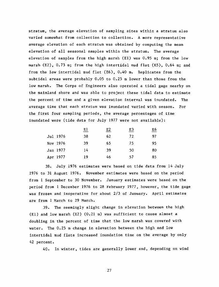
IN REPLY REFER TO: WESYV 31 July 1978
SUBJECT: Transmittal of Technical Report D-77-23, Appendix D
TO: All Report Recipients
1. The technical report transmitted herewith represents the results ofone of a series of research efforts (work units) undertaken as part ofTask 4A (Marsh Development) of the Corps of Engineers' Dredged MaterialResearch Program (DMRP). Task 4A was part of the Habitat DevelopmentProject (HDP) and had as its objective the development and testing ofthe environmental and economic feasibility of using dredged material asa substrate for marsh development.
2. Marsh development using dredged material was investigated by the HDPunder both laboratory and field conditions. The study reported herein(Work Unit 4A11I) was an integral part of a series of research contractsjointly developed to achieve Task 4A objectives at the Windmill PointMarsh Development Site, James River, Virginia, one of eight marshestablishment sites located in several geographic regions of the UnitedStates. Interpretations of this report's findings and recommendationsare best made in context with the other reports in the Windmill Pointsite series (4AllA-M).
3. This report, "Appendix D: Environmental Impacts of Marsh Develop-ment with Dredged Material: Botany, Soils, Aquatic Biology, and Wild-life," is one of six contractor-prepared appendices published relativeto the Waterways Experiment Station's Technical Report D-77-23, entitled"Habitat Development Field Investigations, Windmill Point Marsh Develop-ment Site, James River, Virginia: Summary Report" (4AllM). The appendicesto the Summary Report are studies that provide technical background andsupporting data and may or may not represent discrete research products.Appendices that are largely data tabulations or that clearly have onlysite specif ic relevance are published as microf iche; those with moregeneral application are published as printed reports.
4. The purpose of Work Unit 4A11I was to evaluate the response of plantand animal populations and soil properties to the development of a marshisland habitat at Windmill Point on the James River. The man-made marshwas beneficial to the area, with respect to biological resources, by

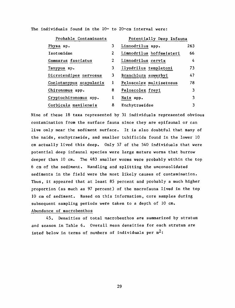
WEsYv 31 July 1978SUBJECT: Transmittal of Technical Report D-77-23, Appendix D
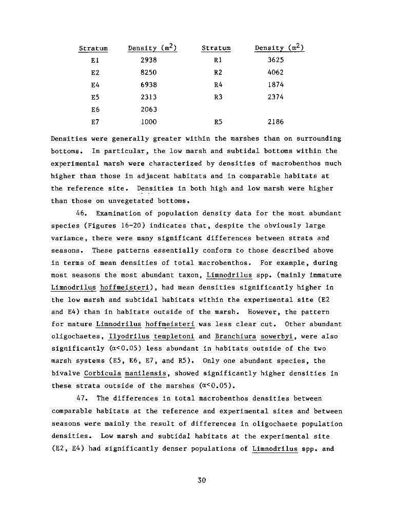
providing an increase in both food and cover for fish and wildliferelative to the original shallow river bottom. The developed areas canalso be compared favorably to nearby natural marshes in terms of fishand wildlife resources and productivity.
5. Data from this report will be included in the Windmill Point SummaryReport (4AllM) and synthesized in the Technical Reports entitled "Uplandand Wetland Habitat Development with Dredged Material: Ecological Con-siderations" (2A08) and "Wetland Habitat Development with Dredged Material:Engineering and Plant Propagation" (4A22).
JOHN L. CANNONColonel, Corps of EngineersCommander and Director
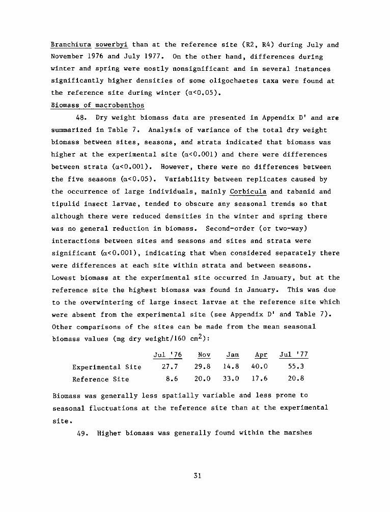
2
UnclassifiedSECURITY CLASSIFICATION OF THIS PAGE (When Data Entered)
FDD jFOR EDITION OF 1 NOV 65 IS OBSOLETE
SECURITY CL ASSI FiCA TION OF THIS PAGE (W~hen Data Entered)
REPORT DOCUMENTATION PAGE BEFREDCOMPLETIGFORM
1. REPORT NUMBER 2. GOVT ACCESSION NO. 3. RECIPIENT'S CAT ALOG NUMBER
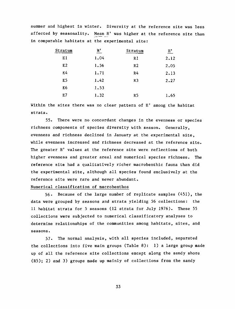
4. TITLE (end Sutte)AIA DEVELOPMENT FIELD INVESTIGA- 5. TYPE OF REPORT & PERIOD COVERED
IIONS, WINDMILL POINT MARSH DEVELOPMENT SITE, JAMES FnlrprRIVER, VIRGINIA; APPENDIX D: ENVIRONMENTAL IMPACTS ____nal ___report____
JF MARSH DEVELOPMENT WITH DREDGED MATERIAL: BOTANY, 6. PERFORMING ORG. REPORT NUMBER
~7. AUTHOR(s) 8. CONTRACT OR GRANT NUMBER(s). . .Contract No.
Virginia Institute of Marine Science DC~-6cO4
9. PERFORMING ORGANIZATION NAME AND ADDRESS 10. PROGRAM ELEMENT, PROJECT, TASKAREA & WORK UNIT NUMBERS
Virginia Institute of Marine ScienceGloucester Point, Va. 23062 DMR P Work Unit No. 4A11I
11. CONTROLLING OFFICE NAME AND ADDRESS 12. REPORT DATE
Office, Chief of Engineers, U. S. Army June 1978
Washington, D. C. 20314 13. NUMBEROFPAGES510
14. MONITORING AGENCY NAME & ADDRESS(If different from Controlling Office) 15. SECURITY CL ASS. (of this report)
U. S. Army Engineer Waterways Experiment StationEnvironmental LaboratoryP. 0. Box 631, Vicksburg, Miss. 39180 I5a. DECLASSIFICATION/DOWNGRADING
SCHEDULE
16. DISTRIBUTION ST ATEMENT (of this Report)
Approved for public release; distribution unlimited.
17. DIST RIBUTION ST ATEMENT (of the abstract entered in Block 20, if different from Report)
18. SUPPLEMENTARY NOTES
Appendices A' through U' to this appendix were reproduced on microfiche andare included in an envelope inside the back cover.
19. K EY WORDS (Continue on reverse aid. if necessary and identify by block number)
Dredged material Fine grained soils Windmill PointEcology HabitatsEnvironmental effects James RiverField investigations Marshes
20x ABQST RACT (Coutfnue en reverse sL*~ ft neeeeay ind ldenti fy by block number)
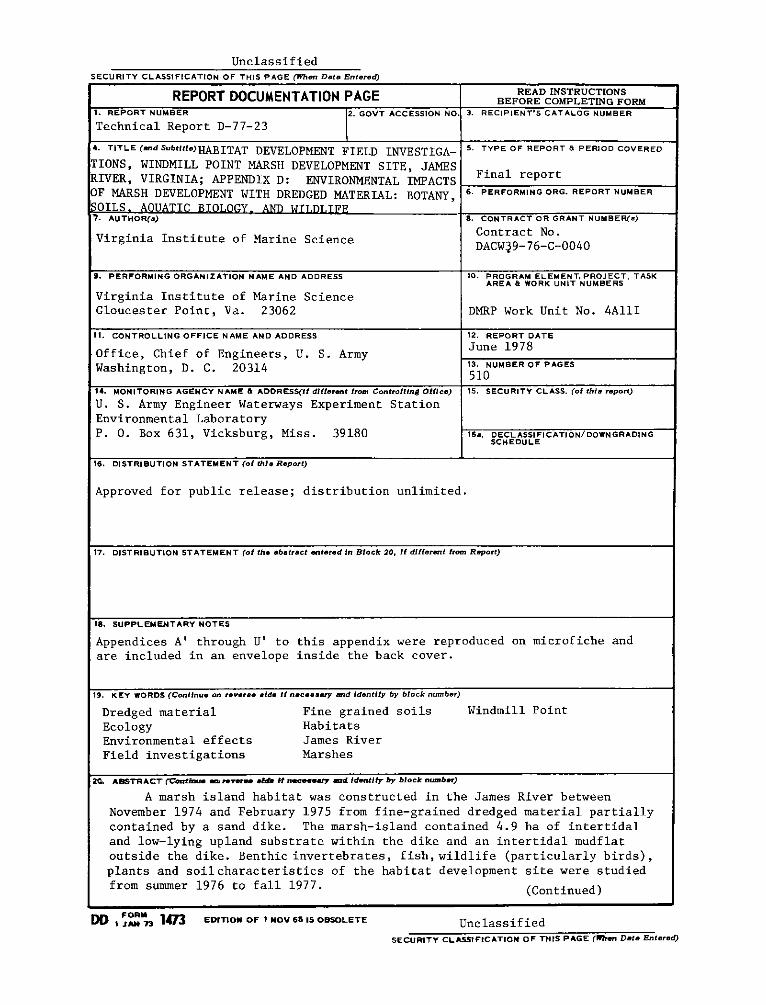
A marsh island habitat was constructed in the James River betweenNovember 1974 and February 1975 from fine-grained dredged material partiallycontained by a sand dike. The marsh-island contained 4.9 ha of intertidaland low-lying upland substrate within the dike and an intertidal mudflatoutside the dike. Benthic invertebrates, fish, wildlife (particularly birds),plants and soilcharacteristics of the habitat development site were studiedfrom summer 1976 to fall 1977. (Continued)
Unclassified
20. ABSTRACT (Continued).
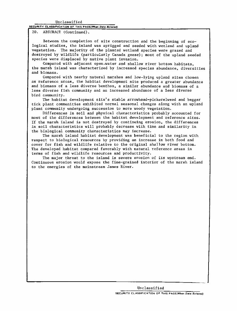
Between the completion of site construction and the beginning of eco-logical studies, the island was sprigged and seeded with wetland and uplandvegetation. The majority of the planted wetland species were grazed anddestroyed by wildlife (particularly Canada geese); most of the upland seededspecies were displaced by native plant invasion.
Compared with adjacent open-water and shallow river bottom habitats,the marsh island was characterized by increased species abundance, diversitiesand biomass.
Compared with nearby natural marshes and low-lying upland sites chosenas reference areas, the habitat development site produced a greater abundanceand biomass of a less diverse benthos, a similar abundance and biomass of aless diverse fish community and an increased abundance of a less diversebird community.
The habitat development site' s stable arrowhead-pickerelweed and beggartick plant communities exhibited normal seasonal changes along with an uplandplant community undergoing succession to more woody vegetation.
Differences in soil and physical characteristics probably accounted formost of the differences between the habitat development and reference sites.If the marsh island is not destroyed by continuing erosion, the differencesin soil characteristics will probably decrease with time and similarity inthe biological community characteristics may increase.
The marsh island habitat development was beneficial to the region withrespect to biological resources by providing an increase in both food andcover for fish and wildlife relative to the original shallow river bottom.The developed habitat compared favorably with natural reference areas interms of fish and wildlife resources and productivity.
The major threat to the island is severe erosion of its upstream end.Continuous erosion would expose the fine-grained interior of the marsh islandto the energies of the mainstream James River.
Unclassified
SECURITY CL ASSIFICATION OF THIS PAGE(When Data Entered)
THE CONTENTS OF THIS REPORT ARE NOT TO BE
USED FOR ADVERTISING, PUBLICATION, OR
PROMOTIONAL PURPOSES. CITATION OF TRADE
NAMES DOES NOT CONSTITUTE AN OFFICIAL
ENDORSEMENT OR APPROVAL OF THE USE OF
SUCH COMMERCIAL PRODUCTS.
1
SUMMARY
The Windmill Point marsh development site is a 9.3-ha dredged
material island located in the James River, 0.4 km west of Windmill
Point, Prince George County, Virginia. The marsh site construction
began in November 1974 and continued in conjunction with routine
maintenance dredging through February 1975. The island, at the
completion of construction, consisted of a sand dike forming a
rectangular perimeter 152 x 396 m, occupying 1.2 ha above mean high
water, confining an area about 5.7 ha of which 4.9 ha was intertidal
substrate composed of dike and dredged material.
After construction, two breaches occurred on the south side. One
breach was successfully repaired; the other repair did not hold and now
functions as one of the main channels of tidal water exchange.
After grading in June and July 1975 to provide a smooth gradient
from the upland (emergent at mean high tide) to intertidal areas, the
island was extensively seeded and sprigged with a number of plants. In
September 1975, alternating bands were fertilized.
In summer 1976, a series of observations and measurements of
benthic biota, fish, wildlife (principally birds), plants, and soils
was initiated to describe changes that were taking place on and around
the island, particularly with regard to biota. To better understand
observations and measurements obtained from the experimental site,
reference areas were selected from a nearby marsh and upland system at
the mouth of Herring Creek, approximately 3.2 km upriver from the
experimental site.
Much of the initial vegetation that was seeded or sprigged was
destroyed within a year after construction, primarily by animal
activity, most notably Canada geese, which ate seeds, foliage, and
roots. Portions of the higher intertidal elevations affected by animal
damage were colonized by native vegetation; the low intertidal
elevations were exposed to erosive wind and wave energies of the
mainstream James River, causing changes in both the size and shape of
2

the dredged material island.
Macrobenthos was qualitatively and quantitatively dominated by
tubificid oligochaetes and larval chironomid insects. The bivalve
Corbicula manilensis was also very abundant. Oligochaetes of the
genus Limnodrilus were the numerical and biomass dominants in most of
the habitats.
Total density and biomass were highest in the low marsh and
subtidal channels of the experimental site. Intermediate density and
biomass were found in the higher marsh at both sites and in low marsh
at the reference site. Lower values were found outside of the marshes
on adjacent tidal flats and on subtidal bottoms used by the project.
The differences were mainly due to differences in populations of
oligochaetes.
The density and biomass of macrobenthos were highest in summer and
lowest in winter. Species diversity was higher at the reference site
than the experimental site due to both a greater number of species and
less dominance by a few species at reference site stations.
Protection of tidal flat macrobenthos from predation by use of an
exclosure cage resulted in a 3-fold increase in density and a 44-fold
increase in biomass over surrounding areas indicating that predation by
fish and birds plays a key role in benthic community structuring.
The permanent meiobenthos was comprised principally of nematodes,
cladocerans, ostracods, and copepods. The density of meiobenthos was
greatest in low marsh, subtidal channel, and tidal flat at the
experimental site. Estimated biomass was greater at comparable
reference sites principally because of greater density of crustaceans.
Secondary production estimates show that meiobenthos were nearly
as important as producers as macrobenthos in the reference site, but
macrobenthos production was much greater in experimental sites.
Benthic organisms were a major part of the diet of the dominant
fishes. Meiobenthic organisms, especially small crustaceans, were very
important in this respect. Larger macrobenthic organisms such as
oligochaetes were not numerically important food for the small fish
3
that made up most of the sample. Overall crustaceans were the most
abundant food, followed in decreasing order by insects, plant seeds,
molluscs, and fish and fish eggs.
The reference site had significantly more fish species and a
higher fish species diversity than the experimental site. The
experimental site was represented by greater apparent abundance and
biomass than the reference site but these differences were not
significant. The greater number of species and higher species
diversity is attributed to a greater diversity of subhabitats (debris,
branches, etc.) at the reference site.
In comparison with adjacent open bottom, the creation of the marsh
has undoubtedly increased abundance and diversity of fish in the area.
The marsh has resulted in more food and protection for many fish. The
abundance of important forage species like the mummichog and spottail
shiner was probably increased since they exhibit a strong dependence on
littoral areas. Two species of some commercial and recreational
importance, the channel catfish and the white perch, use the shoal
areas adjacent to the island for nocturnal feeding.
The most important fish species in terms of abundance, biomass,
and frequency of appearance, in decreasing order, were the spottail
shiner, white perch, American eel, threadf in shad, mummichog, tidewatersilverside, gizzard shad, channel catfish, silvery minnow, and spot.
This corresponded to the general condition of the ichthyofauna in this
section of the James River.
The botanical studies indicated that plants were grouped into four
major zones: an arrowhead-pickerelweed zone occupying the low, broad
interior of the island; a beggar tick zone at higher levels of the
marsh; a panic grass zone, the remnants of the plantings of beachgrass
and switch grass which ran in an interrupted band around the island;
and the only wooded area, a black willow zone consisting of black
willow, cottonwood, and common alder on the eastern portion of the
island. The remainder of the plant zones were heterogeneous mixtures
of two or more species.
4
A floral inventory of the experimental area in 1974 indicated that
prior to dike construction about 55 species occurred fairly evenly
distributed between marsh and supratidal habitats. After construction,
by July 1975, this number roughly doubled by natural invaders and the 6
species artificially introduced. The number of new species declined
between July 1975 and September 1977, but the dike and original island
developed a higher diversity than the marsh.
Species distribution and zonation appear to be primarily a
function of elevation and the closely correlated tidal inundation,
especially in intertidal areas. It appears that the
arrowhead-pickerelweed and beggar tick zones are approaching climax or
near-climax conditions in the marsh areas. In the higher areas of the
original island and the dike, the increasing growth of trees with
changing shade conditions will continue to exhibit changing species
distribution.
In comparison with the reference marshes, insect damage was
relatively light on the island. Muskrats were responsible for
considerable localized damage, but once the muskrats moved on or were
removed, the areas appeared to recover.
Severe winds in 1977 resulted in a sharp decrease in beggar tick
heights, compared to 1976. Shore erosion, particularly on the west
dike, was severe. By late 1977, only a narrow sand berm protected the
interior marsh. The planted panic grass was undermined by wave action
and woody plants such as willows were uprooted.
The experimental site supported a greater number of bird species
than any of the reference sites. The greater number of birds at the
experimental site was primarily due to gulls, terns and wading birds
that were attracted to intertidal flat areas. Four species, the ring
necked gull, red-winged blackbird, laughing gull and Canada goose
comprised two thirds of all the individuals at the experimental site.
Only the mallard, killdeer, red-winged blackbird and possibly the
song sparrow nested on the island. Breeding could only be confirmed
for the mallard and red-winged blackbird. Predation by fish crows and
5
rice rats was considered to have a major impact on nest success of
red-winged blackbirds.
Other than the rice rats, the only mammal to impact the island is
the muskrat, which after birds, was the dominant wildlife on the
island. By the end of the study period, there were 11 muskrat lodges
on the island.
The Windmill Point experimental site is a habitat unique to the
area, by virtue of its large tidal flats and basin, sand beach
perimeter and openness relative to surrounding woodland communities.
It functions as a bird motel, drawing migrants from many groups,
especially those associated with intertidal environments.
Soil studies demonstrated extreme spatial heterogeneity of soil
characteristics at the experimental site. The dike area was generally
sand and sandy loam soils, while the interim dike and marsh areas were
clay and silty loam. Marsh habitats at the experimental area were
generally sandier than corresponding reference areas.
There was significant and positive correlation between %
silt-clay, % volatiles, and organic carbon. Cation exchange capacity
was related significantly to these measures. Reference site soils were
generally higher in % volatiles, organic carbon, soil nitrogen, and
cation exchange capacity. The soil measures generally related to plant
growth and decomposition indicate that the soil system at the
experimental site is still developing. Field observations also
indicate that there is mixing of dike material with the marsh material
which is influencing final soil characterization.
Changes in soil characteristics (particularly higher nitrogen and
cation exchange capacity in the reference marsh) are thought to account
for significantly higher pickerelweed height at the reference site
during the 1976 growing season. With this exception, little causal
soil-plant relationship was discernible from this study. Plant
distribution appeared to be controlled more by physical environmental
factors such as elevation and tidal inundation than differences in soil
characteristics.
6
In summary, the Windmill Point marsh development project has
resulted in creation of an area which has provided an excellent habitat
for the bird and fish species in the area and has generally had a
beneficial effect in terms of the local environment. There is,
however, some concern that because of high erosion on the western side
of the island, the island will erode away and the beneficial effect
will be lost.
At this point in time, approximately three years after
construction, the experimental site is still changing. Disregarding
the threat of erosion for a moment, the interior of the island appears
to have stabilized into an arrowhead-pickerelweed and beggar tick
dominated marsh. The more upland areas are in transition from
essentially low open vegetation to the more typical wooded shore areas
in that region of the James River. As this occurs and as the soils
continue to mature with the addition of more organic material, the
differences between the reference site and the experimental site should
be reduced.
If the western side of the island does not withstand erosion, and
the dike is breached to the inner marsh, an entirely different
community much more similar to surrounding open bottoms will likely
result.
7
PREFACE
This study was part of the Dredged Material Research Program
sponsored by the Office, Chief of Engineers, U. S. Army, and monitored
by the Environmental Laboratory (EL), U. S. Army Engineer Waterways
Experiment Station (WES), Vicksburg, Miss. The investigation was
conducted under Contract No. DACW39-76-C-0040 with the Virginia
Institute of Marine Science (VIMS), Gloucester Point, Va. Contracting
was handled by the U. S. Army Engineer District, Norfolk (NAO);
LTC Ronald H. Routh, CE, was Contracting Officer.
Field work for the projects discussed in this appendix was ini-
tiated in July 1976 and continued through August 1977.
Active interchange between WES personnel and VIMS personnel has
occurred throughout the duration of this study, particularly with
regard to the development of methodology with specific applicability
to the James River experimental and reference sites. Particular notice
should be made of the contributions of Jean Hunt in the area of Wildlife
Studies, Ellis J. Clairain in the area of Nekton Studies, Robert Terry
Huffman in the area of Botanical Studies, and John D. Lunz in the area
of Benthic Studies and overall program scope and integration.
Part II: Aquatic Biology--Benthos was prepared by Robert J. Diaz,
Donald F. Boesch, J. L. Hauer, C. A. Stone, and K. Munson. The field
work was aided by Paul Gapcynski, Nita Rigau, David Ludwig, Betsy Field,
William Lunger, and Jack Gartner. Laboratory processing of samples was
assisted by Paul Gapcynski, Nita Rigau, Betsy Field, and Priscilla Hinde.
William Blystone helped with computer processing of data. Edward Murdy
assisted in identification of insects. John Lunz of WES provided en-
couragement and advice and assisted in the collection of samples for
metals analysis.
Part III: Aquatic Biology--Nekton was prepared by Robert K. Dias,
Marion Hedgepeth, and John V. Merriner. Dr. Merriner supervised the
research. Mr. Dias and Ms. Hedgepeth had the primary responsibility
for field collections, data compilation and analysis, and preparation
8
of this Part. John Gourley, Hugh Brooks, and Jack Gartner assisted
with all phases of the research. Edward Murdy assisted with
identification of food organisms.
Part IV: Botanical Studies was prepared by Damon Doumlele and
Gene Silberhorn. Robert Terry Huffman and Jonathan Clark from WES
provided technical assistance. Field assistance was given by A.
Harris, Jr., M. S. Kowalski, W. M. Rizzo, J. Green, and R. Smith.
Nancy Hudgins and Carole Knox typed the drafts of this Part.
Part V: Wildlife Resources was prepared by Marvin Wass and
Elizabeth Wilkins. Jean Hunt (WES) established the reference site and
its included stations. John Gourley assisted by setting rodent traps
on the island. Arthur Harris photographed a marsh hawk coursing the
island in December 1976. John Pagals, Virginia Commonwealth
University, Richmond, identified the rice rats. Shirley Sterling and
Vanessa Forrest typed the drafts of this Part.
Part VI: Soils Analysis was prepared by Richard Wetzel and Susan
Powers. J. Scott Boyce (WES) provided invaluable technical assistance
during this investigation. Don Hayward, Mark S. Kowalski, William M.
Rizzo, and Linda Bowman provided field and technical aid. Nancy
Hudgins and Carole Knox typed the drafts of this Part.
Project coordination at VIMS was under the direction of Maurice
P. Lynch. Report coordinator was Beverly Laird.
The authors' appreciation goes to Ruth Edwards, Annette Stubbs,
Barbara Crewe, and Claudia Walthall for clerical assistance in the
preparation of this appendix.
The contract was managed by John D. Lunz. The project was under
the general supervision of H. K. Smith, Project Manager, Habitat
Development Project; C. J. Kirby, Chief, Environmental Resources
Division; and John Harrison, Chief, EL. Commanders and Directors at
WES during the preparation and publication of this report were COL G. H.
Hilt, CE, and COL J. L. Cannon, CE. Technical Director was F. R. Brown.
9
CONTENTS
SUM.ARY . . . . . . . . . . . . . .
P REFACE . ... . . ... . . . . .
PART I: INTRODUCTION M. P. Lynch
PART II: AQUATIC BIOLOGY--BENTHOSJ. L. Hauer, C. A. Stone, and
Introduction ........
Materials and Methods . ...
Results. ....... .. .. .
Discussion .........
Summary......... .. .. ..
PART III: AQUATIC BIOLOGY--NEKTONand M. Hedgepeth ......
Introduction . . . . . . . .
Materials and Methods . . . .
Results . . . . . . . . . . .
Discussion and Conclusions .
Summary . . . . . . . . . . .
PART IV: BOTANICAL STUDIES
Introduction 0 0 . .0.
Materials and Methods .
Results and Discussion
Summary and Conclusions
PART V: WILDLIFE RESOURCES
Introduction 0 0 .0 .
Materials and Methods .
Results . * 0 0 0 . .0.
Discussion . 0 0 0 .0.
Summary * - 0 0 * 0 -0-
PART VI: SOILS ANALYSIS R.
Introduction * 0 0 0 -
Materials and Methods .
Results and Discussion
Summary . . . . 0 .0 .
D. Dou
M. Was
R. J. Diaz, D.K. Munson . ..
F. Boesch,
R. K. Dias, J. V. Merriner,
. 0 0 0 . 0 0 0 0 0 . 0 0 .0
. 0 0 0 0 0 0 0 0 0 0 0 0 .0
. 0 . 0 0 0 0 . 0 0 0 0 0 .0
. 0 0 0 0 0 0 0 0 0 0 0 0 .0
miele
0 0 0 0 0 0 0 . .
s and E. Wilkins
. . 0 0 0 0 0 0 .0
. 0 0 0 . 0 0 0 .0
. 0 . 0 0 0 0 0 .0
. 0 0 0 0 0 0 0 .0
Wetzel and S. Powers .
.
.
.
0 . 0 0 79
. . . . 81
. . . . 87
. . .* 89
. . . . 89
. 0 0 . 89
. 0 0 0 92
. . . . 100
. . .* 102
. 0 0 . 103
. 0 0 0 103
. . . . 103
. 0 0 0 112
. * 0 0 117
10
. 0 0 0 0 0 0 0 0 0 0 0 .0
and G. Silberhorn . 0 .0.
. 0 0 0 0 0 0 0 0 0 0 0 0
.
.
.
2
8
13
18
18
19
23
41
52
55
55
55
57
73
75
79
79
.
.
.
.
.
.
.
.
.
.
. . .
.
.
.
.
.
.
.
.
.
.
.
.
.
.
.
.
.
. .
. .
. . .
. . .
. . .. . . .
. . . .
. . . .
. . . .
.
.
.
.
.
.
.
.
.
.
.
.
.
PART VII: SUMMARY AND OVERVIEW M. P. Lynch. ..... ... .. .. .. 120
REFERENCES. ... ............ ....... .. .. ....... .. .. ....128
TABLES 1-63
FIGURES 1-50
APPENDIX A': SEDIMENT PARAMETERS FROM MACROBENTHIC SAMPLINGLOCATIONS*.......... .. .. .. ................ .. .. .. ..... Al
APPENDIX B': OCCURRENCE OF TAXA IN MACROBENTHOS SAMPLES BYSTRATUM AND SEASON*.......................... ..... . . ... ..... Bi
APPENDIX C':AUDNE(UBR10C ) OF MACROBENTHOS INEACH SAMPLE*...................... . .. ........... .. .. .. ... Cl
APPENDIX D': DRY WEIGHT BIOMASS OF MACROBENTHOS IN EACH SAMPLE* . Dl
APPENDIX E': ABUNDANCE AND DIVERSITY MEASURES FORMACROBENTHOS IN EACH SAMPLE (160 CM2)*.......... . ... ...... El
APPENDIX F': ABUNDANCE (NUMBER/3.8 CM ) OF MEIOBENTHOSIN EACH SAMPLE*........................... ... ... .. .. .. ... Fl
APPENDIX G': ABUNDANCE AND DIVERSITY MEASURES FOR MEIOBENTHOSIN EACH SAMPLE (3.8 CM2), JULY 1977*........... . .. .. .. ... Gl
APPENDIX H': SUMMARY OF NEKTON STATION DATA*....... . . ... .. .... Hl
APPENDIX I': DESCRIPTIONS OF NEKTON SAMPLING GEAR*... .. .. .. ... Il
APPENDIX J': LISTING OF NEKTON WATER QUALITY DATA*... ... . .. ... Jl
APPENDIX K': LISTING OF NEKTON CATCH DATA BY COLLECTIONSAMPLE, AND SPECIES*....................... ..... .. .. .. .... Kl
APPENDIX L': STATISTICAL ANALYSIS OF NEKTON CATCH DATA*... .. ..... Ll
APPENDIX M': SUMMARY STATISTICS OF NOTROPIS HUDSONIUS*........ . .. Ml
APPENDIX N' : SPECIES OCCURRENCE AND NUMBER OF FOOD ORGANISMSFROM SELECTED NEKTON SPECIES BY TOTAL LENGTH INTERVALS*.......... Nl
APPENDIX 0': SUMMARY STATISTICS OF ERIMYZON OBLONGUS*.... .. ..... 01
APPENDIX P': SUMMARY STATISTICS OF ICTALURUS PUNCTATUS* ......... P1
APPENDIX Q': SUMMARY STATISTICS OF FUNDULUS HETEROCLITUS* . . . . Ql
APPENDIX R': SUMMARY STATISTICS OF MORONE AMERICANA* ......... . ..Rl
APPENDIX 5': SITE, FREQUENCY, AND RESIDENT TYPE FORAVIFAUNA OBSERVED*.......................... ... . . ... ..... Sl
APPENDIX T': AVIFAUNA OBSERVED DURING THE STUDY PERIOD*. ..... .. Tl
APPENDIX U': PLANTS SUPPORTING BIRD NESTS*...... ... ... . .....Ul
* This appendix was reproduced on microfiche and is included in an
envelope inside the back cover.
11

HABITAT DEVELOPMENT FIELD INVESTIGATIONS
WINDMILL POINT MARSH DEVELOPMENT SITE, JAMES RIVER, VIRGINIA
APPENDIX D: ENVIRONMENTAL IMPACTS OF MARSH DEVELOPMENT
WITH DREDGED MATERIAL: BOTANY, SOILS
AQUATIC BIOLOGY, AND WILDLIFE
PART I: INTRODUCTION
M. P. Lynch
1. The Windmill Point Site, James River, Virginia (Figure 1) is
one of the sites where technical information on the feasibility of
using dredged material for the development of marsh habitats is being
evaluated for the U. S. Army Corps of Engineers.
2. The Windmill Point marsh development site is a 9.3 ha dredged
material disposal island located in the James River below Hopewell,
Virginia, 0.4 km west of Windmill Point, Prince George County,
Virginia. The island consists of a sand dike forming a rectangular
perimeter of 152 by 396 m, occupying approximately 1.2 ha above mean
high water. The dike confines an area of about 5.7 ha, consisting of
an estimated 0.8 ha above mean high water and 4.9 ha of intertidal
substrate composed of dike and dredged material.
3. The marsh development site construction began in November
1974 and continued in conjunction with routine maintenance dredging
through February 1975. Prior to the 1974 disposal operations, the site
existed as a small, about 0.7 ha, horseshoe-shaped island, which
resulted from historically unconfined disposal of channel sediments
dredged from the Windmill Point and Jordan Point navigation channels.
4. The dike was constructed from sand dredged from a borrow area
approximately 2740 m west of the original island. Approximately 62,320
m3 of sand went into the dike. During channel maintenance operations,
approximately 166,680 m3 of dredged material entered the disposal site
at the northwest corner with effluent discharged at the southeast
corner. An elevation gradient consequently developed from the high
influent (NW) end to the low effluent (SE) end. Fines suspended in the
13
effluent slurry settled over and adjacent to the original island,
causing an intertidal mudflat to develop at the eastern end of the
original island.
5. After construction, two breaches occurred on the south side.
One breach was successfully repaired. The other repair did not hold
and that breach now functions as one of the main channels of tidal
water exchange. The dike was graded in June and July 1975 to provide a
smooth transition from the upland (emergent at mean high water) through
the intertidal elevations. By spring 1975, vegetation on the
pre-existing island which was destroyed or disturbed by construction
and disposal operations had begun to regenerate. Additional species
invaded the site by means of seed and vegetative propagules, which
resulted in a total of some 72 species by July.
6. Interior upland portions of the dike and the upland area
within the dike were seeded with tall fescue (Festuca elatior var.
arundinacea), orchard grass (Dactylis glomerata), and Ladina white
clover (Trifolium repens). Exterior upland portions of the dike were
seeded with a mixture of switch grass (Panicum virgatum) and coastal
panic grass (Panicum amarulum). The intertidal zone on the exterior of
the dikes was planted with a mixture of three-square bulrush (Scirpus
americanus) and smooth cordgrass (Spartina alterniflora). Sprigs of
water willow (,usticiaamericana) were planted along the upper
intertidal zone along the west dike. On the original island and the
disposal-created mudflat east of the dike, experimental blocks were
established in which several species (big cordgras, Spartina
cynosuroides; smooth cordgrass; seacoast bulrush, Scirpus robustus; and
arrow arum, Peltandra virginica) were sprigged. Additionally, in
September 1975, intertidal and upland elevations of the dike were
fertilized in a pattern of 45.7-n bands alternating with 15.2-n
unfertilized areas.
7. Much of the planted vegetation, however, was destroyed within
a year after construction by animal activity, most notably Canada
geese, which ate seeds and foliage and dug into the sediments to feed
14
on roots. As a result, almost all of the Spartina and Scirpus
plantings on the exterior of the dikes, as well as the plantings on the
unconfined dredged material, were destroyed. The upland plants were
also grazed, but not as heavily. Portions of the higher intertidal
elevation affected by animal damage were colonized by native
vegetation. Artificial plantings were soon overshadowed by invading
native species. The most conspicuous naturally invading plants within
the dike were arrowhead (Sagittaria latifolia) and pickerelweed
(Pontederia cordata).
8. The selected reference site, composed of a natural marsh and
upland areas at the mouth of Herring Creek, was located approximately
3.2 km upriver from the experimental site. The low marsh at the
reference site was dominated by arrow arum, with lesser amounts of
pickerelweed, water smartweed (Polygonum punctatum), and wild rice
(Zizaria aguatica). The high marsh was more diverse and was generally
characterized as an arrow arum-jewelweed (Impatiens capensis)-
tearthumb (Polygonum arifolium) association. The use of a reference
site in conjunction with an experimental site (the Windmill Point site)
enabled observations and/or measurements taken at the experimental site
to be evaluated in terms of observations and/or measurements taken at a
similar, natural site. Because of the lack of a reference site with
the same exposure and sediment characteristics as the experimental
site, the comparisons could at best be semiquantitative. Without the
use of a reference site, however, trends or changes in measured or
observed biota or characteristics at the experimental site could not be
evaluated in terms of man-forced trends or changes.
9. For wildlife (primarily bird) studies, a section of vegetated
gravel beach strand extending upriver from the mouth of Herring Creek
was selected. This area (approximately 1 ha) was named the James River
Berm reference site. It consists of a narrow, densely vegetated strand
and an adjoining swamp dominated by a few large bald cypress (Taxodium
distichium). More numerous and smaller ash trees (Fraxinus sp.)
comprise the remainder and grow on fringing banks. Large trees on the
15
berm proper include sycamore (ltnsoccidentalis), tulip-tree
(Liriodendron tulipif era), black gum (Nyssa sylvatica), sweet gum
(Liquidambar styraciflua), and black walnut (Juglans nigra). Smaller
trees and shrubs are the buckthorn (Rhamnus caroliniana),
rose-of-sharon (Hibiscus syriacus), swamp dogwood (Cornus stricta), and
common spice bush (Lindera benzoin). Ground cover is scarce in the
open tidal swamp. On the berm, heavy growth of lianas largely preclude
ground cover. In order of dominant cover, they are greenbriar (Smilax
spp.), grapes (Vitis spp.), Virginia creeper (Parthenocissus
quinquefolia), trumpet vine (Campsis radicans), virgin's bower
(Clematis virginia), and poison ivy (Rhus toxicodendron).
10. The research objectives of the studies discussed in this
appendix were to:
a. Document the growth and development process of both
planted and naturally invading wetland vegetation.
b. Relate the botanical growth and development process tovarying chemical and physical properties of theexperimental site.
c. Relate faunal patterns of use to the physicalcharacteristics of the dredged material and vascularplant community.
d. Describe the changes in aquatic biota following thedisposal of dredged material and site development.
e. Document the concentration of selected metals in variousplants and animals associated with the dredged materialsubstrate.
11. The studies conducted by the Virginia Institute of Marine
Science (VIMS) were grouped into five areas, Benthic Studies, Nekton
Studies, Botanical Studies, Wildlife Studies (principally avifauna),
and Soils Studies. The VIMS studies were complemented by geochemical
and water quality studies conducted by Old Dominion University,
topographic monitoring conducted by the Corps of Engineers, and
pollutant mobilization studies (principally involving chlorinated
hydrocarbons) conducted by the U. S. Army Engineer Waterways Experiment
Station (WES). The remainder of this appendix deals with these
elements of the overall study conducted by VIMS.
16
12. The studies at the Windmill Point site are only part of the
Dredged Material Research Program's (DMRP) Habitat Development Project
(HDP). The overall HDP is testing and evaluating concepts of marsh
development and land and water habitat development as environmentally
beneficial disposal alternatives. The studies described in this
appendix focus on a freshwater tidal marsh system. Other studies focus
on different habitats. When taken as a whole, even though different
techniques and study protocol had to be employed at different sites,
the overall Habitat Development Program should provide strong guidance
as to the beneficial use of dredged material for habitat development
and enhancement of wildlife resources.
17
PART II: AQUATIC BIOLOGY--BENTHOS
R. J. Diaz, D. F. Boesch, J. L. Hauer, C. A. Stone,and K. Munson
Introduction
13. Benthic organisms are key secondary producers in marsh
ecosystems. They serve in the principal pathway of energy flow from
primary producers to carnivorous fishes and invertebrates and
ultimately to certain wildlife in the marsh community. Benthic animals
were also important constituents of the shallow water communities
pre-existing in the area of the marsh-habitat development at Windmill
Point (Diaz and Boesch 1977a). Thus, in the assessment of macrobenthic
communities in the vicinity of the Windmill Point experimental site
and the Herring Creek reference site, unique opportunities are
presented to: (a) relate benthic organisms to the productivity and
food chains of the marshes and (b) compare the benthos of shallow water
and wetland habitats.
14. This portion of the post-construction ecological study
attempts to describe the composition and structure of benthic
communities in the various habitats represented at the experimental and
reference sites, to compare the benthos of the experimental marsh with
that of the pre-existing shoal flat and the reference marsh, and to
relate the benthic invertebrate community to the food habits of fishes.
15.* The primary focus of this study has been on the macrobenthos
because it has been previously studied in the area and was presumed
more important than smaller forms as food items of fishes. Preliminary
results of food habit studies indicated that meiobenthic animals were
important prey of some small fishes. Thus, additional exploratory
research was conducted on the meiobenthos later in this study.
18
Materials and Methods
Sampling design
16. After visiting the sites and considering the statistical
advantages of various sampling designs, a stratified random design was
selected. The stratification of the marshes and surrounding bottoms
assured that all tidal elevation and vegetation conditions received a
certain minimum sampling effort. Random placement of sample positions
within strata allowed application of statistical comparisons among
strata. Seven strata at the experimental site and five strata at the
reference site were defined as:
a. El - High intertidal marsh within the dike, includingzones vegetated by cattails (Typha spp.). This stratumfringed the inside of the dike with the most extensivearea in the northeast corner of the site.
b. E2 - Low intertidal marsh within the dike, including mostof the area within the dike. This stratum was vegetatedby pickerelweed, arrow arum, and arrowhead.
c. E3 -Low intertidal areas within the dike which wereessentially nonvegetated, including small subtidal pools.
d. E4 - Subtidal areas within the marsh, including the moatwhich runs along the north and east sides of the dike andthe pool at the northwest corner.
e. E5 - High intertidal mud flat outside of the dike alongthe east end of the site, including the experimentalvegetation plots along the east perimeter.
f. E6 - Low intertidal mud flat outside of the dike along theeast end of the site.
g. E7 - Low intertidal areas around the outside of the dikealong the north, west, and south perimeters. This habitatis basically one of coarse sand and gravel.
h. Ri - High intertidal marsh at the reference sitecorresponding to El.
i. R2 - Low intertidal marsh at the reference sitecorresponding to E2.
.R3 - nonvegetated mud flat at the reference site
corresponding to E3 and E6.
k. R4 - Subtidal creek bed at the reference sitecorresponding to E4.
19
1. R5 - Gravel and sand intertidal area near the referencesite corresponding to E7.
17. Stratum E3 was dropped after July 1976 sampling because it
was felt that there was insufficient separation between vegetated (E2)
and nonvegetated low intertidal marsh within the dike. The strata are
roughly delimited in Figures 2 and 3.
18. A 3-in square grid system was assumed over the experimental
site, using as reference points the stake field placed around the
perimeter of the marsh island at 30.5-in intervals by the Corps. The
reference site was not grided, but was divided into small irregularly
shaped areas, the boundaries of which followed the boundaries of the
strata. Eight replicate samples of macrobenthos and sediments were
taken in each stratum. The positions of the samples were the nodes of
the 3-in grid at the experimental site and the delimited irregular areas
in the reference site. These positions were determined by consulting a
table of random numbers. Random sampling was conducted in July and
November 1976 and January, April, and July 1977. Placements of
replicates for each seasonal sampling period can be seen in Figures
4-13.
Treatment of samples
19. A 160-cm2 rectangular corer was used to take samples of
macrobenthos and sediments'. Cores from July 1976 were 20 cm deep and
were divided into two 10-cm-deep fractions in order to determine the
utilization of deeper sediments by benthos. After removal of
approximately 100 g of sediment with a 2.2-cm ID core tube for sediment
analyses (from both top and bottom halves in July 1976), the remaining
material was sieved through a 500-vim screen, relaxed with a 1 percent
solution of propylene phenoxotol for a half hour, preserved with 5 to
10 percent buffered formalin, and stained with a vital stain (phloxine
B). Later, the samples were microscopically examined and the animals
present sorted into major taxonomic groups and placed in 70 percent
ethanol for later identification and enumeration.
20
Meiobenthos
20. Meiobenthos samples were taken with 3.8-cm2 core tubes to a
depth of 5 cm and preserved with 5 percent formalin. After washing a
few samples through a graded series of sieves from 500 to 63 pim, it was
determined that the greatest number and diversity of animals was
retained on a 125-}im sieve. Thus, the meiobenthos examined in this
study consisted of those organisms that passed through a 500-iim sieve
and were retained on a 125-ym sieve. Washed samples were examined with
a dissecting microscope and all animals placed in 5 percent formalin
for later identification and enumeration.
Sediment analyses
21. Percent sand, silt, and clay were determined by sieving and
pipette analysis following procedures of Folk (1968), with the
exception that 10 ml of 4 percent Alconox was added to disperse the
samples and the samples were mildly shaken by hand and not blended.
The silt and clay suspension of sediment samples with less than 10
percent silt and clay was filtered and not subsampled by pipette.
Sediment descriptions refer to the Udden-Wentworth classification
(Pettijohn 1957). The amount of detritus, or light elutriated material
retained on a 63-}im screen including vermiculite, mica, plant roots,
leaves, and stems, was expressed as a percent of the total dry weight
of the sediment. Total solids and volatile solids concentrations were
determined in accordance with procedures of Standard Methods (American
Public Health Association 1971).
Biomas s
22. Dry weight biomass was determined after drying at 800C to
constant weight. Biomass was determined for the bivalve Corbicula
manilensis, oligochaetes, and chironomids. All other taxa were weighed
as one group. Corbicula larger than 10 cm were removed from their
shells for weighing, but small Corbicula weights include the shell
after chemical decalcification.
21
Numerical methods
23. Species diversity was measured by the commonly used index of
Shannon (H') (Pielou 1975), which expressed the information content per
individual (base 2 logarithms). Species diversity, particularly as
expressed by the Shannon measure, is widely used in impact assessments
and may correlate well with environmental stress (Wilhm and Dorris
1968; Armstrong et al. 1971; Boesch 1972). More adverse and stressful
environmental conditions often exhibit lower species diversity although
this response is often not so simple (Jacobs 1975; Goodmani 1975).
24. As considered above, species diversity is a composite of two
components: species richness, the number of species in a community,
and evenness, how the individuals are distributed among the species.
Two measures of species richness were used: the number of species (s)
per unit area (in this case 160 cm2) or areal richness, and a measure
of numerical richness standardized on the basis of the size of the
sample in terms of numbers of individuals (N): S-1/loge N. Evenness
was expressed as J'=H'/log2S-
25. Numerical classification (Boesch 1977) was used to express
the relationships of the species assemblages among habitats and over
time. The Bray-Curtis (or Czekanowski) coefficient was used for both
normal (collections) and inverse (species) classifications based on
loge (x+1) transformed data. The transformation was applied to dampen
the otherwise overwhelming sensitivity of the index to heavily dominant
species. The flexible sorting strategy was chosen to cluster
collections and species because of its mathematical properties and
proven usefulness in ecology (Boesch 1973; Clifford and Stephenson
1975). The cluster intensity coefficient 6 was set at -0.25, which
effects moderately intense clustering. Details of these techniques may
be found in Clifford and Stephenson (1975) and Boesch (1977).
22
Results
Sediment grain size
26. Sediments at the experimental site were generally sandier
than those in the comparable habitats. At the reference site the only
stratum with sandy sediments was the shore of the berm that separates
Ducking Stool marsh from the James River (stratum R5). Sediments in
the high marsh (Ri) did show some sand in November and January, but it
was patchy and limited to the area adjacent to the berm. (See Appendix
A' for data, and Table 1 and Figure 14 for summary and descriptive
statistics.)
27. The dike around the experimental marsh (E7) and shore of the
berm (R5) were the sandiest strata, reflecting their unprotected
locations where wind and tide energy prevent the accumulation of finer
sediments. During periods of high water and storms, sand from these
locations was transported into the high marsh areas of both sites.
This was most apparent at the experimental site, an island which was
exposed in all directions. The reference site was most exposed to
storms with southerly winds. Sediments in the experimental high marsh
(El) had variable amounts of sand throughout the study but in July 1977
there was a significant (c<O.05) increase in sand content over the
other sampling periods. The dike around the marsh was, by then,
breached regularly during normal high tides at three or four locations
around its perimeter. These breaches accelerated the rate at which
sand was transported into the marsh interior. Sediments in the
subtidal areas within the dike (E4) were sandier than those in either
the high (El) or low (E2) marsh areas. This sand was transported into
the marsh on flooding tide through the tidal inlet on the south side of
the dike. This mechanism allowed the deposition of sand in the
otherwise silty low marsh. In the course of the year of study, a large
tidal flood delta consisting of silty-sand was formed extending from
the tidal inlet 60 to 70 m into the interior of the habitat. Sand in
portions of the experimental marsh away from the influence of the inlet
23
originated in the dredged material, and was concentrated by winnowingof fines during marsh construction, or was supplied by overwash of the
sand dike.
28. Sediments on the mud flat at the east end of the experi-
mental site (E5 and E6) were silty fine sand. The sand was supplied by
the net downstream movement of river sand around Windmill Point.
Through the course of the study, there was a trend toward increasing
sand content on the mud flat. This may have resulted from the
accretion of the flat due to the protection afforded by the island.
Visual observation of the mud flat throughout the study indicated that
it expanded greatly by July 1977 was over twice as large as it had been
in July 1976. The paucity of sand in all habitats within the reference
site indicates that the Ducking Stool marsh is a very protected habitat
and a trap for fine sediments.
29. Silts and clays were virtually absent from the higher energy
environments (E7 and R5). Sediments of the mud flat (E5 and E6 the
only other area exposed to the James River, had the next lowest
percentage of fines with an average range of 19 to 52 percent.
Sediments in the lower mud flat (E6) were slightly siltier than those
higher (ES), which are exposed to more wave energy. Sediments within
the experimental marsh (El, E2, E4) were all predominantly sandy-silt
or clayey-silt. Sediments within the reference marsh (Ri, R2, R3, R4)were silt or clayey-silt, except when sandy-silt patches near the berm
(Ri) were sampled in November and January. In general, sediments
within the reference marsh were finer and had about three times as much
clay as those in the experimental marsh.
30. The sediments at the experimental site were much more
variable from season to season than those at the reference site.
Within-stratum and between-strata variations were also much higher at
the experimental site (Table 1). Sediments at the reference marsh were
homogeneous fine sediments, reflecting the depositional environment
which prevails there. Sediments at the experimental marsh were
patchier and coarser, reflecting both the artificial depositional
24
events which created it and the ongoing erosional processes which seek
to bring it to hydraulic equilibrium. During the period of study,
there was a general trend toward greater concentrations of sand in the
experimental marsh and adjacent flat, while the reference marsh
remained continually muddy.
Detritus
31. The detritus content of the sediments, expressed as a
percent of the total dry weight, was related to exposure, sediment
grain size, and the presence of marsh plants. Generally, detritus was
highest in sediments within the marshes (El, E2, Ri, R2) and the
subtidal channel (E4, R4) where the dead plant material accumulated.
Sediments of the high mud flat (E5), which had some marsh plants
growing in it, had higher amounts of detritus than those of the
nonvegetated lower flat (E6). Subtidal sediments in the reference
marsh (E3) had slightly lower but more consistent amounts of detritus
than those of the other reference strata, except the exposed sandy berm
(R5) (Appendix A', Tables 1 and Figure 15).
32. The low experimental marsh (E2) was the only area to exhibit
a seasonal pattern of detritus abundance, with highs in summer and lows
in winter. Within-stratum and between-strata variations were greatest
at the experimental site with the greatest amounts of detritus found in
July 1976 (grand mean 21 percent), but low levels found in July 1977
(grand mean 7 percent). At the reference site, the grand mean was
about 12 percent for all sampling seasons.
Total and volatile solids
33. Total solids concentration, an indication of water content
of the sediments, was directly related to the amount of sand in the
sediments. Highest total solids concentrations were found in sediments
from strata in the James River (E5, E6, E7, R5) which had the most
sand. In marsh sediments, total solids were lower, with values at the
reference marsh slightly lower than those at the experimental marsh.
Within-stratum and between-strata variations were similar at both sites
(Figure 15).
25
34. Surface deposits (top 1 to 2 cm) were very watery and
exhibited thixotropic properties when disturbed in the low marsh (E2,
R2), subtidal areas within the marsh (E4, R4) and mud flat (E6, R3).
The surface sediments in the high marsh (El Ri) were very plastic and
resembled waterlogged soil.
35. Volatile solids concentration, an estimate of organic matter
in sediments, was, as with total solids concentration, directly related
to the amount of sand in the sediment and also to the amount of
detritus. Volatile solids concentrations were higher at the reference
site than at the experimental site indicating the more depositional
nature of the reference site sediments which have had many years to
accumulate organic material from the marsh plants and allochthonous
sources. The correlation between volatile solids and detritus content
was significantly positive (c<0.Ol) for all seasons and ranged from
0.57 (n = 33) in January to 0.90 (n = 37) in April at the reference
site and at the experimental site ranged from 0.70 (n = 45) in July
1976 to 0.60 (n = 44) in January. The within-stratum and
between-strata variations were higher at the reference site than those
at the experimental site (Figure 15).
Elevation and inundation
36. Detailed topographic data were available from the Corps of
Engineers for the experimental site. This allowed determination of the
elevation of each replicate sample (Table 2). However, the areal
extent of the subtidal stratum (E4) was very small and did not appear
clearly interpretable from the survey charts. Also, much of the low
intertidal area around the dike (E7) was outside the survey limits.
Thus, the elevations of samples from these two strata could not be
quantitatively compared. Almost all replicates from stratum E7 were
taken from approximately 0.25 m above Corps of Engineers low water.
Subtidal areas (E4) were defined based on continuous inundation; thus,
elevations in this stratum were lower than those in the low marsh (E2).
However, the difference between the two strata could not be quantified.
37. Because the replicate samples were randomly placed within a
26
stratum, the average elevation of sampling sites within a stratum also
varied somewhat from collection to collection. A more representative
average elevation of each stratum was obtained by computing the mean
elevation of all seasonal samples within the stratum. The average
elevation of samples from the high marsh (El) was 0.95 m; from the low
marsh (E2), 0.73 m; from the high intertidal mud flat (ES), 0.64 m; and
from the low intertidal mud flat (E6), 0.40 m. Replicates from the
subtidal areas were probably 0.05 to 0.25 m lower than those from the
low marsh. The Corps of Engineers also operated a tidal gage nearby on
the mainland shore and was able to project these tidal data to estimate
the percent of time and a given elevation interval was inundated. The
average time that each stratum was inundated varied with season. For
the first four sampling periods, the average percentages of time
inundated were (tide data for July 1977 were not available):
El E2 E3 E6
Jul 1976 38 62 72 97
Nov 1976 39 65 75 95
Jan 1977 14 39 50 80
Apr 1977 19 46 57 85
38. July 1976 estimates were based on tide data from 14 July
1976 to 31 August 1976. November estimates were based on the period
from 1 September to 30 November. January estimates were based on the
period from 1 December 1976 to 28 February 1977, however, the tide gage
was frozen and inoperative for about 2/3 of January. April estimates
are from 1 March to 29 March.
39. The seemingly slight change in elevation between the high
(El) and low marsh (E2) (0.21 m) was sufficient to cause almost a
doubling in the percent of time that the low marsh was covered with
water. The 0.25 m change in elevation between the high and low
intertidal mud flats increased inundation time on the average by only
42 percent.
40. In winter, tides are generally lower and, depending on wind
27
conditions, elevations that are subtidal most of the time, can be
exposed for several hours. This is reflected in the lower percent of
time inundated for all strata in January.
Composition of macrobenthos
41. A complete list of taxa collected in macrobenthos samples is
given in Table 3; the qualitative occurrence of each taxon by stratum
and season is given in Appendix B', and complete abundance data are
included in Appendix C'. The fauna was qualitatively and
quantitatively dominated by tubificid oligochaetes and larval
chironomid insects (Table 4). The oligochaetes were the most abundant
animals at both experimental and reference sites. The insects were the
most diverse, and they included many species which were relatively rare
or seasonally abundant. The oligochaetes, on the other hand, comprised
fewer species which tended to be ubiquitous and constant in occurrence.
42. Of the 75 species collected, 29 occurred in at least 6
percent of the samples in any collection period (Table 5). Eleven of
these were oligochaetes and six were chironomids. Although seasonality
of occurrence was apparent for some species, e.g. the bivalve Corbicula
manilensis and the chironomids Dicrotendipes nervosus and Tanypus spp.,
most of the common species had a relatively consistent frequency of
occurrence over the study period.
43. In terms of abundance, the oligochaetes outnumbered all
other taxa by four to one, and the genus Limnodrilus accounted for over
80 percent of all of the oligochaetes. The molluscs were also
dominated by one species, Corbicula manilensis, which accounted for 82
percent of all molluscs. The other major taxonomic group,
Chironomidae, did not have one outstanding dominant genus. Chironomus
and Tanypus were most abundant, but many other genera were close in
abundance.
Habitation depth of macrobenthos
44. The top 10 cm of the 93 cores taken in July 1976 yielded
8440 individuals in 50 taxa. Partial analysis (35 of 93 core samples)
of the bottom 10 cm of the cores found only 571 individuals in 18 taxa.
28
The individuals found in the 10- to 20-cm interval were:
Probable Contaminants
Physa sp.
Isotomidae
Gammarus fasciatus
Tanypus sp.
Dicrotendipes nervosus
Coelotanypus scapularis
Chironomus spp.
Cryptochironomus spp.
Corbicula manilensis
3
2
2
3
3
1
8
1
8
Potentially Deep Infauna
Limnodrilus spp. 263
Limnodrilus hoffmeisteri 66
Limnodrilus cervix 4
Ilyodrilus templetoni 73
Branchiura sowerbyi 47
Peloscolex multisetosus 78
Peloscolex freyi 3
Nais spp. 3
Enchytraeidae 3
Nine of these 18 taxa represented by 31 individuals represented obvious
contamination from the surface fauna since they are epifaunal or can
live only near the sediment surface. It is also doubtful that many of
the naids, enchytraeids, and smaller tubificids found in the lower 10
cm actually lived this deep. Only 57 of the 540 individuals that were
potential deep infaunal species were large mature worms that burrow
deeper than 10 cm. The 483 smaller worms were probably within the top
6 cm of the sediment. Handling and splitting the unconsolidated
sediments in the field were the most likely causes of contamination.
Thus, it appeared that at least 85 percent and probably a much higher
proportion (as much as 97 percent) of the macrofauna lived in the top
10 cm of sediment. Based on this information, core samples during
subsequent sampling periods were taken to a depth of 10 cm.
Abundance of macrobenthos
45. Densities of total macrobenthos are summarized by stratum
and season in Table 6. Overall mean densities for each stratum are
isted below in terms of numbers of individuals per 2
29
Stratum Density (m2) Stratum Density (in2 )
El 2938 Ri 3625
E2 8250 R2 4062
E4 6938 R4 1874
E5 2313 R3 2374
E6 2063
E7 1000 R5 2186
Densities were generally greater within the marshes than on surrounding
bottoms. In particular, the low marsh and subtidal bottoms within the
experimental marsh were characterized by densities of macrobenthos much
higher than those in adjacent habitats and in comparable habitats at
the reference site. Densities in both high and low marsh were higher
than those on unvegetated bottoms.
46. Examination of population density data for the most abundant
species (Figures 16-20) indicates that, despite the obviously large
variance, there were many significant differences between strata and
seasons. These patterns essentially conform to those described above
in terms of mean densities of total macrobenthos. For example, during
most seasons the most abundant taxon, Limnodrilus spp. (mainly immature
Limnodrilus hoffmeisteri), had mean densities significantly higher in
the low marsh and subtidal habitats within the experimental site (E2
and E4) than in habitats outside of the marsh. However, the pattern
for mature Limnodrilus hoffmeisteri was less clear cut. Other abundant
oligochaetes, Ilyodrilus templetoni and Branchiura sowerbyi, were also
significantly (c<0.05) less abundant in habitats outside of the two
marsh systems (E5, E6, E7, and R5). Only one abundant species, the
bivalve Corbicula manilensis, showed significantly higher densities in
these strata outside of the marshes (c<O.05).
47. The differences in total macrobenthos densities between
comparable habitats at the reference and experimental sites and between
seasons were mainly the result of differences in oligochaete population
densities. Low marsh and subtidal habitats at the experimental site
(E2, E4) had significantly denser populations of Limnodrilus spp. and
30
Branchiura sowerbyi than at the reference site (R2, R4) during July and
November 1976 and July 1977. On the other hand, differences during
winter and spring were mostly nonsignificant and in several instances
significantly higher densities of some oligochaetes taxa were found at
the reference site during winter (ca<O.O5).
Biomass of macrobenthos
48. Dry weight biomass data are presented in Appendix D' and are
summarized in Table 7. Analysis of variance of the total dry weight
biomass between sites, seasons, and strata indicated that biomass was
higher at the experimental site (ca<O.OO1) and there were differences
between strata (c<O.OO1). However, there were no differences between
the five seasons (ca<O.05). Variability between replicates caused by
the occurrence of large individuals, mainly Corbicula and tabanid and
tipulid insect larvae, tended to obscure any seasonal trends so that
although there were reduced densities in the winter and spring there
was no general reduction in biomass. Second-order (or two-way)
interactions between sites and seasons and sites and strata were
significant (oa<O.O0l), indicating that when considered separately there
were differences at each site within strata and between seasons.
Lowest biomass at the experimental site occurred in January, but at the
reference site the highest biomass was found in January. This was due
to the overwintering of large insect larvae at the reference site which
were absent from the experimental site (see Appendix D' and Table 7).
Other comparisons of the sites can be made from the mean seasonal
biomass values (mg dry weight/160 cm2):
Jul '76 Nov Jan A pr Jul '77
Experimental Site 27.7 29.8 14.8 40.0 55.3
Reference Site 8.6 20.0 33.0 17.6 20.8
Biomass was generally less spatially variable and less prone to
seasonal fluctuations at the reference site than at the experimental
site.
49. Higher biomass was generally found within the marshes
31
compared to bottoms outside of the marsh. At the experimental site,
biomass in the low marsh (E2) and in subtidal areas within the marsh
(E4) was much greater than outside of the dike (E5, E6, and E7).
Similarly, biomass in the high and low marsh strata (Ri, R2) at the
reference site was higher than in nonvegetated bottoms at the site.
Biomass was similar in comparable habitats between experimental and
reference sites except for the low marsh. Average biomass at the
experimental site was about three times that at the reference site, and
in subtidal areas within the marshes (E4, R4) biomass was four times
greater at the experimental site.
50. Oligochaetes were the most consistent contributors to
biomass. They occurred in every stratum during every season and
accounted for 46 percent of the total dry weight biomass (Figure 21,
Table 7).
51. Attempts to correlate biomass of macrobenthos with sediment
parameters were inconclusive. This was largely due to the high
variance of biomass estimates. Oligochaete biomass was less variable
than total biomass and was generally positively related to organic
material (volatile solids) and negatively related to percent sand in
sediments. However, because of the high variability correlations were
seldom significant.
Species diversity of macrobenthos
52. Data for H' species diversity, areal and numerical species
richness, and evenness measures are fully listed in Appendix E' and are
summarized in Table 6.
53. Analysis of variance of H' species diversity by site,
stratum, and season indicated there was strong three-way interaction
(oa<0.004) which made interpretation of main effects very difficult.
Nonetheless, a comparison of means reveals some important trends among
habitat strata and with season.
54. Species diversity at the experimental site tended to be high
during the summer (July 1976 and 1977) and low in January and April.
At the reference site, on the other hand, diversity was lowest in
32
summer and highest in winter. Diversity at the reference site was less
affected by seasonality. Mean H' was higher at the reference site than
in comparable habitats at the experimental site:
Stratum H' Stratum H'
El 1.04 Ri 2.12
E2 1.56 R2 2.05
E4 1.71 R4 2.13
E5 1.42 R3 2.27
E6 1.53
E7 1.32 R5 1.65
Within the sites there was no clear pattern of H' among the habitat
strata.
55. There were no concordant changes in the evenness or species
richness components of species diversity with season. Generally,
evenness and richness declined in January at the experimental site,
while evenness increased and richness decreased at the reference site.
The greater H' values at the reference site were reflections of both
higher evenness and greater areal and numerical species richness. The
reference site had a qualitatively richer macrobenthic fauna than did
the experimental site, although all species found exclusively at the
reference site were rare and never abundant.
Numerical classification of macrobenthos
56. Because of the large number of replicate samples (451), the
data were grouped by seasons and strata yielding 56 collections: the
11 habitat strata for 5 seasons (12 strata for July 1976). These 55
collections were subjected to numerical classificatory analyses to
determine relationships of the communities among habitats, sites, and
seasons.
57. The normal analysis, with all species included, separated
the collections into five main groups (Table 8): 1) a large group made
up of all the reference site collections except along the sandy shore
(R5); 2) and 3) groups made up mainly of collections from the sandy
33
shore areas (E7 and R5); 4) a group of collections from the experi-
mental site which had certain similarities to those from the reference
site; and 5) a group composed mainly of collections from the
experimental high and low marsh (El and E2). The classification of
collections indicates that there were important differences in the
composition of the macrobenthos at the experimental and reference
sites, paralleling the differences in abundance and biomass described
above.
58. Within the reference site there was no clear separation of
collections among the strata, except the sandy shore (R5) which grouped
with the comparable habitat at the experimental site (E7), or seasonal
collections. This indicates a basic homogeneity of the community
within the reference marsh. The two main groups of collections from
the experimental site groups (4 and 5) were heterogeneous in their
inclusion of a combination of strata and seasons. Only collections
from the sand and gravel intertidal habitat (E7 and R5) were suf-
ficiently distinct to form a separate group of collections from all
five sampling periods.
59. The inverse analysis of species distribution patterns was
performed on a reduced data set to eliminate effects of rare species
which tend to group together only because they have rarity in common
(Boesch 1977). Species which occurred in less than 9 percent of the 55
collections were not included. This left a total of 42 species and
excluded 33 species.
60. Six species groups were separated in the inverse
classification (Table 9). Species in group A were the numerically
dominant species at both experimental and reference sites, they are
also characteristic and dominant in the James River proper. Species
group B was composed of species that were characteristic of the sandy
habitats at the experimental site (ES, E6, E7) in July 1977. Group C
species were generally characteristic of the sand and gravel intertidal
habitats (E7 and R5). Group D included those species typical of the
both sites excluding the sandy shores (E7 and R5). Group E and F
34
species were characteristic of the reference site.
61. There were groups of species that were typical of both the
reference and experimental sites, reference site alone, and the
high-energy environments (E7 and R5), but there was no group that was
singularly characteristic of the experimental site. Group A, composed
of dominant species, did contain 3 species, Branchiura sowerbyi,
Limnodrilus cervix, and Tanypus spp., that were more frequent and
abundant at the experimental site; however, commonness and abundance of
these species at the experimental site caused them to cluster with the
other dominant species.
Macrobenthos of the open James River
62. The macrobenthos of a reference station in the open James
River near the reference site at a depth of approximately 1 m below low
water was sampled throughout the period of study. This site was
monitored during July to November 1976 as part of a study of the
effects of open-water dredged material disposal (Diaz and Boesch
1977b). During subsequent sampling of the marsh habitats in January,
April, and July 1977, core samples were also collected at this site
(Table 10).
63. The assemblages of macrobenthos collected at this open-water
site during 1976-1977 were essentially similar to those found during
1974-1975 in the Windmill Point area (Diaz and Boesch 1977a). The
community was very similar in composition of dominant species to those
found in the experimental and reference marsh habitats. The only
exception was the dipteran larva Coelotanypus scapularis which was much
more abundant in the open river than at the marsh sites. The density
and biomass of macrobenthos at the open-water site were similar to
those found on the muddy intertidal habitats of strata E5 and E6 at the
experimental site; thus, they were generally lower than those found
within the marsh habitats.
Effects of predator exclosure
64. An experiment was conducted ancillary to routine sampling in
35
order to determine the effects of predation by birds and fishes on the
macrobenthos. Intensive utilization of intertidal habitats by
shorebirds, gulls, and waterfowl had been observed, and it was further
presumed that predation by fishes might also occur at high tide. A
0.25-in2 cage frame covered with 6-mm galvanized wire mesh identical to
those used by Virnstein (1977) was emplaced in the low intertidal flat
(E6) in November 1976. Other cages placed in strata E4 and E5 were
lost or destroyed. The enclosed bottom was sampled in July 1977. Data
resulting from analyses of macrobenthos are included in Appendixes C'
and D'.
65. One undesired result of caging in soft sediment habitats is
that sediments may be artificially stablized and consequently become
finer when enclosed by a cage structure (Virnstein 1977). Sediments
within the cage in July 1977 were 49.8 percent sand, 31.0 percent silt,
and 19.2 percent clay. Total solids content was 65.2 percent, and the
concentration of volatile solids was 5.9 percent. The sand content
fell below and the clay content and volatile solids concentration fell
above the 95 percent confidence limits for the means for stratum E6 in
July 1977 but were within the ranges observed for these parameters in
this stratum.
66. The exclosure contained many more small Corbicula and large
oligochaetes (mainly Branchiura) than the surrounding bottom. The
total density of macrobenthos was over three times higher in the
exclosure than on the unprotected flat, and the species richness and
diversity were also elevated. However, perhaps the most dramatic
effect was the great increase in biomass in the predator exclosure.
Mean biomass within the cage was 1024 mg dry weight/160 cm2, which was
44 times higher than the mean for the low intertidal mud flat (E6) in
July 1977. This was due to the much larger size of animals in the
exclosure. Mean weight of Corbicula was 34.84 mg/individual compared
to 1.81 mg/individual and for oligochaetes was 1.74 mg/individual
compared to 0.01 mg/individual for the mud flat (E6).
36
Composition and abundance of meiobenthos67. Meiobenthos samples were collected along with the
macrofaunal samples in July 1977 after analysis of fish food habits
revealed that several species of fish were feeding on meiofauna. The
single sampling period for meiobenthos obviously does not give an
indication of seasonal fluctuation but was designed to provide an
accurate representation of species densities and distribution patterns
at both sites.
68. A total of 3748 individuals and 74 species was found in the
88 cores collected for meiobenthos (Table 11 and Appendix F'). These
individuals and species represented both small individuals of
macrofaunal species passing through a 500- m sieve (so-called temporary
meiofauna) and true (permanent) meiofaunal species. Approximately 14
percent of the individuals representing 28 of the 74 species in the
samples were small individuals of the macrofauna. All of these species
were also taken in the samples collected for macrobenthos (Table 12).
69. Densities of permanent meiobenthos ranged from a mean of
approximately 25 to 30/10 cm2 in the sand-gravel habitats (E7 and R5)
to nearly 200/10 cm2 on the intertidal flat (E6). Densities within the
marshes were approximately 100 to 150 individuals/lO cm2. As with the
macrobenthos, densities of meiobenthos were generally higher in the low
marsh and subtidal bottoms within the experimental marsh (E2 and E4)
than within the reference marsh (R2 and R4).
70. Nematodes were the most abundant meiofaunal animals,
accounting for 54 percent of the individuals collected in the samples.
Cladocerans (11 percent), oligochaetes (10 percent), copepods (9
percent), and ostracods (8 percent) were also abundant. Cladocerans
were represented by the most species (15), followed by oligochaetes
(13) insects and acarids (12), nematodes (11), and copepods (10). More
species were found at the reference site than at the experimental site,
particularly cladocerans for which 10 of the 15 species were only found
at the reference site (Table 13).
71. Indices of species diversity of the meiobenthos are listed
in Appendix G' and summarized in Table 14. These show a pattern very
37
similar to that for macrobenthos. H' diversity and species richness
were higher within the marsh than in surrounding habitats and were
generally higher in habitats at the reference site than in comparable
habitats at the experimental site.
72. Normal classification of the combined collections within
strata, using all species in the analysis, primarily separated
collections from the experimental site from those of the reference site
(i.e. the final fusion of the agglomeration combined experimental
strata in one group and reference strata in another group). Within the
experimental site cluster, collections from the sandy habitats (E6 and
E7) were grouped together as were collections within the experimental
site (E2, E4, and E5). Within the reference site cluster, the
collection from the sandy habitat (R5) was separated, and collections
from the vegetated areas (Ri and R2) were grouped together.
73. Inverse classification was applied to those species which
occurred in at least two of the strata. The classification produced
three groups of species primarily characteristic of the experimental
site, three primarily characteristic of the reference site and one
group common to both sites (Table 15). Species in groups A and B were
characteristic of many collections from the experimental site and were
also found in reference high and low marsh strata (Ri and R2). Group C
species were typical of the intertidal mud flat (E6) and sandy shore
(E7). Species in group D were characteristic of collections from
strata Ri, R2, and R5. Species in groups E and F were found in strata
R3 and R4. Group G contained the more ubiquitous and abundant species.
Natural history of meiofauna
74. Copepods were found in all habitats of both sites, with the
cyclopoid species greatly outnumbering the harpacticoids. Of the
cyclopoid species, the only ones considered to be true benthic dwellers
are Paracyclops affinis and Paracyclops fimbriatus, both of which are
morphologically adapted to creeping among weeds or muddy bottoms. The
remaining cyclopoid copepods were more-or-less free-swimming planktonic
forms. However, these later forms were as prevalent throughout all
38
strata sampled as the creeping benthic-dwellers. The harpacticoid
species encountered, mostly canthocamptids, are all considered to be
adapted to benthic life in the muddy bottoms of lakes, seasonal ponds,
and ditches. Gopepods made up approximately 20 percent of the
permanent meiofauna.
75. Cladocerans were found in all strata except the high marsh
(El), and the reason for their exclusion from this habitat is unknown
at this time. The Sididae, Bosminidae, and Daphinidae were present
only at the reference marsh although several of these taxa are well
represented in the plankton of the limnetic James River (Burbidge
1974). The remaining species encountered were in the families
Macrothricidae and Chydoridae, known to frequent shallow, weedy
backwaters. Of these, Ilyocryptus is the best adapted to benthic life
and was the most frequently encountered cladoceran. These species live
in the sediment or creep around on vegetation, camouflaging themselves
with mud and detritus attached to the carapace.
76. Ostracods were encountered in all strata except the sandy
shore (E7). Darwinula stevensoni was found only at the reference site,
where it was present in every stratum. Perhaps it has not yet
colonized the island. Ostracods made up about 5 percent of the total
individuals found at the experimental site and 20 percent of those at
the reference site.
77. The nematode assemblage can best be described in terms of
Wieser's (1953) classification by feeding type as indicated by their
buccal morphology. Two feeding types were found at both sites.
Species in type LB, deposit feeders, which includes all of the
Monohysteridae, were found to constitute the largest percentage of all
nematodes encountered at the sites and occurred in all strata. Species
of type 2B, predators and omnivores, including the Dorylaimidae and the
genus Anatonchus, were found in all strata of the experimental site,
but in fewer numbers than at the reference marsh. Predators/omnivores
were absent from the coarse sand-gravel habitat (R5). The other genera
found in this study were of indeterminate feeding type, but are
39
probably deposit feeders, and were relatively few in number. Nematodes
made up from 60 to 90 percent of all meiofaunal individuals at the
experimental site, and from 10 to 50 percent at the reference site.
78. Tardigrada were encountered most heavily in the high marsh
strata of both sites. High concentration of these cryptobiotic animals
is a reflection of their association with vegetation or detrital
"litter" on the sediment surface in the high marsh.
Estimated biomass of meiobenthos
79. Biomass of meiobenthos was not directly measured but was
estimated from abundance data by using stereotyped values for mass per
individual for the various taxa. These values were obtained by
determining the dry weight of a known number of representative
individuals or in some cases from the literature. Since the mass per
individual can vary widely, only crudely rounded conversion factors
were used. The following values were used: Nematoda (1 pig/indi-
vidual), Cladocera (7 pg/individual), Copepoda (5 pig/individual), and
Ostracoda (10 jg/individual). These numbers tend to be somewhat higher
than those most commonly presented in the literature (e.g. Gerlach
1971; Stripp 1969; Juario 1975; Ankar and Elmgren 1976), primarily
because of the larger sieve size employed in this study (125 i'm).
80. Estimates of mean biomass are presented in Table 16 for each
stratum and for each taxon of the permanent meiofauna. Whereas
nematodes were usually the numerical dominants, crustaceans usually
dominated the biomass. Nematodes were important contributors to
biomass in the marsh habitats at the experimental site (El and E2) and
on the tidal flat at the experimental site (ES and E6). Nematode
biomass was lower at the reference site.
81. Crustaceans strongly dominated the biomass at the reference
marsh, where crustacean biomass, and, thus, total meiofauna biomass was
much larger than at the experimental site. Ostracods were most
important in the high and low marsh (Ri and R2) and copepods and
cladocerans in the low marsh and subtidal channels (R2 and R4).
82. The pattern of the meiobenthos biomass contrasted sharply
40
with that of the macrobenthos. Meiobenthos biomass was higher in thereference marsh strata while macrobenthos biomass was much higher in
the experimental marsh strata, expecially during the summer when the
meiobenthos samples were taken. Biomass of macrobenthos in July 1977
was higher than that estimated for meiobenthos in all habitat strata.
Within the experimental marsh estimated biomass of meiobenthos was 5 to
10 percent of that for macrobenthos. However, at the reference marsh
(Ri, R2, R4), biomass of meiofauna was 32 to 80 percent of that of
macrobenthos. This was due to the higher meiobenthos biomass and lower
macrobenthos biomass at the reference marsh.
Discussion
Effectiveness of sampling design
83. The stratified random sampling scheme was selected because
it seemed the most efficient design to sample the heterogeneous but
identifiable habitats at the sites in a nearly unbiased manner.
Strictly random sampling would have under-censused the limited but
important habitats such as the high marsh and subtidal channels in the
marsh. Furthermore, it would not have allowed comparison of comparable
habitats between the sites which was a central aim of the study design.
Systematic sampling might have better allowed mapping distributions and
correlation with environmental variables; however, considerable small
scale patchiness existed which would preclude meaningful mapping. The
central aim of the study was not to delineate or classify benthic
communities but to characterize the benthos of the perceived habitats.
Fixed-station sampling would have made seasonal comparisons easier but
would have not allowed extrapolation of conclusions to the entire
sites.
84. The a priori division of the sites into habitat strata based
on elevation, vegetation, and gross sediment type proved effective in
that important differences in sediments and biota were demonstrated
among the strata. However, variation of sedimentary and biotic
41
parameters within strata was often very great, and the differences
between some strata were often small with respect to this variation.
In addition to natural variability in the distribution of populations,
this was due to the gradational rather than abrupt changes between some
contiguous strata, e.g. the high and low intertidal mud flat (E5 and
E6), and the mosaic of small-scale habitat conditions in others, e.g.
in the marsh strata (El, E2, Ri, and R2).
85. Differences in the benthos of the habitat strata were best
developed during both of the summer seasons (July 1976 and 1977).
Between-habitat differences were less distinct in winter and spring
when the benthos were less dense and more homogeneous. The gains in
precision through stratification of the environment before random
sampling as opposed to simple random sampling are only expected to be
great when there are large differences in the mean and/or variance for
the parameters measured (Ankar and Elmgren 1976). Because of the high
within-stratum variance and because of the ubiquitous nature of the
benthos in these habitats, these conditions were not ideal.
Benthos of marsh habitats
86. An important objective in the studies of benthos in this
habitat development project is to compare the abundance, productivity,
and resource value of the benthos in the marsh habitat development with
that of the natural habitats it replaced. The site of the dredged
material marsh island was a shallow bar upriver of a small island on
the south shoal of the James River. The pre-existing island and bar
were themselves products of dredged material disposal resulting frommaintenance dredging of the navigation channel over the years.
However, material had not been placed at the site for several years,
and it was presumed that the bar was ecologically similar to other
"natural" shoal habitats in the river.
87. Macrobenthos of the bar and surrounding bottoms was
intensively sampled in November 1974, just prior to commencement of
construction activities, by Diaz and Boesch (1977a). A 0.05-n2 ponar
grab was used rather than the corers used in this study; however the
42
treatment of samples, including sieving, sorting, and species
determinations, was identical. For those stations on the portion of
the bar claimed by the habitat construction, they reported a mean
abundance of macrobenthos of 3964 individuals/n2 . On the lower portion
of the intertidal area east of the island (E6), there was a mean
density of 2875/in2 in November 1976. However significantly higher mean
densities (c<O.05) of 5625/in2 were found in the extensive low marsh at
the experimental site (E2) during November 1976. Densities of
nacrobenthos in the marsh during the summer of 1976 and 1977 were much
higher, such that the overall (all seasons) mean density was 8250/in 2 in
the low marsh (E2) and 6938/in2 in the subtidal channels in the marsh
(E4). These were the only two habitat strata including those at the
reference site which had significantly higher densities of total
sacrobenthos than were found on the pre-construction flat. Dry weight
biomass data were not collected by Diaz and Boesch (1977a), but since
the communities present both before and after development of the marsh
w.ere very similar in quantitative composition and size of individuals,
it is expected that the patterns of macrobenthos biomass essentially
parallel those of density.
88. Any of a number of factors may have been responsible for the
greater abundance of macrobenthos in the marsh. Production by the
vascular vegetation may have increased the food content of sediment
deposits which provide the trophic support for most of the benthos.
However, increases in the abundance of benthos in the summer preceded
the input of this production to the sediments. Other increases of
organic material may have been due indirectly to the emergent
vegetation, which during the growing season may by a baffling effect
cause increased sedimentation. -Shading of the sediment by the dense
summer foilage of broad leaved Pontederia, Peltandra, and Sagittaria
may have allowed less extreme high temperatures to develop on the marsh
sediment surface than on unvegetated tidal flats. Sediment
stabilization by the plants may have enhanced the survival of infauna.
Finally, the vegetation may have helped protect the benthos from
43
predation by fishes and birds much as the exciosure cage on the tidal
flat caused increase abundance of macrobenthos. In this regard, it is
interesting to note that one species favored by the exclosure
experiment, the oligochaete Branchiura sowerbyi, was a common
inhabitant of the marsh while it was usually rare on the unvegetated
flat and it is in the open river.
89. The macrobenthos within the reference marsh did not exhibit
total densities substantially greater than those known for shallow
bottoms in the James River (Diaz and Boesch 1977a, 1977b). However,
densities within the vegetated portions of the marsh (strata Ri and R2)
were greater than on nonvegetated intertidal bottoms adjacent to the
marsh. The very fine sediments which characterize the reference marsh
may have been responsible for the lower densities of both macrobenthos
and meiobenthos found there.
90. The macrobenthos of the tidal freshwater James River is
dominated by a reasonably small number of eurytopic, and hence
ubiquitous species (Diaz 1977; Diaz and Boesch 1977a). It is not
surprising that the macrobenthos of the experimental and reference
marshes was quantitatively very similar to that found widely in the
open river. The dominant annelids, Limnodrilus spp,. (immature),
Limnodrilus hoffmeisteri, and Ilyodrilus tempeltoni, and the dominant
mollusc Corbicula manilensis in the river were also dominants in the'
marshes. Certain common species in the open river such as the larval
insects Coelotanypus scapularis and Hexagenia mingo and the oligochaete
Limnodrilus profundicola were rarer in the marsh habitats. Conversely,
several species commonly found in marsh habitats during this study wereunknown or were very rare in the open river. Notable among these were
several larval insects, Chironomus spp. and Tanypus spp. among the
Chironomidae and tipulids, tabanids, and ceratopogonids.
91. The strong quantitative similarity in the benthic fauna of
the experimental and reference marshes, the tidal flats, and the open
James River contrasts with the considerable dissimilarity of the
macrobenthos of planted and bare dredged material shoals, adjacent
44
creeks, and natural marshes reported by Cammen (1976a, 1976b). He
studied two sandy sediment sites in North Carolina, one in a highsalinity (35 ppt) regime and the other mesohaline (7 to 10 ppt), where
Spartina alterniflora had been propagated on dredged material.
Abundance of macrobenthos was much higher in the nonvegetated creeks
than in the marsh at the high salinity site. Sediment trapping by the
propagated plants raised the elevation of the sediment surface causing
the development of large populations of larval insects which were rare
at lower elevations. Thus, controlling the elevation of a dredged
material marsh may be critical not only for optimizing the growing
conditions of desirable marsh plants but also for the development of
the desired benthos.
Comparison of experimentaland reference marshes
92. The benthos of the experimental marsh at Windmill Point was
different in several respects from that of the reference natural marsh
on Herring Creek. These included differences in species composition,
abundance, and biomass. There were a number of species of macrobenthos
and meiobenthos which were found only at the reference marsh and a few
found only at the experimental marsh. However, the dominant components
of the macrobenthos and meiobenthos were common to both sites. There
did exist some important differences in relative abundance of some
important species. For example, the oligochaete Peloscolex
multisetosus was consistently abundant at the reference marsh but not
elsewhere. Several meiofaunal ostracods were also abundant only at the
reference marsh.
93. Greater densities of macrobenthos in the low marsh and
subtidal channels of the experimental site than in comparable habitats
of the reference site were apparent in the summer. Although the cause
of this is not obvious, it is possible that the very fine sediments
found at the reference marsh created conditions more stressful for the
benthos. Otherwise, it should be noted that important differences
between the marshes existed in terms of vegetation, water drainage and
45
circulation, fishes, and avifauna.
Development of benthosfollowing marsh construction
94. Over 1 year has passed from construction of the retaining
dike, the placement of dredged material, and the colonization of the
experimental site by marsh plants (spring 1975) when this study began.
However, because of the opportunistic nature of the fauna,
establishment of the existing benthic community in the experimental
marsh occurred very rapidly, at least by the fall of 1975. Thixotropic
dredged material discharged on a shoal on the northern side of the
James River across from the experimental site in July 1976 was rapidly
colonized by macrobenthos within weeks (Diaz and Boesch 1977b). By 4
months the community in this disposal area was very similar to that at
an upriver control station.
95. The long-term fate of the benthos of the experimental marsh
is uncertain and dependent not on further biological accommodation but
on modification of the marsh habitat. Composition of the dredged
material has apparently lowered the marsh somewhat since construction.
With marsh development, however, conditions should be favorable for
deposition of new sediments which should compensate for subsidence.
More serious is the erosion of the protective sand dike surrounding the
marsh. During the period of this study, the dike on the western and
northern perimeters suffered substantial erosion, and there were
several washovers and new inlets formed. Should a section of the dike
be completely removed, the very fine sediment in the marsh would be
susceptible to future erosion.
Production of benthos
96. Determination of secondary production by the benthos is a
notoriously intractable problem. However, in order to understand
potential trophic transfers from the benthos to fishes and wildlife, it
is necessary to consider production rather than the static properties
of standing stocks. The direct determination of production from the
seasonal sampling of macrobenthos is not possible because of the lack
46
of, or difficulty in determining, age classes of most species and the
very rapid growth and reproduction which takes place in these
populations of opportunists.
97. An analysis is thus necessarily reduced to estimating rates
of biomass turnover coupled with measuring the standing crop to develop
crude estimates of production. Even then the turnover rates must vary
widely among the macrobenthic and meiobenthic species found; published
turnover rates are often not based on sound data. An attempt was made
to use turnover rates for the various taxa which may not be absolutely
accurate but which are believed to be realistic in a relative sense.
Thus, between-habitat and between-taxon comparisons of estimated
production rates can be made.
98. The standing crop values used in the production estimates
for macrobenthos are the means of July 1976 and July 1977 biomass.
These values represent seasonal maxima. Only July 1977 biomass data
are available for meiobenthos and only permanent meiofauna were
considered as meiobenthos producers. The production of those small
macrofaunal individuals collected in meiobenthos samples is thought to
be reflected in macrobenthos estimates.
99. The annual rate of biomass turnover is a function of the
life cycle turnover rate, the ratio of a cohort's production to its
standing crop, and the number of generations or cohorts per year
(Gerlach 1971). Waters (1969) found from examinations of published
data and from theoretical considerations that life cycle turnover rates
for freshwater benthic invertebrates ranged from 2.5 to 5. All of the
taxa which were important contributions to biomass must have several
annual generations, except perhaps the molluscs. Large species
generally tend to have a large life cycle turnover and a few annual
generations, while small meiofuanal species generally have a smaller
life cycle turnover and many annual generations. The high temperatures
which are found in the tidal James River for 6 to 8 months of the year
undoubtedly cause shorter generation time and more rapid turnover
(Gerlach and Schrage 1971) than is suggested in most of the literature
47
which is based on studies in cold water lakes or boreal marine
environments (Gerlach 1971; Johnson 1974). Thus, although the turnover
rates used here are greater than the 2/year and 10/year commonly used
for macrofauna and meiofauna turnover, respectively, they may well be
below the real turnover rates.
100. Turnover rates of 10/year and 14/year were applied for
oligochaetes and chironomids, respectively. These were based on the
observations of Johnson (1974) who reported rates at least as high as
these for warmer water environments in Lake Ontario. Annual turnover
of Corbicula manilensis was estimated to be 3.5, based on the
conservative assumption of a 3.5 life cycle turnover rate and one
generation per year. For meiofauna the following assumptions were
made:
Taxon Life Cycle Turnover Rate Generation/Year Annual Turnover
Nematoda 2.5 8 20
Copepoda 4 4 16
Cladocera 5 3 15
Ostracoda 5 3 15
Other 3 4 12
101. These turnover rates were applied to summer biomass values
to estimate production of macrofauna and meiofauna in the various
habitats (Figure 22). These computations indicate that macrobenthos
production at the experimental marsh was very much greater than at the
reference marsh or on the unvegetated tidal flat. On the other hand,meiofaunal production was substantially greater at the reference marsh
than in comparable experimental site habitats. In fact, the estimated
production of meiobenthos at the reference marsh was nearly equal to
the production of macrobenthos. Total production of benthos was
highest in the low marsh and subtidal channels at the experimental
site, and this was overwhelmingly attributable to high oligochaete
production. At the reference marsh, oligochaetes were less productive,
and meiofaunal crustaceans (ostracods, cladocerans and copepods) were
48
as productive as or more productive than the oligochaetes.102. The consistency of this basic pattern in all three marsh
habitats indicates that important differences existed in the biologicalstructure of the communities between the experimental and reference
marshes that were less obvious in considerations of the distribution
and density of species of benthos. The potential of an interaction
between macrofauna and meiofauna is suggested by these results.
Although this could be a direct interaction, e.g. the sparser
macrofauna of the reference marsh allowed larger meiofauna production,
more likely it is a result of common factors acting on both components
with different results. There may have been differences in sediment
microhabitats between the two sites which are not adequately reflected
in the measured sediment variables. Another important mechanism
affecting community structure may be differences in the intensity of
predation.
Relationship to fishes and wildlife
103. Parallel investigations of fishes and wildlife at the
experimental site and the reference site demonstrate the key role of
the benthos in trophic support of these living resources. Most of the
fishes and many of the birds found at the sites fed exclusively or
heavily on benthic prey.
104. The food habits of five fishes were examined (Part III),
and meiobenthic Crustacea, larval chironomids, and juvenile Corbicula
were the numerically most important prey items. The spottail shiner
(Notropis hudsonis) was the only fish which fed heavily on Corbicula
which comprised its major prey item at the experimental site.
Meiobenthic crustaceans, mainly cyclopoid copepods and cladocerans,
were more heavily preyed on by the spottail shiner at the reference
site. The creek chubsucker (Erimyzon oblongus) was only taken at the
reference site where it preyed almost exclusively on meiobenthic
crustaceans, especially ostracods and cladocerans of the genus Alona.
The channel catfish (Ictalurus punctatus) preyed mainly on chironomids
and crustaceans. Cladocerans of the genus Sida and harpacticoid
49
copepods were particularly important prey items. Sida was notably rare
in samples of meiobenthos and was probably associated with the marsh
plants or associated periphyton rather than the sediment surface. The
mummichog (Fundulus heteroclitus) fed heavily on ostracods,
particularly Physocrypta, and copepods. Chironomids were important in
the diet of specimens collected from the reference site. Juvenile
white perch (Morone americana) had a diverse diet in which Bosmina
longirostris (cladoceran) was particularly abundant. Bosmina
longirostris is primarily a planktonic cladoceran which is also an
important constituent of the food habits of pelagic feeding herrings in
the James River (Burbidge 1974). Chironomids (especially at the
reference site), other benthic cladocerans, ostracods, cyclopoids, and
ceratopogonid insects were also well represented in white perch
stomachs.
105. Perhaps the most striking feature of the food habits of
these five fishes is the very important role of meiofaunal crustaceans
in their diets. These faunal components comprise a relatively small
portion of the biomass of the benthos, although as discussed above they
can be important producers. Their apparently inordinant importance can
be attributed to several factors: (a) the assessment of importance was
based on numbers of individuals found in stomachs; thus, these small
crustaceans may be less important in terms of biomass consumed; (b) the
fish specimens analyzed were mostly small species or small individuals
of larger species which can be expected to feed on meiofauna rather
than macrofauna; and Cc) these crustaceans are epibenthic and motile
and thus may be more obvious and available prey (Macan 1977).
106. The oligochaetes which usually dominate the biomass of
benthos were noticeably rare in the reported food items. However, they
are without an exoskeleton or resistant integument and thus are very
rapidly digested once consumed by a fish. Oligochaete setae were
frequently present in fish stomachs; however, the importance of
oligochaetes in the diets was very hard to quantify. Tubificids are
long and thread-like worms which live in vertical burrows with their
50
anterior ends at the base of the burrow. Their thin posterior segments
often project out of the burrow when covered by water to assist
respiration. The oligochaetes can rapidly retract their posterior ends
when disturbed as a natural escape response. In this way they may be
able to avoid predation by these small fishes which do not forage
deeply in the sediment.
107. It is difficult to assess the relative value of the benthos
of the various habitats studied in trophic support of fishes. The
reference marsh was more productive of the small crustaceans so
important in the fish diets; however, the experimental marsh apparently
supported more of the fishes. The high marsh was largely inaccessible
to the fishes, but even though they could not be sampled in the low
marsh proper, the fishes actively feed in this habitat when it is
inundated. The subtidal channels within the marshes were particularly
important habitats for the fishes. These channels and pools provided
refuge at low tide and were particularly productive of small epibenthic
crustaceans important to the fishes. The marsh habitats (including the
associated channels and pools) provided protection and food resources
not found on the exposed tidal flat. It thus appears that these
habitats are beneficial to fish production.
108. The assessment of feeding behavior of birds included as
part of the wildlife studies (Part V) indicated that over 20 species of
birds which were observed feed largely on aquatic invertebrates.
Semipalmated sandpipers (Calidris pusillus) and western sandpipers
(Calidris mauri) foraged over the intertidal flats, particularly on the
large flat to the east of the experimental marsh. These shorebirds
were also found within the marsh during the winter when the vegetation
was reduced. They feed by probing the sediments probably for
oligochaetes and insect larvae. Within the marsh, common snipe
(Capella gallinago) were found throughout the year, but in greatest
abundance in spring. Snipe probably fed on moderately large prey such
as the snail Physa, aquatic and terrestrial insects and, perhaps,
oligochaetes. Pectoral sandpipers (Calidris melanotos) also foraged in
51
the marsh in early spring. Kildeer (Charadrius vociferus) were very
common and were most often observed on the more exposed shorelines.
109. The degree of reliance of the wildlife resources on the
benthos is difficult to quantify but appears to be considerable.
Accounts of the specific feeding habits of the birds in this study are
lacking, but there is ample documentation indicating the importance of
benthic invertebrates in the diets of many shore and wading birds
(Holmes 1966; Recher 1966; Chamber and Milne 1975; Rofritz 1977).
Conversely) it is difficult to assess the effects of bird predation on
the benthos. The predator exclosure experiment conducted on the tidal
flat at the experimental site, the habitat most intensely utilized by
wading birds, suggests that these effects may indeed be considerable.
Summary
110. Marsh habitats at the experimental site of Windmill Point
had generally sandier sediments than comparable habitats at the
reference marsh at Herring Creek. The fine dredged material of the
experimental marsh had become mixed with sand from the dike built to
retain the dredged material. The reference marsh was more protected
from waves and currents and had sediments totally comprised of silt and
clay with higher organic content.
111. Because of astronomic and meteorological phenomena, tidal
height and the degree of inundation of marsh habitats were greatest in
the summer and fall and lowest in winter. This may cause more
stressful conditions to marsh fauna in the winter and spring.
112. The macrobenthos was qualitatively and quantitatively
dominated by tubificid oligochaetes and larval chironomid insects. The
introduced bivalve Corbicula manilensis was also very abundant in some
habitats. Oligochaetes of the genus Limnodrilus were the numerical and
biomass dominants in most of the habitats.
113. The total density and biomass of macrobenthos were highest
in the low marsh and subtidal channels of the experimental site.
52

Intermediate density and biomass were found in the higher marsh at bothsites and in the low marsh at the reference site. Lower values were
found outside of the marshes on adjacent tidal flats and on subtidal
bottoms claimed by the habitat development project. These
between-habitat differences were attributable mainly to differences in
populations of oligochaetes.
114. The density and biomass of macrobenthos varied seasonally,
wiith highest values in the summer and lowest in the winter. This is
attributable to more stressful conditions in winter, the presence of
plant cover in summer and life cycle patterns.
115. Species diversity of macrobenthos was higher at the
reference site than in comparable habitats at the experimental site.
This was due both to the greater richness (number of species) and
greater evenness (less dominance by a few species) at the reference
site habitats.
116. The experimental and reference marsh habitats were also
separable on the basis of the species composition of the macrobenthos.
The reference marsh had more unique species, but several widely
distributed species were more common at the experimental marsh.
117. Protection of tidal flat macrobenthos from predation by
means of an exclosure cage resulted in a 3-fold increase in density and
a 44-fold increase in biomass over the surrounding habitat. This
suggests that predation by fishes and birds played an important role in
structuring the benthic community and that the production and resource
value of the benthos would be underestimated by standing crop estimate.
118. Meiobenthos was sampled only during the summer of 1977
after analysis of fish food habits showed meiofauna to be important
components. The permanent meiobenthos was comprised principally of
nematodes, cladocerans, ostracods, and copepods. The density of
meiobenthos was greatest in the low marsh, subtidal channel, and tidal
flat at the experimental site. However, estimated biomass was greater
in reference site habitats than in comparable experimental site
habitats. This was due to the greater densities of crustaceans at the
53
reference site.
119 . Production estimates showed that in the reference marsh
meiobenthos were nearly as important producers as macrobenthos, while
macrobenthos production (principally by oligochaetes) was overwhelming
in experimental marsh habitats. Although total production of benthos
was much higher in experimental marsh habitats than in the reference
marsh or on the open tidal flat, meiobenthos production was greater in
reference marsh habitats.
120. The benthos of the habitats investigated provided critical
support of fish and wildlife resources. Fishes fed largely on
meiobenthic crustaceans and insect larvae. Oligochaetes which were so
abundant were apparently not heavily preyed on, although, because of
the rapid digestion of these soft-bodied forms, the analysis of stomach
contents of the fishes probably underestimate their importance.
Shorebirds which prey on benthic invertebrates were important
components of the avifauna.
54
PART III: AQUATIC BIOLOGY--NEKTON
R. K. Dias, J. V. Merriner, and M. Hedgepeth
Introduction
121. The nekton subproject was to document the qualitative and
quantitative changes in the nektonic community after habitat
development, specifically (a) to relate patterns of animal use to the
vascular plant community and the physical characteristics of the
dredged material and (b) to describe the changes in aquatic biota
following the disposal of dredged material and site development.
122. Previous studies on fishes of the tidal freshwater region of
the James River are few, and detailed data on fishes inhabiting the
marshes and shallows of this region are especially limited. Raney
(1950) reviewed information on the freshwater fishes of the James River
and noted that piedmont and coastal plain fishes had been little
studied. The food habits and distribution of fishes from a lower
piedmont tributary of the James River were studied by Flemer and
Woolcott (1966). Jensen (1974), in an investigation of the
environmental effects of thermal discharge from an electric generating
plant, conducted fish studies in the tidal James River between Hopewell
and Richmond, Virginia. Studies conducted by VIMS on the freshwater
fishes of the James River have dealt primarily with anadromous species
(Burbidge 1972; Hoagman et. al. 1973; Weaver 1975; and Loesch and
Kriete 1976) but have provided information on the distribution and
abundance of other species.
Materials and Methods
123. Quarterly sampling of nekton was conducted in October 1976
and February, April, and July 1977 (Appendix H'). Day (0700 to 1900
hours EST) and night (1900 to 0700 hours EST) samples were collected at
the experimental and reference sites. Sampling stations (Figure 23)
55
and gear used were as follows:
a. Experimental site (Windmill Point):(El) Marsh interior, 6 minnow traps.(E2) Mouth of dike breach, 1 fyke net.(E3) Mouth of culverts, 1 fyke net.(E4) Marsh exterior, 6 minnow traps.(ES) Marsh exterior, 3 beach seinings.
b. Reference site (Herring Creek):(Ri) Marsh interior, 6 minnow traps.(R2) Marsh interior, 1 fyke net.(R3) Marsh exterior, 6 minnow traps.(R4) Marsh exterior, 3 beach seinings.
124. Fyke nets and baited minnow traps were set at the time of
predicted high water and were retrieved after approximately 6 hours.
The beach seine hauls were made when the ebb tidal velocity was
maximum. Each seine haul was about 46 m long and was made parallel to
the shore. Appendix I' contains descriptions of sampling gear. All
specimens collected were preserved in the field in a 10% solution of
buffered formalin with glycerin.
125. Day and night water samples were collected in duplicate
concomitantly with nekton sampling from mid-depth at 4 locations at the
experimental site and 3 locations at the reference site (Figure 23).
Determinations of temperature (OC), salinity (ppt), and dissolved
oxygen (DO, mg/i) followed procedures of the Environmental Protection
Agency (1974). A portable pH meter was used to determine pH, and a
portable colorimeter was used to analyze turbidity (JTU's).
126. In the laboratory, the preserved specimens were identified to
species, counted, measured for total length (mm), and weighed (g). In
large collections, subsamples of 25 specimens per species were randomly
selected for length and weight determinations. Nomenclature of fish
species followed Bailey (1970) with one exception; the silvery minnow
(Hybognathus regius) was considered a separate species from Hybognathus
nuchalis as suggested by Pflieger (1971).
127. After preliminary compilation of the October catch data, 5
species (spottail shiner, Notropis hudsonius; creek chubsucker,
Erimyzon oblongus; channel catfish, Ictalurus punctatus; mummichog,
56
Fundulus heteroclitus; and white perch, Morone americana) were selected
for study of sex, condition of gonads, age, growth, and food habits.
Abundance, biomass, frequency of occurrence, and trophic level of the
species were used as selection criteria.
128. Channel catfish were aged by cross sections from the proximal
portion of pectoral spines. The remaining species were aged by scales
using methods in Lagler (1956). The formula of Poole (1961) was used
for back-calculation of growth.
129. Stomachs and intestines from a maximum of 25 fish per species
per collection were examined by the Borgeson (1963) method. A 25-mm
segment of the anterior gastrointestine was used for the creek
chubsucker which lacks a well formed stomach. One-ml subsamples of
food contents from creek chubsucker intestines were examined with a
Sedgwick-Rafter counting cell. Food organims were identified to the
lowest taxonomic level possible. After identification of taxa, number
of organisms and volume (when measurable) per taxon were determined for
each fish size interval.
130. Volumes per taxon could seldom be determined with precision
because of the preponderance of planktonic and meiobenthic organisms in
the samples. These organisms, although numerically important,
frequently occurred in trace volumes (less than 0.1 ml). We believe
measurement errors were too large in volumetric determinations to yield
meaningful data; therefore, number of organisms per taxon exclusively
was used as a relative measure of importance of food items.
Results
Water quality analysis
131. Water temperature ranged from 3.0 to 32.7 0C (Table 17) and
exhibited an expected seasonal trend with lower temperatures
encountered in February and higher temperatures in July. (A complete
listing of nekton water quality data is given in Appendix J').
57
Between-site and within-site differences were slight. Day temperatures
were higher than night, and ebb tide samples had a higher temperature
than flood tide samples.
132. The total range in pH was from 6.8 to 8.7 (Table 17) with
essentially no difference in mean pH between sampling sites, times,
tides, or stations. The seasonal pH pattern differed for the 2 sites,
suggesting a site-season interaction.
133. Salinity was relatively constant ranging from 0.07 ppt in
April to 0.73 ppt in July (Table 17). No trends in mean salinity were
evident between sampling sites, times, tides, or stations.
134. The total range in dissolved oxygen (DO) was 2.1 to 12.6 mg/i
(Table 17). A seasonal pattern in DO related to temperature was
apparent with February having the highest mean DO and July having the
lowest. The reference site samples had a wider range and a higher mean
DO than did those from the experimental site. Day samples had a higher
mean DO than night samples, and samples from flood tide had a higher
mean DO than those from ebb tide.
135. Turbidity ranged from 4 to 84 JTU's (Table 17). Water at the
reference site had a higher mean turbidity than at the experimental
site. Slight differences in mean turbidity were present between
sampling times, tides, or stations within sites.
General trends in the nektonic community
136. The ichthyofauna of the tidal freshwater region of the James
River is a moderately depauperate one with low diversity dominated by a
few groups, especially cyprinids and clupeids.
137. Nekton sampling at both sites resulted in the capture of 6319
fish specimens which weighed over 144 kg and represented 15 families
and 37 species (Tables 18 through 21). (A complete listing of nekton
catch data is given in Appendix K'). Twelve species (N greater than
100 specimens) accounted for 88 percent of the specimens collected, and
14 species (biomass greater than 1 kg) accounted for 95 percent of the
total biomass. Nine species were represented by 4 or fewer specimens.
58
138. More species were captured at the reference site than at the
experimental site (Table 18). The species composition of the 2 sites
was similar. Six species were unique to the reference site and 3
species were unique to the experimental site (Table 20). About 65
percent of the total specimens and 72 percent of the total biomass were
collected at the experimental site.
139. July collections had the most species and specimens, and
February had the least. A roughly equal biomass (40+ kg) was collected
in October, April, and July, but February was much lower (2 kg).
140. More species, specimens, and biomass were collected at night
than during the day (Table 18). More species and specimens were
captured in the marsh exterior, but a larger biomass was collected in
the marsh interior. Minnow traps captured the smallest number of
species, specimens, and biomass. The beach seine caught the most
species and specimens, and the largest biomass was obtained from fyke
net samples.
141. The relative importance of the species was obtained by
ranking species according to number of specimens, biomass, and
frequency of appearance (the number of samples in which the species was
present). Anderson et. al. (1977) used a similar method to determine
relative importance. For each category the values were ordered, and
the highest value was given a rank of 1, the second highest rank of 2,
etc. The individual importance ranks were weighted equally and summed
to give an overall species importance value (Table 22). The spottail
shiner was first in relative importance, followed in decreasing order
by the white perch, American eel (Anguilla rostrata), threadf in shad
(Dorosoma petenense), mummichog, tidewater silverside (Menidia
beryllina), gizzard shad (Dorosoma cepedianum), channel catfish,
silvery minnow, and spot (Leiostomus xanthurus).
142. Species composition and relative abundance of species in the
present study were similar to unpublished VIMS data, despite the large
differences in sampling gear and effort (Table 23). Six species were
numerically dominant in both data sets: threadf in shad, bay anchovy
59
(Anchoa mitchilli), spottail shiner, channel catfish, tidewater
silverside, and white perch. Five of these species ranked in the top
10 most important species during the present study. Hoagman et. al.
(1973), Jensen (1974), and Loesch and Kriete (1976) also presented
nekton composition and abundance data which were quite similar.
Statistical analysis of catch data
143. Catch data were subjected to statistical analyses including
analysis of covariance, correlation, and multiple regression (a) to
determine the significance of spatial and temporal trends in the
nektonic community and (b) to develop regression models which identify
the major environmental factors of importance to community structure.
Four dependent variables which reflect overall community structure were
included in the analyses (number of species per sample, specimens,
total biomass, and species diversity). Independent variables were
water temperature, pH, salinity, DO, turbidity and dummy variables for
site (reference vs. experimental), period (day vs. night), and station
(marsh interior vs. exterior). Throughout these analyses the data were
treated separately for the 3 gear types (seine, minnow trap, fyke net).
Appendix L' gives a detailed discussion of these analyses. Only major
findings are presented below.
144. The results of the statistical analyses were mixed. The
pattern of response of the dependent variables to environmental factors
differed among the 3 data sets. The effects of temperature, site and
period were not consistent between the seine and minnow trap data.
For example, temperature had a positive partial correlation with number
of specimens for the seine data and a negative one for the minnow trapdata. Also, number of species and species diversity were significantly
higher at the reference site than at the experimental site based upon
seine data, but the reverse was true for the minnow trap data. Number
of specimens and total biomass were significantly higher at night for
the seine data, whereas the converse held for the minnow trap data.
145. The different fishing efficiences and selectivities of the
gear probably resulted in the different patterns of significance
60
observed for some of the independent variables. If forced to choose
the one gear most useful for assessing the major trends of the data,the seine would be selected. Using the coefficient of multiple
determination (R2) as a criterion of goodness of fit, the R2 values for
regression equations developed for the seine data were highest in all
but one case. The equations explained a high percentage (61 to 79%) of
the total variance of the dependent variables. Minnow trap data were
the least useful in analyzing trends with equations explaining less
than 16 percent of the variation in the dependent variables. The high
number of zero catches in the minnow traps and the lack of replication
of the fyke nets resulted in less meaningful data sets for these gears.
Jensen (1974) also found minnow traps to be ineffective gear for
sampling the nektonic community.
146. pH and turbidity did show a consistent relationship with the
dependent variables. pH was retained in many of the equations as a
negatively significant independent variable. A higher catch and
diversity is expected at a lower pH. Turbidity was a positively
significant variable in several equations. Salinity and DO were
retained as significant independent variables in few equations, and the
pattern was not consistent for the 3 gears.
Comparison of nektonic and benthic community structures
147. Benthic organisms are important in the transfer of energy
from primary producers to higher trophic levels, and they are a signifi-
cant part of the diet of many fishes. Analysis of macrobenthic
communities, therefore, should give clues to causes of fluctuations in
the distribution and abundance of fish species.
148. Comparisons between nektonic and macrobenthic communitystructure were based upon number of species, number of specimens,
species diversity, species evenness, and species richness (defined in
Part II). For these comparisons, the nekton data were based on fyke
net and beach seine samples; minnow trap data were deleted because of
the high selectivity of this gear. Benthic data were from stations
similar to those where nekton was collected (E4, E6, E7, R3, R4, and
61

R5; see Part II).
149. The most striking similarity between the nektonic and benthic
communities was that both exhibited the same pattern when comparing the
2 sites (Table 24). For both communities a higher mean number of
specimens were found at the experimental site, whereas the reference
site had higher mean values for the other variables (number of species,
species diversity, richness, and evenness). Samples of nekton and
benthos from the experimental site had more specimens and a lower
diversity than samples from the reference site.
150. The pattern of community structure of nekton and benthos was
also similar in 3 seasons (Table 24). In both communities, the mean
value of the 5 measures representing community structure were highest
in summer (except for nekton where evenness was also high in spring),
and intermediate values of these variables were found in fall and
spring. In winter, however, the pattern was different between
nekton and benthos. Nekton samples taken in winter had the lowest mean
number of species, specimens, diversity, evenness, and richness,
whereas benthic samples showed only small seasonal differences between
fall, winter, and spring. Evidently, some factor other than the
benthos has led to the low abundance and diversity of nekton during the
winter.
151. Samples from different stations at both sites showed a
different community structure when comparing nekton and benthos (Table
24). Nekton samples from the interior of the marshes of both sites had
lower mean values of the community variables than did those from the
exterior (except evenness which was about equal for the interior and
exterior samples). On the other hand, benthic samples showed the
reverse; the 5 variables were higher for benthic samples from the
interior of marshes. These comparisons between marsh interior and
exterior are confounded, however, since different types of gear were
utilized to sample interior and exterior nekton stations.
62
Ecology of selected nekton species
152. Notropis hudsonius, spottail shiner. This species accounted
for one-third (2094 specimens) of all specimens captured, ranked third
in biomass (10.6 kg), and appeared in 34 percent of the nekton samples
(91 out of a total of 264 samples). Almost three-fourths of the
specimens were collected at the experimental site (Table 20). Over
half of the specimens were collected in October and the remainder were
about equally divided among the other 3 sample periods. Twice as many
spottail shiner were collected at night as during the day and 80
percent were captured by beach seine. Additional information on the
size, sex, gonads, and age of the spottail shiner is presented in
Appendix M'.
153. The spottail shiner is abundant in all major Virginia
tributaries of the Chesapeake Bay in fresh and brackish water (up to
10.7 ppt) and is captured both in mainstream and sluggish weedy necks,
creeks, and swamps (Wass 1972). Although of no importance
commercially, this species is important as a prey item for smallmouth
bass, white bass, northern pike, and walleye (McCann 1959).
154. This species most commonly inhabits quiet, shallow water
with a grassy bottom and rarely strays from the immediate shoreline
(Hildebrand and Schroeder, 1928 and McCann 1959) but as summer
progresses they move out of areas where heavier vegetation develops.
In Missouri this species prefers a firm bottom of sand, gravel, and
rubble and avoids strong currents (Pflieger 1975). The experimental
site was characterized by coarser sediments (see Part II) and shallower
water, than the reference site. Although plant stem density was not
determined, the impression of both botanists and ichthyologists was
that the reference site had the higher stem density during the growing
season. Thus the experimental site was preferred by the spottail
shiner because of its physical characteristics.
155. McCann (1959) also captured more spottail shiner at night
than during the day either due to greater susceptibility to sampling
gear or school movements into shallower water at night.
63
156. Molluscs, in particular the pelecypod Corbicula manilensis,
were the dominant food of the spottail shiner and accounted for 27.3
percent of the total food organisms (Table 25). Crustaceans and plant
material were next in importance, each representing about 25 percent of
the total with cladocerans, ostracods, copepods, and plant seeds of
arrowhead and panic grass as dominant groups. Insects represented
about 20 percent of the total food organisms with chironomids and
ceratopogonids in the majority. Fish eggs, especially those from
Dorosoma sp. and Anchoa sp., were also present.
157. Molluscs and plant material were most important at the
experimental site, whereas crustaceans and insects were dominant foods
of the spottail shiner at the reference site (Table 25). Molluscs and
fish eggs appeared in equal numbers in stomachs from the 2 sites.
Plant material was more prevalent in stomachs from the experimental
site, and crustaceans and insects were more abundant per stomach at the
reference site.
158. Seasonal changes in the diet of the spottail shiner were
evident (Table 25). During October molluscs, crustaceans, and plant
seeds were the dominant foods. Crustaceans and insects were most
important in February with other groups forming only a small portion of
the total. Crustaceans were greatly reduced in importance during Apriland molluscs, insects and plant material accounted for over 90 percent
of all food. Fish eggs were first found in spottail shiner stomachs in
April. Crustaceans, insects and, to a lesser degree, molluscs were the
dominant food in July.
159. Diurnal differences in food of the spottail shiner were noted
(Table 25). Molluscs were the dominant food in day samples, and plant
material was dominant in night samples. Molluscs, crustaceans,
insects, and fish eggs from stomachs collected during the day had a
higher average number per stomach than those at night; for plant
material, the converse 'was true.
160. Several authors (Hildebrand and Schroeder 1928; Boesel 1938;
McCann 1959; Smith and Kramer 1964; Pflieger 1975) have found the diet
64
of the spottail shiner to be very similar to that observed in the
present study. This species can be considered omniverous with its
feeding habits determined largely by the availability of both
planktonic and benthic food organisms. For example, macrobenthic
samples showed the mollusc Corbicula manilensis to be more abundant at
the experimental site, and this mollusc was also more important in the
diet of specimens from the experimental site. Insects were a dominant
food of this species from the reference site where the greater amount
of emergent vegetation, overhanging tree limbs, and brush would be
expected to yield a more abundant and diverse insect fauna. McCann
(1959) compared spottail shiner food habits and found larval and adult
insects dominated stomach samples at a station with large amounts of
emergent vegetation, while a station with no emergent vegetation showed
cladocerans as a more important prey.
161. Given the general availability of food organisms, size of the
spottail shiner remains an important factor in determining the food
eaten. Oligochaetes, were the most numerous macrobenthic organisms
but were not eaten by the spottail shiner. This fish is probably too
small to feed effectively upon oligochaetes. Our results parallel
those of Smith and Kramer (1964) who reported oligochaetes and clams
larger than 4 mm as abundant in benthic samples but absent from
spottail shiner stomachs. They reported selection of larger organisms
by larger fish. They found small crustaceans were most important in
small fish, but in fish over 70 mm TL insects predominated. Smaller
fish ate smaller crustaceans (Appendix N'), and specimens over 80 mm TL
preferred the larger nonaquatic insects and were the major consumers of
molluscs.
162. Erimyzon oblongus, creek chubsucker. This species was taken
only at the reference site and ranked fourth in biomass (approximately
10 kg) even though only 26 specimens were captured. Most specimens
were collected in October at night in the fyke net (Table 20).
Additional data on the size, sex, gonads, and age of specimens of the
creek chubsucker are presented in Appendix 0'.
65
163. This freshwater species is a common inhabitant of all major
Virginia tributaries of Chesapeake Bay and frequently occurs in
sluggish streams and swamps (Wass 1972). Pflieger (1975) found it is
an inhabitant of clear, quiet waters with thick growths of submergent
vegetation and it commonly occurs in the deeper pools of small creeks
(confirmed for a lower piedmont tributary of the James River by Flemer
and Woolcott 1966). The absence of this species at the experimental
site probably results from the lack of deep water.
164. Crustaceans accounted for 97.5 percent of the total food
organisms of the creek chubsucker (Table 26 and Appendix N').
Ostracods (in particular Physocypria sp. and Candona sp.) represented
over half of all food organisms encountered. Next in importance were
cladocerans (25.5%) especially Alona sp. followed by copepods (19
percent).
165. Insects (chironomids) were found in small numbers (about 1%
of the total) as were nematodes, molluscs, and other small
invertebrates. Oligochaete setae and algae (mostly diatoms) were noted
in all creek chubsucker stomachs.
166. Flemer and Woolcott (1966) reported similar feeding habits
for this species and considered the prevalence of entomostracans and
microscopic plants as an indication of omnivorous feeding. Pflieger
(1975) suggested that the terminal mouth of this species indicated it
was less a bottom feeder than many other suckers. Our data support
this suggestion and indicate that this species feeds chiefly upon small
planktonic and epibenthic invertebrates and algae that are common forms
found on or near the bottom of weedy littoral areas.
167. Since the creek chubsucker was collected only at the
reference site and mostly in October at night, further comparisons of
feeding habits between sampling sites, seasons, and periods will not be
made. With hindsight another species would have been a more suitable
choice for detailed analysis of feeding habits. At the time of
selection of the 5 nekton species (October) this species appeared to be
a good choice.
66
168. Ictalurus punctatus, channel catfish. Seventy-eight channel
catfish weighing 6.2 kg were captured. About 78 percent of these were
collected at the reference site and 65 percent were collected in
October. This species was most prevalent at night and in beach seine
samples (Table 20). Additional information on the size, sex, gonads,
and age of channel catfish is summarized in Appendix P'.
169. The channel catfish was introduced into Virginia and is now
found in all major tributaries. A common inhabitant of mainstream
waters from fresh to 15.1 ppt, this species is of minor commercial and
sport importance (Wass 1972). In Missouri adults of this species are
most frequently found in deep water or lie about obstructions during
daylight, but at night they move onto riffles or into shallow water to
feed (Pflieger 1975). Menzel (1945) discussed commercial fishing
records of Virginia catfish fishermen which showed that more catfish
entered pots at night. The prevalence of this species at night in
shallow water during this study suggests a similar nocturnal feeding
behavior.
170. Insects were the dominant food item found in channel catfish
stomachs and accounted for 61 percent of all food organisms (Table 27
and Appendix N'). Chironomids were the major insect form found,
especially Chironomus sp., Polypodilum sp., and Tanytarsus sp. The
aquatic larvae of other dipterans were also present (tipulids,
tabanids, syrphids, ceratopogonids). Nonaquatic insects and
terrestrial spiders were found in small amounts.
171. Crustaceans were the next most important food and represented
24 percent of the total. The cladoceran Sida sp., which lives among
the vegetation in lakes and streams, was the most abundant crustacean
prey. Harpacticoid copepods and ostracods were also present.
172. Plant material consisting of berries, grasses, and arrowhead
seeds represented 3 percent of the total food organisms and molluscs
represented about 1 percent. Fish and fish eggs were also present but
in smaller amounts.
67
173. Crustaceans were the dominant food in channel catfish stomachs
from the experimental site (83%) but insects were dominant in those
from the reference site (83%). Crustaceans were more prevalent in day
stomach samples and insects were more prevalent in night samples.
174. The food habits of channel catfish have been investigated by
Boesel (1938), Menzel (1945), Bailey and Harrison (1948), Darnell
(1958), Perry (1969), Pflieger (1975), Lewis (1976), and Griswold and
Tubb (1977). These studies and the present study are in agreement
concerning the feeding habits of this species. The diet of small fish
consists primarily of small aquatic insects and crustaceans. As size
increases the fish becomes more omnivorous with the diet determined by
local availability. In the present study specimens of this species
over 200 mm Th fed chiefly on large insects, molluscs (Physa sp.,
Lymnaea sp., and Corbicula manilensis), and fish (threadf in shad and
tidewater silverside). Bailey and Harrison (1948) also reported small
catfish fed almost exclusively on insect larvae such as midges,
mayf lies, and caddisflies while large catfish (over 250 mm TL) fed on
fish and large insects.
175. Production of catfish depends chiefly on favorable shelter
conditions and an adequate food supply (Bailey and Harrison 1948).
Areas with long straight stretches of stream of uniform depth and with
a shifting sandy bottom are unfavorable catfish habitat. A diversity
of environment is needed for maximum production with suitable shelter
(deep pools, lagoons, backwaters, and obstructions such as stumps,
submerged logs, drift jams, etc.). The presence of overhanging bushes
and trees adds measurably to the supply of food, especially insects.
These characteristics were typical of the reference site but not the
experimental site. With the foregoing in mind, it is not surprising
that over 3 times as many channel catfish were collected at the
reference site than at the experimental site.
176. Fundulus heteroclitus, mumnrtchog. One hundred ninety-two
specimens of the mummichog weighing 0.6 kg were captured. This species
ranked fourth in appearance (13 percent of the samples). A large
68

majority of the specimens were collected at the experimental site and
most specimens were collected in April and during the day. Sixty
percent of the specimens were captured by minnow traps in the marsh
interior and about 34 percent were captured by beach seine (Table 20).
Additional data on this species are summarized in Appendix Q'.
177. This estuarine species is abundant throughout the entire
Chesapeake Bay region occurring from fresh to salt water (0 to 32 ppt),
but is most often found in the mesohaline zone. Mummichogs are
inhabitants of muddy marshes, channels and grass flats in summer and
ascend streams to fresh water or burrow in silt in the winter (Wass
1972). The mummichog is an important forage fish and is also used
extensively as bait by sport fishermen.
178. The main food items of the mummichog were crustaceans,especially ostracods (Physocypria sp.) and cyclopoid copepods, which
represented about 65 percent of all food organisms (Table 28). Insects
accounted for 16 percent of the food items; chief among these were
dipterans and to a lesser degree homopterans. Fish eggs, panic grass
seeds, gastropods, and arachnids were also present.
179. Insects were the dominant food in stomach samples in October
and July, and crustaceans were dominant in April (Table 28). Fish eggs
were present only in April and July stomach samples where they were the
second most prevalent food item.
180. Stomachs from the experimental site contained a higher
diversity of food items and crustaceans were the most prevalent prey.Insects were the most important food in samples from the reference
site. Day stomach samples were dominated by crustaceans. Night
samples had more fish eggs.181. This species has omnivorous feeding behavior (Hildebrand and
Schroeder 1928, Bigelow and Schroeder 1953). Within the limits imposed
by its size the diet of this species, seems to be largely a function of
local availability of food. The capture of most specimens in the marsh
interior during the day with baited traps suggests increased feeding
activity of this species during daylight.
69
182. Morone americana, white perch. This species ranked third in
number of specimens and seventh in biomass collected (719 specimens;
7.7 kg). The white perch appeared in 14 percent of the samples.
Eighty-three percent of the specimens were collected at the
experimental site and 69 percent were collected in July. A large
majority of the specimens were captured at night in beach seine samples
(Table 20). Appendix R' presents additional data on this species.
183. This anadromous species is abundant in all major Virginia
tributaries of Chesapeake Bay. In winter it is predominantly found in
channels and during the remainder of the year it ranges from shallow to
deep water (Wass 1972). This species is of minor commercial and sport
importance.
184. Crustaceans represented almost 52 percent of all food
organisms in stomachs of the white perch (Table 29). Cladocerans
(especially Bosmina sp., Sida sp. and Leydigia sp.) were the dominant
crustaceans; however, amphipods, ostracods (Physocypria sp. and Candona
sp.), and copepods were also important foods.
185. Insects, accounted for about 41 percent of the food items and
chironomids were the dominant insect type. The remaining food
categories (molluscs, fish, and plant material) represented less than
10 percent of the total food organisms. Nematodes and oligochaetes
were present in small numbers.
186. Crustaceans were more prevalent in stomach samples from the
experimental site and in day samples. Insects were the most important
food item at the reference site and in night samples, but the average
number of insects per stomach was greater at the experimental site and
in the day. Perch preferred insects when they were abundant but would
readily switch to crustaceans as conditions changed.
187. White perch larger than 150 mm T ate the mollusc Corbicula
manilensis, ceratopoganid larvae, and fish. Those over 200 mm TL fed
almost exclusively on fish (american eel, spottail shiner, and Fundulus
sp.). Young-of-the-year fish primarily fed on small planktonic
invertebrates and dipteran larvae. Hildebrand and Schroeder (1928) and
70
Reid (1972) have reported similar food habits for the white perch.
188. Webster (1943) observed the movement of young of this
species into shoal areas at night and a return to deeper water during
the day. We found evidence of a diurnal change in feeding behavior and
felt cladocerans which formed the bulk of food from collections made
just after sunset resulted from deep-water feeding prior to movement
into shoal water. The appearance and position in the digestive tract
of ants, scuds, mayfly nymphs, Sialis larvae, and Trichoptera adults as
the night progressed were interpreted as evidence of littoral feeding.
The volume of cladocerans eaten decreased after sunset and the volume
of littoral organisms increased. These findings directly parallel the
results of the present study. A large majority of our specimens were
collected at night by seine.
189. Overall trends in feeding habits. Numerous taxa of food
items were represented in the stomach samples of the 5 nekton species
combined and individually by species (Table 30). All 5 species can be
considered omnivorous.
190. Crustaceans (cladocerans, ostracods, and copepods) were the
most prevalent food item and represented about 47 percent of the total
food items for the combined data from all stomachs. Insects, were the
next most important group (30.5%, mostly chironomids), followed by
plant seeds (9.4%), molluscs (8.6%), and fish and fish eggs (1.9%).
Other taxa represented in the samples included nematodes, rotifers,
annelids, and arachnids.
191. Local availability of food appears to control the diet of
these species. Size of individual fish was also important in
determining prey. As fish size increased the diversity of food types
and size of prey increased. Differences between sites and seasons in
the feeding habits of the species can be explained by changes in prey
abundance. For example, at the experimental site crustaceans were a
consistently more important part of the diet of the nekton than were
insects. At the reference site with its more abundant and diverse
insect fauna insects increased in importance as food. Diurnal changes
71
in feeding habits were observed for some species and for channel
catfish and white perch the change appeared to result from movement
between deep and shallow water.
192. The relative importance of taxa in the benthic community
differed from that of benthic organisms in the fish diets in 2 major
ways. First, the absence of small crustaceans in macrobenthic samples
was a result of sampling methodology so their true importance was not
reflected in these data. Second, oligochaetes dominated the abundance
of macrobenthic organisms (Table 31); Branchiura, Limnodrilus,
Peloscolex, and Nais were numerically important in the macrobenthos but
were represented by only a few specimens in stomachs of the creek
chubsucker and the white perch. Reduced importance of oligochaetes in
the observed diet of the nekton is probably the result of 2 factors:
(a) most fish sampled were small and unable to feed upon the larger
benthic organisms and (b) oligochaetes possess no exoskeleton and were
rapidly digested. Aside from these differences the macrobenthic and
food habits data were similar. Insects were the second most prevalent
group in both the macrobenthos and nekton stomachs. A higher diversity
of insects was found in the nekton stomachs than in the macrobenthos
since many fish had fed upon terrestrial as well as aquatic insects.
193. Meiobenthic data from samples taken in July 1977 more closely
resembled the data from fish stomachs than did the macrobenthic data.
Small crustaceans (cladocerans, ostracods, and copepods) were
numerically important in both meiobenthic and stomach samples.
Chironomid insect larvae were prevalent in both meiobenthic and stomach
samples; but other insects (especially hemipterans, homopterans, and
hymenopterans) were not represented in the meiobenthos but were common
in some fish stomachs.
194. In a few instances selection of particular crustaceans by the
nekton was indicated. Ilyocryptus was the dominant cladoceran in the
meiobenthos but was little utilized as foods by the nekton. Bosmina
and Sida were important food of some fish species but were numerically
reduced in meiobenthic samples. Bosmina may not have been a truly
72
selected food, since it is usually planktonic and its relative
importance in stomachs may simply reflect its abundance in the water
column.
Discussion and Conclusions
195. There were essentially no differences in water quality between
the experimental and reference sites. Only DO had a noticeably higher
mean value at the reference site than at the experimental site. Since
DO was retained in only a few of the regression equations as a
significant predictor of nekton abundance and diversity, we conclude
that factors other than water quality were responsible for the observed
differences in nekton between the 2 sampling sites. Other factors such
as marsh area, kinds and amounts of plant cover, water depth, sediment
characteristics, and exposure were probably important. However, the
effects of these factors and their interactions are difficult to
quantify in a way that is useful to a detailed statistical analysis.
196. Although the findings of the correlation and regression
analyses were mixed, the results from the seine data indicate the
utility of stepwise regression techniques in identifying factors
important to community structure and developing equations with a
predictive capability. For example activities which alter the
temperature, pH or turbidity will significantly change the abundance
and diversity of nekton. The magnitude of these effects can be
estimated by the equations. As the above factors are quantified and
incorporated into future regression models, the accuracy of these
estimates should improve.
197. Examining the seine data, the reference site was found to have
significantly more species and a higher species diversity than the
experimental site. Apparent differences in numbers and biomass between
the 2 sites were not significant. The reference site seining station
had attributes that may have led to high number of species and high
species diversity. These included the presence of partly submerged
73
vegetation, relatively fine bottom sediments, proximity to deep water,
and overhanging tree limbs, rocks, twigs and other debris in and around
the sampling area. The experimental site seining station lacked
vegetation, had coarser bottom sediments, and was clear of debris. The
diversity of subhabitats at the reference site probably resulted in the
higher diversity of nekton species at this site.
198. These observations suggest several ways in which the
diversity of nekton species could be increased at the present and
future artificial islands: (a) increase the stability of the dike to
avoid the erosion and sanding over which is currently taking place, (b)
increase the elevation of the dike and plant shrubs and trees around
the island, (c) increase the internal depth of channels, and (d) offer
an increased diversity of habitat by placing debris in and around the
island.
199. With hindsight, it appears that the sampling design and
methodology of this study could be improved in several ways. Before
additional habitat evaluation studies of this nature are made, nekton
gear development research should receive a high priority. The
development of one kind of gear to effectively sample nekton from the
various habitats encountered would be very beneficial. Lift nets or
drop nets offer a possible solution, but they should be tested for
reliability. Development of gear that is easier to replicate would
allow more frequent sampling at about the same cost. With seasonal
sampling the information derived from the analysis of age, growth, sex
and gonads of selected species was of minimal value to project
objectives. The value of the analysis of nekton feeding habits would
have been increased if seasonal sampling of meiobenthos and terrestrial
insects had been conducted coincident with fish sampling. Future
studies should not overlook these important prey. Finally, the
objectives of this project could not be fully met since
pre-construction studies of nekton were not done. To quantify the
changes after habitat development, preconstruction studies are
required. The distribution and abundance of fish species cannot be
74
directly related to the vascular plant community. The different
sampling characteristics of the gear and the mobility of species
decreased the usefulness of nekton comparisons between vegetated and
unvegetated areas.
200. Some general observations can be made despite our inability
to quantify the changes which occurred after site development.
Undoubtedly, the abundance and diversity of nekton in the area was
increased by the creation of the Windmill Point marsh through provision
of more living space, food, and protection to many nekton species. The
abundance of important forage species like the spottail shiner and the
mummichog was probably increased since they exihibit a high dependence
upon littoral areas and rarely stray from the shoreline. The channel
catfish and the white perch utilized the increased shoal areas for
nocturnal feeding. In summary, we feel the Windmill Point marsh has
benefited the area by providing additional habitat for the nekton and
thereby increased their abundance and production.
Summary
201. Differences in water quality between the experimental and
reference sites were slight. Dissolved oxygen had a higher mean value
at the reference site; but water temperature, pH, salinity, and
turbidity were essentially equal for the 2 sites.
202. Seasonal trends were evident in all water quality variables
monitored. Mean water temperature and salinity were highest in July;
pH and dissolved oxygen peaked in February; and turbidity was highest
in April. February had the lowest mean temperature and turbidity;
April had the lowest salinity; July had the lowest dissolved oxygen;
and October had the lowest pH.
203. Mean water temperature and dissolved oxygen were higher in
the day than at night. Day-night differences in the other water
quality variables were not evident.
75
204. Water samples from ebb tide had a higher mean temperature and
a lower mean dissolved oxygen than those from flood tide; pH, salinity,
and turbidity showed little difference between ebb and flood tide.
205. Nekton sampling resulted in the capture of 6319 specimens
weighing over 144 kg and representing 37 species of fish; relatively
few species (about one-third of all species collected) accounted for
most of the specimens and biomass collected.
206. The species compositon of nekton at both sites were similar.
More species were captured at the reference site, but more specimens
and a greater biomass were collected at the experimental site.
207. The smallest number of nektonic species, specimens, and
biomass were collected in February; the largest number of species and
specimens were collected in July; and the largest biomass was collected
in April.
208. Night samples of nekton resulted in more species, specimens
and biomass than day samples.
209. The smallest number of nekton species, specimens, and biomass
were collected in minnow traps; the most species and specimens were
captured in the beach seine; and the largest biomass was collected in
fyke nets.
210. Overall, the 10 most important nektonic species (in terms of
their abundance, biomass and frequency of appearance) in decreasing
order were the spottail shiner, white perch, american eel, threadfin
shad, mummichog, tidewater silverside, gizzard shad, channel catfish,
silvery minnow, and spot.
211. The ichthyofauna of this area of the James River is a
moderately depauperate one with a low diversity dominated by a few
groups, especially cyprinids and clupeids.
212. The results of a statistical analysis of nekton catch data
were mixed. The pattern of response of nekton to some environmental
factors was not consistent for the 3 gear types.
213. The seine data set was found to be most useful for
statistically assessing trends in the distribution, abundance and
76
diversity of nekton. Using the seine data, it was found that
significantly more species and higher species diversity were at the
reference site, and number os specimens and biomass did not differ
significantly between the 2 sites.
214. The nektonic and benthic community structure exhibited a
similar patter at the 2 sites. For both communities, samples from the
experimental site had more specimens and a lower diversity than samples
from the reference site.
215. It was concluded that the diversity of sub-habitats at the
reference site resulted in the higher diversity of nekton species at
that site. Methods suggested to increase the diversity of nekton at
present and future experimental sites were stabilization of the dike to
avoid erosion and sanding over of the marsh, increase the elevation of
the dike to allow the planting of shrubs and trees around the marsh,
deepening of marsh channels, and addition of debris in and around the
island to increase the habitat diversity.
216. The ecology of 5 nekton species was reviewed including the
spatial and temporal trends in their distribution, abundance and feed
habits. The spottail shiner, mummichog, and white perch were more
abundant at the experimental site, and the creek chubsucker and channel
catfish were more abundant at the reference site. The mummichog was
more abundant in April; the white perch was more abundant in July; and
the remaining 3 species were more abundant in October. All of these
species except the mummichog were more prevalent in night samples than
day samples; channel catfish and white perch appeared to move at nightinto shoal areas for feeding.
217. A high diversity of types of food was found in stomach
samples from these 5 nekton species, and they can be considered
omnivorous. The diet of these species appeared to be controlled
primarily by the local availability and abundance of food. Size of
fish was also important in determining prey. As size increased the
diversity of food types increased. Typically, larger fish ate larger
organisms.
77
218. Benthic organisms were a major part of the diet of the nekton
species examined. The meiobenthic organisms, especially small
crustaceans, were an important part of their diet. Larger macrobenthic
organisms such as oligochaetes were not numerically important foods.
Since most fish sampled were small; this was not considered unusual.
Overall crustaceans were the most prevalent food, followed in
decreasing order by insects, plant seeds, molluscs, and fish and fish
eggs. Other taxa represented in stomach samples included nematodes,
rotifers, annelids, and arachnids.
219. The following recommendations are made to improve the design
and methodology of future studies: (a) develop a nekton sampling gear
that efficiently samples both the interior and exterior of marshes, (b)
sample meiobenthos and terrestrial insects coincident with fish
sampling, and (c) conduct nekton studies in the area prior to site
construction.
220. It was concluded that the Windmill Point marsh had benefited
the area by providing additional habitat for the nekton.
78
PART IV: BOTANICAL STUDIES
D. Doumnlele and G. Silberhorn
Introduction
221. The botanical aspect of the Windmill Point study was designed
to evaluate the success or failure of planted and naturally invading
marsh and supratidal vegetation at the site and to correlate findings
with soil parameters. Information on plant performance and
distribution was obtained by both ground observations and aerial
photography during the 1976 and 1977 growing seasons.
Materials and Methods
Species lists
222. Plant species lists for the experimental site were compiled
from 1974 through 1977. All species were collected, pressed, labeled,
and listed in Tables 32 through 36. Nomenclature follows that of
Radford et al. (1968), and sources for all determinations were Fernald
(1950), Hitchcock (1950), and Gleason (1958).
Sample collection
223. Nondestructive sampling. During the 1976 and 1977 growing
seasons, aerial photographs were taken of the experimental site at
Windmill Point and the reference area near the mouth of Herring Creek
in Ducking Stool Point Marsh. Accurate identification of plant cover
types from the aerial photographs was insured by coincidental ground
observations (Figure 24, 25, and 27). Early in 1977 a decision was
made to conduct a more intensive phytosociological survey of the study
areas. The experimental site was divided into plant zones defined in
the cover maps produced from 1976 aerial photography (Figure 26). The
reference site was divided into botanical zones similar to those
occurring at the experimental site. Plant cover within each plant zone
was estimated from non-destructive observations in 15 1-in2 quadrats per
79
plant zone. The number of quadrats per zone was determined by the use
of a species-area curve (Cain 1938; Qosting 1956). Because of spatial
heterogeneity even within designated plant zones at the experimental
site, three subzones were further identified and sampled. This served
to provide a more accurate spatial and visual characterization of the
entire plant zone. Other observations such as natural invasion, signs
of stress, disease, competition, animal use, and physical damage, were
also noted.
224. The procedure for locating individual quadrats was as
follows: Approximate boundaries of both zones and subzones were noted
in the field. A central location was chosen as the starting point for
random location of the five quadrats to be placed in each zone or
subzone. A number from 1 to 360 was drawn at random to give a compass
heading; another number from 1 to 10 was drawn to give the number of
paces to be taken in that direction. This established the location of
the first quadrat which was used as the starting point for locating the
second quadrat by the same procedure. The other quadrats were located
similarly. Care was taken to ensure that all quadrats were well within
the zone and subzone boundaries. Because of the narrowness of subzones
P1 and P2, the compass heading was not used and only the number of
paces was drawn. The starting point was one end of the zone, and
quadrats were located in a line down the center. Sampling consisted of
placing a i-in2 frame at each quadrat location and estimating species
cover (percent of ground covered per species) for all species growing
within.
225. During the course of the study, 35-mm color slides taken
from established photographic points were used to document visual
changes in vegetation from month to month. One point was located in
each major subzone or zone.
Surveys and tidal data
226. Surveys of the experimental and reference sites conducted
periodically by the U.S. Army Engineer District, Norfolk, and tidal
data provided by WES were used where applicable in correlating plant
80
parameters with elevation and tidal inundation.
Aerial photography and mapping
227. During 1976 several photographic overflights of the
experimental and reference sites were made for the purpose of
constructing vegetation maps. These maps (Figures 25 and 27) were
prepared by WES and were used in assessing seasonal changes in plant
distributions.
Results and Discussion
Zone descriptions
228. Figure 24 outlines the major plant communities present at
the experimental site as of September 1977. Comparison with September
1976 (Figure 27) reveals generally little change in zonal boundaries.
Changes did occur, however, in the vegetational content of some zones,
notably in the vicinity of the pool at the northwest corner. In 1976
the area adjacent to the pool was dominated by two grasses, panic grass
(Panicui dichotomiflorum) and barnyard grass (Echinochloa crusgalli).
In the spring of 1977, jewelweed (Impatiens capensis) was very
prevalent, but by September the area was heavily dominated by rice
cutgrass (Leersia oryzoides) with smaller amounts of barnyard grass and
common cattail. In the supratidal area at the northeast corner,
changes mainly in zonal extent rather than composition took place.
Although not yet dominated by black willow (Salix nigra), the area at
the northeast corner labeled "Mixed Vegetation; 2,4,10" in Figure 24
contained many more willows than in 1976 and will most likely become
dominated by this species in the next few years.
229. The following is a brief description of the major plant
zones found to occur at the experimental and reference sites:
230. Experimental sitea. Arrowhead-pickerelweed. This zone (Figure 28) occupied
the lowest vegetated elevations of the site and waswholly confined to a broad area of the interior. At thelowest elevations arrowhead and pickerelweed almost
81
equally codominated, but at higher elevations beggarticks, barnyard grass, and rice cutgrass became morecommon. Isolated patches of wild rice (Zizaniaaquatica) and southern wild rice (Zizaniopsis miliacea)also occurred.
b. Beggar ticks. This zone (Figure 29) was found at higherelevations of the marsh and was dominated by beggar ticksbut was much more diverse than the arrowhead-pickerelweedzone. Considerable amounts of barnyard grass, watersmartweed (Polygonum punctatum), jewelweed, cattail, andwater hemp (Amaranthus cannabinus) were well-distributedthroughout the zone.
c. Panic grass. This was the only zone sampled which wasartificially planted at the site (Figure 30). It wasrepresented by an interrupted band that surrounded theisland and was located on the dike and original island.Another stand was planted at the inner northeast portionof the island (Figure 24). The Panicum species presentwere P.amarulum (beachgrass) and P. virgatum(switchgrass), with the former being by far the morecommon. Since these two species commonly intermingledand were often difficult to distinguish, they are treatedtogether in this report. Other species found in thiszone included beggar ticks, pigweed (Amaranthus spp.),cocklebur (Xanthium strumarium), and jewelweed.
d. Black willow. Isolated stands of black willow,cottonwood (Populus deltoides), and common alder (Alnusserrulata) occurred on the eastern portion of the islandand represented the only wooded areas of the site.
e. Other zones. The remainder of the plant zones aredepicted in Figure 24 and consisted of heterogeneousmixtures of two or more species. Common species of theseareas included Mexican tea (Chenopodium ambrosioides),bush clover (Lespedeza cuneata), umbrella sedge (Cyperusstrigosus), wild sensitive plant (Cassia nictitans),gerardia (Agalinis purpurea), and evening primrose(Qenothera biennis).
231. Reference site (sampled areas only)a. Low marsh. Arrow arum dominated this zone (Figure 31),
followed in order by pickerelweed, water smartweed, andwild rice. Water hemp and beggar ticks occurredsparingly.
b. High marsh. This diverse zone (Figure 32) generally canbe characterized as an arrow arum-jewelweed-tearthumbassociation. Relative amounts of these species fluctuat-ed greatly during the 1977 growing season (Table 39).
82
Interestingly, beggar ticks was visibly dominant in 1976but was a very minor species by August 1977 (Table 39).
Floral inventories
232. Results of floral inventories are given in Tables 32-37.
Before dike construction, vegetation on the original island consisted
of 55 plant species fairly evenly distributed between marsh and
supratidal habitats (Table 32). Shortly after construction (July 1975)
this number was roughly doubled by new invaders and six planted
species. From July 1975 through September 1977, numbers of new species
in both habitats declined, but the dike and original island developed a
higher diversity than the marsh. This higher diversity was undoubtedly
due to more plant competition as a result of decreased tidal
inundation. Invading species in the dredged material were found mostly
in the beggar ticks zone, which was a more suitable habitat than the
lower arrowhead-pickerelweed zone. The low number of invading species
in September 1977 possibly indicates an approach of climax or
near-climax conditions, especially in the marsh. However, with the
increased growth of trees (willows, cottonwoods, and sycamores) on the
dike and originial island, species distribution there will undoubtedly
continue to change with changing shade conditions.
Estimates of cover
233. Plant cover averages are listed in Tables 38 and 39. As
seen from the tables, most of the dominant species of their respective
zones reached their maximum cover in July or August. Beggar ticks in
the beggar ticks zone and high marsh zone is an exception in that it
peaked in June. The reason for this is most likely a severe windstorm
that swept through the area in July, resulting in many broken stems and
mortality of plants (Figure 33). In addition, the high marsh at the
reference site was invaded by large numbers of grasshoppers and
Japanese beetles, which visibly reduced the cover of most species by
devouring leaves (Figure 32). However, the beggar ticks at the
experimental site recovered, as shown by the rising cover values in
August. The beggar ticks at the reference site continued to decline to
83
a negligible value by late August (Table 39). The reasons for the
decline of beggar ticks in the high marsh are not clear, but perhaps
the additional effect of insect damage was partly responsible. As
beggar ticks in the high marsh decreased, halberd-leaved tearthumb
(Polygonum arifolium), possibly due to increased availability of
sunlight, dramatically increased until by August it and jewelweed
dominated the zone.
234. Two other species, jewelweed and arrow arum, also reached
peaks in June, but probably not as a result of subsequent wind damage.
Jewelweed tends to be more robust and productive in shaded situations
(Jervis 1969) and possibly declined as a result of decreased shading by
beggar ticks. Arrow arum decreased in both the high and low marsh
zones, but the cause of this decline is not known. Similar cover
values for this species, as well as water smartweed, have been reported
by Doumlele (1976) in a vegetationally similar freshwater marsh in
Virginia.
Animal and environmental effects
235. As already mentioned, insects dramatically reduced the
vegetation of the high marsh zone. Grasshoppers and Japanese beetles
were also noted at the experimental site, but insect damage there was
slight. The major plant damage inflicted by animals resulted from
muskrat activity (see Part V: Wildlife Resources). Muskrats destroyed
plants in many areas, whether for food or for lodge construction.
Plants were destroyed by direct consumption of roots and/or shoots and
by tunnels and runways dug by the animals. Several small areas were
almost completely denuded (Figure 34) but during the year many were
revegetated (Figure 35).
236. The effect of severe winds has already been mentioned. The
effect on beggar ticks was much more deleterious, since visual
comparisons of plant heights between 1976 and 1977 revealed a sharp
decrease in beggar ticks height, whereas arrowhead and pickerelweed
were largely unaffected. Apparently, the flexibility of soft-stemmed
plants such as arrowhead and pickerelweed contributed to their survival
84
during the July 1977 windstorm, whereas the taller, rigid stems of such
plants as beggar ticks and water hemp were broken (Figure 33).
237. Shore erosion probably presents the greatest threat to the
future of the island. Erosion on the exposed west dike shifted that
shoreline eastward to the point where, by late 1977, only a narrow sand
berm protected the highly erodable interior marsh. The planted panic
grass on that dike, though apparently a good soil retainer, was
nevertheless undermined by wave action. Even woody plants such as
willows were eventually uprooted. It is unlikely that vegetation alone
will be able to stabilize this shoreline.
Elevational and tidal effects
238. Elevation ranges of areas sampled at the experimental site
are shown graphically in Figure 36. The gradation from low elevations
in the arrowhead zone to high elevations in the panic grass zone is
readily apparent, although there is considerable overlap in the beggar
ticks and panic grass.
239. Although it appears that elevation alone was an important
factor in relation to species distribution, tidal inundation, a
function of elevation, was more critical in the intertidal areas. That
marsh plant species have differing tolerances to submergence is
well-known, as demonstrated by the zonation patterns found in
saltmarshes in response to elevational and inundational differences
(Johnson and York 1915, Miller and Egler 1950, Kerwin and Pedigo 1971).
This was apparently true at the experimental and reference sites,
although zonal boundaries in these freshwater marshes were usually not
as distinct. Thus, arrowhead and pickerelweed almost exclusively
dominated the interior of the experimental site because of their
tolerance of frequent flooding there. Similarly, pickerelweed and
arrow arum dominated the lowest areas at the reference site. At
slightly higher elevations, these three species were present, but their
cover was reduced (Tables 38 and 39), while other species such as
beggar ticks increased in abundance as a result of their ability to
withstand the reduced submergence.
85
Seasonal effects
240. Figure 27 depicts areal extents of zones for three months,
May, July, and September 1976. The most obvious changes from May to
September were the "invasion" of mudflats by arrowhead and pickerelweed
and the subsequent "spread" of beggar ticks into these same areas.
Upland areas remained stable, for the most part.
241. Although one is tempted to explain these changes as
successional in nature, they are no more than stages of a normal
seasonal cycle. Arrowhead and pickerelweed were present during the
winter and early spring, but only as underground tubers and rhizomes
and therefore were not visible from the air. By May the plants had
sprouted but were immature; consequently, the area appeared as a
mudflat with arrowhead and pickerelweed in small amounts. By July,
however, the two species had more fully closed their canopies and thus
had reduced the amount of nonvegetated "mudflat" area. Beggar ticks
appeared to spread into the interior by September but, again, was
probably present there in May and July, as well as the previous winter.
Since seed dispersal of this species takes place in the fall, the seeds
would have been well-distributed throughout the marsh by May of the
following year. Any appearances of beggar ticks in the arrowhead zone
later in the season would have to be explained by the fact that the
seeds were there all along but, because of the greater tidal
inundation, sprouted later than seeds at higher elevations.
Soil-plant relationships
242. Table 40 summarizes the soils and dominant plant community
relationships. Elevation above mean low water obviously played a major
role in determining species composition and distribution at both the
experimental and reference sites. Soil chemical properties (i.e.
nutrient availability, CEO, etc.) probably more influenced within-zone
variability and comparative aspects of species performance than overall
plant distribution. Soil type resulted from both physical and
biological influences. Because of the relatively young nature of the
experimental marsh system, being dominated by physical influences, it
86
can be expected to change in time. Just as elevation probably governed
overall plant distribution, soil type determined to a large extent many
of the measured soil properties (see Part VI: Soil Analysis). The
more subtle interactions between elevation, soil type, and soil
chemical properties determined species composition within a zone.
Competitive interactions, given the same physical and chemical
properties of the soil substrate, determined dominance. Initial plant
invasion of the habitat development site cannot be related specifically
to soil properties except in the broadest terms, since invasion was the
result of stochastic processes. Species replacement and distribution
changes occurred between the 1976 and 1977 growing seasons, suggesting
that the habitat development site is tending toward a more climactic
condition. Soil properties can be expected to follow the same trend as
the system becomes more ecologically mature and to more directly
influence species composition and distribution within similar physical
zones. Without further field and experimentally oriented study, these
changes cannot be predicted or their controls determined.
Summary and Conclusions
243. Botanical data were collected through the use of quadrats
from July through September 1976 and from June through August 1977 at
the experimental and reference sites. Data consisted of species cover
and environmental effects and were collected from five distinct plant
zones from the two sites. These zones were arrowhead-pickerelweed,
beggar ticks, and panic grass at the experimental site, and the high
and low marsh at the reference site.
244. Periodic floral inventories conducted at the experimental
site revealed a large number of naturally invading plant species
shortly after dike construction in 1975, but by late 1977 numbers of
invading species had decreased. The greatest diversity and change in
species composition took place on the dike and original island as a
result of more plant competition from less frequent tidal inundation.
87
245. Maximum plant development at the experimental site appeared
to take place in July and August as opposed to June for the reference
site. Numerous factors may be responsible for this difference,
including differences in soil cation exchange capacity and soil
nitrogen (see Part VI: Soil Analysis) as well as species differences.
246. Wind, insects, and muskrats may have combined to produce
atypical results, especially in the beggar ticks communities at both
sites.
247. Panic grass, beggar ticks, arrowhead-pickerelweed
(combined), and arrow arum were clear-cut dominants of the panic grass,
beggar ticks, arrowhead-pickerelweed, and low marsh zones,
respectively, throughout the summer. The high marsh zone, however,
changed from an arrow arum-beggar ticks to an arrow arum-beggar
ticks-jewelweed to a jewelweed-tearthumb zone late in the summer,
probably as a result of beggar ticks destruction by winds.
248. Species distribution and zonation was found to be a function
of elevation and tidal inundation, especially in the intertidal areas.
The ability of a species to withstand submergence was a major factor in
determining its location at the sites.
249. Apparent successional changes in plant cover as detected
from aerial photographs were actually stages of a normal seasonal
cycle. Successional changes are occurring, as evidenced by changes in
willow distribution at the northeast corner, but accurate assessments
can be made only through long-term studies.
88
PART V: WILDLIFE RESOURCES
M. Wass and E. Wilkins
Introduction
250. This part of the study was intended to evaluate the Windmill
Point Marsh Development site as a marsh habitat attractive to avifauna
and other wildlife. The method was to census bi-monthly at the
experimental and reference sites in the months of July 1976 through
August 1977.
Materials amd Methods
Field methods
251. Censuses of the experimental and reference sites were
scheduled twice monthly over a 14-month period from 1 July 1976 to 30
August 1977. Extreme weather in the winter months precluded regular
censusing, but a total of 37 censuses was made at the experimental site
and 18 at the James River Berm over the 14-month period. The reference
site was established in January 1977, and 13 censuses were made over an
8-month period. A preliminary census was made at the experimental site
on 18 May 1976.
252k At the experimental site and James River Berm, counts were
made by walking slowly through the census areas, recording all birds
seen or heard during that time. The 2 observers worked together on
most occasions, in order that more birds could be flushed and counted.
The duration of each count was determined by the time required to walk
the areas, averaging from about 1.5-2 hours for the experimental site,
1-1.5 hours each for the Berm and reference site.
253. At the Herring Creek reference site, 6 observation stations
were established (Figure 37), and birds were counted during a 10-minute
period at each station. Birds seen between stations were recorded as
miscellaneous, but were later combined with station observations for
89
analysis, as very few birds were seen while observers were stationary.
Birds nearby, but outside the 2.9-ha study area, were not included in
the analysis and were treated as miscellaneous, as was done for the
experimental site and James River Berm. While camping at the
experimental site, species that were seen only after the census were
recorded, but were considered miscellaneous and were not included in
analysis or census data.
254. Censuses were made without respect to time of day, as it was
not feasible to census the 3 areas at a consistent hour over the entire
period. For the experimental site, tide level probably played as
important a role in influencing species and number of individuals seen
as hour of day.
255. Nest searches were conducted at all 3 sites in season, and
active nests were tagged and mapped (Figures 38 and 39). Nest contents
were followed as closely as possible, given the inadequacy of
bi-monthly observations for this purpose. Supporting vegetation was
also recorded.
256. For all censuses, binoculars and a spotting telescope were
used to identify and count birds present.
257. In addition to bird censuses, other wildlife was also
observed. Muskrat (Ondatra zibethicus) lodges were located and mapped
(Figure 40), and toward the end of the study 20 household mouse traps
were set to confirm the presence of small rodents on the island.
Statistical methods
258. Species diversity was measured for each observation date by
the Shannon index (Pielou 1975), given by:
SH' = - I Pi log2 ri
i = 1
where s = number of species in a sample (census) and Pi = proportion of
the ith species in the sample. To assess the contribution to the
species diversity of numbers of species (species richness) and the
distribution of individuals among component species (evenness), the
90
following formulae were used:
Evenness (J') = H'/log~s (Pielou 1975)
Species Richness (SR) = (S-1)/LnN (Margalef 1958)
Community parameters were averaged by season, using these dates
(Anderson 1972):
Late Spring - Apr 16 through Jun 1Early Summer - Jun 2 through Jul 15Late Summer - Jul 16 through Sep 1Fall - Sep 2 through Nov 1Winter - Nov 2 through Mar 1Early Spring - Mar 2 through Apr 15
259. In addition to species diversity, a foraging diversity
(Tomoff 1974) was calculated for each census at each site, using the
above formula for H' with s = number of ecologic feeding categories
(food items) and Pi = proportion of 1) speciesi to total species in the
census, and 2) individuals to total individuals in the census.
260. Resemblance between the experimental site and the reference
site was measured by Dice's similarity coefficient, especially where
the number of positive attributes (such as the number of species at
different sites) is variable (Boesch 1977). The Dice coefficient is
given by:
2a
2a + b + c
where a=number of joint presences (of species), b = number of species
exclusive to entity B (experimental site), and c = number of species
exclusive to entity C (reference site).
261. Relative abundance was calculated for species and individuals
in 3 major feeding categories at the experimental site. The data was
plotted by seasonal means to show changes in abundance due to migration
and food availability.
91
Results
General Characteristics
262. At the experimental site, a total of 10,316 birds was
counted during the study period: 3575 were counted in 13 censuses in
1976, and 6741 in 24 censuses in 1977. The mean number of birds per
census was 275.0 in 1976 and somewhat higher in 1977, at 280.9. At the
reference site, 577 birds were counted in 12 censuses, with a mean of
48.1 per census. Eighteen censuses of the James River Berm produced
553 birds, with a mean of 30.7 birds per census.
263. Bird density varied seasonally, according to food
availability and migration patterns (Tables 41 through 43). At the
experimental site, birds per hectare ranged from a low of 7.53 in the
early summer of 1967, to a high of 69.62 in the early spring of 1977.
This high value resulted from large numbers of ring-billed gulls (Larus
delawarensis) resting on the mud flat at low tide. Fall densities were
also high at the island, with Canada geese (Branta canadensis) and
red-winged blackbirds (Agelaius phoenicius) dominant. The decline in
density in early summer, followed by an increase in late summer, was a
trend which was also observed in the second year of censusing (Figure
41).
264. At the reference marsh, densities were lower, determined
almost entirely by the numbers of seed-eating fringillids and
red-winged blackbirds. Values were highest in winter (mean 36.17 birds
per hectare) and lowest in late spring and early summer (7.08 and 5.20
respectively), when seed availability was low and spring migration had
subsided.
265. At the James River Berm, avian density was also highest in
winter (not including the unusual counts of common grackles (Quiscalus
guiscula) and red-winged blackbirds on 30 August 1977), with a mean of
26.77 birds per hectare. Again, the seed-eaters, in this case
white-throated sparrows (Zoenotrichia albieollis) and cardinals,
(Cardinalis cardinalis) were in abundance. The lows for this study
92
area were in the early summer of 1976 and in the late summer for both
years (again disregarding the outstanding blackbird and grackle count).
The wooded berm, unlike the other sites, is essentially unaffected by
the local presence of migrant shorebirds and swallows, and by the
influx of red-winged blackbirds, which boosted late summer densities in
other areas.
Community structure parameters
266. The number of species at the experimental site averaged 14.6
per census for the entire study, and peaked during migration in late
spring 1977, with a mean of 19.4 species per census (Table 44). The
lowest numbers of species were recorded in the early summer of 1977,
with a mean of 10.8 species per census. The number of breeding species
was low, although some species which bred in the general area obviously
used the island for foraging or loafing. The number of winter resident
species per hectare was quite high, compared with values for other
types of habitats in the Virginia-Maryland area (Table 45).
267. Shannon diversity was also highest in the late spring of 1977
at the experimental site, averaging 3.54 bits/individual (Figure 42),
as were evenness (0.84) and species richness (3.83). Lows for H' and
evenness were in fall 1976, when large flocks of red-winged blackbirds
and Canada geese were present on the island.
268. At the reference site, evenness values were comparable, but
species richness and H' were generally lower (Table 46). Diversity was
highest in winter and early spring, with mean H' of 2.08 and 2.12
respectively, and lowest in late summer. Low diversity at this site
resulted from consistently low numbers of species per census, averaging
6.4 for the study.
269. The James River Berm was also characterized by low numbers of
species but evenness was almost always high (overall mean, 0.84). Most
species were represented by one individual for a given census, which is
typical in woodland habitats. H' was highest in early summer 1977
(3.46 bits/individual) and lowest (excluding blackbird and grackle
counts on 30 August 1977) in early spring when 2 fringillid species
93
comprised 83 per cent of birds censused on that date, thus lowering
evenness (Table 47).
Foraging patterns
270. The most important food items for bird species at the
experimental site were fish, ground seed, and tidal invertebrates
(Table 48), although 12 feeding categories were recognized and included
in calculation of foraging diversity: 1) warm prey and carrion, 2)
plant and animal, 3) fish, 4) tidal invertebrates, 5) air insects, 6)
foliage insects, 7) bole and twig insects, 8) ground insects, 9)
leaves, roots, aquatic seed, 10) tree seed, 11) ground seed, and 12)
nectar (Table 49).
271. Piscivores, mostly gulls, terns and herons, were almost
always present on the island in substantial numbers, averaging 107.6
individuals per census for the 37 censuses. While the gulls and terns
were rarely observed feeding, they certainly benefited from the
expansive mud flats for resting. The herons were seen fishing both in
the interior marsh (at high tide) and on the perimeter. Belted
kingfishers (Megaceryle alcyon) and common mergansers (Mergus
merganser) also fished in the interior channel. Numbers of piscivore
species remained fairly constant seasonally but abundance was low in
the fall (Figure 43).
272. Shorebirds feeding on tidal invertebrates fluctuated
seasonally in abundance and numbers of species, with migration peaks in
the spring of 1977 and late summer of both years. Numbers of
shorebirds were always greatest during low tides, with pectoral
sandpipers (Calidris melanotos) and common snipes (Capella gallinago)
concentrated in the interior marsh, and killdeer (Charadrius
vociferus), and western and semipalmated sandpipers (Calidris mauri and
C. pusillus) on the exterior beaches and mudflat. The snipes and
pectoral sandpipers favored the softer substrate in the interior, as
both species feed by deep probing. Numbers of shorebirds never
exceeded 100 for one census and averaged only 28.0 per census.
However, they formed a diverse group, averaging 21.1% of total species
94
per census. Since most of these species breed and winter to the far
north and south respectively, abundance was lowest during these
seasons.
273. Ground-seed eaters included red-winged blackbirds,
fringillids, and doves. Again, relative abundance of species did not
vary widely by season, except for a slight peak in fall. On the other
hand, numerical abundance did show temporal correlation associated with
seed availability, with greatest numbers in fall and winter, and lowest
in early spring.
274. Waterfowl, eating leaves, roots and aquatic seeds, were also
important fauna at the island. The most abundant species in that
assemblage was the Canada goose, which was largely responsible for an
overall mean of 43.6 individuals per census--15.6 higher than the mean
for the shorebirds. However, numbers of waterfowl species were usually
low, ranging from 1-4 per census, whereas the shorebirds ranged from
1-9 species per census.
275. Of the remaining foraging categories, aerial and ground
insectivores (swallows and wrens respectively) were seasonally
important; and the other groups were represented by single or few
observations for a given census.
Foraging diversity
276. Foraging diversity (Table 50) for species at the experimental
site peaked in fall (2.48) when species were fairly evenly distributed
among an average of 6.6 feeding categories per census. For
individuals, foraging diversity (FD) was highest in late spring of 1977
(Figure 44), corresponding to a similar peak in H' diversity. At this
time, no foraging group was significantly dominant, and the standard
deviation between seasonal abundance means for the 3 major groups was
only 5.6 individuals, compared with 30.8 between means for the 37
censuses.
277. At the reference site, FD was lower for both species and
individuals, with the highest value of a 2.25 occurring on 24 June
1977, when 6 species were counted from 5 feeding groups. The lowest
95
values for foraging diversity were in fall and winter when seed-eaters
dominated both species and individuals. FD was also low for
individuals in late summer as a result of red-winged blackbird and
swallow abundances.
278. The James River Berm was comparable to the experimental site
in grand mean foraging diversity, but both species and individuals were
most diverse with respect to feeding in early summer 1976 (2.52 and
2.45 respectively). Lows were also in early summer of the next year,
but these values for both years are based on 1 census only and are
probably not good indicators of seasonality. Of diversities obtained
from more than one census, the mean for late spring 1977 was highest
(2.48), as was true for the experimental site. Foraging diversity for
individuals was highest at this site, as individuals were most evenly
distributed among species and feeding groups.
Nesting
279. The red-winged blackbird and the mallard (Anas platyrynchos)
were the only species at the experimental site for which breeding was
established. However, killdeer exhibited feigning behavior in 1976,
and the long-billed marsh wren (Cistothorus palustris) constructed a
nest in broad-leaved cattails (Typha latifolia) in 1977 but did not lay
eggs. The song sparrow (Melospiza melodia) may have nested in both
years, as at least 2 singing males were present throughout the spring
and early summer. Nests of this species were not found.
280. The red-winged blackbird, the most common nesting species in
tidal marshes of the Chesapeake Bay (Meanley and Webb 1963), nested at
the site in both years. However, in 1976, only 4 nests were found, in
either beggar's ticks (Bidens laevis) or cattail (Typha spp.). In
1977, 34 nests were found, concentrated mostly in willows (Salix nigra)
and alders (Alnus serrulata) in the northeast corner. Other plant
species were used to a lesser extent (Figure 45). Much of the beggar's
ticks were damaged by heavy winds in July 1977, which may account for
the fact that only one nest was found in that vegetation. Otherwise,
it is likely that the red-wings would have renested in Bidens, as the
96
breeding season for the species typically lasts from late April through
mid-August.
281. Red-winged blackbird nest density was high at the
experimental site, with 310 per hectare in the willow-alder zone (Table
51). Red-wing nest density for the whole census area was also high, at
5.15 nests per hectare, compared with 3.25 per hectare at a disposal
site in Texas (Coastal Zone Resources Division, Ocean Data System Corp.
1977).
282. Nesting success for this abundant species was obviously low
(Figure 45), although it was difficult to follow the nests from
construction through fledging of young. Only 11 per cent of the nests
observed produced fledglings, compared with 46 per cent success for a
tidal fresh water marsh on the Pautuxent River in Maryland (Meanley and
Webb 1963). At the Texas location, success was lower; only 1 of the 41
nests hatched. The investigators cited heavy parasitism by
brown-headed cowbirds (Molothrus ater) as the major factor in nest
failure. No cowbirds were seen at the experimental site, leaving
egg-eaters, such as fish crows and grackles, as likely predators. Egg
shell remains were found in many of the unsuccessful nests. Rice rats
(Oryzomys palustris) may also have been responsible for destruction of
eggs and nests.
283. Mallards also nested at the experimental site. A nest was
found on 18 May 1977 in a low intertidal site at the southwest corner
of the island. Although the nest and 9 eggs were frequently inundated
at high tide, the hen sat on the nest for about 50 days (normal
incubation period is 27-28 days), by which time the nest was collapsing
and the eggs were putrefied. During that time a second hen produced a
brood of at least 10 from an unseen nest. We later observed 7
juveniles in flight at the island, probably from the same brood.
284. At the reference site, red-winged blackbirds nested in
buttonbush (Cephalanthus occidentalis), and nest density was lower than
in the willows and alders at the experimental site. The eastern
kingbird (Tyrannus tyrannus), indigo bunting (Passerina cyanea), and
97
orchard oriole (Icterus spurius) may have nested within a hectare of
the site, as territorial males were observed.
285. A white-eyed vireo's nest with 4 young was the only evidence
of breeding at the James River Berm. It was in a sweetshrub (Lindera
benzoin) limb fork about 1 meter off the ground and overhanging the
Peltandra marsh border.
Comparison between sites
286. The census areas were quite different in vegetation and
topography, resulting in low similarities between avifauna of the 3
sites, as measured by Dice's similarity coefficient (Pielou 1975). The
lowest overall similarity between 2 sites was between the experimental
site and the James River Berm (0.22), followed by the experimental and
the reference site (0.38), and 0.45 between the reference site and the
James River Berm (Table 52).
287. Resemblance between the experimental site and reference site
was greatest in early spring 1977 (0.37) and winter (0.31). Six
species were shared in winter and 9 in early spring (Table 53). Late
spring similarity was very low, with only the red-winged blackbird in
common.
288. Foraging similarity was also calculated for the experimental
and reference sites (Table 54). Again resemblance was greatest in the
early spring, when species from 5 out of 9 foraging categories were
shared. It was lowest in late summer, when only 4 of a total of 11
groups were shared.
Other wildlife
289. Unidentified insect larvae were fed to young red-winged
blackbirds in 1976 and 1977. Other insects were also present at the
experimental site, notably several butterfly species: monarch (Danaus
plexippus), American copper (Lycaena phleas), imported cabbage worm
(Pieris rapae), and several swallowtails (Papilio spp.) were most
abundant. Swarming midges (Chironomidae) attracted swallows in both
years. Although a near plague of grasshoppers (Locustidae) occurred at
the reference marsh in 1977, few were seen at the experimental site.
98
Tiger beetles (Cicindela sp.) were observed at the island in 1976 but
not in 1977. Two nests of a wasp (Polistes fuscatus) were found in
black willows in 1977.
290. Amphibians were also observed at the experimental site.
Small toads (Bufo woodhousei) were seen on several occasions and at
least 2 distinct amphibian calls were heard in spring 1977. A
bullfrog's (Rana catesbeiand) egg mass and a dead adult were found at
the reference site in 1977.
291. Reptiles seen were a red-bellied turtle (Chrysemys
rubriventris) at the experimental site, and a 1.5 meter black rat snake
(Elaphe obsoleta obsoleta) at the James River Berm.
292. Muskrats dominated wildlife, other than avifauna, at the
experimental site. The remains of 3 young were found in the severe
winter of 1976-77, probably left by an avian predator. Two more were
found dead later in 1977. In the absence of trapping, predation could
occur only in winter when marsh hawks hunted over the island.
293. Muskrat lodges were found in the fall of 1976, and continued
to increase in number throughout the study, totalling 11 (Figure 40).
In addition to lodges, numerous runs and cleared feeding pads indicated
a substantial population. Damage to willows at the up-river end of the
island was considerable, as bark was stripped from the lower third of
almost every tree.
294. By contrast, only 1 muskrat dwelling was found at the
reference site. Beavers (Castor canadensis) were present, as was
evidenced by extensive girdling of ash trees.
295. Most perplexing was the discovery in the spring of 1977 of
rice rats on the island. As 9 were trapped in one evening, it is
likely that they had been present for some time. Furthermore, rodent
scat was found in several red-winged blackbird nests, and on one
occasion a small mammal was observed exiting a nest which had
previously held 2 eggs. It is probable, therefore, that rice rats
contributed to nest failure of the red-winged blackbird and possibly
the long-billed marsh wren at the experimental site.
99
Discussion
296. The avifauna at the experimental site is characterized by
marked seasonal fluctuation in species composition and population
density, associated with local nomadism, as well as long range seasonal
migration. For species which are permanent residents in the area,
seasonal movement is associated with requirements for food or nesting.
297. Of the 85 species observed at the island, 30 are year-round
local area residents; only 6 of these 30 species, however, were
observed in all seasons at the experimental site. Of the 36 species
observed at the experimental site which breed locally, only the
mallard, killdeer, red-winged blackbird, and possibly the song sparrow,
nested at the experimental site. At the present successional stage of
the island, birds which might nest there would not include more than 10
species, although taller trees could allow some woodland species to
nest.
298. Densities of fringillids and gregarious red-winged blackbirds
responded to high seed availability in late summer and fall, but were
limited by the 0.10 ha of suitable nesting habitat in the breeding
season. High densities of ring-billed gulls, on the other hand, were
related to flocking preceding departure for breeding grounds in the
northern United States and Canada. Along both the Pacific and Atlantic
coasts, large areas of mud flats and beach serve as courtship "arenas"
for the species, and mating usually occurs prior to arrival at the
breeding site (Bent 1947). Laughing gulls replaced ring-billed gulls
in the summer months.
299. Avifaunal diversity also varied seasonally. Dense
aggregations of dominant species such as red-winged blackbirds, Canada
geese, and ring-billed gulls resulted in low diversities. In the
absence of such overwhelming dominants, shorebirds of 12 species
contributed to high diversities during the spring migration of 1977.
100
300. Of the intertidal habitats available at the island, includingthe interior marsh, beach perimeter and the mud flat, the latter
supported the largest number of shorebird species. The mud flat would
have a greater variety of micro-habitats for foraging than would the
diked perimeter, which is mostly coarse sand and gravel (see Part II).
Few of these species obtain food by deep probing, thus the soft
substrate in the interior marsh did not attract many species, although
snipes and pectoral sandpipers were there in large numbers.
301. With respect to shorebirds, the study supported the finding
by Burger et al. 1977, that species composition and abundance are
associated with tide level, rather than diel time. Although inundation
data are not yet available, greatest numbers of shorebirds were seen
when a large position of the mud flat was exposed, and few, or no,
species remained in the high intertidal zones when the flat was
covered.
302. A major factor in the dissimilarity between study areas is
the presence of mud flats at the experimental site, whereas suitable
intertidal habitat is scarce at the reference marsh and James River
Berm. Thus gulls and migrant shorebirds were rarely observed there,
which lowered similarity by quantitative as well as qualitative
differences in species composition. Other factors affecting
resemblance include size of study area, height above tide levels,
vegetation, and disparities in census effort between sites.
303. Red-winged blackbird nest success at the island was low, and
was apparently affected severely by the presence of rice rats on the
island, either from predation on eggs or chicks, or by occupation of
nest. Fish crows are documented egg-eaters, and may also have affected
nest success.
304. In addition to rice rats, other wildlife has colonized the
disposal site. If the muskrat population continues to increase, damage
to substrate stabilizing vegetation may be severe. It is recommended
that composition of the rodent population be further enumerated and
monitored.
101
Summary
305. Of the 3 sites censused, the experimental site supported the
greatest number of species. Large numbers of gulls and terns were
attracted to the mud flat. Migrating ring-billed gulls were replaced
by post-breeding laughing gulls in summer. Most interesting were the
24 species of shorebirds and rails encountered. Only 1 of that
assemblage, the common snipe, was seen at the reference marsh.
306. Four species comprised two-thirds of all the individuals at
the island: the ring-billed gull, red-winged blackbird, laughing gull,
and Canada goose. The dense flocking of these species is related both
to local seasonal movements and to spring and fall migration. While
such large numbers lowered diversity, numbers of species remained high
through most of the study.
307. Breeding species were few, in spite of the fact that many
species known to nest in the area were seen at the experimental site.
Predation by fish crows or rice rats may be the factors limiting nest
success of at least 1 species, the red-winged blackbird, but further
investigations during the breeding season are needed. Mallards nesting
on the island reared 1 successful brood.
308. In summary, the Windmill Point experimental site is a habitat
unique to the area, by virtue of its large tidal flats and basin, sand
beach perimeter and openness relative to surrounding woodland
communities bordering the upper tidal James River. It functions as an
avian motel, drawing migrants from many groups, especially those
associated with intertidal environments. Nevertheless, unless
successional stages leading to arboreal growth follow, the experimental
site seems unlikely to persist for more than a decade. Hopefully,
future islands constructed from dredged material will be designed for
reasonable longevity to serve as refuges for migrating avifauna and
other wildlife.
102
PART VI: SOILS ANALYSIS
R. Wetzel and S. Powers
Introduction
309. The overall objective of this study was to provide
quantitative soils data for the various plant sampling zones. These
soils data include analyses for various physical, chemical, and
biological parameters in an effort to further our knowledge of
artificial marsh habitat development using dredged material.
310. In October 1976, soil samples were collected from the
experimental site, Windmill Point (WP) and from two natural reference
marshes, Ducking Stool (DS) and Presquile National Wildlife Refuge,
respectively. These samples were transferred to WES in connection with
their separate study of chlorinated hydrocarbons in marsh soils and
vegetation. In November 1976, a second soils sampling was conducted at
Windmill Point and Ducking Stool to supplement concurrent studies of
the natural vascular plant flora of these tidal fresh water marshes
(see Part IV: Botanical Studies). The results of the various soils
analyses for the second field sampling program are presented in this
report. A third field sampling program was carried out in June 1977,
and some of the analyses not obtained during the second effort are
reported.
Materials and Methods
Field sampling
311. November 1976 soil sampling stations at the experimental and
reference marshes were chosen to correspond to the various 1976
vegetation zones. Nine areas were sampled at Windmill Point and two at
Ducking Stool. Because of changes in plant sampling design between
1976 and 1977 growing seasons (see Part IV: Botanical Studies), the
103
soil sampling stations are not paired by specific location but are
representative of general soil conditions within the various vegetation
zones. Ten replicate cores were taken randomly from each plant
sampling zone at the experimental (WP) and reference (DS) sites during
the second field program (November 1976) and processed for the various
soil measures reported herein. Except for presentation of the field
descriptions of the October sampling program, only the results of the
November sampling program at the experimental and reference sites are
given in this report. Table 55 gives a description of each of the
sampling areas, and Figures 46 and 47 map the soil sampling areas for
WP and DS respectively.
312. Soil sampling in each of the areas consisted of hand coring
using acid-cleaned, acrylic 5- by 50-cm (ID by length) core tubes. The
replicate core samples were described as to general physical
characteristics (e.g. soil texture, lithology, odor, color, etc.) on
sampling, capped with plastic air-tight closures, and stored on ice in
a specially constructed core box for transport to the VIMS laboratory
located at Gloucester Point, Virginia. The time interval from first
coring to arrival at the laboratory was usually 6 to 8 hours. General
sampling conditions for each field day were kept as part of the field
record.
Sample processing
313. Core samples were returned to the laboratory and immediately
processed for sample storage and analysis of soil pH, water content,
and volatile and total solids. Processing consisted of extruding the
core sample into a half section of a larger plastic coring tube and
sectioning the core at 15- and 30-cm depths. For many of the
hand-taken cores, 30-cm or greater core lengths were not obtained,
especially for the interior areas of the experimental site. For the
replicate core samples, the top 15-cm and >15-cm sections were used for
compositing into top and bottom samples. The top (0 to 15-cm) and
bottom (>15- to <30-cm) sections of each core from a single sampling
area were combined in a plastic bag and thoroughly mixed by hand,
104
making a single composite soil sample for each coring area. The top
and bottom sections were then divided into four composite subsamples
according to the following scheme:
a. Subsample 1. Approximately 1000 g dry weight (DW) wasplaced in plastic bags and immediately frozen for theanalyses reported herein.
b. Subsample 2. Approximately 500 g DW was placed inacid-washed, distilled-water-rinsed glass jars andair-dried at laboratory temperature (25 to 2700).These samples were later capped and shelf-stored forWES.
c. Subsample 3. Approximately 500 g DW was placed inacid-washed distilled-water-rinsed glass jars andcapped with parafilm-lined caps. The jars werecompletely filled to exclude air and storedrefrigerated at 400 for WES.
d. Subsample 4. Approximately equal weights of the topand bottom composite samples were mixed (combinedweight of approximately 500 g DW) and stored inacid-washed, distilled-water-rinsed glass jars. Thejars were capped with aluminum-f oil-lined caps andstored frozen (-200C) for WES.
Subsample 1 was used for the analyses reported herein. Subsamples 2-4
were for later analysis by contractual arrangement through WES.
Methods of analysis
314 - The following soil parameters were measured for each of the
experimental and reference composite soil samples and are grouped
according to the analysis(es).
315 -pH/Eh, water content, volatile solids, total solids and
organic content. Eh measures were made in situ using a Pt-Ag/AgC1redox electrode couple and a digital microvolt-ohm meter following the
methods of Schindler and Konich (1971). The electrode couple was
standardized against a saturated di-chromate solution (Eh(mV) = 837 @
1800; pH = 2.0; rH = 33) and compared with a Pt-Hg/HgC1 (Calomel) redox
couple (Effenberger 1967; Kaluch 1954). Meter readings were corrected
by the addition of 200 mV to the recorded value (relative to the
standard hydrogen electrode). Cores for in situ Eh measurement were
specially constructed from 5- by 50-cm (ID by length) acrylic core
105
tubes having 5-mm (3/16-in) holes alternately drilled at a 450 angle
and spaced at 1 cm intervals over the length of the core. The holes
were then sealed with silicon rubber cement forming a septum to allow
insertion of the electrodes.
316. Triplicate soil pH determinations were made using a 1:1
(wlv) soil saturation with distilled water mixture immediately after
compositing the core samples. Approximately 20 g (wet weight) was
tared into 100-id glass beakers, and 20 ml of distilled water was
added. The soil was dispersed using a glass rod and stirred at
approximately 5-minute intervals for 30 minutes. The soil suspensions
were then allowed to stand for an additional hour and pH determined
using a Fisher Model 12 pH/mV meter and combination pH probe (Fisher
Scientific Company, Pittsburgh, Pennsylvania). Reported pH values are
at ambient laboratory temperature (2200). In situ measures for pH were
planned, but lack of field compatible equipment necessitated the method
chosen.
317. Water content, concentration of volatile and total solids,
and organic matter content were determined in triplicate on 15- to 30-g
wet weight (WW) subsamples of the composited samples. Subsamples were
taken immediately after compositing the core samples and placed in
precombusted (4 hours @ 55000), tared aluminum weighing pans. For
water content, the subsamples were dried in a forced draft oven at
1000C to a constant weight. Percent water content was calculated on a
dry weight (DW) basis as
WW - DW% moisture DW = DW x 100
318. Total solids and volatile solids, were determined for each
subsample by combusting the dried samples at 55000 for 4 hours,
returning the ignited samples to the oven, and the ash or combusted
sample weights (AW) determined the following day. Using the known dry
weight (DW) and ash weights (AW), volatile solids (VS), and total
106
solids (TS) and organic matter content (OM) were calculated as
% VS =DAX 100DW
% TS = 100 - % VS
319. Salinity. Soil salinity was determined using the methods
suggested by Black et al. (1965). Soil subsamples were dried at 6000
in a forced draft oven, sieved through a 2.0-mm standard screen to
remove larger particles and debris, and approximately 20 g DW tared
into 250-ml Erlenmeyer flasks. Distilled and deionized water (200 ml)
was added to the flasks, and the soil samples were dispersed by shaking
and allowed to stand, covered, overnight. The flask contents were then
filtered through 0.22- membrane filters (Millipore Corp., Bedford,
Massachusetts), and the conductivity of the filtrate was measured using
a Beckman RS 7B Salinometer (Beckman Instruments, Inc., Irvine,
California). Conductivity was converted to salinity using prepared
standard solutions and soil salinity calculated and reported as g/100g
DW of soil.
320. Particle size analysis. The particle size analyses for the
composited soil samples were determined on oven-dried samples (600C) by
a combination wet-dry sieving and sedimentation analysis with pipette
sampling (Black et al. 1965).
321. Organic carbon. Organic carbon was determined as the
readily oxidizable fraction using the Walkley-Black method (Black et
al. 1965). Total organic carbon is only estimated, perhaps grossly, by
this analytical method for water logged marsh soils. Cross comparisons
of sampling areas, particularly those that differ in either plant
associations or general physical characteristics, should therefore be
made with caution and knowledge of this introduced and unknown
107
analytical bias. The method was standardized using glucose and
reported as percent organic carbon (dry weight basis).
322. Nitrogen. The following forms of nitrogen were determined
for the soil samples: Kjeldahl N (TKN); nitrate N (NO3); nitrite N
(NO2 ) and ammonia N (NH4-N). Generally, the methods outlined by Black
et al. (1965) were followed. Total Kjeldahl nitrogen (organic N + NH4)
was determined using standard methods as reported in Black et al.
(1965) for macrodeterminations. NH4 , NO3, and NO2- nitrogen species
were determined by soil extraction using 2 N KC1 with continuous
shaking for 1 hour using a wrist action shaker. Extractant volume to
soil weight (DW) ratios ranged from 2.5 to 3.0 for sandy soils and 5 to
10 for fine-grained, silty soils. The extracted samples were gravity
filtered using Whatman No. 40 paper into 100-ml acid-washed flasks and
the soil washed with 2- by 1O-inl aliquots of 2 N KCl. Final volume was
adjusted to 50 ml using 2 N KC1.
323. Concentrations of the three nitrogen species in the KCl
filtrates were determined using colorimetric methods. NH4 was
determined using phenol-hypochlorite as described by Solorzano (1969).
After reduction to nitrite using a copper-cadmium column, nitrate and
nitrite were determined by a diazotization reaction (Strickland and
Parsons, 1968). Six randomly chosen subsamples were analyzed for
nitrite, and for all trials nitrite was below detection. No further
nitrite determinations were made. All samples were read using a
Spectronic 20 (Beckman Instruments, Inc., Irvine, California) with a
10-mm light path. Standards for sample calculation and column
calibration were made up in 2 N KC1. NH4C1, KNO3, and NaNO2 were used
for standardization.
324. Phosphorus. Soil phosphorus was determined as extractable
phosphorus using oxalate (Owens et al. 1977). Oven-dried samples
(approximately 1 g DW) were placed in acid-washed flasks and 20 ml of
the oxalate extracting solution added. The samples were extracted for
2 hours with continuous agitation using a wrist action shaker and then
gravity filtered using Whatman No. 40 paper into acid-washed flasks.
108
The filtrates were adjusted to volume and PO4-3 determined
colorimetrically using the single reagent method of Murphy and Riley
(1962). Standards were run following the same procedure using KH2PO4instead of soil.
325. Potassium. Potassium was determined by acetate extraction
following the procedures of Black et al. (1965). The extraction
procedure coincides with the methods of Toth and Ott (1970) for the
determination of cation exchange status (CES) using iN neutral ammonium
acetate solution. Following extraction and collection of the acetate
leachates as suggested by Toth and Ott (1970), the filtrates were
analyzed for potassium by flame atomic absorption.
326. Sulf ides. Attempts were made to analyze for total, acid
volatile sulfides in the soil samples. A methodology was devised
following the work of Goldhaber (1974). Approximately 20 g DW of soil
was weighed into tared, 125-nil flasks. The samples were covered with
50 ml distilled water (pH 8.0), stoppered, and attached to the N2
purging system on a wrist action shaker. The flasks were purged for 5
minutes with N2 to remove gaseous sulfur contamination. Each flask was
attached to a sulfide trap consisting of 10 ml of 0.5 N AgNO3 *
Following purging of the system, 10 ml of 6.0 N H2S04 was injected into
the sample flasks to volatilize the sulfides, and purging, with sample
agitation, was continued for 30 minutes. The silver sulfide
precipitate was collected following the acid treatment by vacuum
filtration onto tared, membrane filters. Acid volatile sulf ides were
calculated using dry weights of the filtered precipitates.
327. Cation exchange capacity and CES (exchangeable bases).
Cation exchange capacity (CEO) and CES were determined as discussed in
Black et al (1965), and with slight modification, the methods of Toth
and Ott (1970) were followed. For the data presented in this report,
approximately 10 to 15 g (WW) of freshly thawed soil sample was weighed
into 50-ml, acid-washed Erlenmeyer flasks and covered immediately with
109
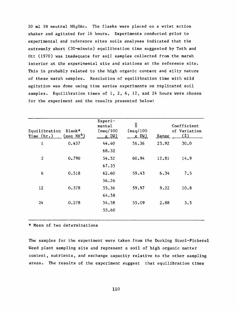
20 ml iN neutral NH4OAc. The flasks were placed on a wrist action
shaker and agitated for 16 hours. Experiments conducted prior to
experimental and reference sites soils analyses indicated that the
extremely short (30-minute) equilibration time suggested by Toth and
Ott (1970) was inadequate for soil samples collected from the marsh
interior at the experimental site and stations at the reference site.
This is probably related to the high organic content and silty nature
of these marsh samples. Resolution of equilibration time with mild
agitation was done using time series experiments on replicated soil
samples. Equilibration times of 1, 2, 6, 12, and 24 hours were chosen
for the experiment and the results presented below:
Equilibration Blank*Time (hr.) (meq NH4 )
1
2
6
0.437
0.790
0.518
0.378
0.278
12
24
Experi-mental(meq/ 100
g DW)
44.40
68.32
54.52
67.35
62.60
56.26
55.36
64.58
54.58
55.60
(meq/ 100
56.36
60.94
59.43
59.97
55.09
Coefficientof Variation
Range (%
23.92 30.0
12.81 14.9
6.34 7.5
9.22 10.8
2.88 3.5
* Mean of two determinations
The samples for the experiment were taken from the Ducking Stool-Pickerel
Weed plant sampling site and represent a soil of high organic matter
content, nutrients, and exchange capacity relative to the other sampling
areas. The results of the experiment suggest that equilibration times
110
should be longer than proposed by Toth and Ott (1978) for marsh soils;
the authors chose 16 hours for the current work as a compromise in terms
of sample processing (i.e., morning preparations, afternoon
equilibration, and sample analysis the following morning) and efficiency
of operation. Following a more thorough study resolving equilibration
times for various soil and sediment types, the authors feel that the
chosen time can be significantly reduced. Sample size to volume ratios
for the various leachates and sample washings were exactly as reported by
Toth and Ott (1970). Gentrifugation was substituted for the suggested
filtration step for collecting the various leachates as a means of
reducing contamination for the NH4 determination and to reduce sample
processing time especially with the silty marsh soils.
328. For the CEC determination, NH4 (the exchanged cation) in the
10% NaCi leachates was determined by the colorimetric method of Solorzano
(1969). NH4C1 standards in 10% NaCi were used for standardization.
329. ECS was determined by the procedures given in Toth and Ott
(1970). Because of apparent Fe contamination in the CEG determinations,
ECS was run on a separate set of soil subsamples. The exchangeable
cations Fe, Mn, Zn, Cu, Ni, Na, K, Ca, and Mg were determined by flame
atomic absorption.
330. The above methods were used for analysis of the November 1976
sampling program. Because of harsh field conditions during the period of
sample collection, field Eh measures were not obtained, and, for some
sampling stations, less than 100 g of material was available for all the
analyses of soil >15 cm in depth due to poor core penetration and sample
retention, expecially for bottom samples from stations 2, 7, and 8
(interior stations at the experimental site). As a result, the analyses
of bottom samples 2, 7, and 8 are incomplete for EGS and some nitrogen
species. For all analyses, the composite core samples were kept frozen
(-200C) until analysis.
331. A third field sampling program was carried out (June 1977)
employing the same methods as before and in situ analyses reported for pH
and Eh profiles and nutrient analyses for specific samples that are not
111
reported for November. Other analyses for this sampling program will be
completed as time permits. All sample handling and analytical techniques
were as discussed.
Results and Discussion
332. Tables 55 and 56 give field descriptions and general
characteristics of the soil sampling stations for the October and
November 1976 sampling programs, respectively. The stations were chosen
to coincide with the 1976 vascular plant sampling areas. The areas were
heterogeneous in terms of both biological (plant) characteristics, origin
of substrate (dredged material, dike construction, and mixtures),
physical influences (exposure and tidal inundation), and, as reported
here, the soil parameters investigated for this study. Soil textural
classes ranged from sand to silty clays.
333. Stations WP3, 4, and 9 at the experimental site were sand
soils and dominated by mixed grasses and small trees (willow). WP1 was a
sandy loam soil and also vegetationally dominated by mixed grasses
(Panicum sp.). WP1 was probably a mixed soil of both dredged material
and dike origin. WP3, 4, and 9 soils were of dike construction origin.
No comparable sites existed at the reference site marsh. These stations
represented the highest elevations at the experimental marsh (range: +
4.4 to + 6.5 feet above mean low water). Table 57 summarizes soil
particle size data.
334. Stations WP5 and WP6 were interior dike sampling areas and
dominated by the Typha-Bidens plant association and are classed as silty
loam and sandy clay loams respectively. The vegetation zone formed a
more or less continuous border around the island interior between the
regularly flooded lower marsh elevations dominated by the
Sagittaria-Pontederia association and the dike itself. The soil was of
dredge material origin and contained a higher percentage silt-clay
fraction than the dike areas. The two stations differed, however, in
particulate size fractionation in the top 15 cm with WP5, located along
112
the southern dike and farther from the direct influence of the discharge
or spillway used during island construction, having a higher silt-clay
fraction (76.81%~) than WP6, located along the northern dike and nearer
the original spillway, having a silt-clay fraction of 38.62% (see Table
57). It is suspected from field observations that some mixing of dike
construction and dredged materials took place in these areas due to
either aeolian or water transport. WP5 in particular showed a
significantly higher gravel content (53.88%) in the >15 cm soil sample
and indicated the extreme heterogeneity of the soil substrate and
possible intrusion of diked material below the surface layers in this
vegetation zone.
335. Stations WP2 and WP7, and WP8 were all interior marsh
stations and characterize the lower intertidal, vegetated and
non-vegetated areas respectively. WP2 and WP7 were dominated by the
Sagittaria-Pontederia plant association with a silty loam soil. WP8 was
a non-vegetated, lower intertidal soil sampling site near the breach in
the southern dike and was a loam soil.
336. The soils of these areas were predominately silt-clays (67 to
84%) in the top 15 cm with silt-sized materials being the major fraction.
The vegetated sites were similar in nearly all respects. WP8 was similar
for most measures except a somewhat lower silt content than the other
stations (see Table 57). There was also evidence of dike materials being
transported into this area (wP8); however, the areas of mixing were
obvious and were avoided during sampling for the present study.
337. Two areas at the reference site were selected as references
for the Sagittaria-Pontederia and Typha-Bidens study sites at Windmill
Point. The Ducking Stool Peltandra-Pontederia site (DSPW) had a silty
clay soil. The Ducking Stool Typha-Bidens area (DSTy) was also a silty
clay soil but contained a higher sand fraction than DSPW and was higher
in elevation. Direct comparison of DSTy with WP4 and WP5 soils was not
possible due to the extreme heterogeneity of the WP sites.
338. Physical analyses, other than particle size for the soils,
are presented in Table 58. Soil pH was near neutral for all stations
113
except WP9 which was more acidic. No explanation can be offered for this
difference. Soil salinity was variable and low, generally reflecting
river salinities reported for the James River in the region of the
experimental site. Percent moisture, volatile solids, and organic carbon
generally correlate directly with the % silt-clay fraction; i.e.,
increases in % silt-clay fraction generally correspond to increase in %
moisture, volatiles, and organic carbon (Figure 48). No apparent
correlation was evident between soil pH (in water) and these parameters.
339. Correlation between % volatiles, as a measure of organic
matter content, and soil organic carbon was not as good as one might
expect. These data are presented in Figure 49 with the 0.4, 0.5, and 0.6
isopleths for % organic carbon: % volatiles ratios drawn. Data points
falling above the 0.4 to 0.6 envelope would indicate the organic carbon
method used underestimated total organic carbon. Points below the
envelope generally indicate contamination and more than likely weighing
errors associated with the % volatiles determination. It is clear in the
figure that many of these data fall above the envelope, particularly the
>15-cm soil samples (solid circles). Because the Walkley-Black technique
measures only the easily oxidizable organic matter fraction, this result
was anticipated. The more refractory organic matter constituents would
be expected in the lower soil layers. These refractile components may,
however, contribute significantly to such other soil measures as CEC and
extractable nutrients.
340. Total organic nitrogen, measured as Kjeldahl nitrogen (TON +
NH4 ), the extractable inrai irgnseisNO 3 , and NH4 , phosphorus
and potassium soil concentrations are presented in Table 59. As
mentioned, nitrite was below detectable limits. Organic nitrogen
accounts for greater than 90% of total soil nitrogen at all stations
followed by NH4f and NO3. Phosphorus and potassium followed the same
general trends as nitrogen with the sand soils low (WP3, 4, and 9), sandy
loam soils intermediate (WP1 and 6), and the silty loam soils and silty
clays progressively higher (WP2, 5, 7, 8, and the reference marsh sites).
These nutrient data follow the same general trend established by the
114
particle size analyses and the physical parameters reported before.
341. Since the study did not include seasonal soils data or
above-below ground plant tissue analyses for carbon, nitrogen,
phosphorus, and potassium, no detailed comparison for plant-nutrient
relationships are possible. It appears that comparable plant sampling
areas at the experimental and reference sites were similar although soil
nitrogen tended to be lower and extractable phosphorus higher for the
interior marsh stations at the experimental site. No statistical degree
of confidence can be ascribed to the measured differences, however.
These stations (WP2, 5, 6, and 7) also were lower in both % volatiles and
organic carbon, indicating that the soil system was still developing at
the experimental site.
342. CEO and CES determinations are presented in Table 60. The
values fall in the higher range reported by Toth and Ott (1970) for
various bay and riverine sediments. The reference marsh soils exhibited
the highest reported values (DSPW and DSTy surface samples). The trends
were similar to those previously discussed and follow the soil textural
classes with sand soils, low progressing to the highest values associated
with the silty clay soils of the reference marsh. The sand soils appear
high relative to the other classes. No causal explanation can be offered
other than re-emphasizing that even within this soil class there was
extreme heterogeneity among samples. The CEO values correlate closely
with the silt-clay soil fraction and organic matter soil content (%volatiles). Figure 50 illustrates the simple linear correlation and
suggests that 70 to 80% of soil CEO can be attributed to organic matter
(presumably the major part of the silt-clay fraction). Toth and Ott
(1970) report that 80% of CEO for bay and riverine sediment is due to the
organic matter content. It is interesting to note, however, that other
factors must also be included for a complete understanding. DSTy soil
samples did not fall within the bounds projected by the regression
analyses. These soils are marked with an asterisk (Figure 50B) and were
not included in the data set for regression calculation. It is
speculated that soil pH, minerology, and the chemical nature of the
115
organic matter contributes to the unexplained variation.
343. Exchangeable bases or CES (Toth and Ott 1970) of the soils
were highly variable. No consistent pattern in terms of absolute
quantity of exchangeable cation (by species) was apparent. All values
appear low, particularly iron and manganese. We have not been able to
account for this. The exchangeable H as presented in the Table is
therefore probably in error since it was based on the difference between
CEC and the sum of exchangeable cations. An alternative explanation is
that the sample handling procedure oxidized the soils sufficiently to
reduce the metals to trace levels. A general pattern, however, was
consistent for all samples with calcium, sodium, and magnesium being the
predominate exchangeable cation and potassium, iron, and manganese lower
and for some soils below detectable limits. The qualitative exchange
status of each cation is presented in Table 61. Only the top (0- to
15-cm) samples are included since four bottom samples stations lacked
enough material for determination.
344. Exchangeable zinc, copper and nickel determinations are
presented in Table 62. These data, as well as the values for iron given
in the previous table, are suspect. Perhac (1974) claims that NH4OAc is
not effective in removing (leaching) metals from sediment. During
analysis, a 5- to 10-fold variation was often encountered in replicate
soil samples. Even on samples with good replication, the concentrations
were at or very near detection limits. It can only be concluded that
either exchangeable zinc, copper, and nickel were present at very low
concentrations at the soil sampling stations or the finding of Perhac
(1974) that the methodology suggested for these analyses is inappropriate
must be supported.
345. Table 63 presents the field data obtained from the third soil
sampling program. These data suggest that the soils were in general not
highly reduced which may in part explain the low exchangeable iron and
manganese values as these would be present in the oxidized state and not
measured as part of CES. WP3 was the only station that indicated
significant reduction potential at depth. These data agree with the
116
general findings of Adams and Darby (1976).
Summary
346. The soils studies carried out during the present investigation
were designed to complement concurrent studies of the vascular plant
flora of the experimental and reference marshes. Few comparative data
exist in the literature for the agronomic measures reported here for
waterlogged, tidal-freshwater marsh soils and the associated vascular
plant flora that make up the major marsh areas; i.e.,
Sagittaria-Pontederia-Peltandra associations. The experimental design
followed does not lend itself to the identification and explanation of
causal plant-soil relationships. The comparisons are descriptive of
general soil conditions within various vegetational zones for one point
in time. The results do suggest areas where more detailed study would be
fruitful for the purposes of the Dredged Material Research Program at
WES. This summary is therefore restricted to comparisons between the
various zones and suggest possible explanations for the observed plant
community characteristics and soil parameters. The following conclusions
are drawn from the data reported.
347. The soil measures reported demonstrate the extreme spatial
heterogeneity of soil characteristics at the experimental site. General
groupings, based on soil textural classes would be the sand and sandy
loam soils (WP1, 3, 4, and 9), the clay and silty loam soils (WP6, 2, 5,
and 7), and the loam and silty clay soils (WP8, DSPW, and DSTy). These
areas generally correspond to the dike, interior dike, and lower
elevations of the marshes at Windmill Point and Ducking Stool
respectively. These areas grade elevationally from the supratidal dike
areas to the low intertidal areas having mean inundation periods of 30 to
40 percent. The zones differ in plant community structure probably as
the result of both elevation and soil characteristics. As mentioned, WP1
demonstrated characteristics intermediate between the other dike areas
and the Typha-Bidens zone. This in all likelihood reflects the mixed
117
nature of the substrate. WP5 and WP6 were also dissimilar in many
respects (i.e. particle size fractionation, organic matter content,
nutrients). This is probably due to original particle size fractionation
and distribution occurring during island construction.
348. For nearly all measures, there was a significant and positive
correlation between % silt-clay, % volatiles, and organic carbon. CEO
relates significantly to these measures and supports the conclusions of
Toth and Ott (1970) and Boyd (1970). These measures also followed the
general elevation gradient relative to mean low water and soil texture
classes.
349. The physical and chemical analyses of soils indicated that
reference site soils were higher with regard to % volatiles, organic
carbon, soil nitrogen, and CEO. In particular, differences in CEO and
soil nitrogen between reference and experimental site soils may account
for the observed significant difference in Pontederia plant height
between these sites for the 1976 growing season. Differences in plant
height and productivity due to different nutrient regimes have been
reported for a variety of marsh ecosystems (e.g., Wetzel et al. 1977;
Chalmers et al. 1976).
350. The data, particularly those soil measures generally related
to plant growth and decomposition (e.g. organic matter content, available
nutrients, and soil measures attributable to organic content such as
CEO), suggest that the soil system at the experimental site is still
developing.
351. Various methods were found inappropriate. Methods modified
after the work of Goldhaber (1974) for sulfide analysis were not
quantitative and generally displayed high variability. Repeated attempts
to standardize the method were not successful considering the reported
low levels of sulf ides present (Adams and Darby 1976). Bremner and Bundy
(1974) have reported and cite the influences of organo-sulfur compounds
on soil nitrogen determinations and soil nitrification. It would seem
appropriate that an adequate sulfur methodology be devised for future
study particularly if such studies include nutrient dynamic aspects. A
118
second method which indicated extreme variability was analysis of
exchangeable metals (iron, manganese, zinc, copper, nickel) employing
acetate for soils extraction. Perhac (1974) has reported on the
inadequacies of acetate leaching, and Harris (Personal Communication,
Richard Harris, VIMS, Gloucester Point, Virginia) confirms his findings
and general conclusions. Because the analysis methodologies are outside
the authors' areas of experience, they can offer no suggestion.
Comparison of exchangeable metals (by the methods suggested) and total
soils metal analyses would suggest that if the acetate leaching methods
are appropriate for determining exchangeable metal species, the soils
metals at the experimental site are not readily available for plant
incorporation.
119
PART VII: SUMMARY AND OVERVIEW
M. P. Lynch
352. The Windmill Point marsh development project succeeded in
constructing an island-marsh habitat that was attractive to plants and
animals indigenous to the local region. Although the feasibility of
constructing successful fresh water tidal marshes was demonstrated, not
all the original goals were achieved.
353. With minor exceptions, the seeded or sprigged species did
not last beyond the first growing season, and no effect of the
alternate treatment of areas with fertilizer was apparent.
354. The western end of the island was severely eroded. By the
end of the study, only a short section of the original dike remained to
protect the interior marsh. Two breaches occurred before completion of
the project. One of these was successfully plugged. The other breach,
on the south side of the island, now functions as one of the main
channels of tidal water exchange.
355. The use of a reference marsh and adjacent uplands for
comparison with the experimental island marsh was only partially
successful, principally because no marshes in the open exposed position
of the experimental site could be located. Sufficient similarity was
obtainable, however, to demonstrate success of the experimental marsh.
356. The principal difference between the experimental site and
the reference site, other than exposure, was the significantly higher
concentration of soil constituents at the reference site, such as%
volatiles, organic carbon, soil nitrogen, and cation exchange capacity,
which are related to accumulation and breakdown of plant detritus.
Higher soil nitrogen at the reference site may have been the cause for
the significantly higher height of the pickerelweed in this area in
1976.
357. Water quality, with the exception of a higher dissolved
oxygen at the reference site, did not differ between the two areas.
358. Soil studies indicated extreme spatial heterogeneity of soil
120
characteristics at the experimental site. The dike, interior dike, and
lower marsh elevations were sand and sandy loam soil, clay and silty
loam soils, and loam and silty clay soils respectively. At the
reference site, loam and silty clay soils were found.
359. For nearly all areas, there was a significant and positive
correlation between % silt-clay, % volatiles, and organic carbon.
These characteristics also followed a general elevation gradient that
reflects the periods of inundation as did the soil types with higher
values in the lower marsh loam and silty clays and lower values in the
higher sand and sandy loam soils.
360. The soil measures generally related to plant growth and
decomposition, such as organic constituents, indicate the soil system
at the experimental site is still developing. Field observations at
the experimental site also indicate there is mixing of dike material
with marsh material which is influencing final soil characterizations.
361. With the exception of the higher nitrogen and cation
exchange capacity previously mentioned that is thought to account for
significantly higher pickerelweed at the reference site during the 1976
growing season, no causal soil-plant relationship was discernible from
this study. Plant distribution and zonation appeared to be controlled
more by physical environmental factors such as elevation and tidal
inundation than differences in soil characteristics.
362. A floral inventory of the experimental site in
1974 indicated that prior to dike construction, about 55 species were
fairly distributed between marsh and supratidal habitats. After
construction, by July 1975 this number was roughly doubled by natural
invaders plus the six introduced species. Between July 1975 and
September 1977, the number of invading species had decreased.
363. The botanical studies indicated that plants were grouped
into four major zones: an arrowhead-pickerelweed zone occupying the
low, broad interior of the island; a beggar tick zone at higher levels
of the marsh; a panic grass zone, the remnants of the plantings of
121
beachgrass and switch grass which ran in an interrupted band around the
island; and the only wooded area, a black willow zone consisting of
black willow, cottonwood, and common alder on the eastern portion of
the island. The remainder of the plant zones were heterogeneous
mixtures of two or more species.
364. Maximum plant development at the experimental site appeared
to take place in July and August as opposed to June for the reference
site. No specific reason for this difference was identified.
365. Apparent successional changes in plant cover as detected
from aerial photographs were actually stages of a normal seasonal
cycle. Successional changes are occurring, as evidenced by changes in
willow distribution at the northeast corner, but accurate assessments
can be made only through long-term studies.
366. It appears that the arrowhead-pickerelweed and beggar tick
zones are approaching climax or near-climax conditions in the
experimental marsh areas. In the higher areas of the original island
and the dike, the increasing growth of trees with changing shade
conditions will continue to exhibit changing species distribution.
367. During 1977, insects dramatically reduced the vegetation of
the reference site. Grasshoppers and Japanese beetles were also noted
at the experimental site, but insect damage there was slight. The
major plant damage inflicted by animals at the experimental site
resulted from muskrat activity. Muskrats destroyed plants in many
areas, whether for food or for lodge construction. Plants were
destroyed by direct consumption of roots and/or shoots and by tunnels
and runways dug by the animals. Several small areas were almost
completely denuded, but during the year many were revegetated.
368. An effect of severe winds was observed. The effect on
beggar ticks was very deleterious, since visual comparisons of plant
heights between 1976 and 1977 revealed a sharp decrease in beggar ticks
height, whereas arrowhead and pickerelweed were largely unaffected.
Apparently, the flexibility of soft-stemmed plants such as arrowhead
and pickerelweed contributed to their survival during the July 1977
122
windstorm, whereas the taller, rigid stems of such plants as beggar
ticks and water hemp were broken.
369. Erosion greatly impacted the vegetation on the western end
of the island. The planted panic grass on the dike, although
apparently a good soil retainer, was undermined by wave action. Even
woody plants such as willows were eventually uprooted.
370. The Windmill Point experimental site provides, by virtue of
its openness relative to surrounding woodland communities, sand beach
perimeter, large tidal flat, and basin, a combination of habitats
unique to the upper tidal James River. The most obvious result of this
combination of habitats is the large number of birds recorded at the
experimental site compared to the reference site. The island-marsh
appears to act as an avian motel drawing migrants from many groups,
especially those associated with intertidal environments.
371. The greater number of birds at the experimental site was
primarily due to gulls, terns, and wading birds that were attracted to
the intertidal flat areas. Four species, the ring-necked gull,
red-winged blackbird, laughing gull, and Canada goose, comprised
two-thirds of all the individuals at the experimental site. At both
the berm and marsh reference sites, the red-winged blackbird and seed
eaters, either fringillids, sparrows, or cardinals, made up the greater
part of the population.
372. Bird density at the experimental site was highest in early
spring and fall and lowest in early summer. This was principally due
to migrants, particularly gulls and geese.
373. Only the mallard, killdeer, red-winged blackbird, and
possibly the song sparrow nested on the island. Breeding could only be
confirmed for the mallard and red-winged blackbird. Predation by fish
crows and rice rats are considered to have a major impact on nest
success of red-winged blackbirds.
374. The most important food items for bird species at the
experimental site were fish, ground seed, and tidal invertebrates.
Waterfowl, eating leaves, roots, and aquatic seeds, were also an
123
important group at the island. Canada geese were the most important
birds in this category and are considered responsible for elimination
of some of the planted species.
375. Muskrats dominated the wildlife other than birds. By the
end of the study, 11 muskrat lodges were located on the island.
Numerous runs and cleared feeding pads indicated a substantial
population. Considerable damage to willows was caused by the muskrats.
The only other mammal noted was the rice rat.
376. Benthic organisms are key secondary producers in both marsh
ecosystems and in the shallow water ecosystems that pre-existed at the
experimental site before island-marsh construction. Initially, only
macrobenthos was sampled, but after preliminary analysis of fish food
habits, meiobenthos was examined.
377. Production estimates showed that in the reference marsh
meiobenthos were nearly as important as producers as macrobenthos,
while macrobenthos production (principally by oligochaetes) was
overwhelming in experimental marsh habitats. Although total production
of benthos was much higher in experimental marsh habitats than in the
reference marsh or on the open tidal flat, meiobenthos production was
greater in reference marsh habitats.
378. Macrobenthos was qualitatively and quantitatively dominated
by tubificid oligochaetes and larval chironomid insects. The bivalve,
Corbicula manilensis, was also very abundant. Oligochaetes of the
genus Limnodrilus were the numerical and biomass dominants in most of
the habitats.
379. Total density and biomass were highest in the low marsh and
subtidal channels of. the experimnental site. Intermediate density and
biomass were found in the higher marsh at both sites and in low marsh
at the reference site. Lower values were found outside of the marshes
on adjacent tidal flats and on subtidal bottoms used by the project.
The differences were mainly due to differences in populations of
oligochaetes.
380. The density and biomass of macrobenthos were highest in
124
summer and lowest in winter. Species diversity was higher at the
reference site than the experimental site due to both a greater number
of species and less dominance by a few species at reference site
stations.
381. Protection of tidal flat macrobenthos from predation by use
of an exclosure cage resulted in a 3-fold increase in density and a
44-fold increase in biomass over surrounding areas indicating that
predation by fish and birds plays a key role in benthic community
structuring.
382. The permanent meiobenthos was comprised principally of
nematodes, cladocerans, ostracods, and copepods. The density of
meiobenthos was greatest in low marsh, subtidal channel, and tidal flat
at the experimental site. Estimated biomass was greater at comparable
reference sites principally because of greater density of crustaceans.
383. Benthic organisms were a major part of the diet of the
dominant fishes. Meiobenthic organisms, especially small crustaceans,
were very important in this respect. Larger macrobenthic organisms
such as oligochaetes were not numerically important food for the small
fish that made up most of the sample. Overall crustaceans were the
most abundant food, followed in decreasing order by insects, plant
seeds, molluscs, and fish and fish eggs.
384. The reference site had significantly more fish species and a
higher fish species diversity than the experimental site. Apparent
differences in numbers and biomass at the 2 sites were,
however, not significant. The greater number of species and higher
species diversity at the reference site are attributed to a greater
diversity of subhabitats (debris, branches, etc.).
385. In comparison with adjacent open bottom, the creation of the
marsh has undoubtedly increased abundance and diversity of fish in the
area. The marsh has resulted in more food and protection for many
fish. The abundance of important forage species like the mummichog and
spottail shiner was probably increased since they exhibit a strong
dependence on littoral areas. Two species of some commercial and
125
recreational importance, the channel catfish and the white perch, use
the shoal areas adjacent to the island for nocturnal feeding.
386. The most important fish species in terms of abundance,
biomass, and frequency of appearance, in decreasing order, were the
spottail shiner, white perch, American eel, threadf in shad, mummichog,
tidewater silverside, gizzard shad, channel catfish, silvery minnow,
and spot. This corresponded to the general condition of the
icthyofauna in this section of the James River.
387. Although this series of studies has demonstrated that tidal
fresh water island-marsh habitats can be constructed and attract local
species, certain questions still remain. By comparison with data from
similar reference site habitats, it is obvious that the island-marsh
system is still evolving towards the more typical marsh system with
adjacent woodlands. If the rapidly eroding western end of the island
becomes stabilized and the internal marsh protected from erosion, it
will be interesting to note whether the soils in the marsh system
continue to increase in those characteristics associated with decaying
plant material such as organic carbon, nitrogen, % volatiles, and
cation exchange capacity, or whether the admixture of sand blowing or
washing over the dikes at high water will be sufficient to retain the
more sandy characteristics at the experimental site.
388. The openness, including lack of substantial trees is
considered to contribute to the large number of bird species at the
experimental site as contrasted to the reference site. It would be
interesting to monitor the bird populations as the larger plant
species, particularly on the higher ground, develop and enable the
invasion of new plant species suited to wooded habitats.
389. If the western end of the island is breached, the response
of the interior marsh to higher energy river water would provide an
interesting case study to evaluate permanence of artificially created
habitats.
390. With respect to enhancement of wildlife resources, the
Windmill Point project has been beneficial to the region through the
126
present. A greater diversity and/or biomass of benthic biota, birds,
fish, and plants is found at the experimental site than in surrounding
shallow water communities. The experimental site also compares
favorably with reference sites in terms of wildlife resources and
productivity.
391. It is strongly recommended that monitoring continue at the
Windmill Point experimental site until the plant communities at the
island become similar to those on adjacent shores or the island
succumbs to erosion. Such data should prove of great value in
predicting the success of future island marsh systems created to obtain
a benefit from dredge material.
127
REFERENCES
Adams, D. D. and D. A. Darby. 1976. The coring operation at the arti-ficial habitat near Windmill Point, James River, Virginia on July17-18, 1975. Contract report to Waterways Experiment Station,Vicksburg, Ms. Contract No. DACW65-75-C-0051.
American Public Health Association. 1971. Standard methods. 13thEdition, Am. Pubi. Health Assn., Washington, D. C. 874 pp.
Anderson, W. D., Jr., J. K. Dias, R. K. Dias, D. M. Cupka, and N. A.Chamberlain. 1977. The macrofauna of the surf zone off Folly Beach,South Carolina. NOAA Tech. Rep. NMFS, SSRF-704. 23 pp.
Ankar, S. and R. Elmgren. 1976. The benthic macro- and meiofauna of theAsko-Lands~rt area (northern Baltic proper). A stratified randomsampling survey. Contr. AskU Lab., Univ. of Stockholm, Sweden.115 pp.
Armstrong, N. W., P. H. Storrs, and E. A. Pearson. 1971. Developmentof a gross toxicity criterion in San Francisco Bay. Proc. 5thIntern. Conf. Water Pollut. Res. III, pp. 1-15.
Bailey, R. M. (ed.). 1970. A list of common and scientific names offishes from the United States and Canada (3rd edition). Am. Fish.Soc. Spec. Publ. No. 6. 150 pp.
Bailey, R. M. and H. M. Harrison, Jr. 1948. Food habits of the southernchannel catfish (Ictalurus lacustris punctatus) in the Des MoinesRiver, Iowa. Trans. Am. Fish. Soc. 75:110-138.
Bent, A. C. 1927. Life histories of North American shorebirds. Part I.Dover Publ. 420 pp.
Beukema, J. J. 1976. Biomass and species richness of the macrobenthicanimals living on the tidal flats of the Dutch Wadden Sea. Nether-lands J. Sea Res. 10:236-261.
Bigelow, H. B. and W. C. Schroeder. 1953. Fishes of the Gulf of Maine.U. S. Fish and Wildlife Service, Fish. Bull. 74, Vol. 53. 577 pp.
Black, C. A., D. D. Evans, I. E. Ensminger, J. L. White, and F. E. Clark.1965. Methods of soil analysis. Am. Soc. Agronomy, Madison, Wisc.
Boesch, D. F. 1972. Species diversity of marine macrobenthos in theVirginia area. Chesapeake Sci. 13:206-211.
Boesch, D. F. 1973. Classification and community structure of macro-benthos in the Hampton Roads area, Virginia. Marine Biol. 21:226-244.
128
Boesch, D. F. 1977. Application of numerical classification inecological investigations of water pollution. U. S. EnvironmentalProtection Agency Ecol. Res. Ser. EPA-600/3.-77-033. 114 pp.
Boesel, M. W. 1938. The food of nine species of fish from the westernend of Lake Erie. Trans. Am. Fish. Soc. 67:215-223.
Borgeson, D. P. 1963. A rapid method for food-habits studies. Trans.Am. Fish. Soc. 92(4):434-435.
Boyd, C. E. 1970. Influence of organic matter on some characteristicsof aquatic soils. Hydrobiologia 36(l):17-21.
Bremner, J. M. and L. G. Bundy. 1974. Effects of organic sulfur com-pounds on methods of determining inorganic forms of nitrogen.Soil Biol. Biochem. 6:97-99.
Burbidge, R. G. 1972. Distribution, growth, selective feeding, andenergy transformations of young-of-the-year blueback herring, Alosaaestivalis (Mitchill), in the James River, Virginia. Ph.D. Disser-tation, Dept. Mar. Science, Univ. Virginia, Charlottesville. 131 pp.
Burbidge, R. G. 1974. Distribution, growth, selective feeding, andenergy transformations of young-of-the-year blueback herring, Alosaaestivalis (Mitchill), in the James River, Virginia. Trans. Am.Fish. Soc. 103:297-311.
Burger, J., M. Howe, D. Hahn, and J. Chase. 1977. Effects of tidecycles on habitat selection and habitat partitioning by migratingshorebirds. Auk 94:743-758.
Cain, S. A. 1938. The species-area curve. Am. Midl. Nat. 19:573-581.
Cainmen, L. M. 1976a. Macroinvertebrate colonization of Spartina marshesartificially established on dredge spoil. Estuar. Coast. Mar. Sci.4: 357-372.
Canimen, L. C. 1976b. Abundance and production of macroinvertebratesfrom natural and artificially established salt marshes in NorthCarolina. Am. Midl. Nat. 96:487-493.
Chalmers, A. G., E. B. Haines, and B. F. Sherr. 1976. Capacity ofSpartina salt marsh to assimilate nitrogen from secondarily treatedsewage. Tech. Completion Rept., USDI/OWRP Project No. A-057-GA,Dept. of Interior, Office of Water Research and Technology. 88 pp.
Chambers, N. R. and H. Nilne. 1975. The production of Macoma baithica(L.) in the Ythan estuary. Estuar. Coast. Mar. Sci. 3:443-455.
Clifford, H. T. and W. Stephenson. 1975. An Introduction to NumericalClassification. Academic Press, New York. 229 pp.
129
Coastal Zone Resources Division, Ocean Data Systems Corp. 1977. Handbookfor terrestrial wildlife habitat development on dredged material.U. S. Army Engineer Waterways Experiment Station, Contract Report,Vicksburg, Miss. 365 p. + Appendix.
Darnell, R. M. 1958. Food habits of fishes and larger invertebrates ofLake Ponchartrain, Louisiana, an estuarine community. Publs. Inst.Mar. Sci., Univ. Texas 5:353-416.
Diaz, R. J. 1977. The effects of pollution on benthic communities ofthe tidal James River, Virginia. Ph.D. Thesis, Univ. Virginia,Charlottesville. 148 pp.
Diaz, R. J. and D. F. Boesch. 1977a. Habitat development and field inves-tigations at Windmill Point habitat development site, James River, Vir-ginia: Appendix E: Assessment of acute impacts of habitat developmentsite on the macrobenthos community. Techn. Rep. D-76, U. S. Army Corpsof Engineers, Environmental Effects Laboratory, Vicksburg, Miss.
Diaz, R. J. and D. F. Boesch. 1977b. Impact of fluid mud dredged materi-al on benthic communities of the tidal James River, Virginia. Techn.Rep. D-77-45, U. S. Army Corps of Engineers, Environmental EffectsLaboratory, Vicksburg, Miss.
Doumlele, D. G. 1976. Primary production and plant community structurein a tidal freshwater marsh. M.A. Thesis, College of William and Mary,Williamsburg, Va. 59 pp.
Draper, N. R. and H. Smith. 1966. Applied regression analysis. JohnWiley and Sons, Inc., New York. 407 pp.
Effenberger, M. 1967. A simple flow cell for the continuous determina-tion of oxidation-reduction potential. Pages 123-126 in H. L. Golter-man (ed.), Chemical Environment in the Aquatic Habitat. North-Holland.
Environmental Protection Agency. 1974. Methods for chemical analysis ofwater and wastes. EPA, Office of Technology Transfer, Washington, D. C.
Fernald, M. L. 1950. Gray's manual of botany. 8th ed., American BookCo., New York. 1632 pp.
Flemer, D. A. and W. S. Woolcott. 1966. Food habits and distribution ofthe fishes of Tuckahoe Creek, Virginia, with special emphasis on thebluegill, Lepomis m. macrochirus Rafinesque. Chesapeake Sci. 7(2):75-89.
Folk, R. L. 1968. Petrology of sedimentary rocks. Hemphill's, Austin,Texas. 170 pp.
Gerlach, S. A. 1971. On the importance of marine meiofauna for benthoscommunities. Oecologia 6:176-190.
130
Gerlach, S. A. and N. Schrage. 1971. Life cycles in marine meiobenthos.Experiments at various temperatures with Monhystera disjuncta andTheristus pertennuis (Nematoda). Mar. Biol. 9:274-280.
Gleason, H. A. 1958. The new Britton and Brown illustrated flora of thenortheastern United States and adjacent Canada. 2nd ed., Lancaster,Pa. 3 vols.
Goldhaber, M. B. 1974. Equilibrium and dynamic aspects of the marinegeochemistry of sulfur. Ph.D. Thesis, Dept. of Geology, UCLA,Los Angeles, Calif.
Goodman, D. 1975. The theory of diversity-stability relationships inecology. Quart. Rev. Biol. 50:237-266.
Griswold, B. L. and R. A. Tubb. 1977. Food of yellow perch, white bass,freshwater drum, and channel catfish in Sandusky Bay, Lake Erie.Ohio J. Sci. 77(l):43-47.
Hildebrand, S. F. and W. C. Schroeder. 1928. Fishes of Chesapeake Bay.U. S. Bureau of Fisheries Bull. 53(1). 388 pp.
Hitchcock, A. 5. 1950. Manual of the grasses of the United States.U. S. Dept. of Agriculture Misc. Pubi. No. 200. 1051 pp.
Hoagman, W. J., J. V. Merriner, R. St. Pierre, and W. L. Wilson. 1973.Biology and management of river herring and shad in Virginia.Completion Report 1970-1973. VIMS, Gloucester Point, Va. 212 pp.
Holmes, R. T. 1966. Feeding ecology of the red-backed sandpiper(Calidris alpina) in arctic Alaska. Ecology 47:32-45.
Jacobs, J. 1975. Diversity, stability, and maturity in ecosystems in-fluenced by human activities. Pages 187-207 in W. H. van Dobbenand R. H. Lowe-McConnell (eds.), Unifying concepts in ecology.Junk, The Hague.
Jensen, L. D. 1974. Environmental responses to thermal discharges fromthe Chesterfield Station, James River, Virginia. Dept. of Geographyand Environmental Engineering, Johns Hopkins Univ., Rept. 13. 180 pp.
Jervis, R. A. 1969. Primary production in the freshwater ecosystem ofTroy Meadows, New Jersey. Bull. Torrey Bot. Club 96:209-231.
Johnson, M. G. 1974. Production and productivity. Pages 46-64 inR. 0. Brinkhurst, The benthos of lakes. St. Martin's Press,New York.
Johnson, D. S. and H. H. York. 1915. The relation of plants to tidelevels. Carnegie Inst. of Washington Pubi. 206.
131
Juario, J. V. 1975. Nematode species cohiposition and seasonal fluctua-tion of a sublittoral mejofauna community in the German Bight.Verl~ff. Inst. Meeresforsch. Bremerh. 15: 283-337.
Kaluch, K. 1954. Redoxpotential-,rH-Messung. Pharmazie a:634-642.
Kerwin, J. A. and R. A. Pedigo. 1971. Synecology of a Virginia saltmarsh. Chesapeake Sci. 12:125-130.
Lagler, K. F. 1956. Freshwater fishery biology. Win. C. Brown Co. Publ.Dubuque, Iowa. 421 pp.
Lewis, G. E. 1976. Summer food of channel catfish in a West Virginiaflood control reservoir. Prog. Fish-Cult. 38(4):177-178.
Loesch, J. G. and W. H. Kriete, Jr. 1976. Biology and management ofriver herring and shad. Completion Report, Anadromous Fish Project,1974-1976. VIMS, Gloucester Point, Va. 226 pp.
Macan, T. T. 1977. The influence of predation on the composition offresh-water animal communities. Biol. Rev. 52:45-70.
Margalef, R. 1958. Information theory in ecology. Gen. Syst. 3:36-71.
McCann. J. A. 1959. Life history studies of the spottail shiner ofClear Lake, Iowa, with particular reference to some sampling problems.Trans. Am. Fish. Soc. 88(4):336-343.
Meanley, B. and J. Webb. 1963. Nesting ecology and reproductive rateof the red-winged blackbird in tidal marshes of the upper ChesapeakeBay region. Chesapeake Sci. 4:90-103.
Menzel, R. W. 1945. The catfish fishery of Virginia. Trans. Am. Fish.Soc. 73:364-372.
Miller, W. R. and F. E. Egler. 1950. Vegetation of the Wequetequock-Pawcatuck tidal-marshes, Connecticut. Ecol. Monogr. 20:143-172.
Murphy, J. and J. P. Riley. 1962. A modified single solution for thedetermination of phosphate in natural waters. Anal. Chem. Acta27: 31-36.
Costing, H. J. 1956. The study of plant communities: An introductionto plant ecology. 2nd ed., W. H. Freeman and Co., San Francisco.440 pp.
Owens, L. B., D. W. Nelson, and L. E. Sommers. 1977. Determination ofinorganic phosphorous in oxalate extracts of soils. Soil Sci. Soc.Am. J. 41:148-149.
132
Perhac, R. M. 1974. Heavy metal distribution in bottom sediment andwater in the Tennessee River-Loudon Lake Reservoir system. Res.Report #40, WRRC, Univ. Tennessee, Knoxville.
Perry, W. G., Jr. 1969. Food habits of blue and channel catfish col-lected from a brackish-water habitat. Prog. Fish-Cult. 31(1):47-50.
Pettijohn, R. J. 1957. Sedimentary rocks. Harpers, New York. 526 pp.
Pielou, E. C. 1975. Ecological diversity. Wiley-Interscience, NewYork. 196 pp.
Pflieger, W. L. 1971. A distributional study of Missouri fishes. Univ.Kanses Pubi., Mus. Nat. Hist. 20(3):225-570.
Pflieger, W. L. 1975. The fishes of Missouri. Missouri Dept. of Con-servation, Jefferson City, Mo. 343 pp.
Poole, J. C. 1961. Age and growth of the fluke in Great South Bay andtheir significance in the sport fishery. N. Y. Fish and Game J.8(1) :1-18.
Radford, A. E., H. E. Ahies, and C. R. Bell. 1968. Manual of thevascular flora of the Carolinas. Univ. of North Carolina Press,Chapel Hill. 1183 pp.
Raney, E. C. 1950. Freshwater fishes. Pages 151-194 in M. H. Stow(Chairman), The James River Basin past, present and future. JamesRiver Project Committee, Va. Acad. Sci.
Recher, H. F. 1966. Some aspects of the ecology of migrant shorebirds.Ecology 47:393-407.
Reid, W. F., Jr. 1972. Utilization of the crayfish Orconectes limosusas forage by white perch in a Maine lake. Trans. Am. Fish. Soc.101(4) :608-612.
Rofritz, D. J. 1977. Oligochaeta as a winter food source for the oldsquaw. J. Wildi. Manage. 41:590-591.
Schindler, J. W. and K. R. Konich. 1971. Oxidation-reduction determina-tions at the mud-water interface. Limnol. Oceanogr. 16(5):837-840.
Smith, L. L. and R. H. Kramer. 1964. The spottail shiner in Lower RedLake, Minnesota. Trans. Am. Fish. Soc. 93:35-45.
Sokal, R. R. and F. J. Rohif. 1969. Biometry. W. H. Freeman and Co.,San Francisco, Calif. 776 pp.
Solorzano, L. 1969. Determination of ammonia in natural waters by thephenol-hypochlorite method. Limnol. Oceanogr. 14:799-801.
133
Strickland, J. D. H. and T. R. Parsons. 1968. A practical handbookof seawater analysis. Fish. Res. Bd. Canada, Ottawa. 311 pp.
Stripp, K. 1969. Das Verh~ltnis von lMakrofauna and Meiofauna in denSedimenten der Helgolhnder Bucht. Ver~ff Inst. Meeresforsch.Bremerh. 12:143-148.
Tomoff, 5. 1974. Avian species diversity in desert scrub. Ecology55:396-403.
Toth, S. J. and A. N. Ott. 1970. Characterization of bottom sediments.Cation exchange capacity and exchangeable cation status. Environ.Sci. Tech. 4(ll):935-939.
Virnstein, R. W. 1977. The importance of predation by crabs and fisheson benthic infauna in Chesapeake Bay. Ecol. Monogr. 47(4): in press.
Wass, M. L. 1972. A check list of the biota of lower Chesapeake Baywith inclusions from the upper Bay and the Virginian Sea. VIMS,Spec. Sci. Rep. No. 65, Gloucester Point, Va. 290 pp.
Wass, N. L. 1976. (Winter bird census of) Coastal disturbed floodplain.Am. Birds 30:1053-1055.
Waters, T. F. 1969. The turnover ratio in production ecology of fresh-water invertebrates. Am. Nat. 103:173-185.
Weaver, J. E. 1975. Food selectivity, feeding chronology, and energytransformations of juvenile alewife (Alosa pseudoharengus) in theJames River near Hopewell, Virginia. Ph.D. Dissertation, Dept. ofMar. Sci., Univ. of Virginia, Charlottesville. 88 pp.
Webster, D. A. 1943. Food progression in young white perch Moroneamericana (Gmelin) from Bantam Lake, Connecticut. Trans. Am. Fish.Soc. 72:136-144.
Wetzel, R. L., 14. 5. Kowalski, W. M. Rizzo, A. Thompson, and K. L. Webb.1977. Characterization of a historically nutrient enriched marshecosystem: Yorktown Creek, Yorktown, Virginia. Spec. Rept. Appl.Mar. Sci. and Ocean Engr., VImS, Gloucester Point, Va. 90 pp.
Wieser, W. 1953. Free-living marine nematodes of the Lund UniversityChile Expedition 1948-1949. IV. General Part. Lunds UniversitetsArsskrift. N.F. Aud. 2Bd. 55. NR. 5:1-111.
Wilhm, J. L. and T. C. Dorris. 1968. Biological parameters for waterquality criteria. BioScience 18:447-481.
134
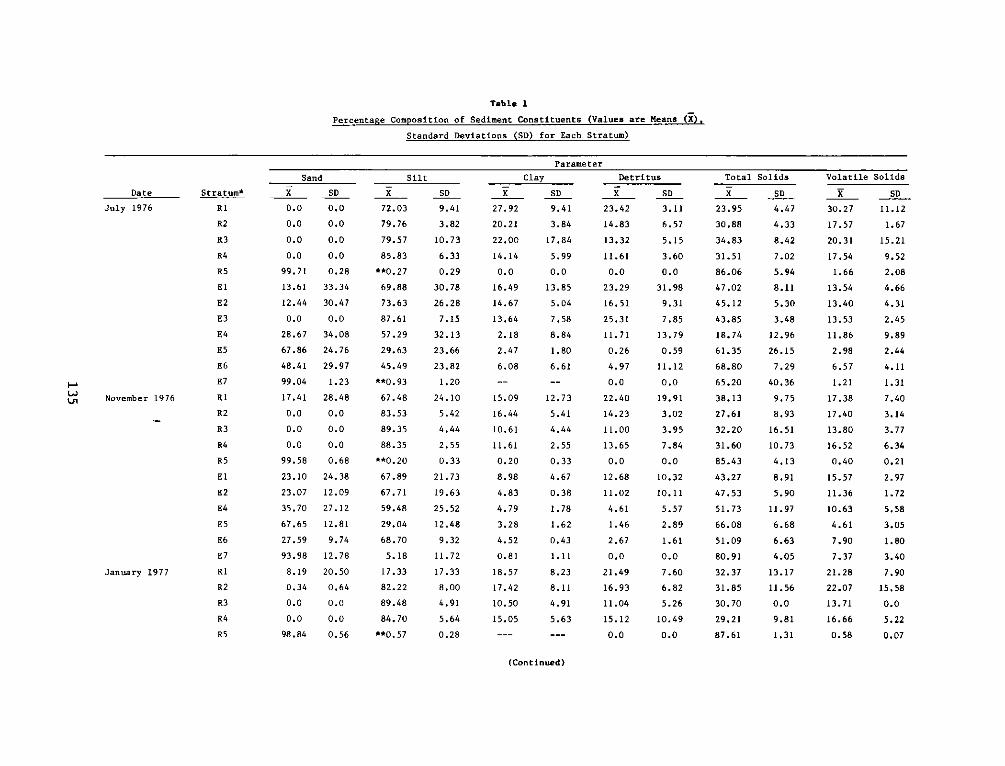
Table 1
Percentage Composition of Sediment Constituents (Values are Means (X),Standard Deviations (SD) for Each Stratum)
Parameter
Date Stratum*
July 1976 Ri
R2
R3
R4
RS
El
E2
E3
E4
ES
E6
pa E7
November 1976 Ri
R2
R3
R4
RS
El
E2
E4
ES
E6
E7
January 1977 Ri
R2
R3
R4
R5
Sand Silt
Xl SD XSD
0.0 0.0 72.03 9.41
0.0 0.0 79.76 3.82
0.0 0.0 79.57 10.73
0.0 0.0 85.83 6.33
99.71 0.28 **0.27 0.2913.61 33.34 69.88 30.78
12.44 30.47 73.63 26.28
0.0 0.0 87.61 7.15
28.67 34.08 57.29 32.13
67.86 24.76 29.63 23.66
48.41 29.97 45.49 23.82
99.04 1.23 **Q.93 1.2017.41 28.48 67.48 24.10
0.0 0.0 83.53 5.42
0.0 0.0 89.35 4.44
0.0 0.0 88.35 2.55
99.58 0.68 **0.20 0.3323.10 24.38 67.89 21.73
23.07 12.09 67.71 19.63
35.70 27.12 59.48 25.52
67.65 12.81 29.04 12.48
27.59 9.74 68.70 9.32
93.98 12.78 5.18 11.72
8.19 20.50 17.33 17.33
0.34 0.64 82.22 8.00
0.0 0.0 89.48 4.91
0.0 0.0 84.70 5.64
98.84 0.56 **Q.57 0.28
Clay Detritus Total Solids
X SD X SD X SD
27.92 9.41 23.42 3.11 23.95 4.47
20.21 3.84 14.83 6.57 30.88 4.33
22.00 17.84 13.32 5.15 34.83 8.42
14.14 5.99 11.61 3.60 31.51 7.02
0.0 0.0 0.0 0.0 86.06 5.94
16.49 13.85 23.29 31.98 47.02 8.11
14.67 5.04 16.51 9.31 45.12 5.30
13.64 7.58 25.31 7.85 43.85 3.48
2.18 8.84 11.71 13.79 18.74 12.962.47 1.80 0.26 0.59 61.35 26.15
6.08 6.61 4.97 11.12 68.80 7.29
-- -- 0.0 0.0 65.20 40.36
15.09 12.73 22.40 19.91 38.13 9.75
16.44 5.41 14.23 3.02 27.61 8.93
10.61 4.44 11.00 3.95 32.20 16.51
11.61 2.55 13.65 7.84 31.60 10.73
0.20 0.33 0.0 0.0 85.43 4.13
8.98 4.67 12.68 10.32 43.27 8.91
4.83 0.38 11.02 10.11 47.53 5.90
4.79 1.78 4.61 5.57 51.73 11.97
3.28 1.62 1.46 2.89 66.08 6.68
4.52 0.43 2.67 1.61 51.09 6.63
0.81 1.11 0.0 0.0 80.91 4.05
18.57 8.23 21.49 7.60 32.37 13.1717.42 8.11 16.93 6.82 31.85 11.56
10.50 4.91 11.04 5.26 30.70 0.015.05 5.63 15.12 10.49 29.21 9.81
-- -- 0.0 0.0 87.61 1.31
Volatile Solids
XSD
30.27 11.12
17.57 1.67
20.31 15.21
17.54 9.52
1.66 2.08
13.54 4.66
13.40 4.31
13.53 2.45
11.86 9.89
2.98 2.44
6.57 4.11
1.21 1.31
17.38 7.40
17.40 3.14
13.80 3.77
16.52 6.34
0.40 0.21
15.57 2.97
11.36 1.72
10.63 5.58
4.61 3.05
7.90 1.807.37 3.40
21.28 7.90
22.07 15.5813.71 0.016.66 5.22
0.58 0.07
(Continued)
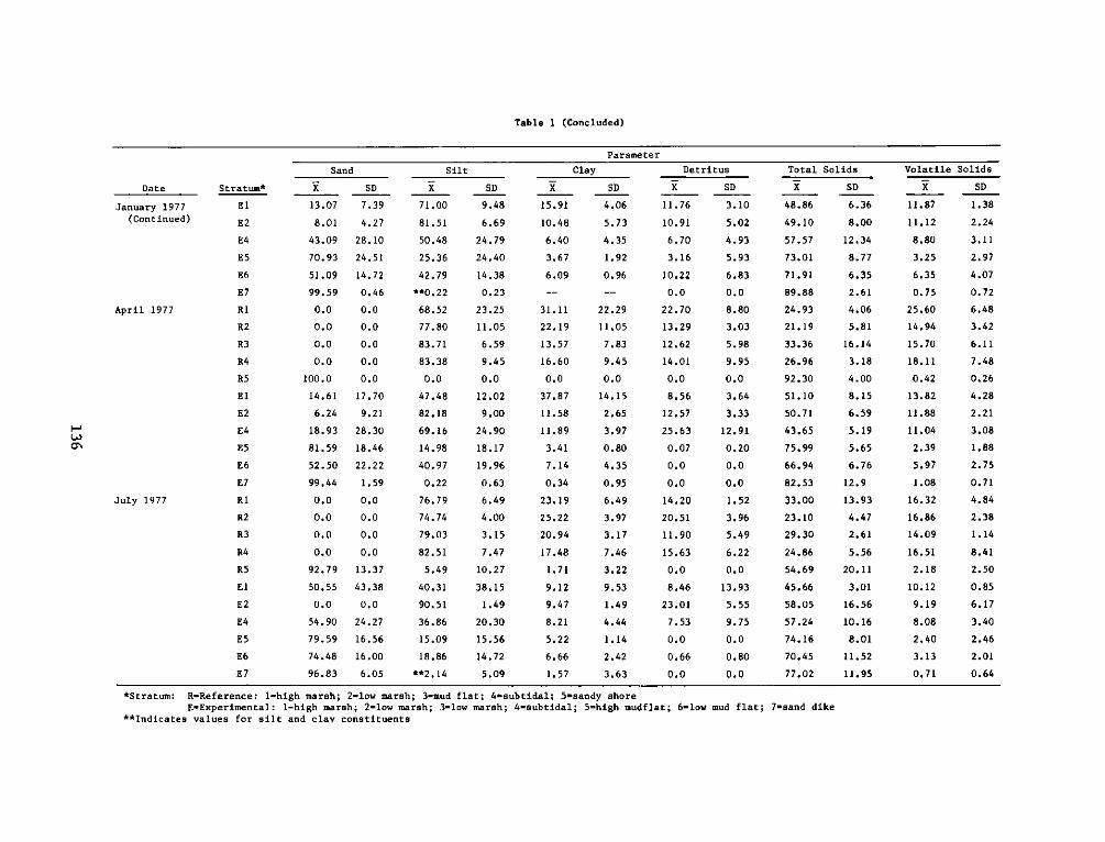
Table 1 (Concluded)
Date Stratum*
January 1977 El(Continued) E2
E4
ES
E6
E7
April 1977 Ri
R2
R3
R4
R5
El
E2
E4
ES
E6
E7
July 1977 Ri
R2
R3
R4
R5
El
E2
E4
ES
E6
E7
a'
Parameter
Sand Silt Clay Detritus Total Solids Volatile Solids
X SD X SD X SD X SD X SD XSD
13.07 7.39 71.00 9.48 15.91 4.06 11.76 3.10 48.86 6.36 11.87 1.38
8.01 4.27 81.51 6.69 10.48 5.73 10.91 5.02 49.10 8.00 11.12 2.24
43.09 28.10 50.48 24.79 6.40 4.35 6.70 4.93 57.57 12.34 8.80 3.11
70.93 24.51 25.36 24.40 3.67 1.92 3.16 5.93 73.01 8.77 3.25 2.97
51.09 14.72 42.79 14.38 6.09 0.96 10.22 6.83 71.91 6.35 6.35 4.07
99.59 0.46 **0.22 0.23 -- -- 0.0 0.0 89.88 2.61 0.75 0.720.0 0.0 68.52 23.25 31.11 22.29 22.70 8.80 24.93 4.06 25.60 6.48
0.0 0.0 77.80 11.05 22.19 11.05 13.29 3.03 21.19 5.81 14.94 3.42
0.0 0.0 83.71 6.59 13.57 7.83 12.62 5.98 33.36 16.14 15.70 6.11
0.0 0.0 83.38 9.45 16.60 9.45 14.01 9.95 26.96 3.18 18.11 7.48
100.0 0.0 0.0 0.0 0.0 0.0 0.0 0.0 92.30 4.00 0.42 0.26
14.61 17.70 47.48 12.02 37.87 14.15 8.56 3.64 51.10 8.15 13.82 4.28
6.24 9.21 82.18 9.00 11.58 2.65 12.57 3.33 50.71 6.59 11.88 2.21
18.93 28.30 69.16 24.90 11.89 3.97 25.63 12.91 43.65 5.19 11.04 3.08
81.59 18.46 14.98 18.17 3.41 0.80 0.07 0.20 75.99 5.65 2.39 1.88
52.50 22.22 40.97 19.96 7.14 4.35 0.0 0.0 66.94 6.76 5.97 2.75
99.44 1.59 0.22 0.63 0.34 0.95 0.0 0.0 82.53 12.9 1.08 0.71
0.0 0.0 76.79 6.49 23.19 6.49 14.20 1.52 33.00 13.93 16.32 4.84
0.0 0.0 74.74 4.00 25.22 3.97 20.51 3.96 23.10 4.47 16.86 2.38
0.0 0.0 79.03 3.15 20.94 3.17 11.90 5.49 29.30 2.61 14.09 1.14
0.0 0.0 82.51 7.47 17.48 7.46 15.63 6.22 24.86 5.56 16.51 8.41
92.79 13.37 5.49 10.27 1.71 3.22 0.0 0.0 54.69 20.11 2.18 2.50
50.55 43.38 40.31 38.15 9.12 9.53 8.46 13.93 45.66 3.01 10.12 0.85
0.0 0.0 90.51 1.49 9.47 1.49 23.01 5.55 58.05 16.56 9.19 6.17
54.90 24.27 36.86 20.30 8.21 4.44 7.53 9.75 57.24 10.16 8.08 3.40
79.S9 16.56 1S.09 15.S6 5.22 1.14 0.0 0.0 74.16 8.01 2.40 2.46
74.48 16.00 18.86 14.72 6.66 2.42 0.66 0.80 70.4S 11.52 3.13 2.01
96.83 6.OS **2.14 5.09 1.57 3.63 0.0 0.0 77.02 11.95 0.71 0.64
*Stratum: R-Reference: 1-high marsh; 2-low marsh; 3-mud flat; 4-subtidal; 5-sandy shoreE=Experimental: 1-high marsh; 2-low marsh; 3-low marsh; 4-subtidal; 5-high mudflat; 6-low mud flat; 7-sand dike
**Indicates values for silt and clay constituents
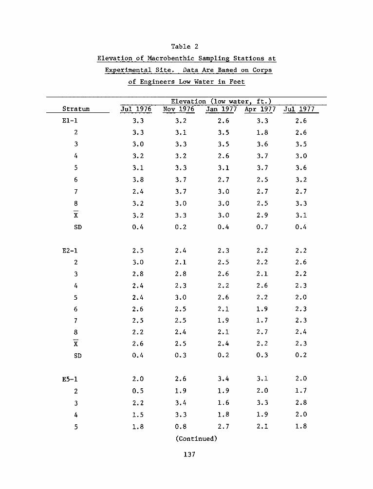
Table 2
Elevation of Nacrobenthic Sampling Stations at
Experimental Site, Data Are Based on Corps
of Engineers Low Water in Feet
Stratum Jul 1976
El-i
2
3
4
5
6
7
8
SD
E2-l
2
3
4
5
6
7
8
SD
2
3
4
5
3.3
3.3
3.0
3.2
3.1
3.8
2.4
3.2
3.2
0.4
2.5
3.0
2.8
2.4
2.4
2.6
2.5
2.2
2.6
0.4
2.0
0.5
2.2
1.5
1.8
Elevation (low water, ft.)Nov 1976
3.2
3.1
3.3
3.2
3.3
3.7
3.7
3.0
3.3
0.2
2.4
2.1
2.8
2.3
3.0
2.5
2.5
2.4
2.5
0.3
Jan 1977 Apr 1977 Jul 1977
2.6
3.5
3.5
2.6
3.1
2.7
3.0
3.0
3.0
0.4
2.3
2.5
2.6
2.2
2.6
2.1
1.9
2.1
2.4
0.2
2.6 3.4
1.9 1.9
3.4 1.6
3.3 1.8
0.8 2.7
(Continued)
137
3.3
1.8
3.6
3.7
3.7
2.5
2.7
2.5
2.9
0.7
2.2
2.2
2.1
2.6
2.2
1.9
1.7
2.7
2.2
0.3
3.1
2.0
3.3
1.9
2.1
2.6
2.6
3.5
3.0
3.6
3.2
2.7
3.3
3.1
0.4
2.2
2.6
2.2
2.3
2.0
2.3
2.3
2.4
2.3
0.2
2.0
1.7
2.8
2.0
1.8
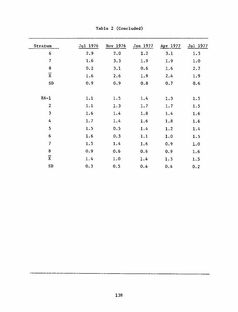
Table 2 (Concluded)
Jul 1976
2.9
1.6
0.2
1.6
0.9
Stratum
6
7
8
SD
Nov 1976
2.0
3.3
3.1
2.6
0.9
1.5
1.3
1.4
1.4
0.5
0.3
1.4
0.6
1.0
0.5
138
Jan 1977
1.2
1.9
0.6
1.9
0.8
1.4
1.7
1.8
1.6
1.4
1.1
1.6
0.6
1. 4
0.4
E6-1
2
3
4
5
6
7
8
SD
Apr 1977
3.1
1.9
1.6
2.4
0.7
1.3
1.7
1.4
1.8
1.2
1.0
0.9
0.9
1. 3
0.4
1.1
1.1
1.6
1.7
1.5
1.6
1.5
0.9
1. 4
0.3
Jul 1977
1.3
1.0
2.7
1.9
0.6
1.5
1.5
1.6
1.6
1.4
1.5
1.0
1.6
1. 5
0.2
1
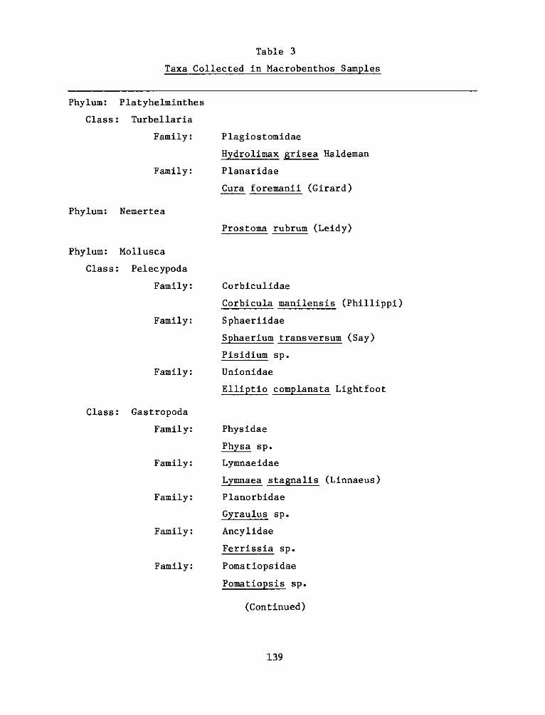
Table 3
Taxa Collected in Macrobenthos Samples
Phylum: Platyhelminthes
Class: Turbellaria
Family:
Family:
Phylum: Nemertea
Phylum: Mollusca
Class: Pelecypoda
Family:
Family:
Family:
Class: Gastropoda
Family:
Family:
Family:
Family:
Family:
Plagiostomidae
Hydrolimax grisea Haldeman
P lanaridae
Cura foremanii (Girard)
Prostoma rubrum (Leidy)
Corbiculidae
Corbicula manilensis (Phillippi)
Sphaeriidae
Sphaerium transversum (Say)
Pisidium sp.
Unionidae
Elliptio complanata Lightfoot
Phys idae
Physa sp.
Lymnae idae
Lymnaea stagnalis (Linnaeus)
Planorbidae
Gyraulus sp.
Ancylidae
Ferrissia sp.
Pomatiopsidae
Pomatiopsis sp.
(Continued)
139
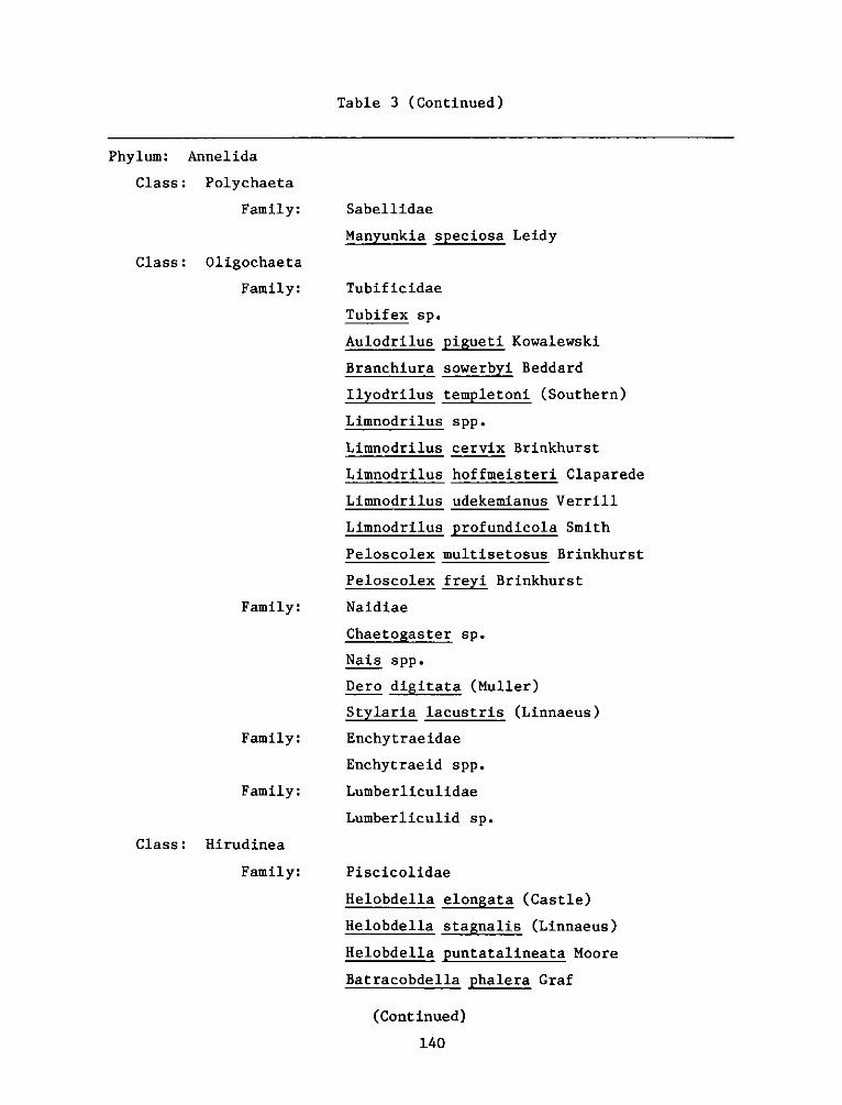
Table 3 (Continued)
Phylum: Annelida
Class: Polychaeta
Family:
Class: Oligochaeta
Family:
Family:
Family:
Family:
Class: Hirudinea
Family:
Sabellidae
Manyunkia speciosa Leidy
Tubif ic idae
Tubifex sp.
Aulodrilus pigueti Kowalewski
Branchiura sowerbyi Beddard
Ilyodrilus templetoni (Southern)
Limnodrilus spp.
Limnodrilus cervix Brinkhurst
Limnodrilus hoffmeisteri Claparede
Limnodrilus udekemianus Verrill
Limnodrilus profundicola Smith
Peloscolex multisetosus Brinkhurst
Peloscolex freyi Brinkhurst
Naidiae
Chaetogaster sp.
Nais spp.
Dero digitata (Muller)
Stylaria lacustris (Linnaeus)
Enchytraeidae
Enchytraeid spp.
Lumberliculidae
Lumberliculid sp.
Piscicolidae
Helobdella elongata (Castle)
Helobdella stagnalis (Linnaeus)
Helobdella puntatalineata Moore
Batracobdella phalera Graf
(Continued)
140
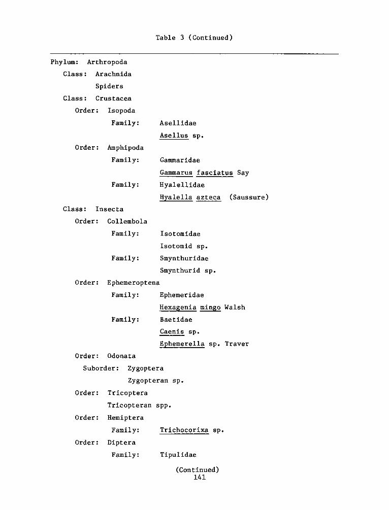
Table 3 (Continued)
Phylum: Arthropoda
Class: Arachnida
Spiders
Class: Crustacea
Order: Isopoda
Family:
Order: Amphipoda
Family:
Family:
Class: Insecta
Order: Collembola
Family:
Family:
Order: Ephemeroptena
Family:
Family:
Order: Odonata
Suborder: Zygoptera
Zygopteran sp.
Order: Tricoptera
Tricopteran spp.
Order: Hemiptera
Family: Tricho4
Order: Diptera
Family: Tipuli
Asellidae
Asellus sp.
Gammaridae
Gammarus fasciatus Say
Hyalellidae
Hyalella azteca (Saussure)
Iso tomidae
Isotomid sp.
Smynthuridae
Smynthurid sp.
Ephemeridae
Hexagenia mingo Walsh
Baetidae
Caenis sp.
Ephemerella sp. Traver
corixa sp.
dae
(Continued)141
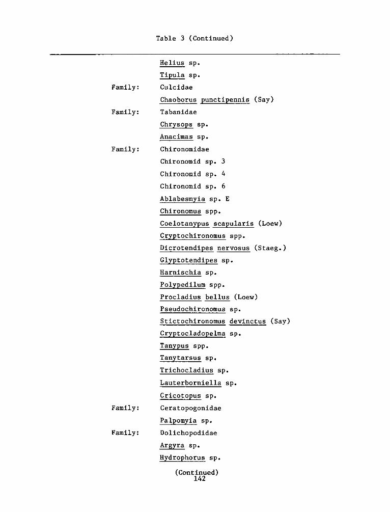
Table 3 (Continued)
Helius sp.
Tipula sp.
Family: Culcidae
Chaoborus punctipennis (Say)
Family: Tabanidae
Chrysops sp.
Anacimas sp.
Family: Chironomidae
Chironomid sp. 3
Chironomid sp. 4
Chironomid sp. 6
Ablabesmyla sp. E
Chironomus spp.
Coelotanypus scapularis (Loew)
Cryptochironomus spp.
Dicrotendipes nervosus (Staeg.)
Glyptotendipes sp.
Harnischia sp.
Polypedilum spp.
Procladius bellus (Loew)
Pseudochironomus s p.
Stictochironomus devinctus (Say)
Cryptocladopelma sp.
Tanypus spp.
Tanytarsus sp.
Trichocladius sp.
Lauterborniella sp.
Cricotopus sp.
Family: Ceratopogonidae
Palpomyia sp.
Family: Dolichopodidae
Argyra sp.
Hydrophorus sp.
(Continued)142

Table 3 (Concluded)
Order: Coleoptera
Family: Chrysomelidae
Donacia sp.
143
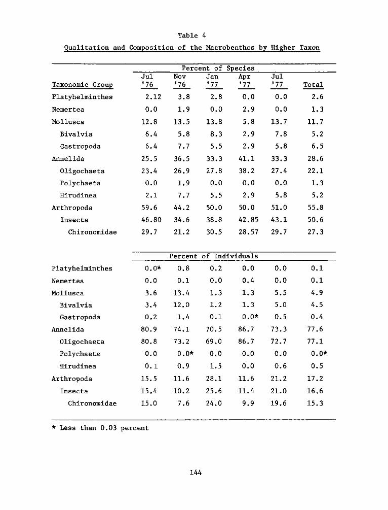
Table 4
Qualitation and Composition of the Macrobenthos by Higher Taxon
Taxonomic Group
Platyhelminthes
Nemertea
Mollusca
Bivalvia
Gas tropoda
Annelida
Oligochaeta
Polychaeta
Hirudinea
Arthropoda
Insecta
Chironomidae
Percent of
'76
2.12
0.0
12.8
6.4
6.4
25.5
23.4
0.0
2.1
59.6
46.80
29.7
'76
3.8
1.9
13.5
5.8
7.7
36.5
26.9
1.9
7.7
44.2
34.6
21.2
Jan'77
2.8
0.0
13.8
8.3
5.5
33.3
27.8
0.0
5.5
50.0
38.8
30.5
Platyhelminthes
Nemertea
Mollusca
Bivalvia
Gastropoda
Annelida
Oligochaeta
Polychaeta
Hirudinea
Arthropoda
Insecta
Chironomidae
0.0*
0.0
3.6
3.4
0.2
80.9
80.8
0.0
0. 1
15.5
15.4
15.0
Percent
0.8
0.1
13.4
12.0
1.4
74.1
73.2
0.0*
0.9
11.6
10.2
7.6
of Individuals
0.2 0.0
0.0 0.4
1.3 1.3
1.2 1.3
0.1 Q.**
70.5 86.7
69.0 86.7
0.0 0.0
1.5 0.0
28.1 11.6
25.6 11.4
24.0 9.9
* Less than 0.03 percent
144
SpeciesApr'77
0.0
2.9
5.8
2.9
2.9
41.1
38.2
0.0
2.9
50.0
42.85
28.57
Jul
'77
0.0
0.0
13.7
7.8
5.8
33.3
27.4
0.0
5.8
51.0
43.1
29.7
Total
2.6
1.3
11.7
5.2
6.5
28.6
22.1
1.3
5.2
55.8
50.6
27.3
0.0
0.0
5.5
5.0
0.5
73.3
72.7
0.0
0.6
21.2
21.0
19.6
0.1
0.1
4.9
4.5
0.4
77.6
77.1
0.0*
0.5
17.2
16.6
15.3
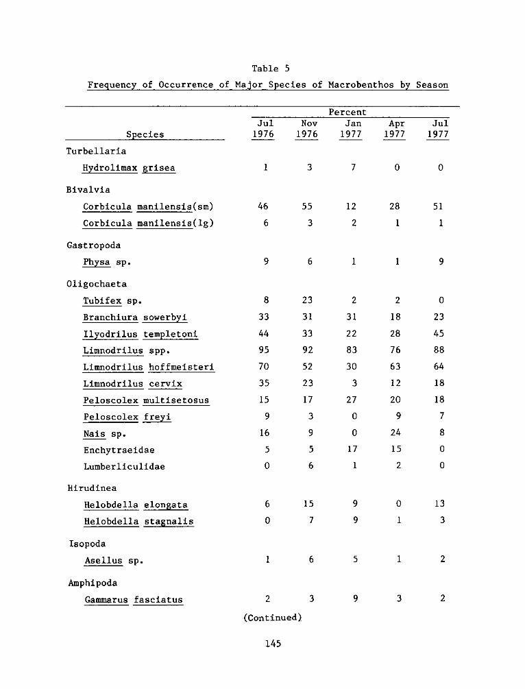
Table 5
Frequency of Occurrence of Major Species of Macrobenthos by Season
PercentJul Nov Jan Apr Jul
Species 1976 1976 1977 1977 1977
Turbellaria
Hydrolimax grisea 1 3 7 0 0
Bivalvia
Corbicula manilensis(sm) 46 55 12 28 51
Corbicula manilensis(lg) 6 3 2 1 1
Gast ropoda
Physa sp. 9 6 1 1 9
Oligochaeta
Tubifex sp. 8 23 2 2 0
Branchiura sowerbyi 33 31 31 18 23
Ilyodrilus templetoni 44 33 22 28 45
Limnodrilus spp. 95 92 83 76 88
Limnodrilus hoffmeisteri 70 52 30 63 64
Limnodrilus cervix 35 23 3 12 18
Peloscolex multisetosus 15 17 27 20 18
Peloscolex freyi 9 3 0 9 7
Nais sp. 16 9 0 24 8
Enchytraeidae 5 5 17 15 0
Lumberliculidae 0 6 1 2 0
Hirud inea
Helobdella elongata 6 15 9 0 13
Helobdella stagnalis 0 7 9 1 3
Isopoda
Asellus sp. 1 6 5 1 2
Amphipoda
Gammarus fasciatus 2 3 9 3 2
(Continued)
145
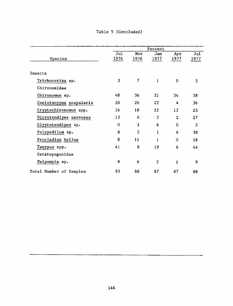
Table 5 (Concluded)
Jul Nov1976 1976
Trichocorixa sp.
Chironomidae
Chironomus sp.
Coelotanypus scapularis
Cryptochironomus spp.
Dicrotendipes nervosus
Glyptotendipes sp.
Polypedilum sp.
Procladius bellus
Tanypus spp.
Ceratopogonidae
Palpomyia sp.
Total Number of Samples
3 7 1 0
48 36 31 34 38
20
16
13
0
8
26 22 4 36
18 22 13 23
0 2 2 27
3
5
8 11
41
8
6
1
1
8 19
6 2
0
6 38
0 18
6 44
1
93 88 87 87 88
146
Species
Insecta
PercentJan
1977Apr1977
Jul1977
5
2
9
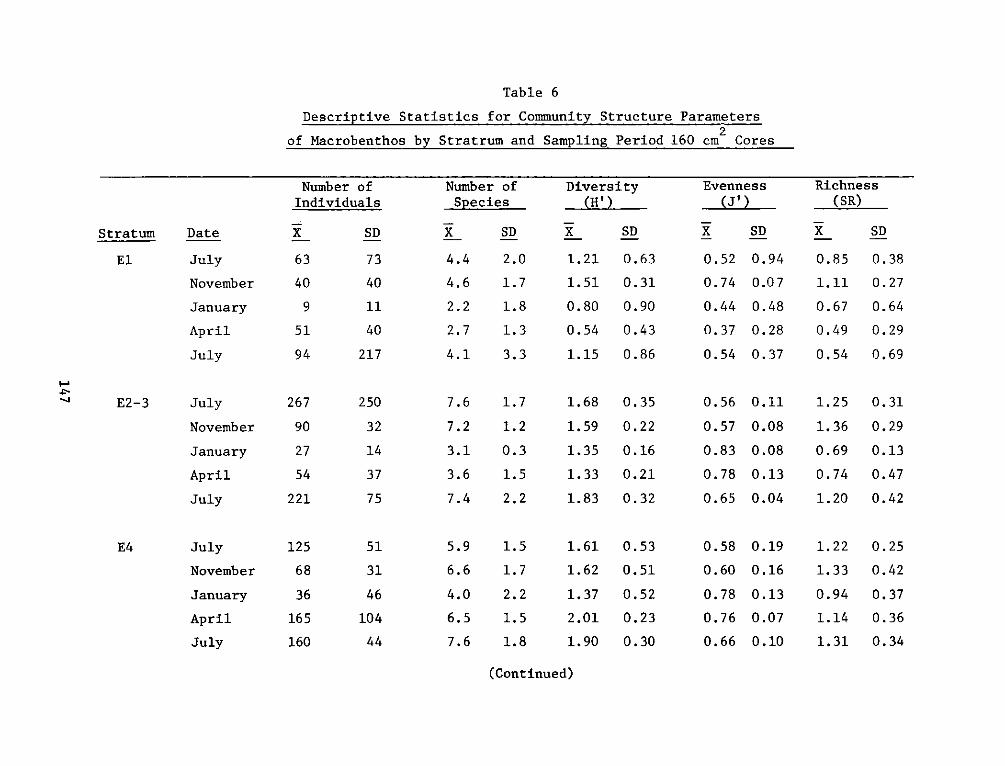
Table 6
Descriptive Statistics for Community Structure Parameters
of _Macrobenthos by Stratrum andSampling Period 160 cm Cores
Number of Richness
Individuals
K SD
63 73
40 40
9 11
51 40
94 217
Date
July
November
January
April
July
July
November
January
April
July
July
November
January
April
July
250
32
14
37
75
51
31
46
104
44
Number ofSpecies
X_4.4
4.6
2.2
2.7
4.1
7.6
7.2
3.1
3.6
7.4
5.9
6.6
4.0
6.5
7.6
SD
2.0
1.7
1.8
1.3
3.3
1.7
1.2
0.3
1.5
2.2
1.5
1.7
2.2
1.5
1.8
Diversity
1.21
1.51
0.80
0.54
1.15
1.68
1.59
1.35
1.33
1.83
1.61
1.62
1.37
2.01
1.90
Evenness(J')
SD
0.63
0.31
0.90
0.43
0.86
0.35
0.22
0.16
0.21
0.32
0.53
0.51
0.52
0.23
0.30
0.52
0.74
0.44
0.37
0.54
0.56
0.57
0.83
0.78
0.65
0.58
0.60
0.78
0.76
0.66
SD
0.94
0.07
0.48
0.28
0.37
0.11
0.08
0.08
0.13
0.04
0.19
0.16
0.13
0.07
0.10
(SR)
XSD
0.85 0.38
1.11 0.27
0.67 0.64
0.49 0.29
0.54 0.69
1.25
1.36
0.69
0.74
1.20
1.22
1.33
0.94
1.14
1.31
0.31
0.29
0.13
0.47
0.42
0.25
0.42
0.37
0.36
0.34
(Continued)
Stratum
El
E2-3
E4
267
90
27
54
221
125
68
36
165
160
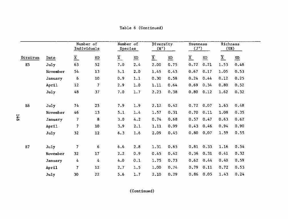
Table 6 (Continued)
Number ofIndividuals
X SD
63 52
54 13
6 10
12 7
48 37
Stratrum
ES
E6
E7
Date
July
November
January
April
July
July
November
January
April
July
July
November
January
April
July
Number of
Species
SSD
7.0 2.4
5.1 2.0
0.9 1.1
2.9 1.0
7.0 1.7
7.9
5.1
3.0
3.9
6.3
6.6
2.2
4.0
2.7
5.6
1.9
1.4
4.2
2.1
1.6
2.8
0.9
0.1
1.5
1.7
Diversity(H')
2.00
1.45
0.30
1.11
2.23
2.12
1.57
0.74
1.11
2.09
1.31
0.45
1.75
1.00
2.10
Eyenness(J')
SD
0.75
0.43
0.58
0.64
0.38
0.42
0.31
0.68
0.99
0.45
0.65
0.42
0.73
0.74
0.29
x0.72
0.67
0.24
0.69
0.80
0.72
0.70
0.57
0.43
0.80
0.81
0.36
0.62
0.79
0.86
SD
0.21
0.17
0.44
0.34
0.12
0.07
0.11
0.47
0.46
0.07
0.33
0.31
0.44
0.11
0.05
Richness(SR)
SSD
1.53 0.48
1.05 0.53
0.12 0.25
0.80 0.52
1.62 0.32
1.63
1.08
0.63
0.94
1.59
1.16
0.41
0.40
0.72
1.43
0.48
0.35
0.62
0.90
0.55
0.54
0.32
0.59
0.53
0.24
(Continued)
74
46
7
7
32
7
32
4
7
30
25
13
8
10
12
6
17
4
12
22
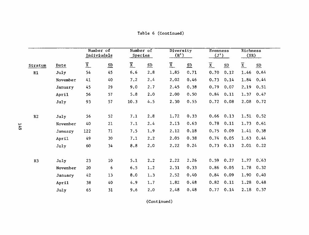
Table 6 (Continued)
Number ofIndiviudals
54
41
45
56
93
56
40
122
49
60
23
20
42
38
65
Stratum
Ri
R2
Number ofSpecies
6.6
7.2
9.0
5.8
10.3
7.1
7.1
7.5
7.1
8.8
5.1
6.5
8.0
4.9
9.6
Date
July
November
January
April
July
July
November
January
April
July
July
November
January
April
July
Diversity(H')
1.85
2.02
2.45
2.00
2.30
1.72
2.13
2.12
2.05
2.22
2.22
2.31
2.52
1.82
2.48
Evenness(J')
SD
45
40
29
57
57
52
21
71
30
34
10
6
13
40
31
0.70
0.73
0.79
0.84
0.72
0.66
0.78
0.75
0.74
0.73
0.59
0.86
0.84
0.82
0.77
SD
2.8
2.4
2.7
2.0
4.5
2.8
2.4
1.9
2.2
2.0
2.2
1.2
1.3
1.7
2.0
Richness(SR)
3ESD
1.46 0.64
1.84 0.44
2.19 0.51
1.37 0.47
2.08 0.72
SD
0.71
0.46
0.38
0.50
0.55
0.33
0.63
0.18
0.38
0.24
2.26
0.33
0.40
0.48
0.48
SD
0.12
0.14
0.07
0.11
0.08
0.13
0.11
0.09
0.05
0.13
0.27
0.05
0.09
0.11
0.14
(Continued)
1.51
1.73
1.41
1.63
2.01
1.27
1.78
1.90
1.28
2.18
'-a
'.0
R3
0.52
0.61
0.38
0.44
0.22
0.63
0.32
0.40
0.48
0.37
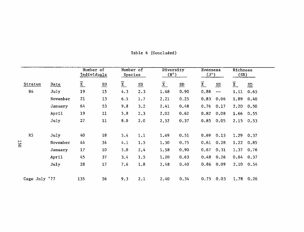
Table 6 (Concluded)
Number ofIndividuals
X_ SD
19 15
21 13
64 53
19 11
27 11
40
44
17
45
28
18
34
10
37
17
Number ofSpecies
4.3
6.5
9.8
5.8
8.0
5.4
4.1
5.0
3.4
7.6
SD
2.3
1.7
3.2
2.3
2.0
1.1
1.5
2.4
1.5
1.8
Diversity(H')
1.48
2.21
2.41
2.02
2.52
1.69
1.30
1.58
1.20
2.48
SD
0.90
0.25
0.48
0.62
0.37
0.51
0.75
0.90
0.63
0.40
Evenness(J')
0.88
0.83
0.76
0.82
0.85
0.69
0.61
0.67
0.48
0.86
SD
0.06
0.17
0.08
0.05
0.15
0.28
0.31
0.26
0.09
Richness(SR)
XSD
1.11 0.65
1.89 0.40
2.20 0.50
1.66 0.55
2.15 0.53
1.29
1.22
1.37
0.64
2.10
CageJul '7713556 9.3 2.1 2.40 0.34 0.5 00 .8 02
StratumR4
R5
U,
Date
July
November
January
April
July
July
November
January
April
July
0.37
0.85
0.76
0.37
0.54
Cage July '77 135 0.75 0.03 1.78 0.26
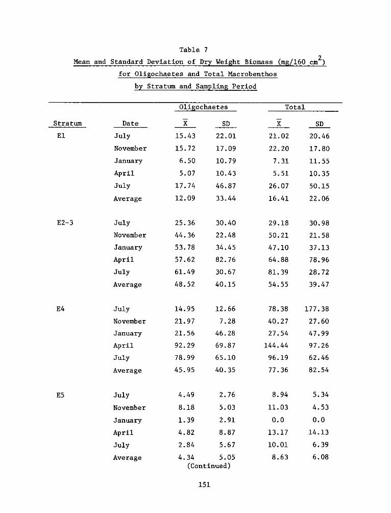
Table 7
Mean and Standard Deviation of Dry Weight Biomass (mg/160 cm2)for Oligochaetes and Total Macrobenthos
by Stratum and Sampling Period
Oligochaetes
Stratum
El
Date
July
November
January
April
July
Average
July
November
January
April
July
Average
July
November
January
April
July
Average
July
November
January
April
July
Average
Total
X__ SD
21.02 20.46
22.20 17.80
7.31 11.55
5.51 10.35
26.07 50.15
16.41 22.06
X15.43
15.72
6.50
5.07
17.74
12.09
25.36
44.36
53.78
57.62
61.49
48.52
14.95
21.97
21.56
92.29
78.99
45.95
4.49
8.18
1.39
4.82
2.84
4.34
SD
22.01
17.09
10.79
10.43
46.87
33.44
30.40
22.48
34.45
82.76
30.67
40.15
12.66
7.28
46.28
69.87
65.10
40.35
2.76
5.03
2.91
8.87
5.67
5.05(Continued)
151
29.18
50.21
47.10
64.88
81.39
54.55
78.38
40.27
27.54
144.44
96.19
77.36
8.94
11.03
0.0
13.17
10.01
8.63
E2-3
E4
ES
30.98
21.58
37.13
78.96
28.72
39.47
177.38
27.60
47.99
97.26
62.46
82.54
S.34
4.53
0.0
14.13
6.39
6.08
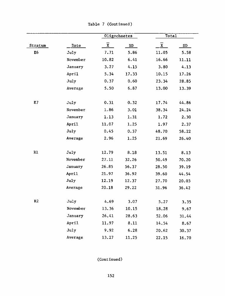
Table 7 (Continued)
Oligochaetes
X__ SD
7.71 5.86
10.82 6.41
3.27 4.15
5.34 17.33
0.37 0.60
5.50 6.87
Stratum
E6
Date
July
November
January
April
July
Average
July
November
January
April
July
Average
July
November
January
April
July
Average
July
November
January
April
July
Average
8.18
32.26
56.37
36.92
12.37
29.22
3.07
10.15
28.63
8.11
6.28
11.25
Total
X SD
11.05 5.58
16.66 11.11
3.80 4.13
10.15 17.26
23.34 28.85
13.00 13.39
17.74
38.34
1.72
1.97
48.70
21.69
13.51
50.49
28.50
39.60
27.70
31.96
5.27
18.28
52.06
14.54
20.62
22.15
44.86
24.24
2.30
2.37
58.22
26.40
8.13
70.20
39.19
44.54
20.03
36.42
3.35
9.67
31.44
8.67
30.37
16.70
(Continued)
152
0.32
3.01
1.31
1.25
0.37
1.25
E7
Ri
R2
0.31
1.86
1.13
11.07
0.45
2.96
12.79
27.11
26.85
21.97
12.19
20.18
4.69
13.36
26.41
11.97
9.92
13.27
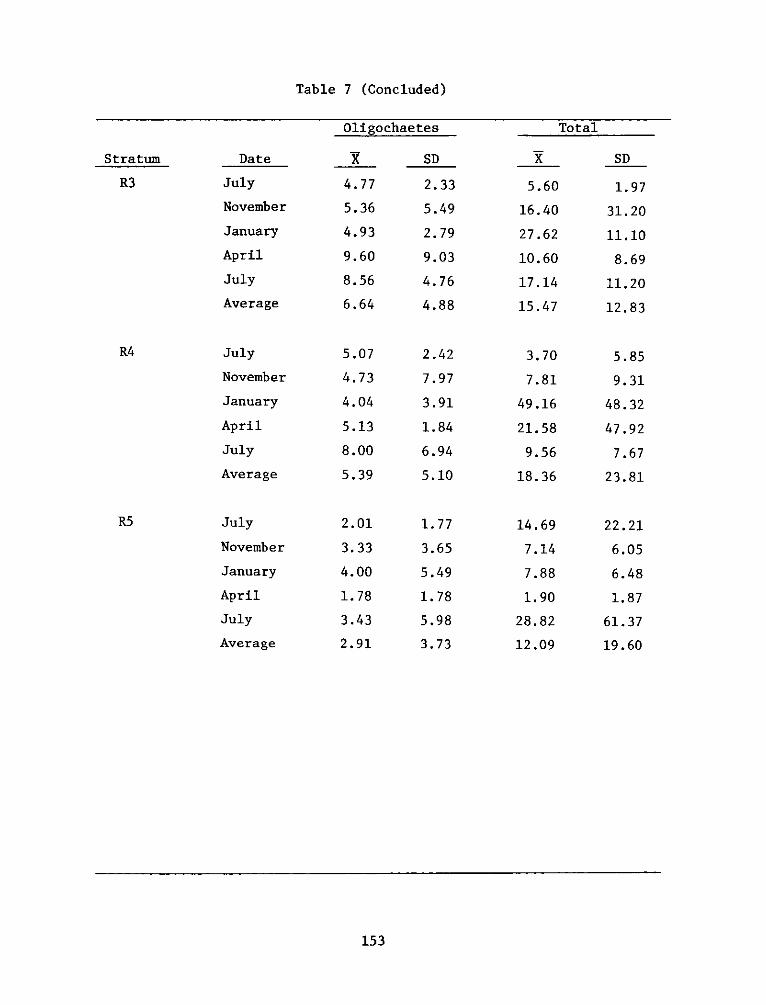
Table 7 (Concluded)
Oligochaetes
X SD
4.77 2.33
5. 36 5. 49
4.93 2.79
9. 60 9 .03
8.56 4.76
6.64 4.88
Stratum
R3
Date
July
November
January
April
July
Average
July
November
January
April
July
Average
July
November
January
April
July
Average
Total
X SD
5.60 1.97
16. 40 31. 20
27.62 11.10
10 .60 8. 69
17.14 11.20
15.47 12.83
3.70
7.81
49.16
21.58
9.56
18.36
14.69
7.14
7.88
1. 90
28.82
12.09
5.85
9.31
48.32
47.92
7.67
23.81
22.21
6.05
6.48
1.87
61.37
19.60
153
2.42
7.97
3.91
1.84
6.94
5.10
1.77
3.65
5.49
1. 78
5.98
3.73
R4
R5
5.07
4.73
4.04
5.13
8.00
5.39
2.01
3.33
4.00
1. 78
3.43
2.91
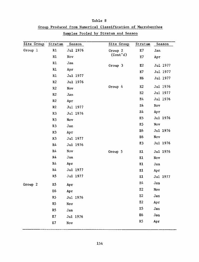
Table 8
Group Produced from Numerical Classification of Macrobenthos
Samples Pooled by Stratum and Season
Site Group Stratum
Group 1 Rl
Rl
Rl
Ri
Rl
R2
R2
R2
R2
R2
R3
R3
R3
R3
R3
R4
R4
R4
R4
R4
R5
Group 2 E5
E6
R5
R5
R5
E7
E7
Site Group
Group 2(Cont'd)
Group 3
Season
Jul 1976
Nov
Jan
Apr
Jul 1977
Jul 1976
Nov
Jan
Apr
Jul 1977
Jul 1976
Nov
Jan
Apr
Jul 1977
Jul 1976
Nov
Jan
Apr
Jul 1977
Jul 1977
Apr
Apr
Jul 1976
Nov
Jan
Jul 1976
Nov
Group 4
Group 5
154
Season
Jan
Apr
Jul
Jul
Jul
1977
1977
1977
Stratum
E7
E7
E2
E7
E6
E2
E2
E4
E4
E4
E5
E5
E6
E6
E3
El
El
El
El
El
E4
E2
E2
E2
E5
E6
R5
Jul 1976
Jul 1977
Jul 1976
Nov
Apr
Jul 1976
Nov
Jul 1976
Nov
Jul 1976
Jul 1976
Nov
Jan
Apr
Jul 1977
Jan
Nov
Jan
Apr
Jan
Jan
Apr
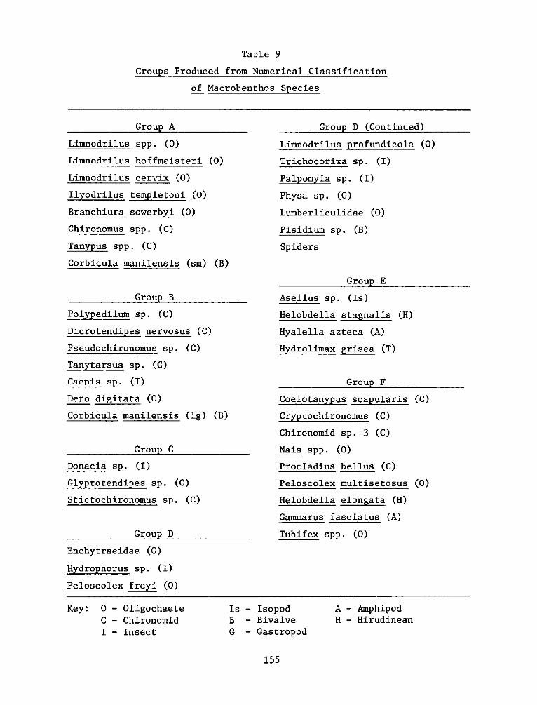
Table 9
Groups Produced from Numerical Classification
of lMacrobenthos Species
Group A
Limnodrilus spp. (0)
Limnodrilus hoffmeisteri (0)
Limnodrilus cervix (0)
Ilyodrilus templetoni (0)
Branchiura sowerbyi (0)
Chironomus spp. (C)
Tanypus spp. (C)
Corbicula manilensis (sin) (B)
Group B
Polypedilum sp. (C)
Dicrotendip es nervosus (C)
Pseudochironomus sp. (C)
Tanytarsus sp. (C)
Caenis sp. (I)
Dero digitata (0)
Corbicula manilensis (lg) (B)
Group C
Donacia sp. (I)
Glyptotendipes sp. (C)
Stictochironomus sp. (C)
Group D
Enchytraeidae (0)
Hydrophorus sp. (I)
Peloscolex freyi (0)
Group D (Continued)
Limnodrilus profundicola (0)
Trichocorixa sp. (I)
Palpomyia sp. (I)
Physa sp. (G)
Lumberliculidae (0)
Pisidium sp. (B)
Spiders
Group E
Asellus sp. (Is)
Helobdella stagnalis (H)
Hyalella azteca (A)
Hydrolimax grisea (T)
Group F
Coelotanypus scapularis (C)
Cryptochironomus (C)
Chironomid sp. 3 (C)
Nais spp. (0)
Procladius bellus (C)
Peloscolex multisetosus (0)
Helobdella elongata (H)
Gammarus fasciatus (A)
Tubifex spp. (0)
Key: 0 - OligochaeteC - ChironomidI - Insect
Is - IsopodB - BivalveG - Gastropod
A - AmphipodH - Hirudinean
155
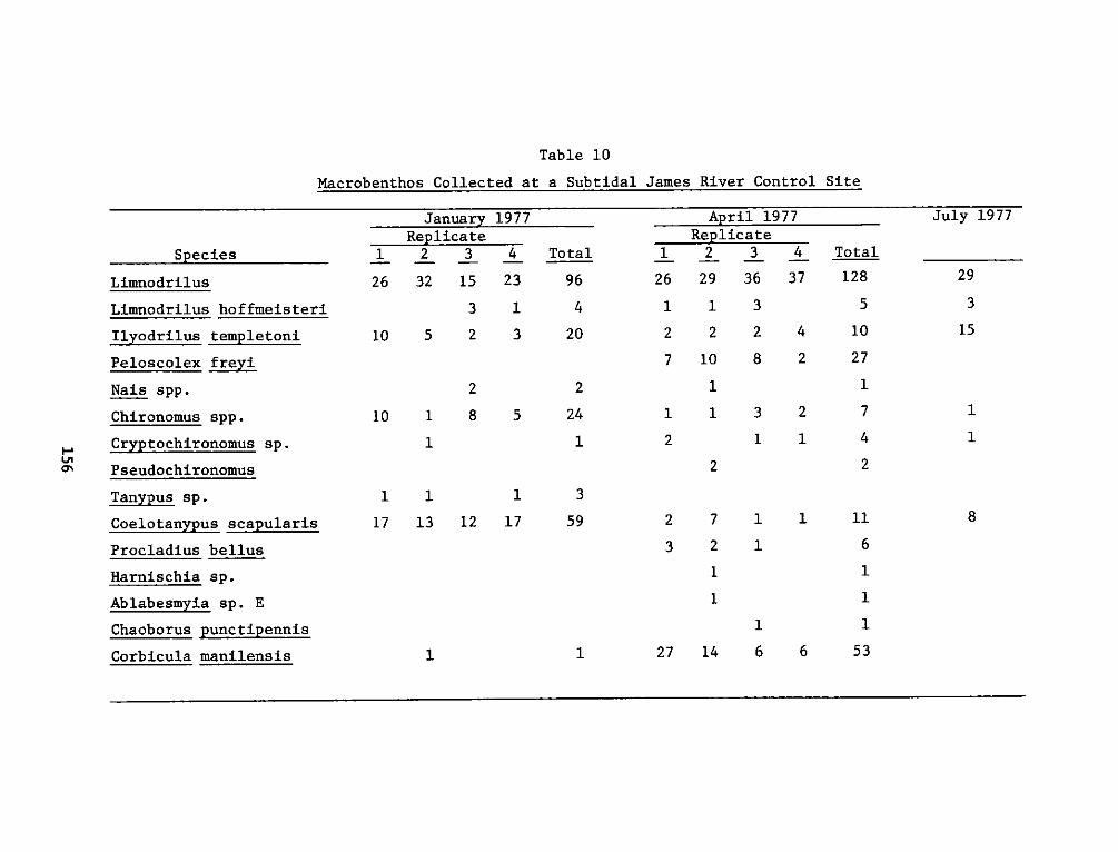
Macrobenthos Collected at
Table 10
a Subtidal James River Control Site
Species
Limnodrilus
Limnodrilus hoffmeisteri
Ilyodrilus templetoni
Peloscolex freyi
Nais spp.
Chironomus spp.
Cryptochironomus sp.
Pseudochironomus
Tanypus sp.
Coelotanypus scapularis
Procladius bellus
Harnischia sp.
Ablabesmyia sp. E
Chaoborus punctipennis
Corbicula manilensis
January 1977Replicate
_1 _2_ _3_ _4_ Total
26 32 15 23 96
3 1 4
10 5 2 3 20
2
10 1 8
1
2
5 24
April 1977Replicate
_1_ _2_ _3_ _4_
26 29 36 37
1 1 3
2 2 2 4
7 10 8 2
1
21
1 3
1
2
1
2
1
17
1
13
1
12 17
3
59
1 1
2 7
3 2
1
1
Total
128
5
10
27
7
4
2
111
6
27 14 6 6 53
'-aU'0%
JULy J1977
29
3
15
1
1
8

Table 11
Taxa Collected in Meiobenthos Samples
Phylum: Aschelminthes
Clas s: Nematoda
Nematode sp. 10
Nematode sp. 11
Order: Monohysteridae
Family: Monohysteridae
Monohystera sp.
Monohystrella sp. 1
Monohystrella sp. 2
Order: Dorylaimida
Family: Dorylaimidae
Dorylaimus sp.
Amphidorylaimus sp.
Thornenema sp.
Family: Mononchidae
Anatonchus sp.
Family: Bathyodontidae
Alaimus sp.
Order: Araeolaimida
Family: Plectidae
Paraplectonema sp.
Phylum: Tardigrada
Class: Eutardigrada
Family: Macrobiotidae
Macrobiotus richtersii J. Murray
Macrobiotus dispar J. Murray
Macrobiotus furcatus Ehrenberg
Macrobiotus hufelandii S. Schultze
Hypsibius sp.
Class: Heterotardigrada
(Continued)
157
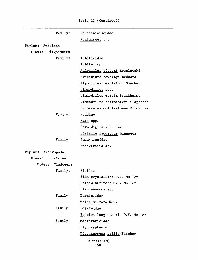
Table 11 (Continued)
Scutechiniscidae
Echiniscus sp.
Phylum: Annelida
Class: Oligochaeta
Family:
Family:
Family:
Phylum: Arthropoda
Class: Crustacea
Order: Cladocera
Family:
Family:
Family:
Family:
Tubificidae
Tubifex sp.
Aulodrilus pigueti Kowalewski
Branchiura sowerbyi Beddard
Ilyodrilus templetoni Southern
Limnodrilus spp.
Limnodrilus cervix Brinkhurst
Limnodrilus hoffmesteri Claparede
Peloscolex multisetosus Brinkhurst
Naidiae
Nais spp.
Dero digitata Muller
tylari lacustris Linnaeus
Enchytrae idae
Enchytraeid sp.
Sididae
Sida crystallina Q.F. Muller
Latona setifera Q.F. Muller
Diaphanosoma sp.
Daphiniidae
Moina micrura Kurz
Bosminidae
Bosmina longirostris O.F. Muller
Macrothricidae
Ilyocryptus spp.
Diaphanosoma agilis Fischer
(Ccntinued)158
Family:
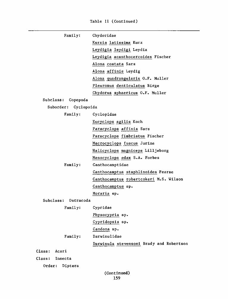
Table 11 (Continued)
Family: Chydoridae
Kurzia latissima Kurz
Leydigia leydigi Leydia
Leydigia acanthocercoides Fischer
Alona costata Sars
Alona affinis Leydig
Alona quadrangularis O.F. Muller
Pleuroxus denticulatus Birg e
Chydorus sphaericus O.F. Muller
Subclass: Copepoda
Suborder: Cyclopoida
Family: Cyclopidae
Eucyclops agilis Koch
Paracyclops affinis Sars
Paracyclops fimbriatus Fischer
Macrocyclops fuscus Jurine
Halicyclops magniceps Lilljeborg
Mesocyclops edax S.A. Forbes
Family: Canthocamptidae
Canthocamptus staphlinoides Pearse
Canthocamptus robertcokeri M.S. Wilson
Canthocamptus sp.
Moraria sp.
Subclass: Ostracoda
Family: Cypridae
Physocypria sp.
Cypridopsis sp.
Candona sp.
Family: Darwinulidae
Darwinula stevensoni Brady and Robertson
Class: Acari
Class: Insecta
Order: Diptera
(Continued)159
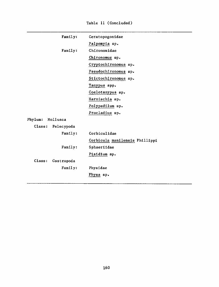
Table 11 (Concluded)
Family:
Family:
Phylum: Mollusca
Class: Pelecypoda
Family:
Family:
Class: Gastropoda
Family:
Corbiculidae
Corbicula manilensis Phillippi
S phaeriidae
Pisidium sp.
Phys idae
Physa sp.
160
Ceratopogonidae
Palpomyla sp.
Chironomidae
Chironomus sp.
C ryptochironomus
Pseudochironomus
S tictochironomus
Tanypus spp.
Coelotanypus sp.
Harnischia sp.
Polypedilum sp.
Procladius sp.
sp.
sp.
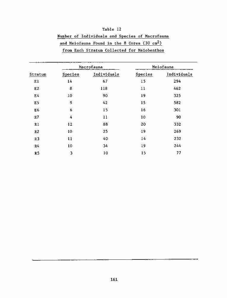
Table 12
Number of Individuals and Species of Macrofauna
and Meiofauna Found in the 8 Cores (30 cm2 )
from Each Stratum Collected for Meiobenthos
Macrofauna
Species Individuals
14 67
8 118
10 90
9 42
6 15
4
12
10
11
10
3
11
88
25
40
34
10
Meiofauna
Species Individuals
15 294
11 462
19 325
15 582
16 301
10 90
20 332
19 269
14 232
19 244
15 77
161
Stratum
El
E2
E4
E5
E6
E7
Ri
R2
R3
R4
R5
.I
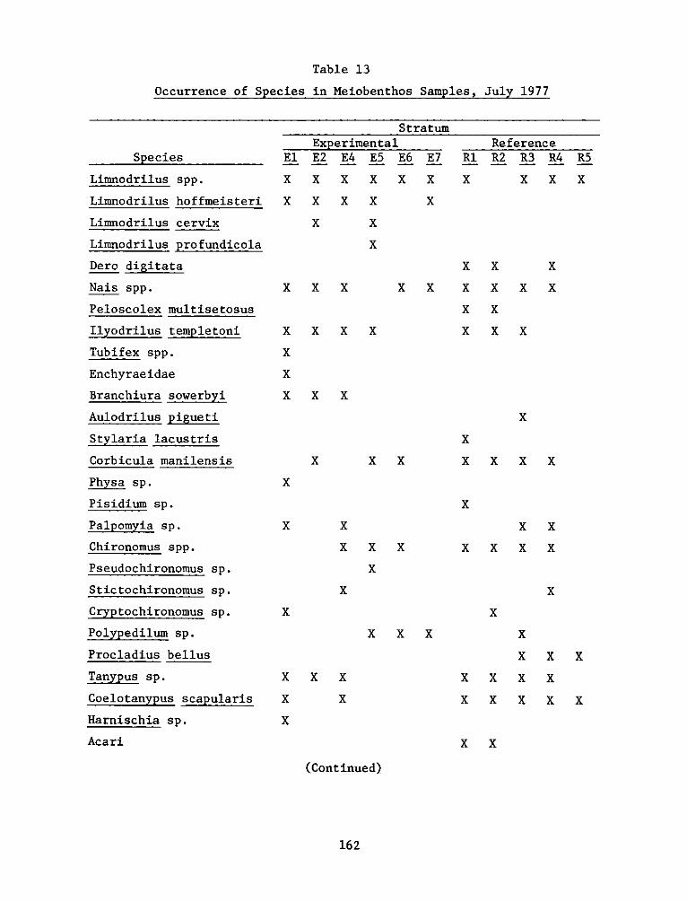
Table 13
Occurrence of Species in M1eiobenthos Samples. July 1977
Species
Limnodrilus spp.
Limnodrilus hoffmeisteri
Limnodrilus cervix
Limnodrilus profundicola
Dero digitata
Nais spp.
Peloscolex multisetosus
Ilyodrilus templetoni
Tubifex spp.
Enchyraeidae
Branchiura sowerbyi
Aulodrilus pigueti
Stylaria lacustris
Corbicula manilensis
Physa sp.
Pisidium sp.
Palpomyta sp.
Chironomus spp.
Pseudochironomus sp.
Stictochironomus sp.
Cryptochironomus sp.
Polypedilum sp.
Procladius bellus
Tanypus sp.
Coelotanypus scapularis
Harnischia sp.
Acari
El
Xx
Experimental
E2 E_4 E5 E6
X X X XX x Xx
Stratum
E7
xX
xX
X X X
xXX
x x X
xX X x
XX
ReferenceRl R2 R3 R4 R5
X X X X
xX X
x
xXXX
X X X
Xx
X
X X
Xx
X
X xX
XX
x
X
x X x
XX x X
X
XX
XX
X X X
xxX
X Xx
XX
XX
XXXX
XXX
X
X
X X(Continued)
162
,
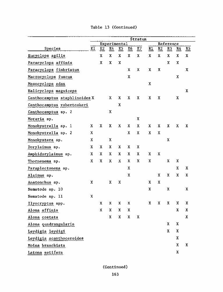
Table 13 (Continued)
Species
Eucyclops agilis
Paracyclops affinis
Paracyclops fimbriatus
Macrocyclops fuscus
Mesocyclops edax
Halicyclops magniceps
Canthocamptus staphlinoides
Canthocamp tus robertcokeri
Canthocamptus sp. 2
Moraria sp.
Monohystrella sp. 1
Monohystrella sp. 2
Monohystera sp.
Dorylaimus sp.
Amphidorylaimus sp.
Thornenema sp.
Paraplectonema sp.
Alaimus sp.
Anatonchus sp.
Nematode sp. 10
Nematode sp. 11
Ilyocryptus spp.
AMona af finis
Alona costata
Alona quadrangularis
Leydigia leydigi
Leydigia acanthoceroides
Moina branchiata
Latona setifera
StratumExperimental Reference
El E2 E4 E5 E6 E7
X X X X XX x X
XX
X
Rl R2 R3 R4 R5
X XX X X
XX
xx x X
XX X X x
x
x X x X xX XX XX X X X Xx x x X xX X X X X
XX
X X X
XXX
xxX
x X XX X
X X
X
x xX
XX XX
X XX X
x X X
X x
XX X x XX X X X
X X X X
X X X
xX
X XX X
XXxXx xX
(Continued)
163
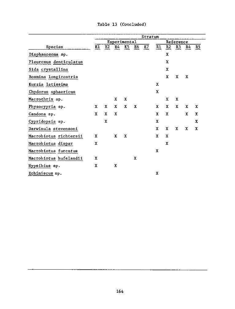
Table 13 (Concluded)
Species
Diaphanosoma sp.
Pleuroxus denticulatus
Sida crystallina
Bosmina longirostris
Kurzia latissima
Chydorus sphaericus
Nacrothrix sp.
Physocypria sp.
Candona sp.
Cypridopsis sp.
Darwinula stevensoni
Macrobiotus richtersii
Macrobiotus dispar
Macrobiotus furcatus
Macrobiotus hufelandii
Hypsibius sp.
Echiniscus sp.
StratumExperimental
El E2 E4 E5 E6 E7
XX
XXX
XX
XX
XxX
XX X
Rl R2 R3 R4 R5
xXXX X X
XX
XXXXX
X
X x
XXx
XXx
XX X x
X XX
X X X
XX
X
164
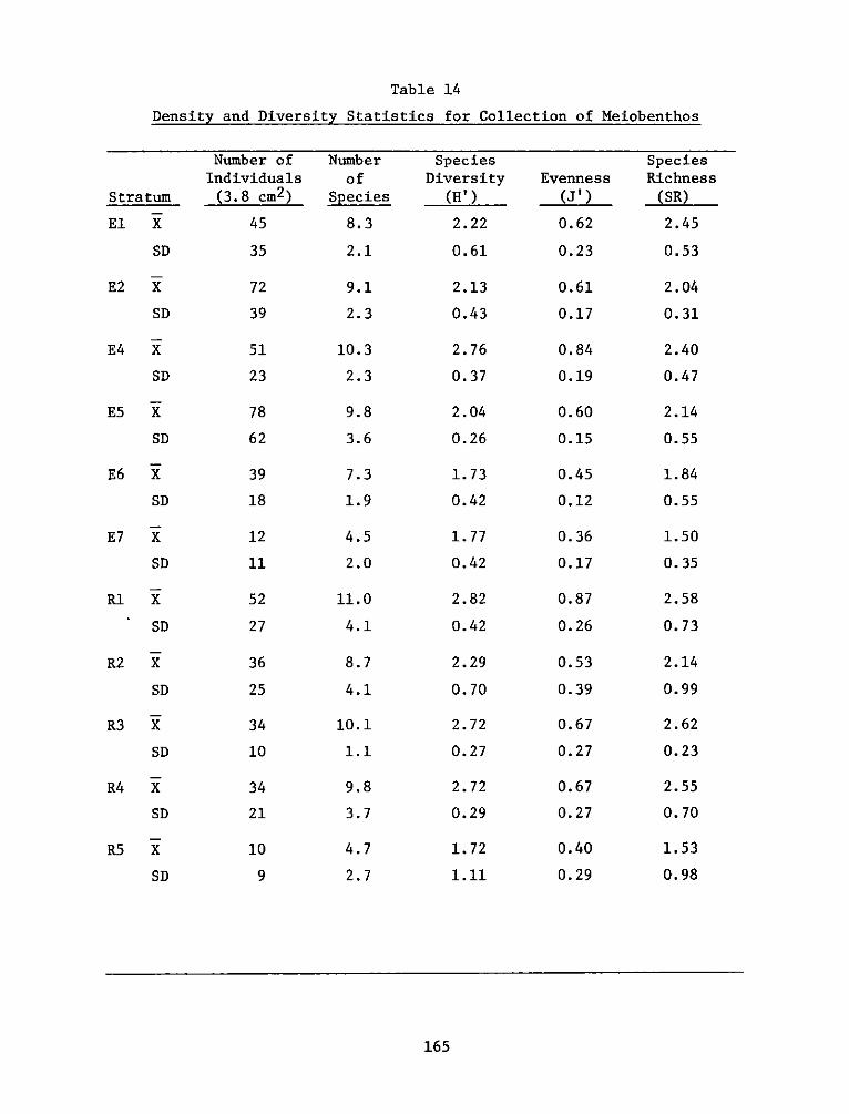
Table 14
Density and Diversity Statistics for Collection of Neiobenthos
Stratum
El X
SD
E2 i
SD
E4 I
SD
ES i
SD
E6 i
SD
E7 iSD
Ri 2
SD
R2 X
SD
R3 i
SD
R4 i
SD
RS i
SD
Number ofIndividuals(3.8 cm2 )
45
35S
72
39
S1
23
78
62
39
18
12
11
S2
27
36
25
34
10
34
21
10
9
Numberof
Species
8.3
2.1
9.1
2.3
10.3
2.3
9.8
3.6
7.3
1.9
4.5
2.0
11.0
4.1
8.7
4.1
10.1
1.1
9.8
3.7
4.7
2.7
165
SpeciesDiversity
(H')
2.22
0.61
2.13
0.43
2.76
0.37
2.04
0.26
1.73
0.42
1.77
0.42
2.82
0.42
2.29
0.70
2.72
0.27
2.72
0.29
1.72
1.11
Evenness(J')
0.62
0.23
0.61
0.17
0.84
0.19
0.60
0.15
0.45
0.12
0.36
0.17
0.87
0.26
0.53
0.39
0.67
0.27
0.67
0.27
0.40
0.29
SpeciesRichness(SR)
2.45
0.53
2.04
0.31
2.40
0.47
2.14
0.55
1.84
0.55
1.50
0.35
2.58
0.73
2.14
0.99
2.62
0.23
2.55
0.70
1.53
0.98
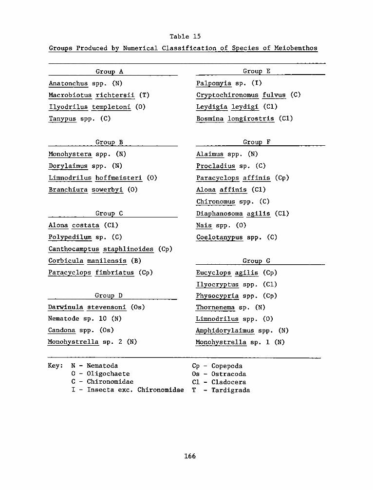
Table 15
Groups Produced by Numerical Classification of Species of Meiobenthos
Group A
Anatonchus spp. (N)
Macrobiotus richtersii (T)
Ilyodrilus templetoni (0)
Tanypus spp. (C)
Group B
Monohystera spp. (N)
Dorylaimus spp. (N)
Limnodrilus hoffmeisteri (0)
Branchiura sowerbyi (0)
Group C
Alona costata (Cl)
Polypedilum sp. (C)
Canthocamptus staphlinoides (Cp)
Corbicula manilensis (B)
Paracyclops fimbriatus (Cp)
Group D
Darwinula stevensoni (Os)
Nematode sp. 10 (N)
Candona spp. (Os)
Monohystrella sp. 2 (N)
Group E
Palpomyia sp. (I)
Cryptochironomus fulvus (C)
Leydigia leydigi (Cl)
Bosmina longirostris (Cl)
Group FAlaimus spp. (N)
Procladius sp. (C)
Paracyclops affinis (Cp)
Alona affinis (Cl)
Chironomus spp. (C)
Diaphanosoma agilis (Cl)
Nais spp. (0)
Coelotanypus spp. (C)
Group G
Eucyclops agilis (Cp)
Ilyocryptus spp. (Cl)
Physocypria spp. (Cp)
Thornenema sp. (N)
Limnodrilus spp. (0)
Amphidorylaimus spp. (N)
Monohystrella sp. 1 (N)
Key: N - NematodaO - OligochaeteC - ChironomidaeI - Insecta exc. Chironomidae
Cp - CopepodaOs - OstracodaCl - CladoceraT - Tardigrada
166
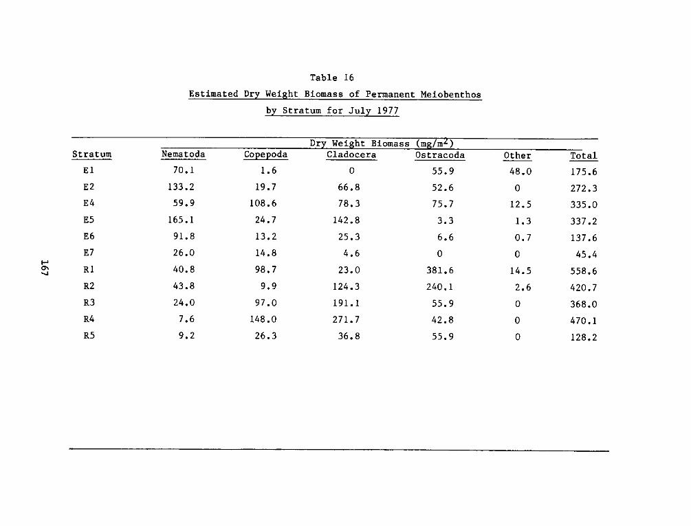
Table 16
Estimated Dry Weight Biomass of Permanent Meiobenthos
by Stratum for July 1977
Dry Weight Biomass (mg/mL)Cladocera Ostracoda
0 55.9
66.8 52.6
78.3 75.7
142.8 3.3
25.3 6.6
4.6 0
23.0 381.6
124.3 240.1
191.1 5S.9
271.7 42.8
36.8 55.9
Other
48.0
0
12.5
1.3
0.7
0
14.5
2.6
0
0
0
Total
175.6
272.3
335.0
337.2
137.6
45.4
558.6
420.7
368.0
470.1
128.2
Stratum
El
E2
E4
ES
E6
E7
Ri
R2
R3
R4
R5
I-a
Nematoda
70.1
133.2
59.9
165.1
91.8
26.0
40.8
43.8
24.0
7.6
9.2
Copepoda
1.6
19.7
108.6
24.7
13.2
14.8
98.7
9.9
97.0
148.0
26.3
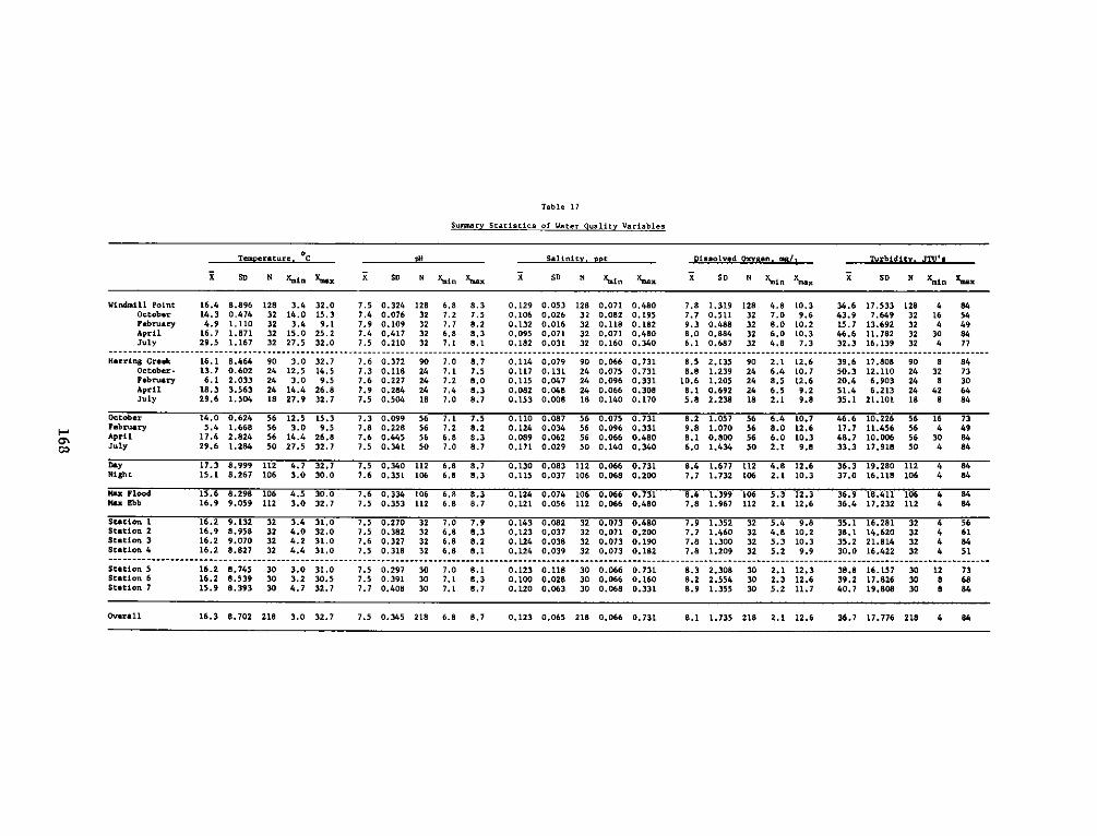
Table 17
Summary Statistics of Water Quality Variables
Temperature, "C p11 Salinity, ppt Dissolved Oxygen. 511/1 Turbidity. JTU'a
K SD N Kiin Euax K SD N lXin Emax K SD N 1Snin 'Snax X SD N Xlin max K SD N anEx
Windmill Point 16.4 8.896 128 3.4 32.0 7.5 0.324 128 6.8 8.3 0.129 0.053 128 0.071 0.480 7.8 1.319 128 4.8 10.3 34.6 17.533 128 4 84October 14.3 0.474 32 14.0 15.3 7.4 0.076 32 7.2 7.5 0.106 0.026 32 0.082 0.195 7.7 0.511 32 7.0 9.6 43.9 7.649 32 16 54February 4.9 1.110 32 3.4 9.1 7.9 0.109 32 7.7 8.2 0.132 0.016 32 0.118 0.182 9.3 0.488 32 8.0 10.2 15.7 13.692 32 4 49April 16.7 1.871 32 15.0 25.2 7.4 0.417 32 6.8 8.3 0.095 0.071 32 0.071 0.480 8.0 0.884 32 6.0 10.3 46.6 11.782 32 30 84July 29.5 1.167 32 27.5 32.0 7.5 0.210 32 7.1 8.1 0.182 0.031 32 0.160 0.340 6.1 0.687 32 4.8 7.3 32.3 16.139 32 4 77
Herring Creek 16.1 8.484 90 3.0 32.7 7.6 0.372 90 7.0 8.7 0.114 0.079 90 0.066 0.731 8.5 2.135 90 2.1 12.6 39.6 17.808 90 8 84October. 13.7 0.602 24 12.5 14.5 7.3 0.118 24 7.1 7.5 0.117 0.131 24 0.075 0.731 8.8 1.239 24 6.4 10.7 50.3 12.110 24 32 73February 6.1 2.033 24 3.0 9.5 7.6 0.227 24 7.2 8.0 0.115 0.047 24 0.096 0.331 10.6 1.205 24 8.5 12.6 20.4 6.903 24 8 30April 18.3 3.563 24 14.4 26.8 7.9 0.284 24 7.4 8.3 0.082 0.048 24 0.066 0.308 8.1 0.692 24 6.5 9.2 51.4 6.213 24 42 64July 29.6 1.504 18 27.9 32.7 7.5 0.504 18 7.0 8.7 0.153 0.008 18 0.140 0.170 5.8 2.238 18 2.1 9.8 35.1 21.101 18 8 84
October 14.0 0.624 56 12.5 15.3 7.3 0.099 56 7.1 7.5 0.110 0.087 56 0.075 0.731 8.2 1.057 56 6.4 10.7 46.6 10.226 56 16 73February 5.4 1.668 56 3.0 9.5 7.8 0.228 56 7.2 8.2 0.124 0.034 56 0.096 0.331 9.8 1.070 56 8.0 12.6 17.7 11.456 56 4 49April 17.4 2.824 56 14.4 26.8 7.6 0.445 56 6.8 8.3 0.089 0.062 56 0.066 0.480 8.1 0.800 56 6.0 10.3 48.7 10.006 56 30 84July 29.6 1.284 50 27.5 32.7 7.5 0.341 50 7.0 8.7 0.171 0.029 50 0.140 0.340 6.0 1.434 50 2.1 9.8 33.3 17.918 50 4 84
Day 17.3 8.999 112 4.7 32.7 7.5 0.340 112 6.8 8.7 0.130 0.083 112 0.066 0.731 8.4 1.677 112 4.8 12.6 36.3 19.280 112 4 84Night 15.1 8.267 106 3.0 30.0 7.6 0.351 106 6.8 8.3 0.115 0.037 106 0.068 0.200 7.7 1.732 106 2.1 10.3 37.0 16.118 106 4 84
Max Flood 15.6 8.298 106 4.5 30.0 7.6 0.334 106 6.8 8.3 0.124 0.074 106 0.066 0.731 8.4 1.399 106 5.3 12.3 36.9 18.411 106 4 84Max Ebb 16.9 9.059 112 3.0 32.7 7.5 0.353 112 6.8 8.7 0.121 0.056 112 0.066 0.480 7.8 1.967 112 2.1 12.6 36.4 17.232 112 4 84
Station 1 16.2 9.132 32 3.4 31.0 7.5 0.270 32 7.0 7.9 0.143 0.082 32 0.073 0.480 7.9 1.352 32 5.4 9.8 35.1 16.281 32 4 56Station 2 16.9 8.958 32 4.0 32.0 7.5 0.382 32 6.8 8.3 0.123 0.037 32 0.071 0.200 7.7 1.460 32 4.8 10.2 38.1 14.620 32 4 61Station 3 16.2 9.070 32 4.2 31.0 7.6 0.327 32 6.8 8.2 0.124 0.038 32 0.073 0.190 7.8 1.300 32 5.3 10.3 35.2 21.814 32 4 84Station 4 16.2 8.827 32 4.4 31.0 7.5 0.318 32 6.8 8.1 0.124 0.039 32 0.073 0.182 7.8 1.209 32 5.2 9.9 30.0 16.422 32 4 51
Station 5 16.2 8.745 30 3.0 31.0 7.5 0.297 30 7.0 8.1 0.123 0.118 30 0.066 0.731 8.3 2.308 30 2.1 12.3 38.8 16.157 30 12 73Station 6 16.2 8.539 30 3.2 30.5 7.5 0.391 30 7.1 8.3 0.100 0.028 30 0.066 0.160 8.2 2.554 30 2.3 12.6 39.2 17.826 30 8 68Station 7 15.9 8.393 30 4.7 32.7 7.7 0.408 30 7.1 8.7 0.120 0.063 30 0.068 0.331 8.9 1.355 30 5.2 11.7 40.7 19.808 30 8 84
Ovrall16.3 8.702 218 3.0 32.7 7.5 0.345 218 6.8 8.7 0.123 0.065 218 0.066 0.731 8.1 1.735 218 2.1 12.6 36.7 17.776 218 4 84Overall
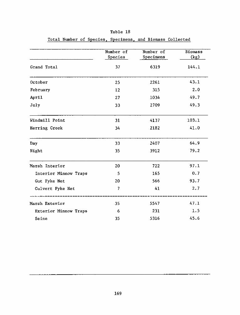
Table 18
Total Number of Species, Specimens, and Biomass Collected
Number of Number of Biomass
___________________ Species Specimens (kg)
Grand Total 37 6319 144.1
October 25 2261 43.1
February 12 315 2.0
April 27 1034 49.7
July 33 2709 49.3
Windmill Point 31 4137 103.1
Herring Creek 34 2182 41.0
Day 33 2407 64.9
Night 35 3912 79.2
Marsh Interior 20 722 97.1
Interior Minnow Traps 5 165 0.7
Gut Fyke Net 20 566 93.7
Culvert Fyke Net 7 41 2.7
Marsh Exterior 35 5547 47.1
Exterior Minnow Traps 6 231 1.5
Seine 35 5316 45.6
169
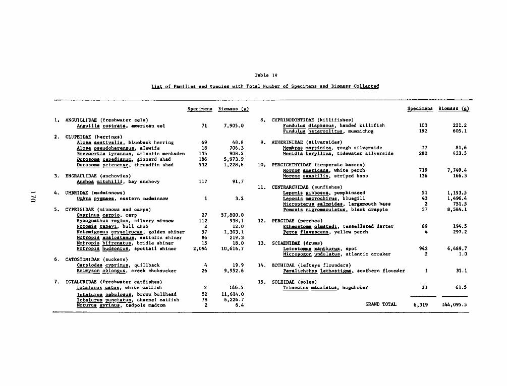
Table 19
with Total Number of Snecimens and Biomas Cletd
Specimens Biomass (g) Specimens Biomass (g)
1. ANGUILLIDAE (freshwater eels)Anguilla rostrata, american eel
2. CLUPEIDAE (herrings)Alosa aestivalis, blueback herringAlosa pseudoharengus, alewifeBrevoortia tyrannus, atlantic menhadenDorosoma cepedianum, gizzard shadDorosoma petenense, threadf in shad
3. ENGRAULIDAE (anchovies)Anchoa mitchilli, bay anchovy
4. UMBRIDAE (mudminnows)Umbra pygmaea, eastern mudminnow
5. CYPRINIDAE (minnows and carps)Cyprinus carpio, carpHybo nathus reis silvery minnowNocomis raneyi, bull chubNotemigonus crysoleucas, golden shinerNotropis analostanus, satinf in shinerNotropis bifrenatus, bridle shinerNotropis hudsonius, spottail shiner
6. CATOSTOMIDAE (suckers)Carpiodes cyprinus, quillbackErimyzon oblongus, creek chubsucker
7. ICTALURIDAE (freshwater catfishes)Ictalurus catus, white catfishIctalurus nebulosus, brown bullheadIctalurus punctatus, channel catfishNoturus gyrinus, tadpole madtom
71 7,905.0
4918
135186532
48.8706.3908.2
5,973.91,228.6
117 91.7
1
2,4
3.2
27 57,800.0112 938.12 12.0
57 1,303.186 219.315 18.0394 10,616.7
4 19.926 9,952.6
252782
146.511,614.06,226.7
6.4
8. CYPRINODONTIDAE (killifishes)Fundulus diaphanus, banded killifishFundulus heteroclitus, munuichog
9. ATHERINIDAE (silversides)Membras martinica, rough silversideMenidia beryllina, tidewater silverside
10. PERCICHThYIDAE (temperate basses)Morone americana, white perchMorone saxatilis, striped bass
11. CENTRARCHIDAE (sunfishes)Lepomis gibbosus, pumpkinseedLepomis macrochirus, bluegillMicropterus salmoides, largemouth bassPomoxis nigromaculatus, black crappie
12. PERCIDAE (perches)Etheostoma olmstedi, tessellated darterPerca flavescens, yellow perch
13. SCIAENIDAE (drums)Leiostomus xanthurus, spotMicropogon undulatus, atlantic croaker
14. BOTHIDAE (lefteye flounders)Paralichthys lethostigma, southern flounder
103 221.2192 605.1
17282
81.6433.5
719 7,749.4136 166.3
51432
37
1,193.51,496.4
751.58,584.1
89 194.54 297.2
942 6,489.72 1.0
1
Trinectes maculatus, hogchoker 33 61.5
GRAND TOTAL 6,319 144,095.5
31.1
4-'
Spst o am es an ec =Li f F ili d i
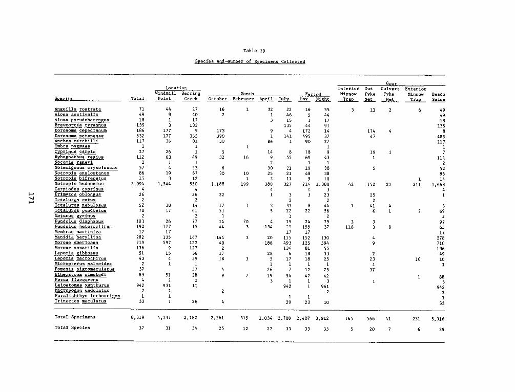
Table 20
Species arnd--Number of Specimens Collected
Species
Anguilla rostrataAlosa aestivalisAlosa pseudoharengusBrevoortia tyrannusDorosoma cepedianumDorosoma petenenseAnchoa mitchilliUmbra pygmaeaCyprinus carpioHybognathus regiusNocomis raneyiNotemigonus crysoleucasNotropis analostanusNotropis bifrenatusNotropis hudsoniusCarpiodes cyprinusErimyzon oblongusIctalurus catusIctalurus nebulosusIctalurus punctatusNoturus gyrinusFundulus diaphanusFundulus heteroclitusMembras martinicaMenidia beryllinaMorone americanaMorone saxatilisLepomis gibbosusLepo4i macrochirusMicropterus salmoidesPomoxis nigromaculatusEtheostoma olmstediPerca flavescensLeiostomus xanthurusMicropogon undulatusParalichthys lethostigmaTrinectes maculatus
GearLoca tion Interior Gut Culvert Exterior
Windmill Herring Month Period Minnow Fyke Fyke Minnow BeachTotal Point Creek October February April July Day Night Trap Net Net Trap Seine
71 44 27 16913
17717736
266314193
1,544
4918
135186532117
271122
578615
2,0944
262
52782
10319217
28271913651432
37894
9422133
4017
1329
35581
1
491
536712
5504
262
14612
7715
14712212736391
37382
11
3817
26177171355979
1541
512
931217
2
17339030
5S32
630
1,188
22
17511
1444
1444021718
49
2
26 4
1 32 22 16 551 46 5 443 15 1 17
135 44 919 4 172 141 141 495 37
86 1 90 27
14 8 18 9L6 9 55 69 43
2 1 130 21 19 38
[0 25 21 48 381 3 11 5 109 380 327 714 1,380
4 1 31 3 3 23
2 21 3 31 8 44
5 22 22 561 2
0 4 15 24 793 134 11 155 37
17 173 20 115 152 130
186 493 125 594134 81 55
28 6 18 333 5 17 18 25
1 1 1 126 7 12 25
7 19 54 47 423 1 1 3
942 1 9412
1 129 23 10
3 11 2
174 447
19 1
5
42 152 21
252
1 41 46 1
3 3116 3 8
49
223
37
6 494918
1358
485117
711125286
114211 1,668
4
62 69
2976517
27871013649
10 10
1883
9422
33
Total Specimens 6,319 4,137 2,182 2,261 315 1,034 2,709 2,407 3,912 165 566 41 231 5,316
Total Species 37 31 34 25 12 27 33 33 35 5 20 7 6 35
19
7
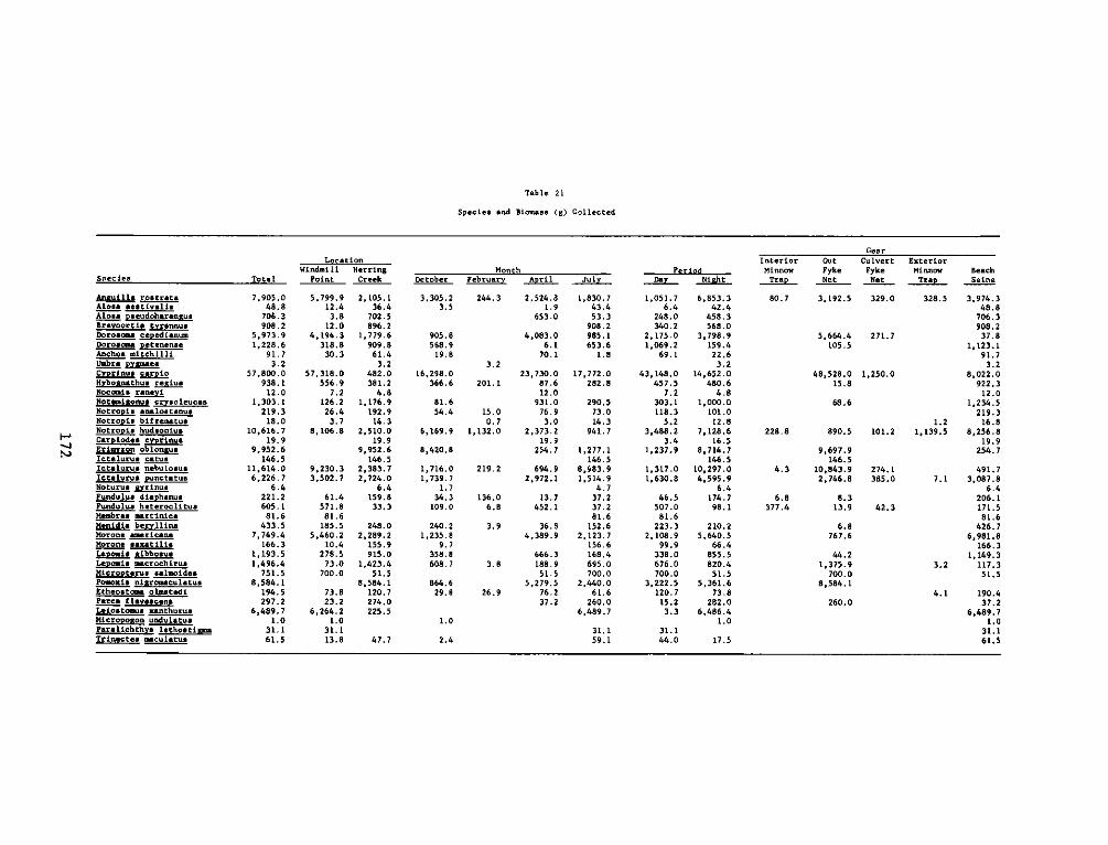
Table 21
Species and Biomase (g) Gollected
Spec les
Anauilla routrataAlosa aestivalisAlosa pseudoharengusBrevoortia tyrannusDoroloma cepedianumDorosoma petenense
Anchoa mitchilliUmbra pygmaeaCyprinus carploNybognathus regiugNocomia raneyiNotemigonue crysoleucasNotropia analoatanueNotropi. bifrenatueNotropie hudeoniug
Carpiodee cyprinusErimyzon oblongueIctalurue catusIctalurue nebulosusIctalurus punctatus
Noturua gyrinumFundulus diaphanusFundulus heteroclitusMembras martinicaMenidia beryllin.Morons amricanaMorone saxatilisLepomis aibbosusLeoomis macrochirusMicropterus saluaoidesPomoxis nigromaculatusEtheostoma olmatediPerca flaveacenaLeiostouss zanthurusMicropogon undulatusParalichthys lethostiuiaTrinactes maculatus
LocationWindmill Mrring Month
Total Point Creek October February April July
7,905.0 5,799.9 2,105.1 3,305.2 244.3 2,524.8 1,830.748.8 12.4 36.4 3.5 1.9 43.4
706.3 3.8 702.5 653.0 53.3908.2 12.0 896.2 908.2
5,973.9 4,194.3 1,779.6 905.8 4,083.0 985.11,228.6 318.8 909.8 568.9 6.1 653.6
91.7 30.3 61.4 19.8 70.1 1.83.2 3.2 3.2
57,800.0 57,318.0 482.0 16,298.0 23,730.0 17,772.0938.1 556.9 381.2 366.6 201.1 87.6 282.8
12.0 7.2 4.8 12.01,303.1 126.2 1,176.9 81.6 931.0 290.5
219.3 26.4 192.9 54.4 15.0 76.9 73.018.0 3.7 14.3 0.7 3.0 14.3
10,616.7 8,106.8 2,510.0 6,169.9 1,132.0 2,373.2 941.719.9 19.9 19.9
9,952.6 9,952.6 8,420.8 254.7 1,277.1146.5 146.5 146.5
11,614.0 9,230.3 2,383.7 1,716.0 219.2 694.9 8,983.96,226.7 3,502.7 2,724.0 1,739.7 2,972.1 1,514.9
6.4 6.4 1.7 4.7221.2 61.4 159.8 34.3 136.0 13.7 37.2605.1 571.8 33.3 109.0 6.8 452.1 37.281.6 81.6 81.6
433.5 185.5 248.0 240.2 3.9 36.8 152.67,749.4 5,460.2 2,289.2 1,235.8 4,389.9 2,123.7
166.3 10.4 155.9 9.7 156.61,193.5 278.5 915.0 358.8 666.3 168.41,496.4 73.0 1,423.4 608.7 3.8 188.9 695.0
751.5 700.0 51.5 51.5 700.08,584.1 8,584.1 864.6 5,279.5 2,440.0
194.5 73.8 120.7 29.8 26.9 76.2 61.6297.2 23.2 274.0 37.2 260.0
6,489.7 6,264.2 225.5 6,489.71.0 1.0 1.0
31.1 31.1 31.161.5 13.8 47.7 2.4 59.1
GearInterior Out Culvert Exterior
Period Minnow Fyke Fyke Minnow BeachDay Night Trap Net Net Trap Seine
1,051.7 6,853.3 80.7 3,192.5 329.0 328.5 3,974.36.4 42.4 48.8
248.0 458.3 706.3340.2 568.0 908.2
2,175.0 3,798.9 5,664.4 271.7 37.81,069.2 159.4 105.5 1,123.1
69.1 22.6 91.73.2 3.2
43,148.0 14,652.0 48,528.0 1,250.0 8,022.0457.5 480.6 15.8 922.3
7.2 4.8 12.0303.1 1,000.0 68.6 1,234.5118.3 101.0 219.3
5.2 12.8 1.2 16.83,488.2 7,128.6 228.8 890.5 101.2 1,139.5 8,256.8
3.4 16.5 19.91,237.9 8,714.7 9,697.9 254.7
146.5 146.51,317.0 10,297.0 4.3 10,843.9 274.1 491.71,630.8 4,595.9 2,746.8 385.0 7.1 3,087.8
6.4 6.446.5 174.7 6.8 8.3 206.1507.0 98.1 377.4 13.9 42.3 171.5
81.6 81.6223.3 210.2 6.8 426.7
2,108.9 5,640.5 767.6 6,981.899.9 66.4 166.3
338.0 855.5 44.2 1,149.3676.0 820.4 1,375.9 3.2 117.3700.0 51.5 700.0 51.5
3,222.5 5,361.6 8,584.1120.7 73.8 4.1 190.415.2 282.0 260.0 37.23.3 6,486.4 6,489.7
1.0 1.031.1 31.144.0 17.5 61.5
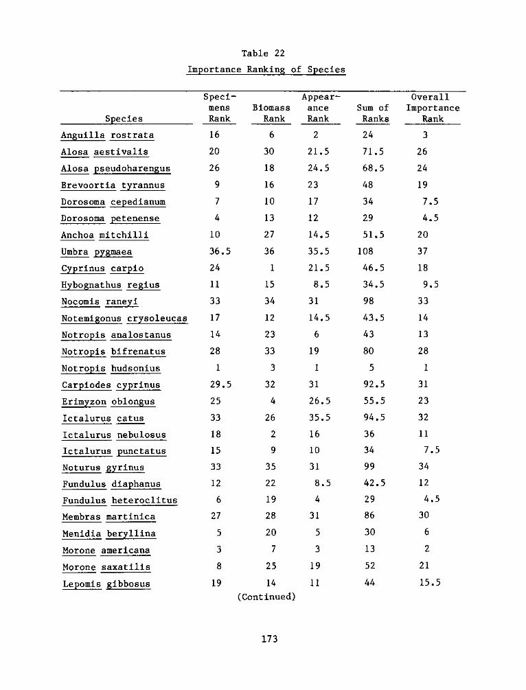
Table 22
Importance Ranking of Species
Species
Anguilla rostrata
Alosa aestivalis
Alosa pseudoharengus
Brevoortia tyrannus
Dorosoma cepedianum
Dorosoma petenense
Anchoa mitchilli
Umbra pygmaea
Cyprinus carpio
Hybognathus regius
Nocomis raneyi
Notemigonus crysoleucas
Nrpis analostanus
Notropis bifrenatus
Notropis hudsonius
Carpiodes cyprinus
Erimyzon oblongus
Ictalurus catus
Ictalurus nebulosus
Ictalurus punctatus
Noturus gyrinus
Fundulus diaphanus
Fundulus heteroclitus
Membras martinica
Menidia beryllina
Morone americana
Morone saxatilis
Lepomis gibbosus
Speci-mens BiomassRank Rank
16 6
20 30
26 18
9 16
7 10
4 13
10 27
36.5 36
24 1
11 15
33 34
17 12
14 23
28 33
1 3
29.5 32
25 4
33 26
18 2
15 9
33 35
12 22
6 19
27 28
5 20
3 7
8 25
19 14
(Continued)
Appear-anceRank
2
21.5
24.5
23
17
12
14.5
35.5
21.5
8.5
31
14.5
6
19
1
31
26.5
35.5
16
10
31
8.5
4
31
5
3
19
11
Sum ofRanks
24
71.5
68.5
48
34
29
51.5
108
46.5
34.5
98
43.5
43
80
5
92.5
55.5
94.5
36
34
99
42.5
29
86
30
13
52
44
OverallImportance
Rank
3
26
24
19
7.5
4.5
20
37
18
9.5
33
14
13
28
1
31
23
32
11
7.5
34
12
4.5
30
6
2
21
15.5
173
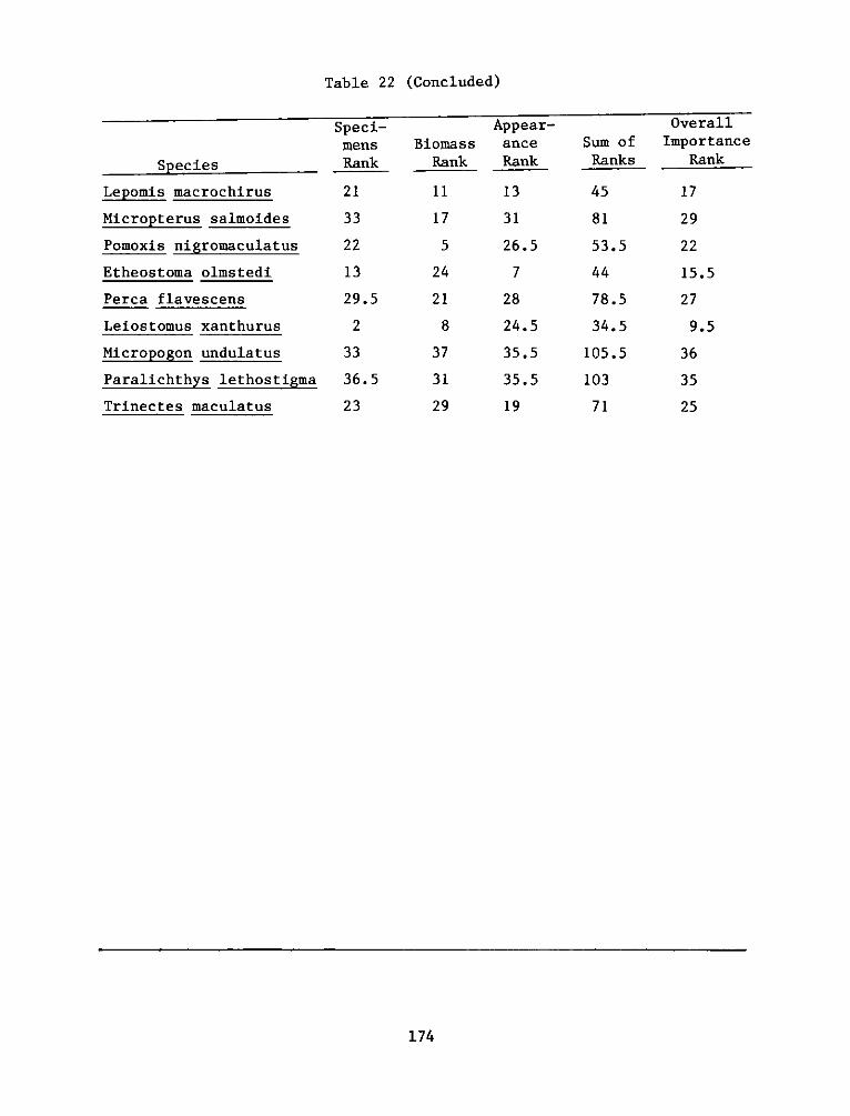
Table 22 (Concluded)
Species
Lepomis macrochirus
Micropterus salmoides
Pomoxis nigromaculatus
Etheostoma olmstedi
Perca flavescens
Lejostomus xanthurus
Micropogon undulatus
Paralichthys lethostigma
Trinectes maculatus
Speci-mensRank
21
33
22
13
29.5
2
33
36.5
23
BiomassRank
11
17
5
24
21
8
37
31
29
Appear-anceRank
13
31
26.5
7
28
24.5
35.5
35.5
19
174
O llSum ofRanks
45
81
53.5
44
78.5
34.5
105.5
103
71
'1verA.a-L
ImportanceRank
17
29
22
15.5
27
9.5
36
35
25
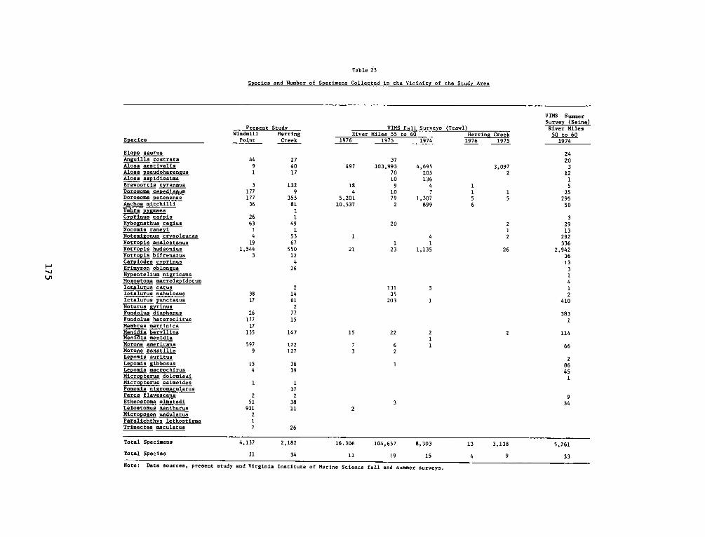
Species anda Numbe f1 pecraena
Table 23
Collected in the Vicinity of the Study Area
Species
Elops saurusAnguilla rostrataAlosa aestivalisAlosa pseudoharengus
Alosa sapidissimaBrevoortia tyrannusDorosoma cepedianumDorosoma petenenseAnchor mitchilliUmbra pygmaea
Cyprinus carpioHybognathus regiusNocomis raneyiNotemigonus crysoleucasNotropis analostanusNotropis hudsoniusNotrpjs bifrenatusCarpiodes cyprinusErimyzon oblongusHypentelium nigricansMoxostoma macrolepidotumIctalurus catusIctalurus nebulosusIctalurus punctatusNoturus gyrinusFundulus diaphanusFundulus heteroclitusMembras martinicaMenidia beryllinaMeiia menidiaMorone americanaNorone saxatilis
Lepoms auritusLepomis gibbosusLepomis macrochirusMicropterus dolomieui
Micropterus salmoidesPomoxis nigromaculatus
Perca flavescensEtheostoma olmatediLeiostomus xanthurusMicropogon undulatusParalichthys lethostigmaTrinectes maculatus
Present StudyWindmill Herring
Point Creek
4491
317717736
266314
191,544
3
3817
2617717
135
5979
154
1
251
9312
7
2740
17
1329
35581
1
491
5367550124
26
214612
7715
147
122
127
3639
1372
3811
VIMS Fall Surveys (Trawl)River Milea 55 to 60 Herring Creek
1976 1975 1974 1976 1975
37497 103,993
70
10
18 94 10
5,201 7910,537 2
21
4,695105136
1,307899
3,0972
1156
20
41 1
23 1,135
131
35203
15
73
22
6
2
1
2
1
15
2
2
26
2
3
26
Li'
VIMS SummerSurvey (Seine)River Miles50 to 601974
2420
312
125
295
50
32913
292336
2,94236133
4
2410
383
114
66
28645
Total Specimens 4,137 2,182 16.306 104,657 8,303 13 3,138 5,261Total Species 31 34 11 19 15 4 9 33
Note: Data sources, present study and Virginia Institute of Marine Science fall and summer surveys.
934
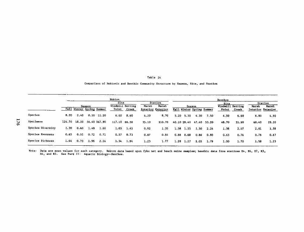
Table 24
Comparison of Nektonic and Benthic Community Structure by Season, Site, and Station
Nekton BenthosSite Station Site Station
Season Windmill Herring Marsh Marsh Season Windmill Herring Marsh Marsh_______________ Fall Winter Spring Suimner Point Creek Interior Exterior Fall Winter Spring Summer Point Creek Interior Exterior
Species 8.20 2.40 8.50 11.20 6.60 8.60 4.20 8.70 5.20 5.30 4.30 7.50 4.50 6.60 6.80 4.90
Specimens 124.70 18.20 56.40 167.90 117.10 66.50 35.10 110.70 40.10 28.40 47.40 53.20 48.70 35.90 68.40 29.20
Species Diversity 1.30 0.60 1.48 1.60 1.03 1.45 0.92 1.35 1.58 1.55 1.50 2.26 1.38 2.07 2.01 1.58
Species Evenness 0.65 0.52 0.72 0.71 0.57 0.73 0.67 0.64 0.66 0.68 0.66 0.80 0.63 0.76 0.76 0.67
Species Richness 1.64 0.70 1.96 2.24 1.34 1.94 1.23 1.77 1.28 1.27 1.05 1.79 1.00 1.70 1.58 1.23
Note: Data are mean values for each category. Nekton data based upon fyke net and beach seine samples; benthic data from stations E4, E6, E7, R3,R4, and R5. See Part II: Aquatic Biology--Benthos.
0'
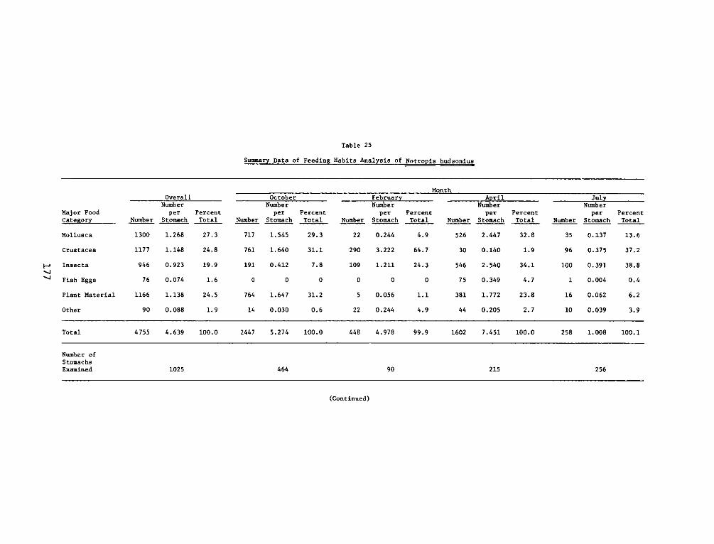
Table 25
Susuary Data of Feeding Habits Analysis of .Notropis hudsonius
MonthOverall October February April July
Number Number Number Number NumberMajor Food per Percent per Percent per Percent per Percent per Percent
Caeory Number Stomach Total Number Stomach Total Number Stomach Total Number Stomach Total Number Stomach Total
Mollusca 1300 1.268 27.3 717 1.545 29.3 22 0.244 4.9 526 2.447 32.8 35 0.137 13.6
Crustacea 1177 1.148 24.8 761 1.640 31.1 290 3.222 64.7 30 0.140 1.9 96 0.375 37.2
i-' Insecta 946 0.923 19.9 191 0.412 7.8 109 1.211 24.3 546 2.540 34.1 100 0.391 38.8
Fish Eggs 76 0.074 1.6 0 0 0 0 0 0 75 0.349 4.7 1 0.004 0.4
Plant Material 1166 1.138 24.5 764 1.647 31.2 5 0.056 1.1 381 1.772 23.8 16 0.062 6.2
Other 90 0.088 1.9 14 0.030 0.6 22 0.244 4.9 44 0.205 2.7 10 0.039 3.9
Total 4755 4.639 100.0 2447 5.274 100.0 448 4.978 99.9 1602 7.451 100.0 258 1.008 100.1
Number ofStomachsExamined 1025 464 90 215 256
(Continued)
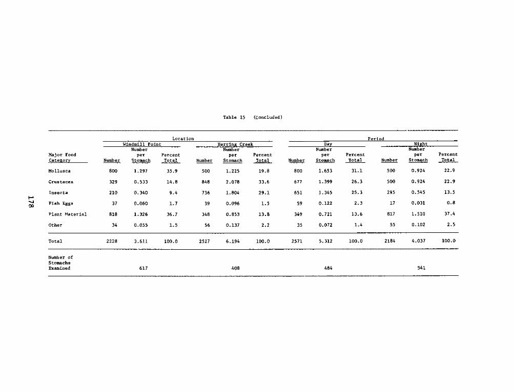
Table 25 (Concluded)
Location PeriodWindmill Point Herring Creek Day Night
Number Number Number NumberMajor Food per Percent per Percent per Percent per PercentCategory Number Stomach Total Number Stomach Total Number Stomach Total Number Stomach Total
Mollusca 800 1.297 35.9 500 1.225 19.8 800 1.653 31.1 500 0.924 22.9
Crus tacea 329 0.533 14.8 848 2.078 33.6 677 1.399 26.3 500 0.924 22.9
Insecta 210 0.340 9.4 736 1.804 29.1 651 1.345 25.3 295 0.545 13.5
Fish Eggs 37 0.060 1.7 39 0.096 1.5 59 0.122 2.3 17 0.031 0.8
Plant Material 818 1.326 36.7 348 0.853 13.8 349 0.721 13.6 817 1.510 37.4
Other 34 0.055 1.5 56 0.137 2.2 35 0.072 1.4 55 0.102 2.5
Total 2228 3.611 100.0 2527 6.194 100.0 2571 5.312 100.0 2184 4.037 100.0
Number ofStomachsExamined 617 408 484 541
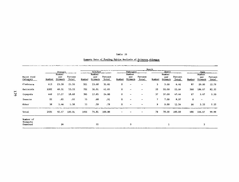
Table 26
Suumiary Data of Feeding Habits Analysis of Erimyzon oblongus
MonthOverall October February April July
Number Number Number Number NumberMajor Food per Percent per Percent per Percent per Percent per PercentCategory Number Stomach Total Number Stomach Total Number Stomach Total Number Stomach Total Number Stomach Total
Cladocera 613 23.58 25.50 521 23.68 31.65 0 - - 5 5.00 6.41 87 29.00 12.79
Ostracoda 1282 49.31 53.33 702 31.91 42.65 0 - - 20 20.00 25.64 560 186.67 82.35
Copepoda 449 17.27 18.68 395 17.95 24.00 0 - - 37 37.00 47.44 17 5.67 2.50
Insecta 22 .85 .92 15 .68 .91 0 - - 7 7.00 8.97 0 - -
Other 38 1.46 1.58 13 .59 .79 0 - - 9 9.00 11.54 16 5.33 2.35
Total 2404 92.47 100.01 1646 74.81 100.00 - - - 78 78.00 100.00 680 226.67 99.99
Number ofStomachsExamined 26 22 0 13
'3
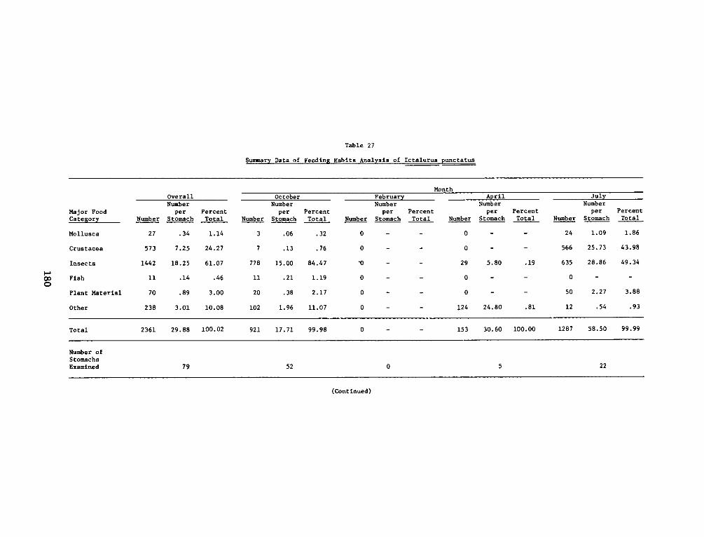
Table 27
Summary Data of Feeding Habits Analysis of Ictalurus punctatus
Major FoodCategory
Mollusca
Crus tacea
Insecta
00 Fish
Plant Material
Other
OverallNumber
per PercentNumber Stomach Total
27 .34 1.14
573 7.25 24.27
1442 18.25 61.07
11 .14 .46
70 .89 3.00
238 3.01 10.08
OctoberNumber
per PercentNumber Stomach Total
3 .06 .32
7 .13 .76
778 15.00 84.47
11 .21 1.19
20 .38 2.17
102 1.96 11.07
FebruaryNumber
per PercentNumber Stomach Total
0 - -
0 - -
10 - -
0 - -
0
0
fonthNu
Number St
0
0
29
April Julyimber Numberper Percent per Percent:omach Total Number Stomach Total
- - 24 1.09 1.86
- - 566 25.73 43.98
5.80 .19 635 28.86 49.34
0 -
- 0 -
- 124 24.80
0 - -
- 50
.81 12
2.27 3.88
.54 .93
Total 2361 29.88 100.02 921 17.71 99.98 0 - - 153 30.60 100.00 1287 58.50 99.99
Number ofStomachsExamined 79 52 0 5 22
(Continued)
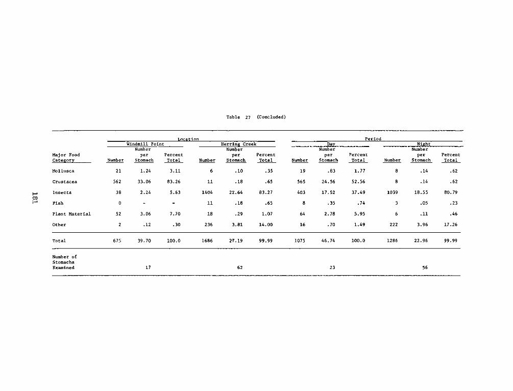
Table 27 (Concluded)
Location PeriodWindmill Point Herring Creek Day Night
Number Number Number NumberMajor Food per Percent per Percent per Percent per PercentCategory Number Stomach Total Number Stomach Total Number Stomach Total Number Stomach Total
Mollusca 21 1.24 3.11 6 .10 .35 19 .83 1.77 8 .14 .62
Crustacea 562 33.06 83.26 11 .18 .65 565 24.56 52.56 8 .14 .62
g..a Insecta 38 2.24 5.63 1404 22.64 83.27 403 17.52 37.49 1039 18.55 80.79
~' Fish 0 - - 11 .18 .65 8 .35 .74 3 .05 .23
Plant Material 52 3.06 7.70 18 .29 1.07 64 2.78 5.95 6 .11 .46
Other 2 .12 .30 236 3.81 14.00 16 .70 1.49 222 3.96 17.26
Total 675 39.70 100.0 1686 2-7.19 99.99 1075 46.74 100.0 1286 22.96 99.99
Number ofStomachsExamined 17 62 23 56
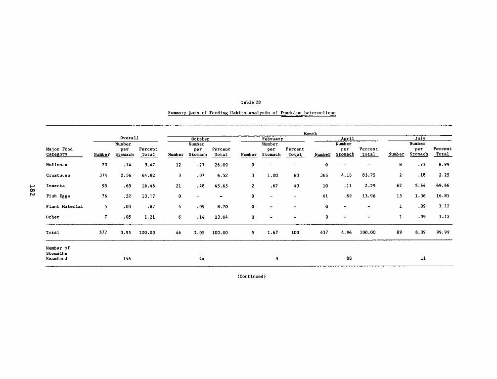
Table 28
Summary Data of Feeding Habits Analysis of Fundulus heteroclitus
MonthOverall October February April July
Number Number Number Number NumberMajor Food per Percent per Percent per Percent per Percent per PercentCaegr Number Stomach Total Number Stomach Total Number Stomach Total Number Stomach Total Number Stomach Total
Mollusca 20 .14 3.47 12 .27 26.09 0 - - 0 - - 8 .73 8.99
Crustacea 374 2.56 64.82 3 .07 6.52 3 1.00 60 366 4.16 83.75 2 .18 2.25
i-a Insecta 95 .65 16.46 21 .48 45.65 2 .67 40 10 .11 2.29 62 5.64 69.6600
60 Fish Eggs 76 .52 13.17 0 - - 0 - - 61 .69 13.96 15 1.36 16.85
Plant Material 5 .03 .87 4 .09 8.70 0 - - 0 - - 1 .09 1.12
Other 7 .05 1.21 6 .14 13.04 0 - - 0 - - 1 .09 1.12
Total 577 3.95 100.00 46 1.05 100.00 5 1.67 100 437 4.96 100.00 89 8.09 99.99
Number ofStomachsExamined 146 44 3 88 11
(Continued)
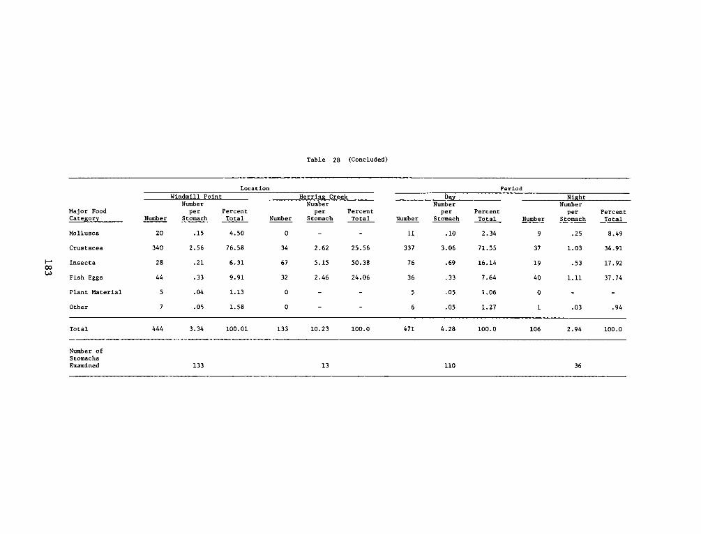
Table 28 (Concluded)
Location PeriodWindmill Point Herring Creek Day Night
Number Number Number NumberMajor Food per Percent per Percent per Percent per PercentCategory Number Stomach Total Number Stomach Total Number Stomach Total Number Stomach Total
Mollusca 20 .15 4.50 0 - - 11 .10 2.34 9 .25 8.49
Crustacea 340 2.56 76.58 34 2.62 25.56 337 3.06 71.55 37 1.03 34.91
1' Insecta 28 .21 6.31 67 5.15 50.38 76 .69 16.14 19 .53 17.92
Fish Eggs 44 .33 9.91 32 2.46 24.06 36 .33 7.64 40 1.11 37.74
Plant Material 5 .04 1.13 0 - - 5 .05 1.06 0 - -
Other 7 .05 1.58 0 - - 6 .05 1.27 1 .03 .94
Total 444 3.34 100.01 133 10.23 100.0 471 4.28 100.0 106 2.94 100.0
Number ofStomachsExamined 133 13 110 36
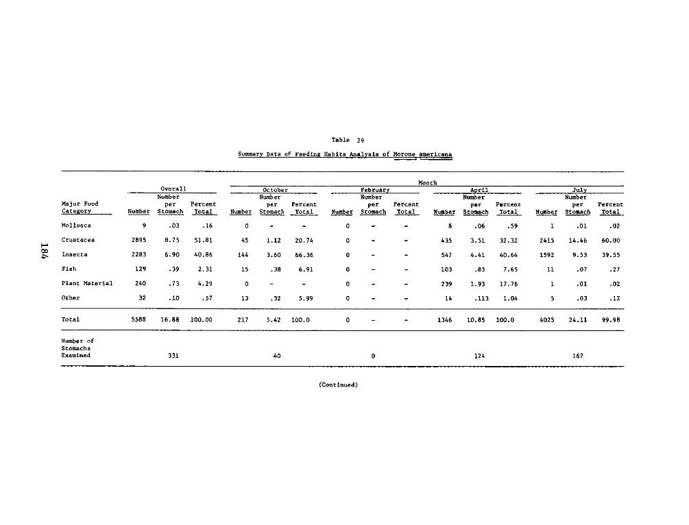
Table 29
Summary Data of Feeding Habits Analysis of Morone americana
MonthOverall October February April JulyNumber Number Number Number Number
Major Food per Percent per Percent per Percent per Percent per PercentCategory Number Stomach Total Number Stomach Total Number Stomach Total Number Stomach Total Number Stomach Total
Mollusca 9 .03 .16 0 - - 0 - - 8 .06 .59 1 .01 .02
Crustacea 2895 8.75 51.81 45 1.12 20.74 0 - - 435 3.51 32.32 2415 14.46 60.00
S Insecta 2283 6.90 40.86 144 3.60 66.36 0 - - 547 4.41 40.64 1592 9.53 39.55
Fish 129 .39 2.31 15 .38 6.91 0 - - 103 .83 7.65 11 .07 .27
Plant Material 240 .73 4.29 0 - - 0 - - 239 1.93 17.76 1 .01 .02
Other 32 .10 .57 13 .32 5.99 0 - - 14 .113 1.04 5 .03 .12
Total 5588 16.88 100.00 217 5.42 100.0 0 - - 1346 10.85 100.0 4025 24.11 99.98
Number ofStomachsExamined 331 40 0 124 167
(Continued)
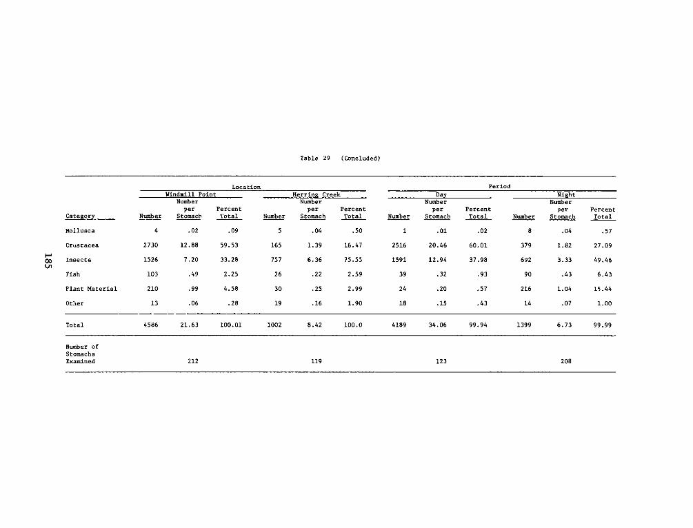
Table 29 (Concluded)
Location PeriodWindmill Point Herring Creek Day Night
Number Number Number Numberper Percent per Percent per Percent per Percent
CaegryNumber Stomach Total Number Stomach Total Number Stomach Total Number Stomach Total
Mollusca 4 .02 .09 5 .04 .50 1 .01 .02 8 .04 .57
Crustacea 2730 12.88 59.53 165 1.39 16.47 2516 20.46 60.01 379 1.82 27.09
oo Insecta 1526 7.20 33.28 757 6.36 75.55 1591 12.94 37.98 692 3.33 49.46
Fish 103 .49 2.25 26 .22 2.59 39 .32 .93 90 .43 6.43
Plant Material 210 .99 4.58 30 .25 2.99 24 .20 .57 216 1.04 15.44
Other 13 .06 .28 19 .16 1.90 18 .15 .43 14 .07 1.00
Total 4586 21.63 100.01 1002 8.42 100.0 4189 34.06 99.94 1399 6.73 99.99
Number ofStomachsExamined 212 119 123 208
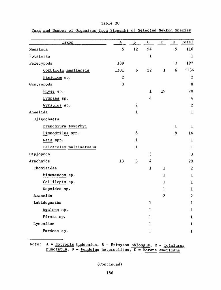
Table 30
Taxa and Number of Organisms from Stomachs of Selected Nekton Species
Taxon
Nematoda
Ro tatoria
Pelecypoda
Corbicula manilensis
Pisidium sp.
Gas tropoda
Physa sp.
Lymnaea sp.
Gyraulus sp.
Annelida
Oligochaeta
Branchiura sowerbyi
Limnodrilus spp.
Nais spp.
Peloscolex multisetosus
Diplopoda
Arachnida
Thomisidae
lMisumenops sp.
Callilepis sp.
Nopsides sp.
Araneida
Labidognatha
Agelena sp.
Pirata sp.
Lycosidae
Pardosa sp.
A
5
189
1101
2
8
B
12
C
94
D E
5
1
3
6 22 1 6
1
4
19
2
Total
116
192
1136
2
8
20
4
2
1
88
1
1
3
13 3 4
1
1
1
1
1
1
1
1
1
1
2
Note: A = Notropis hudsonius, B = Erimyzon oblongus, C = Ictalurus
punctatus, D = Fundulus heteroclitus, E = Morone americana
(Continued)
1
16
3
20
2
1
1
1
2
186
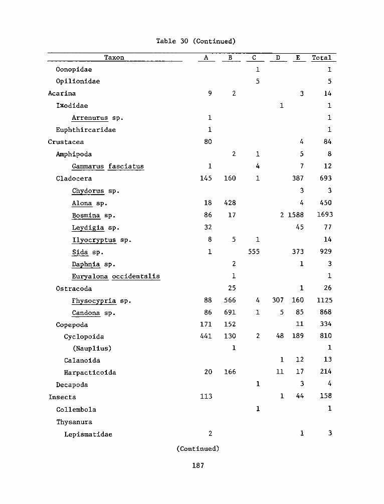
Table 30 (Continued)
Taxon
Oonopidae
Opilionidae
Acarina
Ixodidae
Arrenurus sp.
Euphthircaridae
Crustacea
Amphipoda
Gainmarus fasciatus
Cladocera
Chydorus sp.
Alona sp.
Bosmina sp.
Leydigia sp.
Ilyocryptus sp.
Sida sp.
Daphnia sp.
Euryalona occidentalis
Os tracoda
A B
9 2
C D E Total
5 5
3 14
1
1
1
80
1
145
18
86
32
8
1
88
86
171
441
Fhysocypria sp.
Candona sp.
Copepoda
Cyclopoida
(Nauplius)
Calanoida
Harpacticoida
Decapoda
Insecta
Collembola
Thysanura
Lepismatidae
2 1
4
160 1
428
17 2 1
5 1
555
2
25
566
691
152
130
20 166
1
113
1
4 307
1 5
2 48
1
11
1
4 84
5 8
7 12
387 693
3 3
4 450
.588 1693
45 77
14
373 929
1 3
1 26
160 1125
85 868
11 334
189 810
12 13
17 214
3
1 44
4
158
1
1 32
(Continued)
187
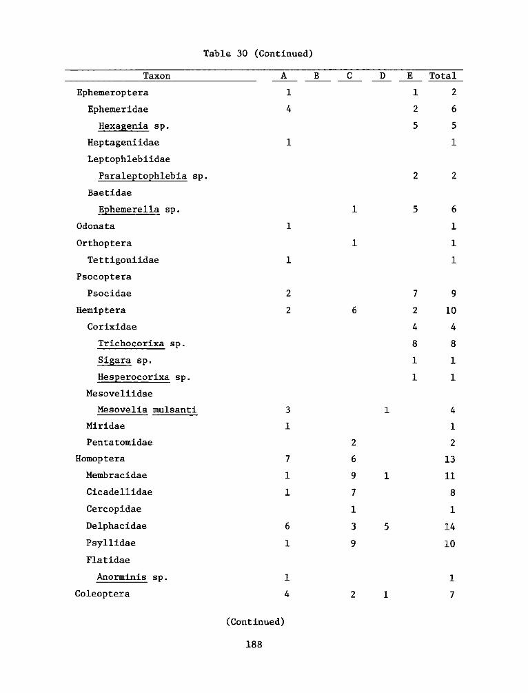
Table 30 (Continued)
Taxon
Ephemeroptera
Ephemeridae
Hexagenia sp.
Heptageniidae
Leptophlebiidae
Paraleptophiebia sp.
Baetidae
Ephemerella sp.
Odonata
Orthoptera
Tettigoniidae
Psocoptera
Psocidae
Hemip tera
Corixidae
Trichocorixa sp.
Sigara sp.
Hesperocorixa sp.
Mesoveliidae
Mesovelia mulsanti
Miridae
Pentatomidae
Homop tera
Membracidae
Cicadellidae
Cercopidae
Delphacidae
Psyllidae
Flatidae
Anorminis sp.
Coleop tera
A B C D E Total
1 1 2
4 2 6
5 5
2 2
1
2
2
3
7
1
1
6
1
4
1
6
2
6
9
7
3
9
5 6
1
1
1
9
10
4
8
1
1
4
2
13
11
8
14
10
7
2
4
8
1
1
1
1
5
72 1
(Continued)
188
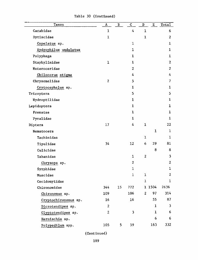
Table 30 (Continued)
Taxon
Carabidae
Dytiscidae
Copelatus sp.
Hydrophilus undulatus
Polyphaga
S taphylinidae
Heteroceridae
Chilocorus stigma
Chrysomelidae
Crytocephalus sp.
Tricoptera
Hydroptilidae
Lepidoptera
Frenatae
Pyralidae
Dip tera
Nematocera
Tachinidae
Tipulidae
Culicidae
Tabanidae
Chrysops sp.
Syrphidae
lMuscidae
Cecidomyiidae
Chironomidae
Chironomus sp.
Cryptochironomus sp.
Dicrotendipes sp.
Glyptotendipes sp.
Harnischia sp.
Polypedilum spp.
A B C
1 4
1 1
2
4
2 5
5
17 4
34 12
344
109
16
2
2
105
15 772
106
16
5 59
D E Total
1 6
1 2
2
2
4
7
5
1 22
1 1
1 1
6 29 81
8 8
2 3
2
1 2
1 1
1 1504 2636
2 97 314
55 87
1 3
1 6
6 6
163 332
(Continued)
189
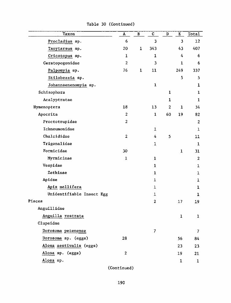
Table 30 (Continued)
Taxon
Procladius sp.
Tanytarsus sp.
Cricotopus sp.
Ceratopogonidae
Palpomyia sp.
Stilobezzia sp.
Johannsenenomyia sp.
Schizophora
Acalyptratae
Hymenoptera
Apocrita
Proctotrupidae
Ichneumonidae
Chalc ididae
Trigonalidae
Formicidae
Myrmicinae
Vespidae
Zethinae
Apidae
Apis mellif era
Unidentifiable Insect Egg
Pisces
Anguillidae
Anguilla rostrata
Clupeidae
Dorosoma petenense
Dorosoma sp. (eggs)
Alosa aestivalis (eggs)
Alosa sp. (eggs)
Alosa sp.
A
6
20
1
2
76
B C
3
1 343
1
3
1 11
D
1
18
2
2
2
30
1
13
1
1
4
1
1
1
1
1
1
1
2
1
1
2
60
5
E Total
3 12
43 407
4 6
1 6
249 337
5 5
1
1
1 34
19 82
2
11
1 31
2
17 19
1 1
7
28 56
23
19
1
2
7
84
23
21
1
(Continued)
190
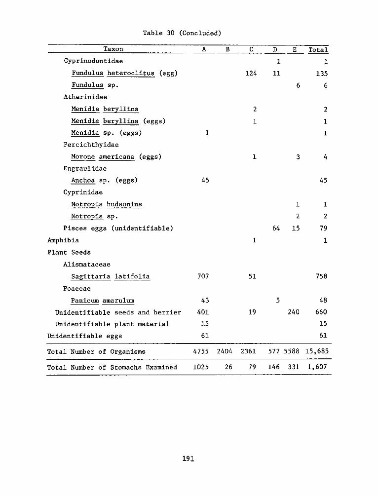
Table 30 (Concluded)
Taxon
Cyprinodontidae
Fundulus heteroclitus (egg)
Fundulus sp.
Atherinidae
Menidia beryllina
Nenidia beryllina (eggs)
Menidia sp. (eggs)
Percichthyidae
Morone americana (eggs)
Engraulidae
Anchoa sp. (eggs)
Cyprinidae
Notropis hudsonius
Notropis sp.
Pisces eggs (unidentifiable)
Amphib ia
Plant Seeds
Alismataceae
Sagittaria latifolia
Poaceae
Panicum amarulum
Unidentifiable seeds and berrier
Unidentifiable plant material
Unidentifiable eggs
A B C D E Total
1 1
124 11 135
6 6
2
1
1
2
1
1
3 4
45
1
2
64 15
1
707
43
401
15
61
51
5
19
45
1
2
79
758
48
240 660
15
61
191
Total Number of Organisms 4755 2404 2361 577 5588 15,685
Total Number of Stomachs Examined 1025 26 79 146 331 1,607
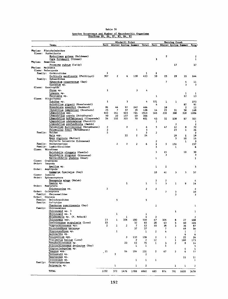
Table 31
Species Occurrence and Number of Hacrobenthic OrganismsStations E4, E6, E7, R3, R4, R5
Windmill Point Herring CreekFell Winter Spring Sunmier Total Fall Winter Spring Summer Total
Phylum: PlatyhelminthesClass: Turbellaria
Hydrolimax grisee (Haldeman)Cure foremanii (Girand)
Phylum: NemerteeProstoma rubrum (Leidy)
Phylum: MolluscaClass: Pelecypoda
Family: Corbiculidee 1Corbicula manilensis (Phillippi) 307 2
Family: Sphaeriidae
Sphaerium transversum (Say)Pisidium sp.
Class: GastropodaPhysa sp. 1Lymnaea ap.Ferrissia ap.
Class: OligocheetaTubifex sp. 1Aulodrilus pigueti (Kowaleoski)
Branchiura sowerbyi (Beddard) 81 46Ilyodrilus templetoni (Southern) 25 7Limnodrilus app. 642 141
Limnodrilus cervix (Brinkhurst) 50 10Limnodrilus hof fmeisteri (Claparede) 54 152Limnodrilus udekemianus (Verrill)Limnodrilus profundicola (Smith)
Peloscolex multisetosus (Brinkhurst) 2Peloscolex freyi (Brinkhurst) 2
Family: Naidee 5S
Nais app.Dero digitata (Huller)Stylaria lacustris (Linnaeus)
Family: Enchytraeidae 2Family: Lumberliculide
Class: HirudineeHelobdella elongate (Castle)Helobdella stagnaus (Linnaeus)Batracobdella phalera (Graf)
Class: CrustaceeOrder: Isopoda
Asellus ap.Order: Amphipoda
Gammarus fasciatus (Say)Class: Insecta
Order: EphemeropteraHexagenia mingo (Walsh)Ceenis ap.
Order: HemipteraTrichocorixa sp. 2
Order: ColeopteraFamily: Chrysomelide
Order: DipteraFamily: Dolichopodidee 5Family: Culicide
Cheoborue punctipennis (Say)Family: Chironomidae
Chironomid ap. 3Chironomid ap. 6Ablabeamyisasp. (E. Roback)Chironomus app. 13 1Coelotanypus scapularia (Loew) 33Cryptochironomus app. 2 1Dicrotendipes nervosusGlyptotendipes ap.Harniachia ap.Polypedilum app.Procladius bellus (Loew)Pseudochironomus ap.Stictochironomus devinctus (Say)
Cryptocladopelma ap.Tanypus app. , 11Pentaneurd ap. 2Tanytarsus ap.Cricotopus sp.
Family: CeratopogonidePalpomyisa p. 1
TOTAL 1232 372
21
1717
16 138 453
3
9757
403157325
3 4
4
242 46639 128
724 191049 26670 601
2 41 3
5S22 2 24
159
2714
14145
43
5
2
22 2 6 1
5
5
1
10
1
2
5
21
2
23
7
1
10
25235
52
47
5
153
2
41
23
7
29 33 144
4 113 3
1 112 13
1 27387 912 12
51 58 148308 318 1006
139 87 321
2 212 8 7223 1 24
218 1 195 10 15
1 3151 1571 6
10 30
3
3
3 3 57
41 9 14
23 103 3
1
1 1356 180 550
32 652 7 12
37 371
3 133 1362 2
23 12 351 1
16 104 1312
1 1
1 2
1476 1780 4860
2 247 326 8 27 40828 43 5 40 11610 38 3 36 87
7 49 562 4 1
6 62 1 1 22 26
12 1 160 1731 3 2 8 14
5 54 4
2 67 2 6 77
11 111 1
1 1 2
68S 974 791 1020 3470
192
Taxon
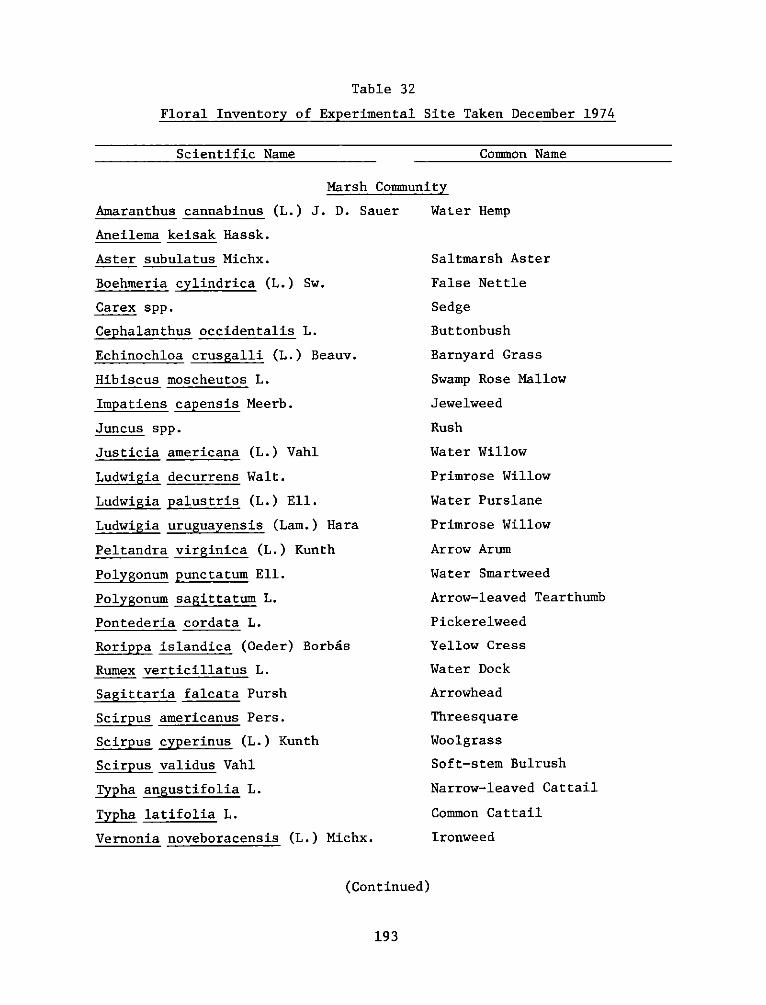
Table 32
Floral Inventory of Experimental Site Taken December 1974
Scientific Name Common Name
Marsh Community
Amaranthus cannabinus (L.) J. D. Sauer Water Hemp
Aneilema keisak Hassk.
Aster subulatus Michx. Saltmarsh
Boehmeria cylindrica (L.) Sw. False Nett:
Carex spp. Sedge
Aster
Le
Cephalanthus occidentalis L.
Echinochloa crusgalli (L.) Beauv.
Hibiscus moscheutos L.
Impatiens capensis Meerb.
Juncus spp.
Justicia americana (L.) Vahl
Ludwigia decurrens Walt.
Ludwigia uruguayensis (Lam.) Hara
Peltandra virginica (L.) Kunth
Polygonum punctatum Eli.
Polygonum sagittatum L.
Pontederia cordata L.
Rorippa islandica (Qeder) Borbis
Rumex verticillatus L.
Sagittaria falcata Pursh
Scirpus americanus Pers.
Scirpus cyperinus (L.) Kunth
Scirpus validus Vahl
Typha angustifolia L.
Typha latifolia L.
Vernonia noveboracensis (L.) Michx.
But tonbush
Barnyard Grass
Swamp Rose Mallow
Jewelweed
Rush
Water Willow
Primrose Willow
Water Purslane
Primrose Willow
Arrow Arum
Water Smartweed
Arrow-leaved Tearthumb
Pickerelweed
Yellow Cress
Water Dock
Arrowhead
Threes quare
Woo lgras s
Soft-stem Bulrush
Narrow-leaved Cattail
Common Cattail
Ironweed
(Continued)
193
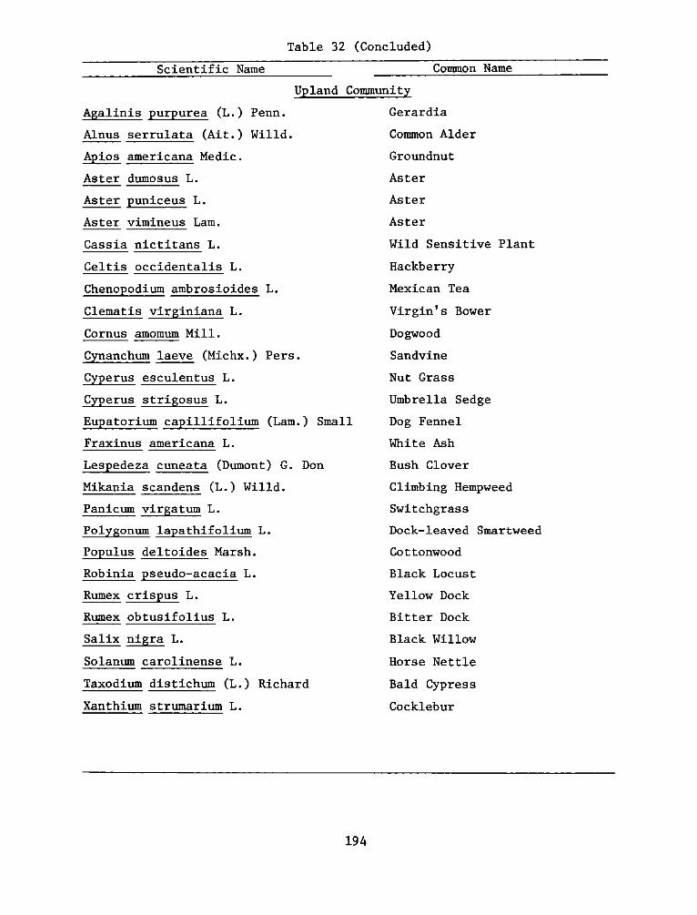
Table 32 (Concluded)
Scientific Name Common Name
Agalinis purpurea (L.) Penn.
Alnus serrulata (Ait.) Willd.
Apios americana Medic.
Aster dumosus L.
Aster puniceus L.
Aster vimineus Lam.
Cassia nictitans L.
Celtis occidentalis L.
Chenopodium ambrosioides L.
Clematis virginiana L.
Cornus amomum Mill.
Cynanchum laeve (Michx.) Pers.
Cyperus esculentus L.
Cyperus strigosus L.
Eupatorium capillifolium (Lam.) St
Fraxinus americana L.
Lespedeza cuneata (Dumont) G. Don
Mikania scandens (L.) Willd.
Panicum virgatum L.
Polygonum lapathifolium L.
Populus deltoides Marsh.
Robinia pseudo-acacia L.
Rumex crispus L.
Rumex obtusifolius L.
Salix nigra L.
Solanum carolinense L.
Taxodium distichum (L.) Richard
Xanthium strumarium L.
id Community
Gerardia
Common Alder
Groundnut
Aster
Aster
Aster
Wild Sensitive Plant
Hackberry
Mexican Tea
Virgin's Bower
Dogwood
Sandvine
Nut Grass
Umbrella Sedge
rall Dog Fennel
White Ash
Bush Clover
Climbing Hempweed
Switchgras s
Dock-leaved Smartweed
Cottonwood
Black Locust
Yellow Dock
Bitter Dock
Black Willow
Horse Nettle
Bald Cypress
Cocklebur
194
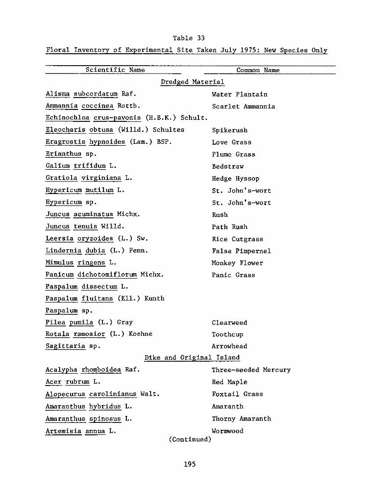
Table 33
Floral Inventory of Experimental Site Taken July 1975; New Species Only
Scientific Name Common Name
Dredged Mate
Alisma subcordatum Raf.
Ammannia coccinea Rottb.
Echinochloa crus-pavonis (H.B.K.) Schult.
Eleocharis obtusa (Willd.) Schultes
Eragrostis hypnoides (Lam.) BSP.
Erianthus sp.
Galium trifidum L.
Gratiola virginiana L.
Hypericum mutilum L.
Hypericum sp.
Juncus acuminatus Michx.
Juncus tenuis Willd.
Leersia oryzoides (L.) Sw.
Lindernia dubia (L.) Penn.
Mimulus ringens L.
Panicum dichotomiflorum Michx.
Paspalum dissectum L.
Ppalum fluitans (Ell.) Kunth
Paspalum sp.
Pilea pumila (L.) Gray
Rotala ramosior (L.) Koehne
Sagittaria sp.
Acalypha rhomboidea Raf.
Acer rubrum L.
Alopecurus carolinianus W~
Amaranthus hybridus L.
Amaranthus spinosus L.
Artemisia annua L.
rial
Water Plantain
Scarlet Ammannia
Spikerush
Love Grass
Plume Grass
Beds traw
Hedge Hyssop
St. John's-wort
St. Jolin's-wort
Rush
Path Rush
Rice Cutgrass
False Pimpernel
Monkey Flower
Panic Grass
Clearweed
Toothcup
Arrowhead
Dike and Original Island
Three-seeded Mercury
Red Maple
ralt. Foxtail Grass
Amaranth
Thorny Amaranth
Wormwood(Continued)
195
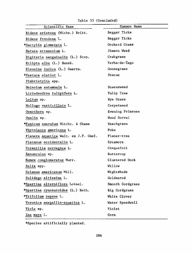
Table 33 (Concluded)
Scientific Name
Bidens aristosa (Michx.) Britt.
Bidens frondosa L.
*Dactylis glomerata L.
Datura stramonium L.
Digitaria sanguinalis (L.) Scop.
Eclipta alba (L.) Hassk.
Eleusine indica (L.) Gaertn.
*Festuca elatior L.
Fimbristylis spp.
Helenium autumnale L.
Liriodendron tulipifera L.
Lolium sp.
Qenothera sp.
Oxalis sp.
*Panicum amarulum Ilitchc. & Chase
Phytolacca americana L.
Planera aguatica Walt. ex J.F. Gm
Platanus occidentalis L.
Potentilla norvegica L.
Ranunculus sp.
Ruinex conglomeratus Nurr.
Salix spp.
Solanum americanum Mill.
Solidago altissima L.
*Sparin alterniflora Loisel.
*Spartina cynosuroides (L.) Roth.
*Trifolium repens L.
Veronica anagallis-aguatica L.
Viola sp.
Zea mays L.
el.
*Species artificially planted.
196
Common Name
Beggar Ticks
Beggar Ticks
Orchard Grass
Jimson Weed
Crabgrass
Yerba-de-Tago
Goosegras s
Fescue
Snee zeweed
Tulip Tree
Rye Grass
Carpetweed
Evening Primrose
Wood Sorrel
Beachgrass
Poke
Planer-tree
Sycamore
Cinquef oil
Buttercup
Clustered Dock
Willow
Nightshade
Goldenrod
Smooth Cordgrass
Big Cordgrass
White Clover
Water Speedwell
Violet
Corn
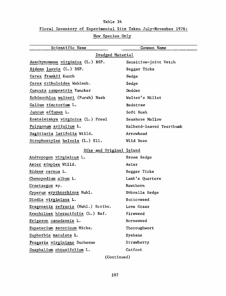
Table 34
Floral Inventory of Experimental Site Taken July-November 1976:
New Species Only
Scientific Name Common Name
Aeschynomene virginica (L.)
Bidens laevis (L.) BSP.
Carex frankii Kunth
Carex tribuloides Wahlenb.
Cuscuta campestris Yuncker
Echinochloa walteri (Pursh)
Galium tinctorium L.
Juncus effusus L.
Kosteletskya virginica (L.)
Polygonum arifolium L.
Sagittaria latifolia Willd.
Strophostyles helvola (L.) I
Dike
Andropogon virginicus L.
Aster simplex Willd.
Bidens cernua L.
Chenopodium album L.
Craetaegus sp.
Cyperus erythrorhizos Muhl.
Diodia virginiana L.
Eragrostis refracta (Muhl.)
Erechtites hieracifolia (L.)
Ergeron canadensis L.
Eupatorium serotinum Michx.
Euphorbia maculata L.
Fragaria virginiana Duchesne
Gnaphalium obtusifolium L.
Dredged Material
BSP. Sensitive-joiat Vetch
Beggar Ticks
Sedge
Sedge
Dodder
Nash Walter's Millet
Bedstraw
Soft Rush
Presl Seashore Mallow
Halberd-leaved Tearthumb
Arrowhead
Ell. Wild Bean
and Original Island
Broom Sedge
Aster
Beggar Ticks
Lamb's Quarters
Hawthorn
Umbrella Sedge
But tonweed
Scribn. Love Grass
Raf. Fireweed
Hors eweed
Thoroughwort
Eyebane
Strawberry
Catfoot
(Continued)
197
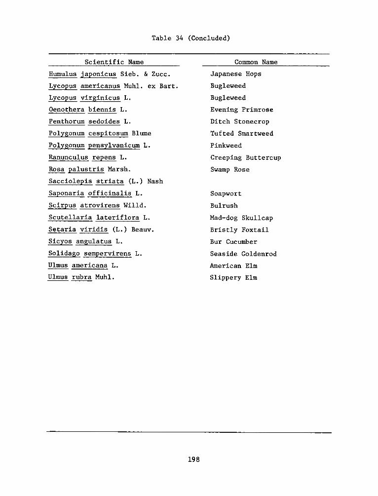
Table 34 (Concluded)
Scientific Name
Hamulus japonicus Sieb. & Zucc.
Lycopus americanus Muhl. ex Bart.
Lycopus virginicus L.
Qenothera biennis L.
Penthorum sedoides L.
Polygonum cespitosum Blume
Polygonum pensylvanicum L.
Ranunculus repens L.
Rosa palustris Marsh.
Sacciolepis striata (L.) Nash
Saponaria officinalis L.
Scirpus atrovirens Willd.
Scutellaria lateriflora L.
Setaria viridis (L.) Beauv.
Sicyos angulatus L.
Solidago sempervirens L.
Ulmus americana L.
Ulmus rubra Muhl.
Common Name
Japanese Hops
Bugleweed
Bugleweed
Evening Primrose
Ditch Stonecrop
Tufted Smartweed
Pinkweed
Creeping Buttercup
Swamp Rose
Soapwort
Bulrush
Mad-dog Skullcap
Bristly Foxtail
Bur Cucumber
Seaside Goldenrod
American Elm
Slippery Elm
198
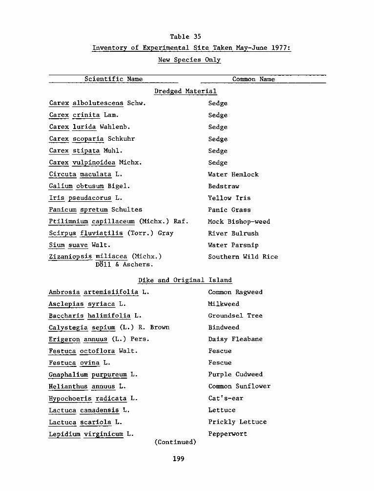
Table 35
Inventory of Experimental Site Taken May-June 1977:
New Species Only
Scientif ic Name Common Name
Carex albolutescens Schw.
Carex crinita Lam.
Carex lurida Wahlenb.
Carex scoparia Schkuhr
Dredged Material
Sedge
Sedge
Sedge
Carex stipata Muhl.
Carex vulpinoidea Michx.
Circuta maculata L.
Galiam obtusum Bigel.
Iris pseudacorus L.
Panicum spretum Schultes
Ptilimnium capillaceum (Michx.) Raf.
Scirpus fluviatilis (Torr.) Gray
Sium suave Walt.
Zizaniopsis miliacea (Michx.)D811 & Aschers.
Sedge
Sedge
Sedge
Water Hemlock
Beds traw
Yellow Iris
Panic Grass
Mock Bishop-weed
River Bulrush
Water Parsnip
Southern Wild Rice
Dike and Original Island
Ambrosia artemisiifolia L.
Asclepias syriaca L.
Baccharis halimifolia L.
Calystegia sepium (L.) R. Brown
Erigeron annuus (L.) Pers.
Festuca octoflora Walt.
Festuca ovina L.
Gnaphalium purpureum L.
Helianthus annuus L.
Hypochoeris radicata L.
Lactuca canadensis L.
Lactuca scariola L.
Lepidium virginicum L.(Continued)
Common Ragweed
Milkweed
Groundsel Tree
Bindweed
Daisy Fleabane
Fescue
Fescue
Purple Cudweed
Common Sunflower
Cat's-ear
Lettuce
Prickly Lettuce
Pepperwort
199
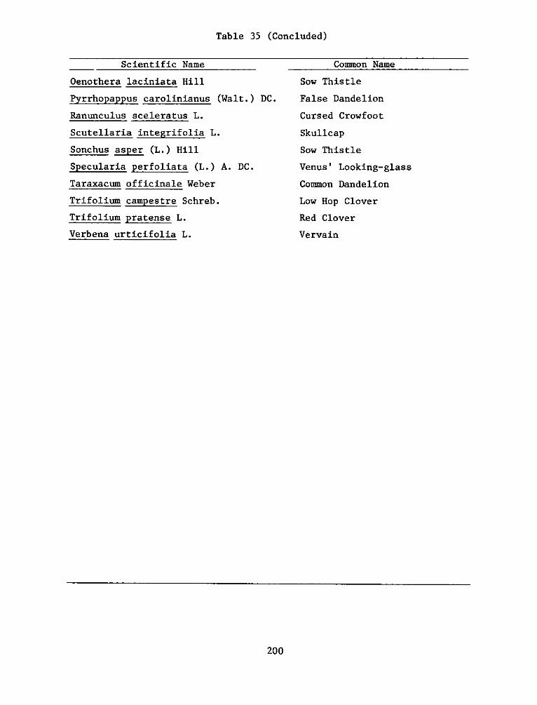
Table 35 (Concluded)
Scientific Name
Qenothera laciniata Hill
Pyrrhopappus carolinianus (Walt.) DC.
Ranunculus sceleratus L.
Scutellaria integrifolia L.
Sonchus asper (L.) Hill
Specularia perfoliata (L.) A. DC.
Taraxacum officinale Weber
Trifolium campestre Schreb.
Trifolium pratense L.
Verbena urticifolia L.
Common Name
Sow Thistle
False Dandelion
Cursed Crowfoot
Skullcap
Sow Thistle
Venus' Looking-glass
Common Dandelion
Low Hop Clover
Red Clover
Vervain
200
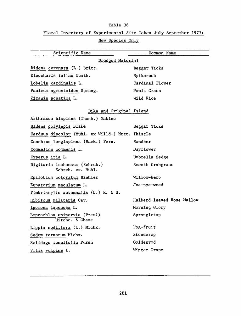
Table 36
Floral Inventory of Experimental Site Taken July-September 1977:
New Species Only
Scientific Name Common Name
Bidens coronata (L.) Britt.
Eleocharis fallax Weath.
Lobelia cardinalis L.
Panicum agrostoides Spreng.
Zizania aguatica L.
Dredged Material
Beggar Ticks
Spikerush
Cardinal Flower
Panic Grass
Wild Rice
Dike and Original Island
Arthraxon hispidus (Thunb.) Makino
Bidens polylepis Blake Beggar
Carduus discolor (Muhl. ex Willd.) Nutt. Thistl
Cenchrus longispinus (Hack.) Fern. Sandbu
Commelina communis L. Dayfloi
Cyperus iria L. Umbrel
Digitaria ischaemum (Schreb.) SmoothSchreb. ex. Muhl.
Epilobium coloratum Biehler Willow-
Eupatorium maculatum L. Joe-py
Fimbristylis autumnalis (L.) R. & S.
Hibiscus militaris Cav. Halber
Ipomoea lacunosa L. Mornin
Letcho uninervia (Presl) Sprang~Hitchc. & Chase
Lippia nodiflora (L.) Michx. Fog-fri
Sedum ternatum Michx. Stoneci
Solidago tenuifolia Pursh Goldeni
Vitis vulpina L. Winter
Ticks
wer
La Sedge
Crab grass
-herb
e-weed
1-leaved Rose Mallow
g Glory
Letop
ut
rop
rod
Grape
201
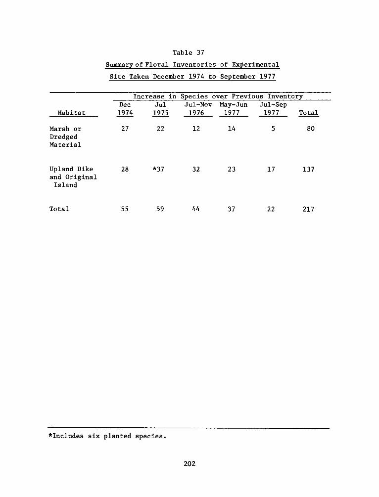
Table 37
Summary of Floral Inventories of Experimental
Site Taken December 1974 to September 1977
Increase inJul1975
22
Species over Previous InventoryJul-Nov May-Jun Jul-Sep1976 1977 1977 T(
12 14 5
)tal
Upland Dikeand OriginalIsland
Total
28 *37
55 59
*Includes six planted species.
202
Dec1974Habitat
Marsh orDredgedMaterial
27 80
1732
44
13723
37 22 217
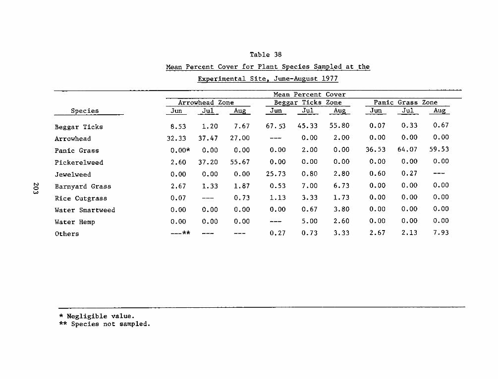
Table 38
Mean Percent Cover for Plant Species Sampled at the
Experimental Site, June-August 1977
Species
Beggar Ticks
Arrowhead
Panic Grass
Pickerelweed
Jewelweed
Barnyard Grass
Rice Cutgrass
Water Smartweed
Water Hemp
Others
0
Arrowhead ZoneJun Jul Aug
8.53
32.33
0.00*
2.60
0.00
2.67
0.07
0.00
0.00
1.20
37.47
0.00
37.20
0.00
1.33
0.00
0.00
7.67
27.00
0.00
55.67
0.00
1.87
0.73
0.00
0.00
Mean PercentBeggar Ticks
Jun Jul
CoverZoneAug
67.53 45.33 55.80
--- 0.00 2.00
0.00 2.00 0.00
0.00 0.00 0.00
25.73 0.80 2.80
0.53 7.00 6.73
1.13 3.33 1.73
0.00 0.67 3.80
--- 5.00 2.60
0.27 0.73 3.33
Panic Grass ZoneJun Jul Aug
0.07
0.00
36.53
0.00
0.60
0.00
0.00
0.00
0.00
2.67
0.33
0.00
64.07
0.00
0.27
0.00
0.00
0.00
0.00
2.13
0.67
0.00
59.53
0.00
0.00
0.00
0.00
0.00
7.93
* Negligible value.** Species not sampled.
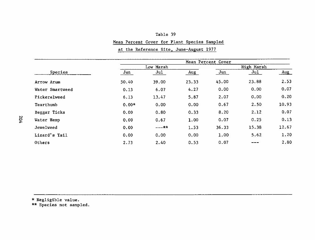
Table 39
Mean Percent Cover for Plant Species Sampled
at the Reference Site, June-August 1977
Species
Arrow Arum
Water Smartweed
Pickerelweed
Tearthumb
Beggar Ticks
Water Hemp
Jewelweed
Lizard's Tail
Others
Jun
50.40
0.13
6.13
0.00*
0.00
0.00
0.00
0.00
2.73
Low MarshJul
39.00
6.07
13.47
0.00
0.80
0.67
0.00
2.40
Mean Percent Cover Hg as
Aug
23.33
4.27
5.87
0.00
0.33
1.00
1.53
0.00
0.53
Jun
45.00
0.00
2.07
0.67
8.20
0.07
36.33
1.00
0.07
Jul
23.88
0.00
0.00
2.50
2.12
0.25
15.38
5.62
* Negligible value.** Species not sampled.
tS)0
Aug
2.53
0.07
0.20
10.93
0.07
0.13
12.67
1.20
2.80
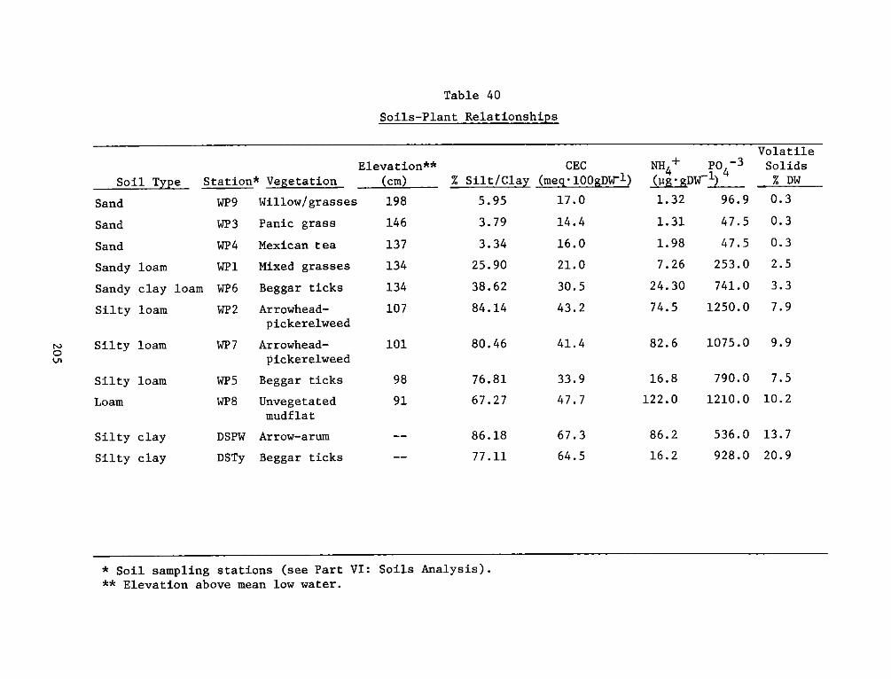
Table 40
Soils-Plant Relationships
Soil Type
Sand
Sand
Sand
Sandy
Sandy
Silty
loam
clay loam
loam
Silty loam
Silty loam
Loam
Silty
Silty
clay
clay
Elevation** CECStation* Vegetation (cm) % Silt/Clay (meg-100gDW-1)
WP9 Willow/grasses
WP3 Panic grass
WP4 Mexican tea
WPl Mixed grasses
WP6 Beggar ticks
WP2 Arrowhead-pickerelweed
WP7 Arrowhead-pickerelweed
WP5 Beggar ticks
WP8 Unvegetatedmudflat
DSPW Arrow-arum
DSTy Beggar ticks
198
146
137
134
134
107
101
98
91
5.95
3.79
3.34
25.90
38.62
84.14
80.46
76.81
67.27
86.18
77.11
17.0
14.4
16.0
21.0
30.5
43.2
41.4
33.9
47.7
67.3
64.5
P0 -3
NHg+ P 3(yg-gDW1l) 4
1.32
1.31
1.98
7.26
24.30
74.5
96.9
47.5
47.5
253.0
741.0
1250.0
82.6 1075.0 9.9
16.8
122.0
86.2
16.2
790.0
1210.0
536.0
928.0
* Soil sampling stations (see Part VI: Soils Analysis).** Elevation above mean low water.
0
VolatileSolids% DW
0.3
0.3
0.3
2.5
3.3
7.9
7.5
10.2
13.7
20.9
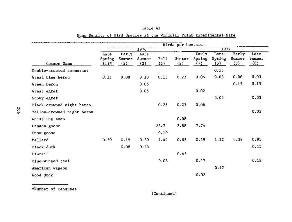
Table 41
Mean Density of Bird Species at the Windmill Point Experimental Site
Birds per hectare
Common Name
Double-crested cormorant
Great blue heron
Green heron
Great egret
Snowy egret
Black-crowned night heron
Yellow-crowned night heron
Whistling swan
Canada goose
Snow goose
Mallard
Black duck
Pintail
Blue-winged teal
American wigeon
Wood duck
LateSpring(1) *
EarlySummer(2)
1976LateSummer(3)
0.15 0.08 0.10
0.05
0.05
__________1977
Early LateFall Winter Spring Spring(6) (2) (7) (5)
0.55
0.13 0.23 0.06 0.03
0.02
0.09
0.25 0.23 0.06
0.30 0.15
0.08
0.30
0.20
23. 7
0.10
1.49
0.08
2.88
EarlySummer(5)
0.06
0.15
LateSummer(6)
0.03
0.15
0.03
0.03
7.74
0.83 0.49 1.12 0.39 0.91
0.15
0.45
0.08 0.17
0.02
0.18
0.12
*Number of censuses(Continued)
0C'
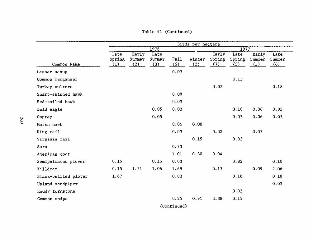
Table 41 (Continued)
Birds per hectare
Common Name
Lesser scaup
Common merganser
Turkey vulture
Sharp-shinned hawk
Red-tailed hawk
Bald eagle
Osprey
Marsh hawk
King rail
Virginia rail
Sora
American coot
Semipalmated plover
Killdeer
Black-bellied plover
Upland sandpiper
Ruddy turns tone
Common snipe
LateSpring(1)
EarlySummer(2)
1976LateSummer(3)
Fall(6)
0.03
Winter(2)
EarlySpring(7)
1977Late
Spring(5)
EarlySummer(5)
LateSummer(6)
0.15
0.02
0.05
0.05
0.15
0.15
1.67
0.15
1.21 1.06
0.08
0.03
0.03
0.05
0.03
0.73
1.01
0.03
1.69
0.03
0.25
(Continued)
0.18
0.03
0.08
0.15
0.02
0.18
0.06
0.06
0.03
0.05
0.03
0.03
0.30 0.04
0.13
0.82
0.18
0.10
0.09 2.06
0.18
0.03
0.03
0.91 3.38 0.15
0
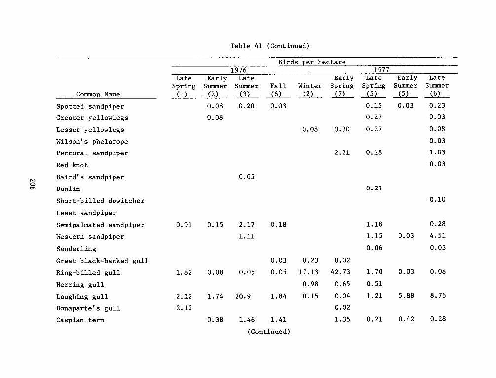
Table 41 (Continued)
Birds per hectare
Common Name
Spotted sandpiper
Greater yellowlegs
Lesser yellowlegs
Wilson' s phalarope
Pectoral sandpiper
Red knot
Baird's sandpiper
Dunlin
Short-billed dowitcher
Least sandpiper
Semipalmated sandpiper
Western sandpiper
Sanderling
Great black-backed gull
Ring-billed gull
Herring gull
Laughing gull
Bonaparte's gull
Caspian tern
LateSpring(1)
EarlySummer(2)
0.08
0.08
1976Late
Summer(3)
0.20
Fall(6)
0.03
1977Early Late
winter Spring Spring(2) (7) (5)
0.15
0.27
0.08 0.30 0.27
EarlySummer(5)
0.03
2.21 0.18
LateSummer(6)
0.23
0.03
0.08
0.03
1.03
0.03
0.05
0.21
0.10
0.91 0.15 2.17 0.18
0.03
1.82 0.08 0.05 0.05
2.12
2.12
1.74 20.9 1.84
0.23
17.13
0.98
0.15
0.38 1.46 1.41
(Continued)
0.02
42.73
0.65
0.04
0.02
1.35
1.18
1.15
0.06
1.70
0.51
1.21
0o
0.28
0.03 4.51
0.03
0.03 0.08
5.88 8.76
0.21 0.42 0.28
W
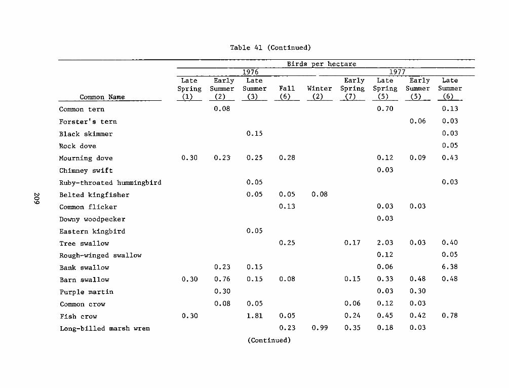
Table 41 (Continued)
Birds per hectare
Common Name
Common tern
Forster's tern
Black skimmer
Rock dove
Mourning dove
Chimney swift
Ruby-throated hummingbird
Belted kingfisher
Common flicker
Downy woodpecker
Eastern kingbird
Tree swallow
Rough-winged swallow
Bank swallow
Barn swallow
Purple martin
Common crow
Fish crow
Long-billed marsh wren
Late EarlySpring Summer(1) (2)
0.08
1976LateSummer(3)
EarlyFall Winter Spring(6) (2) (7)
1977Late
Spring(5)
0.70
0.15
0.30 0.23 0.25 0.28
0.05
0.05
0.12
0.03
Early Lateummer Summer(5) (6)
0.13
0.06 0.03
0.03
0.05
0.09 0.43
0.03
0.05
0.13
0.08
0.03
0.03
0.03
0.05
0.25
0.23
0.30 0.76
0.30
0.08
0.30
0.15
0.15 0.08
0.05
1.81 0.05
0.23
(Continued)
0.17 2.03
0.12
0.06
0.15 0.33
0.03
0.06 0.12
0.24 0.45
0.99 0.35 0.18
0.03 0.40
0.05
6.38
0.48 0.48
0.30
0.03
0.42 0.78
0.03
S
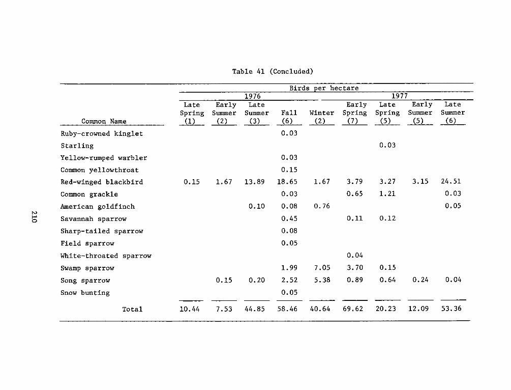
Table 41 (Concluded)
Common Name
Ruby-crowned kinglet
Starling
Yellow-rumped warbler
Common yellowthroat
Red-winged blackbird
Common grackle
American goldfinch
Savannah sparrow
Sharp-tailed sparrow
Field sparrow
White-throated sparrow
Swamp sparrow
Song sparrow
Snow bunting
LateSpring(1)
EarlySummer(2)
1976Late
Summer(3)
Birds per hectare
Fall(6)
0.03
Winter(2)
EarlySpring(7)
l977LateSpring(5)
0.03
0.03
0.15
0.15 1.67 13.89 18.65
0.03
0.10 0.08
0. 45
0.08
0.05
1.99
0.15 0.20 2.52
0.05
10.44 7.53 44.85 58.46
1.67 3.79
0.65
3.27
1.21
0.76
Early LateSummer Summer(5) (6)
3.15 24.51
0.03
0.05
0.11 0.12
7.05
5.38
0.04
3.70
0.89
0.15
0.64 0.24 0.04
Toal40.64 69.62 20.23 12.09 53.36
I\)
0
Total
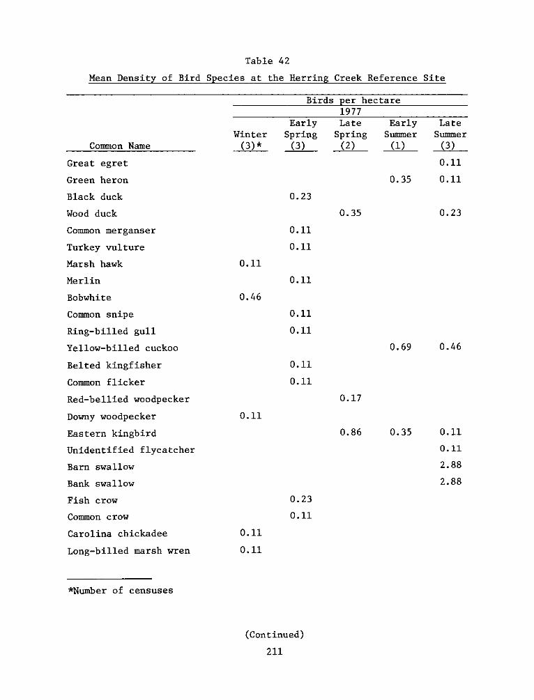
Table 42
Mean Density of Bird Species at the Herring Creek Reference Site
Common Name
Great egret
Green heron
Black duck
Wood duck
Common merganser
Turkey vulture
Marsh hawk
Merlin
Bobwhite
Common snipe
Ring-billed gull
Yellow-billed cuckoo
Belted kingfisher
Common flicker
Red-bellied woodpecker
Downy woodpecker
Eastern kingbird
Unidentified flycatcher
Barn swallow
Bank swallow
Fish crow
Common crow
Carolina chickadee
Long-billed marsh wren
*Number of censuses
Winter(3) *
EarSpri(3)
Birds per hec tare1977
ly Late Ea:ng Spring Suim
(2) (11
rlyner)
0.35
0.11
0.46
0.11
0.23
0.11
0.11
0.11
0.11
0.11
0.11
0.11
0.35
0.69
0.17
0.86 0.35
0.23
0.11
0.11
0.11
(Continued)
211
LateSummer(3)
0.11
0.11
0.23
0.46
0.11
0.11
2.88
2.88
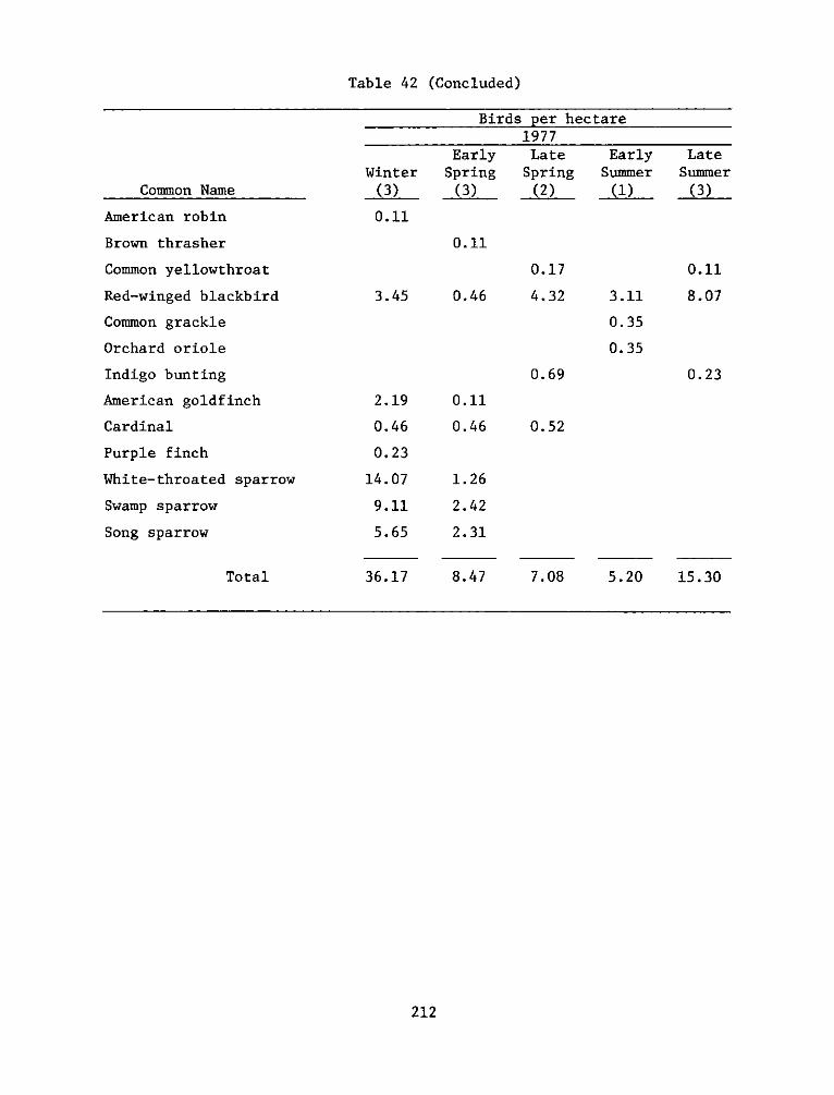
Table 42 (Concluded)
Common Name
American robin
Brown thrasher
Common yellowthroat
Red-winged blackbird
Common grackle
Orchard oriole
Indigo bunting
American goldfinch
Cardinal
Purple finch
White-throated sparrow
Swamp sparrow
Song sparrow
Total
Winter(3)
0.11
3.45
EarSpri
(3)
Birds per hectare1977
*ly Late Eang Spring Sum
(2) (1
0.11
0.46
0.17
4.32
rlymner)
3.11
0.35
0.35
0.69
2.19
0.46
0.23
14.07
9.11
5.65
36.17
0.11
0.46
1.26
2.42
2.31
8.47
LateSummer
(3)
0.11
8.07
0.23
0.52
7.08 5.20 15.30
212
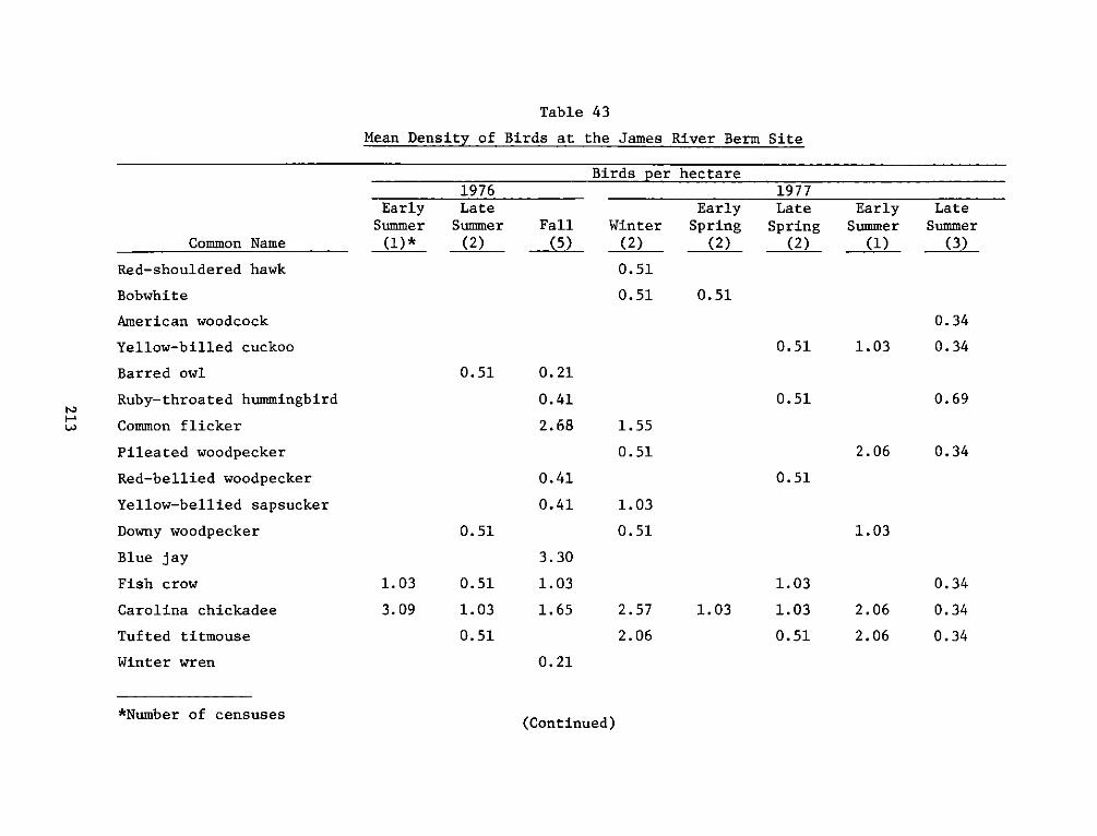
Table 43
Mean Density of Birds at the James River Berm Site
Birds per hec tare1976 1977
Early Late Early Late Early LateSummer Summer Fall Winter Spring Spring Summer Summer
Common Name (1)* (2) (5) (2) (2) (2) (1) (3)
Red-shouldered hawk 0.51
Bobwhite 0.51 0.51
American woodcock 0.34
Yellow-billed cuckoo 0.51 1.03 0.34
Barred owl 0.51 0.21
Ruby-throated hummingbird 0.41 0.51 0.69
Common flicker 2.68 1.55
Pileated woodpecker 0.51 2.06 0.34
Red-bellied woodpecker 0.41 0.51
Yellow-bellied sapsucker 0.41 1.03
Downy woodpecker 0.51 0.51 1.03
Blue jay 3.30
Fish crow 1.03 0.51 1.03 1.03 0.34
Carolina chickadee 3.09 1.03 1.65 2.57 1.03 1.03 2.06 0.34
Tufted titmouse 0.51 2.06 0.51 2.06 0.34
Winter wren 0.21
*Number of censuses (Continued)
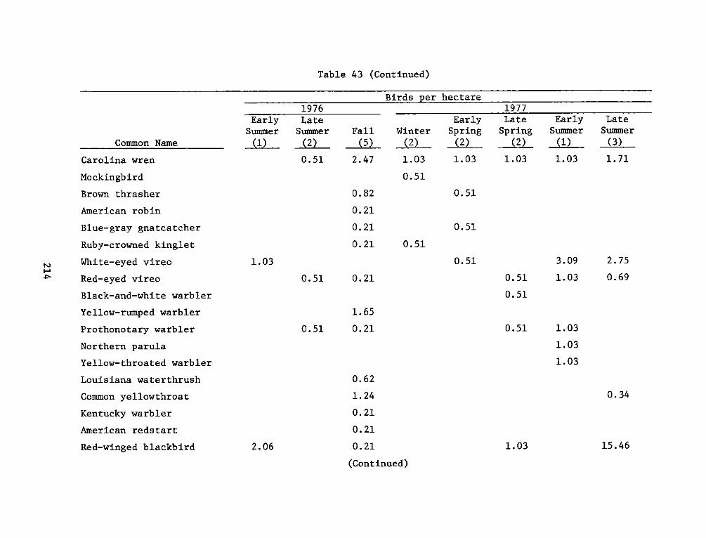
Table 43 (Continued)
Birds per hectare
Common Name
Carolina wren
Mockingbird
Brown thrasher
American robin
Blue-gray gnatcatcher
Ruby-crowned kinglet
White-eyed vireo
Red-eyed vireo
Black-and-white warbler
Yellow-ruxnped warbler
Prothonotary warbler
Northern parula
Yellow-throated warbler
Louisiana waterthrush
Common yellowthroat
Kentucky warbler
American redstart
Red-winged blackbird
EarlySummer(1)
1976LateSummer(2)
0.51
1.03
0.51
0.51
Fall(5)
2.47
0.82
0.21
0.21
0.21
0.21
1.65
0.21
Winter(2)
1.03
0.51
0.51
0.62
1.24
0.21
0.21
2.06 0.21
(Continued)
EarlySpring(2)
1.03
1977Late
Spring(2)
1.03
'-a
EarlySummer(1)
1.03
3.09
1.03
LateSummer(3)
1.71
2.75
0.69
0.51
0.51
0.51
0.51
0.51
0.51 1.03
1.03
1.03
0.34
15.461.03
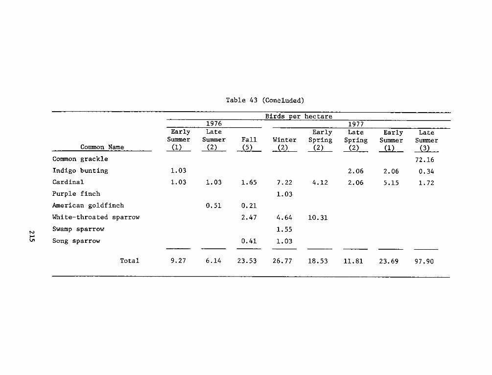
Table 43 (Concluded)
Birds per hec tare1976 1977
Early Late Early Late Early LateSummer Summer Fall Winter Spring Spring Summer Summer
Common Name (1) (2) (5) (2) (2) (2) (1) (3)
Common grackle 72.16
Indigo bunting 1.03 2.06 2.06 0.34
Cardinal 1.03 1.03 1.65 7.22 4.12 2.06 5.15 1.72
Purple finch 1.03
American goldfinch 0.51 0.21
White-throated sparrow 2.47 4.64 10.31
Swamp sparrow 1.55
Song sparrow 0.41 1.03
Total 9.27 6.14 23.53 26.77 18.53 11.81 23.69 97.90
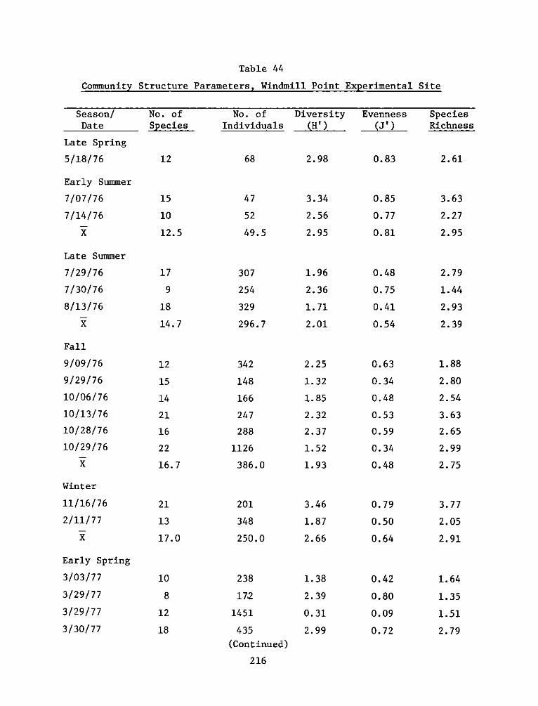
Table 44
Community Structure Parameters, Windmill Point Experimental SiteDiversity Species
Season/!Date
Late Spring
5/18/76
Early Summer
7/07/ 76
7/14/76
Late Summer
7/29/76
7/30/ 76
8/13/76
Fall
9/09/76
9/29/ 76
10/06/76
10/13/76
10/28/76
10/29/76
Winter
11/16/76
2/11/77
Early Spring
3/03/77
3/29/ 77
3/29/ 77
3/30/ 77
No. ofSpecies
12
15
10
12.5
17
9
18
14. 7
12
15
14
21
16
22
16.7
21
13
17.0
10
8
12
18
No. ofIndividuals
68
47
52
49.5
307
254
329
296.7
342
148
166
247
288
1126
386.0
201
348
250.0
238
172
1451
435
(Continued)
216
(H')
2.98
3.34
2.56
2.95
1.96
2.36
1.71
2.01
2.25
1.32
1.85
2.32
2.37
1.52
1.93
3.46
1.87
2.66
1.38
2.39
0.31
2.99
Evenness
(J')
0.83
0.85
0.77
0.81
0.48
0.75
0.41
0.54
0.63
0.34
0.48
0.53
0.59
0.34
0.48
0.79
0.50
0.64
0.42
0.80
0.09
0.72
Richness
2.61
3.63
2.27
2.95
2.79
1.44
2.93
2.39
1.88
2.80
2.54
3.63
2.65
2.99
2.75
3.77
2.05
2.91
1.64
1.35
1.51
2.79
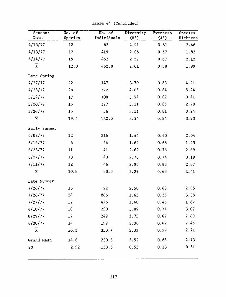
Table 44 (Concluded)
Season/Date
4/13/77
4/13/77
4/14/77
Late Spring
4/27/ 77
4/28/77
5/19/77
5/20/77
5/26/77
Early Summer
6/02/ 77
6/16/77
6/23/ 77
6/27/ 77
7/11/77
Late Summer
7/26/77
7/26/77
7/27/77
8/10/77
8/29/ 77
8/30/ 77
Grand Mean
SD
No. of
Species
12
12
15
12.0
22
28
17
15
15
19.4
12
6
11
13
12
10.8
13
24
12
18
17
14
16.3
14.6
2.92
No. of DiversityIndividuals (H')
62 2.91
419 2.05
453 2.57
462.8 2.01
147
172
108
177
56
132.0
216
54
41
43
46
80.0
92
886
426
250
249
199
350.7
230.6
153.6
3.70
4.05
3.54
3.31
3.11
3.54
1.44
1.69
2.62
2.76
2.96
2.29
2.50
1.63
1.60
3.09
2.75
2.36
2.32
2.52
0.55
217
Evenness(J')
0.81
0.57
0.67
0.58
0.83
0.84
0.87
0.85
0.81
0.84
0.40
0.66
0.76
0.74
0.83
0.68
0.68
0.36
0.45
0.74
0.67
0.62
0.59
0.68
0.13
SpeciesRichness
2.66
1.82
2.12
1.99
4.21
5.24
3.41
2.70
3.24
3.83
2.04
1.25
2.69
3.19
2.87
2.41
2.65
3.38
1.82
3.07
2.89
2.45
2.71
2.73
0.51
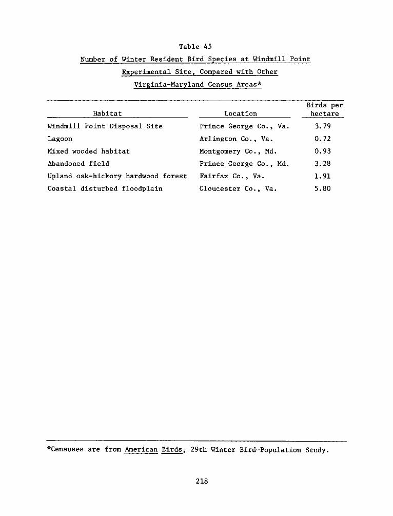
Table 45
Number of Winter Resident Bird Species at Windmill Point
Experimental Site, Compared with Other
Virginia-Maryland Census Areas*
Habitat
Windmill Point Disposal Site
Lagoon
Mixed wooded habitat
Abandoned field
Upland oak-hickory hardwood forest
Coastal disturbed floodplain
Location
Prince George Co., Va.
Arlington Co., Va.
Montgomery Co., Md.
Prince George Co., Md.
Fairfax Co., Va.
Gloucester Co., Va.
218
Birds per
hec tare
3.79
0.72
0.93
3.28
1.91
5.80
*Censuses are from American Birds, 29th Winter Bird-Population Study.
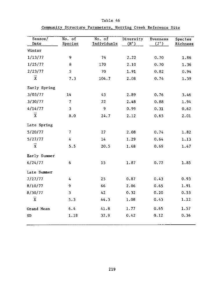
Table 46
Community Structure Parameters, Herring Creek Reference Site
Season/!Date
Winter
1/13/77
1/25/ 77
2/23/ 77
Early Spring
3/03/77
3/30/77
4/14/77
X
Late Spring
5/20/77
5/27/ 77
Early Summer
6/24/ 77
Late Summer
7/27/77
8/10/77
8/30/ 77
Grand Mean
SD
No. ofSpecies
9
8
5S
7.3
14
7
3
8.0
7
4
5.5
6
4
9
3
5.3
6.4
1.18
No. ofIndividuals
74
170
70
104.7
43
22
9
24.7
27
14
20.5
15
25
66
42
44.3
41.8
32.9
Diversity(H')
2.22
2.10
1.91
2.08
2.89
2.48
0.99
2.12
2.08
1.29
1.68
1.87
0.87
2.06
0.32
1.08
1.77
0.42
Evenness Species(J') Richness
0.70
0.70
0.82
0.74
0.76
0.88
0.31
0.65
0.74
0.64
0.69
0.72
0.43
0.65
0.20
0.43
0.65
0.12
1.86
1.36
0.94
1.39
3.46
1.94
0.62
2.01
1.82
1.13
1.47
1.85
0.93
1.91
0.53
1.12
1.57
0.36
219
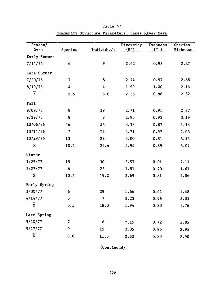
Table 47
Community Structure Parameters, James River Berm
Season/
Date
Early Summer
7/14176
Late Summer
7/30/76
8/19/76
Fall
9/09176
9/29/ 76
10/06/76
10/14/76
10/29/76
Winter
1/25/77
2/23/ 77
Early Spring
3/30/ 77
4/14/77
Late Spring
5/20/ 77
5/27/ 77
Species Individuals
6
7
4
5.5
8
8
16
7
13
10.4
15
6
10.5
6
5
5.5
7
9
8.0
9
8
4
6.0
19
9
36
19
29
22.4
30
22
19.2
29
7
18.0
8
15
11.5
(H')
2.42
2.74
1.99
2.36
2.71
2.95
3.33
2.71
3.00
2.94
3.57
1.81
2.69
1.66
2.23
1.94
2.15
3.05
2.60
Evenness Species(J') Richness
0.93
0.97
1.00
0.98
0.91
0.93
0.83
0.97
0.81
0.89
0.91
0.70
0.81
0.64
0.96
0.80
0.72
0.96
0.80
2.27
2.88
2.16
2.52
2.37
3.19
4.18
2.03
3.56
3.07
4.11
1.61
2.86
1.48
2.05
1.76
2.85
2.95
2.90
(Continued)
220
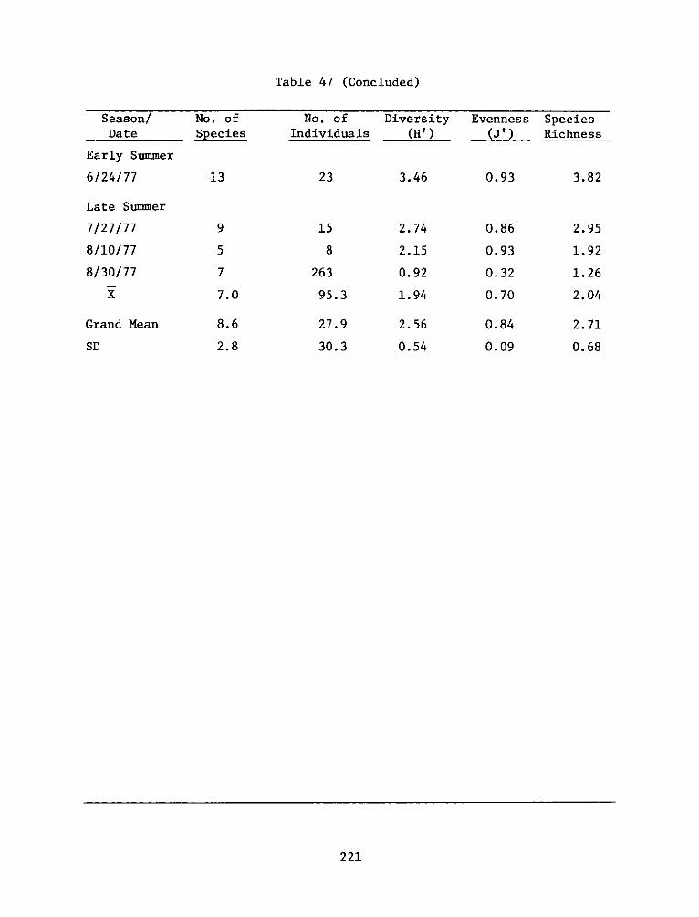
Table 47 (Concluded)No. of Diversity
Season/ No. of
Date Species
Early Summer
6/24/77 13
Late Summer
7/27/ 77
8/10/77
8/30/77
Grand Mean
SD
9
5
7
7.0
8.6
2.8
Individuals
23
15
8
263
95.3
27.9
30.3
(H')
3.46
2.74
2.15
0.92
1.94
2.56
0.54
Evenness Species(J') Richness
0.93
0.86
0.93
0.32
0.70
0.84
0.09
3.82
2.95
1.92
1.26
2.04
2.71
0.68
221
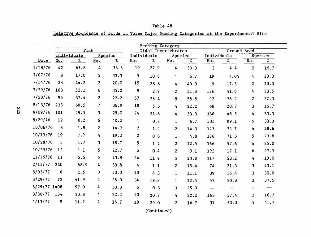
Table 48
Relative Abundance of Birds in Three Major Feeding Categories at the Experimental Site
FishIndividuals
Date No. %___
5/18/ 76 42
7/07/76 8
7/14/ 76 23
7/29/76 163
7/30/ 76 95
8/13/76 233
9/09/76 101
9/29/76 12
10/06/76 3
10/13/76 19
10/28/76 5
10/29/76 12
11/16/76 11
2/11/77 240
3/03/77 6
3/29/77 72
3/29/77 1408
3/30/77 134
4/13/77 8
61.8
17.0
44.2
53.1
37.4
68.5
29.5
8.2
1.8
7.7
1.7
1.1
5.5
68.9
2.5
41.9
97.0
30.8
11.2
SpeciesNo. %___
4
5
2
6
2
7
3
6
2
4
3
5
5
4
3
2
4
4
2
33.3
33.3
20.0
35.2
22.2
38.9
25.0
40.0
14.3
19.0
18.7
22.7
23.8
30.8
30.0
25.0
33.3
22.2
16.7
Feeding CategoryTidal Invertebrates
IndividualsNo. %__
19 27.9
5
15
9
67
18
74
1
2
2
5
5
24
4
10
34
5
90
18
SpeciesNo. %__
4 33.3
10.6
28.8
2.9
26.4
5.3
21.6
0.7
1.2
0.8
1.7
0.4
11.9
1.1
4.3
19.8
0.3
20.7
29.0
6.7
40.0
11.8
55.5
22.2
33.3
6.7
14. 3
4.8
12.5
9.1
23.8
15.4
11.1
12.5
25.0
22.2
16.7
Ground SeedIndividualsNo. %___
3 4.4
19
9
126
92
68
166
131
123
176
166
193
117
74
39
53
163
31
4.04
17.3
41.0
36.2
20.7
48.5
89.1
74.1
71.3
57.6
17.1
58.2
21.3
16.4
30.8
37.4
50.0
SpeciesNo. %__
2 16.7
4 20.0
2 20.0
4 23.5
2 22.3
3 16.7
4 33.3
5 33.3
4 28.6
5 23.8
4 25.0
6 27.3
4 19.0
3 23.1
3 30.0
3 37.5
3 16.7
5 41.7
(Continued)
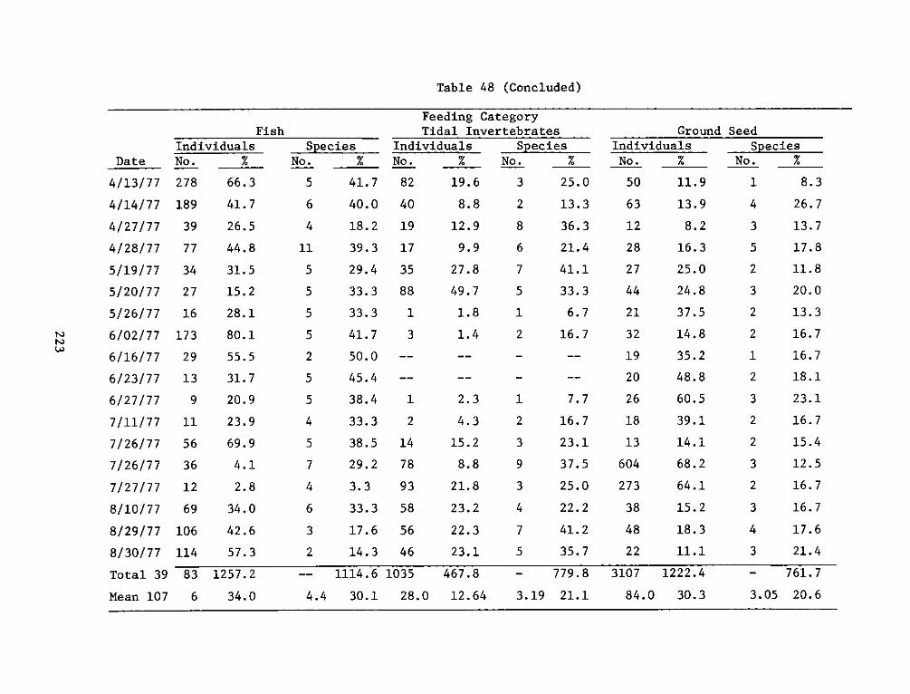
Table 48 (Concluded)
FishIndividuals
Date No. %___
4/13/77
4/14/77
4/27/77
4/28/77
5/19/77
5/20/77
5/26/77
6/02/ 77
6/16/7 7
6/23/ 77
6/27/77
7/11/ 77
7/26/77
7/26/77
7/27/ 77
8/10/ 77
8/29/77
8/30/77
Total 39
278
189
39
77
34
27
16
173
29
13
9
11
56
36
12
69
106
114
83
66.3
41.7
26.5
44.8
31.5
15.2
28.1
80.1
55.5
31.7
20.9
23.9
69.9
4.1
2.8
34.0
42.6
57.3
1257.2
Feeding CategoryTidal Invertebrates
SpeciesNo. %___
5 41.7
6 40.0
4 18.2
11 39.3
5 29.4
5 33.3
5 33.3
5 41.7
2 50.0
5 45.4
5 38.4
4 33.3
5 38.5
7 29.2
4 3.3
6 33.3
3 17.6
2 14.3
-- 1114.6
IndividualsNo. %__
SpeciesNo. %__
Ground SeedIndividualsNo. %___
82 19.6 3 25.0 50
40 8.8 2 13.3 63
19 12.9 8 36.3 12
17 9.9 6 21.4 28
35 27.8 7 41.1 27
88 49.7 5 33.3 44
1 1.8 1 6.7 21
3 1.4 2 16.7 32
-- -- - -- 19
-- -- - -- 20
1 2.3 1 7.7 26
2 4.3 2 16.7 18
14 15.2 3 23.1 13
78 8.8 9 37.5 604
93 21.8 3 25.0 273
58 23.2 4 22.2 38
56 22.3 7 41.2 48
46 23.1 5 35.7 22
~35 467.8 - 779.8 3107
11.9
13.9
8.2
16.3
25.0
24.8
37.5
14.8
35.2
48.8
60.5
39.1
14.1
68.2
64.1
15.2
18.3
11.1
1222.4
SpeciesNo. %__
1 8.3
4 26.7
3 13.7
5 17.8
2 11.8
3 20.0
2 13.3
2 16.7
1 16.7
2 18.1
3 23.1
2 16.7
2 15.4
3 12.5
2 16.7
3 16.7
4 17.6
3 21.4
- 761.7
Mean 107 6 34.0 4.4 30.1 28.0 12.64 3.19 21.1 84.0 30.3 3.05 20.6
I\)
84.0 30.3 3.05 20.6
10
Mean 107 6 34.0 4.4 30.1 28.0 12.64 3.19 21.1
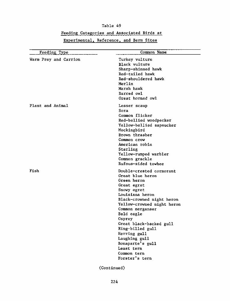
Table 49
Feeding Categories and Associated Birds at
Experimental, Reference, and Berm Sites
Feeding Type
Warm Prey and Carrion
Plant and Animal
Fish
Common Name
Turkey vultureBlack vultureSharp-shinned hawkRed-tailed hawkRed-shouldered hawkMerlinMarsh hawkBarred owlGreat horned owl
Lesser scaupSoraCommon flickerRed-bellied woodpeckerYellow-bellied sapsuckerMockingbirdBrown thrasherCommon crowAmerican robinStarlingYellow-rumped warblerCommon grackleRufous-sided towhee
Double-crested cormorantGreat blue heronGreen heronGreat egretSnowy egretLouisiana heronBlack-crowned night heronYellow-crowned night heronCommon merganserBald eagleOspreyGreat black-backed gullRing-billed gullHerring gullLaughing gullBonaparte's gullLeast ternCommon ternForster' s tern
(Continued)
224
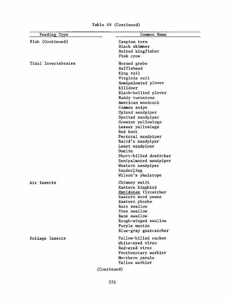
Table 49 (Continued)
Feeding Type
Fish (Continued)
Tidal Invertebrates
Air Insects
Foliage Insects
Common Name
Caspian ternBlack skimmerBelted kingfisherFish crow
Horned grebeBuf fleheadKing railVirginia railSemipalmated ploverKilldeerBlack-bellied ploverRuddy turns toneAmerican woodcockCommon snipeUpland sandpiperSpotted sandpiperGreater yellowlegsLesser yellowlegsRed knotPectoral sandpiperBaird's sandpiperLeast sandpiperDunlinShort-billed dowitcherSemipalmated sandpiperWestern sandpiperSanderlingWilson' s phalarope
Chimney swiftEastern kingbirdEmpidonax flycatcherEastern wood peweeEastern phoebeBarn swallowTree swallowBank swallowRough-winged swallowPurple martinBlue-gray gnatcatcher
Yellow-billed cuckooWhite-eyed vireoRed-eyed vireoProthonotary warblerNorthern parulaYellow warbler
(Continued)
225
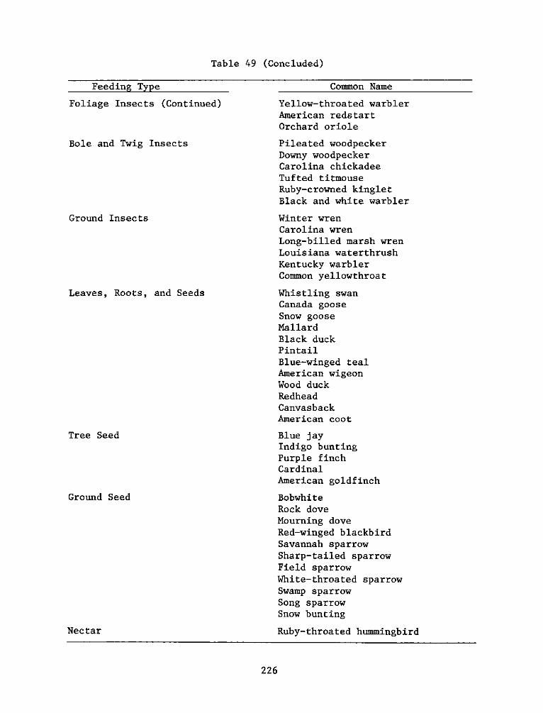
Table 49 (Concluded)
Feeding Type
Foliage Insects (Continued)
Bole and Twig Insects
Ground Insects
Leaves, Roots, and Seeds
Tree Seed
Ground Seed
Nectar
Common Name
Yellow-throated warblerAmerican redstartOrchard oriole
Pileated woodpeckerDowny woodpeckerCarolina chickadeeTufted titmouseRuby-crowned kingletBlack and white warbler
Winter wrenCarolina wrenLong-billed marsh wrenLouisiana waterthrushKentucky warblerCommon yellowthroat
Whistling swanCanada gooseSnow gooseMallardBlack duckPintailBlue-winged tealAmerican wigeonWood duckRedheadCanvasbackAmerican coot
Blue jayIndigo buntingPurple finchCardinalAmerican goldfinch
BobwhiteRock doveMourning doveRed-winged blackbirdSavannah sparrowSharp-tailed sparrowField sparrowWhite-throated sparrowSwamp sparrowSong sparrowSnow bunting
Ruby-throated hummingbird
226
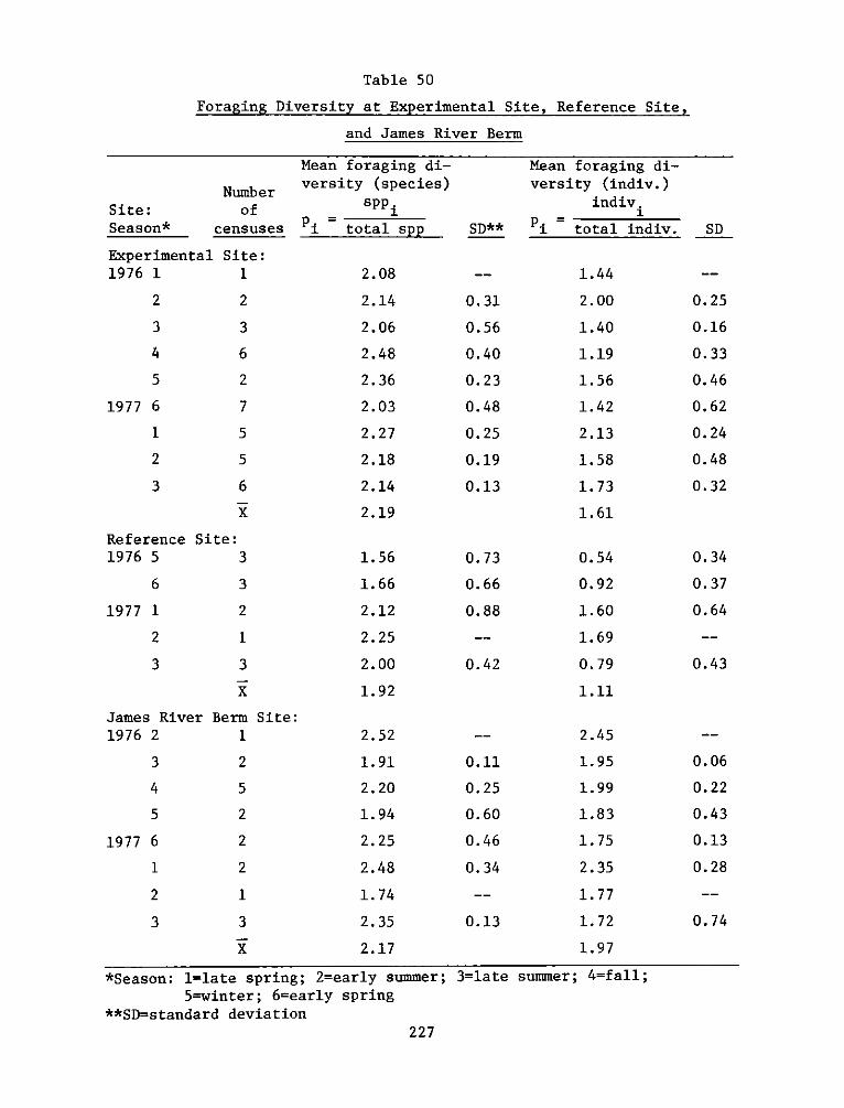
Table 50
Foraging Diversity at Experimental Site, Reference Site,
and James River Berm
NumberSite: ofSeason* censuses
Experimental Site:1976 1 1
2 2
3 3
4 6
5 2
1977 6 7
1 5
2 5
3 6
Reference Site:
1976 5 3
6 3
1977 1 2
2 1
3 3
Mean foraging di-versity (species)
spp.
= total spp
2.08
2.14
2.06
2.48
2.36
2.03
2.27
2.18
2.14
2.19
1.56
1.66
2.12
2.25
2.00
1.92
James River Berm Site:1976 2 1 2.52
3 2 1.91
4 5 2.20
5 2 1.94
1977 6 2 2.25
1 2 2.48
2 1 1.74
3 3 2.35
X 2.17
*Season: l=late spring; 2=early summer;5=winter; 6=early spring
**SDstandard deviation227
Mean foraging di-versity (indiv.)
mndiv.
SD** ~i =total indiv.
0.31
0.56
0.40
0.23
0.48
0.25
0.19
0.13
0.73
0.66
0.88
0.42
1.44
2.00
1.40
1.19
1.56
1.42
2.13
1.58
1.73
1. 61
0.54
0.92
1.60
1.69
0.79
1.11
-- 2.45
0.11 1.95
0.25 1.99
0.60 1.83
0.46 1.75
0.34 2.35
-- 1.77
0.13 1.72
1.97
3=late summer; 4=fall;
SD
0.25
0.16
0.33
0.46
0.62
0.24
0.48
0.32
0.34
0.37
0.64
0.43
0.06
0.22
0.43
0.13
0.28
0.74
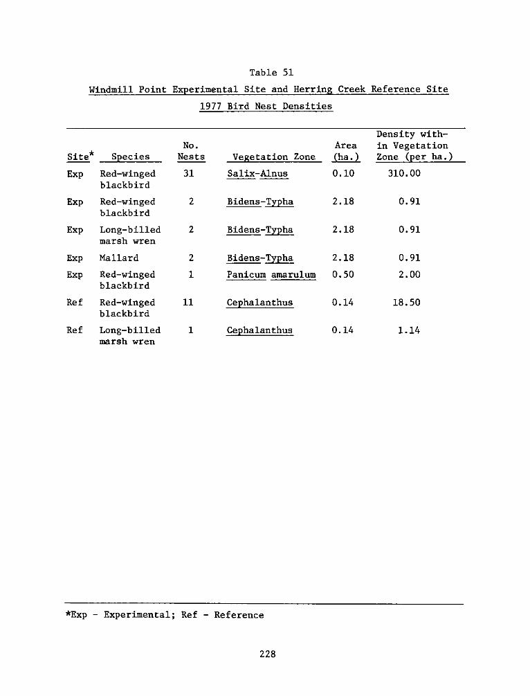
Table 51
Windmill Point Experimental Site and Herring Creek Reference Site
1977 Bird Nest Densities
Species
Red-wingedblackbird
Red-wingedblackbird
Long-billedmarsh wren
Mallard
Red-wingedblackbird
Red-wingedblackbird
Long-billedmarsh wren
No.Nests
31
2
2
2
1
11
1
Vegetation Zone
Salix-Alnus
Bidens-Typha
Bidens-Typha
Bidens-Typha
Panicum amarului
Cephalanthus
Cephalanthus
Area(ha.)
0.10
2.18
2.18
2.18
0.50
0.14
0.14
Density with-in VegetationZone (per ha.)
310.00
0.91
0.91
0.91
2.00
18.50
1.14
*Exp - Experimental; Ref - Reference
228
Site*
Exp
Exp
Exp
Exp
Exp
Ref
Ref
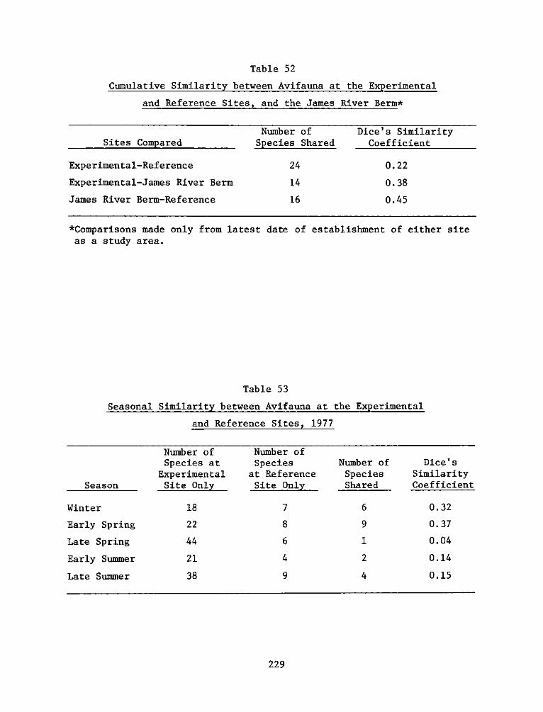
Table 52
Cumulative Similarity between Avifauna at the Experimental
and Reference Sites, and the James River Berm*
Number of Dice's SimilaritySites Compared Species Shared Coefficient
Experimental-Reference 24 0.22
Experimental-James River Berm 14 0.38
James River Berm-Reference 16 0.45
*Comparisons made only from latest date of establishment of either siteas a study area.
Table 53
Seasonal Similarity between Avifauna at the Experimental
and Reference Sites, 1977
Season
Winter
Early Spring
Late Spring
Early Summer
Late Summer
Number ofSpecies at
ExperimentalSite Only
18
22
44
21
38
Number ofSpecies
at ReferenceSite Only
7
8
6
4
9
Number ofSpeciesShared
6
9
1
2
4
Dice'sSimilarityCoefficient
0.32
0.37
0.04
0.14
0.15
229
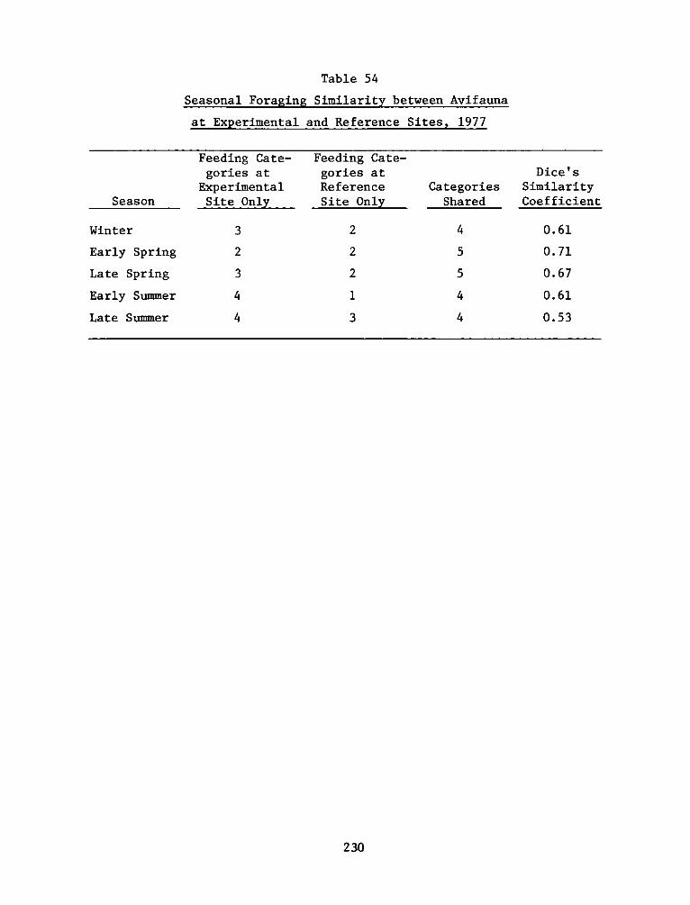
Table 54
Seasonal Foraging Similarity between Avifauna
at Experimental and Reference Sites, 1977
Season
Winter
Early Spring
Late Spring
Early Summer
Late Summer
Feeding Cate-gories at
ExperimentalSite Only
3
2
3
4
4
Feeding Cate-gories atReferenceSite Only
2
2
2
1
3
CategoriesShared
4
5
5
4
4
Dice'sSimilarityCoefficient
0.61
0.71
0.67
0.61
0.53
230
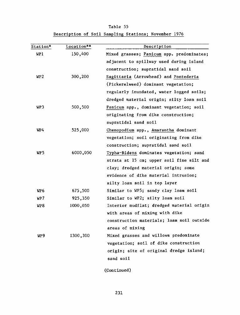
Description of Soil
Table 55
Sampling Stations; November 1976
Station*
WP1
Location**
150,400
300,200
500,500
525 ,000
6000,050
675,500
925,350
1000,050
1300,300
231
WP2
Description
Mixed grasses; Panicum spp. predominates;
adjacent to spillway used during island
construction; supratidal sand soil
Sagittaria (Arrowhead) and Pontederia
(Pickerelweed) dominant vegetation;
regularly inundated, water logged soils;
dredged material origin; silty loam soil
Panicum spp., dominant vegetation; soil
originating from dike construction;
supratidal sand soil
Chenopodium spp., Amarantha dominant
vegetation; soil originating from dike
construction; supratidal sand soil
Typha-Bidens dominates vegetation; sand
strata at 15 cm; upper soil fine silt and
clay; dredged material origin; some
evidence of dike material intrusion;
silty loam soil in top layer
Similar to WP5; sandy clay loam soil
Similar to WP2; silty loam soil
Interior mudflat; dredged material origin
with areas of mixing with dike
construction materials; loam soil outside
areas of mixing
Mixed grasses and willows predominate
vegetation; soil of dike construction
origin; site of original dredge island;
sand soil
(Continued)
WP3
WP4
WP5
WP6
WP7
WP8
WP9
r r v
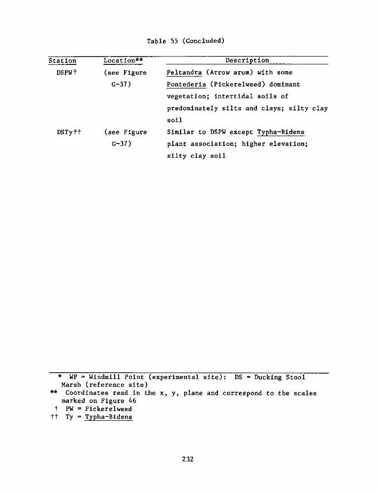
Table 55 (Concluded)
Location**
(see Figure
G-37)
(see Figure
G-37)
Description
Peltandra (Arrow arum) with some
Pontederia (Pickerelweed) dominant
vegetation; intertidal soils of
predominately silts and clays; silty clay
soil
Similar to DSPW except Typha-Bidens
plant association; higher elevation;
silty clay soil
* WP = Windmill Point (experimental site): DS = Ducking StoolMarsh (reference site)
** Coordinates read in the x, y, plane and correspond to the scalesmarked on Figure 46
t PW = Pickerelweedtt Ty = Typha-Bidens
232
Station
DSPWt
DSTy tt
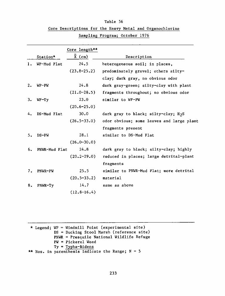
Core Descriptions for
Sampling
Table 56
the Heavy Metal and Organochlorine
Program; October 1976
Station*
1. WP-Mud Flat
2. WP-PW
3. WP-Ty
4. DS-Mud Flat
5. DS-PW
6. PNWR-Mud Flat
7. PNWR-PW
8. PNWR-Ty
Core length**
X (cm)
24.5
(23.8-25.2)
24.8
(21.0-28.5)
23.0
(20.6-25.0)
30.0
(26.5-33.0)
28.1
(26.0-30.0)
24.8
(20.2-29.0)
25.5
(20.5-33.2)
14.7
(12.8-16.4)
Description
heterogeneous soil; in places,
predominately gravel; others silty-
clay; dark gray, no obvious odor
dark gray-green; silty-clay with pl
fragments throughout; no obvious od
similar to WP-PW
ant
or
dark gray to black; silty-clay; H25
odor obvious; some leaves and large plant
fragments present
similar to DS-Mud Flat
dark gray to black; silty-clay; highly
reduced in places; large detrital-plant
fragments
similar to PNWR-Mud Flat; more detrital
material
same as above
* Legend; WP = Windmill Point (experimental site)DS = Ducking Stool Marsh (reference site)PNWR = Presquile National Wildlife RefugePW = Pickerel WeedTy = Typha-Bidens
** Nos. in parenthesis indicate the Range; N = 5
233
a v v
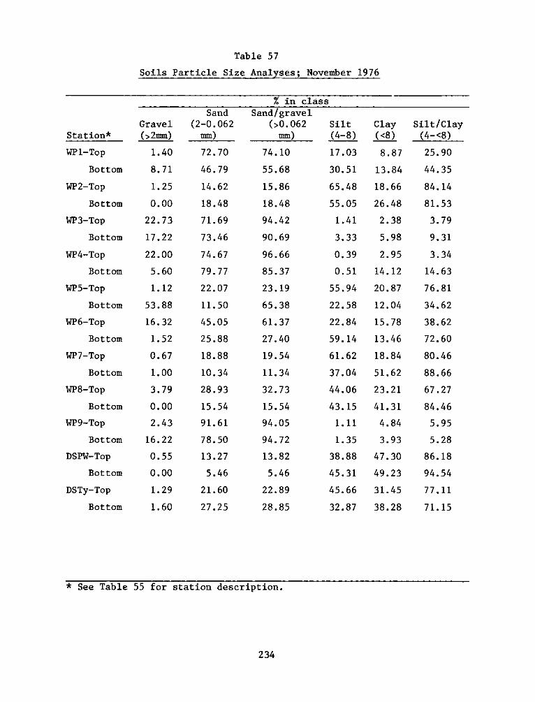
Table 57
Soils Particle Size Analyses; November 1976
% in class
Station*
WP1-Top
Bottom
WP2-Top
Bottom
WP3-Top
Bottom
WP4-Top
Bottom
WP5-Top
Bottom
WP6-Top
Bottom
WP7-Top
Bottom
WP8-Top
Bottom
WP9-Top
Bottom
DSPW-Top
Bottom
DSTy-Top
Bottom
Gravel(>2mm)
1.40
8.71
1.25
0.00
22.73
17.22
22.00
5.60
1.12
53.88
16.32
1.52
0.67
1.00
3.79
0.00
2.43
16.22
0.55
0.00
1.29
1.60
Sand(2-0.062mm)
72.70
46.79
14.62
18.48
71.69
73.46
74.67
79.77
22.07
11.50
45.05
25.88
18.88
10.34
28.93
15.54
91.61
78.50
13.27
5.46
21.60
27.25
Sand/gravel(>0.062mm)
74.10
55.68
15.86
18.48
94.42
90.69
96.66
85.37
23.19
65.38
61.37
27.40
19.54
11.34
32.73
15.54
94.05
94.72
13.82
5.46
22.89
28.85
Silt
(4-8)
17.03
30.51
65.48
55.05
1.41
3.33
0.39
0.51
55.94
22.58
22.84
59.14
61.62
37.04
44.06
43.15
1.11
1.35
38.88
45.31
45.66
32.87
Clay
(<8)
8.87
13.84
18.66
26.48
2.38
5.98
2.95
14.12
20.87
12.04
15.78
13.46
18.84
51.62
23.21
41.31
4.84
3.93
47.30
49.23
31.45
38.28
* See Table 55 for station description.
234
Silt/Clay(4-<8)
25.90
44.35
84.14
81.53
3.79
9.31
3.34
14.63
76.81
34.62
38.62
72.60
80.46
88.66
67.27
84.46
5.95
5.28
86.18
94.54
77.11
71.15
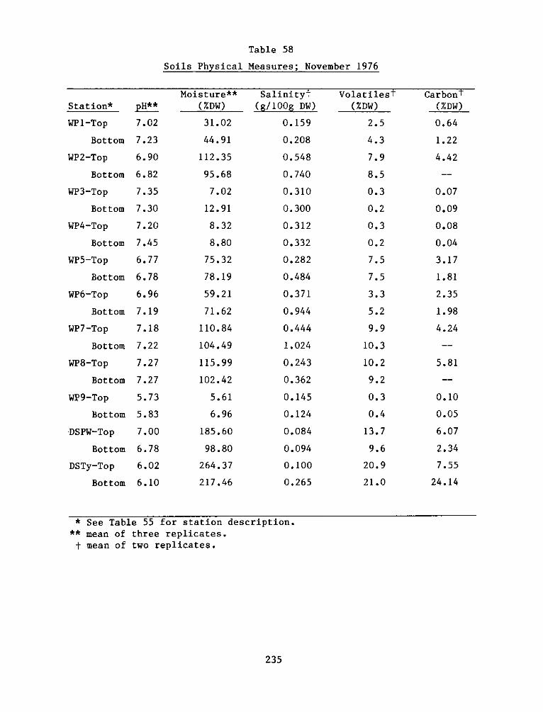
Soils Physical
Table 58
Measures; November 1976
Station*
WP1-Top
Bottom
WP2-Top
Bottom
WP3-Top
Bottom
WP4-Top
Bottom
WP5-Top
Bottom
WP6-Top
Bottom
WP7-Top
Bottom
WP8-Top
Bottom
WP9-Top
Bottom
DSPW-Top
Bottom
DSTy-Top
Bottom
Moisture**
pH** (%DW)
7.02
7.23
6.90
6.82
7.35
7.30
7.20
7.45
6.77
6.78
6.96
7.19
7.18
7.22
7.27
7.27
5.73
5.83
7.00
6.78
6.02
6.10
31.02
44.91
112.35
95.68
7.02
12.91
8.32
8.80
75.32
78.19
59.21
71.62
110.84
104.49
115.99
102.42
5.61
6.96
185.60
98.80
264.37
217.46
Salinityt(g/100g DW)
0.159
0.208
0.548
0.740
0.310
0.300
0.312
0.332
0.282
0.484
0.371
0.944
0.444
1.024
0.243
0.362
0.145
0.124
0.084
0.094
0.100
0.265
Volatilest(%DW)
2.5
4.3
7.9
8.5
0.3
0.2
0.3
0.2
7.5
7.5
3.3
5.2
9.9
10.3
10.2
9.2
0.3
0.4
13.7
9.6
20.9
21.0
* See Table 55 for station description.
** mean of three replicates.t mean of two replicates.
235
CarbonCarbonT
(%Dw)
0.64
1.22
4.42
0.07
0.09
0.08
0.04
3.17
1.81
2.35
1.98
4.24
5.81
0.10
0.05
6.07
2.34
7.55
24.14
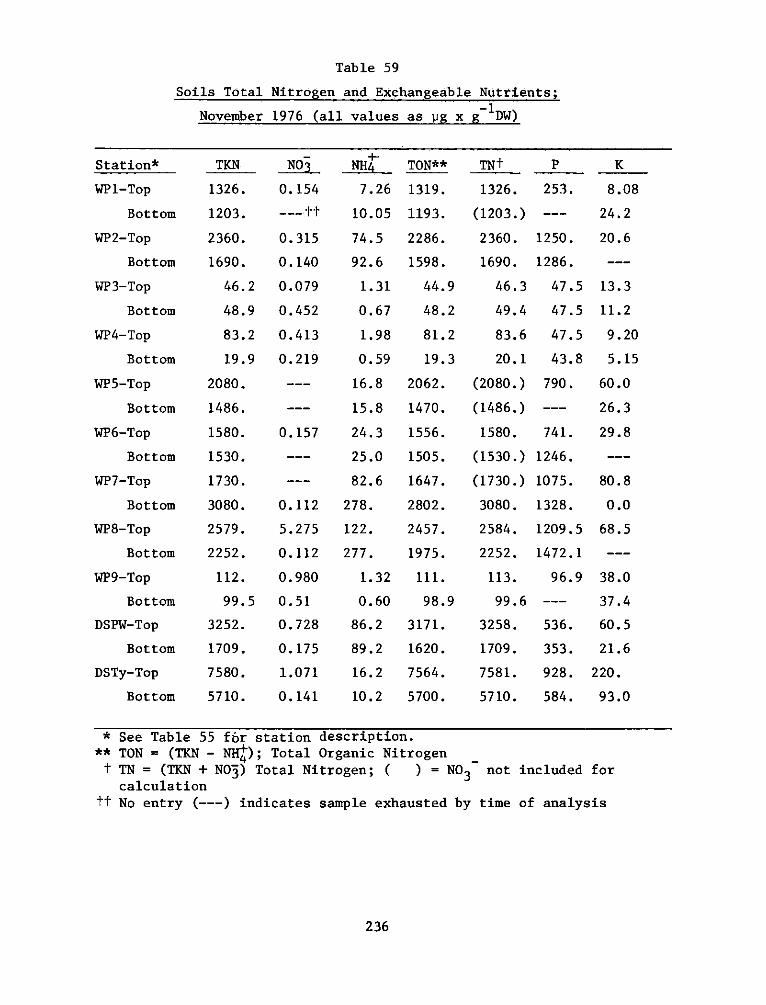
Soils Total
Table 59
Nitrogen and Exchangeable Nutrients;
November 1976 (all values as Vg x g~ DW)
Station*
WP1-Top
Bottom
WP2-Top
Bottom
WP3-Top
Bottom
WP4-Top
Bottom
WP5-Top
Bottom
WP6-Top
Bottom
WP7-Top
Bottom
WP8-Top
Bottom
WP9-Top
Bottom
DSPW-Top
Bottom
DSTy-Top
Bottom
TKN
1326.
1203.
2360.
1690.
46.2
48.9
83.2
19.9
2080.
1486.
1580.
1530.
1730.
3080.
2579.
2252.
112.
99.5
3252.
1709.
7580.
5710.
-I-N03 N!!A
0.154 7.26
--- tt 10.05
0.315 74.5
0.140 92.6
0.079 1.31
0.452 0.67
0.413 1.98
0.219 0.59
--- 16.8
--- 15.8
0.157 24.3
--- 25.0
--- 82.6
0.112 278.
5.275 122.
0.112 277.
0.980 1.32
0.51 0.60
0.728 86.2
0.175 89.2
1.071 16.2
0.141 10.2
* See Table 55 for station description.** TON = (TKN - NH ); Total Organic Nitrogent TN = (TKN + N03) Total Nitrogen; ( ) = NO3 not included for
calculationtt No entry (---) indicates sample exhausted by time of analysis
236
TON**
1319.
1193.
2286.
1598.
44.9
48.2
81.2
19.3
2062.
1470.
1556.
1505.
1647.
2802.
2457.
1975.
111.
98.9
3171.
1620.
7564.
5700.
TNt
1326.
(1203.)
2360.
1690.
46.3
49.4
83.6
20.1
(2080.)
(1486.)
1580.
(1530.)
(1730.)
3080.
2584.
2252.
113.
99.6
3258.
1709.
7581.
5710.
P
253.
1250.
1286.
47.5
47.5
47.5
43.8
790.
741.
1246.
1075.
1328.
1209.5
1472.1
96.9
536.
353.
928.
584.
K
8.08
24.2
20.6
13.3
11.2
9.20
5.15
60.0
26.3
29.8
80.8
0.0
68.5
38.0
37.4
60.5
21.6
220.
93.0
r D V
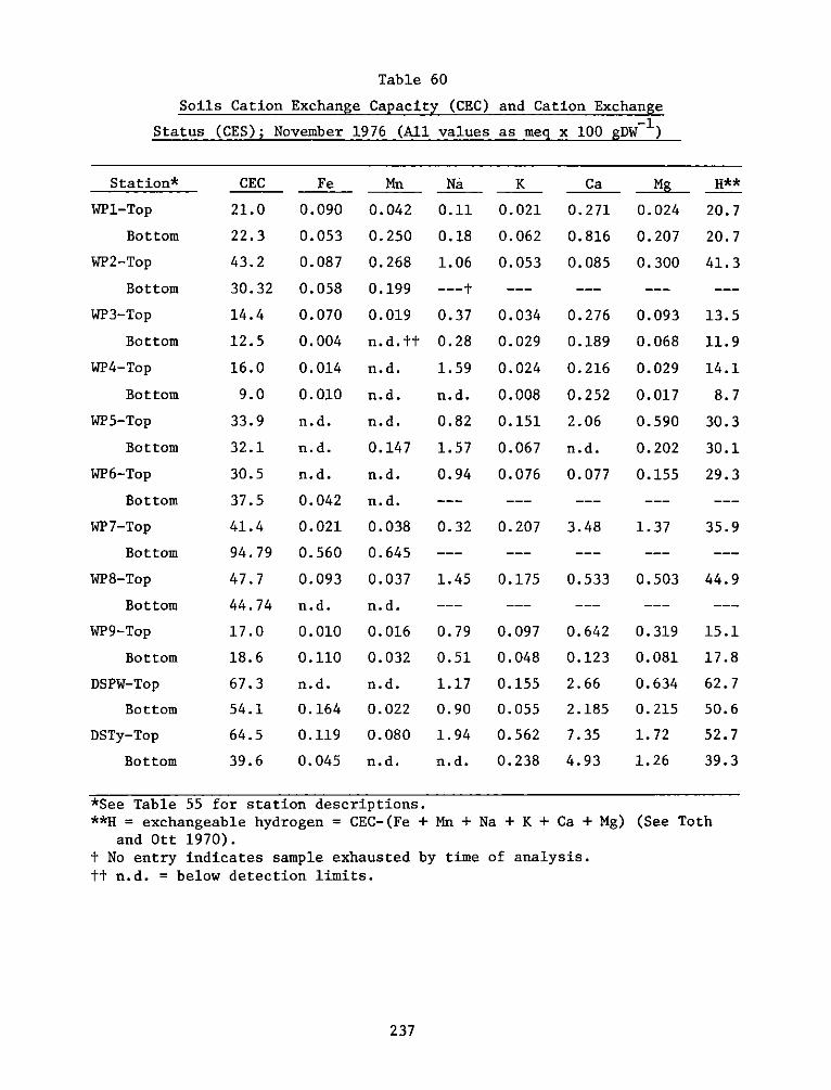
Table 60
Soils Cation Exchange Capacity (CEC)
Status (CES); November 1976 (All
and Cation Exchange
values as meg x 100 gDW 1 )
Station*
WPl-Top
Bottom
WP2-Top
Bottom
WP3-Top
Bottom
WP4-Top
Bottom
WP5-Top
Bottom
WP6-Top
Bottom
WP7-Top
Bottom
WP8-Top
Bottom
WP9-Top
Bottom
DSPW-Top
Bottom
DSTy-Top
Bottom
CEC
21.0
22.3
43.2
30.32
14.4
12.5
16.0
9.0
33.9
32.1
30.5
37.5
41.4
94.79
47.7
44.74
17.0
18.6
67.3
54.1
64.5
39.6
Fe
0.090
0.053
0.087
0.058
0.070
0.004
0.014
0.010
n.d.
n.d.
n.d.
0.042
0.021
0.560
0.093
n.d.
0.010
0.110
n.d.
0.164
0.119
0.045
Mn
0.042
0.250
0.268
0.199
0.019
n.d.tt
n.d.
n.d.
n.d.
0.147
n.d.
n.d.
0.038
0.645
0.037
n.d.
0.016
0.032
n.d.
0.022
0.080
n.d.
Na
0.11
0.18
1.06
--- t
0.37
0.28
1.59
n.d.
0.82
1.57
0.94
K
0.021
0.062
0.053
0.034
0.029
0.024
0.008
0.151
0.067
0.076
Ca
0.271
0.816
0.085
0.276
0.189
0.216
0.252
2.06
n.d.
0.077
Mg
0.024
0.207
0.300
0.093
0.068
0.029
0.017
0.590
0.202
0.155
H**
20.7
20.7
41.3
13.5
11.9
14.1
8.7
30.3
30.1
29.3
0.32 0.207 3.48 1.37 35.9
--- --- --- --- ---1.45 0.175 0.533 0.503 44.9
0.79
0.51
1.17
0.90
1.94
n.d.
0.097
0.048
0.155
0.055
0.562
0.238
0.642
0.123
2.66
2.185
7.35
4.93
0.319
0.081
0.634
0.215
1.72
1.26
15.1
17.8
62.7
50.6
52.7
39.3
*See Table 55 for station descriptions.**H = exchangeable hydrogen = CEC-(Fe + Mn + Na + K + Ca + Mg) (See Toth
and Ott 1970).t No entry indicates sample exhausted by time of analysis.
tt n.d. = below detection limits.
237
v " r v
., Z p
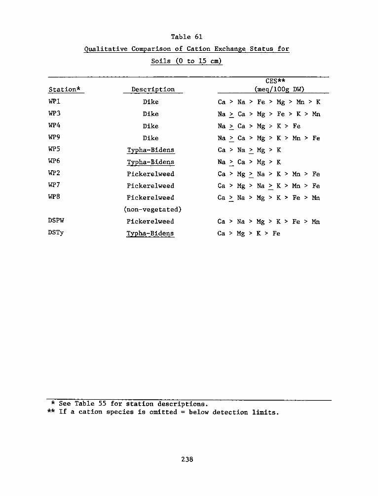
Table 61
Qualitative Comparison of Cation Exchange Status for
Soils (0 to 15 cm)
Description
Dike
Dike
Dike
Dike
Typha-Bidens
Typha-Bidens
Pickerelweed
Pickerelweed
Pickerelweed
(non-vegetated)
Pickerelweed
Typha-Bidens
CES**(meq/100g DW)
Ca
Na
Na
Na
Ca
Na
Ca
Ca
Ca
Na
Ca
Ca
Ca
Na
Ca
Mg
Mg
Na
Ca > Na
Ca > Mg
> Fe
> Mg
> Mg
> Mg
> Mg
> Mg
> Na
> Na
> Mg
> Mg > Mn> K
> Fe > K > Mn
> K > Fe
> K > Mn > Fe
> K
> K
> K > Mn > Fe
> K > Mn > Fe
> K > Fe > Mn
> Mg > K > Fe > Mn
> K > Fe
238
Station*
WP1
WP3
WP4
WP9
WP5
WP6
WP2
WP7
WP8
DSPW
DSTy
* See Table 55 for station descriptions.** If a cation species is omitted = below detection limits.
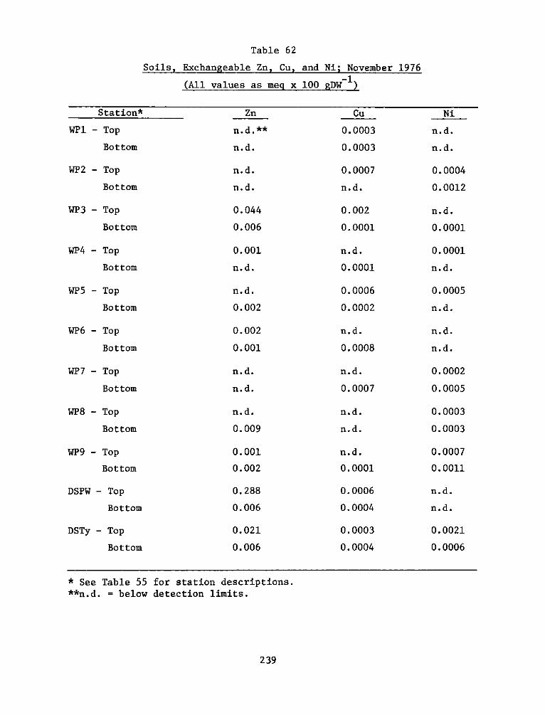
Table 62
Soils, Exchangeable Zn, Cu, and Ni; November 1976
(All values as meg x 100 gDW~1)
Station* Zn Cu Ni
WPl - Top n.d.** 0.0003 n.d.
Bottom n.d. 0.0003 n.d.
WP2 - Top n.d. 0.0007 0.0004
Bottom n.d. n.d. 0.0012
WP3 - Top 0.044 0.002 n.d.
Bottom 0.006 0.0001 0.0001
WP4 - Top 0.001 n.d. 0.0001
Bottom n.d. 0.0001 n.d.
WP5 - Top n.d. 0.0006 0.0005
Bottom 0.002 0.0002 n.d.
WP6 - Top 0.002 n.d. n.d.
Bottom 0.001 0.0008 n.d.
WP7 - Top n.d. n.d. 0.0002
Bottom n.d. 0.0007 0.0005
WP8 - Top n.d. n.d. 0.0003
Bottom 0.009 n.d. 0.0003
WP9 - Top 0.001 n.d. 0.0007
Bottom 0.002 0.0001 0.0011
DSPW - Top 0.288 0.0006 n.d.
Bottom 0.006 0.0004 n.d.
DSTy - Top 0.021 0.0003 0.0021
Bottom 0.006 0.0004 0.0006
* See Table 55 for station descriptions.**n.d. = below detection limits.
239
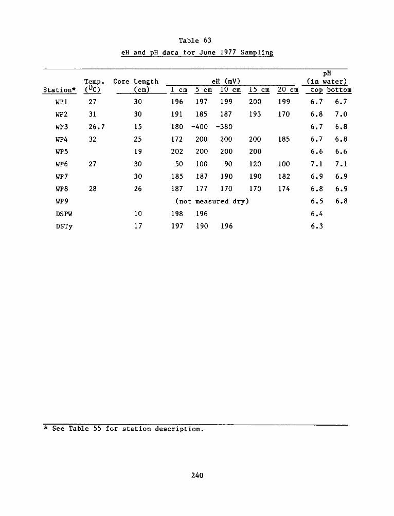
Table 63
eH and pH data for June 1977 Sampling
Core Length_(cm)
30
30
15
25
19
30
30
26
10
17
Temp.
(OC)
27
31
26.7
32
27
28
5 cm
197
185
-400
200
200
100
187
177
eH (mV)10 cm
199
187
-380
200
200
90
190
170
15 cm
200
193
200
200
120
190
170
20 cm
199
170
185
100
182
174
1 cm
196
191
180 -
172
202
50
185
187
(not
198
197
pH(in water)top bottom
6.7 6.7
6.8 7.0
6.7 6.8
6.7 6.8
6.6 6.6
7.1 7.1
6.9 6.9
6.8 6.9
6.5 6.8
6.4
6.3
* See Table 55 for station description.
240
Station*
WP 1
WP2
WP3
WP4
WP5
WP6
WP 7
WP8
WP9
DSPW
DSTy
measured dry)
196
190 196
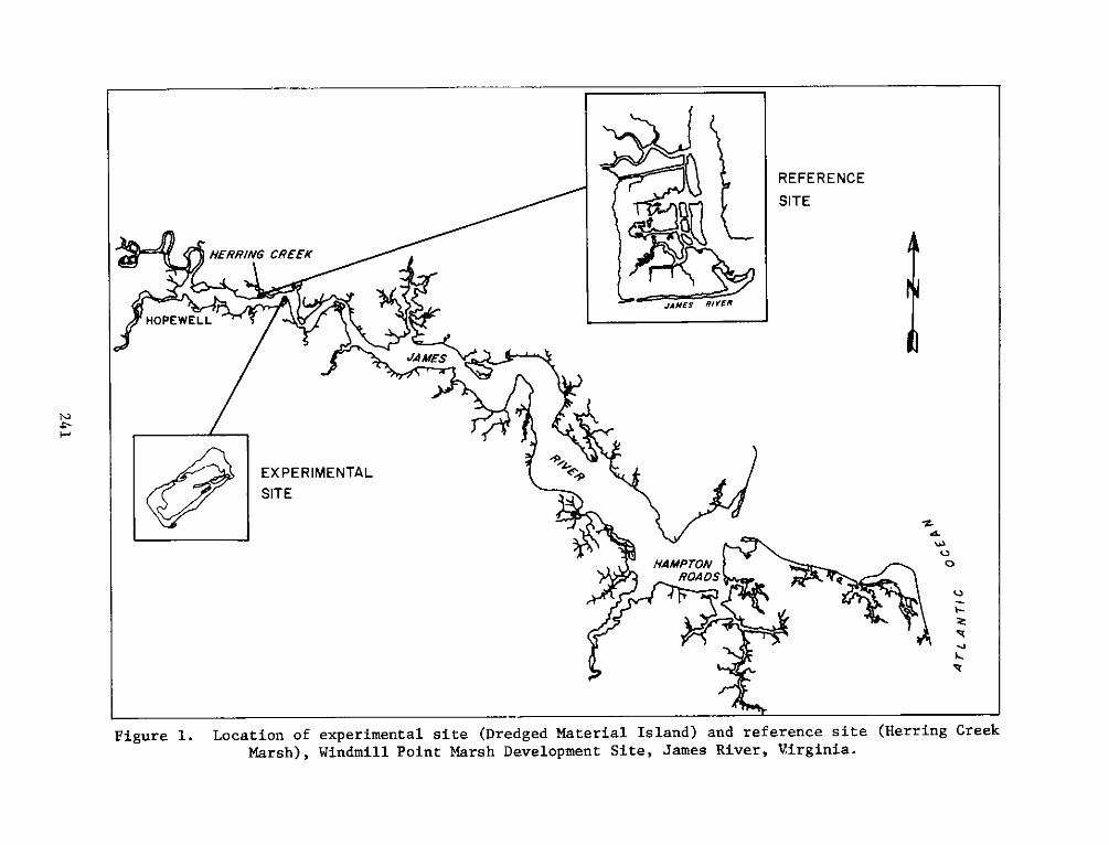
REFERENCE
fl SITE
HERRING CREEK
JAESRVER
HOPEWELL
JAMES
EXPERIMENTAL C
SITE
HAMPTONO
ROADS
Figure 1. Location of experimental site (Dredged Material Island) and reference site (Herring Creek
Marsh), Windmill Point Marsh Development Site, James River, Virginia.
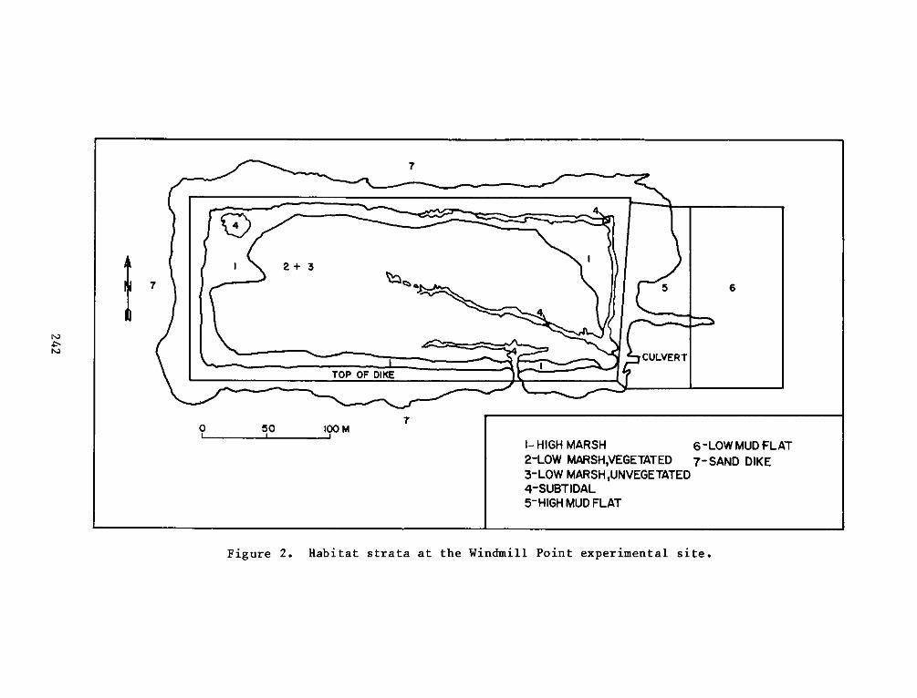
7
1 2 + 3
7 4 5 6
CULVER T
TOP OF DIKE
0 50 lOO M
I- HIGH MARSH 6-LOW MUD FLAT2-LOW MARSH,VEGETATED 7- SAND DIKE3-LOW MARSHUNVEGETATED4-SUBTIDAL5- HIGH MUD FLAT
Figure 2. Habitat strata at the Windmill Point experimental site.
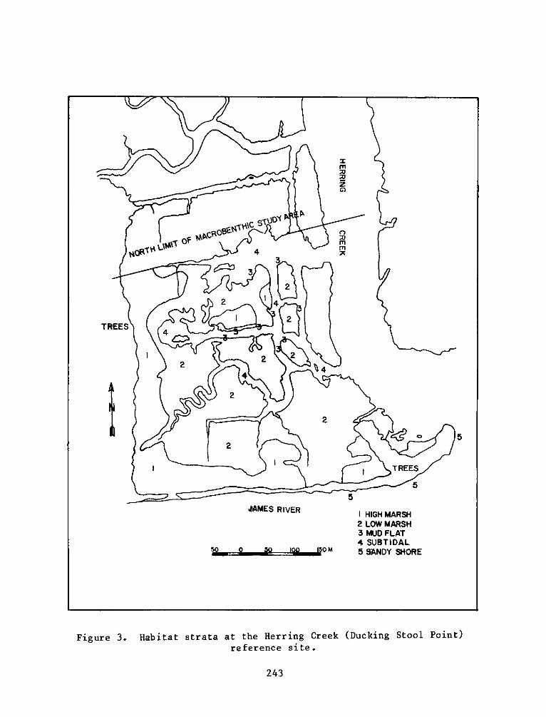
4M
22OWMAS
OF 3 MUD FLAT
Np~tSN4 SUBTIDAL
2.
50 0 0 0 OM 5SND SHOR
22
TTRREE
1 L2 2RS
44S TDA
Figure 3. Habitat strata at the Herring Creek (Ducking Stool Point)reference site.
243
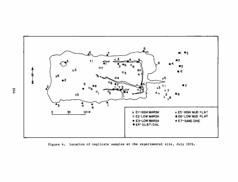
56 "7 " I 2
5 XI owx 2 4 "3
"I 3 06 xg 6 "4 5
o.7
0 2 03 6x " 6
x5 % 4+5"2
5 08 6
2x3 0 0l 0584 x374+ 2 8 8 s++
3 4 8
0 50 100 M x El-HIGH MARSH + E5-HIGH MUD FLATo E2-LOW MARSH E6- LOW MUD FL AT" E3-LOW MARSH ET-SAND DIKE" E4-SUBTIDAL
Figure 4. Location of replicate samples at the experimental site, July 1976.
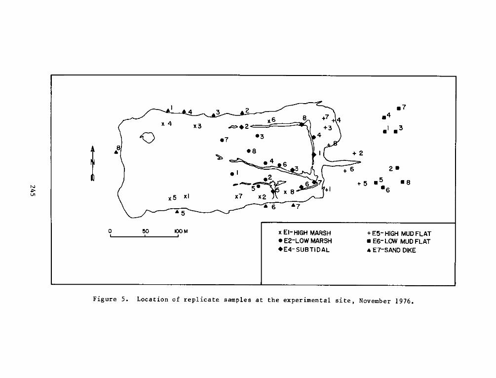
4 3 2 /
x 4 x6 8 +7 +4 4
x4 x3 a"24 +3 I 3"7 .7
"44.4
5 x - I .2
x 5 XI +x+7 +x2 m
S6 "7
"5
0 50 100 M x El- HIGH MARSH + E5- HIGH MUD FLAT" E2-LOW MARSH E6- LOW MUD FLAT*E4-SUBTIDAL " E7-SAND DIKE
Figure 5. Location of replicate samples at the experimental site, November 1976.
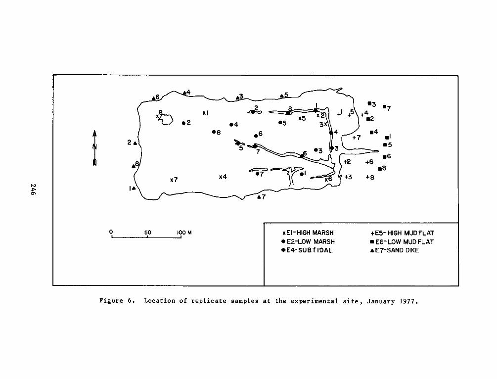
2 x l 5x 2 +1 +5 +46
X5 .2" 2 *4 "5 3x
"8 96 4 "4
2 " o+7 "1
5 7 3 3 "
.6+2 +6
x7x4 070!x +3 +8 =
0 50 100 M x EI-HIGH MARSH + E5- HIGH MUD FLAT* E2-LOW MARSH U E6- LOW MUD FLAT*E4-SUBTIDAL "E7-SAND DIKE
Figure 6. Location of replicate samples at the experimental site, January 1977.
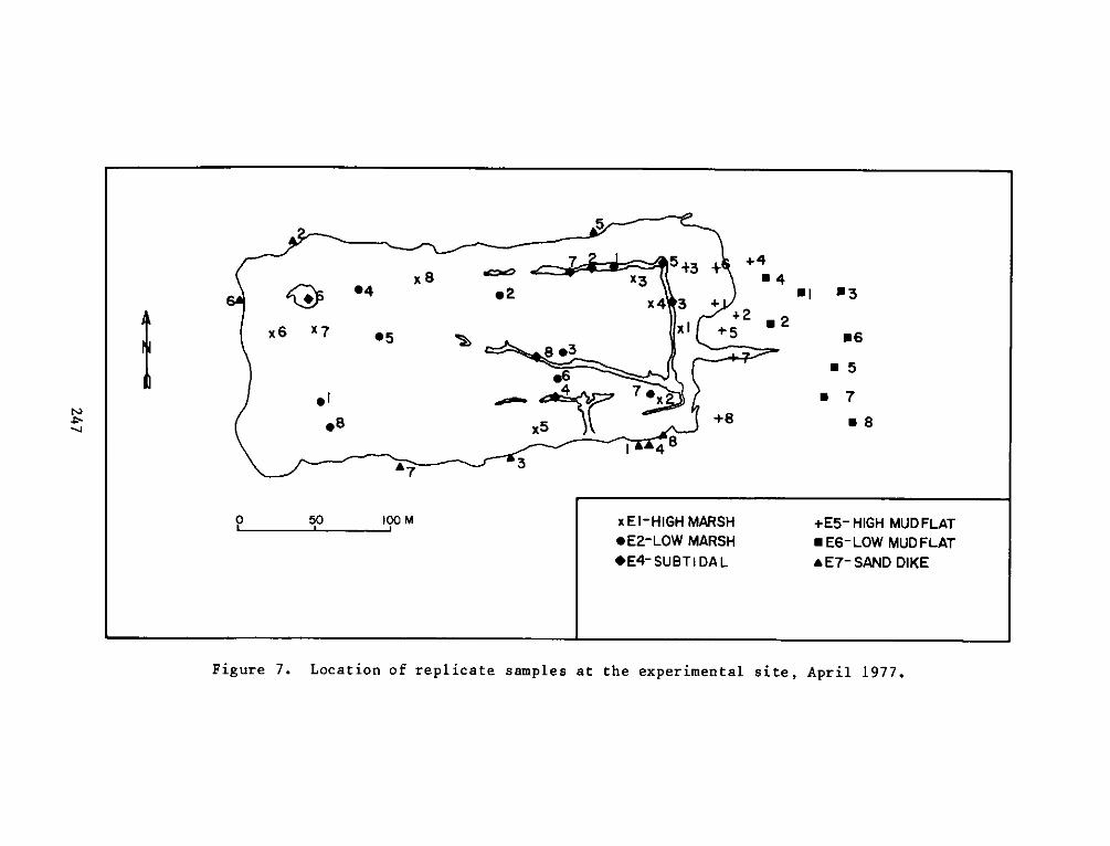
+2 " 2x6 x7 05 xl +5 P6
.. 7
1 4 8
A7 3
0 50 lOOM xEl-HIGH MARSH +E5- HIGH MUD FLAT*E2-LOW MARSH E6- LOW MUD FLAT*E4- SUBT I DAL aE7- SAND DIKE
Figure 7. Location of replicate samples at the experimental site, April 1977.
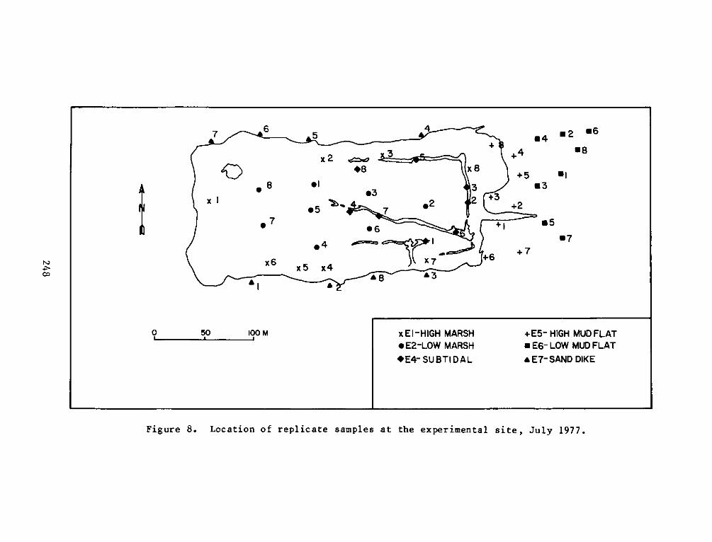
7 6 5 4 4 "2 "6
x 2 As 3 +4 8
"8 x 8 +5 "I
l A1"3 m3
"7 "6 +2 "5
x6 x5 x4+6 +
0 50 100 M xEI-HIGH MARSH +E5- HIGH MUD FLAT" E2-LOW MARSH E6- LOW MUD FLAT
*E4- SUBTI DAL "E7-SAND DIKE
Figure 8. Location of replicate samples at the experimental site, July 1977.
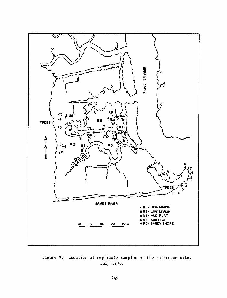
x 3 372
"I
TREES X1 8
x5
8"4
x8
8
+7
TREES + + 4
+ 2
JAMES RIVERx RI - HIGH MARSH*R2- LOW MARSH* R3- MUD FLAT" R4 - SUBTIDAL
50 0 50 0 150 M + R5 - SANDY SHORE
Figure 9. Location of replicate samples at the reference site,
July 1976.
249
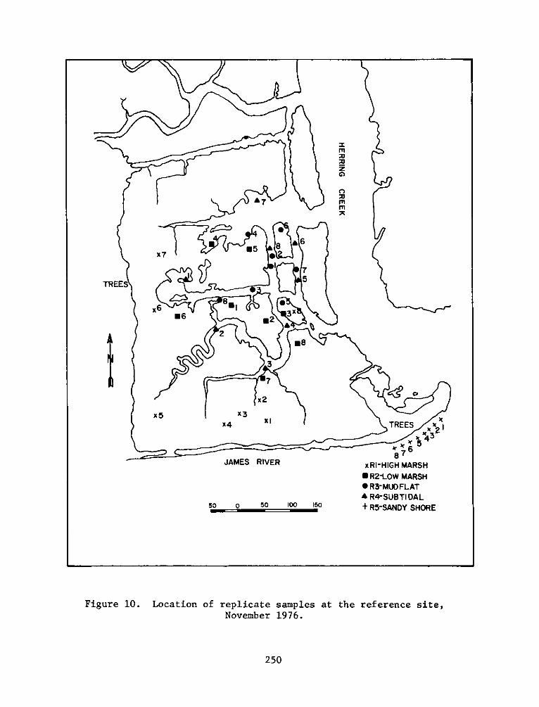
M
C)
x7 65 8 a
7
TREES5
SS
X6MR8VRR G"6 2
22
8
3
7
x2
x5 x3
x4 X1 TREES 21kx43
JAMES RIVER x RI-HIGH MARSH
R2-LOW MARSH. R3-MUD FLATA R4-SUBTI DAL
so 0 50 100 150 + R5-SANDY SHORE
Figure 10. Location of replicate samples at the reference site,November 1976.
250
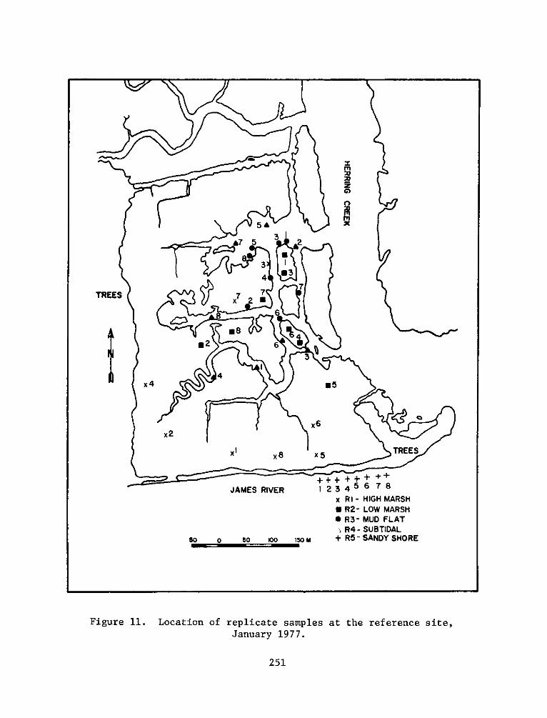
m
z
5" xA7 5 3 2
3
4
TREES 87 2
2 6
4
x4 5
x6
x2
xi X8 X 5 TREES
JAMES RIVER 1 2 3 4 678
50 0 50 o 150M
x R I - HIGH MARSHR2- LOW MARSH
" R3- MUD FLAT5 R4 - SUBTIDAL
+ R5-SANDY SHORE
Figure 11. Location of replicate samples at the reference site,January 1977.
251
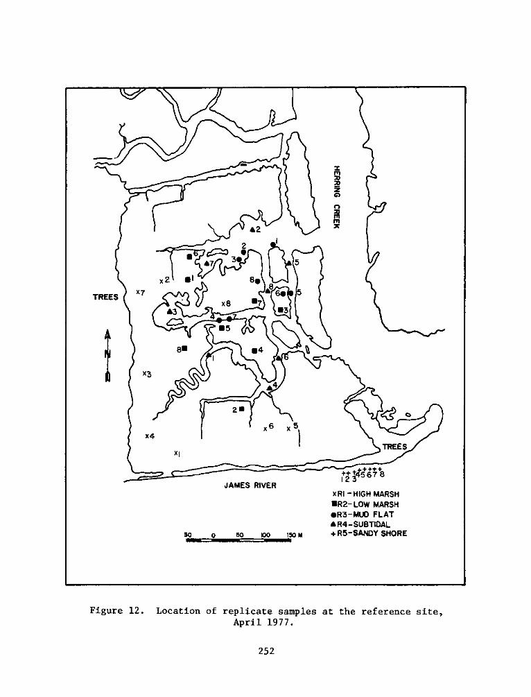
m
z
X2 1 8"
TREES xx '8 6
3 "3
" "4
20
x6 x5x4
TREES
JAMES RIVERxRI -HIGH MARSH"R2-LOW MARSH"R3-MUD FLAT"R4-SUBTIDAL
50 o 50 K0 150 M + R5-SANDY SHORE
Figure 12. Location of replicate samples at the reference site,April 1977.
252
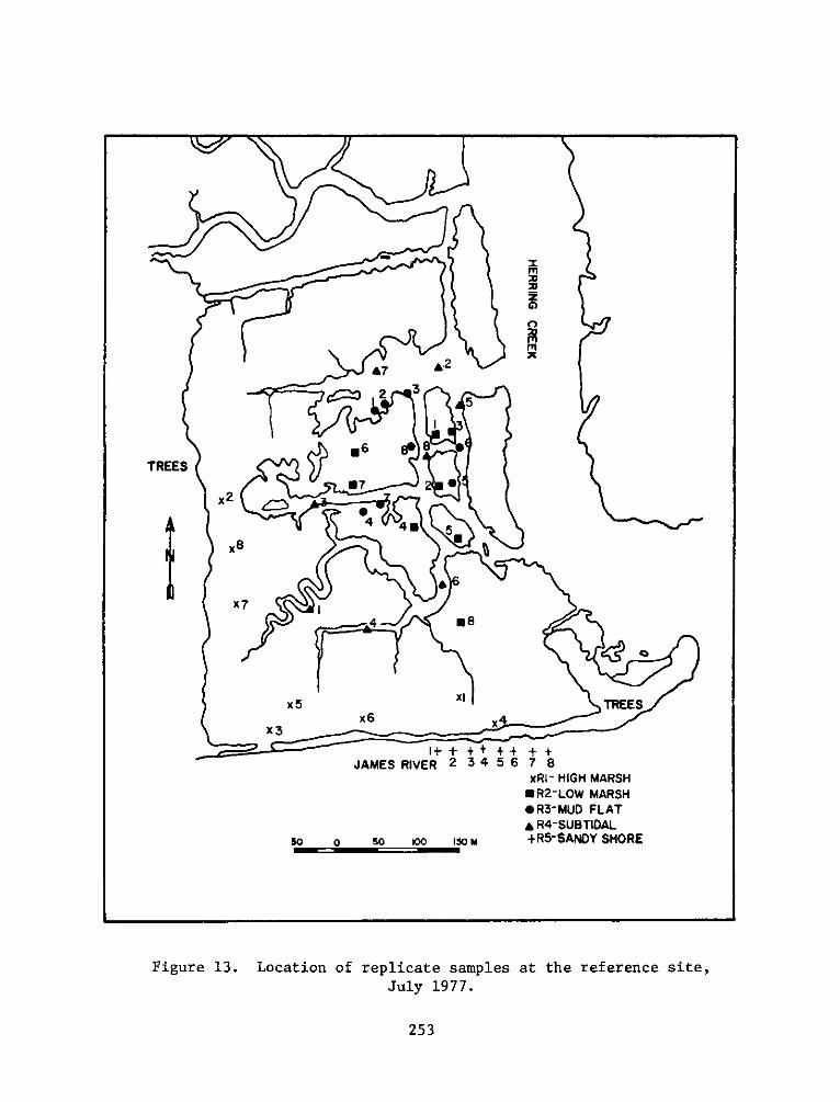
X
m
AA7 &.2
C-o- 2 30g 819
TREES
7"
x2
S6
X74 "8
x5 xiTREES
X3 x
JAMES RIVER 2 3 4 5 6 7 8
xRI- HIGH MARSH*R2-LOW MARSH*R3-MUD FLATa R4-SUBTIDAL+R5-SANDY SHORE
Figure 13. Location of replicate samples at the reference site,July 1977.
253
50 0 50 OO 150M
F F
0
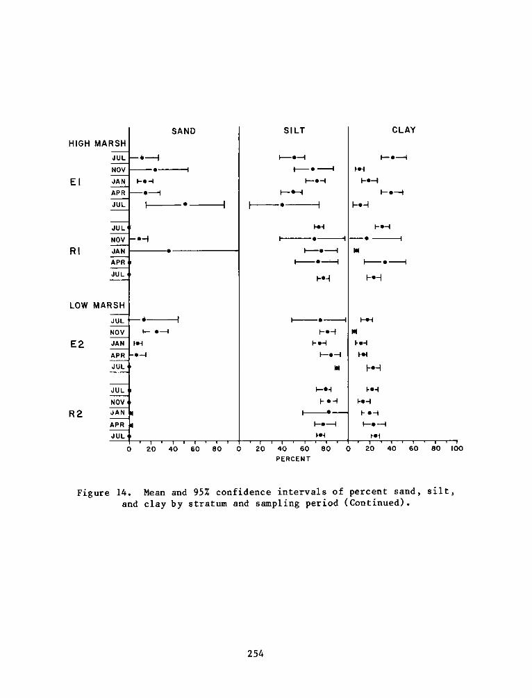
HIGH MARSH
JUL
NOV
E I JAN
APR
JUL
JUL
NOV
R I JAN
APR
JUL4
LOW MARSH
JUL
NOV
E2 JAN
APR
JUL
JUL
NOV
R 2 JANAPR
JULY
SAND
- --
--- Id
i-0 -A0-
0
i
F- 0-4
F".'
-"-4
I . III.
0 20 40
SILT
f-0-F-- "-I
1-4--
1--. -
--- "-- I
I-"--'
H-4
-- 4
I-0-4
-0--
E"04
60 80 0 20 40 60 80
PERCENT0
CLAY
F-"-1
-- "
---- -I
-- --
10-
I.0-
r"1
20 40 60 80 100
Figure 14. Mean and 95% confidence intervals of percent sand, silt,
and clay by stratum and sampling period (Continued).
254
N
N
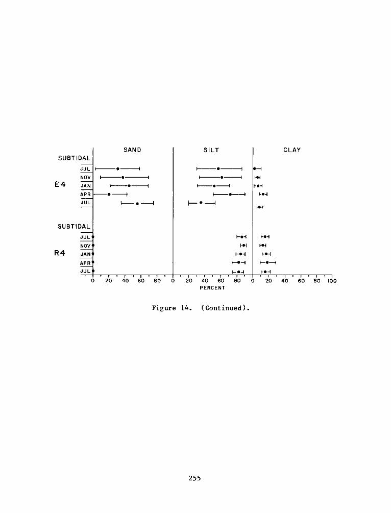
SUBTIDAL
JUL
NOV
E4 JAN
APR
JUL
SUBTIDAL
JUL
NOV
R4 JANE
APR4
JUL4
SAN D
--. d -
SILT
I- " --
FS1
10-4
CLAY
I-i
F.1-
I-0-Ie1
1-0-I
'-0--
- r ' I I i ' *0 20 40 60 80 0 20 40 60 80 0 20 40 60 80 100
PERCENT
Figure 14. (Continued).
255
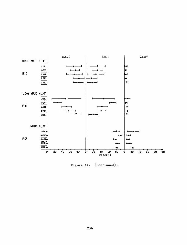
HIGH MUD FLAT
JUL
NOV
E5 JAN
APR
JUL
LOW MUD FLAT
JUL
NOVE6 JAN
APRJUL
R3
MUD FLAT
JULi
NOV
JANAPR4
JUL4
SAND
-0----I
i-, -H
'-0-I
SILT
-- I-
-- e--1
-" -- 1
f -f-
1-+-I
'4--
CLAY
104
"4
104
I.M
I.1-0-4
I.'
1-----1
Foi'-4
I-.-
-r -i- ii T i -i ' ' -r -iwi--0 20 40 60 80 0 20 40 60 80 0 20 40 60 80 100
PERCENT
Figure 14. (Continued).
256
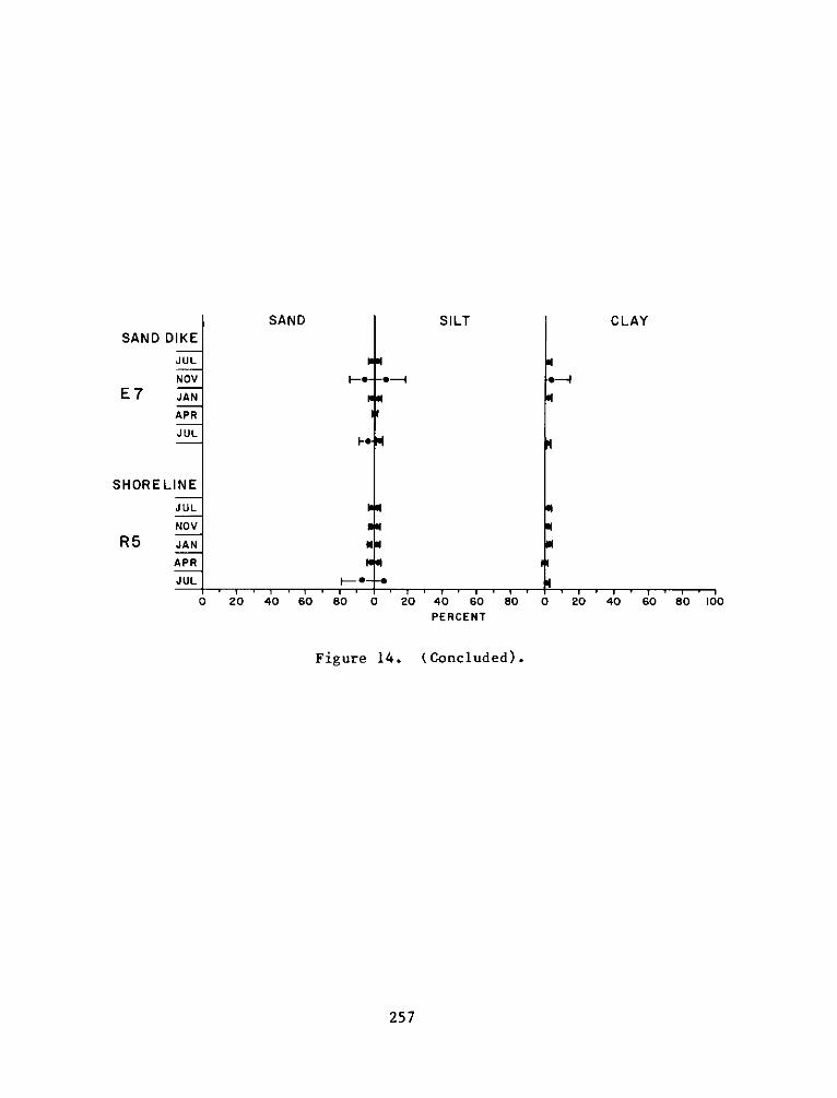
SAND SILT CLAYSAND DIKE
JUL
NOV H-" "-I4
E7 JANAPR
JULF-"
SHORELINE
JUL
NOVR5 JAN U
APR
JUL -0 0
O 20 40 60 80 0 20 40 60 80 0 20 40 60 80 100PERCENT
Figure 14. (Concluded).
257
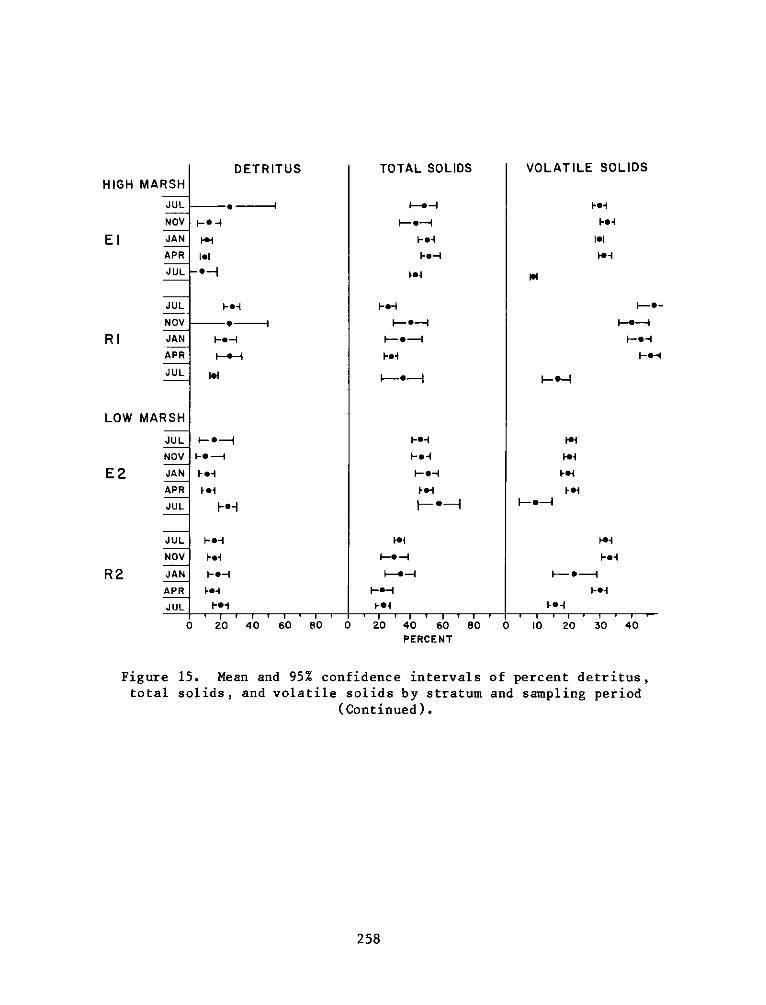
HIGH MARSH
JUL
NOV
E I JAN
APR
JUL
JUL
NOV
R I JANAPR
JUL
LOW MARSH
JUL
NOV
E2 JAN
APR
JUL
JUL
NOV
R2 JAN
APR
JUL
DETRITUS
* -4
I-"'
-'-4
e I
4-0-4
I- 0 -
F -0-IF"1n
eI-"-
I-.-1
1-0-44-4
-- I
0 20
TOTAL SOLIDS
1--"--I4
I-.4I---I
H14I-04
1-0-4N
1-- *-I
14.4
4--0-4
'---
'---
'-.4
VOLATILE SOLIDS
I----
-4
4-.-
----. '1-0-1
F"1
F "1
4-1-
I-"-
I-0-
1- 0--
4-0-
1-0-
40 60 80 0 20 40 60 80 0 10 20 30 40PERCENT
Figure 15. Mean and 95% confidence intervals of percent detritus,total solids, and volatile solids by stratum and sampling period
(Continued).
258
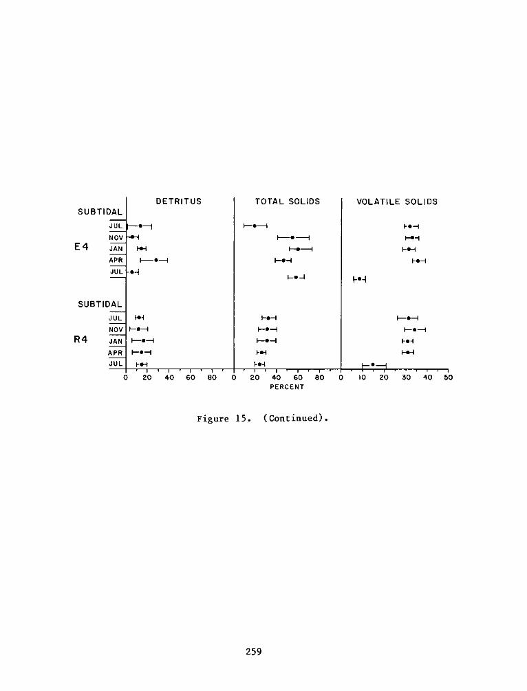
DETRITUS TOTAL SOLIDS VOLATILE SOLIDSSUBTIDAL
JUL s-- --- I i-i
NOV -1-----I -- IE4 JAN 1-I I---- I-s-I
APR I- --I -*-- 1--4
JUL s-II-.-4pe
SUBTIDAL
JUL 1F-I - -4 I-s-
NOV -0-- I-0- I-e-R4 JAN -*- i-----
APR 1-0-1 -s-I 1-+-I
JUL -I -s- _ _ ...
0 20 40 60 80 0 20 40 60 80 0 10 20 30 40 50PERCENT
Figure 15. (Continued).
259
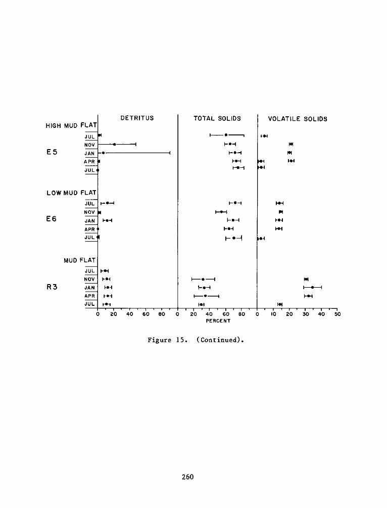
HIGH MUD FLAT
JUL
NOV
E 5 JAN
APR
JUL 4
LOW MUD FLAT
JUL
NOV
E6 JAN
APR
JUL
R3
MUD FLAT
JUL
NOV
JAN
APR
JUL
DETRITUS
-. 1
'0
f-0-4
14"-II- "I
I-'
F| 5
r"-1
0 20 40 60 80 0
TOTAL SOLIDS
F ----" 0--I
-0-4d
I-"-'
-4---1
104
20 40 60PERCENT
VOLATILE SOLIDS
F.4
Fll
F"4
'0414-I
NeI
I.'
80 0 10 20 30 40 50
Figure 15. (Continued).
260
I
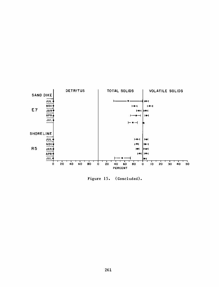
SAND DIKE
JUL
NOVE7 JAN'
APR4
JUL
SHORELINEJUL
NOV
R5 JAN'
APRJUL
DETRITUS TOTAL SOLIDS
e "
Fed
-0-
f-iF- *6
VOLATILE SOLIDS
N-
f1 -I-.-
I.-4
sI
He1
FedF"-INI.-
O 20 40 60 80 0 20 40 60 80 0 10 20 30 40 50PERCENT
Figure 15. (Concluded).
261
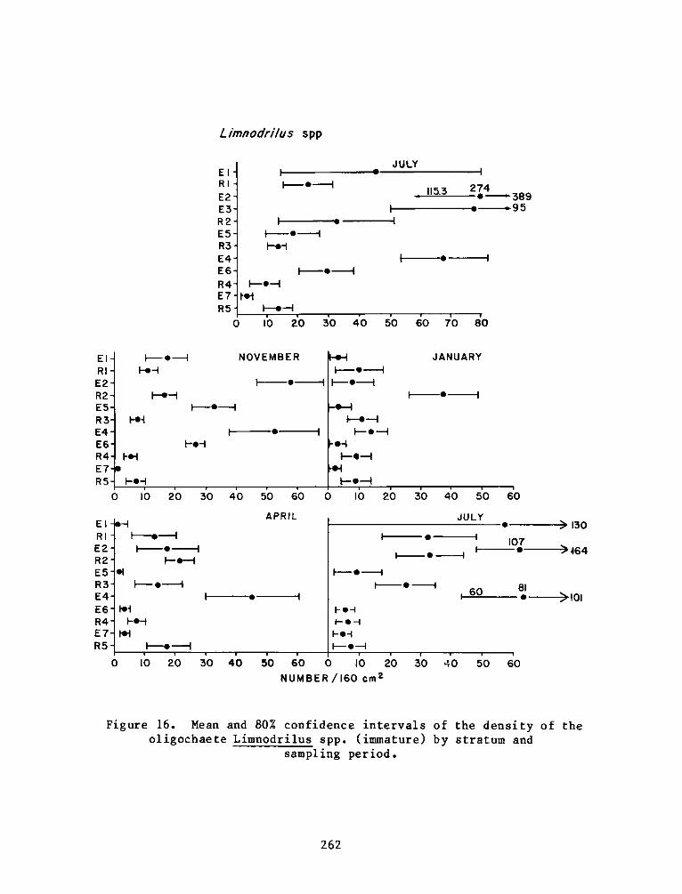
L imnodri/us spp
115.3 274' - 389
I----
I-.-'I-. -
-0--I
-1
b0 20 30 40 50 60 70 80
El -
RI -E2-R2-E5-R3-E4-E6-R4-E7-R5-
El-RI -E2-R2-E5-
I--- -4I-0-'
NOVEMBER
F-.
S4-
10 20 30 40 50 60 0
-I
H-e-I@1
APRIL
R 3 -- e--E4E6 -0 -F0-R4 I-0 -1-E7- 1.1 1--
R5 E-- ---I---
0 10 20 30 40 50 60 0 10NUMBER/160 cm 2
I-----I
H--.-I- -I
"- '--|'
F-e-
JANUARY
h--I
10 20 30 40 50 60
JULY
- - 107I- " _I)"464
I--. --I-- -- 4
20 30 40 50 60
Figure 16. Mean and 80% confidence intervals of the density of theoligochaete Limnodrilus spp. (immature) by stratum and
sampling period.
262
-- e- --
JULYEIRIE2E3R2E5-R3-E4-E6-R4-E7 -R5-
0
130
60 , , 101
loop,-IN&
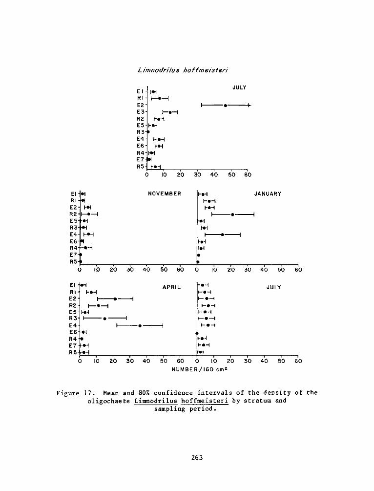
L imnodri/us hoffmeisteri
EIRIE2E3R2E5R3E4E6R4E7R5
0
JULY
1--s-
I-.--'I-.-
I-"'01-
r"--
10 20 30 40 50 60
NOVEMBER
I--e1
1-e--I
441-0--i
---1
10 20 30 40 50 60
I-.-.APRIL
F--. ---0-1
F-.-'H-.----e
-S-I
-0-1
F *-I JANUARY
Fe
F+I
Si
10 20 30 40 50 60
- 0 -110-
hoI
0 10 20 30 40 50 60 0 10 20NUMBER /160 cm 2
30
Figure 17. Mean and 80% confidence intervals of the density of the
oligochaete Limnodrilus hoffmeisteri by stratum andsampling period.
263
ElRI-E2-R2-E 5-R3-E4-E6-R4-E7-R5
C
ElRIE2R2E5-R3-E4-E6-R4E7R5
JULY
40 50 60
-
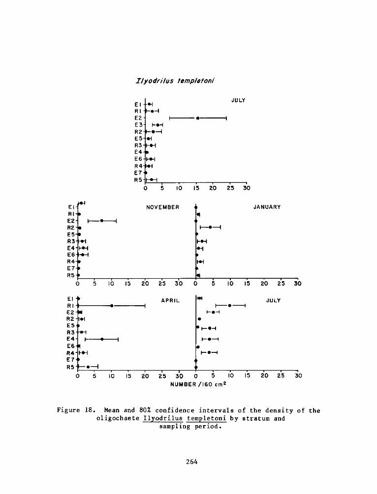
Ilyodri/us temp/etoni
JULY
I e- I
10 15 20 25 30
El-RI-E2-R2 -E5-R3-E4-E6-R4-E7-R5-
El -RI-E2-R2 -E5-R3-E4-E6-R4-E7-
R5-
NOVEMBERI
1-- "--IS
-I
H-op
JANUARY
-- I
I--
0 5 10 I5 20 25 30 0 5 10 I5 20 25 3C
APRIL JULY
F f- - --1 --
e-0-
0-I
0 5 10 15 20 25 30 0 5
NUMBER /160 cm 210 15 20 25 30
Figure 18. Mean and 80% confidence intervals of the density of theoligochaete Ilyodrilus templetoni by stratum and
sampling period.
264
El N-4
R I --IE2E3 -0-4
R2 0 -4E5 "1R3 N-E4E 6 1.-IR4 IE7R5 1-4-1
0 5
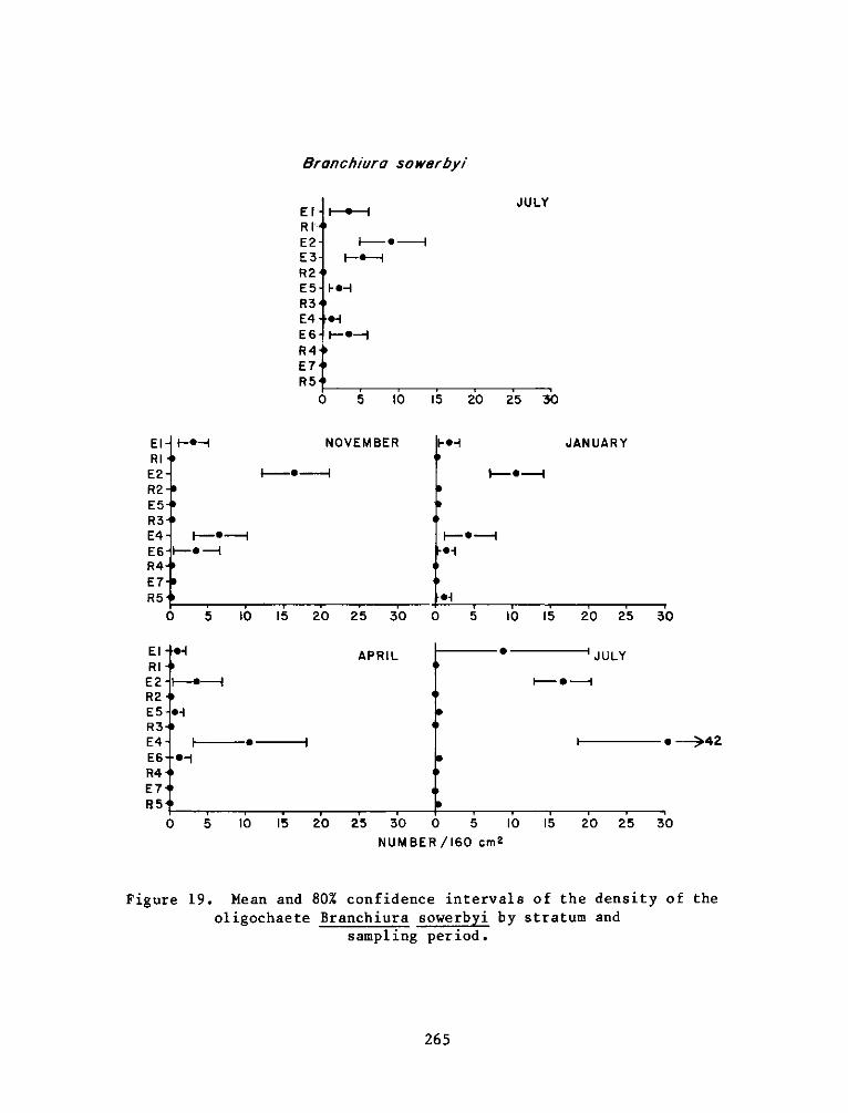
Bronchiura sowerbyi
EfRI'E2E3R2E5R3E4E6R4E7R5
0
JULYI"" -
I-'--
I--".-'.0-I
1e
5 10 15 20 25 30
NOVEMBER
F-01-ed -
I
5 10 15 20 25 30
APRIL
JANUARY
I
I
f--4--
1.-I
5 10 15 20 25 30
JULY
I-. -
I
1 i e -42
5 10 15 20 25 30 0 5 10 15 20 25 30NUMBER /160 cm 2
Figure 19. Mean and 80% confidence intervals of the density of theoligochaete Branchiura sowerbyi by stratum and
sampling period.
265
I-.--iEl-RI
E2-R2-E5-R3E4 -E6-R4--E7-R5-
C
El ERIE2 F-R2E5 *R3E4E6 4
R4E7R5
0
'-I
*1
"-1
r
1
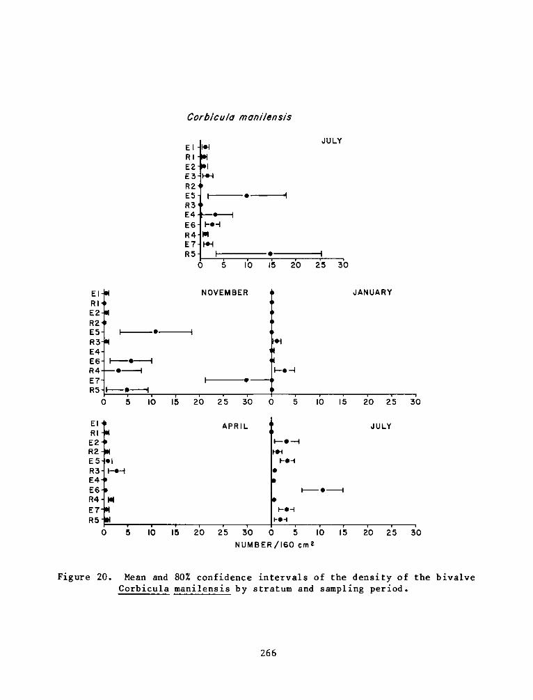
Corbicu/ mani/ensis
El IRIE2E3R2E5R3E4E6R4E7R5
0
JULY
IN-'
i- -l
i-*0-
F- @-"
5 10 5 20 25 30
NOVEMBER
i-0---I
5 10 15 20 25 30
JANUARY
" r-
0 S 10 15 20 25 30
APRIL JULY
i- . -1
I- -- 1
FI-S
5 10 15 20 25 30 0 10NUMBER /160 cm 2
15 20 25 30
Figure 20. Mean and 80% confidence intervals of the density of the bivalveCorbicula manilensis by stratum and sampling period.
266
El-RbIE2-R2+E5-R3-E4-E6-R4-E7-R5 -
EC
'I
M-o-
Ne
ElRIE2R2E5 I
R3 IE4E6R4 IE7R5
0-
I
I
i
4
N-
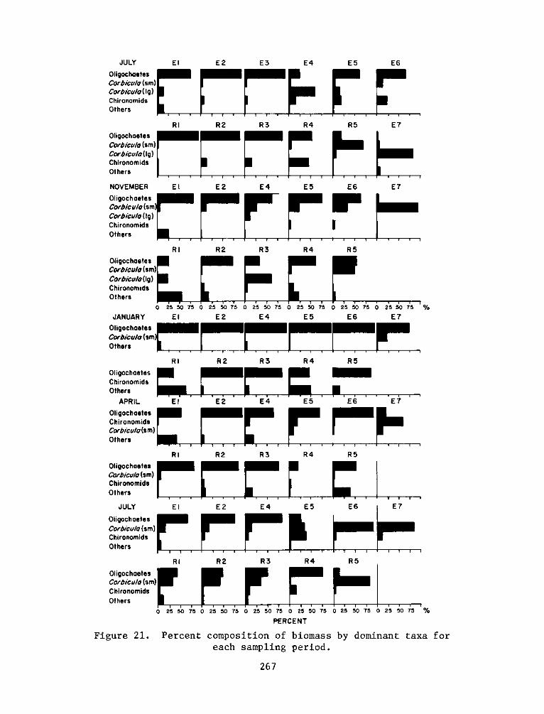
JULY ElOligochaetesCorbicul/o(sm)Corbicu/o(Ig)ChironomidsOthers
E2 E3 E4 E5 E6
IIIm IIIIIm 17
RI R2 R3 R4 R5 E7OligochoetesCorbicul/o(sm)Corbicu/o(Ig )ChironomidsOthers11FI
117
NOVEMBER El
OligochaetesCorbicul/o(smCorbicu/o(Ig)ChironomidsOthers
OligochaetesCorbicu/o(sm)Corbicu/og(Ig)ChironomidsOthers
JANUARY
E2 E4 E5 E6 E7
RI R2 R3 R4 R5
0 25 50 75 0 25 50 75 0 25 50 75 0 25 50 75 0 25 50 75 0 25 50 75 %
El E2 E4 E5 E6 E7
Others f -RI R2 R3 R4 R
Chironomids
Others _________________________________
APRIL El E2 E4 E5 E6 E7OligochaetesChironomidsCorbicu/o (sm) [ ~.~ !Others J____
RIOligoch/etesCorbicu/o (s M)ChironomnidsrOthers
R2 R3 R4 R5
JULY El E2 E4 E5 E6 E7
OligochaetesCorbiculoQ(sm)ChironomidsOthers17
RI R2 R3 R4 R5
Oligochoetesorbicu/ (s m)
ChironomidsOthers 25 02F
0 25 50 75 0 250SO 75 0 25 50 75 0 25 50 75 0 25 50 75 0 25 5O075 %
PERCENT
Figure 21. Percent composition of biomass by dominant taxa for
each sampling period.
267
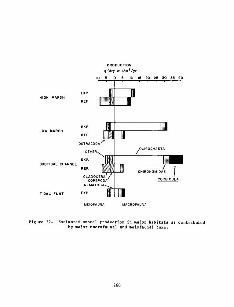
HIGH MARSH
LOW MARSH
SUBTIDAL CHANNEL
TIDAL FLAT
PRODUCTION
g (dry wt.)/m 2/yr
10 5 0 5 10 15 20 25 30 35 40
EXP.
REF.
EXP.
REF.
OSTRACODAf
OTHER
EXP.
REF.
CLADOCERACOPEPODA
NEMATODA-.,
EXP.
111LI
OLIGOCHAETA
CHIRONOMIDAE
CORBICULA
MEIOFAUNA MACROFAUNA
Figure 22. Estimated annual production in major habitats as contributedby major macrofaunal and meiofaunal taxa.
268
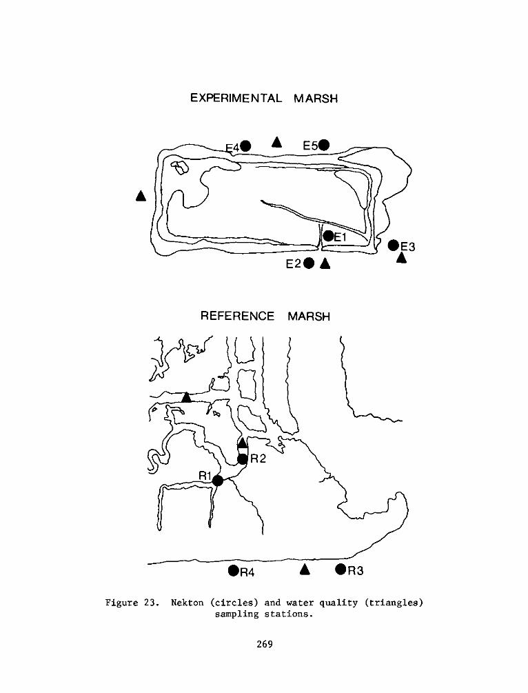
EXPERIMENTAL MARSH
4@ $ E 50
E1 OE3E20 A
REFERENCE MARSH
R2
R1
*R4 A OR3
Figure 23. Nekton (circles) and water quality (triangles)sampling stations.
269
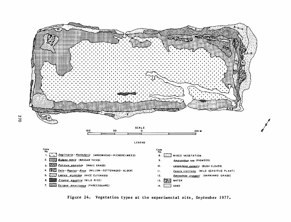
-. **" ovvev vv
I - _- - - -* .. ;T.:- II - I+ # + + -=- ----=-__ ;- .-=.- --*,
il++l+ +II+I ++ + + + + _ - 4-;.-.,-:-,i-*
1111+ +I+I + + + + + + + + + + + + + -._,~a = -- -"
Ill + ++I + + + + ++ + + + + + + + + + + + + + + + + + + -r; *1,
- +++++++++ + + + + + + + + + + + + + + + + + + + + + + + + + + + + + + + -- ;*-
-++++ ++ + + + + + + + + + + + + + + + + + + + + + + + + + + + + + + + + + + + *s
+ + + + t + + + + + + + + + + + + + + + + + + + + + + + + + + + + + + + + + + + + *. "
+ + + + + + + + + + + 4 + + + + + + + + + + + + + + + + + + + + + + + + + + + -. *+
100 50 0 100M
LEGEND
Code CodeNo- No.
I . Sog//tor/o - Ponteder/a (ARROWHEAD - PICKERELWEED) 8. . MIXED VEGE TA TION
2. 8/dens /8ev/s (BEGGAR TICKS) 9. AmOrOn/hUs spp. (PIGWEED)
3. , Pon/cum omoru/um (PANIC GRASS) 10. Lespedezc caneo/o (BUSH CLOVER)
4. ~. So/i-Popu/us- Anus (WILLOW- COT TONWOOD- ALDER) II. Cuss/c n/ct//ons (WILD SENSITIVE PL ANT)
5. L eersic or yzo/des ( R ICE C UT G RA SS) 1 2. Ech/noch/co crusgo//i ( BA R NYA RD G RA SS)6. Z/zun/a eguot/co (WILD RICE) 13. -.-- WATER
7. '****o Sc/rpus omer/conus (THREE SQUARE) 14. EZ~SAND
Figure 24. Vegetation types at the experimental site, September 1977.
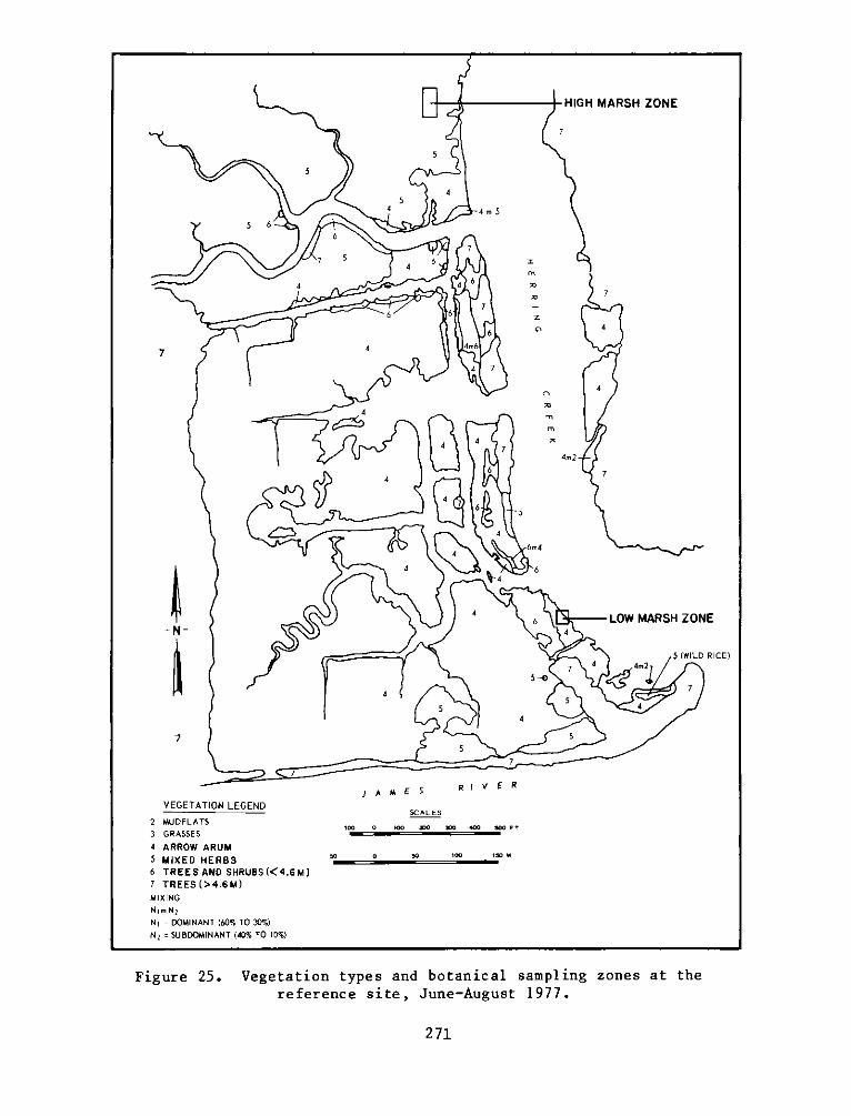
HIGH MARSH ZONE
7
5
5
45
4 4 m5
5 6
67
7 5 4 6
4 4 6
U 7 -
6 6z
6 6H
7 4 4m6
4 7
44
44 m
4 MUDFLATS 64m
4 66
4l ARROWW ARARZUN
5 MIXED HRBS 50(0 0D100 CEO
54 77 4
4ED U5
44
7 TRS(6M
5-4 7
5MIXG R S " " * '* '*
7 ES >.6M
NimN 2N= DOMINANT (60% TO 30%)
N2 SUBDOMINANT (40% TO 10%)
Figure 25. Vegetation types and botanical sampling zones at thereference site, June-August 1977.
271
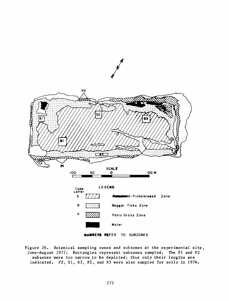
P2
- .. . ..... ...2 . ... . -
SCALE
100 50 0 lOOM
Code LEGENDLetter
S d- Pickereiweed Zone
B :::::: Beggar Ticks Zone
P Panic Grass Zone
Water
NUMBERS REFER TO SUBZONES
Figure 26. Botanical sampling zones and subzones at the experimental site,June-August 1977. Rectangles represent subzones sampled. The P1 and P2
subzones were too narrow to be depicted; thus only their lengths areindicated. P2, Sl, S3, B2, and B3 were also sampled for soils in 1976.
272
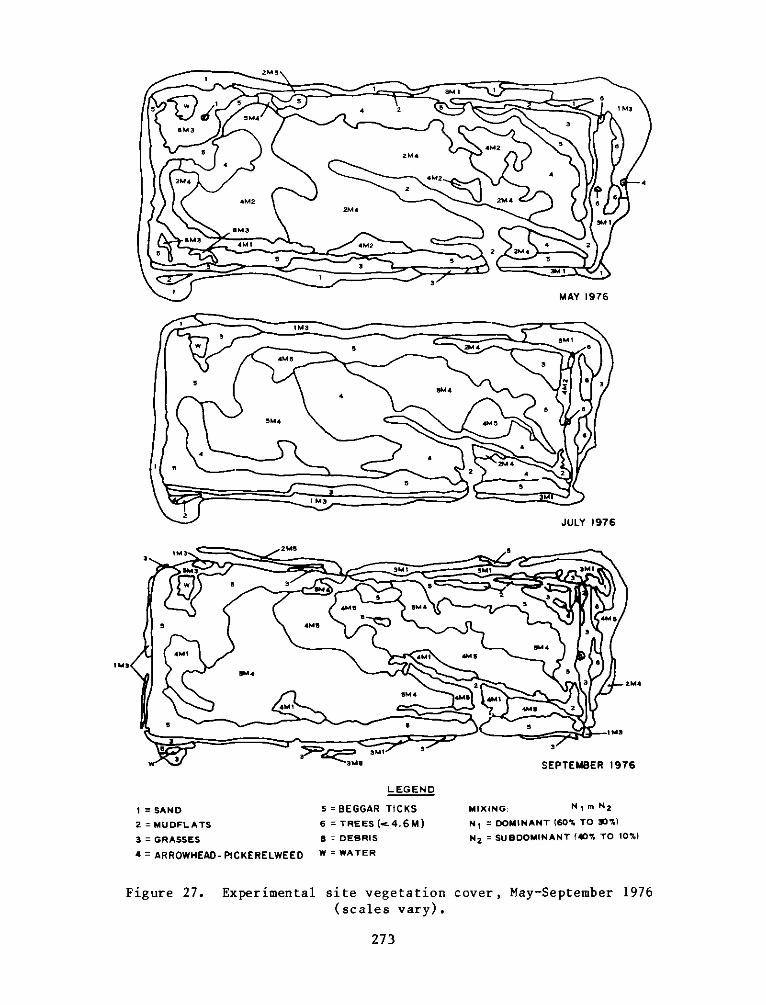
2M 3
1 3M 1
8M8
S4 2M4 M25
4M
4MM2M4 65 2M4
4M24 M24 2
4M22M4M4
3M
BM33
BM 4 1 M245 2 4 M4
45 5
5 6 3
W 24
4
5 56
5M 224
45 4S
1M2 3 2M4
BMS 3M4 3 M13M
BM 5 1
6 2 M 33
6 SPTMBR 97
5LEGEN
1 = AND = EGGA TICS MXING N 1m N
2 4MUFLAT16=TRE S(. .6M Ni=DO I N 6%4O%%
3 =GRASE 8 DERI N2= SBD4MNNT %TM 0%
4 RRWED-PCERLEE 6W E
Fi2e27 xeimna3st eetto2ovrM4-etmbr17
(5M4les vary)
273
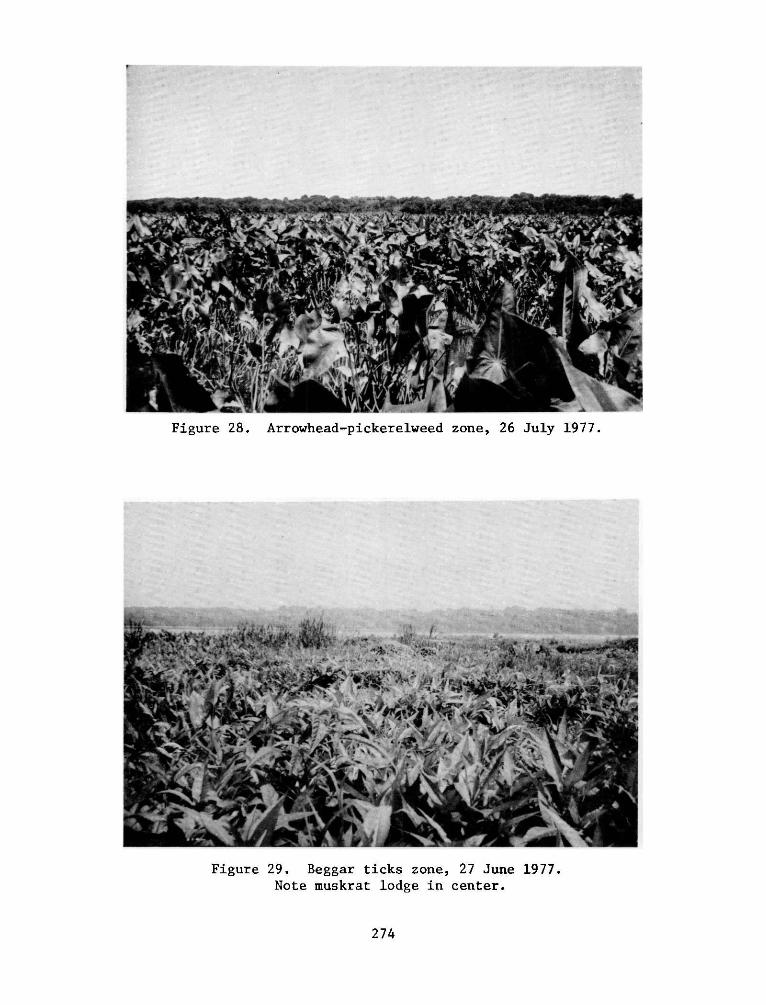
~-
4t __a m..r ___
,~-, -
'I 4 ~fla
Figure 28. Arrowhead-pickerelweed zone, 26 July 1977.
A 7t,
Figure 29. Beggar ticks zone, 27 June 1977.Note muskrat lodge in center.
274
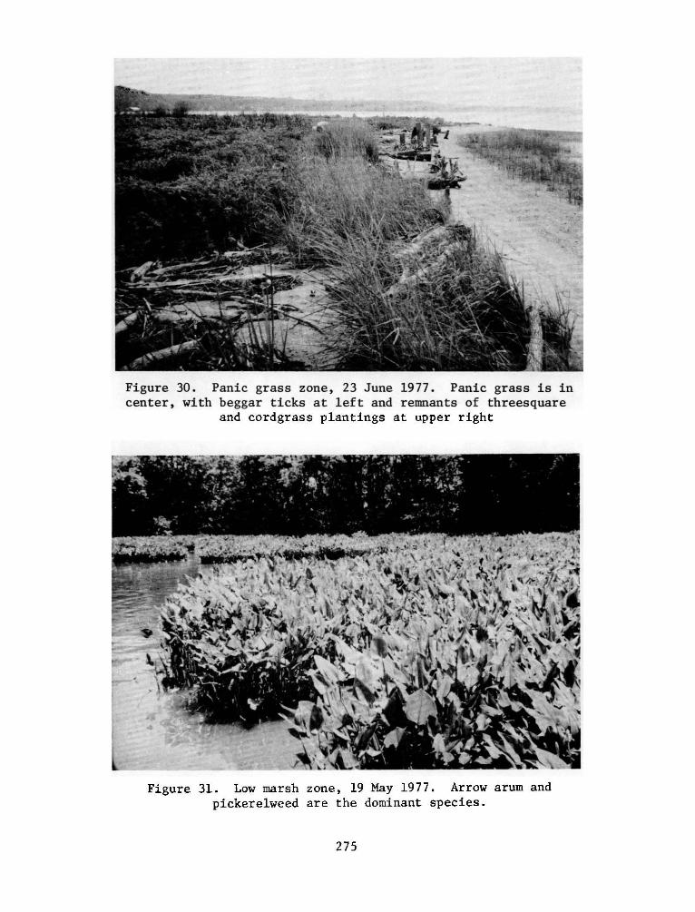
Lt-
~<r
Figure 30. Panic grass zone, 23 June 1977. Panic grass is incenter, with beggar ticks at left and remnants of threesquare
and cordgrass plantings at upper right
*, 4
- 4 i
as ,s%
Figure 31. Low marsh zone, 19 May 1977. Arrow arum and
pickerelweed are the dominant species.
275
tig t .u Tom' Mc _ 3
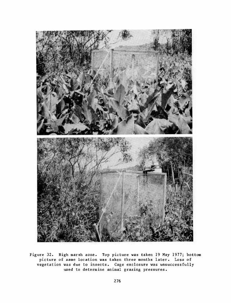
>i1M',r4d"i'
t: _kj/rj,jt~r4
: Iw +
Sj, *41"td4.
I * A t
i+ x4 t
(%i'4 V', rt{
p4 K fr 4E " P' I 6A
,b, 4 fWNy=' .2 i . y c;ra. L :7rePt is. t c
Figure 32. High marsh zone. Top picture was taken 19 May 1977; bottom
picture of same location was taken three months later. Loss of
vegetation was due to insects. Cage exclosure was unsuccessfully
used to determine animal grazing pressures.
276
*4& 1, Awl Is
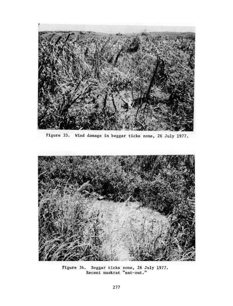
r
r e
'ON'
Figure 33. Wind damage in beggar ticks zone, 26 July 1977.
- y
* It -.
44% .1rr44 Jd~~-rIf
~~t;KCO v M P\
Figur 34. Begga tik zone 26Jl 97
Reetmsrt etot
277
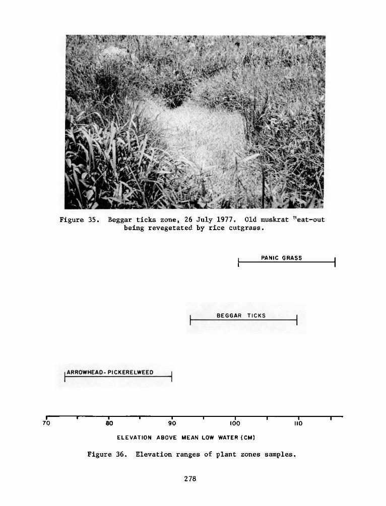
#rj't' s y ,'."'
Y * ,
Begga tick zo e 26- Jul l9 7 Ol mu k a tfeat-
Figure 35.
4i~AA
4 ~44
14,
r F
Beggar ticks zone, 26 July 1977, Old muskrat "eat-out
being revegetated by rice cutgrass.
PANIC GRASS
IEBEGGAR TICKS
jARROWHEAD- PICKERELWEED
80 90 100 110
ELEVATION ABOVE MEAN LOW WATER (CM)
Figure 36. Elevation ranges of plant zones samples.
278
I70
I
i
- a e e
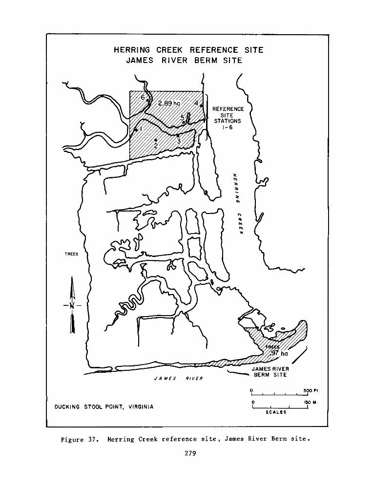
HERRING CREEK REFERENCE SITEJAMES RIVER BERM SITE
6
REFERENCESITE
STATIONS
1-6
2 3
TREES
h0
BERM SITERJAMES RIVER
0 r 500 Ft.
0O150OM.DUCKING STOOL POINT, VIRGINIA scA LE I
SCALES
Figure 37. Herring Creek reference site, James River Berm site.
279
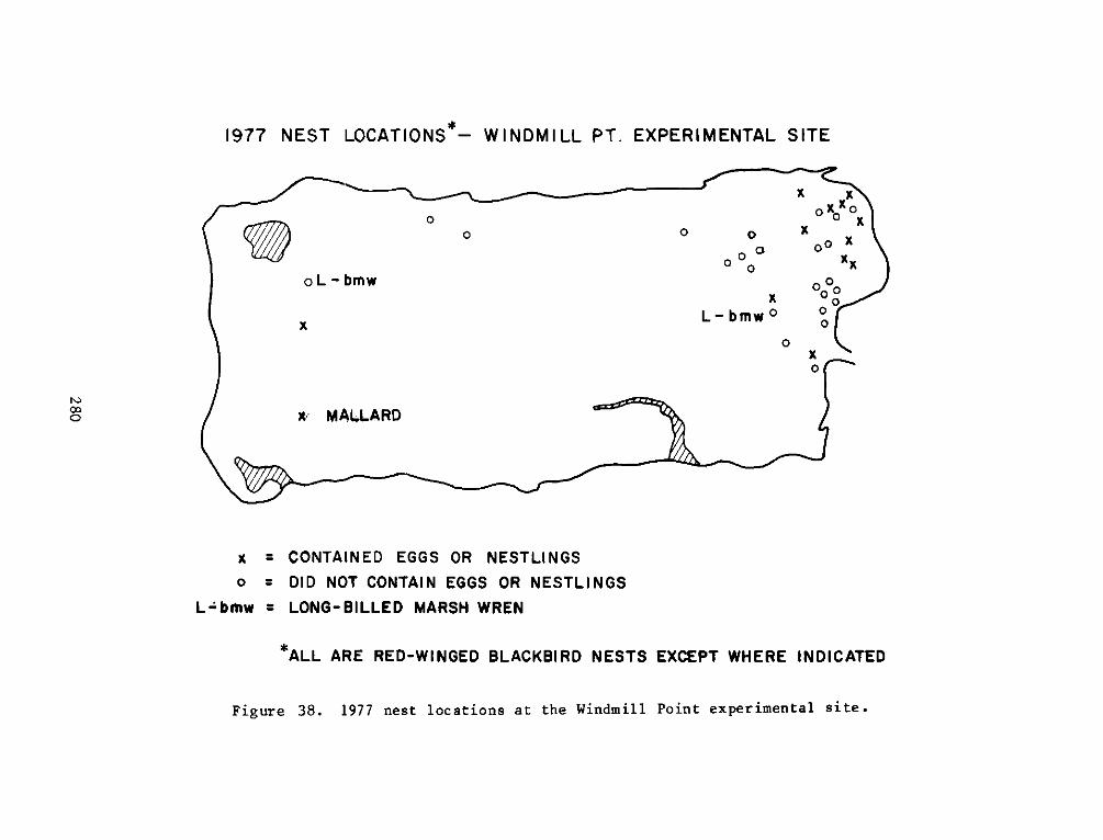
1977 NEST LOCATIONS*- WINDMILL PT. EXPERIMENTAL SITE
V-bmw0 0x 0 x0 0 x
0
o o X
x = CONTAINED EGGS OR NESTLINGSo=DID NOT CONTAIN EGGS OR NESTLINGS
L-bmw = LONG-BILLED MARSH WREN
ALL ARE RED-WINGED BLACKBIRD NESTS EXCEPT WHERE INDICATED
Figure 38. 1977 nest locations at the Windmill Point experimental site.
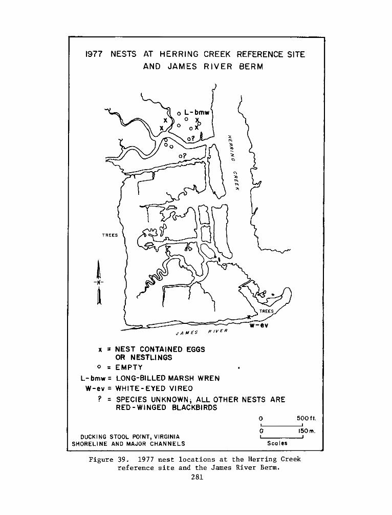
1977 NESTS AT HERRING CREEK REFERENCE SITE
AND JAMES RIVER BERM
o L-bmw
x : EST ONTINEDEGG
x 0T
TREES
TREES
w-ev
J AMES RIVER
x NEST CONTAINED EGGSOR NESTLINGS
0 = EMPTY-
L- bmw = LONG-BILLED MARSH WREN
W-ev = WHITE -EYED VIREO
? = SPECIES UNKNOWN; ALL OTHER NESTS ARE
RED - WINGED BLACKBIRDS
o 500 ftL
o 150 m.DUCKING STOOL POINT, VIRGINIA
SHORELINE AND MAJOR CHANNELS Scales
Figure 39. 1977 nest locations at the Herring Creek
reference site and the James River Berm.
281
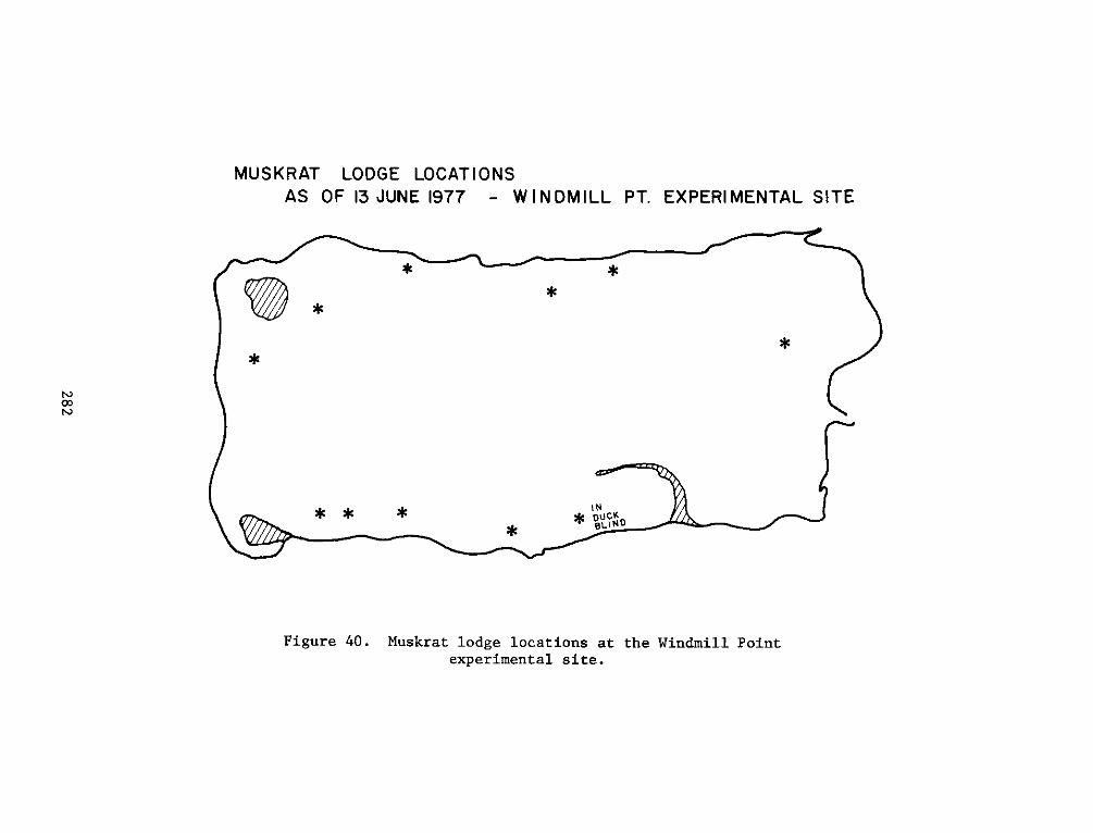
MUSKRAT LODGE LOCATIONSAS OF 13 JUNE 1977 - WINDMILL PT. EXPERIMENTAL SITE
*
* * * * o CC
Figure 40. Muskrat lodge locations at the Windmill Pointexperimental site.
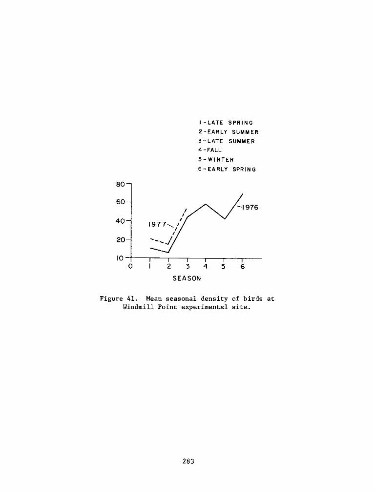
I -LATE SPRING
2-EARLY SUMMER
3-LATE SUMMER4-FALL
5-WINTER
6-EARLY SPRING
80
60X1976
40 1977 /
20-
10 I I I I I0 1 2 3 4 5 6
SEASON
Figure 41. Mean seasonal density of birds atWindmill Point experimental site.
283
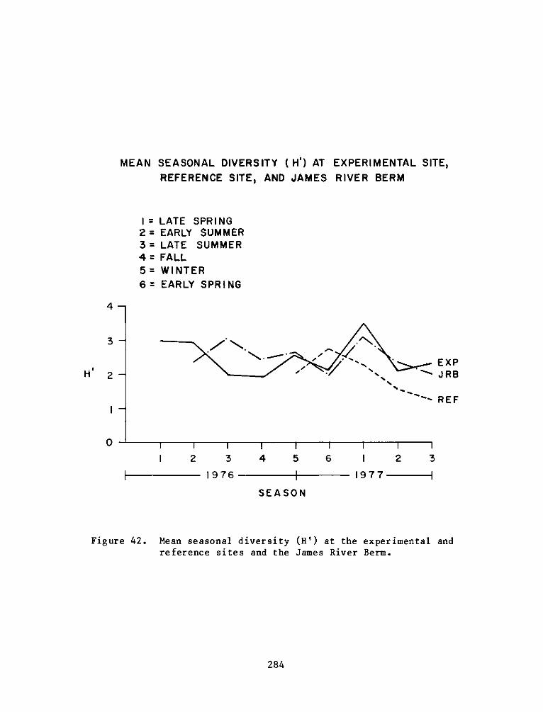
MEAN SEASONAL DIVERSITY (H') AT EXPERIMENTAL SITE,
REFERENCE SITE, AND JAMES RIVER BERM
I= LATE SPRING2 = EARLY SUMMER3= LATE SUMMER4= FALL5= WINTER6= EARLY SPRING
4
3
H' 2JR6
REF
0
I 2 3 4 5 6 I 2 3
|- 1976 1977
SEASON
Figure 42. Mean seasonal diversity (H') at the experimental andreference sites and the James River Berm.
284
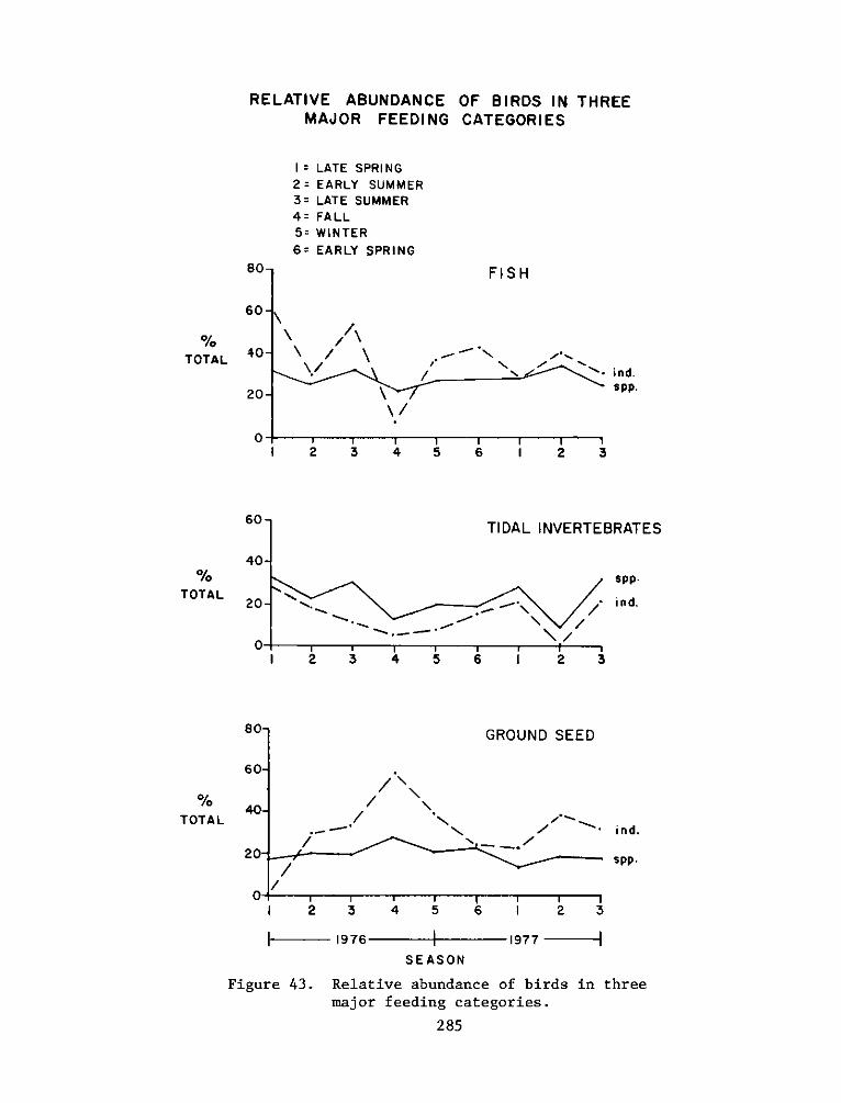
RELATIVE ABUNDANCE OF BIRDS IN THREEMAJOR FEEDING CATEGORIES
I= LATE SPRING2= EARLY SUMMER3= LATE SUMMER4= FALL5= WINTER
6= EARLY SPRING
FISH
\ / \-/ - N %%- ind.
s pp-
I 2 3 4 5 6 I 2 3
TIDAL INVERTEBRATES
' /
spp.
ind.
2 3 4 5 6 I 2 3
GROUND SEED
- i nd.
spp.
I 2 I3I 2 3
I I ,4 5 6 I 2 3
1976 I 1977- |
SEASON
Figure 43. Relative abundance of birds in three
major feeding categories.
285
80-
60
TOTAL 40-
20-
60-
40-
20-
80-
60-
40-
20-
TOTAL
TOTAL
- V -
v-T
1,._ ,./..r .
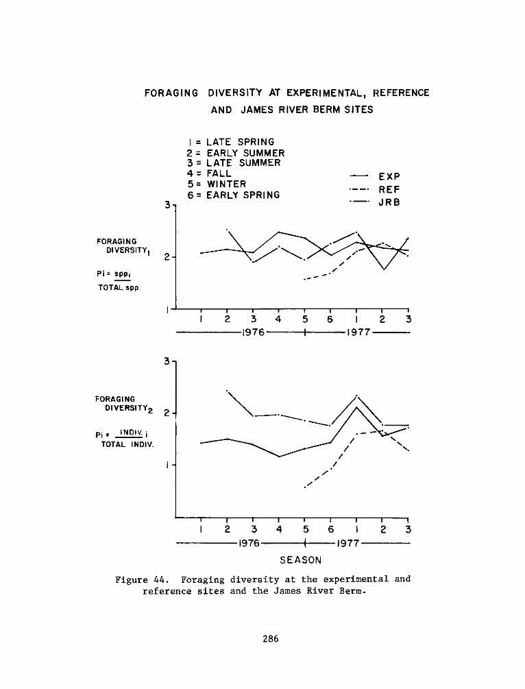
FORAGING DIVERSITY AT EXPERIMENTAL, REFERENCE
AND JAMES RIVER BERM SITES
3-
FORAGINGDIVERSITY 1 2
Pi= spp;
TOTAL spp
z=2:=3=4=5=6=
LATE SPRINGEARLY SUMMERLATE SUMMERFALLWINTEREARLY SPRING
-- EXP
---- REF--. JRB
de
I 2 3 4 5 6 I 2 31976 1977
3-
FORAGINGDIVERSITY 2
p;, INDIV;TOTAL INDIV.
2-
I-
/ N
/ N
I I I 1 I 1 3 1
I 2 3 4 5 6 I 2 31976 | -1977
SEASON
Figure 44. Foraging diversity at the experimental and
reference sites and the James River Berm.
286
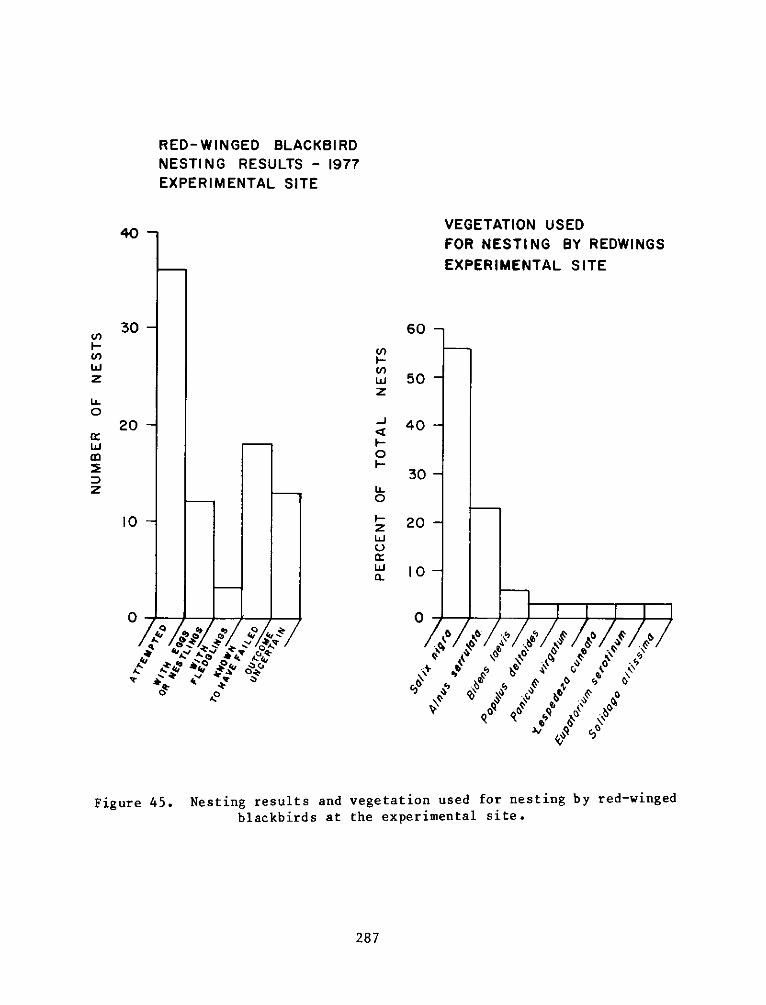
RED-WINGED BLACKBIRDNESTING RESULTS - 1977EXPERIMENTAL SITE
VEGETATION USEDFOR NESTING BY REDWINGSEXPERIMENTAL SITE
30-
U)
I-)wzUi-0
20
w
z
10 -
60 -
U)
wz
-
0
0
zW0
WCL
0
0 '4|1
50
40
30
20
10-
0
Q C, / o
Figure 45. Nesting results and vegetation used for nesting by red-wingedblackbirds at the experimental site.
287
40-7
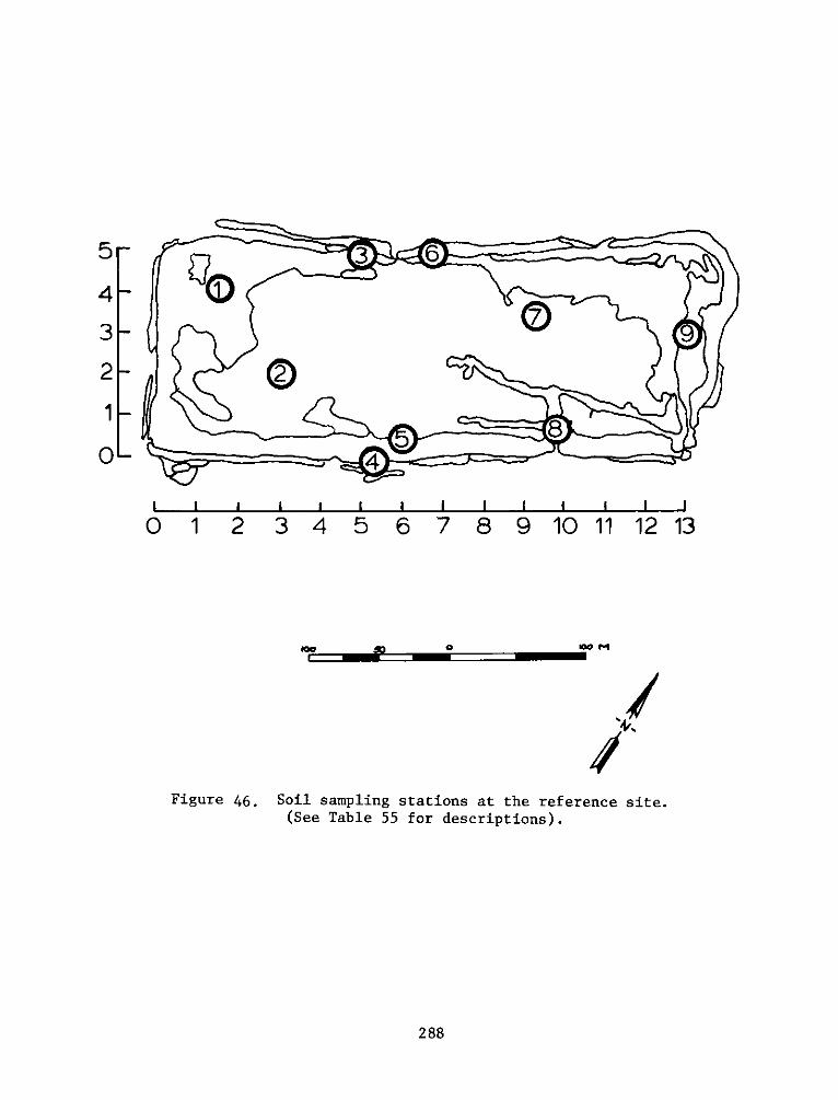
5~ 3 65F
4 0
3 - 9
2 -
1 -
0 4
S i 1 1 I I I I I I I I I
O 1 2 3 4 5 6 7 8 9 10 11 12 13
pp M O me M
Figure 46. Soil sampling stations at the reference site.(See Table 55 for descriptions).
288
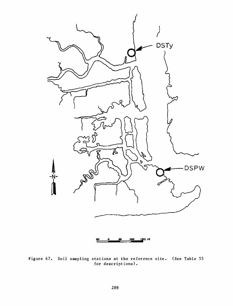
A DSTy
Sb o-So- -00-1D1PW
Figure 47. Soil sampling stations at the reference site. (See Table 55for descriptions).
289
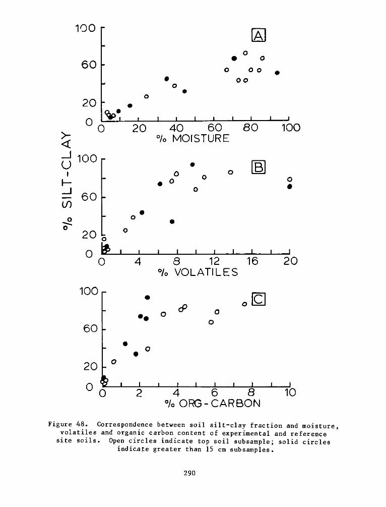
100
60
20
0
.
I I I I I I I I J
40 60/0 MOISTURE
0
0- 0
80
0
I I I I I I I
8 120/ VOLATILES
cr 00
_1 II_ _
4/o ORG-
6 8CARBON
Figure 48. Correspondence between soil silt-clay fraction and moisture,volatiles and organic carbon content of experimental and reference
site soils. Open circles indicate top soil subsample; solid circlesindicate greater than 15 cm subsamples.
290
00 0
0 00
000
00
-4 0
.
0 20
>--J
U2
-J..(9
0
0
100
60
20
00
100
00
00
00 4 16 20
100
60
20
o
0
0
0
09
2 10
1 II
I
o Bg
t-0
i
1
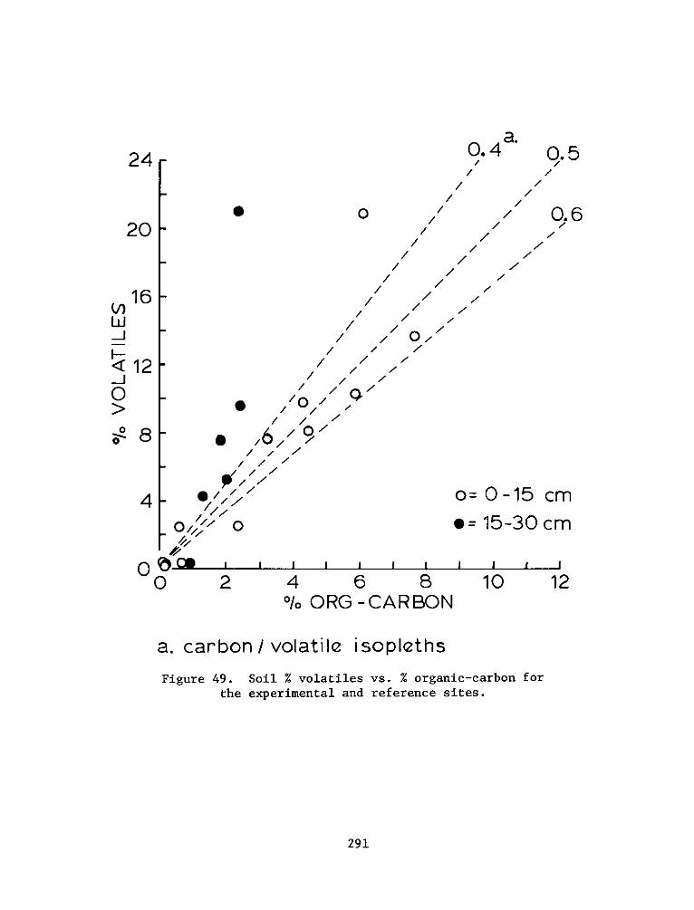
0
//
//
24
20
16w-J
Q 12
0
0 8
/ /,1/ /'
S/ / /,
/0. ,0 /
4 @-
0 200
//
//
0.4a.
// 0.6
//
//
/ //
i 0/ ///
o= 0-15 cm
* = 15-30 cm
4 6 8%o ORG -CARBON
10
a. carbon/ volatile isopleths
Figure 49. Soil % volatiles vs. % organic-carbon for
the experimental and reference sites.
291
0.5
/
J12
-.I-
'Qi
/
,do
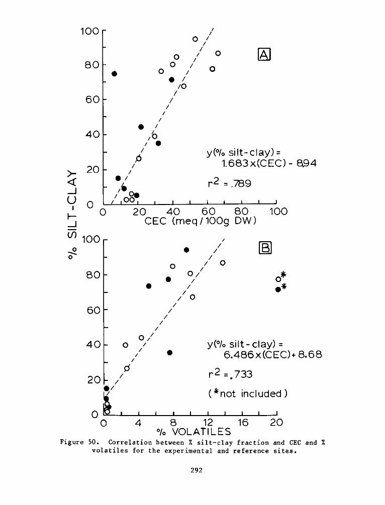
100 -0/
80 0 0 LJo ,
o* 0 / 00 //O
60 -
40 -,'
/y(% silt- clay) =.20 /1.683x(CEC) - 894
<Q .. " ' r2 = .789
_0 / 10U . ' 0d , ,Oo, , ,
0 20 40 60 80 100CEC (meq/100g DW)
V100 -"
o /
80 / o*
/ 0
60-
40 - * y(%Io silt- clay) ='/ "6.486x(CEC)+ 8.68
20 - r 2 =733
(*not included)
0 4 8 12 16 20O/o VOLATILES
Figure 50. Correlation between % silt-clay fraction and CEC and %
volatiles for the experimental and reference sites.
292
In accordance with letter from DAEN-RDC, DAEN-ASI dated22 July 1977, Subject: Facsimile Catalog Cards forLaboratory Technical Publications, a facsimile catalogcard in Library of Congress MARC format is reproducedbelow.
Virginia Institute of Marine Science, Gloucester Point.Habitat development field investigations, Windmill Point
marsh development site, James River, Virginia; Appendix D:Environmental impacts of marsh development with dredgedmaterial: Botany, soils, aquatic biology, and wildlife / byVirginia Institute of Marine Science, Gloucester Point, Va.Vicksburg, Miss. : U. S. Waterways Experiment Station ;Springfield, Va. : available from National Technical Informa-tion Service, 1978.
292 p. : ill. ; 27 cm. (Technical report - U. S. Army Engi-neer Waterways Experiment Station ; D-77-23, Appendix D)
Prepared for Office, Chief of Engineers, U. S. Army, Wash-ington, D. C., under Contract No. DACW39-76-C-0040 (DMRP WorkUnit No. 4A111)
Appendices A'-U' on microfiche in pocket.References: p. 128-134.
1. Dredged material. 2. Ecology. 3. Environmental effects.
(Continued on next card)
Virginia Institute of Marine Science, Gloucester Point.Habitat development field investigations, Windmill Point
marsh development site, James River, Virginia; Appendix D:Environmental impacts of marsh development with dredgedmaterial: Botany, soils, aquatic biology, and wildlife ...1978. (Card 2)
4. Field investigations. 5. Fine grained soils. 6. Habitats.7. James River. 8. Marshes. 9. Windmill Point. I. UnitedStates. Army. Corps of Engineers. II. Series: United States.Waterways Experiment Station, Vicksburg, Miss. Technicalreport ; D-77-23 Appendix D


APPENDICES A' THROUGH U'
DREDGED MATERIAL RESEARCH PROGRAM
ENVIRONMENT AL E FFECTS LABOR ATORYU. S. ARMY ENGINEER WATERWAYS EXPERIMENT STATION
. " Box63

i