AI

HABITAT EVALUATION PROCEDURES AT RAY ROBERTS LAKE:

AN ANALYSIS OF THE RELATIONSHIP WITH ECOLOGICAL

INDICATORS AND A STUDY OF OBSERVER AND

TEMPORAL VARIABILITY

THESIS

Presented to the Graduate Council of the

University of North Texas in Partial

Fulfillment of the Requirements

For the Degree of

MASTER OF SCIENCE

By

Jane M. Wattrus, B.S.

Denton, Texas

December, 1993

6rk4

Wattrus, Jane M., Habitat Evaluation Procedures at Ray

Roberts Lake: An Analysis of the Relationship with

Ecological Indicators and a Study of Observer and Temporal

Variability:. Master of Science (Environmental Science),

December 1993, 98 pp., 4 tables, 18 figures, references 41

titles.

Habitat Evaluation Procedure data gathered at Ray

Roberts Lake in 1989 and 1990 were analysed for temporal

variability, observer variability and relationships between

Habitat Units (HUs) and species density/diversity.

observer variability within a group was analysed by

cluster analysis and bootstrapping. Five out of 36 sites

showed significant differences in Habitat Suitability Index

(HSI) values within the group.

A nonparametric Mann-Whitney test was used to analyze

temporal variability. One of 6 sites showed a significant

difference in HSI values between years.

Using Spearman's Rank Correlation Coefficient, a

correlation was found between indicator species density and

HUs. No significant correlation was indicated between

species diversity and HUs.

ACKNOWLEDGMENTS

I wish to thank my major professor, Dr. Sam Atkinson and

the members of my thesis committee, Dr. Ken Dickson and Dr.

Jim Kennedy.

I would like to thank Dr. Ken Steigman for providing some

of the data used in this study and Gini Kennedy for her

assistance with the preparation of some of the figures.

Finally, I would like to thank my husband Dr. Nigel

Wattrus for his guidance and patience in the preparation of

this thesis.

This work was in part supported with funds provided by

the U. S. Army Corp of Engineers.

iii

TABLE OF CONTENTS

ACKNOWLEDGEMENTS.........................................iii

TABLE OF CONTENTS.......................................iv

LIST OF TABLES............................................vi

LIST OF FIGURES..........................................evii

Chapter

1. INTRODUCTION............................... ...... I

Brief backgroundObjectives of the studyScope of the studyBrief description of contents ofremaining chapters

2. LITERATURE REVIEW........................ ...... 5

Outline of chapter contentsTemporal and observer variabilitySpecies density and habitat quality

3. METHODS AND PROCEDURES...........................19

Outline of chapter contentsStudy area and habitat descriptionsSpecies selection and habitat suitability modelsHabitat Evaluation Procedures field evaluationsBird censusesGuild informationStatistical analyses

4. RESULTS.... - -.................. ................... 36

Outline of chapter contentsHypothesis 1: observer variabilityHypothesis 2: temporal variabilityHypothesis 3: density vs. habitat quality

iv

Hypothesis 4: species diversity vs. habitatquality

5. CONCLUSIONS........... ................. 59

Outline of chapter contentsDiscussion of each hypothesis and resultRecommendations for future study

APPENDIX..-...--..------....--.-....................66

A) Habitat suitability index life requisite valuemodels for indicator species

B) Habitat suitability index values for thevegetational transects

C) Habitat suitability index values for the Impactassessment sites

D) Avian census numbers by habitat type and transectsection for 1987 and 1990

E) Bray-Curtis cluster analysis data

REFERENCES. ............................................ 94

V

LIST OF TABLES

Table Page

1. Indicator species and models used for theHEP analysis at Ray Roberts Lake...................24

2. Matrix of variables and species used per HabitatEvaluation Procedures.---------.................26

3. Avian species guilded with HEP indicator speciesas a result of various guild studies.............. 31

4. Habitat units, indicator species density andspecies richness for various impact sites andtransect habitats.--------............... 56

vi

LIST OF FIGURES

Figure Page

1. Location of Ray Roberts Lake in Relationshipto the Dallas-Fort Worth Metroplex................ 2

2. Location of vegetational transects at RayRoberts Lake and habitat types along eachtransect------..------------...-..............2 3

3. Location of the impact assessment sites usedin the HEP----------------...................... 28

4. Bird guilds of the contiguous U.S.A............. 33

5. Bray-Curtis cluster analysis of mean habitatsuitability index values for five observersat impact site water habitat (Green Heronmodel)...----------- ..-................... 38

6. Water habitat Green Heron model variable 2representing habitat suitability index vs.percent of water area < 25 cm deep............... 39

7. Bray-Curtis cluster analysis of mean habitatsuitability index values for five observers attransect EF water habitat (Green Heron model).... 40

8. Bray-Custer cluster analysis of mean habitatsuitability index values for five observers attransect GH water habitat (Green Heron model).... 41

9. Water habitat Green Heron model variable 1representing habitat suitability index vs.aquatic substrate composition in littoral

10. Water habitat Green Heron model variable 4representing habitat suitability index vs.percent of water surface covered by logs,trees, or woody vegetation...................... 44

11. Bray-Curtis cluster analysis of mean habtatsuitability index values for five observers attransect AB shrublandhabitat....................45

vii

12. Shrubland habitat Eastern Woodrat model variable3 representing habitat suitability index vs.number of refuge sites per 0.4 ha................46

13. Bray-Curtis cluster analysis of mean habitatsuitability index values for five observers attransect EF oldfield habitat (E. Cottontailmodel)........................................... 47

14. Oldfield habitat Eastern Cottontail modelvariable 4 representing habitat suitabilityindex vs. percent shrub crown cover.............. 49

15. Oldfield habitat Eastern Cottontail modelvariable 5 representing habitat suitabilityindex vs. number of refuge sites per 0.4 ha.......50

16. Upland forest habitat Fox Squirrel modelvariable 1 representing habitat suitabilityindex vs. percent tree canopy closure ofmast producing trees > 25 cm dbh.................53

17. Upland forest habitat Fox Squirrel modelvariable 3 representing habitat suitabilityindex vs. average diameter at breast height(dbh) of overstorytrees...................... 54

18- Correlation of Habitat Units and AvianIndicator Species Density at Ray Roberts..........57

viii

CHAPTER I

INTRODUCTION

In July of 1987 the construction of Ray Roberts Lake in

northern Denton County, Texas (Fig. 1) was completed by the

U.S. Army Corps of Engineers. A two year pre-impoundment

environmental study of the lake area was started by the

Institute of Applied Sciences at the University of North

Texas in January of 1986. The objective of this study was to

develop baseline descriptions of the wildlife resources in

the area prior to impoundment. In addition to censuses of

vegetation, fish, mammals and birds another component of the

study entailed applying Habitat Evaluation Procedures-(HEP).

HEP was developed by the U.S. Fish and Wildlife Services

(USFWS) to evaluate habitat quality and quantity.

Habitat Evaluation Procedures were initially developed

in 1974, by USFWS, in response to legislation such as the

Fish and Wildlife Coordination act of 1934 and the National

Environmental Policy Act (NEPA) of 1969. NEPA requires that

all federally funded or permitted projects must consider

possible adverse impacts on fish and wildlife. This created

a need for a system of habitat evaluation that would

facilitate assessment of the effects of actions taken in a

federal project. In 1980, HEP was further developed with

1

2

ISL.E O 05E 4

RAY ROBERTS LAKEJAL F..Y. 4 ;.

L / T T

LEWISVLLE'1LAKE

CEN N - -

I NCX EQUALS MILES

CQ 6APYI N E---

L AK E

FT WCATM ALA

Figure 1. Location of Ray Roberts Lake in Relationship tothe Dallas-Fort Worth Metroplex. (IAS, 1992)

3

the use of documented habitat models and analyses of

individual evaluation species rather than by examining cover

types alone (USFWS, 1980a).

The basic unit of HEP is the Habitat Suitability Index

(HSI). Ecological variables (e.g. percent shrub crown cover,

height of mast producing trees, number of refuge sites per

0.4 ha, etc.) are measured in the field and then entered

into the selected evaluation species model. HSIs range from

0 to 1.0 and are determined by this model. Habitat Units

(HUs) are a product of the HSI and the acreage of the

habitat in question.

HEP provides a habitat-based approach for assessing

environmental impacts of proposed land and water resource

developed projects. It can be used to document the quality

and quantity of habitat available for a selected species.

HEP provides information on the relative value of different

areas at a particular point in time (USFWS, 1980a).

A two year post-impoundment study of Ray Roberts Lake

was begun by the Institute of Applied Sciences in January of

1989. HEP was utilized in an attempt to examine the

condition of wildlife habitat in 1990 and to determine if

any changes in the habitat had occurred since the initial

baseline study in 1987.

During data collection and analyses, several questions

arose about HEP which led to the following hypotheses: (1)

there is no significant difference in Habitat Suitability

Index variable values between individuals in a survey party,

4

(2) there is no significant difference in mean Habitat

Suitability Index values at impact assessment sites between

sampling years, (3) for a particular habitat type there is

no correlation between Habitat Units and avian Indicator

Species density, (4) for a particular habitat type there is

no correlation between Habitat Units and avian species

diversity.

In order to address the above four hypotheses, several

statistical methods were utilized to analyze the HEP data

and bird census data which were gathered and tabulated for

both the 1987 pre-impoundment and 1990 post-impoundment

studies.

The following sections of this thesis contain a review

of the literature pertaining to the outlined hypotheses, a

description of the methods and procedures which were used, a

presentation and analysis of the -results and conclusions.

CHAPTER 2

LITERATURE REVIEW

This section reviews the literature which pertains to

the objectives of this study. The information will be

subdivided into two subsections; 1) Temporal and Observer

Variability; and 2) Species Density/Diversity and Habitat

Quality.

The first subsection deals with previous studies

involved in the assessment of observer variability in

estimating/measuring habitat characteristics, and also what

effect making estimates at different time periods has on the

results at a particular habitat. HEP is traditionally used

to evaluate initial conditions in a habitat and then make

projections about the future condition of that habitat. In

this study HSIs were calculated for initial conditions in

1987 and then calculated at a later time (i.e. :1990) for

specific habitats. The results of these HEP studies

conducted at different times, in the same habitat, were then

compared. Upon reviewing the literature in this area, it was

noted that this was an unconventional way of utilizing HEP,

and prior studies involving temporal variability are scarce.

The second subsection provides a review of a variety of

studies which attempted to relate species abundance measures

to habitat characteristics and quality.

5

6

Temporal and Observer Variability

The collection of habitat information is inherent to

the HEP developed by USFWS. Many of the variables that are

integral in developing a HSI are derived from observer

estimates of specific habitat characteristics (i.e.: percent

herbaceous canopy cover). Inevitably, variation in the

measurements of HSI variables will exist among members of a

survey team, despite "group training" in variable

measurement techniques. Gotfryd and Hansell (1985) note that

the problem of variation due to observer differences has in

the past received little attention in the area of field

ecology.

Smith (1944) studied the accuracy and variation between

estimates of vegetation density made by individuals in a

group. He also described what impact a group training period

had on the results. Eight individuals, familiar with

vegetation density measurements, made estimates over a seven

day period. During that time attempts were made to unify the

individuals estimates. An analysis of variance (ANOVA) of

the data from the first, fourth and seventh days of the

survey showed significant differences among the individuals

in the group (p = 0.05). Results also indicated considerable

change in each individual's estimates of vegetation density

during the week. These became more conservative as the

experiment proceeded. The range of estimates made by the

group also decreased as the week progressed. This was not

unexpected due to the group training which was provided.

In a study by Ellis et al. (1979) four different field

methods of habitat evaluation were tested. Several questions

were addressed: (1) are there seasonal (temporal)

differences in scoring by each evaluation method; (2) does

prior experience in habitat evaluation effect scoring; and

(3) how accurate are observers in estimating vegetational

characteristics. Ninety-seven biologists participated in

five field tests each lasting three consecutive days. Each

observer was assigned one of the following habitat

evaluation methods;

1) HEP Form 3-1101 (USFWS, 1976). This method consists

of a form with columns representing species or groups of

species (evaluation elements) and rows representing

evaluation sites. Test participants assign a score on a

scale of 0 - 10 for each evaluation element. HEP Form 3-1101

is a totally subjective method of habitat evaluation, with

no written criteria.

2) HEP Blue Handbook (Flood et al., 1977). Life history

information is provided for each species grouping (e.g.,

Forest Game Species group - white-tailed deer and wild

turkey). Written criteria are given on five-point or ten-

point scales. Resulting scores are then combined using

formula provided.

3) Line Chart (Whitaker et al., 1976). Vegetative

characteristics are objectively estimated by the user with

7

8

this method. Instructions and definitions are provided.

Estimates are entered on a scaled horizontal line and are

later translated into scores ranging from 0 - 10, for

various wildlife species.

4) Matrix Method (Ellis et al., 1978). This method

includes definitions and instructions and is vegetation

orientated. Columns on this form represent habitat

characteristics, while sites with their estimates are

entered in the rows. Estimates of habitat characteristics

from this form are then translated into scores on a scale of

0 - 10 as with the Line Chart method above.

To determine if there were temporal differences in

scoring by each evaluation method, observers habitat scores

for specific species (i.e. deer, quail, rabbit and turkey)

were examined for consistency within and between seasons.

The coefficient of variation (CV) for scores from all

methods, except HEP Form 3-1101, were low (range: 6-39)

inferring consistency in scoring within each season. The CV

for scores from HEP Form 3-1101 method were high (range:28-

90) suggesting consistent scoring within any test period was

improbable with that methodology.

Mean scores derived by the same methods were found to

differ according to season. For all methods, except for two

cases with the Matrix method, mean scores were lowest in

January. Low scores in January were attributed to difficulty

in assessing sites under winter conditions such as snow

cover, no foliage, etc. (Ellis et al.,1979).

9

ANOVA was used to test for significant differences

between seasons (p = 0.05) and pairs of means were then

compared by least significant differences (LSD) analysis (p

< 0.05). Seasonal differences for all four methods were

detected and attributed to the overall low mean scores in

January.

Coefficients of variation (CV) and mean scores of

experienced versus inexperienced participants were analyzed

to determine the effects of prior experience. Results

indicated that participants using all methods, except HEP

Form 3-1101, produced consistent scores regardless of

experience. Significant differences were detected (ANOVA (p

< 0.05)) in mean scores in Oldfields, between experienced

and inexperienced participants, using both HEP Form 3-1101

and HEP Blue Handbook methods. This was attributed to the

subjective and less structured nature of these two methods

giving advantage to experienced biologists.

Detailed measures of site characteristics were made at

each study site by trained and experienced staff to

determine observer accuracy in estimations of vegetational

characteristics. These data were then considered "baseline"

data and were compared to participant's field estimations.

Results indicate that estimations of percent canopy closure

and timber types were generally accurately estimated. Other

parameters were estimated less accurately and this loss of

accuracy was attributed to two factors: (1) some habitat

characteristics are intrinsically difficult to estimate

10

(i.e. percentage of dead trees in overstory); and (2) some

criteria are subjectively worded (i.e: use of the word

"common").

Gotfryd and Hansell (1985) used multivariate vegetation

observations to evaluate the effects of subjectivity on

habitat analyses. Data were collected by four observers who

independently and repeatedly sampled a series of sites in an

oak-maple forest over a five week period. Data were analyzed

through ANOVA, principal component and discriminant function

analyses (p < 0.01). Results indicate observers

significantly differed in their measurements of 18 out of 20

vegetative variables (e.g. percent canopy cover, ground

cover, etc.). Gotfryd and Hansell (1985) suggest that " Low

variability is no guarantee of accuracy, and high

variability does not necessarily imply that the data are, on

average, inaccurate."

Block et al. (1987) studied observer variability when

estimating vegetation characteristics. Three observers

visually estimated vegetation characteristics in 75 plots

and then these same vegetation characteristics were measured

using established quantitative techniques. Prior to ocular

estimates in any plot, observers discussed estimation

techniques in an attempt to standardize the group methods.

Two-way ANOVA was used to compare ocular estimates of the

vegetation by the observers (p < 0.05). Results showed that

the three observers differed significantly for 31 of the 49

variables estimated. In addition, comparisons of observer

11

estimates and actual measurements further demonstrated

differences among observer estimation. For example, all

observers underestimated tree diameters, tree and shrub

numbers and canopy cover and overestimated tree heights and

percent ground cover. Block et al. (1987) concluded that not

only are there significant difference among estimates of

different observers but also significant differences occur

between observer's estimates and actual measurements for

many variables.

Species Density/Richness and Habitat Quality

HSI models are designed for use in natural resource

planning and environmental impact assessment studies. These

models determine habitat quality but as Schamberger dnd

O'Neil (1984) state "They are not models of carrying

capacity because not all factors that influence animal

abundance are included." Habitat is not the sole factor

determining species abundance, other factors such as

disease, mortality, predation, weather and competition are

all a function of carrying capacity and most habitat models

address few of these factors (Schamberger and O'Neil, 1984).

Therefore, in studying HSI models, it must be acknowledged

that they are not designed as carrying capacity models or

comprehensive population level predictors. However, HSIs do

provide a 0 - 1.0 index of habitat suitability and an HSI

value of 0.9 should indicate better habitat than an HSI of

12

0.1 and therefore should represent a greater "potential"

carrying capacity (Schamberger and O'Neil, 1984).

Prior to actual studies involving HSI model validation,

studies were conducted relating species abundance to

specific habitat characteristics. Sturman's (1967) study of

two chickadee species found, using a multiple regression

analysis, that the abundance of the Chestnut-backed

chickadee Parus rufescens and the Black-capped chickadee

Parus atricapillus was highly correlated to fourteen

different vegetative characteristics (R2 values ranged from

0.959 to 0.297). The Chestnut-backed chickadee abundance was

highly correlated with percent upper canopy volume which is

coniferous (R2 = 0.826) and the average height of upper

story conifers (R2 = 0.918). These two variables accounted

for more than 90 percent of the variability in observed

abundances. For the Black-capped chickadee, canopy volume

of: trees (R2 = 0.796), bushes (R2 = 0.974) and middle-story

trees (R2 = 0.921), together accurately predict it's

abundance. Regression of these three variables account for

greater than 90 percent of the variability in this species

abundance.

Anderson and Shugart (1973) used univariate ANOVA to

test for differences in abundance categories (i.e. rare,

common, etc.) of various species of birds with respect to 28

habitat characteristics (i.e. number of saplings, foliage

biomass, etc.). Differences in habitat preferences within

major bird families were apparent from this analysis (a

13

levels = 0.001, 0.01 and 0.05). Discriminant function

analysis was then used to order habitat variables according

to their strength in separating bird abundance categories.

Results indicated that certain bird species were distributed

according to specific habitat characteristics (a = 0.05).

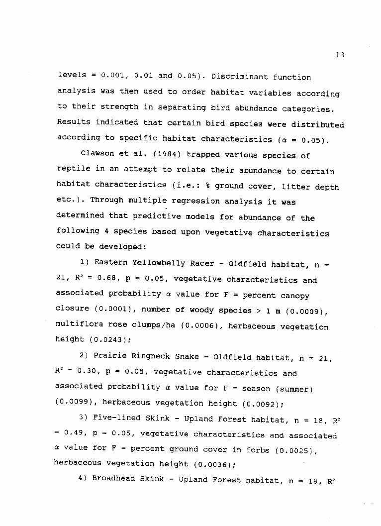
Clawson et al. (1984) trapped various species of

reptile in an attempt to relate their abundance to certain

habitat characteristics (i.e.: % ground cover, litter depth

etc.). Through multiple regression analysis it was

determined that predictive models for abundance of the

following 4 species based upon vegetative characteristics

could be developed:

1) Eastern Yellowbelly Racer - Oldfield habitat, n =

21, R2 = 0.68, p = 0.05, vegetative characteristics and

associated probability a value for F = percent canopy

closure (0.0001), number of woody species > 1 m (0.0009),

multiflora rose clumps/ha (0.0006), herbaceous vegetation

height (0.0243);

2) Prairie Ringneck Snake - Oldfield habitat, n = 21,

R' = 0.30, p = 0.05, vegetative characteristics and

associated probability a value for F = season (summer)

(0.0099), herbaceous vegetation height (0.0092);

3) Five-lined Skink - Upland Forest habitat, n = 18, R2

= 0.49, p = 0.05, vegetative characteristics and associated

a value for F = percent ground cover in forbs (0.0025),

herbaceous vegetation height (0.0036);

4) Broadhead Skink - Upland Forest habitat, n = 18, R2

14

= 0.67, p = 0.05, vegetative characteristics and associated

probability a value for F = season (summer) (0.0004),

understory closure (0.0293).

Van Horne (1983) points out several situations where

habitat quality for a species is not directly correlated

with the density of a species. Reasons cited for the

breakdown in the density-habitat quality relationship are:

(1) "there may be multi-annual variability in local

population densities that reflect small scale variability in

the food source, in predator populations, or in abiotic

environmental factors."; and (2) " .... during years when

species' densities are high, animals may achieve very high

densities in low-quality habitats where survival and

production are low because offspring have been forced into

these habitats by intra-specific competition." Van Horne

(1983) suggests that density may simply reflect conditions

of the recent past or temporary present and not long-term

habitat quality. He adds that a measure of habitat quality

should contain certain components of not only density but

also offspring production and survival.

Larson and Bock (1986) measured habitat variables on

small plots centered on individual birds (bird-centered

analysis or BCA) of four different species. They then

compared these results with data from randomly situated

plots. Bird abundance estimates were determined to be

correlated with several habitat characteristics (e.g.

percent shrub cover, percent bare ground, percent grass

15

cover, maximum height of vegetation, maximum grass/forb

height, maximum shrub height, and percent Sagebrush) for

some of the species studied (p < 0.01). In addition, BCA was

able to identify more significant habitat associations for

specific species than the random plot analysis.

Studies specifically related to HSI models began to

appear in the early 1980's. Many studies were involved with

the development of accurate models, while other research has

been conducted into post facto model verification.

Laymon and Barrett (1986) investigated the pitfalls

that arose in the development and validation of three

different HSI models. The models they tested were the

Spotted Owl, Strix occidentalis (Laymon et al., 1985),

Marten, Martes americana (Spencer et al., 1983) and Douglas'

Squirrel, Tamiasciu.rus douglasii (Laymon and Barrett, 1986).

The Spotted Owl model's ability to predict occupied

Spotted Owl habitat in Sierra Nevada, Ca. was tested by

comparing HSI values from 70 sites where owls were

definitely known to occur (x = 0.53) with HSI values

measured at 70 randomly located sites (x = 0.31), (t = 7.53,

CV of t = 1.96, p < 0.001). In a second test, a field survey

using vocal imitations of Spotted Owl calls was conducted at

56 sites, 14 in each of the following four categories; (1)

unsuitable - (HSI = 0 - 0.23), (2) low - (HSI = 0.24 -

0.47), (3) moderate - (HSI = 0.48 - 0.64), (4) high - (HSI =

0.65 - 1.0). Owls responded at none of the unsuitable sites,

14 percent of the low sites, 36 percent of

16

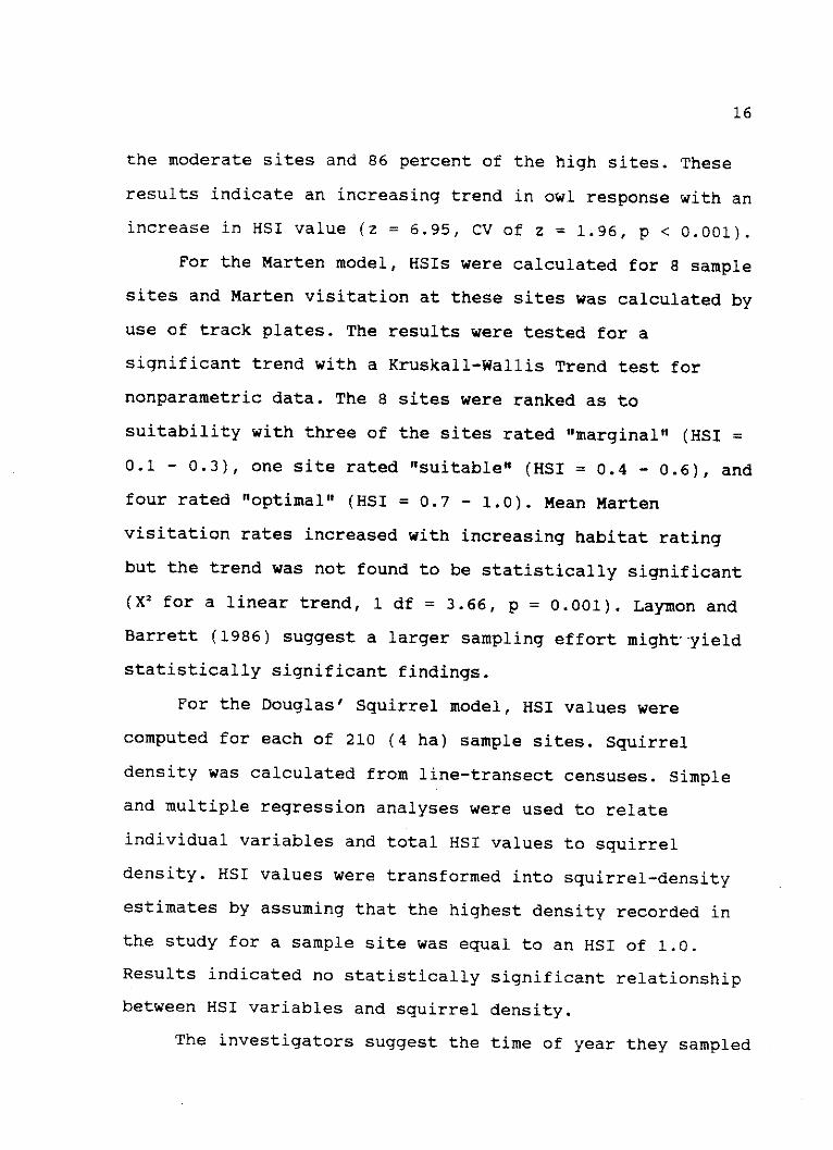
the moderate sites and 86 percent of the high sites. These

results indicate an increasing trend in owl response with an

increase in HSI value (z = 6.95, CV of z = 1.96, p < 0.001).

For the Marten model, HSIs were calculated for 8 sample

sites and Marten visitation at these sites was calculated by

use of track plates. The results were tested for a

significant trend with a Kruskall-Wallis Trend test for

nonparametric data. The 8 sites were ranked as to

suitability with three of the sites rated "marginal" (HSI =

0.1 - 0.3), one site rated "suitable" (HSI = 0.4 - 0.6), and

four rated "optimal" (HSI = 0.7 - 1.0). Mean Marten

visitation rates increased with increasing habitat rating

but the trend was not found to be statistically significant

(X2 for a linear trend, 1 df = 3.66, p = 0.001). Laymon and

Barrett (1986) suggest a larger sampling effort might--yield

statistically significant findings.

For the Douglas' Squirrel model, HSI values were

computed for each of 210 (4 ha) sample sites. Squirrel

density was calculated from line-transect censuses. Simple

and multiple regression analyses were used to relate

individual variables and total HSI values to squirrel

density. HSI values were transformed into squirrel-density

estimates by assuming that the highest density recorded in

the study for a sample site was equal to an HSI of 1.0.

Results indicated no statistically significant relationship

between HSI variables and squirrel density.

The investigators suggest the time of year they sampled

17

squirrel density (late summer) may have been inappropriate

due to young dispersing into less suitable habitats. Laymon

and Barrett (1986) comment that "correlations between

squirrel density and habitat variables might be more

apparent if sampling occurred during the spring...".

Cook and Irwin (1985) field tested the Pronghorn,

Antilocapra americana HSI model (Allen & Armbruster, 1982)

by correlating model outputs with estimates of wintering

Pronghorn densities which they assumed to reflect habitat

quality. Using simple linear regression they regressed HSI

values, against corresponding Pronghorn density estimates.

Results indicate that the model explains 50 percent of the

variation in Pronghorn density (p < 0.001). They conclude

that despite Van Horne's (1983) caution that density may

sometimes be a misleading indicator of habitat quality, the

Pronghorn HSI model produces ratings of habitat.quality

which correlate well with population indicators of habitat

quality. They point out that the model should not be used to

predict actual Pronghorn numbers, but that habitat potential

for Pronghorns can be described.

Schroeder (1990) examined the relationship between

Black-capped Chickadee HSI model values (Schroeder, 1983)

and Black-capped chickadee population densities through

Least Absolute Deviation Regression analysis. The Null

hypothesis for this test was that regression of HSI values

on estimated Black-capped chickadee population densities

would produce a model with a slope significantly different

18

from zero but not different from the slope of a model

predicting ideal maximum population densities. An ideal

maximum population density model was derived using

historical data gathered in a previous Black-capped

chickadee survey. Results indicated that the HSI model

closely approximated ideal maximum population density when

HSI values are at a maximum. He concludes that the HSI model

considers only a subset of a variety of factors which may

influence population density. He suggests that "The HSI is

best viewed as an index of habitat-imposed limitations on a

population. For example, an HSI of 1.0 would indicate no

habitat-related limitations exist, whereas decreasing HSI

values would indicate increasingly significant habitat

limitations" (Schroeder, 1990).

CHAPTER 3

METHODS AND PROCEDURES

The following section contains descriptions of the

methods and procedures used in this study. The first

subsection describes the study area and the specific

habitats analyzed. The second subsection deals with species

selection and Habitat Suitability models chosen. Subsections

three and four describe the procedures used in the HEP field

evaluations and bird censuses. Species Guilds and their

utility in this study are described in subsection five. The

final subsection discusses statistical analyses used to

address the proposed hypotheses.

Study Area and Habitat Descriptions

Ray Roberts Lake is located largely in Denton County,

Texas, along the Elm Fork of the Trinity River, 30 miles

upstream from Lewisville Dam and approximately 10 miles

north of the City of Denton (Fig.1). The area considered for

both the 1987 and 1990 Habitat Evaluation Procedure (HEP)

studies was within the U.S. Army Corps of Engineers Project

Area boundaries for Ray Roberts Lake totalling 48,347 acres.

A Green Belt area below the dam totalling 1,600 acres was

also included in the evaluation. Six habitat types were

19

20

selected for analysis in the initial HEP study in 1987 and

are defined in the Ray Roberts Lake Pre-impoundment

Environmental Study (IAS, 1988) as follows:

Upland Forest

Areas of sandy soil with abundant rocks noticeable on

slopes. Tree densities range from 200 to 500 trees per acre

with canopy heights of 20 to 26 feet. Three species of tree

are co-dominant; Post Oak, Quercus stellata, Blackjack Oak,

Quercus marilandica and Cedar Elm, Ulmus crassifolia.

Undergrowth is generally low with herbs concentrated in

small clearings between trees.

Bottomland Forest

These areas were characterized by taller trees (canopy

heights range from 25 to 40 feet) and a greater herbaceous

component than that of Upland Forests. Tree species

diversity was high in these areas. Shrubs cover 20 to 50

percent of the ground between trees.

Shrubland

Areas with tree densities intermediate between typical

Oldfields and woodlands are designated as Shrubland.

21

Tree densities range from 20 to 120 per acre. Shrubs provide

2 to 20 percent of ground cover.

Pasture

This habitat is defined as a field either clearly

maintained for cattle or one in which evidence of recent

heavy grazing is apparent. Low plant species diversity and

trampled vegetation are signs of heavy grazing. Pastures are

typically treeless and have few shrubs (average < 2 per

acre).

Oldfield

These areas are distinguished from Shrublands by'lower

shrub and tree densities and from Pasture by their lack of

indications of recent heavy grazing. Tree densities range

from 0 to 16 trees per acre and shrub density from 0 to 300

per acre. Agricultural-Cropland acreage are included under

the Oldfield habitat heading for the HEP.

Riverine/Lacustrine

This group includes all Lotic and Lentic habitats such

as streams, rivers, ponds and lakes.

In the 1990 HEP study all the above habitat types were

22

again considered, along the vegetational transects

established in 1987 (Fig. 2), with the exception of Pasture

habitat which was lost due to inundation by the lake.

Species Selection and Habitat Suitability Models

The habitat types chosen within the study area were

evaluated to determine their ability to fulfill "life

requisites" of select species. Two "indicator species" were

selected for each habitat type based on a species inventory

compiled for the area by the Biology Department, University

of North Texas (Table 1). Certain birds were selected as

"indicator species" because they were considered

representative of generalized communities within the

ecoregion. Although bird, mammal and reptile species were

all considered in the Ray Roberts Lake Environmental Report

HEP studies, only avian species will be considered in this

study due to a lack of sufficient mammal and reptile census

data.

Habitat Suitability Index (HSI) models for all

indicator species, with the exception of the Downy

Woodpecker model, were obtained from the U.S. Fish and

Wildlife Service Terrestrial Habitat Evaluation Criterion

Blue Handbook (Ecoregions 2512 & 2320, 1980). The Downy

Woodpecker model was obtained from the U.S. Fish and

Wildlife Service Habitat Suitability Index Models: Downy

Woodpecker (Schroeder, 1982).

23

CL~

00

'00,l 0

a , 0.

00

00

- 0 ~ 00. U13

6 ~ 0

0> r4zA

- -4%

E>Ee

a -4

c IJ

A -.

S-- -

CL

24

Table 1. Indicator Species and Models used for the HEPAnalysis at Ray Roberts Lake (IAS, 1988).

Habitat Species

Riverine/lacustrine(RL)

Pasture (P)

Oldfield (OF)

Shrubland (SH)

Bottomland Forest(BF)

Upland Forest (UF)

Belted kingfisher Megaceryle alcyonGreen heron Butorides virescens

Eastern meadowlark Sturnella magnaRacer Coluber constrictor

Scissor-tailed flycatcherMuscivora forficata

Eastern cottontailSylvilagus floridanos

Eastern Woodrat Neotoma floridanaDowny woodpecker Picoides pubescens

Barred owl Strix variaRaccoon Procyon lotor

Fox squirrel Sciurus nigerCarolina chickadeeParus carolinensis

25

Table 2 lists the model variables. Appendix A contains the

model equations.

HEP Field Evaluations

Field evaluations for the HEP were conducted in early

summer 1987 and again in late summer of 1990. In 1987 six

habitats were selected for analysis along the vegetational

transects (Fig. 2) with two evaluation species analyzed per

habitat (Table 1). The evaluations in 1987 were performed at

fifteen random sampling sites per species, in each habitat,

for a total of 180 sites. These evaluations were made by one

individual. In 1990 there were only five habitat types along

the vegetational transects due to loss of Pasture habitat by

lake inundation. For each of the five habitat types several

locations were studied, for example, Bottomland Forest was

analyzed along transect GH and also transect EF. At each

site a team of five individuals performed three evaluations

each for a total of 360 measurements during the 1990

analysis. These data were then combined to give an average

Life Requisite HSI value for each indicator species.

Appendix B contains the HSI values measured.

In 1987 several "impact assessment areas" were also

chosen and evaluated as a basis for monitoring successional

changes and indirect effects of impoundment. One 20 acre

assessment area per habitat type was selected from areas

above the Flood Pool level where no plans had been made for

26

4141

04)A.Q,

- (J

N

'-4N>>

AL~ca

uxs

satso

XO

jITXX*1TTOuVnc

uiqSsj~ui

uoIa

N 4

- >>N

--fN

0 0%6w

ifw 6wi~c

40dpI0w dv 1 1to4Pd

ip i2

At m

- I9 , .

L s

1* !u.

% r- >f> c

m0)

04"1

00

4P

C40

27

development. These areas were again evaluated in 1990 to

determine if any indirect effects from impoundment had

occurred (Fig. 3). In 1987 at each "impact area" eight

sample sites were randomly chosen and evaluated by a single

individual. In 1990 a team of five individuals made three

evaluations each per "impact area" for a total of fifteen

sample sites per habitat. Appendix C contains the "impact

area" HSI values measured.

Bird Censuses

During the 1987 pre-impoundment and 1990 post-

impoundment environmental studies seasonal bird censuses

were conducted along the vegetational transects (Fig. 2) and

through the habitat types considered in the HEP analyses.

All censuses were conducted by experienced personnel

familiar with the birds of North Central Texas. The strip

transect method (Merikallio, 1958) was considered most

effective for censusing avian populations along the

transects " because of its seasonal versatility and

appropriateness for both flocking and nonflocking species,

and species such as swifts and swallows that cruise above

vegetation" (Emlen, 1971). More elaborate techniques such as

mist-netting were not utilized due to fiscal and personnel

limitations. The same personnel, with few exceptions, were

used to conduct all surveys. Each census was conducted on

foot beginning at sunrise and continuing for a maximum of 3

28

0000004.0--- .1 t % sC j 0u 0 we 0 er-. . o C

E w tor. %0 4 %~- 0Lfl0s0e0-O~ O 0 O~ O~ O0

1. 0 r. N 4Io C Q o qco aM - t% L \

0- 0 co00000c c

-na, e~n -s,."o- o4~a a,

-ocCCLa * .- 4,-

-f - a4,1a, c

0 IA)

fo- 4 )oco

a 0)

- - r. o o to LL.

-4.- 4 - 0).I- - -0-0..-.-:.a-4J)

-x -L- ) .A c

*0-W --U- -- - -- - - -C -.* 0 4, c:

c

n oen

atv

V0

3 CLL t

yZ _

0)o-

C00

CA,-

-a, -U.

29

hours to coincide with peak avian activity (IAS, 1988).

Transects were censused on consecutive days and/or when

weather conditions were similar to avoid detectability bias

due to weather conditions. For each habitat type along a

transect a strip width of approximately 200 feet was

established. Personnel walked down the center of this 200

foot wide strip, parallel to the vegetational transect, and

identified birds via visual and auditory cues obtained no

further than 100 feet away on either side. Density estimates

of each species per habitat type and transect were

calculated by summing the number of each species counted by

the observers in their respective survey areas (i.e. pooling

all personnel transect-strip data)(IAS, 1988). Appendix D

lists all avian census counts for indicator and guild

species by habitat type and vegetational transect section.

Guild Information

In order to expand the available Ray Roberts Lake bird

census data to be used in this study, the concept of guild

theory was explored. Root (1967) defined a guild as "... a

group of species that exploit the same class of

environmental resources in a similar way." The guild concept

has been recommended for extrapolation of results from

evaluation species to larger groupings (Severinghaus, 1981).

The results of three different approaches to

structuring guilds were incorporated into this study in

30

order to expand the available bird census data beyond single

indicator species. For example, the Carolina Chickadee was

the HEP indicator species for Upland Forest habitat,

however, using results of several guild analyses, the Downy

Woodpecker, Tufted Titmouse and Cedar Waxwing species could

all be grouped with the Carolina Chickadee in a common guild

(their census data were included in the analysis).

Short and Burnham (1982) guild "block concept" results

were used in this study. This approach concentrates on

structural features of vegetation and its' relation to

feeding and breeding criteria for birds. They described a

two-dimensional species-habitat matrix by combining

reproductive and feeding loci as the x and y axes

respectively. A specific feeding/reproductive criteria for a

species is therefore defined within the matrix by an (x,y)

coordinate. This coordinate represents a matrix cell that

best describes the habitat needs of that species. Basic

summary statistics were computed for all species and cluster

analysis routines were run to provide species groupings or

guilds. -This information was then arranged in a phenogram

form. Table 3 contains a list of bird species from the

results of this study which have been guilded with the

chosen HEP indicator species.

Results of Severinghaus (1981) guild analysis were also

used in this study. He defined guilds based on factors

attributable to feeding habits. Initially species were

separated based upon feeding strategies (ie; herbivorous

31

Table 3. Avian Species Guilded with HEP Indicator Species asa Result of Various Guild Studies.

Guild Study Habitat Type/Indicator Species Guild Species

Short & Burnham Pasture/Eastern meadowlark Killdeer(1983)

Dickcissel

Savannahsparrow

Severinghaus Red-winged(1981)

blackbird

Payne & Long Scissor-(1986)

tailedflycatcher

Short & Burnham Upland Forest/Carolina Common(1983) chickadee flicker

Downywoodpecker

Severinghaus Tufted(1981)

titmouse

Payne & Long Cedar waxwing(1986)

Cooper's hawkPayne & Long Bottomland Forest/-Cooper's(1986) Barred Owl hawk

Payne & Long Oldfield/Scissor-tailed Eastern(1986) flycatcher meadowlark

Payne & Long Riverine/lacustrine Wood duck(1986) Green heron, Belted kingfisher

32

versus insectivorous etc.) and then further subdivided

according to feeding method, specific food requirements

etc.. Results were displayed in a dendogram format (Fig. 4).

Table 3 lists species used in this study which were derived

from Severinghaus's (1981) dendogram.

Payne and Long (1986) suggested that analysis of

various HSI models for "shared" variables (i.e.; variables

in common in 2 or more different models) provides insight

into how species should be allocated into guilds. By

examining matrices of "indicator species versus HSI model

variables", guilds of bird species were developed according

to shared model variables. If species share 3 or more

variables (average models contain 5 variables) they were

grouped together in a guild. It was noted in developing

guilds in this manner that "the directness with which

inferences can be drawn from one model to another depends

largely on the number of shared model variables and on the

similarity of the variable curves" (Roberts and O'Neil,

1985). Table 3 contains the species used in this study as a

result of this guilding technique.

Statistical Analyses

To test the first hypothesis, that there is no

significant difference in HSI variable values between

individuals in a survey party, a hierarchical cluster

analysis with subsequent bootstrapping was run using the

wil

A

-J-oW.-

3.Is -

a .,

b. 00I e L0

-- i;-~

.j rI

0 J

44n

+ z00

4 10-

ID a

0 0 0

I IL

0

a w

0-

0~

0-

4440

33

I

iIl10a

I i- 3

7 I~I

I

I01~i0

IL

V)4it

r-4

0

4)

4)

cn

0:)

'4J

c*

0

41

I

F/

34

SIGTREE program (Nemec, 1991). SIGTREE is a nonparametric

method which uses a bootstrap technique to identify

statistically significant clusters (Diaconis & Efron, 1983;

Efron, 1979; Nemec & Brinkhurst, 1988). Bootstrapping infers

the variability in an unknown distribution from which the

data were drawn by resampling data from replicate samples,

with replacement, to create a series of bootstrap samples of

the same size as the original data (Kennedy, et. al., 1993).

Each of these samples is analyzed using the Percent

Similarity (PS) index discussed by Bray and Curtis (1957);

PS, = 2(Z min (Aij,Aik))/(Aij + Aik)

For this thesis; the summations are over all mean HSI

variable values (i). A. and Aik represent the mean HSI

variable values in samples j and k. A Bray-Curtis (PS) value

of 0 would indicate that the mean HSI variable values were

entirely different between two different observers; a value

of one suggests complete similarity. Cluster analysis is

performed on the calculated PS values using the unweighted

pair-group method with arithmetic averages (Sneath & Sokal,

1973).

The bootstrap approach then tests for significant

differences between clusters. The null hypothesis (H") is

that two clusters are sufficiently linked that they can be

considered to represent a single common community.

Accordingly, the percent similarity of each bootstrapped

35

community should produce a linkage level comparable (or

higher) than the linkage level in question. If only a small

proportion of the bootstrapped values (i.e., 5% when the

significance level is at 5%) correspond to the original

similarity level, then the two clusters would be considered

dissimilar and the null hypothesis would be rejected.

The linkage between clusters can be shown in a cluster

dendogram. A stacked bar graph summarizes the mean HSI

variable values for the five observers.

For the second hypothesis, that there is no significant

difference in mean HSI values at impact assessment sites

between sampling years, the data were first checked for

normality and homoscedasticity using the F-test (Zar, 1984).

A nonparametric Mann-Whitney test (Zar, 1984) was then used

to test the hypothesis.

A nonparametric Spearman's rank correlation (Zar, 1984)

was used to test the third hypothesis, that for a particular

habitat type there is no correlation between Habitat Units

and Indicator Species density. The Habitat Unit being the

independent variable (X) and Indicator Species density being

the dependent variable (Y).

The fourth hypothesis, that for a particular habitat

type there is no correlation between Habitat Units (X) and

species diversity (Y) was tested using a nonparametric

Spearman's rank correlation (Zar, 1984). Species diversity

was determined by the Shannon-Wiener and Brillouin's index.

CHAPTER 4

RESULTS

Four hypotheses were proposed in the Introduction to

this thesis. A variety of statistical tests were applied to

the data collected at Ray Roberts Lake in 1987 and 1990 to

evaluate these hypotheses. The results of these analyses are

presented in the following section.

Hypothesis 1:

There is no significant difference in Habitat

Suitability Index variable values between individuals in a

survey party. SIGTREE developed by Nemec & Brinkhursi'(1988)

was a successful method for analyzing observer variability

within a group when comparing HSI values for site variables.

Twenty-four transect habitat sites and twelve impact sites

were assessed by an evaluation team of five individuals in

1990. Results indicate that out of the thirty-six sites

analyzed, only five sites showed significant differences in

HSI variable values between the members in the survey party

(Appendix E).

In interpreting the following Bray-Curtis Cluster

analysis dendograms, it should be noted that the five

observers were listed alphabetically and then numbered

sequentially for convenience in data analysis. The order in

36

37

which the observer number falls out in the dendograms is

determined by the cluster analysis. Observers 1 and 3 were

most "experienced" in HEP techniques at the time of this

study and observer 2 the least experienced. Observers 4 and

5 had moderate experience in HEP. -

Three of the five sites where differences were

indicated were Water habitats (Green Heron model). At the

Impact Site Water habitat (Figure 5, Appendix E) observers 1

and 3 reported average HSI values of 0.81 and 0.71 for

Variable 2 ("Percent of water area less than 25 cm deep").

These HSI values represent estimations of percent water area

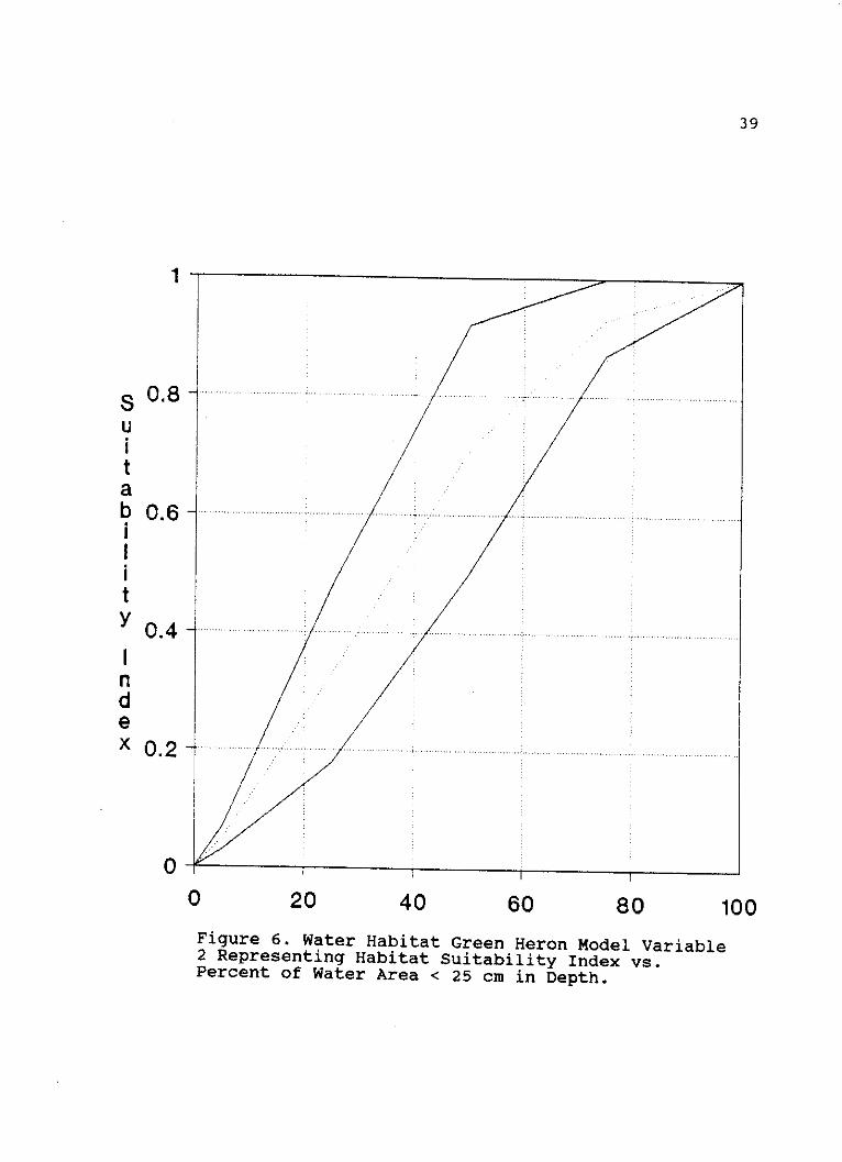
less than 25 cm deep to be 62% and 51% respectively.

Observers 2, 4 and 5 had average HSI values of 0.06, 0.27

and 0.10 representing percent water area less than 25 cm

deep to be 6%, 23% and 10% respectively (Figure 6, Appendix

C).

For the Water Habitat on transect EF (Figure 7,

Appendix E) observers 1 and 3 again gave higher average HSI

values than the rest of the team for Variable 2. These

observers scored average HSI values of 0.99 and 0.98

representing 91% and 92% water area less than 25 cm deep.

Observers 2, 4 and 5 had average HSI values of 0.01, 0.08

and 0.01 representing 8% or less water area less than 25 cm

deep (Figure 6, Appendix B).

For the Water Habitat on GH transect (Figure 8,

Appendix E) observer 1 gave an average HSI value of 0.85 for

Variable 1 ("Aquatic substrate composition in littoral

38

Impact Site Water Habitat (Green Heron Model)

5

3

4Observer

ijjSbeve

Variable 1: Aquatic substrate composition in littoral zoneVariable 2: Percent of water area less than 25 cm deepVariable 3: Percent emergent herbaceous canopy cover in littoral zoneVariable 4: Percent water surface covered by trees, logs, woody vegetationVariable 5: Water regimeVariable 6: Water currentVariable 7: Distance to deciduous forested wetland or shrub wetlandFigure 5. Bray-Curtis Cluster Analysis of Mean HabitatSuitability Index Values for Five Observers at ImpactSite Water Habitat (Green Heron model).

2

Uw

E3 vM W*7ol MaWnOo Vftft*3

ClU aWb13M* b

rdty0

0.2

0.4

06

0.8

S

4

.3

0

------------------------------------------------------------

- - - - - - - - - - - - - - - - - - - - - - - - - - -

1

3 I

I

39

1-

So. 8

U

tabO0.6

t y o..4 ..... . ........ .....................

ndex 0 .2 . . . . . .

0

0 20 40 60 80 100Figure 6. Water Habitat Green Heron Model Variable2 Representing Habitat Suitability Index vs.Percent of Water Area < 25 cm in Depth.

Transect EF Water (Green Heron Model)Similar

07

0 2

0 4

0 6

0.8

5

4

0

4Obsever

.1

4 2Observer

Variable 1: Aquatic substrate composition in littoral zoneVariable 2: Percent of water area less than 25 cm deepVariable 3: Percent herbaceous canopy cover in littoral zoneVariable 4: Percent of water surface covered by logs, trees, woody vegetationVariable 5: Water regimeVariable 6: Water currentVariable 7: Distance to deciduous forested wetland or shrub wetland

Figure 7. Bray-Curtis Cluster Analysis of Mean HabitatSuitability Index Values for Five Observers at TransectEF water Habitat (Green Heron Model).

E varmbe 5

WOruWs3o3 VarWabl2a vowi

3

ity

40

I rn

I

I I f 17 T

41

Transect GH Water (Green Heron Model)itySimilar

0

0.2

0. 4

0 6 ?

0.8 t

4

3

2

C

0

5Ob serv er

oa

owI

3

4

U

3

2

2

5Observer

2

Variable 1: Aquatic substrate composition in littoral zoneVariable 2: Percent of water area less than 25 cm deepVariable 3: Percent herbaceous canopy cover in littoral zoneVariable 4: Percent of water surface covered by logs, trees, woody vegetationVariable 5: Water regimeVariable 6: Water currentVariable 7: Distance to deciduous forested wetland or shrub wetland

Figure 8. Bray-Curtis Cluster Analysis of Mean HabitatSuitability Index Values for Five Observers at TransectGH Water Habitat (Green Heron Model).

r __K4 1

-----------------------------------------

ON,

1

42

zone"), whereas the rest of the team gave average HSI values

of 0.20. This higher score represents a difference in

opinion as to what the "aquatic substrate composition" was,

with observer 1 judging the composition to be "muddy", as

opposed to the rest of the team judging the composition to

be "rocky" (Figure 9, Appendix B).

At the Impact Site water habitat (Figure 5, Appendix E)

observer 3 differed from the group in assessment of Variable

4 ("percent of water surface covered by logs, trees, or

woody vegetation"). This observer reported an average HSI

value of 0.48 representing "coverage" to be approximately

15%, whereas, observers 1, 2, 4 and 5 gave average HSI

values of 0.12 or less indicating "coverage" to be 2% or

less (Figure 10, Appendix C).

Another habitat where differences between the team's

HSI values varied was the Shrubland on AB transect (Eastern

Woodrat model) (Figure 11, Appendix E). Observer 2 had an

average HSI value of 0.0 for Variable 3 ("number of refuge

sites per 0.4 ha") indicating an average of one or less

refuges per 0.4 ha. All other observers averaged at least

four refuge sites per 0.4 ha with HSI values of 0.73, 0.65,

0.97 and 0.97 respectively (Figure 12, Appendix B).

The final site where variability in measurements within

the group were detected was the Oldfield habitat on transect

EF (Eastern Cottontail model) (Figure 13, Appendix E).

For Variable 4 ("percent shrub crown cover") observers 1 and

3 had average HSI values of 0.16 and 0.24 representing

1

0.8

0.6K.

1 F~ TYTT~rt~ 9

U........................0.4

0.2

A B

Figure 9. Water Habitat Green Heron Model Variable1 Representing Habitat Suitability Index vs. AquaticSubstrate Composition in the Littoral Zone.A = Muddy, B = Sandy, C = Rocky.

43

SU

b

ta

bd

.I...................... ........ ......

I K x -, K K xTTTTTrr

O

C

44

1

S

t

b

ty

de

- T -

0.8 f

0.2-

o

0 20 40 60 80 100

Figure 10. Water Habitat Green Heron Model Variable 4Representing Habitat Suitability Index vs. Percent of WaterSurface Covered by Logs, Trees, or Woody Vegetation.

I

f-

.......... ....................

................................ ........... ...................................... .................. ..................... .......................

............. ......... . ......... ......................... ............................ .................... .. ............. ........... ...........................

........... ....... ....... ......... ................................. ............................................................. ........... ... . . . . . . . . . . . ...................

............. ........ ................................................ ......................... .............................................................. .......... .. .............

0.6

45

Transect AB Shrubland (E Woodrat Model)S&rndarit y0

0.2

0.4

0.6

0.8

Ob server

2

15

S

0-

--------------------- ---- ------

----- ----

-.....

2.. ......

o 'MWW 3* tim 2

Observ or

Variable 1: Percent shrub crown coverVariable 2: Percent herbaceous canopy coverVariable 3: Number of refuge sites per 0.4 ha

Figure 11. Bray-Curtis Cluster Analysis of Mean HabitatSuitability Index Values for Five Observers atTransect AB Shrubland Habitat (E. Woodrat Model).

I

a

46

1

S

t

b

ty

dex

III1l 1

0.8-

0.6-

0.4

0

0 2 4Figure 12. Shrubland Habitat Eastern Woodrat Model Variable 3Representing Habitat Suitability Index vs. Number of RefugeSites per 0.4 Ha.

I

...................................... .....................................

................ ................. .................. .................. ............. ....................................................

................. ......... ......... .......... ............................... ................................................ ..................

.................................... .......... ....................................... . . . . . . . . . . .. . . . . . . . . .. . . . . . . . . . . . . . . . . . . . . . . .. . .. . . . . . . . . . . . . .. .. . . . . . . . .

. . . . . . . . .. .. . . . . . . . . ........ . . . . . . .. . . . . . . . . . . . .. . . . . . . . .. . . . . . . . . . . . . . . . . .. . . . . . . . . . . . . . .. .. . . . . . . .. . . . . . . . . . . . . . . . . . . . . . . . . . . . . . . . . . . . . . .. .. ..O.2

6 8 10

Transact EF Oldfield (E CottontaiI)

5 4

Observer3

~Eilllil~L~------~-----

4Observer

Variable 1:Variable 4:Variable 5:

Percent herbaceous canopy coverPercent shrub crown coverNumber of refuge sites per 0.4 ha

Figure 13. Bray-Curtis Cluster Analysis of Mean HabitatSuitability Index Values for Five Observers at TransectEF Oldfield Habitat (E. Cottontail Model).

ity

47

0

0.2

0.4

0.6

0.8

1.4

2

12 -

LI r

---------

c 0.6 7BTFF f0.4 V

0.2

02

r i _

I

I rv

1

1

48

"coverage" of 10% and 15%, whereas, observers 2, 4 and 5 had

average HSI values of 0.0, 0.02 and 0.0 representing

"coverage" of 0%, 1% and 0% (Figure 14, Appendix B). For

Variable 5 ("number of refuge sites per 0.4 ha") observer 4

had an average HSI value of 0.51 representing an average of

2.5 refuges per 0.4 ha. Observer 5 had an average HSI value

of 0.06 representing less than 1 refuge per 0.4 ha. All

other observers estimated between 1 and 2 refuges per 0.4 ha

(Figure 15, Appendix B).

Hypothesis 2:

There is no significant difference in mean Habitat

Suitability Index values at impact assessment sites between

sampling years.

Data from the impact sites in 1987 were collected by

one individual taking many replicate samples (8 data points

per variable). Data collected from these same sites in 1990

were collected by five individuals, each taking three data

points, for a total of fifteen data points per variable. In

order to determine if change or no change in the HSIs at the

impact sites is due to temporal variability, or due to

different sampling methods, it was first necessary to check

these data for normality, inequality of variance and

determine if sample size differences are a problem. Since

the data gathered in 1987 were gathered by one person, it

was assumed that there was consistency in variable

measurements at each impact site by this individual.

49

1-

SU

bO0.6

tyou

d

0

0 20 40 60 80 100Figure 14. Oldfield Habitat (Eastern CottontailModel) Variable 4 Representing Habitat SuitabilityIndex vs. Percent Shrub Crown Cover.

50

1-

SU

t

ty

dexo0.2

0 2 4 6 8

Figure 15. Oldfield Habitat Eastern Cottontail Model Variable5 Representing Habitat Suitability Index vs. Number of RefugeSites per 0.4 Ha.

51

Measurement consistency cannot be assumed for data gathered

by five individuals in 1990. Therefore, these data were

analyzed to check if all measurements taken by the group

could be considered to be of a "common community" by running

SIGTREE (Nemec, 1991). Results indicated group consistency

on all HSI values at all impact sites except Water habitats.

These sites were omitted from further analysis. HSI values

determined for each variable, by the five group members in

1990, at each impact site were then grouped together and

considered as one data set. HSI values for all variables, at

every impact site, in both study years were checked for

normality and then checked for equality of variances

(homoscedasticity between 1987 and 1990 data) using the F-

test (Zar, 1984).

Results indicate nonnormality within the data sets from

both study years. Results of the F-test for all impact

sites, except Shrubland (Downy Woodpecker model), showed

heteroscedasticity. It should be noted that all variance

homogeneity tests are adversely affected by nonnormality.

Although ANOVA is a robust test and can stand some deviation

from underlying assumptions the fact these data sets have

unequal sample sizes in addition to nonnormality and

probable heteroscedasticity suggests ANOVA should not be

used (Zar, 1984). Instead a nonparametric Mann-Whitney test:

U = nin 2 + n1(n1 + 1)/2 - Rl,

52

where; U = Mann-Whitney test statistic,

Rt= sum of the ranks for sample 1

n= number of observations in sample i

(Zar, 1984) was used to analyze mean HSI values for

variables, in both years, at each impact site. Results

indicate that for all impact sites, except Upland Forest

(Fox Squirrel model), mean HSI values between test years

were not significantly different.

The Upland Forest (Fox Squirrel model) result was

significant (a = 0.05, UO.05(2)4 4 = 16, U = 16, p = 0.05).

Mean HSI value of 0.11 for Variable 1 (" Percent tree canopy

closure of mast producing trees greater than 25 cm diameter

breast height (dbh)") indicates a collective judgement by

five individuals in 1990 that the tree canopy closure of

mast producing trees greater than 25 cm dbh was

approximately 10%. In 1987 one individual judged this

"canopy closure" to be approximately 35% (mean HSI value of

0.84) (Figure 16, Appendix B). In 1990 the mean HSI value of

0.04 for variable 3 (" Average dbh of overstory trees")

indicates a collective opinion that "overstory trees" were

on average 5.5 inches dbh. In 1987 the mean HSI value of

0.85 indicates an opinion that "average dbh" was 12 inches

(Figure 17, Appendix B).

Hypothesis 3:

For HEP model habitat types there is no correlation

53

1-

SU

t

b0.6.......

t-

0 .4 .......

d

x 0 .2 -

0

0 20 40 60 80 100Figure 16. Upland Forest Habitat (Fox SquirrelModel) Variable 1 Representing HabitatSuitability Index vs. Percent Tree CanopyClosure of Mast Producing Trees > 25 cm dbh.

54

r

0.8

SU

t

b 0.6-

t

0.4

/

1-/

//

/

/ /

in 0

cm 0

5

12.510

2515

37.5Figure 17. Upland Forest Habitat (Fox Squirrel Model)Variable 3 Representing Habitat Suitability Indexvs. Average Diameter at Breast Height (dbh in in.and cm) of Overstory Trees.

y

ndex

2050

1

55

between Habitat Units (HUs) and Indicator Species density.

Due to the nonnormality of the Habitat Units a

nonparametric Spearman's Rank correlation:

r, = 1 - 6 Z d 2/n - n

where; r. = Spearman Rank correlation coefficient

di = difference between X and Y ranks

(Zar, 1984) was used to test this hypothesis. Results

indicate that there is a correlation between HUs and bird

Indicator Species density (rSO.0 5 (2 ,13 = 0.560, r = 0.643, n =

13, 0.05 < p < 0.02, Nonparametric Spearman's Rank), (Table

4, Figure 18).

Hypothesis 4:

For HEP model habitat types there is no correlation

between HUs and avian species diversity.

Species diversity was determined using both the

Shannon-Weiner index and Brillioun's index:

H' = (Nlog N - Enilogni)/N

and H = (log N! - Zlogni!)/N

where; H' = Shannon-Weiner Index

H = Brillioun's index

n= species abundance

N = sum of abundance

56

Table 4. Habitat Units, Indicator Species Density and SpeciesDiversity* for Various Impact Sites and Transect Habitats.

Habitat Habitat Units Density H' H

Upland Forest

6.053.5

439

0.89 0.801.09 0.90

Bottomland Forest

1.42.8

86

0.84 0.621.11 1.00

Shrubland

0.161.6

AB & EF (1987)Impact Site (1990)Impact Site (1987)

20

9.153.04

11.40

516

65

0.66 1.180.70 0.94

1.410.951.07

1.261.220.98

Oldfield

CDEFWater

EF (BK)**EF (GH)**

30.116.7

6680

22

2.61.3

0.57 1.250.49 1.18

0.84 0.620.84 0.62

* Species diversity indexesand Brillouin Index = H.** (BK) = Belted Kingfisher

used: Shannon-Weaver Index = H'

Model, (GH) = Green Heron Model

CDEF

EFGH

ABCD

Pasture

x

x

\x

x

0C,

-0CMJ

--

C

L(U

Cr--

c0J

4ma

-O ..

LO( I C'l) cm J 0

41> 00

004

CIO

> 44

to 1 -H 4)

H 4): :1

0 *4 ciM04 0Ux

S >,-4

U) 4.)0 41

0 .410

4J) inw0 4J 0*

o- 0 r-*4.CE.O > 4 4~

0 C4 0 0-rq ) 4 4.

o 0 c.$4 M0

0 oc00 0 c

4 $4 4J

41()o~4) o -r - -

C(4 -q

C4J 00t'~-4 ~ 4) :s

-0q 0: a (rz H %-. U

57

C13 -* " D a 0 c 0 --+-#-0

58

Due to the nonnormality of the Habitat Units a

nonparametric Spearman's Rank correlation (Zar, 1984) was

used to test this hypothesis.

Results indicate that there is no correlation between

HUs and species diversity as determined by both diversity

indices (Table 4). (Shannon-Wiener index; r(0.05)2,13, = 0.618,

n = 11, r. = -0.08, p > 0.50, Nonparametric Spearman's

Rank). (Brillouin index; r.(O.OS),, = 0.618, n = 11, r. =

0.384, 0.50 > p < 0.20, Nonparametric Spearman's Rank).

CHAPTER 5

CONCLUSIONS

The final section of this thesis contains a review of

the proposed hypotheses, the statistical tests used to

analyze them, and a discussion of the results along with

recommendations for future study.

The first hypothesis proposed in this thesis was; There

is no significant difference in Habitat Suitability Index

(HSI) variable values between individuals in a survey party.

Results indicate that out of thirty-six sites analyzed only

five sites showed significant differences in HSI values

between group members.

Three of these five sites were Water Habitats (Green

Heron Model). For this model most variability within the

survey party's measurements occurred with variables 1, 2 and

4. The first variable: "Aquatic substrate composition in

littoral zone" was judged by one observer to be "muddy"

whereas all other team members judged the "substrate

composition" to be rocky. Possible explanations for this

difference could be either: a) differing interpretation of

the characteristics of the three substrate types; or b)

misinterpretation of the classification system in that

model. The second variable: "Percent of water area less than

25 cm deep" was judged by Observers 1 and 3 to be 51% or

greater, at two different Water Habitat locations, whereas

59

60

the rest of the survey party judged this to be 23% or less

at these locations. A possible explanation for this

consistent difference in scores could be the fact that,

Observers 1 and 3 were the most experienced team members in

Habitat Evaluation Procedures (HEP) and their prior

experience may have influenced their judgement of this

fairly subjective variable. The fourth variable: "Percent of

water surface covered by logs, trees, or woody vegetation"

was estimated by Observer 3 to be 15%, whereas all other

observers estimated the "coverage" to be 2% or less. This

variable requires observers to estimate the "percentage of

the area covered by material overhanging and projecting from

the water" and so is very subjective and prone to

differences of opinion.

A second habitat where variability between group

measurements occurred was the Oldfield Habitat (Eastern

Cottontail Model). For Variable 4: "Percent shrub crown

cover" Observers 1 and 3 estimated "coverage" to be between

10% and 15%, whereas all other observers estimated

"coverage" to be 1% or less. Once again greater "HEP

experience" may have influenced the judgement of these

individuals, accounting for the differences between them and

the less experienced members of the team. Variable 5:

"Number of refuge sites per 0.4 ha" showed variability

within group measurements at both this habitat (Oldfield)

and the Shrubland Habitat (Eastern Woodrat Model Variable

3).-Observers varied widely in their judgement of how many

61

"refuges" there were at these sites. This variability is

probably due to the subjective nature of this variable as

observers were expected to evaluate the suitability of

burrows, crevices, caves, windthrow and brushpiles in a 0.4

ha area as refuges for these indicator species.

Overall, these results indicate that aquatic habitats

showed the greatest group variability in measurements. This

variability seems to be due in part to the subjective nature

of the variables involved. The amount of prior HEP

experience also seems to have an effect on observer's

measurements of subjective variables.

The second hypothesis proposed in this thesis was:

There is no significant difference in mean HSI values at

impact assessment sites between sampling years. A

nonparametric Mann-Whitney test was used to analyze the mean

HSI values for variables, in both sample years, at each

impact site. Results indicate that for all impact sites,

except Upland Forest (Fox Squirrel model), mean HSI values

between test years were not significantly different. In

future studies the power of this test (1 - 3) would be

greatly increased and the likelihood of committing a Type II

error decreased if a larger sample size were used.

The Upland Forest (Fox Squirrel model) result was

significant (Ut)., 2 , 4 = UO.05(2 ),4 = 16) at the p = 0.05 level.

Variable 1: "Percent tree canopy closure of mast producing

trees greater than 25 cm diameter at breast height (dbh)"

presented variability in mean HSI values between sampling

62

years. "Canopy closure" was judged to be an average of 35%

in 1987 and only an average of 10% in 1990. This difference

may be accounted for, in part, by the fact that the HEP

sampling period in 1987 was done in late Spring/early

Summer, whereas the sampling in 1990 was conducted in late

Summer/early Fall when tree "canopy closure" may indeed be

slightly less. In 1987, variable 3: "Average dbh of

overstory trees" was judged to be on average 12 inches,

whereas in 1990 the "dbh" was estimated at 5.5 inches. The

most likely explanation for this discrepancy in "dbh",

between sampling years, (since there was no evidence of tree

harvesting) is that in reading values off the HSI functional

curve an error was made. This functional curve has an X axis

with two scales on it. One scale in inches and a second in

centimeters. If a "dbh" value of 12.5 cm was estimated in

the field and then erroneously read off the functional curve

in inches, this discrepancy would be accounted for.

The mean HSI values for 5 out of 6 Impact Sites showed

no significant difference between sampling years. The sixth

site (Upland Forest) does show a significant difference in

mean HSI values. Possible explanations for this difference

are: a) seasonal effects on measurements; or b) observer

error in interpreting functional curves in 1987.

The third hypothesis considered in this thesis was: For

HEP model habitat types there is no correlation between

Habitat Units and Indicator Species density. Results of a

nonparametric Spearman's Rank test indicate that the Null

63

hypothesis should be rejected and that there is a positive

correlation between HUs and Indicator Species density at Ray

Roberts Lake (a = 0.05, 0.05 < p < 0.02, r = 0.643, n =

13). Since HUs were designed to indicate habitat quality,

and Indicator Species are supposed to be representative of a

particular habitat, this positive correlation appears to

verify these HEP models. However, density alone may not be a

sufficient indicator of habitat quality (Van Horne, 1983).

Schroeder (1990) suggests "... the HSI, as a measure of key

habitat variables, considers only a subset of all the

factors that may influence individuals and resultant

populations. Thus, habitat measurements may indicate ideal

conditions, but nonhabitat-related factors (such as disease

or severe weather) may cause population declines. The HSI is

best viewed as an index of habitat-imposed limitations on a

population." This implies that a maximum HSI value of 1.0

indicates no habitat-related limitations exist. A low HSI

value such as 0.1 would indicate significant habitat

limitations exist (Schroeder, 1990). Future studies might

include testing other measures of Indicator Species

performance (in addition to just numbers per hectare) such

as number of young fledged or nest success, and increasing

sample size, in order to improve test significance.

Overall, there is a correlation between HUs and avian

indicator species density. However, density alone is not an

adequate indication of habitat quality.

The fourth hypothesis tested in this thesis was: For

64

HEP model habitat types there is no correlation between HUs

and species diversity. Results of a nonparametric Spearman's

Rank test indicate that there is no correlation between HUs

and species diversity as determined by both the Shannon-

Weiner Index and Brillioun's Index (For the Shannon-Weiner

Index, rs(o.o) 2,11 = 0.618, r, = -0.08, p > 0.50: For

Brillioun's Index, r(QQ5 ) 2,1 = 0.618, r, = 0.384, 0.50 > p >

0.2.).

This result seems to indicate that species diversity is

perhaps too general a measurement and therefore not a good

indicator of habitat quality as measured by HUs. An

alternative interpretation of this result is that the data

set used in this analysis was too small to show

significance. A suggestion for future work would be to

increase the sample size.

HEP proved to be a useful tool for examining the

condition of wildlife habitat in both 1987 and 1990. The

results from this thesis can be divided into two categories:

1) observer and temporal variability; and 2) the

relationship of HUs and ecological indicators.

Recommendations for future work within the first

category would be: a) Increase survey team consistency in

variable measurements by a more intensive training period

prior to actual field work. Subjective variables such as

those in the Green Heron model (Water habitat) should be

thoroughly discussed with perhaps example "trial measures"

being taken prior to data collection; b) Insure data is

65

collected at exactly the same time of year and by the same

survey team for each study to increase temporal consistency;

and c) If possible choose models with fewer subjective

variables.

For the second category recommendations are: a) Testing

other measures of Indicator Species performance in addition

to density, such as the number of young fledged or nest

success, mortality, etc.; and b) Increase sample size in

order to improve test significance.

APPENDIX A

HSI LIFE REQUISITE VALUE MODELS FOR INDICATOR SPECIES

66

HSI Life Requisite Value Models for

Species Life Requisite

Belted kingfisher Lotic Food and(R/L) Water Value

Foraging CoverValue

Reproduction

Green heron Food Value(R/L)

Water Value

Eastern Winter Foodmeadowlark Value(P)

Cover andRepro. Value

Racer Food Value(P)

Indicator Species.

Aggregation Function

(vi x v2 x v3 x v4)14

(v6 x v7)1/2

ve

(vi x

(v5 x

vi

v2 x v3)1/3 + v4

vs) 1/2

v2 or (v3 x v4)12 or v,

(2(vl x v2 )12 + v )/2

Scissor-tailedFlycatcher(OF)

EasternCottontail(OF)

Eastern Woodrat(SH)

Downy Woodpecker(SH)

Barred Owl(BF)

Raccoon(BF)

Food Value

Cover andRepro. Value

Winter Food

Cover Type

Cover andRepro. Value

Food Value

Repro. Value

Water Value

Cover andRepro. Value

Water Value

Cover andRepro. Value

(v, x v2)"'2

v3 x v4

v, + v2

v4 + v,

(vI x v2 )1/3 + v3

V,

V2

(v2 x v3 x v4 )1/3

(vI x v2 )1/2

(v3 + v4)/2

67

.

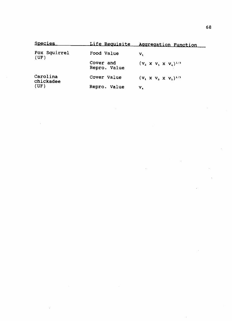
Species-

Fox Squirrel(UF)

Carolinachickadee(UF)

Life Requisite

Food Value

Cover andRepro. Value

Cover Value

Repro. Value

Aggregation Function

vi

(v2 x V 3 X v4)1/3

(v, x v2 x v3 )1/3

V 4

68

APPENDIX B

HABITAT SUITABILITY INDEX VALUES FOR THEVEGETATIONAL TRANSECTS

69

e . C C; -

LO

* *: O O

*: N:- 0---

0i~

* 0000 O

Coc.

' '0000 e

C: _

'0000

re N: v

.. N:

0: :

'0000

Sn SO U'

N

0

U(n t

> >>

4.U)

0

04

4)

0

UIt0'

0

U-J

LU

';

5.I

I-

8

CL

5"UK

ad

C8

. ...*LU

LU ' 0 0 N0 0

'0000 9 e

0:

0000

0I.

000

.n 0. O O

C,,C;

N .,S.

~: :0 0

S0Q.

Qi

'0000 >

. m. OOo'0000OO

N:'N' gg

- - - -

U)- 0000O

SQ.O

'0000OO

vs *

'0000O O

70

4-)

0

041)4.)0

0

000ID

U's0;

LUJ

8

cc

0u

U-J

C;

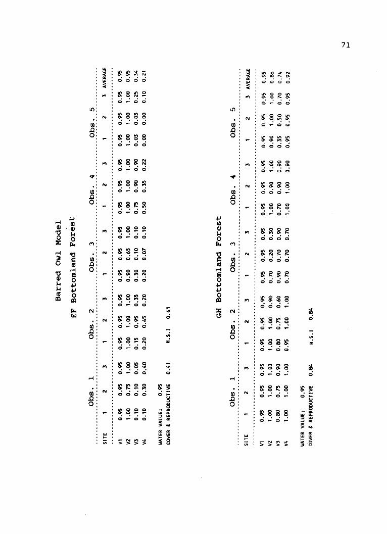
w00 0 0

* ' u o0o o

:N : o.e ~

wo: :0 0

. . 0 w 0 0 o

N: : '~

9: 8

0 ' % 0 0

( cm'

- .:OO

Co c o'0 0

'00000: :u ~

gro

. ~ 0, *0

* ' II 0u'

* ' 0~

-* w

* I-.

* C . O *

4.

40

0

0

OC;

0

'C:3

I--

oe-

Co

a-w

0u.

.~ ooON0 LM00

*'N 0' 0 C

pn m O N

Ok 0 do

0: :; :C

0-Ow

'000o

U) > >

0: AOO

. ' ' e0'

'0000d

I400

0'0'd

000w

''N'

0' moom,,

. 0'000'

: : ;0w-Ow-g

71

r4)

0

'-4

0

w4)0

4114)

h4

04

0m

-4e

0

0

0

I-U

a-

aof:3A

LACo

0'

-J:3

w

U].

0:e

'

00

* J 00 a 0 Ok & k

* (S * O O O O

; 0 0 0.*

* 00000

N . 'Coo

* 000 0

c 14

-* ' - . 0

C; C; C; O

* 00

a o

4N 0 >

0 0* ONO O* 0

S* 0000O

* m 0

N * M .

'-O

* W

* 0000 O

* 0 00

* - N000 4 g

W . ..

000 O

44 > >

4-)

4)04

r4

0

00

0Q

LUJ

OOk

: It : Z. -.*

-0-

0 00 0

O O N

w . .

. .0000.0000

O. .0 0

O. .0000

'0 '

0 .0000

,a: :

. .000..

(fl .OOOO

0 .0000O

1-

8

72

4.)

0

04v

0zUt

0

0

9

o r-q

C)

0

-0-s000-'

H.;

N *U. i

0~

u

L8

-j

wA0uo

U s

C; C0;0.C0 C;Ln:* * 0 0

I N &A 0

0: 0:

a a 0 O 0 O

* a Oe

coc

* a N N0

* m *

o: :e - a 0- 0r 0

-: : N2 0.0

U) a .e

a .000

H' .000

a. r

N N *' c'O

a . 0 0 0 0. .

C; C; 4O O

LU>' >

a',.

73

r4

2f)

0

t1)

0

41)

04

0F--

LU

LUa>

* a

0:a a

0~U a

0 .a

.U)0

H.

a N

U. N

a:

a -

' 0' N. N 0

a 00

.0 0

a 0 0 00

04 Oh.m

466

. O a 0

OO 0

a 04 0 0

0 0k 0 0m

. O iflO

a .0. .'0000

00.

: 00.0;,'.00 0

'0000O

a. 0 0

a 0a-00

'0 a 0 0

0 N 0 0

. . . 0 .a 0 0 0 0

a. -N .

40

.'-

00".

O'

0 0

(A-

0 -

0 0

LU

0

.a0

a'or.

L"

- 0

0.w

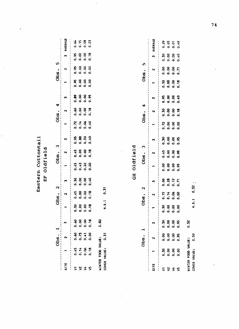
Lu

LU 00 0 0

4'

-

Ok n

F N f n0 00t

0. _

* 0000

N 2 00o

S * 0 0

8 9

' '0a0o0

.N * ' 0 -

* .- *4 '4 N O

* '0000917

* ' N e '4 0 0 '--

0' '

'0 0

0000

(A>4>- 0 >

.0000OO O

LU

I'- **- w- N'4u'i

CA'e> >>

U)

0

'.

U)

0

10

(4.4Var-0

0

0

go

--3Ci

U

m'

U)

0

C'4

(n

0

U)

0

-J

>

LU

0u

U

4 '

r4

'00 0

* 0 0

* 000.-

N 0 0 0 N

000 0

N N 0-

'0000

N 0 0

O O in

=- . *- N 4 t(A I > > > >>

74

'i-q

01

00414J0

4)

v

0

N

N

--J

c3

0Lni

U.

0LU

0u

SU

U -0 00 0

f,*0 0 co 0

S. N .0 . . 0

* *0 C) 0

U).

>- .>0.0. .

* . 0 eo e

* . N * 0 t 0 0en : O NR 9

0 e w -0w-00w

* 0 0 ( 000eo* w-w-0w-

N : O O 0* .O w .0 .

0. eOe0w-ow

w-e . .~ .n 0

N * 0 0 U'. .00 -o O0-

e - * w-N OUe * > - > >

r-

0.9

0 0O

of

LUo

-J

LU

00'

0;

LU

* * u*' LA 0

* * *O * *A

N 0n O 0

e e

.. N e* IA 0C;:

0'l

C;- - -;-8

C O;O

Ok pn 0 0

C; 8

Ln 0

0. *

0 0

e. N .*

cn m

8 8

* * &M 0

> -' >

e N :000w-O

* LU

I-* (0 *

75

0

4

4

f-i

1.

4

0

N 00O0

0

so-J

N

'0

.0)

S

of-JLU

u>0C-)

U

uj C-

pnOn

40't

* O0o

* ' 0 4

U). '> > 00

* '0 0U)0

*' ' 0 o

- - 0 -

** 0 -O O0

.: N:

U)

0

U)

0

4.)

041)41)0

4)U)to~

0 00o 0

0 V.

LU-j

LU

0u-

00o

0

C,

U)

0

U)

0

U)

0

U

(* N 0 -4O

U 0 0 00

S 0

m 0 0 0

* OO

N 00ON

*0 00 0

t O0 00

0000- OO

( A -> > -

'000*

N'8

76

4

(0

4J

-. )

40U)(n

'n

v

0

040

I-

U)

U4

>U

e e . 0

.O *0N

* 0 N O

e e0' * 0* '00

*e N :8'00

8 8

* 0

0s N * 0-

*** ' I 0

* '0O 0

*' N ' 0 0

O: :00

0 0

.0.0

-. eN e

Ue '

t0

C)

0 N

0 00

*>0LUM

*A *

LU)IA. e

0 .00

C; 4

* M * NO

* *0

N 8

.. .:. .

*e .0

* .0

ge . . .

* 88

. .0

. . 0

e .0.0

. .00

* .00-* N * 0" N

* .0

H: :00

N :

* ,* S 8

* * 0 9

* w* I-*

* *, S >

77

ci)

0

ai)

ai)

00

>1

0

C

C

kn

$Me

.j

C

0

w

-

*C

w

w

C'.

LU

0 0 0N

00ON

U, 000

A - -A

00 *0Oa wl ON

' * N IA 0

U. 0000 .

0:' M: 0

O. .l

0 - 0 N 00 0000&

C; C; 0 CN ;

U) *00

0: C

H: CO

N .O:

. . :00> .

0 E' VIO 0

0 0 00 0000 O

0 *U 0. . .0

0 (40

U)

0

0*J

U)

0

'0H

U

0.0

0o 0

4)- '.0

0(l)(0)

U)

0

(1)

0

H

U)0

*.e*eeee.eee*e..

e'-,

*:ee

ee.'|.*eeee

***e

..e*Ieee.e

*e:.|eee,-|,,eee

-*.'e*e

ee*e

*ee

78

U)

U

41 *

* 000* N 0

9: 19.00

Noo

* 0 0- :

C;. c;

* Nu O

000CN

N: r

0 0C03

000

N C

W. O . .

* 0

LU

> >

(I 0

>

a ':uiIx

0%

Q0

LA'

U):

*. N -

-Q.

, w* e -

. .

oN 0 00A 0 t^0

0' 0u'I O .t 0

O o0 0 0 0 0o

o 0 0 0 O 0 0 -

o o 0 d0 0m 0o 0.0 0 0 0 . .

400000C- 0

o o 0 0 0 0 0 C-

40000LOA

o 0 0 009

o o0 0 0 0 0

N01 I G o 0 .

"k do in O M O

C; .; . . . . .:.

p v is 4M O 9 Ic.; . .C .; . ; . .:.

(V Fn t Ln 4

41

0>

U *

a-w09

N

0'

0e

w

I-0-J

U.

a>

8(3

z

.-0-i

LA:

e N

eQ.

4K

* ' N

C'

e e

. uJ* e .

*In

s e e

,, e(A e

o 0 0 0 o 0 o

o 0C; 00C-

0 0

Lon OOto

0000000; o -

00200990

Ck o 4 o O

6n en 0 0 00

0I00 02 0 90 --

In in 0O 0 00O 0 0 o 0 C -

0 0 C;00 C

do mN 4ON

06 n In40 0 0

o o 0 O 0

NM Q " In N o

79

00

"-4

4v.4

4.J

w44-)0J 8

0

LU (Al.

0.

C; C

I--

3

S-0-J

ac0U>200

.-

a0

* LU

* <n

e

. N

* .

* .

-N

e L* I

* I

-eeee

e-ee

eaeeeee- ae-e

-e

ee.eeee,e-ee:*

*- ee

eeee

-eeeae--

eee

ee-eeee

N O 1 I6 %M 00 -t- - 0' 01

0o 0Q 0 00-n '- *n *n *n 0

a O

00~-00

0 0 0 0'0 0 0

0 4 00 0 0

00 000 00

in 0 in 0

000 -- 0000N

In'- 0 0 u *

00-- '- 010 0 0 0 0 0-

0000000 O

0 0 0 0 -0

In 0 0 0 In * 0

0 0 0 0 0

0- 0 0 0 0 0 e

'-Nr t-l e- n0 r

80

, LU

u(3

. I

I-LU

, N

' N

G) u4,)

, Q

, *

.m4.

o iv., ,

'-0 .J. N

a :

Ix,

~eIe n

rw0

"40)

Iz4

,.,

,.,

e.,

e,,

e,,,

e.,,:.

.

e,e-,,e

ee,,

e

e

,e,:e,

0 4 00 0 0

0000N C;-

ry FM C O O

000000

0 N 0 I0

. ..--. .%. O N

NN N0'

0- 0 00o

8 8 8 8OO

00 00

N ?' N e- .

00in00N l000

000 0300

0 NO 0

00 00 0 I 0

0 0 0 0 0 0 0

. .n . . . .o

ONOOM ON N .- '- '-0 00 0 0 0 0 0 0

8 0 0 I 8 88 0

In 0 N e-S 00

.- . . .n .O .

140 0

LU-j

00--

LUc-

C

(I)

0'

0:

U,'0:*

1W *

N

N

F""

N

N

LU

:

0U

0u

M

LU (AIx

0

LUJ

4304

u

0-j

0

4.,

4,

uac0

-

u

0

,.

0

o -0 0 C 0 0

N W i% 0 U

o to 0 0 o 0 0n -

o 0 0 0 0 0 00

o 4^ 0 ion 0U-

C; C qc O

* - . . . .

81

4)r0".4

U)

4

44

14

LU

* 4

LU

.. N -eme

0:

* . N

. N

'-4'

0::

LU

in

: :

000000O U U-

0N9 0 0 0 0 0 -

0 00 0 0

0 0 0 0 0 0 U-

0 0 0 W%00 U00000000w-

W% N in n O

Oh U) 0 Ok

Ok cM o UN In O

0 0 0 o 0 40 0 0 0a

.k . c. . M.0. .hl

N Nin n 0 0 & 0

6Ok O k 40 in C k

0n 0 0U0 0 0 0nU0

N . . . .) .O . .

Ol Ok o n Ok 01.

.^ .%. . . Go.

PO N P.- * 0F' N. N. .Q .

o 000000U) N 0 U) U)U)

&A cm :9 m

WNa W% . .

o N o U -

#0000

0000 0))

N O 04

IF e Ok

CO 40 N m O

0 0 0 40 in

00 014 V- O k1000 W% U00

N 0 - -0-.

0 0 0 0

U,,000 U))e ee0000000o

0000000

00 O n U-' U..

N 0 U - U- r

- - - U- -OO

0 w'- 0 0 0 0 0

co

0 0

LU

-J4

*e

I-

4

aU

4

0

APPENDIX C

HABITAT SUITABILITY INDEX VALUES FOR THEIMPACT ASSESSMENT SITES

82

: , : Sg

U. . 000

:~

, o jooo0. .

- '0000

0. -

o: :000

-.

- U)

U)

0

V.

'0

r13

0

'V

U

00

0N4.

1

L

00

LU

4-:3

U,SQ

0

U)

SQ

0

0

LU

LU>"0('

LU

ugg

- n o-0

N'

0'00

'0E - 0 0

N. I

0 0 0.0

- -0

-;

0''0

(A>N' > 1

83

00

W4UU

4J

0

0

04Ji

4J

0

4I)4.)of-4c41

0

H

N

'A

()0

0

0

U

0

CL

a

09

LU

0

LU

-J

Lu

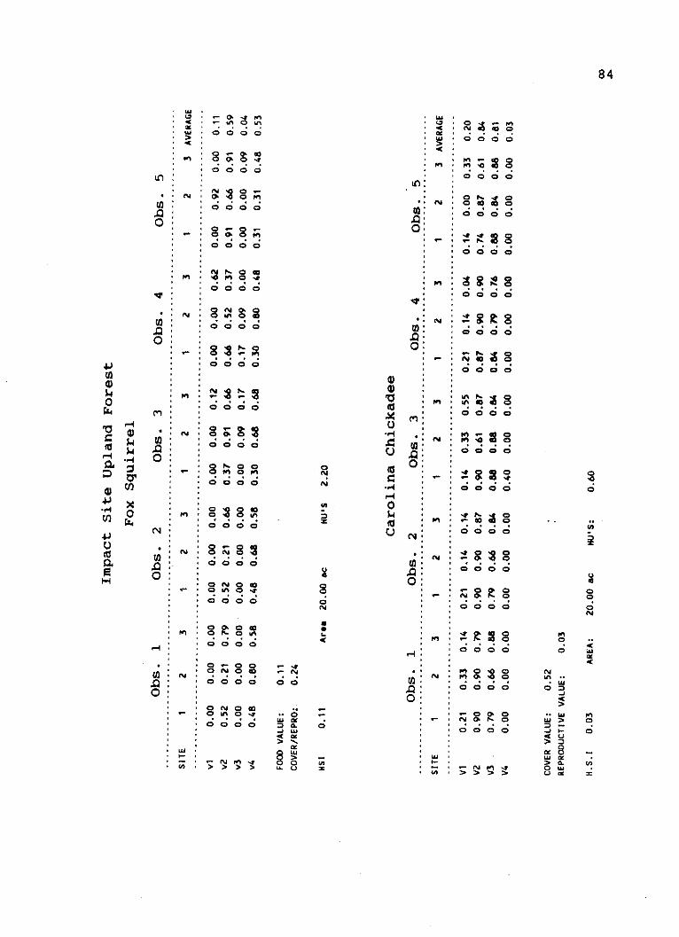
U

* L 0 0 0 0

C)0

ON* ' N * * 4 uv

* O'0000M

* O'0000O'0

0.

6 6

'0; C;

'000

N 0 CO0..

* ' 0w 00e

* C;O 0 0

'0

> '0000

. . 0*~ '0O N O 0

Vi' N . M

* '0 0

* UO

(n * * * .

00'0(U

U*1-4

U

(U

0

(UU

0(J

U

600

0,

-N0 0

LU.."C

0LU

LU

0

0

U)

,-

* LU

L ' 0 0o0c00400

000

Fn 0r4 m Ck

0000CO

*' N 'C- g

> > ..> >

CA:OO

0a ' V N 100

N * Oe

***r'.. .4.** OOO0

e '0000

0' '

_ * ia

0' ' P. 0 0

* N- 0 O

* LU

U. 'e

84

4J

004

Mr--

4J-U2-

En4J

w

01cfl

0

0

LU

.U

C..

0*

LU

LU

ix

4c"

N

0u

U

* .

on,

on 4200 (Y

* * 0Oa 0

. . .'t .

(A - > 0 v-

'00

* '000'-O

* '09-0'-

* '09-004

* ''- -0

* ' 00O n0

* . .w 0 .

* 'OOON

CD 4 eoO

. ,

C'OON

* '0- 0 0O

*' * * * *

* ' e- e 0 O

* 0 0 O O

e * 00O M

* I - - - -

* * O

P-4

'4

Cu0

041

4J0

44)

41

LUN

.U

0-"C

0>L.L U

LUn

0 O k

40 * U 0 0 0

* 0* ' N * -

.' N ' F" 0 0 F"

0:0

'* * *:* '0000

UJO.~ N:

CD: O

* *' 0 0

*' N

, * ' 0 0 0 4-

' N ' 000 * *

9-' ' * N* 0 *

* '0 0 00N e

* * * *

**0000N

* 0 0* '4 0 0

CD' N OO

- - 0''- 0'

* *'0000

* L

* ".>>>>m

85

-4

0

4!J -H.4 to

4J~'U 0(a

00RC

ON

LU

C0c

N

e-o

N

LU

LU

0u

NUe

0

86

Ln -4 0% 00* LU' 'L

* ' ' ' .* u 0 *LU' 00* >,

* '00O , . O L O

S ' ' 0 0 * * . . ..0 0

000

N OO ,OQeO'00 *

C; C;

' 0 0* 0 0

w:w

' '00' 000

4J* r-39 4J

000000

~ e _ 'LAO ' * 0

o O Oen In 0 N IN

CD 0*

- LA:U

>

e F.1e:'000

* ' 0 0

e N eO O ee N 0 N N

Om- ' 0 0 ' - '- - - 0

N : 2 ' '

S '000 ' -' e eO r

wL O

H' * H'O '

* ' 0 0 A VV' * '

N N'

0: ' 0'NO LUC ..

* ** ' * ' ' ' L

(J. C ' *

* ' "N OLU ' - ' MN ) 0

*

* a

*

* '

' N

* N

* N

0:

* p

U* N

* p.

* (

-.*

e.*'-*

ee*e

.*e*e'

'

'ee*e-.e*e*

**es*

***e' ,***

**e

*

**

'

N OVP N00.

U..

I-

3

CL

a

ac

0*U

2

N

..U

at

0

O O N ON

000

00000

N- O O Ou0 Oh uOhO

OONO it

- 000 O

0 00 0 0

87

0

0

c

4)4J

W

0

$4

4)C.)

01

C.)0

LL)

La (a

at ...

*L '00 0 0

* - 0 0

S . Ni

cm- do

' Nw*P * 00 O -

='kn

* - 0> > > .

* o 00O O

VP o 0 ' O 0

* N * 0 Oh 0

0: : Oh 0

* O e . g .VP ' 0 N O 0

* '0 0

fJ) N : 9 0 A ,-

O * OOO,

* LU

(4 *

M0LU

a

LLA

3

S

(.

r4

..

0

LU

-J

* 000 Oh

NOOOu',

N 0 0 0 Ui

N VP "t u

- L

* L

* I'

0. N

* 94

* N

jO)

' N

* N

* U

e

3

*

.e:**

ee

'eee

-*

''*o*

*

IA iA in IA0 0 0 0WN A co A~

0N 0 0 0 Ok00

0 000 0 0

IA IAIA in 0 0 0 0

O~ IA 0 ONO O00

0h 00N 0 Ok0 0

(V M & t N *4 4

N 4. IA ~O 7% 0

> >

40

-j

:3

I-

I.-0-J

o00N 0 0

in O do

W's A ) 0 00

0 0 0 L0 0 0

0 0 0 W,00%

0 0 0 (m00

0 0 0 0 o OO0

. .. . . . . .0 0 0 0 0 0 0- w-

3 * p

0' 4

N 0:N

IA

IA

.0. *

N N

2 ( N1

* .

0*-*0 W

88

*UC

'*

C

-

-

I,4

4-J2

4J)

.0 do0 0 iAIn0

000 0 IAI# O

4A0 00. I V-

0- Ok

0 0 0 0 0 0 0

0 *-A

0 0 0 0 0 0 0

0 0 0 0 0 0 0

O O AOO IAIAO

0004

0 0- 0 0- 0

0 00 0 n00

ONOOO IO O

0 I N 0 LAIAN 0

NN 14)

N - -0000000OO O

IAOOOIIOO

0 IA N O 00 0 0 0- 0 0

N 94 .4 IAm O:3>>>>>>-

(I) *

0 0

LUj

-j

LU

-J

0

7.

U.

2

U

N

*U

0n 0 i0 0 00

0 00 0 0 - -

in g In In A0 0 00 in O o 0 0ON

C;OO

.Lae

w

APPENDIX D

AVIAN CENSUS NUMBERS BY HABITAT TYPE AND TRANSECTSECTION FOR 1987 AND 1990

89

90

Avian Census Numbers by Habitat Type and Transect Section(1987 and 1990)

e . .an p s Tnsect F- orL )rs(17/1990)

Upland Forest CarolinaChickadee*

Common Flicker EF10

Downy CD7Woodpecker CD9

EF10

Tufted CD7Titmouse CD9

EF10

Cedar Waxwing CD9

Cooper's Hawk CD9

BottomlandForest

Shrubland

Pasture

Barred Owl*

CarolinaChickadee

DownyWoodpecker

E. Meadowlark*

Ki 1 deer

Dickcissel

SavannahSparrow

CD7CD9EF10

9/512/75/5

2/-

2/22/-2/1

16/46/94/3

-/15

-/1

1/-1/-

18/-2/-1/-8/82/2

20/4

1/-2/21/-3/-

12/-11/-62/1526/3

AB3GH3

AB3CD11EF4EF8GH1GH3

AB1AB6CD6EF5

AB2EF3GH2GH4

AB2EF3

AB2

AB2EF3

1/-1/-

1/-10/-

Habitat Tun Aui n" i %g - M- --- qo.%449 or& -C r% I - -3 - t .6 A% 0% Ow s m - - 'L

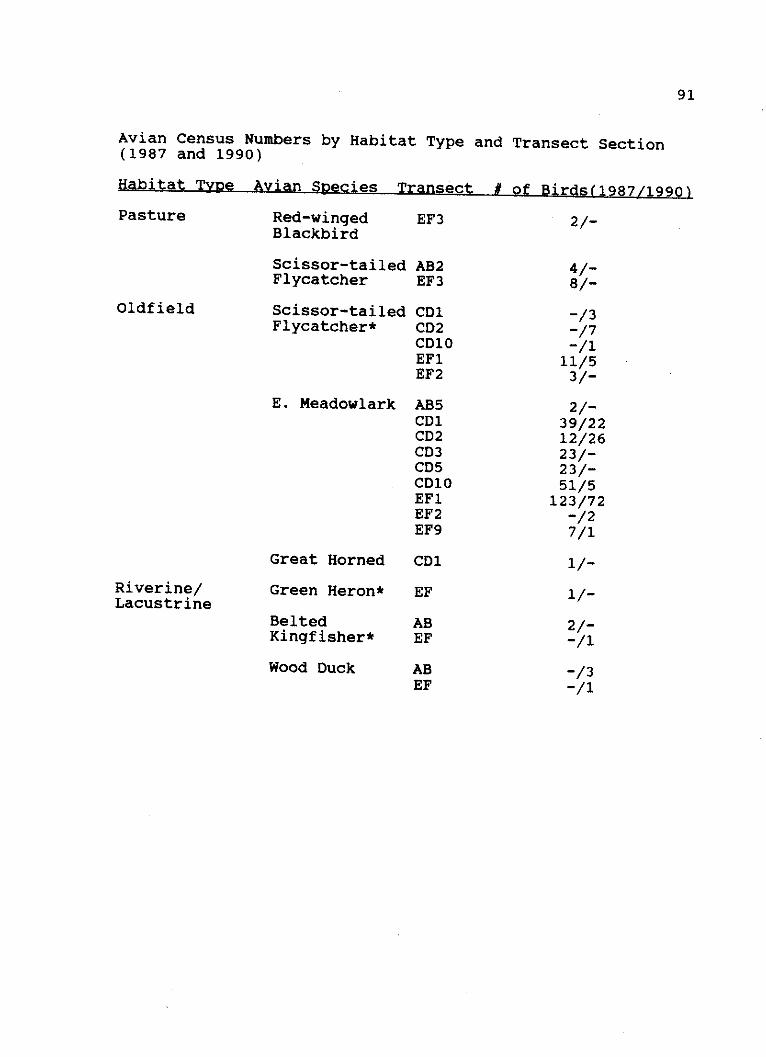
91

Avian Census Numbers by Habitat Type and Transect Section(1987 and 1990)

Habitat Tvnpp_% es rV46anst9 #-ofr d9 )

Red-wingedBlackbird

EF3

Scissor-tailed AB2Flycatcher EF3

oldfield

Riverine/Lacustrine

Scissor-tailedFlycatcher*

E. Meadowlark

Great Horned

Green Heron*

BeltedKingfisher*

Wood Duck

Pasture2/-

4/-8/-

CD1CD2CD10EF1EF2

AB5CD1CD2CD3CD5CD10EF1EF2EF9

-/3-/7-/1

11/53/-

2/-39/2212/2623/-23/-51/5

123/72-/27/1

CD1

EF

ABEF

1/-

1/-

2/--/1

-/3-/1

ABEF

Au ian Sn t- i TM-- "4r.,M "+ Ji lr% %o . -3 - * 1 0% 0% V-D F .6 A.. 'ok .. 1,

APPENDIX E

BRAY-CURTIS CLUSTER ANALYSIS DATA

92

93

Impact Site Water Habitat (Green Heron Model)

Linkage Clusters Linked Similarity Probability

1 2 4 0.95349 0.624002 2 5 0.93649 0.638003 1 2 0.83546 0.020004 1 3 0.80392 0.00600

Transect EF Water Habitat (Green Heron Model)

Linkage Clusters Linked Similarity Probability

1 1 3 0.98606 0.390002 3 5 0.97641 0.158003 2 4 0.96667 0.324004 1 2 0.87007 0.00400

Transect GH Water Habitat (Green Heron Model)

Linkage Clusters Linked Similarity Probability

1 2 5 0.96791 0.574002 3 4 0.93559 0.432003 2 3 0.90995 0.508004 1 2 0.81755 0.02200

Transect AB Shrubland Habitat (Eastern Woodrat Model)

Linkage Clusters Linked Similarity Probability

1 4 5 0.97448 0.808002 1 3 0.94020 0.904003 1 4 0.71176 0.186004 1 2 0.45396 0.02800

Transect EF Oldfield Habitat (Eastern Cottontail Model)

Linkage Clusters Linked Similarity Probability

1 1 3 0.88099 0.724002 4 5 0.69985 0.018003 1 4 0.67425 0.07600

-4 1 2 0.61704 0.02200

REFERENCES

1. Allen, A. W. and M. J. Armbruster, 1982, "PreliminaryEvaluation of a Habitat Suitability Model for thePronghorn", Proc. Biennial Pronghorn Antelope Workshop,Vol. 19, pp. 93-105.

2. Anderson, S. H. and H. H. Shugart, Jr., 1973, "HabitatSelection of Breeding Birds in an East TennesseeDeciduous Forest", Ecology, vol. 55, pp.828-837.

3. Block, W. M. et al., 1987, "On Measuring Bird Habitat:Influence of Observer Variability and Sample Size",The Condor, Vol. 89, No. 2, pp. 241-251.

4. Bray, J. R., and J. T. Curtis, 1957, "An Ordination ofthe Upland Forest Community of Southern Wisconsin",Ecol. Monogr. Vol. 27, pp. 325-349.

5. Clawson, M. E. et al.., 1984, "An Approach to HabitatModeling for Herpetofauna", Wildlife Society Bulletin,Vol. 12, pp.61-69.

6. Cook, J. G. and L. L. Irwin, 1985, "Validation andModification of a Habitat Suitability Model forPronghorns", WildlifeSociety Bulletin, Vol. 13,pp.440 - 448.

7. Diaconis, P. and B. Efron, 1983, "Computer-intensivemethods in statistics", Scientific American, Vol. 248,pp. 116-130.

8. Efron, B., 1979, "Bootstrap methods: another look at thejackknife", Annals of Statistics, Vol. 7, pp. 1-26.

9. Ellis, J. A. et al.,, 1978, "Results of Testing FourMethods of Habitat Evaluation", Report to the ProjectImpact Evaluation Team, Division of Ecological Services,U. S. Fish and Wildlife Service, Fort Collins, Colorado,pp. 1-92.

94

95

10. Ellis, J. A. et al., 1979, "Appraising Four FieldMethods of Terrestrial Habitat Evaluation",NorthAmericanWildlife Conference, Vol.44, pp. 369-379.

11. Emlen, J. T., 1971, "Population Densities of BirdsDerived from Transect Counts", Auk, Vol. 88, pp. 323-342.

12. Flood, B. S. et al., 1977, A Handbook for HabitatEvaluation, Resource Publication 132, U. S. Fish andWildlife Service, Washington, D. C., pp. 1-77.

13. Gotfryd, A. and R. I. C. Hansell, 1985, "The Impact ofObserver Bias on Multivariate Analyses of VegetationStructure", Qikos, Vol. 45, pp. 223-234.

14. Institute of Applied Sciences, University of NorthTexas, 1988, "Ray Roberts Lake Pre-impoundmentEnvironmental Study", Ft. Worth District U.S. Army Corpsof Engineers, 157 pp.

15. Institute of Applied Sciences, University of NorthTexas, 1992, "Ray Roberts Lake Post-impoundmentEnvironmental Study Year Two", Ft. Worth District U.S.Army Corps of Engineers, 221 pp.

16. Kennedy, J. H. et al.,, 1993,, "Sampling and AnalysisStrategy for Biological Effects in Freshwater FieldTests", EWOFFT, Potsdam, Germany, pp. 31-33.

17. Larson, D. L. and C. E. Bock, 1986, "Determining AvianHabitat Preference by Bird-Centered VegetationSampling", Wildlife 2000 Modelling Wildlife Habitats ofTerrestrial Vertebrates, University of WisconsinPress, Madison, Wisconsin, October 7-11, 1984, pp. 37-43.

18. Laymon, S. A. et al., 1985, "Habitat Suitability IndexModels: Spotted Owl", Biological Report 82(10.113), U.S.Department of Interior, Fish and Wildlife Service,Biological Services Program, Washington, D. C., pp. 1-14.

96

19. Laymon, S. A. and R. H. Barrett, 1986, "Developing andTesting Habitat-Capability Models: Pitfalls andRecommendations", Wildlife 2000 Modeling HabitatRelationships of Terrestrial Vertebrates, University ofWisconsin Press, Madison, Wisconsin, October 7-11, 1984,pp. 87-92.

20. Merikallio, E., 1958, Finnish Birds, Their Distributionand Numbers, Fauna Fennilca V. Helsinofors., Finland.

21. Nemec, A. F. L., 1991, "Documentation for Sigtree",Version 3.4, Canada, pp. 1-11.

22. Nemec, A. F. L. and R. 0. Brinkhurst, 1988, "Using theBootstrap to Assess Statistical Significance in theCluster Analysis of Species Abundance Data", Can. J.Fish. Aguat. Sci., Vol. 45 pp. 965-970.

23. Payne, B. S. and K. S. Long, 1986, "Airborne SensorPotential for Habitat Evaluation Procedures (HEP)',Technical Report EL-86-3, Department of the Army,Vicksburg, Mississippi, pp. 1-45.

24. Root, R. B., 1967, "The Niche Exploitation Pattern ofthe Blue-Gray Gnatcatcher", Ecological Monographs, Vol.37, pp. 317-350.

25. Roberts, T. H. and L. J. O'Neil, 1985, "SpeciesSelection for Habitat Assessments", Misc. Paper EL-85-8,Department of the Army, Vicksburg, Mississippi, pp. 1-16.

26. Schamberger, M. L. and L. J. O'Neil, 1986, "Concepts andConstraints of Habitat-Model Testing", Wildlife 2000Modeling Habitat Relationships of TerrestrialVertebrates, University of Wisconsin Press, Madison,Wisconsin, October 7-11, 1984, pp. 5-10.

27. Schroeder, R. L., 1982, "Habitat Suitability IndexModels: Downy Woodpecker", FWS/OBS-82/10.38, U. S. Dept.Int., Fish and Wildlife Service, Washington, D. C., pp.1-10.

97

28. Schroeder, R. L., 1983, "Habitat suitability IndexModels: Black-capped Chickadee", FWS/OBS-82/10.3 7, U. S.Fish and Wildlife Service, Washington, D. C., pp.1-12.

29. Schroeder, R. L., 1990, "Tests of a Habitat SuitabilityModel for Black-capped Chickadees", FWS BiologicalReport 90(10), U. S. Fish and Wildlife Service,Washington, D.C., pp. 1-8.

30. Severinghaus, W. D., 1981, "Guild Theory Development asa Mechanism for Assessing Environmental Impact",Environmental Management, Vol. 5, No. 3, pp. 187-190.

31. Short, H. L. and K. P. Burnham, 1982, "Technique forStructuring Wildlife Guilds to Evaluate Impacts onWildlife Communities", Spec. Sci. Report No. 244, U. S.Fish and Wildlife Service, Fort Collins, Colorado, pp.1-5.

32. Smith, A. D., 1944, "A Study of the Reliability of RangeVegetation Estimates", Ecology, Vol. 25, pp. 441-448.

33. Sneath P. H. A. and R. R. Sokal, 1973, NumericalTaxonomy:-The Principles and Practice of NumericalClassification, W. H. Freeman, San Francisco, CA. 573 p.

34. Spencer, W. D.,, 1983, "Marten Habitat Preferences in theNorthern Sierra Nevada", Journal of WildlifeManagement, Vol. 47, pp.1181-1186.

35. Sturman, W. A., 1967, "Description and Analysis ofBreeding Habitats of the Chickadees, Parus Atricapillusand P. Rufescens", Ecology, Vol. 49, No. 3, pp. 418-431.

36. U. S. Fish and Wildlife Service, 1976, "HabitatEvaluation Procedures", U. S. Fish and WildlifeServices, Division of Ecological Services, Ft. Collins,Colorado, 77 pp.

37. U. S. Fish and Wildlife Service, 1980a, "The HabitatEvaluation Procedures", U. S. Dept. Int. Fish andWildlife Service Ecological Services Manual 102, Ft.Collins, Colorado, 124 pp.

98

38. U. S. Fish and Wildlife Service, 1980b, "TerrestrialHabitat Evaluation Criteria Handbook (Regions 2512 &2320)", U. S. Dept. Int. Fish and Wildlife Service, Ft.Collins, Colorado.

39. Van Horne, B., 1983, "Density as a Misleading Indicatorof Habitat Quality", Journal of Wildlife Management,Vol. 47, No. 4, pp. 893-901.

40. Whitaker, G. A. et al., 1976, "Inventorying Habitats andRating Their Value for Wildlife Species", Proceedings ofthe Southeastern Association of Fish and WildlifeAgencies, Vol. 30, pp.590-601.

41. Zar, J. H., 1984, Biostatistical Analysis, 2nd ed.,Prentice-Hall, Englewood Cliffs, N.J., 718 pp..