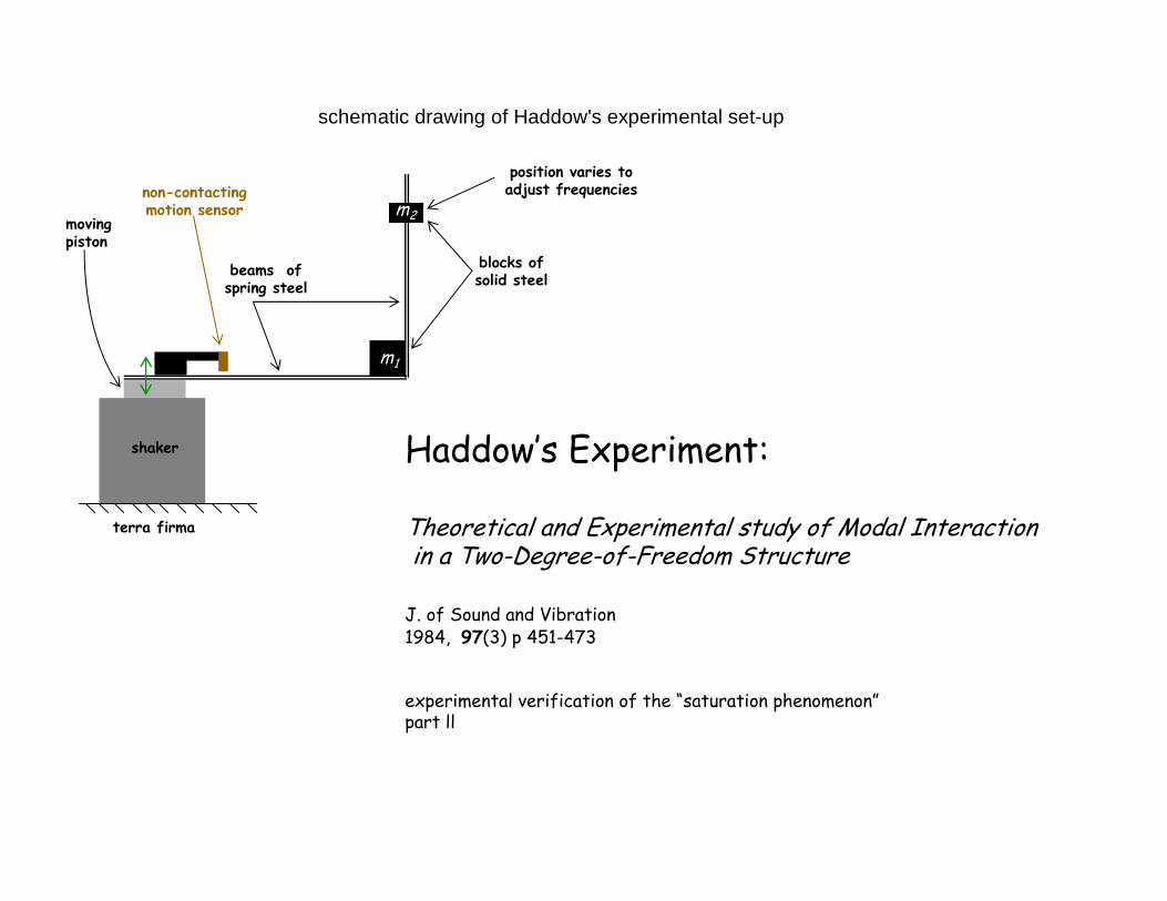
schematic drawing of Haddow's experimental set-up

shaker

movingpiston

beams ofspring steel

blocks ofsolid steel

non-contactingmotion sensor

position varies toadjust frequencies

terra firma

Haddow’s Experiment:

Theoretical and Experimental study of Modal Interactionin a Two-Degree-of-Freedom Structure

J. of Sound and Vibration1984, 97(3) p 451-473

experimental verification of the “saturation phenomenon”part ll

m1

m2

x, segment of the undeflected beamdx

dx

w ww dxx

∂+∂

expanded view

dl

dx

dv

w dxx

∂∂

( )

the axial force is nearly zero, so we assume that theoriginal length of the element, , does not change during the motion

" " indicates that projection of the deflected beam is always shor

dx

dv dx dl= − − −

2 22 2 2 2 2

12 22

2

2

0

ter than that of the undeflected beam

1

11 12

12

1 2

x l

x

w wdx dl dx dl dxx x

w wdl dx dl dxx x

wdx dl dv dxx

wV dxx

=

=

⎡ ⎤∂ ∂⎛ ⎞ ⎛ ⎞= + → = −⎢ ⎥⎜ ⎟ ⎜ ⎟∂ ∂⎝ ⎠ ⎝ ⎠⎢ ⎥⎣ ⎦

⎡ ⎤ ⎡ ⎤∂ ∂⎛ ⎞ ⎛ ⎞= − → = − +⎢ ⎥ ⎢ ⎥⎜ ⎟ ⎜ ⎟∂ ∂⎝ ⎠ ⎝ ⎠⎢ ⎥ ⎢ ⎥⎣ ⎦ ⎣ ⎦

∂⎛ ⎞− = − = ⎜ ⎟∂⎝ ⎠

∂⎛ ⎞= − ⎜ ⎟∂⎝ ⎠∫ the horizontal displacement of the

free end toward the fixed end

an element in the undeflected beam

same element when the beam is deflected

( ) ( )( )

( ) ( )( )

( )( )

( )( )

( )( )

( )

2 311 11 13 2

1 12 212 12 2

2 3 2 3 2 411 11 1 11 11 1 11 11 13 2 21 1

2 1 1 12 2 2 22 12 12 2 12 12 2 12 2

recall the free-vibration modes:

0

23 3 3

3

ii

i

i i ii

i i

k m lx x x x l

k m l

k m l k m l k m lEI EIx l x l x l

l EI EIk m l k m l k

ωφ

ω

ω ω ωφ

ω ω

−= − ≤ ≤

−

⎛ ⎞ ⎛ ⎞− − −⎜ ⎟ ⎜ ⎟= − − + − + −⎜ ⎟ ⎜ ⎟− −⎝ ⎠ ⎝ ⎠ ( )

( )( )

( ) ( )( ) ( )

( )( ) ( )

2 22 12 2

2

1 11 12 1

2 21 22 2

0

now we describe the shapes of the deflected beams in terms of the free-vibration modes

, the are arbitrary

,

i

i

xm l

x l

w x t x x u tu t

w x t x x u t

ω

φ φφ φ

⎛ ⎞⎜ ⎟⎜ ⎟−⎝ ⎠

≤ ≤

⎧ ⎫ ⎡ ⎤ ⎧ ⎫⎪ ⎪ ⎪ ⎪=⎨ ⎬ ⎨ ⎬⎢ ⎥⎪ ⎪ ⎪ ⎪⎩ ⎭ ⎣ ⎦ ⎩ ⎭

( )( )

( )( )

( ) ( )( ) ( )

( )( )

( ) ( )( ) ( )

( )( )

( )

1 1 11 12 1 11 12 1

2 2 21 22 2 21 22 2

22

10

functions of time to be determined

, ,, ,x x

1 1 =2 2

ili

i ix

w x t w x t x x u t x x u tw x t w x t x x u t x x u t

wV dxx

φ φ φ φφ φ φ φ

φ=

′ ′ ′⎧ ⎫ ⎧ ⎫ ⎡ ⎤ ⎧ ⎫ ⎡ ⎤ ⎧ ⎫∂ ∂⎪ ⎪ ⎪ ⎪ ⎪ ⎪ ⎪ ⎪= = =⎨ ⎬ ⎨ ⎬ ⎨ ⎬ ⎨ ⎬⎢ ⎥ ⎢ ⎥′ ′ ′∂ ∂⎪ ⎪ ⎪ ⎪ ⎪ ⎪ ⎪ ⎪⎩ ⎭ ⎩ ⎭ ⎣ ⎦ ⎩ ⎭ ⎣ ⎦ ⎩ ⎭

∂⎛ ⎞ ′= ⎜ ⎟∂⎝ ⎠∫ ( )

( ) ( ) ( )

2 2 2 21 1 2 1 2 2 2 1 1 2 1 2 3 2

0

21

2 211 12 1311 2 1 1 2 1 2 3 2

21 22 232 2 0 0 02

2 2

1 1 12 where , , ,2 2 2

i

i i i

l

i i i i i ix

l l l

i i i i i i ix x x

u u u u dx C u C u u C u

uC C CV

u u C dx C dx C dxC C CV

u

φ φ φ

φ φ φ φ

=

= = =

⎡ ⎤′ ′ ′+ + = + +⎣ ⎦

⎧ ⎫⎡ ⎤⎧ ⎫ ⎪ ⎪ ′ ′ ′ ′= = = =⎨ ⎬ ⎨ ⎬⎢ ⎥

⎩ ⎭ ⎣ ⎦ ⎪ ⎪⎩ ⎭

∫

∫ ∫ ∫

( )

( )1 2

2

1 1 1

the velocity of the shaker head (moving piston) is described by

cos( )

the kinetic energy of is given by the kinetic energy of is given by 12

S

S

W t F t

m m

T m W W V

= Ω

= + + ( ) ( ) ( )

( )

( )( )

( )( ) ( )

2 2 2

1 2 2 1 2 2 1

111 121

221 222

1

2

1 2

where ( ) ,

where

i

j

S

i i x l

ij ij x l

T m W W V W V

W t w x t

u tW tx

u tW t

VV

φ

=

=

⎡ ⎤ ⎡ ⎤= + − + +⎢ ⎥ ⎢ ⎥⎣ ⎦ ⎣ ⎦

⎤≡ ⎦

⎧ ⎫ ⎧ ⎫Φ Φ⎡ ⎤⎪ ⎪ ⎪ ⎪ ⎤= Φ ≡⎨ ⎬ ⎨ ⎬⎢ ⎥ ⎦Φ Φ ⎪ ⎪⎪ ⎪ ⎣ ⎦ ⎩ ⎭⎩ ⎭

⎧ ⎫⎨ ⎬⎩ ⎭

21 1 1

11 12 13 11 12 1311 2 1 2 1 2

21 22 23 21 22 232 22 2 2

22 2 2

2

u u uC C C C C CV

u u u u u uC C C C C CV

u u u

⎧ ⎫ ⎧ ⎫⎧ ⎫⎡ ⎤ ⎡ ⎤⎪ ⎪ ⎪ ⎪ ⎪ ⎪= → = +⎨ ⎬ ⎨ ⎬ ⎨ ⎬⎢ ⎥ ⎢ ⎥⎪ ⎪⎣ ⎦ ⎣ ⎦⎩ ⎭⎪ ⎪ ⎪ ⎪

⎩ ⎭⎩ ⎭

( )( )

( ) ( )

2

2

2 2 21 1 1 1 1 1

note: contains fourth-order terms in the , which in turn leads to third-order terms in EoM;

so we neglect in the expressions for kinetic energy

1 1 22 2

i i

i

S S S

V u

V

T m W W m W W W W= + = + +

= ( ) ( ) ( )

( ) ( )

2 22 2 2 21 11 1 12 2 11 1 11 12 1 2 12 2

2 2 2 2 22 2 1 2 2 1 2 1 1 2 1 2 2 2 1

2 22 11 1 12

1 cos 2 cos 2 . . .2

1 1 2 2 2 22 2

1 cos 2 cos2

S S S S

m F t F t u u u u u u h o t

T m W W V W V m W W W W W V WV W W V

m F t F t u u

⎡ ⎤Ω + Ω Φ +Φ + Φ + Φ Φ + Φ +⎣ ⎦

⎡ ⎤ ⎡ ⎤= + − + + = + + − − + +⎣ ⎦⎢ ⎥⎣ ⎦

= Ω + Ω Φ +Φ( ) ( ) ( )

( ) ( ) ( ) ( )

( ) ( )

2 22 22 11 1 11 12 1 2 12 2

21 1 1 22 1 2 22 1 2 23 2 2 11 1 12 2 21 1 1 22 1 2 22 1 2 23 2 2

2 22 221 1 21 22 1 2 22 2 21 1 22

2

4 cos 4

2 2

u u u u

F t C u u C u u C u u C u u u u C u u C u u C u u C u u

u u u u u

⎡ + Φ + Φ Φ + Φ⎣

− Ω + + + − Φ +Φ + + +

+ Φ + Φ Φ + Φ + Φ +Φ( ) ( )2 11 1 1 12 1 2 12 1 2 13 2 2 . . .u C u u C u u C u u C u u h o t ⎤+ + + + + ⎦

( ) ( ) ( )

( ) ( ) ( ) ( ) ( )

( )

1 1

1

1

2221

1 11 1 12 221 10 0

2 22 2 2 211 1 11 12 1 2 12 2 11 1 12 1 2 13 21 1

0

222

2 220

the expressions for potential energy

2 2

l l

x x

l

x

l

x

wU EI dx EI u u dxx

EI u u u u dx EI K u K u u K u

wU EI dx

φ φ

φ φ φ φ

= =

=

=

⎛ ⎞∂ ′′ ′′= = +⎜ ⎟∂⎝ ⎠

⎡ ⎤′′ ′′ ′′ ′′= + + = + +⎣ ⎦

⎛ ⎞∂= ⎜ ⎟∂⎝ ⎠

∫ ∫

∫

∫ ( ) ( ) ( ) ( )1

2 2 221 1 22 2 21 1 22 1 2 23 22 2

0

21

11 12 131 2 1 2

21 22 23 22

2

2

following Lagrange's procedure, we obtain equations with the following form:

l

x

x EI u u dx EI K u K u u K u

uK K K

U U U u uK K K

u

L T U

φ φ=

′′ ′′= + = + +

⎧ ⎫⎡ ⎤ ⎪ ⎪= + = ⎨ ⎬⎢ ⎥⎣ ⎦ ⎪ ⎪

⎩ ⎭

= +

∫

21

11 12 13 11 12 1311 12 1 11 12 11 2

21 22 23 2121 22 2 21 22 2 22

following Lagrange's procedure, we obtain equations with the following form:

ub b b d d dm m u k k u

u ub b b d dm m u k k u

u

⎧ ⎫⎡ ⎤⎡ ⎤ ⎧ ⎫ ⎡ ⎤ ⎧ ⎫ ⎪ ⎪+ + +⎨ ⎬ ⎨ ⎬ ⎨ ⎬⎢ ⎥⎢ ⎥ ⎢ ⎥

⎣ ⎦ ⎩ ⎭ ⎣ ⎦ ⎩ ⎭ ⎣ ⎦ ⎪ ⎪⎩ ⎭

1 1

1 2 2 122 23

2 2

11 12 1 1

21 22 2 2

21

1 222

e e 2 sin 2 cos

e e

u uu u u u

du u

u gF t F t

u g

uu uu

⎧ ⎫⎡ ⎤ ⎪ ⎪+⎨ ⎬⎢ ⎥⎣ ⎦ ⎪ ⎪

⎩ ⎭

⎡ ⎤ ⎧ ⎫ ⎧ ⎫+ Ω = Ω⎨ ⎬ ⎨ ⎬⎢ ⎥

⎣ ⎦ ⎩ ⎭ ⎩ ⎭

⎧ ⎫⎪⎨ ⎬⎪⎩

Mu +Ku +B

( ) ( ) ( ) ( ) ( )

1 1

1 2 2 1

2 2

21 1 1

1 2 1 2 2 122 2 2

21 1 1 1

2 2 2

sin cos

cos cos

02

0

u uu u u u F t F t

u u

u u uu u u u u u t tu u u

u uu u

μ ωμ

⎧ ⎫⎪ ⎪ ⎪+ + + Ω = Ω⎨ ⎬⎪ ⎪ ⎪

⎩ ⎭⎭

⎧ ⎫ ⎧ ⎫⎪ ⎪ ⎪ ⎪+ + + + + Ω = Ω⎨ ⎬ ⎨ ⎬⎪ ⎪ ⎪ ⎪

⎩ ⎭⎩ ⎭

⎧ ⎫ ⎡ ⎤ ⎧ ⎫+ +⎨ ⎬ ⎨ ⎬⎢ ⎥

⎩ ⎭ ⎣ ⎦ ⎩ ⎭

-1 -1 -1 -1 -1

D Eu G

u M K u M B M D M E u M G

21 1 1

11 12 13 11 12 1311 2 1 2 2 12

21 22 23 21 22 232 222 2 2

00

u u uX X X Y Y Yu

u u u u u uX X X Y Y Yu

u u uω

⎧ ⎫ ⎧ ⎫⎡ ⎤ ⎡ ⎤ ⎡ ⎤⎧ ⎫ ⎪ ⎪ ⎪ ⎪+ + +⎨ ⎬ ⎨ ⎬ ⎨ ⎬⎢ ⎥ ⎢ ⎥ ⎢ ⎥

⎩ ⎭ ⎣ ⎦ ⎣ ⎦⎣ ⎦ ⎪ ⎪ ⎪ ⎪⎩ ⎭⎩ ⎭

11 12 1 1

21 22 2 2

2 sin 2 cosZ Z u G

F t F tZ Z u G⎡ ⎤ ⎧ ⎫ ⎧ ⎫

+ Ω = Ω⎨ ⎬ ⎨ ⎬⎢ ⎥⎣ ⎦ ⎩ ⎭ ⎩ ⎭

( ) ( )( ) ( ) ( )

( )

2

1 1 1 1 2 1 1 1

21 2 2 2 1 1 1 2 1

1 1 1 2 1 1

CASE I: near the equations to eliminate troublesome terms can be reduced to2 4 exp 0

2 4 exp exp 0

1 exp2

modulation equations:sin

i i i

i D A A A A i T

i D A A A i T F i T

A a i

a a a a

ω

μ σ

μ σ σ

β

μ γ

Ω

+ − =

+ − − − =

=

′ + − = 1 1 2 1 12 2

2 2 2 1 1 2 2 2 2 2 1 1 2

1 1 1 1 2 2 2 1 2

2 1 1

0 cos 0

sin sin 0 cos cos 02

2

a a a

a a a F a a a FT T

β γ

μ γ γ β μ γ γγ σ β β γ σ βω ω εσ

′ + =

′ ′+ + − = + + + =

= − + = −

= +

( )

2 2

1 2 2 22 2

2 22 1 2 1 2 2 21 2 1 2

1 1 2 2 2 1

1 1 1

steady-state solutions:

1) 0,

22)

2 2 2

2

Fa a

a F a

T

ω εσ

σ μ

σ σ σ μ μ σ σ σ σμσ μ μ

γ σ

Ω = +

= =+

+ − ⎡ ⎤+ +⎛ ⎞ ⎛ ⎞= ± − + = +⎜ ⎟ ⎜ ⎟⎢ ⎥⎝ ⎠ ⎝ ⎠⎣ ⎦

= − 1 2 2 2 1 2 2 2 1 2 1 1 1 2 1 1 2 and are constant 2T T T Tβ β γ σ β β σ γ β σ σ γ γ+ = − → = − = + − −

( ) ( )

( ) ( ) ( ) ( )

( )

2

2 2 1 2 1 1 1 2 1 2 1

1 1 1 0 1 1 1 0 1 1 0 1

1 1 0 1 1 2 1 2 1

CASE I: near steady-state solutions:

1 12) exp 2 2

1 1exp exp exp exp2 2

1 1exp 2 2

i i iA a i T T T

u A i T cc a i i T cc a i T cc

a i T T T

ω

β β σ γ β σ σ γ γ

ω β ω ω β

ω σ σ γ γ

Ω

= = − = + − −

⎡ ⎤= + = + = + +⎣ ⎦

⎧ ⎫⎡ ⎤= + + − −⎨ ⎢ ⎥⎣ ⎦⎩( )

( ) ( )

( )

( )

1 1 1 0 2 1 2 1

1 2 2 0 2 1 1 0 2 1

1 0 2 1

2 2 2 0 2

1 1 1exp 2 2 2

1 1 1 1 1 1 1exp exp 2 2 2 2 2 2 2

1 1cos 2 2

1exp exp2

cc a i T T cc

a i T cc a i T cc

a T

u A i T cc a i

ω εσ σ γ γ

ω εσ γ γ γ γ

γ γ

ω

⎧ ⎫⎡ ⎤⎛ ⎞+ = + + + − − +⎬ ⎨ ⎬⎜ ⎟⎢ ⎥⎝ ⎠⎭ ⎣ ⎦⎩ ⎭

⎧ ⎫⎡ ⎤ ⎧ ⎫⎛ ⎞ ⎡ ⎤= + − + + = Ω − + +⎨ ⎬ ⎨ ⎬⎜ ⎟⎢ ⎥ ⎢ ⎥⎝ ⎠ ⎣ ⎦⎣ ⎦ ⎩ ⎭⎩ ⎭⎡ ⎤= Ω − +⎢ ⎥⎣ ⎦

= + = ( ) ( ) ( )

( ) ( ) ( )

( )

( )( )

( )

( )

2 2 0 2 2 0 2

2 2 0 2 1 2 2 2 2 0 2 2 0 2

2 0 2

1 2 11 11 12

2 21 222 2

1exp exp2

1 1 1exp exp exp2 2 2

cos

1 1cos ,2 2

,cos

i T cc a i T cc

a i T T cc a i T cc a i T cc

a T

a tw x tw x t

a t

β ω ω β

ω σ γ ω εσ γ γ

γ

γ γφ φφ φ

γ

⎡ ⎤+ = + +⎣ ⎦

⎡ ⎤ ⎡ ⎤ ⎡ ⎤= + − + = + − + = Ω − +⎣ ⎦ ⎣ ⎦ ⎣ ⎦

= Ω −

⎧ ⎡ ⎤Ω − +⎧ ⎫ ⎡ ⎤⎪ ⎪ ⎢ ⎥∝ ⎣ ⎦⎨ ⎬ ⎨⎢ ⎥⎪ ⎪ ⎣ ⎦⎩ ⎭ Ω −

continued on the next slide⎫

⎪ ⎪⎬

⎪ ⎪⎩ ⎭

( )( ) ( )

2

1 11 12

2 22 22 21 222 2

CASE I: near (continued)

steady-state solutions:0,

1) cos,

comparisons of the theoretical (asymptotic) solutions and experimen

w x t Fa tw x t

ω

φ φγφ φμ σ

Ω

⎧ ⎫ ⎧ ⎫⎡ ⎤⎪ ⎪ ∝⎨ ⎬ ⎨ ⎬⎢ ⎥ Ω −⎪ ⎪ + ⎣ ⎦ ⎩ ⎭⎩ ⎭

tal results follow

the stability of the steady-state solutions are obtained in the famliar way

Haddow’s experimental and theoretical results(taken from his paper)

note the sub- and super-critical instabilities, which depend on the detuning parameters and are predicted by theory, do appear in the experimental results

the unstable responses predicted by the theory do not appear in the experimental results, but are indicated (guessed) for one case

saturation and jump phenomena predicted by theory do appearsubcritical instabilitysupercritical instability

modal amplitudes as functions of the amplitude of the excitation(constant frequency of the excitation, Ω ≈ ω2)

( )

,1 2 2 22 2

2 1 2 1 21

22 1 2

1 2 2

22 1 2

2 1

0

22

2

2

σ μ

σ σ σ μ μ

σ σμ σ μ

σ σμ

= =+

+ −=

⎡ + ⎤⎛ ⎞± − + ⎜ ⎟⎢ ⎥⎝ ⎠⎣ ⎦

+⎛ ⎞= + ⎜ ⎟⎝ ⎠

Fa a

a

F

a

from H

addow

guessed, notobserved

modal amplitudes as functions of the frequency of the excitation

(constant amplitude of the excitation F, and Ω = ω2 + εσ2)

a local minimum appears where there is perfect tuning in sharp contrast with the response of a “linear” system

jumps appear here also: increasing frequency, decreasing frequency

if the amplitude of the excitation is small enough, the amplitude of the first mode is zero and the solution essentially is the solution of the linear problem

mod

al a

mpl

itude

s

mod

al a

mpl

itude

s

σ2

Ω

σ2

summary of the modal amplitudes as functions of both amplitude

and frequency of the excitation

forΩ = ω2 + εσ2

when the combination of amplitude, F, and frequency, σ2 , of the excitation lies in:

Region I, the steady-state response always corresponds to the nonlinear solution, 2) above

Region II, the steady-state response always corresponds to the linear solution, 1) above

Region III, the steady-state response can correspond to either, depending on the initial conditions

results of the stability study for Ω near ω2

( ) ( ) ( )( ) ( )

( )

1

1 1 1 1 2 1 1 1 2 1

21 2 2 2 1 1 1

1 1 1 2 1 1

CASE II: near the equations to eliminate troublesome terms can be reduced to2 4 exp exp 0

2 4 exp 0

1 exp2

modulation equations:sin

i i i

i D A A A A i T F i T

i D A A A i T

A a i

a a a a

ω

μ σ σ

μ σ

β

μ γ

Ω

+ − − =

+ − − =

=

′ + − 2 1 1 2 1 1 22 2

2 2 2 1 1 2 2 2 2 1 1

1 1 1 1 2 2 2 1 1

2 1 1

sin 0 cos cos 0

sin 0 cos 02

2

F a a a F

a a a a a aT T

γ β γ γ

μ γ β μ γγ σ β β γ σ βω ω εσ

′− = + + =

′ ′+ + = + + =

= − + = −

= +

( ) ( ) ( )

( )

1 2

26 4 2 2 2 2 2 21 1 2 2 2 1 1 2 2 1 2 1 1 1

21

2 1 2222 2 1

steady-state solutions:

2 2 2 0 cubic in

note: as , 0 2

a a a F a

aa a

ω εσ

μ μ σ σ σ μ σ σ σ μ

σμ σ σ

Ω = +

⎡ ⎤ ⎡ ⎤⎡ ⎤+ − − + + − + − =⎣ ⎦ ⎣ ⎦⎣ ⎦

= → ∞ →+ −

1 2 22 1

1 1 1 1 2 2 2 1 1 1 2 1 2 2 2 1 1 1 2 1

and the 'linear' solution

2 and are constant 2 2

Fa

T T T T T

σ μ

γ σ β β γ σ β β σ γ β σ σ γ γ

→+

= − + = − → = − = − − +

( )

( ) ( ) ( ) ( )

( ) ( )

1

1 2 1 2 2 2 1 1 1 2 1

1 1 1 0 1 1 1 0 1 1 0 1

1 1 0 2 1 2 1 1 2 0 2

CASE II: near steady-state solutions:

1 exp 2 22

1 1exp exp exp exp2 2

1 1exp exp2 2

i i iA a i T T T

u A i T cc a i i T cc a i T cc

a i T T cc a i T

ω

β β σ γ β σ σ γ γ

ω β ω ω β

ω σ γ ω εσ γ

Ω

= = − = − − +

⎡ ⎤= + = + = + +⎣ ⎦

⎡ ⎤ ⎡ ⎤= + − + = + −⎣ ⎦ ⎣

( ) ( )

( ) ( ) ( ) ( )

( ) ( )

( )

1 0 2 1 2

2 2 2 0 2 2 2 0 2 2 0 2

2 2 0 2 1 1 1 2 1 2 2 2 1 0 2 1

2 1 2 0 2 1

1 exp cos2

1 1exp exp exp exp2 2

1 1exp 2 2 exp 2 22 21 exp 2 22

cc

a i T cc a t

u A i T cc a i i T cc a i T cc

a i T T T cc a i T cc

a i T

γ γ

ω β ω ω β

ω σ σ γ γ ω ε σ εσ γ γ

ω εσ γ γ

+⎦

⎡ ⎤= Ω − + = Ω −⎣ ⎦

⎡ ⎤= + = + = + +⎣ ⎦

⎡ ⎤ ⎡ ⎤= + − − + + = + − − + +⎣ ⎦ ⎣ ⎦

⎡ ⎤= + − +⎣ ( )

( )

( )( )

( )( )

2 0 2 1

2 0 2 1

1 1 211 12

2 2 0 2 121 22

1 exp 2 22

cos 2 2

, cos

, cos 2 2

cc a i T cc

a T

w x t a tw x t a T

γ γ

γ γ

γφ φγ γφ φ

⎡ ⎤+ = Ω − + +⎦ ⎣ ⎦

= Ω − +

⎧ ⎫ ⎧ ⎫Ω −⎡ ⎤⎪ ⎪ ⎪ ⎪∝⎨ ⎬ ⎨ ⎬⎢ ⎥ Ω − +⎪ ⎪ ⎪ ⎪⎣ ⎦⎩ ⎭ ⎩ ⎭

mod

al a

mpl

itude

sm

odal

am

plitu

des

a comparison of modal amplitudes as functions of the amplitude of the excitation

theory

experiment

a comparison of theoretical predictions and experimental observations for modal amplitudes as functions of the amplitude of the excitation

a jump phenomenon can occur, depending on the detuning parameter, σ2: increasing amplitude, decreasing amplitude

mod

al a

mpl

itude

s

mod

al a

mpl

itude

s

modal amplitudes as functions of the frequency of the excitation: a comparison between theoretical predictions and experimantal observations

note that the steady-state response is unstable at perfect tunning

again the amplitudes of the response have a local minimum near perfect tuning

jump phenomena are possible

summary of the modal amplitudes as functions of both amplitude

and frequency of the excitation

forΩ = ω1+ εσ2

when the combination of amplitude, F, and frequency, σ2 , of the excitation lies in:

Region I, there is only one steady-state response and it is stable

Region II, there is a continual exchange of energy between the modes

Region III, there are three steady-state responses, with the middle-amplitude response being unstable