Hamilton neural-networkmodel: recognition of the color patterns

Jianwei Shuai, Zhenxiang Chen, Ruitang Liu, and Boxi Wu

A 16-state Hamilton neural-network model is discussed. The storage capacity of the model is analyzedthrough theory and through a computer numerical simulation. The storage-capacity ratio of thepresented model equals that of the Hopfield model. This 16-state neural network can be applied to therecognition of 16-level color patterns, and some examples are discussed.Key words: Hamilton number, neural network, pattern recognition.

1. Introduction

During the past few years, much attention has beenfocused on neural-network models.1–3 Some re-search work in the field of pattern recognition hasbeen donewith neural-networkmodels.4–9 Somemul-tistate neural-network models are discussed to pro-cess gray-level patterns. Rieger7 suggested that, ina Q-state neural-network model,11 multistate signalsare represented by Q integers. Noest8 and Sirat9independently proposed another technique, called thediscrete-state phasor neural network, in which theymapped the gray level to the phase domain. How-ever, colors are the basic information carriers of anynatural scene. When making a gray version of acolored pattern, we not only lose some informationbut also some beauty of the scene.In this paper, a discrete Hamilton–number neural

network is discussed. The model is especially appro-priate to application of recognition of 16-level colorpatterns. In the model, each neuron is assumed tobe a Hamilton number 161, 6i, 6 j, 6k2. The signal-to-noise theory and computer numerical simulationsare used to analyze the storage stability and thestorage capacity of the model. Then its applicationto the recognition of a 16-level color pattern is dis-cussed.

2. Hamilton Number and the Hamilton Neural Network

We are familiar with the natural, integral, real, andcomplex numbers. However, a type of multidimen-

The authors are with the Department of Physics, Xiamen Univer-sity, Xiamen, Fujian, 361005 China.Received 23 June 1994; revised manuscript received 7 March

1995.0003-6935@95@296764-05$06.00@0.

r 1995 Optical Society of America.

6764 APPLIED OPTICS @ Vol. 34, No. 29 @ 10 October 1995

sional numbers are defined, i.e., 2n-element num-bers,10 in mathematics. For n 5 0, 1, a multidimen-sional number stands for the real and the complexnumbers; for n 5 2, 3, 4, it stands for the Hamiltonnumber, the Cayley number, and the Clifford number,respectively. Let us assume that the Hamilton num-ber Q1R2 5 5a: a 5 a 1 bi 1 cj 1 dk; a, b, c, d [ R6,where i, j, k are the three basic unit vectors of theHamilton number. The addition among the Hamil-ton numbers is defined as usual, as is the multiplica-tion between the real number and the Hamiltonnumber. The multiplication betweenthe basic unit vectors is defined as

i2 5 j2 5 k2 5 21, ij 5 2ji 5 k,

jk 5 2kj 5 i, ki 5 2ik 5 j. 112

So the multiplication between two Hamilton numbersis to expand the expression 1a0 1 a1i 1a2 j1

a3k21b0 1 b1i 1 b2 j 1 b3k2 by means of the distributionlaw. From Eq. 112 we know that the Hamilton num-bers don’t obey the exchange law of multiplication, butthey do obey the combination law, i.e., 1ab2g 5 a1bg2. AHamilton number a 5 a 1 bi 1 cj 1 dk has a conjugatenumber that is denoted by an asterisk and is defined asa* 5 a 2 bi 2 cj 2 dk. So aa* 5 a2 1 b2 1 c2 1 d 2.The Hamilton number is introduced into the neural

network so as to form a discrete Hamilton neural-network model. In the model, each neuron is to be a16-state one that has one of the following values:

61, 6i, 6j, 6k.

Suppose there are N neurons and M patterns Sµ

1µ 5 1, 2, . . . ,M2 stored in the network. The Hamil-ton connection matrix is given by the extended Heb-

bian learning rule:

Jmn 5 11 2 dmn2 oµ51

M

Smµ 1Sn

µ2*. 122

The dynamics of the system are defined by thegeneralized Hamilton step function sgn:

Sm1t 1 12 5 sgn3on51

N

JmnSn1t24 . 132

The Hamilton operating rule of the sgn1a2 is asfollows: whenever a real or imaginary component ofa is not smaller than zero, a positive unit is drawn outfor the corresponding component of sgn1a2; otherwise,a negative unit is drawn out. For example,

sgn122 1 5i 2 3k2 5 21 1 i 1 j 2 k.

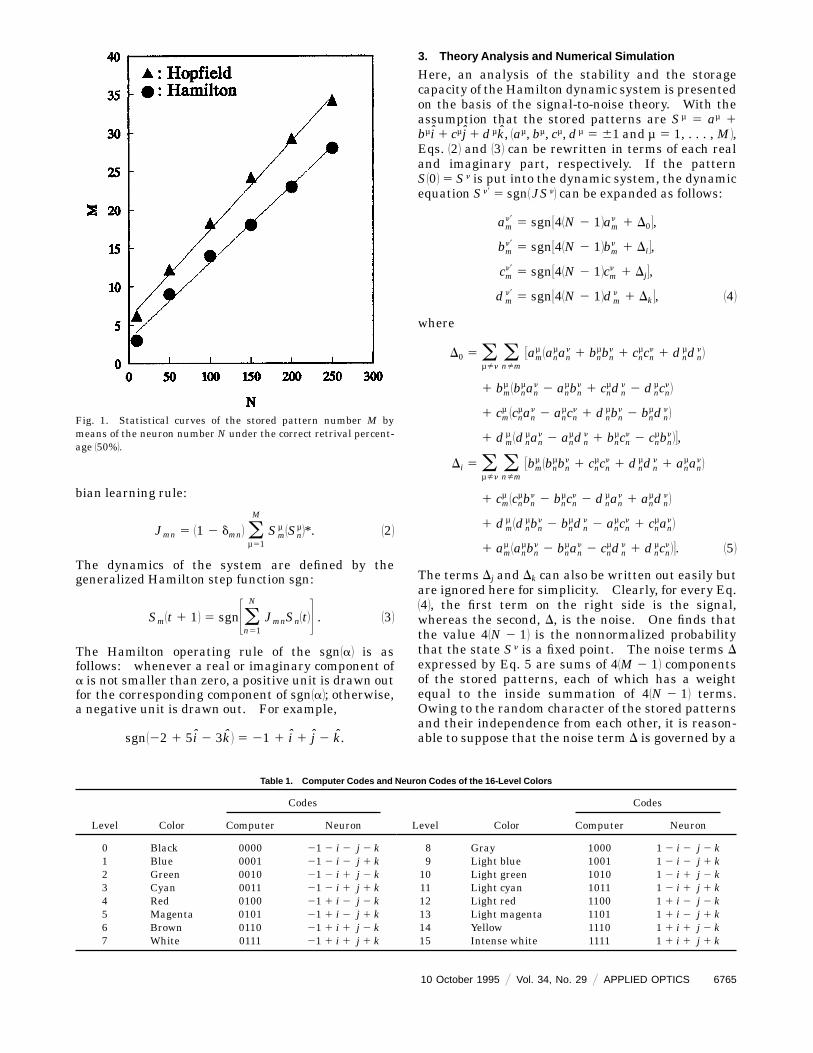
Fig. 1. Statistical curves of the stored pattern number M bymeans of the neuron number N under the correct retrival percent-age 150%2.

3. Theory Analysis and Numerical Simulation

Here, an analysis of the stability and the storagecapacity of the Hamilton dynamic system is presentedon the basis of the signal-to-noise theory. With theassumption that the stored patterns are Sµ 5 aµ 1

bµi1 cµj1 dµk, 1aµ, bµ, cµ, dµ 5 61 and µ 5 1, . . . ,M2,Eqs. 122 and 132 can be rewritten in terms of each realand imaginary part, respectively. If the patternS102 5 Sn is put into the dynamic system, the dynamicequation Sn8 5 sgn1JSn2 can be expanded as follows:

amn8 5 sgn341N 2 12am

n 1 D04,

bmn8 5 sgn341N 2 12bm

n 1 Di4,

cmn8 5 sgn341N 2 12cm

n 1 Dj4,

dmn8 5 sgn341N 2 12dm

n 1 Dk4, 142

where

D0 5 oµfin

onfim

3amµ 1an

µann 1 bn

µbnn 1 cn

µcnn 1 dn

µdnn 2

1 bmµ 1bn

µann 2 an

µbnn 1 cn

µdnn 2 dn

µcnn 2

1 cmµ 1cn

µann 2 an

µcnn 1 dn

µbnn 2 bn

µdnn 2

1 dmµ 1dn

µann 2 an

µdnn 1 bn

µcnn 2 cn

µbnn 24,

Di 5 oµfin

onfim

3bmµ 1bn

µbnn 1 cn

µcnn 1 dn

µdnn 1 an

µann 2

1 cmµ 1cn

µbnn 2 bn

µcnn 2 dn

µann 1 an

µdnn 2

1 dmµ 1dn

µbnn 2 bn

µdnn 2 an

µcnn 1 cn

µann 2

1 amµ 1an

µbnn 2 bn

µann 2 cn

µdnn 1 dn

µcnn 24. 152

The terms Dj and Dk can also be written out easily butare ignored here for simplicity. Clearly, for every Eq.142, the first term on the right side is the signal,whereas the second, D, is the noise. One finds thatthe value 41N 2 12 is the nonnormalized probabilitythat the state Sn is a fixed point. The noise terms D

expressed by Eq. 5 are sums of 41M 2 12 componentsof the stored patterns, each of which has a weightequal to the inside summation of 41N 2 12 terms.Owing to the random character of the stored patternsand their independence from each other, it is reason-able to suppose that the noise term D is governed by a

Table 1. Computer Codes and Neuron Codes of the 16-Level Colors

Level Color

Codes

Level Color

Codes

Computer Neuron Computer Neuron

0 Black 0000 21 2 i 2 j 2 k 8 Gray 1000 1 2 i 2 j 2 k1 Blue 0001 21 2 i 2 j 1 k 9 Light blue 1001 1 2 i 2 j 1 k2 Green 0010 21 2 i 1 j 2 k 10 Light green 1010 1 2 i 1 j 2 k3 Cyan 0011 21 2 i 1 j 1 k 11 Light cyan 1011 1 2 i 1 j 1 k4 Red 0100 21 1 i 2 j 2 k 12 Light red 1100 1 1 i 2 j 2 k5 Magenta 0101 21 1 i 2 j 1 k 13 Light magenta 1101 1 1 i 2 j 1 k6 Brown 0110 21 1 i 1 j 2 k 14 Yellow 1110 1 1 i 1 j 2 k7 White 0111 21 1 i 1 j 1 k 15 Intense white 1111 1 1 i 1 j 1 k

10 October 1995 @ Vol. 34, No. 29 @ APPLIED OPTICS 6765

Gaussian distribution with the expectation value’sbeing zero and the standard deviation’s value being3161N 2 121M 2 1241@2. So the signal-to-noise ratio s ofthe real part or of the three imaginary parts of eachcomponent of Sn is 31N 2 12@1M 2 1241@2.If N : M, then s : 1, and so the neural network

converges to the stored pattern Sn. When a patternS that is close to the stored pattern Sn is put into thenetwork, the above conclusion essentially holds true,and the pattern S automatically converges to thepattern Sn after one or more retrieval processes. Inconclusion, the stored pattern Sn is a stable attractorof the Hamilton neural network.Now the storage capacity ratio r 5 M@N of the

presented model, with the limit in which N, M = `

and r is finite. Without a loss of generality, let usassume that the real component Re1Sm

n 2 5 1; then theprobability that the Re1Sm

n82 5 1 can be given on thebasis of Gaussian distribution of the noise term D is

p 51

Œ2pe

2Œ1@p

`

exp12 x2

2 2dx. 162

Here, s < Œ1@r. Thus, compared with the patternSn, the expected number of errors in the real andimaginary components in the pattern Sn8 is approxi-mately

E1r2 54N

Œ2peŒ1@p

`

exp12 x2

2 2dx. 172

If the number of error components in Sn8 is approxi-mately a Poisson distribution, it follows that theprobability of correct components, i.e., the probabilitythat Sn is indeed a stable attractor, is given approxi-mately by the expression

P 5 exp32E1r24. 182

Suppose that the probability P is a fixed numbervery near 1. We can invert the preceding expressionfor 0 , r 9 1 and obtain the following result:

r ~1

2 ln 4N<

1

2 ln N. 192

This result is equal to that of the Hopfield neural-network model analyzed by Bruce et al.2 and Mcelieceet al.3 So the storage capacities of the Hamilton–number neural-network model and of the Hopfieldmodel are almost at the same level.Now the numerical simulation of the storage capac-

ity of the model for a finite-size system N # 300 isperformed. The statistical curve of the maximumnumber of stored patterns M by means of the neuronnumber N under the correct retrieval percent 150%2 isobtained 1see Fig. 12. The statistical curve M 2 N ofthe Hopfield model is also plotted. From Fig. 1 onecan see that the curves for the two models are similar;in another words, the storage capacity ratios of the

6766 APPLIED OPTICS @ Vol. 34, No. 29 @ 10 October 1995

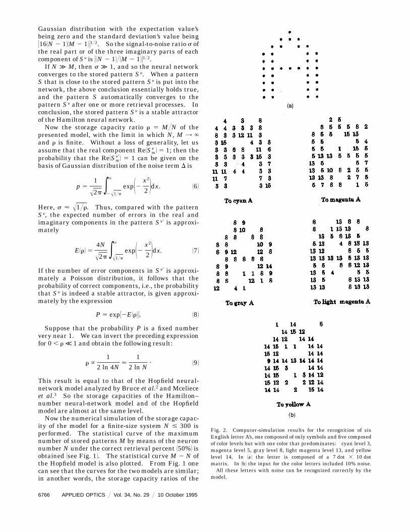
Fig. 2. Computer-simulation results for the recognition of sixEnglish letter A’s, one composed of only symbols and five composedof color levels but with one color that predominates: cyan level 3,magenta level 5, gray level 8, light magenta level 13, and yellowlevel 14. In 1a2 the letter is composed of a 7 dot 3 10 dotmatrix. In 1b2 the input for the color letters included 10% noise.All these letters with noise can be recognized correctly by the

model.

two models are the same. The storage capacity ofthe Hamilton network is slightly smaller than that ofthe Hopfield network.This conclusion can be qualitatively comprehended

as follows: In the Hopfield model,1 the one-dimen-sional input information is cut into two parts—thepositive and the negative—and mapped into twopoints of the output space; in the Q-state model,7 the

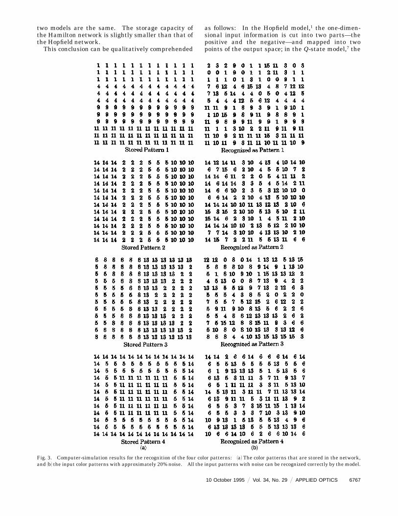
Fig. 3. Computer-simulation results for the recognition of the four color patterns: 1a2 The color patterns that are stored in the network,and 1b2 the input color patterns with approximately 20% noise. All the input patterns with noise can be recognized correctly by the model.

10 October 1995 @ Vol. 34, No. 29 @ APPLIED OPTICS 6767

one-dimensional input information is cut intoQ inter-vals, so the mean-square error of pseudo-orthogonal-ity of the pattern Sn is increased with Q, and thus itraises the noise of the system. To correctly map eachinterval into one of the Q points of the output space,the sensitivity of the dynamics with the noise isincreased with Q2, whereas for the Hamilton neural-network model the input information is placed infour-dimensional space and cut into 16 quadrants.So the difficulty encountered with the Q-state modelis avoided. Thus the sensitivity of the present modelwith the noise is the same as that of the Hopfieldmodel, i.e., the signal-to-noise ratio of the modelequals that of the Hopfield model. The storage-capacity ratios of the networks aremainly assessed bys. Therefore the storage capacity of the Hamiltonmodel equals that of the Hopfield model.

4. Application to Color-Pattern Recognition

The Hamilton neural-network model is especiallyappropriate for recognizing 16-level color patternsconsisting of three basic colors 1red, blue, and green2:The three imaginary parts of the Hamilton numbercan be treated as the three basic colors, and the realpart indicates the color-saturation degree. So the16-state Hamilton neural network can store 16-levelcolor patterns. The corresponding relation betweenthe computer code and the Hamilton neuron code ofthe 16-level colors is listed in Table 1.Using the Hamilton neural network, we process

numerical simulations to recognize the color of En-glish letters that are composed of a 7 dot 3 10 dotmatrix, such as is seen in Fig. 21a2, in which thebackground color is black. For example, five lettersA with each of the colors cyan, magenta, gray, lightmagenta, and yellow, are stored in the model.Numerical-simulation results show that these lettersA, with different colors, are all the stable patternsstored in the Hamilton neural network. Now, if aletter that is slightly different from one of the storedA’s is fed into the neural network, the system canrecognize it and recall to the properA. It shows that,for the input patterns added with approximately 10%random noise 1i.e., 30 error bits2, the correct recogni-tion ratio is more than 90%. Figure 21b2 shows otherletters A with 10% noise in the input patterns. Themodel can recognize them correctly. In the figure,each integer number indicates a color as shown inTable 1.Some numerical simulations to recognize the color

patterns are also processed by means of the presentedmodel. Four color patterns composed of a 12 dot 312 dot matrix, such as are shown in Fig. 31a2, arestably stored in the presented network. Figure 31a2shows that, for input patterns with approximately

6768 APPLIED OPTICS @ Vol. 34, No. 29 @ 10 October 1995

10% or 20% random noise 1i.e., 60 or 110 error bits,respectively2, the correct recognition ratio is nearly95% or 75%, respectively. The set of patterns thatare shown in Fig. 31b2 as input test objects but that arecontaminated with approximately 20% noise can berecognized correctly by the model.

5. Conclusion

In this paper, a 16-state discrete Hamilton neuralnetwork is proposed. The stability and the storagecapacity are analyzed by means of the signal-to-noiseratio theory and numerical simulation. The storage-capacity ratios of the two models are the same, andthe storage capacity of the Hamilton network is just alittle smaller than that of the Hopfield network.Because of the feature of one real part and threeimaginary parts for the Hamilton number, the 16-state discrete Hamilton neural network can be ap-plied to recognize a 16-level color pattern.Naturally, not only can the Hamilton number be

introduced into the neural network, but also the other2n-element numbers, such as the complex numberand Cayley number. For the latter two types ofnumbers, four-level 1i.e., 61, 6i2 and 256-level 1i.e.,61, 6i1, 6i2, 6i3, 6e, 6i1e, 6i2e, 6i3e2 neural net-works can be set up. The detailed work will bediscussed in future papers.

This work is supported by the National NaturalScientific Research Foundation under grant 19334032.

References1. J. J. Hopfield, ‘‘Neural networks and physical systems with

emergent collective computational abilities,’’ Proc. Natl. Acad.Sci. USA 79, 2554–2558 119822.

2. A. D. Bruce, E. J. Gardner, and D. J. Wallace, ‘‘Dynamics andstatistical mechanics of the Hopfield model,’’ J. Phys. A 20,2909–2934 119872.

3. R. J. Mceliece, E. D. Posner, E. R. Rodemich, and S. S.Venkatesh, ‘‘The capacity of the Hopfield associative memory,’’IEEE Trans. Inf. Theory 33, 461–482 119872.

4. H. J. White and W.A. Wright, ‘‘Holographic implementation ofthe Hopfield model with discrete weightings,’’ Appl. Opt. 27,331–338 119872.

5. W. Zhang, K. Itoh, J. Tanida, and Y. Ichioka, ‘‘Hopfield modelwith multistate neurons and its optoelectronic implementa-tion,’’Appl. Opt. 30, 195–200 119912.

6. F. T. S. Yu, C. M. Uang, and S. Yin, ‘‘Gray-level discreteassociative memory,’’Appl. Opt. 32, 1322–1329 119932.

7. H. Rieger, ‘‘Storing an extensive number of grey-toned pat-terns in a neural network using multistate neurons,’’ J. Phys.A 23, 1273–1279 119902.

8. A. J. Noest, ‘‘Discrete-state phasor neural networks,’’ Phys.Rev. A 38, 2196–2199 119882.

9. G. Y. Sirat, A. D. Maruani, and Y. Ichioka, ‘‘Gray-level neuralnetworks,’’Appl. Opt. 28, 414–415 119892.

10. E. U. Conden, H. Odishaw, Handbook of Physics, 2nd ed.1McGraw-Hill, NewYork, 19672, Vol. 1, p. 22.