Embed Size (px)
Citation preview
HAMILTONIAN METHODS INPT -SYMMETRIC SYSTEMS
HAMILTONIAN METHODS IN PT -SYMMETRIC
SYSTEMS
By ALEXANDER CHERNYAVSKY, M.Sc., B.Sc.
A Thesis Submitted to the Department of Mathematics and Statistics and the
School of Graduate Studies in Partial Fulfilment of the Requirements for the Degree
Doctor of Philosophy
McMaster University c© Copyright by Alexander Chernyavsky
DOCTOR OF PHILOSOPHY (2018) McMaster University
(Mathematics) Hamilton, Ontario, Canada
TITLE: Hamiltonian Methods in
PT -symmetric Systems
AUTHOR: Alexander Chernyavsky
M.Sc. (MIET)
B.Sc. (MIET)
SUPERVISOR: Dr. Dmitry Pelinovsky
NUMBER OF PAGES: xii, 152
i
AbstractThis dissertation is concerned with analysis of spectral and orbital stability of solitary
wave solutions to discrete and continuous PT -symmetric nonlinear Schrodinger equa-
tions. The main tools of this analysis are inspired by Hamiltonian systems, where
conserved quantities can be used for proving orbital stability and Krein signature
can be computed for prediction of instabilities in the spectrum of linearization. The
main results are obtained for the chain of coupled pendula represented by a discrete
NLS model, and for the trapped atomic gas represented by a continuous NLS model.
Analytical results are illustrated with various numerical examples.
iii
AcknowledgementsFirst of all, I would like to express my deepest gratitude to my advisor, Dr. Dmitry
Pelinovsky. His guidance and patience with me were priceless throughout my studies
at McMaster, and weekly meetings kept me on my toes at all times. I also want to
thank his family for hosting me and other graduate students for annual dinners at Dr.
Pelinovsky’s house. These evenings gave me a taste of home and made me feel a part
of the family. I have also enjoyed our joint cross-country skiing activies and traveling
together.
I would like to thank McMaster University for providing financial support during
my stay in Canada. A combination of scholarships and teaching duties gave me an
opportunity to do research and work part-time to deepen my knowledge of undergrad-
uate material by conveying it to others. I enjoyed working as a Teaching Assistant for
various courses and even got to teach one as an instructor. This teaching experience
is invaluable for me and would give a great advantage in the future.
My journey will not be the same without all the good people I met here. I cannot
list them all, but I must mention Adrien Thierry, Karsten Hempel, Tyler Mead-
ows, Yusuke Shimabukuro, Lee van Brussel, Niky Hristov, Aaron Saalmann, Zelalem
Negeri, and many, many others. But the list does not end with the graduate students.
I enjoyed taking courses and engaging in conversations with Dr. Stanley Alama, Dr.
Lia Bronsard, Dr. Gail Wolkowicz, Dr. Eric Sawyer, and Dr. Rachel Rensink-Hoff.
They gave me numerous life advices and shared their experiences of being a graduate
student. I also came to know various staff members within and outside the depart-
ment: Pam, Shirley, TJ, Dragan, Kenneth, Brian, Paula, Sheree. They cheered and
supported me even when I was not confident in myself, and I did my best to return
the favor.
Last but not least, I would like to thank my family and friends from home for
calling me regularly and making sure of my well-being. They provided a link to home
and made me proud to be who I am.
iv

To my wife, Lorena
Contents
Abstract iii
Acknowledgements iv
Declaration of Academic Achievement xii
1 Introduction 1
1.1 Hamiltonian Systems . . . . . . . . . . . . . . . . . . . . . . . . . . . 3
1.1.1 Finite-Dimensional Hamiltonian Systems . . . . . . . . . . . . 3
1.1.2 Infinite-Dimensional Hamiltonian Systems . . . . . . . . . . . 7
1.2 PT -Symmetric Systems . . . . . . . . . . . . . . . . . . . . . . . . . 8
1.2.1 PT -Symmetric Linear Operators . . . . . . . . . . . . . . . . 9
1.2.2 Example . . . . . . . . . . . . . . . . . . . . . . . . . . . . . . 11
1.2.3 Pseudo-Hermiticity . . . . . . . . . . . . . . . . . . . . . . . . 12
1.3 Stability in Discrete Systems . . . . . . . . . . . . . . . . . . . . . . . 14
1.4 Stability in Continuous Systems . . . . . . . . . . . . . . . . . . . . . 16
1.5 Preliminaries . . . . . . . . . . . . . . . . . . . . . . . . . . . . . . . 19
1.5.1 Sobolev Spaces . . . . . . . . . . . . . . . . . . . . . . . . . . 19
1.5.2 Sequence Spaces . . . . . . . . . . . . . . . . . . . . . . . . . 20
1.5.3 Bounded and Closed Operators . . . . . . . . . . . . . . . . . 22
1.5.4 Resolvent and Spectrum . . . . . . . . . . . . . . . . . . . . . 22
1.5.5 Adjoint and Fredholm Operators . . . . . . . . . . . . . . . . 23
1.5.6 Useful results . . . . . . . . . . . . . . . . . . . . . . . . . . . 26
2 Breathers in Discrete Systems 28
2.1 Model . . . . . . . . . . . . . . . . . . . . . . . . . . . . . . . . . . . 28
2.2 Symmetries and conserved quantities . . . . . . . . . . . . . . . . . . 31
ii
CONTENTS CONTENTS
2.3 Breathers (time-periodic solutions) . . . . . . . . . . . . . . . . . . . 34
2.4 Stability of zero equilibrium . . . . . . . . . . . . . . . . . . . . . . . 41
2.5 Variational characterization of breathers . . . . . . . . . . . . . . . . 42
2.6 Spectral and orbital stability of breathers . . . . . . . . . . . . . . . . 46
2.7 Summary . . . . . . . . . . . . . . . . . . . . . . . . . . . . . . . . . 60
3 Metastability in Discrete Systems 62
3.1 Background . . . . . . . . . . . . . . . . . . . . . . . . . . . . . . . . 62
3.2 Proof of the global bound . . . . . . . . . . . . . . . . . . . . . . . . 66
3.3 Proof of metastability . . . . . . . . . . . . . . . . . . . . . . . . . . . 68
3.3.1 Characterization of the localized solutions . . . . . . . . . . . 68
3.3.2 Decomposition of the solution . . . . . . . . . . . . . . . . . . 70
3.3.3 Positivity of the quadratic part of ∆ . . . . . . . . . . . . . . 71
3.3.4 Removal of the linear part of ∆ . . . . . . . . . . . . . . . . . 74
3.3.5 Time evolution of ∆ . . . . . . . . . . . . . . . . . . . . . . . 77
3.3.6 Modulation equations in `2c(Z) . . . . . . . . . . . . . . . . . . 81
4 Krein signature in Hamiltonian Systems 83
4.1 Background . . . . . . . . . . . . . . . . . . . . . . . . . . . . . . . . 83
4.2 Krein signature for the NLS equation . . . . . . . . . . . . . . . . . . 86
5 Krein signature in PT -symmetric systems 95
5.1 Background . . . . . . . . . . . . . . . . . . . . . . . . . . . . . . . . 95
5.2 Stationary states, eigenvalues of the linearization, and Krein signature 96
5.3 Necessary condition for instability bifurcation . . . . . . . . . . . . . 103
5.4 Numerical Approximations . . . . . . . . . . . . . . . . . . . . . . . . 110
5.5 Numerical Examples . . . . . . . . . . . . . . . . . . . . . . . . . . . 114
6 Conclusion 121
6.1 Summary of Main Results . . . . . . . . . . . . . . . . . . . . . . . . 121
6.2 Future Directions . . . . . . . . . . . . . . . . . . . . . . . . . . . . . 125
Appendices 126
A Perturbation theory near Hamiltonian case 127
A.1 Series in γ . . . . . . . . . . . . . . . . . . . . . . . . . . . . . . . . . 127
iii
CONTENTS CONTENTS
A.2 O(γ) balance equations . . . . . . . . . . . . . . . . . . . . . . . . . . 129
A.3 O(γ2) balance equations . . . . . . . . . . . . . . . . . . . . . . . . . 130
B Spectrum of the linear problem for Scarf II potential 132
C Wadati potentials: exact solutions 136
C.1 Derivation . . . . . . . . . . . . . . . . . . . . . . . . . . . . . . . . . 136
C.2 An example . . . . . . . . . . . . . . . . . . . . . . . . . . . . . . . . 138
Bibliography 139
iv
List of Figures
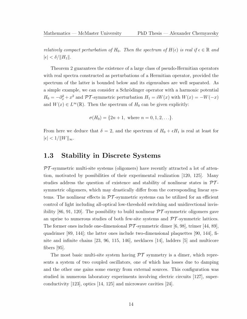
1.1 Left: A schematic picture for the chain of coupled pendula connected
by torsional springs, where each pair is hung on a common string.
Right: The chain of PT -symmetric dimers representing coupled pen-
dula. Filled (empty) circles correspond to sites with gain (loss). . . . 15
2.1 A schematic picture for the chain of coupled pendula connected by
torsional springs, where each pair is hung on a common string. . . . . 29
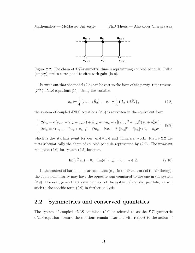
2.2 The chain of PT -symmetric dimers representing coupled pendula. Filled
(empty) circles correspond to sites with gain (loss). . . . . . . . . . . 31
2.3 Solution branches for the dimer equation (2.23). . . . . . . . . . . . . 35
2.4 The spectrum of −iSH′′E for different branches of breathers. . . . . . 57
4.1 The top left panel corresponds to the case of the first excited state, the top
right one corresponds to the second excited state, while the bottom panel
corresponds to the third excited state. Eigenvalues of negative (positive)
Krein signature are shown in red (green), complex eigenvalues are shown in
black. For the first excited state, only the lowest nonzero eigenfrequency has
a negative Krein signature (but its linear degeneracy with a symmetry mode
yields no instability). For the second excited state, there are two degenerate
modes at 2 and 4. Only the latter yields the quartet of complex eigenvalues.
For the third excited states, there are three degenerate modes at 2, 4, and
6, the last two yield quartets of complex eigenvalues. . . . . . . . . . . . 92
v
LIST OF FIGURES LIST OF FIGURES
5.1 Scarf II potential (5.43) with V0 = 2, γ = −2.21. (a) Power curves
versus µ. (b) Amplitude profile for point A. (c) Spectrum of lineariza-
tion for point A. (d) Same for point B. (e) Im(λ) for the spectrum
of linearization versus µ. (f) Krein quantities for isolated eigenvalues
versus µ. . . . . . . . . . . . . . . . . . . . . . . . . . . . . . . . . . 115
5.2 Scarf II potential (5.43) with V0 = 3, γ = −3.7. (a) Power curves ver-
sus µ. (b) Amplitude profile for point A. (c) Spectrum of linearization
for point A. (d) Same for point B. (e) Im(λ) for the spectrum of lin-
earization versus µ. (f) Krein quantities for isolated eigenvalues versus
µ. . . . . . . . . . . . . . . . . . . . . . . . . . . . . . . . . . . . . . 116
5.3 Confining potential (5.44), scaled as in (5.46). (a) Power curves versus
γ. (b) Amplitude profile for point A. (c) Spectrum of linearization
for point A. (d) Same for point B. (e) Im(λ) for the spectrum of lin-
earization versus γ. (f) Krein quantities for isolated eigenvalues versus
γ. . . . . . . . . . . . . . . . . . . . . . . . . . . . . . . . . . . . . . 117
5.4 Confining potential (5.44), scaled as in (5.46). (a) Power curves versus
γ. (b) Amplitude profile for point A. (c) Spectrum of linearization
for point A. (d) Same for point B. (e) Im(λ) for the spectrum of lin-
earization versus γ. (f) Krein quantities for isolated eigenvalues versus
γ. . . . . . . . . . . . . . . . . . . . . . . . . . . . . . . . . . . . . . 118
5.5 The norm of the difference between the two eigenvectors and the two
adjoint eigenvectors prior to a possible coalescence point: (a) for Fig-
ure 5.3 (b) for Figure 5.4. . . . . . . . . . . . . . . . . . . . . . . . . 120
6.1 Time-periodic solutions of the PT -symmetric dimer with A = |U0| =
|V0| versus frequency E for γ = 12
and (a) Ω = 34> γ or (b) Ω = −3
4< −γ.122
B.1 First two eigenvalues for spectral problem (B.1) with n = 0. Red color
corresponds to E(1)0 , whereas blue corresponds to E
(2)0 . a) Real parts
b) Imaginary parts. . . . . . . . . . . . . . . . . . . . . . . . . . . . . 135
vi

List of Tables
2.1 A summary of results on breather solutions for small ε. Here, IB is a
narrow instability bubble seen on panel (b) of Figure 2.4. . . . . . . . 60
5.1 The numerical error for the exact solution (5.45) versus N . . . . . . . 112
vii
Declaration of Academic Achievement
My supervisor, Dr. Dmitry Pelinovsky, and myself, conducted the research presented
in this dissertation. In recognition of this fact, I have chosen to use the personal
pronoun “we” where applicable throughout the text. Original results based on pub-
lished work joint with my supervisor are presented in Chapters 2, 3 and 5. There, I
was responsible for analyzing the problem, programming numerical simulations and
interpreting data, as well as writing the manuscript with the editorial advice and
supervision of Dr. Pelinovsky. Chapter 4 is based on published work developed
in collaboration with Dr. Panayotis Kevrekidis, who provided invaluable insight on
physical applications. In that Chapter, I was responsible for numerical simulations,
analytical computations and writing the manuscript, and Dr. Pelinovsky provided
guidance on the analysis involved.
xii
Chapter 1
Introduction
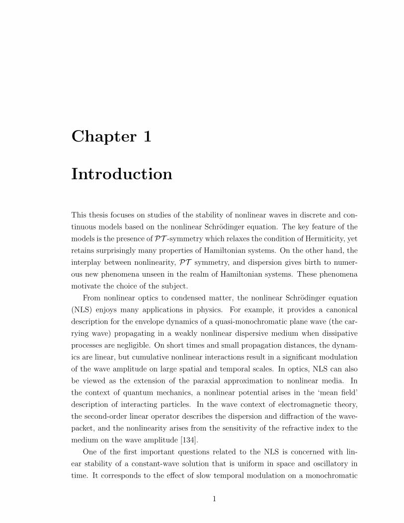
This thesis focuses on studies of the stability of nonlinear waves in discrete and con-
tinuous models based on the nonlinear Schrodinger equation. The key feature of the
models is the presence of PT -symmetry which relaxes the condition of Hermiticity, yet
retains surprisingly many properties of Hamiltonian systems. On the other hand, the
interplay between nonlinearity, PT symmetry, and dispersion gives birth to numer-
ous new phenomena unseen in the realm of Hamiltonian systems. These phenomena
motivate the choice of the subject.
From nonlinear optics to condensed matter, the nonlinear Schrodinger equation
(NLS) enjoys many applications in physics. For example, it provides a canonical
description for the envelope dynamics of a quasi-monochromatic plane wave (the car-
rying wave) propagating in a weakly nonlinear dispersive medium when dissipative
processes are negligible. On short times and small propagation distances, the dynam-
ics are linear, but cumulative nonlinear interactions result in a significant modulation
of the wave amplitude on large spatial and temporal scales. In optics, NLS can also
be viewed as the extension of the paraxial approximation to nonlinear media. In
the context of quantum mechanics, a nonlinear potential arises in the ‘mean field’
description of interacting particles. In the wave context of electromagnetic theory,
the second-order linear operator describes the dispersion and diffraction of the wave-
packet, and the nonlinearity arises from the sensitivity of the refractive index to the
medium on the wave amplitude [134].
One of the first important questions related to the NLS is concerned with lin-
ear stability of a constant-wave solution that is uniform in space and oscillatory in
time. It corresponds to the effect of slow temporal modulation on a monochromatic
1
Mathematics — McMaster University PhD Thesis — Alexander Chernyavsky
wave whose frequency is slightly shifted by the nonlinearity. When the constant-wave
solution is modulationally unstable, the spatial modulation leads to the formation
of solitonic structures resulting from an exact balance between the dispersive and
nonlinear effects.
The discrete nonlinear Schrodinger equation (dNLS) is one of the most fundamen-
tal lattice models. On one hand, it is a prototypical discretization of the nonlinear
Schrodinger equation, on the other hand, it has many physical applications in its own
right. One of the relevant areas for dNLS is the field of optically induced lattices in
photorefractive media, where the dNLS model can yield accurate predictions about
existence and stability of nonlinear localized modes. Since the numerical prediction
in [48] and experimental realization in [55], there has been an tremendous number of
studies in the area of nonlinear waves and solitons in such structures. A number of
them has been predicted and experimentally demonstrated in lattices with induced
self-focusing nonlinearity: dipoles, quadrupoles, necklaces, etc. Such structures have
a potential to be used as carriers for data transmission in all-optical communication
schemes [72].
As we have seen, both continuous and discrete NLS models have a variety of
physical applications. The incorporation of PT symmetry into these models enriches
this variety and introduces fascinating phenomena: existence of continuous families
of nonlinear modes, PT symmetry breaking and stabilization above phase transition.
The study of these phenomena and prediction of instabilities is an important step
towards understanding intrinsic nonlinear processes. This thesis develops the tools
for such analysis and paves the way for the future work relevant to many branches of
modern physics.
This introduction is structured as follows. Section 1.1 gives a brief overview of
Hamiltonian systems and the stability problem. Section 1.2 introduces PT -symmetric
systems and their important features. In Section 1.3 we talk about stability analysis
in discrete systems, and introduce the model studied in Chapters 2 and 3. Section 1.4
gives the outline of stability analysis in continuous system, and presents the material
of Chapters 4 and 5. Section 1.5 introduces spaces and properties of operators that
will be used throughout the thesis.
2
Mathematics — McMaster University PhD Thesis — Alexander Chernyavsky
1.1 Hamiltonian Systems
Hamiltonian systems arise in applications where the damping can be neglected. Hamil-
tonian view of mechanics becomes important for approximate methods of perturbation
theory, e.g. celestial mechanics; for understanding the general character of motion in
complicated mechanical systems, e.g. ergodic theory, statistical mechanics; and in
connection with other areas of physics, e.g. optics, quantum mechanics, etc. [8]. The
rich structure of Hamiltonian systems stems from the conservation of the underlying
energy, the Hamiltonian, as well as other quantities such as mass and momentum.
Linear and nonlinear stability of wave solutions to Hamiltonian systems is an old
field. In 1872 Boussinesq [26], studying water waves, suggested that the constraint
due to symmetry could be used to understand the stability of the critical points
of the energy, represented by the Hamiltonian. General framework of this theory
was developed by Grillakis, Shatah, and Strauss [59, 60] in the infinite-dimensional
Hamiltonian systems in the presence of symmetries. Their approach characterizes the
critical points of systems with symmetry and conserved quantities via the analysis of
a constraint operator. We will review the finite-dimensional theory [69], and show
that minimizers of the Hamiltonian are nonlinearly stable [57, 94].
1.1.1 Finite-Dimensional Hamiltonian Systems
Consider a state vector ~u ∈ R2d for some dimension d ≥ 1, and a Hamiltonian
H : R2d 7→ R, which depends smoothly upon ~u and corresponds to the conserved
energy of the system. The Hamiltonian system describing time evolution of the state
vector ~u in time t takes the form
d~u
dt= J∇uH(~u). (1.1)
Here J is a 2d × 2d nonsingular matrix skew-symmetric with respect to the usual
Euclidean inner product: JT = −J , where superscript T stands for matrix transpose.
Such matrices map a vector into its perpendicular subspace:
〈J~x, ~x〉 = 〈~x, JT~x〉 = −〈~x, J~x〉,
and thus 〈J~x, ~x〉 = 0. Using this property, we can prove the following:
3

Mathematics — McMaster University PhD Thesis — Alexander Chernyavsky
Lemma 1. Let ~u be the solution of (1.1) with initial data ~u(0) = ~u0. Then H(~u(t)) =
H(~u0) for all nonzero t.
Proof. Let us take the time derivative of H(~u(t)):
dH(~u)
dt= 〈∇uH(~u),
d~u
dt〉 = 〈∇uH(~u), J∇uH(~u)〉 = 0.
Thus the functional H is constant.
The canonical Hamiltonian system is derived from the Newton’s second law. The
skew-symmetric matrix J then takes the form
J =
[0d Id
−Id 0d
],
where Id ∈ Rd×d is the identity matrix, and 0d ∈ Rd×d is the zero matrix. The state
vector is written as ~u = [~p, ~q]T for ~p, ~q ∈ Rd, and the Hamiltonian system becomes
dpjdt
=∂H
∂qj,
dqjdt
= −∂H∂pj
.
where j = 1, . . . , d. The vectors ~p = (p1, . . . , pd) and ~q = (q1, . . . , qd) are traditionally
called the momentum and position vectors, respectively. In the context of molecu-
lar physics, Hamiltonian describes the total energy as a combination of kinetic and
potential energy due to interactions between the molecules.
Consider a critical point ~φ of the Hamiltonian energy functional: ∇u(H(~φ)) = 0.
Obviously, ~φ is also an equilibrium of the Hamiltonian system (1.1). Our interest lies
in dynamics of solutions with initial data ~u0 that lies close to ~φ. Asymptotic stability is
generally ruled out in finite-dimensional Hamiltonian systems, since if H(~u0) 6= H(~φ),
then ~u(t) cannot converge to ~φ. If it did, we would have H(~u0) = H(~u(t)) → H(~φ)
as t→∞, which gives us a contradiction. So at most we can have ~u(t) staying close
to ~φ.
Let us study the structure of the Hamiltonian about ~φ. Taking ~v = ~u− ~φ to be a
perturbation of ~φ, a Taylor expansion about φ yields
H(~u) = H(~φ) + 〈∇uH(~φ), ~v〉+1
2〈~v, L~v〉+O(|~v|3), (1.2)
4
Mathematics — McMaster University PhD Thesis — Alexander Chernyavsky
where L ∈ R2d×2d is a Hessian matrix which has the following entries:
Lij =∂H
∂ui∂uj(~φ).
It is important to note that the Hessian operator is symmetric (or Hermitian). Since~φ is a critical point of H, ∇uH(~φ) = 0, and Hamiltonian can be written as
H(~u)−H(~φ) =1
2〈~v, L~v〉+O(|~v|3). (1.3)
Taking ∇v of both sides, we can rewrite Hamiltonian system (1.1) as
d~v
dt= JL~v +N(~v),
where N(~v) = O(|~v|2) denotes nonlinear terms in v, and JL denotes the linearization
about ~φ. Such linearizations typically have the structure outlined in the following
lemma.
Lemma 2. Let L ∈ M2d×2d be a linear symmetric operator: LT = L. The spectrum
σ(JL) is symmetric with respect to the real and imaginary axes of the complex plane,
so that the eigenvalues of JL come in quartets: ±λ,±λ. In particular, either
σ(JL) ⊂ iR, or the critical point ~φ is linearly exponentially unstable.
Proof. Suppose that λ ∈ σ(JL) with the associated eigenvector ~w. Since JL has
real-valued entries,
JL~w = λ~w ⇔ JL~w = λ ~w.
In other words, λ also belongs to the spectrum of JL, with an eigenvector ~w. Moreover,
due to (JL)T = −LJ
JL~w = λ~w ⇔ −LJ(J−1 ~w) = (−λ)J−1 ~w ⇔ (JL)T (J−1 ~w) = −λ(J−1 ~w)
we can see that −λ ∈ σ((JL)T ) with the eigenvector J−1 ~w. On the other hand,
knowing σ(JL) = σ((JL)T ), we can deduce that −λ ∈ σ(JL), as well. By taking
complex conjugation, we also have −λ ∈ σ(JL). The spectral stability statement
follows from the spectral symmetry, since the existence of an eigenvalue with negative
real part implies the existence of an eigenvalue with positive real part.
5
Mathematics — McMaster University PhD Thesis — Alexander Chernyavsky
If ~φ is a nondegenerate minima of H, then it is stable in finite-dimensional Hamil-
tonian systems as per the following lemma.
Lemma 3. Suppose that ~φ is a critical point for the Hamiltonian system (1.1). If~φ is a strict local minimum, i.e. L is a positive-definite matrix, then ~φ is stable.
Specifically, there exist C, δ > 0 such that for |~u0 − ~φ| ≤ δ, the solution ~u of (1.1)
satisfies
|~u(t)− ~φ| ≤ C|~u0 − ~φ|, t ≥ 0.
Proof. Set ~v = ~u− ~φ, and recall the Taylor expansion of H about ~φ:
H(~u)−H(~φ) =1
2〈~v, L~v〉+O(|~v|3).
Since L is symmetric, all of its eigenvalues are real-valued: µj ∈ R, j = 1, 2, . . . , 2d.
Positive-definite property implies that all eigenvalues are positive: µ− := minjµj>0.
Moreover, µ+ := maxjµj ≥ µ−, and
µ−|~v|2 ≤ 〈~v, L~v〉 ≤ µ+|~v|2,
where the inequality is attained at corresponding eigenvectors. The Taylor expansion
implies that there exists a δ > 0 such that for every ~v ∈ R2d satisfying |~v| ≤ δ there
exist constants 0 < C− < C+ <∞ such that
C−|~v|2 ≤ H(~u)−H(~φ) ≤ C+|~v|2.
The lower bound implies that the initial data ~u0 controls the norm of the perturbation:
|~v(t)|2 ≤ 1
C−(H(~u)−H(~φ)) =
1
C−(H(~u0)−H(~φ)),
where we have used the conservation of Hamiltonian. The upper bound allows us to
rewrite the latter estimate as
|~u(t)− ~φ|2 ≤ C+
C−|~u0 − ~φ|2,
where the conclusion of the lemma is achieved with C =√C+/C−.
6
Mathematics — McMaster University PhD Thesis — Alexander Chernyavsky
In practice, Hamiltonian systems often possess symmetries. In that case, the image
of the critical point under these symmetries will generate a manifold of critical points,
and the set of derivatives of this manifold with respect to parameter will lie in the
kernel of the linearization JL about ~φ. Thus L will have a null space and at best
can be semi-definite. This obstacle can be overcome through the notion of orbital
stability, see, e.g., Definition 10 in Chapter 2.
Each symmetry generates a conserved quantity due to Noether’s Theorem [97].
Even when L has eigenvalues of negative real part, the critical point may still be
stable: the conserved quantities can be used to perform a search for a constrained
minimizer. This is realized in the approach of Grillakis-Shatah-Strauss [59, 60], which
we do not review here.
1.1.2 Infinite-Dimensional Hamiltonian Systems
Let X be an infinite-dimensional Hilbert space X with inner product 〈·, ·〉X , ‖ · ‖ be
the induced norm, and X∗ be the dual of X with respect to the inner product in X.
A Hamiltonian on X is a nonlinear functional H : X 7→ R, which we assume to be C2
on all of X. The associated Hamiltonian system then takes the form
du
dt= J δH
δu(u), u : R→ X, (1.4)
where J : X∗ 7→ X is a linear closed operator with dense domain D(J) ⊂ X∗, and
skew-symmetric respect to 〈·, ·〉X :
〈J u, v〉X = −〈u,J v〉X
for all u, v ∈ D(J) ⊂ X∗. Moreover, we assume that J is one-to-one and onto. The
first variation with respect to the X-inner product, denoted δH/δu : X → X∗, is
defined as
limε→0
H(u+ εv)−H(u)
ε=
⟨δHδu
(u), v
⟩X
for all u, v in X. Using the chain rule, we see that smooth solutions of (1.4) conserve
the Hamiltonian:
dH(u(t))
dt=
⟨δHδu
(u),du
dt
⟩X
=
⟨δHδu
(u),J δHδu
(u)
⟩X
= 0.
7
Mathematics — McMaster University PhD Thesis — Alexander Chernyavsky
Let us generalize the finite-dimensional expansion (1.2). Fix φ ∈ X. For u = φ+Iv
with v ∈ X the Hamiltonian admits a formal Taylor expansion
H(u+ εv)−H(φ) =
⟨δHδu
(φ), v
⟩X
+1
2〈Lv, v〉X +O(‖v‖3),
where the quadratic form 〈Lv, v〉X is called the second variation of H, and the self-
adjoint linear operator L is called the Hessian operator:
L :=δ2Hδu2
(φ) : D(L) ⊂ X 7→ X∗.
If φ is a critical point of H, in other words
δHδu
(φ) = 0,
then the Taylor expansion reduces to an infinite-dimensional version of (1.3):
H(u)−H(φ) =1
2〈Lv, v〉+O(‖v‖3).
Compared to the symmetric matrix L in (1.3), the self-adjoint operator L is generally
unbounded and has a nontrivial kernel.
The approach outlined previously for studying stability of wave solutions in finite-
dimensional systems can be readily extended to infinite-dimensional ones.
1.2 PT -Symmetric Systems
In classical quantum mechanics, one usually considers observables as Hermitian op-
erators in the Hilbert space L2. Bender and Boettcher [21] suggested that Hermitian
operators can be replaced by the so-called PT -symmetric operators for an alterna-
tive formulation of quantum mechanics. They have shown that a non-Hermitian
operator might still possess real spectrum if it is symmetric with respect to com-
bined parity P and time-reversal T symmetries. Their idea was later extended in
the works of Mostafazadeh [101, 102] who considered a more general class of pseudo-
Hermitian operators with purely real spectrum. A number of reviews emerged on the
topic [18, 84, 133].
8
Mathematics — McMaster University PhD Thesis — Alexander Chernyavsky
Starting in quantum mechanics, the concept of PT symmetry found applications
in many areas of physics [19, 123, 128]. In particular, there is a lot of interest in
optics due to experimental realizations of paraxial PT symmetric optics [93, 103].
Recent applications include single-mode PT lasers [52, 64] and unidirectional re-
flectionless PT -symmetric metamaterials at optical frequencies [53]. PT symmetric
systems demonstrate many nontrivial non-conservative wave interactions and phase
transitions, which can be employed for signal filtering and switching, opening new
prospects for active control of light [133].
Discovered by John Scott Russell in 1834, solitons have attracted a lot of attention
in many nonlinear physical systems, ranging from optics to BECs [54, 81]. Conserva-
tive solitons requiring balance of nonlinear response and medium dispersion usually
form families with different amplitudes. Nonlinear dissipative systems, however, re-
quire an additional balance between gain and loss to support soliton solutions [4, 122].
This requirement is usually satisfied only for selected soliton amplitudes and shapes,
and no continuous families can generally be found. On the other hand, PT -symmetric
systems, being a subclass of dissipative systems, can commonly support continuous
families of solitons due to symmetry property [141]. Thus PT -symmetric systems,
being dissipative systems, possess features of conservative ones [133].
Let us review the main concepts in the theory of PT -symmetric (or, more gener-
ally, non-Hermitian) linear systems.
1.2.1 PT -Symmetric Linear Operators
Let ψ(~x, t) be a complex valued wave function of a quantum particle, where ~x is a space
variable, and t represents time. Evolution of ψ(~x, t) is governed by the Schrodinger
equation
i∂ψ
∂t= Hψ(~x, t),
where the linear operator H acts in a Hilbert space L2(Rd) equipped with an inner
product
〈φ, ψ〉 =
∫Rdφ(~x, t)ψ(~x, t) ~dx,
d is the space dimension, and we consider units where ~ = m = 1 with m being the
mass of the particle.
9
Mathematics — McMaster University PhD Thesis — Alexander Chernyavsky
Recall that for Hermitian operator H∗ = H, and
〈Hφ,ψ〉 = 〈φ,Hψ〉,
for any φ, ψ ∈ D(H). The spectrum of any Hermitian operator is purely real, while
the opposite is not true: Hermiticity is a sufficient but not necessary condition for
reality of the spectrum.
The two fundamental discrete symmetries in physics [139] are given by the parity
operator P defined as Pψ(~x, t) = ψ(−~x, t), and by the time reversal operator Tdefined as T ψ(~x, t) = ψ(~x,−t). The operator T is antilinear:
T (αφ) = αT φ, T (φ+ ψ) = T φ+ T ψ (1.5)
for any two vectors ψ, φ and a complex number α. Moreover,
P2 = T 2 = I, [P , T ] = 0, (1.6)
where I is the identity operator.
Definition 1 (PT -symmetric operator). An operator H is said to be PT -symmetric
if
[PT , H] = 0, (1.7)
or, using (1.6), H = PT HPT .
In the work of Bender and Boettcher [21], where a connection between PT sym-
metry and reality of the spectrum was pointed out, they also introduced the notion
of unbroken PT symmetry.
Definition 2 (Broken and unbroken PT symmetry). PT symmetry of a PT -symmetric
operator is said to be unbroken if any eigenfunction of H is at the same time an eigen-
function of the PT operator. If the unbroken PT symmetry does not hold, then the
PT symmetry is called broken.
The broken PT symmetry is typically associated with the presence of complex
eigenvalues in the spectrum of H. Since H and PT commute, Hψ = Eψ implies
the existence of λ such that PT ψ = λψ. From (1.5) and (1.6) it follows that there
10
Mathematics — McMaster University PhD Thesis — Alexander Chernyavsky
exists a real constant β such that λ = eiβ. In other words, any eigenvalue of the PToperator is a pure phase [22].
Unlike Hermiticity, PT symmetry is not sufficient for the eigenvalues of H to be
purely real. It becomes sufficient when combined with the requirement for the PTsymmetry to be unbroken. Indeed, let E be an eigenvalue of H with the eigenfunction
ψ, Hψ = Eψ. Applying PT operator to both sides and using (1.6), we obtain
H(PT ψ) = E(PT ψ). Then, if the PT symmetry of H is unbroken, Hψ = Eψ, and
hence the eigenvalue E is real. This procedure is applied to every eigenvalue of H,
therefore the eigenvalues of H are entirely real.
Interestingly, in the case of unbroken PT symmetry it is possible to construct
a similarity transformation that maps a non-Hermitian PT -symmetric Hamiltonian
to an equivalent Hermitian Hamiltonian. The equivalence is understood in the sense
that both Hamiltonians have the same eigenvalues [47, 140]. Unfortunately, in practice
this transformation is too complicated to be constructed except at the perturbative
level [18]. Another problem is that the transformation is a similarity but not a unitary
transformation. That is, orthogonal pairs of vectors are mapped into pairs of vectors
that are not orthogonal.
Let us give an example illustrating basic concepts outlined above.
1.2.2 Example
Consider a Hamiltonian defined by a 2 x 2 matrix [20]:
H =
[iγ κ
κ −iγ
]= kσ1 + iγσ3, (1.8)
where γ ≥ 0 and κ ≥ 0 are real parameters and we use the conventional notations for
Pauli matrices:
σ1 =
[0 1
1 0
], σ2 =
[0 −ii 0
], σ3 =
[1 0
0 −1
].
The Hamiltonian (1.8) acts in a Hilbert space of two-component column vectors
ψ = (ψ1, ψ2)T , with complex entries ψ1, ψ2, and the inner product is defined as
〈φ, ψ〉 = φ1ψ1 + φ2ψ2.
11
Mathematics — McMaster University PhD Thesis — Alexander Chernyavsky
The Hamiltonian (1.8) is PT symmetric with P = σ1 and T being complex conjuga-
tion. The eigenvalues and eigenvectors of H are given by
E1,2 = ±√κ2 − γ2, ψ(1,2) =
[iγ/κ±
√1− γ2/κ2
1
].
Thus PT symmetry is unbroken (all eigenvalues are real) if γ < κ and is broken (both
eigenvalues are imaginary) if γ > κ. At γ = κ, PT symmetry breaking occurs. At
this point, two eigenvalues collide, and eigenvectors become linearly dependent, thus
Hamiltonian has a nondiagonal Jordan block. Algebraic multiplicity of the eigenvalue
is two and is larger than its geometric multiplicity one. Such points in the parameter
space (γ, κ) are called exceptional points [71] or branch points [100].
1.2.3 Pseudo-Hermiticity
A necessary and sufficient condition for the spectrum of a non-Hermitian Hamiltonian
to be purely real can be formulated in terms of a more general property called pseudo-
Hermiticity [88, 101].
Definition 3 (Pseudo-Hermitian operator). A Hamiltonian H is said to be η-pseudo-
Hermitian if there exists a Hermitian invertible linear operator η such that
H∗ = ηHη−1.
Obviously, if η is the identity operator, this definition is equivalent to Hermiticity.
In many cases, pseudo-Hermiticity can be considered as a generalization of PT sym-
metry. For example, if H is a symmetric matrix Hamiltonian, then PT symmetry
implies HP − PH = 0, and then H∗ = H = PHP , i.e. a pseudo-Hermiticity of H.
The notion of pseudo-Hermiticity allows one to formulate necessary and sufficient
condition for a Hamiltonian to possess a purely real spectrum. Let us consider the case
of the discrete spectrum, and let a Hamiltonian have a complete set of biorthonormal
eigenvectors (ψn, φn) defined by
Hψn = Enψn, H∗φn = Enφn, 〈φn, ψn〉 = δn,m.
Then the following theorem holds.
12
Mathematics — McMaster University PhD Thesis — Alexander Chernyavsky
Theorem 1 (Mostafazadeh [102]). Let H be a Hamiltonian that acts in a Hilbert
space, has a discrete spectrum, and admits a complete set of biorthonormal eigenvec-
tors (ψn, φn). Then the spectrum of H is real if and only if there is an invertible
linear operator O such that H is OO∗-pseudo-Hermitian: H = (OO∗)H∗(OO∗)−1.
As an example of application of Theorem 1, consider the PT -symmetric Hamilto-
nian (1.8). It possesses a complete set of biorthonormal eigenvectors unless ε = γ/κ =
1. Since the spectrum is real if ε ∈ (0, 1), Theorem 1 guarantees that for ε ∈ (0, 1)
there exists the operator O such that H is η-pseudo-Hermitian with η = OO∗. Al-
though H is also P -pseudo-Hermitian, this cannot be used in Theorem 1, since the
parity operator P = σ1 does not admit the representation P = OO∗. Therefore
there must exist another operator η 6= P such that η = OO∗. By straightforward
calculation one finds that
η =1
ε2
[1 iε
−iε 1
], O =
1
ε
[0 i√
1− ε2 ε
], ε ∈ (0, 1).
Theorem 1 also indicates that no such operators exist in the broken PT symmetry
case ε > 1.
Although PT symmetry is not sufficient to guarantee the reality of the spectrum
of a Hamiltonian H, it ensures that complex eigenvalues (if any) always exist in
complex-conjugate pairs: if E is a complex eigenvalue with nonzero imaginary part
and ψ is corresponding eigenvector, then E is also an eigenvalue with eigenvector
PT ψ. Thus one can expect that if PT symmetry is unbroken and the real eigenvalues
are simple and isolated from each other, then the reality of the spectrum is “robust”
against relatively small perturbations. For example, it happens when perturbed PT -
symmetric operator is “close” to a self-adjoint operator with simple eigenvalues [30,
29]. Consider a Hermitian operator H0 perturbed as H(ε) = H0 + εH1, where ε is a
small parameter, and H0, H1 are PT -symmetric. Then the spectrum of H(ε) is real
provided ε is small enough. More precisely, the following theorem holds.
Theorem 2 (Caliceti, Graffi, and Sjostandt [30]). Let H0 be a self-adjoint positive
operator in a Hilbert space. Let H0 have only discrete spectrum 0 ≤ λ0 < λ1 < . . . <
λn < . . ., where each eigenvalue λj is simple, and δ = infj≥0λj+1 − λj/2 > 0.
Let also H0 and H1 be PT -symmetric in the sense of (1.7), and assume that H1 is
13
Mathematics — McMaster University PhD Thesis — Alexander Chernyavsky
relatively compact perturbation of H0. Then the spectrum of H(ε) is real if ε ∈ R and
|ε| < δ/‖H1‖.
Theorem 2 guarantees the existence of a large class of pseudo-Hermitian operators
with real spectra constructed as perturbations of a Hermitian operator, provided the
spectrum of the latter is bounded below and its eigenvalues are well separated. As
a simple example, we can consider a Schrodinger operator with a harmonic potential
H0 = −∂2x + x2 and PT -symmetric perturbation H1 = iW (x) with W (x) = −W (−x)
and W (x) ∈ L∞(R). Then the spectrum of H0 can be given explicitly:
σ(H0) = 2n+ 1, where n = 0, 1, 2, . . ..
From here we deduce that δ = 2, and the spectrum of H0 + εH1 is real at least for
|ε| < 1/‖W‖∞.
1.3 Stability in Discrete Systems
PT -symmetric multi-site systems (oligomers) have recently attracted a lot of atten-
tion, motivated by possibilities of their experimental realization [120, 125]. Many
studies address the question of existence and stability of nonlinear states in PT -
symmetric oligomers, which may drastically differ from the corresponding linear sys-
tems. The nonlinear effects in PT -symmetric systems can be utilized for an efficient
control of light including all-optical low-threshold switching and unidirectional invis-
ibility [86, 91, 120]. The possibility to build nonlinear PT -symmetric oligomers gave
an uprise to numerous studies of both few-site systems and PT -symmetric lattices.
The former ones include one-dimensional PT -symmetric dimer [6, 98], trimer [44, 89],
quadrimer [89, 144]; the latter ones include two-dimensional plaquettes [90, 144], fi-
nite and infinite chains [23, 96, 115, 146], necklaces [14], ladders [5] and multicore
fibers [95].
The most basic multi-site system having PT symmetry is a dimer, which repre-
sents a system of two coupled oscillators, one of which has losses due to damping
and the other one gains some energy from external sources. This configuration was
studied in numerous laboratory experiments involving electric circuits [127], super-
conductivity [123], optics [14, 125] and microwave cavities [24].
14
Mathematics — McMaster University PhD Thesis — Alexander Chernyavsky
On the analytical side, dimer equations were found to be completely integrable [13,
117]. Integrability of dimers is obtained by using Stokes variables and it is lost when
more coupled nonlinear oscillators are added into a PT -symmetric system. Never-
theless, it was understood recently [15, 16] that there is a remarkable class of PT -
symmetric dimers with cross-gradient Hamiltonian structure, where the real-valued
Hamiltonians exist both in finite and infinite chains of coupled nonlinear oscillators.
Analysis of synchronization in the infinite chains of coupled oscillators in such class of
models is a subject of Chapters 2 and 3. The results of this analysis were published
in papers [34, 36].
yn
xnxn−1 xn+1
yn+1yn−1 vn+1
un un+1
vn−1 vn
un−1
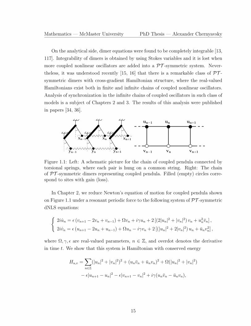
Figure 1.1: Left: A schematic picture for the chain of coupled pendula connected bytorsional springs, where each pair is hung on a common string. Right: The chainof PT -symmetric dimers representing coupled pendula. Filled (empty) circles corre-spond to sites with gain (loss).
In Chapter 2, we reduce Newton’s equation of motion for coupled pendula shown
on Figure 1.1 under a resonant periodic force to the following system of PT -symmetric
dNLS equations:2iun = ε (vn+1 − 2vn + vn−1) + Ωvn + iγun + 2 [(2|un|2 + |vn|2) vn + u2
nvn] ,
2ivn = ε (un+1 − 2un + un−1) + Ωun − iγvn + 2 [(|un|2 + 2|vn|2)un + unv2n] ,
where Ω, γ, ε are real-valued parameters, n ∈ Z, and overdot denotes the derivative
in time t. We show that this system is Hamiltonian with conserved energy
Hu,v =∑n∈Z
(|un|2 + |vn|2)2 + (unvn + unvn)2 + Ω(|un|2 + |vn|2)
− ε|un+1 − un|2 − ε|vn+1 − vn|2 + iγ(unvn − unvn),
15
Mathematics — McMaster University PhD Thesis — Alexander Chernyavsky
and an additional constant of motion
Qu,v =∑n∈Z
(unvn + unvn).
We study breather solutions of this model, which generalize symmetric synchronized
oscillations of coupled pendula. We show existence of three branches of breathers. We
also investigate their spectral stability analytically and numerically. For one of these
branches, we are also able to prove orbital stability and instability from the energy
method.
Chapter 3 is dedicated to the proof of nonlinear stability. It turns out that one of
the branches of breathers is an infinite-dimensional saddle point of the extended energy
functional, and the standard energy methods [69] cannot be applied to the proof of
nonlinear stability of this branch. However, by modifying the energy functional we
achieve long-time nonlinear stability of the breathers on a long but finite time interval.
Such long-time stability is usually referred to as metastability.
1.4 Stability in Continuous Systems
Consider the following nonlinear Schrodinger’s equation (NLSE) with a complex po-
tential U(x):
i∂tψ + ∂2xψ − U(x)ψ + g|ψ|2ψ = 0, (1.9)
where U(x) = V (x) + iγW (x) with V (x) = V (−x) and W (x) = −W (−x), γ ∈ R is a
gain-loss parameter, g = +1 (g = −1) defines focusing (defocusing) nonlinearity, and
U(x) is PT -symmetric:
U(x) = PT U(x) = U(−x). (1.10)
We will focus on potentials that are either localized (U(x) → 0 as x → ±∞) or
unbounded (U(x) → ∞ as x → ±∞). Stationary nonlinear modes in (1.9) have the
form ψ(x, t) = Φ(x)e−iµt, where µ ∈ R is a real propagation parameter, and Φ(x)
solves
Φxx − U(x)Φ + g|Φ|2Φ = µΦ (1.11)
subject to the zero boundary condition: Φ(x)→ 0 as x±∞. Analysis of stability of
these nonlinear modes is the subject of Chapters 4 and 5. The results of this analysis
were published in [33, 35].
16
Mathematics — McMaster University PhD Thesis — Alexander Chernyavsky
The NLSE (1.9) with a PT -symmetric potential is used in the paraxial nonlinear
optics. In that context, time and space have a meaning of longitudinal and trans-
verse coordinates, and complex potential models the complex refractive index [124].
Another possible application of the NLSE (1.9) with complex potential V + iγW is
Bose-Einstein condensate, where it models the dynamics of the self-gravitating boson
gas trapped in a confining potential V . Intervals, where W is positive and negative,
allow one to compensate atom injection and particle leakage, correspondingly [32].
The NLSE (1.9) is PT -symmetric under the condition (1.10) in the sense that if
ψ(x, t) is a solution to (1.9), then
ψ(x, t) = PT ψ(x, t) = ψ(−x,−t)
is also a solution to (1.9).
In Hamiltonian systems, instabilities arising due to coalescence of purely imagi-
nary eigenvalues can be predicted by computing the Krein signature for each eigen-
value, which is defined as the sign of the quadratic part of Hamiltonian restricted
to the associated eigenspace of the linearized problem. When two purely imaginary
eigenvalues coalesce, they bifurcate off to the complex plane only if they have opposite
Krein signatures prior to collision [69]. The concept of Krein signature was introduced
by MacKay [92] in the case of finite-dimensional Hamiltonian systems, although the
idea dates back to the works of Weierstrass [138]. An overview of Krein signature in
Hamiltonian systems is given in Chapter 4.
There have been several attempts to extend the concept of Krein signature to the
non-Hamiltonian PT -symmetric systems. Nixon and Yang [105] considered the linear
Schrodinger equation with a complex-valued PT -symmetric potential and introduced
the indefinite PT -inner product with the induced PT -Krein signature, in the exact
correspondence with the Hamiltonian-Krein signature. In the recent works [5, 7, 131],
a coupled non-Hamiltonian PT -symmetric system was considered and the linearized
system was shown to be block-diagonalizable to the form where Krein signature of
eigenvalues can be introduced. All these cases were too special, the corresponding
Krein signatures cannot be extended to a general PT -symmetric system.
In Chapter 5 we deal with the stationary states in the PT -symmetric NLSE (1.9)
and introduce Krein signature of isolated eigenvalues in the spectrum of their lin-
earization. We prove that the necessary condition for the onset of instability of the
17
Mathematics — McMaster University PhD Thesis — Alexander Chernyavsky
stationary states from a defective eigenvalue of algebraic multiplicity two is the oppo-
site Krein signature of the two simple isolated eigenvalues prior to their coalescence.
Compared to the Hamiltonian systems, or the linear Schrodinger equation in [105],
the Krein signature of eigenvalues cannot be computed from the eigenvectors in the
linearized problem. This is also shown in Appendix A, where perturbation theory
failed to yield a simple relationship between eigenvectors and their adjoint counter-
parts. As a result, the adjoint eigenvectors need to be computed separately and the
sign of the adjoint eigenvector needs to be chosen by a continuity argument.
We show how to compute Krein signature numerically for several examples of
the PT -symmetric potentials. In the focusing case g = 1, we consider the Scarf II
potential studied in [3, 17, 75, 105] with
U(x) = −V0 sech2(x) + iV1 sech(x) tanh(x), (1.12)
where V0 > 0 is a parameter. This potential is a complexification of the real Scarf
potential [11], which bears the name from the pioneer work in [126]. The spectrum
of this potential was found analytically by Ahmed [3] through a transformation of
the corresponding linear Schrodinger equation to the Gauss hypergeometric equation,
and by Bagchi and Quesne [9, 10] via complex Lie algebras. In Appendix B, we
explain the former method and correct an error in [3], where the author omitted some
admissible eigenvalues. When |V1| < Vcr = −V0 + 14, the discrete spectrum consists
of the sequence of real eigenvalues. At |V1| = Vcr, a pair of real eigenvalues coalesce,
and for |V1| > Vcr the double eigenvalue splits into the complex conjugate pairs in the
complex plane. In other words, PT symmetry becomes broken.
The nonlinear model (1.11) for the Scarf II potential has an exact particular solu-
tion [103, 129] for µ = 1:
Φ =
√−V0 − (V1/3)2 − 2
g
exp(iV1/3) arctan(sinh(x))
cosh(x),
where V0, V1 and g are chosen so that the argument of the radical is positive. In
Appendix C, we derive another exact solution for the nonlinear model using the
method developed in [17].
18
Mathematics — McMaster University PhD Thesis — Alexander Chernyavsky
In the defocusing case g = −1, we consider the confining potential studied in [1]
with
U(x) = Ω2x2 + iγxe−x2
2 , (1.13)
where Ω is a parameter. When γ = 0 and U(x) is real, the eigenvalues are given
by En = −(2n + 1), n = 0, 1, 2, . . . whereas the eigenfunctions can be expressed in
terms of Hermite polynomials. A numerical study of the linear spectrum for the PT -
symmetric Gaussian potential with Ω = 0 was performed by Ahmed [3], and nonlinear
modes were recently computed numerically [65, 67]. We will focus on the more general
case with Ω > 0.
In agreement with the theory, we show for both examples (1.12) and (1.13) that the
coalescence of two isolated imaginary eigenvalues in the linearized problem associated
with the stationary states in the NLSE (1.9) leads to instability only if the Krein
signatures of the two eigenvalues are opposite to each other.
1.5 Preliminaries
Before proceeding to technical details presented in the thesis, let us give a few basic
definitions. For further details see classical texts [2, 50, 61, 63, 68, 71, 87, 142].
1.5.1 Sobolev Spaces
Given a function u : R 7→ C, we define the Lp norm for any 1 ≤ p <∞ as
‖u‖p :=
(∫R|u(x)|pdx
)1/p
,
and the L∞ norm as
‖u‖∞ := supx∈R|u(x)|.
For any p ≥ 1 the associated Lebesgue space Lp(R) is given by
Lp(R) := u : ‖u‖p <∞,
19
Mathematics — McMaster University PhD Thesis — Alexander Chernyavsky
and it is known to be a complete metric space (called Banach space). For differentiable
functions we define the W k,p norm with 1 ≤ p <∞ and k ∈ N:
‖u‖Wk,p :=
(k∑i=0
∥∥∥∥∂iu∂xi∥∥∥∥pp
)1/p
,
and the associated Sobolev space
W k,p := u : ‖u‖Wk,p <∞.
The L2-based Sobolev spaces Hk := W k,2 is used frequently. Note that H0(R) =
L2(R).
Let us introduce the inner product
〈f, g〉 =
∫Rf(x)g(x)dx,
with complex conjugation in the second component. The Sobolev spaces Hk(R) with
k ∈ N are Hilbert spaces, since their norm is induced by the inner product
‖u‖2Hk =
k∑i=0
⟨∂iu
∂xi,∂iu
∂xi
⟩.
Moreover, Hk(R) is a Banach algebra with respect to pointwise multiplication for any
k ≥ 1: there exists a constant C ≥ 1 such that for all u ∈ Hk(R)
‖um‖Hk ≤ C‖u‖mHk , m ∈ N.
This property makes the map u 7→ um continuous in the Hk(R) norm. The spaces
Hm(R) ⊂ Hk(R) are dense for m > k, i.e., for each u ∈ Hk(R) there is a sequence
unn∈N ⊂ Hm(R) such that ‖un − u‖Hk → 0 as n→∞.
1.5.2 Sequence Spaces
Consider a linear space of all bi-infinite sequences with complex-valued entries:
x = xnn∈Z, xn ∈ C ∀n ∈ Z.
20
Mathematics — McMaster University PhD Thesis — Alexander Chernyavsky
For an element of this space, we define lp(Z) norm for any 1 ≤ p <∞ as
‖x‖lp =
(∑n∈Z
|xn|p)1/p
.
The space lp(Z) equipped with this norm can be defined as
lp(Z) := x : ‖x‖lp <∞.
lp(Z) is a Banach space for any p ≥ 1. The space of all bounded bi-infinite sequences,
l∞(Z), is also a Banach space:
l∞(Z) := x : ‖x‖l∞ <∞,
where the corresponding norm ‖ · ‖l∞ is given by
‖x‖l∞ = supn∈Z|xn|.
We are going to use embedding of lp spaces: lp(Z) ⊂ lq(Z) with p < q, such that
‖x‖lq ≤ ‖x‖lp .
An element from the space lq(Z) can be approximated by a sequence of elements from
the space lp(Z). In other words, lp(Z) is dense in lq(Z) for p < q.
The sequence space l2(Z) is Hilbert space with the inner product:
〈x, y〉 =∑n∈Z
xnyn,
where x = xnn∈Z and y = ynn∈Z.
The space lp(Z) is a Banach algebra with respect to multiplication:
‖w‖lp ≤ ‖x‖lp‖y‖lp ,
where x, y ∈ lp(Z), and w = xnynn∈Z.
21

Mathematics — McMaster University PhD Thesis — Alexander Chernyavsky
1.5.3 Bounded and Closed Operators
Let X and Y be two Banach spaces, with norms ‖ · ‖X and ‖ · ‖Y , respectively.
Assume that Y ⊂ X is dense, for example X = L2(R) and Y = Hk(R) for any k ≥ 1.
Consider linear operator L : Y ⊂ X → X, where Y is the maximal domain of operator
L denoted by D(L). The kernel of L is given by
ker(L) := u ∈ Y : Lu = 0,
and the range of L is
range(L) := Lu ∈ X : u ∈ Y ⊂ X.
A linear operator L is said to be closed if for any sequence un ⊂ Y with
limn→∞
‖un − u‖X = 0 and limn→∞
‖Lun − v‖X = 0,
we have u ∈ Y and Lu = v. The operator is bounded from Y to X if
sup‖Lu‖X : u ∈ Y, ‖u‖Y = 1 <∞.
From here we can define a norm associated with the space of bounded linear operators
B(Y,X):
‖L‖B(Y,X) := sup‖u‖Y =1
‖Lu‖X .
If X = Y , then the induced norm of L is denoted by ‖L‖. If L is a closed operator
with X = Y , then L is a bounded operator. If for each bounded sequence un ⊂ Y
the sequence Lun ⊂ X has a convergent subsequence, then the operator L is said
to be compact.
1.5.4 Resolvent and Spectrum
Definition 4 (Resolvent set). The resolvent set of L, ρ(L), is the set of complex
numbers λ ∈ C such that
• λI − L is invertible
• (λI − L)−1 is defined on a dense set
• (λI − L)−1 is a bounded linear operator.
22
Mathematics — McMaster University PhD Thesis — Alexander Chernyavsky
Here I : X 7→ X is the identity operator: Iu = u. For λ ∈ ρ(L) the operator
(λI − L)−1 is called the resolvent of L. The spectrum of L is the complement of the
resolvent set, i.e.
σ(L) = C\ρ(L).
A complex number λ ∈ σ(L) is called an eigenvalue if ker(λI −L) 6= 0. The kernel
ker(λI−L) is called the eigenspace associated with the eigenvalue λ, and any element
u ∈ ker(λI −L)\0 is called an eigenvector associated with the eigenvalue λ. If L is
a closed operator, then σ(L) is a closed set. If L is a bounded operator, then σ(L) is
a closed, bounded, and nonempty set.
Suppose that λ ∈ σ(L) is an eigenvalue. The dimension of ker(λI−L) is called the
geometric multiplicity of the eigenvalue. An eigenvalue with geometric multiplicity
one is called geometrically simple. If the eigenvalue is isolated, then the algebraic
multiplicity of the eigenvalue is the dimension of the largest subspace Yλ ⊂ Y , which
• is invariant under the action of L: if uλ ∈ Yλ, then Luλ ∈ Yλ,
• satisfies the property σ(L|Yλ) = λ.
Note that algebraic multiplicity is always greater or equal to geometric multiplicity.
An eigenvalue is called semi-simple if algebraic and geometric multiplicities coincide
and defective if algebraic multiplicity exceeds geometric multiplicity. An eigenvalue
is simple if it is algebraically (and geometrically) simple.
1.5.5 Adjoint and Fredholm Operators
Assume that X is a Hilbert space equipped with the inner product 〈·, ·〉X , and that Lis a closed operator with a dense domain D(L) ⊂ X. Let L∗ be the adjoint operator,
then its domain is the set of all v ∈ X for which the linear functional
u→ 〈Lu, v〉
is continuous in the Hilbert norm on X. From Riesz representation theorem we know
that there exists a unique w ∈ X for which
〈Lu, v〉 = 〈u,w〉.
23
Mathematics — McMaster University PhD Thesis — Alexander Chernyavsky
For such v ∈ D(L∗) the adjoint operator L∗ is uniquely defined by the map L∗v = w.
The adjoint operator is closed, and its domain is also dense in X. The spectrum of
an operator and its adjoint are related as
σ(L∗) = σ(L).
Definition 5 (Self-adjoint operator). A linear operator L : D(L) ⊂ X 7→ X in a
Hilbert space X, with dense domain D(L), is called self-adjoint if its adjoint
L∗ : D(L∗) ⊂ X 7→ X satisfies D(L) = D(L∗) and Lu = L∗u for all u ∈ D(L).
The spectrum of a self-adjoint operator is real. The algebraic and geometric mul-
tiplicities of an isolated eigenvalue λ ∈ σ(L) of a self-adjoint operator are the same,
i.e., every isolated eigenvalue is semi-simple.
Definition 6 (Positive operator). Let X be a Hilbert space. A linear operator
L : X → X is called positive if 〈Lu, u〉 ≥ 0 for all u ∈ X.
Definition 7 (Fredholm operator). The operator L is a Fredholm operator if
• ker(L) is finite-dimensional,
• range(L) is closed with finite codimension.
The integer
ind(L) = dim(ker(L))− codim(range(L)).
is called the Fredholm index.
The operator L is Fredholm if and only if L∗ is, and their indices are related as
ind(L) = − ind(L∗).
If λ ∈ σ(L) is an isolated eigenvalue with finite algebraic multiplicity, then λI −L is
a Fredholm operator with index zero. If Lu = f , then for every v ∈ ker(L∗)
〈f, v〉 = 〈Lu, v〉 = 〈u,L∗v〉 = 0.
In other words, the range of L is orthogonal to the kernel of L∗. It turns out that the
orthogonality 〈f, v〉 = 0 for every v ∈ ker(L∗) is a necessary condition for solvability
24
Mathematics — McMaster University PhD Thesis — Alexander Chernyavsky
of equation Lu = f . It becomes also a sufficient condition if L is a Fredholm operator.
More precisely, the following theorem holds.
Theorem 3 (Fredholm Alternative). Suppose that X is a Hilbert space with inner
product 〈·, ·〉X , and L : D(L) ⊂ X 7→ X is a closed Fredholm operator with dense
domain D(L) ⊂ X. For f ∈ X the nonhomogeneous problem Lu = f has a solution
u ∈ D(L) if and only if f ∈ ker(L∗)⊥:
range(L) = ker(L∗)⊥.
Moreover, the Fredholm index counts the dimensional mismatch between the kernels
of L and L∗:dim(ker(L))− dim(ker(L∗)) = ind(L).
For any Fredholm operator the space X can be decomposed as
X = range(L)⊕ ker(L∗).
Definition 8. Let X be a Banach space and let L : D(L) ⊂ X → X be a closed linear
operator with dense domain D(L) in X. The spectrum of L is decomposed into the
following three sets:
• The point spectrum or discrete spectrum σp(L) is a set of λ ∈ σ(L) such that
the operator λI − L is not invertible.
• The residual spectrum σr(L) is a set of λ ∈ σ(L) such that operator (λI −L)−1
is not defined on a dense set.
• The continuous spectrum σc(L) is a set of λ ∈ σ(L) such that (λI − L)−1 is
defined on a dense set, but (λI − L)−1 is an unbounded operator.
The following spectral properties hold for self-adjoint operators:
Theorem 4. Let L be a self-adjoint operator on a Hilbert space X. Then
• L has no residual spectrum: σr(L) = ∅.
• The spectrum is real: σ(L) ⊂ R.
• Eigenvectors corresponding to distinct eigenvalues of σp(L) are orthogonal.
25
Mathematics — McMaster University PhD Thesis — Alexander Chernyavsky
To locate continuous spectrum, one needs to compute the Fredholm index of an
operator. One of the techniques is to perturb a Fredholm operator.
Definition 9. Let L0 be a closed operator with ρ(L0) 6= ∅. The operator L is called a
relatively compact perturbation of L0 (or relatively L0-compact) if
• D(L) ⊂ D(L − L0)
• (L0 − L)(λI − L0)−1 is compact for some (and hence, for all) λ ∈ ρ(L0).
A number of stability theorems for relatively compact perturbations of Fredholm
operators exist. They are usually referred to as the Weyl Spectrum Theorem:
Theorem 5 (Weyl Spectrum Theorem). Let L and L0 be closed linear operators on
a Hilbert space X. If L is a relatively compact perturbation of L0, then the following
properties hold:
• The operator λI − L is Fredholm if and only if λI − L0 is Fredholm.
• ind(λI − L) = ind(λI − L0).
• The operators L and L0 have the same continuous spectra: σc(L) = σc(L0).
1.5.6 Useful results
Here we list individual results which will be used in this thesis.
Implicit Function Theorem. (Theorem 4.E in [142]) Let X, Y and Z be
Banach spaces and let F (x, y) : X × Y → Z be a C1 map on an open neighborhood of
the point (x0, y0) ∈ X × Y . Assume that
F (x0, y0) = 0
and that
DxF (x0, y0) : X → Z is one-to-one and onto.
There are r > 0 and σ > 0 such that for each y with ‖y − y0‖Y ≤ σ there exists a
unique solution x ∈ X of the nonlinear equation F (x, y) = 0 with ‖x − x0‖X ≤ r.
Moreover, the map Y 3 y 7→ x(y) ∈ X is C1 near y = y0.
26
Mathematics — McMaster University PhD Thesis — Alexander Chernyavsky
Perturbation Theory for Linear Operators. (Theorem VII.1.7 in [71])
Let T (ε) be a family of operators from Banach space X to itself, which depends analyt-
ically on the small parameter ε. If the spectrum of T (0) is separated into two parts, the
subspaces of X corresponding to the separated parts also depend on ε analytically. In
particular, the spectrum of T (ε) is separated into two parts for any ε 6= 0 sufficiently
small.
Lyapunov’s Stability Theorem. [87] Consider the following evolution problem
on a Hilbert space X,d~x
dt= ~f(~x), ~x ∈ X, (1.14)
where ~f : X → X satisfies ~f(~0) = ~0. Let V : X → R satisfy the following properties:
1. V ∈ C2(X) with V (~0) = 0;
2. There exists C > 0 such that V (~x) ≥ C‖~x‖2X for every ~x ∈ X;
3. ddtV (~x) ≤ 0 for every solution of (1.14).
Then the zero equilibrium of the evolution system (1.14) is nonlinearly stable in the
sense: for every ν > 0 there is δ > 0 such that if ~x0 ∈ X satisfies ‖~x0‖X ≤ δ, then
the unique solution ~x(t) of the evolution system (1.14) such that ~x(0) = ~x0 satisfies
‖~x(t)‖X ≤ ε for every t ∈ R+.
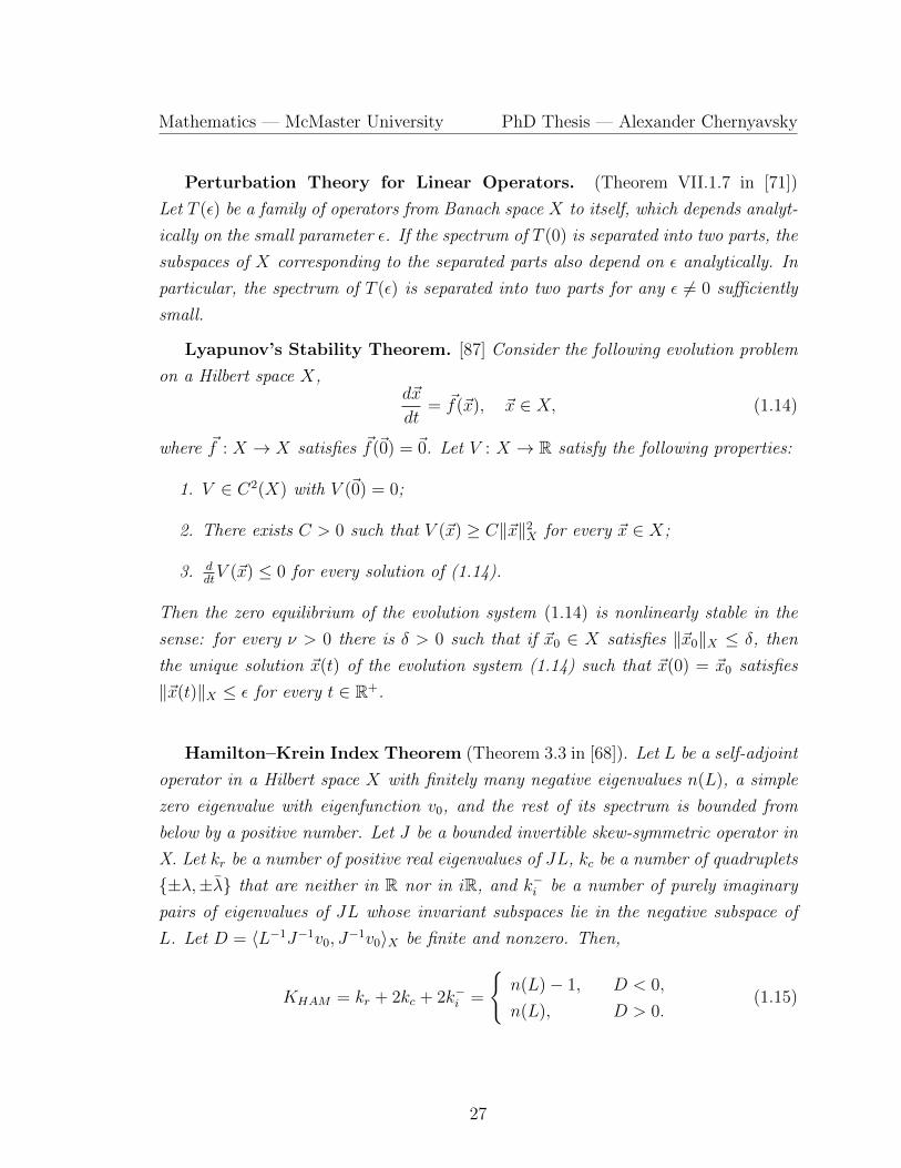
Hamilton–Krein Index Theorem (Theorem 3.3 in [68]). Let L be a self-adjoint
operator in a Hilbert space X with finitely many negative eigenvalues n(L), a simple
zero eigenvalue with eigenfunction v0, and the rest of its spectrum is bounded from
below by a positive number. Let J be a bounded invertible skew-symmetric operator in
X. Let kr be a number of positive real eigenvalues of JL, kc be a number of quadruplets
±λ,±λ that are neither in R nor in iR, and k−i be a number of purely imaginary
pairs of eigenvalues of JL whose invariant subspaces lie in the negative subspace of
L. Let D = 〈L−1J−1v0, J−1v0〉X be finite and nonzero. Then,
KHAM = kr + 2kc + 2k−i =
n(L)− 1, D < 0,
n(L), D > 0.(1.15)
27
Chapter 2
Breathers in Discrete Systems
2.1 Model
A simple yet universal model widely used to study coupled nonlinear oscillators is the
Frenkel-Kontorova (FK) model [85]. It describes a chain of classical particles coupled
to their neighbors and subjected to a periodic on-site potential. In the continuum
approximation, the FK model reduces to the sine-Gordon equation, which is exactly
integrable. The FK model is known to describe a rich variety of important nonlinear
phenomena, which find applications in solid-state physics and nonlinear science [27].
We consider here a two-array system of coupled pendula, where each pendulum is
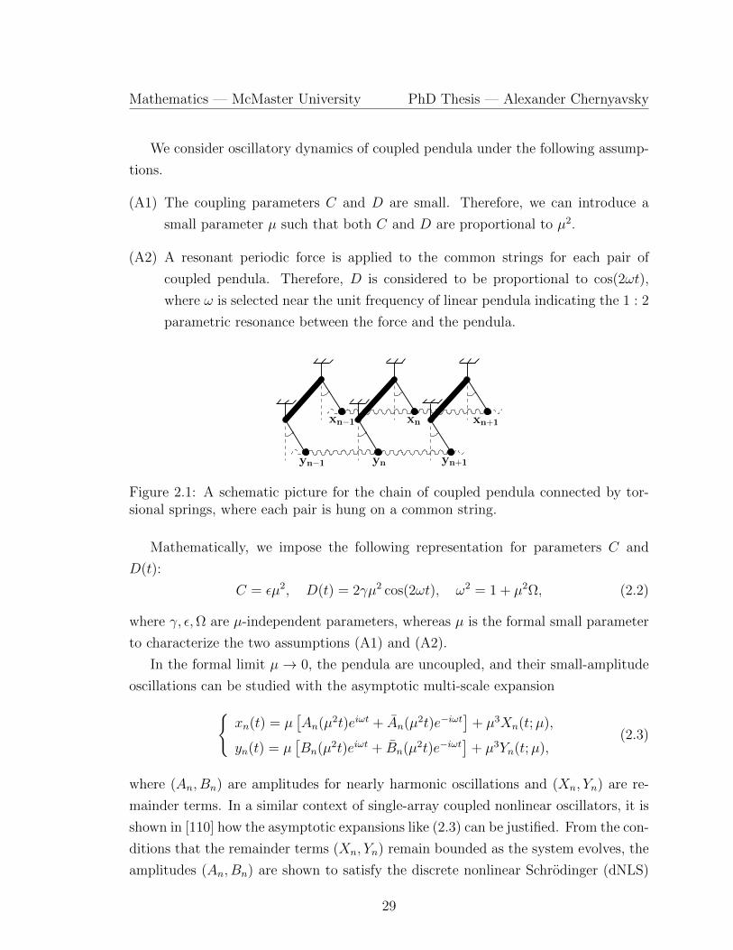
connected to the nearest neighbors by linear couplings. Figure 2.1 shows schematically
that each array of pendula is connected in the longitudinal direction by the torsional
springs, whereas each pair of pendula is connected in the transverse direction by a
common string. Newton’s equations of motion are given byxn + sin(xn) = C (xn+1 − 2xn + xn−1) +Dyn,
yn + sin(yn) = C (yn+1 − 2yn + yn−1) +Dxn,n ∈ Z, t ∈ R, (2.1)
where (xn, yn) correspond to the angles of two arrays of pendula, dots denote deriva-
tives of angles with respect to time t, and the positive parameters C and D describe
couplings between the two arrays in the longitudinal and transverse directions, re-
spectively. The type of coupling between the two pendula with the angles xn and yn
is referred to as the direct coupling between nonlinear oscillators (see Section 8.2 in
[118]).
28
Mathematics — McMaster University PhD Thesis — Alexander Chernyavsky
We consider oscillatory dynamics of coupled pendula under the following assump-
tions.
(A1) The coupling parameters C and D are small. Therefore, we can introduce a
small parameter µ such that both C and D are proportional to µ2.
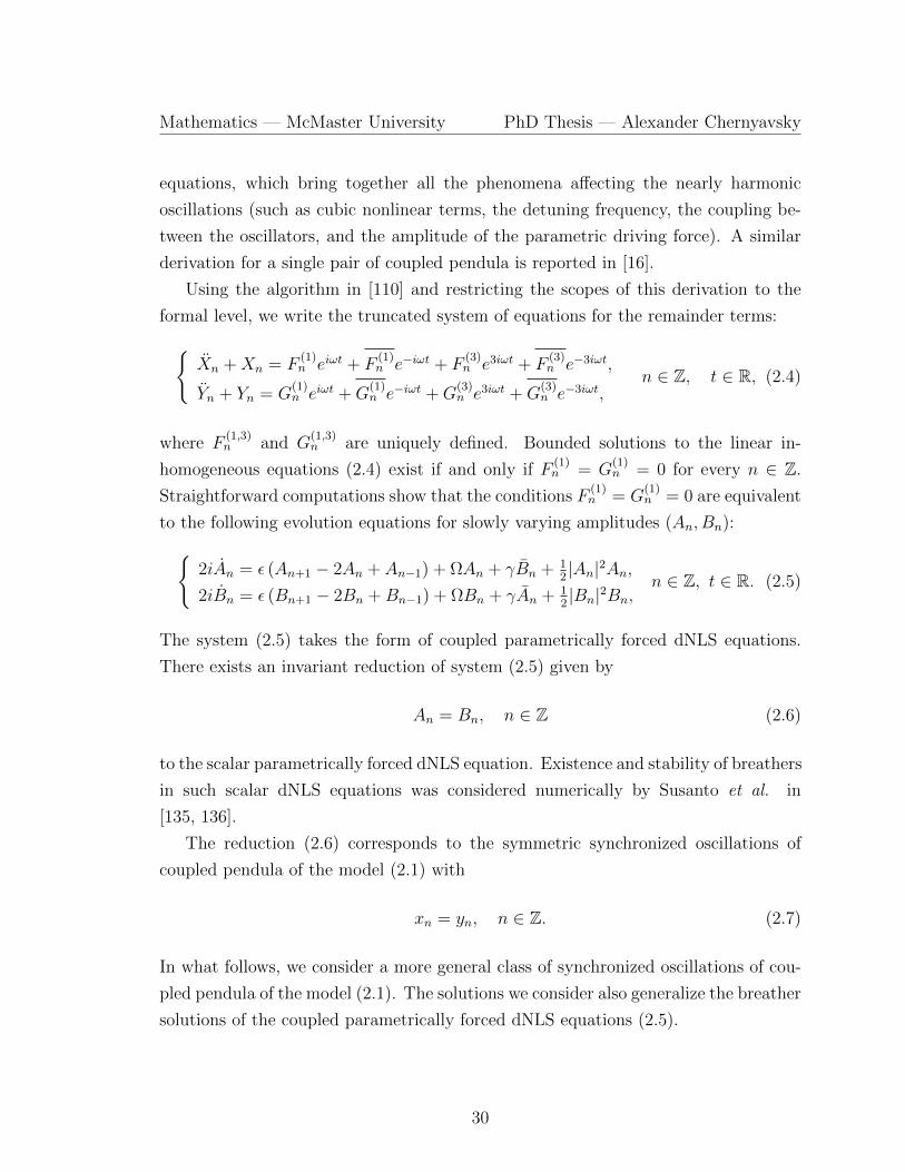
(A2) A resonant periodic force is applied to the common strings for each pair of
coupled pendula. Therefore, D is considered to be proportional to cos(2ωt),
where ω is selected near the unit frequency of linear pendula indicating the 1 : 2
parametric resonance between the force and the pendula.
yn
xnxn−1 xn+1
yn+1yn−1
Figure 2.1: A schematic picture for the chain of coupled pendula connected by tor-sional springs, where each pair is hung on a common string.
Mathematically, we impose the following representation for parameters C and
D(t):
C = εµ2, D(t) = 2γµ2 cos(2ωt), ω2 = 1 + µ2Ω, (2.2)
where γ, ε,Ω are µ-independent parameters, whereas µ is the formal small parameter
to characterize the two assumptions (A1) and (A2).
In the formal limit µ→ 0, the pendula are uncoupled, and their small-amplitude
oscillations can be studied with the asymptotic multi-scale expansionxn(t) = µ
[An(µ2t)eiωt + An(µ2t)e−iωt
]+ µ3Xn(t;µ),
yn(t) = µ[Bn(µ2t)eiωt + Bn(µ2t)e−iωt
]+ µ3Yn(t;µ),
(2.3)
where (An, Bn) are amplitudes for nearly harmonic oscillations and (Xn, Yn) are re-
mainder terms. In a similar context of single-array coupled nonlinear oscillators, it is
shown in [110] how the asymptotic expansions like (2.3) can be justified. From the con-
ditions that the remainder terms (Xn, Yn) remain bounded as the system evolves, the
amplitudes (An, Bn) are shown to satisfy the discrete nonlinear Schrodinger (dNLS)
29
Mathematics — McMaster University PhD Thesis — Alexander Chernyavsky
equations, which bring together all the phenomena affecting the nearly harmonic
oscillations (such as cubic nonlinear terms, the detuning frequency, the coupling be-
tween the oscillators, and the amplitude of the parametric driving force). A similar
derivation for a single pair of coupled pendula is reported in [16].
Using the algorithm in [110] and restricting the scopes of this derivation to the
formal level, we write the truncated system of equations for the remainder terms:Xn +Xn = F
(1)n eiωt + F
(1)n e−iωt + F
(3)n e3iωt + F
(3)n e−3iωt,
Yn + Yn = G(1)n eiωt +G
(1)n e−iωt +G
(3)n e3iωt +G
(3)n e−3iωt,
n ∈ Z, t ∈ R, (2.4)
where F(1,3)n and G
(1,3)n are uniquely defined. Bounded solutions to the linear in-
homogeneous equations (2.4) exist if and only if F(1)n = G
(1)n = 0 for every n ∈ Z.
Straightforward computations show that the conditions F(1)n = G
(1)n = 0 are equivalent
to the following evolution equations for slowly varying amplitudes (An, Bn):2iAn = ε (An+1 − 2An + An−1) + ΩAn + γBn + 1
2|An|2An,
2iBn = ε (Bn+1 − 2Bn +Bn−1) + ΩBn + γAn + 12|Bn|2Bn,
n ∈ Z, t ∈ R. (2.5)
The system (2.5) takes the form of coupled parametrically forced dNLS equations.
There exists an invariant reduction of system (2.5) given by
An = Bn, n ∈ Z (2.6)
to the scalar parametrically forced dNLS equation. Existence and stability of breathers
in such scalar dNLS equations was considered numerically by Susanto et al. in
[135, 136].
The reduction (2.6) corresponds to the symmetric synchronized oscillations of
coupled pendula of the model (2.1) with
xn = yn, n ∈ Z. (2.7)
In what follows, we consider a more general class of synchronized oscillations of cou-
pled pendula of the model (2.1). The solutions we consider also generalize the breather
solutions of the coupled parametrically forced dNLS equations (2.5).
30
Mathematics — McMaster University PhD Thesis — Alexander Chernyavsky
vn+1
un un+1
vn−1 vn
un−1
Figure 2.2: The chain of PT -symmetric dimers representing coupled pendula. Filled(empty) circles correspond to sites with gain (loss).
It turns out that the model (2.5) can be cast to the form of the parity–time reversal
(PT ) dNLS equations [16]. Using the variables
un :=1
4
(An − iBn
), vn :=
1
4
(An + iBn
), (2.8)
the system of coupled dNLS equations (2.5) is rewritten in the equivalent form2iun = ε (vn+1 − 2vn + vn−1) + Ωvn + iγun + 2 [(2|un|2 + |vn|2) vn + u2
nvn] ,
2ivn = ε (un+1 − 2un + un−1) + Ωun − iγvn + 2 [(|un|2 + 2|vn|2)un + unv2n] ,
(2.9)
which is the starting point for our analytical and numerical work. Figure 2.2 de-
picts schematically the chain of coupled pendula represented by (2.9). The invariant
reduction (2.6) for system (2.5) becomes
Im(eiπ4 un) = 0, Im(e−
iπ4 vn) = 0, n ∈ Z. (2.10)
In the context of hard nonlinear oscillators (e.g. in the framework of the φ4 theory),
the cubic nonlinearity may have the opposite sign compared to the one in the system
(2.9). However, given the applied context of the system of coupled pendula, we will
stick to the specific form (2.9) in further analysis.
2.2 Symmetries and conserved quantities
The system of coupled dNLS equations (2.9) is referred to as the PT -symmetric
dNLS equation because the solutions remain invariant with respect to the action of
31
Mathematics — McMaster University PhD Thesis — Alexander Chernyavsky
the parity P and time-reversal T operators given by
P[u
v
]=
[v
u
], T
[u(t)
v(t)
]=
[u(−t)v(−t)
]. (2.11)
The parameter γ introduces the gain–loss coefficient in each pair of coupled oscillators
due to the resonant periodic force. In the absence of all other effects, the γ-term of the
first equation of system (2.9) induces the exponential growth of amplitude un, whereas
the γ-term of the second equation induces the exponential decay of amplitude vn, if
γ > 0.
The system (2.9) truncated at a single site (say n = 0) is called the PT -symmetric
dimer. In the work of Barashenkov et al. [16], it was shown that all PT -symmetric
dimers with physically relevant cubic nonlinearities represent Hamiltonian systems
in appropriately introduced canonical variables. However, the PT -symmetric dNLS
equation on a lattice does not typically have a Hamiltonian form if γ 6= 0.
Nevertheless, the particular nonlinear functions arising in the system (2.9) corre-
spond to the PT -symmetric dimers with a cross–gradient Hamiltonian structure [16],
where variables (un, vn) are canonically conjugate. As a result, the system (2.9) on
the chain Z has additional conserved quantities. This fact looked like a mystery in
the recent works [15, 16].
Here we clarify the mystery in the context of the derivation of the PT -symmetric
dNLS equation (2.9) from the original system (2.1). Indeed, the system (2.1) of clas-
sical Newton particles has a standard Hamiltonian structure with the energy function
Hx,y(t) =∑n∈Z
1
2(x2
n + y2n) + 2− cos(xn)− cos(yn)
+1
2C(xn+1 − xn)2 +
1
2C(yn+1 − yn)2 −D(t)xnyn. (2.12)
Since the periodic movement of common strings for each pair of pendula result in
the time-periodic coefficient D(t), the energy Hx,y(t) is a periodic function of time t.
In addition, no other conserved quantities such as momenta exist typically in lattice
differential systems such as the system (2.1) due to broken continuous translational
symmetry.
32
Mathematics — McMaster University PhD Thesis — Alexander Chernyavsky
After the system (2.1) is reduced to the coupled dNLS equations (2.5) with the
asymptotic expansion (2.3), we can write the evolution problem (2.5) in the Hamilto-
nian form with the standard straight-gradient symplectic structure
2idAndt
=∂HA,B
∂An, 2i
dBn
dt=∂HA,B
∂Bn
, n ∈ Z, (2.13)
where the time variable t stands now for the slow time µ2t and the energy function is
HA,B =∑n∈Z
1
4(|An|4 + |Bn|4) + Ω(|An|2 + |Bn|2) + γ(AnBn + AnBn)
−ε|An+1 − An|2 − ε|Bn+1 −Bn|2. (2.14)
The energy functionHA,B is conserved in the time evolution of the Hamiltonian system
(2.13). In addition, there exists another conserved quantity
QA,B =∑n∈Z
(|An|2 − |Bn|2), (2.15)
which is related to the gauge symmetry (A,B)→ (Aeiα, Beiα) with α ∈ R for solutions
to the system (2.5).
When the transformation of variables (2.8) is used, the PT -symmetric dNLS equa-
tion (2.9) is cast to the Hamiltonian form with the cross-gradient symplectic structure
2idundt
=∂Hu,v
∂vn, 2i
dvndt
=∂Hu,v
∂un, n ∈ Z, (2.16)
where the energy function is
Hu,v =∑n∈Z
(|un|2 + |vn|2)2 + (unvn + unvn)2 + Ω(|un|2 + |vn|2)
−ε|un+1 − un|2 − ε|vn+1 − vn|2 + iγ(unvn − unvn). (2.17)
The gauge-related function is written in the form
Qu,v =∑n∈Z
(unvn + unvn). (2.18)
The functions Hu,v and Qu,v are conserved in the time evolution of the system (2.9).
33

Mathematics — McMaster University PhD Thesis — Alexander Chernyavsky
These functions follow from (2.14) and (2.15) after the transformation (2.8) is used.
Thus, the cross-gradient Hamiltonian structure of the PT -symmetric dNLS equation
(2.9) is inherited from the Hamiltonian structure of the coupled oscillator model (2.1).
2.3 Breathers (time-periodic solutions)
We characterize the existence of breathers supported by the PT -symmetric dNLS
equation (2.9). In particular, breather solutions are continued for small values of
coupling constant ε from solutions of the dimer equation arising at a single site, say
the central site at n = 0. We shall work in a sequence space `2(Z) of square integrable
complex-valued sequences.
Time-periodic solutions to the PT -symmetric dNLS equation (2.9) are given in
the form [80, 115]:
u(t) = Ue−12iEt, v(t) = V e−
12iEt, (2.19)
where the frequency parameter E is considered to be real, the factor 1/2 is introduced
for convenience, and the sequence (U, V ) is time-independent. The breather (2.19)
is a localized mode if (U, V ) ∈ `2(Z), which implies that |Un|, |Vn| → 0 as |n| → ∞.
The breather (2.19) is considered to be PT -symmetric with respect to the operators
in (2.11) if V = U .
The reduction (2.10) for symmetric synchronized oscillations is satisfied if
E = 0 : Im(eiπ4 Un) = 0, Im(e−
iπ4 Vn) = 0, n ∈ Z. (2.20)
The time-periodic breathers (2.19) with E 6= 0 generalize the class of symmetric
synchronized oscillations (2.20).
The time-independent sequence (U, V ) ∈ `2(Z) can be found from the stationary
PT -symmetric dNLS equation: EUn = ε (Vn+1 − 2Vn + Vn−1) + ΩVn + iγUn + 2[(
2|Un|2 + |Vn|2)Vn + U2
nVn],
EVn = ε (Un+1 − 2Un + Un−1) + ΩUn − iγVn + 2[(|Un|2 + 2|Vn|2
)Un + UnV
2n
].
(2.21)
The PT -symmetric breathers with V = U satisfy the following scalar difference equa-
tion
EUn = ε(Un+1 − 2Un + Un−1
)+ ΩUn + iγUn + 6|Un|2Un + 2U3
n. (2.22)
34

Mathematics — McMaster University PhD Thesis — Alexander Chernyavsky
−1.5 −1 −E0 0 E0 1 1.5
E
0.0
0.1
0.2
0.3
0.4
0.5
0.6
0.7
A
(a)1
−1.5 −1 −E0 0 E0 1 1.5
E
0.0
0.1
0.2
0.3
0.4
0.5
0.6
0.7
A
(c)
(b)
4
32
Figure 2.3: Solution branches for the dimer equation (2.23).
Note that the reduction (2.20) is compatible with equation (2.22) in the sense that if
E = 0 and Un = Rne−iπ/4, then R satisfies a real-valued difference equation.
Let us set ε = 0 for now and consider solutions to the dimer equation at the central
site n = 0:
(E − iγ)U0 − ΩU0 = 6|U0|2U0 + 2U30 . (2.23)
The parameters γ and Ω are considered to be fixed, and the breather parameter E
is thought to parameterize continuous branches of solutions to the nonlinear alge-
braic equation (2.23). The solution branches depicted on Figure 2.3 are given in the
following lemma.
Lemma 4. Assume γ 6= 0. The algebraic equation (2.23) admits the following solu-
tions depending on γ and Ω:
(a) Ω > |γ| - two symmetric unbounded branches exist for ±E > E0,
(b) Ω < |γ| - an unbounded branch exists for every E ∈ R,
(c) Ω < −|γ| - a bounded branch exists for −E0 < E < E0,
where E0 :=√
Ω2 − γ2.
Proof. Substituting the decomposition U0 = Aeiθ with A > 0 and θ ∈ [−π, π) into
the algebraic equation (2.23), we obtain
sin(2θ) =γ
4A2 + Ω, cos(2θ) =
E
8A2 + Ω. (2.24)
35
Mathematics — McMaster University PhD Thesis — Alexander Chernyavsky
Excluding θ by using the fundamental trigonometric identity, we obtain the explicit
parametrization of the solutions to the algebraic equation (2.23) by the amplitude
parameter A:
E2 = (8A2 + Ω)2
[1− γ2
(4A2 + Ω)2
]. (2.25)
The zero-amplitude limit A = 0 is reached if |Ω| > |γ|, in which case E = ±E0, where
E0 :=√
Ω2 − γ2. If |Ω| < |γ| , the solution branches (if they exist) are bounded away
from the zero solution.
Now we analyze the three cases of parameters γ and Ω formulated in the lemma.
(a) If Ω > |γ|, then the parametrization (2.25) yields a monotonically increasing
map R+ 3 A2 7→ E2 ∈ (E20 ,∞) because
dE2
dA2=
8(8A2 + Ω)
(4A2 + Ω)3
[2(4A2 + Ω)3 − γ2Ω
]> 0. (2.26)
In the two asymptotic limits, we obtain from (2.25):
E2 = E20 +O(A2) as A→ 0 and E2 = 64A4 +O(A2) as A→∞.
See Figure 2.3(a).
(b) If Ω < |γ|, the parametrization (2.25) yields a monotonically increasing map
(A2+,∞) 3 A2 7→ E2 ∈ R+, where
A2+ :=
|γ| − Ω
4. (2.27)
Indeed, we note that 4A2 + Ω ≥ 4A2+ + Ω = |γ| > 0 and
2(4A2 + Ω)3 − γ2Ω ≥ γ2(2|γ| − Ω) > 0,
so that the derivative in (2.26) is positive for every A2 ≥ A2+. We have
E2 → 0 as A2 → A2+ and E2 = 64A4 +O(A2) as A→∞.
See Figure 2.3(b).
36
Mathematics — McMaster University PhD Thesis — Alexander Chernyavsky
(c) If Ω < −|γ|, then the parametrization (2.25) yields a monotonically decreasing
map (0, A2−) 3 A2 7→ E2 ∈ (0, E2
0), where
A2− := min
|Ω| − |γ|4
,|Ω|8
. (2.28)
In (2.28), the first choice is made if |Ω| ∈ (|γ|, 2|γ|) and the second choice is
made if |Ω| ∈ (2|γ|,∞). Both choices are the same if |Ω| = 2|γ|. We note that
8A2 ≤ |Ω|, therefore, the derivative (2.26) needs to be rewritten in the form
dE2
dA2= −8(|Ω| − 8A2)
(|Ω| − 4A2)3
[2(|Ω| − 4A2)3 − γ2|Ω|
]< 0, (2.29)
where 2(|Ω| − 4A2)3 − γ2|Ω| > 0 for both |Ω| ∈ (|γ|, 2|γ|) and |Ω| ∈ [2|γ|,∞).
In the two asymptotic limits, we obtain from (2.25):
E2 = E20 +O(A2) as A→ 0 and E2 → 0 as A2 → A2
−.
See Figure 2.3(c).
Note that branches (b) and (c) coexist for Ω < −|γ|.
Remark 1. The reduction (2.20) corresponds to the choice:
E = 0, θ = −π4, 4A2 + Ω + γ = 0.
If γ > 0, this choice corresponds to A = A− for Ω ∈ (−2|γ|,−|γ|), that is, the point
E = 0 on branch (c). If γ < 0, it corresponds to A = A+ for any Ω < |γ|, that is, the
point E = 0 on branch (b).
Every solution of Lemma 4 can be extended to a breather on the chain Z which
satisfies the spatial symmetry condition in addition to the PT symmetry:
U−n = Un = Vn = V−n, n ∈ Z. (2.30)
With two applications of the implicit function theorem (see Section 1.5.6), we
prove the following main result of this section.
37
Mathematics — McMaster University PhD Thesis — Alexander Chernyavsky
Theorem 6. Fix γ 6= 0, Ω 6= −2|γ|, and E 6= ±E0, where E0 :=√
Ω2 − γ2 > 0
if |Ω| > |γ|. There exists ε0 > 0 sufficiently small and C0 > 0 such that for every
ε ∈ (−ε0, ε0), there exists a unique solution U ∈ l2(Z) to the difference equation (2.22)
satisfying the symmetry (2.30) and the bound
∣∣U0 − Aeiθ∣∣+ sup
n∈N|Un| ≤ C0|ε|, (2.31)
where A and θ are defined in Lemma 4. Moreover, the solution U is smooth in ε.
Proof. In the first application of the implicit function theorem, we consider the fol-
lowing system of algebraic equations
EUn = ε(Un+1 − 2Un + Un−1
)+ ΩUn + iγUn + 6|Un|2Un + 2U3
n, n ∈ N, (2.32)
where U0 ∈ C is given, in addition to parameters γ, Ω, and E.
Let x = Unn∈N, X = `2(N), y = ε, Y = R, and Z = `2(N). Then, we have
F (0, 0) = 0 and the Jacobian operator DxF (0, 0) is given by identical copies of the
matrix [E − iγ −Ω
−Ω E + iγ
],
with the eigenvalues λ± := E±√
Ω2 − γ2. By the assumption of the lemma, λ± 6= 0,
so that the Jacobian operator DxF (0, 0) is one-to-one and onto. By the implicit
function theorem, for every U0 ∈ C and every ε 6= 0 sufficiently small, there exists a
unique small solution U ∈ `2(N) of the system (2.32) such that
‖U‖l2(N) ≤ C1|ε||U0|, (2.33)
where the positive constant C1 is independent from ε and U0.
Thanks to the symmetry of the difference equation (2.22), we find that U−n = Un,
n ∈ N satisfy the same system (2.32) with −n ∈ N, with the same unique solution.
In the second application of the implicit function theorem, we consider the follow-
ing algebraic equation
EU0 = 2ε(U1 − U0
)+ ΩU0 + iγU0 + 6|U0|2U0 + 2U3
0 , (2.34)
38

Mathematics — McMaster University PhD Thesis — Alexander Chernyavsky
where U1 ∈ C depends on U0, γ, Ω, and E, satisfies the bound (2.33), and is uniquely
defined by the previous result.
Let x = U0, X = C, y = ε, Y = R, and Z = C. Then, we have F (Aeiθ, 0) = 0,
where A and θ are defined in Lemma 4. The Jacobian operator DxF (Aeiθ, 0) is given
by the matrix [E − iγ − 6U2
0 − 6U20 −Ω− 12|U0|2
−Ω− 12|U0|2 E + iγ − 6U20 − 6U2
0
]∣∣∣∣U0=Aeiθ
=
[E − iγ − 12EA2
Ω+8A2 −Ω− 12A2
−Ω− 12A2 E + iγ − 12EA2
Ω+8A2
]. (2.35)
We show in Lemma 5 below that the matrix given by (2.35) is invertible under the
conditions γ 6= 0 and Ω 6= −2|γ|. By the implicit function theorem, for every ε 6= 0
sufficiently small, there exists a unique solution U0 ∈ C to the algebraic equation
(2.34) near Aeiθ such that ∣∣U0 − Aeiθ∣∣ ≤ C2|ε|, (2.36)
where the positive constant C2 is independent from ε. The bound (2.31) holds thanks
to the bounds (2.33) and (2.36). Since both equations (2.32) and (2.34) are smooth
in ε, the solution U is smooth in ε.
In the following result, we show that the matrix given by (2.35) is invertible for
every branch of Lemma 4 with an exception of a single point E = 0 on branch (c) for
Ω = −2|γ|.
Lemma 5. With the exception of the point E = 0 on branch (c) of Lemma 4 for
Ω = −2|γ|, the matrix given by (2.35) is invertible for every γ 6= 0.
Proof. The matrix given by (2.35) has zero eigenvalue if and only if its determinant
is zero, which happens at
E2(Ω− 4A2)2
(Ω + 8A2)2+ γ2 − (Ω + 12A2)2 = 0.
Eliminating E2 by using parametrization (2.25) and simplifying the algebraic equation
for nonzero A2, we reduce it to the form
2(Ω + 4A2)3 = Ωγ2. (2.37)
39
Mathematics — McMaster University PhD Thesis — Alexander Chernyavsky
We now check if this constraint can be satisfied for the three branches of Lemma 4.
(a) If Ω > |γ|, the constraint (2.37) is not satisfied because the left-hand side
2(Ω + 4A2)3 ≥ 2Ω3 > 2Ωγ2
exceeds the right-hand side Ωγ2.
(b) If Ω < |γ| and A2 ≥ A2+, where A2
+ is given by (2.27), the constraint (2.37) is
not satisfied because the left-hand side
2(Ω + 4A2)3 ≥ 2(Ω + 4A2+)3 = 2|γ|3
exceeds the left-hand side Ωγ2 both for Ω ∈ [0, |γ|) and for Ω < 0.
(c) If Ω < −|γ| and A2 ≤ A2−, where A2
− is given by (2.28), the constraint (2.37) is
not satisfied because the left-hand side is estimated by
2(4A2 + Ω)3 ≤ 2(4A2− − |Ω|)3 = min−2|γ|3,−|Ω|3/4.
In the first case, we have |Ω| ∈ (|γ|, 2|γ|), so that the left-hand side is strictly
smaller than −|Ω|γ2. In the second case, we have |Ω| > 2|γ|, so that the left-
hand side is also strictly smaller than −|Ω|γ2. Only if |Ω| = 2|γ|, the constraint
(2.37) is satisfied at E = 0, when A2 = A2− and
2(4A2 + Ω)3 = −2|γ|3 = −|Ω|γ2 = Ωγ2.
Hence, the matrix (2.35) is invertible for all parameter values with one exceptional
case.
Remark 2. In the asymptotic limit E2 = 64A4 + O(A2) as A → ∞, see Lemma 4,
the matrix (2.35) is expanded asymptotically as
−1
2
[E 3|E|
3|E| E
]+O(1) as |E| → ∞, (2.38)
with the two eigenvalues λ1 = E and λ2 = −2E. Thus, the matrix given by (2.38) is
invertible for every branch extending to sufficiently large values of E.
40
Mathematics — McMaster University PhD Thesis — Alexander Chernyavsky
2.4 Stability of zero equilibrium
Here we discuss the linear stability of the zero equilibrium in the PT -symmetric dNLS
equation (2.9). The following proposition yields a simple result.
Proposition 1. The zero equilibrium of the PT -symmetric dNLS equation (2.9) is
linearly stable if |γ| < γ0, where
γ0 :=
Ω− 4ε, Ω > 0,
|Ω|, Ω < 0.(2.39)
The zero equilibrium is linearly unstable if |γ| > γ0.
Proof. Truncating the PT -symmetric dNLS equation (2.9) at the linear terms and
using the Fourier transform
un(t) =1
2π
∫ π
−πU(k)eikn+iω(k)tdk, (2.40)
we obtain the linear homogeneous system
D(k)
[U(k)
V (k)
]=
[0
0
], where D(k) :=
[−2ω(k)− iγ −Ω + 4ε sin2(k/2)
−Ω + 4ε sin2(k/2) −2ω(k) + iγ
].
The determinant of D(k) is zero if and only if ω(k) is found from the quadratic
equation
4ω2(k) + γ2 −(
Ω− 4ε sin2 k
2
)2
= 0. (2.41)
For any |γ| < γ0, where γ0 is given by (2.39), the two branches ±ω(k) found from the
quadratic equation (2.41) are real-valued and non-degenerate for every k ∈ [−π, π].
Therefore, the zero equilibrium is linearly stable.
On the other hand, for any |γ| > γ0, the values of ω(k) are purely imaginary either
near k = ±π if Ω > 0 or near k = 0 if Ω < 0. Therefore, the zero equilibrium is
linearly unstable.
Remark 3. The value γ0 given by (2.39) represents the phase transition threshold
and the PT -symmetric dNLS equation (2.9) has broken PT -symmetry for |γ| > γ0.
If ε = 0, the zero equilibrium is only linearly stable for |γ| < |Ω|. Since the
localized breathers cannot be stable when the zero background is unstable, we shall
41
Mathematics — McMaster University PhD Thesis — Alexander Chernyavsky
study stability of breathers only for the case when |γ| < |Ω|, that is, in the regime of
unbroken PT -symmetry.
2.5 Variational characterization of breathers
It follows from Theorem 6 that each interior point on the solution branches shown
on Figure 2.3 generates a fundamental breather of the PT -symmetric dNLS equation
(2.9). We shall now characterize these breathers as relative equilibria of the energy
function.
Thanks to the cross-gradient symplectic structure (2.16), the stationary PT -
symmetric dNLS equation (2.21) can be written in the gradient form
EUn =∂Hu,v
∂Vn, EVn =
∂Hu,v
∂Un, n ∈ Z. (2.42)
Keeping in mind the additional conserved quantity Qu,v given by (2.18), we conclude
that the stationary solution (U, V ) is a critical point of the combined energy function
given by
HE := Hu,v − EQu,v. (2.43)
If we want to apply the Lyapunov method in order to study nonlinear stability
of stationary solutions in Hamiltonian systems, we shall investigate convexity of the
second variation of the combined energy functional HE at (U, V ). Using the expansion
u = U + u, v = V + v and introducing extended variables Φ and φ with the blocks
Φn := (Un, Un, Vn, Vn), φn := (un, un,vn, vn), (2.44)
we can expand the smooth function HE up to the quadratic terms in φ:
HE(Φ + φ) = HE(Φ) +1
2〈H′′Eφ, φ〉l2 +O(‖φ‖3
l2), (2.45)
whereH′′E is the self-adjoint (Hessian) operator defined on `2(Z) and the scalar product
was used in the following form:
〈x, y〉l2 =∑k∈Z
xkyk.
42
Mathematics — McMaster University PhD Thesis — Alexander Chernyavsky
Using (2.17) and (2.18), the Hessian operator can be computed explicitly as follows
H′′E = L+ ε∆, (2.46)
where blocks of L at each lattice node n ∈ Z are given by
Ln =
Ω + 8|Un|2 2(U2
n + U2n) −E − iγ + 4(U2
n + U2n) 4|Un|2
2(U2n + U2
n) Ω + 8|Un|2 4|Un|2 −E + iγ + 4(U2n + U2
n)
−E + iγ + 4(U2n + U2
n) 4|Un|2 Ω + 8|Un|2 2(U2n + U2
n)
4|Un|2 −E − iγ + 4(U2n + U2
n) 2(U2n + U2
n) Ω + 8|Un|2
and ∆ is the discrete Laplacian operator applied to blocks of φ at each lattice node
n ∈ Z:
(∆φ)n = φn+1 − 2φn + φn−1.
In the expression for Ln, we have used the PT -symmetry condition V = U for the
given stationary solution (U, V ).
We study convexity of the combined energy functional HE at (U, V ). Since the
zero equilibrium is linearly stable only for |γ| < |Ω| (if ε = 0), we only consider
breathers of Theorem 6 for |γ| < |Ω|.With an application of the perturbation theory for linear operators (see Sec-
tion 1.5.6), we prove the following main result of this section.
Theorem 7. Fix γ 6= 0, Ω, and E along branches of the PT -symmetric breathers
(U, V ) given by Theorem 6 such that |Ω|>|γ| and E 6= ±E0, where E0 :=√
Ω2 − γ2> 0.
For every ε > 0 sufficiently small, the operator H′′E admits a one-dimensional kernel
in `2(Z) spanned by the eigenvector σΦ due to the gauge invariance, where the blocks
of the eigenvector are given by
(σΦ)n := (Un,−Un, Vn,−Vn). (2.47)
In addition,
• If |E| > E0, the spectrum of H′′E in `2(Z) includes infinite-dimensional positive
and negative parts.
• If |E| < E0 and Ω < −|γ|, the spectrum of H′′E in `2(Z) includes an infinite-
dimensional negative part and either three or one simple positive eigenvalues for
branches (b) and (c) of Lemma 4 respectively.
43
Mathematics — McMaster University PhD Thesis — Alexander Chernyavsky
Proof. If ε = 0, the breather solution of Theorem 6 is given by Un = 0 for every
n 6= 0 and U0 = Aeiθ, where A and θ are defined by Lemma 4. In this case, the linear
operator H′′E = L decouples into 4-by-4 blocks for each lattice node n ∈ Z.For n = 0, the 4-by-4 block of the linear operator L is given by
L0 =
Ω + 8A2 4A2 cos(2θ) −E − iγ + 8A2 cos(2θ) 4A2
4A2 cos(2θ) Ω + 8A2 4A2 −E + iγ + 8A2 cos(2θ)
−E + iγ + 8A2 cos(2θ) 4A2 Ω + 8A2 4A2 cos(2θ)
4A2 −E − iγ + 8A2 cos(2θ) 4A2 cos(2θ) Ω + 8A2
.
Using relations (2.24) and (2.25), as well as symbolic computations with MAPLE,
we found that the 4-by-4 matrix block L0 admits a simple zero eigenvalue and three
nonzero eigenvalues µ1, µ2, and µ3 given by
µ1 = 2(4A2 + Ω), (2.48)
µ2,3 = 12A2 + Ω±√
(4A2 − Ω)2 +16ΩA2γ2
(4A2 + Ω)2. (2.49)
For each branch of Lemma 4 with γ 6= 0 and E 6= ±E0, we have 4A2 + Ω 6= 0, so that
µ1 6= 0. Furthermore, either µ2 = 0 or µ3 = 0 if and only if
(12A2 + Ω)2(4A2 + Ω)2 = (16A4 − Ω2)2 + 16Ωγ2A2.
Expanding this equation for nonzero A yields constraint (2.37). With the exception
of a single point E = 0 at Ω = −2|γ|, we showed in Lemma 5 that the constraint
(2.37) does not hold for any of the branches of Lemma 4. Therefore, µ2 6= 0 and
µ3 6= 0 along each branch of Lemma 4 and the signs of µ1, µ2, and µ3 for each branch
of Lemma 4 can be obtained in the limit A→∞ for branches (a) and (b) or A→ 0
for branch (c). By means of these asymptotic computations as A→∞ or A→ 0, we
obtain the following results for the three branches shown on Figure 2.3:
(a) µ1, µ2, µ3 > 0.
(b) µ1, µ2, µ3 > 0.
(c) µ1 < 0, µ2 > 0, and µ3 < 0.
44
Mathematics — McMaster University PhD Thesis — Alexander Chernyavsky
For n ∈ Z\0, the 4-by-4 block of the linear operator L is given by
Ln =
Ω 0 −E − iγ 0
0 Ω 0 −E + iγ
−E + iγ 0 Ω 0
0 −E − iγ 0 Ω
. (2.50)
Each block has two double eigenvalues µ+ and µ− given by
µ+ = Ω +√E2 + γ2, µ− = Ω−
√E2 + γ2.
Since there are infinitely many nodes with n 6= 0, the points µ+ and µ− have infinite
multiplicity in the spectrum of the linear operator L. Furthermore, we can sort up
the signs of µ+ and µ− for each point on the three branches shown on Figure 2.3:
(1),(3) If |E| > E0 :=√
Ω2 − γ2, then µ+ > 0 and µ− < 0.
(2),(4) If |E| < E0 and Ω < −|γ|, then µ+, µ− < 0.
By using the perturbation theory for linear operators, we argue as follows:
• Since H′′E is Hermitian on `2(Z), its spectrum is a subset of the real line for
every ε 6= 0.
• The zero eigenvalue persists with respect to ε 6= 0 at zero because the eigenvector
(2.47) belongs to the kernel of H′′E due to the gauge invariance for every ε 6= 0.
• The other eigenvalues of L are isolated away from zero. The spectrum of H′′E is
continuous with respect to ε and includes infinite-dimensional parts near points
µ+ and µ− for small ε > 0 (which may include continuous spectrum and isolated
eigenvalues) as well as simple eigenvalues near µ1,2,3 (if µ1,2,3 are different from
µ±).
The statement of the theorem follows from the perturbation theory and the count
of signs of µ1,2,3 and µ± above.
45
Mathematics — McMaster University PhD Thesis — Alexander Chernyavsky
Remark 4. In the asymptotic limit E2 = 64A4 +O(A2) as A→∞, we can sort out
eigenvalues of H′′E asymptotically as:
µ1 ≈ |E|, µ2 ≈ 2|E|, µ3 ≈ |E|, µ+ ≈ |E|, µ− ≈ −|E|, (2.51)
where the remainder terms are O(1) as |E| → ∞. The values µ1, µ3, and µ+ are
close to each other as |E| → ∞.
Remark 5. It follows from Theorem 7 that for |E| > E0, the breather (U, V ) is a
saddle point of the energy functional HE with infinite-dimensional positive and neg-
ative invariant subspaces of the Hessian operator H′′E. This is very similar to the
Hamiltonian systems of the Dirac type, where stationary states are located in the gap
between the positive and negative continuous spectrum. This property holds for points
1 and 3 on branches (a) and (b) shown on Figure 2.3.
Remark 6. No branches other than |E| > E0 exist for Ω > |γ|. On the other hand,
points 2 and 4 on branches (b) and (c) shown on Figure 2.3 satisfy |E| < E0 and
Ω < −|γ|. The breather (U, V ) is a saddle point of HE for these points and it only
has three (one) directions of positive energy in space `2(Z) for point 2 (point 4).
2.6 Spectral and orbital stability of breathers
Spectral stability of breathers can be studied for small values of coupling constant ε
by using the perturbation theory [115]. First, we linearize the PT -symmetric dNLS
equation (2.9) at the breather (2.19) by using the expansion
u(t) = e−12iEt [U + u(t)] , v(t) = e−
12iEt [V + v(t)] ,
where (u,v) is a small perturbation satisfying the linearized equations
2iun + Eun = ε (vn+1 − 2vn + vn−1) + Ωvn + iγun
+2 [2 (|Un|2 + |Vn|2) vn + (U2n + V 2
n )vn
+ 2(UnVn + UnVn)un + 2UnVnun],
2ivn + Evn = ε (un+1 − 2un + un−1) + Ωun − iγvn
+2 [2 (|Un|2 + |Vn|2) un + (U2n + V 2
n )un
+2 (UnVn + UnVn)vn + 2UnVnvn].
(2.52)
46
Mathematics — McMaster University PhD Thesis — Alexander Chernyavsky
The spectral stability problem arises from the linearized equations (2.52) after the
separation of variables:
u(t) = ϕe12λt, u(t) = ψe
12λt, v(t) = χe
12λt, v(t) = νe
12λt,
where φ := (ϕ, ψ, χ, ν) is the eigenvector corresponding to the spectral parameter λ.
Note that (ϕ, ψ) and (χ, ν) are no longer complex conjugate to each other if λ has a
nonzero imaginary part. The spectral problem can be written in the explicit form
(E + iλ− iγ)ϕn − Ωχn = ε (χn+1 − 2χn + χn−1)
+ 2[2|Un|2(ψn + 2χn) + (U2
n + U2n)(2ϕn + νn)
],
(E − iλ+ iγ)ψn − Ωνn = ε (νn+1 − 2νn + νn−1)
+ 2[2|Un|2(ϕn + 2νn) + (U2
n + U2n)(2ψn + χn)
],
(E + iλ+ iγ)χn − Ωϕn = ε (ϕn+1 − 2ϕn + ϕn−1)
+ 2[2|Un|2(2ϕn + νn) + (U2
n + U2n)(ψn + 2χn)
],
(E − iλ− iγ)νn − Ωψn = ε (ψn+1 − 2ψn + ψn−1)
+ 2[2|Un|2(2ψn + χn) + (U2
n + U2n)(ϕn + 2νn)
],
(2.53)
where we have used the condition V = U for the PT -symmetric breathers. Recalling
definition of the Hessian operator H′′E in (2.46), we can rewrite the spectral problem
(2.53) in the Hamiltonian form:
SH′′Eφ = iλφ, (2.54)
where S is a symmetric matrix with the blocks at each lattice node n ∈ Z given by
S :=
0 0 1 0
0 0 0 −1
1 0 0 0
0 −1 0 0
. (2.55)
We note the Hamiltonian symmetry of the eigenvalues of the spectral problem (2.54).
Proposition 2. Eigenvalues of the spectral problem (2.54) occur either as real or
imaginary pairs or as quadruplets in the complex plane.
47
Mathematics — McMaster University PhD Thesis — Alexander Chernyavsky
Proof. Assume that λ ∈ C is an eigenvalue of the spectral problem (2.54) with
the eigenvector (ϕ, ψ, χ, ν). Then, λ is an eigenvalue of the same problem with
the eigenvector (ψ, ϕ, ν, χ), whereas −λ is also an eigenvalue with the eigenvector
(ν, χ, ψ, ϕ).
If Ω < −|γ| and |E| < E0 :=√
Ω2 − γ2 (points 2 and 4 shown on Figure 2.3),
Theorem 7 implies that the self-adjoint operator H′′E in `2(Z) is negative-definite with
the exception of either three (point 2) or one (point 4) simple positive eigenvalues. In
this case, we can apply Hamilton–Krein index theorem (see Section 1.5.6) in order to
characterize the spectrum of SH′′E.
Lemma 6. Fix γ 6= 0, Ω < −|γ|, and 0<|E|<E0, where E0 :=√
Ω2 − γ2 > 0. For ev-
ery ε > 0 sufficiently small, KHAM = 2 for branch (b) of Lemma 4 and KHAM = 0 for
branch (c) of Lemma 4 with Ω < −2√
2|γ|. For branch (c) with Ω ∈ (−2√
2|γ|,−|γ|),
there exists a value Es ∈ (0, E0) such that KHAM = 1 for 0 < |E| < Es and KHAM = 0
for Es < |E| < E0.
Proof. If γ 6= 0, Ω < −|γ|, |E| < E0, and ε > 0 is sufficiently small, Theorem 7
implies that the spectrum of H′′E in `2(Z) has finitely many positive eigenvalues and
a simple zero eigenvalue with eigenvector σΦ. Therefore, the Hamilton–Krein index
theorem is applied in `2(Z) for L = −H′′E, J = iS, and v0 = σΦ. We shall verify that
H′′E(σΦ) = 0, SH′′E(∂EΦ) = σΦ, (2.56)
where σΦ is given by (2.47) and ∂EΦ denotes derivative of Φ with respect to parameter
E. The first equationH′′E(σΦ) = 0 follows by Theorem 7. By differentiating equations
(2.21) in E, we obtain H′′E(∂EΦ) = SσΦ for every E, for which the solution Φ is
differentiable in E. For ε = 0, the limiting solution of Lemma 4 is differentiable in
E for every E 6= 0 and E 6= ±E0. Due to smoothness of the continuation in ε by
Theorem 7, this property holds for every ε > 0 sufficiently small.
By using (2.56) with S−1 = S, we obtain
D = −〈(H′′E)−1SσΦ,SσΦ〉`2 = −〈∂EΦ,SσΦ〉`2
= −∑n∈Z
∂E(UnVn + UnVn
)= −dQu,v
dE, (2.57)
48
Mathematics — McMaster University PhD Thesis — Alexander Chernyavsky
where we have used the definition of Qu,v in (2.18). We compute the slope condition
at ε = 0:
dQu,v
dE
∣∣∣∣ε=0
= 2d
dE
A2E
8A2 + Ω= 4(8A2 + Ω)
dA2
dE2
[1− Ωγ2
(4A2 + Ω)3
], (2.58)
where relations (2.24) and (2.25) have been used.
For branch (b) of Lemma 4 with Ω < −|γ|, we have dA2/dE2 > 0 and |Ω| < 4A2,
so that dQu,v/dE > 0. By continuity, dQu,v/dE remains strictly positive for small
ε > 0. Thus, D < 0 and KHAM = 2 by the Hamilton–Krein index theorem.
For branch (c) of Lemma 4 with Ω < −|γ|, we have dA2/dE2 < 0 and |Ω| > 8A2.
Therefore, we only need to inspect the sign of the expression (4A2 + Ω)3 − Ωγ2. If
Ω < −2√
2|γ|, then for every A2 ∈ (0, A2−), we have
(4A2 + Ω)3 − Ωγ2 ≤ (4A2− + Ω)3 − Ωγ2 =
1
8Ω3 − Ωγ2 ≤ 1
8Ω(Ω2 − 8γ2) < 0,
therefore, D < 0 and KHAM = 0 by the Hamilton–Krein index theorem.
On the other hand, if −2√
2|γ| < Ω < −|γ|, we have (4A2 + Ω)3 − Ωγ2 < 0 at
A = 0 (E = E0) and (4A2 + Ω)3−Ωγ2 > 0 at A = A− (E = 0). Since the dependence
of A versus E is monotonic, there exists a value Es ∈ (0, E0) such that KHAM = 1 for
0 < |E| < Es and KHAM = 0 for Es < |E| < E0.
If KHAM = 0 and D 6= 0, orbital stability of a critical point of HE in space `2(Z)
can be proved from the Hamilton–Krein theorem (see [68] and references therein).
Orbital stability of breathers is understood in the following sense.
Definition 10. We say that the breather solution (2.19) is orbitally stable in `2(Z)
if for every ν > 0 sufficiently small, there exists δ > 0 such that if ψ(0) ∈ `2(Z)
satisfies ‖ψ(0)− Φ‖`2 ≤ δ, then the unique global solution ψ(t) ∈ `2(Z), t ∈ R to the
PT -symmetric dNLS equation (2.9) satisfies the bound
infα∈R‖eiαψ(t)− Φ‖`2 ≤ ν, for every t ∈ R. (2.59)
The definition of instability of breathers is given by negating Definition 10. The
following result gives orbital stability or instability for branch (c) shown on Figure 2.3.
49
Mathematics — McMaster University PhD Thesis — Alexander Chernyavsky
Theorem 8. Fix γ 6= 0, Ω < −|γ|, and 0 < |E| < E0. For every ε > 0 sufficiently
small, the breather (U, V ) for branch (c) of Lemma 4 is orbitally stable in `2(Z) if
Ω < −2√
2|γ|. For every Ω ∈ (−2√
2|γ|,−|γ|), there exists a value Es ∈ (0, E0) such
that the breather (U, V ) is orbitally stable in `2(Z) if Es < |E| < E0 and unstable if
0 < |E| < Es.
Proof. The theorem is a corollary of Lemma 6 for branch (c) of Lemma 4 and the
orbital stability theory from [68].
Orbital stability of breathers for branches (a) and (b) of Lemma 4 does not follow
from the standard theory because KHAM = ∞ for |E| > E0 and KHAM = 2 > 0 for
branch (b) with |E| < E0. Nevertheless, by using smallness of parameter ε and the
construction of the breather (U, V ) in Theorem 6, spectral stability of breathers can
be considered directly. Spectral stability and instability of breathers is understood in
the following sense.
Definition 11. We say that the breather solution (2.19) is spectrally stable if λ ∈ iRfor every bounded solution of the spectral problem (2.54). On the other hand, if the
spectral problem (2.54) admits an eigenvalue λ /∈ iR with an eigenvector in `2(R), we
say that the breather solution (2.19) is spectrally unstable.
The following theorem gives spectral stability of breathers for branches (a) and
(b) shown on Figure 2.3.
Theorem 9. Fix γ 6= 0, |Ω| > |γ|, and E along branches (a) and (b) of Lemma 4
with E 6= 0 and E 6= ±E0. For every ε > 0 sufficiently small, the spectral problem
(2.54) admits a double zero eigenvalue with the generalized eigenvectors
H′′E(σΦ) = 0, SH′′E(∂EΦ) = σΦ, (2.60)
where the eigenvector σΦ is given by (2.47) and the generalized eigenvector ∂EΦ de-
notes derivative of Φ with respect to parameter E. For every E such that the following
non-degeneracy condition is satisfied,
2
√(4A2 + Ω)2 − Ωγ2
4A2 + Ω6= E ±
√Ω2 − γ2, (2.61)
the breather (U, V ) is spectrally stable.
50
Mathematics — McMaster University PhD Thesis — Alexander Chernyavsky
Proof. If ε = 0, the breather solution of Theorem 6 is given by Un = 0 for every n 6= 0
and U0 = Aeiθ, where A and θ are defined by Lemma 4. In this case, the spectral
problem (2.53) decouples into 4-by-4 blocks for each lattice node n ∈ Z. Recall that
H′′E = L at ε = 0.
For n = 0, eigenvalues λ are determined by the 4-by-4 matrix block −iSL0. Using
relations (2.24) and (2.25), as well as symbolic computations with MAPLE, we found
that the 4-by-4 matrix block −iSL0 has a double zero eigenvalue and a pair of simple
eigenvalues at λ = ±λ0, where
λ0 = 2i
√(4A2 + Ω)2 − Ωγ2
4A2 + Ω. (2.62)
For n ∈ Z\0, eigenvalues λ are determined by the 4-by-4 matrix block −iSLn,
where Ln is given by (2.50). If |γ| < |Ω|, E 6= 0, and E 6= ±E0, where
E0 :=√
Ω2 − γ2, each block has four simple eigenvalues ±λ+ and ±λ−, where
λ± := i(E ± E0), (2.63)
so that λ± ∈ iR. Since there are infinitely many nodes with n 6= 0, the four eigenvalues
are semi-simple and have infinite multiplicity.
If ε > 0 is sufficiently small, we use perturbation theory for linear operators from
Section 2.5.
• The double zero eigenvalue persists with respect to ε 6= 0 at zero because of
the gauge invariance of the breather (U, V ) (with respect to rotation of the
complex phase). Indeed, H′′E(σΦ) = 0 follows from the result of Theorem 7. The
generalized eigenvector is defined by equation SH′′EΨ = σΦ, which is equivalent
to equation H′′EΨ = (V, V , U, U)T . Differentiating equations (2.21) in E, we
obtain Ψ = ∂EΦ. Since dim[Ker(H′′E)] = 1 and
〈σΦ,S∂EΦ〉`2 =∑n∈Z
∂E(UnVn + UnVn
)=dQu,v
dE, (2.64)
the second generalized eigenvector Ψ ∈ `2(Z) exists as a solution of equation
SH′′EΨ = ∂EΦ if and only if dQu,v/dE = 0. It follows from the explicit compu-
tation (2.58) that if ε = 0, then dQu,v/dE 6= 0 for every E along branches (a)
51

Mathematics — McMaster University PhD Thesis — Alexander Chernyavsky
and (b) of Lemma 4. By continuity, dQu,v/dE 6= 0 for small ε > 0. Therefore,
the zero eigenvalue of the operator −iSH′′E is exactly double for small ε > 0.
• Using the same computation (2.58), it is clear that λ0 ∈ iR for every E along
branches (a) and (b) of Lemma 4. Assume that λ0 6= ±λ+ and λ0 6= ±λ−,
which is expressed by the non-degeneracy condition (2.61). Then, the pair ±λ0
is isolated from the rest of the spectrum of the operator −iSH′′E at ε = 0. Since
the eigenvalues λ = ±λ0 are simple and purely imaginary, they persist on the
imaginary axis for ε 6= 0 because they cannot leave the imaginary axis by the
Hamiltonian symmetry of Proposition 2.
• If |γ| < |Ω|, E 6= 0, and E 6= ±E0, the semi-simple eigenvalues ±λ+ and ±λ− of
infinite multiplicity are nonzero and located at the imaginary axis at different
points for ε = 0. They persist on the imaginary axis for ε 6= 0 according to the
following perturbation argument. First, for the central site n = 0, the spectral
problem (2.53) can be written in the following abstract form
(SL0(ε)− 2εS − iλI)φ0 = −εS(φ1 + φ−1),
where L0(ε) denotes a continuation of L0 in ε. Thanks to the non-degeneracy
condition (2.61) as well as the condition λ± 6= 0, the matrix SL0 − iλ±I is
invertible. By continuity, the matrix SL0(ε) − iλI is invertible for every ε and
λ near ε = 0 and λ = λ±. Therefore, there is a unique φ0 given by
φ0 = −ε (SL0(ε)− 2εS − iλI)−1 S(φ1 + φ−1),
which satisfies |φ0| ≤ Cε(|φ1| + |φ−1|) near ε = 0 and λ = λ±, where C is a
positive ε- and λ-independent constant. Next, for either n ∈ N or −n ∈ N, the
spectral problem (2.53) can be represented in the form
SLn(ε)φn + εS(∆φ)n − iλφn = −δn,±1εSφ0, ±n ∈ N,
where Ln(ε) denotes a continuation of Ln given by (2.50) in ε, whereas the
operator ∆ is applied with zero end-point condition at n = 0. We have Ln(ε) =
Ln +O(ε2) and εSφ0 = O(ε2) near ε = 0 and λ = λ±. Therefore, up to the first
order of the perturbation theory, the spectral parameter λ near λ± is defined
52
Mathematics — McMaster University PhD Thesis — Alexander Chernyavsky
from the truncated eigenvalue problem
SLnφn + εS(∆φ)n = iλφn, ±n ∈ N, (2.65)
which is solved with the discrete Fourier transform (2.40). In order to satisfy
the Dirichlet end-point condition at n = 0, the sine–Fourier transform must be
used, which does not affect the characteristic equation for the purely continuous
spectrum of the spectral problem (2.65). By means of routine computations, we
obtain the characteristic equation in the form, see also equation (2.41):
(E ± iλ)2 + γ2 −(
Ω− 4ε sin2 k
2
)2
= 0, (2.66)
where k ∈ [−π, π] is the parameter of the discrete Fourier transform (2.40).
Solving the characteristic equation (2.66), we obtain four branches of the con-
tinuous spectrum
λ = ±i
E ±√(
Ω− 4ε sin2 k
2
)2
− γ2
, (2.67)
where the two sign choices are independent from each other. If |Ω| > |γ| is fixed
and ε > 0 is small, the four branches of the continuous spectrum are located on
the imaginary axis near the points ±λ+ and ±λ− given by (2.63).
In addition to the continuous spectrum given by (2.66), there may exist isolated
eigenvalues near ±λ+ and ±λ−, which are found from the second-order pertur-
bation theory [111]. Under the condition E 6= 0 and E 6= ±E0, these eigenvalues
are purely imaginary. Therefore, the infinite-dimensional part of the spectrum
of the operator −iSH′′E persists on the imaginary axis for ε 6= 0 near the points
±λ+ and ±λ− of infinite algebraic multiplicity.
The statement of the lemma follows from the perturbation theory and the fact that
all isolated eigenvalues and the continuous spectrum of −iSH′′E are purely imaginary.
53
Mathematics — McMaster University PhD Thesis — Alexander Chernyavsky
Remark 7. In the asymptotic limit E2 = 64A4 +O(A2) as A→∞, the eigenvalues
λ0 and λ± defined by (2.62) and (2.63) are given asymptotically by
λ0 ≈ i|E|, λ+ ≈ iE, λ− ≈ iE, (2.68)
where the remainder terms are O(1) as |E| → ∞. The values λ0, λ+, and λ− are
close to each other as E → +∞.
Remark 8. Computations in the proof of Theorem 9 can be extended to the branch
(c) of Lemma 4. Indeed, λ0 ∈ iR for branch (c) with either Ω < −2√
2|γ| or Ω ∈(−2√
2|γ|,−|γ|), and E near ±E0. On the other hand, λ0 ∈ R if Ω ∈ (−2√
2|γ|,−|γ|)and E near 0. As a result, branch (c) is spectrally stable in the former case and is
spectrally unstable in the latter case, in agreement with Theorem 8.
Remark 9. Observe in the proof of Theorem 9 that λ± /∈ iR if |Ω| < |γ|. In this
case, branch (b) of Lemma 4 is spectrally unstable. This instability corresponds to
the instability of the zero equilibrium for |Ω| < |γ|, in agreement with the result of
Proposition 1.
Before presenting numerical approximations of eigenvalues of the spectral problem
(2.54), we compute the Krein signature of wave continuum. This helps to interpret
instabilities and resonances that arise when isolated eigenvalues ±λ0 cross the con-
tinuous bands near points ±λ+ and ±λ−. The Krein signature of simple isolated
eigenvalues is defined as follows.
Definition 12. Let φ ∈ `2(Z) be an eigenvector of the spectral problem (2.54) for an
isolated simple eigenvalue λ0 ∈ iR. Then, the energy quadratic form 〈H′′Eφ, φ〉`2 is
nonzero and its sign is called the Krein signature of the eigenvalue λ0.
Definition 12 is used to simplify the presentation. Similarly, one can define the
Krein signature of isolated multiple eigenvalues and the Krein signature of the con-
tinuous spectral bands in the spectral problem (2.54) [68]. The following lemma char-
acterizes Krein signatures of the spectral points arising in the proof of Theorem 9.
54
Mathematics — McMaster University PhD Thesis — Alexander Chernyavsky
Lemma 7. Fix γ 6= 0, |Ω| > |γ|, and E > 0 with E 6= ±E0. Assume the non-
degeneracy condition (2.61). For every ε > 0 sufficiently small, we have the following
for the corresponding branches of Lemma 4:
(a) the subspaces of −iSH′′E in `2(Z) near ±λ+, ±λ−, and ±λ0 have positive, neg-
ative, and positive Krein signature, respectively;
(b) the subspaces of −iSH′′E in `2(Z) near ±λ+, ±λ−, and ±λ0 have negative, pos-
itive (if E > E0) or negative (if E < E0), and positive Krein signature, respec-
tively;
(c) all subspaces of −iSH′′E in `2(Z) near ±λ+, ±λ−, and ±λ0 (if λ0 ∈ iR) have
negative Krein signature.
Proof. We proceed by the perturbation arguments from the limit ε = 0, where
−iSH′′E = −iSL is a block-diagonal operator consisting of 4 × 4 blocks. In par-
ticular, we consider the blocks for n ∈ Z\0, where Ln is given by (2.50). Solving
(2.53) at ε = 0 and λ = λ±, we obtain the eigenvector
ϕn = −Ω, ψn = 0, χn = ±E0 + iγ, νn = 0, n ∈ Z\0.
As a result, we obtain for the eigenvector φn = (ϕn, ψn, χn, νn):
Kn := 〈Lnφn, φn〉`2 = Ω(|ϕn|2 + |χn|2)− (E + iγ)χnϕn − (E − iγ)ϕnχn
= 2ΩE0(E0 ± E).
For branch (a), Ω > |γ| and E > E0. Therefore, Kn > 0 for λ = λ+ and Kn < 0
for λ = λ−.
For branch (b), Ω < −|γ| and either E > E0 or E ∈ (0, E0). In either case,
Kn < 0 for λ = λ+. On the other hand, for λ = λ−, Kn > 0 if E > E0 and Kn < 0 if
E ∈ (0, E0).
For branch (c), Ω < −|γ| and E ∈ (0, E0). In this case, Kn < 0 for either λ = λ+
or λ = λ−.
Finally, the Krein signature for the eigenvalue λ = λ0 denoted by K0 follows from
the computations of eigenvalues µ1,2,3 in the proof of Theorem 7. We have K0 > 0 for
branches (a) and (b) because µ1,2,3 > 0 and we have K0 < 0 for branch (c) because
µ1,3 < 0, whereas the eigenvalue µ2 > 0 is controlled by the result of Lemma 6.
55
Mathematics — McMaster University PhD Thesis — Alexander Chernyavsky
The signs of all eigenvalues are nonzero and continuous with respect to parameter
ε. Therefore, the count above extends to the case of small nonzero ε.
The spectrum of −iSH′′E is shown at Figure 2.4. Panels (a), (b) and (c) correspond
to branches shown at Figure 2.3.
(a) We can see on panel (a) of Figure 2.4 that λ0, λ± do not intersect for every
E > E0 and are located within fixed distance O(1), as |E| → ∞. Note that the
upper-most λ0 and λ+ have positive Krein signature, whereas the lowest λ− has
negative Krein signature, as is given by Lemma 7.
(b) We observe on panel (b) of Figure 2.4 that λ+ intersects λ0, creating a small
bubble of instability in the spectrum. The insert shows that the bubble shrinks
as ε → 0, in agreement with Theorem 9. There is also an intersection between
λ− and λ0, which does not create instability. These results are explained by the
Krein signature computations in Lemma 7. Instability is induced by opposite
Krein signatures between λ+ and λ0, whereas crossing of λ− and λ0 with the
same Krein signatures is safe of instabilities. Note that for small E, the isolated
eigenvalue λ0 is located above both the spectral bands near λ+ and λ−. The gap
in the numerical data near E = E0 indicates failure to continue the breather
solution numerically in ε, in agreement with the proof of Theorem 6.
(c) We observe from panel (c) of Figure 2.4 that λ0 and −λ− intersect but do not
create instabilities, since all parts of the spectrum have the same signature, as
is given by Lemma 7. In fact, the branch is both spectrally and orbitally stable
as long as λ0 ∈ iR, in agreement with Theorem 8. On the other hand, there is
Es ∈ (0, E0), if Ω ∈ (−2√
2|γ|,−|γ|), such that λ0 ∈ R for E ∈ (0, Es), which
indicates instability of branch (c), again, in agreement with Theorem 8.
As we see on panel (b) of Figure 2.4, λ0 intersects λ+ for some E = E∗ > E0. In
the remainder of this section, we study whether this crossing point is always located
on the right of E0. In fact, the answer to this question is negative. We shall prove for
branch (b) that the intersection of λ0 with either λ+ or −λ− occurs either for E∗ > E0
or for E∗ < E0, depending on parameters γ and Ω.
56
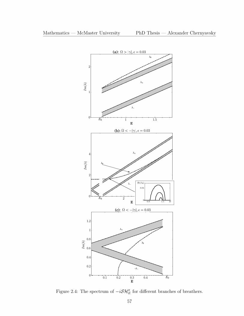
Mathematics — McMaster University PhD Thesis — Alexander Chernyavsky
Figure 2.4: The spectrum of −iSH′′E for different branches of breathers.
57

Mathematics — McMaster University PhD Thesis — Alexander Chernyavsky
Lemma 8. Fix γ 6= 0, Ω < −|γ|, and E > 0 along branch (b) of Lemma 4. There
exists a resonance λ0 = λ+ at E = E∗ with E∗ > E0 if Ω ∈ (Ω∗,−|γ|) and E∗ ∈ (0, E0)
if Ω ∈ (−5|γ|,Ω∗), where
Ω∗ := −√
1 + 5√
2√2
|γ|. (2.69)
Moreover, if Ω < −5|γ|, there exists a resonance λ0 = −λ− at E = E∗ with
E∗ ∈ (0, E0).
Proof. Let us first assume that there exists a resonance λ0 = λ+ at E = E∗ = E0 and
find the condition on γ and Ω, when this is possible. From the definitions (2.62) and
(2.63), we obtain the constraint on A2:
(4A2 + Ω)2 − Ωγ2
4A2 + Ω= E2
0 = Ω2 − γ2.
After canceling 4A2 since A2 ≥ A2+ > 0 with A2
+ given by (2.27), we obtain
16A4 + 12ΩA2 + 2Ω2 + γ2 = 0,
which has two roots
A2 = −3
8Ω± 1
8
√Ω2 − 4γ2.
Since A2 ≥ A2+, the lower sign is impossible because this leads to a contradiction√
|Ω| − 2|γ| −√|Ω|+ 2|γ| ≥ 0.
The upper sign is possible if |Ω| ≥ 2|γ|. Using the parametrization (2.25), we substi-
tute the root for A2 to the equation E20 = E2 and simplify it:
Ω2 − γ2 =(
2|Ω|+√
Ω2 − 4γ2)2
1− 4γ2(|Ω|+
√Ω2 − 4γ2
)2
=
2√
Ω2 − 4γ2(
2|Ω|+√
Ω2 − 4γ2)2(
|Ω|+√
Ω2 − 4γ2) .
58

Mathematics — McMaster University PhD Thesis — Alexander Chernyavsky
This equation further simplifies to the form:√Ω2 − 4γ2(9Ω2 − 7γ2) + Ω(31γ2 − 7Ω2) = 0.
Squaring it up, we obtain
8Ω6 − 4Ω4γ2 − 102Ω2γ4 − 49γ6 = 0,
which has only one positive root for Ω2 given by
Ω2 =1 + 5
√2
2γ2.
This root yields a formula for Ω∗ in (2.69). Since there is a unique value for
Ω ∈ (−∞,−|γ|), for which the case E∗ = E0 is possible, we shall now consider
whether E∗ > E0 or E∗ < E0 for Ω ∈ (−∞,Ω∗) or Ω ∈ (Ω∗,−|γ|).To inspect the range E∗ < E0, we consider a particular case, for which the inter-
section λ0 = λ+ = −λ− happens at E = 0. In this case, A2 = A2+ given by (2.27), so
that the condition λ20 = −E2
0 can be rewritten as
4(γ2 − |γ|Ω) = Ω2 − γ2.
There is only one negative root for Ω and it is given by Ω = −5|γ|. By continuity, we
conclude that λ0 = λ+ for Ω ∈ (−5|γ|,Ω∗) and λ0 = −λ− for Ω ∈ (−∞,−5|γ|), both
cases correspond to E∗ ∈ (0, E0).
Finally, we verify that the case λ0 = λ+ occurs for E∗ > E0 if Ω ∈ (Ω∗,−|γ|).Indeed, λ0 = i(8A2 +2Ω+O(A−2)) and λ+ = i(8A2 +Ω+E0 +O(A−2)) as A→∞, so
that Im(λ0) < Im(λ+) as E →∞. On the other hand, the previous estimates suggest
that Im(λ0) > Im(λ+) for every E ∈ (0, E0) if Ω ∈ (Ω∗,−|γ|). Therefore, there exists
at least one intersection λ0 = λ+ for E∗ > E0 if Ω ∈ (Ω∗,−|γ|).
Remark 10. The existence of the resonance at E = 0 for some parameter configura-
tions predicted by Lemma 8 is in agreement with the numerical results in [135, 136]
on the scalar parametrically forced dNLS equation that follows from system (2.5) un-
der the reduction (2.6). It was reported in [135, 136] that the instability bubble for
breather solutions may appear for every nonzero coupling constant ε = 0 in a narrow
region of the parameter space.
59

Mathematics — McMaster University PhD Thesis — Alexander Chernyavsky
2.7 Summary
We have reduced Newton’s equation of motion for coupled pendula shown on Figure
2.1 under a resonant periodic force to the PT -symmetric dNLS equation (2.9). We
have shown that this system is Hamiltonian with conserved energy (2.17) and an
additional constant of motion (2.18). We have studied breather solutions of this model,
which generalize symmetric synchronized oscillations of coupled pendula that arise if
E = 0. We showed existence of three branches of breathers shown on Figure 2.3. We
also investigated their spectral stability analytically and numerically. The spectral
information on each branch of solutions is shown on Figure 2.4. For branch (c), we
were also able to prove orbital stability and instability from the energy method. The
technical results of this Chapter are summarized in Table 1 and described as follows.
Table 2.1: A summary of results on breather solutions for small ε. Here, IB is anarrow instability bubble seen on panel (b) of Figure 2.4.
|E| > E0 |E| < E0
Parameterintervals
Ω > |γ| Ω < −|γ| Ω < −|γ| Ω < −|γ|Existence point 1 point 3 point 2 point 4
on Figure 2.3 on branch (a) on branch (b) on branch (b) on branch (c)Continuum Sign-indefinite Sign-indefinite Negative Negative
Spectralstability
Yes Yes (IB) Yes (IB)Depends
on parametersOrbitalstability
No NoYes
if |λ0| > |λ±|Yes
if spectrally stable
For branch (a), we found that it is disconnected from the symmetric synchronized
oscillations at E = 0. Along this branch, breathers of small amplitudes A are con-
nected to breathers of large amplitudes A. Every point on the branch corresponds
to the saddle point of the energy function between two wave continua of positive and
negative energies. Every breather along the branch is spectrally stable and is free of
resonance between isolated eigenvalues and continuous spectrum. In Chapter 3, we
will prove long-time orbital stability of breathers along this branch.
For branch (b), we found that the large-amplitude breathers as E → ∞ are con-
nected to the symmetric synchronized oscillations at E = 0, which have the smallest
(but nonzero) amplitude A = A+. Breathers along the branch are spectrally stable
60
Mathematics — McMaster University PhD Thesis — Alexander Chernyavsky
except for a narrow instability bubble, where the isolated eigenvalue λ0 is in resonance
with the continuous spectrum. The instability bubble can occur either for E > E0,
where the breather is a saddle point of the energy function between two wave con-
tinua of opposite energies or for E < E0, where the breather is a saddle point between
the two negative-definite wave continua and directions of positive energy. When the
isolated eigenvalue of positive energy λ0 is above the continuous spectrum near λ+
and ±λ−, orbital stability of breathers can be proved by using the technique in [42],
which was developed for the dNLS equation.
Finally, for branch (c), we found that the small-amplitude breathers at E → E0
are connected to the symmetric synchronized oscillations at E = 0, which have the
largest amplitude A = A−. Breathers are either spectrally stable near E = E0 or
unstable near E = 0, depending on the detuning frequency Ω and the amplitude of
the periodic resonant force γ. When breathers are spectrally stable, they are also
orbitally stable for infinitely long times.
61
Chapter 3
Metastability in Discrete Systems
3.1 Background
We consider the system of amplitude equations (2.9), which is reproduced here for
convenience without factor 2 for the time derivatives:idundt
= ε (vn+1 − 2vn + vn−1) + iγun + Ωvn + 2 [(2|un|2 + |vn|2) vn + u2nvn] ,
idvndt
= ε (un+1 − 2un + un−1)− iγvn + Ωun + 2 [(|un|2 + 2|vn|2)un + unv2n] ,
(3.1)
where un, vnn∈Z are complex-valued amplitudes that depend on time t ∈ R, whereas
(Ω, γ, ε) are real-valued parameters arising in a physical context described below. We
assume Ω 6= 0, γ > 0, and ε > 0 throughout this Chapter.
The remarkable property of the PT -symmetric dNLS equation (3.1) is the exis-
tence of the cross–gradient symplectic structure (2.16) with two conserved quanti-
ties (2.17) and (2.18) bearing the meaning of the energy and charge functions. For
convenience, we reproduce again the cross-gradient symplectic structure
idundt
=∂H
∂vn, i
dvndt
=∂H
∂un, n ∈ Z, (3.2)
and the Hamiltonian function
H =∑n∈Z
(|un|2 + |vn|2)2 + (unvn + unvn)2 + Ω(|un|2 + |vn|2)
−ε|un+1 − un|2 − ε|vn+1 − vn|2 + iγ(unvn − unvn). (3.3)
62
Mathematics — McMaster University PhD Thesis — Alexander Chernyavsky
The Hamiltonian system (3.2) has an additional gauge symmetry, with respect to the
transformation un, vnn∈Z → eiαun, eiαvnn∈Z, where α ∈ R. The charge function
related to the gauge symmetry is written in the form
Q =∑n∈Z
(unvn + unvn). (3.4)
The energy and charge functions H and Q are conserved in the time evolution of the
Hamiltonian system (3.2). Compared to the other physically relevant PT -symmetric
dNLS equations [79, 114, 115], where the Hamiltonian structure is not available
and analysis of nonlinear stability of the zero equilibrium and time-periodic local-
ized breathers is barely possible, we are able to address these questions for the PT -
symmetric dNLS equation (3.1), thanks to the Hamiltonian structure (3.2) with two
conserved quantities (3.3) and (3.4).
The temporal evolution of the PT -symmetric dNLS equation (3.1) is studied in
sequence space `2(Z) for sequences (u, v) as functions of time. Global existence of
solutions in `2(Z) follows from an easy application of Picard’s method and energy
estimates (Proposition 3). The global solution in `2(Z) may still grow at most ex-
ponentially in time, due to the destabilizing properties of the gain-damping terms in
the system (3.1). However, thanks to coercivity of the energy function (3.3) near the
zero equilibrium, we can still obtain a global bound on the `2(Z) norm of the solution
near the zero equilibrium, provided it is linearly stable. Moreover, for Ω > (γ + 4ε),
the global bound holds for arbitrary initial data. The corresponding result is given
by the following theorem (proved in Section 2). A similar result for a single dimer is
deemed as the spontaneous PT -symmetry restoration in [16].
Theorem 10. For every Ω > (γ+4ε) and every initial data (u(0), v(0)) ∈ `2(Z), there
is a positive constant C that depends on parameters and Ω, γ, ε and (‖u(0)‖`2 , ‖v(0)‖`2)
such that
‖u(t)‖2`2 + ‖v(t)‖2
`2 ≤ C, for every t ∈ R. (3.5)
The bound (3.5) also holds for every Ω < −γ and every (u(0), v(0)) ∈ `2(Z) with
sufficiently small `2(Z) norm.
63

Mathematics — McMaster University PhD Thesis — Alexander Chernyavsky
Remark 11. As shown in Chapter 2, the zero equilibrium of the PT -symmetric dNLS
equation (3.1) is linearly stable if |γ| < γ0, where the PT phase transition threshold
γ0 is given by
γ0 :=
Ω− 4ε, Ω > 0
|Ω|, Ω < 0.
The zero equilibrium is linearly unstable if |γ| ≥ γ0. Thus, the constraints on pa-
rameters in Theorem 10 coincide with the criterion of linear stability of the zero
equilibrium.
We shall now characterize breathers supported by the PT -symmetric dNLS equa-
tion (3.1). These are solutions of the form
u(t) = Ue−iEt, v(t) = V e−iEt, (3.6)
where the frequency parameter E is considered to be real and the sequence (U, V ) ∈`2(Z) is time-independent. By continuous embedding, we note that (U, V ) ∈ `2(Z)
implies the decay at infinity: |Un|+ |Vn| → 0 as |n| → ∞. The breather is considered
to be PT -symmetric with respect to the operators in (2.11) if V = U .
Thanks to the cross-gradient symplectic structure (3.2), (U, V ) ∈ `2(Z) in (3.6) is
a critical point of the extended energy function HE : `2(Z)→ R given by
HE := H − EQ, (3.7)
where H and Q are given by (3.3) and (3.4). The Euler–Lagrange equations for HE
produce the stationary PT -symmetric dNLS equation:
EUn = ε(Un+1 − 2Un + Un−1
)+ iγUn + ΩUn + 6|Un|2Un + 2U3
n, (3.8)
which corresponds to the reduction of the PT -symmetric dNLS equation (3.1) for the
breather solution (3.6) under the PT symmetry V = U .
We denote a solution of the PT -symmetric dNLS equation (3.1) in `2(Z) by
ψ = (u, v) and the localized solution of the stationary dNLS equation (3.8) by
Φ = (U, V ). We fix parameters γ > 0, Ω > γ, and E ∈ (−∞,−E0) ∪ (E0,∞). The
following theorem (proved in Section 3) formulates the main result of this Chapter.
64
Mathematics — McMaster University PhD Thesis — Alexander Chernyavsky
Theorem 11. For every ν > 0 sufficiently small, there exists ε0 > 0 and δ > 0 such
that for every ε ∈ (0, ε0) the following is true. If ψ(0) ∈ `2(Z) satisfies ‖ψ(0)−Φ‖l2 ≤δ, then there exist a positive time t0 . ε−1/2 and a C1 function α(t) : [0, t0] →R/(2πZ) such that the unique solution ψ(t) : [0, t0] → `2(Z) to the PT -symmetric
dNLS equation (3.1) satisfies the bound
‖eiα(t)ψ(t)− Φ‖l2 ≤ ν, for every t ∈ [0, t0]. (3.9)
Moreover, there exists a positive constant C such that |α − E| ≤ Cν, for every
t ∈ [0, t0].
Remark 12. The statement of Theorem 11 remains true for ε = 0. In this (anti-
continuum) limit, Theorem 11 gives nonlinear stability of the standing localized state
Φ compactly supported at the central site n = 0. The bound (3.9) is extended in the
case ε = 0 for all times t ∈ R.
Remark 13. It becomes clear from the proof of Theorem 11 for ε 6= 0, see inequality
(3.59) below, that the bound (3.9) on the perturbation φ to the stationary solution Φ
is defined within the size of O(ε1/2 + δ). Therefore, if Φn = O(ε|n|) for every n 6= 0
(Proposition 4), then the perturbation term is φn = O(ε1/2 + δ) for every n ∈ Z. This
is a limitation of the result of Theorem 11. Not only it holds for long but finite times
t0 = O(ε−1/2) but also it gives a larger than expected bound on the perturbation term
φ. It may be quite possible to improve the approximation result with a sequence of
normal form transformations, similar to what was done recently in [110].
Remark 14. The statement of Theorem 11 can be improved on a shorter time scale
t0 = O(1). In this case, see inequality (3.58) below, the perturbation term φ has the
size of O(ε + δ). Thus, the perturbation term φn at n = ±1 is comparable with the
standing localized state Φn at n = ±1, but it is still much larger than Φn for every n
such that |n| ≥ 2.
Remark 15. Theorem 11 cannot be extended to the solution branch with Ω < −γ < 0
and |E| > E0 (point 3 on Figure 2.3) because the second variation of ΛE at (U, V )
is not coercive and does not control the size of perturbation terms. This analytical
difficulty reflects the unfortunate location of the discrete and continuous spectra that
leads to a resonance studied in Chapter 2. No resonance was found for the solution
branch with Ω > γ > 0 and |E| > E0 (point 1 on Figure 2.3) and this numerical
65
Mathematics — McMaster University PhD Thesis — Alexander Chernyavsky
result from Chapter 2 is in agreement with the analytical method used in the proof of
Theorem 11.
The remainder of this Chapter is devoted to the proof of Theorems 10 and 11.
3.2 Proof of the global bound
The following proposition gives the global existence result for the PT -symmetric
dNLS equation (3.1).
Proposition 3. For every (u(0), v(0)) ∈ `2(Z), there exists a unique solution
(u, v)(t) ∈ C1(R, `2(Z)) of the PT -symmetric dNLS equation (3.1) such that
(u, v)(0) = (u(0), v(0)). The unique solution depends continuously on initial data
(u(0), v(0)) ∈ `2(Z).
Proof. Since discrete Laplacian is a bounded operator in `2(Z) and the sequence space
`2(Z) forms a Banach algebra with respect to pointwise multiplication, the local well-
posedness of the initial-value problem for the PT -symmetric dNLS equation (3.1)
follows from the standard Picard’s method. The local solution (u, v)(t) exists in
C0([−t0, t0], `2(Z)) for some finite t0 > 0. Thanks again to the boundedness of the
discrete Laplacian operator in `2(Z), bootstrap arguments extend this solution in
C1([−t0, t0], `2(Z)).
The local solution is continued globally by using the energy method. For any
solution (u, v)(t) in C1([−t0, t0], `2(Z)), we obtain the following balance equation from
system (3.1):d
dt
∑n∈Z
(|un|2 + |vn|2) = −γ∑n∈Z
(|un|2 − |vn|2).
Integrating this equation in time and applying Gronwall’s inequality, we get
‖u(t)‖2l2 + ‖v(t)‖2
l2 ≤(‖u(0)‖2
l2 + ‖v(0)‖2l2
)e|γt|, t ∈ [−t0, t0].
Therefore ‖u(t)‖l2 and ‖v(t)‖l2 cannot blow up in a finite time, so that the local
solution (u, v)(t) ∈ C1([−t0, t0], `2(Z)) is continued for every t0 > 0.
A critical question also addressed in [79, 115] for other PT -symmetric dNLS
equations is whether the `2(Z) norms of the global solution of Proposition 3 remain
66
Mathematics — McMaster University PhD Thesis — Alexander Chernyavsky
bounded as t→∞. In the context of the Hamiltonian PT -symmetric dNLS equation
(3.1), this question can be addressed by using the energy function given by (3.3). In
what follows, we use coercivity of the energy function and prove the result stated in
Theorem 10.
Proof of Theorem 10. We use γ > 0 and ε > 0 everywhere in the proof. If
Ω > (γ + 4ε), the following lower bound is available for the energy function H given
by (3.3) using Cauchy–Schwarz inequality:
H ≥ (Ω− γ − 4ε)(‖u‖2
`2 + ‖v‖2`2
). (3.10)
Since H is time-independent and bounded for any (u, v)(t) ∈ C1(R, `2(Z)) due to the
continuous embedding ‖u‖`4 ≤ ‖u‖`2 , we obtain the time-independent bound (3.5) for
any Ω > (γ + 4ε).
If Ω < −γ, the following lower bound is available for the energy function −H:
−H ≥ (|Ω| − γ)(‖u‖2
`2 + ‖v‖2`2
)−(‖u‖2
`2 + ‖v‖2`2
)2, (3.11)
where the continuous embedding ‖u‖`4 ≤ ‖u‖`2 has been used. If ‖u(0)‖`2 + ‖v(0)‖`2is sufficiently small, then |H| is sufficiently small, and the bound (3.5) with sufficiently
small C holds for every t ∈ R.
Remark 16. For every Ω ≤ (γ + 4ε), the energy functions H or −H do not pro-
duce a useful lower bound, which would result in a time-independent bound on the
`2(Z) norm for the global solution (u, v)(t). This is because the continuous embedding
‖u‖`4 ≤ ‖u‖`2 is not sufficient to control H or −H from below. If the lattice is trun-
cated on a finitely many (say, N) sites, then the bound ‖u‖`2 ≤ N1/4‖u‖`4 can be used
to obtain from (3.3):
H ≥(‖u‖4
`4 + ‖v‖4`4
)− (γ + 4ε− Ω)N1/2
(‖u‖2
`4 + ‖v‖2`4
).
Thus, the time-independent bound on the `4(ZN) (and then `2(ZN)) norms for the
global solution (u, v)(t) restricted on N sites of the lattice Z is available for every Ω.
However, the control becomes impossible in the limit N →∞ if Ω ≤ (γ + 4ε).
67
Mathematics — McMaster University PhD Thesis — Alexander Chernyavsky
Remark 17. It is an interesting open question to investigate if the global dynamics of
the PT -symmetric dNLS equation (3.1) on the infinite lattice is globally bounded in
time for Ω ≤ (γ+ 4ε). This open question would include the case −γ ≤ Ω ≤ (γ+ 4ε),
when the zero equilibrium is linearly unstable, and the case Ω < −γ with sufficiently
large initial data (u(0), v(0)) ∈ `2(Z), when the zero equilibrium is linearly stable but
the bound (3.11) can no longer be closed. This open question is addressed numerically
for a similar model without phase invariance in [46], where it was shown that l2 norm
of the solution grows while l∞ norm remains finite.
3.3 Proof of metastability
We divide the proof of Theorem 11 into several subsections.
3.3.1 Characterization of the localized solutions
For ε = 0, a solution to the stationary dNLS equation (3.8) is supported on the central
site n = 0 and satisfies
(E − iγ)U0 − ΩU0 = 6|U0|2U0 + 2U30 . (3.12)
The parameters γ and Ω are considered to be fixed, and parameter E is thought
to parameterize a continuous branch of solutions of the nonlinear algebraic equation
(3.12). Substituting the decomposition U0 = Aeiθ with A > 0 and θ ∈ [0, 2π) into the
algebraic equation (3.12), we obtain
sin(2θ) =γ
4A2 + Ω, cos(2θ) =
E
8A2 + Ω, (3.13)
from which the solution branches of E versus A are obtained in Chapter 2 as shown
on Figure 2.3. The dependence of E versus A is given analytically by
E2 = (Ω + 8A2)2
[1− γ2
(Ω + 4A2)2
]. (3.14)
Persistence of the central dimer in the unbounded lattice with respect to the coupling
parameter ε is given by the following proposition.
68
Mathematics — McMaster University PhD Thesis — Alexander Chernyavsky
Proposition 4. Fix γ > 0, Ω > γ, and E 6= ±E0, where E0 :=√
Ω2 − γ2 > 0. There
exist ε0 > 0 sufficiently small and C0 > 0 such that for every ε ∈ (−ε0, ε0), there exists
a unique solution U ∈ l2(Z) to the difference equation (3.8) such that
∣∣U0 − Aeiθ∣∣ ≤ C0|ε|, |Un| ≤ C0|ε||n|, n 6= 0, (3.15)
where A and θ are defined in (3.13). Moreover, the solution U is smooth in ε.
Proof. Persistence and smoothness of a solution U ∈ l2(Z) to the difference equation
(3.8) in ε, as well as the first bound in (3.15), were proved in Theorem 6.
It remains to prove the second bound in (3.15), for which we employ the implicit
function theorem (see Section 1.5.6). Inspecting the difference equation (3.8) shows
that if U±1 = O(|ε|) according to the bound (2.33), then Un = U−n can be expressed
by using the scaling transformation
Un = ε|n|W|n|, ±n ∈ N, (3.16)
where the sequence W ∈ `2(N) is found from the system
EWn−iγWn−ΩWn = Wn−1 +ε2Wn+1−2εWn+6ε2|n||Wn|2Wn+2ε2|n|W 3n , n ∈ N, (3.17)
with W0 = U0 given by the previous result. Let x = Wnn∈N, X = `2(N), y = ε,
Y = R, and Z = `2(N) in the definition of system F : X × Y → Z. Then, we have
F (x0, 0) = 0, where x0 = W (0)n n∈N is a unique solution of the recurrence equation
EW (0)n − iγW (0)
n − ΩW (0)n = W
(0)n−1, n ∈ N, (3.18)
starting with a given W(0)0 = U0. Indeed, each block in the left-hand side of system
(3.18) is given by the invertible matrix[E − iγ −Ω
−Ω E + iγ
],
with eigenvalues λ± = E ± E0 6= 0. Hence, a unique solution for W (0) ∈ `∞(N) is
found from the recurrence relation (3.18). Moreover, since DxF (0, 0) : X → Z is one-
to-one and onto (as a lower block-triangular matrix with invertible diagonal blocks),
the solution W (0) is actually in X = `2(N). By the implicit function theorem, for
69
Mathematics — McMaster University PhD Thesis — Alexander Chernyavsky
every ε 6= 0 sufficiently small, there exists a unique solution W ∈ `2(N) to the system
(3.17) such that
‖W −W (0)‖`2(N) < C ′′′|ε|, (3.19)
where a positive constant C ′′′ is independent of ε. Thus, the second bound in (3.15)
is proved from (3.16) and (3.19).
3.3.2 Decomposition of the solution
Let ψ = (u, u, v, v) denote a solution of the PT -symmetric dNLS equation (3.1) in
`2(Z) given by Proposition 3. Let Φ = (U, U , V, V ) denote a localized solution of the
stationary dNLS equation (3.8) given by Proposition 4. Let φ = ψ − Φ = (u, u,v, v)
denote a perturbation to Φ. Note that these are extended 4-component variables
at each lattice site (concatenated by the complex conjugate functions) compared to
the two-component variables used in the formulation of Theorem 11. The extended
variables are more suitable for dealing with the energy functions such as (3.7) or (6.3),
which we reproduce here for convenience:
ΛE := H − E(u0v0 + u0v0). (3.20)
By using the energy function (3.20), we introduce the energy difference function
∆ := ΛE(Φ + φ)− ΛE(Φ). (3.21)
Let us write the expansion for ∆ explicitly:
∆ = N1(φ) +N2(φ) +N3(φ) +N4(φ), (3.22)
where the linear part is
N1(φ) = E∑
n∈Z\0
(Vnun + Vnun + Unvn + Unvn
), (3.23)
the quadratic part is
N2(φ) =1
2〈H′′Eφ, φ〉l2 + E
∑n∈Z\0
(vnun + vnun) , (3.24)
70
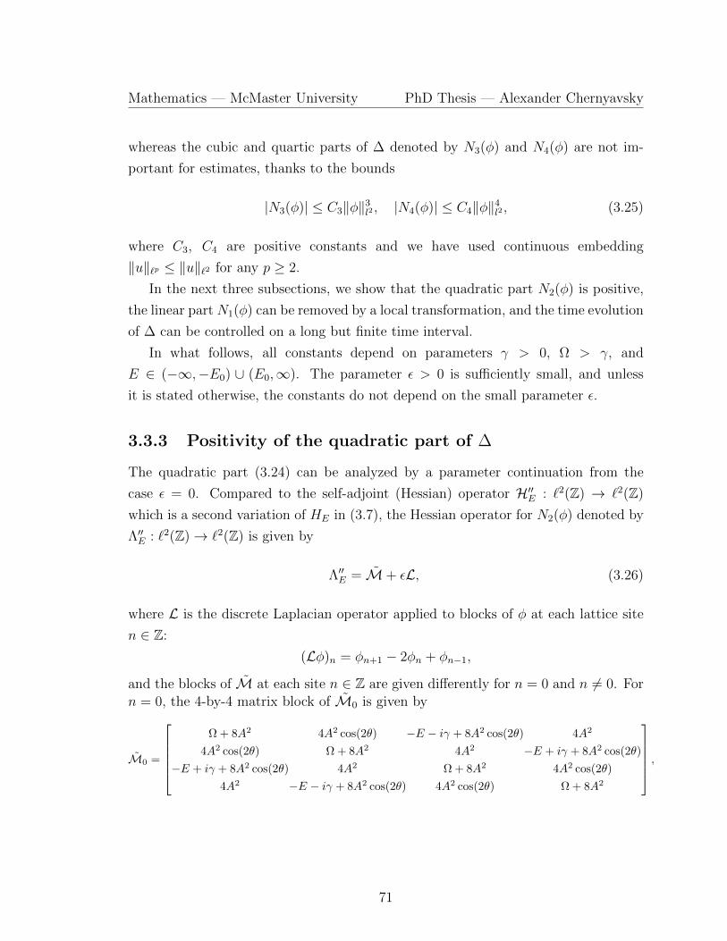
Mathematics — McMaster University PhD Thesis — Alexander Chernyavsky
whereas the cubic and quartic parts of ∆ denoted by N3(φ) and N4(φ) are not im-
portant for estimates, thanks to the bounds
|N3(φ)| ≤ C3‖φ‖3l2 , |N4(φ)| ≤ C4‖φ‖4
l2 , (3.25)
where C3, C4 are positive constants and we have used continuous embedding
‖u‖`p ≤ ‖u‖`2 for any p ≥ 2.
In the next three subsections, we show that the quadratic part N2(φ) is positive,
the linear part N1(φ) can be removed by a local transformation, and the time evolution
of ∆ can be controlled on a long but finite time interval.
In what follows, all constants depend on parameters γ > 0, Ω > γ, and
E ∈ (−∞,−E0) ∪ (E0,∞). The parameter ε > 0 is sufficiently small, and unless
it is stated otherwise, the constants do not depend on the small parameter ε.
3.3.3 Positivity of the quadratic part of ∆
The quadratic part (3.24) can be analyzed by a parameter continuation from the
case ε = 0. Compared to the self-adjoint (Hessian) operator H′′E : `2(Z) → `2(Z)
which is a second variation of HE in (3.7), the Hessian operator for N2(φ) denoted by
Λ′′E : `2(Z)→ `2(Z) is given by
Λ′′E = M+ εL, (3.26)
where L is the discrete Laplacian operator applied to blocks of φ at each lattice site
n ∈ Z:
(Lφ)n = φn+1 − 2φn + φn−1,
and the blocks of M at each site n ∈ Z are given differently for n = 0 and n 6= 0. Forn = 0, the 4-by-4 matrix block of M0 is given by
M0 =
Ω + 8A2 4A2 cos(2θ) −E − iγ + 8A2 cos(2θ) 4A2
4A2 cos(2θ) Ω + 8A2 4A2 −E + iγ + 8A2 cos(2θ)
−E + iγ + 8A2 cos(2θ) 4A2 Ω + 8A2 4A2 cos(2θ)
4A2 −E − iγ + 8A2 cos(2θ) 4A2 cos(2θ) Ω + 8A2
,
71
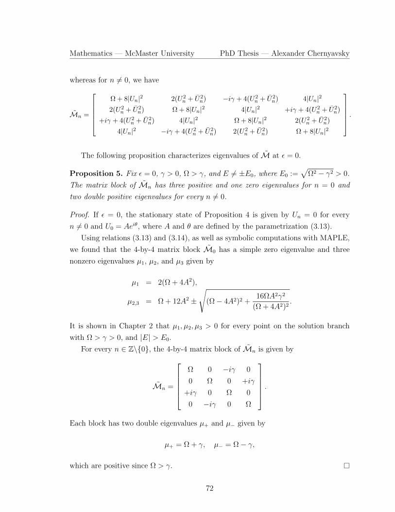
Mathematics — McMaster University PhD Thesis — Alexander Chernyavsky
whereas for n 6= 0, we have
Mn =
Ω + 8|Un|2 2(U2
n + U2n) −iγ + 4(U2
n + U2n) 4|Un|2
2(U2n + U2
n) Ω + 8|Un|2 4|Un|2 +iγ + 4(U2n + U2
n)
+iγ + 4(U2n + U2
n) 4|Un|2 Ω + 8|Un|2 2(U2n + U2
n)
4|Un|2 −iγ + 4(U2n + U2
n) 2(U2n + U2
n) Ω + 8|Un|2
.
The following proposition characterizes eigenvalues of M at ε = 0.
Proposition 5. Fix ε = 0, γ > 0, Ω > γ, and E 6= ±E0, where E0 :=√
Ω2 − γ2 > 0.
The matrix block of Mn has three positive and one zero eigenvalues for n = 0 and
two double positive eigenvalues for every n 6= 0.
Proof. If ε = 0, the stationary state of Proposition 4 is given by Un = 0 for every
n 6= 0 and U0 = Aeiθ, where A and θ are defined by the parametrization (3.13).
Using relations (3.13) and (3.14), as well as symbolic computations with MAPLE,
we found that the 4-by-4 matrix block M0 has a simple zero eigenvalue and three
nonzero eigenvalues µ1, µ2, and µ3 given by
µ1 = 2(Ω + 4A2),
µ2,3 = Ω + 12A2 ±√
(Ω− 4A2)2 +16ΩA2γ2
(Ω + 4A2)2.
It is shown in Chapter 2 that µ1, µ2, µ3 > 0 for every point on the solution branch
with Ω > γ > 0, and |E| > E0.
For every n ∈ Z\0, the 4-by-4 matrix block of Mn is given by
Mn =
Ω 0 −iγ 0
0 Ω 0 +iγ
+iγ 0 Ω 0
0 −iγ 0 Ω
.
Each block has two double eigenvalues µ+ and µ− given by
µ+ = Ω + γ, µ− = Ω− γ,
which are positive since Ω > γ.
72
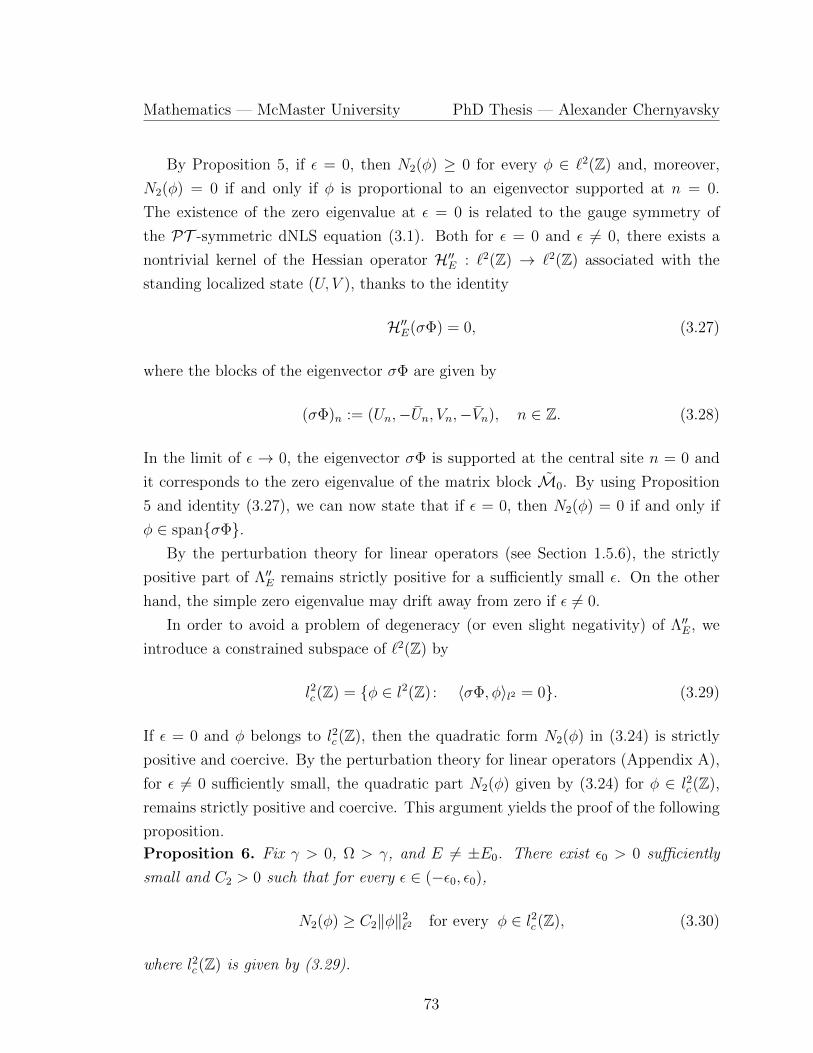
Mathematics — McMaster University PhD Thesis — Alexander Chernyavsky
By Proposition 5, if ε = 0, then N2(φ) ≥ 0 for every φ ∈ `2(Z) and, moreover,
N2(φ) = 0 if and only if φ is proportional to an eigenvector supported at n = 0.
The existence of the zero eigenvalue at ε = 0 is related to the gauge symmetry of
the PT -symmetric dNLS equation (3.1). Both for ε = 0 and ε 6= 0, there exists a
nontrivial kernel of the Hessian operator H′′E : `2(Z) → `2(Z) associated with the
standing localized state (U, V ), thanks to the identity
H′′E(σΦ) = 0, (3.27)
where the blocks of the eigenvector σΦ are given by
(σΦ)n := (Un,−Un, Vn,−Vn), n ∈ Z. (3.28)
In the limit of ε → 0, the eigenvector σΦ is supported at the central site n = 0 and
it corresponds to the zero eigenvalue of the matrix block M0. By using Proposition
5 and identity (3.27), we can now state that if ε = 0, then N2(φ) = 0 if and only if
φ ∈ spanσΦ.By the perturbation theory for linear operators (see Section 1.5.6), the strictly
positive part of Λ′′E remains strictly positive for a sufficiently small ε. On the other
hand, the simple zero eigenvalue may drift away from zero if ε 6= 0.
In order to avoid a problem of degeneracy (or even slight negativity) of Λ′′E, we
introduce a constrained subspace of `2(Z) by
l2c(Z) = φ ∈ l2(Z) : 〈σΦ, φ〉l2 = 0. (3.29)
If ε = 0 and φ belongs to l2c(Z), then the quadratic form N2(φ) in (3.24) is strictly
positive and coercive. By the perturbation theory for linear operators (Appendix A),
for ε 6= 0 sufficiently small, the quadratic part N2(φ) given by (3.24) for φ ∈ l2c(Z),
remains strictly positive and coercive. This argument yields the proof of the following
proposition.
Proposition 6. Fix γ > 0, Ω > γ, and E 6= ±E0. There exist ε0 > 0 sufficiently
small and C2 > 0 such that for every ε ∈ (−ε0, ε0),
N2(φ) ≥ C2‖φ‖2`2 for every φ ∈ l2c(Z), (3.30)
where l2c(Z) is given by (3.29).
73
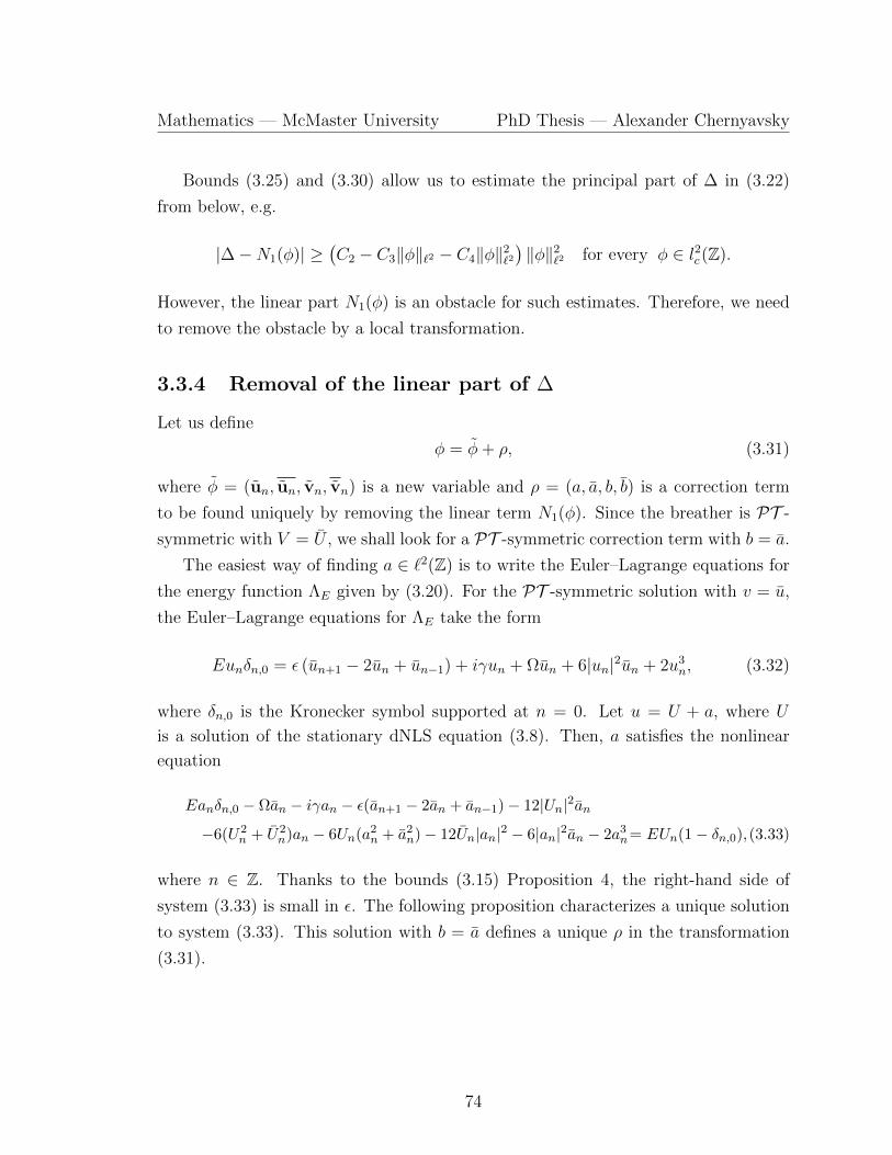
Mathematics — McMaster University PhD Thesis — Alexander Chernyavsky
Bounds (3.25) and (3.30) allow us to estimate the principal part of ∆ in (3.22)
from below, e.g.
|∆−N1(φ)| ≥(C2 − C3‖φ‖`2 − C4‖φ‖2
`2
)‖φ‖2
`2 for every φ ∈ l2c(Z).
However, the linear part N1(φ) is an obstacle for such estimates. Therefore, we need
to remove the obstacle by a local transformation.
3.3.4 Removal of the linear part of ∆
Let us define
φ = φ+ ρ, (3.31)
where φ = (un, un, vn, vn) is a new variable and ρ = (a, a, b, b) is a correction term
to be found uniquely by removing the linear term N1(φ). Since the breather is PT -
symmetric with V = U , we shall look for a PT -symmetric correction term with b = a.
The easiest way of finding a ∈ `2(Z) is to write the Euler–Lagrange equations for
the energy function ΛE given by (3.20). For the PT -symmetric solution with v = u,
the Euler–Lagrange equations for ΛE take the form
Eunδn,0 = ε (un+1 − 2un + un−1) + iγun + Ωun + 6|un|2un + 2u3n, (3.32)
where δn,0 is the Kronecker symbol supported at n = 0. Let u = U + a, where U
is a solution of the stationary dNLS equation (3.8). Then, a satisfies the nonlinear
equation
Eanδn,0 − Ωan − iγan − ε(an+1 − 2an + an−1)− 12|Un|2an−6(U2
n + U2n)an − 6Un(a2
n + a2n)− 12Un|an|2 − 6|an|2an − 2a3
n= EUn(1− δn,0),(3.33)
where n ∈ Z. Thanks to the bounds (3.15) Proposition 4, the right-hand side of
system (3.33) is small in ε. The following proposition characterizes a unique solution
to system (3.33). This solution with b = a defines a unique ρ in the transformation
(3.31).
74
Mathematics — McMaster University PhD Thesis — Alexander Chernyavsky
Proposition 7. Fix γ > 0, Ω > γ, and E 6= ±E0. There exist ε0 > 0 sufficiently
small and C1 > 0 such that for every ε ∈ (−ε0, ε0), there exists a unique solution
a ∈ `2(Z) to the system (3.33) such that
|a0| ≤ C1ε2, |an| ≤ C1|ε||n|, n ∈ Z\0. (3.34)
Proof. The proof repeats the three steps in the proof of Proposition 4. On the sites
n ∈ Z\0, the Jacobian operator DxF (0, 0) is block-diagonal with identical blocks
given by [−iγ −Ω
−Ω iγ
]. (3.35)
Each block is invertible thanks to the constraint Ω > γ. On the central site n = 0, the
Jacobian operator DxF (Aeiθ, 0) coincides with the block (2.35), which is invertible for
every γ 6= 0, Ω > γ > 0, and |E| > E0 (see Theorem 6 in Chapter 2). Thus, existence
and uniqueness of solutions to the nonlinear system (3.33) for small ε is established
with two applications of the implicit function theorem.
In order to justify the bound (3.34), we use (3.16) and substitute
a0 = ε2A0, an = ε|n|A|n|, ±n ∈ N (3.36)
to the system (3.33). The sequence Ann∈N is found from the system
−ΩAn − iγAn − ε2An+1 + 2εAn − An−1(1− δn,1)− ε2A0δn,1
−6ε2|n|(W 2n + W 2
n)An − 12ε2|n||Wn|2An − 6ε2|n|Wn(A2n + A2
n)
−12ε2|n|Wn|An|2 − 6ε2|n||An|2An − 2ε2|n|A3n = EWn, (3.37)
whereas the term A0 satisfies the nonlinear equation
EA0 − ΩA0 − iγA0 − 2A1 + 2εA0 − 6(U20 + U2
0 )A0 − 12|U0|2A0
−6ε2U0(A20 + A2
0)− 12ε2U0|A0|2 − 6ε4|A0|2A0 − 2ε2A30 = 0. (3.38)
It follows from the invertibility of the block (2.35) that there exists a unique solution
to the nonlinear equation (3.38) for A0 ∈ C if ε is sufficiently small and A1 ∈ C is
75
Mathematics — McMaster University PhD Thesis — Alexander Chernyavsky
given. The solution satisfies the bound
|A0| ≤ C ′|A1|, (3.39)
where the positive constant C ′ is ε-independent. By substituting this solution for
A0 ∈ C to the system (3.37), we observe that the leading-order system is given by the
recurrence equation
−ΩA(0)n − iγA(0)
n − A(0)n−1(1− δn,1) = EWn, n ∈ N. (3.40)
Since Ω > γ, there exists a unique solution A(0) ∈ `∞(N) of the leading-order system
(3.40). Moreover, because the Jacobian operator DxF (0, 0) is one-to-one and onto,
the solution A(0) is actually in `2(N). By using the implicit function theorem again,
for ε 6= 0 sufficiently small, there exists a unique solution A ∈ `2(N) to the system
(3.37) satisfying the bound
‖A− A(0)‖`2(N) < C ′′|ε|, (3.41)
where the positive constant C ′′ is ε-independent. Combining bounds (3.39), (3.41)
with the representation (3.36) yields the bounds (3.34).
By using the transformation (3.31), we rewrite the expansion (3.22) in the following
equivalent form
∆ = ∆0 + ∆2(φ) + ∆3(φ) + ∆4(φ), (3.42)
where the φ-independent term ∆0 is given by
∆0 := N1(ρ) +N2(ρ) +N3(ρ) +N4(ρ),
the quadratic and cubic parts ∆2(φ) and ∆3(φ) are ε-close to N2(φ) and N3(φ), while
∆4(φ) = N4(φ). The following proposition characterizes each term of the decompo-
sition (3.42). The new definitions of constants override the previous definitions of
constants.
76
Mathematics — McMaster University PhD Thesis — Alexander Chernyavsky
Proposition 8. Fix γ > 0, Ω > γ, and E 6= ±E0. There exist ε0 > 0 sufficiently
small and C0, C1, C2, C3, C4 > 0 such that for every ε ∈ (−ε0, ε0), we have
|∆0| ≤ C0ε2, (3.43)
‖φ‖l2 ≤ ‖φ‖l2 + C1ε, ‖φ‖l2 ≤ ‖φ‖l2 + C1ε, (3.44)
‖∆3(φ)‖l2 ≤ C3‖φ‖3l2 , ‖∆4(φ)‖l2 ≤ C4‖φ‖4
l2 , (3.45)
and
∆2(φ) ≥ C2‖φ‖2`2 for every φ ∈ l2c(Z). (3.46)
Proof. Since ρ is constructed in Proposition 7 with the PT -symmetric correction term
b = a, it is true that ρ ∈ `2c(Z). Therefore, the condition φ ∈ `2
c(Z) is satisfied if and
only if φ ∈ `2c(Z). Since the constants C2, C3, and C4 in the bounds (3.25) and (3.30)
are ε-independent, whereas ∆2, ∆3, and ∆4 are ε-close to N2, N3, and N4 in space
`2(Z), then the bounds (3.45) and (3.46) follow from the bounds (3.25) and (3.30)
respectively, thanks to the smallness of ε.
In order to obtain the bounds (3.43) and (3.44), we use the bounds (3.15) and
(3.34) and obtain
|N1(ρ)| ≤ C∑
n∈Z\0
ε2|n| ≤ C ′ε2, ‖ρ‖2l2 ≤ C
ε4 +∑
n∈Z\0
ε2|n|
≤ C ′ε2, (3.47)
where the positive constants C, C ′ are ε-independent and ε is sufficiently small. Since
N2, N3, and N4 are quadratic, cubic, and quartic respectively, the bound (3.43) is
obtained from the triangle inequality and the estimates (3.47). The bounds (3.44)
follow from the triangle inequality and the second estimate (3.47).
3.3.5 Time evolution of ∆
We recall that H given by (3.3) is a constant of motion for the PT -symmetric dNLS
equation (3.1). On the other hand, the part of Q at n = 0 satisfies the balance
equation
id
dt(u0v0 + u0v0) = ε [u0(u1 + u−1)− u0(u1 + u−1) + v0(v1 + v−1)− v0(v1 + v−1)] . (3.48)
77
Mathematics — McMaster University PhD Thesis — Alexander Chernyavsky
If the initial data ψ(0) ∈ l2(Z) is close to Φ in the sense of the bound
‖ψ(0)−Φ‖`2 ≤ δ, then the unique solution ψ(t) ∈ C1(R, l2(Z)) to the PT -symmetric
dNLS equation (3.1) with the same initial data can be defined in the modulation form
ψ(t) = e−iα(t)σ [Φ + φ(t)] , (3.49)
as long as the solution remains close to the orbit of Φ under the phase rotation in
the sense of the bound (3.9). Note again that the vectors ψ, Φ, and φ are extended
4-component vectors at each lattice site compared to the 2-component vectors used
in the formulation of Theorem 11. As a result, the gauge symmetry is represented by
the matrix operator σ defined by (3.28).
The decomposition (3.49) is defined uniquely only if a constraint is imposed to
φ(t) ∈ `2(R). In agreement with the definition (3.29) on the constrained space `2c(R),
we impose the orthogonality condition:
〈σΦ, φ(t)〉l2 = 0. (3.50)
The decomposition (3.49) under the orthogonality condition (3.50) and the modu-
lation equation for α are justified in the next section. Here we estimate how the
time-dependent energy quantity ∆ changes along the solution ψ(t) ∈ C1(R, l2(Z))
represented by the decomposition (3.49).
The rate of change of ∆ defined by (3.21) along the solution ψ(t) represented by
(3.49) is obtained from (3.48) as follows:∣∣∣∣d∆
dt
∣∣∣∣ ≤ CEε‖Φ0 + φ0‖ (‖Φ1 + φ1‖+ ‖Φ−1 + φ−1‖) (3.51)
where CE is a positive ε-independent constant. By using the bounds (3.15) and (3.34),
the transformation (3.31), and the triangle inequality (3.44), we obtain from (3.51):∣∣∣∣d∆
dt
∣∣∣∣ ≤ CEε(
1 + ‖φ0‖)(
ε+ ‖φ1‖+ ‖φ−1‖)
≤ C ′Eε(ε+ ‖φ0‖+ ‖φ1‖+ ‖φ−1‖+ ‖φ0‖2 + ‖φ1‖2 + ‖φ−1‖2
), (3.52)
where C ′E is another positive ε-independent constant.
78
Mathematics — McMaster University PhD Thesis — Alexander Chernyavsky
Let us now define a ball in the space `2c(Z) of a finite size K > 0 by
MK :=φ ∈ `2
c(Z) : ‖φ‖`2 ≤ K. (3.53)
From estimates (3.45) and (3.46), there is a positive K-dependent constant CK such
that
∆−∆0 ≥ CK‖φ‖2`2 for every φ ∈MK . (3.54)
By using coercivity (3.54) in the ball MK and the Young inequality
|ab| ≤ α
2a2 +
1
2αb2, a, b ∈ R,
where α ∈ R+ is arbitrary, we estimate
‖φ0‖+ ‖φ1‖+ ‖φ−1‖ ≤√C−1K (∆−∆0) ≤ α
2CK+
1
2α(∆−∆0),
where ∆−∆0 ≥ 0 follows from (3.54). Substituting this estimate to (3.52) yields∣∣∣∣d∆
dt
∣∣∣∣ ≤ CEε(ε+ α + (∆−∆0) + α−1(∆−∆0)
), (3.55)
for another constant CE > 0. In what follows, we will set the scaling parameter α
such that α → 0 as ε → 0. Therefore, the constant α−1 is much larger compared to
unity. Integrating (3.55) with an integrating factor,∣∣∣∣ ddte−CEεα−1t(∆−∆0)
∣∣∣∣ ≤ CEε(ε+ α)e−CEεα−1t,
we obtain with the Gronwall’s inequality:
∆(t)−∆0 ≤ eCEεα−1t
(∆(0)−∆0 + CEε(ε+ α)
∫ t
0
e−CEεα−1sds
)≤ eCEεα
−1t (∆(0)−∆0 + α(ε+ α)) . (3.56)
It is clear from the estimate (3.56) that ∆(t)−∆0 is small only if α→ 0 as ε→ 0. If
α = ε, then
α = ε : ∆(t)−∆0 ≤ eCEt(∆(0) + C0ε
2),
where the bound (3.43) has been used and C0 is an ε-independent constant. Therefore,
79
Mathematics — McMaster University PhD Thesis — Alexander Chernyavsky
if ∆(0) is small, then ∆(t) remains small on the time scale t = O(1) as ε → 0. On
the other hand, if α = ε1/2, then the estimate (3.56) yields
α = ε1/2 : ∆(t)−∆0 ≤ eCEε1/2t (∆(0) + C0ε) ,
so that ∆(t) remains small on the time scale t = O(ε−1/2).
The initial value for ∆(0) is estimated from (3.42), (3.43), and (3.44). By (3.44),
for every φ(0) ∈Mδ with δ > 0 sufficiently small, we have φ(0) ∈MK with K = δ+ε
and there are positive (ε,δ)-independent constants C,C ′ such that
|∆(0)| ≤ C(ε2 + ‖φ(0)‖2
`2
)≤ C ′(ε2 + δ2). (3.57)
By using the triangle inequality (3.44), coercivity (3.54), and the bound (3.57), we
finally obtain the following two estimates:
α = ε : ‖φ(t)‖2`2 ≤ CeCEt
(ε2 + δ2
)and
α = ε1/2 : ‖φ(t)‖2`2 ≤ CeCEε
1/2t(ε+ δ2
),
where the positive constant C is independent of ε and δ. Comparing with the bound
(3.9) stated in Theorem 11, we obtain
α = ε, t0 . 1 : C(ε+ δ) ≤ ν (3.58)
and
α = ε1/2, t0 . ε−1/2 : C(ε1/2 + δ
)≤ ν, (3.59)
where t0 is the final time in the bound (3.9) and C is another positive (ε,δ)-independent
constant. For every ν > 0, there exist ε0 > 0 and δ > 0 such that inequalities (3.58)
and (3.59) can be satisfied for every ε ∈ (0, ε0). The statement of Theorem 11 is
formulated on the extended time scale corresponding to the inequality (3.59). The
short time scale corresponding to the inequality (3.58) is mentioned in Remark 14.
80
Mathematics — McMaster University PhD Thesis — Alexander Chernyavsky
3.3.6 Modulation equations in `2c(Z)
It remains to show how we can define the decomposition (3.49) under the constraint
(3.50) for a solution to the PT -symmetric dNLS equation (3.1) and how the evolution
of α in time t can be estimated from the modulation equation. Here we modify
standard results on modulation equations, see, e.g., Lemmas 6.1 and 6.3 in [56] for
similar analysis. For reader’s convenience, we only give the main ideas behind the
proofs.
Proposition 9. There exist constants ν0 ∈ (0, 1) and C0 ≥ 1 such that, for any
ψ ∈ l2(Z) satisfying
d := infα∈R‖eiασψ − Φ‖l2 ≤ ν0, (3.60)
one can find modulation parameter α ∈ R/(2πZ) such that ψ = e−iασ(Φ + φ) with
φ ∈ `2c(Z) satisfying d ≤ ‖φ‖l2 ≤ C0d.
Proof. We consider a function f : R→ R given by
f(α) := 〈σΦ, eiασψ − Φ〉`2 = 0.
Let α0 ∈ R/(2πZ) be the argument of the infimum in (3.60). Then, |f(α0)| ≤ d‖Φ‖`2by the Cauchy–Schwartz inequality. On the other hand, the derivative f ′(α0) is
bounded away from zero because
f ′(α0) = 〈σΦ, iσeiα0σψ〉`2 = i‖Φ‖2`2 + i〈Φ, eiα0σψ − Φ〉`2 ,
where the second term is bounded by d‖Φ‖`2 and the first term is d-independent.
The function f : R → R is smooth in α. By the implicit function theorem, for any
d > 0 sufficiently small, there is a unique solution of the equation f(α) = 0 for α near
α0 such that |α − α0| ≤ Cd, where C is d-independent. By the triangle inequality,
‖φ‖l2 ≤ C0d, where C0 is also d-independent.
Proposition 10. Assume that the solution ψ(t) to the PT -symmetric dNLS equation
(3.1) satisfies d(t) ≤ ν for every t ∈ [0, t0], where d(t) is given by (3.60). Then
the modulation parameter α(t) defined by (3.49) in Proposition 9 is a continuously
differentiable function of t and there is a positive constant C such that |α−E| ≤ Cν,
for every t ∈ [0, t0].
81
Mathematics — McMaster University PhD Thesis — Alexander Chernyavsky
Proof. Let ψ(t) ∈ C1(R, l2(Z)) be a solution to the PT -symmetric dNLS equation
(3.1). Substituting the decomposition (3.49) into the PT -symmetric dNLS equation
(3.1), we obtain the evolution equation in the form
iφ = SH′′Eφ+ (E − α)σ(Φ + φ) +N(φ), (3.61)
where the bounded invertible operator S : `2(Z) → `2(Z) represents the symplectic
structure (3.2) of the PT -symmetric dNLS equation (3.1), N(φ) contains quadratic
and cubic terms in φ, and the gauge invariance of the PT -symmetric dNLS equation
(3.1) has been used. From the condition (3.50), projecting the evolution equation
(3.61) to σΦ yields
α− E =〈H′′ESσΦ, φ〉`2 + 〈σΦ, N(φ)〉`2
‖Φ‖2`2 + 〈Φ, φ〉`2
. (3.62)
By Proposition 9, if d(t) ≤ ν is sufficiently small for every t ∈ [0, t0], then ‖φ(t)‖`2 ≤C0d(t) for a positive constant C0. Then, the denominator in (3.62) is bounded away
from zero, whereas the numerator is bounded by Cd(t), which yields the bound |α−E| ≤ Cν, for every t ∈ [0, t0].
82
Chapter 4
Krein signature in Hamiltonian
Systems
4.1 Background
We consider the prototypical example of the one-dimensional Gross-Pitaevskii (GP)
equation arising in the context of cigar-shaped Bose–Einstein (BEC) condensates [116,
119]. The model takes the form of the following defocusing nonlinear Schrodinger
(NLS) equation with a harmonic potential [31, 76]:
i∂tu = −∂2xu+ V (x)u+ |u|2u, (4.1)
where u represents the complex wave function and V characterizes the external po-
tential. The probability density of finding atoms at a given location and time is
characterized by |u|2.
In the case of magnetic trapping of the BECs [116, 119], the potential V is real-
valued and is given by
V (x) = Ω2x2, (4.2)
where Ω is the ratio of longitudinal to transverse confinement strengths of the parabolic
trapping. The NLS equation (4.1) with the potential (4.2) is a Hamiltonian system
written in the symplectic form
i∂u
∂t=δH
δu, (4.3)
83
Mathematics — McMaster University PhD Thesis — Alexander Chernyavsky
where H is the following real-valued Hamiltonian function
H(u) =
∫R
[|∂xu|2 + V (x)|u|2 +
1
2|u|4]dx. (4.4)
In the setting of the NLS equation (4.1) with the potential (4.2), the linear Hamil-
tonian system can be formulated as the spectral problem
JLv = λv, (4.5)
where L is a self-adjoint unbounded operator in the space of square-integrable func-
tions L2(R) with a dense domain in L2(R) and J is a skew-adjoint bounded operator
in L2(R). The operators L and J are assumed to satisfy J2 = −I and JL+ LJ = 0,
thanks to the Hamiltonian symmetry.
If λ0 ∈ C is an eigenvalue of the spectral problem (4.5), then it is neutrally stable
if Re(λ0) = 0 and unstable if Re(λ0) > 0. Thanks to the Hamiltonian symmetry of
L and J , the eigenvalues appear in symmetric pairs relative to the axis Re(λ) = 0.
Indeed, if v is an eigenvector of the spectral problem (4.5) for the eigenvalue λ, then
w = −Jv is an eigenvector of the same spectral problem (4.5) with the eigenvalue
−λ. Indeed, substituting v = Jw into (4.5) yields
JLJw = λJw ⇔ Lw = λJw ⇔ JLw = −λw ⇔ JLw = −λw.
Definition 13. For a nonzero eigenvalue λ0 ∈ C of the spectral problem (4.5) with
the eigenvector v0 in the domain of L, we define the Krein quantity K(λ0) by
K(λ0) := 〈Lv0, v0〉, (4.6)
where 〈·, ·〉 is the standard inner product in L2(R).
Proposition 11. Krein quantity in (4.6) satisfies the following properties:
1. K(λ0) is real if λ0 ∈ iR.
2. K(λ0) is nonzero if λ0 ∈ iR\0 is simple.
3. K(λ0) is zero if λ0 ∈ C\iR.
84
Mathematics — McMaster University PhD Thesis — Alexander Chernyavsky
The Krein signature is defined as the sign of the Krein quantity K(λ0) for a
simple neutrally stable eigenvalue λ0 ∈ iR\0. If parameters of the NLS equation
(4.1) change, parameters of the spectral problem (4.5) change, however, the simple
eigenvalue λ0 ∈ iR remains on the axis Re(λ) = 0 unless it coalesces with another
eigenvalue or a part of the continuous spectrum, thanks to the preservation of its
multiplicity and the Hamiltonian symmetry of eigenvalues. In this case, the eigenvalue
λ0 and its Krein quantity K(λ0) are at least continuous functions of the parameters
of the NLS equation (4.1).
It is quite typical in the parameter continuations of the spectral problem (4.5) to
see that the simple eigenvalue λ0 ∈ iR coalesces at a bifurcation point with another
simple eigenvalue λ′0 ∈ iR and that both eigenvalues split into the complex plane as
unstable eigenvalues past the bifurcation point. The Krein signature is a helpful tool
towards predicting this instability bifurcation in the sense of the following necessary
condition.
Theorem 12 (Necessary condition for instability bifurcation.). Under some non-
degeneracy constraints, the double eigenvalue λ0 = λ′0 ∈ iR of the spectral problem
(4.5) with a bifurcation parameter ε ∈ R splits into a pair of complex eigenvalues
symmetric relative to Re(λ) = 0 for ε > 0 only if there exist two simple eigenvalues
λ0, λ′0 ∈ iR with the opposite Krein signature for ε < 0.
In other words, if two neutrally stable eigenvalues of the same Krein signature move
towards each other in the parameter continuation of the spectral problem (4.5), then
their coalescence will not result in the onset of instability, whereas if the two neutrally
stable eigenvalues have the opposite Krein signature, their coalescence is likely to
result in the onset of instability, subject to technical non-degeneracy constraints.
The concept of Krein signature in the infinite-dimensional setting, e.g. for the
NLS equation, was introduced independently in works [68, 107]. It was justified in
a number of mathematical publications [38, 70] and it remains a practical tool to
trace instability bifurcations in physically relevant Hamiltonian systems [113, 130]
(see review in [83]).
The purpose of this Chapter is to explain definitions and properties of the Krein
signature on the prototypical example of the NLS equation (4.1) with the potential
(4.2).
85
Mathematics — McMaster University PhD Thesis — Alexander Chernyavsky
4.2 Krein signature for the NLS equation
In the context of the NLS equation (4.1) with the potential (4.2), we consider the
nonlinear stationary states of the form u(x, t) = e−iµtφ(x), where µ ∈ R is referred to
as the chemical potential [45] and the real-valued function φ satisfies the differential
equation
µφ(x) = −φ′′(x) + x2φ(x) + φ(x)3, (4.7)
where we have set Ω = 1 without loss of generality. In the linear (small-amplitude)
limit, we obtain the quantum harmonic oscillator with the eigenvalues µn = 1 + 2n,
n ∈ N0 := 0, 1, 2, ... and the L2-normalized eigenfunctions
ϕn(x) =1√
2nn!√πHn(x)e−x
2/2, (4.8)
where Hn is the Hermite polynomial of degree n, e.g., H0(x) = 1, H1(x) = 2x,
H2(x) = 4x2 − 2, etc.
Each eigenfunction ϕn for a simple eigenvalue µn generates a branch of solutions
bifurcating in the stationary problem (4.7). This follows from the general Crandall–
Rabinowitz bifurcation theory [41] and is generally used in physics community, see,
e.g., [51, 143]. Each branch can be approximated by the following expansion in terms
of the small parameter ε: µ = µn + ε2µ
(2)n + . . . ,
φ = εϕn + ε3ϕ(3)n + . . . ,
(4.9)
where (µn, ϕn) is the n-th eigenvalue–eigenfunction pair, (µ(2)n , ϕ
(3)n ) are the next-order
correction terms to be found, and the dots denote the higher-order corrections terms.
The n-th branch of the nonlinear stationary states is smooth with respect to the
small parameter ε, which parameterizes both µ and φ, whereas it has a square-root
singularity when it is written in terms of the parameter µ− µn.
The formal solvability condition for the correction terms (µ(2)n , ϕ
(3)n ) yields
µ(2)n =
∫Rϕn(x)4dx > 0, (4.10)
86
Mathematics — McMaster University PhD Thesis — Alexander Chernyavsky
which implies that the branch of nonlinear stationary states extends towards µ > µn.
The limit µ → ∞ can be rescaled as the semi-classical limit of the stationary NLS
equation. Each n-th branch of the nonlinear stationary states is uniquely extended to
the limit µ → ∞, where it is matched with the asymptotic approximation involving
bound states of n dark solitons on the background of V in (4.2) [40, 106].
When considering the stability of the nonlinear stationary state of the form
u(x, t) = e−iµtφ(x), we linearize the NLS equation (4.1) with the expansion
u(x, t) = e−iµt[φ(x) + δ
(a(x)e−λt + b(x)e−λt
)+ . . .
], (4.11)
where δ is a formal small parameter. To the leading order in δ, the eigenvalue–
eigenvector pair (λ, v) with v = (a, b)T is found from the spectral problem
Lv = −iλσ3v, (4.12)
where σ3 = diag(1,−1) and the linear operator L is written in the differential form:
L =
[−∂2
x + x2 − µ+ 2φ(x)2 φ(x)2
φ(x)2 −∂2x + x2 − µ+ 2φ(x)2
]. (4.13)
The operator L is extended to a self-adjoint operator in L2(R) with the domain
H2(R) ∩ L2,2(R) (see [62], Ch. 4, p.37), where H2(R) is the Sobolev space of square
integrable functions and their second derivatives and L2,2(R) is the space of square
integrable functions multiplied by (1 + x2). The spectrum of L is purely discrete
(see [121], Ch. XIII, Theorem 16 on p.120).
The spectral problem (4.12) takes the abstract form (4.5) with the self-adjoint op-
erator L given by (4.13) and the skew-symmetric operator J = iσ3. The Hamiltonian
symmetry J2 = −I and JL + LJ = 0 (or, equivalently, σ3L = Lσ3) is satisfied. The
eigenvalues are symmetric relative to the imaginary axis. To be precise, if λ0 is an
eigenvalue with the eigenvector v0 = (a, b)T , then −λ0 is another eigenvalue with the
eigenvector σ3v0 = (a,−b)T by the Hamiltonian symmetry σ3L = Lσ3.
In addition to the Hamiltonian symmetry, the operator L in (4.13) satisfies
σ1L = Lσ1, which implies that the eigenvalues are symmetric relative to the real
axis. Indeed, if λ0 is an eigenvalue with the eigenvector v0 = (a, b)T , then λ0 is an-
other eigenvalue with the eigenvector σ1v0 = (b, a). Hence, the unstable eigenvalues
87
Mathematics — McMaster University PhD Thesis — Alexander Chernyavsky
with Re(λ0) > 0 occur either as pairs on the real axis or as quadruplets in the complex
plane, whereas the neutrally stable eigenvalues with Re(λ0) = 0 occur as pairs on the
imaginary axis.
For each nonzero eigenvalue λ0 ∈ C of the spectral problem (4.12) with the eigen-
vector v0 = (a, b)T ∈ H2(R) ∩ L2,2(R), the Krein quantity K(λ0) introduced in (4.6)
can be written explicitly as follows:
K(λ0) = 〈Lv0, v0〉 = −iλ0〈σ3v0, v0〉 = −iλ0
∫R(|a(x)|2 − |b(x)|2)dx. (4.14)
If K(λ0) is nonzero and real, the sign of K(λ0) is referred to as the Krein signature.
In what follows, we only consider eigenvalues with λ0 ∈ iR+, for which −iλ0 > 0.
Let us verify the three main properties of the Krein quantity K(λ0).
Proof of Proposition 11.
1. If λ0 ∈ iR, then (−iλ0) ∈ R. The integral in (4.14) is also real. Hence, K(λ0)
is real.
2. Let us write the eigenvalue problem (4.13) for the generalized eigenvector vg:
(L+ iλ0σ3)vg = σ3v0. (4.15)
If λ0 ∈ iR\0, then v0 is in the kernel of the adjoint operator (L + iλ0σ3)∗,
and Fredholm solvability condition of the above equation is 〈σ3v0, v0〉 = 0. If
K(λ0) = 0, then there exists a solution to the nonhomogeneous equation (4.15),
so that λ0 is not simple. Hence, K(λ0) 6= 0.
3. Using self-adjoint property of L, one can write
〈Lv0, v0〉 = 〈v0,Lv0〉,
which can be expanded as
−iλ0〈σ3v0, v0〉 = iλ0〈v0, σ3v0〉,
where the equality holds either for λ0 ∈ iR or 〈σ3v0, v0〉 = 0. Hence K(λ0) = 0
for λ0 6∈ iR.
88
Mathematics — McMaster University PhD Thesis — Alexander Chernyavsky
Let us now illustrate how the Krein signatures can be used to predict instability
bifurcations from multiple neutrally stable eigenvalues of the spectral problem (4.12).
We restrict consideration to the small-amplitude limit. If ε = 0 and µ = µn, the linear
operator (4.13) becomes diagonal:
L0 =
[−∂2
x + x2 − µn 0
0 −∂2x + x2 − µn
](4.16)
and the eigenvalues are located at σ(L0) = 2(m − n), m ∈ N0, where n ∈ N0 is
fixed. Because of the skew-symmetric operator J = iσ3 in the right-hand side of the
spectral problem (4.12), these eigenvalues are mapped to the imaginary axis in the
pairs λ ∈ ±i2(m− n), m ∈ N0.If n = 0, the ground state branch (4.9) leads to a double zero eigenvalue and
a set of simple eigenvalues in pairs λ ∈ ±i2m, m ∈ N0\0. The double zero
eigenvalue is preserved in ε due to gauge symmetry, whereas the simple neutrally stable
eigenvalues are preserved on the imaginary axis due to Hamiltonian symmetry (at least
for small ε). Moreover, each eigenvalue has a positive Krein signature, therefore, by
the necessary condition for instability bifurcations, no complex eigenvalue quartets
can arise in parameter continuations of solutions to the spectral problem (4.12) in ε.
These spectral stability properties are natural for the ground state solution.
If n = 1, the first excited state branch (4.9) associated with a single dark soliton
[40, 106] leads to a double zero eigenvalue, a pair of double eigenvalues λ = ±2i, and
a set of simple eigenvalues in pairs λ ∈ ±i2(m− 1), m ∈ N0\0,±1. The double
zero eigenvalue is again preserved in ε due to gauge symmetry but the pair of nonzero
double eigenvalues λ = ±2i may split if ε 6= 0. Note that two linearly independent
eigenvectors exist for λ0 = 2i:
v1 =
[ϕ2
0
], v2 =
[0
ϕ0
]. (4.17)
The two eigenvectors induce opposite Krein signatures for the coalescent double eigen-
value since K(λ0) > 0 for v1 and K(λ0) < 0 for v2. Therefore, by the necessary condi-
tion on the splitting of the double eigenvalues, we may anticipate unstable eigenvalues
for small ε.
Similarly, if n = 2, the second excited state branch (4.9) associated with two dark
89
Mathematics — McMaster University PhD Thesis — Alexander Chernyavsky
solitons [40, 106] leads to a double zero eigenvalue, two pairs of double eigenvalues
λ = ±2i and λ = ±4i, and a set of simple eigenvalues in pairs λ ∈ ±i2(m − 2),
m ∈ N0\0,±1,±2. The double zero eigenvalue is again preserved in ε due to gauge
symmetry but the pairs of nonzero double eigenvalues λ = ±2i and λ = ±4i may split
if ε 6= 0. Note that two linearly independent eigenvectors exist as follows:
λ0 = 2i : v1 =
[ϕ3
0
], v2 =
[0
ϕ1
](4.18)
and
λ0 = 4i : v1 =
[ϕ4
0
], v2 =
[0
ϕ0
]. (4.19)
Again, the two eigenvectors induce opposite Krein signatures for each coalescent dou-
ble eigenvalue, hence by the necessary condition on the splitting of the double eigen-
values, we may anticipate unstable eigenvalues for small ε.
In order to compute definite predictions whether or not the double eigenvalues
produce instability bifurcations for the first and second excited states, we shall proceed
using perturbation theory arguments. We substitute expansion (4.9) into the spectral
problem (4.12) and expand it into powers of ε2 as follows:
(L0 + ε2L1 + . . . )v = −iλσ3v, (4.20)
where
L1 =
[2ϕn(x)2 − µ(2)
n ϕn(x)2
ϕn(x)2 2ϕn(x)2 − µ(2)n
]. (4.21)
Let −iλ = ω0 + ε2ω1 + . . . , where ω0 is a coalescent double eigenvalue and ω1 is
a correction term. Representing v = c1v1 + c2v2 + . . . and projecting the perturbed
spectral problem (4.20) to the eigenvectors v1 and v2 yield the matrix eigenvalue
problem
M
[c1
c2
]= ω1σ3
[c1
c2
], (4.22)
where Mij = 〈L1vi, vj〉, 1 ≤ i, j ≤ 2, and the L2 normalization of eigenvectors has
been taken into account.
90
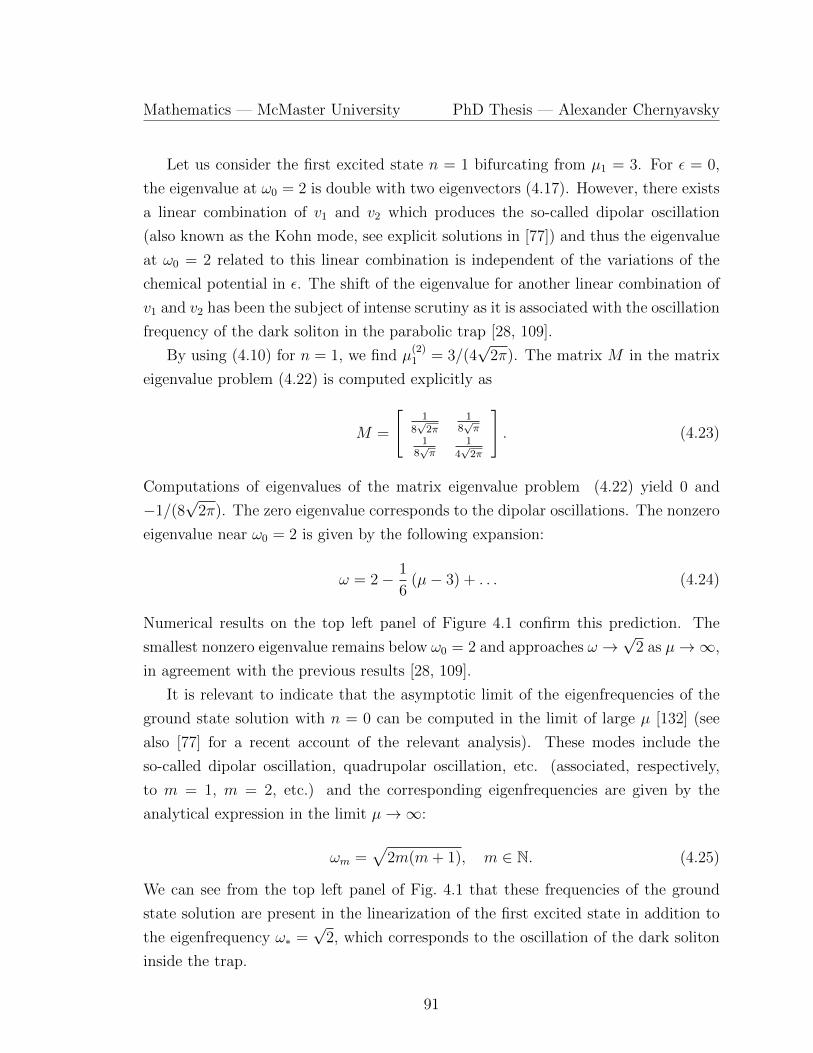
Mathematics — McMaster University PhD Thesis — Alexander Chernyavsky
Let us consider the first excited state n = 1 bifurcating from µ1 = 3. For ε = 0,
the eigenvalue at ω0 = 2 is double with two eigenvectors (4.17). However, there exists
a linear combination of v1 and v2 which produces the so-called dipolar oscillation
(also known as the Kohn mode, see explicit solutions in [77]) and thus the eigenvalue
at ω0 = 2 related to this linear combination is independent of the variations of the
chemical potential in ε. The shift of the eigenvalue for another linear combination of
v1 and v2 has been the subject of intense scrutiny as it is associated with the oscillation
frequency of the dark soliton in the parabolic trap [28, 109].
By using (4.10) for n = 1, we find µ(2)1 = 3/(4
√2π). The matrix M in the matrix
eigenvalue problem (4.22) is computed explicitly as
M =
[1
8√
2π1
8√π
18√π
14√
2π
]. (4.23)
Computations of eigenvalues of the matrix eigenvalue problem (4.22) yield 0 and
−1/(8√
2π). The zero eigenvalue corresponds to the dipolar oscillations. The nonzero
eigenvalue near ω0 = 2 is given by the following expansion:
ω = 2− 1
6(µ− 3) + . . . (4.24)
Numerical results on the top left panel of Figure 4.1 confirm this prediction. The
smallest nonzero eigenvalue remains below ω0 = 2 and approaches ω →√
2 as µ→∞,
in agreement with the previous results [28, 109].
It is relevant to indicate that the asymptotic limit of the eigenfrequencies of the
ground state solution with n = 0 can be computed in the limit of large µ [132] (see
also [77] for a recent account of the relevant analysis). These modes include the
so-called dipolar oscillation, quadrupolar oscillation, etc. (associated, respectively,
to m = 1, m = 2, etc.) and the corresponding eigenfrequencies are given by the
analytical expression in the limit µ→∞:
ωm =√
2m(m+ 1), m ∈ N. (4.25)
We can see from the top left panel of Fig. 4.1 that these frequencies of the ground
state solution are present in the linearization of the first excited state in addition to
the eigenfrequency ω∗ =√
2, which corresponds to the oscillation of the dark soliton
inside the trap.
91
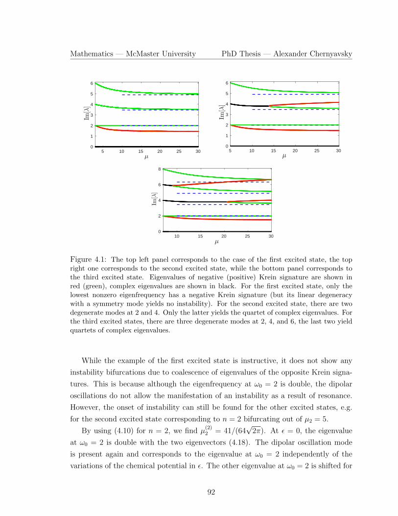
Mathematics — McMaster University PhD Thesis — Alexander Chernyavsky
Figure 4.1: The top left panel corresponds to the case of the first excited state, the topright one corresponds to the second excited state, while the bottom panel corresponds tothe third excited state. Eigenvalues of negative (positive) Krein signature are shown inred (green), complex eigenvalues are shown in black. For the first excited state, only thelowest nonzero eigenfrequency has a negative Krein signature (but its linear degeneracywith a symmetry mode yields no instability). For the second excited state, there are twodegenerate modes at 2 and 4. Only the latter yields the quartet of complex eigenvalues. Forthe third excited states, there are three degenerate modes at 2, 4, and 6, the last two yieldquartets of complex eigenvalues.
While the example of the first excited state is instructive, it does not show any
instability bifurcations due to coalescence of eigenvalues of the opposite Krein signa-
tures. This is because although the eigenfrequency at ω0 = 2 is double, the dipolar
oscillations do not allow the manifestation of an instability as a result of resonance.
However, the onset of instability can still be found for the other excited states, e.g.
for the second excited state corresponding to n = 2 bifurcating out of µ2 = 5.
By using (4.10) for n = 2, we find µ(2)2 = 41/(64
√2π). At ε = 0, the eigenvalue
at ω0 = 2 is double with the two eigenvectors (4.18). The dipolar oscillation mode
is present again and corresponds to the eigenvalue at ω0 = 2 independently of the
variations of the chemical potential in ε. The other eigenvalue at ω0 = 2 is shifted for
92
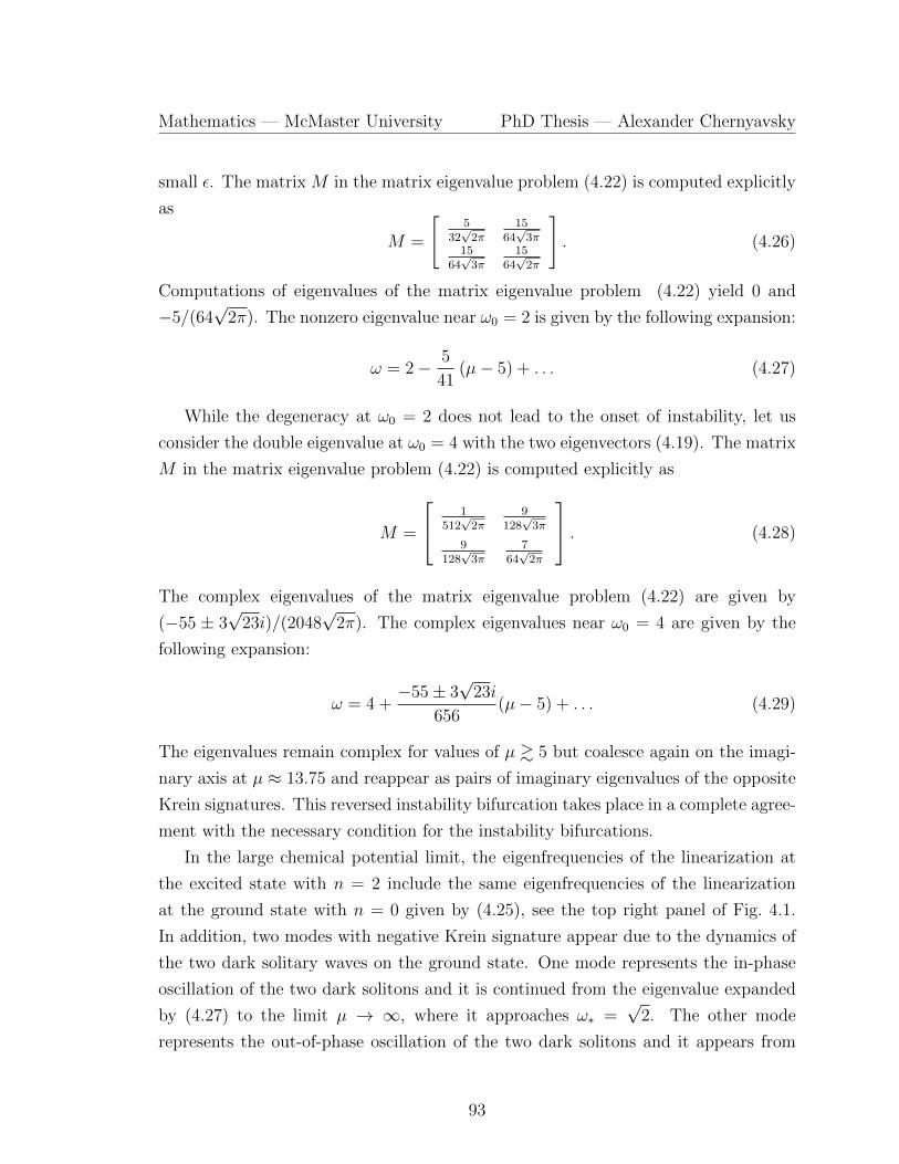
Mathematics — McMaster University PhD Thesis — Alexander Chernyavsky
small ε. The matrix M in the matrix eigenvalue problem (4.22) is computed explicitly
as
M =
[5
32√
2π15
64√
3π15
64√
3π15
64√
2π
]. (4.26)
Computations of eigenvalues of the matrix eigenvalue problem (4.22) yield 0 and
−5/(64√
2π). The nonzero eigenvalue near ω0 = 2 is given by the following expansion:
ω = 2− 5
41(µ− 5) + . . . (4.27)
While the degeneracy at ω0 = 2 does not lead to the onset of instability, let us
consider the double eigenvalue at ω0 = 4 with the two eigenvectors (4.19). The matrix
M in the matrix eigenvalue problem (4.22) is computed explicitly as
M =
1512√
2π9
128√
3π
9128√
3π7
64√
2π
. (4.28)
The complex eigenvalues of the matrix eigenvalue problem (4.22) are given by
(−55 ± 3√
23i)/(2048√
2π). The complex eigenvalues near ω0 = 4 are given by the
following expansion:
ω = 4 +−55± 3
√23i
656(µ− 5) + . . . (4.29)
The eigenvalues remain complex for values of µ & 5 but coalesce again on the imagi-
nary axis at µ ≈ 13.75 and reappear as pairs of imaginary eigenvalues of the opposite
Krein signatures. This reversed instability bifurcation takes place in a complete agree-
ment with the necessary condition for the instability bifurcations.
In the large chemical potential limit, the eigenfrequencies of the linearization at
the excited state with n = 2 include the same eigenfrequencies of the linearization
at the ground state with n = 0 given by (4.25), see the top right panel of Fig. 4.1.
In addition, two modes with negative Krein signature appear due to the dynamics of
the two dark solitary waves on the ground state. One mode represents the in-phase
oscillation of the two dark solitons and it is continued from the eigenvalue expanded
by (4.27) to the limit µ → ∞, where it approaches ω∗ =√
2. The other mode
represents the out-of-phase oscillation of the two dark solitons and it appears from
93
Mathematics — McMaster University PhD Thesis — Alexander Chernyavsky
the complex pair (4.29) which reappears back on the imaginary axis for higher values
of the chemical potential µ. Asymptotic approximation of the out-of-phase oscillation
in the limit µ→∞ is reported in [40].
This pattern continues for other excited states with n ≥ 3. The bottom panel on
Fig. 4.1 shows the case n = 3. For every n ≥ 3, there are n double eigenvalues with
opposite Krein signature at ε = 0. If ε 6= 0, the lowest double eigenvalue does not
lead to instability due to its linear degeneracy with the dipolar symmetry mode. The
remaining n − 1 double eigenvalues may yield instability bifurcations with complex
eigenvalues. For large µ, these eigenvalues reappear on the imaginary axis after the
reversed instability bifurcations in agreement with the necessary condition for the
instability bifurcation. The n eigenvalues of negative Krein signature characterize
n dark solitons on the top of the ground state solution. As such, they provide a
rather lucid example of the nature and relevance the negative Krein signature concept.
Further details can be found in [40] for the large µ case and in [74] for the small µ
case.
94
Chapter 5
Krein signature in PT -symmetric
systems
5.1 Background
In this Chapter, we address the following nonlinear Schrodinger’s equation (NLSE)
with a general complex potential:
i∂tψ + ∂2xψ − (V (x) + iγW (x))ψ + g|ψ|2ψ = 0, (5.1)
where γ ∈ R is a gain–loss parameter, g = +1 (g = −1) defines focusing (defocusing)
nonlinearity, and the real potentials V and W satisfy the even and odd symmetry,
respectively:
V (x) = V (−x), W (−x) = −W (x), x ∈ R. (5.2)
In quantum physics, the complex potential V +iγW is used to describe effects observed
when quantum particles are loaded in an open system [32, 45]. The intervals with
positive and negative imaginary part correspond to the gain and loss of quantum
particles, respectively. When gain exactly matches loss, which happens under the
symmetry condition (5.2), the potential V + iγW is PT -symmetric with respect to
the parity operator P and the time reversal operator T , defined in Chapter 1. The
NLSE (5.1) is PT -symmetric under the condition (5.2) in the sense that if ψ(x, t) is
a solution to (5.1), then
ψ(x, t) = PT ψ(x, t) = ψ(−x,−t)
95
Mathematics — McMaster University PhD Thesis — Alexander Chernyavsky
is also a solution to (5.1).
The NLSE (5.1) with a PT -symmetric potential is also used in the paraxial nonlin-
ear optics. In that context, time and space have a meaning of longitudinal and trans-
verse coordinates, and complex potential models the complex refractive index [124].
Another possible application of the NLSE (5.1) is Bose-Einstein condensate, where it
models the dynamics of the self-gravitating boson gas trapped in a confining poten-
tial V . Intervals, where W is positive and negative, allow one to compensate atom
injection and particle leakage, correspondingly [32].
Here we deal with the stationary states in the NLSE (5.1) and introduce Krein
signature of isolated eigenvalues in the spectrum of their linearization. We prove that
the necessary condition for the onset of instability of the stationary states from a de-
fective eigenvalue of algebraic multiplicity two is the opposite Krein signature of the
two simple isolated eigenvalues prior to their coalescence. Compared to the Hamil-
tonian system in Chapter 4, or the linear Schrodinger equation in [105], the Krein
signature of eigenvalues cannot be computed from the eigenvectors in the linearized
problem, as the adjoint eigenvectors need to be computed separately and the sign of
the adjoint eigenvector needs to be chosen by a continuity argument.
5.2 Stationary states, eigenvalues of the lineariza-
tion, and Krein signature
Let us define the stationary state of the NLSE (5.1) by ψ(x, t) = Φ(x)e−iµt, where
µ ∈ R is a parameter. In the context of Bose-Einstein condensate, µ has the meaning
of the chemical potential [45]. The function Φ(x) : R → C is a suitable solution of
the stationary NLSE in the form
−Φ′′(x) + (V (x) + iγW (x))Φ(x)− g|Φ(x)|2Φ(x) = µΦ(x), (5.3)
where x ∈ R. We say that Φ is a PT -symmetric stationary state if Φ satisfies the
PT symmetry:
Φ(x) = PT Φ(x) = Φ(−x), x ∈ R. (5.4)
In addition to the symmetry constraints on the potentials V and W in (5.2), our basic
assumptions are given below. Here and in what follows, we denote the Sobolev space
96

Mathematics — McMaster University PhD Thesis — Alexander Chernyavsky
of square integrable functions with square integrable second derivatives by H2(R) and
the weighted L2 space with a finite second moment by L2,2(R).
Assumption 1. We assume that the linear Schrodinger operator L0 := −∂2x + V in
L2(R) admits a self-adjoint extension with a dense domain D(L0) in L2(R).
Remark 18. If V ∈ L2(R) ∩ L∞(R) as in (5.43), then Assumption 1 is satisfied
with D(L0) = H2(R) (see [63], Ch. 14, p.143). If V is harmonic as in (5.44), then
Assumption 1 is satisfied with D(L0) = H2(R) ∩ L2,2(R) (see [62], Ch. 4, p.37).
Assumption 2. We assume that W is a bounded and exponentially decaying potential
satisfying
|W (x)| ≤ Ce−κ|x|, x ∈ R,
for some C > 0 and κ > 0.
Remark 19. Both examples in (5.43) and (5.44) satisfy Assumption 2. By Assump-
tion 2, the potential iγW is a relatively compact perturbation to L0 (see [121], Ch.
XIII, p.113). This implies that the continuous spectrum of L0 + iγW is the same
as L0. If V ∈ L2(R) ∩ L∞(R), then the continuous spectrum of L0 is located on the
positive real line. If V is harmonic, then the continuous spectrum of L0 is empty
(see [121], Ch. XIII, Theorem 16 on p.120).
Assumption 3. We assume that for a given µ ∈ R, there exist γ∗ > 0 and a bounded,
exponentially decaying, and PT -symmetric solution Φ ∈ D(L0) ⊂ L2(R) to the sta-
tionary NLSE (5.3) with γ ∈ (−γ∗, γ∗) satisfying (5.4) and
|Φ(x)| ≤ Ce−κ|x|, x ∈ R,
for some C > 0 and κ > 0. Moreover, the map (−γ∗, γ∗) 3 γ 7→ Φ ∈ D(L0) is
real-analytic.
Remark 20. Since the nonlinear equation (5.3) is real-analytic in γ, the Implicit
Function Theorem (see [142], Ch. 4, Theorem 4.E on p.250) provides real analyticity
of the map (−γ∗, γ∗) 3 γ 7→ Φ ∈ D(L0) as long as the Jacobian operator
L :=
[−∂2
x + V + iγW − µ− 2g|Φ|2 −gΦ2
−gΦ2 −∂2
x + V − iγW − µ− 2g|Φ|2
](5.5)
is invertible in the space of PT -symmetric functions in L2(R).
97
Mathematics — McMaster University PhD Thesis — Alexander Chernyavsky
Remark 21. Under Assumption 3, we treat µ as a fixed parameter and γ as a varying
parameter in the interval (−γ∗, γ∗). The interval includes the Hamiltonian case γ = 0.
In the context of the example of V in (5.43), it will be more natural to fix the value
of γ and to consider the parameter continuation of Φ ∈ D(L0) with respect to µ. The
continuation results for the latter case are analogous to what we present here under
Assumption 3.
We perform the standard linearization of the NLSE (5.1) near the stationary state
Φ by substituting
ψ(x, t) = e−iµt [Φ(x) + u(x, t)]
into (5.1) and truncating at the linear terms in u:iut = (−∂2x + V + iγW − µ− 2g|Φ|2)u− gΦ2u,
−iut = (−∂2x + V − iγW − µ− 2g|Φ|2)u− gΦ
2u.
Using u = Y e−λt and u = Ze−λt with the spectral parameter λ yields the spectral
stability problem in the form
L[Y
Z
]= −iλσ3
[Y
Z
], (5.6)
where σ3 = diag(1,−1) is the third Pauli’s matrix and L is given by (5.5). Note that
if λ 6∈ R, then Z 6= Y .
Lemma 9. The continuous spectrum of the operator iσ3L : D(L0)×D(L0)→ L2(R)×L2(R), if it exists, is a subset of iR.
Proof. Thanks to the Assumptions 1, 2 and 3, W and Φ2 terms in (5.5) are relatively
compact perturbations to the diagonal unbounded operator L0 := diag(L0−µ, L0−µ),
where L0 = −∂2x + V is introduced in Assumption (A1). Therefore,
σc(iσ3L) = σc(iσ3L0) ⊂ iR,
where σc(A) denotes the absolutely continuous part of the spectrum of the operator
A : D(A) ⊂ L2(R)→ L2(R).
98
Mathematics — McMaster University PhD Thesis — Alexander Chernyavsky
Remark 22. If V ∈ L2(R) ∩ L∞(R) and µ < 0, then
σc(iσ3L) = i(−∞,−|µ|] ∪ i[|µ|,∞).
If V is harmonic, then σc(iσ3L) is empty.
Definition 14. We say that the stationary state Φ is spectrally stable if every nonzero
solution (Y, Z) ∈ D(L0)×D(L0) to the spectral problem (5.6) corresponds to λ ∈ iR.
We note the quadruple symmetry of eigenvalues in the spectral problem (5.6).
Lemma 10. If λ0 is an eigenvalue of the spectral problem (5.6), so are −λ0, λ0, and
−λ0.
Proof. We note the symmetry of L and σ3:
L = σ1Lσ1, σ3 = −σ1σ3σ1, (5.7)
where σ1 = antidiag(1, 1) is the first Pauli’s matrix. If λ0 is an eigenvalue of the
spectral problem (5.6) with the eigenvector v0 := (Y, Z), then so is λ0 with the
eigenvector σ1v0 = (Z, Y ). We note the second symmetry of L and σ3:
L = PLP , σ3 = Pσ3P . (5.8)
If λ0 is an eigenvalue of the spectral problem (5.6) with the eigenvector v0 := (Y, Z),
then so is −λ0 with the eigenvector PT v0(x) = (Y (−x), Z(−x)). As a consequence
of the two symmetries (5.7) and (5.8), −λ0 is also an eigenvalue with the eigenvector
Pσ1v0(x) = (Z(−x), Y (−x)).
Besides the spectral problem (5.6), we also introduce the adjoint spectral problem
with the adjoint eigenvector denoted by (Y #, Z#):
L∗[Y #
Z#
]= −iλσ3
[Y #
Z#
], (5.9)
where
L∗ :=
[−∂2
x + V − iγW − µ− 2g|Φ|2 −gΦ2
−gΦ2 −∂2
x + V + iγW − µ− 2g|Φ|2
].
99
Mathematics — McMaster University PhD Thesis — Alexander Chernyavsky
Remark 23. Unless γ = 0 or Φ = 0, the adjoint eigenvector (Y #, Z#) cannot be
related to the eigenvector (Y, Z) for the same eigenvalue λ.
Our next assumption is on the existence of a nonzero isolated eigenvalue of the
spectral problem (5.6).
Assumption 4. We assume that there exists a simple isolated eigenvalue λ0 ∈ C\0of the spectral problems (5.6) and (5.9) with the eigenvector v0 := (Y, Z) ∈ D(L0) ×D(L0) and the adjoint eigenvector v#
0 := (Y #, Z#) ∈ D(L0)×D(L0), respectively.
Lemma 11. Under Assumption 4, if λ0 ∈ iR, then the corresponding eigenvectors
v0 := (Y, Z) and v#0 := (Y #, Z#) can be normalized to satisfy
Y (x) = Y (−x), Z(x) = Z(−x), x ∈ R (5.10)
and
Y #(x) = Y #(−x), Z#(x) = Z#(−x), x ∈ R. (5.11)
Proof. By Lemma 10, if λ0 ∈ iR is a nonzero eigenvalue with the eigenvector
v0 := (Y, Z), so is −λ0 = λ0 with the eigenvector PT v0. Since λ0 is a simple eigen-
value, there is a constant C ∈ C such that v0 = CPT v0. Taking norms on both sides,
we have |C| = 1. Therefore C = eiα for some α ∈ [0, 2π], and α can be chosen so
that v0 satisfies v0 = PT v0 as in (5.10). The same argument applies to the adjoint
eigenvector v#0 := (Y #, Z#).
We shall now introduce the main object of our study, the Krein signature of the
simple nonzero isolated eigenvalue λ0 in Assumption 4.
Definition 15. The Krein signature of the eigenvalue λ0 in Assumption 4 is the sign
of the Krein quantity K(λ0) defined by
K(λ0) = 〈v0, σ3v#0 〉 =
∫R
[Y (x)Y #(x)− Z(x)Z#(x)
]dx. (5.12)
The following lemma states the main properties of the Krein quantity K(λ0).
100
Mathematics — McMaster University PhD Thesis — Alexander Chernyavsky
Lemma 12. Assume (A4) and define K(λ0) by (5.12). Then,
1. K(λ0) is real if λ0 ∈ iR\0.
2. K(λ0) 6= 0 if λ0 ∈ iR\0.
3. K(λ0) = 0 if λ0 ∈ C\iR.
Proof. First, we prove that if f and g are PT -symmetric functions, then their inner
product 〈f, g〉 is real-valued. Indeed, this follows from
〈f, g〉 =
∫Rf(x)g(x)dx =
∫ +∞
0
(f(x)g(x) + f(−x)g(−x)
)dx
=
∫ +∞
0
(f(x)g(x) + f(x)g(x)
)dx.
Since λ0 ∈ iR\0 is simple by Assumption 4, then the eigenvectors v0 := (Y, Z) and
v#0 := (Y #, Z#) satisfy the PT -symmetry (5.10) and (5.11) by Lemma 11. Hence,
the inner products in the definition of K(λ0) in (5.12) are real.
Next, we prove that K(λ0) 6= 0 if λ0 ∈ iR\0 is simple. Consider a generalized
eigenvector problem for the spectral problem (5.6):
(L+ iλ0σ3)
[Yg
Zg
]= σ3
[Y
Z
]. (5.13)
Since λ0 /∈ σc(iσ3L) is isolated and simple by Assumption 4, there exists a solu-
tion vg := (Yg, Zg) ∈ D(L0) × D(L0) to the nonhomogeneous equation (5.13) if and
only if σ3v0 is orthogonal to v#0 , which is the kernel of adjoint operator L∗ + iλ0σ3.
The orthogonality condition coincides with K(λ0) = 0. However, no vg exists since
λ0 ∈ iR\0 is simple by Assumption 4. Hence K(λ0) 6= 0.
Finally, we show that K(λ0) = 0 if λ0 ∈ C\iR. Taking inner products for the
spectral problems (5.6) and (5.9) with the corresponding eigenvectors yields〈Lv0, v#0 〉 = −iλ0〈σ3v0, v
#0 〉,
〈v0,L∗v#0 〉 = iλ0〈v0, σ3v
#0 〉,
hencei(λ0 + λ0)K(λ0) = 0.
If λ0 ∈ C\iR, then λ0 + λ0 6= 0 and K(λ0) = 0.
101
Mathematics — McMaster University PhD Thesis — Alexander Chernyavsky
We shall now compare the Krein quantity K(λ0) in (5.12) for simple eigenvalues
of the PT -symmetric spectral problem (5.6) with the corresponding definition of the
Krein quantity in the Hamiltonian case γ = 0 and in the linear PT -symmetric case
Φ = 0.
In the Hamiltonian case (γ = 0), the operator L in the spectral problem (5.6)
is self-adjoint in L2(R), that is, L = L∗. The standard definition of Krein quantity
[69, 92] is given by
γ = 0 : K(λ0) = 〈Lv0, v0〉 = −iλ0
∫R
[|Y (x)|2 − |Z(x)|2
]dx. (5.14)
If γ = 0 and λ0 ∈ iR, then the adjoint eigenvector (Y #, Z#) satisfies the same
equation as (Y, Z). Therefore, it is natural to choose the adjoint eigenvector in the
form:
γ = 0 : Y #(x) = Y (x), Z#(x) = Z(x), x ∈ R, (5.15)
in which case the definition (5.12) yields the integral in the right-hand side of (5.14).
Note that the signs of K(λ0) in (5.12) and (5.14) are the same if λ0 ∈ iR+.
Remark 24. Since the potential V is even in (5.2), the eigenvector v0 := (Y, Z)
of the spectral problem (5.6) for a simple eigenvalue λ0 ∈ iR\0 is either even or
odd in the Hamiltonian case γ = 0 by the parity symmetry. It follows from the PT -
symmetry (5.10) that the PT -normalized eigenvector v0 is real if it is even and is
purely imaginary if it is odd.
Remark 25. Since the adjoint eigenvector v#0 := (Y #, Z#) satisfying the PT -symmetry
condition (5.11) is defined up to an arbitrary sign, the Krein quantity K(λ0) in (5.12)
is defined up to the sign change. In the continuation of the NLSE (5.1) with respect
to the parameter γ from the Hamiltonian case γ = 0, the sign of the Krein quantity
K(λ0) in (5.12) can be chosen so that it matches the sign of K(λ0) in (5.14) for
λ0 ∈ iR+ and γ = 0. In other words, the choice (5.15) is always made for γ = 0 and
the Krein quantity K(λ0) is extended continuously with respect to the parameter γ.
In the linear PT -symmetric case (Φ = 0), the spectral problem (5.6) becomes
diagonal. If Z = 0, then Y satisfies the scalar Schrodinger equation
(−∂2
x + V (x) + iγW (x)− µ)Y (x) = −iλY (x). (5.16)
102

Mathematics — McMaster University PhD Thesis — Alexander Chernyavsky
The PT -Krein signature for the simple eigenvalue λ0 ∈ iR of the scalar Schrodinger
equation (5.16) is defined in [105] as follows:
Φ = 0, Z = 0 : K(λ0) =
∫RY (x)Y (−x)dx. (5.17)
If λ0 ∈ iR, then the adjoint eigenfunction Y # satisfies a complex-conjugate equation
to the spectral problem (5.16), which becomes identical to (5.16) after the parity
transformation. Therefore, it is natural to choose the adjoint eigenfunction Y # in the
form:
Φ = 0, Z = 0 : Y #(x) = Y (−x), x ∈ R,
after which the definition (5.12) with Z = 0 corresponds to the definition (5.17). If
Y = 0, then Z satisfies the scalar Schrodinger equation
(−∂2
x + V (x)− iγW (x)− µ)Z(x) = iλZ(x). (5.18)
The PT -Krein signature for the simple eigenvalue λ0 ∈ iR of the scalar Schrodinger
equation (5.18) is defined by
Φ = 0, Y = 0 : K(λ0) =
∫RZ(x)Z(−x)dx, (5.19)
which coincides with the definition (5.12) for Y = 0 if the adjoint eigenfunction Z#
is chosen in the form:
Φ = 0, Y = 0 : Z#(x) = −Z(−x), x ∈ R. (5.20)
Note that if the choice Z#(x) = Z(−x) is made instead of (5.20), then the definition
(5.12) with Y = 0 is negative with respect to the definition (5.19).
5.3 Necessary condition for instability bifurcation
Recall that the eigenvalue is called semi-simple if algebraic and geometric multiplicities
coincide and defective if algebraic multiplicity exceeds geometric multiplicity. Here
we consider the case when the nonzero eigenvalue λ0 ∈ iR of the spectral problem
(5.6) is defective with geometric multiplicity one and algebraic multiplicity two. This
103

Mathematics — McMaster University PhD Thesis — Alexander Chernyavsky
situation occurs in the parameter continuations of the NLSE (5.1) when two simple
isolated eigenvalues λ1, λ2 ∈ iR\0 coalesce at the point λ0 6= 0 and split into the
complex plane resulting in the instability bifurcation. We will use the parameter γ to
control the coalescence of two simple eigenvalues λ1, λ2 ∈ iR.
Our main result states that the instability bifurcation occurs from the defective
eigenvalue λ0 ∈ iR of algebraic multiplicity two only if the Krein signatures of K(λ1)
and K(λ2) for the two simple isolated eigenvalues λ1, λ2 ∈ iR before coalescence are
opposite to each other. Therefore, we obtain the necessary condition for the instability
bifurcation in the PT -symmetric spectral problem (5.6), which has been proven for
the Hamiltonian spectral problems [69, 92].
Remark 26. The necessary condition for instability bifurcation allows us to predict
the transition from stability to instability when a pair of imaginary eigenvalues collide.
Pairs with the same Krein signature do not bifurcate off the imaginary axis if they
collide, whereas pairs with the opposite Krein signature may bifurcate off the imaginary
axis under a technical non-degeneracy condition (5.27) below.
First, we state why the perturbation theory can be applied to the spectral problem
(5.6).
Lemma 13. Under Assumptions 1, 2, and 3, the operator
L : D(L0)×D(L0)→ L2(R)× L2(R)
in the spectral problem (5.6) is real-analytic with respect to γ ∈ (−γ∗, γ∗). Conse-
quently, if L(γ0) with γ0 ∈ (−γ∗, γ∗) has a spectrum consisting of two separated parts,
then the subspaces of L2(R) × L2(R) corresponding to the separated parts are also
real-analytic in γ.
Proof. Operator L depends on γ via the potential iγW and the bound state Φ, the
latter is real-analytic for γ ∈ (−γ∗, γ∗) by Assumption 3. The assertion of the lemma
follows from Theorem 1.7 in Chapter VII on p.368 in [71].
By Lemma 13, simple isolated eigenvalues λ1, λ2 ∈ iR of the spectral problem (5.6)
and their eigenvectors v1 := (Y1, Z1) and v2 := (Y2, Z2) are continued analytically in γ
before the coalescence point. Similarly, the adjoint eigenvectors v#1 := (Y #
1 , Z#1 ) and
v#2 := (Y #
2 , Z#2 ) of the adjoint spectral problem (5.9) for λ1, λ2 ∈ iR are continued
104
Mathematics — McMaster University PhD Thesis — Alexander Chernyavsky
analytically in γ. Therefore, the Krein quantities K(λ1) and K(λ2) are continued
analytically in γ.
Let γ0 denote the bifurcation point when the two eigenvalues coalesce: λ1 = λ2 =
λ0 ∈ iR\0. For this γ0 ∈ R, we can define a small parameter ε ∈ R such that
γ = γ0 + ε. If L is denoted by L(γ), then L(γ) can be represented by the Taylor
expansion:
L(γ) = L(γ0) + εL′(γ0) + ε2L(ε), (5.21)
where L(ε) denotes the remainder terms,
L′(γ0) =
[iW − 2g∂γ|Φ(γ0)|2 −g∂γΦ2(γ0)
−g∂γΦ2(γ0) −iW − 2g∂γ|Φ(γ0)|2
], (5.22)
and ∂γ denotes a partial derivative with respect to the parameter γ. Since the re-
mainder terms in L(ε) come from the second derivative of Φ in γ near γ0, then
L(ε) ∈ L2(R) ∩ L∞(R) thanks to Assumption 3.
Instead of Assumption 4, we shall now use the following assumption.
Assumption (A4′). For γ = γ0, we assume that there exists a defective isolated
eigenvalue λ0 ∈ iR\0 of the spectral problems (5.6) and (5.9) with the eigenvector
v0 := (Y0, Z0) ∈ D(L0)×D(L0), the generalized eigenvector vg := (Yg, Zg) ∈ D(L0)×D(L0) and the adjoint eigenvector v#
0 := (Y #0 , Z#
0 ) ∈ D(L0) × D(L0), the adjoint
generalized eigenvector v#g := (Y #
g , Z#g ) ∈ D(L0)×D(L0), respectively.
By setting λ0 = iΩ0, we can write the linear equations for the eigenvectors and
generalized eigenvectors in Assumption (A4′):
L(γ0)v0 = Ω0σ3v0,
L(γ0)vg = Ω0σ3vg + σ3v0, (5.23)
L∗(γ0)v#0 = Ω0σ3v
#0 ,
L∗(γ0)v#g = Ω0σ3v
#g + σ3v
#0 . (5.24)
The solvability conditions for the inhomogeneous equations (5.23) and (5.24) yield
the following elementary facts.
105
Mathematics — McMaster University PhD Thesis — Alexander Chernyavsky
Lemma 14. Under Assumption (A4′), we have
K(λ0) = 〈v0, σ3v#0 〉 = 0. (5.25)
and
〈vg, σ3v#0 〉 = 〈v0, σ3v
#g 〉 6= 0. (5.26)
Proof. Since vg exists by Assumption (A4′), the solvability condition for (5.23) implies
(5.25), see similar computations in Lemma 12. Since the eigenvalue λ0 is double, no
second generalized eigenvector vg exists from solutions of the inhomogeneous equation
L(γ0)vg = Ω0σ3vg + σ3vg.
The nonsolvability condition for this equation implies 〈vg, σ3v#0 〉 6= 0. Finally, equa-
tions (5.23) and (5.24) yield
〈vg, σ3v#0 〉 = 〈vg, (L∗ − Ω0σ3)v#
g 〉 = 〈(L − Ω0σ3)vg, v#g 〉
= 〈σ3v0, v#g 〉 = 〈v0, σ3v
#g 〉,
which proves the symmetry in (5.26).
Remark 27. Since the generalized eigenvectors are given by solutions of the inho-
mogeneous linear equations (5.23) and (5.24) and the eigenvectors satisfy the PT -
symmetry (5.10) and (5.11), the generalized eigenvectors also satisfy the same PT -
symmetry (5.10) and (5.11).
The following result gives the necessary condition that the defective eigenvalue λ0
in Assumption (A4′) splits into the complex plane in a one-sided neighborhood of the
bifurcation point γ0.
Theorem 13. Assume 1, 2, 3, (A4′), and the non-degeneracy condition
〈L′(γ0)v0, v#0 〉 6= 0. (5.27)
There exists ε0 > 0 such that two simple eigenvalues λ1, λ2 of the spectral problem
(5.6) exist near λ0 for every ε ∈ (−ε0, ε0)\0 with λ1,2 → λ0 as ε→ 0. On one side
of ε = 0, the eigenvalues are λ1, λ2 ∈ iR and
sign [K(λ1)] = −sign [K(λ2)] . (5.28)
106
Mathematics — McMaster University PhD Thesis — Alexander Chernyavsky
On the other side of ε = 0, the eigenvalues are λ1, λ2 /∈ iR.
Proof. We are looking for an eigenvalue Ω(ε) of the perturbed spectral problem(L0 + εL(ε)
)v(ε) = Ω(ε)σ3v(ε), (5.29)
such that Ω(ε) → Ω0 as ε → 0. Here we denote operators from the decomposition
(5.21) as L0 = L(γ0) and L(ε) = L′(γ0) + εL(ε). Since Ω0 is a defective eigen-
value of geometric multiplicity one and algebraic multiplicity two, we apply Puiseux
expansions [82]: Ω(ε) = Ω0 + ε1/2Ω(ε),
v(ε) = v0 + ε1/2a(ε)vg + εv1(ε),(5.30)
where v0 and vg are the eigenvector and the generalized eigenvector for the eigen-
value Ω0, a(ε) is the projection coefficient to be defined, and Ω(ε) and v1(ε) are the
remainder terms. To define v1(ε) uniquely, we add the orthogonality condition
〈v1(ε), σ3v#0 〉 = 〈v1(ε), σ3v
#g 〉 = 0. (5.31)
Plugging (5.30) into (5.29) and dropping the dependence on ε for L, v1, a and Ω gives
us the nonhomogeneous equation(L0 − Ω0σ3 + εL − ε1/2Ωσ3
)v1 = h, (5.32)
where
h = ε−1/2(Ω− a)σ3v0 − Lv0 + a(Ωσ3 − ε1/2L
)vg.
By Assumption (A4′), the limiting operator σ3(L0 − Ω0σ3) has the two-dimensional
generalized null space X0 = spanv0, vg ⊂ L2(R) × L2(R). Since Ω0 /∈ σc(σ3L0) is
isolated from the rest of the spectrum of σ3L0, the range of σ3(L0−Ω0σ3) is orthogonal
with respect to generalized null space Y0 = spanσ3v#0 , σ3v
#g ⊂ L2(R) × L2(R) of
the adjoint operator (L∗0 − Ω0σ3)σ3. As a result, σ3(L0 − Ω0σ3) is invertible on an
element of Y ⊥0 and the inverse operator is uniquely defined and bounded in Y ⊥0 . In
other words, there exist positive constants ε0, Ω0, and C0 such that for all |ε| ≤ ε0,
|Ω| ≤ Ω0, and all σ3f ∈ Y ⊥0 , there exists a unique (L0 − Ω0σ3)−1f ∈ D(L0)×D(L0)
107
Mathematics — McMaster University PhD Thesis — Alexander Chernyavsky
satisfying the orthogonality conditions (5.31) and the bound
‖(L0 − Ω0σ3)−1f‖L2 ≤ C0‖f‖L2 . (5.33)
In order to provide existence of a unique (L0 − Ω0σ3)−1f , we add the orthogonality
constraints 〈f, v#0 〉 = 〈f, v#
g 〉 = 0. By using (5.26) and (5.31), we obtain two equations
from (5.32):
ε〈Lv1, v#0 〉+ 〈Lv0, v
#0 〉 = Ωa〈vg, σ3v
#0 〉 − ε1/2a〈Lvg, v#
0 〉, (5.34)
and
ε〈Lv1, v#g 〉+ 〈Lv0, v
#g 〉 = Ωa〈vg, σ3v
#g 〉 − ε1/2a〈Lvg, v#
g 〉+ ε−1/2(Ω− a)〈v0, σ3v
#g 〉. (5.35)
Since L and Ωσ3 are relatively compact perturbations to (L0 − Ω0σ3), there exists a
unique solution of the nonhomogeneous equation (5.32) under the constraints (5.34)
and (5.35) satisfying the orthogonality conditions (5.31) and the resolvent estimate (5.33).
In particular, there exist positive constants ε0, Ω0, A0, and C0 such that for all |ε| ≤ ε0,
|Ω| ≤ Ω0, and |a| ≤ A0, the solution v1 ∈ D(L0)×D(L0) of equation (5.32) satisfies
the estimate
‖v1‖L2 ≤ C0
(ε−1/2|a− Ω|+ 1
). (5.36)
Equation (5.35) yields
ε−1/2(a− Ω) =1
〈v0, σ3v#g 〉(
Ωa〈vg, σ3v#g 〉 − ε1/2a〈Lvg, v#
g 〉
− 〈Lv0, v#g 〉 − ε〈Lv1, v
#g 〉),
where 〈v0, σ3v#g 〉 6= 0 due to Lemma 14. Combining with the estimate (5.36), we
obtain for some C1 > 0
|a− Ω| ≤ C1ε1/2 and ‖v1‖L2 ≤ C1. (5.37)
108
Mathematics — McMaster University PhD Thesis — Alexander Chernyavsky
Equation (5.34) yields
Ωa =1
〈vg, σ3v#0 〉(〈Lv0, v
#0 〉+ ε1/2a〈Lvg, v#
0 〉+ ε〈Lv1, v#0 〉),
where 〈vg, σ3v#0 〉 6= 0 due to Lemma 14. Thanks to (5.37), we obtain
|Ω− Ωg| ≤ C2ε1/2,
where C2 > 0 is a constant, and Ωg is a root of the quadratic equation
Ω2g =〈L′(γ0)v0, v
#0 〉
〈vg, σ3v#0 〉
, (5.38)
with L′(γ0) given by (5.22). Since L′(γ0)v0, vg, and v#0 satisfy the PT -symmetry
conditions, both the nominator and the denominator of (5.38) are real-valued by the
same computations as in the proof of Lemma 12. By the assumption (5.27), Ω2g is
nonzero, either positive or negative.
Let us assume that Ω2g > 0 without loss of generality and pick Ωg > 0. Then
ε1/2Ωg ∈ R if ε > 0 and we obtain the expansions for the two simple eigenvalues:Ω1(ε) = Ω0 + ε1/2Ωg +O(ε),
Ω2(ε) = Ω0 − ε1/2Ωg +O(ε)
and their corresponding eigenvectors:v1(ε) = v0 + ε1/2Ωgvg +O(ε),
v2(ε) = v0 − ε1/2Ωgvg +O(ε).
The same expansions hold for eigenvectors of the adjoint spectral problems corre-
sponding to the same eigenvalues Ω1,Ω2:v#1 (ε) = v#
0 + ε1/2Ωgv#g +O(ε),
v#2 (ε) = v#
0 − ε1/2Ωgv#g +O(ε).
109
Mathematics — McMaster University PhD Thesis — Alexander Chernyavsky
The leading order of Krein quantities for eigenvalues λ1 = iΩ1 and λ2 = iΩ2 is given
by K(λ1) = 〈v1, σ3v#1 〉 = ε1/2Ωg〈vg, σ3v
#0 〉+ ε1/2Ωg〈v0, σ3v
#g 〉+O(ε),
K(λ2) = 〈v2, σ3v#2 〉 = −ε1/2Ωg〈vg, σ3v
#0 〉 − ε1/2Ωg〈v0, σ3v
#g 〉+O(ε),
which is simplified with the help of (5.26) toK(λ1) = 2ε1/2Ωg〈vg, σ3v#0 〉+O(ε),
K(λ2) = −2ε1/2Ωg〈vg, σ3v#0 〉+O(ε).
Since ε1/2Ωg ∈ R and 〈vg, σ3v#0 〉 6= 0, we obtain (5.28). If ε < 0, then ε1/2Ωg ∈ iR, so
that λ1, λ2 /∈ iR.
Remark 28. If the non-degeneracy assumption (5.27) is not satisfied, then Ωg = 0
and the perturbation theory must be extended to the next order. In this case, the
defective eigenvalue λ0 = iΩ0 may split along iR both for ε > 0 and ε < 0.
5.4 Numerical Approximations
We approximate nonlinear modes Φ of the stationary NLSE (5.3) and eigenvectors
(Y, Z) of the spectral problem (5.6) with the Chebyshev interpolation method [137].
This method was recently applied to massive Dirac equations in [112]. Chebyshev
polynomials are defined on the interval [−1, 1]. The stationary NLSE (5.3) is defined
on the real line, therefore we make a coordinate transformation for the Chebyshev
grid points zj = cos( jπN
)j=Nj=0 :
xj = L arctanh(zj), j = 1, 2, . . . , N − 1, (5.39)
where x0 = +∞ and xN = −∞. The scaling parameter L is chosen so that the grid
points xjj=N−1j=1 are concentrated in the region where the nonlinear mode Φ changes
fast. We apply the chain rule for the second derivative:
d2u
dx2=
d
dx
(du
dx
)=
d
dz
(du
dz
dz
dx
)=d2u
dz2
(dz
dx
)2
+du
dz
d2z
dx2,
110
Mathematics — McMaster University PhD Thesis — Alexander Chernyavsky
wheredz
dx=
1
Lsech2
(xL
)=
1
L(1− z2)
andd2z
dx2= − 2
L2sech2
(xL
)tanh
(xL
)= − 2
L2z(1− z2).
The first and second derivatives for ∂z and ∂2z are approximated by the Chebyshev
differentiation matrices DN and D2N , respectively (see p.53 in [137]).
The stationary NLSE (5.3) is written in the form:
F (Φ) := (−∂2x + V + iγW − µ− g|Φ|2)Φ = 0. (5.40)
We fix µ, γ, g, V , W and use Newton’s method to look for a solution Φ satisfying
Assumption 3: [Φn+1
Φn+1
]=
[Φn
Φn
]− L−1
n
[F (Φn)
F (Φn)
], (5.41)
where Ln is the Jacobian operator to the nonlinear problem (5.40), which coincides
with (5.5) computed at Φn. Since Φ(x0) = Φ(xN) = 0, the Jacobian operator Ln is
represented by the 2(N − 1)× 2(N − 1) matrix.
It follows by the gauge transformation that
L[
iΦ
−iΦ
]=
[0
0
], (5.42)
where L is computed at Φ. Therefore, L is a singular operator for every parameter
choice of equation (5.40). However, if the eigenvector satisfies the symmetry Z = Y
as in (5.42), then the eigenvector does not satisfy the PT -symmetry:
PT[
iΦ
−iΦ
]=
[−iΦ(−x)
iΦ(−x)
]= −
[iΦ
−iΦ
].
Hence, L is invertible on the space of PT -symmetric functions satisfying (5.4). In
terms of the coefficients of Chebyshev polynomials, the restriction means that the
even-numbered coefficients are purely real, whereas the odd-numbered coefficients are
purely imaginary.
111
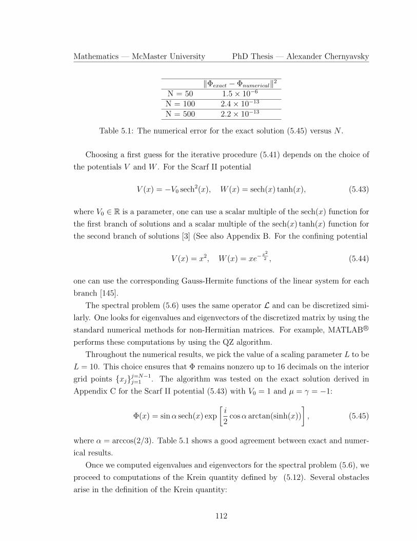
Mathematics — McMaster University PhD Thesis — Alexander Chernyavsky
‖Φexact − Φnumerical‖2
N = 50 1.5× 10⁻⁶
N = 100 2.4× 10⁻¹³
N = 500 2.2× 10⁻¹³
Table 5.1: The numerical error for the exact solution (5.45) versus N .
Choosing a first guess for the iterative procedure (5.41) depends on the choice of
the potentials V and W . For the Scarf II potential
V (x) = −V0 sech2(x), W (x) = sech(x) tanh(x), (5.43)
where V0 ∈ R is a parameter, one can use a scalar multiple of the sech(x) function for
the first branch of solutions and a scalar multiple of the sech(x) tanh(x) function for
the second branch of solutions [3] (See also Appendix B. For the confining potential
V (x) = x2, W (x) = xe−x2
2 , (5.44)
one can use the corresponding Gauss-Hermite functions of the linear system for each
branch [145].
The spectral problem (5.6) uses the same operator L and can be discretized simi-
larly. One looks for eigenvalues and eigenvectors of the discretized matrix by using the
standard numerical methods for non-Hermitian matrices. For example, MATLAB R©
performs these computations by using the QZ algorithm.
Throughout the numerical results, we pick the value of a scaling parameter L to be
L = 10. This choice ensures that Φ remains nonzero up to 16 decimals on the interior
grid points xjj=N−1j=1 . The algorithm was tested on the exact solution derived in
Appendix C for the Scarf II potential (5.43) with V0 = 1 and µ = γ = −1:
Φ(x) = sinα sech(x) exp
[i
2cosα arctan(sinh(x))
], (5.45)
where α = arccos(2/3). Table 5.1 shows a good agreement between exact and numer-
ical results.
Once we computed eigenvalues and eigenvectors for the spectral problem (5.6), we
proceed to computations of the Krein quantity defined by (5.12). Several obstacles
arise in the definition of the Krein quantity:
112
Mathematics — McMaster University PhD Thesis — Alexander Chernyavsky
1. Eigenvectors of the Chebyshev discretization matrices are normalized with re-
spect to z.
2. Eigenvectors are not necessarily PT -symmetric.
3. The sign of the adjoint eigenvectors relative to the eigenvectors is undefined.
Here we explain how to deal with these difficulties.
1. The eigenvectors are normalized in the L2([−1, 1]) norm with respect to the
variable z. In order to normalize them in the L2(R) norm with respect to the
variable x, we perform the change of coordinates (5.39). In particular, we use
integration with the composite trapezoid method on the grid points xjj=N−1j=1
and neglect integrals for (−∞, xN−1) and (x1,+∞).
2. In order to restore the PT -symmetry condition (5.10), we multiply the compo-
nent Y of the eigenvector (Y, Z) by eiθ with θ ∈ [0, 2π] and require
eiθY (x) = e−iθY (−x) ⇒ 2iθ = logY (−x)
Y (x),
where the point x is chosen so that Y (x) and Y (−x) are nonzero. For example,
we compute θ for all interior grid points xjj=N−1j=1 for which Y (xj) 6= 0 and
take the average. Both Y and Z in the same eigenvector are rotated with the
same angle θ. Similarly, this step is performed for Y # and Z# according to the
PT -symmetry condition (5.11).
3. We fix the sign of the adjoint eigenvectors at the Hamiltonian case γ = 0 by
using (5.15). Then we continue the eigenvectors and the adjoint eigenvectors for
simple eigenvalues before coalescence points. Numerically, we take two steps in
γ: γ1 < γ2, with |γ2 − γ1| 1. Suppose that the sign of eigenvector for γ1 has
been chosen already. We take eigenvectors for γ1 and γ2 and compare them. If
eigenvectors have been made PT -symmetric and properly normalized, then the
norm of their difference is either small (the eigenvectors are almost the same)
or close to 2 (the eigenvectors are negatives of each other). We choose the sign
of the eigenvector so that the norm of their difference is small.
113
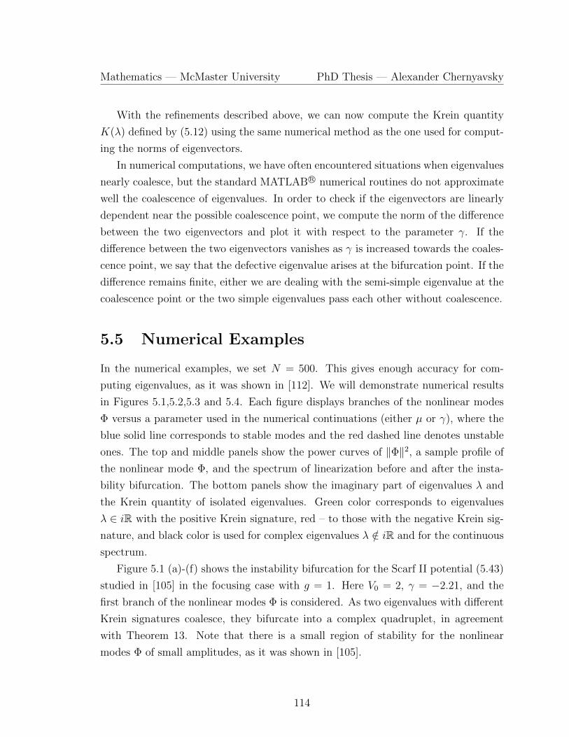
Mathematics — McMaster University PhD Thesis — Alexander Chernyavsky
With the refinements described above, we can now compute the Krein quantity
K(λ) defined by (5.12) using the same numerical method as the one used for comput-
ing the norms of eigenvectors.
In numerical computations, we have often encountered situations when eigenvalues
nearly coalesce, but the standard MATLAB R© numerical routines do not approximate
well the coalescence of eigenvalues. In order to check if the eigenvectors are linearly
dependent near the possible coalescence point, we compute the norm of the difference
between the two eigenvectors and plot it with respect to the parameter γ. If the
difference between the two eigenvectors vanishes as γ is increased towards the coales-
cence point, we say that the defective eigenvalue arises at the bifurcation point. If the
difference remains finite, either we are dealing with the semi-simple eigenvalue at the
coalescence point or the two simple eigenvalues pass each other without coalescence.
5.5 Numerical Examples
In the numerical examples, we set N = 500. This gives enough accuracy for com-
puting eigenvalues, as it was shown in [112]. We will demonstrate numerical results
in Figures 5.1,5.2,5.3 and 5.4. Each figure displays branches of the nonlinear modes
Φ versus a parameter used in the numerical continuations (either µ or γ), where the
blue solid line corresponds to stable modes and the red dashed line denotes unstable
ones. The top and middle panels show the power curves of ‖Φ‖2, a sample profile of
the nonlinear mode Φ, and the spectrum of linearization before and after the insta-
bility bifurcation. The bottom panels show the imaginary part of eigenvalues λ and
the Krein quantity of isolated eigenvalues. Green color corresponds to eigenvalues
λ ∈ iR with the positive Krein signature, red – to those with the negative Krein sig-
nature, and black color is used for complex eigenvalues λ /∈ iR and for the continuous
spectrum.
Figure 5.1 (a)-(f) shows the instability bifurcation for the Scarf II potential (5.43)
studied in [105] in the focusing case with g = 1. Here V0 = 2, γ = −2.21, and the
first branch of the nonlinear modes Φ is considered. As two eigenvalues with different
Krein signatures coalesce, they bifurcate into a complex quadruplet, in agreement
with Theorem 13. Note that there is a small region of stability for the nonlinear
modes Φ of small amplitudes, as it was shown in [105].
114
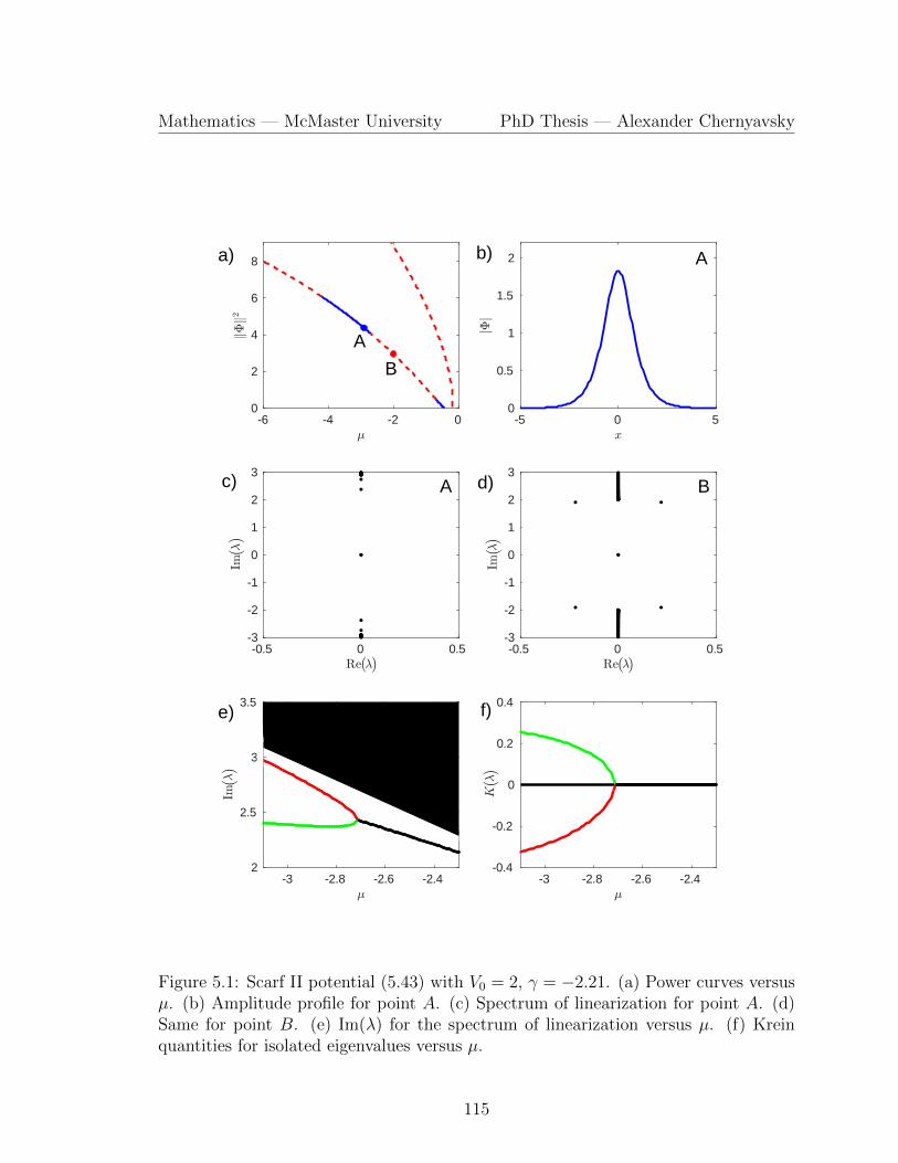
Mathematics — McMaster University PhD Thesis — Alexander Chernyavsky
Figure 5.1: Scarf II potential (5.43) with V0 = 2, γ = −2.21. (a) Power curves versusµ. (b) Amplitude profile for point A. (c) Spectrum of linearization for point A. (d)Same for point B. (e) Im(λ) for the spectrum of linearization versus µ. (f) Kreinquantities for isolated eigenvalues versus µ.
115
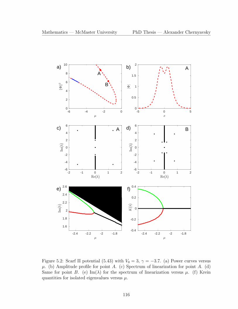
Mathematics — McMaster University PhD Thesis — Alexander Chernyavsky
Figure 5.2: Scarf II potential (5.43) with V0 = 3, γ = −3.7. (a) Power curves versusµ. (b) Amplitude profile for point A. (c) Spectrum of linearization for point A. (d)Same for point B. (e) Im(λ) for the spectrum of linearization versus µ. (f) Kreinquantities for isolated eigenvalues versus µ.
116
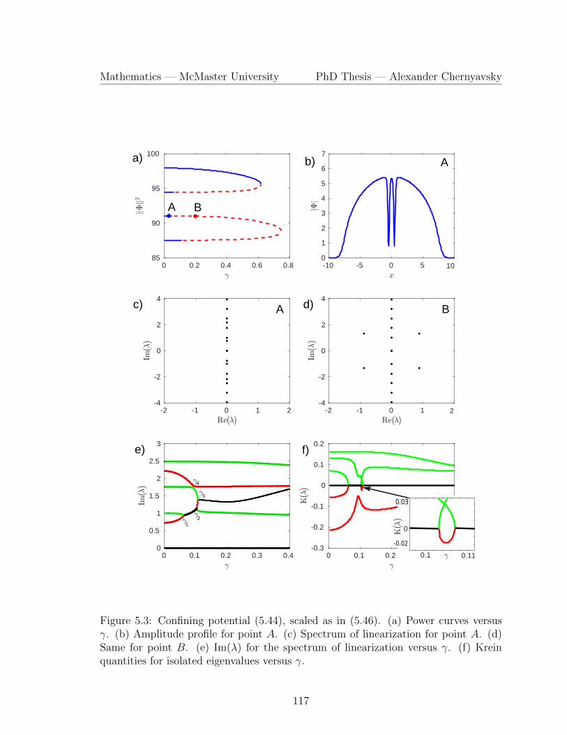
Mathematics — McMaster University PhD Thesis — Alexander Chernyavsky
Figure 5.3: Confining potential (5.44), scaled as in (5.46). (a) Power curves versusγ. (b) Amplitude profile for point A. (c) Spectrum of linearization for point A. (d)Same for point B. (e) Im(λ) for the spectrum of linearization versus γ. (f) Kreinquantities for isolated eigenvalues versus γ.
117
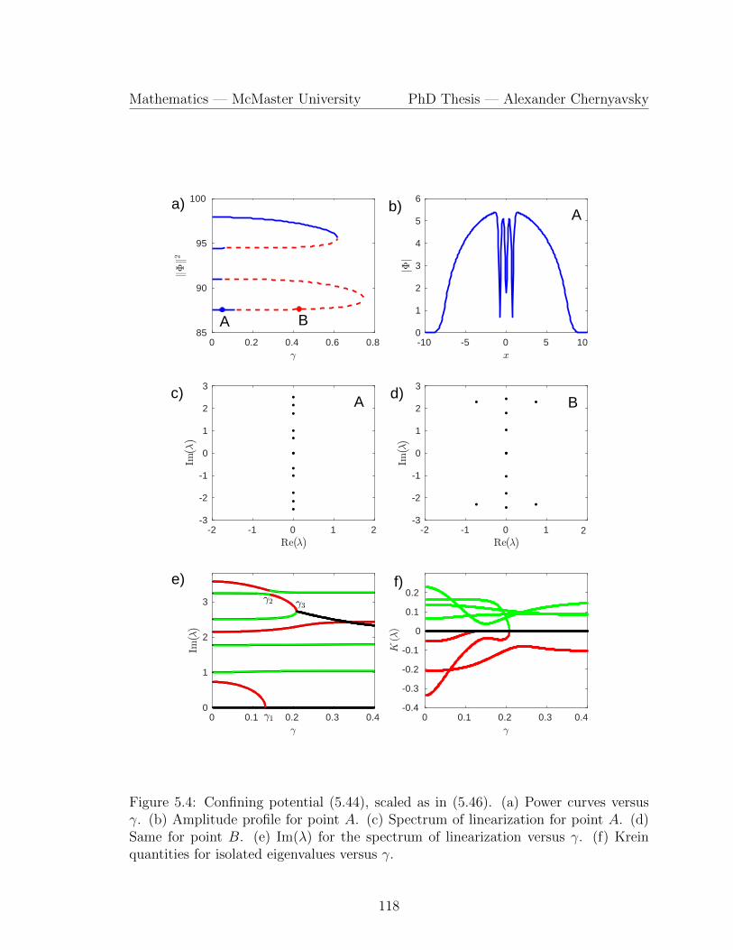
Mathematics — McMaster University PhD Thesis — Alexander Chernyavsky
Figure 5.4: Confining potential (5.44), scaled as in (5.46). (a) Power curves versusγ. (b) Amplitude profile for point A. (c) Spectrum of linearization for point A. (d)Same for point B. (e) Im(λ) for the spectrum of linearization versus γ. (f) Kreinquantities for isolated eigenvalues versus γ.
118
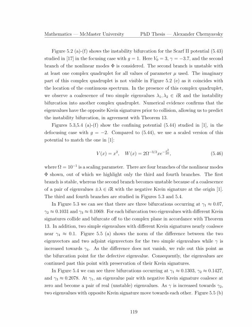
Mathematics — McMaster University PhD Thesis — Alexander Chernyavsky
Figure 5.2 (a)-(f) shows the instability bifurcation for the Scarf II potential (5.43)
studied in [17] in the focusing case with g = 1. Here V0 = 3, γ = −3.7, and the second
branch of the nonlinear modes Φ is considered. The second branch is unstable with
at least one complex quadruplet for all values of parameter µ used. The imaginary
part of this complex quadruplet is not visible in Figure 5.2 (e) as it coincides with
the location of the continuous spectrum. In the presence of this complex quadruplet,
we observe a coalescence of two simple eigenvalues λ1, λ2 ∈ iR and the instability
bifurcation into another complex quadruplet. Numerical evidence confirms that the
eigenvalues have the opposite Krein signatures prior to collision, allowing us to predict
the instability bifurcation, in agreement with Theorem 13.
Figures 5.3,5.4 (a)-(f) show the confining potential (5.44) studied in [1], in the
defocusing case with g = −2. Compared to (5.44), we use a scaled version of this
potential to match the one in [1]:
V (x) = x2, W (x) = 2Ω−3/2xe−x2
2Ω , (5.46)
where Ω = 10−1 is a scaling parameter. There are four branches of the nonlinear modes
Φ shown, out of which we highlight only the third and fourth branches. The first
branch is stable, whereas the second branch becomes unstable because of a coalescence
of a pair of eigenvalues ±λ ∈ iR with the negative Krein signature at the origin [1].
The third and fourth branches are studied in Figures 5.3 and 5.4.
In Figure 5.3 we can see that there are three bifurcations occurring at γ1 ≈ 0.07,
γ2 ≈ 0.1031 and γ3 ≈ 0.1069. For each bifurcation two eigenvalues with different Krein
signatures collide and bifurcate off to the complex plane in accordance with Theorem
13. In addition, two simple eigenvalues with different Krein signatures nearly coalesce
near γ4 ≈ 0.1. Figure 5.5 (a) shows the norm of the difference between the two
eigenvectors and two adjoint eigenvectors for the two simple eigenvalues while γ is
increased towards γ4. As the difference does not vanish, we rule out this point as
the bifurcation point for the defective eigenvalue. Consequently, the eigenvalues are
continued past this point with preservation of their Krein signatures.
In Figure 5.4 we can see three bifurcations occurring at γ1 ≈ 0.1303, γ2 ≈ 0.1427,
and γ3 ≈ 0.2078. At γ1, an eigenvalue pair with negative Krein signature coalesce at
zero and become a pair of real (unstable) eigenvalues. As γ is increased towards γ2,
two eigenvalues with opposite Krein signature move towards each other. Figure 5.5 (b)
119
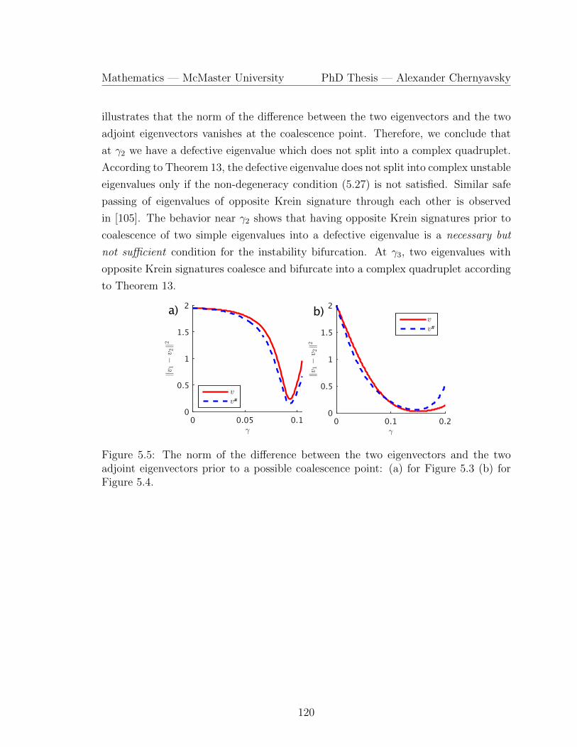
Mathematics — McMaster University PhD Thesis — Alexander Chernyavsky
illustrates that the norm of the difference between the two eigenvectors and the two
adjoint eigenvectors vanishes at the coalescence point. Therefore, we conclude that
at γ2 we have a defective eigenvalue which does not split into a complex quadruplet.
According to Theorem 13, the defective eigenvalue does not split into complex unstable
eigenvalues only if the non-degeneracy condition (5.27) is not satisfied. Similar safe
passing of eigenvalues of opposite Krein signature through each other is observed
in [105]. The behavior near γ2 shows that having opposite Krein signatures prior to
coalescence of two simple eigenvalues into a defective eigenvalue is a necessary but
not sufficient condition for the instability bifurcation. At γ3, two eigenvalues with
opposite Krein signatures coalesce and bifurcate into a complex quadruplet according
to Theorem 13.
#
#
Figure 5.5: The norm of the difference between the two eigenvectors and the twoadjoint eigenvectors prior to a possible coalescence point: (a) for Figure 5.3 (b) forFigure 5.4.
120

Chapter 6
Conclusion
In this thesis, we have presented several new contributions to stability analysis in
PT -symmetric systems both in discrete and continuous settings. Let us review the
original results and provide some possible considerations for future work.
6.1 Summary of Main Results
Chapter 2 is dedicated to the study of existence and stability of breather type solutions
in infinite-dimensional dNLS model (1.3). These are solutions of the form
u(t) = Ue−iEt, v(t) = V e−iEt,
where the frequency parameter E is real, and the sequence (U, V ) ∈ l2(Z) is time-
independent. Existence and spectral stability of breathers can be characterized in
the limit of small coupling constant ε, when breathers bifurcate from solutions of the
dimer equation arising at a single site, say the central site at n = 0. This technique
was introduced for the PT -symmetric systems in [80, 115] and is applied to the system
of amplitude equations (1.3) in Chapter 2.
Figure 6.1 represents branches of the time-periodic solutions of the central dimer
at ε = 0, where the amplitude of the central dimer A = |U0| = |V0| is plotted
versus the frequency parameter E. The left panel corresponds to the solution with
Ω > γ > 0, whereas the right panel corresponds to the solution with Ω < −γ < 0.
The constraint |γ| < |Ω| is used for stability of the zero equilibrium at ε = 0 outside
the central dimer. The values ±E0 with E0 :=√
Ω2 − γ2 correspond to bifurcation
121
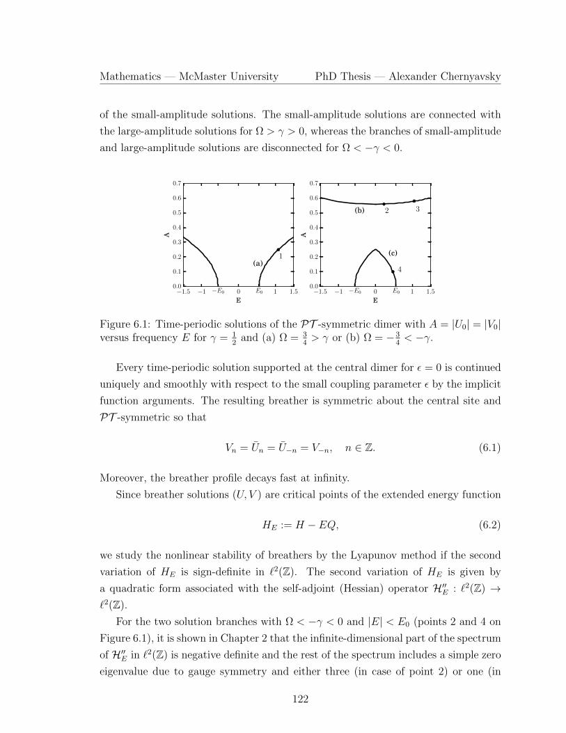
Mathematics — McMaster University PhD Thesis — Alexander Chernyavsky
of the small-amplitude solutions. The small-amplitude solutions are connected with
the large-amplitude solutions for Ω > γ > 0, whereas the branches of small-amplitude
and large-amplitude solutions are disconnected for Ω < −γ < 0.
−1.5 −1 −E0 0 E0 1 1.5
E
0.0
0.1
0.2
0.3
0.4
0.5
0.6
0.7
A
(a)1
−1.5 −1 −E0 0 E0 1 1.5
E
0.0
0.1
0.2
0.3
0.4
0.5
0.6
0.7
A
(c)
(b)
4
32
Figure 6.1: Time-periodic solutions of the PT -symmetric dimer with A = |U0| = |V0|versus frequency E for γ = 1
2and (a) Ω = 3
4> γ or (b) Ω = −3
4< −γ.
Every time-periodic solution supported at the central dimer for ε = 0 is continued
uniquely and smoothly with respect to the small coupling parameter ε by the implicit
function arguments. The resulting breather is symmetric about the central site and
PT -symmetric so that
Vn = Un = U−n = V−n, n ∈ Z. (6.1)
Moreover, the breather profile decays fast at infinity.
Since breather solutions (U, V ) are critical points of the extended energy function
HE := H − EQ, (6.2)
we study the nonlinear stability of breathers by the Lyapunov method if the second
variation of HE is sign-definite in `2(Z). The second variation of HE is given by
a quadratic form associated with the self-adjoint (Hessian) operator H′′E : `2(Z) →`2(Z).
For the two solution branches with Ω < −γ < 0 and |E| < E0 (points 2 and 4 on
Figure 6.1), it is shown in Chapter 2 that the infinite-dimensional part of the spectrum
of H′′E in `2(Z) is negative definite and the rest of the spectrum includes a simple zero
eigenvalue due to gauge symmetry and either three (in case of point 2) or one (in
122
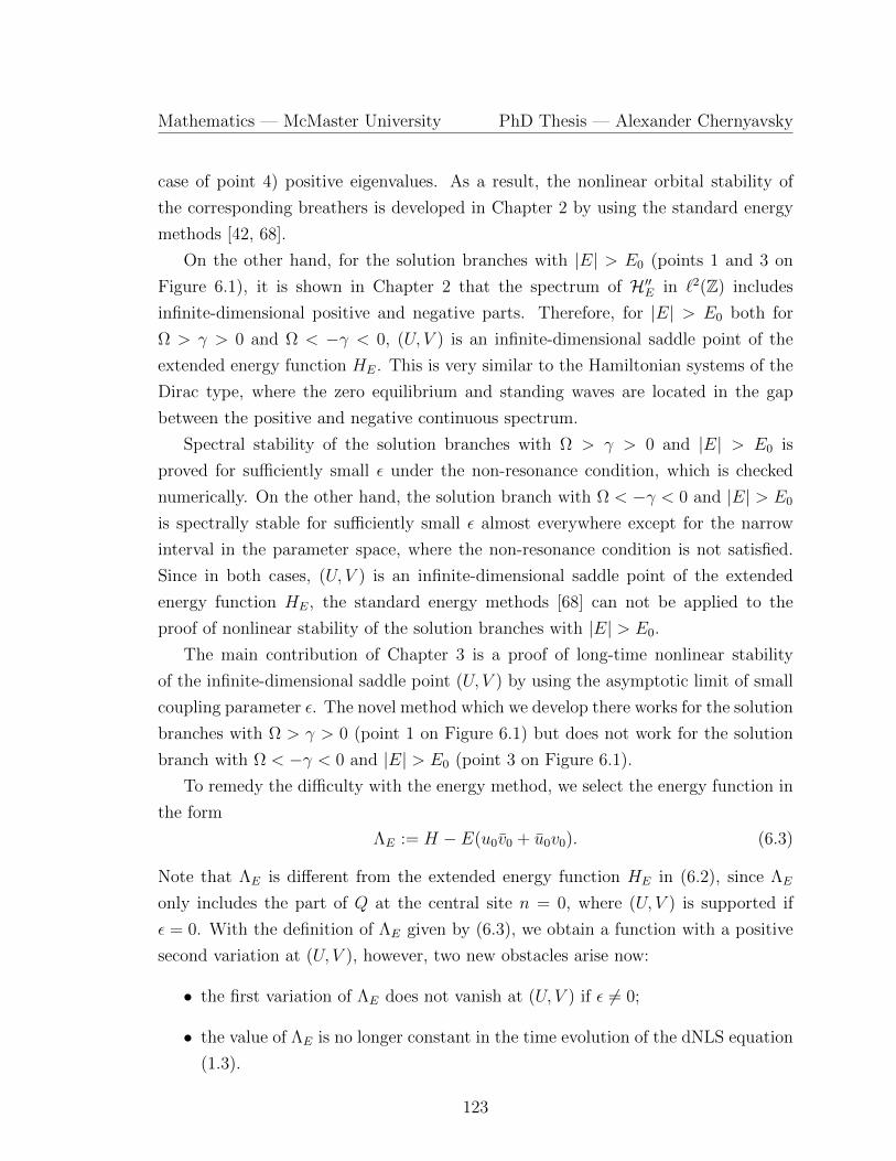
Mathematics — McMaster University PhD Thesis — Alexander Chernyavsky
case of point 4) positive eigenvalues. As a result, the nonlinear orbital stability of
the corresponding breathers is developed in Chapter 2 by using the standard energy
methods [42, 68].
On the other hand, for the solution branches with |E| > E0 (points 1 and 3 on
Figure 6.1), it is shown in Chapter 2 that the spectrum of H′′E in `2(Z) includes
infinite-dimensional positive and negative parts. Therefore, for |E| > E0 both for
Ω > γ > 0 and Ω < −γ < 0, (U, V ) is an infinite-dimensional saddle point of the
extended energy function HE. This is very similar to the Hamiltonian systems of the
Dirac type, where the zero equilibrium and standing waves are located in the gap
between the positive and negative continuous spectrum.
Spectral stability of the solution branches with Ω > γ > 0 and |E| > E0 is
proved for sufficiently small ε under the non-resonance condition, which is checked
numerically. On the other hand, the solution branch with Ω < −γ < 0 and |E| > E0
is spectrally stable for sufficiently small ε almost everywhere except for the narrow
interval in the parameter space, where the non-resonance condition is not satisfied.
Since in both cases, (U, V ) is an infinite-dimensional saddle point of the extended
energy function HE, the standard energy methods [68] can not be applied to the
proof of nonlinear stability of the solution branches with |E| > E0.
The main contribution of Chapter 3 is a proof of long-time nonlinear stability
of the infinite-dimensional saddle point (U, V ) by using the asymptotic limit of small
coupling parameter ε. The novel method which we develop there works for the solution
branches with Ω > γ > 0 (point 1 on Figure 6.1) but does not work for the solution
branch with Ω < −γ < 0 and |E| > E0 (point 3 on Figure 6.1).
To remedy the difficulty with the energy method, we select the energy function in
the form
ΛE := H − E(u0v0 + u0v0). (6.3)
Note that ΛE is different from the extended energy function HE in (6.2), since ΛE
only includes the part of Q at the central site n = 0, where (U, V ) is supported if
ε = 0. With the definition of ΛE given by (6.3), we obtain a function with a positive
second variation at (U, V ), however, two new obstacles arise now:
• the first variation of ΛE does not vanish at (U, V ) if ε 6= 0;
• the value of ΛE is no longer constant in the time evolution of the dNLS equation
(1.3).
123
Mathematics — McMaster University PhD Thesis — Alexander Chernyavsky
The first difficulty is overcome with a local transformation of dependent variables.
However, due to the second difficulty, instead of the nonlinear stability for all times,
as in Lyapunov’s stability theorem (see Section 1.5), we only establish a long-time
nonlinear stability of the breather on a long but finite time interval. This long-time
stability is usually referred as metastability.
We note that the energy functional similar to (6.3) is typically used in the normal
form transformations as the leading-order Hamiltonian, where it can be adopted for
the proof of asymptotic stability of breathers under some restrictive assumptions on
the nonlinear functions [12]. Compared to this approach, we do not use dispersive
decay estimates and hence have no control on the perturbations to extend the time
interval for long-time stability of breathers to all times.
Chapter 4 does not contain original results. We review the Hamiltonian theory,
including the necessary condition for instability bifurcation as a result of the splitting
upon collision of two eigenvalues of opposite Krein signature. An instructive case
example from the area of Bose–Einstein condensation provides a countable sequence
of nonlinear states bifurcating from eigenstates of a quantum harmonic oscillator. The
Krein signature is defined for the linearized NLS equation at each of these nonlinear
states in the Hamiltonian case.
In Chapter 5 we introduce the Krein quantity for simple isolated eigenvalues in
the linearization of the nonlinear modes in the PT -symmetric NLS equation. We
prove that the Krein quantity is zero for complex eigenvalues and nonzero for simple
purely imaginary eigenvalues. When two simple eigenvalues coalesce on the imaginary
axis in a defective eigenvalue, the Krein quantity vanishes and we prove under the
non-degeneracy assumption that this bifurcation point produces complex unstable
eigenvalues on one side of the bifurcation point. This result shows that the main
feature of the instability bifurcation in Hamiltonian systems is extended to the PT -
symmetric NLS equation.
There are nevertheless limitations of this theory in the PT -symmetric systems.
First, the adjoint eigenvectors are no longer related to the eigenvectors of the spectral
problem, which opens up a problem of normalizing the adjoint eigenvector relative to
the eigenvector. We fix the sign of the adjoint eigenvector in the Hamiltonian limit
and continue the sign off the Hamiltonian limit by using continuity of eigenvectors
along the parameters of the model.
124
Mathematics — McMaster University PhD Thesis — Alexander Chernyavsky
Second, if the bifurcation point corresponds to a semi-simple eigenvalue, then the
bifurcation theory does not lead to the same conclusion as in the Hamiltonian case.
The first-order perturbation theory results in the non-Hermitian matrices, hence it is
not clear how to conclude on the splitting of the semi-simple eigenvalues on each side
of the bifurcation point.
Finally, coalescence of the simple purely imaginary eigenvalues at the origin and
the related instability bifurcations are observed frequently in the PT -symmetric sys-
tems and they are not predicted from the Krein quantity. Therefore, we conclude
that the stability theory of Hamiltonian systems cannot be fully extended to the PT -
symmetric NLS equation, only the necessary condition for the instability bifurcation
can be, as is shown in Chapter 5.
6.2 Future Directions
This thesis leads to the following open questions and directions for further studies:
• It is known that in Hamiltonian systems negative Krein signature of an eigen-
value can lead to nonlinear instability even if the stationary state is linearly
stable [78]. It is worthwhile to use our definition of PT -Krein signature to ver-
ify whether the same phenomena is present in general PT -symmetric systems.
• In the studies of the spectral stability problems, we have often encountered bi-
furcation at zero, i.e. when the smallest eigenvalue coalesces with its symmetric
counterpart at λ = 0. The role of bifurcation at zero is not well understood.
Classical bifurcation theory suggests that there might exist additional stationary
states appearing after this bifurcation, i.e., a symmetry-breaking point occurs.
Notice that unlike PT -symmetry breaking point defined in a linear system, this
symmetry-breaking bifurcation occurs in the nonlinear system and is of interest
in its own.
• It is worthwhile to consider two-dimensional PT -symmetric version of nonlinear
Schrodinger equation arising in condensed matter theory [43, 73, 116]. Using
a traditional simplification, one can replace the non-local interaction potential
with a localized short-range interaction proportional to the delta function. This
leads to the Gross–Pitaevskii equation, more precisely to nonlinear Schrodinger
125
Mathematics — McMaster University PhD Thesis — Alexander Chernyavsky
equation with cubic nonlinearity and with a spatially dependent trap poten-
tial stationary in a frame rotating with a certain frequency about the vertical
axis. The equation in question, like many other nonlinear Schrodinger equations,
supports the existence of localized-in-space solutions of different kinds. In par-
ticular, one could look for vortex-type solutions and investigate their stability
properties in the case of complex-valued PT -symmetric potential.
• In the Hamiltonian version of the Gross–Pitaevskii equation (with real-valued
potential) there has been a great progress in numerical algorithms utilizing the
so-called Evans function [83]. Evans function enables one to find spectra more
efficiently and precisely. It will be worthwhile to adapt Evans function to PT -
symmetric systems and equip the algorithm with the ability to compute PT -
Krein signature.
Overall, there are a number of other challenging problems in the topic of PT -symmetry.
One can study formation of PT -symmetric rogue waves in inhomogeneous and non-
Hermitian optical systems, or the connection between modulational instability and
formation of PT -symmetric lattice solitons, to name a few [39].
126
Appendix A
Perturbation theory near
Hamiltonian case
In this Appendix we attempt to build a connection between eigenvectors and adjoint
eigenvectors of the stability problem (5.6) near the Hamiltonian case γ = 0. We
show that there is no simple relationship between eigenvectors of original and adjoint
operators. This is the reason why we have to compute both eigenvectors in Krein
signature definition for PT -symmetric systems.
A.1 Series in γ
Recall the eigenvalue problem (5.6) describing the spectrum of linearization about a
stationary state Φ: [L −Φ2
−Φ2 L∗
][Y
Z
]= iλσ3
[Y
Z
], (A.1)
where L = −∂2x + V (x) + iγW (x) − µ − 2|Φ(x)|2, and W (x),Φ(x) decay to zero at
x→ ±∞. Moreover, V (−x) = V (x),W (−x) = −W (x) are real-valued functions, and
µ ∈ R. Recall that Φ(x) is PT -symmetric: Φ(x) = Φ(−x) and satisfies the equation
µΦ = (−∂2x + V (x) + iγW (x)− |Φ|2)Φ. (A.2)
127
Mathematics — McMaster University PhD Thesis — Alexander Chernyavsky
Let γ = 0 in eigenvalue problem (A.1). Then it can be rewritten as:[L0 −Φ2
0
−Φ20 L0
][Y0
Z0
]= iλ0σ3
[Y0
Z0
], (A.3)
where we have used the fact that operator L0 = −∂2x + V − µ− 2|Φ0|2 is self-adjoint.
We will denote operator in (A.3) as L0. For λ0 ∈ iR problem (A.3) is self-adjoint. If
λ0 is also simple, then the eigenvector for the adjoint operator can be chosen so that[Y ∗0
Z∗0
]=
[Y0
Z0
]. (A.4)
Recall that Φ0 satisfies the following equation:
µΦ0 = (−∂2x + V (x)− |Φ0|2)Φ0. (A.5)
Notice that coefficients in this equation are all real, therefore Φ0(x) ∈ R. Since Φ0(x)
is also PT -symmetric, it follows that it is an even function.
Putting λ0 = iΩ0,Ω0 ∈ R simple, we set γ 6= 0, γ ∈ R and employ perturbation
theory. First of all, we write series in γ for all terms that depend on γ. Notice that
Φ, although not visibly, depends on γ. We write series up to O(γ3):
iλ(γ) = −Ω0 − iγΩ1 − γ2Ω2 +O(γ3),
Φ(γ) = Φ0 + iγΦ1 + γ2Φ2 +O(γ3),[Y (x; γ)
Z(x; γ)
]=
[Y0
Z0
]+ iγ
[Y1
Z1
]+ γ2
[Y2
Z2
]+O(γ3),[
Y ∗(x; γ)
Z∗(x; γ)
]=
[Y0
Z0
]+ iγ
[Y ∗1
Z∗1
]+ γ2
[Y ∗2
Z∗2
]+O(γ3).
Let us write O(γ) terms for (A.2):
µΦ1 = (−∂2x + V (x)− |Φ0|2)Φ1 +WΦ0 − Φ2
0(Φ1 + Φ1). (A.6)
As we can see, this equation has real-valued coefficients and thus Φ1(x) is real-valued.
Symmetries of coefficients in the equation also imply that Φ1(x) is an odd function:
128
Mathematics — McMaster University PhD Thesis — Alexander Chernyavsky
Φ1(−x) = −Φ1(x). For O(γ2) terms, (A.2) gives
µΦ2 = (−∂2x + V (x)− |Φ0|2)Φ2 −WΦ1 − Φ0Φ2
1 − Φ20(Φ2 + Φ2). (A.7)
From here we have Φ2(x) ∈ R, and Φ2(x) is even: Φ2(x) = Φ2(−x).
A.2 O(γ) balance equations
Let us rewrite eigenvalue problem (A.1) for γ 6= 0, keeping only O(γ) terms:
(L0 + Ω0σ3)
[Y1
Z1
]= (−W (x) + 2σ1Φ0Φ1 − Ω1)σ3
[Y0
Z0
], (A.8)
and the adjoint problem becomes
(L0 + Ω0σ3)
[Y ∗1
Z∗1
]= (W (x) + 2σ1Φ0Φ1 − Ω1)σ3
[Y0
Z0
]. (A.9)
According to the Fredholm theory, (A.8) and (A.9) have solutions only when the
right-hand side is orthogonal to the kernel of corresponding adjoint operator, in our
case consisting of a single eigenvector [Y0, Z0]T . Let us split the right-hand side into
several terms and consider them separately:
• W (x)σ3[Y0, Z0]T :⟨W (x)σ3
[Y0
Z0
],
[Y0
Z0
]⟩=
∫RW (x)(Y 2
0 − Z20)dx = 0, (A.10)
as an integral of odd function over the real line is equal to zero.
• σ1Φ0Φ1σ3[Y0, Z0]T :⟨σ1Φ0Φ1σ3
[Y0
Z0
],
[Y0
Z0
]⟩=
∫R
Φ0Φ1(Y0Z0 − Z0Y0) = 0. (A.11)
129
Mathematics — McMaster University PhD Thesis — Alexander Chernyavsky
• Ω1σ3[Y0, Z0]T : ⟨Ω1σ3
[Y0
Z0
],
[Y0
Z0
]⟩= Ω1
∫R(Y 2
0 − Z20)dx, (A.12)
where the integral is nonzero. This follows from nonexistence condition for the
generalized eigenvector [Yg, Zg]T , as eigenvalue λ0 = iΩ0 is assumed to be simple.
Therefore we must choose Ω1 = 0.
Moreover, if [Y1, Z1]T is orthogonal to [Y0, Z0]T , then the solution of (A.8) is unique.
Same holds for the adjoint counterpart. By adding and subtracting (A.8) with (A.9),
we can relate eigenvectors in a unique way.
Note that both (A.8) and (A.9) have real-valued coefficients, which also have odd
symmetry, therefore [Y1, Z1]T and [Y ∗1 , Z∗1 ]T are both real-valued functions and possess
odd symmetry property.
A.3 O(γ2) balance equations
Collecting only O(γ2) terms in (A.1) for γ 6= 0, we get
(L0 + Ω0σ3)
[Y2
Z2
]= (W (x)− 2σ1Φ0Φ1)σ3
[Y1
Z1
]
+
([2Φ2
1 + 4Φ0Φ2 −Φ21 + 2Φ0Φ2
−Φ21 + 2Φ0Φ2 2Φ2
1 + 4Φ0Φ2
]− Ω2σ3
)[Y0
Z0
]. (A.13)
For the adjoint problem we have:
(L0 + Ω0σ3)
[Y ∗2
Z∗2
]= (−W (x)− 2σ1Φ0Φ1)σ3
[Y ∗1
Z∗1
]
+
([2Φ2
1 + 4Φ0Φ2 −Φ21 + 2Φ0Φ2
−Φ21 + 2Φ0Φ2 2Φ2
1 + 4Φ0Φ2
]− Ω2σ3
)[Y0
Z0
]. (A.14)
In both equations (A.13), (A.14), coefficients are given by real-valued even functions,
therefore [Y2, Z2]T , [Y ∗2 , Z∗2 ]T are real-valued and even, as well.
We could employ Fredholm theory again, but this time the projections on the ker-
nel of the adjoint operator would have to be incorporated in the coefficient Ω2, which
130
Mathematics — McMaster University PhD Thesis — Alexander Chernyavsky
will be nonzero, in general. If both [Y2, Z2]T and [Y ∗2 , Z∗2 ]T exist and are orthogo-
nal to [Y0, Z0]T , they are unique and so is their relationship (add or subtract (A.13)
and (A.14)).
To find a relationship between [Y, Z]T and [Y ∗, Z∗]T we could use the obtained
equations to split each eigenvector as [Y, Z]T = [Y +, Z+]T + [Y −, Z−]T , and adjoint
eigenvector as [Y ∗, Z∗]T = [Y +, Z+]T − [Y −, Z−]T . Let us consider this separation for
the first order in γ: [Y1
Z1
]=
[Y +
1
Z+1
]−[Y −1
Z−1
], (A.15)[
Y +1
Z+1
]= (2σ1Φ0Φ1 − Ω1)σ3
[Y0
Z0
],[
Y −1
Z−1
]= W (x)σ3
[Y0
Z0
].
For the next order in γ we get[Y2
Z2
]=
[Y +
2
Z+2
]−[Y −2
Z−2
],[
Y +2
Z+2
]= (−2σ1Φ0Φ1)σ3
[Y1
Z1
]
+
([2Φ2
1 + 4Φ0Φ2 −Φ21 + 2Φ0Φ2
−Φ21 + 2Φ0Φ2 2Φ2
1 + 4Φ0Φ2
]− Ω2σ3
)[Y0
Z0
],[
Y −2
Z−2
]= W (x)σ3
[Y1
Z1
].
Unfortunately, here [Y +2 , Z
+2 ]T depends on both [Y +
1 , Z+1 ]T and [Y −1 , Z
−1 ]T through (A.15).
Therefore the solution cannot be separated into [Y +, Z+]T and [Y −, Z−]T parts inde-
pendent of each other, and there is no simple relationship between eigenvectors and
adjoint eigenvectors for γ 6= 0.
131
Appendix B
Spectrum of the linear problem for
Scarf II potential
In this Appendix we are going to derive analytic formulas for eigenvalues and eigen-
functions of the stationary problem for linear Schrodinger equation with Scarf II type
potential (1.12). Our goal is to correct the mistake of [3], where the author missed
one of the solutions to the eigenvalue problem.
Consider a linear Schrodinger equation:
i∂tψ + ∂2xψ − U(x)ψ = 0,
with Scarf II potential
U(x) = V1 sech2(x) + iV2 sech(x) tanh(x),
where V1, V2 are real constants. We will be looking for stationary modes in the form
ψ(x, t) = Φ(x)eiEt, where E ∈ R, Φ(x) decays to zero at infinity, and solves
Φxx + (−E + V1 sech2(x) + iV2 sech(x) tanh(x))Φ = 0. (B.1)
This equation can also be viewed as an eigenvalue problem for E with eigenfunctions
Φ. In that case the mode Φ is stable when E is real, and unstable otherwise, due to
symmetry of eigenvalues in PT -symmetric systems. Using a change of coordinates
z = 12(1 − i sinh(x)) and a substitution Φ = z−p(1 − z)−qw(z), we can rewrite linear
132
Mathematics — McMaster University PhD Thesis — Alexander Chernyavsky
stationary problem (B.1) as
z(1− z)w′′(z) +
(−2p+
1
2− (−2p− 2q + 1)z
)w′(z)−
((p+ q)2 − E
)w(z) = 0, (B.2)
where p, q are given by:
p1,2 = −1
4± 1
2
√1
4+ V1 + V2, q1,2 = −1
4± 1
2
√1
4+ V1 − V2. (B.3)
Recall Gauss hypergeometric equation [58]:
z(1− z)d2u
dz2+ (γ − (α + β + 1)z)
du
dz− αβu = 0, (B.4)
where α, β, γ ∈ C are constants. Comparing (B.4) with (B.2), one can find α, β, γ:α = 1
2∓ 1
2
√14
+ V1 + V2 ∓ 12
√14
+ V1 − V2 ±√E,
β = 12∓ 1
2
√14
+ V1 + V2 ∓ 12
√14
+ V1 − V2 ∓√E,
γ = 1∓√
14
+ V1 + V2.
(B.5)
The solution of (B.4) is given by hypergeometric series [58]:
u = F (α, β, γ, z)
= 1 +α · βγ · 1 z +
α(α + 1)β(β + 1)
γ(γ + 1) · 1 · 2 z2 +α(α + 1)(α + 2)β(β + 1)(β + 2)
γ(γ + 1)(γ + 2) · 1 · 2 · 3 z3 + . . .
Notice that when α or β is a negative integer, series are truncated and contain finitely
many terms. More precisely, α and β have to satisfy one of the quantization condi-
tions:
α = −n or β = −n, where n = 0, 1, 2, . . . (B.6)
The final solution of (B.1) is given by
Φ(x) =
(1− i sinh(x)
2
)−p(1 + i sinh(x)
2
)−qF
(α, β, γ,
1− i sinh(x)
2
), (B.7)
where by quantization condition F is a polynomial of degree n. In order for the
eigenfunction Φ(x) to satisfy the boundary condition at ±∞, the following inequality
133

Mathematics — McMaster University PhD Thesis — Alexander Chernyavsky
must hold:
0 ≤ n < Re(p+ q),
or, using (B.3),
0 ≤ n < Re
(−1
2± 1
2
√1
4+ V1 + V2 ±
1
2
√1
4+ V1 − V2
), (B.8)
where the upper bound has to be positive. Therefore minus-minus sign combination
cannot be chosen for both ± in (B.8). Note that the expression in brackets is real
when |V2| < V1 + 14.
Using either one of quantization conditions (B.6) and definitions of α, β in (B.5),
we derive a formula for n and discuss all possible cases:
n = −1
2± 1
2
√1
4+ V1 + V2 ±
1
2
√1
4+ V1 − V2 ±
√E. (B.9)
In order for inequality (B.8) to be satisfied, the minus sign for√E must be selected.
Out of 8 possible combinations, there are only 3 left:
n(1) = −1
2+
1
2
√1
4+ V1 + V2 +
1
2
√1
4+ V1 − V2 −
√E,
n(2) = −1
2+
1
2
√1
4+ V1 + V2 −
1
2
√1
4+ V1 − V2 −
√E,
n(3) = −1
2− 1
2
√1
4+ V1 + V2 +
1
2
√1
4+ V1 − V2 −
√E.
The case n(1) was studied in detail in [3], where it was shown that the corresponding
eigenvalue E(1) becomes complex for |V2| > V1 + 14. Unfortunately, in [3] branches n(2)
and n(3) were omitted, and author did not discuss why eigenvalue bifurcates off to
the complex plane. We know from bifurcation theory that generally such bifurcation
happens when two simple discrete eigenvalues coalesce on the real axis, or a simple
discrete eigenvalue collides with continuous spectrum, in our case located on the
real axis [0,+∞). Using expressions for n(j) above, we can write three branches of
134

Mathematics — McMaster University PhD Thesis — Alexander Chernyavsky
eigenvalues explicitly:
E(1)n =
(−n− 1
2+
1
2
√1
4+ V1 + V2 +
1
2
√1
4+ V1 − V2
)2
,
E(2)n =
(−n− 1
2+
1
2
√1
4+ V1 + V2 −
1
2
√1
4+ V1 − V2
)2
,
E(3)n =
(−n− 1
2− 1
2
√1
4+ V1 + V2 +
1
2
√1
4+ V1 + V2
)2
.
Notice that for V2 = V1 + 14, eigenvalues corresponding to first and second branches
coalesce and bifurcate off to the complex plane for V2 > V1+ 14. Also, for V2 = −V1− 1
4,
first and third branches coalesce and bifurcate into the complex plane for V2 < −V1− 14.
For example, for V1 = 1, V2 = 1.2, the upper bound for n for first and second
branches is positive and nonzero, therefore n = 0 gives E(1)0 ≈ 0.1556, E
(2)0 ≈ 0.0292,
and for V2 = 1.25 these two are equal: E(1)0 = E
(2)0 ≈ 0.0844. For V2 > 1.25 both
become complex. See also Figure B.1.
0 1 2
-0.1
0
0.1
0.2
0.3
0.4
0 1 2
-0.4
-0.3
-0.2
-0.1
0
0.1
0.2
0.3
0.4
a) b)
Figure B.1: First two eigenvalues for spectral problem (B.1) with n = 0. Red color
corresponds to E(1)0 , whereas blue corresponds to E
(2)0 . a) Real parts b) Imaginary
parts.
135
Appendix C
Wadati potentials: exact solutions
In this Appendix we derive a formula for exact solutions for PT -symmetric stationary
NLS (1.11) with Wadati-type potentials, for which Scarf II potential (1.12) is a special
case. The technique used here was presented in [17], where authors described the
way to construct potentials for which exact solutions are available. Notice that the
exact solutions are obtained for the full nonlinear equation, unlike the Appendix B.
The exact solutions obtained via this method were used for verification of numerical
algorithms presented in Chapter 5.
C.1 Derivation
Let us write the problem (A.2) for the nonlinear mode Φ:
Φxx + (U2 − iUx)Φ + 2Φ|Φ|2 = µΦ,
where Φ(x) = Φ(−x) is PT -symmetric, µ ∈ R is a real eigenvalue parameter, and
U(x) = U(−x) is a real valued function. Let us rewrite this equation as a system of
equations: dΦdx
= iUΦ−Ψ,
dΨdx
= µΦ− iUΦ + 2|Φ|2Φ,(C.1)
where Ψ = −dΦ/dx+ iUΦ. Take
Φ = aeiθ, Ψ = beiχ, (C.2)
136
Mathematics — McMaster University PhD Thesis — Alexander Chernyavsky
where a(x), b(x), θ(x), χ(x) are real-valued functions of x. Substituting these into
system (C.1), one can get:
ax = −b cos ν,
bx = a(2a2 + µ) cos ν,
a(U − θx) = b sin ν,
b(χx + U) = −a(2a2 + µ) sin ν,
(C.3)
where ν(x) = χ(x)− θ(x). System (C.3) has a conserved quantity:
a2(µ+ a2) + b2 = 0. (C.4)
From here we can see that µ must be chosen negative: µ = −κ2, κ ∈ R.
Using (C.4) and first equation in (C.3), we get:∫ x
0
dy
a√κ2 − a2
= −∫ x
0
cos ν(y)dy + C,
and choosing seed function cos ν(y), we take D(x) to be
D(x) = κ
∫ x
0
cos ν(y)dy + C,
where constant of integration C can be chosen to be zero without loss of generality.
Then we rewrite the equation for a:
a = κ sech(D(x)),
and for b
b = a√κ2 − a2 = κ2 sech(D(x)) tanh(D(x)).
Adding and subtracting two last equations in (C.3), one can get:
U = −νx2
+a
2b(2κ2 − 3a2) sin ν (C.5)
and
θ = −ν2−∫a3
2bsin νdx. (C.6)
137
Mathematics — McMaster University PhD Thesis — Alexander Chernyavsky
The main idea of [17] can be summarized as follows: given a seed function cos ν(x),
find potential U and exact solution Φ(x), namely find a(x) and θ(x). We would also
like to find an exact solution in a simple form.
One can rewrite equation (C.5) as
U =(cos ν(x))′
2 sin ν(x)− κ sin ν(x)
2 tanh(D(x))+
3
2κ sin ν(x) tanh(D(x))
or, using the definition of D(x), as
U =(cos ν(x))′
2 sin ν(x)− κ sin ν(x)
2 tanh(κ∫
cos ν(x)dx) +
3
2κ sin ν(x) tanh
(κ
∫cos ν(x)dx
).
From here we can see that to construct a potential (and a corresponding exact solu-
tion), one needs a smart choice of a seed function cos ν(x). As we see, it is not trivial
to find a seed function cos ν(x) such that U(x) will be independent of κ. Otherwise
the solutions obtained by this method will only be valid for fixed µ.
C.2 An example
Let us select the seed function as
cos ν =sinh(κx)√
1− κ sin2 α + sinh2(κx), (C.7)
where α ∈ (0, π2) is a parameter. Then
D(x) = arctanh
√1− κ sin2 α sech2(κx),
a = κ3/2 sinα sech(κx), (C.8)
b = κ5/2 sinα sech(κx)
√1− κ sin2 α sech2(κx). (C.9)
138
Mathematics — McMaster University PhD Thesis — Alexander Chernyavsky
In order to find U , we need to find νx and sin ν, as well:
νx =−κ cosh(κx)(1− κ sin2 α)
,(cosh2(κx)− κ sin2 α)
√1− κ sin2 α,
sin ν =
√1− κ sin2 α
cosh2(κx)− κ sin2 α.
Let us write equation for U :
U =κ cosh(κx)
√1− κ sin2 α
2(cosh2(κx)− κ sin2 α)+
cosh(κx)√
1− κ sin2 α
2κ(cosh2(κx)− κ sin2 α)(2κ2 − 3κ3 sin2 α sech2(κx))
=3
2κ sech(κx)
√1− κ sin2 α,
where for κ = 1 we obtain Scarf II potential (1.12) with V0 = −94
cos2 α, and
V1 = −32
cosα. The associated exact solution Φ = aeiθ follows from (C.6), (C.8)
and (C.9):
Φ(x) = sinα sech(x) exp
[i
2cosα arctan(sinh(x))
]. (C.10)
139
Bibliography
[1] V. Achilleos, P.G. Kevrekidis, D.J. Frantzeskakis, and R. Carretero-Gonzalez,
Dark solitons and vortices in PT-symmetric nonlinear media: From spontaneous
symmetry breaking to nonlinear PT phase transitions, Phys. Rev. A 86, 013808
(7 pp) (2012).
[2] R. Adams, and J. Fournier, Sobolev spaces (Academic Press, New York, 2003).
[3] Z. Ahmed, Real and complex discrete eigenvalues in an exactly solvable one-
dimensional complex PT-invariant potential, Phys. Lett. A 282, 343–348 (2001).
[4] N. Akhmediev, and A. Ankiewicz, Dissipative Solitons in the Complex Ginzburg-
Landau and Swift-Hohenberg Equations in Dissipative Solitons, Lecture Notes in
Physics 661, 1–17 (Springer, New York, 2005).
[5] N.V. Alexeeva, I.V. Barashenkov, and Yu.S. Kivshar, Solitons in PT -symmetric
ladders of optical waveguides, New J. Phys. 19, 113032 (30 pp) (2017).
[6] N.V. Alexeeva, I.V. Barashenkov, K. Rayanov, and S. Flach, Actively coupled
optical waveguides, Phys. Rev. A 89, 013848 (5 pp) (2014).
[7] N.V. Alexeeva, I.V. Barashenkov, A.A. Sukhorukov, and Yu.S. Kivshar, Optical
solitons in PT -symmetric nonlinear couplers with gain and loss, Phys. Rev. A
85, 063837 (13 pp) (2012).
[8] V.I. Arnold, Mathematical Methods of Classical Mechanics, (Springer–Verlag,
Berlin, 1978).
[9] B. Bagchi and C. Quesne, Non-Hermitian Hamiltonians with real and complex
eigenvalue in a Lie-algebraic framework, Phys. Lett. A 300, 18–26 (2002).
140
Mathematics — McMaster University PhD Thesis — Alexander Chernyavsky
[10] B. Bagchi and C. Quesne, sl(2, C) as a complex Lie algebra and the associated
non-Hermitian Hamiltonians with real eigenvalues, Phys. Lett. A 273, 285–292
(2000).
[11] B. Bagchi, R. Roychoudhury, A new PT-symmetric complex Hamiltonian with a
real spectrum, J. Phys. A: Math. Gen. 33, L1–L3 (2000).
[12] D. Bambusi, Asymptotic stability of breathers in some Hamiltonian networks of
weakly coupled oscillators, Comm. Math. Phys. 324, 515–547 (2013).
[13] I.V. Barashenkov, Hamiltonian formulation of the standard PT-symmetric non-
linear Schrodinger dimer, Phys. Rev. A 90, 045802 (4 pp) (2014).
[14] I.V. Barashenkov, L. Baker, and N.V. Alexeeva, PT-symmetry breaking in a
necklace of coupled optical waveguides, Phys. Rev. A 87, 033819 (5 pp) (2013).
[15] I.V. Barashenkov and M. Gianfreda, An exactly solvable PT-symmetric dimer
from a Hamiltonian system of nonlinear oscillators with gain and loss, J. Phys.
A: Math. Theor. 47, 282001 (18 pp) (2014).
[16] I.V. Barashenkov, D.E. Pelinovsky, and P. Dubard, Dimer with gain and loss:
Integrability and PT -symmetry restoration, J. Phys. A: Math. Theor. 48, 325201
(28 pp) (2015).
[17] I.V. Barashenkov, D.A. Zezyulin, and V.V. Konotop, Exactly solvable Wadati po-
tentials in the PT-symmetric Gross-Pitaevskii equation in Non-Hermitian Hamil-
tonians in Quantum Physics, Springer Proceedings in Physics 184, 143–155
(Cham, Switzerland, 2016).
[18] C.M. Bender, Making Sense of Non-Hermitian Hamiltonians, Rep. Prog. Phys.
70, 947–1018 (2007).
[19] C.M. Bender, B. Berntson, D. Parker and E. Samuel, Observation of PT phase
transition in a simple mechanical system, Am. J. Phys. 81, 173–179 (2013).
[20] C.M. Bender, M.V. Berry, and A. Mandilara, Generalized PT symmetry and real
spectra, J. Phys. A: Math. Gen. 35, L467–L471 (2002).
[21] C.M. Bender, S. Boettcher, Real Spectra in Non-Hermitian Hamiltonians Having
PT Symmetry, Phys. Rev. Lett. 80, 5243–5246 (1998).
141
Mathematics — McMaster University PhD Thesis — Alexander Chernyavsky
[22] C.M. Bender, S. Boettcher, P.N. Meisinger, PT-symmetric quantum mechanics,
J. Math. Phys. 40, 2201–2229 (1999).
[23] O. Bendix, R. Fleischmann, T. Kottos, and B. Shapiro, Exponentially fragile
PT symmetry in lattices with localized eigenmodes, Phys. Rev. Lett. 103, 030402
(4 pp) (2009).
[24] S. Bittner, B. Dietz, U. Gunther, H.L. Harney, M. Miski-Oglu, A. Richter and
F. Schafer, PT Symmetry and Spontaneous Symmetry Breaking in a Microwave
Billiard, Phys. Rev. Lett. 108, 024101 (5 pp) (2012).
[25] I.I. Blekhman, Synchronization in science and technology (ASME Press, New
York, 1988).
[26] J. Boussinesq, Theorie des ondes et des remous qui se propagent le long d’un canal
rectangulaire horizontal, en communiquant an liquide contenu dans ce canal de
vitesses sensiblement pareilles de la surface anfond, Liouvilles, J. Math. 17, 55–
108 (1872).
[27] O. Braun and Y. Kivshar, The Frenkel-Kontorova model: concepts, methods, and
applications (Springer, Berlin, Heidelberg, 2013).
[28] Th. Busch and J.R. Anglin, Motion of Dark Solitons in Trapped Bose-Einstein
Condensates, Phys. Rev. Lett. 84, 2298–2301 (2000).
[29] E. Caliceti, F. Cannata, and S. Graffi, Perturbation theory of PT symmetric
Hamiltonians, Phys. Rev. A: Math. Gen. 39, 10019–10027 (2006).
[30] E. Caliceti, S. Graffi, and J. Sjostrand, Spectra of PT-symmetric operators and
perturbation theory, J. Phys. A: Math. Gen. 38, 185–193 (2005).
[31] R. Carretero-Gonzalez, D.J. Frantzeskakis, and P.G. Kevrekidis, Nonlinear waves
in Bose–Einstein condensates: physical relevance and mathematical techniques,
Nonlinearity 21, R139–R202 (2008).
[32] H. Cartarius and G. Wunner, Model of a PT-symmetric Bose-Einstein condensate
in a δ-function double-well potential, Phys. Rev. A 86, 013612 (5 pp) (2012).
142

Mathematics — McMaster University PhD Thesis — Alexander Chernyavsky
[33] A. Chernyavsky, P.G. Kevrekidis, and D.E. Pelinovsky, Krein signature in Hamil-
tonian and PT-symmetric systems in Parity-time Symmetry and Its Applications,
Springer Tracts in Modern Physics, Volume in press (Springer, New York, 2018).
[34] A. Chernyavsky and D.E. Pelinovsky, Breathers in Hamiltonian PT -symmetric
chains of coupled pendula under a resonant periodic force, Symmetry 8, 59 (26 pp)
(2016).
[35] A. Chernyavsky and D.E. Pelinovsky, Krein signature for instability of PT -
symmetric states, Physica D 371, 48–59 (2018).
[36] A. Chernyavsky and D.E. Pelinovsky, Long-time stability of breathers in Hamilto-
nian PT-symmetric lattices, J. Phys. A: Math. Theor. 49, 475201 (20 pp) (2016).
[37] D.N. Christodoulides, F. Lederer, and Y. Silberberg, Discretizing light behaviour
in linear and nonlinear waveguide lattices, Nature 424, 817–823 (2003).
[38] M. Chugunova and D. Pelinovsky, Count of eigenvalues in the generalized eigen-
value problem, J. Math. Phys. 51, 052901 (19 pp) (2010).
[39] J.T. Cole, K.G. Makris, Z.H. Musslimani, D.N. Christodoulides, and S. Rotter,
Modulational instability in a PT-symmetric vector nonlinear Schrodinger system,
Physica D 336, 53–61 (2016).
[40] M.P. Coles, D.E. Pelinovsky, and P.G. Kevrekidis, Excited states in the large
density limit: a variational approach, Nonlinearity 23, 1753–1770 (2010).
[41] M.G. Crandall and P.H. Rabinowitz, Bifurcation from Simple Eigenvalues,
J. Funct. Anal. 8, 321–340 (1971).
[42] S. Cuccagna, Orbitally but not asymptotically stable ground states for the discrete
NLS, Discr. Cont. Dynam. Syst. 26, 105–134 (2010).
[43] F. Dalfovo, S. Giorgini, L.P. Pitaevskii, and S. Stringari, Theory of Bose–Einstein
condensation in trapped gases, Rev. Mod. Phys. 71, 463–512 (1999).
[44] J. D’Ambroise, P.G. Kevrekidis, and S. Lepri, Asymmetric wave propagation
through nonlinear PT-symmetric oligomers, J. Phys. A 45, 444012 (16 pp) (2012).
143
Mathematics — McMaster University PhD Thesis — Alexander Chernyavsky
[45] D. Dast, D. Haag, and H. Cartarius, Eigenvalue structure of a Bose-Einstein
condensate in a PT-symmetric double well, J. Phys. A 46, 375301 (19 pp) (2013).
[46] E. Destyl, S.P. Nuiro, D.E. Pelinovsky, P. Poullet, Coupled pendula chains under
parametric PT -symmetric driving force, Phys. Lett. A 381, 3884–3892 (2017).
[47] R. Duggan, M.A. Miri and A. Alu, Scattering properties of parity-time symmetric
nanoparticle dimers, in 2017 IEEE International Symposium on Antennas and
Propagation USNC/URSI National Radio Science Meeting, 1067–1068 (2017).
[48] N.K. Efrimidis, S. Sears, D.N. Christodoulides, J.W. Fleischer, and M. Segev,
Discrete solitons in photorefractive optically induced photonic lattices, Phys. Rev.
E 66, 046602 (5 pp) (2002).
[49] H.S. Eisenberg, Y. Silberberg, R. Morandotti, A.R. Boyd, and J.S. Aitchison,
Discrete Spatial Optical Solitons in Waveguide Arrays, Phys. Rev. Lett. 81, 3383–
3386 (1998).
[50] L. Evans, Partial Differential Equations, Graduate Studies in Mathematics
(AMS, Providence, 1998).
[51] D.L. Feder, M.S. Pindzola, L.A. Collins, B.I. Schneider, and C.W. Clark, Dark-
soliton states of Bose-Einstein condensates in anisotropic traps, Phys. Rev. A
62, 053606 (11 pp) (2000).
[52] L. Feng, Z.J. Wong, R. Ma, Y. Wang, and X. Zhang, Single-mode laser by parity-
time symmetry breaking, Science 346, 972–975 (2014).
[53] L. Feng, Y.-L. Xu, W.G. Fegadolli, M.-H. Lu, J.E.B. Oliveira, V.R. Almeida, Y.-
F. Chen, and A. Scherer, Experimental demonstration of a unidirectional reflec-
tionless parity-time metamaterial at optical frequencies, Nat. Matter 12, 108–113
(2013).
[54] A.T. Filippov, The Versatile Soliton (Birkhauser, Boston, 2010).
[55] J.W. Fleischer, M. Segev, N.K. Efremidis, and D.N. Christodoulides, Observa-
tion of two-dimensional discrete solitons in optically induced nonlinear photonic
lattices, Nature 422, 147–150 (2003).
144
Mathematics — McMaster University PhD Thesis — Alexander Chernyavsky
[56] Th. Gallay and D.E. Pelinovsky, Orbital stability in the cubic defocusing NLS
equation. Part I: Cnoidal periodic waves, Journal of Differential Equations 258,
3607–3638 (2015).
[57] H. Goldstein, Classical Mechanics (Addison-Wesley, New York, 1980).
[58] I.S. Gradsteyn, I.M. Ryzhik, Table of integrals, series, and products (Academic
Press, San Diego, 2014).
[59] M. Grillakis, J. Shatah, and W. Strauss, Stability theory of solitary waves in the
presence of symmetry, I, J. Funct. Anal. 74, 160–197 (1987).
[60] M. Grillakis, J. Shatah, and W. Strauss, Stability theory of solitary waves in the
presence of symmetry, II, J. Funct. Anal. 94, 308–348 (1990).
[61] M. Haragus, and G. Iooss, Local Bifurcations, Center Manifolds, and Normal
Forms in Infinite-Dimensional Dynamical Systems (Springer, New York, 2011).
[62] B. Heffler, Spectral Theory and its Applications, Cambridge Studies in Advanced
Mathematics 139 (Cambridge University Press, New York, 2013).
[63] P.D. Hislop and I.M. Sigal, Introduction to Spectral Theory: With Applications
to Schrodinger Operators, Applied Mathematical Sciences 113 (Springer, New
York, 1995).
[64] H. Hodaei, M.-A. Miri, M. Heinrich, D.N. Christodoulides, and M. Khajavikhan,
Parity-time–symmetric microring lasers, Science 346, 975–978 (2014).
[65] S. Hu, X. Ma, D. Lu, Z.Yang, Y. Zheng, and W. Hu, Solitons supported by
complex PT -symmetric Gaussian potentials, Phys. Rev. A 84, 043818 (6 pp)
(2011).
[66] C. Huygens, The pendulum clock or geometrical demonstrations concerning the
motion of pendula as applied to clocks, Iowa State University Press Series in the
History of Technology and Science (Iowa State University Press, Ames, IA, 1986).
[67] C.P. Jisha, L. Devassy, A. Alberucci, and V.C. Kuriakose, Influence of the imag-
inary component of the photonic potential on the properties of solitons in PT -
symmetric systems, Phys. Rev. A 90, 043855 (9 pp) (2014).
145
Mathematics — McMaster University PhD Thesis — Alexander Chernyavsky
[68] T. Kapitula, P.G. Kevrekidis, and B. Sanstede, Counting eigenvalues via the
Krein signature in infinite-dimensional Hamiltonian systems, Physica D 195,
263–282 (2004).
[69] T. Kapitula and K. Promislow, Spectral and dynamical stability of nonlinear
waves, Applied Mathematical Sciences 185 (Springer, Berlin, 2013).
[70] T. Kapitula and K. Promislow, Stability indices for constrained self-adjoint op-
erators, Proc. Amer. Math. Soc. 140, 865–880 (2012).
[71] T. Kato, Perturbation theory for linear operators (Springer–Verlag, Berlin, 1995).
[72] P.G. Kevrekidis, The Discrete Nonlinear Schrodinger Equation: Mathematical
Analysis, Numerical Computations and Physical Perspectives, Springer Tracts in
Modern Physics 232 (Springer–Verlag, Berlin, Heidelberg, 2009).
[73] P.G. Kevrekidis, R. Carretero-Gonzalez, and D.J. Frantzeskakis, Emergent Non-
linear Phenomena in Bose–Einstein Condensates (Springer–Verlag, Berlin, Hei-
delberg, 2008).
[74] P.G. Kevrekidis, R. Carretero-Gonzalez, and D.J. Frantzeskakis, Stability of sin-
gle and multiple matter-wave dark solitons in collisionally inhomogeneous Bose-
Einstein condensates, Int. J. Mod. Phys. B 31, 1742013 (12 pp) (2017).
[75] P.G. Kevrekidis, J. Cuevas-Maraver, A. Saxena, F. Cooper, and A. Khare, In-
terplay between parity-time symmetry, supersymmetry, and nonlinearity: An an-
alytically tractable case example, Phys. Rev. E 92, 042901 (7 pp) (2015).
[76] P.G. Kevrekidis, D.J. Frantzeskakis, and R. Carretero-Gonzalez, The Defocusing
Nonlinear Schrodinger Equation: From Dark Solitons to Vortices and Vortex
Rings (SIAM, Philadelphia, 2015).
[77] P.G. Kevrekidis and D.E. Pelinovsky, Distribution of eigenfrequencies for oscil-
lations of the ground state in the Thomas-Fermi limit, Phys. Rev. A 81, 023627
(5 pp) (2010).
[78] P.G. Kevrekidis, D.E. Pelinovsky, and A. Saxena, When Linear Stability Does
Not Exclude Nonlinear Instability, Phys. Rev. Lett. 114, 214101 (5 pp) (2015).
146
Mathematics — McMaster University PhD Thesis — Alexander Chernyavsky
[79] P.G. Kevrekidis, D.E. Pelinovsky, and D.Y. Tyugin, Nonlinear dynamics in PT -
symmetric lattices, J. Phys. A: Math. Theor. 46, 365201 (17 pp) (2013).
[80] P.G. Kevrekidis, D.E. Pelinovsky and D.Y. Tyugin, Nonlinear stationary states in
PT-symmetric lattices, SIAM Journal of Applied Dynamical Systems 12, 1210–
1236 (2013).
[81] Y.S. Kivshar, and G.P. Agrawal, Optical Solitons: From Fibers to Photonic Crys-
tals (Academic Press, San Diego, 2003).
[82] K. Knopp, Theory of functions, part II (Dover, New York, 1947).
[83] R. Kollar and P. Miller, Graphical Krein Signature Theory and Evans–Krein
Functions, SIAM Rev. 56, 73–123 (2014).
[84] V.V. Konotop, J. Yang, and D.A. Zezyulin, Nonlinear waves in PT -symmetric
systems, Rev. Mod. Phys. 88, 035002 (59 pp) (2016).
[85] T.A. Kontorova and Y.I. Frenkel, The model of dislocation in solid body,
Zh. Eksp. Teor. Fiz. 8, 1340–1348 (1938).
[86] M. Kulishov, J.M. Laniel, N. Belanger, J. Azana, and D.V. Plant, Nonreciprocal
waveguide Bragg gratings, Opt. Express 13, 3068–3078 (2005).
[87] J.P. LaSalle and S. Lefschetz, Stability by Lyapunov’s Second Method with Ap-
plications (Academic Press, New York, 1961).
[88] T.D. Lee, G.C. Wick, Negative metric and the unitarity of the S-matrix,
Nucl. Phys. B 9, 209–243 (1969).
[89] K. Li and P.G. Kevrekidis, PT-symmetric oligomers: Analytical solutions, linear
stability, and nonlinear dynamics, Phys. Rev. E 83, 066608 (7 pp) (2011).
[90] K. Li, P.G. Kevrekidis, B.A. Malomed, and U. Gunther, Nonlinear PT-symmetric
plaquettes, J. Phys. A 45, 444021 (23 pp) (2012).
[91] Z. Lin, H. Ramezani, T. Eichelkraut, T. Kottos, H. Cao, and
D.N. Christodoulides, Unidirectional invisibility induced by PT-symmetric
periodic structures, Phys. Rev. Lett. 106, 213901 (4 pp) (2011).
147
Mathematics — McMaster University PhD Thesis — Alexander Chernyavsky
[92] R.S. MacKay, Stability of equilibria of Hamiltonian systems in Nonlinear phenom-
ena and chaos (Malvern, 1985) 254–270, Malvern Physics Series (Hilger, Bristol,
1986).
[93] K.G. Makris, R. El-Ganainy, D.N. Christodoulides, and Z.H. Musslimani, Beam
Dynamics in PT Symmetric Optical Lattices, Phys. Rev. Lett. 100, 103904 (4 pp)
(2008).
[94] J. Marion, Classical Dynamics of Particles and Systems (Academic Press, New
York, 1970).
[95] A.J. Martinez, M.I. Molina, S.K. Turitsyn, and Y.S. Kivshar, Nonlinear multicore
waveguiding structures with balanced gain and loss, Phys. Rev. A 91, 023822
(8 pp) (2015).
[96] C. Mejia-Cortes, and M.I. Molina, Interplay of disorder and PT symmetry in
one-dimensional optical lattices, Phys. Rev. A 91, 033815 (8 pp) (2015).
[97] K.R. Meyer, G.R. Hall, D. Offin, Introduction to Hamiltonian Dynamical Systems
and the N-Body Problem, Applied Mathematical Sciences 90 (Springer, New
York, 2009).
[98] A.E. Miroshnichenko, B.A. Malomed, and Y.S. Kivshar, Nonlinearly PT-
symmetric systems: Spontaneous symmetry breaking and transmission reso-
nances, Phys. Rev. A 84, 012123 (2 pp) (2011).
[99] Y.A.R.I. Mohamed, M.A. Rahman and R. Seethapathy, Robust line-voltage sen-
sorless control and synchronization of LCL-filtered distributed generation invert-
ers for high power quality grid connection, Power Electronics, IEEE Transactions
27, 87–98 (2012).
[100] N. Moiseyev, S. Friedland, Association of resonance states with the incomplete
spectrum of finite complex-scaled Hamiltonian matrices, Phys. Rev. A 22, 618–
624 (1980).
[101] A. Mostafazadeh, Pseudo-Hermiticity versus PT symmetry: The necessary con-
dition for the reality of the spectrum of a non-Hermitian Hamiltonian, J. Math.
Phys. 43, 205–214 (2002).
148
Mathematics — McMaster University PhD Thesis — Alexander Chernyavsky
[102] A. Mostafazadeh, Pseudo-Hermiticity versus PT symmetry. II. A complete
characterization of non-Hermitian Hamiltonians with a real spectrum, J. Math.
Phys. 43, 2814–2816 (2002).
[103] Z.H. Musslimani, K.G. Makris, R. El-Ganainy, and D.N. Christodoulides, Op-
tical Solitons in PT Periodic Potentials, Phys. Rev. Lett. 100, 030402 (4 pp)
(2008).
[104] H. Nijmeijer, A. Rodriguez-Angeles, Synchronization of mechanical systems
(World Scientific, Singapore, 2003).
[105] S. Nixon and J. Yang, Nonlinear wave dynamics near phase transition in PT-
symmetric localized potentials, Physica D 331, 48–57 (2016).
[106] D. Pelinovsky, Asymptotic properties of excited states in the Thomas-Fermi
limit, Nonlinear Analysis 73, 2631–2643 (2010).
[107] D.E. Pelinovsky, Inertia law for spectral stability of solitary waves in coupled
nonlinear Schrodinger equations, Proc. Roy. Soc. A 461, 783–812 (2005).
[108] D.E. Pelinovsky, Localization in Periodic Potentials: From Schrodinger Opera-
tors to the Gross–Pitaevskii Equation, LMS Lecture Note Series 390 (Cambridge
University Press, Cambridge, 2011).
[109] D.E. Pelinovsky, D. Frantzeskakis, and P.G. Kevrekidis, Oscillations of dark
solitons in trapped Bose-Einstein condensates, Phys. Rev. E 72, 016615 (12 pp)
(2005).
[110] D. Pelinovsky, T. Penati and S. Paleari, Approximation of small-amplitude
weakly coupled oscillators with discrete nonlinear Schrodinger equations, Rev.
Math. Phys 28, 1650015 (25 pp) (2016).
[111] D. Pelinovsky and A. Sakovich, Internal modes of discrete solitons near the
anti-continuum limit of the dNLS equation, Physica D 240, 265–281 (2011).
[112] D. Pelinovsky and Y. Shimabukuro, Transverse instability of line solitary waves
in massive Dirac equations, J. Nonlin. Sci. 26, 365–403 (2016).
[113] D.E. Pelinovsky and J. Yang, Instabilities of Multihump Vector Solitons in Cou-
pled Nonlinear Schrodinger Equations, Stud. Appl. Math. 115, 109–137 (2005).
149
Mathematics — McMaster University PhD Thesis — Alexander Chernyavsky
[114] D.E. Pelinovsky, D.A. Zezyulin, and V.V. Konotop, Global existence of solutions
to coupled PT -symmetric nonlinear Schrodinger equations, Int. J. Theor. Phys.
54, 3920–3931 (2015).
[115] D.E. Pelinovsky, D.A. Zezyulin, and V.V. Konotop, Nonlinear modes in a gener-
alized PT-symmetric discrete nonlinear Schrodinger equation, J. Phys. A: Math.
Theor. 47, 085204 (20 pp) (2014).
[116] C.J. Pethick and H. Smith, Bose–Einstein Condensation in Dilute Gases (Cam-
bridge University Press, Cambridge, 2008).
[117] J. Pickton and H. Susanto, Integrability of PT -symmetric dimers, Phys. Rev.
A 88, 063840 (8 pp) (2013).
[118] A. Pikovsky, M. Rosenblum, and J. Kurths, Synchronization: a universal con-
cept in nonlinear sciences, Cambridge Nonlinear Science Series 12 (Cambridge
University Press, Cambridge, 2003).
[119] L. Pitaevskii and S. Stringari, Bose–Einstein Condensation, International Series
of Monographs on Physics 116 (Oxford University Press, New York, 2003).
[120] H. Ramezani, T. Kottos, R. El Ganainy, and D.N. Christodoulides, Unidirec-
tional nonlinear PT symmetric optical structures, Phys. Rev. A 82, 043803 (6 pp)
(2010).
[121] M. Reed and B. Simon, Methods of modern mathematical physics, Vol. 4: Anal-
ysis of Operators (Academic Press, New York, 1978).
[122] N.N. Rosanov, Spatial Hysteresis and Optical Patterns, Springer Series in Syn-
ergetics (Springer, New York, 2002).
[123] J. Rubinstein, P. Sternberg and Q. Ma, Bifurcation diagram and pattern forma-
tion of phase slip centers in superconducting wires driven with electric currents,
Phys. Rev. Lett. 99, 167003 (4 pp) (2007).
[124] A. Ruschhaupt, F. Delgado, and J.G. Muga, Physical Realization of PT -
symmetric potential scattering in a planar slab waveguide, J. Phys. A: Math
Gen. 38, L171–L176 (2005).
150
Mathematics — McMaster University PhD Thesis — Alexander Chernyavsky
[125] C.E. Ruter, K.G. Makris, R. El-Ganainy, D.N. Christodoulides, M. Segev and
D. Kip, Observation of parity–time symmetry in optics, Nat. Phys. 6, 192-195
(2010).
[126] F.L. Scarf, New Soluble Energy Band Problem, Phys. Rev. 112, 1137–1140
(1958).
[127] J. Schindler, A. Li, M.C. Zheng, F.M. Ellis, T. Kottos, Experimental study of
active LRC circuits with PT symmetries, Phys. Rev. A 84, 040101 (5 pp) (2011).
[128] J. Schindler, Z. Lin, J.M. Lee, H. Ramezani, F.M. Ellis, and T. Kottos, PT -
symmetric electronics, J. Phys. A: Math. Theor. 45, 444029 (15 pp) (2012).
[129] Z. Shi, X. Jiang, X. Zhu, and H. Li, Bright spatial solitons in defocusing Kerr
media with PT -symmetric potentials, Phys. Rev. A 84, 053855 (4 pp) (2011).
[130] D.V. Skryabin, Instabilities of vortices in a binary mixture of trapped Bose-
Einstein condensates: Role of collective excitations with positive and negative
energies, Phys. Rev. A 63, 013602 (10 pp) (2000).
[131] M. Stanislavova and A. Stefanov, On the stability of standing waves for PTsymmetric Schrodinger and Klein-Gordon equations in higher space dimensions,
Proc. AMS 145, 5273–5285 (2017).
[132] S. Stringari, Collective Excitations of a Trapped Bose-Condensed Gas, Phys.
Rev. Lett. 77, 2360–2363 (1996).
[133] S.V. Suchkov, A.A. Sukhorukov, J. Huang, S.V. Dmitriev, C. Lee, Yu.S.
Kivshar, Nonlinear switching and solitons in PT-symmetric photonic systems,
Laser Photonics Rev. 10, 177–213 (2016).
[134] C. Sulem and P.-L. Sulem, The Nonlinear Schrodinger Equation: Self-Focusing
and Wave Collapse, Applied Mathematical Sciences 139 (Springer–Verlag, New
York, 1999).
[135] H. Susanto, Q.E. Hoq, and P.G. Kevrekidis, Stability of discrete solitons in the
presence of parametric driving, Phys. Rev. E 74, 067601 (4 pp) (2006).
[136] M. Syafwan, H. Susanto, and S. M. Cox, Discrete solitons in electromechanical
resonators, Phys. Rev. E 81, 026207 (14 pp) (2010).
151
Mathematics — McMaster University PhD Thesis — Alexander Chernyavsky
[137] L.N. Trefethen, Spectral Methods in MATLAB (SIAM, Philadelphia, 2000).
[138] K. Weierstrass, Mathematische werke, vol. 1 (Johnson Reprint, New York,
1967).
[139] E. Wigner, Group Theory and Its Application to Quantum Mechanics of Atomic
Spectra (Academic Press, New York, 1959).
[140] J. Wu and Xiangbo Yang, Ultrastrong extraordinary transmission and reflec-
tion in PT-symmetric Thue-Morse optical waveguide networks, Opt. Express 25,
27724–27735 (2017)
[141] J.K. Yang, Necessity of PT symmetry for soliton families in one-dimensional
complex potentials, Phys. Lett. A 378, 367–373 (2014).
[142] E. Zeidler, Applied Functional Analysis: Main Principles and Their Applica-
tions, Applied Mathematical Sciences 109 (Springer–Verlag, New York, 1995).
[143] D.A. Zezyulin, G.L. Alfimov, V.V. Konotop, and V.M. Perez-Garcıa, Stability
of excited states of a Bose-Einstein condensate in an anharmonic trap, Phys.
Rev. A 78, 013606 (12 pp) (2008).
[144] D.A. Zezyulin and V.V. Konotop, Nonlinear modes in finite-dimensional PT-
symmetric systems, Phys. Rev. Lett. 108, 213906 (5 pp) (2012).
[145] D.A. Zezyulin and V.V. Konotop, Nonlinear modes in the harmonic PT -
symmetric potential, Phys. Rev. A 85, 043840 (6 pp) (2012).
[146] B.G. Zhu, R. Lu, and S. Chen, Interplay between Fano resonance and PT sym-
metry in non-Hermitian discrete systems, Phys. Rev. A 91, 042131 (6 pp) (2015).
152


![U.S. DEPARTMENT OF ENERGYtauber/nancy16.pdf · Department of Physics & Center for Soft Matter and Biological ... -symmetric Ginzburg–Landau–Wilson Hamiltonian: H[~S] = Z ddx r](https://img.pdfslide.net/doc/110x75/5b8261b77f8b9a32738e71fc/us-department-of-taubernancy16pdf-department-of-physics-center-for-soft.jpg)