Embed Size (px)
Citation preview
The University of Melbourne,Department of Mathematics and Statistics
Hamilton’s Ricci Flow
Nick Sheridan
Supervisor: Associate Professor Craig HodgsonSecond Reader: Professor Hyam Rubinstein
Honours Thesis, November 2006.
Abstract
The aim of this project is to introduce the basics of Hamilton’s Ricci Flow. The Ricci flow is a pdefor evolving the metric tensor in a Riemannian manifold to make it “rounder”, in the hope that onemay draw topological conclusions from the existence of such “round” metrics. Indeed, the Ricci flowhas recently been used to prove two very deep theorems in topology, namely the Geometrizationand Poincare Conjectures. We begin with a brief survey of the differential geometry that is neededin the Ricci flow, then proceed to introduce its basic properties and the basic techniques usedto understand it, for example, proving existence and uniqueness and bounds on derivatives ofcurvature under the Ricci flow using the maximum principle. We use these results to prove the“original” Ricci flow theorem – the 1982 theorem of Richard Hamilton that closed 3-manifoldswhich admit metrics of strictly positive Ricci curvature are diffeomorphic to quotients of the round3-sphere by finite groups of isometries acting freely. We conclude with a qualitative discussion ofthe ideas behind the proof of the Geometrization Conjecture using the Ricci flow.
Most of the project is based on the book by Chow and Knopf [6], the notes by Peter Topping[28] (which have recently been made into a book, see [29]), the papers of Richard Hamilton (inparticular [9]) and the lecture course on Geometric Evolution Equations presented by Ben Andrewsat the 2006 ICE-EM Graduate School held at the University of Queensland. We have reformulatedand expanded the arguments contained in these references in some places. In particular, the proofof Theorem 7.19 is original, based on a suggestion by Gerhard Huisken. We also diverge from theexisting references by emphasising the analogy between the techniques applied to the Ricci flowand those applied to the curve-shortening flow, which we feel helps clarify the important ideasbehind the technical details of the Ricci flow. Chapter 6 is based on [6, Chap. 6, 7], but we havesignificantly reformulated the material and elaborated on the proofs. We feel that our organizationis easier to follow than Chow and Knopf’s book. The attempt to motivate the compactness resultin Section 8.1 is also original.
1
Acknowledgements: Thanks to my supervisor Craig Hodgson for being so generous withhis time and for always explaining things in the best possible way. Thanks also to Ben Andrewsand Gerhard Huisken for the help they gave me at the ICE-EM Graduate School in July of thisyear and afterwards, and thank you to ICE-EM and the University of Queensland for running thisexcellent program.
2
Contents
1 Riemannian Geometry 61.1 Vectors, Tensors and Metrics . . . . . . . . . . . . . . . . . . . . . . . . . . . . . . 61.2 The Covariant Derivative . . . . . . . . . . . . . . . . . . . . . . . . . . . . . . . . 101.3 The Lie Derivative . . . . . . . . . . . . . . . . . . . . . . . . . . . . . . . . . . . . 141.4 Curvature . . . . . . . . . . . . . . . . . . . . . . . . . . . . . . . . . . . . . . . . . 151.5 Topology from Geometry . . . . . . . . . . . . . . . . . . . . . . . . . . . . . . . . 201.6 Scaling . . . . . . . . . . . . . . . . . . . . . . . . . . . . . . . . . . . . . . . . . . . 211.7 Time-evolving metrics . . . . . . . . . . . . . . . . . . . . . . . . . . . . . . . . . . 21
2 Introduction to the Ricci Flow 242.1 The Prehistory of the Ricci Flow – Geometrization . . . . . . . . . . . . . . . . . . 242.2 Hamilton’s Ricci Flow . . . . . . . . . . . . . . . . . . . . . . . . . . . . . . . . . . 252.3 Special Solutions of the Ricci Flow . . . . . . . . . . . . . . . . . . . . . . . . . . . 262.4 Pinching . . . . . . . . . . . . . . . . . . . . . . . . . . . . . . . . . . . . . . . . . . 28
3 The Maximum Principle 303.1 The Heat Equation . . . . . . . . . . . . . . . . . . . . . . . . . . . . . . . . . . . . 303.2 A Scalar Maximum Principle on Manifolds . . . . . . . . . . . . . . . . . . . . . . . 313.3 A Maximum Principle for Vector Bundles . . . . . . . . . . . . . . . . . . . . . . . 33
4 Curve-Shortening Flow 364.1 Steepest Descent Flow for Length . . . . . . . . . . . . . . . . . . . . . . . . . . . . 364.2 Short Time Existence . . . . . . . . . . . . . . . . . . . . . . . . . . . . . . . . . . 384.3 Finite Time Singularity . . . . . . . . . . . . . . . . . . . . . . . . . . . . . . . . . 394.4 Curvature Explodes . . . . . . . . . . . . . . . . . . . . . . . . . . . . . . . . . . . 404.5 Grayson’s Theorem . . . . . . . . . . . . . . . . . . . . . . . . . . . . . . . . . . . . 40
5 Short Time Existence and Uniqueness of the Ricci Flow 425.1 The Linearization of the Ricci Tensor . . . . . . . . . . . . . . . . . . . . . . . . . 425.2 The DeTurck Trick . . . . . . . . . . . . . . . . . . . . . . . . . . . . . . . . . . . . 43
6 Derivative Estimates and Curvature Explosion at Singularities 466.1 Evolution of Geometric Quantities Under the Ricci Flow . . . . . . . . . . . . . . . 466.2 Evolution Equations for Derivatives of Curvature . . . . . . . . . . . . . . . . . . . 476.3 The Bernstein-Bando-Shi Estimates . . . . . . . . . . . . . . . . . . . . . . . . . . 496.4 Curvature Explodes at Finite-time Singularities . . . . . . . . . . . . . . . . . . . . 51
7 3-Manifolds With Positive Ricci Curvature 587.1 The Plan of Attack . . . . . . . . . . . . . . . . . . . . . . . . . . . . . . . . . . . . 587.2 Existence and Finite-time Explosion of Curvature . . . . . . . . . . . . . . . . . . . 597.3 Setting the Scene for the Maximum Principle – The Uhlenbeck Trick . . . . . . . . 607.4 Local Curvature Pinching from the Maximum Principle . . . . . . . . . . . . . . . 637.5 Global Curvature Pinching . . . . . . . . . . . . . . . . . . . . . . . . . . . . . . . 647.6 Normalized Ricci Flow . . . . . . . . . . . . . . . . . . . . . . . . . . . . . . . . . . 657.7 Convergence of the Normalized Flow . . . . . . . . . . . . . . . . . . . . . . . . . . 68
3
7.8 Details . . . . . . . . . . . . . . . . . . . . . . . . . . . . . . . . . . . . . . . . . . . 70
8 Singularities in the Ricci Flow 828.1 Blowing Up at Singularities – Heuristics . . . . . . . . . . . . . . . . . . . . . . . . 828.2 Convergence of Manifolds . . . . . . . . . . . . . . . . . . . . . . . . . . . . . . . . 838.3 Blowing Up at Singularities – Results . . . . . . . . . . . . . . . . . . . . . . . . . 858.4 Perelman’s F- and W-functionals . . . . . . . . . . . . . . . . . . . . . . . . . . . . 87
A Existence Theory for Parabolic PDEs 90A.1 Linear Theory . . . . . . . . . . . . . . . . . . . . . . . . . . . . . . . . . . . . . . . 90A.2 Linearization of Nonlinear PDEs . . . . . . . . . . . . . . . . . . . . . . . . . . . . 91
B Differential Geometry Formulae 93
4

5
Chapter 1
Riemannian Geometry
We will sweep through the basics of Riemannian geometry in this chapter, with a focus on theconcepts that will be important for the Ricci flow later. Most proofs will be neglected for brevity, asthe main point of much of the chapter is to establish conventions. The particularly useful formulaehave been collected in Appendix B. We also give a flavour in Section 1.5 of how geometry canbe used to draw topological conclusions. The material in this chapter is presented in much moredetail in many texts – for example, [14] presents the basics of manifolds, tangent vectors, tensorsand the Lie derivative. The book [18] is an excellent place to learn the theory of curvature.
1.1 Vectors, Tensors and Metrics
A topological space Mn is an n-manifold if it looks like Euclidean space (Rn) near each point.The formal definition has some other technical conditions as well, to avoid certain pathologies thatmay arise:
Definition 1.1. A topological space Mn is a topological n-manifold if:
1. For each p ∈Mn there is an open neighbourhood U of p and a function ϕ : U → Rn that is ahomeomorphism onto an open subset of Rn. The pair (U,ϕ) is called a coordinate chart.We will frequently write ϕ(q) = (x1(q), x2(q), . . . , xn(q)). These xi(q) are referred to as localcoordinates for Mn.
2. Mn is Hausdorff.
3. Mn is paracompact (see [26, Vol. I, App. A, Chap. 1] for a discussion of this condition).
We will usually write M for a generic manifold, and Mn for an n-manifold if the dimensionis of particular relevance. In this project we will deal with smooth manifolds, which have morestructure than topological manifolds. In order to define what a smooth manifold is, we must firstdefine the concept of a smooth function between subsets of Euclidean space.
Definition 1.2. A function f : U → Rm, where U is an open subset of Rn, is called smooth orC∞ if all of its partial derivatives exist and are continuous on U .
Now we can define the concept of a smooth manifold.
Definition 1.3. Given two coordinate charts (U,ϕ) and (V, ψ) on a manifold M, with U ∩V 6= ∅,we call the map ψ ◦ϕ−1 : ϕ(U ∩V )→ ψ(U ∩V ) a transition map. Note that each transition mapis a homeomorphism from an open set in Rn to another open set in Rn. We make the definitions:
1. M is called smooth or C∞ if all the transition maps are smooth.
2. M is orientable if all the transition maps are orientation-preserving.
It is now possible to define the the concept of a smooth map between manifolds.
6
Definition 1.4. Let f :M→ N , where M and N are smooth manifolds. f is called smooth if,for every pair of coordinate charts (U,ϕ) of M and (V, ψ) of N , the function
ψ ◦ f ◦ ϕ−1 : ϕ(U ∩ f−1(V ))→ ψ(f(U) ∩ V )
is smooth.As a special case we can set N = R, which has a natural smooth manifold structure. The set
of all smooth real-valued functions f :M→ R is denoted C∞(M).
Two topological manifolds are equivalent if they are homeomorphic. The notion of equivalenceon smooth manifolds is a bit more subtle.
Definition 1.5. Two smooth manifolds M,N are equivalent if there exists a smooth functionf :M→N which has a smooth inverse. We will call such a function f a diffeomorphism1 andsay that M and N are diffeomorphic.
In 3 dimensions, topological and smooth manifolds are essentially equivalent. That is, anytopological manifold is homeomorphic to a unique smooth manifold, and vice versa. This resultis not true for higher dimensions. However most of the results in this project will deal with 3-manifolds, so it is of interest to note that we do not lose any generality by assuming that our3-manifolds are smooth.
Now that we know what a manifold is, we would like to define a tangent vector to our manifoldM at a point p ∈M.
Definition 1.6. A tangent vector to a smooth manifold M at a point p ∈M is a derivation,that is, an R-linear function X : C∞(M)→ R satisfying the product rule:
X(fg) = X(f)g(p) + f(p)X(g).
The set of all tangent vectors to an n-manifold Mn at p forms an n-dimensional vector spaceTpMn.
We note that this definition is related to the more intuitive notion of a tangent vector as avelocity vector of a curve γ : (−ε, ε) → M in the manifold. If γ(0) = p then we associate to thevelocity vector of γ at p the derivation X ∈ TpM, where
X(f) =d
dtf(γ(t))|t=0.
We then write X = γ(0).If (xi) is a local coordinate system about p on an n-manifold Mn, then the set of derivations
{∂/∂xi, i = 1, 2, . . . , n} forms a basis for TpMn. To avoid unseemly typesetting nightmares wewill often write ∂i for ∂/∂xi if there can be no confusion about the coordinate system being used.The set of all tangent vectors at all points of Mn forms a (2n)-manifold known as the tangentbundle, and denoted TMn.
A vector field on a manifold M is a smoothly-varying choice of tangent vector at each pointp ∈M. Here “smoothly-varying” means X(f) ∈ C∞(M) for any f ∈ C∞(M).
We note in passing that there is some additional structure to TM on top of the vector spacestructure on TpM: given two vector fields X,Y on M, we can form their Lie bracket [X,Y ],defined by
[X,Y ]f = X(Y (f))− Y (X(f))
(it turns out that the [X,Y ] defined in this way is a tangent vector in the sense of being a derivationas described above, although this is not immediately obvious).
The example of tangent vectors is a specific case of a more general construction on a manifold,known as a vector bundle. The idea is that one associates a vector space to each point ofthe manifold M, then glues these vector spaces together so as to get a new, higher-dimensionalmanifold.
1A diffeomorphism is usually defined to be a differentiable map with a differentiable inverse. The distinctionis important when dealing with manifolds of varying levels of differentiability, but in this project we will dealexclusively with smooth manifolds. Thus the slight abuse of terminology will not cause any confusion.
7
Definition 1.7. A k-dimensional vector bundle is a manifold E (the total space) together with amanifold M (the base space) and a surjective map π : E →M (the projection) such that
1. For each p ∈ M, the set Ep := π−1(p) (the fibre of E over p) has a k-dimensional vectorspace structure.
2. For each p ∈ M there is an open neighbourhood U of p and a smooth diffeomorphism ϕ :π−1(U)→ U×Rk (a local trivialization) such that ϕ takes each fibre Ep to the correspondingfibre {p} × Rk by a linear isomorphism.
A section of E is a map F :M→ E such that π ◦F = IdM. The space of sections of E is denotedC∞(E).
The tangent bundle is an n-dimensional vector bundle with base spaceM and projection definedby π(X) = p if X ∈ TpM. A vector field is a section of the tangent bundle.
Another important example of a vector bundle is the dual bundle to the tangent bundle, knownas the cotangent bundle, T ∗M. The fibre T ∗pM = (TpM)∗ consists of all linear functionals actingon the vector space TpM (the covectors or 1-forms at p). Given a local coordinate system (xi),i = 1, . . . , n about p on an n-manifold Mn, the set of covectors {dxi, i = 1, 2, . . . , n} (wheredxi(X) := X(xi)) forms a basis for T ∗pMn.
This method of constructing new vector bundles from old can be generalized. Let V be thecategory of finite-dimensional real vector spaces. Given vector bundles E1, E2, . . . , Ek over M anda covariant functor T : V × V × . . . × V → V , it is possible to form a unique vector bundleE = T (E1, E2, . . . , Ek) over M having fibres Ep = T (E1
p , E2p , . . . , Ekp ) (see [20], Chapter 3). The
cotangent bundle arises in the case k = 1, E1 = TM, and T (V ) = V ∗.In this way we can form the tensor product of vector bundles, by making T the tensor product
functor on vector spaces. We define a(kl
)-tensor field to be a section of
T kl (M) :=
k copies︷ ︸︸ ︷T ∗M⊗ T ∗M⊗ . . .⊗ T ∗M⊗
l copies︷ ︸︸ ︷TM⊗ TM⊗ . . .⊗ TM .
Given a local coordinate system (xi) about p ∈ M, we can express any(kl
)-tensor field F in the
coordinate system as
F = F j1...jli1...ik(p)∂j1 ⊗ . . .⊗ ∂jl ⊗ dxi1 ⊗ . . .⊗ dxik . (1.1)
In this equation we sum over each index jp, iq that is repeated twice, once raised and once lowered –this is known as the Einstein summation convention. We will almost always use this coordinaterepresentation of tensors because it makes technical calculations easier a lot of the time, and wewill often write F j1...jli1...ik
when we mean F .
Definition 1.8. Given a map between manifolds φ : M → N , we define the derivative mapbetween the corresponding tangent spaces, φ∗ : TpM→ Tf(p)N by
(φ∗V )(f) = V (f ◦ φ)
for V ∈ TpM and f ∈ C∞(N ). Defining φ∗(A⊗B) := φ∗(A)⊗φ∗(B), we can extend this definitionto apply to all
(0k
)-tensors.
In a similar way we can define the derivative map between the corresponding cotangent spaces,φ∗ : T ∗f(p)N → T ∗pM, by
(φ∗ω)(V ) = ω(φ∗V )
for V ∈ TpM, ω ∈ T ∗f(p)N . By a similar method to above we can extend φ∗ to apply to all(k0
)-tensors.
Given a tensor F j1...jli1...ik∈ T kl (M) we can take the trace over one raised and one lowered index
as follows:(trF )j2...jli2...ik
= F pj2...jlpi2...ik
8
to get an element of T k−1l−1 (M). Note the use of the Einstein summation convention: the index p
is summed over. Obviously the trace depends on which indices you choose to trace over – herewe traced over the j1 and i1 indices. Although it is not immediately obvious, the resulting tensordoes not depend on the local coordinate system you are working in.
A k-form onM is a section of ∧kT ∗M, i.e. a(k0
)-tensor field that is completely antisymmetric
in all its indices. A k-vector field on M is a section of ∧kTM.
Definition 1.9. For a(
20
)-tensor A we write A > 0 (A ≥ 0) if
A(V, V ) > 0 (A(V, V ) ≥ 0)
for all V ∈ TM, V 6= 0. We can similarly write A > B (A ≥ B) if A−B > 0 (A−B ≥ 0).
Definition 1.10. A Riemannian metric on a smooth manifold M is a smoothly-varying innerproduct on the tangent space at each point of M, i.e. a
(20
)-tensor field which is symmetric and
positive definite at each point of M. We will usually write g for a Riemannian metric, and gij forits coordinate representation. Given such a g, there is an induced norm on each TpM which wewrite
|X|g :=√g(X,X) (1.2)
for X ∈ TpM. A manifold together with a Riemannian metric, (M, g), is called a Riemannianmanifold.
When there is only one metric under consideration, we will usually neglect the subscript g inequation (1.2), but there will be some situations in the study of the Ricci flow where we will needto distinguish between the norms induced by different metrics. We will sometimes use the notation〈X,Y 〉 for g(X,Y ).
Note that a Riemannian metric is not actually a metric (although we will frequently say “metric”rather than “Riemannian metric” for brevity, in contexts where no confusion is possible). It canbe thought of as an “infinitesimal metric”. In fact any Riemannian metric g on a manifold Minduces a bona fide metric on M, as we will now see:
Definition 1.11. Given a Riemannian metric g we can define the length of a piecewise C1 curveγ : [0, 1]→M by
`(γ) :=∫ 1
0
√g(γ(t), γ(t))dt
where γ(t) := dγ/dt.This allows us to define a metric d on M induced by the metric g:
d(p, q) := inf{`(γ) : γ is a piecewise C1 curve in M starting at p and ending at q}.
We will sometimes use the metric space notation for a ball: if (M, g) is a Riemannian manifold,p ∈M and r > 0, then
B(p, r) := {q ∈M : d(p, q) < r}
where d is the metric induced by g.Finally, we say that a map φ : M → N between Riemannian manifolds (M, g) and (N , h) is
an isometry if it is a diffeomorphism and φ∗h = g. In this case we say that the two Riemannianmanifolds are isometric.
It is not hard to see that an isometry between Riemannian manifolds in the sense just definedis also a metric-space isometry between the manifolds, if we view them as metric spaces with themetrics induced by the corresponding Riemannian metrics.
We note that any smooth manifold, by virtue of its paracompactness, admits a smooth Rie-mannian metric. Thus we do not lose any generality by tackling topological properties of smoothmanifolds from the point of view of Riemannian geometry.
Given a Riemannian manifold (M, g) and a manifold N embedded in M (a submanifold ofM), there is an induced Riemannian metric g on N defined by restricting g to TpN at each pointp ∈ N .
9
Given the metric gij , which is a positive-definite symmetric matrix at each point ofM, we definethe metric inverse gij to be the inverse matrix at each point, satisfying gijgjk = δik where δik isthe Kronecker delta. Any inner product on a vector space gives a natural isomorphism V ∼= V ∗,via X 7→ X[, where X[(Y ) = 〈X,Y 〉. In coordinates, (X[)i = gijX
j . In general, we can lower anindex i on a tensor F ijkpq , for example, by setting
F jkipq := gimFmjkpq .
This takes us from an element of T kl (M) to something in T k+1l−1 (M). We can similarly raise an
index using gij . Using the metric inverse we can also define a norm on the space of tensors, forexample
|F ijkpq |2g := gi1i2gj1j2gk1k2gp1p2gq1q2F i1j1k1p1q1 F i2j2k2p2q2 .
We will make frequent use of the very convenient ∗-notation in later chapters. Given twotensors A,B, the expression A ∗ B means “some linear combination of traces of A ⊗ B withcoefficients that do not depend on A or B”. For example if we have A = Aklmij , B = Bspqr, thenA ∗B might represent
17Akilij Bjlqr − n!Alrsqi B
kisr
where n is the dimension of the manifold, or
Aijkij Blklm.
The meaning is obviously very broad, and is of most use when we want to obtain bounds oncomplicated combinations of tensor quantities (as we will in later chapters). The most usefulproperty of this notation is that, for any given expression of the form A ∗B, there is a constant Cwhich does not depend on A or B such that
|A ∗B| ≤ C|A||B|
by the Cauchy-Schwarz inequality. As a particular case that we will use frequently, we have
Lemma 1.1. If A is an n× n matrix then
|A|2 ≥ 1n
(trA)2.
The ∗-notation can obviously be extended to multiple ∗-products like A ∗B ∗ . . . ∗Z or powersA∗n := A ∗ A ∗ . . . ∗ A. We also define ∗(A,B, . . . , Z) to mean any combination of ∗-products ofany powers of A,B, . . . , Z, for example
B∗3 ∗ Z +A∗2 ∗ Z∗4.
In later chapters we will use the notation
∗1 ≤ i ≤ n
(Ai) := ∗(A1, A2, . . . , An).
1.2 The Covariant Derivative
We can differentiate scalar functions on a manifold M without any problem: to find the rate ofchange of a function f in the direction of the tangent vector X, we simply calculate X(f). Weought also to be able to differentiate vector fields, or more generally a section Y of an arbitraryvector bundle, in the direction of a given tangent vector X.
Definition 1.12. Given a vector bundle E over M, a connection in E is a map
∇ : C∞(TM)× C∞(E)→ C∞(E)
with the following properties:
10
1. ∇XY is linear over C∞(M) in X.
2. ∇XY is linear over R in Y .
3. ∇ satisfies the product rule:
∇X(fY ) = X(f)Y + f∇XY.
We call ∇(X,Y ) the covariant derivative of Y in the direction X. We usually write ∇XYrather than ∇(X,Y ).
It is possible to calculate ∇XY (p) if we are given Xp and the values of Y along a curve γ :(−ε, ε)→M such that γ(0) = p and γ′(0) = Xp. A section Y of E defined along a curve γ in Mis said to be parallel along γ if ∇γ(t)Y = 0 along γ.
A connection on the vector bundle E is completely specified by its Christoffel symbols Γkijin a local coordinate system (xi) with a local basis (Ej) for E , defined by:
∇∂iEj = ΓkijEk.
As a very important special case, we can consider connections on the bundles T kl (M).
Lemma 1.2. Given a connection ∇ on the tangent bundle TM, we can define connections on allof the tensor bundles T kl (M) (which we will also denote ∇) satisfying:
1. ∇ is the given connection on TM.
2. For a scalar function f , ∇Xf = X(f).
3. ∇X(F ⊗G) = (∇XF )⊗G+ F ⊗ (∇XG).
4. ∇X commutes with all traces:∇X(trY ) = tr(∇XY )
for all traces (over any indices) of the tensor Y .
If F is a(kl
)-tensor field on M which is given in local coordinates by equation (1.1), we will write
the coordinate form of the covariant derivative ∇F as
(∇XF ) := (∇pF j1...jli1...ik)∂j1 ⊗ . . .⊗ ∂jl ⊗ dxi1 ⊗ . . .⊗ dxikXp.
We can write down the coordinate form of ∇ explicitly:
∇pF j1...jli1...ik= ∂pF
j1...jli1...ik
+l∑
s=1
F j1...q...jli1...ikΓjspq −
k∑s=1
F j1...jli1...q...ikΓqpis . (1.3)
In the second term of the above equation, the upper q index occupies the position normally occupiedby js, and in the third term the lower q index occupies that position normally occupied by is.
Note that equation (1.3) can be expressed using the ∗-notation as
∇F = ∂F + Γ ∗ F. (1.4)
We can generalize this observation:
Lemma 1.3. Let ∇mF denote the mth iterated covariant derivative of F and ∂mF denote thecoordinate expression
(∂mF )i1...im := ∂i1...imF
11
in some local coordinate system2 (xi) defined in a coordinate patch U on the manifold M. Then
∇mF = ∂mF +m−1∑i=0
∗j ≤ m− 1
(∂jΓ
) ∗ ∇iFin U .
Proof. The result follows from equation (1.4) by induction.
Although there are many possible connections on the tangent bundle TM, if M is equippedwith a Riemannian metric then there is one in particular that has more geometric significance.
Lemma 1.4. Given a Riemannian metric gij on M, there is a unique connection ∇ on TM thatsatisfies
1. X(g(Y, Z)) = g(∇XY,Z) + g(Y,∇XZ) (∇ is compatible with g). This is equivalent to∇g = 0 where ∇g is defined by Lemma 1.2.
2. The torsion tensor of ∇,
τ(X,Y ) := ∇XY −∇YX − [X,Y ]
is identically 0.
This connection is known as the Levi-Civita connection of the metric g. Its Christoffel symbolsare given in local coordinates by
Γkij =12gkl(∂igjl + ∂jgil − ∂lgij). (1.5)
Using the Levi-Civita connection we can define the Laplacian:
Definition 1.13. The Laplacian3 is a family of operators
4 : C∞(T kl M)→ C∞(T kl M)
(where (M, g) is a Riemannian manifold) defined by
4F := gij∇i∇jF,
where ∇ is the Levi-Civita connection of the metric g. If F has the coordinate form given inequation (1.1), we will write
4F j1...jli1...ik
for(4F )j1...jli1...ik
.
If we are given a connection on TM (we will usually be using the Levi-Civita connection forsome metric gij) we can define geodesics to be the paths that you could move along in the manifold“without feeling any force”. That is, a path γ : [0, 1] →M is a geodesic if ∇γ(t)γ(t) = 0 at eachpoint. Given an initial point and velocity (or equivalently an element of TM), there is a uniquegeodesic in M setting off from that point with the given initial velocity. If M is complete (inparticular if it is closed, as it will be for all of our applications), the geodesic will exist for all time.
2The coordinate expression ∂mF does not represent any coordinate-independent tensor field in the way that∇mF does. We regard ∂mF as representing the tensor field
∂i1...imFdxi1 ⊗ . . .⊗ dxim ,
defined only in U . We similarly represent by Γ the tensor field
Γkijdx
i ⊗ dxj ⊗ ∂k,
also defined only in U .3There exist other, non-equivalent definitions of the Laplacian in different settings. For that reason the Laplacian
defined here is sometimes called the rough Laplacian. We will only ever use the rough Laplacian in this project,so we simply call it the “Laplacian”.
12
AB
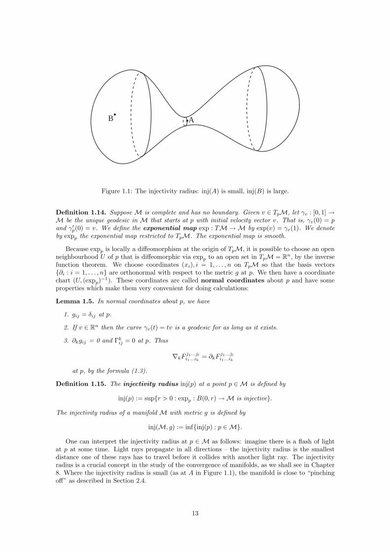
Figure 1.1: The injectivity radius: inj(A) is small, inj(B) is large.
Definition 1.14. Suppose M is complete and has no boundary. Given v ∈ TpM, let γv : [0, 1]→M be the unique geodesic in M that starts at p with initial velocity vector v. That is, γv(0) = pand γ′p(0) = v. We define the exponential map exp : TM→M by exp(v) = γv(1). We denoteby expp the exponential map restricted to TpM. The exponential map is smooth.
Because expp is locally a diffeomorphism at the origin of TpM, it is possible to choose an openneighbourhood U of p that is diffeomorphic via expp to an open set in TpM = Rn, by the inversefunction theorem. We choose coordinates (xi), i = 1, . . . , n on TpM so that the basis vectors{∂i : i = 1, . . . , n} are orthonormal with respect to the metric g at p. We then have a coordinatechart (U, (expp)−1). These coordinates are called normal coordinates about p and have someproperties which make them very convenient for doing calculations:
Lemma 1.5. In normal coordinates about p, we have
1. gij = δij at p.
2. If v ∈ Rn then the curve γv(t) = tv is a geodesic for as long as it exists.
3. ∂kgij = 0 and Γkij = 0 at p. Thus
∇kF j1...jli1...ik= ∂kF
j1...jli1...ik
at p, by the formula (1.3).
Definition 1.15. The injectivity radius inj(p) at a point p ∈M is defined by
inj(p) := sup{r > 0 : expp : B(0, r)→M is injective}.
The injectivity radius of a manifold M with metric g is defined by
inj(M, g) := inf{inj(p) : p ∈M}.
One can interpret the injectivity radius at p ∈ M as follows: imagine there is a flash of lightat p at some time. Light rays propagate in all directions – the injectivity radius is the smallestdistance one of these rays has to travel before it collides with another light ray. The injectivityradius is a crucial concept in the study of the convergence of manifolds, as we shall see in Chapter8. Where the injectivity radius is small (as at A in Figure 1.1), the manifold is close to “pinchingoff” as described in Section 2.4.
13
1.3 The Lie Derivative
The covariant derivative gives one way of differentiating tensor fields. We will now look at a differentway, which can be defined purely from the manifold structure of M, without any reference to aRiemannian metric or the extra structure of a connection.
Given a vector field X on a manifoldM, we define a time-dependent family of diffeomorphismsof M to itself, ϕt :M→M for t ∈ (−ε, ε), such that ϕ0 is the identity and
d
dtϕt = X
at each point (the existence of such ϕt follows from basic existence theorems for differential equa-tions – see [5, Sec. 6-2] for this argument and other details relating to the Lie derivative). This isto be interpreted as a “flow” of the manifold in the direction of the vector field X. We now definethe derivative of some
(kl
)-tensor field F in the direction of X as the change in F when we move
a small step in the direction of X – but we need to have some way of comparing the value of F atthe point a little step away with that at the original point. Rather than making this comparisonusing a “connection” as before, we make it by pushing the value of F at the translated point backto the original point using the diffeomorphism ϕt.
We define
(∗ϕt)Fp(X1, . . . , Xk, ω1, . . . , ωl) := Fϕt(p)(ϕt∗(X1(p)), . . . , ϕt∗(Xk(p)),
(ϕ−1t )∗(ω1
(p)), . . . , (ϕ−1t )∗(ωl(p))).
Note that (∗ϕt)Fp ∈ T kl Mp for all t. It is now possible to define the Lie derivative of F in thedirection X as
LXF =(d
dt(∗ϕt)F
)t=0
Lemma 1.6. The Lie derivative is well-defined. It obeys similar conditions to those satisfied bythe covariant derivative as outlined in Lemma 1.2, with one important exception:
1. For a scalar function f , LXf = X(f).
2. If Y is a vector field then LXY = [X,Y ].
3. LX(F ⊗G) = (LXF )⊗G+ F ⊗ (LXG).
4. LX commutes with all traces:LX(trY ) = tr(LXY )
for all traces (over any indices) of the tensor Y .
Proof. See [5, Sec. 6-2].
Lemma 1.7. On a Riemannian manifold (M, g), we have
(LXg)ij = ∇iXj +∇jXi,
where ∇ denotes the Levi-Civita connection of the metric g, for any vector field X.
Proof. Let ω be the 1-form dual to the vector field X, ω(Y ) = 〈X,Y 〉. Using the product rule(from Lemma 1.6) and the metric compatibility and torsion-free conditions on the Levi-Civitaconnection we have
LXg(Y,Z) = X(g(Y,Z))− g(LXY, Z)− g(Y,LXZ)= 〈∇XY, Z〉+ 〈Y,∇XZ〉 − 〈[X,Y ], Z〉 − 〈Y, [X,Z]〉= 〈∇XY − [X,Y ], Z〉+ 〈Y,∇XZ − [X,Z]〉= 〈∇YX,Z〉+ 〈Y,∇ZX〉= Y 〈X,Z〉 − 〈X,∇Y Z〉+ Z〈Y,X〉 − 〈∇ZY,X〉= Y (ω(Z))− ω(∇Y Z) + Z(ω(Y ))− ω(∇ZY )= (∇Y ω) (Z) + (∇Zω) (Y )
14
which is the coordinate-free way of expressing the identity we wanted. Note that we used theproduct rule again to get the last line.
1.4 Curvature
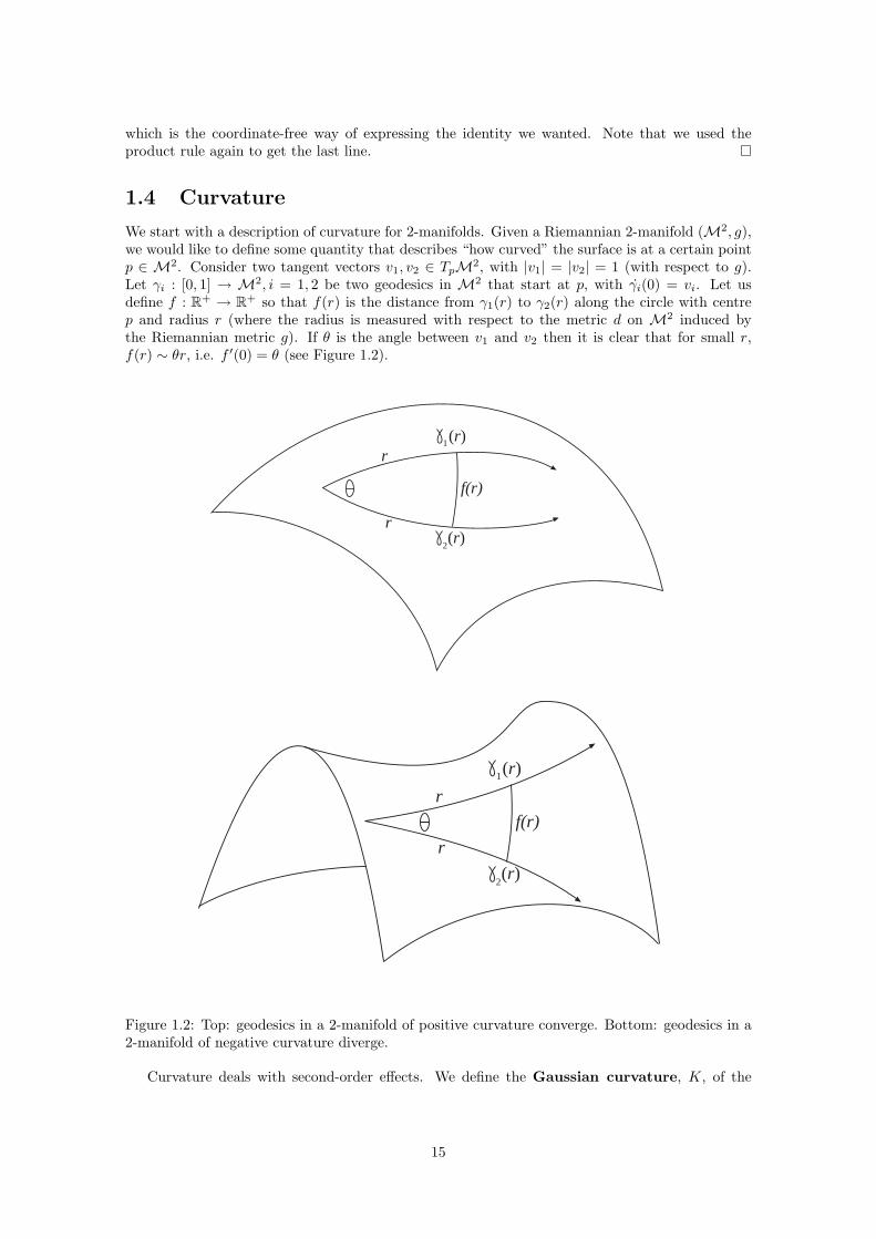
We start with a description of curvature for 2-manifolds. Given a Riemannian 2-manifold (M2, g),we would like to define some quantity that describes “how curved” the surface is at a certain pointp ∈ M2. Consider two tangent vectors v1, v2 ∈ TpM2, with |v1| = |v2| = 1 (with respect to g).Let γi : [0, 1] → M2, i = 1, 2 be two geodesics in M2 that start at p, with γi(0) = vi. Let usdefine f : R+ → R+ so that f(r) is the distance from γ1(r) to γ2(r) along the circle with centrep and radius r (where the radius is measured with respect to the metric d on M2 induced bythe Riemannian metric g). If θ is the angle between v1 and v2 then it is clear that for small r,f(r) ∼ θr, i.e. f ′(0) = θ (see Figure 1.2).
1(r)
2(r)
f(r)
r
r
1(r)
2(r)
f(r)
r
r
Figure 1.2: Top: geodesics in a 2-manifold of positive curvature converge. Bottom: geodesics in a2-manifold of negative curvature diverge.
Curvature deals with second-order effects. We define the Gaussian curvature, K, of the
15
surface at p so thatf(r)r∼ θ
(1− K
6r2
)for small r. See Figure 1.2 for pictures of manifolds with positive curvature (K > 0) and negativecurvature (K < 0). Euclidean space R2 is flat (K = 0).
The generalization to higher-dimensional manifolds of this concept of curvature is not at allobvious, and was first achieved by Riemann. His idea was that the curvature, intuitively, is theobstruction to the “flatness” of a manifold. In other words, non-zero curvature at p is what stopsus from choosing coordinates in which the metric is the Euclidean, flat metric gij = δij in aneighbourhood of p. Normal coordinates about p are, in some sense, “as close as we can get” to aEuclidean metric in a neighbourhood of p: we know from Lemma 1.5 that in normal coordinatesabout p, gij(p) = δij(p) and ∂kgij(p) = 0. However, in general, the second- and higher-orderderivatives of the metric at p may be non-zero.
This motivates the definition of the(
40
)Riemann curvature tensor, which holds all of
the information about the second-order derivatives of g. It is defined to be the(
40
)-tensor with
coordinates Ripqj such that, in normal coordinates about p,
gij(x) = δij +13Ripqjx
pxq + (third- and higher-order terms in x). (1.6)
The factor of 1/3 is introduced so that this definition agrees with the alternative one that weintroduce next.
Since Riemann’s original work, it has emerged that the Riemann curvature tensor can be definedin another way, using the Levi-Civita connection ∇. The
(31
)Riemann curvature tensor is a(
31
)-tensor which can be defined for vector fields X,Y, Z and a 1-form ω by
Rm(X,Y, Z, ω) := ω(R(X,Y )Z) (1.7)
where
R(X,Y )Z = ∇2Z(X,Y )−∇2Z(Y,X)= ∇X(∇Y Z)−∇Y (∇XZ)−∇[X,Y ]Z.
Note here that(∇2Z)(X,Y ) 6= ∇X(∇Y Z).
In fact,(∇2Z)(X,Y ) = ∇X(∇Y Z)−∇∇XY Z.
There is a distinction because, by ∇2Z, we really mean the covariant derivative of the(
11
)-tensor
∇Z. Thus ∇2Z is a(
21
)-tensor.
It is definitely not obvious (but can easily be checked) that this is in fact a(
31
)-tensor (in
particular that, for example, Rm(X,Y, fZ, ω) = fRm(X,Y, Z, ω) for any f ∈ C∞(M)). Werepresent it in terms of local coordinates as Rlijk. The
(31
)curvature tensor Rlijk defined by
equation (1.7) is obtained from the(
40
)curvature tensor Rijkl defined by equation (1.6) by raising
the final index.The coordinates of Rm can be explicitly calculated by applying equation (1.3) with the Levi-
Civita connection ∇:
Lemma 1.8. The Riemann curvature tensor has the explicit form
Rlijk = ∂iΓljk − ∂jΓlik + ΓpjkΓlip − ΓpikΓljp.
Rm has many symmetries, which can be proven by manipulating the defining equation (1.7):
Lemma 1.9. (Symmetries of the curvature tensor) The Riemann curvature tensor has thefollowing properties:
1. Rijkl = Rklij = −Rjikl = −Rijlk
16
2. The first Bianchi identity:Rijkl +Rjkil +Rkijl = 0
3. The second Bianchi identity:
∇pRijkl +∇iRjpkl +∇jRpikl = 0 (1.8)
Proof. See [18, Prop. 7.4].
The first of these symmetries allows us to view Rm as a section of the bundle
∧2T ∗M⊗S ∧2T ∗M
of symmetric bilinear forms on the space of 2-vectors. If φ = φij∂i ∧ ∂j and ψ = ψij∂i ∧ ∂j are2-vectors then we define the action of the curvature operator at p, Rp : ∧2TpM⊗∧2TpM→ R,by
R(φ, ψ) = Rijklφijψlk
(all evaluated at p). Note that the curvature operator is defined on 2-vectors by the antisymmetryin the first two and in the last two indices of Rm, and is symmetric because of the symmetryRijkl = Rklij .
We can now explain the relationship with Gaussian curvature. If there is a 2-plane elementφ ∈ ∧2TpM representing a 2-dimensional subspace Π of TpM, we can imagine the 2-dimensionalsubmanifold ofM that is the image under the exponential map expp of Π (near p). The Gaussiancurvature of this 2-dimensional submanifold at p is called the sectional curvature ofM associatedwith Π, and denoted K(Π).
Lemma 1.10. If Π is a 2-plane in TpM spanned by the vectors X,Y ∈ TpM, and φ = X ∧ Y ,then
K(Π) =R(φ, φ)|φ|2
,
where |φ|2 = gikgjlφijφkl.
Proof. See [18, Prop. 8.8].
Because a rank 4 tensor is a bit awkward to work with, we define some simpler quantities bytaking the trace of Rlijk:
Definition 1.16. The Ricci curvature tensor, Rc, is the(
20
)-tensor with coordinate expression
Rij := Rppij .
It is symmetric: Rij = Rji.The scalar curvature is the trace of the Ricci tensor,
R := gijRij .
On a 2-manifold, it is equal to twice the Gaussian curvature.
The Ricci and scalar curvatures can be interpreted in terms of sectional curvatures:
Lemma 1.11. Let X ∈ TpM be a unit vector. Suppose that X is contained in some orthonormalbasis for TpM. Rc(X,X) is then the sum of the sectional curvatures of planes spanned by X andother elements of the basis.
Given an orthonormal basis for TpM, the scalar curvature at p is the sum of all sectionalcurvatures of planes spanned by pairs of basis elements.
Proof. See [18, end of Chap. 8].
The Ricci and scalar curvatures can also be expressed in terms of the curvature operator.
17
Lemma 1.12. On a 3-dimensional Riemannian manifold (M3, g), let us diagonalize the curvatureoperator R with respect to a basis {e2 ∧ e3, e3 ∧ e1, e1 ∧ e2} of ∧2TM3, where {e1, e2, e3} is anorthonormal basis of TM3 (this is possible because R is symmetric). Suppose that, with respect tothis basis, R is a diagonal matrix with entries λ1, λ2, λ3 down the diagonal. Then with respect tothe basis {e1, e2, e3}, the Ricci tensor takes the form
Rc =12
λ2 + λ3 0 00 λ3 + λ1 00 0 λ1 + λ2
(1.9)
and the scalar curvature isR = λ1 + λ2 + λ3. (1.10)
Proof. Note that for i 6= j, |ei ∧ ej |2 = |ei ⊗ ej − ej ⊗ ei|2 = 12 + 12 = 2 (if we chose a differentnorm on ∧2TM3 the result of Lemma 1.10 would change). Thus, by the result of Lemma 1.11,using Lemma 1.10 to calculate the sectional curvatures, we have
Rc(e1, e1) =12
(R(e1 ∧ e2, e1 ∧ e2) +R(e1 ∧ e3, e1 ∧ e3)) (1.11)
=12
(λ3 + λ2) .
Similarly, Rc(e2, e2) = (λ1 + λ3)/2 and Rc(e3, e3) = (λ1 + λ2)/2. This accounts for the diagonalentries of the matrix of Rc.
We now need to show that the off-diagonal matrix elements of Rc are zero, for example thatRc(e1, e2) = 0. We have
Rc(e1, e2) =Rc(e1 + e2, e1 + e2)− Rc(e1, e1)− Rc(e2, e2)
2,
hence it suffices to show that
Rc(e1 + e2, e1 + e2) = Rc(e1, e1) + Rc(e2, e2). (1.12)
To do this we note that {e1 + e2√
2,e1 − e2√
2, e3
}is also an orthonormal basis for TpM3. We can re-apply formula (1.11) for this new basis tocalculate Rc(e1 + e2, e1 + e2). The result is as in equation (1.12), hence Rc has the stated form.The formula for R follows by taking the trace of Rc.
Definition 1.17. The Einstein tensor on a Riemannian n-manifold (Mn, g) is the tensor
Eij := Rij −1nRgij .
It is also known as the traceless part of the Ricci tensor. A metric g is called Einstein if itsEinstein tensor is identically 0.
In dimension 3, the Einstein tensor has particular significance. We record here a result whichshows that, for 3-dimensional manifolds, the Riemann curvature tensor can be expressed quitesimply in terms of the Einstein tensor and the scalar curvature.
Lemma 1.13. On a 3-manifold,
Rm =R
4(g � g) + E � g,
where � denotes the Kulkarni-Nomizu product of symmetric tensors:
(P �Q)ijkl = PilQjk + PjkQil − PikQjl − PjlQik.
18
Proof. This result follows from the decomposition of Rm, which holds on any n-manifold:
Rm =R
2(n− 1)(n− 2)(g � g) +
1n− 2
(E � g) +W, (1.13)
where W is the so-called “Weyl tensor”, which is defined by equation (1.13). The Weyl tensorvanishes in dimension 3 (see [9, Sec. 8] for a simple proof using the symmetries of W ), from whichthe result follows.
In dimension 3, Einstein metrics are very special.
Lemma 1.14. An Einstein metric on a manifold of dimension n ≥ 3 has constant scalar curvature.If n = 3, the metric has constant sectional curvature.
Proof. Consider the second Bianchi identity (1.8). If we raise the indices k, l we obtain
∇pRijkl +∇iRjpkl +∇jRpikl = 0.
Taking the trace over the indices i, l and using the symmetries of the curvature tensor we obtain
∇pRkj −∇iRjpik −∇jRkp = 0.
Taking the trace over the indices j, k now gives us
∇pR = ∇iRip +∇iRip,
or equivalently
gij∇iRjp =12∇pR.
Thus we have
gij∇iEjp = gij∇i(Rjp −
1nRgjp
)=
12∇pR−
1n∇pR =
(12− 1n
)∇pR (1.14)
(using ∇g = 0). If the metric is Einstein then Ejp = 0, so(12− 1n
)∇pR = 0.
Because n 6= 2 this means ∇R = 0, hence R is constant.If n = 3, we can apply formula (1.9) from Lemma 1.12 and deduce that
Rc =12
λ2 + λ3 0 00 λ3 + λ1 00 0 λ1 + λ2
=R
3g =
C 0 00 C 00 0 C
, (1.15)
where C = 13R is a constant over the whole manifold. Therefore the curvature eigenvalues λi are
all equal to the constant value C, from which it follows that the manifold has constant sectionalcurvature.
If a metric has constant sectional curvature, we call it a constant curvature metric. Thereare three essentially distinct possibilities: the value of the sectional curvatures can be positive, zeroor negative. We have the following examples:
Definition 1.18. Constant Curvature MetricsEuclidean n-space, En := Rn with the standard metric, has constant sectional curvature 0.The n-dimensional sphere of radius R,
SnR = {x ∈ Rn+1 : |x| = R}
with the metric induced as a submanifold of En+1, has constant sectional curvature 1/R2.The hyperbolic n-space of radius R, Hn
R, is the open ball of radius R in Rn with the metric
gij(x) =4R4δij
(R2 − |x|2)2.
It has constant sectional curvature −1/R2 (there are other equivalent ways of representing thisRiemannian manifold).
19
See [18, end of Chap. 8] for more details, including a proof that these spaces have constantcurvature.
Using the theory of Jacobi fields (see [18, Chap. 10]), one can prove many comparison theorems,as well as results about constant curvature metrics. For example one can prove that the localstructure of a metric with constant sectional curvature C is unique (see [18, Prop. 10.9]) – we willsee a more general result in Theorem 1.16. One can also prove the following, which will come inhandy in Chapter 7:
Theorem 1.15. The Bishop-Gunther Volume Comparison Theorem. Let us denote byV kn (r) the volume of the ball of radius r in the complete, simply-connected n-dimensional spaceof constant sectional curvature k (this will be either SnR, En or Hn
R). Suppose that (Mn, g) is aRiemannian n-manifold, and p ∈Mn. Then
1. If there is a constant a > 0 such that Rc ≥ (n− 1)ag then
Vol(B(p, r)) ≤ V an (r).
2. If there is a constant b such that all sectional curvatures of (Mn, g) are bounded above by b,and the exponential map is injective on the ball B(p, r), then
Vol(B(p, r)) ≥ V bn (r).
Proof. See [8, Theorem 3.101].
1.5 Topology from Geometry
The central idea of the Geometrization Conjecture is that the topology of a manifold and the typeof geometry that the manifold can have are intimately related. Here we will record some of thetheorems that relate the geometric structure of a manifold to its topology.
Theorem 1.16. Let (Mn, g) be a complete, simply-connected Riemannian n-manifold with con-stant sectional curvature C. Then Mn is isometric to one of En (if C = 0), SnR (if C = 1/R2) orHnR (if C = −1/R2).
Proof. See [18, Theorem 11.12].
In particular, any simply-connected manifold with constant non-positive sectional curvature isdiffeomorphic to Rn, and any simply-connected manifold with constant positive sectional curvatureis diffeomorphic to Sn.
This also allows us to characterize non-simply-connected manifolds of constant curvature – byapplying Theorem 1.16 to the universal covering space, we see that any of these manifolds mustbe a quotient of Rn,Sn or Hn by a discrete group of isometries acting freely.
We can also derive topological information from bounds on the curvatures, as the followingtheorems show:
Theorem 1.17. (Myers’ Theorem) Suppose (Mn, g) is a complete, connected Riemannian n-manifold whose Ricci tensor satisfies
Rc ≥ (n− 1)Hg
for some constant H. Then Mn is compact with finite fundamental group and diameter at mostπH−
12 .
Proof. See [18, Theorem 11.8].
Theorem 1.18. (The Sphere Theorem) We say that the Riemannian manifold (M, g) isstrictly δ-pinched (for some δ > 0) if there is a constant K > 0 such that all of the sectionalcurvatures of M lie in the interval (δK,K].
If Mn is a complete, simply-connected and strictly 14 -pinched n-manifold then Mn is homeo-
morphic to Sn.
Proof. See [3].
20
1.6 Scaling
We will be interested later on (when we deal with the normalized Ricci flow in Chapter 7) in howvarious geometric quantities scale when the metric is scaled by a constant factor C.
Lemma 1.19. If g = Cg are two Riemannian metrics on an n-manifold Mn, related by a scalingfactor C, then the various geometric quantities scale as follows:
1. gij = C−1gij.
2. Γkij = Γkij.
3. Rlijk = Rlijk.
4. Rijkl = CRijkl.
5. Rij = Rij.
6. R = C−1R.
7. The volume elements: dµ = Cn/2dµ.
1.7 Time-evolving metrics
When our metrics depend on time, as in the Ricci flow, we will want to know how the variousgeometric quantities evolve when the metric evolves.
Lemma 1.20. Suppose that gij(t) is a time-dependent Riemannian metric, and
∂
∂tgij(t) = hij(t).
Then the various geometric quantities evolve according to the following equations:
1. Metric inverse:∂
∂tgij = −hij = −gikgjlhkl. (1.16)
2. Christoffel symbols:∂
∂tΓkij =
12gkl(∇ihjl +∇jhil −∇lhij). (1.17)
3. Riemann curvature tensor:
∂
∂tRlijk =
12glp{∇i∇jhkp +∇i∇khjp −∇i∇phjk−∇j∇ihkp −∇j∇khip +∇j∇phik
}. (1.18)
4. Ricci tensor:
∂
∂tRij =
12gpq(∇q∇ihjp +∇q∇jhip −∇q∇phij −∇i∇jhqp). (1.19)
5. Scalar curvature:∂
∂tR = −4H +∇p∇qhpq − hpqRpq (1.20)
where H = gpqhpq.
6. Volume element:∂
∂tdµ =
H
2dµ. (1.21)
21
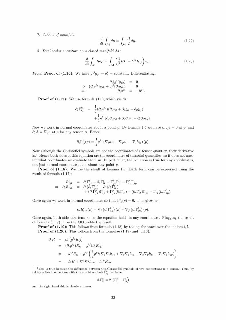
7. Volume of manifold:d
dt
∫Mdµ =
∫M
H
2dµ. (1.22)
8. Total scalar curvature on a closed manifold M:
d
dt
∫MRdµ =
∫M
(12RH − hijRij
)dµ. (1.23)
Proof. Proof of (1.16): We have gijgjk = δik = constant. Differentiating,
∂t(gijgjk) = 0⇒ (∂tgij)gjk + gij(∂tgjk) = 0⇒ ∂tg
ij = −hij .
Proof of (1.17): We use formula (1.5), which yields
∂tΓkij =12
(∂tgkl)(∂igjl + ∂jgil − ∂lgij)
+12gkl(∂i∂tgjl + ∂j∂tgil − ∂l∂tgij).
Now we work in normal coordinates about a point p. By Lemma 1.5 we have ∂igjk = 0 at p, and∂iA = ∇iA at p for any tensor A. Hence
∂tΓkij(p) =12gkl (∇ihjl +∇jhil −∇lhij) (p).
Now although the Christoffel symbols are not the coordinates of a tensor quantity, their derivativeis.4 Hence both sides of this equation are the coordinates of tensorial quantities, so it does not mat-ter what coordinates we evaluate them in. In particular, the equation is true for any coordinates,not just normal coordinates, and about any point p.
Proof of (1.18): We use the result of Lemma 1.8. Each term can be expressed using theresult of formula (1.17):
Rlijk = ∂iΓljk − ∂jΓlik + ΓpjkΓlip − ΓpikΓljp⇒ ∂tR
lijk = ∂i(∂tΓljk)− ∂j(∂tΓlik)
+ (∂tΓpjk)Γlip + Γpjk(∂tΓlip)− (∂tΓ
pik)Γljp − Γpik(∂tΓljp).
Once again we work in normal coordinates so that Γkij(p) = 0. This gives us
∂tRlijk(p) = ∇i
(∂tΓljk
)(p)−∇j
(∂tΓlik
)(p).
Once again, both sides are tensors, so the equation holds in any coordinates. Plugging the resultof formula (1.17) in on the rhs yields the result.
Proof of (1.19): This follows from formula (1.18) by taking the trace over the indices i, l.Proof of (1.20): This follows from the formulae (1.19) and (1.16):
∂tR = ∂t(gijRij
)= (∂tgij)Rij + gij(∂tRij)
= −hijRij + gij(
12gpq(∇q∇ihjp +∇q∇jhip −∇q∇phij −∇i∇jhqp)
)= −4H +∇p∇qhpq − hpqRpq
4This is true because the difference between the Christoffel symbols of two connections is a tensor. Thus, bytaking a fixed connection with Christoffel symbols Γk
ij , we have
∂tΓkij = ∂t
“Γk
ij − Γkij
”and the right hand side is clearly a tensor.
22
(recall that ∇g = 0 and 4 = gij∇i∇j).Proof of (1.21): We will use the formula
dµ =√
det gijdx1 ∧ dx2 ∧ . . . ∧ dxn
(see [14, Sec. 7.5] on the volume form).First we need to calculate the variation in the determinant of a matrix detA, when the matrix
A itself varies. Because A will end up being a metric, we may assume that it is symmetric andhence we can choose a basis in which A is diagonalized with eigenvalues λi 6= 0. Then Aij = λiδij ,and detA =
∏i λi. If we then vary the entry Aij , the determinant will not change unless i = j. If
i = j, we have
∂ detA∂Aii
=∂(∏
j λj
)∂λi
=1λi
∏j
λj =1λi
detA.
Therefore by the chain rule,
d
dtdetA =
n∑i,j=0
(∂ detA∂Aij
)dAijdt
=n∑
i,j=0
δij1λi
detAdAijdt
=(A−1
)ij (dAijdt
)detA
where we have observed that (A−1)ij = δij/λi and we are now using the Einstein summationconvention. This formula manifestly does not depend on the basis we choose as traces are basis-independent.
It now follows by the chain rule that
∂tdµ = ∂t√
det gijdx1 ∧ . . . ∧ dxn
=1
2√
det gijgijhij det gijdx1 ∧ . . . ∧ dxn
=H
2dµ
where H = gijhij .Proof of (1.22): This follows from formula (1.21) by taking the derivative under the integral
sign.Proof of (1.23): This follows from formulae (1.21) and (1.20):
∂
∂t
∫MRdµ =
∫M
(∂tR)dµ+R(∂tdµ)
=∫M
(−4H +∇p∇qhpq − hpqRpq +
12RH
)dµ
=∫M
(12RH − hpqRpq
)dµ.
Here we have used Stokes’ Theorem (see [14, Sec. 7.5]) to get rid of the first two terms in theintegral because they were expressible as the divergence of a vector field on M, and M has noboundary.
23
Chapter 2
Introduction to the Ricci Flow
The main aim of this project is to introduce the basics of Hamilton’s Ricci flow program, which isaimed at proving Thurston’s Geometrization Conjecture and consequently the Poincare Conjecture.In this chapter we will present the context for the Ricci flow: what is it, what are the problemsthat it is intended to solve, and why might it be expected to solve them? In the process we will alsosee some simple solutions to the Ricci flow and try to gain a bit of intuition about its behaviour. Alot of space in this introduction is devoted to material that is not elaborated (or is elaborated verylittle) in the main body of the thesis – namely the description of the Geometrization Conjectureand the section on pinching. That is because the introduction is intended to serve as a “big picture”guide to the reasons we study the Ricci flow, so that the reader understands, when encounteringthe formidable technical details of Chapter 7, why it is all worthwhile.
2.1 The Prehistory of the Ricci Flow – Geometrization
The Poincare Conjecture was one of the iconic unsolved problems of 20th century mathematics.Around 1900, Poincare asked if a simply-connected closed 3-manifold is necessarily the 3-sphereS3. After many years of topological difficulties, William Thurston made promising progress inthe 1970s. He proposed, not only a way of approaching the Poincare Conjecture, but a far moregeneral conjecture that, if proven, would lead to a classification of all compact 3-manifolds. Wewill outline, extremely vaguely, Thurston’s conjecture.
It was already known by the time Thurston came onto the scene that compact orientable 3-manifolds could be decomposed into simpler manifolds using the “connected sum” decomposition.Figure 2.1 shows the connect sum operation # for 2-manifolds. For 3-manifolds, the definitionis analogous: one cuts out a 3-ball from each manifold then glues them together along the S2
boundaries created.If a manifold can not be nontrivially decomposed using the connected sum decomposition then
it is called prime. Hellmuth Kneser showed in 1929 that every compact orientable 3-manifold canbe decomposed into a finite number of prime “factors” (see [16]), and John Milnor showed in 1962that this decomposition is unique (see [19]). Thus, to classify 3-manifolds it suffices to classifyprime 3-manifolds.
The connected sum decomposition involves cutting 3-manifolds along 2-spheres; the next stepis to cut them along 2-tori. Thurston conjectured that any compact, orientable, prime 3-manifoldcan be decomposed by some finite number of embedded tori into pieces so that each piece hasone of eight fundamental, highly symmetric geometric structures (of which the constant-curvaturemetrics on S3,H3,R3 are three). Note the analogy with the 2-dimensional case: any compact,orientable 2-manifold is either S2 (which can be given a metric of constant positive curvature),a torus T 2 (which can be given a metric with zero curvature), or can be decomposed using theconnected sum into tori with holes (which can be given metrics of constant negative curvature)(see [22, Theorem 77.5] for the topological classification and [27, Chap. 1] for a discussion aboutthe existence of geometric structures).
It might not be obvious that the geometric structure will give us useful topological information,but we saw in Chapter 1 how it is possible to make progress towards classifying constant curvature
24
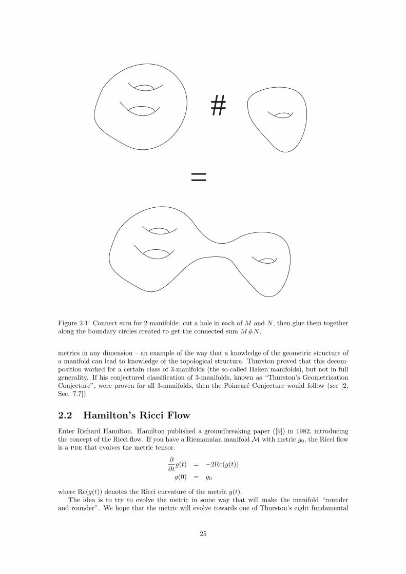
#
=
Figure 2.1: Connect sum for 2-manifolds: cut a hole in each of M and N , then glue them togetheralong the boundary circles created to get the connected sum M#N .
metrics in any dimension – an example of the way that a knowledge of the geometric structure ofa manifold can lead to knowledge of the topological structure. Thurston proved that this decom-position worked for a certain class of 3-manifolds (the so-called Haken manifolds), but not in fullgenerality. If his conjectured classification of 3-manifolds, known as “Thurston’s GeometrizationConjecture”, were proven for all 3-manifolds, then the Poincare Conjecture would follow (see [2,Sec. 7.7]).
2.2 Hamilton’s Ricci Flow
Enter Richard Hamilton. Hamilton published a groundbreaking paper ([9]) in 1982, introducingthe concept of the Ricci flow. If you have a Riemannian manifoldM with metric g0, the Ricci flowis a pde that evolves the metric tensor:
∂
∂tg(t) = −2Rc(g(t))
g(0) = g0
where Rc(g(t)) denotes the Ricci curvature of the metric g(t).The idea is to try to evolve the metric in some way that will make the manifold “rounder
and rounder”. We hope that the metric will evolve towards one of Thurston’s eight fundamental
25
geometric structures, and that the decomposition by spheres and tori will somehow emerge nat-urally. In choosing what should go on the right hand side of the equation of the Ricci flow, weknow that it should be a rank-2 tensor, symmetric (so that the metric g remains symmetric), andit should involve the curvature somehow – the Ricci curvature tensor is the obvious choice. Theminus sign makes the Ricci flow a heat-type (parabolic) equation (as we shall see in Chapter 5),so it is expected to “average out” the curvature. This should make the metric rounder in the waythat we want.
A characteristic property of heat-type equations is the maximum principle, which we will seein Chapter 3. We will use the maximum principle in Chapter 7 to prove quantitatively that thisrounding of the metric does indeed happen in one specific case. The main theorem we will proveis the one proved by Hamilton in the paper that introduced the Ricci flow:
Theorem 2.1. (Hamilton, 1982) Let M3 be a closed 3-manifold which admits a Riemannianmetric with strictly positive Ricci curvature. Then M3 also admits a metric of constant positivecurvature.
In particular, by Theorem 1.16, any simply-connected closed 3-manifold which admits ametric of strictly positive Ricci curvature is diffeomorphic to the 3-sphere. We are certainly startingto get into the territory of the Poincare Conjecture with this result!
More specifically, we will see that if the initial metric g0 has strictly positive Ricci curvaturethen the manifoldM3 will shrink to a point in finite time under the Ricci flow. But if we dilate themetric by a time-dependent factor so that the volume remains constant, the problem of shrinkingto a point is removed. Furthermore, we can show that the rescaled metric converges uniformlyto the desired metric of constant positive curvature on M3. This process of “blowing up” themanifold when it is becoming singular is a crucial one in the Ricci flow program. Because it israther complicated and can get lost in the technical details, we have provided an analogous butmuch simpler argument for the “curve-shortening flow” in Chapter 4 in the hope that this willmake it easier to understand what is going on in later chapters.
We note that the Uniformization Theorem (any Riemannian metric on a closed 2-manifold isconformal to one of constant curvature) can be proved using the Ricci flow as well (see [6, Chap.5] for the bulk of the argument, and [4] for the remainder). Once again we encounter problemswith singularities: the manifold will shrink to a point in some cases and become arbitrarily largein others. As before, the solution is to rescale so that the volume is constant. When we dothis, the rescaled metric converges smoothly to a smooth metric of constant curvature. Notethat the Uniformization Theorem is the closest thing to a 2-dimensional analogue of Thurston’sGeometrization Conjecture, so the fact that the Ricci flow solves it in this way is another strongindicator that we’re heading in the right direction.
In 2002 and 2003, Grisha Perelman posted three papers ([23, 25, 24]) on arXiv.org which claimedto have completed Hamilton’s work towards using the Ricci flow to prove the GeometrizationConjecture. More recently several authors have posted papers elaborating on the technical detailsof Perelman’s papers ([2, 21]). The proof seems to have been accepted by the mathematicalcommunity, wrapping up the 100-year history of the Poincare Conjecture (and the younger but noless important Geometrization Conjecture).
2.3 Special Solutions of the Ricci Flow
In this section we will exhibit some of the special solutions of the Ricci flow. The first thing, ofcourse, is to know what they do on the spaces of constant curvature.
On an n-dimensional sphere of radius r (where n > 1), the metric is given by g = r2g where gis the metric on the unit sphere. The sectional curvatures are all 1/r2. Thus for any unit vectorv, the result of Lemma 1.11 tells us that Rc(v, v) = (n− 1)/r2. Therefore
Rc =n− 1r2
g = (n− 1)g,
26
so the Ricci flow equation becomes an ode:∂∂tg = −2Rc
⇒ ∂∂t (r
2g) = −2(n− 1)g⇒ d(r2)
dt = −2(n− 1).
We have the solutionr(t) =
√R2
0 − 2(n− 1)t,
where R0 is the initial radius of the sphere. The manifold shrinks to a point as t→ R20/(2(n− 1)).
Similarly, for hyperbolic n-space Hn (where n > 1), the Ricci flow reduces to the ode
d(r2)dt
= 2(n− 1)
which has the solutionr(t) =
√R2
0 + 2(n− 1)t.
So the solution expands out to infinity.Of course the flat metric on En has zero Ricci curvature, so it does not evolve at all under the
Ricci flow. There are other non-trivial Riemannian manifolds with vanishing Ricci curvature (themetric is flat, i.e. locally isometric to Euclidean space, if and only if the Riemann curvature tensorvanishes). These metrics can be regarded as the “fixed points” of the Ricci flow. However, weought really to regard Sn and Hn as honorary fixed points of the flow – even though the metricwas changing under the flow, it only ever changed by a rescaling of the metric.
Even more generally, one can regard as “generalized fixed points” of the Ricci flow thosemanifolds which change only by a diffeomorphism and a rescaling under the Ricci flow. Let(Mn, g(t)) be a solution of the Ricci flow, and suppose that ϕt :Mn →Mn is a time-dependentfamily of diffeomorphisms (with ϕ0 = id) and σ(t) is a time-dependent scale factor (with σ(0) = 1).If we then have
g(t) = σ(t)ϕ∗t g(0)
then the solution (Mn, g(t)) is called a Ricci soliton. Taking the derivative of this equation andevaluating at t = 0 yields
∂
∂tg(t) =
dσ(t)dt
ϕ∗t g(0) + σ(t)∂
∂tϕ∗t g(0)
−2Rc(g(0)) = σ′(0)g(0) + LV g(0),
where V = dϕt/dt, by the definition of the Lie derivative given in Section 1.3. Let us set σ′(0) = 2λ.We can now use the result of Lemma 1.7 to write this in coordinates as
−2Rij = 2λgij +∇iVj +∇jVi.
As a special case we can consider the case that V is the gradient vector field of some scalarfunction f on Mn, i.e. Vi = ∇if . The equation then becomes
Rij + λgij +∇i∇jf = 0. (2.1)
Such solutions are known as gradient Ricci solitons. A gradient Ricci soliton is called shrinkingif λ < 0, static if λ = 0, and expanding if λ > 0. The gradient Ricci solitons play a role inmotivating the definition of Perelman’s F- and W-functionals which we will see in Section 8.4.
One example of a gradient Ricci soliton is Hamilton’s cigar soliton: Let Σ2 = R2 with thestandard coordinates and
gij =δij
1 + x2 + y2.
Because the metric is rotationally symmetric, the calculation of the Ricci curvature tensor andthe covariant derivative is particularly simple (by the rotational symmetry we can embed Σ2 inR3 as a manifold of revolution – see [18, Ex. 8.2] for the calculation of the Gaussian curvature ofmanifolds of revolution). We can show that
Rij +∇i∇jf = 0
where f(x, y) = (x2 + y2)/2, hence (Σ2, g) is a static gradient Ricci soliton.
27
S1 x I
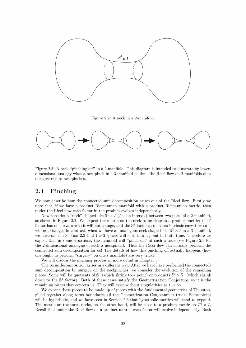
Figure 2.2: A neck in a 2-manifold.
Figure 2.3: A neck “pinching off” in a 2-manifold. This diagram is intended to illustrate by lower-dimensional analogy what a neckpinch in a 3-manifold is like – the Ricci flow on 2-manifolds doesnot give rise to neckpinches.
2.4 Pinching
We now describe how the connected sum decomposition arises out of the Ricci flow. Firstly wenote that, if we have a product Riemannian manifold with a product Riemannian metric, thenunder the Ricci flow each factor in the product evolves independently.
Now consider a “neck” shaped like S1 × I (I is an interval) between two parts of a 2-manifold,as shown in Figure 2.2. We expect the metric on the neck to be close to a product metric; the Ifactor has no curvature so it will not change, and the S1 factor also has no intrinsic curvature so itwill not change. In contrast, when we have an analogous neck shaped like S2 × I in a 3-manifold,we have seen in Section 2.3 that the 2-sphere will shrink to a point in finite time. Therefore weexpect that in some situations, the manifold will “pinch off” at such a neck (see Figure 2.3 forthe 2-dimensional analogue of such a neckpinch). Thus the Ricci flow can actually perform theconnected sum decomposition for us! The details of how this pinching off actually happens (howone ought to perform “surgery” on one’s manifold) are very tricky.
We will discuss the pinching process in more detail in Chapter 8.The torus decomposition arises in a different way. After we have have performed the connected-
sum decomposition by surgery on the neckpinches, we consider the evolution of the remainingpieces. Some will be quotients of S3 (which shrink to a point) or products S2 × S1 (which shrinkdown to the S1 factor). Both of these cases satisfy the Geometrization Conjecture, so it is theremaining pieces that concern us. They will exist without singularities as t→∞.
We expect these pieces to be made up of pieces with the fundamental geometries of Thurston,glued together along torus boundaries (if the Geometrization Conjecture is true). Some pieceswill be hyperbolic, and we have seen in Section 2.3 that hyperbolic metrics will tend to expand.The metric on the torus necks, on the other hand, will be close to a product metric on T 2 × I.Recall that under the Ricci flow on a product metric, each factor will evolve independently. Both
28
factors have zero curvature, so we expect the neck to remain static, with the hyperbolic pieces ofthe manifold expanding around it. If we rescale the flow so that the volume remains constant, thetorus neck will become very thin, in the same way that the S2 × I neck becomes very thin beforea neckpinch. This is how the torus decomposition arises.
Under the rescaling, the manifold splits along tori into hyperbolic pieces with cusps and “col-lapsing” pieces (with injectivity radius shrinking to 0). The collapsing pieces can be identified asso-called “graph manifolds”, which are known to satisfy the Geometrization Conjecture. For amore detailed description of how this decomposition arises, see [1]. For the full story on the proofof the Geometrization Conjecture see [2].
29
Chapter 3
The Maximum Principle
The maximum principle is the key tool in understanding many parabolic partial differentialequations. It appears in many guises, but it always essentially expresses the fact that parabolicor “heat-type” pdes will “average out” the values of whatever quantity is evolving. It is cru-cial to understanding the Ricci flow (which will be shown in Chapter 5 to be parabolic moduloreparametrization), where it can be used to put bounds on the curvature of the metric. In somesituations we will need more refined estimates than can be obtained by applying the maximumprinciple to scalar quantities related to curvature, so we must apply the maximum principle totensor quantities like the curvature operator. The question of what it means for a tensor quantityto “average out” naturally arises.
In this chapter we first motivate the idea of the maximum principle using the example of theheat equation on the real line. We generalize this situation to a scalar function obeying a heat-typeequation on an arbitrary Riemannian manifold (rather than just R), then finally generalize to anarbitrary section of a vector bundle over a manifold (rather than just the trivial R-bundle whosesections are the scalar functions).
3.1 The Heat Equation
The simplest parabolic pde is the heat equation, describing the time evolution of the temperaturedistribution u(x, t) on an infinite 1-dimensional bar:
∂u
∂t=∂2u
∂x2. (3.1)
The maximum principle says that the temperature of the hottest point on the bar is a non-increasingfunction of time, and the temperature of the coldest point on the bar is a non-decreasing functionof time.
This can be seen intuitively from the fundamental or Green’s function solution of the heatequation, which is the temperature distribution due to a delta-function distribution at time t = 0.That is, it solves the pde
∂u
∂t=
∂2u
∂x2
u(x, 0) = δ(x).
The solution is
u(x, t) =exp(−x
2
4t )√
4πt.
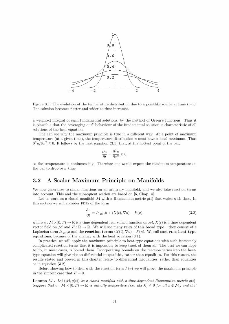
It can be seen in Figure 3.1 that at each time the temperature distribution is Gaussian, andthe distribution becomes flatter and wider as time evolves. This is what we expect of heat flow:the heat spreads out as time evolves, any relatively hot region becomes cooler, and the maximumtemperature on the bar drops over time. Any solution of the heat equation can be expressed as
30
-4 -2 2 4
0.2
0.4
0.6
0.8
1
Figure 3.1: The evolution of the temperature distribution due to a pointlike source at time t = 0.The solution becomes flatter and wider as time increases.
a weighted integral of such fundamental solutions, by the method of Green’s functions. Thus itis plausible that the “averaging out” behaviour of the fundamental solution is characteristic of allsolutions of the heat equation.
One can see why the maximum principle is true in a different way. At a point of maximumtemperature (at a given time), the temperature distribution u must have a local maximum. Thus∂2u/∂x2 ≤ 0. It follows by the heat equation (3.1) that, at the hottest point of the bar,
∂u
∂t=∂2u
∂x2≤ 0,
so the temperature is nonincreasing. Therefore one would expect the maximum temperature onthe bar to drop over time.
3.2 A Scalar Maximum Principle on Manifolds
We now generalize to scalar functions on an arbitrary manifold, and we also take reaction termsinto account. This and the subsequent section are based on [6, Chap. 4].
Let us work on a closed manifold M with a Riemannian metric g(t) that varies with time. Inthis section we will consider pdes of the form
∂u
∂t= 4g(t)u+ 〈X(t),∇u〉+ F (u), (3.2)
where u :M×[0, T )→ R is a time-dependent real-valued function onM, X(t) is a time-dependentvector field on M and F : R → R. We will see many pdes of this broad type – they consist of aLaplacian term 4g(t)u and the reaction terms 〈X(t),∇u〉+F (u). We call such pdes heat-typeequations, because of the analogy with the heat equation (3.1).
In practice, we will apply the maximum principle to heat-type equations with such fearsomelycomplicated reaction terms that it is impossible to keep track of them all. The best we can hopeto do, in most cases, is bound them. Incorporating bounds on the reaction terms into the heat-type equation will give rise to differential inequalities, rather than equalities. For this reason, theresults stated and proved in this chapter relate to differential inequalities, rather than equalitiesas in equation (3.2).
Before showing how to deal with the reaction term F (v) we will prove the maximum principlein the simpler case that F = 0.
Lemma 3.1. Let (M, g(t)) be a closed manifold with a time-dependent Riemannian metric g(t).Suppose that u :M× [0, T )→ R is initially nonpositive (i.e. u(x, 0) ≤ 0 for all x ∈ M) and that
31
it satisfies the differential inequality
∂u
∂t≤ 4g(t)u+ 〈X(t),∇u〉
at all points (x, t) ∈M× [0, T ) where u(x, t) > 0. Then u(x, t) ≤ 0 for all x ∈M and t ∈ [0, T ).
Note the rather strange condition that the inequality is satisfied only at points and timeswhere something has “gone wrong” (in the sense that u(x, t) has become positive). The conditionis designed so that we can apply this lemma in the proof of the more general scalar maximumprinciple (Theorem 3.2).
Proof. The proof will be based on the idea outlined at the end of Section 3.1.Given ε > 0, let us set vε = u − ε(1 + t). Note that vε(x, 0) ≤ −ε < 0. We will show that for
any ε > 0, vε < 0 on M× [0, T ). From the fact that ε > 0 is arbitrary it will follow that u isnon-positive.
First we compute the evolution equation (or evolution inequality) of vε, which follows from thatof u:
∂
∂tvε ≤ 4u+ 〈X,∇u〉 − ε
= 4vε + 〈X,∇vε〉 − ε (3.3)
at any point x and time t where u(x, t) > 0. In particular, because vε < u, the inequality holds atany (x, t) such that vε(x, t) = 0. Note that 4vε = 4u and ∇vε = ∇u because −ε(1 + t) has nospatial dependence.
Now suppose, for a contradiction, that vε(x, t) ≥ 0 for some (x, t) ∈M×[0, T ). By compactness,there exists a first time t0 ∈ [0, T ) and point x0 ∈ M at which vε hits 0. That is, vε(x0, t0) = 0but vε(x, t) < 0 for any t < t0. It follows that
∂vε∂t
(x0, t0) ≥ 0.
Furthermore, x0 must be a local maximum of vε(·, t0), so
∇vε(x0, t0) = 04vε(x0, t0) ≤ 0.
We can plug these inequalities into equation (3.3), which holds at (x0, t0) because vε(x0, t0) = 0.We obtain:
0 ≤ ∂vε∂t
(x0, t0) ≤ 4vε(x0, t0) + 〈X(t0),∇vε(x0, t0)〉 − ε ≤ −ε < 0,
which is a contradiction.Therefore, vε(x, t) < 0 for all (x, t) ∈ M × [0, T ) and for all ε > 0. Hence u(x, t) ≤ 0 for all
(x, t) ∈M× [0, T ), as required.
We can now prove the main result of this section, which shows how to deal with the reactionterm F (u) in equation (3.2).
Theorem 3.2. The Scalar Maximum Principle. Let (M, g(t)) be a closed manifold with atime-dependent Riemannian metric g(t). Suppose that u :M× [0, T )→ R satisfies
∂u
∂t≤ 4g(t)u+ 〈X(t),∇u〉+ F (u)
u(x, 0) ≤ C for all x ∈M,
for some constant C, where X(t) is a time-dependent vector field on M and F : R→ R is locallyLipschitz. Suppose that φ : R → R is the solution of the associated ode, which is formed byneglecting the Laplacian and gradient terms:
dφ
dt= F (φ)
φ(0) = C.
32
Thenu(x, t) ≤ φ(t)
for all x ∈M and t ∈ [0, T ) such that φ(t) exists.
The theorem essentially tells us that our upper bound grows no faster than we would expectfrom the reaction term F (u).
Proof. Let us set v = u− φ. We know that v(x, 0) ≤ 0 for all x ∈ M, and we desire to show thatv(x, t) ≤ 0 for all (x, t) ∈ M × [0, T ). To do this, we fix an arbitrary τ ∈ [0, T ) and show thatv ≤ 0 on [0, τ ], for any τ ∈ [0, T ). First note that
∂v
∂t=
∂(u− φ)∂t
≤ 4u+ 〈X,∇u〉+ F (u)− F (φ)= 4v + 〈X,∇v〉+ (F (u)− F (φ)). (3.4)
Note that ∇u = ∇v and 4u = 4v because φ depends only on t. We now want to deal with thelast term on the rhs.
BecauseM×[0, τ ] is compact, there exists a constant C (dependent on τ) such that |u(x, t)| ≤ Cand |φ(t)| ≤ C on M× [0, τ ]. Because F is locally Lipschitz and the interval [−C,C] is compact,there exists C1 (also dependent on τ) such that |F (x) − F (y)| ≤ C1|x − y| for all x, y ∈ [−C,C].Therefore, because u, φ ∈ [−C,C], |F (u)−F (φ)| ≤ C1|u− φ| = C1|v| onM× [0, τ ]. Plugging thisinto the evolution equation (3.4) for v, we obtain
∂v
∂t≤ 4v + 〈X,∇v〉+ C1|v|.
Now let w = e−C1tv. Then we have
∂w
∂t≤ e−C1t (4v + 〈X,∇v〉+ C1|v| − C1v)
= 4w + 〈X,∇w〉+ C1(|w| − w). (3.5)
We are going to apply Lemma 3.1 to the function w. Because v(x, 0) ≤ 0 for all x ∈ M, we havew(x, 0) ≤ 0 for all x ∈M. Furthermore, if w ≥ 0 then |w| = w, so the differential inequality (3.5)gives us
∂w
∂t≤ 4w + 〈X,∇w〉
at any point (x, t) ∈ M× [0, τ ] such that w(x, t) ≥ 0. Hence, by Lemma 3.1, w(x, t) ≤ 0 for all(x, t) ∈M× [0, τ ].
It follows that v(x, t) ≤ 0, and hence u(x, t) ≤ φ(t) for all (x, t) ∈M× [0, τ ], for any τ ∈ [0, T ).Therefore u(x, t) ≤ φ(t) for any (x, t) ∈M× [0, T ).
3.3 A Maximum Principle for Vector Bundles
In [10], Hamilton showed how to generalize the maximum principle to apply to sections of a vectorbundle (of which scalar functions are a special case). There is a bit of a subtlety in this case though– a heat-type equation has a Laplacian term in it, but what exactly do we mean by a Laplacianin this situation? Let π : E →M be a vector bundle over M with a fixed bundle metric h, ∇(t) asmooth time-dependent family of connections on E compatible with h, and g(t) a time-dependentRiemannian metric onM. Now to define the Laplacian of a section ϕ we need to take two covariantderivatives of ϕ then take the trace. However the first covariant derivative is ∇ϕ ∈ C∞(T ∗M⊗E)(compare Definition 1.12).
There is a problem because ∇ϕ is not a section of E , so we cannot simply take the secondcovariant derivative using ∇(t). To resolve this, we define a connection ∇(t) on the vector bundleE ⊗ T ∗M by the product rule:
∇X(ϕ⊗ ξ) ≡ ∇Xϕ⊗ ξ + ϕ⊗∇Xξ
33
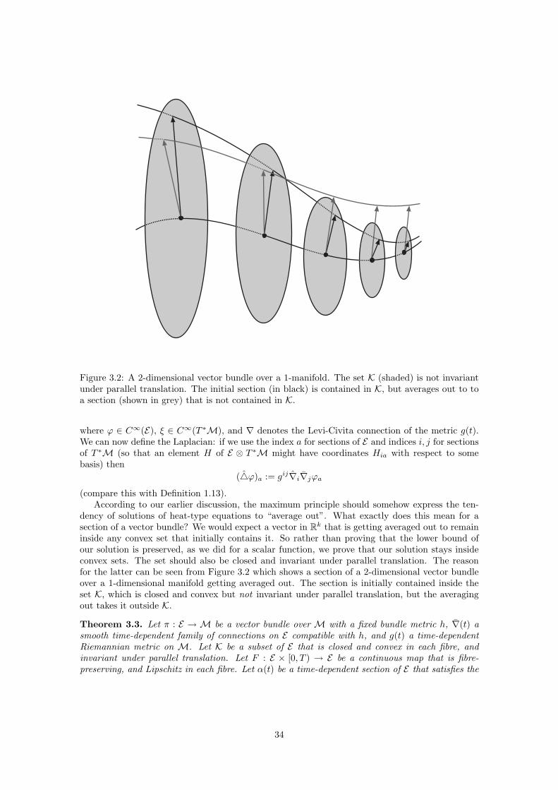
Figure 3.2: A 2-dimensional vector bundle over a 1-manifold. The set K (shaded) is not invariantunder parallel translation. The initial section (in black) is contained in K, but averages out to toa section (shown in grey) that is not contained in K.
where ϕ ∈ C∞(E), ξ ∈ C∞(T ∗M), and ∇ denotes the Levi-Civita connection of the metric g(t).We can now define the Laplacian: if we use the index a for sections of E and indices i, j for sectionsof T ∗M (so that an element H of E ⊗ T ∗M might have coordinates Hia with respect to somebasis) then
(4ϕ)a := gij∇i∇jϕa(compare this with Definition 1.13).
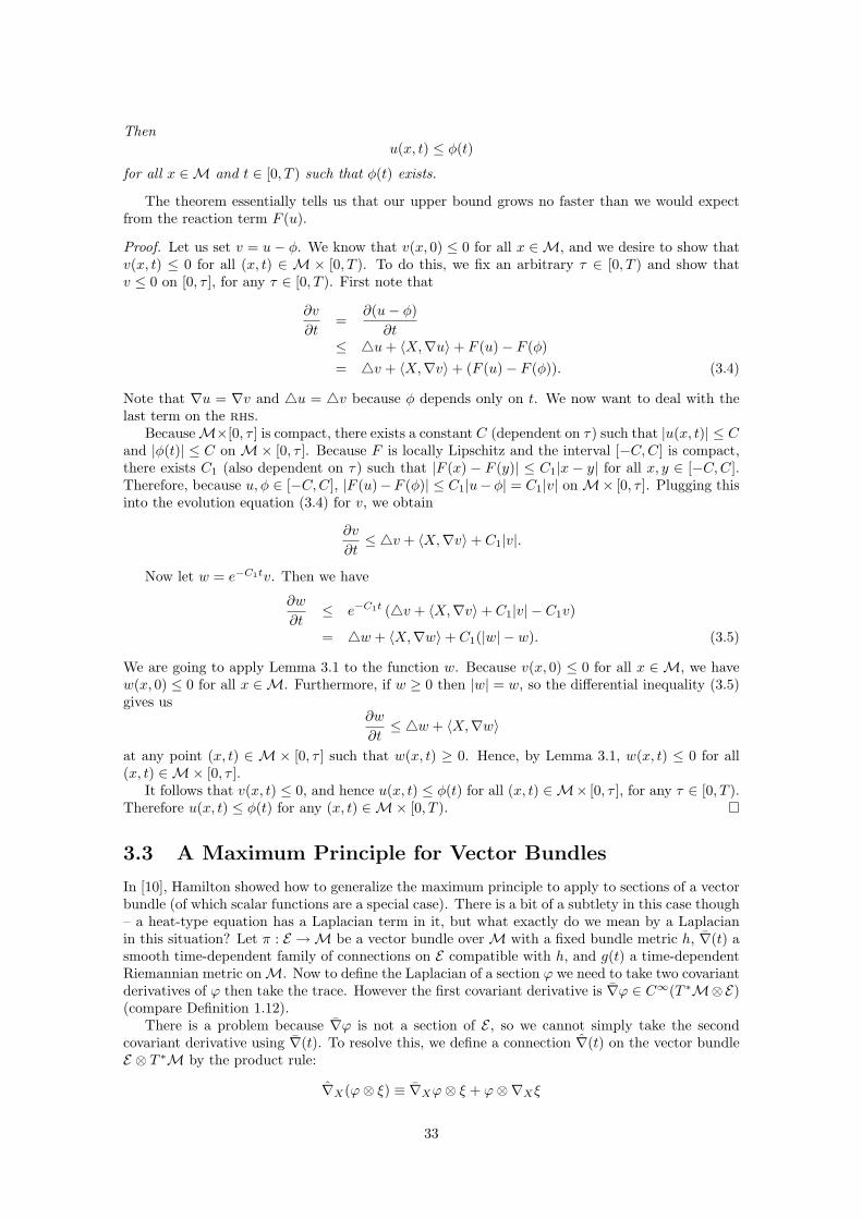
According to our earlier discussion, the maximum principle should somehow express the ten-dency of solutions of heat-type equations to “average out”. What exactly does this mean for asection of a vector bundle? We would expect a vector in Rk that is getting averaged out to remaininside any convex set that initially contains it. So rather than proving that the lower bound ofour solution is preserved, as we did for a scalar function, we prove that our solution stays insideconvex sets. The set should also be closed and invariant under parallel translation. The reasonfor the latter can be seen from Figure 3.2 which shows a section of a 2-dimensional vector bundleover a 1-dimensional manifold getting averaged out. The section is initially contained inside theset K, which is closed and convex but not invariant under parallel translation, but the averagingout takes it outside K.
Theorem 3.3. Let π : E → M be a vector bundle over M with a fixed bundle metric h, ∇(t) asmooth time-dependent family of connections on E compatible with h, and g(t) a time-dependentRiemannian metric on M. Let K be a subset of E that is closed and convex in each fibre, andinvariant under parallel translation. Let F : E × [0, T ) → E be a continuous map that is fibre-preserving, and Lipschitz in each fibre. Let α(t) be a time-dependent section of E that satisfies the
34
conditions
∂
∂tα = 4α+ F (α)
α(0) ∈ K.
Let Kx = π−1(x) ∩ K. Suppose that every solution of the ode
da
dt= F (a)
a(0) ∈ Kx
remains in Kx. Then the solution α(t) of the pde remains in K.
That is, if the reaction term does not force it out, then the solution will remain in K. Notethat the behaviour of the ode is much simpler than the behaviour of the original pde because weneed only consider each fibre individually – the solution of the ode is a time-dependent vector insome vector space rather than a time-dependent section of some vector bundle.
35
Chapter 4
Curve-Shortening Flow
This chapter is based on the lectures on Geometric Evolution Equations given by Ben Andrews atthe ICE-EM Graduate School in July 2006.
When Hamilton introduced the Ricci flow and used it to prove Theorem 2.1, he introducedquite a general method of dealing with geometric evolution equations. This method has sincebeen applied to other flows, such as the mean curvature flow (mcf) and the curve-shortening flow(csf) (see [30] for a description of both). Although these settings for Hamilton’s method of proofemerged after Hamilton’s original Ricci flow paper, the csf in particular is much simpler than theRicci flow. Many of the concepts central to the theory of the Ricci flow presented in Chapters 5,6, 7 and 8 find simpler analogies in the theory of the csf.
In this chapter we will outline the basic theory of the csf, with the aim of providing a“blueprint” for subsequent development of the theory of the Ricci flow. We will not prove allof the results that we state – those proofs and those results that assist in building intuition for themethods of proof employed in later chapters are emphasised.
4.1 Steepest Descent Flow for Length
Given a smooth immersion X0 : R/Z → R2 (i.e. a smooth immersion of a circle into the plane),we can evolve it by taking X : R/Z× [0, T )→ R2 such that
∂X
∂t(u, t) = −κN(u, t) (4.1)
X(u, 0) = X0(u).
Here, κ is the curvature of our curve, and N is the unit normal vector to it, defined by
−κN =∂2X
∂s2
where s is the arclength parameter (see Figure 4.1). The book [15, Chap. 1] is a good referencefor the theory of curves in space.
One might wonder where this definition comes from. The idea is to look for the way to move acurve in the plane that gives the greatest decrease in total length for the smallest total “movement”– we say that the csf is the “steepest descent flow for length”.
Lemma 4.1. Denote the length of the curve u 7→ X(u, t) at time t by
L(t) =∫ 1
0
|Xu|du.
Consider an arbitrary variation of the curve X0(u) = X(u, 0) with
∂X
∂t(u, t) = V (u, t),
36
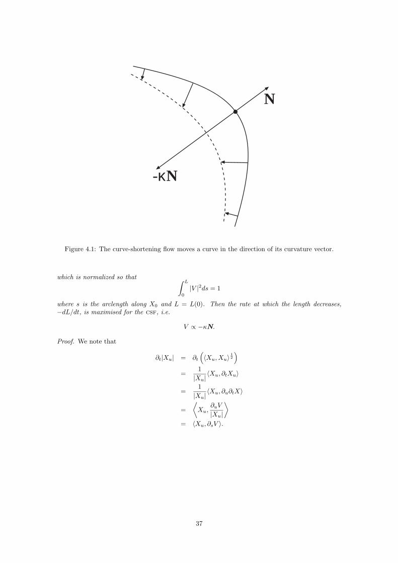
N
-κN
Figure 4.1: The curve-shortening flow moves a curve in the direction of its curvature vector.
which is normalized so that ∫ L
0
|V |2ds = 1
where s is the arclength along X0 and L = L(0). Then the rate at which the length decreases,−dL/dt, is maximised for the csf, i.e.
V ∝ −κN.
Proof. We note that
∂t|Xu| = ∂t
(〈Xu, Xu〉
12
)=
1|Xu|
〈Xu, ∂tXu〉
=1|Xu|
〈Xu, ∂u∂tX〉
=⟨Xu,
∂uV
|Xu|
⟩= 〈Xu, ∂sV 〉.
37
Hence
dL(t)dt
=∫ 1
0
∂t|Xu|du
=∫ L
0
〈Xu, ∂sV 〉ds
|Xu|
=∫ L
0
〈∂sX, ∂sV 〉ds
= [〈∂sX,V 〉]L0 −∫ L
0
〈∂ssX,V 〉ds
=∫ L
0
〈κN, V 〉
≥ −
(∫ L
0
κ2ds
) 12(∫ L
0
|V |2ds
) 12
.
We have integrated by parts, and the boundary terms vanished by periodicity. The last line followsfrom the Cauchy-Schwarz inequality, so equality holds if and only if V ∝ −κN. Thus the csf isexactly the variation that gives the fastest decrease in length.
Example: The shrinking circle. If our initial curve X0 is a circle of radius r0 centred at theorigin, then the solution will take the form X(u, t) = r(t)(cos(u), sin(u)). We have N = X/r, κ =1/r, so the csf equation becomes
dr
dt= −1
rwhich has the solution
X(u, t) = (r20 − 2t)
12 (cos(u), sin(u)). (4.2)
So the circle shrinks to a point at a finite time t =√r20/2 = r0/
√2.
4.2 Short Time Existence
Before anything else we must check that this system has a solution for a short time. To do thiswe will use the existence and uniqueness theorem for parabolic pdes (Theorem A.1). We need tocheck if our system is strongly parabolic before we can apply this theorem.
If we set X(u) = (x(u), y(u)) and use the notation xu = ∂x∂u , then the csf equation becomes
∂
∂t
[xy
]=
1(x2u + y2
u)2
[y2u −xuyu
−xuyu x2u
] [xuuyuu
]For the system to be strongly parabolic, the matrix on the rhs ought to be positive-definite. Itclearly isn’t (it is even singular), so we seem to be in trouble.
Although it appears that our system is not parabolic, all that is going on is that the parabolicnature of the system is being hidden from us by a poor parametrization of our solution. Suppose,for the moment, that we have a solution of the csf given by X : R/Z × [0, T ) → R2. Consider atime-dependent family of diffeomorphisms from the circle to itself:
ϕ : R/Z× [0, T )→ R/Z.
Then we can define X(u, t) = X(ϕ(u, t), t). X is just a time-dependent reparametrization ofX. In particular, it won’t change how the curve “looks”, i.e. its image in R2.
The evolution equation satisfied by X is then
∂
∂tX(u, t) =
∂
∂tX(ϕ(u, t), t) +Xu
∂
∂tϕ(u, t)
= −κN +XuV
=1
(x2u + y2
u)2
[yu−xu
][yu −xu]
[xuuyuu
]+[xuyu
]V
38
where we define∂
∂tϕ(u, t) = V (ϕ(u, t), t). (4.3)
We are free to choose how to reparametrize our curve – that is, we may choose V and thensolve the differential equation (4.3) for ϕ(u, t). We choose V so that our system of csf withtime-dependent reparametrization is strongly parabolic:
V =1
(x2u + y2
u)2
[xu yu][xuuyuu
]. (4.4)
Then we have, setting X = (x, y),
∂
∂t
[xy
]=
1(x2u + y2
u)2
{[yu−xu
][yu −xu]
+[xuyu
][xu yu]
}[xuuyuu
]=
1(x2u + y2
u)
[1 00 1
] [xuuyuu
].
We can now express xu, xuu, yu, yuu in terms of xu, xuu, yu, yuu using the chain rule. This givesus a second-order differential equation for (x, y), which is strongly parabolic because the matrixmultiplying (xuu, yuu) is positive definite. By Theorem A.1 there exists a solution X = (x, y) onsome time interval [0, T ), and the solution is unique for as long as it exists. Using this solution it ispossible to reconstruct ϕ(u, t) from (4.3) – because we know x, y this is a simple ode. Once we knowthe reparametrization used, we can find X(u, t) = X(ϕ−1(u, t), t) and show that it is a solution ofthe csf. Therefore, although the csf is not a strongly parabolic system, by reparametrizing it wecan show that it has a solution on some time interval [0, T ), and it is not difficult to further provethat the solution is unique for as long as it exists. Because of this uniqueness we may withoutambiguity choose
T = sup{τ : X(u, t) exists and is smooth for t ∈ [0, τ)}.
In this situation, we call [0, T ) a maximal time interval – it is the largest time interval on whichthe solution exists (note that T could be ∞).
Theorem 4.2. For any smooth immersion X0 : R/Z→ R2, there is a unique smooth solution
X : R/Z× [0, T )→ R2
satisfying the csf and withX(u, 0) = X0(u)
on a maximal time interval [0, T ).
4.3 Finite Time Singularity
Theorem 4.3. The Avoidance Principle. If X,Y are solutions of the csf on [0, T ), andX(u, 0) 6= Y (v, 0) for all u, v, then X(u, t) 6= Y (v, t) for all u, v, for all t ∈ [0, T ). That is, if thecurves do not intersect initially, they will not intersect at any later time.
This theorem can be proven using a version of the maximum principle to show that the smallestdistance between the two curves is a nondecreasing function of time.
Theorem 4.4. The csf exists for only a finite time before becoming singular. That is, the maximaltime T mentioned in Theorem 4.2 is finite.
Proof. Given any X0, we can take a circle that surrounds it. Running the csf on the circle and thecurve X0, the Avoidance Principle shows that the solution X can never move outside the evolvingcircle. As we showed in (4.2), the circle shrinks to a point in a finite time, “crushing” our solutionX and forcing it to become singular in finite time. Therefore the maximal time T mentioned inTheorem 4.2 must be finite.
39
4.4 Curvature Explodes
Theorem 4.5. Suppose we have a solution of the csf on a maximal time interval [0, T ), whereT <∞ by Theorem 4.4. Then
limt→T
sup{|κ(u, t)| : u ∈ R/Z} =∞.
We will give an outline of the proof. The basic idea is to assume the curvature were boundedas t→ T , and show that the maps Xt(·) = X(·, t) must then converge so nicely as t→ T that it ispossible to extend the solution past T , contradicting the assumption that [0, T ) was the maximaltime interval on which the solution existed.
By differentiating equation (4.1) one can obtain an evolution equation for the curvature:
∂κ
∂t=∂2κ
∂s2+ κ3.
This is a heat-type equation. From it we can derive evolution equations for the derivatives ofthe curvature ∂nκ/∂sn, which will also be heat-type equations. Assuming an upper bound on κ,one can use the maximum principle (in the form of Theorem 3.2) to prove upper bounds on thederivatives of κ. These bounds are analogous to the bounds obtained in Chapter 6 for the Ricciflow.
From the bounds on the derivatives of the curvature, it is possible to prove bounds on thederivatives of X. Once can show that all of the quantities∣∣∣∣ ∂k∂uk ∂l∂tlX
∣∣∣∣are bounded above. This means that all derivatives ofX are equicontinuous, so by the Ascoli-Arzelatheorem, for any k, l > 0 there is a sequence of times (ti) such that the maps
∂k
∂uk∂l
∂tlX(·, ti)
converge uniformly. Because the time-derivatives are also bounded, this means that the maps
∂k
∂uk∂l
∂tlX(·, t)
converge uniformly. Therefore the map X(·, t) and all its derivatives converge uniformly to somesmooth map X(·, T ). We can then use Theorem 4.2 to find a solution X to the csf with the initialcurve X0(·) = X(·, T ), defined on some time interval [0, ε). The solution X can now be “glued ontothe end of X” to extend the solution X past T . Defining X(·, t) = X(·, t − T ) for t ∈ [T, T + ε)(and leaving X unchanged for t ∈ [0, T )), we obtain a smooth solution1 X to the csf with thegiven initial data, which is defined on the time interval [0, T + ε). This contradicts the maximalityof T . Hence the original assumption that the curvature was bounded was incorrect.
4.5 Grayson’s Theorem
We have seen that our curve becomes singular in finite time; in fact it can be shown that anembedded circle will shrink to a point and become round as it approaches the maximal time T .What does “become round” mean though, when our solution is shrinking to a point? To makesense of this, we “blow up” our solution – we dilate it by a time-dependent factor so that the areaenclosed by the curve is constant. Then the solution will not shrink to a point, but will stay of thesame size, and “becomes round” simply means that the curve converges to a circle.
1The solution has smooth u-derivatives at t = T because of the uniform convergence of all derivatives of X(·, t)to X(·, T ) as t→ T . The time-derivatives can be expressed in terms of the space derivatives using the equation ofthe csf, so they too are smooth.
40
Theorem 4.6. (Grayson) Given any embedded circle X0, the solution to the csf X(u, t) withX(u, 0) = X0(u) will remain embedded and will shrink to a point x as t approaches the maximaltime of existence T . Furthermore, if A(t) denotes the area enclosed by the curve X(·, t) at time t,then the curve
X(u, t) =√
π
A(t)(X(u, t)− x)
converges exponentially to a unit circle as t→ T .
Proof. Once again, we will not give a complete proof but will outline one of the main concepts,because it is analogous to the blowup technique that we will introduce for the Ricci flow in Chapter8. See [30, Chap. 1 and Sec. 5.2] for the full proof of this theorem.
If the initial curve X0 is convex, one can prove using derivative estimates that the curvatureconverges uniformly to 1, and all derivatives of curvature are bounded. Once again the Ascoli-Arzela theorem can be employed to show that a limit exists, and that the limit is a smoothembedded curve with curvature 1, hence the unit circle (see [30, Chap. 1] for the details). Thisresult is known as the Gage-Hamilton Theorem (a corresponding result for the mean curvatureflow was proven by Gerhard Huisken).
Grayson proved that any initial curve will eventually become convex under the csf, from whichthe result follows by the Gage-Hamilton Theorem. We will outline the proof presented in [30, Sec.5.2]. We use the result of Theorem 4.5, which says that the curvature explodes as we approachsome singular time T <∞. This means we may choose points pn ∈ R/Z and times tn that convergeto T such that
|κ(pn, tn)| = supp∈R/Z,t≤tn
|κ(p, t)|,
and define Mn := |κ(pn, tn)|, so that limn→∞Mn =∞. We then define rescaled flows Xn by
Xn(p, t) := Mn
(X
(pn + p, tn +
t
M2n
)−X(pn, tn)
).
It is not hard to see that these rescaled flows are solutions of the csf defined for t ∈ [−M2ntn,M
2n(T−
tn)), with Xn(0, 0) = 0 and |κn(p, t)| ≤ |κn(0, 0)| = 1 for t ∈ [−Mntn, 0]. This technique is knownas “blowing up” at a singularity; we rescale the flow so that the curvature no longer diverges.
We saw in the discussion of Theorem 4.5 that it is possible to deduce bounds on derivatives ofthe curvature from a bound on the curvature, using the maximum principle. Moreover, one canget bounds on the derivatives of the maps Xn : R× [−Mntn, 0] (considering Xn as a periodic mapon the real line) from the bounds on derivatives of the curvature. Hence, by the Ascoli-Arzelatheorem there is a subsequence of Xn that converges uniformly in all Ck norms on all compactsubsets of R × (−∞, 0] to a limit solution X∞ : R × (−∞, 0] → R2. This limit solution satisfiesX∞(0, 0) = 0 and κ∞(p, t) = κ∞(0, 0) = 1 for all t ≤ 0.
After considerable work, one can show that this limit of rescaled solutions is convex withcompact image for all t ∈ (−∞, 0], from which it follows that some Xn is eventually convex andhence the csf X(·, t) is eventually convex for large enough t, as required.
41
Chapter 5
Short Time Existence andUniqueness of the Ricci Flow
Before we can do anything with the Ricci flow, we must show that a solution exists for a shorttime. We would like to apply the short-time existence and uniqueness theorem for parabolic pdes(Theorem A.1) to the system
∂
∂tg(t) = −2Rc(g(t))
g(0) = g0.
We need to check if the system is strongly parabolic. This chapter is based on [6, Chap. 3] and[28, Chap. 5].
5.1 The Linearization of the Ricci Tensor
The first thing to do is to work out the linearization of the Ricci tensor in the sense described inAppendix A. Recall that, if we have a time-dependent metric tensor gij(t) (we are not assumingthat this time-dependent metric satisfies the Ricci flow or any other specific equation), we definethe linearization of the Ricci tensor, D[Rc] : C∞(T ∗M⊗S T ∗M)→ C∞(T ∗M⊗S T ∗M) so that
D[Rc](∂gij∂t
)=
∂
∂tRc(gij(t)).
Lemma 5.1. The linearization of the Ricci tensor is given by
D[Rc](h)ij =12gpq(−∇p∇qhij −∇i∇jhpq +∇q∇ihjp +∇q∇jhip).
Proof. This follows from equation (1.19). We have interchanged the indices p and q in places,which we can do because the metric inverse gpq is symmetric.
To check if the system is strongly parabolic we must compute the principal symbol (see Ap-pendix A for the definition). The symbol can be computed easily from the linearization:
Corollary 5.2. The principal symbol of the differential operator −2Rc (as a function of the metricg) is:
σ[−2Rc](ϕ)(h)ij = gpq(ϕpϕqhij + ϕiϕjhpq − ϕqϕihjp − ϕqϕjhip).
Now we recall that the Ricci flow is strongly parabolic if there exists δ > 0 such that for allcovectors ϕ 6= 0 and all (symmetric) hij 6= 0,
〈σ[−2Rc](ϕ)(h), h〉 > δ|ϕ|2|h|2
42
or, by Corollary 5.2,
gpq(ϕpϕqhij + ϕiϕjhpq − ϕqϕihjp − ϕqϕjhip)hij > δϕkϕkhrsh
rs.
However, if we choose hij = ϕiϕj , it is clear that the LHS of this equation is 0, so the inequalitycan not hold. Therefore the Ricci flow is not strongly parabolic.
5.2 The DeTurck Trick
Because the Ricci flow is not strongly parabolic, we can not immediately apply Theorem A.1.Hamilton, in his original paper [9], used the Nash-Moser inverse function theorem to prove short-time existence and uniqueness. Shortly afterwards, Dennis DeTurck introduced (in [7]) a muchsimpler way of proving the short-time existence of the Ricci flow. In this section we show how onedoes the “DeTurck Trick”.
We first rewrite the linearization of the Ricci tensor so that it is possible to see which termsare making it non-parabolic.
Lemma 5.3. The linearization of −2Rc is equal to
D[−2Rc](h)ij = gpq∇p∇qhij +∇iVj +∇jVi + lower-order terms in h (5.1)
whereVi = gpq(
12∇ihpq −∇qhpi).
Proof. From Lemma 5.1 we have
D[−2Rc](h)ij = gpq(∇p∇qhij +∇i∇jhpq −∇q∇ihjp −∇q∇jhip). (5.2)
Applying the formula (B.3) for commuting covariant derivatives, we obtain
∇q∇ihjp = ∇i∇qhjp −Rrqijhrp −Rrqiphjm= ∇i∇qhjp + lower-order terms in h.
Lower-order terms in h make no contribution to the principal symbol. Thus, as far as the principalsymbol is concerned, covariant derivatives commute. We can therefore rearrange equation (5.2) bycommuting covariant derivatives to give
D[−2Rc](h)ij = gpq∇p∇qhij +∇i(12∇jhpq −∇qhjp) +∇j(
12∇ihpq −∇qhip)
+ lower-order terms in h
= gpq∇p∇qhij +∇iVj +∇jVi + lower-order terms in h
(recalling that ∇g = 0).
The lower-order terms in h make no contribution to the principal symbol. The first term inequation (5.1) is a good term (we can identify it as a Laplacian, which has a strictly positiveprincipal symbol), but the terms in V are bad: they make the Ricci flow non-parabolic.
The situation is analogous to that for the curve-shortening flow described in Section 4.2: theflow is not parabolic because we have a bad parametrization of our manifold. To obtain a parabolicsystem, we must introduce a time-dependent reparametrization.
In analogy with the curve-shortening flow, we seek a system
∂
∂tgt = P (gt) (5.3)
that is parabolic, and a time-dependent diffeomorphism ϕt from our manifold M to itself, withϕ0 = id, so that the metric
gt = ϕ∗t gt
43
is a solution to the Ricci flow. We can compute
∂
∂tgt =
∂ (ϕ∗t gt)∂t
=
(∂(ϕ∗t+sgt+s
)∂s
)s=0
=(ϕ∗t∂gt+s∂s
)s=0
+
(∂(ϕ∗t+sgt
)∂s
)s=0
= ϕ∗tP (gt) + ϕ∗tL ∂ϕt∂tgt.
Here we have used the product rule and then the rule for the Lie derivative on tensors (see Section1.3). We choose ϕt to satisfy
∂
∂tϕt = W (t)
ϕ0 = id
for some time-dependent vector field W (t) (this system will have a solution ϕt for as long as W (t)exists – see [6, Lem. 3.15]). The problem now reduces to finding a differential operator P suchthat the system (5.3) is strongly parabolic, and a time-dependent vector field W (t) such that, ifwe define a 1-parameter family of diffeomorphisms that satisfies (5.4), then
ϕ∗tP (gt) + ϕ∗tLW (t)gt = −2Rc(ϕ∗t gt) = −2ϕ∗tRc(gt)
(using the diffeomorphism invariance of the Ricci tensor). This is equivalent to
P (gt) = −2Rc(gt)− LW (t)gt.
Note that the choice of W (t) corresponds to the choice of V in Section 4.2.Now by Lemma 1.7 we have
(LW gt)ij = ∇iWj +∇jWi.
Therefore we can use Lemma 5.3 to write the linearization of P as
D[P ](h) = gpq∇p∇qhij +∇iVj +∇jVi + lower-order terms in h (5.4)−D[∇iWj +∇jWi](h). (5.5)
Recall that the first term in equation (5.4) is a good term: if the other second-order terms cancelledthen the linearization would satisfy the condition for parabolicity. So our aim is to choose W insuch a way that the second-order part of the term (5.5) cancels the second-order part of the termsin V . This will happen if the principal part of the linearization of Wi is equal to that of Vi1.
We defined V by
Vi = gpq(12∇ihpq −∇phqi)
= −12gpq(∇phqi +∇qhpi −∇ihpq).
We recall from formula (1.17) that
D[Γkij ](h) =∂
∂t
(Γkij(g(t))
)=
12gkl(∇ihjl +∇jhil −∇lhij),
where hij = ∂∂tgij . This looks pretty similar to the form of V , so we might try
Wi = −gpqgijΓjpq.1Note that, as far as the principal symbol is concerned, a covariant derivative ∇i is the same as a coordinate
derivative ∂i by formula (1.3). Therefore, if the principal symbol of the linearization of Wi is equal to that of Vi
then the principal symbol of the linearization of ∇jWi is equal to that of ∇jVi.
44
We need to be careful though – this expression depends on the coordinates we choose, because theChristoffel symbol Γ is not a tensor. However, the difference between two connections is a tensor,so we can fix a constant connection with Christoffel symbols Γkij and define
Wi = −gpqgij(
Γjpq − Γjpq),
which is the coordinate form of some coordinate-independent vector field. The fixed backgroundconnection, because it is independent of the metric, will make no contribution to the symbol of W ,so the principal symbol of Wi will be equal to that of Vi and all of the second-order terms otherthan the first in equation (5.4) will cancel.
Thus, making this choice of W , the principal symbol of the linearization of P is just
σ(D[P ])(ϕ)(h)ij = gpqϕpϕqhij ,
so we have〈σ(D[P ])(ϕ)(h), h〉 = |ϕ|2|h|2.
Thus the Ricci-DeTurck flow defined by
∂
∂tgij = P (g) = −2Rij +∇iWj +∇jWi
is strongly parabolic, and therefore has a solution for a short time by Theorem A.1.For as long as this solution exists, the vector field W (t) exists, and the time-dependent dif-
feomorphisms ϕt can be obtained by solving the ode (5.4) with initial condition ϕ0 =id. Oncewe know the ϕt exist, the above calculations show that the pullback metrics gt = ϕ∗t gt satisfy theRicci flow equation. Thus, the Ricci flow has a solution for a short time. In fact the solution isalso unique (see [6, Sec. 4.4]), so we have the following result:
Theorem 5.4. Given a smooth Riemannian metric g0 on a closed manifold M, there exists amaximal time interval [0, T ) such that a solution g(t) of the Ricci flow, with g(0) = g0, exists andis smooth on [0, T ), and this solution is unique.
45
Chapter 6
Derivative Estimates andCurvature Explosion atSingularities
In this chapter we will use the maximum principle in some creative ways to obtain bounds onderivatives of the curvature and metric evolving under the Ricci flow. We will then use ourestimates to show that the curvature must explode1 as we approach a finite-time singularity in theRicci flow, in analogy with Theorem 4.5 for the curve-shortening flow. This result is a key part ofthe proof of Theorem 2.1 that we will present in Chapter 7. The derivative estimates themselvesare also vital to the proof of the compactness result presented in Chapter 8. Our exposition isbased on [6, Chap. 6,7] (with the exception of Corollary 6.13 which is based on results in [28] andSection 6.2 which is based on [9, Sec. 13]), with significant reformulation of many of the arguments.
6.1 Evolution of Geometric Quantities Under the Ricci Flow
To apply maximum principle arguments to the curvature, we need to know what the equationsdescribing the evolution of curvature quantities under the Ricci flow are. We have already donethe bulk of the calculations in Lemma 1.20: the evolution equations for the Ricci flow follow bysubstituting hij = −2Rij into those formulae.
Lemma 6.1. Suppose that gij(t) is a solution of the Ricci flow:
∂
∂tgij = −2Rij .
Then the various geometric quantities evolve according to the following equations:
1. Metric inverse:∂
∂tgij = 2Rij .
2. Christoffel symbols:∂
∂tΓkij = −gkl(∇iRjl +∇jRil −∇lRij).
3. Riemann curvature tensor:
∂
∂tRijkl = 4Rijkl + 2(Bijkl −Bijlk +Bikjl −Biljk)
−(RpiRpjkl +RpjRipkl +RpkRijpl +RplRijkp),
1Some books on the Ricci flow use the words “blow up” here – unfortunately this expressive nomenclature isalready employed to describe our method of examining singularities as in Chapter 8, so we substitute “explode”.All it means is that the curvature goes to +∞, as detailed in Theorem 6.7.
46
whereBijkl ≡ −RqpijR
pqlk.
See Definition 1.13 for the definition of the Laplacian 4.
4. Ricci tensor:∂
∂tRij = 4Rij + 2RpijqRpq − 2RpiRpj .
5. Scalar curvature:∂
∂tR = 4R+ 2|Rc|2.
6. Einstein tensor on a 3-manifold:
∂
∂t|E|2 = 4|E|2 − 2|∇E|2 − 8RjiR
kjR
ik +
263R|Rc|2 − 2R3.
7. Volume element:∂
∂tdµ = −Rdµ.
8. Volume of manifold:∂
∂t
∫Mdµ = −
∫MRdµ.
9. Total scalar curvature (on a closed manifold):
∂
∂t
∫MRdµ =
∫M
(−R2 + 2|Rc|2
)dµ.
Proof. Most of these follow easily from Lemma 1.20, but some require a bit of extra fiddling to putthem in a nice form. The proof of the equation for the Riemann curvature tensor in particular israther lengthy and is contained (along with those for Rc and R) in [6, Sec. 6.1]. The main techniqueis to use the identity (B.3) to commute covariant derivatives, then use the Bianchi identities.
The proof of the evolution equation for |E|2 in dimension 3 can be found in [6, Cor. 6.39]. Itcan be proven using the formula
|E|2 = |Rc|2 − 13R2,
the evolution equations for Rc and R given above, and the result of Lemma 1.13 to express theRiemann curvature tensor in terms of the Ricci tensor. We will not use this result in the currentchapter, but it comes in handy in Chapter 7.
6.2 Evolution Equations for Derivatives of Curvature
We aim to obtain bounds on the derivatives of the curvature, i.e. on quantities of the form |∇kRm|2(here the k is not a raised index, it indicates the kth iterated covariant derivative). Our hope isto apply the maximum principle of Theorem 3.2 to get such bounds, but before we can apply thistheorem we must have some pdes that describe the evolution of the quantities.
Lemma 6.2. If A is a tensor quantity that satisfies a heat-type evolution equation:
∂
∂tA = 4A+ F
under the Ricci flow (where F is a tensor of the same type as A), then the square of its normsatisfies the heat-type equation
∂
∂t|A|2 = 4|A|2 − 2|∇A|2 + F ∗A+ Rc ∗A∗2.
47
Proof. We use gt to denote the metric at time t.
∂
∂tgt(A,A) = 2gt
(∂
∂tA,A
)+∂gt∂t
(A,A)
= 2gt(4A+ F,A) + Rc ∗A∗2
= 4|A|2 − 2|∇A|2 + F ∗A+ Rc ∗A∗2
where the final term in the second line comes from the derivative of the metric (which is −2Rc forthe Ricci flow) and we have used the identity
4|A|2 = 2〈4A,A〉+ 2|∇A|2.
Lemma 6.3. If A is a tensor quantity that satisfies a heat-type evolution equation
∂
∂tA = 4A+ F
under the Ricci flow (where F is a tensor of the same type as A), then its covariant derivativesatisfies a heat-type equation
∂
∂t∇A = 4(∇A) +∇F + Rm ∗ ∇A+∇Rc ∗A.
Proof. Recall from formula (1.3) that ∇A has the form
∇A = ∂A+ f(Γ, A)
where f(Γ, A) is some expression of the form Γ ∗ A, which depends on the type of the tensor A.Also, by Lemma 6.1 we have
∂tΓ =(g−1
)∗ ∇Rc.
It follows that
∂t∇A = ∂t∂A+ ∂tf(Γ, A)= ∂∂tA+ f(Γ, ∂tA) + f(∂tΓ, A) (by the product rule)= ∇(∂tA) + f(g−1 ∗ ∇Rc, A) (because ∂tA is a tensor of the same type as A)= ∇(4A+ F ) +∇Rc ∗A= (4∇A+ Rm ∗ ∇A+∇Rc ∗A) +∇F +∇Rc ∗A= 4∇A+∇F + Rm ∗ ∇A+∇Rc ∗A.
We used the formula
[∇,4]A := ∇4A−4∇A = Rm ∗ ∇A+∇Rc ∗A,
which follows from careful use of formula (B.3) followed by the second Bianchi identity (1.8) (see[6, p. 227]).
Now we note that the formula for the evolution of the Riemann curvature tensor under theRicci flow given in Lemma 6.1 translates into ∗-notation as
∂
∂tRm = 4Rm + Rm∗2. (6.1)
This allows us to use the preceding lemmas to calculate evolution equations for covariant derivativesof the metric.
Lemma 6.4. The evolution equation for the kth iterated covariant derivative of the Riemanncurvature tensor under the Ricci flow is:
∂
∂t∇kRm = 4∇kRm +
k∑j=0
∇jRm ∗ ∇k−jRm.
48
Proof. We prove the result by induction. The evolution equation for Rm given above in equation(6.1) is the base case k = 0. We assume the relation holds true for a given k and apply Lemma 6.3with A = ∇kRm and
F =k∑j=0
∇jRm ∗ ∇k−jRm.
This tells us that
∂
∂t∇∇kRm = 4(∇∇kRm) +∇F + Rm ∗ ∇(∇kRm) +∇Rc ∗ ∇kRm. (6.2)
It is clear that all of the reaction terms on the rhs are of the form∇iRm∗∇jRm where i+j = k+1,hence
∂
∂t∇k+1Rm = 4∇k+1Rm +
k+1∑j=0
∇jRm ∗ ∇k+1−jRm,
completing the inductive step.
Corollary 6.5. The square of the norm of the kth covariant derivative of the Riemann curvaturetensor satisfies the heat-type equation
∂
∂t|∇kRm|2 = 4|∇kRm|2 − 2|∇k+1Rm|2 +
k∑j=0
∇jRm ∗ ∇k−jRm ∗ ∇kRm. (6.3)
Proof. We simply apply Lemma 6.2 with A = ∇kRm and
F =k∑j=0
∇jRm ∗ ∇k−jRm,
by the result of Lemma 6.4. The result is
∂
∂t|∇kRm|2 = 4|∇kRm|2 − 2|∇k+1Rm|2 + F ∗ ∇kRm + Rc ∗ (∇kRm)∗2.
It is clear that all the terms on the left hand side other than the first two are of the form ∇iRm ∗∇jRm ∗ ∇kRm where i+ j = k, and hence
∂
∂t|∇kRm|2 = 4|∇kRm|2 − 2|∇k+1Rm|2 +
k∑j=0
∇jRm ∗ ∇k−jRm ∗ ∇kRm
as required.
6.3 The Bernstein-Bando-Shi Estimates
We now apply the maximum principle to the evolution equations derived in the last section to getbounds on the derivatives of the curvature. We aim to obtain these bounds under the assumptionthat the curvature itself is bounded above by some constant, |Rm| < K. There are two problems weface in trying to apply the maximum principle to the evolution equation we derived for the covariantderivatives of the curvature: firstly, we can not guarantee any initial conditions on the derivativesof the curvature if we are only given bounds on the curvature, and secondly the evolution equationhas some terms in it which we are not sure how to control (namely the terms of the summation inequation (6.3)).
We bypass the first problem by proving time-dependent upper bounds that diverge at t = 0(thus they only give us useful information after t = 0). We will see how to bypass the second inthe process of the proof.
49
Theorem 6.6. The Bernstein-Bando-Shi Estimates. Let (Mn, g(t)) be a solution of theRicci flow on a closed n-manifold. Then for each α > 0 and m ∈ N, there exists a constant Cmdepending only on m,n and max{α, 1} such that if
|Rm(x, t)|g(t) ≤ K for all t ∈ [0, αK ],
then|∇mRm(x, t)|g(t) ≤
CmK
tm/2for all t ∈ (0, αK ].
Proof. We prove the result by induction on m. For m = 0 the result is true by hypothesis, withC0 = 1. Assume the result is true for all p ≤ m− 1. The result of Corollary 6.5 tells us that
∂
∂t|∇mRm|2 = 4|∇mRm|2 − 2|∇m+1Rm|2 +
m∑j=0
∇jRm ∗ ∇m−jRm ∗ ∇mRm
≤ 4|∇mRm|2 − 2|∇m+1Rm|2 +m∑j=0
cmj |∇jRm||∇m−jRm||∇mRm|
≤ 4|∇mRm|2 − 2|∇m+1Rm|2 +
m−1∑j=1
cmjCjtj/2
Cm−jt(m−j)/2
K2|∇mRm|
+ (cm0 + cmm)K|∇mRm|2
≤ 4|∇mRm|2 − 2|∇m+1Rm|2 + C ′mK|∇mRm|2 +C ′′mtm/2
K2|∇mRm|
for t ∈ (0, αK ], where C ′m, C′′m are constants depending only on m and n. We have used the inductive
hypothesis to go from the second to the third line. We can complete the square (in the variable|∇mRm|) on the right hand side then use the inequality (a+ b)2/2 ≤ a2 + b2 to obtain
∂
∂t|∇mRm|2 ≤ 4|∇mRm|2 − 2|∇m+1Rm|2 + CmK
(|∇mRm|2 +
K2
tm
)(6.4)
for some constant Cm.To get the desired bound, we need to find an upper bound on tm|∇mRm|2. This quantity
clearly has an upper bound at t = 0 because it is equal to 0. So to apply the maximum principleand get an upper bound we need only show that the reaction terms in its evolution equation causeit to decrease. The problem we have is that this quantity satisfies the differential inequality
∂
∂t(tm|∇mRm|2) ≤ 4(tm|∇mRm|2)− 2tm|∇m+1Rm|2 + (6.5)
(CmKt+m)tm−1|∇mRm|2 + CmK3, (6.6)
and the reaction terms (6.6) are not negative. This is the “second difficulty” outlined at the startof this section.
To fix this problem, we make use of the term −2|∇k+1Rm|2 in the evolution equation ofCorollary 6.5. By adding the right amount of tm−1|∇m−1Rm|2 (which we know by our inductivehypothesis is bounded above by a constant) we can cancel off the unruly reactionary terms involvingtm|∇mRm|2. In so doing, we will introduce new unruly terms in tm−1|∇m−1Rm|2 – so we willneed to add the right amount of the next derivative down and so on. We define
G = tm|∇mRm|2 +m−1∑j=0
αmjtj |∇jRm|2,
where we will determine the constants αmj so that all the terms cancel as we want them to.By equation (6.5), we have
∂
∂tG ≤ 4G+ (CmKt+m)tm−1|∇mRm|2 + CmK
3
+m−1∑j=0
αmj{−2tj |∇j+1Rm|2 + (CjKt+ j)tj−1|∇jRm|2 + CjK
3}.
50
By the inductive hypothesis there are numbers Dj depending only on j, n for 1 ≤ j ≤ m− 1 suchthat
CjKtj |∇jRm|2 + CjK
3 ≤ DjK3
for all t ∈ (0, αK ]. Hence we have
∂
∂tG ≤ 4G+ (CmKt+m)tm−1|∇mRm|2 + CmK
3)
+m−1∑j=0
αmj{−2tj |∇j+1Rm|2 + jtj−1|∇jRm|2 +DjK
3}
= 4G+ (CmKt+m− 2αm,m−1)tm−1|∇mRm|2
+m−1∑j=0
{jαmj − 2αm,j−1} tj−1|∇jRm|2
+CmK3 +m−1∑j=0
αmjDjK3.
Now we choose the αmj so that the terms in this equation cancel: choose αm,m−1 such that
0 = Cmα+m− 2αm,m−1 ≥ CmKt+m− 2αm,m−1,
where the second step follows because we are working with t ∈ (0, α/K]. Now define αm,m−2,αm,m−3, . . . , αm0 in that order, at each step setting
jαmj − 2αm,j−1 = 0.
If we now define
Bm := Cm +m−1∑j=0
αmjDj
then our evolution can be written as
∂
∂tG ≤ 4G+BmK
3.
The reaction term is simply a constant, so it gives linear growth at worst. BecauseG = αm0|Rm|2 ≤αm0K
2 at t = 0, the scalar maximum principle (Theorem 3.2) tells us that
G ≤ αm0K2 +BmK
3t ≤ (αm0 +Bmα)K2 := C2mK
2
for t ∈ (0, αK ], where Cm is a constant depending only on m, n and max{α, 1}.Therefore, we have
|∇mRm| ≤√G
tm≤ CmK
tm/2for t ∈
(0,α
K
],
as required.
6.4 Curvature Explodes at Finite-time Singularities
This section will be devoted to proving that, if the Ricci flow becomes singular in finite time, thecurvature must explode as we approach the singular time T .
Theorem 6.7. If g0 is a smooth metric on a compact manifold M, the Ricci flow with g(0) = g0
has a unique solution g(t) on a maximal time interval t ∈ [0, T ) where T ≤ ∞. If T <∞ then
limt→T
(supx∈M
|Rm(x, t)|)
=∞.
51
The proof that the curvature must explode as t → T follows the same outline as the proofof the corresponding result for the curve-shortening flow, Theorem 4.5. That is, we assume that|Rm|g is bounded above by a constant K, and show that the metric g(t) converges smoothly to asmooth metric g(T ). It is then possible to use the short-time existence result of Theorem 5.4, withinitial metric g(T ), to extend the solution past T . This contradicts the choice of T as the maximaltime such that the Ricci flow exists on [0, T ).
A key element of the proof is the following theorem and its corollary, which show that a limitmetric g(T ) exists and is continuous:
Theorem 6.8. Let M be a closed manifold and g(t) a smooth time-dependent metric on M,defined for t ∈ [0, T ). If there exists a constant C <∞ such that∫ T
0
∣∣∣∣ ∂∂tg(x, t)∣∣∣∣g(t)
dt ≤ C (6.7)
for all x ∈ M, then the metrics g(t) converge uniformly as t → T to a continuous metric g(T )such that
e−Cg(x, 0) ≤ g(x, T ) ≤ eCg(x, 0).
Note that this means g(T ) is uniformly equivalent to g(0).
Proof. Let x ∈M, t0 ∈ [0, T ), V ∈ TxM be arbitrary. Then∣∣∣∣log(g(x,t0)(V, V )g(x,0)(V, V )
)∣∣∣∣ =∣∣∣∣∫ t0
0
∂
∂t
[log g(x,t)(V, V )
]dt
∣∣∣∣=
∣∣∣∣∣∫ t0
0
∂∂tg(x,t)(V, V )g(x,t)(V, V )
dt
∣∣∣∣∣≤
∫ t0
0
∣∣∣∣ ∂∂tg(x,t)
(V
|V |g(t),
V
|V |g(t)
)∣∣∣∣ dt≤
∫ t0
0
∣∣∣∣ ∂∂tg(x, t)∣∣∣∣g(t)
dt
≤ C
where the penultimate step follows as |A(U,U)| ≤ |A|g for any 2-tensor A and unit vector U .Exponentiating both sides of this inequality gives us:
e−Cg(x,0)(V, V ) ≤ g(x,t0)(V, V ) ≤ eCg(x,0)(V, V ),
for any V . Thuse−Cg(x, 0) ≤ g(x, t0) ≤ eCg(x, 0), (6.8)
so the metrics g(t) are uniformly equivalent.Hence, we have ∫ T
0
∣∣∣∣ ∂∂tg(x, t)∣∣∣∣g(0)
dt ≤ C ′ (6.9)
for some C ′ > 0. Note the difference from equation (6.7): the norm is taken with respect to aconstant metric g(0) rather than the time-dependent one g(t).
We now define
g(x, T ) = g(x, 0) +∫ T
0
∂
∂tg(x, t)dt.
This integral exists as the metrics are smooth and the integrand is absolutely integrable withrespect to the norm induced by g(0), by equation (6.9). Now
|g(x, t)− g(x, T )|g(0) ≤∫ T
t
∣∣∣∣ ∂∂tg(x, t)∣∣∣∣g(0)
→ 0
52
as t → T for each x ∈ M. Because M is compact, this convergence is uniform on M. Henceg(t) → g(T ) uniformly, so g(T ) is continuous. By taking the limit of equation (6.8) we can showthat
e−Cg(x, 0) ≤ g(x, T ) ≤ eCg(x, 0),
hence that g(T ) is positive definite.Therefore, the metrics g(t) converge uniformly to a continuous Riemannian metric g(T ) which
is uniformly equivalent to g(0).
Corollary 6.9. Let (M, g(t)) be a solution of the Ricci flow on a closed manifold. If |Rm|g isbounded on [0, T ) (where T <∞) then g(t) converges uniformly as t→ T to a continuous metricg(T ) which is uniformly equivalent to g(0).
Proof. Any bound on |Rm|g implies one on |Rc|g, and hence on | ∂∂tg|g (by the equation of theRicci flow). The integral (6.7) is then an integral of a bounded quantity over a finite interval, andis hence bounded. Thus Theorem 6.8 applies.
We have now got a foothold: we have shown that there is a limit metric g(T ), and it iscontinuous. We now want to show that this metric is smooth, because we need this if we are to usethe short-time existence result of Theorem 5.4 to extend our solution past T . To do this, we needto make sure the spatial derivatives of g near the limit time T are not exploding – we need boundson them. The first step is to bound the derivatives of the curvature, in analogy with the outlinedproof of Theorem 4.5. We do this via the Bernstein-Bando-Shi derivative estimates (Theorem 6.6),which give bounds on the derivatives of the curvature under the assumption of bounded curvature.
We recall that the Bernstein-Bando-Shi estimates are completely useless at t = 0 (as one mightexpect, for bounds on an arbitrary curvature tensor will not tell us anything about its derivatives– it is only after a period of Ricci flowing that the derivatives start to be brought under control).That is fine for us because we are interested in derivative estimates near t = T . We can useTheorem 6.6 to get such estimates, by considering our Ricci flow as starting at some time shortlybefore T . This gives us
Corollary 6.10. (of Theorem 6.6) Let (Mn, g(t)) be a solution of the Ricci flow on a compactn-manifold. If there exist β,K > 0 such that
|Rm(x, t)|g(t) ≤ K for all t ∈ [0, T ],
where T > β/K, then for each m ∈ N there exists a constant Bm depending only on m,n andmin{β, 1} such that
|∇mRm(x, t)|g(t) ≤ BmK1+m2 for all t ∈
[min{β,1}
K , T].
Proof. We use the result of Theorem 6.6. Let β1 = min{β, 1}. Now, given a time t0 ∈ [β1/K, T ],we consider the Ricci flow as starting at the time T0 = t0 − β1/K. Applying Theorem 6.6 to thisRicci flow, with α = β1, tells us that
|∇mRm| ≤ CmK
(t− T0)m/2
where Cm depends only on m,n and min{α, 1}. Hence at t = t0 we have
|∇mRm| ≤ CmK
(β1K )m/2
=Cmβm1
K1+m/2,
from which the result follows.
Using this bound on the derivatives of curvature near t = T , we can now proceed to bound thederivatives of the metric g near t = T . The following corollary and its proof are a reformulation ofthe argument found in [6, Prop. 6.48].
53
Corollary 6.11. Let (Mn, g(t)) be a solution of the Ricci flow on a closed n-manifold, and let(xi), i = 1, . . . , n be a local coordinate system defined on some coordinate chart U ⊂Mn. If thereexists K > 0 such that
|Rm(x, t)|g(t) ≤ K for all t ∈ [0, T )
then for each m ∈ N there exist constants Cm, C ′m depending only on the chosen coordinate chartsuch that
|∂mg(x, t)| ≤ Cmand
|∂mRc(x, t)| ≤ C ′mfor all (x, t) ∈ U × [0, T ), where the norms are taken with respect to the Euclidean metric in thecoordinate system (xi).
We should explain some of the notation used. By ∂mg we mean the(m+2
0
)-tensor field, defined
only in the coordinate chart U , which has coordinates
∂i1 . . . ∂imgpq
with respect to the coordinate system (xi). The Euclidean metric, which is also defined only in U ,is the metric which has coordinates δij with respect to the coordinate system (xi).
Proof. Throughout this proof, we will treat the Christoffel symbols Γkij as the coordinates, withrespect to the coordinate system (xi), of a tensor Γ (Γ is defined only in U).
Note that by Corollary 6.10, for each m ∈ N there is a uniform upper bound on |∇mRc| on atime interval (β/K, T ). There is also an upper bound on the same quantity on the interval [0, β/K]because the interval is compact, so the quantity is bounded for all m:
|∇mRc| ≤ Dm (6.10)
for all x ∈Mn and t ∈ [0, T ), where Dm is some constant depending on m and the particular Ricciflow (Mn, g(t)).
We will now prove by strong induction that there exist constants Pm, Qm, Rm for each m ∈N ∪ {0} such that
1. |∂m−1Γ| ≤ Pm (we only prove this for m ≥ 1);
2. |∂mRc| ≤ Qm;
3. |∂mg| ≤ Rm
for all t ∈ [0, T ).For the base case m = 0, (2) follows from the bound |Rm| ≤ K and (3) follows from Corollary
6.9.Assume (1) – (3) are satisfied for all m ≤ p−1. We will prove they are true for m = p, starting
with (1). Note that there is some constant C such that |∂p−1Γ| ≤ C at t = 0, because the manifoldMn is compact.
Bounds on |∂mg| imply bounds on |∂m(g−1)| by differentiating the formula gijgjk = δik, mtimes. Recalling the formula for ∂tΓ from Lemma 6.1, we can prove:
∂t∂p−1Γ = ∂p−1(∂tΓ)
= ∂p−1(g−1 ∗ ∇Rc)
=p−1∑i=0
∂p−i−1(g−1) ∗ ∂i∇Rc.
We have bounds on the derivatives of g−1, so we just need to bound the other terms. For i ≤ p−1we have, by Lemma 1.3 (recalling the notation from the end of Section 1.1),
∂i∇Rc = ∇i+1Rc + ∗0 ≤ j ≤ i− 1
k ≤ i
(∂jΓ, ∂kRc
).
54
Note that we have a bound on ∇i+1Rc by equation (6.10), and an inductive upper bound on allof the other terms on the right hand side, because j ≤ i − 1 ≤ p − 2 and k ≤ i ≤ p − 1. Hence|∂i∇Rc| ≤ C for i ≤ p− 1, therefore
|∂t∂p−1Γ| ≤ C
for some constant C (this C is different from the previous one – there are so many constant uniformbounds at play in this and subsequent arguments that we will refer to most of them as ‘C’ forconvenience, and hope that this does not cause too much confusion). Thus |∂p−1Γ| is boundedat t = 0 and experiences, at worst, linear growth on the finite time interval [0, T ). Therefore|∂p−1Γ| ≤ Pp for some constant Pp. This completes the proof of (1).
We can now compute (again by Lemma 1.3)
∂pRc = ∇pRc + ∗j ≤ p− 1k ≤ p− 1
(∂jΓ, ∂kRc
).
All terms on the right hand side are bounded inductively (with the exception of ∂p−1Γ, which wejust showed was bounded as part of the inductive step), so we have |∂pRc| ≤ Qp for some constantQp. This completes the proof of (2).
Finally,|∂t∂pg| = | − 2∂pRc| ≤ C
by the second part of the inductive step, so because we are on a finite time interval, |∂pg| ≤ Rpfor some constant Rp. This proves (3), completing the inductive step.
Therefore the result is true by induction.
Corollary 6.12. The metric g(T ) of Corollary 6.9 is smooth, and the metrics g(t) convergeuniformly in every Ck norm to g(T ) as t→ T .
Proof. To show that g(T ) is smooth we must take derivatives with respect to some system ofcoordinates which we can only choose arbitrarily, so take some coordinate patch U of Mn. Wehave, from the Ricci flow equation,
gij(x, T ) = gij(x, t)− 2∫ T
t
Rij(x, τ)dτ
for any t ∈ [0, T ).Now if α is any multi-index (see Definition A.1), then Corollary 6.11 tells us that ∂|α|
∂xα gij and∂|α|
∂xαRij are uniformly bounded on U × [0, T ), and hence that we may take the derivative under theintegral sign:
∂|α|
∂xαgij(x, T ) =
(∂|α|
∂xαgij
)(x, t)− 2
∫ T
t
(∂|α|
∂xαRij
)(x, τ)dτ (6.11)
for any x ∈ U . In particular, the lhs of the above equation exists for all α, so g(T ) is smooth.Now we show that the convergence is uniform in every Cm norm, in the following sense: we
can choose coordinate charts covering M, such that for any multi-index α, and any ε > 0, thereexists δ > 0 such that ∣∣∣∣ ∂|α|∂xα
gij(x, T )− ∂|α|
∂xαgij(x, t)
∣∣∣∣g(x,T )
< ε (6.12)
in any of the chosen coordinate charts, for any t ∈ [T − δ, T ) and x ∈Mn.Because Mn is compact, we can choose a finite set of coordinate charts such that the closed
unit balls of the coordinate charts cover Mn. Because the closed unit balls are compact, theEuclidean metric on each is equivalent to g(T ). Because there are finitely many coordinate charts,the Euclidean metrics are uniformly equivalent to g(T ). Thus it suffices to prove that equation(6.12) holds if we take the norm with respect to one of the Euclidean metrics at each point x,rather than with respect to g(x, T ).
By Corollary 6.11, for each of the coordinate charts we have chosen there exists C ′m such that|∂mRc| ≤ C ′m with respect to the Euclidean norm in that chart. If we choose C to be the largest
55
of these C ′m where m = |α| (C finite because there are only finitely many coordinate charts), thenequation (6.11) gives us∣∣∣∣ ∂|α|∂xα
gij(x, T )− ∂|α|
∂xαgij(x, t)
∣∣∣∣ =
∣∣∣∣∣2∫ T
t
(∂|α|
∂xαRij
)(x, τ)dτ
∣∣∣∣∣≤ 2
∫ T
t
|∂mRc(x, τ)| dτ
≤ 2C(T − t).
It follows that g(t)→ g(T ) uniformly in any Cm norm as t→ T .
We now prove Theorem 6.7. We assume, for a contradiction, that |Rm(x, t)|g is bounded aboveby K. It follows from Corollaries 6.9 and 6.12 that the metrics g(t) converge uniformly in any Ck
norm to a smooth metric g(T ).Because g(T ) is smooth, it is possible to find a solution to the Ricci flow with initial metric
g(T ), by the result of Theorem 5.4. Thus our solution to the Ricci flow can be extended past t = T ,as we did for the curve-shortening flow in the proof of Theorem 4.5. This extension is smooth,because all spatial derivatives are continuous at t = T (by the convergence of g(t) in any Ck norm).It follows that all space-time derivatives are continuous at t = T because the Ricci flow equationallows us to write time derivatives of quantities related to the metric in terms of space derivativesof those quantities, and the space-derivatives have been shown to be continuous. Therefore, thesolution can be extended past the time t = T , so the time T could not have been maximal. Thisis a contradiction, so the original assumption that |Rm(x, t)|g is bounded must be incorrect. Thiscompletes the proof of Theorem 6.7. �
Corollary 6.13. Suppose that (M, g(t)) is a solution of the Ricci flow on a closed manifold, suchthat |Rm| ≤ K at t = 0. Then there exists a positive constant b depending only on K and thedimension n of the manifold such that the Ricci flow exists for all t ∈ [0, b).
Furthermore, there exists a constant C depending only on n such that
|Rm| ≤ K
1− 12CKt
for as long as the rhs exists.
Proof. We will first prove the second statement, then deduce the first.Let u = |Rm|2. By Corollary 6.5 with k = 0, we have
∂u
∂t≤ 4u+ Cu3/2
for some C > 0 depending only on n. By hypothesis, |Rm|2 ≤ K2 at t = 0. The situation is perfectfor applying the maximum principle (Theorem 3.2). We need only solve the associated ode:
dφ
dt= Cφ3/2 , φ(0) = K2.
The solution is
φ(t) =(
K
1− 12CKt
)2
.
It follows by Theorem 3.2 that
u ≤(
K
1− 12CKt
)2
,
from which it follows that|Rm| ≤ K
1− 12CKt
as required.
56
Now let b = 1/(CK). We then have
|Rm(x, t)| ≤ 2K
for all t ∈ [0, b) and x ∈M, and b depends only on K and the dimension of the manifold. Because
limt→T
supx∈M
|Rm(x, t)| =∞,
where T is the maximal time of existence of the Ricci flow, we must have b < T , hence the Ricciflow exists for all t ∈ [0, b).
57
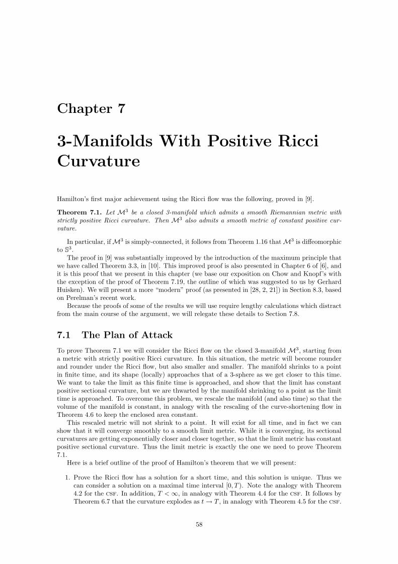
Chapter 7
3-Manifolds With Positive RicciCurvature
Hamilton’s first major achievement using the Ricci flow was the following, proved in [9].
Theorem 7.1. Let M3 be a closed 3-manifold which admits a smooth Riemannian metric withstrictly positive Ricci curvature. Then M3 also admits a smooth metric of constant positive cur-vature.
In particular, ifM3 is simply-connected, it follows from Theorem 1.16 thatM3 is diffeomorphicto S3.
The proof in [9] was substantially improved by the introduction of the maximum principle thatwe have called Theorem 3.3, in [10]. This improved proof is also presented in Chapter 6 of [6], andit is this proof that we present in this chapter (we base our exposition on Chow and Knopf’s withthe exception of the proof of Theorem 7.19, the outline of which was suggested to us by GerhardHuisken). We will present a more “modern” proof (as presented in [28, 2, 21]) in Section 8.3, basedon Perelman’s recent work.
Because the proofs of some of the results we will use require lengthy calculations which distractfrom the main course of the argument, we will relegate these details to Section 7.8.
7.1 The Plan of Attack
To prove Theorem 7.1 we will consider the Ricci flow on the closed 3-manifold M3, starting froma metric with strictly positive Ricci curvature. In this situation, the metric will become rounderand rounder under the Ricci flow, but also smaller and smaller. The manifold shrinks to a pointin finite time, and its shape (locally) approaches that of a 3-sphere as we get closer to this time.We want to take the limit as this finite time is approached, and show that the limit has constantpositive sectional curvature, but we are thwarted by the manifold shrinking to a point as the limittime is approached. To overcome this problem, we rescale the manifold (and also time) so that thevolume of the manifold is constant, in analogy with the rescaling of the curve-shortening flow inTheorem 4.6 to keep the enclosed area constant.
This rescaled metric will not shrink to a point. It will exist for all time, and in fact we canshow that it will converge smoothly to a smooth limit metric. While it is converging, its sectionalcurvatures are getting exponentially closer and closer together, so that the limit metric has constantpositive sectional curvature. Thus the limit metric is exactly the one we need to prove Theorem7.1.
Here is a brief outline of the proof of Hamilton’s theorem that we will present:
1. Prove the Ricci flow has a solution for a short time, and this solution is unique. Thus wecan consider a solution on a maximal time interval [0, T ). Note the analogy with Theorem4.2 for the csf. In addition, T <∞, in analogy with Theorem 4.4 for the csf. It follows byTheorem 6.7 that the curvature explodes as t→ T , in analogy with Theorem 4.5 for the csf.
58
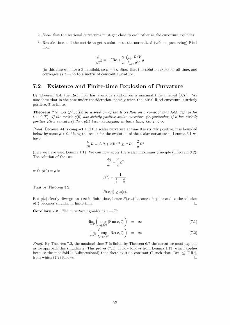
2. Show that the sectional curvatures must get close to each other as the curvature explodes.
3. Rescale time and the metric to get a solution to the normalized (volume-preserving) Ricciflow,
∂
∂tg = −2Rc +
2n
∫Mn RdV∫Mn dV
g
(in this case we have a 3-manifold, so n = 3). Show that this solution exists for all time, andconverges as t→∞ to a metric of constant curvature.
7.2 Existence and Finite-time Explosion of Curvature
By Theorem 5.4, the Ricci flow has a unique solution on a maximal time interval [0, T ). Wenow show that in the case under consideration, namely when the initial Ricci curvature is strictlypositive, T is finite.
Theorem 7.2. Let (M, g(t)) be a solution of the Ricci flow on a compact manifold, defined fort ∈ [0, T ). If the metric g(0) has strictly positive scalar curvature (in particular, if it has strictlypositive Ricci curvature) then g(t) becomes singular in finite time, i.e. T <∞.
Proof. BecauseM is compact and the scalar curvature at time 0 is strictly positive, it is boundedbelow by some ρ > 0. Using the result for the evolution of the scalar curvature in Lemma 6.1 wehave
∂
∂tR = 4R+ 2|Rc|2 ≥ 4R+
2nR2
(here we have used Lemma 1.1). We can now apply the scalar maximum principle (Theorem 3.2).The solution of the ode
dφ
dt=
2nφ2
with φ(0) = ρ is
φ(t) =1
1ρ −
2tn
.
Thus by Theorem 3.2,R(x, t) ≥ φ(t).
But φ(t) clearly diverges to +∞ in finite time, hence R(x, t) becomes singular and so the solutiong(t) becomes singular in finite time.
Corollary 7.3. The curvature explodes as t→ T :
limt→T
(supx∈M3
|Rm(x, t)|)
= ∞ (7.1)
limt→T
(supx∈M3
|Rc(x, t)|)
= ∞ (7.2)
Proof. By Theorem 7.2, the maximal time T is finite; by Theorem 6.7 the curvature must explodeas we approach this singularity. This proves (7.1). It now follows from Lemma 1.13 (which appliesbecause the manifold is 3-dimensional) that there exists a constant C such that |Rm| ≤ C|Rc|,from which (7.2) follows.
59
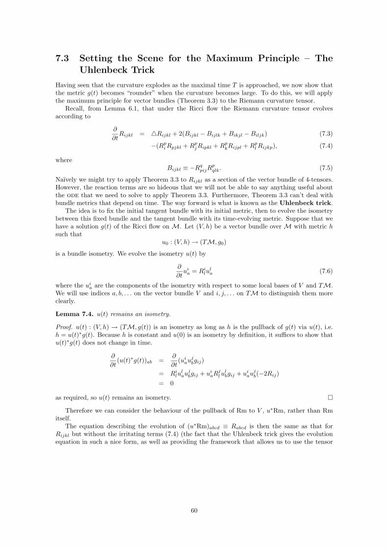
7.3 Setting the Scene for the Maximum Principle – TheUhlenbeck Trick
Having seen that the curvature explodes as the maximal time T is approached, we now show thatthe metric g(t) becomes “rounder” when the curvature becomes large. To do this, we will applythe maximum principle for vector bundles (Theorem 3.3) to the Riemann curvature tensor.
Recall, from Lemma 6.1, that under the Ricci flow the Riemann curvature tensor evolvesaccording to
∂
∂tRijkl = 4Rijkl + 2(Bijkl −Bijlk +Bikjl −Biljk) (7.3)
−(RpiRpjkl +RpjRipkl +RpkRijpl +RplRijkp), (7.4)
whereBijkl ≡ −RqpijR
pqlk. (7.5)
Naıvely we might try to apply Theorem 3.3 to Rijkl as a section of the vector bundle of 4-tensors.However, the reaction terms are so hideous that we will not be able to say anything useful aboutthe ode that we need to solve to apply Theorem 3.3. Furthermore, Theorem 3.3 can’t deal withbundle metrics that depend on time. The way forward is what is known as the Uhlenbeck trick.
The idea is to fix the initial tangent bundle with its initial metric, then to evolve the isometrybetween this fixed bundle and the tangent bundle with its time-evolving metric. Suppose that wehave a solution g(t) of the Ricci flow on M. Let (V, h) be a vector bundle over M with metric hsuch that
u0 : (V, h)→ (TM, g0)
is a bundle isometry. We evolve the isometry u(t) by
∂
∂tuia = Rilu
la (7.6)
where the uia are the components of the isometry with respect to some local bases of V and TM.We will use indices a, b, . . . on the vector bundle V and i, j, . . . on TM to distinguish them moreclearly.
Lemma 7.4. u(t) remains an isometry.
Proof. u(t) : (V, h) → (TM, g(t)) is an isometry as long as h is the pullback of g(t) via u(t), i.e.h = u(t)∗g(t). Because h is constant and u(0) is an isometry by definition, it suffices to show thatu(t)∗g(t) does not change in time.
∂
∂t(u(t)∗g(t))ab =
∂
∂t(uiau
jbgij)
= Rilulaujbgij + uiaR
jl ulbgij + uiau
jb(−2Rij)
= 0
as required, so u(t) remains an isometry.
Therefore we can consider the behaviour of the pullback of Rm to V , u∗Rm, rather than Rmitself.
The equation describing the evolution of (u∗Rm)abcd ≡ Rabcd is then the same as that forRijkl but without the irritating terms (7.4) (the fact that the Uhlenbeck trick gives the evolutionequation in such a nice form, as well as providing the framework that allows us to use the tensor
60

maximum principle, is a little mysterious – Hamilton refers to it as “magic”):
∂
∂tRabcd =
∂
∂t(uiau
jbukcu
ldRijkl)
= (Rimuma )ujbu
kcu
ldRijkl + uia(Rjmu
mb )ukcu
ldRijkl
+uiaujb(R
kmu
mc )uldRijkl + uiau
jbukc (Rlmu
md )Rijkl
+uiaujbukcu
ld[4Rijkl + 2(Bijkl −Bijlk +Bikjl −Biljk)
−(RpiRpjkl +RpjRipkl +RpkRijpl +RplRijkp)]= 4Rabcd + 2(Babcd −Babdc +Bacbd −Badbc) (7.7)
where Babcd is defined by equation (7.5).Recall that we can view Rm as the curvature operator R, which is a section of the bundle
E = ∧2T ∗Mn ⊗S ∧2T ∗Mn
of symmetric bilinear forms on the space ∧2TM3 of 2-vectors. This viewpoint was outlined inSection 1.4.
In 3 dimensions, ∧2TM3 has dimension 3, so each fibre of this bundle E is naturally isomorphicto the vector space of 3× 3 self-adjoint (i.e. symmetric) matrices. We can diagonalize these withrespect to some orthonormal basis {e1 ∧ e2, e2 ∧ e3, e3 ∧ e1} of ∧2TM3, where {e1, e2, e3} is anorthonormal basis of TM3.
Now we would like to apply the vector bundle maximum principle (Theorem 3.3) to R, viewedas a section of E . We must consider the ode corresponding to the pde describing the evolution ofRm (which is given by equation (7.7)), namely
d
dtQabcd = 2(Babcd(Q)−Babdc(Q) +Bacbd(Q)−Badbc(Q))
where Babcd(Q) is defined by analogy with equation (7.5).In 3 dimensions this ode has a particularly convenient form. Choose a basis {ei} of TM3
x sothat Q is diagonal with eigenvalues λ1, λ2, λ3 down the diagonal, then the equation is (see [6, Sec.6.3, 6.4]):
d
dt
λ1 0 00 λ2 00 0 λ3
=
λ21 + λ2λ3 0 0
0 λ22 + λ3λ1 0
0 0 λ23 + λ1λ2
.
In particular, the matrix Q will remain diagonal – this does not happen for higher dimensions,because the matrix on the rhs will not be diagonal (there are other useful decompositions in then = 4 case though – see [10]). Therefore, in three dimensions the three parameters λ1, λ2, λ3
completely describe Q, and we may represent Q as a point λ = (λ1, λ2, λ3) moving in R3 accordingto the ode
d
dt
λ1
λ2
λ3
=
λ21 + λ2λ3
λ22 + λ3λ1
λ23 + λ1λ2
= ∇(
(λ31 + λ3
2 + λ33)
3+ λ1λ2λ3
). (7.8)
We note that the initial value of λ also tells us all about the initial Ricci and scalar curvatures, bythe formulae (1.9) and (1.10):
Rc =12
λ2 + λ3 0 00 λ3 + λ1 00 0 λ1 + λ2
(7.9)
andR = λ1 + λ2 + λ3. (7.10)
We can visualize the behaviour of the ode (7.8) by visualizing the evolution of λ(t). The odeis homogeneous, so we can scale any solution to get another solution. We consider “projecting”the solution λ(t) onto the unit sphere to get a path µ(t) = λ(t)/|λ(t)|. Given µ(0), the evolutionof µ(t) of course depends on which solution λ(t) we choose, satisfying λ(0) = |λ(0)|µ(0). However,
61
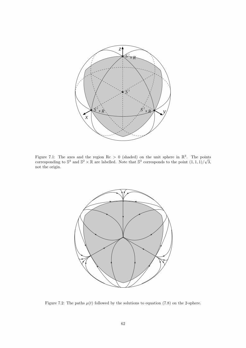
xy
z
S 3
S 2
x R S 2
x R
S 2
x R
Figure 7.1: The axes and the region Rc > 0 (shaded) on the unit sphere in R3. The pointscorresponding to S3 and S2 × R are labelled. Note that S3 corresponds to the point (1, 1, 1)/
√3,
not the origin.
Figure 7.2: The paths µ(t) followed by the solutions to equation (7.8) on the 2-sphere.
62
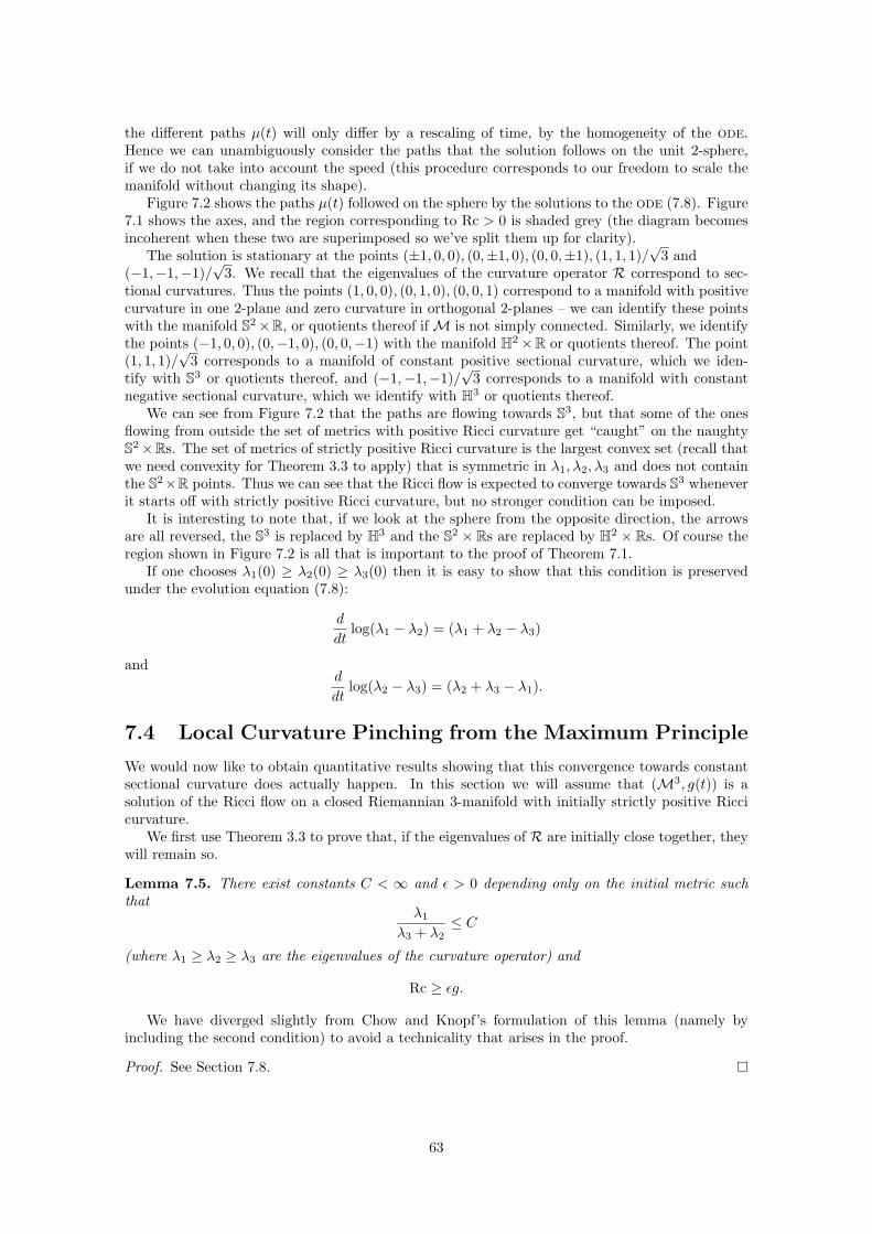
the different paths µ(t) will only differ by a rescaling of time, by the homogeneity of the ode.Hence we can unambiguously consider the paths that the solution follows on the unit 2-sphere,if we do not take into account the speed (this procedure corresponds to our freedom to scale themanifold without changing its shape).
Figure 7.2 shows the paths µ(t) followed on the sphere by the solutions to the ode (7.8). Figure7.1 shows the axes, and the region corresponding to Rc > 0 is shaded grey (the diagram becomesincoherent when these two are superimposed so we’ve split them up for clarity).
The solution is stationary at the points (±1, 0, 0), (0,±1, 0), (0, 0,±1), (1, 1, 1)/√
3 and(−1,−1,−1)/
√3. We recall that the eigenvalues of the curvature operator R correspond to sec-
tional curvatures. Thus the points (1, 0, 0), (0, 1, 0), (0, 0, 1) correspond to a manifold with positivecurvature in one 2-plane and zero curvature in orthogonal 2-planes – we can identify these pointswith the manifold S2×R, or quotients thereof ifM is not simply connected. Similarly, we identifythe points (−1, 0, 0), (0,−1, 0), (0, 0,−1) with the manifold H2×R or quotients thereof. The point(1, 1, 1)/
√3 corresponds to a manifold of constant positive sectional curvature, which we iden-
tify with S3 or quotients thereof, and (−1,−1,−1)/√
3 corresponds to a manifold with constantnegative sectional curvature, which we identify with H3 or quotients thereof.
We can see from Figure 7.2 that the paths are flowing towards S3, but that some of the onesflowing from outside the set of metrics with positive Ricci curvature get “caught” on the naughtyS2×Rs. The set of metrics of strictly positive Ricci curvature is the largest convex set (recall thatwe need convexity for Theorem 3.3 to apply) that is symmetric in λ1, λ2, λ3 and does not containthe S2×R points. Thus we can see that the Ricci flow is expected to converge towards S3 wheneverit starts off with strictly positive Ricci curvature, but no stronger condition can be imposed.
It is interesting to note that, if we look at the sphere from the opposite direction, the arrowsare all reversed, the S3 is replaced by H3 and the S2 × Rs are replaced by H2 × Rs. Of course theregion shown in Figure 7.2 is all that is important to the proof of Theorem 7.1.
If one chooses λ1(0) ≥ λ2(0) ≥ λ3(0) then it is easy to show that this condition is preservedunder the evolution equation (7.8):
d
dtlog(λ1 − λ2) = (λ1 + λ2 − λ3)
andd
dtlog(λ2 − λ3) = (λ2 + λ3 − λ1).
7.4 Local Curvature Pinching from the Maximum Principle
We would now like to obtain quantitative results showing that this convergence towards constantsectional curvature does actually happen. In this section we will assume that (M3, g(t)) is asolution of the Ricci flow on a closed Riemannian 3-manifold with initially strictly positive Riccicurvature.
We first use Theorem 3.3 to prove that, if the eigenvalues of R are initially close together, theywill remain so.
Lemma 7.5. There exist constants C < ∞ and ε > 0 depending only on the initial metric suchthat
λ1
λ3 + λ2≤ C
(where λ1 ≥ λ2 ≥ λ3 are the eigenvalues of the curvature operator) and
Rc ≥ εg.
We have diverged slightly from Chow and Knopf’s formulation of this lemma (namely byincluding the second condition) to avoid a technicality that arises in the proof.
Proof. See Section 7.8.
63
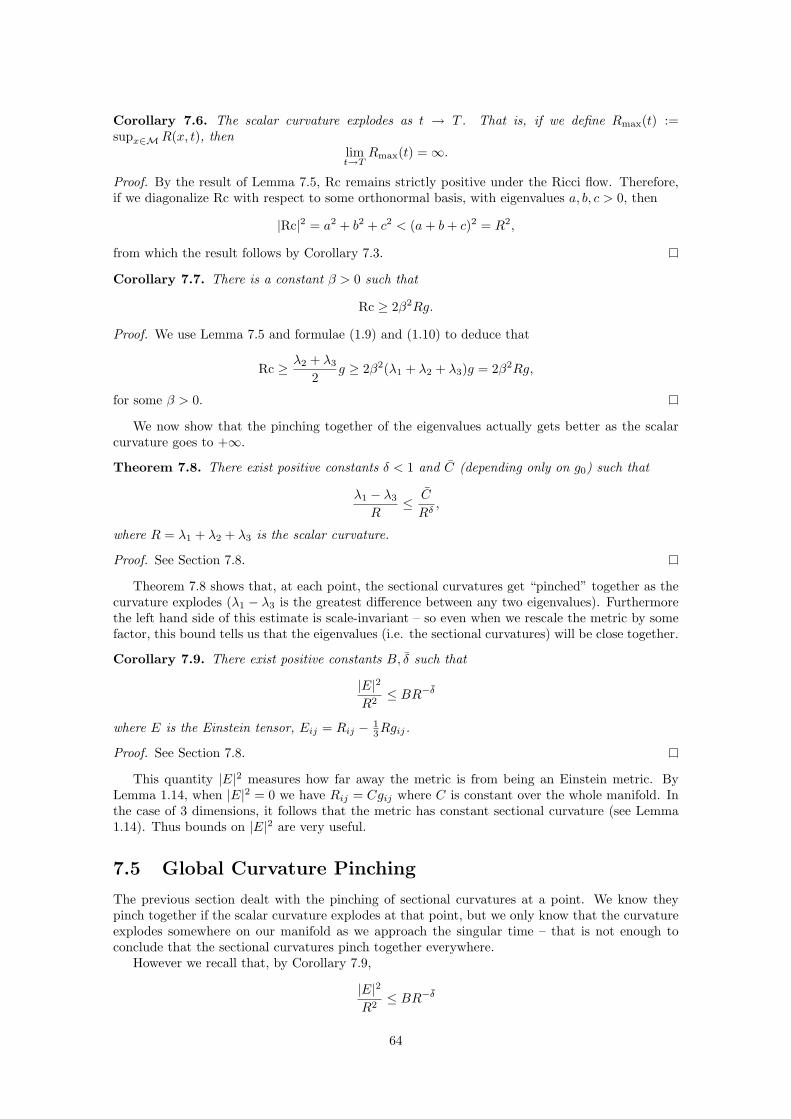
Corollary 7.6. The scalar curvature explodes as t → T . That is, if we define Rmax(t) :=supx∈MR(x, t), then
limt→T
Rmax(t) =∞.
Proof. By the result of Lemma 7.5, Rc remains strictly positive under the Ricci flow. Therefore,if we diagonalize Rc with respect to some orthonormal basis, with eigenvalues a, b, c > 0, then
|Rc|2 = a2 + b2 + c2 < (a+ b+ c)2 = R2,
from which the result follows by Corollary 7.3.
Corollary 7.7. There is a constant β > 0 such that
Rc ≥ 2β2Rg.
Proof. We use Lemma 7.5 and formulae (1.9) and (1.10) to deduce that
Rc ≥ λ2 + λ3
2g ≥ 2β2(λ1 + λ2 + λ3)g = 2β2Rg,
for some β > 0.
We now show that the pinching together of the eigenvalues actually gets better as the scalarcurvature goes to +∞.
Theorem 7.8. There exist positive constants δ < 1 and C (depending only on g0) such that
λ1 − λ3
R≤ C
Rδ,
where R = λ1 + λ2 + λ3 is the scalar curvature.
Proof. See Section 7.8.
Theorem 7.8 shows that, at each point, the sectional curvatures get “pinched” together as thecurvature explodes (λ1 − λ3 is the greatest difference between any two eigenvalues). Furthermorethe left hand side of this estimate is scale-invariant – so even when we rescale the metric by somefactor, this bound tells us that the eigenvalues (i.e. the sectional curvatures) will be close together.
Corollary 7.9. There exist positive constants B, δ such that
|E|2
R2≤ BR−δ
where E is the Einstein tensor, Eij = Rij − 13Rgij.
Proof. See Section 7.8.
This quantity |E|2 measures how far away the metric is from being an Einstein metric. ByLemma 1.14, when |E|2 = 0 we have Rij = Cgij where C is constant over the whole manifold. Inthe case of 3 dimensions, it follows that the metric has constant sectional curvature (see Lemma1.14). Thus bounds on |E|2 are very useful.
7.5 Global Curvature Pinching
The previous section dealt with the pinching of sectional curvatures at a point. We know theypinch together if the scalar curvature explodes at that point, but we only know that the curvatureexplodes somewhere on our manifold as we approach the singular time – that is not enough toconclude that the sectional curvatures pinch together everywhere.
However we recall that, by Corollary 7.9,
|E|2
R2≤ BR−δ
64
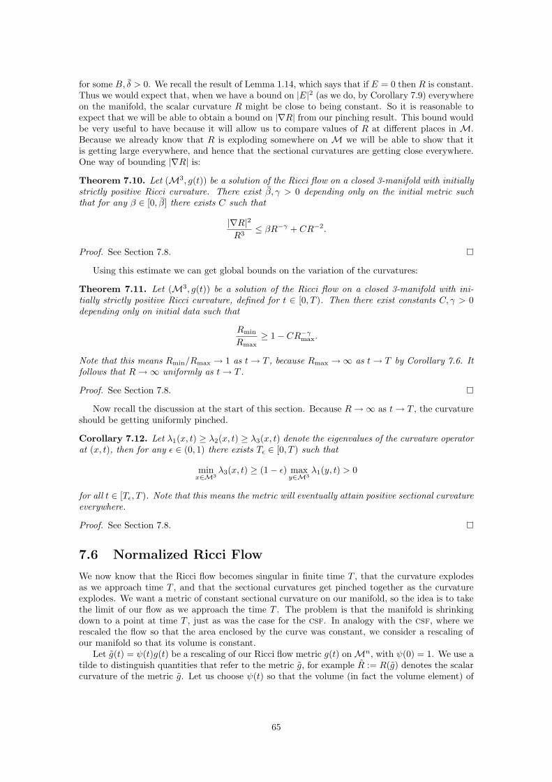
for some B, δ > 0. We recall the result of Lemma 1.14, which says that if E = 0 then R is constant.Thus we would expect that, when we have a bound on |E|2 (as we do, by Corollary 7.9) everywhereon the manifold, the scalar curvature R might be close to being constant. So it is reasonable toexpect that we will be able to obtain a bound on |∇R| from our pinching result. This bound wouldbe very useful to have because it will allow us to compare values of R at different places in M.Because we already know that R is exploding somewhere on M we will be able to show that itis getting large everywhere, and hence that the sectional curvatures are getting close everywhere.One way of bounding |∇R| is:
Theorem 7.10. Let (M3, g(t)) be a solution of the Ricci flow on a closed 3-manifold with initiallystrictly positive Ricci curvature. There exist β, γ > 0 depending only on the initial metric suchthat for any β ∈ [0, β] there exists C such that
|∇R|2
R3≤ βR−γ + CR−2.
Proof. See Section 7.8.
Using this estimate we can get global bounds on the variation of the curvatures:
Theorem 7.11. Let (M3, g(t)) be a solution of the Ricci flow on a closed 3-manifold with ini-tially strictly positive Ricci curvature, defined for t ∈ [0, T ). Then there exist constants C, γ > 0depending only on initial data such that
Rmin
Rmax≥ 1− CR−γmax.
Note that this means Rmin/Rmax → 1 as t→ T , because Rmax →∞ as t→ T by Corollary 7.6. Itfollows that R→∞ uniformly as t→ T .
Proof. See Section 7.8.
Now recall the discussion at the start of this section. Because R→∞ as t→ T , the curvatureshould be getting uniformly pinched.
Corollary 7.12. Let λ1(x, t) ≥ λ2(x, t) ≥ λ3(x, t) denote the eigenvalues of the curvature operatorat (x, t), then for any ε ∈ (0, 1) there exists Tε ∈ [0, T ) such that
minx∈M3
λ3(x, t) ≥ (1− ε) maxy∈M3
λ1(y, t) > 0
for all t ∈ [Tε, T ). Note that this means the metric will eventually attain positive sectional curvatureeverywhere.
Proof. See Section 7.8.
7.6 Normalized Ricci Flow
We now know that the Ricci flow becomes singular in finite time T , that the curvature explodesas we approach time T , and that the sectional curvatures get pinched together as the curvatureexplodes. We want a metric of constant sectional curvature on our manifold, so the idea is to takethe limit of our flow as we approach the time T . The problem is that the manifold is shrinkingdown to a point at time T , just as was the case for the csf. In analogy with the csf, where werescaled the flow so that the area enclosed by the curve was constant, we consider a rescaling ofour manifold so that its volume is constant.
Let g(t) = ψ(t)g(t) be a rescaling of our Ricci flow metric g(t) onMn, with ψ(0) = 1. We use atilde to distinguish quantities that refer to the metric g, for example R := R(g) denotes the scalarcurvature of the metric g. Let us choose ψ(t) so that the volume (in fact the volume element) of
65
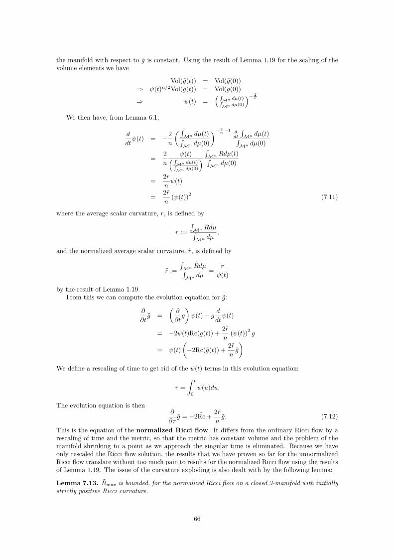
the manifold with respect to g is constant. Using the result of Lemma 1.19 for the scaling of thevolume elements we have
Vol(g(t)) = Vol(g(0))⇒ ψ(t)n/2Vol(g(t)) = Vol(g(0))
⇒ ψ(t) =( R
Mn dµ(t)RMn dµ(0)
)− 2n
We then have, from Lemma 6.1,
d
dtψ(t) = − 2
n
( ∫Mn dµ(t)∫Mn dµ(0)
)− 2n−1 d
dt
∫Mn dµ(t)∫Mn dµ(0)
=2n
ψ(t)( RMn dµ(t)RMn dµ(0)
) ∫Mn Rdµ(t)∫Mn dµ(0)
=2rnψ(t)
=2rn
(ψ(t))2 (7.11)
where the average scalar curvature, r, is defined by
r :=
∫Mn Rdµ∫Mn dµ
,
and the normalized average scalar curvature, r, is defined by
r :=
∫Mn Rdµ∫Mn dµ
=r
ψ(t)
by the result of Lemma 1.19.From this we can compute the evolution equation for g:
∂
∂tg =
(∂
∂tg
)ψ(t) + g
d
dtψ(t)
= −2ψ(t)Rc(g(t)) +2rn
(ψ(t))2g
= ψ(t)(−2Rc(g(t)) +
2rng
)We define a rescaling of time to get rid of the ψ(t) terms in this evolution equation:
τ =∫ t
0
ψ(u)du.
The evolution equation is then∂
∂τg = −2Rc +
2rng. (7.12)
This is the equation of the normalized Ricci flow. It differs from the ordinary Ricci flow by arescaling of time and the metric, so that the metric has constant volume and the problem of themanifold shrinking to a point as we approach the singular time is eliminated. Because we haveonly rescaled the Ricci flow solution, the results that we have proven so far for the unnormalizedRicci flow translate without too much pain to results for the normalized Ricci flow using the resultsof Lemma 1.19. The issue of the curvature exploding is also dealt with by the following lemma:
Lemma 7.13. Rmax is bounded, for the normalized Ricci flow on a closed 3-manifold with initiallystrictly positive Ricci curvature.
66
Proof. We use Corollary 7.7 to deduce that
Rc = Rc ≥ 2β2Rg ≥ 2β2Rming = 2β2Rming
for some β > 0. It follows from Myers’ Theorem (Theorem 1.17) that L, the diameter of M withrespect to the metric g, satisfies
L ≤ π
β√Rmin
.
Now we can also get a lower bound for L from the fact that the volume of our manifold is constantwith respect to g, by the first part of the Bishop-Gunther volume comparison theorem (Theorem1.15). Because Rc = Rc ≥ 0, we have (in the notation of Theorem 1.15):
V = Vol(B(p, L)) ≤ V 03 (L) =
4π3L3
where V is the volume of M with respect to g, which we know is equal to a constant, which wecall V0. Combining these gives us (
3V0
4π
) 13
≤ L ≤ π
β√Rmin
.
This gives us an upper bound for Rmin. Finally, it follows from the first part of Theorem 7.11 andscaling invariance that there exists some C > 0 such that
Rmin
Rmax
=Rmin
Rmax≥ 1C.
Hence the upper bound for Rmin implies one for Rmax, and the proof is complete.
We can now show that our rescaling of time has in fact taken us to an infinite time interval.
Theorem 7.14. If (M3, g(t)) is a solution of the Ricci flow on a closed 3-manifold with initiallystrictly positive Ricci curvature then the corresponding normalized Ricci flow exists for all time.
Proof. First we show that ∫ T
0
Rmax(t)dt =∞,
where Rmax(t) is the maximum scalar curvature of the metric g(t) and [0, T ) is the maximal timeinterval on which the unnormalized Ricci flow exists. This can be done by setting
f(t) = exp[2∫ t
0
Rmax(u)du]Rmax(0),
which then satisfiesdf
dt= 2Rmax(t)f
and hence, using the evolution equation for R given in Lemma 6.1,
∂
∂t(R− f) = 4R+ 2|Rc|2 − 2Rmaxf
≤ 4(R− f) + 2Rmax(R− f)
(using |Rc|2 ≤ R2, which follows as Rc is positive). Now we have (R − f) ≤ 0 initially, asf(0) = Rmax(0). This condition is preserved by the ode obtained by ignoring the Laplacian termin the above equation, as
d
dtφ(t) = 2Rmax(t)φ(t)
67
is equivalent tod
dtlog(|φ(t)|) = 2Rmax(t)
from which we can see that φ never changes sign. Hence the condition (R − f) ≤ 0 is preserved,by the scalar maximum principle. By Corollary 7.6, Rmax → ∞ as t → T , so f → ∞ as t → T .Recalling the definition of f , this means that
limt→T
∫ t
0
Rmax(u)du =∞.
Now the corresponding integral for the normalized flow will be the same:∫ T
0
Rmax(τ)dτ =∫ T
0
r(t)dt =∞
(if we define [0, T ) to be the maximal time interval on which the normalized Ricci flow exists).This follows easily from the scaling results of Lemma 1.19 as Rmaxdτ = (ψ−1Rmax)(ψdt) = rdt. Sothe integral for the normalized flow must also diverge – but the integrand is bounded by Lemma7.13. Hence the region of integration must be infinite, so T = ∞, i.e. the normalized Ricci flowexists for all time.
7.7 Convergence of the Normalized Flow
Now we will prove that the normalized Ricci flow converges as τ → ∞ to a smooth metric g∞ ofconstant positive sectional curvature. We will use the notations
g∞ = g(∞) := limτ→∞
g(τ).
The proof will be very similar to that of Theorem 6.7, and the key element will again be Theorem6.8. To show that g(∞) exists and is continuous, we must show that there exists some C < ∞such that ∫ ∞
0
∣∣∣∣ ∂∂τ g∣∣∣∣g
dτ < C.
Using the normalized Ricci flow equation (7.12), that is equivalent to showing that the integral∫ ∞0
∣∣∣∣Rc− r
3g
∣∣∣∣ dτ (7.13)
is bounded. We know from Corollary 7.9 that∣∣Rc− 13Rg
∣∣2R2
≤ CR−δ.
This is a bound on exactly the right sort of quantity for the unnormalized Ricci flow (Theorem 7.11tells us that as t → ∞, r and R approach one another uniformly). We need a bound that holdsfor the normalized Ricci flow though, and one that will force the integral (7.13) to be boundedtoo. The easiest way to do this is to prove the integrand is bounded by a decaying exponential (aconstant bound will not suffice as it did for Corollary 6.12, as the region of integration is infinite).We will need a few preliminary results.
Lemma 7.15. If (M3, g(τ)) is a solution of the normalized Ricci flow on a closed 3-manifold withinitially strictly positive Ricci curvature then there exists ε > 0 such that R ≥ ε for all τ > 0.
Proof. See Section 7.8.
We are now ready to prove the key estimate that allows us to prove the integral (7.13) isbounded.
68
Theorem 7.16. If (M3, g(τ)) is a solution of the normalized Ricci flow on a closed 3-manifoldwith initially strictly positive Ricci curvature then there exist constants C, δ > 0 such that∣∣∣E∣∣∣ ≤ Ce−δτ .Proof. See Section 7.8.
To apply Theorem 6.8 we must prove an exponential bound on |Rc − r/3g|. The previoustheorem gives us a bound on |E| = |Rc − R/3g| which is almost what we want. We just need togo from R to r. So we need to show that the difference |R− r| is exponentially bounded. We willactually prove something a bit stronger:
Lemma 7.17. There exist constants C, δ > 0 such that
Rmax − Rmin < Ce−δτ .
This Lemma comes from [9, Lemma 17.4].
Proof. See 7.8.
This allows us to prove the following:
Theorem 7.18. If (M3, g(τ)) is a solution of the normalized Ricci flow with initially strictlypositive Ricci curvature, then g(τ) exists for all τ ∈ [0,∞) and converges uniformly as τ → ∞ toa continuous metric g(∞).
Proof. By Theorem 7.16 and Lemma 7.17 we have∫ ∞0
∣∣∣∣∂g∂τ∣∣∣∣ dτ =
∫ ∞0
∣∣∣∣Rc− r
3g
∣∣∣∣ dτ≤
∫ ∞0
∣∣∣∣∣Rc− R
3g
∣∣∣∣∣+
∣∣∣∣∣ R− r3g
∣∣∣∣∣ dτ<
∫ ∞0
Ce−δτdτ <∞
where we have amalgamated the two exponential bounds into one. It follows by Theorem 6.8 thatg(τ) converges uniformly to a continuous metric g(∞) as τ →∞.
The next step is to show that this convergence is smooth. This is important because wewant our limit metric to be smooth, and also because we want the curvatures of the normalizedflow to converge to the corresponding curvatures of the limit metric (as curvature quantities areall essentially second-order derivatives of the metric). That will allow us to conclude that thecurvature pinching results we have proven for the flow lead to similar results for the limit metric,and hence that the limit metric has constant curvature.
Theorem 7.19. The limit metric g∞ := g(∞) of Theorem 7.18 is smooth, and the convergenceof g(τ) to g∞ as τ →∞ is uniform in every Cm norm.
Proof. See Section 7.8.
We are now finally in a position to prove Theorem 7.1. We show that the limit metric g∞ hasthe properties required.
Theorem 7.20. The limit metric g∞ is a smooth metric with constant positive sectional curvature.
Proof. By Theorem 7.19, g(τ) converges to g∞ in the C0, C1 and C2 norms. Because all curvaturequantities are combinations of “0th-order”, 1st-order and 2nd-order derivatives of the metric, thismeans that we can take the limit to show that the Einstein tensor of the metric g∞ vanishes:∣∣∣E∞∣∣∣ = lim
τ→∞
∣∣∣E(τ)∣∣∣ ≤ lim
τ→∞Ce−δτ = 0
by the result of Theorem 7.16. Therefore g∞ is an Einstein metric, so by Lemma 1.14 g∞ hasconstant (positive) sectional curvature.
69
7.8 Details
Proof. (of Lemma 7.5) Note that such a C and ε will exist at time t = 0 by the compactness of themanifold M3: λ1/(λ2 + λ3) is a continuous, positive function at t = 0 so it has an upper bound,and the eigenvalues of Rc are (λ2 +λ3)/2, (λ3 +λ1)/2, (λ1 +λ2)/2, all of which are strictly positiveat time t = 0 so they have a strictly positive lower bound. Thus it suffices to show that theseconditions are preserved under evolution by the Ricci flow.
We use the maximum principle in the form of Theorem 3.3, on the vector bundle E , with theset
K ≡ {Q ∈ E : λ1(Q)− C(λ3(Q) + λ2(Q)) ≤ 0 and λ2 + λ3 ≥ 2ε}.
Note that because λ1 ≥ λ2 ≥ λ3, the last condition states exactly that Rc ≥ εg by formula (1.9).This set is invariant under parallel translation and convex in each fibre. Convexity follows becausethe functions
f(Q) = λ1(Q)= max
|U |=1(Q(U,U))
and
h(Q) = −(λ2(Q) + λ3(Q))= max
|V | = |W | = 1〈V,W 〉 = 0
(−Q(V, V )−Q(W,W ))
are convex, so the function j(Q) = f(Q) + Ch(Q) is convex, therefore the set
K = h−1((−∞,−ε]) ∩ j−1((−∞, 0])
is convex.We just need to show that the solution of the associated ode stays in K. That is, if
λ1
λ2 + λ3≤ C
andλ2 + λ3 ≥ 2ε
initially, then this condition remains true under the evolution (7.8). This can be shown by provingfirst that
d
dt(λ2 + λ3) = λ2
2 + λ23 + λ1(λ2 + λ3) ≥ 0,
from which it follows that the condition λ2 + λ3 ≥ 2ε is preserved, then
d
dtlog(
λ1
λ3 + λ2
)=λ2
2(λ3 − λ1) + λ23(λ2 − λ1)
λ1(λ3 + λ2)≤ 0
by the evolution equation (7.8), because λ2 + λ3 ≥ ε > 0 and hence λ1 > 0 also. This is the solereason for including the condition Rc ≥ εg – to show that the rhs of this equation does not becomesingular.
Thus all the hypotheses of Theorem 3.3 are satisfied, so the solution to the pde stays in K, i.e.the conditions
λ1
λ2 + λ3≤ C
andRc ≥ εg
are preserved.
70
Proof. (of Theorem 7.8) The proof is very similar to that of Lemma 7.5. It suffices to show thatthere exist C, δ such that
λ1 − λ3
λ2 + λ3≤ C
(λ2 + λ3)δ. (7.14)
By compactness, given δ ∈ (0, 1) we can choose such a C at time t = 0, because λ2 + λ3 > 0everywhere by the positive Ricci curvature condition. We show that this condition is preservedusing the maximum principle (Theorem 3.3) with the same vector bundle E as we used in the proofof Lemma 7.5, but a different K:
K ≡ {Q ∈ E : [λ1(Q)− λ3(Q)]− C[λ2(Q) + λ3(Q)]1−δ ≤ 0}
Once again, the set K is invariant under parallel translation and convex in each fiber by asimilar argument to that in the proof of Lemma 7.5.
To show that the solution of the ode stays inside K we compute, from equation 7.8:
d
dtlog(
λ1 − λ3
(λ2 + λ3)1−δ
)≤ δλ1 −
12
(1− δ)(λ3 + λ2).
Now, by Lemma 7.5, it is possible to choose δ small enough that this is always non-positive, so
λ1 − λ3
(λ2 + λ3)1−δ
is non-increasing, hence the inequality (7.14) is preserved by the ode. Thus by the maximumprinciple it is also preserved by the pde.
Proof. (of Corollary 7.9) Using the formulae (1.9) and (1.10) we have
E =16
λ2 + λ3 − 2λ1 0 00 λ3 + λ1 − 2λ2 00 0 λ1 + λ2 − 2λ3
, (7.15)
hence
|E|2
R2=
(λ2 + λ3 − 2λ1)2 + (λ3 + λ1 − 2λ2)2 + (λ1 + λ2 − 2λ3)2
36(λ1 + λ2 + λ3)2
=(λ1 − λ2)2 + (λ2 − λ3)2 + (λ3 − λ1)2
12(λ1 + λ2 + λ3)2
≤ 3(λ3 − λ1)2
12(λ1 + λ2 + λ3)2
≤ BR−δ
by the result of Theorem 7.8, with δ = 2δ (the penultimate step follows as λ1 − λ3 is the greatestdifference between two eigenvalues).
Proof. (of Theorem 7.10) We provide an outline of the proof without showing all of the excruciatingdetails. A more complete outline can be found in [6, Section (6.6)].
Using the evolution equation for R under the Ricci flow, given in Lemma 6.1, it is possible todeduce that
∂
∂t
(|∇R|2
R
)= 4
(|∇R|2
R
)− 2R
∣∣∣∣∇(∇RR)∣∣∣∣2
−2|∇R|2
R2|Rc|2 +
4R〈∇R,∇|Rc|2〉
≤ 4(|∇R|2
R
)− 2R
∣∣∣∣∇(∇RR)∣∣∣∣2
−2|∇R|2
R2|Rc|2 + 8
√3|∇Rc|2
71
where the last line follows from the Cauchy-Schwarz inequality and Lemma 1.1 (to prove |∇R|2 ≤3|∇Rc|2):
4R〈∇R,∇|Rc|2〉 ≤ 4
R|∇R|
∣∣∇|Rc|2∣∣
≤ 8|∇R||∇Rc| |Rc|R
≤ 8√
3|∇Rc|2
(using |Rc| < R because Rc > 0, as in Corollary 7.6). We would like to use the maximum principle(Theorem 3.2) to show that the quantity |∇R|2/R does not increase. All reaction terms on theright hand side of our evolution equation are negative with the exception of the last one in |∇Rc|2.We need to deal with this meddlesome customer. We note that
|∇E|2 ≥ 137|∇Rc|2 (7.16)
where E is the Einstein tensor (which we know ought to be falling away nicely as our manifoldgets rounder). To see why this is true, we combine Lemma 1.1 with equation (1.14) to get
|∇kEij |2 ≥13|∇jEij |2 =
13· 1
36|∇R|2.
Equation (7.16) now follows easily:
|∇Rc|2 − 13|∇R|2 = |∇E|2
≥ 13
136|∇R|2
which can be rearranged to obtain
|∇Rc|2 − 13|∇R|2 ≥ 1
37|∇Rc|2
where |∇E|2 is exactly equal to the lhs.Therefore our evolution equation becomes
∂
∂t
(|∇R|2
R
)≤ 4
(|∇R|2
R
)− 2R
∣∣∣∣∇(∇RR)∣∣∣∣2
−2|∇R|2
R2|Rc|2 + 8
√3 · 37|∇E|2.
We are going to try to get rid of the bad final term of this equation by adding on some multipleof |E|2. The evolution equation for |E|2 under the Ricci flow is given in Lemma 6.1. It is
∂|E|2
∂t= 4|E|2 − 2|∇E|2 +W (7.17)
whereW =
263R|Rc|2 − 8RjiR
kjR
ik − 2R3. (7.18)
The second term on the right hand side of equation (7.17) interests us: we can use it to canceloff the recalcitrant |∇E|2 term in the evolution equation for |∇R|2/R. We set
V :=|∇R|2
R+
372
(8√
3 + 1)|E|2
then calculate∂
∂tV ≤ 4V − |∇Rc|2 + C1W
72
(reusing the inequality (7.16)) where C1 is a positive constant.It is possible to prove that
W ≤ 503R|E|2 (7.19)
purely algebraically; as Rc is positive and symmetric we can diagonalize it with positive realeigenvalues a, b, c. Each term in the inequality can be expressed in terms of a, b and c, and we areleft with an easy homogeneous inequality in three real variables. Equality occurs when a = b = c,i.e. for an Einstein metric (this proof is significantly simpler than that presented in [6]). We alsohave
|∇R|2 ≤ 3|∇Rc|2
by Lemma 1.1.Hence we have
∂
∂tV ≤ 4V − |∇Rc|2 + C2R|E|2
≤ 4V − 13|∇R|2 + C3R
3−2γ
by the result of Corollary 7.9, for some constants C and γ > 0. Now we set
U := V − βR2−γ
where β is to be chosen. It is not difficult to calculate from the result of Lemma 6.1 that
∂
∂tR2−γ = 4(R2−γ)− (2− γ)(1− γ)R−γ |∇R|2 + 2(2− γ)R1−γ |Rc|2,
hence that
∂
∂tU ≤ 4U +
[β(2− γ)(1− γ)R−γ − 1
3
]|∇R|2 (7.20)
+C3R3−2γ − 2β(2− γ)R1−γ |Rc|2.
Now by Theorem 7.8 we have Rc ≥ εg, hence R ≥ 3ε for some ε > 0. Thus we may chooseβ > 0 such that
β <(3ε)γ
3(2− γ)(1− γ),
so that for any β ∈ [0, β] the second term in the evolution equation (7.20) is non-positive. For therest of the terms, we use the inequality 3|Rc|2 ≥ |R|2 to obtain
C3R3−2γ − 2β(2− γ)R1−γ |Rc|2 ≤ C3R
3−2γ − C4R3−γ
where C3, C4 are constants. For large R this term is dominated by the R3−γ term, which isnegative. As it does not diverge at R = 0, there is a uniform upper bound C5 for this term, hencewe have
∂
∂tU ≤ 4U + C5.
Thus the growth in U is at worst linear, by the maximum principle (Theorem 3.2). By Theorem7.2 the time interval we are considering is finite, hence we have a uniform upper bound C for U .Therefore
|∇R|2
R≤ V = U + βR2−γ ≤ C + βR2−γ
from which the result follows.
Proof. (of Theorem 7.11) Our main tool here will be Theorem 7.10, which allows us to comparethe curvature at different points on the manifold. By Corollary 7.6, we also have Rmax → ∞ as
73
t→ T . Thus for t sufficiently close to T , Theorem 7.10 tells us that there exist positive constantsA,α such that
|∇R| ≤ AR3/2−αmax .
Thus we have (for t sufficiently close to T )
|R(x)−R(y)| ≤∫γ
|∇R|ds ≤ AR3/2−αmax d(x, y) (7.21)
(here γ is a minimizing geodesic connecting x and y). Let us choose x(t) such that Rmax(t) = R(x, t)(we can do this as M is compact), and define
L(t) :=1
ε√Rmax(t)
where ε > 0. Then for all y ∈ B(x(t), L(t)) we have, by equation (7.21):
R(y) ≥ R(x)−AR3/2−αmax L ≥ Rmax
(1− A
εR−αmax
). (7.22)
Recall that Rmax →∞ as t→ T . Therefore, given δ > 0, for t sufficiently close to T we have
R(y) ≥ (1− δ)Rmax (7.23)
for all y ∈ B(x(t), L(t)).This will prove the theorem if we can show that B(x(t), L(t)) is all ofM for t sufficiently close
to T . We will prove this using Myers’ Theorem (Theorem 1.17). Define N = B(x(t), L(t)). Wehave the estimate Rc ≥ 2β2Rg for some β > 0 from Corollary 7.7. Hence, by equation (7.23), forany δ > 0
Rc ≥ 2β2(1− δ)Rmaxg
in N for t close enough to T . By the proof of Myers’ Theorem (see [18, Theorem 11.8]), we have
diam(N ) ≤ π
β√
(1− δ)Rmax
<1
δ√Rmax
<1
ε√Rmax
= L
for δ chosen sufficiently small. Because N is defined to be B(x(t), L(t)) but has diameter < L,if there are any points in M that lie outside N then M must be disconnected. We know that itisn’t, hence N must be all of M, from which the result follows by equation (7.22).
Proof. (of Corollary 7.12) We apply Theorem 7.8:
λ3 ≥ λ1 − C(λ1 + λ2 + λ3)1−δ ≥ λ1(1− 3CR−δ) (7.24)
at each point x ∈ M. Now it follows from Theorem 7.11 that R→∞ uniformly as t→ T . Thus,if we are given η > 0, for times t close enough to T we have
λ3(x, t) ≥ (1− η)λ1(x, t) (7.25)(by equation (7.24), as R−δ → 0)
≥ 1− η3
R(x, t)
(as 3λ1 ≥ λ1 + λ2 + λ3 = R)
≥ (1− η)2
3R(y, t)
(as Rmax/Rmin → 1)
≥ (1− η)2
3(λ1(y, t) + 2(1− η)λ1(y, t))
(as λ2 + λ3 ≥ 2λ3 ≥ 2(1− η)λ1, reusing inequality (7.25))≥ (1− η)3λ1(y, t).
The result now follows by taking the supremum over all x, y ∈M .
74
Proof. (of Lemma 7.15) We note that the proof of this Lemma presented in [6] is incorrect. Theproof we present is based on [9, Lemma 16.7].
We use the following lemma, which is used to prove the Sphere Theorem (Theorem 1.18):
Lemma 7.21. If M is a simply connected manifold of dimension ≥ 3 whose sectional curvaturesare pinched between K and 1
4K for some constant K (M is “ 14 -pinched”), then the injectivity
radius of M is at least π/√K.
Proof. See [3], Theorem 5.10.
Now by Corollary 7.12,λ3(x, t)λ1(y, t)
→ 1
as t→ T , uniformly for all x, y ∈M. It follows by scaling invariance and the fact that λ1 ≥ λ2 ≥ λ3
thatλi
λj→ 1
uniformly as τ →∞ for all i, j.Therefore our manifold is eventually as pinched as we care to make it – in particular, it will
eventually be 14 -pinched, with the constant K equal to some multiple of Rmin by the result of
Theorem 7.11. We may now apply Lemma 7.21 to the universal cover N of M. The volume ofN is at least some multiple of the cube of the injectivity radius ρ(N ) by the second part of theBishop-Gunther Volume Comparison Theorem (Theorem 1.15), because we have a uniform upperbound on sectional curvatures by Lemma 7.13. Hence we have
Vol(N ) ≥ C ′ρ(N )3 ≥ C ′(
π√K
)3
≥ CR−32
max. (7.26)
Note that, because the Ricci tensor of M is bounded below by Corollary 7.7, the fundamentalgroup ofM is finite by Myers’ theorem (Theorem 1.17). Furthermore the volume ofM is constantunder the normalized Ricci flow. Hence
Vol(N ) = |π1(M)|Vol(M) = constant.
Combining this with equation (7.26) gives us a lower bound on Rmax. The result of Theorem 7.11now gives a uniform lower bound on Rmin, as required.
We will need, in the proofs of many of the remaining theorems, to use maximum principlearguments similar to those employed in Chapter 6 and early in this chapter. For this we mustknow the evolution equation satisfied by the quantity we are considering under the normalizedRicci flow – luckily there is a very simple way of going from the unnormalized evolution equationto the normalized one. We need to introduce the concept of the degree of a tensor. If P is sometensor involving the metric and the curvature for the unnormalized flow, then by the results ofLemma 1.19, the same quantity calculated for the normalized flow (which is just a dilation of theunnormalized flow by a factor of ψ, as in Section 7.6) will be related to P by a rule of the formP = ψnP . We call n the degree of P . For example, by Lemma 1.19, the scalar curvature R hasdegree −1.
Lemma 7.22. If P satisfies∂P
∂t= 4P +Q
for the unnormalized flow on a 3-manifold, and P has degree n, then Q has degree n − 1 and forthe normalized equation,
∂P
∂τ= 4P + Q+
2rn3P .
75
Proof. Note that Q has degree n− 1 because ∂τ/∂t = ψ so ∂P/∂t has degree n− 1. We also have4 = ψ4, so 4P has degree n− 1, thus Q must have degree n− 1 too.
We now have P = ψnP and the formula (7.11) for dψ/dt, so
∂P
∂τ= ψ−1 ∂(ψnP )
∂t
= ψn−1 ∂P
∂t+ nψn−2 dψ
dtP
= ψn−1(4P +Q) + nψn−2
(2r3ψ2
)P
= 4P + Q+2rn3P
as required.
Proof. (of Theorem 7.16) This proof is a simplification of that presented in [6].Because |E|2 ≤ (λ1− λ3)2/4 as shown in the proof of Corollary 7.9, it suffices for us to prove a
decaying exponential bound on (λ1− λ3). In fact we will prove that there exist constants C, δ > 0such that
λ1 − λ3 ≤ Ce−δτ (λ2 + λ3).
The result will then follow from Lemma 7.13, which gives a uniform upper bound on (λ2 + λ3).We again use the Uhlenbeck trick, this time for the normalized Ricci flow equation. We replace
the isometry evolution equation (7.6) by
∂
∂τuia = Rilu
la −
r
2uia.
The evolution equation for u∗Rm is then (using Lemmas 6.1 and 7.22)
∂
∂tRabcd = 4Rabcd + 2(Babcd − Babdc + Bacbd − Badbc)− rRabcd.
This leads to the analogue of equation (7.8) for the behaviour of the ode corresponding to theRicci flow pde:
d
dτ
λ1
λ2
λ3
=
λ12
+ λ2λ3 − rλ1
λ22
+ λ3λ1 − rλ2
λ32
+ λ1λ2 − rλ3
. (7.27)
We now apply the vector bundle maximum principle (Theorem 3.3) exactly as we did in the proofsof Lemmas 7.5 and 7.8, with the time-dependent pinching set1
K(τ) ≡ {Q ∈ E : eδτ (λ1(Q)− λ3(Q))− C(λ3(Q) + λ2(Q)) ≤ 0}
for some C,α, δ to be chosen. From equation (7.27) we obtain
d
dtlog
(eδt
λ1 − λ3
(λ2 + λ3)
)= δ − (λ2 − λ3)− λ2
2+ λ3
2
λ2 + λ3
≤ δ − 12
(λ2 + λ3)
where we have used the fact that λ2 − λ3 remains non-negative under the normalized Ricci flow,which follows from equation (7.27) in the same way as it did from equation (7.8) for the unnor-malized flow.
By Lemma 7.15, we can also choose ε > 0 such that
2ε ≤ λ1 + λ2 + λ3 ≤ (1 +B)(λ2 + λ3)1Our Theorem 3.3 does not cater for time-dependent pinching sets, but the extension is simple – see [6, Theorem
4.9].
76
for some B > 0, where the last step follows by Lemma 7.5 as, by scale-invariance,
λ1
λ2 + λ3
=λ1
λ2 + λ3≤ B.
We can now choose δ > 0 small enough that
δ − ε
1 +B< 0.
Combining these choices yields
d
dtlog
(eδτ
λ1 − λ3
(λ2 + λ3)
)≤ δ − 1
2(λ2 + λ3)
≤ δ − ε
1 +B≤ 0.
Hence the ode remains inside K(τ) for appropriately chosen C, δ > 0. K(τ) is closed, convex andinvariant under parallel translation by analogous methods to those used in the proofs of Lemma7.5 and Theorem 7.8, so the result follows from the analogue of Theorem 3.3 for time-dependentpinching sets ([6, Theorem 4.9]).
Proof. (of Lemma 7.17) Because we have a uniform upper bound on the diameter of our manifoldfrom Myers’ Theorem (as noted in the proof of Lemma 7.13), it suffices to prove an exponentialbound on |∇R|. This is achieved by a maximum principle argument similar to that of Theorem7.10. Let
G =|∇R|2
R2+ α|E|2,
for some α > 0 chosen later. G then has degree −2, and using similar methods to Theorem 7.10can be shown, for appropriately chosen α > 0, to satisfy an evolution equation of the form
∂
∂tG ≤ 4G+ βR|E|2
for some β > 0 (see [9, Lemma 17.4]). Thus by Lemma 7.22 we have
∂
∂τG ≤ 4G+ βR|E|2 − 4r
3G
≤ 4G+ Ce−δτ − δG
for some C, δ > 0, by the result of Theorem 7.16, and also using the fact that R is bounded belowby Lemma 7.15 to bound r > 3δ/4 for some δ > 0. Therefore
∂
∂τ
(eδτ G− Cτ
)≤ 4
(eδτ G− Cτ
),
so by the maximum principle(eδτ G− Cτ
)≤ C from which it follows that G is exponentially
decaying. Hence, as R is bounded above by Lemma 7.13, |∇R|2 is also exponentially decaying,and the result follows.
Proof. (of Theorem 7.19) The proof we present is different from Hamilton’s original proof in [9],which relied on integral estimates to bound derivatives of the metric. We instead use the maximumprinciple to do the same thing.
As we did in the proof of Corollary 6.12, we must show that in any coordinate patch U , wehave ∫ ∞
0
|∂τ∂kg|dτ <∞
77
for any k ∈ N. From the equation for the normalized Ricci flow, we see that it suffices to prove
|∂kF | ≤ Ce−δτ
whereF = Rc− 1
3rg.
Combining Theorem 7.16 with Lemma 7.17 (as we did in the proof of Theorem 7.18) we seethat |F | is exponentially bounded. The most important step in proving that its derivatives are alsoexponentially bounded will be to prove that its covariant derivatives are exponentially bounded.Because r is constant (in space, not time) and ∇g = 0, this is equivalent to proving that thecovariant derivatives of Rc are exponentially bounded with respect to g(τ) (recall that the metricsg(τ) are uniformly equivalent to g(0), so this is equivalent to proving that the derivatives arebounded with respect to a fixed metric):
Lemma 7.23. There exist positive constants Ck, δk such that
|∇kRc| ≤ Cke−δkτ
for all k ≥ 1.
Proof. The proof will follow very similar lines to the proof of Theorem 6.6, and will also use someof the ideas from the proof of Theorem 7.10. In particular, the proof will be by strong inductionon k, the Einstein tensor E will again be very useful, and C, δ will denote different constants injust about every equation – they are just generic upper bounds.
We note first of all that |Rc| ≤ |Rc− 1/3Rg|+ |R|/3 ≤ C by the results of Theorem 7.16 andLemma 7.13.
Now let us begin the induction. We do not need a base case, because there is a bit of monkeybusiness going on at k = 0 – which is expected because we know that |Rc| is not actually expo-nentially bounded. Assume that |∇jRc| ≤ Ce−δτ for all 1 ≤ j ≤ k− 1, for some positive constantsC, δ. In the k = 1 case this is a null assumption, hence true.
By Lemma 1.13, Rm can be expressed as a linear combination of traces of Rc (because we arein dimension 3). It now follows by Lemma 6.4 that ∇kRc satisfies a heat-type equation which isbasically that given in Lemma 6.4 but with Rc substituted for Rm. It then follows by Lemma 6.2that |∇kRc|2 satisfies a heat-type evolution equation of the form
∂
∂t|∇kRc|2 = 4|∇kRc|2 − 2|∇k+1Rc|2 +
k∑j=0
∇jRc ∗ ∇k−jRc ∗ ∇kRc.
This is the evolution equation for the unnormalized flow; the equation for the normalized flow willbe the same thing except for an extra term of the form (2nr/3)|∇kRc|2, by Lemma 7.22. Thisterm will be absorbed into the j = 0 term of the summation in the evolution equation though, asit is bounded by a term of the form Rc ∗ ∇kRc ∗ ∇kRc (note that by the result of Theorem 7.11,r is uniformly bounded above by CR for some constant C > 0).
Therefore we have the heat-type equation satisfied by |∇kRc|2 under the normalized Ricci flow,and we can simplify it using the inductive hypothesis:
∂t|∇kRc|2 ≤ 4|∇kRc|2 − 2|∇k+1Rc|2 +k∑j=0
∇jRc ∗ ∇k−jRc ∗ ∇kRc
≤ 4|∇kRc|2 − 2|∇k+1Rc|2 + Ce−δτ + Rc ∗ (∇kRc)∗2
≤ 4|∇kRc|2 − 2|∇k+1Rc|2 + Ce−δτ +Bk|∇kRc|2.
We have amalgamated the exponential bounds that came from the inductive hypothesis, and usedthe uniform upper bound on |∇Rc|. This is not quite enough though – the reaction terms herewould lead to exponential growth. We use the same trick as we did in the proof of Theorem 6.6:we add on multiples of the lower-order terms to get rid of the bad reaction terms. However we
78
must be careful: if we add on a multiple of |Rc|2 we will get something that is not exponentiallybounded. We must instead add on a multiple of |E|2, which is exponentially bounded.
Recall the formula (7.17), and combine it with the inequality (7.19) to get
∂t|E|2 ≤ 4|E|2 − 2|∇E|2 +503R|E|2.
Now apply equation (7.16) and Lemma 7.22 to obtain
∂τ |E|2 ≤ 4|E|2 − 237|∇Rc|2 +
503R|E|2 − 4r
3|E|2
≤ 4|E|2 − 237|∇Rc|2 + Ce−δτ
(we used the bounds R ≤ C and |E| ≤ Ce−δτ to get the last term).Now, let us define
V := |∇kRc|2 + αk0|E|2 +k−1∑j=1
αkj |∇jRc|2,
where the αkj are constants that we will choose carefully. V satisfies the evolution equation:
∂τV ≤ 4V + Ce−δτ + (Bk − 2αk,k−1)|∇kRc|2 +k−1∑j=1
(αkjBj − 2αk,j−1)|∇jRc|2
+(αk1B1 −
237αk0
)|∇Rc|2
where we have grouped all of the exponentially decaying terms together.Let us choose the αkj such that:
Bk − 2αk,k−1 ≤ −1αkjBj − 2αk,j−1 ≤ −αkj for 2 ≤ j ≤ k − 1
αk1B1 −237αk0 ≤ −αk1.
The evolution equation for V then becomes
∂τV ≤ 4V + Ce−δτ − V.
We have an upper bound on V at time τ = 0 by the compactness ofM. The ode associated withthis pde will lead to exponential decay:
dφ
dτ= Ce−δτ − φ
has the solutionφ(τ) = Be−τ +
C
1− δe−δτ .
Hence, by the maximum principle (Theorem 3.2), V is exponentially bounded. So
|∇kRc|2 ≤ V ≤ Cke−δkτ
as required.
Now we have to go from bounds on |∇kRc|2 to bounds on |∂kRc|2. As we did in Corollary 6.11we treat the Christoffel symbols as a tensor in some coordinate chart U . To go from covariantderivatives to coordinate derivatives we will need bounds on the derivatives of the Christoffelsymbols.
Lemma 7.24. In a fixed coordinate chart U , for all k ∈ N we have a uniform upper bound
|∂k−1Γ| ≤ Ck.
79
Proof. We will prove the result by strong induction. Assume the result is true for all 1 ≤ k ≤ m−1.As in the previous lemma, no base case is required.
We can now do the inductive step. We can calculate ∂τ Γ from formula (1.17) in Lemma 1.20,with hij = −2Rij + (2r/3)gij for the normalized Ricci flow. The result is
∂τ Γkij = −gkl(∇iRjl + ∇jRil − ∇lRij) (7.28)
(recalling that ∇g = 0 and ∇r = 0). It now follows by Lemma 1.3 and equation (7.28) that
∂m−1∂τ Γ =m−1∑i=0
∗j ≤ m− 2
(∂jΓ
) ∗ ∇i(∂τ Γ)
=m∑i=1
∗j ≤ m− 2
(∂jΓ
) ∗ ∇iRc
By the inductive hypothesis we have a uniform bound on each of the terms ∂jΓ and by Lemma7.23 we have a decaying exponential bound on the terms ∇iRc. Thus we have
|∂τ∂m−1Γ| ≤ Ce−δτ .
It follows that|∂m−1Γ| ≤ |∂m−1Γ|t=0 +
∫ ∞0
Ce−δτdτ ≤ Cm
for some positive constant Cm. This completes the inductive step and hence the proof.
We now have, by Lemma 1.3,
|∂kF | =
∣∣∣∣∣∣∣k∑i=0
∗j ≤ k − 1
(∂jΓ
) ∗ ∇iF∣∣∣∣∣∣∣ ≤ Ce−δτ
for all k ∈ N. We have used the bounds |∂jΓ| ≤ C for j ≤ m−1 from Lemma 7.24 and the bounds|∇iF |2 ≤ Ce−δτ from Lemma 7.23 and Theorem 7.16.
Hence, because we have
g∞(x) = g(x, 0)− 2∫ ∞
0
∂g
∂τdτ
= g(x, 0)− 2∫ ∞
0
F (x, τ)dτ,
we may conclude that for any multi-index α, we can take the derivative under the integral sign:
∂|α|
∂xαg∞(x) =
∂|α|
∂xαg(x, 0)− 2
∫ ∞0
∂|α|
∂xαF (x, τ)dτ,
where the integral is finite by the result proved above:∫ ∞0
∂|α|
∂xαF (x, τ)dτ ≤
∫ ∞0
|∂|α|F (x, τ)|dτ ≤∫ ∞
0
Ce−δτdτ <∞.
Therefore g∞ has derivatives of all orders (it is smooth) and it is clear that the convergence isuniform in any Ck norm, in the same way that it followed for Corollary 6.12.
80

81
Chapter 8
Singularities in the Ricci Flow
This chapter is based on [28, Chap. 6, 7, 8].
8.1 Blowing Up at Singularities – Heuristics
It is time to step back and try to see where the achievements of Chapter 7 take us, in the contextof an attack on Thurston’s Geometrization Conjecture. We saw that, in the specific case of strictlypositive initial Ricci curvature, the Ricci flow has a singularity in finite time, as Rmax → ∞as t → T . In fact we proved more than this; we showed that there is a singularity occurringsimultaneously everywhere in the manifold (this is a consequence of Theorem 7.11). We wereable to rescale the manifold by a time-dependent factor and show that the rescaled flow convergedsmoothly to the geometric structure that we desired (namely a constant-curvature metric). We alsorescaled time, but that was more a matter of convenience because it made the evolution equation(the normalized Ricci flow) easier to deal with.
The Uniformization Theorem for 2-manifolds can be proven using the Ricci flow in a similarway. Once more one introduces the normalized Ricci flow, and shows that it converges smoothlyto a constant-curvature metric (see [6, Chap. 5]).
The normalized Ricci flow can not bypass all of our singularity problems however. The twocases we have mentioned so far are special, because the singularity in the Ricci flow happenseverywhere simultaneously. We saw heuristically in Section 2.4 that singularities can, in general,be expected to develop along some subset of our manifold (for example in neckpinches). In thiscase, a rescaling to make the volume constant would not be expected to remove the singularity, itwould make the manifold unbounded. We need a new technique. We would like to somehow blowour manifold up at the singularity. The aim of this chapter is to describe how this is done inbroad terms, with very little detail. There is a strong analogy with the blowup idea introduced inthe proof of Grayson’s theorem (Theorem 4.6) for the csf.
Consider a Ricci flow (M, g(t)) with a localised singularity at time T . We might have somethinglike the neckpinch discussed in Section 2.4 (see Figure 8.1). The curvature is exploding near somesubset of M as t → T . Let us choose times ti such that ti → T , and points xi ∈ M such that|Rm(g(ti))|(xi) = supM |Rm(g(ti))|.
We then have |Rm(g(ti))|(xi) → ∞. If we rescale our manifold by a factor of |Rm(g(ti))|(xi)at each time ti then (by the result of Lemma 1.19) the curvature will no longer explode as weapproach T , it will always have a maximum of 1. We would like to know what the limit of thesemanifolds as i → ∞ is. That will tell us about the nature of the singularity, and what it meanstopologically. This is the notion of “blowing up” at a singularity. We now need to know what itmeans to take a “limit of manifolds” – this is a subtle question.
Consider, for example, the case of the neckpinch that we have already described. As we blowthe manifold up, the neck itself will remain roughly the same size, but the rest of the manifold(which was not shrinking as we approached the singularity but is now getting dilated by the largefactors needed to keep the neck “open”) will get pushed out to infinity. Thus we expect the limitof these blowups to be an infinite cylinder S2 × R – we completely lose the original topological
82

Curvature explodes
Figure 8.1: Curvature becomes large as the manifold gets close to pinching.
information. Despite all of the manifolds in the flow being compact and homeomorphic to eachother, the limit manifold is neither compact nor homeomorphic to the manifolds in the flow.Note also that the limit depends on “where we are looking”. For example, suppose we had twoneckpinches happening simultaneously in different places. The limit should be well-defined, i.e. itcan’t be both the blowup of the first neckpinch and the blowup of the second neckpinch. Thuswhen we blow up, we need to blow up about a specified point. We define the notion of a pointedRiemannian manifold (M, g, p) as a Riemannian manifold (M, g) together with a distinguishedpoint p ∈M.
8.2 Convergence of Manifolds
The theory of limits and convergence of manifolds was developed by Gromov, Cheeger, Peters,Greene and Wu among others, building on the idea of Hausdorff convergence in metric spaces.The definition we use is as follows:
Definition 8.1. A sequence (Mi, gi, pi) of smooth, complete, pointed Riemannian manifolds issaid to converge smoothly to the smooth, complete, pointed manifold (M, g, p) as i → ∞ if thefollowing are true:
1. There is a sequence of compact sets Ki ⊂M such that any compact subset ofM is containedin Ki for sufficiently large i, and such that p ∈ int(Ki) for all i (we say that the sequence ofsets (Ki) exhausts M).
2. There exist smooth maps φi : Ki → Mi that are diffeomorphic onto their image and suchthat φi(p) = pi for all i.
3. φ∗i gi → g smoothly as i→∞, in the sense that the convergence is uniform in any Ck normon compact subsets of M.
Note that the points pi tell us “where to look”, as explained at the end of Section 8.1.Hamilton proved in [11] the following compactness theorem for pointed Riemannian manifolds:
Theorem 8.1. Suppose that (Mi, gi, pi) is a sequence of complete, smooth, pointed Riemannianmanifolds of dimension n such that
83
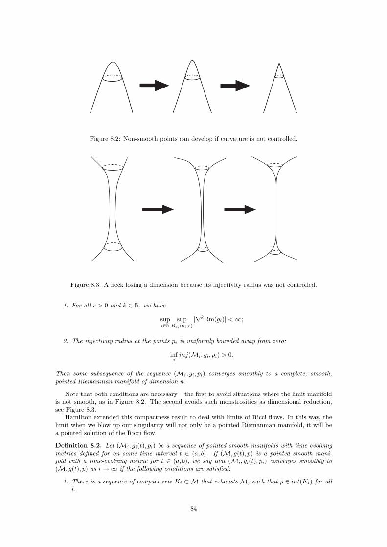
Figure 8.2: Non-smooth points can develop if curvature is not controlled.
Figure 8.3: A neck losing a dimension because its injectivity radius was not controlled.
1. For all r > 0 and k ∈ N, we have
supi∈N
supBgi (pi,r)
|∇kRm(gi)| <∞;
2. The injectivity radius at the points pi is uniformly bounded away from zero:
infiinj(Mi, gi, pi) > 0.
Then some subsequence of the sequence (Mi, gi, pi) converges smoothly to a complete, smooth,pointed Riemannian manifold of dimension n.
Note that both conditions are necessary – the first to avoid situations where the limit manifoldis not smooth, as in Figure 8.2. The second avoids such monstrosities as dimensional reduction,see Figure 8.3.
Hamilton extended this compactness result to deal with limits of Ricci flows. In this way, thelimit when we blow up our singularity will not only be a pointed Riemannian manifold, it will bea pointed solution of the Ricci flow.
Definition 8.2. Let (Mi, gi(t), pi) be a sequence of pointed smooth manifolds with time-evolvingmetrics defined for on some time interval t ∈ (a, b). If (M, g(t), p) is a pointed smooth mani-fold with a time-evolving metric for t ∈ (a, b), we say that (Mi, gi(t), pi) converges smoothly to(M, g(t), p) as i→∞ if the following conditions are satisfied:
1. There is a sequence of compact sets Ki ⊂M that exhausts M, such that p ∈ int(Ki) for alli.
84
2. There is a sequence of smooth maps φi : Ki → Mi which are diffeomorphisms onto theirimage, such that φi(p) = pi.
3. φ∗i gi(t)→ g(t) smoothly in both space and time, in the sense that the convergence is uniformin any Ck norm on any compact subset of M× (a, b).
The compactness theorem for manifolds (Theorem 8.1), can be extended to a compactnesstheorem for Ricci flows (this also first appeared in [11])
Theorem 8.2. Let (Mi, gi(t), pi) be a sequence of n-dimensional pointed solutions of the Ricciflow defined for t ∈ (a, b), where 0 ∈ (a, b). Suppose that
1.sup
i∈N,(x,t)∈Mi×(a,b)
|Rm(gi(t))|(x) <∞;
2.infiinj(Mi, gi(0), pi) > 0.
That is, the curvature is uniformly bounded above and the injectivity radius at pi is uniformlybounded away from zero at t = 0. Then there exists a marked solution of the Ricci flow (M, g(t), p)defined for t ∈ (a, b) such that a subsequence of (Mi, gi(t), pi) converges smoothly to (M, g(t), p).
Note that we do not need control over all derivatives of the curvature as we did for Theorem8.1 because of the Bernstein-Bando-Shi estimates (Theorem 6.6) which give us bounds on allderivatives of the curvature in terms of a bound on the curvature. Of course these estimates relycrucially on the fact that the metrics gi(t) satisfy the Ricci flow equation.
8.3 Blowing Up at Singularities – Results
Let us now apply these compactness results to the blowup of finite-time singularities as describedin Section 8.1. Suppose that a solution of the Ricci flow (M, g(t)) exists on a maximal time intervalt ∈ [0, T ). By the result of Theorem 6.7, the maximum value of |Rm| on M explodes to +∞ ast→ T . Thus we may choose points pi ∈M and times ti ∈ [0, T ) such that ti → T and
|Rm|(pi, ti) = supx∈M,t∈[0,ti]
|Rm|(x, t)→∞. (8.1)
Let us define Mi := |Rm|(pi, ti). Note the analogy with the proof of Grayson’s Theorem (Theorem4.6).
We now blow up the Ricci flows as described in Section 8.1: define
gi(t) = Mig
(ti +
t
Mi
).
This is merely a parabolic1 rescaling of time and the metric in addition to a translation in time,and it is not difficult to see that gi(t) is a solution of the Ricci flow defined on the time interval[−Mti,M(T − ti)). Furthermore, for t ≤ 0 we have
|Rm(gi(t))| =|Rm
(g(ti + t
Mi
))|
Mi≤ Mi
Mi= 1
by the way we defined Mi in equation (8.1). By Corollary 6.13, there exists b > 0 (depending onlyon the dimension of the manifold) such that, for all i, gi(t) is defined for t ∈ (−Mti, b), and
supi∈N,(x,t)∈Mi×(−Mti,b)
|Rm(gi(t))|(x) <∞. (8.2)
1A parabolic rescaling of a system scales time by a factor α and length by a factor√α – it is a characteristic
of heat-type evolution equations that a parabolic rescaling of any solution is another solution.
85
Because the lower limits −Mti of the time intervals tend to −∞, we seek to define a limit flowfor t ∈ (−∞, b) (for any −B < 0 arbitrarily large, the flows gi(t) will eventually be defined on(−B, b) so the limit can be defined). Now equation (8.2) shows that the first condition of Theorem8.2 is satisfied, so the only thing we need in order to pass to a limit flow is to uniform boundthe injectivity radii of the manifolds (M, gi(t)) away from zero, for all i ∈ N and t ∈ (−Mti, b).This turned out to be a major stumbling block for quite a while, but was resolved by Perelman in[23]. We will briefly discuss some of Perelman’s ideas in Section 8.4. An accessible exposition ofPerelman’s proof of the injectivity radius bounds is contained in [28, Chap. 8]. Using Perelman’sinjectivity radius bounds, we can apply Theorem 8.2. The result is (passing to a subsequence of(M, gi(t), pi)):
Theorem 8.3. Suppose that (M, g(t)) is a solution of the Ricci flow defined on a maximal timeinterval [0, T ), where T < ∞. Then there exist points pi ∈ M and times ti ∈ [0, T ), ti → T suchthat
Mi := |Rm|(pi, ti) = supx∈M,t∈[0,ti]
|Rm|(x, t)→∞.
If we now define
gi(t) = Mig
(ti +
t
Mi
)then there exists b > 0 such that (M, gi(t), pi) converges to a Ricci flow (N , g∞(t), p∞) defined fort ∈ (−∞, b). Furthermore |Rm(g∞(0))|(p∞) = 1 and |Rm(g∞(t))| ≤ 1 for t ≤ 0.
One can now seek to classify the possible singularities that one can obtain from such a limitingargument. Note that the limit flow is defined for t ∈ (−∞, b) – such solutions are called ancient.Ancient solutions are very special. If we run the Ricci flow equation in reverse we get a non-parabolic system that tends to develop singularities. Thus we do not expect to be able to extendan arbitrary Ricci flow on some finite interval (a, b) to an ancient one defined on (−∞, b). Becauseancient solutions are so special, we can hope to classify them despite the fact that classification ofarbitrary Ricci flows is a hopelessly complicated task.
Hamilton went a long way towards performing this classification in [12], showing that (if injec-tivity radius bounds were satisfied) the limit of the singularity has to be either a 3-sphere S3 orquotient thereof (which shrinks to a point in finite time) or a cylinder S2 × R, which correspondsto a neckpinch (see Figure 8.4 for the 2-dimensional analogue). He was unable to rule out a thirdpossible limit, namely Σ2 × R where Σ2 is Hamilton’s “cigar soliton” (described in Section 2.3),but Perelman has done away with this difficulty. “Degenerate neckpinches”, in which one of thehalves of the manifold shrinks to a point at the same time as the neck becomes singular (producinga sort of cusp in the manifold) are also possible.
The neckpinches, as described in Section 2.4, correspond to connected sum decompositions ofthe manifold (although some trivial decompositions may occur). The idea is to identify when aneckpinch is happening, and to perform the connected sum decomposition “manually” – that is,we cut out the neck part and seal the ends off with discs, glued on smoothly (compare Figure2.3). This is the process known as “surgery”. The flow can then continue. It might have anynumber of singularities that are either quotients of 3-spheres shrinking to a point in finite time, orproducts S2 × S1 that shrink down to the S1 factor in finite time, or neckpinches which we mustdeal with by surgery. Perelman showed that the surgery times are locally finite (i.e., in any finitetime interval there are only a finite number of times at which surgery occurs). We are left overwith the solutions that have no finite-time singularity, which Perelman showed (building on workby Hamilton in [13]) must satisfy the Geometrization Conjecture (under rescaling the manifold willsplit along tori into expanding hyperbolic pieces with cusps and collapsing “graph manifolds”, asdiscussed in Section 2.4).
To show the power of Theorem 8.3 we provide an alternative proof of Theorem 7.1.
Proof. (of Theorem 7.1) We consider a Ricci flow on a closed 3-manifold with initially strictlypositive Ricci curvature. We showed in Theorem 7.2 that the flow must have a singularity in finitetime, hence Theorem 8.3 applies. Let us say that the maximal time interval of existence is [0, T ).Thus there exist points pi ∈ M, times ti → T and rescaled flows gi(t) defined for t ∈ (−ai, b)
86
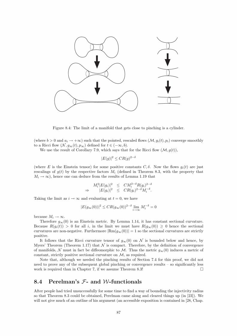
Figure 8.4: The limit of a manifold that gets close to pinching is a cylinder.
(where b > 0 and ai → +∞) such that the pointed, rescaled flows (M, gi(t), pi) converge smoothlyto a Ricci flow (N , g∞(t), p∞) defined for t ∈ (−∞, b).
We use the result of Corollary 7.9, which says that for the Ricci flow (M, g(t)),
|E(g)|2 ≤ CR(g)2−δ
(where E is the Einstein tensor) for some positive constants C, δ. Now the flows gi(t) are justrescalings of g(t) by the respective factors Mi (defined in Theorem 8.3, with the property thatMi →∞), hence one can deduce from the results of Lemma 1.19 that
M2i |E(gi)|2 ≤ CM2−δ
i R(gi)2−δ
⇒ |E(gi)|2 ≤ CR(gi)2−δM−δi .
Taking the limit as i→∞ and evaluating at t = 0, we have
|E(g∞(0))|2 ≤ CR(g∞(0))2−δ limi→∞
M−δi = 0
because Mi →∞.Therefore g∞(0) is an Einstein metric. By Lemma 1.14, it has constant sectional curvature.
Because R(gi(t)) > 0 for all i, in the limit we must have R(g∞(0)) ≥ 0 hence the sectionalcurvatures are non-negative. Furthermore |Rm(g∞(0))| = 1 so the sectional curvatures are strictlypositive.
It follows that the Ricci curvature tensor of g∞(0) on N is bounded below and hence, byMyers’ Theorem (Theorem 1.17) that N is compact. Therefore, by the definition of convergenceof manifolds, N must in fact be diffeomorphic to M. Thus the metric g∞(0) induces a metric ofconstant, strictly positive sectional curvature on M, as required.
Note that, although we needed the pinching results of Section 7.4 for this proof, we did notneed to prove any of the subsequent global pinching or convergence results – so significantly lesswork is required than in Chapter 7, if we assume Theorem 8.3!
8.4 Perelman’s F- and W-functionals
After people had tried unsuccessfully for some time to find a way of bounding the injectivity radiusso that Theorem 8.3 could be obtained, Perelman came along and cleared things up (in [23]). Wewill not give much of an outline of his argument (an accessible exposition is contained in [28, Chap.
87
6,8]) but will present one of the key ideas behind his proof – that the Ricci flow can be formulatedas a gradient flow.
We return to the analogy of the csf. Recall Lemma 4.1, which showed that the csf was asteepest-descent flow for length. Can the Ricci flow be similarly formulated as the steepest-descentflow for some functional? The simplest approaches do not work. In analogy with the lengthfunctional for the csf the simplest functional we might consider is the volume of the manifoldwith the metric g – but we know that some manifolds increase in volume and some decrease involume under the Ricci flow (specifically, hyperbolic manifolds increase in volume while manifoldsof positive sectional curvature decrease in volume – see Section 2.3), so that will not work. Thesecond-simplest functional we might try is the total scalar curvature,
∫Rdµ. The corresponding
gradient flow is, by formula (1.23) in Lemma 1.20,
∂g
∂t= −Rc +
12Rg.
This is similar to the Ricci flow and looks a bit like the unnormalized Ricci flow but is not parabolic(and cannot be made parabolic using methods like the DeTurck trick) so it is completely uselessas an evolution equation.
What clues do we have to the nature of the correct functional? One property it ought to haveis that it should obviously be constant on fixed points of the Ricci flow. But recall from Section 2.3that there exist “generalized fixed points” of the Ricci flow, the so-called Ricci solitons on whichthe Ricci flow is only changing the manifold by reparametrization and scaling. We hypothesizethat the functional we seek should also be constant on gradient Ricci solitons (gradient solitons aremuch easier to deal with than general solitons). For the moment we will consider gradient solitonsthat do not involve any rescaling of the metric, so the constant λ that appears in equation (2.1) is0. Thus we expect our functional to be constant if there exists a scalar function f :M→ R suchthat Rij +∇i∇jf = 0.
This gives us a clue that our functional should not depend on g alone, but should also dependon a scalar function f . In fact we define Perelman’s F-functional:
F(g, f) :=∫M
(R+ |∇f |2
)e−fdµ,
defined for Riemannian metrics g and scalar functions f . To work out what its gradient flow iswe must calculate how it evolves under an arbitrary variation in the metric g and the function f :∂g/∂t = h and ∂f/∂t = k.
Lemma 8.4. The variation of F(g, f) is given by:
d
dtF(g, f) =
∫M
[hij(−Rij −∇i∇jf) + (24f − |∇f |2 +R)
(12hijgij − k
)]e−fdµ.
We will not prove this result, but it follows from the results and methods used in Lemma 1.20.Perelman now defined f so that the volume form e−fdµ is preserved. By formula (1.21) of
Lemma 1.20, we have∂
∂te−fdµ =
(12gijhij − k
)e−fdµ.
So, if we determine the evolution of f by
∂f
∂t=
12gij
∂
∂tgij
and define the (now constant) “modified volume form” dξ := e−fdµ, then the result of Lemma 8.4is:
d
dtF(g, f) =
∫Mhij(−Rij −∇i∇jf)dξ.
Hence the steepest descent flow for this functional is the one with hij = −Rij −∇i∇jf , i.e.
∂
∂tgij = −Rij −∇i∇jf.
88
This is exactly the Ricci flow, with a rescaling of time (as we have −Rij rather than −2Rij onthe rhs) and a time-dependent reparametrisation moving along the gradient vector field of f (asoutlined in the discussion of Ricci solitons in Section 2.3). So the gradient flow of this functionalis equivalent to the Ricci flow. We also note that if the solution is stationary under this flow,it satisfies the gradient Ricci soliton equation (2.1) with no rescaling term, as we have argued itshould.
We would like to extend the F-functional in some way so that the functional is also constant ongradient solitons that include rescaling. This is the idea behind the W-functional. We introduce apositive real-valued scaling parameter τ > 0 and define
W(g, f, τ) :=∫Mn
(τ(R+ |∇f |2) + f − n
)udµ
where n is the dimension of the manifold and
u := (4πτ)−n/2e−f .
The arguments g, f, τ are said to be compatible if∫Mn
udµ = 1.
We would like an evolution equation for W in the style of Lemma 8.4. The analogous result is
Lemma 8.5. If g, f, τ evolve according to
∂g
∂t= −2Rc
∂τ
∂t= −1
∂f
∂t= −4f + |∇f |2 −R+
n
2τ
thend
dtW(g, f, τ) = 2τ
∫Mn
|Rij +∇i∇jf −12τgij |2udµ.
In particular, W is nondecreasing in time and remains constant if and only if
Rij +∇i∇jf −12τgij = 0,
that is, if and only if g is a shrinking gradient Ricci soliton. The condition that g, f, τ are compatibleis preserved under this evolution. Note that the evolution equation for f is a backwards heatequation (because of the − sign in front of the Laplacian). Backwards heat equations are notparabolic, and generally can not be expected to have a solution even for a short time. However, ifwe reverse time we get a normal heat-type equation, which does have a short-time solution. Thus,rather than specifying initial conditions on f , we can only specify final conditions.
Perelman was able to use the W-functional to prove bounds on the volume of balls of givenradius as the metric evolves under the Ricci flow, by defining f so that e−f is a bump functionwith support inside the ball (W then has the form of an integral over the ball, which can be relatedto the ball’s volume). He showed that the volume of such balls will not collapse, from which it ispossible to show that their injectivity radius is bounded below, which is exactly the sort of resultwe needed to prove Theorem 8.3. See [28, Chap. 8] for the full argument.
89

Appendix A
Existence Theory for ParabolicPDEs
In this Appendix we will outline the main existence results for pdes that we will use. This materialis based on [6, Sec 3.2] and [28, Chap. 4].
Consider a vector bundle π : E → M, where M is some Riemannian manifold, with somebundle metric h. We will be interested in pdes describing the evolution of some time-dependentsection of E , u :M× [0, T )→ E , having the form
∂u
∂t= L(u) (A.1)
u(x, 0) = u0(x) (A.2)
where L : C∞(E)→ C∞(E) is some differential operator.
A.1 Linear Theory
In this section we will use the multi-index notation for partial derivatives.
Definition A.1. A multi-index α is an n-tuple of non-negative integers (α1, α2, . . . , αn). Wedefine
|α| =n∑i=1
αi.
If f is a function of n variables x1, x2, . . . , xn then we define
∂αf :=∂|α|f
∂xα11 ∂xα2
2 . . . ∂xαnn.
We first consider the case that L is a linear differential operator. That is, using multi-indexnotation,
L(u) =∑|α|≤k
Lα∂αu (A.3)
where k is the order of L and Lα ∈ Hom(E , E).For example, we might consider a second-order linear differential operator acting on scalar
functions on Rn (so M = Rn, E =M× R, k = 2). This will have the form
L(u) =∑i,j
aij∂i∂ju+
∑i
bi∂iu+ cu.
90
If ϕ is some covector field (i.e. ϕ ∈ C∞(T ∗M)) then we define the total symbol of L in thedirection ϕ to be the bundle homomorphism σ[L](ϕ) : E → E
σ[L](ϕ)(u) =∑|α|≤k
Lα(u)∏j
ϕαj .
In the case of the example L we gave above, the total symbol in the direction ϕ is
σ[L](ϕ)(u) =∑i,j
aijϕiϕju+
∑i
biϕiu+ cu.
We define the principal symbol of L in the direction ϕ to be the bundle homomorphismσ[L](ϕ) : E → E that comes only from the highest order derivative terms in L:
σ[L](ϕ)(u) =∑|α|=k
Lα(u)∏j
ϕαj .
The principal symbol of the example L in the direction ϕ is thus:
σ[L](ϕ)(u) =∑i,j
aijϕiϕju.
The operator L is said to be elliptic if σ[L](ϕ) is a vector bundle isomorphism whenever ϕ 6= 0.For our example L this means that ∑
i,j
aijϕiϕj 6= 0
whenever ϕ 6= 0, i.e. that [aij ] is a non-singular matrix.The system A.1 is said to be strongly parabolic1 if there exists δ > 0 such that at each point
of the manifold M, for all covectors ϕ 6= 0 and elements u 6= 0 of E ,
〈σ[L](ϕ)(u), u〉 > δ|ϕ|2|u|2.
In the order-2 example we considered above, this is saying that∑i,j
aijϕiϕj > δ|ϕ|2
for all ϕ 6= 0, i.e. that the matrix [aij ] is positive-definite.
A.2 Linearization of Nonlinear PDEs
We will mainly deal with non-linear pde’s, where L is not given by the convenient form of A.3.What does it mean for a non-linear pde to be parabolic? We need to define the linearization ofthe non-linear operator L. The linearization is defined in analogy with the derivative of a functionf : Rn → Rm, which is the linear map Df : Rn → Rm defined to “best approximate” f at eachpoint. That is, if we have curve x : [0, 1]→ Rn satisfying
x(0) = p
x′(0) = v
then
Df(v) =d
dtf(x(t))
∣∣∣∣t=0
In a similar way we define the linearization of a non-linear operator L on a vector bundle E . Ifu : [0, 1]→ C∞(E) is a time-dependent section of E such that
u(0) = u0
u′(0) = v.
1We will often just say “parabolic” when we mean “strongly parabolic”
91
We define the linearization of L at u0 to be the linear map D[L] : C∞(E)→ C∞(E) so that
D[L](v) =d
dtL(u(t))
∣∣∣∣t=0
(if it exists).We say that the system A.1 is strongly parabolic at u0 if the system
∂u
∂t= D[L](u) (A.4)
u(x, 0) = u0(x) (A.5)
is strongly parabolic in the sense described previously. We will only be interested in the case whereD[L] has the form
D[L] =∑|α|≤k
Lα∂α
with some finite k.
Theorem A.1. If the system A.1 is strongly parabolic at u0 then there exists a solution on sometime interval [0, T ), and the solution is unique for as long as it exists.
Practically all existence proofs in this project will rely on this theorem. See [17] for the proof.
92
Appendix B
Differential Geometry Formulae
1. Christoffel symbols, for the Levi-Civita connection of the metric gij :
Γkij =12gkl(∂igjl + ∂jgil − ∂lgij)
2. In normal coordinates about the point p:
(a) γV (t) = (tV 1, tV 2, . . . , tV n) is a geodesic
(b) gij(p) = δij
(c) Γkij(p) = 0, ∂igjk(p) = 0
3. Covariant derivative:
∇pF j1...jli1...ik= ∂pF
j1...jli1...ik
+l∑
s=1
F j1...q...jli1...ikΓjspq −
k∑s=1
F j1...jli1...q...ikΓqpis (B.1)
4. Riemann curvature tensor:
[∇i,∇j ]X l ≡ RlijkXk
5. Symmetries of the Riemann curvature tensor:
Rijkl = Rklij = −Rjikl = −Rijlk
6. First Bianchi identity:
Rijkl +Rjkil +Rkijl = 0
7. Second Bianchi identity:
∇pRijkl +∇iRjpkl +∇jRpikl = 0 (B.2)
8. Ricci and scalar curvatures:
Rij ≡ Rmmjk , R ≡ Rii
9. Contracted second Bianchi identity:
∇jRij =12∇iR
93
10. Commuting covariant derivatives:
[∇p,∇q]F j1...jli1...ik=
l∑s=1
RjspqmFj1...m...jli1...ik
−k∑s=1
RmpqisFj1...jli1...m...ik
(B.3)
11. Coordinate form of the Riemann curvature tensor:
Rlijk = ∂iΓljk − ∂jΓlik + ΓpjkΓlip − ΓpikΓljp
94
Bibliography
[1] Michael T. Anderson. Geometrization of 3-manifolds via the Ricci flow. Notices of the AMS,51:184–193, 2004.
[2] Huai-Dong Cao and Xi-Ping Zhu. A complete proof of the Poincare and geometrizationconjectures – application of the Hamilton-Perelman theory of the Ricci flow. Asian J. Math.,10, No. 2:165–492, 2006.
[3] J. Cheeger and D. Ebin. Comparison theorems in Riemannian Manifolds. North-Holland,1975.
[4] XiuXiong Chen, Peng Lu, and Gang Tian. A note on uniformization of Riemann surfaces byRicci flow. http://arXiv.org/math.DG/0505163, 2005.
[5] S.S. Chern, W.H. Chen, and K.S. Lam. Lectures on Differential Geometry. World Scientific,2000.
[6] Bennett Chow and Dan Knopf. The Ricci Flow: An Introduction. AMS Math. Surveys andMonographs, 2004.
[7] Dennis M. DeTurck. Deforming metrics in the direction of their Ricci tensors. Journal ofDifferential Geometry, 18:157–162, 1983.
[8] S. Gallot, D. Hulin, and J. Lafontaine. Riemannian Geometry. Springer-Verlag, 1987.
[9] Richard Hamilton. Three-manifolds with positive Ricci curvature. J. Diff. Geo., 17:255–306,1982.
[10] Richard Hamilton. Four-manifolds with positive curvature operator. J. Diff. Geo., 24:153–179,1986.
[11] Richard Hamilton. A compactness property for solutions of the Ricci flow. American Journalof Mathematics, 117:545–572, 1992.
[12] Richard Hamilton. The formation of singularities in the Ricci flow. Surveys in DifferentialGeometry, 2:1–136, 1995.
[13] Richard Hamilton. Non-singular solutions of the Ricci flow on three-manifolds. Comm. Anal.Geom., 7:695–729, 1999.
[14] Noel J. Hicks. Notes on Differential Geometry. Van Nostrand, 1965.
[15] Wilhelm Klingenberg. A Course in Differential Geometry. Springer-Verlag, 1978.
[16] Hellmuth Kneser. Geschloßene flachen in dreidimensionalen mannigfaltigkeiten. Jahresberichtder Deutschen Mathematischen Verein, 38:248–260, 1929.
[17] O. A. Ladyzenskaja, V. A. Solonnikov, and N. N. Uralceva (Translated from the Russian byS. Smith). Linear and quasilinear equations of parabolic type. Vol. 23 AMS, 1967.
[18] John M. Lee. Riemannian Manifolds: An Introduction to Curvature. Springer-Verlag, 1997.
95
[19] John Milnor. A unique factorization theorem for 3-manifolds. Amer. J. Math., 84:1–7, 1962.
[20] John Milnor and James Stasheff. Characteristic Classes. Princeton University Press, 1974.
[21] John W. Morgan and Gang Tian. Ricci flow and the Poincare conjecture.http://arXiv.org/math.DG/0607607v1, 2006.
[22] James R. Munkres. Topology, 2nd Ed. Prentice Hall, 2000.
[23] Grisha Perelman. The entropy formula for the Ricci flow and its geometric applications.http://arXiv.org/math.DG/0211159v1, 2002.
[24] Grisha Perelman. Finite extinction time for the solutions to the Ricci flow on certain three-manifolds. http://arXiv.org/math.DG/0307245v1, 2002.
[25] Grisha Perelman. Ricci flow with surgery on three-manifolds.http://arXiv.org/math.DG/0303109v1, 2003.
[26] Michael Spivak. A Comprehensive Introduction to Differential Geometry. Publish or Perish,1979.
[27] William P. Thurston. Three-Dimensional Geometry and Topology, Vol. 1. Princeton UniversityPress, 1997.
[28] Peter Topping. Lectures on the Ricci Flow.http://www.maths.warwick.ac.uk/~topping/RFnotes.html, 2005.
[29] Peter Topping. Lectures on the Ricci Flow. Cambridge University Press, 2006.
[30] Xi-Ping Zhu. Lectures on Mean Curvature Flows. International Press, 2002.
96