Embed Size (px)
Citation preview
Handbook of Cluster Analysis (provisional top level file)
C. Hennig, M. Meila, F. Murtagh, R. Rocci (eds.)
March 13, 2015

ii
Contents
1 Dirichlet processes 1
1.1 Introduction . . . . . . . . . . . . . . . . . . . . . . . . . . . . . . . . . . . . 2
1.2 The Dirichlet Process . . . . . . . . . . . . . . . . . . . . . . . . . . . . . . . 3
1.2.1 The Polya urn scheme and the Chinese restaurant process . . . . . . 6
1.2.2 The stick-breaking construction . . . . . . . . . . . . . . . . . . . . . 9
1.2.3 Dirichlet process mixtures and clustering . . . . . . . . . . . . . . . . 11
1.3 Example applications . . . . . . . . . . . . . . . . . . . . . . . . . . . . . . . 13
1.3.1 Clustering microarray expression data . . . . . . . . . . . . . . . . . 13
1.3.2 Bayesian Haplotype inference . . . . . . . . . . . . . . . . . . . . . . 14
1.3.3 Spike sorting . . . . . . . . . . . . . . . . . . . . . . . . . . . . . . . 14
1.4 Posterior inference . . . . . . . . . . . . . . . . . . . . . . . . . . . . . . . . 15
1.4.1 Markov chain Monte Carlo . . . . . . . . . . . . . . . . . . . . . . . . 15
1.4.2 Variational inference . . . . . . . . . . . . . . . . . . . . . . . . . . . 20
1.4.3 Comments on posterior computation . . . . . . . . . . . . . . . . . . 22
i
ii CONTENTS
1.5 Extensions . . . . . . . . . . . . . . . . . . . . . . . . . . . . . . . . . . . . . 22
1.5.1 Exchangeability and consistency . . . . . . . . . . . . . . . . . . . . . 22
1.5.2 Pitman-Yor processes . . . . . . . . . . . . . . . . . . . . . . . . . . . 24
1.5.3 Dependent random measures . . . . . . . . . . . . . . . . . . . . . . . 26
1.6 Discussion . . . . . . . . . . . . . . . . . . . . . . . . . . . . . . . . . . . . . 28
1.7 Acknowledgements . . . . . . . . . . . . . . . . . . . . . . . . . . . . . . . . 29
Chapter 1
Dirichlet process mixtures and
nonparametric Bayesian approaches
to clustering
Vinayak Rao
Department of Statistics,
Purdue University
Abstract
Interest in nonparametric Bayesian methods has grown rapidly as statisticians and machine learning researchers
work with increasingly complex datasets, and as computation grows faster and cheaper. Central to developments in
this field has been the Dirichlet process. In this chapter, we introduce the Dirichlet process, and review its
properties and its different representations. We describe the Dirichlet process mixture model that is fundamental to
clustering problems and review some of its applications. We discuss various approaches to posterior inference, and
conclude with a short review of extensions beyond the Dirichlet process.
1
2 CHAPTER 1. DIRICHLET PROCESSES
1.1 Introduction
The Bayesian framework provides an elegant model-based approach to bringing prior infor-
mation to statistical problems, as well as a simple calculus for inference. Prior beliefs are
represented by probabilistic models of data, often structured by incorporating latent vari-
ables. Given a prior distribution and observations, the laws of probability (in particular,
Bayes’ rule) can be used to calculate posterior distributions over unobserved quantities, and
thus to update beliefs about future observations. This provides a conceptually simple ap-
proach to handling uncertainty, dealing with missing data, and combining information from
different sources. A well known issue is that complex models usually result in posterior
distributions that are intractable to exact analysis; however the availability of cheap compu-
tation, coupled with the development of sophisticated Markov chain Monte Carlo sampling
methods and deterministic approximation algorithms has resulted in a wide application of
Bayesian methods. The field of clustering is no exception, see for example [13, 39], and the
references therein.
There still remain a number of areas of active research, and in this chapter, we consider the
problem of model selection. For clustering, model selection in its simplest form boils down
to choosing the number of clusters underlying a dataset. Conceptually at least, the Bayesian
approach can handle this easily by mixing over different models with different numbers of
clusters. An additional latent variable now identifies which of the smaller submodels actually
generated the data, and a prior belief on model complexity is specified by a probability
distribution over this variable. Given observations, Bayes’ rule can be used to update the
posterior distribution over models.
However, with the increasing application of Bayesian models to complex datasets from
fields like biostatistics, computer vision and natural language processing, modelling data
as a realization of one of a set of finite-complexity parametric models is inadequate. Such
datasets raise the need for prior distributions that capture the notion of a world of unbounded
complexity, so that a priori, one expects larger datasets to require more complicated expla-
nations (e.g. larger numbers of clusters). A mixture of finite cluster models does not really
capture this idea. A realization of such a model would first sample the number of clusters,
1.2. THE DIRICHLET PROCESS 3
and this would remain fixed no matter how many observations are produced subsequently.
Under a truly nonparametric solution, the number of clusters would be infinite, with any
finite dataset ‘uncovering’ only a finite number of active clusters. As more observations are
generated, one would expect more and more clusters to become active. The Bayesian ap-
proach of maintaining full posterior distributions (rather than fitting point estimates) allows
the use of such an approach without concerns about overfitting. Such a solution is also more
elegant and principled than the empirical Bayes approach of adjusting the prior over the
number of clusters after seeing the data [8].
The Dirichlet process (DP), introduced by Ferguson in [12], is the most popular example
of a nonparametric prior for clustering. Ferguson introduced the DP in a slightly different
context, as a probability measure on the space of probability distributions. He noted two
desiderata for such a nonparametric prior: the need for the prior to have large support on
the space of probability distributions, and the need for the resulting posterior distribution
to be tractable. Ferguson described these two properties as antagonistic, and the Dirichlet
process reconciles them at the cost of a peculiar property: a probability measure sampled
from a DP is discrete almost surely (see Figure 1.1). While there has since been considerable
work on constructing priors without this limitation, the discreteness of the DP was seized
upon as ideal for clustering appications, providing a prior over mixing proportions in models
with an infinite number of components.
The next section defines the DP, and introduces various representations useful in applica-
tions and for studying its properties. We introduce the DP mixture model that is typically
used in clustering applications, and in Section 1.3, describe some applications. We follow
that with a description of various approaches to posterior inference (Section 1.4), and end
by outlining some approaches to extending the DP.
1.2 The Dirichlet Process
Consider a positive real number α, as well as a probability measure G0 on some space Θ. For
instance, Θ could be the real line, and G0 could be the normal distribution with mean 0 and

4 CHAPTER 1. DIRICHLET PROCESSES
variance σ2. A Dirichlet process, parametrized by G0 and α, is written as DP(α,G0), and is
a stochastic process whose realizations (which we call G) are probability measures on Θ. G0
is called the base measure, while α is called the concentration parameter. Often, the DP is
parametrized by a single finite measure α(·), in which case, α = α(Θ) and G0(·) = α(·)/α(Θ).
We will adopt the former convention.
Observe that for any probability measure G, and for any finite partition (A1, . . . , An) of Θ,
the vector (G(A1), . . . G(An)) is a probability vector, i.e., it is a point on the (n−1)-simplex,
with nonnegative components that add up to one. We call this vector the projection of G
onto the partition. Then the Dirichlet process is defined as follows: for any finite partition
of Θ, the projected probability vector has a Dirichlet distribution as specified below:
(G(A1), . . . G(An)) ∼ Dirichlet(αG0(A1), . . . , αG0(An)) (1.1)
In words, the marginal distribution induced by projecting the Dirichlet process onto a finite
partition is an appropriately parametrized Dirichlet distribution (in particular, the parameter
vector of the Dirichlet distribution is the projection of the base measureG0 onto the partition,
multiplied by α). A technical question now arises: does there exist a stochastic process whose
projections simultaneously satisfy this condition for all finite partitions of Θ? To answer this,
note that equation (1.1) and the properties of the Dirichlet distribution imply
(G(A1), . . . , G(Ai)+G(Ai+1), . . . G(An)) ∼
Dirichlet(αG0(A1), . . . , αG0(Ai) + αG0(Ai+1), . . . , αG0(An)) (1.2)
This distribution of the projection on the coarsened partition (A1, . . . , Ai ∪ Ai+1, . . . An),
implied indirectly via the distribution on the finer partition (A1, . . . , Ai, Ai+1, . . . An) agrees
with the distribution that follows directly from the definition of the DP. This consistency is
sufficient to imply the existence of the DP via Kolmogorov’s consistency theorem1[22].
We shall see a more constructive definition of the DP in Section 1.2.2, however there are
a number of properties that follow from this definition of the DP. First, note that from the
1While Kolmogorov’s consistency theorem guarantees the existence of a stochastic process with specified finite marginals,a subtle issue concerns whether realizations of this stochastic process are probability measures. This actually requires mildadditional assumptions on the space Θ, see e.g. [14] or [33] for more detailed accounts of this.
1.2. THE DIRICHLET PROCESS 5
properties of the Dirichlet distribution, for any set A, E[G(A)] = G0(A). This being true
for all sets A, we have that the mean of a draw from a DP is the base probability measure
G0. On the other hand, var[G(A)] = G0(A)(1−G0(A))1+α
, so that α controls how concentrated
probability mass is around the mean G0. As α → ∞, G(A) → G0(A) for all A, so that a
draw from the DP equals the base measure G0. We will see in Section 1.2.2 that as α tends
to 0, G approaches a single Dirac measure, whose location is drawn from G0.
To appreciate why the DP has large support on the space of probability distributions,
observe that any probability measure can be approximated arbitrarily well as a piecewise-
constant probability measure on a sufficiently fine, finite partition of Θ. Assuming the
partition has m components, and calling the probability vector p ≡ (p1, . . . , pm), note that
p lies in the support of an m-dimensional Dirichlet distribution Dirichlet(γ1, . . . , γm) only if
for all i such that pi > 0, we have γi > 0. When Dirichlet(γ1, . . . , γm) is the projection of DP
with base measure G0, this is always true if the support of G0 includes all of Θ (e.g. when Θ
is Rn, and G0 is a multivariate normal on Θ: here, for any open set Ai, γi =∫AiG0(dx) > 0).
In this case, the support2 of the DP includes all probability meaures on Θ. More generally,
the weak support of DP(α,G0) includes all probability measures whose support is included
in the support of G0. Somewhat confusingly, in spite of this large support, we will see that
any probability measure sampled from a DP is discrete almost surely.
We next characterize the DP posterior by considering the following hierarchical model:
G ∼ DP(α,G0) (1.3)
θi ∼ G for i in 1 to N (1.4)
Thus, we sample N observations independently from the random probability measure G
(itself drawn from a DP). Let NA represent the number of elements of the sequence θ ≡(θ1, . . . , θN) lying in a set A, i.e. NA =
∑Ni=1 δA(θi), where δA(·) is the indicator function
for the set A. For some partition (A1, . . . , Am), the vector of counts (NA1 , . . . , NAm) is
multinomially distributed with a Dirichlet prior on the probability vector (equation (1.1)).
2weak support, to be precise.
6 CHAPTER 1. DIRICHLET PROCESSES
From the conjugacy of the Dirichlet distribution, we have the posterior distribution
(G(A1), . . . G(Am))|(θ1, . . . , θN) ∼ Dirichlet(αG0(A1) +NA1 , . . . , αG0(Am) +NAm) (1.5)
This must be true for any partition of Θ, so that the posterior is a stochastic process, all of
whose marginals are Dirichlet distributed. It follows that the posterior is again a DP, now
with concentration parameter α +N , and base measure(
αα+N
G0 + 1α+N
∑Ni=1 δθi
):
G|(θ1, . . . , θN) ∼ DP
(α +N,
α
α +NG0 +
1
α +N
N∑i=1
δθi
)(1.6)
This is the conjugacy property of the DP. The fact that the posterior is again a DP allows
one to integrate out the infinite-dimensional random measure G, obtaining a remarkable
characterization of the marginal distribution over observations. We discuss this next.
1.2.1 The Polya urn scheme and the Chinese restaurant process
Consider a single observation θ drawn from the DP-distributed probability measure G. The
definition of the DP in the previous section shows that the probability that θ lies in a set A,
marginalizing out G(A), is just E[G(A)] = G0(A). Since this is true for all A, it follows that
θ ∼ G0. Since the posterior given N observations is also DP-distributed (equation (1.6)),
the predictive distribution of observation N + 1 is just the posterior base measure:
θN+1|θ1, . . . , θN ∼1
α +N
(αG0(·) +
N∑i=1
δθi(·)
)(1.7)
We see that the predictive distribution of a new observation is a mixture of the DP base
measure G0 (weighted by the concentration parameter), and the empirical distribution of the
previous observations (weighted by the number of observations). The result above allows us
to sequentially generate observations from a DP-distributed random probability measure
G, without having to explicitly represent the the infinite-dimensional variable G. This
corresponds to a sequential process knows as a Polya urn scheme [3]. Here, at stage N ,
1.2. THE DIRICHLET PROCESS 7
we have an urn containing N balls, the ith ‘coloured’ with the associated value θi. With
probability α/(α + N), the (N + 1)st ball is assigned a colour θN+1 drawn independently
from the base measure G0, after which it is added to the urn. Otherwise, we uniformly pick a
ball from the urn, and set θN+1 equal to its colour, and return both balls to the urn. Observe
that there is non-zero probability that multiple balls have the same colour, and that the
more balls share a particular colour, the more likely a new ball will be assigned that colour.
This rich-get-richer scheme is key to the clustering properties of the DP.
Let θ∗ ≡ (θ∗1, . . . , θ∗KN
) be the sequence of unique values in θ, KN being the number of
such values. Let πNi index the elements of θ that equal θ∗i , and let πN = {πN1 , . . . , πNKN}.
Clearly, (θ∗, πN) is an equivalent representation of θ. πN is a partition of the integers 1 to
N , while θ∗ represents the parameter assigned to each element of the partition. Define ni
as the size of the ith cluster, so that ni = |πNi |. Equation (1.7) can now be rewritten as
θN+1 ∼1
α +N
(αG0 +
KN∑c=1
ncδθ∗c
)(1.8)
The preceding equation is characterized by a different metaphor called the Chinese restaurant
process (CRP) [35], one that is slightly more relevant to clustering applications. Here, a
partition of N observations is represented by the seating arrangement of N ‘customers’ in
a ‘restaurant’. All customers seated at a table form a cluster, and the dish served at that
table corresponds to its associated parameter, θ∗. When a new customer (observation N+1)
enters the restaurant, with probability proportional to α, she decides to sit by herself at a
new table, ordering a dish drawn from G0. Otherwise, she joins one of the existing KN tables
with probability proportional to the number of customers seated there. We can write down
the marginal distribution over the observations (θ1, . . . , θn):
P (π,θ∗) =
(αKN−1
[α + 1]N1
KN∏c=1
(nc − 1)!
)(KN∏c=1
G0(θ∗c )
)(1.9)
Here, [x]na =∏n−1
i=0 (x+ ia) is the rising factorial. The equation above makes it clear that the
partitioning of observations into clusters, and the assignment of parameters to each cluster
are independent processes. The former is controlled by the concentration parameter α, while
8 CHAPTER 1. DIRICHLET PROCESSES
all clusters are assigned parameters drawn independently from the base measure. As α tends
to infinity, each customer is assigned to her own table, and has her own parameter (agreeing
with the idea that the θ’s are drawn i.i.d. from a smooth probability measure). When α
equals 0, all customers are assigned to a single cluster, showing that the random measure G
they were drawn from was a distribution degenerate at the cluster parameter.
Marginalizing out the cluster parameters θ∗, consider the distribution over partitions
specified by the CRP:
P (πN) =αKN−1
[α + 1]N1
KN∏c=1
(nc − 1)! (1.10)
This can be viewed as a distribution over partitions of the integers 1 to N , and is called the
Ewens’ sampling formula [11]. Ewens’ sampling formula characterizes the clustering structure
induced by the CRP (and thus the DP); for a number of properties of this distribution over
partitions, see [35]. We discuss a few below.
First, observe that the probability of a partition depends only on the number of the
blocks of the partition and their sizes, and is independent of the identity of the elements
that constitute the partition. In other words, the probability of a partition of the integers
1 to N is invariant to permutations of the numbers 1 to N . Thus, despite its sequential
construction, the CRP defines an exchangeable distribution over partitions. Exchangeability
has important consequences which we discuss later in Section 1.5.1.
Next, under the CRP, the probability that customer i creates a new table is α/(α+ i−1).
Thus KN , the number of clusters that N observations will be partitioned into, is distributed
as the sum of N independent Bernoulli variables, the ith having probability α/(α + i − 1).
Letting N (0, 1) be the standard normal distribution, and lettingd→ indicate convergence in
distribution, one can show that as N →∞,
KN/ log(N)→ α, (KN − α log(N))/√α log(N)
d→ N (0, 1) (1.11)
1.2. THE DIRICHLET PROCESS 9
-3 -2 -1 0 1 2 30.0
0.1
0.2
0.3
0.4
0.5
0.6
-3 -2 -1 0 1 2 30.00
0.05
0.10
0.15
0.20
-3 -2 -1 0 1 2 30
0.01
0.02
0.03
0.04
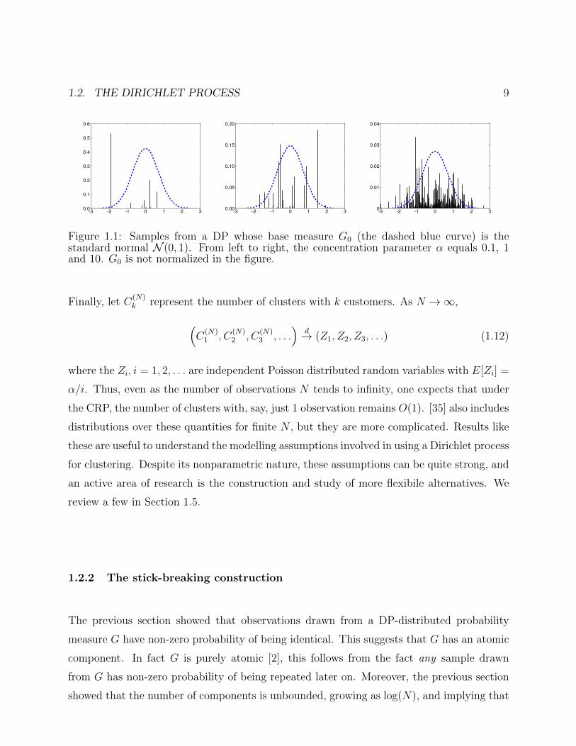
Figure 1.1: Samples from a DP whose base measure G0 (the dashed blue curve) is thestandard normal N (0, 1). From left to right, the concentration parameter α equals 0.1, 1and 10. G0 is not normalized in the figure.
Finally, let C(N)k represent the number of clusters with k customers. As N →∞,
(C
(N)1 , C
(N)2 , C
(N)3 , . . .
)d→ (Z1, Z2, Z3, . . .) (1.12)
where the Zi, i = 1, 2, . . . are independent Poisson distributed random variables with E[Zi] =
α/i. Thus, even as the number of observations N tends to infinity, one expects that under
the CRP, the number of clusters with, say, just 1 observation remains O(1). [35] also includes
distributions over these quantities for finite N , but they are more complicated. Results like
these are useful to understand the modelling assumptions involved in using a Dirichlet process
for clustering. Despite its nonparametric nature, these assumptions can be quite strong, and
an active area of research is the construction and study of more flexibile alternatives. We
review a few in Section 1.5.
1.2.2 The stick-breaking construction
The previous section showed that observations drawn from a DP-distributed probability
measure G have non-zero probability of being identical. This suggests that G has an atomic
component. In fact G is purely atomic [2], this follows from the fact any sample drawn
from G has non-zero probability of being repeated later on. Moreover, the previous section
showed that the number of components is unbounded, growing as log(N), and implying that
10 CHAPTER 1. DIRICHLET PROCESSES
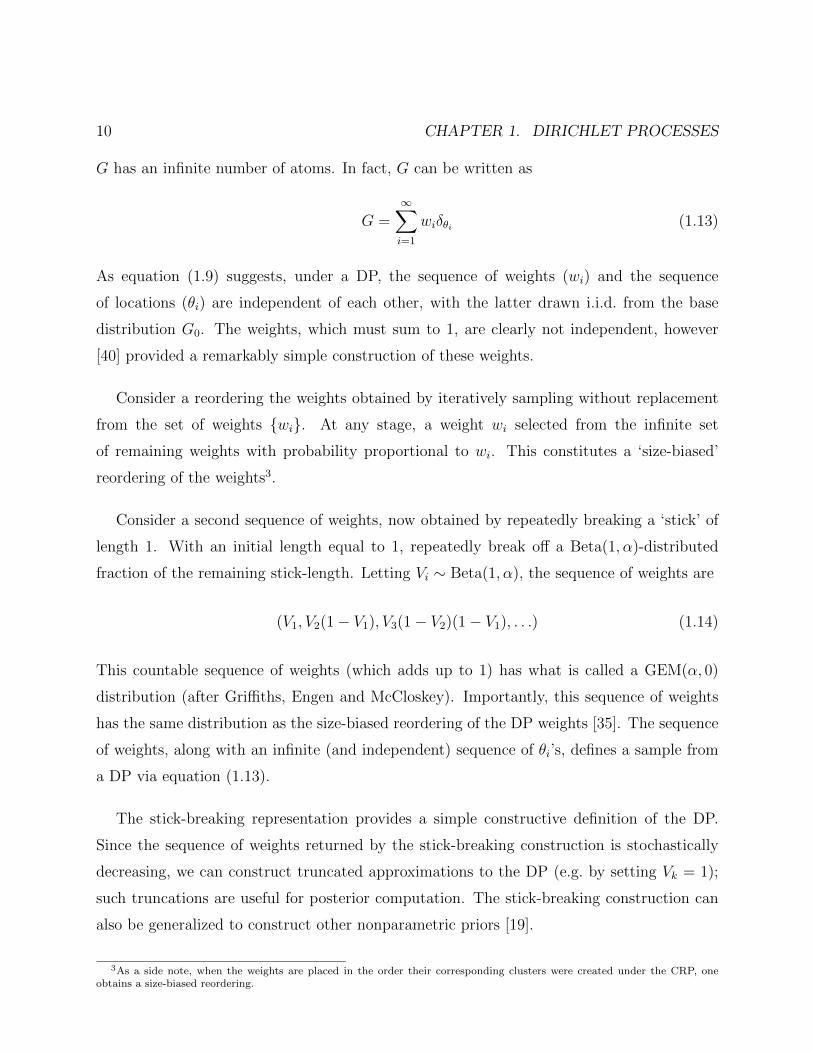
G has an infinite number of atoms. In fact, G can be written as
G =∞∑i=1
wiδθi (1.13)
As equation (1.9) suggests, under a DP, the sequence of weights (wi) and the sequence
of locations (θi) are independent of each other, with the latter drawn i.i.d. from the base
distribution G0. The weights, which must sum to 1, are clearly not independent, however
[40] provided a remarkably simple construction of these weights.
Consider a reordering the weights obtained by iteratively sampling without replacement
from the set of weights {wi}. At any stage, a weight wi selected from the infinite set
of remaining weights with probability proportional to wi. This constitutes a ‘size-biased’
reordering of the weights3.
Consider a second sequence of weights, now obtained by repeatedly breaking a ‘stick’ of
length 1. With an initial length equal to 1, repeatedly break off a Beta(1, α)-distributed
fraction of the remaining stick-length. Letting Vi ∼ Beta(1, α), the sequence of weights are
(V1, V2(1− V1), V3(1− V2)(1− V1), . . .) (1.14)
This countable sequence of weights (which adds up to 1) has what is called a GEM(α, 0)
distribution (after Griffiths, Engen and McCloskey). Importantly, this sequence of weights
has the same distribution as the size-biased reordering of the DP weights [35]. The sequence
of weights, along with an infinite (and independent) sequence of θi’s, defines a sample from
a DP via equation (1.13).
The stick-breaking representation provides a simple constructive definition of the DP.
Since the sequence of weights returned by the stick-breaking construction is stochastically
decreasing, we can construct truncated approximations to the DP (e.g. by setting Vk = 1);
such truncations are useful for posterior computation. The stick-breaking construction can
also be generalized to construct other nonparametric priors [19].
3As a side note, when the weights are placed in the order their corresponding clusters were created under the CRP, oneobtains a size-biased reordering.
1.2. THE DIRICHLET PROCESS 11
10 5 0 5 1016
14
12
10
8
6
4
2
0
2
30 25 20 15 10 5 0 5 10 1515
10
5
0
5
10
15
20
25
30
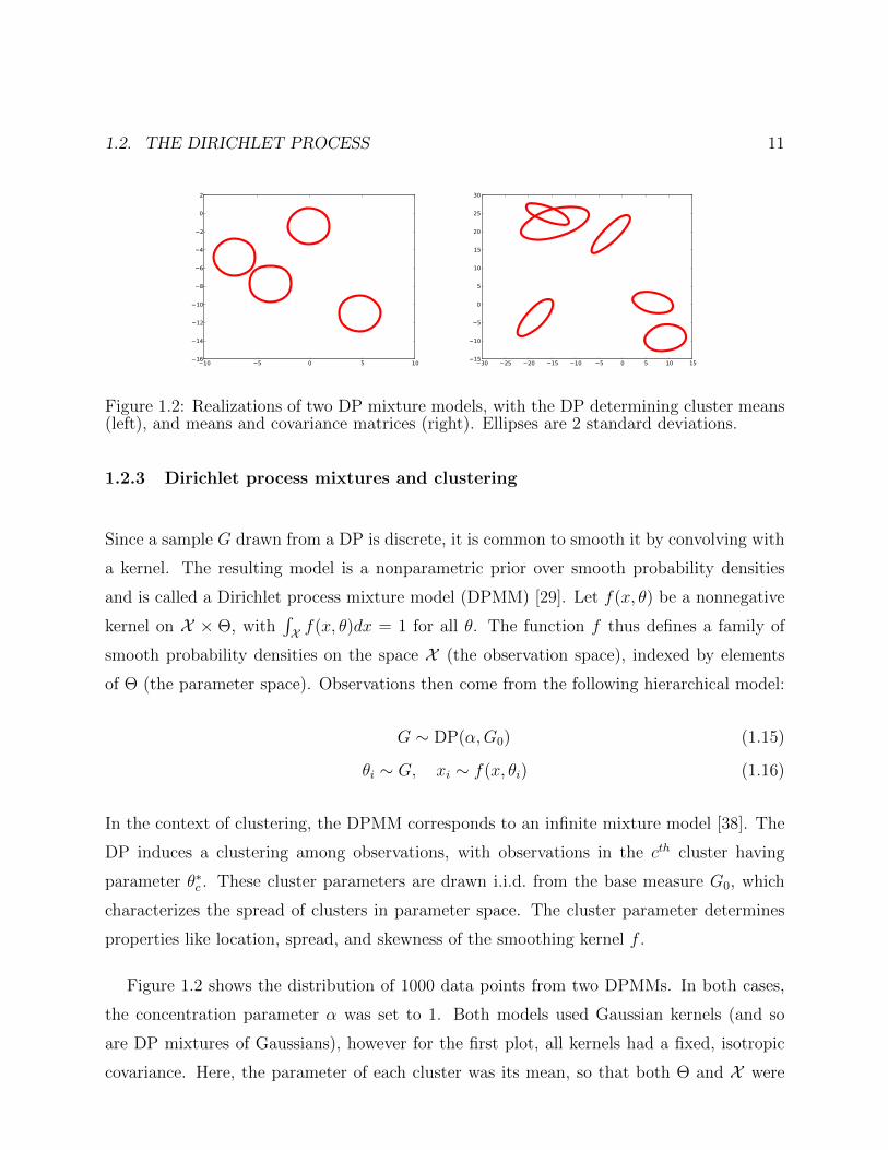
Figure 1.2: Realizations of two DP mixture models, with the DP determining cluster means(left), and means and covariance matrices (right). Ellipses are 2 standard deviations.
1.2.3 Dirichlet process mixtures and clustering
Since a sample G drawn from a DP is discrete, it is common to smooth it by convolving with
a kernel. The resulting model is a nonparametric prior over smooth probability densities
and is called a Dirichlet process mixture model (DPMM) [29]. Let f(x, θ) be a nonnegative
kernel on X × Θ, with∫X f(x, θ)dx = 1 for all θ. The function f thus defines a family of
smooth probability densities on the space X (the observation space), indexed by elements
of Θ (the parameter space). Observations then come from the following hierarchical model:
G ∼ DP(α,G0) (1.15)
θi ∼ G, xi ∼ f(x, θi) (1.16)
In the context of clustering, the DPMM corresponds to an infinite mixture model [38]. The
DP induces a clustering among observations, with observations in the cth cluster having
parameter θ∗c . These cluster parameters are drawn i.i.d. from the base measure G0, which
characterizes the spread of clusters in parameter space. The cluster parameter determines
properties like location, spread, and skewness of the smoothing kernel f .
Figure 1.2 shows the distribution of 1000 data points from two DPMMs. In both cases,
the concentration parameter α was set to 1. Both models used Gaussian kernels (and so
are DP mixtures of Gaussians), however for the first plot, all kernels had a fixed, isotropic
covariance. Here, the parameter of each cluster was its mean, so that both Θ and X were
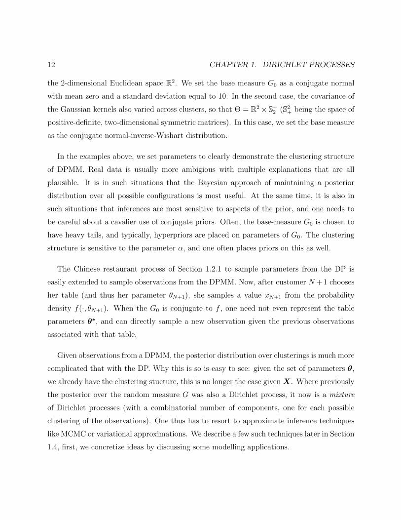
12 CHAPTER 1. DIRICHLET PROCESSES
the 2-dimensional Euclidean space R2. We set the base measure G0 as a conjugate normal
with mean zero and a standard deviation equal to 10. In the second case, the covariance of
the Gaussian kernels also varied across clusters, so that Θ = R2× S+2 (S2
+ being the space of
positive-definite, two-dimensional symmetric matrices). In this case, we set the base measure
as the conjugate normal-inverse-Wishart distribution.
In the examples above, we set parameters to clearly demonstrate the clustering structure
of DPMM. Real data is usually more ambigious with multiple explanations that are all
plausible. It is in such situations that the Bayesian approach of maintaining a posterior
distribution over all possible configurations is most useful. At the same time, it is also in
such situations that inferences are most sensitive to aspects of the prior, and one needs to
be careful about a cavalier use of conjugate priors. Often, the base-measure G0 is chosen to
have heavy tails, and typically, hyperpriors are placed on parameters of G0. The clustering
structure is sensitive to the parameter α, and one often places priors on this as well.
The Chinese restaurant process of Section 1.2.1 to sample parameters from the DP is
easily extended to sample observations from the DPMM. Now, after customer N + 1 chooses
her table (and thus her parameter θN+1), she samples a value xN+1 from the probability
density f(·, θN+1). When the G0 is conjugate to f , one need not even represent the table
parameters θ∗, and can directly sample a new observation given the previous observations
associated with that table.
Given observations from a DPMM, the posterior distribution over clusterings is much more
complicated that with the DP. Why this is so is easy to see: given the set of parameters θ,
we already have the clustering stucture, this is no longer the case givenX. Where previously
the posterior over the random measure G was also a Dirichlet process, it now is a mixture
of Dirichlet processes (with a combinatorial number of components, one for each possible
clustering of the observations). One thus has to resort to approximate inference techniques
like MCMC or variational approximations. We describe a few such techniques later in Section
1.4, first, we concretize ideas by discussing some modelling applications.
1.3. EXAMPLE APPLICATIONS 13
1.3 Example applications
The Dirichlet process has found wide application as a model of clustered data. Often, ap-
plications involve more complicated nonparametric models extending the DP, some of which
we discuss in Section 1.5. Applications include modelling text (clustering words into topics
[45]), modelling images (clustering pixels into segments [41]), genetics (clustering haplotypes
[50]), biostatistics (clustering functional response trajectories of patients [1]), neuroscience
(clustering spikes [49]), as well as fields like cognitive science [16] and econometrics [15]. Even
in density modelling applications, using a DPMM as a prior involves an implicit clustering
of observations, this can be useful in interpreting results. Below, we look at three examples.
1.3.1 Clustering microarray expression data
A microarray experiment returns expression levels yrgt of a group of genes g ∈ {1, . . . , G}across treatment conditions t ∈ {1, . . . , T} over repetitions r ∈ {1, . . . , Rt}. In [9], the
expression levels over repetitions are modelled as i.i.d. draws from a Gaussian with mean
and variance determined by the gene and treatment: yrgt ∼ N (µg + τgt, λ−1g ). Here (µg, λg)
are gene-specific mean and precision parameters, while τgt represent gene-specific treatment
effects. To account for the highly correlated nature of this data, genes are clustered as co-
regulated genes, with elements in the same cluster having the same parameters (µ∗, τ ∗, λ∗).
In [9], this clustering is modelled using a Dirichlet process, with a convenient conjugate base
distribution G0(µ∗, τ ∗, λ∗) governing the distribution of parameters across clusters. Besides
allowing for uncertainty in the number of clusters and the cluster assignments, [9] show how
such a model-based approach allows one to deal with nuisance parameters: in their situation,
they were not interested in the effects of the gene-specific means µg. The model (including
all hyperparameters) was fitted using an MCMC algorithm, and the authors were able to
demonstrate superiority over a number of other clustering methods.

14 CHAPTER 1. DIRICHLET PROCESSES
1.3.2 Bayesian Haplotype inference
Most differences in the genomes of two individuals are variations in single nucleotides at spe-
cific sites in the DNA sequence. These variations are called single nucleotide polymorphisms
(SNPs), and in most cases, individuals in the population have one of two base-pairs at any
SNP site. This results in one of two alleles at each SNP site, labelled either ‘0’ or ‘1’. A
sequence of contiguous alleles in a local region of a single chromosome of an individual is
called a haplotype. Animals like human beings are diploid with two chromosomes, and the
genotype is made up of two haplotypes. Importantly, with present day assaying technology,
the genotype obtained is usually unphased, and does not indicate which haplotype each of
the two base pairs at each site belongs to. Thus, the genotype is a string of ‘00’s,‘11’s and
‘01’s, with the last pair ambiguious about the underlying haplotypes. Given a collection of
length M genotypes from a population, [50] consider the problem of disentangling the two
binary strings (haplotypes) that compose each unphased genotype. To allow statistical shar-
ing across individuals, they treat each haplotype as belonging to one of an infinite number
of clusters, with weights assigned via a Dirichlet process. The parameter of each cluster is
drawn from a product of M independent Bernoulli random variables (this is the base mea-
sure G0), and can be thought of as the cluster prototype. The individual haplotypes in the
cluster differ from the cluster prototype at any location with some small probability of mu-
tation (this forms the kernel f). The two haplotypes of each individual are two independent
samples from the resulting DP mixture model. Given the observed set of genotypes, the
authors infer the latent variables in the model by running an MCMC sampling algorithm.
1.3.3 Spike sorting
Given a sequence of action potentials or spikes recorded by an electrode implanted in an
animal, a neuroscientist has to contend with the fact that a single recording includes activ-
ity from multiple neurons. Spike sorting is essentially the process of clustering these action
potentials, assigning each spike in a spike train to an appropriate neuron. The number of
neurons is unknown, and [49] assume an infinite number using a Dirichlet process. Each neu-
ron has its own stereotypical spike shape, which can be modelled using a Gaussian process as
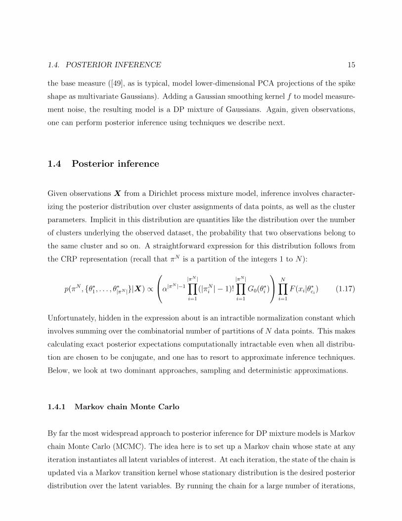
1.4. POSTERIOR INFERENCE 15
the base measure ([49], as is typical, model lower-dimensional PCA projections of the spike
shape as multivariate Gaussians). Adding a Gaussian smoothing kernel f to model measure-
ment noise, the resulting model is a DP mixture of Gaussians. Again, given observations,
one can perform posterior inference using techniques we describe next.
1.4 Posterior inference
Given observations X from a Dirichlet process mixture model, inference involves character-
izing the posterior distribution over cluster assignments of data points, as well as the cluster
parameters. Implicit in this distribution are quantities like the distribution over the number
of clusters underlying the observed dataset, the probability that two observations belong to
the same cluster and so on. A straightforward expression for this distribution follows from
the CRP representation (recall that πN is a partition of the integers 1 to N):
p(πN , {θ∗1, . . . , θ∗|πN |}|X) ∝
α|πN |−1
|πN |∏i=1
(|πNi | − 1)!
|πN |∏i=1
G0(θ∗i )
N∏i=1
F (xi|θ∗ci) (1.17)
Unfortunately, hidden in the expression about is an intractible normalization constant which
involves summing over the combinatorial number of partitions of N data points. This makes
calculating exact posterior expectations computationally intractable even when all distribu-
tion are chosen to be conjugate, and one has to resort to approximate inference techniques.
Below, we look at two dominant approaches, sampling and deterministic approximations.
1.4.1 Markov chain Monte Carlo
By far the most widespread approach to posterior inference for DP mixture models is Markov
chain Monte Carlo (MCMC). The idea here is to set up a Markov chain whose state at any
iteration instantiates all latent variables of interest. At each iteration, the state of the chain is
updated via a Markov transition kernel whose stationary distribution is the desired posterior
distribution over the latent variables. By running the chain for a large number of iterations,
16 CHAPTER 1. DIRICHLET PROCESSES
we obtain a sequence of samples of the unobserved variables whose empirical distribution
converges to the posterior distribution. After discarding initial ‘burn-in’ samples corrupted
by the arbitrary initialization of the chain, the remaining samples can be used to calculate
posterior expectations and to make predictions. Typical quantities of interest include the
probability two observations are co-clustered (often represented by a co-occurence matrix),
the posterior over the number and sizes of clusters, and the posterior over cluster parameters.
Note that each MCMC sample describes a hard clustering of the observations, and very often
a single sample is used to obtain a ‘typical’ clustering of observations.
The different representations of the DP outlined in the earlier sections can be exploited
to construct different samplers with different properties. The simplest class of samplers
are marginal samplers that integrate out the infinite dimensional probability measure G,
and directly represent the partition structure of the data [10]. Both the Chinese restau-
rant process and the Polya urn scheme provide such representations, moreover, they provide
straightforward cluster assignment rules for the last observation. Exploiting the exchange-
ability of these processes, one cycles through all observations, and treating each as the last,
assigns it to a cluster given the cluster assignments of all other observations, and the cluster
parameters.
Algorithm 1.4.1 outlines the steps involved, the most important being step 4. In words,
the probability an observation is assigned to an existing cluster is proportional to the number
of the remaining observations assigned to that cluster, and to how well the cluster parameter
explains the observation value. The observation is assigned to a new cluster with probability
proportional to the product of α and its marginal probability integrating θ out. When the
base measure G0 is conjugate, the latter integration is easy. The nonconjugate case needs
some care, and we refer the reader to [32] for an authoritative account of marginal Gibbs
sampling methods for the DP.

1.4. POSTERIOR INFERENCE 17
Algorithm An iteration of MCMC using the CRP representation
Input: The observations (x1, . . . , xN)
A partition π of the observations, and the cluster parameters θ∗
Output: A new partition π, and new cluster parameters θ∗
1. for i from 1 to N do:
2. Discard cluster assignment ci of observation i, and call the updated partition π\i.
3. If i belonged to its own cluster, discard θci from θ∗.
4. Update π from π\i by assigning i to a cluster with probability
p(ci = k|π\i,θ∗) ∝
|π\ik |f(xi, θ
∗k) k ≤ |π\i|
α∫
Θf(xi, θ)G0(dθ) k = |π\i|+ 1
5. If we assign i to a new cluster, sample a cluster parameter from
p(θ∗ci |π, x1, . . . , xN) ∝ G0(θ∗ci)f(xi, θ∗ci
)
6. end for
7. Resample new cluster parameters θ∗c (with c ∈ {1, . . . , π|}) from the posterior
p(θ∗c |π, x1, . . . , xN) ∝ G0(θ∗c )∏
i s.t. ci=c
f(xi, θ∗c )
While the Gibbs sampler described above is intuitive and easy to implement, it makes very
local moves, making it difficult for the chain to explore multiple posterior modes. Consider
a fairly common situation where two clusterings are equally plausible under the posterior,
one where a set of observations are all allocated to a single cluster, and one where they are
split into two nearby clusters. One would hope that the MCMC sampler spends an equal
amount of time in both configurations, moving from one to the other. However splitting a
18 CHAPTER 1. DIRICHLET PROCESSES
cluster into two requires the Gibbs sampler to sequentially detach observations from a large
cluster, and assign them to a new cluster. The rich-get-richer property of the CRP, which
encourages parsimony by penalizing fragmented clusterings, makes these intermediate states
unlikely, and results in a low probability valley separating these two states. This can lead
to the sampler mixing poorly. To overcome this, one needs to interleave the Gibbs updates
with more complex Metropolis-Hastings proposals that attempt to split or merge clusters.
Marginal samplers that attempt more global moves include [20] and [27].
A second class of samplers are called blocked or conditional Gibbs samplers, and explicitly
represent the latent mixing probability measure G. Since the observations are drawn i.i.d.
from G, conditioned on it, the assignment of observations to the components of G can
be jointly updated. Thus, unlike the marginal Gibbs sampler, conditioned on G, the new
partition structure of the observations is independent of the old. A complication is that
the measure G is infinite-dimensional, and cannot be represented exactly in a computer
simulation. A common approach is to follow [19] and maintain an approximation to G by
truncating the the stick-breaking construction to a finite number of components.
Since the DP weights are stochastically ordered under the stick-breaking construction, one
would expect only a small error for a sufficiently large truncation. In fact, [19] show that if
the stick-breaking process is truncated after K steps, then the error decreases exponentially
with K. Letting N be the number of observations, and ‖G− GK‖1 =∫
Θ|G(dθ)− GK(dθ)|
be the L1-distance between G and its truncated version GK , we have
‖G− GK‖1 ∼ 4N exp (−(K − 1)α) (1.18)
As [19] point out, for N = 150 and α = 5, a truncation level of K = 150 results in an error
bound of 4.57×10⁻⁸, making it effectively indistinguishable from the true model. Algorithm
1.4.1 outlines a conditional sampler with truncation.
1.4. POSTERIOR INFERENCE 19
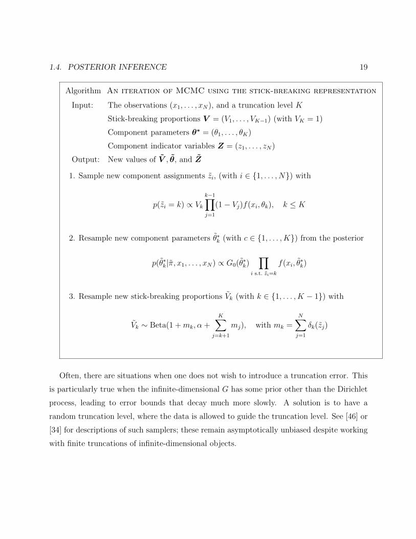
Algorithm An iteration of MCMC using the stick-breaking representation
Input: The observations (x1, . . . , xN), and a truncation level K
Stick-breaking proportions V = (V1, . . . , VK−1) (with VK = 1)
Component parameters θ∗ = (θ1, . . . , θK)
Component indicator variables Z = (z1, . . . , zN)
Output: New values of V , θ, and Z
1. Sample new component assignments zi, (with i ∈ {1, . . . , N}) with
p(zi = k) ∝ Vk
k−1∏j=1
(1− Vj)f(xi, θk), k ≤ K
2. Resample new component parameters θ∗k (with c ∈ {1, . . . , K}) from the posterior
p(θ∗k|π, x1, . . . , xN) ∝ G0(θ∗k)∏
i s.t. zi=k
f(xi, θ∗k)
3. Resample new stick-breaking proportions Vk (with k ∈ {1, . . . , K − 1}) with
Vk ∼ Beta(1 +mk, α +K∑
j=k+1
mj), with mk =N∑j=1
δk(zj)
Often, there are situations when one does not wish to introduce a truncation error. This
is particularly true when the infinite-dimensional G has some prior other than the Dirichlet
process, leading to error bounds that decay much more slowly. A solution is to have a
random truncation level, where the data is allowed to guide the truncation level. See [46] or
[34] for descriptions of such samplers; these remain asymptotically unbiased despite working
with finite truncations of infinite-dimensional objects.
20 CHAPTER 1. DIRICHLET PROCESSES
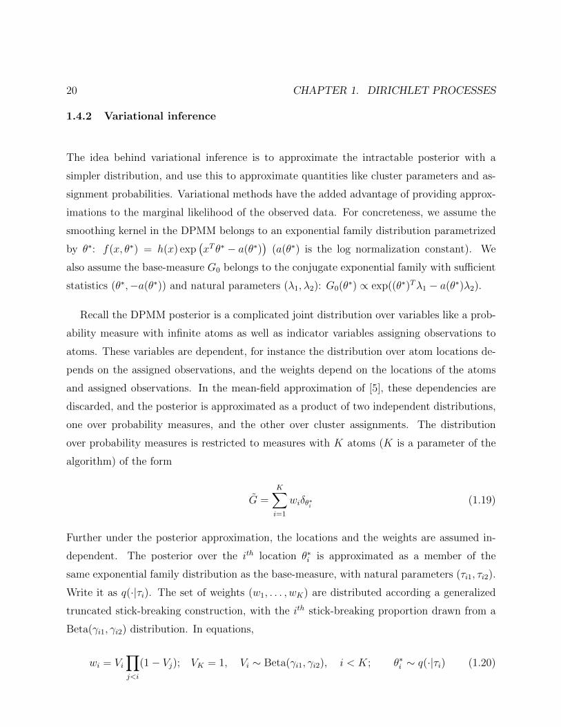
1.4.2 Variational inference
The idea behind variational inference is to approximate the intractable posterior with a
simpler distribution, and use this to approximate quantities like cluster parameters and as-
signment probabilities. Variational methods have the added advantage of providing approx-
imations to the marginal likelihood of the observed data. For concreteness, we assume the
smoothing kernel in the DPMM belongs to an exponential family distribution parametrized
by θ∗: f(x, θ∗) = h(x) exp(xT θ∗ − a(θ∗)
)(a(θ∗) is the log normalization constant). We
also assume the base-measure G0 belongs to the conjugate exponential family with sufficient
statistics (θ∗,−a(θ∗)) and natural parameters (λ1, λ2): G0(θ∗) ∝ exp((θ∗)Tλ1 − a(θ∗)λ2).
Recall the DPMM posterior is a complicated joint distribution over variables like a prob-
ability measure with infinite atoms as well as indicator variables assigning observations to
atoms. These variables are dependent, for instance the distribution over atom locations de-
pends on the assigned observations, and the weights depend on the locations of the atoms
and assigned observations. In the mean-field approximation of [5], these dependencies are
discarded, and the posterior is approximated as a product of two independent distributions,
one over probability measures, and the other over cluster assignments. The distribution
over probability measures is restricted to measures with K atoms (K is a parameter of the
algorithm) of the form
G =K∑i=1
wiδθ∗i (1.19)
Further under the posterior approximation, the locations and the weights are assumed in-
dependent. The posterior over the ith location θ∗i is approximated as a member of the
same exponential family distribution as the base-measure, with natural parameters (τi1, τi2).
Write it as q(·|τi). The set of weights (w1, . . . , wK) are distributed according a generalized
truncated stick-breaking construction, with the ith stick-breaking proportion drawn from a
Beta(γi1, γi2) distribution. In equations,
wi = Vi∏j<i
(1− Vj); VK = 1, Vi ∼ Beta(γi1, γi2), i < K; θ∗i ∼ q(·|τi) (1.20)
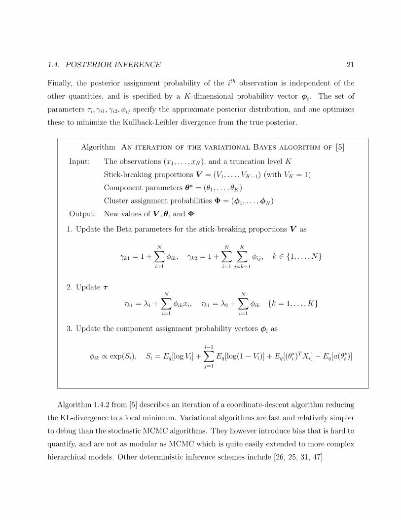
1.4. POSTERIOR INFERENCE 21
Finally, the posterior assignment probability of the ith observation is independent of the
other quantities, and is specified by a K-dimensional probability vector φi. The set of
parameters τi, γi1, γi2, φij specify the approximate posterior distribution, and one optimizes
these to minimize the Kullback-Leibler divergence from the true posterior.
Algorithm An iteration of the variational Bayes algorithm of [5]
Input: The observations (x1, . . . , xN), and a truncation level K
Stick-breaking proportions V = (V1, . . . , VK−1) (with VK = 1)
Component parameters θ∗ = (θ1, . . . , θK)
Cluster assignment probabilities Φ = (φ1, . . . ,φN)
Output: New values of V ,θ, and Φ
1. Update the Beta parameters for the stick-breaking proportions V as
γk1 = 1 +N∑i=1
φik, γk2 = 1 +N∑i=1
K∑j=k+1
φij, k ∈ {1, . . . , N}
2. Update τ
τk1 = λ1 +N∑i=1
φikxi, τk1 = λ2 +N∑i=1
φik {k = 1, . . . , K}
3. Update the component assignment probability vectors φi as
φik ∝ exp(Si), Si = Eq[log Vi] +i−1∑j=1
Eq[log(1− Vi)] + Eq[(θ∗i )TXi]− Eq[a(θ∗t )]
Algorithm 1.4.2 from [5] describes an iteration of a coordinate-descent algorithm reducing
the KL-divergence to a local minimum. Variational algorithms are fast and relatively simpler
to debug than the stochastic MCMC algorithms. They however introduce bias that is hard to
quantify, and are not as modular as MCMC which is quite easily extended to more complex
hierarchical models. Other deterministic inference schemes include [26, 25, 31, 47].
22 CHAPTER 1. DIRICHLET PROCESSES
1.4.3 Comments on posterior computation
In general, beyond a little additional bookkeeping, these algorithms for posterior inference are
not much less efficient than those for the corresponding finite mixture models. For MCMC
sampling algorithms (especially without truncation), the number of clusters will vary from it-
eration to iteration, and a balance must be struck between reallocating/deallocating memory
for the various data structures, and maintaining large and fragmented data structures.
As far as MCMC sampling is concerned, marginal samplers are generally acknowledged
to have better mixing properties, though they usually require some form of split-merge to
get out of local optima. Conditional samplers can suffer from correlations between cluster
assignments and Dirichlet process weights, though the fact that observations can be assigned
to clusters independently offers promise for parallelized algorithms. Samplers are typically
run for 5000 to 10000 iterations, and mixing is assessed using standard MCMC diagnostics
[7] on statistics like the number of clusters, the probability two observations are co-clustered
or the size of the cluster an observation is assigned to.
While variational algorithms offer a number of advantages, these often get trapped in
local optima and might require multiple reruns. Additionally, the mean-field nature of these
algorithms results in updates that are no longer sparse: unlike an MCMC update which
conditions on the cluster assignments of a set of observations, a variational update typically
depends on the probabilities of each observation being assigned to all clusters. Thus, even if
a variational algorithm requires fewer iterations than an MCMC sampler, each update can
require more computation that an MCMC update.
1.5 Extensions
1.5.1 Exchangeability and consistency
Our concern in this chapter was the study of Bayesian nonparametric approaches to clus-
tering. Abstractly, this can viewed as the study of flexible probability distributions over
1.5. EXTENSIONS 23
partitions of integers. Via the Dirichlet process, we arrived at the Ewens’ sampling for-
mula (equation (1.10)) giving probabilities of partitions of the integers 1 to N . Though
constructed sequentially via the Chinese restaurant process, we saw that the resulting prob-
ability is exchangeable: it is independent of the order in which the customers arrive, and is
thus invariant to permutations of the integers 1 to N . Exchangeability is important in many
clustering applications where we do not want the order of observations to affect inferences.
The Ewens’ sampling formula also has a consistency (or projectivity) property: the prob-
ability of πN is equal to the sum of the probabilities of all partitions πN+1 of 1 to N + 1 that
are consistent with πN . Consistency follows directly from the sequential construction of the
CRP and is an important property as well: we do not want observations that were not seen
to affect our inferences, these should remain irrelevant. A sequence of consistent partitions
for all natural numbers implies a distribution over partitions of the natural numbers N [35],
and when each finite distribution is exchangeable as well, the resulting distribution is called
an infinitely exchangeable partition function (EPPF).
There is another way to see why Ewens’ sampling formula is infinitely exchangeable: this
is a consequence of the fact that the observations are drawn i.i.d. from the DP-distributed
probability measure G. Conditioned on G, the order of the observations is irrelevant, and will
remain so with G integrated out. Consistency is an easy consequence of the i.i.d. construction
as well. According to de Finetti’s theorem [22], for any sequence of infinitely exchangeable
observations, there exists a latent variable (possible infinite dimensional), conditioned on
which, the observations are i.i.d. For the CRP, this latent variable is the DP-distributed
probability G. Drawing observations i.i.d. from G induces a partition of N with observa-
tions with the same value in the same cluster. Treating these values as colours drawn i.i.d.
from a ‘paintbox’ G, Kingman’s paintbox construction [24] specializes de Finetti’s theo-
rem to infinitely exchangeable partitions: any infinite EPPF has a mixture of paintboxes
respresentation, and can be induced by sampling from a random probability measure G.
Even if one is only interested in the clustering of observations, a consistent, exchange-
able distribution over clusterings corresponds to an underlying random measure G. This
viewpoint can facilitate the study of asymptotics of clustering processes, the development of
24 CHAPTER 1. DIRICHLET PROCESSES
100 101 102 103 104 105 106
Number of customers
100
101
102
103
Num
bero
ftab
les
α = 100, d = 0
α = 10, d = 0
α = 1, d = 0
100 101 102 103 104 105 106
Number of customers
100
101
102
103
104
Num
bero
ftab
les
α = 10, d = 0.5
α = 1, d = 0.5
α = 10, d = 0.2
α = 1, d = 0.2
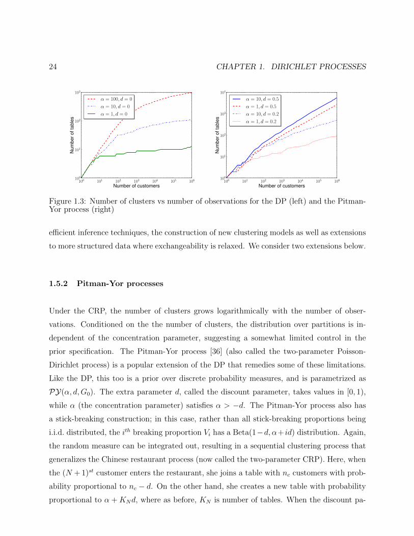
Figure 1.3: Number of clusters vs number of observations for the DP (left) and the Pitman-Yor process (right)
efficient inference techniques, the construction of new clustering models as well as extensions
to more structured data where exchangeability is relaxed. We consider two extensions below.
1.5.2 Pitman-Yor processes
Under the CRP, the number of clusters grows logarithmically with the number of obser-
vations. Conditioned on the the number of clusters, the distribution over partitions is in-
dependent of the concentration parameter, suggesting a somewhat limited control in the
prior specification. The Pitman-Yor process [36] (also called the two-parameter Poisson-
Dirichlet process) is a popular extension of the DP that remedies some of these limitations.
Like the DP, this too is a prior over discrete probability measures, and is parametrized as
PY(α, d,G0). The extra parameter d, called the discount parameter, takes values in [0, 1),
while α (the concentration parameter) satisfies α > −d. The Pitman-Yor process also has
a stick-breaking construction; in this case, rather than all stick-breaking proportions being
i.i.d. distributed, the ith breaking proportion Vi has a Beta(1−d, α+ id) distribution. Again,
the random measure can be integrated out, resulting in a sequential clustering process that
generalizes the Chinese restaurant process (now called the two-parameter CRP). Here, when
the (N + 1)st customer enters the restaurant, she joins a table with nc customers with prob-
ability proportional to nc − d. On the other hand, she creates a new table with probability
proportional to α +KNd, where as before, KN is number of tables. When the discount pa-
1.5. EXTENSIONS 25
rameter equals 0, the Pitman-Yor process reduces to the Dirichlet process. Setting d greater
than 0 allows the probability of a new cluster to increase with the number of existing clusters,
and results in a power-law behaviour:
KN
Nd→ Sd (1.21)
Here Sd is a strictly positive random variable (having the so-called polynomially-tilted
Mittag-Leffler distribution [35]). Power law behaviour has been observed in models of text
and images, and applications of the PY process in these domains [42, 41] have been shown
to perform significantly better than the DP (or simpler parametric models).
The two-parameter CRP representation of the PY-process allows us to write down an
EPPF that generalizes Ewens’ sampling formula:
P (πN) =[α + d]KN−1
d
[α + 1]N1
KN∏c=1
[1− d]nc1 (1.22)
The EPPF above belongs to what is known as a Gibbs-type prior : there exist two sequences
of nonnegative reals v = (v0, v1, . . .) and w = (w1, w2, . . .) such that the probability of a
partition πN is
P (πN) ∝ w|πN |
|πN |∏c=1
v|πNc | (1.23)
This results in a simple sequential clustering process: given a partition πN , the probabil-
ity that customer N + 1 joins cluster c ≤ |πN | is proportional to v|πNc |+1/v|πN
c |, while the
probability of creating a new cluster is v1w|πN |+1/w|πN |. [35] shows that any exchangeable
and consistent Gibbs partition must result from a Pitman-Yor process or an m-dimensional
Dirichlet distribution (or various limits of these). The CRP for the finite Dirichlet distri-
bution has α = −κ < 0 and d = mκ for some m = 1, 2, . . .. Any other consistent and
exchangeable distribution over partitions will result in a more complicated EPPF (and thus,
for example, a more complicated Gibbs sampler). For more details, see [4]
26 CHAPTER 1. DIRICHLET PROCESSES
1.5.3 Dependent random measures
The assumption of exchangeability is sometimes a simplification that disregards structure
in data. Observations might come labelled with ordinates like time, position or category,
and lumping all data points into one homogeneous collection can be undesirable. The other
extreme of assigning each group an independent clustering is also a simplification, it is
important to share statistical information across groups. For instance, a large cluster in
one region of space in one group might a priori suggest a similar cluster in other groups as
well. A popular extension of the DP that achieves this is the hierarchical Dirichlet process
(HDP)[45]. Here, given a set of groups T , any group t ∈ T has its own DP-distributed
random measure Gt (so that observations within each group are exchangeable). The random
measures are coupled via a shared, random base measure G which itself is distributed as a
DP. The resulting hierarchical model corresponds to the following generative process:
G ∼ DP(α0, G0) (1.24)
Gt ∼ DP(α,G) for all t ∈ T (1.25)
θit ∼ Gt for i in 1 to Nt (1.26)
In our discussion so far, we have implicitly assumed the DP base measure to be smooth.
For the group-specific probability measures Gt of the HDP, this is not the case; now, the
base measure G (which itself is DP-distributed) is purely atomic. A consequence is that the
parameters of clusters across groups (which are drawn from G) now have nonzero probability
of being identical. In fact, these parameters themselves are clustered according to a CRP, and
[45] show how all random measures can be marginalized out to give a sequential clustering
process they call the Chinese restaurant franchise. The clustering of parameters means
that the more often a parameter is present, the more likely it is to appear in a new group.
Additionally, a large cluster in one group implies (on average) large clusters (with the same
parameter) in other groups.
A very popular application of the HDP is the construction of infinite topic models for
document modelling. Given a fixed vocabulary of words, a topic is a multinomial distribution
over words. A document, on the other hand, is characterized by a distribution over topics,
1.5. EXTENSIONS 27
20 10 0 10 20
15
10
5
0
5
10
15
20
20 10 0 10 20
1510
50
510
1520
20 40 60 80 100 120
800
900
1000
1100
Number of topics
Per
plex
ity
LDAHDP
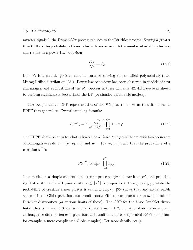
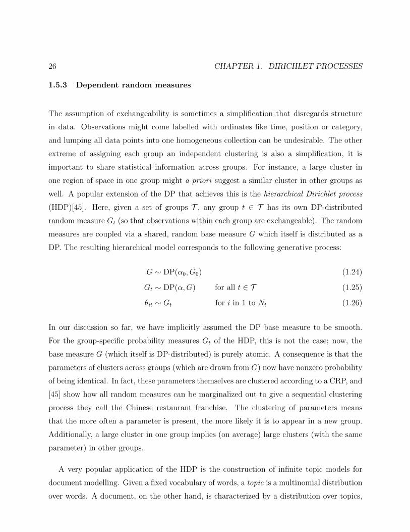
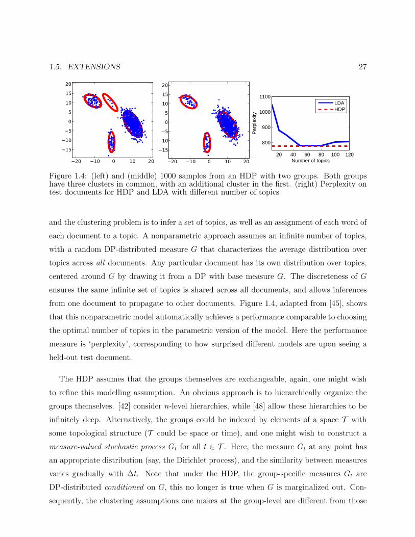
Figure 1.4: (left) and (middle) 1000 samples from an HDP with two groups. Both groupshave three clusters in common, with an additional cluster in the first. (right) Perplexity ontest documents for HDP and LDA with different number of topics
and the clustering problem is to infer a set of topics, as well as an assignment of each word of
each document to a topic. A nonparametric approach assumes an infinite number of topics,
with a random DP-distributed measure G that characterizes the average distribution over
topics across all documents. Any particular document has its own distribution over topics,
centered around G by drawing it from a DP with base measure G. The discreteness of G
ensures the same infinite set of topics is shared across all documents, and allows inferences
from one document to propagate to other documents. Figure 1.4, adapted from [45], shows
that this nonparametric model automatically achieves a performance comparable to choosing
the optimal number of topics in the parametric version of the model. Here the performance
measure is ‘perplexity’, corresponding to how surprised different models are upon seeing a
held-out test document.
The HDP assumes that the groups themselves are exchangeable, again, one might wish
to refine this modelling assumption. An obvious approach is to hierarchically organize the
groups themselves. [42] consider n-level hierarchies, while [48] allow these hierarchies to be
infinitely deep. Alternatively, the groups could be indexed by elements of a space T with
some topological structure (T could be space or time), and one might wish to construct a
measure-valued stochastic process Gt for all t ∈ T . Here, the measure Gt at any point has
an appropriate distribution (say, the Dirichlet process), and the similarity between measures
varies gradually with ∆t. Note that under the HDP, the group-specific measures Gt are
DP-distributed conditioned on G, this no longer is true when G is marginalized out. Con-
sequently, the clustering assumptions one makes at the group-level are different from those
28 CHAPTER 1. DIRICHLET PROCESSES
specified under a DP. An active area of research is the construction of dependent random
probability measures with specified marginal distributions over probability measures, as well
as flexible correlation structures [30].
1.6 Discussion
In this chapter, we introduced the Dirichlet process, and described various theoretical and
practical aspects of its use in clustering applications. There is a vast literature on this topic,
and a number of excellent tutorials. Among these we especially recommend [43, 44, 14].
In spite of its nonparametric nature, the modelling assumptions underlying the DP can be
quite strong. While we briefly discussed a few extensions, there is much we have had to leave
uncovered (see [28] for a nice overview). Many generalizations build on the stick-breaking
representation or the CRP representation of the DP. Another approach extends the DP’s
construction as a normalized Gamma process [12] to construct random probability measures
by normalizing completely random measures [23]; these are atomic measures whose weights
wi are essentially all independent. The resulting class of normalized random measures [21]
form a very flexible class of nonparametric priors that can be used to construct different
extensions of the DP (see for example, [37]).
A different class of nonparametric priors are based on the Beta process [18], and are used
to construct infinite feature models [17]. Here, rather than assigning each observation to one
of a infinite number of clusters, each observation can have a finite subset of a infinite number
of features. Such a distributed representation allows a more refined representation for sharing
statistical information. Infinite feature models also come with notions of exchangeability and
consistency. We recommend [6] for a nice overview of these ideas, and their relation to ideas
discussed here.
A major challenge facing the more widespread use of Bayesian nonparametric methods
is the development of techniques for efficient inference. While we described a few MCMC
and variational approaches, there are many more. More recent areas of research include the
development of algorithms for online inference and parallel inference.
1.7. ACKNOWLEDGEMENTS 29
Finally, there is scope for a more widespread application of nonparametric methods to
practical problems. As our understanding of the properties of these models develops, it
is important that they are applied thoughtfully. At the end, these priors represent rich
and sophisticated modelling assumptions, and should be treated as such, rather than as
convenient ways of bypassing the question “how many clusters?”.
1.7 Acknowledgements
We thank Marina Meila and Ricardo Silva for reading and suggesting improvements to
earlier versions of this chapter. We also thank Jan Gasthaus and Yee Whye Teh for helpful
discussions.
References
[1] J. L. Bigelow and D. B. Dunson. Bayesian semiparametric joint models for functional
predictors. Journal of the American Statistical Association, 104(485):26–36, 2009.
[2] D. Blackwell. Discreteness of Ferguson selections. The Annals of Statistics, 1(2):356–
358, 1973.
[3] D. Blackwell and J. B. MacQueen. Ferguson distributions via Polya urn schemes. Annals
of Statistics, 1:353–355, 1973.
[4] P. De Blasi, S. Favaro, A. Lijoi, R. H. Mena, I. Prunster, and M. Ruggiero. Are Gibbs-
type priors the most natural generalization of the Dirichlet process? DEM Working
Papers Series 054, University of Pavia, Department of Economics and Management,
October 2013.
[5] D. M. Blei and M. I. Jordan. Variational inference for Dirichlet process mixtures.
Bayesian Analysis, 1(1):121–144, 2006.
[6] T. Broderick, M. I. Jordan, and J. Pitman. Clusters and features from combinatorial
stochastic processes. pre-print, June 2012. 1206.5862.
30 CHAPTER 1. DIRICHLET PROCESSES
[7] S. P. Brooks and A. Gelman. General methods for monitoring convergence of iterative
simulations. Journal of Computational and Graphical Statistics, 7(4):434–455, 1998.
[8] G. Casella. An introduction to empirical Bayes data analysis. The American Statistician,
39(2):pp. 83–87, 1985.
[9] D. B. Dahl. Model-based clustering for expression data via a Dirichlet process mixture
model. In Kim-Anh Do, Peter Muller, and Marina Vannucci, editors, Bayesian Inference
for Gene Expression and Proteomics. Cambridge University Press, 2006.
[10] M. D. Escobar and M. West. Bayesian density estimation and inference using mixtures.
Journal of the American Statistical Association, 90:577–588, 1995.
[11] W. J. Ewens. The sampling theory of selectively neutral alleles. Theoretical Population
Biology, 3:87–112, 1972.
[12] T. S. Ferguson. A Bayesian analysis of some nonparametric problems. Annals of Statis-
tics, 1(2):209–230, 1973.
[13] C. Fraley and A. E. Raftery. How many clusters? Which clustering method? - Answers
via model-based cluster analysis. Computer Journal, 41:578–588, 1998.
[14] S. Ghosal. The Dirichlet process, related priors, and posterior asymptotics. In Nils Lid
Hjort, Chris Holmes, Peter Muller, and Stephen G. Walker, editors, Bayesian Nonpara-
metrics. Cambridge University Press, 2010.
[15] J. E. Griffin. Inference in infinite superpositions of non-Gaussian Ornstein–Uhlenbeck
Processes using Bayesian nonparametic methods. Journal of Financial Econometrics,
9(3):519–549, 2011.
[16] T. L. Griffiths, K. R. Canini, A. N. Sanborn, and D. J. Navarro. Unifying rational
models of categorization via the hierarchical Dirichlet process. In Proceedings of the
Annual Conference of the Cognitive Science Society, volume 29, 2007.
[17] T. L. Griffiths, Z. Ghahramani, and P. Sollich. Bayesian nonparametric latent feature
models (with discussion and rejoinder). In Bayesian Statistics, volume 8, 2007.
[18] N. L. Hjort. Nonparametric Bayes estimators based on Beta processes in models for life
history data. Annals of Statistics, 18(3):1259–1294, 1990.
[19] H. Ishwaran and L. F. James. Gibbs sampling methods for stick-breaking priors. Journal
of the American Statistical Association, 96(453):161–173, 2001.
[20] S. Jain and R. M. Neal. A split-merge Markov chain Monte Carlo procedure for the
1.7. ACKNOWLEDGEMENTS 31
Dirichlet process mixture model. Technical report, Department of Statistics, University
of Toronto, 2004.
[21] L. F. James, A. Lijoi, and I. Pruenster. Bayesian inference via classes of normalized
random measures. ICER Working Papers - Applied Mathematics Series 5-2005, ICER
- International Centre for Economic Research, April 2005.
[22] O. Kallenberg. Foundations of Modern Probability. Probability and its Applications.
Springer-Verlag, New York, Second edition, 2002.
[23] J. F. C. Kingman. Completely random measures. Pacific Journal of Mathematics,
21(1):59–78, 1967.
[24] J. F. C. Kingman. Random discrete distributions. Journal of the Royal Statistical
Society, 37:1–22, 1975.
[25] K. Kurihara, M. Welling, and Y. W. Teh. Collapsed variational Dirichlet process mixture
models. In Proceedings of the International Joint Conference on Artificial Intelligence,
volume 20, 2007.
[26] K. Kurihara, M. Welling, and N. Vlassis. Accelerated variational DP mixture models.
In Advances in Neural Information Processing Systems, volume 19, 2007.
[27] P. Liang, M. I. Jordan, and B. Taskar. A permutation-augmented sampler for Dirichlet
process mixture models. In Proceedings of the International Conference on Machine
Learning, 2007.
[28] A. Lijoi and I. Pruenster. Models beyond the Dirichlet process. In N. Hjort, C. Holmes,
P. Muller, and S. Walker, editors, Bayesian Nonparametrics: Principles and Practice.
Cambridge University Press, 2010.
[29] A.Y. Lo. On a class of Bayesian nonparametric estimates: I. density estimates. Annals
of Statistics, 12(1):351–357, 1984.
[30] S. MacEachern. Dependent nonparametric processes. In Proceedings of the Section on
Bayesian Statistical Science. American Statistical Association, 1999.
[31] T. P. Minka and Z. Ghahramani. Expectation propagation for infinite mixtures. Pre-
sented at NIPS2003 Workshop on Nonparametric Bayesian Methods and Infinite Mod-
els, 2003.
[32] R. M. Neal. Markov chain sampling methods for Dirichlet process mixture models.
Journal of Computational and Graphical Statistics, 9:249–265, 2000.
32 CHAPTER 1. DIRICHLET PROCESSES
[33] P. Orbanz. Projective limit random probabilities on Polish spaces. Electron. J. Stat.,
5:1354–1373, 2011.
[34] O. Papaspiliopoulos and G. O. Roberts. Retrospective Markov chain Monte Carlo
methods for Dirichlet process hierarchical models. Biometrika, 95(1):169–186, 2008.
[35] J. Pitman. Combinatorial stochastic processes. Technical Report 621, Department of
Statistics, University of California at Berkeley, 2002. Lecture notes for St. Flour Summer
School.
[36] J. Pitman and M. Yor. The two-parameter Poisson-Dirichlet distribution derived from
a stable subordinator. Annals of Probability, 25:855–900, 1997.
[37] V. Rao and Y. W. Teh. Spatial normalized gamma processes. In Advances in Neural
Information Processing Systems, 2009.
[38] C. E. Rasmussen. The infinite Gaussian mixture model. In Advances in Neural Infor-
mation Processing Systems, volume 12, 2000.
[39] S. Richardson and P. J. Green. On Bayesian analysis of mixtures with an unknown
number of components. Journal of the Royal Statistical Society, 59(4):731–792, 1997.
[40] J. Sethuraman. A constructive definition of Dirichlet priors. Statistica Sinica, 4:639–650,
1994.
[41] E. B. Sudderth and M. I. Jordan. Shared segmentation of natural scenes using dependent
pitman-yor processes. In Advances in Neural Information Processing Systems, pages
1585–1592, 2008.
[42] Y. W. Teh. A hierarchical Bayesian language model based on Pitman-Yor processes.
In Proc. of the 21st International Conference on Comp. Linguistics and 44th Annual
Meeting of the Association for Comp. Linguistics, pages 985–992, 2006.
[43] Y. W. Teh. Dirichlet processes. In Encyclopedia of Machine Learning. Springer, 2010.
[44] Y. W. Teh and M. I. Jordan. Hierarchical Bayesian nonparametric models with appli-
cations. In N. Hjort, C. Holmes, P. Muller, and S. Walker, editors, Bayesian Nonpara-
metrics: Principles and Practice. Cambridge University Press, 2010.
[45] Y. W. Teh, M. I. Jordan, M. J. Beal, and D. M. Blei. Hierarchical Dirichlet processes.
Journal of the American Statistical Association, 101(476):1566–1581, 2006.
[46] S. G. Walker. Sampling the Dirichlet mixture model with slices. Communications in
Statistics - Simulation and Computation, 36:45, 2007.
1.7. ACKNOWLEDGEMENTS 33
[47] L. Wang and D. B. Dunson. Fast Bayesian inference in Dirichlet process mixture models.
Journal of Computational and Graphical Statistics, 2010.
[48] F. Wood, J. Gasthaus, C. Archambeau, L. James, and Y. W. Teh. The sequence
memoizer. Communications of the Association for Computing Machines, 54(2):91–98,
2011.
[49] F. Wood, S. Goldwater, and M. J. Black. A non-parametric Bayesian approach to
spike sorting. In Proceedings of the IEEE Conference on Engineering in Medicine and
Biologicial Systems, volume 28, 2006.
[50] E. P. Xing, M. I. Jordan, and R. Sharan. Bayesian haplotype inference via the Dirichlet
process. Journal of Computational Biology, 14:267–284, 2007.