Handbook of Erosion Modelling

Edited by

R.P.C. MorganNational Soil Resources Institute

Cranfield University

and

M.A. NearingUSDA-ARS

Southwest Watershed Research Center

A John Wiley & Sons, Ltd., Publication

9781405190107_1_pretoc.indd iii9781405190107_1_pretoc.indd iii 10/15/2010 2:32:08 AM10/15/2010 2:32:08 AM

9781405190107_1_pretoc.indd ii9781405190107_1_pretoc.indd ii 10/15/2010 2:32:08 AM10/15/2010 2:32:08 AM

HANDBOOK OF EROSION MODELLING

9781405190107_1_pretoc.indd i9781405190107_1_pretoc.indd i 10/15/2010 2:32:07 AM10/15/2010 2:32:07 AM

9781405190107_1_pretoc.indd ii9781405190107_1_pretoc.indd ii 10/15/2010 2:32:08 AM10/15/2010 2:32:08 AM

Handbook of Erosion Modelling

Edited by

R.P.C. MorganNational Soil Resources Institute

Cranfield University

and

M.A. NearingUSDA-ARS

Southwest Watershed Research Center

A John Wiley & Sons, Ltd., Publication

9781405190107_1_pretoc.indd iii9781405190107_1_pretoc.indd iii 10/15/2010 2:32:08 AM10/15/2010 2:32:08 AM

This edition first published 2011, © 2011 by Blackwell Publishing Ltd

Blackwell Publishing was acquired by John Wiley & Sons in February 2007. Blackwell’s publishing program has been merged with Wiley’s global Scientific, Technical and Medical business to form Wiley-Blackwell.

Registered OfficeJohn Wiley & Sons Ltd, The Atrium, Southern Gate, Chichester, West Sussex, PO19 8SQ, UK

Editorial Offices9600 Garsington Road, Oxford, OX4 2DQ, UK

The Atrium, Southern Gate, Chichester, West Sussex, PO19 8SQ, UK111 River Street, Hoboken, NJ 07030-5774, USA

For details of our global editorial offices, for customer services and for information about how toapply for permission to reuse the copyright material in this book please see our website at

www.wiley.com/wiley-blackwell

The right of the author to be identified as the author of this work has been asserted in accordance with the Copyright, Designs and Patents Act 1988.

All rights reserved. No part of this publication may be reproduced, stored in a retrieval system, or transmitted,in any form or by any means, electronic, mechanical, photocopying, recording or otherwise, except as permitted

by the UK Copyright, Designs and Patents Act 1988, without the prior permission of the publisher.

Wiley also publishes its books in a variety of electronic formats. Some content that appears in print may not be available in electronic books.

Designations used by companies to distinguish their products are often claimed as trademarks. All brand names and product names used in this book are trade names, service marks, trademarks or registered trademarks oftheir respective owners. The publisher is not associated with any product or vendor mentioned in this book.

This publication is designed to provide accurate and authoritative information in regard to the subjectmatter covered. It is sold on the understanding that the publisher is not engaged in rendering professional

services. If professional advice or other expert assistance is required, the services of a competent professional should be sought.

Library of Congress Cataloguing-in-Publication Data

Handbook of erosion modelling / edited by R.P.C. Morgan and M.A. Nearing. p. cm.

Includes bibliographical references and index.ISBN 978-1-4051-9010-7 (cloth)

1. Soil erosion–Simulation methods. I. Morgan, R.P.C. (Royston Philip Charles), 1942– II. Nearing, M.A. (Mark A.)

S627.M36H36 2011631.4′50113–dc22

2010026596

A catalogue record for this book is available from the British Library.This book is published in the following electronic formats: eBook 9781405190107; Wiley Online Library 9781444328455

Set in 9/11.5pt Trump Mediaeval by SPi Publisher Services, Pondicherry, India

1 2011

9781405190107_1_pretoc.indd iv9781405190107_1_pretoc.indd iv 10/15/2010 2:32:08 AM10/15/2010 2:32:08 AM

List of contributors, vii

1 Introduction, 1 R.P.C. Morgan

PART 1 MODEL DEVELOPMENT, 7

2 Model Development: A User ’s Perspective, 9

R.P.C. Morgan

3 Calibration of Erosion Models, 33 V.G. Jetten and M.P. Maneta

4 Dealing with Uncertaintyin Erosion Model Predictions, 52

K.J. Beven and R.E. Brazier

5 A Case Study of Uncertainty: Applying GLUE to EUROSEM, 80

J.N. Quinton, T. Krueger, J. Freer, R.E. Brazier and G.S. Bilotta

6 Scaling Soil Erosion Models in Space and Time, 98

R.E. Brazier, C.J. Hutton, A.J. Parsons and J. Wainwright

7 Misapplications and Misconceptions of Erosion Models, 117

G. Govers

PART 2 MODEL APPLICATIONS, 135

8 Universal Soil Loss Equation and Revised Universal Soil Loss Equation, 137

K.G. Renard, D.C. Yoder, D.T. Lightle and S.M. Dabney

9 Application of WEPP to Sustainable Management of a Small Catchment in South west Missouri,US, Under Present Land Use and with Climatic Change, 168

J.M. Laflen

10 Predicting Soil Loss andRunoff from Forest Roads and Seasonal Cropping Systems in Brazil using WEPP, 186

A.J.T. Guerra and A. Soaresda Silva

11 Use of GUEST Technology to Parameterize a Physically-Based Model for Assessing SoilErodibility and Evaluating Conservation Practices inTropical Steeplands, 195

C.W. Rose, B. Yu, R.K. Misra, K. Coughlan and B. Fentie

Contents

9781405190107_2_toc.indd v9781405190107_2_toc.indd v 10/18/2010 3:44:58 PM10/18/2010 3:44:58 PM

vi Contents

12 Evaluating Effects of Soiland Water Management andLand Use Change on the Loess Plateau of China usingLISEM, 223

R. Hessel, V.G. Jetten, B. Liu and Y. Qiu

13 Modelling the Role of Vegetated Buffer Strips in Reducing Transfer of Sediment from Land to Watercourses, 249

J.H. Duzant, R.P.C. Morgan,G.A. Wood and L.K. Deeks

14 Predicting Impacts of Land Use and Climate Change on Erosion andSediment Yield in RiverBasins usingSHETRAN, 263

J.C. Bathurst

15 Modelling Impacts of Climatic Change: Case Studies using the New Generation of Erosion Models, 289

J.P. Nunes and M.A. Nearing

16 Risk-Based Erosion Assessment: Application to Forest Watershed Management and Planning, 313

W.J. Elliot and P.R. Robichaud

17 The Future Role of Information Technology in Erosion Modelling, 324

D.P. Guertin and D.C. Goodrich

18 Applications of Long-Term Erosion and Landscape Evolution Models, 339

G.R. Willgoose and G.R. Hancock

19 Gully Erosion: Procedures to Adopt When Modelling Soil Erosion in Landscapes Affected by Gullying, 360

J.W.A. Poesen, D.B. Torri and T. Vanwalleghem

PART 3 FUTURE DEVELOPMENTS, 387

20 The Future of Soil Erosion Modelling, 389

M.A. Nearing and P.B. Hairsine

Index, 398

Colour plates appear in between pages 198–199

9781405190107_2_toc.indd vi9781405190107_2_toc.indd vi 10/18/2010 3:44:58 PM10/18/2010 3:44:58 PM

J .C . BATHURST School of Civil Engineering and Geosciences, Newcastle University, New castle upon Tyne NE1 7RU, United Kingdom

K.J . BEVEN Lancaster Environment Centre, Uni-ve r sity of Lancaster, Lancaster LA1 4YW, United Kingdom; GeoCentrum, Uppsala University, Uppsala, Sweden; ECHO/ISTE, EPFL, Lausanne, Switzerland

G.S . BILOTTA School of Environment and Techno-logy, University of Brighton, Cockcroft Building, Brighton BN2 4GJ, United Kingdom

R.E . BR AZIER School of Geography, University of Exeter, Amory Building, Exeter EX4 4RJ, United Kingdom

K. COUGHL AN P O Box 596, Annerley, Queensland, Australia 4103

S.M. DABNEY USDA-ARS, National Sedimentation Laboratory, 598 McElroy Drive, Oxford, MS 38655, USA

L.K. DEEKS National Soil Resources Institute, Cran-field University, Cranfield, Bedfordshire MK43 0AL, United Kingdom

J.H. DUZANT National Soil Resources Institute, Cran-field University, Cranfield, Bedfordshire MK43 0AL, United Kingdom

W.J. ELLIOT USDA Forest Service, Rocky Moun tain Research Station, 1221 South Main Street, Moscow, ID 83843, USA

B. FENTIE Queensland Department of Environ ment and Resource Management, 80 Meiers Road, Indooroopilly, Queensland, Australia 4068

J . FREER School of Geographical Sciences, Uni-ve rsity of Bristol, University Road, Bristol BS8 1SS, United Kingdom

D.C. GOODRICH USDA-ARS, Southwest Watershed Research Center, 2000 East Allen Road, Tucson, AZ 85719, USA

G. GOVERS Physical and Regional Geography Rese arch Group, Department of Earth and Envi-ro nmental Sciences, Katholieke Universiteit Leuven, GEO-Institute, Celestijnenlaan 200E, 3001 Heverlee, Belgium

A.J .T. GUERR A Department of Geography, Insti-tute of Geosciences, Federal University of Rio de Janeiro, Avenida Jose Luiz Ferraz 250, Apto 1706, CEP.22.790-587, Rio de Janeiro, Brazil

D.P. GUERTIN Landscape Studies Program, School of Natural Resources, University of Arizona, Tucson, AZ 85721, USA

P.B . HAIRSINE CSIRO Land and Water Division, G.P.O.Box 1666, Canberra 2601 Australian Capital Territory, Australia

Contributors

9781405190107_3_posttoc.indd vii9781405190107_3_posttoc.indd vii 10/15/2010 10:16:16 PM10/15/2010 10:16:16 PM

viii Contributors

G.R. HANCOCK School of Environment and Life Sciences, Faculty of Science, The University of Newcastle, Callaghan, New South Wales 2308, Australia

R. HESSEL Soil Science Centre, Alterra, Wage ni-ngen University and Research Centre, P O Box 47, 6700 AA Wageningen, The Netherlands

C.J . HUTTON School of Geography, University of Exeter, Amory Building, Exeter EX4 4RJ, United Kingdom

V.G. JETTEN Department of Earth Systems Ana-lysis, International Institute of Geoinforma tion Science and Earth Observation, Hengelos-estraat 99, P O Box 6, 7500 AA, Enschede, The Netherlands

T. KRUEGER School of Environmental Sciences, University of East Anglia, Norwich NR4 7TJ, United Kingdom

J .M. L AFLEN USDA-ARS (retired), 5784 Highway 9, Buffalo Center, IA 5042, USA

D.T. L IGHTLE USDA-NRCS, National Soil Survey Center, 100 Centennial Mall North, Lincoln, NE 68508-3866, USA

B. L IU School of Geography, Beijing Normal Uni-ve rsity, 19 Xinwai Street, Beijing 100875, China

M.P. MANETA Geosciences Department, Uni ve r-sity of Montana, 32 Campus Drive #1296, Missoula, MT 59812, USA

R.K. MISR A Faculty of Engineering and Survey ing, University of Southern Queensland, Too woomba, Queensland, Australia 4350

R.P.C. MORGAN National Soil Resources Institute, Cranfield University, Cranfield, Bedfordshire MK43 0AL, United Kingdom

M.A. NEARING USDA-ARS, Southwest Water shed Research Center, 2000 East Allen Road, Tucson, AZ 85719, USA

J .P. NUNES Centre for Environmental and Marine Studies (CESAM), Department of Environment and Planning, University of Aveiro, Campus Universitário de Santiago, 3810-193 Aveiro, Portugal

A.J . PARSONS Department of Geography, Uni-ver sity of Sheffield, Sheffield S10 2TN, United Kingdom

J .W.A. POESEN Physical and Regional Geogra phy Research Group, Department of Earth and Environmental Sciences, Katholieke Universiteit Leuven, GEO-Institute, Celestijnenlaan 200E, B-3001 Heverlee, Belgium

Y. QIU School of Geography, Beijing Normal Uni ve rsity, 19 Xinwai Street, Beijing 100875, China

J .N. QUINTON Lancaster Environment Centre, Uni versity of Lancaster, Lancaster LA1 4YQ, United Kingdom

K.G. RENARD USDA-ARS, Southwest Watershed Research Center, 2000 East Allen Road, Tucson, AZ 85719-1596, USA

P.R . ROBICHAUD USDA Forest Service, Rocky Moun tain Research Station, 1221 South Main Street, Moscow, ID 83843, USA

C.W. ROSE The Griffith School of Environment, Griffith University, Nathan Campus, Brisbane, Queensland, Australia 4111

A. SOARES DA SILVA Federal University of Rio de Janeiro, Rua Hermengarda 151, Apto 906 – Meier. CEP.20710-010 Rio de Janeiro, Brazil

D.B. TORRI IRPI CNR, Via Madonna Alta 126, 06128 Perugia, Italy

T. VANWALLEGHEM Department of Agronomy, Institute for Sustainable Agriculture – CSIC, Finca Alameda del Obispo, Apartado Correos 4084, Córdoba 14080, Spain

9781405190107_3_posttoc.indd viii9781405190107_3_posttoc.indd viii 10/15/2010 10:16:16 PM10/15/2010 10:16:16 PM

Contributors ix

J. WAINWRIGHT Department of Geography, Uni-ve rsity of Sheffield, Sheffield S10 2TN, United Kingdom

G.R. WILLGOOSE School of Engineering, Faculty of Engineering and the Built Environment, The University of Newcastle, Callaghan, New South Wales 2308, Australia

G.A. WOOD Integrated Environmental Systems Institute, Cranfield University, Cranfield, Bedford shire MK43 0AL, United Kingdom

D.C. YODER Biosystems Engineering and Soil Science, University of Tennessee, 2506 E J Chapman Drive, Knoxville, TN 37996-4531, USA

B. YU School of Engineering, Griffith University, Nathan Campus, Brisbane, Queensland, Australia 4111

9781405190107_3_posttoc.indd ix9781405190107_3_posttoc.indd ix 10/15/2010 10:16:16 PM10/15/2010 10:16:16 PM

9781405190107_3_posttoc.indd x9781405190107_3_posttoc.indd x 10/15/2010 10:16:16 PM10/15/2010 10:16:16 PM

1 Introduction

R . P. C . M O R G A NNational Soil Resources Institute, Cranfield University, Cranfield, Bedfordshire, UK

The movement of sediment and associated pollut-ants over the landscape and into water bodies is of increasing concern with respect to pollution con-trol, prevention of muddy floods and general envi-ronmental protection. This concern exists whether the sediment is derived from farmland, road banks, construction sites, recreation areas or other sources. In today’s environment it is often consid-ered of equal or even greater importance than the effects of loss of soil on- site, with its implications for declining agricultural productivity, loss of bio-diversity and decreased amenity and landscape val-ues. With the expected changes in climate over coming decades, there is a need to predict how environmental problems associated with sediment are likely to be affected so that appropriate man-agement systems can be put in place.

Whilst it is possible to instrument a few indi-vidual farms and catchments in order to obtain the data to evaluate the current situation and pro-pose best management practices, it is not feasible to study every location on the Earth’s surface in detail. Instead, evaluation and predictive tools need to be applied to assess current problems, predict future trends and provide a scientific base for policy and management decisions. Erosion models can fulfil this function provided that they are robust and used correctly. Despite, or maybe even because of, the vast amount of research over

the last 30 years or more on erosion modelling, potential model- users are confronted with a multiplicity of models from which to choose, often with little guidance on which might be the best for particular circumstances or the steps required to apply a selected model to a given situ-ation. Many models have been tested for only a limited range of conditions of climate, soils and land use, and little information is available to enable a user to assess in advance how well a model might perform under different conditions. Models range from empirical to physically- or process- based, and vary considerably in their complexity and the amount of data input required. Very little guidance is available on how accurate that data input has to be, or what effect different levels of accuracy can have on the accuracy of the model output. Further, sediment problems can exist at scales that range from a farmer’s field or a small construction site to the effects of sediment transport and deposition in small and large catch-ments. Somewhat limited information exists on the range of scales over which different models can operate successfully, leaving the user uncer-tain on whether a particular model is the most appropriate for a given scale. In the worst case, as a result of a lack of clear guidance, the user may choose a totally inappropriate model.

Users can obtain a list of the leading soil ero-sion models from the Internet site http:// soilerosion.net/doc/models_menu.html. Links are pro-vided to other sites associated specifically with each model from which the software can be

Handbook of Erosion Modelling, 1st edition. Edited by R.P.C. Morgan and M.A. Nearing. © 2011 Blackwell Publishing Ltd.

9781405190107_4_001.indd 19781405190107_4_001.indd 1 10/15/2010 2:32:12 AM10/15/2010 2:32:12 AM

2 r.p.c. morgan

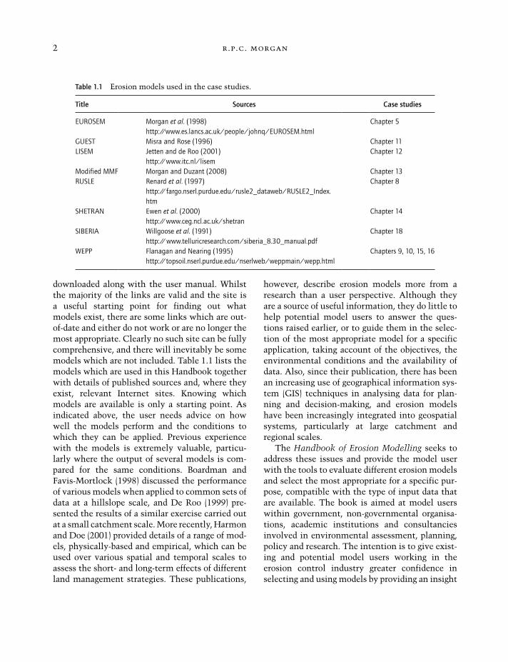
downloaded along with the user manual. Whilst the majority of the links are valid and the site is a useful starting point for finding out what models exist, there are some links which are out- of- date and either do not work or are no longer the most appropriate. Clearly no such site can be fully comprehensive, and there will inevitably be some models which are not included. Table 1.1 lists the models which are used in this Handbook together with details of published sources and, where they exist, relevant Internet sites. Knowing which models are available is only a starting point. As indicated above, the user needs advice on how well the models perform and the conditions to which they can be applied. Previous experience with the models is extremely valuable, particu-larly where the output of several models is com-pared for the same conditions. Boardman and Favis- Mortlock (1998) discussed the performance of various models when applied to common sets of data at a hillslope scale, and De Roo (1999) pre-sented the results of a similar exercise carried out at a small catchment scale. More recently, Harmon and Doe (2001) provided details of a range of mod-els, physically- based and empirical, which can be used over various spatial and temporal scales to assess the short- and long- term effects of different land management strategies. These publications,

however, describe erosion models more from a research than a user perspective. Although they are a source of useful information, they do little to help potential model users to answer the ques-tions raised earlier, or to guide them in the selec-tion of the most appropriate model for a specific application, taking account of the objectives, the environmental conditions and the availability of data. Also, since their publication, there has been an increasing use of geographical information sys-tem (GIS) techniques in analysing data for plan-ning and decision- making, and erosion models have been increasingly integrated into geospatial systems, particularly at large catchment and regional scales.

The Handbook of Erosion Modelling seeks to address these issues and provide the model user with the tools to evaluate different erosion models and select the most appropriate for a specific pur-pose, compatible with the type of input data that are available. The book is aimed at model users within government, non- governmental organisa-tions, academic institutions and consultancies involved in environmental assessment, planning, policy and research. The intention is to give exist-ing and potential model users working in the erosion control industry greater confidence in selecting and using models by providing an insight

Table 1.1 Erosion models used in the case studies.

Title Sources Case studies

EUROSEM Morgan et al. (1998) http://www.es.lancs.ac.uk/people/johnq/EUROSEM.html

Chapter 5

GUEST Misra and Rose (1996) Chapter 11LISEM Jetten and de Roo (2001)

http://www.itc.nl/lisemChapter 12

Modified MMF Morgan and Duzant (2008) Chapter 13RUSLE Renard et al. (1997)

http://fargo.nserl.purdue.edu/rusle2_dataweb/RUSLE2_Index.htm

Chapter 8

SHETRAN Ewen et al. (2000) http://www.ceg.ncl.ac.uk/shetran

Chapter 14

SIBERIA Willgoose et al. (1991) http://www.telluricresearch.com/siberia_8.30_manual.pdf

Chapter 18

WEPP Flanagan and Nearing (1995) http://topsoil.nserl.purdue.edu/nserlweb/weppmain/wepp.html

Chapters 9, 10, 15, 16

9781405190107_4_001.indd 29781405190107_4_001.indd 2 10/15/2010 2:32:13 AM10/15/2010 2:32:13 AM

Introduction 3

into what users can expect of models in terms of robustness, accuracy and data requirements, and by raising the questions that users need to ask when selecting a model that is appropriate to the type and scale of their problem. It is important that users understand both the advantages and limitations of erosion models.

The Handbook is arranged in two main parts. The first part introduces the user to some impor-tant generic issues associated with erosion mod-els. Chapter 2 sets out the various stages that a user should go through when selecting and apply-ing an erosion model, and shows that these are much the same as erosion scientists adopt when developing their models. There is much common ground between model developers and model users, probably more so than most users are aware of. The next four chapters take key issues and dis-cuss them in detail, along with solutions which model users might adopt. Chapter 3 looks at the question of calibration. This is a controversial topic with opinions ranging from those who con-sider that it is impossible to calibrate the more complex, physically- based models and those who believe that calibration is essential. This chapter is broadly in favour of calibration, showing how it can improve the quality of predictions both in terms of erosion rates and the spatial distribution of erosion. Chapter 4 raises the issue of uncer-tainty in model predictions. After discussing why we should worry about uncertainty, various approaches are described which can be used to reduce the level of uncertainty. How successful these are depends on the causes of the uncertainty, and model users need to be encouraged to appreci-ate and understand these. Uncertainty is taken further in Chapter 5, which shows how one approach is used in practice with reference to the application of one specific erosion model. Chapter 6 reviews the issues posed by scale. Many prob-lems faced by users relate to a single scale, be it field, hillslope, small catchment or large catch-ment, but others need to be addressed at a range of scales. This chapter looks at the problems involved when moving from one scale to another with the difficulty of modelling interconnectivity between hillslope and river systems. At present there are

few solutions to the problems that arise when modelling across a range of scales, but several ideas for further research are presented whereby model development and data collection need to become more fully integrated. Chapter 7 shows the importance of choosing the right model for a specific problem and scale, and the implications of using inappropriate models. A frequent occur-rence is the misunderstanding by the user of either the problem being addressed or what specific models are able to achieve. Although a dynamic process- based model is often the best choice, there are many situations in which it will not perform better than a simpler statistical model.

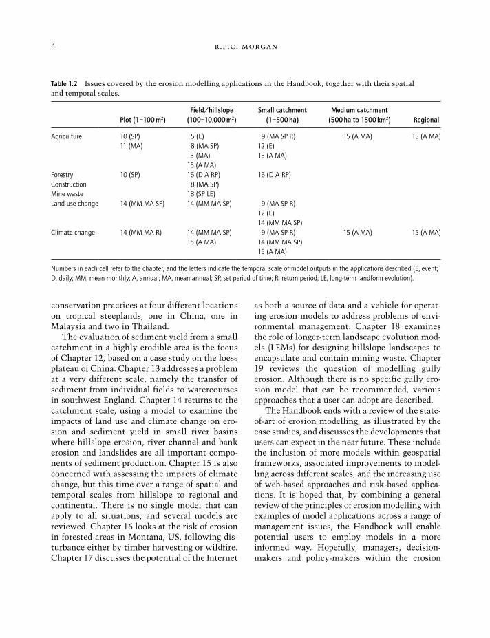
Part 2 of the Handbook looks at specific appli-cations and shows how models are used in prac-tice. Each chapter is really a case study in which a problem commonly faced by environmental planners, consultants and managers is presented. An appropriate model is then chosen and the user is taken through the various steps involved in setting- up and applying the model and interpret-ing its output. Table 1.2 lists the applications under broad subject headings and for each one identifies the relevant chapter and the spatial scale (erosion plot, field, catchment, region) of the problem being considered. Additional infor-mation is provided on the temporal scale, which ranges from individual events to mean annual conditions and long- term landform evolution.

Taking each chapter in turn, Chapter 8 reviews the issues typically faced by field officers of the Natural Resources Conservation Service of the US when predicting erosion from agricul-tural land and planning soil protection measures. Chapter 9 takes a specific example of a small watershed in southwest Missouri and shows how modelling can assist in designing a strategy for sustainable management under both present land use and climatic change. In Chapter 10, modelling is used to predict rates of soil loss in Brazil from hillslopes on forest roads in São Paulo State and from agricultural land under dif-ferent management systems in Minas Gerais State. Chapter 11 examines how a physically- based erosion model can be used to assess soil erodibility and evaluate different soil

9781405190107_4_001.indd 39781405190107_4_001.indd 3 10/15/2010 2:32:13 AM10/15/2010 2:32:13 AM

4 r.p.c. morgan

conservation practices at four different locations on tropical steeplands, one in China, one in Malaysia and two in Thailand.

The evaluation of sediment yield from a small catchment in a highly erodible area is the focus of Chapter 12, based on a case study on the loess plateau of China. Chapter 13 addresses a problem at a very different scale, namely the transfer of sediment from individual fields to watercourses in southwest England. Chapter 14 returns to the catchment scale, using a model to examine the impacts of land use and climate change on ero-sion and sediment yield in small river basins where hillslope erosion, river channel and bank erosion and landslides are all important compo-nents of sediment production. Chapter 15 is also concerned with assessing the impacts of climate change, but this time over a range of spatial and temporal scales from hillslope to regional and continental. There is no single model that can apply to all situations, and several models are reviewed. Chapter 16 looks at the risk of erosion in forested areas in Montana, US, following dis-turbance either by timber harvesting or wildfire. Chapter 17 discusses the potential of the Internet

as both a source of data and a vehicle for operat-ing erosion models to address problems of envi-ronmental management. Chapter 18 examines the role of longer- term landscape evolution mod-els (LEMs) for designing hillslope landscapes to encapsulate and contain mining waste. Chapter 19 reviews the question of modelling gully erosion. Although there is no specific gully ero-sion model that can be recommended, various approaches that a user can adopt are described.

The Handbook ends with a review of the state- of- art of erosion modelling, as illustrated by the case studies, and discusses the developments that users can expect in the near future. These include the inclusion of more models within geospatial frameworks, associated improvements to model-ling across different scales, and the increasing use of web- based approaches and risk- based applica-tions. It is hoped that, by combining a general review of the principles of erosion modelling with examples of model applications across a range of management issues, the Handbook will enable potential users to employ models in a more informed way. Hopefully, managers, decision- makers and policy- makers within the erosion

Table 1.2 Issues covered by the erosion modelling applications in the Handbook, together with their spatial and temporal scales.

Plot (1–100 m2) Field/hillslope

(100–10,000 m2) Small catchment

(1–500 ha) Medium catchment

(500 ha to 1500 km2) Regional

Agriculture 10 (SP) 5 (E) 9 (MA SP R) 15 (A MA) 15 (A MA)11 (MA) 8 (MA SP) 12 (E)

13 (MA) 15 (A MA)15 (A MA)

Forestry 10 (SP) 16 (D A RP) 16 (D A RP)Construction 8 (MA SP)Mine waste 18 (SP LE)Land-use change 14 (MM MA SP) 14 (MM MA SP) 9 (MA SP R)

12 (E)14 (MM MA SP)

Climate change 14 (MM MA R) 14 (MM MA SP) 9 (MA SP R) 15 (A MA) 15 (A MA)15 (A MA) 14 (MM MA SP)

15 (A MA)

Numbers in each cell refer to the chapter, and the letters indicate the temporal scale of model outputs in the applications described (E, event; D, daily; MM, mean monthly; A, annual; MA, mean annual; SP, set period of time; R, return period; LE, long-term landform evolution).

9781405190107_4_001.indd 49781405190107_4_001.indd 4 10/15/2010 2:32:13 AM10/15/2010 2:32:13 AM

Introduction 5

control industry will be encouraged to make more use of models to evaluate present situations, the impacts of control measures and future policies. In addition, model developers may be encouraged to provide better information to model users about the suitability and limitations of their models and what levels of accuracy in prediction they are likely to achieve.

References

Boardman, J. & Davis- Mortlock, D. (1998) Modelling Soil Erosion by Water. NATO ASI Series: Series 1, Global Environmental Change, Vol. 55. Springer- Verlag, Berlin.

De Roo, A.P.J. (1999) Soil erosion modelling at the catchment scale. Catena 37 (3–4).

Ewen, J., Parkin, G. & O’Connell, P.E. (2000) SHETRAN: distributed river basin flow and transport modeling system. Journal of Hydrologic Engineering ASCE 5: 250–258.

Flanagan, D.C. & Nearing, M.A. (1995) USDA Water Erosion Prediction Project: Hillslope Profile and Watershed Model Documentation. USDA- ARS National Soil Erosion Laboratory Report No. 10.

Harman, R.S. & Doe III, W.W. (2001) Landscape Erosion and Evolution Modeling. Kluwer, New York.

Jetten, V. & de Roo, A.P.J. (2001) Spatial analysis of ero-sion conservation measures with LISEM. In Harmon, R.S. & Doe III, W.W. (eds), Landscape Erosion and Evolution Modeling. Kluwer, New York: 429–45.

Misra, R. & Rose, C.W. (1996) Application and sensitiv-ity analysis of process- based erosion model GUEST. European Journal of Soil Science 47: 593–604.

Morgan, R.P.C. & Duzant, J.H. (2008) Modified MMF (Morgan- Morgan- Finney) model for evaluating effects of crops and vegetation cover on soil erosion. Earth Surface Processes and Landforms 33: 90–106.

Morgan, R.P.C., Quinton, J.N., Smith, R.E., et al. (1998) The European Soil Erosion Model (EUROSEM): a dynamic approach for predicting sediment transport from fields and small catchments. Earth Surface Processes and Landforms 23: 527–44.

Renard, K.G., Foster, G.R., Weesies, G.A., et al. (1997) Predicting soil erosion by water. A guide to conserva-tion planning with the Revised Universal Soil Loss Equation (RUSLE). USDA Agricultural Handbook No. 703.

Willgoose, G., Bras, R.L. & Rodriguez- Iturbe, I. (1991) A physically based coupled network growth and hillslope evolution model: 1. Theory. Water Resources Research 27: 1671–84.

9781405190107_4_001.indd 59781405190107_4_001.indd 5 10/15/2010 2:32:13 AM10/15/2010 2:32:13 AM

9781405190107_4_001.indd 69781405190107_4_001.indd 6 10/15/2010 2:32:13 AM10/15/2010 2:32:13 AM

Part 1

Model Development

p01.indd 7p01.indd 7 10/20/2010 7:00:10 PM10/20/2010 7:00:10 PM

p01.indd 8p01.indd 8 10/20/2010 7:00:10 PM10/20/2010 7:00:10 PM

2 Model Development: A User’s Perspective

R. P. C. M O R G A NNational Soil Resources Institute, Cranfield University, Cranfield, Bedfordshire, UK

2.1 Introduction

The last 40 years or so have witnessed the devel-opment of a very large number of erosion models operating at different scales and different levels of complexity, with huge variations in the quantity and type of input data required and, at least according to the model developers, covering a wide range of applications. A potential user of erosion models is therefore faced with a bewilder-ing choice when attempting to select the best model for a particular purpose. All too often, the choice of a model is made more difficult because the user is unable to define the problem precisely enough to state what output is required; for exam-ple, whether knowledge of erosion rates is needed as a mean annual value or for a specific year, sea-son, month, day or storm, and if the latter, whether it is a storm total or a value at the storm peak which is wanted. The user is sometimes uncertain whether this information is needed for a field, a particular hillslope or a catchment. Perhaps knowledge of actual erosion rates is not needed at all, and all that is required is an idea of the location of erosion within the landscape or an indication of the time of year that it is most likely to occur. Even when the requirements are clearly defined, the user is still confronted with the

difficulty that most models are not accompanied by clear statements of the purposes and conditions for which they were designed, their limitations or indicators of the accuracy of their output.

This chapter discusses how the user might deal with these issues. It does so by proposing that users should adopt the same procedures in analys-ing their problem as model developers adopt in constructing their models. By understanding how model developers operate and following a com-mon methodology, users will be better equipped to decide what questions need to be asked when selecting a model to meet their specific objectives. These questions can then be formulated into a set of design requirements that a model must meet in order to be suitable. Users will also gain an appre-ciation of whether they will be able to operate the model software unaided, or whether they will need to seek expert advice in how to set up the model to meet their requirements and interpret the results. Table 2.1 sets out the steps followed by model developers and lists the main points that need to be considered at each stage.

2.2 Some Fundamentals

Any model is a simplification of reality and, for some users, this creates an immediate theoretical issue. How can a problem associated with erosion in a particular location be predicted by a model that describes erosion in a generic way? Surely the only way to deal effectively with a problem in

Handbook of Erosion Modelling, 1st edition. Edited by R.P.C. Morgan and M.A. Nearing. © 2011 Blackwell Publishing Ltd.

c02.indd 9c02.indd 9 10/21/2010 9:31:12 AM10/21/2010 9:31:12 AM

10 r.p.c. morgan

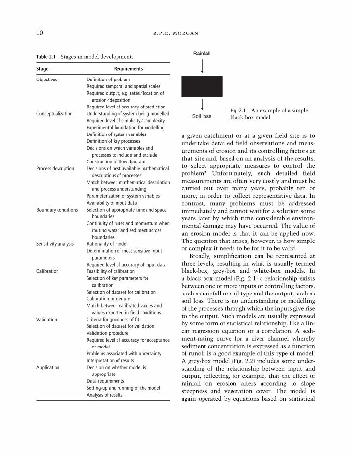
Table 2.1 Stages in model development.

Stage Requirements

Objectives Definition of problemRequired temporal and spatial scalesRequired output, e.g. rates/location of erosion/depositionRequired level of accuracy of prediction

Conceptualization Understanding of system being modelledRequired level of simplicity/complexityExperimental foundation for modellingDefinition of system variablesDefinition of key processesDecisions on which variables and processes to include and excludeConstruction of flow diagram

Process description Decisions of best available mathematical descriptions of processesMatch between mathematical description and process understandingParameterization of system variablesAvailability of input data

Boundary conditions Selection of appropriate time and space boundariesCo ntinuity of mass and momentum when

routing water and sediment across boundaries.

Sensitivity analysis Rationality of modelDetermination of most sensitive input parametersRequired level of accuracy of input data

Calibration Feasibility of calibrationSelection of key parameters for calibrationSelection of dataset for calibrationCalibration procedureMatch between calibrated values and values expected in field conditions

Validation Criteria for goodness of fitSelection of dataset for validationValidation procedureRequired level of accuracy for acceptance of modelProblems associated with uncertaintyInterpretation of results

Application Decision on whether model is appropriateData requirementsSetting-up and running of the modelAnalysis of results

a given catchment or at a given field site is to undertake detailed field observations and meas-urements of erosion and its controlling factors at that site and, based on an analysis of the results, to select appropriate measures to control the problem? Unfortunately, such detailed field measurements are often very costly and must be carried out over many years, probably ten or more, in order to collect representative data. In contrast, many problems must be addressed immediately and cannot wait for a solution some years later by which time considerable environ-mental damage may have occurred. The value of an erosion model is that it can be applied now. The question that arises, however, is how simple or complex it needs to be for it to be valid.

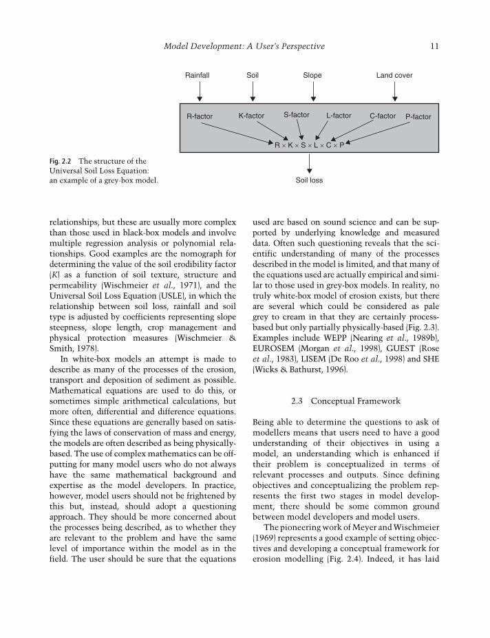
Broadly, simplification can be represented at three levels, resulting in what is usually termed black-box, grey-box and white-box models. In a black-box model (Fig. 2.1) a relationship exists between one or more inputs or controlling factors, such as rainfall or soil type and the output, such as soil loss. There is no understanding or modelling of the processes through which the inputs give rise to the output. Such models are usually expressed by some form of statistical relationship, like a lin-ear regression equation or a correlation. A sedi-ment-rating curve for a river channel whereby sediment concentration is expressed as a function of runoff is a good example of this type of model. A grey-box model (Fig. 2.2) includes some under-standing of the relationship between input and output, reflecting, for example, that the effect of rainfall on erosion alters according to slope steepness and vegetation cover. The model is again operated by equations based on statistical

Rainfall

Soil lossFig. 2.1 An example of a simple black-box model.

c02.indd 10c02.indd 10 10/21/2010 9:31:12 AM10/21/2010 9:31:12 AM

Model Development: A User’s Perspective 11

Rainfall

R-factor K-factor S-factor

R ´ K ´ S ´ L ´ C ´ P

L-factor C-factor P-factor

Soil Slope

Soil loss

Land cover

Fig. 2.2 The structure of the Universal Soil Loss Equation: an example of a grey-box model.

relationships, but these are usually more complex than those used in black-box models and involve multiple regression analysis or polynomial rela-tionships. Good examples are the nomograph for determining the value of the soil erodibility factor (K) as a function of soil texture, structure and permeability (Wischmeier et al., 1971), and the Universal Soil Loss Equation (USLE), in which the relationship between soil loss, rainfall and soil type is adjusted by coefficients representing slope steepness, slope length, crop management and physical protection measures (Wischmeier & Smith, 1978).

In white-box models an attempt is made to describe as many of the processes of the erosion, transport and deposition of sediment as possible. Mathematical equations are used to do this, or sometimes simple arithmetical calculations, but more often, differential and difference equations. Since these equations are generally based on satis-fying the laws of conservation of mass and energy, the models are often described as being physically-based. The use of complex mathematics can be off-putting for many model users who do not always have the same mathematical background and expertise as the model developers. In practice, however, model users should not be frightened by this but, instead, should adopt a questioning approach. They should be more concerned about the processes being described, as to whether they are relevant to the problem and have the same level of importance within the model as in the field. The user should be sure that the equations

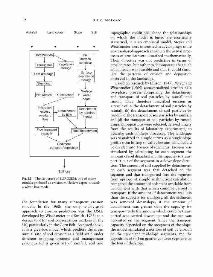
used are based on sound science and can be sup-ported by underlying knowledge and measured data. Often such questioning reveals that the sci-entific understanding of many of the processes described in the model is limited, and that many of the equations used are actually empirical and simi-lar to those used in grey-box models. In reality, no truly white-box model of erosion exists, but there are several which could be considered as pale grey to cream in that they are certainly process-based but only partially physically-based (Fig. 2.3). Examples include WEPP (Nearing et al., 1989b), EUROSEM (Morgan et al., 1998), GUEST (Rose et al., 1983), LISEM (De Roo et al., 1998) and SHE (Wicks & Bathurst, 1996).

2.3 Conceptual Framework

Being able to determine the questions to ask of modellers means that users need to have a good understanding of their objectives in using a model, an understanding which is enhanced if their problem is conceptualized in terms of relevant processes and outputs. Since defining objectives and conceptualizing the problem rep-resents the first two stages in model develop-ment, there should be some common ground between model developers and model users.

The pioneering work of Meyer and Wischmeier (1969) represents a good example of setting objec-tives and developing a conceptual framework for erosion modelling (Fig. 2.4). Indeed, it has laid

c02.indd 11c02.indd 11 10/21/2010 9:31:12 AM10/21/2010 9:31:12 AM

12 r.p.c. morgan

Rainfall Land cover

Soil loss

Interception

Throughfall

Leaf drainage

Stemflow

Net rainfall

Infiltration-excess

overlandflow

Vegetationstorage

Infiltration

Detachmentby flow

Flow transportcapacity

Total detachment

Sedimenttransport /deposition

Detachmentby raindrop

impact

Surfacewaterdepth

Soilsurface

condition

Surfacedepression

storage

Slope Soil

Fig. 2.3 The structure of EUROSEM: one of many models produced as erosion modellers aspire towards a white-box model.

the foundation for many subsequent erosion models. In the 1960s, the only widely-used approach to erosion prediction was the USLE developed by Wischmeier and Smith (1965) as a design tool for soil conservation workers in the US, particularly in the Corn Belt. As noted above, it is a grey-box model which predicts the mean annual rate of soil erosion at a field scale under different cropping systems and management practices for a given set of rainfall, soil and

topographic conditions. Since the relationships on which the model is based are essentially statistical, it is an empirical model. Meyer and Wischmeier were interested in developing a more process-based approach in which the actual proc-esses of erosion were described mathematically. Their objective was not predictive in terms of erosion rates, but rather to demonstrate that such an approach was feasible and that it could simu-late the patterns of erosion and deposition observed in the landscape.

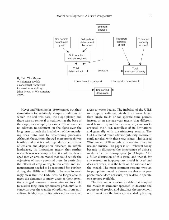
Based on research by Ellison (1947), Meyer and Wischmeier (1969) conceptualized erosion as a two-phase process comprising the detachment and transport of soil particles by rainfall and runoff. They therefore described erosion as a result of (a) the detachment of soil particles by rainfall; (b) the detachment of soil particles by runoff; (c) the transport of soil particles by rainfall; and (d) the transport of soil particles by runoff. Empirical equations were selected, derived largely from the results of laboratory experiments, to describe each of these processes. The landscape was visualized in simple terms as a single slope profile from hilltop to valley bottom which could be divided into a series of segments. Erosion was simulated by calculating for each segment the amount of soil detached and the capacity to trans-port it out of the segment in a downslope direc-tion. The amount of soil supplied by detachment on each segment was that detached on the segment and that transported into the segment from upslope. A simple arithmetical calculation compared the amount of sediment available from detachment with that which could be carried in transport. If the amount of detachment was less than the capacity for transport, all the sediment was removed downslope; if the amount of detachment was greater than the capacity for transport, only the amount which could be trans-ported was carried downslope and the rest was deposited on the segment. Since the transport capacity depended on the steepness of the slope, the model simulated a net loss of soil by erosion on the upper and mid-slope segments, and the deposition of soil on gentler concave segments at the foot of the slope.

c02.indd 12c02.indd 12 10/21/2010 9:31:13 AM10/21/2010 9:31:13 AM

Model Development: A User’s Perspective 13

Meyer and Wischmeier (1969) carried out their simulations for relatively simple conditions in which the soil was bare, the slope planar, and there was no removal of sediment at the base of the slope, for example, by a river. There was also no addition to sediment on the slope over the long term through the breakdown of the underly-ing rock into soil by weathering processes. Although the authors showed their approach was feasible and that it could reproduce the patterns of erosion and deposition observed in simple landscapes, its limitations meant that further research was necessary before it could be devel-oped into an erosion model that could satisfy the objectives of many potential users. In particular, the effects of crop or vegetation cover and soil management needed to be accounted for. Further, during the 1970s and 1980s it became increas-ingly clear that the USLE was no longer able to meet the demands of many users as their atten-tion changed from one of conserving soil in a field to sustain long-term agricultural productivity, to concerns over the transfer of sediment from agri-cultural fields, construction sites and recreational

areas to water bodies. The inability of the USLE to compute sediment yields from areas larger than single fields or for specific time periods instead of an average year meant that different models were required. In their absence, some work-ers used the USLE regardless of its limitations and generally with unsatisfactory results. The USLE suffered much adverse publicity because it could not deal with these new issues. This caused Wischmeier (1978) to publish a warning about its use and misuse. His paper is still relevant today because it illustrates the importance of using a model which is fit-for-purpose (see Chapter 7 for a fuller discussion of this issue) and that if, for any reason, an inappropriate model is used and does not work, it is the fault of the user and not the model. The most common reasons why an inappropriate model is chosen are that an appro-priate model does not exist, or the data to operate one are not available.

The first set of erosion models that adopted the Meyer-Wischmeier approach to describe the processes of erosion and simulate the movement of sediment over the landscape operated by bolting

Soil particledetachment

by rain

Soil detachedon slope segment

Totaldetached soil

if detachment < transport if transport < detachment

Soil carrieddownslope

compare

Soil particledetachment

by runoff

Soil fromupslope

Transportcapacityof rain

Transportcapacityof runoff

Totaltransport capacity

Fig. 2.4 The Meyer-Wischmeier model: a conceptual framework for erosion modelling (after Meyer & Wischmeier, 1969).

c02.indd 13c02.indd 13 10/21/2010 9:31:13 AM10/21/2010 9:31:13 AM

14 r.p.c. morgan

the equations for the erosion processes on to a hydrological model, which was used to generate runoff and transport the resulting water flow over the landscape. Examples include AGNPS (Young et al., 1989), ANSWERS (Beasley et al., 1980) and GAMES (Rudra et al., 1986). Some models, such as CREAMS (Knisel, 1980), allowed a choice between daily simulations based on the USCS Curve Number, a coefficient which describes the soil, slope and land cover characteristics, and storm simulations in which runoff is calculated as the excess of the rainfall intensity over the infiltration rate of the soil. This generation of ero-sion models was process-based as regards the simulation of runoff and sediment, but relied on the factors of the USLE to describe soil erodibility (K), slope length (L), cropping (C) and manage-ment (P) effects.

Current research on erosion modelling is concerned with replacing the coefficients related to soil, slope and land cover with parameters that measure their properties directly and which can therefore take account of variations in both time and space. Instead of a single value to express K, soils are described by properties such as cohesion, shear strength and surface rough-ness, and land cover by architectural properties of the vegetation such as height, percentage cover, stem size and stem density. This means that soil, for example, can be modelled dynami-cally allowing for changes in cohesion as the surface crusts or seals under raindrop impact (Moussa et al., 2003) or human or animal tram-pling, or as surface roughness changes as a result of different tillage practices. Similarly, plant cover effects can be altered in relation to sea-sonal plant growth and decay. The effects of soil and plant cover are sometimes described sepa-rately for each of the four processes of erosion, namely detachment of soil particles by raindrops and runoff, and the transport of the detached material by rainfall and runoff. The outcome is that erosion models have become more complex, since they now incorporate many submodels to describe the behaviour of soil and vegetation. Future models may well account for the move-ment of soil over the landscape by tillage using

methodology developed by Govers et al. (1994) and van Muysen et al. (2002). WATEM (van Oost et al., 2000; Verstraeten et al., 2002) combines these equations with a modification of the Revised Universal Soil Loss Equation (RUSLE) (Renard et al., 1991) to simulate the transport of sediment by runoff and tillage on a mean annual basis. Improved descriptions of the effect of soil will take account of its aggregate struc-ture rather than the size distribution of the primary particles of clay, silt and sand, by using parameters based on aggregate stability (Issa et al., 2006).

With greater concern environmentally about the fate of eroded sediment has come the recogni-tion that the way in which many erosion models simulate the deposition of sediment is too sim-plistic. Just comparing the amount of material available for transport with the transport capac-ity, and dumping the sediment which cannot be transported, results in patterns of deposition over the landscape which are unrealistic. Too much material is deposited too quickly. In models such as WEPP and EUROSEM, an attempt is made to control the rate of deposition by taking account of the settling velocity of the soil particles in the flow and a coefficient expressing the efficiency of the deposition process. Although this approach produces better results, it is analogous to the use of coefficients to describe the effects of plant cover on erosion rather than simulating the physical process. Future models are likely to model deposi-tion explicitly taking account not only of particle settling velocity, but also the velocity of the run-off and the depth of flow. The approaches devel-oped to predict sediment deposition in filter strips (Tollner et al., 1976; Rose et al., 2003) and farm ponds (Verstraeten & Poesen, 2001) are likely to be adapted to describe deposition from runoff. Such developments will lead to even greater com-plexity in erosion models as they attempt to describe the erosion processes more fully. For example, the four erosion processes identified by Meyer and Wischmeier (1969) and the process of deposition will need to be simulated sepa-rately for each soil particle size. Alternatively, ero-sion, transport and deposition can be modelled

c02.indd 14c02.indd 14 10/21/2010 9:31:13 AM10/21/2010 9:31:13 AM

Model Development: A User’s Perspective 15

simultaneously for different erosion/deposition domains, depending on the relative dominance of the three processes (Beuselinck et al., 1999). Ideally this will not be restricted to primary particles, as in Morgan and Duzant (2008) and Fiener et al. (2008), but will cover the sizes of soil aggregates. In addition, since deposited material has different strengths to that of the original soil because cohesion has been lost during detach-ment and transport, erosion models will need to distinguish between the two when simulating the detachment and transport of the sediment (Rose et al., 1983).

2.4 Operating Equations

The simplicity and number of operating equa-tions required to run an erosion model depends on its type and level of complexity. Since this sec-tion is descriptive rather than intended for practi-cal application, the units of the equations are not given. Readers should consult the original sources for these details. A simple grey-box model like the USLE (Wischmeier & Smith, 1978) requires only one equation which multiplies together six numbers:

A R K L S C P= ´ ´ ´ ´ ´ (2.1)

where A is the mean annual soil loss, R is the rainfall erosivity factor, K is the soil erodibility factor, S is the slope steepness factor, L is the slope length factor, C is the crop management factor and P is the erosion-control practice factor. Additional equations are required to determine the values of the S and L factors and, as indicated above, a third equation can be used to estimate the value of K (Wischmeier et al., 1971). Graphical solutions to these additional equations exist in the form of nomographs.

More complex process-based models use sepa-rate equations to describe the various processes of erosion and deposition, and link these together using continuity equations to ensure conserva-tion of energy and mass. The continuity equation

for the volume or mass of sediment passing a given point on the land surface at a given time is:

( ) ( ) ( ) ( ), ,s

AC QCe x t q x t

t x¶ ¶

+ - =¶ ¶

(2.2)

where A is the cross-sectional area of the flow, C is the sediment concentration in the flow, t is time, x is the horizontal distance downslope, e is the net pick-up rate or erosion of sediment on the slope segment, and qs is the rate of input or extraction of sediment per unit length of flow from land external to the segment, for example, from the sides of a convergent slope surface. On a planar slope, qs = 0, and the continuity equation can be rewritten as:

( ) ( )i r

AC QCe e

t x¶ ¶

+ = +¶ ¶

(2.3)

where ei is the net rate of erosion in the inter-rill area of the slope segment and er is the net rate of erosion by rills. This is the form of the continuity equation used in WEPP (Nearing et al., 1989b), EUROSEM (Morgan et al., 1998), LISEM (Jetten & de Roo, 2001) and many other process-based models. In GUEST (Rose et al., 1983) the equation takes a slightly different form. In this model, the soil is described in terms of up to 50 particle-size classes, determined according to their set-tling velocity, and, for each particle-size class, a distinction is made between that eroded from the original soil and that eroded from previously-detached and recently deposited sediment; in addition, deposition is modelled explicitly. The continuity equation becomes:

( ) ( )j jij rj iidj rdj

AC QCe e e e d

t x

¶ ¶+ = + + + -

¶ ¶ (2.4)

where Cj is the concentration of sediment of par-ticle size j in the flow, eij is the rate of erosion of particles of sediment class j in the original soil on the inter-rill area, eidj is the rate of erosion of par-ticles of sediment class j from previously detached soil on the inter-rill area, erj is the rate of erosion of particles of sediment class j from the original

c02.indd 15c02.indd 15 10/21/2010 9:31:13 AM10/21/2010 9:31:13 AM

16 r.p.c. morgan

soil by rills, erdj is the rate of erosion of particles of sediment class j from previously detached soil by rills, and dj is the rate of deposition of particles in sediment class j.

Even where models use the same form of the continuity equation, they differ in the operating functions used to describe erosion and deposition. The user therefore has the possibility of selecting a model according to which functions best describe the way that erosion occurs in a particular study area or which functions are theoretically more satisfying. As an illustration, the way ei and er are described in WEPP and EUROSEM are compared. In WEPP (Nearing et al., 1989b), the inter-rill ero-sion rate (per unit rill width) is given by:

( ) ( )2 0.34 2.51 /PH G

i i se K I F e R W-= -

(2.5)

where Ki is the inter-rill erodibility of the soil, I is the intensity of the rainfall, F is the fraction of the soil protected by the plant canopy, PH is the height of the plant canopy, G is the fraction of the soil covered by ground vegetation or crop residue, Rs is the spacing of the rills and W is the width of the rill computed as a function of the flow discharge. The rate of rill erosion is calcu-lated from:

( ) ( )3/21 /r r c te K C ké ù= - -ë ût t t (2.6)

where Kr is the rill erodibility of the soil, t is the flow shear stress acting on the soil, tc is the criti-cal flow shear stress for detachment to take place, C is the sediment load in the flow, and kt is a sedi-ment transport coefficient. This equation only operates when the sediment load in the flow is less than the sediment transport capacity of the flow. When the sediment load exceeds the trans-port capacity, the equation becomes:

( ) ( ){ }3/2/r r c s te K v q k Cé ù= - -ë ût t t

(2.7)

where vs is the particle settling velocity and q is the flow discharge per unit width.

In EUROSEM (Morgan et al., 1998) a single equation is used to describe the erosion rate by soil particle detachment by raindrop impact and runoff, i.e. ei + er = e. The equation can be applied to unchannelled inter-rill flow or to runoff in rills. Where rills are present, these need to be defined in terms of their number, depth and width. The model initially places all the runoff in the rills and then uses a unified rill model to describe the hydraulic conditions of the flow as the runoff overflows the rills and spreads out over the inter-rill area. The single equation is:

( )

( )( ){ }1.0 2h

DT LD

bs c

e k KE KE e

wv a C

-é ù= +ë ûé ù+ - -ê úë û

h w w (2.8)

where k is the detachability of the soil by raindrop impact, KE is the kinetic energy of the rainfall which is divided into direct throughfall (DT) and that falling from the plant canopy as leaf drainage (LD), h = the depth of surface water, h is an expression of the efficiency of soil parti-cle detachment by flow which is a function of soil cohesion, w is the width of flow, vs is the settling velocity of the particles in the flow, w is the unit stream power of the flow (the product of slope and flow velocity), wc is the critical value of unit stream power for sediment transport, a and b are coefficients related to sediment parti-cle size, and C is the sediment concentration in the flow.

The user therefore has a choice between a model that simulates the detachment of soil par-ticles by raindrop impact as a function of rainfall intensity, and one that uses the kinetic energy of the rain. WEPP allows for the effect of the plant cover by assuming that ground-level vegetation protects the soil completely and that the plant canopy provides some protection dependent upon its height above the ground surface. In EUROSEM, the proportion of the soil surface covered by veg-etation is used to split the rainfall into direct throughfall and leaf drainage. The kinetic energy of the leaf drainage is calculated as a function of

c02.indd 16c02.indd 16 10/21/2010 9:31:18 AM10/21/2010 9:31:18 AM

Model Development: A User’s Perspective 17

plant height but in such a way that, for very tall canopies, the energy can exceed that of the direct throughfall, whereas ground-level vegetation will protect the soil completely. The user also has a choice between a model that simulates the detachment and transport of soil particles as a function of the shear stress exerted by the flow, and one that describes the same processes using unit stream power. The other fundamental differ-ence between WEPP and EUROSEM is that the former operates over a range of time steps from individual storms to daily. Within each time step, steady-state conditions are assumed, which means that each time step is either one of erosion or deposition of sediment. In contrast, EUROSEM uses very short time steps (1–2 minutes) and therefore continuously updates the sediment concentration in the runoff and the transport capacity. The latter is assumed to be the sediment concentration at which erosion and deposition are in balance. EUROSEM is therefore a dynamic rather than a steady-state model, which implies that there is a continuous exchange of soil particles between the runoff and the soil surface which controls the sediment concentration in the flow.

There is no doubt that researchers with an interest in modelling the processes of erosion and deposition will develop even more complex models than WEPP and EUROSEM as they work towards the goal of a comprehensive description of the processes and a dynamic simulation of the factors affecting them. For practical purposes the model user may well question whether all this complexity is necessary. It is well known that in terms of the amount of sediment reaching the bottom of a hillside or discharging into a water course, some erosion processes are more important than others. Indeed, in terms of pro-ducing a relatively simple and efficient model, it is recommended that attention is focused on the most important processes and that those con-tributing little to the generation, transport and deposition of sediment should be ignored (Kirkby, 1980). The user therefore requires some knowledge of the most important processes that affect his or her problem so that a model which

emphasizes these can be selected. Even if a very detailed model is not chosen, the user can gain much by establishing the conceptual framework of the problem as fully as possible. By under-standing the processes involved and their con-trolling factors, it is possible to decide which are the most relevant and which models best match what is required. Without a comprehensive framework, there is a danger that something important will go undetected.

2.5 Spatial Considerations

When selecting an erosion model it is necessary to define the area over which it should operate. This may vary from a small segment of a hillslope, to a complete hillside, a small catchment (typically 0.01–0.5 km2 in area but sometimes as large as 10 km2) encompassing hillslopes and a river chan-nel, or a large catchment (typically 10–100 km2 but sometimes as large as 100,000 km2). A deci-sion is then needed on whether the area can be treated as a single unit or whether it is necessary to know what is taking place at different locations within it. The first approach is suitable where only knowledge of the amount of sediment leaving the area is required. The second is essential where knowledge of the source of the sediment is needed so that the implementation of erosion protection measures can be targeted. Generally the larger the area, the greater the need for internal understand-ing since deposition of sediment may occur at several locations and sediment movement may be concentrated along preferred flow paths, all of which can influence the design of a system for sediment management. These two approaches are catered for respectively by the use of lumped and distributed models.

The most commonly used lumped model in erosion work is the USLE. As already noted, this predicts mean annual soil loss from a single area, in this case a field, within which rainfall, soil, slope and land cover are either considered uni-form or can be represented by coefficients which express the average condition. Lumped models are more commonly used in hydrology. They are

c02.indd 17c02.indd 17 10/21/2010 9:31:24 AM10/21/2010 9:31:24 AM

18 r.p.c. morgan

process-based in that they effectively describe the water balance of a catchment whereby a propor-tion of the incoming rainfall passes into runoff whilst the rest is held in various stores, such as interception by the plant cover, soil moisture and groundwater. An erosion component can be built on to such a model as illustrated by the Stanford Sediment Model (Negev, 1967), which is linked to the Stanford Watershed Model (Crawford & Linsley, 1966). Since most practical applications require knowledge of the way sediment is moved over the landscape so that protection measures can be targeted either at areas of sediment source or along pathways of movement, there is a demand for models which can describe what is happening within a catchment, and lumped mod-els are unable to do this. Lumped models are therefore of value for predicting soil loss from relatively small areas such as an agricultural field, road embankment or construction site. They can also be used to assess erosion over large areas, as illustrated by the PESERA model (Gobin et al., 2006) which estimates mean annual erosion over 1 km2 size units. A process-based approach is used to generate infiltration-excess and saturation overland flow from daily rainfall. The calcula-tions are integrated across the frequency distribu-tion of daily rainfall events. Sediment transport is estimated according to the runoff, soil erodibility and slope of each cell. Both runoff generation and sediment transport are modified by land cover, surface roughness and soil crusting.

Where the need is to determine where erosion and deposition take place within a catchment, distributed models are used. These operate by dividing the catchment into discrete land units and use mathematical procedures to route water and sediment from one unit to another. Such models are necessarily process-based and, in so far as they use input data that can be measured physi-cally in the field and use continuity equations to ensure the conservation of mass and energy as water and sediment are moved in space and over time, they are often considered as physically-based (Beven & Kirkby, 1979). Most of the recently developed erosion models, like WEPP, GUEST, LISEM and EUROSEM, are distributed models.

They are suitable for analysing the effects of changes in land use in different parts of a catch-ment, as well as the effects of variations in rain-fall, soil type, slope and land cover within a catchment.

Some distributed models, like EUROSEM and CREAMS, require land units in a catchment to be identified in terms of similarity in soils, slope and land cover. For most practical purposes, the land units are similar in nature to the land facets identified in terrain analysis (Christian & Stewart, 1968; Webster & Beckett, 1970). These can be grouped into larger units or land systems (usually between 100 m2 and 10,000 m2 in size) which have been shown to be significantly differ-ent from each other in terms of both erosion sta-tus and the rate of change in erosion over time (Morgan et al., 1997). The art in setting up these models is to identify the land units so that they are internally as uniform in their characteristics as possible, and then to determine the likely pat-terns of water flow from one unit to another (Auzet et al., 1995). Although this can be done using aerial photographs, topographic maps or digital elevation models to determine the low points in the landscape along which water will concentrate, there is often the need for field observations to identify where flow paths deviate from those which would occur naturally, for example as a result of installing diversion ter-races or ditches to take water across the slope to a safe outlet rather than allowing it to flow downslope.

In recent years, with the advent of geographi-cal information systems, model users have moved away from defining land units in relation to the natural variations in the landscape, in favour of dividing the catchment into grid cells of uniform size. Although the movement of water from one cell to another is still based on the local topography, the units themselves are less likely to be internally consistent in their soils, slopes and land cover. Unless the grid cells are extremely small, say 10 m × 10 m, it is likely that they will be crossed by boundaries between soil types or slope breaks. The larger the grid cells used, the more likely that each one will

c02.indd 18c02.indd 18 10/21/2010 9:31:24 AM10/21/2010 9:31:24 AM