/

SOLUTIONS AND SOLUTION PROPERTIES Albert M. Schwartz and Allan S. Myerson

1.1. INTRODUCTION AND MOTIVATION

Crystallization is a separation and purification technique employed to produce a wide variety of materials. Crystallization may be defined as a phase change in which a crystalline product is obtained from a solution. A solution is a mixture of two or more species that form a homogeneous single phase. Solutions are nor­mally thought of in terms of Hquids, however, solutions may include solids and even gases. Typically, the term solution has come to mean a liquid solution consisting of a solvent, which is a liquid, and a solute, which is a solid, at the conditions of interest. The term melt is used to describe a material that is solid at normal conditions and is heated until it becomes a molten Hquid. Melts may be pure materials, such as molten silicon used for wafers in semiconductors, or they may be mixtures of materials. In that sense, a homogeneous melt with more than one component is also a solution, however, it is normally referred to as a melt. A solution can also be gaseous; an example of this is a solution of a solid in a supercritical fluid.

Virtually all industrial crystallization processes involve solutions. The development, design, and control of any of these pro­cesses involve knowledge of a number of the properties of the solution. This chapter will present and explain solutions and solution properties, and relate these properties to industrial crystallization operations.

1.2. UNITS

Solutions are made up of two or more components of which one is the solvent and the other is the solute(s). There are a variety of ways to express the composition of a solution. If we consider the simple system of a solvent and a solute, its composition may be expressed in terms of mass fraction, mole fraction, or a variety of concentration units as shown in Table 1.1. The types of units that are commonly used can be divided into those that are ratios of the mass (or moles) of solute to the mass (or moles) of the solvent,

TABLE 1.1 Concentration Units

Type 1: Mass (or moles) solute/mass (or moles) solvent Grams solute/100 grams solvent Moles solute/100 grams solvent Moles solute/1000 grams solvent-molal Ibm solute/lbm solvent Moles solute/moles solvent

Type 2: Mass (or moles) solute/mass (or moles) solution Grams solute/grams total Mass fraction Moles solute/moles total Mole fraction

Type 3: Mass (or moles) solute/volume solution Moles solute/liter of solution-molar Grams solute/liter of solution Ibm solute/gallon solution

those that, are ratios of the mass (or moles) of the solute to the mass (or moles) of the solution, and those that are ratios of the mass (or moles) of the solute to the volume of the solution.

While all three units are commonly used, it is important to note that use of units of type 3, requires knowledge of the solu­tion density to convert these units into those of the other types. In addition, type 3 units must be defined at a particular tempera­ture since the volume of a solution is a function of temperature. The best units to use for solution preparation are mass of solute per mass of solvent. These units have no temperature depend­ence and solutions can be prepared simply by weighing each species. Conversion among mass (or mole) based units is also simple. Example 1.1 demonstrates conversion of units of all three types.

1.3. SOLUBILITY OF INORGANICS

1.3.1. BASIC CONCEPTS

A solution is formed by the addition of a solid solute to the solvent. The soHd dissolves, forming the homogeneous solution. At a given temperature there is a maximum amount of solute that can dissolve in a given amount of solvent. When this maximum is reached the solution is said to be saturated. The amount of solute required to make a saturated solution at a given condition is called the solubility.

Solubilities of common materials vary widely, even when the materials appear to be similar. Table 1.2 Hsts the solubiHty of a number of inorganic species (MuUin 1997 and Myerson et al. 1990). The first five species all have calcium as the cation but their solubihties vary over several orders of magnitude. At 20 °C the solubility of calcium hydroxide is 0.17 g/100 g water while that of calcium iodide is 204 g/100 g water. The same variation can be seen in the six sulfates listed in Table 1.2. Calcium sulfate has a solubil­ity of 0.2 g/100 g water at 20 °C while ammonium sulfate has a solubility of 75.4 g/100 g water.

TABLE 1.2 Solubilities of Inorganics at 20 ""C

Compound

Calcium chloride Calcium iodide Calcium nitrate Calcium hydroxide Calcium sulfate Ammonium sulfate Copper sulfate Lithium sulfate Magnesium sulfate Silver sulfate

Chemical Formula

CaCl2 Calz Ca(N03)2 Ca(0H)2 CaS04 (NH4)2S04 CUSO4 LiS04 MgS04 Ag2S04

Solubility (g anhydrous/100 g H2O)

74.5 204 129

0.17 0.20

75.4 20.7 34 35.5

0.7

(Based on data from Mullin 1997 and Myerson et al. 1990)

2 SOLUTIONS AND SOLUTION PROPERTIES

EXAMPLE 1.1 Conversion of Concentration Units

Given: 1 molar solution of NaCl at 25 °C Density of solution = 1.042 g/cm^ Molecular weight (MW) NaCl = 58.44

1 molar ^ 1 mol NaCl 1 liter 58.44g NaCl 1 cm^

liter of solution lOOOcm^

_ 0.056 g NaCl

g solution

= 0.056 wt fraction NaCl:

mol NaCl 1.042 g

5.6 wt% NaCl

0.056 g NaCl 0.056 g NaCl g solution ~ 0.944 g water + 0.056 g NaCl

= 0.059 gNaCl/g water

0.056wt fraction NaCl = 0.056 g NaCl

0.944 g water + 0.056 g NaCl

0.056 g NaCl 58.44 g/g mol

0.056 g NaCl 0.944 g water 58.44 g/g mol 18 g/g mol

= 0.018 mol fraction NaCl

The solubility of materials depends on temperature. In the majority of cases the solubility increases with increasing tempera­ture, although the rate of the increase varies widely from com­pound to compound. The solubility of several inorganics as a function of temperature are shown in Figure 1.1 (Mullin 1997). Sodium chloride is seen to have a relatively weak temperature dependence with the solubility changing from 35.7 to 39.8g/100g water over a 100 °C range. Potassium nitrate, on the other hand, changes from 13.4 to 247 g/100 g water over the same temperature range. This kind of information is very important in crystallization processes since it will determine the amount of cooling required to

yield a given amount of product and will in fact determine if cooling will provide a reasonable product yield.

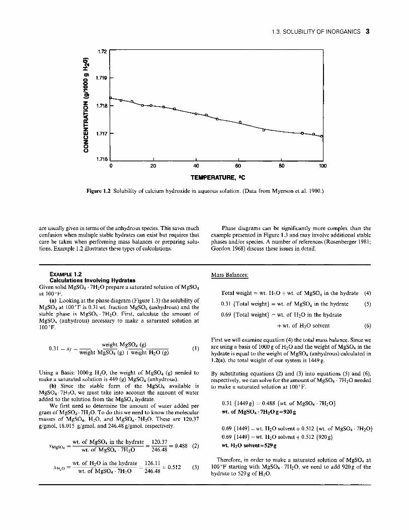
Solubility can also decrease with increasing temperature with sparingly soluble materials. A good example of this is the calcium hydroxide water system shown in Figure 1.2.

The solubihty of a compound in a particular solvent is part of that systems phase behavior and can be described graphically by a phase diagram. In phase diagrams of solid-liquid equilibria the mass fraction of the solid is usually plotted versus temperature. An example is Figure 1.3, which shows the phase diagram for the magnesium sulfate water system. This system demonstrates another common property of inorganic sohds, the formation of hydrates. A hydrate is a solid formed upon crystallization from water that contains water molecules as part of its crystal structure. The chemical formula of a hydrate indicates the number of moles of water present per mole of the solute species by listing a stoichio­metric number and water after the dot in the chemical formula. Many compounds that form hydrates form several with varying amounts of water. From the phase diagram (Figure 1.3) we can see that MgS04 forms four stable hydrates ranging from 12 mol of water/mol MgS04 to 1 mol of water/mol of MgS04. As is usual with hydrates, as the temperature rises, the number of moles of water in the stable hydrate declines and at some temperature the anhydrous material is the stable form.

The phase diagram contains much useful information. Refer­ring to Figure 1.3, the line abcdef is the solubility or saturation Hne that defines a saturated solution at a given temperature. Line ab is the solubility line for the solvent (water) since when a solution in this region is cooled, ice crystallizes out and is in equilibrium with the solution. Point b marks what is known as the eutectic compos­ition. At this composition, 0.165 weight fraction MgS04, if the solution is cooled both ice and MgS04 will separate as soUds. The rest of the curve from b to f represents the solubility of MgS04 as a function of temperature. If we were to start with a solution at 100 °F and 25 wt% MgS04 (point A in Figure 1.3) and cool that solution, the solution would be saturated at the point where a vertical line from A crosses the saturation curve, which is at 80 °F. If the solution were cooled to 60 °F as shown in point D, the solution will have separated at equilibrium into solid MgS04 • 7H2O and a saturated solution of the composition corres­ponding to point C.

The phase diagram also illustrates a general practice concerning hydrate solubility. The solubility of compounds that form hydrates

/-*N

0 ffi Dl) 0 0 0

;z; 0 H

; w u '4. 0 u

3000

2500

2000

1500

1000

500

0 40 60 80

TEMPERATURE °C

120

Figure 1.1 Solubility of KNO3, CUSO4, and NaCl in aqueous solution. (Data from Mullin 1997.)

1.3. SOLUBILITY OF INORGANICS 3

100 40 60

TEMPERATURE, OC

Figure 1.2 Solubility of calcium hydroxide in aqueous solution. (Data from Myerson et al. 1990.)

are usually given in terms of the anhydrous species. This saves much confusion when multiple stable hydrates can exist but requires that care be taken when performing mass balances or preparing solu­tions. Example 1.2 illustrates these types of calculations.

Phase diagrams can be significantly more complex than the example presented in Figure 1.3 and may involve additional stable phases and/or species. A number of references (Rosenberger 1981; Gordon 1968) discuss these issues in detail.

EXAMPLE 1.2 Calculations Involving Hydrates

Given solid MgS04 • 7H2O prepare a saturated solution of MgS04 at 100 °F.

(a) Looking at the phase diagram (Figure 1.3) the solubiUty of MgS04 at 100 °F is 0.31 wt. fraction MgS04 (anhydrous) and the stable phase is MgS04 • 7H2O. First, calculate the amount of MgS04 (anhydrous) necessary to make a saturated solution at 100 °F.

0.31 =Xf = weight MgS04 (g)

weight MgS04 (g) + weight H2O (g) (1)

Using a Basis: lOOOg H2O, the weight of MgS04 (g) needed to make a saturated solution is 449 (g) MgS04 (anhydrous).

(b) Since the stable form of the MgS04 available is MgS04 • 7H2O, we must take into account the amount of water added to the solution from the MgS04 hydrate.

We first need to determine the amount of water added per gram of MgS04 • 7H2O. To do this we need to know the molecular masses of MgS04, H2O, and MgS04 • 7H2O. These are 120.37 g/gmol, 18.015 g/gmol, and 246.48 g/gmol, respectively.

-^MgS04 = _ wt. of MgS04 in the hydrate _ 120.37

wt. of MgS04 • 7H2O ~ 246.48 = 0.488 (2)

^ H 2 0 = • Wt. of H2O in the hydrate _ 126.11

wt. of MgS04 • 7H2O ~ 246.48 = 0.512 (3)

Mass Balances:

Total weight = wt. H2O + wt. of MgS04 in the hydrate (4)

0.31 {Total weight} = wt. of MgS04 in the hydrate (5)

0.69 {Total weight} = wt. of H2O in the hydrate

+ wt. of H2O solvent (6)

First we will examine equation (4) the total mass balance. Since we are using a basis of 1000 g of H2O and the weight of MgS04 in the hydrate is equal to the weight of MgS04 (anhydrous) calculated in 1.2(a), the total weight of our system is 1449 g.

By substituting equations (2) and (3) into equations (5) and (6), respectively, we can solve for the amount of MgS04 • 7H2O needed to make a saturated solution at 100 °F.

0.31 {1449g} = 0.488 {wt. of MgS04 • 7H2O} wt. of MgS04 • 7H2O g = 920 g

0.69 {1449} = wt. H2O solvent + 0.512 {wt. of MgS04 • 7H2O} 0.69 {1449} = wt. H2O solvent+ 0.512 {920g} wtHiO solvent = 529 g

Therefore, in order to make a saturated solution of MgS04 at 100 °F starting with MgS04 • 7H2O, we need to add 920 g of the hydrate to 529 g of H2O.

4 SOLUTIONS AND SOLUTION PROPERTIES

200

190

180

170

160

150

140

130

120

110

100

90)

80

70

60

50

40

30

20

1 1 1 1—1—1—1—nm—1—1—rri — / 1

/ Solution + MgSo H O ]

— > o*/ J » / MgSO^HgO "n

/ 0.87-••

fe n? 1

/ o 1 CM

Liquid solution O / <o

f/ c ^-. O / Solution + MgSO ' 2

— Id k Q

— ^* /

n\

MgSO^ .6H2OI

+ MgSO^ J

i

-H

^

o / 1

/? V O J

_ ^ / Solution + MgSO. • 7HoO > ^^^A' ^^2^ J

/ S + Mgso. n / ^

r / 1 L MgSO^ laHgO / 1 c / i k ? * . ^ /CB 2 /solution + g

1 1 > 1 1* 1 ' 1 ~

-A

-A

i J . MgSO. • 12HoO + MgSO. |

1 l _ 1 1 1 1 0 0.05 0.10 0.15 0.20 0.25 0.30 0.35 0.40 0.45 0.50 0.55 0.60

WEIGHT FRACTION MgS04 Figure 1.3 Phase diagram for MgS04-H20. (Reprinted by permission of John Wiley & Sons, Inc., from R.M. Felder and R.W. Rousseau (1986), Elementary Principles of Chem­ical Processes, 2nd ed., p. 259. © John Wiley and Sons, Inc.)

1.3.2. SPARINGLY SOLUBLE SPECIES—DILUTE SOLUTIONS

As we have seen in the previous section, the solubility of materials varies according to their chemical composition and with tempera­ture. Solubility is also affected by the presence of additional species in the solution, by the pH, and by the use of different solvents (or solvent mixtures). When discussing inorganic species, the solvent is usually water, while with organics, the solvent can be water or a number of organic solvents, or solvent mixtures.

If we start with a sparingly soluble inorganic species such as silver chloride and add silver chloride to water in excess of the saturation concentration, we will eventually have equilibrium

between sohd AgCl and the saturated solution. The AgCl is, as most of the common inorganics, an electrolyte and dissociates into its ionic constituents in solution. The dissociation reaction can be written as

AgCl(s) <^ Ag++ C r (1.1)

The equilibrium constant for this reaction can be written as

K = (aAg+ «C1- )/(«AgCl) (1-2)

where a denotes the activities of the species. If the sohd AgCl is in its stable crystal form and at atmospheric pressure, it is at a

1.3. SOLUBILITY OF INORGANICS 5

standard state and will have an activity of one. The equation can then be written as

Ksp = a^^'a'^'- =7^^'(mAg07^^'(^ci-) (1.3)

where 7 is the activity coefficient of the species and m represents the concentrations in solution of the ions in molal units. For sparingly soluble species, such as AgCl, the activity coefficient can be assumed to be unity (using the asymmetric convention for activity coefficients) so that Eq. (1.3) reduces to

Ksp = [wAg+lI'^cr] (1.4)

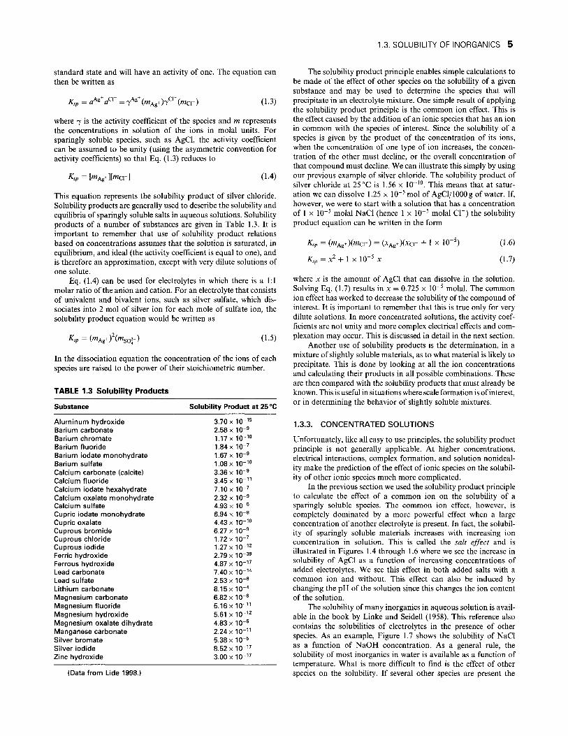
This equation represents the solubility product of silver chloride. Solubility products are generally used to describe the solubility and equiUbria of sparingly soluble salts in aqueous solutions. Solubility products of a number of substances are given in Table 1.3. It is important to remember that use of solubility product relations based on concentrations assumes that the solution is saturated, in equilibrium, and ideal (the activity coefficient is equal to one), and is therefore an approximation, except with very dilute solutions of one solute.

Eq. (1.4) can be used for electrolytes in which there is a 1:1 molar ratio of the anion and cation. For an electrolyte that consists of univalent and bivalent ions, such as silver sulfate, which dis­sociates into 2 mol of silver ion for each mole of sulfate ion, the solubility product equation would be written as

Ksp = ( AgO (^SOl-) (1.5)

In the dissociation equation the concentration of the ions of each species are raised to the power of their stoichiometric number.

TABLE 1.3 Solubility Products

Substance

Aluminum hydroxide Barium carbonate Barium chromate Barium fluoride Barium iodate monohydrate Barium sulfate Calcium carbonate (calcite) Calcium fluoride Calcium iodate hexahydrate Calcium oxalate monohydrate Calcium sulfate Cupric iodate monohydrate Cupric oxalate Cuprous bromide Cuprous chloride Cuprous iodide Ferric hydroxide Ferrous hydroxide Lead carbonate Lead sulfate Lithium carbonate Magnesium carbonate Magnesium fluoride Magnesium hydroxide Magnesium oxalate dihydrate Manganese carbonate Silver bromate Silver iodide Zinc hydroxide

Solubility Product at 25^0

3.70x10-15 2.58x10-9 1.17x10-1° 1.84x10-^ 1.67x10-9

1.08x10-1° 3.36x10-9 3.45x10-11 7.10x10-^ 2.32x10-9 4.93x10-5 6.94 X 10-8 4.43x10-1° 6.27x10-9 1.72x10-7 1.27x10-12 2.79x10-39 4.87 X 10-17 7 .40x10-1* 2.53x10-8 8 .15x10- * 6.82x10-6 5.16x10-11 5.61 X 10-12 4.83x10-6 2.24x10-11 5.38x10-5 8.52x10-17 3.00x10-17

The solubility product principle enables simple calculations to be made of the effect of other species on the solubility of a given substance and may be used to determine the species that will precipitate in an electrolyte mixture. One simple result of applying the solubiUty product principle is the common ion effect. This is the effect caused by the addition of an ionic species that has an ion in common with the species of interest. Since the solubility of a species is given by the product of the concentration of its ions, when the concentration of one type of ion increases, the concen­tration of the other must decline, or the overall concentration of that compound must decline. We can illustrate this simply by using our previous example of silver chloride. The solubility product of silver chloride at 25 °C is 1.56 x 10"^^. This means that at satur­ation we can dissolve 1.25 x 10~^mol of AgCl/lOOOg of water. If, however, we were to start with a solution that has a concentration of 1 x IQ-^ molal NaCl (hence 1 x 10"^ molal CI") the solubility product equation can be written in the form

Ksp = (wAg+)(mcr) = (xAg+)(^cr + 1 x 10 ) (1.6)

(1.7)

(Data from Lide 1998.)

where x is the amount of AgCl that can dissolve in the solution. Solving Eq. (1.7) results in x = 0.725 x 10~^ molal. The common ion effect has worked to decrease the solubiUty of the compound of interest. It is important to remember that this is true only for very dilute solutions. In more concentrated solutions, the activity coef­ficients are not unity and more complex electrical effects and com-plexation may occur. This is discussed in detail in the next section.

Another use of solubility products is the determination, in a mixture of sUghtly soluble materials, as to what material is likely to precipitate. This is done by looking at all the ion concentrations and calculating their products in all possible combinations. These are then compared with the solubility products that must already be known. This is useful in situations where scale formation is of interest, or in determining the behavior of sUghtly soluble mixtures.

1.3.3. CONCENTRATED SOLUTIONS

Unfortunately, like all easy to use principles, the solubility product principle is not generally applicable. At higher concentrations, electrical interactions, complex formation, and solution nonideal-ity make the prediction of the effect of ionic species on the solubil­ity of other ionic species much more complicated.

In the previous section we used the solubility product principle to calculate the effect of a common ion on the solubility of a sparingly soluble species. The common ion effect, however, is completely dominated by a more powerful effect when a large concentration of another electrolyte is present. In fact, the solubil­ity of sparingly soluble materials increases with increasing ion concentration in solution. This is called the salt effect and is illustrated in Figures 1.4 through 1.6 where we see the increase in solubility of AgCl as a function of increasing concentrations of added electrolytes. We see this effect in both added salts with a common ion and without. This effect can also be induced by changing the pH of the solution since this changes the ion content of the solution.

The solubility of many inorganics in aqueous solution is avail­able in the book by Linke and Seidell (1958). This reference also contains the solubilities of electrolytes in the presence of other species. As an example. Figure 1.7 shows the solubility of NaCl as a function of NaOH concentration. As a general rule, the solubihty of most inorganics in water is available as a function of temperature. What is more difficult to find is the effect of other species on the solubility. If several other species are present the

6 SOLUTIONS AND SOLUTION PROPERTIES

2.2x10-3

0.2 0.3

g CaSO4/1000 g H2O

0.4 0J5

Figure 1.4 Solubility of AgCl in aqueous CaS04 solution at 25 °C. (Data from Linke and Seidell 1958, 1965.)

0.002 0.004 0.006

9 NaNOa/IOOO g H2O

0.008 0.01

Figure 1.5 Solubility of AgCl in aqueous NaNOs solution at 30 °C. (Data from Linke and Seidell 1958, 1965.)

O

100 200

g CaCl2/1000 g H2O

300 400

Figure 1.6 Solubility of AgCl in aqueous CaCl2 solution. (Data from Linke and Seidell 1958, 1965.)

1.3. SOLUBILITY OF INORGANICS 7

400

200 400 600 800

gNaOH/1000gH2O

1000 1200 1400

Figure 1.7 Solubility of NaCl in aqueous NaOH solution. (Data from Linke and Seidell 1958, 1965.)

data will usually not be available. Given this situation there are two alternatives. The first is to measure the solubility at the con­ditions and composition of interest. Experimental methods for solubiHty measurement will be discussed in Section 1.4.5. The second alternative is to calculate the solubility. This is a viable alternative when thermodynamic data are available for the pure components (in solution) making up the multicomponent mixture. An excellent reference for calculation techniques in this area is the Handbook of Aqueous Electrolyte Thermodynamics by Zemaitis et al. (1986). A simplified description of calculation techniques is presented in the next section.

Solution Thermodynamics, As we have seen previously, for a solution to be saturated it must be at equilibrium with the solid solute. Thermodynamically this means that the chemical potential of the solute in the solution is the same as the chemical potential of the species in the soUd phase.

^'solid '^'solution (1.8)

If the solute is an electrolyte that completely dissociates in solution (strong electrolyte), Eq. (1.8) can be rewritten as

/^'solid = ^clJ'C + Vafia (1.9)

where v . and v are the stoichiometric numbers, and /Xc and fia are the chemical potentials of the cation and anion, respectively. The chemical potential of a species is related to the species activity by

MT) = M ,,)(T) + RTln(fl,) (1.10)

where at is the activity of species / and /i? x is an arbitrary reference state chemical potential. The activity coefficient is defined as

7,- = ai/mi (1.11)

where m^ is the concentration in molal units. In electrolyte solu­tions, because of the condition of electroneutrality, the charges of the anion and cation will always balance. When a salt dissolves it

will dissociate into its component ions. This has led to the defini­tion of a mean ionic activity coefficient and mean ionic molality defined as

(1.12)

(1.13)

where the v and v are the stoichiometric number of ions of each type present in a given salt. The chemical potential for a salt can be written as

Msalt(a ) ^ fJ^aq) + v R T l n ( 7 ± m ± ) ' (1.14)

where JJ,?. is the sum of the two ionic standard state chemical potentials and v is the stoichiometric number of moles of ions in one mole of solid. In practice, experimental data are usually reported in terms of mean ionic activity coefficients. As we have discussed previously, various concentration units can be used. We have defined the activity coefficient of a molal scale. On a molar scale it is

Oiic)

' (Ci) (1.15)

where yt is the molar activity coefficient and c, is the molar con­centration. We can also define the activity coefficient on a mole fraction scale

/ • =

Xi (1.16)

where / is the activity coefficient and x, the mole fraction. Con­verting activity coefficients from one type of units to another is neither simple nor obvious. Equations that can be used for this con­version have been developed (Zemaitis et al. 1986) and appear below

8 SOLUTIONS AND SOLUTION PROPERTIES

/± = (1.0 + 0.01M,vm)7±

, (p + 0.001c(vM,-M)) /± = y±

Po

7± (p-O.OOlcM) f c \

= y± = — ]y± \mpQj Po

>± = (l+0.001mM) ih-i^. •JTi

(1.17)

(1.18)

(1.19)

(1.20)

where V = stoichiometric number = V4. + v_ p — solution density

Po = solvent density M — molecular weight of the solute

Ms — molecular weight of the solvent

Solubility of a Pure Component Strong Electrolyte. The calcu­lation of the solubility of a pure component solid in solution requires that the mean ionic activity coefficient be known along with a thermodynamic solubility product (a solubility product based on activity). Thermodynamic solubihty products can be calculated from standard state Gibbs free energy of formation data. If, for example, we wished to calculate the solubility of KCIinwaterat25°C,

Kci <^ K+ + c r

The equilibrium constant is given by equation.

Ksp = -^^^^ = (7K+mK+)(7crWcr) = 7 i ^ i «KC1

(1.21)

(1.22)

The equilibrium constant is related to the Gibbs free energy of formation by the relation

Ksp=Qxp{-AGfolRT) (1.23)

The free energy of formation of KCI can be written as

AGyo = A.Gfov + AGyoQ- ~ ^^/^KCi (1-24)

Using data from the literature (Zemaitis et al. 1986) one finds,

AG/0 = -1282cal/g mol (1.25)

so that

Ksp = 8.704 (1.26)

Employing this equilibrium constant and assuming an activity coefficient of 1 yields a solubihty concentration of 2.95 molal. This compares with an experimental value (Linke and Seidell 1958) of 4.803 molal. Obviously assuming an activity coefficient of unity is a very poor approximation in this case and results in a large error.

The calculation of mean ionic activity coefficients can be complex and there are a number of methods available. Several

references (Zemaitis et al. 1986; Robinson and Stokes 1970; Gug­genheim 1987) describe these various methods. The method of Bromley (1972, 1973, 1974) can be used up to a concentradon of 6 molal and can be written as

log7± = A\z+z-

1 + V7

\y/l ((0.06- •0.6B)\z+z-\I)

( > - # i ' ) + BI (1.27)

where 7± = activity coefficient A = Debye-Hiickel constant z = number of charges on the cation or anion / = ionic strength is l/2E/m/z^ B = constant for ion interaction

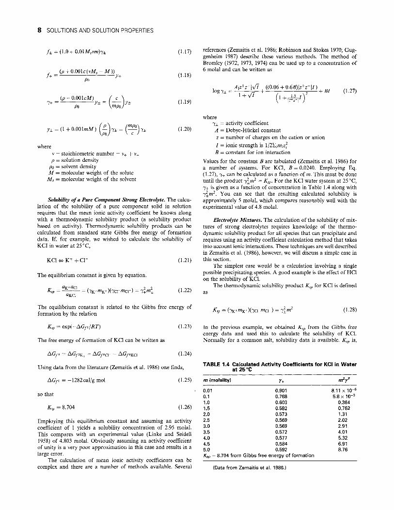
Values for the constant B are tabulated (Zemaitis et al. 1986) for a number of systems. For KCI, B = 0.0240. Employing Eq. (1.27), 7± can be calculated as a function of m. This must be done until the product 7|m^ = Ksp. For the KCI water system at 25 °C, 7+ is given as a function of concentration in Table 1.4 along with 7|m^. You can see that the resulting calculated solubihty is approximately 5 molal, which compares reasonably well with the experimental value of 4.8 molal.

Electrolyte Mixtures, The calculation of the solubility of mix­tures of strong electrolytes requires knowledge of the thermo­dynamic solubility product for all species that can precipitate and requires using an activity coefficient calculation method that takes into account ionic interactions. These techniques are well described in Zemaitis et al. (1986), however, we will discuss a simple case in this section.

The simplest case would be a calculation involving a single possible precipitating species. A good example is the effect of HCl on the solubihty of KCI.

The thermodynamic solubility product Ksp for KCI is defined

Ksp = (TK+'^KOCTCI-WCI-) = yim^ (1.28)

In the previous example, we obtained Kgp from the Gibbs free energy data and used this to calculate the solubility of KCI. Normally for a common salt, solubihty data is available. Ksp is.

TABLE 1.4 Calculated Activity Coefficients for KCI in Water a t 2 5 X

m (molality) nt'f

0.01 0.901 0.1 0.768 1.0 0.603 1.5 0.582 2.0 0.573 2.5 0.569 3.0 0.569 3.5 0.572 4.0 0.577 4.5 0.584 5.0 0.592 Ksp = 8.704 from Gibbs free energy of formation

(Data from Zemaitis et al. 1986.)

8.11 X 10-6 5.8 X 10-3

0.364 0.762 1.31 2.02 2.91 4.01 5.32 6.91 8.76

1.3. SOLUBILITY OF INORGANICS 9

therefore, obtained from the experimental solubihty data and activity coefficients. Using the experimental KCl solubility at 25 °C (4.8 molal) and the Bromley activity coefficients yields a Ksp = 8.01. If we wish to calculate the KCl solubihty in a 1 molal HCl solution, we can write the following equations

5.00

( 7 K + ^ K + ) ( 7 C I - ^ C I - ) = 1

(fromKCl) (from HCL) (from KCl) (from HCl)

(1.29)

(1.30)

Eqs. (1.29) and (1.30) must be satisfied simultaneously for a fixed value of 1 molal HCl.

Using Bromley's method for multicomponent electrolytes

log 7/ -Az^Vl + Fj

l + y/l (1.31)

where A = Hiickel constant / = ionic strength / = any ion present

Zi = number of charges on ion / Fi is an interaction parameter term

Fi = EBijzlmj

where 7 indicates all ions of opposite charge to i

_ Zj + Zj

where nij = molahty of ion j

((0.06 + 0.6g)|z,z,|) , „ Oij = ; 2 '" " ('*m

(1.32)

(1.33)

(1.34)

Employing these equations the activity coefficient for K" and CI" are calculated as a function of KCl concentration at a fixed HCl concentration of 1 molar. These values along with the molahties of the ions are then substituted in Eq. (1.29) until it is an equality (within a desired error). The solubihty of KCl in a 1 molal solution of HCl is found to be 3.73 molal, which compares with an experi­mental value of 3.92 molal. This calculation can then be repeated for other fixed HCl concentrations. Figure 1.8 compares the calculated and experimental values of KCl solubility over a range of HCl concentrations. Unfortunately, many systems of interest include species that form complexes, intermediates, and undis-sociated aqueous species. This greatly increases the complexity of solubility calculations because of the large number of possible species. In addition, mixtures with many species often include a number of species that may precipitate. These calculations are extremely tedious and time consuming to do by hand or to write a specific computer program for each application. Commercial software is available for calculations in complex electrolyte mixtures. The ProChem software developed by OLI Systems Inc. (Morris Plains, New Jersey) is an excellent example. The purpose of the package is to simultaneously consider the effects of the detailed reactions as well as the underlying species interactions

HCl MOLALITY

Figure 1.8 Calculated versus experimental KCl solubility in aqu­eous HCl solution at 25 °C. (Reproduced from J.F. Zemaitis, Jr., D.M. Clark, M. Rafal, and N.C. Scrivner (1986), Handbook of Aqueous Electrolyte Thermodynamics, p. 284. Used by permission of the American Institute of Chemical Engineers. © 1986 AIChE.)

TABLE 1.5 Calculated Results for Cr(0H)3 Solubility at 25 X

Equilibrium Constant

H2O CrOH+2 Cr(0H)2+ Cr(0H)3 (aq.) Cr(0H)3 (crystal) Cr(0H)4-Cr2(OH)2+* Cr3(OH)4+5 Liquid phase pH =

Species

H2O H+ OH" Cr+3 CrOH+2 Cr(0H)2+ Cr(0H)3 (aq) Cr(0H)4-Cr2(OH)2+* Cr3(OH)4+5

cr Na+

^10

Moles

55.5 1.22 X 1.00 X 2.21 X 9.32 X 1.65 X 6.56 X 3.95 X 2.98 X 4.48 X 1.00 X 1.01 X

10-10-10-10-10-10-10-10-10-10-10-

-10

-4

-18

-13

-8

/ -6

21

22

2

2

fC{mol/kg)

9.94 X 1.30 X 2.72 X 2.03 X 6.44 X 1.67 X 2.35 X 2.52 X

10-1^ 10-1^ 10-9 10-6 10-31

10-s 10-^ 10-^

Ionic strength = 1.01 x 10"^

Activity Coefficient

1.0 0.904 0.902 0.397 0.655 0.899 1.0 0.899 0.185 0.0725 0.898 0.898

(Data from Zemaitis et al. 1986.)

10 SOLUTIONS AND SOLUTION PROPERTIES

that determine the actual activity coefficient values. Only by such a calculation can the solubility be determined.

A good example of the complexity of these calculations can be seen when looking at the solubility of Cr(OH)3. Simply assuming the dissociation reaction

Cr(OH)3 4= Cr+3 + SOH" (1.35)

and calculation a solubiUty using the Ksp obtained from Gibbs free energy of formation leads to serious error. That is because a number of other dissociation reactions and species are possible. These include: Cr(0H)3 (undissociated molecule in solution); Cr(0H)4 ; Cr(OH)J; Cr(OH)2+; Cr2(OH)^+; and Cr3(0H)^+.

Calculation of the solubility of Cr(0H)3 as a function of pH using HCl and NaOH to adjust the pH requires taking into account all species, equihbrium relationships, mass balance, and electroneutrahty, as well as calculation of the ionic activity coef­ficients. The results of such a calculation (employing Prochem software) appears in Table 1.5 and Figures 1.9 and 1.10. Table 1.5 shows the results obtained at a pH of 10. Figure 1.9 gives the solubility results obtained from a series of calculations and also shows the concentration of the various species while Figure 1.10 compares the solubility obtained with that calculated from a solubility product. The solubility results obtained by the simple solubihty product calculation are orders of magnitude less than those obtained by the complex calculation, demonstrating

1x10-04

1x10-05

1x10-06

1x10-07

1x10-08

1x10-09

1x10-10

> 1x10-11

< 1x10-12 -J

S 1x10-13

1x10-14

1x10-15

1x10-16

1x10-17

1x10-18

1x10-19

1x10-20

M M H I I I i I I 11 I 11 I I 11 I i I I I I I I i I I i I H I I I I I I I I I

Cr2(OH)2(4+)

" " I " • •! " M ' M M l l l l I I I I I i h W i l M M l \ l l o o o \n c^ \n CD s : r^ 8

00

o in od

o o o in o o o

o in d 8

pH Figure 1.9 Chrome hydroxide solubility and speciation versus pH at 25 °C. (Reproduced from J.F. Zemaitis, Jr., D.M. Clark, M. Rafal, and N.C. Scrivner (1986), Handbook of Aqueous Electrolyte Thermodynamics, p. 661. Used by permission of the American Institute of Chemical Engineers. © 1986 AlChe.)

1.4 SOLUBILITY OF ORGANICS 11

10"*

f > •

CD

3 o (0 UJ

S o X

o

10-5

10-6

10-7

PURE WATER

C r ^ FROM SOLUBILITY PRODUCT

_L 8 10

Figure 1.10 Chrome solubility versus pH. (Reproduced with permission of OLI Systems.)

the importance of considering all possible species in the calcula­tion.

1.4. SOLUBILITY OF ORGANICS

In crystallization operations involving inorganic materials we vir­tually always employ water as the solvent, thus requiring solubility data on inorganic water systems. Since most inorganic materials are ionic, this means that dissociation reactions, ionic interactions, and pH play a major role in determining the solubility of a par­ticular inorganic species in aqueous solution. When dealing with organic species (or inorganics in nonaqueous solvents) a wide variety of solvents and solvent mixtures can usually be employed. The interaction between the solute and the solvent determines the differences in solubility commonly observed for a given organic species in a number of different solvents. This is illustrated in Figures 1.11 and 1.12 for hexamethylene tetramine and adipic acid in several different solvents. In the development of crystallization processes this can be a powerful tool. In many cases the solvent chosen for a particular process is an arbitrary choice made in the laboratory with no thought of the downstream processing con­sequences. Many times, from a chemical synthesis or reaction point of view, a number of different solvents could be used with no significant change in product yield or quality. This means that the solubility and physical properties of the solvent (solubility as a function of temperature, absolute solubility, and vapor pressure) should be evaluated so that the solvent that provides the best characteristics for the crystallization step is chosen. This of course requires that the process development engineers be in contact with the synthetic organic chemists early in a process development.

In this section we will describe the basic principles required to estimate and calculate the solubility of an organic solute in differ­ent solvents and explain how to assess mixed solvents.

1.4.1. THERMODYNAMIC CONCEPTS AND IDEAL SOLUBILITY

As we have shown previously, the condition for equilibrium between a solid solute and a solvent is given by the relation

0.08-4

0.07 4

0.06 H

c o •g 0.05. 2 o I 0.04.

5 003 •

ISOPROPANOL + WATER

3 o (0

0.02-J

o.oH

0.00

ETHANOL

10.00 T" T T"

15.00 20.00 25.00

TEMPERATURE, °C

30.00 T -| 35.00 40.00

Figure 1.11 Solubility of hexamethylenetetramine in different solv­ents. (Reprinted with permission from S. Decker, W.P. Fan, and A.S. Myerson, "Solvent Selection and Batch Crystallization," Ind. Eng. Chem. Fund. 25, 925. © 1986 American Chemical Society.)

o O S ••> 0)

o E >-- 1 CD

3 o (0

U.i iU-

0.15-

0.10-

0.05-

0.00

IDEAL ^ ^

IN ETHANOL

IN WATER

1 , — 1

IN IRA

T 1 1 20.0 25.0 30.0 35.0 40.0

TEMPERATURE, °C

45.0

'^'solid ^'solution (1.36)

Figure 1.12 Solubility of adipic acid in different solvents. (Reprinted with permissions from S. Decker, W.P. Fan, and A.S. Myerson (1986), "Solvent Selection and Batch Crystallization," Ind. Eng. Chem. Fund. 25, 925. © 1986 American Chemical Society.)

12 SOLUTIONS AND SOLUTION PROPERTIES

A thermodynamic function known as the fugacity can be defined

M,-M? = RTln/ / /« (1.37)

Comparing Eq. (1.10) with Eq. (1.37) shows us that the activity at =filfi^. Through a series of manipulations it can be shown (Prausnitz et al. 1999) that for phases in equilibrium

f. = f. J 'solid J h

'solution (1.38)

Eq. (1.38) will be more convenient for us to use in describing the solubility of organic soUds in various solvents. The fugacity is often thought of as a "corrected pressure" and reduces to pressure when the solution is ideal. Eq. (1.38) can be rewritten as

Aolid = 72-^2/2 (1.39)

where /2 = fugacity of the solid X2 = mole fraction of the solute in the solution / 2 = Standard state fugacity 72 = activity coefficient of the solute

X2 = 72/2'

(1.40)

Eq. (1.40) is a general equation for the solubiUty of any solute in any solvent. We can see from this equation that the solubility depends on the activity coefficient and on the fugacity ratio /2//2- The standard state fugacity normally used for solid-liquid equilibrium is the fugacity of the pure solute in a subcooled liquid state below its melting point. We can simphfy Eq. (1.40) further by assuming that our solid and subcooled liquid have small vapor pressures. We can then substitute vapor pressure for fugacity. If we further assume that the solute and solvent are chemically similar so that 72 = 1, then we can write

X2 = - solid solute

Pi, (1.41)

^subcooled liquid solute

Eq. (1.41) gives the ideal solubility. Figure 1.13, an example phase diagram for a pure component, illustrates several points. First, we are interested in temperatures below the triple point since we are interested in conditions where the solute is a soHd. Second, the subcooled liquid pressure is obtained by extrapolating the liquid-vapor line to the correct temperature.

Eq. (1.41) gives us two important pieces of information. The first is that the ideal solubility of the solute does not depend on the solvent chosen; the ideal solubihty depends only on the solute properties. The second is that it shows the differences in the pure component phase diagrams that result from structural differences in materials will alter the triple point and hence the ideal solubi­lity.

A general equation for the fugacity ratio is

In fi AHtp ( 1

J ^subcooled liquid solute R

' RT {P-Ptp)

AC, I n ^ ^ + 1

(1.42)

Critical • Point

UJ flC 3 (0 0) liJ

OL

subcooled liquid

TEMPERATURE

Figure 1.13 Schematic of a pure component phase diagram. (Reprinted by permission of Prentice Hall, Englewood Cliffs, New Jersey, from J.M. Prausnitz, R.N. Lichenthaler, and E. Gomes de Azevedo, Molecular Thermodynamics of Fluid-Phase Equilibria, 2nd ed., © 1986, p. 417.)

where IS.Htp = enthalpy change for the liquid solute transformation

at the triple point Ttp = triple point temperature

AC;, = difference between the Cp of the liquid and the solid AV = volume change

If substituted into Eq. (1.40) this yields the solubihty equation

X2 = —exp 72

AV RT

A7/,„

R \Tt

{P-Ptp)

R \ T T )

(1.43)

Eq. (1.43) is the most general form of the solubihty equation. In most situations (though not all) the effect of pressure on solubility is negligible so that the last term on the right-hand side of the equation can be dropped. In addition, the heat capacity term can also usually be dropped from the equation. This yields

1 X2 = —exp

72

AT/,, 1

or smce

AS = AHtplTtp

1 X2 = —exp

72 [ (.- - T,plT)

(1.44)

(1.45)

(1.46)

In many instances, the triple point temperature of a substance is not known. In those cases, the enthalpy of melting (fusion) and melting point temperature are used since they are usually close to the triple point temperature

1 X2— — exp

72

^Hm (1.47)

1.4 SOLUBILITY OF ORGANICS 13

TABLE 1.7 Permanent Dipole Moments lueai ouiuui i i i

Substance

Oft/70-chloronitrobenzene /Wefa-chloronitrobenzene Para-chloronitrobenzene Napthalene Urea Phenol Anthracene Phenanthrene Biphenyl

y u i \ji\§ai

r (K)

307.5 317.6 356.7 353.4 406.0 314.1 489.7 369.5 342.2

UM ouiu icd a

A H ^ (cal/mol)

4546 4629 4965 4494 3472 2695 6898 4456 4235

L £.U \*

Ideal Solubility

(mol%)

79 62 25 31 21 79

1 23 39

Molecule

CO C3H6 CgHsCHs PH3 HBr CHCI3 (C2H5)20 NH3 C6H5NH2 CSHBCI

C2H5SH SO2

fi (Debyes)

0.10 0.35 0.37 0.55 0.80 1.05 1.18 1.47 1.48 1.55 1.56 1.61

Molecule

CH3I CH3COOCH3 C2H5OH H2O HF C2H5F {CH3)2C0 C6H5COCH3 C2H5NO2 CH3CN

CO(NH2)2 KBr

fi (Debyes)

1.64 1.67 1.70 1.84 1.91 1.92 2.87 3.00 3.70 3.94 4.60 9.07

(Based on data from Walas 1985.) (Data from Prausnitz et al. 1986.)

For an ideal solution when the activity coefficient equation equals one, this reduces to

X2 = exp Aif^

R (1.48)

Eq. (1.48) allows the simple calculation of ideal solubilities and can be used profitably to see the differences in solubility of chemically similar species with different structures. This is illustrated in Table 1.6 where calculated ideal solubilities are shown together with AHm and 7^. Isomers of the same species can have widely different ideal solubilities based on changes in their physical properties, which relate back to their chemical structures. Eq. (1.48) also tells us that for an ideal solution, solubihty increases with increasing temperature. The rate of increase is approximately proportional to the magnitude of the heat of fusion (melting). For materials with similar melting temperatures, the lower the heat of fusion, the higher the solubihty. For materials with similar heats of fusion, the material with the lower melting temperature has the higher solubihty. A good example of this is shown in Table 1.6 when looking at ortho-, meta-, and /7«r«-chloronitrobenzene. The lower melting ortho has an ideal solubihty of 79 mol% compared with 25 mol% for the higher melting para. While Eq. (1.48) is useful for comparing relative solubihties of various solutes, it takes no account of the solvent used or solute-solvent interactions. To account for the role of the solvent, activity coefficients must be calculated.

is less symmetrical in terms of its electrical charge. A hst of mol­ecules and their dipole moments is given in Table 1.7. As you can see from the table, water is quite polar. There are also molecules with more complex charge distributions called quadrupoles, which also display this asymmetric charge behavior. This shows that even without ions, electrostatic interactions between polar solvent mol­ecules and polar solute molecules will be of importance in activity coefficient calculations and will therefore affect the solubility.

Organic solutes and solvents are usually classified as polar or nonpolar, though, of course, there is a range of polarity. Nonpolar solutes and solvents also interact through forms of attraction and repulsion known as dispersion forces. Dispersion forces result from oscillations of electrons around the nucleus and have a rather complex explanation; however, it is sufficient to say that non-idealities can result from molecule-solvent interactions that result in values of the activity coefficient not equal to 1. An excellent reference in this area is the book of Prausnitz et al. (1999).

Generally, the activity coefficients are < 1 when polar inter­actions are important, with a resulting increase in solubility of compounds compared with the ideal solubihty. The opposite is often true in nonpolar systems where dispersion forces are import­ant, with the activity coefficients being > 1. A variety of methods are used to calculate activity coefficients of solid solutes in solution. A frequently used method is that of Scatchard-Hildebrand, which is also known as "regular" solution theory (Prausnitz et al. 1999).

In 72 = Vi{8,-82f^\

RT (1.50)

1.4.2. REGULAR SOLUTION THEORY

In electrolytic solutions we were concerned with electrostatic inter­actions between ions in the solution and with the solvent (water). In solutions of nonelectrolytes we will be concerned with molecule-solvent interactions due to electrostatic forces, dispersion forces, and chemical forces.

Even though a solution contains no ions, electrostatic inter­actions can still be significant. This is because of a property called polarity. An electrically neutral molecule can have a dipole moment that is due to an asymmetric distribution of its electrical charge. This means that one end of the molecule is positive and the other end is negative. The dipole moment is defined by

fi = el (1.49)

where e is the magnitude of the electric charge and / is the distance between the two charges. The dipole moment is a measure of how polar a molecule is. As the dipole moment increases, the molecule

where V2 = molar volume of the subcooled liquid solute 62 = solubility parameter of the subcooled liquid 1 = solubility parameter of the solvent $ = volume fraction, or the solvent defined by

$: xiVt

• ^ i F f - •X2V^

The solubility parameters are defined by the relations

61 = Au\ 1/2 -m 1/2

(1.51)

(1.52)

where Aw is the enthalpy of vaporization and v is the molar liquid volume. Solubihty parameters for a number of solvents and solutes are given in Table 1.8. This method works moderately well at predicting solubihties in nonpolar materials. Calculated solubihty

14 SOLUTIONS AND SOLUTION PROPERTIES

TABLE 1.8 Solubility Parameters at 25 X

Substance J(cal/cm3)i/2

Anthracene Naphthalene Phenanthrene Acetic acid Acetone Aniline 1-Butanol Carbon disulfide Carbon tetrachloride Chloroform Cyclohexane Cyclohexanol Diethyl ether Ethanol n-Hexane Methanol Phenol 1-Propanol 2-Propanol Perfluoro-n-heptane Neopentane Isopentane n-Pentane 1-Hexene n-Octane n-Hexadecane Ethyl benzene Toluene Benzene Styrene Tetrachloroethylene Bronnine

9.9 9.38

10.52 10.05 9.51

11.46 11.44 9.86 9.34 9.24 8.19

11.4 7.54

12.92 7.27

14.51 12.11 12.05 11.57 6.0 6.2 6.8 7.1 7.3 7.5 8.0 8.8 8.9 9.2 9.3 9.3

11.5

(Based on data from Prausnitz et al. 1986 and Walas 1985.)

results employing this theory are shown in Table 1.9 along with experimentally determined values. It is apparent that in many cases this theory predicts results very far from the experiment. A variety of modifications of the Scatchard-Hildebrand theory as well as other methods are available for activity coefficient calculations and are described by Walas (1985), Prausnitz et al. (1999), and Reid et al. (1987), however, no accurate general method is avail­able for activity coefficient calculation of solid-solutes in liquids.

TABLE 1.9 Solubility of Napthalene in Various Solvents by UNIFAC and Scatchard-Hildebrand Theory

Solvent

Methanol Ethanol 1-Propanol 2-Propanol 1-Butanol n-Hexane Cyclohexanol Acetic acid Acetone Chloroform

Experimental

4.4 7.3 9.4 7.6

11.6 22.2 22.5 11.7 37.8 47.3

Ideal solubility

Solubility (mol%)

UNIFAC

4.8 5.4 9.3 9.3

11.1 25.9 20.5 12.5 35.8 47.0

= 4.1mol%

Scatchard-Hildebrand

0.64 4.9

11.3 16.3 18.8 11.5 20.0 40.1 42.2 37.8

(Data from Walas 1985.)

1.4.3. GROUP CONTRIBUTION METHODS

As we discussed in Section 1.3, on inorganic materials, industrial crystallization rarely takes place in systems that contain only the solute and solvent. In many situations, additional components are present in the solution that affect the solubility of the species of interest. With an organic solute, data for solubility in a particular solvent is often not available, while data for the effect of other species on the solubiUty is virtually nonexistent. This means that the only option available for determining solubility in a complex mixture of solute, solvent, and other components (impurities or by-products) is through calculation or experimental measurement. While experimental measurement is often necessary, estimation through calculation can be worthwhile.

The main methods available for the calculation of activity coefficients in multicomponent mixtures are called group contribu­tion methods. This is because they are based on the idea of treating a molecule as a combination of functional groups and summing the contribution of the groups. This allows the calculation of properties for a large number of components from a limited num­ber of groups. Two similar methods are used for these types of calculations, ASOG (analytical solution of groups) and UNIFAC (UNIQUAC functional group activity coefficient), and they are explained in detail in a number of references (Reid et al. 1987; Walas 1985; Kojima and Tochigi 1979; Frendenslund et al. 1977).

Both of these methods rely on the use of experimental activity coefficient data to obtain parameters that represent interaction between pairs of structural groups. These parameters are then combined to predict activity coefficients for complex species and mixtures of species made up from a number of these functional groups. An example of this would be the calculation of the behav­ior of a ternary system by employing data on the three possible binary pairs. Lists of parameters and detailed explanations of these calculations can be found in the references previously mentioned.

The groups contribution methods can also be used to calculate solubility in binary (solute-solvent) systems. A compari­son of solubihties calculated employing the UNIFAC method with experimental values and values obtained from the Scatch­ard-Hildebrand theory is given in Table 1.9.

1.4.4. SOLUBILITY IN MIXED SOLVENTS

In looking for an appropriate solvent system for a particular solute to allow for the development of a crystaUization process, often the desired properties cannot be obtained with the pure solvents that can be used. For a number of economic, safety, or product stability reasons, you may be forced to consider a small group of solvents. The solute might not have the desired solubility in any of these solvents, or if soluble, the solubility may not vary with temperature sufficiently to allow cooling crystallization. In these cases a pos­sible solution is to use a solvent mixture to obtain the desired solution properties. The solubility of a species in a solvent mixture can significantly exceed the solubility of the species in either pure component solvent. This is illustrated in Figure 1.14 for the solute phenanthrene in the solvents cyclohexane and methyl iodide. Instead of a linear relation between the solvent composition and the solubility, the solubility has a maximum at a solvent compo­sition of 0.33 wt% methyl iodide (solute-free basis). The large change in solubility with solvent composition can be very useful in crystallization processes. It provides a method other than tem­perature change to alter the solubility of the system. The solubility can be easily altered up or down by adding the appropriate solvent to the system. The method of changing solvent composition to induce crystallization will be discussed in more detail in Section 1.5.3.

1.4 SOLUBILITY OF ORGANICS 15

m z UJ

UJ X Q.

Z o

UL UJ

o

0.35 h

0.30 h

0.25 h

0.20 b

0.15

0.10 h

0.05 h

0.00

CH2I2 C6H12

Figure 1.14 Solubility of phenanthrene in cyclohexane-methylene iodide mixtures. (Reprinted with permission from L.J. Gordon and R.L. Scott, "Enhanced Methylene Iodide SolubiUty in Solvent Mixtures. I. The System Phenanthrene—Cyclohexane-Methylene Iodide," / . Am. Chem. Soc. 74, 4138. © 1952 American Chemical Society.)

Finding an appropriate mixed solvent system should not be done on a strictly trial and error basis. It should be examined systematically based on the binary solubility behavior of the solute in solvents of interest. It is important to remember that the mixed solvent system with the solute present must be miscible at the conditions of interest. The observed maximum in the solubility of solutes in mixtures is predicted by Scatchard-Hildebrand theory. Looking at Eq. (1.50) we see that when the solubility parameter of the solvent is the same as that of the subcooled liquid solute, the activity coefficient will be 1. This is the minimum value of the activity coefficient possible employing this relation. When the activity coefficient is equal to 1, the solubility of the solute is at a maximum. This then tells us that by picking two solvents with solubility parameters that are greater than and less than the solu­bility parameter of the solute, we can prepare a solvent mixture in which the solubility will be a maximum. As an example, let us look at the solute anthracene. Its solubiUty parameter is 9.9 (cal/cm ) /" . Looking at Table 1.8, which Hsts solubihty parameters for a num­ber of common solvents, we see that ethanol and toluene have solubility parameters that bracket the value of anthracene. If we define a mean solubility parameter by the relation

6 = (1.53)

we can then calculate the solvent composition that will have the maximum solubility. This is a useful way to estimate the opti­mum solvent composition prior to experimental measurement. Examples of these calculations can be found in Walas (1985).

Another useful method is to employ the group contribution methods described in the previous section with data obtained on the binary pairs that make up the system.

Recently, Frank et al. (1999) presented a good review of these and other calculation-based methods to quickly screen solvents for use in organic soHds crystallization processes.

1.4.5. MEASUREMENT OF SOLUBILITY

Accurate solubility data is a crucial part of the design, develop­ment, and operation of a crystallization process. When confronted with the need for accurate solubility data, it is often common to find that the data is not available for the solute at the conditions of interest. This is especially true for mixed and nonaqueous solvents, and for systems with more than one solute. In addition, most industrial crystallization processes involve solutions with impur­ities present. If it is desired to know the solubihty of the solute in the actual working solution with all impurities present, it is very unlikely that data will be available in the literature. Methods for the calculation of solubility have been discussed previously. These can be quite useful, but often are not possible because of lack of adequate thermodynamic data. This means that the only method available to determine the needed information is solubility meas­urement.

The measurement of solubility appears to be quite simple, however, it is a measurement that can easily be done incorrectly, resulting in very large errors. Solubility should always be measured at a constant controlled temperature (isothermal) with-agitation employed. A procedure for measuring solubility is given below:

1. To a jacketed or temperature-controlled vessel (temperature control should be 0.1 °C or better), add a known mass of solvent.

2. Bring the solvent to the desired temperature. If the temperature is above room temperature or the solvent is organic, use a condenser to prevent evaporation.

3. Add the solute in excess (having determined the total mass added) and agitate the solution for a period of at least 4 h. A time period of 24 h is preferable.

4. Sample the solution and analyze for the solute concentration.

If solute analysis is not simple or accurate, step 4 can be replaced by filtering the solution, drying the remaining solid, and weighing. The amount of undissolved solute is subtracted from the total initially added. The long period of time is necessary because dis­solution rates become very slow near saturation. If a short time period is used (1 h or less), the solubihty will generally be under­estimated.

If care is taken, data obtained using this procedure will be as accurate as the concentration measurement or weighing accuracy achieved.

Two common errors in solubility measurement that produce large errors involve using nonisothermal techniques. In one tech­nique a solution of known concentration is made at a given tem­perature above room temperature and cooled until the first crystals appear. It is assumed that this temperature is the saturation tem­perature of the solution of the concentration initially prepared. This is incorrect. As we will see in Section 1.5, solutions become supersaturated (exceed their solubility concentration) before they crystallize. The temperature that the crystals appeared is likely to be significantly below the saturation temperature for that concen­tration so that the solubility has been significantly overestimated.

Another method that will result in error is to add a known amount of solute in excess to the solution and raise the tempera­ture until it all dissolves. It is assumed that the temperature at which the last crystal disappears is the solubility temperature at the concentration of solution (total solute added per solvent in sys­tem). This is again incorrect because dissolution is not an instant­aneous process and, in fact, becomes quite slow as the saturation

16 SOLUTIONS AND SOLUTION PROPERTIES

temperature is approached. This method will underestimate the solubility because the solution will have been heated above the saturation temperature.

Accurate solubiHty data is worth the time and trouble it will take to do the experiment correctly. Avoid the common errors discussed and be suspicious of data where the techniques used in measurement are not known.

1.5. SUPERSATURATION AND METASTABILITY

As we have seen in the previous section, solubility provides the concentration at which the solid solute and the liquid solution are at equilibrium. This is important because it allows calculation of the maximum yield of product crystals accompanying a change of state from one set of concentration to another in which crystals form. For example, if we look at Figure 1.15, which gives us the solubihty diagram for KCl, if we start with 1000 kg of a solution at 100 °C and a concentration of 567g/kg water and cool it to 10 °C at equihbrium, we will have 836 kg of solution with a KCl con­centration of 310g/kg water and 164 kg of solid KCl. While this mass balance is an important part of crystallization process design, development, and experimentation, it tells us nothing about the rate at which the crystals form and the time required to obtain this amount of solid. That is because thermodynamics tells us about equilibrium states but not about rates. Crystallization is a rate process, this means that the time required for the crystallization depends on some driving force. In the case of crystallization the driving force is called the super saturation.

Supersaturation can be easily understood by referring to Fig­ure 1.15. If we start at point A and cool the solution of KCl to a temperature of 40°C, the solution is saturated. If we continue to cool a small amount past this point to B, the solution is hkely to remain homogeneous. If we allow the solution to sit for a period of time or stir this solution, it will eventually crystallize. A solution in which the solute concentration exceeds the equihbrium (satura­tion) solute concentration at a given temperature is known as a supersaturated solution. Supersaturated solutions are metastable. We can see what that means by looking at Figure 1.16. A stable solution is represented by Figure 1.16a and appears as a minimum. A large disturbance is needed to change the state in this instance. An unstable solution is represented by Figure 1.16b and is just the

opposite, with the solution being represented by a sharp maximum so that a differential change will result in a change in the state of the system. A metastable solution is represented by Figure 1.16c as an inflection point where a small change is needed to change the state of the system, but one which is finite. MetastabiHty is an important concept that we will discuss in greater detail in Section 1.5.2.

1.5.1. UNITS

Supersaturation is the fundamental driving force for crystallization and can be expressed in dimensionless form as

RT = ln—= ln

a* 7c

(1.54)

where /x is the chemical potential, c is the concentration, a is the activity, 7 is the activity coefficient, and * represents the property at saturation. In most situations, the activity coefficients are not known and the dimensionless chemical potential difference is approximated by a dimensionless concentration difference

c = c — - (1.55)

This substitution is only accurate when 7/7* = 1 or cr < 1 so that ln(cr+ 1) = cr. It has been shown that this is generally a poor approximation at a > 0.1 (Kim and Myerson 1996), but it is still normally used because the needed thermodynamic data are usually unavailable. Supersaturation is also often expressed as a concen­tration difference

Ac = c — c*

and as a ratio of concentrations

^-?

(1.56)

(1.57)

It is important to note that these definitions of supersaturation assume an ideal solution with an activity coefficient of 1. It is common practice to ignore activity coefficients in most cases and employ concentrations in expressions of supersaturadon, however, in very nonideal solutions and in precise studies of crystal growth and nucleation, activity coefficients are often used.

O CM

X O)

s o

O)

550

500

450

400

350

300

250

-

J 1 J 1 1

20 80 100 40 60

TEMPERATURE ^C

Figure 1.15 Solubihty of KCl in aqueous solution. (Data from Linke and Seidell 1958, 1965.)

120

1.5 SUPERSATURATION AND METASTABILITY 17

STABLE UNSTABLE a b

Figure 1.16 Stability states.

Another practice is to refer to supersaturation in terms of degrees. This refers to the difference between the temperature of the solution and the saturation temperature of the solution at the existing concentration. A simpler way to explain this is that the degrees of supersaturation are simply the number of degrees a saturated solution of the appropriate concentration was cooled to reach its current temperature. This is generally not a good unit to use, however, it is often mentioned in the literature.

1.5.2. METASTABILITY AND THE METASTABLE LIMIT

As we have seen previously, supersaturated solutions are meta-stable. This means that supersaturating a solution some amount will not necessarily result in crystallization. Referring to the solu­bility diagram shown in Figure 1.17, if we were to start with a solution at point A and cool to point B just below saturation, the solution would be supersaturated. If we allowed that solution to sit, it might take days before crystals formed. If we took another sample, cooled it to point C. and let it sit, this might crystallize in a matter of hours; eventually we will get to a point where the solu­tion crystallized rapidly and no longer appears to be stable. As we can see from this experiment, the metastability of a solution decreases as the supersaturation increases. It is important to note however that we are referring to homogeneous solutions only. If crystals of the solute are placed in any supersaturated solution, they will grow, and the solution will eventually reach equilibrium. The obvious question that comes to mind is why are supersatu­rated solutions metastable. It seems reasonable to think that if the solubility is exceeded in a solution, crystals should form. To under­stand why they do not, we will have to discuss something called nucleation. Nucleation is the start of the crystallization process and involves the birth of a new crystal. Nucleation theory tells us that when the solubility of a solution is exceeded and it is supersatu­rated, the molecules start to associate and form aggregates (clus­ters), or concentration fluctuations. If we assume that these aggregates are spherical, we can write an equation for the Gibbs free energy change required to form a cluster of a given size

METASTABLE c

15 20 25 30

TEMPERATURE ( C)

50

AG = Aixr^a- {^f\RT ln(l + S)

Figure 1.17 Metastable zone width for KCl-water system. (Data from Chang 1984.)

where r is the cluster radius, a is the soHd-liquid interfacial tension, and Vm is the specific volume of a solute molecule.

The first term is the Gibbs free energy change for forming the surface, and the second term is for the volume. For small numbers of molecules the total Gibbs free energy change is positive. This means that the clusters are unstable and will dissolve. A plot of AG as a function of cluster size (Figure 1.18) shows that as the cluster size increases, we reach a point where the Gibbs free energy change is negative and the cluster would grow spontaneously. When this happens, nucleation will occur. The reason that supersaturated solutions are metastable is, therefore, because of the need for a critical sized cluster to form. From Eq. (1.58) we can derive an expression for the critical size by setting the derivative dAG/dr = 0 (the minimum in Figure 1.18) yields

(1.58) rc=2V^alRT In(H-S) (1.59)

18 SOLUTIONS AND SOLUTION PROPERTIES

1 ^f^-^ ^ r* — - \ H

A^v

A°s

A^cr i t -\rr(jx\\

^^7^ \

\

\ \ \ \ \ \ \

TABLE 1.10 Metastable Zone Width

O <]

O cc UJ z UJ UJ UJ

SIZE OF NUCLEUS, r

Figure 1.18 Free energy versus cluster radius. (Reproduced with permission from Mullin 1972.)

We can see from this equation that as the supersaturation increases, the critical size decreases. That is why solutions become less and less stable as the supersaturation is increased. Unfor­tunately, Eqs. (1.58) and (1.59) are not useful for practical calcu­lations because one of the parameters, a = the cluster interfacial tension, is not available or measurable and has a very significant effect on the calculation.

Every solution has a maximum amount that it can be super­saturated before it becomes unstable. The zone between the satura­tion curve and this unstable boundary is called the metastable zone and is where all crystallization operations occur. The boundary between the unstable and metastable zones has a thermodynamic definition and is called the spinodal curve. The spinodal is the absolute limit of the metastable region where phase separation must occur immediately. In practice, however, the practical limits of the metastable zone are much smaller and vary as a function of conditions for a given substance. This is because the presence of dust and dirt, the cooling rate employed and/or solution history, and the use of agitation can all aid in the formation of nuclei and decrease the metastable zone. Figure 1.17 gives an estimated meta­stable zone width for KCl in water.

Measurement of the metastable zone width and values for the metastable zone width obtained by a variety of methods for inor­ganic materials can be found in the work of Nyvlt et al. (1985). In general there are two types of methods for the measurement of the metastable limit. In the first method, solutions are cooled to a given temperature rapidly and the dme required for crystallization is measured. When this dme becomes short then the effective metastable limit has been approached. A second method is to cool a solution at some rate and observe the temperature where the first crystals form. The temperature at which crystals are first observed will vary with the cooling rate used. Measured metastable limits for a number of materials are given in Table 1.10.

Data on the effective metastable limit at the conditions you are interested in (composition, cooling rate, and stirring) are important because you normally wish to operate a crystallizer away from the edge of the effective metastable zone. As we will see in later chapters, formation of small crystals, which are known 3LS fines, is a common problem. Fines cause filtration problems and

Substance

Ba(N03)2 CUSO4 •5H2O

FeS04 • 7H2O

KBr

KCl

MgS04-7H20 NH4AI(S04)2-12H20

NaBr-2H20

Equilibrium Temperature

( X )

30.8 33.6 60.4 30.0 40.6 30.3 61.0 29.8 59.8 32 30.2 63 30.6

Maximum Undercooling Before Nucleation

2°C/h

1.65 5.37 0.93 0.89 0.57 1.62 1.69 1.62 1.02 1.95 0.81 1.19 4.6

Cooling Rate

5 X / h

2.17 6.82 1.30 1.21 0.83 2.33 2.41 1.86 1.18 2.63 1.34 1.95 6.97

20°C/h

3.27 9.77 2.16 1.93 1.46 4.03 4.11 2.30 1.48 4.15 2.88 4.13

13.08

(Data from Nyvlt et al. 1985.)

often are not wanted for various reasons in the final product. When a crystallization occurs at a high supersaturation (near the metastable limit) this usually means small crystals. The effective metastable zone width is an important process development and experimental design tool, and is worth the time to estimate.

1.5.3. METHODS TO CREATE SUPERSATURATION

In our discussions of supersaturation and metastabihty, we have always focused on situations where supersaturation is created by temperature change (cooling). While this is a very common method to generate supersaturation and induce crystallization, it is not the only method available.

There are four main methods to generate supersaturation that follow:

1. Temperature change. 2. Evaporation of solvent. 3. Chemical reaction. 4. Changing the solvent composition.

As we have discussed previously, the solubility of most materials declines with declining temperature so that cooling is often used to generate supersaturation. In many cases however, the solubility of a material remains high even at low temperatures or the solubility changes very little over the temperature range of interest. In these cases, other methods for the creation of supersaturation must be considered.

After cooling, evaporation is the most commonly used method for creating supersaturation. This is especially true when the solv­ent is nonaqueous and has a relatively high vapor pressure. The principle of using evaporation to create supersaturation is quite simple. Solvent is being removed from the system, thereby increas­ing the system concentration. If this is done at a constant tempera­ture, eventually the system will become saturated and then supersaturated. After some maximum supersaturation is reached, the system will begin to crystallize.

There are a number of common methods used to evaporate solvents and crystallize materials based on the materials properties and solubility. One very common method for a material that has a solubility that decreases with decreasing temperature is to cool the system by evaporating solvent. Evaporation causes cooling in any system because of the energy of vaporization. If a system is put under a vacuum at a given temperature, the solvent will evaporate

1.5 SUPERSATURATION AND METASTABILITY 19

> 3 S 3 o (0

15 H

10 J

5H

60 70 80

% VOLUME DMSO

Figure 1.19 Solubility of terephthalic acid in DMSO-water mix­tures at 25 °C. (Data from Saska 1984.)

and the solution will cool. In this case the concentration of the system increases while the temperature of the system decreases. In some cases, the cooling effect of the evaporation slows the evap­oration rate by decreasing the system vapor pressure; in these cases, heat is added to the system to maintain the temperature and thereby the evaporation rate. Virtually all evaporations are done under vacuum.

As we saw in our discussion of solubiHty, the mixing of solvents can result in a large change in the solubility of the solute in the solution. This can be used to design a solvent system with specific properties and can also be used as a method to create supersaturation. If we took, for example, a solution of terephthalic acid (TPA) in the solvent dimethylsulfoxide (DMSO) at 25 °C, the solubihty of the TPA at this temperature is 16.5 wt%. A coohng-

crystallization starting from some temperature above this to 23 °C (about room temperature) would leave far too much product in solution.

Imagine that evaporation cannot be used because of the lack of reasonable equipment, or because the solvent is not volatile enough and the product is heat sensitive. The third option is to add another solvent to the system to create a mixed solvent system in which the solubility of the solute is greatly decreased. If we were to add water to the TPA-DMSO system, the solubiHty changes rapidly from 16.5 wt% to essentially zero wt% with the addition of 30% water (by volume on the solute-free basis). This is shown in Figure 1.19. By controUing the rate of the addition, we can control the rate of supersaturation just as we can by cooling or by evap­oration. In this case however, good mixing conditions are import­ant so that we do not have local regions of high supersaturation and other regions of undersaturation.

This method of creating supersaturation is often called drown­ing out or adding a miscible nonsolvent. Normally you can find an appropriate solvent to add by looking for a material in which the solute is not soluble, that is miscible with the solute-solvent sys­tem. This can be done experimentally or screening can be done using solubility calculations prior to experimental tests. This is a particularly valuable technique with organic materials.

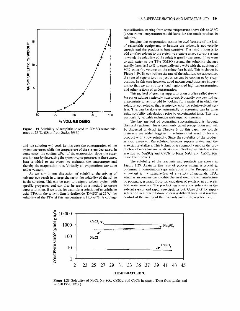
The last method of generating supersaturation is through chemical reaction. This is commonly called precipitation and will be discussed in detail in Chapter 6. In this case, two soluble materials are added together in solution that react to form a product with a low solubility. Since the solubility of the product is soon exceeded, the solution becomes supersaturated and the material crystallizes. This technique is commonly used in the pro­duction of inorganic materials. An example of a precipitation is the reaction of Na2S04 and CaCl2 to form NaCl and CaS04 (the insoluble product).

The solubility of the reactants and products are shown in Figure 1.20. Again in this type of process mixing is crucial in obtaining a homogenous supersaturation profile. Precipitation is important in the manufacture of a variety of materials. TPA, which is an organic commodity chemical used in the manufacture of polymers, is made from the oxidation of /^-xylene in an acetic acid water mixture. The product has a very low solubility in the solvent system and rapidly precipitates out. Control of the super-saturation in a precipitation process is difficult because it involves control of the mixing of the reactants and or the reaction rate.

21 23 25 27 29 31 33 35 37 39 41 43 45

TEMPERATURE°C

Figure 1.20 Solubility of NaCl, Na2S04, CaS04, and CaC^ in water. (Data from Linke and Seidell 1958, 1965.)

20 SOLUTIONS AND SOLUTION PROPERTIES

TABLE 1.11 Density and Viscosity of Common Solvents

Substance Density at 20 °C

(g/cm^) Viscosity at 20 °C

(cP)

Water Acetone Benzene Toluene Carbon tetrachloride Methanol Ethanol n-Propanol

0.999 0.789 0.879 0.866 1.595 0.791 0.789 0.804

1.00 0.322 0.654 0.587 0.975 0.592 1.19 2.56

(Based on data from Mulin 1972 and Weast 1975.)

In general, you usually have the choice of more than one method to generate supersaturation. You should evaluate the system equipment available, solubility versus temperature of the material, and the production rate required before choosing one of the methods we discussed.

1.6. SOLUTION PROPERTIES

1.6.1. DENSITY

The density of the solution is often needed for mass balance, flow rate, and product yield calculations. Density is also needed to convert from concentration units based on solution volume to units of concentration based on mass or moles of the solution. Density is defined as the mass per unit volume and is commonly reported in g/cm , however, other units such as pounds mass (Ibm)/ft^ and kg/m^ are often used. When dealing with solutions, density refers to a homogeneous solution (not including any crystal present). Spe­cific volume is the volume per unit mass and is equal to l/p.

Densities of pure solvents are available in handbooks like the Handbook of Chemistry and Physics (Lide 1999). The densities of a number of common solvents appear in Table 1.11. The densities of solutions as a function of concentration are difficult to find except for some common solutes in aqueous solution. The density of NaCl and sucrose as a function of concentration are given in Figure 1.21.

Densities are a function of temperature and must be reported at a specific temperature. A method for reporting densities uses a ratio known as the specific gravity. Specific gravity is the ratio of the density of the substance of interest to that of a reference

substance (usually water) at a particular temperature. To make use of specific gravity data it is necessary to know the density of the reference material at the correct temperature and to multiply the specific gravity by the reference density.

If density data is not available for the solution of interest, the density can be estimated by using the density of the pure solvent and pure solid solute at the temperature of interest and assuming the volumes are additive

1 _ H^crystal >^solvent

Psolution Pcrystal ^solvent (1.60)

where w is the mass fraction of crystal or solvent. Calculating the density of a saturated solution of NaCl at 25 °C using Eq. (1.60) results in a value of 1.17g/cm^ compared with the experimental value of 1.20 g/cm^. Density can be calculated with more accuracy using thermodynamic techniques described in Reid et al. (1987).

Density can be measured in the laboratory in a number of different ways depending on the need for accuracy and the number of measurements required. Solution density can be easily estimated with reasonable accuracy by weighing a known volume of solution. Very precise instruments for the measurement of density that work employing a vibrating quartz element in a tube are sold by the Mettler Company (Hightstown, New Jersey). The period of vibra­tion of the element is proportional to the density of the material placed in the tube. With careful calibration and temperature con­trol the accuracy of these instruments ranges from 1 x 10"^ to 1 X 10~^g/cm^. It is possible to use these instruments for on-line solution density measurement of fluid in a crystallizer (Rush 1991).

Another term typically used to describe solid-liquid mixtures is slurry or magma density. This is usually defined in terms of the mass of sohds per unit volume of solution. A 10% slurry density therefore would indicate 100 g of solids/1 of solution. Slurry density is not actually a true density but is a convenient term for indicating the amount of suspended soUds in the solution.

1.6.2. VISCOSITY

The design of any equipment that involves the flow or stirring of liquids requires a knowledge of the fluids viscosity. Since crystal­lization operations involve the stirring and movement of suspen­sions of particles in fluids, the viscosity of suspensions is important in crystallization design and operation. Viscosity is a property of a

CO E o

^.2

1.15

1.1

1.05

1

NaCl

^ —

- ^ ^ - r i ^ " ^ 1 1 1 1

""SUCROSE

1 i 1 i 1 1 1 . 20 40 60 80 100 120 140 160 180 200 220 240

CONCENTRATION, g/kg WATER

Figure 1.21 Density of sodium chloride and sucrose aqueous solutions as 20 °C. (Data from Weast 1975.)

1.6 SOLUTION PROPERTIES 21

TABLE 1.12 Viscosity Units and Conversion Factors

Given a Quantity in

These Units:

Multiply by Table Value

to Convert to These Units: —>

g cm"^s"^ kg m""'s~'' Ibm ft- ' 's- ' ' Ibf s- ' ' f t - i cP lbmf t - ' 'h - ' '

g cm ""s"

1 10 1.4882 X 10^ 4.7880 X 102 10-2 4.1338 X 10-3

kg m-^s"^

10-1 1 1.4882 4.7880 X 10^ 10-3 4.1338 X 10-*

ibm n-'s-'

6.7197 X 10-2 6.7197 X 10-2 1 32.1740 6.7197 X 10-* 2.7778 X 10-*

Ibf s - i f t -2

2.0886 X 10-3 2.0886 X 10-3 3.1081 X 10-2 1 2.0886 X 10-5 8.6336 X 10-^

cP

102 103 1.4882 X 103 4.7880 X 10* 1 4.1338 X 10-1

Ibm f t - ' h - i

2.4191 X 102 2.4191 X 103 3600 1.1583 X 10^ 2.4191 1

(Reprinted by permission of John Wiley & Sons, Inc. from R.B. Bird, W.E. Stewart, and E.N. Lightfoot (1960), Transport Phenomena. 1960 John Wiley & Sons, Inc.)

particular material defined as the ratio of the shear stress and the shear rate. Viscosity can be thought of as a measure of the resist­ance of a fluid to flow. When the relationship between shear stress and shear rate is linear and passes through the origin, the material is said to be Newtonian and the relationship can be represented by

-fi dux^

dy (1.61)

where Tyx = shear stress dux —r- = shear rate dy

fj, = viscosity

Most common solvents are Newtonian fluids. Looking at Eq. (1.61) we can see that the units of viscosity will be given by the ratio of the shear stress and the shear rate which is mass/distance-time. Typical units used for viscosity are given in Table 1.12 along with their conversion factors. The ratio of the viscosity and the density is another commonly used term that is known as the

kinematic viscosity. The kinematic viscosity has units of length squared per unit time.

The viscosity of most common solvents is available in the literature. The values for some common solvents appear in Table 1.12. The viscosity of solutions of solids dissolved in liquids is normally not available at high concentrations except for common solutes in aqueous solution.

Viscosity increases with increasing concentration in solutions and decreases with increasing temperature. Recent work (Myerson et al. 1990; Ginde and Myerson 1991) has shown that the viscosity of supersaturated solutions increases with increasing concentration much more rapidly than in undersaturated solutions. This is demonstrated in Figures 1.22 and 1.23 for KCl and glycine in aqueous solutions. This rise in viscosity has been attributed to the formation of precritical molecular clusters in the solution. The formation of clusters in solution is a time-dependent process with the cluster size increasing with increasing time. This would indicate a possible dependence of viscosity on solution "age." In recent experiments (Ginde and Myerson 1991) this has been observed in the glycine-water system, however, the effect is quite small.

In crystallization operations, the viscosity of the slurry of solu­tion and crystals is of importance. The viscosity of a slurry of

CL O

^ (0 o o (/) >

1.05

1

0.95

0.9

0.85

0.8

* " • • • • • • • •

_ _ 1 _ . . .

"^•T" •

• •

1

m^^^ m_^

1

/ •

Cs 1

/ / / / •

10 20 30 40

CONCENTRATION (g/100 g H2O)

Figure 1.22 Viscosity of aqueous KCl solutions at 25 °C. (Reproduced from R.M. Ginde and A.S. Myerson (1991), "Viscosity and Diffusivity in Metastable Solutions," AlChe Symposium Series, vol. 87, no. 284, pp. 124-129. Used by permission of the American Institute of Chemical Engineers. © 1991 AIChE.)

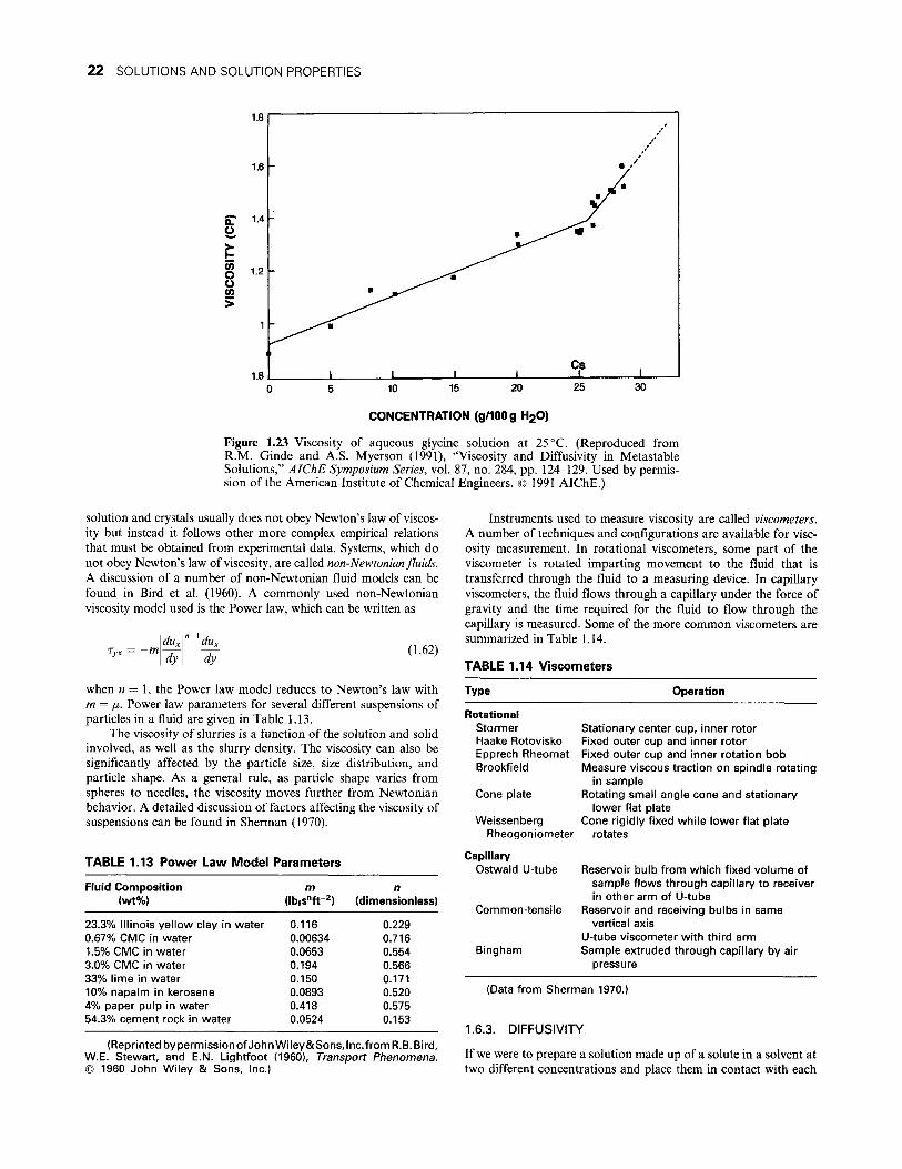
22 SOLUTIONS AND SOLUTION PROPERTIES

O

(0

8 (0

>

1.8

1.6

1.4

1.2

1

1

1.8

-

1

^.^^"'^

1

• - ^

I

^ .,-' *

J_

•

1

• y

^ - ^

Cs >

/'

1 1 10 15 20 25 30

CONCENTRATION (g/IOOg H2O)

Figure 1.23 Viscosity of aqueous glycine solution at 25 °C. (Reproduced from R.M. Ginde and A.S. Myerson (1991), "Viscosity and Diffusivity in Metastable Solutions," AIChE Symposium Series, vol. 87, no. 284, pp. 124-129. Used by permis­sion of the American Institute of Chemical Engineers. © 1991 AIChE.)

solution and crystals usually does not obey Newton's law of viscos­ity but instead it follows other more complex empirical relations that must be obtained from experimental data. Systems, which do not obey Newton's law of viscosity, are called non-Newtonian fluids. A discussion of a number of non-Newtonian fluid models can be found in Bird et al. (1960). A commonly used non-Newtonian viscosity model used is the Power law, which can be written as

dux dy

(1.62)

when « = 1, the Power law model reduces to Newton's law with m = ji. Power law parameters for several different suspensions of particles in a fluid are given in Table 1.13.

The viscosity of slurries is a function of the solution and solid involved, as well as the slurry density. The viscosity can also be significantly affected by the particle size, size distribution, and particle shape. As a general rule, as particle shape varies from spheres to needles, the viscosity moves further from Newtonian behavior. A detailed discussion of factors affecting the viscosity of suspensions can be found in Sherman (1970).

TABLE 1.13 Power Law M o d e l Parameters

Fluid Composit ion (wt%)

m (lb,s"ft-2)

n (dimensionless)

23.3% Illinois yel low clay in water 0.116 0.229 0.67% CMC in water 0.00634 0.716 1.5% CMC in water 0.0653 0.554 3.0% CMC in water 0.194 0.566 33% lime in water 0.150 0.171 10% napalm in kerosene 0.0893 0.520 4% paper pulp in water 0.418 0.575 54.3% cement rock in water 0.0524 0.153

(Reprinted bypermissionofJohnWiley&SonsJnc. f romR.B. Bird, W.E. Stewart, and E.N. Lightfoot (1960), Transport Phenomena. © 1960 John Wiley & Sons, Inc.)

Instruments used to measure viscosity are called viscometers. A number of techniques and configurations are available for visc­osity measurement. In rotational viscometers, some part of the viscometer is rotated imparting movement to the fluid that is transferred through the fluid to a measuring device. In capillary viscometers, the fluid flows through a capillary under the force of gravity and the time required for the fluid to flow through the capillary is measured. Some of the more common viscometers are summarized in Table 1.14.

TABLE 1.14 Viscometers

Type Operation

Rotational Stormer Haake Rotovisko Epprech Rheomat Brookfield

Cone plate

Weissenberg Rheogoniometer

Capillary Ostwald U-tube

Common-tensile

Bingham

Stationary center cup, inner rotor Fixed outer cup and inner rotor Fixed outer cup and inner rotation bob Measure viscous traction on spindle rotating

in sample Rotating small angle cone and stationary

lower flat plate Cone rigidly fixed while lower flat plate

rotates

Reservoir bulb f rom which fixed volume of sample f lows through capillary to receiver in other arm of U-tube

Reservoir and receiving bulbs in same vertical axis

U-tube viscometer wi th third arm Sample extruded through capillary by air

pressure

(Data from Sherman 1970.)

1.6.3. DIFFUSIVITY

If we were to prepare a solution made up of a solute in a solvent at two different concentrations and place them in contact with each

1.6 SOLUTION PROPERTIES 23

other, eventually they would achieve the same concentration through the process of diffusion. The solute molecules would diffuse from the region of high concentration to the region of lower concentration, and the solvent molecules would diffuse in the opposite direction (from higher to lower concentration of water). This process is described by Pick's first law of diffusion, which is written below

J A = —DAB dCA

dx (1.63)

where J A = molar diffusive flux CA = the concentration

DAB = the diffusivity (or diffusion coefficient)

The diffusion coefficient is a property of a given solute in a given solvent and tells us the rate in which the solute will diffuse under a concentration gradient. The units of diffusivity are length squared/ time. Diffusion coefficients vary with temperature and with solute concentration. The diffusion coefficient is important to crystal­lization operations because it is one of the properties that deter­mines the degree of agitation required. If insufficient agitation is used in a crystallization process, the crystal growth rate can be controlled by the rate of solute transfer from the bulk solution to the crystal-liquid interface. This is called mass transfer controlled crystal growth. Normally this is undesirable because the crystal growth rate obtained is usually significantly slower than the rate that would be obtained if interfacial attachment kinetics were the rate-controlling step. This will be discussed in more detail in Chapter 2, however, the important point is that the diffusion coefficient is a property that must be taken into account in looking at mass transfer, mixing, and agitation in crystallization processes.

Data on the diffusion coefficients of sohd solutes in liquid solvents are difficult to find and, if available, are usually found at low concentrations (or infinite dilution) at only one temperature. The concentration and temperature dependence of diffusion coef­

ficients in the glycine-water system is illustrated in Figure 1.24. The behavior shown in Figure 1.24 is typical nonelectrolyte behav­ior, with the diffusivity declining from a maximum value at infinite dilution in an approximately linear fashion. A comparison of the curves at different temperatures shows that the diffusion coefficient increases with increasing temperature. The data dis­played in Figure 1.24 was for an undersaturated solution only. The diffusivity of glycine in supersaturated solutions is shown in Figure 1.25. The diffusivity decUnes rapidly with increasing con­centration in the supersaturated region. In addition. Figure 1.25 shows that the diffusivity is a function of solution "age," decreas­ing as the solution age increases.

The diffusivity of KCl in aqueous solutions is shown in Figure 1.26. In electrolytes, the diffusivity initially decreases with increasing concentration, reaches a minimum, and then increases until saturation. The diffusivity then rapidly declines with increas­ing concentration in the supersaturated region.

The behavior of the diffusion coefficient in supersaturated solutions can be explained in two different ways, one based on thermodynamics, and the second based on metastable solution structure and nucleation theory. If we think of this thermodynam-ically, it is useful to look at equations used to predict concentra­tion-dependent diffusion coefficients. Two examples are listed below

n = D'>(l+^)f^ (Gordon)

D = D^ /^ln«2 \ (Stokes-Einstein) \d\nx2J

where

D^ = diffusivity at infinite dilution fi\ = viscosity of the solvent fis = viscosity of the solution

(1.64)

(1.65)

CONCENTRATION (MOLAR)

Figure 1.24 Diffusion coefficients of aqueous glycine solutions at 25, 35, and 45 °C. (Data from Chang 1984.)

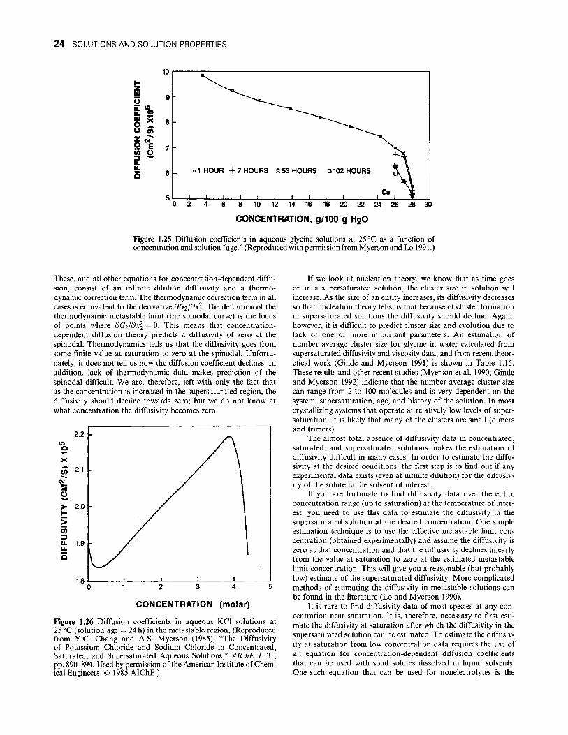
24 SOLUTIONS AND SOLUTION PROPERTIES

6 8 10 12 14 16 18 20 22 24 26 28 30

CONCENTRATION, g/100 g H2O

Figure 1.25 Diffusion coefficients in aqueous glycine solutions at 25 °C as a function of concentration and solution "age." (Reproduced with permission from Myerson and Lo 1991.)

These, and all other equations for concentration-dependent diffu­sion, consist of an infinite dilution diffusivity and a thermo­dynamic correction term. The thermodynamic correction term in all cases is equivalent to the derivative dGijdx^. The definition of the thermodynamic metastable limit (the spinodal curve) is the locus of points where OGi/dxl = 0. This means that concentration-dependent diffusion theory predicts a diffusivity of zero at the spinodal. Thermodynamics tells us that the diffusivity goes from some finite value at saturation to zero at the spinodal. Unfortu­nately, it does not tell us how the diffusion coefficient declines. In addition, lack of thermodynamic data makes prediction of the spinodal difficult. We are, therefore, left with only the fact that as the concentration is increased in the supersaturated region, the diffusivity should decline towards zero; but we do not know at what concentration the diffusivity becomes zero.

CONCENTRATION (molar)

Figure 1.26 Diffusion coefficients in aqueous KCl solutions at 25 °C (solution age = 24 h) in the metastable region, (Reproduced from Y.C. Chang and A.S. Myerson (1985), "The Diffusivity of Potassium Chloride and Sodium Chloride in Concentrated, Saturated, and Supersaturated Aqueous Solutions," AIChE / . 31, pp. 890-894. Used by permission of the American Institute of Chem­ical Engineers. © 1985 AIChE.)

If we look at nucleation theory, we know that as time goes on in a supersaturated solution, the cluster size in solution will increase. As the size of an entity increases, its diffusivity decreases so that nucleation theory tells us that because of cluster formation in supersaturated solutions the diffusivity should decline. Again, however, it is difficult to predict cluster size and evolution due to lack of one or more important parameters. An estimation of number average cluster size for glycine in water calculated from supersaturated diffusivity and viscosity data, and from recent theor­etical work (Ginde and Myerson 1991) is shown in Table 1.15. These results and other recent studies (Myerson et al. 1990; Ginde and Myerson 1992) indicate that the number average cluster size can range from 2 to 100 molecules and is very dependent on the system, supersaturation, age, and history of the solution. In most crystallizing systems that operate at relatively low levels of super-saturation, it is likely that many of the clusters are small (dimers and trimers).

The almost total absence of diffusivity data in concentrated, saturated, and supersaturated solutions makes the estimation of diffusivity difficult in many cases. In order to estimate the diffu­sivity at the desired conditions, the first step is to find out if any experimental data exists (even at infinite dilution) for the diffusiv­ity of the solute in the solvent of interest.

If you are fortunate to find diffusivity data over the entire concentration range (up to saturation) at the temperature of inter­est, you need to use this data to estimate the diffusivity in the supersaturated solution at the desired concentration. One simple estimation technique is to use the effective metastable limit con­centration (obtained experimentally) and assume the diffusivity is zero at that concentration and that the diffusivity dechnes linearly from the value at saturation to zero at the estimated metastable limit concentration. This will give you a reasonable (but probably low) estimate of the supersaturated diffusivity. More complicated methods of estimating the diffusivity in metastable solutions can be found in the Uterature (Lo and Myerson 1990).

It is rare to find diffusivity data of most species at any con­centration near saturation. It is, therefore, necessary to first esti­mate the diffusivity at saturation after which the diffusivity in the supersaturated solution can be estimated. To estimate the diffusiv­ity at saturation from low concentration data requires the use of an equation for concentration-dependent diffusion coefficients that can be used with sohd solutes dissolved in Hquid solvents. One such equation that can be used for nonelectrolytes is the

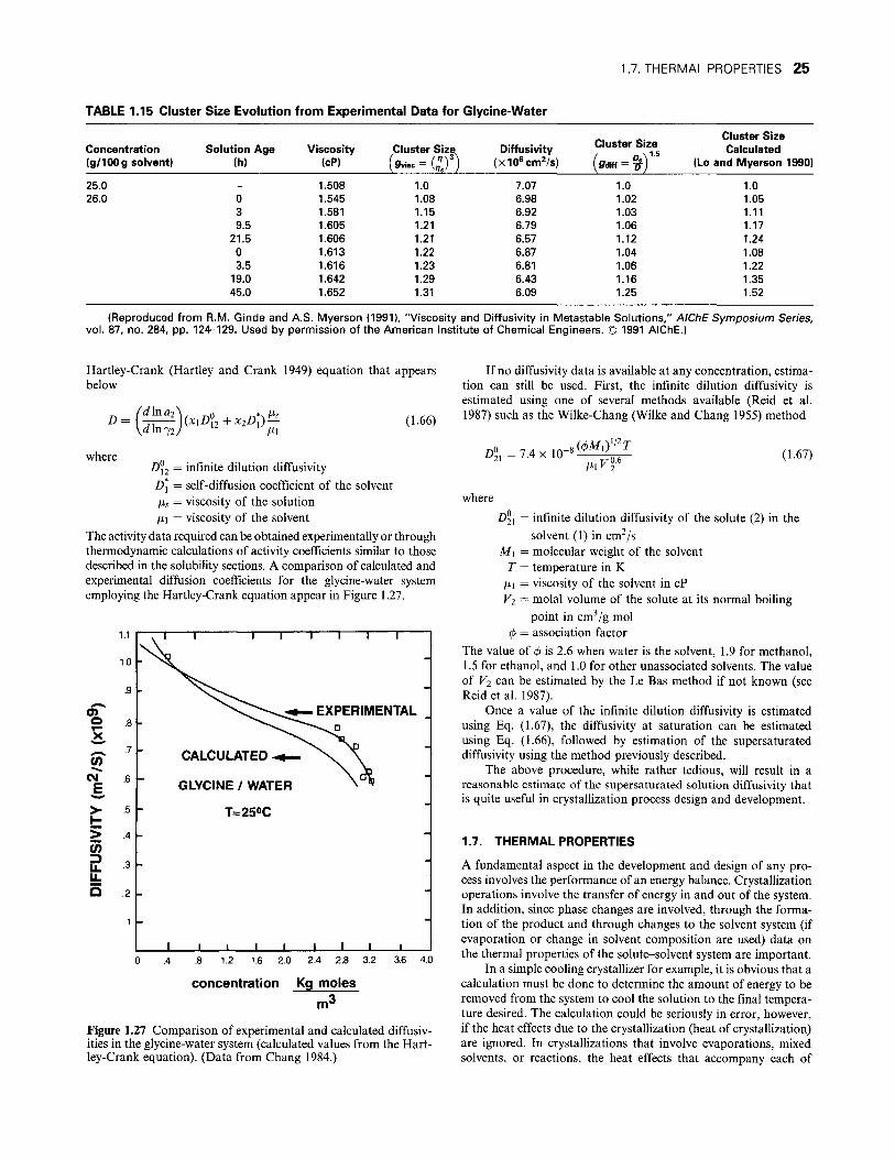
1.7. THERMAL PROPERTIES 25

TABLE 1.15 Cluster Size Evolution from Experimental Data for Glycine-Water

Concentration (g/IOOg solvent)

Solution Age (h)

Viscosity (cP)

Cluster Size Diffusivity (xlO^cm^/s)

Cluster Size

[9dm --lii: Cluster Size Calculated

(Lo and Myerson 1990)

25.0 26.0

-0 3 9.5

21.5 0 3.5

19.0 45.0

1.508 1.545 1.581 1.605 1.606 1.613 1.616 1.642 1.652

1.0 1.08 1.15 1.21 1.21 1.22 1.23 1.29 1.31

7.07 6.98 6.92 6.79 6.57 6.87 6.81 6.43 6.09

1.0 1.02 1.03 1.06 1.12 1.04 1.06 1.16 1.25

1.0 1.05 1.11 1.17 1.24 1.08 1.22 1.35 1.52

(Reproduced from R.M. Ginde and A.S. Myerson (1991), "Viscosity and Diffusivity in Metastable Solutions/' AlChE Symposium Series, vol. 87, no. 284, pp. 124-129. Used by permission of the American Institute of Chemical Engineers. © 1991 AlChE.)

Hartley-Crank (Hartley and Crank 1949) equation that appears below

^ - ( ^ ) ' " ^ ' ^ « ^ ; ' ' " Ml (1.66)

where Z) 2 = infinite dilution diffusivity D\ = self-diffusion coefficient of the solvent fis = viscosity of the solution fi\ = viscosity of the solvent

The activity data required can be obtained experimentally or through thermodynamic calculations of activity coefficients similar to those described in the solubility sections. A comparison of calculated and experimental diffusion coefficients for the glycine-water system employing the Hartley-Crank equation appear in Figure 1.27.

1.1

1.0

o .8

"»—

>

D ! o

.6 H

•5 h

.4 h

•3 h

2 H

l ^ L

1 [•

k

h

k h

h

T T • 1 - | 1 1 1 1

^ 1

^ v > ^ 1

^ ^ ;;;;\ ^ J ^^^^***v/ ^*^"^v° 1

CALCULATED -*— \ X 1

GLYCINE / WATER ^ ^ 1

T=250C 1

A A

1 i 1 I 1 i 1 -L J 1 0 .4 .8 1.2 1.6 2.0 2.4 2.8 3.2 3.6 4.0

concentration Kg moles

m3

Figure L27 Comparison of experimental and calculated diffusiv-ities in the glycine-water system (calculated values from the Hart­ley-Crank equation). (Data from Chang 1984.)

If no diffusivity data is available at any concentration, estima­tion can still be used. First, the infinite dilution diffusivity is estimated using one of several methods available (Reid et al. 1987) such as the Wilke-Chang (Wilke and Chang 1955) method

/)?, = 7.4 X 10" (1.67)

where

Z>2i = infinite dilution diffusivity of the solute (2) in the solvent (1) in cm^/s

Ml = molecular weight of the solvent T = temperature in K

ji\ = viscosity of the solvent in cP V2 = molal volume of the solute at its normal boiling

point in cm^/g mol 0 = association factor

The value of 0 is 2.6 when water is the solvent, 1.9 for methanol, 1.5 for ethanol, and 1.0 for other unassociated solvents. The value of V2 can be estimated by the Le Bas method if not known (see Reid et al. 1987).

Once a value of the infinite dilution diffusivity is estimated using Eq. (1.67), the diffusivity at saturation can be estimated using Eq. (1.66), followed by estimation of the supersaturated diffusivity using the method previously described.

The above procedure, while rather tedious, will result in a reasonable estimate of the supersaturated solution diffusivity that is quite useful in crystallization process design and development.

1.7. THERMAL PROPERTIES

A fundamental aspect in the development and design of any pro­cess involves the performance of an energy balance. CrystalHzation operations involve the transfer of energy in and out of the system. In addition, since phase changes are involved, through the forma­tion of the product and through changes to the solvent system (if evaporation or change in solvent composition are used) data on the thermal properties of the solute-solvent system are important.

In a simple cooling crystaUizer for example, it is obvious that a calculation must be done to determine the amount of energy to be removed from the system to cool the solution to the final tempera­ture desired. The calculation could be seriously in error, however, if the heat effects due to the crystallization (heat of crystallization) are ignored. In crystallizations that involve evaporations, mixed solvents, or reactions, the heat effects that accompany each of

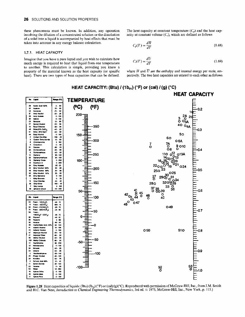
26 SOLUTIONS AND SOLUTION PROPERTIES

these phenomena must be known. In addition, any operation involving the dilution of a concentrated solution or the dissolution of a solid into a liquid is accompanied by heat effects that must be taken into account in any energy balance calculation.

1.7.1. HEAT CAPACITY

Imagine that you have a pure liquid and you wish to calculate how much energy is required to heat that Uquid from one temperature to another. This calculation is simple, providing you know a property of the material known as the heat capacity (or specific heat). There are two types of heat capacities that can be defined.

The heat capacity at constant temperature (Cp) and the heat cap­acity at constant volume (Cv), which are defined as follows

^"^^ ' dT

C.(T) = dl£ dT

(1.68)

(1.69)

where H and U are the enthalpy and internal energy per mole, res­pectively. The two heat capacities are related to each other as follows

"•^ "<>•"

29 Aceric Acid 100%

32 AcMoM

52 Ammonia

37 Amyl Alcohol

26 Amyl AcM«to

30 Aniline

23 Benzon*

27 Benzyl Alcohol

10 Bezyl Chlorid*

49 Brin«.25% CalCtg

51 Brine, 25% NaCI

44 Butyl Alcohol

1 2 CartXM) Disulfide

1 3 Cartxw Tetrachloride

1 8 Chlorobenzine

1 4 Chloroform

1 21 Decane

6A DichkMoethane

5 Dichloroelhane

IS Oiphenyl

22 Diphenylmethane

I 16 Oiphenyl Oxide

1 16 Dowthem A

24 Ethyl Acetate

42 Ethyl Alcohol 100%

46 Ethyl Alcohol 80%

1 50 Ethyl Alcohol 50%

1 25 Ethyl Benzene

1 1 Ethyl Bromide

1 13 Ethyl Chloride

1 36 Ethyl Ether

1 7 Ethyl Iodide

1 39 Ethylene Glycol

R a n a e f Q |

0- 80 1 2 0 - SO

•70 . 50

-SO- 25 1 0-100 0-130 1

10-80 •20- 30 1 •30 - 30

-40- 20 1 -40- 20 1

0-100 1 •100 • 25

10-60 0-100 0- 50

•80-25 •30-60 •40-50 80-120 30-100

1 0-200 0-200

-50-25 30- 80 2 0 - 8 0 2 0 - 8 0 0-100 5 - 2 5

-30-40 -100- 25

0-100 -40-200

HEAT CAPACITY: (Btu) / (Ibm) (°F) or (cal) /(g) (°C)

HEAT CAPACITY TEMPERATURE

(OC) (OF)

2 0 0 - ^

No. Uquid

2A Freon - 11(Ca3F) '

6 Freon - 12(CCIF2)

4A Freon • 21(CHCl2F)

7A Freon - 22(CHCIF2)

3A Freon -

113(CCl2f^-CCIF2)

38 Glycerol

28 Heptane

35 Hexane

48 Hydrochlolic Acid. 30%

41 itoamil Alcohol

43 isobutyl Alcohol

47 Isopropyl Alcohol

31 Isopropyl Ether

40 Methyl Alcohol

13A Methyl Chloride

14 Naphthalene

12 Nitrobenzene

34 Nonane

33 Octane

3 Perchlorethylene

1 45 Propyl Alcohol

20 Pyridine

9 Sulfuric Acid 98%

1 11 Sulfur Dioxide

1 23 Toluene

1 53 Wkter

1 19 Xylene Ortho

1 18 Xylene MOM

1 17 Xylene Para

Range (>C) 1

-20-70 1 400-15 1 -20-70 -20-60 1

•20-70 •40-20 1

0-60 1 •80-20 1 20-100 1 10-100 0-100 1

- 2 0 - 5 0

•80 - 20

•40- 20

•80- 20

9 0 - 2 0 0

0 - 1 0 0

•SO^ 25

•50^ 25

•30 • 140

•20 • 100

• 5 0 - 2 5

1 0 - 4 5

•20 • 100

0 - 6 0

10^200

0 - 1 0 0

0 • 100

0 • 100

^ 0 . 2 1(t

1 5 0 ^

1 0 0 - ^

-350

-300

-250

-200

-150

3'^2ct: 003A 40 04A

F-0.3 5o

60

7 O

06A tZ 9010 O

7A O 08

110 c}^ o13A P13

^-!0

22oo17"l9''21o24 250 23

42

46

41 8 45

O 047

27 29C6° 31 ' 320°8ff

o

280

40

P-0.4

P-0.5

049 3 — 5 0

- 5 0 - 3

-100-

O50 510

-50

m — - 1 0 0

-0.6

F^O.7

-0.8

F-0.9

52 O

53 O -1.0

Figure 1.28 Heat capacities of liquids: (Btu) (Ibm) (°F) or (cal)/(g)(°C). Reproduced with permission of McGraw-Hill, Inc., from J.M. Smith and H.C. Van Ness, Introduction to Chemical Engineering Thermodynamics, 3rd ed. © 1975, McGraw-Hill, Inc., New York, p. 115.)

1.7. THERMAL PROPERTIES 27

Ideal gases: Cp = C^ + R

Liquids and solids: Cp ^ Cy

(1.70)

(1.71)

Heat capacities are given in units of energy per mole (or mass) per unit temperature interval. Typical units used and conversion fac­tors appear in Table 1.12.

Specific heat is another term used when heat capacity is expressed on a per mass basis. Heat capacities are a function of temperature and are usually expressed as a polynomial such as

Cp{T) = a + bT + cT^ + dT^ (1.72)

developed and are summarized in Reid et al. (1987). Heat cap­acities of liquid mixtures can be estimated by calculating an aver­age heat capacity from the heat capacities of the components using the relation

Cpavg(T) — / ^XjCpijT) (1.73)

The heat capacity of solutions of sohds dissolved in Uquids is usually not available. If the solution is dilute, the usual practice is to neglect the solute and to use the solvent heat capacity. For a concentrated solution, neglecting the solute can lead to inaccur­acies so that the use of enthalpy data is suggested.

Tables of heat capacities for a variety of pure substances can be found in the Chemical Engineers Handbook (Perry and Green 1997). The heat capacity of a number of Hquids is given in Figure 1.28.

Heat capacity data is available for most liquids and gases, and for many solids. If not available, estimation techniques have been

1.7.2. LATENT HEAT

When a pure material undergoes a phase change, the process takes place at a constant temperature and pressure. Even though the tem­perature remains the same, there is an enthalpy change associated

TABLE 1.16 Enthalpy of Fusion and Mel t ing Tempera ture of S o m e Organics

Compound Tn,

rc) -182.5 -183.3 -187.7 -138.4 -159.6 -129.7 -159.9 -16.6 -95.4 -153.7 -99.9 -128.5 -90.6 -118.3 -118.6 -123.8 -119.2 -134.5 -24.9 -56.8 -120.5 -120.9 -53.5 -29.6

-9 .6 28.2

5.5 -94.9 -94.9 -25.1 -47.9

13.3 -99.5 -96.0 -25.4 -43.8 -44.7

6.5 -126.5 -111.3 -33.5 - 5 0 . 0

88.1

Molecular Weight

16.04 30.07 44.09 58.12 38.12 72.13 72.13 72.13 86.17 86.17 86.17 86.17

100.2 100.2 100.2 100.2 100.2 100.2 100.2 114.2 114.2 114.2 128.2 142.3 170.3 254.4

78.1 92.1

106.1 106.1 106.1 106.1 120.1 120.1 120.1 120.1 120.1 84.1 98.1

112.2 112.2 112.2 112.2

(cal/g)

AH„,

(cal/g mol)

Methane Ethane Propane n-Butane Isobutane n-Pentane isopentane Neopentane n-Hexane 2-Methylpentane 2,2-Dimethylbutane 2,3-Dimethylbutane n-Heptane 2-Methylhexane 3-Ethylpentane 2,2-Dlmethylpentane 2,4-Dimethylpentane 3,3-Dimethylpentane 2,2,3-Trimethylbutane n-Octane 3-Methylheptane 4-Methylheptane n-Nonane n-Decane /7-Dodecane n-Octadecane Benzene Toluene Ethylbenzene o-Xylene m-Xylene p-Xylene n-Propylbenzene Isopropylbenzene 1,2,3-Trinnethylbenzene 1,2,4-Trimethyl benzene 1,3,5-Trimethylbenzene Cyclohexane Methylcyclohexane Ethylcyclohexane 1,1-Dimethylcyclohexane 1,c/s-2-Dimethylcyclohexane 1,frans-2-Dlmethylcyclohexane

14.03 22.73 19.10 19.17 18.67 27.81 17.06 10.79 36.14 17.41

1.61 2.25

33.47 21.91 22.78 13.89 16.32 16.86 5.39

43.40 23.81 22.68 28.83 48.24 51.69 57.65 30.09 17.1 20.63 30.61 26.04 38.5 16.97 14.15 16.6 25.54 19.14 7.57

16.4 17.73

1.32 3.50

22.34

225 683 842

1114 1085 2006 1231 779

3114 1500

139 194

3350 2195 2283 1392 1635 1689 540

4956 2719 2590 3696 6865 8803

14,660 2350 1575 2188 3250 2760 4080 2040 1700 1990 3070 2300

637 1610 1930

148 393

2507

(Data f rom Reid et al. 1987.)

28 SOLUTIONS AND SOLUTION PROPERTIES

with the phase change that must be taken into account in energy balance calculations. These enthalpy changes associated with phase changes in pure materials are often referred to as latent heat. The latent heat of vaporization refers to the enthalpy change required to vaporize a given amount of a saturated liquid to saturated vapor at a constant temperature and pressure. Other latent heats commonly mentioned are fusion (melting a material) and sublimation (solid to gas). It is important to note that there are also heat effects that accompany phase changes from one solid phase to another. If a material crystallizes in one crystal form and then transforms to another crystal form, there will be an enthalpy change involved.

Latent heats vary as a function of temperature and to a smaller extent pressure. The latent heat for a phase change at 1 atm (101.29 kPa) is often called the standard heat of phase change and is available for many materials in the literature (Perry and Green 1997).

A number of techniques have been developed to estimate the, latent heat of vaporization and, to a lesser extent, the latent heat of fusion and sublimation. A description of these techniques can be found in Reid et al. (1987). One very useful and commonly used method known as the Watson correlation appears below

AHy(T2) = AH,(Ti) (1 0.38

(1.74)

where AHyiTi) and AHy{T\) are the heats of vaporization at T2 and T\, and Tc is the critical temperature. Eq. (1.74) allows calcu­lation of the latent heat of vaporization at any temperature if the heat of vaporization is known at one temperature. If no heat of vaporization data are available, and the normal boiling point (boihng point at 1 atm) of the hquid is known, Chen's equation can be used to estimate the heat of vaporization at the boiling point by

AH,b = RTcTbr?^.91STbr - 3.938 + 1.555 InP,

1.07-r^,. (1.75)

where

Tbr = reduced boiling point temperature (Tb/Tc) Pc = critical pressure

Latent heats of vaporization can be calculated from vapor pressure data employing the Clausius-Clapeyron equation.

H, _d{\np'') ' ^ ~ d{\IT)

(1.76)

where /?* is the vapor pressure at a particular temperature. By plotting In p* versus IjT and obtaining the slope at the tempera­ture of interest, Eq. (1.76) can be used to calculate the heat of vaporization.

Calculation of latent heats of fusion and sublimation are more difficult and less accurate than calculating heats of vaporization. Reid et al. (1987) summarized available methods. A crude but simple approximation for standard heats of formation is (Felder and Rousseau 1986)

A]5'^(kJ/mol) « 0.0092r^(K)(Metallic elements)

^ 0.025 r^(K)(Inorganic compounds)

? 0.050T;„(K)(Organic compounds)

The melting temperature and latent heats of fusion for a number of organic species appear in Table 1.16.

1.7.3. HEATS OF MIXING, SOLUTION, AND CRYSTALLIZATION

In any process where the concentration of a solution is changed, there will be an enthalpy change accompanying the concentration change. This is true when two liquids are mixed, a concentrated solution is diluted, a soHd is dissolved in a liquid, or when a solute crystaUizes from solution. These enthalpy changes are known as heats of mixing, solution, and crystallization, respectively, and can be very significant in energy balance calculations.

The heat of mixing refers to the enthalpy change accompany­ing the mixing of two or more pure substances to form a solution at a constant temperature and pressure. When one species being mixed is a gas or solid, this enthalpy change is known as the heat of solution. Heats of solution are often given in terms of the dis­solution of 1 mol of solute in moles of solvent at a particular tem­perature. This is known as an integral heat of solution. Integral heats of solution for HCl, NaOH, and H2SO4 appear in Table 1.17. The table shows that for each of these substances, the heat of solution is negative, meaning that the solution process results in the evolution of heat. In addition. Table 1.17 shows that the heat of solution is a function of concentration, increasing as the solution becomes less concentrated («, the moles of water per moles of solute increases) to a limiting maximum value. This maximum value is known as the heat of solution at infinite dilution. Data in Table 1.17 can be used to calculate the enthalpy change that would result from making a solution of desired concentration from its components. It also can be used to calculate the enthalpy change that would result from the dilution of a concentrated solution.

The substances Usted in Table 1.17 all have negative heats of solution, meaning that heat is released when the materials are dissolved, or a concentrated solution is diluted. This is not gener­ally true; many substances have positive heats of solution, indicat­ing that heat is absorbed when they are dissolved. The heats of

TABLE 1.17 Integral Heats of Solution at 25 X

n (mol water/mol solute)

0.5 1 1.5 2 3 4 5

10 20 25 30 40 50

100 200 500

1000 2000 5000

10,000 50,000

100,000 500,000

00

(AHs)HCI(g) (kJ/mol HCl)

— -26.22

— -48.82 -56.85 -61.20 -64.05 -69.49 -71.78

— -72.59 -73.00 -73.26 -73.85 -74.20 -74.52 -74.68 -74.82 -74.93 -74.99 -75.08 -75.10

— -75.14

(AHs)NaOH(s) (kJ/mol NaOH)

— — —

-28.87 -34.43 -37.74 -42.51 -42.84

— -42.72 -42.59 -42.51 -42.34 -42.26 -42.38 -42.47 -42.55 -42.68 -42.72 -42.80

— —

-42.89

(AHm)H2S04 (kJ/mol H2SO4)

-15.73 -28.07 -36.90 -41.92 -48.99 -54.06 -58.03 -67.03

— -72.30

— —

-73.34 -73.97

— -76.73 -78.57

— -84.43 -87.07

— -93.64 -95.31 -96.19

(Reprinted by permission of John Wiley & Sons, Inc. from R.M. Felder and R.W. Rousseau (1986), Elementary Principles of Chemical Processes, 2nd ed. © 1986 John Wiley & Sons, Inc.)

NOMENCLATURE 2 9

TABLE 1.18 Heats of Solut ion in Wate r at Infinite Dilution of 18 °C

N O M E N C L A T U R E

Substance Formula AHs

(kcal/gmoi)

Ammonium chloride Ammonium nitrate Ammonium sulfate Barium bromide

Calcium chloride

Lithium bromide

Magnesium sulfate

Potassium sulfate Benzoic acid Citric acid Dextrin Hexamethylenetetramine m-Nitrophenol o-Nitrophenol p-Nitrophenol Phthalic acid Urea

NH4CI NH4NO3 (NH4)2S04 BaBr2 BaBr2 BaBr2 CaCl2 CaClz CaClz CaCl2 CaClz LiBr L iBr .H20 LiBr.2H20 LiBr-3H20 MgS04 MgS04 MgS04 MgS04 MgS04 MgS04 K2SO4 C7H8O2 CeHsOy C12H20O10 C6H12N4 C6H5NO3 C6H5NO3 C6H5NO3 C8H6O4 CH4N2O

H2O 2H2O

H2O 2H2O 4H2O 6H2O

H2O 2H2O 4H2O 6H2O 7H2O

-3.82 -6.47 -2 .75 +5.3 -0 .8 -3.87 +4.9

+12.3 +12.5

+2.4 -4.11

+11.54 +5.30 +2.05 -1.59

+21.1 +14.0 +11.7

+4.9 +0.55 -3 .18 -6.32 -6 .5 -5 .4 +0.268 +4.78 -5 .2 -6 .3 -4 .5 -4.87 -3 .61

(Data f rom Perry and Green 1997.)

solution of selected organic and inorganic species in water appear in Table 1.18. Additional data can be found in Perry and Green (1997).

The data in Table 1.18 illustrates two other points. The first is that for hydrated compounds, the heats of solution vary as a function of the number of waters of hydration present in the solid. Looking at magnesium sulfate, we see that the heat of solution at infinite dilution at 18 °C varies from -21.1 kcal/gmol for the anhy­drous form to +3.18 kcal/gmol for MgS04 • 7H2O (which is the stable form at this temperature). The second point is that organic compounds with the same chemical formula but different struc­tures such as para-, meta-, and ortho-nitrophenol have differing heats of solution. In this case, they are 4.49, 5.21, and 6.3 kcal/gmol, respectively, at infinite dilution and 18 °C.

The enthalpy change that results from the crystallization of a species from solution is called the heat of crystallization. The heat of crystallization is normally assumed to be of the same magnitude but opposite sign as the heat of solution at a concentration near saturation. This is not exactly correct since the supersaturated solution from which the crystallization is occurring has a higher concentration than a saturated solution, however, the error should be relatively small.

For binary systems of solutes and solvents that are relatively common or have industrial importance, enthalpy concentration diagrams often exist that are quite useful in energy balance calcu­lations involving solution, dilution, or crystallization. An example of an enthalpy concentration diagram for the NaOH-H20 system appears in Figure 1.29. It is important to be aware of the reference state on which the diagram is based when employing this data in energy balance calculations.

a A B C Cs

Cp Cv

DAB

D*i

D\, dCAJdx dvx/dy e Fi

fi

H I i

JA

K Ksp

I M Ms

m

n P P* Pc

P'l R r S T Tbr

Tc

Ttp V V Vm

vk w •^2

yi z

Ac ACp

AGfo ^Hm ^H,p

AH, Au

Activity Debye-Hiickel constant Constant for ion interaction Concentration of solution Saturation concentration Specific heat at constant pressure Specific heat at constant volume Diffusion coefficient Self-diffusion coefficient of the

solvent Infinite dilution diffusivity Concentration gradient Shear rate Magnitude of the electric charge Interaction parameter Fugacity, mole fraction.

activity coefficient Enthalpy per mole Ionic strength Any ion present Molar diffusive flux Equilibrium constant Solubility product Distance between two charges Molecular weight of the solute Molecular weight of the solvent Concentration of species in

solution, empirical viscosity parameter

Power law exponent Pressure vapor pressure Critical pressure Vapor pressure of component 2 Gas constant Cluster radius Supersaturation ratio Temperature, °C Reduced boiling point Critical temperature Triple point temperature, °C Molar volume Internal energy per mole Specific volume of solute Molar volume of subcooled hquid Mass fraction Mole fraction of the solute Molar activity coefficient Number of charges on the cation

or anion Supersaturation Difference in specific heats of the

liquid or sohd Gibbs free energy of formation Latent heat of fusion Enthalpy change at the triple point Heat of vaporization Enthalpy of vaporization

Eq. (1.2) Eq. (1.26) Eq. (1.26) Eq. (1.54) Eq. (1.54)

Eq. (1.68) Eq. (1.69) Eq. (1.63)

Eq. (1.66) Eq. (1.66) Eq. (1.63) Eq. (1.61) Eq. (1.49) Eq.(1.32)

Eqs. (1.16), (1.37 Eq. (1.68) Eq. (1.26) Eq.(1.31) Eq. (1.63) Eq.(1.2) Eq.(1.4) Eq. (1.44) Eq. (1.18) Eq.(1.17)

Eqs. (1.3), (1.62) Eq. (1.62) Eq. (1.42) Eq. (1.76) Eq.(1.75) Eq. (1.41) Eq. (1.10) Eq. (1.58) Eq.(1.57) Eq. (1.10) Eq.(1.75) Eq. (1.74) Eq. (1.42) Eq. (1.52) Eq. (1.69) Eq. (1.58) Eq. (1.50) Eq. (1.60) Eq.(1.39) Eq.(1.15)

Eq.(1.27) Eq. (1.56)

Eq. (1.42) Eq. (1.23) Eq. (1.47) Eq. (1.42) Eq. (1.74) Eq. (1.52)

Av Volume change for Hquid-soHd transformation Eq. (1.42)

30 SOLUTIONS AND SOLUTION PROPERTIES

500 H

400 ^

3 o CO

u. 300 ^ O £ 3 4 -ffi >^ a - I < z

200

z u lU >

-J til c 100 H

NaOH, PERCENT BY WEIGHT

Figure 1.29 Enthalpy concentration diagram for NaOH-H20 . (Reprinted by permission of John Wiley & Sons, Inc. from G. Brown (1950), Unit Operations. © 1950 John Wiley & Sons, Inc.)

Greek Letters

7 fJ' V

P Po 6u ^2

0 a

'^yx

M

Activity coefficient Chemical potential Stoichiometric number Solution density Solvent density Solubility parameters of the

solvent and subcooled Hquid, respectively

Volume fraction of the solvent Relative supersaturation,

solid-liquid interfacial tension Shear stress Viscosity

Eq.(1.3) Eq.(1.8) Eq.(1.9) Eq. (1.19) Eq. (1.19)

Eq. (1.50) Eq. (1.50)

Eqs. (1.55), (1.58) Eq. (1.61) Eq. (1.61)

REFERENCES

Bird, R.B., Stewart, W.E., and Lightfoot, E.N. (1960). Transport Phenom­ena, Wiley, New York.

Bromley, L.A. (1972). / . Chem. Thermo. 4, 669. Bromley, L.A. (1973). AIChE J. 19, 313. Bromley, L.A. (1974). AlChEJ. 20, 336. Brown, G. (1950). Unit Operations, McGraw-Hill Book Co., New York. Chang, Y.C (1984). Ph.D. dissertation, Georgia Institute of Technology,

Atlanta, GA. Chang, Y.C, and Myerson, A.S. (1984). AlChEJ. 31, 890. Decker. S., Fan, W.P., and Myerson, A.S. (1986). Ind. Eng. Chem. Fund.

25, 925. Felder, R.M., and Rousseau, R.W. (1996). Elementary Principles of Chem­

ical Processes, 2nd ed., John Wiley & Sons, Inc., New York. Frank, T.C, Downey, J.R., and Gupta, S. (1999) Chem. Eng. Prog. 95, 12. Frendenslund, A., Gmehling, A.J., Micheisen, M.L., Rasmussen, P., and

Prausnitz, J.M. (1977). Ind. Eng. Chem. Process Des. Dev. 16, 450.

REFERENCES 31

Ginde, R.M., and Myerson, A.S. (1991). AlChE Symposium Series, vol. 87, 284, 124-129.

Ginde, R., and Myerson, A.S. (1992). J. Cryst. Growth 116, 41. Gordon, L.J., and Scott, R.L. (1952). / . Am. Chem. Sac. 74, 4138. Gordon, P. (1968). Principles of Phase Diagrams in Materials Science,

McGraw-Hill Book Co., New York. Guggenheim, F.A. (1987). Thermodynamics, 5th ed.. North Holland Pub­

lishing Company, Amsterdam. Hartley, G.S., and Crank, J. (1949). Trans. Faraday Soc. 45, 80. Kim, S. and Myerson, A.S. (1996). Industrial and Engineering Chemistry

Research 35, 1078. Kojima, K., and Tochigi, K. (1979). Prediction of Vapor-Liquid Equilibria

by the ASOG Method, Elsevier Science PubHshing, Inc., New York. Linke, W.R., and Seidell, A. (1958). Solubilities-Inorganic and Metal-

Organic Compounds, vol. 1 (vol. II, 1965), American Chemical Society, Washington, DC.

Lide, D.R. (1999). Handbook of Chemistry and Physics, 79th ed., CRC Press Cleveland, OH.

Lo, P.Y., and Myerson, A.S. (1990). J. Cryst. Growth 99, 1048. Mullin, J.W. (1997). Crystallization, Butterworths, London. Myerson, A.S., and Lo, P.Y. (1991). / . Cryst. Growth 110, 26. Myerson, A.S., Lo, P.Y., Kim, Y.C., and Ginde, R. (1990). In Proceedings

of the 11th Symposium on Industrial Crystallization (Mersmann, A., ed.), p. 847, European Fed. of Chemical Engineers, Munich, Germany.

Nyvlt, J., Sohnel, O., Matuchova, M., and Brout, M. (1985). The Kinetics of Industrial Crystallization, Elsevier, Amsterdam.

Perry, R.H., and Green, D.W. (1997). Chemical Engineers Handbook. 7th ed., McGraw-Hill Book Co., New York.

Prausnitz, J.M., Lichenthaler, R.N., and Gomes de Azevedo, E. (1999). Molecular Thermodynamics of Fluid-Phase Equilibria, 3rd ed., Prentice-Hall. Inc., Englewood Cliffs, NJ.

Reid, R.C., Prausnitz, J.M., and Poling, B.E. (1987). The Properties of Gases and Liquids, 4th ed., McGraw-Hill Book Co., New York.

Robinson, R.A., and Stokes, R.H. (1970). Electrolyte Solutions, 2nd ed., Butterworths, London.

Rosenberger, F. (1981). Fundamentals of Crystal Growth, Springer-Verlag, New York.

Rush, S. (1991). M.S. thesis in Progress, Polytechnic University. Brooklyn, NY. Saska, M. (1994). Ph.D. dissertation, Georgia Institute of Technology,

Atlanta, GA. Sherman, P. (1970). Industrial Rheology, Academic Press, New York. Smith, J.M;, and Van Ness, H.C. (1975). In Introduction to Chemical En­

gineering Thermodynamics, 3rd ed., p. 115, McGraw-Hill Book Co., New York,

Walas, S.M. (1985). Phase Equilibria in Chemical Engineering, Butter­worths, Boston.

Wilke, C.R., and Chang, P. (1955). AIChE J. 1, 264. Zemaitis, J.F. Jr., Clark, D.M., Rafal, M., and Scrivner, N.C. (1986).

Handbook of Aqueous Electrolyte Thermodynamics, American Institute of Chemical Engineers, New York.