Embed Size (px)
Citation preview

HANDBOOK
ON
PRICE AND VOLUME MEASURES
IN
NATIONAL ACCOUNTS
Eurostat
Luxembourg, December 2013

PREFACE
Economic and Monetary Union and the common currency require good macro-economic
statistics. In particular, the Stability and Growth Pact, agreed by the Member States in 1997,
created a renewed demand for higher quality and more comparable data on economic growth.
To meet this demand, Eurostat has been working with the Member States to develop improved
methods and procedures for the measurement of prices and volumes in the national accounts.
In 1998, a Commission Decision was adopted that provided the first step in this process. Much
more work on various challenging areas has been undertaken since then by numerous Task
Forces of national experts.
This work was brought together in the Handbook on Price and Volume Measures in National
Accounts and published in 2001. Since then there has been a considerable discussion on aspects
of measuring volume growth in the national accounts, and given the publication of an update of
ESA 95 to a new European standard for national accounts, ESA 2010, it was decided to carry out
an update of the handbook. The areas where the most significant changes have been made are
non-market production, and production of Research and Development services. The coding
system has been updated to reflect NACE Rev. 2 and the associated CPA published in 2008.
This handbook provides a complete discussion of the issues involved in measuring prices and
volumes, from the general principles to the deflation of individual goods and services. It is fully
consistent with the principles of the European System of Accounts 2010, and is intended to
elaborate that framework. It also includes a brief chapter on issues of price and volume
measurement in the quarterly accounts. Further detail can be found in the Handbook on
Quarterly National Accounts1.
The handbook is precise in its recommendations: it classifies methods into good methods, less
good but acceptable methods and methods that are to be avoided. The handbook thereby
provides a very useful tool for Member States, candidate countries and other countries to
develop the price and volume measures in their national accounts in a harmonised way.
1 See
http://epp.eurostat.ec.europa.eu/portal/page/portal/product_details/publication?p_product_co
de=KS-GQ-13-004

Handbook on Price and Volume Measures in National Accounts
1. INTRODUCTION ....................................................................................................................... 7
1.1. Background and aim of this handbook ......................................................................... 7
1.2. Scope of this handbook ................................................................................................ 9
1.3. The distinction between price, volume, quantity and quality .................................... 10
1.4. The A/B/C classification .............................................................................................. 11
1.5. How to read this handbook ........................................................................................ 12
2. A/B/C METHODS FOR GENERAL PROCEDURES ..................................................................... 14
2.1. The use of an integrated approach ............................................................................. 14
2.1.1. An accounting approach to volume estimations ......................................... 14
2.1.2. Advantage of balancing volume data .......................................................... 16
2.1.3. Valuation problems ..................................................................................... 17
2.1.4. The case of price discrimination .................................................................. 19
2.2. The three principles from the Commission Decision .................................................. 21
2.2.1. The elementary level of aggregation ........................................................... 21
2.2.2. The choice of index formula and base year ................................................. 22
2.2.3. The non-additivity problem ......................................................................... 24
2.3. Criteria for appropriate price and volume indicators ................................................. 27
2.4. Quality changes .......................................................................................................... 28
2.4.1. The problem of quality changes .................................................................. 28
2.4.2. Accounting for quality changes in price indices .......................................... 30
2.4.3. Accounting for quality change in volume indicators ................................... 33
2.4.4. A, B and C methods ..................................................................................... 34
2.5. Unique products ......................................................................................................... 35
2.6. Unit values versus price indices .................................................................................. 37
3. A/B/C METHODS BY TRANSACTION CATEGORY .................................................................... 40
3.1. Market and non-market output ................................................................................. 40
3.1.1. Market output and output for own final use .............................................. 40
3.1.1.1. Price deflation methods ............................................................. 40
3.1.1.2. Volume extrapolation methods ................................................. 44
3.1.1.3. A, B and C methods .................................................................... 44
3.1.2. Non-market output ..................................................................................... 46
3.1.2.1 Input, activity, output and outcome .......................................... 46
Table of contents
3.1.2.2 Output indicator methods ......................................................... 48
3.1.2.3 Taking quality changes into account .......................................... 49
3.1.2.4 A, B and C methods .................................................................... 50
3.2. Special topic: Products provided without charge to the user .................................... 51
3.3. Intermediate consumption ......................................................................................... 53
3.4. Value added ................................................................................................................ 55
3.5. Final consumption expenditure .................................................................................. 57
3.5.1. Final consumption expenditure by households .......................................... 57
3.5.2. Final consumption expenditure by government and NPISHs ...................... 61
3.6. Gross fixed capital formation ..................................................................................... 62
3.7. Changes in inventories ................................................................................................ 65
3.7.1. Introduction ................................................................................................. 65
3.7.2. Some important definitions and relations .................................................. 65
3.7.3. If perfect information is available ............................................................... 67
3.7.4. If only information of values of inventories is available .............................. 67
3.7.5. If no information is available at all .............................................................. 68
3.7.6. A, B and C methods ..................................................................................... 69
3.8. Acquisition less disposals of valuables ....................................................................... 69
3.8.1. Introduction ................................................................................................. 69
3.8.2. Some important definitions and relations .................................................. 70
3.8.3. Different types of transaction ..................................................................... 70
3.8.4. A, B and C methods ..................................................................................... 71
3.9. Exports and imports of goods and services ................................................................ 72
3.9.1. Introduction ................................................................................................. 72
3.9.2. Goods ........................................................................................................... 73
3.9.3. Services ........................................................................................................ 77
3.10. Taxes and subsidies on products ................................................................................ 78
3.10.1. Taxes and subsidies related to quantities of products ................................ 79
3.10.2. Taxes and subsidies related to values of products ...................................... 80
3.10.3. Collection rate issues ................................................................................... 82
3.10.4. A, B and C methods ..................................................................................... 83
3.11. Components of value added ....................................................................................... 83
3.11.1. Other taxes and subsidies on production .................................................... 83
3.11.2. Compensation of employees ....................................................................... 85
3.11.3. Consumption of fixed capital ....................................................................... 90
4. A/B/C METHODS FOR OUTPUT BY PRODUCT ........................................................................ 93
4.1 CPA A - Products of agriculture, forestry and fishing ................................................. 93
4.2 CPA B - Mining and quarrying ..................................................................................... 95
4.3 CPA C - Manufactured products ................................................................................. 96
Table of contents
4.3.1 General recommendations for manufactured products ............................. 96
4.3.2 Large equipment goods ............................................................................... 97
4.3.3 Computers ................................................................................................. 100
4.3.4 Repair and installation services of machinery and equipment
(CPA33). ..................................................................................................... 103
4.4 CPA D - Electricity, gas, steam and air conditioning; ................................................ 103
4.5 CPA E - Water supply; sewerage, waste management and remediation
services ..................................................................................................................... 105
4.6 CPA F – Constructions and construction works ........................................................ 106
4.7 CPA G - Wholesale and retail trade services; repair services of motor
vehicles and motorcycles .......................................................................................... 109
4.7.1 Wholesale and retail trade margins .......................................................... 109
4.7.2 CPA 45 - Wholesale and retail trade and repair services of motor
vehicles and motorcycles .......................................................................... 115
4.7.3 CPA 46 - Wholesale trade services, except of motor vehicles and
motorcycles ............................................................................................... 115
4.7.4 CPA 47 - Retail trade services, except of motor vehicles and
motorcycles ............................................................................................... 115
4.8 CPA H – Transportation and storage services ........................................................... 116
4.8.1 CPA 49, 50 and 51 - Transport by land, water and air ............................... 116
Passenger transport................................................................................... 116
Freight transport........................................................................................ 119
4.8.2 CPA 52 - Warehousing and support services for transportation ............... 120
4.8.3 CPA 53 - Postal and courier services ......................................................... 122
4.9 CPA I – Accommodation and food services .............................................................. 123
4.10 CPA J – Information and communication services ................................................... 124
4.10.1 CPA 58 - Publishing services ...................................................................... 124
4.10.2 CPA 59 - Motion picture, video and television programme
production services, sound recording and music publishing and
CPA 60 - Programming and broadcasting services .................................... 126
4.10.3 CPA 61 - Telecommunication services ....................................................... 127
4.10.4 CPA 62 - Computer programming, consultancy and related services ....... 129
4.10.5 CPA 63 - Information services ................................................................... 131
4.11 CPA K - Financial and insurance services .................................................................. 132
4.11.1 CPA 64 - Financial services, except insurance and pension funding ......... 133
4.11.2 CPA 65 - Insurance, reinsurance and pension funding services,
except compulsory social security services ............................................... 136
4.11.3 CPA 66 - Services auxiliary to financial services and insurance
services ...................................................................................................... 138
4.12 CPA L - Real estate services ...................................................................................... 139
4.12.1 CPA 68 - Real estate services ..................................................................... 139
Table of contents
4.12.2 Dwelling services of owner-occupiers ....................................................... 141
4.13 CPA M - Professional, scientific and technical services ............................................ 143
4.13.1 CPA 69.1 - Legal services ........................................................................... 143
4.13.2 CPA 69.2 - Accounting, bookkeeping and auditing services; tax
consulting services ..................................................................................... 145
4.13.3 CPA 70.1 - Services of head offices ............................................................ 146
4.13.4 CPA 70.2 - Management consulting services ............................................ 146
4.13.5 CPA 71 - Architectural and engineering services; technical testing
and analysis services .................................................................................. 147
4.13.6 CPA 72 - Scientific research and development services ............................ 148
4.13.7 CPA 73 - Advertising and market research services .................................. 150
4.13.8 CPA 74 - Other professional, scientific and technical services .................. 151
4.13.9 CPA 75 - Veterinary services ...................................................................... 152
4.14 CPA N – Administrative and support services .......................................................... 152
4.14.1 CPA 77 - Rental and leasing services ......................................................... 152
4.14.2 CPA 78 - Employment services .................................................................. 153
4.14.3 CPA 79 - Travel agency, tour operator and other reservation
services and related services ..................................................................... 154
4.14.4 CPA 80 - Security and investigation services ............................................. 155
4.14.5 CPA 81 - Services to buildings and landscape............................................ 155
4.14.6 CPA 82 - Office administration, office support, and other business
support services ......................................................................................... 156
4.15 CPA O - Public administration and defence services; compulsory social
security services ........................................................................................................ 156
4.16 CPA P - Education services ........................................................................................ 158
4.17 CPA Q - Human health and social work services ...................................................... 163
4.17.1 CPA 86.1 - Hospital services ...................................................................... 166
4.17.2 CPA 86.2 - Medical and dental practice services ....................................... 170
4.17.3 CPA 86.9 - Other human health services ................................................... 171
4.17.4 CPA 87 - Residential care services ............................................................. 171
4.17.5 CPA 88 - Social work services without accommodation ............................ 171
4.18 CPA R - Arts, entertainment and recreation services ............................................... 172
4.18.1 CPA 90 – Creative, arts and entertainment services ................................. 172
4.18.2 CPA 91 - Library, archive, museum and other cultural services ................ 173
4.18.3 CPA 92 - Gambling and betting services .................................................... 174
4.18.4 CPA 93 - Sporting services and amusement and recreation services ....... 176
Sports facilities .......................................................................................... 176
4.19 CPA S – Other services .............................................................................................. 177
4.19.1 CPA 94 - Services furnished by membership organisations n.e.c. ............. 177

Table of contents
4.19.2 CPA 95 - Repair services of computers and personal and household
goods ......................................................................................................... 178
4.19.3 CPA 96 - Other personal services .............................................................. 178
CPA 96.01 - Washing and dry cleaning services of textiles and fur
products ................................................................................... 178
CPA 96.02 - Hairdressing and other beauty treatment services ............... 178
CPA 96.03 - Funeral and related services .................................................. 178
CPA 96.04 - Physical well-being services and CPA 96.09 - Other
personal services ...................................................................... 178
4.20 CPA T - Services of households as employers of domestic personnel ...................... 179
5. APPLICATION TO QUARTERLY ACCOUNTS ........................................................................... 180
5.1 Introduction .............................................................................................................. 180
5.2 Data availability ........................................................................................................ 180
5.3 Specific issues ........................................................................................................... 181
5.3.1 Agricultural Output .................................................................................... 182
5.3.2 Seasonal products and product differentiation ........................................ 182
5.3.3 Non-market services .................................................................................. 183
5.3.4 Inventories ................................................................................................. 183
5.3.5 Tourism ...................................................................................................... 184
5.4 Use of price data ....................................................................................................... 184
5.5 The classification of indirect methods ...................................................................... 185
5.6 Seasonality ................................................................................................................ 186
5.7 Conclusion................................................................................................................. 187
ANNEX 1 – CAPTURING QUALITY EFFECTS THROUGH STRATIFICATION ...................................... 188
USEFUL REFERENCES AND LINKS .................................................................................................. 190
General references .............................................................................................................. 190
Chaining, index formulae and the level of aggregation ...................................................... 191
Producer Price Indices and Consumer Price Indices ........................................................... 191
Quality changes and new products ..................................................................................... 192
Computers, other high technology goods and capital goods .............................................. 193
Market services ................................................................................................................... 194
Non-market services ............................................................................................................ 194


Chapter 1 Introduction
7
1. Introduction
1.1. Background and aim of this handbook Economic and monetary policy of the European Union (EU) is increasingly
integrated. This requires higher and higher standards of national accounts data as
a solid foundation for the formulation and monitoring of economic policy. Key
players such as the Council, the European Commission and the European Central
Bank need in particular high quality and comparable data on price developments
and economic growth. Within the EU, national accounts data are also increasingly
important for more administrative purposes such as the determination of
countries' contributions to the EU budget, assessment of economic convergence,
regional funds, etc.
This broad international use of national accounts data has led to an extensive set
of international definitions and guidelines, necessary to ensure the reliability and
comparability of data. These definitions and guidelines are contained in the
System of National Accounts, 2008 (2008 SNA) for worldwide application and the
European System of Accounts, 2010 (ESA 2010), which is the EU version. Besides
that, a lot of more practical work has been done on the harmonisation of GNI data
for the purpose of the Member States' EU budget contributions.
Most of the harmonisation work of national accounts has focussed on current
price data, such as the level of GNI. 2008 SNA and ESA 2010 each contain one
relatively short chapter on price and volume measures, while in fact the volume
growth of GDP is one of the most utilised figures of the national accounts. In the
area of price statistics, the work on harmonising the Consumer Price Indices within
the EU, resulting in the 'Harmonised Index of Consumer Prices', has been
proceeding for a number of years.
Renewed demand for more harmonised national accounts price and volume data
came when the European Council in July 1997, agreed on the so-called "Stability
and Growth Pact"2. In this political instrument for ensuring the stability of the
Euro, the Member States commit themselves to keep their government deficits
below 3% of GDP. Only in cases of severe recessions, countries may have a higher
deficit. A severe recession is defined by the Pact as "an annual fall in real GDP of at
least 2%". "Real GDP" must be understood here as the growth of the volume of
GDP, not the purchasing power of GDP (see section 1.2). This was the first time
that growth data were used for administrative purposes, and this stimulated the
work that led to this handbook.
The handbook came about following a program that started in 1997. A Task Force
"Volume Measures" showed at that time that the comparability of price and
volume data in the EU could be improved. It discussed the issues of the choice of
index formula and base year and the adjustments for quality changes. In both
2 Official Journal L 209 of 2.8.1997,p. 6 and Official Journal C 236 of 2.8.1997, p.1.
Chapter 1 Introduction
8
cases, it concluded that differences in choices made by different countries could
lead to significant differences in growth rates.
The Task Force also noted that the ever increasing importance of the service
sector in the economy, for which price and volume measures are underdeveloped,
can seriously hamper the reliability and comparability of GDP growth rates. The
economy becomes more and more "intangible", so that it becomes increasingly
difficult to apply the traditional price and volume concepts. This is evidenced for
example by the difficulties in measuring the impact of the growth of investment in
computers and software or research and development.
It was concluded that the existing guidance given by the international standards
was not sufficient to guarantee harmonised price and volume data. Therefore
Eurostat initiated a work program to provide further guidance. The first step was a
Commission Decision, based on the work done by the Task Force that defined the
framework for the further work on price and volume measures.
Commission Decision 98/715 3 (in this handbook referred to simply as the
Commission Decision) specified three main principles that price and volume
measurement should follow (see section 2.2 of this handbook). Furthermore, it
introduced the A/B/C classification for methods, defining - broadly, see section 1.4
for more precise definitions - which are good (A), which are acceptable (B) and
which are unacceptable (C) methods. The Decision specifies A, B and C methods
for a number of products, but not for all.
Those products for which no classification could be given were referred to a
research program that was to be concluded by the end of 2000. The research
program consisted of in total 10 Task Forces, consisting of participants from those
Member States known to have particular expertise in that area plus Eurostat and
the OECD, on the following topics:
Health services, education services, public administration, construction, large
equipment, computers and software, financial intermediation services, real
estate, renting and other business services, post and telecommunication
services.
Information on best practices outside the EU was also used extensively. Each Task
Force produced a final report, including recommendations on A, B and C methods
that was presented to the National Accounts Working Group (NAWG). Besides
those Task Forces, various topics were discussed at the NAWG, such as changes in
inventories and exports and imports.
This handbook is the culmination of the research program that was established by
the Commission Decision. It integrates the Commission Decision with the
conclusions and recommendations of the Task Forces, and extends on them by
discussing those issues that were not the topic of a Task Force or NAWG
discussion. It formulates A, B and C methods for all relevant transaction categories
3 Official Journal of the European Communities, 16 December 1998, L 340, p. 33

Chapter 1 Introduction
9
of ESA 2010 and for all products of CPA. It reflects the work of an additional task
force on prices and volumes, meeting in 2011 and 2012, which considered the
treatment of quality adjustment in the measurement of non-market output. ESA
2010 rules out the use of quality adjustments to direct output measures, beyond
the quality effects incorporated in the use of quantity indicators at as detailed
level of homogeneous activities as possible.
It is the aim of this handbook to provide detailed guidelines for price and
volume measures which are consistent with ESA 2010; and
both theoretically sound and practically useful for improving existing methods, incorporating best practice from within the EU and from other experienced countries;
This handbook is of course not the final word on price and volume measures in
national accounts; it does not pretend to have all the answers to the difficulties
that national accountants are confronted with. Work on implementing, reviewing
and improving the methods described here will continue.
1.2. Scope of this handbook Price and volume measurement relates to the decomposition of transaction values
in current prices into their price and volume components. In principle, the price
components should include changes arising solely from price changes, while all
other changes (relating to quantity, quality and compositional changes) should be
included in the volume components. The aim is to analyse which changes in
aggregates are due to price movements, and which to volume changes.
Due to its background related to the Stability and Growth Pact, as outlined in
section 1.1, the focus of this handbook is on the measurement of the volume
growth of GDP, i.e. intertemporal price and volume measurement. There are
however other uses of price and volume data, for example interspatial
comparisons, where price and volume levels between countries are analysed. To a
large extent the same issues are relevant for intertemporal and interspatial
measures, but there are differences too (see 2008 SNA, par. 15.198 and further).
This handbook will not discuss interspatial price and volume measures.
Nor will it discuss application to the measurement of purchasing power of income
flows, where values are divided by price indices related to some selected basket of
goods and services. There can be many choices of the basket of goods and services
to use as the deflator in these circumstances and the choice depends on the use to
be made of the result. The results are often referred to as "real" values.
The objective and process to be followed when deriving "real" measures are
fundamentally different from those used when deflating goods and services to
produce volume measures. The main purpose of this handbook is to describe the
methods suitable for price and volume measurement in the national accounts
rather than the estimation of "real" measures.
Therefore, it is preferable not to refer to the volume measure of GDP as "real
GDP" as this may suggest deflation of GDP by some general price indices not
Chapter 1 Introduction
10
necessarily that of GDP itself. This handbook will speak either of the (growth of
the) volume of GDP or of GDP at previous year’s prices.
1.3. The distinction between price, volume, quantity and quality The nature of estimates at previous year’s prices is different from that of
estimates at current prices in some fundamental respects. Current price accounts
can be considered as the aggregation, within an accounting framework, of
transactions that took place and can be evidenced. However, volume accounts
describe an economic situation of a particular year in the prices of the previous
year. In reality, the transactions of the current year would not take place in an
identical manner at the prices of the previous year.
The price of a product is defined as the value of one unit of that product. This price
will vary directly with the size of the unit of quantity selected. For a single
homogeneous product, the value of a transaction (v) is equal to the price per unit
of quantity (p) multiplied by the number of units of quantity (q), that is:
v = p x q.
Quantities of different products cannot however be aggregated without a certain
weighting mechanism. For aggregate products, the term volume is used instead of
quantity. Price and volume measures have to be constructed for each aggregate of
transactions in products within the accounts so that:
value index = price index x volume index
This means that each and every change in the value of a given flow must be
attributed either to a change in price or to a change in volume or to a combination
of the two.
In principle, the price component should include only changes in price. Price
changes for a given transaction flow can occur only as a result of changes in price
for individual products. All other changes should be reflected in changes in
volumes.
In the economy, most products are available in several varieties of differing
quality, each with its own price. Products of different quality are sufficiently
different to each other to make them readily distinguishable from an economic
point of view. However, they are similar enough to be described by the same
generic term. For example, potatoes can be of different varieties (new or old) and
available in different states of preparation (washed, unwashed, pre-packed,
loose). These can be considered as different qualities of the potato product. Whilst
physical characteristics are perhaps the most readily identifiable measure of
different qualities they are not the only one. Differences in quality can also be
reflected by deliveries in different locations or at different times of the day or at
different periods of the year. Differences in the conditions of sale, the
circumstances or the environment in which the goods or services are supplied are
also aspects of quality.
Chapter 1 Introduction
11
Changes in quality over time need to be recorded as changes in volume and not as
changes in price. Compositional changes in a transaction flow, resulting from a
shift from or to higher quality products, need also to be recorded as changes in
volume. Similarly, shifts between markets with different prices should also be
recorded as changes in volume, provided the different prices are not the result of
price discrimination.
The volume index can therefore in principle be broken down into the following
three components:
Changes due to changes in the quantity of the products,
Changes due to changes in the characteristics of the products, and
Changes due to compositional changes in an aggregate.
In section 2.4 the problem of quality changes will be discussed in more detail.
1.4. The A/B/C classification This handbook describes possible methods that can be used for the estimation of
prices and volumes. Once described, they are classified according to their
suitability. The Commission Decision divides methods into three groups, as
follows:
A methods: most appropriate methods;
B methods: those methods which can be used in case an A method
cannot be applied; and
C methods: those methods which shall not be used.
The same classification will be used throughout this handbook. A methods are the
methods that approximate the ideal as closely as possible. B methods are
acceptable alternatives: they are further away from the ideal but still provide an
acceptable approximation. C methods are too far away from the ideal to be
acceptable. They would generate too great a bias or would simply measure the
wrong thing. In some cases, where it is not clear what the ideal would be, it may
not be possible to define A methods.
The A/B/C classification is aimed at improvement of current practice. It sets out in
what direction improvements can be made. It is therefore important that the
criteria for distinguishing A, B and C methods are absolute criteria, i.e. that they do
not depend on the present availability of data. In this way, it becomes clear where
the biggest problems exist in terms of missing data. It also makes clear how far
current practice is away from good practice. It may well be that in some cases A
methods are difficult to attain in practice.
The classification of methods can differ from product to product. What is
considered a good method for one product can be a less good, or even
Chapter 1 Introduction
12
unacceptable, method for another. For example, the use of unit value indices can
only be accepted if the products to be deflated are homogeneous.
There can be several A or B methods for one product. Institutional differences
between countries may lead to different data sources being available and
therefore different applicable methods. The results of the methods can
nevertheless be comparable. The A/B/C classification shows which methods are
considered to give comparable results. It gives the framework for a harmonised
approach to improvement of reliability and comparability of price and volume data
in national accounts.
1.5. How to read this handbook The handbook is structured following a "top-down" approach:
Chapter 2 discusses the issues that concern all transaction categories and all products, e.g. the fact that quality changes should be taken into account.
Chapter 3 discusses the issues that concern specific transaction categories, e.g. the valuation of output, intermediate consumption, final consumption, etc.
Chapter 4 goes into still more detail by focussing on those issues that concern price and volume measurement of the output of specific products.
These chapters concentrate on estimate for the annual national accounts. Finally,
chapter 5 describes the application of the recommendations of the earlier
chapters to the quarterly accounts. The updated Handbook on Quarterly National
Accounts [add link] provides detailed guidance on the compilation of quarterly
national accounts, including a chapter on volume estimates.
This structure, combined with extensive cross-referencing, avoids repetition of
issues. The principles described in chapters 2 apply to all transaction categories
and products described in chapters 3 and 4. Chapter 4, as said above, focusses on
output by product. For guidance on the measurement of e.g. gross fixed capital
formation of a particular product, the recommendations of chapters 3 and 4
should be combined.
The handbook does not repeat the 2008 SNA, ESA 2010 or the Commission
Decision, but attempts to integrate those texts. At various points, the reader is
referred to those texts for more discussion. At the same time, the handbook is
much more detailed, in particular in the recommendations on individual products.
It is however not very detailed on specific practical issues related for example to
price index compilation. Three other manuals deal with such issues in great detail:
- the manual on Producer Price Indices prepared by the IMF4,
4 See http://www.imf.org/external/pubs/ft/ppi/2010/manual/ppi.pdf for current drafts.

Chapter 1 Introduction
13
- the Eurostat-OECD Methodological Guide for Developing Producer Price
Indices for Services, and
- the manual on Consumer Price Indices prepared by the ILO5.
In addition, the Manual of Supply, Use and Input-Output Tables
(http://epp.eurostat.ec.europa.eu/portal/page/portal/product_details/publication
?p_product_code=KS-RA-07-013) contains a chapter on supply and use tables at
constant prices. The focus of the Input-Output Handbook is on the specific input-
output aspects, the focus of this handbook is on aspects relating to the
price/volume decomposition.
Finally, another useful source is the OECD implementation manual for an index of
services which contains guidelines and methodologies to measure short-term
production activities of the services sector (http://www.oecd-
ilibrary.org/economics/compilation-manual-for-an-index-of-services-
production_9789264034440-en).
5 See http://www.ilo.org/public/english/bureau/stat/guides/cpi/

Chapter 2 A/B/C Methods for general procedures
14
2. A/B/C methods for general procedures
2.1. The use of an integrated approach
2.1.1. An accounting approach to volume estimations
One of the central features of national accounts is the systems approach: all
transactions taking place in the economy are recorded in a consistent and
systematic way, by making use of accounting rules. A simple rule is for example
that total supply (domestic production and imports) and total use (domestic uses
and exports) should be equal for each product. Another rule is that total output of
an industry should equal its inputs (intermediate consumption plus value added)
(see below for further discussion).
The accounting constraints are used to integrate data from a large variety of basic
sources, to ensure their consistency and completeness, and in the end to present
one unique picture of the economy. Although GDP in current prices can be
approached from the output side, the expenditure side or the income side, in the
end there is only one GDP, which should be established by balancing the data from
the three approaches.
In volume terms, direct measurement of GDP can be obtained only from the
output and expenditure sides. The income approach cannot be used to measure
GDP volume, since one of its components, the operating surplus, cannot be
measured directly in volume terms. Following the output approach, GDP at market
prices is equal to
Output at basic prices
-/- intermediate consumption at purchasers' prices
+ sum of taxes minus subsidies on products.
Following the expenditure approach, GDP can be obtained as:
Final consumption expenditure by households
+ final consumption expenditure by government
+ final consumption expenditure by NPISH
+ gross fixed capital formation
+ changes in inventories
+ acquisitions less disposals of valuables
+ exports of goods and services
-/- imports of goods and services.
It is important to compile one unique measure of GDP volume growth. Although
one may argue whether or not conceptually differences may exist between GDP
volume from the output and expenditure approaches, in practice it would be
highly undesirable to publish two different GDP growth rates.
Chapter 2 A/B/C Methods for general procedures
15
Compiling one unique measure of GDP volume requires full consistency between
the concepts of price and volume used within the output approach and the
expenditure approach. For example, adjustments for quality change of products
should be made in the same way on both sides of the accounts.
In many countries, the measurement of GDP volume growth is currently based
heavily on only one of the two approaches. This can be either the output or the
expenditure approach, depending on the strengths and weaknesses of the data
sources in a particular country, which can be very different from other countries.
That does not only depend on the quality of the price and volume information, but
also on that of the current price data.
In some countries, for example, data on intermediate consumption are scarce, so
that the double deflation approach (see section 3.4) becomes unreliable, making
the balance swing towards the expenditure approach. In other countries, data on,
for example, household consumption expenditure might be regarded as less
reliable than output data, so that generally the output approach is preferred.
It can however also be that for one particular product output data are more
reliable and for another product the expenditure data. Therefore, in general, the
best result will be obtained when the best of both approaches are combined. This
can be achieved by using the same accounting framework as used in current
prices.
To measure GDP volume, it suffices to breakdown the flows covered by the Supply
and Use Table framework in price and volume components. Indeed, the Supply
and Use Table system is an excellent framework through which price and volume
measures can be established in a consistent and systematic way.
The Supply and Use Table framework (see Chapter 9 of ESA 2010) is based on two
accounting constraints, already touched upon above:
Per product: output + imports = intermediate consumption + final consumption expenditure + gross capital formation + exports
Per industry: output = intermediate consumption + gross value added.
In chapter 4 of this handbook the appropriate methods for each product are
described. This product approach is chosen because prices and volumes are first of
all observed for products. Each element of the first constraint should be deflated
with an appropriate price index, and the resulting volumes can then be compared
to evaluate the reliability of the results. If one would limit oneself to this
constraint, it would not be necessary to breakdown output and intermediate
consumption of a product by industry.
Output of an industry is obtained by summing the outputs of the various primary
and secondary products produced by that industry. The same is true for
intermediate consumption of an industry. An important check on the results of
this first step can be achieved by applying the second constraint as well. For that
step, it is necessary to make the breakdowns by industry. Then, for each industry,
Chapter 2 A/B/C Methods for general procedures
16
the double deflation procedure can be carried out to estimate gross value added
at previous year’s prices. In this procedure, the volume trends of intermediate
consumption, value added and output can be checked on plausibility.
Without applying the second constraint, intermediate consumption by product
often becomes a residual item. It is not possible to verify the plausibility of an
estimate of total intermediate consumption of a product, without checking it
against the output of the main industries that use that product (in current as well
as in previous year’s prices). Hence, for a full balancing procedure both accounting
constraints have to be applied, i.e. the full Supply and Use Table system has to be
filled. Generally, the more detail used in the supply and use tables, the better the
results of the balancing procedure will be (see also section 2.2.1)
Balancing volume data in a Supply and Use Table framework requires the use of
Laspeyres volume and Paasche price indices. When Fisher price and volume
indices were used, it would not be possible to calculate volumes that could be
used for balancing, because the volume estimates are by definition non-additive
(see section 2.2.3 for more discussion).
Using the accounting framework also permits the calculation of balancing items,
such as value added and GDP, at previous year’s prices, in the same way as they
are calculated at current prices. While balancing items do not have underlying
price and volume concepts, by calculating them as a residual at previous year’s
prices it is nevertheless possible to indirectly derive price and volume components
(see section 3.4).
It should be noted that the ESA 2010 transmission program (Annex B)6 requires
the EU Member States to compile supply and use tables at previous year’s prices
on an annual basis from reporting year 2015 onwards until end of 2018 at the
latest.
2.1.2. Advantage of balancing volume data
The advantage of balancing volume data is the ability to ensure the consistency of
the various estimates. For example:
Per product: price indices collected from different sources (e.g. PPIs, CPIs,
export and import prices) for the same product can be compared and checked
for plausibility. E.g. a large difference between the price change of household
consumption and that of domestic production is difficult to explain in cases
where households consume a large share of domestic production (unless a
major tax or subsidy change has occurred).
Per industry: the volume changes of intermediate consumption, value added
and output can be compared and checked on plausibility. E.g.: a large deviation
between the volume growth of output of steel and the volume growth of the
6 http://epp.eurostat.ec.europa.eu/portal/page/portal/esa_2010/key_legal_documents

Chapter 2 A/B/C Methods for general procedures
17
input of iron ore may indicate problems with the reliability of the price or
volume information used.
In some cases, for one particular element of the supply table, one can collect
data on the price change and the volume change, as well as the change in
value. The product of the price and volume change should be equal to the
change in value.
Most countries currently compile the volume data after the compilation of the
current price data. The volume data are in this way somewhat subordinate to the
current price data. It can happen that in the process of checking and balancing the
volume data, errors are discovered in the current price data. If it is no longer
possible to change current price data, then the errors will have to be absorbed by
adjusting the growth rates and deflators.
More generally, the price and volume information underlying current price data
can help to obtain a better picture of the reliability of the current price data. By
not only analysing changes in values but also the changes in prices or volumes,
more validation of the basic sources can be done. The preferred procedure would
therefore be to balance current and previous year price data simultaneously, i.e. in
one and the same process. In that way the possibilities that an accounting
framework offers are used to the maximum.
The essential element of simultaneous balancing is that current price estimates
are still open to revision when compiling volume estimates. This could also be
obtained with an iterative procedure, in which the first step is the balancing of
current price data, then the balancing of previous year’s prices leading to
adjustments to the current prices, which then have to be balanced again leading
probably to adjustments in previous year price data, etc. until it converges to a
final solution. Such a procedure seems however to be more complicated than
simultaneous balancing in which value, price and volume information is integrated
in one step.
Simultaneous balancing can also be resource demanding, certainly in an
introduction phase. However, it might well lead to efficiencies in the longer term,
since the same group of people can carry out the current and volume calculations.
Much more detail on simultaneous balancing and how it can work in practice can
be found in the Eurostat Manual of Supply, Use and Input-Output Tables.
2.1.3. Valuation problems
One practical problem that has to be overcome when balancing volume data is the
difference in valuation between the supply and use sides. As is well known, data
on the supply side are valued at basic prices, while data on uses are valued at
purchasers' prices. Therefore, as elaborated in chapters 3 and 4, output is
preferably deflated by a PPI at basic prices, while household consumption is
deflated by a CPI at purchasers' prices. This presents the problem of how to
compare price indices that have a different valuation.
Chapter 2 A/B/C Methods for general procedures
18
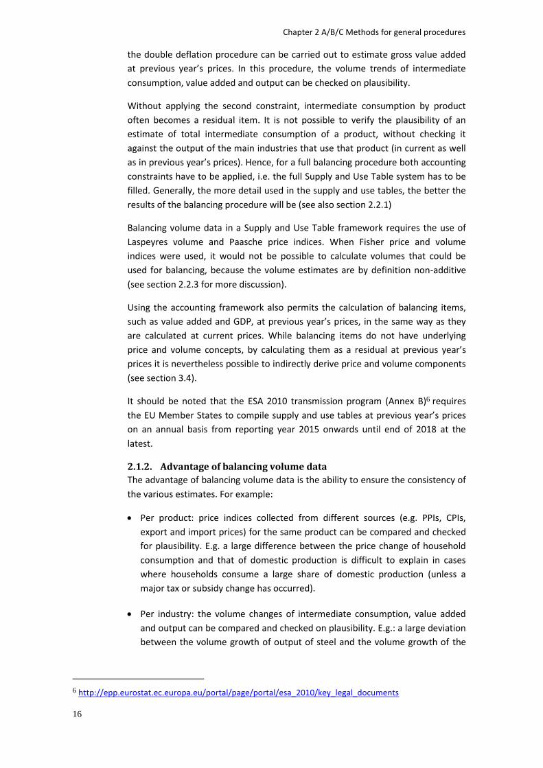
The issue is explained by means of the following example of a homogeneous
product that is only consumed by households.
Output Trade
Margin
Taxes on
Products
Household
Consumption
Value T 305 60 130 495
Price index 111 118 113
Volume T (prices T-1) 275 110 440
Volume index 110 110 110
Value T-1 250 50 100 400
The observed price index for household consumption is 113, while for output only
111 is registered. This yields volume indices for both sides of 110. The quantity (or
volume) change of output and consumption must be the same since there is just
one homogeneous product (without quality change) and no users other than
households. (In general, with aggregate products and various uses there will of
course be different volume growth rates.) In the example, the difference in the
price indices must come from changes in the tax rates and margin rates.
For taxes on products, the volume index must equal the volume of the underlying
product flow (see section 3.10 for further discussion). It follows that the tax rate
increased by 18%. This has to be checked against actual data on tax rate changes.
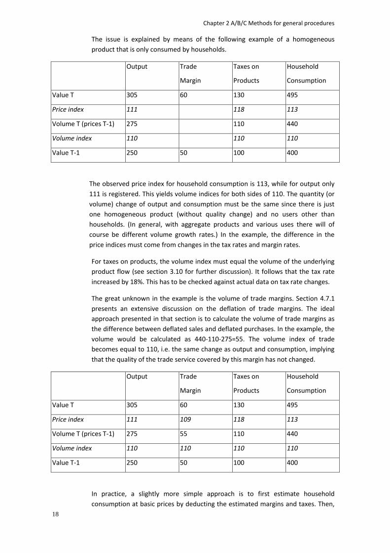
The great unknown in the example is the volume of trade margins. Section 4.7.1
presents an extensive discussion on the deflation of trade margins. The ideal
approach presented in that section is to calculate the volume of trade margins as
the difference between deflated sales and deflated purchases. In the example, the
volume would be calculated as 440-110-275=55. The volume index of trade
becomes equal to 110, i.e. the same change as output and consumption, implying
that the quality of the trade service covered by this margin has not changed.
Output Trade
Margin
Taxes on
Products
Household
Consumption
Value T 305 60 130 495
Price index 111 109 118 113
Volume T (prices T-1) 275 55 110 440
Volume index 110 110 110 110
Value T-1 250 50 100 400
In practice, a slightly more simple approach is to first estimate household
consumption at basic prices by deducting the estimated margins and taxes. Then,
Chapter 2 A/B/C Methods for general procedures
19
a PPI at basic prices can be used to deflate household consumption at basic prices.
(The opposite way is also possible: estimate output at purchaser's prices by
including margins and taxes, and deflating by a CPI.) The supply and use tables will
balance automatically since only one price index is used per product.
Although this approach is attractive in the sense that it is easier to implement, the
clear drawback is that a less appropriate price index (a PPI) is used to deflate
consumption, while in fact the more appropriate price index (a CPI) is readily
available. Not only valuation is important for appropriateness of deflators, but also
whether the price index reflects accurately the prices of the products included in
the flow (see section 2.3).
It is important in such a case that a check on plausibility is made by comparing PPIs
with CPIs.
2.1.4. The case of price discrimination
In section 2.1.1 it was said that - in a Laspeyres volume/Paasche price framework -
the data at previous year’s prices should balance, i.e. that the quantities of supply
and use in year T valued at prices of year T-1 should be equal. This is based on the
following logic. Each individual transaction is a contract between one seller and one
purchaser for one quantity and at one price. For both seller and purchaser, the
price and quantity increase compared to the base year transactions are the same.
In principle, one could express each transaction in the price that prevailed in the
base year, and add all transactions together, so that supply and demand will
balance.
In some cases, however, it is not possible to compile a consistent Supply and Use
Table balance in which supply and use are distributed by producers and consumers.
These cases are where price variations exist between different consumers of a
product that cannot be attributed to quality changes, such as cases of price
discrimination, parallel markets or limited information (see ESA 2010 par. 10.13
and further). Price variations due to price discrimination do not constitute
differences in volume (ESA 2010 par. 10.16).
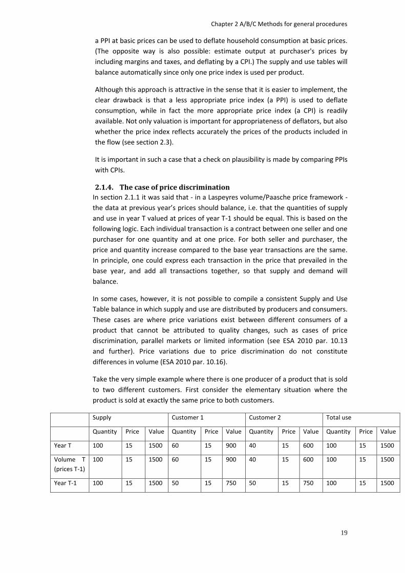
Take the very simple example where there is one producer of a product that is sold
to two different customers. First consider the elementary situation where the
product is sold at exactly the same price to both customers.
Supply Customer 1 Customer 2 Total use
Quantity Price Value Quantity Price Value Quantity Price Value Quantity Price Value
Year T 100 15 1500 60 15 900 40 15 600 100 15 1500
Volume T
(prices T-1)
100 15 1500 60 15 900 40 15 600 100 15 1500
Year T-1 100 15 1500 50 15 750 50 15 750 100 15 1500
Chapter 2 A/B/C Methods for general procedures
20
The 100 units of output are evenly distributed over both customers in year T-1. The
distribution of output changes in year T but it is assumed that the price does not
change, so that the volume in year T equals the value in year T. The volume of
supply equals the sum of the volumes consumed.
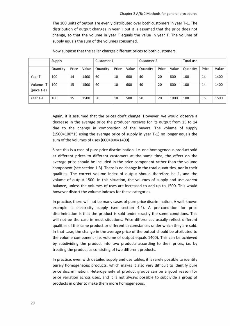
Now suppose that the seller charges different prices to both customers.
Supply Customer 1 Customer 2 Total use
Quantity Price Value Quantity Price Value Quantity Price Value Quantity Price Value
Year T 100 14 1400 60 10 600 40 20 800 100 14 1400
Volume T
(price T-1)
100 15 1500 60 10 600 40 20 800 100 14 1400
Year T-1 100 15 1500 50 10 500 50 20 1000 100 15 1500
Again, it is assumed that the prices don't change. However, we would observe a
decrease in the average price the producer receives for its output from 15 to 14
due to the change in composition of the buyers. The volume of supply
(1500=100*15 using the average price of supply in year T-1) no longer equals the
sum of the volumes of uses (600+800=1400).
Since this is a case of pure price discrimination, i.e. one homogeneous product sold
at different prices to different customers at the same time, the effect on the
average price should be included in the price component rather than the volume
component (see section 1.3). There is no change in the total quantities, nor in their
qualities. The correct volume index of output should therefore be 1, and the
volume of output 1500. In this situation, the volumes of supply and use cannot
balance, unless the volumes of uses are increased to add up to 1500. This would
however distort the volume indexes for these categories.
In practice, there will not be many cases of pure price discrimination. A well-known
example is electricity supply (see section 4.4). A pre-condition for price
discrimination is that the product is sold under exactly the same conditions. This
will not be the case in most situations. Price differences usually reflect different
qualities of the same product or different circumstances under which they are sold.
In that case, the change in the average price of the output should be attributed to
the volume component (i.e. volume of output equals 1400). This can be achieved
by subdividing the product into two products according to their prices, i.e. by
treating the product as consisting of two different products.
In practice, even with detailed supply and use tables, it is rarely possible to identify
purely homogeneous products, which makes it also very difficult to identify pure
price discrimination. Heterogeneity of product groups can be a good reason for
price variation across uses, and it is not always possible to subdivide a group of
products in order to make them more homogeneous.
Chapter 2 A/B/C Methods for general procedures
21
2.2. The three principles from the Commission Decision Commission Decision 98/715 specified three main principles concerning the
measurement of prices and volumes in national accounts. The three principles
concerned the level of detail applied in the calculations, the choice of index
formula and the choice of base year. Below, these three principles are briefly
reviewed.
It is important to note that for these fundamental issues, it is desirable that all
countries base their calculations on the same principles. Therefore there is no
A/B/C classification specified here.
2.2.1. The elementary level of aggregation
The first principle formulated by the Commission Decision relates to the level of
aggregation:
Principle 1:
In the measurement of prices and volumes a detailed level of aggregation of
products shall be used. This level of aggregation, which is referred to as the
elementary level of aggregation, shall be at least as detailed as the A*64 / P*64
level of ESA 2010, for output as well as all categories of (intermediate and final)
use.
The measurement of prices and volumes should start from a detailed breakdown of
products for the different transaction categories. For each product distinguished
for each transaction category, a price index should be found with which the current
price value can be deflated, or a volume indicator should be found to extrapolate a
base year value. In the ideal case, each product would be distinguished separately,
and the pure price and volume changes of that product could be estimated.
In statistical practice, however, it is necessary to aggregate products, which means
that price and volume changes of different products have to be weighted together.
The statistical sources from which the price indices and volume indicators are
derived can use differing weighting methodologies (i.e. differing formulas or
differing base years). In the national accounts, however, one consistent weighting
methodology for all variables has to be used (see the second and third principles
below). If indices with a different weighting methodology than the national
accounts weighting are used in the national accounts, then implicitly the
assumption is made that the indices used are elementary indices, so that the
underlying weighting scheme is assumed to be irrelevant. Then, a fixed-weighted
Laspeyres index can for example be assumed to be equal to a Paasche index, or a
previous-year weighted Laspeyres index. Clearly, the implicit assumption that the
indices used are elementary indices is most valid when it is applied on a very
detailed level.
Therefore, the more detailed the product breakdown is, the more accurate the
results can be expected to be. At a detailed level the products can be assumed to
be more homogeneous, yielding indices that are closer to elementary indices, as
well as more detailed weighting schemes. Also, by distinguishing more products,
Chapter 2 A/B/C Methods for general procedures
22
the quality change that lies in the shifts between products is better covered (see
section 2.4). It may well be that the effect on the overall GDP growth figure of
introducing more detail is larger than the effect of the choice of base year or index
formula.
In practice, there is however a limit to what can reliably be broken down. For
example, the more detailed the product groups for which price indices are
compiled, usually the smaller the sample of prices and products becomes. It might
therefore be that the reliability of a more aggregated price index is higher than of a
more detailed index.
For the purpose of this handbook, the term elementary level of aggregation is used
to denote the precise level of aggregation at which the assumption that the indices
used are elementary indices is applied in the national accounts. It is often - but not
necessarily - equal to the number of products distinguished in the supply and use
tables which are used for balancing purposes.
It is clearly essential that an effort is made in constructing detailed breakdowns of
products for deflation purposes. As quoted above, for the EU Member States, the
elementary level of aggregation, for output as well as all categories of
(intermediate and final) use, should be at least as detailed as the A*64 / P*64 level
of the ESA 2010 Transmission Programme requirements, and the level that is to be
used for the submission of supply and use tables to Eurostat. In practice, to obtain
good results, this level is probably far from optimal, and more detailed breakdowns
need to be used.
Additional minimum breakdowns for estimating deflators or volume indicators are
described for some transaction categories in chapters 3 and 4.
2.2.2. The choice of index formula and base year
Having defined the elementary level of aggregation, the price and volume indices
available at that level have to be weighted together to obtain the price and volume
measures of all national accounts aggregates. The second principle relates to the
choice of index formula to be used for this purpose. This issue is related to the
choice of base year, which is dealt with by the third principle.
Principle 2:
Volume measures available at the elementary level of aggregation shall be
aggregated using the Laspeyres formula to obtain the volume measures of all
national accounts aggregates. Price measures available at the elementary level of
aggregation shall be aggregated using the Paasche formula to obtain the price
measures of all national accounts aggregates.
Principle 3:
Volume measures derived at the elementary level of aggregation shall be
aggregated using weights derived from the previous year.
Chapter 2 A/B/C Methods for general procedures
23
2008 SNA, chapter 15, contains a full description of the various index formulae,
their relationships, advantages and disadvantages. Here, we will only summarise
the essentials.
The most frequently used index formulae in national accounts are those of
Laspeyres, Paasche and Fisher. Essentially, Laspeyres uses weights from a base
year, Paasche from the current year and Fisher is the geometric average of
Laspeyres and Paasche and hence the weights are a combination of base year and
current year values. Simplified, the following relationships hold:
Value index = Laspeyres volume index * Paasche price index
= Paasche volume index * Laspeyres price index
= Fisher volume index * Fisher price index.
The term "base year" has a slightly different meaning in the context of
Laspeyres/Paasche and Fisher indices. In a Laspeyres volume index, the base year is
the year whose current price values are used to weight the detailed volume
measures. Using Laspeyres volume indices results in values expressed in prices of
the base year, e.g. it gives what GDP would have been if the quantities of 2011
were produced against the prices of 2010. This is the traditional and most easily
interpretable form of volume data. In principle, any year can be chosen as base
year, but in national accounts only the previous year is allowed. The base year
should be distinguished clearly from the reference year (see section 2.2.3).
In a Fisher index, the "base year" is a sort of average of two years, of which one is
the current year. Normally Fisher indices are calculated on the basis of the previous
year and the current year. The advantage of that is that the weights are the most
representative for the periods compared, which reduces the so-called substitution
bias (see e.g. 2008 SNA, par. 15.16 and further). Using Fisher indices however does
not lead to volume data that can be interpreted in the above "traditional" way. One
can of course deflate a value by a Fisher price index, but the result cannot be
interpreted as the value of that transaction in prices of the base year.
Laspeyres volume indices have the convenient property that the volume data are
additive when expressed in prices of the base year (but not necessarily when
expressed in prices of another year, see section 2.2.3). Additivity means that the
volumes of sub-aggregates add up to the volume of the aggregate. Additivity is not
an essential property of volume data, but it is convenient, because it allows the
balancing of volume data as outlined in section 2.1 and the construction of
internally consistent volume supply and use tables.
Fisher volume data are non-additive, even if the base year is a recent one. That
makes it impossible to use Fisher indices in a balancing process of volume data, nor
to compile consistent supply and use tables in previous year’s prices. It is possible,
however, to compile Fisher indices for the aggregates after the balancing of the
supply and use tables (using Laspeyres/Paasche) is completed. This would assume
that the price and volume indices as given by the Supply and Use Table framework
are elementary indices.

Chapter 2 A/B/C Methods for general procedures
24
A close substitute to Fisher indices is however to use Laspeyres volume and
Paasche price indices combined with the most recent weights, normally those of
the year prior to the current year. The Laspeyres/Paasche combination then gives
additive data in prices of this base year. It might well be that the benefit of being
able to balance the volume data, and thus to carefully check all data on consistency
and reliability, adds more to the precision and validity of the estimates than using
Fisher indices. According to ESA 2010 (10.20) the use of Laspeyres volume/Paasche
price indices on the basis of previous year's weights is mandatory. This choice is is
essentially a compromise solution: it gives additive volume data at the expense of a
somewhat larger risk of substitution bias.
2.2.3. The non-additivity problem
For a discussion of the non-additivity problem it is convenient to make a clear
distinction between the base year and the reference year:
– the base year is the year whose current price values are used to weight the price and volume measures derived at the elementary level of aggregation;
– the reference year is the year which is used for the presentation of a time series of volume data. In a series of index numbers it is the year that takes the value 100.
For example take the following series of index numbers:
2005 2006 2007 2008 2009
100 105 108 112 120
Suppose these numbers were calculated using the weights of the previous year.
This could for example lead to the following series of year-to-year changes:
2005 2006 2007 2008 2009
100 105 102 103 106
For each of these indices holds: t-1 = 100, hence the reference year is equal to the
base year, but changes each year. It is easily possible to express the series on one
reference year by ‘re-referencing’ or 'chaining'. This would yield:
2005 2006 2007 2008 2009
100 105 107.1 110.3 116.9
(107.1=105*102/100; 110.3=107.1*103/100, etc.)
It is important that a change of the reference year does not affect the year-to-year
indices. This is obvious for a single series as in this example, but when a variable
consists of several sub-variables this is no longer obvious. To keep all year-to-year
growth rates of each variable unchanged when the reference year is changed, one
should re-reference each variable separately, be it an elementary index, a sub-total
or an overall aggregate such as GDP. The consequence is that, in the chained
volume data of a fixed reference year, discrepancies will arise between individual
elements and their totals. This is the 'non-additivity' problem. These discrepancies
have to remain in the published data without adjustment (ESA 2010, par. 10.23), as

Chapter 2 A/B/C Methods for general procedures
25
any adjustment would again distort the growth rates. See the following example
for further clarification.
Example: Re-referencing aggregates and their components
Consider two products A and B, and their total. Assume that these are
homogeneous products; that means that we can determine price and volume
indices for these products which do not depend on an underlying weighting
scheme, i.e. these are elementary indices. The volume and price indices for A and B
combined however depends on how A and B are weighted together.
In the following scheme, the volume changes for the total between t-1 and t are
weighted together by the current price values of year t-1. As these are the most up-
to-date weights these growth rates can be seen as the most accurate.
Product A Product B A & B combined
2005 current prices 100 300 400
Volume change 05-06 105.0 110.0 108.8
2006 at prices of 2005 105 330 435
Price change 05-06 110.0 95.0 98.6
2006 current prices 115.5 313.5 429.0
Volume change 06-07 102.0 90.0 93.2
2007 at prices of 2006 117.8 282.2. 400.0
Price change 06-07 108.0 105.0 105.9
2007 current prices 127.2 296.3 423.5
Volume change 07-08 103.0 95.0 97.4
2008 at prices of 2007 131.1 281.4 412.5
Price change 07-08 105.0 102.0 103.0
2008 current prices 137.6 287.1 424.7
Chapter 2 A/B/C Methods for general procedures
26
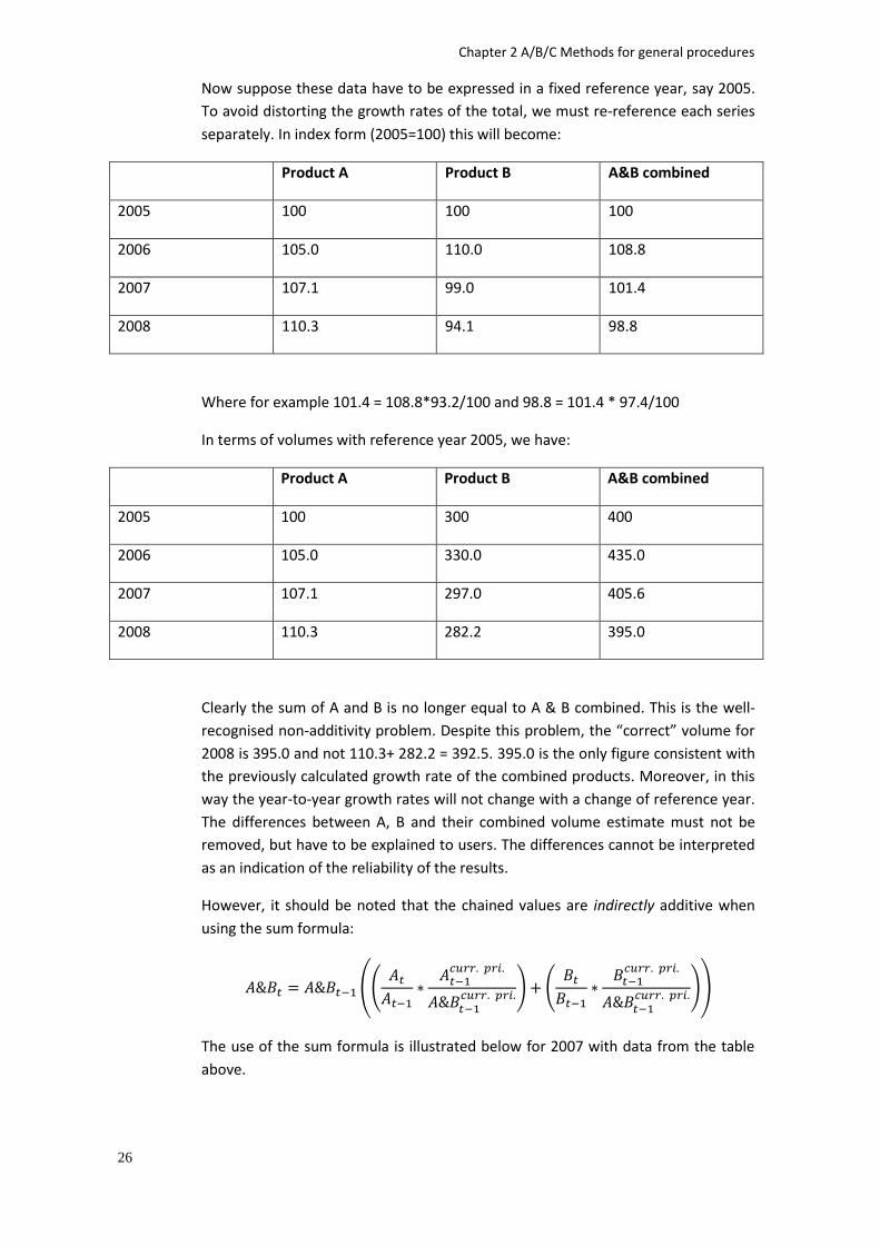
Now suppose these data have to be expressed in a fixed reference year, say 2005.
To avoid distorting the growth rates of the total, we must re-reference each series
separately. In index form (2005=100) this will become:
Product A Product B A&B combined
2005 100 100 100
2006 105.0 110.0 108.8
2007 107.1 99.0 101.4
2008 110.3 94.1 98.8
Where for example 101.4 = 108.8*93.2/100 and 98.8 = 101.4 * 97.4/100
In terms of volumes with reference year 2005, we have:
Product A Product B A&B combined
2005 100 300 400
2006 105.0 330.0 435.0
2007 107.1 297.0 405.6
2008 110.3 282.2 395.0
Clearly the sum of A and B is no longer equal to A & B combined. This is the well-
recognised non-additivity problem. Despite this problem, the “correct” volume for
2008 is 395.0 and not 110.3+ 282.2 = 392.5. 395.0 is the only figure consistent with
the previously calculated growth rate of the combined products. Moreover, in this
way the year-to-year growth rates will not change with a change of reference year.
The differences between A, B and their combined volume estimate must not be
removed, but have to be explained to users. The differences cannot be interpreted
as an indication of the reliability of the results.
However, it should be noted that the chained values are indirectly additive when
using the sum formula:
((
) (
))
The use of the sum formula is illustrated below for 2007 with data from the table
above.
Chapter 2 A/B/C Methods for general procedures
27
((
) (
))
The sum formula provides the possibility to add series of chained values which in
many cases can be of good value. For example it can be used to calculate the sum
of gross value added (GVA) for a range of industries where the chained GVA figures
for each industry are already available. Moreover, the formula can be re-arranged
to be used as a formula of subtraction of chained values. This could for example be
used to calculate GVA for “all industries” excluding one or more selected industries.
The sum formula as presented above can easily be generalised to n elements.
The choice of base year and the choice of reference year are in principle unrelated
issues. For the calculation of price and volume measures, only the choice of base
year is relevant.
Because of the need to re-reference or chain data calculated with the previous year
as base year are to be expressed in a fixed reference year, this system of always
using the previous year as base year is also known as a system of "chain indices".
However, for the calculation of the year-to-year price and volume changes, no
chaining is required.
2.3. Criteria for appropriate price and volume indicators There is duality in the measurement of prices and volumes: one can either deflate a
current year value with a price index, or alternatively extrapolate a base year value
with a volume index to arrive at an estimate in prices of the base year. Therefore,
only one of the two possible measures is required, and the other can be derived as
a residual.
The two alternative approaches are in practice however not entirely equivalent.
Deflation with a price index is generally preferred. There are two reasons for this:
A sample of price observations is normally more representative than an equally
sized sample of quantity observations. In an open market there cannot be large
differences in the changes of the prices charged for the same product by
different producers. There can however be significant differences in the
changes of the quantities of that product produced by different companies.
This makes it necessary to have larger samples for quantity indicators than for
price indicators. In fact, for quantity indicators one would prefer to have nearly
exhaustive observation of all transactions.
Price index compilation is usually based on the fixed-basket methodology: the
prices of a fixed basket of precisely specified goods and services are compared
between two periods. In this way, the quality of the goods and services
compared is held constant, and the price index measures pure price changes. If
a quantity or volume index is compiled directly, there is no guarantee that the
units counted in one year are of the same quality as in the next year, unless
one has very detailed quantity information dealing with homogeneous
products. It is therefore more difficult to control for quality changes when
volume indicators are used (see also section 2.4.3).
Chapter 2 A/B/C Methods for general procedures
28
For each approach there is a variety of different indicators that can be chosen. To
assess the appropriateness of an indicator the following general criteria can be
used (drawn from Commission Decision 98/715, p.40):
the completeness of the coverage of the product heading by the indicator. For
example whether the indicator covers all of the products under the heading or
just a selection of them, such as only those products sold to households;
the valuation basis of the indicator. For e.g. market output, this should be basic
prices, rather than, for example, purchasers' prices or input costs, whilst for
e.g. final consumption expenditure it should be purchasers' prices;
the indicator should take quality changes into account, recording them within
the volume estimates (see section 2.4);
the conceptual consistency between the indicator and the national
accounts concepts.
Indicators satisfying all four criteria generally will constitute A methods. If one or
more criteria are not satisfied, the methods will become B methods or C methods
according to how far away the method is from an A method. The precise distinction
between A, B and C depends on the product and its specific circumstances. For
example use of an indicator relating purely to prices charged to household
consumers would be a B method if it could be shown that business prices closely
followed household prices or that the proportion of business expenditure in total
expenditure on the product was sufficiently low. It is important that appropriate
research is undertaken to determine if use of a particular indicator can lead to
systematically poor or biased estimates.
2.4. Quality changes
2.4.1. The problem of quality changes
The measurement of year-on-year price changes of goods and services is
complicated by the fact that these goods and services may change between those
years. The observed price changes may reflect changes both in characteristics and
pure price changes. A value has then to be estimated for the change in the
characteristics, in order for the price index to reflect pure price changes only. This
is commonly known as the problem of quality changes.
The quality of a product is defined by its (physical and non-physical) characteristics.
In principle, whenever a characteristic of a product changes, it is to be considered a
different quality of the product. These changes in characteristics are to be recorded
as changes in volume and not as changes in price (cf. ESA 2010, par. 10.18).
Valuing those quality changes is one of the most difficult problems in price and
volume measurement. For a producer, quality change of an input will be related to
its use in the production process and the profit that can be made, and it might be
possible to more or less objectively put a value to the change. For a consumer,
however, the quality of a product is essentially linked to the utility he or she gets

Chapter 2 A/B/C Methods for general procedures
29
out of it. Utility is not quantifiable, making the measurement of quality change for
consumers a rather subjective matter. In economic statistics, one can only analyse
aggregate consumer preferences as revealed by their purchasing behaviour, on the
basis of observed market prices.
According to economic theory, in a situation of perfect competition the market
price of a product will reflect both the purchaser’s preferences and the producer’s
production costs. The market price will reflect exactly what the purchaser wants to
pay for an extra unit of this product as well as what the producer needs to receive
in order not to make a loss.
In this situation, a difference in price that exists between two products at the same
time can be interpreted as the value that consumers attach to the quality
difference between the two products. This implies that a higher price is associated
with a higher quality. If shifts in the quantity of consumption occur between the
different products this should be seen as a volume change, implying that the
quality difference between the two products is exactly equal to the price
difference.
Unfortunately, in most cases there is no perfect competition. Generally, price
differences between different products can exist for various reasons. For example,
consumers do not always have perfect information, leading them to buy at too high
prices. Also, markets may not react promptly to the introduction of new products.
It can happen that the “old” products are being put on sale when new products are
introduced, implying that the difference in price between the old and new products
cannot immediately be used to value the quality difference. Other reasons for price
differences may be price discrimination and the existence of parallel markets. All
the price differences mentioned here should be seen as price differences and not
as quality differences (see ESA 2010, par. 10.14 – 10.18).
In some markets, e.g. for computers, it frequently occurs that new products have a
higher quality but are introduced at the same, or a lower price than the old
products. In such a case, the usual assumption that a higher price corresponds to a
higher quality is no longer valid.
Therefore, market prices do not always properly reflect quality differences. The
situation of perfect competition can however be used as the benchmark situation,
i.e. the prices that would occur in a perfect competition situation would give us the
correct quality evaluations. The correct quality adjustments can – in theory – be
found by analysing the market prices supposing that perfect competition would
prevail. The appropriateness of a particular method for quality adjustment
therefore depends on the characteristics of the market in question: if a market is
close to perfect competition, comparing market prices will usually give good
results. If a market is further from perfect competition, e.g. due to the existence of
a monopolist, perhaps other methods should be sought.
The limiting case of quality changes is when new products appear on the market. In
such a case it is impossible to find prices that can be compared between the two
years. It is important that new products are introduced into price samples as soon
Chapter 2 A/B/C Methods for general procedures
30
as possible after they appear on the market. At the moment of introduction, an
estimate has to be made of the price of the new product in the period just before
its introduction. The methods that can be used for making such estimates are not
essentially different from the methods to deal with quality changes that will be
described in the next section.
2.4.2. Accounting for quality changes in price indices
The conventional approach to the compilation of a price index for a particular good
or service is to follow the prices of a fixed sample of items over time. The price
changes are averaged to obtain the price index for the product. The rationale
behind the fixed sample procedure is to make sure that only pure price changes are
measured. However, in practice the goods and services in the sample do not
remain constant: their characteristics may change continuously. Furthermore,
there may be changes outside the sample, e.g. when new products are introduced.
The classical problem of quality adjustment can be posed as follows. An item, say
item A in the price index for a certain product group disappears from the market. A
new item, say item B, is chosen to replace it. How to measure the price change
over time? Below, the various methods that were developed to answer this
question are briefly described.
Overlapping
In many cases there will be one or more periods where both A and B are on the
market (i.e. they “overlap”). In this situation prices are available for both item A
and item B at, say, time t, so that price change up to t could be based on item A
and after t, on item B.
It is then implicitly assumed that the price difference between A and B in period t is
a measure of the value of the quality difference. As made clear in the previous
section, whether or not this is a reasonable assumption depends on the market
situation of the product in question. In situations that are close to perfect
competition, the overlapping method will give appropriate results.
However, in certain circumstances, e.g. when new varieties of the product are
introduced frequently and prices change quickly, the overlapping method may not
give good results. The main problem is that very different results can be obtained
depending on when items are introduced into, or dropped out of, the price sample.
For example, if new models of computers are introduced into the price sample as
soon as they appear and kept in the sample as long as they are sold, then it is likely
that a rapidly declining price index will be the result because of the large
discounting which applies to an old model once a new one is introduced. On the
other hand, a price index which declines little (if at all) can be obtained if the prices
of old models are dropped out of the sample as soon as a new model is introduced.
For other products, other patterns may prevail. For example, cars are often
introduced at reduced prices.
Chapter 2 A/B/C Methods for general procedures
31
Unadjusted price comparison
(Also called “direct price comparison”.) This is a simple method in which the price
difference between A and B is taken unadjusted into the index. Thus it is assumed
that there is no quality difference between A and B. This method is clearly not
suitable in areas of rapid quality change such as high-tech goods.
Automatic linking
(Also called “link-to-show-no-price-change”.) In this method, the items are simply
called non-comparable and the price level is considered unchanged. Hence, the
measured price difference is fully attributed to the quality change. This method
generally gives a systematic underestimation of inflation and is therefore banned
by EU regulation for the HICPs.
Matched models only
(Also called “imputation” or “imputed price change – implicit quality adjustment”.)
This method includes in the price index only the price changes of items that exist in
the two periods compared, while disregarding all non-matching items. So, items A
and B will both be dropped from the sample, and the price index is only based on
those items for which no quality change occurred. The implicit assumption is that
the price change of the matching items is representative for the price change of the
non-matching items. Whether this is realistic depends on the extent in which price
changes are introduced at times when new varieties of products are introduced,
which is the case in many markets.
Option prices
If the difference between A and B is the inclusion of an extra option, for example a
CD-ROM drive in a PC, this option could be valued by its price as if it were
purchased separately. Thus, if B includes a CD-ROM drive, then its price can be
reduced by the price of that drive to arrive at an estimate for the price of A, which
didn’t have the CD-ROM, in period t.
It is however not always the case that the price of the product with the option is
equal to the price of the product plus the price of the option. For example the price
of separately purchased software is usually much higher than if it were purchased
together with a PC.
Clearly, this method is only possible when the quality difference can be described
in this way and when a separate price for the option exists. Note that this method
uses prices to the consumer and not production costs.
Production costs
In some cases, there will not exist a separate price for the new option. In such cases
the producer can be asked how much the new option costs to produce. More
generally, producers can be asked for data on the difference in production costs

Chapter 2 A/B/C Methods for general procedures
32
between A and B. Note that in this method costs are used instead of prices, so that
the user’s preferences are not taken into account. The method can be improved in
this respect by including the producer’s profit margin.
Judgmental approach
Another possibility is to ask the producers, consumers or other experts to give an
estimate of the value of the quality difference between A and B. This method is for
obvious reasons rather subjective, and its results cannot be objectively verified.
Hedonic adjustment
In this method, data on the market prices and characteristics of various models of a
product are collected. A regression is carried out to investigate which
characteristics are the determinants of the price differences between the models.
Two basic variants of this method exist:
Calculate the implicit prices of each of the characteristics. This information can then be used to estimate a price for an item in a period in which it was not on the market.
Calculate the price index directly from the regression. In such a case the regression usually will contain time dummy variables whose coefficients will reflect those price changes that cannot be associated with a change in the characteristics.
In the literature, many examples of the second variant are found. These are usually
backwards looking studies in which the price movements over a number of years
are estimated in one regression. This variant seems to be less appropriate for
official price statistics when, in a continuously running program of price
observations, adjustments have to be made as quality changes occur.
The first variant seems more relevant for official statistics. It can be used alongside
other methods of quality adjustment. The implicit prices are estimated in a
particular base period and then used in a number of periods. The hedonic method
is mostly used in cases where there are rapid changes in the products, such as in
the computer market. In those cases, the regression will have to be re-estimated
frequently (at least more than once a year) since the characteristics and their prices
will change often.
The hedonic method is only possible when characteristics can be defined that
influence the price and can be quantified.
The OECD published a Handbook on Hedonic Indices and Quality Adjustment in
Price Indices (http://www.oecd-ilibrary.org/science-and-technology/handbook-on-
hedonic-indexes-and-quality-adjustments-in-price-indexes_643587187107), in
which the technical aspects of hedonics are elaborated as well as a comparison is
made with other quality adjustment methods.
Chapter 2 A/B/C Methods for general procedures
33
Resampling
This method could also be labelled aggregate overlap pricing. It means that in each
period a new sample of items is priced. Thus up to, say, period t the estimate of
the price change is based on an old sample called A, and after t on a new sample
called B.
As for simple overlap pricing, resampling depends on the differences between
average prices between A and B to be genuine reflections of quality differences.
A version of this method that has been informally tested and found interesting in a
CPI context is called “Monthly Chaining and Resampling” (MCR). This involves
observing the prices of all varieties (or at least a representative sample of them) of
a product that are on the market each month (hence monthly resampling). The
price change is then computed from one month to the next as an average over
those items that are in the sample in both months. Price changes between months
that are further apart are calculated by multiplying the month-to-month changes
(hence monthly chaining).
The advantage of the method is that the sample of matched models that
determine the price index is sufficiently large due to the monthly resampling. The
difference with traditional methods is that one no longer tries to follow the same
sample through time, but instead one looks at what is actually on the market in
each period. New products are therefore included earlier than with a fixed basket.
Preliminary testing seems to have shown that indexes based on this method yield
similar results as hedonic indices.
2.4.3. Accounting for quality change in volume indicators
When a volume measure is not obtained by deflation with a price index but
instead by extrapolation with a volume index, quality changes should also be
accounted for. This however provides some special problems.
Suppose for example that we would measure the volume of the output of cars by
the number of cars sold. However, the quality of cars is constantly changing.
Suppose we managed to find an indicator for this quality, say the maximum speed
the car can reach. How can the quantity indicator then be combined with the
quality indicator? If the car can now do 200 km/h instead of 180 km/h, is that then
a quality change of (200-180)/180*100 = 11%? Should the number of cars be
adjusted with this percentage? It is clear that a number of very arbitrary
calculations are made in such a case. In general, there seem to be few objective
criteria to link quality indicators to quantity indicators.
One possible solution is to adjust the implicit prices. Quality adjustments are, as
spelled out in section 2.4.1, essentially a matter of putting a money value to
changes in products. If the total turnover of cars were divided by the number of
cars, an implicit (average) price of cars would be found. Then, an estimate needs
to be made of the price increase of the cars that is due to the increased

Chapter 2 A/B/C Methods for general procedures
34
capabilities, that is the value that consumers attach to this increase in speed. For
this, the same approaches can be used as listed in the previous section.
When volume indicators with a detailed breakdown of products are used, shifts
between the different products will be included in the volume component.
Therefore, part of the quality change (that part due to compositional changes in an
aggregate, see section 1.3) can be captured by differentiating as many qualities of
a product as possible. These different qualities are then in fact treated as different
products.
2.4.4. A, B and C methods
The most appropriate method for quality change will depend to a large extent on
the particular circumstances. A few general criteria can be specified however. An
appropriate method for quality adjustments:
makes explicit evaluations of the quality change rather than implicit ones;
does so in a verifiable way;
takes both user’s preferences and producer’s costs into account (normally by considering differences in market prices).
In general, the following methods can become A methods if applied under the
right circumstances:
the hedonic approach, if characteristics can be identified that influence the price and can be quantified;
option prices, if separately priced options can be distinguished, and the price of a separately purchased option is not very different when it is included in the product;
overlapping, if there is no large discounting of an old item when a new item is introduced;
the resampling method, if the sample is representative and large enough.
Those methods will become B methods if they are applied under less favourable
circumstances. For example, resampling is less good if the sample size is less than
optimal, and the hedonic approach should be used with care if the hedonic
function only explains a limited part of the price variation.
Similarly, the following methods for quality adjustment could be B methods, again
subject to the circumstances in which they are used:
matched models only, if the price change of the matching items is reasonably representative for the price change of the non-matching item;
production costs, if it can be shown that the change in costs gives a reasonably good approximation of the change in price;
judgmental approach, if expert knowledge is available.

Chapter 2 A/B/C Methods for general procedures
35
The unadjusted price comparison method should normally be avoided, unless it is
clear that the quality change is really very small. The automatic linking method is
always a C method.
Some methods are more suited to some products, other methods to others. In the
various sections of chapter 4, where necessary and appropriate, further
specifications of this general A, B and C classification will be given. If there is no
further specification, the above guidance should be applied.
2.5. Unique products A price index is based on the comparison of movements in prices for a selected set
of products across a period of time. But there is a particular problem with unique
products which are by definition “one-offs” and do not appear in another time
period. One can view this as the appearance of a new product and the immediate
disappearance of it – the unique product represents a discontinuity in the
calculation of price indices.
The problem of unique products is especially prevalent in the areas of major
equipment projects (for example ships, aircraft and special purpose machinery),
construction, intellectual property products such as R&D services and tailored
business services (for example management consultancy). These areas are covered
in sections 4.3.2, 4.6, 4.12 respectively.
In many cases, whilst a project may be seen as unique in its entirety, it is likely to
be made up of a number of rather more generic sub-activities. The uniqueness
arises more from the way in which these sub-activities are combined, rather than
the activities themselves. For example a house may look unique, but actually it is
made up of a series of contributions of skilled tradesmen, who may well be
producing what for them seems like a more or less standard product.
There is obviously fertile ground here for examining the sub-activities separately,
to see if their price movements can be combined meaningfully to an overall price
movement for the unique product. There are two ways of looking at this in
aggregate:
i) Model Pricing: This is where a model product is specified in some detail (usually
based on real past products), then the contributory elements are re-priced in
successive time periods. An example of this is in construction, where one can
specify a typical family house, say, and then re-price all of the constituent
elements (such as roof, foundations, kitchen unit) of that house in successive
periods. For business services, there may be a standard (or generic) contract which
can be used. The key criteria for the use of model pricing are:
Regular updating of the models used, to ensure that they do not become out of
date;
Chapter 2 A/B/C Methods for general procedures
36
Representativeness of the models – partly this is achieved through regular
updating, but also choosing models that are applicable across regions (for
example house designs can vary between different regions, so a suitable range
of models is needed);
Use of actual prices charged, taking account of the producers’ profit margins
and any discounts offered to customers. This applies first of all if the model is
based on an actual (past) product. Furthermore, for the estimation of the price
of the model when it no longer exists, an attempt should be made to take into
account usual discounts offered in this industry;
Formulation of the model in terms of outputs, not of inputs. For example, a
model should not contain specifications like "a contract of 100 hours of work",
but rather “a tiled wall of 20 square metres”.
ii) Specification pricing: This is where a real product is broken down into a number
of key elements or components, which are priced, and then in successive periods,
individual projects are examined and the key elements compared. Crucially, the
elements should be separately identifiable, their qualities and impact on final
performance of the product should be quantifiable, and prices should be available
in different periods. This method differs from the “model pricing” approach
because no ideal models are actually specified. It has the advantage that there are
no model products to become out of date, but of course the key elements
identified in the specification method may be less and less relevant over time, and
it is important that the key elements are measured in terms of outputs rather than
inputs.
There are clear similarities between these methods and the hedonic method
explained in section 2.4.2. In the hedonic method, regression analysis is used to
determine the characteristics of products that are the main determinants for the
price. Those characteristics can be, but are not necessarily, components of the
products.
Both model pricing and specification pricing are resource-intensive methods. In
certain cases, international co-operation in developing such methods could be
useful. Section 4.3.2 on large equipment goods describes this in some further
detail, including also the possibility of "importing" price indices from other
countries.
A, B and C methods
The breakdown of methods is described in more detail in the various sections
dealing with the respective products (cited above). In general:
Methods that decompose a product into meaningful and measurable sub-
products (such as model and specification pricing) are A methods. If any of the
first three criteria set out above (regular updating of models,
representativeness, actual prices) are not met, then the method becomes a B
method.

Chapter 2 A/B/C Methods for general procedures
37
The use of international price indices can be a B method for certain products
(see section 4.3.2).
The use of input prices is a B method for unique production, such as R&D
services, as the methods described above are not applicable. .
In other cases a method (including a decomposition method) which relies
wholly on measurement of inputs or uses unadjusted quantity indicators is
generally considered a C method. The unit value method is also considered a C
method for unique products because, by definition, unique products are not
produced in batches of homogenous units.
2.6. Unit values versus price indices In some cases, a choice can be made between a ‘unit value index’ and a price
index. Traditionally, unit value indices appear in foreign trade statistics and the
discussion on the pros and cons of unit value indices and price indices takes place
in the context of deflation of exports and imports, see section 3.9. However, the
arguments used in this discussion can also be used in other contexts, such as the
deflation of compensation of employees, or the price measurement of certain
business services. This section will develop these arguments in a general way,
which can subsequently be applied to numerous individual cases.
A price index is based on the observation of prices of a fixed sample of products in
two different periods. The reliability of the price index depends to a large extent
on how representative the sample is. If the sample misses out a significant portion
of the universe of products, and the missing part has a price trend that is
significantly different from the sampled part, the resulting price index will be
distorted. Also, the sample needs to be kept up-to-date by introducing new
products and removing products no longer available in a timely way.
A unit value index is based on a – usually – exhaustive observation of the total
value and the total quantity of a group of products. A ‘unit value’ is calculated by
dividing the total value with the total quantity. Comparing this unit value in two
different periods gives a unit value index, which can be used as a measure for the
price trend. While complete and thus representative coverage of the observations
is guaranteed, the problem in this method is the heterogeneity of the products,
which can cause a large variability in the index. Furthermore, any changes in the
composition of the products can influence the unit value index resulting in a price
change although such changes should in fact be included in the volume
component. It is not possible to adjust unit value indices for quality changes in the
products in the same way as can be done for price indices.
This can be illustrated by the following example, where prices and quantities of
two products (A and B) are known in two years.
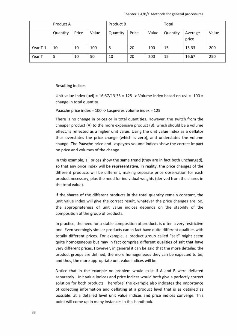
Chapter 2 A/B/C Methods for general procedures
38
Product A Product B Total
Quantity Price Value Quantity Price Value Quantity Average
price
Value
Year T-1 10 10 100 5 20 100 15 13.33 200
Year T 5 10 50 10 20 200 15 16.67 250
Resulting indices:
Unit value index (uvi) = 16.67/13.33 = 125 -> Volume index based on uvi = 100 =
change in total quantity.
Paasche price index = 100 -> Laspeyres volume index = 125
There is no change in prices or in total quantities. However, the switch from the
cheaper product (A) to the more expensive product (B), which should be a volume
effect, is reflected as a higher unit value. Using the unit value index as a deflator
thus overstates the price change (which is zero), and understates the volume
change. The Paasche price and Laspeyres volume indices show the correct impact
on price and volumes of the change.
In this example, all prices show the same trend (they are in fact both unchanged),
so that any price index will be representative. In reality, the price changes of the
different products will be different, making separate price observation for each
product necessary, plus the need for individual weights (derived from the shares in
the total value).
If the shares of the different products in the total quantity remain constant, the
unit value index will give the correct result, whatever the price changes are. So,
the appropriateness of unit value indices depends on the stability of the
composition of the group of products.
In practice, the need for a stable composition of products is often a very restrictive
one. Even seemingly similar products can in fact have quite different qualities with
totally different prices. For example, a product group called "salt" might seem
quite homogeneous but may in fact comprise different qualities of salt that have
very different prices. However, in general it can be said that the more detailed the
product groups are defined, the more homogeneous they can be expected to be,
and thus, the more appropriate unit value indices will be.
Notice that in the example no problem would exist if A and B were deflated
separately. Unit value indices and price indices would both give a perfectly correct
solution for both products. Therefore, the example also indicates the importance
of collecting information and deflating at a product level that is as detailed as
possible: at a detailed level unit value indices and price indices converge. This
point will come up in many instances in this handbook.
Chapter 2 A/B/C Methods for general procedures
39
The distinction between unit value indices and price indices can also be applied to
other examples. For example, for the deflation of wages and salaries, one can
sometimes choose between a wage rate index and an index based on average
wages (see also section 3.53.11.2). The wage rate index will be based on a sample
of wage rates for representative categories of employees, that have to be
weighted with the share of these categories of employees in the total wages and
salaries. This is equivalent to the procedure of compiling a price index. Some
countries possess a database of wages of all employees (for the government
sector for example). With such an exhaustive database average wages can be
calculated for the different categories of employees, yielding an index of average
wages. This is equivalent to a unit value calculation. The result depends entirely on
the stratification of employees chosen. In principle, both methods can yield the
same result if applied at a very detailed level. If a country possesses such an
exhaustive database it is difficult to find conceptual arguments for not using this
source and favouring a sample of wage rate observations instead (there might be
of course other reasons for using wage rates, e.g. the time they become available).
Another application of this discussion can be found in the compilation of deflators
for some types of business services. Such services (of lawyers or accountants for
example) are often paid for on the basis of an hourly fee. There are two ways of
compiling an index of these fees. One could observe a sample of rates that these
service providers use (this method is labelled ‘charge-out rates’ in this handbook)
or one could collect data on total turnover and divide that by the number of hours
worked (which is labelled the ‘hourly fees’ method). Again, the first method
corresponds to the price index methodology (therefore dependent on how
representative the charge-out rates observed are), while the second corresponds
to the unit value approach (therefore suffering from the heterogeneity problem).
Chapter 3 A/B/C Methods by transaction category
40
3. A/B/C methods by transaction category
3.1. Market and non-market output This section will give general principles for the deflation of output. They will be made
much more precise in chapter 4 where they are applied to each individual CPA product
heading.
3.1.1. Market output and output for own final use
Market output and output for own final use will be dealt with together. ESA 2010, par.
3.45 states that “output for own final use (P.12) is valued at the basic prices of similar
products sold on the market”. Therefore, when such prices are available, volume
measures of output for own final use are calculated in the same way as market output.
At the outset, it is important to stress that an essential criterion for appropriate
methods for market output is that the price or volume of the output itself is measured
and not of a proxy for the output (such as an input or another output).
The discussion below and in chapter 4 focuses on output by product. To deflate total
output of a branch, its output should first be classified into the various (primary and
secondary) products produced, as is done in a supply table. Each product should then
be separately deflated by an appropriate procedure. According to the Laspeyres
volume framework as set in out in chapter 2, the sum of the value of the products
constitutes the value of the output of the branch measured in previous year prices.
3.1.1.1. Price deflation methods
Methods in this group all search for information on the price change of the output, so
as to construct a price index with which the value of output in current prices can be
deflated.
Deflation by producer price indices (PPIs and SPPIs)
PPIs come in many varieties. In this handbook, the term PPI will be used exclusively for
an index of the price change of output of a product, whether it is a good or a service.
Output includes both domestic uses and exports. The standard PPI compilation method
is to observe the price of a sample of representative products produced by a local kind-
of-activity unit or enterprise over time. The observed price changes are weighted by
the shares these units or enterprises represent in the total output of the product.
Indices for aggregate product categories (or industries) are derived by weighting with
shares of the individual products in the value of total output (often national accounts
data). This standard method is well established for manufacturing products and
increasingly so for service products.
Chapter 3 A/B/C Methods by transaction category
41
Deflation by PPIs can normally be considered to be the preferred method, since they
directly measure product prices, and quality changes can be taken into account.
However, PPI compilation requires specific surveys, which can be expensive and
difficult to organise, especially for services. This handbook cannot be a guide to the
practical compilation of PPIs. For this, one should consult the PPI manual prepared by
the IMF. Also, the OECD Methodological Guide for Developing Producer Price Indices
for Services and Eurostat’s PEEIs in Focus: a summary of the services producer prices
indices provides guidance for the compilation of SPPIs.
PPIs are often compiled as Laspeyres price indices. As set out in section 2.2, in national
accounts Paasche price indices should be used. That implies, that at the "elementary
level of aggregation" (see section 2.2.1 for a definition), the assumption is made that
the indices are elementary indices, i.e. that Paasche and Laspeyres indices give the
same result. Clearly, the more detailed the level of aggregation, the more plausible this
assumption is. It is recommended that regular tests are made to validate the
assumption made. In certain cases, especially where price or quantity fluctuations are
large, the PPIs could be recalculated to Paasche indices.
PPIs are usually compiled as monthly or quarterly indices. To deflate annual data with
PPIs it is therefore necessary to take the structure of the flow through the year into
account. If the volume of products produced is reasonably constant during the year, a
simple average of monthly or quarterly indices can suffice. If, however, there are large
fluctuations in the volume through the year, the sub-annual indices should be weighted
by the volumes in each month or quarter concerned. Monthly information might be
difficult to gather in practice though.
Model pricing or specification pricing
There are situations where the standard PPI compilation is difficult, for example when
companies produce different products each year so that no prices can be compared. In
such a case a "model price" or "specification price" approach might be a solution.
Section 2.5 on unique products describes this in more detail.
The main advantage of model pricing is that it has an in-built consistency, since the
same project or output is priced in different periods and so, in theory, product quality
is unchanged. However, because of this in-built stability with model prices, there is an
issue of whether the product remains representative, particularly in areas of rapid
product change. So in order to keep the model representative, it needs to be updated
regularly.
Another significant practical disadvantage is that contributors often have difficulties
with delivering a model-price estimate – because of its complexity and the consequent
impact on contributors’ compliance costs.

Chapter 3 A/B/C Methods by transaction category
42
Charge-out rates or hourly fees
In other cases it can be difficult to identify the products; this is particularly the case for
some services. In connection with that, it can be difficult to identify a price: in some
cases payment can be related to, for example, the number of hours worked (for
instance by a lawyer) instead of to the output delivered. In the latter case, the charge-
out rate (price charged per hour) can be used as a price indicator.
Whilst this has the relative advantage of ease of collection, productivity or quality
changes will not be captured, because it does not take into account changes in the
amount of work done per hour charged. Furthermore, charge-out rates suffer from the
“list price” problem: the actual price paid can be quite different from the quoted
charge-out rates, due to discounts negotiated on a bilateral basis. Similarly, hourly fees
can be calculated by dividing total turnover by number of hours worked (this has
similarities to unit value indices, see section 2.6).
Hourly fees and charge-out rate methods differ from input methods using wage rate
indices (see below) in the fact that the operating surplus and other inputs including
compensation of employees are included in turnover. In both methods, however,
changes in the amount of work done per hour will be reflected as price changes rather
than productivity changes.
The hourly fee method is best applied at a very detailed level, by defining the products
in as much detail as possible, and by distinguishing between different types of labour.
Consumer price indices (CPIs)
CPIs are compiled for almost all goods and services consumed by households. If CPIs
are to be used to deflate output (rather than household consumption), it has to be
considered that business consumption and exports can differ significantly from
household consumption in both mix of products and price changes. The
appropriateness of using CPI information to deflate output depends therefore on the
share of household consumption in total output and on the difference in price changes
and composition between intermediate use and final use of the product group in
question.
Also, CPIs normally measure the change in the purchasers' price of a product rather
than the basic price, and therefore have to be adjusted to the correct price base if they
are used for deflation of output. The adjustment has to take account of changes in
trade and transport margins, and changes in the rates of taxes and subsidies on
products. For example:
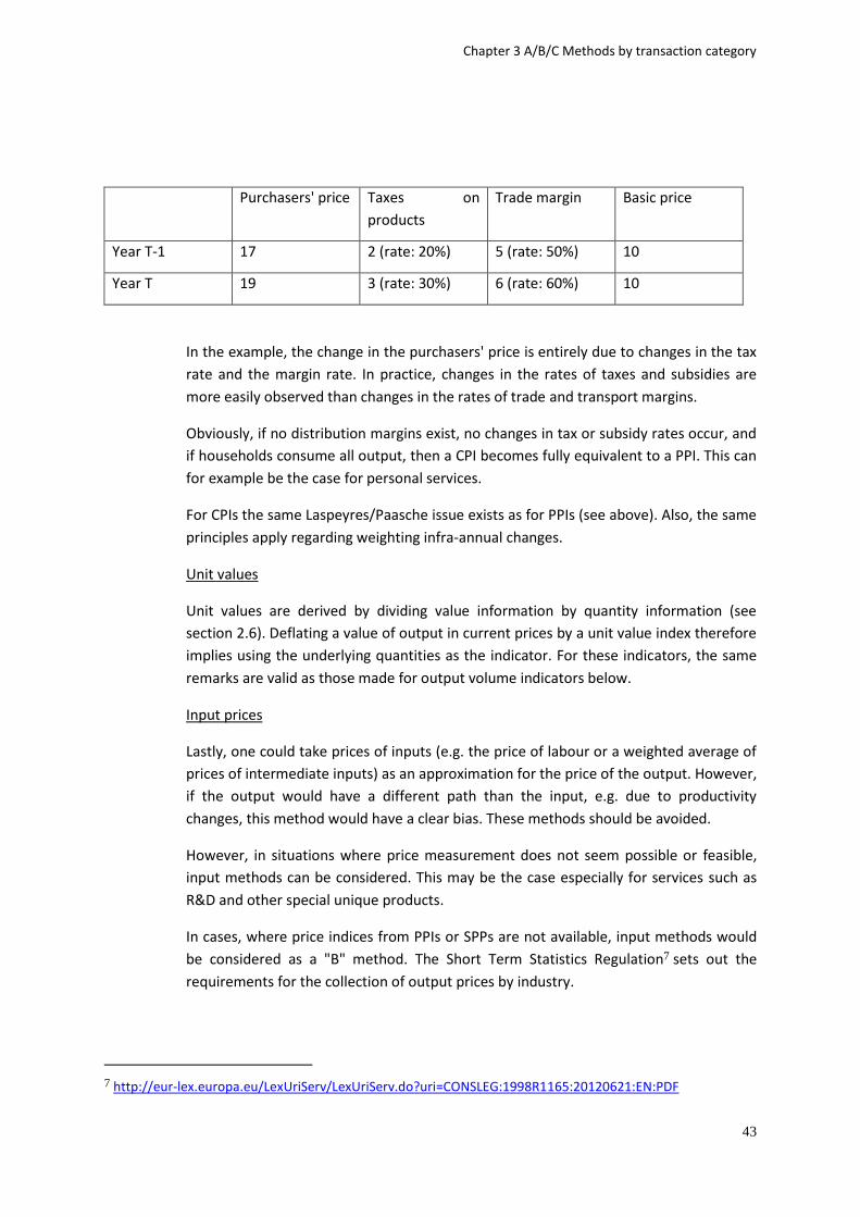
Chapter 3 A/B/C Methods by transaction category
43
Purchasers' price Taxes on
products
Trade margin Basic price
Year T-1 17 2 (rate: 20%) 5 (rate: 50%) 10
Year T 19 3 (rate: 30%) 6 (rate: 60%) 10
In the example, the change in the purchasers' price is entirely due to changes in the tax
rate and the margin rate. In practice, changes in the rates of taxes and subsidies are
more easily observed than changes in the rates of trade and transport margins.
Obviously, if no distribution margins exist, no changes in tax or subsidy rates occur, and
if households consume all output, then a CPI becomes fully equivalent to a PPI. This can
for example be the case for personal services.
For CPIs the same Laspeyres/Paasche issue exists as for PPIs (see above). Also, the same
principles apply regarding weighting infra-annual changes.
Unit values
Unit values are derived by dividing value information by quantity information (see
section 2.6). Deflating a value of output in current prices by a unit value index therefore
implies using the underlying quantities as the indicator. For these indicators, the same
remarks are valid as those made for output volume indicators below.
Input prices
Lastly, one could take prices of inputs (e.g. the price of labour or a weighted average of
prices of intermediate inputs) as an approximation for the price of the output. However,
if the output would have a different path than the input, e.g. due to productivity
changes, this method would have a clear bias. These methods should be avoided.
However, in situations where price measurement does not seem possible or feasible,
input methods can be considered. This may be the case especially for services such as
R&D and other special unique products.
In cases, where price indices from PPIs or SPPs are not available, input methods would
be considered as a "B" method. The Short Term Statistics Regulation7 sets out the
requirements for the collection of output prices by industry.
7 http://eur-lex.europa.eu/LexUriServ/LexUriServ.do?uri=CONSLEG:1998R1165:20120621:EN:PDF

Chapter 3 A/B/C Methods by transaction category
44
3.1.1.2. Volume extrapolation methods
In these methods indicators are collected that describe the trends in the volume of
output directly. Volume indices are constructed and applied to the value of output in
the base year to arrive at the volume of output in the current year.
Output volume indicators
In situations where price measurement does not seem possible or feasible, the direct
measurement of the volume of output can be considered. This can be the case, for
example, for service areas where consumers are implicitly charged for services
provided, such as in banking and insurance (see section 4.11). In other cases, where
there are very homogeneous products without large quality changes and detailed
quantity information is available, it can be equivalent to price deflation.
Section 2.3 has already discussed briefly the major disadvantages of volume indicators
relative to price indices. To overcome these disadvantages, volume indicators should:
be collected at a very detailed level, so as to distinguish homogeneous products that do not change over time, and
be representative for all outputs in question.
The use of output volume indicators might also be necessary in cases of high inflation.
When prices change very rapidly, price indices become increasingly unreliable. To
describe the real economic developments in such situations volume indicators might
give better results. For a more elaborate discussion on high inflation see "Inflation
Accounting: A Manual on National Accounting Under Conditions of High
Inflation", published by the OECD in 2003.
Input volume indicators
In these methods, indicators on the volume of inputs (e.g. the number of employees or
the volume change of intermediate inputs) are used to approximate the volume of
output. The use of such methods means that the resulting data are biased when
productivity changes occur. As for input price methods, these methods should be
avoided.
3.1.1.3. A, B and C methods
A general classification of methods for measuring prices and volumes of market output
into A, B and C methods is given below. In chapter 4, this general classification is further
elaborated for each individual product heading.
A method: For deflating output, in principle, using appropriate PPIs will be an A method.
Each product should be deflated separately by an appropriate PPI. An appropriate PPI
satisfies the following criteria, based on the general criteria given in section 2.3:
Chapter 3 A/B/C Methods by transaction category
45
it is an index of the (domestic and export) price(s) of the output of exactly that (group of) product(s);
it takes account of changes in quality of the product(s);
it is valued at basic prices;
the underlying concepts are consistent with the national accounts concepts.
Any method that can be shown to be fully equivalent to the use of PPIs can also be seen
as an A method. This could for example be a CPI for a service that is only used by
households, on which no distribution margins apply and for which tax or subsidy rates
don't change. Or it could be output volume indicators that are fully representative,
available on a detailed level and quality-adjusted.
B methods: If an appropriate PPI is not available, several alternative types of indicators
exist. For example the following will usually be B methods:
a less appropriate PPI, e.g. an index without quality adjustments, or having a
smaller or larger coverage than the product heading;
a Consumer Price Index (CPI). The same three criteria as for PPIs apply (CPIs will
normally have to be corrected for taxes, subsidies and margins in order to obtain
valuation in basic prices), and in addition the weighting should be appropriate and the
concepts should correspond to national accounting concepts;
output volume indicators that are not fully representative, lack quality-
adjustments or are lacking sufficient detail.
Input methods for unique products, if no other method can generate better
results. Input methods are also considered B methods where specific PPIs or SPPIs are
not collected.
Such indicators do not in general respect all four of the criteria for A methods.
C methods: The use of some other possible indicators, as follows, will usually be C
methods.
input methods (both input prices and input volume indicators) except for special
unique products and where specific PPIs or SPPIs are available;
secondary indicators, i.e. indicators not directly related to the output;
PPIs, CPIs or volume indicators that do not correspond at all with the product(s)
in question, e.g. the overall CPI.
Chapter 3 A/B/C Methods by transaction category
46
Such indicators will, in general, fall a long way short of respecting the four criteria, much
more so than the B methods do.
3.1.2. Non-market output
ESA 2010, paragraph 3.23, defines "non-market output" as that output that is provided
free, or at prices that are not economically significant, to other units. This section only
deals with the general issues of the volume measurement of non-market output. In
chapter 4, the more specific issues related to the respective CPA sections, such as
health, education and public administration will be discussed.
Non-market output can only be produced by non-market producers (local KAUs), that
may or may not also produce some market output. The total value of output of a non-
market producer is defined by convention as the total costs of production (i.e. the net
operating surplus is assumed to be zero). In the case of a local KAU with secondary
market output, non-market output is defined as a residual item, i.e. as the difference
between the total costs of production minus the revenues from market output.
It is important to note that this valuation principle (calculating current price output as
sum of costs) is applied to the producer rather than the product. Non-market producers
are either public producers or non-profit institutions, classified in the sectors
government or NPISH, respectively.
Non-market output can be subdivided into two types of output:
individual goods and services: those that are consumed by individual
households; and
collective services: those that are provided simultaneously to the society as a
whole (by definition, goods cannot be collective).
ESA 2010, paragraphs 3.101-3.108, defines the two categories more precisely, in fact
partly based on convention. Examples of individual products are education, health,
social security, recreation services and cultural services. Examples of collective services
are general public administration, defence, police services and research and
development.
3.1.2.1 Input, activity, output and outcome
The problem of measuring prices and volumes for non-market output arises from the
fact that by definition no market prices exist. For that reason, the value of non-market
output at current prices is defined as the sum of costs minus market output or output
for own final use of the unit. Without prices for the output, there are only two options
for volume measurement: deflating inputs and direct volume measurement.
Chapter 3 A/B/C Methods by transaction category
47
Deflating inputs assumes that the change in the volume of inputs is representative of
the change in the volume of output. Using this assumption makes it impossible to
analyse changes in productivity, and will wrongly estimate the output change if this is
different from the change in inputs.
Volume indicators can relate to:
Inputs,
for example the number of employees. This would simply assume that twice as many
government service employees would mean twice as much output, irrespective of how
those additional personnel were deployed. The advantage of the method is the ease of
implementation, and the ready availability of data. This method however ignores
changes in productivity e.g. due to improved equipment (for example increased use of
computers) or more efficient procedures.
A possibility would be to complement input methods with adjustments for changes in
productivity. It is sometimes argued that any productivity adjustment is better than
none. However, there is no reason why for example a 1% productivity adjustment
would be more plausible than a 0% adjustment. Productivity might just as well have
declined.
The problem is that such adjustments are inevitably based on assumptions, which
cannot be verified without genuine measurement of the output. And if output could be
measured, then input methods would not be necessary. Another problem is that there
might be double counting of productivity changes, if the quality changes of the inputs
(e.g. the labour) were already taken into account (see paragraph 3.1.2.3).
Another argument is that, even if input methods are not perfect, they could at least be
the basis for comparable estimates for the Member States: if the same assumption
about productivity is made in all countries, for example if all countries assume no
change in productivity or all assume +0.5%. However, a harmonised assumption about
productivity does nothing to make the resulting estimates of output more comparable.
The more different the developments in productivity among Member States, the less
comparable are the results from using the same productivity change assumption.
Activity,
for example number of operations in hospitals or number of patrols carried out by the
police over a month or a quarter. Such data can often be found. Activity indicators
reflect what the non-market units are actually doing with their inputs and are therefore
closer to output. However, suppose for example that new improved forms of medical
treatment reduce the number of operations necessary. Taking the number of
operations as an indicator would imply a decrease of output, which does not seem
Chapter 3 A/B/C Methods by transaction category
48
appropriate in this case. However, for some collective services, activity indicators may
be the only indicators of output that can be found.
Output,
the preferred approach. However, it is not always easy to define exactly what the unit
of output is. For individual goods and services it is in principle possible to define the
output, since an actual delivery of that output takes place from the producer to the
consumer(s) (see ESA 2010 paragraph 3.101). For example, for education, an output
measure is the amount of teaching received by a pupil. For hospital services, an output
measure is the amount of care received by a patient. For cultural services, an output
measure is the number of theatre plays consumed. For collective services, however,
there is no transaction between producer and consumer since the services are provided
simultaneously to society as a whole. It becomes therefore very difficult to define the
output. It is very difficult to say for example what the unit of output is of defence or
police services.
Outcome,
for example indicators of the level of education of the population, life expectancy, or
level of crime. Such indicators can be influenced by factors that are unrelated to the
activity, and are not representative of output. ESA2010 has rejected the outcome
approach.
3.1.2.2 Output indicator methods
Suppose the output of a non-market producer can be described as the number of units
of products produced. Then we get the following relations:
In current prices:
number of units * unit costs = total costs = output in current prices
In volume terms:
number of units * unit costs in the previous year = output in unit costs of the previous year
(For non-market products, the unit costs play the role of the price, see ESA 2010
paragraph 10.29.)
To measure output in current prices it suffices to calculate the total costs (i.e. no
calculation of the number of units produced has to be made). However, output in
volume terms (or in prices of the previous year) cannot be observed directly. In an
output indicator method, the number of units produced and the unit costs in the
previous year are estimated. In an input method, the output in unit costs of the
Chapter 3 A/B/C Methods by transaction category
49
previous year is approximated by deflating the current year costs or extrapolating
previous year costs.
The following criteria can be formulated for the appropriate use of output indicators:
they should cover services produced by the producer that are provided to external users;
they should be weighted by the costs of each type of output in the previous year;
they should be defined at as detailed a level as possible;
These are requirements that are not easy to meet in practice. However, increasingly,
governments are collecting output data for public services, typically starting with
services to individuals such as health and education, because they need this information
for good management and to assure taxpayers that resources are being efficiently and
effectively deployed. Some data sources on outputs have been available for many years
because they are required for administrative reasons (for example pupil and patient
numbers, numbers of social security and tax cases handled).
Data collection for NPISHs is generally more difficult because of their small size and
often reduced reporting requirements to government. Nevertheless data are available
when NPISHs have to register with the government, and most NPISHs are required to
keep accounts, even if these are less detailed than accounts for private businesses.
Some countries undertake special surveys of NPISHs to gather data, and it is possible to
use data from NPI satellite accounts, where they are prepared, to supplement the
available data.
3.1.2.3 Taking quality changes into account
Taking quality changes into account for non-market output is not an easy task. In
paragraph 2.4.2, general procedures for estimating quality adjustments were described.
In many cases, such procedures use market prices to evaluate the quality differences
between two products, since the market prices are supposed to reflect consumer
preferences. For non-market output no market prices exist, making it very difficult to
adjust for quality changes.
When output indicators are used, it was said above that these indicators should be
defined as detailed and homogeneous as possible, especially with regard to their unit
costs. With a detailed breakdown of outputs, structural changes within the aggregate
output - which is part of the quality change - will be included in the volume estimate.
For example, when health care output is subdivided into a large number of treatments,
then shifts between treatments will be included in the volume component. In this case,
a treatment with higher unit costs will implicitly be seen as a treatment of higher
quality.
Chapter 3 A/B/C Methods by transaction category
50
There are three approaches to adjust for quality changes:
Direct measurement of the quality of the output itself. For example, a survey on the
quality of public services could give indications of the changes in quality over time.
For education, reports of school inspections could help. However, there are
considerable difficulties. The information that is obtained can be subjective and may
not be consistent over time or between units. Furthermore, there is a risk that the
quality of the production process is evaluated rather than the quality of the output.
Measuring the quality of the inputs. For example, compensation of employees could
be estimated such that quality changes in the work force are included in the volume
component. An assumption is then made that the quality change of the inputs leads
automatically to a quality change of the output. However, this assumption cannot be
verified without actually measuring the quality of the output.
Using outcomes. The quality of the output lies in its results, i.e. in the outcome. For
example, if the level of crime decreases, this could be due (probably in part) to
improved effectiveness of the police. A practical problem with using outcome
measures is that other external factors can also cause changes in outcome
separately from changes in the direct output measures. For example rising levels of
affluence in society may cause a decrease in crime.
For non-market output of individual services, given the conceptual difficulties and the
absence of consensus on quality adjustment methods, adjusting direct output measures
for quality is excluded from the central framework of ESA 2010 –see ESA 2010
paragraph 10.30:
“In the European Union, given the conceptual difficulties and the absence of consensus
on output methods adjusted for quality (based on outcome), such methods are excluded
from the central framework in order to preserve the comparability of the results. Such
methods are reserved on an optional basis for supplementary tables, while continuing
research.”
3.1.2.4 A, B and C methods
Individual services
For individual services, the preferred methods are those that measure output. Due to
the difficulties to distinguish homogeneous products, input methods are allowed with
one exception: for individual non-market education services, output measures without
direct quality adjustment have to be used. They are specified in chapter (4.17)
For individual non-market health services, output measures without quality adjustment
are recommended, if those indicators provide good coverage and are sufficiently

Chapter 3 A/B/C Methods by transaction category
51
detailed. They are specified in chapter (4.18). For other individual services, input
methods can be used.
For example: in the case of education support services, an output method without
quality adjustment or an input method can be used.
An output indicator method is an A-method if the indicators satisfy the criteria
formulated in section 3.1.2.2.
If the criteria are not fully satisfied, for example if the level of detail could be improved,
the output method becomes a B method. The input method is a B method as well for all
individual non-market services except for individual education services.
If a volume indicator method measures inputs rather than outputs, or if the coverage of
the output is not representative, this method is a C method. An output method with
direct quality adjustment is a C method. For individual education services an input
method is a C method.
Collective services
For collective services, the classification of methods is broadly the same as for individual
services. Due to the difficulty in defining the output of collective services:
input methods are B methods for collective services;
the use of volume indicators of activity is a B method.
The use of a single input volume indicator is not a B method: if input methods are used,
they should estimate the volume of each input separately, taking quality changes of the
inputs into account,, in particular of compensation of employees. No additional
productivity or quality adjustments to the sum of the volume of quality-adjusted inputs
should be applied.
For each category of inputs (intermediate consumption, other taxes and subsidies on
production, compensation of employees, and consumption of fixed capital)
recommendations on measurement methods are given elsewhere in the handbook.
3.2. Special topic: Products provided without charge to the user The treatment of products provided without charge to the user is an interesting issue
for measurement at both current and previous year’s prices. The term 'free product' will
be used in this section as a shorthand term for products provided without charge to the
user. Free products are an extreme example of products where the cost is supported by
the sale of other products, so that users do not pay a price that reflects the full costs of
the product. Examples of these free products include:
Chapter 3 A/B/C Methods by transaction category
52
Computer software given away on electronic media or that can be downloaded from the internet without charge;
Access to the internet through an internet service provider that does not charge directly for the service;
Television and radio programmes provided without charge to the viewer; and
Newspapers provided without charge to the reader.
However, these products are of course not provided free. They are funded by the
support of others. The producer expects to recover the cost from others. This may be by
selling advertising space that meets the cost or by taking a share in a distribution charge
associated with the product. For example, an internet service provider may present
advertisements on their webpages or receive an element of the telephone call charge
paid by the user to the telecommunications provider.
Free products by their very nature are provided without charge to their consumers (be
they households, government, NPISH or businesses). As such, they generate no final
consumption expenditure and can therefore have no direct impact on GDP. However,
transactions do actually take place and these need to be recorded somewhere in the
system of national accounts. These transactions consist entirely of sales and purchases
between businesses and, as such, should be recorded as intermediate consumption.
The application of appropriate price or volume indicators together with suitable
indicators to ensure changes in quality are correctly taken into account are particularly
important for the volume measurement of free products.
Let us consider the example of advertising sponsoring a free product, such as a
newspaper. In this case, output at current prices will be generated from the value of the
sale of advertising space within the newspaper. When constructing estimates at
previous year’s prices it then becomes necessary to apply price or volume indices to the
output at current price. These price or volume indices must be appropriate to the
output to which they are applied. In the example of the free newspaper, a price index
would need to reflect the advertising rates charged by the newspaper and a volume
indicator the quality and quantity of advertising space sold. It would be conceptually
wrong to apply a price index that reflects the cover price of newspapers that are
actually purchased, such as the CPI for newspapers. This is because the price
development of the advertising space being sold is unlikely to be the same as that of the
cover price of newspapers. A classification of methods appropriate for the
measurement of price and volume for advertising is given in section 4.13.6.
The difficulty then comes in how to adequately reflect changes in the number of copies
distributed or the quality of the free newspaper. As discussed above, the output of free
Chapter 3 A/B/C Methods by transaction category
53
products (the advertising space) is used as intermediate consumption and therefore
changes in quality or quantity can effect only intermediate consumption and have no
impact on GDP (except perhaps for a part sold to non-resident businesses). Changes in
the number of copies distributed can easily be interpreted as increases in the quality of
the advertising service provided: the more people reached by the newspaper, the
higher the quality of the advertising. If the newspaper improves its quality, e.g. by
including more news or by the use of colour, the effectiveness of the newspaper as a
communication source is enhanced which can be expected to again result in more
readers and therefore a higher quality advertising service. Thus the number of readers
could be used as an indication of the quality of the service provided.
Similarly, if access to the internet is provided without charge to the user and this is paid
for through advertising, the output is the sale of advertising space rather than ISP
subscriptions. In constructing price and volume measures it would therefore be
important to ensure that changes in the number of active users of the free ISP were
reflected adequately as improved quality of the advertising services produced.
However, any change that comes from products other than the ISP should be reflected
in those products, for example if improved quality phone lines gives improved access to
the internet this should be reflected in the quality of the telecommunications service.
This leads to the general conclusion that for price or volume indicators to be considered
appropriate for the correct measurement of free products, they need to be relevant to
the product that supports the cost, usually advertising. However, the user of the free
product can experience improvements in the quality of the free product. Also, the
quantity of output of the free product can increase. In measuring prices and volumes of
free products it is important to ensure that these improvements in quantity and quality
are reflected if volumes are to be correctly measured. These improvements can only be
recorded in the system in the output, and subsequent intermediate consumption, of the
product from which the sales are generated. This results in changes in quality of free
products being seen to impact on the productivity measure of the industries involved.
3.3. Intermediate consumption Intermediate consumption includes the value of goods and services consumed as inputs
by a production process (excluding the use of fixed assets). Deflating intermediate
consumption is necessary when double deflation is used to measure value added in
previous year’s prices (see section 3.4), or more generally when price and volume
measures are estimated in a system of supply and use tables.
Intermediate consumption consists of the use of domestically produced products and
imported products. For both parts different price indices should be used, unless it can
be assumed that the price changes of domestic output and imports are similar.
Chapter 3 A/B/C Methods by transaction category
54
Intermediate consumption should be deflated product-by-product. This requires first of
all a breakdown by product of intermediate consumption in current prices. This
breakdown can be made in the use table. The advantage of employing the use table for
this purpose is that intermediate consumption of all branches is described in the same
product classification, so that the various deflators used for a particular product can be
compared systematically (see also section 2.1). The total volume of intermediate
consumption for each individual branch is derived by adding up the volumes of inputs of
all products (this of course only works in a Laspeyres volume framework because this is
additive).
Ideally, genuine price data on intermediate uses, collected from the purchasers (and
reflecting purchasers’ prices), should be used to deflate. Such data is rarely collected
however. As an alternative, intermediate consumption of domestically produced
products can be deflated using the same methods as described in chapter 4 for the
output of that product, taking into account that intermediate consumption is valued at
purchasers' prices (i.e. adding back changes in taxes and subsidies on products where
appropriate). In doing so, differences in prices for different users should be taken into
account. An example is electricity, for which large price discrimination can exist
between different user branches. It is possible that quantity data exist for some
products (for example the products of mining) and, subject to sufficient product detail
and homogenous quality, this can be used to construct volume indices.
Intermediate use of imported products should be deflated by import price indices or the
alternative methods described in section 3.9.
A, B and C methods
An A method for deflating intermediate consumption satisfies the following criteria:
Deflation takes place product-by-product;
Domestically produced products and imported products are deflated separately;
Products are valued at purchaser prices;
Either genuine price data on intermediate consumption are used, or, for
domestically produced products, the A methods described in chapter 4 (taking
into account the different valuation basis) and for imported products the A
methods described in section 3.9;
B methods may fail to distinguish between domestic produce and imports, or they use
methods that are classified as B methods in chapter 4 or section 3.9.

Chapter 3 A/B/C Methods by transaction category
55
If intermediate consumption is deflated at the aggregate level, without product detail,
this is a C method. Also, if deflation methods are used that are classified as C methods
in chapter 4 or section 3.9, these are C methods for intermediate consumption as well.
3.4. Value added Value added at current prices is defined as the difference between output (at basic
prices) and intermediate consumption (at purchasers' prices). Value added is therefore
a balancing item in the system of national accounts. There is conceptually no price or
volume component of value added, since it is essentially an income concept. However,
if GDP volume growth is calculated according to the production approach, the value
added of all branches is summed (plus taxes less subsidies on products), so that it is
necessary to have a measure of value added at previous year’s prices.
Value added in volume terms has to be defined by convention. Paragraph 10.32 of ESA
2010 defines value added in volume terms as the difference between output in volume
terms and intermediate consumption in volume terms ESA 2010 subsequently states
that "the theoretically correct method to calculate value added in volume terms is by
double deflation, i.e. deflating separately the two flows of the production account
(output and intermediate consumption) and calculating the balance of those two
revalued flows.
The term "double deflation" might be better expressed as "double indicator method",
since it also encompasses methods that are based on volume extrapolation. The
essential point of double indicator methods is that separate, independent, estimates for
the volume of output and intermediate consumption of an industry are made. The
alternative is a "single indicator method" in which an output or input indicator is
directly applied to value added. Single indicator methods use either (input or output)
price indices to deflate current year value added or (input or output) volume indicators
to extrapolate base year value added. In the first case it is assumed that prices of input
and output develop in the same way, in the second case it is assumed that volumes of
input and output are changing at the same pace, i.e. the ratio between volumes of input
and output is constant. Single indicator methods are therefore not useful for analysing
input/output ratios, for example for productivity analyses.
It is not possible to specify a preference within single indicator methods for deflation
with price indices or for extrapolation with volume indices. This will depend on the
quality of the data that can be obtained in practice.
Clearly, in a double indicator method the available indicators are put to a more
appropriate use: to apply output or input indicators to value added directly is less
appropriate than to apply them to output or input.
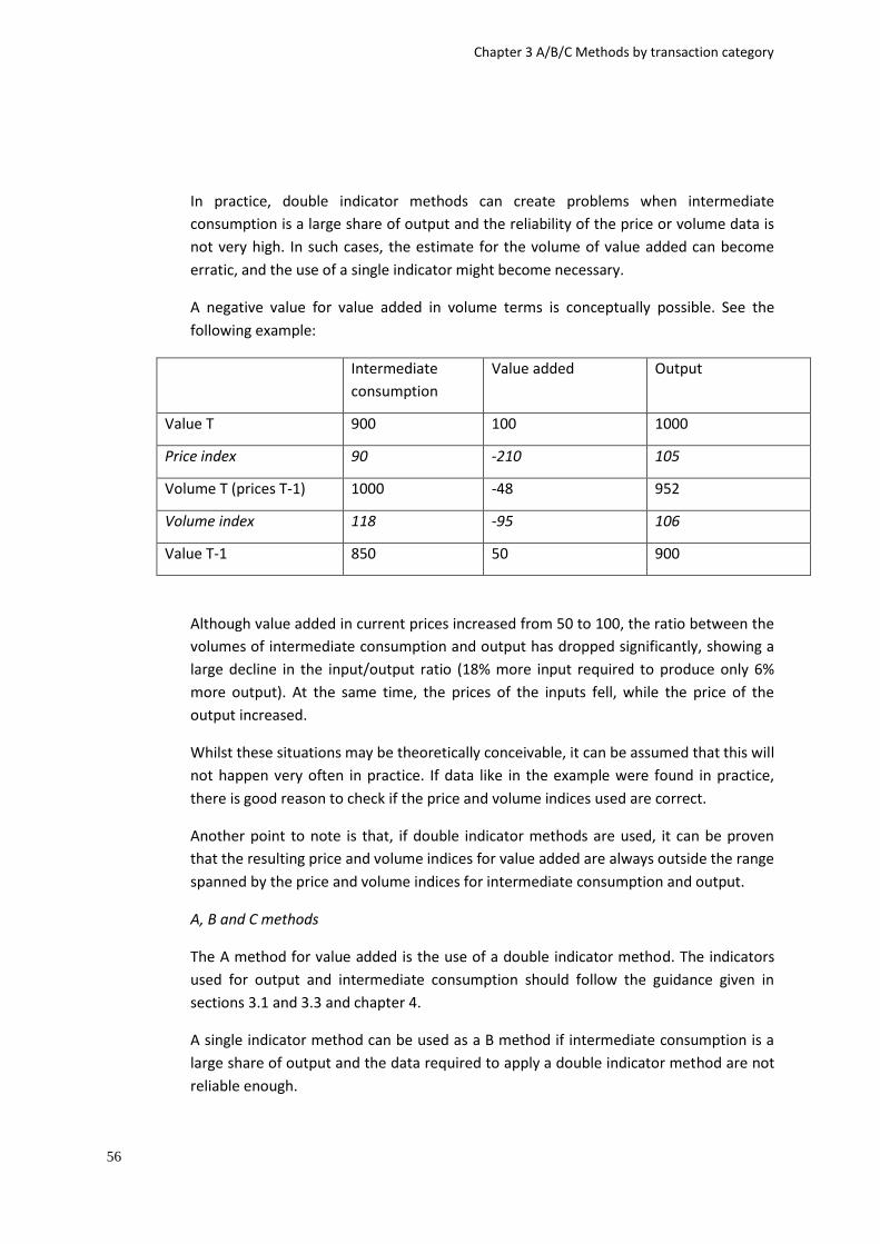
Chapter 3 A/B/C Methods by transaction category
56
In practice, double indicator methods can create problems when intermediate
consumption is a large share of output and the reliability of the price or volume data is
not very high. In such cases, the estimate for the volume of value added can become
erratic, and the use of a single indicator might become necessary.
A negative value for value added in volume terms is conceptually possible. See the
following example:
Intermediate
consumption
Value added Output
Value T 900 100 1000
Price index 90 -210 105
Volume T (prices T-1) 1000 -48 952
Volume index 118 -95 106
Value T-1 850 50 900
Although value added in current prices increased from 50 to 100, the ratio between the
volumes of intermediate consumption and output has dropped significantly, showing a
large decline in the input/output ratio (18% more input required to produce only 6%
more output). At the same time, the prices of the inputs fell, while the price of the
output increased.
Whilst these situations may be theoretically conceivable, it can be assumed that this will
not happen very often in practice. If data like in the example were found in practice,
there is good reason to check if the price and volume indices used are correct.
Another point to note is that, if double indicator methods are used, it can be proven
that the resulting price and volume indices for value added are always outside the range
spanned by the price and volume indices for intermediate consumption and output.
A, B and C methods
The A method for value added is the use of a double indicator method. The indicators
used for output and intermediate consumption should follow the guidance given in
sections 3.1 and 3.3 and chapter 4.
A single indicator method can be used as a B method if intermediate consumption is a
large share of output and the data required to apply a double indicator method are not
reliable enough.

Chapter 3 A/B/C Methods by transaction category
57
3.5. Final consumption expenditure
3.5.1. Final consumption expenditure by households
Households are defined in par. 2.118 of ESA 2010. Final consumption expenditure of
households is primarily made up of goods and services purchased in the market but also
includes consumption of household production for own final use, such as the services of
owner-occupied dwellings, and goods or services received as income in kind. It does not
include social transfers in kind, intermediate consumption or gross capital formation,
acquisitions of non-produced assets, payments to NPISHs, taxes other than taxes on
products, or voluntary transfers (see par. 3.95 – 3.96 of ESA 2010)
The obvious approach to deflating the components of household final consumption is to
draw upon detailed Consumer Price Indices (CPIs) since these are intended to show the
change in consumer prices. Use of general indices (such as an all-items CPI or a cost of
living index) is not recommended for the deflation of individual components of
household expenditure. CPIs often follow national accounts concepts (for example in
the distinction between consumption and capital formation, and in the separation of
taxes from purchases of services). However there are usually a number of differences
between CPIs and national accounts methodology that may need to be taken into
account.
Countries may compile different types of CPIs for their own needs (and national
accountants should be aware of the methods employed if these CPIs are used), but a
harmonised standard is set for EU Member States by EU Regulations for the
Harmonised Index of Consumer Prices (HICP). It is recommended for EU Member States
that where suitable HICPs are available, these are drawn upon in compiling national
accounts. There are, however some differences between HICP methods and the
definitions required in the national accounts:
i) Differences of coverage
Consumption of own-produced goods and services. These items are not included
in the HICP definition of ‘final monetary consumption expenditure’ (the prices
used in the HICP relate to monetary transactions only). The general rule here is
that products produced for own-consumption should be valued at the prevailing
basic price for equivalent products, or at costs of production if market prices are
not available (par. 3.45 of ESA 2010). Where output for own final use is a
significant part of total consumption of a certain product, it will be necessary to
separately deflate it by a suitable basic price index; otherwise use of the HICP is
appropriate.
Goods and services received as income in kind. As with the point above, these
items are excluded from the HICP calculation. Valuation of these products is at
Chapter 3 A/B/C Methods by transaction category
58
basic prices if they are produced by the employer, and at market prices if the
employer has to purchase them from a third party. If the former types of
products are significant, then deflation should be undertaken using a suitable
basic price index.
Goods and services purchased abroad by resident households. The HICP covers all
purchases made by resident and non-resident households on the economic
territory of a country (see Regulation 1688/98 for more details). Household
consumption in the national accounts covers the expenditure of resident
households, including those purchases made abroad, but excludes the
expenditure of tourists on the economic territory of the country which is
covered by the HICPs. Within the Supply and Use Table framework, final
consumption by product is normally compiled for total purchases made on
domestic territory, with the net difference of purchases abroad and by non-
residents domestically made as a global adjustment. If purchases abroad by
residents form a significant proportion of total household consumption, and
prices are evolving differently from domestic prices, then this should be
reflected in the calculations of the volume series for the net adjustment – one
method to undertake this could be to use the HICP data from another Member
State to deflate expenditure abroad, adjusting for exchange rate changes if
necessary and reflecting the different mix of products that travellers tend to
purchase. Adjusting for exchange rates would imply that the effects of exchange
rate movements feed through into prices fully and immediately.
Pension funding and life insurance services. These should be measured as the
changes in service charges implied by the difference between gross
contributions/premiums (including supplementary contributions and premiums)
and benefits, adjusted for changes in actuarial reserves. Life insurance services
are excluded from the HICP and, because of the difficulties in separating life
insurance from pension services, pension services will also be excluded.
Miscellaneous items such as the service charges for lotteries and gambling,
prostitution and narcotics are excluded from the HICP owing to the practical
difficulties in price collection and measurement.
Where the HICP does not cover certain products, it will be necessary to examine other
data sources. As a starting point, one should bear in mind potential differences between
the COICOP/HICP and CPA classification systems, given that the CPA system is
commonly used for producer and import/export price indices and volume measures. It
is important to undertake the deflation at a sufficiently detailed product level, so that
these potential classification difficulties are minimised.

Chapter 3 A/B/C Methods by transaction category
59
ii) Differences in concepts
Services of owner-occupied dwellings. These are a special case of the products
for own consumption point above (and are defined in par. 3.75 of ESA 2010).
They represent a high proportion of final consumption of households. The HICP
compilers in Europe are currently investigating the possible use of house prices,
but no decisions have yet been made. The recommended method for deflating
this element in the national accounts is by a suitable index of actual rent levels
(based on the methodology set out in Commission Decision 95/309/EC, Euratom)
and this method is further described in section 4.12.2. The HICP contains a
potentially useful series for “actual rents for housing”, although the weighting
and survey methods used may differ from that set down in the Commission
decision.
Non-life insurance services. Regulation 1617/99 recommends a ‘representative
pricing’ method for the HICP, based on gross premiums for policies whose
“price-determining specifications” are kept constant. This is because the service
charge on an individual level cannot in practice be obtained on a monthly basis.
Section 4.11.2 of this handbook recommends that other methods be used for
deflation of insurance services in the national accounts, since use of gross
premiums is unlikely to be a good reflection of the changing price of the service
charge.
iii) Differences of index number calculation
HICPs are Laspeyres-type indices. Technically, the deflators used in the national
accounts for household consumption in the national accounts should be constructed on
a Paasche basis, and therefore a re-calculation might be necessary to generate a
Paasche-like index from HICP data. However, a Laspeyres-type index can potentially
provide a reasonable approximation to a Paasche-type index if the index is calculated in
sufficient detail (it is recommended that the reasonableness be tested in practice). The
HICP legal framework sets out minimum standards for the compilation of sub-indices,
requiring sufficient elementary aggregates to represent the diversity of items within
each category of the COICOP/HICP and further requiring that sufficient prices are
collected within each elementary aggregate to reflect price movements in the
population.
It is essential that the price indices used should take proper account of changes in
quality of products, to ensure that they are measured as a volume change. The HICP
implementation Regulation defines quality change as arising from a change in
specification of an existing product, which results in significantly different utility to the
consumer, where a new variety or model of a good or a service replaces a good or
Chapter 3 A/B/C Methods by transaction category
60
service previously selected for pricing in the HICP. The process of quality adjustment
requires that replacement should in general be selected according to their similarity of
utility to the consumer and not according to their similarity in price, where
replacements have to be made after goods and services have been offered at reduced
prices. Where no estimates for quality adjustments are available, the price changes are
estimated as the difference in price between the selected substitute and the item it has
replaced. (Council Regulation 1749/96 Article 2 paragraphs c and d, in conjunction with
Article 5). Furthermore, this Regulation prohibits the estimation of quality change as the
whole of the difference in price between two items, unless this can be justified as
appropriate. It also encourages the timely addition of ‘newly significant’ products to the
basket of goods, and the sufficient representativeness of products chosen for compiling
elementary aggregates. All of these principles are consistent with the discussion of
quality change in section 2.4 of this handbook.
A, B and C methods
Those methods based on deflation of household expenditure using appropriate CPIs are
A methods. An index is appropriate if it:
is an index of the price consumers pay for exactly that (group of) product(s);
takes proper account of changes in the quality of products;
is valued at purchasers’ prices including VAT;
follows the same concepts as the national accounts.
Use of a CPI which does not meet all of the standards set out above is a B method.
Where a detailed HICP or CPI is not available, B methods include the use of other
indicators completely or partially covering the products in question – for example, PPIs
adjusted for valuation differences, import/export prices, or volume indicators where
these are available. The main reason why use of adjusted PPIs is not an A method is that
they will generally cover products consumed by businesses as well as those consumed
by households.
Any method using an index that does not correspond at all to the product in question is
a C method.
The volume of services provided by persons employed in private households must be
measured in the same way on the supply and on the use side. The method is explained
in chapter 4.15.

Chapter 3 A/B/C Methods by transaction category
61
3.5.2. Final consumption expenditure by government and NPISHs
The general government sector, defined in ESA 2010 (par 2.111), typically consists of
institutional units producing both market and non-market goods and services. The
treatment of production of market goods and services by government follows the same
rules as for such production in other sectors (see section 3.1). The non-profit
institutions serving households (NPISHs) sector is defined in par. 2.129 of ESA 2010 –
the principles applied to this sector are similar to those applicable in the general
government sector, so the two sectors are discussed together in this section.
By convention, the final consumption expenditure of general government and NPISHs
consists of (ESA 2010 par 3.98):
the value of non-market goods and services produced by government or NPISHs other than own-account capital formation and sales;
purchases by general government and NPISHs of goods and services produced by market producers that are supplied, without any transformation, to households as social transfers in kind.
Final consumption expenditure consists of both individual and collective consumption
(defined in ESA 2010 par. 3.101 – 3.102), whose value is measured by convention as the
sum of costs – compensation to employees, intermediate consumption (including the
cost of products purchased for social transfer in kind), consumption of fixed capital and
other taxes less subsidies on production (ESA 2010 par. 3.49) – less any sales to
households and other units.
ESA 2010 also identifies the concept of “actual final consumption” which, for general
government, consists of collective consumption (ESA 2010 par 3.106). The actual final
consumption of NPISHs is zero because they are assumed to produce only services to
individuals.
Whilst the value of government and NPISHs final consumption is measured using an
“input” approach, this does not mean that the only method for deriving volume data is
to deflate the value of inputs by suitable deflators. In fact, other sections of the
handbook (notably sections 3.1, 4.14 to 4.18) advise that there are suitable methods
based on direct output indicators for individual consumption, such as “pupil hours” for
education, “patient treatments by type” for health, and “members by type” for NPISHs.
However output destined for collective consumption (especially those relating to ‘public
administration’) presents more difficulties, and suitable deflation of the inputs may be
the only viable option in many cases.

Chapter 3 A/B/C Methods by transaction category
62
A, B and C methods
For a classification of A, B and C methods for non-market goods and services, see
section 3.1.2.4.
For social transfers in kind consisting of goods or services purchased by government
from the market, deflation by suitably detailed CPIs would be A methods if:
allowance is made for any discounts which the Government may have
negotiated directly with suppliers, and
adjustments are introduced for any contributions which are payable by those
receiving the transfers.
3.6. Gross fixed capital formation Gross fixed capital formation (GFCF) covers both goods and intellectual property fixed
assets. This represents a large range of different products, many of which can be
unique, for example an oil rig, a specialised piece of plant and machinery, or intellectual
property such as R&D services. The large range of different products calls for methods
to be applied at a detailed product level to ensure good quality estimates of GFCF in
volume terms. The general problem of unique products is discussed in section 2.5.
Specific guidance on large equipment goods, computers, construction and R&D services
can be found in sections 4.3.2, 4.3.3, 4.6 and 4.11 respectively. Computer software is
also an important element within the category of intellectual property and specific
guidance on its treatment can be found in section 4.11.
Like other categories of expenditure, GFCF can be measured from either the supply or
demand side. However, the use of the supply side approach as the main measurement
method is more frequent for GFCF because it presents a less resource intensive option
compared to measuring GFCF independently from the demand side.
Measurement from the supply side uses data on domestic output less exports plus
imports of capital goods at the product level. Product classifications are generally quite
detailed, but still do not always allow the differentiation of products between those of a
capital nature and those that should be considered intermediate or final consumption.
This limitation needs to be kept in mind when considering methods for estimating
prices and volumes from the supply side.
Measurement from the demand side uses data from purchasers of capital goods on the
purchases they have made. The product classification of GFCF from the demand
(consumption) side generally has limited product detail. For example, ESA 2010
provides a regrouping and coding for investment that, at its most detailed, is limited to
only six products (AN_F6). Compiling volume estimates of GFCF at such a limited level of
Chapter 3 A/B/C Methods by transaction category
63
detail is unlikely to produce high quality results, given the many different products and
their unique nature. It therefore seems appropriate when considering the criteria for
the classification of methods to provide further guidance on the minimum level of detail
to be used.
Valuation is an important issue when considering the suitability of price indices for the
deflation of GFCF. For price indices to be entirely appropriate they should measure
changes in the purchasers' price of the particular products, including any non-
deductible VAT included in the price. Price indices of this kind are often referred to as
investment price indices. The direct use of PPIs, even if the product match is exact, can
therefore be seen as not entirely suitable because PPIs are measured at basic prices.
The use of PPIs for the deflation of GFCF would assume that the change in basic price
and purchasers' price is the same, i.e. taxes, transport, installation and the other costs
of ownership remain constant in volume terms.
Another important consideration is that some goods recorded as GFCF will have been
imported. This creates the need to ensure a consistent approach to the deflation of
products within imports and GFCF, taking account of any difference in price, for
example due to taxes and subsidies on imports.
A, B and C methods
The use of genuine investment price indices (IPIs) for the deflation of GFCF will be an A
method, providing they satisfy the following criteria:
it is an index with a coverage of exactly that (group of) product(s);
it takes proper account of changes in quality of the product(s);
it is valued in purchasers' prices including non-deductible VAT; and
the concepts underlying the index correspond to those of the national accounts.
The use of PPIs adjusted to purchasers' prices would also be an A method provided they
satisfy the criteria described above for investment price indices.
The very different nature of the products covered within GFCF makes it unlikely that the
criteria for an A method specified above will be satisfied for all products. This is
particularly true for the criteria that coverage of the price index should be exact.
Therefore when considering the criteria for B methods it seems sensible to specify a
minimum level of product detail to be used in the deflation of GFCF. The significance of
a particular product in its contribution to the total of GFCF also needs to be taken into
account when considering the level of detail that should be used. IPIs, or PPIs adjusted
to purchasers' prices, where the coverage is not exactly that of the products or that do
not take account of changes in quality are a B method providing a minimum level of
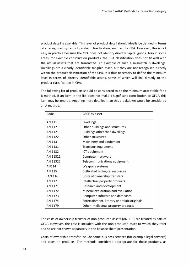
Chapter 3 A/B/C Methods by transaction category
64
product detail is available. This level of product detail should ideally be defined in terms
of a recognised system of product classification, such as the CPA. However, this is not
easy in practice because the CPA does not identify directly capital goods. Also in some
areas, for example construction products, the CPA classification does not fit well with
the actual assets that are transacted. An example of such a mismatch is dwellings.
Dwellings are a clearly identifiable tangible asset, but they are not recognised directly
within the product classification of the CPA. It is thus necessary to define the minimum
level in terms of directly identifiable assets, some of which will link directly to the
product classification in CPA.
The following list of products should be considered to be the minimum acceptable for a
B method. If an item in the list does not make a significant contribution to GFCF, this
item may be ignored. Anything more detailed than this breakdown would be considered
an A method.
Code GFCF by asset
AN.111
AN.112
AN.1121
AN.1122
AN.113
AN.1131
AN.1132
AN.11321
AN.11322
AN114
AN.115
(AN.116
AN.117
AN.1171
AN.1172
AN.1173
AN.1174
AN.1179
Dwellings
Other buildings and structures
Buildings other than dwellings
Other structures
Machinery and equipment
Transport equipment
ICT equipment
Computer hardware
Telecommunications equipment
Weapons systems
Cultivated biological resources
Costs of ownership transfer)
Intellectual property products
Research and development
Mineral exploration and evaluation
Computer software and databases
Entertainment, literary or artistic originals
Other intellectual property products
The costs of ownership transfer of non-produced assets (AN.116) are treated as part of
GFCF. However, the cost is included with the non-produced asset to which they refer
and so are not shown separately in the balance sheet presentation.
Costs of ownership transfer include some business services (for example legal services)
and taxes on products. The methods considered appropriate for these products, as
Chapter 3 A/B/C Methods by transaction category
65
described in section 3.10 and 4.11, should also be applied to the measurement of price
or volume of this component of GFCF.
Methods that do not reflect adequately the level of product detail suggested above are
C methods.
3.7. Changes in inventories
3.7.1. Introduction
The calculations of changes in inventories (CI) at current and previous year’s prices are
often closely interlinked. If good current price estimates can be made because good
data exist, then it is often possible to make good volume estimates as well, since the
same data are used. Sometimes estimation at previous year’s prices precedes
estimation at current prices. Moreover, the estimation of CI is often linked to the
estimation of other transaction categories such as output, intermediate consumption,
etc. That means that a classification of estimation methods should also take the current
price methodology into account.
In practice, the data available for the calculation of changes in inventories do not allow
a ‘perfect’ estimation. Assumptions and approximations have to be made. The
estimation methodology for CI (both at current and previous year’s prices) is highly
dependent on the kind of information on inventories that is available. This section will
therefore be organised according to different data situations. First the ideal situation of
full, perfect, information is described. It is necessary to consider this situation to be able
to assess other methodologies against the ideal. Then the more realistic situation when
information is only available on values of levels of inventories is described. Finally, the
options for estimating CI at current and previous year’s prices when no direct
information is available at all are discussed.
Perhaps a rather obvious observation, but still worthwhile taking into account, is that
volume-indices of CI are meaningless. Only price indices can be meaningfully calculated,
and only for homogeneous products.
3.7.2. Some important definitions and relations
ESA 2010 defines CI as follows:
Changes in inventories are measured by the value of the entries into inventories less the
value of withdrawals and the value of any recurrent losses of goods held in inventories.
The following types of inventories are distinguished:
materials and supplies (AN.121)
work-in-progress (AN.122)
finished goods (AN.123)
Chapter 3 A/B/C Methods by transaction category
66
military inventories (AN.124)
goods for resale (AN.125).
ESA 2010, par. 10.45, says the following about the estimation of volumes of inventories
at the prices of the previous year:
10.45 Changes in inventories are measured by the value of entries to inventories
less the value of withdrawals from inventories, and the value of any recurrent losses of
goods held in inventories during a given period. Volumes at the prices of the previous
year can be derived by the deflation of these components. In practice, however, it is rare
for entries and withdrawals of stocks to be actually known, and often the only available
information is the value of the stocks at the start and at the end of the period. In such
cases, it will often be necessary to assume regular entries and withdrawals during the
current period, so that the average price for the period can be considered relevant for
both entries and withdrawals. In such circumstances calculating the variation in stocks
by the difference between the values of the entries and withdrawals amounts to the
same as calculating the difference between the values of the initial and final stocks. The
variation in stocks in volume terms can then be calculated by deflating the initial and
final stocks to bring them in line with the average price of the base period. When the
variations in stocks are known in quantity terms, it is possible, again assuming regular
entries and withdrawals, to calculate the volume of the variation in stocks by applying
the average price of the base period to the variation in stocks in quantity terms.
Closely related to the calculation of changes in inventories are holding gains. Holding
gains are the result of price changes during the period for which the inventory is held.
Such gains are not part of output. Holding gains can be negative, in which case they are
called holding losses. If there are no price changes during the accounting period, the
holding gain is zero. Holding gains can be calculated using the following identity:
value of inventory at end of accounting period
less value of inventory at beginning of accounting period
= change in inventory + holding gains.
Other important identities are:
output = sales + CI of finished products + change in work-in-progress
intermediate consumption = purchases – CI of materials and supplies.
For a wholesale or retail trader:
output = sales – purchases (of goods for resale) + CI of goods for resale.
(where changes in inventories are positive if the inventories are growing and negative
otherwise). Enterprises usually report on sales and purchases rather than output and
Chapter 3 A/B/C Methods by transaction category
67
intermediate consumption. Hence, the calculation of CI (and thus holding gains) goes
hand-in-hand with the calculation of output and intermediate consumption.
3.7.3. If perfect information is available
Consider the estimation of CI of a certain product of a certain agent. In the ideal case,
information is available on the exact times and quantities of additions to and
withdrawals from the inventory and the price of the product at those times. Then it is in
principle straightforward to calculate the CI at current and at previous year’s prices.
Additions and withdrawals have to be valued at the prices prevailing at the times at
which they take place. The sum of all additions minus the sum of all withdrawals then
gives the value of CI over the year. The mathematically correct method is therefore
dependent on the path of prices and quantities in the course of the year. In practice,
this calculation should be done on a monthly or quarterly basis. The annual value is the
sum of CI in the months or quarters.
The CI at previous year’s prices is calculated by valuing the quantities of additions and
withdrawals at the average annual prices of the previous year, which are calculated by
weighting with the changes in the quantities of the inventories in each month or
quarter.
In a slightly less ideal world we will not have detailed information on additions and
withdrawals, but only the levels of inventories (in quantities) at the beginning and end
of the year. In this case, CI (both at current and previous year’s prices) is calculated by
multiplying the change in quantity with an average price of the year (current year or
previous year, respectively). If the price of the product has been constant during the
year, this provides an exact estimation. The same is true if the quantities do not change
or change at a constant rate. If the price and the change in quantity have fluctuated,
however, this method provides only an approximation of the ideal. The degree of
fluctuation determines the accuracy of the approximation. The more prices or
quantities vary during the year, the more necessary it becomes to calculate CI and
holding gains on a quarterly or monthly basis.
3.7.4. If only information of values of inventories is available
In many cases, enterprises will not be able to give data on quantities, but only on the
value of the level of their inventories at the beginning and end of the year according to
their own bookkeeping system.
These bookkeeping systems generally do not value inventories according to ESA rules,
but for example following historic cost system, LIFO system, etc.. Therefore, these
values cannot be used directly in the national accounts. In this case, the change in
volume has first to be derived, which can then be multiplied with an appropriate price
index to arrive at CI at current prices.
Chapter 3 A/B/C Methods by transaction category
68
In order to calculate correctly the change in volume of inventories, information is
needed on the bookkeeping system used in the enterprise. Some countries ask this
information in their production or inventory surveys. If no information is available, an
assumption will have to be made. On the basis of the known or assumed bookkeeping
system, the values of the levels of inventories can be deflated:
if prices are available, then the values can be divided by these prices to obtain
quantity information. The change in quantity then has to be multiplied with the
average price of the desired year to obtain CI (at current or previous year’s
prices).
If a price index is available that describes the price development of the stock
according to the known or assumed bookkeeping practice, the values can be
deflated to arrive at CI at previous year’s prices directly. This should then be
reflated with an average price index according to national accounts valuation
rules to determine CI at current prices.
The price indexes used should be in accordance with the kind of inventory in question.
For inventories of finished products, PPIs at basic prices are the appropriate choice. For
inventories of materials and supplies, similar indices as used for intermediate
consumption should be used. These are preferably genuine intermediate consumption
prices, but in practice mostly PPIs adjusted to purchasers’ prices. For inventories of
goods for resale a PPI will usually be a good indicator (for retailers, strictly speaking, a
PPI should be adjusted for wholesale trade margins).
As regards work-in-progress, ESA 2010 gives clear rules on the valuation (see par. 3.148
and further). Deflation should obviously be carried out in a consistent way with the
deflation of output, i.e. with output price indexes at basic prices. The problem here is
that appropriate price indexes for the products concerned (e.g. large equipment,
construction work) are often not available. See section 2.5 for a discussion of this
problem.
Often only data on the total inventory are available, not by product. For inventories of
finished products and work-in-progress, the assumption can be made that the data
relate to the main product of the enterprise. For inventories of materials and supplies, it
should be investigated which are the main inputs in the production process of which
inventories are held. For inventories of goods for resale, assumptions have to be made
on the basis of the main traded products.
3.7.5. If no information is available at all
The worst case scenario is when enterprises provide no information on values or
quantities of levels or changes in inventories at all. In the absence of direct data, CI is
usually estimated in an indirect way. CI is then calculated – for a particular product –

Chapter 3 A/B/C Methods by transaction category
69
with the “commodity flow method” as the difference between total supply (output and
imports) and total use (intermediate consumption, final consumption expenditure,
gross fixed capital formation and exports). This procedure is flawed, since output and
intermediate consumption can only be calculated after CI is known. The outcome of this
method, therefore, will more likely reflect measurement errors in the various
aggregates than the measurement of actual CI.
The use of this “residual” method should therefore be discouraged.
3.7.6. A, B and C methods
A true A method can only be achieved if good information is available from enterprises.
This can be either direct quantity information or value information combined with
knowledge about the bookkeeping system. Furthermore, appropriate price information
is required (which does not necessarily have to come from enterprises in an inventory
survey but could come from price statistics). Appropriate price indices are defined
according to the general criteria specified in section 2.3. If prices and quantities vary
considerably within the year, it becomes important to calculate CI and holding gains on
a quarterly or monthly basis (either from information on additions and withdrawals or
from levels at beginning and end of quarters or months), and calculate the annual total
by summing the quarters or months.
If assumptions have to be made concerning the bookkeeping system, or if deflation is
undertaken with less appropriate price indices, the calculation method becomes a B
method. Less appropriate price indices are for example indices that do not exactly
relate to the products in question, a consumer price index for the deflation of
inventories of finished goods, etc.
If deflation of CI is carried out with proxy or inappropriate indicators then the method
becomes a C method.
If CI of a product is calculated with the commodity flow method without resort to any
direct data, this is also a C method. In the worst case, CI in previous year’s prices is
calculated as a residual at the macro-level.
3.8. Acquisition less disposals of valuables
3.8.1. Introduction
Valuables contribute to GDP in two ways – the value added when they are first
constructed, through the production account, and value added by traders of valuables
through trade margins or commissions. Changes in their value during acquisitions and
disposals are recorded as revaluation effect, which does not contribute to overall GDP.
Nevertheless transfers of valuables between sectors do have an important influence on
Chapter 3 A/B/C Methods by transaction category
70
sectoral aggregates, and the unique nature of valuables poses difficulties for valuing
production in volume terms.
3.8.2. Some important definitions and relations
ESA 2010 defines valuables as follows:
3.154 Valuables are non-financial goods that are not used primarily for
production or consumption, do not deteriorate (physically) over time under normal
conditions and that are acquired and held primarily as stores of value.
The following 3 categories of valuables are identified:
Precious metals and stones.
Antiques and other art objects.
Other valuables (for example jewellery and collector’s items).
ESA 2010, par. 3.157, says that production of valuables should be valued at basic prices.
All acquisitions of valuables should be valued at purchasers’ prices, including agents’
fees or commissions and dealers’ trade margins. Disposals of valuables are valued at
prices received by sellers - that is, after deduction of fees and commissions.
There are two different ways of looking at the concept of a “volume of valuables”. The
first is to consider them as a store of purchasing power for the holder, which implies
that the volume should be measured as the change in value of the valuable divided by
some general purchasers’ price index. The second way of considering valuables is that
they are products in themselves, and therefore the appropriate approach to measuring
the volume is to deflate by a specific price index for the valuable concerned. The
recommended approach, and the one described in this section, is the second approach
because we are concerned here with the narrow concept of production and trade in the
valuables themselves (in much the same way as we measure the volume of expenditure
on capital items by observed prices for these items, rather than using a “productive
potential” approach).
3.8.3. Different types of transaction
It is important to distinguish between the different transactions that can involve
valuables, since they pose different challenges for expressing flows in volume terms.
The creation of valuables through production is valued at basic prices, which can
obviously change as costs, margins, and consumer tastes evolve. The key challenge to
valuing these flows in volume terms is that the products involved are generally unique
or available in only very limited quantities (for example a painting is unique, whereas
there might be several examples of an antique manufactured good in very similar
condition). This is compounded by the fact that the quality of valuables is very difficult
Chapter 3 A/B/C Methods by transaction category
71
to define – for most people it will be some intrinsic artistic quality (where judgement
might vary quite widely), whilst for others it will be the potential gain in value over time.
The issue of unique goods is discussed in section 2.5, and with reference to large
equipment and construction in sections 4.3.2 and 4.6 respectively. There are several
options available – product decomposition into the constituent elements (perhaps
possible for a piece of jewellery, but hardly viable for a painting), comparison with a
similar piece sold domestically or in another country (the common method for initial
valuation by experts in “the trade”), and deflation of the costs of inputs.
Expressing the trade of existing valuables in volume terms suffers from the unique
goods and quality measurement problems. Nevertheless there may be more that can be
done – the individual product has probably been sold before (although it may be many
periods before) which could allow an interpolation method to be employed, or the
product may be one of a series of closely related products (eg. paintings by the same
artist during a certain ‘period’).
For traders and dealers in existing valuables, the principles set out in section 4.12.1 for
handling real estate agents’ fees may well be appropriate – since commissions for
mediating transactions are often based on a percentage of the value of the article(s), a
suitable price index for deflating turnover would follow both the percentage and price
of the traded valuable(s). Auctioneers are classified in CPA 69.10 Legal services.
Museums and art galleries are in CPA 91.0 These services will not be in acquisitions less
disposals of valuables.
Finally, the margins of traders/dealers in newly produced valuables can sometimes be
measured separately (for example in the jewellery trade) and the methods set out in
section 4.7.1 (wholesale and retail trade margins) applied as appropriate.
3.8.4. A, B and C methods
The A method applicable to production of valuables is if there is a suitable PPI for an
industry producing valuables, which is adjusted properly for changes in quality (this may
be possible for the jewellery industry for example). For some types of valuables, a
model or specification pricing approach could be an A method if it meets the criteria set
out in section 2.5.
For services on a fee basis, where the fee is a percentage of a value of the articles
handled, a proper price index would combine the change in fee percentages and the
change in worth of (that particular subset of) valuables. This would constitute an A
method.
B methods for measuring volume flows for production of valuables are comparison with
closely related products (either domestically or internationally) such as a painting by the
Chapter 3 A/B/C Methods by transaction category
72
same painter, and decomposition into constituent elements (more suitable for jewellery
and complex products).
B methods for measuring volume commissions or trade margins could be the use of an
index based on worth of valuables. Since mediation fees for valuables are often
percentages of the worth of the valuables it is reasonable to think that both are
correlated enough to constitute a B method. It is then implicitly assumed that the fee
percentage is constant.
Less good, but still a B method, is the use of numbers of units of valuables traded,
broken down by type. This is more appropriate for more homogenous products.
3.9. Exports and imports of goods and services
3.9.1. Introduction
Exports and imports are an important element of the national accounts that require
careful treatment in the measurement of prices and volumes. This is especially true
within an input-output framework that requires a consistent approach to deflation of
exports and imports to be used. For example, exported products appear as output in
the supply table and as exports in the use table, imports on the other hand appear as
intermediate or final consumption in the use table and as imports in the supply table.
Although the valuation basis in the separate supply and use tables is different, ie basic
and purchasers prices respectively, the need to ensure consistency remains if the tables
are to balance.
Transport costs are an important element of exports and imports. Transport products
are covered in section 4.8. Imports and exports of products are recorded at border
values. Total imports and exports are valued at the exporter's customs frontier, referred
to as free on board (f.o.b.). Foreign transport and insurance services between the
importer's and the exporter's frontiers should not be included in the value of goods, but
recorded as services. However, it is not always possible to obtain f.o.b. values at the
detailed product level and details of foreign trade are then shown valued at the
importer's frontier. In this case, all transport and insurance services to the importer's
frontier are included in the value of imports, referred to as cost, insurance and freight
(c.i.f.). This is the valuation used for imports in the supply and use tables. Where the
price of exports and imports includes an element of transport or insurance service,
these need to be dealt with correctly in the price and volume measures. Import price
indices, where available, will usually be on the basis of the cif valuation. As such, when
they are used for the deflation of imports on a cif valuation in the supply and use table
this represents the correct method. However, it is then necessary to apply a global
adjustment within the supply and use table to correct imports from a c.i.f. valuation to
the required f.o.b. basis. This adjustment requires deflation for the compilation of
supply and use tables at previous year’s prices. A suitable price index for the deflation

Chapter 3 A/B/C Methods by transaction category
73
of this c.i.f./f.o.b. adjustment would need to take account of the price development of
transport and insurance services for imported goods. These price developments are
likely to be different for different products being imported for different countries. In
constructing price indices better quality results are likely to be achieved as the level of
detail used increases. However, in practice it may not be possible to obtain detailed
prices by product and importing country or to find suitable weights to allow them to be
combined. In these circumstance price indices for transport and insurance services by
country offer an acceptable alternative.
When considering methods appropriate for the measurement of prices and volumes it
is useful to consider goods and services separately.
ESA2010 has introduced new approaches for goods for processing and merchanting.
Under ESA 2010, goods sent abroad for processing are recorded on a strict change of
ownership basis, meaning that where goods sent abroad do not change ownership, they
are excluded from the trade in goods data. Instead, the cost of the processing service is
recorded as trade in services (manufacturing services on physical inputs owned by
others).
Merchanting occurs when merchants or commodity dealers buy from non-residents and
then sell again to non-residents. According to ESA2010 purchases and sales of
merchanted goods are recorded under exports. Purchases are shown as negative
exports. If they are not sold in the same accounting period the negative exports are
balanced by an increase in inventories of goods for resale. Goods under merchanting
should be separately identified by either national accounts or balance of payments
enterprise surveys of merchants and deflated using export and import price indices for
the products purchased and sold under merchanting.
3.9.2. Goods
There are a number of methods that are potentially suitable for the estimation of
goods. These are:
Actual export and import prices
Unit value indices (UVIs)
Adjusted PPIs, and
Export prices of a foreign country.
Actual prices, UVIs and adjusted PPIs are potentially suitable methods for both exports
and imports. Export prices of a foreign country are only really suitable for consideration
for imports. The remainder of this section will consider each potential method in turn
Chapter 3 A/B/C Methods by transaction category
74
and assess the advantages and disadvantages. A more general discussion of the
usefulness of price indices and unit values can be found in section 2.6.
Actual export and import prices
Export and import price indices can be compiled based on the prices actually charged by
exporters of goods, in the case of exports, or paid by consumers, in the case of imports.
Prices have the advantage that they cope better with the problem of heterogeneous
products as the price index is constructed to reflect a fixed specification that allows
price effects to be isolated and quality changes to be controlled. However, this can
result in incomplete coverage of the actual exports and imports of products to which
they are applied as deflators. Price indices are costly to produce and represent a burden
on respondents. Price indices may also reflect inadequately the actual prices paid by
purchasers. This may be an important factor for export and import prices where the use
of forward contracts and currency hedging instruments may mask the actual prices
paid.
Unit value indices (UVIs)
UVIs are readily available from trade statistics being derived as the ratio of value to
volume (weight or quantity). They do not generally control for changes in the product
mix within one item, leading to quality changes mistakenly included in the price
component. Their coverage of products is generally complete, but even at the most
detailed level of trade classification can often include a range of different products.
Where the products within an item of the trade classification may appear to be
homogeneous this may in reality not be the case as products of similar description may
be of very different quality. It may be possible to construct more homogeneous UVIs if
the country of origin (or destination) is also taken into account. UVIs are clearly
unsuitable for products that are unique or change quickly in specification.
Adjusted PPIs
It is also possible to use domestic PPIs to deflate current price estimates for exports and
imports in the same way as actual export and import prices may be used. PPIs reflect
prices on the domestic market and may not be a good reflection of the prices charged
for exports or imports in some circumstances, for example luxury goods, where
competition between domestically produced products and imports is of minimal
importance and has little impact on price. However, there may be little difference
between domestic prices and those of imports or exports where these compete directly
with each other in the market. In these conditions, the use of PPIs for exports or
imports may be acceptable.
Chapter 3 A/B/C Methods by transaction category
75
A way of improving the domestic PPIs to make them more representative of exports
and imports would be to adjust them in some way to reflect better the actual export
and import prices. Such an adjustment could be made in a number of ways.
The most simple would be to take account of exchange rate movements between the
domestic currency and that of the countries to which the exports are going to or the
imports coming from. Such an approach is based on the assumption that movements in
export and import prices differ from domestic price movements only in respect of
movements in the exchange rate.
A more complex approach could be to derive an adjustment factor based on some other
variable, for example, UVIs. The adjustment factor could be derived as follows. First,
select a group of products that have stable UVIs and construct an overall UVI for this
group of products. Second, construct an overall PPI with the same coverage of products
as that used for the overall UVI. The final stage is to derive the ratio of these two
indices. This ratio is then applied to a PPI that represents a range of products present in
the export or import estimates for which other more suitable price or volume indicators
are not available. In this way the resulting adjusted PPI is based on the price movements
exhibited in the UVI, but without the volatility of some of the products. The aim of this
approach is to reduce the various shortcomings of UVIs by using a wide mix of products.
If some actual export and import prices are available a similar method for adjusting the
PPIs could be used, but using the actual prices in place of the UVIs.
Adjusted export prices from foreign countries
In this approach the export prices from a foreign country are used to deflate imports.
Imports need to be broken down by product group and country to make best use of this
method. Such an approach is most suited to unique products of a specialised nature and
this is considered further in section 2.5 on unique products. Adjustments may be
necessary to account for exchange rate movements, on the assumption that
movements in exchange rates impact directly and immediately on the price of the
imports. To further improve this method, additional adjustments that take account of
other factors that affect prices between the exporting and importing countries, such as
transport margins, can be made.
A, B and C methods
In striking a balance between the cost of price indices and the availability of UVIs, the
suitability of the existing UVIs could be explored first. Comparisons of UVIs and price
indices for Germany, Denmark and The Netherlands have shown the two methods give
significantly different results. Based on these comparisons, it has not been possible to
clearly identify types of products where these differences are limited, making UVIs
acceptable. This is not unexpected, as the comparisons have been carried out at a high
Chapter 3 A/B/C Methods by transaction category
76
level where problems of heterogeneous products present themselves. However, the use
of UVIs for some products is clearly inappropriate. These include products of a unique
nature where price methods (for example, model or specification pricing) should always
be used. Price methods may also be more appropriate than UVIs for capital goods.
A methods should be based on the use of quality adjusted price indices for all exports
and imports. The price indices should be consistent with the product classification used
in the value data being deflated. Their valuation should correspond to the valuation
used for the current price data, i.e. f.o.b. for exports and either f.o.b. or c.i.f. for
imports.
Deflation with price indices that do not adequately reflect changes in quality should be
considered B methods.
For product groups that are sufficiently homogeneous over time, UVIs can also be
considered B methods. The volatility of the UVIs should be examined as a test for
suitability rather than simply relying on the understanding of the content of any
particular trade group.
The suitability of PPIs, whether adjusted in some way or not, needs to be assessed on a
case by case basis before they can be considered appropriate. First of all, the coverage
of the indices used should be appropriate. Where prices on the domestic and import
market are similar, because of competition, then the direct use of PPIs can be
considered as suitable, as there will be little difference in price. Where market
conditions are such that domestic prices do not reflect adequately the price of imported
or exported goods then PPIs will need to be adjusted to reflect these differences before
they can be considered suitable as B methods. If movements in the exchange rate are
the only factor that influence export or import prices then PPIs would need to be
adjusted for this to be considered a B method. Where other factors influence prices
then more complex adjustments to the PPI would be necessary before they can be
considered suitable. The usefulness of the method relies on the fact that the less
representative the adjustment factor to the total the lower in quality will be the result.
The use of foreign country export prices for the deflation of imports is a B method
where the coverage of the product is exact and adjustment for the different changes in
prices between the two countries has been made. This method is considered in more
detail in section 4.3.2 on large equipment.
All other methods should be considered C methods. This would include the use of UVIs for insufficiently homogeneous product groups and input methods (except for special unique products for which input methods are appropriate).
Chapter 3 A/B/C Methods by transaction category
77
3.9.3. Services
Exports and imports of services consist of a large range of different services. The
estimation of prices and volumes for exports and imports of services is an area where
existing methods are less well developed. This is not unexpected considering methods
for domestically produced services are also less well developed. It seems sensible when
making proposals for the classification of methods for export and imports of services
that these should be guided by those recommendations for similar domestically
produced or consumed services. The classification of methods to be used for
domestically produced services is included in chapter 4 of this handbook.
Apart from a few particular types of services, generally, actual price indices are the
preferred method for deflation. For exports and imports, these prices need to reflect
the actual prices charged in the case of exports and the prices paid for imports. These
prices will differ from those in the domestic market because of exchange rate influences
and potentially different pricing policies in the case of domestic and export sales. A
further difficulty associated with the collection of export and import prices is the
identification of the sampling frame necessary for the collection of prices.
Cross-border consumption, i.e. expenditure by non-resident individuals or governments
on the domestic territory and the expenditure of resident individuals or governments
whilst abroad, is one element of exports and imports of services that is not covered in
the sections on domestically produced services. Examples of cross-border consumption
include the holiday and business expenditures of residents outside their domestic
territory, the expenditures of governments on embassies and military units overseas.
Cross-border transactions will be considered separately in the following classification of
methods for exports and imports of services.
A, B and C methods
Detailed recommendations on the classification of methods for domestically produced
services are made in chapter 4 and these will not be repeated here. Appropriate
methods for the estimation of prices and volumes for exports and imports of services
should simply reflect those methods. However, where price indices have been
recommended these should reflect the actual export or import prices paid when these
are used for the deflation of exports and imports of services.
For the expenditure of non-residents (either individuals or governments) on the
domestic territory these should be deflated using CPIs consistent with the range of
products that are purchased by non-residents for this to be an A method. If CPIs that
have a narrower or wider coverage of products than those purchased by non-residents
are used, this would be a B method. It may be necessary to make some adjustment for
taxes for tourists from countries outside of the EC as they can claim back the VAT they
Chapter 3 A/B/C Methods by transaction category
78
have paid on their purchases. If CPIs are used in these circumstances they may need to
be adjusted to reflect these tax free prices, if tax rates change over time.
For the expenditure of domestic residents abroad (individuals or government), the use
of detailed and appropriate CPIs for the country visited, adjusted for exchange rates,
would be an A method. The use of foreign country CPIs that have a wider or narrower
coverage would be a B method.
Processing can be classified according to the Standard Industrial Activity (SIC2007) of
the goods being processed eg clothing products, petroleum products, computer
products. If it can be assumed that prices charged for each processing activity move in
line with the Producer Price Index (PPI) for that manufacturing activity, the PPI can be
used as the deflator. This would be an A method. If the PPI for the manufacturing
activity is not appropriate and information about the service price is not available input
methods may be used. This would be a B method. Processing on behalf of domestic
clients can use the same approach as for non-resident clients.
Goods sent abroad for processing (imports of manufacturing services) should be
deflated by the relevant manufacturing service PPI in the economy in which the
processing takes place. As processing is likely to take place in several countries for many
different manufacturing services, an A method would be to weight the PPIs in line with
the value of the processing services provided by each country. If such detailed data is
not available, a B method would be to use the aggregate manufacturing PPI from the
main country to which goods are sent abroad for processing (from trade in services or
IMTS statistics) to deflate imports of manufacturing services. It will also be necessary to
adjust for exchange rate movements, if the processing fees are priced in a foreign
currency.
Any measure using deflation of inputs is considered a C method (except for unique
services such as R&D).
3.10. Taxes and subsidies on products Taxes and subsidies on products play an important role in an integrated system of price
and volume measures as being (part of) the difference between the basic price of a
product and its purchasers' price. This has been discussed in section 2.1. For an
individual product, output should be deflated by a price index in basic prices and
consumption should be deflated by a price index in purchasers' prices. In this process,
the way prices and volumes of taxes and subsidies on products are defined is important.
The category ‘taxes and subsidies on products’ includes taxes and subsidies on imports.
As with other taxes and subsidies, taxes less subsidies on imports are added to the total
of gross value added at basic prices to obtain GDP from the output approach. This
means that any change in the application of taxes and subsidies across products can
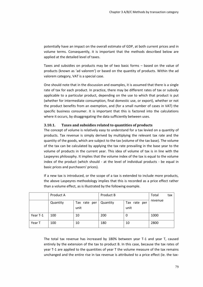
Chapter 3 A/B/C Methods by transaction category
79
potentially have an impact on the overall estimate of GDP, at both current prices and in
volume terms. Consequently, it is important that the methods described below are
applied at the detailed level of taxes.
Taxes and subsidies on products may be of two basic forms – based on the value of
products (known as ‘ad valorem’) or based on the quantity of products. Within the ad
valorem category, VAT is a special case.
One should note that in the discussion and examples, it is assumed that there is a single
rate of tax for each product. In practice, there may be different rates of tax or subsidy
applicable to a particular product, depending on the use to which that product is put
(whether for intermediate consumption, final domestic use, or export), whether or not
the product benefits from an exemption, and (for a small number of cases in VAT) the
specific business consumer. It is important that this is factored into the calculations
where it occurs, by disaggregating the data sufficiently between uses.
3.10.1. Taxes and subsidies related to quantities of products
The concept of volume is relatively easy to understand for a tax levied on a quantity of
products. Tax revenue is simply derived by multiplying the relevant tax rate and the
quantity of the goods, which are subject to the tax (volume of the tax base). The volume
of the tax can be calculated by applying the tax rate prevailing in the base year to the
volume of products in the current year. This idea of volume of tax is in line with the
Laspeyres philosophy. It implies that the volume index of the tax is equal to the volume
index of the product (which should - at the level of individual products - be equal in
basic prices and purchasers' prices).
If a new tax is introduced, or the scope of a tax is extended to include more products,
the above Laspeyres methodology implies that this is recorded as a price effect rather
than a volume effect, as is illustrated by the following example.
Product A Product B Total tax
revenue Quantity Tax rate per
unit
Quantity Tax rate per
unit
Year T-1 100 10 200 0 1000
Year T 100 10 180 10 2800
The total tax revenue has increased by 180% between year T-1 and year T, caused
entirely by the extension of the tax to product B. In this case, because the tax rates of
year T-1 are applied to the quantities of year T the volume measure of the tax remains
unchanged and the entire rise in tax revenue is attributed to a price effect (ie. the tax-
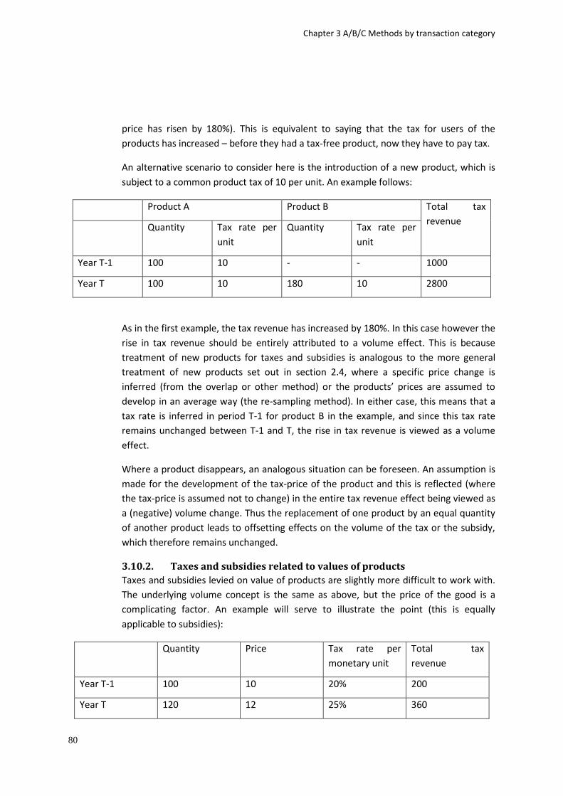
Chapter 3 A/B/C Methods by transaction category
80
price has risen by 180%). This is equivalent to saying that the tax for users of the
products has increased – before they had a tax-free product, now they have to pay tax.
An alternative scenario to consider here is the introduction of a new product, which is
subject to a common product tax of 10 per unit. An example follows:
Product A Product B Total tax
revenue Quantity Tax rate per
unit
Quantity Tax rate per
unit
Year T-1 100 10 - - 1000
Year T 100 10 180 10 2800
As in the first example, the tax revenue has increased by 180%. In this case however the
rise in tax revenue should be entirely attributed to a volume effect. This is because
treatment of new products for taxes and subsidies is analogous to the more general
treatment of new products set out in section 2.4, where a specific price change is
inferred (from the overlap or other method) or the products’ prices are assumed to
develop in an average way (the re-sampling method). In either case, this means that a
tax rate is inferred in period T-1 for product B in the example, and since this tax rate
remains unchanged between T-1 and T, the rise in tax revenue is viewed as a volume
effect.
Where a product disappears, an analogous situation can be foreseen. An assumption is
made for the development of the tax-price of the product and this is reflected (where
the tax-price is assumed not to change) in the entire tax revenue effect being viewed as
a (negative) volume change. Thus the replacement of one product by an equal quantity
of another product leads to offsetting effects on the volume of the tax or the subsidy,
which therefore remains unchanged.
3.10.2. Taxes and subsidies related to values of products
Taxes and subsidies levied on value of products are slightly more difficult to work with.
The underlying volume concept is the same as above, but the price of the good is a
complicating factor. An example will serve to illustrate the point (this is equally
applicable to subsidies):
Quantity Price Tax rate per
monetary unit
Total tax
revenue
Year T-1 100 10 20% 200
Year T 120 12 25% 360
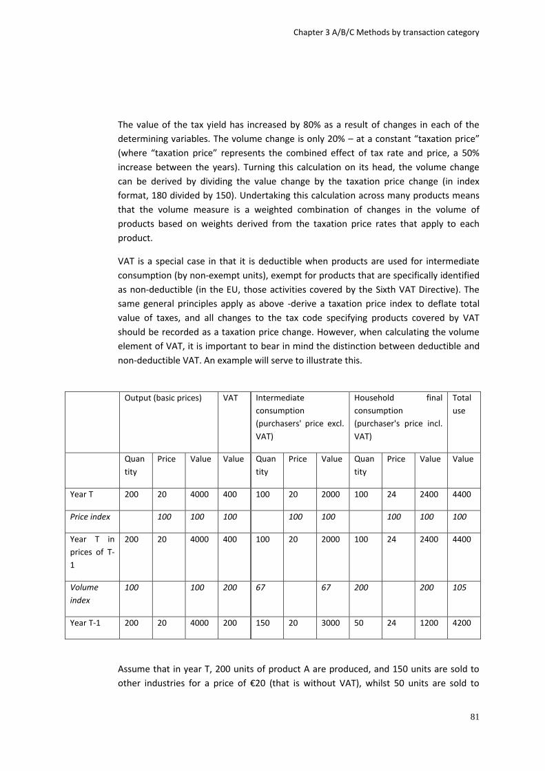
Chapter 3 A/B/C Methods by transaction category
81
The value of the tax yield has increased by 80% as a result of changes in each of the
determining variables. The volume change is only 20% – at a constant “taxation price”
(where “taxation price” represents the combined effect of tax rate and price, a 50%
increase between the years). Turning this calculation on its head, the volume change
can be derived by dividing the value change by the taxation price change (in index
format, 180 divided by 150). Undertaking this calculation across many products means
that the volume measure is a weighted combination of changes in the volume of
products based on weights derived from the taxation price rates that apply to each
product.
VAT is a special case in that it is deductible when products are used for intermediate
consumption (by non-exempt units), exempt for products that are specifically identified
as non-deductible (in the EU, those activities covered by the Sixth VAT Directive). The
same general principles apply as above -derive a taxation price index to deflate total
value of taxes, and all changes to the tax code specifying products covered by VAT
should be recorded as a taxation price change. However, when calculating the volume
element of VAT, it is important to bear in mind the distinction between deductible and
non-deductible VAT. An example will serve to illustrate this.
Output (basic prices) VAT Intermediate
consumption
(purchasers' price excl.
VAT)
Household final
consumption
(purchaser's price incl.
VAT)
Total
use
Quan
tity
Price Value Value Quan
tity
Price Value Quan
tity
Price Value Value
Year T 200 20 4000 400 100 20 2000 100 24 2400 4400
Price index 100 100 100 100 100 100 100 100
Year T in
prices of T-
1
200 20 4000 400 100 20 2000 100 24 2400 4400
Volume
index
100 100 200 67 67 200 200 105
Year T-1 200 20 4000 200 150 20 3000 50 24 1200 4200
Assume that in year T, 200 units of product A are produced, and 150 units are sold to
other industries for a price of €20 (that is without VAT), whilst 50 units are sold to
Chapter 3 A/B/C Methods by transaction category
82
households for a price of €24 (that is, including VAT at an assumed 20% rate). Total VAT
revenue from product A is €200.
In year T+1, the VAT rate remains unchanged at 20%, and 200 units of product A are
again produced. But this time 100 units are sold to other industries and 100 units sold
to households. Total VAT revenue from product A is now €400, an increase of 100%
over the previous year.
In this example, the full 100% change in VAT revenue is considered as a volume effect.
No prices have changed, and therefore the increase in VAT collected is caused solely by
an increase in the quantity of goods subject to VAT (caused by a change in the pattern
of consumption). By analogy with the general principles set out above, this represents a
volume change.
Similarly, one can note that a change in the balance of products for export (not subject
to VAT) and for home consumption will also lead to a change in the total tax collected,
and a volume change of the tax, even if the quantity of products produced has not
changed.
Both of these examples are an illustration of the general point discussed towards the
start of this section – one should undertake the calculations at the highest possible level
of detail in order to capture within the taxation price effect any variations in tax rates
determined by the use to which a product is put.
3.10.3. Collection rate issues
Finally one should consider the difference between theoretical and actual tax revenues.
For the example of a particular product subject to a value tax, the value of the product
multiplied by the prevailing tax rate will often be greater than the actual tax revenue
stream, because the tax system is rarely 100% successful at collecting all possible
revenues. This is equivalent to adding a further variable to the calculation:
Actual Tax Revenue = Quantity x Price x Tax Rate x Collection Rate
It is important to decide where the collection rate effect should be recorded – whether
a volume or a taxation price effect. It may be argued that the collection rate is actually
analogous to the tax rate (that is, comprehensiveness of collection is under the control
of the Government in the same way that the tax rate is) and therefore it should be
included as part of the taxation price effect. The collection rate for any particular
product can be readily calculated as the ratio between actual and theoretical tax
revenue.
There is a particular point to consider here when calculating the volume element of
VAT. The current price measure of VAT in the EU includes amounts that are not actually
collected where the non-collection was caused ‘without complicity’ between the
Chapter 3 A/B/C Methods by transaction category
83
transacting parties (Commission Decision 98/527/EC). Applying this definition to the
calculation of prices and volumes, the ‘collection rate’ must relate to the “with
complicity” element of uncollected VAT.
3.10.4. A, B and C methods
The principles set down in ESA 2010 par. 10.36 – 10.41 (and summarised above) for
taxes and subsidies on products are A methods provided that variations in the collection
ratio of taxes and the coverage of taxes and subsidies are both included in the taxation
price effect and not the volume effect.
If different taxes or subsidies are not fully separable (for example two different taxes
are set on a particular product but there is no separate information available on each)
then the methods described above become C methods because this would mean that
the price and volume elements of taxes would not be correctly separated.
3.11. Components of value added In section 2.1 it was stated that the income approach cannot be used for measuring
GDP volume growth, since income components do not have underlying price and
volume concepts. Nevertheless, in certain cases, it can be necessary to calculate the
components of value added in volume terms. This is for example the case when input
methods are used for unique market or non-market output. Also, measures of the
volume of labour input can be demanded. Therefore, and for reasons of completeness,
the next three sections discuss the possibilities of measuring components of value
added in volume terms.
3.11.1. Other taxes and subsidies on production
“Other taxes and subsidies on production” are defined in paragraphs 4.22-4.24 and
4.36-4.40 of ESA 2010. Taxes and subsidies on production are one of the determinants
of the basic price of a product.
Taxes on production consist of all taxes incurred by enterprises which are not directly
related to the quantity or value of products produced or sold. Examples include taxes
on the payroll of enterprises (but not taxes paid by employees), taxes on pollution,
licences where there is no service element, and taxes on the use of vehicles and land.
Subsidies on production, similarly, are not linked to the number of units of production
(that is, they are not intended to reduce prices to the consumer) but, like taxes, they are
intended to change the behaviour of the firm in the way that it employs its inputs or
undertakes the production process; for example, subsidies to reduce pollution.
Importantly, both taxes and subsidies on production should be recorded at the time at
which the underlying activity is taking place. This also means that the price and volume
calculations should be recorded in this way, not when the taxes are paid.
Chapter 3 A/B/C Methods by transaction category
84
The major conceptual difficulty with deriving a volume of taxes and subsidies on
production is that, unlike for taxes and subsidies on products (discussed in section 3.10),
there is no single quantifiable determining factor for the “tax/subsidy base”. It is
therefore important to draw out the underlying equivalents for the “tax/subsidy base”
for each type of tax and subsidy on production – in each case there will probably be
specific criteria written into legislation. For example:
Payroll taxes – These might for example be levied on the total number of employees
or the total salary bill. In the former case, an index of total number of employees
covered by the tax would be a suitable volume measure. Where the taxes are levied
as a percentage of salary bill, an adjustment should be made to the volume
calculation for the underlying wage rate changes (which are a price effect). Further
discussion of the deflation of compensation of employees can be found in section
3.53.11.2.
Taxes on ownership or use of an asset – These might be levied on the number
and/or size of assets used (for example cars, property). As with payroll taxes, where
the tax is levied on a value of assets, the changes in the unit price of the asset should
be measured as a price effect. Further discussion of the deflation of capital
expenditure and assets can be found in section 3.6.
Taxes in the form of licences – In line with ESA 2010 principles, licences are
considered a tax if there is no service provided. Licences are often levied as a flat
rate on the businesses affected, and therefore the number of business units subject
to the licence requirement can be seen as the underlying volume measure.
Subsidies on certain processes (eg. those reducing pollution) – Subsidies may be
administered in a number of different ways: as a flat rate per qualifying firm, as a
reimbursement for certain types of expenditure, or in proportion to a firm’s size of
turnover. Where there is a flat rate system, the number of qualifying firms would
form the basis of a volume measure. For a reimbursement system, a suitable
measure would be the volume of goods or services reimbursed.
For those taxes or subsidies related to a production process or ownership of an asset, or
restricted to selected firms, it is unlikely that complete volume data can be collected
from the firms concerned. It would be more straightforward to examine the
administrative records of the Government authority concerned to determine the
tax/subsidy base on which the payments are based (though care must be taken to
ensure that the records are complete and allow the calculation of accrued rather than
cash measures). For “per unit” taxes and subsidies (eg. per firm, per quantity of assets),
the Government records may yield the necessary information directly, or units can be

Chapter 3 A/B/C Methods by transaction category
85
calculated by dividing the total values by the tax/subsidy rate. It is important to use the
greatest possible detail for these calculations.
A, B and C methods
A methods will be based on complete and accrued data, with each individual tax or
subsidy examined and treated separately, and will use an appropriate index for
deflation (based on the recommendations in other sections of this handbook) where
the tax/subsidy is based on a value of assets, goods or services.
B methods are used where:
it is not possible to separate taxes and subsidies fully by their underlying tax/subsidy base, or
where the indices used for deflation do not meet the standards required in other sections of this handbook for A methods.
In practice it is very unlikely that a method based on collecting volume data from a
direct survey of firms paying and receiving taxes and subsidies will be sufficiently
comprehensive to reach the necessary coverage for a B method.
3.11.2. Compensation of employees
“Compensation of employees” is defined in paragraph 4.02 of ESA 2010. It is important
to note that this category includes wages and salaries and social contributions, and that
monetary flows are imputed for wages and salaries in kind, and for certain employers’
social contributions. One should also note that this category does not include the mixed
income of self-employed persons.
ESA 2010 describes the measurement of the volume of employee labour in paragraph
10.44, and defines the quantity of employee labour as “an hour’s work of a given type
and level of skill”. This definition however does not specify what types and levels of skill
have to be distinguished, and clearly there are a number of possible ways in which this
can be reflected (educational level, type of job, level of compensation, grade), each of
which may produce a different estimate of the volume component. This issue is further
discussed below.
Paragraphs 11.35 to 11.37 of ESA 2010 provide a further explanation of the calculation
of employee labour input in volume terms, namely that it should be labour input valued
at the levels of compensation of employees existing during a base period.
Given the rather strict definition of volume of compensation of employees set in the
ESA 2010, the price element of compensation of employees can be seen by implication

Chapter 3 A/B/C Methods by transaction category
86
to include all changes in compensation of employees not related to skills-adjusted hours
worked. This means that all changes in those elements of compensation of employees
not directly related to hours worked (for example most income in kind, structure and
level of social contributions) are included in the price effect. Thus it is possible to
concentrate on two methods to estimate volume – using quantity of hours worked data
directly (the extrapolation method) or deflating wages and salaries in cash (the
deflation method) – with the price effect simply calculated at the end of the process as
the implied ratio between current value and volume. There is no need to deflate the
individual elements of compensation of employees, and concentrating on wages and
salaries in cash is sufficient, if one assumes that all hours worked are reflected in wages
and salaries in cash (that is, there are no hours worked which are wholly compensated
for by income in kind).
Extrapolation method
The extrapolation method is based on a direct measurement of the quantity of labour –
perhaps using hours worked or the ‘full-time equivalent’ number of employees, broken
down by type of employee. If sufficient detail is available and the data can be
considered complete, then the quantity extrapolation method is viable. The definition
of “hours worked” is given in ESA 2010 paragraphs 11.27-11.29 – for extrapolating
compensation of employees, of course, the hours worked should be purely for
employees.
It may be necessary in practice to seek another measure of labour input for all or some
areas of the labour market, to act as a proxy for hours worked. One alternative is to use
“hours paid” as a quantity measure, though this does not represent the actual labour
input to the production process (for example, paid holidays and sick leave are included).
The total number of employees as an indicator of labour input cannot be considered
suitable – any change in the proportion of part-time employment would not be
captured.
The next step is to find a method of reflecting the skill levels of employees, so that the
labour input data can be weighted appropriately and changes in the mix of skills over
time can be reflected as a volume change. This can be seen as equivalent to
determining the quality of labour input and allocating it to the volume component of
compensation of employees. There are several possibilities here:
By educational level – the use of a classification system based on ISCED
(International Standard Classification of Education) will give a breakdown by the
highest educational level achieved. The main concern with using this breakdown
is that academic skills are given greater weight, and these may be less important
amongst more experienced workers.

Chapter 3 A/B/C Methods by transaction category
87
By occupation – labour force surveys and structural earnings surveys typically
use a detailed occupational classification (ISCO 2008, the International Standard
Classification of Occupations), which can, for example, distinguish between
different kinds of workers in the same industry.
By salary – the rationale here is that workers with greater skills can command
higher salaries. This assumes that there are no distortions or rigidities in the
labour market that could cause relative salaries to imperfectly reflect relative
skills.
By grade – this is possible in those organisations or sectors where there is a
common, established career structure. A good example is central government,
where one can often find a common grading structure across ministries. Grade is
often closely linked with salary, so one might expect similar results to using
salary as a skill indicator.
The key point here is to define the “skill” that has to be measured. A possible definition
is as follows “the skill of a labour input reflects the physical and mental ability that an
employee brings to a particular job”. One should note two important points:
The definition of skill is specifically related to the job undertaken. So a
university graduate working as a waiter would not count as a higher level of skill
than a waiter with no formal educational qualifications.
The level of skill does not measure how hardworking a particular employee
is. So a lazy employee with given ability would be measured in the same way as
an equivalent hard-working employee. This means that ‘skill’ is not necessarily
equivalent to ‘productivity’, though at the aggregate level we would expect a
strong relation between the two concepts.
None of the four measures described above exactly measure the given definition of skill,
so the task is to find the measure or combination of measures that could best
approximate the definition. Various possibilities are discussed in the OECD productivity
manual, including some quite complex multi-variable approaches.
There are both theoretical and practical difficulties with each of the possible skill
measures. Use of grade is only possible for a very limited number of organisations and
would not lead to a suitably harmonised approach. Use of salaries data, as a market
proxy for skill, will tend to reflect prevailing supply and demand conditions; for
example, the fact that there are a large number of skilled engineers looking for a job at
a particular time, and therefore the relative wage of engineers falls, does not mean the
skill of engineers has decreased relative to other occupations. Therefore salaries can be
seen as only an approximate, longer-term, indicator for skill.
Chapter 3 A/B/C Methods by transaction category
88
Of the two remaining measures, the use of an education measure might be seen to
violate the ‘job specific’ requirement set out in point i) above, although it may also
provide an indicator of general transferable skills which an employee can bring to the
job. Given the difficulties with job-specificity and the need to specify a harmonised
approach the recommendation of this manual is therefore to use occupation as the
variable to adjust labour hours for skill, unless it can be shown that education and
occupation are strongly correlated, in which case education could be used as an
indicator. The level of detail used for occupation should be at least the 1-digit level of
the ISCO classification. It is important to verify that the ISCO classification is being
applied rigorously in the basic statistics (whether labour force surveys or structure of
earnings surveys) so that there is no erosion over time in the basic standards applied.
Deflation method
An alternative approach, if hours worked data are not collected or are not available in
sufficient detail, is to use wage indices to deflate the value of cash wages and salaries.
This approach requires that the wage indices used meet certain criteria:
a) They should be based on actual cash wages per hour. This means that if the data are
available on only a per month or per year basis, they must be converted to a per hour
basis, and;
b) They should be broken down in sufficient detail to provide a deflator for groups of
staff of homogenous skill.
In practice, meeting both these criteria perfectly will be extremely difficult. The first is
less problematic because one can use contracted hours to make the conversion. But the
second can present particular practical problems, depending on the structure of the
labour market. There are two possible methods which can be used to approximate the
required result.
The first is the Wage Rate (WR) method. Here, the work force is classified into a number
of different categories of employee, and for each category the hourly wage rate of a
“representative employee” is used, perhaps based on an official or industry-level rate.
Weighting is preferably undertaken using the wages for the category in the current year
to obtain a Paasche-type index, but a Laspeyres-type index may be a reasonable
approximation to this if calculated at a sufficient level of detail.
In general, the stratification of the work force should be such that categories for which
significantly different changes in wage rates occur are separately distinguished. In the
extreme case that all employees always receive the same wage increase, no
stratification at all is necessary.
Chapter 3 A/B/C Methods by transaction category
89
The WR method defines the price/volume decomposition in the following way - if a
price change is not specified in the wage rate change for a certain category, it will end
up in the volume component.
The WR method is most suitable when there is a system of collective agreements in
place that set common wage rates for large groups of employees. This is the case in
various countries, and the method assumes that the collective wage increases give an
indication of the actual changes in the price of labour, while all other wage increases
are related to performance and hence are included in volume.
The second method available is the Average Wage (AW) method. This method uses
average wages for categories of employee, but assumes that the total number of hours
worked is not available. The starting point is an exhaustive set of data on numbers of
employees and their salaries, in a detailed breakdown of grades and activities. The
average wage increase per employee is determined for each of the detailed categories
of employees, so that the wages of each category can be deflated separately. This
approach implies that the decomposition into price and volume is implicit in the
classification made in grades, activities, etc., and the detail of those classifications: shifts
between the categories end up in the volume component, while wage increases within
categories are included in the price component. Hence, the coverage of the volume
component is increased when a more detailed stratification is used. The method is
much more data-intensive than the WR method, and is most applicable to deflating the
wages and salaries of government employees.
The AW method is comparable to a unit value approach, while the WR method is
comparable to a price index compilation (see section 2.6). Each method requires certain
conditions to be met if it is to be applied properly. For the WR method:
the work force should be stratified such that those categories of employees with
different wage rate increases are separately identified;
the wage rate used for each category should be representative for that category;
the wage rate should include the general wage rate change, specific wage rate
changes for categories of employees, changes in allowances or bonuses that are
not related to performance, and changes due to seniority;
the weights should be total wages of each category of the current year or,
alternatively, a recent year.
And for the AW method:
Chapter 3 A/B/C Methods by transaction category
90
the work force should be stratified such that those shifts between the categories
of employees, which should be in the volume component, are separately
identified;
which implies that the work force should be stratified at least by grades,
functions/activities, and seniority.
The level at which the calculation is conducted is an important determinant of the
difference between the two methods. At the finest level of detail the WR method
should converge with the AW method.
Nevertheless, both methods have weaknesses when compared with the extrapolation
method, because neither method can lead in practice to a measure of volume that
matches the ESA 2010 definition. The WR method suffers from an inability to distinguish
between price changes caused by changes in skill and other price changes. The AW
method suffers from the use of employee data rather than hours worked. Both of the
methods can nevertheless reach an acceptable standard.
A, B and C methods
The quantity extrapolation method will be an A method if sufficient detail is available in
the data to reflect the skill levels of employees (using occupation at a minimum
breakdown of the 1-digit ISCO classification or education at the 1-digit ISCED level of
occupation and education can be shown to be highly correlated), and if an “hours
worked” measure is available for extrapolation. Use of “hours paid” to extrapolate, or
the use of a less detailed occupational breakdown, will constitute B methods. Use of
number of employees as a quantity indicator would constitute a C method.
Both the average wage and wage rate methods will be B methods if the conditions set
out above are met; in particular that a sufficient level of stratification is used to
distinguish reasonably homogenous groups of employees. As explained above, these
methods cannot be A methods in practice because they will not lead to the required
definition of volume.
Deflation of compensation of employees by an unrepresentative or general wage index
is a C method. Deflation using a consumer price index is a C method since the result is a
measure of the purchasing power of compensation, rather than the volume of input
from employee labour.
3.11.3. Consumption of fixed capital
Consumption of fixed capital represents the amount of fixed assets used up during an
accounting period. It should be calculated for all types of assets, both tangible and
intangible, except animals. The main use of estimates of the consumption of fixed
capital is to transform gross estimates (ie those that do not take account of the
Chapter 3 A/B/C Methods by transaction category
91
consumption of fixed capital) into net measures. However, for non-market services,
where output in current prices is derived as the sum of costs, the calculation of
consumption of fixed capital directly influences the calculation of output.
The methods used for the estimation of the consumption of fixed capital at current
prices are based on the stock of fixed assets and their probable economic life. The
calculation of volume measures presents few problems when good data on the
composition of the stock of fixed assets are available.
Most countries use the perpetual inventory method for the estimation of the
consumption of fixed capital at current prices. This method requires the stock of fixed
assets at previous year’s prices to be calculated as an intermediate step in the current
price calculation. The method employs detailed data on gross fixed capital formation
and price indices. These detailed price indices allow the capital formation acquired over
a number of years, and valued at their historic cost, to be revalued in terms of their
replacement cost at a base year price. The price and volume indices derived in the
process can be used to derive estimates of the consumption of fixed capital in volume
terms. Further detail on the perpetual inventory method for the estimation of capital
stock and the consumption of fixed capital can be found in the OECD manual on capital
stock.
When there is no perpetual inventory of the stock of fixed capital, estimates of the
consumption of fixed capital at previous year’s prices can be derived by deflation of the
current price estimates by suitable price indices. The price indices used can be those
derived from data on gross fixed capital formation by product, see section 3.6. When
using price indices from this source it is necessary to take account of the age structure
of the capital goods within the stock of fixed assets.
The quality of the consumption of fixed capital estimates depends heavily on the quality
of the price indices used for gross fixed capital formation, irrespective of the calculation
method employed. The issues associated with the measurement of prices for gross fixed
capital formation are discussed in section 3.6 and will not be repeated here.
A, B and C methods
The estimation of the consumption of fixed capital is closely linked to that for gross
fixed capital formation. As such, the classification of methods that apply to gross fixed
capital formation also apply to the consumption of fixed capital, see section 3.6. In
summary, these are:
The use of genuine investment price indices (IPIs) will be an A method. The use of PPIs
adjusted to purchasers' prices would also be an A method. To be an A method the
coverage of these price indices should match exactly that of the products.

Chapter 3 A/B/C Methods by transaction category
92
IPIs, or PPIs adjusted to purchasers' prices, where the coverage is not exactly that of the
products or that do not take account of changes in quality would be a B method.

Chapter 4 A/B/C Methods for output by product
93
4. A/B/C methods for output by product
4.1 CPA A - Products of agriculture, forestry and fishing Key aspects
Agricultural and fishing products are produced both for the market and for own final
use, across incorporated and unincorporated enterprises. The methodology for
measuring the output from economic activities of the agriculture and forestry industries
is fully documented in the Manual on the Economic Accounts for Agriculture and
Forestry (Rev 1.1 – 2000 Edition), which describes the volume valuation of activity in
Section V. Three particularly important issues for National Accounts can be identified:
The production process may be spread over more than one accounting period. Whilst in
Europe the production cycle is shorter than a year for the majority of crops, this
becomes a major issue for forestry, fish farming, livestock rearing, and when quarterly
accounts are prepared (see chapter 5 for further discussion). ESA 2010 is very specific
on the method to be used for dealing with this: “The output of agricultural products is
recorded as being produced continuously over the entire period of production (and not
only when the crops are harvested or animals slaughtered)” (ESA 2010 3.54). The SNA
2008 (6.137 – 6.138) recommends that production should be recorded as work-in-
progress, distributed according to costs incurred, and that accumulated work-in-
progress should be transferred into inventories of finished products at the time of
harvest (see section 3.7 for a discussion of volume issues for inventories and work-in-
progress). In the EU this procedure is used for “cultivated forests” only, as defined by
Member States in accordance with ESA principles; timber output from non-cultivated
forests is measured at the time of cutting.
Agricultural prices tend to be very seasonal. There is often a distinct seasonal pattern in
prices of fresh agricultural and fishing products, in both the wholesale and consumer
markets. Discussion of methods to deal with this in the quarterly accounts can be found
in chapter 5; the conclusion there is that the product detail used must be sufficient to
distinguish seasonal varieties.
The complex nature of subsidies arising from the Common Agricultural Policy (CAP),
Common Fisheries Policy (CFP), and domestic policies of the Member States, together
with the range of tax benefits often available to farmers and fishermen, mean that
adjustments for taxes, levies and subsidies need to be undertaken particularly carefully
so that the basic price concept is followed. This is also true for the measurement of
cross-border trade in agricultural goods, where tariffs and export subsidies are
common, and where the general principle is that the prices are measured ‘f.o.b.’ for
exports and ‘c.i.f.’ for imports (at the product level). Sections 3.9 and 3.10 cover the
volume issues associated with these types of flows in more detail.
The agriculture and fishing industries have very detailed quality classifications for its
products, with a well-developed (if complex) market pricing system, and a combination
of slow innovation in products and generally overlapping sale of different products
Chapter 4 A/B/C Methods for output by product
94
means that measurement of quality change is not such a problem as it is in some
manufacturing areas. That does not mean that major developments such as genetically
modified and organic products should be ignored, but more data are generally available
to undertake adjustments.
One important point to watch on quality is the extent to which products are processed
on the farm or the boat – any change in the degree of processing should be dealt with
as a volume change. Processed products (such as butter and cheese) are considered
industrial products and should be classified accordingly. Statistical enquiries should
cover this point adequately.
A practical point to watch when collecting data is the degree to which agricultural units
undertake other non-agricultural activities, such as tourism or leisure services. This is a
general point for national accounts, but is particularly relevant in agriculture. National
accounts compilers should discuss with the agricultural colleagues the treatment of
secondary activities within data sources, and in particular those that are considered
“inseparable”, to ensure that the product-based data used is as close to the CPA
definition as possible.
Under ESA 2010 (paragraph 1.95), non-marketed production (whether bartered or used
for own-consumption) should be valued wherever possible at prevailing market prices
(and therefore deflation to previous year’s prices should be undertaken on the same
basis). This ensures a consistent treatment between market and non-market
production.
Data availability
All Member States produce full annual agricultural economic accounts (at current and in
volume terms), and undertake substantial data collection on agriculture and fishing, for
both administrative and statistical purposes. Agricultural data collection typically takes
the form of an annual census of production and a detailed structural survey every ten
years. Member States define “representative products”, which are important products
in domestic markets and which have clearly defined qualities. Fishing data are collected
continuously, though no Member States as yet produces separate fishing accounts, and
data for fish farming are sparse.
However it is necessary to ensure that the data used for national accounts purposes
fully follow national accounts methodologies, and for this reason the relatively small
differences between Economic Accounts for agriculture and National Accounts practices
are set out in “Bridge Tables” (see Appendix XI of the Manual on Economic Accounts for
Agriculture and Forestry http://epp.eurostat.ec.europa.eu/cache/ITY_OFFPUB/KS-27-
00-782/EN/KS-27-00-782-EN.PDF).
Information on subsidies is available from CAP and CFP-related data, or from
governments’ records (in the case of national subsidies). However, one should be
careful to distinguish between subsidies on products and other subsidies on production
(including “set aside” payments) – the former must be taken into account in any price

Chapter 4 A/B/C Methods for output by product
95
indices used, the latter should not be (see sections 3.10 and 3.53.11.1 for further
details). One must also take account of the periods for which subsidies are paid and
ensure that subsidies are allocated to the time periods when the production was
deemed to be undertaken.
A, B and C methods
Use of data from the Agricultural Economic Accounts, suitably adjusted for the small
methodological differences with the National Accounts, and undertaken in line with the
principles set out in chapter V of the Manual on the Economic Accounts for Agriculture
and Forestry (particularly in relation to the elementary level of aggregation), is an A
method.
There should be little reason to resort to B methods for agricultural and fisheries
production since the necessary data is already collected by Member States, but it may
be that some products are not fully separable into different varieties and seasons, or
quality adjustments are not fully possible. Using approximate quality adjustments for
these products would be considered B methods. This may be true, for example, for the
output of farmed fish.
Any other methods which do not take quality into account or are based entirely on
inputs are C methods.
4.2 CPA B - Mining and quarrying Key aspects
The mining and quarrying heading covers the products of extraction of naturally
occurring substances, such as coal, crude petroleum, and stone. It does not cover the
processing of these substances, nor the subsequent sale of the processed products.
As with the agriculture and fishing industries, the mining and quarrying industry has
very detailed quality classifications for its products, with a well-developed (spot and
forward) market pricing system. There are two other aspects of this branch, which aid
data collection – an industry generally concentrated in large (sometimes state-owned)
firms, and little or no household production. One point to watch is the presence of
subsidies or special tax regimes in some industries (for example in coal) which may be
reflected in prices. It is also important to note that inventories are common in the
industry and must be recorded appropriately (see section 3.7).
Data availability
For historical reasons, and because of the advantages to data collection set out above,
there is an abundance of data available on the major mining and extraction industries –
both for prices (PPIs are common) and volumes. Some products (for example extracted
salt, fertilisers, and sand/gravel) may however be less comprehensively covered than
major energy products such as coal and oil.

Chapter 4 A/B/C Methods for output by product
96
Information on subsidies and tax regimes should be readily available from government
administrative sources.
A, B and C methods
Since volume data are collected in some detail for the major products (with sub-
divisions by quality) it is possible to measure volume output for extraction directly from
this source. Value of output can also be deflated by actual price data, in the form of
PPIs, so long as they meet the criteria set out in section 3.1.1. It is also possible to use
unit values if the products included within each unit value calculation are perfectly
homogeneous. These are the A methods.
There should be no reason to resort to B methods for mining and quarrying extraction,
but there may be a lack of detailed data for some areas of the quarrying industry. Use of
approximate quality adjustments, or using PPIs that do not meet all of the required
criteria, would all be considered B methods.
4.3 CPA C - Manufactured products
4.3.1 General recommendations for manufactured products
Key aspects
This section deals with methods applicable to most of the diverse products classified to
CPA C. Particular issues related to the measurement of volume output for large
equipment goods and computers are covered in the following two sections.
CPA C covers manufactured goods including processed food products, clothing, refined
fuels and chemicals, equipment of various kinds, and consumer durables. The features
of manufactured goods – sold into a market, often produced in concentrated industries,
tangible characteristics – together with the historical emphasis in statistical offices on
measuring manufacturing (reflected for example in a detailed product classification),
mean that theoretical and practical measurement are generally more straightforward
than for some other CPA categories. However it is important to ensure that the general
issues mentioned earlier in the handbook are satisfactorily covered, in particular:
Quality – Changes in the quality of a product should be properly reflected as
changes in volume. Section 2.4 discusses possible methods in more detail. For
some products in CPA C, such as fashion goods (clothes, footwear) or high
technology electrical goods, the definition of “quality” is not always
straightforward. It may be, for example, that the hedonic methods described in
section 4.3.3 on computers will need to be applied to other electrical products
where the technology is changing rapidly (for example mobile phones).
Price basis – The value of output should be deflated by a price index based on
basic prices, and these should be based on actual prices not list prices (so that
discounts are reflected in the price).
Chapter 4 A/B/C Methods for output by product
97
Accruals basis – The data should relate to transactions in the period in question,
not when the goods are paid for. This is particularly important for quarterly data
collection (see chapter 5).
Data availability
There is generally no shortage of price or quantity data for manufactured products. For
EU Member States, the Short Term Statistics Regulation (1165/98) requires the monthly
production of indices of producer prices (PPIs), broken down by industry. These
industry-level indices are themselves constructed from more detailed indices at product
level. CPI data are available for manufactured goods sold to consumers, but these will
have to be adjusted to basic prices before they can be used to deflate output.
A, B and C methods
The A method for manufactured goods is to use suitable PPIs to deflate the value of
output, in particular PPIs that are representative of the product group, are valued at
basic prices, and take proper account of quality. Clearly the PPIs should be sufficiently
disaggregated to undertake deflation at the lowest possible product level. See also
section 3.1.1 on the general procedures for deflating market output.
For certain manufactured products, where there are precise quality standards set for a
homogenous product, an A method could also be to use data on the quantities of
product at the necessary level of disaggregation, as long as these quantity data are fully
representative. Examples of products that could be suitable for this treatment include
bulk chemicals, wood pulp and petroleum.
One B method is to use detailed CPI data adjusted to basic prices for deflating the value
of output. Use of less appropriate PPIs, for example where there is incomplete product
coverage, would also be a B method.
Any methods based on input costs (except for unique products like large equipment
goods), or which use an unrepresentative price index, are considered C methods.
4.3.2 Large equipment goods
Key aspects
The concept of volume measurement is founded in tracking the price of a basket of
products between one period and the next. But this is not straightforward when a
product changes significantly over time, or when it is a “one off” (see section 2.5). A
large proportion of such unique products are found in the area of machinery and
equipment; here referred to as "large equipment goods". Examples are ships, oil rigs,
aeroplanes and special purpose machinery.
Some of these products can, in themselves, have a significant impact on small, and even
medium sized, economies. It is therefore important that they are not simply ignored by
statisticians as an intractable problem; evidence from a number of countries confirms
that the choice of method can have a significant effect on the volume measure.
Chapter 4 A/B/C Methods for output by product
98
The measures used should of course be completely consistent with National Accounts
concepts:
It is often the case that certain services are bundled with the sale of a capital
good (for example aircraft manufacturers have a comprehensive “after-sales”
service). These services should be included in any assessment of the quality of
the product and therefore any changes must be seen as changes in volume.
Many major capital projects span more than one accounting period. It is
important that output and price measurements are taken for the period in
question, and data adjusted if it relates to different (or many) accounting
periods. It is particularly important to distinguish between tender prices and
actual prices. Any work-in-progress must be identified, booked correctly, and
deflated using the same method as output.
It is possible that the international market in large capital equipment is rather
competitive, and therefore that international price movements (for example from a
major producer of equipment of that type) can be taken as representative of the price
movements in an individual country. The price movements should relate to the
producer prices for the same or very similar equipment. One problem to overcome is
how to deal with the effect of changes in exchange rates and inflation rates over time in
different countries. There are three options:
(i) Using prices directly – this would use the direct price of the goods with no
adjustment for inflation or exchange rates. The only suitable direct comparison would
be if the contracts were specified in some common currency (such as euros).
(ii) Using a relative price index of the form:
Bg
j
Ag
j
p
p
p
p
where pj is the price of equipment good j, pg is the general price level excluding the
equipment good, and A,B are different countries. This assumes that the price of the
equipment good in country A relative to general inflation in country A evolves in the
same way as the price of the equipment good in country B (a major producer) relative
to the general inflation in country B. The effect is to control for different changes in
general inflation between the two countries.
(iii) Adjusting for exchange rate movements – this assumes that changes in exchange
rates fully feed through into changes in prices, which is a questionable assumption and
includes exchange rate volatility within the price measure.
The choice of adjustment method can have a large impact on the measured price
movement. If contract prices are specified in a major currency, option (i) is possible. If
not, then for preference the relative price approach (option (ii)) could be used. A simple

Chapter 4 A/B/C Methods for output by product
99
adjustment for exchange rate movements (option iii) may be suitable in a limited
number of circumstances where it can be shown that domestic prices of the specific
good are extremely sensitive to the exchange rate.
Data availability
Only a handful of countries produce PPI's for goods such as ships and aircraft. Within
Europe countries with small or no domestic industries producing major capital goods
tend to use international pricing data for import flows, whilst others use a combination
of input-based data, or output data from industries producing similar products. A
couple of European countries, and the US, currently use methods which involve
decomposing large products into a series of more generic elements (“specification
pricing”) or collecting data period-by-period on a specific combination of generic
elements (“model pricing”). These techniques are described in more detail in section
2.5. Use of the techniques does involve a greater use of resources, both in the statistical
office and in the responding organisations.
The European Regulation on Short Term Statistics (Council Regulation 1165/98)
explicitly excluded the requirement to produce output price indices for defence,
aerospace and shipping capital products. Nevertheless a number of Member States and
others are examining their methodology with a view to moving towards output prices in
due course.
A, B and C methods
The major product items considered here are ships, aircraft, trains, oil rigs and
machinery for specialist industries (such as paper production). However the general
principle for large equipment can be clearly stated – methods using unadjusted quantity
indicators or based on unit value measures are considered as C methods.
Methods based on model pricing or specification pricing (see section 2.5) may be
considered as A methods if the criteria set out in that section - namely regularly
updated and representative models, and use of actual prices - are satisfied.
Two alternative methods can be employed:
Use of international prices can be a B method if the prices can be considered
representative of the Member State’s domestic production (at the most detailed
product level) and cross-border trade flows – the markets must be competitive,
the data properly stratified and weighted, a suitable method used for adjusting
for exchange rate movements, and foreign trade data should include second-
hand equipment. It is recommended in any case that Member States remain in
close contact over price changes for large goods, and draw on each other’s
experience as much as possible. In some cases, a country considered the major
European producer could play the “lead role”, in co-operation with Eurostat, to
produce a suitable price index for use across all Member States.
Chapter 4 A/B/C Methods for output by product
100
Use of specific and robust quality adjustment methods can be A or B methods
depending on the suitability of the industry (for example, trains and special
purpose machinery could be suitable industries for this method), though ideally
they should be used in combination with the decomposition of major assets into
their constituent elements. Various methods are examined in section 2.4.
For ships, the A method would be model pricing if the characteristics mentioned above
and in section 2.5 are satisfied.
For oil rigs, the A method is the specification pricing approach to identify the modular
elements of the rig, so long as adjustments for quality are applied to the elements.
Pricing of the components with an adjustment for company margins and labour
productivity would be considered a B method, as would use of an international index
for certain types of ships – of large size and modular construction - which share the
characteristics of oil rigs.
For aeroplanes, any method employed must be based on a careful stratification of the
industry, must take into account the complex flows associated with co-operative
projects (for example Airbus), and must adjust for exchange rate changes where prices
are quoted in US dollars. The A methods here are model pricing and the specification
pricing approaches, and both should benefit from the pre-dominance of commercial
customers in the aeroplane market.
Model pricing and quality adjustment based on option prices (that is, estimating the
marginal price of additional features) methods are both A methods for trains, provided
that stratification at least extends to wagons/coaches/locomotives and to the different
forms of propulsion technology.
For special purpose machinery (for example paper machinery), the A methods are
model pricing and the specification pricing approaches, but appropriate quality
adjustment methods can be used directly where the machinery is not suited for a
decomposition method.
For defence goods, it is possible to apply similar methods to those described above
(indeed it may be that military and civilian product prices move in a very similar way),
but it is also common for defence ministries to compile their own price indices (often
based on reports from contractors) so as to manage their financial affairs. National
accountants should examine the methods employed carefully – if they are quality
adjusted and based on actual evolution of output prices, they could be considered as
produced by an A method.
Input methods will be acceptable, if none of these methods is applicable.
4.3.3 Computers
Computers are treated separately in this handbook because of two specific issues:
The bundling of hardware and software, and
Chapter 4 A/B/C Methods for output by product
101
The rapid technological changes that characterise these products.
The first issue is discussed in more detail in section 4.9 on computer and related
services. The most evident example of bundling is the sale of a PC with operating
system and perhaps other software.
The second issue becomes more and more important with the increased share of
computers in investment expenditure. Although the impact on the volume of GDP can
be limited if most computers are imported, the measurement of the volume increase of
output of computers can have a significant impact on the measurement of components
of GDP (such as GFCF and final consumption expenditure by households).
The problem is one of quality change, which was discussed at length in section 2.4. The
various methods of handling quality changes were introduced there. The following
methods can be appropriate to use for computers:
the hedonic approach, since it is possible to determine and quantify the characteristics that influence the price;
option prices, since in many cases separately priced options can be distinguished (such as additional memory or a DVD drive);
the resampling method, as long as the sample is representative and large enough.
In view of the discounting practices for computers, in particular for PCs, the overlap
method is less appropriate for these products.
The hedonic approach seems to be the best way to go in the end since it is very well
possible to define and measure the characteristics that determine computer prices. The
hedonic approach has proven itself in the USA as a useful and feasible tool for handling
the problems of fast technological change. The hedonic approach is most appropriate if
it is used for the estimation of prices of characteristics (and thus for quality adjustments
only), and not for a direct price index. It is also possible to combine it with other
methods such as option prices.
Comprehensive data on prices and technical characteristics of computers are required
when applying hedonic adjustment techniques. Therefore, the hedonic approach is the
most resource-intensive of the above techniques. The hedonic technique is a relatively
complex method with a couple of different mathematical variants. It needs in particular
considerable resources to set-up, but once set-up, the running of a hedonic method is
not very resource-intensive. However, the model needs to be updated regularly.
Besides the profound knowledge of statistical methods good knowledge of the technical
aspects of computers is required, too. The technical characteristics covered (or not)
have a direct effect on the results.
These costs can be reduced however by international co-operation. It can be expected
that the hedonic function is not very different across countries due to the openness and
competitiveness of the computer market worldwide. It would therefore be in principle

Chapter 4 A/B/C Methods for output by product
102
sufficient to estimate one hedonic model for e.g. the EU as a whole. The coefficients in
this model could then be applied in national price index programs to adjust prices when
replacements occur.
Due to the rapid turnover of models, for PCs price observation should be at least
monthly. Preferably, price collection is carried out directly from the manufacturers or
retailers. However, at least for the consumer market, price collection through
magazines or the internet can also provide reliable enough data. If computers are sold
together with software, this software needs to be recognized as a characteristic of the
computer in the hedonic model.
Data availability
In most countries, price indices for computers are compiled within the frameworks of
the producer price index (PPI) and the consumer price index (CPI).
Price data for PCs and related equipment such as printers, servers, etc. are generally
readily available. Several countries rely on magazine prices, either for their PPIs or their
CPIs. Data for larger systems are less widely available and their collection is more
difficult. Catalogue prices are less likely to give an accurate reflection of market prices
and the smaller quantities may make monitoring of actual transactions difficult.
A, B and C methods
An A method is deflation with a PPI that uses an appropriate quality adjustment
procedure, which can be, as said above, the hedonic approach, option prices, or
resampling.
For household consumption of PCs, list prices will provide an acceptable alternative for
actual prices, but only for that case. List prices can for example be obtained from
computer magazines or from the internet.
B methods are less appropriate PPIs, e.g. with a less appropriate quality adjustment
procedure, such as the judgmental approach or production costs.
Another possible B method is the use of information from the US price index for
computers, provided it can be shown that it is sufficiently representative for the
domestic prices. The most appropriate option in this case is to use the US prices of
computer characteristics, and to use these to make explicit quality adjustments to price
data collected domestically. An appropriate mechanism for taking into account different
general price changes or exchange rate changes should be applied. See section 4.3.2 for
a discussion of the various possibilities.
Proxy methods, such as using price indexes from other electronic products should be
classified as C methods. Also, methods based upon unit values are C methods. The use
of a price index that does not take account of quality changes is also a C method. The
unadjusted price comparison method and automatic linking are always C methods for
computers.
Chapter 4 A/B/C Methods for output by product
103
4.3.4 Repair and installation services of machinery and equipment
(CPA33).
The A method for repair and installation services is to use suitable PPIs to deflate the
value of output, in particular PPIs that are representative of the service, are valued at
basic prices, and take proper account of quality. The PPIs should be sufficiently
disaggregated to undertake deflation at the lowest possible product level. An
alternative A method is to collect data on hourly rates or quotes for ‘model’ jobs from
contractors, and then to use these as indicators of price.
Use of less appropriate PPIs, for example where there is incomplete product coverage,
would also be a B method. Any methods based on input costs, or which use an
unrepresentative price index, are considered C methods.
4.4 CPA D - Electricity, gas, steam and air conditioning; Key aspects
This section includes production and distribution of electricity, gas and air conditioning
services to both business and household consumers. It does not include extraction of
gas (which is included under CPA B)
There are two distinct characteristics that make measuring volume output for this
particular product category easier than for many other categories:
The major products are relatively homogenous – a KW hour of electricity, a cubic
metre of gas – and values are calculated as price times volume. So quantity
measures can be used directly in measuring volume output.
The industries are generally concentrated, with one or very few large firms,
often state-owned, so data gathering is relatively straightforward. The issue of
distribution networks is discussed in more detail below.
There are a couple of issues which do require careful treatment:
Price discrimination within the market – most utility companies charge different
prices for different users (for example between bulk business users, other
business users, and private customers). This can create a similar problem of
complex tariffs as that encountered in the telecommunications industry (see
section 4.8), particularly as markets are liberalised and the tariff structures
become more complicated. It is important, if using price indices, that a clear
distinction is drawn between price differences based on quality (for example
electricity supplied at night compared with supply during the day, or gas
supplied in the summer compared with gas supplied in the winter, or there may
be a different tariff for "green" electricity) and price discrimination. The former
case can be treated as different products (see the discussion of seasonal
products in section 5.3.2). ESA 2010 par. 10.16 says that price discrimination only
applies when different prices are charged for identical products sold under
exactly the same circumstances. An example would be sales of electricity to a
Chapter 4 A/B/C Methods for output by product
104
small business and to a private house at a particular hour of the day – whilst the
product is exactly the same, and the small business may not benefit from any
bulk discounts, it is often the case that the business is charged at a different rate
(business tariff) from the household. It is of course important that any discounts
given to bulk users are included within price movements.
A common structure in these industries is for a division between producers and
distributors. Sometimes this occurs in a single, vertically integrated, enterprise
(though this may well have distinct kind-of-activity units), but often more than
one enterprise is present, and the raw products sold by producers to
distributors. There are two possible methodologies for recording distribution:
‘net’ – that is, the output of distributors is the margin for distribution, and 'gross'
– where the output of the company is measured in terms of the product
delivered. For net recording, this means that there are similar issues to section
4.7.1 in the measurement of margins at previous year’s prices.
Data availability
As discussed above, data are widely available on volumes of product, and producer
price indices are compiled. Data on distribution are less readily available. Consumer
price indices are also widely available, but these are only applicable to output sold to
households.
A, B and C methods
We can distinguish between production and distribution for the discussion of
appropriate methods:
Production
The A method here is to deflate value of output by the available PPIs, assuming that
they satisfy the standard conditions set out in section 3.1.1, and take full account of any
‘standing charges’ (payments unrelated to consumption) levied by the companies. A
fully equivalent approach, which would also be an A method, is to directly use the
quantity data available on products, providing the quantity data is sufficiently detailed
(i.e. it identifies the quantities delivered by tariff and customer type).
Distribution
There are two sets of methods for distribution, depending on whether a gross or net
(margin) basis of recording is used.
Net recording
The A method for measuring distribution margins is a method taking the changes in
quality of the distribution services into account. Section 4.7.1 contains a fuller
explanation of the issues and techniques for measuring margins at previous year’s
prices. So far, the only method that can properly account for quality changes – in theory
Chapter 4 A/B/C Methods for output by product
105
– is deflating sales and purchases separately. A suitable B method is to assume that the
volume of the service follows the quantity of the product distributed, e.g. the volume of
electricity distribution output follows the quantity of electricity output.
Any other method, in particular the deflation of margin output directly by a producer
price index, is a C method.
Gross recording
In the case of gross recording, the A method for deflating output is to use a suitable PPI
to deflate value of output at basic prices, where the PPI has been compiled for the
combination of production and distribution components of output. Suitable B methods
include using CPI data to deflate total output if this can be shown to be representative
for output consumed by businesses, and using the quantity of output to provide an
indicator of the combined production and distribution products.
Any other method, especially those based on input costs, is a C method.
4.5 CPA E - Water supply; sewerage, waste management and
remediation services This includes:
CPA 36 - Natural water, water treatment and supply services
CPA 37 - Sewerage services; sewage sludge;
CPA 38 - Waste collection, treatment and disposal services; materials recovery
services
CPA 39 - Remediation services and other waste management services
Key aspects
These product divisions consist mostly of market services, though waste collection and
disposal services can be provided as non-market or market services. The particular
difficulty here is not so much with defining output (for example tonnes of rubbish
collected or quantity of sewage treated) as with separating the individual price of the
service from those of other products. For example, waste collection and disposal
services may be paid for as part of a general charge or local taxation for businesses and
households, and sewage service charges may be included in a general charge for water
supply and disposal.
Data availability
Given that sewage services tend to be provided by major utilities (whether publicly or
privately owned), and waste collection disposal services by units of local government,
price and volume data might be readily available, though enquiries will need to
separate the services from others provided in the same charge. The CPI could capture
data on services provided to households.
Chapter 4 A/B/C Methods for output by product
106
A, B and C methods
A methods include the use of suitable PPIs where they are available, and output volume
indicators (such as tonnes of refuse collected) adjusted for certain quality features of
the service, such as regularity of collection and treatment of speciality refuse (e.g. toxic
waste).
B methods include the use of detailed CPI indices for both household and business
consumption (where the evolution of prices for services to businesses is shown to be
similar to services to households). For non-market services, use of output volume
indicators would be considered a B method if those indicators provide good coverage
and are sufficiently detailed.
4.6 CPA F – Constructions and construction works Key aspects
Construction output covers a wide range of products including one-dwelling and multi-
dwelling buildings, industrial and commercial buildings, highways, railways, and other
major civil engineering projects. The output covers new construction, major
improvement of existing structures and regular repair and maintenance. In addition to
this broad coverage, other features of the construction sector require close attention in
measuring output at both current prices and in volume terms:
Some new building or improvement projects may span two or more accounting
periods, and there may be a significant delay between the signature of a contract
and the work commencing. Thus output must be allocated to accounting
periods, and in prices determined for each period.
Every building project can be considered unique – even seemingly identical
buildings may be different because of site conditions – which complicates the
measurement of quality. Projects should therefore be decomposed wherever
possible into standard activities that can be priced between periods. Small and
medium sized firms, together with the self-employed, produce a significant
proportion (and sometimes majority) of construction output in Member States.
They are often linked to larger firms and with each other by complex sub-
contracting arrangements, which complicates data collection. The nature of the
industry means that adjustments are likely to be needed for the hidden
economy. Construction output includes own-account construction undertaken
by households, which requires a different data collection mechanism.
The broad mix of output between residential and non-residential building and
civil engineering projects can and does change between accounting periods, so it
is important that sufficient detail is used in the weighting. In addition,
construction output tends to be very cyclical over time, following (and even
leading) the overall economic cycle closely.
Chapter 4 A/B/C Methods for output by product
107
It is clear however that whichever method selected will have to satisfy the basic criteria
set out in section 3.1.1 – be consistent with National Accounts concepts; using the
appropriate ‘basic’ price basis; provide full coverage of the activities under the
classification heading (both functionally and geographically); treat quality changes as
volume changes; use actual rather than artificial prices; and ensure that all measures
are appropriate to the time period.
Data availability
The OECD-Eurostat publication Construction Price Indices provides a review of the types
of price indices available in EU Member States. Most Member States have input price
indices, whilst some also have output price indices (using various methods, including
hedonic methods for new houses). Whether input or output, the price indices do not
generally cover all types of construction. Moreover countries having both input and
output price indices do not necessarily have them for the same types of construction.
The Regulation on Short Term Statistics (Council Regulation 1165/98) does not require
output price data for construction, but only input price data. The joint Eurostat – OECD
publication Sources and Methods Construction Price Indices sets out the conceptual
problems and Member States approaches to compile price indices for construction.
The Purchasing Power Parities (PPPs) programme for construction has resulted in an
annual collection of detailed data which can be used to price a ‘standard’ output. This
should be considered a helpful comparative source for work on construction data, but is
not suitable for direct use in deflating construction output in the national accounts;
adjustments would need to be made for actual prices, to improve comparability across
time, and a wider range of standard outputs collected (so that the outputs are more
relevant for individual Member States).
The choice of methods will have resource implications for the National Statistical
Institute – some methods are certainly more resource intensive than others. It is worth
pointing out that construction statistics often receive a far lower proportion of
statistical resources than the sector’s importance in the economy would warrant.
A, B and C methods
Whilst all Member States collect input price indices, very few collect output price
indices. The experience of a number of countries has shown that the use of input price
indices to deflate output leads to significantly different results from use of genuine
output indices (especially at the turning points of the economic cycle) – use of input
indices to deflate output is therefore discouraged and is viewed as a C method. There is
a range of possible methods for estimating output price indices:
The “actual prices” method takes data from real projects undertaken during the
period, or adjusts tender price indices to match the relevant time period, and
can be considered an A method provided that the constructions priced in
different periods are directly comparable, or if the prices are suitably quality-
adjusted when changes in the constructions being compared exist. This method
Chapter 4 A/B/C Methods for output by product
108
is resource intensive, but can be used for all types of construction, if suitably
weighted, if some generic designs are used repeatedly, and if a sufficiently large
sample of projects is taken. However it will not be suitable if the projects are
genuinely unique.
The “model pricing” method, which constructs a theoretical “model project”
(such as a one-family dwelling) using tender price data from standard price
books or statistical surveys. It can be considered an A method if the model
projects are sufficiently representative of the population of construction
projects, and if a method can be found to encourage surveyed firms to provide
reasonably representative estimates (perhaps by asking for the firms to report
their discount rates).
The “hedonic” method, which attempts to define the quality of a structure in
terms of its characteristics and regress them against price (see section 2.4.2) can
be considered a B method. However the regression must employ good quality
data, including the use of actual prices. It is important that the hedonic method
is employed only in suitable areas of construction (it is unlikely that the method
will be generally applicable).
Volume methods (such as measuring cubic metres of construction, or the number of
building permits issued) are to be considered C methods.
The above methods are generally applicable to non-civil construction. It is important to
consider methods for both civil engineering projects, and for repair/maintenance of
existing structures.
Civil Engineering – These projects are generally large and unique. Many of the
principles set out in section 2.5 of this manual on the pricing of major projects
are equally applicable here, particularly the decomposition of the project into a
set of more measurable components. Some Member States collect detailed
prices as part of the administrative control of public building contracts, and this
can be considered a B method if the data are representative.
Repair/Maintenance – For paid repair and maintenance work, it is possible to
collect data on hourly rates or quotes for ‘model’ jobs from contractors, and
then to use these as indicators of price. For small repair and maintenance work
undertaken by private households CPI indices for materials commonly used in
these activities can be employed.
Finally, construction output on “own account” (where a structural improvement
takes place) by households should be deflated by an appropriate index. Whilst
much of this activity is probably undertaken using the services of specialist sole
traders (often informally), the B method here is to deflate activity by the closest
market-based index available, for example relating to residential dwellings or
even a subset of that.
Chapter 4 A/B/C Methods for output by product
109
4.7 CPA G - Wholesale and retail trade services; repair services of
motor vehicles and motorcycles
4.7.1 Wholesale and retail trade margins
Introduction
The main part of the output of CPA G consists of wholesale and retail trade margins. A
trade margin is – broadly speaking – the difference between the sales price and the
purchase price of a good that is being traded (see ESA 2010 par. 3.56 for a more precise
definition). The trade margin can be seen as the price the buyer pays for the trade
service although there is no direct transaction.
Wholesale and retail trade is thus treated rather differently than other activities in the
national accounts. Traders play an essential role in the distribution of goods in the
economy. In the national accounts, traders do not process the products they trade,
except for some cleaning or packaging. They supply services rather than goods
(although consumers may have a different perception of this). Although keeping an
inventory of goods for resale may be seen as an essential part of their activity and part
of the service provided to consumers, this is not seen in the national accounts as part of
the output. For traders, a distinction has to be made between products purchased for
resale and products purchased for intermediate consumption.
One advantage of the net treatment of trade services adopted by the national accounts
is that the consumption of households by product can be shown explicitly. If a gross
treatment were adopted, households would only be buying trade products, and it
would be difficult to analyse the product composition of consumption.
In measuring the volume of the output of trade services, in principle an analysis should
be made of the actual services provided by the trader to the customer. Generally
speaking, the service provided is to make available various goods at a location and time
convenient for the customer. There are many aspects consumers (implicitly or explicitly)
consider in deciding in which shop their purchases will be made. These include:
the price level
the quality of the products
the quality of the trade service provided, e.g.
– the range of products on sale (can one buy everything one needs in one shop
or does one have to go to several shops)
– the accessibility of the shop (availability of parking space, distance from
home, opening hours, etc.)
– general service level of the staff (friendliness, knowledge of the products,
guarantees, waiting times at check-out, etc.).
Chapter 4 A/B/C Methods for output by product
110
Different forms of trade provide different services, and these services change
continuously over time. Good volume measurement would imply keeping track of the
amount of each different service provided over time, including their changes in quality.
It is however very difficult to exactly define the types of services provided, let alone to
measure their quantities. The current state of statistical information on wholesale and
retail trade does at least not allow such measurement.
Therefore, statistical offices have so far used data on the volume of sales as indicators
for the volume of trade services. In general, one can expect that there is a reasonable
correlation between the volume of sales and the volume of trade services, but it does
leave aside all changes in the (quality of) trade services provided, and therefore does
not give a complete picture of the activity of this branch.
One approach that could in theory take changes in the quality of trade services into
account is to apply the way output in current prices is calculated (as the margin) also to
the volume calculations, i.e. to calculate the margin in previous year’s prices as the
difference between the sales and the purchases in previous year’s prices. This is
elaborated in the next section.
Taking quality changes of trade services into account
Consider the following example of a retailer (disregard changes in inventories).
Purchases of goods
for resale
Retail trade margin Sales of goods for
resale
Value T 214 47 (18%) 261
Price index 101.9 105.4 102.5
Volume T (prices T-1) 210 44.6 (17.5%) 254.6
Volume index 105.0 111.5 106.1
Value T-1 200 40 (16.7%) 240
The margin-to-sales ratio in current prices increased from 16.7% to 18%. The question is
how much of that is a volume change and how much a price change. Suppose we have a
price index for the sales (i.e. a retail price index, in the example 102.5) and a separate
index for the purchases (i.e. a wholesale price index, in the example 101.9). The sales
price index will relate to the composite product “good+trade service”. That means that
this price index should take account of changes in the quality of the good as well as of
the trade service. The price index for the purchases only captures the price change of
the good (and perhaps other services included up to this point, but ignored here).
We can now derive the margin in previous year’s prices by deflating sales and purchases
with the corresponding price indices. The value of the margin in prices of the previous
year is equal to the difference between the values of sales and purchases in prices of
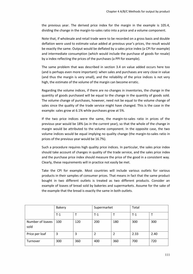
Chapter 4 A/B/C Methods for output by product
111
the previous year. The derived price index for the margin in the example is 105.4,
dividing the change in the margin-to-sales ratio into a price and a volume component.
Note that, if wholesale and retail trade were to be recorded on a gross basis and double
deflation were used to estimate value added at previous year’s prices, the result would
be exactly the same. Output would be deflated by a sales price index (a CPI for example)
and intermediate consumption (which would include the purchase of goods for resale)
by a index reflecting the prices of the purchases (a PPI for example).
The same problem that was described in section 3.4 on value added occurs here too
(and is perhaps even more important): when sales and purchases are very close in value
(and thus the margin is very small), and the reliability of the price indices is not very
high, the estimate of the volume of the margin can become erratic.
Regarding the volume indices, if there are no changes in inventories, the change in the
quantity of goods purchased will be equal to the change in the quantity of goods sold.
The volume change of purchases, however, need not be equal to the volume change of
sales since the quality of the trade service might have changed. This is the case in the
example: sales grow at 6.1% while purchases grow at 5%.
If the two price indices were the same, the margin-to-sales ratio in prices of the
previous year would be 18% (as in the current year), so that the whole of the change in
margin would be attributed to the volume component. In the opposite case, the two
volume indices would be equal implying no quality change (the margin-to-sales ratio in
prices of the previous year would be 16.7%).
Such a procedure requires high quality price indices. In particular, the sales price index
should take account of changes in quality of the trade service, and the sales price index
and the purchase price index should measure the price of the good in a consistent way.
Clearly, these requirements will in practice not easily be met.
Take the CPI for example. Most countries will include various outlets for various
products in their samples of consumer prices. That means in fact that the same product
bought in two different outlets is treated as two different products. Consider an
example of loaves of bread sold by bakeries and supermarkets. Assume for the sake of
the example that the bread is exactly the same in both outlets.
Bakery Supermarket Total
T-1 T T-1 T T-1 T
Number of loaves
sold
100 120 200 180 300 300
Price per loaf 3 3 2 2 2.33 2.40
Turnover 300 360 400 360 700 720
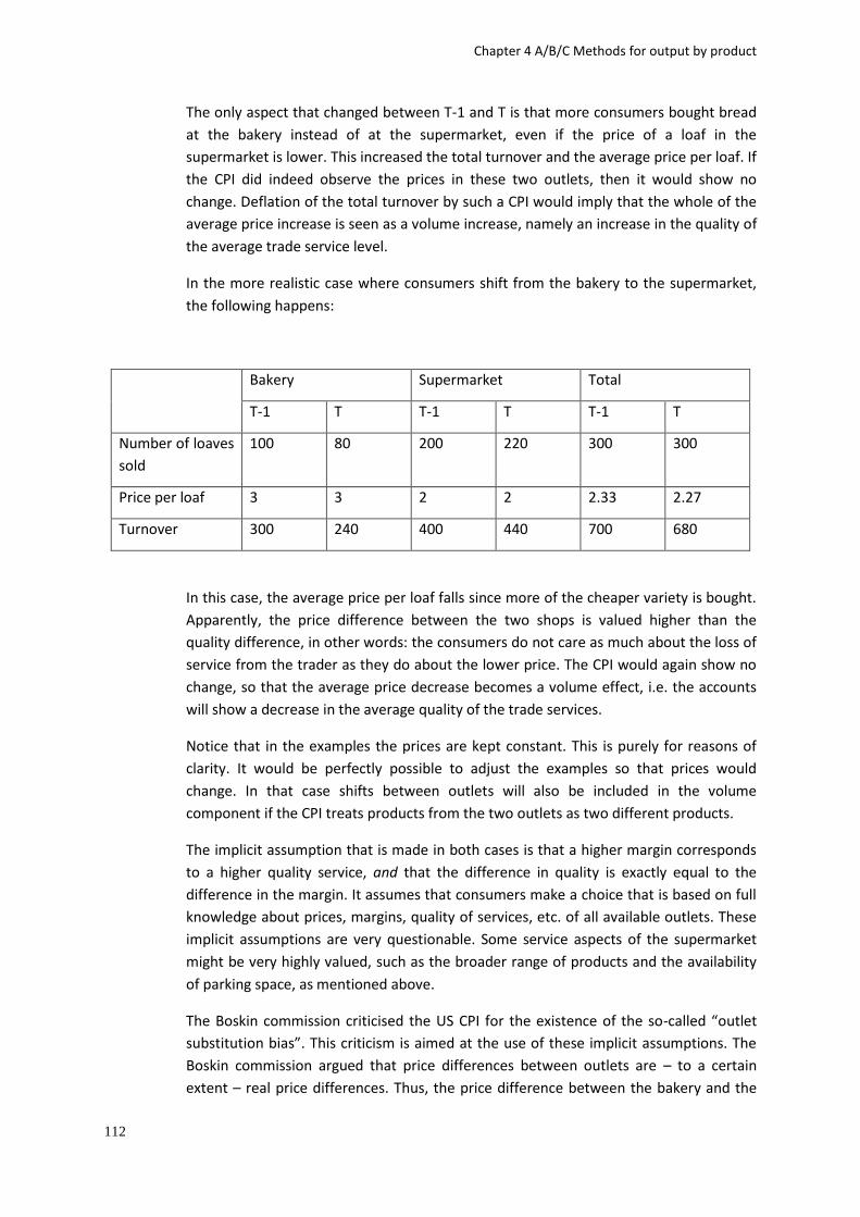
Chapter 4 A/B/C Methods for output by product
112
The only aspect that changed between T-1 and T is that more consumers bought bread
at the bakery instead of at the supermarket, even if the price of a loaf in the
supermarket is lower. This increased the total turnover and the average price per loaf. If
the CPI did indeed observe the prices in these two outlets, then it would show no
change. Deflation of the total turnover by such a CPI would imply that the whole of the
average price increase is seen as a volume increase, namely an increase in the quality of
the average trade service level.
In the more realistic case where consumers shift from the bakery to the supermarket,
the following happens:
Bakery Supermarket Total
T-1 T T-1 T T-1 T
Number of loaves
sold
100 80 200 220 300 300
Price per loaf 3 3 2 2 2.33 2.27
Turnover 300 240 400 440 700 680
In this case, the average price per loaf falls since more of the cheaper variety is bought.
Apparently, the price difference between the two shops is valued higher than the
quality difference, in other words: the consumers do not care as much about the loss of
service from the trader as they do about the lower price. The CPI would again show no
change, so that the average price decrease becomes a volume effect, i.e. the accounts
will show a decrease in the average quality of the trade services.
Notice that in the examples the prices are kept constant. This is purely for reasons of
clarity. It would be perfectly possible to adjust the examples so that prices would
change. In that case shifts between outlets will also be included in the volume
component if the CPI treats products from the two outlets as two different products.
The implicit assumption that is made in both cases is that a higher margin corresponds
to a higher quality service, and that the difference in quality is exactly equal to the
difference in the margin. It assumes that consumers make a choice that is based on full
knowledge about prices, margins, quality of services, etc. of all available outlets. These
implicit assumptions are very questionable. Some service aspects of the supermarket
might be very highly valued, such as the broader range of products and the availability
of parking space, as mentioned above.
The Boskin commission criticised the US CPI for the existence of the so-called “outlet
substitution bias”. This criticism is aimed at the use of these implicit assumptions. The
Boskin commission argued that price differences between outlets are – to a certain
extent – real price differences. Thus, the price difference between the bakery and the
Chapter 4 A/B/C Methods for output by product
113
supermarket in the example above cannot entirely be explained by the quality
difference in the trade service provided. This would imply that the consumers
experienced a price decline, not shown by the CPI.
The situation is even more complicated if new trade channels appear such as e-
commerce. Internet supermarkets, book stores and the like are able to survive on lower
margins because they have much lower costs. The appearance of such new outlets
effectively reduce the overall price level for the consumer.
In addition, consumers are increasingly purchasing goods over the internet, some of
which will be sourced from abroad. In this case, the retail price will include the cost of
distribution and may also be affected by any exchange rate movements. Deflation of
such trade should therefore be exchange rate adjusted.
In conclusion, a good-quality CPI would take quality changes in trade services into
account as far as they concern substitution between different outlets. It is unlikely that
in the compilation of CPIs often quality adjustments are made for changes in the
services provided by a particular outlet. And given the above remarks on the outlet
substitution bias, we can only conclude that even a good-quality CPI can take only
limited account of quality changes in trade services. That means that the above-outlined
procedure of deflating sales and purchases separately takes quality into account only to
the same extent as the CPI (or another index used for deflating sales).
Using the volume of sales
The most widely used method of estimating the volume of margin output is to assume
that the volume of margins follows the volume of sales. This assumes that margin-to-
sales ratios are constant in previous year’s prices. As can be seen from the first example
in the previous section (take the case where the margin-to-sales ratio in prices of the
previous year would be 16.7%), this implies that it is assumed that there are no quality
changes in the trade service.
A volume index of sales can be obtained by deflating sales by a sales price index. For
retail trade, this should be an index of retail sales prices, e.g. a CPI. For wholesale trade,
the appropriate index would be a wholesale price index, provided this measures the
sales prices of wholesalers (and not the price of their purchases). Where a wholesale
price index is not available, a CPI or PPI can be used as proxy. Which one is the more
appropriate depends on the product in question and on the importance of wholesale
compared with retail in the distribution chain of the product.
In the example (that relates to a retailer), the sales price index (e.g. the CPI) is 102.5,
yielding a volume index of 106.1. The latter would be used to extrapolate the margin
value of the previous year. The result would be as follows:
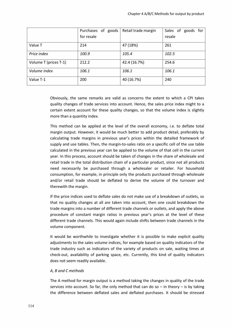
Chapter 4 A/B/C Methods for output by product
114
Purchases of goods
for resale
Retail trade margin Sales of goods for
resale
Value T 214 47 (18%) 261
Price index 100.9 105.4 102.5
Volume T (prices T-1) 212.2 42.4 (16.7%) 254.6
Volume index 106.1 106.1 106.1
Value T-1 200 40 (16.7%) 240
Obviously, the same remarks are valid as concerns the extent to which a CPI takes
quality changes of trade services into account. Hence, the sales price index might to a
certain extent account for these quality changes, so that the volume index is slightly
more than a quantity index.
This method can be applied at the level of the overall economy, i.e. to deflate total
margin output. However, it would be much better to add product detail, preferably by
calculating trade margins in previous year’s prices within the detailed framework of
supply and use tables. Then, the margin-to-sales ratio on a specific cell of the use table
calculated in the previous year can be applied to the volume of that cell in the current
year. In this process, account should be taken of changes in the share of wholesale and
retail trade in the total distribution chain of a particular product, since not all products
need necessarily be purchased through a wholesaler or retailer. For household
consumption, for example, in principle only the products purchased through wholesale
and/or retail trade should be deflated to derive the volume of the turnover and
therewith the margin.
If the price indices used to deflate sales do not make use of a breakdown of outlets, so
that no quality changes at all are taken into account, then one could breakdown the
trade margins into a number of different trade channels or outlets, and apply the above
procedure of constant margin ratios in previous year’s prices at the level of these
different trade channels. This would again include shifts between trade channels in the
volume component.
It would be worthwhile to investigate whether it is possible to make explicit quality
adjustments to the sales volume indices, for example based on quality indicators of the
trade industry such as indicators of the variety of products on sale, waiting times at
check-out, availability of parking space, etc. Currently, this kind of quality indicators
does not seem readily available.
A, B and C methods
The A method for margin output is a method taking the changes in quality of the trade
services into account. So far, the only method that can do so – in theory – is by taking
the difference between deflated sales and deflated purchases. It should be stressed

Chapter 4 A/B/C Methods for output by product
115
though that it is necessary to continue research into more accurate descriptions of the
trade industry, in order to improve the volume measurement and in general our
understanding of the trends in wholesale and retail trade.
A number of countries are experimenting with "margin price indices". These are price
indices that view the margin as the price of the trade service provided, and follow these
margins over time keeping the quality of the trade services constant. This method has
the potential of becoming an A method, provided it can indeed take appropriate
account of quality changes.
As a B method can be used the assumption that the volume of margins follows the
volume of sales, or – equivalently – that margin-to-sales ratios are constant in previous
year’s prices. This should preferably be applied in the framework of detailed supply and
use tables in previous year’s prices, and – if possible – in such a way that shifts between
outlets are included in the volume component of output.
Any other methods, in particular the deflation of margin output directly by a sales price
index, are C methods.
4.7.2 CPA 45 - Wholesale and retail trade and repair services of motor
vehicles and motorcycles
Apart from wholesale and retail trade services, yielding margin output, this division of
CPA contains the service output for maintenance and repair of motor vehicles and
motorcycles. For this type of output, PPIs could be available, in which case they
constitute the A method. If they are not available, the products can be deflated using
CPIs (corrected for any taxes or subsidies), which are a B method, because it might not
sufficiently cover business expenditure.
Furthermore, there are trade services that are paid for on a fee or contract basis. This
refers to situations where someone sells a product on behalf of someone else, thus
without purchasing the product him- or herself. For these services, the fees paid should
be the basis for deflation, in combination with the prices of the products sold. See e.g.
section 4.12.1 on real estate services for a similar case of services paid on a fee or
contract basis.
4.7.3 CPA 46 - Wholesale trade services, except of motor vehicles and
motorcycles
This division is divided into 46.1 Sales on a fee or contract basis and 46.2 to 46.7
Wholesale trade services (of various products). Wholesale trade services give rise to
trade margins and are covered in section 4.7.1. In section 4.7.2 some remarks are made
on sales on a fee or contract basis.
4.7.4 CPA 47 - Retail trade services, except of motor vehicles and
motorcycles
This division of CPA reflects the margin output of retail trade services discussed in
section 4.7.1
Chapter 4 A/B/C Methods for output by product
116
4.8 CPA H – Transportation and storage services In considering methods suitable for the estimation of prices and volumes for CPA H it is
useful to distinguish three separate groupings of services: transport services; supporting
and auxiliary transport services; and postal and courier services. For transport services,
the additional distinction between passenger transport and freight transport has to be
made.
4.8.1 CPA 49, 50 and 51 - Transport by land, water and air
Passenger transport
Key aspects
Transport services whilst very diverse in terms of the mode of transportation, have
much in common with one another. The service being provided is to move people from
one place to another. Within the different forms of travel (air, sea, rail and road) quality
is an important issue. Factors such as speed, convenience, comfort, reliability,
timeliness need to be considered because shifts can occur that need to be reflected
correctly in price or volume. This calls for measurement to be carried out at a detailed
level.
Some forms of passenger transport, principally those by bus and train, can be
purchased in different ways. Examples of these are the purchase of a ticket for a 'one-
off' journey or a season ticket that gives the right to travel any number of times within a
defined time period. Each different type of ticket could be seen as a separate product,
giving different rights under varying conditions. The output in current prices is
essentially equal to the number of tickets sold times the price per ticket, for all different
types of tickets. It follows that output in previous year’s prices should be equal to the
number of tickets sold times the price of each ticket in the previous year. This approach
is also followed in the compilation of price indices, where the prices of the different
forms of tickets are usually observed and weighted with total sales or purchases of each
type of ticket in the base year.
The consequences of this approach should be carefully considered. It implies for
example, that a kilometre travelled by train on a 'one-off' ticket is a different output
than a kilometre travelled on a season ticket. It also implies that a train travelling
without passengers still produces output, since season ticket holders have already paid.
In this case, output may be seen as not being directly related to the use of the transport
service, but as the right of access to it.
In many instances, volume data on the amount of passenger-kilometres produced are
available and are used in the national accounts as volume indicators. The use of such an
indicator typically assumes that only the actual transport of passengers yields output
(i.e. an empty train does not produce output).
To compare the variation in passenger-kilometres and tickets sold (per type of ticket),
the following formula can be used:

Chapter 4 A/B/C Methods for output by product
117
number of tickets sold * average number of travels per ticket * average distance per
travel
=
number of passenger-kilometres for this type of ticket.
From this formula it can easily be seen that if, for one type of ticket, the travel habits of
the population do not change over time, changes in the two indicators (tickets sold and
passenger-kilometres) will show the same trend.
For single (one-way) tickets, passenger-kilometres will give similar results as counting
the number of such tickets sold (since the average number of travels per tickets is by
definition equal to one). However, there are examples where such a ticket permits
travel within a pre-defined area rather than simply from one location to another, for
example city travel tickets. Then, the relation between the number of tickets and
passenger-kilometres depends on the changes in the average distance travelled per
ticket.
For season tickets, the relation between passenger-kilometres and tickets sold depends
both on the average number of travels per ticket and the average distance travelled
each time. It is possible to imagine the case where the season ticket holder makes no
actual journeys, in which case the number of passenger-kilometres is zero, but still
output is produced.
The opposite case is that of free travel: in some cases, students or elderly people can
travel for free on bus or train. Then, this travel will be included in the number of
passenger-kilometres but not in an index based on tickets sold. One could wonder
however if this travel is indeed truly free-of-charge. Usually, the government will pay
the transport company for the travel of those people.
Tickets restricted to peak or off-peak travel and first class or second class travel also
represent different qualities of product. Quality has already been identified as an
important issue for transport services. Prices of different tickets are readily available,
and conditions of sale can be monitored relatively easily. This should allow the correct
estimation of price and volume provided the output at current prices can be identified
separately for each type of ticket.
Discounts are also commonly offered for passenger transport services. Road, rail and
sea transport may be offered at reduced prices on presentation of a discount card. Air
tickets are often available for the same journey at different prices depending on factors
such as the degree of flexibility offered to the traveller or the time before the date of
travel that the ticket is purchased. Regular flyer programmes also offer discounted
airfares, free flights or upgrades, all of which represent different quality products that
need to be reflected correctly in prices and volumes.
A significant complication in the deflation of output of passenger transport is the
frequent occurrence of subsidies. Whereas transport companies have become market
Chapter 4 A/B/C Methods for output by product
118
producers in most countries, they are often largely subsidised in order to keep prices
affordable or to keep certain unprofitable routes open. The nature of the subsidies can
vary considerably between countries. In some cases they are given per passenger-
kilometres produced, in other cases they are a lump-sum amount. ESA 2010, par.
4.35(c), states that such subsidies are to be seen as subsidies on products (D319), and
are therefore part of the basic price. Deflation of subsidies on products is discussed in
section 3.10.
Data availability
For transport services provided to households, CPIs are generally available. PPIs for
transport are increasingly collected, although volume indicators such as passenger-
kilometres are more widely available. However, the level of detail for such volume
indicators is often limited.
A, B and C methods
The very different nature of the products covered within this CPA category makes it
sensible to define a minimum level of detail to be used in estimating prices and
volumes. For passenger transport, the product level used should, subject to each
product making a significant contribution to output, at least identify separately:
transport via railways,
other land transport,
water transport and
air transport.
If these breakdowns are not attained, any method will be a C method.
Detailed current price data is required as weights for price or volume indices. If product
level detail at current prices is not available at the level described above, other
indicators could be used as weights. These other indicators will still need to distinguish
the different types of transport and approximate the current prices as closely as
possible.
The use of appropriate PPIs is an A method. For PPIs to be considered appropriate they
would need to cover the various types of tickets available.
The use of a CPI adjusted to basic prices for passenger transport is a B method providing
it takes sufficient account of quality changes.
Volume indicator methods based on passenger-kilometres for passenger transport are B
methods, since it has to be assumed that travel habits of the population do not change
significantly. The more detail available for these volume indicators, the better will be
the result. For passenger transport the volume indicators should at least distinguish
between the different classes of travel, for example first and second class for rail
transport and economy and business class for air transport.
Chapter 4 A/B/C Methods for output by product
119
All other methods are C methods, including the use of volume indicator methods based
only on the number of passengers transported.
Freight transport
Key aspects
For freight transport, it is more difficult to compile price indices than it is for passenger
transport. That is because there are in general no fixed tariffs. The price for transporting
goods from A to B can depend on a variety of factors, such as the distance between A
and B, the weight of the freight, whether it concerns a domestic or an international
journey, whether there is return freight from B to A, the kind of product transported
(livestock, bulk products, chemicals, etc., they require different facilities and are
therefore differently priced), etc. Thus, one can say that freight transport has - at least
to a certain extent - the characteristics of unique products.
One way of compiling price indices is therefore to resort to a form of model pricing (see
also section 2.5). A set of representative standard journeys could be formulated which
would be priced by the producers of the transport services. A hedonic approach in
which the price of each journey is regressed on its characteristics is also imaginable. In
each case, the characteristics "weight of load" and "distance" would be included in the
analysis. But both approaches offer the opportunity to monitor for other (quality)
aspects of the journeys.
The volume of output can also be approximated directly by the use of volume indicators
such as tonne-kilometres. This indicator, however, only accounts for load and distance
and therefore cannot take changes in other aspects into account.
Transport services can also be an important component of exports or imports of
services and methods described here are also appropriate for external trade in services.
Furthermore, a large part of the output of transport services (i.e. the part related to the
transport of newly produced goods) forms part of the difference between the basic
price and the purchaser's price of a good. These are the transport margins (see ESA
2010, par. 9.37 for a definition). For the deflation of the transport margins, the same
rules apply as for transport services in general.
Data availability
PPIs for freight transport are not widely available, probably due to the problems of
measurement mentioned above. However, volume data on tonne-kilometres are widely
available, generally broken down by mode of transport.
A, B and C methods
For freight transport, the product level used should, subject to each product making a
significant contribution to output, at least identify separately:
transport via railways,
Chapter 4 A/B/C Methods for output by product
120
other land transport,
transport via pipelines,
sea and coastal water transport,
inland water transport and
air transport.
If these breakdowns are not attained, any method will be a C method.
Detailed current price data are required as weights for price or volume indices. If
product level detail at current prices is not available at the level described above, other
indicators could be used as weights. These other indicators will still need to distinguish
the different types of transport and approximate the current prices as closely as
possible.
The use of appropriate PPIs, possibly based on the model pricing approach, would
constitute an A method for freight transport. Volume indicator methods based on
tonne-kilometres transported are B methods.
All other methods are C methods, including the use of volume indicator methods based
only on the number of tonnes transported.
4.8.2 CPA 52 - Warehousing and support services for transportation
Key aspects
Many of the services of this branch are provided only to businesses. The services are
generally provided on payment of a fee or commission that will either be rendered on
an individual transaction basis or for a contracted period. Some services may be unique
or not widely used, such as those supporting air and water transport where the service
may be provided centrally for a region or even a country, for example air traffic control.
Fees will be set based on a number of possible methods, examples of which are:
according to the amount of time the service has been used, for example car
parking;
on the basis of both the time and volume of the service used, for example
storage where the amount of space occupied is an important factor as well as
time;
the number of items on which the service is provided, for example cargo
handling services provided for freight in containers or the number of tickets sold
by a ticket office;
the weight of the items on which the service is provided, for example cargo
handling services provided on non-containerised freight or passenger baggage;
Chapter 4 A/B/C Methods for output by product
121
a fee fixed in advance for the provision of a package of services over a period of
time, for example air traffic control or the service provided by lighthouses.
Data availability
PPIs for warehousing and storage services and for cargo handling services are broadly
available. CPIs might be available for a number of these services that are provided to
households. Some volume indicators are potentially available, but their coverage is
unlikely to be as comprehensive as necessary to capture adequately any shifts between
products or changes in quality.
A, B and C methods
The very different ways in which prices are determined for these products makes it
difficult to define a classification of methods by product. It is easier to classify methods
in terms of the way prices are determined and this approach will be used in the
paragraphs that follow.
Where prices are set according to the amount of time used, price indices that reflect the
change in unit price will be an A method. The use of volume indicators that are time
based (minutes, hours, days, weeks etc depending on the charging period) would be B
methods. If pricing is banded into time units with different unit prices for bands, ie the
two-hour rate is not twice the one-hour rate, volume indicators would need to reflect
these bands to be B methods.
For services where the charge is dependent on both time and volume, price indices
would need to reflect these characteristics to be A methods. Where many rates are
available for a service charged in this way it may be more appropriate to use model
pricing and this would also be an A method providing the models were representative
of the full range of services produced. Volume indicators would need to take account of
both the time and the volume, for example, volume indicators for storage should be
measured in cubic metre days or an equivalent that related to the charging method
used for the supply of the service.
Where the service charge is directly related to the number or weight of items on which
the service is provided, the use of appropriate price indices would be an A method
provided account is taken of changes in quality or a B method if not. Volume indicator
methods that relate to the number or weight of items handled would also be a B
method.
Where services are provided against payment of a fixed fee the use of appropriate price
indices would be an A method. The use of model prices would also be an A method
providing the models are representative of the full range of services provided. Changes
in quality can be an important factor for services provided by a fixed fee and if this is
not reflected in the price indices their use would be a B method. Volume indicator
methods would also need to take account of changes in quality to be B methods.
Chapter 4 A/B/C Methods for output by product
122
4.8.3 CPA 53 - Postal and courier services
Key aspects
This product group covers postal services under universal service obligation and other
postal and courier services .
For most types of postal services the price is determined by a range of factors, such as
size of packet, weight of packet, speed of delivery and destination. The price for other
postal services, such as post-restante or mailbox rental, are usually set on a fee or
transaction basis. Price tariffs can be complicated because of the range of different
products offered, but they are readily available for the household consumer.
Prices for business customers are more likely to be based on contract prices that are
more difficult to measure and may require a model pricing approach. It is also necessary
to take account of discounts for business users. Discounts may be based around such
diverse factors as the quantity of the service consumed or the fact that the business
customer pre-sorts the post before it is handed over to the postal company for delivery.
Data availability
PPIs are widely available. CPIs are generally available. Volume indicators are available
for the services of the National Post although these may not be at a sufficient level of
detail to ensure homogeneous products.
A, B and C methods
The use of appropriate and representative PPIs that take account of quality changes
would be an A method. For PPIs to be considered appropriate and representative they
would need to cover the full range of services produced and take account of any
discounts. The use of a CPI for post services, adjusted to basic prices, would be a
suitable A method only for that part of output provided to households.
PPIs that do not cover the full range of services or do not take account of changes in
quality would be a B method. UVIs for truly homogeneous products, would also be a B
method. Volume indicator methods based on detailed indicators of the many types of
services provided, for example number of letters/parcels broken down by different
postage rate, are B methods.
The use of detailed CPIs to deflate output other than that consumed by households can
be a B method if price developments can be shown to be similar for households and
businesses. However, CPIs are unlikely to be suitable for the full range of postal
services, because of the availability of discounts and the different range of products
consumed by businesses. Using detailed CPIs for business purchases where it is know
that businesses receive discounts or purchase a different range of products than
households would be a C method.
Chapter 4 A/B/C Methods for output by product
123
4.9 CPA I – Accommodation and food services Key aspects
The accommodation and food services heading covers the provision of accommodation
(from campsites and youth hostels to expensive hotels) and food services, including the
output of bars, discotheques and work canteens. The basic product (a room, meal or
drink) is often bundled together with other services such as room service and breakfast
in a hotel, and music or other entertainment in a bar. It is therefore important that any
services that are not included in the price are classified and measured separately. An
example would be laundry services in a hotel, which are usually optional extras for the
guest, and should be measured under CPA S.
There are three major issues to be considered when compiling data for these services:
Quality – The wide coverage of this product heading means that very different
qualities of products are included – youth hostels and five star hotels, take-away
kebab stalls and Michelin-rated restaurants. Proper price and volume
measurement would imply that the greatest possible product detail is obtained
in the data, so that separate prices and values are collected, and any aggregate
data are constructed using appropriately weighted subsets. For example, in hotel
services, separate collection of data for different ratings of hotels enhances the
measurement of price and volume movements.
Group bookings and discounts – One common feature of the hotel trade is that
there can be considerable discounts available for block bookings, for example
when a tour operator purchases a block of rooms for a season. Changes in these
discounts should be viewed as a price effect and recorded in the price index.
Household and Business consumption – Whilst the product consumed is unlikely
to differ for household and business consumption (business people and private
persons can stay in the same hotels and eat in the same restaurants), it is
possible that the weighting structure will be rather different, with private
persons consuming a greater proportion of the cheaper products. Of course, the
discounting of rooms for tour operators could mean that some private persons
can afford higher quality rooms than they would be able to afford at the regular
hotel price.
Data availability
Price data on the accommodation and food service industries are collected as part of
compilation of CPIs, whilst value data are collected from surveys of businesses in the
industry. PPIs are rare particularly in those areas of the industry characterised by many
small producers (such as the cheaper end of the takeaway market), and often cover
only part of the product heading.
Volume data are often available for “bed-nights” in accommodation and “meals served”
in restaurants, but the level of detail is usually not very high.
Chapter 4 A/B/C Methods for output by product
124
A, B and C methods
Where PPIs are available which meet the general criteria set out in section 2.3, deflation
of output by these indices at an appropriate level of detail is an A method. If the PPIs
are only partially representative, or do not completely reflect quality changes, this
becomes a B method.
Use of the CPI data adjusted to basic prices is considered an A method where it can be
shown that prices for business people and private consumers move in a similar way and
the compositions of consumption are comparable. Where studies indicate that the price
movements or weights differ significantly, use of the adjusted CPI data becomes a B
method.
It may be that for some areas, the variety of goods and services bundled with the
standard product is such that it is difficult to isolate price movements (for example
where entertainment is provided along with a meal or drink). It may be appropriate
here to employ a model pricing method, as described in section 2.5, and this could
represent an A method if the conditions set out in that section are met.
Use of volume indicators such as “bed nights” and meals sold are B methods so long as
the breakdown by type of product is sufficiently detailed to give confidence that major
variations in quality are captured.
Any method based on the use of input data, or crude volume data (such as number of
clients in a hotel or bar), is a C method.
4.10 CPA J – Information and communication services CPA J covers a wide range of products including publishing services, motion picture
services, programming and broadcasting services, computer services and information
services. These are discussed in turn.
4.10.1 CPA 58 - Publishing services
Key aspects
Publishing services includes traditional printed books, as well as on-line books,
newspapers, computer games (both packaged and downloads) and software (packaged
and downloads),
Some of these services are for business use only, while others can be purchased by both
consumers and businesses. Prices should be observable for both, either through the CPI
or PPI (although not mandatory in Europe). Packaged software are usually standard
products, either system or application software, and prices should be observable.
ESA 2010 recognises computer software as an intangible fixed asset, and as such
expenditure on software should be recorded as gross fixed capital formation. This
includes a significant share of software produced on own account (to be valued at basic
prices). Hence, expenditure on software - which is ever increasing - adds directly to
GDP, and the choice of deflator for software has a direct effect on the volume growth of

Chapter 4 A/B/C Methods for output by product
125
GDP. This can be compensated however if a large share of the software is imported and
the same deflators are used for those imports.
An increasingly important phenomenon is the supply of free software, for example via
the internet. There can be various reasons for supplying software for free. A company
could use it as a "loss leader" (the loss will be very small anyway since the marginal cost
of producing extra copies of software is virtually zero) to generate purchases of other
software or to generate internet subscriptions. In other cases, the software is in fact
funded by advertisement, either in the software package itself or on the website it can
be downloaded from. See section 3.2 for more discussion of the treatment of free
output funded by advertising.
Software packages are continuously being developed. New versions with more
functions than the previous one are frequently brought on the market. These appear
often in the form of upgrades, which should be seen as a different product than a
complete version of the package. Nowadays, software can also be purchased via the
internet at lower prices than in a retail shop. These different outlets have to be
distinguished when constructing price indices. Also, for businesses, the price of the
software often depends on the number of user licences purchased rather than the
actual number of copies of the software.
These quality changes are still taking place at a very fast rate (although on the average
probably not as fast as for computers), making proper quality adjustments for software
very important but also very difficult to implement. Whereas for computers, the quality
can be determined by their technical characteristics, for software those determinants
are much more difficult to recognise. Furthermore, new software versions usually
require more system resources in terms of memory size, hard disk, monitor, etc. Should
this be seen as a quality improvement or deterioration?
The market for operating systems and general office applications is rather dominated by
one large enterprise. This raises doubts about the competitiveness of the market and
hence about the usefulness of market prices for evaluating quality changes. On the
other hand, good coverage of the market is relatively easy to obtain.
As discussed in section 3.2.2, the price of newspapers may be reduced by the
advertising income. In this case, a price index would need to reflect the advertising
rates charged by the newspaper and a volume indicator the quality and quantity of
advertising space sold. It would be conceptually wrong to apply a price index that
reflects the cover price of newspapers or software that are actually purchased, such as
the CPI for newspapers. This is because the price development of the advertising space
being sold is unlikely to be the same as that of the cover price of newspapers. If data is
available, the advertising revenue should be recorded as a secondary product and
recorded under CPA73.
The same issue will also apply to some computer software, where the price to the
consumer is reduced because of the advertising that is included in the “package”. The
Chapter 4 A/B/C Methods for output by product
126
price index in this case should also reflect the advertising rates charged by the software
provider and a volume indicator the quality and quantity of advertising space sold.
Data availability
CPIs may include packaged software. They may also implicitly include software
purchased together with computers in the CPI for computers.
A, B and C methods
For packaged software, the A method is to deflate with an appropriate PPI. Quality
changes play a significant role, so an appropriate quality adjustment procedure (e.g.
based on hedonics) is essential. It is doubtful whether a CPI for packaged software can
give a reasonable approximation of the output price. The business market for packaged
software is quite different from the consumer market. For example, businesses buy
licenses in large quantities and can therefore obtain discounts. Hence, although a CPI
can be used to deflate household consumption of software, it will be a C method for the
deflation of output. There are also two different groups of business purchasers, those
that buy software for inclusion in their own products which is intermediate
consumption (e.g. a computer manufacturer who bundles software with their
hardware) and that purchased for use directly within the business (capital formation).
The prices for these business purchases will be different and PPIs need to reflect this
adequately for them to be considered suitable as an A method.
Less appropriate PPIs will be B methods.
In view of the differences in the speed of quality changes, the use of an index for
hardware to deflate software should be called a “C” method.
4.10.2 CPA 59 - Motion picture, video and television programme
production services, sound recording and music publishing and CPA 60 -
Programming and broadcasting services
Key aspects
The major part of this group of products is the production of original films, TV and radio
programmes (where each product is unique).
Certain of these products may be provided without charge to the user, or at a charge
which is significantly below production costs. This issue is discussed in section 3.2 of this
handbook, where a suitable recording method is suggested.
Data availability
Data on production of films and programmes is difficult to collect. It may be possible to
use “model pricing” methods, where a standard TV or radio series is priced by
production companies (see section 2.5 for further discussion). Within Europe, the
annual AUVIS (audio-visual) questionnaire collects data on production of radio, TV and
cinematic programmes.

Chapter 4 A/B/C Methods for output by product
127
A, B and C methods
Possible B methods for film and TV/radio programming production are to collect prices
for certain model products (e.g. half an hour of a domestic TV comedy, an hour of a
radio documentary), or to use quantity data on programming broken down by major
categories of programme and weighted by the share in value of total programming.
4.10.3 CPA 61 - Telecommunication services
Key aspects
Telecommunication services are an area with a wide range of products that are
developing quickly. Products include fixed lines, mobile phones, internet service
provision, voice over internet telephony, and home programme distribution. Whilst the
charging mechanisms employed are often very complex they are based around three
broad elements - a 'one-off' connection fee, a regular rental charge and a usage (call)
charge. Not all three charging elements necessarily apply to all products, for example
there may be no 'one-off' connection fee for some products or there may be no charge
made for the actual use made.
The charging elements used are often arranged in different combinations to target
particular groups of users, for example a low rental with high call charges for low use
(household) customers or a high rental with low call charges for high use (business)
customers. The creation of these many different packages, and their continued
evolution, is one of the factors that make the measurement of prices for
telecommunications difficult.
Technological developments bring about changes in the quality of products. These
developments are particularly rapid in the area of telecommunication services. This
makes it important to ensure that any changes in quality are adequately reflected in
whatever methods are used. For mobile phone services the use of hedonic methods
may be seen as a suitable way of ensuring that the many quality changes that occur
both often and quickly are adequately captured.
Discounts are another important factor that need to be reflected adequately in any
method to ensure the correct measurement of price and volume. Again discounts are
designed by the telecommunication service providers to target the many different kinds
of user of their services. For example, discounts are offered to high volume business
users whilst at the same time low user discounts are also available. Discounts can also
be designed around a specific type of usage, for example the offer of a cheaper call
charge for certain telephone numbers identified by the customer. Discounts may be
offered in terms of extra minutes, texts or additional bandwidth, rather than a simply
reduction in price. This may be difficult to price, as such discounts may not affect the
price of the service, but the capacity has increased. An additional problem when
considering discounts for telecommunications services is the actual take up of the
discount by customers, as they are not provided automatically. Producers of
telecommunication services often require their customers to register for a particular

Chapter 4 A/B/C Methods for output by product
128
discount scheme before the actual discounts are made available, resulting in not all
customers actually receiving the discounts on offer.
The bundling of products is also an issue that needs to be considered for this product
group, particularly for mobile phone services. It is becoming more and more common
for the mobile phone handset to be bundled into a package with the communication
service. The handset can be offered without direct charge, at a price less than its full
value or at its full value, each of these handset pricing options being linked to different
charging mechanisms for the telecommunication service. The primary aim of offering
the handset at low or no charge is to reduce the initial cost of access to the
telecommunication service. The telecommunication service provider then recovers the
cost of the subsidy they have made on the handset through higher rental and/or call
charges. The customer is usually required to enter into an agreement with the
telecommunications provider to subscribe to the phone service for a minimum length of
time, to ensure the provider recovers the subsidy they have made on the handset.
When constructing price or volume indicators these bundled products should be
considered as different products. This bundling is no different to that seen with other
products, for example computers and software and can be treated in similar ways, see
section 4.8.6. An interesting secondary issue to consider with a bundled product is to
which product group it should be related, for example is a bundled mobile handset and
telecommunication service a telecommunication product (a service) or a handset
product (a good). In the case of a bundled handset and telecommunication service it
seems sensible to consider this a telecommunication product as the motivation for
acquiring the handset is to make it possible to use the telecommunication service. Any
quality change associated with the handset that is provided as part of such a bundled
service would then need to be correctly reflected in the price and volume measures of
the telecommunication service.
Pricing telecommunication services may be affected by wholesaling arrangements
between the service provider and the owner of the network/infrastructure. Similarly
tailored packaging will make tracking prices for a representative proportion of the
services provided difficult.
Internet service provision (ISP) consists only of the provision of services necessary to
access the internet. This product does not include other services associated with the
internet such as web hosting, domain name registration or the provision of advertising
which are part of professional, scientific and technical services. ISP is an interesting
element of this product group. This is not only because the product is relatively new and
developing rapidly, but also because of the creation of new charging mechanisms and
the bundling of this product together with others. For example, some companies make
the ISP product available without charge to the user or they bundle it together with
telephone services. Whilst the introduction of these new products creates challenges
for the correct measurement of price and volume, they present no new conceptual
problems. The provision of ISP without charge to the user can be seen as no different
from that of 'free' newspapers, television or software and the recording in the accounts
should be similar. Further detail on the treatment of products provided without charge
Chapter 4 A/B/C Methods for output by product
129
to the user can be found in section 3.2. The bundling of ISP with other
telecommunication services is also no different from bundling of other services, such as
computers and software, or mobile phone calls and handsets, and they should be
treated similarly.
Data availability
PPIs are available in most countries, CPIs are more widely available although their
coverage is often limited to only fixed line telecommunication services. A number of
methods have been studied and a unit value approach has been shown to be feasible
and to provide acceptable results.
A, B and C methods
When considering the suitability of methods it is important to ensure that indicators are
fully representative of the products and the full range of charges made. For example,
where the provision of the service is dependent on the payment of a connection charge,
regular rental payments and individual call changes, these will all need to be reflected in
the indicators used if they are to be considered suitable.
The deflation of output by quality adjusted PPIs would be an A method. The use of CPIs,
adjusted to basic prices, for the output consumed by households (for example television
cable services) would also be an A method. In constructing price indices it is important
to ensure that the weights used are up-to-date and that the coverage of the individual
prices is representative of the full range of output. This is especially true for
telecommunication services where products change rapidly.
The use of PPIs where their coverage does not exactly match the products or where
there is no adjustment for quality is a B method. UVIs for products that are entirely
homogeneous would also be a B method. The use of volume indicators that reflect the
full range of outputs is a B method.
The use of detailed CPIs to deflate output other than that consumed by households can
be a B method if price developments can be shown to be similar for households and
businesses. However, CPIs are unlikely to be suitable for the full range of
telecommunication services, because of the availability of discounts and the different
range of products consumed by businesses. Using detailed CPIs for business purchases
where it is know that businesses receive discounts or purchase a different range of
products than households would be a C method.
4.10.4 CPA 62 - Computer programming, consultancy and related services
Key aspects
CPA 62 Computer and related services can be roughly subdivided into a number of
services according to their price mechanism:
Computer programming services (62.01
Computer consultancy services (62.02)
Chapter 4 A/B/C Methods for output by product
130
Computer facilities management services (62.03):
Repair services of computers are included in CPA 95. Computer software is included in
CPA 58.
Some of these services are for business use only, while others can be purchased by both
consumers and businesses.
Bundling computer services with hardware is now the norm. The most evident example
is the bundled sale of PC and operating system, but also in the business market
software is increasingly incorporated into industrial machinery or maintenance
contracts are part of the package. The present product classification does not recognize
this bundling problem, which may create problems in measurement.
For example, it can be assumed that the data on household consumption of personal
computers will include expenditure on software purchased together with the PC.
However, software is usually produced separately from the hardware (and classified in
CPA 58). Hence, the data sources on production and consumption will differ in their
content. The same holds true for the data sources on prices of production and
consumption of computers and software: producer prices will usually separate
hardware from software, while consumer prices will often combine these. The problem
is acute in particular when the 'packaging' is done by wholesale or retail traders, since
then in principle there is no producer of the bundled product.
Most of the software included when buying a PC will also be available separately. One
cannot however take the price of the software if purchased separately as an indication
of the share of the software in the price of the PC, since bundled software is usually sold
at discounted prices.
One suggestion to deal with this problem in compiling national accounts is to introduce
at the working level one or more special product groups for the combination of
hardware and software. This would make it easier to balance the accounts. However, in
the end the combined product will have to be either separated again to compile the
supply and use tables, or included in either hardware or software. An alternative could
be to regard the packaging of hardware and software as a specific transformation
process resulting in a new product. However, the general classification rules concerning
assembling would not support such a solution.
In any case, it is important that for the deflation of whatever product the price index
used is relevant for that product. Thus, if household consumption of PCs contains a fair
share of software, the price index used for deflating that expenditure should take this
into account, and should measure the price change of the combined product. That
means for example that changes in the software provided with the PC are to be treated
as quality changes of the PC.

Chapter 4 A/B/C Methods for output by product
131
Data availability
An increasing number of price indices for computer services are currently available. In
some countries second-best solutions are employed, such as input-indicator approaches
(use of wage rates, number of employees).
In relation to the availability of suitable data on computer service prices, there is an
important distinction between standard (non-customised) products and customised
products. Prices of standard products (e.g. packaged software) can be collected
relatively easily, through observations of actual transactions or, alternatively, through
magazines or on the internet. Customised products are unique, and therefore product
definition and price measurement are much more difficult (see section 2.5).
A, B and C methods
In view of the increasing importance of investment in information and communication
technology in general and computer services in particular, it becomes more and more
urgent to develop high-quality price indices for these services.
For customised services (both hardware and software consultancy) an approach based
on "representative pricing" (see section 4.13.1 on legal services) could be explored and
has the potential to constitute an A method. Another A method could be an approach
based on model pricing, i.e. an approach based on asking producers to price a “standard
service”, as long as the models are representative. In practice, due to the difficulties in
defining representative models, model pricing will usually be a B method. The result of
the model pricing approach could also be used as a proxy for the price of software
produced on own-account (B method), if it can be shown that the own-produced
software could also have been produced by an external company.
For the service of renting out programmers on a per-diem basis, as a B method the
charge-out rate could be used.
4.10.5 CPA 63 - Information services
Key aspects
Information services include data processing, hosting and related services; web portals
and the output of news agencies. There are a number of private companies providing
these services.
Web portal and news agencies services are often provided on a subscription basis, but
there are also some industry-level organisations such as Press Associations. The output
of freelance journalists and cameramen also counts under this product heading.
The number of news items released could be seen as a suitable indicator for the output
of news agencies. Whilst the individual news items are unique, there may be a
classification system for the quality of the material (which then determines the price)
and the overall volume of product (whether as “column inches” or number of
photographic images).
Chapter 4 A/B/C Methods for output by product
132
Data processing is normally charged on a per unit basis, while hosting will also be
provided and charged according to the service provided. While some may be standard
packages, others are likely to be bespoke, so that they become complex to measure. In
addition, as web services improve (such as through improved bandwidth), it becomes
important to measure quality change.
Data availability
Where the news agency business is dominated by a few large firms or associations, data
collection should be relatively straightforward, and use can be made of quality and
volume indicators used by the firms for their own internal management. Measuring the
output of many freelance journalists and cameramen is much more difficult – the only
reliable source is the newspapers and magazines accepting the information, but
reporting this input separately would be a considerable additional burden.
PPIs for data processing, hosting and related services, and web portals are available in
some countries.
A, B and C methods
The A method for web hosting and news agency services is to use a model pricing
method based on subscriptions. The model pricing method should conform to the
general principles set down in section 2.5, particularly for representativeness (the range
of models should cover the major subscription types). Clearly, this method may be
suitable only for some news agency activities.
The B method for web hosting and news agencies is to use quantity and quality
indicators employed by the firms themselves to measure output, so long as these can
reasonably be compared across the industry and are stable in definition from one
period to the next.
The A method for data processing, hosting and related services is to use a model pricing
method based on the volume of data being processed or the volume of storage
provided, covering the range of services provided under this category. The B method
would be to use the quantity information from the companies directly.
4.11 CPA K - Financial and insurance services The products and services provided by financial intermediation are many in number and
can be subject to rapid change as customer requirements and market conditions
develop. Output, at current prices, for the part of financial intermediation that is
indirectly measured (FISIM) and for insurance is measured by convention in the national
accounts. These conventions make measurement in volume terms even more
problematic, especially where quality change is considered an important factor.
Chapter 4 A/B/C Methods for output by product
133
4.11.1 CPA 64 - Financial services, except insurance and pension funding
Key aspects
The output of financial services can be seen as the activities associated with the
management of accounts, loans and saving and investment instruments. When
considering suitable methods for the measurement of prices and volumes for financial
services it is helpful to look at the different possible methods of charging for these
products rather than the individual products themselves. This is because different
methods of charging can be used over time for the same product or by different
countries. For example, it is possible to offer cheque account services either by direct
charges for each individual transaction, by some indirect method that is not directly
related to the service provided, or a combination of the two. In this way banking
enterprises can in some way hide the real cost of the services they provide from their
customers.
The output of financial services consists of two main components: financial
intermediation services directly charged by financial intermediaries to their clients
(measured as the sum of fees and commissions charged) and FISIM, the English
acronym for “financial intermediation services indirectly measured”. Though FISIM is
still the largest component by far in Member States, the importance of fees and
commissions is increasing over time. As far as volume measurement and deflation are
concerned, FISIM causes some major conceptual and practical problems. This is related
to the way FISIM has been defined and has to be calculated.
In considering methods suitable for these products it is appropriate to consider FISIM
separately.
Financial intermediation services indirectly measured (FISIM)
FISIM can be defined as the value of financial intermediation services that are not
charged for explicitly. Financial intermediaries pay lower rates of interest than would
otherwise be the case to those who lend them money and charge higher rates of
interest to those who borrow from them. Differences between the reference rate (a
‘virtual’ interest rate between the two effective interest rates) and the effective rate on
loans or deposits represents the margin earned by the financial intermediary.
Financial intermediation outside FISIM
Apart from FISIM, output of financial intermediation services consists of selling products
for which fees or commissions are charged directly to the customers, just as for other
products. Fees and commissions can take a number of forms, such as:
A flat rate fee for a transaction or service. For example, a charge for the
provision of a credit/charge card or a handling fee associated directly to a
financial transaction;
A fee based on the value of a transaction stock or flow, ie ad valorem charge. For
example, the fee for the management of an investment fund is likely to be linked
Chapter 4 A/B/C Methods for output by product
134
directly to the value of the fund whereas the fee charged for the sale of a
security is linked to the value of that sale.
A combination of a flat rate fee and ad valorem charge. For example, the charge
associated with the conversion of one currency into another where the total
charge to the customer can be on the basis of a flat rate fee and a percentage of
the value of the currency being converted.
Change in quality is a factor that needs to be reflected adequately in any method
employed. The length of opening hours for bank branches, the proximity of a local
branch, the availability of direct access to a full range of services and products, the
quality of investment advice and the performance of investment fund managers are
some of the features that determine quality for financial intermediation services.
One exception where direct charging is not appropriate is the central bank. ESA 2010
par. 3.63 explains that the output of the central bank is measured as the sum of its
costs.
Data availability
Financial intermediation services are not well covered by price indices. Some CPIs do
exist, but these relate only to the prices charged to households and are unlikely to
reflect adequately the range of services and charges made to businesses.
Volume indicators are more readily available and are being used by the Netherlands in
their calculation of volume output for banking services.
A, B and C methods
To allow the classification of methods it is helpful to consider services provided using
charges from fees and commissions separately from FISIM. The use of a combination of
direct and indirect charges by financial institutions creates a problem for accurate price
and volume measurement because over time there may be a move away from the use
of FISIM to direct charges or vice versa. The impact of this problem can be reduced by
keeping the base year and weights for the FISIM calculation up-to-date. In this way the
base period margin being applied (in the reference rate approach, see below) or the
weight given to the detailed volume indicators (in the output indicator approach, see
below) better reflect any change between the use of direct charges and FISIM.
Financial intermediation services indirectly measured (FISIM)
The following method is a B method.
Volume estimates of FISIM are calculated using stocks of loans and deposits deflated to
base period prices using a general price index such as the implicit price deflator for
domestic final demand.
The price of FISIM has two components: the first is the difference between the bank
rate of interest and the reference rate (or the reverse in the case of deposits) which
Chapter 4 A/B/C Methods for output by product
135
represents the margin earned by the financial intermediary; the second is the price
index used to deflate the stocks of loans and deposits to base period prices.
FISIM in volume terms are calculated as follows:
FISIM in volume on the loans granted to the institutional sector =( FISIM on the loans
granted to the institutional sector)/ price index * base period margin /effective margin
FISIM in volume on the deposits of the institutional sector = (FISIM on the deposits of
the institutional sector)/ price index * base period margin/effective margin
Base period margin on loans = the effective interest rate on loans less the reference
rate.
Base period margin on deposits = the reference rate less the effective interest rate on
deposits.
In nominal terms, the effective margin is equal to the ratio of FISIM to stocks, so
replacing the effective margin by this expression in the two above formulas gives the
following:
FISIM in volume on the loans granted to the institutional sector = stocks of loans
granted to the institutional sector/price index * base period margin
FISIM in volume on the deposits of the institutional sector = stocks of deposits of the
institutional sector/price index * base period margin.
Financial intermediation outside FISIM
When separate prices exist for any charged services, using an output price of a
representative set of those services as a deflator is an A method. If quality is an
important contributing factor, this will need to be reflected in the price indices used to
be an A method. The use of price indices without quality adjustment would be a B
method. To be considered representative, price indices must cover a major part of the
entire range of charged-for services. Where the activities are highly heterogeneous (eg
retail banks, merchant banks and saving banks act very differently) the set of services
must be selected for each part of the market for them to be considered representative.
Not taking into account those differences is a B method. The price of packages of
products may be included if they contain similar services throughout the market. When
this is not the case a hedonic method or a model price approach are appropriate for
comparing the price of those packages. The use of detailed volume indicators that
reflect adequately the output would be B methods.
For ad valorem charges it is possible to construct price indices that reflect both changes
in the percentage charged and the changes in value of the underlying asset (stock or
flow) to which this percentage rate is applied. This is an A method. The use of volume
indicators that reflect adequately the output would be B methods. Examples of suitable
volume indicators for different products are:
Chapter 4 A/B/C Methods for output by product
136
For the transfer of funds (payments, etc), the number of transfers or a volume
indicator based on the amounts transferred is a B method.
For money funds, using the amounts managed deflated by a price index that
measures the change in the underlying purchasing power of money (as described
above in the section on A, B and C methods for FISIM) is a suitable volume
indicator.
For financial leasing, the leasing price can mix service charges and FISIM. The
decomposition of these two elements into separate parts will therefore be difficult in
practice. Where it is possible to separate the service charge from FISIM then
appropriate price indices can be used to deflate the service charge element for this to
be an A method. However, the use of output price indices to deflate the output of
leasing in total should be considered a C method as it fails to measure the output from
FISIM appropriately. The value of the outstanding credits deflated by a price index that
measures the change in the underlying purchasing power of money (as described above
in the section on A, B and C methods for FISIM) would be a suitable volume indicator for
a B method. Quality change here relates to the quality of the financial leasing service
provided and not to any improvement in quality of the underlying asset. This view of
quality for finance leasing is the opposite to that expressed in section 4.14.1.3 for
renting services where quality relates to the asset being rented. This is because for
finance leasing the service provided relates to the lending of money for the purchase of
an asset rather than to the supply of the asset itself.
Output prices or volume indicators that reflect a small limited range of financial
products or services, or use of a general price index are C methods.
Services of holding companies (CPA 64.2), trusts, funds and similar financial entities
(CPA 64.3) and other financial services (CPA64.9) are similar in nature to head offices
(see CPA 70.1 for more information). Little data is available, so the best approach is to
apply a detailed input method, in which wages and salaries are deflated in such a way
that changes in the composition of the workforce are included in the volume
component. This could be seen as a B method here.
4.11.2 CPA 65 - Insurance, reinsurance and pension funding services, except
compulsory social security services
Key aspects
The value of insurance and pension funds services is defined at current prices by
convention. Output of life insurance is measured as (see ESA 2010, par. 3.74):
premiums earned
plus premium supplements
less benefits due
less increases (plus decreases) in life insurance technical reserves

Chapter 4 A/B/C Methods for output by product
137
Output of non-life insurance services is measured as (see ESA 2010, par. 3.74):
total premiums earned
plus implicit premium supplements (equal to the property income earned
on technical reserves)
less adjusted claims due
From the definition set by convention, it can be seen that a direct measure of the
output price of the service provided is impossible because of the nature of the
components that constitute the output. Deflation by an index of gross premiums - a
concept used in the consumer price statistics - is a conceptually inappropriate method
for the national accounts. This is because the change over time of gross premiums is
unlikely to be a good reflection of the changing price of the service charge.
A particular issue for insurance services is the bundling of products, as a number of
specific insurance products may be tailored to meet the particular needs of a customer.
For example, to offer a package of house and car insurance at a different price to that
for the two products if purchased separately.
The output of non-life insurance is slightly different from those of life insurance because
of the relatively short-term nature of the risk being transferred or pooled. However,
provisions can still be seen as a suitable indicator of risk. Non-life insurance contracts
generally are renewed annually with each renewal being a separate contract between
the supplier and purchaser. The products that make up the output of the non-life
insurance branch are also more heterogeneous in type than those associated with other
products in CPA 65. Quality is an important aspect of non-life insurance with the
introduction of different methods of purchase (traditional agents, telephone and
internet sales methods).
The wide variety of products has already been mentioned and this is a particularly
important issue when considering the suitability of volume indicator methods.
Data availability
Structural Business Statistics provide a wide source of data on the insurance industry
about the number of policies and the financial activities of insurance enterprises.
CPIs for some types of insurance are available, but are not suitable for use in the
national accounts as they do not conform to the required concepts and definitions. This
is because these CPIs measure changes over time in the gross premiums for insurance,
these are unlikely to be a good reflection of the changing price of the actual insurance
service charge.
A, B and C methods
Even from a purely theoretical viewpoint it seems impossible to implement a concept of
deflating the service output on the basis of output price statistics. The main reason is

Chapter 4 A/B/C Methods for output by product
138
that there is no directly observable price or quantity that is truly representative of the
output. An A method is therefore considered not possible.
Volume indicator methods that make use of detailed indicators, such as the acquisition
and administration of policies and the administration of claims is a B method. Such a
method (sometimes known as the direct service method) requires indicators at a very
detailed level that take account of changes in the product mix. Whilst much financial
data are available for insurance, this method requires activity level detail on the
different services produced together with detailed expenditure information to provide
weights. This can be resource intensive to collect. Also, accounting for quality may be
difficult.
The use of provisions adjusted for claims deflated by a price index that measures the
change in the underlying purchasing power of money (as described above in the section
on A, B and C methods for FISIM) is also a B method, as it aims to approximate the
transfer or pooling of risk.
For non-life insurance the number of policies, by product (household, motor vehicle,
third party liability etc) and type of purchaser, also represent a suitable volume
indicator for non-life insurance and is a B method. For life insurance and pension funds
these methods are C methods.
4.11.3 CPA 66 - Services auxiliary to financial services and insurance
services
Key aspects
These services are generally provided against payment of a fixed fee or ad valorem
based charges. It is important to stress that it is the transaction fee that should be
measured, not the value of the stock that is traded.
An exception are services auxiliary to insurance services and pension funding where a
commission may be paid, usually recovered from the companies providing the actual
intermediation service.
Data availability
PPIs for these services generally do not exist and will be potentially difficult to collect
because of the large number of different services covered by the group and the limited
nature of the product classification. The CPI potentially covers some of these services
that are provided to households, but this is not comprehensive. Suitable volume
indicators are available, but again these are currently unlikely to cover fully all the
services produced.
A, B and C methods
In the case of fixed fees, where separate prices exist for a charged-for service, current
price output deflated by a PPI is an A method if changes in quality are reflected or a B
method if quality change is not reflected.

Chapter 4 A/B/C Methods for output by product
139
For services paid for by ad valorem charges, the use of volume indicators is a B method.
The appropriate indicator depends on the activity. Such volume indicators can include
number of transactions broken down by value size classes or deflated transaction
amounts. For auxiliaries to insurance, volume indicators based on the number of
insurance policies by type or deflated gross premiums, using a price index of gross
premiums, is a B method.
4.12 CPA L - Real estate services
4.12.1 CPA 68 - Real estate services
Key aspects
CPA 68 consists of three different types of products:
68.1 Buying and selling services of own real estate
68.2 Rental and operating services of own or leased real estate
68.3 Real estate services on a fee or contract basis.
Part of the services in the first group consists of the development of real estate projects
to sell. The activities comprise bringing together financial, technical and human
resources necessary to realise the projects. Projects can be either residential or non-
residential buildings (shopping centre, offices, hotels, etc.). For price measurement,
these services are very difficult to measure due to the uniqueness of the projects.
The other part of this group is the buying and selling of own real estate, in essence a
trade activity, which the national accounts should record on a net basis.
Letting services of own property include letting of dwellings, non-residential buildings or
land. Real estate services on a fee or contract basis are the services of real estate agents
that intermediate in buying, selling or letting real estate. As the name suggests, payment
is on a fee or contract basis, often as a percentage of the selling price, or – in the case of
letting – as a percentage of say the monthly rent. This group also includes the
management of real estate on a fee or contract basis.
For deflation of real estate services the distinction between residential and non-
residential real estate is very important, since price developments in both markets can
be quite different.
Quality changes play a role for real estate services as well. For example, real estate
agents can also provide the legal services involved in buying a house, so that it is no
longer necessary to use the services of a lawyer. Also, the phenomenon of “multi-
listing”, i.e. offering a house through more than one agent, affects the price setting.
A particular practical problem for the measurement of real estate services is the time of
recording. In many cases the activity of a real estate agent takes place before he knows
what price he will receive for his service. The question is therefore what the "accruals"
Chapter 4 A/B/C Methods for output by product
140
point is. The only possible measurement point is the moment the agent sends the
invoice. Until then, the activity should be seen as work-in-progress.
It should be noted that a large part of these services is gross fixed capital formation, as
part of the transfer costs of buildings.
Data availability
Actual output price indices for real estate services are rarely available yet. Some
countries do however have e.g. house price indices or investment price indices for new
dwellings. Often volume information is available on e.g. the number of houses sold. For
letting services, often CPI information is available on residential buildings. For letting of
non-residential buildings, some countries compile PPIs.
A, B and C methods
For services on a fee basis, where the fee is a percentage of a property price, a proper
price index would combine the change in fee percentages and the change in house
prices. This would constitute an A method. Instead of following actual prices the real
estate agents could be asked to quote a price of selling e.g. a standard dwelling. This
model price approach could also be an A method provided the models are sufficiently
representative. For the development of real estate (68.1), model pricing seems to be the
only option, although it will be very difficult to apply properly. In any case, this activity is
expected to be relatively small in size.
Proxies (B methods) could be the use of an price index of investments in new dwellings
or an index based on property values (house prices). Regarding the latter, since the real
estate services are percentages of the property values it is reasonable to think that both
are correlated enough to constitute a B method. It is then implicitly assumed that the
fee percentage is constant.
Less good, but still B methods, is the use of numbers of houses sold or numbers of
transactions of notaries, if broken down by types of houses (e.g. by size). This is probably
more appropriate for the trade in property (in 68.1) than for intermediation (in 68.3). A
disadvantage is that it is difficult to differentiate the types of activities: real estate
agencies are involved in all the services and distinctions are hard to realise.
Furthermore, it is difficult to take quality changes into account.
For the part referring to letting of residential buildings, CPI information is usually
available; this will constitute an A method, since this output is only consumed by
households. For letting of non-residential buildings, the use of PPIs on the basis of e.g.
rents per m2 office space is an A method, provided sufficient detail is available on
different types of buildings and their quality.
Alternatively, the use of volume indicators relating to the volume of the stock of
residential or non-residential property could be a B method. It might be necessary in this
case to adjust for changes in the ratio of rented/owner-occupied dwellings.
Chapter 4 A/B/C Methods for output by product
141
Lastly, the price changes of non-residential buildings could be proxied by the CPI for
residential buildings. However, the underlying assumption here is quite unrealistic.
Unless the contrary can be shown this is a C method.
4.12.2 Dwelling services of owner-occupiers
Key aspects
The output of dwelling services of owner-occupiers at current prices is in many countries
estimated by linking the actual rents paid by those renting similar properties in the
rented sector to those of owner-occupiers. This allows the imputation of a notional rent
for the service owner-occupiers receive from their property. This calculation is usually
only carried out for a benchmark year, as few countries have the necessary data to apply
the method on an annual basis. The benchmark is then interpolated and extrapolated
using indicators that reflect the change over time in the price of rent and the volume of
dwellings.
The benchmark estimate makes use of detailed data on the housing stock broken down
between owner-occupied and rented property and by attributes of these properties that
influence the rent they can be expected to generate. Examples of these attributes are
the floor area, number of rooms, location and the existence of facilities (bathrooms,
heating, etc.) of the dwellings. This method is known to some as the 'stratification
method' because it is based on the stratification of dwelling attributes and rent. This is
the approach agreed by EU Member States for the satisfactory estimation of the output
of dwelling services and set down in Commission Decision 95/309/EC. The approach can
be seen simply as the use of price and quantity data, at a detailed level, for the
estimation of output for a particular year.
Estimates for years other than a benchmark year, are estimated by projecting forward
the housing stock and rents with indicators that reflect the development of these
variables over time. The indicators are chosen to reflect adequately the three separate
components of change: that of change in price, change in the quantity of the stock and
change in the quality of the stock.
The stratification method thus contains in its calculation of estimates at current prices all
the data necessary for the decomposition of the value of output into its price and
volume component. The use of this same price, quantity and quality information to
produce estimates at previous year’s prices ensures consistency between the final
results at current and previous year’s prices.
The choice of indicators for the extrapolation and interpolation of the benchmark
estimates of dwelling services is an important factor in the quality of the resulting
estimate. This is true for the quality of both the current and volume estimates providing
the same basic data are used for both. Therefore it could be argued that when the same
price index is used for the calculation at previous year’s prices as that used in the
calculation of the current price estimates, this would be the most appropriate method.
Chapter 4 A/B/C Methods for output by product
142
If the stratification method is not used then price indices or volume indicators need to
be constructed. Quality changes of the dwellings is an important factor that needs to be
reflected in any method to ensure that changes in quality are correctly recorded as part
of the volume change and not as changes in price. In constructing price indices, it is also
important to ensure these reflect adequately what is being measured by the output of
owner-occupied dwelling services. The concept of dwelling services for owner-occupied
rents is that these should be related to the actual rents that could be expected from the
dwelling. Such a rent is more likely to be comparable with that from private rented
dwellings rather than all rented dwellings or only those from the public rented sector
that may include an element of social housing. This is because of the possible existence
of differential pricing between public and private rented dwellings from subsidies, rent
controls or other factors.
Data availability
EU countries apply the stratification method at current prices and therefore have readily
available the consistent output price information necessary for deflation. CPIs for rented
accommodation are widely available and may also be available split between private and
public rents.
A, B and C methods
When the stratification method is used for current prices
The use of the same price, quality and quantity information for the estimation at
previous year’s prices as for current prices would be an A method.
If different price, quality or quantity information is used for the estimation of previous
year’s prices to those used at current prices, this would be a B method provided the
indicators used were appropriate. The CPI for privately rented dwellings would be an
appropriate price index. The CPI for rents where coverage was wider than private rents
would also be appropriate providing differential pricing between public and private rents
did not exist. The stock of owner-occupied dwellings, broken down in sufficient detail,
would be a B method.
The use of the acquisition price of new dwellings would be a C method as this does not
relate to the rental income of the dwelling, but to its acquisition price.
When the stratification method is not used for current prices
The use of a CPI for privately rented dwellings that takes full account of changes in
quality to deflate output would be an A method.
The use of a CPI for rents where coverage was wider than private rents or where
changes in quality were not fully taken into account would be a B method.
The use of volume indicator methods based of the stock of owner-occupied dwellings,
broken down in sufficient detail, would also be a B method.
Chapter 4 A/B/C Methods for output by product
143
The use of the acquisition price of new dwellings would be a C method as this does not
relate to the rental income of the dwelling, but to its acquisition price.
4.13 CPA M - Professional, scientific and technical services One characteristic that a large part of the services within CPA M have in common is that
the service provided is basically one of “knowledge”. A lawyer, for example, can sell his
services to others because he possesses specialised knowledge that is useful to other
people. The product of the lawyer is the application of this knowledge to the specific
case at hand. The same holds for e.g. accountants, architects, engineers, management
consultants, real estate agents, researchers, etc. The intrinsic difficulty of defining these
services is that this knowledge cannot be easily quantified or valued.
Due to these difficulties, and despite the growing importance of services, statistics in
the field covered by CPA M are less well developed than those for the traditional
“goods-producing” industries, such as agriculture, mining and manufacturing. Generally
it is possible to directly measure the total output of a large part of the services
industries in current price terms. It is however not straightforward to identify the
individual products of the services industries. This is reflected in the poor development
of the product classifications for (business) services.
Within CPA M, due to the characteristics of these services, many products are unique;
i.e. they are only produced once. For example, a management consultant may be asked
to advise a major enterprise on its restructuring process. Each project of this nature is
likely to be different because of the broad range of problems underlying a decision to
restructure a business. The output is the advice passed on to the managers of the
business rather than the report eventually produced. An approach to pricing which has
proven satisfactory in the area of unique goods is to set up a model (e.g. a standard
accountancy contract) for which price quotes are obtained in each period (see further
discussion in section 2.5).
Even if it is possible to identify outputs in a number of cases, as well as to identify that
quality changes have occurred, it is still more difficult to satisfactorily quantify these
quality changes. An example would be criminal court cases handled by lawyers. It is
possible to identify an output indicator simply by counting the number of court cases
classified by type of case. However, the complexity of such cases and the quality of the
lawyers’ work in court make it difficult to measure the quality.
4.13.1 CPA 69.1 - Legal services
Key aspects
These services consists of advisory and legal representation, drafting legal documents,
and other services like those of justice auxiliaries, receivers, giving legal advice and
assistance in registering patents. Consumers are both companies and households. A
particular feature is the recording of e.g. notary fees for the transfer of a property as
gross fixed capital formation.
Chapter 4 A/B/C Methods for output by product
144
The means of remuneration for these services can be very variable: remuneration can
be based on contracts, fixed tariffs, fees proportional to the values of the transactions,
negotiated fees and, sometimes, results-based fees.
The legal activities industry is particularly dependent on the institutional framework in
the various countries. In many countries, for example, a distinction is made between
“notaries” and “lawyers”. In English-speaking countries however, the terms “solicitors”
and “barristers” are used, where the division of functions differs to that of notaries and
lawyers. However, it seems likely that the pricing issues are very similar in all countries.
Data availability
For standard type legal services, such as those usually carried out by notaries or
solicitors, CPI information can be available. In addition, the Short Term Statistics
requirement is for an aggregate PPI that includes legal (CPA 69.1), accounting (CPA 69.2)
and management consulting services CPA 70.2). To meet this requirement, Member
states will also be in a position to generate a PPI for legal services.
One other approach that merits a mention is what could be labelled "representative
pricing". In this approach, the producing firms are asked to identify a list of
representative products or contracts, which stay more or less constant, so that the
prices can be followed over time. In fact, such an approach is not far off from normal
practice in PPIs for manufacturing products.
A, B and C methods
From the pricing point-of-view, probably the easiest type of legal service is the standard
type of service that is mostly carried out for households, such as drawing up contracts
for buying houses, wills, marriage contracts, etc. (“notary” services). For such services
fixed tariffs often exist; which are often covered by the CPI. An index that follows these
tariffs should give a reasonable price index since discounts will be rare. Hence, this can
be regarded as an A method. Furthermore, for these standard services, it will be easier
to collect volume indicators (number of contracts drawn up, etc.). This will be a B
method for those services, unless a method is found to adjust these indicators for
quality changes.
In most countries, the biggest part of the output of legal services goes to gross fixed
capital formation, being part of the transfer costs of buying property. This can be both
by households and businesses, but is nearly always related to the cost of buildings. That
means that a price or volume index related to those buildings could serve as a proxy for
the price or volume of the legal services. An important aspect in this respect is the
relationship between the fee for the legal service and the price of the building. Where a
fixed fee is charged, it is sufficient to follow the change of this fee over time. Where the
fee is a percentage of the price of the building, the price index should be a combination
of changes in the fee percentage and changes in the price of the building. In both cases,
it will be a B method, because quality changes are difficult to capture.
Chapter 4 A/B/C Methods for output by product
145
For the services to businesses, there are two basic price mechanisms in this market:
lawyers can be hired by the hour or for a fixed-rate on the basis of a contract. For the
former, charge-out rates or hourly fee approaches can be used as B methods. For the
latter (services for a fixed rate on the basis of a contract), an A method would be to
closely follow the prices of the contracts, e.g. following the "representative pricing"
approach, if the types of contract were homogeneous. A model pricing approach could
also work well, and be an A method. It is not easy to envisage volume indicators that
could be used for this type of service.
4.13.2 CPA 69.2 - Accounting, bookkeeping and auditing services; tax
consulting services
Key aspects
A large part of the work in this CPA class consists of work under contract. Often, the
work is of a routine nature, which enables output to be defined and associated quantity
indicators to be identified (e.g. the number of individuals’ tax returns filed, the number
of small business tax returns filed etc). Many auditing contracts are the same year-by-
year, so prices can be observed.
However, a significant part of the work will be unique. Such work will be paid for on the
basis of charge-out rates, particularly at the upper end on one-off types of jobs such as
receiverships, auditing etc.
Data availability
The Short Term Statistics requirement is for an aggregate PPI that includes legal (CPA
69.1), accounting (CPA 69.2) and management consulting services CPA 70.2). To meet
this requirement, Member states will also be in a position to generate a PPI for
accounting services. The "representative pricing" approach has been explored for these
services as well. Some quantity indicators could be readily available, but they will not
cover the whole area.
A, B and C methods
The A method for accounting services would be to construct deflators based on contract
prices for a range of the most important services provided under contract by
accountants, e.g. using the "representative pricing" approach. It would be necessary to
regularly monitor the services priced to ensure that external influences such as changes
in accounting standards or changes in accounting requirements under legislation (e.g.
for taxation returns) would not result in significant changes in the outputs being
measured or in changes in the quality of the output. An A method can also be obtained
with a model price approach, but it seems that this could be a more costly approach
than obtaining a broad range of actual contract prices because of the amount of work
required to set up and maintain a broad set of representative models.
Using quantity indicators such as the number of tax returns filed (classified by broad
categories) would be a B method for part of the industry. Keeping track of quality
changes (e.g. those caused by legislative changes) could be difficult and time-
Chapter 4 A/B/C Methods for output by product
146
consuming. However, there are some potentially high-value one-off types of work for
which such an approach would not be appropriate.
Using charge-out rates or hourly fees would be a B method since it would miss out
some of the productivity changes. Productivity increases could be quite significant for
these services because of the high degree of computerisation for a number of the more
routine jobs such as filing tax returns.
4.13.3 CPA 70.1 - Services of head offices
Key aspects
These services are by nature only consumed by businesses. They are services of head
offices (parents) rendered to subsidiary companies (daughters). Therefore, they take
place exclusively within enterprises. There is no real market for these services, and
hence there is no market price.
Data availability
Currently, very little data are collected on prices or volumes of head office services.
Generally, only wage data are available.
A, B and C methods
Due to the peculiarity of this category of services, there is no A method here. The best
one can probably do is to apply a detailed input method, in which wages and salaries
are deflated in such a way that changes in the composition of the work force are
included in the volume component. As an exception to the general rule, this could be
seen as a B method here. Care should be taken that appropriate wage indices are used.
It is likely that the work force of head offices consists of a high proportion of high-skilled
labour (see section 3.53.11.2 for guidelines on the deflation of compensation of
employees).
4.13.4 CPA 70.2 - Management consulting services
Key aspects
These services are very heterogeneous and have in most cases the common
characteristic that they are tailor-made for the client, and therefore by nature unique.
Most frequently enterprises work on a contract basis for their clients. This can be either
on a permanent basis with perhaps annual contracts, e.g. on public relations services or
on contracts on a specific task e.g. consultancy services in connection with reduction of
personnel. Working by the hour will be less frequent.
It is often the case that business and management consultancy activities take place in
similar or even within the very same companies as legal activities and accounting,
bookkeeping, auditing and tax consultancy activities. The cost bearing characteristics of
the activities are furthermore probably rather similar.

Chapter 4 A/B/C Methods for output by product
147
Data availability
In some cases, business and management consultancy services are included in output
price indices of accounting services, since they are often difficult to separate. Very little
other information is currently collected about prices or quantities of those services.
A, B and C methods
An A method for these services would be the collection of actual contract prices. It will
be necessary to control for changes in quality of the contracts over time and, since the
services supplied are very heterogeneous and rather unique from client to client, it is
necessary during this price collection process to be in close contact with a large
proportion of the different enterprises in the industry.
Collecting model prices would be an alternative to collecting actual prices and the
method would also be an A method if it satifies the criteria set out in section 2.5.
For services carried out on a fee-per-hour basis the charge-out rates or hourly fees
could be used to form a B method.
Using as a proxy an actual output price index for either legal services or accounting,
bookkeeping, auditing and tax consultancy activities would - due to the common cost
determinants for these different services - be a B method.
4.13.5 CPA 71 - Architectural and engineering services; technical testing
and analysis services
Key aspects
Architectural and engineering contracts may cover different types of services ranging
from a simple pre-feasibility study to a complete study - including the studies for the
pilot project, implementation of the project and follow-up of delivery of the project.
The services may be limited to simple technical recommendations but may also entail
wide-ranging responsibilities. They may also entail, for example, the complete supply of
an installation and extend beyond technical assistance to actual exploitation of the
system. These services are of a particularly varied nature since they may involve
building a hospital, a factory (agro-food, chemical or nuclear), an art installation or a
railroad.
CPA 71 also includes mineral exploration. ESA 2010 (par. 3.127) specifies that mineral
exploration is to be considered as gross fixed capital formation (acquisition less
disposals of intangible fixed assets). 2008 SNA (paras 6.231 and 10.106 – 10.108)
specifies that exploration should be recorded as output even if unsuccessful, and that
the output is equivalent to the costs incurred in test drilling, surveys, transportation,
and other activities.
Chapter 4 A/B/C Methods for output by product
148
Data availability
PPIs for architectural and engineering services are now available in many EU countries.
A, B and C methods
Clearly, the majority of architectural and engineering services is unique by definition.
Therefore it is not possible to design a single framework that measures the prices of
repetitive services, as can be done for other services. Each service possesses its own
characteristics and is generally not comparable to a similar service performed
previously. For this reason it is difficult to define an A method based on the collection of
actual prices. Model prices seems to be a method that potentially could give an A
method. The hedonic approach (as developed in Norway) needs further investigation.
Using charge-out rates or hourly fees can be considered in this case as a B method. For
mineral exploration an option is to use a volume measure, for example the number of
test drills made, or area surveyed, though this would need to be broken down by type
of mineral and method of exploration in order to be considered a B method.
4.13.6 CPA 72 - Scientific research and development services
Key aspects
Research and development (R&D) is carried out by three different kinds of units. They
are:
a) Units which sell their R&D services on the market. They work mostly on the basis
of contracts, and are often active in the more practically oriented type of
research (for which a market exists). These characterisations are not very precise,
since in practice the borderlines are often quite vague. E.g. universities also
compete on the research market.
b) Units within an enterprise producing R&D products for use exclusively within the
enterprise or its parent company which will often be a large multinational. The
product will not be marketed outside the multinational, and may not be
patented, depending on secrecy to preserve its value for the owner.
c) Non-market units such as educational institutions, public hospitals, and non-
profit research institutes of different kinds. The R&D is more often fundamental
research, funded by the government.
The activity of R&D is by nature a unique activity that only takes place once. In most
cases this makes ordinary price comparisons over time impossible.
The output of the production process is correspondingly difficult to identify in advance.
Some research projects end up giving the result that one had hoped for or had
expected; others seem to be a dead end or end up giving a very different result than
expected: one that might be useless to the original customer but turns out to be very
useful in another research project taking place later on. It should be noted that even
projects that end up with no useful result have produced output.
Chapter 4 A/B/C Methods for output by product
149
The problem with R&D is different from the pricing problem involved in connection with
e.g. large equipment. In that case the problem with collecting an actual output price
index is that the item in question is actually only produced once. However 'model
prices' can be collected since it does make sense to ask e.g. shipyards to price a similar
ship in successive periods because it is conceptually possible to build this ship in each of
all the periods in question. This does however not apply for R&D projects. An R&D
product is a product of knowledge and once this knowledge has been achieved the price
of achieving it again in the next period is zero. It is therefore not conceptually possible
to construct a model of an R&D project that can be used for collecting 'model prices'.
It can be expected though that the prevailing pricing mechanism for marketed R&D is to
price the hours worked by the researchers, i.e. a charge-out rate approach. That means
that data on charge-out rates or hourly fees can in principle be collected.
ESA 2010 paragraph 3.83 gives the following guidance on measuring the output of R&D
services:
a) R&D by specialised commercial research laboratories or institutes is valued at
the revenues from sales, contracts, commissions, fees etc. in the usual way;
b) The output of R&D for use within the same enterprise is valued on the basis of
the estimated basic prices that would be paid if the research was sub-
contracted. In the absence of a market for subcontracting R&D of a similar
nature, it is valued as the sum of production costs plus a mark-up (except for
non-market producers) for Net Operating Surplus or mixed income.
c) R&D by government units, universities and non-profit research institutes is
valued as the sum of costs of production. Revenues from the sale of R&D are to
be recorded as revenues from secondary market output.
Expenditure on R&D is distinguished from that on education and training. Expenditure
on R&D does not include the costs of developing software as a principal or secondary
activity.
Data availability
The Frascati Manual surveys on research and development will typically gather
information on expenditure for R&D services. These will include current expenses,
employment and wage rates for research staff, and capital expenditure on assets
directly used in the creation of the R&D services. This information is the basis of
estimating the value of the R&D through summing of costs, in the absence of marketed
output. Reducing these measures to volume terms and weighting them by the value of
expenditures gives a measure of volume change over time.
A, B and C methods
In the main, an A method in this case does not exist. Neither collection of actual output
prices from e.g. the research institutes nor 'model prices' makes sense since you cannot
meaningfully price the same R&D output in two periods in succession. For this reason,
input methods are B methods.
Chapter 4 A/B/C Methods for output by product
150
For marketed output, charge-out rates, or hourly fees should be collected as much as
possible (see paragraph 3.1.1.1 for a discussion on charge-out rates and hourly fees).
Deflating these by a general measure of inflation, in combination with an index of
average wage rates will give a measure in volume terms. The rationale for using a
combined inflation and wage rates deflator is that many services use a high proportion
of labour and purchased goods and services in the production process, so both affect
the output price. These would be B methods.
For in-house production, wage rates and price movements of the goods and services
purchased can be collected, and weighted to give a price movement of inputs. This can
be used as a proxy for the implied price of the in-house production. Again this is a B
method.
For non-market output, by government or non-profit bodies, the usual methods for
producing volume growth estimates of collective services as set out in paragraph 3.1.1.2
are to be used.
4.13.7 CPA 73 - Advertising and market research services
This includes advertising services (CPA 73.1) and market research services (CPA 73.2)
Key aspects
There are two distinct and significant services that form the large bulk of the advertising
product. In general terms these are ‘Placement’ – the selling of advertising space,
whatever the media; and ‘Creation’ – excluding associated costs such as film production
or photography services.
The pricing mechanism for 'Placement' can be readily identified as price per second for
TV advertising; cost of a half page newspaper advert, the price of a square metre of
billboard space or the price of a "banner" on a web-page. Prices for all of these activities
should be available. It is important however to take into account changes in the number
of people that see the advert. An advert in a national newspaper (large circulation) is a
higher quality product than an advert in a local newspaper (small circulation). If
advertising space is produced to fund another activity that is provided for free or at a
low charge (e.g. providing internet access, television programmes or football matches),
the number of users/viewers should be used in the estimation of the volume of the
advertising output and therewith in the estimate of the output of the internet service
provider, television producer etc. See section 3.2 for a further discussion on the
treatment of free output funded by advertising.
The mechanism for 'Creation' is a little more difficult to define since it relates to the
creative thinking and planning that results in the final product, but not the associated
market research or subsequent production of the advert. In practice it is often difficult
to separate production costs and creative thinking.
Chapter 4 A/B/C Methods for output by product
151
Data availability
As said above, prices for placement activities are in principle observable. For creation
activities, there is very little price information collected.
A, B and C methods
The A method for ‘Placement’ is self-evident. That is to collect actual contract prices,
using quotes for the activities defined above, but also including other media such as
consumer magazines; telephone directories; radio; cinema; and transport advertising.
As said above, it is important that the number of viewers of the advert is taken into
account as a quality aspect. At least some attempt should be made to adjust for ‘peak-
time-viewing’ differentials. Model prices would also be an A method, although it does
not seem to be necessary to use these since actual output prices should be available.
Quantity measures could also be used but these would need to be compiled at a very
detailed and representative level with quality changes accounted for to be an A
method.
For ‘Creation’, in principle, it should be possible to collect contract prices. The product is
arguably standard when considered in the context of quotes such as the creation of a
two-minute television advertisement; one-minute radio advert; or new company name.
The difficulty is that the pricing mechanism normally includes the associated market
research and production costs. If contract prices can be collected, then these would
form an A method, however care would need to be taken in the interpretation of the
collected prices to ensure they did not include production costs. A model prices
approach could also be considered as A, if it satisfies the criteria set out in section 2.5.
Charge-out rates or hourly fees are related to the actual output in so far as ‘creative
thinking’ involves little intermediate consumption or capital and is, in the main, human-
resource-intensive, and so these should be viewed as B methods.
All other approaches are C methods.
Market research services will have aspects of research and development, although
generally it will be more standard and continuous, and therefore easier to price.
4.13.8 CPA 74 - Other professional, scientific and technical services
This includes specialised design services (CPA 74.1), photographic services (CPA 74.2),
translation and interpretation services (74.3) and other professional, scientific and
technical services n.e.c (74.9).
These categories will include a mix of standard services for which prices in principle can
be collected, but also some services of a unique nature.
Other professional, scientific and technical services n.e.c are an amalgam of special
types of services that will usually be of a unique nature.
Chapter 4 A/B/C Methods for output by product
152
4.13.9 CPA 75 - Veterinary services
Almost all of these services are provided as market services so that the use of the
appropriate component of the CPI is the recommended approach. If an adjustment is
made to basic prices this is an A method, if not a B method.
4.14 CPA N – Administrative and support services This covers rental and leasing services, licensing services for the right to use intellectual
property and similar products, employment services, travel agency services, security
and investigation services, services to buildings and landscape and office
administration.
4.14.1 CPA 77 - Rental and leasing services
CPA 77.1 – CPA 77.3 Rental and leasing services of goods
CPA 77.1 - Rental and leasing services of motor vehicles
The output of this group is relatively easy to define. However the market situation of
the private customer usually differs from that of a business customer. Most private
customers rent cars by the day or for a relatively short period of time. Businesses rent
cars for shorter periods of time but for longer periods too; where contracts tend to be
used. Obviously the prices may differ for the different kinds of customers but the price
is observable and easily defined.
CPA 77.12 - Rental and leasing services of trucks;
These services are almost exclusively directed towards businesses and a renting
contract is in many cases unique for the company in question and of a one-off character
which makes ordinary price comparison over time difficult.
CPA 77.2 - Rental and leasing services of personal and household goods
These services are exclusively supplied to households and are often standard services,
which makes ordinary price collection possible.
It is worth noting that CPA 77 explicitly excludes financial leasing activities so that only
the activities concerning operational leasing remain.
Data availability
For renting services to households, generally CPI information is available. Problems of
data availability exist in particular for renting of equipment and machinery. Only a few
countries are trying to compile actual output price indices for these renting services.
A, B and C methods
An A method for these services would be to collect actual rental prices. For services
supplied according to a contract it is necessary to control for changes in quality over
time. Furthermore, since the services can be unique, from client to client, close contact
with the different enterprises in the industry is needed. It should be noted that changes
Chapter 4 A/B/C Methods for output by product
153
in the quality of the item rented (i.e. not only of the rental service) should also be
reflected in the volume of the rental services. For unique services, the use of model
prices satisfying the criteria specified in section 2.5 would also be an A method.
Regarding services supplied only to households, CPI information will often be available,
and in that case making use of a CPI, adjusted to basic prices, will be an A method for
deflating output. In the cases where services are supplied to both businesses and
private households, use of a CPI to deflate output will be a B method since it only covers
the consumer market.
If no observable price of the rental service exists the price index of the actual product
can be considered a B method: on the assumption that there is a correlation between
changes in the price of the item and changes in the rental price of the item.
CPA 77.3 - Rental and leasing services of other machinery, equipment and tangible
goods
These services are almost exclusively directed towards businesses and a renting
contract is in many cases unique for the company in question and of a one-off character
which makes ordinary price comparison over time difficult.
CPA 77.4 - Licensing services for the right to use intellectual property and similar
products, except copyrighted works
This includes CPA 77.40.11 Payments for use of R&D
The asset boundary has been extended in ESA 2010 to include the products created as a
result of Research and Development. Where these products are used in-house, then the
capital services provided as the product is used in future production are represented in
the national accounts by the consumption of fixed capital, but with no allowance for a
return to capital except for non-market producers. These in-house capital services
cannot be measured reliably at present and remain an unidentified component of gross
operating surplus.
Where the R&D product is made available to other users through a licencing system,
then the fees paid for the use of the products are service payments and can in principle
be broken down into price and quantity components. However, as described earlier in
paragraph 4.10.5, the unique nature of R&D products, prevents general price
movements being estimated. It is therefore proposed that service payments for the use
of R&D are deflated by a general price indicator of the economy such as the PPI.
4.14.2 CPA 78 - Employment services
Key aspects
Recruitment agencies largely charge businesses in one of two ways. In the first the
employee is paid directly by the recruitment agency and to that extent output includes
the wages of the employee. In the second the employee is paid by the business rather

Chapter 4 A/B/C Methods for output by product
154
than the recruitment agency and so the output of the agency records only the
recruitment costs: usually a percentage of the achieved salary.
In both cases a breakdown between the types of labour supplied is necessary. For
example, distinctions between supply services of office personnel and industrial
workers should be made.
Data availability
Generally, data on wages should be available. Data on fees are probably more difficult
to get. Producer price indices of employment services have been developed in many EU
member states.
A, B and C methods
Where the employee is paid by the recruitment agency, methods based on wage rate
indices relating to the personnel hired out seem to readily lend themselves as B
methods. An A method would include productivity and quality adjustments and also
reflect the administrative costs imposed by the recruitment agency. To that extent
contract prices, which include quotes for specific types of workers, would be A
methods, provided quality changes are properly accounted for. Model prices could also
constitute an A method, if properly done.
Where a percentage of the salary applies the above methods and classifications apply
except in this case they should be combined with information on percentage fees. If
information relating to percentages is not available then the use of wage rate indices
could be considered a B method. It is then assumed that the percentage does not
change.
4.14.3 CPA 79 - Travel agency, tour operator and other reservation
services and related services
The output of travel agency services needs to be considered differently from some
other services included in this product group. The full cost incurred by the purchaser of
the travel is not the output. Output can be considered as being derived from either a
direct charge (if a fee or commission is charged) or as the difference between the full
payment made by the final purchaser and the total of the expenditures made on the
various elements of transport and accommodation provided.
The output of tour operators on the other hand is the full expenditure made by the
purchaser. They can be considered as the purchaser of a number of different services
that are repackaged into one final product for consumption, for example, the provision
of an air ticket and hotel accommodation. Methods used for prices and volumes will
need to reflect this.

Chapter 4 A/B/C Methods for output by product
155
4.14.4 CPA 80 - Security and investigation services
Key aspects
The most frequently occurring situation for the largest part of the output of these
services – for example surveillance and guarding services – is that enterprises work
under a continuous contract for a client. Sometimes guards can be hired by the hour.
Output can be defined as man-hours of surveillance or guarding, adjusted for quality
changes (such as introduction of new technologies).
Another part of the output, with a different type of price mechanism, is private
investigation services. This is expected to be limited in size. Outputs will be diverse, so
that few standard services exist.
Data availability
Output price indices of security services have been developed in many EU member
states.
A, B and C methods
The A method would be to collect actual contract prices. The services supplied under
these contracts have to be closely monitored in order to control for quality changes if
necessary. Close contact with the enterprises that supply the data is desirable. The use
of model prices would also be an A method under the usual conditions.
For those services that are carried out on a fee-per-hour basis, charge-out rates or
hourly fees could be used to form a B method.
Useful volume indicators for security services could be man-hours of surveillance or
guarding and number of cases or clients served by private investigators. If sufficiently
appropriate, these volume indicators can be B methods.
4.14.5 CPA 81 - Services to buildings and landscape
This includes facilities support services, cleaning services and landscape services.
Key aspects
These services are quite similar to the previous CPA as far as market mechanisms are
concerned: in most cases cleaning enterprises will have medium to long term contracts
with the companies they work for. Some services are also consumed by households
such as window cleaning and chimney cleaning.
Data availability
These are often standard services for which standard prices could be collected.
Producer price indices of cleaning services have been developed in many EU member
states.

Chapter 4 A/B/C Methods for output by product
156
A, B and C methods
For household services such as window cleaning and chimney cleaning, consumer price
information could be used, as an A method for household consumption, and a B
method for intermediate consumption.
For cleaning services, office areas (in m2) cleaned or similar indicators could be used. If
these are not available, it can be assumed that the amount of cleaning work to be done
is proportional to the total office area, or similar assumptions.
4.14.6 CPA 82 - Office administration, office support, and other business
support services
Key aspects
This covers a range of services including office administration services, call centre
services, convention and trade show organisation and packaging services.
Data availability
There will be a mix of standard type services, for which prices in principle can be
collected and services of unique nature.
A, B and C methods
The A method would be to collect actual contract prices. The use of model prices would
also be an A method under the usual conditions.
For those services that are carried out on a fee-per-hour basis, charge-out rates or
hourly fees could be used to form a B method.
4.15 CPA O - Public administration and defence services; compulsory
social security services Key aspects
Section O of CPA consists mainly of non-market services. They are subdivided into
84.1: administration services of the State and the economic and social policy of the community (e.g. general public services)
84.2: provision of services to the community as a whole (e.g. defence, justice, police, fire brigade)
84.3: compulsory social security services.
While direct output measurement for individual services is preferable, appropriate
input methods are classified as B methods. For collective services, due to the difficulty
of defining what the output is, input methods are classified as B methods.

Chapter 4 A/B/C Methods for output by product
157
In this section, some examples will be given of possible output indicators that can be
used for certain types of services. These should be interpreted as starting points: more
research is needed to improve on them and to extend them to other services.
In general, the approach to be followed for a particular product is to determine the
universe of producing government units (ministries, institutions, agencies, local
authorities, etc.). For a representative sample of producers, one or several outputs
should be defined in co-operation with those producers. The changes in these outputs
should then be weighted by the sum of the costs of each producer (preferably also the
unit costs of each output, but such data may be hard to obtain).
Output for compulsory social security services could for example be measured by
the number of people that receive benefits or allowances.
Output of tax authorities could be measured by the number of tax assessments
completed, preferably broken down by type of tax and between routine
assessments and investigations.
Output of patent offices could be measured by the number of patent
applications dealt with;
Output of law courts could be measured by the number of court cases
completed, preferably broken down by type of case.
Output of prisons could be measured by the number of prisoner-days.
Output of audit offices could be measured by the number of audits or
investigations completed.
For many other units or activities, such as the activities of ministries, defence, police,
etc., the output definitions are not easy to find.
Data availability
Data on government expenditure are normally readily available. Data on the numbers
of persons receiving benefits from compulsory social security and the other examples of
indicators given above will usually also be available. Data on the costs of each producing
unit is also required to be able to weight the various outputs.
Indicators for the output or even activity of the other services are scarce. However, due
to the ever-increasing interest of the general public in the efficiency and effectiveness
of the government, it can be expected that more effort will be made to measure output
and efficiency within the public sector, and this may lead to the identification of
acceptable output indicators.
A, B and C methods

Chapter 4 A/B/C Methods for output by product
158
For individual services, output indicator methods are A methods provided they satisfy
the criteria given in paragraph 3.1.2.4. If the criteria are not fully satisfied, for example if
the level of detail could be improved, the method becomes a B method. If a volume
indicator method does not really measure output but rather input or outcome, and/or if
the coverage of the output is not representative, this method is a C method. Activity
indicators are C methods for individual services, but can be B methods for collective
services.
ESA2010 paragraph 10.30 states that quality adjustment of output methods should not
be used:
In the European Union, given the conceptual difficulties and the absence of consensus on
output methods adjusted for quality (based on outcome), such methods are excluded
from the central framework in order to preserve the comparability of the results. Such
methods are reserved on an optional basis for supplementary tables, while continuing
research.
For individual and collective services, input methods are B methods (see paragraph
3.1.2.4). When input methods are used, they should estimate the volume of each input
separately, taking quality changes of the inputs into account. For each category of
inputs (intermediate consumption, other taxes and subsidies on production,
compensation of employees, and consumption of fixed capital) recommendations on
measurement methods are given in the appropriate paragraphs of this handbook.
Applying productivity or quality adjustments to the sum of the volume of inputs is not
recommended. Such adjustments contribute neither to the quality of the results nor to
their comparability.
4.16 CPA P - Education services Key aspects
The education classification category contains a wide diversity of types of institutional
units (schools, universities, further education colleges, vocational institutes, private
driving schools, etc.), across a number of sectors (various levels of government, non-
profit institutions and non-financial corporations), and can be delivered as a market or a
non-market output. Two key features common to almost all education services are:
Education is an “individual” service, delivered to pupils by educational
establishments, which themselves use the inputs of staff time, capital consumption,
and intermediate consumption. This chapter does not consider the ‘policy-making’
function in provision of education; this is covered with other collective services in
chapter 3.
Teaching is generally undertaken in groups, which can range from very small groups
with close coaching to large seminar or lecture groups of over 100 pupils. But the
output measure should focus on individual benefit for pupils and not be based on
the group level.
Chapter 4 A/B/C Methods for output by product
159
Education output can be defined as follows:
Education output is the amount of teaching received by the students for each type of
education.
The quantity of teaching received by students can be measured by the number of hours
they spent at being taught. This measure is referred to as the number of "student-
hours" (or "pupil-hours"). Where this measure is not available, the simple number of
students or pupils can be an alternative, provided that the hours of tuition that an
average student receives remain broadly stable over time. For some levels of education
(for example tertiary education and distance-learning) the number of students may in
fact be a better indicator of the education service delivered, since formally taught hours
may comprise a variable and even small part of the education service (which may be
more in the form of written material or informal teaching).
It is important that any output indicator chosen is composed of cost-weighted data at
the level of education delivered and the method of delivery (for example, part-time or
home-study courses should be considered separately). At a minimum the data must be
broken down into the internationally-accepted broad levels of education (see A, B and C
methods section below for more details). This is because the cost per pupil is known to
vary significantly between, and even within, these levels.
Certain education services require a more detailed approach. In the case of higher
education, there can be a large variation in the complexity (and therefore cost) of
particular courses. For example, medical training is much more resource-intensive than
an arts course. Therefore, higher education student numbers should be stratified by
type of course, to reflect the different education products which are being offered.
In the case of vocational training (including apprenticeships) the education output to be
measured is that for teaching, not ‘on the job’ training. So if an apprentice receives 10
hours per week of teaching at a college, and works productively for 20 hours under the
supervision of a work colleague, the 10 hours is measured as education output whilst
the 20 hours is an input to the production process.
Where education is delivered as a non-market output, the current price value of output
is determined by reference to the inputs (compensation of employees, intermediate
consumption). However the measurement of volume output should not be calculated
by simply deflating inputs.
For the purposes of comparability, it is important that any non-education services
provided alongside educational services (for example school meals, transport and
research in universities) are separately identified and deflated using appropriate price
indices where these are available, or using the methods described in other chapters of
this handbook.
Chapter 4 A/B/C Methods for output by product
160
Data availability
Data availability reflects to a great extent the different educational systems in Member
States. Some Member States rely more heavily on private funding and provision than
others (though in all Member States, public money is the main source of financing for
education). Some Member States have quite sophisticated schools inspection and
performance measurement systems, whilst in others this is minimal. In some Member
States the education system is heavily centralised, whereas in others it is devolved to
regional or local authorities.
Nevertheless, one can generalise. There are abundant data on student numbers (at
least at the start of the academic year) and graduates from universities and colleges,
together with the number of teaching staff and their salaries. Where there is market
provision of education services, the fees charged can be observed over time. Whilst
overall cost data are usually readily available for non-market education provision (from
public finance systems), there is usually a problem with identifying the average cost for
each level of education because of the structure of public finance systems.
There are a number of international programmes to collect and disseminate
comparative statistics on education. The OECD collects a number of key indicators from
its members (see the latest annual “Education at a glance” publication for an overview)
and maintains an education database. UNESCO operates a system for “World Education
Indicators” and also promotes an international classification for levels of education
(known as “ISCED”). Eurostat also collects and publishes data on education for
European countries – see the “Key Data on Education in Europe” publication for further
details.
A, B and C methods
The methods discussed below are rather general in nature. The choice of methods must
be based on a rigorous statistical and expert analysis of the alternatives available and
any A or B method should satisfy the following general criteria:
Non-market services
a) Complete or near-complete coverage;
b) Stratification at least to CPA 2008 section P class level
Chapter 4 A/B/C Methods for output by product
161
Stratification
Pre-primary education
85.10 Pre-primary education
Primary education
85.20 Primary education
Secondary education
85.31 - General secondary education
85.32 - Technical and vocational secondary education, because the
costs for these types of education are different.
Higher education
85.41 - Post-secondary non-tertiary education
85.42 - Tertiary education
Other education (85.5)8
Educational support services
85.60 Educational support services
c) Stratification for tertiary education: Tertiary education (CPA 2008 P85.42) should be
stratified in line with annex 4 of the International Standard Classification of Education
(ISCED) 20119:
0. General programmes
1. Education
2. Humanities and Arts
3. Social sciences, business and law
4. Science
5. Engineering, manufacturing and construction
6. Agriculture
7. Health and welfare
8. Services
9. Other
The ISCED is agreed at UN level and adopted formally by the General Conference of
UNESCO Member States. It is also implemented in EU Member States and referenced to
in EU legislation for statistics on education and training.10 The ISCED Fields of Education
and Training (ISCED-F) will be revised11 with implementation in the EU planned in 2016.
8 A breakdown of “other education” is not necessary as these groupings will be of minimal importance.
9 The ISCED 2011 is available at http://www.uis.unesco.org/Education/Documents/isced-2011-en.pdf
10 See COMMISSION REGULATION (EU) No 912/2013 of 23 September 2013 on "implementing Regulation (EC)
No 452/2008 of the European Parliament and of the Council concerning the production and development
of statistics on education and lifelong learning, as regards statistics on education and training systems".
11 For details see http://www.uis.unesco.org/Education/Documents/isced-37c-fos-review-222729e.pdf .
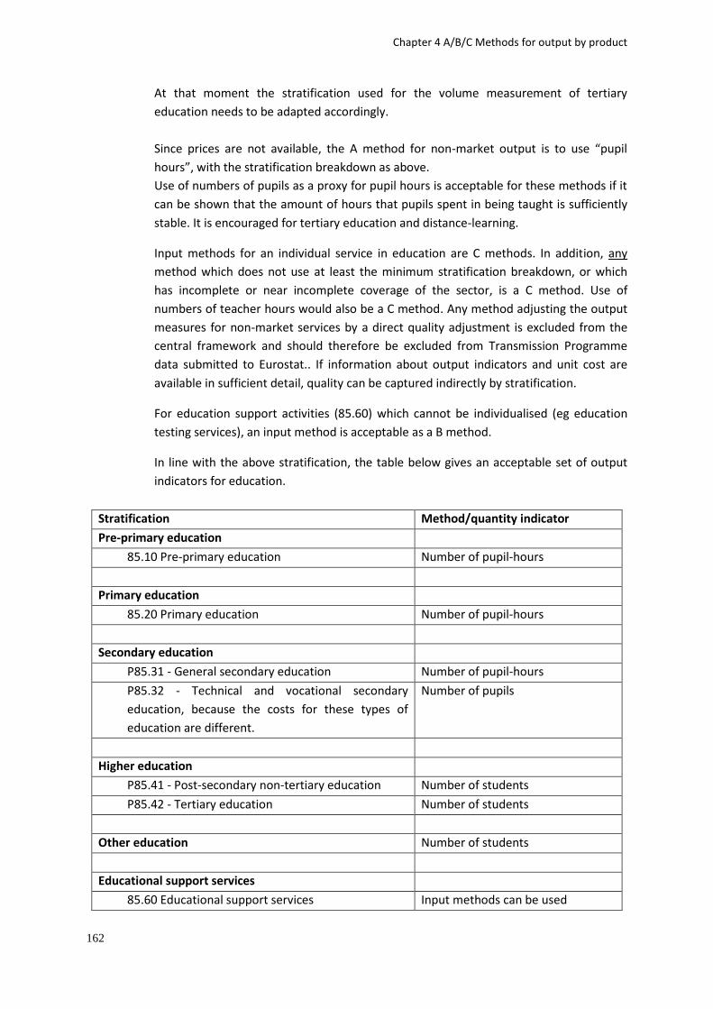
Chapter 4 A/B/C Methods for output by product
162
At that moment the stratification used for the volume measurement of tertiary
education needs to be adapted accordingly.
Since prices are not available, the A method for non-market output is to use “pupil
hours”, with the stratification breakdown as above.
Use of numbers of pupils as a proxy for pupil hours is acceptable for these methods if it
can be shown that the amount of hours that pupils spent in being taught is sufficiently
stable. It is encouraged for tertiary education and distance-learning.
Input methods for an individual service in education are C methods. In addition, any
method which does not use at least the minimum stratification breakdown, or which
has incomplete or near incomplete coverage of the sector, is a C method. Use of
numbers of teacher hours would also be a C method. Any method adjusting the output
measures for non-market services by a direct quality adjustment is excluded from the
central framework and should therefore be excluded from Transmission Programme
data submitted to Eurostat.. If information about output indicators and unit cost are
available in sufficient detail, quality can be captured indirectly by stratification.
For education support activities (85.60) which cannot be individualised (eg education
testing services), an input method is acceptable as a B method.
In line with the above stratification, the table below gives an acceptable set of output
indicators for education.
Stratification Method/quantity indicator
Pre-primary education
85.10 Pre-primary education Number of pupil-hours
Primary education
85.20 Primary education Number of pupil-hours
Secondary education
P85.31 - General secondary education Number of pupil-hours
P85.32 - Technical and vocational secondary
education, because the costs for these types of
education are different.
Number of pupils
Higher education
P85.41 - Post-secondary non-tertiary education Number of students
P85.42 - Tertiary education Number of students
Other education Number of students
Educational support services
85.60 Educational support services Input methods can be used

Chapter 4 A/B/C Methods for output by product
163
Market Services - An A method is deflating output by suitable PPIs for each type of
education service. The price indices should take account of the quality of the service
provided (drawing on the possible methods described above), and a check made to
ensure that basic prices are used (i.e. including any subsidies on products).
A possible B method is to use appropriate CPIs, corrected to valuation in basic prices
and reflecting the quality of the service provided. In the EU HICP, the “price” observed
is that for ‘education services’, if it is possible to separate this from educational
materials and support (see Council Regulation 2166/99), net of any reimbursements
from the state.
If these methods are not available for market services, it is also acceptable to use the A
and B output indicator methods described below for non-market services. Any input-
based method would be considered a C method.
4.17 CPA Q - Human health and social work services Key aspects
This CPA section covers individual health and social work services. Their provision can
be organised in many different ways: the services can be delivered as market or non-
market output; providers include government, non-profit institutions and non-financial
corporations; services may be funded through payments by patients (with or without
reimbursement by third parties) or through direct financing by government or
corporations.
ESA 2010 requires that the minimum level of detail needed to measure non-market
production of health services volume growth through output measures is the class level
of CPA 2008, as set out below.

Chapter 4 A/B/C Methods for output by product
164
86 Human health services
86.1 Hospital services
86.10 Hospital services
86.2 Medical and dental practice services
86.21 General medical practice services
86.22 Specialist medical practice services
86.23 Dental practice services
86.9 Other human health services
86.90 Other human health services
87 Residential care activities
87.1 Residential nursing care activities
87.2 Residential care activities for mental health etc.
87.3 Residential care activities for the elderly and disabled
87.9 Other residential care activities
88 Social work activities without accommodation
88.1 Social work activities without accommodation for the elderly and
disabled
88.9 Other social work activities without accommodation
ESA 2010 paragraph 10.30 sets out the case for adopting output methods for non-
market health services. However, the implementation of output methods may not be
easy, and significant investigations by statistical offices are required. Health output
constitutes a significant share of GDP, and so it is important to improve the methods for
the measurement of its volume.
ESA 2010 paragraph 10.30 recognises that data availability is a challenge in this area,
and says
“Although the use of input-based methods is generally to be avoided, it is possible, in the
field of health, to apply the input method when the variety of the services is such that it
is practically impossible to determine homogeneous products.”
The recommendations in this section are based on the following definition of health
output:
“Health output is the quantity of health care received by patients, for each type of
health care. The quantities should be weighted together using data on the costs or
prices of the health care provided. The quantity of health care received by patients
should be measured in terms of complete treatments.”
For volume measurement the focus is on outputs.
Using a complete treatment as the measurement unit requires account to be taken of
the whole bundle of complementary services constituting a treatment: medical services,
paramedical services, laboratory and radiological services and, in the case of
hospitalisation, non-medical services such as the provision of food and accommodation.
In practice, the feasibility of measuring complete treatments is dependent a lot on the

Chapter 4 A/B/C Methods for output by product
165
degree of fragmentation of the services making up a treatment (i.e. to what extent the
various medical acts which constitute a treatment are supplied by different providers).
It is due to data availability and hence a practical compromise that the
recommendations in the handbook are based on a narrow concept of treatment which
aims at capturing full treatments only within each CPA class.
A specific aspect of the concept of a complete treatment is the re-admission problem. If
a patient has to go back to hospital because of the same illness this means that the
original treatment has not yet been completed. A second treatment for the same
person is only recorded if the patient is sent back to hospital to be treated for a
different disease. A kind of re-admission problem also exists for medical and dental
practice services. A patient who is treated by a specialist for a specific disease will often
need several consultations. Ideally, all visits (first visit + continuation visits) related to
the same diagnosis should be counted as one treatment. Later in this section, the
argument is made that the equation: one visit = one treatment is likely to hold only for
general practitioners.
For hospital services, output (= treatments) can be measured on the basis of so-called
DRG-type classifications. DRG (Diagnosis Related Groups) systems are used to classify
hospital stays into groups that are medically meaningful and as homogeneous as
possible with regard to resource use. Each hospital stay is classified in one, and only
one, DRG based on medical and administrative information about discharges. DRG
systems vary across countries, but they are sufficiently similar. They are always very
detailed consisting of several hundreds of diagnosis related groups.
Technological improvements and health research advances make the quality changes in
health services an important issue. Improvements cover both changes from the
introduction of new treatments and improvements of existing treatments. Whilst
classifications like the DRGs can capture changes in the treatment mix – and the more
detailed they are the better they can do this – changes in the quality of a single given
treatment are very difficult to measure.
Data availability
The implementation of DRG systems for management and funding purposes in many
countries is improving the availability of output data for hospitals (above all general and
specialised hospitals). Nevertheless, there are still a number of problems relating to the
characteristics of the classifications and the handling of changes.
Normally, information on consultations by general practitioners and medical specialists
is available. Such data may be lacking, however, in special situations where, for
example, general practitioners work under a collective agreement with a health
insurance company or the Ministry of Health to care for the health of a certain group of
people and remuneration is not linked to the number of consultations.
Experience shows that, while for many health services satisfactory output indicators are
available, the data needed to calculate the necessary weights are much more difficult to

Chapter 4 A/B/C Methods for output by product
166
obtain. Whether in terms of output values or costs, weights should ideally be based on
exhaustive information, or on representative samples. If such an ideal solution is not
possible other, less satisfactory options exist, at least in the case of non-market output,
such as: indirect cost weights (derived from costs of complementary activities) or even
cost weights based on expert judgment. Both are acceptable only if they are well-
founded and sensitivity analyses show the stability of the resulting volume measures.
PPIs for market health services are not widely produced so that deflation of output
values by such indices is not an option for most of CPA 2008 Q. CPIs, on the other hand,
cover health care related market services and are generally available. But they can only
be used for deflation if the relevant prices are recorded gross of any subsequent
reimbursements. This is not the case for the EU's HICP.
A, B and C methods
For non-market output, the focus of the descriptive text for the categories of CPA 86 –
Human health services – is on the identification and use of sufficiently robust output
indicators with the associated cost weights for previous years. However, when such
indicators and their cost weights are not considered to be measured to an acceptable
standard, input methods are to be used.
Health services are continually improved through new scientific developments,
reflecting for example new medicines and new surgical techniques. Stratification to
homogeneous products cannot in itself capture all of these increases in the volume
output of the services, as the product level detail to which meaningful descriptions can
be applied does not capture underlying characteristics which determine the cost
allocation decisions of the health provider. The classical approach to such fundamental
changes in products reflecting a different bundle of desirable characteristics is through
linking new products onto old products. This can be achieved in non-market services by
using unit costs as a proxy for prices, and by building hedonic models which link product
characteristics to previous unit prices. Such methods have usually been applied to
marketed products where there are a variety of similar products whose prices and
values can be observed in the market place. The application of similar methods for non-
market services such as health is much more difficult, and requires detailed historical
information from management accounting systems within the health service. Further
work on the nature of the information required and the extent of its availability is
desirable.
See Annex 1 for a worked example of how stratification can be used to capture quality
change.
4.17.1 CPA 86.1 - Hospital services
Market output
Where PPIs are available which meet the criteria set out in paragraph 2.3, deflation of
market output of hospitals by these indices is an A method. The use of a CPI is also an A
method provided prices are recorded gross of any reimbursements and the index is
Chapter 4 A/B/C Methods for output by product
167
adjusted to basic prices (in case there are subsidies on products). If prices are recorded
net, the use of a CPI is a C method. The use of less appropriate PPIs qualifies as a B
method.
Output indicator methods which are classified as A or B below are also relevant for
market output.
Non-market output
Volume estimates have to be calculated on the basis of direct output measures, without
adjusting for quality. Such methods are to be applied at a detailed level. As stated
earlier in this section, input methods are allowed when the variety of products is such
that it is impossible to determine homogenous products.
A distinction is made between the different types of hospital services within CPA 86.11
to take account of the varying complexity of the different classes of services.
a) services to inpatients by general and specialised hospitals
DRGs that cover changes in the treatment mix will fulfil the requirements for a B
method.
Methods which use the ICD (International Classification of Diseases) to classify
discharges can also be a B method provided the diagnoses are recorded at a very
detailed level and appropriate cost weights are used.
Use of crude output indicators like the simple number of discharges is classified as a C
method.
b) hospital psychiatric services
Again, detailed DRGs appropriate cost weights are a B method.
A somewhat weaker method, but still to be considered as B, is the number of occupant
days (days of hospitalisation) by level of care weighted together using representative
cost information. If hospital psychiatric services are organised in such a way that each
type of hospital provides only one specific level of care it is possible to take account of
the product mix even if no formal nomenclature of care levels is implemented. It is
justifiable to have less demanding requirements regarding the details of the product
mix than described above for services by general and specialised hospitals because
hospital psychiatric services are more homogeneous.
Output methods that do not distinguish levels of care at all are classified as C.
c) hospital rehabilitation services
DRGs taking changes in mix of treatments are a B method.
Chapter 4 A/B/C Methods for output by product
168
The same holds if the number of occupant days by level of care is used. If it can be
demonstrated that the different rehabilitation services are relatively homogeneous
then the simple number of occupant days could be accepted as a B method.
Unadjusted occupant days by level of care meet the requirements of a B method. In
situations where there is relative homogeneity of services, the simple number of
occupant days may be accepted as a B method.
Introducing a new product in a volume index
As stated in paragraph 4.18.1, health services are continually improved through new
scientific developments, reflecting for example new medicines and new surgical
techniques. As stratification to homogeneous products cannot in itself capture these
increases in the volume output of services, this leaves the question of how to
incorporate substantially improved treatments in the index. They cannot simply be
added to the existing (related) category, as this violates the assumption of homogeneity
and would introduce a bias in the index. They cannot be ignored, as this would mean
underestimating production. The solution is to introduce the improved treatment as an
entirely new good (or service) into the index. That is, a good that did not exist in the
base period. Since there is not a base period cost weight, one needs to be imputed. In
the example below, it is suggested to use the cost of the new treatment when it was
first introduced as a proxy, as this can be interpreted as the value attached to the new
product by the government in its role as customer.
For the sake of simplicity, in the example below two treatments A and B are
distinguished in period T. In period T+1, a new (substantially improved) treatment C is
introduced for patients who previously received treatment A. C is a new surgical
technique that, while being much more expensive than A, offers much better prospects
of improved health than A.
So, how should we compile the volume index?
In option 1, treatment C is considered equivalent to treatment A; the difference in
quality is completely ignored. The much higher cost of treatment C is completely
reflected in the price index; the volume index remains unchanged. This approach
underestimates the “true” volume change of the production of health services.
In option 2, treatment C is considered a new product. Using the introduction “price” of
the new product at T+1 as a proxy of the base period cost weight, the substantial
improvement is reflected in the volume index. While option 2 is dependent on the
assumption that using the cost of treatment B when it was first introduced as a proxy
for the base period costs weight, it is preferable to simply combining the treatment with
another non-homogeneous product. This approach is broadly in line with the principles
set out for incorporating new products in the Producer Price Index Manual (IMF 2004)
chapter 21. The assumption behind option 2 can be restated as follows: We assume
there is a competitive market, and to win new customers, the product on introduction
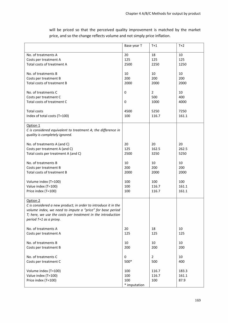
Chapter 4 A/B/C Methods for output by product
169
will be priced so that the perceived quality improvement is matched by the market
price, and so the change reflects volume and not simply price inflation.
Base year T T+1 T+2
No. of treatments A Costs per treatment A Total costs of treatment A No. of treatments B Costs per treatment B Total costs of treatment B No. of treatments C Costs per treatment C Total costs of treatment C Total costs Index of total costs (T=100)
20 125 2500 10 200 2000 0 0 4500 100
18 125 2250 10 200 2000 2 500 1000 5250 116.7
10 125 1250 10 200 2000 10 400 4000 7250 161.1
Option 1 C is considered equivalent to treatment A; the difference in quality is completely ignored. No. of treatments A (and C) Costs per treatment A (and C) Total costs per treatment A (and C) No. of treatments B Costs per treatment B Total costs of treatment B Volume index (T=100) Value index (T=100) Price index (T=100)
20 125 2500 10 200 2000 100 100 100
20 162.5 3250 10 200 2000 100 116.7 116.7
20 262.5 5250 10 200 2000 100 161.1 161.1
Option 2 C is considered a new product; in order to introduce it in the volume index, we need to impute a “price” for base period T; here, we use the costs per treatment in the introduction period T+1 as a proxy. No. of treatments A Costs per treatment A No. of treatments B Costs per treatment B No. of treatments C Costs per treatment C Volume index (T=100) Value index (T=100) Price index (T=100)
20 125 10 200 0 500* 100 100 100 * imputation
18 125 10 200 2 500 116.7 116.7 100
10 125 10 200 10 400 183.3 161.1 87.9
Chapter 4 A/B/C Methods for output by product
170
4.17.2 CPA 86.2 - Medical and dental practice services
Market output
The use of PPIs is an A method although, in practice, these are unlikely to be available.
The use of a CPI is also an A method provided prices are recorded gross of any
reimbursements. CPIs which record prices net of reimbursements are a C method. All
non-market output methods classified as A or B below are also appropriate.
Non-market output
The main distinction is between services by general medical practitioners on the one
hand and services by specialists on the other, the former being less complex.
a) CPA 86.21 services by general practitioners.
The services of GPs are such that each visit can be considered as constituting one
treatment. Consequently, the recommended A method is the number of consultations
by type of treatment, It might be difficult, however, to obtain the corresponding cost
weights. In the case of proxy weights or only partial quality adjustment the number of
consultations by treatment is a B method. The simple number of consultations can also
be accepted as a B method if the different types of treatment are sufficiently
homogeneous with regard to the resource requirements (similar cost weights).
b) CPA 86.22 services by medical specialists
On the assumption that treatments by specialists are normally such that a first visit is
followed by follow-up visits it is justifiable to take the number of first visits as an
indicator of complete treatments. Admittedly, this hypothesis requires further testing. If
it proves valid, the number of first visits broken down by type of specialist and type of
treatment, weighted with appropriate cost weights, is the B method. If a distinction by
type of treatment cannot be made, the number of first visits is not the appropriate
indicator. Under these conditions (as in the case of dental practice services) the total
number of visits is considered to be a B method. The distinction between specialists is
indispensable for a B method.
c) CPA 86.23 - Dental practice services
Most dental services are market services. An A method is the use of the CPI adjusted to
basic prices and quality changes. Prices must be recorded gross of any reimbursements
and the CPI must be calculated at a sufficient level of detail. If prices are recorded net of
reimbursements the use of a CPI is a C method. An output indicator method which
meets the requirements of a B method is the number of treatments by type of
treatment. As in the case of medical specialists the number of first visits can be
assumed to indicate the number of complete treatments.
If a distinction by type of treatment cannot be made it is not meaningful to count only
first visits. Under these conditions the total number of consultations (visits), seems to
be the better indicator because then the types of treatment which consist of a higher
Chapter 4 A/B/C Methods for output by product
171
number of visits and are assumed to be more resource-intensive get a higher weight.
The total number of visits is considered to be a B method.
4.17.3 CPA 86.9 - Other human health services
Where these services are provided as market services, the use of the appropriate
component of the CPI is the recommended approach. If an adjustment is made to basic
prices this is an A method, if not a B method.
Non-market output
This category includes the activities of nurses, midwives, physiotherapists or other
paramedical practitioners in the field of optometry, hydrotherapy, medical massage,
occupational therapy, etc.
The DRG system does not cover nursing services. In view of the limited degree of
diversity of these services, occupant days by level of care are an A method. Different
care levels can be captured directly by systematically applying classifications or
indirectly by grouping institutions that provide the same level of care.
Input methods are considered a B method for this category.
4.17.4 CPA 87 - Residential care services
These services include welfare services delivered through residential institutions to old
persons, handicapped persons, children and young people. They do not include a
medical service component provided by doctors. If lodging is combined with medical
services under the direction of a doctor CPA 86.1 (hospital services) is the relevant CPA
item. The borderline between the two, however, may sometimes be blurred.
For market output deflation by the appropriate component of the CPI (adjusted to basic
prices) is the A method. Occupant days by type of institution will meet the requirements
for a B method. This supposes that the services provided within each type of institution
are sufficiently homogeneous.
For non-market output, input methods are allowed as a B method. Output volume
indicators without quality adjustment would also be considered a B method if those
indicators provide good coverage and are sufficiently detailed.
4.17.5 CPA 88 - Social work services without accommodation
To the extent that these services are market services the use of the relevant CPI
component adjusted to basic prices is an A method. Without this valuation adjustment
to the CPI a B method is obtained.
For non-market output, input methods are allowed, although use of output volume
indicators without quality adjustment would also be considered a B method if those
indicators provide good coverage and are sufficiently detailed. The number of persons
receiving care by level of care is a B method for non-market output.
Chapter 4 A/B/C Methods for output by product
172
4.18 CPA R - Arts, entertainment and recreation services There are features of some of the services in CPA R that create particular challenges
when measuring price and volume changes. Particular methodological issues include
the treatment of unique products (e.g. services of performing artists), the bundling of
products (e.g. library services), and the provision of a product to a number of
consumers at the same time (e.g. a theatre performance). Quality is difficult to measure
for some services, particularly where individuals’ personal enjoyment is a determining
factor. There are also practical issues, especially dealing with the large number of small
providers for some services, and distinguishing between business and household
consumption.
In line with the recommendations given in other areas of the handbook, any methods
for the market products in CPA R which are based on inputs rather than outputs would
be considered C methods.
4.18.1 CPA 90 – Creative, arts and entertainment services
It is useful to deal with those services provided to an audience of consumers for the
purposes of entertainment (for example showing films and plays) separately from the
services provided to individuals or businesses (for example film processing and betting
services).
Services provided to an audience
Key aspects
This sub-group includes motion picture projection in cinemas, presentation of theatrical
or musical productions in theatres, fairs and circuses, museums and zoological gardens,
and sports events. The common feature is that an entertainment service is provided to
a group of spectators. The output of the service is the presentation of the ‘performance’
to the spectators. The outcome of the service is the personal enjoyment and education
given to the audience by the performance. As with provision of transport services (see
section 4.6), the key principle here is that output should ideally be linked to the number
of tickets sold for access to the service, specified by the various types of tickets (so that
purchase of a “season ticket” implies a different service than a one-off ticket).
Quality is an important factor here – different forms of entertainment may be perceived
as different products or of different qualities. Similarly, some seats in desirable
locations within the auditorium or for particular performances are sold for higher prices
– this represents a different quality of service which should be reflected in the volume
measure. And certain performances may be perceived as of a different quality because
of their timing (for example matinees are often cheaper than evening performances)
The availability and quality points above imply that methods using the number of tickets
sold as an indicator of output should be undertaken at a high level of detail,
distinguishing season tickets from single-use tickets, the location of seats, and the
different types of entertainment productions.
Chapter 4 A/B/C Methods for output by product
173
One point to watch is the availability of discount prices for large groups, or cheaper
promotional prices, which should be fully reflected in the price measures. There may
also be a significant subsidy system in operation for some services – for example a
museum that grants entry for free (where the basic price is in effect the subsidy per
entrant because the subsidies are treated as subsidies on products – see ESA 2010 para
4.35c). In this case, the number of entrances is an important indicator for the volume of
services provided.
Data availability
Service providers will often collect the attendance at cinemas, theatres, circuses and
sports events by type of ticket, so this should be available for collection. However, the
availability of the data to the statistical office may be determined by the concentration
of the industry – for example, if the cinema industry is dominated by a few large firms,
ticket data can be expected to be reasonably accessible. But a large number of service
providers in some classes of service can mean that data collection is not always
straightforward. Administrative records may be available from the Culture Ministry, or
Trade Associations (e.g. a theatre association) may collect data from their members.
Within Europe the annual ‘AUVIS’ (audio-visual) questionnaire collects data on cinema
admissions and average ticket prices.
It is very likely that the price data for the major audience services will be collected for
the CPI. In the EU, the HICP specifically requires collection of data on cultural services
such as cinemas, theatres and museums. Therefore these data should be readily
available.
A, B and C methods
The A method here for services provided purely to households is to use detailed CPI
series adjusted to basic prices as deflators for the value of tickets sold. The method
would need to take account of discounted tickets, and any other features that will have
a significant influence on quality (for example free programmes or telephone booking).
The B methods here are to use the CPI for services which are also provided to
businesses (providing that it can be shown that this is a reasonable assumption), or to
use the number of tickets sold broken down by type of seat and performance as a
volume measure. In the event of ticket data being unavailable, the number of
performances could be used as a measure, though this is barely a B method.
Any methods which use a CPI to inappropriately deflate business purchase, which use
an insufficient breakdown of product detail, or which use input-based data, are
considered C methods.
4.18.2 CPA 91 - Library, archive, museum and other cultural services
Key aspects
A library may have a number of outputs – primarily the lending of books and other
materials, but also making available reference material, and providing a location within
Chapter 4 A/B/C Methods for output by product
174
which to read books, newspapers and periodicals. Government typically provides
libraries as non-market services, although individual libraries may also provide market
services for payment (such as the renting of videos) which can be measured in the same
way as other market services.
The key decision to make here is whether to adopt the number of books and other
products lent as a volume indicator for the whole of library output, or to include an
indicator for visits to the library alongside lending. Ideally one would use both sets of
information, but data on visits are not always available. Alongside this, one should take
account of changes in quality (for example increases in the stock of books or an
expanded reference section).
Data availability
Data on items lent may be available from library records where these are kept
electronically, broken down into the major types of items (books, music etc). Data on
visits may be available from physical counts by library staff or from surveys of library
members. In some cases government uses these data for funding and other decision-
making purposes.
A, B and C methods
The A method for libraries is to combine output data on lending (broken down by major
item type) with data on visits, adjusted for quality factors such as the range of reference
material available. This combination is best achieved using a cost-weighted approach.
Any market services provided need to be measured by value of sales deflated by an
appropriate price index.
The B method for libraries is to use data on lending (broken down by major item type)
as an indicator of the overall output of the library.
4.18.3 CPA 92 - Gambling and betting services
Key aspects
Gambling and betting services provide entertainment to gamblers by allowing them the
chance for making future gains in wealth. There is some analogy with non-life insurance
services, in the sense that the insurance company is offering a service for pooling risk,
although the gambling firm’s financial reserves are held purely for the operation of the
firm rather than for individual consumers and the total size of the bets is usually
determined by the gambler, not the betting firm.
There are a number of different types of gambling and betting service, and it is
important to distinguish between them for practical purposes (even if the underlying
philosophy is the same):
Lotteries (state and private)
Casinos

Chapter 4 A/B/C Methods for output by product
175
Betting services (phone, internet, shops)
Gaming machines
The means of measuring the activities of lotteries and gambling at current prices is set
out in paragraph 4.135 of ESA 2010. The amounts paid in are split into two elements -
the service charge levied by the operator and the amount transferred to successful
gamblers.
Ideally, the service charge of the gambling service would be directly measurable. This
may be true for some heavily regulated areas of the gambling industry, such as state-
run lotteries. If the information is readily available, and adjustments can be made for
quality changes (for example, faster payouts or type of game), then this does not pose a
particular problem for price and volume measurement.
In the absence of detailed information on service charges, the total number of bets
made by gamblers would be the most appropriate quantity indicator to use. This would
not of course reflect changes in the average amount wagered per gambler or per bet,
but it is questionable whether the overall size of the bet corresponds with the
entertainment service provided to the gambler.
It is also important to consider quality of the service. The outlet is obviously an
important determiner of quality because it determines the “personal” nature of the
service received and the accompanying benefits to the gambler. For example a betting
service can be provided through a shop, over the telephone, at a sports event, or over
the internet. In the latter case, development of computer and direct payment
technology has allowed substantial productivity improvements to be made. Each of
these outlets can be considered a separate quality of service, and therefore the data
should be broken down by type of outlet wherever possible. The volume changes of
each outlet can then be weighted by total turnover in the base period.
The design of the game may also have an impact on entertainment quality. It is also
possible that the odds of winning could be viewed as a quality, though (given the usual
organisation of the industry) summing the odds of winning across all gamblers would
largely offset changes in the number of bets, since (other things remaining equal) a
greater number of bets would reduce the overall chances of winning.
The following example illustrates the calculation of volume of betting services:
Number of
bets
Total amount
bet
Number of
payouts
Total payout Output of
service
Year T-1 100 1000 10 800 200
Year T 120 1400 20 1100 300
Overall value of output has increased by 50% between the two years. The number of
bets made has risen by 20%, and this gives the change in the volume of the service.
Chapter 4 A/B/C Methods for output by product
176
In the case of casinos, it may be more straightforward to treat the entire casino as an
entertainment service (since the casino will probably offer a wide range of services
other than pure gaming) and, by analogy with a public performance of a film (see
section 0), to use the number of persons entering the casino as the measure of the
volume of the service.
Finally, there is a timing point to consider. Some bets may be made well in advance of
expected payout (for example a bet at the start of the football season on the expected
winner at the end). If the balance of bets changes year on year, this may introduce a
discontinuity into the volume series. However it may be assumed that the majority of
bets made will be paid out in the same accounting period.
Data availability
Betting and gaming firms can be expected to have information readily available on the
number of bets made.
Data from casinos on individual bets and payments is probably impossible to gather,
and the most likely measures available (as discussed above) will be number of persons
entering the casino. This is unlikely to be difficult to collect from casinos.
A, B and C methods
The A method for gambling and betting services is to directly deflate service charge data
by a price index of these services, with adjustments for quality changes as appropriate.
This is only really suitable for a state-run lottery, or other heavily regulated service,
where direct data on service charges are available.
The B method for betting is to use the number of bets made as a volume indicator. Each
type of betting outlet (telephone, internet, shops) should be distinguished and (ideally)
different types of games should also be distinguished, with weighting provided by the
proportion of total amount bet in the base period. The B method for casinos is to use
data on the number of persons entering.
4.18.4 CPA 93 - Sporting services and amusement and recreation services
The same principles that are applied to CPA90 under 4.16.1.1 apply to this heading.
Sports facilities
Key aspects
The output of sports facilities (whether specific facilities, leisure centres or through
sports associations) is best measured by the number of tickets purchased for access to
the facilities. Ideally a visit which takes advantage of several, separately charged,
services (e.g. swimming and gym at a leisure centre) would count as a higher volume of
output than a visit using a single service. Where a season ticket system is in operation,
allowing multiple entries on a single ticket, this should count as a separate product. If
possible, the quality of the facilities provided should also be taken into account.
Chapter 4 A/B/C Methods for output by product
177
Data availability
CPIs will generally record a range of sports services to the public and is therefore a good
source of data.
Data on tickets sold broken down by type should be readily available from leisure
centres and other sports facilities.
A, B and C methods
The A methods here are to use detailed CPI data, adjusted to basic prices, or to use the
number of tickets sold broken down by type of ticket and, if possible, activities
undertaken. Some adjustment should be made for quality of the facilities, and paying
spectators should be measured separately from participants.
The B method is to use tickets sold which are not broken down sufficiently to reflect the
different types of services, or which use detailed CPI data which is not fully
representative of the activities.
4.19 CPA S – Other services This product division covers services furnished by membership organisations; repair
services of computers and personal and household goods; and other personal services.
The major services included within this section are discussed below.
4.19.1 CPA 94 - Services furnished by membership organisations n.e.c.
Key aspects
This product division consists almost entirely of non-market services, provided by Non
Profit Institutions (NPIs) such as professional bodies, trade unions, and religious
organisations. The common feature is that payment of a membership fee covers a range
of services, which may or may not be used by the individual member in a particular time
period.
Data availability
The large number of small units providing some of these services, and the exemptions
often granted to them by Government (e.g. for taxation purposes), mean that there can
be a shortage of suitable data in this area. Nevertheless the organisations can be
expected to maintain reasonably comprehensive and up-to-date membership registers,
identifying different types of membership (e.g. full member, part member, non-voting
member etc), and there is sometimes a mandatory provision of information at least
once a year to the Government administration responsible for monitoring NPIs
(including a set of accounts where monetary flows are significant).
A, B and C methods
The only suitable A method here is to obtain detailed information on the provision of
services actually provided to members, broken down into a fine detail and weighted by
the costs of provision. For example, a professional organisation providing legal advice,

Chapter 4 A/B/C Methods for output by product
178
conferences, and examination and accreditation services to members would provide
data on each of these activities, or a religious organisation would provide data on
attendance at services or number of services held. Clearly this kind of data collection
could impose a substantial burden on these organisations.
The B method is to use number of members as a proxy for output, but the different
types of membership must be captured if they give significantly different entitlements
to receive services, and it must be clear that the average use of services by members
does not change significantly year on year.
4.19.2 CPA 95 - Repair services of computers and personal and household
goods
For the output of repair of personal and household goods, CPIs (adjusted to reflect basic
prices) can be used. As there will be little business expenditure on these services, a CPI
will be quite appropriate, and might be regarded as an A method. However, various CPI
headings will have to be used as various different products are included here.
Therefore, deflation is necessary on a detailed level in order to be able to apply the
various detailed CPI headings involved.
4.19.3 CPA 96 - Other personal services
CPA 96.01 - Washing and dry cleaning services of textiles and fur products
These services are provided to both businesses and households. For households, CPI
data could be available on these services (costs for using a laundromat, and for the dry
cleaning of standard items). For business services, there is often a contractual
relationship and suitable volume indicators may be number of kg of material washed or
number of standard ‘loads’. Use of the CPI and volume data are both considered B
methods.
CPA 96.02 - Hairdressing and other beauty treatment services
This product is almost entirely provided to households and is captured by the CPI. The
best method is to use a “model price”, where the model is a standard representative
product such as a shampoo and cut. Use of CPI data represents an A method if an
adjustment is made to basic prices.
CPA 96.03 - Funeral and related services
This product is entirely provided to households and is captured by the CPI. There are
standard products available in the industry, so pricing is straightforward, and use of CPI
data represents an A method if adjusted to basic prices.
CPA 96.04 - Physical well-being services and CPA 96.09 - Other personal services
These cover a variety of services, most of which are delivered as standard products (e.g.
pet care services, dating agencies, astrologists, prostitutes), which can be priced in
different time periods and a price index constructed. Use of these standard products
would be an A method if all quality effects were taken into account, and a B method
otherwise.

Chapter 4 A/B/C Methods for output by product
179
4.20 CPA T - Services of households as employers of domestic
personnel Key aspects
This product category covers those services provided to households by paid staff who
are not themselves classified as independent units of production (the production of
such units is classified elsewhere within the CPA). Examples include cleaning ladies,
nannies, butlers and gardeners. By convention the national accounts production
boundary excludes unpaid services produced by householders themselves for their own
consumption. The valuation of output is defined in par. 3.87 of ESA 2010 as equivalent
to the compensation of employees paid, including any income in kind.
Data availability
Data are likely to be available from tax administration records and labour force surveys
for this category of staff relating to both the number of staff and their earnings
(including income in kind), and some CPI data are collected for the prices of domestic
services. Charge-out rates may be available for some categories of staff.
A, B and C methods
Whilst the best theoretical method to measure volume of output of these services
would be to collect data on the activities of staff (for example number of rooms
cleaned, number of hours of childminding), this is very unlikely to be feasible in
practice.
There are three other possible B methods for estimating output at previous year’s
prices:
use of CPI data adjusted to basic prices,
use of wages or charge-out rate data and,
volume extrapolation using the number of staff as the extrapolator.
The first two methods should take into account income in kind. Given the possibly
incomplete coverage of the CPI in this area, and the problems of adjusting wages and
staff numbers for productivity changes, the three methods described are all B methods.
Any CPI or wages data method which does not take into account income in kind should
be considered a C method.
Chapter 5 Application to quarterly accounts
180
5. Application to Quarterly accounts
5.1 Introduction The preceding chapters in this handbook have been primarily concerned with
discussing the methods available for constructing chained volume national
accounts on an annual basis. However the evolution of the quarterly GDP, and its
components, at previous year’s prices is an extremely important short-term
economic indicator. The compilation of quarterly accounts at previous year’s prices
raises a number of methodological and practical issues, which will be examined in
this chapter.
The ESA 2010 covers quarterly accounts only briefly in chapter 12, but was
supplemented by a detailed Eurostat Handbook on Quarterly National Accounts.12
Also relevant are the IMF “Quarterly National Accounts manual”13 and the OECD
“Compilation Manual for an Index of Services14”. It is not the intention of this
chapter to duplicate the discussion in these manuals, and cross-references are
made where appropriate.
5.2 Data availability The most common problem encountered when compiling quarterly national
accounts is that some data sources (such as the annual industry enquiry or
company accounts) are only available on an annual basis. However some others are
routinely available quarterly or even monthly (such as price indices). In general
there is a necessity to use less complete data sources – in terms of coverage, detail,
or classification. Chapter 4 in the Eurostat quarterly handbook explains the options
available for estimating quarterly data when basic data is not available.
Compilation of quarterly accounts at previous year’s prices increases the data
requirements, and therefore adds to the difficulties found for compilation at
current prices.
ESA2010 makes it clear that quarterly accounts should “adopt the same principles,
definitions and structure as the annual accounts.” (par. 12.03). Given that the
A/B/C classification used in this handbook is based on a theoretical assessment of
suitability, rather than a practical assessment, it is clear that the same standards
applied for the annual accounts should apply equally to the quarterly accounts. This
will undoubtedly mean that A methods are less achievable for a quarterly
environment and more B methods will be used. But it does not mean that C 12 Available from the European Publications Office; ISBN 92-828-7259-9
13 See http://www.imf.org/external/pubs/ft/qna/2000/textbook/index.htm
14 See http://www.oecd-ilibrary.org/economics/compilation-manual-for-an-index-of-services-
production_9789264034440-en
Chapter 5 Application to quarterly accounts
181
methods are any more acceptable for the quarterly accounts than they are for the
annual accounts. A section later in this chapter considers the application of A/B/C
standards to the mathematical and statistical (“indirect”) methods commonly used
by some countries to estimate their quarterly accounts.
A general difficulty raised when compiling chained volume quarterly accounts is the
availability of data to undertake the “double-deflation” methods that are
recommended in this handbook for calculation of GDP from the production side
(see section 3.4). Usually this is caused by a lack of information on intermediate
consumption. The most common methods used in the quarterly area are “single
indicator” methods that extrapolate value added by using an output indicator.
These methods are discussed below.
Despite the data availability difficulties, there can be considerable advantage in
employing a multi-approach method (at least from the production and expenditure
approach); chapter 8 of the Eurostat quarterly accounts handbook covers this in
some detail. Whilst resource constraints may limit the compilation of a complete
set of quarterly Supply and Use Tables at previous year’s prices, even at a less
detailed product level, the use of a Supply and Use Table framework provides an
opportunity to reconcile different (often incomplete) data sources. Data availability
and reliability will determine which method carries greatest weight in the
reconciliation. Estimates of production, based on quarterly business surveys, may
provide a very comprehensive coverage of many products, though (as mentioned
above) intermediate consumption data is usually more difficult to collect, and
services may be less well covered. By contrast some expenditure data, for example
government and foreign trade data, are more readily available on a quarterly basis,
as are consumer and foreign trade price indices. However, the collection of
household consumption data, and data for investment (particularly for changes in
inventories), is more difficult on a quarterly basis, not least because of the
associated accruals problems.
It may well be that, for some industries, quantity indicators are in fact more widely
available on a quarterly basis than value or price data. The IMF quarterly manual
provides some examples of possible sources in paragraph 3.41, whilst pointing out
in the preceding paragraph that use of quantity indicators may be unsuitable under
certain circumstances (for example, where products are heterogeneous or where
secondary production is significant).
5.3 Specific issues In addition to practical problems of data availability, there are also some
theoretical questions, both in individual subject areas (discussed one by one below)
but also at a general level – for example, the choice of chaining method and the
treatment of seasonality in the accounts – which are covered in the following
sections. Many of the issues are common to both current and chained volume
measurement, but measurement in previous year’s prices raises further
complications.
Chapter 5 Application to quarterly accounts
182
5.3.1 Agricultural Output
A general question arises of measuring output on an accruals basis, where a
continuous production process spans a number of accounting periods. This is most
pronounced for agriculture where, for example, the growing season for crops will
span three quarters of the year, with the harvest taking place in the third quarter,
and preparation of the fields taking place in the last quarter of the preceding year.
ESA 2010 is clear that production of agricultural output is a continuous process, and
therefore production should be allocated to each period, with work-in-progress
being recorded at the end of each period. The Eurostat quarterly handbook
(paragraphs 2.54 – 2.72) suggests two possible solutions to this issue at current
prices – either:
The recommended method - to distribute forecasts of the value of harvest
output in proportion to the input costs in each quarter, or;
The alternative method - to assume that output in those quarters with no
production of finished goods is equivalent to input costs.
When calculating the volume of quarterly agricultural output, the main difficulty is
to decide which price index to use. Theoretically the price to be applied should be
the price prevailing during the period of production, but in practice the prices
prevailing during quarters out of the harvest season might be rather unsuitable. If
the recommended method from the Eurostat quarterly handbook is adopted, the
forecast of value of output requires a suitable price and quantity forecast for each
type of product, where the price relates to the basic price forecast for final harvest
output (not the price prevailing during different quarters). It is therefore possible
to use the quantity forecasts as a volume indicator (providing that the detail is
sufficient to differentiate quality), although revisions will need to be made to the
data when the final output data are known. If the alternative method is adopted,
and input costs are used as an estimate of output, one should continue to use a
forecast of the product price as a deflator, since deflation by a price index for
inputs would only generate the volume of inputs.
5.3.2 Seasonal products and product differentiation
There are some products whose price varies significantly over the year, and other
products that are only produced and sold at certain times of the year. In the first
case, price movements can be measured and applied to the value of flows – this
does not present a conceptual difficulty. However in the second case, a difficulty is
created if the quantity of a product sold falls to zero in one or more quarters of the
year. This is particularly important for agricultural products, where seasonal
varieties are commonplace (for example, potatoes) and where both production and
consumption tend to be seasonal. A rather different example is business audits,
which may take place only annually after the close of the financial year. In other
cases, consumption is seasonal but production may occur throughout the year (for
example clothing).

Chapter 5 Application to quarterly accounts
183
The recommended method to deal with this in compilation for volume of GDP is to
treat the seasonal products as separate products, using quantity or price
information at the greatest possible level of detail. This may mean that products
appear during only certain quarters of the year, but if this is a regular event, the
chaining methods recommended below can reflect the good in the weighting
pattern.
Seasonal products present more of a challenge for compilation of price indices. If a
price index such as a CPI is used to deflate value of consumption at a less detailed
level of product breakdown, it is important that the national accountant
understands the way the price statisticians treat seasonal products for the product
groups where they are significant.
5.3.3 Non-market services
Section 3.1.2 of this handbook discusses the issues relating to measurement of
non-market output at previous year’s prices. The concept of measuring non-market
output at current prices does not differ between quarterly and annual accounts –
output is estimated as the sum of costs. Given that the largest input for non-market
services is labour, one would expect to see a reasonably steady quarterly profile of
costs over the year (unless numbers of staff changed substantially during the year
for some reason). When viewed on a quarterly volume basis however, the output
of some non-market services (as defined earlier in this handbook) is likely to be
seasonal – for example education output of schools will be low during the school
holidays (as pupils are not being taught), and the health services will generally be
more busy during the winter months.
The idea of seasonal patterns of production here is no different from a firm
shutting its factory over the summer or Christmas break, but in the case of a
factory the (lower) output figures for the period will reflect the holidays. If volume
of output is measured as the deflated sum of input costs, and input costs continue
to be paid even when production is not taking place, this imputes output when it is
not in fact taking place. The same can be said of methods that extrapolate output
from the numbers of employees (as described in paras 2.78 to 2.79 of the Eurostat
quarterly handbook).
The A/B/C classification applied in sections 3 and 4 should continue to be applied,
even if the practical obstacles are greater on a quarterly basis. Input methods are
no more acceptable for quarterly estimates than they are for annual estimates.
5.3.4 Inventories
Methods available for the measurement of inventories at previous year’s prices are
considered in section 3.7 of this handbook. The Eurostat Quarterly National
Accounts Handbook15 discusses inventories in paragraphs 2.136 – 2.161.
15 http://epp.eurostat.ec.europa.eu/portal/page/portal/product_details/publication?p_product_co
de=KS-GQ-13-004
Chapter 5 Application to quarterly accounts
184
5.3.5 Tourism
Many products predominantly consumed by tourists are likely to show significant
seasonal variations in prices and volumes over the year. Some products (for
example ski holidays) may only be available at certain times of the year, and this
generates a ‘seasonal products’ problem that is discussed above. It may be helpful
to examine the data available from tourism satellite accounts (if they are compiled)
to gain a feel for the issues involved. There are two main points that need to be
considered for products predominantly consumed by tourists:
Where package holidays are purchased well in advance of actual consumption,
this can create a difficulty in determining the appropriate price to deflate the
value of output. Whilst booking in advance is of course common in many service
industries (such as entertainment and personal services), many people will book
their holidays significantly in advance so that the booking falls in a different
quarter, or even in a different year. The measurement principle to follow here is
that if the same holiday is booked at different times, then in fact it is a different
quality of holiday (that is, the price difference must be seen as a volume effect,
as for airline tickets). If the CPI is used for deflation purposes here it is
instructive to look at the methodology used in the CPI to measure package
holiday prices, to ensure that it lines up with the required methodology in the
national accounts. Some CPIs may record prices when the holidays are booked,
although within the EU Harmonised Index of Consumer Prices (HICP) the
requirement is to record the prices for services when the consumption of those
services can commence.
Where a tour operator is not organising a package of tourism products,
domestic tourism can be broken down into a number of constituent products –
travel products, accommodation products, food and entertainment products,
and travel agency services. Whilst one might expect that the seasonality of
prices of these products might be similar in some areas, each of these products
should be treated separately according to the methods described in chapter 4 of
this handbook.
5.4 Use of price data Price data are widely available on a sub-annual basis – generally monthly for
consumer and producer prices. The price movements used in compiling the annual
accounts are usually based on the sub-annual data. Definitions of prices are the
same for quarterly and annual accounts. These points should ensure consistency
between the deflation of annual and quarterly data.
However, one must consider the issue of which price to use for deflating output.
For any particular quarter, the national accountant may have monthly data
available for each of the three months, together with derived quarterly data (which
may or may not be available from the price statisticians themselves). Theoretically,
the best price measure to use is one that reflects the pattern of expenditure
throughout the period – it cannot be acceptable to use prices that prevail at only
one point in the period.
Chapter 5 Application to quarterly accounts
185
Price statisticians tend to use a fixed set of weights when calculating the monthly
evolution during a particular year, and use chaining based around the overlap in a
specific month of the year (for example December in the case of the EU’s
Harmonised Index of Consumer prices) to link the series. The national accountant
should understand the compilation and chaining methods used in price indices and
ensure that these are appropriate for deflating national accounts data. For
example, it may be that the majority of output occurred in one particular month,
when prices were lower than in the other two months. Applying a quarterly price
index in this case would tend to underestimate output, and it would be more
appropriate in the national accounts to weight the monthly price changes by the
quantities of products transacted in each month (see section 3.4).
5.5 The classification of indirect methods Whilst all countries experience substantial gaps in the data available on a quarterly
basis, some countries choose to rely heavily on mathematical and statistical models
to derive their quarterly accounts from short-term indicators. These methods are
described in detail in chapter 5 of the Eurostat quarterly handbook.
Choice of chaining method
The choice of chaining method cannot be seen in isolation from two other key
compilation methods (benchmarking and seasonal adjustment), which are
discussed later in this chapter.
Within the EU, Commission Decision 715/98 sets out the requirement in the annual
accounts for chain linking a series based on weights derived from the previous year
(Laspeyres formula). The Decision gives no specific requirement for chain linking in
the quarterly accounts, other than they should be as consistent with the annual
accounts as possible.
There are three possible methods for constructing quarterly estimates within an
annual chain linked system:
Annual overlap – This uses average price data from the previous year (t-1) as
the weighting for each of the quarters in the current year (t), with the linking
factors being derived from the annual data.
Quarterly overlap – This requires the compilation of one quarter (say the fourth
quarter of each year) at both the average prices of the current year and the
average prices of the previous year, which then provides the linking factor for
the current year
Over the year – This requires the compilation of all quarters at the weighted
average prices of both the current year and the previous year, which then
allows extrapolation of the reference year level.
The Quarterly National Accounts Handbook discusses the advantages and
disadvantages of these three methods and provides worked examples in
paragraphs 6.41 – 6.75.
Chapter 5 Application to quarterly accounts
186
Benchmarking
The process of benchmarking is described in the Eurostat quarterly accounts
handbook (chapter 5). The underlying aims are to ensure that the quarterly
accounts are consistent with annual accounts, a key requirement of customers, and
for data quality improvement. The consistency between annual and quarterly data
should apply to both current and chained volume data, where the chained volume
data are expressed in prices of the same base year as the annual data.
The starting point for benchmarking is to determine which of the annual or
quarterly data can be considered the most reliable. In almost all cases the (well
established) annual data will be the most reliable, because it will be available in
greater detail and will usually be based on a fuller survey, or even census, source.
The comparison of different sources is usually very helpful in testing and improving
the quality of estimates. For some data, the annual source might be the same
source as the quarterly data.
A major concern when benchmarking is to avoid the introduction of a “step” into
the series – this might occur if the first quarter of a year is adjusted, thereby
altering the growth rate from the last quarter of the previous year. This problem
will tend to occur if a “pro-rata” solution is adopted – that is, simply distributing the
difference between the sum of the quarters and the annual total over each of the
quarters in proportion to the existing quarterly value.
In order to avoid the step problem, it is necessary to maintain the relationship
between the benchmark figure and the indicator series over the period of
estimation. There are three approaches for undertaking this:
– Pro-rata adjustment;
– Denton difference method;
– Denton proportional method.
These are discussed in Chapter 5 of the Quarterly National Accounts Handbook.
5.6 Seasonality Seasonal adjustment of quarterly accounts is discussed in the Eurostat quarterly
handbook (chapter 7). For many products, there will be little or no seasonality
(other than that introduced by traditional holiday periods) in either price or
volume. However, as noted above, there are a number of products for which both
price and volume can be markedly seasonal, and this naturally introduces
seasonality into the national accounts estimates. It is recommended that both
seasonally and non-seasonally adjusted series be derived for chained volume
quarterly accounts.
Standard seasonal adjustment techniques are of course equally applicable to both
current and chained volume data (the Eurostat quarterly handbook discusses the
different models and packages available). Nevertheless for prices and volumes
data, there is a choice between seasonally adjusting the value, volume and price

Chapter 5 Application to quarterly accounts
187
series independently, or seasonally adjusting two series and then deriving the third
by imputation.
5.7 Conclusion This chapter has shown that there are specific conceptual and data availability
problems to be addressed when dealing with quarterly prices and volumes data in
the national accounts. Nevertheless, the key principle remains that the A/B/C
classification described in the remainder of this handbook remains unchanged
when applied to a quarterly environment. This will undoubtedly mean that more B,
and perhaps even C, methods will need to be employed, but this reflects the
practical difficulties with deriving intra-annual data.
Annex 1 – Capturing quality effects through stratification Consider a box of chocolates which includes a mix of milk and plain chocolates. In the base
year, there are thirty chocolates in the box and it costs 7.5 euros to buy a box. Over time,
the mix of chocolates changes, there being more plain chocolates than milk chocolates and
this pushes up the price of the box. So in a later year, the cost of a box of chocolates is 13.5
euros.
Considering the box as simply a box of mixed chocolates, there has been no change in the
quantity of chocolates in the box (thirty) and so the quantity index remains unchanged. The
rise in price is accounted for through a rise in price of the chocolates, which was 0.25 euros
in the first instance, and this has risen to 0.45 in the later year.
However, if information is available about the price and quantity of the plain and milk
chocolates making up the box, we can capture the quality change in the box that reflects
the increase in the proportion of the more desirable and enjoyable plain chocolates.
If the mix of the box in the first year is 20 milk and 10 plain chocolates, at a price of 0.125
euros and 0.5 euros respectively, then this accounts for the number of chocolates (thirty)
and the overall cost (2.5 euros milk and 5 euros plain, giving a total cost of 7.5 euros). In the
later year, we know that in fact there are only 4 milk chocolates in the box and 26 plain
chocolates. The price of each type of chocolate has remained the same - milk chocolate
0.125 euros and plain chocolate 0.5 euros.
Now we can measure the change in quantity of the milk and plain chocolates separately,
allowing for the different utility of each chocolate type reflected through the price.
So the number of milk chocolates with a base year cost 2.5 euros, changed from 20 to 4. The
number of plain chocolates with a base year cost of 5, changed from 10 to 26.
Weighting together the two changes by the relative costs in the base year gives:
2.5 * 4/20 + 5 * 26/10 = 10/20 + 130/10 = 0.5 + 1.3 = 1.8 or 180 with a base of 100.
So by stratifying the chocolates by type, where there are significant differences in cost and
quantity change, we capture the quality change in the final box reflected in the increased
amount of more costly and desirable chocolates, the plain ones.
For this simple case of no price change in each type of chocolate, this can be restated as
follows:
the plain ones are 4 times more desirable than the milk ones, as reflected in the price of an
individual chocolate 0.5 as opposed to 0.125 euros. So each plain chocolate is worth four
milk chocolates. So the base year box has the equivalent of 60 milk chocolates, and the later
year box has 108. The change in quantity is therefore 108/60 = 1.8 or 180 with base as a
100.
The example is set out in the table below, showing a time series for the change in chocolate
mix from the base year to the later year.
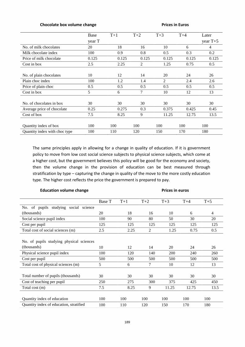
189
Chocolate box volume change Prices in Euros
Base
year T
T+1 T+2 T+3 T+4 Later
year T+5
No. of milk chocolates 20 18 16 10 6 4
Milk chocolate index 100 0.9 0.8 0.5 0.3 0.2
Price of milk chocolate 0.125 0.125 0.125 0.125 0.125 0.125
Cost in box 2.5 2.25 2 1.25 0.75 0.5
No. of plain chocolates 10 12 14 20 24 26
Plain choc index 100 1.2 1.4 2 2.4 2.6
Price of plain choc 0.5 0.5 0.5 0.5 0.5 0.5
Cost in box 5 6 7 10 12 13
No. of chocolates in box 30 30 30 30 30 30
Average price of chocolate 0.25 0.275 0.3 0.375 0.425 0.45
Cost of box 7.5 8.25 9 11.25 12.75 13.5
Quantity index of box 100 100 100 100 100 100
Quantity index with choc type 100 110 120 150 170 180
The same principles apply in allowing for a change in quality of education. If it is government
policy to move from low cost social science subjects to physical science subjects, which come at
a higher cost, but the government believes this policy will be good for the economy and society,
then the volume change in the provision of education can be best measured through
stratification by type – capturing the change in quality of the move to the more costly education
type. The higher cost reflects the price the government is prepared to pay.
Education volume change Prices in euros
Base T T+1 T+2 T+3 T+4 T+5
No. of pupils studying social science
(thousands) 20 18 16 10 6 4
Social science pupil index 100 90 80 50 30 20
Cost per pupil 125 125 125 125 125 125
Total cost of social sciences (m) 2.5 2.25 2 1.25 0.75 0.5
No. of pupils studying physical sciences
(thousands) 10 12 14 20 24 26
Physical science pupil index 100 120 140 200 240 260
Cost per pupil 500 500 500 500 500 500
Total cost of physical sciences (m) 5 6 7 10 12 13
Total number of pupils (thousands) 30 30 30 30 30 30
Cost of teaching per pupil 250 275 300 375 425 450
Total cost (m) 7.5 8.25 9 11.25 12.75 13.5
Quantity index of education 100 100 100 100 100 100
Quantity index of education, stratified 100 110 120 150 170 180

190
Useful references and links
General references Commission of the European Communities, IMF, OECD, United Nations and
Worldbank (2008) System of National Accounts 2008
http://unstats.un.org/unsd/nationalaccount/sna2008.asp
Commission of the European Communities/Eurostat (2013) European System of
Accounts 2010
http://eur-
lex.europa.eu/LexUriServ/LexUriServ.do?uri=OJ:L:2013:174:0001:0727:EN:PDF
2002/990/EC: Commission Decision of 17 December 2002 further clarifying Annex
A to Council Regulation (EC) No 2223/96 as concerns the principles for measuring
prices and volumes in national accounts (Text with EEA relevance) (notified under
document number C(2002) 5054)
http://eur-
lex.europa.eu/LexUriServ/LexUriServ.do?uri=CELEX:32002D0990:EN:HTML
International Monetary Fund (2001) Quarterly National Accounts Manual:
Concepts, Data Sources and Compilation (Chapter 9)
http://www.imf.org/external/pubs/ft/qna/2000/textbook/ch1.pdf
OECD (2002) Inflation Accounting: A Manual on National Accounting under
Conditions of High Inflation
http://www.oecd-ilibrary.org/economics/inflation-accounting_9789264299511-en
Eurostat (1998-2000) Reports of the Task Forces on price and volume measures for:
Health
Education
Public Administration
Construction
Large equipment
Computers and software
Financial intermediation
Real estate, renting and business services
Post and telecommunication
https://circabc.europa.eu/w/browse/64dcd7a3-5b22-437c-bccf-c8a22997ffbc
Eurostat (2013) Handbook on quarterly national accounts
http://epp.eurostat.ec.europa.eu/portal/page/portal/product_details/publication?p_pr
oduct_code=KS-GQ-13-004
Eurostat (2000) Manual on the Economic Accounts for Agriculture and Forestry (rev
1.1)
191
http://epp.eurostat.ec.europa.eu/cache/ITY_OFFPUB/KS-27-00-782/EN/KS-27-00-
782-EN.PDF
Eurostat (2008) Manual on Supply, Use and Input-Output Tables
http://epp.eurostat.ec.europa.eu/cache/ITY_OFFPUB/KS-RA-07-013/EN/KS-RA-07-
013-EN.PDF
Price and volume measurement has been on the agenda of the annual OECD
Meeting of National Accounts Experts for a number of years. All papers of the
meetings since 1997 can be found via the OECD website.
http://www.oecd.org/std/na/nationalaccountsmeetings-archiveofpapers.htm
Chaining, index formulae and the level of aggregation See the papers presented to the annual OECD Meetings of National Accounts
Experts mentioned above
Australian Bureau of Statistics (1998) Introduction of Chain Volume Measures in
the Australian National Accounts, Information Paper no. 5248.0
http://www.abs.gov.au/AusStats/[email protected]/MF/5248.0S. de Boer and G.A.A.M.
Broesterhuizen (1986) The simultaneous compilation of current price and deflated
input-output tables, National Accounts Occasional Paper no. NA-13
S. de Boer, W. van Nunspeet and T. Takema (2000) Supply and use tables in current
and constant prices for the Netherlands: an experience of fifteen years, National
Accounts Occasional Paper no. NA-092
http://www.cbs.nl/nr/rdonlyres/cbe5041f-b4c3-492b-9e9e-
4822be6fca39/0/2000092p30pub.pdfhttp://www.cbs.nl/en/products/articles/mac
ro-economics/national-accounts/occpapers.htm
E. Dalgaard (1997) Implementing the revised SNA; recommendations on price and
volume measures Review of Income and Wealth, Series 43, Number 4, p. 487-503
E. R. Diewert (1976) Exact and Superlative Index Numbers, Journal of Econometrics
4:2
P. von der Lippe (2001) Chain indices - A Study in Price Index Theory, Spectrum of
Federal Statistics, Volume 16, Statistisches Bundesamt, Germany
Statistisches Bundesamt (2000) Effects of level of aggregation of GDP and its
aggregates, study report for Eurostat, available upon request
Producer Price Indices and Consumer Price Indices International Monetary Fund (2010) Producer Price Index Manual
www.imf.org/external/pubs/ft/ppi/2010/manual/ppi.pdf
International Labour Organisation Consumer price index manual: theory and
practice (2004)

192
http://www.ilo.org/public/english/bureau/stat/guides/cpi/
Eurostat (1998) Methodological Aspects of Producer Prices on the Export Market
http://bookshop.europa.eu/en/methodological-aspects-of-producer-prices-on-
the-export-market-pbCA1197172/
Eurostat (2001) Compendium of HICP reference documents
Many papers on Consumer Price Indices can be found via the website of the
Ottawa Group - International Conference on Price Indices:
http://www.ottawagroup.org/
Furthermore, papers from a 2012 UNECE meeting on Consumer Price Indices can
be found at
http://www.unece.org/stats/documents/2012.05.cpi.html
M.J. Boskin, E.R. Dulberger, Z. Griliches, R.J. Gordon, D.W. Jorgenson (1996)
Toward a more accurate measure of the cost of living, Final report to the Senate
Finance Committee from the Advisory Commission to study the consumer price
index
http://www.ssa.gov/history/reports/boskinrpt.html
OECD (2005) Methodological Guide for Developing Producer Price Indices for
Services Production.
http://www.oecd.org/std/prices-ppp/36274111.pdf
OECD (2007), Compilation Manual for an Index of Services
http://www.oecd-ilibrary.org/economics/compilation-manual-for-an-index-of-
services-production_9789264034440-en
Quality changes and new products T.F. Bresnahan and R. Gordon (Eds.) (1996) The economics of new goods, National
Bureau of Economic Research, University of Chicago Press
W.D. Nordhaus (1998) Quality changes in price indexes, Journal of Economic
Perspectives, Volume 12(1), p. 59-68
D. Sellwood (1995) The Harmonisation of Quality adjustment Practices in the
European Union, in: Eurostat Improving the Quality of Price Indices: CPIs and PPIs,
proceedings of an International Seminar in Florence, Italy
J.E. Triplett, J. E. (1983) Concepts of Quality in Input and Output Price Measures: A
Resolution of the User-Value Resource-Cost Debate, in M.F. Foss (Ed.) The U.S.
National Income and Product Accounts: Selected Topics National Bureau of
Economic Research, Studies in Income and Wealth, vol. 47
193
Computers, other high technology goods and capital goods E.R. Berndt, E.R. Dulberger and N.J. Rappaport (2000) Price and quality of desktop
and mobile personal computers: a quarter century of history, paper presented to
the NBER Summer Institute 2000
http://ideas.repec.org/a/aea/aecrev/v91y2001i2p268-273.html
J. Dalén (1989) Using Hedonic regression for Computer equipment in the Producer
Price Index, R&D Report Statistics Sweden, 1989:25
D. Harhoff and D. Moch (1996) Price Indexes for PC Database Software and the
value of Code Compatibility, ZEW Discussion Paper No 96-17, Mannheim, Germany
J.S. Landefeld and B.T. Grimm (2000) The impact of hedonics and computers on
real GDP, Survey of Current Business, December 2000, p. 17-22
http://www.bea.gov/scb/pdf/beawide/2000/1200hm.pdf
J.S. Landefeld and B.M. Fraumeni (2001) Measuring the new economy, Survey of
Current Business, March 2001, p. 23-40
http://www.bea.gov/scb/pdf/beawide/2001/0301mne.pdf
L.A. Lunde, S.L. Røgeberg, L. Sandberg (1999) Price Indices for Capital Goods, Part 1
- descriptive studies, study report for Eurostat on countries practices on capital
goods, available upon request
P. McCarthy (1997) Computer Prices: How good is the quality adjustment?, paper
presented at the March 1997 Capital Stock Conference
http://citeseerx.ist.psu.edu/viewdoc/download?doi=10.1.1.124.1525&rep=rep1&t
ype=pdf
A. Moreau (1996) Methodology of the Price Index for Microcomputers and Printers
in France in OECD Proceedings: Industry Productivity, International Comparison
and Measurement Issues
http://www.oecd.org/industry/publicationsdocuments/reports/48/
W. D. Nordhaus (2001) The Progress of Computing, paper presented to the NBER
Summer Institute 2001
http://www.nber.org/~confer/2001/si2001/prbprg.html
P. Schreyer (1998) Information and communication technology and the
measurement of real output, final demand and productivity, OECD STI Working
Paper 1998/2
http://www.oecd-
ilibrary.org/docserver/download/5lgsjhvj7nbr.pdf?expires=1387448754&id=id&ac
cname=guest&checksum=AA58FD08112CBDB1ACEC9FDDC4CDCBC6
P. Schreyer (2001) Computer price indices and international growth and
productivity comparisons, OECD STD/DOC(2001)/1

194
http://search.oecd.org/officialdocuments/displaydocumentpdf/?doclanguage=en
&cote=STD/DOC(2001)1
Statistik Austria (2001) Preisindex für Ausrüstungsinvestitionen – 1995 bis 2000,
Schnellbericht 5.7 (in German, available from Statistik Austria)
J.E. Triplett (1991) Hedonic Methods in Statistical Agency Environments: An
Intellectual Biopsy, in E.R. Berndt and J.E. Triplett (Eds.) Fifty Years of Economic
Measurement: National Bureau of Economic Research, Studies in Income and
Wealth, No. 54
J.E. Triplett (2001) Handbook on Quality Adjustment of Price Indexes for
Information and Communication Technology Products (draft), OECD
J.E. Triplett (2004) Handbook on Hedonic Indexes and Quality Adjustment in Price
Indexes, OECD
http://www.oecd-ilibrary.org/science-and-technology/handbook-on-hedonic-
indexes-and-quality-adjustments-in-price-indexes_643587187107
Market services Many papers on the development of Producer Price Indices for services can be
found on the website of the Voorburg Group on Service Statistics
http://www.voorburggroup.org/
Eurostat (1996) Methodological Aspects of Construction Price Indices
http://bookshop.europa.eu/en/methodological-aspects-of-construction-price-
indices-pbCA9896300/
Non-market services At the annual OECD meetings many papers on development in measuring non-
market services were presented, see above for the link.
Ministry of Finance, Sweden (1996) Productivity Trends in the Public Sector in
Sweden, Fritzes, Stockholm
OECD (2011) A System of Health Accounts
http://www.oecd.org/els/health-systems/asystemofhealthaccounts2011.htm
D.M. Cutler and E.R. Berndt (Eds.) (2001) Medical care output and productivity,
University of Chicago Press (see http://www.nber.org/bookstoc/medoutput.html
for the table of contents)
J.E. Triplett (Ed.) (1999) Measuring the prices of medical treatments, Brookings
Institution Press
http://www.brookings.edu/~/media/research/files/papers/2009/11/22%20health
%20system%20productivity%20triplett/1122_health_system_productivity_triplett.

195
P. Schreyer (2012), Output, outcome and quality adjustment in measuring health
and education services. Wiley Online Library
http://onlinelibrary.wiley.com/doi/10.1111/j.1475-4991.2012.00504.x/full