Embed Size (px)
Citation preview
8/22/2019 Handbook Volume 01
http://slidepdf.com/reader/full/handbook-volume-01 1/440
HANDBOOK OF MAGMA FUNCTIONS
Volume 1
Language, Aggregates and Semigroups
John Cannon Wieb Bosma
Editors
Version 2.13
Sydney
September 22, 2006

8/22/2019 Handbook Volume 01
http://slidepdf.com/reader/full/handbook-volume-01 2/440
ii
8/22/2019 Handbook Volume 01
http://slidepdf.com/reader/full/handbook-volume-01 3/440
MAGMAC O M P U T E R • A L G E B R A
HANDBOOK OF MAGMA FUNCTIONS
Editors:
John Cannon Wieb Bosma
Handbook Contributors:
Geoff Bailey, Wieb Bosma, Gavin Brown, Herbert Bruck-
ner, Nils Bruin, John Cannon, Jon Carlson, Scott Contini,
Bruce Cox, Steve Donnelly, Willem de Graaf, Claus Fieker,
Volker Gebhardt, Sergei Haller, Michael Harrison, FlorianHeß, David Kohel, Axel Kohnert, Dimitri Leemans, Paulette
Lieby, Graham Matthews, Scott Murray, Eamonn O’Brien,
Ben Smith, Bernd Souvignier, William Stein, Allan Steel,
Nicole Sutherland, Don Taylor, Bill Unger, Alexa van der
Waall, Paul van Wamelen, Helena Verrill, John Voight, Mark
Watkins, Greg White
Production Editors:
Wieb Bosma Claus Fieker Allan Steel Nicole Sutherland
HTML Production:
Claus Fieker Allan Steel

8/22/2019 Handbook Volume 01
http://slidepdf.com/reader/full/handbook-volume-01 4/440
8/22/2019 Handbook Volume 01
http://slidepdf.com/reader/full/handbook-volume-01 5/440
PREFACE
The computer algebra system Magma is designed to provide a software environment forcomputing with the structures which arise in areas such as algebra, number theory, al-gebraic geometry and (algebraic) combinatorics. Magma enables users to define and tocompute with structures such as groups, rings, fields, modules, algebras, schemes, curves,graphs, designs, codes and many others. The main features of Magma include:
• Algebraic Design Philosophy: The design principles underpinning both the user lan-guage and system architecture are based on ideas from universal algebra and categorytheory. The language attempts to approximate as closely as possible the usual mathe-matical modes of thought and notation. In particular, the principal constructs in the
user language are set, (algebraic) structure and morphism.• Explicit Typing: The user is required to explicitly define most of the algebraic structures
in which calculations are to take place. Each object arising in the computation is thendefined in terms of these structures.
• Integration: The facilities for each area are designed in a similar manner using genericconstructors wherever possible. The uniform design makes it a simple matter to pro-gram calculations that span different classes of mathematical structures or which involvethe interaction of structures.
• Relationships: Magma provides a mechanism that manages “relationships” between
complex bodies of information. For example, when substructures and quotient struc-tures are created by the system, the natural homomorphisms that arise are alwaysstored. These are then used to support automatic coercion between parent and childstructures.
• Mathematical Databases: Magma has access to a large number of databases containinginformation that may be used in searches for interesting examples or which form anintegral part of certain algorithms. Examples of current databases include factorizationsof integers of the form pn ± 1, p a prime; modular equations; strongly regular graphs;maximal subgroups of simple groups; integral lattices; K 3 surfaces; best known linearcodes and many others.
• Performance: The intention is that Magma provide the best possible performanceboth in terms of the algorithms used and their implementation. The design philosophypermits the kernel implementor to choose optimal data structures at the machine level.Most of the major algorithms currently installed in the Magma kernel are state-of-the-art and give performance similar to, or better than, specialized programs.
The theoretical basis for the design of Magma is founded on the concepts and methodologyof modern algebra. The central notion is that of an algebraic structure . Every objectcreated during the course of a computation is associated with a unique parent algebraicstructure. The type of an object is then simply its parent structure.
8/22/2019 Handbook Volume 01
http://slidepdf.com/reader/full/handbook-volume-01 6/440
vi PREFACE
Algebraic structures are first classified by variety : a variety being a class of structureshaving the same set of defining operators and satisfying a common set of axioms. Thus,
the collection of all rings forms a variety. Within a variety, structures are partitioned intocategories . Informally, a family of algebraic structures forms a category if its members allshare a common representation. All varieties possess an abstract category of structures(the finitely presented structures). However, categories based on a concrete representationare as least as important as the abstract category in most varieties. For example, withinthe variety of algebras, the family of finitely presented algebras constitutes an abstractcategory, while the family of matrix algebras constitutes a concrete category.
Magma comprises a novel user programming language based on the principles outlinedabove together with program code and databases designed to support computational re-search in those areas of mathematics which are algebraic in nature. The major areas
represented in Magma V2.13 include group theory, ring theory, commutative algebra,arithmetic fields and their completions, module theory and lattice theory, finite dimen-sional algebras, Lie theory, representation theory, the elements of homological algebra,general schemes and curve schemes, modular forms and modular curves, finite incidencestructures, linear codes and much else.
This set of volumes (known as the Handbook) constitutes the main reference work onMagma. It aims to provide a comprehensive description of the Magma language and themathematical facilities of the system, In particular, it documents every function and oper-ator available to the user. Our aim (not yet achieved) is to list not only the functionalityof the Magma system but also to show how the tools may be used to solve problems inthe various areas that fall within the scope of the system. This is attempted through the
inclusion of tutorials and sophisticated examples. Finally, starting with the edition corre-sponding to release V2.8, this work aims to provide some information about the algorithmsand techniques employed in performing sophisticated or time-consuming operations. It willtake some time before this goal is fully realised.
We give a brief overview of the organization of the Handbook.
• Volume 1 contains a terse summary of the language together with a description of thecentral datatypes: sets, sequences, tuples, mappings, etc. It also describes the facilitiesfor semigroups and monoids. An index of all intrinsics appears at the end of the volume.
• Volume 2 describes the facilities for finite groups and, in particular, discusses permu-
tation groups, matrix groups and finite soluble groups defined by a power-conjugatepresentation. A chapter is devoted to databases of groups.
• Volume 3 describes the machinery provided for infinite groups. In Magma these cor-respond mainly to various kinds of finitely presented groups. Included are abeliangroups, general finitely presented groups, polycyclic groups, braid groups, automaticgroups and subgroups of P SL2(R).
• Volume 4 deals with basic rings and linear algebra. The rings include the integers, therationals, finite fields, univariate and multivariate polynomial rings and the real andcomplex fields. The linear algebra section covers matrices and vector spaces.
8/22/2019 Handbook Volume 01
http://slidepdf.com/reader/full/handbook-volume-01 7/440
PREFACE vii
• Volume 5 covers ring extensions. The major topics are number fields and their orders,function fields, local rings and fields, power series rings including Laurent and Puiseux
series rings, and algebraically closed fields.
• Volume 6 is devoted to module theory and (linear) algebras. The module theory in-cludes R-modules, basic homological algebra and lattices. Most of the material relatingto algebras is concerned with finite dimensional associate algebras including matrixalgebras, group algebras, basic algebras and quaternion algebras.
• Volume 7 is concerned with representation theory and Lie theory. The representa-tion theory includes K [G]-modules, character theory and invariant theory. Lie theoryincludes root systems, root data, Lie algebras, Coxeter groups, reflection groups, Liegroups and quantum groups.
• Volume 8 covers commutative algebra and algebraic geometry. The commutative alge-bra material includes constructive ideal theory, affine algebras and modules over affinealgebras. In algebraic geometry, the main topics are schemes, curves and surfaces.
• Volume 9 describes the machinery pertaining to arithmetic geometry. The main topicsinclude the arithmetic properties of low genus curves such as elliptic and hyperellipticcurves, modular curves and modular forms and L-series.
• In general terms, Volume 10 is concerned with combinatorial theory and (finite) inci-dence structures. The topics include graphs, designs, finite planes, incidence geometry,linear codes, pseudo-random sequences and a small chapter on optimization (linear
programming).
Although the Handbook has been compiled with care, it is possible that the semantics of some facilities have not been described adequately. We regret any inconvenience that thismay cause, and we would be most grateful for any comments and suggestions for improve-ment. We would like to thank users for numerous helpful suggestions for improvement andfor pointing out misprints in previous versions.
The development of Magma has only been possible through the dedication and enthu-siasm of a group of very talented mathematicians and computer scientists. Since 1990,the principal members of the Magma group have included: Geoff Bailey, Mark Bofinger,
Wieb Bosma, Gavin Brown, John Brownie, Herbert Bruckner, Nils Bruin, Steve Collins,Scott Contini, Bruce Cox, Steve Donnelly, Willem de Graaf, Claus Fieker, Damien Fisher,Alexandra Flynn, Volker Gebhardt, Katharina Geißler, Sergei Haller, Michael Harrison,Emanuel Herrmann, Florian Heß, David Kohel, Paulette Lieby, Graham Matthews, ScottMurray, Anne O‘Kane, Catherine Playoust, Richard Rannard, Colva Roney-Dougal, An-drew Solomon, Bernd Souvignier, Ben Smith, Allan Steel, Damien Stehle, Nicole Suther-land, Bill Unger, John Voight, Alexa van der Waall, Mark Watkins and Greg White.
John CannonSydney, June 2006

8/22/2019 Handbook Volume 01
http://slidepdf.com/reader/full/handbook-volume-01 8/440
8/22/2019 Handbook Volume 01
http://slidepdf.com/reader/full/handbook-volume-01 9/440
ACKNOWLEDGEMENTS
The Magma Development Team
Current Members
Geoff Bailey, BSc (Hons) (Sydney), [1995-]: Main interests include elliptic curves (espe-cially those defined over the rationals), virtual machines and computer language design.Has implemented part of the elliptic curve facilities especially the calculation of Mordell-Weil groups. Other main areas of contribution include combinatorics, local fields and the
Magma system internals.
John Cannon Ph.D. (Sydney), [1971-]: Research interests include computational meth-ods in algebra, geometry, number theory and combinatorics; the design of mathematicalprogramming languages and the integration of databases with Computer Algebra systems.Contributions include overall concept and planning, language design, specific design formany categories, numerous algorithms (especially in group theory) and general manage-ment.
Steve Donnelly, Ph.D. (Georgia) [2005-]: Research interests are in arithmetic geometry.Major contributions have been to the elliptic curve machinery with particular emphasis ondescent methods.
Claus Fieker, Ph.D. (TU Berlin), [2000-]: Formerly a member of the KANT project.Research interests are in constructive algebraic number theory and, especially, relativeextensions and computational class field theory. Main contributions are the developmentof explicit algorithmic class field theory in the case of both number and function fields.Contributed to the module theory over Dedekind domains and is currently developinggeneric constructive techniques for Drinfeld modules.
Damien Fisher, BSc (Advanced) (Sydney), BSc (Hons) (UNSW), [2002-]: Implementeda new package for p-adic rings and their extensions that places a strong emphasis on fastarithmetic. Played a major role in the installation (in 2004-2005) of the MPFR package
in place of the previous MP and Pari real packages. Current projects focus on extensionsto the Magma language, and include a Magma profiler.
Sergei Haller, Ph.D. (Eindhoven) [2004, 2006-]: Works in the area of linear algebraicgroups. Implemented new algorithms for element operations in (split and twisted) groupsof Lie type, non-reduced and extended root data, Cartan type Lie algebras, Galois coho-mology, and cohomology of finite non-abelian groups.
Michael Harrison, Ph.D. (Cambridge,UK 1992), [2003-]: Research interests are in num-ber theory, arithmetic and algebraic geometry. Implemented the p-adic methods for count-ing points on hyperelliptic curves and their Jacobians over finite fields: Kedlaya’s method
8/22/2019 Handbook Volume 01
http://slidepdf.com/reader/full/handbook-volume-01 10/440
x ACKNOWLEDGEMENTS
and the modular parameter method of Mestre. Currently working on machinery for generalsurfaces and cohomology for projective varieties.
Allan Steel, BA (Hons, University Medal) (Sydney), [1989-]: Has developed many of the fundamental data structures and algorithms in Magma for multiprecision integers,finite fields, matrices and modules, polynomials and Grobner bases, aggregates, memorymanagement, environmental features, and the package system, and has also worked on theMagma language interpreter. In collaboration, he has developed the code for lattice theory(with Bernd Souvignier), invariant theory (with Gregor Kemper) and module theory (withJon Carlson and Derek Holt).
Damien Stehle, Ph.D. (Nancy) [2006]: Works in the areas of algorithmic number theory(in particular, the geometry of numbers) and computer arithmetic. Implemented theproveably correct floating-point LLL algorithm together with a number of fast non-rigorous
variants.
Nicole Sutherland, BSc (Hons) (Macquarie), [1999-]: Works in the areas of numbertheory and algebraic geometry. Developed the machinery for Newton polygons and lazypower series and contributed to the code for local fields, number fields, modules overDedekind domains, function fields, schemes and has done some work with Algebras.
Bill Unger, Ph.D. (Sydney), [1998-]: Works in computational group theory, with par-ticular emphasis on algorithms for permutation and matrix groups. Implemented manyof the current permutation and matrix group algorithms for Magma, in particular BSGSverification, solvable radical and chief series algorithms. Recently developed a new method
for computing character tables of finite groups.John Voight, Ph.D. (Berkeley) [2005-]: Works in the area of algebraic number theory andarithmetic geometry. Implemented algorithms for quaternion algebras (including recogni-tion functions, and computation of maximal orders and ideal classes over number fields),associative orders (with Nicole Sutherland), and Shimura curves.
Greg White, BSc (Hons) (Sydney), [2000-]: Research interests include cryptography andcoding theory. Contributions include a database of best known linear codes database forbinary and quaternary codes, machinery for codes over finite rings, and a package forYoung Tableaux. Current projects include discrete logarithms in finite fields and quantumerror correcting codes.
8/22/2019 Handbook Volume 01
http://slidepdf.com/reader/full/handbook-volume-01 11/440
ACKNOWLEDGEMENTS xi
Former Members
Wieb Bosma, [1989-1996]: Responsible for the initial development of number theoryin Magma and the coordination of work on commutative rings. Also has continuinginvolvement with the design of Magma.
Gavin Brown,[1998-2001]: Developed code in basic algebraic geometry, applications of Grobner bases, number field and function field kernel operations; applications of Hilbertseries to lists of varieties.
Herbert Bruckner, [1998–1999]: Developed code for constructing the ordinary irre-ducible representations of a finite soluble group and the maximal finite soluble quotient of a finitely presented group.
Nils Bruin, [2002–2003]: Contributions include Selmer groups of elliptic curves and hy-perelliptic Jacobians over arbitrary number fields, local solubility testing for arbitrary pro-
jective varieties and curves, Chabauty-type computations on Weil-restrictions of ellipticcurves and some algorithms for, and partial design of, the differential rings module.
Bruce Cox, [1990–1998]: A member of the team that worked on the design of the Magma
language. Responsible for implementing much of the first generation Magma machineryfor permutation and matrix groups.
Alexandra Flynn, [1995–1998]: Incorporated various Pari modules into Magma, anddeveloped much of the machinery for designs and finite planes.
Volker Gebhardt, [1999–2003]: Author of the Magma categories for infinite polycyclicgroups and for braid groups. Other contributions include machinery for general finitelypresented groups.
Katharina Geißler, [1999–2001]: Developed the code for computing Galois groups of number fields and function fields.
Willem de Graaf , [2004-2005]: Contributed functions for computing with finite-dimensional Lie algebras, finitely-presented Lie algebras, universal enveloping algebrasand quantum groups.
Emanuel Herrmann, [1999]: Developed code for computing integral points and S -
integral points on elliptic curves.Florian Heß, [1999–2001]: Developed a substantial part of the algebraic function fieldmodule in Magma including algorithms for the computation of Riemann-Roch spacesand class groups. His most recent contribution (2005) is a package for computing allisomorphisms between a pair of function fields.
David Kohel, [1999–2002]: Contributions include a model for schemes (with G Brown);algorithms for curves of low genus; implementation of elliptic curves, binary quadraticforms, quaternion algebras, Brandt modules, spinor genera and genera of lattices, modularcurves, conics (with P Lieby), modules of supersingular points (with W Stein), Witt rings.
8/22/2019 Handbook Volume 01
http://slidepdf.com/reader/full/handbook-volume-01 12/440
xii ACKNOWLEDGEMENTS
Paulette Lieby, [1999–2003]: Contributed to the development of algorithms for alge-braic geometry, abelian groups and incidence structures. Developed datastructures for
multigraphs and implemented algorithms for planarity, triconnectivity and network flows.
Graham Matthews, [1989–1993]: Involved in the design of the Magma semantics, userinterface, and internal organisation.
Richard Rannard, [1997–1998]: Contributed to the code for elliptic curves over finitefields including a first version of the SEA algorithm.
Colva M. Roney-Dougal, [2001–2003]: Completed the classification of primitive per-mutation groups up to degree 999 (with Bill Unger). Also undertook a constructive clas-sification of the maximal subgroups of the classical simple groups.
Michael Slattery, [1987–2006]: Contributed a large part of the machinery for finite
soluble groups including subgroup lattice and automorphism group.
Ben Smith, [2000–2003]: Contributed to an implementation of the Number Field Sieveand a package for integer linear programming.
Bernd Souvignier, [1996–1997]: Contributed to the development of algorithms and codefor lattices, local fields, finite dimensional algebras and permutation groups.
Alexa van der Waall, [2003]: Implemented the module for differential Galois theory.
Paul B. van Wamelen, [2002–2003]: Implemented analytic Jacobians of hyperellipticcurves in Magma.
Mark Watkins, [2003, 2004-2005]: Implemented a range of analytic tools for the studyof elliptic curves including analytic rank, modular degree, set of curves Q-isogenous to agiven curve, 4-descent, Heegner points and other point searching methods.
8/22/2019 Handbook Volume 01
http://slidepdf.com/reader/full/handbook-volume-01 13/440
ACKNOWLEDGEMENTS xiii
External Contributors
The Magma system has benefited enormously from contributions made by many membersof the mathematical community. We list below those persons and research groups who havegiven the project substantial assistance either by allowing us to adapt their software forinclusion within Magma or through general advice and criticism. We wish to express ourgratitude both to the people listed here and to all those others who participated in someaspect of the Magma development.
Group Theory
Constructive recognition of quasi-simple groups belonging to the Suzuki and Ree familieshas been implemented by Hendrik Baarnhielm (QMUL). The package includes code forconstructing the Sylow p-subgroups of Suzuki and Ree groups.
A database of all groups having order at most 2000, excluding order 1024 has been madeavailable by Hans Ulrich Besche (Aachen), Bettina Eick (Braunschweig), and Ea-monn O’Brien (Auckland). This library incorporates “directly” the libraries of 2-groupsof order dividing 256 and the 3-groups of order dividing 729, which were prepared anddistributed at various intervals by Mike Newman (ANU) and Eamonn O’Brien andvarious assistants, the first release dating from 1987.
Peter Brooksbank (Ohio) gave the Magma group permission to base its implementationof the Kantor-Seress algorithm for black-box recognition of linear, symplectic and unitarygroups on his GAP implementations.
The soluble quotient algorithm in Magma was designed and implemented by HerbertBruckner (Aachen).
Michael Downward and Eamonn O’Brien (Auckland) provided functions to accessmuch of the data in the on-line Atlas of Finite Simple Groups for the sporadic groups. Afunction to select “good” base points for sporadic groups was provided by Eamonn andRobert Wilson (London).
A new algorithm for computing all normal subgroups of a finitely presented group up to aspecified index has been designed and implemented by David Firth and Derek Holt.
Derek Holt (Warwick) has implemented his algorithm for testing whether two finitely
presented groups are isomorphic in Magma.
Procedures to list irreducible (soluble) subgroups of GL(2, q ) and GL(3, q ) for arbitrary q are provided by Dane Flannery (Galway) and Eamonn O’Brien (Auckland).
Greg Gamble (UWA) helped refine the concept of a G-set for a permutation group anddrafted several sections of the chapter on permutation groups.
The descriptions of the groups of order p4, p5, p6, p7 for p > 3 were contributed byBoris Girnat, Robert McKibbin, Mike Newman, Eamonn O’Brien, and MikeVaughan-Lee.
8/22/2019 Handbook Volume 01
http://slidepdf.com/reader/full/handbook-volume-01 14/440
xiv ACKNOWLEDGEMENTS
Versions of Magma from V2.8 onwards employ the Advanced Coset Enumerator designedby George Havas (Queensland) and implemented by Colin Ramsay (also of Queens-
land). George has also contributed to the design of the machinery for finitely presentedgroups.
Machinery for computing group cohomology and for producing group extensions has beenprovided by Derek Holt (Warwick). There are two parts to this machinery. The firstpart comprises Derek’s older C-language package for permutation groups while the secondpart comprises a recent Magma language package for group cohomology.
Calculation of automorphism groups (for permutation and matrix groups) and determin-ing group isomorphism (for finite groups) is performed by code written by Derek Holt(Warwick).
Derek Holt (Warwick) developed a modified version of his program, kbmag, for inclusionwithin Magma. The Magma facilities for groups and monoids defined by confluent rewritesystems, as well as automatic groups, are supported by this code.
Derek Holt (Warwick) has implemented the Magma version of the Bratus/Pak algorithmfor black-box recognition of the symmetric and alternating groups.
The function for determining whether a given finite permutation group is a homomor-phic image of a finitely presented group has been implemented in C by Volker Gebhardt(Magma) from a Magma language prototype developed by Derek Holt (Warwick).
Alexander Hulpke (Colorado State) has made available his database of all transitive
permutation groups of degree up to 30. This incorporates the earlier database of GregButler (Concordia) and John McKay (Concordia) containing all transitive groups of degree up to 15.
Most of the algorithms for p-groups and many of the algorithms implemented in Magma
for finite soluble groups are largely due to Charles Leedham–Green (QMW, London).
The PERM package developed by Jeff Leon (UIC) for efficient backtrack searching inpermutation groups is used for most of the permutation group constructions that employbacktrack search.
A Monte-Carlo algorithm to determine the defining characteristic of a quasisimple group
of Lie type has been contributed by Martin Liebeck (Imperial) and Eamonn O’Brien(Auckland).
A Monte-Carlo algorithm for non-constructive recognition of simple groups has been con-tributed by Gunter Malle (Kaiserslautern) and Eamonn O’Brien (Auckland). Thisprocedure includes the algorithm of Babai et al. to name a quasisimple group of Lie type.
Magma incorporates a database of the maximal finite rational subgroups of GL(n, Q) upto dimension 31. This database is due to Gabriele Nebe (Ulm) and Wilhelm Plesken(Aachen). A database of quaternionic matrix groups constructed by Gabriele is also in-cluded.
8/22/2019 Handbook Volume 01
http://slidepdf.com/reader/full/handbook-volume-01 15/440
ACKNOWLEDGEMENTS xv
A function that determines whether a matrix group G (defined over a finite field) is thenormaliser of an extraspecial group in the case where the degree of G is an odd prime uses
the new Monte-Carlo algorithm of Alice Niemeyer (Perth) and has been implementedin Magma by Eamonn O’Brien (Auckland).
The NQ program of Werner Nickel (Darmstadt) is used to compute nilpotent quotientsof finitely presented groups.
The package for recognizing large degree classical groups over finite fields was designedand implemented by Alice Niemeyer (Perth) and Cheryl Praeger (Perth). It has beenextended to include 2-dimensional linear groups by Eamonn O’Brien (Auckland).
The p-quotient program, developed by Eamonn O’Brien (Auckland) based on earlierwork by George Havas and Mike Newman (ANU), provides a key facility for studying
p-groups in Magma. Eamonn’s extensions in Magma of this package for generating p-groups, computing automorphism groups of p-groups, and deciding isomorphism of p-groups are also included. He has contributed software to count certain classes of p-groupsand to construct central extensions of soluble groups.
Eamonn O’Brien (Auckland) has contributed a Magma implementation of algorithmsfor determining the Aschbacher category of a subgroup of GL(n, q ). The correspondingsections of the Handbook were written by Eamonn.
Eamonn O’Brien (Auckland) has provided implementations of constructive recognitionalgorithms for matrix groups as either (P)SL(2, q) or (P)SL(3, q).
The package for classifying metacyclic p-groups has been developed by Eamonn O’Brien
(Auckland) and Mike Vaughan-Lee (Oxford).A fast algorithm for determining subgroup conjugacy based on Aschbacher’s theorem clas-sifying the maximal subgroups of a linear group has been designed and implemented byColva Roney-Dougal (Sydney).
Colva Roney-Dougal (Sydney) has implemented the Beals et al algorithm for black-boxrecognition of the symmetric and alternating groups.
A package for constructing the Sylow p-subgroups of the classical groups has been imple-mented by Mark Stather (Warwick).
Generators for matrix representations for groups of Lie type were constructed and imple-
mented by Don Taylor (Sydney) with some assistance from Leanne Rylands (WesternSydney).
The low index subgroup function is implemented by code that is based on a Pascal programwritten by Charlie Sims (Rutgers).
A package for computing with subgroups of finite index in the group PSL(2 , R) has beendeveloped by Helena Verrill (Hannover).
A Magma database has been constructed from the permutation and matrix representationscontained in the on-line Atlas of Finite Simple Groups with the assistance of its authorRobert Wilson (Birmingham).
8/22/2019 Handbook Volume 01
http://slidepdf.com/reader/full/handbook-volume-01 16/440
xvi ACKNOWLEDGEMENTS
Basic Rings
A facility for computing with arbitrary but fixed precision reals was based on RichardBrent’s (ANU) FORTRAN package MP. Richard has also made available his database of 237, 578 factorizations of integers of the form pn ± 1, together with his intelligent factor-ization code FACTOR.
Stefi Cavallar (CWI, Amsterdam) has adapted her code for filtering relations in the CWINumber Field Sieve so as to run as part of the Magma Number Field Sieve.
The group headed by Henri Cohen (Bordeaux) made available parts of their Pari systemfor computational number theory for inclusion in Magma. Pascal Letard of the Pari
group visited Sydney for two months in 1994 and recoded large sections of Pari for Magma.The Pari facilities installed in Magma include arithmetic for real and complex fields (the
‘free’ model), approximately 100 special functions for real and complex numbers, quadraticfields and other features.
Xavier Gourdon (INRIA, Paris) made available his C implementation of A. Schonhage’ssplitting-circle algorithm for the fast computation of the roots of a polynomial to a specifiedprecision. Xavier also assisted with the adaptation of his code for the Magma kernel.
One of the main integer factorization tools available in Magma is due to ArjenK. Lenstra (EPFL) and his collaborators: a multiple polynomial quadratic sieve de-veloped by Arjen from his “factoring by email” MPQS during visits to Sydney in 1995 and1998.
The primality of integers is proven using the ECPP (Elliptic Curves and Primality Prov-
ing) package written by Francois Morain (Ecole Polytechnique and INRIA). The ECPP
program in turn uses the BigNum package developed jointly by INRIA and Digital PRL.
The code for Coppersmith’s index-calculus algorithm (used to compute logarithms in finitefields of characteristic 2) was developed by Emmanuel Thome (Ecole Polytechnique).
Magma uses the GMP-ECM implementation of the Elliptic Curve Method (ECM) forinteger factorisation. This was developed by Paul Zimmermann (Nancy).
Some portions of the GNU GMP multiprecision integer library (http://swox.com/gmp)are used for integer multiplication.
Most real and complex arithmetic in Magma is based on the MPFR package which is
being developed by Paul Zimmermann (Nancy) and associates. (See www.mpfr.org).
Extensions of Rings
The algebraic function field module in Magma is based on machinery developed in KANT.It was further developed by Florian Heß (TU Berlin) while at the University of Sydneyover the period September, 1999 - January, 2001. In 2005 Florian contributed a majorpackage for determining all isomorphisms between a pair of algebraic function fields.
David Kohel (Singapore, Sydney) has contributed to the machinery for binary quadraticforms and has implemented rings of Witt vectors.
8/22/2019 Handbook Volume 01
http://slidepdf.com/reader/full/handbook-volume-01 17/440
ACKNOWLEDGEMENTS xvii
Jurgen Kluners (Kassel) has made major contributions to the Galois theory machineryfor function fields and number fields. In particular, he implemented the subfield and
automorphism group functions as well as the computation of the subfield lattice of thenormal closure of a field.
Jurgen Kluners (Kassel) and Gunter Malle (Kassel) made available their extensivetables of polynomials realising all Galois groups over Q up to degree 15.
Sebastian Pauli (TU Berlin) has implemented his algorithm for factoring polynomialsover local fields within Magma. This algorithm may also be used for the factorization of ideals, the computation of completions of global fields, and for splitting extensions of localfields into towers of unramified and totally ramified extensions.
Class fields over local fields are computed using a new algorithm and implementation due
to Sebastian Pauli (TU Berlin).The facilities for general number fields in Magma are provided by the KANT V4 packagedeveloped by Michael Pohst and collaborators, originally at Dusseldorf and now at TU,Berlin. This package provides extensive machinery for computing with maximal orders of number fields and their ideals, Galois groups and function fields. Particularly noteworthyare functions for computing the class group, the unit group, systems of fundamental units,and subfields of a number field.
Linear Algebra and Module Theory
The functions for computing automorphism groups and isometries of lattices are based on
the AUTO and ISOM programs of Bernd Souvignier (Nijmegen).
The packages for chain complexes and basic algebras have been developed by Jon F.Carlson (Athens, GA).
Derek Holt (Warwick) has made a number of important contributions to the design of the module theory algorithms employed in Magma.
Charles Leedham-Green (QMW, London) was responsible for the original versions of the submodule lattice and endomorphism ring algorithms.
A collection of lattices from the on-line tables of lattices prepared by Neil Sloane (AT&TResearch) and Gabriele Nebe (Ulm) is included in Magma.
Parts of the ATLAS (Automatically Tuned Linear Algebra Software) of R. Clint Whaleyet al. are used for some fundamental matrix algorithms over machine-int-sized prime finitefields.
Algebras and Representation Theory
Gregor Kemper (Heidelberg) has contributed most of the major algorithms of the In-variant Theory module of Magma, together with many other helpful suggestions in thearea of Commutative Algebra.
8/22/2019 Handbook Volume 01
http://slidepdf.com/reader/full/handbook-volume-01 18/440
xviii ACKNOWLEDGEMENTS
Quaternion algebras over the rational field Q have been implemented by David Kohel(Singapore, Sydney).
The vector enumeration program of Steve Linton (St. Andrews) provides Magma withthe capability of constructing matrix representations for finitely presented associative al-gebras.
The Magma implementation of the Dixon–Schneider algorithm for computing the tableof ordinary characters of a finite group is based on an earlier version written for Cayley byGerhard Schneider (Karlsruhe).
John Voight generalised the machinery for quaternion algebras to apply to algebras overnumber fields.
Lie TheoryThe major structural machinery for Lie algebras has been implemented for Magma byWillem de Graaf (Utrecht) and is based on his ELIAS package written in GAP.
A fast algorithm for multiplying Coxeter group elements has been designed and imple-mented by Bob Howlett (Sydney).
The original version of the code for root systems and permutation Coxeter groups wasmodelled, in part, on the Chevie package of GAP and implemented by Don Taylor(Sydney) with the assistance of Frank Lubeck (Aachen).
The current version of Lie theory in Magma has been implemented by Scott H. Mur-
ray (Sydney) with some assistance from Don Taylor (Sydney). It includes the threecontributions listed immediately above.
Functions that construct any finite irreducible unitary reflection group in C n have beenimplemented by Don Taylor (Sydney). Extension to the infinite case was implementedby Scott H. Murray (Sydney).
Algebraic Geometry
The machinery for working with Hilbert series of polarised varieties and the associateddatabases of K3 surfaces and Fano 3-folds has been constructed by Gavin Brown (War-wick).
The Magma facility for determining the Mordell-Weil group of an elliptic curve over therational field is based on the mwrank programs of John Cremona (Nottingham).
John Cremona (Nottingham) has contributed his code implementing Tate’s algorithmfor computing local minimal models for elliptic curves defined over number fields.
The widely-used database of all elliptic curves over Q having conductor up to 130,000constructed by John Cremona (Nottingham) is also included.
The implementation of 3-descent on elliptic curves that is available in Magma is mainlydue to John Cremona (Nottingham) and Michael Stoll (Bremen).
8/22/2019 Handbook Volume 01
http://slidepdf.com/reader/full/handbook-volume-01 19/440
ACKNOWLEDGEMENTS xix
Tim Dokchitser (Edinburgh) has implemented his techniques for computing special val-ues of motivic L-functions in Magma.
A package contributed by Tom Fisher (Cambridge) deals with curves of genus 1 givenby models of a special kind (genus one normal curves) having degree 2, 3, 4 and 5.
Various point-counting algorithms for hyperelliptic curves have been implemented by Pier-rick Gaudry (Ecole Polytechnique, Paris). These include an implementation of the Schoof algorithm for genus 2 curves.
Martine Girard (Sydney) has contributed her fast code for determining the heights of apoint on an elliptic curve defined over a number field or a function field.
A Magma package for calculating Igusa and other invariants for genus 2 hyperellipticcurves functions was written by Everett Howe (CCR, San Diego) and is based on gp
routines developed by Fernando Rodriguez–Villegas (Texas) as part of the Computa-tional Number Theory project funded by a TARP grant.
Hendrik Hubrechts (Leuven) has made available his package for point-counting andcomputing zeta-functions using deformation methods for parametrized families of hyper-elliptic curves and their Jacobians in small, odd characteristic.
David Kohel (Singapore, Sydney) has provided implementations of division polynomialsand isogeny structures for elliptic curves, Brandt modules and modular curves. He devel-oped the machinery for conics with Paulette Lieby (Magma), and, jointly with WilliamStein (Harvard), he implemented the module of supersingular points.
Reynard Lercier (Rennes) provided much advice and assistance to the Magma groupconcerning the implementation of the SEA point counting algorithm for elliptic curves.
Miles Reid (Warwick) has been heavily involved in the design and development of adatabase of K 3 surfaces within Magma.
Jasper Scholten (Leuven) has developed much of the code for computing with ellipticcurves over function fields.
A package for computing with modular symbols (known as HECKE) has been developedby William Stein (Harvard). William has also provided a package for modular forms.
In 2003–2004, William Stein (Harvard) developed extensive machinery for computingwith modular abelian varieties within Magma.
A database of 136, 924, 520 elliptic curves with conductors up to 108 has been provided byWilliam Stein (Harvard) and Mark Watkins (Penn State).
Much of the initial development of the package for computing with hyperelliptic curves isdue to Michael Stoll (Dusseldorf).
Tom Womack (Nottingham) contributed code for performing four-descent and for locat-ing Heegner points on an elliptic curve.
8/22/2019 Handbook Volume 01
http://slidepdf.com/reader/full/handbook-volume-01 20/440
xx ACKNOWLEDGEMENTS
Incidence Structures, Codes and Optimization
Michel Berkelaar (Eindhoven) gave us permission to incorporate his lp solve packagefor linear programming.
The first stage of the Magma database of Hadamard and skew-Hadamard matrices wasprepared with the assistance of Stelios Georgiou (Athens), Ilias Kotsireas (WilfridLaurier) and Christos Koukouvinos (Athens). In particular, they made available theirtables of Hadamard matrices of orders 32, 36, 44, 48 and 52.
The construction of a database of Best Known Linear Codes over GF (2) was a joint projectwith Markus Grassl (IAKS, Karlsruhe). Other contributors to this project include:Andries Brouwer, Zhi Chen, Stephan Grosse, Aaron Gulliver, Ray Hill, David
Jaffe, Simon Litsyn, James B. Shearer and Henk van Tilborg. Markus Grassl hasalso made many other contributions to the Magma coding theory machinery.
The databases of Best Known Linear Codes over GF (3) and GF (4) were constructed byMarkus Grassl (IAKS, Karlsruhe).
The Magma machinery for symmetric functions is based on the Symmetrica packagedeveloped by Abalbert Kerber (Bayreuth) and colleagues. The Magma version wasimplemented by Axel Kohnert of the Bayreuth group.
The Magma kernel code for computing with incidence geometries has been developed byDimitri Leemans (Brussels).
The PERM package developed by Jeff Leon (UIC) is used to determine automorphismgroups of codes, designs and matrices.
The calculation of the automorphism groups of graphs and the determination of graphisomorphism is performed using Brendan McKay’s (ANU) program nauty (version 2.2).Databases of graphs and machinery for generating such databases have also been madeavailable by Brendan. He has also collaborated in the design of the sparse graph machinery.
Graham Norton (Queensland) has provided substantial advice and help in the develop-ment of Z4-codes in Magma.
The code to perform the regular expression matching in the regexp intrinsic function
comes from the V8 regexp package by Henry Spencer (Toronto).
8/22/2019 Handbook Volume 01
http://slidepdf.com/reader/full/handbook-volume-01 21/440
ACKNOWLEDGEMENTS xxi
Handbook Contributors
Introduction
The Handbook of Magma Functions is the work of many individuals. It was based on asimilar Handbook written for Cayley in 1990. Up until 1997 the Handbook was mainlywritten by Wieb Bosma, John Cannon and Allan Steel but in more recent times, as Magmaexpanded into new areas of mathematics, additional people became involved. It is notuncommon for some chapters to comprise contributions from 8 to 10 people. Because of the complexity and dynamic nature of chapter authorship, rather than ascribe chapterauthors, in the table below we attempt to list those people who have made significantcontributions to chapters.
We distinguish between:• Principal Author, i.e. one who primarily conceived the core element(s) of a chapterand who was also responsible for the writing of a large part of its current content, and
◦ Contributing Author, i.e. one who has written a significant amount of content butwho has not had primary responsibility for chapter design and overall content.
It should be noted that attribution of a person as an author of a chapter carries no im-plications about the authorship of the associated computer code: for some chapters it willbe true that the author(s) listed for a chapter are also the authors of the correspondingcode, but in many chapters this is either not the case or only partly true. Some informa-tion about code authorship may be found in the sections Magma Development Team andExternal Contributors .
The attributions given below reflect the authorship of the material comprising the V2.13edition. Since many of the authors have since moved on to other careers, we have notbeen able to check that all of the attributions below are completely correct. We wouldappreciate hearing of any omissions.
In the chapter listing that follows, for each chapter the start of the list of principal authors(if any) is denoted by • while the start of the list of contributing authors is denoted by ◦.
People who have made minor contributions to one or more chapters are listed in a generalacknowledgement following the chapter listing.
8/22/2019 Handbook Volume 01
http://slidepdf.com/reader/full/handbook-volume-01 22/440
xxii ACKNOWLEDGEMENTS
The Chapters
1 Statements and Expressions • W. Bosma, A. Steel
2 Functions, Procedures and Packages • W. Bosma, A. Steel
3 Input and Output • W. Bosma, A. Steel
4 Environment and Options • A. Steel ◦ W. Bosma
5 Magma Semantics • G. Matthews
6 The Magma Profiler • D. Fisher
7 Debugging Magma Code • D. Fisher
8 Introduction to Aggregates • W. Bosma
9 Sets • W. Bosma, J. Cannon ◦ A. Steel
10 Sequences • W. Bosma, J. Cannon
11 Tuples and Cartesian Products • W. Bosma 12 Lists • W. Bosma
13 Coproducts • A. Steel
14 Records • W. Bosma
15 Mappings • W. Bosma
16 Finitely Presented Semigroups • J. Cannon
17 Monoids Given by Rewrite Systems • D. Holt ◦ G. Matthews
18 Groups • J. Cannon ◦ W. Unger
19 Permutation Groups • J. Cannon ◦ B. Cox, W. Unger
20 Matrix Groups over General Rings • J. Cannon ◦ B. Cox, E.A. O’Brien, A. Steel
21 Matrix Groups over Finite Fields • E.A. O’Brien ◦ H.B¨ a¨ arnhielm, D. Holt,
M. Stather
22 Finite Soluble Groups • J. Cannon, M. Slattery
23 Finite p-Groups • E.A. O’Brien
24 Generic Abelian Groups • P. Lieby
25 Black-box Groups • W. Unger
26 Automorphism Groups • D. Holt ◦ W. Unger
27 Cohomology and Extensions • D. Holt ◦ S. Haller
28 Databases of Groups • W. Unger ◦ V. Gebhardt
29 Finitely Presented Abelian Groups • J. Cannon 30 Finitely Presented Groups • J. Cannon ◦ V. Gebhardt
31 Finitely Presented Groups: Advanced • H.Br¨ uckner, V. Gebhardt ◦ E.A. O’Brien
32 Polycyclic Groups • V. Gebhardt
33 Braid Groups • V. Gebhardt
34 Groups Defined by Rewrite Systems • D. Holt ◦ G. Matthews
35 Automatic Groups • D. Holt ◦ G. Matthews
36 Groups of Straight-line Programs • J. Cannon
37 Subgroups of PSL2(R) • H. Verrill
8/22/2019 Handbook Volume 01
http://slidepdf.com/reader/full/handbook-volume-01 23/440
ACKNOWLEDGEMENTS xxiii
38 Introduction to Rings • W. Bosma
39 Ring of Integers • W. Bosma, A. Steel ◦ S. Contini, B. Smith
40 Rational Field • W. Bosma 41 Finite Fields • W. Bosma, A. Steel
42 Univariate Polynomial Rings • A. Steel
43 Multivariate Polynomial Rings • A. Steel
44 Real and Complex Fields • W. Bosma
45 Matrices • A. Steel
46 Sparse Matrices • A. Steel
47 Vector Spaces • J. Cannon, A. Steel
48 Orders and Algebraic Fields • W. Bosma, C. Fieker ◦ J. Cannon, N. Sutherland
49 Binary Quadratic Forms • D. Kohel 50 Quadratic Fields • W. Bosma
51 Cyclotomic Fields • W. Bosma, C. Fieker
52 Class Field Theory • C. Fieker
53 Algebraically Closed Fields • A. Steel
54 Rational Function Fields • A. Steel
55 Algebraic Function Fields • F. Hess ◦ C. Fieker, N. Sutherland
56 Modules over Dedekind Domains • C. Fieker, N. Sutherland
57 Valuation Rings • W. Bosma
58 Newton Polygons • G. Brown, N. Sutherland
59 p-adic Rings and their Extensions • D. Fisher, B. Souvignier ◦ N. Sutherland
60 Galois Rings • A. Steel
61 Power, Laurent and Puiseux Series • A. Steel
62 Lazy Power Series Rings • N. Sutherland
63 Introduction to Modules • J. Cannon
64 Free Modules • J. Cannon, A. Steel
65 Chain Complexes • J. Carlson
66 Lattices • B. Souvignier, A. Steel ◦ D. Stehle
67 Algebras • J. Cannon, B. Souvignier
68 Structure Constant Algebras • J. Cannon, B. Souvignier 69 Associative Algebras • J. Cannon, B. Souvignier
70 Matrix Algebras • J. Cannon, A. Steel ◦ J. Carlson
71 Basic Algebras • J. Carlson
72 Quaternion Algebras • D. Kohel, J. Voight
73 Orders of Associative Algebras • J. Voight ◦ N. Sutherland
74 Finitely Presented Algebras • A. Steel, S. Linton
75 Differential Rings, Fields and Operators • A. van der Waall
76 Modules over An Algebra • J. Cannon, A. Steel
8/22/2019 Handbook Volume 01
http://slidepdf.com/reader/full/handbook-volume-01 24/440
xxiv ACKNOWLEDGEMENTS
77 Group Algebras • J. Cannon, B. Souvignier
78 K [G]-Modules and Group Representations • J. Cannon, A. Steel
79 Characters of Finite Groups • W. Bosma, J. Cannon 80 Representation Theory of Symmetric Groups • A. Kohnert
81 Invariant Rings of Finite Groups • A. Steel
82 Introduction to Lie Theory • S. Murray ◦ D. Taylor
83 Coxeter Systems • S. Murray ◦ D. Taylor
84 Root Systems • S. Murray ◦ S. Haller, D. Taylor
85 Root Data • S. Haller, S. Murray ◦ D. Taylor
86 Coxeter Groups • S. Murray ◦ D. Taylor
87 Coxeter Groups as Permutation Groups • S. Murray, D. Taylor
88 Reflection Groups • S. Murray ◦ D. Taylor 89 Groups of Lie Type • S. Haller, S. Murray ◦ D. Taylor
90 Lie Algebras • W. de Graaf ◦ S. Haller, S. Murray
91 Finitely Presented Lie Algebras • W. de Graaf
92 Quantum Groups • W. de Graaf
93 Universal Enveloping Algebras • W. de Graaf
94 Ideal Theory and Grobner Bases • A. Steel ◦ M. Harrison
95 Affine Algebras • A. Steel
96 Modules over Affine Algebras • A. Steel
97 Schemes • G. Brown ◦ J. Cannon, M. Harrison, N. Sutherland
98 Algebraic Curves • G. Brown ◦ N. Bruin, J. Cannon, M. Harrison
99 Resolution Graphs and Splice Diagrams • G. Brown
100 Hilbert Series of Polarised Varieties • G. Brown
101 Rational Curves and Conics • D. Kohel, P. Lieby ◦ M. Watkins
102 Elliptic Curves ◦ G. Bailey, W. Bosma, N. Bruin, , D. Kohel, M. Watkins
103 Elliptic Curves over Finite Fields • M. Harrison ◦ P. Lieby
104 Elliptic Curves over Function Fields • J. Scholten
105 Models of Genus One Curves • T. Fisher
106 Hyperelliptic Curves ◦ N. Bruin, , M. Harrison, D. Kohel, P. van Wamelen
107 Modular Curves • D. Kohel 108 Modular Symbols • W. Stein ◦ K. Buzzard
109 Brandt Modules • D. Kohel
110 Supersingular Divisors on Modular Curves • D. Kohel, W. Stein
111 Modular Forms • W. Stein ◦ K. Buzzard
112 Modular Abelian Varieties • W. Stein
113 L-functions • T. Dokchitser
114 Enumerative Combinatorics • G. Bailey ◦ G. White
115 Partitions, Words and Young Tableaux • G. White
8/22/2019 Handbook Volume 01
http://slidepdf.com/reader/full/handbook-volume-01 25/440
ACKNOWLEDGEMENTS xxv
116 Symmetric Functions • A. Kohnert
117 Graphs • J. Cannon, P. Lieby ◦ G. Bailey
118 Multigraphs • J. Cannon, P. Lieby 119 Networks • P. Lieby
120 Incidence Structures and Designs • J. Cannon
121 Hadamard Matrices • G. Bailey
122 Finite Planes • J. Cannon
123 Incidence Geometry • D. Leemans
124 Linear Codes over Finite Fields • J. Cannon, A. Steel ◦ G. White
125 Algebraic-geometric Codes • J. Cannon, G. White
126 Low Density Party Check Codes • G. White
127 Linear Codes over Finite Rings • A. Steel ◦ G. White 128 Additive Codes • G. White
129 Quantum Codes • G. White
130 Pseudo-random Bit Sequences • S. Contini
131 Linear Programming • B. Smith
General Acknowledgements
In addition to the contributors listed above, we gratefully acknowledge the contributionsto the Handbook made by the following people:
J. Brownie (group theory)
K. Geißler (Galois groups)
A. Flynn (algebras and designs)
E. Herrmann (elliptic curves)
E. Howe (Igusa invariants)
B. McKay (graph theory)
S. Pauli (local fields)
C. Playoust (data structures, rings)
C. Roney-Dougal (groups)
P. Walford (elliptic and modular functions)T. Womack (elliptic curves)

8/22/2019 Handbook Volume 01
http://slidepdf.com/reader/full/handbook-volume-01 26/440
8/22/2019 Handbook Volume 01
http://slidepdf.com/reader/full/handbook-volume-01 27/440
USING THE HANDBOOK
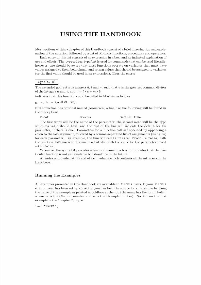
Most sections within a chapter of this Handbook consist of a brief introduction and expla-nation of the notation, followed by a list of Magma functions, procedures and operators.
Each entry in this list consists of an expression in a box, and an indented explanation of use and effects. The typewriter typefont is used for commands that can be used literally;however, one should be aware that most functions operate on variables that must havevalues assigned to them beforehand, and return values that should be assigned to variables(or the first value should be used in an expression). Thus the entry:
Xgcd(a, b)
The extended gcd; returns integers d, l and m such that d is the greatest common divisorof the integers a and b, and d = l ∗ a + m ∗ b.
indicates that this function could be called in Magma as follows:
g, a, b := Xgcd(23, 28);
If the function has optional named parameters , a line like the following will be found inthe description:
Proof BoolElt Default : true
The first word will be the name of the parameter, the second word will be the typewhich its value should have, and the rest of the line will indicate the default for theparameter, if there is one. Parameters for a function call are specified by appending acolon to the last argument, followed by a comma-separated list of assignments (using :=)for each parameter. For example, the function call IsPrime(n: Proof := false) callsthe function IsPrime with argument n but also with the value for the parameter Proof
set to false.Whenever the symbol # precedes a function name in a box, it indicates that the par-
ticular function is not yet available but should be in the future.An index is provided at the end of each volume which contains all the intrinsics in the
Handbook.
Running the Examples
All examples presented in this Handbook are available to Magma users. If your Magma
environment has been set up correctly, you can load the source for an example by usingthe name of the example as printed in boldface at the top (the name has the form H mEn,where m is the Chapter number and n is the Example number). So, to run the firstexample in the Chapter 28, type:
load "H28E1";

8/22/2019 Handbook Volume 01
http://slidepdf.com/reader/full/handbook-volume-01 28/440
xxviii USING THE HANDBOOK
8/22/2019 Handbook Volume 01
http://slidepdf.com/reader/full/handbook-volume-01 29/440
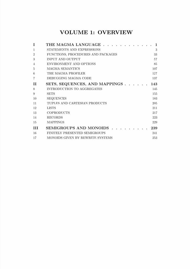
VOLUME 1: OVERVIEW
I THE MAGMA LANGUAGE . . . . . . . . . . . . 1
1 STATEMENTS AND EXPRESSIONS 3
2 FUNCTIONS, PROCEDURES AND PACKAGES 33
3 INPUT AND OUTPUT 57
4 ENVIRONMENT AND OPTIONS 85
5 MAGMA SEMANTICS 107
6 THE MAGMA PROFILER 127
7 DEBUGGING MAGMA CODE 137
II SETS, SEQUENCES, AND MAPPINGS . . . . . . 143
8 INTRODUCTION TO AGGREGATES 145
9 SETS 155
10 SEQUENCES 183
11 TUPLES AND CARTESIAN PRODUCTS 205
12 LISTS 211
13 COPRODUCTS 217
14 RECORDS 223
15 MAPPINGS 229
III SEMIGROUPS AND MONOIDS . . . . . . . . . 239
16 FINITELY PRESENTED SEMIGROUPS 241
17 MONOIDS GIVEN BY REWRITE SYSTEMS 253
8/22/2019 Handbook Volume 01
http://slidepdf.com/reader/full/handbook-volume-01 30/440
VOLUME 2: OVERVIEW
IV FINITE GROUPS . . . . . . . . . . . . . . . 271
18 GROUPS 273
19 PERMUTATION GROUPS 327
20 MATRIX GROUPS OVER GENERAL RINGS 439
21 MATRIX GROUPS OVER FINITE FIELDS 509
22 FINITE SOLUBLE GROUPS 567
23 FINITE p-GROUPS 635
24 GENERIC ABELIAN GROUPS 653
25 BLACK-BOX GROUPS 675
26 AUTOMORPHISM GROUPS 681
27 COHOMOLOGY AND EXTENSIONS 699
28 DATABASES OF GROUPS 723
8/22/2019 Handbook Volume 01
http://slidepdf.com/reader/full/handbook-volume-01 31/440
VOLUME 3: OVERVIEW
V INFINITE GROUPS . . . . . . . . . . . . . . 773
29 FINITELY PRESENTED ABELIAN GROUPS 775
30 FINITELY PRESENTED GROUPS 797
31 FINITELY PRESENTED GROUPS: ADVANCED 907
32 POLYCYCLIC GROUPS 983
33 BRAID GROUPS 1023
34 GROUPS DEFINED BY REWRITE SYSTEMS 1075
35 AUTOMATIC GROUPS 1093
36 GROUPS OF STRAIGHT-LINE PROGRAMS 1113
37 SUBGROUPS OF PSL2(R) 1123
8/22/2019 Handbook Volume 01
http://slidepdf.com/reader/full/handbook-volume-01 32/440
VOLUME 4: OVERVIEW
VI BASIC RINGS AND LINEAR ALGEBRA . . . . 1147
38 INTRODUCTION TO RINGS 1149
39 RING OF INTEGERS 1169
40 RATIONAL FIELD 1229
41 FINITE FIELDS 1241
42 UNIVARIATE POLYNOMIAL RINGS 1269
43 MULTIVARIATE POLYNOMIAL RINGS 1301
44 REAL AND COMPLEX FIELDS 1329
45 MATRICES 1373
46 SPARSE MATRICES 1409
47 VECTOR SPACES 1429
8/22/2019 Handbook Volume 01
http://slidepdf.com/reader/full/handbook-volume-01 33/440
VOLUME 5: OVERVIEW
VII EXTENSIONS OF RINGS . . . . . . . . . . . 1453
48 ORDERS AND ALGEBRAIC FIELDS 1455
49 BINARY QUADRATIC FORMS 1569
50 QUADRATIC FIELDS 1583
51 CYCLOTOMIC FIELDS 1595
52 CLASS FIELD THEORY 1603
53 ALGEBRAICALLY CLOSED FIELDS 1639
54 RATIONAL FUNCTION FIELDS 1661
55 ALGEBRAIC FUNCTION FIELDS 1673
56 MODULES OVER DEDEKIND DOMAINS 1787
57 VALUATION RINGS 1809
58 NEWTON POLYGONS 1815
59 p-ADIC RINGS AND THEIR EXTENSIONS 1843
60 GALOIS RINGS 1891
61 POWER, LAURENT AND PUISEUX SERIES 1899
62 LAZY POWER SERIES RINGS 1921
8/22/2019 Handbook Volume 01
http://slidepdf.com/reader/full/handbook-volume-01 34/440
VOLUME 6: OVERVIEW
VIII MODULES AND ALGEBRAS . . . . . . . . . 1937
63 INTRODUCTION TO MODULES 1939
64 FREE MODULES 1943
65 CHAIN COMPLEXES 1967
66 LATTICES 1983
67 ALGEBRAS 2065
68 STRUCTURE CONSTANT ALGEBRAS 2077
69 ASSOCIATIVE ALGEBRAS 2087
70 MATRIX ALGEBRAS 2097
71 BASIC ALGEBRAS 2137
72 QUATERNION ALGEBRAS 2173
73 ORDERS OF ASSOCIATIVE ALGEBRAS 2209
74 FINITELY PRESENTED ALGEBRAS 2227
IX DIFFERENTIAL RINGS . . . . . . . . . . . 2263
75 DIFFERENTIAL RINGS, FIELDS AND OPERATORS 2265
8/22/2019 Handbook Volume 01
http://slidepdf.com/reader/full/handbook-volume-01 35/440
VOLUME 7: OVERVIEW
X REPRESENTATION THEORY . . . . . . . . . 2313
76 MODULES OVER AN ALGEBRA 2315
77 GROUP ALGEBRAS 2351
78 K [G]-MODULES AND GROUP REPRESENTATIONS 2365
79 CHARACTERS OF FINITE GROUPS 2389
80 REPRESENTATION THEORY OF SYMMETRIC GROUPS 2403
81 INVARIANT RINGS OF FINITE GROUPS 2411
XI LIE THEORY . . . . . . . . . . . . . . . . 244182 INTRODUCTION TO LIE THEORY 2443
83 COXETER SYSTEMS 2449
84 ROOT SYSTEMS 2473
85 ROOT DATA 2495
86 COXETER GROUPS 2541
87 COXETER GROUPS AS PERMUTATION GROUPS 2555
88 REFLECTION GROUPS 2579
89 GROUPS OF LIE TYPE 2605
90 LIE ALGEBRAS 2641
91 FINITELY PRESENTED LIE ALGEBRAS 2683
92 QUANTUM GROUPS 2691
93 UNIVERSAL ENVELOPING ALGEBRAS 2717
8/22/2019 Handbook Volume 01
http://slidepdf.com/reader/full/handbook-volume-01 36/440
VOLUME 8: OVERVIEW
XII COMMUTATIVE ALGEBRA . . . . . . . . . 2725
94 IDEAL THEORY AND GROBNER BASES 2727
95 AFFINE ALGEBRAS 2805
96 MODULES OVER AFFINE ALGEBRAS 2821
XIII ALGEBRAIC GEOMETRY . . . . . . . . . . 2847
97 SCHEMES 2849
98 ALGEBRAIC CURVES 2957
99 RESOLUTION GRAPHS AND SPLICE DIAGRAMS 3037100 HILBERT SERIES OF POLARISED VARIETIES 3053
8/22/2019 Handbook Volume 01
http://slidepdf.com/reader/full/handbook-volume-01 37/440
VOLUME 9: OVERVIEW
XIV ARITHMETIC GEOMETRY . . . . . . . . . . 3087
101 RATIONAL CURVES AND CONICS 3089
102 ELLIPTIC CURVES 3113
103 ELLIPTIC CURVES OVER FINITE FIELDS 3209
104 ELLIPTIC CURVES OVER FUNCTION FIELDS 3227
105 MODELS OF GENUS ONE CURVES 3243
106 HYPERELLIPTIC CURVES 3259
107 MODULAR CURVES 3335
108 MODULAR SYMBOLS 3347
109 BRANDT MODULES 3405
110 SUPERSINGULAR DIVISORS ON MODULAR CURVES 3419
111 MODULAR FORMS 3435
112 MODULAR ABELIAN VARIETIES 3471
113 L-FUNCTIONS 3609
8/22/2019 Handbook Volume 01
http://slidepdf.com/reader/full/handbook-volume-01 38/440
VOLUME 10: OVERVIEW
III FINITE INCIDENCE STRUCTURES . . . . . . 3639
114 ENUMERATIVE COMBINATORICS 3641
115 PARTITIONS, WORDS AND YOUNG TABLEAUX 3647
116 SYMMETRIC FUNCTIONS 3681
117 GRAPHS 3707
118 MULTIGRAPHS 3787
119 NETWORKS 3835
120 INCIDENCE STRUCTURES AND DESIGNS 3855
121 HADAMARD MATRICES 3889
122 FINITE PLANES 3899
123 INCIDENCE GEOMETRY 3935
IV CODING THEORY . . . . . . . . . . . . . . 3957
124 LINEAR CODES OVER FINITE FIELDS 3959
125 ALGEBRAIC-GEOMETRIC CODES 4033
126 LOW DENSITY PARTY CHECK CODES 4041
127 LINEAR CODES OVER FINITE RINGS 4053
128 ADDITIVE CODES 4085
129 QUANTUM CODES 4109
V CRYPTOGRAPHY . . . . . . . . . . . . . . 4147
130 PSEUDO-RANDOM BIT SEQUENCES 4149
VI OPTIMIZATION . . . . . . . . . . . . . . . 4157
131 LINEAR PROGRAMMING 4159
8/22/2019 Handbook Volume 01
http://slidepdf.com/reader/full/handbook-volume-01 39/440
VOLUME 1: CONTENTS xxxix
VOLUME 1: CONTENTS
I THE MAGMA LANGUAGE 1
1 STATEMENTS AND EXPRESSIONS . . . . . . . . . . . . . 3
1.1 Introduction 5
1.2 Starting, Interrupting and Terminating 5
1.3 Identifiers 5
1.4 Assignment 6 1.4.1 Simple Assignment 6
1.4.2 Indexed Assignment 71.4.3 Generator Assignment 8
1.4.4 Mutation Assignment 91.4.5 Deletion of Values 10
1.5 Boolean values 10
1.5.1 Creation of Booleans 111.5.2 Boolean Operators 11
1.5.3 Equality Operators 111.5.4 Iteration 12
1.6 Coercion 13
1.7 The where . . . is Construction 14
1.8 Conditional Statements and Expressions 16
1.8.1 The Simple Conditional Statement 161.8.2 The Simple Conditional Expression 171.8.3 The Case Statement 18
1.8.4 The Case Expression 18
1.9 Error Handling Statements 19 1.9.1 The Error Objects 191.9.2 Error Checking and Assertions 19
1.9.3 Catching Errors 20
1.10 Iterative Statements 211.10.1 Definite Iteration 21
1.10.2 Indefinite Iteration 211.10.3 Early Exit from Iterative Statements 23
1.11 Runtime Evaluation: the eval Expression 241.12 Comments and Continuation 25
1.13 Timing 26
1.14 Types, Category Names, and Structures 28
1.15 Random Object Generation 30
1.16 Miscellaneous 32
1.17 Bibliography 32
8/22/2019 Handbook Volume 01
http://slidepdf.com/reader/full/handbook-volume-01 40/440
xl VOLUME 1: CONTENTS
2 FUNCTIONS, PROCEDURES AND PACKAGES . . . . . . . 33
2.1 Introduction 35
2.2 Functions and Procedures 35 2.2.1 Functions 352.2.2 Procedures 392.2.3 The forward Declaration 412.3 Packages 42 2.3.1 Introduction 422.3.2 Intrinsics 432.3.3 Resolving calls to intrinsics 452.3.4 Attaching and Detaching Package Files 462.3.5 Related Files 472.3.6 Importing Constants 472.3.7 Argument Checking 482.3.8 Package Specification files 492.3.9 User Startup Specification Files 50
2.4 Attributes 512.4.1 Predefined System Attributes 512.4.2 User-defined Attributes 522.4.3 Accessing Attributes 522.4.4 User-defined Verbose Flags 532.4.5 Examples 53
3 INPUT AND OUTPUT . . . . . . . . . . . . . . . . . . . 57
3.1 Introduction 59 3.2 Character Strings 59 3.2.1 Representation of Strings 593.2.2 Creation of Strings 60
3.2.3 Integer-Valued Functions 613.2.4 Character Conversion 613.2.5 Boolean Functions 623.2.6 Parsing Strings 653.3 Printing 66 3.3.1 The print-Statement 663.3.2 The printf and fprintf Statements 673.3.3 Verbose Printing (vprint, vprintf) 693.3.4 Automatic Printing 693.3.5 Indentation 723.3.6 Printing to a File 723.3.7 Printing to a String 733.3.8 Redirecting Output 733.4 External Files 74
3.4.1 Opening Files 743.4.2 Operations on File Objects 743.4.3 Reading a Complete File 763.5 Pipes 77 3.5.1 Pipe Creation 773.5.2 Operations on Pipes 783.6 Sockets 78 3.6.1 Socket Creation 793.6.2 Socket Properties 803.6.3 Socket Predicates 803.6.4 Socket I/O 803.7 Interactive Input 82 3.8 Loading a Program File 82
8/22/2019 Handbook Volume 01
http://slidepdf.com/reader/full/handbook-volume-01 41/440
VOLUME 1: CONTENTS xli
3.9 Saving and Restoring Workspaces 82
3.10 Logging a Session 83
3.11 Memory Usage 83 3.12 System Calls 83
3.13 Creating Names 84
4 ENVIRONMENT AND OPTIONS . . . . . . . . . . . . . . 85
4.1 Introduction 87
4.2 Command Line Options 87
4.3 Environment Variables 89
4.4 Set and Get 90
4.5 Verbose Levels 94
4.6 Other Information Procedures 95
4.7 History 96
4.8 The Magma Line Editor 97 4.8.1 Key Bindings (Emacs and VI mode) 984.8.2 Key Bindings in Emacs mode only 1004.8.3 Key Bindings in VI mode only 100
4.9 The Magma Help System 103 4.9.1 Internal Help Browser 105
5 MAGMA SEMANTICS . . . . . . . . . . . . . . . . . . 107
5.1 Introduction 109
5.2 Terminology 109
5.3 Assignment 110
5.4 Uninitialized Identifiers 110 5.5 Evaluation in Magma 1115.5.1 Call by Value Evaluation 1115.5.2 Magma’s Evaluation Process 1125.5.3 Function Expressions 1135.5.4 Function Values Assigned to Identifiers 1145.5.5 Recursion and Mutual Recursion 1145.5.6 Function Application 1155.5.7 The Initial Context 116
5.6 Scope 116 5.6.1 Local Declarations 1175.6.2 The ‘first use’ Rule 1175.6.3 Identifier Classes 1185.6.4 The Evaluation Process Revisited 1195.6.5 The ‘single use’ Rule 119
5.7 Procedure Expressions 119
5.8 Reference Arguments 121
5.9 Dynamic Typing 122
5.10 Traps for Young Players 123 5.10.1 Trap 1 1235.10.2 Trap 2 123
5.11 Appendix A: Precedence 125
5.12 Appendix B: Reserved Words 126
8/22/2019 Handbook Volume 01
http://slidepdf.com/reader/full/handbook-volume-01 42/440
xlii VOLUME 1: CONTENTS
6 THE MAGMA PROFILER . . . . . . . . . . . . . . . . 127
6.1 Introduction 129
6.2 Profiler Basics 129 6.3 Exploring the Call Graph 1316.3.1 Internal Reports 1316.3.2 HTML Reports 1336.4 Recursion and the Profiler 133
7 DEBUGGING MAGMA CODE . . . . . . . . . . . . . . 137
7.1 Introduction 139 7.2 Using the Debugger 139
8/22/2019 Handbook Volume 01
http://slidepdf.com/reader/full/handbook-volume-01 43/440
VOLUME 1: CONTENTS xliii
II SETS, SEQUENCES, AND MAPPINGS 143
8 INTRODUCTION TO AGGREGATES . . . . . . . . . . . 1458.1 Introduction 147 8.2 Restrictions on Sets and Sequences 147 8.2.1 Universe of a Set or Sequence 1488.2.2 Modifying the Universe of a Set or Sequence 1498.2.3 Parents of Sets and Sequences 1518.3 Nested Aggregates 152 8.3.1 Multi-indexing 152
9 SETS . . . . . . . . . . . . . . . . . . . . . . . . . . 155
9.1 Introduction 157 9.1.1 Enumerated Sets 157
9.1.2 Formal Sets 1579.1.3 Indexed Sets 1579.1.4 Multisets 1579.1.5 Compatibility 1589.1.6 Notation 1589.2 Creating Sets 158 9.2.1 The Formal Set Constructor 1589.2.2 The Enumerated Set Constructor 1599.2.3 The Indexed Set Constructor 1619.2.4 The Multiset Constructor 1629.2.5 The Arithmetic Progression Constructors 1649.3 Power Sets 165 9.3.1 The Cartesian Product Constructors 1679.4 Sets from Structures 167
9.5 Accessing and Modifying Sets 168 9.5.1 Accessing Sets and their Associated Structures 1689.5.2 Selecting Elements of Sets 1699.5.3 Modifying Sets 1729.6 Operations on Sets 175 9.6.1 Boolean Functions and Operators 1759.6.2 Binary Set Operators 1769.6.3 Other Set Operations 1779.7 Quantifiers 178 9.8 Reduction and Iteration over Sets 181
10 SEQUENCES . . . . . . . . . . . . . . . . . . . . . . 183
10.1 Introduction 185 10.1.1 Enumerated Sequences 18510.1.2 Formal Sequences 18510.1.3 Compatibility 18610.2 Creating Sequences 186 10.2.1 The Formal Sequence Constructor 18610.2.2 The Enumerated Sequence Constructor 18710.2.3 The Arithmetic Progression Constructors 18810.2.4 Literal Sequences 18910.3 Power Sequences 189 10.4 Operators on Sequences 190 10.4.1 Access Functions 19010.4.2 Selection Operators on Enumerated Sequences 191
8/22/2019 Handbook Volume 01
http://slidepdf.com/reader/full/handbook-volume-01 44/440
xliv VOLUME 1: CONTENTS
10.4.3 Modifying Enumerated Sequences 19210.4.4 Creating New Enumerated Sequences from Existing Ones 197
10.5 Predicates on Sequences 199 10.5.1 Membership Testing 200
10.5.2 Testing Order Relations 201
10.6 Recursion, Reduction, and Iteration 202 10.6.1 Recursion 202
10.6.2 Reduction 202
10.7 Iteration 203
10.8 Bibliography 204
11 TUPLES AND CARTESIAN PRODUCTS . . . . . . . . . . 205
11.1 Introduction 207
11.2 Cartesian Product Constructor and Functions 207 11.3 Creating and Modifying Tuples 208
11.4 Tuple Access Functions 210
11.5 Equality 210
12 LISTS . . . . . . . . . . . . . . . . . . . . . . . . . 211
12.1 Introduction 213
12.2 Construction of Lists 213
12.3 Creation of New Lists 213
12.4 Access Functions 214
12.5 Assignment Operator 215
13 COPRODUCTS . . . . . . . . . . . . . . . . . . . . . 217
13.1 Introduction 219
13.2 Creation Functions 219
13.2.1 Creation of Coproducts 21913.2.2 Creation of Coproduct Elements 219
13.3 Accessing Functions 220
13.4 Retrieve 220
13.5 Flattening 221
13.6 Universal Map 221
14 RECORDS . . . . . . . . . . . . . . . . . . . . . . . 223
14.1 Introduction 225
14.2 The Record Format Constructor 225
14.3 Creating a Record 226
14.4 Access and Modification Functions 227
8/22/2019 Handbook Volume 01
http://slidepdf.com/reader/full/handbook-volume-01 45/440
VOLUME 1: CONTENTS xlv
15 MAPPINGS . . . . . . . . . . . . . . . . . . . . . . . 229
15.1 Introduction 231
15.1.1 The Map Constructors 23115.1.2 The Graph of a Map 23215.1.3 Rules for Maps 23215.1.4 Homomorphisms 23215.1.5 Checking of Maps 23215.2 Creation Functions 233 15.2.1 Creation of Maps 23315.2.2 Creation of Partial Maps 23415.2.3 Creation of Homomorphisms 23415.2.4 Coercion Maps 23515.3 Operations on Mappings 235 15.3.1 Composition 23515.3.2 (Co)Domain and (Co)Kernel 23615.3.3 Inverse 236
15.3.4 Function 23615.4 Images and Preimages 237 15.5 Parents of Maps 238
8/22/2019 Handbook Volume 01
http://slidepdf.com/reader/full/handbook-volume-01 46/440
xlvi VOLUME 1: CONTENTS
III SEMIGROUPS AND MONOIDS 239
16 FINITELY PRESENTED SEMIGROUPS . . . . . . . . . . 24116.1 Introduction 243 16.2 The Construction of Free Semigroups and their Elements 243 16.2.1 Structure Constructors 24316.2.2 Element Constructors 24416.3 Elementary Operators for Words 24416.3.1 Multiplication and Exponentiation 24416.3.2 The Length of a Word 24416.3.3 Equality and Comparison 24516.4 Specification of a Presentation 246 16.4.1 Relations 24616.4.2 Presentations 24616.4.3 Accessing the Defining Generators and Relations 247
16.5 Subsemigroups, Ideals and Quotients 248 16.5.1 Subsemigroups and Ideals 24816.5.2 Quotients 24916.6 Extensions 249 16.7 Elementary Tietze Transformations 250 16.8 String Operations on Words 251
17 MONOIDS GIVEN BY REWRITE SYSTEMS . . . . . . . . 253
17.1 Introduction 255 17.1.1 Terminology 25517.1.2 The Category of Rewrite Monoids 25517.1.3 The Construction of a Rewrite Monoid 255
17.2 Construction of a Rewrite Monoid 256 17.3 Basic Operations 26117.3.1 Accessing Monoid Information 26117.3.2 Properties of a Rewrite Monoid 26217.3.3 Construction of a Word 26417.3.4 Arithmetic with Words 26417.4 Homomorphisms 266 17.4.1 General remarks 26617.4.2 Construction of Homomorphisms 26617.5 Set Operations 266 17.6 Conversion to a Finitely Presented Monoid 268 17.7 Bibliography 269
8/22/2019 Handbook Volume 01
http://slidepdf.com/reader/full/handbook-volume-01 47/440
VOLUME 2: CONTENTS xlvii
VOLUME 2: CONTENTS
IV FINITE GROUPS 271
18 GROUPS . . . . . . . . . . . . . . . . . . . . . . . . 273
18.1 Introduction 277 18.1.1 The Categories of Finite Groups 277
18.2 Construction of Elements 278 18.2.1 Construction of an Element 278
18.2.2 Coercion 27818.2.3 Homomorphisms 27818.2.4 Arithmetic with Elements 280
18.3 Construction of a General Group 282 18.3.1 The General Group Constructors 28218.3.2 Construction of Subgroups 28618.3.3 Construction of Quotient Groups 287
18.4 Standard Groups and Extensions 289 18.4.1 Construction of a Standard Group 28918.4.2 Construction of Extensions 291
18.5 Transfer Functions Between Group Categories 292
18.6 Basic Operations 295 18.6.1 Accessing Group Information 295
18.7 Operations on the Set of Elements 296 18.7.1 Order and Index Functions 29718.7.2 Membership and Equality 29818.7.3 Set Operations 29918.7.4 Action on a Coset Space 301
18.8 Standard Subgroup Constructions 302 18.8.1 Abstract Group Predicates 304
18.9 Characteristic Subgroups and Normal Structure 305 18.9.1 Characteristic Subgroups and Subgroup Series 30518.9.2 The Abstract Structure of a Group 307
18.10 Conjugacy Classes of Elements 308
18.11 Conjugacy Classes of Subgroups 312
18.11.1 Conjugacy Classes of Subgroups 31218.11.2 The Poset of Subgroup Classes 316
18.12 Cohomology 322
18.13 Characters and Representations 323 18.13.1 Character Theory 32318.13.2 Representation Theory 323
18.14 Databases of Groups 326
18.15 Bibliography 326
8/22/2019 Handbook Volume 01
http://slidepdf.com/reader/full/handbook-volume-01 48/440
xlviii VOLUME 2: CONTENTS
19 PERMUTATION GROUPS . . . . . . . . . . . . . . . . 327
19.1 Introduction 333
19.1.1 Terminology 33319.1.2 The Category of Permutation Groups 33319.1.3 The Construction of a Permutation Group 33319.2 Creation of a Permutation Group 33419.2.1 Construction of the Symmetric Group 33419.2.2 Construction of a Permutation 33519.2.3 Construction of a General Permutation Group 33719.3 Elementary Properties of a Group 338 19.3.1 Accessing Group Information 33819.3.2 Group Order 34019.3.3 Abstract Properties of a Group 34019.4 Homomorphisms 34119.5 Building Permutation Groups 34419.5.1 Some Standard Permutation Groups 34419.5.2 Direct Products and Wreath Products 34619.6 Permutations 348 19.6.1 Coercion 34819.6.2 Arithmetic with Permutations 34819.6.3 Properties of Permutations 34919.6.4 Predicates for Permutations 34919.6.5 Set Operations 35019.7 Conjugacy 353 19.8 Subgroups 360 19.8.1 Construction of a Subgroup 36019.8.2 Membership and Equality 36219.8.3 Elementary Properties of a Subgroup 36319.8.4 Standard Subgroups 363
19.8.5 Maximal Subgroups 36619.8.6 Conjugacy Classes of Subgroups 36819.8.7 Classes of Subgroups Satisfying a Condition 37319.9 Quotient Groups 37419.9.1 Construction of Quotient Groups 37419.9.2 Abelian, Nilpotent and Soluble Quotients 37519.10 Permutation Group Actions 377 19.10.1 G-Sets 37719.10.2 Creating a G-Set 37719.10.3 Images, Orbits and Stabilizers 38019.10.4 Action on a G-Space 38519.10.5 Action on Orbits 38619.10.6 Action on a G-invariant Partition 38819.10.7 Action on a Coset Space 393
19.10.8 Reduced Permutation Actions 39319.11 Normal and Subnormal Subgroups 39419.11.1 Characteristic Subgroups and Normal Series 39419.11.2 Maximal and Minimal Normal Subgroups 39719.11.3 Lattice of Normal Subgroups 39719.11.4 Composition and Chief Series 39819.11.5 The Socle 40119.11.6 The Soluble Radical and its Quotient 40419.11.7 Complements and Supplements 40619.11.8 Abelian Normal Subgroups 40819.12 Cosets and Transversals 409 19.12.1 Cosets 40919.12.2 Transversals 411
8/22/2019 Handbook Volume 01
http://slidepdf.com/reader/full/handbook-volume-01 49/440
VOLUME 2: CONTENTS xlix
19.13 Presentations 41119.13.1 Generators and Relations 41219.13.2 Permutations as Words 41219.14 Automorphism Groups 413 19.15 Cohomology 415 19.16 Representation Theory 417 19.17 Identification 419 19.17.1 Identification as an Abstract Group 41919.17.2 Identification as a Permutation Group 41919.18 Base and Strong Generating Set 423 19.18.1 Construction of a Base and Strong Generating Set 42319.18.2 Defining Values for Attributes 42619.18.3 Accessing the Base and Strong Generating Set 42719.18.4 Working with a Base and Strong Generating Set 42819.18.5 Modifying a Base and Strong Generating Set 43019.19 Permutation Representations of Linear Groups 430
19.20 Permutation Group Databases 436 19.21 Bibliography 436
20 MATRIX GROUPS OVER GENERAL RINGS . . . . . . . . 439
20.1 Introduction 443 20.1.1 Introduction to Matrix Groups 44320.1.2 The Support 44420.1.3 The Category of Matrix Groups 44420.1.4 The Construction of a Matrix Group 44420.2 Creation of a Matrix Group 44420.2.1 Construction of the General Linear Group 44420.2.2 Construction of a Matrix Group Element 44520.2.3 Construction of a General Matrix Group 44720.2.4 Changing Rings 44820.2.5 Coercion between Matrix Structures 44920.2.6 Accessing Associated Structures 44920.3 Homomorphisms 450 20.3.1 Construction of Extensions 45220.4 Operations on Matrices 453 20.4.1 Arithmetic with Matrices 45420.4.2 Predicates for Matrices 45620.4.3 Matrix Invariants 45620.5 Global Properties 459 20.5.1 Group Order 46020.5.2 Membership and Equality 46120.5.3 Set Operations 462
20.6 Abstract Group Predicates 46420.7 Conjugacy 466 20.8 Subgroups 469 20.8.1 Construction of Subgroups 46920.8.2 Elementary Properties of Subgroups 47020.8.3 Standard Subgroups 47120.8.4 Low Index Subgroups 47220.8.5 Conjugacy Classes of Subgroups 47320.9 Quotient Groups 475 20.9.1 Construction of Quotient Groups 47620.9.2 Abelian, Nilpotent and Soluble Quotients 47720.10 Matrix Group Actions 478 20.10.1 Orbits and Stabilizers 478
8/22/2019 Handbook Volume 01
http://slidepdf.com/reader/full/handbook-volume-01 50/440
l VOLUME 2: CONTENTS
20.10.2 Orbit and Stabilizer Functions for Large Groups 48120.10.3 Action on Orbits 48520.10.4 Action on a Coset Space 48720.10.5 Action on the Natural G-Module 48820.11 Normal and Subnormal Subgroups 489 20.11.1 Characteristic Subgroups and Subgroup Series 48920.11.2 The Soluble Radical and its Quotient 49120.11.3 Composition and Chief Factors 49220.12 Coset Tables and Transversals 49420.13 Presentations 495 20.13.1 Presentations 49520.13.2 Matrices as Words 49520.14 Automorphism Groups 496 20.15 Representation Theory 499 20.16 Base and Strong Generating Set 50120.16.1 Introduction 501
20.16.2 Controlling Selection of a Base 50220.16.3 Construction of a Base and Strong Generating Set 50320.16.4 Defining Values for Attributes 50420.16.5 Accessing the Base and Strong Generating Set 50520.17 Soluble Matrix Groups 506 20.17.1 Conversion to a PC-Group 50620.17.2 Soluble Group Functions 50620.17.3 p-group Functions 50620.17.4 Abelian Group Functions 50620.18 Bibliography 507
21 MATRIX GROUPS OVER FINITE FIELDS . . . . . . . . . 509
21.1 Introduction 511
21.1.1 Overview 51121.2 Monte-Carlo Functions 512 21.3 Aschbacher Reduction 513 21.3.1 Introduction 51321.3.2 Primitivity 51421.3.3 Semilinearity 51621.3.4 Tensor Products 51821.3.5 Tensor-induced Groups 52021.3.6 Normalisers of Extraspecial r-groups and Symplectic 2-groups 52121.3.7 Writing Representations over Subfields 52321.3.8 Decompositions with Respect to a Normal Subgroup 52521.4 Creating Finite Groups of Lie Type 529 21.4.1 Classical Groups 53021.4.2 General and Special Unitary Groups 531
21.4.3 Symplectic Groups 53121.4.4 Orthogonal Groups 53221.4.5 Exceptional Groups 53421.5 Group Recognition 536 21.5.1 Determining the Type of a Finite Group of Lie Type 53621.5.2 Classical forms 53921.5.3 Recognizing Classical Groups in their Natural Representation 54221.5.4 Constructive Recognition of Linear Groups 54521.5.5 Constructive Recognition of Suzuki Groups 54821.5.6 Constructive Recognition of Ree Groups 55321.6 Properties of Finite Groups Of Lie Type 556 21.6.1 Sylow Subgroups of the Classical Groups 55621.6.2 Sylow Subgroups of Exceptional Groups 558
8/22/2019 Handbook Volume 01
http://slidepdf.com/reader/full/handbook-volume-01 51/440
VOLUME 2: CONTENTS li
21.6.3 Conjugacy of Subgroups of the Classical Groups 56121.6.4 Irreducible Subgroups of the General Linear Group 56121.7 Atlas Data for the Sporadic Groups 562 21.8 Bibliography 565
22 FINITE SOLUBLE GROUPS . . . . . . . . . . . . . . . 567
22.1 Introduction 57122.1.1 Power-Conjugate Presentations 57122.2 Creation of Finite Soluble Groups 572 22.2.1 Construction Functions 57222.2.2 Definition by Presentation 57322.2.3 Possibly Inconsistent Presentations 57622.3 Basic Group Properties 577 22.3.1 Infrastructure 57722.3.2 Numerical Invariants 577
22.3.3 Predicates 57822.4 Homomorphisms 579 22.5 New Groups from Existing 58122.6 Elements 585 22.6.1 Definition of Elements 58622.6.2 Arithmetic Operations on Elements 58722.6.3 Properties of Elements 58822.6.4 Predicates for Elements 58922.6.5 Set Operations 59022.7 Conjugacy 592 22.8 Subgroups 595 22.8.1 Definition of Subgroups by Generators 59522.8.2 Membership and Coercion 59622.8.3 Inclusion and Equality 59822.8.4 Standard Subgroup Constructions 59822.8.5 Properties of Subgroups 60022.8.6 Predicates for Subgroups 60022.8.7 Hall π-Subgroups and Sylow Systems 60222.8.8 Conjugacy Classes of Subgroups 60322.9 Quotient Groups 607 22.9.1 Construction of Quotient Groups 60722.9.2 Abelian and p-Quotients 60822.10 Normal Subgroups and Subgroup Series 609 22.10.1 Characteristic Subgroups 60922.10.2 Subgroup Series 60922.10.3 Normal Subgroups and Complements 61122.11 Transfer Between Group Categories 613 22.11.1 Transfer to GrpPC 61322.11.2 Transfer from GrpPC 61422.12 More About Presentations 616 22.12.1 Conditioned Presentations 61622.12.2 Special Presentations 61722.12.3 CompactPresentation 62122.13 Cosets 622 22.13.1 Coset Tables and Transversals 62222.13.2 Action on a Coset Space 62222.14 Automorphism Group 623 22.15 Representation Theory 626 22.16 Central Extensions 629 22.17 Optimizing Magma Code 632
8/22/2019 Handbook Volume 01
http://slidepdf.com/reader/full/handbook-volume-01 52/440
lii VOLUME 2: CONTENTS
22.17.1 PowerGroup 63222.18 Bibliography 633
23 FINITE p-GROUPS . . . . . . . . . . . . . . . . . . . 635
23.1 Introduction 637 23.2 Basic Group Properties 637 23.3 Subgroups and Subgroup Series 638 23.4 Generating p-groups 638 23.5 Isomorphism Testing and Standard Presentations 642 23.5.1 Automorphism Group Algorithm 64523.6 Counting p-groups 646 23.7 The p-groups of Order Dividing p7 647 23.8 Metacyclic p-groups 648 23.9 Miscellanous p-group functions 650 23.10 Bibliography 651
24 GENERIC ABELIAN GROUPS . . . . . . . . . . . . . . 653
24.1 Introduction 655 24.2 Construction of a Generic Abelian Group 655 24.3 Elements of a Generic Abelian Group 658 24.3.1 Constructing an Element of a Generic Abelian Group 65824.3.2 Pull-Back of an Element 65924.3.3 Representation of an Element 65924.4 Structure Computation 66124.5 Subgroups 662 24.5.1 Construction of Subgroups 66224.5.2 Construction of p-Sylow Subgroups 665
24.6 Access Functions 666 24.7 Arithmetic with Elements 667 24.7.1 Addition and Subtraction 66724.8 Operations on Elements 668 24.8.1 Order and Discrete Logarithm 66824.8.2 Equality and Comparison 67124.9 Set-Theoretic Operations 67124.9.1 Membership and Equality 67124.10 Homomorphisms 672 24.11 Bibliography 674
25 BLACK-BOX GROUPS . . . . . . . . . . . . . . . . . . 675
25.1 Introduction 677
25.2 Construction of an SLP-Group and its Elements 677 25.2.1 Structure Constructors 67725.2.2 Construction of an Element 67725.3 Arithmetic with Elements 677 25.3.1 Accessing the Defining Generators 67825.4 Operations on Elements 678 25.4.1 Equality and Comparison 67825.4.2 Attributes of Elements 67825.5 Set-Theoretic Operations 679 25.5.1 Membership and Equality 67925.5.2 Set Operations 68025.5.3 Coercions Between Related Groups 680
8/22/2019 Handbook Volume 01
http://slidepdf.com/reader/full/handbook-volume-01 53/440
VOLUME 2: CONTENTS liii
26 AUTOMORPHISM GROUPS . . . . . . . . . . . . . . . 681
26.1 Introduction 683
26.2 Creation of Automorphism Groups 68426.3 Access Functions 686 26.4 Order Functions 687 26.5 Representations of an Automorphism Group 688 26.6 Automorphisms 69126.7 Stored Attributes of an Automorphism Group 693 26.8 Holomorphs 696 26.9 Bibliography 697
27 COHOMOLOGY AND EXTENSIONS . . . . . . . . . . . 699
27.1 Introduction 70127.2 Creation of a Cohomology Module 702
27.3 Accessing Properties of the Cohomology Module 703 27.4 Calculating Cohomology 70427.5 Cocycles 705 27.6 Constructing Extensions 708 27.7 Constructing Distinct Extensions 71127.8 Finite Group Cohomology 715 27.8.1 Creation of Gamma-groups 71527.8.2 Accessing Information 71727.8.3 One Cocycles 71727.8.4 Group Cohomology 71827.9 Bibliography 721
28 DATABASES OF GROUPS . . . . . . . . . . . . . . . . 723
28.1 Introduction 727 28.2 Database of Small Groups 728 28.2.1 Basic Small Group Functions 72828.2.2 Processes 73328.2.3 Small Group Identification 73528.2.4 Accessing Internal Data 73628.3 Database of Perfect Groups 737 28.3.1 Specifying an Entry of the Database 73828.3.2 Creating the Database 73828.3.3 Accessing the Database 73828.3.4 Finding Legal Keys 74028.4 Database of Almost-Simple Groups 742 28.4.1 The Record Fields 74228.4.2 Creating the Database 74328.4.3 Accessing the Database 74428.5 Database of Transitive Groups 746 28.5.1 Accessing the Databases 74628.5.2 Processes 74828.5.3 Transitive Group Identification 75028.6 Database of Primitive Groups 750 28.6.1 Accessing the Databases 75128.6.2 Processes 75328.6.3 Primitive Group Identification 75428.7 Database of Rational Maximal Finite Matrix Groups 755 28.8 Database of Finite Quaternionic Matrix Groups 757

8/22/2019 Handbook Volume 01
http://slidepdf.com/reader/full/handbook-volume-01 54/440
liv VOLUME 2: CONTENTS
28.9 Database of Irreducible Matrix Groups 758 28.9.1 Accessing the Database 75928.10 Database of Soluble Irreducible Groups 760 28.10.1 Basic Functions 76028.10.2 Searching with Predicates 76128.10.3 Associated Functions 76228.10.4 Processes 76328.11 Database of ATLAS Groups 76428.11.1 Accessing the Database 76528.11.2 Accessing the ATLAS Groups 76528.11.3 Representations of the ATLAS Groups 76628.12 Fundamental Groups of 3-Manifolds 767 28.12.1 Basic Functions 76828.12.2 Accessing the Data 76828.13 Bibliography 770
8/22/2019 Handbook Volume 01
http://slidepdf.com/reader/full/handbook-volume-01 55/440
VOLUME 3: CONTENTS lv
VOLUME 3: CONTENTS
V INFINITE GROUPS 773
29 FINITELY PRESENTED ABELIAN GROUPS . . . . . . . . 775
29.1 Introduction 777
29.2 Construction of a Free Abelian Group and its Elements 777 29.2.1 Structure Constructors 77729.2.2 Construction of an Element 778
29.2.3 Deconstruction of an Element 778
29.3 Arithmetic with Elements 778 29.3.1 Addition and Subtraction 77829.3.2 Relations 779
29.4 Construction of Subgroups and Quotient Groups 780 29.4.1 Construction of Subgroups 78029.4.2 Construction of Quotient Groups 780
29.5 Specification of a Presentation 78129.5.1 Accessing the Defining Generators and Relations 782
29.6 Standard Constructions and Conversions 782
29.7 Operations on Elements 783 29.7.1 Order of an Element 783
29.7.2 Equality and Comparison 78329.8 Invariants of an Abelian Group 784
29.9 Canonical Decomposition 784
29.10 Set-Theoretic Operations 785 29.10.1 Functions Relating to Group Order 78529.10.2 Membership and Equality 78529.10.3 Set Operations 786
29.11 Coset Spaces 787
29.12 The Subgroup Structure 787
29.13 General Group Properties 788 29.13.1 General Properties of Subgroups 78929.13.2 Coercions Between Groups and Subgroups 789
29.14 Normal Structure and Characteristic Subgroups 790 29.14.1 Characteristic Subgroups and Subgroup Series 79029.14.2 Subgroup Structure 791
29.15 Conjugacy 792
29.16 Representation Theory 793
29.17 Computation of Hom 794
29.18 Cohomology 795
29.19 Bibliography 795
8/22/2019 Handbook Volume 01
http://slidepdf.com/reader/full/handbook-volume-01 56/440
lvi VOLUME 3: CONTENTS
30 FINITELY PRESENTED GROUPS . . . . . . . . . . . . 797
30.1 Introduction 801
30.1.1 Overview of Facilities 80130.1.2 The Construction of Finitely Presented Groups 80130.2 Free Groups and Words 802 30.2.1 Construction of a Free Group 80230.2.2 Construction of Words 80330.2.3 Access Functions for Words 80330.2.4 Arithmetic Operators for Words 80530.2.5 Comparison of Words 80630.2.6 Relations 80730.3 Construction of an FP-Group 809 30.3.1 The Quotient Group Constructor 80930.3.2 The FP-Group Constructor 81130.3.3 Construction from a Finite Permutation or Matrix Group 81230.3.4 Construction of the Standard Presentation for a Coxeter Group 814
30.3.5 Conversion from a Special Form of FP-Group 81530.3.6 Construction of a Standard Group 81630.3.7 Construction of Extensions 81830.3.8 Accessing the Defining Generators and Relations 82030.4 Homomorphisms 820 30.4.1 General Remarks 82030.4.2 Construction of Homomorphisms 82130.4.3 Accessing Homomorphisms 82130.4.4 Computing Homomorphisms to Permutation Groups 82430.4.5 Searching for Isomorphisms 83130.5 Abelian, Nilpotent and Soluble Quotient 833 30.5.1 Abelian Quotient 83330.5.2 p-Quotient 83630.5.3 The Construction of a p-Quotient 83730.5.4 Nilpotent Quotient 83930.5.5 Soluble Quotient 84230.6 Subgroups 845 30.6.1 Specification of a Subgroup 84530.6.2 Index of a Subgroup: The Todd-Coxeter Algorithm 84830.6.3 Implicit Invocation of the Todd-Coxeter Algorithm 85230.6.4 Constructing a Presentation for a Subgroup 85430.7 Subgroups of Finite Index 858 30.7.1 Low Index Subgroups 85830.7.2 Subgroup Constructions 86630.7.3 Properties of Subgroups 87130.8 Coset Spaces and Tables 875 30.8.1 Coset Tables 876
30.8.2 Coset Spaces: Construction 87830.8.3 Coset Spaces: Elementary Operations 87830.8.4 Accessing Information 87930.8.5 Double Coset Spaces: Construction 88330.8.6 Coset Spaces: Selection of Cosets 88430.8.7 Coset Spaces: Induced Homomorphism 88630.9 Simplification 888 30.9.1 Reducing Generating Sets 88830.9.2 Tietze Transformations 88930.10 Representation Theory 900 30.11 Small Group Identification 90430.12 Bibliography 905
8/22/2019 Handbook Volume 01
http://slidepdf.com/reader/full/handbook-volume-01 57/440
VOLUME 3: CONTENTS lvii
31 FINITELY PRESENTED GROUPS: ADVANCED . . . . . . 907
31.1 Introduction 911
31.2 Low Level Operations on Presentations and Words 91131.2.1 Modifying Presentations 91231.2.2 Low Level Operations on Words 91431.3 Interactive Coset Enumeration 916 31.3.1 Introduction 91631.3.2 Constructing and Modifying a Coset Enumeration Process 91731.3.3 Starting and Restarting an Enumeration 92231.3.4 Accessing Information 92431.3.5 Induced Permutation Representations 93331.3.6 Coset Spaces and Transversals 93431.4 p-Quotients (Process Version) 937 31.4.1 The p-Quotient Process 93731.4.2 Using p-Quotient Interactively 93831.5 Soluble Quotients 947 31.5.1 Introduction 94731.5.2 Construction 94731.5.3 Calculating the Relevant Primes 94931.5.4 The Functions 94931.5.5 Soluble Quotient Processes 95331.5.6 Initialisation 95431.5.7 Access Functions 95431.5.8 Symbolic Collector 95731.5.9 Relevant Primes 95931.5.10 Irreducible Modules 95931.5.11 Extension Spaces 96031.5.12 Lifting a Quotient 96131.5.13 Lifting a Quotient by Choosing an Individual Cocycle 96331.5.14 Soluble Quotient Process Tools 964
31.5.15 Miscellaneous Functions 96631.5.16 Calculation of Standard Sections 96731.6 Bibliography 981
32 POLYCYCLIC GROUPS . . . . . . . . . . . . . . . . . 983
32.1 Introduction 985 32.2 Polycyclic Groups and Polycyclic Presentations 985 32.2.1 Introduction 98532.2.2 Specification of Elements 98632.2.3 Access Functions for Elements 98632.2.4 Arithmetic Operations on Elements 98732.2.5 Operators for Elements 988
32.2.6 Comparison Operators for Elements 98832.2.7 Specification of a Polycyclic Presentation 98932.2.8 Properties of a Polycyclic Presentation 99332.3 Subgroups, Quotient Groups, Homomorphisms and Extensions 993 32.3.1 Construction of Subgroups 99332.3.2 Coercions Between Groups and Subgroups 99432.3.3 Construction of Quotient Groups 99532.3.4 Homomorphisms 99532.3.5 Construction of Extensions 99632.3.6 Construction of Standard Groups 99632.4 Conversion between Categories 999 32.5 Access Functions for Groups 1000 32.6 Set-Theoretic Operations in a Group 1001
8/22/2019 Handbook Volume 01
http://slidepdf.com/reader/full/handbook-volume-01 58/440
lviii VOLUME 3: CONTENTS
32.6.1 Functions Relating to Group Order 100132.6.2 Membership and Equality 100132.6.3 Set Operations 100232.7 Coset Spaces 1003 32.8 The Subgroup Structure 1006 32.8.1 General Subgroup Constructions 100632.8.2 Subgroup Constructions Requiring a Nilpotent Covering Group 100632.9 General Group Properties 1007 32.9.1 General Properties of Subgroups 100832.9.2 Properties of Subgroups Requiring a Nilpotent Covering Group 100832.10 Normal Structure and Characteristic Subgroups 1010 32.10.1 Characteristic Subgroups and Subgroup Series 101032.10.2 The Abelian Quotient Structure of a Group 101432.11 Conjugacy 101432.12 Representation Theory 1015 32.13 Power Groups 1021
32.14 Bibliography 1022
33 BRAID GROUPS . . . . . . . . . . . . . . . . . . . . 1023
33.1 Introduction 1025 33.1.1 Lattice Structure and Simple Elements 102633.1.2 Representing Elements of a Braid Group 102733.1.3 Normal Form for Elements of a Braid Group 102833.1.4 Mixed Canonical Form and Lattice Operations 102933.1.5 Conjugacy Testing and Conjugacy Search 103033.2 Constructing and Accessing Braid Groups 1032 33.3 Creating Elements of a Braid Group 1033 33.4 Working with Elements of a Braid Group 1039 33.4.1 Accessing Information 103933.4.2 Computing Normal Forms of Elements 104233.4.3 Arithmetic Operators and Functions for Elements 104533.4.4 Boolean Predicates for Elements 104933.4.5 Lattice Operations 105333.4.6 Invariants of Conjugacy Classes 105733.5 Homomorphisms 1066 33.5.1 General Remarks 106633.5.2 Constructing Homomorphisms 106633.5.3 Accessing Homomorphisms 106733.5.4 Representations of Braid Groups 107033.6 Bibliography 1072
34 GROUPS DEFINED BY REWRITE SYSTEMS . . . . . . . 1075
34.1 Introduction 1077 34.1.1 Terminology 107734.1.2 The Category of Rewrite Groups 107734.1.3 The Construction of a Rewrite Group 107734.2 Constructing Confluent Presentations 1078 34.2.1 The Knuth-Bendix Procedure 107834.2.2 Defining Orderings 107934.2.3 Setting Limits 108134.2.4 Accessing Group Information 108334.3 Properties of a Rewrite Group 1085 34.4 Arithmetic with Words 1086 34.4.1 Construction of a Word 1086
8/22/2019 Handbook Volume 01
http://slidepdf.com/reader/full/handbook-volume-01 59/440
VOLUME 3: CONTENTS lix
34.4.2 Element Operations 1087
34.5 Operations on the Set of Group Elements 1089
34.6 Homomorphisms 109134.6.1 General Remarks 109134.6.2 Construction of Homomorphisms 1091
34.7 Conversion to a Finitely Presented Group 1092
34.8 Bibliography 1092
35 AUTOMATIC GROUPS . . . . . . . . . . . . . . . . . . 1093
35.1 Introduction 1095 35.1.1 Terminology 109535.1.2 The Category of Automatic Groups 109535.1.3 The Construction of an Automatic Group 1095
35.2 Creation of Automatic Groups 1096 35.2.1 Construction of an Automatic Group 109635.2.2 Modifying Limits 109735.2.3 Accessing Group Information 1100
35.3 Properties of an Automatic Group 1102
35.4 Arithmetic with Words 1103 35.4.1 Construction of a Word 110335.4.2 Operations on Elements 1104
35.5 Homomorphisms 1107 35.5.1 General remarks 110735.5.2 Construction of Homomorphisms 1107
35.6 Set Operations 1107
35.7 The Growth Function 1109
35.8 Bibliography 1111
36 GROUPS OF STRAIGHT-LINE PROGRAMS . . . . . . . . 1113
36.1 Introduction 1115
36.2 Construction of an SLP-Group and its Elements 1115 36.2.1 Structure Constructors 111536.2.2 Construction of an Element 1116
36.3 Arithmetic with Elements 1116 36.3.1 Accessing the Defining Generators and Relations 1116
36.4 Addition of Extra Generators 1117
36.5 Creating Homomorphisms 1117
36.6 Operations on Elements 1119 36.6.1 Equality and Comparison 1119
36.7 Set-Theoretic Operations 1119 36.7.1 Membership and Equality 111936.7.2 Set Operations 112036.7.3 Coercions Between Related Groups 1121
36.8 Bibliography 1121
8/22/2019 Handbook Volume 01
http://slidepdf.com/reader/full/handbook-volume-01 60/440
lx VOLUME 3: CONTENTS
37 SUBGROUPS OF PSL2(R) . . . . . . . . . . . . . . . . 1123
37.1 Introduction 1125
37.2 Congruence Subgroups 1126 37.2.1 Creation of Subgroups of PSL2(R) 112737.2.2 Relations 112837.2.3 Basic Attributes 112937.3 Structure of Congruence Subgroups 1129 37.3.1 Cusps and Elliptic Points of Congruence Subgroups 113137.4 Elements of PSL2(R) 1132 37.4.1 Creation 113237.4.2 Membership and Equality Testing 113237.4.3 Basic Functions 113337.5 The Upper Half Plane 1133 37.5.1 Creation 113437.5.2 Basic Attributes 113437.6 Action of PSL2(R) on the Upper Half Plane 1135 37.7 Farey Symbols and Fundamental Domains 1136 37.8 Points and Geodesics 1138 37.9 Graphical Output 1138 37.10 Bibliography 1146
8/22/2019 Handbook Volume 01
http://slidepdf.com/reader/full/handbook-volume-01 61/440
VOLUME 4: CONTENTS lxi
VOLUME 4: CONTENTS
VI BASIC RINGS AND LINEAR ALGEBRA 1147
38 INTRODUCTION TO RINGS . . . . . . . . . . . . . . . 1149
38.1 Overview 115138.2 The World of Rings 1152 38.2.1 New Rings from Existing Ones 115238.2.2 Attributes 115338.3 Coercion 1153 38.3.1 Automatic Coercion 115438.3.2 Forced Coercion 115638.4 Generic Ring Functions 1157 38.4.1 Related Structures 115838.4.2 Numerical Invariants 115838.4.3 Predicates and Boolean Operations 115938.5 Generic Element Functions 1160 38.5.1 Parent and Category 116038.5.2 Creation of Elements 116138.5.3 Arithmetic Operations 116138.5.4 Equality and Membership 116238.5.5 Predicates on Ring Elements 116338.5.6 Comparison of Ring Elements 116438.6 Ideals and Quotient Rings 1165
38.6.1 Defining Ideals and Quotient Rings 116538.6.2 Arithmetic Operations on Ideals 116538.6.3 Boolean Operators on Ideals 116638.7 Other Ring Constructions 1166 38.7.1 Residue Class Fields 116638.7.2 Localization 116638.7.3 Completion 116738.7.4 Transcendental Extension 1167
39 RING OF INTEGERS . . . . . . . . . . . . . . . . . . 1169
39.1 Introduction 1175 39.1.1 Representation 117539.1.2 Coercion 1175
39.1.3 Homomorphisms 117539.2 Creation Functions 1176 39.2.1 Creation of Structures 117639.2.2 Creation of Elements 117639.2.3 Printing of Elements 117739.2.4 Element Conversions 117839.3 Structure Operations 1179 39.3.1 Related Structures 117939.3.2 Numerical Invariants 118039.3.3 Ring Predicates and Booleans 118039.4 Element Operations 1180 39.4.1 Arithmetic Operations 118039.4.2 Equality and Membership 1181
8/22/2019 Handbook Volume 01
http://slidepdf.com/reader/full/handbook-volume-01 62/440
lxii VOLUME 4: CONTENTS
39.4.3 Parent and Category 118139.4.4 Predicates on Ring Elements 118139.4.5 Comparison of Ring Elements 118339.4.6 Conjugates, Norm and Trace 118339.4.7 Other Elementary Functions 118339.5 Random Numbers 1185 39.6 Common Divisors and Common Multiples 1186 39.7 Arithmetic Functions 1187 39.8 Combinatorial Functions 1189 39.9 Ideals 119139.9.1 Q as a Number Field 119139.10 Residue Class Rings 1192 39.10.1 Representation 119239.10.2 Coercion 119239.10.3 Homomorphisms 119239.10.4 Creation Functions 1193
39.10.5 Structure Operations 119439.10.6 Numerical Invariants 119439.10.7 Ring Predicates and Booleans 119539.10.8 Arithmetic Operators 119539.10.9 Equality and Membership 119539.10.10 Parent and Category 119539.10.11 Predicates on Ring Elements 119539.10.12 Other Element Functions 119639.10.13 Solving Linear Equations in Z/mZ 119739.10.14 Ideal Operations 119739.11 Primes and Primality Testing 1198 39.11.1 Primality 119839.11.2 Other Functions Relating to Primes 120039.12 Factorization 1201
39.12.1 General Factorization 120239.12.2 Specific Factorization Algorithms 120439.12.3 Factorization Related Functions 120839.13 Factorization Sequences 1209 39.13.1 Creation and Conversion 121039.13.2 Arithmetic 121039.13.3 Divisors 121039.13.4 Predicates 121139.14 Modular Arithmetic 121139.14.1 Arithmetic Operations 121139.14.2 The Solution of Modular Equations 121239.15 Infinities 1213 39.15.1 Creation 121339.15.2 Arithmetic 121439.15.3 Comparison 121439.15.4 Miscellaneous 121439.16 Advanced Factorization Techniques: The Number Field Sieve 121439.16.1 The Magma Number Field Sieve implementation 121439.16.2 Naive NFS 121539.16.3 Factoring with NFS Processes 121639.16.4 Data files 122039.16.5 Distributing NFS factorizations 122139.16.6 Magma and CWI NFS interoperability 122339.16.7 Tools for Finding a Suitable Polynomial 122339.17 Bibliography 1226
8/22/2019 Handbook Volume 01
http://slidepdf.com/reader/full/handbook-volume-01 63/440
VOLUME 4: CONTENTS lxiii
40 RATIONAL FIELD . . . . . . . . . . . . . . . . . . . . 1229
40.1 Introduction 1231
40.1.1 Representation 123140.1.2 Coercion 123140.1.3 Homomorphisms 123240.2 Creation Functions 1233 40.2.1 Creation of Structures 123340.2.2 Creation of Elements 123340.3 Structure Operations 123440.3.1 Related Structures 123440.3.2 Numerical Invariants 123640.3.3 Ring Predicates and Booleans 123640.4 Element Operations 1237 40.4.1 Parent and Category 123740.4.2 Arithmetic Operators 123740.4.3 Numerator and Denominator 1237
40.4.4 Equality and Membership 123740.4.5 Predicates on Ring Elements 123840.4.6 Comparison 123840.4.7 Conjugates, Norm and Trace 123840.4.8 Absolute Value and Sign 123940.4.9 Rounding and Truncating 123940.4.10 Rational Reconstruction 123940.4.11 Valuation 124040.4.12 Sequence Conversions 1240
41 FINITE FIELDS . . . . . . . . . . . . . . . . . . . . . 1241
41.1 Introduction 1243
41.1.1 Representation of Finite Fields 124341.1.2 Conway Polynomials 124341.1.3 Ground Field and Relationships 124441.2 Creation Functions 124441.2.1 Creation of Structures 124441.2.2 Creating Relations 124841.2.3 Special Options 124841.2.4 Homomorphisms 125041.2.5 Creation of Elements 125041.2.6 Special Elements 125141.2.7 Sequence Conversions 125241.3 Structure Operations 1252 41.3.1 Related Structures 125241.3.2 Numerical Invariants 1254
41.3.3 Polynomials for Finite Fields 125541.3.4 Ring Predicates and Booleans 125641.3.5 Roots 125641.4 Element Operations 1258 41.4.1 Arithmetic Operators 125841.4.2 Equality and Membership 125841.4.3 Parent and Category 125841.4.4 Predicates on Ring Elements 125841.4.5 Minimal and Characteristic Polynomial 125941.4.6 Norm and Trace 125941.4.7 Order and Roots 126041.5 Discrete Logarithms 1262 41.6 Permutation Polynomials 1265
8/22/2019 Handbook Volume 01
http://slidepdf.com/reader/full/handbook-volume-01 64/440
lxiv VOLUME 4: CONTENTS
41.7 Bibliography 1267
42 UNIVARIATE POLYNOMIAL RINGS . . . . . . . . . . . 1269
42.1 Introduction 1273 42.1.1 Representation 1273
42.2 Creation Functions 1273 42.2.1 Creation of Structures 127342.2.2 Print Options 127442.2.3 Creation of Elements 1275
42.3 Structure Operations 1277 42.3.1 Related Structures 127742.3.2 Changing Rings 127742.3.3 Numerical Invariants 127842.3.4 Ring Predicates and Booleans 1278
42.3.5 Homomorphisms 127842.4 Element Operations 1279 42.4.1 Parent and Category 127942.4.2 Arithmetic Operators 127942.4.3 Equality and Membership 127942.4.4 Predicates on Ring Elements 128042.4.5 Coefficients and Terms 128042.4.6 Degree 128142.4.7 Roots 128142.4.8 Derivative, Integral 128342.4.9 Evaluation, Interpolation 128442.4.10 Quotient and Remainder 128442.4.11 Modular Arithmetic 1285
42.4.12 Other operations 128542.5 Common Divisors and Common Multiples 1286 42.5.1 Common Divisors and Common Multiples 128642.5.2 Content and Primitive Part 1287
42.6 Polynomials over the Integers 1288
42.7 Polynomials over Finite Fields 1288
42.8 Factorization 1289 42.8.1 Factorization and Irreducibility 128942.8.2 Resultant and Discriminant 129342.8.3 Hensel Lifting 1294
42.9 Ideals and Quotient Rings 1295 42.9.1 Creation of Ideals and Quotients 129542.9.2 Ideal Arithmetic 129542.9.3 Other Functions on Ideals 129642.9.4 Other Functions on Quotients 1297
42.10 Special Families of Polynomials 1297 42.10.1 Orthogonal Polynomials 129742.10.2 Permutation Polynomials 129842.10.3 The Bernoulli Polynomial 129942.10.4 Swinnerton-Dyer Polynomials 1299
42.11 Bibliography 1299
8/22/2019 Handbook Volume 01
http://slidepdf.com/reader/full/handbook-volume-01 65/440
VOLUME 4: CONTENTS lxv
43 MULTIVARIATE POLYNOMIAL RINGS . . . . . . . . . . 1301
43.1 Introduction 1303
43.1.1 Representation 130343.2 Polynomial Rings and Polynomials 130443.2.1 Creation of Polynomial Rings 130443.2.2 Print Names 130643.2.3 Graded Polynomial Rings 130643.2.4 Creation of Polynomials 130743.3 Structure Operations 1307 43.3.1 Related Structures 130743.3.2 Numerical Invariants 130843.3.3 Ring Predicates and Booleans 130843.3.4 Changing Coefficient Ring 130843.3.5 Homomorphisms 130843.4 Element Operations 1309 43.4.1 Arithmetic Operators 1309
43.4.2 Equality and Membership 130943.4.3 Predicates on Ring Elements 131043.4.4 Coefficients, Monomials and Terms 131043.4.5 Degrees 131543.4.6 Univariate Polynomials 131643.4.7 Derivative, Integral 131743.4.8 Evaluation, Interpolation 131843.4.9 Quotient and Reductum 131943.4.10 Diagonalizing a Polynomial of Degree 2 131943.5 Greatest Common Divisors 1320 43.5.1 Common Divisors and Common Multiples 132043.5.2 Content and Primitive Part 132243.6 Factorization and Irreducibility 1322 43.7 Resultants and Discriminants 1326
43.8 Polynomials over the Integers 1327 43.9 Symmetric Polynomials 1327 43.10 Bibliography 1328
44 REAL AND COMPLEX FIELDS . . . . . . . . . . . . . . 1329
44.1 Introduction 1333 44.1.1 Overview of Real Numbers in Magma 133344.1.2 Coercion 133444.1.3 Homomorphisms 133544.1.4 Special Options 133544.2 Creation Functions 1336 44.2.1 Creation of Structures 1336
44.2.2 Creation of Elements 133744.3 Structure Operations 1339 44.3.1 Related Structures 133944.3.2 Numerical Invariants 133944.3.3 Ring Predicates and Booleans 133944.3.4 Other Structure Functions 133944.4 Element Operations 1340 44.4.1 Generic Element Functions and Predicates 134044.4.2 Comparison of and Membership 134044.4.3 Other Predicates 134044.4.4 Arithmetic 134144.4.5 Conversions 134144.4.6 Rounding 1342
8/22/2019 Handbook Volume 01
http://slidepdf.com/reader/full/handbook-volume-01 66/440
lxvi VOLUME 4: CONTENTS
44.4.7 Precision 134244.4.8 Constants 134344.4.9 Simple Element Functions 134344.4.10 Roots 134444.4.11 Continued Fractions 134944.4.12 Algebraic Dependencies 135044.5 Transcendental Functions 1350 44.5.1 Exp onential, Logarithmic and Polylogarithmic Functions 135044.5.2 Trigonometric Functions 135244.5.3 Inverse Trigonometric Functions 135444.5.4 Hyperbolic Functions 135644.5.5 Inverse Hyperbolic Functions 135744.6 Elliptic and Modular Functions 1358 44.6.1 Eisenstein Series 135844.6.2 Weierstrass Series 136044.6.3 The Jacobi θ and Dedekind η-functions 136144.6.4 The j-invariant and the Discriminant 136244.6.5 Weber’s Functions 136344.7 Theta Functions 136444.8 Gamma, Bessel and Associated Functions 1365 44.9 The Hypergeometric Function 1367 44.10 Other Special Functions 1368 44.11 Numerical Functions 1370 44.11.1 Summation of Infinite Series 137044.11.2 Integration 137044.12 Bibliography 1371
45 MATRICES . . . . . . . . . . . . . . . . . . . . . . . 1373
45.1 Introduction 1375
45.2 Creation of Matrices 1375 45.2.1 General Matrix Construction 137545.2.2 Shortcuts 137745.2.3 Construction of Structured Matrices 137945.2.4 Construction of Random Matrices 138245.2.5 Creating Vectors 138345.3 Elementary Properties 1383 45.4 Accessing or Modifying Entries 138445.4.1 Indexing 138445.4.2 Extracting and Inserting Blocks 138545.4.3 Row and Column Operations 138845.5 Building Block Matrices 1390 45.6 Changing Ring 1392
45.7 Elementary Arithmetic 1392 45.8 Nullspaces and Solutions of Systems 1393 45.9 Predicates 1396 45.10 Determinant and Other Properties 1397 45.11 Minimal and Characteristic Polynomials and Eigenvalues 1398 45.12 Canonical Forms 1400 45.12.1 Canonical Forms over General Rings 140045.12.2 Canonical Forms over Fields 140145.12.3 Canonical Forms over Euclidean Domains 140445.13 Orders of Invertible Matrices 1406 45.14 Miscellaneous Operations on Matrices 1407 45.15 Bibliography 1408
8/22/2019 Handbook Volume 01
http://slidepdf.com/reader/full/handbook-volume-01 67/440
VOLUME 4: CONTENTS lxvii
46 SPARSE MATRICES . . . . . . . . . . . . . . . . . . . 1409
46.1 Introduction 1411
46.2 Creation of Sparse Matrices 141146.2.1 Construction of Initialized Sparse Matrices 141146.2.2 Construction of Trivial Sparse Matrices 141246.3 Accessing Sparse Matrices 141446.3.1 Elementary Properties 141446.3.2 Weights 141446.3.3 Predicates 141546.4 Accessing or Modifying Entries 1415 46.5 Conversion to and from Dense Matrices 1417 46.6 Changing Ring 1418 46.7 Multiplying Vectors or Matrices by Sparse Matrices 1418 46.8 Non-trivial Properties 1418 46.8.1 Nullspace 1419
46.8.2 Rank 141946.8.3 Elementary Divisors (Smith Form) 141946.8.4 Verbosity 142046.9 Linear Systems (Structured Gaussian Elimination) 1420 46.10 Bibliography 1427
47 VECTOR SPACES . . . . . . . . . . . . . . . . . . . . 1429
47.1 Introduction 143147.1.1 Vector Space Categories 143147.1.2 The Construction of a Vector Space 143147.2 Creation of Vector Spaces and Arithmetic with Vectors 1432 47.2.1 Construction of a Vector Space 143247.2.2 Construction of a Vector Space with Inner Pro duct Matrix 1433
47.2.3 Construction of a Vector 143347.2.4 Deconstruction of a Vector 143547.2.5 Arithmetic with Vectors 143547.2.6 Indexing Vectors and Matrices 143847.3 Subspaces, Quotient Spaces and Homomorphisms 1440 47.3.1 Construction of Subspaces 144047.3.2 Construction of Quotient Vector Spaces 144247.4 Changing the Coefficient Field 144447.5 Basic Operations 1445 47.5.1 Accessing Vector Space Invariants 144547.5.2 Membership and Equality 144647.5.3 Operations on Subspaces 144747.6 Reducing Vectors Relative to a Subspace 1447 47.7 Bases 1448 47.8 Operations with Linear Transformations 1450
8/22/2019 Handbook Volume 01
http://slidepdf.com/reader/full/handbook-volume-01 68/440
lxviii VOLUME 5: CONTENTS
VOLUME 5: CONTENTS
VII EXTENSIONS OF RINGS 1453
48 ORDERS AND ALGEBRAIC FIELDS . . . . . . . . . . . 1455
48.1 Introduction 146148.2 Creation Functions 1463 48.2.1 Creation of General Algebraic Fields 146348.2.2 Creation of Orders and Fields from Orders 147048.2.3 Orders and Ideals 1477
48.2.4 Creation of Elements 147948.2.5 Creation of Homomorphisms 148148.3 Special Options 1483 48.4 Structure Operations 1485 48.4.1 General Functions 148548.4.2 Related Structures 148648.4.3 Representing Fields as Vector Spaces 149348.4.4 Invariants 149548.4.5 Basis Representation 149848.4.6 Ring Predicates 150248.4.7 Order Predicates 150348.4.8 Field Predicates 150448.4.9 Setting Properties of Orders 150548.5 Element Operations 1505
48.5.1 Parent and Category 150548.5.2 Arithmetic 150548.5.3 Equality and Membership 150648.5.4 Predicates on Elements 150648.5.5 Finding Special Elements 150748.5.6 Real and Complex Valued Functions 150848.5.7 Norm, Trace, and Minimal Polynomial 151048.5.8 Other Functions 151248.6 Ideal Class Groups 1513 48.6.1 Setting the Class Group Bounds Globally 151948.7 Unit Groups 1520 48.8 Automorphism Groups 1522 48.9 Galois Groups 1529 48.10 Subfields 1534
48.10.1 The Subfield Lattice 153548.11 Solving Equations 1537 48.11.1 Norm Equations 153748.11.2 Thue Equations 154148.11.3 Unit Equations 154348.11.4 Index Form Equations 154348.12 Ideals and Quotients 154448.12.1 Creation of Ideals in Orders 154548.12.2 Invariants 154648.12.3 Basis Representation 154948.12.4 Two–Element Presentations 155048.12.5 Predicates on Ideals 155148.12.6 Ideal Arithmetic 1553
8/22/2019 Handbook Volume 01
http://slidepdf.com/reader/full/handbook-volume-01 69/440
VOLUME 5: CONTENTS lxix
48.12.7 Roots of Ideals 155548.12.8 Factorization and Primes 155548.12.9 Other Ideal Operations 155648.12.10 Quotient Rings 1560
48.13 Places and Divisors 1562 48.13.1 Creation of Structures 156248.13.2 Operations on Structures 156248.13.3 Creation of Elements 156248.13.4 Arithmetic with Places and Divisors 156348.13.5 Other functions for Divisors and Places 1563
48.14 Bibliography 1565
49 BINARY QUADRATIC FORMS . . . . . . . . . . . . . . 1569
49.1 Introduction 1571
49.2 Creation Functions 157149.2.1 Creation of Structures 157149.2.2 Creation of Forms 1572
49.3 Basic Invariants 1572
49.4 Operations on Forms 1573 49.4.1 Arithmetic 157349.4.2 Attribute Access 157449.4.3 Boolean Operations 157449.4.4 Related Structures 1575
49.5 Class Group 1575
49.6 Class Group Coercions 1578
49.7 Discrete Logarithms 1578
49.8 Elliptic and Modular Invariants 1579 49.9 Class Invariants 1580
49.10 Matrix Action on Forms 1581
49.11 Bibliography 1581
50 QUADRATIC FIELDS . . . . . . . . . . . . . . . . . . 1583
50.1 Introduction 1585 50.1.1 Representation 1585
50.2 Creation of Structures 1586
50.3 Operations on Structures 1587 50.3.1 Ideal Class Group 158850.3.2 Norm Equations 1589
50.4 Special Element Operations 1590 50.4.1 Greatest Common Divisors 159150.4.2 Modular Arithmetic 159150.4.3 Factorization 159150.4.4 Conjugates 159250.4.5 Other Element Functions 1592
50.5 Special Functions for Ideals 1593
50.6 Bibliography 1594
8/22/2019 Handbook Volume 01
http://slidepdf.com/reader/full/handbook-volume-01 70/440
lxx VOLUME 5: CONTENTS
51 CYCLOTOMIC FIELDS . . . . . . . . . . . . . . . . . 1595
51.1 Introduction 1597
51.2 Creation Functions 1597 51.2.1 Creation of Cyclotomic Fields 159751.2.2 Creation of Elements 159851.3 Structure Operations 1599 51.3.1 Invariants 160051.4 Element Operations 1600 51.4.1 Predicates on Elements 160051.4.2 Conjugates 1600
52 CLASS FIELD THEORY . . . . . . . . . . . . . . . . . 1603
52.1 Introduction 1605 52.1.1 Overview 1605
52.1.2 Magma 160652.2 Creation 1609 52.2.1 Ray Class Groups 160952.2.2 Maps 161452.2.3 Abelian Extensions 161552.2.4 Binary Operations 162052.3 Galois Module Structure 1620 52.3.1 Predicates 162152.3.2 Constructions 162152.4 Conversion to Number Fields 1622 52.5 Invariants 1623 52.6 Automorphisms 1625 52.7 Norm Equations 1627 52.8 Attributes 1630
52.8.1 Orders 163052.8.2 Abelian Extensions 163352.9 Group Theoretic Functions 1637 52.9.1 Generic Groups 163752.10 Bibliography 1638
53 ALGEBRAICALLY CLOSED FIELDS . . . . . . . . . . . 1639
53.1 Introduction 164153.2 Representation 164153.3 Creation of Structures 1642 53.4 Creation of Elements 1643 53.4.1 Coercion 1643
53.4.2 Roots 164353.4.3 Variables 164453.5 Related Structures 1649 53.6 Properties 1649 53.7 Ring Predicates and Properties 1650 53.8 Element Operations 1650 53.8.1 Arithmetic Operators 165153.8.2 Equality and Membership 165153.8.3 Parent and Category 165153.8.4 Predicates on Ring Elements 165153.8.5 Minimal Polynomial, Norm and Trace 165253.9 Simplification 165453.10 Absolute Field 1655
8/22/2019 Handbook Volume 01
http://slidepdf.com/reader/full/handbook-volume-01 71/440
VOLUME 5: CONTENTS lxxi
53.11 Bibliography 1659
54 RATIONAL FUNCTION FIELDS . . . . . . . . . . . . . 166154.1 Introduction 1663 54.2 Creation Functions 1663 54.2.1 Creation of Structures 166354.2.2 Names 166454.2.3 Creation of Elements 166554.3 Structure Operations 1665 54.3.1 Related Structures 166554.3.2 Invariants 166654.3.3 Ring Predicates and Booleans 166654.3.4 Homomorphisms 166654.4 Element Operations 1667 54.4.1 Arithmetic 1667
54.4.2 Equality and Membership 166754.4.3 Numerator, Denominator and Degree 166854.4.4 Predicates on Ring Elements 166854.4.5 Evaluation 166854.4.6 Derivative 166954.4.7 Partial Fraction Decomposition 1669
55 ALGEBRAIC FUNCTION FIELDS . . . . . . . . . . . . . 1673
55.1 Introduction 168155.1.1 Representations of Fields 168155.2 Creation of Algebraic Function Fields and their Orders 1682 55.2.1 Creation of Algebraic Function Fields 168255.2.2 Creation of Orders of Algebraic Function Fields 168555.2.3 Orders and Ideals 168955.3 Related Structures 1690 55.3.1 Parent and Category 169055.3.2 Other Related Structures 169055.4 General Structure Invariants 169455.4.1 Galois Groups 169955.4.2 Subfields 170355.4.3 Automorphism Group 170455.5 Global Function Fields 171155.5.1 Functions relative to the Exact Constant Field 171155.5.2 Functions Relative to the Constant Field 171355.5.3 Functions related to Class Group 171455.6 Structure Predicates 1718
55.7 Homomorphisms 1719 55.8 Elements 1720 55.8.1 Creation of Elements 172055.8.2 Parent and Category 172255.8.3 Sequence Conversions 172255.8.4 Arithmetic Operators 172355.8.5 Equality and Membership 172355.8.6 Predicates on Elements 172455.8.7 Functions related to Norm and Trace 172555.8.8 Functions related to Orders and Integrality 172655.8.9 Functions related to Places and Divisors 172655.8.10 Other Operations on Elements 173055.9 Ideals 1732
8/22/2019 Handbook Volume 01
http://slidepdf.com/reader/full/handbook-volume-01 72/440
lxxii VOLUME 5: CONTENTS
55.9.1 Creation of Ideals 173255.9.2 Parent and Category 173355.9.3 Arithmetic Operators 173355.9.4 Roots of Ideals 173355.9.5 Equality and Membership 173555.9.6 Predicates on Ideals 173555.9.7 Further Ideal Operations 173755.10 Places 1743 55.10.1 Creation of Structures 174355.10.2 Creation of Elements 174355.10.3 Related Structures 174455.10.4 Structure Invariants 174555.10.5 Structure Predicates 174655.10.6 Element Operations 174655.10.7 Completion at Places 174855.11 Divisors 1748 55.11.1 Creation of Structures 174855.11.2 Creation of Elements 174955.11.3 Related Structures 174955.11.4 Structure Invariants 175055.11.5 Structure Predicates 175055.11.6 Element Operations 175055.11.7 Functions related to Divisor Class Groups of Global Function Fields 176055.12 Class Field Theory 1766 55.12.1 Creation of Structures 176655.12.2 Creation of Class Fields 176955.12.3 Properties of Class Fields 177055.12.4 The Ring of Finite Witt Vectors 177255.12.5 Related Functions 177455.12.6 Enumeration of Places 1776
55.13 Differentials 1777 55.13.1 Creation of Structures 177755.13.2 Creation of Elements 177755.13.3 Related Structures 177755.13.4 Subspaces 177755.13.5 Structure Predicates 177955.13.6 Operations on Elements 177955.14 Weil Descent 1783 55.15 Bibliography 1785
56 MODULES OVER DEDEKIND DOMAINS . . . . . . . . . 1787
56.1 Introduction 1789 56.2 Creation of Modules 1790
56.3 Elementary Functions 1796 56.4 Predicates on Modules 1798 56.5 Arithmetic with Modules 1798 56.6 Basis of a Module 1800 56.7 Other Functions on Modules 180156.8 Homomorphisms between Modules 1803 56.9 Elements of Modules 1805 56.9.1 Creation of Elements 180556.9.2 Arithmetic with Elements 180656.9.3 Other Functions on Elements 180756.10 Pseudo Matrices 1807 56.10.1 Construction of a Pseudo Matrix 1807
8/22/2019 Handbook Volume 01
http://slidepdf.com/reader/full/handbook-volume-01 73/440
VOLUME 5: CONTENTS lxxiii
56.10.2 Elementary Functions 180756.10.3 Basis of a Pseudo Matrix 180856.10.4 Predicates 180856.10.5 Operations with Pseudo Matrices 1808
57 VALUATION RINGS . . . . . . . . . . . . . . . . . . . 1809
57.1 Introduction 181157.2 Creation Functions 181157.2.1 Creation of Structures 181157.2.2 Creation of Elements 181157.3 Structure Operations 1812 57.3.1 Related Structures 181257.3.2 Numerical Invariants 181257.4 Element Operations 1812 57.4.1 Arithmetic Operations 1812
57.4.2 Equality and Membership 181257.4.3 Parent and Category 181257.4.4 Predicates on Ring Elements 181357.4.5 Other Element Functions 1813
58 NEWTON POLYGONS . . . . . . . . . . . . . . . . . . 1815
58.1 Introduction 1817 58.2 Newton Polygons 1819 58.2.1 Creation of Newton Polygons 181958.2.2 Vertices and Faces of Polygons 182158.2.3 Tests for Points and Faces 182558.3 Polynomials Associated with Newton Polygons 1826 58.4 Finding Valuations of Roots of Polynomials from Newton Polygons 1827 58.5 Using Newton Polygons to Find Roots of Polynomials over Series Rings 1827 58.5.1 Operations not associated with Duval’s Algorithm 182758.5.2 Operations associated with Duval’s algorithm 183358.5.3 Roots of Polynomials 183958.6 Bibliography 1841
59 p-ADIC RINGS AND THEIR EXTENSIONS . . . . . . . . 1843
59.1 Introduction 1847 59.2 Background 1847 59.3 Overview of the p-adics in Magma 1848 59.3.1 p-adic Rings 184859.3.2 p-adic Fields 1848
59.3.3 Free Precision Rings and Fields 184959.3.4 Precision of Extensions 184959.4 Creation of Local Rings and Fields 1849 59.4.1 Creation Functions for the p-adics 184959.4.2 Creation Functions for Unramified Extensions 185159.4.3 Creation Functions for Totally Ramified Extensions 185259.4.4 Creation Functions for Unbounded Precision Extensions 185459.4.5 Miscellaneous Creation Functions 185559.4.6 Other Elementary Constructions 185559.4.7 Attributes of Local Rings and Fields 185559.5 Elementary Invariants 1856 59.6 Operations on Structures 1859 59.7 Element Constructions and Conversions 1861
8/22/2019 Handbook Volume 01
http://slidepdf.com/reader/full/handbook-volume-01 74/440
lxxiv VOLUME 5: CONTENTS
59.7.1 Constructions 186159.7.2 Element Decomposers 186459.8 Operations on Elements 1865 59.8.1 Arithmetic 186559.8.2 Equality and Membership 186759.8.3 Properties 186859.8.4 Precision and Valuation 186959.8.5 Logarithms and Exponentials 187059.8.6 Norm and Trace Functions 187159.9 Linear Algebra 1873 59.10 Roots of Elements 1873 59.11 Polynomials 187459.11.1 Operations for Polynomials 187459.11.2 Roots of Polynomials 187659.11.3 Factorization 188059.12 Automorphisms of Local Rings and Fields 1884
59.13 Completions 1886 59.14 Class Field Theory 1887 59.14.1 Unit Group 188759.14.2 Norm Group 188859.14.3 Class Fields 188959.15 Extensions 1889 59.16 Bibliography 1890
60 GALOIS RINGS . . . . . . . . . . . . . . . . . . . . . 1891
60.1 Introduction 1893 60.2 Creation Functions 1893 60.2.1 Creation of Structures 189360.2.2 Names 189460.2.3 Creation of Elements 189560.2.4 Sequence Conversions 189560.3 Structure Operations 1896 60.3.1 Related Structures 189660.3.2 Numerical Invariants 189760.3.3 Ring Predicates and Booleans 189760.4 Element Operations 1897 60.4.1 Arithmetic Operators 189760.4.2 Euclidean Operations 189860.4.3 Equality and Membership 189860.4.4 Parent and Category 189860.4.5 Predicates on Ring Elements 1898
61 POWER, LAURENT AND PUISEUX SERIES . . . . . . . . 1899
61.1 Introduction 190161.1.1 Kinds of Series 190161.1.2 Puiseux Series 190161.1.3 Representation of Series 190261.1.4 Precision 190261.1.5 Free and Fixed Precision 190261.1.6 Equality 190361.1.7 Polynomials over Series Rings 190361.2 Creation Functions 1903 61.2.1 Creation of Structures 190361.2.2 Special Options 1905
8/22/2019 Handbook Volume 01
http://slidepdf.com/reader/full/handbook-volume-01 75/440
VOLUME 5: CONTENTS lxxv
61.2.3 Creation of Elements 190661.3 Structure Operations 1907 61.3.1 Related Structures 190761.3.2 Invariants 190761.3.3 Ring Predicates and Booleans 190861.4 Basic Element Operations 1908 61.4.1 Parent and Category 190861.4.2 Arithmetic Operators 190861.4.3 Equality and Membership 190861.4.4 Predicates on Ring Elements 190861.4.5 Precision 190961.4.6 Coefficients and Degree 190961.4.7 Evaluation and Derivative 191161.4.8 Square Root 191161.4.9 Composition and Reversion 191261.5 Transcendental Functions 1913 61.5.1 Exponential and Logarithmic Functions 191461.5.2 Trigonometric Functions and their Inverses 191561.5.3 Hyperbolic Functions and their Inverses 191661.6 The Hypergeometric Series 1916 61.7 Polynomials over Series Rings 1917 61.8 Extensions of Series Rings 1917 61.8.1 Constructions of Extensions 191761.8.2 Operations on Extensions 191861.8.3 Elements of Extensions 191961.8.4 Optimized Representation 192061.9 Bibliography 1920
62 LAZY POWER SERIES RINGS . . . . . . . . . . . . . . 1921
62.1 Introduction 1923 62.2 Creation of Lazy Series Rings 192462.3 Functions on Lazy Series Rings 192462.4 Elements 1925 62.4.1 Creation of Finite Lazy Series 192562.4.2 Arithmetic with Lazy Series 192862.4.3 Finding Coefficients of Lazy Series 192962.4.4 Predicates on Lazy Series 193262.4.5 Other Functions on Lazy Series 1933
8/22/2019 Handbook Volume 01
http://slidepdf.com/reader/full/handbook-volume-01 76/440
lxxvi VOLUME 6: CONTENTS
VOLUME 6: CONTENTS
VIII MODULES AND ALGEBRAS 1937
63 INTRODUCTION TO MODULES . . . . . . . . . . . . . 1939
63.1 Overview 1941
63.2 General Modules 1941
63.3 The Presentation of Submodules 1942
64 FREE MODULES . . . . . . . . . . . . . . . . . . . . 1943
64.1 Introduction 1945 64.1.1 Free Modules 194564.1.2 Module Categories 194564.1.3 Presentation of Submodules 194664.1.4 Notation 1946
64.2 Definition of a Module 1946 64.2.1 Construction of Modules of n-tuples 194664.2.2 Construction of Modules of m × n Matrices 194764.2.3 Construction of a Module with Specified Basis 1947
64.3 Accessing Module Information 1947
64.4 Standard Constructions 1948 64.4.1 Changing the Coefficient Ring 194864.4.2 Direct Sums 1948
64.5 Elements 1948
64.6 Construction of Elements 1949 64.6.1 Deconstruction of Elements 195064.6.2 Operations on Module Elements 195064.6.3 Properties of Vectors 195264.6.4 Inner Products 1952
64.7 Bases 1953
64.8 Submodules 1953 64.8.1 Construction of Submodules 195364.8.2 Operations on Submodules 195464.8.3 Membership and Equality 195464.8.4 Operations on Submodules 1955
64.9 Quotient Modules 1955 64.9.1 Construction of Quotient Modules 1955
64.10 Homomorphisms 1956 64.10.1 HomR(M,N ) for R-modules 195664.10.2 HomR(M,N ) for Matrix Modules 195764.10.3 Modules HomR(M,N ) with Given Basis 195964.10.4 The Endomorphsim Ring 195964.10.5 The Reduced Form of a Matrix Module 196064.10.6 Construction of a Matrix 196364.10.7 Element Operations 1964
8/22/2019 Handbook Volume 01
http://slidepdf.com/reader/full/handbook-volume-01 77/440
VOLUME 6: CONTENTS lxxvii
65 CHAIN COMPLEXES . . . . . . . . . . . . . . . . . . 1967
65.1 Complexes of Modules 1969
65.1.1 Creation 196965.1.2 Subcomplexes and Quotient Complexes 197065.1.3 Access Functions 197065.1.4 Elementary operations 197165.1.5 Extensions 197265.1.6 Predicates 197365.2 Chain Maps 1975 65.2.1 Creation 197665.2.2 Access Functions 197665.2.3 Elementary Operations 197765.2.4 Predicates 197765.2.5 Maps on Homology 1980
66 LATTICES . . . . . . . . . . . . . . . . . . . . . . . 198366.1 Introduction 1987 66.2 Presentation of Lattices 1988 66.3 Creation of Lattices 1989 66.3.1 Elementary Creation of Lattices 198966.3.2 Lattices from Linear Codes 199366.3.3 Lattices from Algebraic Number Fields 199466.3.4 Special Lattices 199666.4 Lattice Elements 1997 66.4.1 Creation of Lattice Elements 199766.4.2 Operations on Lattice Elements 199766.4.3 Predicates and Boolean Operations 199966.4.4 Access Operations 1999
66.5 Properties of Lattices 200166.5.1 Associated Structures 200166.5.2 Attributes of Lattices 200166.5.3 Predicates and Booleans on Lattices 200266.5.4 Base Ring and Base Change 200366.6 Construction of New Lattices 2003 66.6.1 Sub- and Superlattices and Quotients 200466.6.2 Standard Constructions of New Lattices 200666.7 Reduction of Matrices and Lattices 2007 66.7.1 LLL Reduction 200766.7.2 Pair Reduction 201766.7.3 Seysen Reduction 201866.8 Minima and Element Enumeration 2020 66.8.1 Minimum, Density and Kissing Number 2020
66.8.2 Shortest and Closest Vectors 202166.8.3 Short and Close Vectors 202466.8.4 Short and Close Vector Processes 202966.8.5 Successive Minima and Theta Series 203066.9 Voronoi Cells, Holes and Covering Radius 203166.10 Orthogonalization 2033 66.11 Testing Matrices for Definiteness 2035 66.12 Automorphism Group and Isometry Testing 2036 66.13 Genera and Spinor Genera 2043 66.13.1 Genus Constructions 204366.13.2 Invariants of Genera and Spinor Genera 204366.13.3 Invariants of p-adic Genera 204566.13.4 Neighbour Relations and Graphs 2045
8/22/2019 Handbook Volume 01
http://slidepdf.com/reader/full/handbook-volume-01 78/440
lxxviii VOLUME 6: CONTENTS
66.14 Attributes of Lattices 2049
66.15 Lattices from Matrix Groups 2049
66.15.1 Creation of G-Lattices 205066.15.2 Operations on G-Lattices 205066.15.3 Related Operations on Matrix Groups 2051
66.15.4 Invariant Forms 205166.15.5 Endomorphisms 205566.15.6 G-invariant Sublattices 2056
66.16 Database of Lattices 2059
66.16.1 Creating the Database 205966.16.2 Database Information 206066.16.3 Accessing the Database 2061
66.17 Bibliography 2062
67 ALGEBRAS . . . . . . . . . . . . . . . . . . . . . . . 2065
67.1 Introduction 2067 67.1.1 The Categories of Algebras 2067
67.2 Construction of General Algebras and their Elements 2067 67.2.1 Construction of a General Algebra 206867.2.2 Construction of an Element of a General Algebra 2069
67.3 Construction of Subalgebras, Ideals and Quotient Algebras 2069
67.3.1 Subalgebras and Ideals 206967.3.2 Quotient Algebras 2070
67.4 Operations on Algebras and Subalgebras 2070 67.4.1 Invariants of an Algebra 2070
67.4.2 Changing Rings 2071
67.4.3 Bases 207167.4.4 Decomposition of an Algebra 2072
67.4.5 Operations on Subalgebras 2074
67.5 Operations on Elements of an Algebra 2075
67.5.1 Operations on Elements 207567.5.2 Comparisons and Membership 207667.5.3 Predicates on Elements 2076
68 STRUCTURE CONSTANT ALGEBRAS . . . . . . . . . . 2077
68.1 Introduction 2079
68.2 Construction of Structure Constant Algebras and Elements 2079
68.2.1 Construction of a Structure Constant Algebra 207968.2.2 Construction of Elements of a Structure Constant Algebra 2080
68.3 Operations on Structure Constant Algebras and Elements 2081
68.3.1 Operations on Structure Constant Algebras 208168.3.2 Indexing Elements 208268.3.3 The Module Structure of a Structure Constant Algebra 2082
68.3.4 Homomorphisms 2083
8/22/2019 Handbook Volume 01
http://slidepdf.com/reader/full/handbook-volume-01 79/440
VOLUME 6: CONTENTS lxxix
69 ASSOCIATIVE ALGEBRAS . . . . . . . . . . . . . . . . 2087
69.1 Introduction 2089
69.2 Construction of Associative Algebras 2089 69.2.1 Construction of an Asso ciative Structure Constant Algebra 208969.2.2 Associative Structure Constant Algebras from other Algebras 2090
69.3 Operations on Associative Algebras and their Elements 209169.3.1 Operations on Associative Algebras 209169.3.2 Operations on Elements 209369.3.3 Representations of Associative Algebras 209469.3.4 Decomposition of an Associative Algebra 2094
69.4 Bibliography 2096
70 MATRIX ALGEBRAS . . . . . . . . . . . . . . . . . . 2097
70.1 Introduction 210170.2 Construction of Matrix Algebras and their Elements 210170.2.1 Construction of the Complete Matrix Algebra 210170.2.2 Construction of a Matrix 210170.2.3 Constructing a General Matrix Algebra 210370.2.4 The Invariants of a Matrix Algebra 2104
70.3 Construction of Subalgebras, Ideals and Quotient Rings 2105
70.4 The Construction of Extensions and their Elements 2107 70.4.1 The Construction of Direct Sums and Tensor Products 210770.4.2 Construction of Direct Sums and Tensor Products of Elements 2109
70.5 Operations on Matrix Algebras 2110
70.6 Changing Rings 2110
70.7 Elementary Operations on Elements 2110
70.7.1 Arithmetic 211070.7.2 Predicates 2111
70.8 Elements of M n as Homomorphisms 2115
70.9 Elementary Operations on Subalgebras and Ideals 2116 70.9.1 Bases 211670.9.2 Intersection of Subalgebras 211670.9.3 Membership and Equality 2116
70.10 Accessing and Modifying a Matrix 2117 70.10.1 Indexing 211770.10.2 Extracting and Inserting Blocks 211870.10.3 Joining Matrices 211870.10.4 Row and Column Operations 2119
70.11 Canonical Forms 2119
70.11.1 Canonical Forms for Matrices over Euclidean Domains 211970.11.2 Canonical Forms for Matrices over a Field 2121
70.12 Diagonalising Commutative Algebras over a Field 2124
70.13 Solutions of Systems of Linear Equations 2126
70.14 Presentations for Matrix Algebras 2127 70.14.1 Quotients and Idempotents 212770.14.2 Generators and Presentations 213070.14.3 Solving the Word Problem 2134
70.15 Bibliography 2136
8/22/2019 Handbook Volume 01
http://slidepdf.com/reader/full/handbook-volume-01 80/440
lxxx VOLUME 6: CONTENTS
71 BASIC ALGEBRAS . . . . . . . . . . . . . . . . . . . 2137
71.1 Introduction 2139
71.2 Basic Algebras 2139 71.2.1 Creation 213971.2.2 Access Functions 214071.2.3 Elementary Operations 2142
71.3 Modules over Basic Algebras 2145 71.3.1 Indecomposable Projective Modules 214571.3.2 Creation 214671.3.3 Access Functions 214671.3.4 Predicates 214771.3.5 Elementary Operations 2147
71.4 Homomorphisms 2149 71.4.1 Creation 215071.4.2 Access Functions 2151
71.4.3 Projective Covers 215171.5 Opposite Algebras 2155 71.5.1 Creation 215671.5.2 Injective Modules 2156
71.6 Cohomology 2159
71.7 Group algebras of p-groups 2165 71.7.1 Access Functions 216571.7.2 Projective Resolutions 216571.7.3 Cohomology Generators 216671.7.4 Cohomology Rings 216771.7.5 Restrictions and inflations 2167
72 QUATERNION ALGEBRAS . . . . . . . . . . . . . . . . 2173
72.1 Introduction 2175
72.2 Creation of Quaternion Algebras 2176
72.3 Creation of Quaternion Orders 2180 72.3.1 Creation of Quaternion Orders over Number Rings 2184
72.4 Elements of Quaternion Algebras 218472.4.1 Creation of Elements 218472.4.2 Arithmetic of Elements 2185
72.5 Attributes of Quaternion Algebras 2187
72.6 Hilbert Symbols and Embeddings 2188
72.7 Predicates on Algebras 2191
72.8 Recognition Functions 2191
72.9 Attributes of Orders 2194
72.10 Operations with Orders 2194
72.11 Ideal Theory of Orders 2195 72.11.1 Creation and Access Functions 219572.11.2 Enumeration of Ideal Classes 219872.11.3 Operations on Ideals 2200
72.12 Norm Spaces and Basis Reduction 2201
72.13 Isomorphisms 2203
72.14 Units and Unit Groups 2206
72.15 Bibliography 2207
8/22/2019 Handbook Volume 01
http://slidepdf.com/reader/full/handbook-volume-01 81/440
VOLUME 6: CONTENTS lxxxi
73 ORDERS OF ASSOCIATIVE ALGEBRAS . . . . . . . . . 2209
73.1 Introduction 2211
73.2 Creation of Associative Orders 221173.3 Attributes of Associative Orders 221473.4 Bases of Associative Orders 2215 73.5 Predicates on Orders 2217 73.6 Operations with Orders 2217 73.7 Quaternionic Orders 2218 73.8 Elements of Associative Orders 2218 73.8.1 Creation of Elements 221873.8.2 Arithmetic of Elements 221973.8.3 Predicates on Elements 222073.8.4 Other Operations with Elements 222073.9 Ideals of Associative Orders 222173.9.1 Creation of Ideals 2221
73.9.2 Attributes of Associative Ideals 222173.9.3 Arithmetic of Ideals 222273.9.4 Predicates on Ideals 222373.9.5 Other Operations on Ideals 222373.10 Bibliography 2225
74 FINITELY PRESENTED ALGEBRAS . . . . . . . . . . . 2227
74.1 Introduction 2229 74.2 Representation and Monomial Orders 2229 74.3 Creation of Free Algebras and Elements 2230 74.3.1 Creation of Free Algebras 223074.3.2 Print Names 223074.3.3 Creation of Polynomials 2230
74.4 Structure Operations 223174.4.1 Related Structures 223174.4.2 Numerical Invariants 223174.4.3 Homomorphisms 223174.5 Element Operations 2233 74.5.1 Arithmetic Operators 223374.5.2 Equality and Membership 223374.5.3 Predicates on Algebra Elements 223374.5.4 Coefficients, Monomials, Terms and Degree 223374.5.5 Evaluation 223674.6 Ideals and Grobner Bases 2237 74.6.1 Creation of Ideals 223774.6.2 Grobner Bases 223774.6.3 Verbosity 223974.6.4 Related Functions 223974.7 Basic Operations on Ideals 2242 74.7.1 Construction of New Ideals 224274.7.2 Ideal Predicates 224374.7.3 Operations on Elements of Ideals 224374.8 Changing Coefficient Ring 224474.9 Finitely Presented Algebras 224474.10 Creation of FP-Algebras 2245 74.11 Operations on FP-Algebras 2246 74.12 Finite Dimensional FP-Algebras 2248 74.13 Vector Enumeration 2252 74.13.1 Finitely Presented Modules 2252

8/22/2019 Handbook Volume 01
http://slidepdf.com/reader/full/handbook-volume-01 82/440
lxxxii VOLUME 6: CONTENTS
74.13.2 S -algebras 225274.13.3 Finitely Presented Algebras 225274.13.4 Vector Enumeration 225374.13.5 The Isomorphism 225474.13.6 Sketch of the Algorithm 225474.13.7 Weights 225574.13.8 Setup Functions 225574.13.9 The Quotient Module Function 225574.13.10 Structuring Presentations 225674.13.11 Options and Controls 225674.13.12 Weights 225774.13.13 Limits 225774.13.14 Logging 225874.13.15 Miscellaneous 226074.14 Bibliography 2262
8/22/2019 Handbook Volume 01
http://slidepdf.com/reader/full/handbook-volume-01 83/440
VOLUME 6: CONTENTS lxxxiii
IX DIFFERENTIAL RINGS 2263
75 DIFFERENTIAL RINGS, FIELDS AND OPERATORS . . . . 226575.1 Introduction 2269 75.2 Differential Rings and Fields 2270 75.2.1 Creation 227075.2.2 Creation of Differential Ring Elements 227275.3 Structure Operations on Differential Rings 2272 75.3.1 Category and Parent 227275.3.2 Related Structures 227375.3.3 Derivation and Differential 227575.3.4 Numerical Invariants 227575.3.5 Predicates and Booleans 227575.4 Element Operations on Differential Ring Elements 2276 75.4.1 Category and Parent 2276
75.4.2 Arithmetic 227775.4.3 Predicates and Booleans 227775.4.4 Coefficients and Terms 227875.4.5 Conjugates, Norm and Trace 227975.4.6 Functions on Elements 228075.5 Changing Related Structures 2280 75.6 Ring and Field Extensions 2283 75.7 Ideals and Quotient Rings 2286 75.7.1 Defining Ideals and Quotient Rings 228675.7.2 Boolean Operations on Ideals 228775.8 Wronskian Matrix 2287 75.9 Differential Operator Rings 2288 75.9.1 Creation 228875.9.2 Creation of Differential Operators 2289
75.10 Structure Operations on Differential Operator Rings 2290 75.10.1 Category and Parent 229075.10.2 Related Structures 229075.10.3 Derivation and Differential 229075.10.4 Predicates and Booleans 229175.11 Element Operations on Differential Operators 229175.11.1 Category and Parent 229175.11.2 Arithmetic 229275.11.3 Predicates and Booleans 229375.11.4 Coefficients and Terms 229375.11.5 Order and Degree 229475.11.6 Related Differential Operators 229575.11.7 Application of Operators 229675.12 Related Maps 2297 75.13 Changing Related Structures 2298 75.14 Euclidean Algorithms, GCDs and LCMs 2300 75.14.1 Euclidean Right and Left Division 230075.14.2 Greatest Common Right and Left Divisors 230175.14.3 Least Common Left Multiples 230275.15 Related Matrices 230475.16 Singular Places and Indicial Polynomials 2305 75.16.1 Singular Places 230575.16.2 Indicial Polynomials 230775.17 Rational Solutions 2308 75.18 Newton Polygons 2309 75.19 Symmetric Powers 2311

8/22/2019 Handbook Volume 01
http://slidepdf.com/reader/full/handbook-volume-01 84/440
lxxxiv VOLUME 6: CONTENTS
75.20 Differential Operators of Algebraic Functions 2312 75.21 Bibliography 2312
8/22/2019 Handbook Volume 01
http://slidepdf.com/reader/full/handbook-volume-01 85/440
VOLUME 7: CONTENTS lxxxv
VOLUME 7: CONTENTS
X REPRESENTATION THEORY 2313
76 MODULES OVER AN ALGEBRA . . . . . . . . . . . . . 2315
76.1 Introduction 2317 76.2 Modules over a Matrix Algebra 2318 76.2.1 Construction of an A-Module 231876.2.2 Accessing Module Information 231976.2.3 Standard Constructions 232176.2.4 Element Construction and Operations 2322
76.2.5 Submodules 232476.2.6 Quotient Modules 232776.2.7 Structure of a Module 232876.2.8 Decomposability and Complements 233476.2.9 Lattice of Submodules 233676.2.10 Homomorphisms 234076.3 Modules over a General Algebra 2346 76.3.1 Introduction 234676.3.2 Construction of Algebra Modules 234676.3.3 The Action of an Algebra Element 234776.3.4 Related Structures of an Algebra Module 234776.3.5 Properties of an Algebra Module 234876.3.6 Creation of Algebra Modules from other Algebra Modules 2348
77 GROUP ALGEBRAS . . . . . . . . . . . . . . . . . . . 2351
77.1 Introduction 2353 77.2 Construction of Group Algebras and their Elements 2353 77.2.1 Construction of a Group Algebra 235377.2.2 Construction of a Group Algebra Element 235577.3 Construction of Subalgebras, Ideals and Quotient Algebras 2356 77.4 Operations on Group Algebras and their Subalgebras 2358 77.4.1 Operations on Group Algebras 235877.4.2 Operations on Subalgebras of Group Algebras 235977.5 Operations on Elements 2361
78 K [G]-MODULES AND GROUP REPRESENTATIONS . . . . 2365
78.1 Introduction 2367 78.2 Construction of K [G]-Modules 2367 78.2.1 General K [G]-Modules 236778.2.2 Natural K [G]-Modules 236978.2.3 Action on an Elementary Abelian Section 237078.2.4 Permutation Modules 237178.2.5 Action on a Polynomial Ring 237378.3 The Representation Afforded by a K [G]-module 237478.4 Standard Constructions 2376 78.4.1 Changing the Coefficient Ring 237678.4.2 Writing a Module over a Smaller Field 237678.4.3 Direct Sum 2377
8/22/2019 Handbook Volume 01
http://slidepdf.com/reader/full/handbook-volume-01 86/440
lxxxvi VOLUME 7: CONTENTS
78.4.4 Tensor Products of K [G]-Modules 237878.4.5 Induction and Restriction 237878.4.6 The Fixed-point Space of a Module 238078.4.7 Changing Basis 2380
78.5 The Construction of all Irreducible Modules 2380 78.5.1 Generic Functions for Finding Irreducible Modules 238178.5.2 The Burnside Algorithm 238378.5.3 The Schur Algorithm for Soluble Groups 2385
79 CHARACTERS OF FINITE GROUPS . . . . . . . . . . . 2389
79.1 Creation Functions 239179.1.1 Structure Creation 239179.1.2 Element Creation 239179.1.3 The Table of Irreducible Characters 2392
79.2 Structure Operations 2393 79.2.1 Related Structures 239379.2.2 Numerical Invariants 239479.2.3 Ring Predicates and Booleans 2394
79.3 Element Operations 239479.3.1 Arithmetic 239479.3.2 Predicates and Booleans 239479.3.3 Accessing Class Functions 239579.3.4 Conjugation of Class Functions 239679.3.5 Functions Returning a Scalar 239779.3.6 Attribute 239779.3.7 Induction, Restriction, Extension 239779.3.8 Symmetrization 2398
79.3.9 Permutation Character 239979.3.10 Composition and Decomposition 239979.3.11 Finding Irreducibles 2399
79.4 Bibliography 2402
80 REPRESENTATION THEORY OF SYMMETRIC GROUPS . . 2403
80.1 Introduction 2405
80.2 Representations of the Symmetric Group 2405 80.2.1 Integral Representations 240580.2.2 The Seminormal and Orthogonal Representations 2406
80.3 Characters of the Symmetric Group 2407 80.3.1 Single Values 240780.3.2 Irreducible Characters 240780.3.3 Character Table 2407
80.4 Representations of the Alternating Group 2407
80.5 Characters of the Alternating Group 2408 80.5.1 Single Values 240880.5.2 Irreducible Characters 240880.5.3 Character Table 2408
80.6 Bibliography 2409
8/22/2019 Handbook Volume 01
http://slidepdf.com/reader/full/handbook-volume-01 87/440
VOLUME 7: CONTENTS lxxxvii
81 INVARIANT RINGS OF FINITE GROUPS . . . . . . . . . 2411
81.1 Introduction 2413
81.2 Creation of Invariant Rings 2413 81.3 Accessing Invariant Rings 241481.4 Group Actions on Polynomials 241481.4.1 Permutation Group Actions on Polynomials 241581.4.2 Matrix Group Actions on Polynomials 241581.5 Construction of G-modules 2416 81.6 Verbosity 2418 81.7 Construction of Invariants of Specified Degree 2418 81.8 Molien Series 2422 81.9 Primary Invariants 2423 81.10 Secondary Invariants 2423 81.11 Fundamental Invariants 2425 81.12 The Module of an Invariant Ring 2426
81.13 The Algebra of an Invariant Ring and Algebraic Relations 2428 81.14 Properties of Invariant Rings 243181.15 Steenrod Operations 2433 81.16 Minimalization and Homogeneous Module Testing 2433 81.17 Attributes of Invariant Rings 2437 81.18 Bibliography 2439
8/22/2019 Handbook Volume 01
http://slidepdf.com/reader/full/handbook-volume-01 88/440
lxxxviii VOLUME 7: CONTENTS
XI LIE THEORY 2441
82 INTRODUCTION TO LIE THEORY . . . . . . . . . . . . 244382.1 Descriptions of Coxeter Groups 2445 82.2 Root Systems and Root Data 2446 82.3 Coxeter and Reflection Groups 2446 82.4 Lie Algebras and Groups of Lie Type 2446 82.5 Bibliography 2447
83 COXETER SYSTEMS . . . . . . . . . . . . . . . . . . 2449
83.1 Introduction 245183.2 Coxeter Matrices 245183.3 Coxeter Graphs 2453 83.4 Cartan Matrices 2455 83.5 Dynkin Digraphs 2458 83.6 Finite and Affine Coxeter Groups 2460 83.7 Hyperbolic Groups 2468 83.8 Related Structures 2469 83.9 Bibliography 2471
84 ROOT SYSTEMS . . . . . . . . . . . . . . . . . . . . 2473
84.1 Introduction 2475 84.1.1 Reflections 247584.1.2 Definition of a Root System 247684.1.3 Non-reduced Root Systems 247684.1.4 Simple and Positive Roots 2476
84.1.5 The Coxeter Group 247784.2 Constructing Root Systems 2477 84.3 Operators on Root Systems 2480 84.4 Properties of Root Systems 2483 84.5 Roots and Coroots 248484.5.1 Accessing Roots and Coroots 248484.5.2 Reflections 248784.5.3 Operations and Properties for Roots and Coroot Indices 248984.6 Creating New Root Systems from Existing 2492 84.7 Related Structures 249484.8 Bibliography 2494
85 ROOT DATA . . . . . . . . . . . . . . . . . . . . . . 2495
85.1 Introduction 2499 85.1.1 Reflections 249985.1.2 Definition of a Split Root Datum 250085.1.3 Non-reduced Root Data 250085.1.4 Simple and Positive Roots 250085.1.5 The Coxeter Group 250185.1.6 Extended Root Data 250185.1.7 Isogeny of Split Root Data 250285.2 Constructing Root Data 2502 85.3 Operators on Root Data 2508 85.4 Properties of Root Data 2515 85.5 Roots, Coroots and Weights 2517
8/22/2019 Handbook Volume 01
http://slidepdf.com/reader/full/handbook-volume-01 89/440
VOLUME 7: CONTENTS lxxxix
85.5.1 Accessing Roots and Coroots 251785.5.2 Reflections 252485.5.3 Operations and Properties for Root and Coroot Indices 252585.5.4 Weights 252885.6 Creating New Root Data from Existing 2530 85.7 Morphisms of Root Data 2533 85.8 Constants Associated with Root Data 253485.9 Sparse Root Data 2536 85.9.1 Constructing Sparse Root Data 253685.9.2 Conversion Between Representations 253785.10 Related Structures 2538 85.11 Bibliography 2539
86 COXETER GROUPS . . . . . . . . . . . . . . . . . . . 2541
86.1 Introduction 2543
86.1.1 The Normal Form for Words 254386.2 Constructing Coxeter Groups 254486.3 Operations on Coxeter Groups 2546 86.4 Properties of Coxeter Groups 2548 86.5 Operations on Words 2549 86.6 Reflections 255186.7 Constructing Coxeter Groups from Existing Coxeter Groups 255186.8 Braid Groups 2552 86.9 Related Structures 2553 86.10 Bibliography 2554
87 COXETER GROUPS AS PERMUTATION GROUPS . . . . . 2555
87.1 Introduction 2557 87.2 Construction of Coxeter Groups 2557 87.3 Operations 2559 87.4 Properties of Coxeter Groups 2562 87.5 Operations on Elements 2563 87.6 Roots, Coroots and Reflections 2565 87.6.1 Accessing Roots and Coroots 256587.6.2 Reflections 256887.6.3 Operations and Properties for Root and Coroot Indices 257087.6.4 Weights 257287.7 Constructing Coxeter Groups from Existing Coxeter Groups 2573 87.8 Actions 2576 87.9 Related Structures 2578
87.10 Bibliography 2578
88 REFLECTION GROUPS . . . . . . . . . . . . . . . . . 2579
88.1 Introduction 258188.2 Construction of Reflections and Pseudoreflections 258188.3 Construction of Reflection Groups 2583 88.4 Construction of Real Reflection Groups 258488.5 Construction of Finite Complex Reflection Groups 2586 88.6 Operations on Reflection Groups 2593 88.7 Properties of Reflection Groups 2596 88.8 Roots, Coroots and Reflections 2598
8/22/2019 Handbook Volume 01
http://slidepdf.com/reader/full/handbook-volume-01 90/440
xc VOLUME 7: CONTENTS
88.8.1 Accessing Roots and Coroots 259888.8.2 Reflections 260188.8.3 Weights 260288.9 Related Structures 260488.10 Bibliography 2604
89 GROUPS OF LIE TYPE . . . . . . . . . . . . . . . . . 2605
89.1 Introduction 2607 89.1.1 The Steinberg Presentation 260789.1.2 Bruhat Normalisation 260789.2 Constructing Groups of Lie Type 2608 89.3 Operations on Groups of Lie Type 261189.4 Properties of Groups of Lie Type 261489.5 Constructing Elements 2615 89.6 Operations on Elements 2616
89.7 Roots, Coroots and Weights 2619 89.7.1 Accessing Roots and Coroots 262089.7.2 Reflections 262289.7.3 Operations and Properties for Root and Coroot Indices 262389.7.4 Weights 262489.8 Creating New Groups from Existing 262489.9 Automorphisms 2626 89.10 Algebraic homomorphisms 2628 89.11 Galois Cohomology 2628 89.12 Twisted Groups of Lie Type 263189.13 Twisted Tori 2633 89.14 Sylow subgroups 2635 89.15 Representations 2636
89.15.1 Constructing Representations 263789.15.2 Operations on Representations 263889.16 Bibliography 2639
90 LIE ALGEBRAS . . . . . . . . . . . . . . . . . . . . . 2641
90.1 Introduction 2643 90.2 Construction of Lie Algebras 2643 90.2.1 Classical Semisimple and Reductive Lie Algebras 264590.2.2 Cartan-Type Lie algebras 264790.2.3 Construction of Matrix Lie Algebras 265190.3 Construction of Elements 265190.3.1 Construction of Elements of Structure Constant Algebras 2652
90.3.2 Construction of Matrix Elements 265290.4 Construction of Subalgebras, Ideals and Quotients 2653 90.5 Operations on Lie Algebras 265490.5.1 Basic Invariants 265490.5.2 Changing Base Rings 265590.5.3 Bases 265590.5.4 Operations for Semisimple and Reductive Lie Algebras 265590.6 Operations on Subalgebras and Ideals 2659 90.6.1 Standard Ideals and Series 266090.7 Properties of Lie Algebras and Ideals 266490.8 Operations on Elements 2665 90.8.1 Indexing 266690.9 The Natural Module 2667
8/22/2019 Handbook Volume 01
http://slidepdf.com/reader/full/handbook-volume-01 91/440
VOLUME 7: CONTENTS xci
90.10 Operations on Matrix Lie Algebras and Elements 2668 90.11 Homomorphisms 2668
90.12 Automorphisms of Classical-type Reductive Algebras 2669 90.13 Representations 2669 90.14 Restrictable Lie Algebras 2676 90.15 Solvable Lie Algebras Classification 2678 90.15.1 The List of Solvable Lie Algebras 267890.15.2 Comments on the Classification over Finite Fields 267990.15.3 Functions for Working with the Classification 268090.16 Bibliography 2682
91 FINITELY PRESENTED LIE ALGEBRAS . . . . . . . . . 2683
91.1 Introduction 2685 91.2 Construction of the Free Lie Algebra 2685 91.3 Operations on Elements of the Free Lie Algebra 2686
91.4 Construction of Finitely-Presented Lie Algebras 2687 91.5 Bibliography 2689
92 QUANTUM GROUPS . . . . . . . . . . . . . . . . . . 2691
92.1 Introduction 2693 92.2 Background 2693 92.2.1 Gaussian Binomials 269392.2.2 Quantized Enveloping Algebras 269492.2.3 Representations of U q(L) 269592.2.4 PBW-type Bases 269592.2.5 The Z-form of U q(L) 269692.2.6 The Canonical Basis 269792.2.7 The Path Model 269892.3 Gauss Numbers 2699 92.4 Construction 2700 92.5 Related Structures 270192.6 Operations on Elements 2702 92.7 Representations 270492.8 Hopf Algebra Structure 2707 92.9 Automorphisms 2708 92.10 Kashiwara Operators 2710 92.11 The Path Model 271192.12 Elements of the Canonical Basis 2713 92.13 Homomorphisms to the Universal Enveloping Algebra 2715 92.14 Bibliography 2716
93 UNIVERSAL ENVELOPING ALGEBRAS . . . . . . . . . 2717
93.1 Introduction 2719 93.2 Background 2719 93.2.1 Universal Enveloping Algebras 271993.2.2 The Integral Form of a Universal Enveloping Algebra 272093.3 Construction of Universal Enveloping Algebras 2720 93.4 Related Structures 272193.5 Elements of Universal Enveloping Algebras 272193.5.1 Creation of Elements 272293.5.2 Operations on Elements 272393.6 Bibliography 2723
8/22/2019 Handbook Volume 01
http://slidepdf.com/reader/full/handbook-volume-01 92/440
xcii VOLUME 8: CONTENTS
VOLUME 8: CONTENTS
XII COMMUTATIVE ALGEBRA 2725
94 IDEAL THEORY AND GROBNER BASES . . . . . . . . . 2727
94.1 Introduction 273194.2 Representation and Monomial Orders 273194.2.1 Lexicographical: lex 273294.2.2 Graded Lexicographical: glex 273294.2.3 Graded Reverse Lexicographical: grevlex 273294.2.4 Elimination (k): elim 2733
94.2.5 Elimination List: elim 273394.2.6 Inverse Block: invblock 273394.2.7 Univariate: univ 273494.2.8 Weight: weight 273494.2.9 Graded Reverse Lexicographical with Weights: grevlexw 273494.3 Creation of Polynomial Rings and Ideals 273494.3.1 Creation of Polynomial Rings 273494.3.2 Creation of Ideals and Accessing their Bases 273694.4 Grobner Bases 2737 94.4.1 Grobner Bases over Fields 273794.4.2 Grobner Bases over Euclidean Rings 273794.4.3 Construction of Grobner Bases 273994.4.4 Verbosity 274394.4.5 Related Functions 2744
94.5 Basic Operations on Ideals 275494.5.1 Construction of New Ideals 275494.5.2 Ideal Predicates 275694.5.3 Operations on Elements of Ideals 275894.6 Computation of Varieties 2760 94.7 Elimination 2762 94.7.1 Construction of Elimination Ideals 276294.7.2 Univariate Elimination Ideal Generators 276494.7.3 Relation Ideals 276794.8 Changing Coefficient Ring 2768 94.9 Changing Monomial Order 2768 94.10 Variable Extension of Ideals 2770 94.11 Homogenization of Ideals 2771
94.12 Extension and Contraction of Ideals 277194.13 Dimension of Ideals 2772 94.14 Radical and Decomposition of Ideals 2772 94.14.1 Radical 277394.14.2 Primary Decomposition 277494.14.3 Triangular Decomposition 278094.14.4 Equidimensional Decomposition 278294.15 Normalisation and Noether Normalisation 2783 94.15.1 Noether Normalisation 278394.15.2 Normalisation 278494.16 Graded Polynomial Rings 2787 94.16.1 Creation of Graded Polynomial Rings 278894.16.2 Elements of Graded Polynomial Rings 2788
8/22/2019 Handbook Volume 01
http://slidepdf.com/reader/full/handbook-volume-01 93/440
VOLUME 8: CONTENTS xciii
94.16.3 Degree-d Grobner Bases 278994.17 Hilbert Series and Hilbert Polynomial 2792
94.18 Hilbert-driven Grobner Basis Construction 279494.19 Syzygy Modules 2796 94.20 Maps between Rings 2798 94.21 Symmetric Polynomials 2799 94.22 Functions for Polynomial Algebra and Module Generators 2800 94.23 Bibliography 2803
95 AFFINE ALGEBRAS . . . . . . . . . . . . . . . . . . . 2805
95.1 Introduction 2807 95.2 Creation of Affine Algebras 2807 95.3 Operations on Affine Algebras 2809 95.4 Maps between Affine Algebras 2812
95.5 Finite Dimensional Affine Algebras 2812 95.6 Affine Algebras which are Fields 281495.7 Rings and Fields of Fractions of Affine Algebras 2816
96 MODULES OVER AFFINE ALGEBRAS . . . . . . . . . . 2821
96.1 Introduction 2823 96.2 Reduced Modules 2823 96.2.1 Creation of Free Modules 282396.2.2 Creation of Module Elements 282496.2.3 Module Element Access and Operations 282496.2.4 Creation of Submodules and Quotient Modules 282596.2.5 Module Access 282696.2.6 Predicates 2827
96.2.7 Module Operations 282796.2.8 Free Resolutions 282896.2.9 Homomorphisms between Modules and Matrix Modules 282996.3 Embedded Modules 283196.3.1 Introduction 283196.3.2 Creation of Generic Free Modules 283396.3.3 Print Options 283596.3.4 Creation of Module Elements 283596.3.5 Module Element Access and Operations 283696.3.6 Creation of Submodules and Quotient Modules 283896.3.7 Module Access 283996.3.8 Predicates 283996.3.9 Module Bases 284096.3.10 Module Operations 2840
96.3.11 Homogeneous Modules 284296.3.12 Syzygy Modules 284396.3.13 Free Resolutions 284496.4 Bibliography 2845
8/22/2019 Handbook Volume 01
http://slidepdf.com/reader/full/handbook-volume-01 94/440
xciv VOLUME 8: CONTENTS
XIII ALGEBRAIC GEOMETRY 2847
97 SCHEMES . . . . . . . . . . . . . . . . . . . . . . . . 284997.1 Introduction and First Examples 2853 97.1.1 Ambient Spaces 285497.1.2 Schemes 285597.1.3 Rational Points 285697.1.4 Projective Closure 285897.1.5 Maps 285997.1.6 Linear Systems 286197.1.7 Aside: Types of Schemes 286297.2 Ambients 2863 97.2.1 Affine and Projective Spaces 286397.2.2 Scrolls and Products 286597.2.3 Functions and Homogeneity on Ambient Spaces 2867
97.2.4 Prelude to Points 286897.3 Constructing Schemes 2870 97.4 Different Types of Scheme 287497.5 Basic Attributes of Schemes 2875 97.5.1 Functions of the Ambient Space 287597.5.2 Functions of the Equations 287697.6 Function Fields and their Elements 2878 97.7 Rational Points and Point Sets 288197.8 Zero-dimensional Schemes 2885 97.9 Local Geometry of Schemes 2887 97.9.1 Point conditions 288897.9.2 Point computations 288897.10 Global Geometry of Schemes 2889 97.11 Base Change for Schemes 289197.12 Affine Patches and Projective Closure 289497.13 Arithmetic Properties of Schemes and Points 2896 97.13.1 Height 289697.13.2 Local Solubility 289697.13.3 Searching for Points 290097.14 Maps between Schemes 290197.14.1 Creation of Maps 290297.14.2 Basic Attributes 291197.14.3 Maps and Points 291397.14.4 Maps and Schemes 291497.14.5 Maps and Closure 291897.14.6 Automorphisms 291997.15 Tangent and Secant Varieties and Isomorphic Pro jections 2929
97.15.1 Tangent Varieties 293097.15.2 Secant Varieties 293197.15.3 Isomorphic Projection to Subspaces 293297.16 Linear Systems 293497.16.1 Creation of Linear Systems 293597.16.2 Basic Algebra of Linear Systems 294097.16.3 Linear Systems and Maps 294597.17 Parametrization of Del Pezzo Surfaces 2945 97.18 Advanced Examples 2952 97.18.1 A Pair of Twisted Cubics 295297.18.2 Curves in Space 295597.19 Bibliography 2956
8/22/2019 Handbook Volume 01
http://slidepdf.com/reader/full/handbook-volume-01 95/440
VOLUME 8: CONTENTS xcv
98 ALGEBRAIC CURVES . . . . . . . . . . . . . . . . . . 2957
98.1 First Examples 2961
98.1.1 Ambients 296198.1.2 Curves 296298.1.3 Projective Closure 296398.1.4 Points 296498.1.5 Choosing Coordinates 296598.1.6 Function Fields and Divisors 2966
98.2 Ambient Spaces 2969
98.3 Algebraic Curves 297198.3.1 Creation 297198.3.2 Base Change 297298.3.3 Basic Attributes 297498.3.4 Basic Invariants 297698.3.5 Random Curves 2976
98.3.6 Ordinary Plane Curves 297898.4 Local Geometry 2982 98.4.1 Creation of Points on Curves 298298.4.2 Operations at a Point 298398.4.3 Singularity Analysis 298498.4.4 Resolution of Singularities 298598.4.5 Local Intersection Theory 2987
98.5 Global Geometry 2988 98.5.1 Genus and Singularities 298898.5.2 Projective Closure and Affine Patches 298998.5.3 Special Forms of Curves 2990
98.6 Maps and Curves 2992 98.6.1 Elementary Maps 2993
98.6.2 Maps Induced by Morphisms 299598.7 Automorphism Groups of Curves 2996 98.7.1 Group Creation Functions 299798.7.2 Automorphisms 299898.7.3 Automorphism Group Operations 299998.7.4 Pullbacks and Pushforwards 3000
98.8 Function Fields 3003 98.8.1 Function Fields 300498.8.2 Representations of the Function Field 300998.8.3 Differentials 3009
98.9 Divisors 3013 98.9.1 Places 301498.9.2 Divisor Group 3019
98.9.3 Creation of Divisors 301998.9.4 Arithmetic of Divisors 302298.9.5 Other Operations on Divisors 3024
98.10 Linear Equivalence of Divisors 3025 98.10.1 Linear Equivalence and Class Group 302598.10.2 Riemann–Roch Spaces 3027
98.11 Advanced Examples 3030 98.11.1 Trigonal Curves 303098.11.2 Algebraic Geometric Codes 3032
98.12 Bibliography 3036
8/22/2019 Handbook Volume 01
http://slidepdf.com/reader/full/handbook-volume-01 96/440
xcvi VOLUME 8: CONTENTS
99 RESOLUTION GRAPHS AND SPLICE DIAGRAMS . . . . . 3037
99.1 Introduction 3039
99.2 Resolution Graphs 3039 99.2.1 Graphs, Vertices and Printing 304099.2.2 Creation from Curve Singularities 304299.2.3 Creation from Pencils 304499.2.4 Creation by Hand 304599.2.5 Modifying Resolution Graphs 304699.2.6 Numerical Data Associated to a Graph 304799.3 Splice Diagrams 3048 99.3.1 Creation of Splice Diagrams 304899.3.2 Numerical Functions of Splice Diagrams 305099.4 Translation Between Graphs 305199.4.1 Splice Diagrams from Resolution Graphs 305199.5 Bibliography 3052
100 HILBERT SERIES OF POLARISED VARIETIES . . . . . . 3053
100.1 Introduction 3055 100.1.1 Key Warning and Disclaimer 3055100.1.2 Overview of the Chapter 3057100.2 Hilbert Series and Graded Rings 3058 100.2.1 Hilbert Series and Hilbert Polynomials 3058100.2.2 Interpreting the Hilbert Numerator 3060100.3 Baskets of Singularities 3063 100.3.1 Point Singularities 3064100.3.2 Curve Singularities 3066100.3.3 Baskets of Singularities 3068100.3.4 Curves and Dissident Points 3070
100.4 Generic Polarised Varieties 3070 100.4.1 Accessing the Data 3071100.4.2 Generic Creation, Checking, Changing 3072100.5 Subcanonical Curves 3073 100.5.1 Creation of Subcanonical Curves 3073100.5.2 Catalogue of Subcanonical Curves 3074100.6 K3 Surfaces 3074100.6.1 Creating and Comparing K3 Surfaces 3074100.6.2 Accessing the Key Data 3075100.6.3 Modifying K3 Surfaces 3075100.7 The K3 Database 3076 100.7.1 Searching the K3 Database 3076100.7.2 Working with the K3 Database 3079100.8 Fano 3-folds 3080
100.8.1 Creation: f = 1, 2 or ≥ 3 3081100.8.2 A Preliminary Fano Database 3082100.9 Calabi–Yau 3-folds 3082 100.10 Building Databases 3083 100.10.1 The K3 Database 3083100.10.2 Making New Databases 3084100.11 Bibliography 3085
8/22/2019 Handbook Volume 01
http://slidepdf.com/reader/full/handbook-volume-01 97/440
VOLUME 9: CONTENTS xcvii
VOLUME 9: CONTENTS
XIV ARITHMETIC GEOMETRY 3087
101 RATIONAL CURVES AND CONICS . . . . . . . . . . . . 3089
101.1 Introduction 3091101.2 Rational Curves and Conics 3092 101.2.1 Rational Curve and Conic Creation 3092101.2.2 Access Functions 3093101.2.3 Rational Curve and Conic Examples 3093101.3 Conics 3097 101.3.1 Elementary Invariants 3097101.3.2 Alternative Defining Polynomials 3097101.3.3 Alternative Models 3098101.3.4 Other Functions on Conics 3098101.4 Local–Global Correspondence 3099 101.4.1 Local Conditions for Conics 3099101.4.2 Norm Residue Symbol 3099101.5 Rational Points on Conics 3101101.5.1 Finding Points 3101101.5.2 Point Reduction 3103101.6 Isomorphisms 3105 101.6.1 Isomorphisms with Standard Models 3105101.7 Automorphisms 3108
101.7.1 Automorphisms of Rational Curves 3109101.7.2 Automorphisms of Conics 3109101.8 Bibliography 3111
102 ELLIPTIC CURVES . . . . . . . . . . . . . . . . . . . 3113
102.1 Introduction 3117 102.2 Creation Functions 3118 102.2.1 Creation of an Elliptic Curve 3118102.2.2 Creation Predicates 3122102.2.3 Changing the Base Ring 3122102.2.4 Alternative Models 3123102.2.5 Predicates on Curve Models 3124102.2.6 Twists of Elliptic Curves 3125
102.3 Operations on Curves 3128 102.3.1 Elementary Invariants 3128102.3.2 Associated Structures 3131102.3.3 Predicates on Elliptic Curves 3131102.4 Subgroup Schemes 3132 102.4.1 Creation of Subgroup Schemes 3132102.4.2 Associated Structures 3133102.4.3 Predicates on Subgroup Schemes 3133102.4.4 Points of Subgroup Schemes 3133102.5 Operations on Point Sets 3134102.5.1 Creation of Point Sets 3135102.5.2 Associated Structures 3135102.5.3 Predicates on Point Sets 3136
8/22/2019 Handbook Volume 01
http://slidepdf.com/reader/full/handbook-volume-01 98/440
xcviii VOLUME 9: CONTENTS
102.6 Operations on Points 3137 102.6.1 Creation of Points 3137102.6.2 Creation Predicates 3138102.6.3 Access Operations 3138102.6.4 Associated Structures 3138102.6.5 Arithmetic 3139102.6.6 Division Points 3139102.6.7 Point Order 3142102.6.8 Predicates on Points 3142102.6.9 Weil Pairing 3144102.7 Polynomials 3145 102.8 Curves over the Rationals 3146 102.8.1 Local Invariants 3146102.8.2 Kodaira Symbols 3147102.8.3 Complex Multiplication 3148102.8.4 Isogenous Curves 3149102.8.5 Mordell–Weil Group 3150102.8.6 Heights and Height Pairing 3153102.8.7 Two-Descent and Two-Coverings 3158102.8.8 Four-Descent 3160102.8.9 Three-Descent 3163102.8.10 Heegner Points 3169102.8.11 Analytic Information 3175102.9 Integral and S -integral Points 3180 102.9.1 Integral Points 3180102.9.2 S -integral Points 3181102.10 Elliptic Curve Database 3183 102.11 Curves over Number Fields 3187 102.11.1 Local Invariants 3187102.11.2 Complex Multiplication 3188102.11.3 Torsion Information 3188102.11.4 Heights 3189102.11.5 Selmer Groups 3189102.11.6 Mordell–Weil Group 3194102.11.7 Elliptic Curve Chabauty 3195102.11.8 Auxiliary functions for etale algebras 3197102.12 Morphisms 3199 102.12.1 Creation Functions 3199102.12.2 Structure Operations 3203102.12.3 The Endomorphism Ring 3204102.12.4 The Automorphism Group 3205102.12.5 Predicates on Isogenies 3205102.13 Curves over p-adic Fields 3206 102.13.1 Local Invariants 3206102.14 Bibliography 3206
103 ELLIPTIC CURVES OVER FINITE FIELDS . . . . . . . . 3209
103.1 Supersingular Curves 3211103.2 The Order of the Group of Points 3212 103.2.1 Point Counting 3212103.2.2 Zeta Functions 3217103.2.3 Cryptographic Elliptic Curve Domains 3217103.3 Enumeration of Points 3219 103.4 Abelian Group Structure 3219 103.5 Weil Pairing and the MOV Attack 3221103.6 Weil Descent in Characteristic Two 3222
8/22/2019 Handbook Volume 01
http://slidepdf.com/reader/full/handbook-volume-01 99/440
VOLUME 9: CONTENTS xcix
103.7 Discrete Logarithms 3224103.8 Bibliography 3225
104 ELLIPTIC CURVES OVER FUNCTION FIELDS . . . . . . 3227
104.1 An Overview of Relevant Theory 3229 104.2 Local computations 3231104.3 Heights 3232 104.4 The Torsion Subgroup 3233 104.5 The Mordell-Weil Group 3234104.6 The L-function, and counting points 3235 104.7 Action of Frobenius 3237 104.8 Extended Examples 3238 104.9 Bibliography 3241
105 MODELS OF GENUS ONE CURVES . . . . . . . . . . . . 3243105.1 Introduction 3245 105.2 Related functionality 3246 105.3 Creation of Genus One Models 3246 105.4 Predicates on Genus One Models 3248 105.5 Access Functions 3249 105.6 Minimisation and Reduction 3250 105.7 Genus One Models as Coverings 3251105.8 Families of Elliptic Curves with Prescribed n-Torsion 3252 105.9 Transformations between Genus One Models 3252 105.10 Invariants for Genus One Models 3254105.11 Covariants and Contravariants for Genus One Models 3254
105.12 Extended Example 3255 105.13 Bibliography 3257
106 HYPERELLIPTIC CURVES . . . . . . . . . . . . . . . . 3259
106.1 Introduction 3263 106.2 Creation Functions 3263 106.2.1 Creation of a Hyperelliptic Curve 3263106.2.2 Creation Predicates 3264106.2.3 Changing the Base Ring 3265106.2.4 Models 3266106.2.5 Predicates on Models 3268106.2.6 Twisting Hyperelliptic Curves 3268106.2.7 Type Change Predicates 3270
106.3 Operations on Curves 3270 106.3.1 Elementary Invariants 3270106.3.2 Igusa Invariants 3270106.3.3 Base Ring 3273106.4 Creation from Invariants 3273 106.5 Function Field 3274106.5.1 Function Field and Polynomial Ring 3275106.6 Points 3275 106.6.1 Creation of Points 3275106.6.2 Random Points 3276106.6.3 Predicates on Points 3277106.6.4 Access Operations 3277106.6.5 Arithmetic of Points 3277
8/22/2019 Handbook Volume 01
http://slidepdf.com/reader/full/handbook-volume-01 100/440
c VOLUME 9: CONTENTS
106.6.6 Enumeration and Counting Points 3277106.6.7 Frobenius 3279
106.7 Isomorphisms and Transformations 3279 106.7.1 Creation of Isomorphisms 3279106.7.2 Arithmetic with Isomorphisms 3280106.7.3 Invariants of Isomorphisms 3281106.7.4 Automorphism Group and Isomorphism Testing 3281
106.8 Jacobians 3285 106.8.1 Creation of a Jacobian 3285106.8.2 Access Operations 3285106.8.3 Base Ring 3285106.8.4 Changing the Base Ring 3286
106.9 Points on the Jacobian 3286 106.9.1 Creation of Points 3287106.9.2 Random Points 3290
106.9.3 Booleans and Predicates for Points 3291106.9.4 Access Operations 3291106.9.5 Arithmetic of Points 3291106.9.6 Order of Points on the Jacobian 3292106.9.7 Frobenius 3293106.9.8 Weil Pairing 3293
106.10 Rational Points and Group Structure over finite fields 3294106.10.1 Enumeration of Points 3294106.10.2 Counting Points on the Jacobian 3294106.10.3 Deformation Point Counting 3299106.10.4 Abelian Group Structure 3300
106.11 Jacobians over Number Fields or Q 3301106.11.1 Searching For Points 3301
106.11.2 Torsion 3301106.11.3 Heights and Regulator 3303106.11.4 The 2-Selmer Group 3307
106.12 Chabauty’s Method 3312
106.13 Kummer Surfaces 3317 106.13.1 Creation of a Kummer Surface 3317106.13.2 Structure Operations 3317106.13.3 Base Ring 3317106.13.4 Changing the Base Ring 3317
106.14 Points on the Kummer Surface 3318 106.14.1 Creation of Points 3318106.14.2 Access Operations 3318106.14.3 Predicates on Points 3318
106.14.4 Arithmetic of Points 3319106.14.5 Rational Points on the Kummer Surface 3319106.14.6 Pullback to the Jacobian 3320
106.15 Analytic Jacobians of Hyperelliptic Curves 3320 106.15.1 Creation and Access Functions 3321106.15.2 Maps between Jacobians 3323106.15.3 From Period Matrix to Curve 3329106.15.4 Voronoi Cells 3331
106.16 Bibliography 3332
8/22/2019 Handbook Volume 01
http://slidepdf.com/reader/full/handbook-volume-01 101/440
VOLUME 9: CONTENTS ci
107 MODULAR CURVES . . . . . . . . . . . . . . . . . . . 3335
107.1 Introduction 3337
107.2 Creation Functions 3337 107.2.1 Creation of a Modular Curve 3337107.2.2 Creation of Points 3337
107.3 Invariants 3338
107.4 Modular Polynomial Databases 3339
107.5 Parametrized Structures 3342
107.6 Associated Structures 3344
107.7 Automorphisms 3345
107.8 Class Polynomials 3345
107.9 Bibliography 3346
108 MODULAR SYMBOLS . . . . . . . . . . . . . . . . . . 3347
108.1 Introduction 3349 108.1.1 Modular Symbols 3349
108.2 Basics 3350 108.2.1 Verbose Output 3350108.2.2 Categories 3350
108.3 Creation Functions 3351108.3.1 Ambient Spaces 3352108.3.2 Labels 3355108.3.3 Creation of Elements 3357108.3.4 Dirichlet Characters 3360
108.4 Bases 3363
108.5 Associated Vector Space 3365
108.6 Degeneracy Maps 3367
108.7 Decomposition 3369
108.8 Subspaces 3373
108.9 Operators 3375
108.10 The Hecke Algebra 3379
108.11 The Intersection Pairing 3381
108.12 q-Expansions 3382
108.13 Special Values of L-functions 3385 108.13.1 Winding Elements 3387
108.14 The Associated Complex Torus 3388 108.14.1 The Period Map 3393
108.14.2 Projection Mappings 3394108.15 Modular Abelian Varieties 3395 108.15.1 Modular Degree and Torsion 3395108.15.2 Tamagawa Numbers and Orders of Component Groups 3397
108.16 Elliptic Curves 3400
108.17 Dimension Formulas 3401
108.18 Bibliography 3402
8/22/2019 Handbook Volume 01
http://slidepdf.com/reader/full/handbook-volume-01 102/440
cii VOLUME 9: CONTENTS
109 BRANDT MODULES . . . . . . . . . . . . . . . . . . . 3405
109.1 Introduction 3407
109.2 Brandt Module Creation 3407 109.2.1 Creation of Elements 3409109.2.2 Operations on Elements 3409109.2.3 Categories and Parent 3410109.2.4 Elementary Invariants 3410109.2.5 Associated Structures 3411109.2.6 Verbose Output 3412109.3 Subspaces and Decomposition 3413 109.3.1 Boolean Tests on Subspaces 3414109.4 Hecke Operators 3415 109.5 q-Expansions 3416 109.6 Dimensions of Spaces 3416 109.7 Bibliography 3417
110 SUPERSINGULAR DIVISORS ON MODULAR CURVES . . . 3419
110.1 Introduction 3421110.1.1 Categories 3422110.1.2 Verbose Output 3422110.2 Creation Functions 3422 110.2.1 Ambient Spaces 3422110.2.2 Elements 3423110.2.3 Subspaces 3424110.3 Basis 3425 110.4 Properties 3426 110.5 Associated Spaces 3427 110.6 Predicates 3428 110.7 Arithmetic 3429 110.8 Operators 3431110.9 The Monodromy Pairing 3432 110.10 Bibliography 3433
111 MODULAR FORMS . . . . . . . . . . . . . . . . . . . 3435
111.1 Introduction 3437 111.1.1 Modular Forms 3437111.1.2 Status and Future Directions 3438111.1.3 Categories 3439111.1.4 Verbose Output 3439111.1.5 An Illustrative Overview 3439
111.2 Creation Functions 3443 111.2.1 Ambient Spaces 3443111.2.2 Base Extension 3445111.2.3 Elements 3446111.3 Bases 3447 111.4 q-Expansions 3448 111.5 Arithmetic 3450 111.6 Predicates 3451111.7 Properties 3453 111.8 Subspaces 3454111.9 Operators 3456 111.10 Eisenstein Series 3458
8/22/2019 Handbook Volume 01
http://slidepdf.com/reader/full/handbook-volume-01 103/440
VOLUME 9: CONTENTS ciii
111.11 Newforms 3459 111.11.1 Labels 3461111.12 Reductions and Embeddings 3463 111.13 Congruences 3465 111.14 Algebraic Relations 3466 111.15 Elliptic Curves 3467 111.16 Modular Symbols 3468 111.17 Bibliography 3469
112 MODULAR ABELIAN VARIETIES . . . . . . . . . . . . 3471
112.1 Introduction 3477 112.1.1 Categories 3478112.1.2 Verbose Output 3478112.2 Creation and Basic Functions 3479 112.2.1 Creating the Modular Jacobian J 0(N ) 3479
112.2.2 Creating the Modular Jacobians J 1(N ) and J H (N ) 3480112.2.3 Abelian Varieties Attached to Modular Forms 3482112.2.4 Abelian Varieties Attached to Modular Symbols 3484112.2.5 Creation of Abelian Subvarieties 3485112.2.6 Creation Using a Label 3486112.2.7 Invariants 3487112.2.8 Conductor 3490112.2.9 Number of Points 3490112.2.10 Inner Twists and Complex Multiplication 3491112.2.11 Predicates 3494112.2.12 Equality and Inclusion Testing 3499112.2.13 Modular Embedding and Parameterization 3500112.2.14 Coercion 3501112.2.15 Modular Symbols to Homology 3504
112.2.16 Embeddings 3505112.2.17 Base Change 3507112.2.18 Additional Examples 3508112.3 Homology 3511112.3.1 Creation 3511112.3.2 Invariants 3512112.3.3 Functors to Categories of Lattices and Vector Spaces 3512112.3.4 Modular Structure 3514112.3.5 Additional Examples 3515112.4 Homomorphisms 3516 112.4.1 Creation 3517112.4.2 Restriction, Evaluation, and Other Manipulations 3518112.4.3 Kernels 3522112.4.4 Images 3523
112.4.5 Cokernels 3525112.4.6 Matrix Structure 3526112.4.7 Arithmetic 3528112.4.8 Polynomials 3531112.4.9 Invariants 3532112.4.10 Predicates 3533112.5 Endomorphism Algebras and Hom Spaces 3536 112.5.1 Creation 3536112.5.2 Subgroups and Subrings 3537112.5.3 Pullback and Pushforward of Hom Spaces 3540112.5.4 Arithmetic 3540112.5.5 Quotients 3541112.5.6 Invariants 3542
8/22/2019 Handbook Volume 01
http://slidepdf.com/reader/full/handbook-volume-01 104/440
civ VOLUME 9: CONTENTS
112.5.7 Structural Invariants 3544112.5.8 Matrix and Module Structure 3545112.5.9 Predicates 3547112.5.10 Elements 3549112.6 Arithmetic of Abelian Varieties 3550 112.6.1 Direct Sum 3550112.6.2 Sum in an Ambient Variety 3552112.6.3 Intersections 3553112.6.4 Quotients 3555112.7 Decomposing and Factoring Abelian Varieties 3556 112.7.1 Decomposition 3556112.7.2 Factorization 3557112.7.3 Decomposition with respect to an Endomorphism or a Commutative Ring 3558112.7.4 Additional Examples 3558112.8 Building blocks 3560 112.8.1 Background and Notation 3560
112.9 Orthogonal Complements 3564112.9.1 Complements 3564112.9.2 Dual Abelian Variety 3565112.9.3 Intersection Pairing 3567112.9.4 Projections 3568112.9.5 Left and Right Inverses 3569112.9.6 Congruence Computations 3571112.10 New and Old Subvarieties and Natural Maps 3572 112.10.1 Natural Maps 3572112.10.2 New Subvarieties and Quotients 3574112.10.3 Old Subvarieties and Quotients 3575112.11 Elements of Modular Abelian Varieties 3576 112.11.1 Arithmetic 3577112.11.2 Invariants 3578
112.11.3 Predicates 3579112.11.4 Homomorphisms 3581112.11.5 Representation of Torsion Points 3582112.12 Subgroups of Modular Abelian Varieties 3583 112.12.1 Creation 3583112.12.2 Elements 3585112.12.3 Arithmetic 3586112.12.4 Underlying Abelian Group and Lattice 3588112.12.5 Invariants 3589112.12.6 Predicates and Comparisons 3590112.13 Rational Torsion Subgroups 3592 112.13.1 Cuspidal Subgroup 3592112.13.2 Upper and Lower Bounds 3594112.13.3 Torsion Subgroup 3595
112.14 Hecke and Atkin-Lehner Operators 3595 112.14.1 Creation 3595112.14.2 Invariants 3597112.15 L-series 3598 112.15.1 Creation 3598112.15.2 Invariants 3599112.15.3 Characteristic Polynomials of Frobenius Elements 3600112.15.4 Values at Integers in the Critical Strip 3601112.15.5 Leading Coefficient 3603112.16 Complex Period Lattice 3604112.16.1 Period Map 3604112.16.2 Period Lattice 3604112.17 Tamagawa Numbers and Component Groups of Neron Models 3604
8/22/2019 Handbook Volume 01
http://slidepdf.com/reader/full/handbook-volume-01 105/440
VOLUME 9: CONTENTS cv
112.17.1 Component Groups 3604112.17.2 Tamagawa Numbers 3605112.18 Elliptic Curves 3606 112.18.1 Creation 3606112.18.2 Invariants 3607112.19 Bibliography 3608
113 L-FUNCTIONS . . . . . . . . . . . . . . . . . . . . . 3609
113.1 Overview 3611113.2 Built-in L-series 3612 113.3 Computing L-values 3617 113.4 Arithmetic with L-series 3619 113.5 General L-series 3621113.5.1 Terminology 3621113.5.2 Constructing a General L-Series 3622
113.5.3 Setting the Coefficients 3626113.5.4 Specifying the Coefficients Later 3626113.5.5 Generating the Coefficients from Local Factors 3628113.6 Accessing the Invariants 3628 113.7 Precision 3630 113.7.1 L-series with Unusual Coefficient Growth 3630113.7.2 Computing L(s) when Im(s) is Large (ImS Parameter) 3631113.7.3 Implementation of L-series Computations (Asymptotics Parameter) 3631113.8 Verbose Printing 3631113.9 Advanced Examples 3632 113.9.1 Self-made L-series of an Elliptic Curve 3632113.9.2 Self-made Dedekind Zeta Function 3633113.9.3 L-series of a Genus 2 Hyperelliptic Curve 3633113.9.4 Experimental Mathematics for Small Conductor 3635113.9.5 Tensor Product of L-series Coming from l-adic Representations 3636113.9.6 Non-abelian Twist of an Elliptic Curve 3637113.10 Bibliography 3638
8/22/2019 Handbook Volume 01
http://slidepdf.com/reader/full/handbook-volume-01 106/440
cvi VOLUME 10: CONTENTS
VOLUME 10: CONTENTS
III FINITE INCIDENCE STRUCTURES 3639
114 ENUMERATIVE COMBINATORICS . . . . . . . . . . . . 3641
114.1 Introduction 3643 114.2 Combinatorial Functions 3643 114.3 Subsets of a Finite Set 3644
115 PARTITIONS, WORDS AND YOUNG TABLEAUX . . . . . 3647
115.1 Introduction 3649 115.2 Partitions 3649 115.3 Words 3652 115.3.1 Ordered Monoids 3652115.3.2 Plactic Monoids 3655115.4 Tableaux 3658 115.4.1 Tableau Monoids 3658115.4.2 Creation of Tableaux 3660115.4.3 Enumeration of Tableaux 3663115.4.4 Random Tableaux 3665115.4.5 Basic Access Functions 3666115.4.6 Properties 3669115.4.7 Operations 3671
115.4.8 The Robinson-Schensted-Knuth Correspondence 3674115.4.9 Counting Tableaux 3678115.5 Bibliography 3680
116 SYMMETRIC FUNCTIONS . . . . . . . . . . . . . . . . 3681
116.1 Introduction 3683 116.2 Creation 3685 116.2.1 Creation of Symmetric Function Algebras 3685116.2.2 Creation of Symmetric Functions 3687116.3 Structure Operations 3690 116.3.1 Related Structures 3690116.3.2 Ring Predicates and Booleans 3691116.3.3 Predicates on Basis Types 3691
116.4 Element Operations 3691116.4.1 Parent and Category 3691116.4.2 Print Styles 3692116.4.3 Additive Arithmetic Operators 3692116.4.4 Multiplication 3693116.4.5 Plethysm 3694116.4.6 Boolean Operators 3694116.4.7 Accessing Elements 3695116.4.8 Multivariate Polynomials 3696116.4.9 Frobenius Homomorphism 3697116.4.10 Inner Product 3698116.4.11 Combinatorial Objects 3698116.4.12 Symmetric Group Character 3698
8/22/2019 Handbook Volume 01
http://slidepdf.com/reader/full/handbook-volume-01 107/440
VOLUME 10: CONTENTS cvii
116.4.13 Restrictions 3699116.5 Transition Matrices 3700 116.5.1 Transition Matrices from Schur Basis 3700116.5.2 Transition Matrices from Monomial Basis 3702116.5.3 Transition Matrices from Homogeneous Basis 3703116.5.4 Transition Matrices from Power Sum Basis 3704116.5.5 Transition Matrices from Elementary Basis 3705116.6 Bibliography 3706
117 GRAPHS . . . . . . . . . . . . . . . . . . . . . . . . 3707
117.1 Introduction 3711117.2 Construction of Graphs and Digraphs 3712 117.2.1 Bounds on the Graph Order 3712117.2.2 Construction of a General Graph 3713117.2.3 Construction of a General Digraph 3716
117.2.4 Operations on the Support 3718117.2.5 Construction of a Standard Graph 3719117.2.6 Construction of a Standard Digraph 3721117.3 Graphs with a Sparse Representation 3722 117.4 The Vertex–Set and Edge–Set of a Graph 3724117.4.1 Introduction 3724117.4.2 Creating Edges and Vertices 3724117.4.3 Operations on Vertex-Sets and Edge-Sets 3726117.4.4 Operations on Edges and Vertices 3727117.5 Labelled, Capacitated and Weighted Graphs 3728 117.6 Standard Constructions for Graphs 3728 117.6.1 Subgraphs and Quotient Graphs 3728117.6.2 Incremental Construction of Graphs 3730117.6.3 Constructing Complements, Line Graphs; Contraction, Switching 3733
117.7 Unions and Products of Graphs 3735 117.8 Converting between Graphs and Digraphs 3737 117.9 Construction from Groups, Codes and Designs 3737 117.9.1 Graphs Constructed from Groups 3737117.9.2 Graphs Constructed from Designs 3738117.9.3 Miscellaneous Graph Constructions 3739117.10 Elementary Invariants of a Graph 3740 117.11 Elementary Graph Predicates 3741117.12 Adjacency and Degree 3743 117.12.1 Adjacency and Degree Functions for a Graph 3743117.12.2 Adjacency and Degree Functions for a Digraph 3744117.13 Connectedness 3746 117.13.1 Connectedness in a Graph 3746117.13.2 Connectedness in a Digraph 3747117.13.3 Graph Triconnectivity 3747117.13.4 Maximum Matching in Bipartite Graphs 3749117.13.5 General Vertex and Edge Connectivity in Graphs and Digraphs 3750117.14 Distances, Paths and Circuits in a Graph 3753 117.14.1 Distances, Paths and Circuits in a Possibly Weighted Graph 3753117.14.2 Distances, Paths and Circuits in a Non-Weighted Graph 3753117.15 Maximum Flow, Minimum Cut, and Shortest Paths 3754117.16 Matrices and Vector Spaces Associated with a Graph or Digraph 3755 117.17 Spanning Trees of a Graph or Digraph 3755 117.18 Directed Trees 3756 117.19 Colourings 3757 117.20 Cliques, Independent Sets 3758
8/22/2019 Handbook Volume 01
http://slidepdf.com/reader/full/handbook-volume-01 108/440
cviii VOLUME 10: CONTENTS
117.21 Planar Graphs 3763
117.22 Automorphism Group of a Graph or Digraph 3766
117.22.1 The Automorphism Group Function 3766117.22.2 nauty Invariants 3767117.22.3 Graph Colouring and Automorphism Group 3769117.22.4 Variants of Automorphism Group 3770117.22.5 Action of Automorphisms 3774
117.23 Symmetry and Regularity Properties of Graphs 3777
117.24 Graph Database and Graph Generation 3779 117.24.1 Strongly Regular Graphs 3779117.24.2 Generating Graphs 3781117.24.3 A General Facility 3784
117.25 Bibliography 3786
118 MULTIGRAPHS . . . . . . . . . . . . . . . . . . . . . 3787
118.1 Introduction 3791
118.2 Construction of Multigraphs 3792 118.2.1 Construction of a General Multigraph 3792118.2.2 Construction of a General Multidigraph 3793118.2.3 Printing of a Multi(di)graph 3794118.2.4 Operations on the Support 3795
118.3 The Vertex–Set and Edge–Set of Multigraphs 3796
118.4 Vertex and Edge Decorations 3799 118.4.1 Vertex Decorations: Labels 3799118.4.2 Edge Decorations 3800118.4.3 Unlabelled, or Uncapacitated, or Unweighted Graphs 3803
118.5 Standard Construction for Multigraphs 3806
118.5.1 Subgraphs 3806118.5.2 Incremental Construction of Multigraphs 3808118.5.3 Vertex Insertion, Contraction 3812118.5.4 Unions of Multigraphs 3813
118.6 Conversion Functions 3814118.6.1 Orientated Graphs 3815118.6.2 Converse 3815118.6.3 Converting between Simple Graphs and Multigraphs 3815
118.7 Elementary Invariants and Predicates for Multigraphs 3816
118.8 Adjacency and Degree 3818 118.8.1 Adjacency and Degree Functions for Multigraphs 3818118.8.2 Adjacency and Degree Functions for Multidigraphs 3819
118.9 Connectedness 3821
118.9.1 Connectedness in a Multigraph 3821118.9.2 Connectedness in a Multidigraph 3822118.9.3 Triconnectivity for Multigraphs 3822118.9.4 Maximum Matching in Bipartite Multigraphs 3823118.9.5 General Vertex and Edge Connectivity in Multigraphs and Multidigraphs 3823
118.10 Spanning Trees 3825
118.11 Planar Graphs 3825
118.12 Distances, Shortest Paths and Minimum Weight Trees 3829
118.13 Bibliography 3834
8/22/2019 Handbook Volume 01
http://slidepdf.com/reader/full/handbook-volume-01 109/440
VOLUME 10: CONTENTS cix
119 NETWORKS . . . . . . . . . . . . . . . . . . . . . . 3835
119.1 Introduction 3837
119.2 Construction of Networks 3837 119.2.1 Magma Output: Printing of a Network 3839
119.3 Standard Construction for Networks 3841
119.3.1 Subgraphs 3841119.3.2 Incremental Construction: Adding Edges 3845
119.3.3 Union of Networks 3846
119.4 Maximum Flow and Minimum Cut 3847
119.5 Bibliography 3853
120 INCIDENCE STRUCTURES AND DESIGNS . . . . . . . . 3855
120.1 Introduction 3857 120.2 Construction of Incidence Structures and Designs 3858
120.3 The Point-Set and Block-Set of an Incidence Structure 3862
120.3.1 Introduction 3862120.3.2 Creating Point-Sets and Block-Sets 3863
120.3.3 Creating Points and Blocks 3863
120.4 General Design Constructions 3865 120.4.1 The Construction of Related Structures 3865
120.4.2 The Witt Designs 3868120.4.3 Difference Sets and their Development 3868
120.5 Elementary Invariants of an Incidence Structure 3870
120.6 Elementary Invariants of a Design 3871
120.7 Operations on Points and Blocks 3873
120.8 Elementary Prop erties of Incidence Structures and Designs 3875
120.9 Resolutions, Parallelisms and Parallel Classes 3877
120.10 Conversion Functions 3880
120.11 Identity and Isomorphism 3881
120.12 The Automorphism Group of an Incidence Structure 3882
120.12.1 Construction of Automorphism Groups 3882120.12.2 Action of Automorphisms 3885
120.13 Incidence Structures, Graphs and Codes 3887
120.14 Bibliography 3888
121 HADAMARD MATRICES . . . . . . . . . . . . . . . . . 3889
121.1 Introduction 3891
121.2 Equivalence Testing 3891
121.3 Asso ciated 3–Designs 3893
121.4 Automorphism Group 3894
121.5 Databases 3894121.5.1 Updating the Databases 3895
8/22/2019 Handbook Volume 01
http://slidepdf.com/reader/full/handbook-volume-01 110/440
cx VOLUME 10: CONTENTS
122 FINITE PLANES . . . . . . . . . . . . . . . . . . . . 3899
122.1 Introduction 3901
122.1.1 Planes in Magma 3901122.2 Construction of a Plane 3901122.3 The Point-Set and Line-Set of a Plane 3904122.3.1 Introduction 3904122.3.2 Creating Point-Sets and Line-Sets 3904122.3.3 Using the Point-Set and Line-Set to Create Points and Lines 3904122.3.4 Retrieving the Plane from Points, Lines, Point-Sets and Line-Sets 3908122.4 The Set of Points and Set of Lines 3908 122.5 The Defining Points of a Plane 3909 122.6 Subplanes 3910 122.7 Structures Associated with a Plane 3911122.8 Numerical Invariants of a Plane 3912 122.9 Properties of Planes 3913
122.10 Identity and Isomorphism 3913 122.11 The Connection between Projective and Affine Planes 3914122.12 Operations on Points and Lines 3915 122.12.1 Elementary Operations 3915122.12.2 Deconstruction Functions 3916122.12.3 Other Point and Line Functions 3919122.13 Arcs 3920 122.14 Unitals 3923 122.15 The Collineation Group of a Plane 3924122.15.1 The Collineation Group Function 3925122.15.2 General Action of Collineations 3926122.15.3 Central Collineations 3930122.15.4 Transitivity Properties 3931122.16 Translation Planes 3932
122.17 Planes and Designs 3932 122.18 Planes, Graphs and Codes 3933
123 INCIDENCE GEOMETRY . . . . . . . . . . . . . . . . 3935
123.1 Introduction 3937 123.2 Construction of Incidence and Coset Geometries 3938 123.2.1 Construction of an Incidence Geometry 3938123.2.2 Construction of a Coset Geometry 3942123.3 Elementary Invariants 3945 123.4 Conversion Functions 3947 123.5 Residues 3948 123.6 Truncations 3949
123.7 Shadows 3949 123.8 Shadow Spaces 3949 123.9 Automorphism Group and Correlation Group 3950 123.10 Properties of Incidence Geometries and Coset Geometries 3950 123.11 Diagram of an Incidence Geometry 3952
8/22/2019 Handbook Volume 01
http://slidepdf.com/reader/full/handbook-volume-01 111/440
VOLUME 10: CONTENTS cxi
IV CODING THEORY 3957
124 LINEAR CODES OVER FINITE FIELDS . . . . . . . . . . 3959124.1 Introduction 3963 124.2 Construction of Codes 3964124.2.1 Construction of General Linear Codes 3964124.2.2 Some Trivial Linear Codes 3966124.2.3 Some Basic Families of Codes 3967124.3 Invariants of a Code 3969 124.3.1 Basic Numerical Invariants 3969124.3.2 The Ambient Space and Alphabet 3969124.3.3 The Code Space 3970124.3.4 The Dual Space 3970124.3.5 The Information Space and Information Sets 3971124.3.6 The Syndrome Space 3972
124.3.7 The Generator Polynomial 3973124.4 Operations on Codewords 3974124.4.1 Construction of a Codeword 3974124.4.2 Arithmetic Operations on Codewords 3974124.4.3 Distance and Weight 3975124.4.4 Vector Space and Related Operations 3975124.4.5 Predicates for Codewords 3976124.4.6 Accessing Components of a Codeword 3977124.5 Coset Leaders 3977 124.6 Subcodes 3979 124.6.1 The Subcode Constructor 3979124.6.2 Sum, Intersection and Dual 3980124.6.3 Membership and Equality 3982124.7 Properties of Codes 3982
124.8 The Weight Distribution 3984124.8.1 The Minimum Weight 3984124.8.2 The Weight Distribution 3989124.8.3 The Weight Enumerator 3990124.8.4 The MacWilliams Transform 3992124.8.5 Words 3993124.8.6 Covering Radius and Diameter 3995124.9 Families of Linear Codes 3996 124.9.1 Cyclic and Quasicyclic Codes 3996124.9.2 BCH Codes and their Generalizations 3998124.9.3 Quadratic Residue Codes and their Generalizations 4001124.9.4 Reed–Solomon and Justesen Codes 4002124.9.5 Maximum Distance Separable Codes 4003124.10 New Codes from Existing 4003
124.10.1 Standard Constructions 4003124.10.2 Changing the Alphabet of a Code 4006124.10.3 Combining Codes 4007124.11 Coding Theory and Cryptography 4012 124.11.1 Standard Attacks 4012124.11.2 Generalized Attacks 4014124.12 Bounds 4014124.12.1 Best Known Bounds for Linear Codes 4015124.12.2 Bounds on the Cardinality of a Largest Code 4016124.12.3 Bounds on the Minimum Distance 4017124.12.4 Asymptotic Bounds on the Information Rate 4017124.12.5 Other Bounds 4018124.13 Best Known Linear Codes 4018
8/22/2019 Handbook Volume 01
http://slidepdf.com/reader/full/handbook-volume-01 112/440
cxii VOLUME 10: CONTENTS
124.14 Decoding 4024124.15 Transforms 4025 124.15.1 Mattson–Solomon Transforms 4025124.15.2 Krawchouk Polynomials 4026124.16 Automorphism Groups 4026 124.16.1 Introduction 4026124.16.2 Group Actions 4027124.16.3 Automorphism Group 4028124.16.4 Equivalence and Isomorphism of Codes 4031124.17 Bibliography 4031
125 ALGEBRAIC-GEOMETRIC CODES . . . . . . . . . . . . 4033
125.1 Introduction 4035 125.2 Creation of an Algebraic Geometric Code 4036 125.3 Properties of AG–Codes 4038
125.4 Access Functions 4039 125.5 Decoding AG Codes 4039 125.6 Bibliography 4040
126 LOW DENSITY PARTY CHECK CODES . . . . . . . . . . 4041
126.1 Introduction 4043 126.1.1 Constructing LDPC Codes 4043126.1.2 Access Functions 4044126.1.3 LDPC Decoding and Simulation 4046126.1.4 Density Evolution 4048
127 LINEAR CODES OVER FINITE RINGS . . . . . . . . . . 4053
127.1 Introduction 4055 127.2 Construction of Codes 4055 127.2.1 Construction of General Linear Codes 4055127.2.2 Construction of Simple Linear Codes 4058127.2.3 Construction of General Cyclic Codes 4059127.3 Invariants of Codes 4061127.4 Co des over Z4 4062 127.4.1 The Gray Map 4062127.4.2 Families of Codes over Z4 4064127.4.3 Derived Binary Codes 4066127.4.4 The Standard Form 4067127.4.5 Other Z4 functions 4068127.5 Construction of Subcodes of Linear Codes 4068
127.5.1 The Subcode Constructor 4069127.6 Weight Distributions 4070 127.6.1 Hamming Weight 4070127.6.2 Lee Weight 4071127.6.3 Euclidean Weight 4072127.7 Weight Enumerators 4073 127.8 Constructing New Codes from Old 4076 127.8.1 Sum, Intersection and Dual 4076127.8.2 Standard Constructions 4077127.9 Operations on Codewords 4080 127.9.1 Construction of a Codeword 4080127.9.2 Operations on Codewords and Vectors 4081127.9.3 Accessing Components of a Codeword 4083
8/22/2019 Handbook Volume 01
http://slidepdf.com/reader/full/handbook-volume-01 113/440
VOLUME 10: CONTENTS cxiii
127.10 Boolean Predicates 4083 127.11 Bibliography 4084
128 ADDITIVE CODES . . . . . . . . . . . . . . . . . . . 4085
128.1 Introduction 4087 128.2 Construction of Additive Codes 4088 128.2.1 Construction of General Additive Codes 4088128.2.2 Some Trivial Additive Codes 4090128.3 Invariants of an Additive Code 4091128.3.1 The Ambient Space and Alphabet 4091128.3.2 Basic Numerical Invariants 4092128.3.3 The Code Space 4093128.3.4 The Dual Space 4093128.4 Operations on Codewords 4094128.4.1 Construction of a Codeword 4094
128.4.2 Arithmetic Operations on Codewords 4094128.4.3 Distance and Weight 4095128.4.4 Vector Space and Related Operations 4095128.4.5 Predicates for Codewords 4096128.4.6 Accessing Components of a Codeword 4096128.5 Subcodes 4096 128.5.1 The Subcode Constructor 4096128.5.2 Sum, Intersection and Dual 4098128.5.3 Membership and Equality 4099128.6 Properties of Codes 4099 128.7 The Weight Distribution 4100 128.7.1 The Minimum Weight 4100128.7.2 The Weight Distribution 4103128.7.3 The Weight Enumerator 4103
128.7.4 The MacWilliams Transform 4104128.7.5 Words 4104128.8 Families of Linear Codes 4105 128.8.1 Cyclic Codes 4105128.8.2 Quasicyclic Codes 4106128.9 New Codes from Old 4106 128.9.1 Standard Constructions 4107128.9.2 Combining Codes 4108128.10 Automorphism Group 4108
129 QUANTUM CODES . . . . . . . . . . . . . . . . . . . 4109
129.1 Introduction 4111
129.2 Constructing Quantum Codes 4113 129.2.1 Construction of General Quantum Codes 4113129.2.2 Construction of Special Quantum Codes 4118129.2.3 CSS Codes 4118129.2.4 Cyclic Quantum Codes 4119129.2.5 Quasi-Cyclic Quantum Codes 4122129.3 Access Functions 4123 129.3.1 Quantum Error Group 4124129.4 Inner Products and Duals 4126 129.5 Weight Distribution and Minimum Weight 4128 129.6 New Codes From Old 4131129.7 Best Known Quantum Codes 4132 129.8 Best Known Bounds 4135

8/22/2019 Handbook Volume 01
http://slidepdf.com/reader/full/handbook-volume-01 114/440
cxiv VOLUME 10: CONTENTS
129.9 Automorphism Group 4136 129.10 Hilbert Spaces 4138 129.10.1 Creation of Quantum States 4139129.10.2 Manipulation of Quantum States 4141129.10.3 Inner Product and Probabilities of Quantum States 4142129.10.4 Unitary Transformations on Quantum States 4145129.11 Bibliography 4146

8/22/2019 Handbook Volume 01
http://slidepdf.com/reader/full/handbook-volume-01 115/440
VOLUME 10: CONTENTS cxv
V CRYPTOGRAPHY 4147
130 PSEUDO-RANDOM BIT SEQUENCES . . . . . . . . . . . 4149130.1 Introduction 4151130.2 Linear Feedback Shift Registers 4151130.3 Number Theoretic Bit Generators 4152 130.4 Correlation Functions 4154130.5 Decimation 4155

8/22/2019 Handbook Volume 01
http://slidepdf.com/reader/full/handbook-volume-01 116/440
cxvi VOLUME 10: CONTENTS
VI OPTIMIZATION 4157
131 LINEAR PROGRAMMING . . . . . . . . . . . . . . . . 4159131.1 Introduction 4161131.2 Explicit LP Solving Functions 4162 131.3 Creation of LP objects 4164131.4 Operations on LP objects 4164131.5 Bibliography 4167
8/22/2019 Handbook Volume 01
http://slidepdf.com/reader/full/handbook-volume-01 117/440
PART ITHE MAGMA LANGUAGE
1 STATEMENTS AND EXPRESSIONS 3
2 FUNCTIONS, PROCEDURES AND PACKAGES 33
3 INPUT AND OUTPUT 57
4 ENVIRONMENT AND OPTIONS 85
5 MAGMA SEMANTICS 107
6 THE MAGMA PROFILER 127
7 DEBUGGING MAGMA CODE 137

8/22/2019 Handbook Volume 01
http://slidepdf.com/reader/full/handbook-volume-01 118/440
8/22/2019 Handbook Volume 01
http://slidepdf.com/reader/full/handbook-volume-01 119/440
1 STATEMENTS AND EXPRESSIONS
1.1 Introduction . . . . . . . . . 5
1.2 Starting, Interrupting and Termi-nating . . . . . . . . . . . . 5
<Ctrl>-C 5quit; 5<Ctrl>-D 5<Ctrl>-\ 5
1.3 Identifiers . . . . . . . . . . 5
1.4 Assignment . . . . . . . . . . 6
1.4.1 Simple Assignment . . . . . . . . 6
x := e ; 6x1, x2, ..., xn := e ; 6:= e ; 6
assigned 6
1.4.2 Indexed Assignment . . . . . . . . 7
x[e 1][e 2]...[e n] := e ; 7x[e 1,e 2,...,e n] := e ; 7
1.4.3 Generator Assignment . . . . . . . 8
E<x1, x2, ...xn> := e ; 8E<[x]> := e ; 8AssignNames(∼S, [s1, ... sn] ) 9
1.4.4 Mutation Assignment . . . . . . . 9
x o:= e ; 9
1.4.5 Deletion of Values . . . . . . . . . 1 0
delete 10
1.5 Boolean values . . . . . . . . 10
1.5.1 Creation of Booleans . . . . . . . . 11
Booleans() 11# 11true 11false 11Random(B) 11
1.5.2 Boolean Op erators . . . . . . . . 11
and 11
or 11xor 11not 11
1.5.3 Equality Operators . . . . . . . . 11
eq 11ne 12cmpeq 12cmpne 12
1.5.4 Iteration . . . . . . . . . . . . . 12
1.6 Coercion . . . . . . . . . . . 13
! 13
IsCoercible(S, x) 13
1.7 The where . . . is Construction . 14
e 1 where id is e 2 14e 1 where id := e 2 14
1.8 Conditional Statements andExpressions . . . . . . . . . . 16
1.8.1 The Simple Conditional Statement . 16
1.8.2 The Simple Conditional Expression . 17
bool select e 1 else e 2 17
1.8.3 The Case Statement . . . . . . . . 1 8
1.8.4 The Case Expression . . . . . . . . 18
1.9 Error Handling Statements . . . 19
1.9.1 The Error Ob jects . . . . . . . . . 1 9
Error(x) 19e‘Position 19e‘Traceback 19e‘Object 19e‘Type 19
1.9.2 Error Checking and Assertions . . . 19
error e , ..., e ; 19error if bool , e , ..., e ; 19assert bool ; 20
1.9.3 Catching Errors . . . . . . . . . . 20
1.10 Iterative Statements . . . . . . 21
1.10.1 Definite Iteration . . . . . . . . . 21
1.10.2 Indefinite Iteration . . . . . . . . 21
1.10.3 Early Exit from Iterative Statements . 23
continue; 23continue id; 23break; 23break id; 23
1.11 Runtime Evaluation: the eval Ex-
pression . . . . . . . . . . . 24eval expression 24
1.12 Comments and Continuation . . 25
// 25/* */ 25\ 25
1.13 Timing . . . . . . . . . . . . 26
Cputime() 26Cputime(t) 26Realtime() 26Realtime(t) 26
8/22/2019 Handbook Volume 01
http://slidepdf.com/reader/full/handbook-volume-01 120/440
4 THE MAGMA LANGUAGE Part I
time statement; 26vtime flag : statement; 27vtime flag , n: statement: 27
1.14 Types, Category Names, andStructures . . . . . . . . . . 28
Type(x) 28Category(x) 28ExtendedType(x) 28ExtendedCategory(x) 28ISA(T, U) 28MakeType(S) 28ElementType(S) 28CoveringStructure(S, T) 28
ExistsCoveringStructure(S, T) 29
1.15 Random Object Generation . . . 30
SetSeed(s, c) 30SetSeed(s) 30GetSeed() 30Random(S) 30Random(a, b) 30Random(b) 30
1.16 Miscellaneous . . . . . . . . . 32
IsIntrinsic(S) 32
1.17 Bibliography . . . . . . . . . 32
8/22/2019 Handbook Volume 01
http://slidepdf.com/reader/full/handbook-volume-01 121/440
Chapter 1
STATEMENTS AND EXPRESSIONS
1.1 Introduction
This chapter contains a very terse overview of the basic elements of the Magma language.
1.2 Starting, Interrupting and Terminating
If Magma has been installed correctly, it may be activated by typing ‘magma’.
<Ctrl>-C
Interrupt Magma while it is performing some task (that is, while the user doesnot have a ‘prompt’) to obtain a new prompt. Magma will try to interrupt at aconvenient point (this may take some time). If <Ctrl>-C is typed twice within half a second, Magma will exit completely immediately.
quit;
<Ctrl>-D
Terminate the current Magma-session.
<Ctrl>-\
Immediately quit Magma (send the signal SIGQUIT to the Magma process onUnix machines). This is occasionally useful when <Ctrl>-C does not seem to work.
1.3 Identifiers
Identifiers (names for user variables, functions etc.) must begin with a letter, and thisletter may be followed by any combination of letters or digits, provided that the name is
not a reserved word (see the chapter on reserved words a complete list). In this definitionthe underscore is treated as a letter; but note that a single underscore is a reserved word.Identifier names are case-sensitive; that is, they are distinguished from one another bylower and upper case.
Intrinsic Magma functions usually have names beginning with capital letters (currentexceptions are pCore, pQuotient and the like, where the p indicates a prime). Note thatthese identifiers are not reserved words; that is, one may use names of intrinsic functionsfor variables.
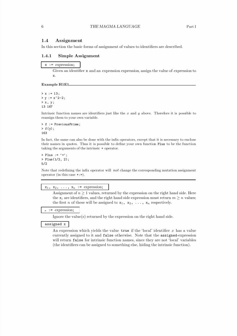
8/22/2019 Handbook Volume 01
http://slidepdf.com/reader/full/handbook-volume-01 122/440
6 THE MAGMA LANGUAGE Part I
1.4 Assignment
In this section the basic forms of assignment of values to identifiers are described.
1.4.1 Simple Assignment
x := expression;
Given an identifier x and an expression expression, assign the value of expression tox.
Example H1E1
> x := 13;
> y := x^2-2;
> x, y;13 167
Intrinsic function names are identifiers just like the x and y above. Therefore it is possible toreassign them to your own variable.
> f := PreviousPrime;
> f(y);
163
In fact, the same can also be done with the infix operators, except that it is necessary to enclosetheir names in quotes. Thus it is possible to define your own function Plus to be the functiontaking the arguments of the intrinsic + operator.
> Plus := ’+’;
> Plus(1/2, 2);
5/2
Note that redefining the infix operator will not change the corresponding mutation assignmentoperator (in this case +:=).
x1, x2, ..., xn := expression;
Assignment of n ≥ 1 values, returned by the expression on the right hand side. Herethe xi are identifiers, and the right hand side expression must return m ≥ n values;
the first n of these will be assigned to x1, x2, ..., xn respectively.
:= expression;
Ignore the value(s) returned by the expression on the right hand side.
assigned x
An expression which yields the value true if the ‘local’ identifier x has a valuecurrently assigned to it and false otherwise. Note that the assigned-expressionwill return false for intrinsic function names, since they are not ‘local’ variables(the identifiers can be assigned to something else, hiding the intrinsic function).
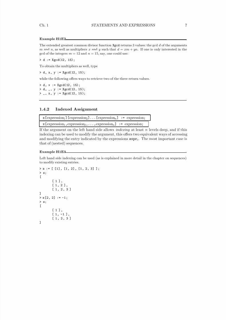
8/22/2019 Handbook Volume 01
http://slidepdf.com/reader/full/handbook-volume-01 123/440
Ch. 1 STATEMENTS AND EXPRESSIONS 7
Example H1E2
The extended greatest common divisor function Xgcd returns 3 values: the gcd d of the arguments
m and n, as well as multipliers x and y such that d = xm + yn. If one is only interested in thegcd of the integers m = 12 and n = 15, say, one could use:
> d := Xgcd(12, 15);
To obtain the multipliers as well, type
> d, x, y := Xgcd(12, 15);
while the following offers ways to retrieve two of the three return values.
> d, x := Xgcd(12, 15);
> d, _, y := Xgcd(12, 15);
> _, x, y := Xgcd(12, 15);
1.4.2 Indexed Assignment
x[expression1][expression2]...[expressionn] := expression;
x[expression1,expression2,...,expressionn] := expression;
If the argument on the left hand side allows indexing at least n levels deep, and if thisindexing can be used to modify the argument, this offers two equivalent ways of accessingand modifying the entry indicated by the expressions expri. The most important case is
that of (nested) sequences.
Example H1E3
Left hand side indexing can be used (as is explained in more detail in the chapter on sequences)to modify existing entries.
> s := [ [1], [1, 2], [1, 2, 3] ];
> s;
[
[ 1 ] ,
[ 1 , 2 ] ,
[ 1 , 2 , 3 ]
]> s[2, 2] := -1;
> s;
[
[ 1 ] ,
[ 1, -1 ],
[ 1 , 2 , 3 ]
]
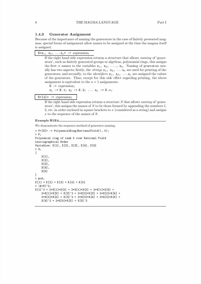
8/22/2019 Handbook Volume 01
http://slidepdf.com/reader/full/handbook-volume-01 124/440
8 THE MAGMA LANGUAGE Part I
1.4.3 Generator Assignment
Because of the importance of naming the generators in the case of finitely presented mag-
mas, special forms of assignment allow names to be assigned at the time the magma itself is assigned.
E<x1, x2, ...xn> := expression;
If the right hand side expression returns a structure that allows naming of ‘gener-ators’, such as finitely generated groups or algebras, polynomial rings, this assignsthe first n names to the variables x1, x2, ..., xn. Naming of generators usu-ally has two aspects; firstly, the strings x1, x2, ...xn are used for printing of thegenerators, and secondly, to the identifiers x1, x2, ...xn are assigned the valuesof the generators. Thus, except for this side effect regarding printing, the aboveassignment is equivalent to the n + 1 assignments:
E := expression;x1 := E.1; x2 := E.2; ... xn := E.n;
E<[x]> := expression;
If the right hand side expression returns a structure S that allows naming of ‘gener-ators’, this assigns the names of S to be those formed by appending the numbers 1,2, etc. in order enclosed in square brackets to x (considered as a string) and assignsx to the sequence of the names of S .
Example H1E4
We demonstrate the sequence method of generator naming.
> P<[X]> := PolynomialRing(RationalField(), 5);
> P;
Polynomial ring of rank 5 over Rational Field
Lexicographical Order
Variables: X[1], X[2], X[3], X[4], X[5]
> X;
[
X[1],
X[2],
X[3],
X[4],
X[5]]
> &+X;
X[1] + X[2] + X[3] + X[4] + X[5]
> (&+X)^2;
X[1]^2 + 2*X[1]*X[2] + 2*X[1]*X[3] + 2*X[1]*X[4] +
2*X[1]*X[5] + X[2]^2 + 2*X[2]*X[3] + 2*X[2]*X[4] +
2*X[2]*X[5] + X[3]^2 + 2*X[3]*X[4] + 2*X[3]*X[5] +
X[4]^2 + 2*X[4]*X[5] + X[5]^2
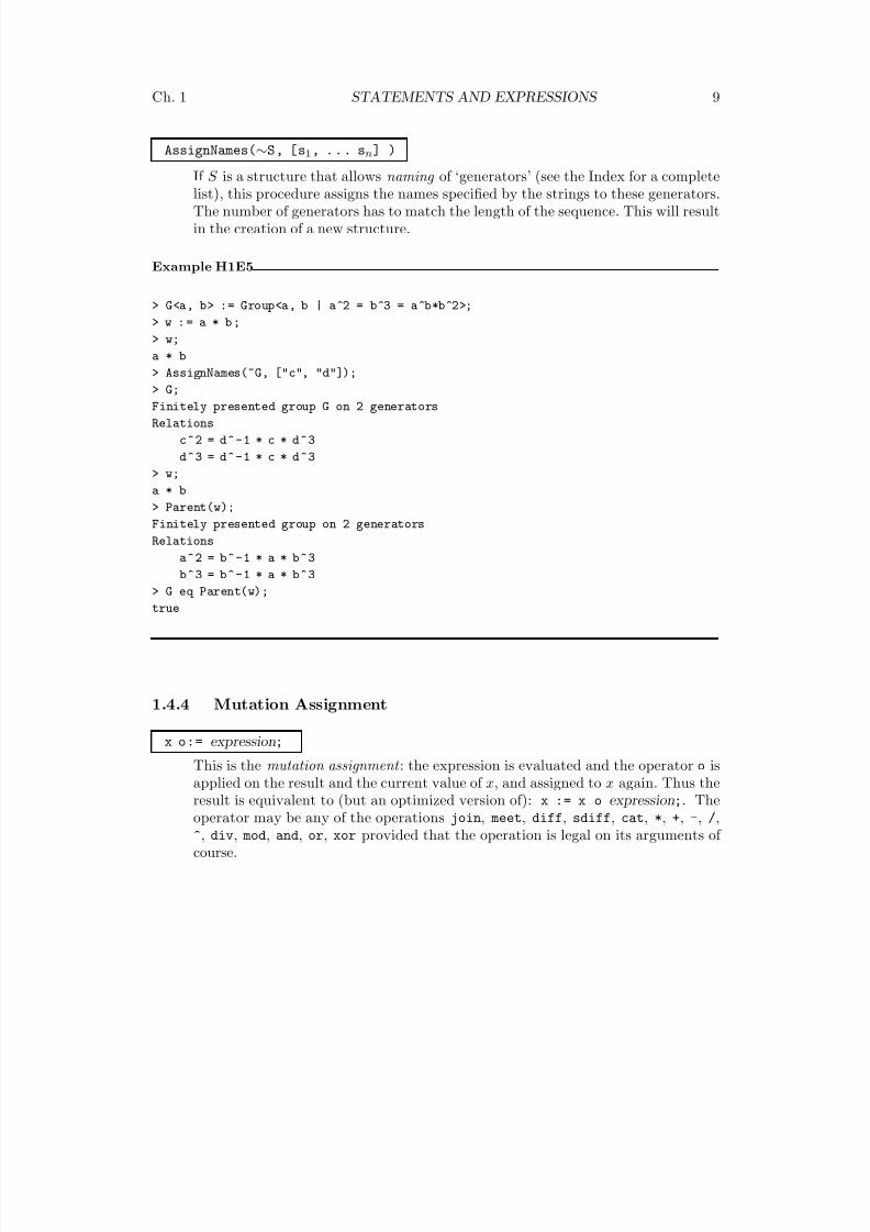
8/22/2019 Handbook Volume 01
http://slidepdf.com/reader/full/handbook-volume-01 125/440
Ch. 1 STATEMENTS AND EXPRESSIONS 9
AssignNames(∼S, [s1, ... sn] )
If S is a structure that allows naming of ‘generators’ (see the Index for a completelist), this procedure assigns the names specified by the strings to these generators.The number of generators has to match the length of the sequence. This will resultin the creation of a new structure.
Example H1E5
> G<a, b> := Group<a, b | a^2 = b^3 = a^b*b^2>;
> w : = a * b ;
> w;
a * b
> AssignNames(~G, ["c", "d"]);> G;
Finitely presented group G on 2 generators
Relations
c^2 = d^-1 * c * d^3
d^3 = d^-1 * c * d^3
> w;
a * b
> Parent(w);
Finitely presented group on 2 generators
Relations
a^2 = b^-1 * a * b^3b^3 = b^-1 * a * b^3
> G eq Parent(w);
true
1.4.4 Mutation Assignment
x o:= expression;
This is the mutation assignment : the expression is evaluated and the operator o isapplied on the result and the current value of x, and assigned to x again. Thus theresult is equivalent to (but an optimized version of): x := x o expression;. Theoperator may be any of the operations join, meet, diff, sdiff, cat, *, +, -, /,^, div, mod, and, or, xor provided that the operation is legal on its arguments of course.
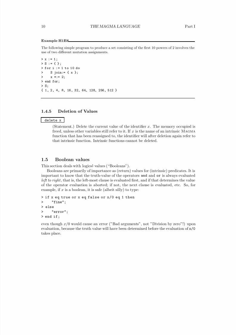
8/22/2019 Handbook Volume 01
http://slidepdf.com/reader/full/handbook-volume-01 126/440
10 THE MAGMA LANGUAGE Part I
Example H1E6
The following simple program to produce a set consisting of the first 10 powers of 2 involves theuse of two different mutation assignments.
> x : = 1 ;
> S : = { } ;
> for i := 1 to 10 do
> S join:= { x };
> x *:= 2;
> end for;
> S;
{ 1, 2, 4, 8, 16, 32, 64, 128, 256, 512 }
1.4.5 Deletion of Values
delete x
(Statement.) Delete the current value of the identifier x. The memory occupied isfreed, unless other variables still refer to it. If x is the name of an intrinsic Magma
function that has been reassigned to, the identifier will after deletion again refer tothat intrinsic function. Intrinsic functions cannot be deleted.
1.5 Boolean values
This section deals with logical values (“Booleans”).Booleans are primarily of importance as (return) values for (intrinsic) predicates. It is
important to know that the truth-value of the operators and and or is always evaluatedleft to right , that is, the left-most clause is evaluated first, and if that determines the valueof the operator evaluation is aborted; if not, the next clause is evaluated, etc. So, forexample, if x is a boolean, it is safe (albeit silly) to type:
> if x eq true or x eq false or x/0 eq 1 then
> "fine";> else
> "error";
> end if;
even though x/0 would cause an error (”Bad arguments”, not ”Division by zero”!) uponevaluation, because the truth value will have been determined before the evaluation of x/0
takes place.
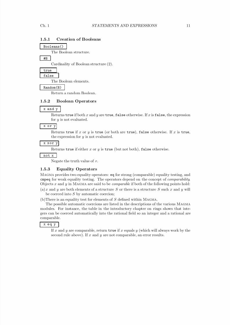
8/22/2019 Handbook Volume 01
http://slidepdf.com/reader/full/handbook-volume-01 127/440
Ch. 1 STATEMENTS AND EXPRESSIONS 11
1.5.1 Creation of Booleans
Booleans()
The Boolean structure.
#B
Cardinality of Boolean structure (2).
true
false
The Boolean elements.
Random(B)
Return a random Boolean.
1.5.2 Boolean Operators
x and y
Returns true if both x and y are true, false otherwise. If x is false, the expressionfor y is not evaluated.
x o r y
Returns true if x or y is true (or both are true), false otherwise. If x is true,the expression for y is not evaluated.
x xor y
Returns true if either x or y is true (but not both), false otherwise.
not x
Negate the truth value of x.
1.5.3 Equality Operators
Magma provides two equality operators: eq for strong (comparable) equality testing, andcmpeq for weak equality testing. The operators depend on the concept of comparability .Objects x and y in Magma are said to be comparable if both of the following points hold:
(a) x and y are both elements of a structure S or there is a structure S such x and y will
be coerced into S by automatic coercion;(b)There is an equality test for elements of S defined within Magma.
The possible automatic coercions are listed in the descriptions of the various Magma
modules. For instance, the table in the introductory chapter on rings shows that inte-gers can be coerced automatically into the rational field so an integer and a rational arecomparable.
x e q y
If x and y are comparable, return true if x equals y (which will always work by thesecond rule above). If x and y are not comparable, an error results.
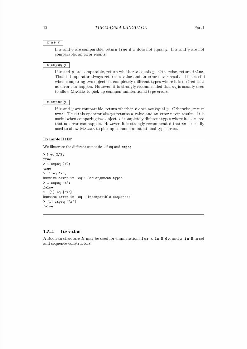
8/22/2019 Handbook Volume 01
http://slidepdf.com/reader/full/handbook-volume-01 128/440
12 THE MAGMA LANGUAGE Part I
x n e y
If x and y are comparable, return true if x does not equal y. If x and y are notcomparable, an error results.
x cmpeq y
If x and y are comparable, return whether x equals y. Otherwise, return false.Thus this operator always returns a value and an error never results. It is usefulwhen comparing two objects of completely different types where it is desired thatno error can happen. However, it is strongly recommended that eq is usually usedto allow Magma to pick up common unintentional type errors.
x cmpne y
If x and y are comparable, return whether x does not equal y. Otherwise, returntrue. Thus this operator always returns a value and an error never results. It isuseful when comparing two objects of completely different types where it is desiredthat no error can happen. However, it is strongly recommended that ne is usuallyused to allow Magma to pick up common unintentional type errors.
Example H1E7
We illustrate the different semantics of eq and cmpeq .
> 1 eq 2/2;
true
> 1 cmpeq 2/2;
true
> 1 eq "x";
Runtime error in ’eq’: Bad argument types
> 1 cmpeq "x";
false
> [1] eq ["x"];
Runtime error in ’eq’: Incompatible sequences
> [1] cmpeq ["x"];
false
1.5.4 Iteration
A Boolean structure B may be used for enumeration: for x in B do, and x i n B in setand sequence constructors.
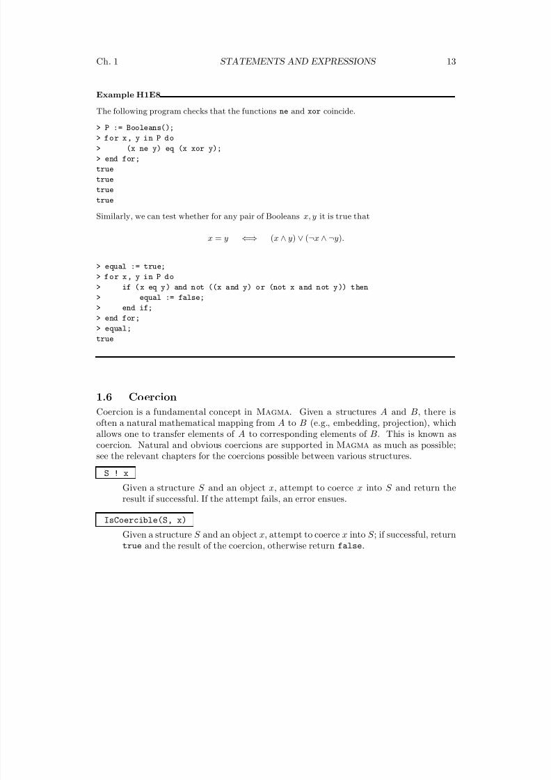
8/22/2019 Handbook Volume 01
http://slidepdf.com/reader/full/handbook-volume-01 129/440
Ch. 1 STATEMENTS AND EXPRESSIONS 13
Example H1E8
The following program checks that the functions ne and xor coincide.
> P := Booleans();
> for x, y in P do
> (x ne y) eq (x xor y);
> end for;
true
true
true
true
Similarly, we can test whether for any pair of Booleans x, y it is true that
x = y ⇐⇒ (x ∧ y) ∨ (¬x ∧ ¬y).
> equal := true;
> for x, y in P do
> if (x eq y) and not ((x and y) or (not x and not y)) then
> equal := false;
> end if;
> end for;
> equal;
true
1.6 Coercion
Coercion is a fundamental concept in Magma. Given a structures A and B, there isoften a natural mathematical mapping from A to B (e.g., embedding, projection), whichallows one to transfer elements of A to corresponding elements of B. This is known ascoercion. Natural and obvious coercions are supported in Magma as much as possible;see the relevant chapters for the coercions possible between various structures.
S ! x
Given a structure S and an object x, attempt to coerce x into S and return theresult if successful. If the attempt fails, an error ensues.
IsCoercible(S, x)
Given a structure S and an object x, attempt to coerce x into S ; if successful, returntrue and the result of the coercion, otherwise return false.
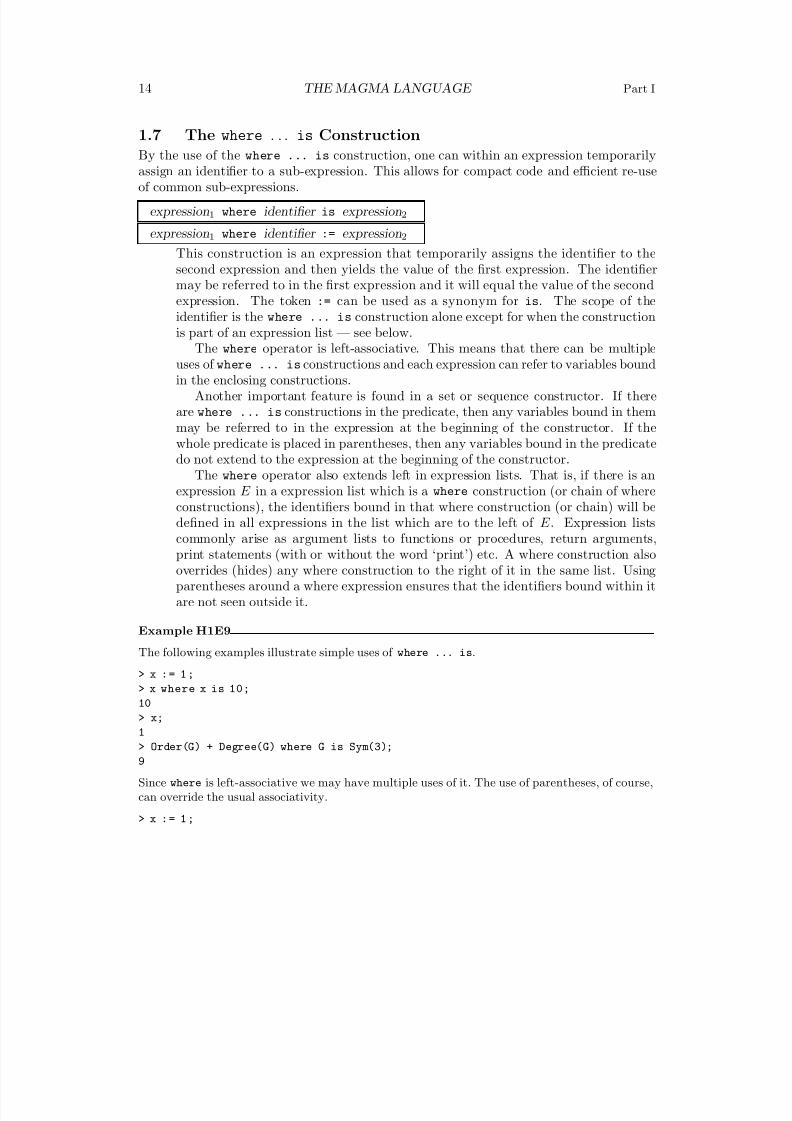
8/22/2019 Handbook Volume 01
http://slidepdf.com/reader/full/handbook-volume-01 130/440
14 THE MAGMA LANGUAGE Part I
1.7 The where . . . is Construction
By the use of the where ... is construction, one can within an expression temporarily
assign an identifier to a sub-expression. This allows for compact code and efficient re-useof common sub-expressions.
expression1 where identifier is expression2
expression1 where identifier := expression2
This construction is an expression that temporarily assigns the identifier to thesecond expression and then yields the value of the first expression. The identifiermay be referred to in the first expression and it will equal the value of the secondexpression. The token := can be used as a synonym for is. The scope of theidentifier is the where ... is construction alone except for when the construction
is part of an expression list — see below.The where operator is left-associative. This means that there can be multipleuses of where ... is constructions and each expression can refer to variables boundin the enclosing constructions.
Another important feature is found in a set or sequence constructor. If thereare where ... is constructions in the predicate, then any variables bound in themmay be referred to in the expression at the beginning of the constructor. If thewhole predicate is placed in parentheses, then any variables bound in the predicatedo not extend to the expression at the beginning of the constructor.
The where operator also extends left in expression lists. That is, if there is anexpression E in a expression list which is a where construction (or chain of where
constructions), the identifiers bound in that where construction (or chain) will bedefined in all expressions in the list which are to the left of E . Expression listscommonly arise as argument lists to functions or procedures, return arguments,print statements (with or without the word ‘print’) etc. A where construction alsooverrides (hides) any where construction to the right of it in the same list. Usingparentheses around a where expression ensures that the identifiers bound within itare not seen outside it.
Example H1E9
The following examples illustrate simple uses of where ... is.
> x : = 1 ;> x where x is 10;
10
> x;
1
> Order(G) + Degree(G) where G is Sym(3);
9
Since where is left-associative we may have multiple uses of it. The use of parentheses, of course,can override the usual associativity.
> x : = 1 ;
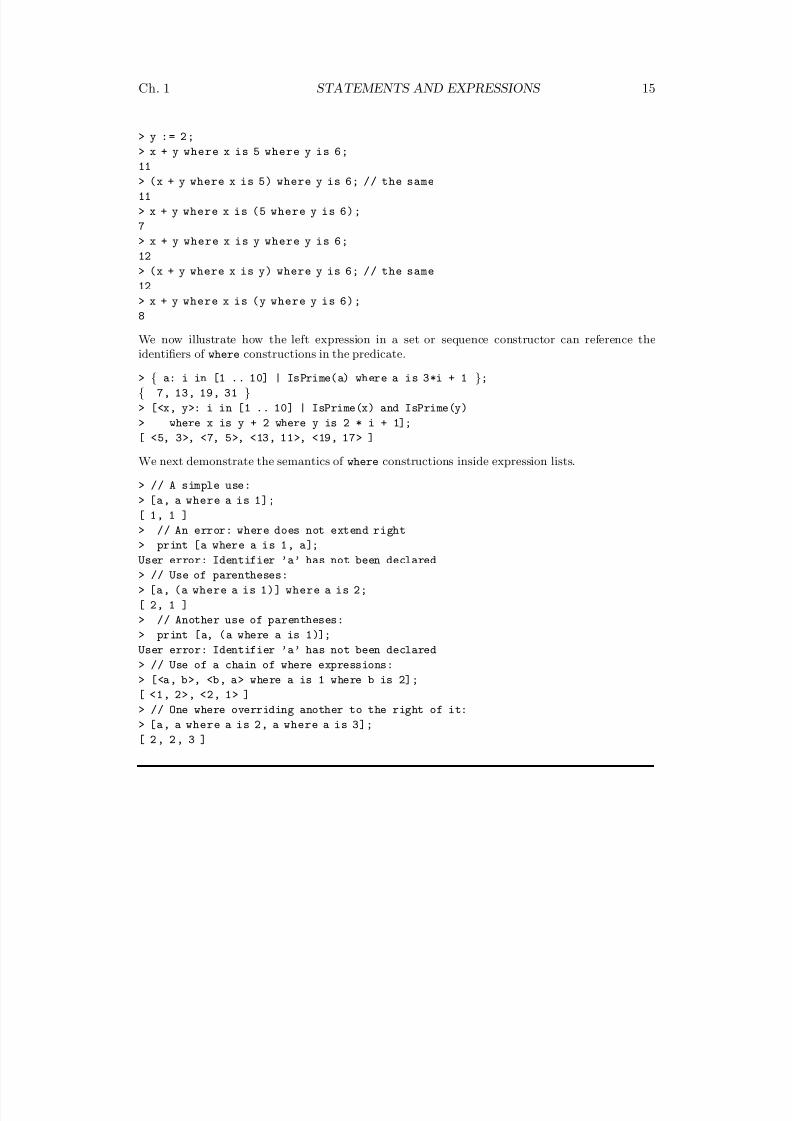
8/22/2019 Handbook Volume 01
http://slidepdf.com/reader/full/handbook-volume-01 131/440
Ch. 1 STATEMENTS AND EXPRESSIONS 15
> y : = 2 ;
> x + y where x is 5 where y is 6;
11> (x + y where x is 5) where y is 6; // the same
11
> x + y where x is (5 where y is 6);
7
> x + y where x is y where y is 6;
12
> (x + y where x is y) where y is 6; // the same
12
> x + y where x is (y where y is 6);
8
We now illustrate how the left expression in a set or sequence constructor can reference theidentifiers of where constructions in the predicate.
> { a: i in [1 .. 10] | IsPrime(a) where a is 3*i + 1 };
{ 7, 13, 19, 31 }> [<x, y>: i in [1 .. 10] | IsPrime(x) and IsPrime(y)
> where x is y + 2 where y is 2 * i + 1];
[ <5, 3>, <7, 5>, <13, 11>, <19, 17> ]
We next demonstrate the semantics of where constructions inside expression lists.
> // A simple use:
> [a, a where a is 1];[ 1, 1 ]
> // An error: where does not extend right
> print [a where a is 1, a];
User error: Identifier ’a’ has not been declared
> // Use of parentheses:
> [a, (a where a is 1)] where a is 2;
[ 2, 1 ]
> // Another use of parentheses:
> print [a, (a where a is 1)];
User error: Identifier ’a’ has not been declared
> // Use of a chain of where expressions:
> [<a, b>, <b, a> where a is 1 where b is 2];
[ <1, 2>, <2, 1> ]
> // One where overriding another to the right of it:
> [a, a where a is 2, a where a is 3];
[ 2 , 2 , 3 ]
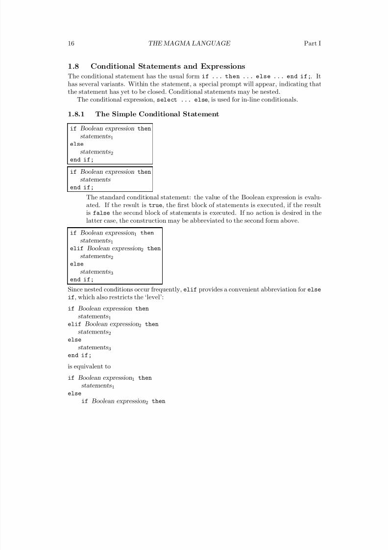
8/22/2019 Handbook Volume 01
http://slidepdf.com/reader/full/handbook-volume-01 132/440
16 THE MAGMA LANGUAGE Part I
1.8 Conditional Statements and Expressions
The conditional statement has the usual form if ... then ... else ... end if;. It
has several variants. Within the statement, a special prompt will appear, indicating thatthe statement has yet to be closed. Conditional statements may be nested.
The conditional expression, select ... else, is used for in-line conditionals.
1.8.1 The Simple Conditional Statement
if Boolean expression then
statements 1else
statements 2end if;
if Boolean expression then
statements end if;
The standard conditional statement: the value of the Boolean expression is evalu-ated. If the result is true, the first block of statements is executed, if the resultis false the second block of statements is executed. If no action is desired in thelatter case, the construction may be abbreviated to the second form above.
if Boolean expression1 then
statements 1
elif Boolean expression2 thenstatements 2
else
statements 3end if;
Since nested conditions occur frequently, elif provides a convenient abbreviation for else
if, which also restricts the ‘level’:
if Boolean expression then
statements 1elif Boolean expression2 then
statements 2else
statements 3end if;
is equivalent to
if Boolean expression1 then
statements 1else
if Boolean expression2 then
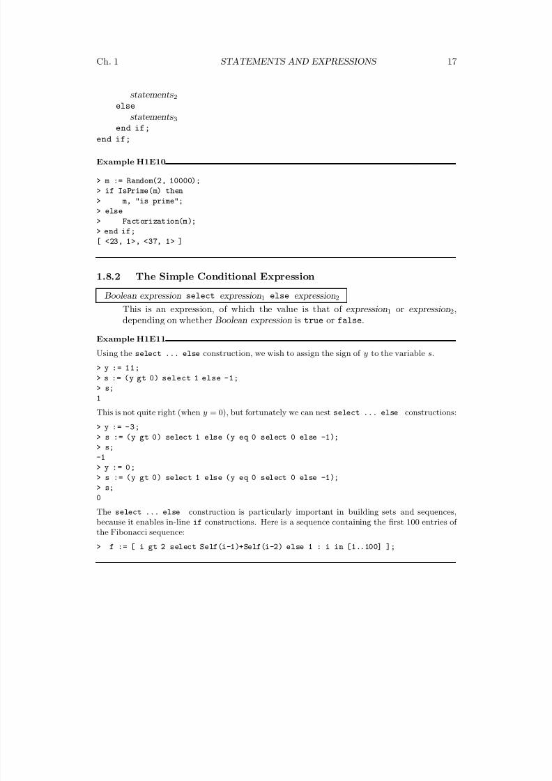
8/22/2019 Handbook Volume 01
http://slidepdf.com/reader/full/handbook-volume-01 133/440
Ch. 1 STATEMENTS AND EXPRESSIONS 17
statements 2else
statements 3end if;
end if;
Example H1E10
> m := Random(2, 10000);
> if IsPrime(m) then
> m, "is prime";
> else
> Factorization(m);
> end if;[ <23, 1>, <37, 1> ]
1.8.2 The Simple Conditional Expression
Boolean expression select expression1 else expression2
This is an expression, of which the value is that of expression1 or expression2,depending on whether Boolean expression is true or false.
Example H1E11
Using the select ... else construction, we wish to assign the sign of y to the variable s.
> y := 11;
> s := (y gt 0) select 1 else -1;
> s;
1
This is not quite right (when y = 0), but fortunately we can nest select ... else constructions:
> y := -3;
> s := (y gt 0) select 1 else (y eq 0 select 0 else -1);
> s;
-1
> y : = 0 ;> s := (y gt 0) select 1 else (y eq 0 select 0 else -1);
> s;
0
The select ... else construction is particularly important in building sets and sequences,because it enables in-line if constructions. Here is a sequence containing the first 100 entries of the Fibonacci sequence:
> f := [ i gt 2 select Self(i-1)+Self(i-2) else 1 : i in [1..100] ];
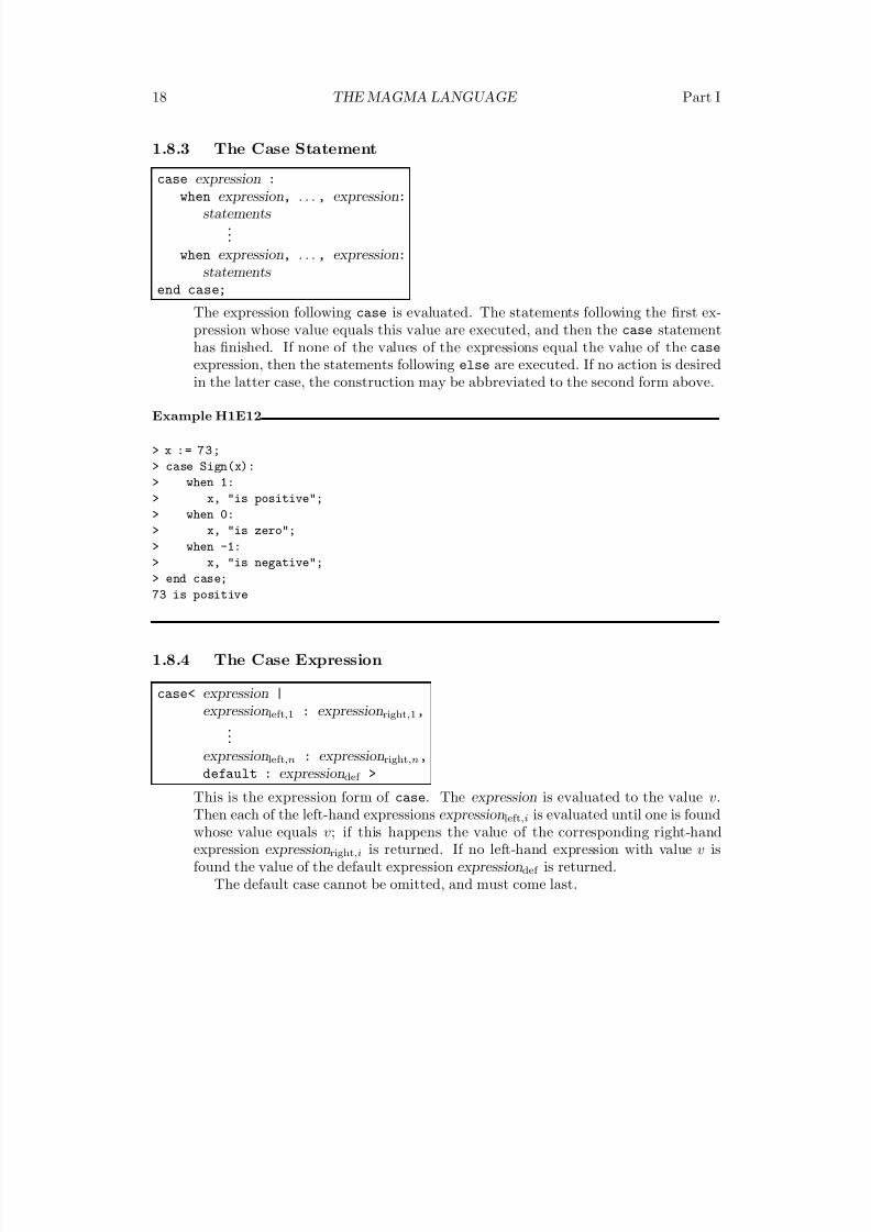
8/22/2019 Handbook Volume 01
http://slidepdf.com/reader/full/handbook-volume-01 134/440
18 THE MAGMA LANGUAGE Part I
1.8.3 The Case Statement
case expression :when expression, . . . , expression:
statements ...
when expression, . . . , expression:
statements end case;
The expression following case is evaluated. The statements following the first ex-pression whose value equals this value are executed, and then the case statementhas finished. If none of the values of the expressions equal the value of the case
expression, then the statements following else are executed. If no action is desiredin the latter case, the construction may be abbreviated to the second form above.
Example H1E12
> x := 73;
> case Sign(x):
> when 1:
> x, "is positive";
> when 0:
> x, "is zero";
> when -1:
> x, "is negative";
> end case;
73 is positive
1.8.4 The Case Expression
case< expression |
expressionleft,1 : expressionright,1,...
expressionleft,n : expressionright,n,
default : expressiondef >
This is the expression form of case. The expression is evaluated to the value v.Then each of the left-hand expressions expressionleft,i is evaluated until one is foundwhose value equals v; if this happens the value of the corresponding right-handexpression expressionright,i is returned. If no left-hand expression with value v isfound the value of the default expression expressiondef is returned.
The default case cannot be omitted, and must come last.
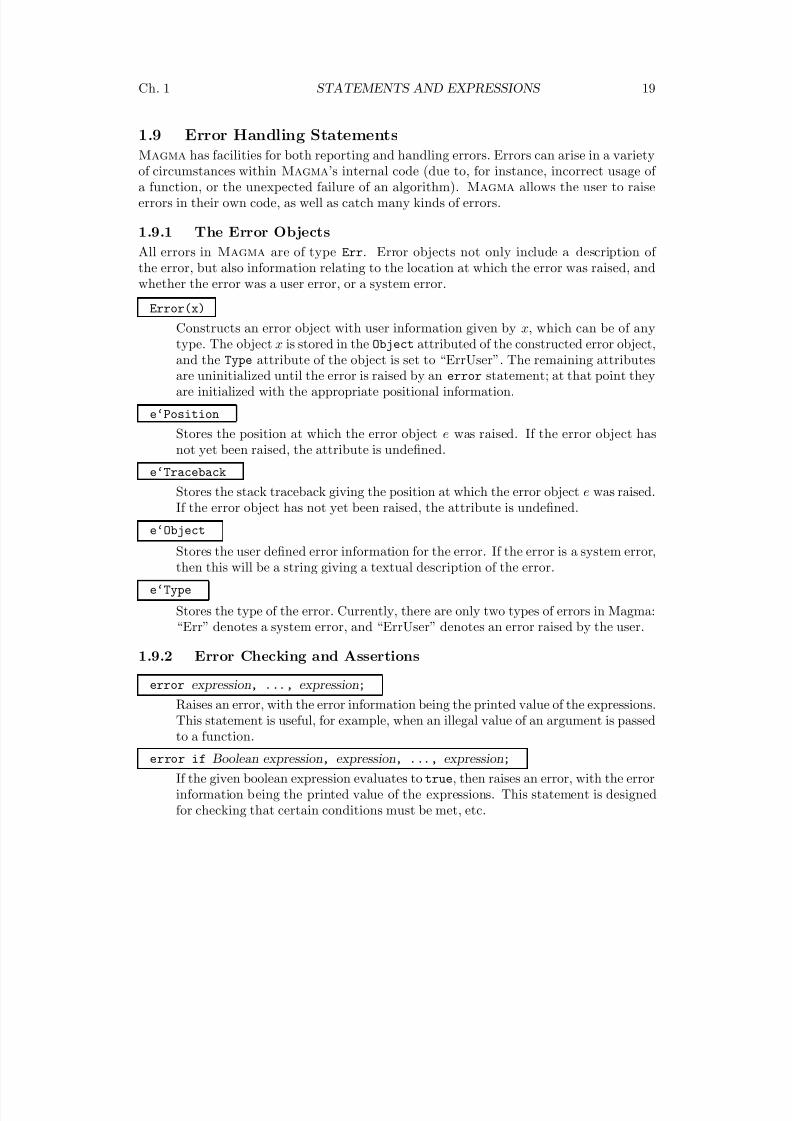
8/22/2019 Handbook Volume 01
http://slidepdf.com/reader/full/handbook-volume-01 135/440
Ch. 1 STATEMENTS AND EXPRESSIONS 19
1.9 Error Handling Statements
Magma has facilities for both reporting and handling errors. Errors can arise in a variety
of circumstances within Magma’s internal code (due to, for instance, incorrect usage of a function, or the unexpected failure of an algorithm). Magma allows the user to raiseerrors in their own code, as well as catch many kinds of errors.
1.9.1 The Error Objects
All errors in Magma are of type Err. Error objects not only include a description of the error, but also information relating to the location at which the error was raised, andwhether the error was a user error, or a system error.
Error(x)
Constructs an error object with user information given by x, which can be of anytype. The object x is stored in the Object attributed of the constructed error object,and the Type attribute of the object is set to “ErrUser”. The remaining attributesare uninitialized until the error is raised by an error statement; at that point theyare initialized with the appropriate positional information.
e‘Position
Stores the position at which the error object e was raised. If the error object hasnot yet been raised, the attribute is undefined.
e‘Traceback
Stores the stack traceback giving the position at which the error object e was raised.
If the error object has not yet been raised, the attribute is undefined.
e‘Object
Stores the user defined error information for the error. If the error is a system error,then this will be a string giving a textual description of the error.
e‘Type
Stores the type of the error. Currently, there are only two types of errors in Magma:“Err” denotes a system error, and “ErrUser” denotes an error raised by the user.
1.9.2 Error Checking and Assertions
error expression, ..., expression;
Raises an error, with the error information being the printed value of the expressions.This statement is useful, for example, when an illegal value of an argument is passedto a function.
error if Boolean expression, expression, ..., expression;
If the given boolean expression evaluates to true, then raises an error, with the errorinformation being the printed value of the expressions. This statement is designedfor checking that certain conditions must be met, etc.
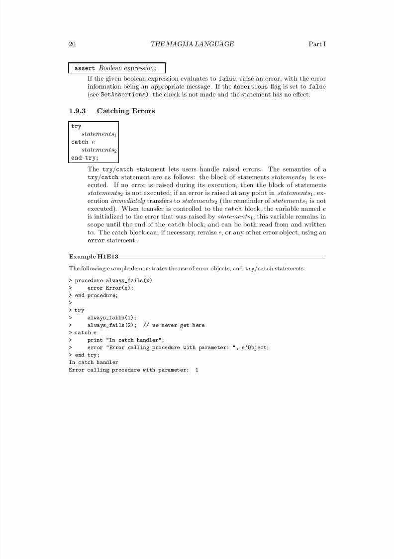
8/22/2019 Handbook Volume 01
http://slidepdf.com/reader/full/handbook-volume-01 136/440
20 THE MAGMA LANGUAGE Part I
assert Boolean expression;
If the given boolean expression evaluates to false, raise an error, with the error
information being an appropriate message. If the Assertions flag is set to false
(see SetAssertions), the check is not made and the statement has no effect.
1.9.3 Catching Errors
try
statements1catch e
statements2end try;
The try/catch statement lets users handle raised errors. The semantics of atry/catch statement are as follows: the block of statements statements1 is ex-ecuted. If no error is raised during its execution, then the block of statementsstatements2 is not executed; if an error is raised at any point in statements1, ex-ecution immediately transfers to statements2 (the remainder of statements1 is notexecuted). When transfer is controlled to the catch block, the variable named eis initialized to the error that was raised by statements1; this variable remains inscope until the end of the catch block, and can be both read from and writtento. The catch block can, if necessary, reraise e, or any other error object, using anerror statement.
Example H1E13
The following example demonstrates the use of error objects, and try/catch statements.
> procedure always_fails(x)
> error Error(x);
> end procedure;
>
> try
> always_fails(1);
> always_fails(2); // we never get here
> catch e
> print "In catch handler";
> error "Error calling procedure with parameter: ", e‘Object;
> end try;
In catch handler
Error calling procedure with parameter: 1
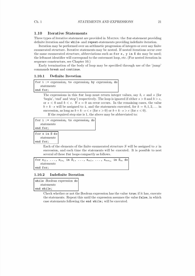
8/22/2019 Handbook Volume 01
http://slidepdf.com/reader/full/handbook-volume-01 137/440
Ch. 1 STATEMENTS AND EXPRESSIONS 21
1.10 Iterative Statements
Three types of iterative statement are provided in Magma: the for-statement providing
definite iteration and the while- and repeat-statements providing indefinite iteration.Iteration may be performed over an arithmetic progression of integers or over any finite
enumerated structure. Iterative statements may be nested. If nested iterations occur overthe same enumerated structure, abbreviations such as for x, y in X do may be used;the leftmost identifier will correspond to the outermost loop, etc. (For nested iteration insequence constructors, see Chapter 10.)
Early termination of the body of loop may be specified through use of the ‘jump’commands break and continue.
1.10.1 Definite Iteration
for i := expression1 to expression2 by expression3 dostatements end for;
The expressions in this for loop must return integer values, say b, e and s (for‘begin’, ‘end’ and ‘step’) respectively. The loop is ignored if either s > 0 and b > e,or s < 0 and b < e. If s = 0 an error occurs. In the remaining cases, the valueb + k · s will be assigned to i, and the statements executed, for k = 0, 1, 2, . . . insuccession, as long as b + k · s < e (for e > 0) or b + k · s > e (for e < 0).
If the required step size is 1, the above may be abbreviated to:
for i := expression1 to expression2 do
statements end for;
for x in S do
statements end for;
Each of the elements of the finite enumerated structure S will be assigned to x insuccession, and each time the statements will be executed. It is possible to nestseveral of these for loops compactly as follows.
for x11, ..., x1n1 in S1, ..., xm1, ..., xmnm in Sm do
statements end for;
1.10.2 Indefinite Iteration
while Boolean expression do
statements end while;
Check whether or not the Boolean expression has the value true; if it has, executethe statements. Repeat this until the expression assumes the value false, in whichcase statements following the end while; will be executed.
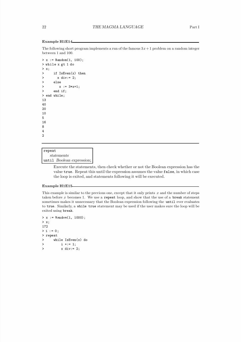
8/22/2019 Handbook Volume 01
http://slidepdf.com/reader/full/handbook-volume-01 138/440
22 THE MAGMA LANGUAGE Part I
Example H1E14
The following short program implements a run of the famous 3x + 1 problem on a random integer
between 1 and 100.
> x := Random(1, 100);
> while x gt 1 do
> x;
> if IsEven(x) then
> x div:= 2;
> else
> x := 3*x+1;
> end if;
> end while;
13
40
20
10
5
16
8
4
2
repeat
statements until Boolean expression;
Execute the statements, then check whether or not the Boolean expression has thevalue true. Repeat this until the expression assumes the value false, in which casethe loop is exited, and statements following it will be executed.
Example H1E15
This example is similar to the previous one, except that it only prints x and the number of stepstaken before x becomes 1. We use a repeat loop, and show that the use of a break statementsometimes makes it unnecessary that the Boolean expression following the until ever evaluates
to true. Similarly, a while true statement may be used if the user makes sure the loop will beexited using break.
> x := Random(1, 1000);
> x;
172
> i : = 0 ;
> repeat
> while IsEven(x) do
> i +:= 1;
> x div:= 2;
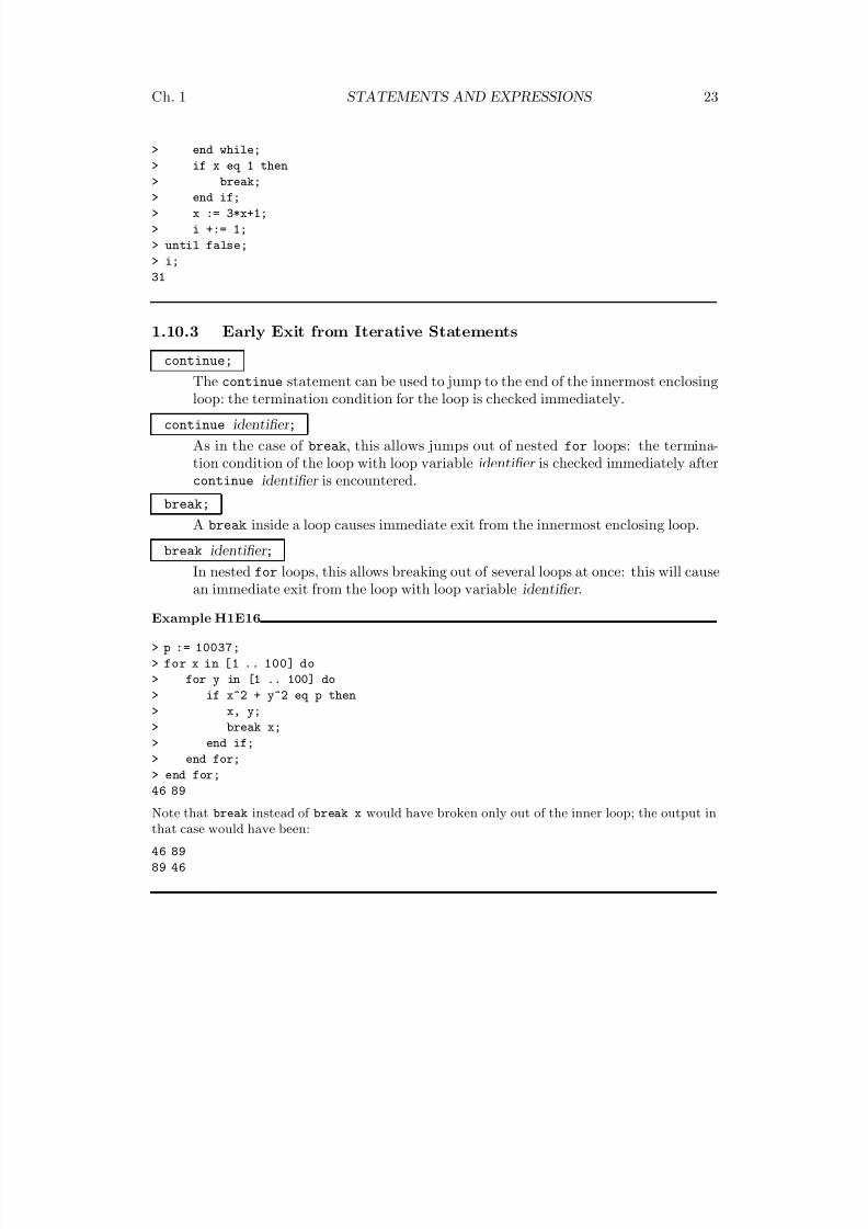
8/22/2019 Handbook Volume 01
http://slidepdf.com/reader/full/handbook-volume-01 139/440
Ch. 1 STATEMENTS AND EXPRESSIONS 23
> end while;
> if x eq 1 then
> break;> end if;
> x := 3*x+1;
> i +:= 1;
> until false;
> i;
31
1.10.3 Early Exit from Iterative Statements
continue;
The continue statement can be used to jump to the end of the innermost enclosingloop: the termination condition for the loop is checked immediately.
continue identifier ;
As in the case of break, this allows jumps out of nested for loops: the termina-tion condition of the loop with loop variable identifier is checked immediately aftercontinue identifier is encountered.
break;
A break inside a loop causes immediate exit from the innermost enclosing loop.
break identifier ;In nested for loops, this allows breaking out of several loops at once: this will causean immediate exit from the loop with loop variable identifier .
Example H1E16
> p := 10037;
> for x in [1 .. 100] do
> for y in [1 .. 100] do
> if x^2 + y^2 eq p then
> x, y;
> break x;
> end if;> end for;
> end for;
46 89
Note that break instead of break x would have broken only out of the inner loop; the output inthat case would have been:
46 89
89 46
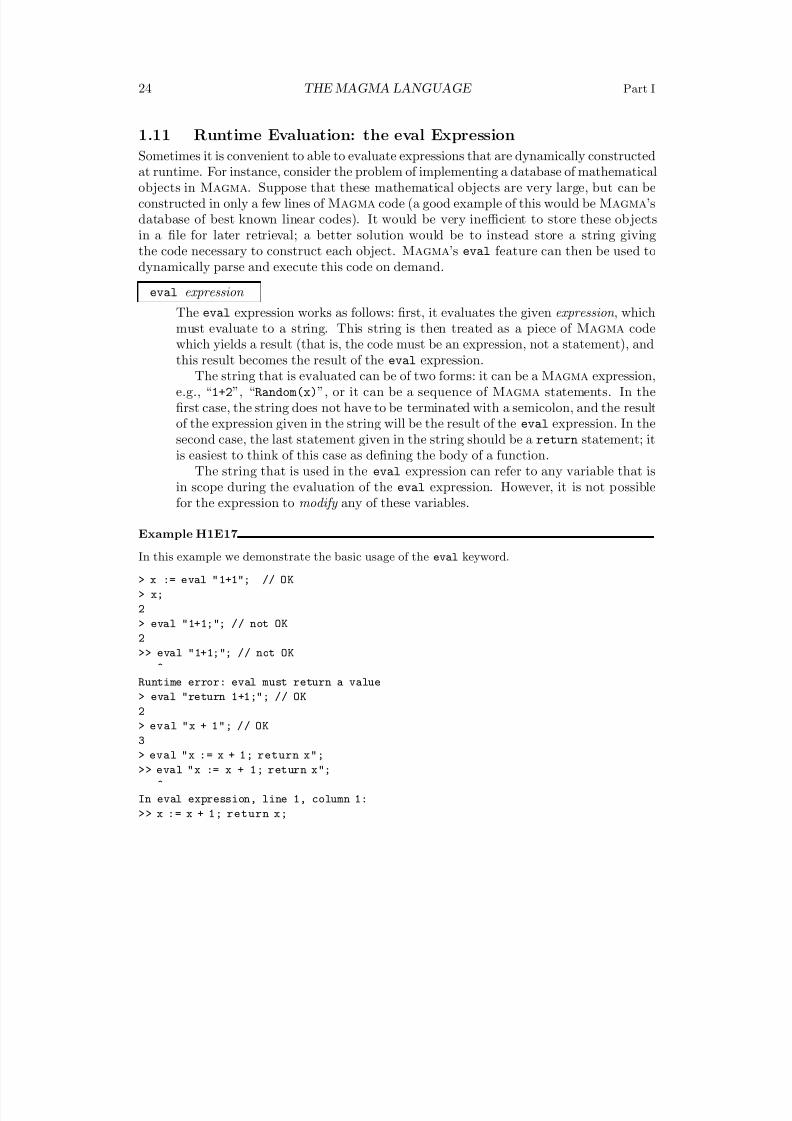
8/22/2019 Handbook Volume 01
http://slidepdf.com/reader/full/handbook-volume-01 140/440
24 THE MAGMA LANGUAGE Part I
1.11 Runtime Evaluation: the eval Expression
Sometimes it is convenient to able to evaluate expressions that are dynamically constructed
at runtime. For instance, consider the problem of implementing a database of mathematicalobjects in Magma. Suppose that these mathematical objects are very large, but can beconstructed in only a few lines of Magma code (a good example of this would be Magma’sdatabase of best known linear codes). It would be very inefficient to store these objectsin a file for later retrieval; a better solution would be to instead store a string givingthe code necessary to construct each object. Magma’s eval feature can then be used todynamically parse and execute this code on demand.
eval expression
The eval expression works as follows: first, it evaluates the given expression , whichmust evaluate to a string. This string is then treated as a piece of Magma codewhich yields a result (that is, the code must be an expression, not a statement), andthis result becomes the result of the eval expression.
The string that is evaluated can be of two forms: it can be a Magma expression,e.g., “1+2”, “Random(x)”, or it can be a sequence of Magma statements. In thefirst case, the string does not have to be terminated with a semicolon, and the resultof the expression given in the string will be the result of the eval expression. In thesecond case, the last statement given in the string should be a return statement; itis easiest to think of this case as defining the body of a function.
The string that is used in the eval expression can refer to any variable that isin scope during the evaluation of the eval expression. However, it is not possible
for the expression to modify any of these variables.
Example H1E17
In this example we demonstrate the basic usage of the eval keyword.
> x := eval "1+1"; // OK
> x;
2
> eval "1+1;"; // not OK
2
>> eval "1+1;"; // not OK
^
Runtime error: eval must return a value
> eval "return 1+1;"; // OK
2
> eval "x + 1"; // OK
3
> eval "x := x + 1; return x";
>> eval "x := x + 1; return x";
^
In eval expression, line 1, column 1:
>> x := x + 1; return x;
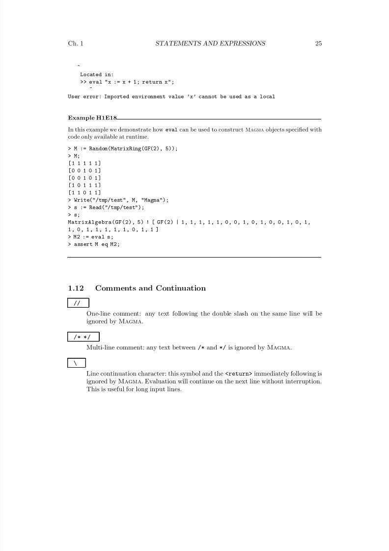
8/22/2019 Handbook Volume 01
http://slidepdf.com/reader/full/handbook-volume-01 141/440
Ch. 1 STATEMENTS AND EXPRESSIONS 25
^
Located in:
>> eval "x := x + 1; return x";^
User error: Imported environment value ’x’ cannot be used as a local
Example H1E18
In this example we demonstrate how eval can be used to construct Magma objects specified withcode only available at runtime.
> M := Random(MatrixRing(GF(2), 5));
> M;
[ 1 1 1 1 1 ][ 0 0 1 0 1 ]
[ 0 0 1 0 1 ]
[ 1 0 1 1 1 ]
[ 1 1 0 1 1 ]
> Write("/tmp/test", M, "Magma");
> s := Read("/tmp/test");
> s;
MatrixAlgebra(GF(2), 5) ! [ GF(2) | 1, 1, 1, 1, 1, 0, 0, 1, 0, 1, 0, 0, 1, 0, 1,
1, 0, 1, 1, 1, 1, 1, 0, 1, 1 ]
> M2 := eval s;
> assert M eq M2;
1.12 Comments and Continuation
//
One-line comment: any text following the double slash on the same line will beignored by Magma.
/* */
Multi-line comment: any text between /* and */ is ignored by Magma.
\
Line continuation character: this symbol and the <return> immediately following isignored by Magma. Evaluation will continue on the next line without interruption.This is useful for long input lines.
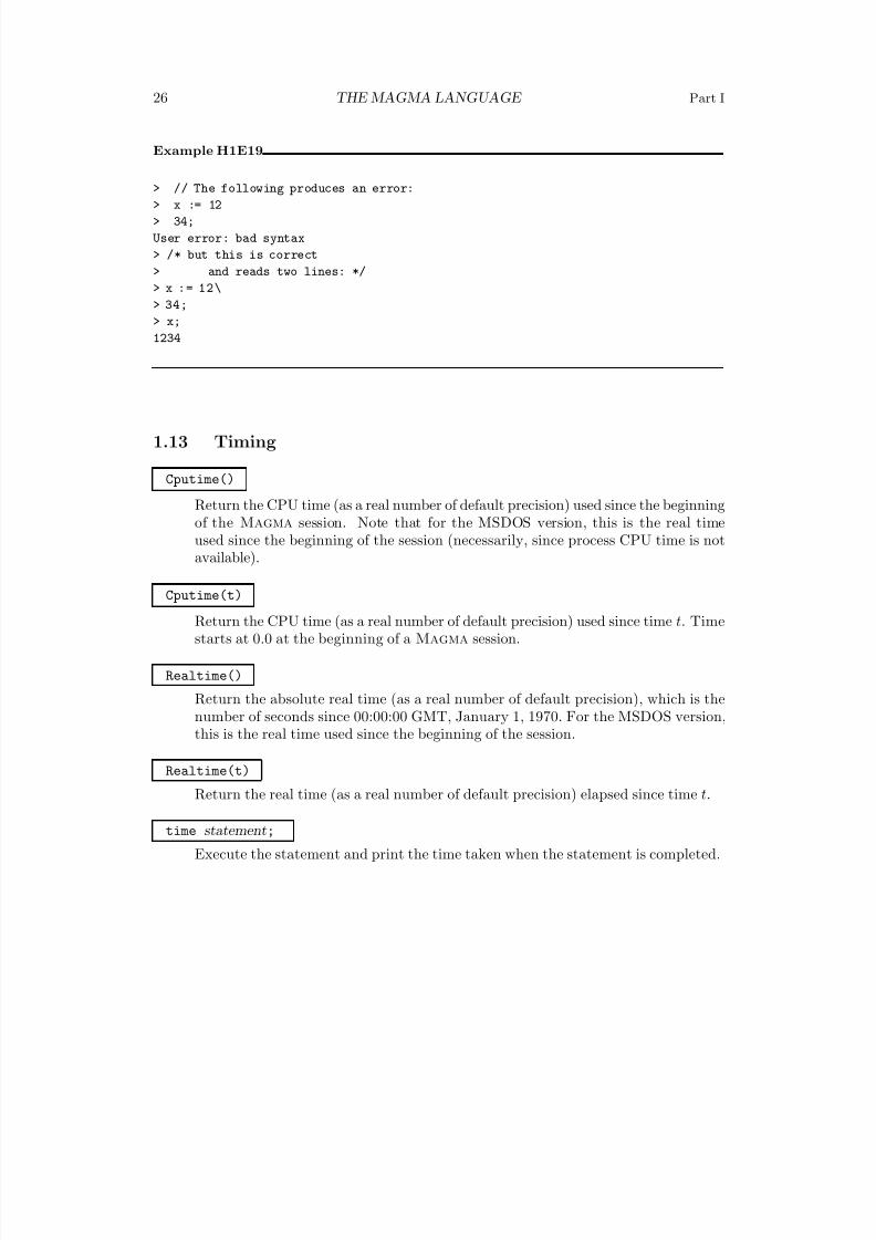
8/22/2019 Handbook Volume 01
http://slidepdf.com/reader/full/handbook-volume-01 142/440
26 THE MAGMA LANGUAGE Part I
Example H1E19
> // The following produces an error:> x := 12
> 34;
User error: bad syntax
> /* but this is correct
> and reads two lines: */
> x := 12\
> 34;
> x;
1234
1.13 Timing
Cputime()
Return the CPU time (as a real number of default precision) used since the beginningof the Magma session. Note that for the MSDOS version, this is the real timeused since the beginning of the session (necessarily, since process CPU time is not
available).
Cputime(t)
Return the CPU time (as a real number of default precision) used since time t. Timestarts at 0.0 at the beginning of a Magma session.
Realtime()
Return the absolute real time (as a real number of default precision), which is thenumber of seconds since 00:00:00 GMT, January 1, 1970. For the MSDOS version,this is the real time used since the beginning of the session.
Realtime(t)
Return the real time (as a real number of default precision) elapsed since time t.
time statement;
Execute the statement and print the time taken when the statement is completed.
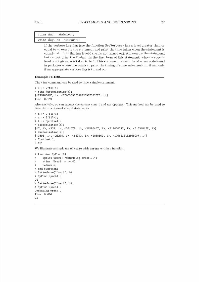
8/22/2019 Handbook Volume 01
http://slidepdf.com/reader/full/handbook-volume-01 143/440
Ch. 1 STATEMENTS AND EXPRESSIONS 27
vtime flag : statement;
vtime flag , n: statement:
If the verbose flag flag (see the function SetVerbose) has a level greater than orequal to n, execute the statement and print the time taken when the statement iscompleted. If the flag has level 0 (i.e., is not turned on), still execute the statement,but do not print the timing. In the first form of this statement, where a specificlevel is not given, n is taken to be 1. This statement is useful in Magma code foundin packages where one wants to print the timing of some sub-algorithm if and onlyif an appropriate verbose flag is turned on.
Example H1E20
The time command can be used to time a single statement.
> n := 2^109-1;
> time Factorization(n);
[<745988807, 1>, <870035986098720987332873, 1>]
Time: 0.149
Alternatively, we can extract the current time t and use Cputime. This method can be used totime the execution of several statements.
> m := 2^111-1;
> n := 2^113-1;
> t := Cputime();
> Factorization(m);
[<7, 1>, <223, 1>, <321679, 1>, <26295457, 1>, <319020217, 1>, <616318177, 1>]
> Factorization(n);
[<3391, 1>, <23279, 1>, <65993, 1>, <1868569, 1>, <1066818132868207, 1>]
> Cputime(t);
0.121
We illustrate a simple use of vtime with vprint within a function.
> function MyFunc(G)
> vprint User1: "Computing order...";
> vtime User1: o := #G;
> return o;
> end function;> SetVerbose("User1", 0);
> MyFunc(Sym(4));
24
> SetVerbose("User1", 1);
> MyFunc(Sym(4));
Computing order...
Time: 0.000
24
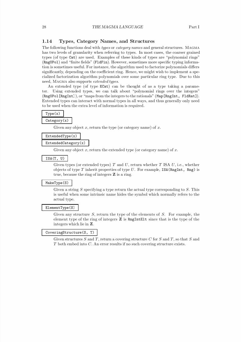
8/22/2019 Handbook Volume 01
http://slidepdf.com/reader/full/handbook-volume-01 144/440
28 THE MAGMA LANGUAGE Part I
1.14 Types, Category Names, and Structures
The following functions deal with types or category names and general structures. Magma
has two levels of granularity when referring to types. In most cases, the coarser grainedtypes (of type Cat) are used. Examples of these kinds of types are “polynomial rings”(RngUPol) and “finite fields” (FldFin). However, sometimes more specific typing informa-tion is sometimes useful. For instance, the algorithm used to factorize polynomials differssignificantly, depending on the coefficient ring. Hence, we might wish to implement a spe-cialized factorization algorithm polynomials over some particular ring type. Due to thisneed, Magma also supports extended types .
An extended type (of type ECat) can be thought of as a type taking a parame-ter. Using extended types, we can talk about “polynomial rings over the integers”(RngUPol[RngInt]), or “maps from the integers to the rationals” (Map[RngInt, FldRat]).
Extended types can interact with normal types in all ways, and thus generally only needto be used when the extra level of information is required.
Type(x)
Category(x)
Given any object x, return the type (or category name) of x.
ExtendedType(x)
ExtendedCategory(x)
Given any object x, return the extended type (or category name) of x.
ISA(T, U)
Given types (or extended types) T and U , return whether T ISA U , i.e., whetherobjects of type T inherit properties of type U . For example, ISA(RngInt, Rng) istrue, because the ring of integers Z is a ring.
MakeType(S)
Given a string S specifying a type return the actual type corresponding to S . Thisis useful when some intrinsic name hides the symbol which normally refers to theactual type.
ElementType(S)
Given any structure S , return the type of the elements of S . For example, theelement type of the ring of integers Z is RngIntElt since that is the type of theintegers which lie in Z.
CoveringStructure(S, T)
Given structures S and T , return a covering structure C for S and T , so that S andT both embed into C . An error results if no such covering structure exists.
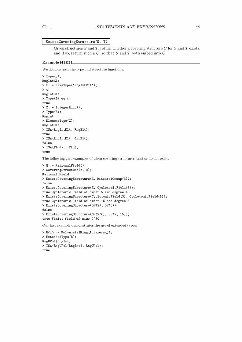
8/22/2019 Handbook Volume 01
http://slidepdf.com/reader/full/handbook-volume-01 145/440
Ch. 1 STATEMENTS AND EXPRESSIONS 29
ExistsCoveringStructure(S, T)
Given structures S and T , return whether a covering structure C for S and T exists,and if so, return such a C , so that S and T both embed into C .
Example H1E21
We demonstrate the type and structure functions.
> Type(3);
RngIntElt
> t := MakeType("RngIntElt");
> t;
RngIntElt
> Type(3) eq t;
true> Z := IntegerRing();
> Type(Z);
RngInt
> ElementType(Z);
RngIntElt
> ISA(RngIntElt, RngElt);
true
> ISA(RngIntElt, GrpElt);
false
> ISA(FldRat, Fld);
true
The following give examples of when covering structures exist or do not exist.
> Q := RationalField();
> CoveringStructure(Z, Q);
Rational Field
> ExistsCoveringStructure(Z, DihedralGroup(3));
false
> ExistsCoveringStructure(Z, CyclotomicField(5));
true Cyclotomic Field of order 5 and degree 4
> ExistsCoveringStructure(CyclotomicField(3), CyclotomicField(5));
true Cyclotomic Field of order 15 and degree 8
> ExistsCoveringStructure(GF(2), GF(3));false
> ExistsCoveringStructure(GF(2^6), GF(2, 15));
true Finite field of size 2^30
Our last example demonstrates the use of extended types:
> R<x> := PolynomialRing(Integers());
> ExtendedType(R);
RngUPol[RngInt]
> ISA(RngUPol[RngInt], RngUPol);
true
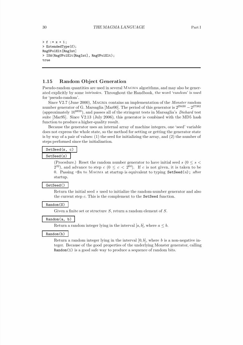
8/22/2019 Handbook Volume 01
http://slidepdf.com/reader/full/handbook-volume-01 146/440
30 THE MAGMA LANGUAGE Part I
> f : = x + 1 ;
> ExtendedType(f);
RngUPolElt[RngInt]> ISA(RngUPolElt[RngInt], RngUPolElt);
true
1.15 Random Object Generation
Pseudo-random quantities are used in several Magma algorithms, and may also be gener-ated explicitly by some intrinsics. Throughout the Handbook, the word ‘random’ is usedfor ‘pseudo-random’.
Since V2.7 (June 2000), Magma contains an implementation of the Monster randomnumber generator of G. Marsaglia [Mar00]. The period of this generator is 229430 − 227382
(approximately 108859), and passes all of the stringent tests in Marsaglia’s Diehard testsuite [Mar95]. Since V2.13 (July 2006), this generator is combined with the MD5 hashfunction to produce a higher-quality result.
Because the generator uses an internal array of machine integers, one ‘seed’ variabledoes not express the whole state, so the method for setting or getting the generator stateis by way of a pair of values: (1) the seed for initializing the array, and (2) the number of steps performed since the initialization.
SetSeed(s, c)
SetSeed(s)
(Procedure.) Reset the random number generator to have initial seed s (0 ≤ s <232), and advance to step c (0 ≤ c < 264). If c is not given, it is taken to be0. Passing -Sn to Magma at startup is equivalent to typing SetSeed(n ); afterstartup.
GetSeed()
Return the initial seed s used to initialize the random-number generator and alsothe current step c. This is the complement to the SetSeed function.
Random(S)
Given a finite set or structure S , return a random element of S .
Random(a, b)
Return a random integer lying in the interval [a, b], where a ≤ b.
Random(b)
Return a random integer lying in the interval [0, b], where b is a non-negative in-teger. Because of the good properties of the underlying Monster generator, callingRandom(1) is a good safe way to produce a sequence of random bits.
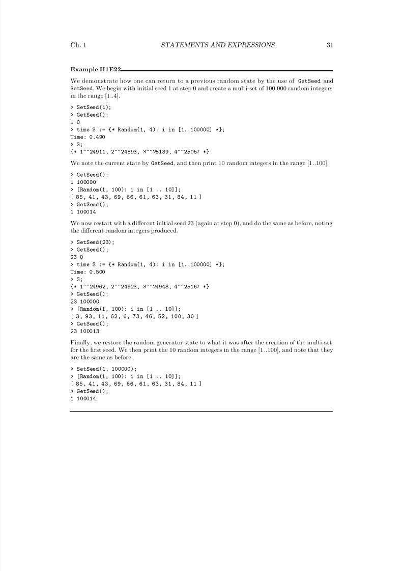
8/22/2019 Handbook Volume 01
http://slidepdf.com/reader/full/handbook-volume-01 147/440
Ch. 1 STATEMENTS AND EXPRESSIONS 31
Example H1E22
We demonstrate how one can return to a previous random state by the use of GetSeed andSetSeed. We begin with initial seed 1 at step 0 and create a multi-set of 100,000 random integersin the range [1..4].
> SetSeed(1);
> GetSeed();
1 0
> time S := {* Random(1, 4): i in [1..100000] *};
Time: 0.490
> S;
{* 1^^24911, 2^^24893, 3^^25139, 4^^25057 *}
We note the current state by GetSeed, and then print 10 random integers in the range [1..100].
> GetSeed();
1 100000
> [Random(1, 100): i in [1 .. 10]];
[ 85, 41, 43, 69, 66, 61, 63, 31, 84, 11 ]
> GetSeed();
1 100014
We now restart with a different initial seed 23 (again at step 0), and do the same as before, notingthe different random integers produced.
> SetSeed(23);
> GetSeed();
23 0> time S := {* Random(1, 4): i in [1..100000] *};
Time: 0.500
> S;
{* 1^^24962, 2^^24923, 3^^24948, 4^^25167 *}
> GetSeed();
23 100000
> [Random(1, 100): i in [1 .. 10]];
[ 3, 93, 11, 62, 6, 73, 46, 52, 100, 30 ]
> GetSeed();
23 100013
Finally, we restore the random generator state to what it was after the creation of the multi-setfor the first seed. We then print the 10 random integers in the range [1 ..100], and note that theyare the same as before.
> SetSeed(1, 100000);
> [Random(1, 100): i in [1 .. 10]];
[ 85, 41, 43, 69, 66, 61, 63, 31, 84, 11 ]
> GetSeed();
1 100014
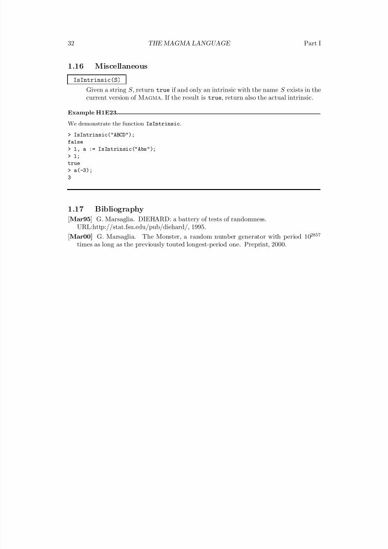
8/22/2019 Handbook Volume 01
http://slidepdf.com/reader/full/handbook-volume-01 148/440
32 THE MAGMA LANGUAGE Part I
1.16 Miscellaneous
IsIntrinsic(S)Given a string S , return true if and only an intrinsic with the name S exists in thecurrent version of Magma. If the result is true, return also the actual intrinsic.
Example H1E23
We demonstrate the function IsIntrinsic.
> IsIntrinsic("ABCD");
false
> l, a := IsIntrinsic("Abs");
> l;
true> a(-3);
3
1.17 Bibliography
[Mar95] G. Marsaglia. DIEHARD: a battery of tests of randomness.URL:http://stat.fsu.edu/pub/diehard/, 1995.
[Mar00] G. Marsaglia. The Monster, a random number generator with period 102857
times as long as the previously touted longest-period one. Preprint, 2000.
8/22/2019 Handbook Volume 01
http://slidepdf.com/reader/full/handbook-volume-01 149/440
2 FUNCTIONS, PROCEDURES
AND PACKAGES
2.1 Introduction . . . . . . . . . 35
2.2 Functions and Procedures . . . 35
2.2.1 Functions . . . . . . . . . . . . 35
f := func< x1, ..., xn: - | e >; 36f := func< x1, ..., xn, ...: - | e >; 36
2.2.2 Procedures . . . . . . . . . . . . 39
p := proc< x1, ..., xn: - | e >; 40p := proc< x1, ..., xn, ...: - | e >; 40
2.2.3 The forward Declaration . . . . . . 41
forward 41
2.3 Packages . . . . . . . . . . . 42
2.3.1 Introduction . . . . . . . . . . . 42
2.3.2 Intrinsics . . . . . . . . . . . . . 43
intrinsic 43
2.3.3 Resolving calls to intrinsics . . . . . 45
2.3.4 Attaching and Detaching Package Files46
Attach(F) 47Detach(F) 47
freeze; 472.3.5 Related Files . . . . . . . . . . . 47
2.3.6 Importing Constants . . . . . . . . 47
import "filename ": ident list; 47
2.3.7 Argument Checking . . . . . . . . 48
require condition: print args ; 48requirerange v, L, U; 48requirege v, L; 48
2.3.8 Package Specification files . . . . . 49
AttachSpec(S) 49DetachSpec(S) 49
2.3.9 User Startup Specification Files . . . 50
2.4 Attributes . . . . . . . . . . 51
2.4.1 Predefined System Attributes . . . . 51
2.4.2 User-defined Attributes . . . . . . 52
AddAttribute(C, F) 52declare attributes C : F 1, . . . , F n; 52
2.4.3 Accessing Attributes . . . . . . . . 52
S‘fieldname 52assigned 52S‘fieldname := e ; 52delete S‘fieldname ; 53GetAttributes(C) 53ListAttributes(C) 53
2.4.4 User-defined Verbose Flags . . . . . 53
declare verbose F , m; 53
2.4.5 Examples . . . . . . . . . . . . 53

8/22/2019 Handbook Volume 01
http://slidepdf.com/reader/full/handbook-volume-01 150/440
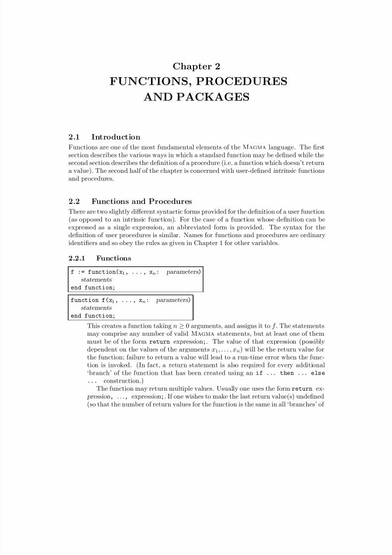
8/22/2019 Handbook Volume 01
http://slidepdf.com/reader/full/handbook-volume-01 151/440
Chapter 2
FUNCTIONS, PROCEDURESAND PACKAGES
2.1 Introduction
Functions are one of the most fundamental elements of the Magma language. The firstsection describes the various ways in which a standard function may be defined while thesecond section describes the definition of a procedure (i.e. a function which doesn’t returna value). The second half of the chapter is concerned with user-defined intrinsic functionsand procedures.
2.2 Functions and Procedures
There are two slightly different syntactic forms provided for the definition of a user function(as opposed to an intrinsic function). For the case of a function whose definition can beexpressed as a single expression, an abbreviated form is provided. The syntax for thedefinition of user procedures is similar. Names for functions and procedures are ordinaryidentifiers and so obey the rules as given in Chapter 1 for other variables.
2.2.1 Functions
f := function(x1, ..., xn: parameters )statements
end function;
function f(x1, ..., xn: parameters )statements
end function;
This creates a function taking n ≥ 0 arguments, and assigns it to f . The statements
may comprise any number of valid Magma statements, but at least one of themmust be of the form return expression;. The value of that expression (possiblydependent on the values of the arguments x1, . . . , xn) will be the return value forthe function; failure to return a value will lead to a run-time error when the func-tion is invoked. (In fact, a return statement is also required for every additional‘branch’ of the function that has been created using an if ... then ... else
... construction.)The function may return multiple values. Usually one uses the form return ex-
pression, . . ., expression;. If one wishes to make the last return value(s) undefined(so that the number of return values for the function is the same in all ‘branches’ of
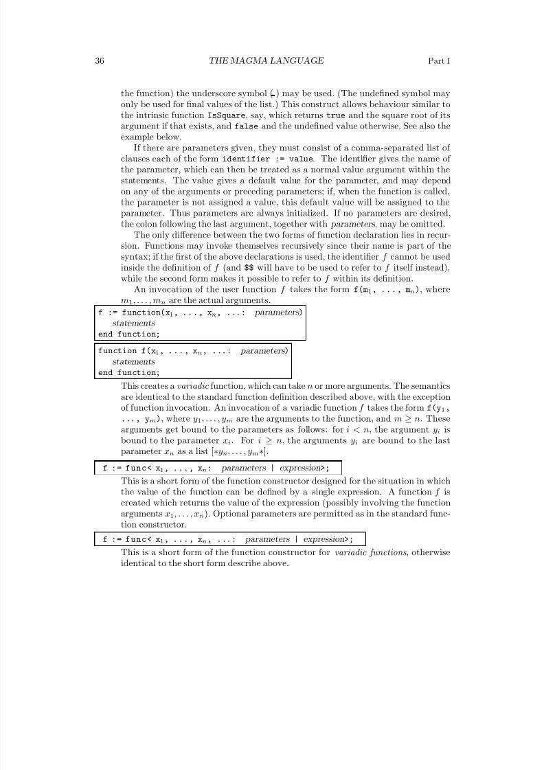
8/22/2019 Handbook Volume 01
http://slidepdf.com/reader/full/handbook-volume-01 152/440
36 THE MAGMA LANGUAGE Part I
the function) the underscore symbol ( ) may be used. (The undefined symbol mayonly be used for final values of the list.) This construct allows behaviour similar to
the intrinsic function IsSquare, say, which returns true and the square root of itsargument if that exists, and false and the undefined value otherwise. See also theexample below.
If there are parameters given, they must consist of a comma-separated list of clauses each of the form identifier := value. The identifier gives the name of the parameter, which can then be treated as a normal value argument within thestatements. The value gives a default value for the parameter, and may dependon any of the arguments or preceding parameters; if, when the function is called,the parameter is not assigned a value, this default value will be assigned to theparameter. Thus parameters are always initialized. If no parameters are desired,the colon following the last argument, together with parameters , may be omitted.
The only difference between the two forms of function declaration lies in recur-sion. Functions may invoke themselves recursively since their name is part of thesyntax; if the first of the above declarations is used, the identifier f cannot be usedinside the definition of f (and $$ will have to be used to refer to f itself instead),while the second form makes it possible to refer to f within its definition.
An invocation of the user function f takes the form f(m1, ..., mn), wherem1, . . . , mn are the actual arguments.
f := function(x1, ..., xn, ...: parameters )statements
end function;
function f(x1, ..., xn, ...: parameters )statements
end function;
This creates a variadic function, which can take n or more arguments. The semanticsare identical to the standard function definition described above, with the exceptionof function invocation. An invocation of a variadic function f takes the form f(y1,
..., ym), where y1, . . . , ym are the arguments to the function, and m ≥ n. Thesearguments get bound to the parameters as follows: for i < n, the argument yi isbound to the parameter xi. For i ≥ n, the arguments yi are bound to the lastparameter xn as a list [∗yn, . . . , ym∗].
f := func< x1, ..., xn: parameters | expression>;
This is a short form of the function constructor designed for the situation in whichthe value of the function can be defined by a single expression. A function f iscreated which returns the value of the expression (possibly involving the functionarguments x1, . . . , xn). Optional parameters are permitted as in the standard func-tion constructor.
f := func< x1, ..., xn, ...: parameters | expression>;
This is a short form of the function constructor for variadic functions , otherwiseidentical to the short form describe above.
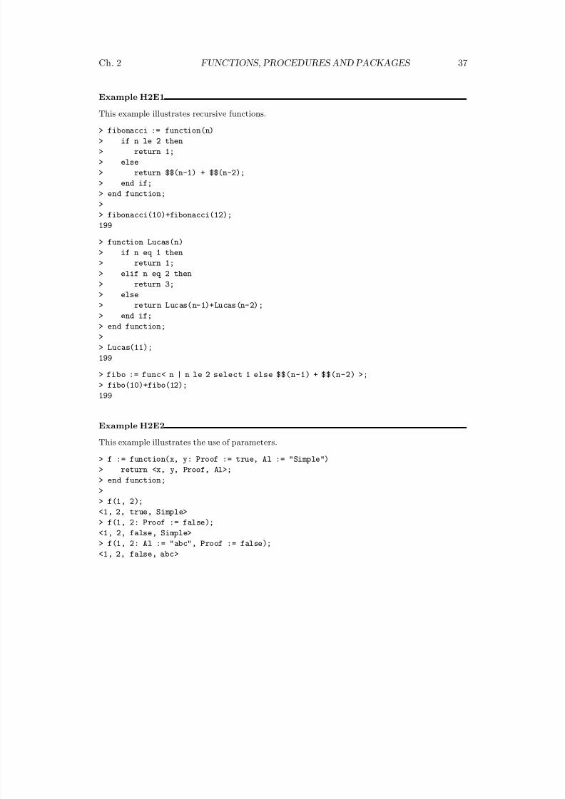
8/22/2019 Handbook Volume 01
http://slidepdf.com/reader/full/handbook-volume-01 153/440
Ch. 2 FUNCTIONS, PROCEDURES AND PACKAGES 37
Example H2E1
This example illustrates recursive functions.
> fibonacci := function(n)
> if n le 2 then
> return 1;
> else
> return $$(n-1) + $$(n-2);
> end if;
> end function;
>
> fibonacci(10)+fibonacci(12);
199
> function Lucas(n)> if n eq 1 then
> return 1;
> elif n eq 2 then
> return 3;
> else
> return Lucas(n-1)+Lucas(n-2);
> end if;
> end function;
>
> Lucas(11);
199
> fibo := func< n | n le 2 select 1 else $$(n-1) + $$(n-2) >;
> fibo(10)+fibo(12);
199
Example H2E2
This example illustrates the use of parameters.
> f := function(x, y: Proof := true, Al := "Simple")
> return <x, y, Proof, Al>;
> end function;>
> f(1, 2);
<1, 2, true, Simple>
> f(1, 2: Proof := false);
<1, 2, false, Simple>
> f(1, 2: Al := "abc", Proof := false);
<1, 2, false, abc>
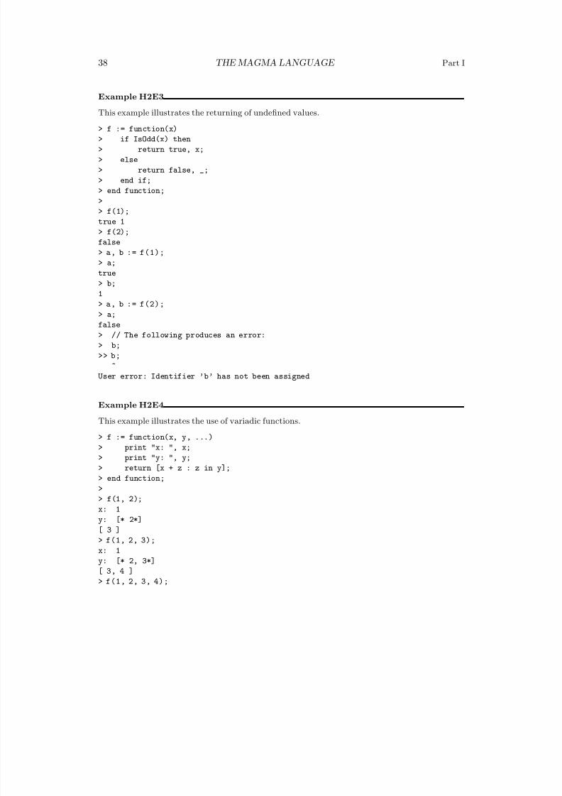
8/22/2019 Handbook Volume 01
http://slidepdf.com/reader/full/handbook-volume-01 154/440
38 THE MAGMA LANGUAGE Part I
Example H2E3
This example illustrates the returning of undefined values.
> f := function(x)
> if IsOdd(x) then
> return true, x;
> else
> return false, _;
> end if;
> end function;
>
> f(1);
true 1
> f(2);
false> a, b := f(1);
> a;
true
> b;
1
> a, b := f(2);
> a;
false
> // The following produces an error:
> b;
>> b;^
User error: Identifier ’b’ has not been assigned
Example H2E4
This example illustrates the use of variadic functions.
> f := function(x, y, ...)
> print "x: ", x;
> print "y: ", y;
> return [x + z : z in y];
> end function;>
> f(1, 2);
x: 1
y: [* 2*]
[ 3 ]
> f(1, 2, 3);
x: 1
y: [* 2, 3*]
[ 3, 4 ]
> f(1, 2, 3, 4);
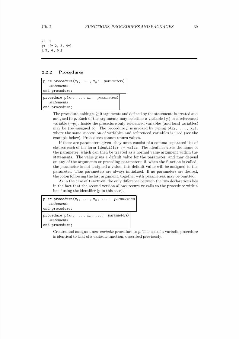
8/22/2019 Handbook Volume 01
http://slidepdf.com/reader/full/handbook-volume-01 155/440
Ch. 2 FUNCTIONS, PROCEDURES AND PACKAGES 39
x: 1
y: [* 2, 3, 4*]
[ 3 , 4 , 5 ]
2.2.2 Procedures
p := procedure(x1, ..., xn: parameters )statements
end procedure;
procedure p(x1, ..., xn: parameters )
statements end procedure;
The procedure, taking n ≥ 0 arguments and defined by the statements is created andassigned to p. Each of the arguments may be either a variable (yi) or a referencedvariable (∼yi). Inside the procedure only referenced variables (and local variables)may be (re-)assigned to. The procedure p is invoked by typing p(x1, ..., xn),where the same succession of variables and referenced variables is used (see theexample below). Procedures cannot return values.
If there are parameters given, they must consist of a comma-separated list of clauses each of the form identifier := value. The identifier gives the name of
the parameter, which can then be treated as a normal value argument within thestatements. The value gives a default value for the parameter, and may dependon any of the arguments or preceding parameters; if, when the function is called,the parameter is not assigned a value, this default value will be assigned to theparameter. Thus parameters are always initialized. If no parameters are desired,the colon following the last argument, together with parameters , may be omitted.
As in the case of function, the only difference between the two declarations liesin the fact that the second version allows recursive calls to the procedure withinitself using the identifier ( p in this case).
p := procedure(x1, ..., xn, ...: parameters )
statements end procedure;
procedure p(x1, ..., xn, ...: parameters )statements
end procedure;
Creates and assigns a new variadic procedure to p. The use of a variadic procedureis identical to that of a variadic function, described previously.
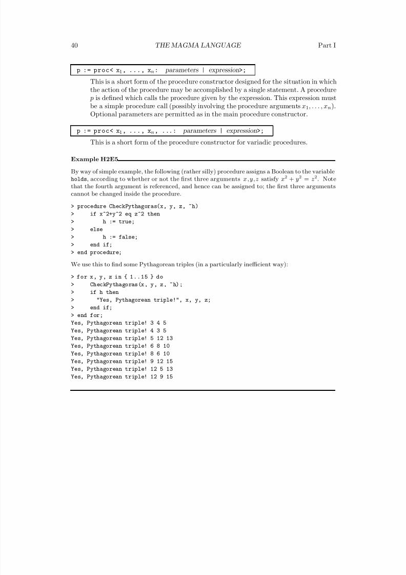
8/22/2019 Handbook Volume 01
http://slidepdf.com/reader/full/handbook-volume-01 156/440
40 THE MAGMA LANGUAGE Part I
p := proc< x1, ..., xn: parameters | expression>;
This is a short form of the procedure constructor designed for the situation in whichthe action of the procedure may be accomplished by a single statement. A procedure
p is defined which calls the procedure given by the expression. This expression mustbe a simple procedure call (possibly involving the procedure arguments x1, . . . , xn).Optional parameters are permitted as in the main procedure constructor.
p := proc< x1, ..., xn, ...: parameters | expression>;
This is a short form of the procedure constructor for variadic procedures.
Example H2E5
By way of simple example, the following (rather silly) procedure assigns a Boolean to the variableholds, according to whether or not the first three arguments x,y,z satisfy x2 + y2 = z 2. Notethat the fourth argument is referenced, and hence can be assigned to; the first three argumentscannot be changed inside the procedure.
> procedure CheckPythagoras(x, y, z, ~h)
> if x^2+y^2 eq z^2 then
> h := true;
> else
> h := false;
> end if;
> end procedure;
We use this to find some Pythagorean triples (in a particularly inefficient way):
> for x, y, z in { 1..15 } do
> CheckPythagoras(x, y, z, ~h);
> if h then
> "Yes, Pythagorean triple!", x, y, z;
> end if;
> end for;
Yes, Pythagorean triple! 3 4 5
Yes, Pythagorean triple! 4 3 5
Yes, Pythagorean triple! 5 12 13
Yes, Pythagorean triple! 6 8 10Yes, Pythagorean triple! 8 6 10
Yes, Pythagorean triple! 9 12 15
Yes, Pythagorean triple! 12 5 13
Yes, Pythagorean triple! 12 9 15
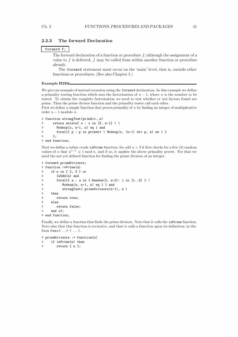
8/22/2019 Handbook Volume 01
http://slidepdf.com/reader/full/handbook-volume-01 157/440
Ch. 2 FUNCTIONS, PROCEDURES AND PACKAGES 41
2.2.3 The forward Declaration
forward f;The forward declaration of a function or procedure f ; although the assignment of avalue to f is deferred, f may be called from within another function or procedurealready.
The forward statement must occur on the ‘main’ level, that is, outside otherfunctions or procedures. (See also Chapter 5.)
Example H2E6
We give an example of mutual recursion using the forward declaration. In this example we definea primality testing function which uses the factorization of n − 1, where n is the number to betested. To obtain the complete factorization we need to test whether or not factors found areprime. Thus the prime divisor function and the primality tester call each other.First we define a simple function that proves primality of n by finding an integer of multiplicativeorder n − 1 modulo n.
> function strongTest(primdiv, n)
> return exists{ x : x in [2..n-1] | \
> Modexp(x, n-1, n) eq 1 and
> forall{ p : p in primdiv | Modexp(x, (n-1) div p, n) ne 1 }
> };
> end function;
Next we define a rather crude isPrime function: for odd n > 3 it first checks for a few (3) random
values of a that an−1
≡ 1 mod n, and if so, it applies the above primality prover. For that weneed the not yet defined function for finding the prime divisors of an integer.
> forward primeDivisors;
> function isPrime(n)
> if n in { 2, 3 } or
> IsOdd(n) and
> forall{ a : a in { Random(2, n-2): i in [1..3] } |
> Modexp(a, n-1, n) eq 1 } and
> strongTest( primeDivisors(n-1), n )
> then
> return true;
> else> return false;
> end if;
> end function;
Finally, we define a function that finds the prime divisors. Note that it calls the isPrime function.Note also that this function is recursive, and that it calls a function upon its definition, in theform func< ..> ( .. ).
> primeDivisors := function(n)
> if isPrime(n) then
> return { n };
8/22/2019 Handbook Volume 01
http://slidepdf.com/reader/full/handbook-volume-01 158/440
42 THE MAGMA LANGUAGE Part I
> else
> return func< d | primeDivisors(d) join primeDivisors(n div d) >
> ( rep{ d : d in [2..Isqrt(n)] | n mod d eq 0 });> end if;
> end function;
> isPrime(1087);
true;
2.3 Packages
2.3.1 Introduction
For brevity, in this section we shall use the term function to include both functions andprocedures.
The term intrinsic function or intrinsic refers to a function whose signature is stored inthe system table of signatures. In terms of their origin, there are two kinds of intrinsics,system intrinsics (or standard functions ) and user intrinsics , but they are indistinguishablein their use. A system intrinsic is an intrinsic that is part of the definition of the Magma
system, whereas a user intrinsic is an informal addition to Magma, created by a user of the system. While most of the standard functions in Magma are implemented in C, agrowing number are implemented in the Magma language. User intrinsics are defined inthe Magma language using a package mechanism (the same syntax, in fact, as that used
by the implementors to write standard functions in the Magma language).This section explains the construction of user intrinsics by means of packages. Fromnow on, intrinsic will be used as an abbreviation for user intrinsic .
It is useful to summarize the properties possessed by an intrinsic function that are notpossessed by an ordinary user-defined function. Firstly, the signature of every intrinsicfunction is stored in the system’s table of signatures. In particular, such functions willappear when signatures are listed and printing the function’s name will produce a summaryof the behaviour of the function. Secondly, intrinsic functions are compiled into the Magma
internal pseudo-code. Thus, once an intrinsic function has been debugged, it does not haveto be compiled every time it is needed. If the definition of the function involves a largebody of code, this can save a significant amount of time when the function definition has
to be loaded.An intrinsic function is defined in a special type of file known as a package . In general
terms a package is a Magma source file that defines constants, one or more intrinsicfunctions, and optionally, some ordinary functions. The definition of an intrinsic functionmay involve Magma standard functions, functions imported from other packages andfunctions whose definition is part of the package. It should be noted that constants andfunctions (other than intrinsic functions) defined in a package will not be visible outsidethe package, unless they are explicitly imported.
The syntax for the definition of an intrinsic function is similar to that of an ordinaryfunction except that the function header must define the function’s signature together with
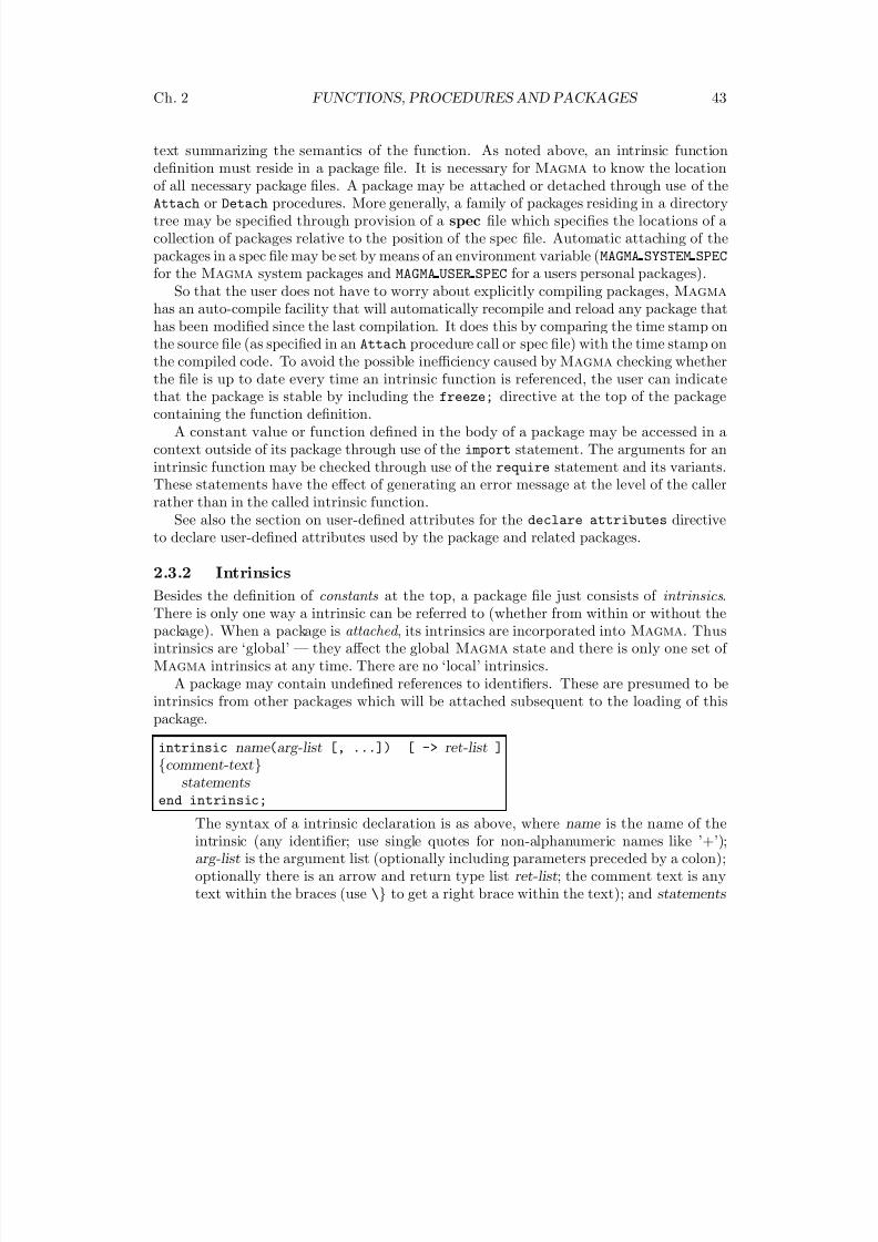
8/22/2019 Handbook Volume 01
http://slidepdf.com/reader/full/handbook-volume-01 159/440
Ch. 2 FUNCTIONS, PROCEDURES AND PACKAGES 43
text summarizing the semantics of the function. As noted above, an intrinsic functiondefinition must reside in a package file. It is necessary for Magma to know the location
of all necessary package files. A package may be attached or detached through use of theAttach or Detach procedures. More generally, a family of packages residing in a directorytree may be specified through provision of a spec file which specifies the locations of acollection of packages relative to the position of the spec file. Automatic attaching of thepackages in a spec file may be set by means of an environment variable ( MAGMA SYSTEM SPEC
for the Magma system packages and MAGMA USER SPEC for a users personal packages).So that the user does not have to worry about explicitly compiling packages, Magma
has an auto-compile facility that will automatically recompile and reload any package thathas been modified since the last compilation. It does this by comparing the time stamp onthe source file (as specified in an Attach procedure call or spec file) with the time stamp onthe compiled code. To avoid the possible inefficiency caused by Magma checking whether
the file is up to date every time an intrinsic function is referenced, the user can indicatethat the package is stable by including the freeze; directive at the top of the packagecontaining the function definition.
A constant value or function defined in the body of a package may be accessed in acontext outside of its package through use of the import statement. The arguments for anintrinsic function may be checked through use of the require statement and its variants.These statements have the effect of generating an error message at the level of the callerrather than in the called intrinsic function.
See also the section on user-defined attributes for the declare attributes directiveto declare user-defined attributes used by the package and related packages.
2.3.2 Intrinsics
Besides the definition of constants at the top, a package file just consists of intrinsics .There is only one way a intrinsic can be referred to (whether from within or without thepackage). When a package is attached , its intrinsics are incorporated into Magma. Thusintrinsics are ‘global’ — they affect the global Magma state and there is only one set of Magma intrinsics at any time. There are no ‘local’ intrinsics.
A package may contain undefined references to identifiers. These are presumed to beintrinsics from other packages which will be attached subsequent to the loading of thispackage.
intrinsic name (arg-list [, ...]) [ -> ret-list ]{comment-text}
statements end intrinsic;
The syntax of a intrinsic declaration is as above, where name is the name of theintrinsic (any identifier; use single quotes for non-alphanumeric names like ’+’);arg-list is the argument list (optionally including parameters preceded by a colon);optionally there is an arrow and return type list ret-list; the comment text is anytext within the braces (use \} to get a right brace within the text); and statements
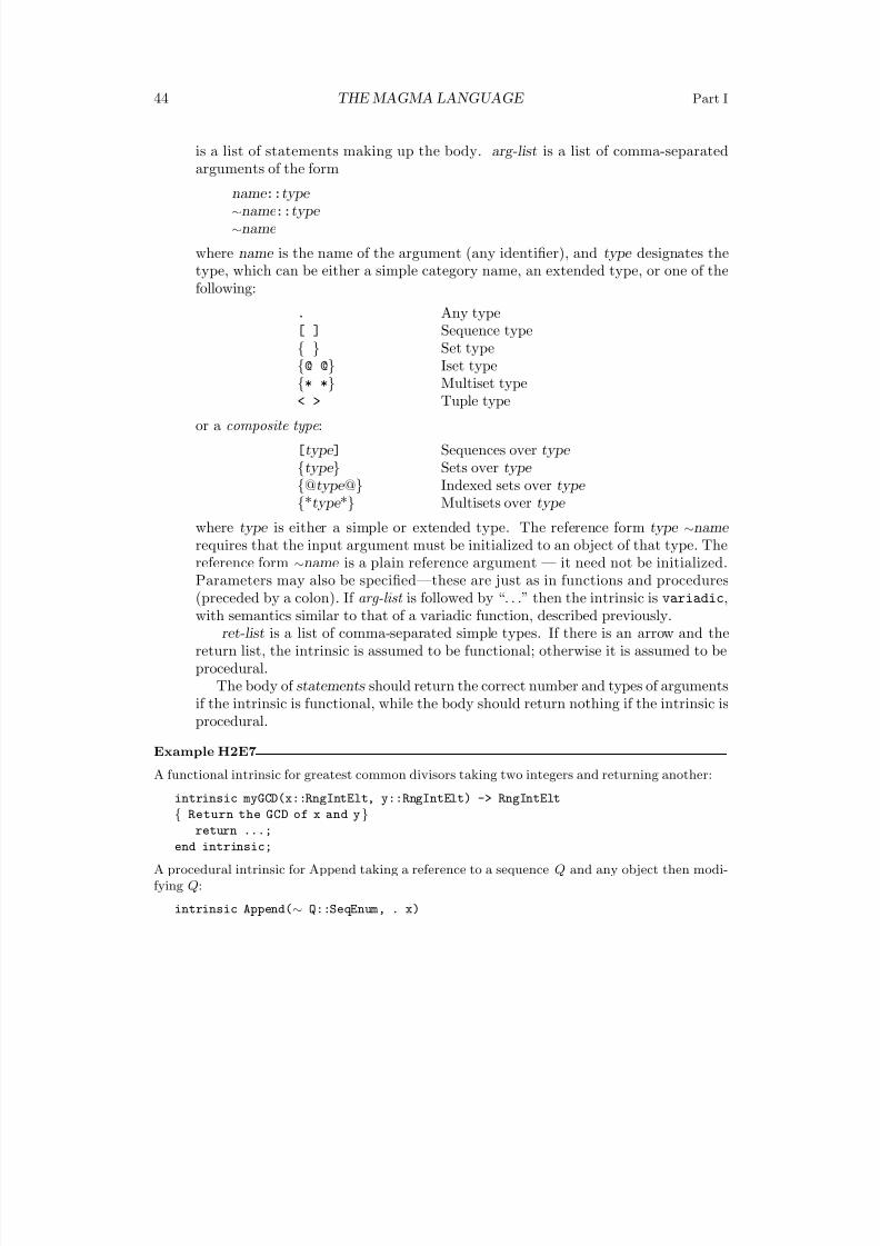
8/22/2019 Handbook Volume 01
http://slidepdf.com/reader/full/handbook-volume-01 160/440
44 THE MAGMA LANGUAGE Part I
is a list of statements making up the body. arg-list is a list of comma-separatedarguments of the form
name ::type ∼name ::type ∼name
where name is the name of the argument (any identifier), and type designates thetype, which can be either a simple category name, an extended type, or one of thefollowing:
. Any type[ ] Sequence type{ } Set type{@ @} Iset type{* *} Multiset type< > Tuple type
or a composite type :
[type ] Sequences over type {type } Sets over type {@type @} Indexed sets over type {*type *} Multisets over type
where type is either a simple or extended type. The reference form type ∼name requires that the input argument must be initialized to an object of that type. The
reference form ∼name is a plain reference argument — it need not be initialized.Parameters may also be specified—these are just as in functions and procedures(preceded by a colon). If arg-list is followed by “. . .” then the intrinsic is variadic,with semantics similar to that of a variadic function, described previously.
ret-list is a list of comma-separated simple types. If there is an arrow and thereturn list, the intrinsic is assumed to be functional; otherwise it is assumed to beprocedural.
The body of statements should return the correct number and types of argumentsif the intrinsic is functional, while the body should return nothing if the intrinsic isprocedural.
Example H2E7
A functional intrinsic for greatest common divisors taking two integers and returning another:
intrinsic myGCD(x::RngIntElt, y::RngIntElt) -> RngIntElt
{ Return the GCD of x and y}return ...;
end intrinsic;
A procedural intrinsic for Append taking a reference to a sequence Q and any object then modi-fying Q:
intrinsic Append(∼ Q::SeqEnum, . x)
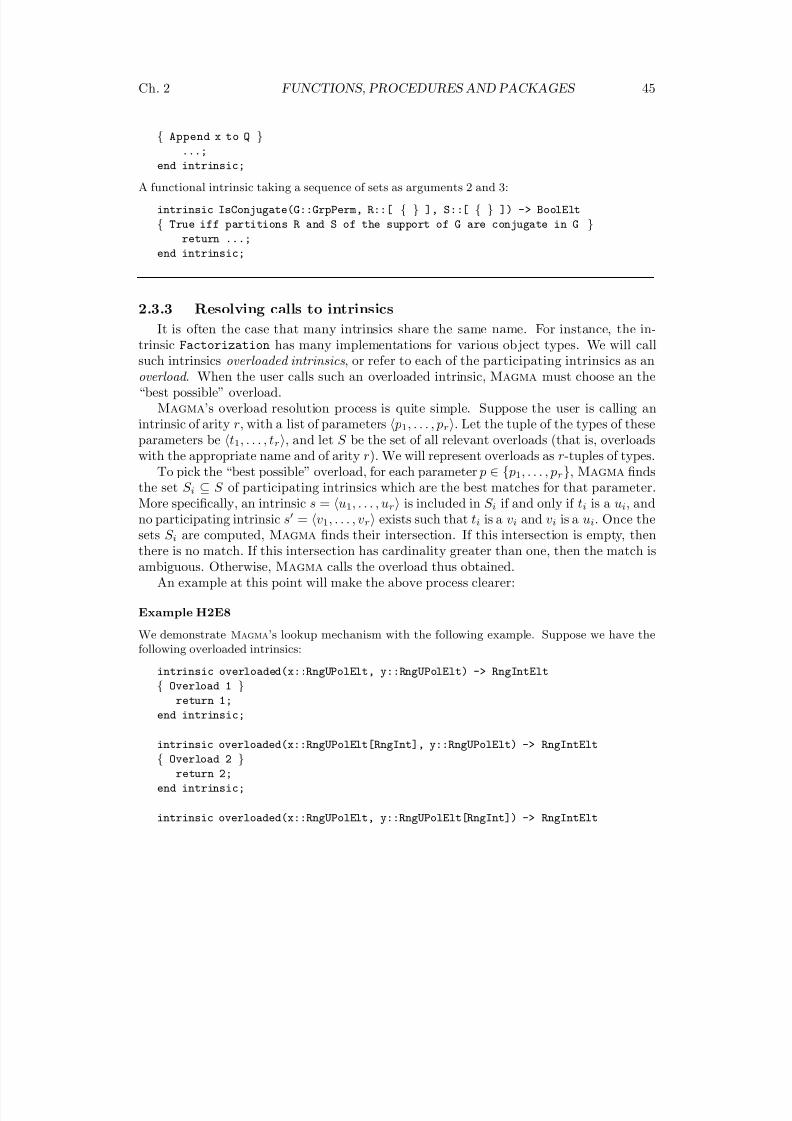
8/22/2019 Handbook Volume 01
http://slidepdf.com/reader/full/handbook-volume-01 161/440
Ch. 2 FUNCTIONS, PROCEDURES AND PACKAGES 45
{ Append x to Q }...;
end intrinsic;
A functional intrinsic taking a sequence of sets as arguments 2 and 3:
intrinsic IsConjugate(G::GrpPerm, R::[ { } ], S::[ { } ]) -> BoolElt
{ True iff partitions R and S of the support of G are conjugate in G }return ...;
end intrinsic;
2.3.3 Resolving calls to intrinsics
It is often the case that many intrinsics share the same name. For instance, the in-trinsic Factorization has many implementations for various object types. We will callsuch intrinsics overloaded intrinsics , or refer to each of the participating intrinsics as anoverload . When the user calls such an overloaded intrinsic, Magma must choose an the“best possible” overload.
Magma’s overload resolution process is quite simple. Suppose the user is calling anintrinsic of arity r, with a list of parameters p1, . . . , pr. Let the tuple of the types of theseparameters be t1, . . . , tr, and let S be the set of all relevant overloads (that is, overloadswith the appropriate name and of arity r). We will represent overloads as r-tuples of types.
To pick the “best possible” overload, for each parameter p ∈ { p1, . . . , pr}, Magma findsthe set S i ⊆ S of participating intrinsics which are the best matches for that parameter.
More specifically, an intrinsic s = u1, . . . , ur is included in S i if and only if ti is a ui, andno participating intrinsic s = v1, . . . , vr exists such that ti is a vi and vi is a ui. Once thesets S i are computed, Magma finds their intersection. If this intersection is empty, thenthere is no match. If this intersection has cardinality greater than one, then the match isambiguous. Otherwise, Magma calls the overload thus obtained.
An example at this point will make the above process clearer:
Example H2E8
We demonstrate Magma’s lookup mechanism with the following example. Suppose we have thefollowing overloaded intrinsics:
intrinsic overloaded(x::RngUPolElt, y::RngUPolElt) -> RngIntElt{ Overload 1 }
return 1;
end intrinsic;
intrinsic overloaded(x::RngUPolElt[RngInt], y::RngUPolElt) -> RngIntElt
{ Overload 2 }return 2;
end intrinsic;
intrinsic overloaded(x::RngUPolElt, y::RngUPolElt[RngInt]) -> RngIntElt
8/22/2019 Handbook Volume 01
http://slidepdf.com/reader/full/handbook-volume-01 162/440
46 THE MAGMA LANGUAGE Part I
{ Overload 3 }return 3;
end intrinsic;
intrinsic overloaded(x::RngUPolElt[RngInt], y::RngUPolElt[RngInt]) -> RngIntElt
{ Overload 4 }return 4;
end intrinsic;
The following Magma session illustrates how the lookup mechanism operates for the intrinsicoverloaded:
> R1<x> := PolynomialRing(Integers());
> R2<y> := PolynomialRing(Rationals());
> f 1 : = x + 1 ;> f 2 : = y + 1 ;
> overloaded(f2, f2);
1
> overloaded(f1, f2);
2
> overloaded(f2, f1);
3
> overloaded(f1, f1);
4
2.3.4 Attaching and Detaching Package Files
The procedures Attach and Detach are provided to attach or detach package files. Once afile is attached, all intrinsics within it are included in Magma. If the file is modified, it isautomatically recompiled just after the user hits return and just before the next statementis executed. So there is no need to re-attach the file (or ‘re-load’ it). If the recompilation of a package file fails (syntax errors, etc.), all of the intrinsics of the package file are removedfrom the Magma session and none of the intrinsics of the package file are included againuntil the package file is successfully recompiled. When errors occur during compilation of a package, the appropriate messages are printed with the string ‘[PC]’ at the beginning of
the line, indicating that the errors are detected by the Magma package compiler.If a package file contains the single directive freeze; at the top then the package file
becomes frozen — it will not be automatically recompiled after each statement is enteredinto Magma. A frozen package is recompiled if need be, however, when it is attached (thusallowing fixes to be updated) — the main point of freezing a package which is ‘stable’ isto stop Magma looking at it between every statement entered into Magma interactively.
When a package file is complete and tested, it is usually installed in a spec file so itis automatically attached when the spec file is attached. Thus Attach and Detach aregenerally only used when one is developing a single package file containing new intrinsics.
8/22/2019 Handbook Volume 01
http://slidepdf.com/reader/full/handbook-volume-01 163/440
Ch. 2 FUNCTIONS, PROCEDURES AND PACKAGES 47
Attach(F)
Procedure to attach the package file F .
Detach(F)
Procedure to detach the package file F .
freeze;
Freeze the package file in which this appears at the top.
2.3.5 Related Files
There are two files related to any package source file file.m:
file.sig sig file containing signature information;file.lck lock file.
The lock file exists while a package file is being compiled. If someone else tries tocompile the file, it will just sit there till the lock file disappears. In various circumstances(system down, Magma crash) .lck files may be left around; this will mean that the nexttime Magma attempts to compile the associated source file it will just sit there indefinitelywaiting for the .lck file to disappear. In this case the user should search for .lck filesthat should be removed.
2.3.6 Importing Constants
import "filename ": ident list;
This is the general form of the import statement, where "filename " is a string andident list is a list of identifiers.
The import statement is a normal statement and can in fact be used anywhere inMagma, but it is recommended that it only be used to import common constantsand functions/procedures shared between a collection of package files. It has the fol-lowing semantics: for each identifier I in the list ident list, that identifier is declared
just like a normal identifier within Magma. Within the package file referenced byfilename , there should be an assignment of the same identifier I to some object O.
When the identifier I is then used as an expression after the import statement, thevalue yielded is the object O.
The file that is named in the import statement must already have been attachedby the time the identifiers are needed. The best way to achieve this in practice is toplace this file in the spec file, along with the package files, so that all the files canbe attached together.
Thus the only way objects (whether they be normal objects, procedures or func-tions) assigned within packages can be referenced from outside the package is by anexplicit import with the ‘import’ statement.
8/22/2019 Handbook Volume 01
http://slidepdf.com/reader/full/handbook-volume-01 164/440
48 THE MAGMA LANGUAGE Part I
Example H2E9
Suppose we have a spec file that lists several package files. Included in the spec file is the filedefs.m containing:
MY LIMIT := 10000;
function fred(x)
return 1/x;
end function;
Then other package files (in the same directory) listed in the spec file which wish to use thesedefinitions would have the line
import "defs.m": MY LIMIT, fred;
at the top. These could then be used inside any intrinsics of such package files. (If the package
files are not in the same directory, the pathname of defs.m will have to be given appropriately inthe import statement.)
2.3.7 Argument Checking
Using ‘require’ etc. one can do argument checking easily within intrinsics. If a necessarycondition on the argument fails to hold, then the relevant error message is printed and theerror pointer refers to the caller of the intrinsic. This feature allows user-defined intrinsicsto treat errors in actual arguments in exactly the same way as they are treated by theMagma standard functions.
require condition: print args ;
The expression condition may be any yielding a Boolean value. If the value is false,then print args is printed and execution aborts with the error pointer pointing tothe caller. The print arguments print args can consist of any expressions (dependingon arguments or variables already defined in the intrinsic).
requirerange v, L, U;
The argument variable v must be the name of one of the argument variables (includ-ing parameters) and must be of integer type. L and U may be any expressions each
yielding an integer value. If v is not in the range [L , . . . , U ], then an appropriateerror message is printed and execution aborts with the error pointer pointing to thecaller.
requirege v, L;
The argument variable v must be the name of one of the argument variables (in-cluding parameters) and must be of integer type. L must yield an integer value. If v is not greater than or equal to L, then an appropriate error message is printedand execution aborts with the error pointer pointing to the caller.
8/22/2019 Handbook Volume 01
http://slidepdf.com/reader/full/handbook-volume-01 165/440
Ch. 2 FUNCTIONS, PROCEDURES AND PACKAGES 49
Example H2E10
A trivial version of Binomial(n, k) which checks that n ≥ 0 and 0 ≤ k ≤ n.
intrinsic Binomial(n::RngIntElt, k::RngIntElt) -> RngIntElt
{ Return n choose k }requirege n, 0;
requirerange k, 0, n;
return Factorial(n) div Factorial(n - k) div Factorial(k);
end intrinsic;
A simple function to find a random p-element of a group G.
intrinsic pElement(G::Grp, p::RngIntElt) -> GrpElt
{ Return p-element of group G }require IsPrime(p): "Argument 2 is not prime";
x := random{x: x in G | Order(x) mod p eq 0};
return x^(Order(x) div p);
end intrinsic;
2.3.8 Package Specification files
A spec file (short for ‘specification file’) lists a complete tree of Magma package files.
This makes it easy to collect many package files together and attach them simultaneously.The specification file consists of a list of tokens which are just space-separated words.
The tokens describe a list of package files and directories containing other packages. Thelist is described as follows. The files that are to be attached in the directory indicated byS are listed enclosed in { and } characters. A directory may be listed there as well, if it isfollowed by a list of files from that directory (enclosed in braces again); arbitrary nestingis allowed this way. A filename of the form +spec is interpreted as another specification filewhose contents will be recursively attached when AttachSpec (below) is called. The filesare taken relative to the directory that contains the specification file. See also the examplebelow.
AttachSpec(S)
If S is a string indicating the name of a spec file, this command attaches all the fileslisted in S . The format of the spec file is given above.
DetachSpec(S)
If S is a string indicating the name of a spec file, this command detaches all the fileslisted in S . The format of the spec file is given above.
8/22/2019 Handbook Volume 01
http://slidepdf.com/reader/full/handbook-volume-01 166/440
50 THE MAGMA LANGUAGE Part I
Example H2E11
Suppose we have a spec file /home/user/spec consisting of the following lines:
{
Group
{
chiefseries.m
socle.m
}
Ring
{
funcs.m
Field
{
galois.m
}
}
}
Then there should be the files
/home/user/spec/Group/chiefseries.m
/home/user/spec/Group/socle.m
/home/user/spec/Ring/funcs.m
/home/user/spec/Ring/Field/galois.m
and if one typed within Magma
AttachSpec("/home/user/spec");
then each of the above files would be attached. If instead of the filename galois.m we have+galspec, then the file /home/user/spec/Ring/Field/galspec would be a specification file itself whose contents would be recursively attached.
2.3.9 User Startup Specification Files
The user may specify a list of spec files to be attached automatically when Magma startsup. This is done by setting the environment variable MAGMA USER SPEC to a colon separated
list of spec files.
Example H2E12
One could have
setenv MAGMA USER SPEC "$HOME/Magma/spec:/home/friend/Magma/spec"
in one’s .cshrc . Then when Magma starts up, it will attach all packages listed in the spec files$HOME/Magma/spec and /home/friend/Magma/spec.
8/22/2019 Handbook Volume 01
http://slidepdf.com/reader/full/handbook-volume-01 167/440
Ch. 2 FUNCTIONS, PROCEDURES AND PACKAGES 51
2.4 Attributes
This section is placed beside the section on packages because the use of attributes is most
common within packages.
For any structure within Magma, it is possible to have attributes associated with it. Theseare simply values stored within the structure and are referred to by named fields in exactlythe same manner as Magma records.
There are two kinds of structure attributes: predefined system attributes and user-defined attributes. Both kinds are discussed in the following subsections. A description of how attributes are accessed and assigned then follows.
2.4.1 Predefined System Attributes
The valid fields of predefined system attributes are automatically defined at the startup of
Magma. These fields now replace the old method of using the procedure AssertAttributeand the function HasAttribute (which will still work for some time to preserve backwardscompatibility). For each name which is a valid first argument for AssertAttribute andHasAttribute, that name is a valid attribute field for structures of the appropriate cate-gory. Thus the backquote method for accessing attributes described in detail below shouldnow be used instead of the old method. For such attributes, the code:
> S‘Name := x;
is completely equivalent to the code:
> AssertAttribute(S, "Name", x);
(note that the function AssertAttribute takes a string for its second argument so thename must be enclosed in double quotes). Similarly, the code:
> if assigned S‘Name then
> x := S‘Name;
> // do something with x...
> end if;
is completely equivalent to the code:
> l, x := HasAttribute(S, "Name");
> if l then
> // do something with x...
> end if;
(note again that the function HasAttribute takes a string for its second argument so thename must be enclosed in double quotes).
Note also that if a system attribute is not set, referring to it in an expression (using thebackquote operator) will not trigger the calculation of it (while the corresponding intrinsicfunction will if it exists); rather an error will ensue. Use the assigned operator to testwhether an attribute is actually set.
8/22/2019 Handbook Volume 01
http://slidepdf.com/reader/full/handbook-volume-01 168/440
52 THE MAGMA LANGUAGE Part I
2.4.2 User-defined Attributes
For any category C , the user can stipulate valid attribute fields for structures of C . After
this is done, any structure of category C may have attributes assigned to it and accessedfrom it.
There are two ways of adding new valid attributes to a category C : by the procedureAddAttribute or by the declare attributes package declaration. The former should beused outside of packages (e.g. in interactive usage), while the latter must be used withinpackages to declare attribute fields used by the package and related packages.
AddAttribute(C, F)
(Procedure.) Given a category C , and a string F , append the field name F tothe list of valid attribute field names for structures belonging to category C . This
procedure should not be used within packages but during interactive use. Previousfields for C are still valid – this just adds another valid one.
declare attributes C : F 1, . . . , F n;
Given a category C , and a comma-separated list of identifiers F 1, . . . , F n appendthe field names specified by the identifiers to the list of valid attribute field namesfor structures belonging to category C . This declaration directive must be usedwithin (and only within) packages to declare attribute fields used by the packageand packages related to it which use the same fields. It is not a statement buta directive which is stored with the other information of the package when it iscompiled and subsequently attached – not when any code is actually executed.
2.4.3 Accessing Attributes
Attributes of structures are accessed in the same way that records are: using the backquote(‘) operator.
S‘fieldname
Given a structure S and a field name, return the current value for the given field inS . If the value is not assigned, an error results. The field name must be valid forthe category of S .
assigned S‘fieldname Given a structure S and a field name, return whether the given field in S currentlyhas a value. The field name must be valid for the category of S .
S‘fieldname := expression;
Given a structure S and a field name, assign the given field of S to be the value of the expression (any old value is first discarded). The field name must be valid forthe category of S .
8/22/2019 Handbook Volume 01
http://slidepdf.com/reader/full/handbook-volume-01 169/440
Ch. 2 FUNCTIONS, PROCEDURES AND PACKAGES 53
delete S‘fieldname ;
Given a structure S and a field name, delete the given field of S . The field then
becomes unassigned in S . The field name must be valid for the category of S and thefield must be currently assigned in S . This statement is not allowed for predefinedsystem attributes.
GetAttributes(C)
Given a category C , return the valid attribute field names for structures belongingto category C as a sorted sequence of strings.
ListAttributes(C)
(Procedure.) Given a category C , list the valid attribute field names for structuresbelonging to category C .
2.4.4 User-defined Verbose Flags
Since version V2.7, verbose flags may be defined by users within packages.
declare verbose F , m;
Given a verbose flag name F (without quotes), and a literal integer m, create theverbose flag F , with the maximal allowable level for the flag set to m. This directivemay only be used within package files.
2.4.5 Examples
In this subsection we give examples which illustrate all of the above features.
Example H2E13
We illustrate how the predefined system attributes may be used. Note that the valid arguments forAssertAttribute and HasAttribute documented elsewhere now also work as system attributes sosee the documentation for these functions for details as to the valid system attribute field names.
> // Create group G.
> G := PSL(3, 2);
> // Check whether order known.
> assigned G‘Order;
false> // Attempt to access order -- error since not assigned.
> G‘Order;
>> G‘Order;
^
Runtime error in ‘: Attribute ’Order’ for this structure
is valid but not assigned
> // Force computation of order by intrinsic Order.
> Order(G);
168
> // Check Order field again.
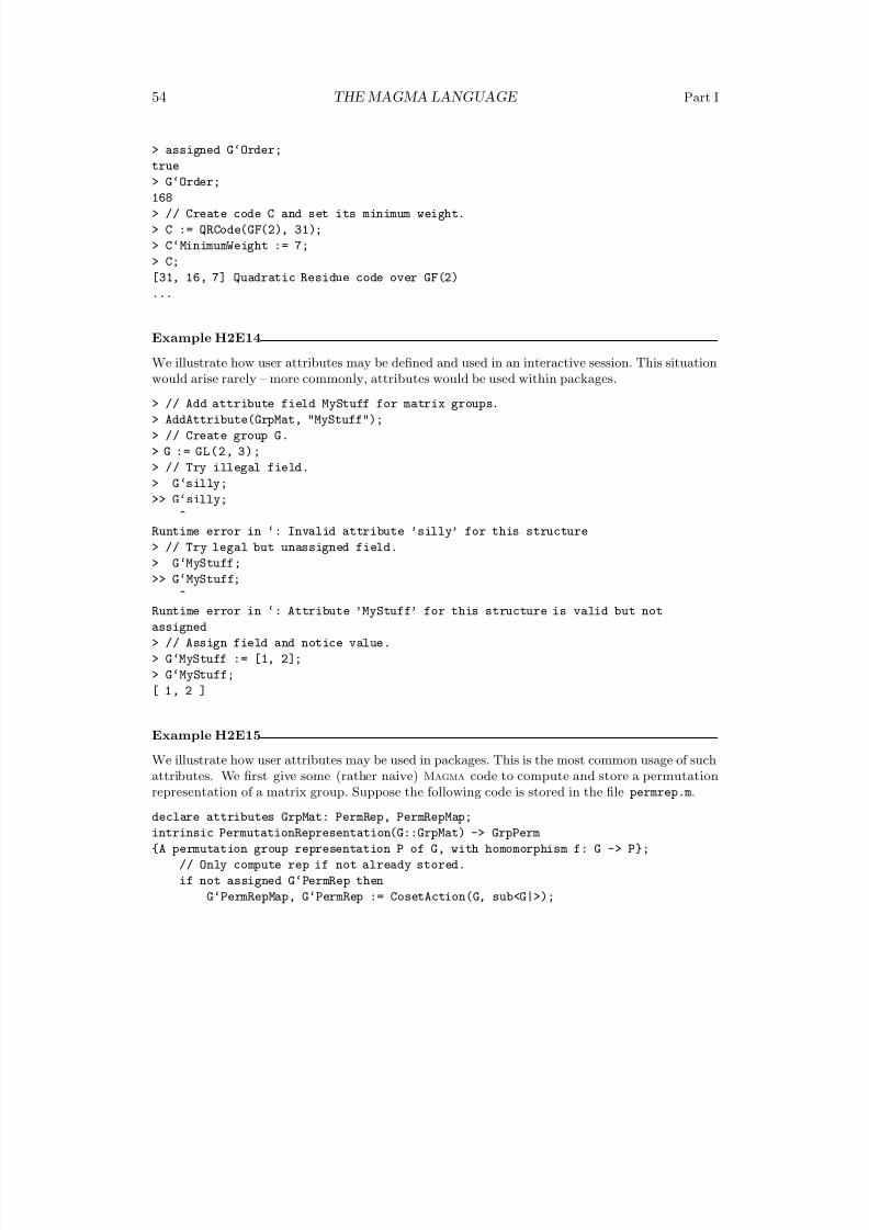
8/22/2019 Handbook Volume 01
http://slidepdf.com/reader/full/handbook-volume-01 170/440
54 THE MAGMA LANGUAGE Part I
> assigned G‘Order;
true
> G‘Order;168
> // Create code C and set its minimum weight.
> C := QRCode(GF(2), 31);
> C‘MinimumWeight := 7;
> C;
[31, 16, 7] Quadratic Residue code over GF(2)
...
Example H2E14
We illustrate how user attributes may be defined and used in an interactive session. This situationwould arise rarely – more commonly, attributes would be used within packages.
> // Add attribute field MyStuff for matrix groups.
> AddAttribute(GrpMat, "MyStuff");
> // Create group G.
> G := GL(2, 3);
> // Try illegal field.
> G‘silly;
>> G‘silly;
^
Runtime error in ‘: Invalid attribute ’silly’ for this structure
> // Try legal but unassigned field.
> G‘MyStuff;
>> G‘MyStuff;
^
Runtime error in ‘: Attribute ’MyStuff’ for this structure is valid but not
assigned
> // Assign field and notice value.
> G‘MyStuff := [1, 2];
> G‘MyStuff;
[ 1, 2 ]
Example H2E15We illustrate how user attributes may be used in packages. This is the most common usage of suchattributes. We first give some (rather naive) Magma code to compute and store a permutationrepresentation of a matrix group. Suppose the following code is stored in the file permrep.m.
declare attributes GrpMat: PermRep, PermRepMap;
intrinsic PermutationRepresentation(G::GrpMat) -> GrpPerm
{A permutation group representation P of G, with homomorphism f: G -> P};
// Only compute rep if not already stored.
if not assigned G‘PermRep then
G‘PermRepMap, G‘PermRep := CosetAction(G, sub<G|>);
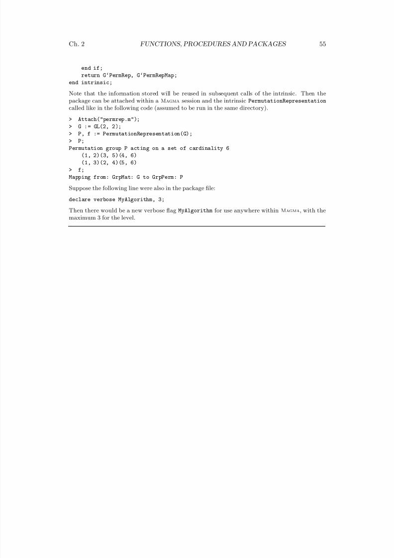
8/22/2019 Handbook Volume 01
http://slidepdf.com/reader/full/handbook-volume-01 171/440
Ch. 2 FUNCTIONS, PROCEDURES AND PACKAGES 55
end if;
return G‘PermRep, G‘PermRepMap;
end intrinsic;
Note that the information stored will be reused in subsequent calls of the intrinsic. Then thepackage can be attached within a Magma session and the intrinsic PermutationRepresentation
called like in the following code (assumed to be run in the same directory).
> Attach("permrep.m");
> G := GL(2, 2);
> P, f := PermutationRepresentation(G);
> P;
Permutation group P acting on a set of cardinality 6
(1, 2)(3, 5)(4, 6)
(1, 3)(2, 4)(5, 6)
> f;Mapping from: GrpMat: G to GrpPerm: P
Suppose the following line were also in the package file:
declare verbose MyAlgorithm, 3;
Then there would be a new verbose flag MyAlgorithm for use anywhere within Magma, with themaximum 3 for the level.

8/22/2019 Handbook Volume 01
http://slidepdf.com/reader/full/handbook-volume-01 172/440
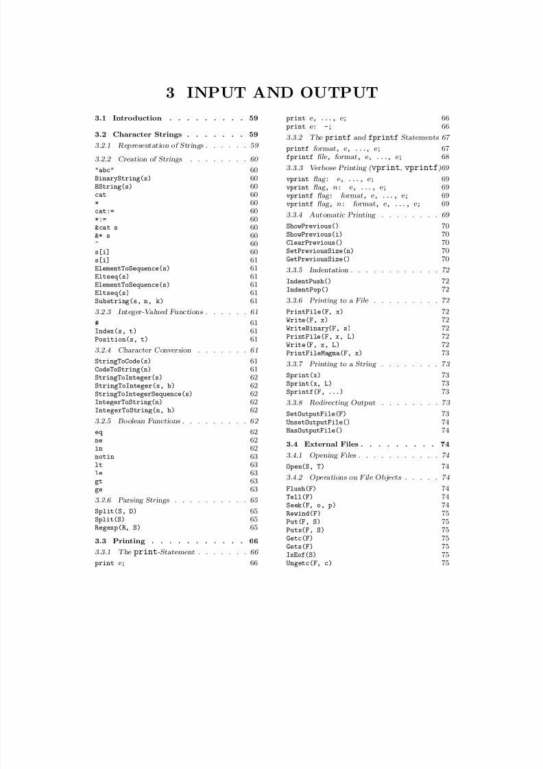
8/22/2019 Handbook Volume 01
http://slidepdf.com/reader/full/handbook-volume-01 173/440
3 INPUT AND OUTPUT
3.1 Introduction . . . . . . . . . 59
3.2 Character Strings . . . . . . . 59
3.2.1 Representation of Strings . . . . . . 59
3.2.2 Creation of Strings . . . . . . . . 60
"abc" 60BinaryString(s) 60BString(s) 60cat 60* 60cat:= 60*:= 60&cat s 60&* s 60^ 60s[i] 60s[i] 61ElementToSequence(s) 61Eltseq(s) 61ElementToSequence(s) 61Eltseq(s) 61Substring(s, n, k) 61
3.2.3 Integer-Valued Functions . . . . . . 61
# 61Index(s, t) 61Position(s, t) 61
3.2.4 Character Conversion . . . . . . . 61
StringToCode(s) 61CodeToString(n) 61StringToInteger(s) 62StringToInteger(s, b) 62StringToIntegerSequence(s) 62IntegerToString(n) 62IntegerToString(n, b) 62
3.2.5 Boolean Functions . . . . . . . . . 62
eq 62ne 62in 62notin 63
lt 63le 63gt 63ge 63
3.2.6 Parsing Strings . . . . . . . . . . 65
Split(S, D) 65Split(S) 65Regexp(R, S) 65
3.3 Printing . . . . . . . . . . . 66
3.3.1 The print-Statement . . . . . . . 66
print e ; 66
print e , ..., e ; 66print e : -; 66
3.3.2 The printf and fprintf Statements 67
printf format, e , ..., e ; 67fprintf file , format, e , ..., e ; 68
3.3.3 Verbose Printing ( vprint, vprintf)69
vprint flag : e , ..., e ; 69vprint flag , n: e , ..., e ; 69vprintf flag : format, e , ..., e ; 69vprintf flag , n: format, e , ..., e ; 69
3.3.4 Automatic Printing . . . . . . . . 69
ShowPrevious() 70ShowPrevious(i) 70ClearPrevious() 70SetPreviousSize(n) 70GetPreviousSize() 70
3.3.5 Indentation . . . . . . . . . . . . 72
IndentPush() 72IndentPop() 72
3.3.6 Printing to a File . . . . . . . . . 72
PrintFile(F, x) 72Write(F, x) 72WriteBinary(F, s) 72PrintFile(F, x, L) 72
Write(F, x, L) 72PrintFileMagma(F, x) 73
3.3.7 Printing to a String . . . . . . . . 7 3
Sprint(x) 73Sprint(x, L) 73Sprintf(F, ...) 73
3.3.8 Redirecting Output . . . . . . . . 7 3
SetOutputFile(F) 73UnsetOutputFile() 74HasOutputFile() 74
3.4 External Files . . . . . . . . . 74
3.4.1 Opening Files . . . . . . . . . . . 74
Open(S, T) 74
3.4.2 Operations on File Objects . . . . . 74
Flush(F) 74Tell(F) 74Seek(F, o, p) 74Rewind(F) 75Put(F, S) 75Puts(F, S) 75Getc(F) 75Gets(F) 75IsEof(S) 75Ungetc(F, c) 75
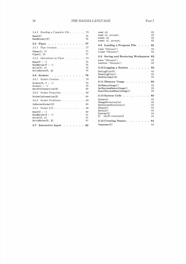
8/22/2019 Handbook Volume 01
http://slidepdf.com/reader/full/handbook-volume-01 174/440
58 THE MAGMA LANGUAGE Part I
3.4.3 Reading a Complete File . . . . . . 76
Read(F) 76
ReadBinary(F) 763.5 Pipes . . . . . . . . . . . . 77
3.5.1 Pipe Creation . . . . . . . . . . . 77
POpen(C, T) 77Pipe(C, S) 77
3.5.2 Operations on Pipes . . . . . . . . 78
Read(P : -) 78ReadBytes(P : -) 78Write(P, s) 78WriteBytes(P, Q) 78
3.6 Sockets . . . . . . . . . . . 78
3.6.1 Socket Creation . . . . . . . . . . 79 Socket(H, P : -) 79Socket( : -) 79WaitForConnection(S) 80
3.6.2 So cket Properties . . . . . . . . . 80
SocketInformation(S) 80
3.6.3 So cket Predicates . . . . . . . . . 80
IsServerSocket(S) 80
3.6.4 Socket I/O . . . . . . . . . . . . 80
Read(S : -) 80ReadBytes(S : -) 81Write(S, s) 81WriteBytes(S, Q) 81
3.7 Interactive Input . . . . . . . 82
read id; 82read id, prompt; 82readi id; 82readi id, prompt; 82
3.8 Loading a Program File . . . . 82
load "filename "; 82iload "filename "; 82
3.9 Saving and Restoring Workspaces 82
save "filename "; 82restore "filename "; 82
3.10 Logging a Session . . . . . . . 83
SetLogFile(F) 83UnsetLogFile() 83SetEchoInput(b) 83
3.11 Memory Usage . . . . . . . . 83
GetMemoryUsage() 83GetMaximumMemoryUsage() 83ResetMaximumMemoryUsage() 83
3.12 System Calls . . . . . . . . . 83
Alarm(s) 83ChangeDirectory(s) 83GetCurrentDirectory() 83Getpid() 84Getuid() 84System(C) 84%! shell-command 84
3.13 Creating Names . . . . . . . . 84
Tempname(P) 84
8/22/2019 Handbook Volume 01
http://slidepdf.com/reader/full/handbook-volume-01 175/440
Chapter 3
INPUT AND OUTPUT
3.1 Introduction
This chapter is concerned with the various facilities provided for communication betweenMagma and its environment. The first section describes character strings and their op-erations. Following this, the various forms of the print-statement are presented. Nextthe file type is introduced and its operations summarized. The chapter concludes with
a section listing system calls. These include facilities that allow the user to execute anoperating system command from within Magma or to run an external process.
3.2 Character Strings
Strings of characters play a central role in input/output so that the operations provided forstrings to some extent reflect this. However, if one wishes, a more general set of operationsare available if the string is first converted into a sequence. We will give some examples of this below.
Magma provides two kinds of strings: normal character strings, and binary strings .Character strings are an inappropriate choice for manipulating data that includes non-printable characters. If this is required, a better choice is the binary string type. This typeis similar semantically to a sequence of integers, in which each character is represented byits ASCII value between 0 and 255. The difference between a binary string and a sequenceof integers is that a binary string is stored internally as an array of bytes, which is a morespace-efficient representation.
3.2.1 Representation of Strings
Character strings may consist of all ordinary characters appearing on your keyboard, in-cluding the blank (space). Two symbols have a special meaning: the double-quote " andthe backslash \. The double-quote is used to delimit a character string, and hence cannot
be used inside a string; to be able to use a double-quote in strings the backslash is designedto be an escape character and is used to indicate that the next symbol has to be takenliterally; thus, by using \" inside a string one indicates that the symbol " has to be takenliterally and is not to be interpreted as the end-of-string delimiter. Thus:
> "\"Print this line in quotes\"";
"Print this line in quotes"
To obtain a literal backslash, one simply types two backslashes; for characters other thandouble-quotes and backslash it does not make a difference when a backslash precedes them
8/22/2019 Handbook Volume 01
http://slidepdf.com/reader/full/handbook-volume-01 176/440
60 THE MAGMA LANGUAGE Part I
inside a string, with the exception of n, r and t. Any occurrence of \n or \r inside a stringis converted into a <new-line> while \t is converted into a <tab>. For example:
> "The first line,\nthe second line, and then\ran\tindented line";
The first line,
the second line, and then
an indented line
Note that a backslash followed by a return allows one to conveniently continue the currentconstruction on the next line; so \<return> inside a string will be ignored, except thatinput will continue on a new line on your screen.
Binary strings, on the hand, can consist of any character, whether printable or non-printable. Binary strings cannot be constructed using literals, but must be constructedeither from a character string, or during a read operation from a file.
3.2.2 Creation of Strings
"abc"
Create a string from a succession of keyboard characters (a, b, c) enclosed in doublequotes " ".
BinaryString(s)
BString(s)
Create a binary string from the character string s.
s cat t
s * t
Concatenate the strings s and t.
s cat:= t
s *:= t
Modification-concatenation of the string s with t: concatenate s and t and put theresult in s.
&cat s
&* s
Given an enumerated sequence s of strings, return the concatenation of these strings.
s ^ n
Form the n-fold concatenation of the string s, for n ≥ 0. If n = 0 this is the emptystring, if n = 1 it equals s, etc.
s[i]
Returns the substring of s consisting of the i-th character.
8/22/2019 Handbook Volume 01
http://slidepdf.com/reader/full/handbook-volume-01 177/440
Ch. 3 INPUT AND OUTPUT 61
s[i]
Returnsthe numeric value representing the i-th character of s.
ElementToSequence(s)
Eltseq(s)
Returns the sequence of characters of s (as length 1 strings).
ElementToSequence(s)
Eltseq(s)
Returns the sequence of numeric values representing the characters of s.
Substring(s, n, k)
Return the substring of s of length k starting at position n.
3.2.3 Integer-Valued Functions
#s
The length of the string s.
Index(s, t)
Position(s, t)
This function returns the position (an integer p with 0 < p ≤ #s) in the string swhere the beginning of a contiguous substring t occurs. It returns 0 if t is not asubstring of s. (If t is the empty string, position 1 will always be returned, even if s is empty as well.)
3.2.4 Character Conversion
To perform more sophisticated operations, one may convert the string into a sequenceand use the extensive facilities for sequences described in the next part of this manual; seethe examples at the end of this chapter for details.
StringToCode(s)
Returns the code number of the first character of string s. This code depends onthe computer system that is used; it is ASCII on most UNIX machines.
CodeToString(n)
Returns a character (string of length 1) corresponding to the code number n, wherethe code is system dependent (see previous entry).
8/22/2019 Handbook Volume 01
http://slidepdf.com/reader/full/handbook-volume-01 178/440
62 THE MAGMA LANGUAGE Part I
StringToInteger(s)
Returns the integer corresponding to the string of decimal digits s. All non-spacecharacters in the string s must be digits (0, 1, . . . , 9), except the first character,which is also allowed to be + or −. An error results if any other combination of characters occurs. Leading zeros are omitted.
StringToInteger(s, b)
Returns the integer corresponding to the string of digits s, all assumed to be writtenin base b. All non-space characters in the string s must be digits less than b (if b isgreater than 10, ‘A’ is used for 10, ‘B’ for 11, etc.), except the first character, whichis also allowed to be + or −. An error results if any other combination of charactersoccurs.
StringToIntegerSequence(s)
Returns the sequence of integers corresponding to the string s of space-separateddecimal numbers. All non-space characters in the string s must be digits (0, 1, . . . , 9),except the first character after each space, which is also allowed to be + or −.An error results if any other combination of characters occurs. Leading zeros areomitted. Each number can begin with a sign (+ or −) without a space.
IntegerToString(n)
Convert the integer n into a string of decimal digits; if n is negative the first characterof the string will be −. (Note that leading zeros and a + sign are ignored when
Magma builds an integer, so the resulting string will never begin with + or 0characters.)
IntegerToString(n, b)
Convert the integer n into a string of digits with the given base (which must be inthe range [2 . . . 36]); if n is negative the first character of the string will be −.
3.2.5 Boolean Functions
s e q t
Returns true if and only if the strings s and t are identical. Note that blanks aresignificant.
s n e t
Returns true if and only if the strings s and t are distinct. Note that blanks aresignificant.
s i n t
Returns true if and only if s appears as a contiguous substring of t. Note that theempty string is contained in every string.
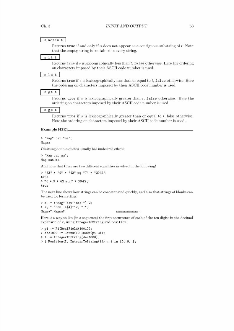
8/22/2019 Handbook Volume 01
http://slidepdf.com/reader/full/handbook-volume-01 179/440
Ch. 3 INPUT AND OUTPUT 63
s notin t
Returns true if and only if s does not appear as a contiguous substring of t. Note
that the empty string is contained in every string.
s l t t
Returns true if s is lexicographically less than t, false otherwise. Here the orderingon characters imposed by their ASCII code number is used.
s l e t
Returns true if s is lexicographically less than or equal to t, false otherwise. Herethe ordering on characters imposed by their ASCII code number is used.
s g t t
Returns true if s is lexicographically greater than t, false otherwise. Here theordering on characters imposed by their ASCII code number is used.
s g e t
Returns true if s is lexicographically greater than or equal to t, false otherwise.Here the ordering on characters imposed by their ASCII code number is used.
Example H3E1
> "Mag" cat "ma";
Magma
Omitting double-quotes usually has undesired effects:
> "Mag cat ma";
Mag cat ma
And note that there are two different equalities involved in the following!
> "73" * "9" * "42" eq "7" * "3942";
true
> 73 * 9 * 42 eq 7 * 3942;
true
The next line shows how strings can be concatenated quickly, and also that strings of blanks canbe used for formatting:
> s := ("Mag" cat "ma? ")^2;
> s, " "^30, s[4]^12, "!";
Magma? Magma? mmmmmmmmmmmm !
Here is a way to list (in a sequence) the first occurrence of each of the ten digits in the decimalexpansion of π, using IntegerToString and Position.
> pi := Pi(RealField(1001));
> dec1000 := Round(10^1000*(pi-3));
> I := IntegerToString(dec1000);
> [ Position(I, IntegerToString(i)) : i in [0..9] ];
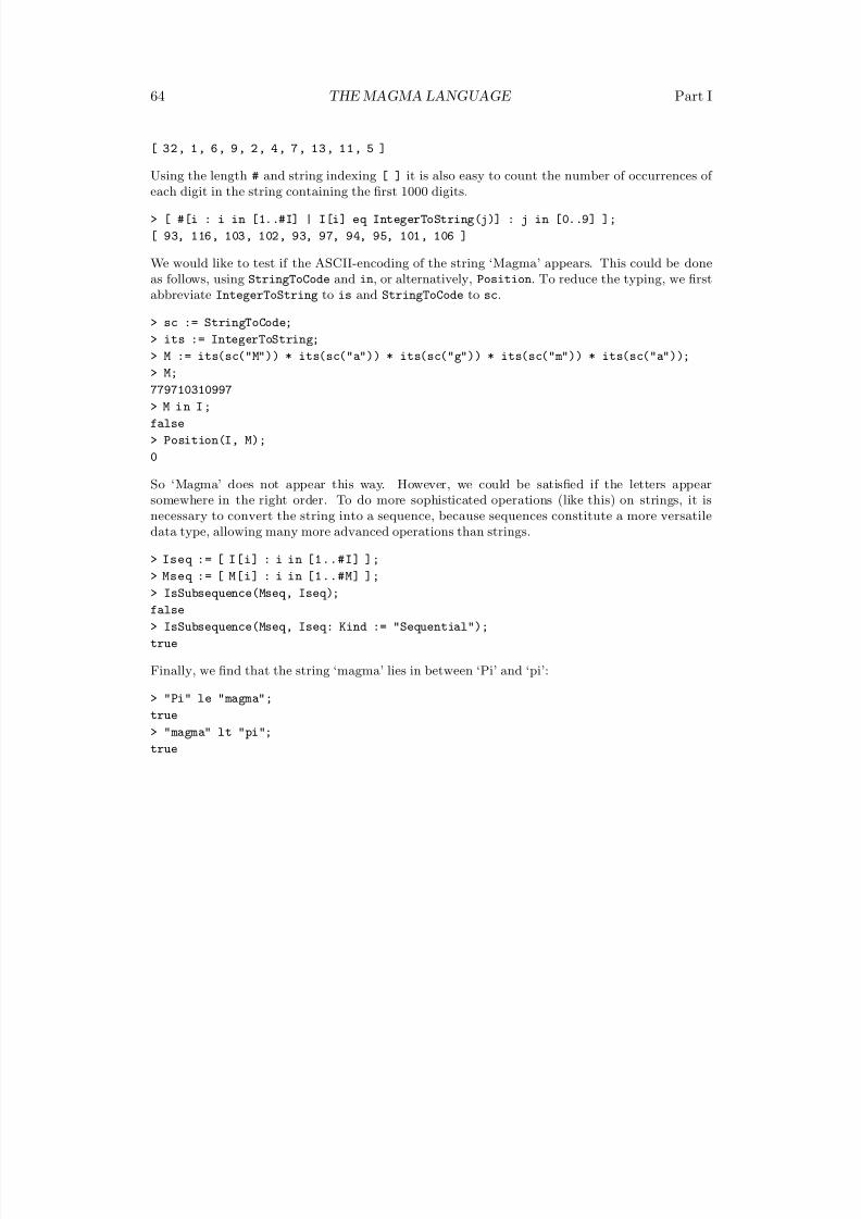
8/22/2019 Handbook Volume 01
http://slidepdf.com/reader/full/handbook-volume-01 180/440
64 THE MAGMA LANGUAGE Part I
[ 32, 1, 6, 9, 2, 4, 7, 13, 11, 5 ]
Using the length # and string indexing [ ] it is also easy to count the number of occurrences of each digit in the string containing the first 1000 digits.
> [ #[i : i in [1..#I] | I[i] eq IntegerToString(j)] : j in [0..9] ];
[ 93, 116, 103, 102, 93, 97, 94, 95, 101, 106 ]
We would like to test if the ASCII-encoding of the string ‘Magma’ appears. This could be doneas follows, using StringToCode and in, or alternatively, Position. To reduce the typing, we firstabbreviate IntegerToString to is and StringToCode to sc.
> sc := StringToCode;
> its := IntegerToString;
> M := its(sc("M")) * its(sc("a")) * its(sc("g")) * its(sc("m")) * its(sc("a"));
> M;
779710310997
> M i n I ;
false
> Position(I, M);
0
So ‘Magma’ does not appear this way. However, we could be satisfied if the letters appearsomewhere in the right order. To do more sophisticated operations (like this) on strings, it isnecessary to convert the string into a sequence, because sequences constitute a more versatiledata type, allowing many more advanced operations than strings.
> Iseq := [ I[i] : i in [1..#I] ];
> Mseq := [ M[i] : i in [1..#M] ];
> IsSubsequence(Mseq, Iseq);
false
> IsSubsequence(Mseq, Iseq: Kind := "Sequential");
true
Finally, we find that the string ‘magma’ lies in between ‘Pi’ and ‘pi’:
> "Pi" le "magma";
true
> "magma" lt "pi";true
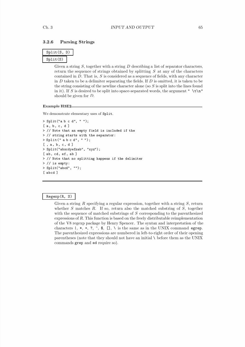
8/22/2019 Handbook Volume 01
http://slidepdf.com/reader/full/handbook-volume-01 181/440
Ch. 3 INPUT AND OUTPUT 65
3.2.6 Parsing Strings
Split(S, D)
Split(S)
Given a string S , together with a string D describing a list of separator characters,return the sequence of strings obtained by splitting S at any of the characterscontained in D. That is, S is considered as a sequence of fields, with any characterin D taken to be a delimiter separating the fields. If D is omitted, it is taken to bethe string consisting of the newline character alone (so S is split into the lines foundin it). If S is desired to be split into space-separated words, the argument " \t\n"
should be given for D.
Example H3E2
We demonstrate elementary uses of Split.
> Split("a b c d", " ");
[ a , b , c , d ]
> // Note that an empty field is included if the
> // string starts with the separator:
> Split(" a b c d", " ");
[ , a , b , c , d ]
> Split("abxcdyefzab", "xyz");
[ ab, cd, ef, ab ]
> // Note that no splitting happens if the delimiter
> // is empty:
> Split("abcd", "");
[ abcd ]
Regexp(R, S)
Given a string R specifying a regular expression, together with a string S , return
whether S matches R. If so, return also the matched substring of S , togetherwith the sequence of matched substrings of S corresponding to the parenthesizedexpressions of R. This function is based on the freely distributable reimplementationof the V8 regexp package by Henry Spencer. The syntax and interpretation of thecharacters |, *, +, ?, ^, $, [], \ is the same as in the UNIX command egrep.The parenthesized expressions are numbered in left-to-right order of their openingparentheses (note that they should not have an initial \ before them as the UNIXcommands grep and ed require so).
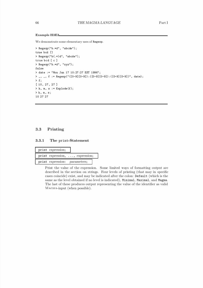
8/22/2019 Handbook Volume 01
http://slidepdf.com/reader/full/handbook-volume-01 182/440
66 THE MAGMA LANGUAGE Part I
Example H3E3
We demonstrate some elementary uses of Regexp
.> Regexp("b.*d", "abcde");
true bcd []
> Regexp("b(.*)d", "abcde");
true bcd [ c ]
> Regexp("b.*d", "xyz");
false
> date := "Mon Jun 17 10:27:27 EST 1996";
> _, _, f := Regexp("([0-9][0-9]):([0-9][0-9]):([0-9][0-9])", date);
> f;
[ 10, 27, 27 ]
> h, m, s := Explode(f);
> h, m, s;
10 27 27
3.3 Printing
3.3.1 The print-Statement
print expression;
print expression, ..., expression;
print expression: parameters ;
Print the value of the expression. Some limited ways of formatting output are
described in the section on strings. Four levels of printing (that may in specificcases coincide) exist, and may be indicated after the colon: Default (which is thesame as the level obtained if no level is indicated), Minimal, Maximal, and Magma.The last of these produces output representing the value of the identifier as validMagma-input (when possible).
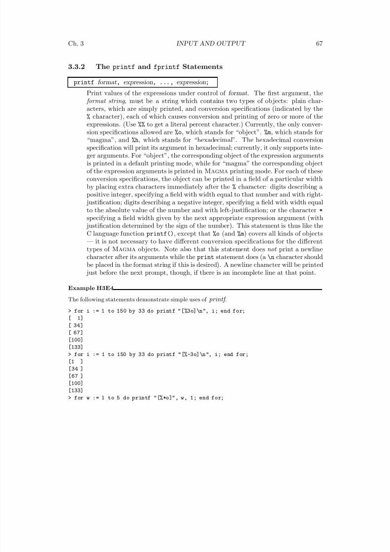
8/22/2019 Handbook Volume 01
http://slidepdf.com/reader/full/handbook-volume-01 183/440
Ch. 3 INPUT AND OUTPUT 67
3.3.2 The printf and fprintf Statements
printf format, expression, ..., expression;
Print values of the expressions under control of format. The first argument, the format string , must be a string which contains two types of objects: plain char-acters, which are simply printed, and conversion specifications (indicated by the% character), each of which causes conversion and printing of zero or more of theexpressions. (Use %% to get a literal percent character.) Currently, the only conver-sion specifications allowed are %o, which stands for “object”, %m, which stands for“magma”, and %h, which stands for “hexadecimal”. The hexadecimal conversionspecification will print its argument in hexadecimal; currently, it only supports inte-ger arguments. For “object”, the corresponding object of the expression arguments
is printed in a default printing mode, while for “magma” the corresponding objectof the expression arguments is printed in Magma printing mode. For each of theseconversion specifications, the object can be printed in a field of a particular widthby placing extra characters immediately after the % character: digits describing apositive integer, specifying a field with width equal to that number and with right-
justification; digits describing a negative integer, specifying a field with width equalto the absolute value of the number and with left-justification; or the character *
specifying a field width given by the next appropriate expression argument (with justification determined by the sign of the number). This statement is thus like theC language function printf(), except that %o (and %m) covers all kinds of objects— it is not necessary to have different conversion specifications for the different
types of Magma objects. Note also that this statement does not print a newlinecharacter after its arguments while the print statement does (a \n character shouldbe placed in the format string if this is desired). A newline character will be printed
just before the next prompt, though, if there is an incomplete line at that point.
Example H3E4
The following statements demonstrate simple uses of printf .
> for i := 1 to 150 by 33 do printf "[%3o]\n", i; end for;
[ 1]
[ 34]
[ 67][100]
[133]
> for i := 1 to 150 by 33 do printf "[%-3o]\n", i; end for;
[1 ]
[34 ]
[67 ]
[100]
[133]
> for w := 1 to 5 do printf "[%*o]", w, 1; end for;
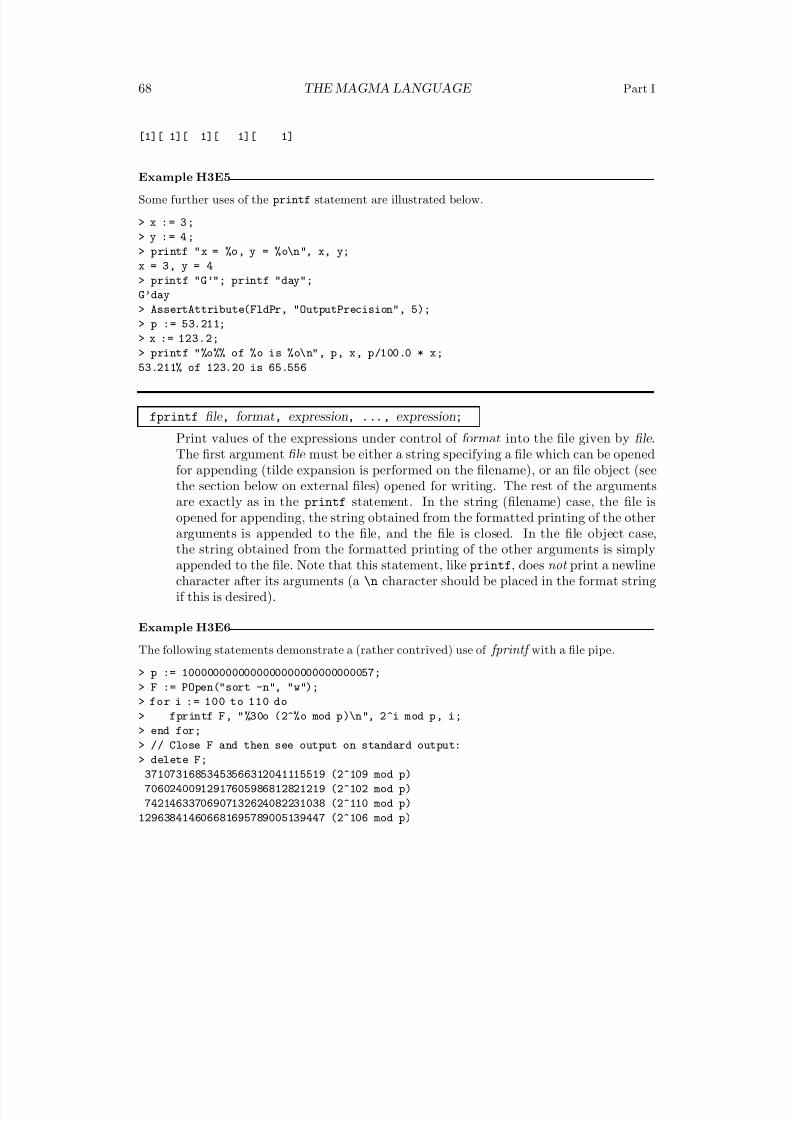
8/22/2019 Handbook Volume 01
http://slidepdf.com/reader/full/handbook-volume-01 184/440
68 THE MAGMA LANGUAGE Part I
[1][ 1][ 1][ 1][ 1]
Example H3E5
Some further uses of the printf statement are illustrated below.
> x : = 3 ;
> y : = 4 ;
> printf "x = %o, y = %o\n", x, y;
x = 3, y = 4
> printf "G’"; printf "day";
G’day
> AssertAttribute(FldPr, "OutputPrecision", 5);
> p := 53.211;
> x := 123.2;> printf "%o%% of %o is %o\n", p, x, p/100.0 * x;
53.211% of 123.20 is 65.556
fprintf file , format, expression, ..., expression;
Print values of the expressions under control of format into the file given by file .The first argument file must be either a string specifying a file which can be openedfor appending (tilde expansion is performed on the filename), or an file object (seethe section below on external files) opened for writing. The rest of the arguments
are exactly as in the printf statement. In the string (filename) case, the file isopened for appending, the string obtained from the formatted printing of the otherarguments is appended to the file, and the file is closed. In the file object case,the string obtained from the formatted printing of the other arguments is simplyappended to the file. Note that this statement, like printf, does not print a newlinecharacter after its arguments (a \n character should be placed in the format stringif this is desired).
Example H3E6
The following statements demonstrate a (rather contrived) use of fprintf with a file pipe.
> p := 1000000000000000000000000000057;> F := POpen("sort -n", "w");
> for i := 100 to 110 do
> fprintf F, "%30o (2^%o mod p)\n", 2^i mod p, i;
> end for;
> // Close F and then see output on standard output:
> delete F;
37107316853453566312041115519 (2^109 mod p)
70602400912917605986812821219 (2^102 mod p)
74214633706907132624082231038 (2^110 mod p)
129638414606681695789005139447 (2^106 mod p)
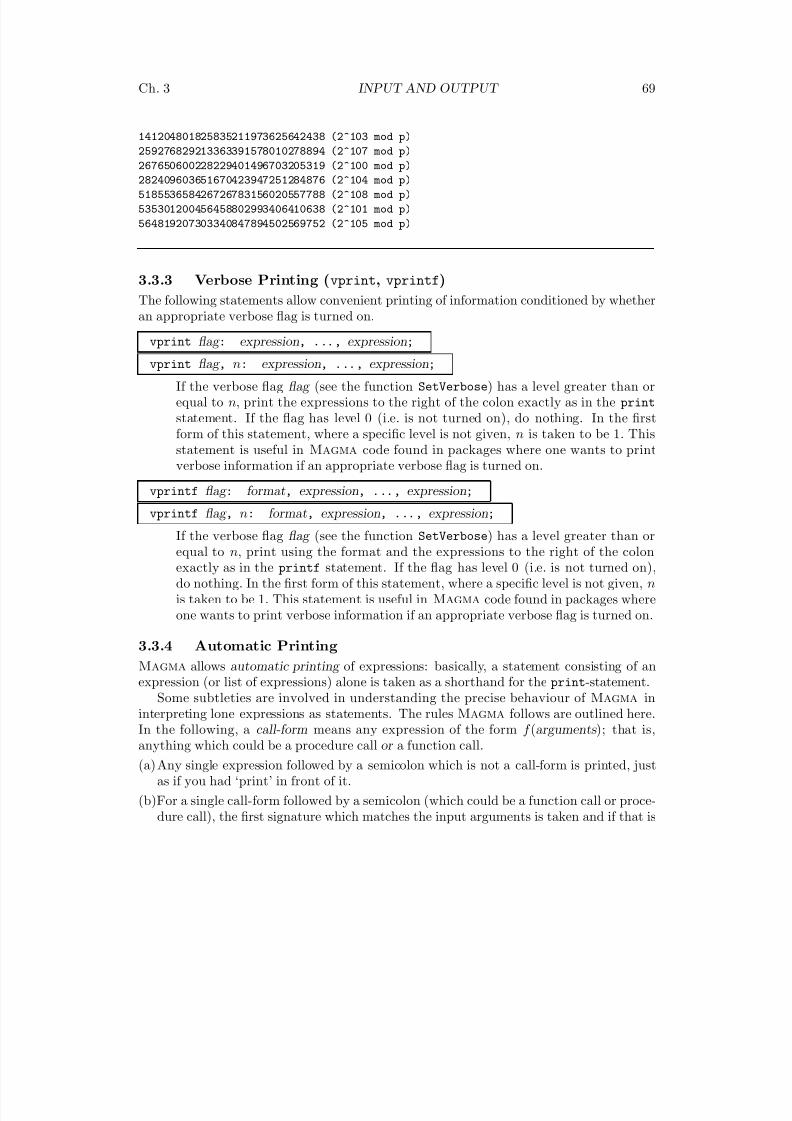
8/22/2019 Handbook Volume 01
http://slidepdf.com/reader/full/handbook-volume-01 185/440
Ch. 3 INPUT AND OUTPUT 69
141204801825835211973625642438 (2^103 mod p)
259276829213363391578010278894 (2^107 mod p)
267650600228229401496703205319 (2^100 mod p)282409603651670423947251284876 (2^104 mod p)
518553658426726783156020557788 (2^108 mod p)
535301200456458802993406410638 (2^101 mod p)
564819207303340847894502569752 (2^105 mod p)
3.3.3 Verbose Printing (vprint, vprintf)
The following statements allow convenient printing of information conditioned by whetheran appropriate verbose flag is turned on.
vprint flag : expression, ..., expression;
vprint flag , n: expression, ..., expression;
If the verbose flag flag (see the function SetVerbose) has a level greater than orequal to n, print the expressions to the right of the colon exactly as in the print
statement. If the flag has level 0 (i.e. is not turned on), do nothing. In the firstform of this statement, where a specific level is not given, n is taken to be 1. Thisstatement is useful in Magma code found in packages where one wants to printverbose information if an appropriate verbose flag is turned on.
vprintf flag : format, expression, ..., expression;
vprintf flag , n: format, expression, ..., expression;
If the verbose flag flag (see the function SetVerbose) has a level greater than orequal to n, print using the format and the expressions to the right of the colonexactly as in the printf statement. If the flag has level 0 (i.e. is not turned on),do nothing. In the first form of this statement, where a specific level is not given, nis taken to be 1. This statement is useful in Magma code found in packages whereone wants to print verbose information if an appropriate verbose flag is turned on.
3.3.4 Automatic Printing
Magma allows automatic printing of expressions: basically, a statement consisting of anexpression (or list of expressions) alone is taken as a shorthand for the print-statement.
Some subtleties are involved in understanding the precise behaviour of Magma ininterpreting lone expressions as statements. The rules Magma follows are outlined here.In the following, a call-form means any expression of the form f (arguments ); that is,anything which could be a procedure call or a function call.
(a) Any single expression followed by a semicolon which is not a call-form is printed, justas if you had ‘print’ in front of it.
(b)For a single call-form followed by a semicolon (which could be a function call or proce-dure call), the first signature which matches the input arguments is taken and if that is
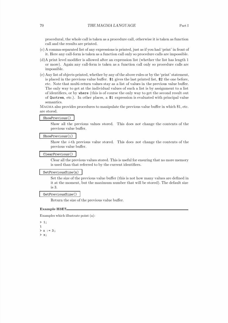
8/22/2019 Handbook Volume 01
http://slidepdf.com/reader/full/handbook-volume-01 186/440
70 THE MAGMA LANGUAGE Part I
procedural, the whole call is taken as a procedure call, otherwise it is taken as functioncall and the results are printed.
(c) A comma-separated list of any expressions is printed, just as if you had ‘print’ in front of it. Here any call-form is taken as a function call only so procedure calls are impossible.
(d)A print level modifier is allowed after an expression list (whether the list has length 1or more). Again any call-form is taken as a function call only so procedure calls areimpossible.
(e) Any list of objects printed, whether by any of the above rules or by the ‘print’ statement,is placed in the previous value buffer. $1 gives the last printed list, $2 the one before,etc. Note that multi-return values stay as a list of values in the previous value buffer.The only way to get at the individual values of such a list is by assignment to a listof identifiers, or by where (this is of course the only way to get the second result out
of Quotrem, etc.). In other places, a $1 expression is evaluated with principal valuesemantics.
Magma also provides procedures to manipulate the previous value buffer in which $1, etc.are stored.
ShowPrevious()
Show all the previous values stored. This does not change the contents of theprevious value buffer.
ShowPrevious(i)
Show the i-th previous value stored. This does not change the contents of the
previous value buffer.
ClearPrevious()
Clear all the previous values stored. This is useful for ensuring that no more memoryis used than that referred to by the current identifiers.
SetPreviousSize(n)
Set the size of the previous value buffer (this is not how many values are defined init at the moment, but the maximum number that will be stored). The default sizeis 3.
GetPreviousSize()Return the size of the previous value buffer.
Example H3E7
Examples which illustrate point (a):
> 1;
1
> x : = 3 ;
> x;
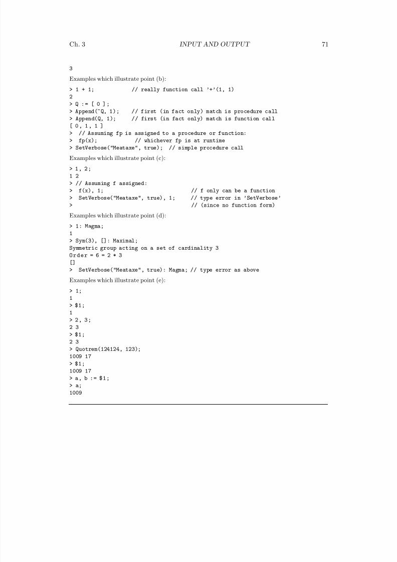
8/22/2019 Handbook Volume 01
http://slidepdf.com/reader/full/handbook-volume-01 187/440
Ch. 3 INPUT AND OUTPUT 71
3
Examples which illustrate point (b):
> 1 + 1; // really function call ’+’(1, 1)
2
> Q : = [ 0 ] ;
> Append(~Q, 1); // first (in fact only) match is procedure call
> Append(Q, 1); // first (in fact only) match is function call
[ 0 , 1 , 1 ]
> // Assuming fp is assigned to a procedure or function:
> fp(x); // whichever fp is at runtime
> SetVerbose("Meataxe", true); // simple procedure call
Examples which illustrate point (c):
> 1, 2;1 2
> // Assuming f assigned:
> f(x), 1; // f only can be a function
> SetVerbose("Meataxe", true), 1; // type error in ’SetVerbose’
> // (since no function form)
Examples which illustrate point (d):
> 1: Magma;
1
> Sym(3), []: Maximal;
Symmetric group acting on a set of cardinality 3
O r d e r = 6 = 2 * 3[]
> SetVerbose("Meataxe", true): Magma; // type error as above
Examples which illustrate point (e):
> 1;
1
> $1;
1
> 2, 3;
2 3
> $1;
2 3
> Quotrem(124124, 123);
1009 17
> $1;
1009 17
> a, b := $1;
> a;
1009
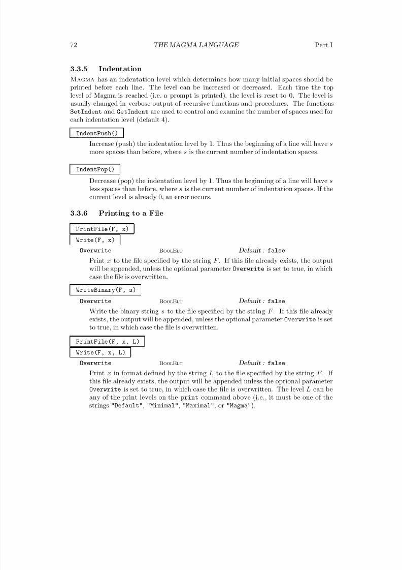
8/22/2019 Handbook Volume 01
http://slidepdf.com/reader/full/handbook-volume-01 188/440
72 THE MAGMA LANGUAGE Part I
3.3.5 Indentation
Magma has an indentation level which determines how many initial spaces should be
printed before each line. The level can be increased or decreased. Each time the toplevel of Magma is reached (i.e. a prompt is printed), the level is reset to 0. The level isusually changed in verbose output of recursive functions and procedures. The functionsSetIndent and GetIndent are used to control and examine the number of spaces used foreach indentation level (default 4).
IndentPush()
Increase (push) the indentation level by 1. Thus the beginning of a line will have smore spaces than before, where s is the current number of indentation spaces.
IndentPop()Decrease (pop) the indentation level by 1. Thus the beginning of a line will have sless spaces than before, where s is the current number of indentation spaces. If thecurrent level is already 0, an error occurs.
3.3.6 Printing to a File
PrintFile(F, x)
Write(F, x)
Overwrite BoolElt Default : false
Print x to the file specified by the string F . If this file already exists, the outputwill be appended, unless the optional parameter Overwrite is set to true, in whichcase the file is overwritten.
WriteBinary(F, s)
Overwrite BoolElt Default : false
Write the binary string s to the file specified by the string F . If this file alreadyexists, the output will be appended, unless the optional parameter Overwrite is setto true, in which case the file is overwritten.
PrintFile(F, x, L)Write(F, x, L)
Overwrite BoolElt Default : false
Print x in format defined by the string L to the file specified by the string F . If this file already exists, the output will be appended unless the optional parameterOverwrite is set to true, in which case the file is overwritten. The level L can beany of the print levels on the print command above (i.e., it must be one of thestrings "Default", "Minimal", "Maximal", or "Magma").
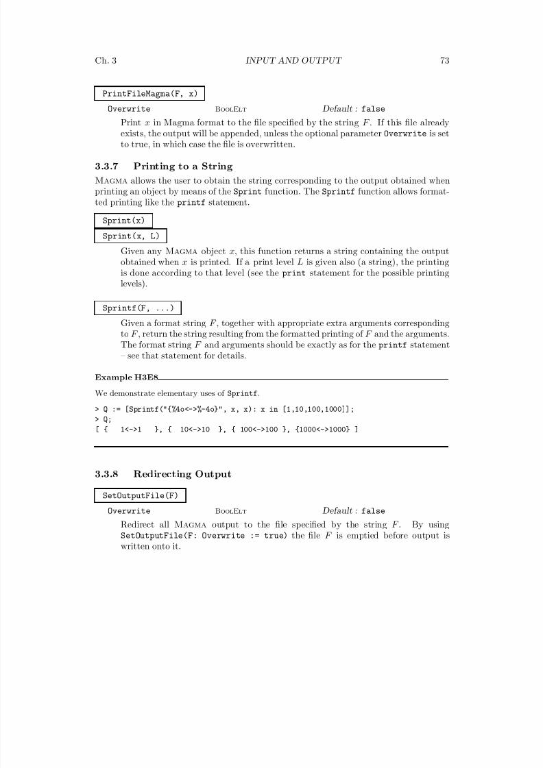
8/22/2019 Handbook Volume 01
http://slidepdf.com/reader/full/handbook-volume-01 189/440
Ch. 3 INPUT AND OUTPUT 73
PrintFileMagma(F, x)
Overwrite BoolElt Default : false
Print x in Magma format to the file specified by the string F . If this file alreadyexists, the output will be appended, unless the optional parameter Overwrite is setto true, in which case the file is overwritten.
3.3.7 Printing to a String
Magma allows the user to obtain the string corresponding to the output obtained whenprinting an object by means of the Sprint function. The Sprintf function allows format-ted printing like the printf statement.
Sprint(x)
Sprint(x, L)
Given any Magma object x, this function returns a string containing the outputobtained when x is printed. If a print level L is given also (a string), the printingis done according to that level (see the print statement for the possible printinglevels).
Sprintf(F, ...)
Given a format string F , together with appropriate extra arguments correspondingto F , return the string resulting from the formatted printing of F and the arguments.
The format string F and arguments should be exactly as for the printf statement– see that statement for details.
Example H3E8
We demonstrate elementary uses of Sprintf.
> Q := [Sprintf("{%4o<->%-4o}", x, x): x in [1,10,100,1000]];
> Q;
[ { 1<->1 }, { 10<->10 }, { 100<->100 }, {1000<->1000} ]
3.3.8 Redirecting Output
SetOutputFile(F)
Overwrite BoolElt Default : false
Redirect all Magma output to the file specified by the string F . By usingSetOutputFile(F: Overwrite := true) the file F is emptied before output iswritten onto it.
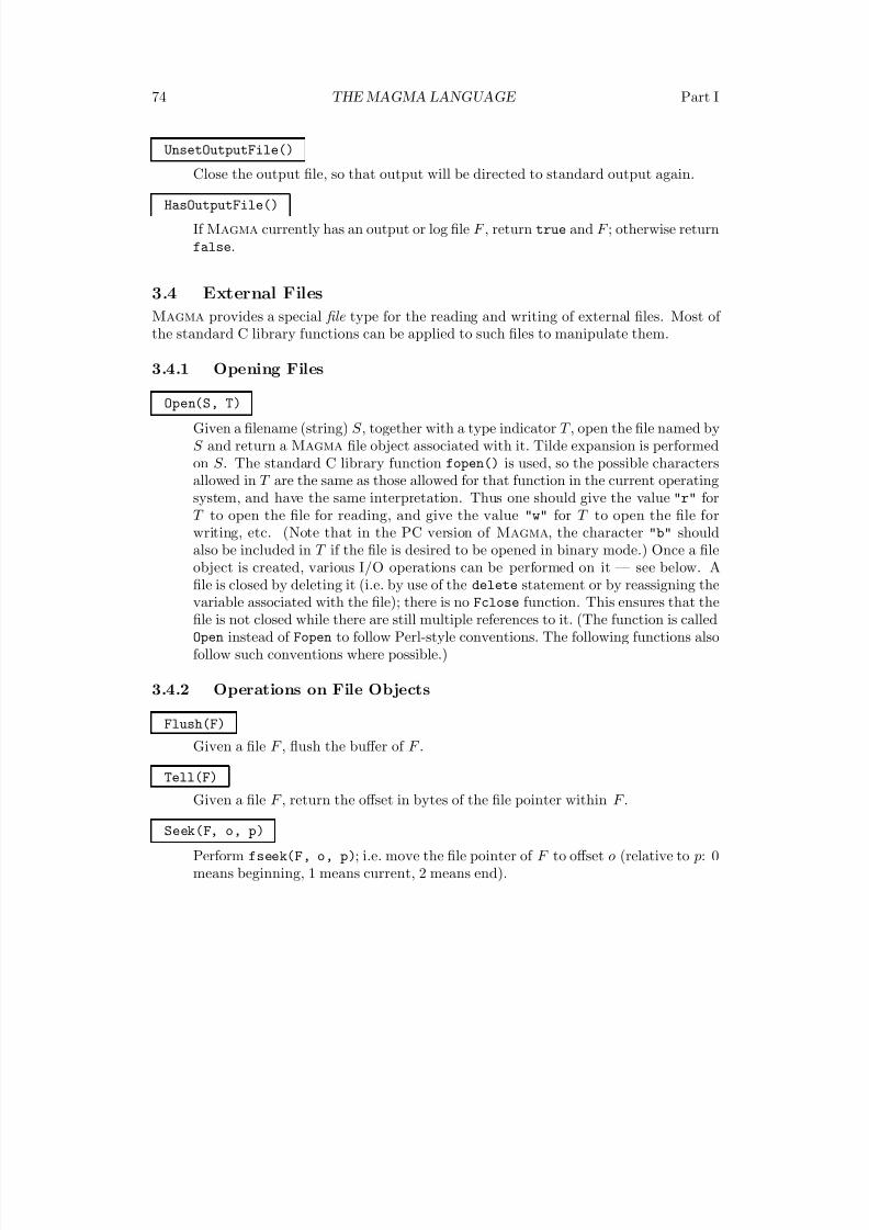
8/22/2019 Handbook Volume 01
http://slidepdf.com/reader/full/handbook-volume-01 190/440
74 THE MAGMA LANGUAGE Part I
UnsetOutputFile()
Close the output file, so that output will be directed to standard output again.
HasOutputFile()
If Magma currently has an output or log file F , return true and F ; otherwise returnfalse.
3.4 External Files
Magma provides a special file type for the reading and writing of external files. Most of the standard C library functions can be applied to such files to manipulate them.
3.4.1 Opening Files
Open(S, T)
Given a filename (string) S , together with a type indicator T , open the file named byS and return a Magma file object associated with it. Tilde expansion is performedon S . The standard C library function fopen() is used, so the possible charactersallowed in T are the same as those allowed for that function in the current operatingsystem, and have the same interpretation. Thus one should give the value "r" forT to open the file for reading, and give the value "w" for T to open the file forwriting, etc. (Note that in the PC version of Magma, the character "b" should
also be included in T if the file is desired to be opened in binary mode.) Once a fileobject is created, various I/O operations can be performed on it — see below. Afile is closed by deleting it (i.e. by use of the delete statement or by reassigning thevariable associated with the file); there is no Fclose function. This ensures that thefile is not closed while there are still multiple references to it. (The function is calledOpen instead of Fopen to follow Perl-style conventions. The following functions alsofollow such conventions where possible.)
3.4.2 Operations on File Objects
Flush(F)
Given a file F , flush the buffer of F .
Tell(F)
Given a file F , return the offset in bytes of the file pointer within F .
Seek(F, o, p)
Perform fseek(F, o, p); i.e. move the file pointer of F to offset o (relative to p: 0means beginning, 1 means current, 2 means end).
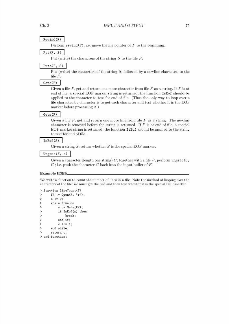
8/22/2019 Handbook Volume 01
http://slidepdf.com/reader/full/handbook-volume-01 191/440
Ch. 3 INPUT AND OUTPUT 75
Rewind(F)
Perform rewind(F); i.e. move the file pointer of F to the beginning.
Put(F, S)
Put (write) the characters of the string S to the file F .
Puts(F, S)
Put (write) the characters of the string S , followed by a newline character, to thefile F .
Getc(F)
Given a file F , get and return one more character from file F as a string. If F is atend of file, a special EOF marker string is returned; the function IsEof should be
applied to the character to test for end of file. (Thus the only way to loop over afile character by character is to get each character and test whether it is the EOFmarker before processing it.)
Gets(F)
Given a file F , get and return one more line from file F as a string. The newlinecharacter is removed before the string is returned. If F is at end of file, a specialEOF marker string is returned; the function IsEof should be applied to the stringto test for end of file.
IsEof(S)
Given a string S , return whether S is the special EOF marker.
Ungetc(F, c)
Given a character (length one string) C , together with a file F , perform ungetc(C,
F); i.e. push the character C back into the input buffer of F .
Example H3E9
We write a function to count the number of lines in a file. Note the method of looping over thecharacters of the file: we must get the line and then test whether it is the special EOF marker.
> function LineCount(F)
> FP := Open(F, "r");> c := 0;
> while true do
> s := Gets(FP);
> if IsEof(s) then
> break;
> end if;
> c +:= 1;
> end while;
> return c;
> end function;
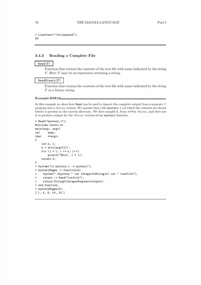
8/22/2019 Handbook Volume 01
http://slidepdf.com/reader/full/handbook-volume-01 192/440
76 THE MAGMA LANGUAGE Part I
> LineCount("/etc/passwd");
59
3.4.3 Reading a Complete File
Read(F)
Function that returns the contents of the text-file with name indicated by the stringF . Here F may be an expression returning a string.
ReadBinary(F)
Function that returns the contents of the text-file with name indicated by the stringF as a binary string.
Example H3E10
In this example we show how Read can be used to import the complete output from a separate C
program into a Magma session. We assume that a file mystery.c (of which the contents are shownbelow) is present in the current directory. We first compile it, from within Magma, and then useit to produce output for the Magma version of our mystery function.
> Read("mystery.c");
#include <stdio.h>
main(argc, argv)int argc;
char **argv;
{
int n, i;
n = atoi(argv[1]);
for (i = 1; i <= n; i++)
printf("%d\n", i * i);
return 0;
}
> System("cc mystery.c -o mystery");
> mysteryMagma := function(n)> System("./mystery " cat IntegerToString(n) cat " >outfile");
> output := Read("outfile");
> return StringToIntegerSequence(output);
> end function;
> mysteryMagma(5);
[ 1, 4, 9, 16, 25 ]
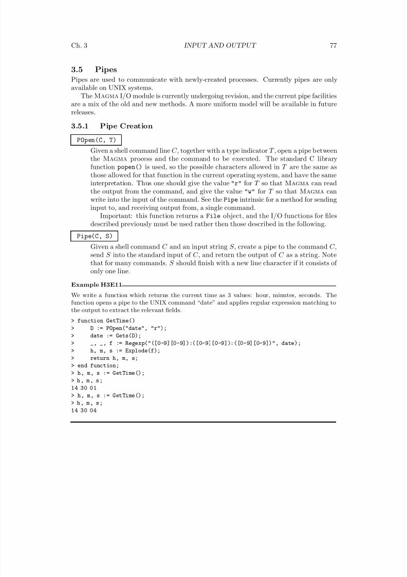
8/22/2019 Handbook Volume 01
http://slidepdf.com/reader/full/handbook-volume-01 193/440
Ch. 3 INPUT AND OUTPUT 77
3.5 Pipes
Pipes are used to communicate with newly-created processes. Currently pipes are only
available on UNIX systems.The Magma I/O module is currently undergoing revision, and the current pipe facilities
are a mix of the old and new methods. A more uniform model will be available in futurereleases.
3.5.1 Pipe Creation
POpen(C, T)
Given a shell command line C , together with a type indicator T , open a pipe betweenthe Magma process and the command to be executed. The standard C libraryfunction popen() is used, so the possible characters allowed in T are the same as
those allowed for that function in the current operating system, and have the sameinterpretation. Thus one should give the value "r" for T so that Magma can readthe output from the command, and give the value "w" for T so that Magma canwrite into the input of the command. See the Pipe intrinsic for a method for sendinginput to, and receiving output from, a single command.
Important: this function returns a File object, and the I/O functions for filesdescribed previously must be used rather then those described in the following.
Pipe(C, S)
Given a shell command C and an input string S , create a pipe to the command C ,send S into the standard input of C , and return the output of C as a string. Note
that for many commands, S should finish with a new line character if it consists of only one line.
Example H3E11
We write a function which returns the current time as 3 values: hour, minutes, seconds. Thefunction opens a pipe to the UNIX command “date” and applies regular expression matching tothe output to extract the relevant fields.
> function GetTime()
> D := POpen("date", "r");
> date := Gets(D);
> _, _, f := Regexp("([0-9][0-9]):([0-9][0-9]):([0-9][0-9])", date);
> h, m, s := Explode(f);
> return h, m, s;
> end function;
> h, m, s := GetTime();
> h, m, s;
14 30 01
> h, m, s := GetTime();
> h, m, s;
14 30 04
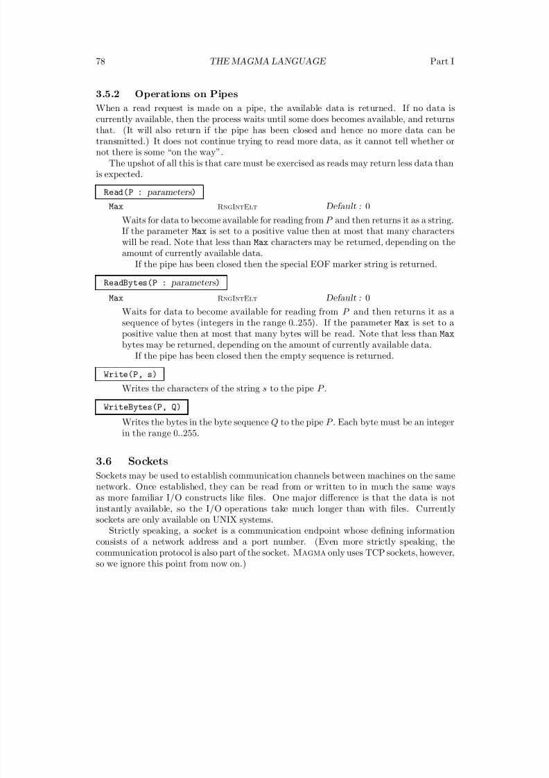
8/22/2019 Handbook Volume 01
http://slidepdf.com/reader/full/handbook-volume-01 194/440
78 THE MAGMA LANGUAGE Part I
3.5.2 Operations on Pipes
When a read request is made on a pipe, the available data is returned. If no data is
currently available, then the process waits until some does becomes available, and returnsthat. (It will also return if the pipe has been closed and hence no more data can betransmitted.) It does not continue trying to read more data, as it cannot tell whether ornot there is some “on the way”.
The upshot of all this is that care must be exercised as reads may return less data thanis expected.
Read(P : parameters )
Max RngIntElt Default : 0
Waits for data to become available for reading from P and then returns it as a string.
If the parameter Max is set to a positive value then at most that many characterswill be read. Note that less than Max characters may be returned, depending on theamount of currently available data.
If the pipe has been closed then the special EOF marker string is returned.
ReadBytes(P : parameters )
Max RngIntElt Default : 0
Waits for data to become available for reading from P and then returns it as asequence of bytes (integers in the range 0..255). If the parameter Max is set to apositive value then at most that many bytes will be read. Note that less than Max
bytes may be returned, depending on the amount of currently available data.If the pipe has been closed then the empty sequence is returned.
Write(P, s)
Writes the characters of the string s to the pipe P .
WriteBytes(P, Q)
Writes the bytes in the byte sequence Q to the pipe P . Each byte must be an integerin the range 0..255.
3.6 Sockets
Sockets may be used to establish communication channels between machines on the samenetwork. Once established, they can be read from or written to in much the same waysas more familiar I/O constructs like files. One major difference is that the data is notinstantly available, so the I/O operations take much longer than with files. Currentlysockets are only available on UNIX systems.
Strictly speaking, a socket is a communication endpoint whose defining informationconsists of a network address and a port number. (Even more strictly speaking, thecommunication protocol is also part of the socket. Magma only uses TCP sockets, however,so we ignore this point from now on.)
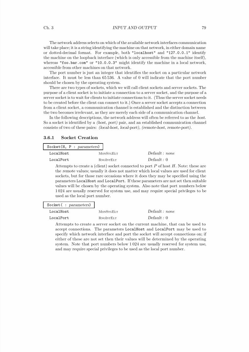
8/22/2019 Handbook Volume 01
http://slidepdf.com/reader/full/handbook-volume-01 195/440
Ch. 3 INPUT AND OUTPUT 79
The network address selects on which of the available network interfaces communicationwill take place; it is a string identifying the machine on that network, in either domain name
or dotted-decimal format. For example, both "localhost" and "127.0.0.1" identifythe machine on the loopback interface (which is only accessible from the machine itself),whereas "foo.bar.com" or "10.0.0.3" might identify the machine in a local network,accessible from other machines on that network.
The port number is just an integer that identifies the socket on a particular networkinterface. It must be less than 65 536. A value of 0 will indicate that the port numbershould be chosen by the operating system.
There are two types of sockets, which we will call client sockets and server sockets. Thepurpose of a client socket is to initiate a connection to a server socket, and the purpose of aserver socket is to wait for clients to initiate connections to it. (Thus the server socket needsto be created before the client can connect to it.) Once a server socket accepts a connectionfrom a client socket, a communication channel is established and the distinction betweenthe two becomes irrelevant, as they are merely each side of a communication channel.
In the following descriptions, the network address will often be referred to as the host.So a socket is identified by a (host, port) pair, and an established communication channelconsists of two of these pairs: (local-host, local-port), (remote-host, remote-port).
3.6.1 Socket Creation
Socket(H, P : parameters )
LocalHost MonStgElt Default : none
LocalPort RngIntElt Default : 0Attempts to create a (client) socket connected to port P of host H . Note: these arethe remote values; usually it does not matter which local values are used for clientsockets, but for those rare occasions where it does they may be specified using theparameters LocalHost and LocalPort. If these parameters are not set then suitablevalues will be chosen by the operating system. Also note that port numbers below1 024 are usually reserved for system use, and may require special privileges to beused as the local port number.
Socket( : parameters )
LocalHost MonStgElt Default : noneLocalPort RngIntElt Default : 0
Attempts to create a server socket on the current machine, that can be used toaccept connections. The parameters LocalHost and LocalPort may be used tospecify which network interface and port the socket will accept connections on; if either of these are not set then their values will be determined by the operatingsystem. Note that port numbers below 1 024 are usually reserved for system use,and may require special privileges to be used as the local port number.
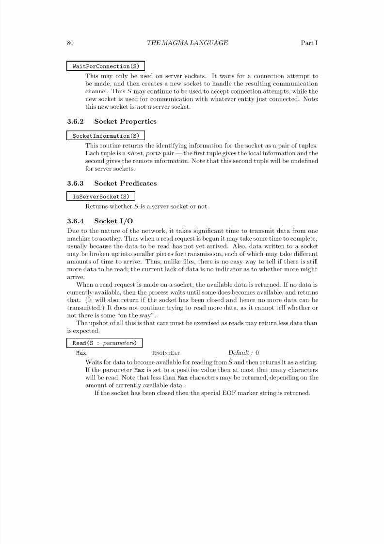
8/22/2019 Handbook Volume 01
http://slidepdf.com/reader/full/handbook-volume-01 196/440
80 THE MAGMA LANGUAGE Part I
WaitForConnection(S)
This may only be used on server sockets. It waits for a connection attempt to
be made, and then creates a new socket to handle the resulting communicationchannel. Thus S may continue to be used to accept connection attempts, while thenew socket is used for communication with whatever entity just connected. Note:this new socket is not a server socket.
3.6.2 Socket Properties
SocketInformation(S)
This routine returns the identifying information for the socket as a pair of tuples.Each tuple is a <host, port> pair — the first tuple gives the local information and the
second gives the remote information. Note that this second tuple will be undefinedfor server sockets.
3.6.3 Socket Predicates
IsServerSocket(S)
Returns whether S is a server socket or not.
3.6.4 Socket I/O
Due to the nature of the network, it takes significant time to transmit data from onemachine to another. Thus when a read request is begun it may take some time to complete,
usually because the data to be read has not yet arrived. Also, data written to a socketmay be broken up into smaller pieces for transmission, each of which may take differentamounts of time to arrive. Thus, unlike files, there is no easy way to tell if there is stillmore data to be read; the current lack of data is no indicator as to whether more mightarrive.
When a read request is made on a socket, the available data is returned. If no data iscurrently available, then the process waits until some does becomes available, and returnsthat. (It will also return if the socket has been closed and hence no more data can betransmitted.) It does not continue trying to read more data, as it cannot tell whether ornot there is some “on the way”.
The upshot of all this is that care must be exercised as reads may return less data thanis expected.
Read(S : parameters )
Max RngIntElt Default : 0
Waits for data to become available for reading from S and then returns it as a string.If the parameter Max is set to a positive value then at most that many characterswill be read. Note that less than Max characters may be returned, depending on theamount of currently available data.
If the socket has been closed then the special EOF marker string is returned.
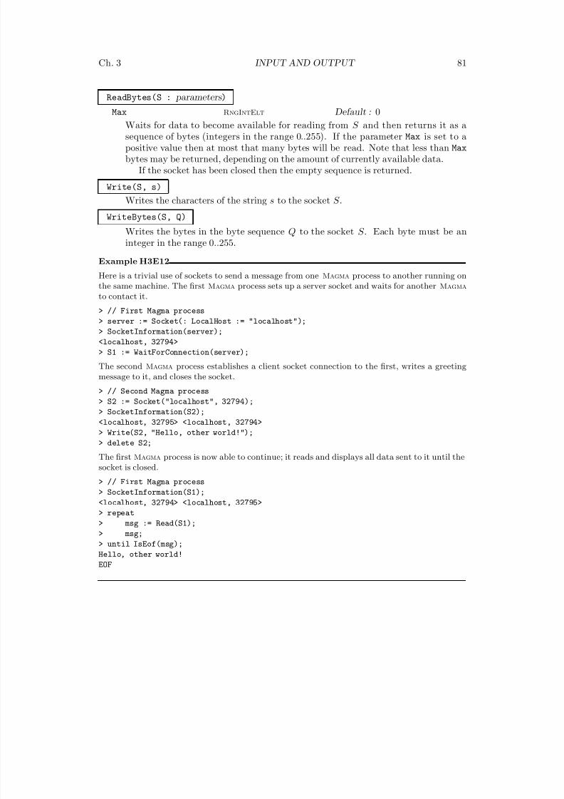
8/22/2019 Handbook Volume 01
http://slidepdf.com/reader/full/handbook-volume-01 197/440
Ch. 3 INPUT AND OUTPUT 81
ReadBytes(S : parameters )
Max RngIntElt Default : 0
Waits for data to become available for reading from S and then returns it as asequence of bytes (integers in the range 0..255). If the parameter Max is set to apositive value then at most that many bytes will be read. Note that less than Max
bytes may be returned, depending on the amount of currently available data.If the socket has been closed then the empty sequence is returned.
Write(S, s)
Writes the characters of the string s to the socket S .
WriteBytes(S, Q)
Writes the bytes in the byte sequence Q to the socket S . Each byte must be an
integer in the range 0..255.
Example H3E12
Here is a trivial use of sockets to send a message from one Magma process to another running onthe same machine. The first Magma process sets up a server socket and waits for another Magma
to contact it.
> // First Magma process
> server := Socket(: LocalHost := "localhost");
> SocketInformation(server);
<localhost, 32794>
> S1 := WaitForConnection(server);
The second Magma process establishes a client socket connection to the first, writes a greetingmessage to it, and closes the socket.
> // Second Magma process
> S2 := Socket("localhost", 32794);
> SocketInformation(S2);
<localhost, 32795> <localhost, 32794>
> Write(S2, "Hello, other world!");
> delete S2;
The first Magma process is now able to continue; it reads and displays all data sent to it until thesocket is closed.
> // First Magma process> SocketInformation(S1);
<localhost, 32794> <localhost, 32795>
> repeat
> msg := Read(S1);
> msg;
> until IsEof(msg);
Hello, other world!
EOF
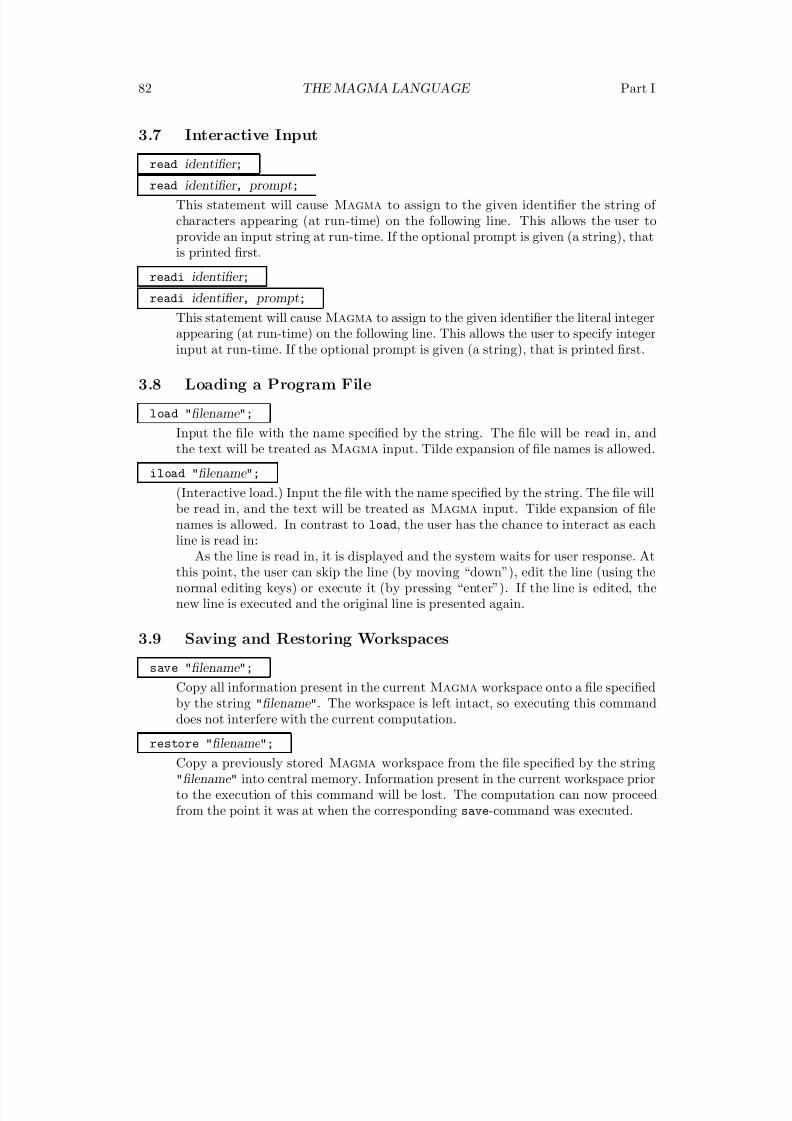
8/22/2019 Handbook Volume 01
http://slidepdf.com/reader/full/handbook-volume-01 198/440
82 THE MAGMA LANGUAGE Part I
3.7 Interactive Input
read identifier ;read identifier , prompt;
This statement will cause Magma to assign to the given identifier the string of characters appearing (at run-time) on the following line. This allows the user toprovide an input string at run-time. If the optional prompt is given (a string), thatis printed first.
readi identifier ;
readi identifier , prompt;
This statement will cause Magma to assign to the given identifier the literal integer
appearing (at run-time) on the following line. This allows the user to specify integerinput at run-time. If the optional prompt is given (a string), that is printed first.
3.8 Loading a Program File
load "filename ";
Input the file with the name specified by the string. The file will be read in, andthe text will be treated as Magma input. Tilde expansion of file names is allowed.
iload "filename ";
(Interactive load.) Input the file with the name specified by the string. The file will
be read in, and the text will be treated as Magma input. Tilde expansion of filenames is allowed. In contrast to load, the user has the chance to interact as eachline is read in:
As the line is read in, it is displayed and the system waits for user response. Atthis point, the user can skip the line (by moving “down”), edit the line (using thenormal editing keys) or execute it (by pressing “enter”). If the line is edited, thenew line is executed and the original line is presented again.
3.9 Saving and Restoring Workspaces
save "filename
";
Copy all information present in the current Magma workspace onto a file specifiedby the string "filename ". The workspace is left intact, so executing this commanddoes not interfere with the current computation.
restore "filename ";
Copy a previously stored Magma workspace from the file specified by the string"filename " into central memory. Information present in the current workspace priorto the execution of this command will be lost. The computation can now proceedfrom the point it was at when the corresponding save-command was executed.
8/22/2019 Handbook Volume 01
http://slidepdf.com/reader/full/handbook-volume-01 199/440
Ch. 3 INPUT AND OUTPUT 83
3.10 Logging a Session
SetLogFile(F)Overwrite BoolElt Default : false
Set the log file to be the file specified by the string F : all input and output will besent to this log file as well as to the terminal. If a log file is already in use, it is closedand F is used instead. By using SetLogFile(F: Overwrite := true) the file F isemptied before input and output are written onto it. See also HasOutputFile.
UnsetLogFile()
Stop logging Magma’s output.
SetEchoInput(b)
Set to true or false according to whether or not input from external files should alsobe sent to standard output.
3.11 Memory Usage
GetMemoryUsage()
Return the current memory usage of Magma (in bytes as an integer). This is theprocess data size, which does not include the executable code.
GetMaximumMemoryUsage()
Return the maximum memory usage of Magma (in bytes as an integer) which hasbeen attained since last reset (see ResetMaximumMemoryUsage). This is the maxi-mum process data size, which does not include the executable code.
ResetMaximumMemoryUsage()
Reset the value of the maximum memory usage of Magma to be the current memoryusage of Magma (see GetMaximumMemoryUsage).
3.12 System Calls
Alarm(s)A procedure which when used on UNIX systems, sends the signal SIGALRM to theMagma process after s seconds. This allows the user to specify that a Magma-process should self-destruct after a certain period.
ChangeDirectory(s)
Change to the directory specified by the string s. Tilde expansion is allowed.
GetCurrentDirectory()
Returns the current directory as a string.
8/22/2019 Handbook Volume 01
http://slidepdf.com/reader/full/handbook-volume-01 200/440
84 THE MAGMA LANGUAGE Part I
Getpid()
Returns Magma’s process ID (value of the Unix C system call getpid()).
Getuid()
Returns the user ID (value of the Unix C system call getuid()).
System(C)
Execute the system command specified by the string C . This is done by calling theC function system().
This also returns the system command’s return value as an integer. On mostUnix systems, the lower 8 bits of this value give the process status while the next 8bits give the value given by the command to the C function exit() (see the Unix
manual entries for system(3) or wait(2), for example). Thus one should normallydivide the result by 256 to get the exit value of the program on success.See also the Pipe intrinsic function.
%! shell-command
Execute the given command in the Unix shell then return to Magma. Note that thistype of shell escape (contrary to the one using a System call) takes place entirelyoutside Magma and does not show up in Magma’s history.
3.13 Creating Names
Sometimes it is necessary to create names for files from within Magma that will not clashwith the names of existing files.
Tempname(P)
Given a prefix string P , return a unique temporary name derived from P (by use of the C library function mktemp()).
8/22/2019 Handbook Volume 01
http://slidepdf.com/reader/full/handbook-volume-01 201/440
4 ENVIRONMENT AND OPTIONS
4.1 Introduction . . . . . . . . . 87
4.2 Command Line Options . . . . 87
magma -b 87 magma -c filename 87 magma -d 88 magma -n 88 magma -r workspace 88 magma -s filename 88 magma -S integer 88
4.3 Environment Variables . . . . . 89
MAGMA STARTUP FILE 89MAGMA PATH 89MAGMA MEMORY LIMIT 89MAGMA LIBRARY ROOT 89MAGMA LIBRARIES 89MAGMA SYSTEM SPEC 89MAGMA USER SPEC 89MAGMA HELP DIR 89
4.4 Set and Get . . . . . . . . . 90
SetAssertions(b) 90GetAssertions() 90SetAutoColumns(b) 90GetAutoColumns() 90SetAutoCompact(b) 90GetAutoCompact() 90SetBeep(b) 90GetBeep() 90SetColumns(n) 90GetColumns() 90GetCurrentDirectory() 90SetEchoInput(b) 91GetEchoInput() 91SetHistorySize(n) 91GetHistorySize() 91SetIgnorePrompt(b) 91GetIgnorePrompt() 91SetIgnoreSpaces(b) 91GetIgnoreSpaces() 91SetIndent(n) 91
GetIndent() 91SetLibraries(s) 91GetLibraries() 91SetLibraryRoot(s) 92GetLibraryRoot() 92SetLineEditor(b) 92GetLineEditor() 92SetLogFile(F) 92UnsetLogFile() 92SetMemoryLimit(n) 92GetMemoryLimit() 92SetOutputFile(F) 92UnsetOutputFile() 92
SetPath(s) 92GetPath() 92SetPrintLevel(l) 93GetPrintLevel() 93SetPrompt(s) 93GetPrompt() 93SetQuitOnError(b) 93SetRows(n) 93GetRows() 93SetTraceback(n) 93GetTraceback() 93SetSeed(s, c) 93GetSeed() 93GetVersion() 94
SetViMode(b) 94GetViMode() 94
4.5 Verbose Levels . . . . . . . . 94
SetVerbose(s, i) 94SetVerbose(s, b) 94GetVerbose(s) 94IsVerbose(s) 94IsVerbose(s, l) 94ListVerbose() 94ClearVerbose() 94
4.6 Other Information Procedures . 95
ShowMemoryUsage() 95
ShowIdentifiers() 95ShowValues() 95Traceback() 95ListSignatures(C) 95ListCategories() 95ListTypes() 95
4.7 History . . . . . . . . . . . 96
%p 96%pn 96%pn1 n2 96%P 96%Pn 96%Pn1 n2 96
%s 96%sn 96%sn1 n2 96%S 96%Sn 96%Sn1 n2 97% 97%n 97%n1 n2 97%e 97%en 97%en1 n2 97%! shell-command 97
8/22/2019 Handbook Volume 01
http://slidepdf.com/reader/full/handbook-volume-01 202/440
86 THE MAGMA LANGUAGE Part I
4.8 The Magma Line Editor . . . . 97
SetViMode 97
SetViMode 974.8.1 Key Bindings (Emacs and VI mode) . 98
<Return> 98<Backspace> 98<Delete> 98<Tab> 98<Ctrl>-A 98<Ctrl>-B 98<Ctrl>-C 98<Ctrl>-D 98<Ctrl>-E 98<Ctrl>-F 98<Ctrl>-H 98<Ctrl>-I 98
<Ctrl>-J 98<Ctrl>-K 98<Ctrl>-L 99<Ctrl>-M 99<Ctrl>-N 99<Ctrl>-P 99<Ctrl>-U 99<Ctrl>-Vchar 99<Ctrl>-W 99<Ctrl>-X 99<Ctrl>-Y 99<Ctrl>-Z 99<Ctrl>- 100<Ctrl>-\ 100
4.8.2 Key Bindings in Emacs mode only . 100
Mb 100MB 100Mf 100MF 100
4.8.3 Key Bindings in VI mode only . . 100
0 100$ 100<Ctrl>-space 100% 100; 100, 100B 101
b 101
E 101e 101Fchar 101fchar 101h 101H 101l 101L 101Tchar 101tchar 101w 101W 101A 102a 102C 102crange 102D 102
drange 102I 102i 102j 102k 102P 102p 102R 102rchar 102S 102s 103U 103u 103X 103
x 103Y 103yrange 103
4.9 The Magma Help System . . . 103
SetHelpExternalBrowser(S, T) 104SetHelpExternalBrowser(S) 104SetHelpUseExternalBrowser(b) 104SetHelpExternalSystem(s) 104SetHelpUseExternalSystem(b) 105GetHelpExternalBrowser() 105GetHelpExternalSystem() 105GetHelpUseExternal() 105
4.9.1 Internal Help Browser . . . . . . 105
8/22/2019 Handbook Volume 01
http://slidepdf.com/reader/full/handbook-volume-01 203/440
Chapter 4
ENVIRONMENT AND OPTIONS
4.1 Introduction
This chapter describes the environmental features of Magma, together with options whichcan be specified at start-up on the command line, or within Magma by the Set- proce-dures. The history and line-editor features of Magma are also described.
4.2 Command Line OptionsWhen starting up Magma, various command-line options can be supplied, and a list of files to be automatically loaded can also be specified. These files may be specified by simplylisting their names as normal arguments (i.e., without a - option) following the Magma
command. For each such file name, a search for the specified file is conducted, starting inthe current directory, and in directories specified by the environment variable MAGMA PATH
after that if necessary. It is also possible to have a startup file , in which one would usuallystore personal settings of parameters and variables. The startup file is specified by theMAGMA STARTUP FILE environment variable which should be set in the user’s .cshrc file orsimilar. This environment variable can be overridden by the -s option, or cancelled by the
-n option. The files specified by the arguments to Magma are loaded after the startupfile. Thus the startup file is not cancelled by giving extra file arguments, which is what isusually desired.
Magma also allows one to set variables from the command line — if one of the argu-ments is of the form var :=val , where var is a valid identifier (consisting of letters, under-scores, or non-initial digits) and there is no space between var and the :=, then the variablevar is assigned within Magma to the string value val at the point where that argumentis processed. (Functions like StringToInteger should be used to convert the value to anobject of another type once inside Magma.)
magma -b
If the -b argument is given to Magma, the opening banner and all other introduc-tory messages are suppressed. The final “total time” message is also suppressed.This is useful when sending the whole output of a Magma process to a file so thatextra removing of unwanted output is not needed.
magma -c filename
If the -c argument is given to Magma, followed by a filename, the filename is as-sumed to refer to a package source file and the package is compiled and Magma thenexits straight away. This option is rarely needed since packages are automaticallycompiled when attached.
8/22/2019 Handbook Volume 01
http://slidepdf.com/reader/full/handbook-volume-01 204/440
88 THE MAGMA LANGUAGE Part I
magma -d
If the -d option is supplied to Magma, the licence for the current magmapassfile
is dumped. That is, the expiry date and the valid hostids are displayed. Magma
then exits.
magma -n
If the -n option is supplied to Magma, any startup file specified by the environmentvariable MAGMA STARTUP FILE or by the -s option is cancelled.
magma -r workspace
If the -r option is supplied to Magma, together with a workspace file, thatworkspace is automatically restored by Magma when it starts up.
magma -s filename
If the -s option is supplied to Magma, the given filename is used for thestartup file for Magma. This overrides the variable of the environment variableMAGMA STARTUP FILE if it has been set. This option should not be used (as it wasbefore), for automatically loading files since that can be done by just listing themas arguments to the Magma process.
magma -S integer
When starting up Magma, it is possible to specify a seed for the generation of
pseudo-random numbers. (Pseudo-random quantities are used in several Magmaalgorithms, and may also be generated explicitly by some intrinsics.) The seedshould be in the range 0 to (232 − 1) inclusive. If -S is not followed by any number,or if the -S option is not used, Magma selects the seed itself.
Example H4E1
By typing the command
magma file1 x:=abc file2
Magma would start up, read the user’s startup file specified by MAGMA STARTUP FILE if existent,then read the file file1, then assign the variable x to the string value "abc", then read the file
file2, then give the prompt.
8/22/2019 Handbook Volume 01
http://slidepdf.com/reader/full/handbook-volume-01 205/440
Ch. 4 ENVIRONMENT AND OPTIONS 89
4.3 Environment Variables
This section lists some environment variables used by Magma. These variables are setby an appropriate operating system command and are used to define various search pathsand other run-time options.
MAGMA STARTUP FILE
The name of the default start-up file. It can be overridden by the magma -s com-mand.
MAGMA PATH
Search path for files that are loaded (a colon separated list of directories). It need notinclude directories for the libraries, just personal directories. This path is searchedbefore the library directories.
MAGMA MEMORY LIMIT
Limit on the size of the memory that may be used by a Magma-session (in bytes).
MAGMA LIBRARY ROOT
The root directory for the Magma libraries (by supplying an absolute path name).From within Magma SetLibraryRoot and GetLibraryRoot can be used to changeand view the value.
MAGMA LIBRARIESGive a list of Magma libraries (as a colon separated list of sub-directories of thelibrary root directory). From within Magma SetLibraries and GetLibraries canbe used to change and view the value.
MAGMA SYSTEM SPEC
The Magma system spec file containing the system packages automatically attachedat start-up.
MAGMA USER SPEC
The personal user spec file containing the user packages automatically attached atstart-up.
MAGMA HELP DIR
The root directory for the Magma help files.
8/22/2019 Handbook Volume 01
http://slidepdf.com/reader/full/handbook-volume-01 206/440
90 THE MAGMA LANGUAGE Part I
4.4 Set and Get
The Set- procedures allow the user to attach values to certain environment variables. The
Get- functions enable one to obtain the current values of these variables.
SetAssertions(b)
GetAssertions()
Controls the checking of assertions (see the assert statement in the chapter on thelanguage). Default is SetAssertions(true).
SetAutoColumns(b)
GetAutoColumns()
If enabled, the IO system will try to determine the number of columns in the win-
dow by using ioctl(); when a window change or a stop/cont occurs, the Columnsvariable (below) will be automatically updated. If disabled, the Columns vari-able will only be changed when explicitly done so by SetColumns. Default isSetAutoColumns(true).
SetAutoCompact(b)
GetAutoCompact()
Control whether automatic compaction is performed. Normally the memory man-ager of Magma will compact all of its memory between each statement at the toplevel. This removes fragmentation and reduces excessive memory usage. In somevery rare situations, the compactions may become very slow (one symptom is thatan inordinate pause occurs between prompts when only a trivial operation or noth-ing is done). In such cases, turning the automatic compaction off may help (at thecost of possibly more use of memory). Default is SetAutoCompact(true).
SetBeep(b)
GetBeep()
Controls ‘beeps’. Default is SetBeep(true).
SetColumns(n)
GetColumns()
Controls the number of columns used by the IO system. This affects the line editorand the output system. (As explained above, if AutoColumns is on, this variablewill be automatically determined.) The number of columns will determine howwords are wrapped. If set to 0, word wrap is not performed. The default value isSetColumns(80) (unless SetAutoColumns(true)).
GetCurrentDirectory()
Returns the current directory as a string. (Use ChangeDirectory(s) to change theworking directory.)
8/22/2019 Handbook Volume 01
http://slidepdf.com/reader/full/handbook-volume-01 207/440
Ch. 4 ENVIRONMENT AND OPTIONS 91
SetEchoInput(b)
GetEchoInput()
Set to true or false according to whether or not input from external files shouldalso be sent to standard output.
SetHistorySize(n)
GetHistorySize()
Controls the number of lines saved in the history. If the number is set to 0, nohistory is preserved.
SetIgnorePrompt(b)
GetIgnorePrompt()
Controls the option to ignore the prompt to allow the pasting of input lines backin. If enabled, any leading ’>’ characters (possibly separated by white space) areignored by the history system when the input file is a terminal, unless the lineconsists of the ’>’ character alone (without a following space), which could notcome from a prompt since in a prompt a space or another character follows a ’>’.Default is SetIgnorePrompt(false).
SetIgnoreSpaces(b)
GetIgnoreSpaces()
Controls the option to ignore spaces when searching in the line editor. If the user
moves up or down in the line editor using <Ctrl>-P or <Ctrl>-N (see the line editorkey descriptions) and if the cursor is not at the beginning of the line, a search ismade forwards or backwards, respectively, to the first line which starts with thesame string as the string consisting of all the characters before the cursor. Whiledoing the search, spaces are ignored if and only if this option is on (value true).Default is SetIgnoreSpaces(true).
SetIndent(n)
GetIndent()
Controls the indentation level for formatting output. The default is SetIndent(4).
SetLibraries(s)
GetLibraries()
Controls the Magma library directories via environment variable MAGMA LIBRARIES.The procedure SetLibraries takes a string, which will be taken as the (colon-separated) list of sub-directories in the library root directory for the libraries; thefunction GetLibraryRoot returns the current value as a string. These directorieswill be searched when you try to load a file; note however that first the directoriesindicated by the current value of your path environment variable MAGMA PATH willbe searched. See SetLibraryRoot for the root directory.
8/22/2019 Handbook Volume 01
http://slidepdf.com/reader/full/handbook-volume-01 208/440
92 THE MAGMA LANGUAGE Part I
SetLibraryRoot(s)
GetLibraryRoot()
Controls the root directory for the Magma libraries, via the environment variableMAGMA LIBRARY ROOT. The procedure SetLibraryRoot takes a string, which will bethe absolute pathname for the root of the libraries; the function GetLibraryRoot
returns the current value as a string. See also SetLibraries
SetLineEditor(b)
GetLineEditor()
Controls the line editor. Default is SetLineEditor(true).
SetLogFile(F)
Overwrite BoolElt Default : false
UnsetLogFile()
Procedure. Set the log file to be the file specified by the string F : all input andoutput will be sent to this log file as well as to the terminal. If a log file is alreadyin use, it is closed and F is used instead. The parameter Overwrite can be used toindicate that the file should be truncated before writing input and output on it; bydefault the file is appended.
SetMemoryLimit(n)
GetMemoryLimit()
Set the limit (in bytes) of the memory which the memory manager will allocate (nolimit if 0). Default is SetMemoryLimit(0).
SetOutputFile(F)
Overwrite BoolElt Default : false
UnsetOutputFile()
Start/stop redirecting all Magma output to a file (specified by the string F ). Theparameter Overwrite can be used to indicate that the file should be truncated
before writing output on it.
SetPath(s)
GetPath()
Controls the path by which the searching of files is done. The path consists of a colonseparated list of directories which are searched in order (“.” implicitly assumed atthe front). Tilde expansion is done on each directory. (May be overridden by theenvironment variable MAGMA PATH.)
8/22/2019 Handbook Volume 01
http://slidepdf.com/reader/full/handbook-volume-01 209/440
Ch. 4 ENVIRONMENT AND OPTIONS 93
SetPrintLevel(l)
GetPrintLevel()
Controls the global printing level, which is one of "Minimal", "Magma", "Maximal","Default". Default is SetPrintLevel("Default").
SetPrompt(s)
GetPrompt()
Controls the terminal prompt (a string). Expansion of the following % escapesoccurs:
%% The character %
%h The current history line number.
%S The parser ‘state’: when a new line is about to be read while the parserhas only seen incomplete statements, the state consists of a stack of wordslike “if”, “while”, indicating the incomplete statements.
%s Like %S except that only the topmost word is displayed.
Default is SetPrompt("%S> ").
SetQuitOnError(b)
Set whether Magma should quit on any error to b. If b is true, Magma
will completely quit when any error (syntax, runtime, etc.) occurs. Default isSetQuitOnError(false).
SetRows(n)
GetRows()
Controls the number of rows in a page used by the IO system. This affects theoutput system. If set to 0, paging is not performed. Otherwise a prompt is givenafter the given number of rows for a new page. The default value is SetRows(0).
SetTraceback(n)
GetTraceback()
Controls whether Magma should produce a traceback of user function calls beforeeach error message. The default value is SetTraceback(true).
SetSeed(s, c)
GetSeed()
Controls the initialization seed and step number for pseudo-random number gener-ation. For details, see the section on random object generation in the chapter onstatements and expressions.
8/22/2019 Handbook Volume 01
http://slidepdf.com/reader/full/handbook-volume-01 210/440
94 THE MAGMA LANGUAGE Part I
GetVersion()
Return integers x, y and z such the current version of Magma is Vx.y–z.
SetViMode(b)
GetViMode()
Controls the type of line editor used: Emacs (false) or VI style. Default isSetViMode(false).
4.5 Verbose Levels
By turning verbose printing on for certain modules within Magma, some information oncomputations that are performed can be obtained. For each option, the verbosity may
have different levels. The default is level 0 for each option.There are also 5 slots available for user-defined verbose flags. The flags can be set inuser programs by SetVerbose("Usern", true) where n should be one of 1, 2, 3, 4, 5, andthe current setting is returned by GetVerbose("Usern").
SetVerbose(s, i)
SetVerbose(s, b)
Set verbose level for s to be level i or b. Here the argument s must be a string. Theverbosity may have different levels. An integer i for the second argument selects theappropriate level. A second argument i of 0 or b of false means no verbosity. Aboolean value for b of true for the second argument selects level 1. (See above forthe valid values for the string s).
GetVerbose(s)
Return the value of verbose flag s as an integer. (See above for the valid values forthe string s).
IsVerbose(s)
Return the whether the value of verbose flag s is non-zero. (See above for the validvalues for the string s).
IsVerbose(s, l)Return the whether the value of verbose flag s is greater than or equal to l. (Seeabove for the valid values for the string s).
ListVerbose()
List all verbose flags. That is, print each verbose flag and its maximal level.
ClearVerbose()
Clear all verbose flags. That is, set the level for all verbose flags to 0.
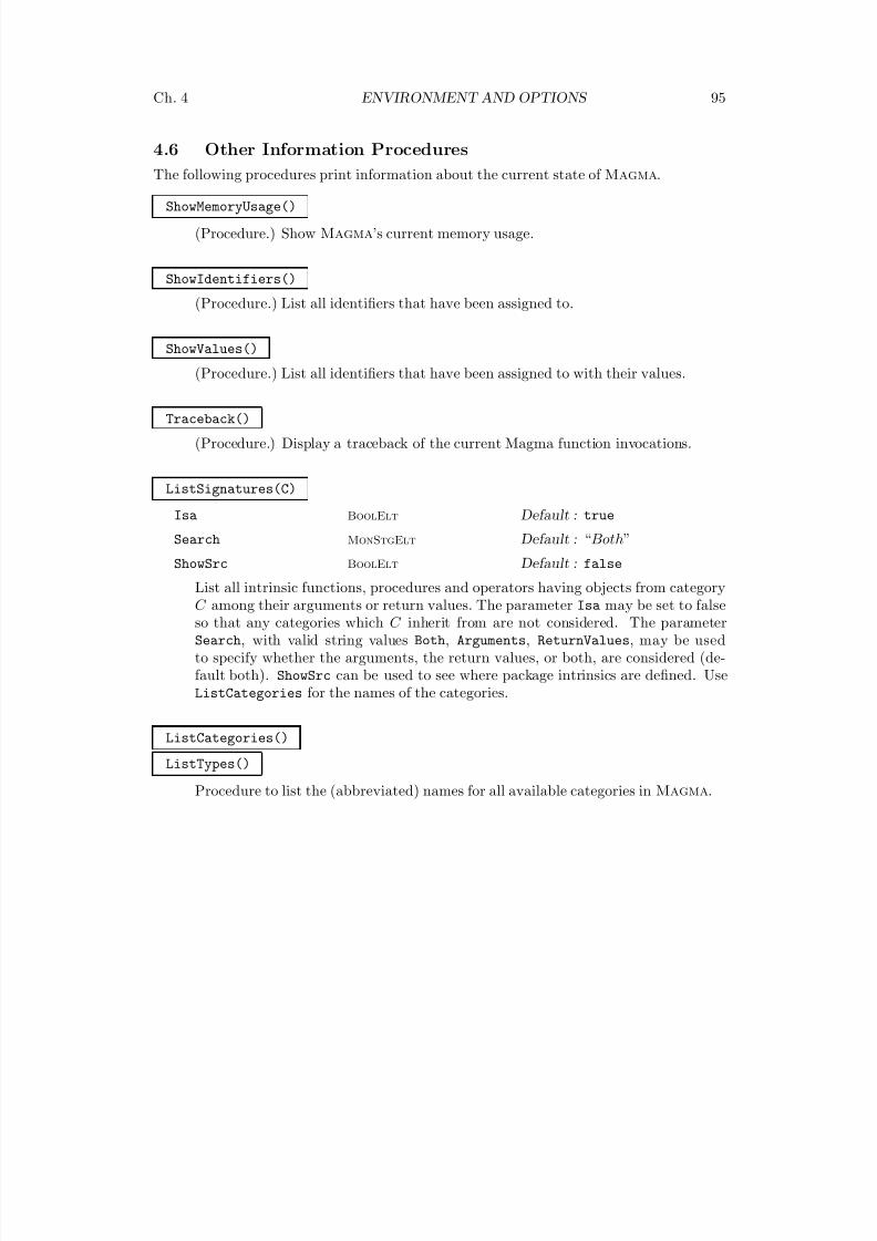
8/22/2019 Handbook Volume 01
http://slidepdf.com/reader/full/handbook-volume-01 211/440
Ch. 4 ENVIRONMENT AND OPTIONS 95
4.6 Other Information Procedures
The following procedures print information about the current state of Magma.
ShowMemoryUsage()
(Procedure.) Show Magma’s current memory usage.
ShowIdentifiers()
(Procedure.) List all identifiers that have been assigned to.
ShowValues()
(Procedure.) List all identifiers that have been assigned to with their values.
Traceback()
(Procedure.) Display a traceback of the current Magma function invocations.
ListSignatures(C)
Isa BoolElt Default : true
Search MonStgElt Default : “Both”
ShowSrc BoolElt Default : false
List all intrinsic functions, procedures and operators having objects from categoryC among their arguments or return values. The parameter Isa may be set to falseso that any categories which C inherit from are not considered. The parameterSearch, with valid string values Both, Arguments, ReturnValues, may be usedto specify whether the arguments, the return values, or both, are considered (de-fault both). ShowSrc can be used to see where package intrinsics are defined. UseListCategories for the names of the categories.
ListCategories()
ListTypes()
Procedure to list the (abbreviated) names for all available categories in Magma.
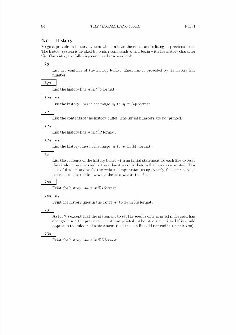
8/22/2019 Handbook Volume 01
http://slidepdf.com/reader/full/handbook-volume-01 212/440
96 THE MAGMA LANGUAGE Part I
4.7 History
Magma provides a history system which allows the recall and editing of previous lines.
The history system is invoked by typing commands which begin with the history character‘%’. Currently, the following commands are available.
%p
List the contents of the history buffer. Each line is preceded by its history linenumber.
%pn
List the history line n in %p format.
%pn1 n2
List the history lines in the range n1 to n2 in %p format.
%P
List the contents of the history buffer. The initial numbers are not printed.
%Pn
List the history line n in %P format.
%Pn1 n2
List the history lines in the range n1 to n2 in %P format.
%s
List the contents of the history buffer with an initial statement for each line to resetthe random number seed to the value it was just before the line was executed. Thisis useful when one wishes to redo a computation using exactly the same seed asbefore but does not know what the seed was at the time.
%sn
Print the history line n in %s format.
%sn1 n2
Print the history lines in the range n1 to n2 in %s format.
%S
As for %s except that the statement to set the seed is only printed if the seed haschanged since the previous time it was printed. Also, it is not printed if it wouldappear in the middle of a statement (i.e., the last line did not end in a semicolon).
%Sn
Print the history line n in %S format.
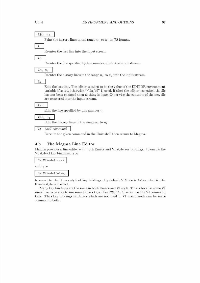
8/22/2019 Handbook Volume 01
http://slidepdf.com/reader/full/handbook-volume-01 213/440
Ch. 4 ENVIRONMENT AND OPTIONS 97
%Sn1 n2
Print the history lines in the range n1 to n2 in %S format.
%
Reenter the last line into the input stream.
%n
Reenter the line specified by line number n into the input stream.
%n1 n2
Reenter the history lines in the range n1 to n2 into the input stream.
%e
Edit the last line. The editor is taken to be the value of the EDITOR environmentvariable if is set, otherwise “/bin/ed” is used. If after the editor has exited the filehas not been changed then nothing is done. Otherwise the contents of the new fileare reentered into the input stream.
%en
Edit the line specified by line number n.
%en1 n2
Edit the history lines in the range n1 to n2.
%! shell-command
Execute the given command in the Unix shell then return to Magma.
4.8 The Magma Line Editor
Magma provides a line editor with both Emacs and VI style key bindings. To enable theVI style of key bindings, type
SetViMode(true)
and type
SetViMode(false)
to revert to the Emacs style of key bindings. By default ViMode is false; that is, theEmacs style is in effect.
Many key bindings are the same in both Emacs and VI style. This is because some VIusers like to be able to use some Emacs keys (like <Ctrl>-P) as well as the VI commandkeys. Thus key bindings in Emacs which are not used in VI insert mode can be madecommon to both.
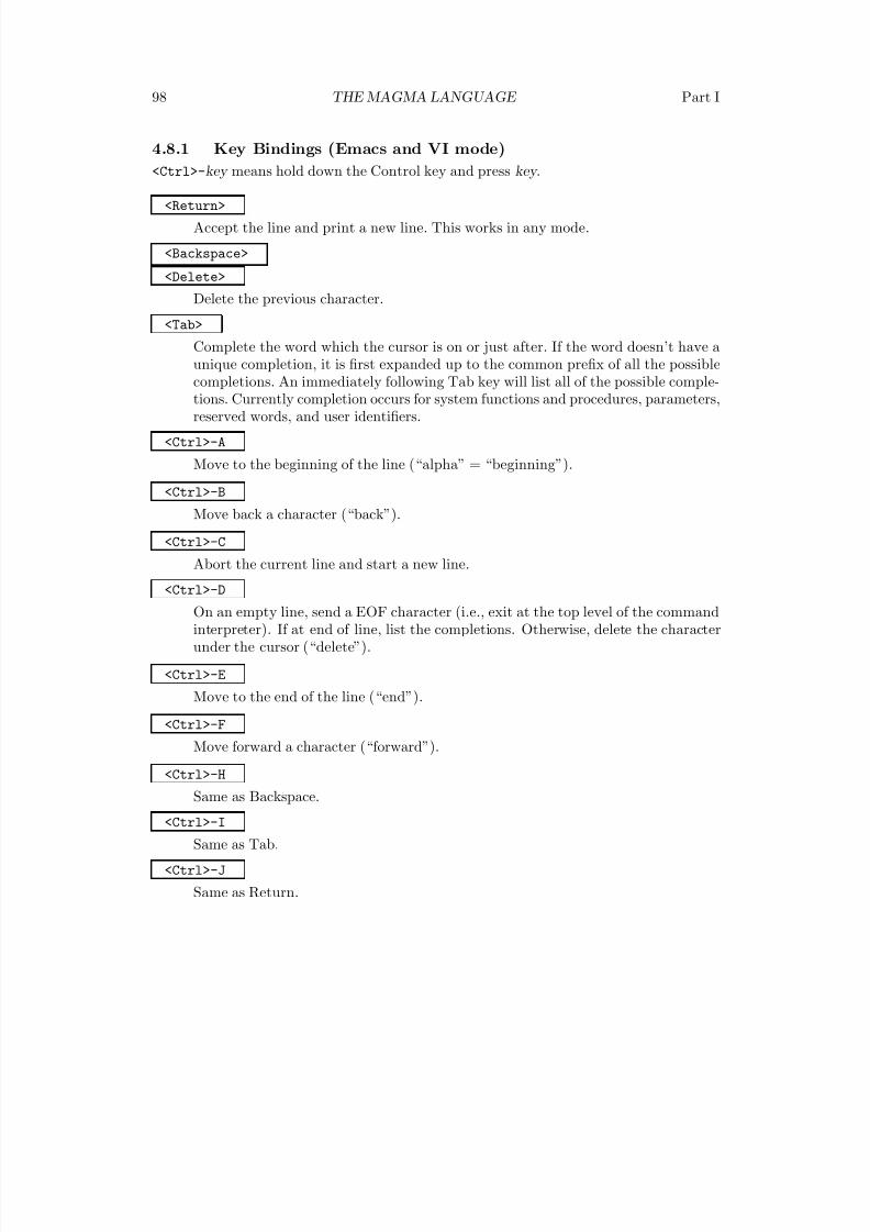
8/22/2019 Handbook Volume 01
http://slidepdf.com/reader/full/handbook-volume-01 214/440
98 THE MAGMA LANGUAGE Part I
4.8.1 Key Bindings (Emacs and VI mode)
<Ctrl>-key means hold down the Control key and press key .
<Return>
Accept the line and print a new line. This works in any mode.
<Backspace>
<Delete>
Delete the previous character.
<Tab>
Complete the word which the cursor is on or just after. If the word doesn’t have a
unique completion, it is first expanded up to the common prefix of all the possiblecompletions. An immediately following Tab key will list all of the possible comple-tions. Currently completion occurs for system functions and procedures, parameters,reserved words, and user identifiers.
<Ctrl>-A
Move to the beginning of the line (“alpha” = “beginning”).
<Ctrl>-B
Move back a character (“back”).
<Ctrl>-C
Abort the current line and start a new line.
<Ctrl>-D
On an empty line, send a EOF character (i.e., exit at the top level of the commandinterpreter). If at end of line, list the completions. Otherwise, delete the characterunder the cursor (“delete”).
<Ctrl>-E
Move to the end of the line (“end”).
<Ctrl>-F
Move forward a character (“forward”).
<Ctrl>-H
Same as Backspace.
<Ctrl>-I
Same as Tab.
<Ctrl>-J
Same as Return.
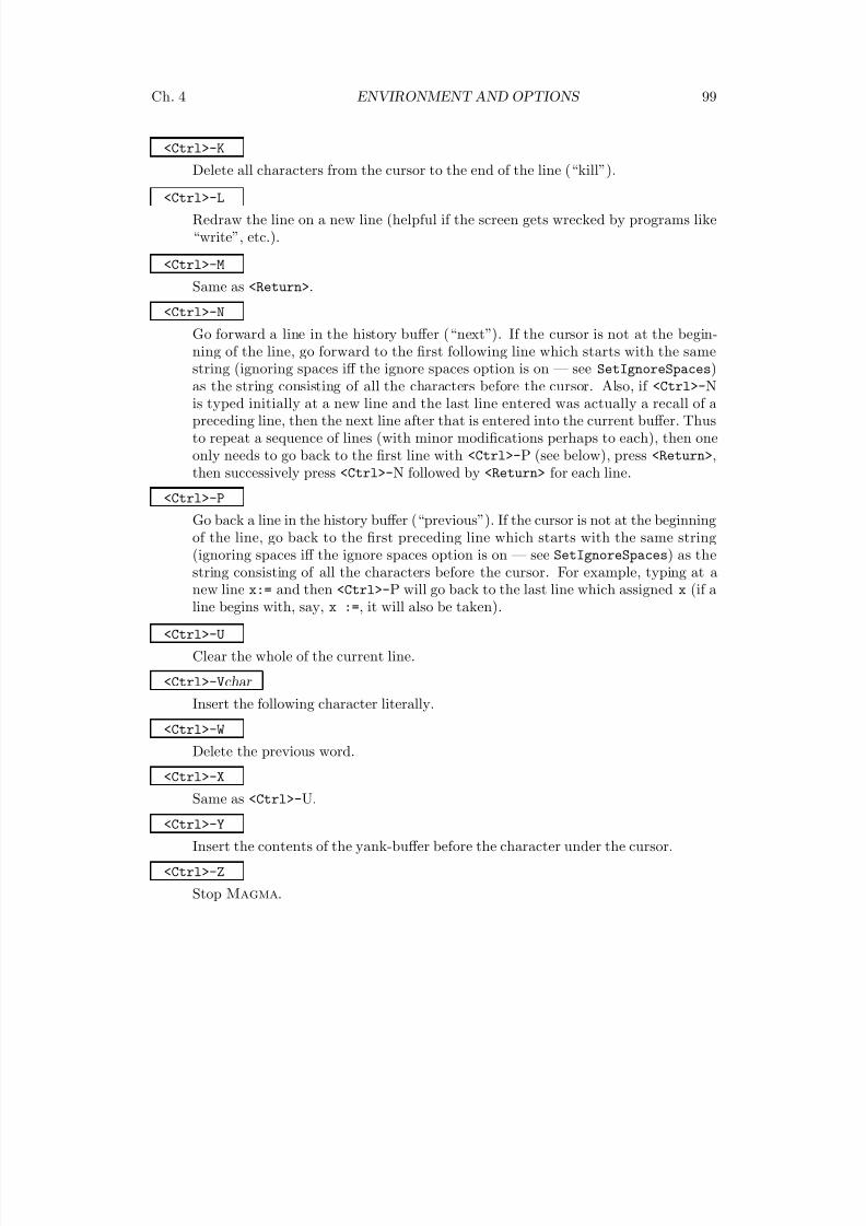
8/22/2019 Handbook Volume 01
http://slidepdf.com/reader/full/handbook-volume-01 215/440
Ch. 4 ENVIRONMENT AND OPTIONS 99
<Ctrl>-K
Delete all characters from the cursor to the end of the line (“kill”).
<Ctrl>-L
Redraw the line on a new line (helpful if the screen gets wrecked by programs like“write”, etc.).
<Ctrl>-M
Same as <Return>.
<Ctrl>-N
Go forward a line in the history buffer (“next”). If the cursor is not at the begin-ning of the line, go forward to the first following line which starts with the same
string (ignoring spaces iff the ignore spaces option is on — see SetIgnoreSpaces)as the string consisting of all the characters before the cursor. Also, if <Ctrl>-Nis typed initially at a new line and the last line entered was actually a recall of apreceding line, then the next line after that is entered into the current buffer. Thusto repeat a sequence of lines (with minor modifications perhaps to each), then oneonly needs to go back to the first line with <Ctrl>-P (see below), press <Return>,then successively press <Ctrl>-N followed by <Return> for each line.
<Ctrl>-P
Go back a line in the history buffer (“previous”). If the cursor is not at the beginningof the line, go back to the first preceding line which starts with the same string
(ignoring spaces iff the ignore spaces option is on — see SetIgnoreSpaces) as thestring consisting of all the characters before the cursor. For example, typing at anew line x:= and then <Ctrl>-P will go back to the last line which assigned x (if aline begins with, say, x :=, it will also be taken).
<Ctrl>-U
Clear the whole of the current line.
<Ctrl>-Vchar
Insert the following character literally.
<Ctrl>-W
Delete the previous word.
<Ctrl>-X
Same as <Ctrl>-U.
<Ctrl>-Y
Insert the contents of the yank-buffer before the character under the cursor.
<Ctrl>-Z
Stop Magma.
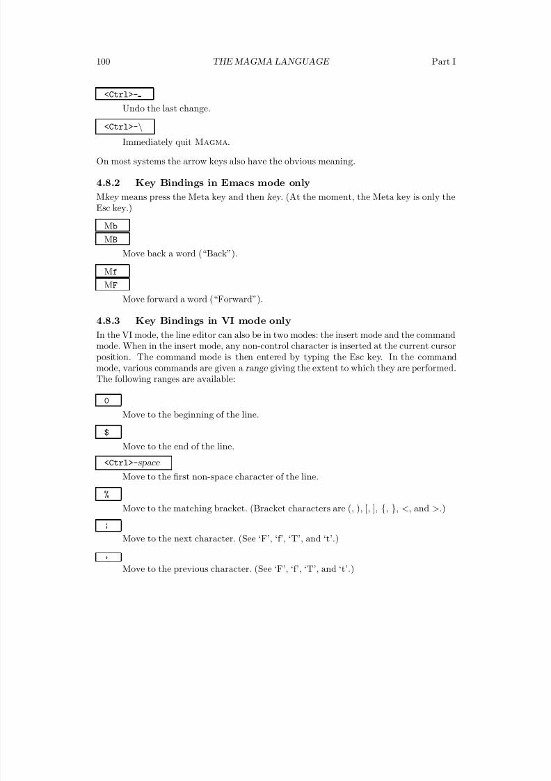
8/22/2019 Handbook Volume 01
http://slidepdf.com/reader/full/handbook-volume-01 216/440
100 THE MAGMA LANGUAGE Part I
<Ctrl>-
Undo the last change.
<Ctrl>-\
Immediately quit Magma.
On most systems the arrow keys also have the obvious meaning.
4.8.2 Key Bindings in Emacs mode only
Mkey means press the Meta key and then key . (At the moment, the Meta key is only theEsc key.)
Mb
MB
Move back a word (“Back”).
Mf
MF
Move forward a word (“Forward”).
4.8.3 Key Bindings in VI mode only
In the VI mode, the line editor can also be in two modes: the insert mode and the commandmode. When in the insert mode, any non-control character is inserted at the current cursorposition. The command mode is then entered by typing the Esc key. In the commandmode, various commands are given a range giving the extent to which they are performed.The following ranges are available:
0
Move to the beginning of the line.
$
Move to the end of the line.
<Ctrl>-space
Move to the first non-space character of the line.
%
Move to the matching bracket. (Bracket characters are (, ), [, ], {, }, <, and >.)
;
Move to the next character. (See ‘F’, ‘f’, ‘T’, and ‘t’.)
,
Move to the previous character. (See ‘F’, ‘f’, ‘T’, and ‘t’.)
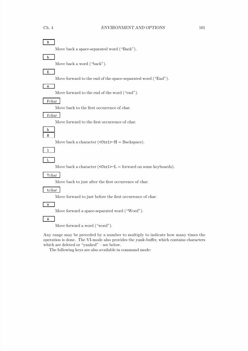
8/22/2019 Handbook Volume 01
http://slidepdf.com/reader/full/handbook-volume-01 217/440
Ch. 4 ENVIRONMENT AND OPTIONS 101
B
Move back a space-separated word (“Back”).
b
Move back a word (“back”).
E
Move forward to the end of the space-separated word (“End”).
e
Move forward to the end of the word (“end”).
Fchar
Move back to the first occurrence of char .
fchar
Move forward to the first occurrence of char .
h
H
Move back a character (<Ctrl>-H = Backspace).
l
L
Move back a character (<Ctrl>-L = forward on some keyboards).
Tchar
Move back to just after the first occurrence of char .
tchar
Move forward to just before the first occurrence of char .
w
Move forward a space-separated word (“Word”).
W
Move forward a word (“word”).
Any range may be preceded by a number to multiply to indicate how many times theoperation is done. The VI-mode also provides the yank-buffer , which contains characterswhich are deleted or “yanked” – see below.
The following keys are also available in command mode:
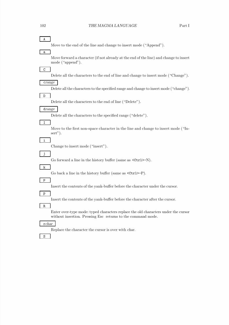
8/22/2019 Handbook Volume 01
http://slidepdf.com/reader/full/handbook-volume-01 218/440
102 THE MAGMA LANGUAGE Part I
A
Move to the end of the line and change to insert mode (“Append”).
a
Move forward a character (if not already at the end of the line) and change to insertmode (“append”).
C
Delete all the characters to the end of line and change to insert mode (“Change”).
crange
Delete all the characters to the specified range and change to insert mode (“change”).
DDelete all the characters to the end of line (“Delete”).
drange
Delete all the characters to the specified range (“delete”).
I
Move to the first non-space character in the line and change to insert mode (“In-sert”).
i
Change to insert mode (“insert”).
j
Go forward a line in the history buffer (same as <Ctrl>-N).
k
Go back a line in the history buffer (same as <Ctrl>-P).
P
Insert the contents of the yank-buffer before the character under the cursor.
p
Insert the contents of the yank-buffer before the character after the cursor.
R
Enter over-type mode: typed characters replace the old characters under the cursorwithout insertion. Pressing Esc returns to the command mode.
rchar
Replace the character the cursor is over with char .
S
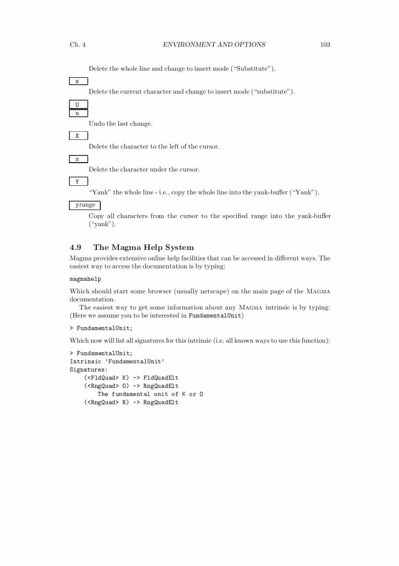
8/22/2019 Handbook Volume 01
http://slidepdf.com/reader/full/handbook-volume-01 219/440
Ch. 4 ENVIRONMENT AND OPTIONS 103
Delete the whole line and change to insert mode (“Substitute”).
s
Delete the current character and change to insert mode (“substitute”).
U
u
Undo the last change.
X
Delete the character to the left of the cursor.
x
Delete the character under the cursor.Y
“Yank” the whole line - i.e., copy the whole line into the yank-buffer (“Yank”).
yrange
Copy all characters from the cursor to the specified range into the yank-buffer(“yank”).
4.9 The Magma Help System
Magma provides extensive online help facilities that can be accessed in different ways. Theeasiest way to access the documentation is by typing:
magmahelp
Which should start some browser (usually netscape) on the main page of the Magma
documentation.The easiest way to get some information about any Magma intrinsic is by typing:
(Here we assume you to be interested in FundamentalUnit)
> FundamentalUnit;
Which now will list all signatures for this intrinsic (i.e. all known ways to use this function):
> FundamentalUnit;
Intrinsic ’FundamentalUnit’
Signatures:
(<FldQuad> K) -> FldQuadElt
(<RngQuad> O) -> RngQuadElt
The fundamental unit of K or O
(<RngQuad> R) -> RngQuadElt
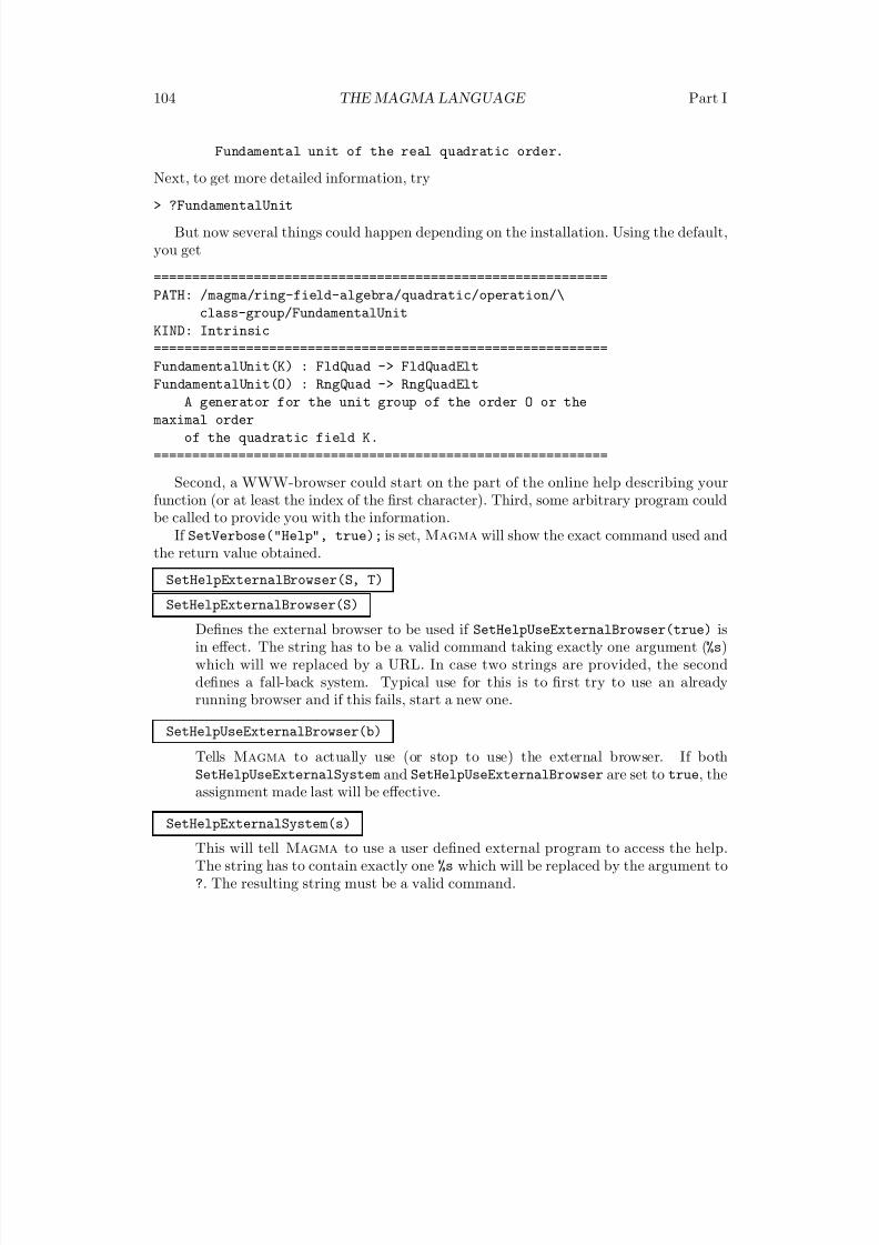
8/22/2019 Handbook Volume 01
http://slidepdf.com/reader/full/handbook-volume-01 220/440
104 THE MAGMA LANGUAGE Part I
Fundamental unit of the real quadratic order.
Next, to get more detailed information, try
> ?FundamentalUnit
But now several things could happen depending on the installation. Using the default,you get
===========================================================
PATH: /magma/ring-field-algebra/quadratic/operation/\
class-group/FundamentalUnit
KIND: Intrinsic
===========================================================
FundamentalUnit(K) : FldQuad -> FldQuadElt
FundamentalUnit(O) : RngQuad -> RngQuadElt
A generator for the unit group of the order O or the
maximal order
of the quadratic field K.
===========================================================
Second, a WWW-browser could start on the part of the online help describing yourfunction (or at least the index of the first character). Third, some arbitrary program couldbe called to provide you with the information.
If SetVerbose("Help", true); is set, Magma will show the exact command used andthe return value obtained.
SetHelpExternalBrowser(S, T)
SetHelpExternalBrowser(S)
Defines the external browser to be used if SetHelpUseExternalBrowser(true) isin effect. The string has to be a valid command taking exactly one argument (%s)which will we replaced by a URL. In case two strings are provided, the seconddefines a fall-back system. Typical use for this is to first try to use an alreadyrunning browser and if this fails, start a new one.
SetHelpUseExternalBrowser(b)
Tells Magma to actually use (or stop to use) the external browser. If bothSetHelpUseExternalSystem and SetHelpUseExternalBrowser are set to true, theassignment made last will be effective.
SetHelpExternalSystem(s)
This will tell Magma to use a user defined external program to access the help.The string has to contain exactly one %s which will be replaced by the argument to?. The resulting string must be a valid command.
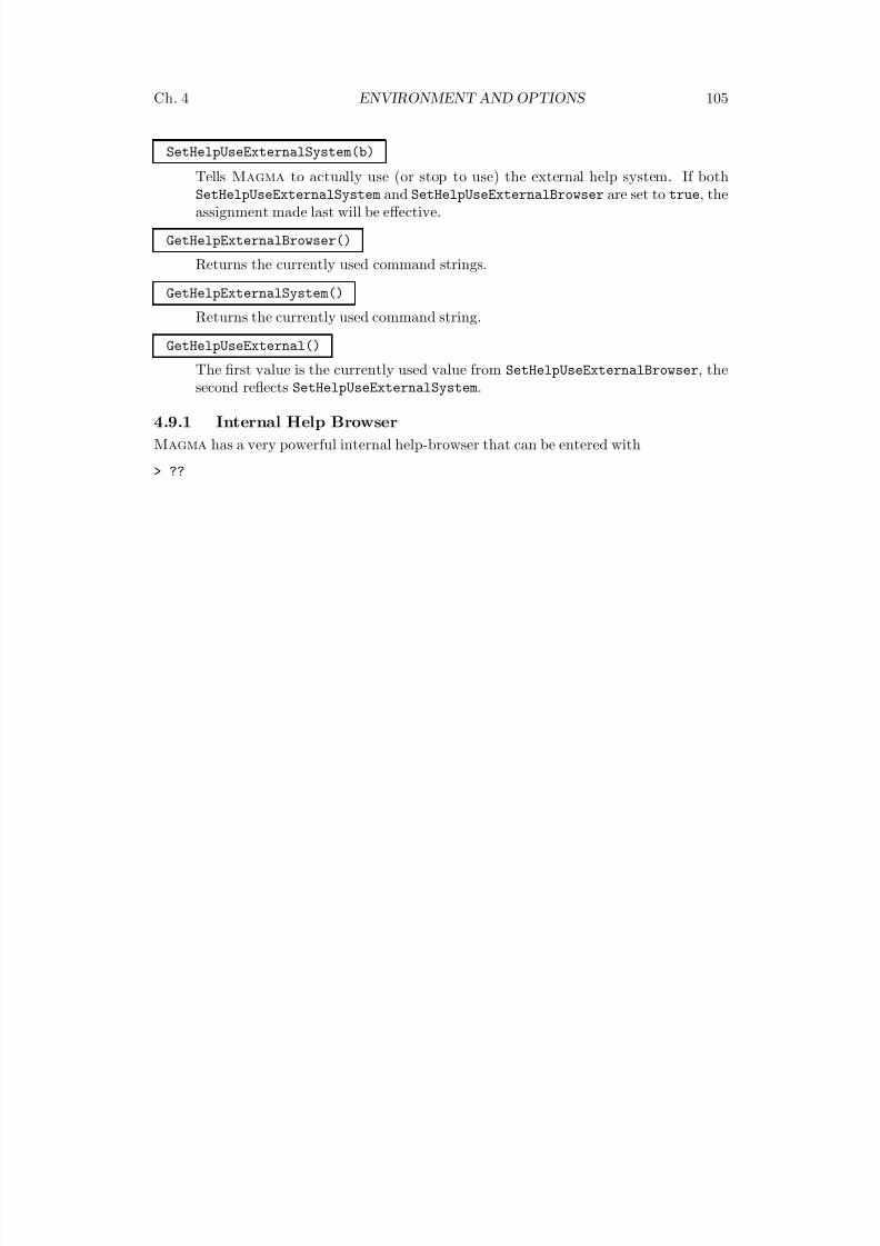
8/22/2019 Handbook Volume 01
http://slidepdf.com/reader/full/handbook-volume-01 221/440
Ch. 4 ENVIRONMENT AND OPTIONS 105
SetHelpUseExternalSystem(b)
Tells Magma to actually use (or stop to use) the external help system. If bothSetHelpUseExternalSystem and SetHelpUseExternalBrowser are set to true, theassignment made last will be effective.
GetHelpExternalBrowser()
Returns the currently used command strings.
GetHelpExternalSystem()
Returns the currently used command string.
GetHelpUseExternal()
The first value is the currently used value from SetHelpUseExternalBrowser, thesecond reflects SetHelpUseExternalSystem.
4.9.1 Internal Help Browser
Magma has a very powerful internal help-browser that can be entered with
> ??

8/22/2019 Handbook Volume 01
http://slidepdf.com/reader/full/handbook-volume-01 222/440
8/22/2019 Handbook Volume 01
http://slidepdf.com/reader/full/handbook-volume-01 223/440
5 MAGMA SEMANTICS
5.1 Introduction . . . . . . . . 109
5.2 Terminology . . . . . . . . 109
5.3 Assignment . . . . . . . . . 110
5.4 Uninitialized Identifiers . . . 110
5.5 Evaluation in Magma . . . . 111
5.5.1 Call by Value Evaluation . . . . . 111
5.5.2 Magma’s Evaluation Process . . . 112
5.5.3 Function Expressions . . . . . . 113
5.5.4 Function Values Assigned to Identifiers114
5.5.5 Recursion and Mutual Recursion . 114
5.5.6 Function Application . . . . . . 115
5.5.7 The Initial Context . . . . . . . 116
5.6 Scope . . . . . . . . . . . 116
5.6.1 Local Declarations . . . . . . . . 117
5.6.2 The ‘first use’ Rule . . . . . . . 117
5.6.3 Identifier Classes . . . . . . . . 118
5.6.4 The Evaluation Process Revisited . 119
5.6.5 The ‘single use’ Rule . . . . . . . 119
5.7 Procedure Expressions . . . . 119
5.8 Reference Arguments . . . . 121
5.9 Dynamic Typing . . . . . . 122
5.10 Traps for Young Players . . . 123
5.10.1 Trap 1 . . . . . . . . . . . . . 123
5.10.2 Trap 2 . . . . . . . . . . . . . 123
5.11 Appendix A: Precedence . . . 125
5.12 Appendix B: Reserved Words . 126

8/22/2019 Handbook Volume 01
http://slidepdf.com/reader/full/handbook-volume-01 224/440
8/22/2019 Handbook Volume 01
http://slidepdf.com/reader/full/handbook-volume-01 225/440
Chapter 5
MAGMA SEMANTICS
5.1 Introduction
This chapter describes the semantics of Magma (how expressions are evaluated, howidentifiers are treated, etc.) in a fairly informal way. Although some technical languageis used (particularly in the opening few sections) the chapter should be easy and essentialreading for the non-specialist. The chapter is descriptive in nature, describing how Magma
works, with little attempt to justify why it works the way it does. As the chapter proceeds,
it becomes more and more precise, so while early sections may gloss over or omit thingsfor the sake of simplicity and learnability, full explanations are provided later.
It is assumed that the reader is familiar with basic notions like a function, an operator,an identifier, a type ...
And now for some buzzwords: Magma is an imperative, call by value, statically scoped,dynamically typed programming language, with an essentially functional subset. Theremainder of the chapter explains what these terms mean, and why a user might want toknow about such things.
5.2 Terminology
Some terminology will be useful. It is perhaps best to read this section only briefly, andto refer back to it when necessary.
The term expression will be used to refer to a textual entity. The term value will beused to refer to a run-time value denoted by an expression. To understand the differencebetween an expression and a value consider the expressions 1+2 and 3. The expressionsare textually different but they denote the same value, namely the integer 3.
A function expression is any expression of the form function ... end function or of the form func< ... | ... >. The former type of function expression will be said to bein the statement form, the latter in the expression form. A function value is the run-timevalue denoted by a function expression. As with integers, two function expressions can be
textually different while denoting the same (i.e., extensionally equal) function value. Toclearly distinguish function values from function expressions, the notation FUNC( ... : ...) will be used to describe function values .
The formal arguments of a function in the statement form are the identifiers thatappear between the brackets just after the function keyword, while for a function in theexpression form they are the identifiers that appear before the |. The arguments to afunction are the expressions between the brackets when a function is applied.
The body of a function in the statement form is the statements after the formal ar-guments. The body of a function in the expression form is the expression after the |
symbol.
8/22/2019 Handbook Volume 01
http://slidepdf.com/reader/full/handbook-volume-01 226/440
110 THE MAGMA LANGUAGE Part I
An identifier is said to occur inside a function expression when it is occurs textuallyanywhere in the body of a function.
5.3 Assignment
An assignment is an association of an identifier to a value . The statement,
> a := 6;
establishes an association between the identifier a and the value 6 (6 is said to be the value of a, or to be assigned to a). A collection of such assignments is called a context.
When a value V is assigned to an identifier I one of two things happens:
(1)if I has not been previously assigned to, it is added to the current context and associated
with V . I is said to be declared when it is assigned to for the first time.(2)if I has been previously assigned to, the value associated with I is changed to V . I is
said to be re-assigned .
The ability to assign and re-assign to identifiers is why Magma is called an imperative language.
One very important point about assignment is illustrated by the following example.Say we type,
> a := 6;
> b := a+7;
After executing these two lines the context is [ (a,6), (b,13) ]. Now say we type,> a := 0;
The context is now [ (a,0), (b,13) ]. Note that changing the value of a does not
change the value of b because b’s value is statically determined at the point where it isassigned. Changing a does not produce the context [ (a,0), (b,7) ].
5.4 Uninitialized Identifiers
Before executing a piece of code Magma attempts to check that it is semantically well
formed (i.e., that it will execute without crashing). One of the checks Magma makes is tocheck that an identifier is declared (and thus initialized) before it is used in an expression.So, for example assuming a had not been previously declared, then before executing eitherof the following lines Magma will raise an error:
> a;
> b := a;
Magma can determine that execution of either line will cause an error since a has no as-signed value. The user should be aware that the checks made for semantic well-formednessare necessarily not exhaustive!
8/22/2019 Handbook Volume 01
http://slidepdf.com/reader/full/handbook-volume-01 227/440
Ch. 5 MAGMA SEMANTICS 111
There is one important rule concerning uninitialized identifiers and assignment. Con-sider the line,
> a := a;
Now if a had been previously declared then this is re-assignment of a. If not then it isan error since a on the right hand side of the := has no value. To catch this kind of error Magma checks the expression on the right hand side of the := for semantic wellformedness before it declares the identifiers on the left hand side of the :=. Put anotherway the identifiers on the left hand side are not considered to be declared in the right handside, unless they were declared previously.
5.5 Evaluation in MagmaEvaluation is the process of computing (or constructing) a value from an expression. Forexample the value 3 can be computed from the expression 1+2. Computing a value froman expression is also known as evaluating an expression.
There are two aspects to evaluation, namely when and how it is performed. This sectiondiscusses these two aspects.
5.5.1 Call by Value Evaluation
Magma employs call by value evaluation. This means that the arguments to a functionare evaluated before the function is applied to those arguments. Assume f is a function
value. Say we type,> r := f( 6+7, true or false );
Magma evaluates the two arguments to 13 and true respectively, before applying f .While knowing the exact point at which arguments are evaluated is not usually very
important, there are cases where such knowledge is crucial. Say we type,
> f := function( n, b )
> if b then return n else return 1;
> end function;
and we apply f as follows
> r := f( 4/0, false );
Magma treats this as an error since the 4/0 is evaluated, and an error produced, before
the function f is applied.By contrast some languages evaluate the arguments to a function only if those argu-
ments are encountered when executing the function. This evaluation process is known ascall by name evaluation. In the above example r would be set to the value 1 and the ex-pression 4/0 would never be evaluated because b is false and hence the argument n wouldnever be encountered.
8/22/2019 Handbook Volume 01
http://slidepdf.com/reader/full/handbook-volume-01 228/440
112 THE MAGMA LANGUAGE Part I
Operators like + and ∗ are treated as infix functions. So
> r := 6+7;
is treated as the function application,
> r := ’+’(6,7);
Accordingly all arguments to an operator are evaluated before the operator is applied.There are three operators, ‘select’, ‘and’ and ‘or’ that are exceptions to this rule and
are thus not treated as infix functions. These operators use call by name evaluation andonly evaluate arguments as need be. For example if we type,
> false and (4/0 eq 6);
Magma will reply with the answer false since Magma knows that false and X for all X
is false.
5.5.2 Magma’s Evaluation Process
Let us examine more closely how Magma evaluates an expression as it will help later inunderstanding more complex examples, specifically those using functions and maps. Toevaluate an expression Magma proceeds by a process of identifier substitution, followed bysimplification to a canonical form. Specifically expression evaluation proceeds as follows,
(1) replace each identifier in the expression by its value in the current context.
(2) simplify the resultant value to its canonical form.
The key point here is that the replacement step takes an expression and yields an unsim-plified value ! A small technical note: to avoid the problem of having objects that are partexpressions, part values, all substitutions in step 1 are assumed to be done simultaneouslyfor all identifiers in the expression. The examples in this chapter will however show thesubstitutions being done in sequence and will therefore be somewhat vague about whatexactly these hybrid objects are!
To clarify this process assume that we type,
> a := 6;
> b := 7;
producing the context [ (a,6), (b,7) ]. Now say we type,
> c := a+b;
This produces the context [ (a,6), (b,7), (c,13) ]. By following the process outlinedabove we can see how this context is calculated. The steps are,
(1)replace a in the expression a+b by its value in the current context giving 6+b.
(2)replace b in 6+b by its value in the current context giving 6+7.
(3) simplify 6+7 to 13
The result value of 13 is then assigned to c giving the previously stated context.
8/22/2019 Handbook Volume 01
http://slidepdf.com/reader/full/handbook-volume-01 229/440
Ch. 5 MAGMA SEMANTICS 113
5.5.3 Function Expressions
Magma’s evaluation process might appear to be an overly formal way of stating the obvious
about calculating expression values. This formality is useful, however when it comes tofunction (and map) expressions.
Functions in Magma are first class values, meaning that Magma treats function values just like it treats any other type of value (e.g., integer values). A function value may bepassed as an argument to another function, may be returned as the result of a function,and may be assigned to an identifier in the same way that any other type of value is. Mostimportantly however function expressions are evaluated exactly as are all other expressions.The fact that Magma treats functions as first class values is why Magma is said to havean essentially functional subset.
Take the preceding example. It was,
> a := 6;> b := 7;
> c := a+b;
giving the context [ (a,6),(b,7),(c,13) ]. Now say I type,
> d := func< n | a+b+c+n >;
Magma uses the same process to evaluate the function expression func< n | a+b+c+n >
on the right hand side of the assignment d := ... as it does to evaluate expression a+b onthe right hand side of the assignment c := .... So evaluation of this function expressionproceeds as follows,
(1)replace a in the expression func< n | a+b+c+n > by its value in the current contextgiving func< n | 6+b+c+n >.
(2)replace b in func< n | 6+b+c+n > by its value in the current context giving func< n
| 6+7+c+n >.
(3)replace c in func< n | 6+7+c+n > by its value in the current context giving FUNC(n :
6+7+13+n)
(4) simplify the resultant value FUNC(n : 6+7+13+n) to the value FUNC(n : 26+n).
Note again that the process starts with an expression and ends with a value, and thatthroughout the function expression is evaluated just like any other expression. A small
technical point: function simplification may not in fact occur but the user is guaranteedthat the simplification process will at least produce a function extensionally equal to thefunction in its canonical form.
The resultant function value is now assigned to d just like any other type of value wouldbe assigned to an identifier yielding the context [ (a,6),(b,7), (c,8), (d,FUNC(n :
26+n)) ].As a final point note that changing the value of any of a, b, and c, does not change the
value of d!
8/22/2019 Handbook Volume 01
http://slidepdf.com/reader/full/handbook-volume-01 230/440
114 THE MAGMA LANGUAGE Part I
5.5.4 Function Values Assigned to Identifiers
Say we type the following,
> a := 1;
> b := func< n | a >;
> c := func< n | b(6) >;
The first line leaves a context of the form [ (a,1) ]. The second line leaves a context of the form [ (a,1), (b,FUNC(n : 1)) ].
The third line is evaluated as follows,
(1)replace the value of b in the expression func< n | b(6) > by its value in the currentcontext giving FUNC(n : (FUNC(n : 1))(6)).
(2)simplify this value to FUNC(n : 1) since applying the function value FUNC(n : 1)
to the argument 6 always yields 1.The key point here is that identifiers whose assigned value is a function value (in this caseb), are treated exactly like identifiers whose assigned value is any other type of value.
Now look back at the example at the end of the previous section. One step in the seriesof replacements was not mentioned. Remember that + is treated as a shorthand for aninfix function. So a+b is equivalent to ’+’(a,b). + is an identifier (assigned a functionvalue), and so in the replacement part of the evaluation process there should have been anextra step, namely,
(4)replace + in func< n : 6+7+13+n > by its value in the current context giving FUNC(n
: A( A( A(6,7), 13 ), n )).
(5)simplify the resultant value to FUNC(n : A( 26, n )). where A is the (function)value that is the addition function.
5.5.5 Recursion and Mutual Recursion
How do we write recursive functions? Function expressions have no names so how can afunction expression apply itself to do recursion?
It is tempting to say that the function expression could recurse by using the identifierthat the corresponding function value is to be assigned to. But the function value maynot be being assigned at all: it may simply be being passed as an actual argument tosome other function value. Moreover even if the function value were being assigned to an
identifier the function expression cannot use that identifier because the assignment rulessay that the identifiers on the left hand side of the := in an assignment statement are notconsidered declared on the right hand side, unless they were previously declared.
The solution to the problem is to use the $$ pseudo-identifier. $$ is a placeholder forthe function value denoted by the function expression inside which the $$ occurs. Anexample serves to illustrate the use of $$. A recursive factorial function can be defined asfollows,
> factorial := function(n)
> if n eq 1 then
> return 1;
8/22/2019 Handbook Volume 01
http://slidepdf.com/reader/full/handbook-volume-01 231/440
Ch. 5 MAGMA SEMANTICS 115
> else
> return n * $$(n-1);
> end if;> end function;
Here $$ is a placeholder for the function value that the function expression function(n)
if n eq ... end function denotes (those worried that the denoted function value ap-pears to be defined in terms of itself are referred to the fixed point semantics of recursivefunctions in any standard text on denotational semantics).
A similar problem arises with mutual recursion where a function value f applies anotherfunction value g, and g likewise applies f . For example,
> f := function(...) ... a := g(...); ... end function;
> g := function(...) ... b := f(...); ... end function;
Again Magma’s evaluation process appears to make this impossible, since to construct f Magma requires a value for g, but to construct g Magma requires a value for f . Againthere is a solution. An identifier can be declared ‘forward’ to inform Magma that afunction expression for the forward identifier will be supplied later. The functions f andg above can therefore be declared as follows,
> forward f, g;
> f := function(...) ... a := g(...); ... end function;
> g := function(...) ... b := f(...); ... end function;
(strictly speaking it is only necessary to declare g forward as the value of f will be known by
the time the function expression function(...) ... b := f(...); ... end function
is evaluated).
5.5.6 Function Application
It was previously stated that Magma employs call by value evaluation, meaning that thearguments to a function are evaluated before the function is applied. This subsectiondiscusses how functions are applied once their arguments have been evaluated.
Say we type,
> f : = func< a , b | a+b > ;
producing the context [ (f,FUNC(a,b : a+b)) ].Now say we apply f by typing,
> r := f( 1+2, 6+7 ).
How is the value to be assigned to r calculated? If we follow the evaluation process we willreach the final step which will say something like,
“simplify (FUNC(a, b : A(a,b)))(3,13) to its canonical form”
where as before A is the value that is the addition function. How is this simplificationperformed? How are function values applied to actual function arguments to yield result
8/22/2019 Handbook Volume 01
http://slidepdf.com/reader/full/handbook-volume-01 232/440
116 THE MAGMA LANGUAGE Part I
values? Not unsurprisingly the answer is via a process of substitution. The evaluation of a function application proceeds as follows,
(1) replace each formal argument in the function body by the corresponding actual argu-ment.
(2) simplify the function body to its canonical form.
Exactly what it means to “simplify the function body ...” is intentionally left vague as thekey point here is the process of replacing formal arguments by values in the body of thefunction.
5.5.7 The Initial Context
The only thing that remains to consider with the evaluation semantics, is how to get the
ball rolling. Where do the initial values for things like the addition function come from?The answer is that when Magma starts up it does so with an initial context defined. Thisinitial context has assignments of all the built-in Magma function values to the appropriateidentifiers. The initial context contains for example the assignment of the addition functionto the identifier +, the multiplication function to the identifier *, etc.
If, for example, we start Magma and immediately type,
> 1+2;
then in evaluating the expression 1+2 Magma will replace + by its value in the initialcontext.
Users interact with this initial context by typing statements at the top level (i.e.,statements not inside any function or procedure). A user can change the initial contextthrough re-assignment or expand it through new assignments.
5.6 Scope
Say we type the following,
> temp := 7;
> f := function(a,b)
> temp := a * b;> return temp^2;
> end function;
If the evaluation process is now followed verbatim, the resultant context will look like[ (temp,7), (f,FUNC(a,b : 7 := a*b; return 7^2;)) ], which is quite clearly notwhat was intended!
8/22/2019 Handbook Volume 01
http://slidepdf.com/reader/full/handbook-volume-01 233/440
Ch. 5 MAGMA SEMANTICS 117
5.6.1 Local Declarations
What is needed in the previous example is some way of declaring that an identifier, in this
case temp, is a ‘new’ identifier (i.e., distinct from other identifiers with the same name)whose use is confined to the enclosing function. Magma provides such a mechanism, calleda local declaration. The previous example could be written,
> temp := 7;
> f := function(a,b)
> local temp;
> temp := a * b;
> return temp^2;
> end function;
The identifiertemp
inside the body of f is said to be ‘(declared) local’ to the enclosingfunction. Evaluation of these two assignments would result in the context being [ (temp,
7), (f, FUNC(a,b : local temp := a*b; return local temp^2;)) ] as intended.It is very important to remember that temp and local temp are distinct ! Hence if we
now type,
> r := f(3,4);
the resultant context would be [ (temp,7), (f,FUNC(a,b : local temp := a*b;
return local temp^2;)), (r,144) ]. The assignment to local temp inside the bodyof f does not change the value of temp outside the function. The effect of an assignmentto a local identifier is thus localized to the enclosing function.
5.6.2 The ‘first use’ Rule
It can become tedious to have to declare all the local variables used in a function body.Hence Magma adopts a convention whereby an identifier can be implicitly declared ac-cording to how it is first used in a function body. The convention is that if the first useof an identifier inside a function body is on the left hand side of a :=, then the identifieris considered to be local, and the function body is considered to have an implicit localdeclaration for this identifier at its beginning. There is in fact no need therefore to declaretemp as local in the previous example as the first use of temp is on the left hand side of a:= and hence temp is implicitly declared local.
It is very important to note that the term ‘first use’ refers to the first textual use of anidentifier. Consider the following example,
> temp := 7;
> f := function(a,b)
> if false then
> temp := a * b;
> return temp;
> else
> temp;
> return 1;
8/22/2019 Handbook Volume 01
http://slidepdf.com/reader/full/handbook-volume-01 234/440
118 THE MAGMA LANGUAGE Part I
> end if;
> end function;
The first textual use of temp in this function body is in the line
> temp := a * b;
Hence temp is considered as a local inside the function body. It is not relevant that theif false ... condition will never be true and so the first time temp will be encounteredwhen f is applied to some arguments is in the line
> temp;
‘First use’ means ‘first textual use’, modulo the rule about examining the right hand side
of a := before the left!
5.6.3 Identifier Classes
It is now necessary to be more precise about the treatment of identifiers in Magma. Everyidentifier in a Magma program is considered to belong to one of three possible classes,these being:
(a) the class of value identifiers
(b)the class of variable identifiers
(c) the class of reference identifiers
The class an identifier belongs to indicates how the identifier is used in a program.The class of value identifiers includes all identifiers that stand as placeholders for values,
namely:
(a) the formal arguments to a function expression.
(b)all loop identifiers.
(c) the $$ pseudo-identifier.
(d)all identifiers whose first use in a function expression is as a value (i.e., not on the lefthand side of an :=, nor as an actual reference argument to a procedure).
Because value identifiers stand as placeholders for values to be substituted during the
evaluation process, they are effectively constants, and hence they cannot be assigned to.Assigning to a value identifier would be akin to writing something like 7 := 8;!
The class of variable identifiers includes all those identifiers which are declared as local,either implicitly by the first use rule, or explicitly through a local declaration. Identifiersin this class may be assigned to.
The class of reference identifiers will be discussed later.
8/22/2019 Handbook Volume 01
http://slidepdf.com/reader/full/handbook-volume-01 235/440
Ch. 5 MAGMA SEMANTICS 119
5.6.4 The Evaluation Process Revisited
The reason it is important to know the class of an identifier is that the class of an identifier
effects how it is treated during the evaluation process. Previously it was stated that theevaluation process was,
(1) replace each identifier in the expression by its value in the current context.
(2) simplify the resultant value to its canonical form.
Strictly speaking the first step of this process should read,
(1) replace each free identifier in the expression by its value in the current context, wherean identifier is said to be free if it is a value identifier which is not a formal argument,a loop identifier, or the $$ identifier.
This definition of the replacement step ensures for example that while computing the value
of a function expression F , Magma does not attempt to replace F ’s formal arguments withvalues from the current context!
5.6.5 The ‘single use’ Rule
As a final point on identifier classes it should be noted that an identifier may belong toonly one class within an expression. Specifically therefore an identifier can only be usedin one way inside a function body. Consider the following function,
> a := 7;
> f := function(n) a := a; return a; end function;
It is not the case that a is considered as a variable identifier on the left hand side of the:=, and as a value identifier on the right hand side of the :=. Rather a is considered to bea value identifier as its first use is as a value on the right hand side of the := (rememberthat Magma inspects the right hand side of an assignment, and hence sees a first as avalue identifier, before it inspects the left hand side where it sees a being used as a variableidentifier).
5.7 Procedure Expressions
To date we have only discussed function expressions, these being a mechanism for com-
puting new values from the values of identifiers in the current context. Together withassignment this provides us with a means of changing the current context – to compute anew value for an identifier in the current context, we call a function and then re-assign theidentifier with the result of this function. That is we do
> X := f(Y);
where Y is a list of arguments possibly including the current value of X .At times however using re-assignment to change the value associated with an identifier
can be both un-natural and inefficient. Take the problem of computing some reduced formof a matrix. We could write a function that looked something like this,
8/22/2019 Handbook Volume 01
http://slidepdf.com/reader/full/handbook-volume-01 236/440
120 THE MAGMA LANGUAGE Part I
reduce :=
function( m )
local lm;...
lm := m;
while not reduced do
...
lm := some_reduction(m);
...
end while;
...
end function;
Note that the local lm is necessary since we cannot assign to the function’s formal argument m since it stands for a value (and values cannot be assigned to). Note also that the functionis inefficient in its space usage since at any given point in the program there are at leasttwo different copies of the matrix (if the function was recursive then there would be morethan two copies!).
Finally the function is also un-natural. It is perhaps more natural to think of writing aprogram that takes a given matrix and changes that matrix into its reduced form (i.e., theoriginal matrix is lost). To accommodate for this style of programming, Magma includesa mechanism, the procedure expression with its reference arguments , for changing anassociation of an identifier and a value in place .
Before examining procedure expressions further, it is useful to look at a simple example
of a procedure expression. Say we type,
> a := 5; b := 6;
giving the context [ (a,5), (b,6) ]. Now saw we type the following,
> p := procedure( x, ~y ) y := x; end procedure;
This gives us a context that looks like [ (a,5), (b,6), (p, PROC(x,∼y : y := x;))
], using a notation analogous to the FUNC notation.Say we now type the following statement ,
> p(a, ~b);
This is known as a call of the procedure p (strictly it should be known as a call to theprocedure value associated with the identifier p, since like functions, procedures in Magmaare first class values!). Its effect is to change the current context to [ (a,5), (b,5),
(p, PROC(a,∼b : b := a;)) ]. a and x are called actual and formal value arguments respectively since they are not prefixed by a ∼, while b and y are called actual and formal reference arguments respectively because they are prefixed by a ∼.
This example illustrates the defining attribute of procedures, namely that rather thanreturning a value, a procedure changes the context in which it is called. In this case thevalue of b was changed by the call to p. Observe however that only b was changed by the
8/22/2019 Handbook Volume 01
http://slidepdf.com/reader/full/handbook-volume-01 237/440
Ch. 5 MAGMA SEMANTICS 121
call to p as only b in the call, and its corresponding formal argument y in the definition,are reference arguments (i.e., prefixed with a ∼). A procedure may therefore only change
that part of the context associated with its reference arguments! All other parts of thecontext are left unchanged. In this case a and p were left unchanged!
Note that apart from reference arguments (and the corresponding fact that that pro-cedures do not return values), procedures are exactly like functions. In particular:
a) procedures are first class values that can be assigned to identifiers, passed as arguments,returned from functions, etc.
b) procedure expressions are evaluated in the same way that function expressions are.
c) procedure value arguments (both formal and actual) behave exactly like function argu-ments (both formal and actual). Thus procedure value arguments obey the standardsubstitution semantics.
d) procedures employ the same notion of scope as functions.
e) procedure calling behaves like function application.
f) procedures may be declared ‘forward’ to allow for (mutual) recursion.
g) a procedure may be assigned to an identifier in the initial context.
The remainder of this section will thus restrict itself to looking at reference arguments, thepoint of difference between procedures and functions.
5.8 Reference Arguments
If we look at a context it consists of a set of pairs, each pair being a name (an identifier)and a value (that is said to be assigned to that identifier).
When a function is applied actual arguments are substituted for formal arguments,and the body of the function is evaluated. The process of evaluating an actual argumentyields a value and any associated names are ignored. Magma’s evaluation semantics treatsidentifiers as ’indexes’ into the context – when Magma wants the value of say x it searchesthrough the context looking for a pair whose name component is x. The correspondingvalue component is then used as the value of x and the name part is simply ignoredthereafter.
When we call a procedure with a reference argument, however, the name components
of the context become important. When, for example we pass x as an actual referenceargument to a formal reference argument y in some procedure, Magma remembers thename x. Then if y is changed (e.g., by assignment) in the called procedure, Magma,knowing the name x, finds the appropriate pair in the calling context and updates it bychanging its corresponding value component. To see how this works take the example inthe previous section. It was,
> a := 5; b := 6;
> p := procedure( x, ~y ) y := x; end procedure;
8/22/2019 Handbook Volume 01
http://slidepdf.com/reader/full/handbook-volume-01 238/440
122 THE MAGMA LANGUAGE Part I
> p(a, ~b);
In the call Magma remembers the name b. Then when y is assigned to in the body of p,Magma knows that y is really b in the calling context, and hence changes b in the callingcontext appropriately. This example shows that an alternate way of thinking of referencearguments is as synonyms for the same part of (or pair in) the calling context.
5.9 Dynamic Typing
Magma is a dynamically typed language. In practice this means that:
(a) there is no need to declare the type of identifiers (this is especially important for iden-tifiers assigned function values!).
(b)type violations are only checked for when the code containing the type violation isactually executed.
To make these ideas clearer consider the following two functions,
> f : = func< a , b | a+b > ;
> g := func< a, b | a+true >;
First note that there are no declarations of the types of any of the identifiers.Second consider the use of + in the definition of function f . Which addition function
is meant by the + in a+b? Integer addition? Matrix addition? Group addition? ... Orin other words what is the type of the identifier + in function f ? Is it integer addition,matrix addition, etc.? The answer to this question is that + here denotes all possible
addition function values (+ is said to denote a family of function values), and Magma willautomatically chose the appropriate function value to apply when it knows the type of aand b.
Say we now type,
> f(1,2);
Magma now knows that a and b in f are both integers and thus + in f should be takento mean the integer addition function. Hence it will produce the desired answer of 3.
Finally consider the definition of the function g. It is clear X+true for all X is a typeerror, so it might be expected that Magma would raise an error as soon as the definition of g is typed in. Magma does not however raise an error at this point. Rather it is only wheng is applied and the line return a + true is actually executed that an error is raised.
In general the exact point at which type checking is done is not important. Sometimeshowever it is. Say we had typed the following definition for g,
> g := function(a,b)
> if false then
> return a+true;
> else
> return a+b;
> end if;
8/22/2019 Handbook Volume 01
http://slidepdf.com/reader/full/handbook-volume-01 239/440
Ch. 5 MAGMA SEMANTICS 123
> end function;
Now because the if false condition will never be true, the line return a+true will never
be executed, and hence the type violation of adding a to true will never be raised!One closing point: it should be clear now that where it was previously stated that
the initial context “contains assignments of all the built-in Magma function values to theappropriate identifiers”, in fact the initial context contains assignments of all the built-inMagma function families to the appropriate identifiers.
5.10 Traps for Young Players
This section describes the two most common sources of confusion encountered when usingMagma’s evaluation strategy.
5.10.1 Trap 1
We boot Magma. It begins with an initial context something like [ ..., (’+’,A),
(’-’,S), ... ] where A is the (function) value that is the addition function, and S isthe (function) value that is the subtraction function.
Now say we type,
> ’+’ := ’-’;
> 1 + 2;
Magma will respond with the answer -1.
To see why this is so consider the effect of each line on the current context. After thefirst line the current context will be [ ..., (’+’,S), (’-’,S), ... ], where S is asbefore. The identifier + has been re-assigned. Its new value is the value of the identifier ’-’in the current context, and the value of ’-’ is the (function) value that is the subtractionfunction. Hence in the second line when Magma replaces the identifier + with its value inthe current context, the value that is substituted is therefore S, the subtraction function!
5.10.2 Trap 2
Say we type,
> f := func< n | n + 1 >;
> g : = func< m | m + f (m) > ;
After the first line the current context is [ (f,FUNC( n : n+1)) ]. After the sec-ond line the current context is [ (f,FUNC( n : n+1)), (g,FUNC(m : m + FUNC(n :
n+1)(m))) ].If we now type,
> g(6);
Magma will respond with the answer 13.
8/22/2019 Handbook Volume 01
http://slidepdf.com/reader/full/handbook-volume-01 240/440
124 THE MAGMA LANGUAGE Part I
Now say we decide that our definition of f is wrong. So we now type in a new definitionfor f as follows,
> f := func< n | n + 2 >;
If we again type,
> g(6);
Magma will again reply with the answer 13!To see why this is so consider how the current context changes. After typing in the
initial definitions of f and g the current context is [ (f, FUNC(n : n+1)), (g, FUNC(m
: m + FUNC(n : n+1)(m))) ]. After typing in the second definition of f the currentcontext is [ (f, FUNC(n : n+2)), (g, FUNC(m : m + FUNC(n : n+1)(m)))]. Re-member that changing the value of one identifier, in this case f , does not change the value
of any other identifiers, in this case g! In order to change the value of g to reflect the newvalue of f , g would have to be re-assigned.
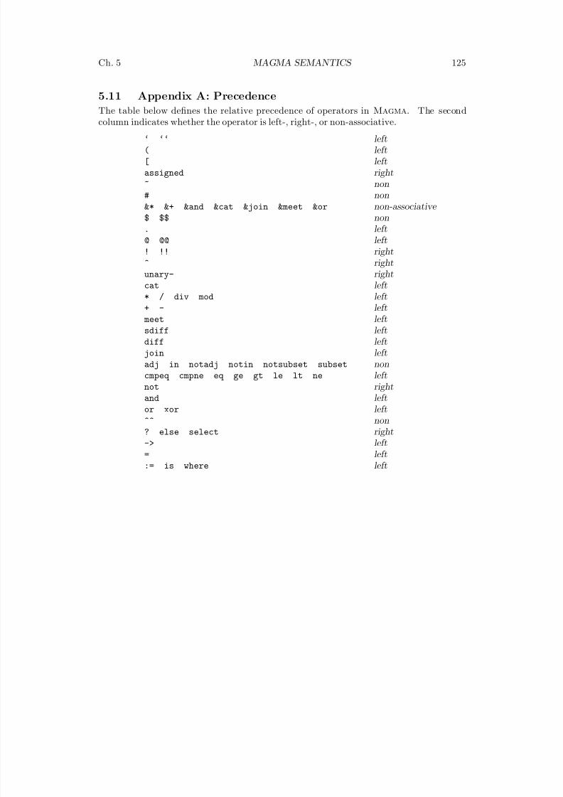
8/22/2019 Handbook Volume 01
http://slidepdf.com/reader/full/handbook-volume-01 241/440
Ch. 5 MAGMA SEMANTICS 125
5.11 Appendix A: Precedence
The table below defines the relative precedence of operators in Magma. The second
column indicates whether the operator is left-, right-, or non-associative.
‘ ‘‘ left( left[ leftassigned right~ non# non&* &+ &and &cat &join &meet &or non-associative $ $$ non. left
@ @@ left! !! right^ rightunary- rightcat left* / div mod left+ - left meet leftsdiff leftdiff leftjoin leftadj in notadj notin notsubset subset noncmpeq cmpne eq ge gt le lt ne leftnot rightand leftor xor left^^ non? else select right-> left= left:= is where left
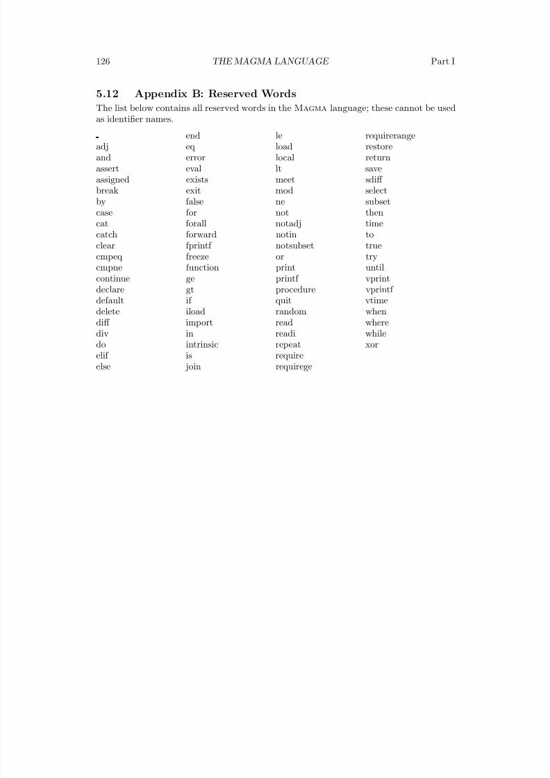
8/22/2019 Handbook Volume 01
http://slidepdf.com/reader/full/handbook-volume-01 242/440
126 THE MAGMA LANGUAGE Part I
5.12 Appendix B: Reserved Words
The list below contains all reserved words in the Magma language; these cannot be used
as identifier names.
end le requirerangeadj eq load restoreand error local returnassert eval lt saveassigned exists meet sdiff break exit mod selectby false ne subsetcase for not thencat forall notadj time
catch forward notin toclear fprintf notsubset truecmpeq freeze or trycmpne function print untilcontinue ge printf vprintdeclare gt procedure vprintf default if quit vtimedelete iload random whendiff import read wherediv in readi whiledo intrinsic repeat xorelif is requireelse join requirege

8/22/2019 Handbook Volume 01
http://slidepdf.com/reader/full/handbook-volume-01 243/440
6 THE MAGMA PROFILER
6.1 Introduction . . . . . . . . 129
6.2 Profiler Basics . . . . . . . 129
SetProfile(b) 129ProfileReset() 129ProfileGraph() 130
6.3 Exploring the Call Graph . . 131
6.3.1 Internal Reports . . . . . . . . 131
ProfilePrintByTotalCount(G) 132ProfilePrintByTotalTime(G) 132ProfilePrintChildrenByCount(G, n) 132ProfilePrintChildrenByTime(G, n) 132
6.3.2 HTML Reports . . . . . . . . . 133
ProfileHTMLOutput(G, prefix) 133
6.4 Recursion and the Profiler . . 133

8/22/2019 Handbook Volume 01
http://slidepdf.com/reader/full/handbook-volume-01 244/440
8/22/2019 Handbook Volume 01
http://slidepdf.com/reader/full/handbook-volume-01 245/440
Chapter 6
THE MAGMA PROFILER
6.1 Introduction
One of the most important aspects of the development cycle is optimization. It is often thecase that during the implementation of an algorithm, a programmer makes erroneous as-sumptions about its run-time behavior. These errors can lead to performance which differsin surprising ways from the expected output. The unfortunate tendency of programmersto optimize code before establishing run-time bottlenecks tends to exacerbate the problem.
Experienced programmers will thus often be heard repeating the famous mantra “Pre-mature optimization is the root of all evil”, coined by Sir Charles A. R. Hoare, the inventorof the Quick sort algorithm. Instead of optimizing during the initial implementation, it isgenerally better to perform an analysis of the run-time behaviour of the complete program,to determine what are the actual bottlenecks. In order to assist in this task, Magma pro-vides a profiler , which gives the programmer a detailed breakdown of the time spent in aprogram. In this chapter, we provide an overview of how to use the profiler.
6.2 Profiler Basics
The Magma profiler records timing information for each function, procedure, map, andintrinsic call made by your program. When the profiler is switched on, upon the entry andexit to each such call the current system clock time is recorded. This information is thenstored in a call graph, which can be viewed in various ways.
SetProfile(b)
Turns profiling on (if b is true) or off (if b is false). Profiling information is storedcumulatively, which means that in the middle of a profiling run, the profiler canbe switched off during sections for which profiling information is not wanted. At
startup, the profiler is off. Turning the profiler on will slow down the execution of your program slightly.
ProfileReset()
Clear out all information currently recorded by the profiler. It is generally a goodidea to do this after the call graph has been obtained, so that future profiling runsin the same Magma session begin with a clean slate.
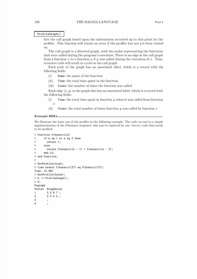
8/22/2019 Handbook Volume 01
http://slidepdf.com/reader/full/handbook-volume-01 246/440
130 THE MAGMA LANGUAGE Part I
ProfileGraph()
Get the call graph based upon the information recorded up to this point by theprofiler. This function will return an error if the profiler has not yet been turnedon.
The call graph is a directed graph, with the nodes representing the functionsthat were called during the program’s execution. There is an edge in the call graphfrom a function x to a function y if y was called during the execution of x. Thus,recursive calls will result in cycles in the call graph.
Each node in the graph has an associated label, which is a record with thefollowing fields:
(i) Name: the name of the function
(ii) Time: the total time spent in the function
(iii) Count: the number of times the function was called
Each edge x, y in the graph also has an associated label, which is a record withthe following fields:
(i) Time: the total time spent in function y when it was called from functionx
(ii) Count: the total number of times function y was called by function x
Example H6E1
We illustrate the basic use of the profiler in the following example. The code we test is a simple
implementation of the Fibonacci sequence; this can be replaced by any Magma code that needsto be profiled.
> function fibonacci(n)
> if n eq 1 or n eq 2 then
> return 1;
> else
> return fibonacci(n - 1) + fibonacci(n - 2);
> end if;
> end function;
>
> SetProfile(true);
> time assert fibonacci(27) eq Fibonacci(27);Time: 10.940
> SetProfile(false);
> G := ProfileGraph();
> G;
Digraph
Vertex Neighbours
1 2 3 6 7 ;
2 2 3 4 5 ;
3 ;
4 ;
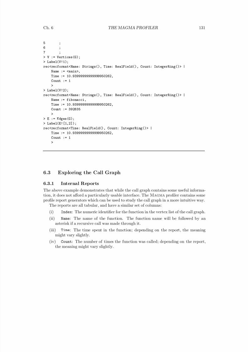
8/22/2019 Handbook Volume 01
http://slidepdf.com/reader/full/handbook-volume-01 247/440
Ch. 6 THE MAGMA PROFILER 131
5 ;
6 ;
7 ;> V := Vertices(G);
> Label(V!1);
rec<recformat<Name: Strings(), Time: RealField(), Count: IntegerRing()> |
Name := <main>,
Time := 10.93999999999999950262,
Count := 1
>
> Label(V!2);
rec<recformat<Name: Strings(), Time: RealField(), Count: IntegerRing()> |
Name := fibonacci,
Time := 10.93999999999999950262,Count := 392835
>
> E := Edges(G);
> Label(E![1,2]);
rec<recformat<Time: RealField(), Count: IntegerRing()> |
Time := 10.93999999999999950262,
Count := 1
>
6.3 Exploring the Call Graph
6.3.1 Internal Reports
The above example demonstrates that while the call graph contains some useful informa-tion, it does not afford a particularly usable interface. The Magma profiler contains someprofile report generators which can be used to study the call graph in a more intuitive way.
The reports are all tabular, and have a similar set of columns:
(i) Index: The numeric identifier for the function in the vertex list of the call graph.(ii) Name: The name of the function. The function name will be followed by an
asterisk if a recursive call was made through it.
(iii) Time: The time spent in the function; depending on the report, the meaningmight vary slightly.
(iv) Count: The number of times the function was called; depending on the report,the meaning might vary slightly.
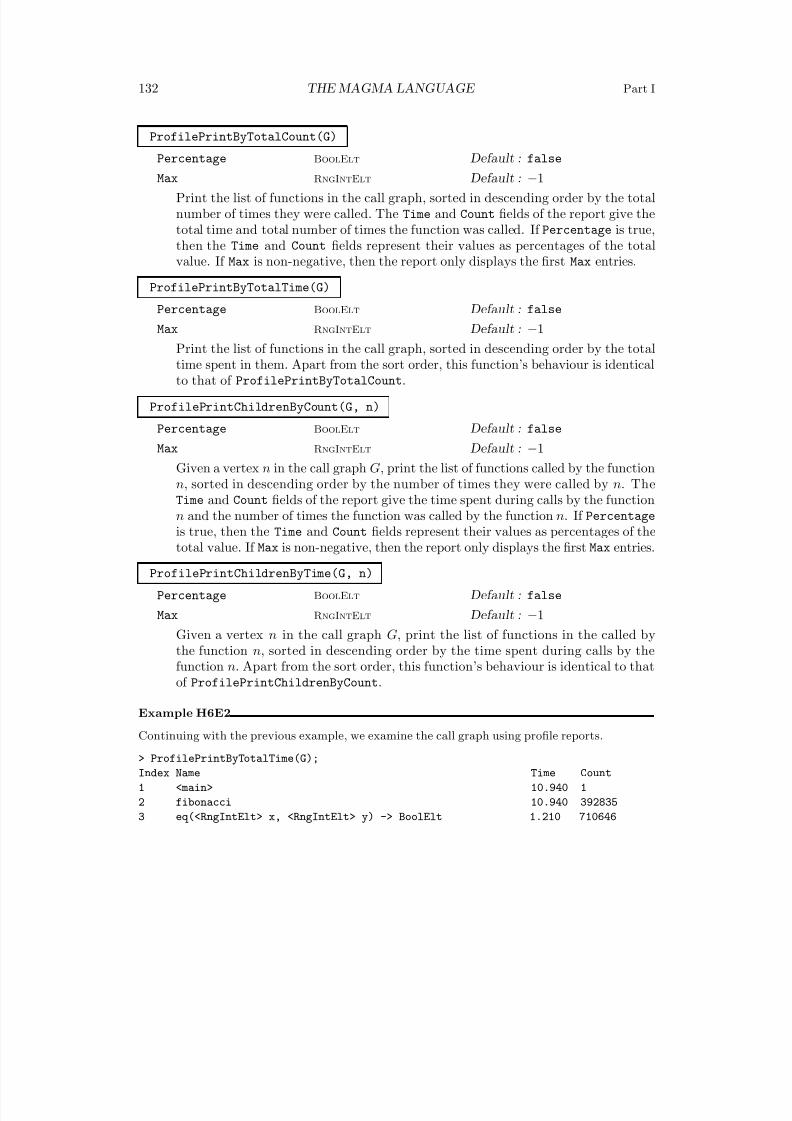
8/22/2019 Handbook Volume 01
http://slidepdf.com/reader/full/handbook-volume-01 248/440
132 THE MAGMA LANGUAGE Part I
ProfilePrintByTotalCount(G)
Percentage BoolElt Default : false
Max RngIntElt Default : −1
Print the list of functions in the call graph, sorted in descending order by the totalnumber of times they were called. The Time and Count fields of the report give thetotal time and total number of times the function was called. If Percentage is true,then the Time and Count fields represent their values as percentages of the totalvalue. If Max is non-negative, then the report only displays the first Max entries.
ProfilePrintByTotalTime(G)
Percentage BoolElt Default : false
Max RngIntElt Default : −1
Print the list of functions in the call graph, sorted in descending order by the totaltime spent in them. Apart from the sort order, this function’s behaviour is identicalto that of ProfilePrintByTotalCount.
ProfilePrintChildrenByCount(G, n)
Percentage BoolElt Default : false
Max RngIntElt Default : −1
Given a vertex n in the call graph G, print the list of functions called by the functionn, sorted in descending order by the number of times they were called by n. The
Time and Count fields of the report give the time spent during calls by the functionn and the number of times the function was called by the function n. If Percentage
is true, then the Time and Count fields represent their values as percentages of thetotal value. If Max is non-negative, then the report only displays the first Max entries.
ProfilePrintChildrenByTime(G, n)
Percentage BoolElt Default : false
Max RngIntElt Default : −1
Given a vertex n in the call graph G, print the list of functions in the called bythe function n, sorted in descending order by the time spent during calls by thefunction n. Apart from the sort order, this function’s behaviour is identical to thatof ProfilePrintChildrenByCount.
Example H6E2
Continuing with the previous example, we examine the call graph using profile reports.
> ProfilePrintByTotalTime(G);
Index Name Time Count
1 <main> 10.940 1
2 fibonacci 10.940 392835
3 eq(<RngIntElt> x, <RngIntElt> y) -> BoolElt 1.210 710646
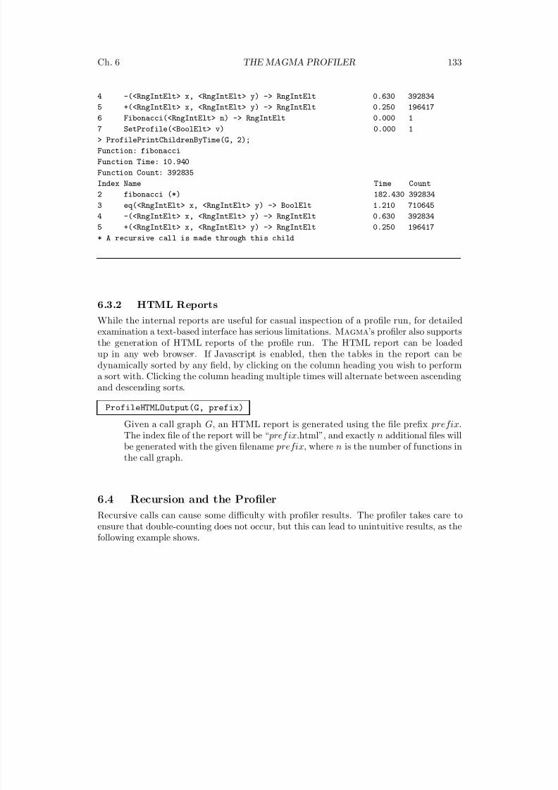
8/22/2019 Handbook Volume 01
http://slidepdf.com/reader/full/handbook-volume-01 249/440
Ch. 6 THE MAGMA PROFILER 133
4 -(<RngIntElt> x, <RngIntElt> y) -> RngIntElt 0.630 392834
5 +(<RngIntElt> x, <RngIntElt> y) -> RngIntElt 0.250 196417
6 Fibonacci(<RngIntElt> n) -> RngIntElt 0.000 17 SetProfile(<BoolElt> v) 0.000 1
> ProfilePrintChildrenByTime(G, 2);
Function: fibonacci
Function Time: 10.940
Function Count: 392835
Index Name Time Count
2 fibonacci (*) 182.430 392834
3 eq(<RngIntElt> x, <RngIntElt> y) -> BoolElt 1.210 710645
4 -(<RngIntElt> x, <RngIntElt> y) -> RngIntElt 0.630 392834
5 +(<RngIntElt> x, <RngIntElt> y) -> RngIntElt 0.250 196417
* A recursive call is made through this child
6.3.2 HTML Reports
While the internal reports are useful for casual inspection of a profile run, for detailedexamination a text-based interface has serious limitations. Magma’s profiler also supportsthe generation of HTML reports of the profile run. The HTML report can be loaded
up in any web browser. If Javascript is enabled, then the tables in the report can bedynamically sorted by any field, by clicking on the column heading you wish to performa sort with. Clicking the column heading multiple times will alternate between ascendingand descending sorts.
ProfileHTMLOutput(G, prefix)
Given a call graph G, an HTML report is generated using the file prefix prefix.The index file of the report will be “ pref ix.html”, and exactly n additional files willbe generated with the given filename prefix, where n is the number of functions inthe call graph.
6.4 Recursion and the Profiler
Recursive calls can cause some difficulty with profiler results. The profiler takes care toensure that double-counting does not occur, but this can lead to unintuitive results, as thefollowing example shows.
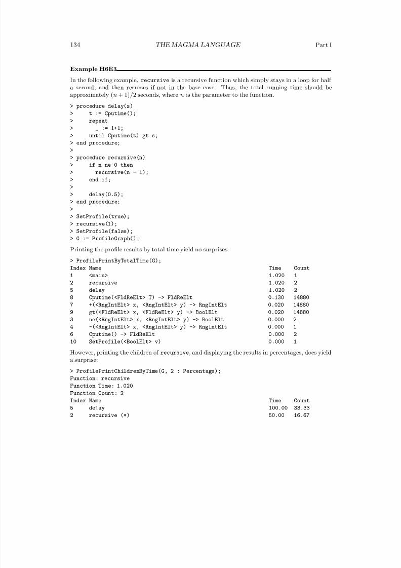
8/22/2019 Handbook Volume 01
http://slidepdf.com/reader/full/handbook-volume-01 250/440
134 THE MAGMA LANGUAGE Part I
Example H6E3
In the following example, recursive is a recursive function which simply stays in a loop for half
a second, and then recurses if not in the base case. Thus, the total running time should beapproximately (n + 1)/2 seconds, where n is the parameter to the function.
> procedure delay(s)
> t := Cputime();
> repeat
> _ := 1+1;
> until Cputime(t) gt s;
> end procedure;
>
> procedure recursive(n)
> if n ne 0 then
> recursive(n - 1);> end if;
>
> delay(0.5);
> end procedure;
>
> SetProfile(true);
> recursive(1);
> SetProfile(false);
> G := ProfileGraph();
Printing the profile results by total time yield no surprises:
> ProfilePrintByTotalTime(G);
Index Name Time Count
1 <main> 1.020 1
2 recursive 1.020 2
5 delay 1.020 2
8 Cputime(<FldReElt> T) -> FldReElt 0.130 14880
7 +(<RngIntElt> x, <RngIntElt> y) -> RngIntElt 0.020 14880
9 gt(<FldReElt> x, <FldReElt> y) -> BoolElt 0.020 14880
3 ne(<RngIntElt> x, <RngIntElt> y) -> BoolElt 0.000 2
4 -(<RngIntElt> x, <RngIntElt> y) -> RngIntElt 0.000 1
6 Cputime() -> FldReElt 0.000 2
10 SetProfile(<BoolElt> v) 0.000 1
However, printing the children of recursive, and displaying the results in percentages, does yielda surprise:
> ProfilePrintChildrenByTime(G, 2 : Percentage);
Function: recursive
Function Time: 1.020
Function Count: 2
Index Name Time Count
5 delay 100.00 33.33
2 recursive (*) 50.00 16.67
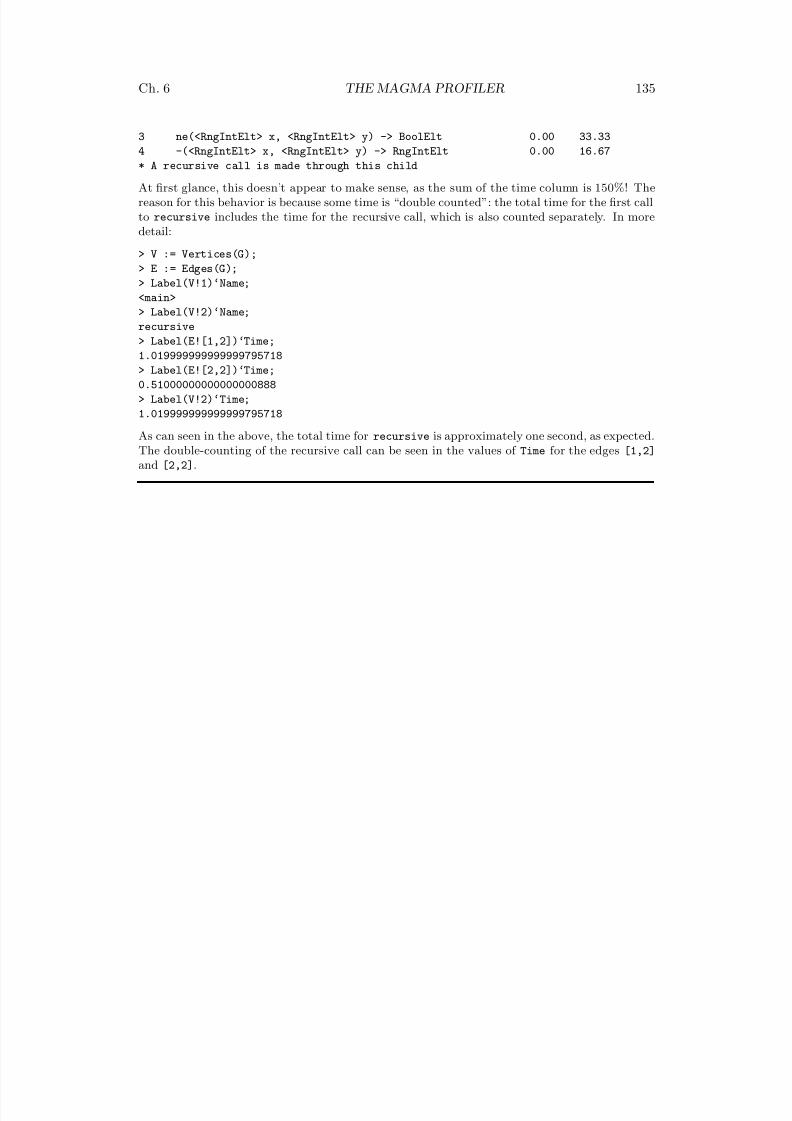
8/22/2019 Handbook Volume 01
http://slidepdf.com/reader/full/handbook-volume-01 251/440
Ch. 6 THE MAGMA PROFILER 135
3 ne(<RngIntElt> x, <RngIntElt> y) -> BoolElt 0.00 33.33
4 -(<RngIntElt> x, <RngIntElt> y) -> RngIntElt 0.00 16.67
* A recursive call is made through this child
At first glance, this doesn’t appear to make sense, as the sum of the time column is 150%! Thereason for this behavior is because some time is “double counted”: the total time for the first callto recursive includes the time for the recursive call, which is also counted separately. In moredetail:
> V := Vertices(G);
> E := Edges(G);
> Label(V!1)‘Name;
<main>
> Label(V!2)‘Name;
recursive
> Label(E![1,2])‘Time;1.019999999999999795718
> Label(E![2,2])‘Time;
0.51000000000000000888
> Label(V!2)‘Time;
1.019999999999999795718
As can seen in the above, the total time for recursive is approximately one second, as expected.The double-counting of the recursive call can be seen in the values of Time for the edges [1,2]
and [2,2].

8/22/2019 Handbook Volume 01
http://slidepdf.com/reader/full/handbook-volume-01 252/440

8/22/2019 Handbook Volume 01
http://slidepdf.com/reader/full/handbook-volume-01 253/440
7 DEBUGGING MAGMA CODE
7.1 Introduction . . . . . . . . 139
SetDebugOnError(f) 139
7.2 Using the Debugger . . . . . 139

8/22/2019 Handbook Volume 01
http://slidepdf.com/reader/full/handbook-volume-01 254/440
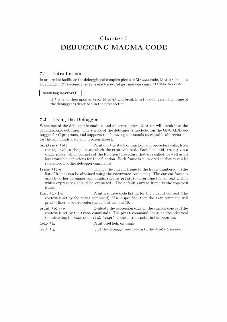
8/22/2019 Handbook Volume 01
http://slidepdf.com/reader/full/handbook-volume-01 255/440
Chapter 7
DEBUGGING MAGMA CODE
7.1 Introduction
In ordered to facilitate the debugging of complex pieces of Magma code, Magma includesa debugger. This debugger is very much a prototype, and can cause Magma to crash.
SetDebugOnError(f)
If f is true, then upon an error Magma will break into the debugger. The usage of the debugger is described in the next section.
7.2 Using the Debugger
When use of the debugger is enabled and an error occurs, Magma will break into thecommand-line debugger. The syntax of the debugger is modelled on the GNU GDB de-bugger for C programs, and supports the following commands (acceptable abbreviationsfor the commands are given in parentheses):
backtrace (bt) Print out the stack of function and procedure calls, fromthe top level to the point at which the error occurred. Each line i this trace gives asingle frame , which consists of the function/procedure that was called, as well as alllocal variable definitions for that function. Each frame is numbered so that it can bereferenced in other debugger commands.
frame (f) n Change the current frame to the frame numbered n (thelist of frames can be obtained using the backtrace command). The current frame isused by other debugger commands, such as print, to determine the context withinwhich expressions should be evaluated. The default current frame is the top-mostframe.
list (l) [n] Print a source code listing for the current context (thecontext is set by the frame command). If n is specified, then the list command willprint n lines of source code; the default value is 10.
print (p) expr Evaluate the expression expr in the current context (thecontext is set by the frame command). The print command has semantics identicalto evaluating the expression eval "expr" at the current point in the program.
help (h) Print brief help on usage.
quit (q) Quit the debugger and return to the Magma session.
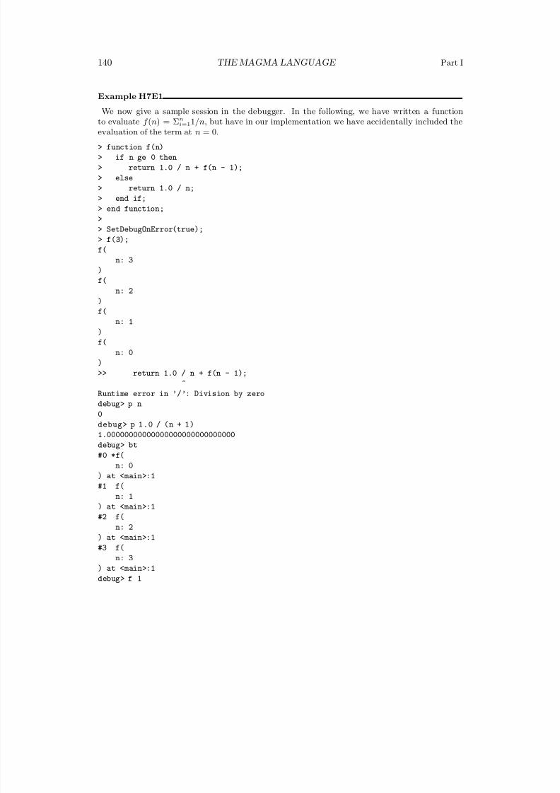
8/22/2019 Handbook Volume 01
http://slidepdf.com/reader/full/handbook-volume-01 256/440
140 THE MAGMA LANGUAGE Part I
Example H7E1
We now give a sample session in the debugger. In the following, we have written a function
to evaluate f (n) = Σni=11/n, but have in our implementation we have accidentally included the
evaluation of the term at n = 0.
> function f(n)
> if n ge 0 then
> return 1.0 / n + f(n - 1);
> else
> return 1.0 / n;
> end if;
> end function;
>
> SetDebugOnError(true);
> f(3);f(
n: 3
)
f(
n: 2
)
f(
n: 1
)
f(
n: 0
)
>> return 1.0 / n + f(n - 1);
^
Runtime error in ’/’: Division by zero
debug> p n
0
debug> p 1.0 / (n + 1)
1.00000000000000000000000000000
debug> bt
#0 *f(
n: 0
) at <main>:1#1 f(
n: 1
) at <main>:1
#2 f(
n: 2
) at <main>:1
#3 f(
n: 3
) at <main>:1
debug> f 1

8/22/2019 Handbook Volume 01
http://slidepdf.com/reader/full/handbook-volume-01 257/440
Ch. 7 DEBUGGING MAGMA CODE 141
debug> p n
1
debug> p 1.0 / n1.00000000000000000000000000000

8/22/2019 Handbook Volume 01
http://slidepdf.com/reader/full/handbook-volume-01 258/440
8/22/2019 Handbook Volume 01
http://slidepdf.com/reader/full/handbook-volume-01 259/440
PART IISETS, SEQUENCES, AND MAPPINGS
8 INTRODUCTION TO AGGREGATES 145
9 SETS 155
10 SEQUENCES 183
11 TUPLES AND CARTESIAN PRODUCTS 205
12 LISTS 211
13 COPRODUCTS 217
14 RECORDS 223
15 MAPPINGS 229

8/22/2019 Handbook Volume 01
http://slidepdf.com/reader/full/handbook-volume-01 260/440
8/22/2019 Handbook Volume 01
http://slidepdf.com/reader/full/handbook-volume-01 261/440
8 INTRODUCTION TO AGGREGATES
8.1 Introduction . . . . . . . . 147
8.2 Restrictions on Sets andSequences . . . . . . . . . 147
8.2.1 Universe of a Set or Sequence . . . 148
8.2.2 Modifying the Universe of a Set or Se-quence . . . . . . . . . . . . . 149
8.2.3 Parents of Sets and Sequences. . . 151
8.3 Nested Aggregates . . . . . 152
8.3.1 Multi-indexing . . . . . . . . . 152

8/22/2019 Handbook Volume 01
http://slidepdf.com/reader/full/handbook-volume-01 262/440
8/22/2019 Handbook Volume 01
http://slidepdf.com/reader/full/handbook-volume-01 263/440
Chapter 8
INTRODUCTION TO AGGREGATES
8.1 Introduction
This part of the Handbook comprises four chapters on aggregate objects in Magma aswell as a chapter on maps.
Sets, sequences, tuples and lists are the four main types of aggregates, and each has itsown specific purpose. Sets are used to collect objects that are elements of some common
structure, and the most important operation is to test element membership. Sequences also contain objects of a common structure, but here the emphasis is on the ordering of the objects, and the most important operation is that of accessing (or modifying) elementsat given positions. Sets will contain at most one copy of any element, whereas sequencesmay contain arbitrarily many copies of the same object. Enumerated sets and sequencesare of arbitrary but finite length and will store all elements explicitly (with the exceptionof arithmetic progressions), while formal sets and sequences may be infinite, and use aBoolean function to test element membership. Indexed sets are a hybrid form of sets al-lowing indexing like sequences. Elements of Cartesian products of structures in Magma
will be called tuples ; they are of fixed length, and each coefficient must be in the corre-
sponding structure of the defining Cartesian product. Lists are arbitrary finite orderedcollections of objects of any type, and are mainly provided to the user to store assorteddata to which access is not critical.
8.2 Restrictions on Sets and Sequences
Here we will explain the subtleties behind the mechanism dealing with sets and sequencesand their universes and parents. Although the same principles apply to their formalcounterparts, we will only talk about enumerated sets and sequences here, for two reasons:the enumerated versions are much more useful and common, and the very restricted number
of operations on formal sets/sequences make issues of universe and overstructure of lessimportance for them.In principle, every object e in Magma has some parent structure S such that e ∈ S ;
this structure can be used for type checking (are we allowed to apply function f to e?),algorithm look-up etc. To avoid storing the structure with every element of a set orsequence and having to look up the structure of every element separately, only elementsof a common structure are allowed in sets or sequences, and that common parent will onlybe stored once.
8/22/2019 Handbook Volume 01
http://slidepdf.com/reader/full/handbook-volume-01 264/440
148 SETS, SEQUENCES, AND MAPPINGS Part II
8.2.1 Universe of a Set or Sequence
This common structure is called the universe of the set or sequence. In the general con-
structors it may be specified up front to make clear what the universe for the set or sequencewill be; the difference between the sets i and s in
> i := { IntegerRing() | 1, 2, 3 };
> s := { RationalField() | 1, 2, 3 };
lies entirely in their universes. The specification of the universe may be omitted if there isan obvious common overstructure for the elements. Thus the following provides a shorterway to create the set containing 1, 2, 3 and having the ring of integers as universe:
> i := { 1, 2, 3 };
Only empty sets and sequences that have been obtained directly from the constructions
> S := { };
> T := [ ];
do not have their universe defined – we will call them the null set or sequence. (Thereare two other ways in which empty sets and sequences arise: it is possible to create emptysequences with a prescribed universe, using
> S := { U | };
> T := [ U | ];
and it may happen that a non-empty set/sequence becomes empty in the course of a
computation. In both cases these empty objects have their universe defined and will notbe null ).Usually (but not always: the exception will be explained below) the universe of a set
or sequence is the parent for all its elements; thus the ring of integers is the parent of 2in the set i = {1, 2, 3}, rather than that set itself. The universe is not static, and it is notnecessarily the same structure as the parent of the elements before they were put in theset or sequence. To illustrate this point, suppose that we try to create a set containingintegers and rational numbers, say T = {1, 2, 1/3}; then we run into trouble with the rulethat the universe must be common for all elements in T ; the way this problem is solvedin Magma is by automatic coercion: the obvious universe for T is the field of rationalnumbers of which 1/3 is already an element and into which any integer can be coerced in
an obvious way. Hence the assignment
> T := { 1, 2, 1/3 }
will result in a set with universe the field of rationals (which is also present when Magma
is started up). Consequently, when we take the element 1 of the set T , it will have therational field as its parent rather than the integer ring! It will now be clear that
> s := { 1/1, 2, 3 };
is a shorter way to specify the set of rational numbers 1,2, 3 than the way we saw before, butin general it is preferable to declare the universe beforehand using the { U | } notation.
8/22/2019 Handbook Volume 01
http://slidepdf.com/reader/full/handbook-volume-01 265/440
Ch. 8 INTRODUCTION TO AGGREGATES 149
Of course
> T := { Integers() | 1, 2, 1/3 }
would result in an error because 1/3 cannot be coerced into the ring of integers.So, usually not every element of a given structure can be coerced into another structure,
and even if it can, it will not always be done automatically. The possible (automatic)coercions are listed in the descriptions of the various Magma modules. For instance, thetable in the introductory chapter on rings shows that integers can be coerced automaticallyinto the rational field.
In general, every Magma structure is valid as a universe. This includes enumeratedsets and sequences themselves, that is, it is possible to define a set or sequence whoseelements are confined to be elements of a given set or sequence. So, for example,
> S := [ [ 1..10 ] | x^2+x+1 : x in { - 3 . . 2 b y 1 } ];
produces the sequence [7, 3, 1, 1, 3, 7] of values of the polynomial x2 + x +1 for x ∈ Z with−3 ≤ x ≤ 2. However, an entry of S will in fact have the ring of integers as its parent(and not the sequence [1..10]), because the effect of the above assignment is that the valuesafter the | are calculated and coerced into the universe, which is [1..10]; but coercing anelement into a sequence or set means that it will in fact be coerced into the universe of that sequence/set, in this case the integers. So the main difference between the aboveassignment and
> T := [ Integers() | x^2+x+1 : x in { -3 .. 2 by 1} ];
is that in the first case it is checked that the resulting values y satisfy 1 ≤ y ≤ 10, and anerror would occur if this is violated:
> S := [ [ 1..10 ] | x^2+x+1 : x in { -3 .. 3 by 1} ];
leads to a run-time error.In general then, the parent of an element of a set or sequence will be the universe of the
set or sequence, unless that universe is itself a set or sequence, in which case the parentwill be the universe of this universe, and so on, until a non-set or sequence is encountered.
8.2.2 Modifying the Universe of a Set or Sequence
Once a (non-null) set or sequence S has been created, the universe has been defined. If oneattempts to modify S (that is, to add elements, change entries etc. using a procedure thatwill not reassign the result to a new set or sequence), the universe will not be changed,and the modification will only be successful if the new element can be coerced into thecurrent universe. Thus,
> Z := Integers();
> T := [ Z | 1, 2, 3/3 ];
> T[2] := 3/4;
will result in an error, because 3/4 cannot be coerced into Z .
8/22/2019 Handbook Volume 01
http://slidepdf.com/reader/full/handbook-volume-01 266/440
150 SETS, SEQUENCES, AND MAPPINGS Part II
The universe of a set or sequence S can be explicitly modified by creating a parent forS with the desired universe and using the ! operator for the coercion; as we will see in
the next subsection, such a parent can be created using the PowerSet and PowerSequencecommands. Thus, for example, the set {1, 2} can be made into a sequence of rationals asfollows:
> I := { 1, 2 };
> P := PowerSet( RationalField() );
> J := P ! I;
The coercion will be successful if every element of the sequence can be coerced into thenew universe, and it is not necessary that the old universe could be coerced completelyinto the new one: the set {3/3} of rationals can be coerced into PowerSet(Integers()).As a consequence, the empty set (or sequence) with any universe can be coerced into the
power set (power sequence) of any other universe.Binary functions on sets or sequences (like join or cat) can only applied to sets and
sequences that are compatible : the operation on S with universe A and T with universe Bcan only be performed if a common universe C can be found such that the elements of S and T are all elements of C . The compatibility conditions are dependent on the particularMagma module to which A and B belong (we refer to the corresponding chapters of thismanual for further information) and do also apply to elements of a ∈ A and b ∈ B —that is, the compatibility conditions for S and T are the same as the ones that determinewhether binary operations on a ∈ A and b ∈ B are allowed. For example, we are able to
join a set of integers and a set of rationals:
> T := { 1, 2 } join { 1/3 };for the same reason that we can do
> c := 1 + 1/3;
(automatic coercion for rings). The resulting set T will have the rationals as universe.The basic rules for compatibility of two sets or sequences are then:
(1)every set/sequence is compatible with the null set/sequence (which has no universedefined (see above));
(2) two sets/sequences with the same universe are compatible;
(3)a set/sequence S with universe A is compatible with set/sequence T with universe B
if the elements of A can be automatically coerced into B, or vice versa;(4) more generally, a set/sequence S with universe A is also compatible with set/sequence
T with universe B if Magma can automatically find an over-structure for the parentsA and B (see below);
(5)nested sets and sequences are compatible only when they are of the same ‘depth’ and‘type’ (that is, sets and sequences appear in exactly the same recursive order in both)and the universes are compatible.
The possibility of finding an overstructure C for the universe A and B of sets or sequencesS and T (such that A ⊂ C ⊃ B), is again module dependent. We refer the reader for
8/22/2019 Handbook Volume 01
http://slidepdf.com/reader/full/handbook-volume-01 267/440
Ch. 8 INTRODUCTION TO AGGREGATES 151
details to the Introductions of Parts III–VI, and we give some examples here; the nextsubsection contains the rules for parents of sets and sequences.
8.2.3 Parents of Sets and Sequences
The universe of a set or sequence S is the common parent for all its elements; but S itself is a Magma object as well, so it should have a parent too.
The parent of a set is a power set: the set of all subsets of the universe of S . Itcan be created using the PowerSet function. Similarly, PowerSequence(A) creates theparent structure for a sequence of elements from the structure A – that is, the elements of PowerSequence(A) are all sequences of elements of A.
The rules for finding a common overstructure for structures A and B, where either A orB is a set/sequence or the parent of a set/sequence, are as follows. (If neither A nor B is
a set, sequence, or its parent we refer to the Part of this manual describing the operationson A and B.)
(1) The overstructure of A and B is the same as that of B and A.
(2)If A is the null set or sequence (empty, and no universe specified) the overstructure of A and B is B.
(3)If A is a set or sequence with universe U , the overstructure of A and B is the over-structure of U and B; in particular, the overstructure of A and A will be the universeU of A.
(4)If A is the parent of a set (a power set), then A and B can only have a commonoverstructure if B is also the parent of a set, in which case the overstructure is thepower set of the overstructure of the universes U and V of A and B respectively.Likewise for sequences instead of sets.
We give two examples to illustrate rules (3) and (4). It is possible to create a set with aset as its universe:
> S := { { 1..100 } | x^3 : x in [ 0..3 ] };
If we wish to intersect this set with some set of integers, say the formal set of odd integers
> T := {! x : x in Integers() | IsOdd(x) !};
> W := S meet T;
then we can only do that if we can find a universe for W , which must be the commonoverstructure of the universe U = {1, 2, . . . , 100} of S and the universe ‘ring of integers’ of T . By rule (3) above, this overstructure of U = {1, 2, . . . , 100} will be the overstructureof the universe of U and the ring of integers; but the universe of U is the ring of integers(because it is the default for the set {1, 2, . . . , 100}), and hence the overstructure we arelooking for (and the universe for W ) will be the ring of integers.
For the second example we look at sequences of sequences:
> a := [ [ 1 ], [ 1, 2, 3 ] ];
8/22/2019 Handbook Volume 01
http://slidepdf.com/reader/full/handbook-volume-01 268/440
152 SETS, SEQUENCES, AND MAPPINGS Part II
> b := [ [ 2/3 ] ];
so a is a sequence of sequences of integers, and b is a sequence of sequences of rationals. If we wish to concatenate a and b,
> c := a cat b;
we will only succeed if we find a universe for c. This universe must be the commonoverstructure of the universes of a and b, which are the ‘power sequence of the integers’and the ‘power sequence of the rationals’ respectively. By rule (4), the overstructure of these two power sequences is the power sequence of the common overstructure of therationals and the integers, which is the rationals themselves. Hence c will be a sequenceof sequences of rationals, and the elements of a will have to be coerced.
8.3 Nested AggregatesEnumerated sets and sequences can be arbitrarily nested (that is, one may create sets of sets, as well as sequences of sets etc.); tuples can also be nested and may be freely mixedwith sets and sequences (as long as the proper Cartesian product parent can be created).Lists can be nested, and one may create lists of sets or sequences or tuples.
8.3.1 Multi-indexing
Since sequences (and lists) can be nested, assignment functions and mutation operatorsallow you to use multi-indexing , that is, one can use a multi-index i1, i2, . . . , ir rather thana single i to reach r levels deep. Thus, for example, if S = [ [1, 2], [2, 3] ], instead of
> S[2][2] := 4;
one may use the multi-index 2, 2 to obtain the same effect of changing the 3 into a 4:
> S[2,2] := 4;
All ij in the multi-index i1, i2, . . . , ir have to be greater than 0, and an error will also beflagged if any ij indexes beyond the length at level j, that is, if ij > #S [i1, . . . , ij−1],(which means i1 > #S for j = 1). There is one exception: the last index ir is allowed toindex beyond the current length of the sequence at level r if the multi-index is used on theleft-hand side of an assignment, in which case any intermediate terms will be undefined.This generalizes the possibility to assign beyond the length of a ‘flat’ sequence. In the
above example the following assignments are allowed:> S[2,5] := 7;
(and the result will be S = [ [1, 2], [2, 3, undef , undef , 7] ])
> S[4] := [7];
(and the result will be S = [ [1, 2], [2, 3], undef , [7] ]). But the following results in anerror:
> S[4,1] := 7;
Finally we point out that multi-indexing should not be confused with the use of sequences as
8/22/2019 Handbook Volume 01
http://slidepdf.com/reader/full/handbook-volume-01 269/440
Ch. 8 INTRODUCTION TO AGGREGATES 153
indexes to create subsequences. For example, to create a subsequence of S = [5, 13, 17, 29]consisting of the second and third terms, one may use
> S : = [ 5, 1 3, 1 7, 2 9 ];
> T := S[ [2, 3] ];
To obtain the second term of this subsequence one could have done:
> x := S[ [2, 3] ][2];
(so x now has the value S [3] = 17), but it would have been more efficient to index theindexing sequence, since it is rather expensive to build the subsequence [ S [2], S [3] ] first,so:
> x := S[ [2, 3][2] ];
has the same effect but is better (of course x := S[3] would be even better in this simpleexample.) To add to the confusion, it is possible to mix the above constructions forindexing, since one can use lists of sequences and indices for indexing; continuing ourexample, there is now a third way to do the same as above, using an indexing list thatfirst takes out the subsequence consisting of the second and third terms and then extractsthe second term of that:
> x := S[ [2, 3], 2 ];
Similarly, the construction
> X := S[ [2, 3], [2] ];
pulls out the subsequence consisting of the second term of the subsequence of terms twoand three of S , in other words, this assigns the sequence consisting of the element 17, not
just the element itself!

8/22/2019 Handbook Volume 01
http://slidepdf.com/reader/full/handbook-volume-01 270/440
8/22/2019 Handbook Volume 01
http://slidepdf.com/reader/full/handbook-volume-01 271/440
9 SETS
9.1 Introduction . . . . . . . . 157
9.1.1 Enumerated Sets . . . . . . . . 157
9.1.2 Formal Sets . . . . . . . . . . . 157
9.1.3 Indexed Sets . . . . . . . . . . 157
9.1.4 Multisets . . . . . . . . . . . . 157
9.1.5 Compatibility . . . . . . . . . . 158
9.1.6 Notation . . . . . . . . . . . . 158
9.2 Creating Sets . . . . . . . . 158
9.2.1 The Formal Set Constructor . . . 158
{! x in F | P(x) !} 1589.2.2 The Enumerated Set Constructor . 159
{ } 159{ U | } 159{ e1, e2, ..., en } 159{ U | e1, e2, ..., en } 159{ e(x) : x in E | P(x) } 160{ U | e (x) : x i n E | P(x) } 160{ e(x1,...,xk) : x1 in E1, ..., xk
in Ek | P(x1, ..., xk) } 160{ U | e(x1,...,xk) : x1 in E1, ...,
xk in Ek | P(x1, ..., xk) } 160
9.2.3 The Indexed Set Constructor . . . 161
{@ @} 161{@ U | @} 161{@ e1, e2, ..., en @} 161{@ U | e1, e2, ..., em @} 161{@ e (x) : x i n E | P (x) @} 161{@ U | e(x) : x in E | P(x) @} 161{@ e(x1,...,xk) : x1 in E1, ..., xk
in Ek | P(x1, ..., xk) @} 162{@ U | e ( x1,...,xk) : x1 in E1, ...,
xk in Ek | P(x1, ..., xk)@} 162
9.2.4 The Multiset Constructor . . . . 162
{* *} 162{* U | *} 162
{* e1, e2, ..., en *} 163{* U | e1, e2, ..., em *} 163{* e (x) : x i n E | P (x) *} 163{* U | e(x) : x in E | P(x) *} 163{* e(x1,...,xk) : x1 in E1, ..., xk
in Ek | P(x1, ..., xk) *} 163{* U | e ( x1,...,xk) : x1 in E1, ...,
xk in Ek | P(x1, ..., xk)*} 163
9.2.5 The Arithmetic Progression Construc-tors . . . . . . . . . . . . . . 164
{ i..j } 164{ U | i..j } 164{ i .. j by k } 165
{ U | i .. j by k } 165
9.3 Power Sets . . . . . . . . . 165
PowerSet(R) 165PowerIndexedSet(R) 165PowerMultiset(R) 166in 166PowerFormalSet(R) 166in 166in 166! 166! 166! 166
9.3.1 The Cartesian Product Constructors 167
9.4 Sets from Structures . . . . . 167
Set(M) 167FormalSet(M) 167
9.5 Accessing and Modifying Sets . 168
9.5.1 Accessing Sets and their AssociatedStructures . . . . . . . . . . . 168
# 168Category(S) 168Type(S) 168Parent(R) 168Universe(R) 168
Index(S, x) 168Position(S, x) 168S[i] 168S[I] 168
9.5.2 Selecting Elements of Sets . . . . 169
Random(R) 170random{ e(x) : x i n E | P (x) } 170random{e(x1, ..., xk) : x1 in E1,
..., xk in Ek | P(x1, ..., xk)} 170Representative(R) 170Rep(R) 170ExtractRep(∼R, ∼r) 171rep{ e(x) : x i n E | P (x) } 171
rep{ e(x1, ..., xk) : x1 in E1, ...,xk in Ek | P(x1, ..., xk) } 171Minimum(S) 172Min(S) 172Maximum(S) 172Max(S) 172Hash(x) 172
9.5.3 Modifying Sets . . . . . . . . . 172
Include(∼S, x) 172Include(S, x) 172Exclude(∼S, x) 172Exclude(S, x) 172ChangeUniverse(∼S, V) 173
8/22/2019 Handbook Volume 01
http://slidepdf.com/reader/full/handbook-volume-01 272/440
156 SETS, SEQUENCES, AND MAPPINGS Part II
ChangeUniverse(S, V) 173CanChangeUniverse(S, V) 173SetToIndexedSet(E) 174IndexedSetToSet(S) 174Isetset(S) 174IndexedSetToSequence(S) 174Isetseq(S) 174MultisetToSet(S) 174SetToMultiset(E) 174SequenceToMultiset(Q) 174
9.6 Operations on Sets . . . . . 175
9.6.1 Boolean Functions and Operators . 175
IsNull(R) 175IsEmpty(R) 175eq 175ne 175in 175notin 175subset 176notsubset 176eq 176ne 176IsDisjoint(R, S) 176
9.6.2 Binary Set Operators . . . . . . 176
join 176 meet 177diff 177sdiff 177
9.6.3 Other Set Operations . . . . . . 177
Multiplicity(S, x) 177
Multiplicities(S) 177Subsets(S) 177Subsets(S, k) 177Multisets(S, k) 178Subsequences(S, k) 178Permutations(S) 178Permutations(S, k) 178
9.7 Quantifiers . . . . . . . . . 178
exists(t){ e(x): x in E | P(x) } 178exists(t1, ..., tr){ e(x) :
x in E | P(x) } 178exists(t){e(x1, ..., xk): x1 in E1,
..., xk in Ek | P(x1, ..., xk)} 179exists(t1, ..., tr){ e(x1, ..., x
k) :
x1 in E1, ..., xk in Ek | P } 179forall(t){ e(x) : x in E | P(x) } 179forall(t1, ..., tr){ e(x) :
x in E | P(x) } 179forall(t){e(x1, ..., xk): x1 in E1,
..., xk in Ek | P(x1, ..., xk)} 180forall(t1, ..., tr){ e(x1, ..., xk) :
x1 in E1, ..., xk in Ek | P } 180
9.8 Reduction and Iteration over Sets181
x i n S 181& 181
8/22/2019 Handbook Volume 01
http://slidepdf.com/reader/full/handbook-volume-01 273/440
Chapter 9
SETS
9.1 Introduction
A set in Magma is a (usually unordered) collection of objects belonging to some commonstructure (called the universe of the set). There are four basic types of sets: enumer-ated sets , whose elements are all stored explicitly (with one exception, see below); formal sets , whose elements are stored implicitly by means of a predicate that allows for testingmembership; indexed sets , which are restricted enumerated sets having a numbering on
elements; and multisets , which are enumerated sets with possible repetition of elements.In particular, enumerated and indexed sets and multisets are always finite, and formal setsare allowed to be infinite.
9.1.1 Enumerated Sets
Enumerated sets are finite, and can be specified in three basic ways (see also section 2below): by listing all elements; by an expression involving elements of some finite structure;and by an arithmetic progression. If an arithmetic progression is specified, the elementsare not calculated explicitly until a modification of the set necessitates it; in all other casesall elements of the enumerated set are stored explicitly.
9.1.2 Formal SetsA formal set consists of the subset of elements of some carrier set (structure) on which acertain predicate assumes the value ‘true’.
The only set-theoretic operations that can be performed on formal sets are union,intersection, difference and symmetric difference, and element membership testing.
9.1.3 Indexed Sets
For some purposes it is useful to be able to access elements of a set through an index map,which numbers the elements of the set. For that purpose Magma has indexed sets, onwhich a very few basic set operations are allowed (element membership testing) as wellas some sequence-like operations (such as accessing the i-th term, getting the index of an
element, appending and pruning).
9.1.4 Multisets
For some purposes it is useful to construct a set with some of its members repeated. Forthat purpose Magma has multisets, which take into account the repetition of members.The number of times an object x occurs in a multiset S is called the multiplicity of xin S . Magma has the ˆˆ operator to specify a multiplicity: the expression x^^n meansthe object x with multiplicity n. In the following, whenever any multiset constructor orfunction expects an element y, the expression xˆˆn may usually be used.
8/22/2019 Handbook Volume 01
http://slidepdf.com/reader/full/handbook-volume-01 274/440
158 SETS, SEQUENCES, AND MAPPINGS Part II
9.1.5 Compatibility
The binary operators for sets do not allow mixing of the four types of sets (so one cannot
take the intersection of an enumerated set and a formal set, for example), but it is easy toconvert an enumerated set into a formal set – see the section on binary operators below –and there are functions provided for making an enumerated set out of an indexed set or amultiset (and vice versa).
By the limitation on their construction formal sets can only contain elements from onestructure in Magma. The elements of enumerated sets are also restricted, in the sensethat either some universe must be specified upon creation, or Magma must be able to findsuch universe automatically. The rules for compatibility of elements and the way Magma
deals with these universes are the same for sequences and sets, and are described in theprevious chapter. The restrictions on indexed sets are the same as those for enumeratedsets.
9.1.6 Notation
Certain expressions appearing in the sections below (possibly with subscripts) have astandard interpretation:
U the universe: any Magma structure;
E the carrier set for enumerated sets: any enumerated structure (it must be possible toloop over its elements – see the Introduction to this Part (Chapter 8));
F the carrier set for formal sets: any structure for which membership testing using in isdefined – see the Introduction to this Part (Chapter 8));
x a free variable which successively takes the elements of E (or F in the formal case) asits values;
P a Boolean expression that usually involves the variable(s) x, x1, . . . , xk;
e an expression that also usually involves the variable(s) x, x1, . . . , xk.
9.2 Creating Sets
The customary braces { and } are used to define enumerated sets. Formal sets are delimitedby the composite braces {! and !}. For indexed sets {@ and @} are used. For multisets {*
and *} are used.
9.2.1 The Formal Set ConstructorThe formal set constructor has the following fixed format (the expressions appearing inthe construct are defined above):
{! x in F | P(x) !}
Form the formal set consisting of the subset of elements x of F for which P (x) istrue. If P (x) is true for every element of F , the set constructor may be abbreviatedto {! x in F !}. Note that the universe of a formal set will always be equal tothe carrier set F .
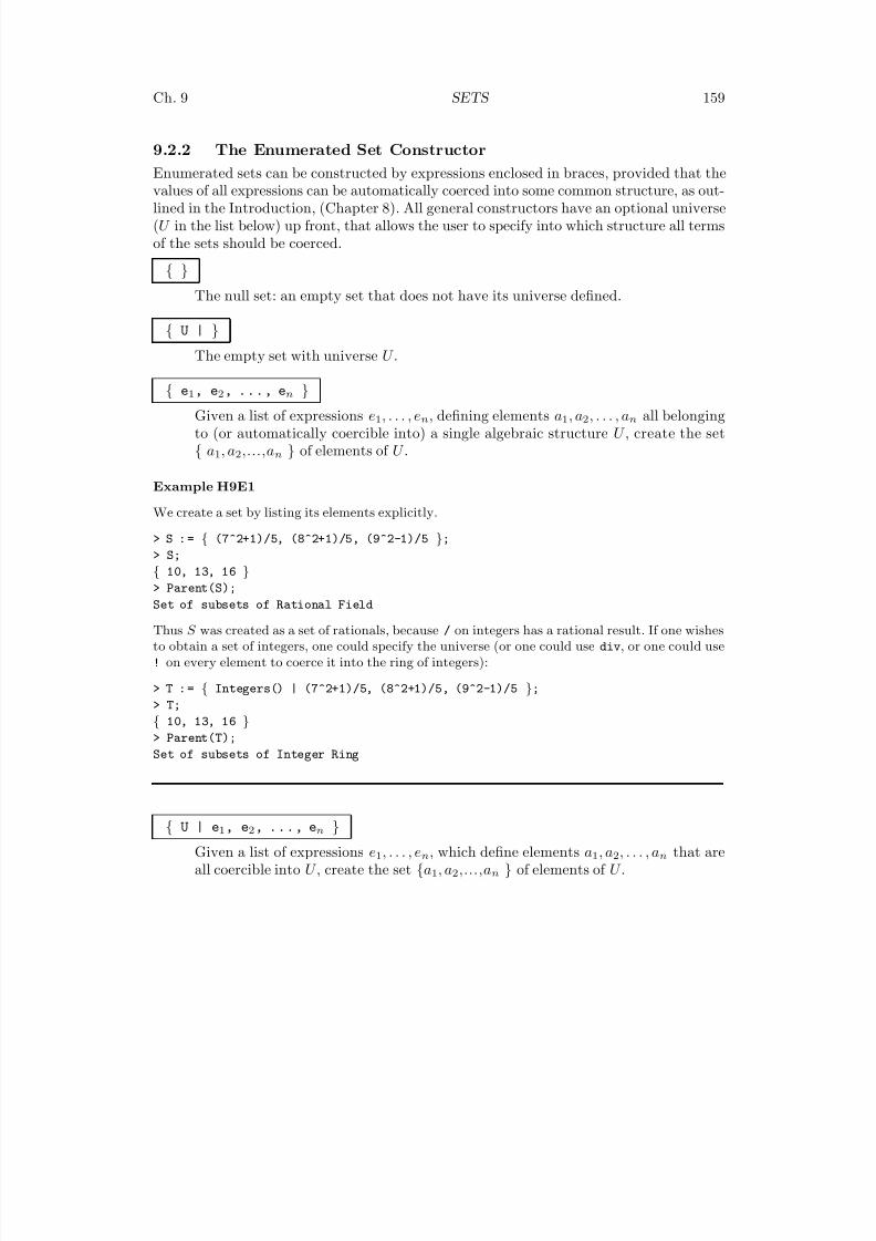
8/22/2019 Handbook Volume 01
http://slidepdf.com/reader/full/handbook-volume-01 275/440
Ch. 9 SETS 159
9.2.2 The Enumerated Set Constructor
Enumerated sets can be constructed by expressions enclosed in braces, provided that the
values of all expressions can be automatically coerced into some common structure, as out-lined in the Introduction, (Chapter 8). All general constructors have an optional universe(U in the list below) up front, that allows the user to specify into which structure all termsof the sets should be coerced.
{ }
The null set: an empty set that does not have its universe defined.
{ U | }
The empty set with universe U .
{ e1, e2, ..., en }
Given a list of expressions e1, . . . , en, defining elements a1, a2, . . . , an all belongingto (or automatically coercible into) a single algebraic structure U , create the set{ a1, a2,...,an } of elements of U .
Example H9E1
We create a set by listing its elements explicitly.
> S : = { (7^2+1)/5, (8^2+1)/5, (9^2-1)/5 };
> S;{ 10, 13, 16 }> Parent(S);
Set of subsets of Rational Field
Thus S was created as a set of rationals, because / on integers has a rational result. If one wishesto obtain a set of integers, one could specify the universe (or one could use div, or one could use! on every element to coerce it into the ring of integers):
> T : = { Integers() | (7^2+1)/5, (8^2+1)/5, (9^2-1)/5 };
> T;
{ 10, 13, 16 }> Parent(T);
Set of subsets of Integer Ring
{ U | e1, e2, ..., en }
Given a list of expressions e1, . . . , en, which define elements a1, a2, . . . , an that areall coercible into U , create the set {a1, a2,...,an } of elements of U .
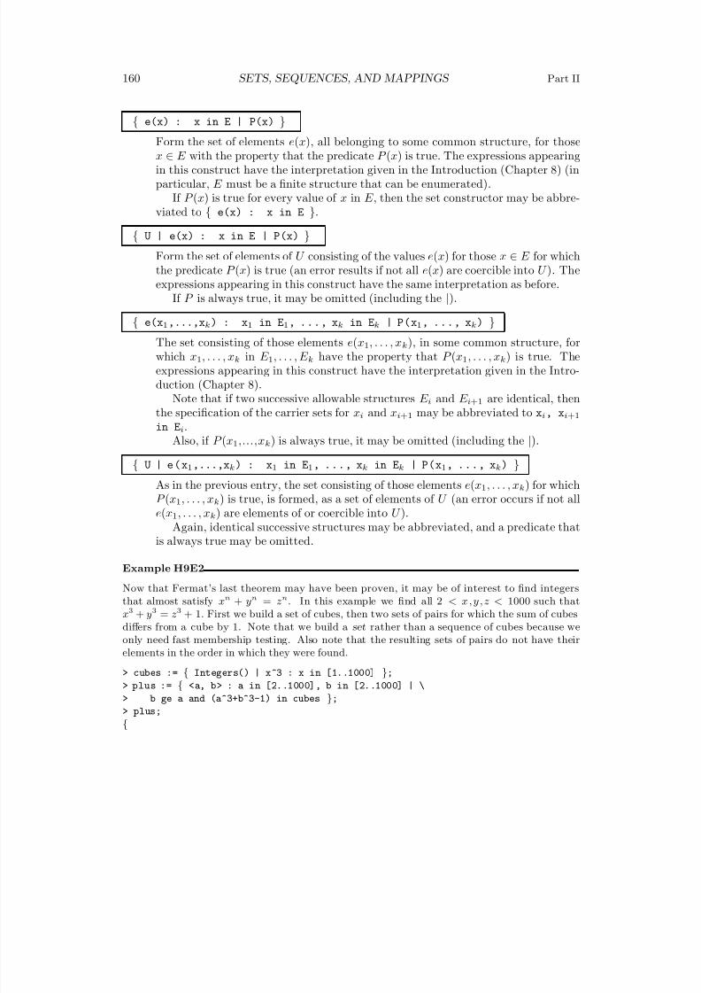
8/22/2019 Handbook Volume 01
http://slidepdf.com/reader/full/handbook-volume-01 276/440
160 SETS, SEQUENCES, AND MAPPINGS Part II
{ e(x) : x in E | P(x) }
Form the set of elements e(x), all belonging to some common structure, for thosex ∈ E with the property that the predicate P (x) is true. The expressions appearingin this construct have the interpretation given in the Introduction (Chapter 8) (inparticular, E must be a finite structure that can be enumerated).
If P (x) is true for every value of x in E , then the set constructor may be abbre-viated to { e(x) : x in E }.
{ U | e(x) : x in E | P(x) }
Form the set of elements of U consisting of the values e(x) for those x ∈ E for whichthe predicate P (x) is true (an error results if not all e(x) are coercible into U ). Theexpressions appearing in this construct have the same interpretation as before.
If P is always true, it may be omitted (including the |).
{ e(x1,...,xk) : x1 in E1, ..., xk in Ek | P(x1, ..., xk) }
The set consisting of those elements e(x1, . . . , xk), in some common structure, forwhich x1, . . . , xk in E 1, . . . , E k have the property that P (x1, . . . , xk) is true. Theexpressions appearing in this construct have the interpretation given in the Intro-duction (Chapter 8).
Note that if two successive allowable structures E i and E i+1 are identical, thenthe specification of the carrier sets for xi and xi+1 may be abbreviated to xi, xi+1
in Ei.Also, if P (x1,...,xk) is always true, it may be omitted (including the |).
{ U | e(x1,...,xk) : x1 in E1, ..., xk in Ek | P(x1, ..., xk) }
As in the previous entry, the set consisting of those elements e(x1, . . . , xk) for whichP (x1, . . . , xk) is true, is formed, as a set of elements of U (an error occurs if not alle(x1, . . . , xk) are elements of or coercible into U ).
Again, identical successive structures may be abbreviated, and a predicate thatis always true may be omitted.
Example H9E2
Now that Fermat’s last theorem may have been proven, it may be of interest to find integers
that almost satisfy xn + yn = z n. In this example we find all 2 < x , y , z < 1000 such thatx3 + y3 = z 3 + 1. First we build a set of cubes, then two sets of pairs for which the sum of cubesdiffers from a cube by 1. Note that we build a set rather than a sequence of cubes because weonly need fast membership testing. Also note that the resulting sets of pairs do not have theirelements in the order in which they were found.
> cubes := { Integers() | x^3 : x in [1..1000] };
> plus := { <a, b> : a in [2..1000], b in [2..1000] | \
> b ge a and (a^3+b^3-1) in cubes };
> plus;
{
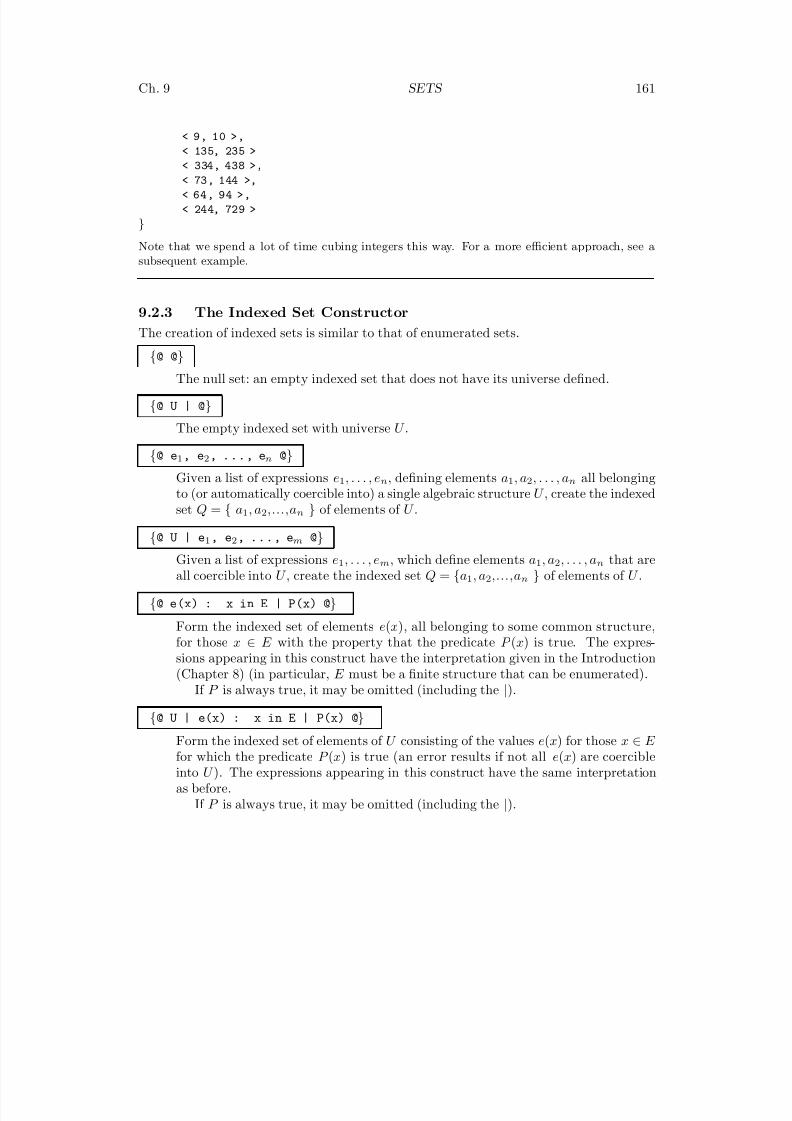
8/22/2019 Handbook Volume 01
http://slidepdf.com/reader/full/handbook-volume-01 277/440
Ch. 9 SETS 161
< 9, 10 >,
< 135, 235 >
< 334, 438 >,< 73, 144 >,
< 64, 94 >,
< 244, 729 >
}
Note that we spend a lot of time cubing integers this way. For a more efficient approach, see asubsequent example.
9.2.3 The Indexed Set Constructor
The creation of indexed sets is similar to that of enumerated sets.{@ @}
The null set: an empty indexed set that does not have its universe defined.
{@ U | @}
The empty indexed set with universe U .
{@ e1, e2, ..., en @}
Given a list of expressions e1, . . . , en, defining elements a1, a2, . . . , an all belongingto (or automatically coercible into) a single algebraic structure U , create the indexed
set Q = { a1, a2,...,an } of elements of U .
{@ U | e1, e2, ..., em @}
Given a list of expressions e1, . . . , em, which define elements a1, a2, . . . , an that areall coercible into U , create the indexed set Q = {a1, a2,...,an } of elements of U .
{@ e(x) : x in E | P(x) @}
Form the indexed set of elements e(x), all belonging to some common structure,for those x ∈ E with the property that the predicate P (x) is true. The expres-sions appearing in this construct have the interpretation given in the Introduction
(Chapter 8) (in particular, E must be a finite structure that can be enumerated).If P is always true, it may be omitted (including the |).
{@ U | e(x) : x in E | P(x) @}
Form the indexed set of elements of U consisting of the values e(x) for those x ∈ E for which the predicate P (x) is true (an error results if not all e(x) are coercibleinto U ). The expressions appearing in this construct have the same interpretationas before.
If P is always true, it may be omitted (including the |).
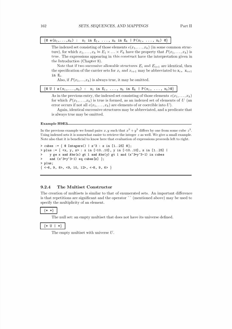
8/22/2019 Handbook Volume 01
http://slidepdf.com/reader/full/handbook-volume-01 278/440
162 SETS, SEQUENCES, AND MAPPINGS Part II
{@ e(x1,...,xk) : x1 in E1, ..., xk in Ek | P(x1, ..., xk) @}
The indexed set consisting of those elements e(x1
, . . . , xk) (in some common struc-ture), for which x1, . . . , xk in E 1 × . . . × E k have the property that P (x1, . . . , xk) istrue. The expressions appearing in this construct have the interpretation given inthe Introduction (Chapter 8).
Note that if two successive allowable structures E i and E i+1 are identical, thenthe specification of the carrier sets for xi and xi+1 may be abbreviated to xi, xi+1
in Ei.Also, if P (x1,...,xk) is always true, it may be omitted.
{@ U | e ( x1,...,xk) : x1 in E1, ..., xk in Ek | P(x1, ..., xk)@}
As in the previous entry, the indexed set consisting of those elements e(x1, . . . , xk)
for which P (x1, . . . , xk) is true is formed, as an indexed set of elements of U (anerror occurs if not all e(x1, . . . , xk) are elements of or coercible into U ).
Again, identical successive structures may be abbreviated, and a predicate thatis always true may be omitted.
Example H9E3
In the previous example we found pairs x, y such that x3 + y3 differs by one from some cube z 3.Using indexed sets it is somewhat easier to retrieve the integer z as well. We give a small example.Note also that it is beneficial to know here that evaluation of expressions proceeds left to right.
> cubes := { @ Integers() | z^3 : z in [1..25] @};
> plus := { <x, y, z> : x in [-10..10], y in [-10..10], z in [1..25] |
> y ge x and Abs(x) gt 1 and Abs(y) gt 1 and (x^3+y^3-1) in cubes
> and (x^3+y^3-1) eq cubes[z] };
> plus;
{ <-6, 9, 8>, <9, 10, 12>, <-8, 9, 6> }
9.2.4 The Multiset Constructor
The creation of multisets is similar to that of enumerated sets. An important difference
is that repetitions are significant and the operator ˆˆ (mentioned above) may be used tospecify the multiplicity of an element.
{* *}
The null set: an empty multiset that does not have its universe defined.
{* U | *}
The empty multiset with universe U .
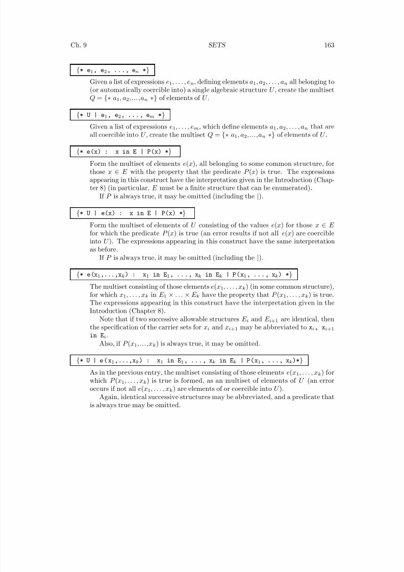
8/22/2019 Handbook Volume 01
http://slidepdf.com/reader/full/handbook-volume-01 279/440
Ch. 9 SETS 163
{* e1, e2, ..., en *}
Given a list of expressions e1, . . . , en, defining elements a1, a2, . . . , an all belonging to(or automatically coercible into) a single algebraic structure U , create the multisetQ = {∗ a1, a2,...,an ∗} of elements of U .
{* U | e1, e2, ..., em *}
Given a list of expressions e1, . . . , em, which define elements a1, a2, . . . , an that areall coercible into U , create the multiset Q = {∗ a1, a2,...,an ∗} of elements of U .
{* e(x) : x in E | P(x) *}
Form the multiset of elements e(x), all belonging to some common structure, for
those x ∈ E with the property that the predicate P (x) is true. The expressionsappearing in this construct have the interpretation given in the Introduction (Chap-ter 8) (in particular, E must be a finite structure that can be enumerated).
If P is always true, it may be omitted (including the |).
{* U | e(x) : x in E | P(x) *}
Form the multiset of elements of U consisting of the values e(x) for those x ∈ E for which the predicate P (x) is true (an error results if not all e(x) are coercibleinto U ). The expressions appearing in this construct have the same interpretationas before.
If P is always true, it may be omitted (including the |).
{* e(x1,...,xk) : x1 in E1, ..., xk in Ek | P(x1, ..., xk) *}
The multiset consisting of those elements e(x1, . . . , xk) (in some common structure),for which x1, . . . , xk in E 1 × . . . × E k have the property that P (x1, . . . , xk) is true.The expressions appearing in this construct have the interpretation given in theIntroduction (Chapter 8).
Note that if two successive allowable structures E i and E i+1 are identical, thenthe specification of the carrier sets for xi and xi+1 may be abbreviated to xi, xi+1
in Ei.
Also, if P (x1,...,xk) is always true, it may be omitted.
{* U | e ( x1,...,xk) : x1 in E1, ..., xk in Ek | P(x1, ..., xk)*}
As in the previous entry, the multiset consisting of those elements e(x1, . . . , xk) forwhich P (x1, . . . , xk) is true is formed, as an multiset of elements of U (an erroroccurs if not all e(x1, . . . , xk) are elements of or coercible into U ).
Again, identical successive structures may be abbreviated, and a predicate thatis always true may be omitted.
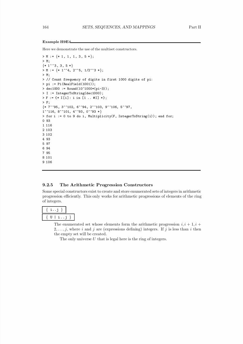
8/22/2019 Handbook Volume 01
http://slidepdf.com/reader/full/handbook-volume-01 280/440
164 SETS, SEQUENCES, AND MAPPINGS Part II
Example H9E4
Here we demonstrate the use of the multiset constructors.
> M : = {* 1 , 1 , 1 , 3 , 5 *};
> M;
{* 1^^3, 3, 5 *}> M : = {* 1^^4, 2^^5, 1/2^^3 *};
> M;
> // Count frequency of digits in first 1000 digits of pi:
> pi := Pi(RealField(1001));
> dec1000 := Round(10^1000*(pi-3));
> I := IntegerToString(dec1000);
> F := {* I[i]: i in [1 .. #I] *};
> F;{* 7^^95, 3^^102, 6^^94, 2^^103, 9^^106, 5^^97,
1^^116, 8^^101, 4^^93, 0^^93 *}> for i := 0 to 9 do i, Multiplicity(F, IntegerToString(i)); end for;
0 93
1 116
2 103
3 102
4 93
5 97
6 94
7 95
8 101
9 106
9.2.5 The Arithmetic Progression Constructors
Some special constructors exist to create and store enumerated sets of integers in arithmeticprogression efficiently. This only works for arithmetic progressions of elements of the ringof integers.
{ i..j }
{ U | i..j }
The enumerated set whose elements form the arithmetic progression i, i + 1, i +2, . . . , j, where i and j are (expressions defining) integers. If j is less than i thenthe empty set will be created.
The only universe U that is legal here is the ring of integers.
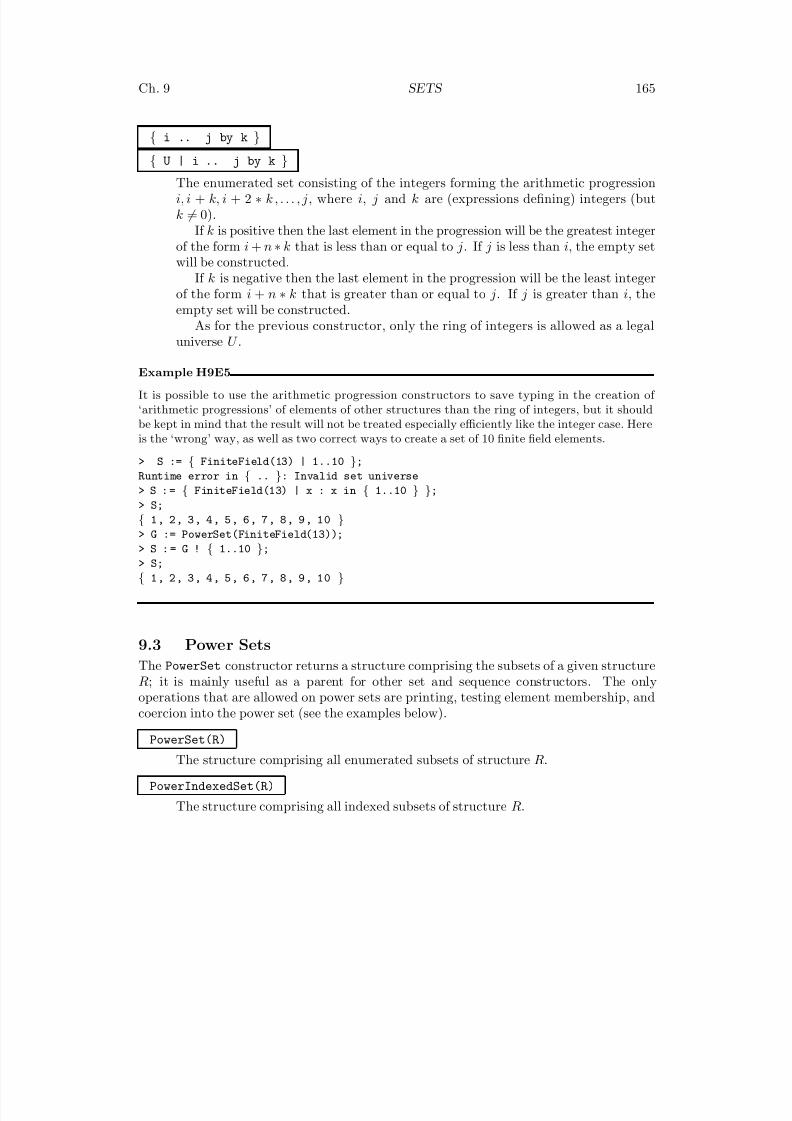
8/22/2019 Handbook Volume 01
http://slidepdf.com/reader/full/handbook-volume-01 281/440
Ch. 9 SETS 165
{ i .. j by k }
{ U | i .. j by k }
The enumerated set consisting of the integers forming the arithmetic progressioni, i + k, i + 2 ∗ k , . . . , j, where i, j and k are (expressions defining) integers (butk = 0).
If k is positive then the last element in the progression will be the greatest integerof the form i + n ∗ k that is less than or equal to j. If j is less than i, the empty setwill be constructed.
If k is negative then the last element in the progression will be the least integerof the form i + n ∗ k that is greater than or equal to j. If j is greater than i, theempty set will be constructed.
As for the previous constructor, only the ring of integers is allowed as a legal
universe U .
Example H9E5
It is possible to use the arithmetic progression constructors to save typing in the creation of ‘arithmetic progressions’ of elements of other structures than the ring of integers, but it shouldbe kept in mind that the result will not be treated especially efficiently like the integer case. Hereis the ‘wrong’ way, as well as two correct ways to create a set of 10 finite field elements.
> S := { FiniteField(13) | 1..10 };
Runtime error in { .. }: Invalid set universe
> S : = { FiniteField(13) | x : x in { 1..10 } };
> S;{ 1, 2, 3, 4, 5, 6, 7, 8, 9, 10 }> G := PowerSet(FiniteField(13));
> S : = G ! { 1..10 };
> S;
{ 1, 2, 3, 4, 5, 6, 7, 8, 9, 10 }
9.3 Power Sets
The PowerSet constructor returns a structure comprising the subsets of a given structureR; it is mainly useful as a parent for other set and sequence constructors. The onlyoperations that are allowed on power sets are printing, testing element membership, andcoercion into the power set (see the examples below).
PowerSet(R)
The structure comprising all enumerated subsets of structure R.
PowerIndexedSet(R)
The structure comprising all indexed subsets of structure R.
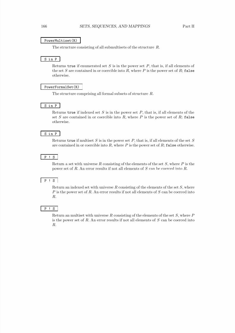
8/22/2019 Handbook Volume 01
http://slidepdf.com/reader/full/handbook-volume-01 282/440
166 SETS, SEQUENCES, AND MAPPINGS Part II
PowerMultiset(R)
The structure consisting of all submultisets of the structure R.
S i n P
Returns true if enumerated set S is in the power set P , that is, if all elements of the set S are contained in or coercible into R, where P is the power set of R; false
otherwise.
PowerFormalSet(R)
The structure comprising all formal subsets of structure R.
S i n P
Returns true if indexed set S is in the power set P , that is, if all elements of theset S are contained in or coercible into R, where P is the power set of R; false
otherwise.
S i n P
Returns true if multiset S is in the power set P , that is, if all elements of the set S are contained in or coercible into R, where P is the power set of R; false otherwise.
P ! S
Return a set with universe R consisting of the elements of the set S , where P is thepower set of R. An error results if not all elements of S can be coerced into R.
P ! S
Return an indexed set with universe R consisting of the elements of the set S , whereP is the power set of R. An error results if not all elements of S can be coerced intoR.
P ! S
Return an multiset with universe R consisting of the elements of the set S , where P is the power set of R. An error results if not all elements of S can be coerced intoR.
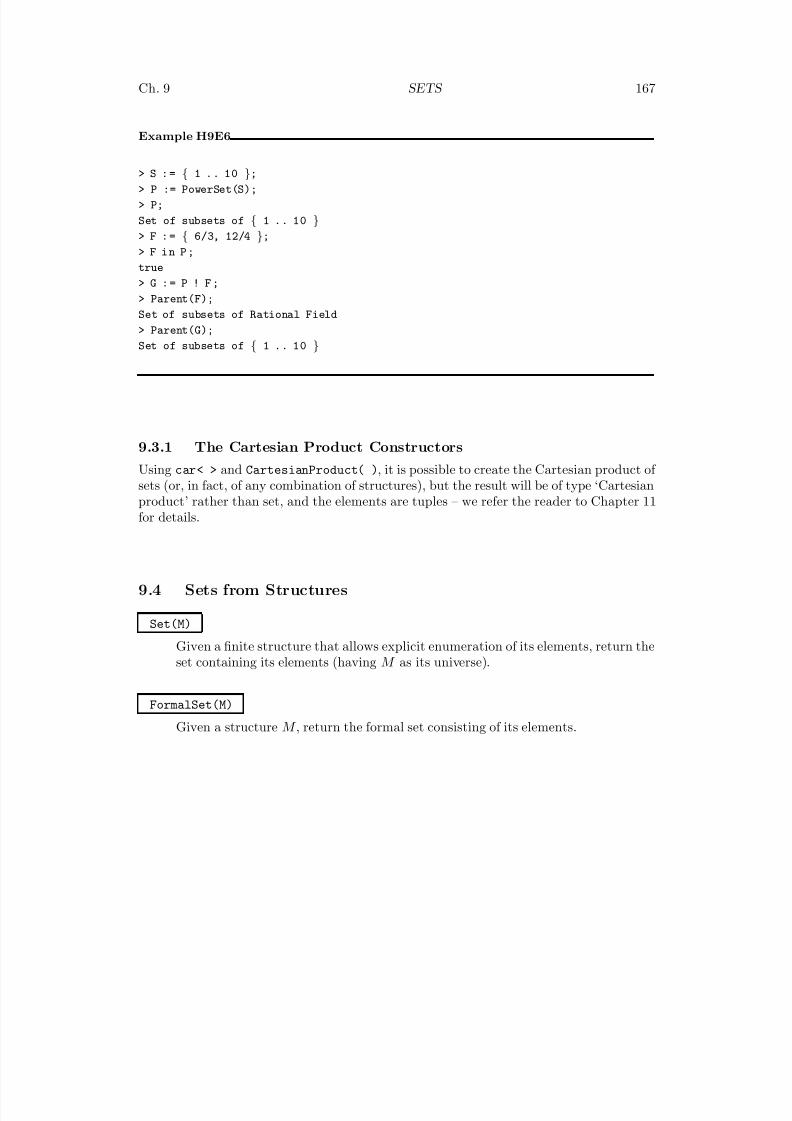
8/22/2019 Handbook Volume 01
http://slidepdf.com/reader/full/handbook-volume-01 283/440
Ch. 9 SETS 167
Example H9E6
> S : = { 1 .. 10 };
> P := PowerSet(S);
> P;
Set of subsets of { 1 .. 10 }
> F : = { 6/3, 12/4 };
> F i n P ;
true
> G : = P ! F ;
> Parent(F);
Set of subsets of Rational Field
> Parent(G);
Set of subsets of { 1 .. 10 }
9.3.1 The Cartesian Product Constructors
Using car< > and CartesianProduct( ), it is possible to create the Cartesian product of sets (or, in fact, of any combination of structures), but the result will be of type ‘Cartesian
product’ rather than set, and the elements are tuples – we refer the reader to Chapter 11for details.
9.4 Sets from Structures
Set(M)
Given a finite structure that allows explicit enumeration of its elements, return theset containing its elements (having M as its universe).
FormalSet(M)
Given a structure M , return the formal set consisting of its elements.
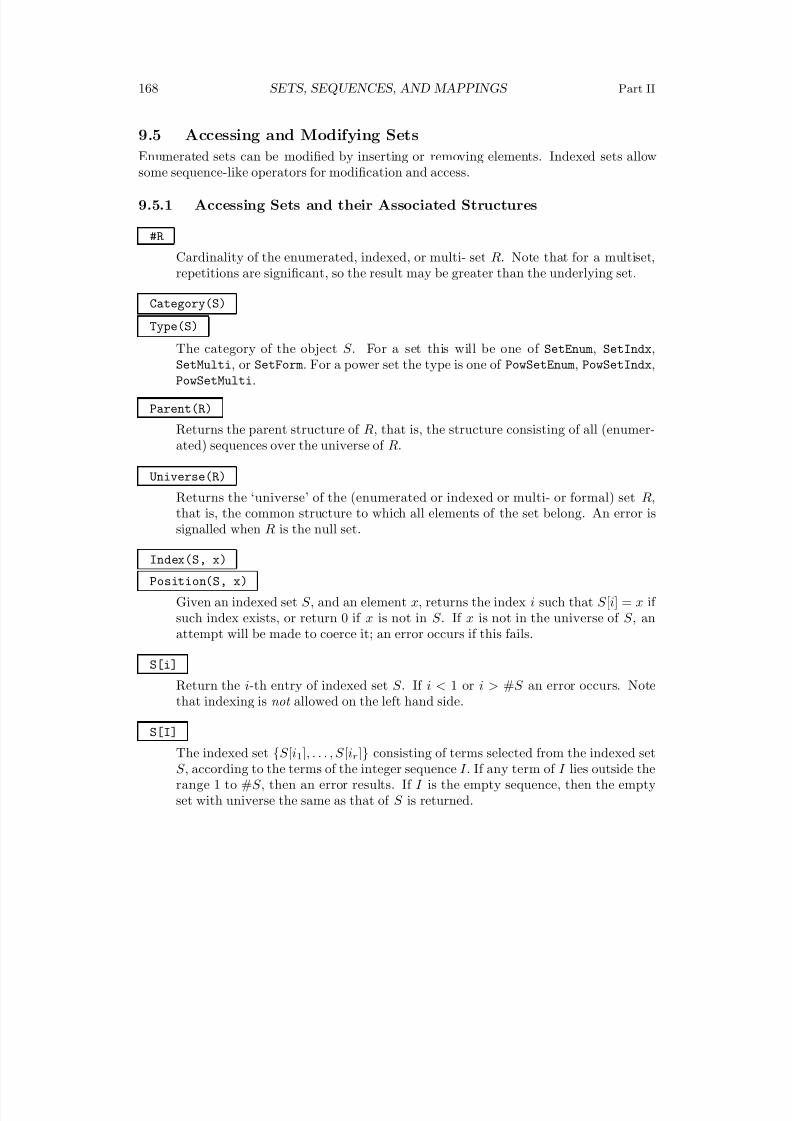
8/22/2019 Handbook Volume 01
http://slidepdf.com/reader/full/handbook-volume-01 284/440
168 SETS, SEQUENCES, AND MAPPINGS Part II
9.5 Accessing and Modifying Sets
Enumerated sets can be modified by inserting or removing elements. Indexed sets allow
some sequence-like operators for modification and access.
9.5.1 Accessing Sets and their Associated Structures
#R
Cardinality of the enumerated, indexed, or multi- set R. Note that for a multiset,repetitions are significant, so the result may be greater than the underlying set.
Category(S)
Type(S)
The category of the object S . For a set this will be one of SetEnum, SetIndx,SetMulti, or SetForm. For a power set the type is one of PowSetEnum, PowSetIndx,PowSetMulti.
Parent(R)
Returns the parent structure of R, that is, the structure consisting of all (enumer-ated) sequences over the universe of R.
Universe(R)
Returns the ‘universe’ of the (enumerated or indexed or multi- or formal) set R,that is, the common structure to which all elements of the set belong. An error issignalled when R is the null set.
Index(S, x)
Position(S, x)
Given an indexed set S , and an element x, returns the index i such that S [i] = x if such index exists, or return 0 if x is not in S . If x is not in the universe of S , anattempt will be made to coerce it; an error occurs if this fails.
S[i]
Return the i-th entry of indexed set S . If i < 1 or i > #S an error occurs. Notethat indexing is not allowed on the left hand side.
S[I]
The indexed set {S [i1], . . . , S [ir]} consisting of terms selected from the indexed setS , according to the terms of the integer sequence I . If any term of I lies outside therange 1 to #S , then an error results. If I is the empty sequence, then the emptyset with universe the same as that of S is returned.
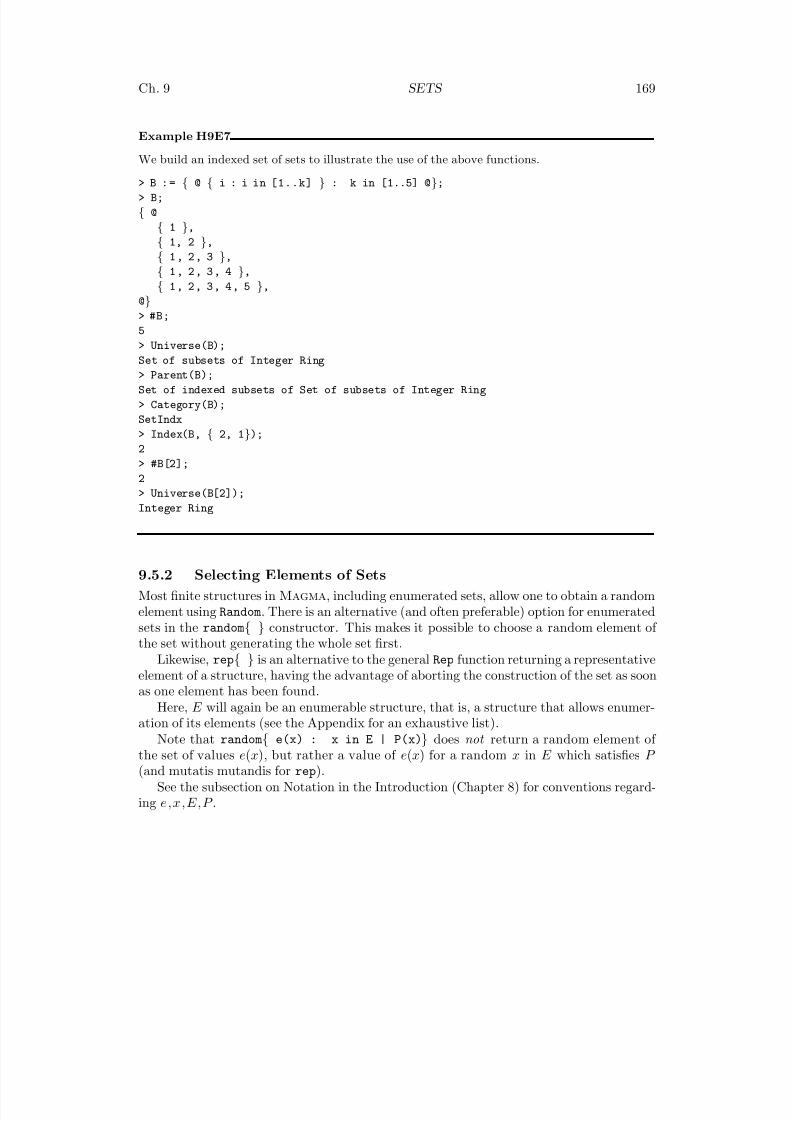
8/22/2019 Handbook Volume 01
http://slidepdf.com/reader/full/handbook-volume-01 285/440
Ch. 9 SETS 169
Example H9E7
We build an indexed set of sets to illustrate the use of the above functions.
> B : = { @ { i : i in [1..k] } : k in [1..5] @};
> B;
{ @
{ 1 },
{ 1, 2 },
{ 1, 2, 3 },
{ 1, 2, 3, 4 },
{ 1, 2, 3, 4, 5 },
@}> #B;
5
> Universe(B);
Set of subsets of Integer Ring
> Parent(B);
Set of indexed subsets of Set of subsets of Integer Ring
> Category(B);
SetIndx
> Index(B, { 2, 1});
2
> #B[2];
2
> Universe(B[2]);
Integer Ring
9.5.2 Selecting Elements of Sets
Most finite structures in Magma, including enumerated sets, allow one to obtain a randomelement using Random. There is an alternative (and often preferable) option for enumeratedsets in the random{ } constructor. This makes it possible to choose a random element of the set without generating the whole set first.
Likewise, rep{ } is an alternative to the general Rep function returning a representative
element of a structure, having the advantage of aborting the construction of the set as soonas one element has been found.
Here, E will again be an enumerable structure, that is, a structure that allows enumer-ation of its elements (see the Appendix for an exhaustive list).
Note that random{ e(x) : x in E | P(x)} does not return a random element of the set of values e(x), but rather a value of e(x) for a random x in E which satisfies P (and mutatis mutandis for rep).
See the subsection on Notation in the Introduction (Chapter 8) for conventions regard-ing e,x,E,P .

8/22/2019 Handbook Volume 01
http://slidepdf.com/reader/full/handbook-volume-01 286/440
170 SETS, SEQUENCES, AND MAPPINGS Part II
Random(R)
A random element chosen from the enumerated, indexed or multi- set R. Every
element has an equal probability of being chosen for enumerated or indexed sets,and a weighted probability in proportion to its multiplicity for multisets. Succes-sive invocations of the function will result in independently chosen elements beingreturned as the value of the function. If R is empty an error occurs.
random{ e(x) : x in E | P(x) }
Given an enumerated structure E and a Boolean expression P , return the value of the expression e(y) for a randomly chosen element y of E for which P (y) is true.
P may be omitted if it is always true.
random{e(x1, ..., xk) : x1 in E1, ..., xk in Ek | P(x1, ..., xk)}Given enumerated structures E 1, . . . , E k, and a Boolean expression P (x1, . . ., xk),return the value of the expression e(y1, · · · , yk) for a randomly chosen element <y1, . . . , yk > of E 1 × · · · × E k, for which P (y1, . . . , yk) is true.
P may be omitted if it is always true.If successive structures E i and E i+1 are identical, then the abbreviation xi, xi+1
in Ei may be used.
Example H9E8
Here are two ways to find a ‘random’ primitive element for a finite field.
> p := 10007;
> F := FiniteField(p);
> proots := { z : z in F | IsPrimitive(z) };
> #proots;
5002
> Random(proots);
5279
This way, a set of 5002 elements is built (and primitivity is checked for all elements of F ), and arandom choice is made. Alternatively, we use random.
> random{ x : x in F | IsPrimitive(x) };
4263
In this case random elements in F are chosen until one is found that is primitive. Since almost half of F ’s elements are primitive, only very few primitivity tests will be done before success occurs.
Representative(R)
Rep(R)
An arbitrary element chosen from the enumerated, indexed, or multi- set R.
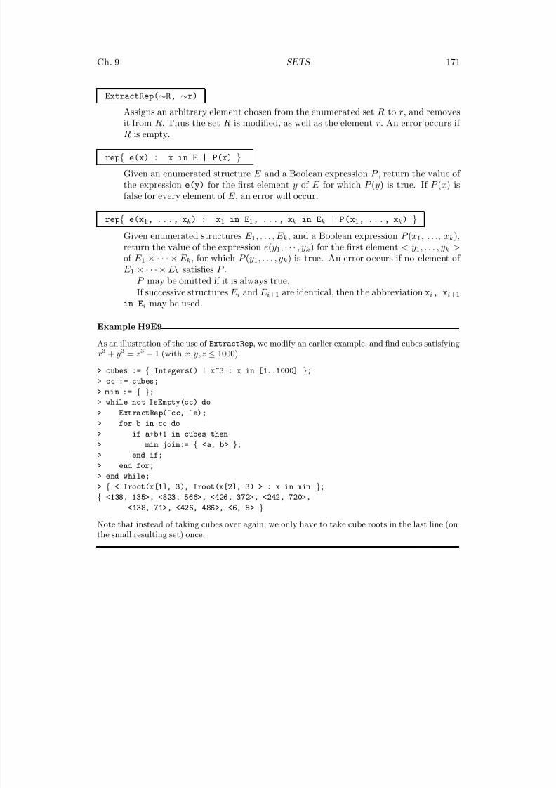
8/22/2019 Handbook Volume 01
http://slidepdf.com/reader/full/handbook-volume-01 287/440
Ch. 9 SETS 171
ExtractRep(∼R, ∼r)
Assigns an arbitrary element chosen from the enumerated set R to r, and removesit from R. Thus the set R is modified, as well as the element r. An error occurs if R is empty.
rep{ e(x) : x in E | P(x) }
Given an enumerated structure E and a Boolean expression P , return the value of the expression e(y) for the first element y of E for which P (y) is true. If P (x) isfalse for every element of E , an error will occur.
rep{ e(x1, ..., xk) : x1 in E1, ..., xk in Ek | P(x1, ..., xk) }
Given enumerated structures E 1, . . . , E k, and a Boolean expression P (x1, . . ., xk),return the value of the expression e(y1, · · · , yk) for the first element < y1, . . . , yk >of E 1 × · · · × E k, for which P (y1, . . . , yk) is true. An error occurs if no element of E 1 × · · · × E k satisfies P .
P may be omitted if it is always true.If successive structures E i and E i+1 are identical, then the abbreviation xi, xi+1
in Ei may be used.
Example H9E9
As an illustration of the use of ExtractRep, we modify an earlier example, and find cubes satisfying
x3
+ y3
= z 3
− 1 (with x,y,z ≤ 1000).
> cubes := { Integers() | x^3 : x in [1..1000] };
> cc := cubes;
> min := { };
> while not IsEmpty(cc) do
> ExtractRep(~cc, ~a);
> for b in cc do
> if a+b+1 in cubes then
> min join:= { <a, b> };
> end if;
> end for;
> end while;> { < Iroot(x[1], 3), Iroot(x[2], 3) > : x in min };
{ <138, 135>, <823, 566>, <426, 372>, <242, 720>,
<138, 71>, <426, 486>, <6, 8> }
Note that instead of taking cubes over again, we only have to take cube roots in the last line (onthe small resulting set) once.
8/22/2019 Handbook Volume 01
http://slidepdf.com/reader/full/handbook-volume-01 288/440
172 SETS, SEQUENCES, AND MAPPINGS Part II
Minimum(S)
Min(S)
Given a non-empty enumerated, indexed, or multi- set S , such that lt and eq aredefined on the universe of S , this function returns the minimum of the elements of S . If S is an indexed set, the position of the minimum is also returned.
Maximum(S)
Max(S)
Given a non-empty enumerated, indexed, or multi- set S , such that lt and eq aredefined on the universe of S , this function returns the maximum of the elements of S . If S is an indexed set, the position of the maximum is also returned.
Hash(x)
Given a Magma object x which can be placed in a set, return the hash value of x used by the set machinery. This is a fixed but arbitrary non-negative integer(whose maximum value is the maximum value of a C unsigned long on the particularmachine). The crucial property is that if x and y are objects and x equals y then thehash values of x and y are equal (even if x and y have different internal structures).Thus one could implement sets manually if desired by the use of this function.
9.5.3 Modifying Sets
Include(∼S, x)Include(S, x)
Create the enumerated, indexed, or multi- set obtained by putting the element x inS (S is unchanged if S is not a multiset and x is already in S ). If S is an indexedset, the element will be appended at the end. If S is a multiset, the multiplicity of x will be increased accordingly. If x is not in the universe of S , an attempt will bemade to coerce it; an error occurs if this fails.
There are two versions of this: a procedure, where S is replaced by the new set,and a function, which returns the new set. The procedural version takes a reference∼ S to S as an argument.
Note that the procedural version is much more efficient since the set S will notbe copied.
Exclude(∼S, x)
Exclude(S, x)
Create a new set by removing the element x from S . If S is an enumerated set,nothing happens if x is not in S . If S is a multiset, the multiplicity of x will bedecreased accordingly. If x is not in the universe of S , an attempt will be made tocoerce it; an error occurs if this fails.
8/22/2019 Handbook Volume 01
http://slidepdf.com/reader/full/handbook-volume-01 289/440
Ch. 9 SETS 173
There are two versions of this: a procedure, where S is replaced by the new set,and a function, which returns the new set. The procedural version takes a reference
∼ S to S as an argument.Note that the procedural version is much more efficient since the set S will not
be copied.
ChangeUniverse(∼S, V)
ChangeUniverse(S, V)
Given an enumerated, indexed, or multi- set S with universe U and a structureV which contains U , construct a new set of the same type which consists of theelements of S coerced into V .
There are two versions of this: a procedure, where S is replaced by the new set,
and a function, which returns the new set. The procedural version takes a reference∼ S to S as an argument.Note that the procedural version is much more efficient since the set S will not
be copied.
CanChangeUniverse(S, V)
Given an enumerated, indexed, or multi- set S with universe U and a structure V which contains U , attempt to construct a new set T of the same type which consistsof the elements of S coerced into V ; if successful, return true and T , otherwisereturn false.
Example H9E10
This example uses Include and Exclude to find a set (if it exists) of cubes of integers such thatthe elements of a given set R can be expressed as the sum of two of those.
> R : = { 218, 271, 511 };
> x : = 0 ;
> cubes := { 0 };
> while not IsEmpty(R) do
> x +:= 1;
> c := x^3;
> Include(~cubes, c);
> Include(~cubes, -c);> for z in cubes do
> Exclude(~R, z+c);
> Exclude(~R, z-c);
> end for;
> end while;
We did not record how the elements of R were obtained as sums of a pair of cubes. For that, thefollowing suffices.
> R : = { 218, 271, 511 }; // it has been emptied !
> { { x, y } : x, y in cubes | x+y in R };
8/22/2019 Handbook Volume 01
http://slidepdf.com/reader/full/handbook-volume-01 290/440
174 SETS, SEQUENCES, AND MAPPINGS Part II
{
{ -729, 1000 },
{ -125, 343 },{ -1, 512 },
}
SetToIndexedSet(E)
Given an enumerated set E , this function returns an indexed set with the sameelements (and universe) as E .
IndexedSetToSet(S)
Isetset(S)
Given an indexed set S , this function returns an enumerated set with the sameelements (and universe) as E .
IndexedSetToSequence(S)
Isetseq(S)
Given an indexed set S , this function returns a sequence with the same elements(and universe) as E .
MultisetToSet(S)
Given a multiset S , this function returns an enumerated set with the same elements(and universe) as S .
SetToMultiset(E)
Given an enumerated set E , this function returns a multiset with the same elements
(and universe) as E .
SequenceToMultiset(Q)
Given an enumerated sequence E , this function returns a multiset with the sameelements (and universe) as E .
8/22/2019 Handbook Volume 01
http://slidepdf.com/reader/full/handbook-volume-01 291/440
Ch. 9 SETS 175
9.6 Operations on Sets
9.6.1 Boolean Functions and OperatorsAs explained in the Introduction (Chapter 8), when elements are taken out of a set theirparent will be the universe of the set (or, if the universe is itself a set, the universe of theuniverse, etc.); in particular, the set itself is not the parent. Hence equality testing on setelements is in fact equality testing between two elements of certain algebraic structures,and the sets are irrelevant. We only list the (in)equality operator for convenience here.
Element membership testing is of critical importance for all types of sets.Testing whether or not R is a subset of S can be done if R is an enumerated or indexed
set and S is any set; hence (in)equality testing is only possible between sets that are notformal sets.
IsNull(R)
Returns true if and only if the enumerated, indexed, or multi- set R is empty anddoes not have its universe defined.
IsEmpty(R)
Returns true if and only if the enumerated, indexed or multi- set R is empty.
x e q y
Given an element x of a set R with universe U and an element y of a set S with
universe V , where a common overstructure W can be found with U ⊂ W ⊃ V (seethe Introduction (Chapter 8) for details on overstructures), return true if and onlyif x and y are equal as elements of W .
x n e y
Given an element x of a set R with universe U and an element y of a set S withuniverse V , where a common overstructure W can be found with U ⊂ W ⊃ V (seethe Introduction (Chapter 8) for details on overstructures), return true if and onlyif x and y are distinct as elements of W .
x i n R
Returns true if and only if the element x is a member of the set R. If x is not anelement of the universe U of R, it is attempted to coerce x into U ; if this fails, anerror occurs.
x notin R
Returns true if and only if the element x is not a member of the set R. If x is notan element of the parent structure U of R, it is attempted to coerce x into U ; if thisfails, an error occurs.
8/22/2019 Handbook Volume 01
http://slidepdf.com/reader/full/handbook-volume-01 292/440
176 SETS, SEQUENCES, AND MAPPINGS Part II
R subset S
Returns true if the enumerated, indexed or multi- set R is a subset of the set S ,
false otherwise. For multisets, if an element x of R has multiplicity n in R, themultiplicity of x in S must be at least n. Coercion of the elements of R into S isattempted if necessary, and an error occurs if this fails.
R notsubset S
Returns true if the enumerated, indexed, or multi- set R is a not a subset of the setS , false otherwise. Coercion of the elements of R into S is attempted if necessary,and an error occurs if this fails.
R e q S
Returnstrue
if and only if R and S are identical sets, where R and S are enumerated,indexed or multi- sets For indexed sets, the index function is irrelevant for decidingequality. For multisets, matching multiplicities must also be equal. Coercion of theelements of R into S is attempted if necessary, and an error occurs if this fails.
R n e S
Returns true if and only if R and S are distinct sets, where R and S are enumeratedindexed, or multi- sets. For indexed sets, the index function is irrelevant for decidingequality. For multisets, matching multiplicities must also be equal. Coercion of theelements of R into S is attempted if necessary, and an error occurs if this fails.
IsDisjoint(R, S)Returns true iff the enumerated, indexed or multi- sets R and S are disjoint. Co-ercion of the elements of R into S is attempted if necessary, and an error occurs if this fails.
9.6.2 Binary Set Operators
For each of the following operators, R and S are sets of the same type. If R and S areboth formal sets, then an error will occur unless both have been constructed with the samecarrier structure F in the definition. If R and S are both enumerated, indexed, or multi-sets, then an error occurs unless the universes of R and S are compatible, as defined in
the Introduction to this Part (Chapter 8).Note that
Q := { ! x i n R !}
converts an enumerated set R into a formal set Q.
R join S
Union of the sets R and S (see above for the restrictions on R and S ). For multisets,matching multiplicities are added in the union.
8/22/2019 Handbook Volume 01
http://slidepdf.com/reader/full/handbook-volume-01 293/440
Ch. 9 SETS 177
R meet S
Intersection of the sets R and S (see above for the restrictions on R and S ). For
multisets, the minimum of matching multiplicities is stored in the intersection.
R diff S
Difference of the sets R and S , i.e., the set consisting of those elements of R whichare not members of S (see above for the restrictions on R and S ).
R sdiff S
Symmetric difference of the sets R and S , i.e., the set consisting of those elementswhich are members of either R or S but not both (see above for the restrictions onR and S ).
Example H9E11
> R : = { 1, 2, 3 };
> S : = { 1, 1/2, 1/3 };
> R join S;
{ 1/3, 1/2, 1, 2, 3 }> R meet S;
{ 1 }> R diff S;
{ 2, 3 }> S diff R;
{ 1/3, 1/2 }> R sdiff S;
{ 1/3, 1/2, 2, 3 }
9.6.3 Other Set Operations
Multiplicity(S, x)
Return the multiplicity in multiset S of element x. If x is not in S , zero is returned.
Multiplicities(S)
Returns the sequence of multiplicities of distinct elements in the multiset S . Theorder is the same as the internal enumeration order of the elements.
Subsets(S)
The set of all subsets of S .
Subsets(S, k)
The set of subsets of S of size k. If k is larger than the cardinality of S then theresult will be empty.
8/22/2019 Handbook Volume 01
http://slidepdf.com/reader/full/handbook-volume-01 294/440
178 SETS, SEQUENCES, AND MAPPINGS Part II
Multisets(S, k)
The set of multisets consisting of k not necessarily distinct elements of S .
Subsequences(S, k)
The set of sequences of length k with elements from S .
Permutations(S)
The set of permutations (stored as sequences) of the elements of S .
Permutations(S, k)
The set of permutations (stored as sequences) of each of the subsets of S of cardi-
nality k.
9.7 Quantifiers
To test whether some enumerated set is empty or not, one may use the IsEmpty function.However, to use IsEmpty, the set has to be created in full first. The existential quantifierexists enables one to do the test and abort the construction of the set as soon as anelement is found; moreover, the element found will be assigned to a variable.
Likewise, forall enables one to abort the construction of the set as soon as an elementnot satisfying a certain property is encountered.
Note that exists(t){ e(x) : x in E | P(x) } is not designed to return true if anelement of the set of values e(x) satisfies P , but rather if there is an x ∈ E satisfying P (x)(in which case e(x) is assigned to t).
For the notation used here, see the beginning of this chapter.
exists(t){ e(x): x in E | P(x) }
exists(t1, ..., tr){ e(x) : x in E | P(x) }
Given an enumerated structure E and a Boolean expression P (x), the Boolean valuetrue is returned if E contains at least one element x for which P (x) is true. If P (x)is not true for any element x of E , then the Boolean value false is returned.
Moreover, if P (x) is found to be true for the element y, say, of E , then in the firstform of the exists expression, variable t will be assigned the value of the expressione(y). If P (x) is never true for an element of E , t will be left unassigned. In thesecond form, where r variables t1, . . . , tr are given, the result e(y) should be a tupleof length r; each variable will then be assigned to the corresponding component of the tuple. Similarly, all the variables will be left unassigned if P (x) is never true.The clause (t) may be omitted entirely.
P may be omitted if it is always true.
8/22/2019 Handbook Volume 01
http://slidepdf.com/reader/full/handbook-volume-01 295/440
Ch. 9 SETS 179
exists(t){e(x1, ..., xk): x1 in E1, ..., xk in Ek | P(x1, ..., xk)}
exists(t1
, ..., tr
){ e(x1
, ..., xk
) : x1
in E1
, ..., xk
in Ek
| P }
Given enumerated structures E 1, . . . , E k, and a Boolean expression P (x1, . . ., xk),the Boolean value true is returned if there is an element < y1, . . ., yk > in theCartesian product E 1 × · · · × E k, such that P (y1, . . . , yk) is true. If P (x1, . . . , xk) isnot true for any element (y1, . . ., yk) of E 1 × · · · × E k, then the Boolean value falseis returned.
Moreover, if P (x1, . . ., xk) is found to be true for the element < y1, . . . , yk > of E 1 × · · · × E k, then in the first form of the exists expression, the variable t will beassigned the value of the expression e(y1, · · · , yk). If P (x1, . . ., xk) is never true foran element of E 1× · · · ×E k, then the variable t will be left unassigned. In the secondform, where r variables t1, . . . , tr are given, the result e(y1, · · · , yk) should be a tuple
of length r; each variable will then be assigned to the corresponding component of the tuple. Similarly, all the variables will be left unassigned if P (x1, . . ., xk) is nevertrue. The clause (t) may be omitted entirely.
P may be omitted if it is always true.If successive structures E i and E i+1 are identical, then the abbreviation xi, xi+1
in Ei may be used.
Example H9E12
As a variation on an earlier example, we check whether or not some integers can be written assums of cubes (less than 103 in absolute value):
> exists(t){ <x, y> : x, y in [ t^3 : t in [-10..10] ] | x + y eq 218 };
true
> t;
<-125, 343>
> exists(t){ <x, y> : x, y in [ t^3 : t in [1..10] ] | x + y eq 218 };
false
> t;
>> t;
^
User error: Identifier ’t’ has not been declared
forall(t){ e(x) : x in E | P(x) }
forall(t1, ..., tr){ e(x) : x in E | P(x) }
Given an enumerated structure E and a Boolean expression P (x), the Boolean valuetrue is returned if P (x) is true for every element x of E .
If P (x) is not true for at least one element x of E , then the Boolean value falseis returned.
Moreover, if P (x) is found to be false for the element y, say, of E , then in the firstform of the exists expression, variable t will be assigned the value of the expression
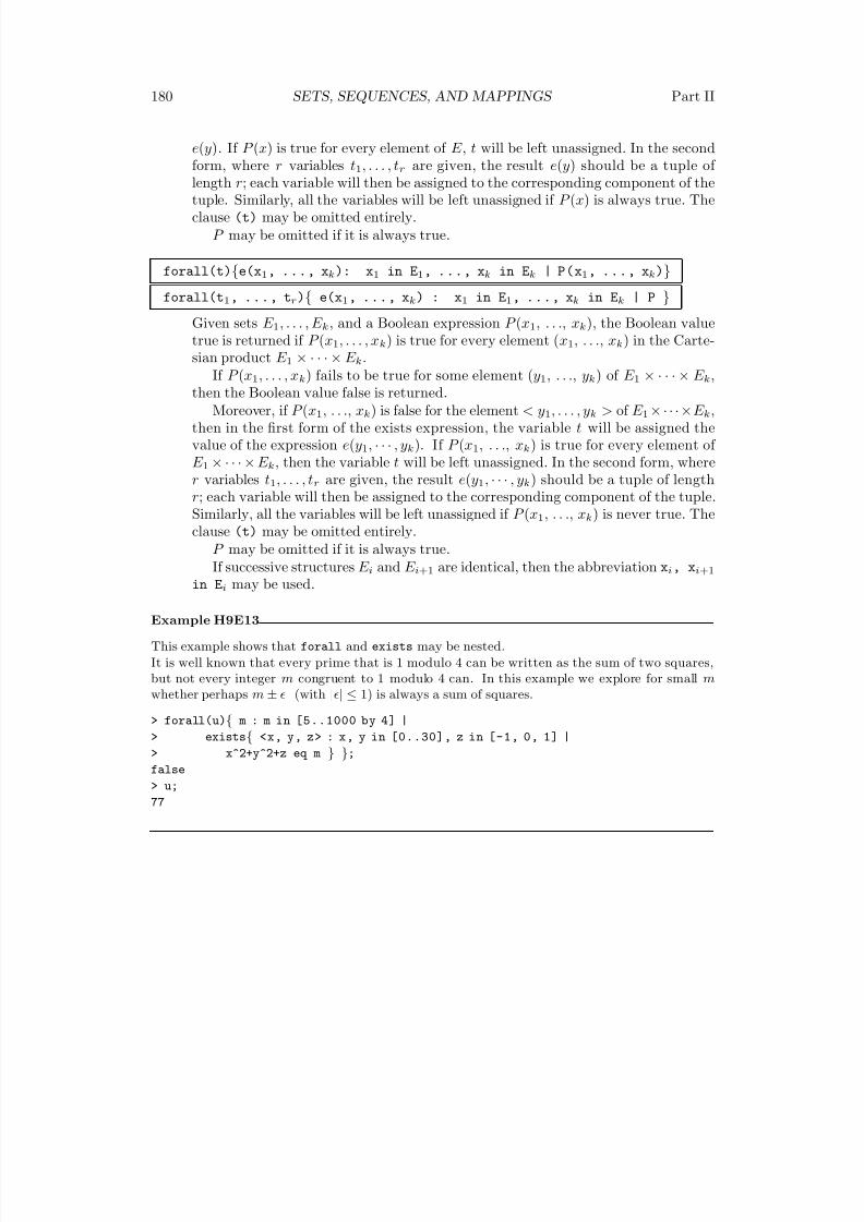
8/22/2019 Handbook Volume 01
http://slidepdf.com/reader/full/handbook-volume-01 296/440
180 SETS, SEQUENCES, AND MAPPINGS Part II
e(y). If P (x) is true for every element of E , t will be left unassigned. In the secondform, where r variables t1, . . . , tr are given, the result e(y) should be a tuple of
length r; each variable will then be assigned to the corresponding component of thetuple. Similarly, all the variables will be left unassigned if P (x) is always true. Theclause (t) may be omitted entirely.
P may be omitted if it is always true.
forall(t){e(x1, ..., xk): x1 in E1, ..., xk in Ek | P(x1, ..., xk)}
forall(t1, ..., tr){ e(x1, ..., xk) : x1 in E1, ..., xk in Ek | P }
Given sets E 1, . . . , E k, and a Boolean expression P (x1, . . ., xk), the Boolean valuetrue is returned if P (x1, . . . , xk) is true for every element (x1, . . ., xk) in the Carte-sian product E 1 × · · · × E k.
If P (x1, . . . , xk) fails to be true for some element (y1, . . ., yk) of E 1 × · · · × E k,then the Boolean value false is returned.
Moreover, if P (x1, . . ., xk) is false for the element < y1, . . . , yk > of E 1× · · · ×E k,then in the first form of the exists expression, the variable t will be assigned thevalue of the expression e(y1, · · · , yk). If P (x1, . . ., xk) is true for every element of E 1 × · · · × E k, then the variable t will be left unassigned. In the second form, wherer variables t1, . . . , tr are given, the result e(y1, · · · , yk) should be a tuple of lengthr; each variable will then be assigned to the corresponding component of the tuple.Similarly, all the variables will be left unassigned if P (x1, . . ., xk) is never true. Theclause (t) may be omitted entirely.
P may be omitted if it is always true.If successive structures E i and E i+1 are identical, then the abbreviation xi, xi+1
in Ei may be used.
Example H9E13
This example shows that forall and exists may be nested.
It is well known that every prime that is 1 modulo 4 can be written as the sum of two squares,but not every integer m congruent to 1 modulo 4 can. In this example we explore for small mwhether perhaps m ± (with || ≤ 1) is always a sum of squares.
> forall(u){ m : m in [5..1000 by 4] |
> exists{ <x, y, z> : x, y in [0..30], z in [-1, 0, 1] |> x^2+y^2+z eq m } };
false
> u;
77
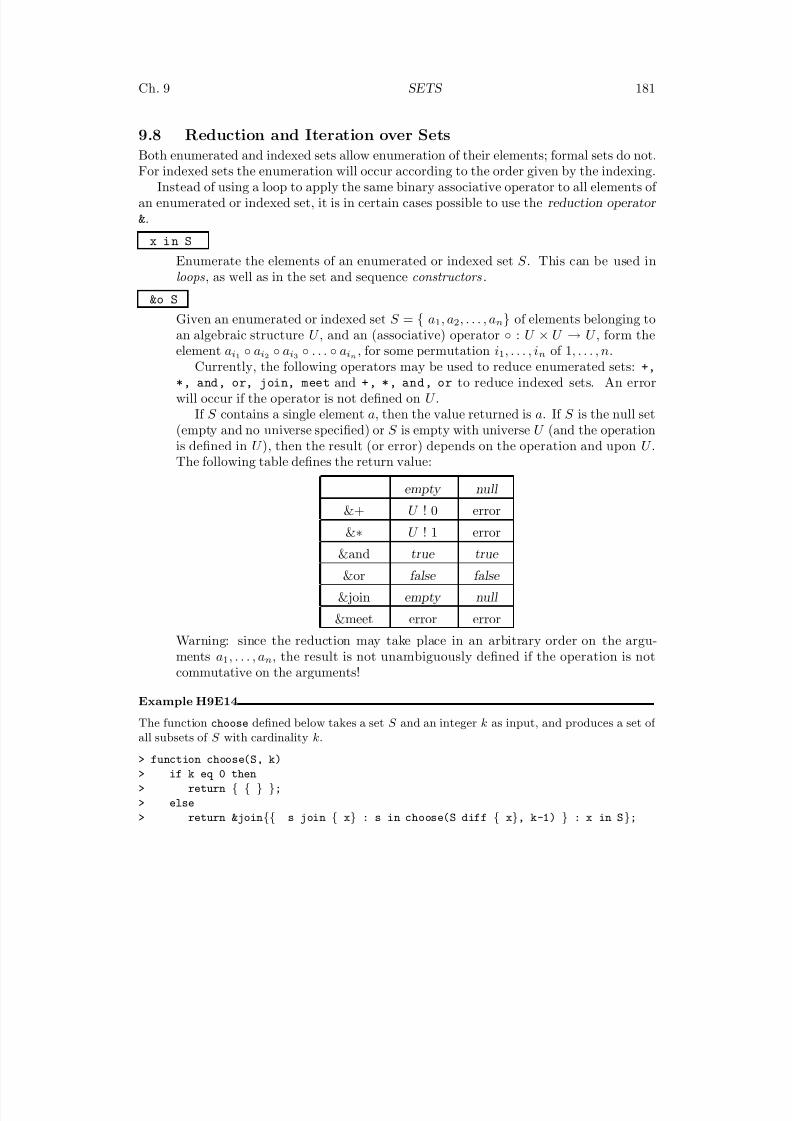
8/22/2019 Handbook Volume 01
http://slidepdf.com/reader/full/handbook-volume-01 297/440
Ch. 9 SETS 181
9.8 Reduction and Iteration over Sets
Both enumerated and indexed sets allow enumeration of their elements; formal sets do not.
For indexed sets the enumeration will occur according to the order given by the indexing.Instead of using a loop to apply the same binary associative operator to all elements of
an enumerated or indexed set, it is in certain cases possible to use the reduction operator &.
x i n S
Enumerate the elements of an enumerated or indexed set S . This can be used inloops , as well as in the set and sequence constructors .
&o S
Given an enumerated or indexed set S = { a1, a2, . . . , an} of elements belonging to
an algebraic structure U , and an (associative) operator ◦ : U × U → U , form theelement ai1 ◦ ai2 ◦ ai3 ◦ . . . ◦ ain , for some permutation i1, . . . , in of 1, . . . , n.
Currently, the following operators may be used to reduce enumerated sets: +,
*, and, or, join, meet and +, *, and, or to reduce indexed sets. An errorwill occur if the operator is not defined on U .
If S contains a single element a, then the value returned is a. If S is the null set(empty and no universe specified) or S is empty with universe U (and the operationis defined in U ), then the result (or error) depends on the operation and upon U .The following table defines the return value:
empty null
&+ U ! 0 error
&∗ U ! 1 error
&and true true
&or false false
&join empty null
&meet error error
Warning: since the reduction may take place in an arbitrary order on the argu-ments a1, . . . , an, the result is not unambiguously defined if the operation is not
commutative on the arguments!
Example H9E14
The function choose defined below takes a set S and an integer k as input, and produces a set of all subsets of S with cardinality k.
> function choose(S, k)
> if k eq 0 then
> return { { } };
> else
> return &join{{ s join { x} : s in choose(S diff { x}, k-1) } : x in S};
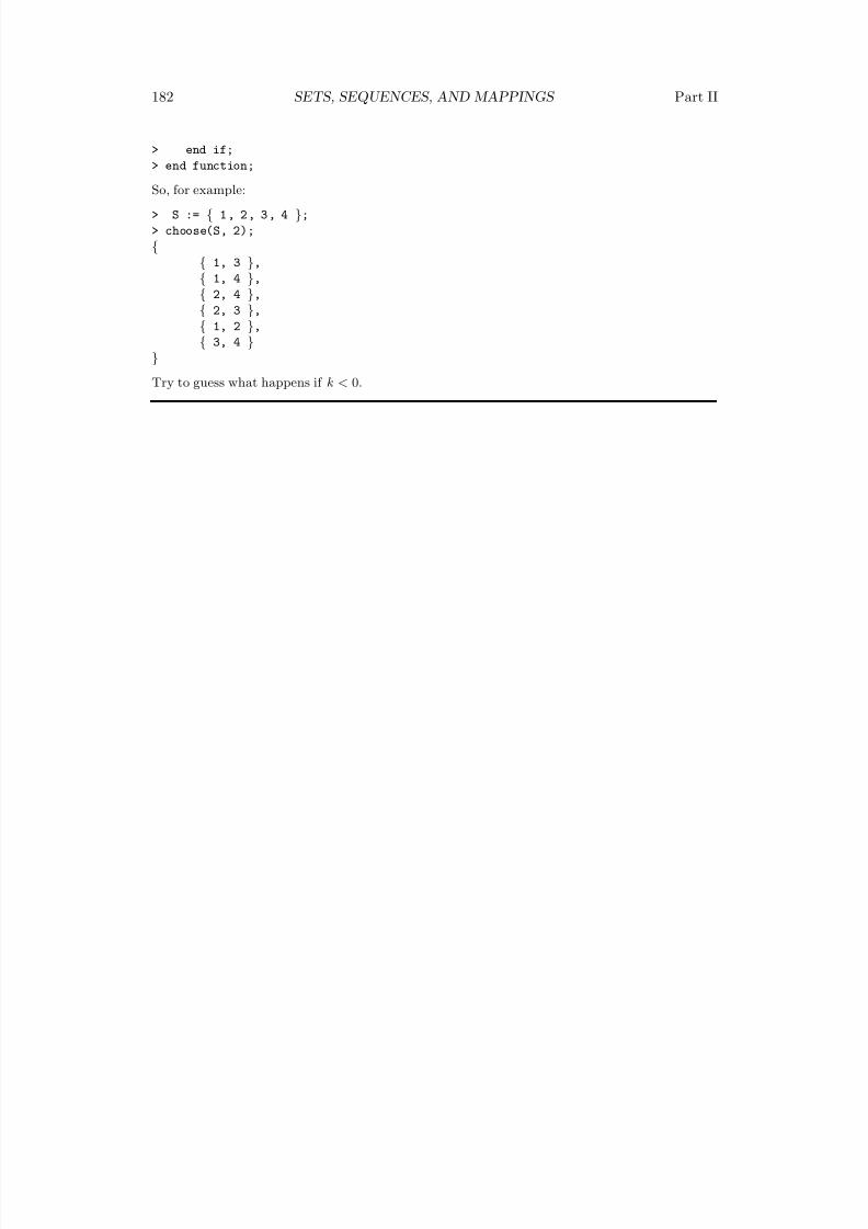
8/22/2019 Handbook Volume 01
http://slidepdf.com/reader/full/handbook-volume-01 298/440
182 SETS, SEQUENCES, AND MAPPINGS Part II
> end if;
> end function;
So, for example:
> S := { 1, 2, 3, 4 };
> choose(S, 2);
{{ 1, 3 },
{ 1, 4 },
{ 2, 4 },
{ 2, 3 },
{ 1, 2 },
{ 3, 4 }}
Try to guess what happens if k < 0.
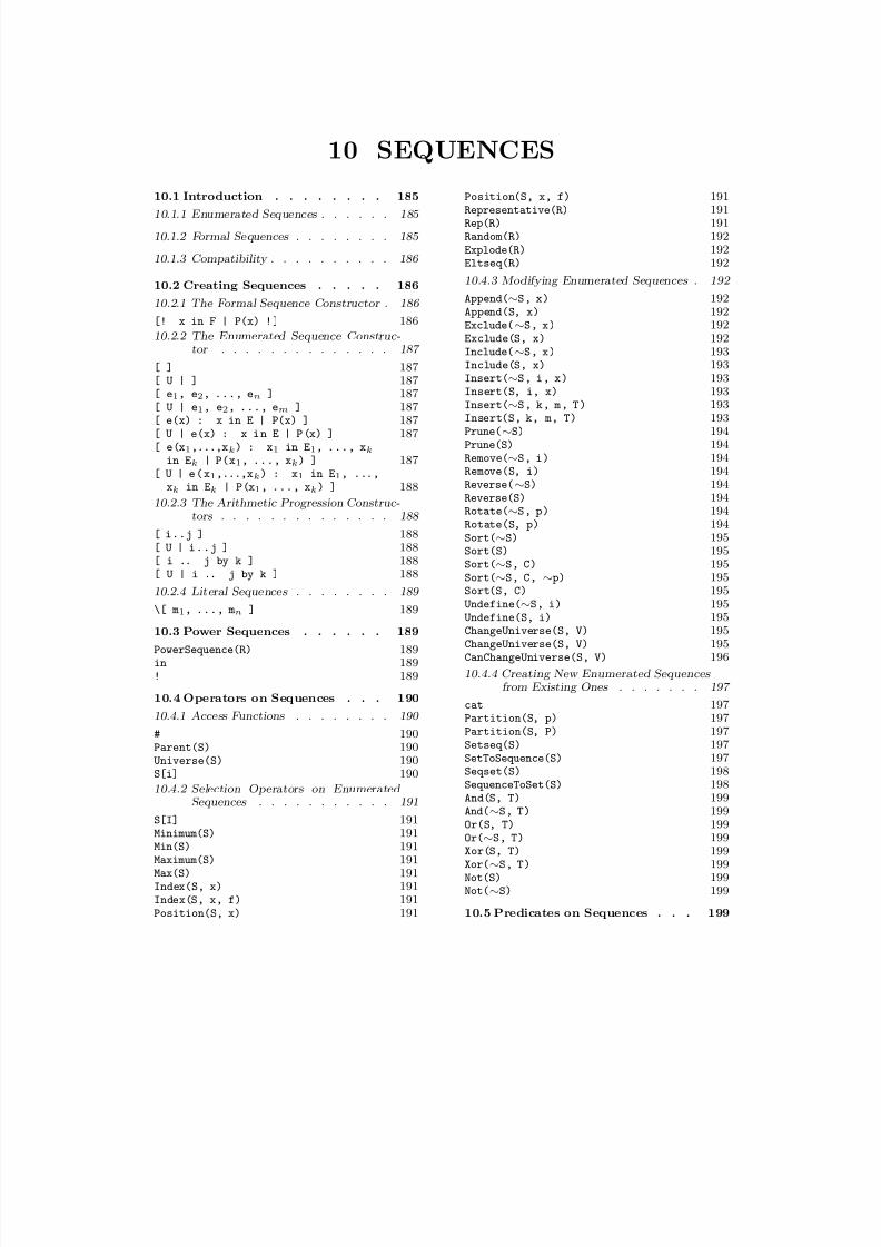
8/22/2019 Handbook Volume 01
http://slidepdf.com/reader/full/handbook-volume-01 299/440
10 SEQUENCES
10.1 Introduction . . . . . . . . 185
10.1.1 Enumerated Sequences . . . . . . 185
10.1.2 Formal Sequences . . . . . . . . 185
10.1.3 Compatibility . . . . . . . . . . 186
10.2 Creating Sequences . . . . . 186
10.2.1 The Formal Sequence Constructor . 186
[! x in F | P(x) ! ] 186
10.2.2 The Enumerated Sequence Construc-tor . . . . . . . . . . . . . . 187
[ ] 187[ U | ] 187[ e1, e2, ..., en ] 187[ U | e1, e2, ..., em ] 187[ e(x) : x in E | P(x) ] 187[ U | e(x) : x i n E | P (x) ] 187[ e(x1,...,xk) : x1 in E1, ..., xk
in Ek | P(x1, ..., xk) ] 187[ U | e ( x1,...,xk) : x1 in E1, ...,
xk in Ek | P(x1, ..., xk) ] 188
10.2.3 The Arithmetic Progression Construc-tors . . . . . . . . . . . . . . 188
[ i..j ] 188[ U | i..j ] 188
[ i .. j by k ] 188[ U | i .. j by k ] 188
10.2.4 Literal Sequences . . . . . . . . 189
\[ m1, ..., mn ] 189
10.3 Power Sequences . . . . . . 189
PowerSequence(R) 189in 189! 189
10.4 Operators on Sequences . . . 190
10.4.1 Access Functions . . . . . . . . 190
# 190
Parent(S) 190Universe(S) 190S[i] 190
10.4.2 Selection Operators on EnumeratedSequences . . . . . . . . . . . 191
S[I] 191Minimum(S) 191Min(S) 191Maximum(S) 191Max(S) 191Index(S, x) 191Index(S, x, f) 191Position(S, x) 191
Position(S, x, f) 191Representative(R) 191Rep(R) 191Random(R) 192Explode(R) 192Eltseq(R) 192
10.4.3 Modifying Enumerated Sequences . 192
Append(∼S, x) 192Append(S, x) 192Exclude(∼S, x) 192Exclude(S, x) 192Include(∼S, x) 193Include(S, x) 193
Insert(∼S, i, x) 193Insert(S, i, x) 193Insert(∼S, k, m, T) 193Insert(S, k, m, T) 193Prune(∼S) 194Prune(S) 194Remove(∼S, i) 194Remove(S, i) 194Reverse(∼S) 194Reverse(S) 194Rotate(∼S, p) 194Rotate(S, p) 194Sort(∼S) 195Sort(S) 195
Sort(∼S, C) 195Sort(∼S, C, ∼p) 195Sort(S, C) 195Undefine(∼S, i) 195Undefine(S, i) 195ChangeUniverse(S, V) 195ChangeUniverse(S, V) 195CanChangeUniverse(S, V) 196
10.4.4 Creating New Enumerated Sequences from Existing Ones . . . . . . . 197
cat 197Partition(S, p) 197Partition(S, P) 197
Setseq(S) 197SetToSequence(S) 197Seqset(S) 198SequenceToSet(S) 198And(S, T) 199And(∼S, T) 199Or(S, T) 199Or(∼S, T) 199Xor(S, T) 199Xor(∼S, T) 199Not(S) 199Not(∼S) 199
10.5 Predicates on Sequences . . . 199
8/22/2019 Handbook Volume 01
http://slidepdf.com/reader/full/handbook-volume-01 300/440
184 SETS, SEQUENCES, AND MAPPINGS Part II
IsComplete(S) 199IsDefined(S, i) 199IsEmpty(S) 200IsNull(S) 200
10.5.1 Membership Testing . . . . . . . 200
in 200notin 200IsSubsequence(S, T) 200IsSubsequence(S, T: Kind := o ) 200eq 200ne 200
10.5.2 Testing Order Relations . . . . . 201
lt 201le 201
ge 201gt 201
10.6 Recursion, Reduction, and Itera-tion . . . . . . . . . . . . 202
10.6.1 Recursion . . . . . . . . . . . 202
Self(n) 202Self() 202
10.6.2 Reduction . . . . . . . . . . . 202
& 202
10.7 Iteration . . . . . . . . . . 203
for x in S do st; end for; 203
10.8 Bibliography . . . . . . . . 204
8/22/2019 Handbook Volume 01
http://slidepdf.com/reader/full/handbook-volume-01 301/440
Chapter 10
SEQUENCES
10.1 Introduction
A sequence in Magma is a linearly ordered collection of objects belonging to some commonstructure (called the universe of the sequence).
There are two types of sequence: enumerated sequences , of which the elements are all
stored explicitly (with one exception, see below); and formal sequences , of which elementsare stored implicitly by means of a predicate that allows for testing membership. Inparticular, enumerated sequences are always finite, and formal sequences are allowed to beinfinite. In this chapter a sequence will be either a formal or an enumerated sequence.
10.1.1 Enumerated Sequences
An enumerated sequence of length l is an array of indefinite length of which only finitelymany terms – including the l-th term, but no term of bigger index — have been definedto be elements of some common structure. Such sequence is called complete if all of theterms (from index 1 up to the length l) are defined.
In practice the length of any sequence is bounded by the constant integer beta (usually229).
Incomplete enumerated sequences are allowed as a convenience for the programmer inbuilding complete enumerated sequences. Some sequence functions require their argumentsto be complete; if that is the case, it is mentioned explicitly in the description below.However, all functions using sequences in other Magma modules always assume thata sequence that is passed in as an argument is complete. Note that the following lineconverts a possibly incomplete sequence S into a complete sequence T :
T := [ s : s in S ];
because the enumeration using the in operator simply ignores undefined terms.
Enumerated sequences of Booleans are highly optimized (stored as bit-vectors).
10.1.2 Formal Sequences
A formal sequence consists of elements of some range set on which a certain predicateassumes the value ‘true’.
There is only a very limited number of operations that can be performed on them.
8/22/2019 Handbook Volume 01
http://slidepdf.com/reader/full/handbook-volume-01 302/440
186 SETS, SEQUENCES, AND MAPPINGS Part II
10.1.3 Compatibility
The binary operators for sequences do not allow mixing of the formal and enumerated
sequence types (so one cannot take the concatenation of an enumerated sequence and aformal sequence, for example); but it is easy to convert an enumerated sequence into aformal sequence – see the section on binary operators below.
By the limitation on their construction formal sequences can only contain elements fromone structure in Magma. The elements of enumerated sequences are also restricted, inthe sense that either some common structure must be specified upon creation, or Magma
must be able to find such universe automatically. The rules for compatibility of elementsand the way Magma deals with these parents is the same for sequences and sets, and isoutlined in the Introduction to this Part of the Handbook.
10.2 Creating Sequences
Square brackets are used for the definition of enumerated sequences; formal sequences aredelimited by the composite brackets [! and !].
Certain expressions appearing below (possibly with subscripts) have the standard in-terpretation:
U the universe: any Magma structure;
E the range set for enumerated sequences: any enumerated structure (it must be possibleto loop over its elements – see the Introduction to this Part);
F the range set for formal sequences: any structure for which membership testing usingin is defined – see the Introduction to this Part);
x a free variable which successively takes the elements of E (or F in the formal case) asits values;
P a Boolean expression that usually involves the variable(s) x, x1, . . . , xk;
e an expression that also usually involves the variable(s) x, x1, . . . , xk.
10.2.1 The Formal Sequence Constructor
The formal sequence constructor has the following fixed format (the expressions appearing
in the construct are defined above):
[! x in F | P(x) !]
Create the formal sequence consisting of the subsequence of elements x of F forwhich P (x) is true. If P (x) is true for every element of F , the sequence constructormay be abbreviated to [! x in F !]
8/22/2019 Handbook Volume 01
http://slidepdf.com/reader/full/handbook-volume-01 303/440
Ch. 10 SEQUENCES 187
10.2.2 The Enumerated Sequence Constructor
Sequences can be constructed by expressions enclosed in square brackets, provided that
the values of all expressions can be automatically coerced into some common structure,as outlined in the Introduction. All general constructors have the universe U optionallyup front, which allows the user to specify into which structure all terms of the sequencesshould be coerced.
[ ]
The null sequence (empty, and no universe specified).
[ U | ]
The empty sequence with universe U .
[ e1, e2, ..., en ]Given a list of expressions e1, . . . , en, defining elements a1, a2, . . . , an all belonging to(or automatically coercible into) a single algebraic structure U , create the sequenceQ = [a1, a2,...,an ] of elements of U .
[ U | e1, e2, ..., em ]
Given a list of expressions e1, . . . , em, which define elements a1, a2, . . . , an that areall coercible into U , create the sequence Q = [a1, a2,...,an ] of elements of U .
[ e(x) : x in E | P(x) ]
Form the sequence of elements e(x), all belonging to some common structure, forthose x ∈ E with the property that the predicate P (x) is true. The expressionsappearing in this construct have the interpretation given at the beginning of thissection.
If P (x) is true for every element of E , the sequence constructor may be abbre-viated to [ e(x) : x in E ] .
[ U | e(x) : x in E | P(x) ]
Form the sequence of elements of U consisting of the values e(x) for those x ∈ E for which the predicate P (x) is true (an error results if not all e(x) are coercibleinto U ). The expressions appearing in this construct have the same interpretation
as above.[ e(x1,...,xk) : x1 in E1, ..., xk in Ek | P(x1, ..., xk) ]
The sequence consisting of those elements e(x1, . . . , xk), in some common structure,for which x1, . . . , xk in E 1, . . . , E k have the property that P (x1, . . . , xk) is true.
The expressions appearing in this construct have the interpretation given at thebeginning of this section.
Note that if two successive ranges E i and E i+1 are identical, then the specificationof the ranges for xi and xi+1 may be abbreviated to xi, xi+1 in Ei.
Also, if P (x1,...,xk) is always true, it may be omitted.
8/22/2019 Handbook Volume 01
http://slidepdf.com/reader/full/handbook-volume-01 304/440
188 SETS, SEQUENCES, AND MAPPINGS Part II
[ U | e ( x1,...,xk) : x1 in E1, ..., xk in Ek | P(x1, ..., xk) ]
As in the previous entry, the sequence consisting of those elements e(x1, . . . , xk)
for which P (x1, . . . , xk) is true is formed, as a sequence of elements of U (an erroroccurs if not all e(x1, . . . , xk) are coercible into U ).
10.2.3 The Arithmetic Progression Constructors
Since enumerated sequences of integers arise so often, there are a few special constructorsto create and handle them efficiently in case the entries are in arithmetic progression. Theuniverse must be the ring of integers. Some effort is made to preserve the special way of storing arithmetic progressions under sequence operations.
[ i..j ]
[ U | i . . j ]
The enumerated sequence of integers whose elements form the arithmetic progressioni, i + 1, i + 2, . . . , j, where i and j are (expressions defining) arbitrary integers. If jis less than i then the empty sequence of integers will be created.
The universe U , if it is specified, has to be the ring of integers; any other universewill lead to an error.
[ i .. j by k ]
[ U | i .. j by k ]
The enumerated sequence consisting of the integers forming the arithmetic progres-sion i, i + k, i + 2 ∗ k , . . . , j, where i, j and k are (expressions defining) arbitraryintegers (but k = 0).
If k is positive then the last element in the progression will be the greatest integerof the form i + n ∗ k that is less than or equal to j; if j is less than i, the emptysequence of integers will be constructed.
If k is negative then the last element in the progression will be the least integerof the form i + n ∗ k that is greater than or equal to j; if j is greater than i, theempty sequence of integers will be constructed.
The universe U , if it is specified, has to be the ring of integers; any other universewill lead to an error.
Example H10E1
As in the case of sets, it is possible to use the arithmetic progression constructors to save sometyping in the creation of sequences of elements of rings other than the ring of integers, but theresult will not be treated especially efficiently.
> s := [ IntegerRing(200) | x : x in [ 25..125 ] ];
8/22/2019 Handbook Volume 01
http://slidepdf.com/reader/full/handbook-volume-01 305/440
Ch. 10 SEQUENCES 189
10.2.4 Literal Sequences
A literal sequence is an enumerated sequence all of whose terms are from the same structure
and all of these are ‘typed in’ literally. The sole purpose of literal sequences is to loadcertain enumerated sequences very fast and very space-efficiently; this is only useful whenreading in very large sequences (all of whose elements must have been specified literally,that is, not as some expression other than a literal), but then it may save a lot of time.The result will be an enumerated sequence, that is, not distinguished in any way fromother such sequences.
At present, only literal sequences of integers are supported.
\[ m1, ..., mn ]
Given a succession of literal integers m1, . . . , mn, build the enumerated sequence[m1, . . . , mn], in a time and space efficient way.
10.3 Power Sequences
The PowerSequence constructor returns a structure comprising the enumerated sequencesof a given structure R; it is mainly useful as a parent for other set and sequence con-structors. The only operations that are allowed on power sequences are printing, testingelement membership, and coercion into the power sequence (see the examples below).
PowerSequence(R)
The structure comprising all enumerated sequences of elements of structure R. If R
itself is a sequence (or set) then the power structure of its universe is returned.S i n P
Returns true if enumerated sequence S is in the power sequence P , that is, if allelements of the sequence S are contained in or coercible into R, where P is thepower sequence of R; false otherwise.
P ! S
Return a sequence with universe R consisting of the entries of the enumerated se-quence S , where P is the power sequence of R. An error results if not all elementsof S can be coerced into R.
Example H10E2
> S : = [ 1 . . 1 0 ] ;
> P := PowerSequence(S);
> P;
Set of sequences over [ 1 .. 10 ]
> F := [ 6/3, 12/4 ];
> F i n P ;
true
> G : = P ! F ;
8/22/2019 Handbook Volume 01
http://slidepdf.com/reader/full/handbook-volume-01 306/440
190 SETS, SEQUENCES, AND MAPPINGS Part II
> Parent(F);
Set of sequences over Rational Field
> Parent(G);Set of sequences over [ 1 .. 10 ]
10.4 Operators on Sequences
This section lists functions for obtaining information about existing sequences, for modify-ing sequences and for creating sequences from others. Most of these operators only apply
to enumerated sequences.
10.4.1 Access Functions
#S
Returns the length of the enumerated sequence S , which is the index of the lastterm of S whose value is defined. The length of the empty sequence is zero.
Parent(S)
Returns the parent structure for a sequence S , that is, the structure consisting of all (enumerated) sequences over the universe of S .
Universe(S)
Returns the ‘universe’ of the sequence S , that is, the common structure to which allelements of the sequence belong. This universe may itself be a set or sequence. Anerror is signalled when S is the null sequence.
S[i]
The i-th term si of the sequence S . If i ≤ 0, or i > #S + 1, or S [i] is not defined,then an error results. Here i is allowed to be a multi-index (see Introduction forthe interpretation). This can be used as the left hand side of an assignment: S[i]
:= x redefines the i-th term of the sequence S to be x. If i ≤ 0, then an errorresults. If i > n, then the sequence [s1, . . . , sn, sn+1, . . . , si−1, x] replaces S , wheresn+1, . . . , si−1 are all undefined. Here i is allowed to be a multi-index.
An error occurs if x cannot be coerced into the universe of S .
8/22/2019 Handbook Volume 01
http://slidepdf.com/reader/full/handbook-volume-01 307/440
Ch. 10 SEQUENCES 191
10.4.2 Selection Operators on Enumerated Sequences
Here, S denotes an enumerated sequence [s1, . . . , sn]. Further, i and j are integers or
multi-indices (see Introduction).
S[I]
The sequence [si1 , . . . , sir ] consisting of terms selected from the sequence S , accord-ing to the terms of the integer sequence I . If any term of I lies outside the range 1to #S , then an error results. If I is the empty sequence, then the empty set withuniverse the same as that of S is returned.
The effect of T := S[I] differs from that of T := [ S[i] : i in I ]: if inthe first case an undefined entry occurs for i ∈ I between 1 and #S it will be copied
over; in the second such undefined entries will lead to an error.
Minimum(S)
Min(S)
Given a non-empty, complete enumerated sequence S such that lt and eq are definedon the universe of S , this function returns two values: a minimal element s in S , aswell as the first position i such that s = S [i].
Maximum(S)
Max(S)
Given a non-empty, complete enumerated sequence S such that gt and eq are definedon the universe of S , this function returns two values: a maximal element s in S , aswell as the first position i such that s = S [i].
Index(S, x)
Index(S, x, f)
Position(S, x)
Position(S, x, f)
Returns either the position of the first occurrence of x in the sequence S , or zero
if S does not contain x. The second variants of each function starts the search atposition f . This can save time in second (and subsequent) searches for the sameentry further on. If no occurrence of x in S from position f onwards is found, thenzero is returned.
Representative(R)
Rep(R)
An (arbitrary) element chosen from the enumerated sequence R
8/22/2019 Handbook Volume 01
http://slidepdf.com/reader/full/handbook-volume-01 308/440
192 SETS, SEQUENCES, AND MAPPINGS Part II
Random(R)
A random element chosen from the enumerated sequence R. Every element has an
equal probability of being chosen. Successive invocations of the function will resultin independently chosen elements being returned as the value of the function. If Ris empty an error occurs.
Explode(R)
Given an enumerated sequence R of length r this function returns the r entries of the sequence (in order).
Eltseq(R)
The enumerated sequence R itself. This function is just included for completeness.
10.4.3 Modifying Enumerated Sequences
The operations given here are available as both procedures and functions. In the procedureversion, the given sequence is destructively modified ‘in place’. This is very efficient, sinceit is not necessary to make a copy of the sequence. In the function version, the givensequence is not changed, but a modified version of it is returned. This is more suitable if the old sequence is still required. Some of the functions also return useful but non-obviousvalues.
Here, S denotes an enumerated sequence, and x an element of some structure V . Themodifications involving S and x will only be successful if x can be coerced into the universeof S ; an error occurs if this fails. (See the Introduction to this Part).
Append(∼S, x)
Append(S, x)
Create an enumerated sequence by adding the object x to the end of S , i.e., theenumerated sequence [s1, . . . sn, x].
There are two versions of this: a procedure, where S is replaced by the appendedsequence, and a function, which returns the new sequence. The procedural versiontakes a reference ∼ S to S as an argument.
Note that the procedural version is much more efficient since the sequence S willnot be copied.
Exclude(∼S, x)
Exclude(S, x)
Create an enumerated sequence obtained by removing the first occurrence of theobject x from S , i.e., the sequence [s1,. . . si−1, si+1, . . ., sn], where si is the firstterm of S that is equal to x. If x is not in S then this is just S .
There are two versions of this: a procedure, where S is replaced by the newsequence, and a function, which returns the new sequence. The procedural versiontakes a reference ∼ S to S as an argument.
8/22/2019 Handbook Volume 01
http://slidepdf.com/reader/full/handbook-volume-01 309/440
Ch. 10 SEQUENCES 193
Note that the procedural version is much more efficient since the sequence S willnot be copied.
Include(∼S, x)
Include(S, x)
Create a sequence by adding the object x to the end of S , provided that no term of S is equal to x. Thus, if x does not occur in S , the enumerated sequence [s1, . . . , sn, x]is created.
There are two versions of this: a procedure, where S is replaced by the newsequence, and a function, which returns the new sequence. The procedural versiontakes a reference ∼ S to S as an argument.
Note that the procedural version is much more efficient since the sequence S will
not be copied.
Insert(∼S, i, x)
Insert(S, i, x)
Create the sequence formed by inserting the object x at position i in S and movingthe terms S [i], . . . , S [n] down one place, i.e., the enumerated sequence [s1,. . . si−1,x, si, . . ., sn]. Note that i may be bigger than the length n of S , in which case thenew length of S will be i, and the entries S [n + 1], . . . , S [i − 1] will be undefined.
There are two versions of this: a procedure, where S is replaced by the newsequence, and a function, which returns the new sequence. The procedural version
takes a reference ∼ S to S as an argument.Note that the procedural version is much more efficient since the sequence S will
not be copied.
Insert(∼S, k, m, T)
Insert(S, k, m, T)
Create the sequence [s1, . . ., sk−1, t1, . . ., tl, sm+1, . . ., sn]. If k ≤ 0 ork > m + 1, then an error results. If k = m + 1 then the terms of T will beinserted into S immediately before the term sk. If k > n, then the sequence[s1, . . . , sn, sn+1, . . . , sk−1, t1, . . . , tl] is created, where sn+1, . . . , sk−1 are all unde-fined. In the case where T is the empty sequence, terms sk, . . . , sm are deleted fromS .
There are two versions of this: a procedure, where S is replaced by the newsequence, and a function, which returns the new sequence. The procedural versiontakes a reference ∼ S to S as an argument.
Note that the procedural version is much more efficient since the sequence S willnot be copied.
8/22/2019 Handbook Volume 01
http://slidepdf.com/reader/full/handbook-volume-01 310/440
194 SETS, SEQUENCES, AND MAPPINGS Part II
Prune(∼S)
Prune(S)
Create the enumerated sequence formed by removing the last term of the sequenceS , i.e., the sequence [s1, . . ., sn−1]. An error occurs if S is empty.
There are two versions of this: a procedure, where S is replaced by the newsequence, and a function, which returns the new sequence. The procedural versiontakes a reference ∼ S to S as an argument.
Note that the procedural version is much more efficient since the sequence S willnot be copied.
Remove(∼S, i)
Remove(S, i)
Create the enumerated sequence formed by removing the i-th term from S , i.e., thesequence [s1,. . . si−1, si+1, . . ., sn]. An error occurs if i < 1 or i > n.
There are two versions of this: a procedure, where S is replaced by the newsequence, and a function, which returns the new sequence. The procedural versiontakes a reference ∼ S to S as an argument.
Note that the procedural version is much more efficient since the sequence S willnot be copied.
Reverse(∼S)
Reverse(S)
Create the enumerated sequence formed by reversing the order of the terms in thecomplete enumerated sequence S , i.e., the sequence [sn, . . . , s1].
There are two versions of this: a procedure, where S is replaced by the newsequence, and a function, which returns the new sequence. The procedural versiontakes a reference ∼ S to S as an argument.
Note that the procedural version is much more efficient since the sequence S willnot be copied.
Rotate(∼S, p)
Rotate(S, p)
Given a complete sequence S and an integer p, create the enumerated sequenceformed by cyclically rotating the terms of the sequence p terms: if p is positive,rotation will be to the right; if p is negative, S is cyclically rotated − p terms to theleft; if p is zero nothing happens.
There are two versions of this: a procedure, where S is replaced by the newsequence, and a function, which returns the new sequence. The procedural versiontakes a reference ∼ S to S as an argument.
Note that the procedural version is much more efficient since the sequence S willnot be copied.
8/22/2019 Handbook Volume 01
http://slidepdf.com/reader/full/handbook-volume-01 311/440
Ch. 10 SEQUENCES 195
Sort(∼S)
Sort(S)
Given a complete enumerated sequence S whose terms belong to a structure on whichlt and eq are defined, create the enumerated sequence formed by (quick-)sortingthe terms of S into increasing order.
There are two versions of this: a procedure, where S is replaced by the newsequence, and a function, which returns the new sequence. The procedural versiontakes a reference ∼ S to S as an argument.
Note that the procedural version is much more efficient since the sequence S willnot be copied.
Sort(∼S, C)
Sort(∼S, C, ∼p)
Sort(S, C)
Given a complete enumerated sequence S and a comparison function C which com-pares elements of S , create the enumerated sequence formed by sorting the termsof S into increasing order with respect to C . The comparison function C must taketwo arguments and return an integer less than, equal to, or greater than 0 accord-ing to whether the first argument is less than, equal to, or greater than the secondargument (e.g.: func<x, y | x - y>).
There are three versions of this: a procedure, where S is replaced by the newsequence, a procedure, where S is replaced by the new sequence and the correspond-
ing permutation p is set, and a function, which returns the new sequence and thecorresponding permutation. The procedural version takes a reference ∼ S to S asan argument. Note that the procedural version is much more efficient since thesequence S will not be copied.
Undefine(∼S, i)
Undefine(S, i)
Create the sequence which is the same as the enumerated sequence S but with thei-th term of S undefined; i may be bigger than #S , but i ≤ 0 produces an error.
There are two versions of this: a procedure, where S is replaced by the new
sequence, and a function, which returns the new sequence. The procedural versiontakes a reference ∼ S to S as an argument.
Note that the procedural version is much more efficient since the sequence S willnot be copied.
ChangeUniverse(S, V)
ChangeUniverse(S, V)
Given a sequence S with universe U and a structure V which contains U , constructa sequence which consists of the elements of S coerced into V .
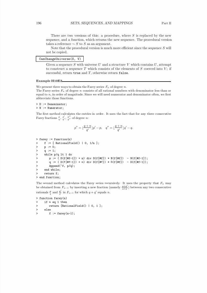
8/22/2019 Handbook Volume 01
http://slidepdf.com/reader/full/handbook-volume-01 312/440
196 SETS, SEQUENCES, AND MAPPINGS Part II
There are two versions of this: a procedure, where S is replaced by the newsequence, and a function, which returns the new sequence. The procedural version
takes a reference ∼ S to S as an argument.Note that the procedural version is much more efficient since the sequence S will
not be copied.
CanChangeUniverse(S, V)
Given a sequence S with universe U and a structure V which contains U , attemptto construct a sequence T which consists of the elements of S coerced into V ; if successful, return true and T , otherwise return false.
Example H10E3
We present three ways to obtain the Farey series F n of degree n.The Farey series F n of degree n consists of all rational numbers with denominator less than orequal to n, in order of magnitude. Since we will need numerator and denominator often, we firstabbreviate those functions.
> D := Denominator;
> N := Numerator;
The first method calculates the entries in order. It uses the fact that for any three consecutive
Farey fractions p
q, p
q, p
qof degree n:
p = q + n
q p − p, q =
q + n
q q − q.
> farey := function(n)
> f := [ RationalField() | 0, 1/n ];
> p := 0;
> q := 1;
> while p/q lt 1 do
> p := ( D(f[#f-1]) + n) div D(f[#f]) * N(f[#f]) - N(f[#f-1]);
> q := ( D(f[#f-1]) + n) div D(f[#f]) * D(f[#f]) - D(f[#f-1]);
> Append(~f, p/q);
> end while;
> return f;
> end function;
The second method calculates the Farey series recursively. It uses the property that F n may
be obtained from F n−1 by inserting a new fraction (namely p+p
q+q) between any two consecutive
rationals p
qand p
qin F n−1 for which q + q equals n.
> function farey(n)
> if n eq 1 then
> return [RationalField() | 0, 1 ];
> else
> f := farey(n-1);
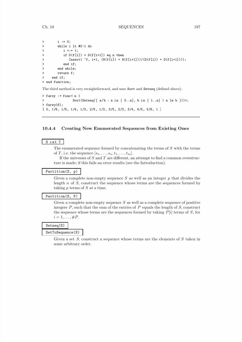
8/22/2019 Handbook Volume 01
http://slidepdf.com/reader/full/handbook-volume-01 313/440
Ch. 10 SEQUENCES 197
> i := 0;
> while i lt #f-1 do
> i +:= 1;> if D(f[i]) + D(f[i+1]) eq n then
> Insert( ~f, i+1, (N(f[i]) + N(f[i+1]))/(D(f[i]) + D(f[i+1])));
> end if;
> end while;
> return f;
> end if;
> end function;
The third method is very straightforward, and uses Sort and Setseq (defined above).
> farey := func< n |
> Sort(Setseq({ a/b : a in { 0..n}, b i n { 1..n} | a le b }))>;
> farey(6);
[ 0, 1/6, 1/5, 1/4, 1/3, 2/5, 1/2, 3/5, 2/3, 3/4, 4/5, 5/6, 1 ]
10.4.4 Creating New Enumerated Sequences from Existing Ones
S cat T
The enumerated sequence formed by concatenating the terms of S with the terms
of T , i.e. the sequence [s1, . . . , sn, t1, . . . , tm].If the universes of S and T are different, an attempt to find a common overstruc-ture is made; if this fails an error results (see the Introduction).
Partition(S, p)
Given a complete non-empty sequence S as well as an integer p that divides thelength n of S , construct the sequence whose terms are the sequences formed bytaking p terms of S at a time.
Partition(S, P)
Given a complete non-empty sequence S as well as a complete sequence of positive
integers P , such that the sum of the entries of P equals the length of S , constructthe sequence whose terms are the sequences formed by taking P [i] terms of S , fori = 1, . . . , #P .
Setseq(S)
SetToSequence(S)
Given a set S , construct a sequence whose terms are the elements of S taken insome arbitrary order.
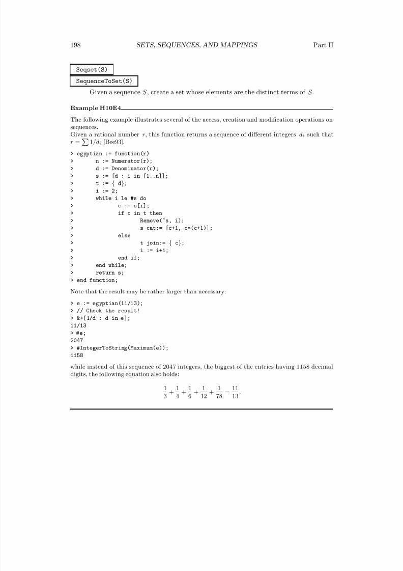
8/22/2019 Handbook Volume 01
http://slidepdf.com/reader/full/handbook-volume-01 314/440
198 SETS, SEQUENCES, AND MAPPINGS Part II
Seqset(S)
SequenceToSet(S)
Given a sequence S , create a set whose elements are the distinct terms of S .
Example H10E4
The following example illustrates several of the access, creation and modification operations onsequences.Given a rational number r, this function returns a sequence of different integers di such thatr =
1/di [Bee93].
> egyptian := function(r)
> n := Numerator(r);
> d := Denominator(r);
> s := [d : i in [1..n]];
> t := { d};
> i := 2;
> while i le #s do
> c := s[i];
> if c in t then
> Remove(~s, i);
> s cat:= [c+1, c*(c+1)];
> else
> t join:= { c};
> i := i+1;
> end if;> end while;
> return s;
> end function;
Note that the result may be rather larger than necessary:
> e := egyptian(11/13);
> // Check the result!
> &+[1/d : d in e];
11/13
> #e;
2047
> #IntegerToString(Maximum(e));
1158
while instead of this sequence of 2047 integers, the biggest of the entries having 1158 decimaldigits, the following equation also holds:
1
3+
1
4+
1
6+
1
12+
1
78=
11
13.
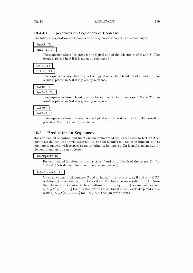
8/22/2019 Handbook Volume 01
http://slidepdf.com/reader/full/handbook-volume-01 315/440
Ch. 10 SEQUENCES 199
10.4.4.1 Operations on Sequences of Booleans
The following operation work pointwise on sequences of booleans of equal length.
And(S, T)
And(∼S, T)
The sequence whose ith entry is the logical and of the ith entries of S and T . Theresult is placed in S if it is given by reference (∼).
Or(S, T)
Or(∼S, T)
The sequence whose ith entry is the logical or of the ith entries of S and T . Theresult is placed in S if it is given by reference.
Xor(S, T)
Xor(∼S, T)
The sequence whose ith entry is the logical xor of the ith entries of S and T . Theresult is placed in S if it is given by reference.
Not(S)
Not(∼S)
The sequence whose ith entry is the logical not of the ith entry of S . The result is
placed in S if it is given by reference.
10.5 Predicates on Sequences
Boolean valued operators and functions on enumerated sequences exist to test whetherentries are defined (see previous section), to test for membership and containment, and tocompare sequences with respect to an ordering on its entries. On formal sequences, onlyelement membership can be tested.
IsComplete(S)
Boolean valued function, returning true if and only if each of the terms S [i] for
1 ≤ i ≤ #S is defined, for an enumerated sequence S .
IsDefined(S, i)
Given an enumerated sequence S and an index i, this returns true if and only if S [i]is defined. (Hence the result is false if i > #S , but an error results if i < 1.) Notethat the index i is allowed to be a multi-index; if i = [i1, . . . , ir] is a multi-index andij > #S [i1, . . . , ij−1] the function returns false, but if S is s levels deep and r > swhile ij ≤ #S [i1, . . . , ij−1] for 1 ≤ j ≤ s, then an error occurs.
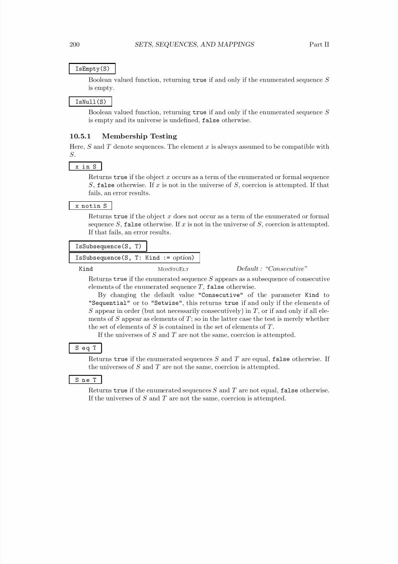
8/22/2019 Handbook Volume 01
http://slidepdf.com/reader/full/handbook-volume-01 316/440
200 SETS, SEQUENCES, AND MAPPINGS Part II
IsEmpty(S)
Boolean valued function, returning true if and only if the enumerated sequence S is empty.
IsNull(S)
Boolean valued function, returning true if and only if the enumerated sequence S is empty and its universe is undefined, false otherwise.
10.5.1 Membership Testing
Here, S and T denote sequences. The element x is always assumed to be compatible withS .
x i n SReturns true if the object x occurs as a term of the enumerated or formal sequenceS , false otherwise. If x is not in the universe of S , coercion is attempted. If thatfails, an error results.
x notin S
Returns true if the object x does not occur as a term of the enumerated or formalsequence S , false otherwise. If x is not in the universe of S , coercion is attempted.If that fails, an error results.
IsSubsequence(S, T)
IsSubsequence(S, T: Kind := option)
Kind MonStgElt Default : “Consecutive”
Returns true if the enumerated sequence S appears as a subsequence of consecutiveelements of the enumerated sequence T , false otherwise.
By changing the default value "Consecutive" of the parameter Kind to"Sequential" or to "Setwise", this returns true if and only if the elements of S appear in order (but not necessarily consecutively) in T , or if and only if all ele-ments of S appear as elements of T ; so in the latter case the test is merely whetherthe set of elements of S is contained in the set of elements of T .
If the universes of S and T are not the same, coercion is attempted.
S e q T
Returns true if the enumerated sequences S and T are equal, false otherwise. If the universes of S and T are not the same, coercion is attempted.
S n e T
Returns true if the enumerated sequences S and T are not equal, false otherwise.If the universes of S and T are not the same, coercion is attempted.
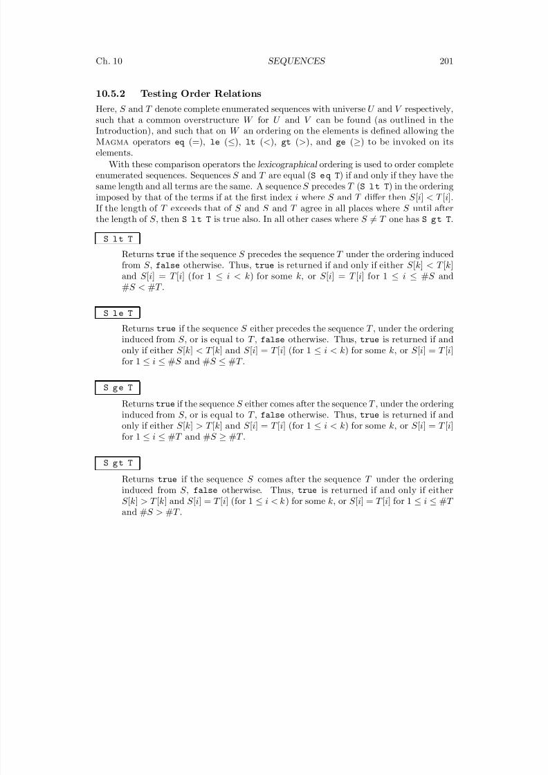
8/22/2019 Handbook Volume 01
http://slidepdf.com/reader/full/handbook-volume-01 317/440
Ch. 10 SEQUENCES 201
10.5.2 Testing Order Relations
Here, S and T denote complete enumerated sequences with universe U and V respectively,
such that a common overstructure W for U and V can be found (as outlined in theIntroduction), and such that on W an ordering on the elements is defined allowing theMagma operators eq (=), le (≤), lt (<), gt (>), and ge (≥) to be invoked on itselements.
With these comparison operators the lexicographical ordering is used to order completeenumerated sequences. Sequences S and T are equal (S e q T) if and only if they have thesame length and all terms are the same. A sequence S precedes T (S l t T) in the orderingimposed by that of the terms if at the first index i where S and T differ then S [i] < T [i].If the length of T exceeds that of S and S and T agree in all places where S until afterthe length of S , then S l t T is true also. In all other cases where S = T one has S g t T.
S l t T
Returns true if the sequence S precedes the sequence T under the ordering inducedfrom S , false otherwise. Thus, true is returned if and only if either S [k] < T [k]and S [i] = T [i] (for 1 ≤ i < k) for some k, or S [i] = T [i] for 1 ≤ i ≤ #S and#S < #T .
S l e T
Returns true if the sequence S either precedes the sequence T , under the orderinginduced from S , or is equal to T , false otherwise. Thus, true is returned if and
only if either S [k] < T [k] and S [i] = T [i] (for 1 ≤ i < k) for some k, or S [i] = T [i]for 1 ≤ i ≤ #S and #S ≤ #T .
S g e T
Returns true if the sequence S either comes after the sequence T , under the orderinginduced from S , or is equal to T , false otherwise. Thus, true is returned if andonly if either S [k] > T [k] and S [i] = T [i] (for 1 ≤ i < k) for some k, or S [i] = T [i]for 1 ≤ i ≤ #T and #S ≥ #T .
S g t TReturns true if the sequence S comes after the sequence T under the orderinginduced from S , false otherwise. Thus, true is returned if and only if eitherS [k] > T [k] and S [i] = T [i] (for 1 ≤ i < k) for some k, or S [i] = T [i] for 1 ≤ i ≤ #T and #S > #T .
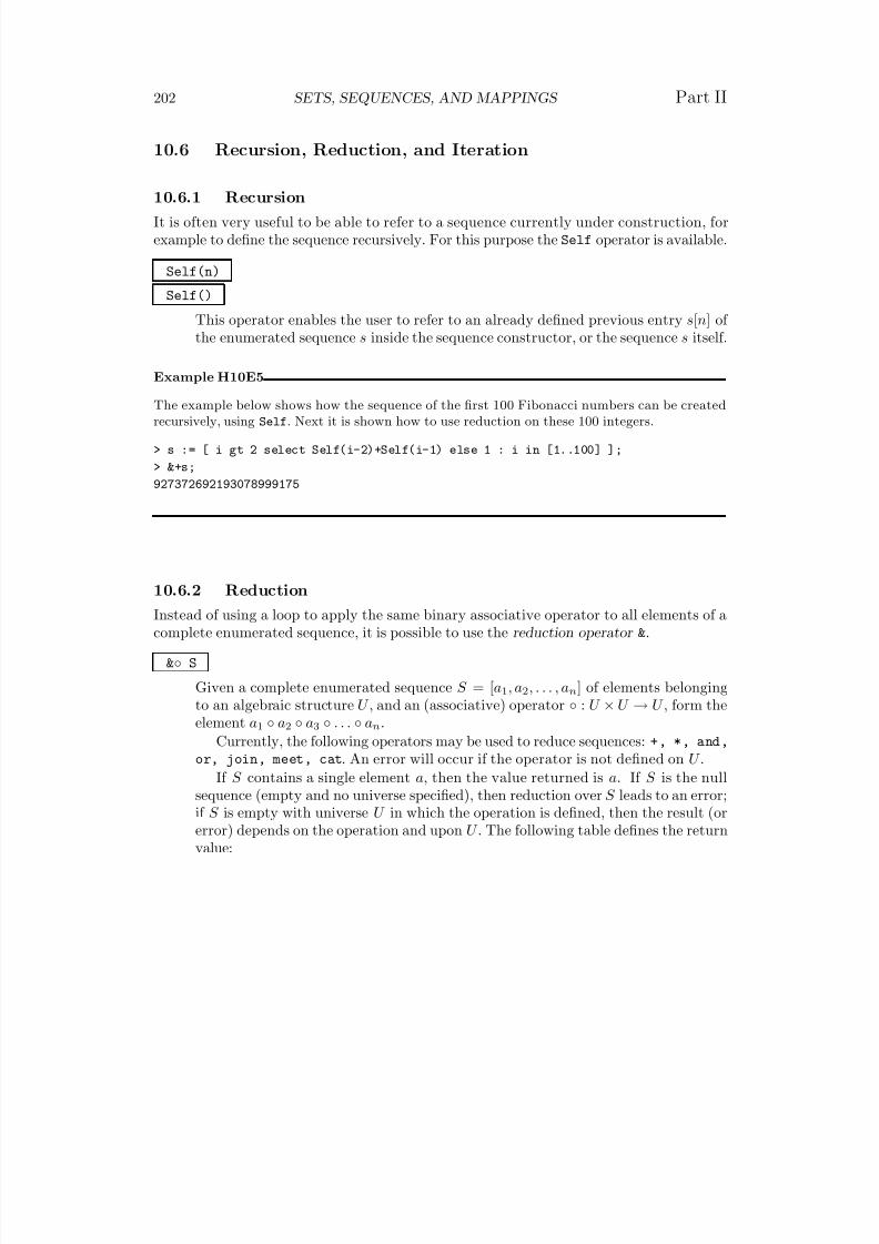
8/22/2019 Handbook Volume 01
http://slidepdf.com/reader/full/handbook-volume-01 318/440
202 SETS, SEQUENCES, AND MAPPINGS Part II
10.6 Recursion, Reduction, and Iteration
10.6.1 Recursion
It is often very useful to be able to refer to a sequence currently under construction, forexample to define the sequence recursively. For this purpose the Self operator is available.
Self(n)
Self()
This operator enables the user to refer to an already defined previous entry s[n] of the enumerated sequence s inside the sequence constructor, or the sequence s itself.
Example H10E5
The example below shows how the sequence of the first 100 Fibonacci numbers can be createdrecursively, using Self. Next it is shown how to use reduction on these 100 integers.
> s := [ i gt 2 select Self(i-2)+Self(i-1) else 1 : i in [1..100] ];
> &+s;
927372692193078999175
10.6.2 Reduction
Instead of using a loop to apply the same binary associative operator to all elements of acomplete enumerated sequence, it is possible to use the reduction operator &.
&◦ S
Given a complete enumerated sequence S = [a1, a2, . . . , an] of elements belongingto an algebraic structure U , and an (associative) operator ◦ : U × U → U , form theelement a1 ◦ a2 ◦ a3 ◦ . . . ◦ an.
Currently, the following operators may be used to reduce sequences: +, *, and,or, join, meet, cat. An error will occur if the operator is not defined on U .
If S contains a single element a, then the value returned is a. If S is the nullsequence (empty and no universe specified), then reduction over S leads to an error;if S is empty with universe U in which the operation is defined, then the result (orerror) depends on the operation and upon U . The following table defines the returnvalue:
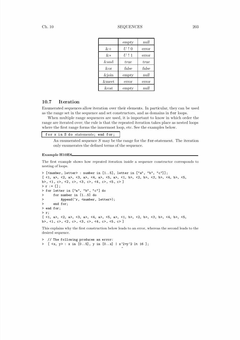
8/22/2019 Handbook Volume 01
http://slidepdf.com/reader/full/handbook-volume-01 319/440
Ch. 10 SEQUENCES 203
empty null
&+ U ! 0 error
&∗ U ! 1 error
&and true true
&or false false
&join empty null
&meet error error
&cat empty null
10.7 IterationEnumerated sequences allow iteration over their elements. In particular, they can be usedas the range set in the sequence and set constructors, and as domains in for loops.
When multiple range sequences are used, it is important to know in which order therange are iterated over; the rule is that the repeated iteration takes place as nested loopswhere the first range forms the innermost loop, etc. See the examples below.
for x in S do statements ; end for;
An enumerated sequence S may be the range for the for-statement. The iterationonly enumerates the defined terms of the sequence.
Example H10E6
The first example shows how repeated iteration inside a sequence constructor corresponds tonesting of loops.
> [<number, letter> : number in [1..5], letter in ["a", "b", "c"]];
[ <1, a>, <2, a>, <3, a>, <4, a>, <5, a>, <1, b>, <2, b>, <3, b>, <4, b>, <5,
b>, <1, c>, <2, c>, <3, c>, <4, c>, <5, c> ]
> r := [];
> for letter in ["a", "b", "c"] do
> for number in [1..5] do
> Append(~r, <number, letter>);
> end for;> end for;
> r;
[ <1, a>, <2, a>, <3, a>, <4, a>, <5, a>, <1, b>, <2, b>, <3, b>, <4, b>, <5,
b>, <1, c>, <2, c>, <3, c>, <4, c>, <5, c> ]
This explains why the first construction below leads to an error, whereas the second leads to thedesired sequence.
> // The following produces an error:
> [ <x, y> : x in [0..5], y in [0..x] | x^2+y^2 lt 16 ];
^
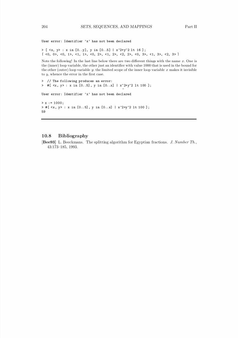
8/22/2019 Handbook Volume 01
http://slidepdf.com/reader/full/handbook-volume-01 320/440
204 SETS, SEQUENCES, AND MAPPINGS Part II
User error: Identifier ’x’ has not been declared
> [ <x, y> : x in [0..y], y in [0..5] | x^2+y^2 lt 16 ];[ <0, 0>, <0, 1>, <1, 1>, <0, 2>, <1, 2>, <2, 2>, <0, 3>, <1, 3>, <2, 3> ]
Note the following! In the last line below there are two different things with the name x. One isthe (inner) loop variable, the other just an identifier with value 1000 that is used in the bound forthe other (outer) loop variable y: the limited scope of the inner loop variable x makes it invisibleto y, whence the error in the first case.
> // The following produces an error:
> #[ <x, y> : x in [0..5], y in [0..x] | x^2+y^2 lt 100 ];
^
User error: Identifier ’x’ has not been declared
> x := 1000;> #[ <x, y> : x in [0..5], y in [0..x] | x^2+y^2 lt 100 ];
59
10.8 Bibliography
[Bee93] L. Beeckmans. The splitting algorithm for Egyptian fractions. J. Number Th.,43:173–185, 1993.
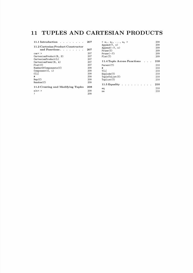
8/22/2019 Handbook Volume 01
http://slidepdf.com/reader/full/handbook-volume-01 321/440
11 TUPLES AND CARTESIAN PRODUCTS
11.1 Introduction . . . . . . . . 207
11.2 Cartesian Product Constructorand Functions . . . . . . . . 207
car< > 207CartesianProduct(R, S) 207CartesianProduct(L) 207CartesianPower(R, k) 207Flat(C) 207NumberOfComponents(C) 208Component(C, i) 208C[i] 208# 208Rep(C) 208
Random(C) 208
11.3 Creating and Modifying Tuples 208
elt< > 208! 208
< a1, a2, ..., ak > 208Append(T, x) 208Append(∼T, x) 209Prune(T) 209Prune(∼T) 209Flat(T) 209
11.4 Tuple Access Functions . . . 210
Parent(T) 210# 210T[i] 210Explode(T) 210TupleToList(T) 210Tuplist(T) 210
11.5 Equality . . . . . . . . . . 210
eq 210ne 210

8/22/2019 Handbook Volume 01
http://slidepdf.com/reader/full/handbook-volume-01 322/440
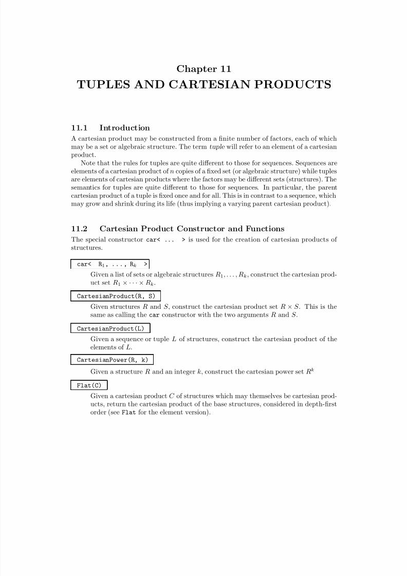
8/22/2019 Handbook Volume 01
http://slidepdf.com/reader/full/handbook-volume-01 323/440
Chapter 11
TUPLES AND CARTESIAN PRODUCTS
11.1 Introduction
A cartesian product may be constructed from a finite number of factors, each of whichmay be a set or algebraic structure. The term tuple will refer to an element of a cartesianproduct.
Note that the rules for tuples are quite different to those for sequences. Sequences are
elements of a cartesian product of n copies of a fixed set (or algebraic structure) while tuplesare elements of cartesian products where the factors may be different sets (structures). Thesemantics for tuples are quite different to those for sequences. In particular, the parentcartesian product of a tuple is fixed once and for all. This is in contrast to a sequence, whichmay grow and shrink during its life (thus implying a varying parent cartesian product).
11.2 Cartesian Product Constructor and Functions
The special constructor car< ... > is used for the creation of cartesian products of structures.
car< R1, ..., Rk >
Given a list of sets or algebraic structures R1, . . . , Rk, construct the cartesian prod-uct set R1 × · · · × Rk.
CartesianProduct(R, S)
Given structures R and S , construct the cartesian product set R × S . This is thesame as calling the car constructor with the two arguments R and S .
CartesianProduct(L)
Given a sequence or tuple L of structures, construct the cartesian product of the
elements of L.
CartesianPower(R, k)
Given a structure R and an integer k, construct the cartesian power set Rk
Flat(C)
Given a cartesian product C of structures which may themselves be cartesian prod-ucts, return the cartesian product of the base structures, considered in depth-firstorder (see Flat for the element version).
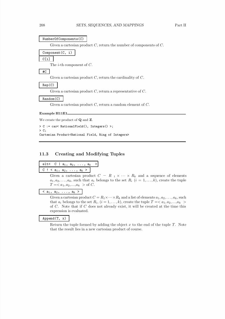
8/22/2019 Handbook Volume 01
http://slidepdf.com/reader/full/handbook-volume-01 324/440
208 SETS, SEQUENCES, AND MAPPINGS Part II
NumberOfComponents(C)
Given a cartesian product C , return the number of components of C .
Component(C, i)
C[i]
The i-th component of C .
#C
Given a cartesian product C , return the cardinality of C .
Rep(C)
Given a cartesian product C , return a representative of C .
Random(C)
Given a cartesian product C , return a random element of C .
Example H11E1
We create the product of Q and Z.
> C := car< RationalField(), Integers() >;
> C;
Cartesian Product<Rational Field, Ring of Integers>
11.3 Creating and Modifying Tuples
elt< C | a1, a2, ..., ak >
C ! < a1, a2, ..., ak >
Given a cartesian product C = R 1 × · · · × Rk and a sequence of elementsa1, a2, . . . , ak, such that ai belongs to the set Ri (i = 1, . . . , k), create the tupleT =< a1, a2,...,ak > of C .
< a1, a2, ..., ak >Given a cartesian product C = R1×···×Rk and a list of elements a1, a2, . . . , ak, suchthat ai belongs to the set Ri, (i = 1, . . . , k), create the tuple T =< a1, a2,...,ak >of C . Note that if C does not already exist, it will be created at the time thisexpression is evaluated.
Append(T, x)
Return the tuple formed by adding the object x to the end of the tuple T . Notethat the result lies in a new cartesian product of course.
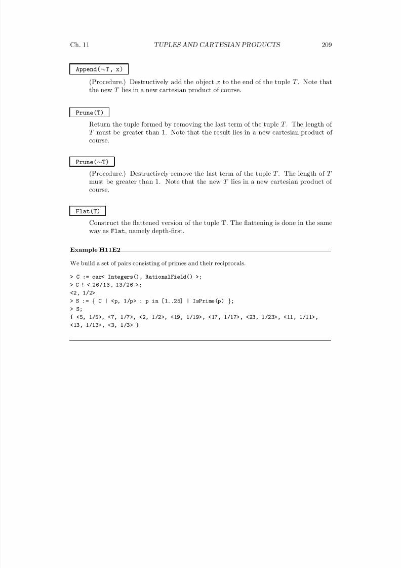
8/22/2019 Handbook Volume 01
http://slidepdf.com/reader/full/handbook-volume-01 325/440
Ch. 11 TUPLES AND CARTESIAN PRODUCTS 209
Append(∼T, x)
(Procedure.) Destructively add the object x to the end of the tuple T . Note thatthe new T lies in a new cartesian product of course.
Prune(T)
Return the tuple formed by removing the last term of the tuple T . The length of T must be greater than 1. Note that the result lies in a new cartesian product of course.
Prune(∼T)
(Procedure.) Destructively remove the last term of the tuple T . The length of T must be greater than 1. Note that the new T lies in a new cartesian product of course.
Flat(T)
Construct the flattened version of the tuple T. The flattening is done in the sameway as Flat, namely depth-first.
Example H11E2
We build a set of pairs consisting of primes and their reciprocals.
> C := car< Integers(), RationalField() >;
> C ! < 26/13, 13/26 >;
<2, 1/2>
> S : = { C | <p, 1/p> : p in [1..25] | IsPrime(p) };
> S;
{ <5, 1/5>, <7, 1/7>, <2, 1/2>, <19, 1/19>, <17, 1/17>, <23, 1/23>, <11, 1/11>,
<13, 1/13>, <3, 1/3> }
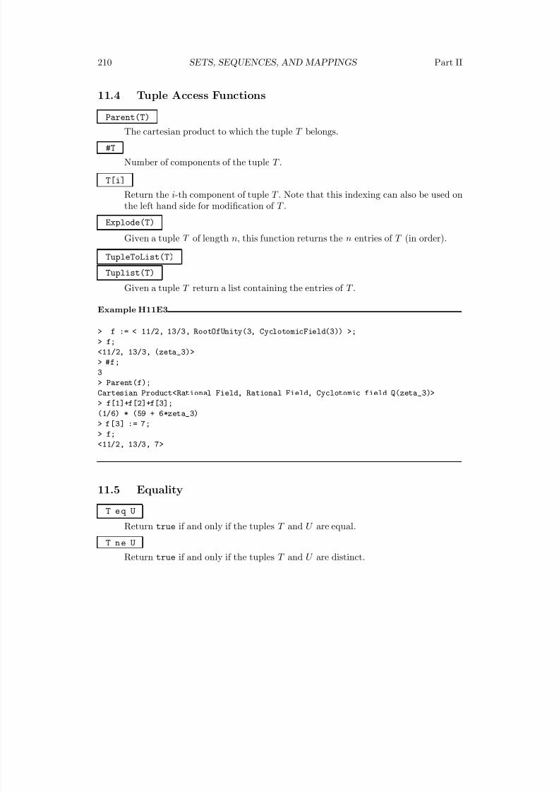
8/22/2019 Handbook Volume 01
http://slidepdf.com/reader/full/handbook-volume-01 326/440
210 SETS, SEQUENCES, AND MAPPINGS Part II
11.4 Tuple Access Functions
Parent(T)The cartesian product to which the tuple T belongs.
#T
Number of components of the tuple T .
T[i]
Return the i-th component of tuple T . Note that this indexing can also be used onthe left hand side for modification of T .
Explode(T)
Given a tuple T of length n, this function returns the n entries of T (in order).
TupleToList(T)
Tuplist(T)
Given a tuple T return a list containing the entries of T .
Example H11E3
> f := < 11/2, 13/3, RootOfUnity(3, CyclotomicField(3)) >;
> f;
<11/2, 13/3, (zeta_3)>
> #f;
3
> Parent(f);
Cartesian Product<Rational Field, Rational Field, Cyclotomic field Q(zeta_3)>
> f[1]+f[2]+f[3];
(1/6) * (59 + 6*zeta_3)
> f[3] := 7;
> f;
<11/2, 13/3, 7>
11.5 Equality
T e q U
Return true if and only if the tuples T and U are equal.
T n e U
Return true if and only if the tuples T and U are distinct.
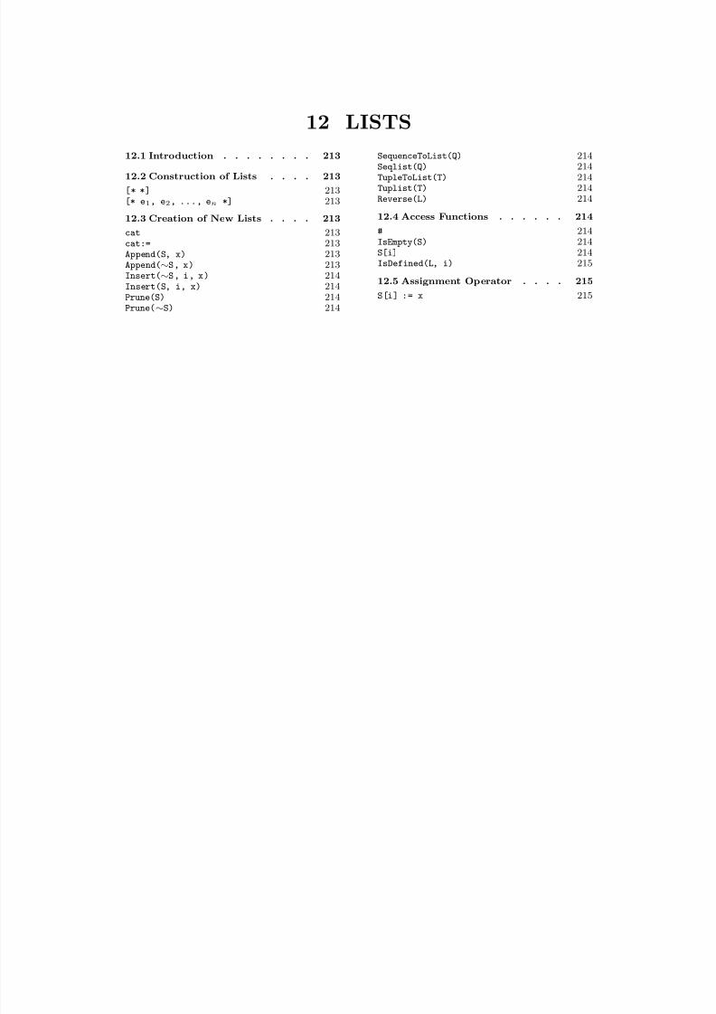
8/22/2019 Handbook Volume 01
http://slidepdf.com/reader/full/handbook-volume-01 327/440
12 LISTS
12.1 Introduction . . . . . . . . 213
12.2 Construction of Lists . . . . 213
[* *] 213[* e1, e2, ..., en *] 213
12.3 Creation of New Lists . . . . 213
cat 213cat:= 213Append(S, x) 213Append(∼S, x) 213Insert(∼S, i, x) 214Insert(S, i, x) 214Prune(S) 214Prune(∼S) 214
SequenceToList(Q) 214Seqlist(Q) 214TupleToList(T) 214Tuplist(T) 214Reverse(L) 214
12.4 Access Functions . . . . . . 214
# 214IsEmpty(S) 214S[i] 214IsDefined(L, i) 215
12.5 Assignment Operator . . . . 215
S[i] := x 215

8/22/2019 Handbook Volume 01
http://slidepdf.com/reader/full/handbook-volume-01 328/440

8/22/2019 Handbook Volume 01
http://slidepdf.com/reader/full/handbook-volume-01 329/440
Chapter 12
LISTS
12.1 Introduction
A list in Magma is an ordered finite collection of objects. Unlike sequences, lists arenot required to consist of objects that have some common parent. Lists are not storedcompactly and the operations provided for them are not extensive. They are mainlyprovided to enable the user to gather assorted objects temporarily together.
12.2 Construction of Lists
Lists can be constructed by expressions enclosed in special brackets [* and *].
[* *]
The empty list.
[* e1, e2, ..., en *]
Given a list of expressions e1, . . . , en, defining elements a1, a2, . . . , an, create the listcontaining a1, a2, . . . , an.
12.3 Creation of New Lists
Here, S denotes the list [∗ s1, . . . , sn ∗], while T denotes the list [∗ t1, . . . , tm ∗].
S cat T
The list formed by concatenating the terms of the list S with the terms of the listT , i.e. the list [∗ s1, . . . , sn, t1, . . . , tm ∗].
S cat:= T
(Procedure.) Destructively concatenate the terms of the list T to S ; i.e. so S becomesthe list [∗ s1, . . . , sn, t1, . . . , tm ∗].
Append(S, x)
The list formed by adding the object x to the end of the list S , i.e. the list[∗ s1, . . . sn, x ∗].
Append(∼S, x)
(Procedure.) Destructively add the object x to the end of the list S ; i.e. so S becomes the list [∗ s1, . . . sn, x ∗].
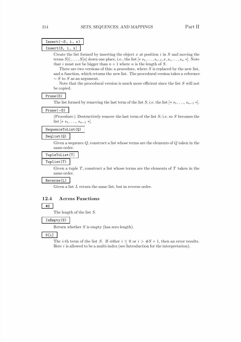
8/22/2019 Handbook Volume 01
http://slidepdf.com/reader/full/handbook-volume-01 330/440
214 SETS, SEQUENCES, AND MAPPINGS Part II
Insert(∼S, i, x)
Insert(S, i, x)
Create the list formed by inserting the object x at position i in S and moving theterms S [i], . . . , S [n] down one place, i.e., the list [∗ s1, . . . , si−1, x , si, . . . , sn ∗]. Notethat i must not be bigger than n + 1 where n is the length of S .
There are two versions of this: a procedure, where S is replaced by the new list,and a function, which returns the new list. The procedural version takes a reference∼ S to S as an argument.
Note that the procedural version is much more efficient since the list S will notbe copied.
Prune(S)
The list formed by removing the last term of the list S , i.e. the list [∗ s1, . . ., sn−1 ∗].
Prune(∼S)
(Procedure.) Destructively remove the last term of the list S ; i.e. so S becomes thelist [∗ s1, . . ., sn−1 ∗].
SequenceToList(Q)
Seqlist(Q)
Given a sequence Q, construct a list whose terms are the elements of Q taken in thesame order.
TupleToList(T)
Tuplist(T)
Given a tuple T , construct a list whose terms are the elements of T taken in thesame order.
Reverse(L)
Given a list L return the same list, but in reverse order.
12.4 Access Functions
#S
The length of the list S .
IsEmpty(S)
Return whether S is empty (has zero length).
S[i]
The i-th term of the list S . If either i ≤ 0 or i > #S + 1, then an error results.Here i is allowed to be a multi-index (see Introduction for the interpretation).
8/22/2019 Handbook Volume 01
http://slidepdf.com/reader/full/handbook-volume-01 331/440
Ch. 12 LISTS 215
IsDefined(L, i)
Checks weather the ith item in L is defined or not, that is it returns true if i is at
most the length of L and false otherwise.
12.5 Assignment Operator
S[i] := x
Redefine the i-th term of the list S to be x. If i ≤ 0, then an error results. If i = #S + 1, then x is appended to S . Otherwise, if i > #S + 1, an error results.Here i is allowed to be a multi-index.

8/22/2019 Handbook Volume 01
http://slidepdf.com/reader/full/handbook-volume-01 332/440
8/22/2019 Handbook Volume 01
http://slidepdf.com/reader/full/handbook-volume-01 333/440
13 COPRODUCTS
13.1 Introduction . . . . . . . . 219
13.2 Creation Functions . . . . . 219
13.2.1 Creation of Coproducts . . . . . 219
cop< > 219cop< > 219
13.2.2 Creation of Coproduct Elements . 219
m(e) 219! 219
13.3 Accessing Functions . . . . . 220
Injections(C) 220
# 220Constituent(C, i) 220Index(x) 220
13.4 Retrieve . . . . . . . . . . 220
Retrieve(x) 220
13.5 Flattening . . . . . . . . . 221
Flat(C) 221
13.6 Universal Map . . . . . . . 221
UniversalMap(C, S, [ n1, ..., nm ]) 221

8/22/2019 Handbook Volume 01
http://slidepdf.com/reader/full/handbook-volume-01 334/440
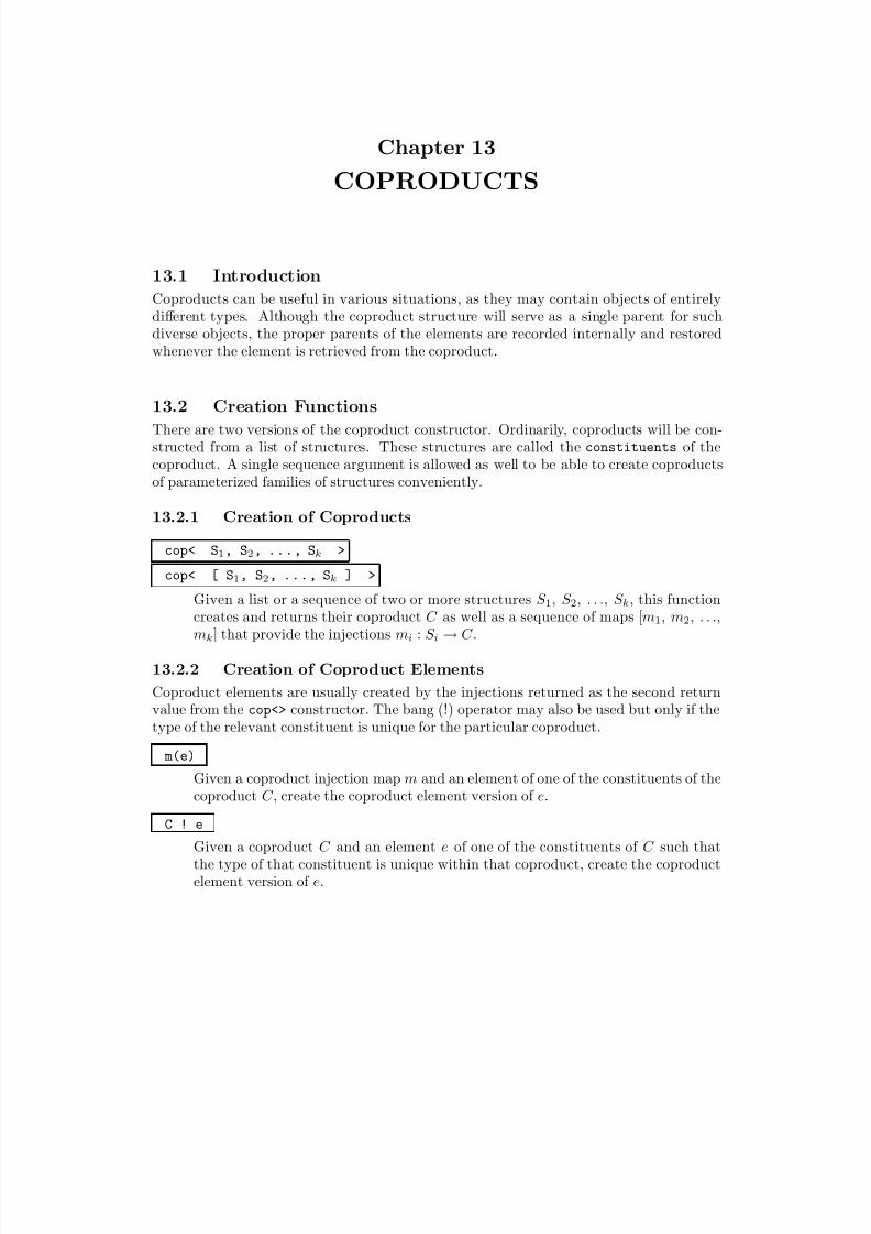
8/22/2019 Handbook Volume 01
http://slidepdf.com/reader/full/handbook-volume-01 335/440
Chapter 13
COPRODUCTS
13.1 Introduction
Coproducts can be useful in various situations, as they may contain objects of entirelydifferent types. Although the coproduct structure will serve as a single parent for suchdiverse objects, the proper parents of the elements are recorded internally and restoredwhenever the element is retrieved from the coproduct.
13.2 Creation Functions
There are two versions of the coproduct constructor. Ordinarily, coproducts will be con-structed from a list of structures. These structures are called the constituents of thecoproduct. A single sequence argument is allowed as well to be able to create coproductsof parameterized families of structures conveniently.
13.2.1 Creation of Coproducts
cop< S1, S2, ..., Sk >cop< [ S1, S2, ..., Sk ] >
Given a list or a sequence of two or more structures S 1, S 2, . . ., S k, this functioncreates and returns their coproduct C as well as a sequence of maps [m1, m2, . . .,mk] that provide the injections mi : S i → C .
13.2.2 Creation of Coproduct Elements
Coproduct elements are usually created by the injections returned as the second returnvalue from the cop<> constructor. The bang (!) operator may also be used but only if thetype of the relevant constituent is unique for the particular coproduct.
m(e)
Given a coproduct injection map m and an element of one of the constituents of thecoproduct C , create the coproduct element version of e.
C ! e
Given a coproduct C and an element e of one of the constituents of C such thatthe type of that constituent is unique within that coproduct, create the coproductelement version of e.
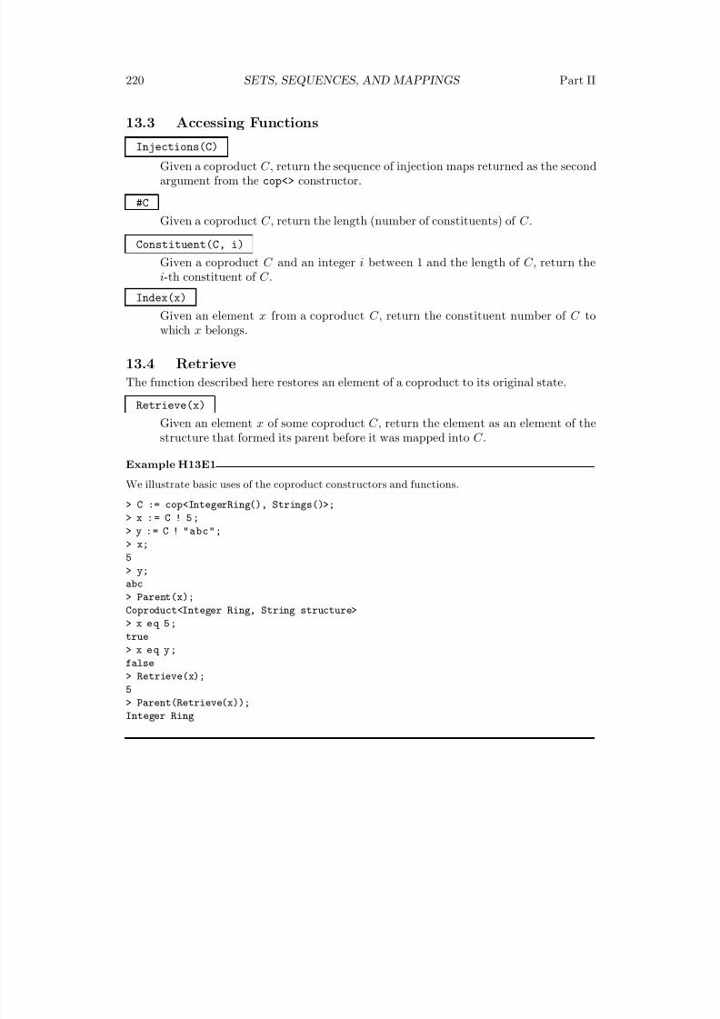
8/22/2019 Handbook Volume 01
http://slidepdf.com/reader/full/handbook-volume-01 336/440
220 SETS, SEQUENCES, AND MAPPINGS Part II
13.3 Accessing Functions
Injections(C)
Given a coproduct C , return the sequence of injection maps returned as the secondargument from the cop<> constructor.
#C
Given a coproduct C , return the length (number of constituents) of C .
Constituent(C, i)
Given a coproduct C and an integer i between 1 and the length of C , return thei-th constituent of C .
Index(x)
Given an element x from a coproduct C , return the constituent number of C towhich x belongs.
13.4 Retrieve
The function described here restores an element of a coproduct to its original state.
Retrieve(x)
Given an element x of some coproduct C , return the element as an element of thestructure that formed its parent before it was mapped into C .
Example H13E1
We illustrate basic uses of the coproduct constructors and functions.
> C := cop<IntegerRing(), Strings()>;
> x : = C ! 5 ;
> y := C ! "abc";
> x;
5
> y;
abc
> Parent(x);
Coproduct<Integer Ring, String structure>> x e q 5 ;
true
> x e q y ;
false
> Retrieve(x);
5
> Parent(Retrieve(x));
Integer Ring
8/22/2019 Handbook Volume 01
http://slidepdf.com/reader/full/handbook-volume-01 337/440
Ch. 13 COPRODUCTS 221
13.5 Flattening
The function described here enables the ‘concatenation’ of coproducts into a single one.
Flat(C)
Given a coproduct C of structures which may themselves be coproducts, return thecoproduct of the base structures, considered in depth-first order.
13.6 Universal Map
UniversalMap(C, S, [ n1, ..., nm ])
Given maps n1, . . ., nm from structures S 1, . . ., S m that compose the coproduct C ,to some structure S , this function returns the universal map C → S .

8/22/2019 Handbook Volume 01
http://slidepdf.com/reader/full/handbook-volume-01 338/440

8/22/2019 Handbook Volume 01
http://slidepdf.com/reader/full/handbook-volume-01 339/440
14 RECORDS
14.1 Introduction . . . . . . . . 225
14.2 The Record Format Constructor 225
recformat< > 225
14.3 Creating a Record . . . . . . 226
rec< > 226
14.4 Access and ModificationFunctions . . . . . . . . . 227
Format(r) 227Names(F) 227Names(r) 227r‘fieldname 227r‘fieldname := e ; 227delete 227assigned 227r‘‘s 227

8/22/2019 Handbook Volume 01
http://slidepdf.com/reader/full/handbook-volume-01 340/440
8/22/2019 Handbook Volume 01
http://slidepdf.com/reader/full/handbook-volume-01 341/440
Chapter 14
RECORDS
14.1 Introduction
In a record several objects can be collected. The objects in a record are stored in record fields , and are accessed by using fieldnames . Records are like tuples (and unlike sets orsequences) in that the objects need not all be of the same kind. Though records andtuples are somewhat similar, there are several differences too. The components of tuplesare indexed by integers, and every component must be defined. The fields of records areindexed by fieldnames, and it is possible for some (or all) of the fields of a record not tobe assigned; in fact, a field of a record may be assigned or deleted at any time. A recordmust be constructed according to a pre-defined record format, whereas a tuple may beconstructed without first giving the Cartesian product that is its parent, since Magma
can deduce the parent from the tuple.In the definition of a record format, each field is given a fieldname. If the field is also
given a parent magma or a category, then in any record created according to this format,that field must conform to this requirement. However, if the field is not given a parentmagma or category, there is no restriction on the kinds of values stored in that field;different records in the format may contain disparate values in that field. By contrast,every component of a Cartesian product is a magma, and the components of all tuples in
this product must be elements of the corresponding magma.Because of the flexibility of records, with respect to whether a field is assigned and whatkind of value is stored in it, Boolean operators are not available for comparing records.
14.2 The Record Format Constructor
The special constructor recformat< ... > is used for the creation of record formats. Arecord format must be created before records in that format are created.
recformat< L >
(and optional parents or categories) in LConstruct the record format corresponding to the non-empty fieldname list L. Each
term of L must be one of the following:(a) fieldname in which case there is no restriction on values that may be stored in
this field of records having this format;
(b)fieldname :expression where the expression evaluates to a magma which will bethe parent of values stored in this field of records having this format; or
(c) fieldname :expression where the expression evaluates to a category which willbe the category of values stored in this field of records having this format;
where fieldname consists of characters that would form a valid identifier name. Notethat it is not a string.
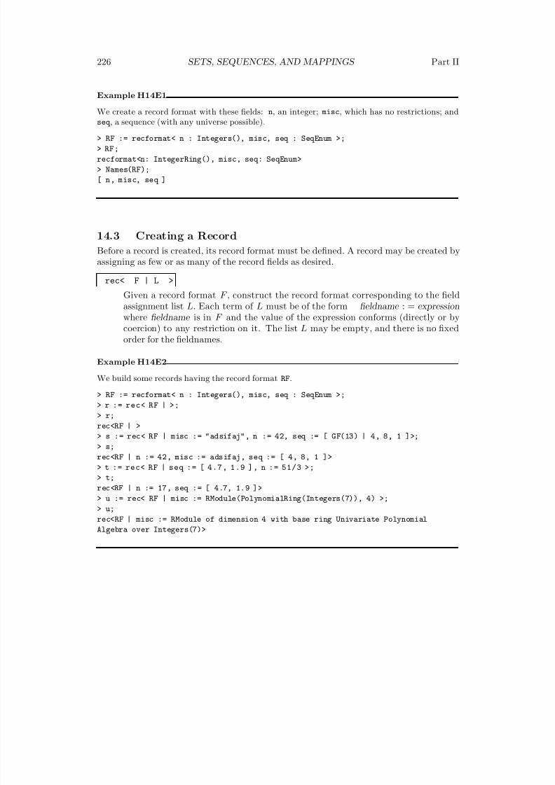
8/22/2019 Handbook Volume 01
http://slidepdf.com/reader/full/handbook-volume-01 342/440
226 SETS, SEQUENCES, AND MAPPINGS Part II
Example H14E1
We create a record format with these fields: n, an integer; misc, which has no restrictions; andseq , a sequence (with any universe possible).
> RF := recformat< n : Integers(), misc, seq : SeqEnum >;
> RF;
recformat<n: IntegerRing(), misc, seq: SeqEnum>
> Names(RF);
[ n, misc, seq ]
14.3 Creating a RecordBefore a record is created, its record format must be defined. A record may be created byassigning as few or as many of the record fields as desired.
rec< F | L >
Given a record format F , construct the record format corresponding to the fieldassignment list L. Each term of L must be of the form fieldname : = expressionwhere fieldname is in F and the value of the expression conforms (directly or bycoercion) to any restriction on it. The list L may be empty, and there is no fixedorder for the fieldnames.
Example H14E2
We build some records having the record format RF.
> RF := recformat< n : Integers(), misc, seq : SeqEnum >;
> r := rec< RF | >;
> r;
rec<RF | >
> s := rec< RF | misc := "adsifaj", n := 42, seq := [ GF(13) | 4, 8, 1 ]>;
> s;
rec<RF | n := 42, misc := adsifaj, seq := [ 4, 8, 1 ]>
> t := rec< RF | seq := [ 4.7, 1.9 ], n := 51/3 >;
> t;
rec<RF | n := 17, seq := [ 4.7, 1.9 ]>
> u := rec< RF | misc := RModule(PolynomialRing(Integers(7)), 4) >;
> u;
rec<RF | misc := RModule of dimension 4 with base ring Univariate Polynomial
Algebra over Integers(7)>
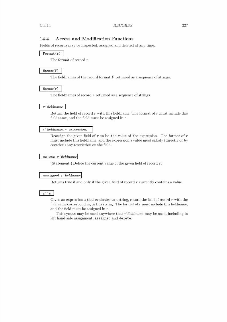
8/22/2019 Handbook Volume 01
http://slidepdf.com/reader/full/handbook-volume-01 343/440
Ch. 14 RECORDS 227
14.4 Access and Modification Functions
Fields of records may be inspected, assigned and deleted at any time.
Format(r)
The format of record r.
Names(F)
The fieldnames of the record format F returned as a sequence of strings.
Names(r)
The fieldnames of record r returned as a sequence of strings.
r‘fieldname
Return the field of record r with this fieldname. The format of r must include thisfieldname, and the field must be assigned in r.
r‘fieldname := expression;
Reassign the given field of r to be the value of the expression. The format of rmust include this fieldname, and the expression’s value must satisfy (directly or by
coercion) any restriction on the field.
delete r‘fieldname
(Statement.) Delete the current value of the given field of record r.
assigned r‘fieldname
Returns true if and only if the given field of record r currently contains a value.
r‘‘sGiven an expression s that evaluates to a string, return the field of record r with thefieldname corresponding to this string. The format of r must include this fieldname,and the field must be assigned in r.
This syntax may be used anywhere that r‘fieldname may be used, including inleft hand side assignment, assigned and delete.
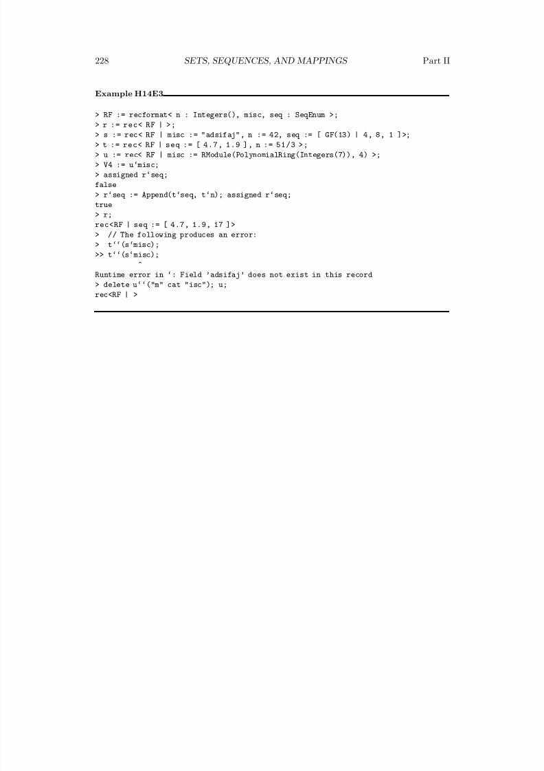
8/22/2019 Handbook Volume 01
http://slidepdf.com/reader/full/handbook-volume-01 344/440
228 SETS, SEQUENCES, AND MAPPINGS Part II
Example H14E3
> RF := recformat< n : Integers(), misc, seq : SeqEnum >;> r := rec< RF | >;
> s := rec< RF | misc := "adsifaj", n := 42, seq := [ GF(13) | 4, 8, 1 ]>;
> t := rec< RF | seq := [ 4.7, 1.9 ], n := 51/3 >;
> u := rec< RF | misc := RModule(PolynomialRing(Integers(7)), 4) >;
> V4 := u‘misc;
> assigned r‘seq;
false
> r‘seq := Append(t‘seq, t‘n); assigned r‘seq;
true
> r;
rec<RF | seq := [ 4.7, 1.9, 17 ]>
> // The following produces an error:> t‘‘(s‘misc);
>> t‘‘(s‘misc);
^
Runtime error in ‘: Field ’adsifaj’ does not exist in this record
> delete u‘‘("m" cat "isc"); u;
rec<RF | >
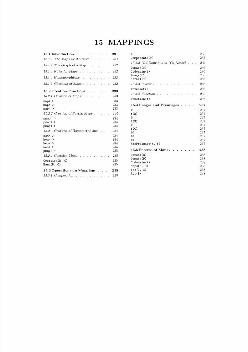
8/22/2019 Handbook Volume 01
http://slidepdf.com/reader/full/handbook-volume-01 345/440
15 MAPPINGS
15.1 Introduction . . . . . . . . 231
15.1.1 The Map Constructors . . . . . . 231
15.1.2 The Graph of a Map . . . . . . . 232
15.1.3 Rules for Maps . . . . . . . . . 232
15.1.4 Homomorphisms . . . . . . . . 232
15.1.5 Checking of Maps . . . . . . . . 232
15.2 Creation Functions . . . . . 233
15.2.1 Creation of Maps . . . . . . . . 233
map< > 233
map< > 233 map< > 233
15.2.2 Creation of Partial Maps . . . . . 234
pmap< > 234pmap< > 234pmap< > 234
15.2.3 Creation of Homomorphisms . . . 234
hom< > 234hom< > 234hom< > 234hom< > 235pmap< > 235
15.2.4 Coercion Maps . . . . . . . . . 235
Coercion(D, C) 235Bang(D, C) 235
15.3 Operations on Mappings . . . 235
15.3.1 Composition . . . . . . . . . . 235
* 235Components(f) 235
15.3.2 (Co)Domain and (Co)Kernel . . . 236
Domain(f) 236Codomain(f) 236Image(f) 236Kernel(f) 236
15.3.3 Inverse . . . . . . . . . . . . . 236
Inverse(m) 236
15.3.4 Function . . . . . . . . . . . . 236
Function(f) 236
15.4 Images and Preimages . . . . 237@ 237f(a) 237@ 237f(S) 237@ 237f(C) 237@@ 237@@ 237@@ 237HasPreimage(x, f) 237
15.5 Parents of Maps . . . . . . . 238
Parent(m) 238
Domain(P) 238Codomain(P) 238Maps(D, C) 238Iso(D, C) 238Aut(S) 238

8/22/2019 Handbook Volume 01
http://slidepdf.com/reader/full/handbook-volume-01 346/440
8/22/2019 Handbook Volume 01
http://slidepdf.com/reader/full/handbook-volume-01 347/440
Chapter 15
MAPPINGS
15.1 Introduction
Mappings play a fundamental role in algebra and, indeed, throughout mathematics. Re-flecting this importance, mappings are one of the fundamental datatypes in our language.The most general way to define a mapping f : A → B in a programming language isto write a function which, given any element of A, will return its image under f in B.While this approach to the definition of mappings is completely general, it is desirable to
have mappings as an independent datatype. It is then possible to provide a very compactnotation for specifying important classes of mappings such as homomorphisms. Further, arange of operations peculiar to the mapping type can be provided.
Mappings are created either through use of mapping constructors as described in thisChapter, or through use of certain standard functions that return mappings as eitherprimary or secondary values.
All mappings are objects in the Magma category Map.
15.1.1 The Map Constructors
There are three main mapping constructors: the general map constructor map< >, the ho-
momorphism constructor hom< >, and the partial map constructor pmap< >. The generalform of all constructors is the same: inside the angle brackets there are two componentsseparated by a pipe |. To the left the user specifies a domain A and a codomain B, sepa-rated by ->; to the right of the pipe the user specifies how images are obtained for elementsof the domain. The latter can be done in one of several ways: one specifies either the graph
of the map, or a rule describing how images are to be formed, or for homomorphisms, onespecifies generator images. We will describe each in the next subsections. The result issomething like map< A -> B | expression>.
The domain and codomain of the map can be arbitrary magmas. When a full map(as opposed to a partial map) is constructed by use of a graph, the domain is necessarilyfinite.
The main difference between maps and partial maps is that a partial map need not bedefined for every element of the domain. The main difference between these two types of map and homomorphisms is that the latter are supposed to provide structure-preserving
maps between algebraic structures. On the one hand this makes it possible to allow thespecification of images for homomorphisms in a different fashion: homomorphism can begiven via images for generators of the domain. On the other hand homomorphisms arerestricted to cases where domain and (image in the) codomain have a similar structure.The generator image form only makes sense for domains that are finitely presented . Ho-momorphisms are described in more detail below.
8/22/2019 Handbook Volume 01
http://slidepdf.com/reader/full/handbook-volume-01 348/440
232 SETS, SEQUENCES, AND MAPPINGS Part II
15.1.2 The Graph of a Map
Let A and B be structures. A subgraph of the cartesian product C = A × B is a subset G
of C such that each element of A appears at most once among the first components of thepairs < a, b > of G. A subgraph having the additional property that every element of Aappears as the first component of some pair < a, b > of G is called a graph of A × B.
A mapping between A and B can be identified with a graph G of A × B, a partial mapcan be identified with a subgraph. We now describe how a graph may be represented inthe context of the map constructor. An element of the graph of A × B can be given eitheras a tuple <a, b>, or as an arrow pair a - > b. The specification of a (sub)graph in a mapconstructor should then consist of either a (comma separated) list, a sequence, or a set of such tuples or arrow pairs (a mixture is permitted).
15.1.3 Rules for MapsThe specification of a rule in the map constructor involves a free variable and an expression,usually involving the free variable, separated by :->, for example x :-> 3*x - 1. Thescope of the free variable is restricted to the map constructor (so the use of x does notinterfere with values of x outside the constructor). A general expression is allowed in therule, which may involve intrinsic or user functions, and even in-line definitions of suchfunctions.
15.1.4 Homomorphisms
Probably the most useful form of the map-constructor is the version for homomorphisms.Most interesting mappings in algebra are homomorphisms, and if an algebraic structureA belongs to a family of algebraic structures which form a variety we have the fundamen-tal result that a homomorphism is uniquely determined by the images of any generatingset. This provides us with a particularly compact way of defining and representing homo-morphisms. While the syntax of the homomorphism constructor is similar to that of thegeneral mapping constructor, the semantics are sometimes different.
The kind of homomorphism built by the hom-constructor is determined entirely by thedomain: thus, a group homomorphism results from applying hom to a domain A that isone of the types of group in Magma, a ring homomorphism results when A is a ring, etc.As a consequence, the requirements on the specification of homomorphisms are dependenton the category to which A belongs. Often, the codomain of a homomorphism is required
to belong to the same variety. But even within a category the specification may dependon the type of structure; for details we refer the reader to the specific chapters.A homomorphism can be specified using either a rule map or by generator images. In
the latter case the processor will seek to express an element as a word in the generators of A when asked to compute its image. Thus A needs to be finitely presented.
15.1.5 Checking of Maps
It should be pointed out that checking the ‘correctness’ of mappings can be done to alimited extent only. If the mapping is given by means of a graph, Magma will checkthat no multiple images are specified, and that an image is given for every element of the
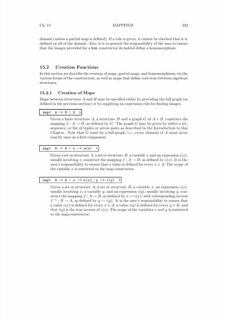
8/22/2019 Handbook Volume 01
http://slidepdf.com/reader/full/handbook-volume-01 349/440
Ch. 15 MAPPINGS 233
domain (unless a partial map is defined). If a rule is given, it cannot be checked that it isdefined on all of the domain. Also, it is in general the responsibility of the user to ensure
that the images provided for a hom constructor do indeed define a homomorphism.
15.2 Creation Functions
In this section we describe the creation of maps, partial maps, and homomorphisms via thevarious forms of the constructors, as well as maps that define coercions between algebraicstructures.
15.2.1 Creation of Maps
Maps between structures A and B may be specified either by providing the full graph (asdefined in the previous section) or by supplying an expression rule for finding images.
map< A -> B | G >
Given a finite structure A, a structure B and a graph G of A × B, construct themapping f : A → B, as defined by G. The graph G may be given by either a set,sequence, or list of tuples or arrow-pairs as described in the Introduction to thisChapter. Note that G must be a full graph, i.e., every element of A must occurexactly once as a first component.
map< A -> B | x :-> e(x) >
Given a set or structure A, a set or structure B, a variable x and an expression e(x),usually involving x, construct the mapping f : A → B, as defined by e(x). It is theuser’s responsibility to ensure that a value is defined for every x ∈ A. The scope of the variable x is restricted to the map-constructor.
map< A -> B | x :-> e(x), y :-> i(y) >
Given a set or structure A, a set or structure B, a variable x, an expression e(x),
usually involving x, a variable y, and an expression i(y), usually involving y, con-struct the mapping f : A → B, as defined by x → e(x), with corresponding inversef −1 : B → A, as defined by y → i(y). It is the user’s responsibility to ensure thata value e(x) is defined for every x ∈ A, a value i(y) is defined for every y ∈ B, andthat i(y) is the true inverse of e(x). The scope of the variables x and y is restrictedto the map-constructor.
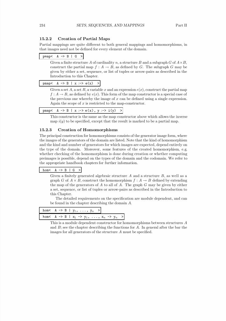
8/22/2019 Handbook Volume 01
http://slidepdf.com/reader/full/handbook-volume-01 350/440
234 SETS, SEQUENCES, AND MAPPINGS Part II
15.2.2 Creation of Partial Maps
Partial mappings are quite different to both general mappings and homomorphisms, in
that images need not be defined for every element of the domain.
pmap< A -> B | G >
Given a finite structure A of cardinality n, a structure B and a subgraph G of A×B,construct the partial map f : A → B, as defined by G. The subgraph G may begiven by either a set, sequence, or list of tuples or arrow-pairs as described in theIntroduction to this Chapter.
pmap< A -> B | x :-> e(x) >
Given a set A, a set B, a variable x and an expression e(x), construct the partial mapf : A → B, as defined by e(x). This form of the map constructor is a special case of the previous one whereby the image of x can be defined using a single expression.Again the scope of x is restricted to the map-constructor.
pmap< A -> B | x :-> e(x), y :-> i(y) >
This constructor is the same as the map constructor above which allows the inversemap i(y) to be specified, except that the result is marked to be a partial map.
15.2.3 Creation of Homomorphisms
The principal construction for homomorphisms consists of the generator image form, wherethe images of the generators of the domain are listed. Note that the kind of homomorphism
and the kind and number of generators for which images are expected, depend entirely onthe type of the domain. Moreover, some features of the created homomorphism, e.g.whether checking of the homomorphism is done during creation or whether computingpreimages is possible, depend on the types of the domain and the codomain. We refer tothe appropriate handbook chapters for further information.
hom< A -> B | G >
Given a finitely generated algebraic structure A and a structure B, as well as agraph G of A × B, construct the homomorphism f : A → B defined by extendingthe map of the generators of A to all of A. The graph G may be given by eithera set, sequence, or list of tuples or arrow-pairs as described in the Introduction to
this Chapter.The detailed requirements on the specification are module dependent, and can
be found in the chapter describing the domain A.
hom< A -> B | y1, ..., yn >
hom< A -> B | x1 -> y1, ..., xn -> yn >
This is a module dependent constructor for homomorphisms between structures Aand B; see the chapter describing the functions for A. In general after the bar theimages for all generators of the structure A must be specified.
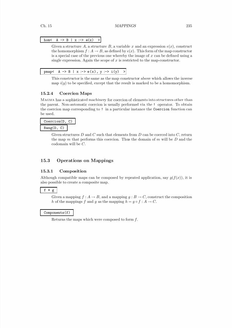
8/22/2019 Handbook Volume 01
http://slidepdf.com/reader/full/handbook-volume-01 351/440
Ch. 15 MAPPINGS 235
hom< A -> B | x :-> e(x) >
Given a structure A, a structure B, a variable x and an expression e(x), constructthe homomorphism f : A → B, as defined by e(x). This form of the map constructoris a special case of the previous one whereby the image of x can be defined using asingle expression. Again the scope of x is restricted to the map-constructor.
pmap< A -> B | x :-> e(x), y :-> i(y) >
This constructor is the same as the map constructor above which allows the inversemap i(y) to be specified, except that the result is marked to be a homomorphism.
15.2.4 Coercion Maps
Magma has a sophisticated machinery for coercion of elements into structures other thanthe parent. Non-automatic coercion is usually performed via the ! operator. To obtainthe coercion map corresponding to ! in a particular instance the Coercion function canbe used.
Coercion(D, C)
Bang(D, C)
Given structures D and C such that elements from D can be coerced into C , returnthe map m that performs this coercion. Thus the domain of m will be D and thecodomain will be C .
15.3 Operations on Mappings
15.3.1 Composition
Although compatible maps can be composed by repeated application, say g(f (x)), it isalso possible to create a composite map.
f * g
Given a mapping f : A → B, and a mapping g : B → C , construct the compositionh of the mappings f and g as the mapping h = g ◦ f : A → C .
Components(f)
Returns the maps which were composed to form f .
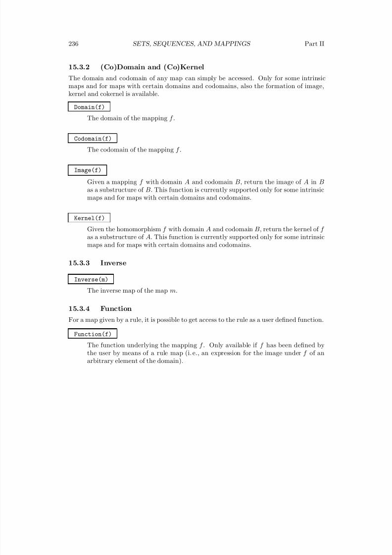
8/22/2019 Handbook Volume 01
http://slidepdf.com/reader/full/handbook-volume-01 352/440
236 SETS, SEQUENCES, AND MAPPINGS Part II
15.3.2 (Co)Domain and (Co)Kernel
The domain and codomain of any map can simply be accessed. Only for some intrinsicmaps and for maps with certain domains and codomains, also the formation of image,kernel and cokernel is available.
Domain(f)
The domain of the mapping f .
Codomain(f)
The codomain of the mapping f .
Image(f)
Given a mapping f with domain A and codomain B, return the image of A in Bas a substructure of B. This function is currently supported only for some intrinsicmaps and for maps with certain domains and codomains.
Kernel(f)
Given the homomorphism f with domain A and codomain B, return the kernel of f as a substructure of A. This function is currently supported only for some intrinsicmaps and for maps with certain domains and codomains.
15.3.3 Inverse
Inverse(m)
The inverse map of the map m.
15.3.4 Function
For a map given by a rule, it is possible to get access to the rule as a user defined function.
Function(f)
The function underlying the mapping f . Only available if f has been defined bythe user by means of a rule map (i. e., an expression for the image under f of anarbitrary element of the domain).
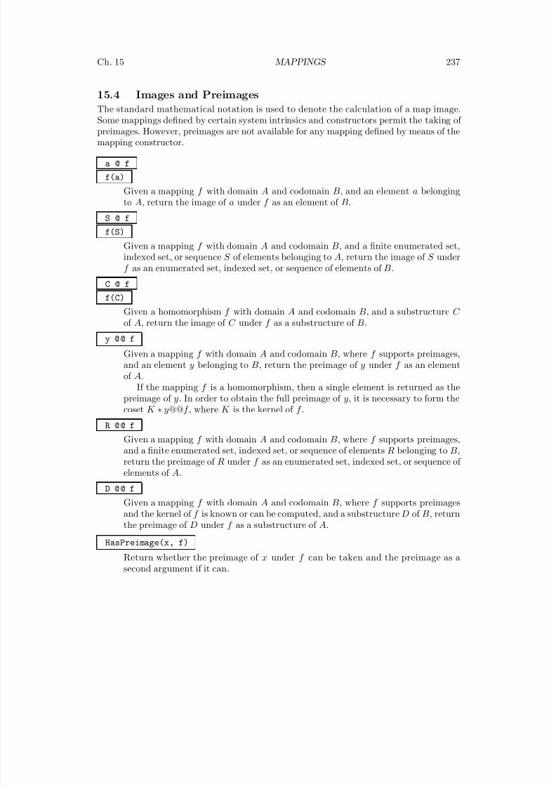
8/22/2019 Handbook Volume 01
http://slidepdf.com/reader/full/handbook-volume-01 353/440
Ch. 15 MAPPINGS 237
15.4 Images and Preimages
The standard mathematical notation is used to denote the calculation of a map image.
Some mappings defined by certain system intrinsics and constructors permit the taking of preimages. However, preimages are not available for any mapping defined by means of themapping constructor.
a @ f
f(a)
Given a mapping f with domain A and codomain B, and an element a belongingto A, return the image of a under f as an element of B.
S @ f
f(S)
Given a mapping f with domain A and codomain B, and a finite enumerated set,indexed set, or sequence S of elements belonging to A, return the image of S underf as an enumerated set, indexed set, or sequence of elements of B.
C @ f
f(C)
Given a homomorphism f with domain A and codomain B, and a substructure C of A, return the image of C under f as a substructure of B.
y @ @ f
Given a mapping f with domain A and codomain B, where f supports preimages,and an element y belonging to B, return the preimage of y under f as an elementof A.
If the mapping f is a homomorphism, then a single element is returned as thepreimage of y. In order to obtain the full preimage of y, it is necessary to form thecoset K ∗ y@@f , where K is the kernel of f .
R @ @ f
Given a mapping f with domain A and codomain B, where f supports preimages,and a finite enumerated set, indexed set, or sequence of elements R belonging to B,return the preimage of R under f as an enumerated set, indexed set, or sequence of
elements of A.D @ @ f
Given a mapping f with domain A and codomain B, where f supports preimagesand the kernel of f is known or can be computed, and a substructure D of B, returnthe preimage of D under f as a substructure of A.
HasPreimage(x, f)
Return whether the preimage of x under f can be taken and the preimage as asecond argument if it can.
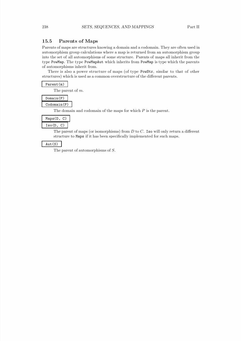
8/22/2019 Handbook Volume 01
http://slidepdf.com/reader/full/handbook-volume-01 354/440
238 SETS, SEQUENCES, AND MAPPINGS Part II
15.5 Parents of Maps
Parents of maps are structures knowing a domain and a codomain. They are often used in
automorphism group calculations where a map is returned from an automorphism groupinto the set of all automorphisms of some structure. Parents of maps all inherit from thetype PowMap. The type PowMapAut which inherits from PowMap is type which the parentsof automorphisms inherit from.
There is also a power structure of maps (of type PowStr, similar to that of otherstructures) which is used as a common overstructure of the different parents.
Parent(m)
The parent of m.
Domain(P)
Codomain(P)
The domain and codomain of the maps for which P is the parent.
Maps(D, C)
Iso(D, C)
The parent of maps (or isomorphisms) from D to C . Iso will only return a differentstructure to Maps if it has been specifically implemented for such maps.
Aut(S)
The parent of automorphisms of S .

8/22/2019 Handbook Volume 01
http://slidepdf.com/reader/full/handbook-volume-01 355/440
PART IIISEMIGROUPS AND MONOIDS
16 FINITELY PRESENTED SEMIGROUPS 241
17 MONOIDS GIVEN BY REWRITE SYSTEMS 253

8/22/2019 Handbook Volume 01
http://slidepdf.com/reader/full/handbook-volume-01 356/440
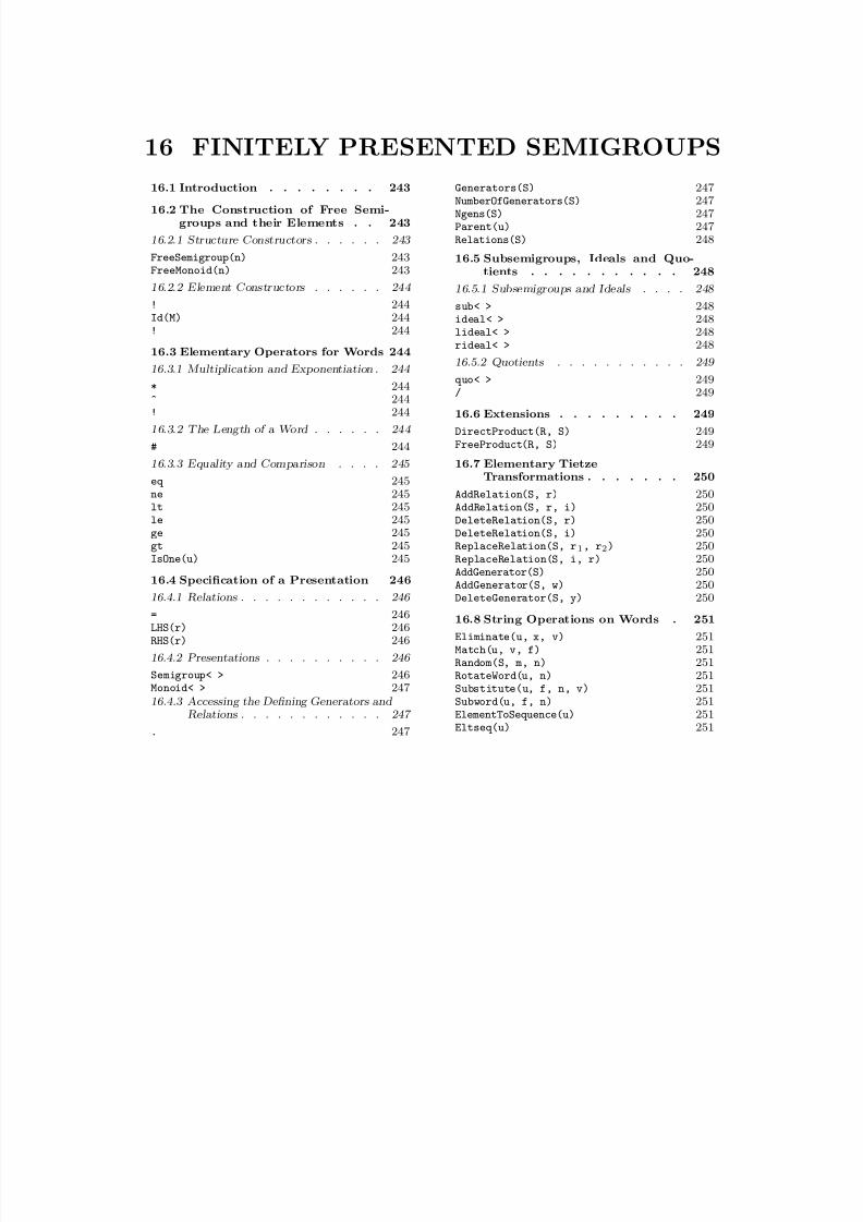
8/22/2019 Handbook Volume 01
http://slidepdf.com/reader/full/handbook-volume-01 357/440
16 FINITELY PRESENTED SEMIGROUPS
16.1 Introduction . . . . . . . . 243
16.2 The Construction of Free Semi-groups and their Elements . . 243
16.2.1 Structure Constructors . . . . . . 243
FreeSemigroup(n) 243FreeMonoid(n) 243
16.2.2 Element Constructors . . . . . . 244
! 244Id(M) 244! 244
16.3 Elementary Operators for Words 244
16.3.1 Multiplication and Exponentiation . 244* 244^ 244! 244
16.3.2 The Length of a Word . . . . . . 244
# 244
16.3.3 Equality and Comparison . . . . 245
eq 245ne 245lt 245le 245ge 245
gt 245IsOne(u) 245
16.4 Specification of a Presentation 246
16.4.1 Relations . . . . . . . . . . . . 246
= 246LHS(r) 246RHS(r) 246
16.4.2 Presentations . . . . . . . . . . 246
Semigroup< > 246Monoid< > 24716.4.3 Accessing the Defining Generators and
Relations . . . . . . . . . . . . 247
. 247
Generators(S) 247NumberOfGenerators(S) 247Ngens(S) 247Parent(u) 247Relations(S) 248
16.5 Subsemigroups, Ideals and Quo-tients . . . . . . . . . . . 248
16.5.1 Subsemigroups and Ideals . . . . 248
sub< > 248ideal< > 248lideal< > 248rideal< > 248
16.5.2 Quotients . . . . . . . . . . . 249 quo< > 249/ 249
16.6 Extensions . . . . . . . . . 249
DirectProduct(R, S) 249FreeProduct(R, S) 249
16.7 Elementary TietzeTransformations . . . . . . . 250
AddRelation(S, r) 250AddRelation(S, r, i) 250DeleteRelation(S, r) 250DeleteRelation(S, i) 250
ReplaceRelation(S, r1, r2) 250ReplaceRelation(S, i, r) 250AddGenerator(S) 250AddGenerator(S, w) 250DeleteGenerator(S, y) 250
16.8 String Operations on Words . 251
Eliminate(u, x, v) 251Match(u, v, f) 251Random(S, m, n) 251RotateWord(u, n) 251Substitute(u, f, n, v) 251Subword(u, f, n) 251ElementToSequence(u) 251Eltseq(u) 251

8/22/2019 Handbook Volume 01
http://slidepdf.com/reader/full/handbook-volume-01 358/440
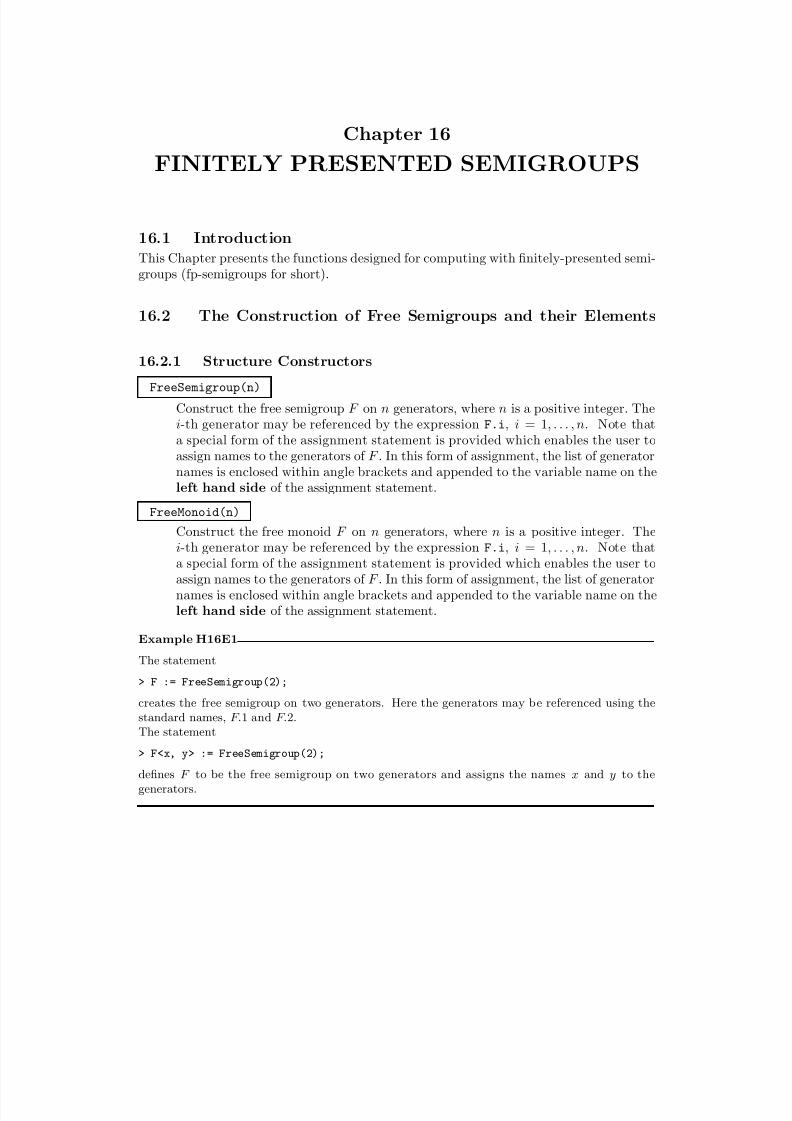
8/22/2019 Handbook Volume 01
http://slidepdf.com/reader/full/handbook-volume-01 359/440
Chapter 16
FINITELY PRESENTED SEMIGROUPS
16.1 Introduction
This Chapter presents the functions designed for computing with finitely-presented semi-groups (fp-semigroups for short).
16.2 The Construction of Free Semigroups and their Elements
16.2.1 Structure Constructors
FreeSemigroup(n)
Construct the free semigroup F on n generators, where n is a positive integer. Thei-th generator may be referenced by the expression F.i, i = 1, . . . , n. Note thata special form of the assignment statement is provided which enables the user toassign names to the generators of F . In this form of assignment, the list of generatornames is enclosed within angle brackets and appended to the variable name on theleft hand side of the assignment statement.
FreeMonoid(n)
Construct the free monoid F on n generators, where n is a positive integer. Thei-th generator may be referenced by the expression F.i, i = 1, . . . , n. Note thata special form of the assignment statement is provided which enables the user toassign names to the generators of F . In this form of assignment, the list of generatornames is enclosed within angle brackets and appended to the variable name on theleft hand side of the assignment statement.
Example H16E1
The statement
> F := FreeSemigroup(2);
creates the free semigroup on two generators. Here the generators may be referenced using thestandard names, F.1 and F.2.The statement
> F<x, y> := FreeSemigroup(2);
defines F to be the free semigroup on two generators and assigns the names x and y to thegenerators.
8/22/2019 Handbook Volume 01
http://slidepdf.com/reader/full/handbook-volume-01 360/440
244 SEMIGROUPS AND MONOIDS Part III
16.2.2 Element Constructors
Suppose S is an fp-semigroup, not necessarily free, for which generators have already been
defined. A word is defined inductively as follows:
(i) A generator is a word;
(ii)The product uv of the words u and v is a word;
(iii)The power of a word, un, where u is a word and n is an integer, is a word.
An element (word) of S may be constructed as an expression in the generators as outlinedbelow.
S ! [ i1, ... is]
Given a semigroup S defined on r generators and a sequence Q = [i1, · · · , is] of
integers lying in the range [1, r], construct the word G.i1G.i2 · · · G.is.
Id(M)
M ! 1
Construct the identity element (empty word) for the fp-monoid M .
16.3 Elementary Operators for Words
16.3.1 Multiplication and Exponentiation
The word operations defined here may be applied either to the words of a free semigroupor the words of a semigroup with non-trivial relations.
u * v
Given words u and v belonging to the same fp-semigroup S , return the product of u and v.
u ^ n
The n-th power of the word u, where n is a positive integer.
G ! Q
Given a sequence Q of words belonging to the fp-semigroup G, return the productQ[1]Q[2] · · · Q[n] of the terms of Q as a word in G.
16.3.2 The Length of a Word
#u
The length of the word u.
8/22/2019 Handbook Volume 01
http://slidepdf.com/reader/full/handbook-volume-01 361/440
Ch. 16 FINITELY PRESENTED SEMIGROUPS 245
16.3.3 Equality and Comparison
The words of an fp-semigroup S are ordered first by length and then lexicographically.
The lexicographic ordering is determined by the following ordering on the generators:
S.1 < S.2 < S.3 < S.4 < · · ·
Here, u and v are words belonging to some common fp-semigroup.
u e q v
Returns true if the words u and v are identical (as elements of the appropriate freesemigroup), false otherwise.
u n e v
Returns true if the words u and v are not identical (as elements of the appropriatefree semigroup), false otherwise.
u l t v
Returns true if the word u precedes the word v, with respect to the ordering definedabove for elements of an fp-semigroup, false otherwise.
u l e v
Returns true if the word u either precedes, or is equal to, the word v, with respectto the ordering defined above for elements of an fp-semigroup, false otherwise.
u g e v
Returns true if the word u either follows, or is equal to, the word v, with respectto the ordering defined above for elements of an fp-semigroup, false otherwise.
u g t v
Returns true if the word u follows the word v, with respect to the ordering defined
above for elements of an fp-semigroup.
IsOne(u)
Returns true if the word u, belonging to the monoid M , is the identity word, false
otherwise.
8/22/2019 Handbook Volume 01
http://slidepdf.com/reader/full/handbook-volume-01 362/440
246 SEMIGROUPS AND MONOIDS Part III
16.4 Specification of a Presentation
16.4.1 Relations
w1 = w2
Given words w1 and w2 over the generators of an fp-semigroup S , create the relationw1 = w2. Note that this relation is not automatically added to the existing set of defining relations R for S . It may be added to R, for example, through use of thequo-constructor (see below).
LHS(r)
Given a relation r over the generators of S , return the left hand side of the relationr. The object returned is a word over the generators of S .
RHS(r)
Given a relation r over the generators of S , return the right hand side of the relationr. The object returned is a word over the generators of S .
16.4.2 Presentations
A semigroup with non-trivial relations is constructed as a quotient of an existing semigroup,possibly a free semigroup.
Semigroup< generators | relations >
Given a generators clause consisting of a list of variables x1, · · · , xr, and a set of relations relations over these generators, first construct the free semigroup F onthe generators x1, · · · , xr and then construct the quotient of F corresponding to theideal of F defined by relations .
The syntax for the relations clause is the same as for the quo-constructor. Thefunction returns:
(a) The quotient semigroup S ;
(b)The natural homomorphism φ : F → S .Thus, the statement
S< y1, ..., yr > := Semigroup< x1, ..., xr | w1, ..., ws >;
is an abbreviation forF< x1, ..., xr > := FreeSemigroup(r);
S< y1, ..., yr > : = q u o < F | w1, ..., ws >;
8/22/2019 Handbook Volume 01
http://slidepdf.com/reader/full/handbook-volume-01 363/440
Ch. 16 FINITELY PRESENTED SEMIGROUPS 247
Monoid< generators | relations >
Given a generators clause consisting of a list of variables x1, · · · , xr, and a set of
relations relations over these generators, first construct the free monoid F on thegenerators x1, · · · , xr and then construct the quotient of F corresponding to theideal of F defined by relations .
The syntax for the relations clause is the same as for the quo-constructor. Thefunction returns:
(a) The quotient monoid M ;
(b)The natural homomorphism φ : F → M .
Thus, the statementM< y1, ..., yr > := Monoid< x1, ..., xr | w1, ..., ws >;
is an abbreviation forF< x1, ..., xr > := FreeMonoid(r);M< y1, ..., yr > : = q u o < F | w1, ..., ws >;
Example H16E2
We create the monoid defined by the presentation < x, y | x2, y2, (xy)2 >.
> M<x,y> := Monoid< x, y | x^2, y^2, (x*y)^2 >;
> M;
Finitely presented monoid
Relations:
x^2 = Id(M)
y^2 = Id(M)(x * y)^2 = Id(M)
16.4.3 Accessing the Defining Generators and Relations
The functions in this group provide access to basic information stored for a finitely-presented semigroup G.
S . i
The i-th defining generator for S .
Generators(S)
A set containing the generators for S .
NumberOfGenerators(S)
Ngens(S)
The number of generators for S .
Parent(u)
The parent semigroup S of the word u.
8/22/2019 Handbook Volume 01
http://slidepdf.com/reader/full/handbook-volume-01 364/440
248 SEMIGROUPS AND MONOIDS Part III
Relations(S)
A sequence containing the defining relations for S .
16.5 Subsemigroups, Ideals and Quotients
16.5.1 Subsemigroups and Ideals
sub< S | L1, ..., Lr >
Construct the subsemigroup R of the fp-semigroup S generated by the words spec-ified by the terms of the generator list L1,. . ., Lr.A term Li of the generator list may consist of any of the following objects:
(a)A word;
(b)A set or sequence of words;
(c) A sequence of integers representing a word;
(d)A set or sequence of sequences of integers representing words;
(e) A subsemigroup of an fp-semigroup;
(f) A set or sequence of subsemigroups.
The collection of words and semigroups specified by the list must all belong tothe semigroup S , and R will be constructed as a subgroup of S .
The generators of R consist of the words specified directly by terms Li togetherwith the stored generating words for any semigroups specified by terms of Li. Rep-
etitions of an element and occurrences of the identity element are removed (unlessR is trivial).
ideal< S | L1, ..., Lr >
Construct the two-sided ideal I of the fp-semigroup S generated by the words spec-ified by the terms of the generator list L1,. . ., Lr.
The possible forms of a term Li of the generator list are the same as for thesub-constructor.
lideal< G | L1, ..., Lr >
Construct the left ideal I of the fp-semigroup S generated by the words specified by
the terms of the generator list L1,. . ., Lr.The possible forms of a term Li of the generator list are the same as for the
sub-constructor.
rideal< G | L1, ..., Lr >
Construct the right ideal I of the fp-semigroup S generated by the words specifiedby the terms of the generator list L1,. . ., Lr.
The possible forms of a term Li of the generator list are the same as for thesub-constructor.
8/22/2019 Handbook Volume 01
http://slidepdf.com/reader/full/handbook-volume-01 365/440
Ch. 16 FINITELY PRESENTED SEMIGROUPS 249
16.5.2 Quotients
quo< F | relations >
Given an fp-semigroup F , and a list of relations relations over the generators of F ,construct the quotient of F by the ideal of F defined by relations .
The expression defining F may be either simply the name of a previously con-structed semigroup, or an expression defining an fp-semigroup.
Each term of the list relations must be a relation, a relation list or, if S is amonoid, a word .
A word is interpreted as a relator if S is a monoid.A relation consists of a pair of words, separated by ‘=’. (See above).A relation list consists of a list of words, where each pair of adjacent words
is separated by ‘=’: w1 = w2 = · · · = wr. This is interpreted as the relationsw1 = wr, . . . , wr−1 = wr.
Note that the relation list construct is only meaningful in the context of the fp
semigroup-constructor.In the context of the quo-constructor, the identity element (empty word) of a
monoid may be represented by the digit 1.Note that this function returns:
(a) The quotient semigroup S ;
(b)The natural homomorphism φ : F → S .
S / I
Given an ideal I of the semigroup S , construct the quotient of S by the ideal I . Thequotient is formed by taking the presentation for S and including the generatingwords of I as additional relations.
16.6 Extensions
DirectProduct(R, S)Given two fp-semigroups R and S , construct the direct product of R and S .
FreeProduct(R, S)
Given two fp-semigroups R and S , construct the free product of R and S .
8/22/2019 Handbook Volume 01
http://slidepdf.com/reader/full/handbook-volume-01 366/440
250 SEMIGROUPS AND MONOIDS Part III
16.7 Elementary Tietze Transformations
AddRelation(S, r)AddRelation(S, r, i)
Given an fp-semigroup S and a relation r in the generators of S , create the quotientsemigroup obtained by adding the relation r to the defining relations of S . If aninteger i is specified as third argument, insert the new relation after the i-th relationof S . If the third argument is omitted, r is added to the end of the relations thatare carried across from S .
DeleteRelation(S, r)
Given an fp-semigroup S and a relation r that occurs among the given definingrelations for S , create the semigroup T , having the same generating set as S butwith the relation r removed.
DeleteRelation(S, i)
Given an fp-semigroup S and an integer i, 1 ≤ i ≤ m, where m is the number of defining relations for S , create the semigroup T having the same generating set asS but with the i-th relation omitted.
ReplaceRelation(S, r1, r2)
Given an fp-semigroup S and relations r1 and r2 in the generators of S , where r1is one of the given defining relations for S , create the semigroup T having the samegenerating set as S but with the relation r1 replaced by the relation r2.
ReplaceRelation(S, i, r)
Given an fp-semigroup S , an integer i, 1 ≤ i ≤ m, where m is the number of definingrelations for S , and a relation r in the generators of S , create the semigroup T havingthe same generating set as S but with the i-th relation of S replaced by the relationr.
AddGenerator(S)
Given an fp-semigroup S with presentation < X | R >, create the semigroup T withpresentation < X ∪ {y} | R >, where y denotes a new generator.
AddGenerator(S, w)
Given an fp-semigroup S with presentation < X | R > and a word w in the gener-ators of S , create the semigroup T with presentation < X ∪ {y} | R ∪ {y = w} >,where y denotes a new generator.
DeleteGenerator(S, y)
Given an fp-semigroup S with presentation < X | R > and a generator y of S suchthat either S has no relations involving y, or a single relation r containing a singleoccurrence of y, create the semigroup T with presentation < X − {y} | R − {r} >.
8/22/2019 Handbook Volume 01
http://slidepdf.com/reader/full/handbook-volume-01 367/440
Ch. 16 FINITELY PRESENTED SEMIGROUPS 251
16.8 String Operations on Words
Eliminate(u, x, v)Given words u and v, and a generator x, belonging to a semigroup S , return theword obtained from u by replacing each occurrence of x by v.
Match(u, v, f)
Suppose u and v are words belonging to the same semigroup S , and that f is aninteger such that 1 ≤ f ≤ #u. If v is a subword of u, the function returns true, aswell as the least integer l such that:
(a) l ≥ f ; and,
(b)v appears as a subword of u, starting at the l-th letter of u.
If no such l is found, Match returns only false.
Random(S, m, n)
A random word of length l in the generators of the semigroup S , where m ≤ l ≤ n.
RotateWord(u, n)
The word obtained by cyclically permuting the word u by n places. If n is positive,the rotation is from left to right, while if n is negative the rotation is from right toleft. In the case where n is zero, the function returns u.
Substitute(u, f, n, v)
Given words u and v belonging to a semigroup S , and non-negative integers f andn, this function replaces the substring of u of length n, starting at position f , by theword v. Thus, if u = xi1 · · · xif · · · xif +n−1 · · · xim then the substring xif · · · xif +n−1
is replaced by v. If u and v belong to a monoid M and the function is invoked withv =Id(M), then the substring xif · · · xif +n−1 of u is deleted.
Subword(u, f, n)
The subword of the word u comprising the n consecutive letters commencing at thef -th letter of u.
ElementToSequence(u)
Eltseq(u)
The sequence obtained by decomposing u into the indices of its constituent genera-tors. Thus, if u = xi1 . . . xim, then the sequence constructed by ElementToSequence
is [i1, i2, . . . , im].

8/22/2019 Handbook Volume 01
http://slidepdf.com/reader/full/handbook-volume-01 368/440
8/22/2019 Handbook Volume 01
http://slidepdf.com/reader/full/handbook-volume-01 369/440
17 MONOIDS GIVEN BY
REWRITE SYSTEMS
17.1 Introduction . . . . . . . . 255
17.1.1 Terminology . . . . . . . . . . 255
17.1.2 The Category of Rewrite Monoids . 255
17.1.3 The Construction of a Rewrite Monoid255
17.2 Construction of a Rewrite Monoid256
RWSMonoid(Q: -) 256SetVerbose("KBMAG", v) 258
17.3 Basic Op erations . . . . . . 261
17.3.1 Accessing Monoid Information . . 261
. 261Generators(M) 261NumberOfGenerators(M) 261Ngens(M) 261Relations(M) 261NumberOfRelations(M) 261Nrels(M) 261Ordering(M) 261Parent(w) 261
17.3.2 Properties of a Rewrite Monoid . . 262
IsConfluent(M) 262IsFinite(M) 262Order(M) 263# 263
17.3.3 Construction of a Word . . . . . 264
Identity(M) 264Id(M) 264! 264
! 264
17.3.4 Arithmetic with Words . . . . . . 264
* 265^ 265eq 265ne 265IsId(w) 265IsIdentity(w) 265# 265ElementToSequence(u) 265Eltseq(u) 265
17.4 Homomorphisms . . . . . . 266
17.4.1 General remarks . . . . . . . . 266
17.4.2 Construction of Homomorphisms . 266
hom< > 266
17.5 Set Operations . . . . . . . 266
Random(M, n) 266Random(M) 266Representative(M) 266Rep(M) 266Set(M, a, b) 267
Set(M) 267Seq(M, a, b) 267Seq(M) 267
17.6 Conversion to a Finitely PresentedMonoid . . . . . . . . . . 268
17.7 Bibliography . . . . . . . . 269

8/22/2019 Handbook Volume 01
http://slidepdf.com/reader/full/handbook-volume-01 370/440
8/22/2019 Handbook Volume 01
http://slidepdf.com/reader/full/handbook-volume-01 371/440
Chapter 17
MONOIDS GIVEN BYREWRITE SYSTEMS
17.1 Introduction
The category of monoids defined by finite sets of rewrite rules provide a Magma level in-terface to Derek Holt’s KBMAG programs, and specifically to KBMAG’s Knuth–Bendixcompletion procedure on monoids defined by a finite presentation. As such much of thedocumentation in this chapter is taken from the KBMAG documentation [Hol97]. Famil-iarity with the Knuth–Bendix completion procedure is assumed. Some familiarity withKBMAG would be beneficial.
17.1.1 Terminology
A rewrite monoid M is a finitely presented monoid in which equality between elementsof M , called words or strings , is decidable via a sequence of rewriting equations, calledreduction relations, rules, or equations . In the interests of efficiency the reduction rules arecodified into a finite state automaton called a reduction machine . The words in a rewritemonoid M are ordered, as are the reduction relations of M . Several possible orderings of words are supported, namely short-lex, recursive, weighted short-lex and wreath-product
orderings. A rewrite monoid can be confluent or non-confluent. If a rewrite monoid M isconfluent its reduction relations, or more specifically its reduction machine, can be usedto reduce words in M to their irreducible normal forms under the given ordering, and sothe word problem for M can be efficiently solved.
17.1.2 The Category of Rewrite Monoids
The family of all rewrite monoids forms a category. The objects are the rewrite monoidsand the morphisms are monoid homomorphisms. The Magma designation for this categoryof monoids is MonRWS. Elements of a rewrite monoid are designated as MonRWSElt.
17.1.3 The Construction of a Rewrite Monoid
A rewrite monoid M is constructed in a three-step process:(i) A free monoid F of the appropriate rank is defined.
(ii)A quotient Q of F is created.
(iii) The Knuth–Bendix completion procedure is applied to the monoid Q to produce amonoid M defined by a rewrite system.
The Knuth–Bendix procedure may or may not succeed. If it fails the user may needto perform the above steps several times, manually adjusting parameters that controlthe execution of the Knuth–Bendix procedure. If it succeeds then the rewrite systemsconstructed will be confluent.
8/22/2019 Handbook Volume 01
http://slidepdf.com/reader/full/handbook-volume-01 372/440
256 SEMIGROUPS AND MONOIDS Part III
17.2 Construction of a Rewrite Monoid
RWSMonoid(Q: parameters )The Knuth–Bendix completion procedure for monoids is run, with the relations of Q taken as the initial reduction rules for the procedure. Regardless of whetheror not the completion procedure succeeds, the result will be a rewrite monoid,M , containing a reduction machine and a sequence of reduction relations. If theprocedure succeeds M will be marked as confluent, and the word problem for M istherefore decidable. If, as is very likely, the procedure fails then M will be markedas non-confluent. In this case M will contain both the reduction relations and thereduction machine computed up to the point of failure.
As the Knuth–Bendix procedure will more often than not run forever, someconditions must be specified under which it will stop. These take the form of limitsthat are placed on certain variables, such as the number of reduction relations. If any of these limits are exceeded during a run of the completion procedure it willfail, returning a non-confluent rewrite monoid. The optimal values for these limitsvaries from example to example.
MaxRelations RngIntElt Default : 32767
Limit the maximum number of reduction equations to MaxRelations.
GeneratorOrder SeqEnum Default :
Give an ordering for the generators. This ordering affects the ordering of wordsin the alphabet. If not specified the ordering defaults to the order induced by Q’s
generators, that is [g1, . . . , gn] where g1, . . . , gn are the generators of Q.Ordering MonStgElt Default : “ShortLex”
Levels SeqEnum Default :
Weights SeqEnum Default :
Ordering := "ShortLex": Use the short-lex ordering on strings. Shorter wordscome before longer, and for words of equal length lexicographical ordering is used,using the given ordering of the generators.Ordering := "Recursive" | "RTRecursive": Use a recursive ordering on strings.There are various ways to define this. Perhaps the quickest is as follows. Let u andv be strings in the generators. If one of u and v, say v, is empty, then u ≥ v.
Otherwise, let u = ua and v = vb, where a and b are generators. Then u > v if and only if one of the following holds:
(i) a = b and u > v;
(ii)a > b and u > v ;
(iii) b > a and u > v.
The RTRecursive ordering is similar to the Recursive ordering, but with u = au
and v = bv. Occasionally one or the other runs significantly quicker, but usuallythey perform similarly.
8/22/2019 Handbook Volume 01
http://slidepdf.com/reader/full/handbook-volume-01 373/440
Ch. 17 MONOIDS GIVEN BY REWRITE SYSTEMS 257
Ordering := "WTShortLex": Use a weighted-lex ordering. Weights should be asequence of non-negative integers, with the i-th element of Weights giving the weight
of the i-the generator. The length of Weights must equal the number of generators.The length of words in the generators is then computed by adding up the weightsof the generators in the words. Otherwise, ordering is as for short-lex.Ordering := "Wreath": Use a wreath-product ordering. Levels should be a se-quence of non-negative integers, with the i-th element of Levels giving the level of the i-the generator. The length of Levels must equal the number of generators. Inthis ordering, two strings involving generators of the same level are ordered usingshort-lex, but all strings in generators of a higher level are larger than those involv-ing generators of a lower level. That is not a complete definition; one can be foundin [Sim94, pp. 46–50]. Note that the recursive ordering is the special case in whichthe level of generator number i is i.
TidyInt RngIntElt Default : 100
After finding TidyInt new reduction equations, the completion procedure interruptsthe main process of looking for overlaps, to tidy up the existing set of equations.This will eliminate any redundant equations performing some reductions on theirleft and right hand sides to make the set as compact as possible. (The point is thatequations discovered later often make older equations redundant or too long.)
RabinKarp Tup Default :
Use the Rabin-Karp algorithm for word-reduction on words having length at leastl, provided that there are at least n equations, where RabinKarp := <l, n>. This
uses less space than the default reduction automaton, but it is distinctly slower, soit should only be used when seriously short of memory. Indeed this option is onlyreally useful for examples in which collapse occurs - i.e. at some intermediate stageof the calculation there is a very large set of equations, which later reduces to amuch smaller confluent set. Collapse is not uncommon when analysing pathologicalpresentations of finite groups, and this is one situation where the performance of theKnuth–Bendix algorithm can be superior to that of Todd-Coxeter coset enumeration.The best setting for RabinKarp varies from example to example - generally speaking,the smaller l is, the slower things will be, so set it as high as possible subject to notrunning out of memory. The number of equations n should be set higher than theexpected final number of equations.
MaxStates RngIntElt Default :
Limit the maximum number of states of the finite state automaton used for wordreduction to MaxStates. By default there is no limit, and the space allocated isincreased dynamically as required. The space needed for the reduction automatoncan also be restricted by using the RabinKarp parameter. This limit is not usuallyneeded.
MaxReduceLen RngIntElt Default : 32767
Limit the maximum allowed length that a word can reach during reduction toMaxReduceLen. It is only likely to be exceeded when using the recursive ordering
8/22/2019 Handbook Volume 01
http://slidepdf.com/reader/full/handbook-volume-01 374/440
258 SEMIGROUPS AND MONOIDS Part III
on words. This limit is usually not needed.
ConfNum RngIntElt Default : 500
If ConfNum overlaps are processed and no new equations are discovered, then theoverlap searching process is interrupted, and a fast check for confluence performedon the existing set of equations. Doing this too often wastes time, but doing it at theright moment can also save a lot of time. If ConfNum = 0, then the fast confluencecheck is performed only when the search for overlaps is complete.
Warning: Changing the default setting for any of the following parameters mayeither cause the procedure to terminate without having found a confluent presenta-tion or change the monoid.
MaxStoredLen Tup Default :
Only equations in which the left and right hand sides have lengths at most l and r,respectively, where MaxStoredLen := <l, r> are kept. Of course this may causethe overlap search to complete on a set of equations that is not confluent. Insome examples, particularly those involving collapse (i.e. a large intermediate set of equations, which later simplifies to a small set), it can result in a confluent set beingfound much more quickly. It is most often useful when using a recursive orderingon words. Another danger with this option is that sometimes discarding equationscan result in information being lost, with the effect of changing the monoid definedby the equations.
MaxOverlapLen RngIntElt Default :
Only overlaps of total length at most MaxOverlapLen are processed. Of course this
may cause the overlap search to complete on a set of equations that is not confluent.
Sort BoolElt Default : false
MaxOpLen RngIntElt Default : 0
If Sort is set to true then the equations will be sorted in order of increasing lengthof their left hand sides, rather than the default, which is to leave them in the orderin which they were found. MaxOpLen should be a non-negative integer. If MaxOpLen
is positive, then only equations with left hand sides having length at most MaxOpLen
are output. If MaxOpLen is zero, then all equations are sorted by length. Of course,if MaxOpLen is positive, there is a danger that the monoid defined by the outputequations may be different from the original.
SetVerbose("KBMAG", v)
Set the verbose printing level for the Knuth-Bendix completion algorithm. Settingthis level allows a user to control how much extra information on the progress of thealgorithm is printed. Currently the legal values for v are 0 to 3 inclusive. Settingv to 0 corresponds to the ‘-silent’ option of KBMAG in which no extra output isprinted. Setting v to 2 corresponds to the ‘-v’ (verbose) option of KBMAG in whicha small amount of extra output is printed. Setting v to 3 corresponds to the ‘-vv’(very verbose) option of KBMAG in which a huge amount of diagnostic informationis printed.
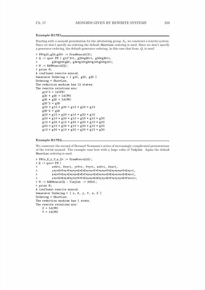
8/22/2019 Handbook Volume 01
http://slidepdf.com/reader/full/handbook-volume-01 375/440
Ch. 17 MONOIDS GIVEN BY REWRITE SYSTEMS 259
Example H17E1
Starting with a monoid presentation for the alternating group A4, we construct a rewrite system.
Since we don’t specify an ordering the default ShortLex ordering is used. Since we don’t specifya generator ordering, the default generator ordering, in this case that from Q, is used.
> FM<g10,g20,g30> := FreeMonoid(3);
> Q := quo< FM | g10^2=1, g20*g30=1, g30*g20=1,
> g20*g20=g30, g30*g10*g30=g10*g20*g10>;
> M := RWSMonoid(Q);
> print M;
A confluent rewrite monoid.
Generator Ordering = [ g10, g20, g30 ]
Ordering = ShortLex.
The reduction machine has 12 states.
The rewrite relations are:g10^2 = Id(FM)
g20 * g30 = Id(FM)
g30 * g20 = Id(FM)
g20^2 = g30
g30 * g10 * g30 = g10 * g20 * g10
g30^2 = g20
g20 * g10 * g20 = g10 * g30 * g10
g30 * g10 * g20 * g10 = g20 * g10 * g30
g10 * g20 * g10 * g30 = g30 * g10 * g20
g20 * g10 * g30 * g10 = g30 * g10 * g20
g10 * g30 * g10 * g20 = g20 * g10 * g30
Example H17E2
We construct the second of Bernard Neumann’s series of increasingly complicated presentationsof the trivial monoid. The example runs best with a large value of TidyInt. Again the defaultShortLex ordering is used.
> FM<x,X,y,Y,z,Z> := FreeMonoid(6);
> Q := quo< FM |
> x*X=1, X*x=1, y*Y=1, Y*y=1, z*Z=1, Z*z=1,
> y*y*X*Y*x*Y*z*y*Z*Z*X*y*x*Y*Y*z*z*Y*Z*y*z*z*Y*Z*y=1,
> z*z*Y*Z*y*Z*x*z*X*X*Y*z*y*Z*Z*x*x*Z*X*z*x*x*Z*X*z=1,> x*x*Z*X*z*X*y*x*Y*Y*Z*x*z*X*X*y*y*X*Y*x*y*y*X*Y*x=1>;
> M := RWSMonoid(Q : TidyInt := 3000);
> print M;
A confluent rewrite monoid.
Generator Ordering = [ x, X, y, Y, z, Z ]
Ordering = ShortLex.
The reduction machine has 1 state.
The rewrite relations are:
Z = Id(FM)
Y = Id(FM)
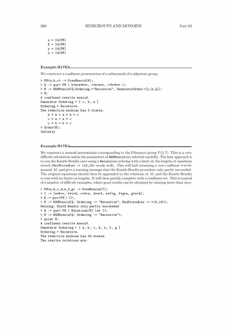
8/22/2019 Handbook Volume 01
http://slidepdf.com/reader/full/handbook-volume-01 376/440
260 SEMIGROUPS AND MONOIDS Part III
z = Id(FM)
X = Id(FM)
y = Id(FM)x = Id(FM)
Example H17E3
We construct a confluent presentation of a submonoid of a nilpotent group.
> FM<a,b,c> := FreeMonoid(6);
> Q := quo< FM | b*a=a*b*c, c*a=a*c, c*b=b*c >;
> M := RWSMonoid(Q:Ordering:="Recursive", GeneratorOrder:=[c,b,a]);
> M;
A confluent rewrite monoid.Generator Ordering = [ c, b, a ]
Ordering = Recursive.
The reduction machine has 3 states.
b * a = a * b * c
c * a = a * c
c * b = b * c
> Order(M);
Infinity
Example H17E4
We construct a monoid presentation corresponding to the Fibonacci group F (2, 7). This is a verydifficult calculation unless the parameters of RWSMonoid are selected carefully. The best approach isto run the Knuth-Bendix once using a Recursive ordering with a limit on the lengths of equationsstored (MaxStoredLen := <15,15> works well). This will halt returning a non-confluent rewritemonoid M , and give a warning message that the Knuth-Bendix procedure only partly succeeded.The original equations should then be appended to the relations of M , and the Knuth-Bendixre-run with no limits on lengths. It will then quickly complete with a confluent set. This is typicalof a number of difficult examples, where good results can be obtained by running more than once.
> FM<a,b,c,d,e,f,g> := FreeMonoid(7);
> I := [a*b=c, b*c=d, c*d=e, d*e=f, e*f=g, f*g=a, g*a=b];
> Q := quo<FM | I>;> M := RWSMonoid(Q: Ordering := "Recursive", MaxStoredLen := <15,15>);
Warning: Knuth Bendix only partly succeeded
> Q := quo< FM | Relations(M) cat I>;
> M := RWSMonoid(Q: Ordering := "Recursive");
> print M;
A confluent rewrite monoid.
Generator Ordering = [ a, b, c, d, e, f, g ]
Ordering = Recursive.
The reduction machine has 30 states.
The rewrite relations are:
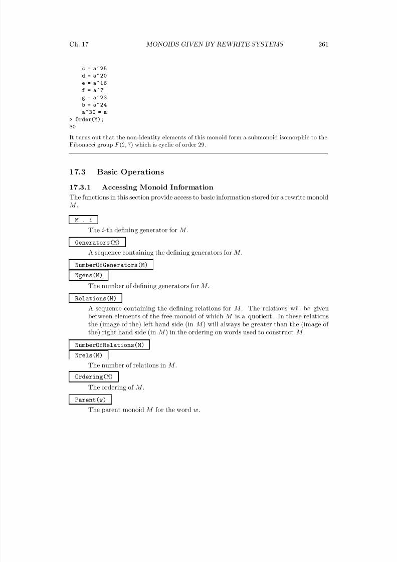
8/22/2019 Handbook Volume 01
http://slidepdf.com/reader/full/handbook-volume-01 377/440
Ch. 17 MONOIDS GIVEN BY REWRITE SYSTEMS 261
c = a^25
d = a^20
e = a^16f = a^7
g = a^23
b = a^24
a^30 = a
> Order(M);
30
It turns out that the non-identity elements of this monoid form a submonoid isomorphic to theFibonacci group F (2, 7) which is cyclic of order 29.
17.3 Basic Operations
17.3.1 Accessing Monoid Information
The functions in this section provide access to basic information stored for a rewrite monoidM .
M . i
The i-th defining generator for M .
Generators(M)
A sequence containing the defining generators for M .NumberOfGenerators(M)
Ngens(M)
The number of defining generators for M .
Relations(M)
A sequence containing the defining relations for M . The relations will be givenbetween elements of the free monoid of which M is a quotient. In these relationsthe (image of the) left hand side (in M ) will always be greater than the (image of the) right hand side (in M ) in the ordering on words used to construct M .
NumberOfRelations(M)
Nrels(M)
The number of relations in M .
Ordering(M)
The ordering of M .
Parent(w)
The parent monoid M for the word w.
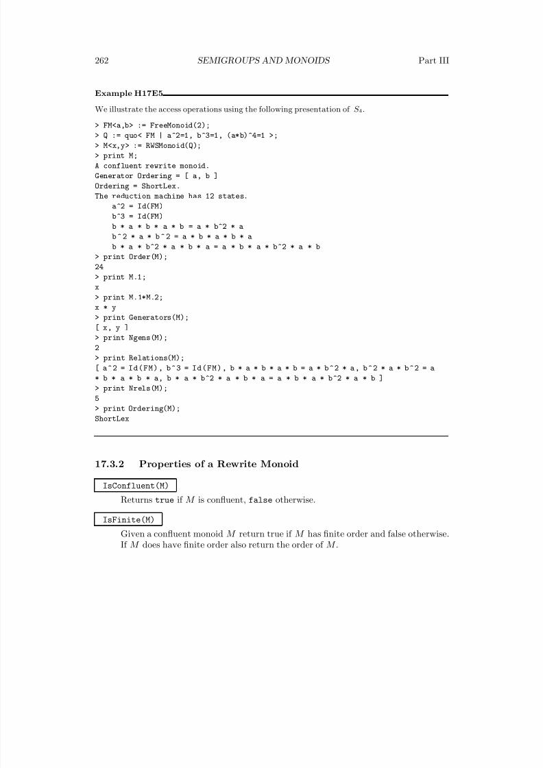
8/22/2019 Handbook Volume 01
http://slidepdf.com/reader/full/handbook-volume-01 378/440
262 SEMIGROUPS AND MONOIDS Part III
Example H17E5
We illustrate the access operations using the following presentation of S 4.
> FM<a,b> := FreeMonoid(2);
> Q := quo< FM | a^2=1, b^3=1, (a*b)^4=1 >;
> M<x,y> := RWSMonoid(Q);
> print M;
A confluent rewrite monoid.
Generator Ordering = [ a, b ]
Ordering = ShortLex.
The reduction machine has 12 states.
a^2 = Id(FM)
b^3 = Id(FM)
b * a * b * a * b = a * b^2 * a
b ^ 2 * a * b ^ 2 = a * b * a * b * a
b * a * b^2 * a * b * a = a * b * a * b^2 * a * b
> print Order(M);
24
> print M.1;
x
> print M.1*M.2;
x * y
> print Generators(M);
[ x, y ]
> print Ngens(M);
2> print Relations(M);
[ a^2 = Id(FM), b^3 = Id(FM), b * a * b * a * b = a * b^2 * a, b^2 * a * b^2 = a
* b * a * b * a, b * a * b^2 * a * b * a = a * b * a * b^2 * a * b ]
> print Nrels(M);
5
> print Ordering(M);
ShortLex
17.3.2 Properties of a Rewrite Monoid
IsConfluent(M)
Returns true if M is confluent, false otherwise.
IsFinite(M)
Given a confluent monoid M return true if M has finite order and false otherwise.If M does have finite order also return the order of M .
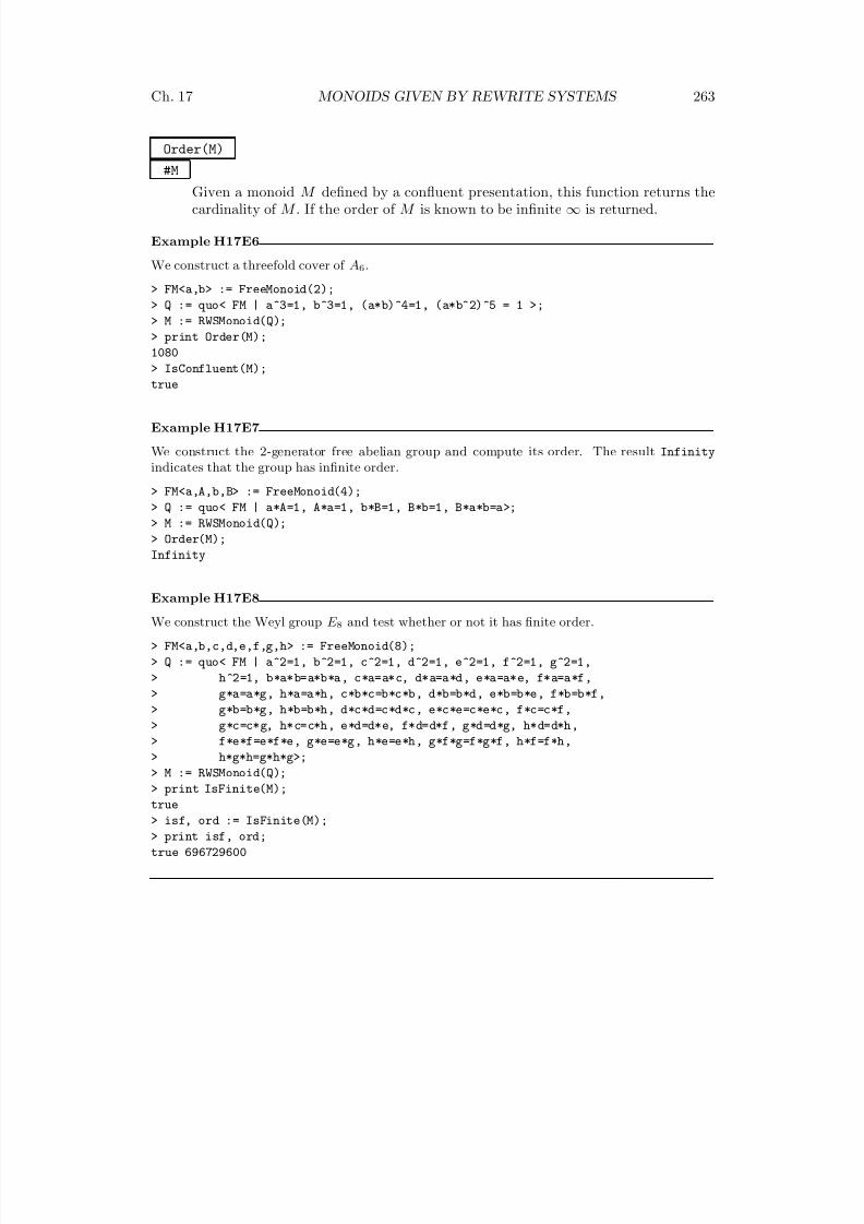
8/22/2019 Handbook Volume 01
http://slidepdf.com/reader/full/handbook-volume-01 379/440
Ch. 17 MONOIDS GIVEN BY REWRITE SYSTEMS 263
Order(M)
#M
Given a monoid M defined by a confluent presentation, this function returns thecardinality of M . If the order of M is known to be infinite ∞ is returned.
Example H17E6
We construct a threefold cover of A6.
> FM<a,b> := FreeMonoid(2);
> Q := quo< FM | a^3=1, b^3=1, (a*b)^4=1, (a*b^2)^5 = 1 >;
> M := RWSMonoid(Q);
> print Order(M);
1080
> IsConfluent(M);true
Example H17E7
We construct the 2-generator free abelian group and compute its order. The result Infinity
indicates that the group has infinite order.
> FM<a,A,b,B> := FreeMonoid(4);
> Q := quo< FM | a*A=1, A*a=1, b*B=1, B*b=1, B*a*b=a>;
> M := RWSMonoid(Q);
> Order(M);
Infinity
Example H17E8
We construct the Weyl group E 8 and test whether or not it has finite order.
> FM<a,b,c,d,e,f,g,h> := FreeMonoid(8);
> Q := quo< FM | a^2=1, b^2=1, c^2=1, d^2=1, e^2=1, f^2=1, g^2=1,
> h^2=1, b*a*b=a*b*a, c*a=a*c, d*a=a*d, e*a=a*e, f*a=a*f,
> g*a=a*g, h*a=a*h, c*b*c=b*c*b, d*b=b*d, e*b=b*e, f*b=b*f,
> g*b=b*g, h*b=b*h, d*c*d=c*d*c, e*c*e=c*e*c, f*c=c*f,
> g*c=c*g, h*c=c*h, e*d=d*e, f*d=d*f, g*d=d*g, h*d=d*h,
> f*e*f=e*f*e, g*e=e*g, h*e=e*h, g*f*g=f*g*f, h*f=f*h,> h*g*h=g*h*g>;
> M := RWSMonoid(Q);
> print IsFinite(M);
true
> isf, ord := IsFinite(M);
> print isf, ord;
true 696729600
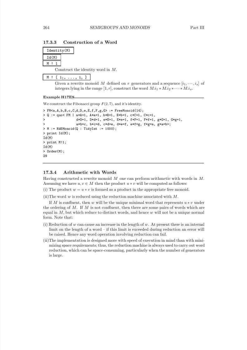
8/22/2019 Handbook Volume 01
http://slidepdf.com/reader/full/handbook-volume-01 380/440
264 SEMIGROUPS AND MONOIDS Part III
17.3.3 Construction of a Word
Identity(M)
Id(M)
M ! 1
Construct the identity word in M .
M ! [ i1, ..., is ]
Given a rewrite monoid M defined on r generators and a sequence [i1, · · · , is] of integers lying in the range [1, r], construct the word M.i1 ∗ M.i2 ∗ · · · ∗ M.is.
Example H17E9
We construct the Fibonacci group F (2, 7), and it’s identity.> FM<a,A,b,B,c,C,d,D,e,E,f,F,g,G> := FreeMonoid(14);
> Q := quo< FM | a*A=1, A*a=1, b*B=1, B*b=1, c*C=1, C*c=1,
> d*D=1, D*d=1, e*E=1, E*e=1, f*F=1, F*f=1, g*G=1, G*g=1,
> a*b=c, b*c=d, c*d=e, d*e=f, e*f=g, f*g=a, g*a=b>;
> M := RWSMonoid(Q : TidyInt := 1000);
> print Id(M);
Id(M)
> print M!1;
Id(M)
> Order(M);
29
17.3.4 Arithmetic with Words
Having constructed a rewrite monoid M one can perform arithmetic with words in M .Assuming we have u, v ∈ M then the product u ∗ v will be computed as follows:
(i) The product w = u ∗ v is formed as a product in the appropriate free monoid.
(ii)The word w is reduced using the reduction machine associated with M .
If M is confluent, then w will be the unique minimal word that represents u ∗ v underthe ordering of M . If M is not confluent, then there are some pairs of words which areequal in M , but which reduce to distinct words, and hence w will not be a unique normalform. Note that:
(i) Reduction of w can cause an increase in the length of w. At present there is an internallimit on the length of a word – if this limit is exceeded during reduction an error willbe raised. Hence any word operation involving reduction can fail.
(ii)The implementation is designed more with speed of execution in mind than with mini-mizing space requirements; thus, the reduction machine is always used to carry out wordreduction, which can be space-consuming, particularly when the number of generatorsis large.
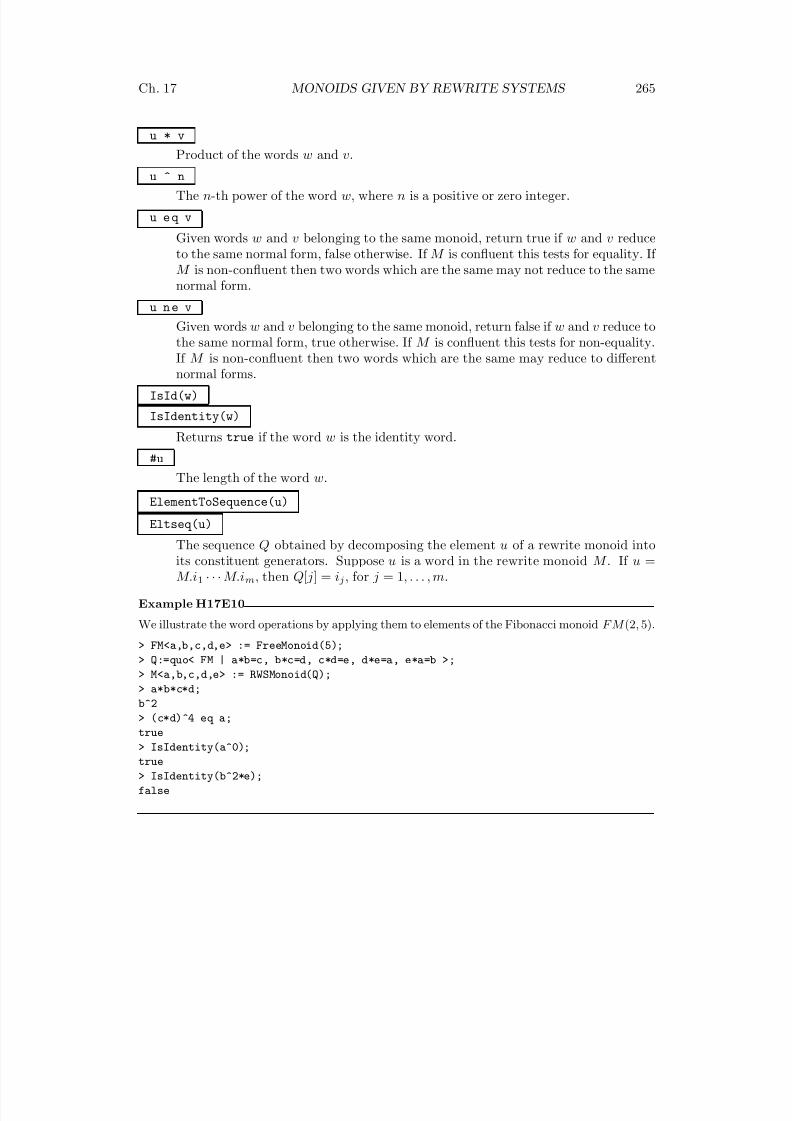
8/22/2019 Handbook Volume 01
http://slidepdf.com/reader/full/handbook-volume-01 381/440
Ch. 17 MONOIDS GIVEN BY REWRITE SYSTEMS 265
u * v
Product of the words w and v.
u ^ n
The n-th power of the word w, where n is a positive or zero integer.
u e q v
Given words w and v belonging to the same monoid, return true if w and v reduceto the same normal form, false otherwise. If M is confluent this tests for equality. If M is non-confluent then two words which are the same may not reduce to the samenormal form.
u n e v
Given words w and v belonging to the same monoid, return false if w and v reduce tothe same normal form, true otherwise. If M is confluent this tests for non-equality.If M is non-confluent then two words which are the same may reduce to differentnormal forms.
IsId(w)
IsIdentity(w)
Returns true if the word w is the identity word.
#u
The length of the word w.
ElementToSequence(u)Eltseq(u)
The sequence Q obtained by decomposing the element u of a rewrite monoid intoits constituent generators. Suppose u is a word in the rewrite monoid M . If u =M.i1 · · · M.im, then Q[ j] = ij , for j = 1, . . . , m.
Example H17E10
We illustrate the word operations by applying them to elements of the Fibonacci monoid F M (2, 5).
> FM<a,b,c,d,e> := FreeMonoid(5);
> Q:=quo< FM | a*b=c, b*c=d, c*d=e, d*e=a, e*a=b >;
> M<a,b,c,d,e> := RWSMonoid(Q);> a*b*c*d;
b^2
> (c*d)^4 eq a;
true
> IsIdentity(a^0);
true
> IsIdentity(b^2*e);
false
8/22/2019 Handbook Volume 01
http://slidepdf.com/reader/full/handbook-volume-01 382/440
266 SEMIGROUPS AND MONOIDS Part III
17.4 Homomorphisms
For a general description of homomorphisms, we refer to chapter 15. This section describes
some special aspects of homomorphisms whose domain is a rewrite monoid.
17.4.1 General remarks
Monoids in the category MonRWS currently are accepted as codomains only for monoidhomomorphisms, whose codomain is a rewrite monoid as well.
17.4.2 Construction of Homomorphisms
hom< M -> N | S >
Returns the homomorphism from the rewrite group M to the monoid N defined bythe expression S which must be the one of the following:
(i) A list, sequence or indexed set containing the images of the n generatorsM.1, . . . , M . n of M . Here, the i-th element of S is interpreted as the imageof M.i, i.e. the order of the elements in S is important.
(ii)A list, sequence, enumerated set or indexed set, containing n tuples < xi, yi > orarrow pairs xi −> yi, where xi is a generator of M and yi ∈ N (i = 1, . . . , n) andthe set {x1, . . . , xn} is the full set of generators of M . In this case, yi is assignedas the image of xi, hence the order of the elements in S is not important.It is the user’s responsibility to ensure that the provided generator images ac-
tually give rise to a well-defined homomorphism. No checking is performed by theconstructor. Presently, N must be either a rewrite monoid or a group, and it isnot possible to define a homomorphism by assigning images to the elements of anarbitrary generating set of M .
17.5 Set Operations
Random(M, n)
A random word of length at most n in the generators of M .
Random(M)
A random word (of length at most the order of M ) in the generators of M .
Representative(M)
Rep(M)
An element chosen from M .
8/22/2019 Handbook Volume 01
http://slidepdf.com/reader/full/handbook-volume-01 383/440
Ch. 17 MONOIDS GIVEN BY REWRITE SYSTEMS 267
Set(M, a, b)
Search MonStgElt Default : “DF S ”
Create the set of words, w, in M with a ≤ length(w) ≤ b. If Search is set to "DFS"
(depth-first search) then words are enumerated in lexicographical order. If Search
is set to "BFS" (breadth-first-search) then words are enumerated in lexicographi-cal order for each individual length (i.e. in short-lex order). Depth-first-search ismarginally quicker. Since the result is a set the words may not appear in the resul-tant set in the search order specified (although internally they will be enumeratedin this order).
Set(M)
Search MonStgElt Default : “DF S ”
Create the set of words that is the carrier set of M . If Search is set to "DFS" (depth-first search) then words are enumerated in lexicographical order. If Search is setto "BFS" (breadth-first-search) then words are enumerated in lexicographical orderfor each individual length (i.e. in short-lex order). Depth-first-search is marginallyquicker. Since the result is a set the words may not appear in the resultant set in thesearch order specified (although internally they will be enumerated in this order).
Seq(M, a, b)
Search MonStgElt Default : “DF S ”
Create the sequence S of words, w, in M with a ≤ length(w) ≤ b. If Search
is set to "DFS" (depth-first search) then words will appear in S in lexicographicalorder. If Search is set to "BFS" (breadth-first-search) then words will appear in S in lexicographical order for each individual length (i.e. in short-lex order). Depth-first-search is marginally quicker.
Seq(M)
Search MonStgElt Default : “DF S ”
Create a sequence S of words from the carrier set of M . If Search is set to "DFS"
(depth-first search) then words will appear in S in lexicographical order. If Search
is set to "BFS" (breadth-first-search) then words will appear in S in lexicographi-cal order for each individual length (i.e. in short-lex order). Depth-first-search ismarginally quicker.
Example H17E11
We construct the group D22, together with a representative word from the group, a random wordand a random word of length at most 5 from the group, and the set of elements of the group.
> FM<a,b,c,d,e,f> := FreeMonoid(6);
> Q := quo< FM | a^2=1, f^2=1,
> d*a=a*c, e*b=b*f, d*c=c*e, d*f=a*d, a*e=e*b, b*f*c=f >;
> M<a,b,c,d,e,f> := RWSMonoid(Q);
8/22/2019 Handbook Volume 01
http://slidepdf.com/reader/full/handbook-volume-01 384/440
268 SEMIGROUPS AND MONOIDS Part III
> print Order(M);
22
> print Representative(M);Id(M)
> print Random(M);
c * e
> print Random(M, 5);
d
> Set(M);
{ a * c , e , a * d , f , a * e , a * f , I d ( M ) , a * c * e , b * a ,
b * d , a * d * b , b * e , c * e , a * b * a , d * b , a * b * d ,
a , a * b * e , b , c , a * b , d }
> Seq(M : Search := "BFS");
[ Id(M), a, b, c, d, e, f, a * b, a * c, a * d, a * e, a * f,
b * a , b * d , b * e , c * e , d * b , a * b * a , a * b * d ,a * b * e, a * c * e, a * d * b ]
17.6 Conversion to a Finitely Presented Monoid
There is a standard way to convert a rewrite monoid into a finitely presented monoid usingthe function Relations. This is shown in the following example.
Example H17E12
We construct the Fibonacci monoid F M (2, 4) as a rewrite monoid, and then convert it into afinitely presented monoid.
> FM<a,b,c,d> := FreeMonoid(4);
> Q := quo< FM | a*b=c, b*c=d, c*d=a, d*a=b >;
> M := RWSMonoid(Q);
> Order(M);
11
> P<w,x,y,z> := quo < FM | Relations(M) >;
> P;
Finitely presented monoid
Relations
w * x = yx * y = z
y * z = w
z * w = x
y ^ 2 = w * z
z ^ 2 = x * w
z * y = x ^ 2
y * x = w ^ 2
x * w * z = x^2
w ^ 3 = w * z
x * w^2 = x * z
8/22/2019 Handbook Volume 01
http://slidepdf.com/reader/full/handbook-volume-01 385/440
Ch. 17 MONOIDS GIVEN BY REWRITE SYSTEMS 269
x ^ 2 * z = x
w ^ 2 * y = w
x ^ 3 = x * wx ^ 2 * w = z
z * x = x * z
y * w = w * y
w ^ 2 * z = y
x * w * y = x
17.7 Bibliography
[Hol97] Derek Holt. KBMAG – Knuth-Bendix in Monoids and Automatic Groups . Uni-
versity of Warwick, 1997.[Sim94] Charles C. Sims. Computation with finitely presented groups . Cambridge Uni-
versity Press, Cambridge, 1994.

8/22/2019 Handbook Volume 01
http://slidepdf.com/reader/full/handbook-volume-01 386/440
8/22/2019 Handbook Volume 01
http://slidepdf.com/reader/full/handbook-volume-01 387/440
INDEX OF INTRINSICS
!, 1-13 , 1-166 , 1-189 , 1-208 , 1-219 ,1-244, 1-264, 2-278 , 2-318 , 2-320 ,2-335, 336 , 2-348 , 2-445, 446 , 2-449 ,2-586 , 2-597 , 2-658 , 2-677 , 2-680 ,2-691, 3-778 , 3-789 , 3-803 , 3-986 ,3-994, 3-1033–1035 , 3-1086 , 3-1103,1104, 3-1116 , 3-1121, 3-1132 ,3-1134, 4-1161, 4-1177 , 4-1193 ,4-1233, 1234, 4-1250 , 4-1275 , 4-1307 ,4-1338 , 4-1434, 5-1479, 1480 , 5-1535 ,5-1561, 5-1572 , 5-1578 , 5-1643 ,
5-1665 , 5-1720–1722 , 5-1743 , 5-1749 ,5-1772 , 5-1805 , 5-1811, 5-1862 ,5-1895 , 5-1906 , 5-1925 , 6-1949 ,6-1963 , 6-1997 , 6-2069 , 6-2080 ,6-2101, 2102 , 6-2184, 2185 , 6-2218,2219 , 6-2230 , 6-2272 , 6-2289 ,7-2323 , 7-2337, 2338 , 7-2341, 7-2355 ,7-2359 , 7-2391, 2392 , 7-2549 , 7-2615 ,7-2651, 2652 , 7-2686 , 7-2702 , 7-2722 ,8-2824, 8-2835, 2836 , 8-2868 , 8-2879 ,8-2882 , 8-2970 , 8-2982 , 8-2998 ,8-3005 , 8-3019 , 8-3041, 9-3137 ,9-3275 , 9-3287, 3288 , 9-3318 , 9-3358 ,9-3409 , 9-3423 , 9-3446 , 9-3501,
9-3549 , 10-3652, 3653 , 10-3655,3656 , 10-3660, 3661, 10-3688, 3689 ,10-3696 , 10-3724, 3725 , 10-3796, 3797 ,10-3863, 3864, 10-3904, 3905 , 10-3974,10-4080 , 10-4094, 10-4139
!!, 2-348 , 5-1545 , 5-1733 , 9-3368 ∼, 10-3694( , ), 2-280 , 2-349 , 2-454, 2-677 , 3-805 ,
3-1088 , 3-1105 , 4-1436 , 6-1952 ,6-2093 , 10-3975 , 10-4081, 10-4095
( , , ), 2-280 , 2-349 , 2-454, 2-588 ,2-691, 3-805 , 3-988 , 3-1088 , 3-1105
(,), 7-2617 ( ), 1-219 , 1-237 , 3-808 , 3-821, 3-879 ,
3-1067 , 4-1450 , 6-1964, 7-2396 ,9-3135
*, 1-60 , 1-235 , 1-244, 1-265 , 2-280 ,2-348 , 2-350 , 2-409 , 2-454, 2-479 ,2-587 , 2-668 , 2-677 , 2-691, 3-779 ,3-805 , 3-878, 879 , 3-987 , 3-1046 ,3-1087 , 3-1105 , 3-1116 , 3-1133 ,3-1135 , 4-1161, 4-1165 , 4-1181,4-1195 , 4-1198 , 4-1210 , 4-1214,4-1237 , 4-1258 , 4-1279 , 4-1295 ,4-1309 , 4-1341, 4-1392 , 4-1418 ,4-1435 , 4-1450 , 5-1505 , 5-1536 ,5-1545 , 5-1553 , 5-1561, 5-1563 ,
5-1573 , 5-1581, 5-1620 , 5-1651,5-1667 , 5-1723 , 5-1732, 1733 , 5-1746 ,5-1749, 1750 , 5-1772 , 5-1779 , 5-1798 ,5-1806, 1807 , 5-1812 , 5-1865 , 5-1897 ,5-1908 , 5-1919 , 5-1928 , 6-1950 ,6-1964, 6-1977 , 6-1998 , 6-2004,6-2074, 2075 , 6-2111, 6-2142 , 6-2147 ,6-2185 , 6-2200 , 6-2219 , 6-2221, 2222 ,6-2233 , 6-2242 , 6-2247 , 6-2277 ,6-2292 , 7-2323 , 7-2357 , 7-2361,7-2394, 7-2549 , 7-2616 , 7-2627 ,
7-2654, 7-2665 , 7-2686 , 7-2702 ,7-2723 , 8-2754, 8-2810 , 8-2825 ,8-2836, 2837 , 8-2879 , 8-2907 , 8-2998 ,8-3011, 8-3017 , 8-3022 , 9-3139 ,9-3205 , 9-3253 , 9-3280 , 9-3292 ,9-3319 , 9-3361, 9-3409 , 9-3429 ,9-3450 , 9-3528 , 9-3550 , 9-3577 ,9-3619 , 10-3653 , 10-3656 , 10-3671,10-3693 , 10-3974, 10-4081, 10-4094,10-4141
*:=, 1-60 , 2-588 , 3-987 , 3-1046 , 4-1162 ,4-1181, 4-1195 , 4-1237 , 4-1258 ,4-1279 , 4-1309 , 4-1341, 5-1651,5-1667 , 5-1812 , 5-1897 , 6-1998 ,
6-2233 , 9-3139 , 9-3292 , 10-3693 +, 2-667 , 3-778 , 3-1135 , 4-1161, 4-1165 ,
4-1181, 4-1195 , 4-1198 , 4-1210 ,4-1214, 4-1237 , 4-1258 , 4-1279 ,4-1295 , 4-1309 , 4-1341, 4-1392 ,4-1435 , 4-1447 , 5-1476 , 5-1505 ,5-1553 , 5-1561, 5-1563 , 5-1651,5-1667 , 5-1688 , 5-1723 , 5-1733 ,5-1746 , 5-1750 , 5-1772 , 5-1779 ,5-1798 , 5-1806 , 5-1812 , 5-1865 ,5-1897 , 5-1908 , 5-1919 , 5-1928 ,6-1950 , 6-1955 , 6-1977 , 6-1997 ,6-2006 , 6-2075 , 6-2110 , 6-2142 ,6-2185 , 6-2217 , 6-2219 , 6-2222 ,
6-2233 , 6-2242 , 6-2247 , 6-2277 ,6-2292 , 7-2323 , 7-2326 , 7-2338 ,7-2361, 7-2394, 7-2492 , 7-2531,7-2665 , 7-2686 , 7-2702 , 7-2723 ,8-2754, 8-2810 , 8-2825 , 8-2827 ,8-2836 , 8-2840 , 8-2879 , 8-3011,8-3017 , 8-3022 , 9-3139 , 9-3251,9-3291, 9-3409 , 9-3429 , 9-3450 ,9-3528, 3529 , 9-3540 , 9-3552 , 9-3577 ,9-3586 , 10-3693 , 10-3730–3732 ,10-3808–3810 , 10-3845, 3846 , 10-3974,10-3980 , 10-4076 , 10-4081, 10-4094,10-4098 , 10-4141
8/22/2019 Handbook Volume 01
http://slidepdf.com/reader/full/handbook-volume-01 388/440
ii INDEX OF INTRINSICS
+:=, 4-1162 , 4-1181, 4-1195 , 4-1237 ,4-1258 , 4-1279 , 4-1309 , 4-1341,5-1651, 5-1667 , 5-1812 , 5-1897 ,6-1998 , 6-2233 , 9-3139 , 9-3291,10-3693 , 10-3731, 3732 , 10-3809, 3810 ,10-3846
-, 2-667, 668 , 3-778 , 4-1161, 4-1181,4-1195 , 4-1210 , 4-1214, 4-1237 ,4-1258 , 4-1279 , 4-1309 , 4-1341,4-1392 , 4-1435 , 5-1505 , 5-1561,5-1563 , 5-1651, 5-1667 , 5-1723 ,5-1746 , 5-1750 , 5-1772 , 5-1779 ,5-1806 , 5-1812 , 5-1865 , 5-1897 ,5-1908 , 5-1919 , 5-1928 , 6-1950 ,6-1997 , 6-2075 , 6-2110, 2111, 6-2185 ,6-2219 , 6-2233 , 6-2277 , 6-2292 ,7-2323 , 7-2361, 7-2394, 7-2665 ,7-2686 , 7-2702 , 7-2723 , 8-2825 ,8-2836 , 8-2879 , 8-3011, 8-3017 ,8-3022 , 9-3139 , 9-3277 , 9-3288 ,9-3291, 9-3319 , 9-3409 , 9-3429 ,9-3450 , 9-3529 , 9-3577 , 10-3693 ,10-3731, 10-3733 , 10-3809 , 10-3811,3812 , 10-3974, 10-4081, 10-4094,10-4141
-:=, 4-1162 , 4-1181, 4-1195 , 4-1237 ,4-1258 , 4-1279 , 4-1309 , 4-1341,5-1651, 5-1667 , 5-1812 , 5-1897 ,6-1998 , 6-2233 , 9-3139 , 9-3292 ,10-3693 , 10-3731, 10-3733 , 10-3809 ,10-3812
., 1-247 , 1-261, 2-295 , 2-338 , 2-449 ,2-577 , 2-666 , 2-678 , 2-691, 3-782 ,3-820 , 3-1000 , 3-1033, 1034, 3-1084,3-1100 , 3-1116 , 4-1250, 1251, 4-1275 ,4-1296 , 4-1307 , 4-1337 , 4-1445 ,5-1486 , 5-1507 , 5-1644, 5-1665 ,5-1720 , 5-1772 , 5-1796 , 5-1857 ,5-1895 , 5-1906 , 5-1919 , 5-1924,6-1947 , 6-1997 , 6-2071, 6-2104,6-2140 , 6-2185 , 6-2218 , 6-2230 ,6-2246 , 6-2272 , 6-2289 , 7-2319 ,7-2655 , 7-2702 , 7-2722 , 8-2809 ,8-2824, 8-2836 , 8-2864, 8-2874,8-2879 , 8-2998 , 9-3409 , 9-3423 ,
9-3446 , 9-3544, 9-3585 , 10-3652 ,10-3655 , 10-3687 , 10-3724, 3725 ,10-3863 , 10-3904, 3905 , 10-3970 ,10-4061, 10-4093
/, 1-249 , 2-280 , 2-288 , 2-348 , 2-374,2-454, 2-476 , 2-588 , 2-607 , 3-780 ,3-810 , 3-988 , 3-995 , 3-1046 , 3-1087 ,3-1105 , 4-1162 , 4-1165 , 4-1181,4-1195 , 4-1198 , 4-1210 , 4-1214,4-1233 , 4-1237 , 4-1258 , 4-1279 ,4-1309 , 4-1341, 4-1435 , 4-1442 ,5-1505 , 5-1553 , 5-1561, 5-1651,5-1667 , 5-1723 , 5-1733 , 5-1779 ,
5-1806 , 5-1812 , 5-1866 , 6-1950 ,6-1998 , 6-2004, 2005 , 6-2070 , 6-2075 ,6-2185 , 6-2219 , 6-2233 , 6-2242 ,6-2245 , 6-2277 , 7-2324, 7-2357 ,7-2394, 7-2653 , 8-2754, 8-2807 ,8-2827 , 8-2840 , 8-2879 , 8-3011,9-3139 , 9-3450 , 9-3541, 9-3555 ,9-3586 , 9-3620
/:=, 2-588 , 3-988 , 3-1046 , 4-1162 ,4-1181, 4-1195 , 4-1237 , 4-1341,9-3139
< >, 1-208 =, 1-246 , 3-779 , 3-807 @, 1-237 , 3-821, 3-879 , 3-1067 , 6-2296 ,
7-2396 , 8-2870 , 8-3000 , 8-3005 ,9-3281, 9-3524, 9-3581
@@, 1-237 , 3-822 , 3-1067 , 8-2913, 2914,8-3000 , 9-3281, 9-3524, 9-3581[. . .], 1-60, 61, 1-168 , 1-187, 188 , 1-190,
191, 1-208 , 1-210 , 1-214, 215 , 3-808 ,4-1385 , 4-1415 , 4-1439 , 5-1512 ,5-1535 , 6-1950 , 6-2082 , 6-2117 ,6-2235 , 7-2324, 7-2395, 2396 , 7-2666,2667 , 8-2869 , 8-2970 , 8-2983 ,9-3138 , 9-3277 , 9-3291, 9-3318 ,10-3916, 3917 , 10-3977 , 10-4096
[* *], 1-213 [], 3-779 , 3-807, 808 , 4-1384, 4-1415 ,
4-1438 , 5-1574, 6-1950 , 6-2082 ,6-2117 , 7-2324, 7-2362 , 7-2666, 2667 ,
8-2824, 8-2836 , 10-3653 , 10-4083 " ", 1-60 #, 1-11, 1-61, 1-168 , 1-190 , 1-208 ,
1-210 , 1-214, 1-220 , 1-244, 1-263 ,1-265 , 2-297 , 2-318 , 2-340 , 2-410 ,2-460 , 2-577 , 2-666 , 2-687 , 2-740 ,2-744, 2-755 , 2-757 , 2-765 , 3-785 ,3-803 , 3-827 , 3-879 , 3-1001, 3-1039 ,3-1061, 3-1085 , 3-1088 , 3-1102 ,3-1105 , 3-1116 , 4-1158 , 4-1194,4-1254, 4-1278 , 4-1308 , 5-1535 ,5-1859 , 5-1897 , 6-2044, 6-2060 ,6-2070 , 6-2231, 7-2337 , 7-2396 ,7-2654, 9-3133 , 9-3184, 9-3212 ,
9-3277 , 9-3294, 9-3589 , 10-3653 ,10-3656 , 10-3726 , 10-3870 , 10-3873 ,10-3912 , 10-3969 , 10-4061, 10-4093
#A, 9-3490 &, 1-181, 1-202 &*, 1-60 &cat, 1-60 &meet, 5-1536 &meet S, 4-1447 , 8-2755 \[. . .], 1-189 ^, 1-60 , 1-244, 1-265 , 2-280 , 2-302,
303 , 2-306 , 2-348 , 2-363 , 2-365 ,2-380 , 2-454, 2-471, 2-479 , 2-490 ,
8/22/2019 Handbook Volume 01
http://slidepdf.com/reader/full/handbook-volume-01 389/440
INDEX OF INTRINSICS iii
2-588 , 2-592 , 2-598, 599 , 2-677 ,2-691, 3-787 , 3-792 , 3-805 , 3-866,867 , 3-987, 988 , 3-1006 , 3-1046 ,3-1087, 1088 , 3-1105 , 3-1116 , 3-1133 ,4-1162 , 4-1181, 4-1195 , 4-1210 ,4-1214, 4-1237 , 4-1258 , 4-1279 ,4-1309 , 4-1341, 4-1392, 1393 , 5-1505 ,5-1553 , 5-1561, 5-1573 , 5-1651,5-1667 , 5-1723 , 5-1733 , 5-1772 ,5-1812 , 5-1866 , 5-1897 , 5-1908 ,5-1919 , 5-1928 , 6-1964, 6-2074, 2075 ,6-2111, 6-2142 , 6-2219 , 6-2233 ,6-2277 , 6-2292 , 7-2322 , 7-2347 ,7-2380 , 7-2394, 7-2396 , 7-2415 ,7-2549 , 7-2616 , 7-2627 , 7-2654,7-2702, 2703 , 7-2723 , 8-2754, 8-2810 ,8-2879 , 8-2998 , 9-3361, 9-3450 ,
9-3528 , 9-3550 , 10-3693 , 10-3736 ,10-3926 , 10-4027
^:=, 2-588 , 3-987, 988 , 3-1046 , 4-1162 ,4-1181, 4-1195 , 4-1237 , 4-1341
‘, 1-52 , 1-227 ‘‘, 1-227 { }, 1-159 , 1-164, 165 {* *}, 1-162, 163 {@ @}, 1-161A, 9-3556 AbelianBasis, 2-307 , 2-609 AbelianExtension, 5-1615, 1616 , 5-1618 AbelianGroup, 2-283 , 2-289 , 2-344,
2-572 , 2-614, 2-661, 3-781, 782 ,
3-816 , 3-996 , 3-999 , 9-3151, 9-3220 ,9-3300 , 9-3588
AbelianInvariants, 2-307 , 2-506 , 2-609 AbelianLieAlgebra, 7-2645 AbelianNormalQuotient, 2-408 AbelianNormalSubgroup, 2-408 AbelianpExtension, 5-1616 AbelianQuotient, 2-375 , 2-477 , 2-608 ,
3-782 , 3-833 , 3-1014AbelianQuotientInvariants, 2-608 , 3-833,
834, 3-1014AbelianSection, 3-968 AbelianSubgroups, 2-313 , 2-373 , 2-604Abs, 4-1183 , 4-1239 , 4-1288 , 4-1327 ,
4-1343 AbsoluteAffineAlgebra, 5-1655 AbsoluteAlgebra, 9-3197 AbsoluteBasis, 4-1235 , 5-1499 AbsoluteCharacteristicPolynomial, 5-1510 AbsoluteDegree, 4-1236 , 5-1495 , 5-1623 ,
5-1695 AbsoluteDiscriminant, 4-1236 , 5-1495 ,
5-1623 , 5-1696 AbsoluteField, 5-1487 AbsoluteGaloisGroup, 5-1627 AbsoluteInvariants, 9-3273 AbsoluteLogarithmicHeight, 5-1508
AbsolutelyIrreducibleConstituents, 7-2384AbsolutelyIrreducibleModule, 7-2328 AbsolutelyIrreducibleModules, 7-2381AbsolutelyIrreducibleModulesBurnside,
7-2383 AbsolutelyIrreducibleModulesInit, 7-2387 AbsolutelyIrreducibleModulesSchur, 2-627 ,
7-2385 AbsolutelyIrreducibleRepresentationProc-
essDelete, 7-2387 AbsolutelyIrreducibleRepresentationsInit,
7-2387 AbsolutelyIrreducibleRepresentationsSchur,
2-627 AbsoluteMinimalPolynomial, 5-1511AbsoluteModuleOverMinimalField, 7-2377
AbsoluteModulesOverMinimalField, 7-2377 AbsoluteNorm, 4-1260 , 5-1510 , 5-1547 AbsoluteOrder, 5-1487 , 5-1691AbsolutePolynomial, 5-1655 AbsolutePrecision, 5-1869 , 5-1909 , 5-1919 AbsoluteQuotientRing, 5-1655 AbsoluteRank, 7-2511AbsoluteRationalScroll, 8-2867 AbsoluteRepresentation, 2-489 AbsoluteRepresentationMatrix, 5-1511AbsoluteTotallyRamifiedExtension, 5-1855 AbsoluteTrace, 4-1260 , 5-1510 AbsoluteValue, 4-1183 , 4-1239 , 4-1288 ,
4-1327 , 4-1343 AbsoluteValues, 5-1508 Absolutize, 5-1655 ActingGroup, 2-717 , 7-2629 ActingWord, 2-413 Action, 2-378 , 2-385 , 3-879 , 6-2146 ,
7-2320 , 10-3774, 10-3885 , 10-3927 ActionGenerator, 6-2051, 6-2145 , 7-2320 ,
7-2374ActionGenerators, 7-2375 ActionGroup, 7-2375 ActionImage, 2-385 , 10-3775 , 10-3885 ,
10-3927 ActionKernel, 2-385 , 10-3775 , 10-3886 ,
10-3927 ActionMatrix, 7-2347 AddAttribute, 1-52 AddColumn, 4-1388 , 6-2119 AddConstraints, 10-4164AddCubics, 9-3168 , 9-3251AddEdge, 10-3732 , 10-3810, 3811, 10-3846 AddEdges, 10-3732, 3733 , 10-3811, 10-3846 AddGenerator, 1-250 , 3-912 , 5-1637 AdditiveCode, 10-4088, 4089 AdditiveCyclicCode, 10-4105 AdditiveGroup, 4-1179 , 4-1194, 4-1252 AdditiveHilbert90, 4-1260
8/22/2019 Handbook Volume 01
http://slidepdf.com/reader/full/handbook-volume-01 390/440
iv INDEX OF INTRINSICS
AdditiveOrder, 7-2491, 7-2527 , 7-2568 ,7-2623
AdditiveQuasiCyclicCode, 10-4106 AdditiveRepetitionCode, 10-4090 AdditiveUniverseCode, 10-4091AdditiveZeroCode, 10-4090 AdditiveZeroSumCode, 10-4091AddNormalizingGenerator, 2-430 AddPrimes, 3-959 AddRedundantGenerators, 3-1117 AddRelation, 1-250 , 3-912 , 5-1518 AddRelator, 3-920 AddRow, 4-1388 , 6-2119 AddSubgroupGenerator, 3-920 AddVertex, 10-3731, 10-3809 AddVertices, 10-3731, 10-3809 adj, 10-3741, 10-3817 AdjacencyMatrix, 6-2046 , 10-3755 Adjoin, 6-2217 Adjoint, 4-1400 , 6-2114, 6-2295 AdjointIdeal, 8-2979 AdjointIdealForNodalCurve, 8-2979 AdjointLinearSystem, 8-2980 AdjointLinearSystemForNodalCurve, 8-2979 AdjointLinearSystemFromIdeal, 8-2979 AdjointMatrix, 7-2666 AdjointRepresentation, 7-2637 , 7-2669 Adjoints, 8-2980 Advance, 2-734, 2-749 , 2-754, 2-763 AffineAction, 2-402 AffineAlgebra, 5-1650 , 8-2808
AffineAlgebraMapKernel, 8-2812 AffineDecomposition, 8-2896 , 8-2922 AffineGammaLinearGroup, 2-431AffineGeneralLinearGroup, 2-430 , 2-530 AffineImage, 2-402 AffineKernel, 2-402 AffinePatch, 8-2894, 8-2989 AffinePlane, 8-2969 AffineSigmaLinearGroup, 2-431AffineSpace, 8-2863, 2864, 8-2969 AffineSpecialLinearGroup, 2-431, 2-531AFRNumber, 8-3075 AGammaL, 2-431AGCode, 10-4036
AGDecode, 10-4039 AGDualCode, 10-4036 Agemo, 2-638 , 3-790 AGL, 2-430 AGM, 4-1368 AHom, 6-2150 , 7-2341aInvariants, 9-3128 , 9-3254Alarm, 1-83 Algebra, 4-1235 , 5-1493 , 6-1970 , 6-2068 ,
6-2079, 2080 , 6-2090 , 6-2146 , 6-2214,6-2221, 6-2248 , 7-2347 , 7-2358 ,7-2428 , 7-2651, 7-2721
AlgebraGenerators, 6-2131
AlgebraicClosure, 5-1642 AlgebraicGenerators, 7-2612 AlgebraicGeometricCode, 10-4036 AlgebraicGeometricDualCode, 10-4036 AlgebraMap, 8-2912 AlgebraStructure, 6-2131AlgorithmicFunctionField, 8-3009 AllCliques, 10-3760, 3761AllCompactChainMaps, 6-2166 AllDefiningPolynomials, 8-2912 Alldeg, 10-3743 , 10-3745 , 10-3818 ,
10-3820 AllExtensions, 5-1889 AllFaces, 5-1822 AllInformationSets, 10-3971AllInverseDefiningPolynomials, 8-2912
AllIrreduciblePolynomials, 4-1255 AllLinearRelations, 4-1350 AllPairsShortestPaths, 10-3831AllParallelClasses, 10-3878 AllParallelisms, 10-3878 AllPartitions, 2-389 AllPassants, 10-3921AllResolutions, 10-3877 AllRoots, 4-1261AllSecants, 10-3921AllSlopes, 5-1825 AllSolvableLieAlgebrasSLAC, 7-2680 AllSqrts, 4-1197 AllSquareRoots, 4-1197
AllTangents, 10-3921, 10-3923 AllVertices, 5-1822 AlmostSimpleGroupDatabase, 2-743 Alphabet, 10-3969 , 10-4061, 10-4091Alt, 2-289 , 2-344, 3-816 AlternantCode, 10-3999 AlternatingCharacter, 7-2408 AlternatingCharacterTable, 7-2408 AlternatingCharacterValue, 7-2408 AlternatingGroup, 2-289 , 2-344, 3-816 AlternatingSum, 4-1370 Ambient, 8-2940 AmbientModule, 9-3411AmbientSpace, 6-2001, 8-2875 , 8-2940 ,
8-2974, 10-3969 , 10-4061, 10-4092 AmbientVariety, 9-3589 AmbiguousForms, 5-1576 AModule, 6-2146 , 6-2165 AnalyticHomomorphisms, 9-3325 AnalyticInformation, 9-3236 AnalyticJacobian, 9-3321AnalyticRank, 9-3177 , 9-3235 And, 1-199 and, 1-11AnisotropicSubdatum, 7-2512 AntiAutomorphismTau, 7-2708 Antipode, 7-2707
8/22/2019 Handbook Volume 01
http://slidepdf.com/reader/full/handbook-volume-01 391/440
INDEX OF INTRINSICS v
AntisymmetricForms, 6-2052 AntisymmetricMatrix, 4-1380, 1381ApparentCodimension, 8-3063 , 8-3072 ApparentEquationDegrees, 8-3063 , 8-3072 ApparentSyzygyDegrees, 8-3063 , 8-3072 Append, 1-192 , 1-208, 209 , 1-213 Apply, 6-2296 ApplyTransformation, 9-3253 ApproximateByTorsionGroup, 9-3583 ApproximateByTorsionPoint, 9-3582 ApproximateOrder, 9-3578 ApproximateStabiliser, 2-483 AQInvariants, 2-608 , 3-833, 834, 3-1014Arccos, 4-1354, 5-1916 Arccosec, 4-1355 Arccot, 4-1355 Arcsec, 4-1355 Arcsin, 4-1354, 5-1915 Arctan, 4-1355 , 5-1916 Arctan2, 4-1355 AreCohomologous, 2-717 AreIdentical, 3-1050 Arg, 4-1341Argcosech, 4-1357 Argcosh, 4-1357 , 5-1916 Argcoth, 4-1358 Argsech, 4-1357 Argsinh, 4-1357 , 5-1916 Argtanh, 4-1357 , 5-1916 Argument, 4-1341ArithmeticGenus, 8-2889 , 8-2988
ArithmeticGeometricMean, 4-1368 Arrows, 8-3051ArtinMap, 5-1625 ArtinSchreierExtension, 5-1784ArtinSchreierImage, 5-1773 ArtinSchreierMap, 5-1773 ASigmaL, 2-431ASL, 2-431AssertAttribute, 2-357 , 2-426 , 2-468 ,
2-502 , 2-504, 4-1205 , 4-1248, 1249 ,5-1905 , 7-2397 , 8-2835
AssertEmbedding, 9-3506 AssignCapacities, 10-3800, 3801AssignCapacity, 10-3800
assigned, 1-6 , 1-52 , 1-227 AssignEdgeLabels, 10-3801AssignLabel, 10-3799, 3800 AssignLabels, 10-3799, 3800 AssignLDPCMatrix, 10-4044AssignNamePrefix, 5-1642 AssignNames, 1-9 , 4-1249 , 4-1275 , 4-1306 ,
4-1336 , 5-1486 , 5-1587 , 5-1664,5-1683 , 5-1743 , 5-1749 , 5-1859 ,5-1894, 5-1906 , 5-1919 , 5-1924,6-2176 , 6-2230 , 6-2271, 6-2288 ,8-2864, 8-2874, 8-2879 , 9-3360
AssignVertexLabels, 10-3799
AssignWeight, 10-3800 AssignWeights, 10-3800, 3801AssociatedEllipticCurve, 9-3158 , 9-3161AssociatedHyperellipticCurve, 9-3161AssociatedNewSpace, 9-3370 AssociativeAlgebra, 6-2068 , 6-2089, 2090 AtkinLehner, 9-3376 AtkinLehnerInvolution, 9-3345 AtkinLehnerOperator, 9-3415 , 9-3431,
9-3456 , 9-3595, 3596 AtkinModularPolynomial, 9-3339 ATLASGroup, 2-765 ATLASGroupNames, 2-765 Attach, 1-47 AttachSpec, 1-49 Augmentation, 7-2362
AugmentationIdeal, 7-2359 AugmentationMap, 7-2358 AugmentCode, 10-4003 , 10-4107 Aut, 1-238 , 8-2925 , 9-3279 , 10-3884,
10-4029 AutoCorrelation, 10-4154AutomaticGroup, 3-1096, 1097 Automorphism, 7-2626 , 8-2919 , 8-2922 ,
8-2925 , 8-2993 , 9-3109, 3110 , 9-3200 AutomorphismGroup, 2-413 , 2-496 , 2-623 ,
2-645 , 2-684, 2-686 , 4-1235 , 4-1254,5-1523, 1524, 5-1625 , 5-1704, 5-1708 ,5-1884, 6-2036 , 6-2038 , 7-2344,7-2626 , 8-2925 , 8-2997 , 9-3282 ,
10-3766 , 10-3882 , 10-3925 , 10-3950 ,10-4028 , 10-4108 , 10-4136
AutomorphismGroupStabilizer, 10-3883 ,10-4029
AutomorphismOmega, 7-2708 Automorphisms, 5-1522 , 5-1704, 5-1707,
1708 , 5-1884, 8-2997 AutomorphismSubgroup, 10-3883 , 10-4028 AutomorphismTalpha, 7-2708 AutomorphousClasses, 6-2044AuxiliaryLevel, 9-3426 BachBound, 5-1515 BadPlaces, 9-3187 , 9-3231
BadPrimes, 9-3099 , 9-3146 , 9-3307 BaerDerivation, 10-3932 BaerSubplane, 10-3932 Ball, 10-3754Bang, 1-235 BarAutomorphism, 7-2708 Base, 2-427 , 2-505 BaseChange, 6-2003 , 8-2892 , 8-2973 ,
9-3122, 3123 , 9-3265 , 9-3286 , 9-3317 BaseChangeMatrix, 6-2156 BaseComponent, 8-2941BaseCurve, 9-3344BaseElement, 3-1061
8/22/2019 Handbook Volume 01
http://slidepdf.com/reader/full/handbook-volume-01 392/440
vi INDEX OF INTRINSICS
BaseExtend, 6-2003 , 7-2611, 8-2892 ,9-3122, 3123 , 9-3265 , 9-3286 , 9-3317 ,9-3361, 9-3408 , 9-3445 , 9-3507 ,9-3536
BaseField, 4-1235 , 4-1247 , 4-1445 ,5-1486 , 5-1623 , 5-1649 , 5-1690, 1691,5-1772 , 5-1857 , 6-2187 , 6-2273 ,7-2482 , 8-2875 , 8-2974, 9-3093 ,9-3273 , 9-3285 , 9-3317 , 9-3322
BaseImage, 2-428 BaseImageWordStrip, 2-429 BaseModule, 6-2104, 7-2668 BaseMPolynomial, 4-1223 BasePoint, 2-427 , 2-505 BasePoints, 8-2916 , 8-2943 BaseRing, 2-449 , 3-1129 , 4-1277 , 4-1307 ,
4-1384, 4-1414, 5-1487 , 5-1623 ,5-1665 , 5-1690, 1691, 5-1772 , 5-1796 ,5-1857 , 5-1907 , 5-1918 , 5-1924,6-1947 , 6-2003 , 6-2070 , 6-2104,6-2140 , 6-2187 , 6-2214, 6-2231,6-2273 , 6-2290 , 7-2319 , 7-2482 ,7-2511, 7-2611, 7-2632 , 7-2654,8-2826 , 8-2839 , 8-2875 , 8-2974,9-3093 , 9-3131, 9-3133 , 9-3249 ,9-3273 , 9-3285 , 9-3317 , 9-3322 ,9-3410 , 9-3426 , 9-3487 , 10-3690
BaseScheme, 8-2916 , 8-2941BasicAlgebra, 6-2139, 2140 BasicDegrees, 7-2547 , 7-2562 , 7-2595 BasicOrbit, 2-427 , 2-505
BasicOrbitLength, 2-427 , 2-505 BasicOrbitLengths, 2-427 , 2-505 BasicOrbits, 2-427 BasicStabiliser, 2-427 , 2-505 BasicStabiliserChain, 2-427 , 2-505 BasicStabilizer, 2-427 , 2-505 BasicStabilizerChain, 2-427 , 2-505 Basis, 4-1235 , 4-1448 , 5-1498 , 5-1549 ,
5-1695 , 5-1739 , 5-1755 , 5-1800 ,5-1808 , 6-1953 , 6-2002 , 6-2071,6-2116 , 6-2141, 6-2187 , 6-2215 ,6-2222 , 6-2237 , 7-2347 , 7-2392 ,7-2655 , 8-2737 , 8-2840 , 8-3027 ,9-3233 , 9-3363 , 9-3410 , 9-3425 ,
9-3447 , 9-3544, 10-3970 , 10-4061,10-4093
BasisChange, 7-2519 BasisElement, 4-1448 , 6-2071, 6-2116 ,
6-2237 , 7-2655 , 8-2737 , 8-2840 BasisMatrix, 4-1448 , 5-1499 , 5-1549 ,
5-1695 , 5-1739 , 6-2002 , 6-2194,6-2222 , 7-2359 , 8-2840 , 10-3970 ,10-4093
BasisOfDifferentialsFirstKind, 5-1777 ,8-3010
BasisOfHolomorphicDifferentials, 5-1777 ,8-3010
BasisProduct, 6-2080 , 7-2652 BasisProducts, 6-2080 , 7-2652 BasisReduction, 6-2014Basket, 8-3069 , 8-3071BBSModulus, 10-4154BCHBound, 10-4017 BCHCode, 10-3998 BDLC, 10-4020 BDLCLowerBound, 10-4015 BDLCUpperBound, 10-4015 BerlekampMassey, 10-4151BernoulliApproximation, 4-1368 , 10-3644BernoulliNumber, 4-1368 , 10-3644BernoulliPolynomial, 4-1299 , 10-3644BesselFunction, 4-1366 BestApproximation, 4-1349
BestDimensionLinearCode, 10-4020 BestKnownLinearCode, 10-4019 BestKnownQuantumCode, 10-4133 BestLengthLinearCode, 10-4019 BestTranslation, 4-1225 BettiNumber, 9-3237 BettiNumbers, 8-3072 BFSTree, 10-3756 , 10-3825 Bicomponents, 10-3747 , 10-3821BigO, 5-1862 , 5-1907 BigPeriodMatrix, 9-3322 BinaryQuadraticForms, 5-1571BinaryResidueCode, 10-4066 BinaryString, 1-60
BinaryTorsionCode, 10-4066 Binomial, 4-1189 , 10-3643 bInvariants, 9-3129 , 9-3254BipartiteGraph, 10-3719 Bipartition, 10-3744, 10-3817 BiquadraticResidueSymbol, 5-1592 BitFlip, 10-4145 BKLC, 10-4019 BKLCLowerBound, 10-4015 BKLCUpperBound, 10-4015 BKQC, 10-4133 BLLC, 10-4019 BLLCLowerBound, 10-4015 BLLCUpperBound, 10-4015
Block, 10-3863 , 10-3874BlockDegree, 10-3871, 10-3873 BlockDegrees, 10-3871BlockGraph, 10-3739 , 10-3887 BlockGroup, 10-3883 BlockMatrix, 4-1390 Blocks, 2-514, 10-3870 BlocksAction, 2-389 BlockSet, 10-3863 BlocksImage, 2-389 , 2-514BlockSize, 10-3871, 10-3873 BlockSizes, 10-3871BlocksKernel, 2-389
8/22/2019 Handbook Volume 01
http://slidepdf.com/reader/full/handbook-volume-01 393/440
INDEX OF INTRINSICS vii
Blowup, 8-2985 BlumBlumShub, 10-4153 BlumBlumShubModulus, 10-4154BogomolovNumber, 8-3081Booleans, 1-11BorderedDoublyCirculantQRCode, 10-4001Borel, 10-3946 BorelSubgroup, 10-3946 Bottom, 2-318 , 5-1535 , 7-2337 BoundaryMap, 6-1971, 9-3374BoundaryMaps, 6-1971BoundedFSubspace, 9-3561BraidGroup, 3-816 , 3-1032 , 7-2552 BranchVertexPath, 10-3757 BrandtModule, 9-3407, 3408 , 9-3427 BrandtModuleDimension, 9-3416
BrauerClass, 9-3562 BravaisGroup, 6-2051BreadthFirstSearchTree, 10-3756 , 10-3825 Bruhat, 7-2617 BSGS, 2-423 , 2-503 BString, 1-60 BurauRepresentation, 3-1071BurnsideMatrix, 2-604CalabiYau, 8-3082 CalculateCanonicalClass, 8-3046 CalculateMultiplicities, 8-3046 CalculateTransverseIntersections, 8-3047 CalderbankShorSteaneCode, 10-4118 CambridgeMatrix, 6-2102
CanChangeRing, 9-3507 CanChangeUniverse, 1-173 , 1-196 CanContinueEnumeration, 3-923 CanDetermineIsomorphism, 9-3494CanIdentifyGroup, 2-735 CanonicalBasis, 7-2705 CanonicalClass, 8-3047 CanonicalDissidentPoints, 8-3070 CanonicalDivisor, 5-1749 , 8-3022 CanonicalElements, 7-2713 CanonicalFactorRepresentation, 3-1039 CanonicalGraph, 10-3770 CanonicalHeight, 9-3154, 9-3303 CanonicalImage, 8-3029
CanonicalInvolution, 9-3345 CanonicalLength, 3-1040 CanonicalLinearSystem, 8-2980 CanonicalLinearSystemFromIdeal, 8-2979 CanonicalMap, 8-3029 CanonicalModularPolynomial, 9-3340 CanRedoEnumeration, 3-923 CanteautChabaudsAttack, 10-4013 Capacities, 10-3802 Capacity, 10-3802 car, 1-207 CarmichaelLambda, 4-1187 CartanInteger, 7-2534
CartanMatrix, 6-2132 , 7-2455, 2456 ,7-2463 , 7-2481, 7-2510 , 7-2561,7-2594, 7-2613 , 8-3048
CartanName, 7-2466 , 7-2481, 7-2509 ,7-2546 , 7-2560 , 7-2593 , 7-2613 ,7-2655
CartanSubalgebra, 7-2661CartesianPower, 1-207 CartesianProduct, 1-207 , 10-3736 Cartier, 5-1782 , 8-3012 CartierRepresentation, 5-1782 , 8-3012 CasselsMap, 9-3190 cat, 1-60 , 1-197 , 1-213 , 10-4007 ,
10-4078 , 10-4108 cat:=, 1-60 , 1-213 Catalan, 4-1343 , 10-3643 Category, 1-28 , 1-168 , 4-1158 , 4-1160 ,
4-1179 , 4-1181, 4-1194, 1195 , 4-1234,4-1237 , 4-1252 , 4-1258 , 4-1277 ,4-1279 , 4-1307 , 4-1339, 1340 , 5-1485 ,5-1505 , 5-1575 , 5-1649 , 5-1651,5-1666 , 5-1690 , 5-1722 , 5-1733 ,5-1746 , 5-1812 , 5-1896 , 5-1898 ,5-1907, 1908 , 6-2001, 6-2231, 6-2272 ,6-2276 , 6-2290, 2291, 7-2393 , 9-3093 ,9-3131, 9-3133 , 9-3135 , 9-3138 ,9-3410 , 10-3690, 3691
CayleyGraph, 10-3737 Ceiling, 4-1184, 4-1239 , 4-1342 Center, 2-305 , 2-395 , 2-489 , 2-609 ,
3-790 , 3-1010 , 4-1158 , 4-1179 ,
4-1194, 5-1812 , 7-2660 CenterDensity, 6-2020 CenterPolynomials, 7-2618 CentralCollineationGroup, 10-3930 CentralEndomorphisms, 6-2056 CentralExtension, 2-630 CentralExtensionProcess, 2-630 CentralExtensions, 2-630 CentralIdempotents, 6-2095 Centraliser, 2-303 , 2-321, 2-364, 2-599 ,
3-788 , 3-1006, 1007 , 6-2091, 6-2093 ,7-2360 , 7-2362 , 7-2660
CentralisingMatrix, 2-516 Centralizer, 2-303 , 2-321, 2-364, 2-471,
2-599 , 3-788 , 3-1006, 1007 , 6-2091,6-2093 , 6-2110 , 7-2360 , 7-2362 ,7-2660
CentralizerOfNormalSubgroup, 2-364Centre, 2-305 , 2-395 , 2-489 , 2-609 ,
3-790 , 3-1010 , 4-1158 , 4-1252 ,5-1491, 5-1649 , 5-1896 , 6-2091,6-2110 , 7-2393 , 7-2660
CentredAffinePatch, 8-2896 CentreDensity, 6-2020 CentreOfEndomorphismRing, 6-2055 CentrePolynomials, 7-2618 CFP, 3-1039
8/22/2019 Handbook Volume 01
http://slidepdf.com/reader/full/handbook-volume-01 394/440
viii INDEX OF INTRINSICS
Chabauty, 9-3195 , 9-3312 Chabauty0, 9-3312 ChainMap, 6-1976 ChangeBase, 2-430 ChangeDerivation, 6-2280 , 6-2298 ChangeDirectory, 1-83 ChangeOfBasisMatrix, 2-500 ChangeOrder, 8-2768, 2769 ChangePrecision, 4-1342 , 5-1860 , 5-1869 ,
5-1907 , 5-1918 ChangeRepresentationType, 7-2359 ChangeRing, 2-448 , 4-1277 , 4-1308 ,
4-1392 , 4-1418 , 5-1924, 6-1948 ,6-2003 , 6-2071, 6-2110 , 6-2244,7-2322 , 7-2376 , 7-2611, 7-2655 ,8-2768 , 9-3122 , 9-3247 , 9-3265 ,9
-3507 ChangeSupport, 10-3718 , 10-3795 ChangeUniverse, 1-173 , 1-195 , 6-1948 ChangGraphs, 10-3740 CharacterDegrees, 2-323 , 2-626 , 2-637 CharacterDegreesPGroup, 2-637 Characteristic, 4-1158 , 4-1180 , 4-1194,
4-1236 , 4-1254, 4-1278 , 4-1308 ,4-1339 , 5-1495 , 5-1650 , 5-1666 ,5-1694, 5-1812 , 5-1859 , 5-1897 ,5-1907 , 6-2231, 7-2394
CharacteristicPolynomial, 2-458 , 4-1259 ,4-1399 , 5-1510 , 5-1725 , 6-2114,6-2186 , 6-2220 , 9-3531, 10-3740 ,
10-4151CharacteristicPolynomialFromTraces, 9-3237 CharacteristicSeries, 2-686 CharacteristicVector, 4-1434, 6-1949 CharacterRing, 7-2391CharacterTable, 2-323 , 2-417 , 2-499 ,
2-626 , 3-793 , 7-2392 CharacterTableConlon, 2-637 ChebyshevFirst, 4-1297 ChebyshevSecond, 4-1297 ChebyshevT, 4-1297 ChebyshevU, 4-1297 CheckCodimension, 8-3072 CheckFunctionalEquation, 9-3624
CheckPolynomial, 10-3973 ChevalleyBasis, 7-2657 ChevalleyGroup, 2-529 ChiefFactors, 2-398 , 2-493 ChiefSeries, 2-398 , 2-493 , 2-610 , 3-790 ChienChoyCode, 10-3999 ChineseRemainderTheorem, 4-1191, 4-1212 ,
4-1285 , 5-1556 Cholesky, 6-2034ChromaticIndex, 10-3757 ChromaticNumber, 10-3757 ChromaticPolynomial, 10-3757 cInvariants, 9-3129 , 9-3254
Class, 2-309 , 2-315 , 2-353 , 2-466 ,2-592 , 3-792
ClassCentraliser, 2-355 , 2-467 Classes, 2-309 , 2-353 , 2-466 , 2-593 ,
3-793 , 10-3779 ClassField, 5-1889 ClassFunctionSpace, 7-2391ClassGroup, 4-1179 , 4-1235 , 5-1514,
5-1576 , 5-1588 , 5-1715 , 5-1761,8-3025
ClassGroupAbelianInvariants, 5-1715 ,5-1762 , 8-3026
ClassGroupCyclicFactorGenerators, 5-1516 ClassGroupExactSequence, 5-1715 , 5-1763 ClassGroupGenerationBound, 5-1761ClassGroupPRank, 5-1716 , 5-1765 , 8-3026 ClassGroupStructure, 5-
1576 ClassicalForms, 2-539 ClassicalModularPolynomial, 9-3340 ClassicalPeriod, 9-3393 ClassicalSylow, 2-557 ClassicalSylowNormaliser, 2-557 ClassicalSylowToPC, 2-557 ClassicalType, 2-544ClassMap, 2-309 , 2-355 , 2-466 , 2-593 ,
3-793 ClassMatrix, 3-793 ClassNumber, 5-1515 , 5-1575 , 5-1589 ,
5-1715 , 5-1762 , 8-3025 ClassNumberApproximation, 5-1761
ClassNumberApproximationBound, 5-1761ClassPowerCharacter, 7-2396 ClassRepresentative, 2-310 , 2-355 , 2-467 ,
2-593 , 3-793 , 4-1191, 5-1556 ClassTwo, 2-646 ClearDenominator, 9-3532 ClearPrevious, 1-70 ClearVerbose, 1-94ClebschGraph, 10-3740 ClebschInvariants, 9-3271ClebschToIgusaClebsch, 9-3273 CliqueNumber, 10-3760 ClosestVectors, 6-2022 ClosestVectorsMatrix, 6-2022
CloseVectors, 6-2024CloseVectorsMatrix, 6-2025 CloseVectorsProcess, 6-2029 ClosureGraph, 10-3738 Cluster, 8-2871, 8-2886 cmpeq, 1-12 cmpne, 1-12 CMPoints, 9-3172 CMTwists, 9-3491CocycleMap, 2-718 CodeComplement, 10-4003 , 10-4107 CodeToString, 1-61Codimension, 8-2889 , 8-3071
8/22/2019 Handbook Volume 01
http://slidepdf.com/reader/full/handbook-volume-01 395/440
INDEX OF INTRINSICS ix
Codomain, 1-236 , 1-238 , 2-342 , 2-451,3-822 , 3-1067 , 4-1450 , 6-1964,6-2151, 7-2628 , 8-2911, 9-3281,9-3532 , 9-3543
Coefficient, 4-1280 , 4-1311, 5-1864,5-1875 , 5-1910 , 5-1929 , 6-2293 ,7-2362 , 9-3448 , 10-3695
CoefficientField, 4-1445 , 5-1486 , 5-1690,1691, 5-1857 , 7-2393 , 7-2414,8-2875 , 10-4091
CoefficientHeight, 5-1509 , 5-1547 CoefficientIdeals, 5-1807 CoefficientLength, 5-1509 , 5-1547 CoefficientMap, 8-2943 CoefficientRing, 2-449 , 4-1277 , 4-1307 ,
4-1384, 4-1414, 5-1487 , 5-1623 ,5-1665 , 5-1690, 1691, 5-1796 , 5-1857 ,5-1907 , 5-1918 , 5-1924, 6-1947 ,6-2003 , 6-2070 , 6-2104, 6-2140 ,6-2214, 6-2231, 6-2246 , 6-2290 ,7-2319 , 7-2347 , 7-2414, 7-2611,7-2632 , 7-2654, 7-2701, 7-2721,8-2809 , 8-2826 , 8-2839 , 8-2875 ,8-2974, 9-3131, 9-3133 , 9-3273 ,9-3285 , 9-3317 , 9-3322 , 10-3690
Coefficients, 4-1280 , 4-1310 , 5-1864,5-1909 , 5-1919 , 5-1929 , 6-2233 ,6-2293 , 7-2362 , 7-2703 , 7-2723 ,9-3128
CoefficientsNonSpiral, 5-1931CoefficientSpace, 8-2943
CoeffientField, 5-1623 Coercion, 1-235 CohomologicalDimension, 2-322 , 2-415 ,
2-704Cohomology, 2-718 CohomologyClass, 2-717 CohomologyElementToChainMap, 6-2167 CohomologyElementToCompactChainMap, 6-2167 CohomologyGeneratorToChainMap, 6-2160, 2161CohomologyGroup, 2-704CohomologyLeftModuleGenerators, 6-2160 CohomologyModule, 2-702 CohomologyRightModuleGenerators, 6-2160 CohomologyRing, 6-2167
CohomologyRingGenerators, 6-2159 CoisogenyGroup, 7-2514, 7-2561, 7-2595 ,
7-2614Cokernel, 4-1451, 6-1964, 6-1976 , 6-2151,
9-3525 , 9-3555 Collect, 3-940 CollectRelations, 3-938 CollineationGroup, 10-3925 CollineationGroupStabilizer, 10-3925 CollineationSubgroup, 10-3925 Colon, 6-2223 ColonIdeal, 5-1554, 5-1733 , 8-2755 Column, 10-3667
ColumnLength, 10-3668 Columns, 10-3667 ColumnSkewLength, 10-3667 ColumnSubmatrix, 4-1386, 1387 ColumnSubmatrixRange, 4-1387 ColumnWeight, 4-1415 ColumnWeights, 4-1415 ColumnWord, 10-3669 CommonEigenspaces, 6-2124CommonModularStructure, 9-3500 CommonOverfield, 4-1247 CommonZeros, 5-1727 , 8-3016 CommutatorIdeal, 6-2091, 6-2196 CommutatorModule, 6-2091CommutatorSubgroup, 2-303 , 2-364, 2-471,
2-599 , 2-609 , 3-787 , 3-1006
comp, 4-1167 , 5-1492 CompactInjectiveResolution, 6-2157 CompactPresentation, 2-621CompactProjectiveResolution, 6-2152 ,
6-2166 CompactProjectiveResolutionPGroup, 6-2166 CompanionMatrix, 4-1294, 6-2102 , 6-2304Complement, 4-1447 , 8-2943 , 9-3374,
9-3564, 10-3733 , 10-3865 ComplementaryDivisor, 5-1760 , 8-3025 ComplementaryErrorFunction, 4-1369 ComplementBasis, 2-602 ComplementOfImage, 9-3564Complements, 2-406 , 2-612 , 7-2334
Complete, 3-826 , 3-1062 CompleteClassGroup, 5-1518 CompleteDigraph, 10-3721CompleteGraph, 10-3720 CompleteKArc, 10-3920 CompleteTheSquare, 9-3246 CompleteUnion, 10-3736 CompleteWeightEnumerator, 10-3991,
10-4073 , 10-4103, 4104Completion, 4-1167 , 4-1233 , 5-1492, 1493 ,
5-1748 , 5-1886 , 6-2282 , 6-2298 Complex, 6-1969 ComplexConjugate, 4-1183 , 4-1238 , 4-1343 ,
5-1592 , 5-1600
ComplexEmbeddings, 9-3463 ComplexField, 4-1336, 1337 ComplexReflectionGroup, 7-2591ComplexToPolar, 4-1341ComplexValue, 3-1135 Component, 1-208 , 8-3046 , 10-3746, 3747 ,
10-3821, 3822 ComponentGroupOfIntersection, 9-3553 ComponentGroupOfKernel, 9-3522 ComponentGroupOrder, 9-3398 , 9-3604Components, 1-235 , 5-1622 , 8-2907 ,
10-3746 , 10-3821ComposeQuotients, 3-967
8/22/2019 Handbook Volume 01
http://slidepdf.com/reader/full/handbook-volume-01 396/440
x INDEX OF INTRINSICS
ComposeTransformations, 9-3253 Composite, 5-1855 CompositeFields, 5-1468 Composition, 5-1573 , 5-1709 , 5-1912 ,
7-2399 CompositionFactors, 2-307 , 2-399 , 2-492 ,
2-610 , 7-2329 CompositionSeries, 2-610 , 6-2072 , 7-2329 ,
7-2662 Comultiplication, 7-2707 ConcatenatedCode, 10-4007 CondensationMatrices, 6-2132 CondensedAlgebra, 6-2128 ConditionalClassGroup, 5-1515 ConditionedGroup, 2-616 Conductor, 4-1236 , 5-1498 , 5-1573 ,
5-1588 , 5-1600 , 5-1623 , 5-1770, 1771,
6-2194, 9-3146 , 9-3187 , 9-3206 ,9-3231, 9-3410 , 9-3490
ConductorRange, 9-3184ConformalHamiltonianLieAlgebra, 7-2650 ConformalSpecialLieAlgebra, 7-2649 CongruenceGroup, 9-3390 , 9-3465 CongruenceModulus, 9-3396 , 9-3571CongruenceSubgroup, 3-1127 Conic, 8-2972 , 9-3092 , 9-3105 , 10-3920 ConjecturalRegulator, 9-3178 ConjugacyClasses, 2-309 , 2-353 , 2-466 ,
2-593 , 3-793 , 7-2547 , 7-2561Conjugate, 2-302 , 2-363 , 2-471, 2-598 ,
3-787 , 3-866 , 3-1006 , 4-1183 ,
4-1238 , 5-1508 , 5-1573 , 5-1592, 1593 ,5-1601, 6-2185 , 6-2200 , 6-2218 ,10-3671
ConjugatePartition, 10-3666 Conjugates, 2-309 , 2-315 , 2-353 , 2-466 ,
2-592 , 3-792 , 5-1508 , 5-1653 Connect, 8-3046 ConnectedKernel, 9-3522 ConnectingHomomorphism, 6-1980 ConnectionNumber, 10-3874ConnectionPolynomial, 10-4151Consistency, 3-938 ConstaCyclicCode, 10-3996 ConstantField, 5-1690 , 6-2273
ConstantFieldExtension, 5-1693 , 6-2281,6-2298
ConstantMap, 8-2904ConstantRing, 6-2273 , 6-2290 ConstantWords, 10-3993 Constituent, 1-220 Constituents, 7-2330 ConstituentsWithMultiplicities, 7-2330 Constraint, 10-4165 Construction, 2-757, 758 ConstructionX, 10-4008 ConstructionX3, 10-4009 ConstructionX3u, 10-4009
ConstructionXChain, 10-4008 ConstructionXX, 10-4009 ConstructionY1, 10-4011ConstructTable, 7-2359 ContactLieAlgebra, 7-2650 ContainsQuadrangle, 10-3919 Content, 4-1287 , 4-1322 , 5-1548 , 5-1593 ,
6-2001, 10-3653 , 10-3656 , 10-3669 ContentAndPrimitivePart, 4-1287 , 4-1322 Contents, 5-1796 Continuations, 5-1885 ContinuedFraction, 4-1349 ContinueEnumeration, 3-923 Contpp, 4-1287 , 4-1322 Contract, 10-3734, 10-3813 Contraction, 10-3865
Contravariants, 9-3254ControlledNot, 10-4145 Convergents, 4-1349 Converse, 10-3739 , 10-3815 ConvertFromManinSymbol, 9-3358 ConvertToCWIFormat, 4-1223 Convolution, 5-1912 ConwayPolynomial, 4-1256 Coordelt, 6-1997 Coordinate, 8-2869 , 8-2983 CoordinateLattice, 6-1991CoordinateMatrix, 8-2745 CoordinateRing, 6-2003 , 8-2867 , 8-2876 ,
8-2970 , 8-2975
Coordinates, 4-1448 , 6-1953 , 6-1999 ,6-2083 , 6-2116 , 6-2186 , 7-2360 ,7-2667 , 8-2745 , 8-2837 , 8-2869 ,8-2970 , 8-2983 , 10-3917 , 10-3975 ,10-4081, 10-4095
CoordinateSpace, 6-2001CoordinatesToElement, 6-1997 CoordinateVector, 6-2000 cop, 1-219 Coppersmith, 4-1263 CoprimeBasis, 4-1208 CoprimeRepresentative, 5-1556 CordaroWagnerCode, 10-3966 Core, 2-303 , 2-365 , 2-471, 2-599 , 3-788 ,
3-867 , 3-1007 CoreflectionGroup, 7-2576 CoreflectionMatrices, 7-2487 , 7-2524,
7-2569 , 7-2601CoreflectionMatrix, 7-2487 , 7-2524,
7-2569 , 7-2601Coroot, 7-2485 , 7-2519 , 7-2566 , 7-2599 ,
7-2620 CorootAction, 7-2576 CorootGSet, 7-2576 CorootHeight, 7-2489 , 7-2526 , 7-2571,
7-2623 CorootLattice, 7-2517
8/22/2019 Handbook Volume 01
http://slidepdf.com/reader/full/handbook-volume-01 397/440
INDEX OF INTRINSICS xi
CorootNorm, 7-2490 , 7-2526 , 7-2571,7-2623
CorootNorms, 7-2489 , 7-2526 , 7-2571,7-2623
CorootPosition, 7-2485 , 7-2519 , 7-2566 ,7-2599 , 7-2620
Coroots, 7-2485 , 7-2518 , 7-2566 , 7-2599 ,7-2620
CorootSpace, 7-2484, 7-2517 , 7-2565 ,7-2598 , 7-2620
Correlation, 10-4068 CorrelationGroup, 10-3950 Cos, 4-1353 , 5-1915 Cosec, 4-1353, 1354Cosech, 4-1356 CosetAction, 2-293 , 2-302 , 2-393 , 2-487 ,
2-622 ,
3-886 ,
3-933 ,
3-1004CosetDistanceDistribution, 10-3995
CosetEnumerationProcess, 3-917 CosetGeometry, 10-3942 , 10-3947 CosetImage, 2-293 , 2-302 , 2-393 , 2-488 ,
2-622 , 3-886 , 3-934, 3-1005 CosetKernel, 2-293 , 2-302 , 2-393 , 2-488 ,
2-622 , 3-886 , 3-934, 3-1005 CosetLeaders, 10-3977 CosetRepresentatives, 3-1129 , 3-1137 CosetSatisfying, 3-884, 3-924CosetSpace, 3-878 , 3-934CosetsSatisfying, 3-884, 3-924CosetTable, 2-301, 2-410 , 2-494, 2-622 ,
3-876 , 3-925 , 3-1003 CosetTableToPermutationGroup, 3-876 CosetTableToRepresentation, 3-876 Cosh, 4-1356 , 5-1916 Cot, 4-1353 Coth, 4-1356 Counit, 7-2707 CountPGroups, 2-647 Covalence, 10-3871CoveringCovariants, 9-3254CoveringRadius, 6-2032 , 10-3995 CoveringStructure, 1-28 CoweightLattice, 7-2528 , 7-2572 , 7-2602 ,
7-2624
CoxeterDiagram, 7-2468 , 7-2481, 7-2509 ,7-2546 , 7-2560 , 7-2593 , 7-2613
CoxeterElement, 7-2550 , 7-2563 , 7-2595 ,7-2616
CoxeterForm, 7-2487 , 7-2523 , 7-2568 CoxeterGraph, 7-2453 , 7-2462 , 7-2481,
7-2510 , 7-2547 , 7-2561, 7-2594,7-2613
CoxeterGroup, 3-814, 3-816 , 7-2470 ,7-2494, 7-2538 , 7-2544–2546 , 7-2553,2554, 7-2557, 2558 , 7-2578 , 7-2604
CoxeterGroupFactoredOrder, 7-2452, 2453 ,7-2457 , 7-2459 , 7-2465
CoxeterGroupOrder, 7-2452, 2453 , 7-2457 ,7-2459 , 7-2465 , 7-2482 , 7-2513
CoxeterLength, 7-2549 , 7-2563 , 7-2602 CoxeterMatrix, 7-2452 , 7-2462 , 7-2481,
7-2510 , 7-2546 , 7-2561, 7-2594,7-2613
CoxeterNumber, 7-2550 , 7-2563 , 7-2595 Cputime, 1-26 CreateCharacterFile, 4-1219 CreateCycleFile, 4-1219 CreateK3Data, 8-3083 CremonaDatabase, 9-3183 CremonaReference, 9-3185 CriticalStrip, 9-3599 CrossCorrelation, 10-4155 CRT, 4-1212 , 4-1285 , 5-1556 CryptographicCurve, 9-3218 CrystalGraph, 7-2712 CSSCode, 10-4118 CubicFromPoint, 9-3247 Cunningham, 4-1204Current, 2-734, 2-749 , 2-754, 2-763 CurrentLabel, 2-734, 2-749 , 2-754, 2-763 Curve, 8-2876 , 8-2882, 2883 , 8-2971,
2972 , 8-2982, 2983 , 8-2999 , 8-3004,8-3010, 3011, 8-3014, 8-3017 , 8-3019 ,8-3067 , 9-3133 , 9-3135 , 9-3138 ,9-3249 , 9-3285 , 10-4039
CurveDifferential, 8-3009 CurveDivisor, 8-3009 CurvePlace, 8-3009
Curves, 8-3069 CuspidalSubgroup, 9-3592 CuspidalSubspace, 9-3373 , 9-3413 , 9-3424,
9-3454Cusps, 3-1131, 3-1137 CuspWidth, 3-1131CutVertices, 10-3747 , 10-3821Cycle, 2-380 , 3-1047 CycleCount, 4-1219 CycleDecomposition, 2-380 CycleStructure, 2-349 CyclicCode, 10-3967 , 10-3996 , 10-4059 CyclicGroup, 2-289 , 2-344, 2-572 , 3-817 ,
3-997
CyclicSubgroups, 2-314, 2-373 , 2-604CyclotomicAutomorphismGroup, 5-1600 CyclotomicFactors, 10-4059 CyclotomicField, 5-1597 CyclotomicOrder, 5-1600 CyclotomicPolynomial, 5-1598 CyclotomicRelativeField, 5-1600 D), 9-3288 Darstellungsgruppe, 3-818 Data, 2-736 DawsonIntegral, 4-1368 Decimation, 10-4155 Decode, 10-4024
8/22/2019 Handbook Volume 01
http://slidepdf.com/reader/full/handbook-volume-01 398/440
xii INDEX OF INTRINSICS
DecodingAttack, 10-4014DecomposeAutomorphism, 7-2627 DecomposeExteriorPower, 7-2671DecomposeSymmetricPower, 7-2671DecomposeTensorProduct, 7-2671DecomposeUsing, 9-3558 DecomposeVector, 4-1447 Decomposition, 4-1191, 4-1235 , 5-1513 ,
5-1555 , 5-1562, 1563 , 5-1737 , 5-1743 ,7-2399 , 8-3021, 9-3369 , 9-3413 ,9-3424, 9-3556
DecompositionField, 5-1525 , 5-1623, 1624DecompositionGroup, 5-1524, 5-1624DecompositionType, 5-1555 , 5-1624,
5-1737 , 5-1743 , 5-1771DecompositionTypeFrequency, 5-1624Decycle, 3-1048 DedekindEta, 4-1361DedekindTest, 4-1288 DeepHoles, 6-2032 DefinesAbelianSubvariety, 9-3485 DefinesHomomorphism, 3-826 DefiningConstantField, 5-1690 DefiningEquations, 9-3249 DefiningIdeal, 8-2876 , 8-2974, 9-3093 DefiningMap, 5-1856 DefiningPoints, 5-1820 DefiningPolynomial, 4-1236 , 4-1255 ,
5-1497 , 5-1695 , 5-1856 , 5-1918 ,8-2876 , 8-2974, 9-3093 , 9-3145 ,9-3275 , 9-3317
DefiningPolynomials, 5-1695 , 8-2876 ,8-2911
DefiningSubschemePolynomial, 9-3133 DefRing, 7-2632 DegeneracyMap, 9-3367 DegeneracyMatrix, 9-3367 Degree, 2-338 , 2-349 , 2-378 , 2-449 ,
2-456 , 4-1191, 4-1236 , 4-1254,4-1281, 4-1315 , 4-1445 , 5-1495 ,5-1535 , 5-1547 , 5-1564, 5-1623 ,5-1649 , 5-1668 , 5-1694, 5-1727 ,5-1742 , 5-1746 , 5-1754, 5-1796 ,5-1856 , 5-1897 , 5-1910 , 6-1976 ,6-2001, 6-2082 , 6-2104, 6-2214,
6-2294, 7-2397 , 7-2667 , 7-2703 ,7-2723 , 8-2826 , 8-2839 , 8-2886 ,8-2889 , 8-2941, 8-2975 , 8-2995 ,8-3018 , 8-3022 , 8-3050 , 8-3067 ,8-3071, 9-3204, 9-3249 , 9-3270 ,9-3411, 9-3426 , 9-3453 , 9-3532 ,9-3578 , 10-3695 , 10-3743 , 10-3745 ,10-3818 , 10-3820
Degree6DelPezzoType2 1, 8-2949 Degree6DelPezzoType2 2, 8-2949 Degree6DelPezzoType2 3, 8-2949 Degree6DelPezzoType3, 8-2949 Degree6DelPezzoType4, 8-2949
Degree6DelPezzoType6, 8-2949 DegreeMap, 9-3562 DegreeOfExactConstantField, 5-1696 , 5-1771DegreeOfFieldExtension, 2-516 DegreeOnePrimeIdeals, 5-1514DegreeRange, 10-3894DegreeReduction, 2-394Degrees, 6-1970 , 10-3894DegreeSequence, 10-3744, 10-3746 , 10-3819,
3820 DegreesOfCohomologyGenerators, 6-2160 Delaunay, 9-3331delete, 1-10 , 1-227 , 2-729 DeleteCapacities, 10-3803 DeleteCapacity, 10-3803 DeleteCollector, 3-958
DeleteData, 2-409 DeleteEdgeLabels, 10-3803 DeleteGenerator, 1-250 , 3-912 DeleteLabel, 10-3799 , 10-3803 DeleteLabels, 10-3800 , 10-3803 DeleteNonsplitCollector, 3-958 DeleteNonsplitSolutionspace, 3-961DeleteRelation, 1-250 , 3-912, 913 DeleteSplitCollector, 3-958 DeleteSplitSolutionspace, 3-961DeleteVertexLabels, 10-3800 DeleteWeight, 10-3803 DeleteWeights, 10-3803 DelsarteGoethalsCode, 10-4065
Delta, 4-1362, 1363 Denominator, 4-1179 , 4-1237 , 5-1506 ,
5-1546 , 5-1668 , 5-1726 , 5-1738 ,5-1754, 6-2222 , 8-2816 , 8-2879, 2880 ,8-3022 , 9-3532
Density, 4-1384, 4-1414, 6-2020 DensityEvolutionBinarySymmetric, 10-4049 DensityEvolutionGaussian, 10-4051Depth, 2-617 , 3-987 , 4-1435 , 6-1952 ,
7-2432 DepthFirstSearchTree, 10-3756 , 10-3825 Derivation, 6-2275 , 6-2290 Derivative, 4-1283 , 4-1317 , 5-1669 ,
5-1875 , 5-1911, 5-1933 , 6-2280
DerivedGroup, 2-306 , 2-394, 2-490 , 2-609 ,3-790 , 3-846 , 3-1011
DerivedLength, 2-305 , 2-394, 2-489 ,2-610 , 3-790 , 3-1010
DerivedSeries, 2-306 , 2-394, 2-490 ,2-610 , 3-790 , 3-1011, 7-2662
DerivedSubgroup, 2-306 , 2-394, 2-490 ,2-609 , 3-790 , 3-846 , 3-1011
Descendants, 2-639 DescentMaps, 9-3190 Design, 10-3860 , 10-3881, 10-3932 Detach, 1-47 DetachSpec, 1-49
8/22/2019 Handbook Volume 01
http://slidepdf.com/reader/full/handbook-volume-01 399/440
INDEX OF INTRINSICS xiii
Determinant, 2-458 , 4-1397 , 5-1796 ,6-2002 , 6-2043 , 6-2045 , 6-2113 ,8-3048
Development, 10-3869 DFSTree, 10-3756 , 10-3825 DiagonalAutomorphism, 7-2626 , 7-2669 DiagonalForm, 4-1319 Diagonalisation, 6-2125 Diagonalization, 6-2034, 6-2125 DiagonalJoin, 4-1391, 6-2118, 2119 DiagonalMatrix, 4-1379 , 6-2102 , 7-2652 DiagonalModel, 9-3247 DiagonalSum, 10-3671Diagram, 10-3952 DiagramAutomorphism, 7-2709 Diameter, 4-1344, 10-3753 , 10-3995 DiameterPath, 10-3753 DickmanRho, 4-1226 DicksonFirst, 4-1265 , 4-1298 DicksonSecond, 4-1265 , 4-1298 diff, 1-177 Difference, 8-2873 DifferenceSet, 10-3868 Different, 5-1498 , 5-1513 , 5-1560 ,
5-1698 , 5-1730 , 5-1739 DifferentDivisor, 5-1749 Differential, 5-1777 , 6-2275 , 6-2290 ,
8-3010 DifferentialBasis, 5-1760 , 5-1778 ,
8-3010 , 8-3028 DifferentialFieldExtension, 6-2283 DifferentialIdeal, 6-2286 DifferentialLaurentSeriesRing, 6-2271DifferentialOperator, 6-2312 DifferentialOperatorRing, 6-2288 DifferentialRing, 6-2270 DifferentialRingExtension, 6-2283 DifferentialSpace, 5-1692 , 5-1760 , 5-1777,
1778 , 8-3010 , 8-3028 Differentiation, 5-1730 DifferentiationSequence, 5-1730 Digraph, 10-3716 DihedralGroup, 2-289 , 2-344, 2-572 ,
3-817 , 3-997 Dilog, 4-1351
Dimension, 2-703 , 4-1445 , 4-1448 , 5-1754,5-1796 , 5-1808 , 6-2001, 6-2045 ,6-2070 , 6-2116 , 6-2141, 6-2146 ,6-2214, 6-2248 , 7-2338 , 7-2348 ,7-2482 , 7-2511, 7-2561, 7-2612 ,7-2654, 8-2772 , 8-2812 , 8-2889 ,8-2941, 8-3027 , 8-3065 , 8-3068 ,8-3071, 9-3285 , 9-3322 , 9-3411,9-3426 , 9-3453 , 9-3487 , 9-3512 ,9-3544, 10-3969 , 10-4092 , 10-4138
DimensionCuspForms, 9-3402 DimensionCuspFormsGamma0, 9-3401DimensionCuspFormsGamma1, 9-3401
DimensionNewCuspFormsGamma0, 9-3401DimensionNewCuspFormsGamma1, 9-3401DimensionOfCentreOfEndomorphismRing,
6-2056 DimensionOfEndomorphismRing, 6-2055 DimensionOfExactConstantField, 5-1696 DimensionOfFieldOfGeometricIrreducibility,
8-3006 DimensionOfHighestWeightModule, 7-2670 DimensionOfHomology, 6-1971DimensionsOfHomology, 6-1971DimensionsOfInjectiveModules, 6-2141DimensionsOfProjectiveModules, 6-2141DimensionsOfTerms, 6-1971DirectProduct, 1-249 , 2-291, 2-346 ,
2-452 , 2-581, 3-818 , 3-996 , 7-2625 ,
8-2866 , 8-2969 , 9-3550 , 10-4004,10-4078 , 10-4107 DirectSum, 3-782 , 6-1948 , 6-1971, 6-2006 ,
6-2081, 6-2107 , 6-2109 , 7-2322 ,7-2348 , 7-2377 , 7-2492 , 7-2531,7-2551, 7-2575 , 7-2659 , 9-3550 ,10-4004, 10-4077 , 10-4107 , 10-4131
DirectSumDecomposition, 7-2493 , 7-2532 ,7-2659 , 7-2673
DirichletCharacter, 9-3487 DirichletCharacters, 9-3453 , 9-3487 DirichletGroup, 9-3360 Disconnect, 8-3046 Discriminant, 4-1236 , 4-1293 , 4-1326 ,
5-1495 , 5-1572 , 5-1588 , 5-1593 ,5-1623 , 5-1696 , 5-1858 , 6-2187 ,6-2194, 6-2214, 9-3097 , 9-3129 ,9-3254, 9-3270 , 9-3410 , 9-3543
DiscriminantDivisor, 5-1771DiscriminantOfHeckeAlgebra, 9-3380 DisownChildren, 9-3353 Display, 3-939 DisplayBurnsideMatrix, 2-604DisplayFareySymbolDomain, 3-1140 DisplayPolygons, 3-1138 Distance, 4-1344, 5-1882 , 10-3753 ,
10-3830 , 10-3975 , 10-4081, 10-4095 DistanceMatrix, 10-3755
DistancePartition, 10-3754Distances, 10-3830 DistinctDegreeFactorization, 4-1293 DistinctExtensions, 2-711DistinguishedOrbitsPi, 7-2511div, 4-1181, 4-1279 , 4-1284, 4-1309 ,
4-1319 , 5-1505 , 5-1563 , 5-1723 ,5-1746 , 5-1750 , 5-1812 , 5-1866 ,5-1875 , 5-1898 , 5-1919 , 6-1998 ,6-2219 , 6-2233 , 6-2277 , 8-2837 ,8-3017 , 8-3022
div:=, 4-1181, 4-1309 , 6-2233 , 8-2837 DivideOutIntegers, 9-3518
8/22/2019 Handbook Volume 01
http://slidepdf.com/reader/full/handbook-volume-01 400/440
xiv INDEX OF INTRINSICS
DivisionPoints, 9-3139 DivisionPolynomial, 9-3145 Divisor, 5-1563 , 5-1727 , 5-1739 , 5-1749 ,
5-1780 , 8-3011, 8-3019–3021, 10-4039 DivisorGroup, 5-1562 , 5-1692 , 5-1745 ,
5-1748 , 8-3019 DivisorIdeal, 6-2246 , 8-2809 DivisorMap, 8-3028 DivisorOfDegreeOne, 5-1750 , 8-3008 Divisors, 4-1208 , 4-1210 , 5-1513 , 5-1556 DivisorSigma, 4-1187 Dodecacode, 10-4118 Domain, 1-236 , 1-238 , 2-342 , 2-450 ,
3-822 , 3-1067 , 4-1450 , 6-1964,6-2151, 7-2628 , 8-2911, 9-3281,9-3532 , 9-3543
DominantCharacter, 7-2670 DominantLSPath, 7-2711DominantWeight, 7-2529 , 7-2572 , 7-2603 ,
7-2624Double, 9-3319 DoubleCoset, 2-409 , 3-883 DoubleCosetRepresentatives, 2-409 DoubleCosets, 3-883 DoubleGenusOneModel, 9-3252 DoublyCirculantQRCode, 10-4001DoublyCirculantQRCodeGF4, 10-4001Dual, 3-795 , 5-1801, 6-1970 , 6-2006 ,
6-2156 , 7-2378 , 7-2493 , 7-2532 ,7-2575 , 7-2597 , 7-2625 , 9-3565 ,10-3865 , 10-3911, 10-3970 , 10-3980 ,
10-4076 , 10-4093 , 10-4098 DualAtkinLehner, 9-3377 DualBasisLattice, 6-2006 DualCoxeterForm, 7-2487 , 7-2523 , 7-2568 DualEuclideanWeightDistribution, 10-4072 DualHeckeOperator, 9-3376 DualIsogeny, 9-3203 DualLeeWeightDistribution, 10-4071DualMorphism, 7-2533 DualQuotient, 6-2006 DualStarInvolution, 9-3377 DualVectorSpace, 9-3366 DualWeightDistribution, 10-3989 , 10-4070 ,
10-4103
DuvalPuiseuxExpansion, 5-1833 DynkinDiagram, 7-2467 , 7-2481, 7-2509 ,
7-2560 , 7-2593 , 7-2613 DynkinDigraph, 7-2459 , 7-2463 , 7-2481,
7-2510 , 7-2561, 7-2594, 7-2613 E, 4-1337 e, 4-1337 E . i, 10-3797 Ealpha, 7-2710, 2711EARNS, 2-401EasyIdeal, 8-2744EchelonForm, 4-1400 , 6-2119 EcheloniseWord, 3-940
ECM, 4-1206 ECMFactoredOrder, 4-1208 ECMOrder, 4-1208 ECMSteps, 4-1207 EdgeCapacities, 10-3803 EdgeConnectivity, 10-3751, 10-3824EdgeDeterminant, 8-3050 EdgeGroup, 10-3770 EdgeIndices, 10-3796 EdgeLabels, 8-3050 , 10-3803 EdgeMultiplicity, 10-3796 Edges, 10-3724, 10-3796 EdgeSeparator, 10-3751, 10-3824EdgeSet, 10-3724EdgeUnion, 10-3736 , 10-3814EdgeWeights, 10-3803
EFAModuleMaps, 3-1015 EFAModules, 3-1016 EFASeries, 3-1011EffectiveSubcanonicalCurves, 8-3074Eigenspace, 4-1400 , 6-2115 , 8-3065 Eigenvalues, 4-1400 , 6-2115 Eisenstein, 4-1358, 1359 , 5-1579 EisensteinData, 9-3458 EisensteinSeries, 9-3458 EisensteinSubspace, 9-3373 , 9-3413 ,
9-3424, 9-3454Element, 9-3582 ElementaryAbelianGroup, 3-997 ElementaryAbelianNormalSubgroup, 2-408
ElementaryAbelianQuotient, 2-375 , 2-477 ,2-608 , 3-784, 3-833 , 3-1014
ElementaryAbelianSection, 3-968 ElementaryAbelianSeries, 2-405 , 2-492 ,
2-610 , 3-790 ElementaryAbelianSeriesCanonical, 2-405 ,
2-492 , 2-610 ElementaryAbelianSubgroups, 2-313 , 2-373 ,
2-604ElementaryDivisors, 4-1405 , 4-1419 ,
5-1801, 6-2120 ElementarySymmetricPolynomial, 4-1327 ,
8-2799 ElementaryToHomogeneousMatrix, 10-3706
ElementaryToMonomialMatrix, 10-3705 ElementaryToPowerSumMatrix, 10-3706 ElementaryToSchurMatrix, 10-3705 Elements, 3-1061, 9-3360 , 9-3585 ,
10-3945 ElementSequence, 2-630 ElementSet, 2-350 ElementToSequence, 1-61, 1-251, 1-265 ,
2-336 , 2-446 , 2-586 , 2-659 , 3-778 ,3-803 , 3-986 , 3-1039 , 3-1088 ,3-1106 , 4-1210 , 4-1240 , 4-1252 ,4-1280 , 4-1384, 4-1435 , 5-1512 ,5-1562 , 5-1574, 5-1722 , 5-1807 ,
8/22/2019 Handbook Volume 01
http://slidepdf.com/reader/full/handbook-volume-01 401/440
INDEX OF INTRINSICS xv
5-1864, 5-1895 , 5-1909 , 5-1919 ,6-1950 , 6-1999 , 6-2082 , 6-2117 ,6-2186 , 6-2220 , 7-2323 , 7-2362 ,7-2667 , 9-3128 , 9-3138 , 9-3277 ,9-3291, 9-3318 , 10-3653 , 10-3917
ElementType, 1-28 EliasAsymptoticBound, 10-4017 EliasBound, 10-4016 Eliminate, 1-251, 3-892 , 3-914EliminateGenerators, 3-892 EliminateRedundancy, 3-939 Elimination, 8-2906 EliminationIdeal, 8-2762 EllipticCurve, 8-2991, 9-3118–3120 ,
9-3184, 9-3467 , 9-3606 EllipticCurveDatabase, 9-3183 EllipticCurveFromjInvariant, 9-3118 EllipticCurves, 9-3186 EllipticCurveWithjInvariant, 9-3118 EllipticExponential, 9-3176 EllipticInvariants, 9-3607 EllipticLogarithm, 9-3176 EllipticPeriods, 9-3607 EllipticPoints, 3-1131elt, 1-208 , 2-278 , 2-335 , 2-445 , 4-1176,
1177 , 4-1193 , 4-1234, 4-1250 ,4-1275 , 4-1307 , 4-1337, 1338 , 4-1433 ,5-1479, 1480 , 5-1572 , 5-1665 , 5-1720,1721, 5-1862 , 5-1906 , 5-1926 ,6-1949 , 6-1997 , 6-2080 , 6-2101,6-2230 , 7-2322 , 7-2355 , 7-2391,
7-2615 , 7-2652 , 9-3275 , 9-3287, 3288 ,10-3974, 10-4080 , 10-4094
elt< >, 9-3137 Eltlist, 7-2616 Eltseq, 1-61, 1-192 , 1-251, 1-265 ,
2-336 , 2-446 , 2-586 , 2-659 , 3-778 ,3-803 , 3-986 , 3-1039 , 3-1088 ,3-1106 , 3-1133 , 4-1179 , 4-1210 ,4-1240 , 4-1252 , 4-1280 , 4-1384,4-1435 , 5-1512 , 5-1562 , 5-1574,5-1722 , 5-1772 , 5-1807 , 5-1864,5-1895 , 5-1909 , 5-1919 , 6-1950 ,6-1999 , 6-2082 , 6-2117 , 6-2186 ,6-2220 , 6-2278 , 6-2293 , 7-2323 ,
7-2362 , 7-2667 , 8-2824, 8-2836 ,9-3128 , 9-3138 , 9-3249 , 9-3277 ,9-3291, 9-3318 , 9-3409 , 9-3426 ,9-3453 , 9-3526 , 9-3582 , 10-3653 ,10-3917
Embed, 4-1248 , 5-1491, 6-2190, 2191,6-2218
Embedding, 10-3764, 10-3826 EmbeddingMap, 5-1491, 5-1535 EmbeddingMatrix, 6-2194Embeddings, 9-3505 EmbeddingSpace, 5-1796 EmbedPlaneCurveInP3, 8-2933
EmptyBasket, 8-3069 EmptyDigraph, 10-3721EmptyGraph, 10-
3720 EmptySubscheme, 8-2872 End, 9-3536 EndomorphismAlgebra, 6-1959 , 7-2344EndomorphismRing, 6-2055 , 9-3326 Endomorphisms, 6-2055 EndpointWeight, 7-2711EndVertices, 5-1823 , 10-3727 , 10-3797 Enumerate, 6-2202 , 6-2218 eq, 1-11, 1-62 , 1-175, 176 , 1-200 , 1-210 ,
1-245 , 1-265 , 2-280 , 2-298 , 2-320 ,2-349 , 2-362 , 2-410 , 2-456 , 2-461,2-589 , 2-598 , 2-671, 672 , 2-678 ,2-691, 3-783 , 3-786 , 3-806 , 3-872 ,3-879 , 3-988 , 3-1002 , 3-1050 ,3-1088 , 3-1105 , 3-1119 , 3-1128 ,3-1132 , 3-1135 , 4-1160 , 4-1162 ,4-1166 , 4-1180, 1181, 4-1195 , 4-1198 ,4-1214, 4-1236, 1237 , 4-1256 , 4-1258 ,4-1278, 1279 , 4-1296 , 4-1308, 1309 ,4-1339, 1340 , 4-1415 , 4-1446 , 5-1502 ,5-1506 , 5-1536 , 5-1551, 5-1553 ,5-1561, 1562 , 5-1574, 5-1620 , 5-1650 ,5-1652 , 5-1666, 1667 , 5-1718 , 5-1723 ,5-1735 , 5-1746 , 5-1750, 1751, 5-1772 ,5-1779 , 5-1798 , 5-1807, 1808 , 5-1812 ,5-1860 , 5-1867 , 5-1897, 1898 , 5-1908 ,5-1919 , 5-1924, 5-1932 , 6-1954,6-1999 , 6-2002 , 6-2044, 2045 , 6-2074,6-2076 , 6-2112 , 6-2117 , 6-2185 ,6-2217 , 6-2220 , 6-2223 , 6-2233 ,6-2243 , 6-2247 , 6-2275 , 6-2277 ,6-2291, 6-2293 , 7-2326 , 7-2338 ,7-2394, 2395 , 7-2480 , 7-2508 , 7-2549 ,7-2611, 7-2654, 7-2711, 8-2756 ,8-2809 , 8-2825 , 8-2827 , 8-2837 ,8-2840 , 8-2865 , 8-2877 , 8-2879 ,8-2882 , 8-2912 , 8-2940 , 8-2983 ,8-2988 , 8-2998 , 8-3011, 8-3014,8-3017 , 8-3019 , 8-3023 , 8-3041,8-3049 , 8-3065 , 8-3068 , 8-3072 ,
9-3131, 9-3133 , 9-3136 , 9-3143 ,9-3148 , 9-3205 , 9-3277 , 9-3281,9-3291, 9-3318 , 9-3409 , 9-3428 ,9-3499 , 9-3535 , 9-3548 , 9-3579 ,9-3591, 10-3653 , 10-3656 , 10-3671,10-3691, 10-3694, 10-3726 , 10-3742 ,10-3797 , 10-3817 , 10-3881, 10-3913 ,10-3915, 3916 , 10-3976 , 10-3982 ,10-4083 , 10-4096 , 10-4099 , 10-4138 ,10-4141
EqualDegreeFactorization, 4-1293 Equality, 5-1709 EqualizeDegrees, 6-1973
8/22/2019 Handbook Volume 01
http://slidepdf.com/reader/full/handbook-volume-01 402/440
xvi INDEX OF INTRINSICS
EquationOrder, 5-1471, 1472 , 5-1586 ,5-1622 , 5-1685
EquationOrderFinite, 5-1685 EquationOrderInfinite, 5-1685 Equations, 9-3249 EquidimensionalDecomposition, 8-2782 EquidimensionalPart, 8-2782 EquitablePartition, 10-3754EquivalentPoint, 3-1136 EquivalentQuotients, 3-964Erf, 4-1368 Erfc, 4-1369 Error, 1-19 ErrorFunction, 4-1368 EstimateOrbit, 2-482 Eta, 7-2355 EuclideanDistance, 10-4072 EuclideanLeftDivision, 6-2300 EuclideanNorm, 4-1183 , 4-1285 , 5-1813 EuclideanRightDivision, 6-2300 EuclideanWeight, 10-4072 EuclideanWeightDistribution, 10-4072 EuclideanWeightEnumerator, 10-4074EulerCharacteristic, 8-3051EulerFactor, 9-3298 EulerFactorModChar, 9-3298 EulerFactorsByDeformation, 9-3299 EulerGamma, 4-1343 EulerianNumber, 10-3644EulerPhi, 4-1187 EulerPhiInverse, 4-1188
EulerProduct, 5-1518 Evaluate, 3-1117 , 4-1284, 4-1318 , 5-1542 ,
5-1564, 5-1668 , 5-1726 , 5-1747 ,5-1875 , 5-1911, 5-1933 , 6-2236 ,8-2870 , 8-3005 , 8-3018 , 9-3281,9-3361, 9-3518 , 9-3601, 9-3617
EvaluateAt, 10-4164EvaluateByPowerSeries, 8-2994EvaluateClassGroup, 5-1518 EvaluatePolynomial, 9-3275 EvenWeightCode, 10-3966 ExactConstantField, 5-1690 , 6-2273 ExactExtension, 6-1973 ExactQuotient, 4-1181, 4-1284, 4-1319
ExactValue, 3-1135 ExceptionalUnitOrbit, 5-1522 ExceptionalUnits, 5-1522 Exclude, 1-172 , 1-192 ExcludedConjugate, 3-925 ExcludedConjugates, 3-880 , 3-925 ExistsConwayPolynomial, 4-1256 ExistsCosetSatisfying, 3-926 ExistsCoveringStructure, 1-29 ExistsExcludedConjugate, 3-926 ExistsGroupData, 2-744ExistsModularCurveDatabase, 9-3340 ExistsNormalisingCoset, 3-926
ExistsNormalizingCoset, 3-926 Exp, 4-1350, 1351, 5-1871, 5-1914Expand, 5-1727 , 5-1869 , 8-2909 , 8-3005 ExpandToPrecision, 5-1828 ExplicitCoset, 3-879 Explode, 1-192 , 1-210 Exponent, 2-310 , 2-356 , 2-468 , 2-577 ,
3-785 , 9-3589 ExponentDenominator, 5-1910 ExponentialFieldExtension, 6-2285 ExponentialIntegral, 4-1369 ExponentialIntegralE1, 4-1369 ExponentLaw, 3-939 Exponents, 4-1314, 6-2278 ExponentSum, 3-803 ExpurgateCode, 10-4004
ExpurgateWeightCode, 10-4004ext, 4-1167 , 4-1245, 1246 , 5-1465 ,5-1474, 5-1682 , 5-1686 , 5-1851, 1852 ,5-1854, 6-2004, 6-2284
Extend, 8-2909 ExtendBasis, 4-1448 , 6-2071, 7-2655 ExtendCode, 10-4004, 10-4078 , 10-4107 ,
10-4131ExtendedCategory, 1-28 ExtendedCohomologyClass, 2-718 ExtendedGreatestCommonDivisor, 4-1186 ,
4-1286 , 5-1813 ExtendedGreatestCommonLeftDivisor, 6-2301ExtendedGreatestCommonRightDivisor, 6-2301
ExtendedLeastCommonLeftMultiple, 6-2302 ExtendedOneCocycle, 2-718 ExtendedType, 1-28 ExtendField, 2-448 , 4-1444, 10-4006 ExtendGaloisCocycle, 7-2629 Extends, 5-1564Extension, 2-322 , 2-415 , 2-581, 582 ,
2-708 , 7-2397, 2398 , 8-2771, 8-2798 ExtensionClasses, 2-741ExtensionExponents, 2-740 ExtensionField, 4-1246 ExtensionNumbers, 2-740 ExtensionPrimes, 2-740 ExtensionProcess, 2-322 , 2-415
ExtensionsOfElementaryAbelianGroup, 2-712 ExtensionsOfSolubleGroup, 2-713 Exterior, 10-3921ExteriorPower, 6-2109 , 7-2674ExteriorSquare, 6-2007 , 6-2109 , 7-2378 ExternalLines, 10-3921ExtGenerators, 2-629 ExtractBlock, 4-1385 , 6-2118 ExtractBlockRange, 4-1386 ExtractGenerators, 3-862 ExtractGroup, 3-862 , 3-941ExtractRep, 1-171ExtraSpecialAction, 2-522
8/22/2019 Handbook Volume 01
http://slidepdf.com/reader/full/handbook-volume-01 403/440
INDEX OF INTRINSICS xvii
ExtraSpecialBasis, 2-522 ExtraSpecialGroup, 2-290 , 2-345 , 2-522 ,
2-572 , 3-817 , 3-997 ExtraSpecialNormaliser, 2-522 ExtraspecialPair, 7-2534ExtraspecialPairs, 7-2534ExtraSpecialParameters, 2-522 ExtraspecialSigns, 7-2534f, 8-2870 , 8-2913 , 8-2915 , 8-3000 ,
8-3005 Face, 10-3764, 10-3826 FaceFunction, 5-1826 Faces, 5-1821, 10-3764, 10-3826 FacesContaining, 5-1824Facint, 4-1178 , 4-1210 Facpol, 4-1290 Factor, 4-1220 FactorBasis, 5-1515 FactorBasisCreate, 5-1518 FactorBasisVerify, 5-1519 FactoredCarmichaelLambda, 4-1187 FactoredCharacteristicPolynomial, 4-1399 ,
9-3531FactoredDefiningPolynomials, 8-2911FactoredDiscriminant, 6-2187, 2188 , 6-2214FactoredEulerPhi, 4-1188 FactoredEulerPhiInverse, 4-1188 FactoredHeckePolynomial, 9-3598 FactoredIndex, 2-297 , 2-363 , 2-470 ,
2-600 , 3-785 , 3-849 , 3-1001FactoredInverseDefiningPolynomials, 8-2912
FactoredMCPolynomials, 4-1400 FactoredMinimalAndCharacteristicPolynom-
ials, 4-1400 FactoredMinimalPolynomial, 4-1399 FactoredModulus, 4-1194FactoredOrder, 2-297 , 2-340 , 2-457 ,
2-460 , 2-577 , 2-687 , 3-785 , 3-849 ,3-941, 3-1001, 4-1260 , 4-1407 ,6-2114, 7-2612 , 8-2999 , 9-3133 ,9-3142 , 9-3212 , 9-3298
FactoredProjectiveOrder, 2-458 , 4-1407 ,6-2114
Factorial, 4-1189 , 10-3643 Factorisation, 4-1203 , 4-1289 , 5-1555 ,
5-1591, 5-1737 , 9-3557 FactorisationOverSplittingField, 4-1257 FactorisationToInteger, 4-1178 Factorization, 4-1203 , 4-1289 , 4-1322 ,
5-1555 , 5-1591, 5-1737 , 5-1881,5-1917 , 9-3557
FactorizationOverSplittingField, 4-1257 FactorizationToInteger, 4-1178 , 4-1210 Falpha, 7-2710, 2711Fano, 8-3081, 3082 FanoBaseGenus, 8-3081FanoDatabase, 8-3082 FanoGenus, 8-3081
FanoIndex, 8-3081FareySymbol, 3-1136 Fibonacci, 4-1190 , 10-3643 Field, 10-3911, 10-3969 , 10-4091,
10-4138 FieldAutomorphism, 7-2627 FieldMorphism, 5-1709 FieldOfDefinition, 9-3488 , 9-3532 ,
9-3543 , 9-3578 , 9-3589 FieldOfFractions, 4-1179 , 4-1233 , 4-1252 ,
5-1474, 5-1649 , 5-1664, 5-1691,5-1812 , 5-1855 , 5-1896 , 5-1918 ,6-2271, 8-2816
FieldOfGeometricIrreducibility, 8-3006 FindCommonEmbeddings, 9-3552 FindDependencies, 4-1220 FindFirstGenerators, 8-
3062 FindGenerators, 5-1637 FindN, 8-3082 FindRelations, 4-1219 FindRelationsInCWIFormat, 4-1223 FindWord, 3-1129 FineEquidimensionalDecomposition, 8-2782 FiniteAffinePlane, 10-3902, 3903 , 10-3914,
10-3932 FiniteField, 4-1244, 1245 FiniteProjectivePlane, 10-3901, 3902 ,
10-3932 FireCode, 10-4000 FirstIndexOfColumn, 10-3668
FirstIndexOfRow, 10-3667 FirstWeights, 8-3072 FittingGroup, 2-609 , 3-1011FittingLength, 3-1011FittingSeries, 3-1011FittingSubgroup, 2-306 , 2-395 , 2-609 ,
3-790 , 3-1011Fix, 2-380 , 7-2380 , 10-4027 FixedArc, 3-1136 FixedField, 5-1524FixedGroup, 5-1524FixedPoints, 3-1135 Flat, 1-207 , 1-209 , 1-221, 5-1512 Flexes, 8-2988
FlipCoordinates, 8-2993 Floor, 4-1184, 4-1239 , 4-1342 Flow, 10-3850 Flush, 1-74FormalPoint, 8-2983 FormalSet, 1-167 Format, 1-227 FormType, 2-541forward, 1-41FourCoverPullback, 9-3162 FourDescent, 9-3160 FourToTwoCovering, 9-3252 FPAlgebra, 6-2245
8/22/2019 Handbook Volume 01
http://slidepdf.com/reader/full/handbook-volume-01 404/440
xviii INDEX OF INTRINSICS
FPGroup, 2-293 , 2-412 , 2-495 , 2-614,2-689 , 2-703 , 3-783 , 3-812 , 3-815 ,3-999
FPGroupStrong, 2-412 , 2-495 , 3-813 FPQuotient, 2-412 FrattiniSubgroup, 2-306 , 2-395 , 2-506 ,
2-609 , 3-790 FreeAbelianGroup, 3-777 , 3-997 FreeAbelianQuotient, 3-784, 3-1014FreeAlgebra, 6-2230 , 6-2255 FreeGroup, 3-802 FreeLieAlgebra, 7-2685 FreeMonoid, 1-243 FreeNilpotentGroup, 3-997 FreeProduct, 1-249 , 3-818 FreeResolution, 7-2432 , 8-2828 , 8-2844FreeSemigroup, 1-243 Frobenius, 9-3237 , 9-3279 , 9-3293 ,
10-3697 FrobeniusActionOnPoints, 9-3237 FrobeniusActionOnReducibleFiber, 9-3238 FrobeniusActionOnTrivialLattice, 9-3238 FrobeniusAutomorphism, 5-1625 FrobeniusAutomorphisms, 2-516 FrobeniusForm, 4-1402 FrobeniusImage, 4-1407 , 5-1773 FrobeniusMap, 5-1773 , 9-3204FrobeniusPolynomial, 9-3600 FrobeniusTraceDirect, 9-3147 FromAnalyticJacobian, 9-3323 FullCorootLattice, 7-2517
FullRootLattice, 7-2517 Function, 1-236 FunctionDegree, 8-2912 FunctionField, 5-1663, 1664, 5-1682, 1683 ,
5-1691, 5-1745, 1746 , 5-1749 , 5-1754,5-1774, 5-1777 , 8-2867 , 8-2970 ,8-3004, 9-3275 , 9-3344
FunctionFieldDifferential, 8-3009 FunctionFieldDivisor, 8-3009 FunctionFieldPlace, 8-3009 FundamentalCoweights, 7-2528 , 7-2572 ,
7-2602 , 7-2624FundamentalDiscriminant, 5-1573 FundamentalDomain, 3-1129 , 3-1137
FundamentalElement, 3-1033 FundamentalGroup, 7-2457 , 7-2459 , 7-2466 ,
7-2514, 7-2561, 7-2594, 7-2614FundamentalInvariants, 7-2425 FundamentalQuotient, 5-1578 FundamentalUnit, 5-1588 FundamentalUnits, 5-1717 FundamentalWeights, 7-2528 , 7-2572 ,
7-2602 , 7-2624G, 7-2612 GabidulinCode, 10-4000 GallagerCode, 10-4043 GaloisCohomology, 7-2629
GaloisConjugate, 7-2396 GaloisField, 4-1244, 1245 GaloisGroup, 4-1254, 5-1529–1531, 5-1699 GaloisImage, 5-1872 GaloisOrbit, 7-2396 GaloisProof, 5-1531GaloisQuotient, 5-1534GaloisRing, 5-1893, 1894GaloisRoot, 5-1531GaloisSubgroup, 5-1534Gamma, 4-1365 Gamma0, 3-1127 Gamma1, 3-1127 GammaAction, 2-717 , 7-2511GammaActionPi, 7-2511GammaD, 4-1366
GammaGroup, 2-715 , 2-718 , 7-2628 GammaOrbitOnRoots, 7-2511GammaOrbitsOnRoots, 7-2511GammaOrbitsRepresentatives, 7-2521GammaUpper0, 3-1127 GammaUpper1, 3-1127 GapNumbers, 5-1698 , 5-1756 , 8-3007 ,
8-3018 , 8-3028 GaussianBinomial, 7-2699 GaussianFactorial, 7-2699 GaussNumber, 7-2699 GCD, 3-1054, 4-1186 , 4-1197 , 4-1286 ,
4-1320, 1321, 5-1554, 5-1591, 5-1750 ,5-1813 , 5-1875 , 5-1898 , 8-3024
Gcd, 3-1054, 4-1186 , 4-1197 , 4-1210 ,4-1286 , 4-1320 , 5-1554, 5-1591,5-1737 , 5-1750 , 5-1813 , 5-1875 ,8-3024
ge, 1-63 , 1-201, 1-245 , 2-320 , 3-806 ,3-1051, 4-1164, 4-1183 , 4-1214,4-1238 , 4-1278 , 4-1340 , 5-1751,8-3023
GegenbauerPolynomial, 4-1298 GeneralisedRowReduction, 7-2638 GeneralizedFibonacciNumber, 4-1190 ,
10-3643 GeneralizedSrivastavaCode, 10-4000
GeneralLinearGroup, 2-444, 2-530 GeneralOrthogonalGroup, 2-532 GeneralOrthogonalGroupMinus, 2-533 GeneralOrthogonalGroupPlus, 2-532 GeneralUnitaryGroup, 2-531GenerateGraphs, 10-3781GeneratepGroups (p, d, c : -), 2-639 GeneratingWords, 3-867 Generator, 4-1191, 4-1251, 5-1895 GeneratorMatrix, 10-3970 , 10-4061,
10-4093 GeneratorNumber, 3-804GeneratorPolynomial, 10-3973
8/22/2019 Handbook Volume 01
http://slidepdf.com/reader/full/handbook-volume-01 405/440
INDEX OF INTRINSICS xix
Generators, 1-247 , 1-261, 2-295 , 2-338 ,2-449 , 2-577 , 2-666 , 2-678 , 2-686 ,3-782 , 3-820 , 3-1000 , 3-1033 ,3-1084, 3-1101, 3-1116 , 3-1129 ,3-1137 , 4-1445 , 5-1507 , 5-1550 ,5-1622 , 5-1739 , 6-1947 , 6-2104,6-2141, 6-2273 , 7-2319 , 7-2611,8-2999 , 9-3151, 9-3220 , 9-3234,9-3544, 9-3585 , 10-3970 , 10-4061,10-4093
GeneratorsSequence, 2-338 GeneratorStructure, 3-940 Generic, 2-295 , 2-338 , 2-450 , 4-1446 ,
6-1948 , 6-2104, 6-2242 , 7-2668 ,8-2755 , 8-2839 , 9-3133 , 10-3969 ,10-4061, 10-4092
GenericAbelianGroup, 2-655
GenericGroup, 5-1637 GenericModel, 9-3247 GenericPoint, 8-2881Genus, 3-1129 , 5-1696 , 5-1771, 6-2043 ,
8-2988 , 8-3006 , 8-3075 , 9-3270 ,9-3322 , 9-3338
GenusContribution, 8-3048 GenusField, 5-1621GenusOneModel, 9-3246 GenusRepresentatives, 6-2046 Geodesic, 10-3753 , 10-3831GeodesicExists, 10-3830 Geodesics, 10-3831GeodesicsIntersection, 3-1138
GeometricAutomorphismGroup, 9-3284GeometricGenus, 8-2988 GeometricMordellWeilLattice, 9-3234GeometricSupport, 10-4039 GeometricTorsionBound, 9-3233 GetAssertions, 1-90 GetAttributes, 1-53 GetAutoColumns, 1-90 GetAutoCompact, 1-90 GetBeep, 1-90 Getc, 1-75 GetChild, 3-956 GetChildren, 3-956 GetColumns, 1-90
GetCurrentDirectory, 1-83 , 1-90 GetDefaultRealField, 4-1335 GetEchoInput, 1-91GetElementPrintFormat, 3-1032 GetForceCFP, 3-1032 GetHelpExternalBrowser, 1-105 GetHelpExternalSystem, 1-105 GetHelpUseExternal, 1-105 GetHistorySize, 1-91GetIgnorePrompt, 1-91GetIgnoreSpaces, 1-91GetIndent, 1-91GetLibraries, 1-91
GetLibraryRoot, 1-92 GetLineEditor, 1-92 GetMaximumMemoryUsage, 1-83 GetMemoryLimit, 1-92 GetMemoryUsage, 1-83 GetModule, 3-955 GetModules, 3-955 GetParent, 3-956 GetPath, 1-92 Getpid, 1-84GetPresentation, 3-1032 GetPreviousSize, 1-70 GetPrimes, 3-955 GetPrintLevel, 1-93 GetPrompt, 1-93 GetQuotient, 3-955
GetRep, 2-409 GetRows, 1-93 Gets, 1-75 GetSeed, 1-30 , 1-93 GetTraceback, 1-93 Getuid, 1-84Getvecs, 2-762 GetVerbose, 1-94GetVersion, 1-94GetViMode, 1-94GewirtzGraph, 10-3740 GF, 4-1244, 1245 GHomOverCentralizingField, 7-2341GilbertVarshamovAsymptoticBound, 10-4018
GilbertVarshamovBound, 10-4016 GilbertVarshamovLinearBound, 10-4016 Girth, 10-3754GirthCycle, 10-3754GL, 2-444GlobalUnitGroup, 5-1716 , 5-1763 , 8-3025 GModule, 2-323, 324, 2-418 , 2-450 , 2-488 ,
2-499, 500 , 2-626, 627 , 3-900, 901,3-1016 , 6-2165 , 7-2319 , 7-2367 ,7-2369, 2370 , 7-2373 , 7-2416, 2417
GModuleAction, 7-2374GModulePrimes, 3-900 , 3-1017 GoethalsCode, 10-4064GoethalsDelsarteCode, 10-4065
GolayCode, 10-4001GolayCodeZ4, 10-4065 GoodBasePoints, 2-502 GoodBasePoints (G, str : -), 2-563 GoodLDPCEnsemble, 10-4051GoppaCode, 10-3998 GoppaDesignedDistance, 10-4039 GPCGroup, 2-293 , 2-614, 3-999 GR, 5-1893, 1894GradientVector, 5-1824Gradings, 8-2867 GramMatrix, 5-1579 , 6-2002 , 6-2201,
9-3411
8/22/2019 Handbook Volume 01
http://slidepdf.com/reader/full/handbook-volume-01 406/440
xx INDEX OF INTRINSICS
GramReduction, 6-2014Graph, 10-3713 , 10-3779 , 10-3947 GraphAutomorphism, 7-2627 , 7-2669 Graphs, 10-3779 GraphSizeInBytes, 10-3712 GrayMap, 10-4062 GrayMapImage, 10-4063 GreatestCommonDivisor, 3-1054, 4-1186 ,
4-1197 , 4-1286 , 4-1320 , 5-1554,5-1591, 5-1750 , 5-1813 , 5-1875 ,8-3024
GreatestCommonLeftDivisor, 6-2301GreatestCommonRightDivisor, 6-2301GriesmerBound, 10-4016 GriesmerLengthBound, 10-4018 GriesmerMinimumWeightBound, 10-4017 Groebner, 6-2238 , 8-2739 , 8-2840 GroebnerBasis, 6-2238 , 8-2742, 2743 ,
8-2789 , 8-2876 GroebnerBasisUnreduced, 8-2742 GroundField, 4-1247 , 5-1486 Group, 2-283 , 2-320 , 2-378 , 2-686 ,
2-703 , 2-717 , 2-730 , 2-739 , 2-756,757 , 2-760 , 3-811, 3-880 , 3-893 ,3-927 , 3-1137 , 6-2050 , 7-2320 ,7-2359 , 7-2393 , 7-2414, 10-3946
GroupAlgebra, 6-2068 , 7-2353 , 7-2359 GroupData, 2-744GroupOfLieType, 7-2471, 7-2538 , 7-2578 ,
7-2604, 7-2608–2610 GroupOfLieTypeFactoredOrder, 7-2514
GroupOfLieTypeHomomorphism, 7-2538 , 7-2628 GroupOfLieTypeOrder, 7-2513 GrowthFunction, 3-1109 GRSCode, 10-4002 GSet, 2-338 , 2-378 GSetFromIndexed, 2-377 gt, 1-63 , 1-201, 1-245 , 3-806 , 4-1164,
4-1183 , 4-1214, 4-1238 , 4-1278 ,4-1340 , 5-1751, 8-3023 , 9-3414
GuessAltsymDegree, 2-422 H2 G A, 5-1621H2 G QmodZ, 3-795 HadamardAutomorphismGroup, 10-3894HadamardCanonicalForm, 10-3891
HadamardColumnDesign, 10-3893 HadamardDatabase, 10-3894HadamardDatabaseInformation, 10-3896 HadamardDatabaseInformationEmpty, 10-3896 HadamardGraph, 10-3739 HadamardInvariant, 10-3891HadamardMatrixFromInteger, 10-3892 HadamardMatrixToInteger, 10-3892 HadamardNormalize, 10-3891HadamardRowDesign, 10-3893 HadamardTrasformation, 10-4145 HallSubgroup, 2-602 HamiltonianLieAlgebra, 7-2650
HammingAsymptoticBound, 10-4018 HammingCode, 10-3968 HammingWeightEnumerator, 10-4074HarmonicNumber, 10-3644HasAdditionAlgorithm, 9-3300 HasAllPQuotientsMetacyclic (G), 2-649 HasAllPQuotientsMetacyclic (G, p), 2-649 HasAttribute, 2-502 , 2-504, 2-623 , 2-693 ,
4-1249 , 5-1905 , 8-2835 HasClique, 10-3759 HasClosedCosetTable, 3-925 HasCM, 9-3561HasComplement, 2-407 , 7-2334HasCompleteCosetTable, 3-925 HasComplexConjugate, 5-1503 HasComplexMultiplication, 9-3148 , 9-3188
HasComputableAbelianQuotient, 3-834HasComputableLCS, 3-1011HasDefinedModuleMap, 6-1977 HasDefiningMap, 5-1856 HasDenseAndSparseRep, 10-3723 HasDenseRep, 10-3723 HasDenseRepOnly, 10-3723 HasElementaryBasis, 10-3691HasEmbedding, 6-2190 HasExtraspecialSigns, 7-2534HasFiniteDimension, 8-2812 HasFiniteKernel, 9-3534HasFiniteOrder, 2-457 , 4-1406 HasFunctionField, 8-2867 , 8-3004
HasGCD, 4-1160 HasGNB, 5-1851HasGroebnerBasis, 8-2744Hash, 1-172 HasHomogeneousBasis, 10-3691HasInfiniteComputableAbelianQuotient,
3-834HasIntersectionProperty, 10-3951HasIntersectionPropertyN, 10-3951HasInverse, 5-1709 HasIrregularFibres, 8-3050 HasKnownInverse, 8-2906 HasLeviSubalgebra, 7-2664HasLinearGrayMapImage, 10-4063
HasMonomialBasis, 10-3691HasMultiplicityOne, 9-3494HasNegativeWeightCycle, 10-3831HasNonsingularPoint, 8-2884HasOddDegreeModel, 9-3266 HasOnlyOrdinarySingularities, 8-2979 HasOnlyOrdinarySingularitiesMonteCarlo,
8-2979 HasOrder, 9-3292 HasOutputFile, 1-74HasParallelClass, 10-3878 HasParallelism, 10-3877 HasPlace, 5-1713 , 5-1744, 8-3015
8/22/2019 Handbook Volume 01
http://slidepdf.com/reader/full/handbook-volume-01 407/440
INDEX OF INTRINSICS xxi
HasPointsOverExtension, 8-2886 HasPolynomial, 5-1826 HasPolynomialFactorization, 4-1290 HasPowerSumBasis, 10-3691HasPreimage, 1-237 HasPRoot, 5-1857 HasRationalPoint, 9-3101HasRationalSolutions, 6-2308 HasResolution, 10-3877 HasRoot, 4-1282 , 5-1840 , 5-1879 HasRootOfUnity, 5-1857 HasSchurBasis, 10-3691HasseWittInvariant, 5-1716 , 5-1765 ,
8-3026 HasSingularPointsOverExtension, 8-2988 HasSparseRep, 10-3723 HasSparseRepOnly, 10-3723 HasSquareSha, 9-3307 HasSupplement, 2-407 HasTwistedHopfStructure, 7-2707 HasValidCosetTable, 3-925 HasValidIndex, 3-927 HasWeakIntersectionProperty, 10-3951HBinomial, 7-2722 HeckeAlgebra, 9-3380 , 9-3537 HeckeBound, 9-3379 HeckeEigenvalueField, 9-3380 HeckeEigenvalueRing, 9-3380 HeckeOperator, 9-3376 , 9-3415 , 9-3431,
9-3456 , 9-3596 HeckePolynomial, 9-3376 , 9-3456 , 9-3597
HeegnerDiscriminants, 9-3171HeegnerForms, 9-3171HeegnerPoint, 9-3169, 3170 Height, 9-3154, 9-3189 , 9-3232 , 9-3303 HeightConstant, 9-3303 HeightOnAmbient, 8-2896 HeightPairing, 9-3154, 9-3232 , 9-3304HeightPairingLattice, 9-3232 HeightPairingMatrix, 9-3154, 9-3232 ,
9-3304HenselLift, 4-1294, 4-1349 , 5-1877 ,
5-1880 , 5-1917 HermiteForm, 4-1404, 5-1808 , 6-2120 HermitePolynomial, 4-1298
HermitianCode, 10-4036 HermitianFunctionField, 5-1682 HesseCovariants, 9-3255 HesseModel, 9-3247 HessenbergForm, 4-1402 , 6-2114HessePolynomials, 9-3255 Hessian, 9-3254HessianMatrix, 8-2877 , 8-2975 Hexacode, 10-4118 HighestCoroot, 7-2486 , 7-2520 HighestLongCoroot, 7-2486 , 7-2520 HighestLongRoot, 7-2486 , 7-2520 , 7-2567 ,
7-2621
HighestRoot, 7-2486 , 7-2520 , 7-2567 ,7-2621
HighestShortCoroot, 7-2486 , 7-2521HighestShortRoot, 7-2486 , 7-2521, 7-2567 ,
7-2622 HighestWeightModule, 7-2673 , 7-2704HighestWeightRepresentation, 7-2637 ,
7-2672 , 7-2704HighestWeights, 7-2638 HighestWeightsAndVectors, 7-2673 , 7-2705 HighestWeightVectors, 7-2638 Hilbert90, 4-1260 HilbertClassField, 5-1618 HilbertClassPolynomial, 5-1580 , 9-3345 HilbertFunction, 8-3060 HilbertGroebnerBasis, 8-2795
HilbertNumerator, 8-3061, 8-3071HilbertPolynomial, 8-2793 HilbertPolynomialOfCurve, 8-3073 HilbertSeries, 7-2431, 8-2792 , 8-2842 ,
8-3060 , 8-3072 HilbertSeriesApproximation, 7-2431HilbertSeriesMultipliedByMinimalDenomina-
tor, 8-3061HilbertSpace, 10-4138 HilbertSymbol, 6-2188 , 9-3100 HirschNumber, 3-1001Holes, 6-2032 Holomorph, 2-696 Hom, 3-794, 4-1432 , 5-1804, 6-1956, 1957 ,
7-2341, 8-2830 , 9-3536 hom, 1-234, 235 , 1-266 , 2-278, 279 , 2-342 ,2-450 , 2-579 , 2-672 , 3-821, 3-996 ,3-1066 , 3-1091, 3-1107 , 3-1117 ,4-1175 , 4-1192 , 4-1250 , 4-1278 ,4-1308 , 5-1481, 5-1483 , 5-1667 ,5-1719 , 5-1803 , 6-2083 , 6-2110 ,6-2231, 7-2341, 7-2533 , 7-2668
hom< >, 4-1232 , 4-1335 HomGenerators, 2-630 , 3-794HomogeneousComponent, 8-2789 HomogeneousComponents, 8-2789 HomogeneousModuleTest, 7-2434, 8-2800 HomogeneousModuleTestBasis, 8-2801
HomogeneousToElementaryMatrix, 10-3703 HomogeneousToMonomialMatrix, 10-3703 HomogeneousToPowerSumMatrix, 10-3703 HomogeneousToSchurMatrix, 10-3703 Homogenization, 8-2771HomologicalDimension, 7-2432 , 8-2844Homology, 6-1971, 9-3511HomologyBasis, 9-3322 HomologyOfChainComplex, 6-1971Homomorphism, 2-672 , 3-826 Homomorphisms, 2-580 , 3-794, 3-824, 3-827 HomomorphismsProcess, 3-825 HookLength, 10-3669
8/22/2019 Handbook Volume 01
http://slidepdf.com/reader/full/handbook-volume-01 408/440
xxii INDEX OF INTRINSICS
HorizontalJoin, 4-1390, 1391, 6-2118 Hull, 10-3971HyperbolicCoxeterGraph, 7-2469 HyperbolicCoxeterMatrix, 7-2469 Hypercenter, 2-305 , 2-395 , 2-609 , 3-790 Hypercentre, 2-305 , 2-395 , 2-609 , 3-790 HyperellipticCurve, 9-3249 , 9-3263, 3264HyperellipticCurveFromIgusaClebsch, 9-3274HyperellipticCurveOfGenus, 9-3264HyperellipticPolynomial, 9-3321HyperellipticPolynomials, 9-3129 , 9-3270 HypergeometricSeries, 4-1367 , 5-1916 HypergeometricU, 4-1367 HyperplaneAtInfinity, 8-2895 Id, 1-244, 1-264, 2-278 , 2-336 , 2-446 ,
2-586 , 2-658 , 2-677 , 2-691, 3-778 ,3-803 , 3-986 , 3-1033 , 3-1086 ,3-1104, 3-1116 , 4-1161, 5-1749 ,5-1777 , 7-2392 , 7-2549 , 7-2615 ,7-2626 , 8-2998 , 8-3019 , 9-3137 ,9-3287 , 10-3652 , 10-3655
IdDataSLAC, 7-2680 Ideal, 5-1563 , 5-1575 , 5-1593 , 5-1650 ,
5-1733 , 5-1747 , 8-3015 , 8-3024ideal, 1-248 , 4-1165 , 4-1295 , 5-1545 ,
5-1732 , 6-2070 , 6-2106 , 6-2196 ,6-2221, 6-2237 , 7-2357 , 7-2653 ,8-2736
ideal< >, 4-1197 Idealiser, 6-2091, 7-2360 Idealizer, 6-2091, 7-2360
IdealQuotient, 5-1554, 8-2755 Ideals, 5-1733 , 5-1754IdealWithFixedBasis, 8-2736 Idempotent, 10-3973 IdempotentActionGenerators, 6-2145 IdempotentGenerators, 6-2141IdempotentPositions, 6-2141Idempotents, 5-1556 IdentificationNumber, 2-739 IdentifyAlmostSimpleGroup, 2-744IdentifyGroup, 2-735 , 3-904IdentifyOneCocycle, 2-706 IdentifyTwoCocycle, 2-706 IdentifyZeroCocycle, 2-705
Identity, 1-264, 2-278 , 2-336 , 2-446 ,2-586 , 2-658 , 2-677 , 2-691, 3-778 ,3-803 , 3-986 , 3-1033 , 3-1086 ,3-1104, 3-1116 , 3-1129 , 4-1177 ,4-1193 , 4-1234, 4-1250 , 4-1276 ,4-1307 , 4-1339 , 5-1480 , 5-1572 ,5-1643 , 5-1665 , 5-1721, 5-1749 ,5-1777 , 5-1895 , 5-1907 , 6-2231,6-2272 , 7-2392 , 7-2549 , 7-2615 ,8-2998 , 8-3010 , 8-3019 , 9-3137 ,9-3287
IdentityAutomorphism, 7-2626 , 7-2669 ,8-2919 , 8-2993
IdentityFieldMorphism, 5-1709 IdentityHomomorphism, 2-279 , 2-579 IdentityIsogeny, 9-3204IdentityMap, 8-2904, 8-2919 , 9-3204, 3205 ,
9-3517 IgusaClebschInvariants, 9-3271, 3272 IgusaClebschToIgusa, 9-3273 IgusaInvariants, 9-3272 IharaBound, 5-1712 , 8-3008 Ilog, 4-1183 Ilog2, 4-1183 Im, 4-1342 Image, 1-236 , 2-342 , 2-380 , 2-451,
3-822 , 3-1067 , 4-1450 , 6-1964,6-1976 , 6-2115 , 8-2915 , 9-3524,10-3774, 10-3885 , 10-3926
ImageSystem, 8-2936 ImageWithBasis, 7-2325 Imaginary, 3-1134, 4-1342 ImplicitFunction, 5-1829 Implicitization, 8-2798 ImprimitiveAction, 2-514ImprimitiveBasis (G), 2-514ImprimitiveReflectionGroup, 7-2590 ImproveAutomorphismGroup, 5-1626 in, 1-62 , 1-166 , 1-175 , 1-189 , 1-200 ,
2-298 , 2-362 , 2-410 , 2-461, 2-596 ,2-671, 2-679 , 3-785 , 3-871, 3-879 ,3-1001, 3-1049 , 3-1062 , 3-1119 ,3-1132 , 4-1162 , 4-1166 , 4-1181,
4-1195 , 4-1198 , 4-1237 , 4-1258 ,4-1279 , 4-1296 , 4-1309 , 4-1340 ,4-1446 , 5-1506 , 5-1551, 5-1554,5-1574, 5-1652 , 5-1667 , 5-1723 ,5-1735 , 5-1746 , 5-1751, 5-1772 ,5-1779 , 5-1798 , 5-1812 , 5-1867 ,5-1898 , 5-1908 , 6-1954, 6-1999 ,6-2076 , 6-2116 , 6-2185 , 6-2217 ,6-2223 , 6-2233 , 6-2243 , 7-2326 ,7-2394, 2395 , 7-2414, 8-2758 , 8-2825 ,8-2837 , 8-2882, 2883 , 8-2944, 8-2983 ,8-2999 , 8-3011, 8-3017 , 8-3023 ,9-3143 , 9-3280 , 9-3340 , 9-3410 ,9-3535 , 9-3579 , 10-3726 , 10-3742 ,
10-3817 , 10-3873 , 10-3916 , 10-3982 ,10-4083 , 10-4099
IncidenceDigraph, 10-3717 IncidenceGeometry, 10-3938 , 10-3947 IncidenceGraph, 10-3714, 10-3738, 3739 ,
10-3887 , 10-3933 , 10-3946 IncidenceMatrix, 10-3755 , 10-3871,
10-3911IncidenceStructure, 10-3858 , 10-3880 ,
10-3887 IncidentEdges, 10-3727 , 10-3744, 10-3746 ,
10-3796 , 10-3819 , 10-3821Include, 1-172 , 1-193
8/22/2019 Handbook Volume 01
http://slidepdf.com/reader/full/handbook-volume-01 409/440
INDEX OF INTRINSICS xxiii
IncludeAutomorphism, 10-3989 IncludeWeight, 8-3073 , 8-3075 InclusionMap, 2-598 , 3-994IndecomposableSummands, 7-2334InDegree, 10-3744, 10-3819 IndentPop, 1-72 IndentPush, 1-72 IndependenceNumber, 10-3761IndependentUnits, 5-1520 , 5-1717 Index, 1-61, 1-168 , 1-191, 1-220 , 2-297 ,
2-363 , 2-470 , 2-600 , 3-785 , 3-849 ,3-927 , 3-1001, 3-1128 , 3-1137 ,5-1496 , 5-1513 , 5-1546 , 5-1699 ,5-1931, 6-2005 , 8-3041, 8-3049 ,8-3065 , 8-3068 , 8-3078 , 9-3541,10-3725 , 10-3797 , 10-3916
IndexedCoset, 3-879 IndexedSetToSequence, 1-174IndexedSetToSet, 1-174IndexFormEquation, 5-1543 IndexOfPartition, 10-3650 IndexOfSpeciality, 5-1754, 8-3028 Indices, 9-3339 , 10-3796 IndicialPolynomial, 6-2307 IndivisibleSubdatum, 7-2532 IndivisibleSubsystem, 7-2493 InducedAutomorphism, 5-1614InducedGammaGroup, 2-715 InducedMap, 5-1614InducedMapOnHomology, 6-1980 InducedOneCocycle, 2-717
InducedPermutation, 3-1040 Induction, 7-2378 , 7-2397 IneffectiveSubcanonicalCurves, 8-3074InertiaDegree, 5-1547 , 5-1564, 5-1742 ,
5-1747 , 5-1856 , 5-1918 InertiaField, 5-1525 InertiaGroup, 5-1524Infimum, 3-1040 InfinitePlaces, 5-1563 InfiniteSum, 4-1370 Infinity, 4-1213 InflationMap, 6-2168 InflectionPoints, 8-2988 InformationRate, 10-3969 , 10-4062 ,
10-4093 InformationSet, 10-3971InformationSpace, 10-3971InitialCoefficients, 8-3072 Initialize, 3-954InitialVertex, 10-3727 , 10-3797 Injection, 6-2145 Injections, 1-220 InjectiveHull, 6-2156 InjectiveModule, 6-2156 InjectiveResolution, 6-2156 InjectiveSyzygyModule, 6-2157 InNeighbors, 10-3746 , 10-3820
InNeighbours, 10-3746 , 10-3820 InnerAutomorphism, 7-2626 , 7-2669 InnerAutomorphismGroup, 7-2669 InnerFaces, 5-1821InnerGenerators, 2-686 InnerProduct, 4-1436 , 6-1952 , 6-1998 ,
6-2083 , 7-2397 , 7-2667 , 9-3409 ,10-3698 , 10-3975 , 10-4081, 10-4095 ,10-4142
InnerProductMatrix, 6-2002 , 9-3411InnerShape, 10-3666 InnerSlopes, 5-1825 InnerTwists, 9-3491, 9-3561InnerVertices, 5-1822 Insert, 1-193 , 1-214InsertBlock, 4-1386 , 6-2118
InsertVertex, 10-3734, 10-3813 IntegerRing, 4-1176 , 4-1193 , 4-1233 ,5-1470 , 5-1472 , 5-1586 , 5-1665 ,5-1855 , 5-1907 , 5-1919 , 8-2879
Integers, 4-1176 , 4-1193 , 4-1233 , 5-1470 ,5-1472 , 5-1855 , 5-1907 , 5-1919 ,8-2879
IntegerSolutionVariables, 10-4165 IntegerToSequence, 4-1178 IntegerToString, 1-62 , 4-1178, 1179 Integral, 4-1284, 4-1317 , 5-1911, 5-1933 IntegralBasis, 4-1234, 5-1498 , 9-3363 IntegralClosure, 5-1685 IntegralGroup, 6-2051
IntegralHeckeOperator, 9-3376 IntegralHomology, 9-3512 IntegralMapping, 9-3394IntegralMatrix, 9-3526 IntegralMatrixOverQ, 9-3526 IntegralModel, 9-3123 , 9-3266 IntegralPoints, 9-3180 IntegralQuarticPoints, 9-3181IntegralSplit, 5-1554, 5-1726 , 5-1738 ,
8-2880 IntegralUEA, 7-2720 IntegralUEAlgebra, 7-2720 IntegralUniversalEnvelopingAlgebra, 7-2720 Interior, 10-3921
InternalEdges, 3-1137 Interpolation, 4-1284, 4-1318 , 4-1370 Intersection, 3-1128 , 8-2872 , 8-2944,
9-3553 IntersectionArray, 10-3778 IntersectionGroup, 9-3391IntersectionMatrix, 10-3755 IntersectionNumber, 8-2987 , 10-3871IntersectionOfImages, 9-3553 IntersectionPairing, 9-3381, 9-3567 IntersectionPairingIntegral, 9-3567 IntersectionWithNormalSubgroup, 2-364IntersectKernels, 3-966
8/22/2019 Handbook Volume 01
http://slidepdf.com/reader/full/handbook-volume-01 410/440
xxiv INDEX OF INTRINSICS
intrinsic , 1-43 Intseq, 4-1178 InvariantFactors, 4-1402 , 6-2122 InvariantForms, 6-2051, 2052 InvariantRing, 7-2414Invariants, 2-307 , 2-506 , 2-609 , 2-667 ,
2-703 , 3-784, 9-3254, 9-3589 InvariantsMetacyclicPGroup (P), 2-649 InvariantsOfDegree, 7-2419 Inverse, 1-236 , 3-1046 , 3-1088 , 3-1105 ,
8-2906 , 8-2998 , 9-3280 , 9-3528 InverseDefiningPolynomials, 8-2912 InverseJeuDeTaquin, 10-3671InverseKrawchouk, 10-4026 InverseMattsonSolomonTransform, 10-4025 InverseMod, 4-1211, 5-1554InverseRoot, 5-1874InverseRowInsert, 10-3672 InverseRSKCorrespondenceDoubleWord,
10-3675 InverseRSKCorrespondenceMatrix, 10-3676 InverseRSKCorrespondenceSingleWord,
10-3675 InverseSqrt, 5-1873, 1874InverseSquareRoot, 5-1873, 1874InverseWordMap, 2-413 , 2-495 Involution, 7-2362 , 9-3277 Iroot, 4-1184IrreducibleCartanMatrix, 7-2464IrreducibleCoxeterGraph, 7-2464IrreducibleCoxeterGroup, 7-2545 , 7-2557
IrreducibleCoxeterMatrix, 7-2464IrreducibleDynkinDigraph, 7-2464IrreducibleLowTermGF2Polynomial, 4-1255 IrreducibleMatrixGroup, 2-759 IrreducibleModule, 6-2146 IrreducibleModules, 7-2381IrreducibleModulesBurnside, 7-2384IrreducibleModulesInit, 7-2387 IrreducibleModulesSchur, 2-628 , 7-2386 IrreduciblePolynomial, 4-1255 IrreducibleReflectionGroup, 7-2584IrreducibleRepresentationsInit, 7-2387 IrreducibleRepresentationsSchur, 2-628 IrreducibleRootDatum, 7-2507
IrreducibleRootSystem, 7-2479 IrreducibleSecondaryInvariants, 7-2424IrreducibleSolubleSubgroups, 2-561IrreducibleSparseGF2Polynomial, 4-1255 IrreducibleSubgroups, 2-561IrregularLDPCEnsemble, 10-4043 ISA, 1-28 ISABaseField, 5-1690 IsAbelian, 2-304, 2-340 , 2-464, 2-578 ,
3-788 , 3-1007 , 5-1504, 5-1621,5-1885 , 7-2614, 7-2664
IsAbelianVariety, 9-3494IsAbsoluteField, 5-1504
IsAbsolutelyIrreducible, 2-489 , 7-2328 ,8-3006
IsAbsoluteOrder, 5-1503 , 5-1718 IsAdditiveOrder, 7-2491, 7-2527 IsAdjoint, 7-2516 , 7-2614IsAffine, 2-401, 7-2548 , 8-2874, 2875 IsAffineLinear, 8-2913 IsAlgebraic, 7-2628 IsAlgebraicallyDependent, 4-1310 IsAlgebraicallyIsomorphic, 7-2611IsAlgebraicDifferentialField, 6-2276 IsAlgebraicField, 5-1502 IsAlgebraicGeometric, 10-4038 IsAlternating, 2-419 IsAltsym, 2-420 IsAmbient, 8-2874, 9-3411
IsAmbientSpace, 9-3428 , 9-3451IsAnalyticallyIrreducible, 8-2984IsAnisotropic, 7-2517 IsArc, 10-3920 IsAssociative, 6-2081IsAttachedToModularSymbols, 9-3494, 9-3514IsAttachedToNewform, 9-3494IsAutomaticGroup, 3-1096, 1097 IsAutomorphism, 8-2919 IsBalanced, 10-3876 IsBasePointFree, 8-2941IsBiconnected, 10-3746 , 10-3821IsBijective, 6-1965 IsBipartite, 10-3742 , 10-3817
IsBlock, 2-388 , 10-3874IsBlockTransitive, 10-3886 IsBogomolovUnstable, 8-3081IsBoundary, 5-1826 IsCanonical, 5-1751, 5-1777 , 8-3023 ,
8-3066 , 8-3068, 3069 IsCapacitated, 10-3801IsCartanEquivalent, 7-2457 , 7-2465 ,
7-2480 , 7-2508 , 7-2559 , 7-2593 ,7-2611
IsCartanMatrix, 7-2455 IsCentral, 2-304, 2-363 , 2-470 , 2-600 ,
3-789 , 3-1008 , 5-1621, 7-2618 IsCentralCollineation, 10-3930
IsChainMap, 6-1977 IsCharacter, 7-2395 IsClassicalType, 7-2664IsCluster, 8-2874IsCM, 9-3561IsCoercible, 1-13 , 8-2883 , 10-3688 IsCohenMacaulay, 7-2431IsCollinear, 10-3919 IsCommutative, 4-1159 , 4-1180 , 4-1195 ,
4-1236 , 4-1256 , 4-1278 , 4-1308 ,4-1339 , 5-1502 , 5-1650 , 5-1666 ,5-1897 , 5-1908 , 6-2081, 6-2247 ,7-2394, 9-3547 , 10-3691
8/22/2019 Handbook Volume 01
http://slidepdf.com/reader/full/handbook-volume-01 411/440
INDEX OF INTRINSICS xxv
IsCompactHyperbolic, 7-2548 , 7-2563 IsComplete, 1-199 , 3-880 , 8-2941,
10-3742 , 10-3818 , 10-3876 , 10-3920 IsComplex, 5-1564IsConcurrent, 10-3919 IsConditioned, 2-616 IsConfluent, 1-262 , 3-1085 IsCongruence, 3-1129 IsConic, 8-2875 , 9-3092 IsConjugate, 2-304, 2-310 , 2-356 , 2-381,
2-467 , 2-589 , 2-593 , 2-600 , 3-789 ,3-793 , 3-872 , 3-1008 , 3-1014, 3-1051
IsConnected, 10-3746 , 10-3821IsConsistent, 2-576 , 3-993 , 4-1394,
6-2126 IsConstant, 5-1724, 9-3205 IsConstantCurve, 9-3232 IsConway, 4-1256 IsCoxeterAffine, 7-2462 IsCoxeterCompactHyperbolic, 7-2468, 2469 IsCoxeterFinite, 7-2462 IsCoxeterGraph, 7-2453 IsCoxeterHyperbolic, 7-2468, 2469 IsCoxeterIrreducible, 7-2453 , 7-2458 IsCoxeterIsomorphic, 7-2452 , 7-2456 ,
7-2465 , 7-2546 , 7-2559 , 7-2593 IsCoxeterMatrix, 7-2452 IsCrystallographic, 7-2458 , 7-2483 ,
7-2515 , 7-2562 , 7-2597 IsCurve, 8-2875 , 8-2972 IsCusp, 3-1135 , 8-2984
IsCuspidal, 9-3373 , 9-3414, 9-3451IsCyclic, 2-304, 2-340 , 2-464, 2-578 ,
3-788 , 3-1007 , 10-3982 , 10-4083 IsDecomposable, 7-2334IsDeficient, 9-3307 IsDefined, 1-199 , 1-215 IsDefinite, 6-2191IsDenselyRepresented, 10-4138 IsDesarguesian, 10-3913 IsDesign, 10-3876 IsDiagonal, 4-1396 , 6-2112 IsDifferenceSet, 10-3869 IsDifferentialField, 6-2275 IsDifferentialIdeal, 6-2287
IsDifferentialLaurentSeriesRing, 6-2276 IsDifferentialOperatorRing, 6-2291IsDifferentialSeriesRing, 6-2276 IsDirected, 10-3818 IsDirectSummand, 7-2334IsDiscriminant, 5-1572 IsDisjoint, 1-176 IsDistanceRegular, 10-3777 IsDistanceTransitive, 10-3777 IsDivisibleBy, 4-1181, 4-1284, 4-1310 ,
5-1724, 9-3139 IsDivisionRing, 4-1159 , 4-1180 , 4-1195 ,
4-1236 , 4-1256 , 4-1278 , 4-1308 ,
4-1339 , 5-1650 , 5-1666 , 5-1718 ,5-1897 , 5-1908 , 7-2394, 10-3691
IsDomain, 4-1160 , 4-1180 , 4-1195 , 4-1236 ,4-1256 , 4-1278 , 4-1308 , 4-1339 ,5-1503 , 5-1650 , 5-1666 , 5-1718 ,5-1897 , 5-1908 , 6-2275 , 7-2394,10-3691
IsDominant, 8-2913 IsDoublePoint, 8-2984IsDoublyEven, 10-3983 IsDualComputable, 9-3565 IsDynkinDigraph, 7-2459 IsEdgeCapacitated, 10-3801IsEdgeLabelled, 10-3801IsEdgeTransitive, 10-3777 IsEdgeWeighted, 10-3802
IsEffective, 5-1751, 8-3022 , 8-3073 IsEisenstein, 5-1853 , 9-3373 , 9-3414,
9-3451IsEisensteinSeries, 9-3452 , 9-3458 IsElementaryAbelian, 2-304, 2-340 , 2-464,
2-578 , 3-788 , 3-1007 IsEllipticCurve, 9-3122 , 9-3270 IsEllipticWeierstrass, 8-2990 IsEmpty, 1-175 , 1-200 , 1-214, 2-630 ,
2-734, 2-749 , 2-753 , 2-763 , 3-826 ,3-862 , 3-1061, 6-2030 , 8-2889 ,8-2897 , 10-3743 , 10-3818
IsEmptySimpleQuotientProcess, 3-830 IsEmptyWord, 3-1050 IsEndomorphism, 8-2919 , 9-3534IsEof, 1-75 IsEquationOrder, 5-1503 , 5-1718 IsEquidistant, 10-3982 IsEquitable, 10-3754IsEquivalent, 3-1132 , 3-1135 , 5-1574,
9-3159 , 9-3248 , 10-4031Isetseq, 1-174Isetset, 1-174IsEuclideanDomain, 4-1159 , 4-1180 ,
4-1195 , 4-1236 , 4-1256 , 4-1278 ,4-1308 , 4-1339 , 5-1502 , 5-1650 ,5-1666 , 5-1718 , 5-1897 , 5-1908 ,
7-2394, 10-3691IsEuclideanRing, 4-1159 , 4-1180 , 4-1195 ,
4-1236 , 4-1256 , 4-1278 , 4-1308 ,4-1339 , 5-1650 , 5-1666 , 5-1718 ,5-1897 , 5-1908 , 7-2394, 10-3691
IsEulerian, 10-3742 IsEven, 2-349 , 2-420 , 4-1181, 4-1211,
6-2003 , 9-3307 , 9-3361, 10-3983 IsExact, 3-1135 , 5-1779 , 6-1973, 1974,
6-2002 , 8-3011, 9-3579 IsExactlyDivisible, 5-1866 IsExceptionalUnit, 5-1522 IsExtension, 2-582
8/22/2019 Handbook Volume 01
http://slidepdf.com/reader/full/handbook-volume-01 412/440
xxvi INDEX OF INTRINSICS
IsExtraSpecial, 2-304, 2-340 , 2-506 ,2-637
IsExtraSpecialNormaliser, 2-522 IsFace, 5-1825 IsFaithful, 2-385 , 7-2395 IsField, 4-1159 , 4-1180 , 4-1195 , 4-1236 ,
4-1256 , 4-1278 , 4-1308 , 4-1339 ,5-1502 , 5-1650 , 5-1666 , 5-1718 ,5-1897 , 5-1908 , 6-2275 , 7-2394,9-3547 , 10-3691
IsFinite, 1-262 , 2-460 , 3-785 , 3-1007 ,3-1085 , 3-1102 , 4-1159 , 4-1180 ,4-1195 , 4-1214, 4-1236 , 4-1256 ,4-1278 , 4-1308 , 4-1339 , 5-1502 ,5-1564, 5-1650 , 5-1666 , 5-1746 ,5-1897 , 5-1908 , 7-2394, 7-2515 ,7-2548 , 7-2612 , 9-3590 , 10-3691
IsFiniteOrder, 5-1718 IsFirm, 10-3950 IsFlex, 8-2983 IsForest, 10-3743 IsFree, 8-2941IsFrobenius, 2-383 IsFTGeometry, 10-3950 IsFuchsianOperator, 6-2306 IsFundamentalDiscriminant, 5-1573 IsGamma0, 3-1129 , 9-3452 IsGamma1, 3-1129 , 9-3452 IsGE, 3-1051IsGe, 3-1051
IsGeneralizedCharacter, 7-2395 IsGenus, 6-2043 IsGenusOneModel, 9-3248 IsGeometricallyHyperelliptic, 8-2991IsGL2Equivalent, 9-3281IsGLattice, 6-2050 IsGLConjugate, 2-468 , 2-561IsGlobal, 5-1718 IsGlobalUnit, 5-1724, 5-1763 IsGlobalUnitWithPreimage, 5-1724, 5-1763 IsGorensteinSurface, 8-3066 , 8-3069 IsGraph, 10-3951IsGroebner, 8-2744IsHadamard, 10-3891
IsHadamardEquivalent, 10-3891IsHeckeAlgebra, 9-3547 IsHeckeOperator, 9-3534IsHomeomorphic, 10-3764, 10-3826 IsHomogeneous, 8-2788 , 8-2840 , 8-2868 ,
10-3694IsHomomorphism, 2-342 , 2-451, 2-579 IsHyperbolic, 7-2548 , 7-2563 IsHyperelliptic, 8-2991IsHyperellipticCurve, 9-3264IsHyperellipticCurveOfGenus, 9-3264IsHyperellipticWeierstrass, 8-2990 IsHypersurface, 8-2877
IsId, 1-265 , 2-281, 2-349 , 2-456 , 2-589 ,2-671, 3-783 , 3-989 , 3-1050 , 3-1088 ,3-1105 , 9-3142
IsIdeal, 7-2360 IsIdempotent, 4-1163 , 4-1182 , 4-1196 ,
4-1238 , 4-1258 , 4-1280 , 4-1310 ,4-1340 , 5-1507 , 5-1652 , 5-1668 ,5-1724, 5-1813 , 5-1898 , 5-1908 ,6-2076 , 6-2233
IsIdentical, 5-1909 , 6-2275 , 6-2291IsIdenticalPresentation, 2-642 , 3-993 IsIdentity, 1-265 , 2-281, 2-349 , 2-456 ,
2-589 , 2-671, 3-783 , 3-989 , 3-1050 ,3-1088 , 3-1105 , 5-1574, 5-1709 ,9-3142 , 9-3291
IsInCorootSpace, 7-2520 IsIndecomposable, 9-3414IsIndefinite, 6-2191IsIndependent, 4-1448, 1449 , 6-2071,
7-2655 IsIndivisibleRoot, 7-2490 , 7-2527 IsInduced, 2-716 IsInert, 5-1552 , 5-1735 IsInertial, 5-1851IsInfinite, 5-1564IsInflectionPoint, 8-2983 IsInImage, 8-2798 IsInjective, 6-1965 , 6-1977 , 6-2147 ,
9-3534IsInner, 2-692 , 7-2517 IsInRadical, 8-2758
IsInRootSpace, 7-2520 IsInSecantVariety, 8-2931IsInSmallGroupDatabase, 2-729 IsInt, 5-1534IsInTangentVariety, 8-2930 IsInteger, 9-3534IsIntegral, 4-1182 , 4-1238 , 4-1340 ,
5-1506 , 5-1551, 5-1735 , 5-1868 ,6-2003 , 9-3143 , 9-3268
IsIntegralDomain, 4-1160 IsIntegralModel, 9-3124, 3125 IsInterior, 5-1826 IsIntersection, 8-2987 IsIntrinsic, 1-32
IsInTwistedForm, 7-2629 IsInvariant, 7-2415 IsInvertible, 8-2906 IsIrreducible, 2-488 , 4-1163 , 4-1182 ,
4-1196 , 4-1238 , 4-1258 , 4-1280 ,4-1293 , 4-1310 , 4-1323 , 4-1340 ,5-1507 , 5-1652 , 5-1724, 5-1880 ,5-1908 , 6-2233 , 7-2328 , 7-2395 ,7-2483 , 7-2515 , 7-2548 , 7-2562 ,7-2614, 8-2890 , 8-2976 , 9-3370
IsIrregularSingularPlace, 6-2306 IsIsogenous, 7-2508 , 7-2611, 9-3131,
9-3326 , 9-3494
8/22/2019 Handbook Volume 01
http://slidepdf.com/reader/full/handbook-volume-01 413/440
INDEX OF INTRINSICS xxvii
IsIsogenousPeriodMatrices, 9-3326 IsIsogeny, 7-2533 , 9-3534IsIsolated, 8-3066 , 8-3069 IsIsometric, 6-2041, 2042 IsIsomorphic, 2-413 , 2-497 , 2-642 ,
5-1504, 5-1707 , 5-1882 , 5-1885 ,6-2041, 2042 , 6-2203 , 6-2218 , 7-2344,7-2480 , 7-2508 , 7-2559 , 8-2997 ,9-3131, 9-3282 , 9-3325 , 9-3495 ,10-3770 , 10-3882 , 10-3913 , 10-4031
IsIsomorphicBigPeriodMatrices, 9-3325 IsIsomorphicOverQt, 5-1706 IsIsomorphicSmallPeriodMatrices, 9-3325 IsIsomorphism, 6-1977 , 8-2912 , 9-3200 ,
9-3534IsKEdgeConnected, 10-3751, 10-3824IsKnuthEquivalent, 10-
3653 IsKVertexConnected, 10-3751, 10-3823 IsLabelled, 10-3799 , 10-3801IsLDPC, 10-4044IsLE, 3-1051IsLe, 3-1051IsLeaf, 7-2686 IsLeftIdeal, 6-2223 , 7-2360 IsLeftIsomorphic, 6-2203 , 6-2218 IsLeftModule, 7-2348 IsLexicographicallyOrdered, 10-3674IsLie, 6-2081IsLinear, 7-2395 , 8-2913 IsLinearGroup, 2-543
IsLinearlyEquivalent, 8-3025 IsLinearlyIndependent, 9-3144, 9-3156 IsLinearSpace, 10-3876 IsLineRegular, 10-3876 IsLineTransitive, 10-3931IsLittlewoodRichardson, 10-3669 IsLocallySolvable, 8-2899 IsLocalNorm, 5-1627, 1628 IsLongRoot, 7-2490 , 7-2526 , 7-2571,
7-2623 IsLowerSymmetric, 4-1396 IsMagmaEuclideanRing, 4-1159 IsMatrixRing, 6-2191IsMaximal, 2-304, 2-366 , 2-470 , 2-600 ,
3-789 , 3-872 , 5-1503 , 5-1718 ,6-2184, 6-2218 , 8-2757
IsMaximisingFunction, 10-4165 IsMaximumDistanceSeparable, 10-3982 IsMDS, 10-3982 IsMemberBasicOrbit, 2-428 IsMetacyclicPGroup (P), 2-649 IsMinimalModel, 9-3125 IsMinusOne, 4-1163 , 4-1182 , 4-1196 ,
4-1238 , 4-1258 , 4-1280 , 4-1310 ,4-1340 , 4-1396 , 5-1507 , 5-1562 ,5-1651, 5-1668 , 5-1724, 5-1813 ,5-1868 , 5-1898 , 5-1908 , 5-1919 ,
5-1932 , 6-2076 , 6-2112 , 6-2233 ,7-2395 , 8-2879 , 10-3694
IsModuleHomomorphism, 6-2151, 7-2341IsMonic, 4-1280 , 6-2293 IsMorphism, 5-1708 , 9-3533 IsNearLinearSpace, 10-3876 IsNearlyPerfect, 10-3983 IsNegative, 7-2489 , 7-2525 , 7-2570 IsNegativeDefinite, 6-2035 IsNegativeSemiDefinite, 6-2036 IsNew, 9-3373 , 9-3452 IsNewform, 9-3452 IsNilpotent, 2-304, 2-340 , 2-464, 2-578 ,
3-788 , 3-1007 , 4-1163 , 4-1182 ,4-1196 , 4-1238 , 4-1258 , 4-1280 ,4-1310 , 4-1340 , 5-1507 , 5-1652 ,5-1668 , 5-1724, 5-1813 , 5-1898 ,5-1908 , 6-2076 , 6-2112 , 6-2233 ,6-2248 , 7-2664, 8-2813
IsNodalCurve, 8-2976 IsNode, 8-2984IsNonsingular, 8-2888, 2889 , 8-2976 ,
8-2983 IsNorm, 5-1628 IsNormal, 2-304, 2-363 , 2-470 , 2-600 ,
3-789 , 3-872 , 3-1008 , 4-1258, 1259 ,5-1504, 5-1621, 5-1884, 1885
IsNormalised, 2-716 IsNormalising, 7-2610 IsNull, 1-175 , 1-200 , 10-3743 , 10-3818 IsNumberField, 5-1502
Iso, 1-238 , 9-3279 iso, 2-673 , 8-2902 IsOdd, 4-1181, 4-1211, 9-3361IsogenousCurves, 9-3149 Isogeny, 9-3342 IsogenyFromKernel, 9-3202 IsogenyFromKernelFactored, 9-3202 IsogenyGroup, 7-2514, 7-2561, 7-2594,
7-2614IsogenyMapOmega, 9-3204IsogenyMapPhi, 9-3204IsogenyMapPhiMulti, 9-3204IsogenyMapPsi, 9-3203 IsogenyMapPsiMulti, 9-3203
IsogenyMapPsiSquared, 9-3203 IsolGroup, 2-760 IsolGroupDatabase, 2-760 IsolGroupOfDegreeFieldSatisfying, 2-762 IsolGroupOfDegreeSatisfying, 2-762 IsolGroupSatisfying, 2-761IsolGroupsOfDegreeFieldSatisfying, 2-762 IsolGroupsOfDegreeSatisfying, 2-762 IsolGroupsSatisfying, 2-762 IsolGuardian, 2-760 IsolInfo, 2-760 IsolIsPrimitive, 2-760 IsolMinBlockSize, 2-760
8/22/2019 Handbook Volume 01
http://slidepdf.com/reader/full/handbook-volume-01 414/440
xxviii INDEX OF INTRINSICS
IsolNumberOfDegreeField, 2-760 IsolOrder, 2-760 IsolProcess, 2-763 IsolProcessOfDegree, 2-763 IsolProcessOfDegreeField, 2-763 IsolProcessOfField, 2-763 IsomorphicProjectionToSubspace, 8-2933 Isomorphism, 2-673 , 6-2203 , 9-3199 IsomorphismData, 9-3200 Isomorphisms, 5-1706 , 5-1708 , 8-2997 IsomorphismToIsogeny, 9-3200 IsOne, 1-245 , 4-1163 , 4-1182 , 4-1196 ,
4-1211, 4-1238 , 4-1258 , 4-1280 ,4-1310 , 4-1340 , 4-1396 , 5-1507 ,5-1561, 5-1651, 5-1668 , 5-1724,5-1735 , 5-1813 , 5-1868 , 5-1898 ,5-1908 , 5-1919 , 5-1932 , 6-2076 ,6-2112 , 6-2233 , 6-2277 , 6-2293 ,7-2395 , 8-2879 , 10-3694
IsOneCocycle, 2-717 IsOnlyMotivic, 9-3495 IsOptimal, 9-3534IsOrbit, 2-386 IsOrder, 9-3143 IsOrdered, 4-1159 , 4-1180 , 4-1195 ,
4-1236 , 4-1256 , 4-1278 , 4-1308 ,4-1339 , 5-1502 , 5-1650 , 5-1666 ,5-1897 , 5-1908 , 7-2394, 10-3691
IsOrderTerm, 6-2277 IsOrdinary, 9-3211IsOrdinaryProjective, 8-2876
IsOrdinaryProjectiveSpace, 8-2874IsOrdinarySingularity, 8-2888 , 8-2984IsOrthogonalGroup, 2-544IsotropicLLLGram, 6-2015 IsOuter, 7-2517 IsOverQ, 9-3548 IsOverSmallerField (G, k: -), 2-523 IsOverSmallerField (G: -), 2-523 IsParallel, 10-3919 IsParallelClass, 10-3878 IsParallelism, 10-3878 IsPartialRoot, 5-1830 IsPartition, 10-3649 IsPartitionRefined, 10-3769
IsPath, 10-3743 IsPerfect, 2-305 , 2-340 , 2-464, 2-578 ,
3-788 , 3-835 , 3-1007 , 5-1694,10-3983 , 10-4099
IsPID, 4-1159 , 4-1180 , 4-1195 , 4-1236 ,4-1256 , 4-1278 , 4-1308 , 4-1339 ,5-1503 , 5-1650 , 5-1666 , 5-1718 ,5-1897 , 5-1908 , 7-2394, 10-3691
IspIntegral, 9-3268 IsPIR, 4-1160 IsPlanar, 10-3763 , 10-3825 IsPlaneCurve, 8-2875 IspLieAlgebra, 7-2676
IspMaximal, 6-2184, 6-2218 IspMinimal, 9-3268 IspNormal, 9-3268 IsPoint, 5-1826 , 9-3138 , 9-3276 , 9-3318 IsPointRegular, 10-3876 IsPointTransitive, 10-3886 , 10-3931IsPolygon, 10-3743 IsPolynomial, 8-2912 IsPositive, 5-1751, 7-2489 , 7-2525 ,
7-2570 , 8-3022 IsPositiveDefinite, 6-2035 IsPositiveSemiDefinite, 6-2035 IsPower, 4-1182 , 4-1261, 5-1506, 1507 ,
5-1555 , 5-1644, 5-1733 , 5-1874IsPrimary, 8-2756 , 8-2810 IsPrime, 4-1163 , 4-1182 , 4-1196 , 4-1199 ,
4-1211, 4-1238 , 4-1258 , 4-1280 ,4-1310 , 4-1340 , 5-1507 , 5-1551,5-1652 , 5-1724, 5-1735 , 5-1908 ,6-2233 , 8-2756 , 8-2810
IsPrimeField, 4-1247 IsPrimePower, 4-1199 , 4-1211IsPrimitive, 2-382 , 2-388 , 2-514, 4-1196 ,
4-1211, 4-1258 , 5-1507 , 10-3777 IsPrincipal, 5-1551, 5-1735 , 5-1751,
6-2204, 6-2218 , 8-2756 , 8-3025 IsPrincipalIdealDomain, 4-1159 IsPrincipalIdealRing, 4-1160 , 4-1180 ,
4-1195 , 4-1236 , 4-1256 , 4-1278 ,4-1308 , 4-1339 , 5-1503 , 5-1650 ,
5-1666 , 5-1718 , 5-1897 , 5-1908 ,7-2394, 10-3691IsProbablePrime, 4-1199 IsProbablyMaximal, 2-367 IsProbablyPerfect, 2-512 IsProbablyPermutationPolynomial, 4-1266 IsProbablyPrime, 4-1199 IsProbablySupersingular, 9-3211IsProductOfParallelDescendingCycles,
3-1035 IsProjective, 6-2147 , 8-2874, 8-2876 ,
10-3983 IsProjectivelyIrreducible, 7-2483 , 7-2515 IsProper, 6-2247 , 8-2756 , 8-2810
IsProperChainMap, 6-1977 IsProportional, 2-518 IsPseudoreflection, 7-2582 IsPure, 10-4130 Isqrt, 4-1184IsQuadratic, 5-1504, 5-1586 IsQuadraticTwist, 9-3126 , 9-3269 IsQuadricIntersection, 9-3162 IsQuasisplit, 7-2516 IsQuaternionAlgebra, 6-2192 IsQuaternionic, 9-3495 IsRadical, 8-2757 , 8-2810 IsRamified, 5-1551, 5-1735 , 6-2188
8/22/2019 Handbook Volume 01
http://slidepdf.com/reader/full/handbook-volume-01 415/440
INDEX OF INTRINSICS xxix
IsRationalCurve, 8-2875 , 9-3092 IsRationalFunctionField, 5-1718 IsRC, 10-3951IsReal, 4-1340 , 5-1564, 5-1600 , 7-2395 IsRealisableOverSmallerField, 7-2376 IsRealisableOverSubfield, 7-2376 IsRealReflectionGroup, 7-2596 IsReduced, 5-1574, 7-2483 , 7-2515, 2516 ,
8-2890 , 8-2976 , 8-3050 , 9-3103 IsReductive, 7-2664IsReflection, 7-2551, 7-2568 , 7-2581IsReflectionGroup, 7-2583 , 7-2596 IsReflectionSubgroup, 7-2574IsRegular, 2-382 , 4-1182 , 4-1196 , 4-1238 ,
4-1258 , 4-1280 , 4-1310 , 5-1507 ,5-1652 , 5-1668 , 5-1724, 5-1813 ,5
-1908 ,6
-2076 ,6
-2233 ,8
-2912 ,8-3050 , 10-3743 , 10-3818 IsRegularLDPC, 10-4045 IsRegularPlace, 6-2305 IsRegularSingularOperator, 6-2306 IsRegularSingularPlace, 6-2305 IsResiduallyConnected, 10-3951IsResolution, 10-3877 IsRestrictable, 7-2676 IsRestricted, 7-2676 IsRestrictedSubalgebra, 7-2677 IsReverseLatticeWord, 10-3653 IsRightIdeal, 6-2223 , 7-2360 IsRightIsomorphic, 6-2203 , 6-2218
IsRightModule, 7-2348 IsRing, 9-3547 IsRingHomomorphism, 5-1483 , 5-1719 IsRingOfAllModularForms, 9-3452 IsRoot, 10-3756 IsRootedTree, 10-3756 IsSatisfied, 3-821IsSaturated, 8-2876 , 9-3548 IsScalar, 2-456 , 4-1396 , 6-2093 , 6-2112 ,
6-2220 IsSelfDual, 9-3495 , 10-3875 , 10-3913 ,
10-3982 , 10-4083 , 10-4099 IsSelfNormalising, 2-305 , 2-363 , 3-1008 IsSelfNormalizing, 2-305 , 2-363 , 2-600 ,
3-873 , 3-1008 IsSelfOrthogonal, 10-3982 , 10-4083 ,
10-4099 IsSemiLinear, 2-516 IsSemiregular, 2-383 IsSemisimple, 6-2072 , 6-2147 , 7-2332 ,
7-2483 , 7-2515 , 7-2562 , 7-2614,7-2618 , 7-2664
IsSeparable, 4-1293 , 10-3746 , 10-3821IsSeparating, 5-1724IsServerSocket, 1-80 IsSharplyTransitive, 2-382 IsShortExactSequence, 6-1974, 6-1977
IsShortRoot, 7-2490 , 7-2526 , 7-2571,7-2623
IsSimilar, 4-1402 , 6-2122 IsSimple, 2-305 , 2-341, 2-464, 2-578 ,
3-789 , 3-1007 , 3-1050 , 5-1503 ,6-2072 , 7-2614, 7-2664, 9-3495 ,10-3818 , 10-3875
IsSimplifiedModel, 9-3124, 9-3268 IsSimplyConnected, 7-2516 , 7-2614IsSimplyLaced, 7-2453, 2454, 7-2458, 2459 ,
7-2465 , 7-2483 , 7-2515 , 7-2548 ,7-2562 , 7-2597 , 7-2614
IsSinglePrecision, 4-1182 IsSingular, 4-1397 , 8-2888, 2889 , 8-2976 ,
8-2983 IsSIntegral, 9-3143 IsSkew, 10-3669 IsSoluble, 2-305 , 2-340 , 2-464, 2-578 ,
2-686 , 2-730 , 3-789 , 3-1008 , 7-2664IsSolvable, 2-305 , 2-340 , 2-464, 2-578 ,
2-686 , 2-730 , 3-789 , 3-1008 , 7-2664IsSpecial, 2-305 , 2-340 , 2-506 , 2-637 ,
5-1751, 8-3028 IsSpinorGenus, 6-2043 IsSpinorNorm, 6-2044IsSplit, 5-1552 , 5-1735 , 7-2516 IsSplittingField, 6-2190 IsSPrincipal, 5-1764IsSquare, 4-1182 , 4-1195 , 4-1211, 4-1259 ,
5-1506 , 5-1555 , 5-1644, 5-1733 ,5-1873 , 5-1935
IsSquarefree, 4-1182 , 4-1211IsStandard, 10-3669 IsStandardAffinePatch, 8-2894IsStandardParabolicSubgroup, 7-2574IsSteiner, 10-3876 IsStronglyAG, 10-4039 IsStronglyConnected, 10-3747 , 10-3822 IsSubcanonicalCurve, 8-3073 IsSubfield, 5-1504, 5-1705 IsSubgraph, 10-3742 , 10-3817 IsSubgroup, 3-1128 IsSubmodule, 5-1804IsSubnormal, 2-305 , 2-363 , 2-470 , 2-600 ,
3-789
IsSubsequence, 1-200 IsSubsystem, 8-2944IsSUnit, 5-1764IsSUnitWithPreimage, 5-1764IsSupersingular, 9-3211IsSuperSummitRepresentative, 3-1050 IsSurjective, 6-1965 , 6-1977 , 8-2798 ,
9-3534IsSuzukiGroup, 2-549 IsSymmetric, 2-419 , 4-1327 , 4-1396 ,
6-2112 , 8-2799 , 10-3777 , 10-3876 IsSymplecticGroup, 2-544IsSymplecticMatrix, 4-1397
8/22/2019 Handbook Volume 01
http://slidepdf.com/reader/full/handbook-volume-01 416/440
xxx INDEX OF INTRINSICS
IsSymplecticSelfDual, 10-4127 IsSymplecticSelfOrthogonal, 10-4127 IsTamelyRamified, 5-1503, 1504, 5-1552 ,
5-1718 , 5-1736 IsTangent, 8-2984IsTensor, 2-518 IsTensorInduced, 2-520 IsTerminalThreefold, 8-3066 , 8-3069 IsThick, 10-3951IsThin, 10-3951IsTorsionUnit, 5-1507 IsTotallyRamified, 5-1551, 1552 , 5-1718 ,
5-1736 IsTotallySplit, 5-1553 , 5-1736 IsTransformation, 9-3253 IsTransitive, 2-382 , 10-3777 , 10-3931IsTransverse, 8-2987 IsTree, 10-3743 IsTriconnected, 10-3748 , 10-3822 IsTrivial, 2-305 , 2-578 , 9-3361, 10-3875 IsTwist, 9-3126 IsTwisted, 7-2516 , 7-2632 IsTwoSidedIdeal, 6-2223 IsUFD, 4-1160 , 4-1180 , 4-1195 , 4-1236 ,
4-1256 , 4-1278 , 4-1308 , 4-1339 ,5-1503 , 5-1650 , 5-1666 , 5-1718 ,5-1897 , 5-1908 , 7-2394, 10-3691
IsUltraSummitRepresentative, 3-1050 IsUndirected, 10-3818 IsUniform, 10-3875 IsUnipotent, 6-2113 , 7-2618
IsUniqueFactorizationDomain, 4-1160 IsUniquePartialRoot, 5-1830 IsUnit, 4-1163 , 4-1182 , 4-1196 , 4-1211,
4-1238 , 4-1258 , 4-1280 , 4-1310 ,4-1340 , 4-1396 , 5-1507 , 5-1562 ,5-1652 , 5-1668 , 5-1724, 5-1813 ,5-1868 , 5-1898 , 5-1908 , 5-1919 ,5-1932 , 6-2076 , 6-2112 , 6-2220 ,6-2233 , 6-2248 , 8-2813 , 8-2879
IsUnital, 10-3923 IsUnitary, 4-1159 , 4-1180 , 4-1195 ,
4-1236 , 4-1256 , 4-1278 , 4-1308 ,4-1339 , 5-1502 , 5-1650 , 5-1666 ,5-1897 , 5-1908 , 7-2394, 10-3691
IsUnitaryGroup, 2-544IsUnitWithPreimage, 5-1724IsUnivariate, 4-1316 IsUnramified, 5-1503, 1504, 5-1552 ,
5-1718 , 5-1736 , 6-2188 IsUpperSymmetric, 4-1396 IsValid, 3-826 , 3-862 IsVerbose, 1-94IsVertex, 5-1826 , 8-3041IsVertexLabelled, 10-3799 IsVertexTransitive, 10-3777 IsWeaklyAG, 10-4038 IsWeaklyAGDual, 10-4038
IsWeaklyConnected, 10-3747 , 10-3822 IsWeaklyEqual, 5-1909 , 5-1933 , 6-2277 ,
6-2293 IsWeaklyMonic, 6-2293 IsWeaklyZero, 5-1909 , 5-1933 , 6-2277 ,
6-2293 IsWeierstrassModel, 9-3124IsWeierstrassPlace, 5-1746 , 5-1759 ,
8-3018 IsWeighted, 10-3802 IsWildlyRamified, 5-1503, 1504, 5-1552 ,
5-1719 , 5-1736 IsWreathProduct, 2-341IsZero, 4-1163 , 4-1182 , 4-1196 , 4-1238 ,
4-1258 , 4-1280 , 4-1310 , 4-1340 ,4-1396 , 4-1415 , 4-1436 , 5-1507 ,
5-1551, 5-1561, 5-1651, 5-1668 ,5-1724, 5-1735 , 5-1751, 5-1779 ,5-1813 , 5-1868 , 5-1898 , 5-1908 ,5-1919 , 5-1932 , 6-1952 , 6-1977 ,6-1999 , 6-2074, 6-2076 , 6-2112 ,6-2220 , 6-2233 , 6-2243 , 6-2247 ,6-2277 , 6-2293 , 7-2324, 7-2395 ,7-2711, 8-2756 , 8-2810 , 8-2825 ,8-2827 , 8-2837 , 8-2839 , 8-2879 ,8-3011, 8-3023 , 9-3142 , 9-3205 ,9-3291, 9-3534, 9-3580 , 10-3694,10-3976 , 10-4083 , 10-4096
IsZeroAt, 9-3601IsZeroComplex, 6-1974
IsZeroDimensional, 8-2757 IsZeroDivisor, 4-1163 , 4-1182 , 4-1196 ,4-1238 , 4-1258 , 4-1280 , 4-1310 ,4-1340 , 5-1507 , 5-1652 , 5-1668 ,5-1724, 5-1813 , 5-1898 , 5-1908 ,6-2076 , 6-2233
IsZeroMap, 6-1974IsZeroTerm, 6-1974Jacobi, 3-940 Jacobian, 9-3167 , 9-3251, 9-3285 JacobianIdeal, 8-2758 , 8-2877 , 8-2975 JacobianMatrix, 4-1317 , 8-2877 , 8-2975 JacobianOrdersByDeformation, 9-3299 JacobiSymbol, 4-1188
JacobiTheta, 4-1361JacobiThetaNullK, 4-1361JacobsonRadical, 6-2072 , 6-2094, 6-2146 ,
7-2332 , 7-2338 JBessel, 4-1367 JenningsLieAlgebra, 7-2677 JenningsSeries, 2-306 , 2-395 , 2-506 ,
2-638 JeuDeTaquin, 10-3671jFunction, 9-3344JH, 9-3480, 3481jInvariant, 4-1362 , 5-1579 , 9-3129 JInvariants, 9-3272
8/22/2019 Handbook Volume 01
http://slidepdf.com/reader/full/handbook-volume-01 417/440
INDEX OF INTRINSICS xxxi
JohnsonBound, 10-4016 join, 1-176 , 7-2492 , 7-2531, 8-2873 ,
10-3735 , 10-3813, 3814JOne, 9-3480 JordanForm, 4-1401, 6-2121Js, 9-3480 JustesenCode, 10-4003 Juxtaposition, 10-4007 , 10-4108 JZero, 9-3479 K3Copy, 8-3074K3Database, 8-3078 K3Surface, 8-3074, 8-3079, 3080 , 8-3083,
3084K3SurfaceRaw, 8-3084K3SurfaceToRecord, 8-3083 kArc, 10-3920 KBessel, 4-1367 KBessel2, 4-1367 KBinomial, 7-2702 KCubeGraph, 10-3720 KDegree, 7-2703 KeepAbelian, 3-965 KeepElementary, 3-965 KeepElementaryAbelian, 3-966 KeepGeneratorAction, 3-965 KeepGeneratorOrder, 3-965 KeepPrimePower, 3-964KeepSplit, 3-965 KeepSplitAbelian, 3-966 KeepSplitElementaryAbelian, 3-966 KerdockCode, 10-4064
Kernel, 1-236 , 2-342 , 2-451, 2-580 ,3-822 , 4-1393 , 4-1419 , 4-1451,6-1965 , 6-1976 , 6-2115 , 6-2151,7-2393 , 7-2668 , 9-3204, 9-3373 ,9-3424, 9-3522 , 10-3946
KernelMatrix, 4-1393 , 4-1419 Kernels, 10-3946 KillingMatrix, 7-2661KissingNumber, 6-2021KMatrixSpace, 4-1432 , 4-1445 KMatrixSpaceWithBasis, 6-1959 KModule, 4-1432 , 4-1445 KModuleWithBasis, 4-1448 Knot, 5-1628 , 10-3921
KnownAutomorphismSubgroup, 10-3989 KnownIrreducibles, 7-2392 KodairaSymbol, 9-3147 KodairaSymbols, 9-3147 , 9-3231KostkaNumber, 10-3679 KrawchoukPolynomial, 10-4026 KrawchoukTransform, 10-4026 KroneckerCharacter, 9-3360 KroneckerProduct, 4-1391KroneckerSymbol, 4-1188 KSpace, 4-1432, 1433 , 4-1445 , 5-1493 ,
6-2141KSpaceWithBasis, 4-1448
KummerSurface, 9-3317 L, 6-2296 , 9-3601Label, 10-3799 , 10-3802 Labelling, 2-378 Labels, 3-1137 , 10-3799 , 10-3802 LaguerrePolynomial, 4-1297, 1298 Laplace, 5-1911LargestConductor, 9-3184LargestDimension, 2-755 , 2-757 , 6-2060 LastIndexOfColumn, 10-3668 LastIndexOfRow, 10-3667 Lattice, 2-756–758 , 5-1492 , 5-1557 ,
5-1579 , 6-1989 , 6-1993, 1994, 6-1996 ,6-2050 , 6-2061, 9-3366 , 9-3512 ,9-3545 , 9-3588
LatticeCoordinates, 9-3582
LatticeData, 6-2061LatticeDatabase, 6-2059 LatticeName, 6-2060 LatticeWithBasis, 6-1990 , 6-2050 LatticeWithGram, 6-1991, 6-2050 LaurentSeriesRing, 5-1904LayerBoundary, 2-619 LayerLength, 2-618 LazyPowerSeriesRing, 5-1924LazySeries, 5-1926 LCfRequired, 9-3628 LCM, 3-1055 , 4-1187 , 4-1197, 1198 ,
4-1287 , 4-1321, 5-1554, 5-1591,5-1750 , 5-1898 , 8-3024
Lcm, 3-1055 , 4-1187 , 4-1197, 1198 ,4-1210 , 4-1287 , 4-1321, 5-1554,5-1591, 5-1737 , 5-1750 , 8-3024
LDPCBinarySymmetricThreshold, 10-4049 LDPCCode, 10-4043 LDPCDecode, 10-4046 LDPCDensity, 10-4045 LDPCEnsembleRate, 10-4045 LDPCGaussianThreshold, 10-4050 LDPCGirth, 10-4045 LDPCMatrix, 10-4045 LDPCSimulate, 10-4048 le, 1-63 , 1-201, 1-245 , 2-320 , 3-806 ,
3-1051, 4-1164, 4-1183 , 4-1214,
4-1238 , 4-1278 , 4-1340 , 5-1751,8-3023
LeadingCoefficient, 4-1280 , 4-1311,5-1875 , 5-1910 , 5-1930 , 6-2233 ,6-2293 , 9-3603
LeadingExponent, 2-617 , 3-987 LeadingGenerator, 2-617 , 3-804, 3-987 LeadingMonomial, 4-1312 , 6-2234LeadingMonomialIdeal, 8-2755 LeadingTerm, 2-616 , 3-987 , 4-1281,
4-1313 , 5-1910 , 5-1930 , 6-2234,6-2294
LeadingTotalDegree, 4-1315 , 6-2235
8/22/2019 Handbook Volume 01
http://slidepdf.com/reader/full/handbook-volume-01 418/440
xxxii INDEX OF INTRINSICS
LeadingWeightedDegree, 8-2788 LeastCommonLeftMultiple, 6-2302 LeastCommonMultiple, 3-1055 , 4-1187 ,
4-1197, 1198 , 4-1287 , 4-1321, 5-1554,5-1591, 5-1750 , 5-1875 , 8-3024
LeeBrickellsAttack, 10-4012 LeeDistance, 10-4071LeeWeight, 10-3975 , 10-4071LeeWeightDistribution, 10-4071LeeWeightEnumerator, 10-4074LeftAnnihilator, 6-2091, 7-2360 LeftConjugate, 3-1047 LeftCosetSpace, 3-878 , 3-935 LeftDescentSet, 7-2550 , 7-2564, 7-2596 LeftDiv, 3-1047 LeftExactExtension, 6-1972 LeftGCD, 3-1054LeftGcd, 3-1054LeftGreatestCommonDivisor, 3-1054LeftIdeal, 6-2195 LeftIdealClasses, 6-2198 , 6-2218 LeftInverse, 9-3569 LeftInverseMorphism, 9-3569 LeftIsomorphism, 6-2203 LeftLCM, 3-1055 LeftLcm, 3-1055 LeftLeastCommonMultiple, 3-1055 LeftMixedCanonicalForm, 3-1043 LeftNormalForm, 3-1043 LeftOrder, 6-2197 , 6-2221LeftRepresentationMatrix, 6-2220
LeftString, 7-2490 , 7-2525 , 7-2570 LeftStringLength, 7-2490 , 7-2526 , 7-2570 LeftZeroExtension, 6-1973 LegendreModel, 9-3098 LegendrePolynomial, 4-1297 , 9-3097 LegendresMethod, 9-3103 LegendreSymbol, 4-1188 Length, 2-321, 4-1311, 5-1509 , 5-1772 ,
5-1808 , 6-1999 , 6-2234, 7-2549 ,7-2563 , 7-2602 , 8-2868 , 10-3653 ,10-3656 , 10-3695 , 10-3969 , 10-4061,10-4092
LengthenCode, 10-4004Lengths, 8-2868
LeonsAttack, 10-4012 Level, 3-1129 , 6-2194, 9-3338 , 9-3410 ,
9-3426 , 9-3453 , 9-3488 LevenshteinBound, 10-4016 LexicographicalOrdering, 10-3674LexProduct, 10-3736 LFSRSequence, 10-4151LFSRStep, 10-4151LFunction, 9-3235 LGetCoefficients, 9-3628 LHS, 1-246 , 3-779 , 3-807 lideal, 1-248 , 6-2069 , 6-2106 , 6-2195 ,
6-2221, 6-2237 , 7-2356 , 7-2653
LieAlgebra, 6-2068 , 6-2091, 7-2471,7-2494, 7-2538 , 7-2578 , 7-2604,7-2637 , 7-2643–2646 , 7-2651, 7-2687
LieAlgebraHomorphism, 7-2538 LieBracket, 6-2093 LieCharacteristic, 2-536 LieConstant C, 7-2535 LieConstant epsilon, 7-2535 LieConstant eta, 7-2535 LieConstant M, 7-2535 LieConstant N, 7-2535 LieConstant p, 7-2534LieConstant q, 7-2534LieType, 2-537 Lift, 5-1726 , 5-1747 , 8-3018 LiftCharacter, 7-2397
LiftCharacters, 7-2398 LiftHomomorphism, 6-2150 LiftMap, 6-2297 LiftNonsplitExtension, 3-962 LiftNonsplitExtensionRow, 3-962 LiftPoint, 8-2899 LiftSplitExtension, 3-961LiftSplitExtensionRow, 3-962 Line, 8-2972 , 10-3874LinearCharacters, 2-499 , 7-2393 LinearCode, 10-3887 , 10-3934, 10-3964,
3965 , 10-4006 , 10-4055, 4056 LinearRelation, 4-1350 LinearSpace, 10-3859 , 10-3881
LinearSystem, 8-2935–2937 , 8-2939, 2940 LinearSystemTrace, 8-2939 LineAtInfinity, 8-2989 LineGraph, 10-3734, 10-3739 , 10-3933 LineGroup, 10-3925 LineOrbits, 2-479 Lines, 10-3908 LineSet, 10-3904Linking, 8-3050 LinkingNumbers, 8-3050 ListAttributes, 1-53 ListCategories, 1-95 ListSignatures, 1-95 ListTypes, 1-95
ListVerbose, 1-94LLL, 5-1488 , 6-2011, 6-2015 LLLBasisMatrix, 6-2015 LLLGram, 6-2014LLLGramMatrix, 6-2015 Ln k, 7-2680 loc, 4-1166 LocalCoxeterGroup, 7-2574LocalFactorization, 5-1881LocalGenera, 6-2044LocalHeight, 9-3154, 9-3189 , 9-3232 LocalInformation, 9-3146, 3147 , 9-3187 ,
9-3206 , 9-3231
8/22/2019 Handbook Volume 01
http://slidepdf.com/reader/full/handbook-volume-01 419/440
INDEX OF INTRINSICS xxxiii
Localization, 4-1166 , 6-2298, 2299 LocalRing, 5-1493 , 5-1773 , 5-1886 LocalTwoSelmerMap, 9-3198 LocalUniformizer, 5-1747 Log, 2-670 , 4-1262, 1263 , 4-1351, 5-1578 ,
5-1870 , 5-1914, 9-3224, 3225 LogarithmicFieldExtension, 6-2285 LogDerivative, 4-1366 LogGamma, 4-1366 LogIntegral, 4-1369 Logs, 5-1509 LongestElement, 7-2550 , 7-2563 , 7-2595 LongExactSequenceOnHomology, 6-1980 LowerCentralSeries, 2-306 , 2-394, 2-490 ,
2-610 , 3-1011, 7-2663 LowerFaces, 5-1821LowerSlopes, 5-1825 LowerTriangularMatrix, 4-1379, 1380 LowerVertices, 5-1822 LowIndexNormalSubgroups, 3-866 LowIndexProcess, 3-861LowIndexSubgroups, 2-370 , 2-472 , 3-858 LPolynomial, 5-1712 , 8-3008 LPProcess, 10-4164LRatio, 9-3386 , 9-3601LRatioOddPart, 9-3386 LSeries, 9-3385 , 9-3598 , 9-3613–3615 ,
9-3622 LSeriesData, 9-3628 LSeriesLeadingCoefficient, 9-3385 LSetCoefficients, 9-3626
LSetPrecision, 9-3630 LStar, 9-3618 lt, 1-63 , 1-201, 1-245 , 2-320 , 3-806 ,
4-1164, 4-1183 , 4-1214, 4-1238 ,4-1278 , 4-1340 , 5-1751, 8-3023 ,9-3370 , 9-3414
LTaylor, 9-3618 Lucas, 4-1190 , 10-3643 MacWilliamsTransform, 10-3992 , 10-4104MagicNumber, 8-3068 MakeBasket, 8-3069 MakeCoprime, 5-1556 MakePCMap, 8-2918 MakeProjectiveClosureMap, 8-2918
MakeResolutionGraph, 8-3045 MakeSpliceDiagram, 8-3049 MakeType, 1-28 Manifold, 2-768 ManifoldDatabase, 2-768 ManinSymbol, 9-3358 MantissaExponent, 4-1341 map, 1-233 , 8-2902 , 8-2904Mapping, 7-2626 Maps, 1-238 MargulisCode, 10-4043 MarkGroebner, 6-2239 , 8-2744Match, 1-251, 3-915
MatRep, 2-766 MatRepCharacteristics, 2-766 MatRepDegrees, 2-766 MatRepFieldSizes, 2-766 MatRepKeys, 2-766 Matrices, 9-3249 , 10-3894Matrix, 4-1375 , 4-1377–1379 , 4-1392 ,
4-1417 , 5-1807 , 8-2925 , 9-3249 ,9-3526 , 10-3894
MatrixAlgebra, 4-1253 , 6-2068 , 6-2094,6-2101, 6-2103 , 6-2192 , 6-2248 ,8-2813 , 9-3545
MatrixGroup, 2-282 , 2-447 , 2-766 , 7-2320 MatrixLieAlgebra, 7-2651MatrixOfIsomorphism, 7-2680 MatrixRepresentation, 6-2194
MatrixRing,6
-2101,6
-2103 ,6
-2192 MatrixUnit, 6-2102 MattsonSolomonTransform, 10-4025 Max, 1-172 , 1-191Maxdeg, 10-3743 , 10-3745 , 10-3818 ,
10-3820 MaximalAbelianSubfield, 5-1618 MaximalIdeals, 6-2072 , 7-2662 MaximalIncreasingSequence, 10-3653 MaximalIncreasingSequences, 10-3654MaximalIntegerSolution, 10-4162 MaximalLeftIdeals, 6-2072 MaximalNormalSubgroup, 2-397 MaximalNumberOfCosets, 3-927
MaximalOrder, 4-1233 , 5-1470, 1471,5-1586 , 5-1622 , 5-1686 , 6-2180 ,6-2184, 6-2213 , 6-2218
MaximalOrderFinite, 5-1685 MaximalOrderInfinite, 5-1685 MaximalOvergroup, 3-867 MaximalParabolics, 10-3946 MaximalPartition, 2-388 MaximalRightIdeals, 6-2072 MaximalSolution, 10-4162 MaximalSubfields, 5-1536 MaximalSubgroups, 2-321, 2-367 , 2-475 ,
2-563 , 2-604, 3-791MaximalSubgroupsData (str : -), 2-563
MaximalSubmodules, 7-2332 , 7-2338 MaximalZeroOneSolution, 10-4162 Maximum, 1-172 , 1-191, 4-1164, 4-1183 ,
4-1214, 4-1238 , 4-1340 MaximumClique, 10-3760 MaximumDegree, 10-3743 , 10-3745 , 10-3818 ,
10-3820 MaximumFlow, 10-3850 MaximumInDegree, 10-3745 , 10-3819 MaximumIndependentSet, 10-3761MaximumMatching, 10-3749 , 10-3823 MaximumOutDegree, 10-3745 , 10-3820 Maxindeg, 10-3745 , 10-3819
8/22/2019 Handbook Volume 01
http://slidepdf.com/reader/full/handbook-volume-01 420/440
xxxiv INDEX OF INTRINSICS
MaxNorm, 4-1288 , 4-1327 Maxoutdeg, 10-3745 , 10-3820 MaxParabolics, 10-3946 McElieceEtAlAsymptoticBound, 10-4017 McEliecesAttack, 10-4012 MCPolynomials, 4-1399 MDSCode, 10-4003 MEANS, 2-408, 409 Meataxe, 7-2328 meet, 1-177 , 2-302 , 2-363 , 2-471, 2-598 ,
3-787 , 3-866 , 3-1006 , 3-1128 ,4-1165 , 4-1198 , 4-1247 , 4-1295 ,4-1447 , 5-1536 , 5-1554, 5-1620 ,5-1737, 1738 , 5-1801, 6-1955 , 6-2006 ,6-2074, 6-2116 , 6-2194, 6-2200 ,7-2326 , 7-2338 , 7-2654, 8-2755 ,8-2810 , 8-2827 , 8-2840 , 8-2872 ,8-2944, 9-3413 , 9-3429 , 9-3540 ,9-3553 , 9-3586 , 10-3916 , 10-3980 ,10-4076 , 10-4098
meet:=, 2-598 , 3-787 , 3-1006 , 4-1447 MergeFields, 5-1468 MergeFiles, 4-1220 MergeUnits, 5-1521MetacyclicPGroups, 2-648 Min, 1-172 , 1-191, 5-1546 Mindeg, 10-3744, 3745 , 10-3819, 3820 MinimalAlgebraGenerators, 7-2433 , 8-2800 MinimalAndCharacteristicPolynomials,
4-1399 MinimalBasis, 8-2842 , 8-2877
MinimalCyclotomicField, 5-1598 MinimalDegreeModel, 9-3232 MinimalElementConjugatingToPositive,
3-1064MinimalElementConjugatingToSuperSummit,
3-1064MinimalElementConjugatingToUltraSummit,
3-1064MinimalField, 2-489 , 4-1234, 1235 , 7-2329 MinimalFreeResolution, 7-2432 , 8-2828 ,
8-2844MinimalHeckePolynomial, 9-3598 MinimalIdeals, 6-2072 , 7-2662 MinimalInteger, 5-1546
MinimalIntegerSolution, 10-4162 MinimalLeftIdeals, 6-2072 MinimalModel, 9-3098 , 9-3124, 9-3232 MinimalNormalSubgroup, 2-612 MinimalNormalSubgroups, 2-397 MinimalOverfields, 5-1536 MinimalOvergroup, 3-867 MinimalOvergroups, 2-321MinimalParabolics, 10-3946 MinimalPartition, 2-388 MinimalPartitions, 2-388 MinimalPolynomial, 2-458 , 4-1183 , 4-1238 ,
4-1259 , 4-1398 , 5-1511, 5-1652 ,
5-1725 , 5-1872 , 6-2075 , 6-2114,6-2186 , 6-2221, 6-2248 , 6-2279 ,8-2813 , 9-3531
MinimalQuadraticTwist, 9-3128 MinimalRelations, 6-2167 MinimalRightIdeals, 6-2072 MinimalSolution, 10-4162 MinimalSubmodule, 7-2332 MinimalSubmodules, 7-2332 MinimalSupermodules, 7-2338 MinimalSyzygyModule, 8-2843 MinimalWeierstrassModel, 9-3266 MinimalZeroOneSolution, 10-4162 Minimise, 5-1599 , 9-3250 MinimiseWeights, 8-3073 Minimize, 5-1599
Minimum, 1-172 , 1-191, 4-1164, 4-1183 ,4-1214, 4-1238 , 4-1340 , 5-1546 ,5-1726 , 5-1738 , 5-1747 , 6-2020
MinimumCut, 10-3849 MinimumDegree, 10-3744, 3745 , 10-3819, 3820 MinimumDistance, 10-3985 , 10-4070 ,
10-4100 MinimumDominatingSet, 10-3744MinimumEuclideanDistance, 10-4072 MinimumEuclideanWeight, 10-4072 MinimumInDegree, 10-3745 , 10-3819 MinimumLeeDistance, 10-4071MinimumLeeWeight, 10-4071MinimumOutDegree, 10-3745 , 10-3820 MinimumWeight, 10-3985 , 10-4070 , 10-4100 ,
10-4129 MinimumWeightBounds, 10-3986 MinimumWeightTree, 10-3831MinimumWord, 10-3987 MinimumWords, 10-3987 Minindeg, 10-3745 , 10-3819 MinkowskiBound, 5-1515 MinkowskiLattice, 5-1492 , 5-1557 , 6-1994MinkowskiSpace, 5-1492 , 6-1995 MinorBoundary, 2-618 MinorLength, 2-618 Minors, 4-1398
Minoutdeg, 10-3745 , 10-3820 MinParabolics, 10-3946 MinusInfinity, 4-1213 MinusTamagawaNumber, 9-3398 MinusVolume, 9-3386 MixedCanonicalForm, 3-1043 mod, 4-1181, 4-1211, 4-1279 , 4-1285 ,
5-1554, 5-1561, 5-1590 , 5-1723 ,5-1746 , 5-1750 , 5-1875 , 5-1898 ,8-3017 , 8-3022
mod:=, 4-1181ModelToString, 9-3249 ModelType, 9-3338
8/22/2019 Handbook Volume 01
http://slidepdf.com/reader/full/handbook-volume-01 421/440
INDEX OF INTRINSICS xxxv
Modexp, 4-1211, 4-1285 , 5-1505 , 5-1591,5-1723
ModifySelfintersection, 8-3047 ModifyTransverseIntersection, 8-3047 Modinv, 4-1211, 5-1554, 5-1723 Modorder, 4-1211Modsqrt, 4-1211ModularAbelianVariety, 9-3482 , 9-3484,
9-3487 , 9-3599 , 9-3606 ModularCurve, 9-3337 ModularCurveDatabase, 9-3340 ModularDegree, 9-3179 , 9-3395 , 9-3571ModularEmbedding, 9-3500 ModularEquation, 9-3426 ModularForm, 9-3446 , 9-3467 ModularForms, 9-3443 ModularKernel, 9-3390 ModularParameterization, 9-3500 ModularParametrisation, 9-3170, 3171ModularParametrization, 9-3170 ModularPolarization, 9-3565 ModularSolution, 4-1420 ModularSymbols, 9-3352 , 9-3356 , 9-3368 ,
9-3400 , 9-3427 , 9-3468 , 9-3484,9-3515
ModularSymbolToIntegralHomology, 9-3504ModularSymbolToRationalHomology, 9-3504Module, 2-703 , 5-1550 , 5-1728 , 5-1780 ,
5-1790 , 6-2082 , 6-2215 , 7-2338 ,7-2346 , 7-2359 , 7-2427 , 7-2667 ,8-2833 , 8-3006 , 8-3011
ModuleMap, 6-1976 ModuleOverSmallerField, 7-2377 Modules, 3-959 ModulesOverCommonField, 7-2377 ModulesOverSmallerField, 7-2377 ModuleWithBasis, 7-2348 Moduli, 6-1947 ModuliPoints, 9-3337 Modulus, 4-1194, 4-1297 , 4-1341, 5-1560 MoebiusMu, 4-1188 , 4-1210 MolienSeries, 7-2422 MolienSeriesApproximation, 7-2422 MonicDifferentialOperator, 6-2295 MonodromyPairing, 9-3432
MonodromyWeights, 9-3432 Monoid, 1-247 Monomial, 4-1314MonomialBasis, 8-2813 MonomialCoefficient, 4-1280 , 4-1312 ,
6-2234MonomialGroup, 10-4028 MonomialGroupStabilizer, 10-4029 Monomials, 4-1281, 4-1312 , 6-2234,
7-2702 , 7-2723 MonomialsOfDegree, 8-2789 MonomialsOfWeightedDegree, 8-2789 MonomialSubgroup, 10-4028
MonomialToElementaryMatrix, 10-3702 MonomialToHomogeneousMatrix, 10-3702 MonomialToPowerSumMatrix, 10-3702 MonomialToSchurMatrix, 10-3702 MordellWeilGroup, 9-3151, 9-3234MordellWeilLattice, 9-3234MordellWeilRank, 9-3150 MordellWeilRankBounds, 9-3150 Morphism, 3-789 , 4-1440 , 5-1804, 6-1965 ,
6-2074, 7-2325 , 7-2327 , 7-2338 ,7-2654
MPQS, 4-1207 Multidegree, 8-2868 MultiDigraph, 10-3793 MultiGraph, 10-3792 Multinomial, 4-1189 , 10-3643
MultipartiteGraph, 10-3720 MultiplicationByMMap, 9-3204MultiplicationTable, 5-1501, 6-2215 MultiplicativeGroup, 4-1179 , 4-1194,
4-1252 , 5-1520 , 5-1560 , 6-2206 ,6-2218
MultiplicativeJordanDecomposition, 7-2618 MultiplicatorRing, 5-1477 , 5-1689 ,
5-1737 , 6-2223 Multiplicities, 1-177 , 8-3047 Multiplicity, 1-177 , 8-2888 , 8-2943 ,
8-2984, 10-3796 Multiplier, 2-765 MultiplyByTranspose, 4-1418 MultiplyColumn, 4-1389 , 6-2119 MultiplyFrobenius, 5-1784MultiplyRow, 4-1388 , 6-2119 Multisets, 1-178 , 10-3644MultisetToSet, 1-174MultivariatePolynomial, 4-1307 MurphyAlphaApproximation, 4-1224N), 8-2826 NagataAutomorphism, 8-2923 Nagens, 6-2051, 7-2375 NaiveHeight, 9-3153 , 9-3189 , 9-3232 ,
9-3303 Nalggens, 7-2612
Name, 4-1249 , 4-1275 , 4-1306 , 4-1336 ,5-1486 , 5-1588 , 5-1664, 5-1720 ,5-1859 , 5-1894, 5-1906 , 6-2185 ,6-2230 , 6-2272 , 6-2289 , 8-2864,8-2874, 10-4061
Names, 1-227 NameSimple, 2-419 NaturalActionGenerator, 6-2051NaturalBlackBoxGroup, 2-677 NaturalFreeAlgebraCover, 6-2127, 2128 NaturalGroup, 6-2051NaturalMap, 9-3573 NaturalMaps, 9-3573
8/22/2019 Handbook Volume 01
http://slidepdf.com/reader/full/handbook-volume-01 422/440
xxxvi INDEX OF INTRINSICS
ncl, 2-286 , 2-360 , 2-469 , 2-595 , 3-787 ,3-846 , 3-993 , 3-1006
Nclasses, 2-311, 2-356 , 2-468 , 2-593 ,3-793
Ncols, 4-1383 , 4-1414, 4-1435 , 6-2111,9-3526
nCovering, 9-3251ne, 1-12 , 1-62 , 1-175, 176 , 1-200 , 1-210 ,
1-245 , 1-265 , 2-281, 2-298 , 2-349 ,2-362 , 2-410 , 2-456 , 2-461, 2-589 ,2-598 , 2-671, 672 , 2-678 , 2-692 ,3-783 , 3-786 , 3-806 , 3-872 , 3-879 ,3-988 , 3-1002 , 3-1051, 3-1088 ,3-1105 , 3-1119 , 4-1160 , 4-1162 ,4-1166 , 4-1180, 1181, 4-1195 , 4-1198 ,4-1214, 4-1236, 1237 , 4-1256 , 4-1258 ,4-1278, 1279 , 4-1296 , 4-1308, 1309 ,
4-1339, 1340 , 4-1446 , 5-1503 , 5-1506 ,5-1551, 5-1561, 5-1650 , 5-1652 ,5-1666, 1667 , 5-1718 , 5-1723 , 5-1735 ,5-1746 , 5-1750, 1751, 5-1812 , 5-1860 ,5-1867 , 5-1897, 1898 , 5-1908 , 6-1955 ,6-1999 , 6-2002 , 6-2074, 6-2076 ,6-2112 , 6-2117 , 6-2185 , 6-2220 ,6-2233 , 6-2243 , 7-2394, 2395 , 7-2654,8-2756 , 8-2998 , 8-3014, 8-3017 ,8-3019 , 8-3023 , 9-3131, 9-3133 ,9-3136 , 9-3143 , 9-3148 , 9-3277 ,9-3291, 9-3318 , 10-3691, 10-3694,10-3726 , 10-3881, 10-3913 , 10-3915,3916 , 10-3976 , 10-3982 , 10-4083 ,
10-4096 , 10-4099 , 10-4138 , 10-4141NearLinearSpace, 10-3858 , 10-3880 NegationMap, 9-3205 Negative, 7-2489 , 7-2525 , 7-2570 NegativeGammaOrbitsOnRoots, 7-2511NegativeRelativeRoots, 7-2521Neighbor, 6-2045 NeighborClosure, 6-2046 Neighbors, 6-2045 , 10-3744, 10-3819 Neighbour, 6-2045 NeighbourClosure, 6-2046 Neighbours, 6-2045 , 10-3744, 10-3819 Network, 10-3838 Newform, 9-3459 , 9-3482
NewformDecomposition, 9-3370 Newforms, 9-3459–3461NewQuotient, 9-3574NewSubspace, 9-3373 , 9-3454NewSubvariety, 9-3574NewtonPolygon, 5-1819, 1820 , 5-1876 ,
6-2309 NewtonPolynomial, 6-2309 NewtonPolynomials, 6-2309 NextClass, 3-937 NextElement, 3-826 , 3-1062 NextExtension, 2-630 NextGraph, 10-3782
NextModule, 7-2387 NextPrime, 4-1200 NextRepresentation, 7-2387 NextSimpleQuotient, 3-829 NextSubgroup, 3-862 NextVector, 6-2029 NFaces, 10-3764, 10-3826 NFS, 4-1215 NFSProcess, 4-1216 Ngens, 1-247 , 1-261, 2-295 , 2-338 ,
2-449 , 2-577 , 2-667 , 2-678 , 2-686 ,3-782 , 3-820 , 3-893 , 3-1000 , 3-1033 ,3-1084, 3-1101, 3-1116 , 4-1446 ,5-1796 , 6-2104, 6-2141, 6-2275 ,7-2320 , 7-2611, 8-2999 , 9-3152 ,9-3220 , 9-3360 , 9-3544, 9-3585 ,10-
4062 , 10-
4093 NGrad, 8-2867 NilpotencyClass, 2-306 , 2-394, 2-490 ,
2-610 , 3-791, 3-1011NilpotentBoundary, 2-618 NilpotentLength, 2-618 NilpotentPresentation, 3-1012 NilpotentQuotient, 2-375 , 2-477 , 3-840 ,
7-2688 NilpotentSection, 3-969 NilpotentSubgroups, 2-314, 2-373 , 2-604Nilradical, 7-2660 nIsogeny, 9-3517 NNZEntries, 4-1383 , 4-1414
NoetherNormalisation, 8-2783 , 8-3071NoetherNormalization, 8-2783 NoetherNumerator, 8-3071NoetherWeights, 8-3071NonIdempotentActionGenerators, 6-2145 NonIdempotentGenerators, 6-2141NonNilpotentElement, 7-2665 NonPrimitiveAlternantCode, 10-4000 NonsolvableSubgroups, 2-314, 2-373 NonSpecialDivisor, 5-1775 NonsplitAbelianSection, 3-969 NonsplitCollector, 3-957 NonsplitElementaryAbelianSection, 3-969 NonsplitExtensionSpace, 3-960
NonsplitSection, 3-969 Norm, 4-1183 , 4-1238 , 4-1259 , 4-1344,
4-1436 , 5-1510 , 5-1546 , 5-1652 ,5-1725 , 5-1738 , 5-1747 , 5-1754,5-1871, 1872 , 5-1889 , 6-1952 , 6-1998 ,6-2186 , 6-2200 , 6-2220 , 6-2223 ,7-2397 , 9-3409
NormAbs, 4-1260 , 5-1510 , 5-1547 NormalClosure, 2-303 , 2-306 , 2-365 ,
2-471, 2-490 , 2-599 , 3-788 , 3-867 ,3-1006
NormalComplements, 2-612 NormalElement, 4-1251
8/22/2019 Handbook Volume 01
http://slidepdf.com/reader/full/handbook-volume-01 423/440
INDEX OF INTRINSICS xxxvii
NormalForm, 3-1043 , 6-2243 , 8-2758, 2759 ,8-2837
NormalisaionCoefficient, 10-4141Normalisation, 8-2784, 10-4141Normalise, 4-1196 , 4-1436 , 6-1951, 7-2617 Normaliser, 2-303 , 2-321, 2-365 , 2-599 ,
3-788 , 3-867 , 3-1007 , 7-2660 NormaliserCode, 10-4123 NormaliserMatrix, 10-4123 NormalizaionCoefficient, 10-4141Normalization, 8-2784, 10-4141Normalize, 4-1196 , 4-1287 , 4-1321,
4-1436 , 6-1951, 7-2617 , 8-2837 ,10-3974, 10-4081, 10-4094
Normalizer, 2-303 , 2-321, 2-365 , 2-471,2-599 , 3-788 , 3-867 , 3-1007 , 7-2660
NormalizerCode, 10-4123 NormalizerMatrix, 10-4123 NormalLattice, 2-306 , 2-397 , 2-611NormalNumber, 8-3068 NormalSubgroupRandomElement, 2-512 NormalSubgroups, 2-306 , 2-373 , 2-397 ,
2-611NormEquation, 4-1212 , 4-1260 , 5-1538–1540 ,
5-1589 , 5-1628 , 5-1888 NormGroup, 5-1623 , 5-1775 , 5-1888 NormGroupDiscriminant, 5-1889 NormKernel, 5-1889 NormModule, 6-2201NormResidueSymbol, 9-3099 NormSpace, 6-2201Not, 1-199 not, 1-11notadj, 10-3741, 10-3817 notin, 1-63 , 1-175 , 1-200 , 2-298 , 2-362 ,
2-410 , 2-461, 2-596 , 2-671, 3-785 ,3-872 , 3-879 , 3-1001, 3-1050 ,3-1062 , 3-1119 , 4-1162 , 4-1166 ,4-1181, 4-1195 , 4-1198 , 4-1237 ,4-1258 , 4-1279 , 4-1296 , 4-1309 ,4-1340 , 4-1446 , 5-1551, 5-1652 ,5-1667 , 5-1723 , 5-1735 , 5-1746 ,5-1751, 5-1812 , 5-1867 , 5-1898 ,5-1908 , 6-1954, 6-2076 , 6-2117 ,6-2185 , 6-2217 , 6-2223 , 6-2233 ,
6-2243 , 7-2395 , 8-2759 , 8-3017 ,8-3023 , 10-3726 , 10-3742 , 10-3817 ,10-3873 , 10-3916 , 10-3982 , 10-4083 ,10-4099
notsubset, 1-176 , 2-298 , 2-362 , 2-461,2-598 , 2-671, 672 , 3-785, 786 , 3-872 ,3-1002 , 3-1119 , 4-1166 , 4-1198 ,4-1296 , 4-1446 , 6-1954, 6-2074,6-2117 , 6-2243 , 7-2654, 8-2756 ,10-3726 , 10-3873 , 10-3916 , 10-3982 ,10-4083 , 10-4099
NPCGenerators, 2-577 NPCgens, 2-577 , 3-1000
Nqubits, 10-4138 Nrels, 1-261, 3-893 , 3-1084Nrows, 4-1383 , 4-1414, 4-1436 , 6-2111,
9-3526 Nsgens, 2-428 , 2-505 NthPrime, 4-1226 nTorsionSubgroup, 9-3583 NuclearRank, 3-941NullGraph, 10-3720 Nullity, 9-3532 NullSpace, 4-1451, 6-1965 , 6-2115 Nullspace, 4-1393 , 4-1419 , 7-2668 NullspaceMatrix, 4-1393 , 4-1419 NullspaceOfTranspose, 4-1393 , 4-1419 ,
6-2115 , 7-2668 Number, 8-3078
NumberField, 5-1463, 1464, 5-1474, 1475 ,5-1535 , 5-1564, 5-1586 , 5-1622 NumberFieldSieve, 4-1215 NumberingMap, 2-299 , 2-351, 2-462 , 2-590 ,
3-786 NumberOfActionGenerators, 6-2051, 7-2320 ,
7-2375 NumberOfAlgebraicGenerators, 7-2612 NumberOfAntisymmetricForms, 6-2053 NumberOfBlocks, 10-3870 NumberOfClasses, 2-311, 2-356 , 2-468 ,
2-593 , 3-793 , 10-3779 NumberOfColumns, 4-1383 , 4-1414, 4-1435 ,
6-2111
NumberOfComponents, 1-208 , 9-3232 NumberOfConstantWords, 10-3993 NumberOfConstraints, 10-4164NumberOfCoordinates, 8-2868 NumberOfCurves, 9-3184NumberOfDivisors, 4-1187 , 4-1210 NumberOfExtensions, 5-1890 NumberOfFaces, 10-3764, 10-3826 NumberOfFixedSpaces, 2-481NumberOfGenerators, 1-247 , 1-261, 2-295 ,
2-338 , 2-449 , 2-577 , 2-667 , 2-678 ,2-686 , 3-782 , 3-820 , 3-893 , 3-1000 ,3-1033 , 3-1084, 3-1101, 3-1116 ,4-1446 , 5-1796 , 6-2104, 6-2141,
7-2547 , 7-2561, 7-2594, 7-2611,8-2999 , 9-3152 , 9-3220 , 10-3969 ,10-4062 , 10-4093
NumberOfGradings, 8-2867 NumberOfGraphs, 10-3779 NumberOfGroups, 2-740 , 2-744, 2-755 ,
2-757 NumberOfInclusions, 2-321NumberOfInvariantForms, 6-2052 NumberOfIrreducibleMatrixGroups, 2-759 NumberOfIsogenyClasses, 9-3184NumberOfLattices, 2-755 , 2-757 , 6-2060 NumberOfLines, 10-3912
8/22/2019 Handbook Volume 01
http://slidepdf.com/reader/full/handbook-volume-01 424/440
xxxviii INDEX OF INTRINSICS
NumberOfMatrices, 10-3894NumberOfMetacyclicPGroups (p, n), 2-649 NumberOfNewformClasses, 9-3459 NumberOfNonZeroEntries, 4-1383 , 4-1414NumberOfPartitions, 4-1190 , 10-3649 NumberOfPCGenerators, 2-577 , 3-941,
3-1000 NumberOfPermutations, 10-3643 NumberOfPlacesDegECF, 5-1711, 5-1745 ,
8-3007 NumberOfPlacesOfDegreeOne, 5-1771NumberOfPlacesOfDegreeOneECF, 5-1711,
5-1745 , 8-3008 NumberOfPlacesOfDegreeOneECFBound, 5-1712 ,
5-1745 , 8-3008 NumberOfPlacesOfDegreeOneOverExact-
ConstantField, 5-1711, 5-1745 , 8-3008 NumberOfPlacesOfDegreeOneOverExact-
ConstantFieldBound, 5-1712 , 5-1745 ,8-3008
NumberOfPlacesOfDegreeOverExactConstant-Field, 5-1711, 5-1745 , 8-3007
NumberOfPoints, 10-3870 , 10-3912 NumberOfPointsAtInfinity, 9-3277 NumberOfPointsOnSurface, 9-3236 NumberOfPositiveRoots, 7-2457 , 7-2466 ,
7-2485 , 7-2518 , 7-2547 , 7-2566 ,7-2599 , 7-2620
NumberOfPrimePolynomials, 4-1288 NumberOfPrimitiveAffineGroups, 2-751NumberOfPrimitiveAlmostSimpleGroups, 2-751
NumberOfPrimitiveDiagonalGroups, 2-751NumberOfPrimitiveGroups, 2-751NumberOfPrimitiveProductGroups, 2-751NumberOfPrimitiveSolubleGroups, 2-751NumberOfProjectives, 6-2140 NumberOfPunctures, 8-2988 NumberOfQubits, 10-4138 NumberOfRationalPoints, 9-3490 NumberOfRelations, 1-261, 3-893 , 3-1084NumberOfRelationsRequired, 4-1219 NumberOfRepresentations, 2-739 NumberOfRows, 4-1383 , 4-1414, 4-1436 ,
6-2111, 10-3667 NumberOfSkewRows, 10-3667
NumberOfSmallGroups, 2-729 NumberOfSmoothDivisors, 5-1750 NumberOfSolubleIrreducibleMatrixGroups,
2-759 NumberOfStandardTableaux, 10-3678 NumberOfStandardTableauxOnWeight, 10-3678 NumberOfStrings, 3-1033 NumberOfStrongGenerators, 2-428 , 2-505 NumberOfSubgroupsAbelianPGroup (A), 2-650 NumberOfSymmetricForms, 6-2052 NumberOfTableauxOnAlphabet, 10-3679 NumberOfTransitiveGroups, 2-746 NumberOfVariables, 10-4164
NumberOfWords, 10-3993 , 10-4104NumbersOfPointsOnSurface, 9-3237 Numerator, 4-1237 , 5-1506 , 5-1668 ,
5-1726 , 5-1754, 8-2816 , 8-2879, 2880 ,8-3022 , 8-3071
NumExtraspecialPairs, 7-2534NumPosRoots, 7-2457 , 7-2466 , 7-2485 ,
7-2518 , 7-2547 , 7-2566 , 7-2599 ,7-2620
O, 5-1862 , 5-1907 , 6-2278 ObjectiveFunction, 10-4165 Obstruction, 10-3764, 10-3826 ObstructionDescentBuildingBlock, 9-3562 OddGraph, 10-3739 OldQuotient, 9-3575 OldSubvariety, 9-3575
Omega, 2-533 , 2-638 , 3-791OmegaMinus, 2-533, 534OmegaPlus, 2-533 One, 4-1161, 4-1177 , 4-1193 , 4-1234,
4-1250 , 4-1276 , 4-1307 , 4-1339 ,5-1480 , 5-1643 , 5-1665 , 5-1721,5-1861, 5-1895 , 5-1907 , 6-2069 ,6-2184, 6-2218 , 6-2231, 6-2272 ,6-2289 , 7-2392 , 7-2626 , 7-2702 ,7-2722
OneCocycle, 2-706 , 2-717 OneCohomology, 2-718 OnlyUpToIsogeny, 9-3534Open, 1-74
OpenGraphFile, 10-3784OpenSmallGroupDatabase, 2-729 OppositeAlgebra, 6-2156 OptimalEdgeColouring, 10-3757 OptimalSkewness, 4-1224OptimalVertexColouring, 10-3757 OptimisedRepresentation, 5-1469 , 5-1476 ,
5-1920 , 6-2202 , 6-2218 OptimizedRepresentation, 5-1469 , 5-1476 ,
5-1920 , 6-2202 , 6-2218 Or, 1-199 or, 1-11Orbit, 2-381, 2-479 , 10-3774, 10-3885 ,
10-3926
OrbitAction, 2-386 , 2-485 OrbitActionBounded, 2-486 OrbitalGraph, 10-3738 OrbitBounded, 2-479 OrbitClosure, 2-381, 2-479 OrbitImage, 2-386 , 2-486 OrbitImageBounded, 2-486 OrbitKernel, 2-386 , 2-486 OrbitKernelBounded, 2-486 OrbitRepresentatives, 2-381Orbits, 2-381, 2-479 , 10-3774, 10-3885 ,
10-3926 OrbitsOfSpaces, 2-481
8/22/2019 Handbook Volume 01
http://slidepdf.com/reader/full/handbook-volume-01 425/440
INDEX OF INTRINSICS xxxix
OrbitsPartition, 10-3777 OrbitsPi, 7-2511Order, 1-263 , 2-281, 2-297 , 2-321,
2-340 , 2-349 , 2-457 , 2-460 , 2-577 ,2-588 , 2-666 , 2-669 , 2-678 , 2-687 ,2-691, 2-765 , 3-783 , 3-785 , 3-849 ,3-941, 3-988 , 3-1001, 3-1085 ,3-1102 , 4-1196 , 4-1260 , 4-1407 ,5-1474, 5-1476, 1477 , 5-1546 , 5-1574,5-1687, 1688 , 5-1691, 5-1738 , 5-1807 ,6-2114, 6-2183 , 6-2211, 2212 , 6-2221,6-2294, 7-2397 , 7-2612 , 8-2998, 2999 ,9-3133 , 9-3142 , 9-3212 , 9-3215 ,9-3292 , 9-3294, 9-3578 , 9-3589 ,10-3740 , 10-3816 , 10-3871, 10-3912
OrderAutomorphismGroupAbelianPGroup (A),2-650
OrderedIntegerMonoid, 10-3652 OrderedMonoid, 10-3652 , 10-3655 , 10-3659 Ordering, 1-261, 3-1084OreConditions, 5-1890 OrientatedGraph, 10-3737 , 10-3815 Origin, 8-2869 , 8-2970 OriginalRing, 6-2247 , 8-2809 OrthogonalComplement, 9-3413 , 9-3424OrthogonalComponent, 7-2398 OrthogonalComponents, 7-2398 OrthogonalDecomposition, 6-2007 Orthogonalize, 6-2033, 2034OrthogonalizeGram, 6-2034OrthogonalSum, 6-2006
Orthonormalize, 6-2034OutDegree, 10-3744, 10-3819 OuterFaces, 5-1822 OuterFPGroup, 2-689 OuterOrder, 2-687 OuterShape, 10-3666 OuterVertices, 5-1822 OutNeighbors, 10-3746 , 10-3821OutNeighbours, 10-3746 , 10-3821OvalDerivation, 10-3932 Overdatum, 7-2574, 7-2597 OverDimension, 4-1446 , 6-1947 Overgroup, 7-2574, 7-2597 P, 4-1337
p, 4-1337 PadCode, 10-4004, 10-4078 , 10-4107 pAdicEllipticLogarithm, 9-3176 pAdicEmbeddings, 9-3463 pAdicField, 5-1849, 1850 , 5-1857 pAdicQuotientRing, 5-1850 pAdicRing, 5-1849, 1850 , 5-1857 PairReduce, 6-2017, 2018 PairReduceGram, 6-2017 PaleyGraph, 10-3738 PaleyTournament, 10-3738 ParallelClass, 10-3919 ParallelClasses, 10-3919
Parameters, 10-3871Parametrization, 5-1760 , 8-3018 , 9-3107 ParametrizationMatrix, 9-3106 ParametrizationToPuiseux, 5-1834ParametrizeDegree6DelPezzo, 8-2948 ParametrizeDegree8DelPezzo, 8-2946 ParametrizeDegree9DelPezzo, 8-2946 ParametrizeOrdinaryCurve, 9-3107 ParametrizeRationalNormalCurve, 9-3107 Parent, 1-168 , 1-190 , 1-210 , 1-238 ,
1-247 , 1-261, 2-295 , 2-338 , 2-450 ,2-588 , 2-678 , 3-779 , 3-782 , 3-804,3-808 , 3-988 , 3-1021, 3-1039 ,3-1087 , 3-1104, 3-1116 , 4-1158 ,4-1160 , 4-1179 , 4-1181, 4-1194, 1195 ,4-1234, 4-1237 , 4-1252 , 4-1258 ,4
-1277 ,4
-1279 ,4
-1307 ,4
-1339, 1340 ,4-1446 , 5-1485 , 5-1505 , 5-1575 ,5-1649 , 5-1651, 5-1666 , 5-1690 ,5-1722 , 5-1733 , 5-1746 , 5-1812 ,5-1869 , 5-1896 , 5-1898 , 5-1907, 1908 ,6-1947 , 6-2075 , 6-2104, 6-2231,6-2272 , 6-2276 , 6-2290, 2291, 7-2319 ,7-2393 , 9-3138 , 9-3281, 9-3410 ,10-3690, 3691, 10-3975 , 10-4082 ,10-4095
ParentGraph, 10-3726 ParentPlane, 10-3908 ParentRing, 5-1826 ParityCheckMatrix, 10-3970 , 10-4062 ,
10-4093 PartialFactorization, 4-1209 PartialFractionDecomposition, 5-1669 PartialWeightDistribution, 10-3990 Partition, 1-197 PartitionCovers, 10-3666 Partitions, 4-1189 , 10-3649 PascalTriangle, 10-3872 Path, 10-3830 PathExists, 10-3830 PathGraph, 10-3720 Paths, 10-3830 PathTree, 6-2145 PCClass, 2-617
pCentralSeries, 2-306 , 2-395 , 2-506 ,2-611
PCExponents, 3-1001PCGenerators, 2-577 , 3-1000 PCGroup, 2-293 , 2-477 , 2-506 , 2-613 ,
2-621, 3-782 , 3-999 pClass, 2-637 , 3-941pClosure, 7-2677 PCMap, 6-2165 , 8-2895 pCore, 2-303 , 2-395 , 2-471, 2-602 ,
2-609 , 3-788 pCover, 2-322 , 2-415 , 2-709 pCoveringGroup, 3-940
8/22/2019 Handbook Volume 01
http://slidepdf.com/reader/full/handbook-volume-01 426/440
xl INDEX OF INTRINSICS
PCPrimes, 2-617 pElementaryAbelianNormalSubgroup, 2-408 Pencil, 10-3919 PerfectGroupDatabase, 2-738 PerfectSubgroups, 2-314, 2-373 PeriodMapping, 9-3393 , 9-3604Periods, 9-3175 , 9-3393 , 9-3604PermRep, 2-766 PermRepDegrees, 2-766 PermRepKeys, 2-766 Permutation, 2-428 PermutationAutomorphism, 8-2922 PermutationCharacter, 2-323 , 2-418 ,
2-499 , 7-2399 PermutationCode, 10-3965 , 10-4056 PermutationGroup, 2-282 , 2-337 , 2-688 ,
2-740 , 2-766 , 3-783 , 8-2999 , 10-4028 ,10-4108 , 10-4136
PermutationMatrix, 4-1381PermutationModule, 2-324, 2-418 , 2-500 ,
7-2319 , 7-2371PermutationRepresentation, 2-688 , 2-739 ,
8-2999 Permutations, 1-178 , 10-3644PermutationSupport, 2-688 Pfaffian, 4-1398 Pfaffians, 4-1398 pFundamentalUnits, 5-1521PGammaL, 2-432 PGammaU, 2-433 PGL, 2-431
PGO, 2-434PGOMinus, 2-434PGOPlus, 2-434PGroupSection, 3-969 PGroupStrong, 3-813 PGU, 2-432 PhaseFlip, 10-4145 phi, 9-3524, 9-3581PHom, 6-2150 Pi, 4-1343 PicardGroup, 5-1589 PicardNumber, 5-1589 pIntegralModel, 9-3267 Pipe, 1-77
Place, 5-1562 , 5-1742, 1743 , 8-3015 PlaceEnumCopy, 5-1776 PlaceEnumCurrent, 5-1776 PlaceEnumInit, 5-1776 PlaceEnumNext, 5-1776 PlaceEnumPosition, 5-1776 Places, 5-1562 , 5-1692 , 5-1713 , 5-1743,
1744, 5-1749 , 8-3014, 3015 PlacticIntegerMonoid, 10-3655 PlacticMonoid, 10-3655 PlotkinAsymptoticBound, 10-4017 PlotkinBound, 10-4016 PlotkinSum, 10-4005 , 10-4078 , 10-4107
pMap, 7-2676 pmap, 1-234, 235 pMatrixRing, 6-2190 , 6-2218 pMaximalOrder, 5-1477 , 5-1689 , 5-1737 ,
6-2184, 6-2218 pMinimalWeierstrassModel, 9-3267 pMinimise, 9-3250 pMinus1, 4-1205 pMultiplicator, 2-322 , 2-415 , 2-708 pMultiplicatorRank, 3-941pNormalModel, 9-3267 Point, 8-3065 , 10-3863 PointDegree, 10-3873 PointDegrees, 10-3870 PointGraph, 10-3739 , 10-3887 PointGroup, 10-3883 , 10-3925
Points, 8-3069 , 9-3102 , 9-3133 , 9-3137 ,9-3219 , 9-3275 , 9-3278 , 9-3288 ,9-3294, 9-3301, 9-3318 , 9-3320 ,10-3870 , 10-3908 , 10-3945
PointsAtInfinity, 8-2989 , 9-3138 , 9-3276,3277
PointsCubicModel, 8-3035 PointSearch, 8-2900 PointSet, 8-2882 , 9-3135 , 10-3863 ,
10-3904PointsKnown, 9-3278 PointsOverSplittingField, 8-2886 PointsQI, 9-3162 Polarisation, 8-3065
PolarisedVariety, 8-3070 PolarToComplex, 4-1341Poles, 5-1727 , 5-1743 , 8-3016 PollardRho, 4-1205 PolycyclicGenerators, 2-506 PolycyclicGroup, 2-283 , 2-574, 3-990 PolygonGraph, 10-3720 Polylog, 4-1351, 1352 PolylogD, 4-1352 PolylogDold, 4-1352 PolylogP, 4-1352 PolyMapKernel, 8-2798 Polynomial, 4-1276 , 5-1826 PolynomialAlgebra, 4-1273 , 4-1304,
8-2735 , 8-2788 PolynomialCoefficient, 5-1935 PolynomialMap, 8-2943 PolynomialRing, 4-1273 , 4-1304, 7-2414,
8-2735 , 8-2788 , 9-3249 PolynomialSieve, 4-1225 POmega, 2-435 POmegaMinus, 2-436 POmegaPlus, 2-435 POpen, 1-77 Position, 1-61, 1-168 , 1-191PositiveConjugates, 3-1058 PositiveConjugatesProcess, 3-1061
8/22/2019 Handbook Volume 01
http://slidepdf.com/reader/full/handbook-volume-01 427/440
INDEX OF INTRINSICS xli
PositiveCoroots, 7-2485 , 7-2519 , 7-2566 ,7-2599 , 7-2620
PositiveDefiniteForm, 6-2053 PositiveGammaOrbitsOnRoots, 7-2511PositiveRelativeRoots, 7-2521PositiveRoots, 7-2485 , 7-2519 , 7-2566 ,
7-2599 , 7-2620 PositiveRootsPerm, 7-2701PositiveSum, 4-1370 PossibleCanonicalDissidentPoints, 8-3070 PossibleSimpleCanonicalDissidentPoints,
8-3070 Power, 5-1573 PowerFormalSet, 1-166 PowerGroup, 3-1021PowerIdeal, 4-1165 PowerIndexedSet, 1-165 PowerMap, 2-311, 2-356 , 2-468 , 2-593 ,
3-793 PowerMultiset, 1-166 PowerPolynomial, 4-1285 PowerRelation, 4-1350 PowerResidueCode, 10-4001PowerSequence, 1-189 PowerSeries, 9-3382 , 9-3448 PowerSeriesRing, 5-1903 PowerSet, 1-165 PowerSumToElementaryMatrix, 10-3705 PowerSumToHomogeneousMatrix, 10-3705 PowerSumToMonomialMatrix, 10-3705 PowerSumToSchurMatrix, 10-3704
pPlus1, 4-1206 pPowerTorsion, 9-3188 pPrimaryComponent, 3-784pPrimaryInvariants, 3-784pQuotient, 2-292 , 2-375 , 2-477 , 2-608 ,
2-613 , 3-837 , 7-2677 pQuotientProcess, 3-937 pRadical, 5-1477 , 5-1689 , 5-1738 pRank, 10-3871, 10-3912 pRanks, 2-637 Precision, 4-1339 , 4-1342 , 5-1857 ,
5-1869 , 5-1907 , 5-1918 , 9-3448 PrecisionBound, 9-3449 PreimageIdeal, 6-2247 , 8-2809
PreimageRing, 4-1297 , 6-2247 , 8-2809 PreparataCode, 10-4064Preprune, 6-1972 Presentation, 6-2132 , 7-2578 PresentationIsSmall, 3-993 PresentationLength, 3-820 , 3-893 PresentationOfSimpleGroup, 2-549 PreviousPrime, 4-1201Primary, 5-1592 PrimaryAlgebra, 7-2429 PrimaryComponents, 8-2890 PrimaryDecomposition, 8-2774, 8-2810 PrimaryIdeal, 7-2429
PrimaryInvariantFactors, 4-1402 , 6-2122 PrimaryInvariants, 3-784, 7-2423 PrimaryRationalForm, 4-1401, 6-2121Prime, 5-1856 , 6-2045 , 9-3426 PrimeBasis, 4-1201, 4-1208 PrimeComponents, 8-2890 PrimeDivisors, 4-1201, 4-1208 , 4-1210 PrimeField, 4-1158 , 4-1234, 4-1247 ,
4-1252 , 4-1339 , 5-1491, 5-1649 ,5-1690 , 5-1857 , 5-1896
PrimeForm, 5-1572 PrimeIdeal, 6-2196 PrimePolynomials, 4-1288 PrimePowerRepresentation, 5-1730 PrimeRing, 4-1158 , 4-1179 , 4-1194,
4-1252 , 4-1277 , 4-1307 , 5-1491,5
-1649 ,5
-1666 ,5
-1690 ,5
-1812 ,5-1857 , 5-1896 , 6-2231, 10-3690 Primes, 3-959 PrimesInInterval, 4-1226 PrimesUpTo, 4-1226 PrimitiveElement, 4-1196 , 4-1251, 5-1507,
1508 , 5-1546 , 5-1695 PrimitiveGroup, 2-751PrimitiveGroupDatabaseLimit, 2-751PrimitiveGroupDescription, 2-751PrimitiveGroupIdentification, 2-754PrimitiveGroupProcess, 2-753 PrimitiveGroups, 2-752 PrimitiveIdempotentData, 6-2128
PrimitiveIdempotents, 6-2128 PrimitivePart, 4-1287 , 4-1322 PrimitivePolynomial, 4-1255 PrimitiveQuotient, 2-393 PrimitiveRoot, 4-1196 , 4-1212 PrimitiveWreathProduct, 2-346 PrincipalCharacter, 7-2392 PrincipalDivisor, 5-1727 , 8-3020 PrincipalDivisorMap, 5-1763 PrincipalIdealMap, 5-1714PrincipalUnitGroup, 5-1887 PrincipalUnitGroupGenerators, 5-1887 PrintCollector, 3-955 PrintExtensions, 3-956
PrintFile, 1-72 PrintFileMagma, 1-73 PrintModules, 3-955 PrintPrimes, 3-955 PrintProbabilityDistribution, 10-4142 PrintProcess, 3-956 PrintQuotient, 3-955 PrintRelat, 3-956 PrintSeries, 3-956 PrintSortedProbabilityDistribution,
10-4143 PrintSylowSubgroupStructure, 7-2635 PrintTermsOfDegree, 5-1929
8/22/2019 Handbook Volume 01
http://slidepdf.com/reader/full/handbook-volume-01 428/440
xlii INDEX OF INTRINSICS
PrintToPrecision, 5-1929 Probability, 10-4142 ProbabilityDistribution, 10-4142 ProbableAutomorphismGroup, 5-1625 ProbableRadicalDecomposition, 8-2774ProcessLadder, 2-409 ProductCode, 10-4004ProductProjectiveSpace, 8-2867 ProductRepresentation, 5-1512 , 5-1730 ProfileGraph, 1-130 ProfileHTMLOutput, 1-133 ProfilePrintByTotalCount, 1-132 ProfilePrintByTotalTime, 1-132 ProfilePrintChildrenByCount, 1-132 ProfilePrintChildrenByTime, 1-132 ProfileReset, 1-129 Proj, 8-2864, 8-2872 Projection, 8-2904ProjectionFromNonsingularPoint, 8-2905 ProjectionOnto, 9-3568 ProjectionOntoImage, 9-3568 ProjectiveClosure, 8-2894, 8-2918 , 8-2989 ProjectiveClosureMap, 8-2895 ProjectiveCover, 6-2152 ProjectiveEmbedding, 10-3914ProjectiveFunction, 8-2879 , 8-3005 ProjectiveGammaLinearGroup, 2-432 ProjectiveGammaUnitaryGroup, 2-433 ProjectiveGeneralLinearGroup, 2-431ProjectiveGeneralOrthogonalGroup, 2-434ProjectiveGeneralOrthogonalGroupMinus,
2-434ProjectiveGeneralOrthogonalGroupPlus,
2-434ProjectiveGeneralUnitaryGroup, 2-432 ProjectiveMap, 8-2905 ProjectiveModule, 6-2145, 2146 ProjectiveOmega, 2-435 ProjectiveOmegaMinus, 2-436 ProjectiveOmegaPlus, 2-435 ProjectiveOrder, 2-458 , 4-1407 , 6-2114ProjectivePlane, 8-2969 ProjectiveRationalFunction, 8-2879 ProjectiveResolution, 6-2152 , 6-2166 ProjectiveResolutionPGroup, 6-2166
ProjectiveSigmaLinearGroup, 2-432 ProjectiveSigmaSymplecticGroup, 2-433 ProjectiveSigmaUnitaryGroup, 2-433 ProjectiveSpace, 8-2864, 8-2969 ProjectiveSpecialLinearGroup, 2-432 ProjectiveSpecialOrthogonalGroup, 2-434ProjectiveSpecialOrthogonalGroupMinus,
2-435 ProjectiveSpecialOrthogonalGroupPlus,
2-435 ProjectiveSpecialUnitaryGroup, 2-432 ProjectiveSuzukiGroup, 2-436 ProjectiveSymplecticGroup, 2-433
Projectivity, 8-2924Prune, 1-194, 1-209 , 1-214, 5-1654,
6-1971, 8-2909 pSelmerGroup, 5-1612 , 9-3198 PseudoAdd, 9-3319 PseudoAddMultiple, 9-3319 PseudoBasis, 5-1800 , 6-2215 , 6-2222 PseudoDimension, 10-4062 PSeudoGenerators, 5-1800 PseudoMatrix, 5-1807 , 6-2215 , 6-2222 PseudoMordellWeilGroup, 9-3194PseudoRandom, 2-680 Pseudoreflection, 7-2582 PseudoRemainder, 4-1285 Psi, 4-1366 PSigmaL, 2-432
PSigmaSp, 2-433 PSigmaU, 2-433 PSL, 2-432 PSL2, 3-1127 PSO, 2-434PSOMinus, 2-435 PSOPlus, 2-435 PSp, 2-433 PSU, 2-432 pSubalgebra, 7-2676 PSz, 2-436 PuiseuxExpansion, 5-1827 PuiseuxExponents, 5-1832 PuiseuxExponentsCommon, 5-1832
PuiseuxSeriesRing, 5-1904PuiseuxToParametrization, 5-1834Pullback, 3-901, 3-1065 , 6-2150 , 8-2913,
2914, 8-2945 , 8-2995 , 9-3281, 9-3540 PunctureCode, 10-4005 , 10-4078 , 10-4108 ,
10-4131PureBraidGroup, 7-2552 PureLattice, 6-2007 Pushforward, 8-2995 Pushout, 6-2150 PushThroughIsogeny, 9-3202 Put, 1-75 Puts, 1-75 QECC, 10-4133
QECCLowerBound, 10-4135 QECCUpperBound, 10-4135 qEigenform, 9-3382 qExpansion, 9-3448 qExpansionBasis, 9-3383 , 9-3416 qIntegralBasis, 9-3383 QMatrix, 4-1293 QRCode, 10-4001QRCodeZ4, 10-4065 Qround, 5-1506 QuadraticField, 5-1586 QuadraticForm, 2-541, 5-1593 , 6-2002 ,
10-3921
8/22/2019 Handbook Volume 01
http://slidepdf.com/reader/full/handbook-volume-01 429/440
INDEX OF INTRINSICS xliii
QuadraticForms, 5-1571QuadraticOrder, 5-1575 QuadraticTransformation, 8-2928 QuadraticTwist, 9-3125, 3126 , 9-3268 QuadraticTwists, 9-3126 , 9-3269 QuadricIntersection, 9-3161, 3162 , 9-3249 QuantizedUEA, 7-2700 QuantizedUEAlgebra, 7-2700 QuantizedUniversalEnvelopingAlgebra,
7-2700 QuantumBasisElement, 10-4123 QuantumBinaryErrorGroup, 10-4124QuantumCode, 10-4113 , 10-4116, 4117 QuantumCyclicCode, 10-4119–4121QuantumErrorGroup, 10-4124, 4125 QuantumQuasiCyclicCode, 10-4122 QuantumState, 10-4139 QuarticG4Covariant, 9-3159 QuarticG6Covariant, 9-3159 QuarticHSeminvariant, 9-3159 QuarticIInvariant, 9-3159 QuarticJInvariant, 9-3159 QuarticMinimise, 9-3159 QuarticNumberOfRealRoots, 9-3159 QuarticPSeminvariant, 9-3159 QuarticQSeminvariant, 9-3159 QuarticReduce, 9-3159 QuarticRSeminvariant, 9-3159 QuasiCyclicCode, 10-3996 QuasiTwistedCyclicCode, 10-3996 QuaternionAlgebra, 6-2068 , 6-2176–2178 ,
6-2194, 9-3110 QuaternionicMatrixGroupDatabase, 2-757 QuaternionOrder, 6-2182, 2183 QUAToIntegralUEAMap, 7-2715 quo, 1-249 , 2-287 , 2-374, 2-476 , 2-575 ,
2-607 , 3-780 , 3-809 , 3-989 , 3-995 ,4-1165 , 4-1193 , 4-1295 , 4-1442 ,5-1468 , 5-1560 , 5-1794, 5-1850 ,6-1955 , 6-1970 , 6-2005 , 6-2070 ,6-2245 , 7-2327 , 7-2349 , 7-2357 ,7-2653 , 8-2807 , 8-2826 , 8-2839 ,10-3729
quo< >, 4-1197 Quotient, 9-3541, 9-3586 , 10-3946
QuotientMap, 5-1578 QuotientModule, 6-2255 , 6-2257, 2258 ,
6-2260 , 8-2826 QuotientModuleAction, 2-489 QuotientModuleImage, 2-489 QuotientRelations, 8-2839 QuotientRing, 5-1650 , 6-2286 Quotrem, 4-1184, 4-1284, 5-1746 , 5-1750 ,
5-1813 , 5-1898 , 8-3017 , 8-3022 Radical, 2-306 , 2-404, 2-491, 7-2532 ,
8-2773 RadicalDecomposition, 8-2774, 8-2810 RadicalExtension, 5-1467
RadicalQuotient, 2-405 , 2-492 RamificationDegree, 5-1547 , 5-1741,
5-1746 , 5-1856 , 5-1918 RamificationDivisor, 5-1698 , 5-1759 ,
8-2995 , 8-3022 , 8-3028 RamificationField, 5-1525 RamificationGroup, 5-1524RamificationIndex, 4-1191, 5-1547 ,
5-1741, 5-1746 , 5-1918 RamifiedPlaces, 6-2187, 2188 RamifiedPrimes, 6-2187 Random, 1-11, 1-30 , 1-170 , 1-192 , 1-208 ,
1-251, 1-266 , 2-300 , 2-318 , 2-351,2-462 , 2-590 , 2-658 , 3-786, 787 ,3-803 , 3-1003 , 3-1035 , 3-1089 ,3-1107 , 3-1120 , 3-1132 , 4-1161,4-1185 , 4-1193 , 4-1234, 4-1250 ,4-1434, 5-1480 , 5-1535 , 5-1722 ,5-1773 , 5-1861, 5-1895 , 6-1949 ,6-2069 , 6-2102 , 6-2141, 6-2219 ,7-2323 , 7-2337 , 7-2616 , 7-2627 ,7-2651, 8-2941, 9-3101, 9-3184,9-3219 , 9-3276 , 9-3290 , 9-3360 ,10-3727 , 10-3863, 3864, 10-3905 ,10-3916 , 10-3974, 10-4062 , 10-4094
RandomAdditiveCode, 10-4091RandomAutomorphism, 7-2627 RandomBits, 4-1185 RandomCFP, 3-1035 RandomConsecutiveBits, 4-1185
RandomCurveByGenus, 8-2977 RandomDigraph, 10-3721RandomGenusOneModel, 9-3247 RandomGLnZ, 4-1382 RandomGraph, 10-3720 , 10-3780 RandomHookWalk, 10-3665 RandomLinearCode, 10-3966 , 10-4058 RandomMatrix, 4-1382 RandomModel, 9-3247 RandomNodalCurve, 8-2976 RandomOrdinaryPlaneCurve, 8-2977 RandomPartition, 10-3650 RandomPlace, 5-1713 , 5-1744, 8-3015 RandomPrime, 4-1185 , 4-1201
RandomPrimePolynomial, 4-1288 RandomProcess, 2-299 , 2-351, 2-462 ,
2-590 , 3-786 , 3-1002 , 3-1120 RandomProcessWithValues, 2-299 RandomProcessWithWords, 2-299 RandomProcessWithWordsAndValues, 2-299 RandomQuantumCode, 10-4117 RandomRightIdeal, 6-2221RandomSchreier, 2-424, 2-503 RandomSequenceBlumBlumShub, 10-4153 RandomSequenceRSA, 10-4152, 4153 RandomSLnZ, 4-1382 RandomSubcomplex, 6-1970
8/22/2019 Handbook Volume 01
http://slidepdf.com/reader/full/handbook-volume-01 430/440
xliv INDEX OF INTRINSICS
RandomSymplecticMatrix, 4-1382 RandomTableau, 10-3665 RandomTransformation, 9-3253 RandomTree, 10-3720 RandomUnimodularMatrix, 4-1382 RandomWord, 3-1035 Rank, 4-1278 , 4-1308 , 4-1398 , 4-1419 ,
4-1450 , 5-1649 , 5-1666 , 5-1924,6-1953 , 6-1965 , 6-2001, 6-2113 ,6-2231, 6-2246 , 7-2482 , 7-2511,7-2547 , 7-2561, 7-2594, 7-2613 ,8-2809 , 9-3150 , 9-3411, 9-3533 ,9-3544, 10-3945
RankBound, 9-3192 , 9-3308 RankBounds, 9-3150 , 9-3308 RanksOfPrimitiveIdempotents, 6-2128 RationalCurve, 9-3092 RationalCuspidalSubgroup, 9-3593 RationalDifferentialField, 6-2270 RationalExtensionRepresentation, 5-1691RationalField, 4-1233 RationalForm, 4-1401, 6-2122 RationalFunction, 5-1730 RationalFunctionField, 5-1663, 1664RationalHomology, 9-3512 RationalMap, 9-3201RationalMapping, 9-3394RationalMatrixGroupDatabase, 2-755 RationalPoint, 9-3101RationalPoints, 8-2883 , 8-2886 , 9-3102 ,
9-3133 , 9-3137 , 9-3219 , 9-3275 ,
9-3278 , 9-3288 , 9-3294, 9-3301,9-3319, 3320
RationalPointsByFibration, 8-2884RationalReconstruction, 4-1240 Rationals, 4-1233 RationalSequence, 7-2711RationalSolutions, 6-2308 RawBasket, 8-3071RayClassField, 5-1615, 1616 , 5-1769 RayClassGroup, 5-1609 , 5-1766 RayClassGroupDiscLog, 5-1767 RayResidueRing, 5-1611, 5-1766 Re, 4-1341Reachable, 10-3753 , 10-3830
Read, 1-76 , 1-78 , 1-80 ReadBinary, 1-76 ReadBytes, 1-78 , 1-81Real, 3-1134, 4-1341RealField, 4-1336 RealHomology, 9-3512 RealInjection, 7-2482 RealMatrix, 9-3526 RealPeriod, 9-3175 RealTamagawaNumber, 9-3398 Realtime, 1-26 RealVectorSpace, 9-3512 RealVolume, 9-3386
rec, 1-226 recformat, 1-225 ReciprocalPolynomial, 4-1285 RecogniseAlternating, 2-421RecogniseAlternatingOrSymmetric, 2-420 RecogniseClassical, 2-543 RecogniseRee, 2-554RecogniseSL3, 2-547 RecogniseSymmetric, 2-421RecogniseSz, 2-549 RecognizeClassical, 2-543 RecognizeSL2, 2-545 RecognizeSL3, 2-547 Rectify, 10-3671RedoEnumeration, 3-922 Reduce, 5-1694, 6-1960 , 6-2240 , 8-2745 ,
9-3250 ReduceCharacters, 7-2400 ReducedBasis, 6-2201, 2202 , 6-2218 ,
9-3157 , 9-3304ReducedDiscriminant, 5-1496 ReducedForm, 5-1574ReducedForms, 5-1575 ReducedGramMatrix, 6-2201ReducedLegendreModel, 9-3098 ReducedLegendrePolynomial, 9-3097 ReducedMinimalWeierstrassModel, 9-3267 ReducedModel, 9-3267 ReducedOrbits, 5-1575 ReducedSubscheme, 8-2890
ReduceGenerators, 2-430 , 3-889 ReduceGroebnerBasis, 8-2745 ReduceQuadrics, 9-3250 ReduceVector, 4-1447 Reduction, 5-1574, 5-1593 , 5-1756 ,
8-2941, 8-3027 , 9-3103 , 9-3188 ReductionOrbit, 5-1574Reductions, 9-3463 ReductionStep, 5-1574ReductionType, 9-3147 ReductiveLieAlgebra, 7-2645 ReductiveRank, 7-2613 Reductum, 4-1285 , 4-1319 ReedMullerCode, 10-3968
ReedMullerCodeZ4, 10-4064ReedSolomonCode, 10-4002 ReeElementToWord, 2-555 ReeGroup, 2-536 ReeIrreducibleRepresentation, 2-555 ReeRecognition, 2-555 ReeSylow, 2-559 ReeSylowConjugacy, 2-560 RefineSection, 2-403 Reflection, 7-2568 , 7-2581, 7-2622 ReflectionGroup, 7-2471, 7-2494, 7-2538 ,
7-2554, 7-2576 , 7-2578 , 7-2583–2586 ,7-2590
8/22/2019 Handbook Volume 01
http://slidepdf.com/reader/full/handbook-volume-01 431/440
INDEX OF INTRINSICS xlv
ReflectionMatrices, 7-2487 , 7-2524,7-2569 , 7-2601
ReflectionMatrix, 7-2487 , 7-2524, 7-2569 ,7-2601
ReflectionPermutation, 7-2488 , 7-2524,7-2568 , 7-2602
ReflectionPermutations, 7-2488 , 7-2524,7-2568 , 7-2601
Reflections, 7-2551, 7-2568 , 7-2622 ReflectionSubgroup, 7-2573 ReflectionWord, 7-2488 , 7-2524, 7-2569 ,
7-2602 ReflectionWords, 7-2488 , 7-2524, 7-2551,
7-2569 , 7-2602 Regexp, 1-65 RegularLDPCEnsemble, 10-4043 RegularRepresentation, 6-2094, 6-2146 RegularSpliceDiagram, 8-3048 RegularSubgroups, 2-314Regulator, 5-1496 , 5-1714, 9-3154, 9-3304RegulatorLowerBound, 5-1496 RelationIdeal, 7-2429 , 8-2767 RelationMatrix, 5-1516 , 8-2826 Relations, 1-248 , 1-261, 3-782 , 3-820 ,
3-1084, 5-1516 , 5-1729 , 5-1781,7-2428 , 8-3006 , 8-3012 , 9-3466
RelativeField, 5-1487 RelativePrecision, 5-1869 , 5-1909 , 5-1919 RelativeRank, 7-2511RelativeRootDatum, 7-2521RelativeRootElement, 7-2632
RelativeRoots, 7-2521RelativeRootSpace, 7-2518 Remove, 1-194RemoveColumn, 4-1389 RemoveConstraint, 10-4165 RemoveEdge, 10-3733 , 10-3812 RemoveEdges, 10-3733 , 10-3812 RemoveFiles, 4-1220 RemoveIrreducibles, 7-2400 RemoveRow, 4-1389 RemoveRowColumn, 4-1389 RemoveVertex, 10-3731, 10-3809 RemoveVertices, 10-3731, 10-3809 RemoveWeight, 8-3073 , 8-3075
Rep, 1-170 , 1-191, 1-208 , 1-266 , 2-300 ,2-351, 2-590 , 2-680 , 3-787 , 3-1002 ,3-1033 , 3-1061, 3-1089 , 3-1107 ,3-1120 , 4-1161, 5-1535 , 10-3727 ,10-3863, 3864, 10-3905 , 10-3916
RepetitionCode, 10-3966 , 10-4058 ReplacePrimes, 3-959 ReplaceRelation, 1-250 , 3-913 ReplicationNumber, 10-3871Representation, 2-659 , 7-2374RepresentationMatrix, 5-1511, 5-1725 ,
6-2093 , 6-2220 , 6-2248 , 8-2813 RepresentationNumber, 5-1579
RepresentationType, 7-2359 Representative, 1-170 , 1-191, 1-266 ,
2-300 , 2-351, 2-590 , 3-1002 , 3-1033 ,3-1061, 3-1089 , 3-1107 , 4-1161,4-1177 , 4-1193 , 4-1234, 4-1250 ,4-1276 , 4-1307 , 4-1339 , 5-1480 ,5-1535 , 5-1643 , 5-1665 , 5-1722 ,5-1861, 5-1895 , 5-1907 , 6-2043–2045 ,6-2231, 10-3727 , 10-3863, 3864,10-3905 , 10-3916
RepresentativeCocycles, 2-630 RepresentativePoint, 8-3017 Representatives, 6-2046 Res H2 G QmodZ, 3-795 ResetMaximumMemoryUsage, 1-83 ResetMinimumWeightBounds, 10-3986 Residual, 10-3866 Residue, 5-1780 , 8-3011, 8-3018 , 10-3948 ResidueClassDegree, 5-1742 , 5-1747 ResidueClassField, 4-1166 , 5-1547 ,
5-1565 , 5-1742 , 5-1747 , 5-1857 ,5-1907 , 5-1918 , 8-3018
ResidueClassRing, 4-1193 ResidueField, 5-1897 ResolutionData, 6-2165 ResolutionGraph, 8-3041, 3042 , 8-3044ResolutionGraphVertex, 8-3041RestrictDegree, 10-3699 RestrictedPartitions, 4-1190 , 10-3649 RestrictedSubalgebra, 7-2676
RestrictEndomorphism, 9-3518 RestrictField, 2-448 , 4-1444, 10-4006 Restriction, 7-2378 , 7-2398 , 8-2880 ,
8-2908 , 9-3518 , 10-3866 RestrictionChainMap, 6-2168 RestrictionData, 6-2167 RestrictionMap, 7-2676 RestrictionOfGenerators, 6-2168 RestrictionToImage, 9-3518 RestrictionToPatch, 8-2879 , 8-2918 RestrictPartitionLength, 10-3699 RestrictParts, 10-3699 RestrictResolution, 6-2168 Resultant, 4-1293 , 4-1326
ResumeEnumeration, 3-923 Retrieve, 1-220 Reverse, 1-194, 1-214, 5-1912 Reversion, 5-1912 RevertClass, 3-940 Rewind, 1-75 Rewrite, 3-854, 855 ReynoldsOperator, 7-2419 RHS, 1-246 , 3-779 , 3-808 rideal, 1-248 , 6-2070 , 6-2106 , 6-2195 ,
6-2221, 6-2237 , 7-2357 , 7-2653 RiemannRochSpace, 5-1755 , 8-3027 RiemannZeta, 9-3612
8/22/2019 Handbook Volume 01
http://slidepdf.com/reader/full/handbook-volume-01 432/440
xlvi INDEX OF INTRINSICS
RightAction, 7-2320 RightActionGenerator, 7-2374RightAnnihilator, 6-2091, 7-2360 RightCosetSpace, 3-878 , 3-935 RightDescentSet, 7-2550 , 7-2564, 7-2596 RightExactExtension, 6-1972 RightGCD, 3-1054RightGcd, 3-1054RightGreatestCommonDivisor, 3-1054RightIdeal, 6-2195 RightIdealClasses, 6-2198 , 6-2218 RightInverse, 9-3570 RightInverseMorphism, 9-3570 RightIsomorphism, 6-2204RightLCM, 3-1055, 1056 RightLcm, 3-1055, 1056 RightLeastCommonMultiple, 3-1055, 1056 RightMixedCanonicalForm, 3-1044RightNormalForm, 3-1043 RightOrder, 6-2197 , 6-2221RightRegularModule, 6-2146 RightRepresentationMatrix, 6-2220 RightString, 7-2490 , 7-2525 , 7-2570 RightStringLength, 7-2490 , 7-2526 , 7-2570 RightTransversal, 2-302 , 2-411, 2-494,
2-622 , 3-787 , 3-880 , 3-935 , 3-1003 RightZeroExtension, 6-1973 Ring, 2-703 , 8-2882 , 9-3135 RingGeneratedBy, 9-3538 RingMap, 8-2882 RingOfFractions, 6-2271, 8-2816 RingOfIntegers, 4-1176 , 4-1193 , 4-1233 ,
5-1470 , 5-1472 , 5-1586 , 5-1665 ,5-1855 , 5-1907 , 5-1919
RMatrixSpace, 6-1947 , 6-1956 , 8-2829 ,9-3545
RMatrixSpaceWithBasis, 6-1947 , 6-1959 RModule, 6-1946 , 7-2318 , 8-2823 , 8-2833 RModuleWithAction, 9-3546 RModuleWithBasis, 6-1947 RombergQuadrature, 4-1370 Root, 4-1261, 4-1344, 5-1506 , 5-1555 ,
5-1644, 5-1733 , 5-1874, 7-2485 ,7-2519 , 7-2566 , 7-2599 , 7-2620 ,10-3756
RootAction, 7-2576 RootClosure, 7-2527 RootDatum, 7-2470 , 7-2494, 7-2503 ,
7-2506 , 7-2537 , 7-2560 , 7-2594,7-2613 , 7-2657 , 7-2701
RootGSet, 7-2576 RootHeight, 7-2489 , 7-2526 , 7-2571,
7-2623 RootImages, 7-2533 RootLattice, 7-2517 RootNorm, 7-2490 , 7-2526 , 7-2571, 7-2623 RootNorms, 7-2489 , 7-2526 , 7-2571, 7-2623 RootNumber, 9-3177 , 9-3188 , 9-3206
RootOfUnity, 4-1234, 4-1257 , 5-1598, 1599 ,5-1643
RootPermutation, 7-2533 RootPosition, 7-2485 , 7-2519 , 7-2566 ,
7-2599 , 7-2620 Roots, 4-1256 , 4-1281, 1282 , 4-1347 ,
5-1643 , 5-1729 , 5-1839 , 5-1878 ,7-2485 , 7-2518 , 7-2566 , 7-2599 ,7-2620
RootSide, 10-3756 RootsInSplittingField, 4-1256 RootsNonExact, 4-1348 RootSpace, 7-2484, 7-2517 , 7-2565 ,
7-2598 , 7-2620 RootSystem, 7-2469 , 7-2478, 2479 , 7-2538 ,
7-2560 , 7-2594, 7-2656 RootSystemMatrix, 7-2590 RootVertex, 8-3049 RosenhainInvariants, 9-3329 Rotate, 1-194, 4-1436 , 6-1951, 10-3976 ,
10-4082 , 10-4095 RotateWord, 1-251, 3-915 Round, 4-1184, 4-1239 , 4-1281, 4-1342 Row, 10-3667 RowInsert, 10-3672 RowLength, 10-3667 RowNullSpace, 6-2115 , 7-2668 Rows, 9-3526 , 10-3667 RowSequence, 4-1384RowSkewLength, 10-3667
RowSpace, 6-2115 RowSubmatrix, 4-1386 RowSubmatrixRange, 4-1386 RowWeight, 4-1414RowWeights, 4-1414RowWord, 10-3669 RSAModulus, 10-4153 RSKCorrespondence, 10-3675 RSpace, 2-450 , 6-1946 , 9-3427 , 10-3969 ,
10-4062 RSpaceWithBasis, 6-1947 RubinSilverbergPolynomials, 9-3252 RuledSurface, 8-2866, 2867 , 8-2969 RWSGroup, 3-1078, 1079
RWSMonoid, 1-256 , 3-1082 SatisfiesSL2Presentation, 2-545 SatisfiesSzPresentation, 2-550 Saturate, 8-2874Saturation, 8-2755 , 9-3151, 9-3538 ScalarMatrix, 4-1379 , 6-2102 , 7-2652 ScaledIgusaInvariants, 9-3273 ScaledLattice, 6-1991ScalingFactor, 9-3253 Scheme, 8-2871, 8-2879 , 8-2882, 2883 ,
9-3135 , 9-3138 SchreierGenerators, 3-868 SchreierGraph, 10-3738
8/22/2019 Handbook Volume 01
http://slidepdf.com/reader/full/handbook-volume-01 433/440
INDEX OF INTRINSICS xlvii
SchreierSystem, 3-868 SchreierVector, 2-428 SchreierVectors, 2-428 Schur, 7-2397 SchurToElementaryMatrix, 10-3701SchurToHomogeneousMatrix, 10-3701SchurToMonomialMatrix, 10-3700 SchurToPowerSumMatrix, 10-3701SClassGroup, 5-1764SClassGroupAbelianInvariants, 5-1764SClassGroupExactSequence, 5-1764SClassNumber, 5-1764sdiff, 1-177 SEA, 9-3212 Search, 3-892 SearchEqual, 3-893 SearchForDecomposition, 2-525 SearchForIsomorphism, 3-831SearchPGroups, 2-647 Sec, 4-1353 SecantVariety, 8-2931Sech, 4-1356 SecondaryInvariants, 7-2424SectionCentraliser, 2-364SectionCentralizer, 2-364Sections, 8-2941Seek, 1-74Self, 1-202 SelfIntersections, 8-3047 SelmerGroup, 9-3191Semidir, 2-762
Semigroup, 1-246 SemiLinearGroup, 2-452 SemisimpleEFAModuleMaps, 3-1017 SemisimpleEFAModules, 3-1017 SemisimpleEFASeries, 3-1012 SemisimpleGeneratorData, 6-2130 SemisimpleLieAlgebra, 7-2645, 2646 SemisimpleRank, 7-2613 SemisimpleType, 7-2655 SeparatingElement, 5-1698 SeparationVertices, 10-3748 , 10-3822 Seq, 1-267 , 3-1090 , 3-1108 Seqelt, 4-1252 SeqFact, 4-1210
Seqint, 4-1178 Seqlist, 1-214Seqset, 1-198 SequenceOfRadicalGenerators, 6-2132 SequenceToElement, 4-1252 SequenceToFactorization, 4-1210 SequenceToInteger, 4-1178 SequenceToList, 1-214SequenceToMultiset, 1-174SequenceToSet, 1-198 SerreBound, 5-1712 , 8-3008 Set, 1-167 , 1-267 , 3-1090 , 3-1108 ,
4-1194, 4-1253 , 10-3874, 10-3917
SetAllInvariantsOfDegree, 7-2421SetAssertions, 1-90 SetAttribute, 2-693 SetAutoColumns, 1-90 SetAutoCompact, 1-90 SetBeep, 1-90 SetBufferSize, 9-3184SetClassGroupBoundMaps, 5-1519 SetClassGroupBounds, 5-1519 SetColumns, 1-90 SetDebugOnError, 1-139 SetDefaultRealField, 4-1335 SetDisplayLevel, 3-941SetEchoInput, 1-83 , 1-91SetElementPrintFormat, 3-1032 SetEntry, 4-1416
SetExtraspecialSigns, 7-2534SetForceCFP, 3-1032 SetGlobalTCParameters, 3-853 SetHeckeBound, 9-3380 SetHelpExternalBrowser, 1-104SetHelpExternalSystem, 1-104SetHelpUseExternalBrowser, 1-104SetHelpUseExternalSystem, 1-105 SetHistorySize, 1-91SetIgnorePrompt, 1-91SetIgnoreSpaces, 1-91SetIndent, 1-91SetIntegerSolutionVariables, 10-4165 SetKantPrecision, 5-1485
SetKantPrinting, 5-1485 SetLibraries, 1-91SetLibraryRoot, 1-92 SetLineEditor, 1-92 SetLogFile, 1-83 , 1-92 SetLowerBound, 10-4165 SetMaximiseFunction, 10-4165 SetMemoryLimit, 1-92 SetObjectiveFunction, 10-4165 SetOptions, 3-892 SetOrderMaximal, 5-1505 , 5-1686 SetOrderTorsionUnit, 5-1505 SetOrderUnitsAreFundamental, 5-1505 SetOutputFile, 1-73 , 1-92
SetPath, 1-92 SetPowerPrinting, 4-1249 SetPrecision, 9-3448 SetPresentation, 3-1032 SetPreviousSize, 1-70 SetPrimitiveElement, 4-1251SetPrintKetsInteger, 10-4139 SetPrintLevel, 1-93 SetProcessParameters, 3-921SetProfile, 1-129 SetPrompt, 1-93 SetQuitOnError, 1-93 SetRows, 1-93
8/22/2019 Handbook Volume 01
http://slidepdf.com/reader/full/handbook-volume-01 434/440
xlviii INDEX OF INTRINSICS
SetSeed, 1-30 , 1-93 Setseq, 1-197 SetsOfSingularPlaces, 6-2306 SetToIndexedSet, 1-174SetToMultiset, 1-174SetToSequence, 1-197 SetTraceback, 1-93 SetUpperBound, 10-4165 SetVerbose, 1-94, 1-258 , 2-314, 3-841,
3-1083 , 3-1098 , 4-1202 , 4-1204,4-1215 , 4-1264, 4-1283 , 4-1290 ,4-1323 , 4-1420 , 5-1483 , 5-1827 ,6-2016 , 6-2239 , 7-2336 , 7-2418 ,8-2743, 2744, 8-2775 , 8-2795 , 8-2946 ,9-3215 , 9-3218 , 9-3268 , 9-3294,10-3897
SetViMode, 1-94, 1-97 Seysen, 6-2018, 2019 SeysenGram, 6-2018 SFA, 10-3686 SFAElementary, 10-3686 SFAHomogeneous, 10-3686 SFAMonomial, 10-3686 SFAPower, 10-3686 SFASchur, 10-3686 Shadow, 10-3949 ShadowSpace, 10-3949 Shape, 7-2711, 10-3666 ShephardTodd, 7-2591Shift, 6-1972 ShiftToDegreeZero, 6-1972
ShortBasis, 5-1755 , 8-3027 ShortCosets, 2-411ShortenCode, 10-4005 , 10-4078 , 10-4108 ,
10-4131ShortestPath, 10-3830 ShortestPaths, 10-3830 ShortestVectors, 6-2021ShortestVectorsMatrix, 6-2022 ShortVectors, 6-2024ShortVectorsMatrix, 6-2024ShortVectorsProcess, 6-2029 ShowIdentifiers, 1-95 ShowMemoryUsage, 1-95 ShowOptions, 3-891
ShowPrevious, 1-70 ShowValues, 1-95 ShrikhandeGraph, 10-3740 ShrinkingGenerator, 10-4152 Sieve, 4-1263 Sign, 2-349 , 4-1184, 4-1214, 4-1239 ,
4-1288 , 4-1327 , 4-1343 , 9-3488 Signature, 4-1180 , 4-1236 , 5-1496 SignDecomposition, 8-3022 SiksekBound, 9-3155 SilvermanBound, 9-3155 SimpleCanonicalDissidentPoints, 8-3070 SimpleCohomologyDimensions, 6-2157
SimpleCoreflectionMatrices, 7-2487 ,7-2524, 7-2569 , 7-2601
SimpleCoroots, 7-2484, 7-2518 , 7-2565 ,7-2598 , 7-2620
SimpleEpimorphisms, 3-830 SimpleExtension, 5-1487 SimpleGroupName, 2-537 SimpleGroupOfLieType, 7-2610 SimpleHomologyDimensions, 6-2152 SimpleLieAlgebra, 7-2646 SimpleModule, 6-2146 SimpleOrders, 7-2598 SimpleQuotientAlgebras, 6-2127 SimpleQuotientProcess, 3-829 SimpleQuotients, 3-829 SimpleReflectionMatrices, 7-2487 , 7-2524,
7-2569 ,
7-2601SimpleReflectionPermutations, 7-2488 ,
7-2524, 7-2568 , 7-2601SimpleReflections, 7-2568 SimpleRelativeRoots, 7-2521SimpleRoots, 7-2484, 7-2518 , 7-2565 ,
7-2598 , 7-2620 SimpleSubgroups, 2-314, 2-374Simplex, 8-2869 SimplexAlphaCodeZ4, 10-4065 SimplexBetaCodeZ4, 10-4065 SimplexCode, 10-3968 SimplifiedModel, 9-3124, 9-3266 Simplify, 3-889 , 3-892 , 5-1488 , 5-1654,
5-1688 , 5-1796 , 10-3866 SimplifyLength, 3-891, 892 SimplifyPresentation, 3-892 SimpsonQuadrature, 4-1371SimsSchreier, 2-424Sin, 4-1352, 1353 , 5-1915 Sincos, 4-1353 , 5-1915 SingerDifferenceSet, 10-3868 SingletonAsymptoticBound, 10-4017 SingletonBound, 10-4016 SingularPoints, 8-2988 SingularRank, 8-3075 SingularSubscheme, 8-2890 Sinh, 4-1356 , 5-1916
SIntegralDesbovesPoints, 9-3183 SIntegralLjunggrenPoints, 9-3183 SIntegralPoints, 9-3181SIntegralQuarticPoints, 9-3182 Size, 8-3047 , 8-3051, 10-3740 , 10-3817 SkewHadamardDatabase, 10-3894SkewShape, 10-3666 SkewWeight, 10-3667 SL2Characteristic, 2-545 SL2ElementToWord, 2-545 SL2Presentation, 2-545 SL3ElementToWord (G, g), 2-547 SL4Invariants, 9-3254
8/22/2019 Handbook Volume 01
http://slidepdf.com/reader/full/handbook-volume-01 435/440
INDEX OF INTRINSICS xlix
Slope, 10-3919 Slopes, 5-1825 SLPGroup, 3-1115 SmallerField, 2-523 SmallerFieldBasis (G), 2-524SmallerFieldImage (G, g), 2-524SmallGroup, 2-730, 731SmallGroupDatabase, 2-729 SmallGroupDatabaseLimit, 2-729 SmallGroupDecoding, 2-736 SmallGroupEncoding, 2-736 SmallGroupIsInsoluble, 2-731SmallGroupIsInsolvable, 2-731SmallGroupIsSoluble, 2-730 SmallGroupIsSolvable, 2-730 SmallGroupProcess, 2-734SmallGroups, 2-731, 732 SmallPeriodMatrix, 9-3321SmallRoots, 4-1282 SmithForm, 4-1405 , 6-2120 Socket, 1-79 SocketInformation, 1-80 Socle, 2-401, 6-2146 , 7-2332 SocleAction, 2-402 SocleFactor, 2-401SocleFactors, 2-401, 7-2333 SocleImage, 2-402 SocleKernel, 2-402 SocleQuotient, 2-402 SocleSeries, 2-401, 7-2333 SolubleQuotient, 2-375 , 2-477 , 2-614,
3-842, 843 , 3-950 SolubleQuotientProcess, 3-954SolubleRadical, 2-404, 2-491, 7-2625 ,
7-2660 SolubleResidual, 2-307 , 2-394, 2-490 SolubleSchreier, 2-424SolubleSubgroups, 2-314Solution, 4-1197 , 4-1212 , 4-1394, 6-2126 ,
10-4165 Solutions, 5-1542 SolvableQuotient, 2-375 , 2-477 , 2-614,
3-842, 843 , 3-950 SolvableRadical, 2-404, 2-491, 7-2660 SolvableResidual, 2-307 , 2-394, 2-490
SolvableSchreier, 2-424SolvableSubgroups, 2-314, 2-373 Sort, 1-195 SortDecomposition, 9-3370 , 9-3413 SpaceOfDifferentialsFirstKind, 5-1777 ,
8-3010 SpaceOfHolomorphicDifferentials, 5-1777 ,
8-3010 SpanningForest, 10-3755 , 10-3825 SpanningTree, 10-3755 , 10-3825 SparseIrreducibleRootDatum, 7-2536 SparseMatrix, 4-1411, 1412 , 4-1417, 1418 SparseRootDatum, 7-2536, 2537
SparseStandardRootDatum, 7-2536 Spec, 8-2864, 8-2872 SpecialLieAlgebra, 7-2649 SpecialLinearGroup, 2-530 SpecialOrthogonalGroup, 2-532 SpecialOrthogonalGroupMinus, 2-533 SpecialOrthogonalGroupPlus, 2-532 SpecialPresentation, 2-618 SpecialUnitaryGroup, 2-531SpecialWeights, 2-618 Spectrum, 10-3740 Sphere, 10-3754SpherePackingBound, 10-4016 SpinorCharacters, 6-2044SpinorGenera, 6-2043 SpinorGenerators, 6-2044
SpinorGenus, 6-2043 SpinorRepresentatives, 6-2046 Splice, 6-1972 SpliceDiagram, 8-3048, 3049 , 8-3051, 3052 SpliceDiagramVertex, 8-3049 Split, 1-65 SplitAbelianSection, 3-968 SplitCollector, 3-957 Splitcomponents, 10-3748 , 10-3822 SplitElementaryAbelianSection, 3-969 SplitExtension, 2-322 , 2-415 , 2-708 SplitExtensionSpace, 3-960 SplitSection, 3-968 SplittingField, 4-1246 , 5-1467 , 5-1855
SPolynomial, 8-2759 , 8-2837 SPrincipalDivisorMap, 5-1764Sprint, 1-73 Sprintf, 1-73 SQ check, 3-964Sqrt, 4-1196 , 4-1261, 4-1344, 5-1506 ,
5-1555 , 5-1644, 5-1733 , 5-1873 ,5-1911, 5-1934
Squarefree, 4-1184, 4-1210 SquareFreeFactorization, 5-1881SquarefreeFactorization, 4-1184, 4-1292 ,
4-1323 SquarefreePart, 4-1323 SquarefreePartialFractionDecomposition,
5-1669 SquareLatticeGraph, 10-3740 SquareRoot, 4-1196 , 4-1261, 4-1344,
5-1506 , 5-1555 , 5-1644, 5-1733 ,5-1873 , 5-1911, 5-1934
SQUFOF, 4-1206 SRegulator, 5-1764SrivastavaCode, 10-4000 Stabiliser, 2-382 StabiliserCode, 10-4123 StabiliserGroup, 10-4125 StabiliserMatrix, 10-4123 StabiliserOfSpaces, 2-483
8/22/2019 Handbook Volume 01
http://slidepdf.com/reader/full/handbook-volume-01 436/440
l INDEX OF INTRINSICS
Stabilizer, 2-382 , 2-479 , 3-1136 ,10-3774, 10-3885 , 10-3926
StabilizerCode, 10-4123 StabilizerGroup, 10-4125 StabilizerLadder, 2-410 StabilizerMatrix, 10-4123 StandardAction, 7-2577 , 7-2597 StandardActionGroup, 7-2577 , 7-2597 StandardForm, 6-2188 , 10-3971, 10-4067 StandardFormConjugationMatrices, 6-2132 StandardGenerators (G, str : -), 2-562 StandardGraph, 10-3718 , 10-3795 StandardGroup, 2-334StandardLattice, 6-1991StandardMaximalTorus, 7-2625 StandardMetacyclicPGroup (P), 2-649 StandardParabolicSubgroup, 7-2551, 7-2573 StandardPresentation, 2-562 , 2-642 StandardRepresentation, 7-2637 , 7-2669 StandardRootDatum, 7-2507 StandardRootSystem, 7-2480 StandardTableaux, 10-3663 StandardTableauxOfWeight, 10-3663 StarInvolution, 9-3377 StartEnumeration, 3-922 StartNewClass, 3-938 Stauduhar, 5-1532 SteenrodOperation, 7-2433 SteinitzClass, 5-1801SteinitzForm, 5-1801SternsAttack, 10-4013 StirlingFirst, 4-1190 , 10-3644StirlingSecond, 4-1190 , 10-3644StringToCode, 1-61StringToInteger, 1-62 StringToIntegerSequence, 1-62 Strip, 2-429 StrongApproximation, 5-1774StrongGenerators, 2-428 , 2-505 StronglyConnectedComponents, 10-3747 ,
10-3822 StronglyRegularGraphsDatabase, 10-3779 StructureConstant, 7-2397 StructureConstants, 7-2535 sub, 1-248 , 2-286 , 2-360 , 2-469 , 2-595 ,
2-662 , 3-780 , 3-845 , 3-993 , 4-1179 ,4-1194, 4-1246 , 4-1440 , 5-1468 ,5-1474, 5-1586 , 5-1794, 6-1953 ,6-1970 , 6-2004, 6-2069 , 6-2105 ,7-2324, 7-2349 , 7-2356 , 7-2492 ,7-2530 , 7-2653 , 8-2825 , 8-2838 ,10-3728 , 10-3806 , 10-3841, 10-3910 ,10-3979 , 10-4069 , 10-4096
SubalgebraModule, 7-2348 SubcanonicalCurve, 8-3073 Subcode, 10-3979 , 10-4069 , 10-4096, 4097 ,
10-4118 SubcodeBetweenCode, 10-3979 , 10-4097
SubcodeWordsOfWeight, 10-3979 , 10-4097 SubfieldCode, 10-4007 SubfieldLattice, 5-1535 SubfieldRepresentationCode, 10-4006 SubfieldRepresentationParityCode, 10-4006 Subfields, 5-1534, 1535 , 5-1703 SubfieldSubcode, 10-4006 SubfieldSubplane, 10-3910 Subgroup, 3-880 , 3-927 , 9-3537, 3538 ,
9-3583 SubgroupClasses, 2-313 , 2-368 , 2-473 ,
2-603 SubgroupLattice, 2-316 , 2-604SubgroupOfTorus, 9-3388 Subgroups, 2-313 , 2-368 , 2-473 , 2-563 ,
2-603 , 3-791
SubgroupScheme, 9-3132 , 9-3342 SubgroupsData (str), 2-563 SubgroupsLift, 2-370 , 2-475 Sublattices, 6-2056, 2057 Submatrix, 4-1385 , 6-2118 SubmatrixRange, 4-1386 Submodule, 8-2826 SubmoduleAction, 2-488 SubmoduleImage, 2-489 SubmoduleLattice, 7-2336 SubmoduleLatticeAbort, 7-2336 Submodules, 7-2336 SubnormalSeries, 2-307 , 2-395 , 2-490 ,
2-611, 3-791
SubOrder, 5-1472 , 5-1691Subring, 9-3538 Subsequences, 1-178 , 10-3644subset, 1-176 , 2-298 , 2-320 , 2-362 ,
2-461, 2-598 , 2-671, 672 , 3-785, 786 ,3-872 , 3-1001, 1002 , 3-1119 , 4-1166 ,4-1198 , 4-1296 , 4-1446 , 5-1503 ,5-1536 , 5-1551, 5-1553 , 5-1620 ,5-1798 , 6-1954, 6-2074, 6-2116 ,6-2223 , 6-2243 , 6-2247 , 7-2326 ,7-2338 , 7-2492 , 7-2531, 7-2654,8-2756 , 8-2810 , 8-2827 , 8-2839 ,8-2877 , 8-2883 , 8-2944, 8-2988 ,8-2999 , 9-3414, 9-3428 , 9-3499 ,
9-3548 , 9-3591, 10-3726 , 10-3873 ,10-3914, 10-3916 , 10-3982 , 10-4083 ,10-4099
Subsets, 1-177 , 10-3644Substitute, 1-251, 3-915 Substring, 1-61SubsystemSubgroup, 7-2624Subword, 1-251, 3-915 SuccessiveMinima, 6-2030 SuggestedPrecision, 5-1881Sum, 7-2489 , 7-2525 , 7-2570 , 10-3866 SumNorm, 4-1288 , 4-1327 SumOf, 9-3552
8/22/2019 Handbook Volume 01
http://slidepdf.com/reader/full/handbook-volume-01 437/440
INDEX OF INTRINSICS li
SumOfDivisors, 4-1187 , 4-1210 SumOfImages, 9-3552 SumOfMorphismImages, 9-3552 SUnitAction, 5-1558 SUnitDiscLog, 5-1559 SUnitGroup, 5-1557 , 5-1763 SuperScheme, 8-2875 SupersingularEllipticCurve, 9-3120 SupersingularModule, 9-3422 SuperSummitCanonicalLength, 3-1041SuperSummitInfimum, 3-1041SuperSummitProcess, 3-1061SuperSummitRepresentative, 3-1058 SuperSummitSet, 3-1058 SuperSummitSupremum, 3-1041Supplements, 2-407 Support, 2-379 , 4-1414, 4-1436 , 5-1563 ,
5-1743 , 5-1754, 6-1952 , 6-2083 ,7-2324, 7-2361, 7-2667 , 8-3021,10-3695 , 10-3718 , 10-3795 , 10-3870 ,10-3874, 10-3909 , 10-3975 , 10-4081,10-4095
Supremum, 3-1040 SurjectivePart, 9-3519 SuzukiGroup, 2-534SuzukiIrreducibleRepresentation, 2-550 SuzukiSylow, 2-558 SuzukiSylowConjugacy, 2-558 SVPermutation, 2-429 SVWord, 2-429 SwapColumns, 4-1388 , 6-2119
SwapRows, 4-1388 , 6-2119 SwinnertonDyerPolynomial, 4-1299 Switch, 10-3734Sylow, 2-303 , 2-365 , 2-471, 2-603 ,
2-665 , 3-788 , 9-3300 SylowBasis, 2-602 SylowConjClassical, 2-557 SylowSubgroup, 2-303 , 2-365 , 2-471,
2-603 , 3-788 , 7-2635 Sym, 2-290 , 2-334, 2-344, 3-817 SymmetricBilinearForm, 2-540 , 4-1319 SymmetricCharacter, 7-2407 , 10-3698 SymmetricCharacterTable, 7-2407 SymmetricCharacterValue, 7-2407
SymmetricComponents, 7-2398 SymmetricForms, 6-2052 SymmetricFunctionAlgebra, 10-3686 SymmetricFunctionAlgebraElementary,
10-3686 SymmetricFunctionAlgebraHomogeneous,
10-3686 SymmetricFunctionAlgebraMonomial, 10-3686 SymmetricFunctionAlgebraPower, 10-3686 SymmetricFunctionAlgebraSchur, 10-3686 SymmetricGroup, 2-290 , 2-334, 2-344,
3-817 SymmetricMatrix, 4-1380
SymmetricNormaliser, 2-365 SymmetricNormalizer, 2-365 SymmetricPower, 6-2109 , 6-2311, 7-2673 SymmetricRepresentation, 3-1070 , 7-2405 SymmetricRepresentationOrthogonal, 7-2406 SymmetricRepresentationSeminormal, 7-2406 SymmetricSquare, 6-2007 , 6-2109 , 7-2378 SymmetricWeightEnumerator, 10-4074Symmetrization, 7-2398 SymplecticComponent, 7-2398 SymplecticComponents, 7-2399 SymplecticDual, 10-4126 SymplecticForm, 2-540 SymplecticGroup, 2-532 SymplecticInnerProduct, 10-4126 Syndrome, 10-3974
SyndromeSpace, 10-3972 System, 1-84SystemNormaliser, 2-603 SystemNormalizer, 2-603 SystemOfEigenvalues, 9-3383 SyzygyMatrix, 8-2796 SyzygyModule, 6-2152 , 8-2796 , 8-2843 SzElementToWord, 2-549 Tableau, 10-3660 TableauIntegerMonoid, 10-3658 TableauMonoid, 10-3658 Tableaux, 10-3698 TableauxOfShape, 10-3663 TableauxOnShapeWithContent, 10-3663
TableauxWithContent, 10-3663 Tails, 3-938 TamagawaNumber, 9-3146 , 9-3398 , 9-3605 TamagawaNumbers, 9-3146 TameOrder, 6-2184Tan, 4-1353 , 5-1915 Tangent, 10-3921TangentCone, 8-2888 , 8-2984TangentLine, 8-2984TangentSpace, 8-2888 TangentVariety, 8-2930 Tanh, 4-1356 , 5-1916 TannerGraph, 10-4045 TateLichtenbaumPairing, 5-1765
TeichmuellerSystem, 5-1773 Tell, 1-74Tempname, 1-84TensorBasis, 2-518 TensorFactors, 2-518 TensorInducedAction, 2-520 TensorInducedBasis, 2-520 TensorInducedPermutations, 2-520 TensorPower, 7-2378 TensorProduct, 4-1436 , 4-1447 , 6-2007 ,
6-2107 , 6-2109 , 6-2140 , 7-2378 ,7-2673 , 7-2706 , 9-3620 , 10-3736
TensorWreathProduct, 2-452
8/22/2019 Handbook Volume 01
http://slidepdf.com/reader/full/handbook-volume-01 438/440
lii INDEX OF INTRINSICS
Term, 4-1313 , 6-1971TerminalIndex, 8-3066 TerminalPolarisation, 8-3066 TerminalVertex, 10-3727 , 10-3797 Terms, 4-1280 , 4-1312 , 6-1971, 6-2234,
6-2294Theta, 4-1364ThetaOperator, 9-3377 ThetaSeries, 5-1579 , 6-2030 , 9-3416 ThreeDescent, 9-3164ThreeDescentCubic, 9-3166 ThreeIsogenyDescent, 9-3166 ThreeIsogenyDescentCubic, 9-3167 ThreeIsogenySelmerGroups, 9-3167 ThreeSelmerElement, 9-3168 ThreeSelmerGroup, 9-3165 ThreeTorsionMatrices, 9-3169 ThreeTorsionPoints, 9-3168 ThreeTorsionType, 9-3168 Thue, 5-1541TietzeProcess, 3-891To2DUpperHalfSpaceFundamentalDomian,
9-3325 ToAnalyticJacobian, 9-3323 ToddCoxeter, 3-848 ToddCoxeterSchreier, 2-424, 2-504Top, 2-318 , 5-1535 , 7-2337 TopQuotients, 2-740 ToralRootDatum, 7-2507 ToralRootSystem, 7-2480 TorsionBound, 9-3188 , 9-3233 , 9-3301,
9-3396 TorsionFreeRank, 3-784, 3-835 TorsionFreeSubgroup, 3-784TorsionInvariants, 2-667 , 3-784TorsionLowerBound, 9-3594TorsionMultiple, 9-3594TorsionSubgroup, 3-784, 9-3151, 9-3188 ,
9-3220 , 9-3233 , 9-3301, 9-3595 TorsionSubgroupScheme, 9-3132 TorsionUnitGroup, 5-1520 TorusTerm, 7-2615 TotalDegree, 4-1315 , 5-1668 , 6-2235 TotalLinking, 8-3050 TotallyRamifiedExtension, 5-1852 , 5-1917
TotalNumberOfCosets, 3-927 Trace, 2-458 , 4-1183 , 4-1238 , 4-1260 ,
4-1398 , 4-1437 , 5-1510 , 5-1652 ,5-1725 , 5-1872 , 6-2113 , 6-2186 ,6-2220 , 7-2362 , 9-3215 , 9-3533 ,10-3976 , 10-4007 , 10-4095
TraceAbs, 4-1260 , 5-1510 Traceback, 1-95 TraceInnerProduct, 10-4095 TraceMatrix, 5-1501TraceOfFrobenius, 9-3215 TracesOfFrobenius, 9-3147 TraceZeroSubspace, 6-2215
TrailingCoefficient, 4-1280 , 4-1311, 1312 ,6-2234
TrailingTerm, 4-1281, 4-1313 , 6-2234Transformation, 9-3280 TransformationMatrix, 5-1499 , 5-1549 ,
5-1695 , 5-1739 TransformForm, 2-542 TransitiveGroup, 2-746, 747 TransitiveGroupDatabaseLimit, 2-746 TransitiveGroupDescription, 2-746 TransitiveGroupIdentification, 2-750 TransitiveGroupProcess, 2-749 TransitiveGroups, 2-747 TransitiveQuotient, 2-393 Transitivity, 2-382 Translation, 6-2295 , 8-2922 , 8-2926 ,
8-2993 TranslationMap, 6-2297 , 9-3201
TranslationOfSimplex, 8-2926 TranslationToInfinity, 8-2993 Transport, 3-1065 Transpose, 4-1393 , 5-1808 , 6-2113 Transversal, 2-302 , 2-411, 2-494, 2-622 ,
3-787 , 3-868 , 3-880 , 3-935 , 3-1003 ,4-1447 , 7-2574
TransversalElt, 7-2574TransversalProcess, 2-411TransversalProcessNext, 2-411TransversalProcessRemaining, 2-411TransverseIndex, 8-3068
TransverseIntersections, 8-3048 TransverseType, 8-3067 TrapezoidalQuadrature, 4-1371TrialDivision, 4-1205 , 5-1591TriangularDecomposition, 8-2780 TriangularGraph, 10-3740 TrivialModule, 7-2367 TrivialOneCocycle, 2-717 TrivialRootDatum, 7-2508 TrivialRootSystem, 7-2480 Truncate, 4-1184, 4-1239 , 4-1342 , 5-1910 ,
6-2278 Truncation, 10-3949 TupleToList, 1-210 , 1-214
Tuplist, 1-210 , 1-214TwistedCartanName, 7-2509 TwistedGroup, 2-718 TwistedGroupOfLieType, 7-2631TwistedQRCode, 10-4001TwistedRootDatum, 7-2532 TwistedTori, 7-2634TwistedToriOrders, 7-2634TwistedTorus, 7-2634TwistedTorusOrder, 7-2633 TwistedWindingElement, 9-3387 TwistedWindingSubmodule, 9-3388 TwistingDegree, 7-2512
8/22/2019 Handbook Volume 01
http://slidepdf.com/reader/full/handbook-volume-01 439/440
INDEX OF INTRINSICS liii
Twists, 9-3126 TwoCocycle, 2-706 TwoCoverPullback, 9-3162 TwoDescent, 9-3158 TwoElement, 5-1550 , 5-1738 TwoElementNormal, 4-1191, 5-1550 TwoGenerators, 5-1747 , 8-3015 TwoGenus, 8-3075 TwoIsogeny, 9-3201TwoSelmerGroup, 9-3192 , 9-3234, 9-3308 TwoSidedIdealClasses, 6-2198 TwoTorsionPolynomial, 9-3145 TwoTorsionSubgroup, 5-1576 , 9-3301TwoTransitiveGroupIdentification, 2-420 Type, 1-28 , 1-168 , 4-1158 , 4-1160 ,
6-2001, 6-2272 , 6-2276 , 6-2290, 2291,9-3093 , 9-3131, 9-3133 , 9-3135 ,9-3138 , 9-3410
Types, 10-3945 UltraSummitProcess, 3-1061UltraSummitRepresentative, 3-1058 UltraSummitSet, 3-1058 UncapacitatedGraph, 10-3804Undefine, 1-195 UnderlyingDigraph, 10-3737 , 10-3815 UnderlyingElement, 2-678 UnderlyingField, 5-1692 , 6-2273 UnderlyingGraph, 8-3046 , 8-3049 , 10-3737 ,
10-3815 UnderlyingMultiDigraph, 10-3816 UnderlyingMultiGraph, 10-3815
UnderlyingNetwork, 10-3816 UnderlyingRing, 5-1692 , 6-2273 UnderlyingVertex, 8-3049 Ungetc, 1-75 UniformizingElement, 5-1546 , 5-1565 ,
5-1747 , 5-1857 , 5-1862 , 5-1906 ,5-1918
UniformizingParameter, 8-3006 , 8-3018 Union, 8-2873 , 8-2972 , 10-3735 , 10-3813,
3814, 10-3866 UnipotentStabiliser, 2-484UnitalFeet, 10-3923 UnitaryForm, 2-541UnitEquation, 5-1543
UnitGroup, 4-1179 , 4-1194, 4-1235 ,4-1252 , 5-1520 , 5-1560 , 5-1714,5-1888 , 6-2206 , 6-2218
UnitGroupGenerators, 5-1888 UnitRank, 5-1496 , 5-1521, 5-1714Units, 6-2206 , 6-2218 Unity, 5-1772 UnivariateEliminationIdealGenerator,
8-2764UnivariateEliminationIdealGenerators,
8-2764UnivariatePolynomial, 4-1316 UniversalEnvelopingAlgebra, 7-2720
UniversalMap, 1-221UniversalPropertyOfCokernel, 9-3519 Universe, 1-168 , 1-190 , 2-666 UniverseCode, 10-3966 , 10-4058 UnlabelledCayleyGraph, 10-3737 UnlabelledGraph, 10-3803 UnlabelledSchreierGraph, 10-3738 UnramifiedExtension, 5-1851, 5-1917 UnramifiedQuotientRing, 5-1851UnsetBounds, 10-4165 UnsetGlobalTCParameters, 3-853 UnsetLogFile, 1-83 , 1-92 UnsetOutputFile, 1-74, 1-92 UntwistedOvergroup, 7-2632 UntwistedRootDatum, 7-2532 UnweightedGraph, 10-3804
UpdateHadamardDatabase, 10-3896 UpperCentralSeries, 2-307 , 2-394, 2-490 ,2-611, 3-791, 3-1012 , 7-2663
UpperHalfPlaneWithCusps, 3-1134UpperTriangularMatrix, 4-1380 UserGenerators, 2-666 UserRepresentation, 2-659 UsesBrandt, 9-3428 UsesMestre, 9-3428 UseTwistedHopfStructure, 7-2707 Valence, 10-3744Valency, 8-3050 ValidateCryptographicCurve, 9-3218 Valuation, 4-1184, 4-1191, 4-1240 ,
4-1281, 5-1513 , 5-1547 , 5-1563 ,5-1726 , 5-1738 , 5-1747 , 5-1755 ,5-1780 , 5-1813 , 5-1869 , 5-1910 ,5-1919 , 5-1929 , 8-3006 , 8-3011,8-3017, 3018 , 8-3024
ValuationRing, 5-1666 , 5-1811ValuationsOfRoots, 5-1827 , 5-1876 VanLintBound, 10-4016 VariableExtension, 8-2770 VariableWeights, 8-2788 Variety, 8-2760 VarietySequence, 8-2760 VarietySizeOverAlgebraicClosure, 8-2761Vector, 4-1383
VectorSpace, 2-450 , 4-1235 , 4-1253 ,4-1432, 1433 , 4-1445 , 5-1493 , 6-2141,6-2248 , 8-2812 , 9-3366 , 9-3512 ,9-3545 , 10-3911, 10-3969
VectorSpaceWithBasis, 4-1448 Verify, 2-425 , 2-504VerifyMinimumDistanceLowerBound, 10-3987 VerifyMinimumDistanceUpperBound, 10-3987 VerifyMinimumWeightUpperBound, 10-3987 VerschiebungImage, 5-1773 VerschiebungMap, 5-1773 Vertex, 8-3041, 8-3049 VertexConnectivity, 10-3750 , 10-3823
8/22/2019 Handbook Volume 01
http://slidepdf.com/reader/full/handbook-volume-01 440/440
liv INDEX OF INTRINSICS
VertexLabels, 8-3050 , 10-3799 VertexPath, 8-3051, 10-3757 VertexSeparator, 10-3750 , 10-3823 VertexSet, 10-3724VerticalJoin, 4-1391, 5-1808 , 6-2118 Vertices, 5-1822 , 8-3049 , 10-3724Voronoi, 9-3332 VoronoiCell, 6-2031VoronoiGraph, 6-2032 w, 7-2549 WaitForConnection, 1-80 WeakDegree, 6-2294WeakOrder, 6-2294WeberClassPolynomial, 5-1580 , 9-3345 WeberF, 4-1363 WeberF1, 4-1363 WeberF2, 4-1363 WeberToHilbertClassPolynomial, 9-3346 WeierstrassForm, 8-2991WeierstrassModel, 9-3123 WeierstrassPlaces, 5-1698 , 5-1745 ,
5-1759 , 8-3015 , 8-3028 WeierstrassPoints, 8-3028 WeierstrassSeries, 4-1360 , 5-1579 Weight, 3-803 , 4-1437 , 5-1825 , 6-1952 ,
7-2638 , 9-3453 , 10-3650 , 10-3666 ,10-3802 , 10-3975 , 10-4081, 10-4095
WeightClass, 2-617 WeightDistribution, 10-3989 , 10-4070 ,
10-4103 , 10-4128 WeightedDegree, 5-1668 , 8-2788
WeightEnumerator, 10-3990 , 10-4074,10-4103
WeightLattice, 7-2528 , 7-2572 , 7-2602 ,7-2624
WordProblem, 6-2134WordProblemData, 6-2134Words, 10-3993 , 10-4104WordsOfBoundedLeeWeight, 10-4071WordsOfBoundedWeight, 10-3993 , 10-4104WordsOfLeeWeight, 10-4071WordStrip, 2-429 WordToSequence, 3-1039 WordToTableau, 10-3660 WreathProduct, 2-347 , 2-452 , 2-582, 583 Write, 1-72 , 1-78 , 1-81WriteBinary, 1-72 WriteBytes, 1-78 , 1-81WriteHadamardDatabase, 10-3896 WriteK3Data, 8-3084WriteOverLargerField, 2-516
WriteOverSmallerField, 2-512 , 7-2376 WriteRawHadamardData, 10-3897 WronskianDeterminant, 6-2287 WronskianMatrix, 6-2287 WronskianOrders, 5-1698 , 5-1759 , 8-3007 ,
8-3028 X, 8-2882 XGCD, 4-1186 , 4-1286 , 5-1813 , 5-1898 Xgcd, 4-1186 , 4-1286 , 5-1813 Xor, 1-199 xor, 1-11YoungSubgroup, 2-345 YoungSubgroupLadder, 2-410 Z4CodeFromBinaryChain, 10-4066
ZBasis, 6-2215 , 6-2222 Zero, 4-1161, 4-1177 , 4-1193 , 4-1234,
4-1250 , 4-1276 , 4-1307 , 4-1339 ,4-1434, 5-1480 , 5-1643 , 5-1665 ,5-1721 5-1772 5-1861 5-1895