Embed Size (px)
Citation preview
Artificial Intelligence (CS607)
© Copyright Virtual University of Pakistan 141
Handling uncertainty with fuzzy systems
1 Introduction
Ours is a vague world. We humans, talk in terms of ‘maybe’, ‘perhaps’, things which cannot be defined with cent percent authority. But on the other hand, conventional computer programs cannot understand natural language as computers cannot work with vague concepts. Statements such as: “Umar is tall”, are difficult for computers to translate into definite rules. On the other hand, “Umar’s height is 162 cm”, doesn’t explicitly state whether Umar is tall or short. We’re driving in a car, and we see an old house. We can easily classify it as an old house. But what exactly is an old house? Is a 15 years old house, an old house? Is 40 years old house an old house? Where is the dividing line between the old and the new houses? If we agree that a 40 years old house is an old house, then how is it possible that a house is considered new when it is 39 years, 11 months and 30 days old only. And one day later it has become old all of a sudden? That would be a bizarre world, had it been like that for us in all scenarios of life. Similarly human beings form vague groups of things such as ‘short men’, ‘warm days’, ‘high pressure’. These are all groups which don’t appear to have a well defined boundary but yet humans communicate with each other using these terminologies.
2 Classical sets
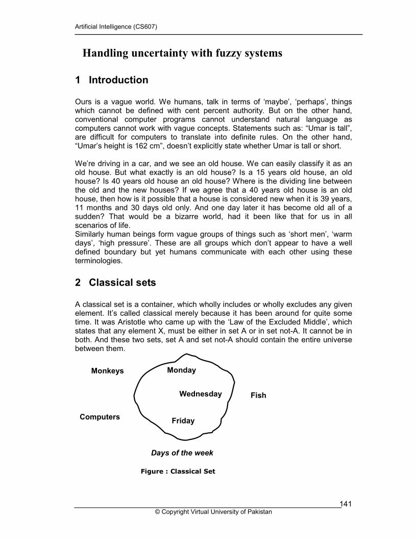
A classical set is a container, which wholly includes or wholly excludes any given element. It’s called classical merely because it has been around for quite some time. It was Aristotle who came up with the ‘Law of the Excluded Middle’, which states that any element X, must be either in set A or in set not-A. It cannot be in both. And these two sets, set A and set not-A should contain the entire universe between them.
Figure : Classical Set
Computers
Fish
Monday
Wednesday
Friday
Monkeys
Days of the week

Artificial Intelligence (CS607)
© Copyright Virtual University of Pakistan 142
Let’s take the example of the set ‘Days of the week’. This is a classical set in which all the 7 days from Monday up until Sunday belong to the set, and everything possible other than that that you can think of, monkeys, computers, fish, telephone, etc, are definitely not a part of this set. This is a binary classification system, in which everything must be asserted or denied. In the case of Monday, it will be asserted to be an element of the set of ‘days of the week’, but tuna fish wil not be an element of this set.
3 Fuzzy sets
Fuzzy sets, unlike classical sets, do not restrict themselves to something lying wholly in either set A or in set not-A. They let things sit on the fence, and are thus closer to the human world. Let us, for example, take into consideration ‘days of the weekend’. The classical set would say strictly that only Saturday and Sunday are a part of weekend, whereas most of us would agree that we do feel like it’s a weekend somewhat on Friday as well. Actually we’re more excited about the weekend on a Friday than on Sunday, because on Sunday we know that the next day is a working day. This concept is more vividly shown in the following figure.
Figure : Fuzzy Sets
Another diagram that would help distinguish between crisp and fuzzy representation of days of the weekend is shown below.
Figure : Crisp v/s Fuzzy
The left side of the above figure shows the crisp set ‘days of the weekend’, which is a Boolean two-valued function, so it gives a value of 0 for all week days except Saturday and Sunday where it gives an abrupt 1 and then back to 0 as soon as
Saturday
Sunday
Monkeys
Computers
Fish
Days of the weekend
Friday Tuesday
Monday
Thursday
Artificial Intelligence (CS607)
© Copyright Virtual University of Pakistan 143
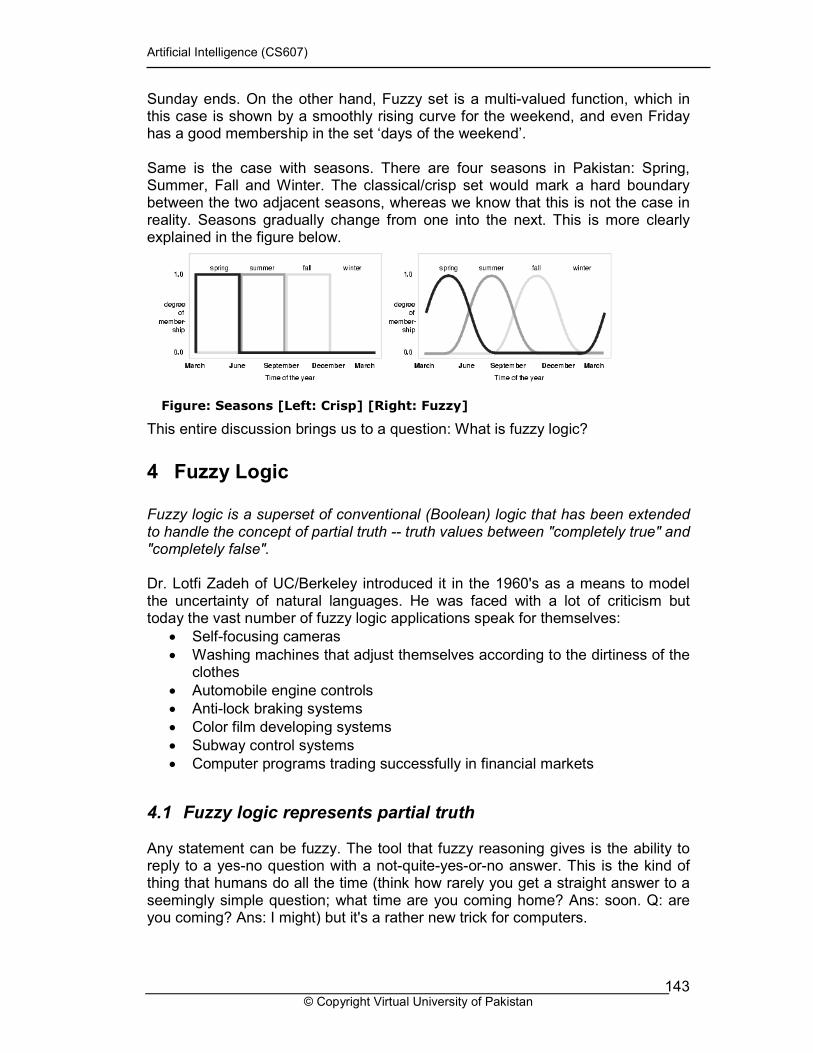
Sunday ends. On the other hand, Fuzzy set is a multi-valued function, which in this case is shown by a smoothly rising curve for the weekend, and even Friday has a good membership in the set ‘days of the weekend’. Same is the case with seasons. There are four seasons in Pakistan: Spring, Summer, Fall and Winter. The classical/crisp set would mark a hard boundary between the two adjacent seasons, whereas we know that this is not the case in reality. Seasons gradually change from one into the next. This is more clearly explained in the figure below.
Figure: Seasons [Left: Crisp] [Right: Fuzzy]
This entire discussion brings us to a question: What is fuzzy logic?
4 Fuzzy Logic
Fuzzy logic is a superset of conventional (Boolean) logic that has been extended to handle the concept of partial truth -- truth values between "completely true" and "completely false". Dr. Lotfi Zadeh of UC/Berkeley introduced it in the 1960's as a means to model the uncertainty of natural languages. He was faced with a lot of criticism but today the vast number of fuzzy logic applications speak for themselves:
• Self-focusing cameras
• Washing machines that adjust themselves according to the dirtiness of the clothes
• Automobile engine controls
• Anti-lock braking systems
• Color film developing systems
• Subway control systems
• Computer programs trading successfully in financial markets
4.1 Fuzzy logic represents partial truth
Any statement can be fuzzy. The tool that fuzzy reasoning gives is the ability to reply to a yes-no question with a not-quite-yes-or-no answer. This is the kind of thing that humans do all the time (think how rarely you get a straight answer to a seemingly simple question; what time are you coming home? Ans: soon. Q: are you coming? Ans: I might) but it's a rather new trick for computers.
Artificial Intelligence (CS607)
© Copyright Virtual University of Pakistan 144
How does it work? Reasoning in fuzzy logic is just a matter of generalizing the familiar yes-no (Boolean) logic. If we give "true" the numerical value of 1 and "false" the numerical value of 0, we're saying that fuzzy logic also permits in-between values like 0.2 and 0.7453. “In fuzzy logic, the truth of any statement becomes matter of degree” We will understand the concept of degree or partial truth by the same example of days of the weekend. Following are some questions and their respective answers: – Q: Is Saturday a weekend day? – A: 1 (yes, or true) – Q: Is Tuesday a weekend day? – A: 0 (no, or false) – Q: Is Friday a weekend day? – A: 0.7 (for the most part yes, but not completely) – Q: Is Sunday a weekend day? – A: 0.9 (yes, but not quite as much as Saturday)
4.2 Boolean versus fuzzy
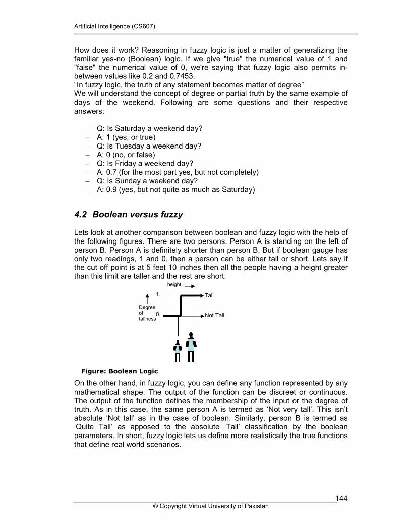
Lets look at another comparison between boolean and fuzzy logic with the help of the following figures. There are two persons. Person A is standing on the left of person B. Person A is definitely shorter than person B. But if boolean gauge has only two readings, 1 and 0, then a person can be either tall or short. Lets say if the cut off point is at 5 feet 10 inches then all the people having a height greater than this limit are taller and the rest are short.
Figure: Boolean Logic
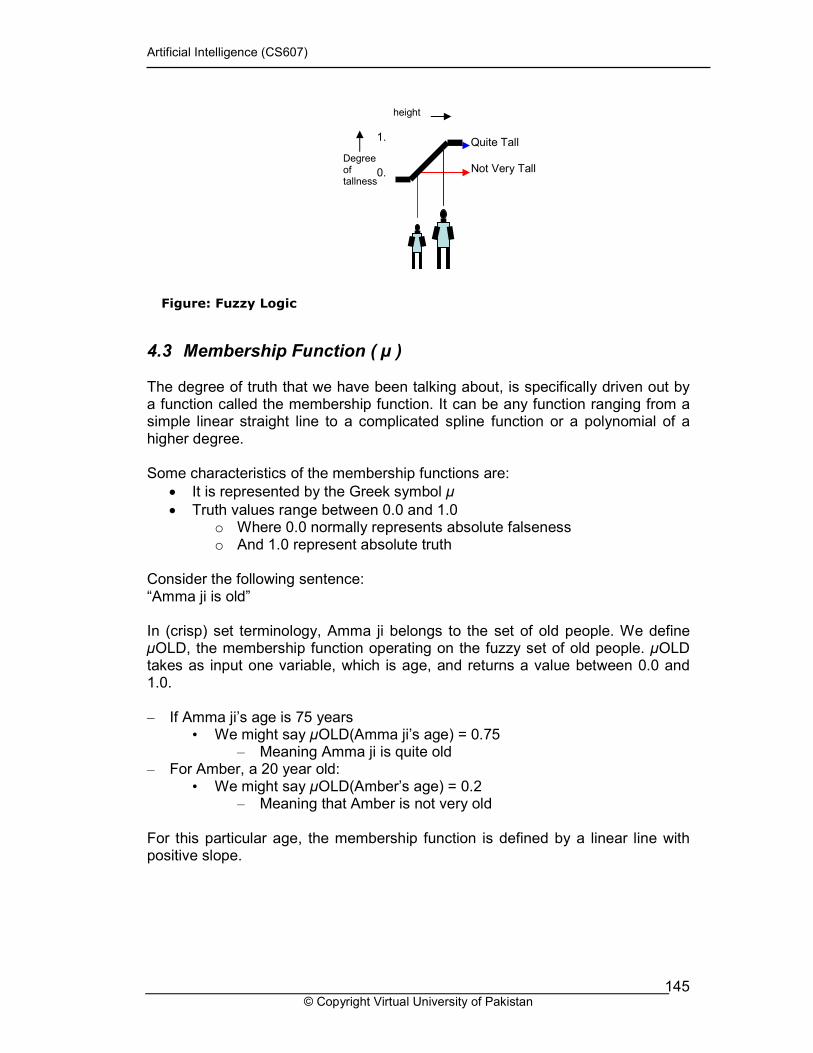
On the other hand, in fuzzy logic, you can define any function represented by any mathematical shape. The output of the function can be discreet or continuous. The output of the function defines the membership of the input or the degree of truth. As in this case, the same person A is termed as ‘Not very tall’. This isn’t absolute ‘Not tall’ as in the case of boolean. Similarly, person B is termed as ‘Quite Tall’ as apposed to the absolute ‘Tall’ classification by the boolean parameters. In short, fuzzy logic lets us define more realistically the true functions that define real world scenarios.
Degree of tallness
height
0.0
1.0
Not Tall (0.0)
Tall (1.0)
Artificial Intelligence (CS607)
© Copyright Virtual University of Pakistan 145
Figure: Fuzzy Logic
4.3 Membership Function ( µ )
The degree of truth that we have been talking about, is specifically driven out by a function called the membership function. It can be any function ranging from a simple linear straight line to a complicated spline function or a polynomial of a higher degree. Some characteristics of the membership functions are:
• It is represented by the Greek symbol µ
• Truth values range between 0.0 and 1.0 o Where 0.0 normally represents absolute falseness o And 1.0 represent absolute truth
Consider the following sentence: “Amma ji is old” In (crisp) set terminology, Amma ji belongs to the set of old people. We define µOLD, the membership function operating on the fuzzy set of old people. µOLD takes as input one variable, which is age, and returns a value between 0.0 and 1.0. – If Amma ji’s age is 75 years
• We might say µOLD(Amma ji’s age) = 0.75 – Meaning Amma ji is quite old
– For Amber, a 20 year old: • We might say µOLD(Amber’s age) = 0.2
– Meaning that Amber is not very old For this particular age, the membership function is defined by a linear line with positive slope.
height
Not Very Tall (0.2)
Quite Tall (0.8) Degree
of tallness
0.0
1.0
Artificial Intelligence (CS607)
© Copyright Virtual University of Pakistan 146
4.4 Fuzzy vs probability
Its important to distinguish at this point the difference between probability and fuzzy, as both operate over the same range [0.0 to 1.0]. To understand their differences lets take into account the following case, where Amber is a 20 years old girl. µOLD(Amber) = 0.2 In probability theory: There is a 20% chance that Amber belongs to the set of old people, there’s an 80% chance that she doesn’t belong to the set of old people. In fuzzy terminology: Amber is definitely not old or some other term corresponding to the value 0.2. But there are certainly no chances involved, no guess work left for the system to classify Amber as young or old.
4.5 Logical and fuzzy operators
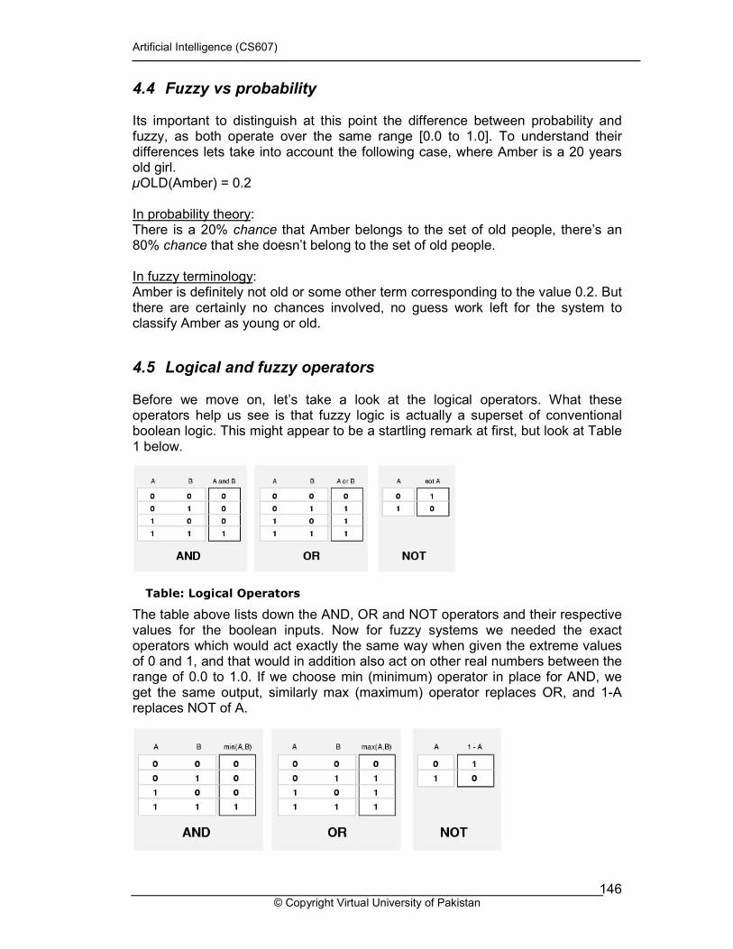
Before we move on, let’s take a look at the logical operators. What these operators help us see is that fuzzy logic is actually a superset of conventional boolean logic. This might appear to be a startling remark at first, but look at Table 1 below.
Table: Logical Operators
The table above lists down the AND, OR and NOT operators and their respective values for the boolean inputs. Now for fuzzy systems we needed the exact operators which would act exactly the same way when given the extreme values of 0 and 1, and that would in addition also act on other real numbers between the range of 0.0 to 1.0. If we choose min (minimum) operator in place for AND, we get the same output, similarly max (maximum) operator replaces OR, and 1-A replaces NOT of A.
Artificial Intelligence (CS607)
© Copyright Virtual University of Pakistan 147
Table: Fuzzy Operators
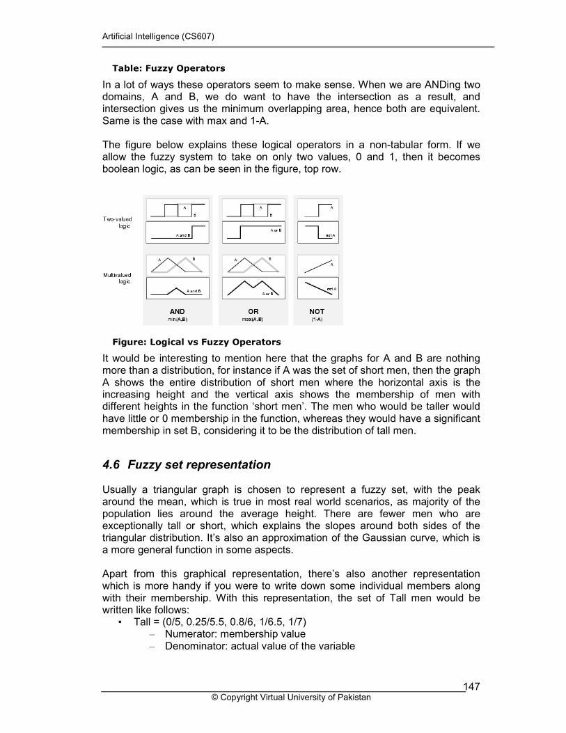
In a lot of ways these operators seem to make sense. When we are ANDing two domains, A and B, we do want to have the intersection as a result, and intersection gives us the minimum overlapping area, hence both are equivalent. Same is the case with max and 1-A. The figure below explains these logical operators in a non-tabular form. If we allow the fuzzy system to take on only two values, 0 and 1, then it becomes boolean logic, as can be seen in the figure, top row.
Figure: Logical vs Fuzzy Operators
It would be interesting to mention here that the graphs for A and B are nothing more than a distribution, for instance if A was the set of short men, then the graph A shows the entire distribution of short men where the horizontal axis is the increasing height and the vertical axis shows the membership of men with different heights in the function ‘short men’. The men who would be taller would have little or 0 membership in the function, whereas they would have a significant membership in set B, considering it to be the distribution of tall men.
4.6 Fuzzy set representation
Usually a triangular graph is chosen to represent a fuzzy set, with the peak around the mean, which is true in most real world scenarios, as majority of the population lies around the average height. There are fewer men who are exceptionally tall or short, which explains the slopes around both sides of the triangular distribution. It’s also an approximation of the Gaussian curve, which is a more general function in some aspects. Apart from this graphical representation, there’s also another representation which is more handy if you were to write down some individual members along with their membership. With this representation, the set of Tall men would be written like follows: • Tall = (0/5, 0.25/5.5, 0.8/6, 1/6.5, 1/7)
– Numerator: membership value – Denominator: actual value of the variable

Artificial Intelligence (CS607)
© Copyright Virtual University of Pakistan 148
For instance, the first element is 0/5 meaning, that a height of 5 feet has 0 membership in the set of tall people, likewise, men who are 6.5 feet or 7 feet tall have a membership value of maximum 1.
4.7 Fuzzy rules
First of all, let us revise the concept of simple If-Then rules. The rule is of the form: If x is A then y is B Where x and y are variables and A and B are some distributions/fuzzy sets. For example: If hotel service is good then tip is average Here hotel service is a linguistic variable, which when given to a real fuzzy system would have a certain crisp value, maybe a rating between 0 and 10. This rating would have a membership value in the fuzzy set of ‘good’. We shall evaluate this rule in more detail in the case study that follows. Antecedents can have multiple parts: • If wind is mild and racquets are good then playing badminton is fun
In this case all parts of the antecedent are resolved simultaneously and resolved to a single number using logical operators The consequent can have multiple parts as well • if temperature is cold then hot water valve is open and cold water valve is
shut How is the consequent affected by the antecedent? The consequent specifies that a fuzzy set be assigned to the output. The implication function then modifies that fuzzy set to the degree specified by the antecedent. The most common ways to modify the output fuzzy set are truncation using the min function (where the fuzzy set is "chopped off“). Consider the following figure, which demonstrates the working of fuzzy rule system on one rule, which states: “If service is excellent or food is delicious then tip is generous”
Artificial Intelligence (CS607)
© Copyright Virtual University of Pakistan 149
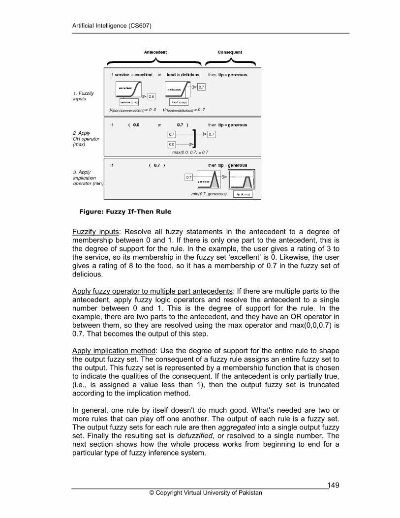
Figure: Fuzzy If-Then Rule
Fuzzify inputs: Resolve all fuzzy statements in the antecedent to a degree of membership between 0 and 1. If there is only one part to the antecedent, this is the degree of support for the rule. In the example, the user gives a rating of 3 to the service, so its membership in the fuzzy set ‘excellent’ is 0. Likewise, the user gives a rating of 8 to the food, so it has a membership of 0.7 in the fuzzy set of delicious. Apply fuzzy operator to multiple part antecedents: If there are multiple parts to the antecedent, apply fuzzy logic operators and resolve the antecedent to a single number between 0 and 1. This is the degree of support for the rule. In the example, there are two parts to the antecedent, and they have an OR operator in between them, so they are resolved using the max operator and max(0,0,0.7) is 0.7. That becomes the output of this step. Apply implication method: Use the degree of support for the entire rule to shape the output fuzzy set. The consequent of a fuzzy rule assigns an entire fuzzy set to the output. This fuzzy set is represented by a membership function that is chosen to indicate the qualities of the consequent. If the antecedent is only partially true, (i.e., is assigned a value less than 1), then the output fuzzy set is truncated according to the implication method. In general, one rule by itself doesn't do much good. What's needed are two or more rules that can play off one another. The output of each rule is a fuzzy set. The output fuzzy sets for each rule are then aggregated into a single output fuzzy set. Finally the resulting set is defuzzified, or resolved to a single number. The next section shows how the whole process works from beginning to end for a particular type of fuzzy inference system.
Artificial Intelligence (CS607)
© Copyright Virtual University of Pakistan 150
5 Fuzzy inference system
Fuzzy inference system (FIS) is the process of formulating the mapping from a given input to an output using fuzzy logic. This mapping then provides a basis from which decisions can be made, or patterns discerned Fuzzy inference systems have been successfully applied in fields such as automatic control, data classification, decision analysis, expert systems, and computer vision. Because of its multidisciplinary nature, fuzzy inference systems are associated with a number of names, such as fuzzy-rule-based systems, fuzzy expert systems, fuzzy modeling, fuzzy associative memory, fuzzy logic controllers, and simply (and ambiguously !!) fuzzy systems. Since the terms used to describe the various parts of the fuzzy inference process are far from standard, we will try to be as clear as possible about the different terms introduced in this section. Mamdani's fuzzy inference method is the most commonly seen fuzzy methodology. Mamdani's method was among the first control systems built using fuzzy set theory. It was proposed in 1975 by Ebrahim Mamdani as an attempt to control a steam engine and boiler combination by synthesizing a set of linguistic control rules obtained from experienced human operators. Mamdani's effort was based on Lotfi Zadeh's 1973 paper on fuzzy algorithms for complex systems and decision processes.
5.1 Five parts of the fuzzy inference process
• Fuzzification of the input variables • Application of fuzzy operator in the antecedent (premises) • Implication from antecedent to consequent • Aggregation of consequents across the rules • Defuzzification of output
To help us understand these steps, let’s do a small case study.
5.2 Case Study: dinner for two
We present a small case study in which two people go for a dinner to a restaurant. Our fuzzy system will help them decide the percentage of tip to be given to the waiter (between 5 to 25 percent of the total bill), based on their rating of service and food. The rating is between 0 and 10. The system is based on three fuzzy rules: Rule1: If service is poor or food is rancid then tip is cheap Rule2: If service is good then tip is average

Artificial Intelligence (CS607)
© Copyright Virtual University of Pakistan 151
Rule3: If service is excellent or food is delicious then tip is generous Based on these rules and the input by the diners, the Fuzzy inference system gives the final output using all the inference steps listed above. Let’s take a look at those steps one at a time.
Figure: Dinner for Two
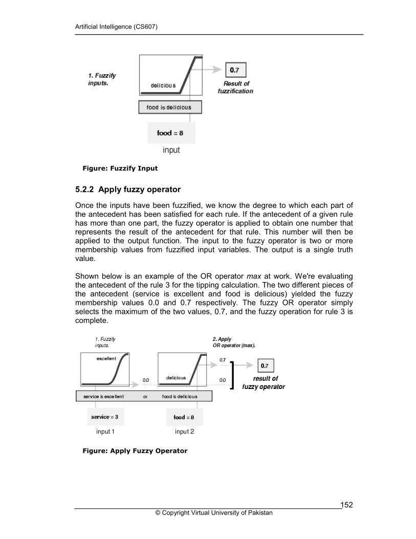
5.2.1 Fuzzify Inputs
The first step is to take the inputs and determine the degree to which they belong to each of the appropriate fuzzy sets via membership functions. The input is always a crisp numerical value limited to the universe of discourse of the input variable (in this case the interval between 0 and 10) and the output is a fuzzy degree of membership in the qualifying linguistic set (always the interval between 0 and 1). Fuzzification of the input amounts to either a table lookup or a function evaluation. The example we're using in this section is built on three rules, and each of the rules depends on resolving the inputs into a number of different fuzzy linguistic sets: service is poor, service is good, food is rancid, food is delicious, and so on. Before the rules can be evaluated, the inputs must be fuzzified according to each of these linguistic sets. For example, to what extent is the food really delicious? The figure below shows how well the food at our hypothetical restaurant (rated on a scale of 0 to 10) qualifies, (via its membership function), as the linguistic variable "delicious." In this case, the diners rated the food as an 8, which, given our graphical definition of delicious, corresponds to µ = 0.7 for the "delicious" membership function.
Artificial Intelligence (CS607)
© Copyright Virtual University of Pakistan 152
Figure: Fuzzify Input
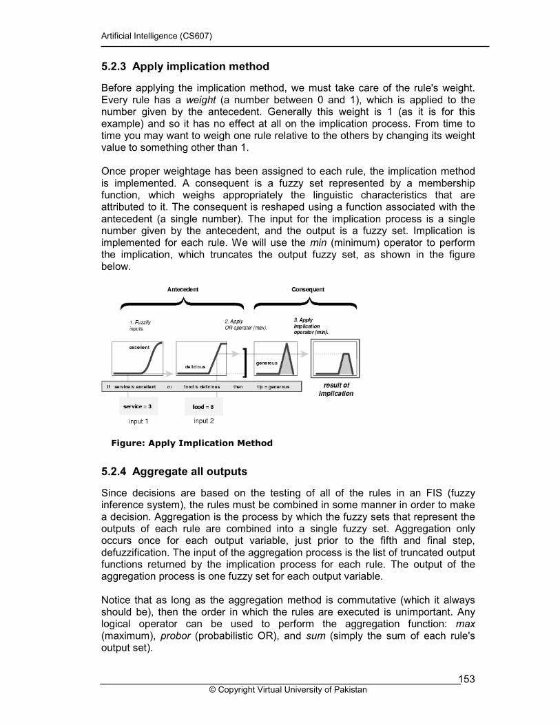
5.2.2 Apply fuzzy operator
Once the inputs have been fuzzified, we know the degree to which each part of the antecedent has been satisfied for each rule. If the antecedent of a given rule has more than one part, the fuzzy operator is applied to obtain one number that represents the result of the antecedent for that rule. This number will then be applied to the output function. The input to the fuzzy operator is two or more membership values from fuzzified input variables. The output is a single truth value. Shown below is an example of the OR operator max at work. We're evaluating the antecedent of the rule 3 for the tipping calculation. The two different pieces of the antecedent (service is excellent and food is delicious) yielded the fuzzy membership values 0.0 and 0.7 respectively. The fuzzy OR operator simply selects the maximum of the two values, 0.7, and the fuzzy operation for rule 3 is complete.
Figure: Apply Fuzzy Operator
Artificial Intelligence (CS607)
© Copyright Virtual University of Pakistan 153
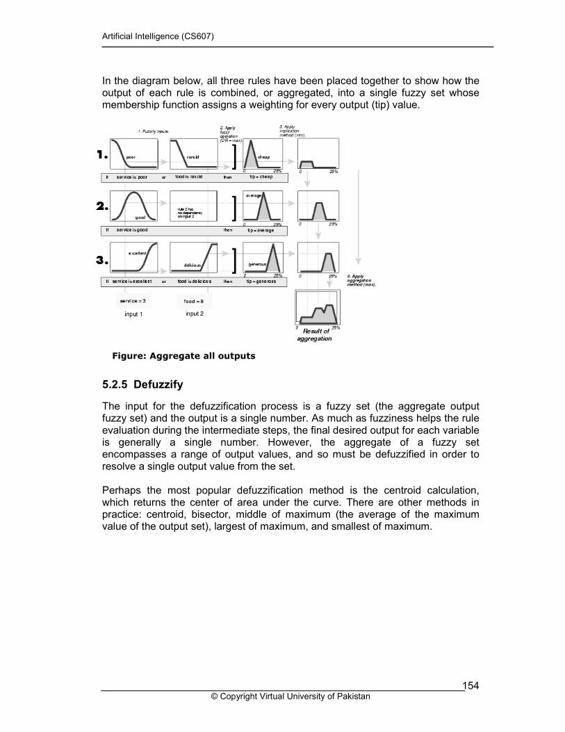
5.2.3 Apply implication method
Before applying the implication method, we must take care of the rule's weight. Every rule has a weight (a number between 0 and 1), which is applied to the number given by the antecedent. Generally this weight is 1 (as it is for this example) and so it has no effect at all on the implication process. From time to time you may want to weigh one rule relative to the others by changing its weight value to something other than 1. Once proper weightage has been assigned to each rule, the implication method is implemented. A consequent is a fuzzy set represented by a membership function, which weighs appropriately the linguistic characteristics that are attributed to it. The consequent is reshaped using a function associated with the antecedent (a single number). The input for the implication process is a single number given by the antecedent, and the output is a fuzzy set. Implication is implemented for each rule. We will use the min (minimum) operator to perform the implication, which truncates the output fuzzy set, as shown in the figure below.
Figure: Apply Implication Method
5.2.4 Aggregate all outputs
Since decisions are based on the testing of all of the rules in an FIS (fuzzy inference system), the rules must be combined in some manner in order to make a decision. Aggregation is the process by which the fuzzy sets that represent the outputs of each rule are combined into a single fuzzy set. Aggregation only occurs once for each output variable, just prior to the fifth and final step, defuzzification. The input of the aggregation process is the list of truncated output functions returned by the implication process for each rule. The output of the aggregation process is one fuzzy set for each output variable. Notice that as long as the aggregation method is commutative (which it always should be), then the order in which the rules are executed is unimportant. Any logical operator can be used to perform the aggregation function: max (maximum), probor (probabilistic OR), and sum (simply the sum of each rule's output set).
Artificial Intelligence (CS607)
© Copyright Virtual University of Pakistan 154
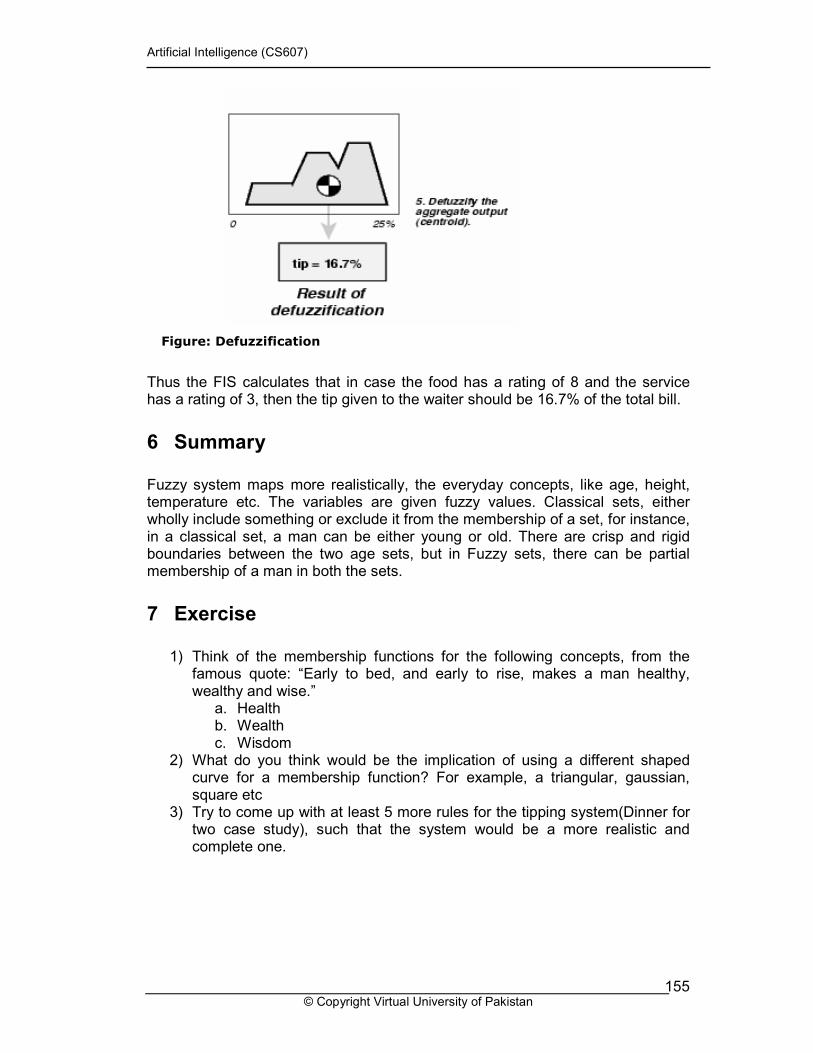
In the diagram below, all three rules have been placed together to show how the output of each rule is combined, or aggregated, into a single fuzzy set whose membership function assigns a weighting for every output (tip) value.
Figure: Aggregate all outputs
5.2.5 Defuzzify
The input for the defuzzification process is a fuzzy set (the aggregate output fuzzy set) and the output is a single number. As much as fuzziness helps the rule evaluation during the intermediate steps, the final desired output for each variable is generally a single number. However, the aggregate of a fuzzy set encompasses a range of output values, and so must be defuzzified in order to resolve a single output value from the set. Perhaps the most popular defuzzification method is the centroid calculation, which returns the center of area under the curve. There are other methods in practice: centroid, bisector, middle of maximum (the average of the maximum value of the output set), largest of maximum, and smallest of maximum.
Artificial Intelligence (CS607)
© Copyright Virtual University of Pakistan 155
Figure: Defuzzification
Thus the FIS calculates that in case the food has a rating of 8 and the service has a rating of 3, then the tip given to the waiter should be 16.7% of the total bill.
6 Summary
Fuzzy system maps more realistically, the everyday concepts, like age, height, temperature etc. The variables are given fuzzy values. Classical sets, either wholly include something or exclude it from the membership of a set, for instance, in a classical set, a man can be either young or old. There are crisp and rigid boundaries between the two age sets, but in Fuzzy sets, there can be partial membership of a man in both the sets.
7 Exercise
1) Think of the membership functions for the following concepts, from the famous quote: “Early to bed, and early to rise, makes a man healthy, wealthy and wise.”
a. Health b. Wealth c. Wisdom
2) What do you think would be the implication of using a different shaped curve for a membership function? For example, a triangular, gaussian, square etc
3) Try to come up with at least 5 more rules for the tipping system(Dinner for two case study), such that the system would be a more realistic and complete one.

Artificial Intelligence (CS607)
© Copyright Virtual University of Pakistan 156
8 Introduction to learning
8.1 Motivation
Artificial Intelligence (AI) is concerned with programming computers to perform tasks that are presently done better by humans. AI is about human behavior, the discovery of techniques that will allow computers to learn from humans. One of the most often heard criticisms of AI is that machines cannot be called Intelligent until they are able to learn to do new things and adapt to new situations, rather than simply doing as they are told to do. There can be little question that the ability to adapt to new surroundings and to solve new problems is an important characteristic of intelligent entities. Can we expect such abilities in programs? Ada Augusta, one of the earliest philosophers of computing, wrote: "The Analytical Engine has no pretensions whatever to originate anything. It can do whatever we know how to order it to perform." This remark has been interpreted by several AI critics as saying that computers cannot learn. In fact, it does not say that at all. Nothing prevents us from telling a computer how to interpret its inputs in such a way that its performance gradually improves. Rather than asking in advance whether it is possible for computers to "learn", it is much more enlightening to try to describe exactly what activities we mean when we say "learning" and what mechanisms could be used to enable us to perform those activities. [Simon, 1993] stated "changes in the system that are adaptive in the sense that they enable the system to do the same task or tasks drawn from the same population more efficiently and more effectively the next time".
8.2 What is learning ?
Learning can be described as normally a relatively permanent change that occurs in behavior as a result of experience. Learning occurs in various regimes. For example, it is possible to learn to open a lock as a result of trial and error; possible to learn how to use a word processor as a result of following particular instructions. Once the internal model of what ought to happen is set, it is possible to learn by practicing the skill until the performance converges on the desired model. One begins by paying attention to what needs to be done, but with more practice, one will need to monitor only the trickier parts of the performance. Automatic performance of some skills by the brain points out that the brain is capable of doing things in parallel i.e. one part is devoted to the skill whilst another part mediates conscious experience. There’s no decisive definition of learning but here are some that do justice:
• "Learning denotes changes in a system that ... enables a system to do the same task more efficiently the next time." --Herbert Simon
• "Learning is constructing or modifying representations of what is being experienced." --Ryszard Michalski
• "Learning is making useful changes in our minds." --Marvin Minsky
Artificial Intelligence (CS607)
© Copyright Virtual University of Pakistan 157
8.3 What is machine learning ?
It is a very difficult to define precisely what machine learning is. We can best enlighten ourselves by exactly describing the activities that we want a machine to do when we say learning and by deciding on the best possible mechanism to enable us to perform those activities. Generally speaking, the goal of machine learning is to build computer systems that can learn from their experience and adapt to their environments. Obviously, learning is an important aspect or component of intelligence. There are both theoretical and practical reasons to support such a claim. Some people even think intelligence is nothing but the ability to learn, though other people think an intelligent system has a separate "learning mechanism" which improves the performance of other mechanisms of the system.
8.4 Why do we want machine learning
One response to the idea of AI is to say that computers can not think because they only do what their programmers tell them to do. However, it is not always easy to tell what a particular program will do, but given the same inputs and conditions it will always produce the same outputs. If the program gets something right once it will always get it right. If it makes a mistake once it will always make the same mistake every time it runs. In contrast to computers, humans learn from their mistakes; attempt to work out why things went wrong and try alternative solutions. Also, we are able to notice similarities between things, and therefore can generate new ideas about the world we live in. Any intelligence, however artificial or alien, that did not learn would not be much of an intelligence. So, machine learning is a prerequisite for any mature programme of artificial intelligence.
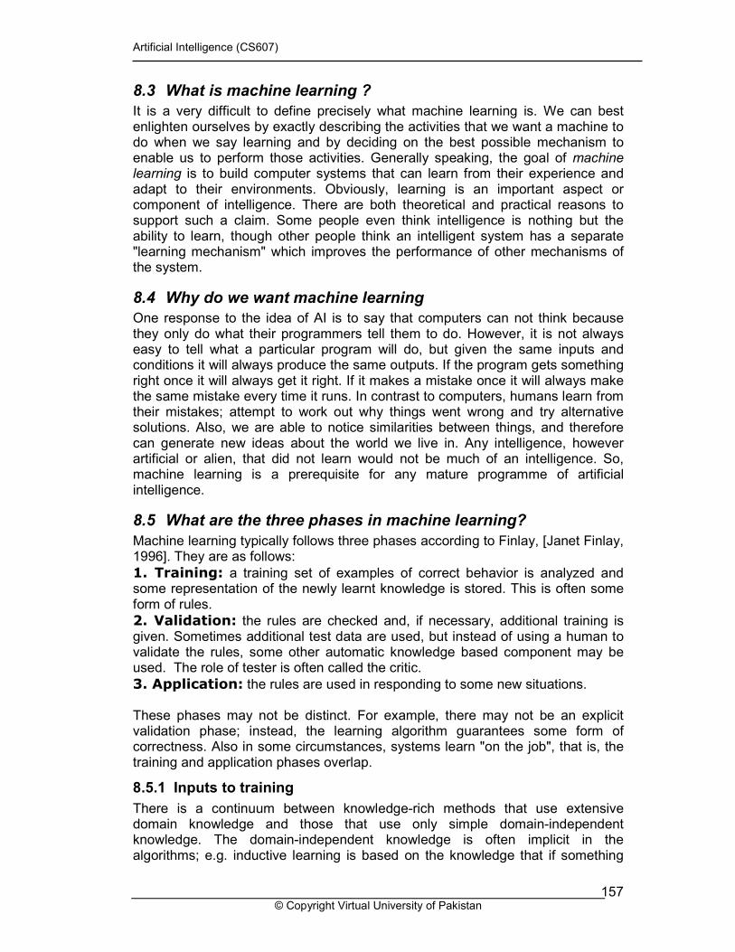
8.5 What are the three phases in machine learning?
Machine learning typically follows three phases according to Finlay, [Janet Finlay, 1996]. They are as follows:
1. Training: a training set of examples of correct behavior is analyzed and some representation of the newly learnt knowledge is stored. This is often some form of rules.
2. Validation: the rules are checked and, if necessary, additional training is given. Sometimes additional test data are used, but instead of using a human to validate the rules, some other automatic knowledge based component may be used. The role of tester is often called the critic.
3. Application: the rules are used in responding to some new situations. These phases may not be distinct. For example, there may not be an explicit validation phase; instead, the learning algorithm guarantees some form of correctness. Also in some circumstances, systems learn "on the job", that is, the training and application phases overlap.
8.5.1 Inputs to training
There is a continuum between knowledge-rich methods that use extensive domain knowledge and those that use only simple domain-independent knowledge. The domain-independent knowledge is often implicit in the algorithms; e.g. inductive learning is based on the knowledge that if something
Artificial Intelligence (CS607)
© Copyright Virtual University of Pakistan 158
happens a lot it is likely to be generally true. Where examples are provided, it is important to know the source. The examples may be simply measurements from the world, for example, transcripts of grand master tournaments. If so, do they represent "typical" sets of behavior or have they been filtered to be "representative"? If the former is true then it is possible to infer information about the relative probability from the frequency in the training set. However, unfiltered data may also be noisy, have errors, etc., and examples from the world may not be complete, since infrequent situations may simply not be in the training set. Alternatively, the examples may have been generated by a teacher. In this case, it can be assumed that they are a helpful set which cover all the important cases. Also, it is advisable to assume that the teacher will not be ambiguous. Finally the system itself may be able to generate examples by performing experiments on the world, asking an expert, or even using the internal model of the world. Some form of representation of the examples also has to be decided. This may partly be determined by the context, but more often than not there will be a choice. Often the choice of representation embodies quite a lot of the domain knowledge.
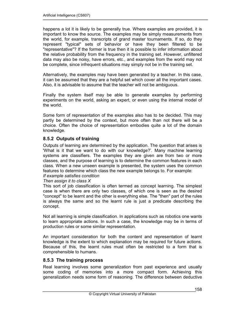
8.5.2 Outputs of training
Outputs of learning are determined by the application. The question that arises is 'What is it that we want to do with our knowledge?’. Many machine learning systems are classifiers. The examples they are given are from two or more classes, and the purpose of learning is to determine the common features in each class. When a new unseen example is presented, the system uses the common features to determine which class the new example belongs to. For example: If example satisfies condition Then assign it to class X This sort of job classification is often termed as concept learning. The simplest case is when there are only two classes, of which one is seen as the desired "concept" to be learnt and the other is everything else. The "then" part of the rules is always the same and so the learnt rule is just a predicate describing the concept. Not all learning is simple classification. In applications such as robotics one wants to learn appropriate actions. In such a case, the knowledge may be in terms of production rules or some similar representation. An important consideration for both the content and representation of learnt knowledge is the extent to which explanation may be required for future actions. Because of this, the learnt rules must often be restricted to a form that is comprehensible to humans.
8.5.3 The training process
Real learning involves some generalization from past experience and usually some coding of memories into a more compact form. Achieving this generalization needs some form of reasoning. The difference between deductive
Artificial Intelligence (CS607)
© Copyright Virtual University of Pakistan 159
reasoning and inductive reasoning is often used as the primary distinction between machine learning algorithms. Deductive learning working on existing facts and knowledge and deduces new knowledge from the old. In contrast, inductive learning uses examples and generates hypothesis based on the similarities between them. One way of looking at the learning process is as a search process. One has a set of examples and a set of possible rules. The job of the learning algorithm is to find suitable rules that are correct with respect to the examples and existing knowledge.
8.6 Learning techniques available
8.6.1 Rote learning
In this kind of learning there is no prior knowledge. When a computer stores a piece of data, it is performing an elementary form of learning. This act of storage presumably allows the program to perform better in the future. Examples of correct behavior are stored and when a new situation arises it is matched with the learnt examples. The values are stored so that they are not re-computed later. One of the earliest game-playing programs is [Samuel, 1963] checkers program. This program learned to play checkers well enough to beat its creator/designer.
8.6.2 Deductive learning
Deductive learning works on existing facts and knowledge and deduces new knowledge from the old. This is best illustrated by giving an example. For example, assume: A = B B = C Then we can deduce with much confidence that: C = A Arguably, deductive learning does not generate "new" knowledge at all, it simply memorizes the logical consequences of what is known already. This implies that virtually all mathematical research would not be classified as learning "new" things. However, regardless of whether this is termed as new knowledge or not, it certainly makes the reasoning system more efficient.
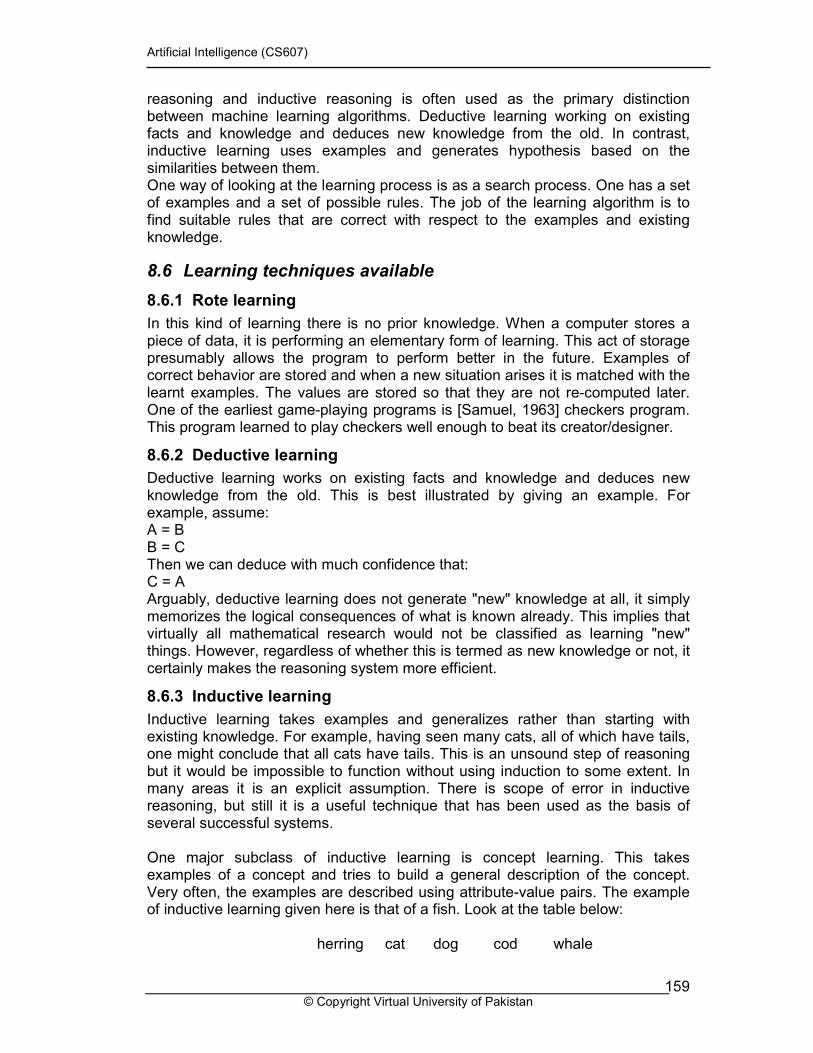
8.6.3 Inductive learning
Inductive learning takes examples and generalizes rather than starting with existing knowledge. For example, having seen many cats, all of which have tails, one might conclude that all cats have tails. This is an unsound step of reasoning but it would be impossible to function without using induction to some extent. In many areas it is an explicit assumption. There is scope of error in inductive reasoning, but still it is a useful technique that has been used as the basis of several successful systems. One major subclass of inductive learning is concept learning. This takes examples of a concept and tries to build a general description of the concept. Very often, the examples are described using attribute-value pairs. The example of inductive learning given here is that of a fish. Look at the table below:
herring cat dog cod whale
Artificial Intelligence (CS607)
© Copyright Virtual University of Pakistan 160
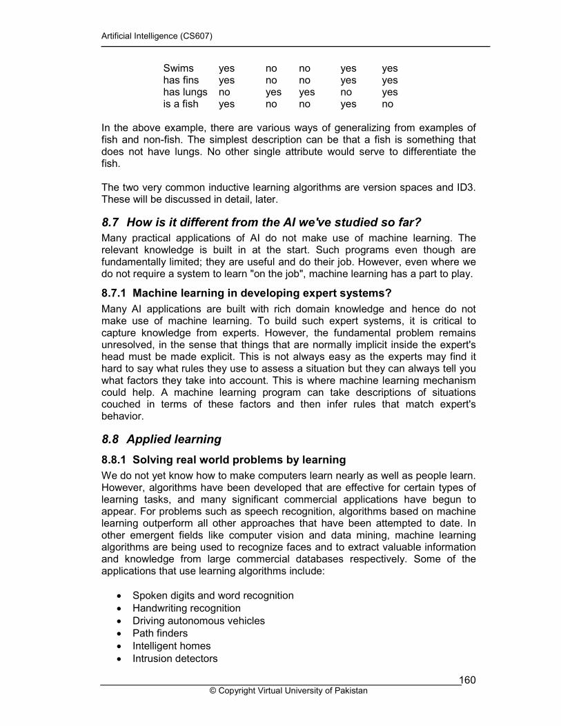
Swims yes no no yes yes has fins yes no no yes yes has lungs no yes yes no yes is a fish yes no no yes no
In the above example, there are various ways of generalizing from examples of fish and non-fish. The simplest description can be that a fish is something that does not have lungs. No other single attribute would serve to differentiate the fish. The two very common inductive learning algorithms are version spaces and ID3. These will be discussed in detail, later.
8.7 How is it different from the AI we've studied so far?
Many practical applications of AI do not make use of machine learning. The relevant knowledge is built in at the start. Such programs even though are fundamentally limited; they are useful and do their job. However, even where we do not require a system to learn "on the job", machine learning has a part to play.
8.7.1 Machine learning in developing expert systems?
Many AI applications are built with rich domain knowledge and hence do not make use of machine learning. To build such expert systems, it is critical to capture knowledge from experts. However, the fundamental problem remains unresolved, in the sense that things that are normally implicit inside the expert's head must be made explicit. This is not always easy as the experts may find it hard to say what rules they use to assess a situation but they can always tell you what factors they take into account. This is where machine learning mechanism could help. A machine learning program can take descriptions of situations couched in terms of these factors and then infer rules that match expert's behavior.
8.8 Applied learning
8.8.1 Solving real world problems by learning
We do not yet know how to make computers learn nearly as well as people learn. However, algorithms have been developed that are effective for certain types of learning tasks, and many significant commercial applications have begun to appear. For problems such as speech recognition, algorithms based on machine learning outperform all other approaches that have been attempted to date. In other emergent fields like computer vision and data mining, machine learning algorithms are being used to recognize faces and to extract valuable information and knowledge from large commercial databases respectively. Some of the applications that use learning algorithms include:
• Spoken digits and word recognition
• Handwriting recognition
• Driving autonomous vehicles
• Path finders
• Intelligent homes
• Intrusion detectors
Artificial Intelligence (CS607)
© Copyright Virtual University of Pakistan 161
• Intelligent refrigerators, tvs, vacuum cleaners
• Computer games
• Humanoid robotics This is just the glimpse of the applications that use some intelligent learning components. The current era has applied learning in the domains ranging from agriculture to astronomy to medical sciences.
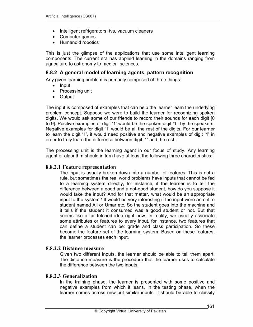
8.8.2 A general model of learning agents, pattern recognition
Any given learning problem is primarily composed of three things:
• Input
• Processing unit
• Output The input is composed of examples that can help the learner learn the underlying problem concept. Suppose we were to build the learner for recognizing spoken digits. We would ask some of our friends to record their sounds for each digit [0 to 9]. Positive examples of digit ‘1’ would be the spoken digit ‘1’, by the speakers. Negative examples for digit ‘1’ would be all the rest of the digits. For our learner to learn the digit ‘1’, it would need positive and negative examples of digit ‘1’ in order to truly learn the difference between digit ‘1’ and the rest. The processing unit is the learning agent in our focus of study. Any learning agent or algorithm should in turn have at least the following three characteristics:
8.8.2.1 Feature representation The input is usually broken down into a number of features. This is not a rule, but sometimes the real world problems have inputs that cannot be fed to a learning system directly, for instance, if the learner is to tell the difference between a good and a not-good student, how do you suppose it would take the input? And for that matter, what would be an appropriate input to the system? It would be very interesting if the input were an entire student named Ali or Umar etc. So the student goes into the machine and it tells if the student it consumed was a good student or not. But that seems like a far fetched idea right now. In reality, we usually associate some attributes or features to every input, for instance, two features that can define a student can be: grade and class participation. So these become the feature set of the learning system. Based on these features, the learner processes each input.
8.8.2.2 Distance measure Given two different inputs, the learner should be able to tell them apart. The distance measure is the procedure that the learner uses to calculate the difference between the two inputs.
8.8.2.3 Generalization In the training phase, the learner is presented with some positive and negative examples from which it leans. In the testing phase, when the learner comes across new but similar inputs, it should be able to classify
Artificial Intelligence (CS607)
© Copyright Virtual University of Pakistan 162
them similarly. This is called generalization. Humans are exceptionally good at generalization. A small child learns to differentiate between birds and cats in the early days of his/her life. Later when he/she sees a new bird, never seen before, he/she can easily tell that it’s a bird and not a cat.
9 LEARNING: Symbol-based Ours is a world of symbols. We use symbolic interpretations to understand the world around us. For instance, if we saw a ship, and were to tell a friend about its size, we will not say that we saw a 254.756 meters long ship, instead we’d say that we saw a ‘huge’ ship about the size of ‘Eiffel tower’. And our friend would understand the relationship between the size of the ship and its hugeness with the analogies of the symbolic information associated with the two words used: ‘huge’ and ‘Eiffel tower’. Similarly, the techniques we are to learn now use symbols to represent knowledge and information. Let us consider a small example to help us see where we’re headed. What if we were to learn the concept of a GOOD STUDENT. We would need to define, first of all some attributes of a student, on the basis of which we could tell apart the good student from the average. Then we would require some examples of good students and average students. To keep the problem simple we can label all the students who are “not good” (average, below average, satisfactory, bad) as NOT GOOD STUDENT. Let’s say we choose two attributes to define a student: grade and class participation. Both the attributes can have either of the two values: High, Low. Our learner program will require some examples from the concept of a student, for instance:
1. Student (GOOD STUDENT): Grade (High) ^ Class Participation (High) 2. Student (GOOD STUDENT): Grade (High) ^ Class Participation (Low) 3. Student (NOT GOOD STUDENT): Grade (Low) ^ Class Participation
(High) 4. Student (NOT GOOD STUDENT): Grade (Low) ^ Class Participation (Low)
As you can see the system is composed of symbolic information, based on which the learner can even generalize that a student is a GOOD STUDENT if his/her grade is high, even if the class participation is low: Student (GOOD STUDENT): Grade (High) ^ Class Participation (?) This is the final rule that the learner has learnt from the enumerated examples. Here the ‘?’ means that the attribute class participation can have any value, as long as the grade is high. In this section we will see all the steps the learner has to go through to actually come up with the final conclusion like this.
9.1 Problem and problem spaces
Before we get down to solving a problem, the first task is to understand the problem itself. There are various kinds of problems that require solutions. In theoretical computer science there are two main branches of problems:
• Tractable
• Intractable Those problems that can be solved in polynomial time are termed as tractable, the other half is called intractable. The tractable problems are further divided into
Artificial Intelligence (CS607)
© Copyright Virtual University of Pakistan 163
structured and complex problems. Structured problems are those which have defined steps through which the solution to the problem is reached. Complex problems usually don’t have well-defined steps. Machine learning algorithms are particularly more useful in solving the complex problems like recognition of patterns in images or speech, for which it’s hard to come up with procedural algorithms otherwise. The solution to any problem is a function that converts its inputs to corresponding outputs. The domain of a problem or the problem space is defined by the elements explained in the following paragraphs. These new concepts will be best understood if we take one example and exhaustively use it to justify each construct. Example: Let us consider the domain of HEALTH. The problem in this case is to distinguish between a sick and a healthy person. Suppose we have some domain knowledge; keeping a simplistic approach, we say that two attributes are necessary and sufficient to declare a person as healthy or sick. These two attributes are: Temperature (T) and Blood Pressure (BP). Any patient coming into the hospital can have three values for T and BP: High (H), Normal (N) and Low (L). Based on these values, the person is to be classified as Sick (SK). SK is a Boolean concept, SK = 1 means the person is sick, and SK = 0 means person is healthy. So the concept to be learnt by the system is of Sick, i.e., SK=1.
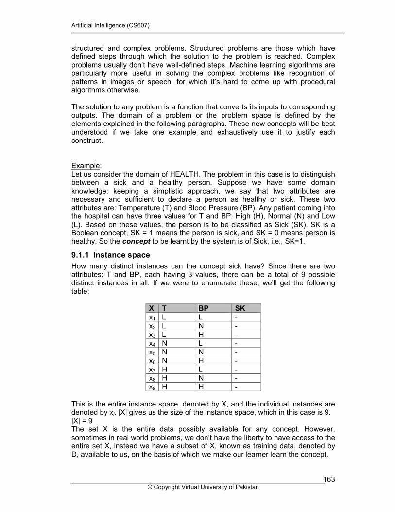
9.1.1 Instance space
How many distinct instances can the concept sick have? Since there are two attributes: T and BP, each having 3 values, there can be a total of 9 possible distinct instances in all. If we were to enumerate these, we’ll get the following table:
X T BP SK
x1 L L -
x2 L N - x3 L H - x4 N L - x5 N N - x6 N H - x7 H L -
x8 H N - x9 H H -
This is the entire instance space, denoted by X, and the individual instances are denoted by xi. |X| gives us the size of the instance space, which in this case is 9. |X| = 9 The set X is the entire data possibly available for any concept. However, sometimes in real world problems, we don’t have the liberty to have access to the entire set X, instead we have a subset of X, known as training data, denoted by D, available to us, on the basis of which we make our learner learn the concept.
Artificial Intelligence (CS607)
© Copyright Virtual University of Pakistan 164
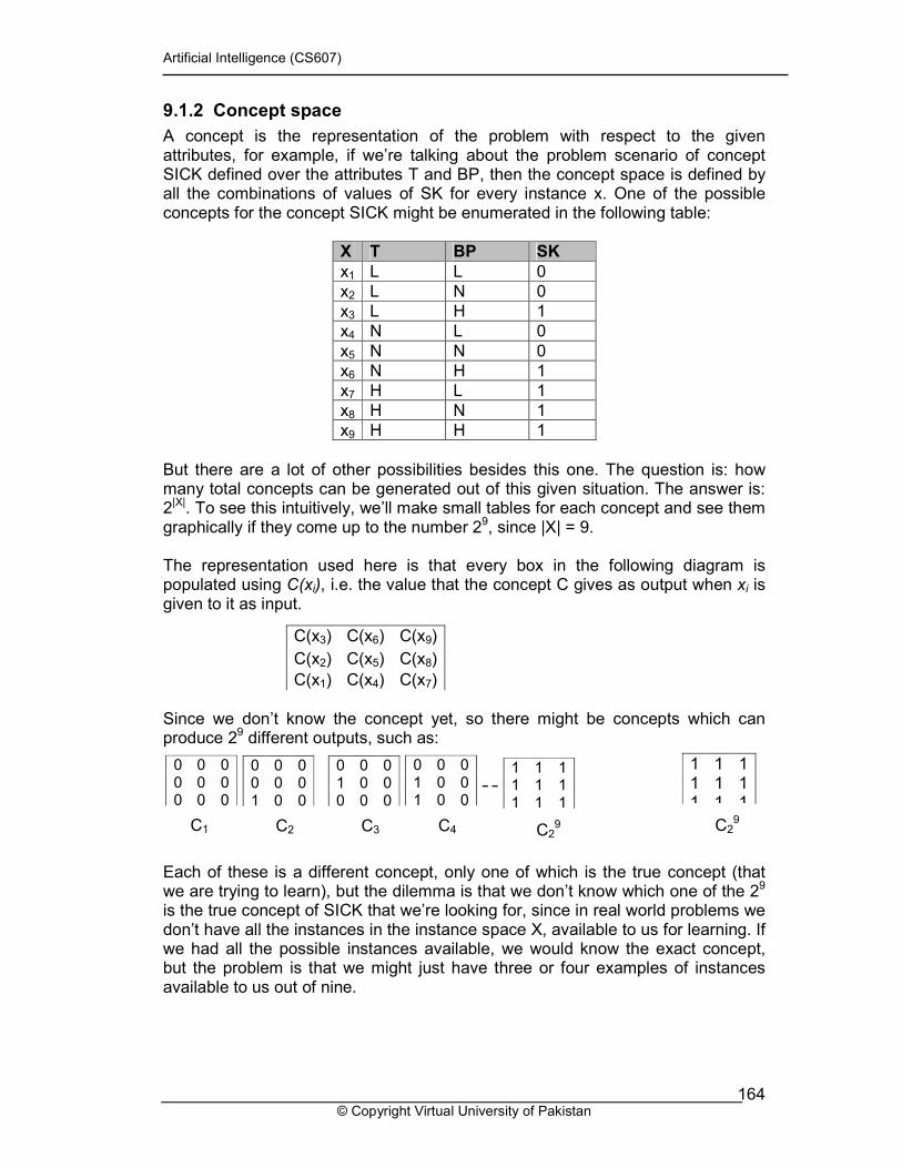
9.1.2 Concept space
A concept is the representation of the problem with respect to the given attributes, for example, if we’re talking about the problem scenario of concept SICK defined over the attributes T and BP, then the concept space is defined by all the combinations of values of SK for every instance x. One of the possible concepts for the concept SICK might be enumerated in the following table:
X T BP SK
x1 L L 0 x2 L N 0 x3 L H 1 x4 N L 0
x5 N N 0 x6 N H 1 x7 H L 1 x8 H N 1 x9 H H 1
But there are a lot of other possibilities besides this one. The question is: how many total concepts can be generated out of this given situation. The answer is: 2|X|. To see this intuitively, we’ll make small tables for each concept and see them graphically if they come up to the number 29, since |X| = 9. The representation used here is that every box in the following diagram is populated using C(xi), i.e. the value that the concept C gives as output when xi is given to it as input. Since we don’t know the concept yet, so there might be concepts which can produce 29 different outputs, such as:
Each of these is a different concept, only one of which is the true concept (that we are trying to learn), but the dilemma is that we don’t know which one of the 29 is the true concept of SICK that we’re looking for, since in real world problems we don’t have all the instances in the instance space X, available to us for learning. If we had all the possible instances available, we would know the exact concept, but the problem is that we might just have three or four examples of instances available to us out of nine.
C(x3) C(x6) C(x9)
C(x2) C(x5) C(x8)
C(x1) C(x4) C(x7)
0 0 0 0 0 0 0 0 0
C1
0 0 0 0 0 0 1 0 0
C2
0 0 0 1 0 0 0 0 0
C3
0 0 0 1 0 0 1 0 0
C4
1 1 1 1 1 1 1 1 1
C29
1 1 1 1 1 1 1 1 1
C29
Artificial Intelligence (CS607)
© Copyright Virtual University of Pakistan 165
D T BP SK
x1 N L 1 x2 L N 0
x3 N N 0
Notice that this is not the instance space X, in fact it is D: the training set. We don’t have any idea about the instances that lie outside this set D. The learner is to learn the true concept C based on only these three observations, so that once it has learnt, it could classify the new patients as sick or healthy based on the input parameters.
9.1.3 Hypothesis space
The above condition is typically the case in almost all the real world problems where learning is to be done based on a few available examples. In this situation, the learner has to hypothesize. It would be insensible to exhaustively search over the entire concept space, since there are 29 concepts. This is just a toy problem with only 9 possible instances in the instance space; just imagine how huge the concept space would be for real world problems that involve larger attribute sets. So the learner has to apply some hypothesis, which has either a search or the language bias to reduce the size of the concept space. This reduced concept space becomes the hypothesis space. For example, the most common language bias is that the hypothesis space uses the conjunctions (AND) of the attributes, i.e. H = <T, BP> H is the denotive representation of the hypothesis space; here it is the conjunction of attribute T and BP. If written in English it would mean: H = <T, BP>: IF “Temperature” = T AND “Blood Pressure” = BP THEN
H = 1 ELSE
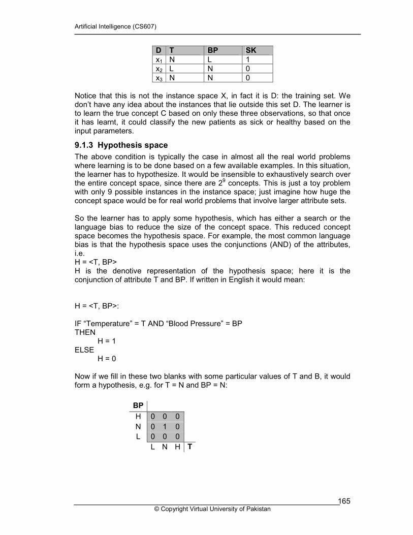
H = 0 Now if we fill in these two blanks with some particular values of T and B, it would form a hypothesis, e.g. for T = N and BP = N:
BP
H 0 0 0
N 0 1 0
L 0 0 0
L N H T
Artificial Intelligence (CS607)
© Copyright Virtual University of Pakistan 166
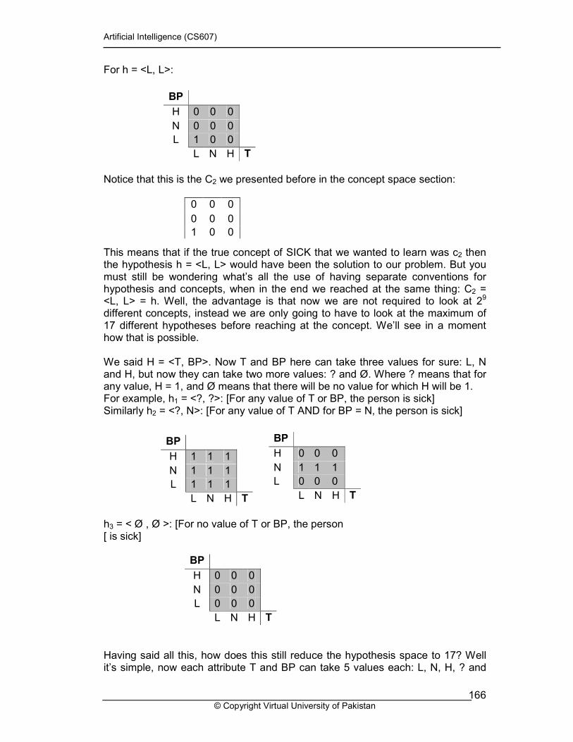
For h = <L, L>:
Notice that this is the C2 we presented before in the concept space section: This means that if the true concept of SICK that we wanted to learn was c2 then the hypothesis h = <L, L> would have been the solution to our problem. But you must still be wondering what’s all the use of having separate conventions for hypothesis and concepts, when in the end we reached at the same thing: C2 = <L, L> = h. Well, the advantage is that now we are not required to look at 29 different concepts, instead we are only going to have to look at the maximum of 17 different hypotheses before reaching at the concept. We’ll see in a moment how that is possible. We said H = <T, BP>. Now T and BP here can take three values for sure: L, N and H, but now they can take two more values: ? and Ø. Where ? means that for any value, H = 1, and Ø means that there will be no value for which H will be 1. For example, h1 = <?, ?>: [For any value of T or BP, the person is sick] Similarly h2 = <?, N>: [For any value of T AND for BP = N, the person is sick]
h3 = < Ø , Ø >: [For no value of T or BP, the person [ is sick]
Having said all this, how does this still reduce the hypothesis space to 17? Well it’s simple, now each attribute T and BP can take 5 values each: L, N, H, ? and
BP
H 0 0 0
N 1 1 1
L 0 0 0
L N H T
BP
H 0 0 0
N 0 0 0
L 1 0 0
L N H T
0 0 0
0 0 0
1 0 0
BP
H 1 1 1
N 1 1 1
L 1 1 1
L N H T
BP
H 0 0 0
N 0 0 0
L 0 0 0
L N H T
Artificial Intelligence (CS607)
© Copyright Virtual University of Pakistan 167
Ø. So there are 5 x 5 = 25 total hypotheses possible. This is a tremendous reduction from 29 = 512 to 25. But if we want to represent h4 = < Ø , L>, it would be the same as h3, meaning that there are some redundancies within the 25 hypotheses. These redundancies are caused by Ø, so if there’s this ‘Ø’ in the T or the BP or both, we’ll have the same hypothesis h3 as the outcome, all zeros. To calculate the number of semantically distinct hypotheses, we need one hypothesis which outputs all zeros, since it’s a distinct hypothesis than others, so that’s one, plus we need to know the rest of the combinations. This primarily means that T and BP can now take 4 values instead of 5, which are: L, N, H and ?. This implies that there are now 4 x 4 = 16 different hypotheses possible. So the total distinct hypotheses are: 16 + 1 = 17. This is a wonderful idea, but it comes at a vital cost. What if the true concept doesn’t lie in the conjunctive hypothesis space? This is often the case. We can try different hypotheses then. Some prior knowledge about the problem always helps.
9.1.4 Version space and searching
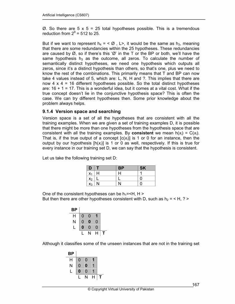
Version space is a set of all the hypotheses that are consistent with all the training examples. When we are given a set of training examples D, it is possible that there might be more than one hypotheses from the hypothesis space that are consistent with all the training examples. By consistent we mean h(xi) = C(xi). That is, if the true output of a concept [c(xi)] is 1 or 0 for an instance, then the output by our hypothesis [h(xi)] is 1 or 0 as well, respectively. If this is true for every instance in our training set D, we can say that the hypothesis is consistent. Let us take the following training set D:
D T BP SK
x1 H H 1
x2 L L 0 x3 N N 0
One of the consistent hypotheses can be h1=<H, H > But then there are other hypotheses consistent with D, such as h2 = < H, ? >
Although it classifies some of the unseen instances that are not in the training set
BP
H 0 0 1
N 0 0 0
L 0 0 0
L N H T
BP
H 0 0 1
N 0 0 1
L 0 0 1
L N H T
Artificial Intelligence (CS607)
© Copyright Virtual University of Pakistan 168
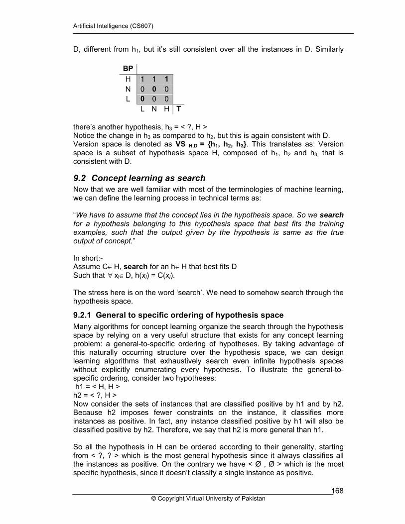
D, different from h1, but it’s still consistent over all the instances in D. Similarly
there’s another hypothesis, h3 = < ?, H > Notice the change in h3 as compared to h2, but this is again consistent with D. Version space is denoted as VS H,D = {h1, h2, h3}. This translates as: Version space is a subset of hypothesis space H, composed of h1, h2 and h3, that is consistent with D.
9.2 Concept learning as search
Now that we are well familiar with most of the terminologies of machine learning, we can define the learning process in technical terms as: “We have to assume that the concept lies in the hypothesis space. So we search for a hypothesis belonging to this hypothesis space that best fits the training examples, such that the output given by the hypothesis is same as the true output of concept.” In short:- Assume C∈H, search for an h∈H that best fits D Such that ∀ xi∈D, h(xi) = C(xi). The stress here is on the word ‘search’. We need to somehow search through the hypothesis space.
9.2.1 General to specific ordering of hypothesis space
Many algorithms for concept learning organize the search through the hypothesis space by relying on a very useful structure that exists for any concept learning problem: a general-to-specific ordering of hypotheses. By taking advantage of this naturally occurring structure over the hypothesis space, we can design learning algorithms that exhaustively search even infinite hypothesis spaces without explicitly enumerating every hypothesis. To illustrate the general-to-specific ordering, consider two hypotheses: h1 = < H, H > h2 = < ?, H > Now consider the sets of instances that are classified positive by h1 and by h2. Because h2 imposes fewer constraints on the instance, it classifies more instances as positive. In fact, any instance classified positive by h1 will also be classified positive by h2. Therefore, we say that h2 is more general than h1. So all the hypothesis in H can be ordered according to their generality, starting from < ?, ? > which is the most general hypothesis since it always classifies all the instances as positive. On the contrary we have < Ø , Ø > which is the most specific hypothesis, since it doesn’t classify a single instance as positive.
BP
H 1 1 1
N 0 0 0
L 0 0 0
L N H T
Artificial Intelligence (CS607)
© Copyright Virtual University of Pakistan 169
9.2.2 FIND-S
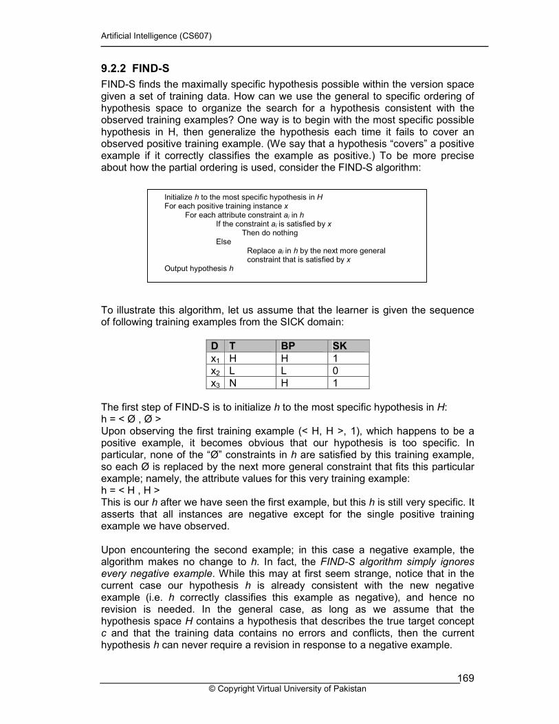
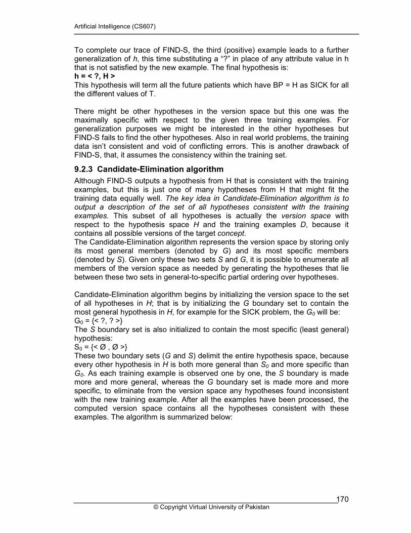
FIND-S finds the maximally specific hypothesis possible within the version space given a set of training data. How can we use the general to specific ordering of hypothesis space to organize the search for a hypothesis consistent with the observed training examples? One way is to begin with the most specific possible hypothesis in H, then generalize the hypothesis each time it fails to cover an observed positive training example. (We say that a hypothesis “covers” a positive example if it correctly classifies the example as positive.) To be more precise about how the partial ordering is used, consider the FIND-S algorithm: To illustrate this algorithm, let us assume that the learner is given the sequence of following training examples from the SICK domain:
D T BP SK
x1 H H 1 x2 L L 0 x3 N H 1
The first step of FIND-S is to initialize h to the most specific hypothesis in H: h = < Ø , Ø > Upon observing the first training example (< H, H >, 1), which happens to be a positive example, it becomes obvious that our hypothesis is too specific. In particular, none of the “Ø” constraints in h are satisfied by this training example, so each Ø is replaced by the next more general constraint that fits this particular example; namely, the attribute values for this very training example: h = < H , H > This is our h after we have seen the first example, but this h is still very specific. It asserts that all instances are negative except for the single positive training example we have observed. Upon encountering the second example; in this case a negative example, the algorithm makes no change to h. In fact, the FIND-S algorithm simply ignores every negative example. While this may at first seem strange, notice that in the current case our hypothesis h is already consistent with the new negative example (i.e. h correctly classifies this example as negative), and hence no revision is needed. In the general case, as long as we assume that the hypothesis space H contains a hypothesis that describes the true target concept c and that the training data contains no errors and conflicts, then the current hypothesis h can never require a revision in response to a negative example.
Initialize h to the most specific hypothesis in H For each positive training instance x
For each attribute constraint ai in h If the constraint ai is satisfied by x
Then do nothing Else
Replace ai in h by the next more general constraint that is satisfied by x
Output hypothesis h
Artificial Intelligence (CS607)
© Copyright Virtual University of Pakistan 170
To complete our trace of FIND-S, the third (positive) example leads to a further generalization of h, this time substituting a “?” in place of any attribute value in h that is not satisfied by the new example. The final hypothesis is: h = < ?, H > This hypothesis will term all the future patients which have BP = H as SICK for all the different values of T. There might be other hypotheses in the version space but this one was the maximally specific with respect to the given three training examples. For generalization purposes we might be interested in the other hypotheses but FIND-S fails to find the other hypotheses. Also in real world problems, the training data isn’t consistent and void of conflicting errors. This is another drawback of FIND-S, that, it assumes the consistency within the training set.
9.2.3 Candidate-Elimination algorithm
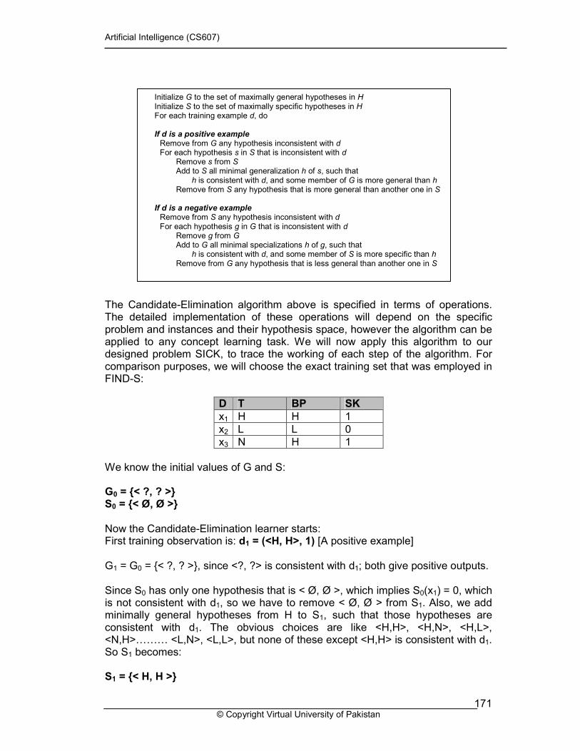
Although FIND-S outputs a hypothesis from H that is consistent with the training examples, but this is just one of many hypotheses from H that might fit the training data equally well. The key idea in Candidate-Elimination algorithm is to output a description of the set of all hypotheses consistent with the training examples. This subset of all hypotheses is actually the version space with respect to the hypothesis space H and the training examples D, because it contains all possible versions of the target concept. The Candidate-Elimination algorithm represents the version space by storing only its most general members (denoted by G) and its most specific members (denoted by S). Given only these two sets S and G, it is possible to enumerate all members of the version space as needed by generating the hypotheses that lie between these two sets in general-to-specific partial ordering over hypotheses. Candidate-Elimination algorithm begins by initializing the version space to the set of all hypotheses in H; that is by initializing the G boundary set to contain the most general hypothesis in H, for example for the SICK problem, the G0 will be: G0 = {< ?, ? >} The S boundary set is also initialized to contain the most specific (least general) hypothesis: S0 = {< Ø , Ø >} These two boundary sets (G and S) delimit the entire hypothesis space, because every other hypothesis in H is both more general than S0 and more specific than G0. As each training example is observed one by one, the S boundary is made more and more general, whereas the G boundary set is made more and more specific, to eliminate from the version space any hypotheses found inconsistent with the new training example. After all the examples have been processed, the computed version space contains all the hypotheses consistent with these examples. The algorithm is summarized below:
Artificial Intelligence (CS607)
© Copyright Virtual University of Pakistan 171
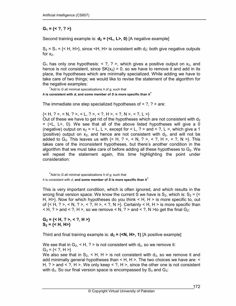
The Candidate-Elimination algorithm above is specified in terms of operations. The detailed implementation of these operations will depend on the specific problem and instances and their hypothesis space, however the algorithm can be applied to any concept learning task. We will now apply this algorithm to our designed problem SICK, to trace the working of each step of the algorithm. For comparison purposes, we will choose the exact training set that was employed in FIND-S:
D T BP SK
x1 H H 1 x2 L L 0 x3 N H 1
We know the initial values of G and S: G0 = {< ?, ? >} S0 = {< Ø, Ø >} Now the Candidate-Elimination learner starts: First training observation is: d1 = (<H, H>, 1) [A positive example] G1 = G0 = {< ?, ? >}, since <?, ?> is consistent with d1; both give positive outputs. Since S0 has only one hypothesis that is < Ø, Ø >, which implies S0(x1) = 0, which is not consistent with d1, so we have to remove < Ø, Ø > from S1. Also, we add minimally general hypotheses from H to S1, such that those hypotheses are consistent with d1. The obvious choices are like <H,H>, <H,N>, <H,L>, <N,H>……… <L,N>, <L,L>, but none of these except <H,H> is consistent with d1. So S1 becomes: S1 = {< H, H >}
Initialize G to the set of maximally general hypotheses in H Initialize S to the set of maximally specific hypotheses in H For each training example d, do If d is a positive example Remove from G any hypothesis inconsistent with d For each hypothesis s in S that is inconsistent with d Remove s from S Add to S all minimal generalization h of s, such that h is consistent with d, and some member of G is more general than h Remove from S any hypothesis that is more general than another one in S
If d is a negative example Remove from S any hypothesis inconsistent with d For each hypothesis g in G that is inconsistent with d Remove g from G Add to G all minimal specializations h of g, such that h is consistent with d, and some member of S is more specific than h Remove from G any hypothesis that is less general than another one in S
Artificial Intelligence (CS607)
© Copyright Virtual University of Pakistan 172
G1 = {< ?, ? >} Second training example is: d2 = (<L, L>, 0) [A negative example] S2 = S1 = {< H, H>}, since <H, H> is consistent with d2: both give negative outputs for x2. G1 has only one hypothesis: < ?, ? >, which gives a positive output on x2, and hence is not consistent, since SK(x2) = 0, so we have to remove it and add in its place, the hypotheses which are minimally specialized. While adding we have to take care of two things; we would like to revise the statement of the algorithm for the negative examples:
“Add to G all minimal specializations h of g, such that
h is consistent with d, and some member of S is more specific than h” The immediate one step specialized hypotheses of < ?, ? > are: {< H, ? >, < N, ? >, < L, ? >, < ?, H >, < ?, N >, < ?, L >} Out of these we have to get rid of the hypotheses which are not consistent with d2 = (<L, L>, 0). We see that all of the above listed hypotheses will give a 0 (negative) output on x2 = < L, L >, except for < L, ? > and < ?, L >, which give a 1 (positive) output on x2, and hence are not consistent with d2, and will not be added to G2. This leaves us with {< H, ? >, < N, ? >, < ?, H >, < ?, N >}. This takes care of the inconsistent hypotheses, but there’s another condition in the algorithm that we must take care of before adding all these hypotheses to G2. We will repeat the statement again, this time highlighting the point under consideration:
“Add to G all minimal specializations h of g, such that
h is consistent with d, and some member of S is more specific than h” This is very important condition, which is often ignored, and which results in the wrong final version space. We know the current S we have is S2, which is: S2 = {< H, H>}. Now for which hypotheses do you think < H, H > is more specific to, out of {< H, ? >, < N, ? >, < ?, H >, < ?, N >}. Certainly < H, H > is more specific than < H, ? > and < ?, H >, so we remove < N, ? > and < ?, N >to get the final G2: G2 = {< H, ? >, < ?, H >} S2 = {< H, H>} Third and final training example is: d3 = (<N, H>, 1) [A positive example] We see that in G2, < H, ? > is not consistent with d3, so we remove it: G3 = {< ?, H >} We also see that in S2, < H, H > is not consistent with d3, so we remove it and add minimally general hypotheses than < H, H >. The two choices we have are: < H, ? > and < ?, H >. We only keep < ?, H >, since the other one is not consistent with d3. So our final version space is encompassed by S3 and G3:
Artificial Intelligence (CS607)
© Copyright Virtual University of Pakistan 173
G3 = {< ?, H >} S3 = {< ?, H >} It is only a coincidence that both G and S sets are the same. In bigger problems, or even here if we had more examples, there was a chance that we’d get different but consistent sets. These two sets of G and S outline the version space of a concept. Note that the final hypothesis is the same one that was computed by FIND-S.
9.3 Decision trees learning
Up untill now we have been searching in conjunctive spaces which are formed by ANDing the attributes, for instance: IF Temperature = High AND Blood Pressure = High THEN Person = SICK But this is a very restrictive search, as we saw the reduction in hypothesis space from 29 total possible concepts to 17. This can be risky if we’re not sure if the true concept will lie in the conjunctive space. So a safer approach is to relax the searching constraints. One way is to involve OR into the search. Do you think we’ll have a bigger search space if we employ OR? Yes, most certainly; consider, for example, the statement: IF Temperature = High OR Blood Pressure = High THEN Person = SICK If we could use these kind of OR statements, we’d have a better chance of finding the true concept, if the concept does not lie in the conjunctive space. These are also called disjunctive spaces.
9.3.1 Decision tree representation
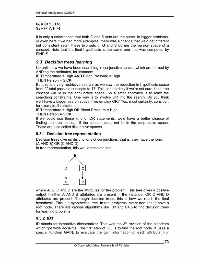
Decision trees give us disjunctions of conjunctions, that is, they have the form: (A AND B) OR (C AND D) In tree representation, this would translate into: where A, B, C and D are the attributes for the problem. This tree gives a positive output if either A AND B attributes are present in the instance; OR C AND D attributes are present. Through decision trees, this is how we reach the final hypothesis. This is a hypothetical tree. In real problems, every tree has to have a root node. There are various algorithms like ID3 and C4.5 to find decision trees for learning problems.
9.3.2 ID3
ID stands for interactive dichotomizer. This was the 3rd revision of the algorithm which got wide acclaims. The first step of ID3 is to find the root node. It uses a special function GAIN, to evaluate the gain information of each attribute. For
A
B
C
D
Artificial Intelligence (CS607)
© Copyright Virtual University of Pakistan 174
example if there are 3 instances, it will calculate the gain information for each. Whichever attribute has the maximum gain information, becomes the root node. The rest of the attributes then fight for the next slots.
9.3.2.1 Entropy In order to define information gain precisely, we begin by defining a measure commonly used in statistics and information theory, called entropy, which characterizes the purity/impurity of an arbitrary collection of examples. Given a collection S, containing positive and negative examples of some target concept, the entropy of S relative to this Boolean classification is: Entropy(S) = - p+log2 p+ - p-log2 p- where p+ is the proportion of positive examples in S and p- is the proportion of negative examples in S. In all calculations involving entropy we define 0log 0 to be 0. To illustrate, suppose S is a collection of 14 examples of some Boolean concept, including 9 positive and 5 negative examples, then the entropy of S relative to this Boolean classification is: Entropy(S) = - (9/14)log2 (9/14) - (5/14)log2 (5/14) = 0.940 Notice that the entropy is 0, if all the members of S belong to the same class (purity). For example, if all the members are positive (p+ = 1), then p- = 0 and so: Entropy(S) = - 1log2 1 - 0log2 0 = - 1 (0) - 0 [since log2 1 = 0, also 0log2 0 = 0] = 0 Note the entropy is 1 when the collection contains equal number of positive and negative examples (impurity). See for yourself by putting p+ and p- equal to 1/2. Otherwise if the collection contains unequal numbers of positive and negative examples, the entropy is between 0 and 1.
9.3.2.2 Information gain Given entropy as a measure of the impurity in a collection of training examples, we can now define a measure of the effectiveness of an attribute in classifying the training data. The measure we will use, called information gain, is simply the expected reduction in entropy caused by partitioning the examples according to this attribute. That is, if we use the attribute with the maximum information gain as the node, then it will classify some of the instances as positive or negative with 100% accuracy, and this will reduce the entropy for the remaining instances. We will now proceed to an example to explain further.
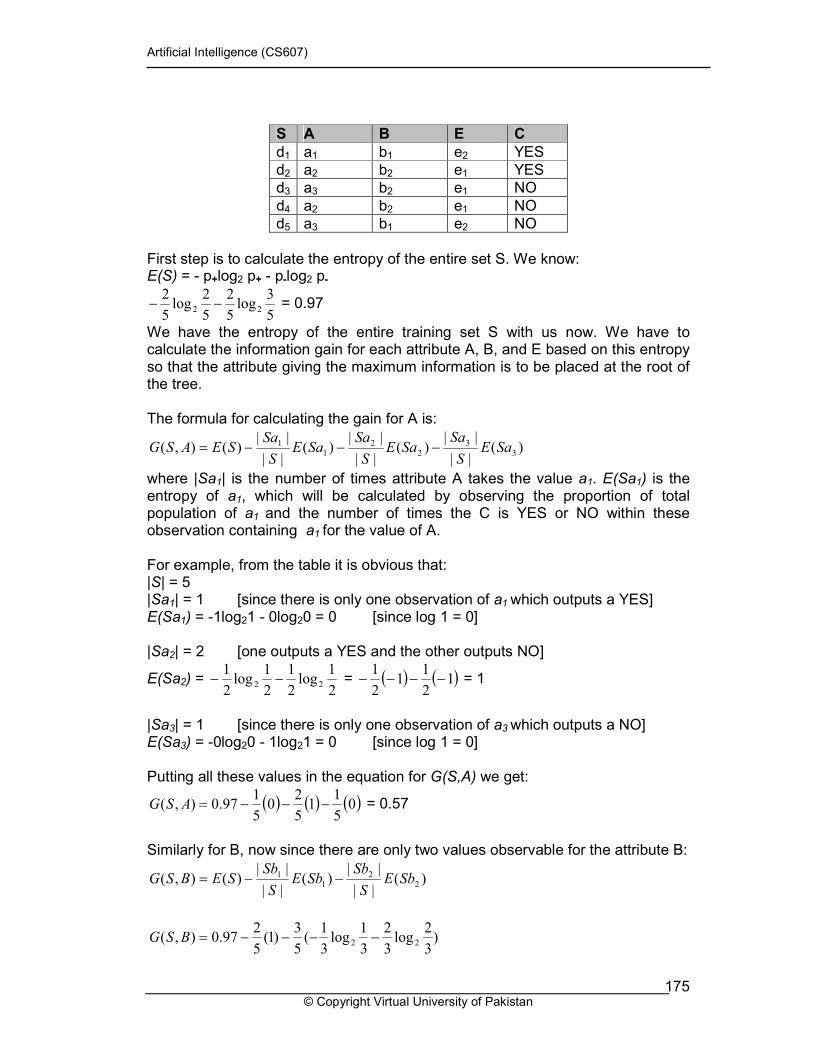
9.3.2.3 Example Suppose we have the following hypothetical training data available to us given in the table below. There are three attributes: A, B and E. Attribute A can take three values: a1, a2 and a3. Attribute B can take two values: b1 and b2. Attribute E can also take two values: e1 and e2. The concept to be learnt is a Boolean concept, so C takes a YES (1) or a NO (0), depending on the values of the attributes.
Artificial Intelligence (CS607)
© Copyright Virtual University of Pakistan 175
S A B E C
d1 a1 b1 e2 YES d2 a2 b2 e1 YES d3 a3 b2 e1 NO
d4 a2 b2 e1 NO d5 a3 b1 e2 NO
First step is to calculate the entropy of the entire set S. We know: E(S) = - p+log2 p+ - p-log2 p-
5
3log5
2
5
2log5
222 −− = 0.97
We have the entropy of the entire training set S with us now. We have to calculate the information gain for each attribute A, B, and E based on this entropy so that the attribute giving the maximum information is to be placed at the root of the tree. The formula for calculating the gain for A is:
)(||
||)(
||
||)(
||
||)(),( 3
32
21
1SaE
S
SaSaE
S
SaSaE
S
SaSEASG −−−=
where |Sa1| is the number of times attribute A takes the value a1. E(Sa1) is the entropy of a1, which will be calculated by observing the proportion of total population of a1 and the number of times the C is YES or NO within these observation containing a1 for the value of A. For example, from the table it is obvious that: |S| = 5 |Sa1| = 1 [since there is only one observation of a1 which outputs a YES] E(Sa1) = -1log21 - 0log20 = 0 [since log 1 = 0] |Sa2| = 2 [one outputs a YES and the other outputs NO]
E(Sa2) = 2
1log2
1
2
1log2
122 −− = ( ) ( )1
2
11
2
1−−−− = 1
|Sa3| = 1 [since there is only one observation of a3 which outputs a NO] E(Sa3) = -0log20 - 1log21 = 0 [since log 1 = 0] Putting all these values in the equation for G(S,A) we get:
( ) ( ) ( )05
11
5
20
5
197.0),( −−−=ASG = 0.57
Similarly for B, now since there are only two values observable for the attribute B:
)(||
||)(
||
||)(),( 2
21
1SbE
S
SbSbE
S
SbSEBSG −−=
)3
2log3
2
3
1log3
1(5
3)1(
5
297.0),( 22 −−−−=BSG
Artificial Intelligence (CS607)
© Copyright Virtual University of Pakistan 176
)39.052.0(5
34.097.0),( +−−=BSG = 0.02
Similarly for E
)(||
||)(
||
||)(),( 2
21
1SeE
S
SeSeE
S
SeSEESG −−= = 0.02
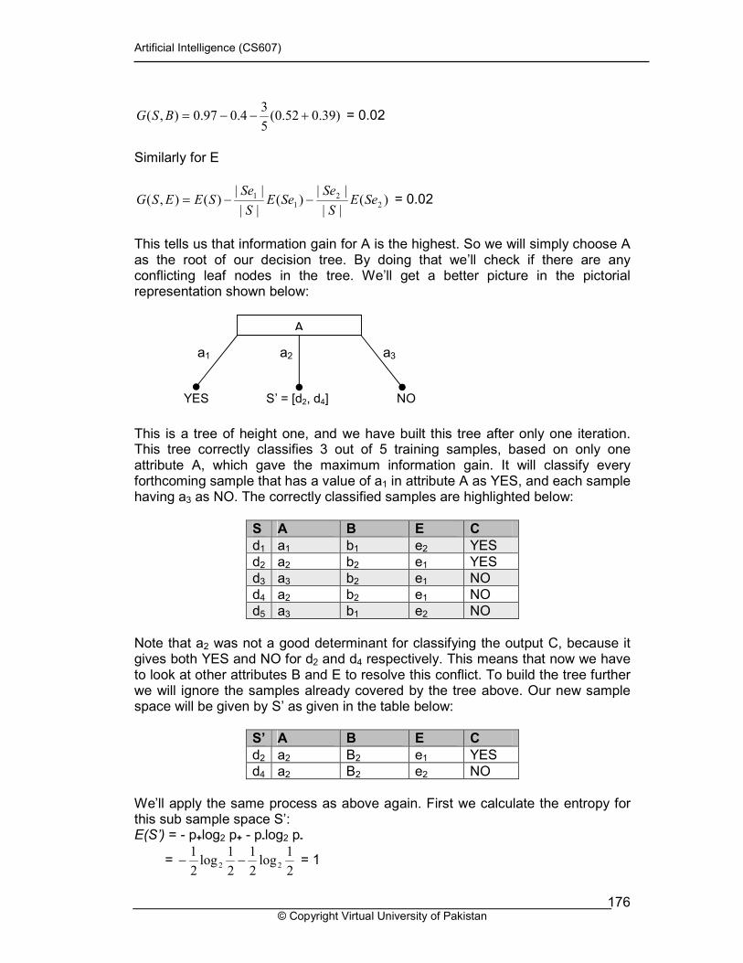
This tells us that information gain for A is the highest. So we will simply choose A as the root of our decision tree. By doing that we’ll check if there are any conflicting leaf nodes in the tree. We’ll get a better picture in the pictorial representation shown below: This is a tree of height one, and we have built this tree after only one iteration. This tree correctly classifies 3 out of 5 training samples, based on only one attribute A, which gave the maximum information gain. It will classify every forthcoming sample that has a value of a1 in attribute A as YES, and each sample having a3 as NO. The correctly classified samples are highlighted below:
S A B E C
d1 a1 b1 e2 YES d2 a2 b2 e1 YES d3 a3 b2 e1 NO d4 a2 b2 e1 NO d5 a3 b1 e2 NO
Note that a2 was not a good determinant for classifying the output C, because it gives both YES and NO for d2 and d4 respectively. This means that now we have to look at other attributes B and E to resolve this conflict. To build the tree further we will ignore the samples already covered by the tree above. Our new sample space will be given by S’ as given in the table below:
S’ A B E C
d2 a2 B2 e1 YES d4 a2 B2 e2 NO
We’ll apply the same process as above again. First we calculate the entropy for this sub sample space S’: E(S’) = - p+log2 p+ - p-log2 p-
= 2
1log2
1
2
1log2
122 −− = 1
S’ = [d2, d4] YES NO
a1 a2 a3
A
Artificial Intelligence (CS607)
© Copyright Virtual University of Pakistan 177
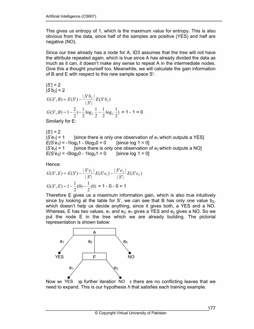
This gives us entropy of 1, which is the maximum value for entropy. This is also obvious from the data, since half of the samples are positive (YES) and half are negative (NO). Since our tree already has a node for A, ID3 assumes that the tree will not have the attribute repeated again, which is true since A has already divided the data as much as it can, it doesn’t make any sense to repeat A in the intermediate nodes. Give this a thought yourself too. Meanwhile, we will calculate the gain information of B and E with respect to this new sample space S’: |S’| = 2 |S’b2| = 2
)'(|'|
|'|)'(),'( 2
2bSE
S
bSSEBSG −=
)2
1log2
1
2
1log2
1(2
21),'( 22 −−−=BSG = 1 - 1 = 0
Similarly for E: |S’| = 2 |S’e1| = 1 [since there is only one observation of e1 which outputs a YES] E(S’e1) = -1log21 - 0log20 = 0 [since log 1 = 0] |S’e2| = 1 [since there is only one observation of e2 which outputs a NO] E(S’e2) = -0log20 - 1log21 = 0 [since log 1 = 0] Hence:
)'(|'|
|'|)'(
|'|
|'|)'(),'( 2
21
1eSE
S
eSeSE
S
eSSEESG −−=
)0(2
1)0(
2
11),'( −−=ESG = 1 - 0 - 0 = 1
Therefore E gives us a maximum information gain, which is also true intuitively since by looking at the table for S’, we can see that B has only one value b2, which doesn’t help us decide anything, since it gives both, a YES and a NO. Whereas, E has two values, e1 and e2; e1 gives a YES and e2 gives a NO. So we put the node E in the tree which we are already building. The pictorial representation is shown below: Now we will stop further iterations since there are no conflicting leaves that we need to expand. This is our hypothesis h that satisfies each training example.
YES NO
a1 a2 a3
YES NO
e1 e2
A
E
Artificial Intelligence (CS607)
© Copyright Virtual University of Pakistan 178
10 LEARNING: Connectionist Although ID3 spanned more of the concept space, but still there is a possibility that the true concept is not simply a mixture of disjunctions of conjunctions, but some more complex arrangement of attributes. (Artificial Neural Networks) ANNs can compute more complicated functions ranging from linear to any higher order quadratic, especially for non-Boolean concepts. This new learning paradigm takes its roots from biology inspired approach to learning. Its primarily a network of parallel distributed computing in which the focus of algorithms is on training rather than explicit programming. Tasks for which connectionist approach is well suited include: • Classification
• Fruits – Apple or orange • Pattern Recognition
• Finger print, Face recognition • Prediction
• Stock market analysis, weather forecast
10.1 Biological aspects and structure of a neuron
The brain is a collection of about 100 billion interconnected neurons. Each neuron is a cell that uses biochemical reactions to receive, process and transmit information. A neuron's dendritic tree is connected to a thousand neighboring neurons. When one of those neurons fire, a positive or negative charge is received by one of the dendrites. The strengths of all the received charges are added together through the processes of spatial and temporal summation. Spatial summation occurs when several weak signals are converted into a single large one, while temporal summation converts a rapid series of weak pulses from one source into one large signal. The aggregate input is then passed to the soma (cell body). The soma and the enclosed nucleus don't play a significant role in the processing of incoming and outgoing data. Their primary function is to perform the continuous maintenance required to keep the neuron functional. The part of the soma that does concern itself with the signal is the axon hillock. If the aggregate input is greater than the axon hillock's threshold value, then the neuron fires, and an output signal is transmitted down the axon. The strength of the output is constant, regardless of whether the input was just above the threshold, or a hundred times as great. The output strength is unaffected by the many divisions in the axon; it reaches each terminal button with the same intensity it had at the axon hillock. This uniformity is critical in an analogue device such as a brain where small errors can snowball, and where error correction is more difficult than in a digital system. Each terminal button is connected to other neurons across a small gap called a synapse.
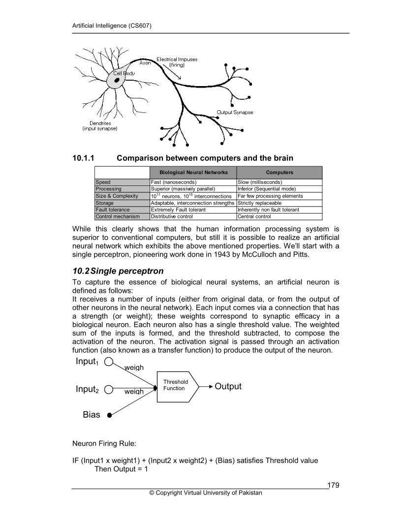
Artificial Intelligence (CS607)
© Copyright Virtual University of Pakistan 179
10.1.1 Comparison between computers and the brain
While this clearly shows that the human information processing system is superior to conventional computers, but still it is possible to realize an artificial neural network which exhibits the above mentioned properties. We’ll start with a single perceptron, pioneering work done in 1943 by McCulloch and Pitts.
10.2 Single perceptron
To capture the essence of biological neural systems, an artificial neuron is defined as follows: It receives a number of inputs (either from original data, or from the output of other neurons in the neural network). Each input comes via a connection that has a strength (or weight); these weights correspond to synaptic efficacy in a biological neuron. Each neuron also has a single threshold value. The weighted sum of the inputs is formed, and the threshold subtracted, to compose the activation of the neuron. The activation signal is passed through an activation function (also known as a transfer function) to produce the output of the neuron.
Neuron Firing Rule: IF (Input1 x weight1) + (Input2 x weight2) + (Bias) satisfies Threshold value Then Output = 1
Input1
Input2
Bias
Output Threshold Function
weigh
weigh
Biological Neural Networks Computers
Speed Fast (nanoseconds) Slow (milliseconds)
Processing Superior (massively parallel) Inferior (Sequential mode)
Size & Complexity 1011 neurons, 1015 interconnections Far few processing elements
Storage Adaptable, interconnection strengths Strictly replaceable
Fault tolerance Extremely Fault tolerant Inherently non fault tolerant
Control mechanism Distributive control Central control

Artificial Intelligence (CS607)
© Copyright Virtual University of Pakistan 180
Else Output = 0
10.2.1 Response of changing bias
The response of changing the bias of a neuron results in shifting the decision line up or down, as shown by the following figures taken from matlab.
10.2.2 Response of changing weight
The change in weight results in the rotation of the decision line. Hence this up and down shift, together with the rotation of the straight line can achieve any linear decision.
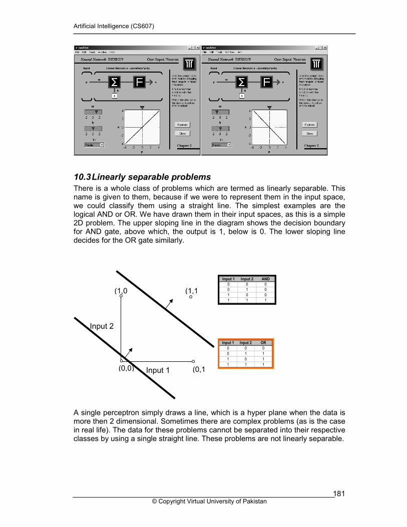
Artificial Intelligence (CS607)
© Copyright Virtual University of Pakistan 181
10.3 Linearly separable problems
There is a whole class of problems which are termed as linearly separable. This name is given to them, because if we were to represent them in the input space, we could classify them using a straight line. The simplest examples are the logical AND or OR. We have drawn them in their input spaces, as this is a simple 2D problem. The upper sloping line in the diagram shows the decision boundary for AND gate, above which, the output is 1, below is 0. The lower sloping line decides for the OR gate similarly.
A single perceptron simply draws a line, which is a hyper plane when the data is more then 2 dimensional. Sometimes there are complex problems (as is the case in real life). The data for these problems cannot be separated into their respective classes by using a single straight line. These problems are not linearly separable.
(0,0) (0,1
(1,0
Input 2
Input 1
Input 1 Input 2 AND
0 0 0
0 1 0
1 0 0
1 1 1
Input 1 Input 2 OR
0 0 0
0 1 1
1 0 1
1 1 1
(1,1
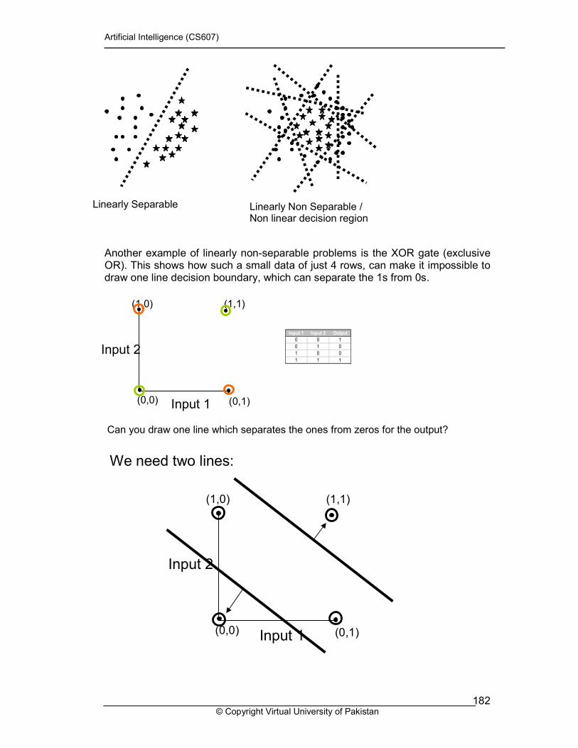
Artificial Intelligence (CS607)
© Copyright Virtual University of Pakistan 182
Another example of linearly non-separable problems is the XOR gate (exclusive OR). This shows how such a small data of just 4 rows, can make it impossible to draw one line decision boundary, which can separate the 1s from 0s.
Linearly Separable Linearly Non Separable / Non linear decision region
Input 1 Input 2 Output
0 0 1
0 1 0
1 0 0
1 1 1
(0,0) (0,1)
(1,0)
Input 2
Input 1
(1,1)
Can you draw one line which separates the ones from zeros for the output?
(0,0) (0,1)
(1,0)
Input 2
Input 1
(1,1)
We need two lines:
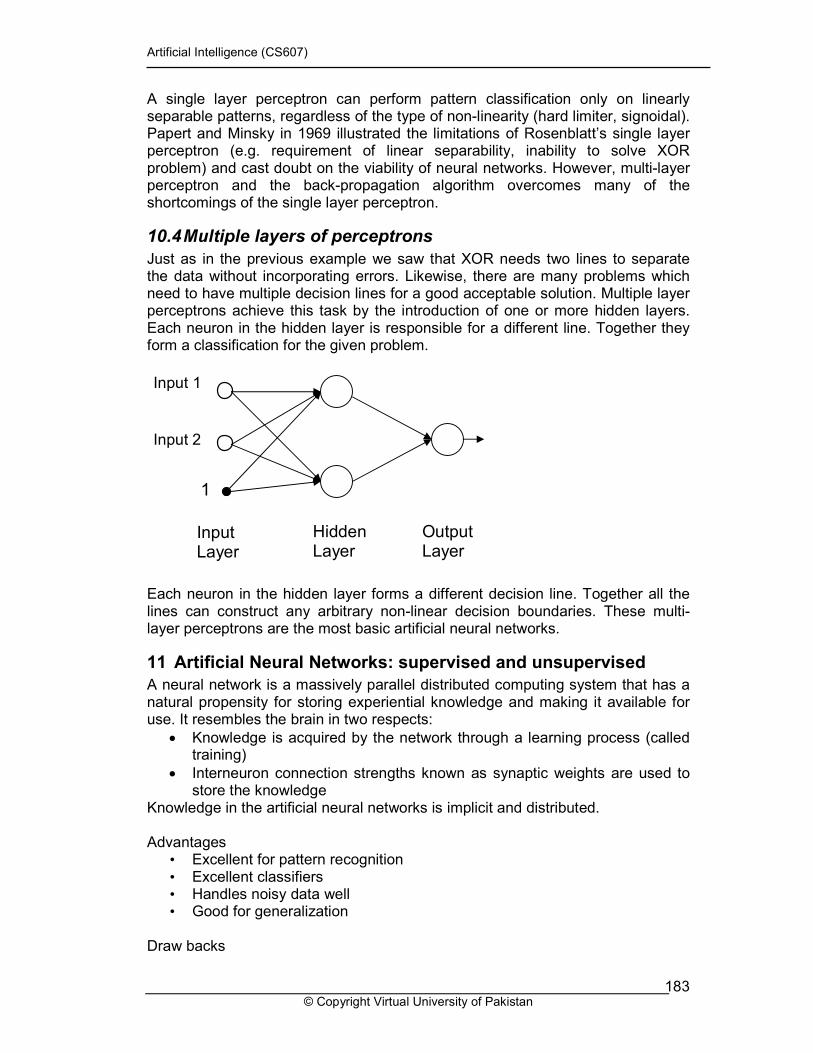
Artificial Intelligence (CS607)
© Copyright Virtual University of Pakistan 183
A single layer perceptron can perform pattern classification only on linearly separable patterns, regardless of the type of non-linearity (hard limiter, signoidal). Papert and Minsky in 1969 illustrated the limitations of Rosenblatt’s single layer perceptron (e.g. requirement of linear separability, inability to solve XOR problem) and cast doubt on the viability of neural networks. However, multi-layer perceptron and the back-propagation algorithm overcomes many of the shortcomings of the single layer perceptron.
10.4 Multiple layers of perceptrons
Just as in the previous example we saw that XOR needs two lines to separate the data without incorporating errors. Likewise, there are many problems which need to have multiple decision lines for a good acceptable solution. Multiple layer perceptrons achieve this task by the introduction of one or more hidden layers. Each neuron in the hidden layer is responsible for a different line. Together they form a classification for the given problem.
Each neuron in the hidden layer forms a different decision line. Together all the lines can construct any arbitrary non-linear decision boundaries. These multi-layer perceptrons are the most basic artificial neural networks.
11 Artificial Neural Networks: supervised and unsupervised
A neural network is a massively parallel distributed computing system that has a natural propensity for storing experiential knowledge and making it available for use. It resembles the brain in two respects:
• Knowledge is acquired by the network through a learning process (called training)
• Interneuron connection strengths known as synaptic weights are used to store the knowledge
Knowledge in the artificial neural networks is implicit and distributed. Advantages • Excellent for pattern recognition • Excellent classifiers • Handles noisy data well • Good for generalization
Draw backs
Input 1
1
Input 2
Input Layer
Hidden Layer
Output Layer
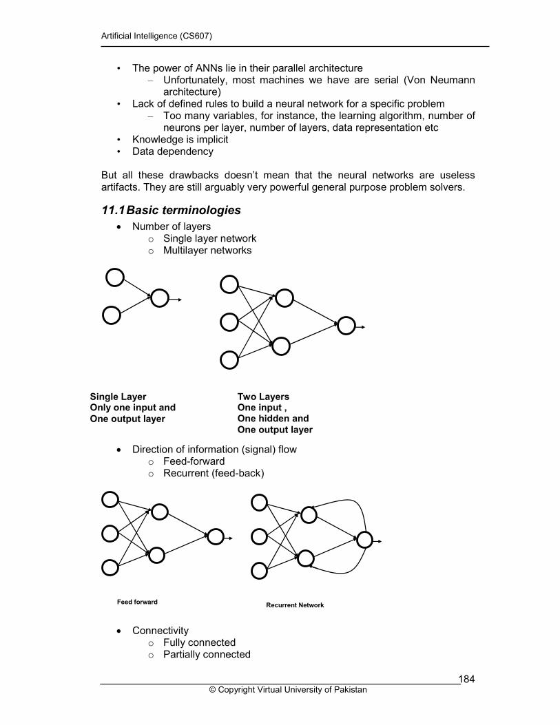
Artificial Intelligence (CS607)
© Copyright Virtual University of Pakistan 184
• The power of ANNs lie in their parallel architecture – Unfortunately, most machines we have are serial (Von Neumann
architecture) • Lack of defined rules to build a neural network for a specific problem
– Too many variables, for instance, the learning algorithm, number of neurons per layer, number of layers, data representation etc
• Knowledge is implicit • Data dependency
But all these drawbacks doesn’t mean that the neural networks are useless artifacts. They are still arguably very powerful general purpose problem solvers.
11.1 Basic terminologies
• Number of layers o Single layer network o Multilayer networks
• Direction of information (signal) flow
o Feed-forward o Recurrent (feed-back)
• Connectivity o Fully connected o Partially connected
Single Layer Only one input and One output layer
Two Layers One input , One hidden and One output layer
Feed forward Recurrent Network
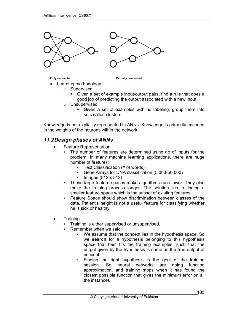
Artificial Intelligence (CS607)
© Copyright Virtual University of Pakistan 185
• Learning methodology
o Supervised � Given a set of example input/output pairs, find a rule that does a
good job of predicting the output associated with a new input. o Unsupervised
� Given a set of examples with no labeling, group them into sets called clusters
Knowledge is not explicitly represented in ANNs. Knowledge is primarily encoded in the weights of the neurons within the network
11.2 Design phases of ANNs
• Feature Representation • The number of features are determined using no of inputs for the
problem. In many machine learning applications, there are huge number of features: • Text Classification (# of words) • Gene Arrays for DNA classification (5,000-50,000) • Images (512 x 512)
• These large feature spaces make algorithms run slower. They also make the training process longer. The solution lies in finding a smaller feature space which is the subset of existing features.
• Feature Space should show discrimination between classes of the data. Patient’s height is not a useful feature for classifying whether he is sick or healthy
• Training • Training is either supervised or unsupervised. • Remember when we said:
• We assume that the concept lies in the hypothesis space. So we search for a hypothesis belonging to this hypothesis space that best fits the training examples, such that the output given by the hypothesis is same as the true output of concept
• Finding the right hypothesis is the goal of the training session. So neural networks are doing function approximation, and training stops when it has found the closest possible function that gives the minimum error on all the instances
Fully connected Partially connected
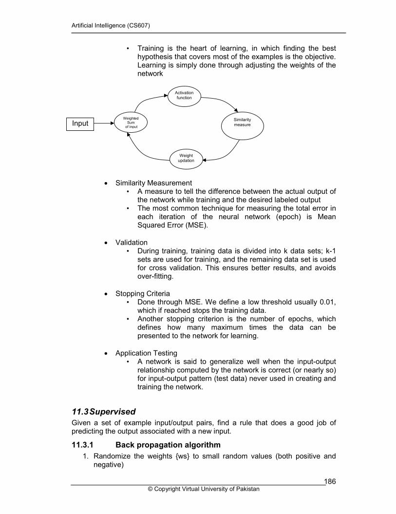
Artificial Intelligence (CS607)
© Copyright Virtual University of Pakistan 186
• Training is the heart of learning, in which finding the best hypothesis that covers most of the examples is the objective. Learning is simply done through adjusting the weights of the network
• Similarity Measurement • A measure to tell the difference between the actual output of
the network while training and the desired labeled output • The most common technique for measuring the total error in
each iteration of the neural network (epoch) is Mean Squared Error (MSE).
• Validation • During training, training data is divided into k data sets; k-1
sets are used for training, and the remaining data set is used for cross validation. This ensures better results, and avoids over-fitting.
• Stopping Criteria • Done through MSE. We define a low threshold usually 0.01,
which if reached stops the training data. • Another stopping criterion is the number of epochs, which
defines how many maximum times the data can be presented to the network for learning.
• Application Testing • A network is said to generalize well when the input-output
relationship computed by the network is correct (or nearly so) for input-output pattern (test data) never used in creating and training the network.
11.3 Supervised
Given a set of example input/output pairs, find a rule that does a good job of predicting the output associated with a new input.
11.3.1 Back propagation algorithm
1. Randomize the weights {ws} to small random values (both positive and negative)
Weighted Sum
of input
Similarity measure
Activation function
Weight updation
Input
Artificial Intelligence (CS607)
© Copyright Virtual University of Pakistan 187
2. Select a training instance t, i.e., a. the vector {xk(t)}, i = 1,...,Ninp (a pair of input and output patterns),
from the training set 3. Apply the network input vector to network input 4. Calculate the network output vector {zk(t)}, k = 1,...,Nout 5. Calculate the errors for each of the outputs k , k=1,...,Nout, the difference
between the desired output and the network output 6. Calculate the necessary updates for weights -ws in a way that minimizes
this error 7. Adjust the weights of the network by - ws 8. Repeat steps for each instance (pair of input–output vectors) in the training
set until the error for the entire system
11.4 Unsupervised
• Given a set of examples with no labeling, group them into sets called clusters
• A cluster represents some specific underlying patterns in the data
• Useful for finding patterns in large data sets
• Form clusters of input data
• Map the clusters into outputs
• Given a new example, find its cluster, and generate the associated output
11.4.1 Self-organizing neural networks: clustering, quantization, function approximation, Kohonen maps
1. Each node's weights are initialized 2. A data input from training data (vector) is chosen at random and presented
to the cluster lattice 3. Every cluster centre is examined to calculate which weights are most like
the input vector. The winning node is commonly known as the Best Matching Unit (BMU)
4. The radius of the neighborhood of the BMU is now calculated. Any nodes found within this radius are deemed to be inside the BMU's neighborhood
5. Each neighboring node's (the nodes found in step 4) weights are adjusted to make them more like the input vector. The closer a node is to the BMU, the more its weights get altered
6. Repeat steps for N iterations
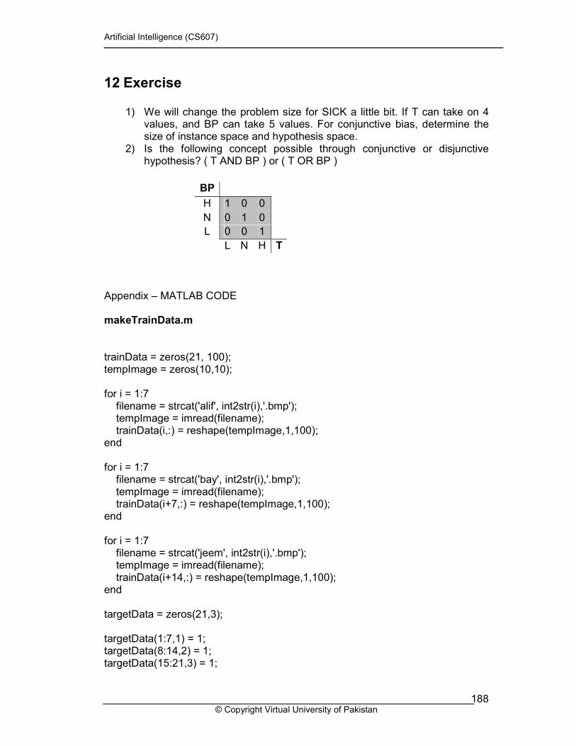
Artificial Intelligence (CS607)
© Copyright Virtual University of Pakistan 188
12 Exercise
1) We will change the problem size for SICK a little bit. If T can take on 4 values, and BP can take 5 values. For conjunctive bias, determine the size of instance space and hypothesis space.
2) Is the following concept possible through conjunctive or disjunctive hypothesis? ( T AND BP ) or ( T OR BP )
Appendix – MATLAB CODE makeTrainData.m trainData = zeros(21, 100); tempImage = zeros(10,10); for i = 1:7 filename = strcat('alif', int2str(i),'.bmp'); tempImage = imread(filename); trainData(i,:) = reshape(tempImage,1,100); end for i = 1:7 filename = strcat('bay', int2str(i),'.bmp'); tempImage = imread(filename); trainData(i+7,:) = reshape(tempImage,1,100); end for i = 1:7 filename = strcat('jeem', int2str(i),'.bmp'); tempImage = imread(filename); trainData(i+14,:) = reshape(tempImage,1,100); end targetData = zeros(21,3); targetData(1:7,1) = 1; targetData(8:14,2) = 1; targetData(15:21,3) = 1;
BP
H 1 0 0
N 0 1 0
L 0 0 1
L N H T

Artificial Intelligence (CS607)
© Copyright Virtual University of Pakistan 189
save 'trainData' trainData targetData ; makeTestData.m testData = zeros(9, 100); tempImage = zeros(10,10); for i = 1:3 filename = strcat('alif', int2str(i),'.bmp'); tempImage = imread(filename); testData(i,:) = reshape(tempImage,1,100); end for i = 1:3 filename = strcat('bay', int2str(i),'.bmp'); tempImage = imread(filename); testData(i+3,:) = reshape(tempImage,1,100); end for i = 1:3 filename = strcat('jeem', int2str(i),'.bmp'); tempImage = imread(filename); testData(i+6,:) = reshape(tempImage,1,100); end targetData = zeros(9,3); targetData(1:3,1) = 1; targetData(4:6,2) = 1; targetData(7:9,3) = 1; save 'testData' testData targetData;

Artificial Intelligence (CS607)
© Copyright Virtual University of Pakistan 190
trainNN.m load 'trainData.mat'; minMax = [min(trainData) ; max(trainData)]'; bpn = newff(minMax, [10 3],{'tansig' 'tansig'}); bpn.trainParam.epochs = 15; bpn.trainParam.goal = 0.01; bpn = train(bpn,trainData',targetData'); save 'bpnNet' bpn; testNN.m load('trainData'); load('bpnNet'); Y = sim(bpn, trainData'); [X,I] = max(Y); errorCount = 0; for i = 1 : length(targetData) if ceil(i/7) ~= I(i) errorCount = errorCount + 1; end end percentageAccuracyOnTraining = (1-(errorCount/length(targetData))) * 100 %%%%%%%%%%%%%%%%%%%%%%%%%% load('testData'); Y = sim(bpn, testData'); [X,I] = max(Y); errorCount = 0; for i = 1 : length(targetData) if ceil(i/3) ~= I(i) errorCount = errorCount + 1; end end percentageAccuracyOnTesting = (1-(errorCount/length(targetData))) * 100

Artificial Intelligence (CS607)
© Copyright Virtual University of Pakistan 191
13 Planning
13.1 Motivation
We started study of AI with the classical approach of problem solving that founders of AI used to exhibit intelligence in programs. If you look at problem solving again you might now be able to imagine that for realistically complex problems too problem solving could work. But when you think more you might guess that there might be some limitation to this old approach. Lets take an example. I have just landed on Lahore airport as a cricket-loving tourist. I have to hear cricket commentary live on radio at night at a hotel where I have to reserve a room. For doing that, I have to find the hotel to get my room reserved before its too late, and also I have to find the market to buy the radio from. Now this is a more realistic problem. Is this a tougher problem? Let’s see. One thing easily visible is that this problem can be broken into multiple problems i.e. is composed of small problems like finding market and finding the hotel. Another observation is that different things are dependent on others like listening to radio is dependent upon the sub-problem of buying the radio or finding the market. Ignore the observations made above for a moment. If we start formulating this problem as usual, be assured that the state design will have more information in it. There will be more operators. Consequently, the search tree we generate will be much bigger. The poor system that will run this search will have much more load than any of the examples we have studied so far. The search tree will consume more space and it will take more calculations in the process. A state design and operators for the sample problem formulation could be as shown in figure.
Turn right Turn left Move forward Buy radio Get reservation Listen radio Sleep And maybe more…
Initial state Operators Figure – Sample problem formulation
If we apply say, BFS in this problem the tree can easily become something huge like this rough illustration.
Location Has radio? Sells radio? IsHotel? IsMarket? Reservation done? And maybe more…

Artificial Intelligence (CS607)
© Copyright Virtual University of Pakistan 192
Figure – Search space of a moderate problem
Although this tree is just a depiction of how a search space grows for realistic problems, yet after seeing this tree we can very well imagine for even more complex problems that the search tree could be too big, big enough to trouble us. So the question is, can we make such inefficient problem solving any better? Good news is that the answer is yes. How? Simply speaking, this ‘search’ technique could be improved
by acting a bit logically instead of blindly. For example not using operators at a state where their usage is illogical. Like operator ‘sleeping’ should not be even tried to generate children nodes from a state where I am not at the hotel, or even haven’t reserved the room. The field of acting logically to solve problems is known as Planning. Planning is based on logic representation that we have already studied, so you will not find it too difficult and thus we have kept it short.
13.2 Definition of Planning
The key in planning is to use logic in order to solve problem elegantly. People working in AI have devised different techniques and algorithms for planning. We will now introduce a basic definition of planning. Planning is an advanced form problem solving which generates a sequence of operators that guarantee the goal. Furthermore, such sequence of operators or actions (commonly used in planning literature) is called a plan.
Location=Airport Has radio?=No Sells radio?=No IsHotel?=No IsMarket?=No ReservationDone?=No . .
Location=Airport Has radio?=No Sells radio?=No IsHotel?=No IsMarket?=No ReservationDone?=No . . .
BuyRadio
XXX
XXX
XXX
XXX
XXX
XXX
XXX
XXX
XXX
TurnRight TurnLeft
Artificial Intelligence (CS607)
© Copyright Virtual University of Pakistan 193
13.3 Planning vs. problem solving
Planning introduces the following improvements with respect to classical problem solving:
• Each state is represented in predicate logic. De-facto representation of a state is the conjunction (AND) of predicates that are true in that state.
• The goal is also represented as states, i.e. conjunction of predicates.
• Each action (or operator) is associated with some logic preconditions that must be true for that action to be applied. Thus a planning system can avoid any action that is just not possible at a particular state.
• Each action is associated with an ‘effect’ or post-conditions. These post-conditions specify the added and/or deleted predicates when the action is applied.
• The inference mechanism used is that of backward chaining so as to use only the actions and states that are really required to reach goal state.
• Optional: The sequence of actions (plan) is minimally ordered. Only those actions are ordered in a sequence when any other order will not achieve the desired goal. Therefore, planning allows partial ordering i.e. there can be two actions that are not in any order from each other because any particular order used amongst them will achieve the same goal.
13.4 Planning language
STRIPS is one of the founding languages developed particularly for planning. Let us understand planning to a better level by seeing what a planning language can represent.
13.4.1 Condition predicates
Condition predicates are the predicates that define states. For example, a predicate that specifies that we are at location ‘X’ is given as. at(X)
13.4.2 State
State is a conjunction of predicates represented in well-known form, for example, a state where we are at the hotel and do not have either cash or radio is represented as, at(hotel) ∧ ¬have(cash) ∧ ¬have(radio)
13.4.3 Goal
Goal is also represented in the same manner as a state. For example, if the goal of a planning problem is to be at the hotel with radio, it is represented as, at(hotel) ∧ have(radio)
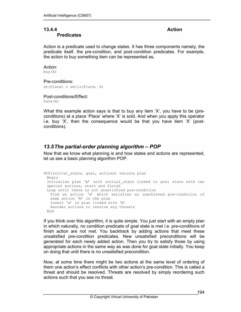
Artificial Intelligence (CS607)
© Copyright Virtual University of Pakistan 194
13.4.4 Action Predicates
Action is a predicate used to change states. It has three components namely, the predicate itself, the pre-condition, and post-condition predicates. For example, the action to buy something item can be represented as, Action: buy(X)
Pre-conditions: at(Place) ∧ sells(Place, X)
Post-conditions/Effect: have(X)
What this example action says is that to buy any item ‘X’, you have to be (pre-conditions) at a place ‘Place’ where ‘X’ is sold. And when you apply this operator i.e. buy ‘X’, then the consequence would be that you have item ‘X’ (post-conditions).
13.5 The partial-order planning algorithm – POP
Now that we know what planning is and how states and actions are represented, let us see a basic planning algorithm POP. POP(initial_state, goal, actions) returns plan
Begin
Initialize plan ‘p’ with initial_state linked to goal state with two
special actions, start and finish Loop until there is not unsatisfied pre-condition
Find an action ‘a’ which satisfies an unachieved pre-condition of some action ‘b’ in the plan
Insert ‘a’ in plan linked with ‘b’ Reorder actions to resolve any threats
End
If you think over this algorithm, it is quite simple. You just start with an empty plan in which naturally, no condition predicate of goal state is met i.e. pre-conditions of finish action are not met. You backtrack by adding actions that meet these unsatisfied pre-condition predicates. New unsatisfied preconditions will be generated for each newly added action. Then you try to satisfy those by using appropriate actions in the same way as was done for goal state initially. You keep on doing that until there is no unsatisfied precondition. Now, at some time there might be two actions at the same level of ordering of them one action’s effect conflicts with other action’s pre-condition. This is called a threat and should be resolved. Threats are resolved by simply reordering such actions such that you see no threat.
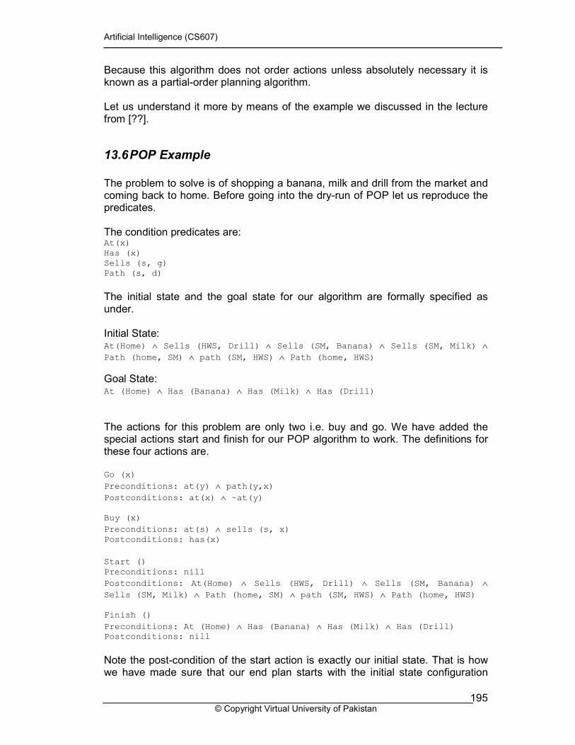
Artificial Intelligence (CS607)
© Copyright Virtual University of Pakistan 195
Because this algorithm does not order actions unless absolutely necessary it is known as a partial-order planning algorithm. Let us understand it more by means of the example we discussed in the lecture from [??].
13.6 POP Example
The problem to solve is of shopping a banana, milk and drill from the market and coming back to home. Before going into the dry-run of POP let us reproduce the predicates. The condition predicates are: At(x)
Has (x)
Sells (s, g)
Path (s, d)
The initial state and the goal state for our algorithm are formally specified as under. Initial State: At(Home) ∧ Sells (HWS, Drill) ∧ Sells (SM, Banana) ∧ Sells (SM, Milk) ∧
Path (home, SM) ∧ path (SM, HWS) ∧ Path (home, HWS)
Goal State: At (Home) ∧ Has (Banana) ∧ Has (Milk) ∧ Has (Drill)
The actions for this problem are only two i.e. buy and go. We have added the special actions start and finish for our POP algorithm to work. The definitions for these four actions are. Go (x)
Preconditions: at(y) ∧ path(y,x)
Postconditions: at(x) ∧ ~at(y)
Buy (x)
Preconditions: at(s) ∧ sells (s, x)
Postconditions: has(x)
Start ()
Preconditions: nill
Postconditions: At(Home) ∧ Sells (HWS, Drill) ∧ Sells (SM, Banana) ∧
Sells (SM, Milk) ∧ Path (home, SM) ∧ path (SM, HWS) ∧ Path (home, HWS)
Finish ()
Preconditions: At (Home) ∧ Has (Banana) ∧ Has (Milk) ∧ Has (Drill) Postconditions: nill
Note the post-condition of the start action is exactly our initial state. That is how we have made sure that our end plan starts with the initial state configuration
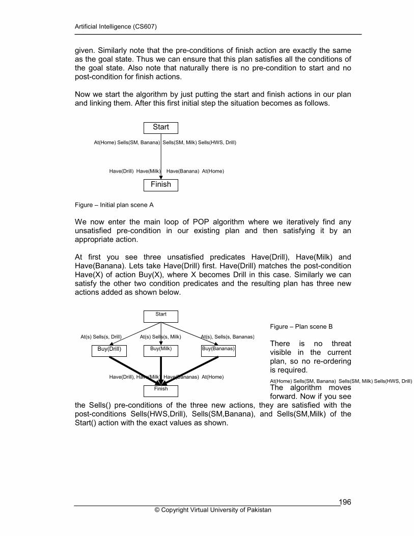
Artificial Intelligence (CS607)
© Copyright Virtual University of Pakistan 196
given. Similarly note that the pre-conditions of finish action are exactly the same as the goal state. Thus we can ensure that this plan satisfies all the conditions of the goal state. Also note that naturally there is no pre-condition to start and no post-condition for finish actions. Now we start the algorithm by just putting the start and finish actions in our plan and linking them. After this first initial step the situation becomes as follows. Figure – Initial plan scene A
We now enter the main loop of POP algorithm where we iteratively find any unsatisfied pre-condition in our existing plan and then satisfying it by an appropriate action. At first you see three unsatisfied predicates Have(Drill), Have(Milk) and Have(Banana). Lets take Have(Drill) first. Have(Drill) matches the post-condition Have(X) of action Buy(X), where X becomes Drill in this case. Similarly we can satisfy the other two condition predicates and the resulting plan has three new actions added as shown below.
Figure – Plan scene B
There is no threat visible in the current plan, so no re-ordering is required. The algorithm moves forward. Now if you see
the Sells() pre-conditions of the three new actions, they are satisfied with the post-conditions Sells(HWS,Drill), Sells(SM,Banana), and Sells(SM,Milk) of the Start() action with the exact values as shown.
At(Home) Sells(SM, Banana) Sells(SM, Milk) Sells(HWS, Drill)
Start
At(Home) Sells(SM, Banana) Sells(SM, Milk) Sells(HWS, Drill)
Finish
Have(Drill) Have(Milk) Have(Banana) At(Home)
Start
At(s) Sells(s, Drill) At(s) Sells(s, Milk) At(s), Sells(s, Bananas)
Finish
Have(Drill), Have(Milk), Have(Bananas) At(Home)
Buy(Drill) Buy(Milk) Buy(Bananas)
Artificial Intelligence (CS607)
© Copyright Virtual University of Pakistan 197
Figure – Plan scene C
We now move forward and see what other pre-conditions are not satisfied. At(HWS) is not satisfied in action Buy(Drill). Similarly At(SM) is not satisfied in actions Buy(Milk) and Buy(Banana). Only action Go() has post-conditions that can satisfy these pre-conditions. Adding them one-by-one to satisfy all these pre-conditions our plan becomes,
Figure – Plan scene D
Now if we check for threats we find that if we go to HWS from Home we cannot go to SM from Home. Meaning, post-condition of
Go(HWS) threats the pre-
condition At(Home) of Go(SM) and vice versa. So as
given in our POP algorithm, we have to resolve the threat by reordering these actions such that no action threat pre-conditions of other action. That is how POP proceeds by adding actions to satisfy preconditions and reordering actions to resolve any threat in the plan. The final plan using this algorithm becomes.
Start
At(HWS), Sells(HWS, Drill) At(SM), Sells(SM, Milk) At(SM), Sells(SM, Bananas)
Finish
Have(Drill), Have(Milk), Have(Bananas) At(Home)
Buy(Drill) Buy(Milk) Buy(Bananas)
Start
At(HWS), Sells(HWS, Drill) At(SM), Sells(SM, Milk) At(SM), Sells(SM, Bananas)
Finish
Have(Drill), Have(Milk), Have(Bananas) At(Home)
Buy(Drill) Buy(Milk) Buy(Bananas)
Go(HWS) Go(SM)
At(Home) At(Home)

Artificial Intelligence (CS607)
© Copyright Virtual University of Pakistan 198
Figure – Plan scene E
You can see how reordering is done from this illustration. For example the threat we
observed between
Go(HWS) and Go(SM), the link from Start to Go(SM) has been deleted and a new links
have been established from Go(HWS) and Buy(Drill) to Go(SM). To feel more comfortable on the plan we have achieved from this problem, lets narrate our solution in plain English. “Start by going to hardware store. Then you can buy drill and then go to the super market. At the super market, buy milk and banana in any order and then go home. You are done.”
13.7 Problems
1. A Farmer has a tiger, a goat and a bundle of grass. He is standing at one
side of the river with a very week boat which can hold only one of his belongings at a time. His goal is has to take all three of his belongings to the other side. The constraint is that the farmer cannot leave either goat and tiger, or goat and grass, at any side of the river unattended because one of them will eat the other. Using the simple POP algorithm we studied in the lecture, solve this problem. Show all the intermediate and final plans step by step.
2. A robot has three slots available to put the blocks A, B, C. The blocks are
initially placed at slot 1, one upon the other (A placed on B placed on C) and it’s goal is to move all three to slot 3 in the same order. The constraint to this robot is that it can only move one block from any slot to any other slot, and it can only pick the top most block from a slot to move. Using the simple POP algorithm we studied in the lecture, solve this problem. Show all the intermediate and final plans step by step.
Start
At(HWS), Sells(HWS, Drill) At(SM), Sells(SM, Milk) At(SM), Sells(SM, Bananas)
Finish
Have(Drill), Have(Milk), Have(Bananas) At(Home)
Buy(Drill) Buy(Milk) Buy(Bananas)
Go(HWS) Go(SM)
At(Home) At(Home)
Go(Home)
Artificial Intelligence (CS607)
© Copyright Virtual University of Pakistan 199
14 Computer vision It is a subfield of Artificial Intelligence. The purpose of computer vision is to study algorithms, techniques and applications that help us make machines that can "understand" images and videos. In other words, it deals with procedures that extract useful information from static pictures and sequence of images. Enabling a machine to see, percieve and understand exactly as humans see, percieve and understand is the aim of Computer Vision. Computer vision finds its applications in medicine, military, security and surveillance, quality inspection, robotics, automotive industry and many other areas. Few areas of vision in which research is benig actively conducted thoughout the world are as follows:
� The detection, segmentation, localisation, and recognition of certain objects in images (e.g., human faces)
� Tracking an object through an image sequence
� Object Extraction from a video sequence
� Automated Navigation of a robot or a vehicle
� Estimation of the three-dimensional pose of humans and their limbs
� Medical Imaging, automated analysis of different body scans (CT Scan,
Bone Scan, X-Rays)
� Searching for digital images by their content (content-based image retrieval)
� Registration of different views of the same scene or object
Computer vision encompases topics from pattern recognition, machine learning, geometry, image processing, artificial intelligence, linear algebra and other subjects. Apart from its applications, computer vision is itself interesting to study. Many detailed turorials regarding the field are freely avalible on the internet. Readers of this text are encouraged to read though these tutorials get indepth knowledge about the limits and contents of the field.
14.1 Exercise Question
Search though the internet and read about intersting happeneing and reseach going on around the globe in the are of Computer Vision.

Artificial Intelligence (CS607)
© Copyright Virtual University of Pakistan 200
http://www.cs.ucf.edu/~vision/ The above link might be useful to explore knowledge about computer vision.
15 Robotics Robotics is the highly advanced and totally hyped field of today. Literally speaking, robotics is the study of robots. Robots are nothing but a complex combination of hardware and intelligence, or mechanics and brains. Thus robotics is truly a multi-disciplinary area, having active contributions from, physics, mechanics, biology, mathematics, computer science, statistics, control thory, philosophy, etc. The features that constitute a robot are:
• Mobility
• Perception
• Planning
• Searching
• Reasoning
• Dealing with uncertainty
• Vision
• Learning
• Autonomy
• Physical Intelligence What we can see from the list is that robotics is the most profound manifestation of AI in practice. The most crucial or defining ones from the list above are mobility, autonomy and dealing with uncertainety The area of robotics have been followed with enthusiasm by masses from fiction, science and industry. Now robots have entered the common household, as robot pets (Sony Aibo entertainment robot), oldage assistant and people carriers (Segway human transporter).
15.1 Exercise Question
Search though the internet and read about intersting happeneing and reseach going on around the globe in the are of robotics. http://www.cs.dartmouth.edu/~brd/Teaching/AI/Lectures/Summaries/robotics.html The above link might be useful to explore knowledge about robotics.
16 Softcomputing
Artificial Intelligence (CS607)
© Copyright Virtual University of Pakistan 201
Softcomputing is a relatively new term coined to encapsulate the emergence of new hybrid area of work in AI. Different technologies including fuzzy systems, genetic algorithms, neural networks and a few statistical methods have been combined together in different orientations to successfully solve today’s complex real-world problems. The most common combinations are of the pairs
• genetic algorithms – fuzzy systems (genetic fuzzy)
• Neural Networks – fuzzy systems (neuro-fuzzy systems)
• Genetic algorithms – Neural Networks (neuro-genetic systems) Softcomputing is naturally applied in machine learning applications. For example one usage of genetic-fuzzy system is of ‘searching’ for an acceptable fuzzy system that conforms to the training data. In which, fuzzy sets and rules combined, are encoded as individuals, and GA iterations refine the individuals i.e. fuzzy system, on the basis of their fitness evaluations. The fitness function is usually MSE of the invidual fuzzy system on the training data. Very similar applications have been developed in the other popular neuro-fuzzy systems, in which neural networks are used to find the best fuzzy system for the given data through means of classical ANN learning algorithms. Genetic algorithms have been employed in finding the optimal initial weights of neural networks.
16.1 Exercise Question
Search though the internet and read about intersting happeneing and reseach going on around the globe in the are of softcomputing. http://www.soft-computing.de/ The above link might be useful to explore knowledge about softcomputing.
17 Clustering Clustering is a form of unsupervised learning, in which the training data is available but without the classification information or class labels. The task of clustering is to identify and group similar individual data elements based on some measure of similarity. So basically using clustering algorithms, classification information can be ‘produced’ from a training data which has no classification data at the first place. Naturally, there is no supervision of classification in clustering algorithms for their learning/clustering, and hence they fall under the category of unsupervised learning. The famous clustering algorithms are Self-organizing maps (SOM), k-means, linear vector quantization, Density based data analysis, etc.
Artificial Intelligence (CS607)
© Copyright Virtual University of Pakistan 202
17.1 Exercise Question
Search though the internet and read about intersting happeneing and reseach going on around the globe in the are of clustering. http://www.elet.polimi.it/upload/matteucc/Clustering/tutorial_html/ The above link might be useful to explore knowledge about clustering.
18 Conclusion
We have now come to the end of this course and we have tried to cover all the core technologies of AI at the basic level. We hope that the set of topics we have studied so far can give you the essential base to work into specialized, cutting-edge areas of AI. Let us recap what have we studied and concluded so far. The list of major topics that we covered in the course is:
• Introduction to intelligence and AI
• Classical problem solving
• Genetic algorithms
• Knowledge representation and reasoning
• Expert systems
• Fuzzy systems
• Learning
• Planning
• Advanced topics Let us review each of them very briefly.
18.1 Intelligence and AI
Intelligence is defined by some characteristics that are common in different intelligent species, including problem solving, uncertainty handling, planning, perception, information processing, recognition, etc. AI is classified differently by two major schools of thought. One school classifies AI as study of systems that think like humans i.e. strong AI and the other classifies AI as study of systems that act like humans i.e. weak AI. Most of the techniques prevalent today are counted in the latter classification.
18.2 Problem solving
Many people view AI as nothing but problem solving. Early work in AI was done around the generic concept of problem solving, starting with the basic technique of generate and test. Although such classical problem solving did not get extraordinary success but still it provided a conceptual backbone for almost each approach to the systematic exploration of alternatives.
Artificial Intelligence (CS607)
© Copyright Virtual University of Pakistan 203
The basic technique used in classical problem solving is searching. There are several algorithms for searching for problem solving, including BFS, DFS, hill climbing, beam search, A* etc. broadly categorized on the basis of completeness, optimality and informed ness. A special branch of problem solving through searching involved adversarial problems like classical two-player games, handled in classical problem solving by adversarial search algorithms like Minimax.
18.3 Genetic Algorithms
Genetic algorithms is a modern advancement to the hill climbing search based problem solving. Genetic algorithms are inspired by the biological theory of evolution and provide facilities of parallel search agents using collaborative hill climbing. We have seen that many otherwise difficult problems to solve through classical programming or blind search techniques are easily but undeterministically solved using genetic algorithms. At this point we introduced the cycle of AI to set base for systematic approach to study contemporary techniques in AI.
18.4 Knowledge representation and reasoning
Reasoning has been presented by most researchers in AI as the core ability of an intelligent being. By nature, reasoning is tightly coupled with knowledge representation i.e. the reasoning process must exactly know how the knowledge is kept to manipulate and extract new knowledge from it. As we are yet to decode the exact representation of knowledge in natural intelligent beings like humans, we have based our knowledge representation and hence reasoning on man-made logical representation namely logic i.e. predicate logic and family.
18.5 Expert systems
The first breakthrough successful application of AI came from the subject of knowledge representation and reasoning and was name expert systems. Based on its components i.e. knowledge base, inference and working memory, expert systems have been successfully applied to diagnosis, interpretation, prescription, design, planning, simulations, etc.
18.6 Fuzzy systems
Predicate logic and the classical and successful expert systems were limited in that they could only deal with perfect boolean logic alone. Fuzzy logic provided the new base of knowledge and logic representation to capture uncertain information and thus fuzzy reasoning systems were developed. Just like expert systems, fuzzy systems have almost recently found exceptional success and are one of the most used AI systems of today, with applications ranging from self-focusing cameras to automatic intelligent stock trading systems.
18.7 Learning
Artificial Intelligence (CS607)
© Copyright Virtual University of Pakistan 204
Having covered the core intelligence characteristic of reasoning, we shifted to the other major half contributed to AI i.e. learning or formally machine learning. The KRR and fuzzy systems perform remarkably but they cannot add or improve their knowledge at all, and that is where learning was felt essential i.e. the ability of knowledge based systems to improve through experience. Learning has been categorized into rote, inductive and deductive learning. Out of these all almost all the prevalent learning techniques are attributed to inductive learning, including concept learning, decision tree learning and neural networks.
18.8 Planning
In the end we have studied a rather specialized part of AI namely planning. Planning is basically advancement to problem solving in which concepts of KRR are fused with the knowledge of classical problem solving to construct advanced systems to solve reasonably complex real world problems with multiple, interrelated and unrelated goals. We have learned that using predicate logic and regression, problems could be elegantly solved which would have been nightmare for machines in case of classical problem solving approach.
18.9 Advanced Topics
You have been given just a hint of where the field of AI is moving by mentioning some of the exciting areas of AI of today including vision, robotics, soft-computing and clustering. Of these we saw robotics as the most comprehensive field in which the other topics like vision can be considered as a sub-part. Now, it’s up to you to take these thoughts and directions along with the basics and move forward into advanced study and true application of the field of Artificial Intelligence.