Hans Permana - RMIT Research Repository - RMIT University

An Investigation of Extraocular and Intraocular Wireless Communication Techniques on a Retinal Prosthesis

System

Hans Permana

Doctor of Philosophy

2013

RMIT

An Investigation of Extraocular and Intraocular Wireless Communication Techniques on a Retinal Prosthesis

System

A dissertation submitted in fulfilment of the requirements for the Doctor of Philosophy

Hans Permana B.Eng, Hons

School of Electrical and Computer Engineering College of Science, Engineering, and Health

RMIT University April 2013

Genius is 1% inspiration and 99% perspiration…

- Thomas Alva Edison

iv

Declaration I certify that except where due acknowledgement has been made, the work is that of the

author alone; the work has not been submitted previously, in whole or in part, to qualify for

any other academic award; the content of the thesis is the result of work which has been

carried out since the official commencement date of the approved research program; and,

any editorial work, paid or unpaid, carried out by a third party is acknowledged.

Hans Permana

12 April 2013

v

Acknowledgement

First and foremost, this thesis would not have been possible without the continuous

supports of people around me, of whom only a few can be specifically mentioned here.

I would like to express my most sincere appreciation to my primary supervisor, Dr.

John Fang, who had always been supportive from the moment I decided to do a PhD,

right until the writing of my thesis. With his patience and understanding, he guided me in

finishing my candidature according to schedule. I would also like to thank Dr. Wayne

Rowe for his expertise in the antenna design process. Thank you for your time in sharing

your extensive knowledge and experience, also for your comments about my antenna

experiments. Without his help, my candidature would not have reached up to this level. I

also owe sincere and earnest thankfulness to Prof. Irena Cosic, whom at my early days of

my candidature had been source of inspiration as well as motivation in pursuing my

degree.

Mr. David Welch, one of the Technical Officers in RMIT University, has provided me

tremendous assistance with his kind and patient nature throughout my research. He has

particularly managed the fabrication of the antennas, organized the anechoic chamber

availability, as well as provided countless feedbacks on the antenna design with his vast

knowledge and experience.

This is also a great opportunity for me to express my deepest gratitude to my girlfriend,

Ms. Aurelia Trisliana, for her day to day support and motivation and also to my parents

and my little sister who had been behind my back from the day one of my candidature.

Without them, I would not have been strong enough to hurdle all the obstacles until the

finish line.

I would like to acknowledge the financial, academic, and technical support of RMIT

University, Melbourne, Australia. I am pleased to thank the university especially for the

RMIT PhD Scholarship that was awarded to me to provide financial aid in this research.

Also, my appreciation goes to two separate travel grants from the university, which

allowed me to attend two big conferences in San Diego and Tainan and to present my work

there while at the same time gaining more new information that undoubtedly enriched my

knowledge.

I would like to express my sincere gratitude on the generosity of Mr. Chris Zombolas

and Mr. Peter Jakubiec from EMC Technologies, Melbourne, Victoria, Australia, for

vi

assisting this project by supplying Vitreous Humour mimicking fluid. The fluid was

indispensable in the measurement process in this research.

Mr. Charan Shah, a fellow PhD candidate, also deserved a mention in this section due

to his kind assistance in developing a Polydimethylsiloxane (PDMS) encapsulation for my

antenna as well as in sharing his expertise about the material.

Mr. Zhe Zhang, another fellow PhD candidate, has been a great company since he

started his candidature. Thank you for wonderful time together in the lab, in the office, in

the staff room, or during the usual Friday lunch at Rose Garden, which were always very

refreshing and enjoyable.

Last but not least, I would like to thank all my colleagues, who at any stage of my

researches had provided some assistance to me, whether just by being a listener to me or as

someone who provided my some useful information. I wish you all the best towards the

completion of your candidatures.

vii

Table of Contents Declaration ...................................................................................................................... iv

Acknowledgement ........................................................................................................... v

Table of Contents ............................................................................................................ vii

List of Tables ................................................................................................................... xii

List of Figures .................................................................................................................. xiii

Abbreviations ................................................................................................................. xviii

Abstract ............................................................................................................................ xx

List of Publications .......................................................................................................... xxi

Chapter 1: Introduction ................................................................................................ 1

1.1.Background .......................................................................................................... 1

1.2.Rationale .............................................................................................................. 3

1.3.Thesis Organisation ............................................................................................. 4

Chapter 2: Retinal Prosthesis ....................................................................................... 6

2.1.Overview ............................................................................................................. 6

2.1.1. Background ................................................................................................ 6

2.1.2. Human Eyeball Anatomy .......................................................................... 7

2.2.Retinal Prosthesis ................................................................................................ 9

2.2.1. What is Retinal Prosthesis? ....................................................................... 9

2.2.2. Significance ............................................................................................... 11

2.2.3. Current Technologies ................................................................................ 12

2.2.3.1. Second Sight Group, California, USA ........................................ 12

2.2.3.2. Nara Institute of Science and Technology, Nara, Japan ............. 17

2.2.3.3. University of New South Wales and Bionic Vision Australia .... 19

2.3.Existing Implants Communication Methods ....................................................... 22

2.3.1. Capsule Endoscope .................................................................................... 22

2.3.2. Implantable Body Sensor Network ............................................................ 23

2.3.3. Retinal Prosthesis ...................................................................................... 23

2.4. Summary ............................................................................................................. 24

viii

Chapter 3: Frequency Selection ................................................................................... 25

3.1.Important factors in frequency selection ............................................................. 25

3.1.1. Bandwidth .................................................................................................. 25

3.1.2. External Interference ................................................................................. 27

3.1.3. Antenna Size .............................................................................................. 27

3.1.4. SAR Values ............................................................................................... 27

3.2.High Frequency (HF) ......................................................................................... 28

3.3.Medical Implant Communication Service (MICS) ............................................. 29

3.4.Industrial, Scientific, and Medical (ISM) 915 MHz ............................................ 30

3.5.Industrial, Scientific, and Medical (ISM) 2.45 GHz ........................................... 30

3.6.SAR values calculation ........................................................................................ 31

3.7.Frequency selection ............................................................................................. 39

3.8.Summary .............................................................................................................. 41

Chapter 4: Antenna Design .......................................................................................... 42

4.1. Antenna ............................................................................................................. 42

4.1.1. Basic Principle ........................................................................................... 42

4.1.2. Antenna in Free Space ............................................................................... 44

4.1.3. Antenna inside High Dielectric and Conductive Medium ........................ 45

4.2. Previous Implantable Antenna Designs .............................................................. 47

4.3. Antenna Model Selection ................................................................................... 54

4.3.1. Constraints ................................................................................................. 54

4.3.2. Microstrip Antenna .................................................................................... 54

4.3.3. Antenna Miniaturization ............................................................................ 56

4.4. Summary ............................................................................................................. 58

Chapter 5: Simulation ................................................................................................... 59

5.1. Electromagnetic (EM) Software Choices Based on Numerical Technique ....... 59

5.1.1. FDTD ......................................................................................................... 60

5.1.2. FIT ............................................................................................................. 61

5.1.3. FEM ........................................................................................................... 62

5.2. Simulation Configurations .................................................................................. 63

5.2.1. Geometry Design and Material Selection .................................................. 64

5.2.2. Excitation Port Assignment ....................................................................... 64

ix

5.2.3. Boundary Set-up ........................................................................................ 65

5.2.4. Frequency Sweep ....................................................................................... 67

5.2.5. Simulation and Post-processing ................................................................ 67

5.2.6. Optimisation .............................................................................................. 68

5.3. Antenna Design Process ..................................................................................... 68

5.3.1. Model development based on empirical approach .................................... 68

5.3.1.1. Modification #1 .......................................................................... 68

5.3.1.2. Modification #2 .......................................................................... 70

5.3.1.3. Modification #3 .......................................................................... 71

5.3.1.4. Modification #4 .......................................................................... 71

5.3.1.5. Modification #5 .......................................................................... 72

5.3.1.6. Modification #6 .......................................................................... 74

5.3.1.7. Modification #7 .......................................................................... 74

5.3.1.8. Modification #8 .......................................................................... 75

5.3.1.9. Modification #9 .......................................................................... 76

5.3.1.10. Modification #10 ...................................................................... 77

5.3.1.11. Modification #11 ...................................................................... 77

5.3.1.12. Modification #12 ...................................................................... 78

5.3.1.13. Modification #13 ...................................................................... 79

5.3.1.14. Modification #14 ...................................................................... 80

5.2.1.15. Summary ................................................................................... 84

5.3.2. Variation on Encapsulation Height ............................................................ 86

5.3.3. Different Cases for Real Life Testing ....................................................... 86

5.4. Summary ............................................................................................................. 91

Chapter 6: Measurement .............................................................................................. 92

6.1. Antenna Fabrication ........................................................................................... 92

6.2. Free Space Measurement .................................................................................... 97

6.2.1. Return Loss ................................................................................................ 98

6.2.2. Radiation Pattern ....................................................................................... 100

6.2.3. Gain .......................................................................................................... 106

6.3. Measurement inside the Vitreous Humour Liquid ............................................. 108

6.3.1. Fluid and Model Generation ...................................................................... 109

6.3.2. Return Loss ................................................................................................ 113

x

6.3.3. Radiation Pattern ....................................................................................... 114

6.3.4. Gain ........................................................................................................... 116

6.4. Summary ............................................................................................................. 116

Chapter 7: Data Interpretation and Analysis ............................................................. 117

7.1. Return Loss ......................................................................................................... 117

7.2. Radiation pattern ................................................................................................ 120

7.3. Gain .................................................................................................................... 121

7.4. Comparison with other Antennas ....................................................................... 124

7.5. Summary ............................................................................................................. 127

Chapter 8: Implantable Antenna for Implantable Body Sensor Network ............... 128

8.1. Introduction ........................................................................................................ 128

8.2. Tissue Model ...................................................................................................... 130

8.3. Antenna Design .................................................................................................. 130

8.4. Simulation ........................................................................................................... 132

8.4.1. Inside the 3-layer Tissue ............................................................................ 132

8.4.2. Free Space .................................................................................................. 134

8.5. Measurement ...................................................................................................... 136

8.6. Discussion ........................................................................................................... 138

8.7. Summary ............................................................................................................. 139

Chapter 9: Conclusion and Future Works .................................................................. 140

9.1. Overview ............................................................................................................ 140

9.2. Major Findings ................................................................................................... 141

9.3. Possible Future Works ........................................................................................ 142

Bibliography .................................................................................................................... 144

Appendix 1 – Radiall R124.463.000 SMA Connector datasheet .................................... 153

Appendix 2 – Dow Corning® 184 Silicone Elastomer datasheet ................................... 155

Appendix 3 – Dataset of return loss measurement on case A .......................................... 159

Appendix 4 – Dataset of return loss measurement on case B ......................................... 162

Appendix 5 – Dataset of return loss measurement on case D ......................................... 164

xi

Appendix 6 – Matlab code for radiation pattern plot ...................................................... 167

Appendix 7 – Dataset of gain and radiation pattern measurement on case A ................. 168

Appendix 8 – Dataset of gain and radiation pattern measurement on case B ................. 174

Appendix 9 – Dataset of gain and radiation pattern measurement on case D ................. 180

xii

List of Tables Table 2.1 : Thermal Effects due to Operation of the Secondary Coil ................................. 15

Table 3.1 : Electrical Characteristics of Human Head Components at 402, 915, and

2400 MHz Frequency Band ............................................................................. 34

Table 3.2 : Summary of simulation SAR values from 3 different antenna designs in 4

different power levels ...................................................................................... 38

Table 3.3 : Summary of antenna attributes and performances in different frequency

band .................................................................................................................. 39

Table 4.1 : Dielectric properties of human tissues in terms of conductivity (S/m) and

relative permittivity ......................................................................................... 46

Table 4.2 : Summary of antenna performance on the previous studies ............................. 52

Table 5.1 : List of materials that were assigned to the antenna and medium geometry .... 64

Table 5.2 : Summary of the antenna performance based on each modification ................ 85

Table 5.3 : Antenna Performance on Different Enclosure Height ..................................... 86

Table 5.4 : Simulated antenna performance on four different scenarios ........................... 89

Table 6.1 : Measured Antenna Performance on 2 different configurations ....................... 100

Table 6.2 : Measured gain of the antenna in case A and B ................................................ 108

Table 7.1 : Simulated antenna performance on different setups ........................................ 117

Table 7.2 : The comparison between simulated and measured gain of the antenna in

all four scenarios .............................................................................................. 122

Table 7.3 : Simulated antenna performance on different setups ........................................ 125

Table 8.1 : Electrical properties of human tissues at 402 MHz ......................................... 130

Table 8.2 : Performance comparison between RP antenna and IBSN antenna ................. 139

xiii

List of Figures Figure 2.1 : The visual perception of (a) people suffering from RP, (b) normal

people, and (c) people suffering from AMD .............................................. 7

Figure 2.2 : Human eyeball anatomy ............................................................................... 7

Figure 2.3 : Retinal layer anatomy .................................................................................. 8

Figure 2.4 : The placement of subretinal implant in regards to the eyeball ................... 9

Figure 2.5 : Epiretinal prosthesis system configuration .............................................. 10

Figure 2.6 : Illustration of Argus II retinal prosthesis device and its placement

during the operation ................................................................................. 15

Figure 2.7 : Assembly process of the multi-chip neural interface device on a

polyimide substrate .................................................................................. 18

Figure 2.8 : The improved assembly process of the electrode array for a better

encapsulation ............................................................................................ 19

Figure 2.9 : The desired position of the implant .......................................................... 20

Figure 3.1 : Return loss of an antenna ......................................................................... 26

Figure 3.2 : Top view and side view of 402 MHz antenna .......................................... 31

Figure 3.3 : Top view and side view of 915 MHz antenna .......................................... 32

Figure 3.4 : Top view and side view of 2.4 GHz antenna ........................................... 33

Figure 3.5 : Spherical head model used for the simulation ......................................... 33

Figure 3.6 : The position of the antenna with respect to the head model seen from

side view and front view ............................................................................. 34

Figure 3.7 : Average 1g SAR of 402 MHz antenna from front view and cross-

sectional view, both from the same angle ................................................... 35







Figure 3.11 : Average 1g SAR of 2.4 GHz antenna from (a) front view and (b)

cross-sectional view, both from the same angle ......................................... 37

xiv

Figure 3.12 : Average 10g SAR of 2.4 GHz antenna from (a) front view and (b)

cross-sectional view, both from the same angle ......................................... 38

Figure 4.1 : Electromagnetic wave propagation mechanism based on Maxwell’s

theorems ...................................................................................................... 43

Figure 5.1 : Electric and magnetic field components representation in Yee lattice ....... 60

Figure 5.2 : The computational domain is broken down into grid cells, where each

cell comprises of a component in two orthogonal grids ............................. 61

Figure 5.3 : The spatial and temporal grid complex of FIT and the allocation of the

local discrete field quantities ...................................................................... 62

Figure 5.4 : A flow chart representing the algorithm of designing and simulating an

antenna in HFSS software package ............................................................. 63

Figure 5.5 : The wave port was positioned at the end of the coaxial connector ............. 65

Figure 5.6 : Finite conductivity boundary applied to the 3 microstrip conductor

paths ............................................................................................................ 66

Figure 5.7 : Finite conductivity layer on the ground plane ............................................. 66

Figure 5.8 : Finite conductivity boundary applied to the outer coaxial cylinder to

resemble the outer conductor of the coaxial connector .............................. 66

Figure 5.9 : A vacuum or air-filled sphere was created as a platform of

implementing radiation boundary to the structure ...................................... 67

Figure 5.10 : The conductor pattern on layer 2 and layer 3 of an implantable antenna

design by Liu [83] ....................................................................................... 69

Figure 5.11 : Modification #1 antenna ............................................................................. 69









Figure 5.20 : Modification #10 antenna ........................................................................... 77




xv


Figure 5.25 : The ground plane of the antenna from the top view ................................... 82

Figure 5.26 : The first conductor layer of the antenna from the top view ........................ 82

Figure 5.27 : The second conductor layer of the antenna from the top view ................... 83

Figure 5.28 : The third conductor layer of the antenna from the top view ....................... 83

Figure 5.29 : The position of the antenna with respect to the eyeball model and the

direction of the signal propagation ............................................................. 87

Figure 5.30 : Return losses of the antenna in four different simulation setups. The

letters A to D correspond to the case A to case D of the configuration ...... 88

Figure 5.31 : 2D Representation of simulated radiation pattern in YZ plane and XY

plane ............................................................................................................ 90

Figure 6.1 : Ground plane of the antenna after the etching process ............................... 92

Figure 6.2 : Layer 2 of the antenna after the etching process ......................................... 93



Figure 6.5 : Vernier calliper was utilized to accurately mark the pin hole positions

before the drilling ........................................................................................ 94

Figure 6.6 : Radiall R124.463.000 SMA Connector on side view and top view ........... 95

Figure 6.7 : The fabricated multilayer microstrip antenna seen from top view and

side view ..................................................................................................... 95

Figure 6.8 : The diagram of the antenna placement during the PDMS encapsulation

process ......................................................................................................... 97

Figure 6.9 : The fabricated multilayer microstrip antenna after the PDMS

encapsulation, seen from top view and side view ....................................... 97

Figure 6.10 : The equipment configuration of the return loss measurement .................... 98

Figure 6.11 : A screenshot of case A return loss measurement using Agilent E5071B

Network Analyzer ....................................................................................... 98

Figure 6.12 : A screenshot of case A return loss measurement using Agilent E5071B

Network Analyzer, displaying the data in Smith Chart .............................. 99

Figure 6.13 : A screenshot of case B return loss measurement using Agilent E5071B


Figure 6.14 : A screenshot of case B return loss measurement using Agilent E5071B


xvi

Figure 6.15 : The equipment and cable configuration of the vertical E-field radiation

pattern and gain measurement of the AUT for all the 3 cases .................... 101

Figure 6.16 : The equipment and cable configuration of the horizontal E-field

radiation pattern and gain measurement of the AUT for all the 3 cases ..... 102

Figure 6.17 : The E-field orientation with respect to the antenna position ...................... 103

Figure 6.18 : Standard spherical coordinate system used in antenna measurement ......... 103

Figure 6.19 : The radiation pattern of the antenna in case A with horizontal E-field ...... 104

Figure 6.20 : The radiation pattern of the antenna in case A with vertical E-field ........... 105

Figure 6.21 : The radiation pattern of the antenna in case B with horizontal E-field ....... 105

Figure 6.22 : The radiation pattern of the antenna in case B with vertical E-field ........... 106

Figure 6.23 : The equipment and cable configuration of the vertical E-field reference

antenna gain measurement ........................................................................... 107

Figure 6.24 : The equipment and cable configuration of the vertical E-field reference

antenna gain measurement .......................................................................... 107

Figure 6.25 : Relative permittivity of the fluid as a function of frequency for

different sugar contents ............................................................................... 109

Figure 6.26 : Conductivity of the fluid as a function of frequency for different sugar

contents ....................................................................................................... 110

Figure 6.27 : Relative permittivity of the fluid as a function of frequency for

different salt contents .................................................................................. 110

Figure 6.28 : Conductivity of the fluid as a function of frequency for different salt

contents ....................................................................................................... 111

Figure 6.29 : The top part of the ball was cut with the aid of a Dremel. ........................... 112

Figure 6.30 : The Vitreous Humour liquid was injected through a small hole on the

ball surface .................................................................................................. 112

Figure 6.31 : The configuration of the antenna inside the table tennis ball ...................... 113

Figure 6.32 : A screenshot of case D return loss measurement using Agilent E5071B


Figure 6.33 : A screenshot of case D return loss measurement using Agilent E5071B


Figure 6.34 : Measurement configuration of case D on (a) vertical E-field and (b)

horizontal E-field inside an anechoic chamber ........................................... 114

Figure 6.35 : The radiation pattern of the antenna in case B with horizontal E-field ....... 115

Figure 6.36 : The radiation pattern of the antenna in case B with vertical E-field ........... 115

xvii

Figure 7.1 : Return loss comparison between the simulation and the measurement

results for case A configuration .................................................................. 118


results for case B configuration .................................................................. 119


results for case D configuration .................................................................. 119

Figure 7.4 : 2D Representation of simulated radiation pattern in (a) YZ plane and

(b) XY plane ............................................................................................... 121

Figure 7.5 : Top view schematic of the anechoic chamber. The slope on the wall

edge was evident at the top right corner in this schematic ......................... 123

Figure 7.6 : Ferrite Core clamp that was utilised to minimize the spurious radiation

of the coaxial cable ..................................................................................... 124

Figure 8.1 : The proposed antenna design from (a) side view or YZ plane and (b)

top view or XY plane .................................................................................. 131

Figure 8.2 : Return loss of the proposed antenna with a minimum of -23.6 dB at

404.2 MHz .................................................................................................. 132

Figure 8.3 : Radiation pattern of the proposed antenna (a) in 2D on XZ plane and

(b) in 3D view ............................................................................................. 133

Figure 8.4 : 1g average SAR on 1W input power from (a) the side view or YZ

plane and (b) the 3D view ........................................................................... 133

Figure 8.5 : 10g average SAR on 1W input power from (a) the side view or YZ

plane and (b) the 3D view ........................................................................... 133

Figure 8.6 : Return loss of the proposed antenna in free space with a minimum of -

2.29 dB at 417.2 MHz ................................................................................. 135

Figure 8.7 : Radiation pattern of the proposed antenna (a) in 2D on XZ plane and

(b) in 3D view ............................................................................................. 135

Figure 8.8 : Return loss measurement result of the antenna in free space ...................... 136

Figure 8.9 : The measured radiation pattern of the antenna in (a) horizontal E-field

and (b) vertical E-field ................................................................................ 137

xviii

Abbreviations WHO : World Health Organization

AMD : Age-related Macular Degeneration

RP : Retinitis Pigmentosa

LGN : Lateral Geniculate Nucleus

SAR : Specific Absorption Rate

HFSS : High Frequency Structure Simulator

FDA : Food and Drug Administration

MRI : Magnetic Resonance Imaging

RPE : Retinal Pigment Epithelium

NLM : National Library of Medicine

FDTD : Finite Difference Time Domain

VPU : Video Processing Unit

PFM : Pulse Frequency Modulator

STS : Suprachoroidal Transretinal Stimulation

EEP : Electrically Evoked Potential

CT : Computer Tomography

ASIC : Application Specific Integrated Circuit

OIS : Optical imaging of Intrinsic Signals

PI : Phosphene Image

IBSN : Implantable Body Sensor Network

HF : High Frequency

MICS : Medical Implant Communication Service

ISM : Industrial Scientific and Medical

FCC : Federal Communications Commission

ICNIRP : International Commission on Non-Ionizing Radiation Protection

ASK : Amplitude Shift Keying

PWM : Pulse-Width Modulation

CMOS : Complimentary Metal-oxide Semiconductor

EMF : Electromagnetic Field

RFID : Radio Frequency Identification

NFC : Near Field Communication

xix

GSM : Global System for Mobile Communications

CST : Computer Simulation Technology

PIFA : Planar Inverted-f Antenna

CSF : Cerebro Spinal Fluid

FIT : Finite Integration Technique

GPS : Global Positioning System

ZOR : Zeroth-order Resonance

DC : Direct Current

RCS : Radar Cross Section

FEM : Finite Element Method

LCP : Liquid Crystal Polymer

PDMS : Polydimethylsiloxane

PCB : Printed Circuit Board

MMTC : Microelectronics and Materials Technology Centre

AUT : Antenna under Test

xx

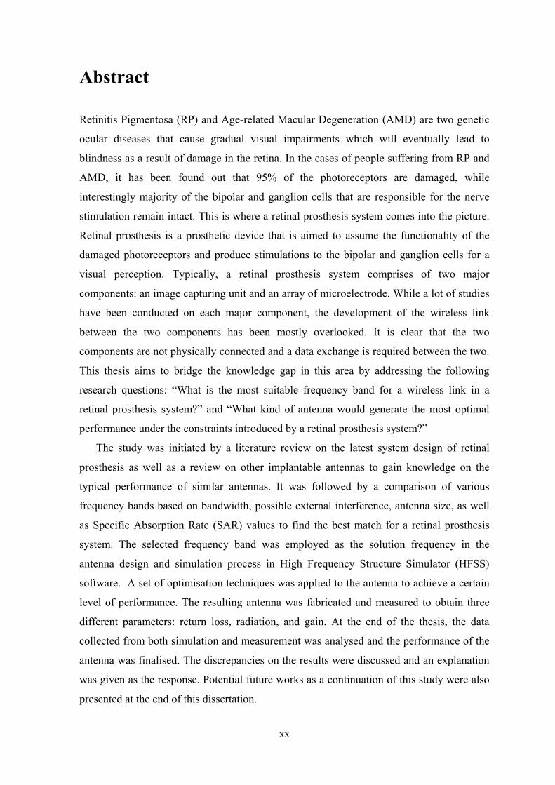
Abstract Retinitis Pigmentosa (RP) and Age-related Macular Degeneration (AMD) are two genetic

ocular diseases that cause gradual visual impairments which will eventually lead to

blindness as a result of damage in the retina. In the cases of people suffering from RP and

AMD, it has been found out that 95% of the photoreceptors are damaged, while

interestingly majority of the bipolar and ganglion cells that are responsible for the nerve

stimulation remain intact. This is where a retinal prosthesis system comes into the picture.

Retinal prosthesis is a prosthetic device that is aimed to assume the functionality of the

damaged photoreceptors and produce stimulations to the bipolar and ganglion cells for a

visual perception. Typically, a retinal prosthesis system comprises of two major

components: an image capturing unit and an array of microelectrode. While a lot of studies

have been conducted on each major component, the development of the wireless link

between the two components has been mostly overlooked. It is clear that the two

components are not physically connected and a data exchange is required between the two.

This thesis aims to bridge the knowledge gap in this area by addressing the following

research questions: “What is the most suitable frequency band for a wireless link in a

retinal prosthesis system?” and “What kind of antenna would generate the most optimal

performance under the constraints introduced by a retinal prosthesis system?”

The study was initiated by a literature review on the latest system design of retinal

prosthesis as well as a review on other implantable antennas to gain knowledge on the

typical performance of similar antennas. It was followed by a comparison of various

frequency bands based on bandwidth, possible external interference, antenna size, as well

as Specific Absorption Rate (SAR) values to find the best match for a retinal prosthesis

system. The selected frequency band was employed as the solution frequency in the

antenna design and simulation process in High Frequency Structure Simulator (HFSS)

software. A set of optimisation techniques was applied to the antenna to achieve a certain

level of performance. The resulting antenna was fabricated and measured to obtain three

different parameters: return loss, radiation, and gain. At the end of the thesis, the data

collected from both simulation and measurement was analysed and the performance of the

antenna was finalised. The discrepancies on the results were discussed and an explanation

was given as the response. Potential future works as a continuation of this study were also

presented at the end of this dissertation.

xxi

List of Publication Following is the list of papers that have been submitted or accepted during the candidature

period (the newest first):

Permana, H., Fang, Q., Lee, S.Y., “Comparison study on specific absorption rate

of three implantable antennas designed for retinal prosthesis systems”

Published in IET Microwaves, Antennas & Propagation, Vol. 7, Issue 11, pp. 1-8,

2013.

Permana, H., Fang, Q., Lee, S.Y., “A microstrip antenna designed for implantable

body sensor network”

Published in ICOT 2013 – 1st International Conference on Orange Technologies,

art. no. 6521168, pp. 103-106.

Permana, H., Fang, Q., Rowe, W.S.T., “Hermetic implantable antenna inside

vitreous humour simulating fluid”

Published in Progress In Electromagnetic Research, Vol. 133, 591-605, 2013.

Permana, H., Fang, Q., Rowe, W.S.T., “Implantable Multilayer Microstrip

Antenna for Retinal Prosthesis: Antenna Testing”

Published in Proceedings of the Annual International Conference of the IEEE

Engineering in Medicine and Biology Society, EMBS, art. no. 6346270 , pp. 1679-

1682.

Permana, H., Fang, Q., Cosic, I., “3-layer Implantable Microstrip Antenna

Optimised for Retinal Prosthesis System in MICS Band”

Published in Proceedings of 2011 International Symposium on Bioelectronics and

Bioinformatics, ISBB 2011, art. no. 6107646 , pp. 65-68.

xxii

Fang, Q., Lee, S.Y., Permana, H., Ghorbani, K., Cosic, I., “Developing a Wireless

Implantable Body Sensor Network in MICS Band”

Published in IEEE Transactions on Information Technology in Biomedicine vol.15

no.4 page 567-576.

Permana, H., Fang, Q., Cosic, I., “ Simulation of EMF Absorption on Human

Head at 402 MHz, 900 MHz, and 2.4 GHz”

Accepted for International Symposium on Bioelectronics and Bioinformatics in

Melbourne, Australia, 9-11 December 2009.

1

Chapter 1

Introduction

1.1. Background

Based on a research conducted by World Health Organization (WHO), Age-related

Macular Degeneration (AMD) ranked third as the cause of blindness worldwide, with a

prevalence of 8.7% [1]. Retinitis Pigmentosa (RP), on the other hand, has an incidence of 1

in 4000 people worldwide [2], while the number varies in different races like Navajo

Indians (1 in 1800) [3]. Both diseases are predicted to burden the government with a US$

75-833 million annually [4]. Without proper solution, these problems will deliver a

massive hit to the health bill, money which could be better spent elsewhere. The first step

to achieve a concrete solution is to fully understand the diseases. What are AMD and RP?

What are the causes and which technologies may provide a solid answer to resolve these

problems?

AMD and RP are both genetic diseases that cause gradual visual impairments as a

result of damage in the retina [2, 5]. In the case of AMD, the symptom starts with what

looks like a small mark at the central vision, which grows progressively until the subject’s

vision is completely blocked. In RP, peripheral vision lost is common as an early symptom

and it eventually leads to a permanent loss of the central vision. To gain an insight on how

the diseases affect the visual recognition, one has to understand the light perception

process inside the human eye. The light perception process involves retina, optic nerve,

optic chiasm, optic tract, Lateral Geniculate Nucleus (LGN), optic radiations, and striate

cortex [6]. The light comes into the eyeball and through to the retina layer, in which it will

be detected by photoreceptors [7]. The photoreceptors convert light energy into a neuronal

signal that is passed to the bipolar cell and the amacrine cell, and then to the ganglion cell.

The signal is then transmitted to the optic nerve and is subsequently passed onto the brain

[6]. In the case of people who suffer from AMD and RP, it was found out that at the later

stage of the disease, up to 95% of the photoreceptors are damaged, which means the

majority of incoming lights could not be detected [8]. The study also revealed that in most

of the cases, the bipolar and ganglion cells, which are responsible for the nerve stimulation,

2

have remained intact. This is where a technology can be proposed to provide a solution to

both diseases.

Retinal prosthesis is a prosthetic device aimed at helping to partially restore the vision

of people who suffer RP and AMD by either bypassing or replacing the function of the

defective photoreceptors and creating stimulation to the neurons. Although there are

different types of the systems, a retinal prosthesis system basically comprises of two

components: an image capturing unit and an array of microelectrode. The positioning of

the latter component with respect to the retinal layer is what differentiates one type to

another. With the assistance of this system, patients would be able to recognize nearby

objects by detecting the reflection of the objects’ edges. A preliminary study has revealed

that such system would allow patients to perform a cutting task, a pouring task, a reading

task, and a symbol recognition task [9]. The benefit that would be generated by such a

system is clearly significant.

Currently there are several research groups who are working on a retinal prosthesis

system development with their own distinct approaches. Second Sight group, Sylmar,

USA, has been developing an epiretinal prosthesis, a kind of retinal prosthesis system in

which the electrode array is attached on the inner layer of the retina, with an emphasize on

the electrode material, the phosphene shapes in relation to the stimulation amplitude, the

possible thermal elevation caused by the system, as well as the wireless link that connects

the extraocular and intraocular components [10-18]. Clinical trials have also been

conducted by this company. Another group is from Nara, Japan, and the prominent feature

of this study has been in the photosensor design, which can be applied in both epiretinal

and subretinal system [20-25]. In contrary to the epiretinal system, subretinal prosthesis is

a retinal prosthesis system where the electrode array placement is at the outer layer of the

human retina. The system has been tested inside rabbits’ eyes. There is also collaboration

between University of New South Wales and Bionic Vision Australia, Australia, in an

attempt to build a retinal prosthesis system. This group has done rigorous studies on the

neurophysiology aspect to gain the knowledge of the biological response to the implanted

device. Several testings have been conducted in vivo using cats [26].

The previous paragraphs showcased the development of retinal prosthesis systems by

three leading groups of researchers. There has been plenty of coverage on the

photosensors, microelectrode arrays, tissue behaviour post-implantation, the material

selection, or the manufacturing technique of the system. However, one issue is seemingly

overlooked: the wireless link between the extraocular and the intraocular components. It is

3

clear that the two major components of the system cannot be physically connected and

there has to be a data communication between the two. The lack of studies in this area

raises questions such as “what frequency should the data be modulated in?” or “how big is

the antenna?” or “what type of the antenna is the most suitable for the system?” or “will

the transmission be the same as a free space transmission?”. These are the questions that

fundamentally motivated this research.

1.2. Rationale

The rationale of this research was to obtain an answer to these two research questions:

“what is the most suitable frequency band for a wireless link in a retinal prosthesis

system?” and “what kind of antenna would generate the most optimal performance under

the constraints introduced by a retinal prosthesis system?”. In order to answer these two

questions, the following research framework is proposed. The research was initiated by the

frequency band analysis in order to determine the most optimal frequency range for the

wireless communication link of the system. This was implemented by designing an

antenna for three different frequency bands and observation of its performance and

characteristic in terms of maximum allowable bandwidth, ideal antenna aperture, as well as

the maximum specific absorption rate (SAR) value. The fundamental design of the

antennas was based on the antenna designs that had been published in literatures with some

adjustments to achieve optimal performance at the desired frequency band. The whole

process would be discussed comprehensively in Chapter 3 of this dissertation. After a

series of evaluations, a frequency band was selected for the operation of the wireless

communication link of the system. The next step of this research was the design of the

implantable antenna to be operated inside the eyeball at the selected frequency band. This

process involved the development of the antenna based on experimental approach with the

aid of High Frequency Structure Simulator (HFSS) simulation software. The antenna

underwent various modifications in order to achieve the most optimal performance. Once a

simulation produced a satisfying result, the antenna was fabricated for the data validation.

The study was concluded by a discussion on the discrepancies between the simulation and

the measurement as well as an observation on how the antenna performed in comparison to

other implantable antennas.

4

1.3. Thesis Organization

This thesis investigates the realization of an implantable antenna for an operation inside

Vitreous Humour liquid, which resembles its operation in a retinal prosthesis system. An

introduction about a retinal prosthesis system is presented in Chapter 2 of this thesis. A

rationale behind a retinal prosthesis system is stated at the beginning of the chapter,

followed by the information on the system mechanism. Current technologies on the system

as well as the wireless communication components are also covered to conclude the

chapter. Chapter 3 explores possible frequency bands for an optimal implementation of

wireless communication link in the retinal prosthesis system. A selection process based on

multiple aspects such as bandwidth, possible external interference, antenna size, as well as

SAR values, is presented in this chapter. At the end of the chapter, the most suitable

frequency band is selected to bring the project to the next step, antenna design. Chapter 4

explores the basic principle of an antenna as well as its operation in free space and in a

high dielectric and conductive medium. Past literatures about implantable antenna designs

are brought into the picture as a basic reference for the current design. At the end of this

chapter, the process of the antenna design is initialized, starting with the constraints

encountered by the antenna, the antenna model selection, as well as the miniaturization of

the antenna. The last part of this Section shows the final antenna design for this project. In

Chapter 5, the simulation aspect of the project is showcased. A selection of numerical

solver tool for solving Maxwell’s Equations associated with the antenna design is

presented, followed by the design procedure using HFSS software. The chapter also

discloses the simulation results of the final antenna design after a series of optimisation

process. The manufacturing process of the antenna is demonstrated in Chapter 6 as part of

measurement process. The measurement in two different conditions, free space and inside

Vitreous Humour liquid is conducted and the antenna performance is presented in three

different parameters: return loss, radiation pattern, and gain. The configuration for each

measurement is also covered in this chapter. Chapter 7 summarizes the simulation and

measurement results and includes analyses on the resulting antenna performance.

Discrepancies are identified and discussed for a more comprehensive knowledge about the

behaviour of the antenna. At the end, the antenna is compared against previously designed

antennas to observe the actual level of the antenna performance. In Chapter 8, a derivative

study of this research in the implantable antenna design for an Implantable Body Sensor

Network (IBSN) is presented. It covers the antenna design as well as the simulation and

5

measurement results of the antenna. Chapter 9 concludes the thesis by signifying the major

findings in this project as well as possible future works as a continuation of this study.

6

Chapter 2

Retinal Prosthesis

In this chapter, the introduction to a retinal prosthesis system would be covered

extensively. A number of important facts will provide the readers an interesting

perspective on the essentiality of the system. Subsequently, the mechanism of the system

will be explained, including what significance it would bring to the prospective users. This

information would provide a thorough introduction to the core part of this chapter, a

compilation of current technologies developed by several leading researchers on the field.

This Section would allow the reader to have an insight on various types of the system, in

which this thesis will be focused on. Ultimately, at the latter part of this chapter, the

attention will be intensified on the wireless communication components of the system,

which is specifically narrowed down to implantable antennas. A short review on existing

wireless communication techniques for other medical purpose implantable systems will

provide a useful idea on the design procedure of the retinal prosthesis system.

2. 1. Overview

2. 1. 1. Background

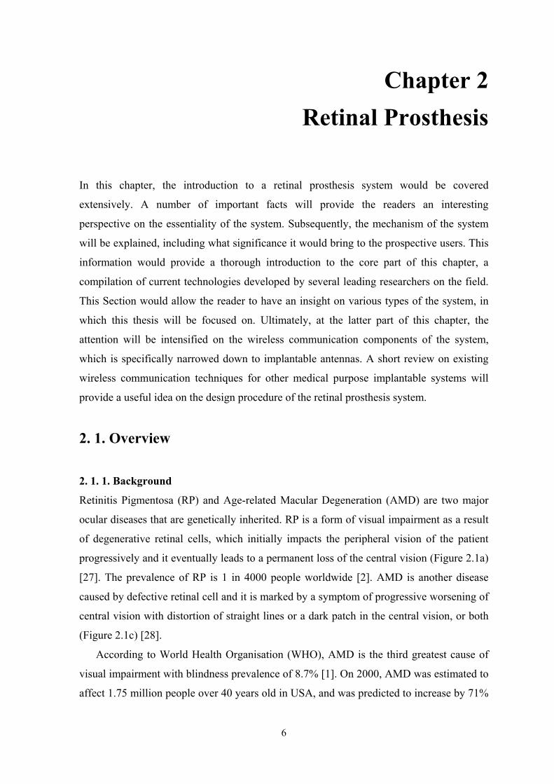
Retinitis Pigmentosa (RP) and Age-related Macular Degeneration (AMD) are two major

ocular diseases that are genetically inherited. RP is a form of visual impairment as a result

of degenerative retinal cells, which initially impacts the peripheral vision of the patient

progressively and it eventually leads to a permanent loss of the central vision (Figure 2.1a)

[27]. The prevalence of RP is 1 in 4000 people worldwide [2]. AMD is another disease

caused by defective retinal cell and it is marked by a symptom of progressive worsening of

central vision with distortion of straight lines or a dark patch in the central vision, or both

(Figure 2.1c) [28].

According to World Health Organisation (WHO), AMD is the third greatest cause of

visual impairment with blindness prevalence of 8.7% [1]. On 2000, AMD was estimated to

affect 1.75 million people over 40 years old in USA, and was predicted to increase by 71%

7

by 2020 [29] and approximately 10 times by the year of 2050 [30] with total annual direct

cost of US$ 75-733 million [4]. Without a proper solution, RP and AMD could become a

big financial burden worldwide in the future.

2. 1. 2. Human Eyeball Anatomy

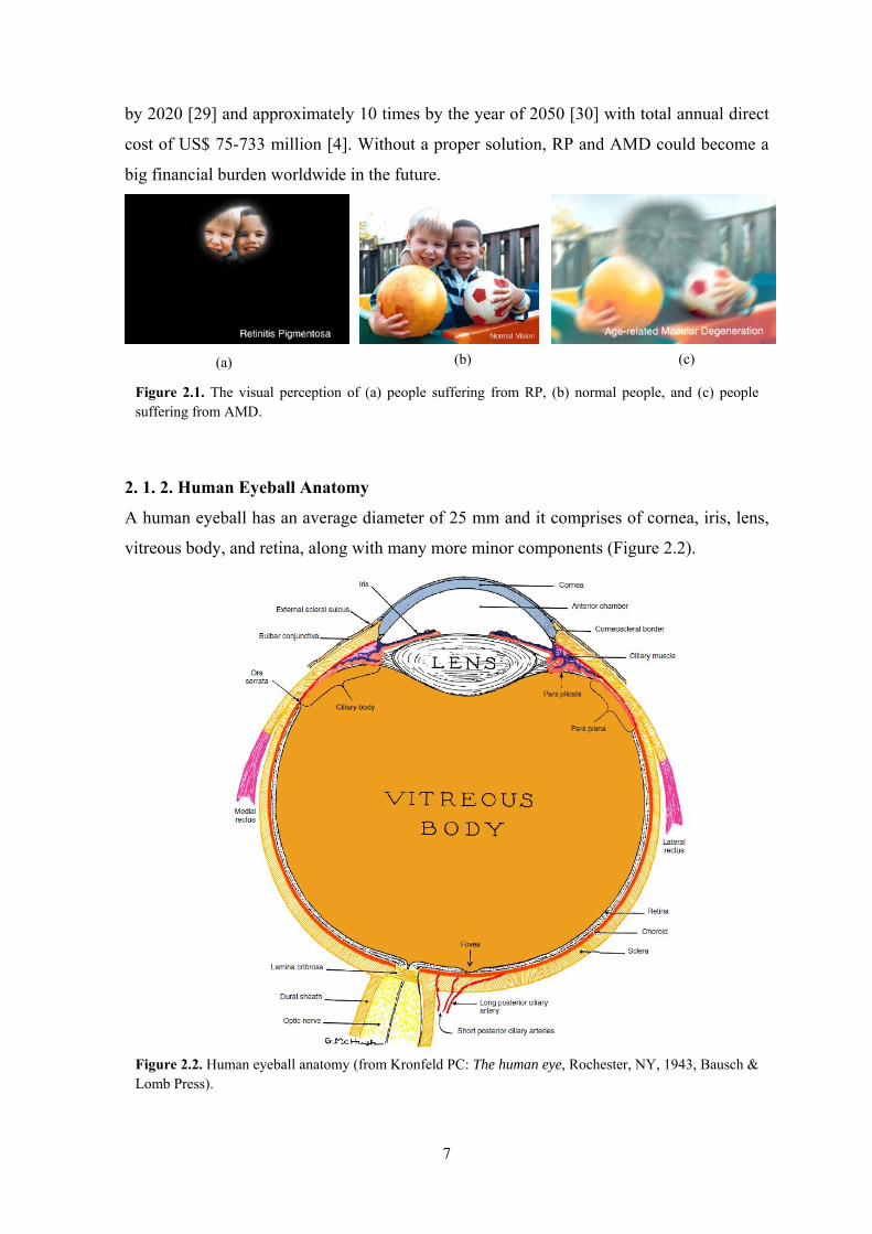
A human eyeball has an average diameter of 25 mm and it comprises of cornea, iris, lens,

vitreous body, and retina, along with many more minor components (Figure 2.2).

(a) (b) (c)

Figure 2.1. The visual perception of (a) people suffering from RP, (b) normal people, and (c) people suffering from AMD.

Figure 2.2. Human eyeball anatomy (from Kronfeld PC: The human eye, Rochester, NY, 1943, Bausch & Lomb Press).

8

From the eyeball diagram, it is clear that Vitreous cavity forms majority of the eyeball.

It is filled with clear fluid called Vitreous Humour, which is composed of 99%

physiological saline and 1% hylaruonic acid [6, 31]. When a foreign object is inserted into

the cavity, a portion of the fluid has to be removed, which can be done with a vitrectomy

procedure [32]. The volume of the removed fluid should be equivalent to the object’s

volume.

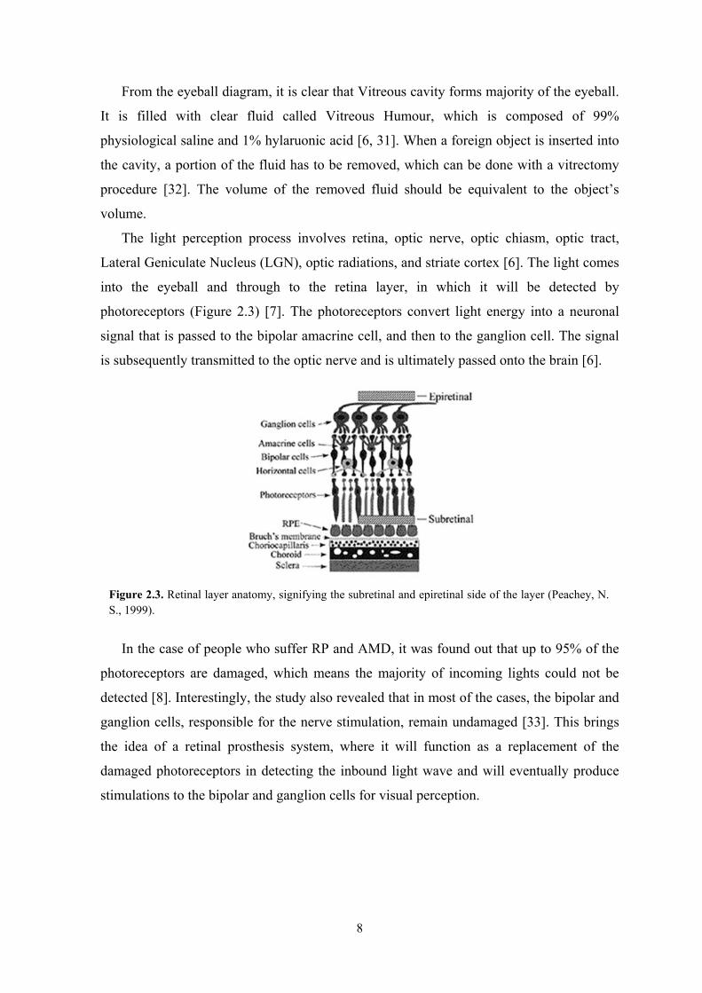
The light perception process involves retina, optic nerve, optic chiasm, optic tract,

Lateral Geniculate Nucleus (LGN), optic radiations, and striate cortex [6]. The light comes

into the eyeball and through to the retina layer, in which it will be detected by

photoreceptors (Figure 2.3) [7]. The photoreceptors convert light energy into a neuronal

signal that is passed to the bipolar amacrine cell, and then to the ganglion cell. The signal

is subsequently transmitted to the optic nerve and is ultimately passed onto the brain [6].

In the case of people who suffer RP and AMD, it was found out that up to 95% of the

photoreceptors are damaged, which means the majority of incoming lights could not be

detected [8]. Interestingly, the study also revealed that in most of the cases, the bipolar and

ganglion cells, responsible for the nerve stimulation, remain undamaged [33]. This brings

the idea of a retinal prosthesis system, where it will function as a replacement of the

damaged photoreceptors in detecting the inbound light wave and will eventually produce

stimulations to the bipolar and ganglion cells for visual perception.

Figure 2.3. Retinal layer anatomy, signifying the subretinal and epiretinal side of the layer (Peachey, N. S., 1999).

9

2. 2. Retinal Prosthesis

2. 2. 1. What is Retinal Prosthesis?

Retinal prosthesis is a prosthetic device aimed at helping to restore partial vision of people

who suffer from RP and AMD by either bypassing or replacing the function of the

defective photoreceptors and creating stimulation to the neurons. Based on the electrode

placement, there are several variations of retinal prosthesis system: suprachoroidal retinal

prosthesis, subretinal prosthesis, as well as epiretinal prosthesis [31]. By looking at the

retina layer diagram (Figure 2.3), it is easier to comprehend the basic idea of where the

stimulators are located for each system. The suprachoroidal type is an approach of a

retinal prosthesis system by placing the stimulator on the choroidal pocket of the eyeball.

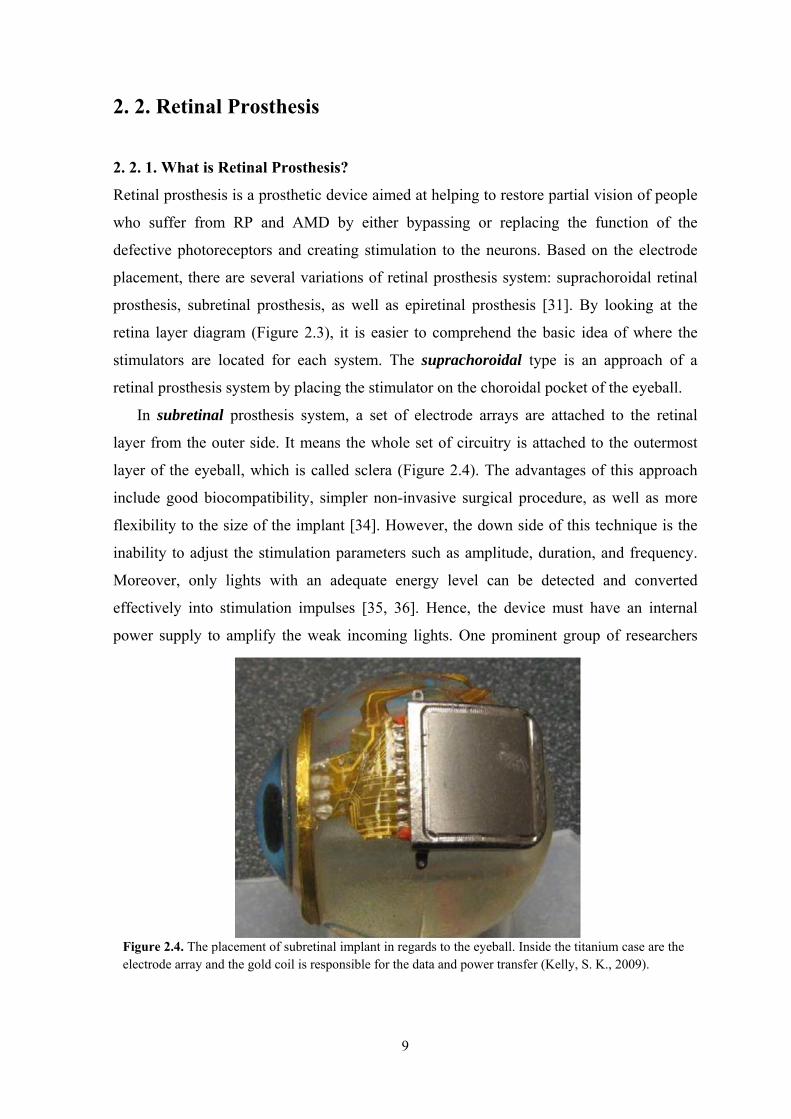
In subretinal prosthesis system, a set of electrode arrays are attached to the retinal

layer from the outer side. It means the whole set of circuitry is attached to the outermost

layer of the eyeball, which is called sclera (Figure 2.4). The advantages of this approach

include good biocompatibility, simpler non-invasive surgical procedure, as well as more

flexibility to the size of the implant [34]. However, the down side of this technique is the

inability to adjust the stimulation parameters such as amplitude, duration, and frequency.

Moreover, only lights with an adequate energy level can be detected and converted

effectively into stimulation impulses [35, 36]. Hence, the device must have an internal

power supply to amplify the weak incoming lights. One prominent group of researchers

Figure 2.4. The placement of subretinal implant in regards to the eyeball. Inside the titanium case are the electrode array and the gold coil is responsible for the data and power transfer (Kelly, S. K., 2009).

10

has been pursuing this technique [119], where a number of human trials have been

successfully conducted by implementing subretinal prosthesis system of 1500 photodiodes.

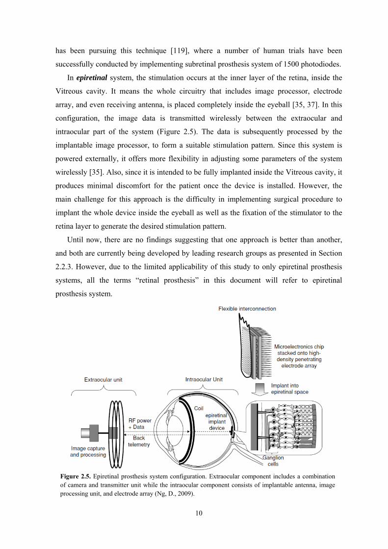
In epiretinal system, the stimulation occurs at the inner layer of the retina, inside the

Vitreous cavity. It means the whole circuitry that includes image processor, electrode

array, and even receiving antenna, is placed completely inside the eyeball [35, 37]. In this

configuration, the image data is transmitted wirelessly between the extraocular and

intraocular part of the system (Figure 2.5). The data is subsequently processed by the

implantable image processor, to form a suitable stimulation pattern. Since this system is

powered externally, it offers more flexibility in adjusting some parameters of the system

wirelessly [35]. Also, since it is intended to be fully implanted inside the Vitreous cavity, it

produces minimal discomfort for the patient once the device is installed. However, the

main challenge for this approach is the difficulty in implementing surgical procedure to

implant the whole device inside the eyeball as well as the fixation of the stimulator to the

retina layer to generate the desired stimulation pattern.

Until now, there are no findings suggesting that one approach is better than another,

and both are currently being developed by leading research groups as presented in Section

2.2.3. However, due to the limited applicability of this study to only epiretinal prosthesis

systems, all the terms “retinal prosthesis” in this document will refer to epiretinal

prosthesis system.

Figure 2.5. Epiretinal prosthesis system configuration. Extraocular component includes a combination of camera and transmitter unit while the intraocular component consists of implantable antenna, image processing unit, and electrode array (Ng, D., 2009).

11

2. 2. 2. Significance

The system will be beneficial for people who are visually impaired due to RP and AMD

with healthy bipolar and ganglion cells. The system will assist the patients to actually

recognize nearby objects by detecting the reflection of the objects’ edges.

There have been a number of studies on different tasks that can be performed or

different objects that can be identified with a variation of electrode numbers. Most

experiments were conducted by covering healthy subjects’ eyes with perforated masks and

there were different requirement on the number of electrodes depending on the requested

tasks, which vary from wandering around a room to identifying objects and faces [8, 38,

39]. In this study [38], it was hypothesized that an array of 25 x 25 electrodes within an

area of 1 cm2 could produce a visual perception that could be useful for pattern

recognition. In another experiment [9], the subjects’ visions were masked by 4 x 4, 6 x 10,

and 16 x 16 dots to resemble the electrode patterns, and they were made to perform a set of

tasks including a cutting task, a pouring task, symbol recognition, and also reading tasks.

The result showed that the highest performance was expectedly achieved on the 16 x 16.

However, the most interesting finding from this experiment was that even by using the

lowest resolution array of 4 x 4, the subjects could still manage to do symbol identification

and cutting task with the spontaneously developed response to overcome the device

limitation. For example, in the case of symbol recognition and cutting task, scanning and

tactile information was used by the subjects, respectively.

Another study focused on the effect of different phosphene shape and grid parameters

to find the best configuration [39]. Sixteen conditions were created by modifying the array

size from 10 x 10 to 32 x 32, as well as varying the grid size, dot size, gap width, dot

dropout rate, and greyscale resolution. It is obvious that the best accuracy was achieved by

the highest number configuration (32 x 32). However, the most valuable information that

could be extracted from the study is that the size of each phosphene was very influential to

the accuracy level of the response. For a dot size of 2.3 times bigger on the same electrode

number, the accuracy was about two times higher.

These results showed that a retinal prosthesis system, even at the very low level in

terms of the number of electrodes, could assist people who are visually impaired as a result

of RP and AMD. It is obvious that higher electrode number corresponds to better image

perception, but the limiting factor would be the size [36] as well as the complexity in data

multiplexing [40]. The promising results even by 4 x 4 arrays shows that even at the very

basic level, this device could have a significant influence for people who are visually

12

impaired. Combined with a proper training and supervision, this device would improve the

quality of life of the users.

2. 2. 3. Current Technologies

Retinal prosthesis system is currently developed by multiple research groups with each

group putting the focus on different aspects. Here is the summary on the progress of each

group from the technical as well as clinical perspective.

2.2.3.1. Second Sight Group, California, USA

Second Sight is a company based in Sylmar, California, USA, and is focused on building

retinal prosthesis system to assist people who suffer RP and AMD. Until now, this

company has developed two products, named Argus I and Argus II. The first clinical trial

for Argus I was conducted on 2002 while the 2nd generation device’s trial was initiated on

2006. Thirty subjects who suffered severe outer retinal degeneration had been enrolled

between June 2007 and August 2009 with follow-up cares of up to 2 years and 8 months

[41]. This latest product has also been tested on 21 patients with RP with the objective of

guiding fine hand movements [42]. The device was waiting for a regulatory approval from

Food and Drug Administration (FDA) for commercial use, which was expected to come by

late 2012 [43].

Feasibility studies had been conducted prior to the prototype design to gain a deep

understanding about the predicted system behaviour and the effect to the surrounding

environment. The studies covered the investigation of the electrode array substrate material

[10], phosphene amplitude variation in relation to the visual perception [11], the effect of

the system to the surrounding tissues as part of the safety measure [12-14], as well as the

investigation of the wireless link between the extraocular and the intraocular components

[16-17]. Post-production study has also been conducted to understand the device behaviour

when it is exposed to Magnetic Resonance Imaging (MRI) [19].

Electrode substrate is a crucial component in an electrode array where its main purpose

is to provide a mechanically steady platform for all the electrodes. The task of selecting the

substrate material is therefore very crucial. Three polymer materials were investigated in

this study [10]: polyimide, parylene, and silicone. Each material was manufactured with its

specific process and was individually tested in canine eye. The testing revealed that

polyimide has the advantage of being the easiest to fabricate due to the already matured

phase of this material in the market. However, polyimide is also the least flexible material,

13

which requires special treatment during the implantation process. Parylene, on the other

hand, requires a slightly more complex manufacturing process, but resulted in an

exceptional biocompatible property. The fabrication of the substrate using silicone material

is less common and a new, untested, production technique was conducted for the testing

purpose in this investigation. It resulted in the most biocompatible material, in terms of

damage inflicted to the retina. However, the implementation of this material reduced the

performance of the system, marked with the presence of the distortion on the signal. Based

on the testing results, it was agreed that parylene has the best properties, even though it is

still not ideal. An alternative solution would be a multi-polymer approach for a single

substrate, which would require a further investigation.

An investigation on the effect of stimulation amplitude variation to the phosphene

shapes was launched [11]. The experiment was conducted on the test subjects who had

been implanted with a 4 x 4 electrode array and stimulator. The stimulation patterns were

produced by a PC and the data was transmitted to the implant using a serial cable. Each

subject was then required to reconstruct the phosphene data on a grid screen using a

tracked digital pen to see the actual perception. The input current to the electrodes was

subsequently varied to four different levels. The findings from this experiment suggested

that the phosphenes change in form and size due to amplitude variation. Although it could

not be guarantee that the shapes drawn by the subjects were 100%, it was clear that there

was a uniform change at the size of the patterns. This information would provide a useful

insight on how the retina reacts as a response of the stimulations.

Several studies about the safety aspect had been conducted to gain a better

understanding on the thermal elevation effect due to the retinal prosthesis system. In this

study [15], the relationship between the heat and power dissipation effect on the retina was

investigated. A custom intraocular heater probe was attached to 5 different areas on the

retinal layer of dog with various power levels. It was found out that the liquid environment

of the eye acts as a heat sink that is capable of dissipating a significant amount of power.

As a result, a heat source that was located further away from the retina boasted higher

power allowance. On a further study, a single platinum microelectrode was inserted into

the vitreous cavity of rats and was supplied with different level of input current pulses

(0.05 to 0.2 μC/phase) [14]. The placement of the microelectrode was also repeatedly

altered to understand its mechanical impact to the retina. The experiment suggested that

retinal damage was greatest when the retina was directly contacted by the electrode,

whether or not electrical stimulation was applied. The combination of retinal contact and

14

electrical stimulation produced the most damage. High charge density stimulation from an

epiretinal electrode in normal rats damages photoreceptors more severely than the inner

retina and ganglion cells. Moderate to severe changes were noted in the retina, Retinal

Pigment Epithelium (RPE), and choroid, only when the electrode was in contact with the

retina. Contact with no electrical stimulation still resulted in retinal damage. The results

imply that a successful retinal prosthesis design will consider carefully both electrical and

mechanical safety issues.

The study about the thermal elevation was extended further by involving the prototype

of the retinal prosthesis system. These papers [12, 13] investigated a temperature increase

on eye components due to the first and the second generation epiretinal prosthesis. Human

head and eye models were constructed based on the Visible Man Project from the National

Library of Medicine (NLM, Bethesda, USA) with the resolution of 1 mm. An implant

model was inserted into the head and eye model and was numerically calculated using Bio-

Heat Equation and finite difference time domain (FDTD) as the solver. The results were

verified by implanting a temperature sensor fitted chip package into canine eyes for an in

vivo measurement. The measurement result of the first generation implant revealed that a

temperature elevation of 0.26°C was observed in the vitreous cavity after 26 minutes of

continuous operation while the chip’s temperature itself raised by 0.82°C [13]. Table 2.1

shows the resulting temperature increase in multiple eye components due to the implanted

coil on the second generation implant [12].

This group has also spent some efforts on investigating the wireless link between the

extraocular and the intraocular components of the system. In this study [18], the group

investigated the feasibility of data telemetry link at the frequency 1.45 GHz and 2.45 GHz

with the internal antenna dimension 6 x 6 mm. Microstrip antennas were designed for each

frequency and were calculated using FDTD technique. The measurement was executed by

immersing the manufactured antenna into an eye phantom, which was mimicked by a mix

of water, sugar, and salt at a certain proportion. At a separation of 25 mm between the

external and internal antenna, in the frequency band of 1.45 GHz, the coupling was

measured to be 42.5 dB in free space, and it was improved to 37.2 dB when the intraocular

antenna was immersed in the eye phantom. At 2.45 GHz, the corresponding experimental

free-space coupling was 32 dB, and it was improved to 31.1 dB in the presence of the eye

phantom. Numerical and experimental values agreed well for all cases at a separation of 25

mm [18]. In separate experiment, a 3D dipole antenna was designed and tested to be

operating inside Vitreous Humour mimicking solution at 1.9 to 2.33 GHz frequency [16].

15

The idea of using 3D dipole antenna was proposed to reduce the planar dimension of the

antenna while improving the bandwidth performance. The hypothesis was confirmed by

the measurement inside the phantom.

There have been two retinal prosthesis devices built by this company, the Argus I and

the Argus II. Argus I was the first generation device, employing 4 x 4 electrodes and was

launched a decade ago. Argus II is their most recent product(currently waiting for approval

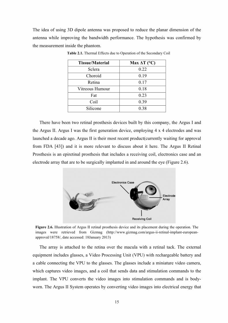
from FDA [43]) and it is more relevant to discuss about it here. The Argus II Retinal

Prosthesis is an epiretinal prosthesis that includes a receiving coil, electronics case and an

electrode array that are to be surgically implanted in and around the eye (Figure 2.6).

The array is attached to the retina over the macula with a retinal tack. The external

equipment includes glasses, a Video Processing Unit (VPU) with rechargeable battery and

a cable connecting the VPU to the glasses. The glasses include a miniature video camera,

which captures video images, and a coil that sends data and stimulation commands to the

implant. The VPU converts the video images into stimulation commands and is body-

worn. The Argus II System operates by converting video images into electrical energy that

Table 2.1. Thermal Effects due to Operation of the Secondary Coil

Tissue/Material Max ΔT (°C)

Sclera 0.22

Choroid 0.19

Retina 0.17

Vitreous Humour 0.18

Fat 0.23

Coil 0.39

Silicone 0.38

Figure 2.6. Illustration of Argus II retinal prosthesis device and its placement during the operation. The images were retrieved from Gizmag (http://www.gizmag.com/argus-ii-retinal-implant-european-approval/18758/, date accessed: 18January 2013)

16

activates retinal cells, delivering the signal through the optic nerve to the brain where it is

perceived as light [19].

Clinical tests have been conducted to characterize the device behaviour as well as to

comprehend if the device was indeed significant for the test subjects. In this particular test

[44], the 4 x 4 retinal prosthesis system was implanted into three test subjects suffering RP.

The objective was to see how electrodes proximity affected the subjects’ perception. First

of all, it was discovered that the subjects who were chronically implanted with prototype

retinal prostheses have perceptual thresholds lower than those obtained during acute

studies. It was also revealed that the proximity to the retina played a role in determining

the threshold and impedance, but only for electrodes that were greater than 0.5 mm from

the retina. Within this distance, perception thresholds and impedances did not seem to be

strongly dependent on the proximity of the electrode to the retina. Thresholds did not seem

to depend on the diameter of the electrode either [44]. In another clinical trial, thirty

subjects were enrolled in the United States and Europe between June 6, 2007, and August

11, 2009 and all subjects were followed up for a minimum of 6 months and up to 2.7 years

[41]. The results suggested that subjects performed statistically better with the system for

the following tasks: object localization (96% of subjects), motion discrimination (57%),

and discrimination of oriented gratings (23%). The best recorded visual acuity was

20/1260 [41].

An additional post-production study was conducted on the second generation device to

test the device compliance (the intraocular part) under the exposure of MRI equipment

[19]. A patient with Argus II retinal prosthesis device implanted underwent an MRI with

the magnetic strength of 1.5 T and 3 T. The experiment revealed that there was no

significant divergence on the magnetic field interaction on MRI equipment and the retinal

prosthesis device, which consequently means that patients are not required to remove the

intraocular component in order to undergo MRI scanning.

In summary, the Second Sight group has managed to build two products, Argus I and

II, both with the concept of epiretinal prosthesis system. Numerous studies had been

conducted prior to the design process for each prototype on the electrode substrate

material, the phosphene shapes in relation to the stimulation amplitude, the possible

thermal elevation, as well as the wireless link between the intraocular and the extraocular

parts. Clinical trials have been conducted to verify the functionality of the product and

satisfying responses were obtained. Post-production testing was also conducted to

investigate the compatibility of the intraocular component of the system with the MRI

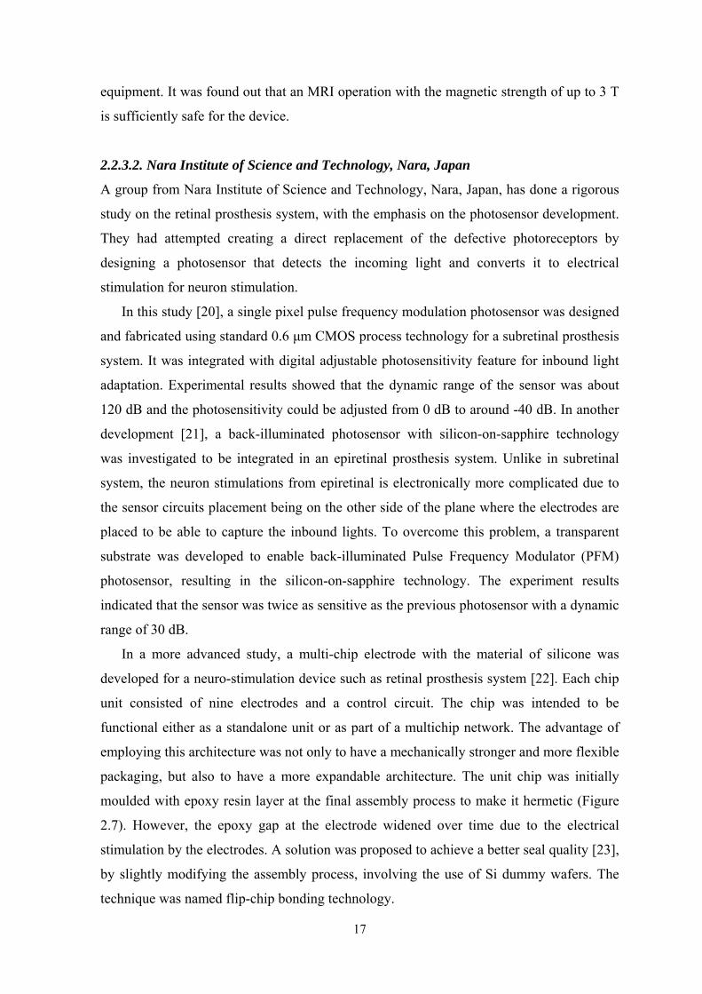
17

equipment. It was found out that an MRI operation with the magnetic strength of up to 3 T

is sufficiently safe for the device.

2.2.3.2. Nara Institute of Science and Technology, Nara, Japan

A group from Nara Institute of Science and Technology, Nara, Japan, has done a rigorous

study on the retinal prosthesis system, with the emphasis on the photosensor development.

They had attempted creating a direct replacement of the defective photoreceptors by

designing a photosensor that detects the incoming light and converts it to electrical

stimulation for neuron stimulation.

In this study [20], a single pixel pulse frequency modulation photosensor was designed

and fabricated using standard 0.6 μm CMOS process technology for a subretinal prosthesis

system. It was integrated with digital adjustable photosensitivity feature for inbound light

adaptation. Experimental results showed that the dynamic range of the sensor was about

120 dB and the photosensitivity could be adjusted from 0 dB to around -40 dB. In another

development [21], a back-illuminated photosensor with silicon-on-sapphire technology

was investigated to be integrated in an epiretinal prosthesis system. Unlike in subretinal

system, the neuron stimulations from epiretinal is electronically more complicated due to

the sensor circuits placement being on the other side of the plane where the electrodes are

placed to be able to capture the inbound lights. To overcome this problem, a transparent

substrate was developed to enable back-illuminated Pulse Frequency Modulator (PFM)

photosensor, resulting in the silicon-on-sapphire technology. The experiment results

indicated that the sensor was twice as sensitive as the previous photosensor with a dynamic

range of 30 dB.

In a more advanced study, a multi-chip electrode with the material of silicone was

developed for a neuro-stimulation device such as retinal prosthesis system [22]. Each chip

unit consisted of nine electrodes and a control circuit. The chip was intended to be

functional either as a standalone unit or as part of a multichip network. The advantage of

employing this architecture was not only to have a mechanically stronger and more flexible

packaging, but also to have a more expandable architecture. The unit chip was initially

moulded with epoxy resin layer at the final assembly process to make it hermetic (Figure

2.7). However, the epoxy gap at the electrode widened over time due to the electrical

stimulation by the electrodes. A solution was proposed to achieve a better seal quality [23],

by slightly modifying the assembly process, involving the use of Si dummy wafers. The

technique was named flip-chip bonding technology.

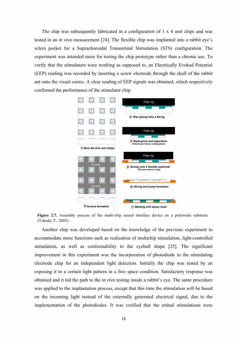
18

The chip was subsequently fabricated in a configuration of 1 x 4 unit chips and was

tested in an in vivo measurement [24]. The flexible chip was implanted into a rabbit eye’s

sclera pocket for a Suprachoroidal Transretinal Stimulation (STS) configuration. The

experiment was intended more for testing the chip prototype rather than a chronic use. To

verify that the stimulators were working as supposed to, an Electrically Evoked Potential

(EEP) reading was recorded by inserting a screw electrode through the skull of the rabbit

ant onto the visual cortex. A clear reading of EEP signals was obtained, which respectively

confirmed the performance of the stimulator chip.

Another chip was developed based on the knowledge of the previous experiment to

accommodate more functions such as realization of multichip stimulation, light-controlled

stimulation, as well as conformability to the eyeball shape [25]. The significant

improvement in this experiment was the incorporation of photodiode to the stimulating

electrode chip for an independent light detection. Initially the chip was tested by an

exposing it to a certain light pattern in a free space condition. Satisfactory response was

obtained and it led the path to the in vivo testing inside a rabbit’s eye. The same procedure

was applied to the implantation process, except that this time the stimulation will be based

on the incoming light instead of the externally generated electrical signal, due to the

implementation of the photodiodes. It was verified that the retinal stimulations were

Figure 2.7. Assembly process of the multi-chip neural interface device on a polyimide substrate (Tokuda, T., 2005).

19

correctly corresponding to the inbound light judging by the relationship between the EEP

traces and the light source.

In summary, this group proposed a different approach on designing a retinal prosthesis

system. The main focus was the design of photosensor using a pulse frequency modulation,

intended for both subretinal and epiretinal system. Multichip electrodes were also

developed in an effort to provide a robust, flexible, and biocompatible chip. Both

technologies, the photosensor and the electrode chip, were combined to create a real retinal

prosthesis system. The system was tested in vivo using rabbits’ eyes, but no clinical trials

on human to date.

2.2.3.3. University of New South Wales and Bionic Vision Australia

This group is based in Australia and started the retinal prosthesis study following the

success of their cochlear implant product. The group began the study from the

neurophysiological approach, by investigating the response of various stimulations to the

visual cortex activity. Different types of stimulator array in regards to their positions have

been fabricated and tested: subretinal, epiretinal, and suprachoroidal array. Most of the

device has been manufactured and implanted into cats’ eyes to obtain the in vivo

performance.

Figure 2.8. The improved assembly process of the electrode array for a better encapsulation (Tokuda, T., 2006). The technique is called flip-chip bonding technology.

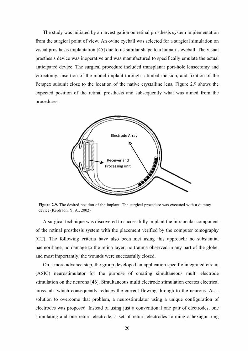
20

The study was initiated by an investigation on retinal prosthesis system implementation

from the surgical point of view. An ovine eyeball was selected for a surgical simulation on

visual prosthesis implantation [45] due to its similar shape to a human’s eyeball. The visual

prosthesis device was inoperative and was manufactured to specifically emulate the actual

anticipated device. The surgical procedure included transplanar port-hole lensectomy and

vitrectomy, insertion of the model implant through a limbal incision, and fixation of the

Perspex subunit close to the location of the native crystalline lens. Figure 2.9 shows the

expected position of the retinal prosthesis and subsequently what was aimed from the

procedures.

A surgical technique was discovered to successfully implant the intraocular component

of the retinal prosthesis system with the placement verified by the computer tomography

(CT). The following criteria have also been met using this approach: no substantial

haemorrhage, no damage to the retina layer, no trauma observed in any part of the globe,

and most importantly, the wounds were successfully closed.

On a more advance step, the group developed an application specific integrated circuit

(ASIC) neurostimulator for the purpose of creating simultaneous multi electrode

stimulation on the neurons [46]. Simultaneous multi electrode stimulation creates electrical

cross-talk which consequently reduces the current flowing through to the neurons. As a

solution to overcome that problem, a neurostimulator using a unique configuration of

electrodes was proposed. Instead of using just a conventional one pair of electrodes, one

stimulating and one return electrode, a set of return electrodes forming a hexagon ring

Figure 2.9. The desired position of the implant. The surgical procedure was executed with a dummy device (Kerdraon, Y. A., 2002)

Electrode Array

Receiver and

Processing unit

21

surrounding each stimulating electrode was implemented. This configuration was intended

to isolate one stimulating electrode from another to avoid any electrical cross-talks. The

system was built and tested to operate well within the specifications. The principle was

then applied to drive 100 electrodes in 14 different locations [47].

In another attempt to improve the neural stimulation responses, an optical imaging of

intrinsic signals (OIS imaging), in addition to EEP, was employed to record the activity at

the visual cortex [48]. This technique allowed a better resolution data recording over large

area of tissue, which would be beneficial to the further neurophysiological analysis of

prosthetic vision. In this study, adult cats were anesthetized and were exposed to corneal,

intra-vitreal, as well as visual stimulations.

A feasibility study was conducted to verify the possibility of retinal stimulation from

suprachoroidal [49]. This marked a shift of research direction from the previous epiretinal

approach. The advantages of the suprachoroidal stimulation technique included reduced

long term risk as a result of indirect contact to the retina tissue, as well as relative

practicality in the surgical procedure. The down side of this technique was the higher

power threshold on the electrodes, which translated to higher power requirement for the

implant. Both 6-return and 1-return electrode systems were implanted to cats’ eyes and it

was found out that the use of 6-return electrode system resulted in a lower recorded signal

amplitude at the cortex compared to the single-return system. The study was followed up

by a suprachoroidal electrode array design [26], which was manufactured using a flexible

polyimide substrate material and was coated with silicone. The device was implanted

inside an adult cat’s eye by accommodating a pocket within the suprachoroidal space. The

experiment was conducted to obtain the antenna performance in terms of impedance,

thresholds and input-output function slopes with variations on the number of return

electrodes, electrode sizes, the number of simultaneous stimulating electrode, and the pulse

widths. The result suggested that the introduction of suprachroidal approach is feasible for

a retinal prosthesis system, as the implant induced visual cortex activity. A new knowledge

was also obtained for reducing the voltage requirement by employing larger diameter

electrodes and wider pulse widths for monopolar stimulation.

A study on image analysis was conducted in an attempt to model the most efficient

algorithm to convert a raw image to a phosphine image (PI) [50]. A mutual-information

function was employed to determine the amount of information to be passed through to the

PI observer (device user) based on visual stimuli. The parameters of the function included

the number of phosphenes and their locations, the number of levels of phosphene

22

quantification, and also the image analysis scheme. An implementation of the image

processing algorithm has been demonstrated in a prototype wearable real-time image

processor [51]. The device, which was to be attached on the user’s waist, featured dual-

core OMAP5912 microprocessor from Texas Instruments (Dallas, TX, USA). The image

processing procedure was divided into 4 steps: image acquisition by the camera, image

enhancements, image pixelation, and command generation. It was concluded that using the

proposed image processing technique, the use of general-purpose embedded micro-

processors would not be sufficient for a real-time visual prosthesis.

To summarize, this group has done rigorous studies about the retinal prosthesis from

the neurophysiological approach. A lot of efforts were spent on the experiment to gain the

knowledge of the biological response to the implanted device. To date, no human trials

have been reported on the journals and cats were regularly involved in the in vivo testing.

2. 3. Existing Implants Communication Methods

In epiretinal prosthesis system (Figure 2.5), there is a data communication exchange

between the extraocular and the intraocular components. The specific communication

methodology for the retinal prosthesis system has not been rigorously investigated, but

there has been relatively more research about wireless link on other implantable medical

applications, such as capsule endoscope and implantable body sensor network.

2. 3. 1. Capsule Endoscope

In the capsule endoscope system, a capsule-sized camera module that is an integration of

antenna, sensors, and the camera itself is ingested. As the capsule travels following the

digestion path, the camera repeatedly captures images of the internal section of the organs

while actively transmits the images to the external receiver wirelessly. In any wireless

communications, antenna is a very crucial component, transforming electric signals to

electromagnetic waves. In this scenario, the role of an antenna is even more important due

to severe challenges of the surrounding.

Instead of operating at free space, just like other standard antennas, the antenna in this

system has to transmit the signal from inside the body, which in this case has a dielectric

constant of 56 and conductivity of 0.83 S/m [52]. Moreover, the antenna is also subjected

to the dimensional as well as orientation constraints which as a result create a demand of a

small, wide bandwidth, and omnidirectional characteristic.

23

In this experiment, a printed spiral antenna with a diameter of 10.1 mm and height of 3

mm was proposed for a capsule endoscopy system [52]. The selection of the spiral shape

was to improve the bandwidth of the antenna. The antenna was intended for operation at

450 MHz, but measurement inside a tissue simulating fluid reflected a shift to 465 MHz

with a bandwidth of 70 MHz. In a further development, the bandwidth of the antenna was

improved even more by the implementation of thick arm spiral [53]. The width of the arm

and its gap from one another were varied to study their effects on the resulting bandwidth.

The antenna was tested inside a cylinder filled with liquid human phantom and produced a

bandwidth of 104 MHz at 500 MHz resonant frequency.

2. 3. 2. Implantable Body Sensor Network

The advancement of sensor technology introduces the possibilities of various implantable

sensors for the purpose of measuring as well as monitoring physiological signals in vivo.

Implantable sensors for measuring SvO2, blood oxygen, blood glucose, neural activity, as

well as internal imaging, are currently investigated comprehensively. In an implantable

body sensor network (IBSN), all the sensors were designed to exchange data wirelessly by

employing master-slave mechanism [54]. To realize this, implantable communication must

be considered at the core design of the architecture.

Although the medium surrounding the implantable antenna is different to the one in

capsule endoscope system, the constraints remain the same because generally human

tissues have high dielectric constant and high conductivity which translates to high

propagating loss. In this study [54], a microstrip antenna with the dimension of 22 mm x

18 mm x 9.5 mm was designed and simulated to be operating at MICS band. The

implementation of high permittivity substrate material was done as an approach for a

miniaturization. The antenna was simulated inside the fat layer in a 3-layer tissue model

and Specific Absorption Rate (SAR) values were recorded.

2. 3. 3. Retinal Prosthesis

Back to the retinal prosthesis system, the same constraints of the implantable antenna that

were applied to the previous two systems are also applied here. However, in retinal

prosthesis, the surrounding medium (Vitreous Humour) is particularly more challenging,

with its relative permittivity of 69 and conductivity of 1.53 S/m at MICS band and the

cavity diameter of only 25 mm.

24

In this study [55], a system with a pair of coils was designed for a wireless data

telemetry and power transfer between the extraocular and the intraocular components. The

external antenna was placed at the front of the cornea while the internal coil is at the

middle of the eyeball. The operating frequency was 6 MHz, hence both antennas were

operating at each other’s near field zone.

As already discussed at the Second Sight Group development, a 3D dipole antenna was

designed and tested to be operating inside Vitreous Humour mimicking solution at 1.9 to

2.33 GHz frequency [16]. The idea of using 3D dipole antenna was proposed to reduce the

planar dimension of the antenna while improving the bandwidth performance. The

hypothesis was confirmed by the measurement inside the phantom.

2.4. Summary

It is clear that human body characteristic is naturally very complex as it has very high

dielectric and conductivity values and they are frequency dependent. It makes it difficult to

design an antenna for multiple implantation scenarios in different medium. Therefore,

implantable antenna design requires a careful planning to gather all the exact information

needed to resemble the real operating condition of the antenna. The design procedure starts

from the operating frequency selection, followed by the design of the antenna, design of

the surrounding medium(s), simulation, and verification of the results.

In this chapter, information regarding retinal prosthesis system, including the rationale

of the system, how the system works, and the current developments, has been presented.

The focus was then intensified on the wireless communication component of the system

for the relevance to the thesis topic. Existing technologies employed by other medical

implants were reviewed to obtain more knowledge about the design challenges of the

implantable antenna. The information gathered would be essential in the frequency

selection process, which will be presented in the next chapter.

25

Chapter 3

Frequency Selection

Frequency selection is an integral part in the design phase of any wireless communication

systems due to its significance in determining the antenna design. However, choosing a

frequency band for a specific purpose is not a straightforward task considering there are

various aspects that need to be looked at, such as bandwidth, possible external interference,

antenna size, and SAR value. In this chapter, all these factors will be individually

investigated for subsequent feasibility study on several frequency bands for the retinal

prosthesis system that include High Frequency (HF) band, Medical Implant

Communication Service (MICS) band, and Industrial Scientific and Medical (ISM) band.

Simulation results on SAR values calculation will be presented next, and ultimately a

frequency band will be selected based on the analysis test on all possible frequency bands.

3.1. Important factors in frequency selection

As mentioned previously, there are four aspects that would be influential in the selection

process: bandwidth, external interference, antenna size, and SAR value.

3.1.1. Bandwidth

There are numerous definitions of the term bandwidth depending on the specific

applications. In this thesis, however, the term’s interpretation will be narrowed down for

two different scenarios: in the frequency selection process and in the antenna design

process.

The first definition of bandwidth is an authorized bandwidth parameter assigned by a

legal communication body to specify the spectrum allowed in the data transmission process

[56]. The two most recognized communication bodies include Federal Communications

Commission (FCC) from USA and International Commission on Non-Ionizing Radiation

Protection (ICNIRP), based in Germany, and their standards have been commonly adopted

by other countries. The bodies basically govern the maximum bandwidth, or in this case

spectrum slot, to avoid any inter-signal interference during the transmission. The signal

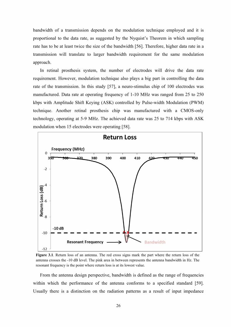
26

bandwidth of a transmission depends on the modulation technique employed and it is

proportional to the data rate, as suggested by the Nyquist’s Theorem in which sampling

rate has to be at least twice the size of the bandwidth [56]. Therefore, higher data rate in a

transmission will translate to larger bandwidth requirement for the same modulation

approach.

In retinal prosthesis system, the number of electrodes will drive the data rate

requirement. However, modulation technique also plays a big part in controlling the data

rate of the transmission. In this study [57], a neuro-stimulus chip of 100 electrodes was

manufactured. Data rate at operating frequency of 1-10 MHz was ranged from 25 to 250

kbps with Amplitude Shift Keying (ASK) controlled by Pulse-width Modulation (PWM)

technique. Another retinal prosthesis chip was manufactured with a CMOS-only

technology, operating at 5-9 MHz. The achieved data rate was 25 to 714 kbps with ASK

modulation when 15 electrodes were operating [58].

From the antenna design perspective, bandwidth is defined as the range of frequencies

within which the performance of the antenna conforms to a specified standard [59].

Usually there is a distinction on the radiation patterns as a result of input impedance

Figure 3.1. Return loss of an antenna. The red cross signs mark the part where the return loss of the antenna crosses the -10 dB level. The pink area in between represents the antenna bandwidth in Hz. The resonant frequency is the point where return loss is at its lowest value.

27

variations. Therefore, input impedance is adopted as an indicator of the antenna

performance. Generally, a value of lower than -10 dB indicates a good performance of an

antenna and the region between the two points where the return loss crossed the -10 dB

mark is the bandwidth of the antenna, as represented by the pink area in Figure 3.1.

In the antenna design process, some applications require a very wide bandwidth while

for the others it is insignificant. It is also important that the bandwidth of the antenna is

large enough to maximize the spectrum allocated for the transmission. As discussed in the

previous Section, in retinal prosthesis the bandwidth requirement is affected by the number

of electrodes as well as the modulation technique. A successful antenna design will need to

incorporate the bandwidth requirement of the system into the consideration.

3.1.2. External interference

External electromagnetic interference comes as a result of multiple usages of the frequency

band by different devices. To overcome this problem, implementation of higher power or

special shielding is required. Selecting a frequency with the least possible external

interference is desirable to minimize the need of dealing with the radio frequency signal

interference.

3.1.3. Antenna size

Antenna size is very closely related to the frequency selection process in the way that an

antenna aperture’s size has to be at least a quarter wavelength to achieve ideal radiation

efficiency. Wavelength in itself is inversely proportional to the signal frequency, which

means that low frequency operation will require bigger antenna size to achieve an ideal

performance. However, in the case of retinal prosthesis system, there is a limiting factor on

the size of the antenna due to its anticipated position inside the eyeball.

3.1.4. SAR values

SAR is the rate at which electromagnetic field (EMF) energy is absorbed by the human

body and it has become a standard to identify the limit of safe EMF exposure level to the

human body. Every device that produces EMF will cause thermal and non-thermal effect to

living tissues [60]. The non-thermal effect, due to its complexity and lack of published

reports, is not considered in this investigation. The thermal effect relates directly to the

temperature increase on parts of human body due to EMF absorption. SAR is used as an

indication whether the EMF exposure is maintained at the safe level. It is important and

28

necessary to investigate the SAR distribution pattern for an implanted retinal prosthesis

system. The implanted device, which will be in a continuous operation for uninterrupted

vision, will be put inside a human eye that is only a few centimetres away to the most vital

human organ, the brain. The basic formula for SAR calculation can be defined as:

EESAR22 1

(3.1)

where E is the electric field at a point in the body (V/m), σ is the conductivity (S/m), ρ is

the mass density of the body (kg/m3), ω is the angular frequency (ω = 2πf radians), and ε is

the permittivity of the body part (F/m). According to ICNIRP [60], the limit of SAR value

is 2 W/kg over 10g of body tissue (for frequency range of 100 kHz to 10 GHz), whereas

based on FCC standard, the limit of SAR value is 1.6 W/kg over 1g of body tissue [61].

The SAR value difference between those two standards is very little, but the fact is that in

the ICNIRP standard, the SAR value is obtained as an average of 10g body tissue

surrounding the emitter, while in the FCC standard, it is an average of 1g body tissue.

What this means is that the ICNIRP standard allows higher point SAR value within the

measured volume than the FCC standard. FCC and ICNIRP standards have been adopted

by a majority of countries around the world, which was the reason why the 10g and 1g

SAR threshold values were used in this experiment as the reference of the standard safety

level.

The analysis of each frequency band in the following Sections will be based on evaluating

each factor. At the end of the chapter, a summary on the performance of each band will be

presented and the operating frequency is ultimately selected.

3.2. High Frequency (HF)

HF band is a radio frequency band with the range of 3-30 MHz. Within this frequency

range, there are three radio bands allocated by FCC for licensed uses: 6.78 MHz, 13.56

MHz, and 27.12 MHz [62]. Maximum bandwidth has been set by FCC for licensed usages

to avoid interferences between each device. The maximum bandwidth of 30 kHz, 14 kHz,

and 326 kHz were set for the radio bands of 6.78 MHz, 13.56 MHz, and 27.12 MHz,

respectively [62].

Common applications for High Frequency band include shortwave radio, Radio-

frequency Identification (RFID), and Near Field Communication (NFC) standard. For the

29

unlicensed operation, this band has been regularly used for amateur radio activities. Short

wave radio applications utilize frequency band between 1.8 MHz to 30 MHz and it is

typically associated with international and domestic broadcasting with the spacing for each

channel is 5 kHz. RFID is another application that operates at HF band, specifically at

13.56 MHz. Due to its low cost and compact shape, RFID is currently being implemented

on massive range of applications from different areas that include commerce,

transportation, logistics, personal identification, sports, and telemetries. NFC is another

technology that employs 13.56 MHz frequency and it is largely based on the RFID

technology. However, in addition to RFID’s read or write operation mode, the technology

is also incorporated with card emulation and peer-to-peer modes [63]. NFC technology is

currently still at the early stage, which explains low adoption rate, but future possible

applications in the public transportation, office, money transaction, or sport sectors will

make NFC the new RFID.

Ideal antenna size for free space operation in this frequency is 2.5 to 25 m based on the

condition mentioned on Section 3.1.3. However, the nature of retinal prosthesis system

requires the antenna to be surrounded by Vitreous Humour. The relative permittivity and

the conductivity of the fluid (εr = 70, σ = 1.5 S/m at HF [64]) affect the minimum aperture

requirement of the antenna due to resonant frequency shift [65]:

√

(3.2)

According to formula (3.2), the resonant frequency is shifted by the factor√

. Hence,

the minimum free space aperture is also shifted by the same factor to obtain the minimum

aperture inside the medium. In this scenario, the minimum aperture was calculated to be

0.3 to 3 m, down from 2.5 to 25 m.

3.3. Medical Implant Communication Service (MICS)

MICS band is a frequency band that is allocated specifically for medical implant purposes

with the frequency range of 401 to 406 MHz [66]. In this band, the maximum bandwidth is

divided into 2 categories: 300 kHz for the 402 to 405 MHz and 100 kHz for both 401-402

MHz and 405-406 MHz [66].

MICS band is currently utilized for medical systems like cardiac pacemaker [67] and

implantable body sensor network (IBSN) [54], which can comprise of implantable sensors

30

for the measurement of SvO2, blood oxygen, blood glucose, neural activity, as well as

internal imaging.

The dielectric property of Vitreous Humour at MICS band is like the following: εr =

69, σ = 1.53 S/m at 402 MHz [64]. By using Equation (3.2), the ideal antenna aperture

inside the Vitreous Humour at MICS band is 22.46 mm, down from 186.57 mm at free

space environment.

3.4. Industrial, Scientific, and Medical (ISM) 915 MHz

This band, just like the other ISM bands, is dedicated to the industrial, scientific, and

medical purposes other than telecommunications. The frequency range of this band is from

902 to 928 MHz with the maximum licensed bandwidth of around 4.58 MHz [68]

depending on the centre frequency.

The only major licensed usage for this band is Global System for Mobile

Communications (GSM) 900, a standard developed for cellular phone network. GSM-900

is being utilized globally except for some countries like USA and Canada. In GSM-900,

the uplink frequency is 890-915 MHz and the downlink is 935-960 MHz with the spacing

between each channel 200 kHz [69]. It is clear that the uplink frequency of the GSM-900

overlaps with the part of the ISM 915 MHz band and it will probably cause interference

during the transmission.

For this band, the ideal free space antenna aperture using the quarter wavelength

method is 82 mm. When the antenna is operating inside the Vitreous Humour liquid with εr

= 68.9 and σ = 1.64 S/m at 915 MHz [64], the minimum antenna size is reduced to 9.87

mm.

3.5. Industrial, Scientific, and Medical (ISM) 2.45 GHz

Probably the most popular ISM band, this band has a frequency range of 2.4 to 2.5 GHz.

With the range of 100 MHz, the maximum bandwidth imposed for each transmission is

around 12.25 MHz, depending on the centre frequency [68].

There are plenty of applications utilizing this frequency band, namely Bluetooth (IEEE

802.15.1), Wi-Fi (802.11), ZigBee (IEEE 802.15.4), cordless phones, baby monitors, and

microwave ovens. These are everyday applications and therefore the signal interferences in

this band are practically everywhere.

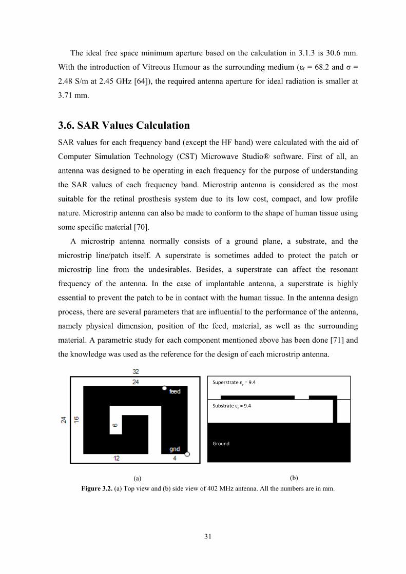
31

The ideal free space minimum aperture based on the calculation in 3.1.3 is 30.6 mm.

With the introduction of Vitreous Humour as the surrounding medium (εr = 68.2 and σ =

2.48 S/m at 2.45 GHz [64]), the required antenna aperture for ideal radiation is smaller at

3.71 mm.

3.6. SAR Values Calculation

SAR values for each frequency band (except the HF band) were calculated with the aid of

Computer Simulation Technology (CST) Microwave Studio® software. First of all, an

antenna was designed to be operating in each frequency for the purpose of understanding

the SAR values of each frequency band. Microstrip antenna is considered as the most

suitable for the retinal prosthesis system due to its low cost, compact, and low profile

nature. Microstrip antenna can also be made to conform to the shape of human tissue using

some specific material [70].

A microstrip antenna normally consists of a ground plane, a substrate, and the

microstrip line/patch itself. A superstrate is sometimes added to protect the patch or

microstrip line from the undesirables. Besides, a superstrate can affect the resonant

frequency of the antenna. In the case of implantable antenna, a superstrate is highly

essential to prevent the patch to be in contact with the human tissue. In the antenna design

process, there are several parameters that are influential to the performance of the antenna,

namely physical dimension, position of the feed, material, as well as the surrounding

material. A parametric study for each component mentioned above has been done [71] and

the knowledge was used as the reference for the design of each microstrip antenna.

Figure 3.2. (a) Top view and (b) side view of 402 MHz antenna. All the numbers are in mm.

(a) (b)

Superstrate εr = 9.4

Substrate εr = 9.4

Ground

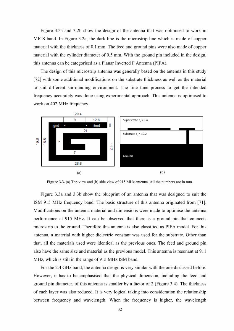
32

Figure 3.2a and 3.2b show the design of the antenna that was optimised to work in

MICS band. In Figure 3.2a, the dark line is the microstrip line which is made of copper

material with the thickness of 0.1 mm. The feed and ground pins were also made of copper

material with the cylinder diameter of 0.5 mm. With the ground pin included in the design,

this antenna can be categorised as a Planar Inverted F Antenna (PIFA).

The design of this microstrip antenna was generally based on the antenna in this study

[72] with some additional modifications on the substrate thickness as well as the material

to suit different surrounding environment. The fine tune process to get the intended

frequency accurately was done using experimental approach. This antenna is optimised to

work on 402 MHz frequency.

Figure 3.3a and 3.3b show the blueprint of an antenna that was designed to suit the

ISM 915 MHz frequency band. The basic structure of this antenna originated from [71].

Modifications on the antenna material and dimensions were made to optimise the antenna

performance at 915 MHz. It can be observed that there is a ground pin that connects

microstrip to the ground. Therefore this antenna is also classified as PIFA model. For this

antenna, a material with higher dielectric constant was used for the substrate. Other than

that, all the materials used were identical as the previous ones. The feed and ground pin

also have the same size and material as the previous model. This antenna is resonant at 911

MHz, which is still in the range of 915 MHz ISM band.

For the 2.4 GHz band, the antenna design is very similar with the one discussed before.

However, it has to be emphasised that the physical dimension, including the feed and

ground pin diameter, of this antenna is smaller by a factor of 2 (Figure 3.4). The thickness

of each layer was also reduced. It is very logical taking into consideration the relationship

between frequency and wavelength. When the frequency is higher, the wavelength

Figure 3.3. (a) Top view and (b) side view of 915 MHz antenna. All the numbers are in mm.

(a) (b)

Superstrate εr = 9.4

Substrate εr= 10.2

Ground

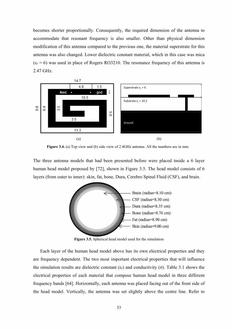
33

becomes shorter proportionally. Consequently, the required dimension of the antenna to

accommodate that resonant frequency is also smaller. Other than physical dimension

modification of this antenna compared to the previous one, the material superstrate for this

antenna was also changed. Lower dielectric constant material, which in this case was mica

(εr = 6) was used in place of Rogers RO3210. The resonance frequency of this antenna is

2.47 GHz.

The three antenna models that had been presented before were placed inside a 6 layer

human head model proposed by [72], shown in Figure 3.5. The head model consists of 6

layers (from outer to inner): skin, fat, bone, Dura, Cerebro Spinal Fluid (CSF), and brain.

Each layer of the human head model above has its own electrical properties and they

are frequency dependent. The two most important electrical properties that will influence

the simulation results are dielectric constant (εr) and conductivity (σ). Table 3.1 shows the

electrical properties of each material that compose human head model in three different

frequency bands [64]. Horizontally, each antenna was placed facing out of the front side of

the head model. Vertically, the antenna was set slightly above the centre line. Refer to

Figure 3.4. (a) Top view and (b) side view of 2.4GHz antenna. All the numbers are in mm.

(a) (b)

Superstrate εr = 6

Substrate εr= 10.2

Ground

Figure 3.5. Spherical head model used for the simulation

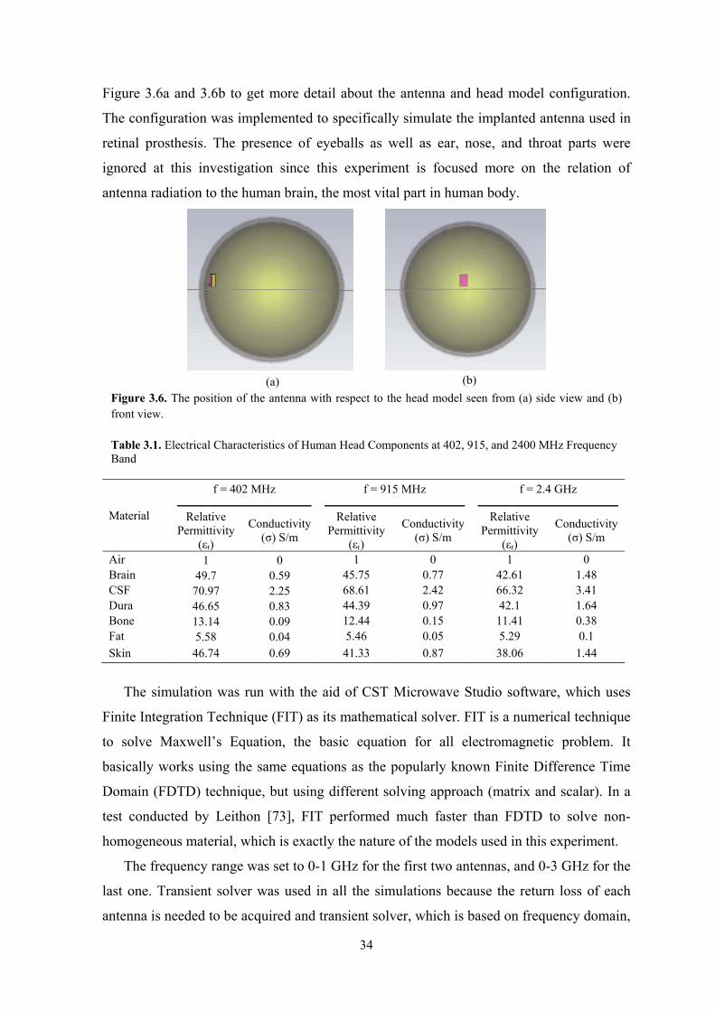
34

Figure 3.6a and 3.6b to get more detail about the antenna and head model configuration.

The configuration was implemented to specifically simulate the implanted antenna used in

retinal prosthesis. The presence of eyeballs as well as ear, nose, and throat parts were

ignored at this investigation since this experiment is focused more on the relation of

antenna radiation to the human brain, the most vital part in human body.

The simulation was run with the aid of CST Microwave Studio software, which uses

Finite Integration Technique (FIT) as its mathematical solver. FIT is a numerical technique

to solve Maxwell’s Equation, the basic equation for all electromagnetic problem. It

basically works using the same equations as the popularly known Finite Difference Time

Domain (FDTD) technique, but using different solving approach (matrix and scalar). In a

test conducted by Leithon [73], FIT performed much faster than FDTD to solve non-

homogeneous material, which is exactly the nature of the models used in this experiment.

The frequency range was set to 0-1 GHz for the first two antennas, and 0-3 GHz for the

last one. Transient solver was used in all the simulations because the return loss of each

antenna is needed to be acquired and transient solver, which is based on frequency domain,

Figure 3.6. The position of the antenna with respect to the head model seen from (a) side view and (b) front view.

(a) (b)

Table 3.1. Electrical Characteristics of Human Head Components at 402, 915, and 2400 MHz Frequency Band

Material

f = 402 MHz f = 915 MHz f = 2.4 GHz

Relative Permittivity

(εr)

Conductivity (σ) S/m


(εr)



(εr)


Air 1 0 1 0 1 0 Brain 49.7 0.59 45.75 0.77 42.61 1.48 CSF 70.97 2.25 68.61 2.42 66.32 3.41 Dura 46.65 0.83 44.39 0.97 42.1 1.64 Bone 13.14 0.09 12.44 0.15 11.41 0.38 Fat 5.58 0.04 5.46 0.05 5.29 0.1

Skin 46.74 0.69 41.33 0.87 38.06 1.44

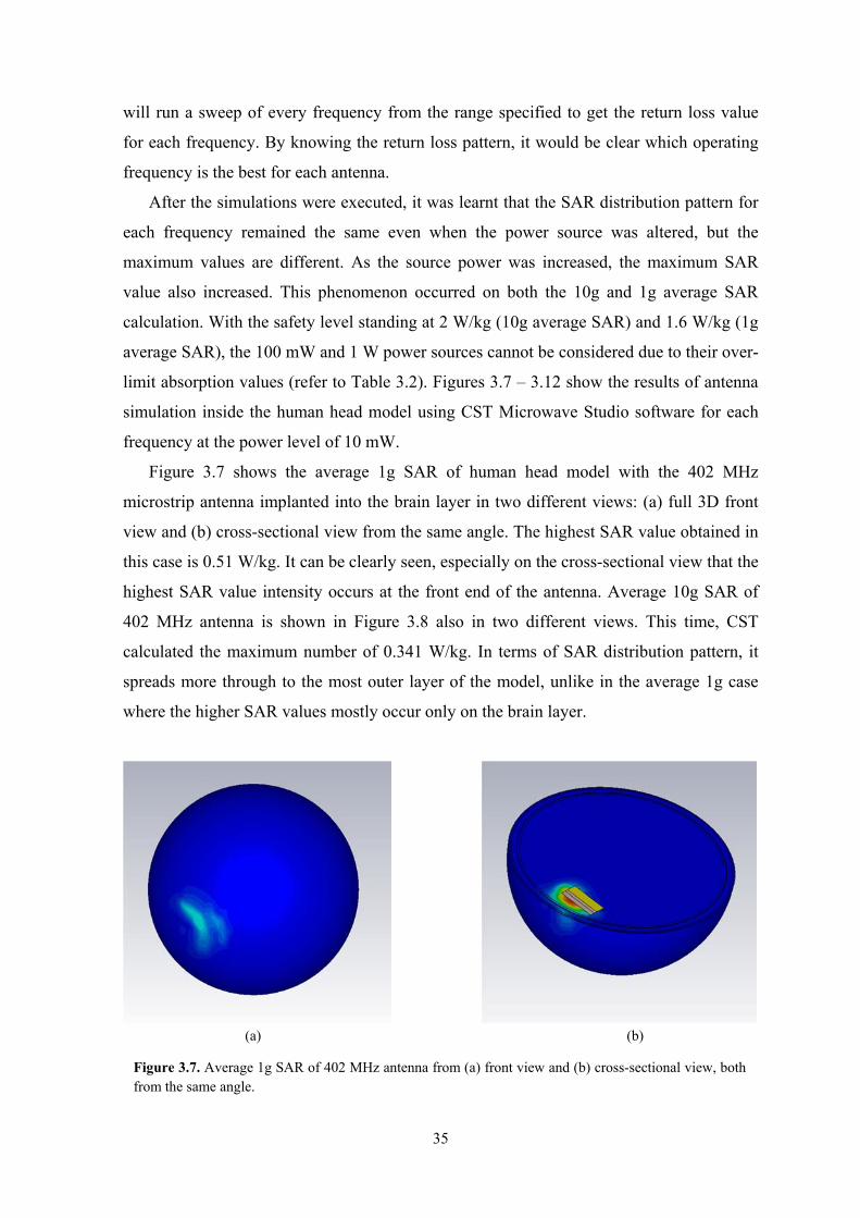
35

will run a sweep of every frequency from the range specified to get the return loss value

for each frequency. By knowing the return loss pattern, it would be clear which operating

frequency is the best for each antenna.

After the simulations were executed, it was learnt that the SAR distribution pattern for

each frequency remained the same even when the power source was altered, but the

maximum values are different. As the source power was increased, the maximum SAR

value also increased. This phenomenon occurred on both the 10g and 1g average SAR

calculation. With the safety level standing at 2 W/kg (10g average SAR) and 1.6 W/kg (1g

average SAR), the 100 mW and 1 W power sources cannot be considered due to their over-

limit absorption values (refer to Table 3.2). Figures 3.7 – 3.12 show the results of antenna

simulation inside the human head model using CST Microwave Studio software for each

frequency at the power level of 10 mW.

Figure 3.7 shows the average 1g SAR of human head model with the 402 MHz

microstrip antenna implanted into the brain layer in two different views: (a) full 3D front

view and (b) cross-sectional view from the same angle. The highest SAR value obtained in

this case is 0.51 W/kg. It can be clearly seen, especially on the cross-sectional view that the

highest SAR value intensity occurs at the front end of the antenna. Average 10g SAR of

402 MHz antenna is shown in Figure 3.8 also in two different views. This time, CST

calculated the maximum number of 0.341 W/kg. In terms of SAR distribution pattern, it

spreads more through to the most outer layer of the model, unlike in the average 1g case

where the higher SAR values mostly occur only on the brain layer.

Figure 3.7. Average 1g SAR of 402 MHz antenna from (a) front view and (b) cross-sectional view, both from the same angle.

(a) (b)

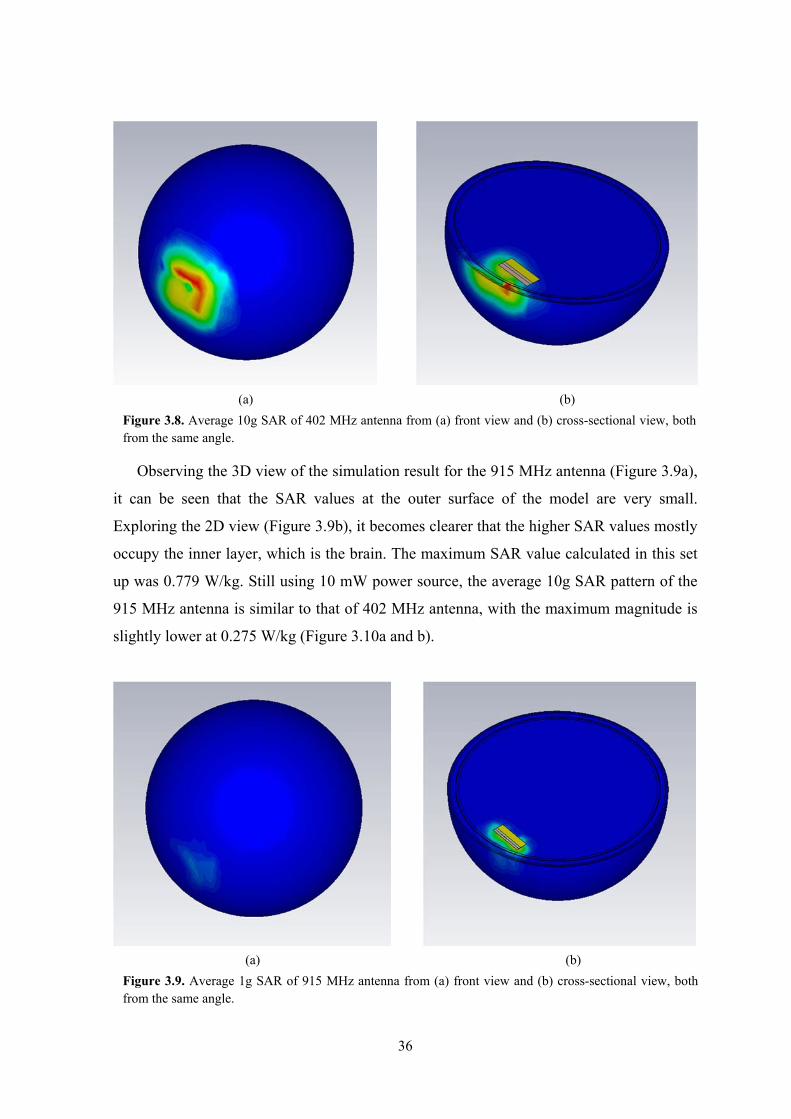
36

Observing the 3D view of the simulation result for the 915 MHz antenna (Figure 3.9a),

it can be seen that the SAR values at the outer surface of the model are very small.

Exploring the 2D view (Figure 3.9b), it becomes clearer that the higher SAR values mostly

occupy the inner layer, which is the brain. The maximum SAR value calculated in this set

up was 0.779 W/kg. Still using 10 mW power source, the average 10g SAR pattern of the

915 MHz antenna is similar to that of 402 MHz antenna, with the maximum magnitude is

slightly lower at 0.275 W/kg (Figure 3.10a and b).


(a) (b)


(a) (b)

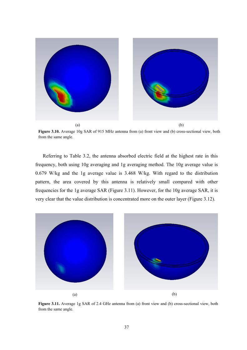
37

Referring to Table 3.2, the antenna absorbed electric field at the highest rate in this

frequency, both using 10g averaging and 1g averaging method. The 10g average value is

0.679 W/kg and the 1g average value is 3.468 W/kg. With regard to the distribution

pattern, the area covered by this antenna is relatively small compared with other

frequencies for the 1g average SAR (Figure 3.11). However, for the 10g average SAR, it is

very clear that the value distribution is concentrated more on the outer layer (Figure 3.12).


(a) (b)

(a) (b)

Figure 3.11. Average 1g SAR of 2.4 GHz antenna from (a) front view and (b) cross-sectional view, both from the same angle.

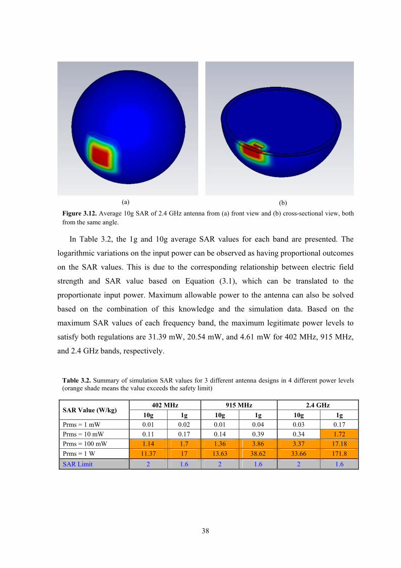
38

In Table 3.2, the 1g and 10g average SAR values for each band are presented. The

logarithmic variations on the input power can be observed as having proportional outcomes

on the SAR values. This is due to the corresponding relationship between electric field

strength and SAR value based on Equation (3.1), which can be translated to the

proportionate input power. Maximum allowable power to the antenna can also be solved

based on the combination of this knowledge and the simulation data. Based on the

maximum SAR values of each frequency band, the maximum legitimate power levels to

satisfy both regulations are 31.39 mW, 20.54 mW, and 4.61 mW for 402 MHz, 915 MHz,

and 2.4 GHz bands, respectively.

Figure 3.12. Average 10g SAR of 2.4 GHz antenna from (a) front view and (b) cross-sectional view, both from the same angle.

(a) (b)

Table 3.2. Summary of simulation SAR values for 3 different antenna designs in 4 different power levels (orange shade means the value exceeds the safety limit)

SAR Value (W/kg) 402 MHz 915 MHz 2.4 GHz

10g 1g 10g 1g 10g 1g

Prms = 1 mW 0.01 0.02 0.01 0.04 0.03 0.17

Prms = 10 mW 0.11 0.17 0.14 0.39 0.34 1.72

Prms = 100 mW 1.14 1.7 1.36 3.86 3.37 17.18

Prms = 1 W 11.37 17 13.63 38.62 33.66 171.8

SAR Limit 2 1.6 2 1.6 2 1.6

39

3.7. Frequency Selection

Based on the analysis on each frequency band, the results can be compiled in Table 3.3.

Table 3 provides a summary of the analysis of each frequency band with regards to

maximum bandwidth, possible external interferences, antenna size, and SAR values.

According to the table above, the main barrier of employing HF band is the fact that bigger

antenna size is required to maintain the antenna performance. In this retinal prosthesis

system, it is crucial that antenna size does not exceed the human eyeball diameter of 25

mm. This will prove very difficult even with the implementation of miniaturization

technique. Another aspect that will undermine HF band’s case is the low maximum

bandwidth imposed by the regulators of 14 and 39 kHz. Based on the chip performance,

the modulation technique will require up to 250 kHz and 714 kHz for 100 and 15

electrodes, respectively [57, 58]. That rules out the feasibility of this frequency band for

the retinal prosthesis system.

MICS band is naturally the first choice frequency band for this system due to its

specific allocation for implantable medical devices. In this band, there are relatively less

external interferences that would affect the performance of this system. The relatively low

maximum usable bandwidth of 300 kHz may cause a slight concern for future development

that will incorporate higher number of electrodes. However, it has been proven that with a

certain modulation technique, the data rate of the transmission can be suppressed [57]. The

Table 3.3. Summary of antenna attributes and performances in different frequency bands

HF MICS ISM (A) ISM (B)

Range 3-30 MHz 401 - 406 MHz 902 - 928 MHz 2.4 - 2.5 GHz

Common Usage

short wave AM RFID

Amateur Radio NFC

Pacemakers Medical Implants

GSM

Bluetooth Wi-Fi

ZigBee Cordless Phone Baby Monitor

Microwave Oven

Maximum Bandwidth

39, 14, 326 kHz 300 kHz 4.8 MHz 12.25 MHz

Ideal Antenna Aperture (free space)

2.5 - 25 m 0.19 m 82 mm 30.6 mm

Ideal Antenna Aperture (Vit. Humour)

0.3 – 3 m 22.46 mm 9.87 mm 3.71 mm

Max SAR 1g - 17 W/kg 38.62 W/kg 171.8 W/kg

Max SAR 10g - 11.37 W/kg 13.63 W/kg 33.66 W/kg

40

ideal antenna aperture for this frequency band will barely fit into the human eyeball, but

with a certain miniaturization technique, this problem will find its solution. Regarding the

SAR value, this band caused the least electromagnetic absorption on the surrounding

tissues compared to the two ISM bands, due to lower conductivity value of the tissues at

that frequency band.

The ISM 915 MHz band is also a good candidate to be utilized for the retinal prosthesis

system due to its high bandwidth (4.8 MHz) and smaller minimum antenna aperture (9.87

mm). The calculated SAR values for this frequency band are slightly higher than the ones

in MICS band, but the maximum allowable power for the antenna is only reduced by

34.5%. The down side of this frequency band is the partial overlapping with the GSM in

some countries. GSM-900 band is a communication platform which forms an integral part

to people’s daily life and is popularly used everywhere. The overlapping with this band,

albeit only the uplink component, would give undesirable results to the system. Unlicensed

uses are also available in this band which means even more interferences may be

generated.

The ISM 2.4 GHz is undoubtedly the most popular band out of the four. The

implementation of this frequency band would mean that the compatibility with other

devices in the future would be very smooth. However, from different perspective, the

number of applications operating in this band means that signal interferences will present

very frequently. Bluetooth and Wi-Fi are just two of the applications occupying the band

and they are available almost on every device at this time. On the positive side, this ISM

band will allow generous 12.25 MHz bandwidth and the required antenna aperture inside

Vitreous Humour is 3.71 mm, well below the eyeball diameter. However, as a result of

high conductivities of human tissues at this band, the resulting SAR values become high.

Consequently, the maximum allowable input power to the antenna is very low (maximum

9.3 mW, based on the 1g SAR value) in order not to damage the surrounding tissues.

Based on the analysis of each frequency band, it has been decided that MICS band is

the most suitable candidate for the retinal prosthesis system. This frequency band will be

employed as the reference in the design process of the antenna as well as the tissue

modelling at the electromagnetic simulation software.

41

3.8. Summary

In this chapter, a feasibility study on utilization of frequency bands for the retinal

prosthesis system was conducted. Four frequency bands were investigated, including HF

band, MICS band, ISM band 915 MHz, and ISM band 2.4 GHz, with respect to their

performance in terms of maximum bandwidth, possible external interference, minimum

antenna aperture, as well as SAR values. These factors were selected due to their influence

to the performance of the proposed implantable antenna. MICS band was selected as the

best candidate for this system due to its specific allocation at the frequency spectrum,

lower chance of external interferences, as well as its low SAR values. On the next chapter,

an antenna will be designed to be operating at MICS band inside the human eyeball.

42

Chapter 4

Antenna Design

In the previous chapter, the investigation on the most suitable frequency for the retinal

prosthesis system was conducted. The next step is to comprehend the basic theory

underlying the antenna design since this is the component that has paramount importance

in the wireless communication link between the extraocular and the intraocular

components of the system. In this chapter, the basic principle of an antenna will be

discussed and it is followed by the operation of an antenna in free space as well as inside

dispersive and conductive medium. A set of reviews on previously designed implantable

antennas will also be presented to provide a reference on typical antenna designs and their

performance. Ultimately, a series of analysis will be executed to determine the most

suitable antenna geometry and structure to produce a strong performance despite the

constraints.

4.1. Antenna

4.1.1. Basic Principle

It is a common courtesy that antenna is always associated with a wireless communication

system. But what exactly is an antenna? An antenna is defined as “transitional structure

between free-space and a guiding device, which may take the form of a coaxial line or a

hollow pipe (waveguide)” [70]. By this definition, any conductors can serve this function

with a guided electromagnetic wave input. However, a proper antenna is designed to

radiate or receive electromagnetic wave with a certain direction and minimal reflection

to/from the transmission line [74]. Hence, impedance matching between an antenna and its

connecting circuitry is very important in the antenna design process.

The mechanism is based on the underlying principle of electromagnetic theory,

particularly Maxwell’s Equations. There are four equations that define Maxwell’s theorem:

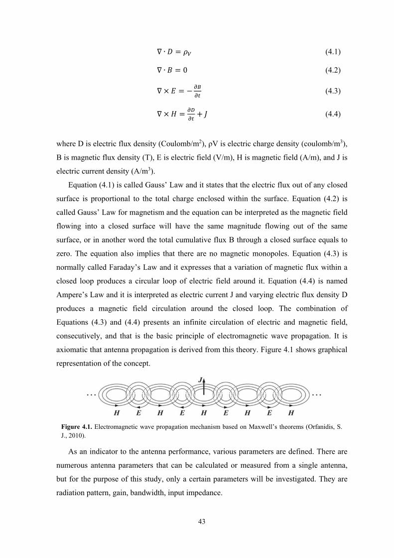
43

∙ (4.1)

∙ 0 (4.2)

(4.3)

(4.4)

where D is electric flux density (Coulomb/m2), ρV is electric charge density (coulomb/m3),

B is magnetic flux density (T), E is electric field (V/m), H is magnetic field (A/m), and J is

electric current density (A/m3).

Equation (4.1) is called Gauss’ Law and it states that the electric flux out of any closed

surface is proportional to the total charge enclosed within the surface. Equation (4.2) is

called Gauss’ Law for magnetism and the equation can be interpreted as the magnetic field

flowing into a closed surface will have the same magnitude flowing out of the same

surface, or in another word the total cumulative flux B through a closed surface equals to

zero. The equation also implies that there are no magnetic monopoles. Equation (4.3) is

normally called Faraday’s Law and it expresses that a variation of magnetic flux within a

closed loop produces a circular loop of electric field around it. Equation (4.4) is named

Ampere’s Law and it is interpreted as electric current J and varying electric flux density D

produces a magnetic field circulation around the closed loop. The combination of

Equations (4.3) and (4.4) presents an infinite circulation of electric and magnetic field,

consecutively, and that is the basic principle of electromagnetic wave propagation. It is

axiomatic that antenna propagation is derived from this theory. Figure 4.1 shows graphical

representation of the concept.

As an indicator to the antenna performance, various parameters are defined. There are

numerous antenna parameters that can be calculated or measured from a single antenna,

but for the purpose of this study, only a certain parameters will be investigated. They are

radiation pattern, gain, bandwidth, input impedance.

Figure 4.1. Electromagnetic wave propagation mechanism based on Maxwell’s theorems (Orfanidis, S. J., 2010).

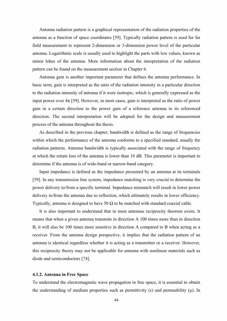
44

Antenna radiation pattern is a graphical representation of the radiation properties of the

antenna as a function of space coordinates [59]. Typically radiation pattern is used for far

field measurement to represent 2-dimension or 3-dimension power level of the particular

antenna. Logarithmic scale is usually used to highlight the parts with low values, known as

minor lobes of the antenna. More information about the interpretation of the radiation

pattern can be found on the measurement section in Chapter 6.

Antenna gain is another important parameter that defines the antenna performance. In

basic term, gain is interpreted as the ratio of the radiation intensity in a particular direction

to the radiation intensity of antenna if it were isotropic, which is generally expressed as the

input power over 4π [59]. However, in most cases, gain is interpreted as the ratio of power

gain in a certain direction to the power gain of a reference antenna in its referenced

direction. The second interpretation will be adopted for the design and measurement

process of the antenna throughout the thesis.

As described in the previous chapter, bandwidth is defined as the range of frequencies

within which the performance of the antenna conforms to a specified standard, usually the

radiation patterns. Antenna bandwidth is typically associated with the range of frequency

at which the return loss of the antenna is lower than 10 dB. This parameter is important to

determine if the antenna is of wide-band or narrow-band category.

Input impedance is defined as the impedance presented by an antenna at its terminals

[59]. In any transmission line system, impedance matching is very crucial to determine the

power delivery to/from a specific terminal. Impedance mismatch will result in lower power

delivery to/from the antenna due to reflection, which ultimately results in lower efficiency.

Typically, antenna is designed to have 50 Ω to be matched with standard coaxial cable.

It is also important to understand that in most antennas reciprocity theorem exists. It

means that when a given antenna transmits in direction A 100 times more than in direction

B, it will also be 100 times more sensitive in direction A compared to B when acting as a

receiver. From the antenna design perspective, it implies that the radiation pattern of an

antenna is identical regardless whether it is acting as a transmitter or a receiver. However,

this reciprocity theory may not be applicable for antenna with nonlinear materials such as

diode and semiconductors [74].

4.1.2. Antenna in Free Space

To understand the electromagnetic wave propagation in free space, it is essential to obtain

the understanding of medium properties such as permittivity (ε) and permeability (μ). In

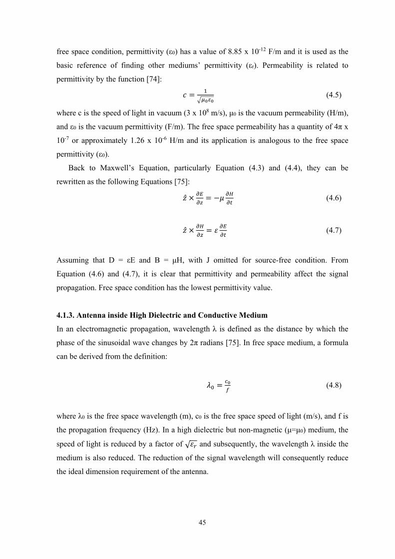
45

free space condition, permittivity (ε0) has a value of 8.85 x 10-12 F/m and it is used as the

basic reference of finding other mediums’ permittivity (εr). Permeability is related to

permittivity by the function [74]:

(4.5)

where c is the speed of light in vacuum (3 x 108 m/s), μ0 is the vacuum permeability (H/m),

and ε0 is the vacuum permittivity (F/m). The free space permeability has a quantity of 4π x

10-7 or approximately 1.26 x 10-6 H/m and its application is analogous to the free space

permittivity (ε0).

Back to Maxwell’s Equation, particularly Equation (4.3) and (4.4), they can be

rewritten as the following Equations [75]:

(4.6)

(4.7)

Assuming that D = εE and B = μH, with J omitted for source-free condition. From

Equation (4.6) and (4.7), it is clear that permittivity and permeability affect the signal

propagation. Free space condition has the lowest permittivity value.

4.1.3. Antenna inside High Dielectric and Conductive Medium

In an electromagnetic propagation, wavelength λ is defined as the distance by which the

phase of the sinusoidal wave changes by 2π radians [75]. In free space medium, a formula

can be derived from the definition:

(4.8)

where λ0 is the free space wavelength (m), c0 is the free space speed of light (m/s), and f is

the propagation frequency (Hz). In a high dielectric but non-magnetic (μ=μ0) medium, the

speed of light is reduced by a factor of √ and subsequently, the wavelength λ inside the

medium is also reduced. The reduction of the signal wavelength will consequently reduce

the ideal dimension requirement of the antenna.

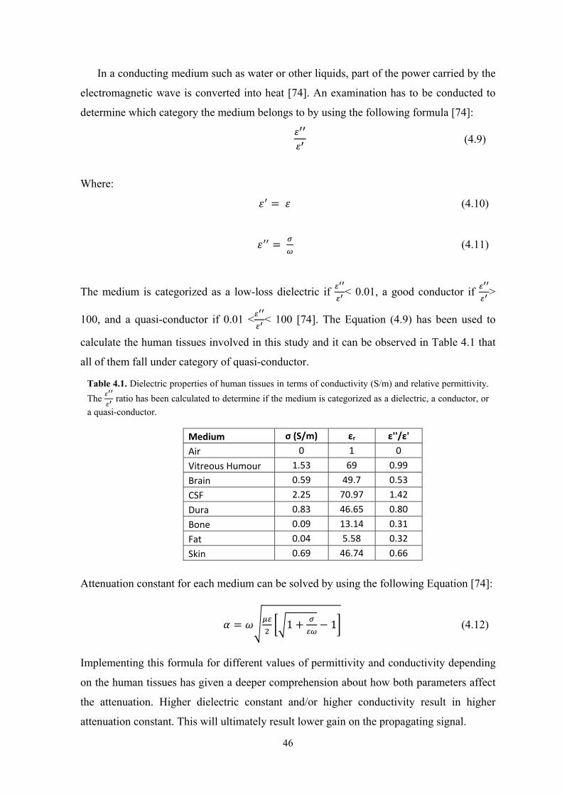
46

In a conducting medium such as water or other liquids, part of the power carried by the

electromagnetic wave is converted into heat [74]. An examination has to be conducted to

determine which category the medium belongs to by using the following formula [74]:

(4.9)

Where:

(4.10)

(4.11)

The medium is categorized as a low-loss dielectric if < 0.01, a good conductor if >

100, and a quasi-conductor if 0.01 < < 100 [74]. The Equation (4.9) has been used to

calculate the human tissues involved in this study and it can be observed in Table 4.1 that

all of them fall under category of quasi-conductor.

Attenuation constant for each medium can be solved by using the following Equation [74]:

1 1 (4.12)

Implementing this formula for different values of permittivity and conductivity depending

on the human tissues has given a deeper comprehension about how both parameters affect

the attenuation. Higher dielectric constant and/or higher conductivity result in higher

attenuation constant. This will ultimately result lower gain on the propagating signal.

Table 4.1. Dielectric properties of human tissues in terms of conductivity (S/m) and relative permittivity.

The ratio has been calculated to determine if the medium is categorized as a dielectric, a conductor, or

a quasi-conductor.

Medium σ (S/m) εr ε''/ε'

Air 0 1 0

Vitreous Humour 1.53 69 0.99

Brain 0.59 49.7 0.53

CSF 2.25 70.97 1.42

Dura 0.83 46.65 0.80

Bone 0.09 13.14 0.31

Fat 0.04 5.58 0.32

Skin 0.69 46.74 0.66

47

4.2. Previous Implantable Antenna Designs

After gaining a valuable insight on the fundamental principle of how an implantable

antenna works, this Section will present a review on published literatures about

implantable antenna designs. The focus will be on the antenna parameters as well as the

simulation and measurement technique in each experiment. The obtained knowledge will

provide a good direction on the design and simulation process of the proposed antenna.

In a study conducted by Soontornpipit (2004) [71], microstrip antenna parameters

such as shape, length, size, feeding placement, materials, and layer thickness were

investigated to accomplish a useful knowledge for antenna optimisation. Microstrip

antenna type was selected and simulation inside both 2/3 human muscle and human

shoulder model was executed using finite-difference time-domain (FDTD) technique at

402-405 MHz frequency band. The parametric study determined that a microstrip planar

inverted-F (PIFA) antenna with a dimension of 29.4 x 19.6 x 6 mm3 was the most

optimized geometry implantable antenna. The simulation inside 2/3 human muscle (εr =

42.8, σ = 0.65 S/m at 402 MHz) produced a good return loss of -30 dB at 402 MHz.

However, a switch of the medium to a heterogeneous shoulder model developed by

University of Utah, the resonant frequency was shifted to approximately 430 MHz. The

proposed antenna produced a bandwidth of 20 MHz and maximum gain of -38 dB.

In a study by Kim (2004) [72], the adoption of PIFA geometry is investigated and

compared against the conventional microstrip antenna. Both models were identical except

for the presence of a pin connecting the conductor to the ground layer. The dimension of

the antenna was 40 x 36 x 4 mm3 and the material of both substrate and superstrate was

high permittivity Rogers RO3210 (εr = 10.2). Both antenna configuration was simulated

and measured inside a human tissue simulating fluid with dielectric characteristic of εr =

49.6, σ = 0.51 S/m at 402 MHz. The simulation using FDTD technique produced a return

loss of -20 dB at 402 MHz (PIFA) and 413 MHz (Microstrip) inside the tissue simulating

fluid. However, the resonant frequencies from the measurement were shifted to 438 MHz

and 427 MHz for the microstrip and the PIFA antenna, respectively. From the simulation,

the radiation efficiency of the antenna was 0.25% for the PIFA and 0.16% for the

microstrip antenna. The results indicated that the implementation of PIFA geometry for the

same microstrip antenna pattern lowers the resonance frequency and increases the radiation

efficiency.

48

In another research by Azad (2009) [76], an implantable antenna was designed for the

purpose of integration to global positioning system (GPS) as part of Alzheimer’s disease

telemetry system. The PIFA microstrip antenna occupied a volume of 20 x 20 x 6 mm3

with the conductor line resembling Hilbert pattern. Biocompatible materials such as

Silicone and Macor were selected for the substrate and superstrate of the antenna,

respectively. In this experiment, the antenna was immersed into a block of human muscle

with dielectric properties of εr = 42.81 and σ = 0.65 S/m. The simulation achieved a return

loss of -12 dB at 1.575 GHz with a bandwidth span of 44.1 MHz.

An implantable printed spiral antenna was designed, simulated, and tested to be

integrated into a capsule endoscope system (Kwak, 2006) [52]. Due to the nature of the

transmission, which requires a high data rate for high resolution image data transfer, a

wideband antenna is proposed. A spiral conductor with a diameter of 10.1 mm was printed

on RF 35-A with relative permittivity (εr) of 3.5 and thickness of 3 mm. The proposed

antenna was simulated inside a tissue-simulating fluid (εr = 56, σ = 0.83 S/m) at the

operating frequency of 450 MHz with the aid of CST Microwave Studio software. The

simulation achieved a return loss of -23 dB at 450 MHz, with the measurement verification

showed a 30 MHz discrepancy on the resonant frequency. The proposed antenna also had a

wide bandwidth characteristic of 70 MHz, which spans from 430 to 500 MHz.

A different approach of antenna miniaturization was proposed by Lee (2007) [77] by

incorporating a multilayer microstrip antenna design. In this study, three substrate layers

with thickness of 0.635 mm and material of RO3210 were selected as dielectric materials

in between each conductor layer. The overall dimension of the antenna was π x (7.5)2 x 1.9

mm3 and is intended to be operating at MICS band. The antenna was immersed inside

human tissue fluid (εr = 46.7, σ = 0.69 S/m at 402 MHz) in the HFSS simulation. For the

verification of the simulation, a tissue liquid composed of deionized water, sugar, salt, and

cellulose was created. The proposed antenna achieved return loss of -44 dB at 402 MHz,

verified by the measurement result of -28 dB at 402 MHz. The radiation pattern was

omnidirectional with maximum gain and radiation efficiency achieved were -26 dB and

0.31%, respectively. The antenna also produced a large bandwidth of 50 MHz, as a result

of the multilayer technique. Another microstrip antenna was proposed by the same author

Lee (2008) [78] with a focus on wider bandwidth realization. A π-shaped microstrip PIFA

antenna with a substrate dimension of 22.5 x 22.5 x 1.27 mm3 was proposed to operate on

the same human tissue fluid at the same frequency band (MICS band). The 10 dB

bandwidth of the antenna was 80 MHz, in which two dips were observed, and the

49

maximum gain was -25 dB. In terms of volume occupied by the antenna geometry, this

antenna required twice as much space compared to the first antenna. A further

improvement to this antenna was proposed by the implementation of additional substrate

layer to obtain wider bandwidth and smaller dimension (2009) [79]. The π-shaped

conductor was still preserved in this design and the dimension of the antenna was slightly

modified to 22.5 x 18.5 x 1.9 mm3. A HFSS simulation inside a grinded pork leg (εr = 54,

σ = 0.8 S/m) produced a return loss of -24 dB at 440 MHz and it was validated by the

measurement result (-34 dB at 440 MHz). The achievable bandwidth in this configuration

was 132 MHz with the maximum gain achieved was -27 dB.

A three dimensional dipole antenna was developed as part of a retinal prosthesis

system by Soora (2008) as part of the Second Sight Group [16]. In this study, the proposed

antenna occupied 5.25 x 5.25 x 4 mm3 and it was simulated inside a human eye phantom

(εr = 65.67, σ = 1.8 to 2.6 S/m at 2 to 2.6 GHz), which was created by mixing salt and

sugar into water. Measurement inside the tissue simulating fluid produced a return loss of -

32.4 dB at 2.33 GHz, with a bandwidth of 151 GHz and maximum gain of -32.4 dB.

In a more recent study, an implantable serpentine microstrip antenna was designed for

the purpose of continuous glucose monitoring (Karacolak, 2008) [80]. With a dimension

of 22.5 x 22.5 x 2.5 mm3, the antenna achieved a dual-band operation at MICS band and

ISM 2.4 GHz, with the return loss values of -25 dB and -26 dB at 402 MHz and 2.4 GHz,

respectively. This was achieved after the implementation of particle swarm optimisation

for finding the best geometry of the antenna. The verification of the antenna was executed

inside a mixture of deionized water, sugar, salt, and agarose to mimic the skin

characteristic at 402 MHz and 2.4 GHz. The measurement inside the fluid was successful

in replicating the simulation results by achieving -24 dB and -11 dB return loss at 402

MHz and 2.45 GHz, respectively. The maximum gain achieved at MICS band was -24 dB

with a measured bandwidth 131.91 MHz. The next step of this study was the

implementation of rat skin for a further testing of the antenna [81]. Slight modification was

applied to the antenna design for an optimized operation inside the rat skin (εr = 33, σ = 0.5

S/m at 402 MHz). A verification process was then conducted by embedding the fabricated

antenna into the real rat skin. The results showed an agreement with the antenna

measurement inside the rat skin mimicking material. This antenna was further tested in an

in vivo experiment involving rats supplied by Mississippi State University’s College of

Veterinary Medicine [82]. Before the implantation process, the antenna was encapsulated

50

by Silastic MDS4-4210 Biomedical-Grade Base Elastomer with εr = 3.3 for

biocompatibility characteristic.

Another multi-layer configuration was investigated for an implantable microstrip

antenna [83] by Liu (2008). With a dimension of 10 x 10 x 1.9 mm3, this antenna adopted

PIFA configuration and featured 50 MHz bandwidth. The verification of the simulation

was done by immersing the antenna to a cylinder filled with skin simulating fluid (εr =

46.7, σ = 0.69 S/m at 403 MHz). Maximum gain achieved by the antenna was -26 dB with

the radiation efficiency of 0.61%. Another multilayer microstrip antenna was developed by

Liu (2009) [84] for the purpose of increasing the bandwidth of the antenna. The new

antenna design was implementing hooked-shaped slots at the edges of the radiating patches

and occupied 8 x 8 x 1.9 mm3 space. The bandwidth of the antenna was increased to 122

MHz, with a reduction on the radiation efficiency (0.55%) and the maximum gain (-37.96

dB) compared to the previous antenna. The measurement procedure for this antenna was

identical with the previous one.

A study by Abadia (2009) highlighted an innovative implantable antenna

miniaturization technique by connecting all the conductor path in 3D, resulting in a 3D

microstrip antenna [85]. With a total dimension of 14 x 14 x 15 mm3, this antenna achieved

a return loss of -37 dB at 425 MHz for a simulation inside the muscle fluid. For the data

validation, the antenna was submerged to a cylinder filled with muscle fluid (εr = 57.1 and

σ = 0.796 S/m at 402 MHz). The measurement results generally agreed with the simulation

data, with the return loss achieved was -39 dB at 427 MHz with a bandwidth 225 MHz.

The maximum achievable gain was recorded at -28.5 dB. In another experiment, this group

attempted another antenna design by maximizing the 3D structure of the packaging [86].

The proposed design was called multilayer pyramidal structure, which was basically a

multilayer microstrip antenna with different substrate dimensions on each layer. The

antenna, with total dimension of 13.1 x 8 x 5.2 mm3, was operating on two frequency

bands (MICS and ISM 2.4 GHz). Compared to the previous design, this antenna achieved a

much lower bandwidth at 12 MHz with comparable maximum gain of -28.8 dB.

Another attempt to miniaturize an implantable antenna was done by employing a very

high dielectric substrate (Chien, 2010) [87]. The antenna consisted of a substrate layer,

which was created from ceramic substrate (εr = 28), and a monopole strip on top of it. No

superstrate was included in the design. The antenna had a dimension of 18 x 16 x 1 mm3

(just the antenna) and 18 x 16 x 1.4 mm3 (with added Al2O3superstrate). Both antennas

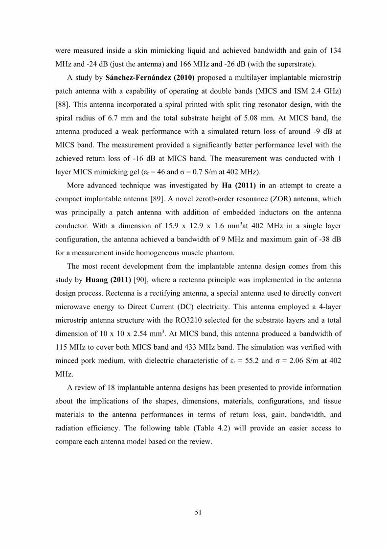
51

were measured inside a skin mimicking liquid and achieved bandwidth and gain of 134

MHz and -24 dB (just the antenna) and 166 MHz and -26 dB (with the superstrate).

A study by Sánchez-Fernández (2010) proposed a multilayer implantable microstrip

patch antenna with a capability of operating at double bands (MICS and ISM 2.4 GHz)

[88]. This antenna incorporated a spiral printed with split ring resonator design, with the

spiral radius of 6.7 mm and the total substrate height of 5.08 mm. At MICS band, the

antenna produced a weak performance with a simulated return loss of around -9 dB at

MICS band. The measurement provided a significantly better performance level with the

achieved return loss of -16 dB at MICS band. The measurement was conducted with 1

layer MICS mimicking gel (εr = 46 and σ = 0.7 S/m at 402 MHz).

More advanced technique was investigated by Ha (2011) in an attempt to create a

compact implantable antenna [89]. A novel zeroth-order resonance (ZOR) antenna, which

was principally a patch antenna with addition of embedded inductors on the antenna

conductor. With a dimension of 15.9 x 12.9 x 1.6 mm3at 402 MHz in a single layer

configuration, the antenna achieved a bandwidth of 9 MHz and maximum gain of -38 dB

for a measurement inside homogeneous muscle phantom.

The most recent development from the implantable antenna design comes from this

study by Huang (2011) [90], where a rectenna principle was implemented in the antenna

design process. Rectenna is a rectifying antenna, a special antenna used to directly convert

microwave energy to Direct Current (DC) electricity. This antenna employed a 4-layer

microstrip antenna structure with the RO3210 selected for the substrate layers and a total

dimension of 10 x 10 x 2.54 mm3. At MICS band, this antenna produced a bandwidth of

115 MHz to cover both MICS band and 433 MHz band. The simulation was verified with

minced pork medium, with dielectric characteristic of εr = 55.2 and σ = 2.06 S/m at 402

MHz.

A review of 18 implantable antenna designs has been presented to provide information

about the implications of the shapes, dimensions, materials, configurations, and tissue

materials to the antenna performances in terms of return loss, gain, bandwidth, and

radiation efficiency. The following table (Table 4.2) will provide an easier access to

compare each antenna model based on the review.

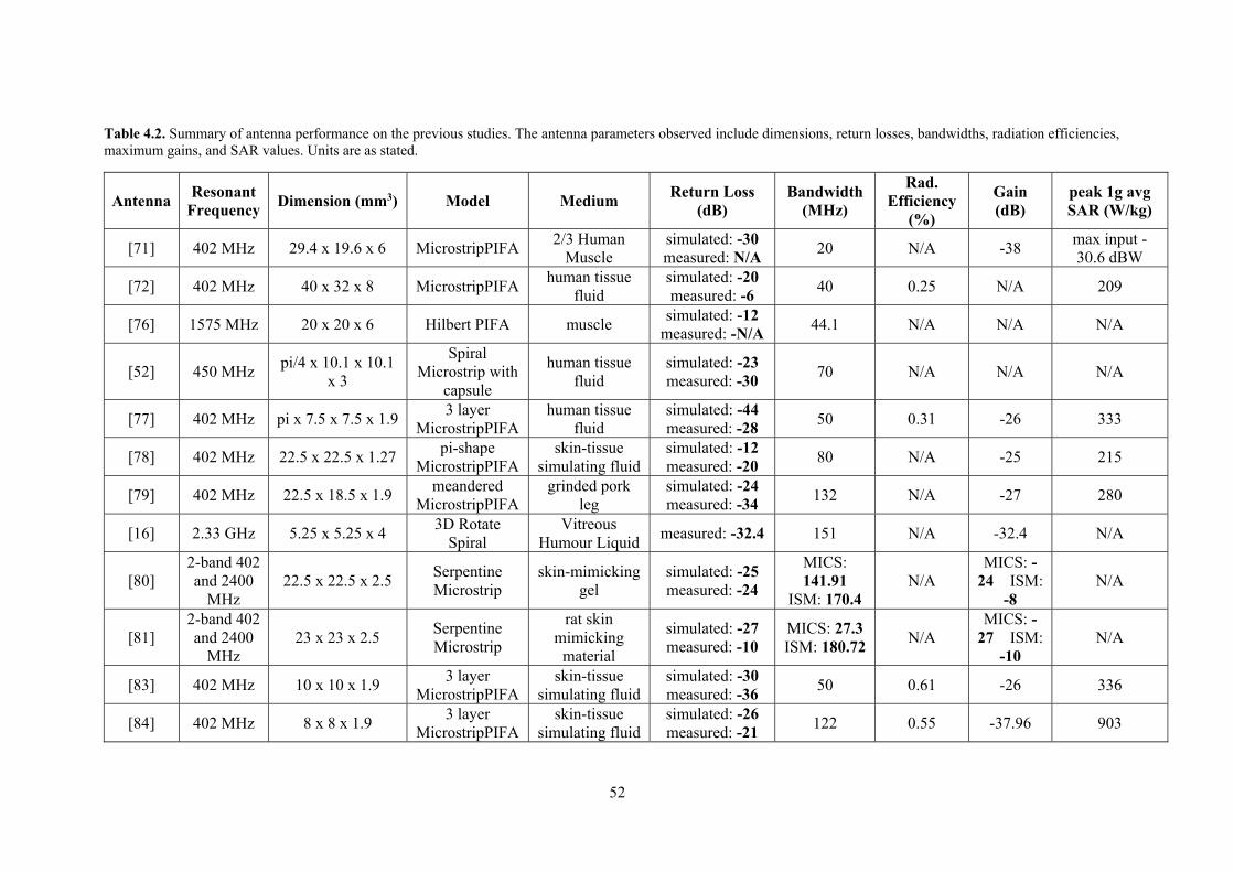
52

Table 4.2. Summary of antenna performance on the previous studies. The antenna parameters observed include dimensions, return losses, bandwidths, radiation efficiencies, maximum gains, and SAR values. Units are as stated.

Antenna Resonant

Frequency Dimension (mm3) Model Medium

Return Loss (dB)

Bandwidth (MHz)

Rad. Efficiency

(%)

Gain (dB)

peak 1g avg SAR (W/kg)

[71] 402 MHz 29.4 x 19.6 x 6 MicrostripPIFA 2/3 Human

Muscle simulated: -30 measured: N/A

20 N/A -38 max input -30.6 dBW

[72] 402 MHz 40 x 32 x 8 MicrostripPIFA human tissue

fluid simulated: -20 measured: -6

40 0.25 N/A 209

[76] 1575 MHz 20 x 20 x 6 Hilbert PIFA muscle simulated: -12

measured: -N/A 44.1 N/A N/A N/A

[52] 450 MHz pi/4 x 10.1 x 10.1

x 3

Spiral Microstrip with

capsule

human tissue fluid

simulated: -23 measured: -30

70 N/A N/A N/A

[77] 402 MHz pi x 7.5 x 7.5 x 1.9 3 layer

MicrostripPIFA human tissue

fluid simulated: -44 measured: -28

50 0.31 -26 333

[78] 402 MHz 22.5 x 22.5 x 1.27 pi-shape

MicrostripPIFA skin-tissue

simulating fluid simulated: -12 measured: -20

80 N/A -25 215

[79] 402 MHz 22.5 x 18.5 x 1.9 meandered

MicrostripPIFA grinded pork

leg simulated: -24 measured: -34

132 N/A -27 280

[16] 2.33 GHz 5.25 x 5.25 x 4 3D Rotate

Spiral Vitreous

Humour Liquid measured: -32.4 151 N/A -32.4 N/A

[80] 2-band 402 and 2400

MHz 22.5 x 22.5 x 2.5

Serpentine Microstrip

skin-mimicking gel


MICS: 141.91

ISM: 170.4 N/A

MICS: -24 ISM:

-8 N/A

[81] 2-band 402 and 2400

MHz 23 x 23 x 2.5

Serpentine Microstrip

rat skin mimicking

material


MICS: 27.3 ISM: 180.72

N/A MICS: -

27 ISM: -10

N/A

[83] 402 MHz 10 x 10 x 1.9 3 layer



50 0.61 -26 336

[84] 402 MHz 8 x 8 x 1.9 3 layer



122 0.55 -37.96 903

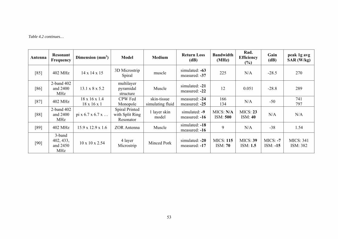
53

Table 4.2 continues…

Antenna Resonant

Frequency Dimension (mm3) Model Medium

Return Loss (dB)

Bandwidth (MHz)

Rad. Efficiency

(%)

Gain (dB)

peak 1g avg SAR (W/kg)

[85] 402 MHz 14 x 14 x 15 3D Microstrip

Spiral muscle


225 N/A -28.5 270

[86] 2-band 402 and 2400

MHz 13.1 x 8 x 5.2

multilayer pyramidal structure

Muscle simulated: -21 measured: -22

12 0.051 -28.8 289

[87] 402 MHz 18 x 16 x 1.4 18 x 16 x 1

CPW Fed Monopole

skin-tissue simulating fluid

measured: -24 measured: -25

166 134

N/A -50 741 797

[88] 2-band 402 and 2400

MHz pi x 6.7 x 6.7 x …

Spiral Printed with Split Ring

Resonator

1 layer skin model


MICS: N/A ISM: 500

MICS: 23 ISM: 40

N/A N/A

[89] 402 MHz 15.9 x 12.9 x 1.6 ZOR Antenna Muscle simulated: -18 measured: -16

9 N/A -38 1.54

[90]

3-band 402, 433, and 2450

MHz

10 x 10 x 2.54 4 layer

Microstrip Minced Pork


MICS: 115 ISM: 70

MICS: 39 ISM: 1.5

MICS: -7 ISM: -15

MICS: 341 ISM: 382

54

4.3. Antenna Model Selection

The review about various implantable antenna designs provided a good insight on factors

affecting the implantable antenna operation. The knowledge gained from the articles was

continually referred to during the design process. In this subchapter, an antenna model

selection process will be presented. The process involved matching the antenna design

with the constraints associated with the surrounding medium. The constraints will be

defined and followed by the proposal of the most suitable design alternative.

4.3.1. Constraints

Designing an implantable antenna is a challenging task due to inevitable constraints that

have to be considered, such as size, electrical characteristic of the surrounding materials,

antenna material, as well as the SAR value limitation. In this case, the antenna is intended

to be implanted inside a human eyeball with a diameter of around 24-25 mm.

Consequently, an antenna that fits spherical dimension of 25 mm diameter is desirable.

Each part of human body has unique electrical characteristic, and the frequency

dependability of each part makes it even more complicated. To satisfy the purpose of the

antenna, Vitreous Humour was applied as the surrounding material in the simulation. As

stated in Chapter 2, Vitreous Humour is a semisolid gel structure inside an eyeball that is

based on water (98%) and contains small amount of solid matters in the form of collagen,

vitrosin, and hyaluronic acids. Compared to other parts of human body, Vitreous Humour

has a high relative permittivity and conductivity at 402 MHz (εr = 69, σ = 1.5296 S/m)

[64], which makes it an inefficient medium for electromagnetic signal propagation. Due to

the surrounding medium being a living tissue, it is imperative that the antenna has to be

made of, or enclosed by, a biocompatible material. This is to avoid any bad reaction by the

antenna’s surrounding tissue.

Since the antenna is placed right in the middle of the tissue, the direct electromagnetic

exposure to the surrounding tissue will result in higher SAR values. As mentioned in

Chapter 3, the SAR values on any 10 g average of tissues must not exceed 2 W/kg.

4.3.2. Microstrip Antenna

Due to the constraints presented on the previous Section, it is inevitable that microstrip

antenna model is adopted for the retinal prosthesis system purpose. A microstrip antenna

consists of very thin metallic strip separated to a ground plane by a dielectric material,

55

typically referred to as substrate [70]. The advantages of microstrip antenna include

compact and low profile characteristic, straightforward fabrication procedure, possibility of

multiband operation, and low radar cross section (RCS – useful for military purposes) [91].

These aspects exist to compensate the fact that a microstrip antenna generally produces a

narrow bandwidth, low power, and produces large insertion loss [70].

A microstrip antenna is a resonant-style radiator, which means one of its apertures has

to have dimension around half of the wavelength. The resonant dimension of the antenna

will also depend on the shape of the patch conductor. When a voltage is applied to the

feeding point, a current will be excited on the patch and vertical electric fields will be

generated between the patch and the ground plane. When the gap between the edge of the

patch and the ground plane is half the wavelength, the radiated fields will create an

efficient resonant radiator [91]. The feeding placement greatly influences the input

impedance value, with a placement near the edge resulting high input impedance in

contrast to low impedance when the feed is placed at the centre of the patch.

There are countless possibilities on the conductor shapes of the microstrip antenna and

each pattern has its own characteristic. The most utilized conductor geometry is the

rectangular and the square shapes. For this pattern, the length of the patch controls the

resonant frequency while the width affects the impedance level as well as the bandwidth

[91]. With this configuration, dual polarized radiation can be generated by placing the

feeding pin along the diagonal plane. Due to the large area occupied by this geometry,

rectangular and square patches generally produce higher bandwidth. Circular and elliptical

shapes are also common in the microstrip antenna designs. With circular geometry, it has

only one degree of freedom in its shape through its radius and it will affect the resonant

frequency of the antenna. This pattern was rigorously investigated in the past due to its

inherent symmetry which in turn allows more efficient computation on the full-wave

analysis tool. With the advancement of full-wave design software, this geometry is

becoming increasingly rare. Modern conductor geometries have evolved to something

beyond the conventional shapes. In this case, traditional analysis on the geometry is very

difficult due to the complex nature of current flow on the conductor. The utilization of

electromagnetic solver is inevitable.

There are four excitation methods of microstrip antenna: edge fed, probe fed, aperture-

coupled, and proximity-coupled. However, only the edge fed and probe fed techniques will

be discussed in this Section. In the edge fed method, the microstrip feed-line is in direct

contact with the patch conductor. The advantages of this approach include simple

56

fabrication, easy to model, and efficient, while the drawback is narrow bandwidth [91]. In

the probe fed method, a probe extends through the ground plane and is connected to the

conductor with the aid of soldering work. The probe is typically the inner conductor of a

coaxial cable and its position on the conductor patch greatly influences the input

impedance of the antenna. The advantages of implementing probe fed to a microstrip

antenna are the isolation of the antenna to the ground plane and high efficiency. There are

also issues in adopting this approach, namely low bandwidth, difficult to analyse

accurately, and the generation of unintentional cross-polarized fields. However, despite

these drawbacks, it has been decided that probe fed method will be adopted in the antenna

design process to take advantage of the isolation between the antenna conductor and the

ground plane. This would be useful in minimizing the spurious radiation.

4.3.3. Antenna Miniaturization

One of the constraints in the antenna design for the retinal prosthesis system is the size

limitation. The diameter of a human eyeball is 25 mm, while the ideal antenna aperture for

an operation inside Vitreous Humour at 402 MHz is 22.46 mm (Table 3.3). Although

mathematically possible, the implementation of the ideal aperture is not very practical from

the sustainability point of view. The potential implant will cause a lot of pressure to the

surrounding eyeball components and there is little option for the placement of the antenna

other than along the centre line.

The proposed solution to counteract this problem is to reduce the size of the antenna.

The performance of the resized antenna would inevitably be inferior compared to the one

in ideal size, but there are some miniaturization techniques to prevent significant penalty to

the antenna performance. They are [92]: a) use lump-element loaded antenna, b) use high

permittivity substrate or superstrate, c) short circuit to ground plane, and d) geometry

optimisation.

The idea of using lump-element as an extension of the antenna conductor is raised to

counteract strong reactive input impedance caused by the antenna dimension reduction to

less than half a wavelength. The implementation of this technique will result in lower

efficiency and smaller bandwidth. This technique has been applied in one of the previous

antenna designs [89].

Modification on substrate material on a microstrip antenna will produce different

antenna characteristic. The adoption of high permittivity material as a substrate will

particularly lower the resonant frequency of the antenna based on the principle that the

57

wavelength is shorter inside the material. This advantage comes in expense of lower

bandwidth and gain of the antenna. A high dielectric ceramic material MgTa1.5Nb0.5O6 (εr

= 28) has been specially developed for an implantable antenna.

The idea of creating a connection between a conductor and a ground plane is to utilize

the ground plane as a virtual half of dipole arm in respect to the entire antenna. This

method has been widely used (as PIFA) because it is very easy to implement. In Table 2, it

can be seen that majority of the microstrips antenna incorporate PIFA configuration in

their designs.

Geometry adjustment of an antenna, particularly microstrip antenna, includes

modification on the patch pattern as well as substrate geometry and configuration.

However, with this optimisation technique, the application of the antenna is limited to that

specific purpose. Many studies have incorporated innovative geometry optimisation

approach such as stacked pyramidal structure [86] or 3D rotated dipole antenna [16] to

boost the performance of the antenna.

In addition to design problems, there are also problems associated with small antenna

measurements. Due to the small ground size, the antenna is neither balanced nor

unbalanced, makes it difficult to obtain an accurate measurement result. In addition,

spurious radiations from the coaxial cable produce a great degree of distortion to the

antenna characteristic. The polarizations are also difficult to define due to the conductor

length being shorter than the wavelength [92].

58

4.4. Summary

This chapter has provided an insight on the underlying principle of an antenna, including

its operation in free space as well as inside high dielectric and conductive medium like

Vitreous Humour. An extensive review on the previous implantable antenna designs

published on the journal articles were also presented for an indicator on how an

implantable antenna should behave. The information obtained from the theory, combined

with the past antenna designs, was applied in determining the design of the proposed

antenna. Several constraints were listed as potential obstacles in the design process. As a

result, microstrip antenna was selected as the antenna type and miniaturization technique

was also discussed as a measure to comply the limited space available. On the next

chapter, the simulation aspect of the study would be revealed. The evolution of the antenna

design through multiple modifications would also be disclosed, followed by the simulation

of the antenna in the real case scenarios.

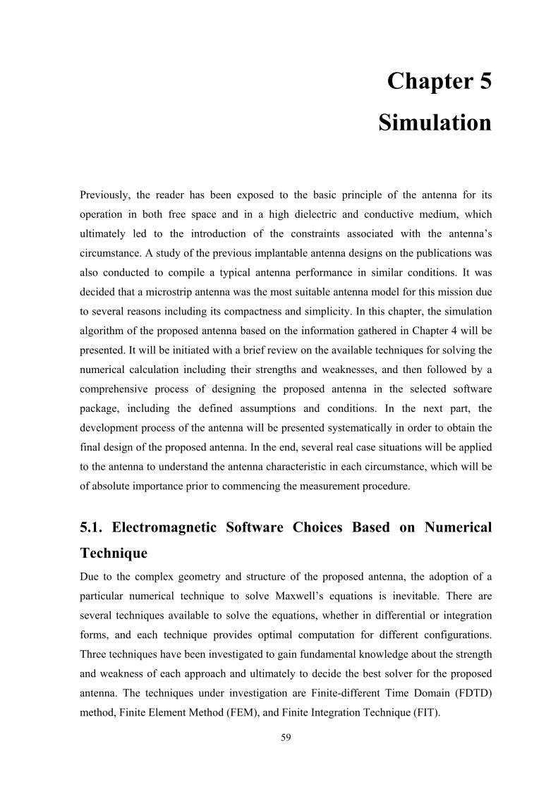
59

Chapter 5

Simulation

Previously, the reader has been exposed to the basic principle of the antenna for its

operation in both free space and in a high dielectric and conductive medium, which

ultimately led to the introduction of the constraints associated with the antenna’s

circumstance. A study of the previous implantable antenna designs on the publications was

also conducted to compile a typical antenna performance in similar conditions. It was

decided that a microstrip antenna was the most suitable antenna model for this mission due

to several reasons including its compactness and simplicity. In this chapter, the simulation

algorithm of the proposed antenna based on the information gathered in Chapter 4 will be

presented. It will be initiated with a brief review on the available techniques for solving the

numerical calculation including their strengths and weaknesses, and then followed by a

comprehensive process of designing the proposed antenna in the selected software

package, including the defined assumptions and conditions. In the next part, the

development process of the antenna will be presented systematically in order to obtain the

final design of the proposed antenna. In the end, several real case situations will be applied

to the antenna to understand the antenna characteristic in each circumstance, which will be

of absolute importance prior to commencing the measurement procedure.

5.1. Electromagnetic Software Choices Based on Numerical

Technique

Due to the complex geometry and structure of the proposed antenna, the adoption of a

particular numerical technique to solve Maxwell’s equations is inevitable. There are

several techniques available to solve the equations, whether in differential or integration

forms, and each technique provides optimal computation for different configurations.

Three techniques have been investigated to gain fundamental knowledge about the strength

and weakness of each approach and ultimately to decide the best solver for the proposed

antenna. The techniques under investigation are Finite-different Time Domain (FDTD)

method, Finite Element Method (FEM), and Finite Integration Technique (FIT).

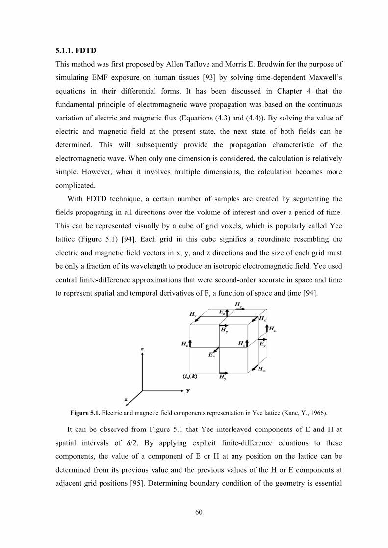
60

5.1.1. FDTD

This method was first proposed by Allen Taflove and Morris E. Brodwin for the purpose of

simulating EMF exposure on human tissues [93] by solving time-dependent Maxwell’s

equations in their differential forms. It has been discussed in Chapter 4 that the

fundamental principle of electromagnetic wave propagation was based on the continuous

variation of electric and magnetic flux (Equations (4.3) and (4.4)). By solving the value of

electric and magnetic field at the present state, the next state of both fields can be

determined. This will subsequently provide the propagation characteristic of the

electromagnetic wave. When only one dimension is considered, the calculation is relatively

simple. However, when it involves multiple dimensions, the calculation becomes more

complicated.

With FDTD technique, a certain number of samples are created by segmenting the

fields propagating in all directions over the volume of interest and over a period of time.

This can be represented visually by a cube of grid voxels, which is popularly called Yee

lattice (Figure 5.1) [94]. Each grid in this cube signifies a coordinate resembling the

electric and magnetic field vectors in x, y, and z directions and the size of each grid must

be only a fraction of its wavelength to produce an isotropic electromagnetic field. Yee used

central finite-difference approximations that were second-order accurate in space and time

to represent spatial and temporal derivatives of F, a function of space and time [94].

It can be observed from Figure 5.1 that Yee interleaved components of E and H at

spatial intervals of δ/2. By applying explicit finite-difference equations to these

components, the value of a component of E or H at any position on the lattice can be

determined from its previous value and the previous values of the H or E components at

adjacent grid positions [95]. Determining boundary condition of the geometry is essential

Figure 5.1. Electric and magnetic field components representation in Yee lattice (Kane, Y., 1966).

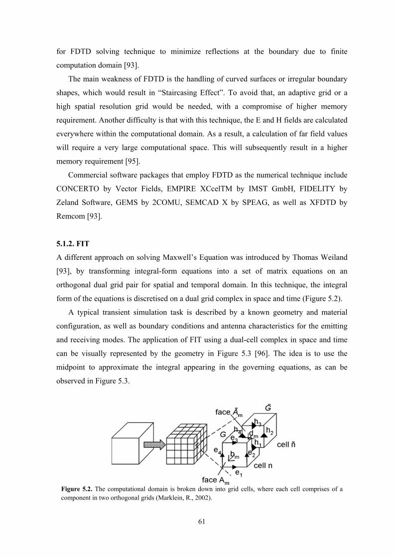
61

for FDTD solving technique to minimize reflections at the boundary due to finite

computation domain [93].

The main weakness of FDTD is the handling of curved surfaces or irregular boundary

shapes, which would result in “Staircasing Effect”. To avoid that, an adaptive grid or a

high spatial resolution grid would be needed, with a compromise of higher memory

requirement. Another difficulty is that with this technique, the E and H fields are calculated

everywhere within the computational domain. As a result, a calculation of far field values

will require a very large computational space. This will subsequently result in a higher

memory requirement [95].

Commercial software packages that employ FDTD as the numerical technique include

CONCERTO by Vector Fields, EMPIRE XCcelTM by IMST GmbH, FIDELITY by

Zeland Software, GEMS by 2COMU, SEMCAD X by SPEAG, as well as XFDTD by

Remcom [93].

5.1.2. FIT

A different approach on solving Maxwell’s Equation was introduced by Thomas Weiland

[93], by transforming integral-form equations into a set of matrix equations on an

orthogonal dual grid pair for spatial and temporal domain. In this technique, the integral

form of the equations is discretised on a dual grid complex in space and time (Figure 5.2).

A typical transient simulation task is described by a known geometry and material

configuration, as well as boundary conditions and antenna characteristics for the emitting

and receiving modes. The application of FIT using a dual-cell complex in space and time

can be visually represented by the geometry in Figure 5.3 [96]. The idea is to use the

midpoint to approximate the integral appearing in the governing equations, as can be

observed in Figure 5.3.

Figure 5.2. The computational domain is broken down into grid cells, where each cell comprises of a component in two orthogonal grids (Marklein, R., 2002).

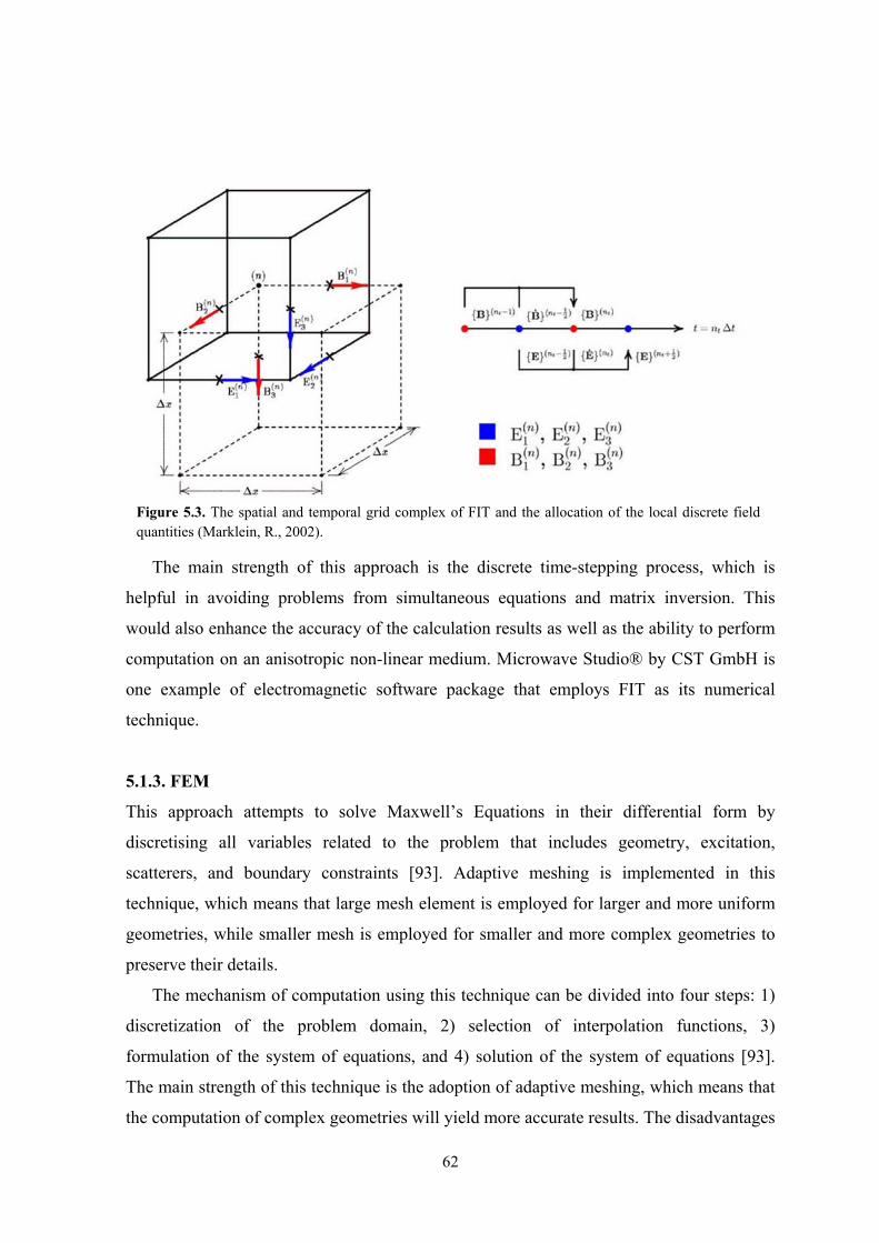
62

The main strength of this approach is the discrete time-stepping process, which is

helpful in avoiding problems from simultaneous equations and matrix inversion. This

would also enhance the accuracy of the calculation results as well as the ability to perform

computation on an anisotropic non-linear medium. Microwave Studio® by CST GmbH is

one example of electromagnetic software package that employs FIT as its numerical

technique.

5.1.3. FEM

This approach attempts to solve Maxwell’s Equations in their differential form by

discretising all variables related to the problem that includes geometry, excitation,

scatterers, and boundary constraints [93]. Adaptive meshing is implemented in this

technique, which means that large mesh element is employed for larger and more uniform

geometries, while smaller mesh is employed for smaller and more complex geometries to

preserve their details.

The mechanism of computation using this technique can be divided into four steps: 1)

discretization of the problem domain, 2) selection of interpolation functions, 3)

formulation of the system of equations, and 4) solution of the system of equations [93].

The main strength of this technique is the adoption of adaptive meshing, which means that

the computation of complex geometries will yield more accurate results. The disadvantages

Figure 5.3. The spatial and temporal grid complex of FIT and the allocation of the local discrete field quantities (Marklein, R., 2002).

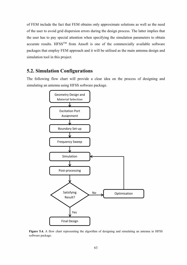
63

of FEM include the fact that FEM obtains only approximate solutions as well as the need

of the user to avoid grid dispersion errors during the design process. The latter implies that

the user has to pay special attention when specifying the simulation parameters to obtain

accurate results. HFSSTM from Ansoft is one of the commercially available software

packages that employ FEM approach and it will be utilised as the main antenna design and

simulation tool in this project.

5.2. Simulation Configurations

The following flow chart will provide a clear idea on the process of designing and

simulating an antenna using HFSS software package.

Geometry Design and

Material Selection

Excitation Port

Assignment

Boundary Set‐up

Frequency Sweep

Simulation

Satisfying

Result?

Post‐processing

Optimisation

Final Design

No

Figure 5.4. A flow chart representing the algorithm of designing and simulating an antenna in HFSS software package.

Yes

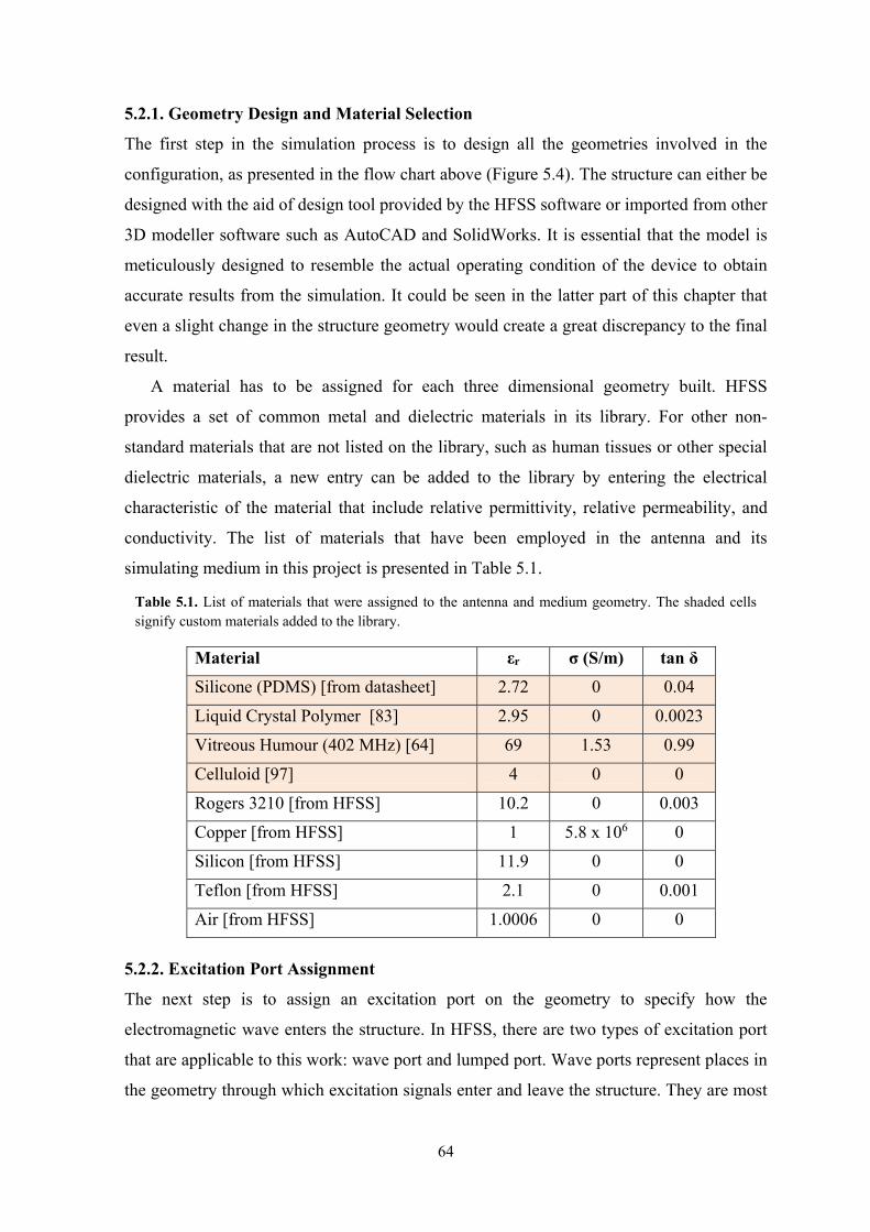
64

5.2.1. Geometry Design and Material Selection

The first step in the simulation process is to design all the geometries involved in the

configuration, as presented in the flow chart above (Figure 5.4). The structure can either be

designed with the aid of design tool provided by the HFSS software or imported from other

3D modeller software such as AutoCAD and SolidWorks. It is essential that the model is

meticulously designed to resemble the actual operating condition of the device to obtain

accurate results from the simulation. It could be seen in the latter part of this chapter that

even a slight change in the structure geometry would create a great discrepancy to the final

result.

A material has to be assigned for each three dimensional geometry built. HFSS

provides a set of common metal and dielectric materials in its library. For other non-

standard materials that are not listed on the library, such as human tissues or other special

dielectric materials, a new entry can be added to the library by entering the electrical

characteristic of the material that include relative permittivity, relative permeability, and

conductivity. The list of materials that have been employed in the antenna and its

simulating medium in this project is presented in Table 5.1.

5.2.2. Excitation Port Assignment

The next step is to assign an excitation port on the geometry to specify how the

electromagnetic wave enters the structure. In HFSS, there are two types of excitation port

that are applicable to this work: wave port and lumped port. Wave ports represent places in

the geometry through which excitation signals enter and leave the structure. They are most

Table 5.1. List of materials that were assigned to the antenna and medium geometry. The shaded cells signify custom materials added to the library.

Material εr σ (S/m) tan δ

Silicone (PDMS) [from datasheet] 2.72 0 0.04

Liquid Crystal Polymer [83] 2.95 0 0.0023

Vitreous Humour (402 MHz) [64] 69 1.53 0.99

Celluloid [97] 4 0 0

Rogers 3210 [from HFSS] 10.2 0 0.003

Copper [from HFSS] 1 5.8 x 106 0

Silicon [from HFSS] 11.9 0 0

Teflon [from HFSS] 2.1 0 0.001

Air [from HFSS] 1.0006 0 0

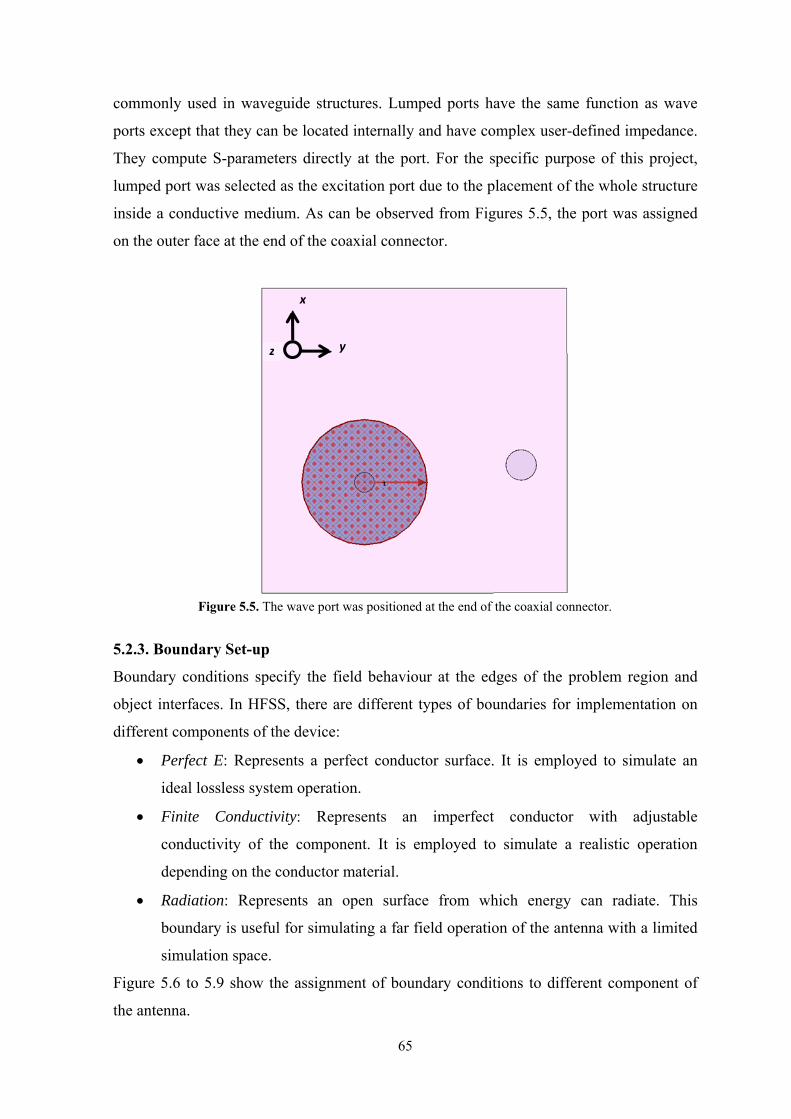
65

commonly used in waveguide structures. Lumped ports have the same function as wave

ports except that they can be located internally and have complex user-defined impedance.

They compute S-parameters directly at the port. For the specific purpose of this project,

lumped port was selected as the excitation port due to the placement of the whole structure

inside a conductive medium. As can be observed from Figures 5.5, the port was assigned

on the outer face at the end of the coaxial connector.

5.2.3. Boundary Set-up

Boundary conditions specify the field behaviour at the edges of the problem region and

object interfaces. In HFSS, there are different types of boundaries for implementation on

different components of the device:

Perfect E: Represents a perfect conductor surface. It is employed to simulate an

ideal lossless system operation.

Finite Conductivity: Represents an imperfect conductor with adjustable

conductivity of the component. It is employed to simulate a realistic operation

depending on the conductor material.

Radiation: Represents an open surface from which energy can radiate. This

boundary is useful for simulating a far field operation of the antenna with a limited

simulation space.

Figure 5.6 to 5.9 show the assignment of boundary conditions to different component of

the antenna.

Figure 5.5. The wave port was positioned at the end of the coaxial connector.

yz

x

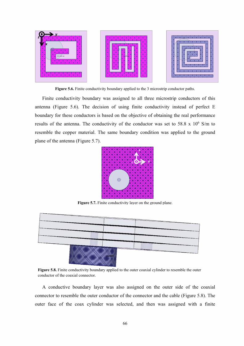
66

Finite conductivity boundary was assigned to all three microstrip conductors of this

antenna (Figure 5.6). The decision of using finite conductivity instead of perfect E

boundary for these conductors is based on the objective of obtaining the real performance

results of the antenna. The conductivity of the conductor was set to 58.8 x 106 S/m to

resemble the copper material. The same boundary condition was applied to the ground

plane of the antenna (Figure 5.7).

A conductive boundary layer was also assigned on the outer side of the coaxial

connector to resemble the outer conductor of the connector and the cable (Figure 5.8). The

outer face of the coax cylinder was selected, and then was assigned with a finite

Figure 5.6. Finite conductivity boundary applied to the 3 microstrip conductor paths.

y

x

z

Figure 5.7. Finite conductivity layer on the ground plane.

yz

x

x

Figure 5.8. Finite conductivity boundary applied to the outer coaxial cylinder to resemble the outer conductor of the coaxial connector.

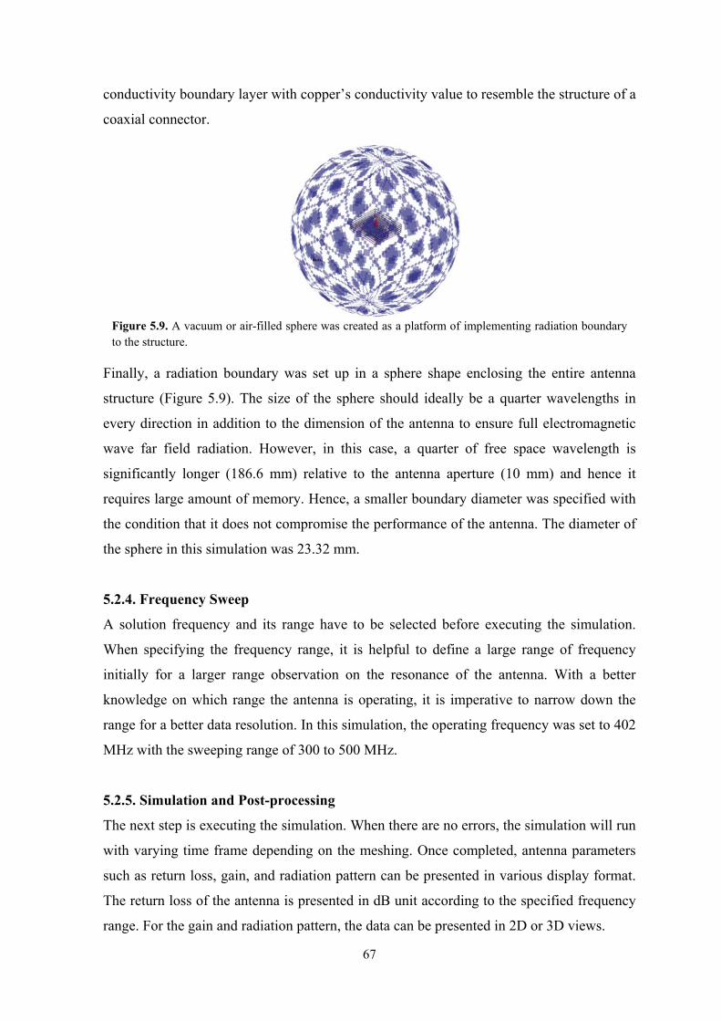
67

conductivity boundary layer with copper’s conductivity value to resemble the structure of a

coaxial connector.

Finally, a radiation boundary was set up in a sphere shape enclosing the entire antenna

structure (Figure 5.9). The size of the sphere should ideally be a quarter wavelengths in

every direction in addition to the dimension of the antenna to ensure full electromagnetic

wave far field radiation. However, in this case, a quarter of free space wavelength is

significantly longer (186.6 mm) relative to the antenna aperture (10 mm) and hence it

requires large amount of memory. Hence, a smaller boundary diameter was specified with

the condition that it does not compromise the performance of the antenna. The diameter of

the sphere in this simulation was 23.32 mm.

5.2.4. Frequency Sweep

A solution frequency and its range have to be selected before executing the simulation.

When specifying the frequency range, it is helpful to define a large range of frequency

initially for a larger range observation on the resonance of the antenna. With a better

knowledge on which range the antenna is operating, it is imperative to narrow down the

range for a better data resolution. In this simulation, the operating frequency was set to 402

MHz with the sweeping range of 300 to 500 MHz.

5.2.5. Simulation and Post-processing

The next step is executing the simulation. When there are no errors, the simulation will run

with varying time frame depending on the meshing. Once completed, antenna parameters

such as return loss, gain, and radiation pattern can be presented in various display format.

The return loss of the antenna is presented in dB unit according to the specified frequency

range. For the gain and radiation pattern, the data can be presented in 2D or 3D views.

Figure 5.9. A vacuum or air-filled sphere was created as a platform of implementing radiation boundary to the structure.

68

5.2.6. Optimisation

The flowchart in Figure 5.4 indicates that the simulation and the optimisation stages are

done iteratively until the antenna performance meets the requirement. The optimisation

process is generally done by adjusting one or more variables progressively and observing

the response on the next simulation. There has been a study on antenna optimisation

process by Soontornpipit [71] and it has served as a good guideline for optimizing the

proposed antenna. It was stated that a serpentine antenna has higher resonant frequency

compared to spiral antenna for the same physical length. Longer conductor path and higher

permittivity substrate material would lower the resonant frequency of the antenna. The

substrate thickness was also analysed in this study with a verdict that thicker substrate

would make the antenna appear electrically longer and hence slightly lower resonant

frequency.

5.3. Antenna Design Process

In this subchapter, the development of the antenna from the initial design until the final

design would be presented, together with its justification based on the performance results

of each stage. When the design was finalised, it would be configured in 4 different

scenarios. More detail about this would be presented on Section 5.3.3.

5.3.1. Model Development Based on Empirical Approach

The characteristic of an implantable microstrip antenna is very difficult to predict due to

the complex human tissue characteristic and as a consequence the basic antenna design

principle for general antennas could not be applied, as evident later in this Section.

Alternatively, an experiment based approach with the aid of electromagnetic simulation

software was implemented in this work in order to produce a final implantable antenna

design with a strong performance.

5.3.1.1. Modification #1 – Implementation of Liu’s antenna [83]

Initially, a specific antenna design from [83] was adopted with a consideration of its strong

performance relative to its compact size. This antenna, implemented with 3-layer

microstrip antenna geometry, was designed for operation inside human skin tissues. Slight

modifications were made by reducing the substrate dimension from 10 x 10 x 1.9 mm3 to 9

x 9 x 1.8 mm3 as well as the feed and ground pin radius to 0.1 mm to adjust with a change

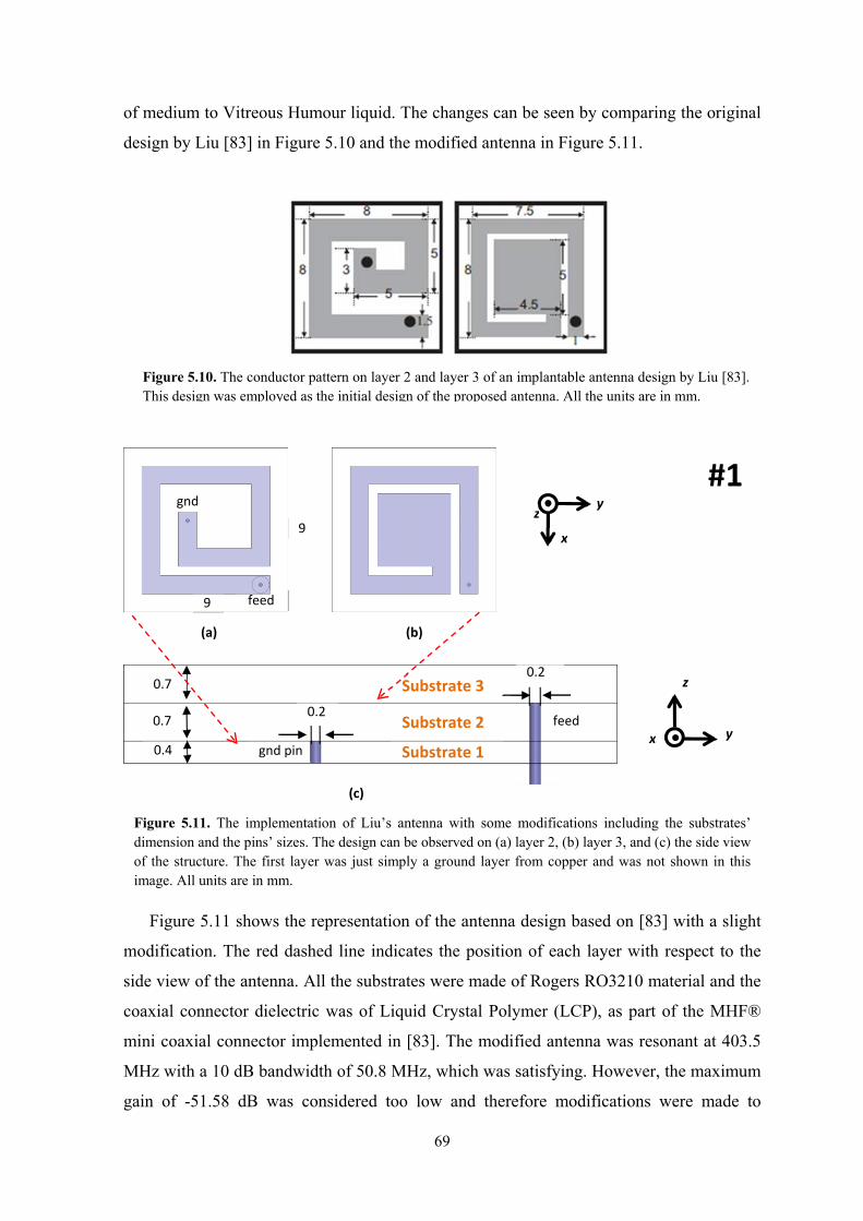
69

of medium to Vitreous Humour liquid. The changes can be seen by comparing the original

design by Liu [83] in Figure 5.10 and the modified antenna in Figure 5.11.

Figure 5.11 shows the representation of the antenna design based on [83] with a slight

modification. The red dashed line indicates the position of each layer with respect to the

side view of the antenna. All the substrates were made of Rogers RO3210 material and the

coaxial connector dielectric was of Liquid Crystal Polymer (LCP), as part of the MHF®

mini coaxial connector implemented in [83]. The modified antenna was resonant at 403.5

MHz with a 10 dB bandwidth of 50.8 MHz, which was satisfying. However, the maximum

gain of -51.58 dB was considered too low and therefore modifications were made to

Figure 5.10. The conductor pattern on layer 2 and layer 3 of an implantable antenna design by Liu [83]. This design was employed as the initial design of the proposed antenna. All the units are in mm.

9

9

0.2

0.20.7

0.7

0.4

y

x

z

#1

yx

z

feed

feed

gnd

gnd pin Substrate 1

Substrate 2

Substrate 3

Figure 5.11. The implementation of Liu’s antenna with some modifications including the substrates’ dimension and the pins’ sizes. The design can be observed on (a) layer 2, (b) layer 3, and (c) the side view of the structure. The first layer was just simply a ground layer from copper and was not shown in this image. All units are in mm.

(a) (b)

(c)

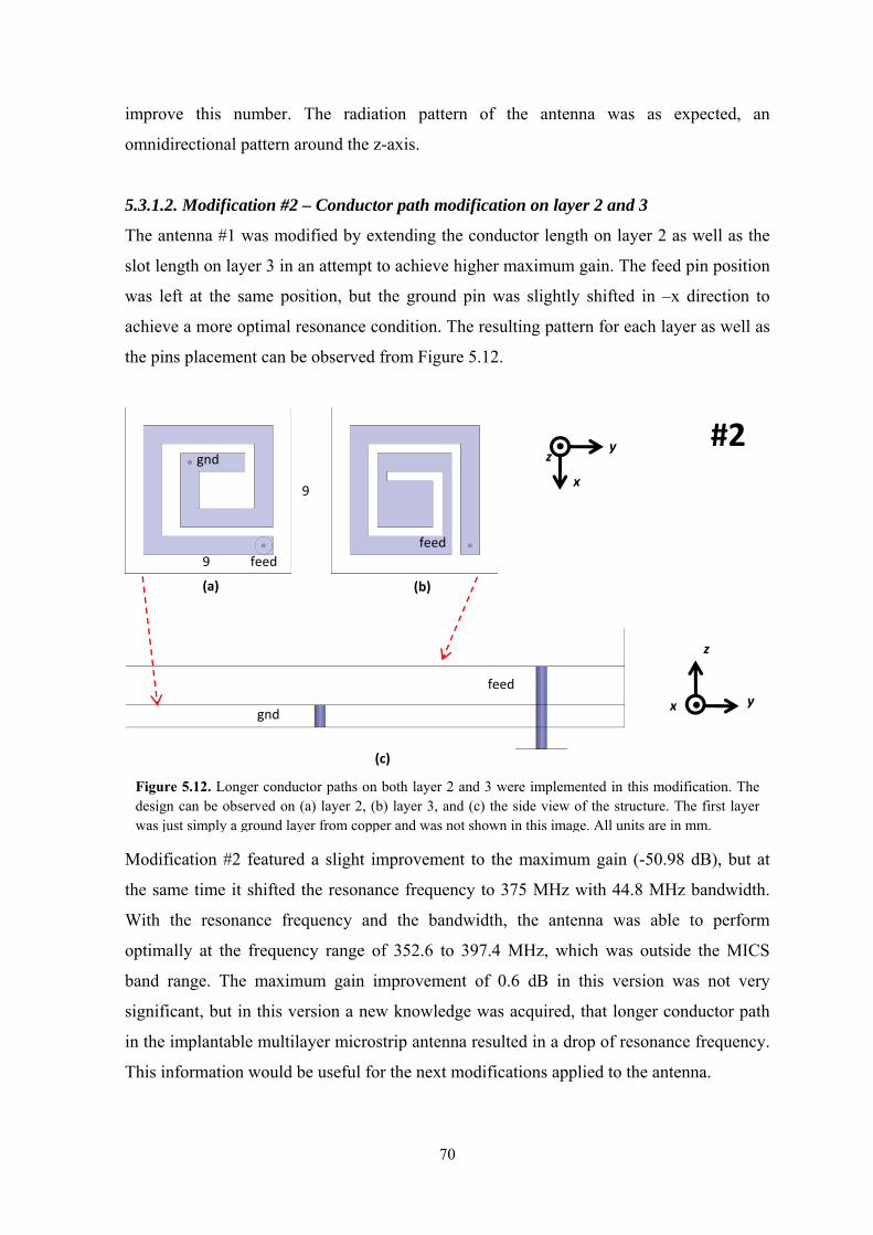
70

improve this number. The radiation pattern of the antenna was as expected, an

omnidirectional pattern around the z-axis.

5.3.1.2. Modification #2 – Conductor path modification on layer 2 and 3

The antenna #1 was modified by extending the conductor length on layer 2 as well as the

slot length on layer 3 in an attempt to achieve higher maximum gain. The feed pin position

was left at the same position, but the ground pin was slightly shifted in –x direction to

achieve a more optimal resonance condition. The resulting pattern for each layer as well as

the pins placement can be observed from Figure 5.12.

Modification #2 featured a slight improvement to the maximum gain (-50.98 dB), but at

the same time it shifted the resonance frequency to 375 MHz with 44.8 MHz bandwidth.

With the resonance frequency and the bandwidth, the antenna was able to perform

optimally at the frequency range of 352.6 to 397.4 MHz, which was outside the MICS

band range. The maximum gain improvement of 0.6 dB in this version was not very

significant, but in this version a new knowledge was acquired, that longer conductor path

in the implantable multilayer microstrip antenna resulted in a drop of resonance frequency.

This information would be useful for the next modifications applied to the antenna.

9

9

gnd

feed

gnd

feed

y

x

z

yx

z

feed

Figure 5.12. Longer conductor paths on both layer 2 and 3 were implemented in this modification. The design can be observed on (a) layer 2, (b) layer 3, and (c) the side view of the structure. The first layer was just simply a ground layer from copper and was not shown in this image. All units are in mm.

(a) (b)

(c)

#2

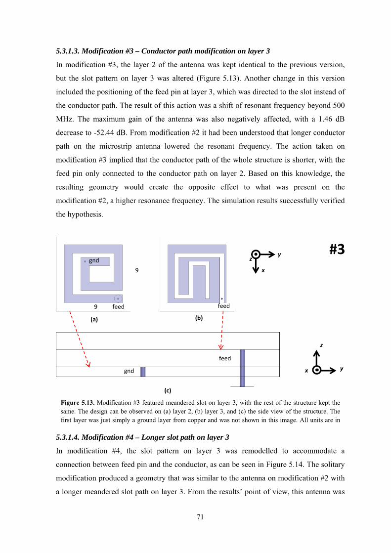
71

5.3.1.3. Modification #3 – Conductor path modification on layer 3

In modification #3, the layer 2 of the antenna was kept identical to the previous version,

but the slot pattern on layer 3 was altered (Figure 5.13). Another change in this version

included the positioning of the feed pin at layer 3, which was directed to the slot instead of

the conductor path. The result of this action was a shift of resonant frequency beyond 500

MHz. The maximum gain of the antenna was also negatively affected, with a 1.46 dB

decrease to -52.44 dB. From modification #2 it had been understood that longer conductor

path on the microstrip antenna lowered the resonant frequency. The action taken on

modification #3 implied that the conductor path of the whole structure is shorter, with the

feed pin only connected to the conductor path on layer 2. Based on this knowledge, the

resulting geometry would create the opposite effect to what was present on the

modification #2, a higher resonance frequency. The simulation results successfully verified

the hypothesis.

5.3.1.4. Modification #4 – Longer slot path on layer 3

In modification #4, the slot pattern on layer 3 was remodelled to accommodate a

connection between feed pin and the conductor, as can be seen in Figure 5.14. The solitary

modification produced a geometry that was similar to the antenna on modification #2 with

a longer meandered slot path on layer 3. From the results’ point of view, this antenna was

#3 y

x

z

yx

z

9

9

feed feed

feed

gnd

gnd

(a) (b)

(c)

Figure 5.13. Modification #3 featured meandered slot on layer 3, with the rest of the structure kept the same. The design can be observed on (a) layer 2, (b) layer 3, and (c) the side view of the structure. The first layer was just simply a ground layer from copper and was not shown in this image. All units are in

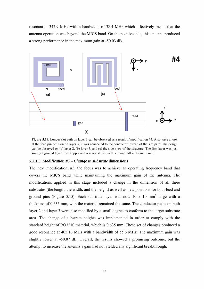
72

resonant at 347.9 MHz with a bandwidth of 38.4 MHz which effectively meant that the

antenna operation was beyond the MICS band. On the positive side, this antenna produced

a strong performance in the maximum gain at -50.03 dB.

5.3.1.5. Modification #5 – Change in substrate dimensions

The next modification, #5, the focus was to achieve an operating frequency band that

covers the MICS band while maintaining the maximum gain of the antenna. The

modifications applied in this stage included a change in the dimension of all three

substrates (the length, the width, and the height) as well as new positions for both feed and

ground pins (Figure 5.15). Each substrate layer was now 10 x 10 mm2 large with a

thickness of 0.635 mm, with the material remained the same. The conductor paths on both

layer 2 and layer 3 were also modified by a small degree to conform to the larger substrate

area. The change of substrate heights was implemented in order to comply with the

standard height of RO3210 material, which is 0.635 mm. These set of changes produced a

good resonance at 405.16 MHz with a bandwidth of 55.6 MHz. The maximum gain was

slightly lower at -50.87 dB. Overall, the results showed a promising outcome, but the

attempt to increase the antenna’s gain had not yielded any significant breakthrough.

#4 y

x

z

yx

z

9

9

feed feed

gnd

gnd

feed

Figure 5.14. Longer slot path on layer 3 can be observed as a result of modification #4. Also, take a look at the feed pin position on layer 3, it was connected to the conductor instead of the slot path. The design can be observed on (a) layer 2, (b) layer 3, and (c) the side view of the structure. The first layer was just simply a ground layer from copper and was not shown in this image. All units are in mm.

(a) (b)

(c)

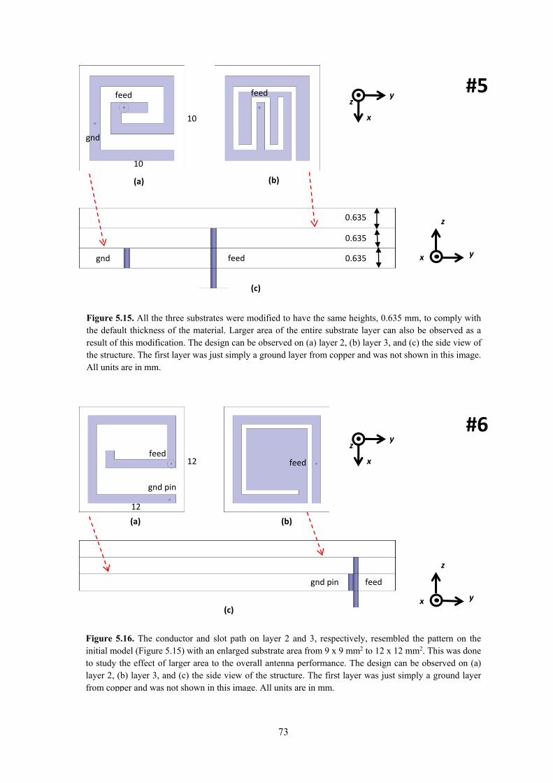
73

#5 y

x

z

yx

z

10

10

feed

gnd

feed

feedgnd

0.635

0.635

0.635

Figure 5.15. All the three substrates were modified to have the same heights, 0.635 mm, to comply with the default thickness of the material. Larger area of the entire substrate layer can also be observed as a result of this modification. The design can be observed on (a) layer 2, (b) layer 3, and (c) the side view of the structure. The first layer was just simply a ground layer from copper and was not shown in this image. All units are in mm.

(a) (b)

(c)

12

12 feed

gnd pin

feed

feedgnd pin

#6 y

x

z

yx

z

Figure 5.16. The conductor and slot path on layer 2 and 3, respectively, resembled the pattern on the initial model (Figure 5.15) with an enlarged substrate area from 9 x 9 mm2 to 12 x 12 mm2. This was done to study the effect of larger area to the overall antenna performance. The design can be observed on (a) layer 2, (b) layer 3, and (c) the side view of the structure. The first layer was just simply a ground layer from copper and was not shown in this image. All units are in mm.

(a) (b)

(c)

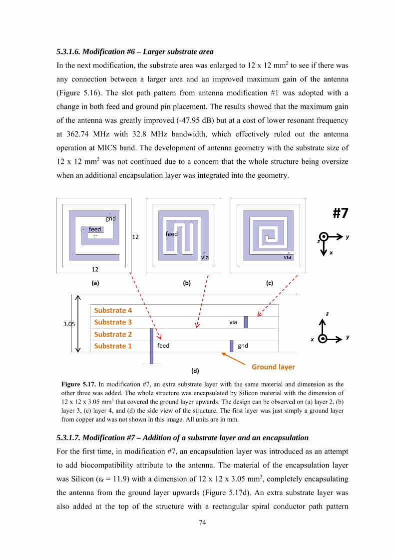
74

5.3.1.6. Modification #6 – Larger substrate area

In the next modification, the substrate area was enlarged to 12 x 12 mm2 to see if there was

any connection between a larger area and an improved maximum gain of the antenna

(Figure 5.16). The slot path pattern from antenna modification #1 was adopted with a

change in both feed and ground pin placement. The results showed that the maximum gain

of the antenna was greatly improved (-47.95 dB) but at a cost of lower resonant frequency

at 362.74 MHz with 32.8 MHz bandwidth, which effectively ruled out the antenna

operation at MICS band. The development of antenna geometry with the substrate size of

12 x 12 mm2 was not continued due to a concern that the whole structure being oversize

when an additional encapsulation layer was integrated into the geometry.

5.3.1.7. Modification #7 – Addition of a substrate layer and an encapsulation

For the first time, in modification #7, an encapsulation layer was introduced as an attempt

to add biocompatibility attribute to the antenna. The material of the encapsulation layer

was Silicon (εr = 11.9) with a dimension of 12 x 12 x 3.05 mm3, completely encapsulating

the antenna from the ground layer upwards (Figure 5.17d). An extra substrate layer was

also added at the top of the structure with a rectangular spiral conductor path pattern

12

12

#7

y

x

z

yx

z

feed feed

via

gnd

via

via

feed gnd

3.05

Figure 5.17. In modification #7, an extra substrate layer with the same material and dimension as the other three was added. The whole structure was encapsulated by Silicon material with the dimension of 12 x 12 x 3.05 mm3 that covered the ground layer upwards. The design can be observed on (a) layer 2, (b) layer 3, (c) layer 4, and (d) the side view of the structure. The first layer was just simply a ground layer from copper and was not shown in this image. All units are in mm.

(a) (b) (c)

(d)

Substrate 1

Substrate 2

Substrate 3

Substrate 4

Ground layer

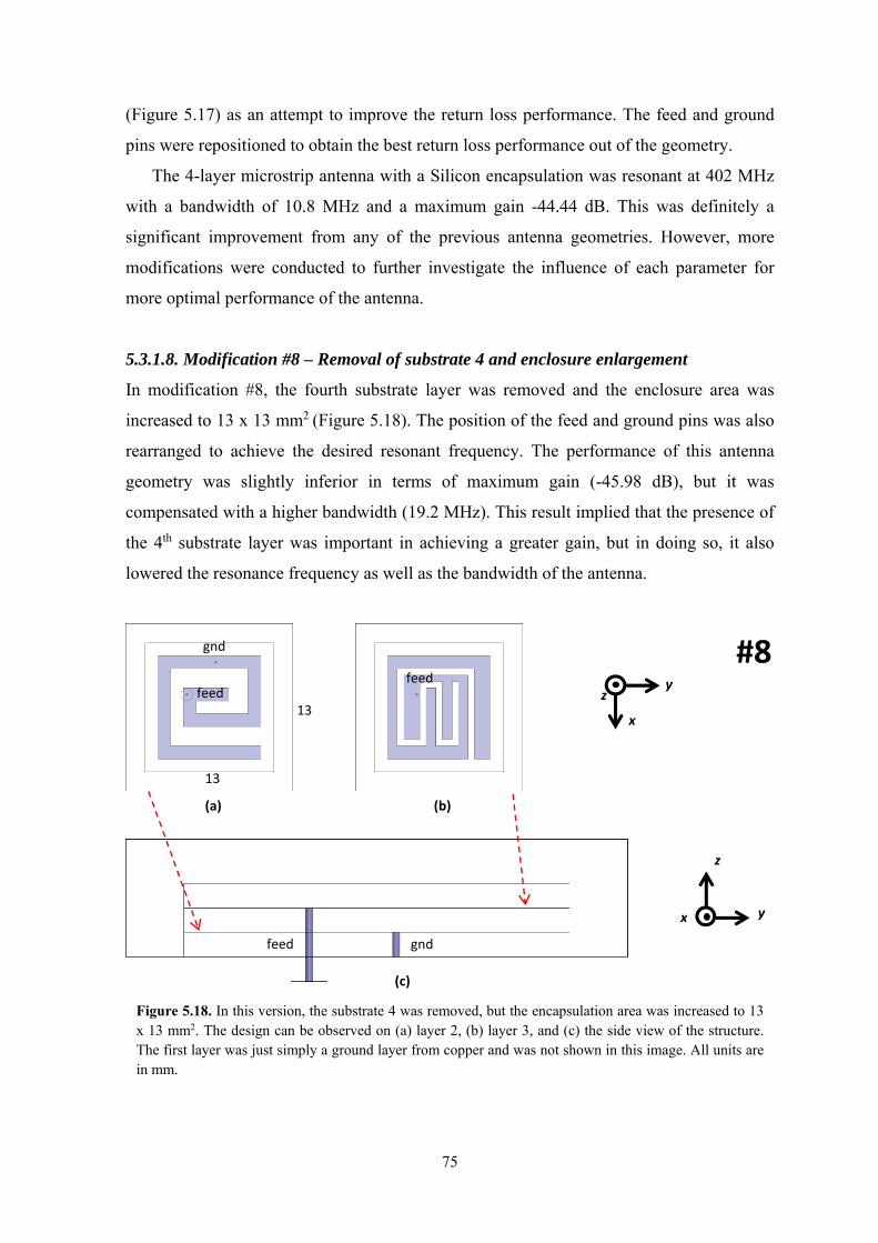
75

(Figure 5.17) as an attempt to improve the return loss performance. The feed and ground

pins were repositioned to obtain the best return loss performance out of the geometry.

The 4-layer microstrip antenna with a Silicon encapsulation was resonant at 402 MHz

with a bandwidth of 10.8 MHz and a maximum gain -44.44 dB. This was definitely a

significant improvement from any of the previous antenna geometries. However, more

modifications were conducted to further investigate the influence of each parameter for

more optimal performance of the antenna.

5.3.1.8. Modification #8 – Removal of substrate 4 and enclosure enlargement

In modification #8, the fourth substrate layer was removed and the enclosure area was

increased to 13 x 13 mm2 (Figure 5.18). The position of the feed and ground pins was also

rearranged to achieve the desired resonant frequency. The performance of this antenna

geometry was slightly inferior in terms of maximum gain (-45.98 dB), but it was

compensated with a higher bandwidth (19.2 MHz). This result implied that the presence of

the 4th substrate layer was important in achieving a greater gain, but in doing so, it also

lowered the resonance frequency as well as the bandwidth of the antenna.

13

13

#8

y

x

z

yx

z

feed feed

feed

gnd

gnd

Figure 5.18. In this version, the substrate 4 was removed, but the encapsulation area was increased to 13 x 13 mm2. The design can be observed on (a) layer 2, (b) layer 3, and (c) the side view of the structure. The first layer was just simply a ground layer from copper and was not shown in this image. All units are in mm.

(a) (b)

(c)

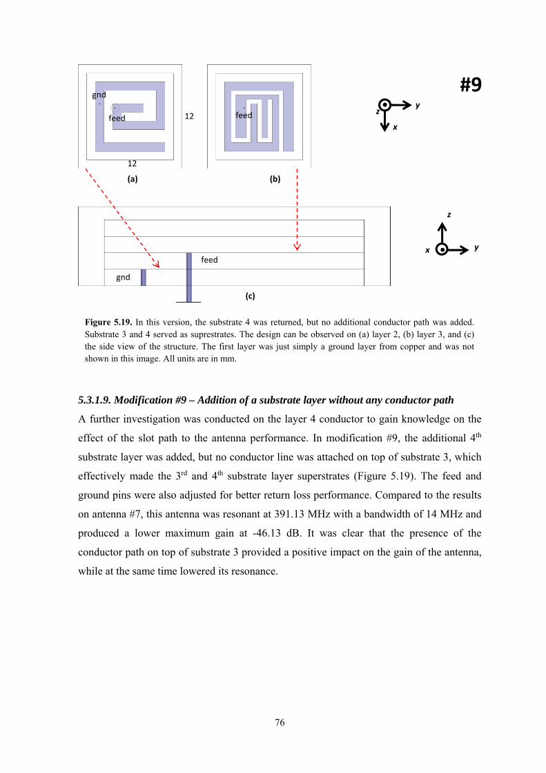
76

5.3.1.9. Modification #9 – Addition of a substrate layer without any conductor path

A further investigation was conducted on the layer 4 conductor to gain knowledge on the

effect of the slot path to the antenna performance. In modification #9, the additional 4th

substrate layer was added, but no conductor line was attached on top of substrate 3, which

effectively made the 3rd and 4th substrate layer superstrates (Figure 5.19). The feed and

ground pins were also adjusted for better return loss performance. Compared to the results

on antenna #7, this antenna was resonant at 391.13 MHz with a bandwidth of 14 MHz and

produced a lower maximum gain at -46.13 dB. It was clear that the presence of the

conductor path on top of substrate 3 provided a positive impact on the gain of the antenna,

while at the same time lowered its resonance.

12

12

#9

y

x

z

yx

z

feed feed

feed

gnd

gnd

Figure 5.19. In this version, the substrate 4 was returned, but no additional conductor path was added. Substrate 3 and 4 served as suprestrates. The design can be observed on (a) layer 2, (b) layer 3, and (c) the side view of the structure. The first layer was just simply a ground layer from copper and was not shown in this image. All units are in mm.

(a) (b)

(c)

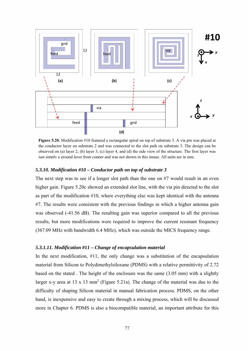
77

5.3.10. Modification #10 – Conductor path on top of substrate 3

The next step was to see if a longer slot path than the one on #7 would result in an even

higher gain. Figure 5.20c showed an extended slot line, with the via pin directed to the slot

as part of the modification #10, where everything else was kept identical with the antenna

#7. The results were consistent with the previous findings in which a higher antenna gain

was observed (-41.56 dB). The resulting gain was superior compared to all the previous

results, but more modifications were required to improve the current resonant frequency

(367.09 MHz with bandwidth 6.4 MHz), which was outside the MICS frequency range.

5.3.1.11. Modification #11 – Change of encapsulation material

In the next modification, #11, the only change was a substitution of the encapsulation

material from Silicon to Polydimethylsiloxane (PDMS) with a relative permittivity of 2.72

based on the stated . The height of the enclosure was the same (3.05 mm) with a slightly

larger x-y area at 13 x 13 mm2 (Figure 5.21a). The change of the material was due to the

difficulty of shaping Silicon material in manual fabrication process. PDMS, on the other

hand, is inexpensive and easy to create through a mixing process, which will be discussed

more in Chapter 6. PDMS is also a biocompatible material, an important attribute for this

12

12

#10

y

x

z

yx

z

feed feed

feed

gnd

gnd

via

via

Figure 5.20. Modification #10 featured a rectangular spiral on top of substrate 3. A via pin was placed at the conductor layer on substrate 2 and was connected to the slot path on substrate 3. The design can be observed on (a) layer 2, (b) layer 3, (c) layer 4, and (d) the side view of the structure. The first layer was just simply a ground layer from copper and was not shown in this image. All units are in mm.

(a) (b) (c)

(d)

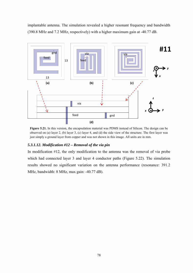
78

implantable antenna. The simulation revealed a higher resonant frequency and bandwidth

(390.8 MHz and 7.2 MHz, respectively) with a higher maximum gain at -40.77 dB.

5.3.1.12. Modification #12 – Removal of the via pin

In modification #12, the only modification to the antenna was the removal of via probe

which had connected layer 3 and layer 4 conductor paths (Figure 5.22). The simulation

results showed no significant variation on the antenna performance (resonance: 391.2

MHz, bandwidth: 8 MHz, max gain: -40.77 dB).

13

13

#11

y

x

z

yx

z

feed

feed

feed

via viagnd

gnd

via

Figure 5.21. In this version, the encapsulation material was PDMS instead of Silicon. The design can be observed on (a) layer 2, (b) layer 3, (c) layer 4, and (d) the side view of the structure. The first layer was just simply a ground layer from copper and was not shown in this image. All units are in mm.

(a) (b) (c)

(d)

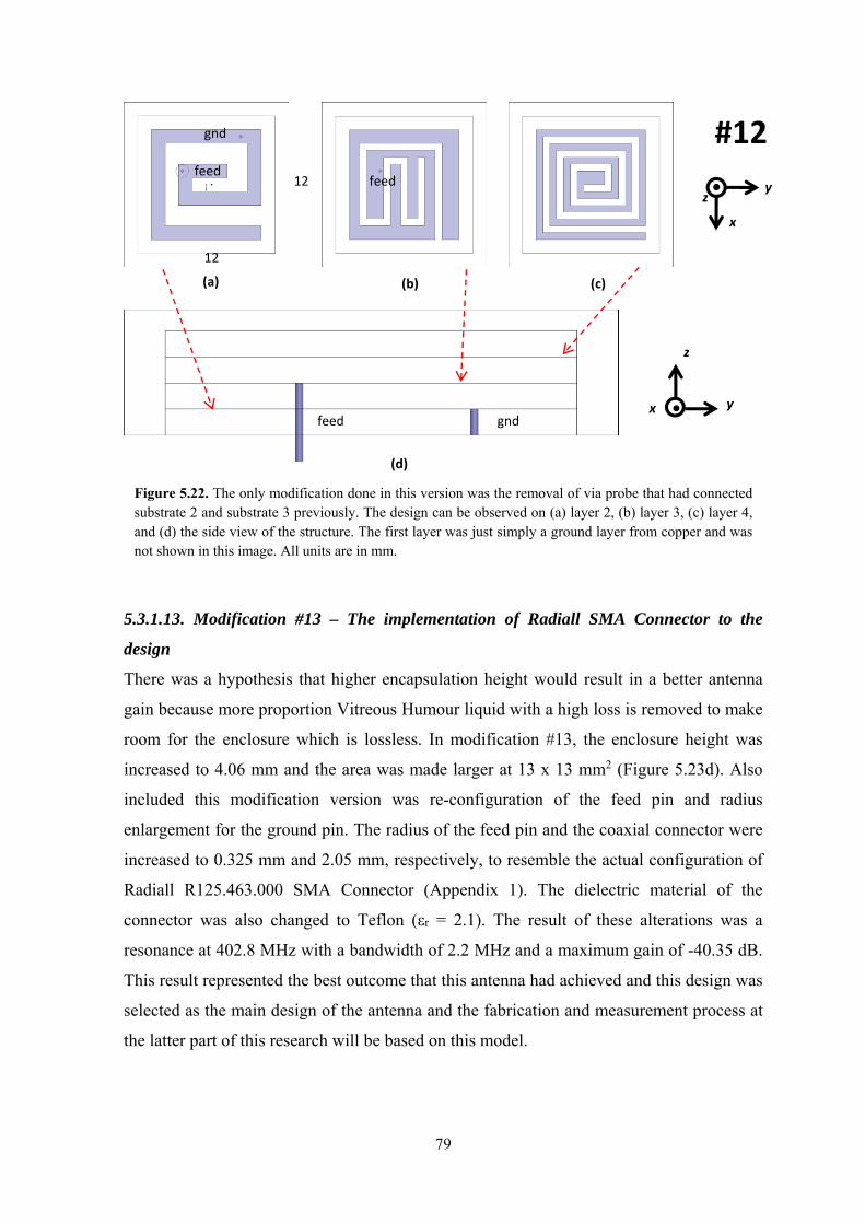
79

5.3.1.13. Modification #13 – The implementation of Radiall SMA Connector to the

design

There was a hypothesis that higher encapsulation height would result in a better antenna

gain because more proportion Vitreous Humour liquid with a high loss is removed to make

room for the enclosure which is lossless. In modification #13, the enclosure height was

increased to 4.06 mm and the area was made larger at 13 x 13 mm2 (Figure 5.23d). Also

included this modification version was re-configuration of the feed pin and radius

enlargement for the ground pin. The radius of the feed pin and the coaxial connector were

increased to 0.325 mm and 2.05 mm, respectively, to resemble the actual configuration of

Radiall R125.463.000 SMA Connector (Appendix 1). The dielectric material of the

connector was also changed to Teflon (εr = 2.1). The result of these alterations was a

resonance at 402.8 MHz with a bandwidth of 2.2 MHz and a maximum gain of -40.35 dB.

This result represented the best outcome that this antenna had achieved and this design was

selected as the main design of the antenna and the fabrication and measurement process at

the latter part of this research will be based on this model.

#12

y

x

z

yx

z

12

12

feed

feed feed

gnd

gnd

Figure 5.22. The only modification done in this version was the removal of via probe that had connected substrate 2 and substrate 3 previously. The design can be observed on (a) layer 2, (b) layer 3, (c) layer 4, and (d) the side view of the structure. The first layer was just simply a ground layer from copper and was not shown in this image. All units are in mm.

(a) (b) (c)

(d)

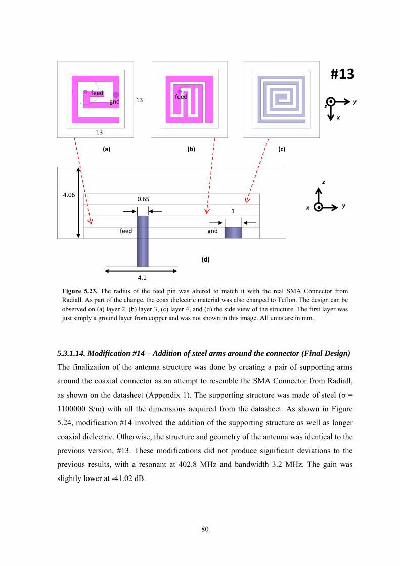
80

5.3.1.14. Modification #14 – Addition of steel arms around the connector (Final Design)

The finalization of the antenna structure was done by creating a pair of supporting arms

around the coaxial connector as an attempt to resemble the SMA Connector from Radiall,

as shown on the datasheet (Appendix 1). The supporting structure was made of steel (σ =

1100000 S/m) with all the dimensions acquired from the datasheet. As shown in Figure

5.24, modification #14 involved the addition of the supporting structure as well as longer

coaxial dielectric. Otherwise, the structure and geometry of the antenna was identical to the

previous version, #13. These modifications did not produce significant deviations to the

previous results, with a resonant at 402.8 MHz and bandwidth 3.2 MHz. The gain was

slightly lower at -41.02 dB.

y

x

z

yx

z

#13

13

13 feed

feed

feed

gnd

gnd

4.06 0.65

1

4.1

Figure 5.23. The radius of the feed pin was altered to match it with the real SMA Connector from Radiall. As part of the change, the coax dielectric material was also changed to Teflon. The design can be observed on (a) layer 2, (b) layer 3, (c) layer 4, and (d) the side view of the structure. The first layer was just simply a ground layer from copper and was not shown in this image. All units are in mm.

(a) (b) (c)

(d)

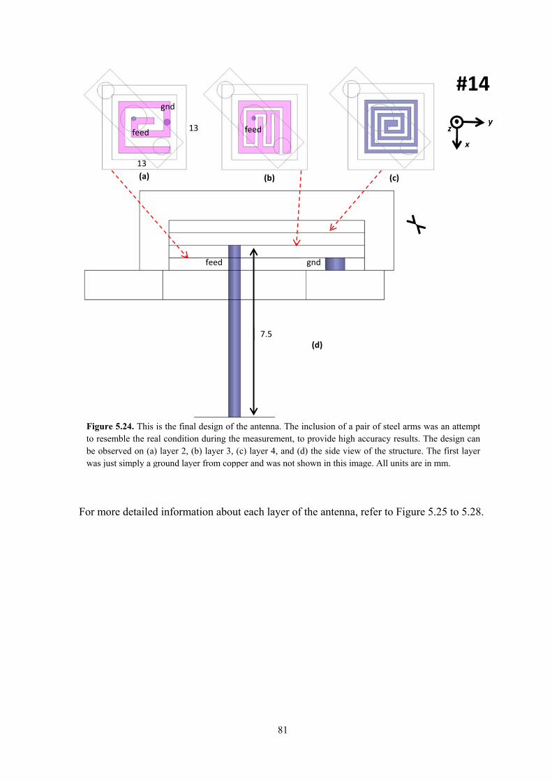
81

For more detailed information about each layer of the antenna, refer to Figure 5.25 to 5.28.

y

x

z

#14

feed feed

feed

gnd

gnd

7.5

13

13

Figure 5.24. This is the final design of the antenna. The inclusion of a pair of steel arms was an attempt to resemble the real condition during the measurement, to provide high accuracy results. The design can be observed on (a) layer 2, (b) layer 3, (c) layer 4, and (d) the side view of the structure. The first layer was just simply a ground layer from copper and was not shown in this image. All units are in mm.

(a) (b) (c)

(d)

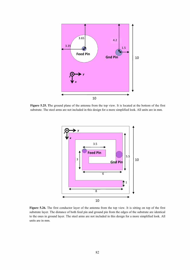
82

Figure 5.25. The ground plane of the antenna from the top view. It is located at the bottom of the first substrate. The steel arms are not included in this design for a more simplified look. All units are in mm.

10

10 Feed Pin

Gnd Pin

y

x

z

3.65

3.35

4.2

1.5

Figure 5.26. The first conductor layer of the antenna from the top view. It is sitting on top of the first substrate layer. The distance of both feed pin and ground pin from the edges of the substrate are identical to the ones in ground layer. The steel arms are not included in this design for a more simplified look. All units are in mm.

Gnd Pin

Feed Pin

10

10

1

8

6

3.5

5.53

y

x

z

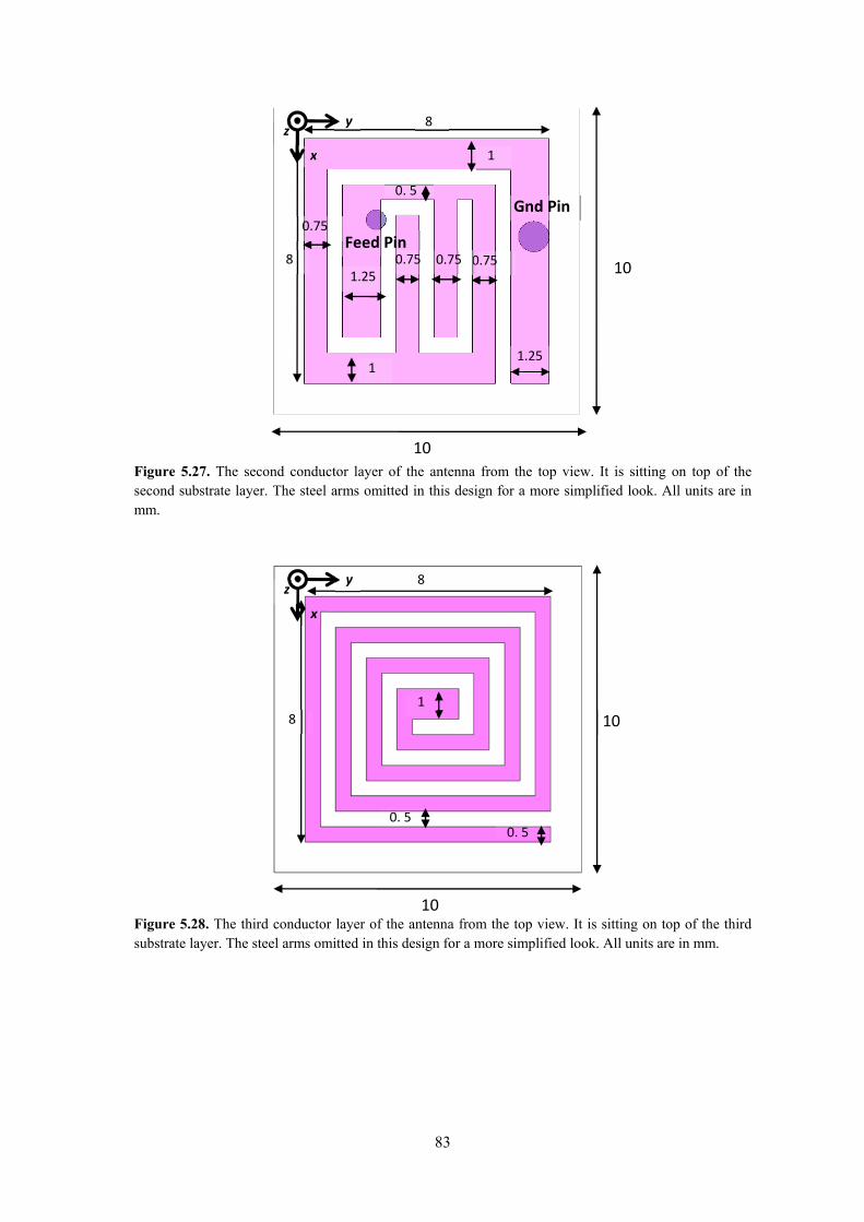
83

Figure 5.27. The second conductor layer of the antenna from the top view. It is sitting on top of the second substrate layer. The steel arms omitted in this design for a more simplified look. All units are in mm.

Gnd Pin

Feed Pin

10

10 8

1.25

1

0.75

1

0.75 0.750.751.25

0. 5

y

x

z 8

Figure 5.28. The third conductor layer of the antenna from the top view. It is sitting on top of the third substrate layer. The steel arms omitted in this design for a more simplified look. All units are in mm.

10

10

8

8

y

x

z

0. 5

1

0. 5

84

5.3.1.15. Summary

Table 5.2 summarizes 14 modifications that had been applied to the antenna with the

resulting antenna performances. From this table, it could be clearly seen how each

modification affected the antenna performance. Modification #14 was conducted as part of

building an accurate model based on the detail of each component. The resulting simulated

antenna performance was satisfying and the operation was within the range of MICS band.

This antenna model was subsequently fabricated and measured in both free space and

Vitreous Humour liquid to verify its performance.

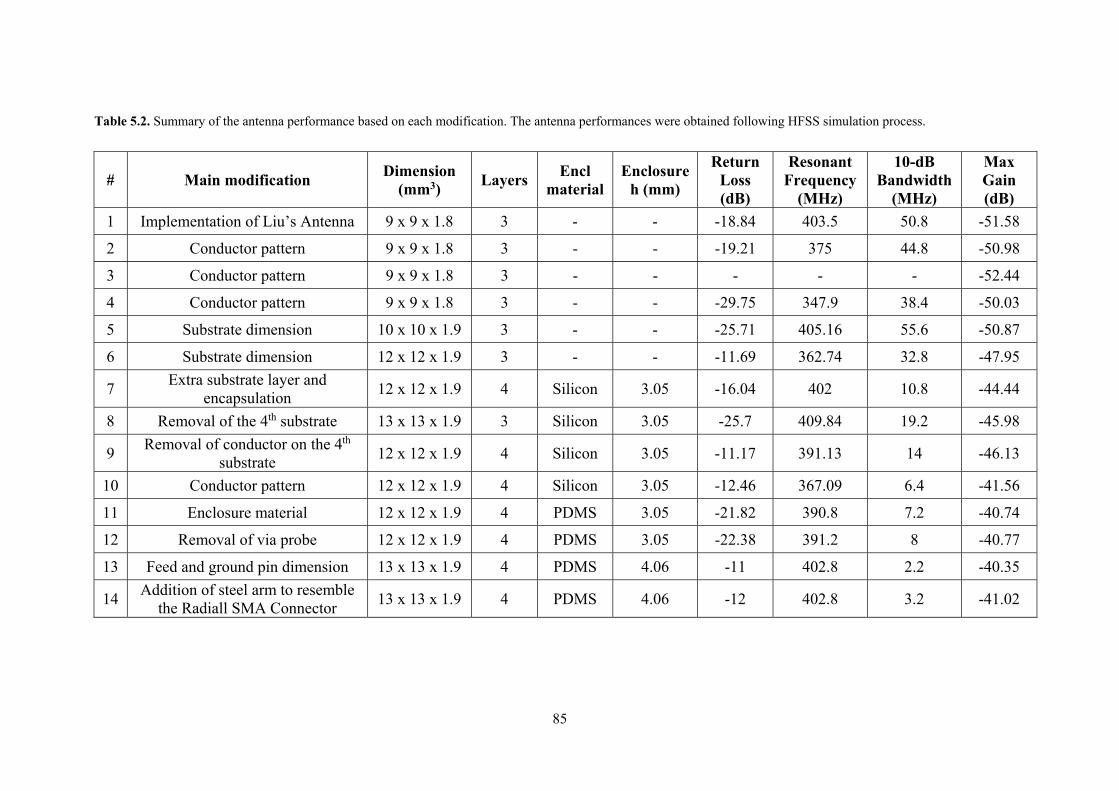
85

Table 5.2. Summary of the antenna performance based on each modification. The antenna performances were obtained following HFSS simulation process.

# Main modification Dimension

(mm3) Layers

Encl material

Enclosure h (mm)

Return Loss (dB)

Resonant Frequency

(MHz)

10-dB Bandwidth

(MHz)

Max Gain (dB)

1 Implementation of Liu’s Antenna 9 x 9 x 1.8 3 - - -18.84 403.5 50.8 -51.58

2 Conductor pattern 9 x 9 x 1.8 3 - - -19.21 375 44.8 -50.98

3 Conductor pattern 9 x 9 x 1.8 3 - - - - - -52.44

4 Conductor pattern 9 x 9 x 1.8 3 - - -29.75 347.9 38.4 -50.03

5 Substrate dimension 10 x 10 x 1.9 3 - - -25.71 405.16 55.6 -50.87

6 Substrate dimension 12 x 12 x 1.9 3 - - -11.69 362.74 32.8 -47.95

7 Extra substrate layer and

encapsulation 12 x 12 x 1.9 4 Silicon 3.05 -16.04 402 10.8 -44.44

8 Removal of the 4th substrate 13 x 13 x 1.9 3 Silicon 3.05 -25.7 409.84 19.2 -45.98

9 Removal of conductor on the 4th

substrate 12 x 12 x 1.9 4 Silicon 3.05 -11.17 391.13 14 -46.13

10 Conductor pattern 12 x 12 x 1.9 4 Silicon 3.05 -12.46 367.09 6.4 -41.56

11 Enclosure material 12 x 12 x 1.9 4 PDMS 3.05 -21.82 390.8 7.2 -40.74

12 Removal of via probe 12 x 12 x 1.9 4 PDMS 3.05 -22.38 391.2 8 -40.77

13 Feed and ground pin dimension 13 x 13 x 1.9 4 PDMS 4.06 -11 402.8 2.2 -40.35

14 Addition of steel arm to resemble

the Radiall SMA Connector 13 x 13 x 1.9 4 PDMS 4.06 -12 402.8 3.2 -41.02

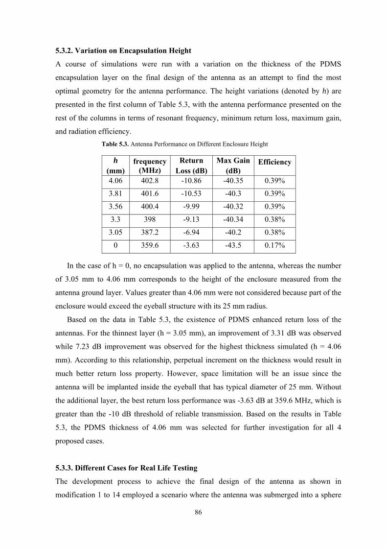
86

5.3.2. Variation on Encapsulation Height

A course of simulations were run with a variation on the thickness of the PDMS

encapsulation layer on the final design of the antenna as an attempt to find the most

optimal geometry for the antenna performance. The height variations (denoted by h) are

presented in the first column of Table 5.3, with the antenna performance presented on the

rest of the columns in terms of resonant frequency, minimum return loss, maximum gain,

and radiation efficiency.

In the case of h = 0, no encapsulation was applied to the antenna, whereas the number

of 3.05 mm to 4.06 mm corresponds to the height of the enclosure measured from the

antenna ground layer. Values greater than 4.06 mm were not considered because part of the

enclosure would exceed the eyeball structure with its 25 mm radius.

Based on the data in Table 5.3, the existence of PDMS enhanced return loss of the

antennas. For the thinnest layer (h = 3.05 mm), an improvement of 3.31 dB was observed

while 7.23 dB improvement was observed for the highest thickness simulated (h = 4.06

mm). According to this relationship, perpetual increment on the thickness would result in

much better return loss property. However, space limitation will be an issue since the

antenna will be implanted inside the eyeball that has typical diameter of 25 mm. Without

the additional layer, the best return loss performance was -3.63 dB at 359.6 MHz, which is

greater than the -10 dB threshold of reliable transmission. Based on the results in Table

5.3, the PDMS thickness of 4.06 mm was selected for further investigation for all 4

proposed cases.

5.3.3. Different Cases for Real Life Testing

The development process to achieve the final design of the antenna as shown in

modification 1 to 14 employed a scenario where the antenna was submerged into a sphere

Table 5.3. Antenna Performance on Different Enclosure Height

h (mm)

frequency (MHz)

Return Loss (dB)

Max Gain (dB)

Efficiency

4.06 402.8 -10.86 -40.35 0.39%

3.81 401.6 -10.53 -40.3 0.39%

3.56 400.4 -9.99 -40.32 0.39%

3.3 398 -9.13 -40.34 0.38%

3.05 387.2 -6.94 -40.2 0.38%

0 359.6 -3.63 -43.5 0.17%

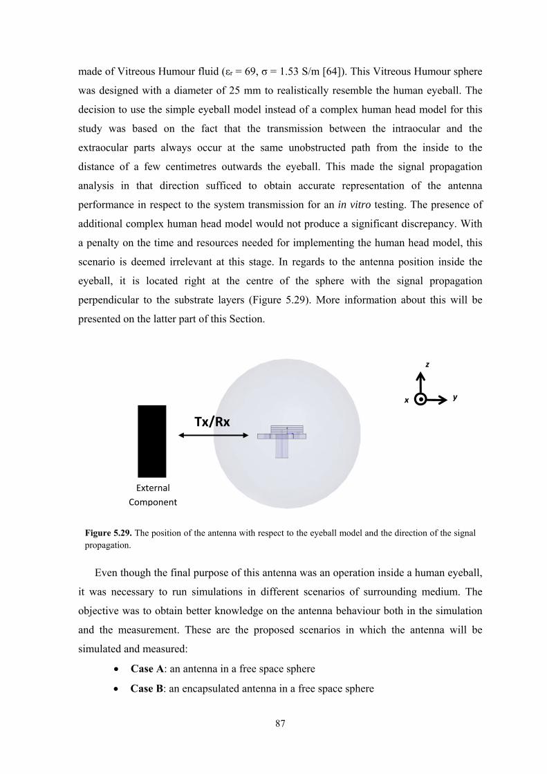
87

made of Vitreous Humour fluid (εr = 69, σ = 1.53 S/m [64]). This Vitreous Humour sphere

was designed with a diameter of 25 mm to realistically resemble the human eyeball. The

decision to use the simple eyeball model instead of a complex human head model for this

study was based on the fact that the transmission between the intraocular and the

extraocular parts always occur at the same unobstructed path from the inside to the

distance of a few centimetres outwards the eyeball. This made the signal propagation

analysis in that direction sufficed to obtain accurate representation of the antenna

performance in respect to the system transmission for an in vitro testing. The presence of

additional complex human head model would not produce a significant discrepancy. With

a penalty on the time and resources needed for implementing the human head model, this

scenario is deemed irrelevant at this stage. In regards to the antenna position inside the

eyeball, it is located right at the centre of the sphere with the signal propagation

perpendicular to the substrate layers (Figure 5.29). More information about this will be

presented on the latter part of this Section.

Even though the final purpose of this antenna was an operation inside a human eyeball,

it was necessary to run simulations in different scenarios of surrounding medium. The

objective was to obtain better knowledge on the antenna behaviour both in the simulation

and the measurement. These are the proposed scenarios in which the antenna will be

simulated and measured:

Case A: an antenna in a free space sphere

Case B: an encapsulated antenna in a free space sphere

Figure 5.29. The position of the antenna with respect to the eyeball model and the direction of the signal propagation.

yx

z

External

Component

Tx/Rx

88

Case C: an encapsulated antenna in a Vitreous Humour sphere at the size of

human eyeball

Case D: an encapsulated antenna in a Vitreous Humour sphere at the size of

table tennis ball with diameter 40 mm.

In case A, the presence of both Vitreous Humour liquid and the PDMS encapsulation is

excluded and the antenna is positioned in the middle of an air-filled sphere. This case

would be useful to know the characteristic of the antenna right after the fabrication

process, before the encapsulation and immersion stage.

In case B, a PDMS encapsulation layer is incorporated to the antenna structure. The

antenna would still be placed inside an air-filled sphere. This stage would provide an

important information should the behaviour of the antenna is not as expected.

Case C is the condition in which the antenna was originally designed for. The

encapsulated antenna structure is positioned inside a Vitreous Humour that mimics a

human eyeball. However, it would not be possible to replicate this scenario in the reality

due to the difficulty in obtaining an ethic approval. Instead, case D was proposed to

provide a close representation of this case C.

In case D, the encapsulated antenna is positioned inside a sphere that is filled with

Vitreous Humour mimicking liquid. The sphere would have a larger diameter at 40 mm to

create an accurate representation of a table tennis ball. That is where the antenna and the

Vitreous Humour liquid are positioned for the measurement process. Table tennis ball is a

hollow sphere with a skin material of Celluloid (electrical characteristic in Table 5.1) and a

skin thickness of 0.35 mm. A small experiment has also been done in an attempt to find the

most suitable PDMS layer thickness for achieving the most optimal antenna performance.

More detail about this will be presented later in this Section.

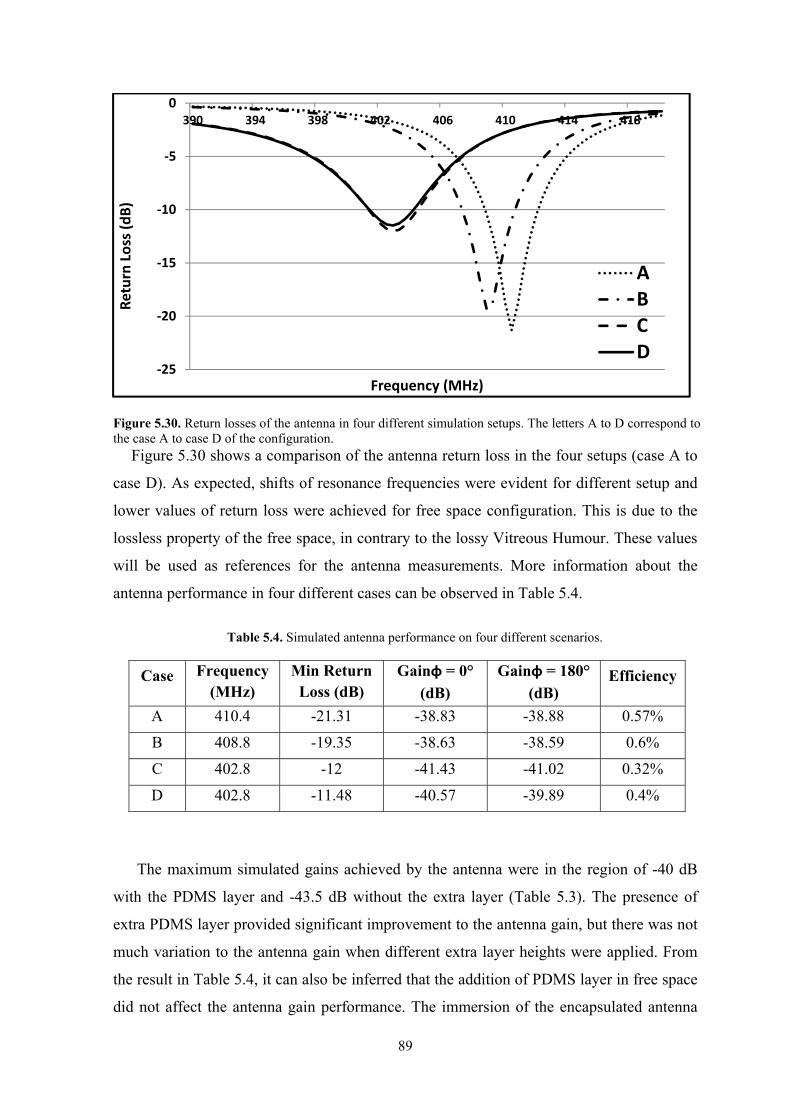
89

Figure 5.30. Return losses of the antenna in four different simulation setups. The letters A to D correspond to the case A to case D of the configuration.

Figure 5.30 shows a comparison of the antenna return loss in the four setups (case A to

case D). As expected, shifts of resonance frequencies were evident for different setup and

lower values of return loss were achieved for free space configuration. This is due to the

lossless property of the free space, in contrary to the lossy Vitreous Humour. These values

will be used as references for the antenna measurements. More information about the

antenna performance in four different cases can be observed in Table 5.4.

The maximum simulated gains achieved by the antenna were in the region of -40 dB

with the PDMS layer and -43.5 dB without the extra layer (Table 5.3). The presence of

extra PDMS layer provided significant improvement to the antenna gain, but there was not

much variation to the antenna gain when different extra layer heights were applied. From

the result in Table 5.4, it can also be inferred that the addition of PDMS layer in free space

did not affect the antenna gain performance. The immersion of the encapsulated antenna

‐25

‐20

‐15

‐10

‐5

0390 394 398 402 406 410 414 418

Return Loss (dB)

Frequency (MHz)

ABCD

Table 5.4. Simulated antenna performance on four different scenarios.

Case Frequency (MHz)

Min Return Loss (dB)

Gainφ = 0°

(dB)

Gainφ = 180°

(dB) Efficiency

A 410.4 -21.31 -38.83 -38.88 0.57%

B 408.8 -19.35 -38.63 -38.59 0.6%

C 402.8 -12 -41.43 -41.02 0.32%

D 402.8 -11.48 -40.57 -39.89 0.4%

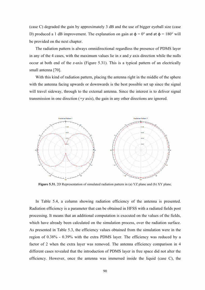
90

(case C) degraded the gain by approximately 3 dB and the use of bigger eyeball size (case

D) produced a 1 dB improvement. The explanation on gain at φ = 0° and at φ = 180° will

be provided on the next chapter.

The radiation pattern is always omnidirectional regardless the presence of PDMS layer

in any of the 4 cases, with the maximum values lie in x and y axis direction while the nulls

occur at both end of the z-axis (Figure 5.31). This is a typical pattern of an electrically

small antenna [70].

With this kind of radiation pattern, placing the antenna right in the middle of the sphere

with the antenna facing upwards or downwards is the best possible set up since the signal

will travel sideway, through to the external antenna. Since the interest is to deliver signal

transmission in one direction (+y axis), the gain in any other directions are ignored.

In Table 5.4, a column showing radiation efficiency of the antenna is presented.

Radiation efficiency is a parameter that can be obtained in HFSS with a radiated fields post

processing. It means that an additional computation is executed on the values of the fields,

which have already been calculated on the simulation process, over the radiation surface.

As presented in Table 5.3, the efficiency values obtained from the simulation were in the

region of 0.38% - 0.39% with the extra PDMS layer. The efficiency was reduced by a

factor of 2 when the extra layer was removed. The antenna efficiency comparison in 4

different cases revealed that the introduction of PDMS layer in free space did not alter the

efficiency. However, once the antenna was immersed inside the liquid (case C), the

Figure 5.31. 2D Representation of simulated radiation pattern in (a) YZ plane and (b) XY plane.

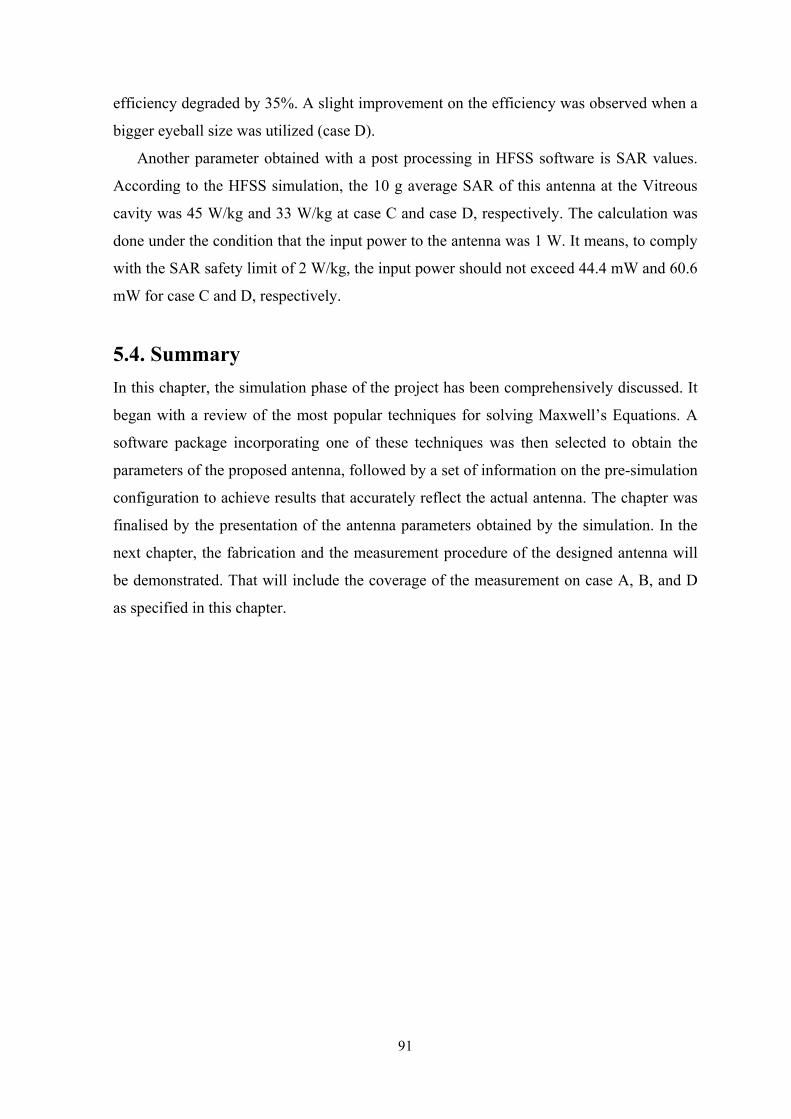
91

efficiency degraded by 35%. A slight improvement on the efficiency was observed when a

bigger eyeball size was utilized (case D).

Another parameter obtained with a post processing in HFSS software is SAR values.

According to the HFSS simulation, the 10 g average SAR of this antenna at the Vitreous

cavity was 45 W/kg and 33 W/kg at case C and case D, respectively. The calculation was

done under the condition that the input power to the antenna was 1 W. It means, to comply

with the SAR safety limit of 2 W/kg, the input power should not exceed 44.4 mW and 60.6

mW for case C and D, respectively.

5.4. Summary

In this chapter, the simulation phase of the project has been comprehensively discussed. It

began with a review of the most popular techniques for solving Maxwell’s Equations. A

software package incorporating one of these techniques was then selected to obtain the

parameters of the proposed antenna, followed by a set of information on the pre-simulation

configuration to achieve results that accurately reflect the actual antenna. The chapter was

finalised by the presentation of the antenna parameters obtained by the simulation. In the

next chapter, the fabrication and the measurement procedure of the designed antenna will

be demonstrated. That will include the coverage of the measurement on case A, B, and D

as specified in this chapter.

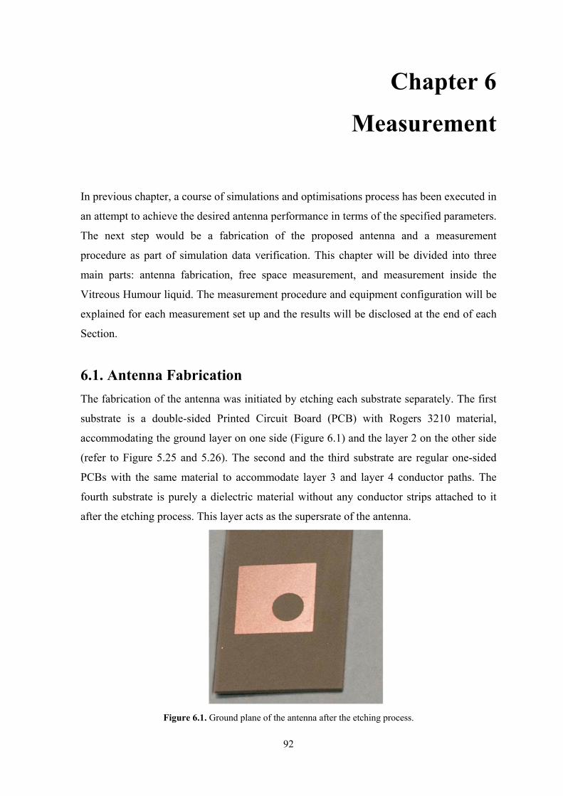
92

Chapter 6

Measurement

In previous chapter, a course of simulations and optimisations process has been executed in

an attempt to achieve the desired antenna performance in terms of the specified parameters.

The next step would be a fabrication of the proposed antenna and a measurement

procedure as part of simulation data verification. This chapter will be divided into three

main parts: antenna fabrication, free space measurement, and measurement inside the

Vitreous Humour liquid. The measurement procedure and equipment configuration will be

explained for each measurement set up and the results will be disclosed at the end of each

Section.

6.1. Antenna Fabrication

The fabrication of the antenna was initiated by etching each substrate separately. The first

substrate is a double-sided Printed Circuit Board (PCB) with Rogers 3210 material,

accommodating the ground layer on one side (Figure 6.1) and the layer 2 on the other side

(refer to Figure 5.25 and 5.26). The second and the third substrate are regular one-sided

PCBs with the same material to accommodate layer 3 and layer 4 conductor paths. The

fourth substrate is purely a dielectric material without any conductor strips attached to it

after the etching process. This layer acts as the supersrate of the antenna.

Figure 6.1. Ground plane of the antenna after the etching process.

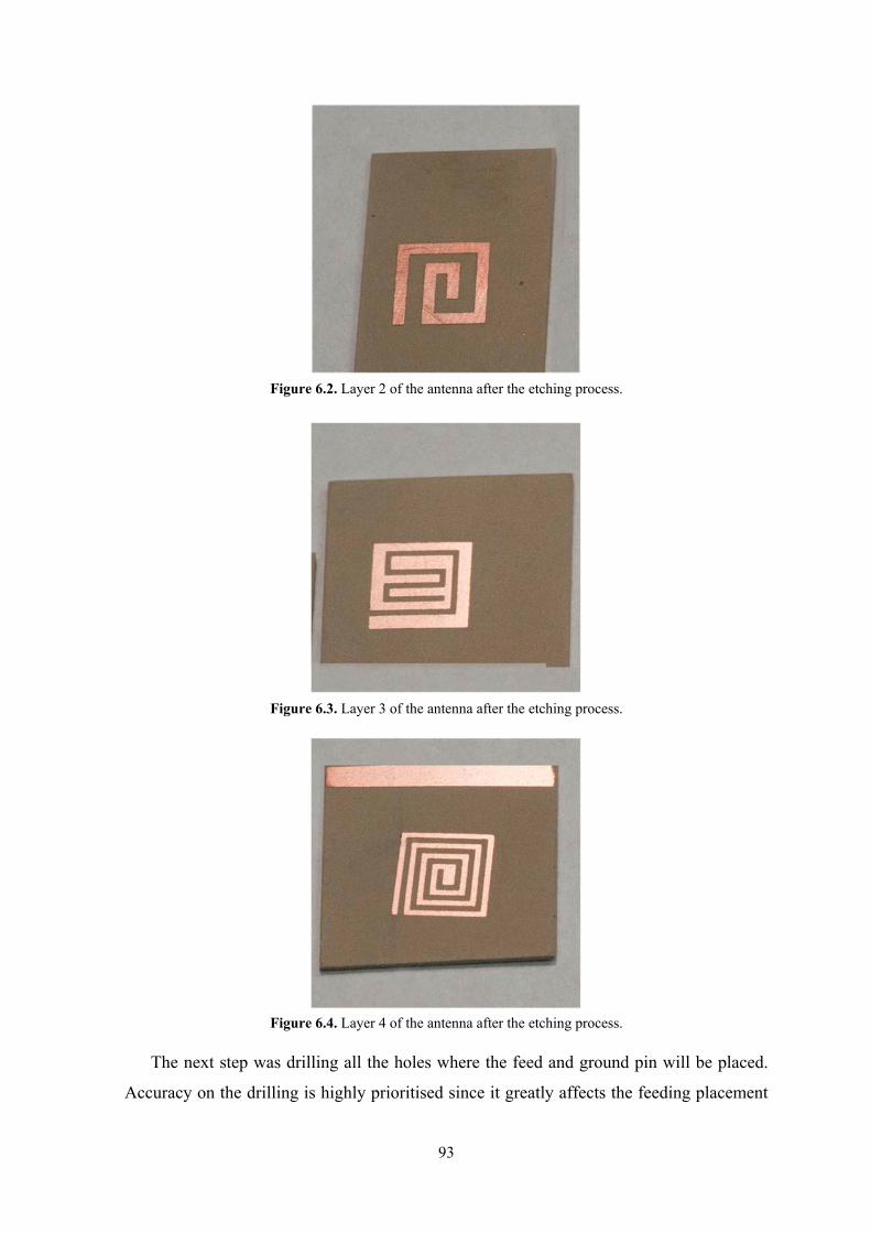
93

The next step was drilling all the holes where the feed and ground pin will be placed.

Accuracy on the drilling is highly prioritised since it greatly affects the feeding placement

Figure 6.2. Layer 2 of the antenna after the etching process.



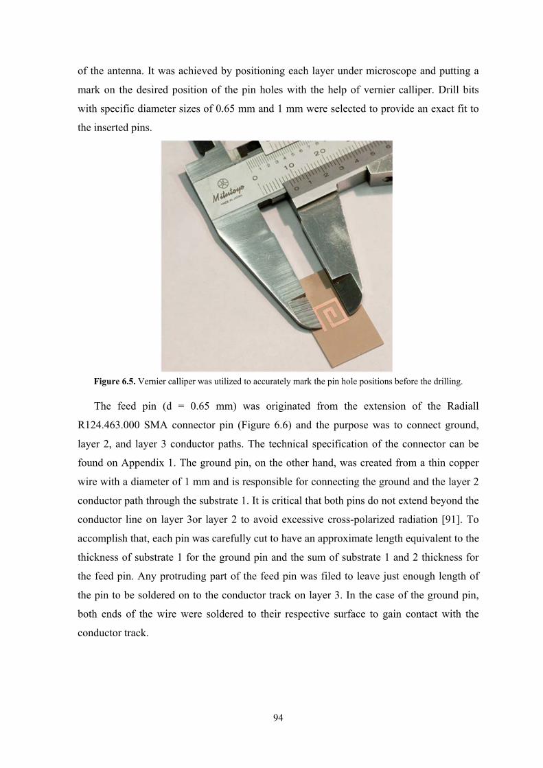
94

of the antenna. It was achieved by positioning each layer under microscope and putting a

mark on the desired position of the pin holes with the help of vernier calliper. Drill bits

with specific diameter sizes of 0.65 mm and 1 mm were selected to provide an exact fit to

the inserted pins.

The feed pin (d = 0.65 mm) was originated from the extension of the Radiall

R124.463.000 SMA connector pin (Figure 6.6) and the purpose was to connect ground,

layer 2, and layer 3 conductor paths. The technical specification of the connector can be

found on Appendix 1. The ground pin, on the other hand, was created from a thin copper

wire with a diameter of 1 mm and is responsible for connecting the ground and the layer 2

conductor path through the substrate 1. It is critical that both pins do not extend beyond the

conductor line on layer 3or layer 2 to avoid excessive cross-polarized radiation [91]. To

accomplish that, each pin was carefully cut to have an approximate length equivalent to the

thickness of substrate 1 for the ground pin and the sum of substrate 1 and 2 thickness for

the feed pin. Any protruding part of the feed pin was filed to leave just enough length of

the pin to be soldered on to the conductor track on layer 3. In the case of the ground pin,

both ends of the wire were soldered to their respective surface to gain contact with the

conductor track.

Figure 6.5. Vernier calliper was utilized to accurately mark the pin hole positions before the drilling.

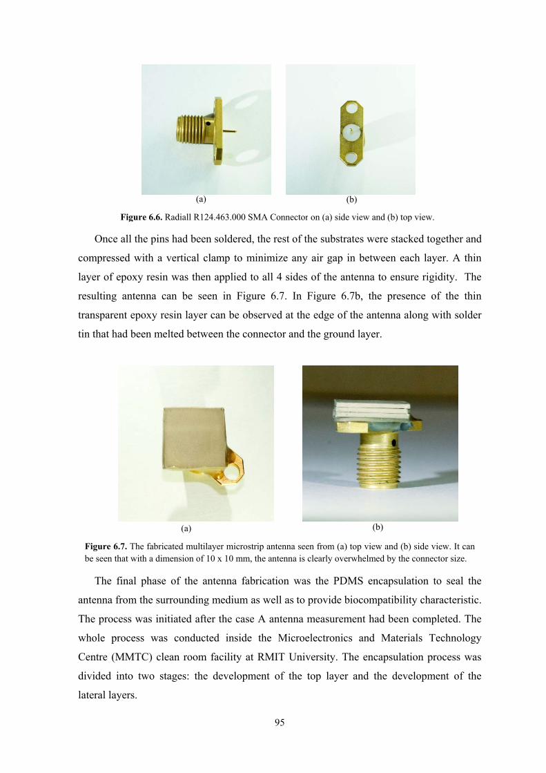
95

Once all the pins had been soldered, the rest of the substrates were stacked together and

compressed with a vertical clamp to minimize any air gap in between each layer. A thin

layer of epoxy resin was then applied to all 4 sides of the antenna to ensure rigidity. The

resulting antenna can be seen in Figure 6.7. In Figure 6.7b, the presence of the thin

transparent epoxy resin layer can be observed at the edge of the antenna along with solder

tin that had been melted between the connector and the ground layer.

The final phase of the antenna fabrication was the PDMS encapsulation to seal the

antenna from the surrounding medium as well as to provide biocompatibility characteristic.

The process was initiated after the case A antenna measurement had been completed. The

whole process was conducted inside the Microelectronics and Materials Technology

Centre (MMTC) clean room facility at RMIT University. The encapsulation process was

divided into two stages: the development of the top layer and the development of the

lateral layers.

(a) (b)

Figure 6.6. Radiall R124.463.000 SMA Connector on (a) side view and (b) top view.

(a)

Figure 6.7. The fabricated multilayer microstrip antenna seen from (a) top view and (b) side view. It can be seen that with a dimension of 10 x 10 mm, the antenna is clearly overwhelmed by the connector size.

(b)

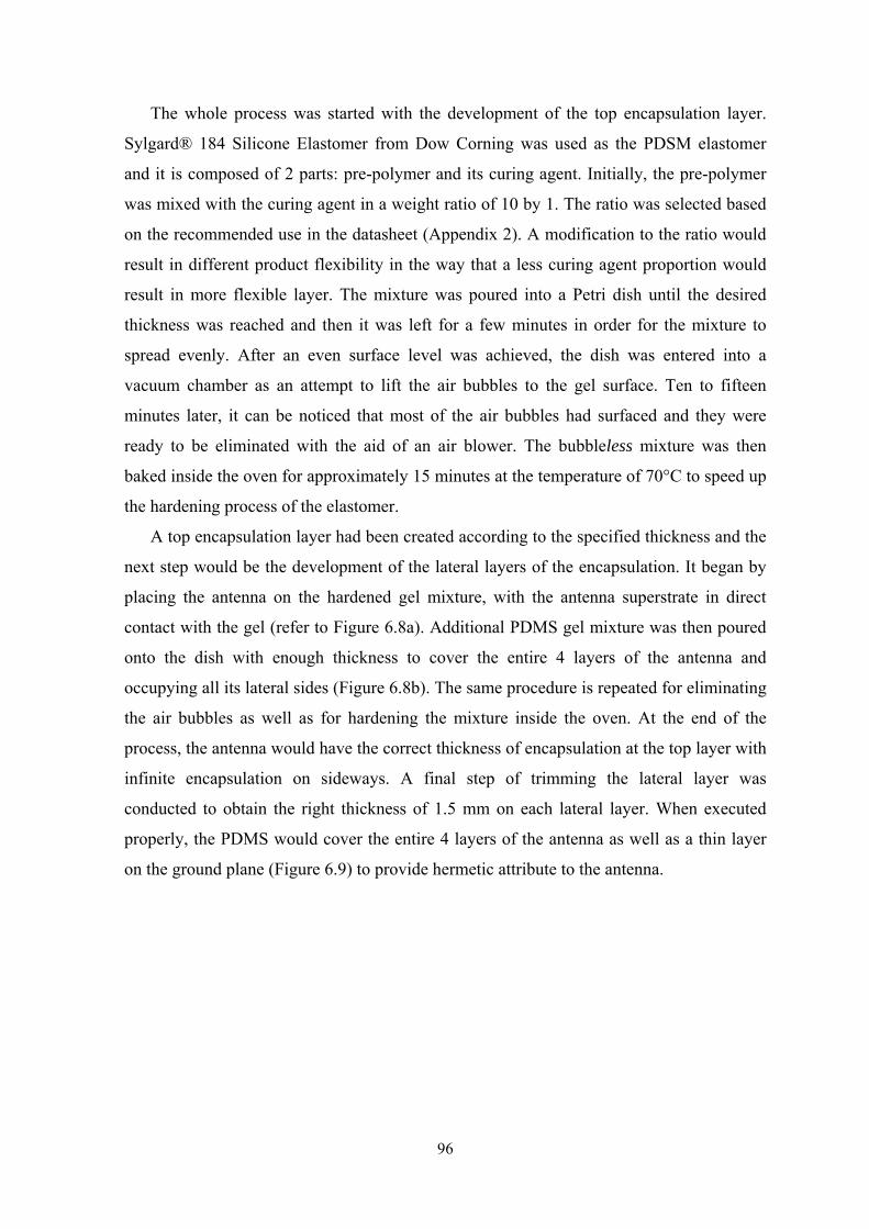
96

The whole process was started with the development of the top encapsulation layer.

Sylgard® 184 Silicone Elastomer from Dow Corning was used as the PDSM elastomer

and it is composed of 2 parts: pre-polymer and its curing agent. Initially, the pre-polymer

was mixed with the curing agent in a weight ratio of 10 by 1. The ratio was selected based

on the recommended use in the datasheet (Appendix 2). A modification to the ratio would

result in different product flexibility in the way that a less curing agent proportion would

result in more flexible layer. The mixture was poured into a Petri dish until the desired

thickness was reached and then it was left for a few minutes in order for the mixture to

spread evenly. After an even surface level was achieved, the dish was entered into a

vacuum chamber as an attempt to lift the air bubbles to the gel surface. Ten to fifteen

minutes later, it can be noticed that most of the air bubbles had surfaced and they were

ready to be eliminated with the aid of an air blower. The bubbleless mixture was then

baked inside the oven for approximately 15 minutes at the temperature of 70°C to speed up

the hardening process of the elastomer.

A top encapsulation layer had been created according to the specified thickness and the

next step would be the development of the lateral layers of the encapsulation. It began by

placing the antenna on the hardened gel mixture, with the antenna superstrate in direct

contact with the gel (refer to Figure 6.8a). Additional PDMS gel mixture was then poured

onto the dish with enough thickness to cover the entire 4 layers of the antenna and

occupying all its lateral sides (Figure 6.8b). The same procedure is repeated for eliminating

the air bubbles as well as for hardening the mixture inside the oven. At the end of the

process, the antenna would have the correct thickness of encapsulation at the top layer with

infinite encapsulation on sideways. A final step of trimming the lateral layer was

conducted to obtain the right thickness of 1.5 mm on each lateral layer. When executed

properly, the PDMS would cover the entire 4 layers of the antenna as well as a thin layer

on the ground plane (Figure 6.9) to provide hermetic attribute to the antenna.

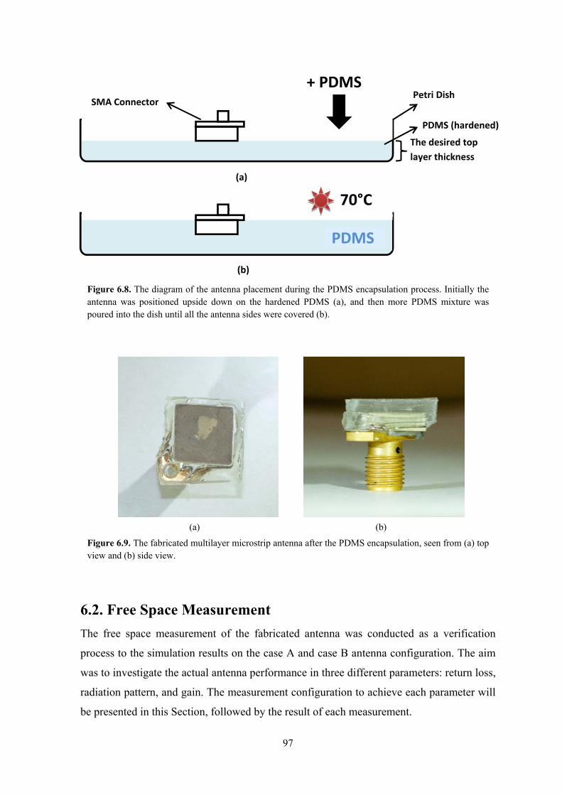
97

6.2. Free Space Measurement

The free space measurement of the fabricated antenna was conducted as a verification

process to the simulation results on the case A and case B antenna configuration. The aim

was to investigate the actual antenna performance in three different parameters: return loss,

radiation pattern, and gain. The measurement configuration to achieve each parameter will

be presented in this Section, followed by the result of each measurement.

The desired top

layer thickness

SMA Connector Petri Dish

+ PDMS

(a)

(b)

PDMS (hardened)

PDMS

Figure 6.8. The diagram of the antenna placement during the PDMS encapsulation process. Initially the antenna was positioned upside down on the hardened PDMS (a), and then more PDMS mixture was poured into the dish until all the antenna sides were covered (b).

70°C

(a)

Figure 6.9. The fabricated multilayer microstrip antenna after the PDMS encapsulation, seen from (a) top view and (b) side view.

(b)

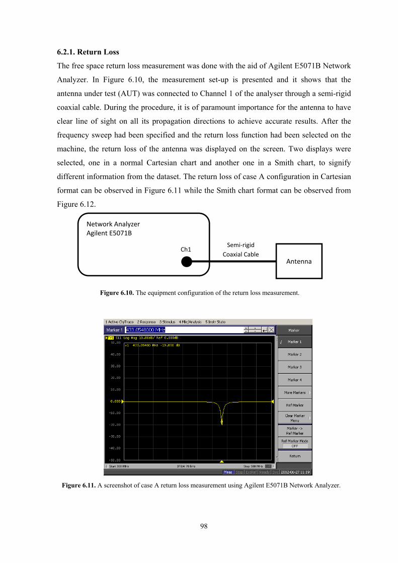
98

6.2.1. Return Loss

The free space return loss measurement was done with the aid of Agilent E5071B Network

Analyzer. In Figure 6.10, the measurement set-up is presented and it shows that the

antenna under test (AUT) was connected to Channel 1 of the analyser through a semi-rigid

coaxial cable. During the procedure, it is of paramount importance for the antenna to have

clear line of sight on all its propagation directions to achieve accurate results. After the

frequency sweep had been specified and the return loss function had been selected on the

machine, the return loss of the antenna was displayed on the screen. Two displays were

selected, one in a normal Cartesian chart and another one in a Smith chart, to signify

different information from the dataset. The return loss of case A configuration in Cartesian

format can be observed in Figure 6.11 while the Smith chart format can be observed from

Figure 6.12.

Network Analyzer Agilent E5071B Antenna

Semi‐rigid

Coaxial Cable Ch1

Figure 6.10. The equipment configuration of the return loss measurement.

Figure 6.11. A screenshot of case A return loss measurement using Agilent E5071B Network Analyzer.

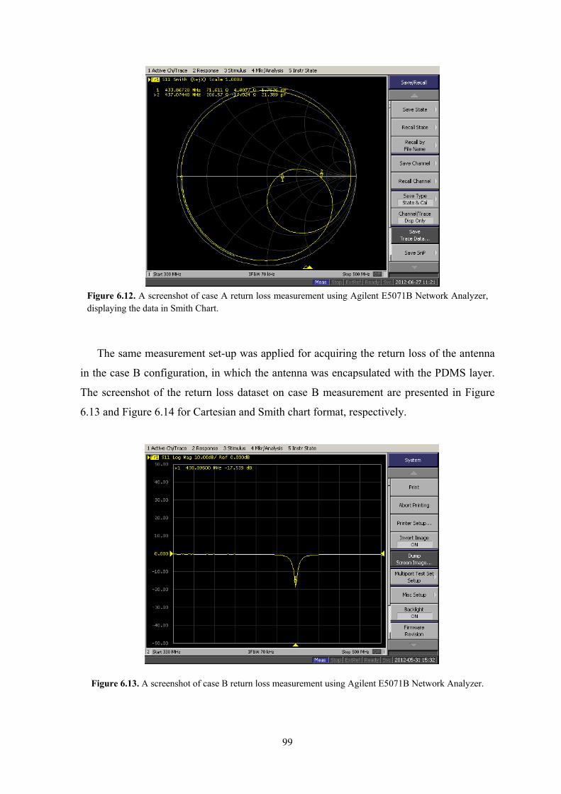
99

The same measurement set-up was applied for acquiring the return loss of the antenna

in the case B configuration, in which the antenna was encapsulated with the PDMS layer.

The screenshot of the return loss dataset on case B measurement are presented in Figure

6.13 and Figure 6.14 for Cartesian and Smith chart format, respectively.

Figure 6.12. A screenshot of case A return loss measurement using Agilent E5071B Network Analyzer, displaying the data in Smith Chart.

Figure 6.13. A screenshot of case B return loss measurement using Agilent E5071B Network Analyzer.

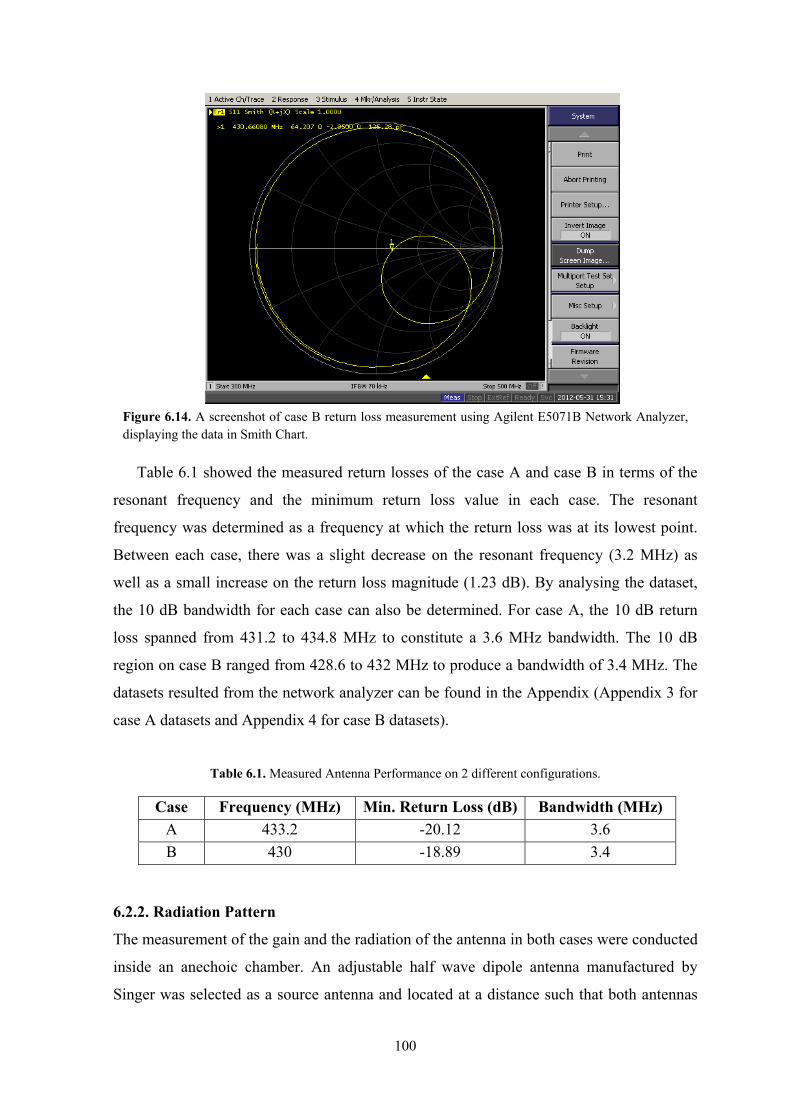
100

Table 6.1 showed the measured return losses of the case A and case B in terms of the

resonant frequency and the minimum return loss value in each case. The resonant

frequency was determined as a frequency at which the return loss was at its lowest point.

Between each case, there was a slight decrease on the resonant frequency (3.2 MHz) as

well as a small increase on the return loss magnitude (1.23 dB). By analysing the dataset,

the 10 dB bandwidth for each case can also be determined. For case A, the 10 dB return

loss spanned from 431.2 to 434.8 MHz to constitute a 3.6 MHz bandwidth. The 10 dB

region on case B ranged from 428.6 to 432 MHz to produce a bandwidth of 3.4 MHz. The

datasets resulted from the network analyzer can be found in the Appendix (Appendix 3 for

case A datasets and Appendix 4 for case B datasets).

6.2.2. Radiation Pattern

The measurement of the gain and the radiation of the antenna in both cases were conducted

inside an anechoic chamber. An adjustable half wave dipole antenna manufactured by

Singer was selected as a source antenna and located at a distance such that both antennas

Figure 6.14. A screenshot of case B return loss measurement using Agilent E5071B Network Analyzer, displaying the data in Smith Chart.

Table 6.1. Measured Antenna Performance on 2 different configurations.

Case Frequency (MHz) Min. Return Loss (dB) Bandwidth (MHz)

A 433.2 -20.12 3.6

B 430 -18.89 3.4

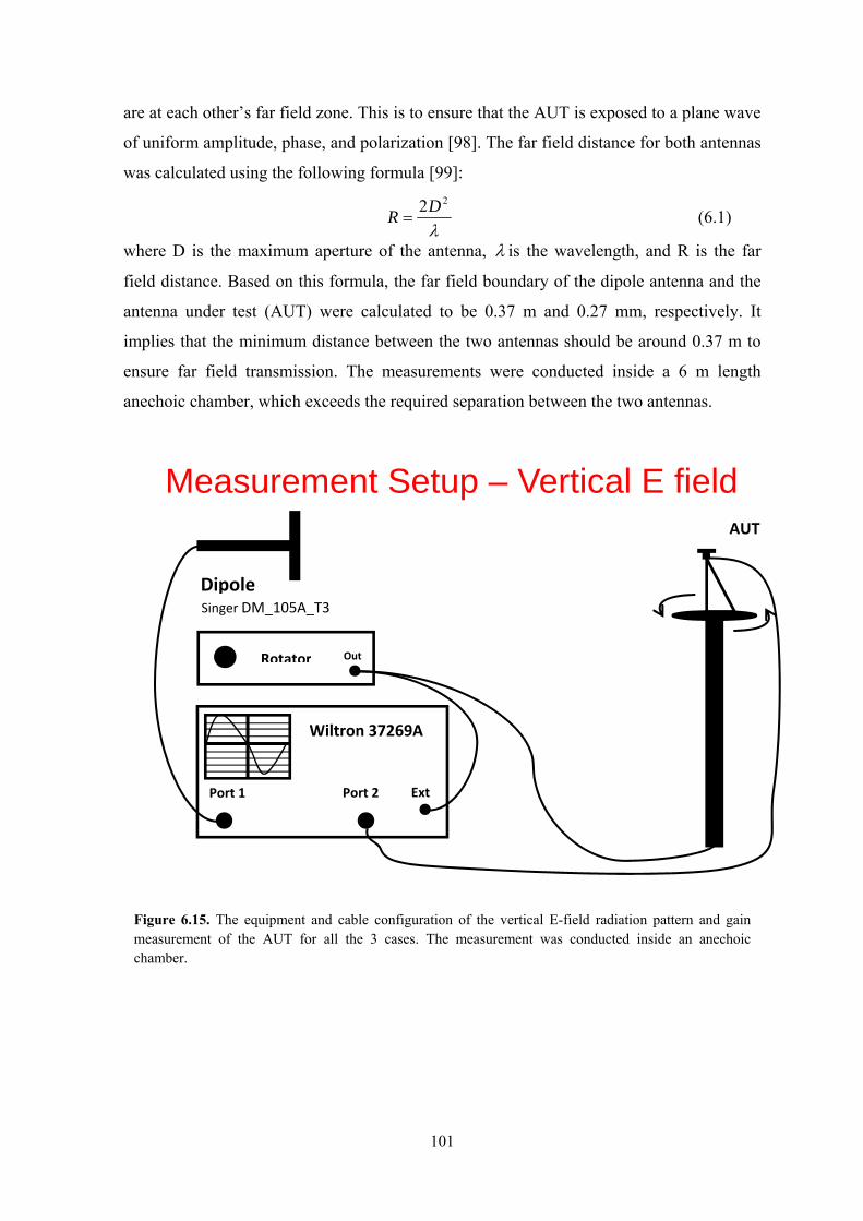
101

are at each other’s far field zone. This is to ensure that the AUT is exposed to a plane wave

of uniform amplitude, phase, and polarization [98]. The far field distance for both antennas

was calculated using the following formula [99]:

22DR (6.1)

where D is the maximum aperture of the antenna, is the wavelength, and R is the far

field distance. Based on this formula, the far field boundary of the dipole antenna and the

antenna under test (AUT) were calculated to be 0.37 m and 0.27 mm, respectively. It

implies that the minimum distance between the two antennas should be around 0.37 m to

ensure far field transmission. The measurements were conducted inside a 6 m length

anechoic chamber, which exceeds the required separation between the two antennas.

Measurement Setup – Vertical E field

Port 1 Port 2 Ext

Wiltron 37269A

Rotator Out

DipoleSinger DM_105A_T3

AUT

Figure 6.15. The equipment and cable configuration of the vertical E-field radiation pattern and gain measurement of the AUT for all the 3 cases. The measurement was conducted inside an anechoic chamber.

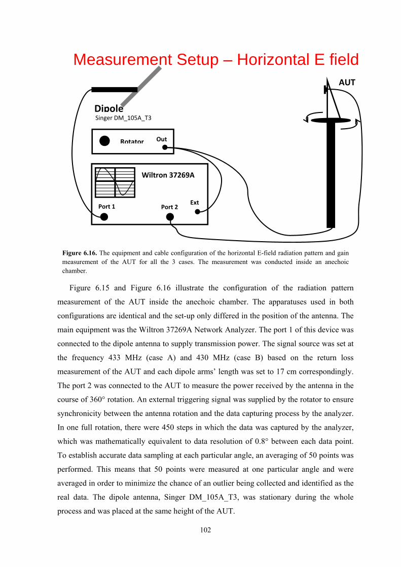
102

Figure 6.15 and Figure 6.16 illustrate the configuration of the radiation pattern

measurement of the AUT inside the anechoic chamber. The apparatuses used in both

configurations are identical and the set-up only differed in the position of the antenna. The

main equipment was the Wiltron 37269A Network Analyzer. The port 1 of this device was

connected to the dipole antenna to supply transmission power. The signal source was set at

the frequency 433 MHz (case A) and 430 MHz (case B) based on the return loss

measurement of the AUT and each dipole arms’ length was set to 17 cm correspondingly.

The port 2 was connected to the AUT to measure the power received by the antenna in the

course of 360° rotation. An external triggering signal was supplied by the rotator to ensure

synchronicity between the antenna rotation and the data capturing process by the analyzer.

In one full rotation, there were 450 steps in which the data was captured by the analyzer,

which was mathematically equivalent to data resolution of 0.8° between each data point.

To establish accurate data sampling at each particular angle, an averaging of 50 points was

performed. This means that 50 points were measured at one particular angle and were

averaged in order to minimize the chance of an outlier being collected and identified as the

real data. The dipole antenna, Singer DM_105A_T3, was stationary during the whole

process and was placed at the same height of the AUT.

Measurement Setup – Horizontal E field

Port 1 Port 2 Ext

Wiltron 37269A


Rotator Out

AUT

Figure 6.16. The equipment and cable configuration of the horizontal E-field radiation pattern and gain measurement of the AUT for all the 3 cases. The measurement was conducted inside an anechoic chamber.

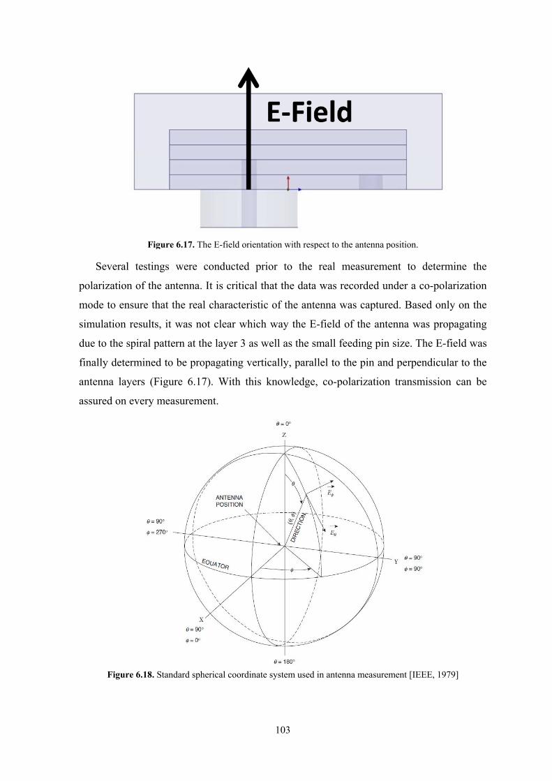
103

Several testings were conducted prior to the real measurement to determine the

polarization of the antenna. It is critical that the data was recorded under a co-polarization

mode to ensure that the real characteristic of the antenna was captured. Based only on the

simulation results, it was not clear which way the E-field of the antenna was propagating

due to the spiral pattern at the layer 3 as well as the small feeding pin size. The E-field was

finally determined to be propagating vertically, parallel to the pin and perpendicular to the

antenna layers (Figure 6.17). With this knowledge, co-polarization transmission can be

assured on every measurement.

Figure 6.17. The E-field orientation with respect to the antenna position.

Figure 6.18. Standard spherical coordinate system used in antenna measurement [IEEE, 1979]

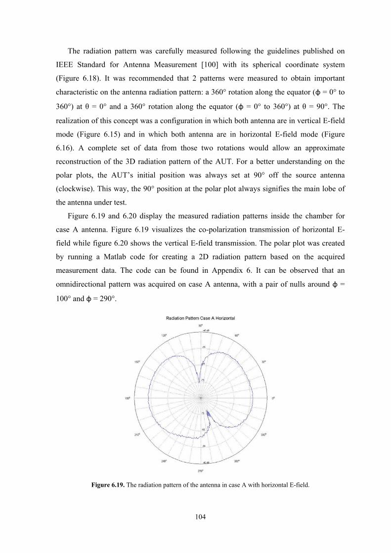
104

The radiation pattern was carefully measured following the guidelines published on

IEEE Standard for Antenna Measurement [100] with its spherical coordinate system

(Figure 6.18). It was recommended that 2 patterns were measured to obtain important

characteristic on the antenna radiation pattern: a 360° rotation along the equator (φ = 0° to

360°) at θ = 0° and a 360° rotation along the equator (φ = 0° to 360°) at θ = 90°. The

realization of this concept was a configuration in which both antenna are in vertical E-field

mode (Figure 6.15) and in which both antenna are in horizontal E-field mode (Figure

6.16). A complete set of data from those two rotations would allow an approximate

reconstruction of the 3D radiation pattern of the AUT. For a better understanding on the

polar plots, the AUT’s initial position was always set at 90° off the source antenna

(clockwise). This way, the 90° position at the polar plot always signifies the main lobe of

the antenna under test.

Figure 6.19 and 6.20 display the measured radiation patterns inside the chamber for

case A antenna. Figure 6.19 visualizes the co-polarization transmission of horizontal E-

field while figure 6.20 shows the vertical E-field transmission. The polar plot was created

by running a Matlab code for creating a 2D radiation pattern based on the acquired

measurement data. The code can be found in Appendix 6. It can be observed that an

omnidirectional pattern was acquired on case A antenna, with a pair of nulls around φ =

100° and φ = 290°.

Figure 6.19. The radiation pattern of the antenna in case A with horizontal E-field.

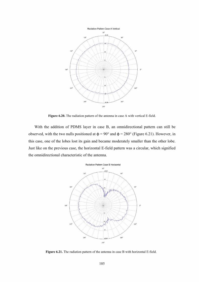
105

With the addition of PDMS layer in case B, an omnidirectional pattern can still be

observed, with the two nulls positioned at φ = 90° and φ = 280° (Figure 6.21). However, in

this case, one of the lobes lost its gain and became moderately smaller than the other lobe.

Just like on the previous case, the horizontal E-field pattern was a circular, which signified

the omnidirectional characteristic of the antenna.

Figure 6.20. The radiation pattern of the antenna in case A with vertical E-field.

Figure 6.21. The radiation pattern of the antenna in case B with horizontal E-field.

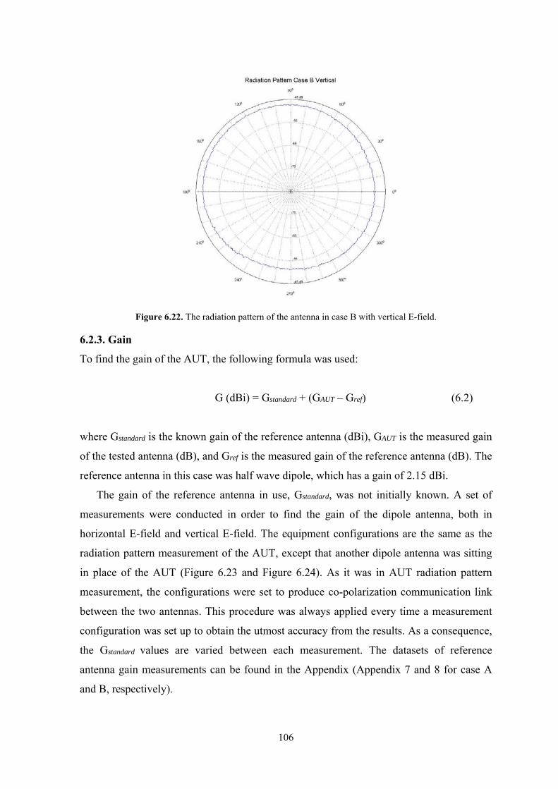
106

6.2.3. Gain

To find the gain of the AUT, the following formula was used:

G (dBi) = Gstandard + (GAUT – Gref) (6.2)

where Gstandard is the known gain of the reference antenna (dBi), GAUT is the measured gain

of the tested antenna (dB), and Gref is the measured gain of the reference antenna (dB). The

reference antenna in this case was half wave dipole, which has a gain of 2.15 dBi.

The gain of the reference antenna in use, Gstandard, was not initially known. A set of

measurements were conducted in order to find the gain of the dipole antenna, both in

horizontal E-field and vertical E-field. The equipment configurations are the same as the

radiation pattern measurement of the AUT, except that another dipole antenna was sitting

in place of the AUT (Figure 6.23 and Figure 6.24). As it was in AUT radiation pattern

measurement, the configurations were set to produce co-polarization communication link

between the two antennas. This procedure was always applied every time a measurement

configuration was set up to obtain the utmost accuracy from the results. As a consequence,

the Gstandard values are varied between each measurement. The datasets of reference

antenna gain measurements can be found in the Appendix (Appendix 7 and 8 for case A

and B, respectively).

Figure 6.22. The radiation pattern of the antenna in case B with vertical E-field.

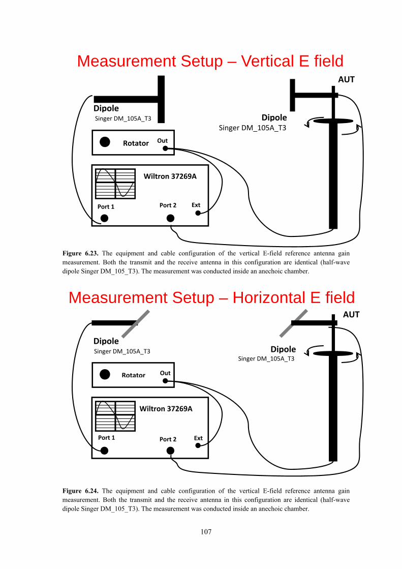
107

Measurement Setup – Vertical E field

Port 1 Port 2 Ext

Wiltron 37269A


Rotator Out

Dipole

Singer DM_105A_T3

AUT

Figure 6.23. The equipment and cable configuration of the vertical E-field reference antenna gain measurement. Both the transmit and the receive antenna in this configuration are identical (half-wave dipole Singer DM_105_T3). The measurement was conducted inside an anechoic chamber.

Measurement Setup – Horizontal E field

Port 1 Port 2 Ext

Wiltron 37269A


Rotator Out

Dipole

Singer DM_105A_T3

AUT

Figure 6.24. The equipment and cable configuration of the vertical E-field reference antenna gain measurement. Both the transmit and the receive antenna in this configuration are identical (half-wave dipole Singer DM_105_T3). The measurement was conducted inside an anechoic chamber.

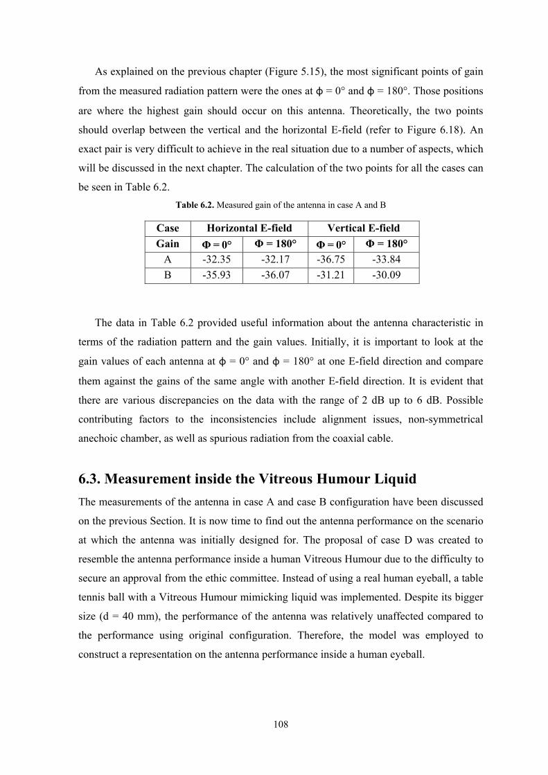
108

As explained on the previous chapter (Figure 5.15), the most significant points of gain

from the measured radiation pattern were the ones at φ = 0° and φ = 180°. Those positions

are where the highest gain should occur on this antenna. Theoretically, the two points

should overlap between the vertical and the horizontal E-field (refer to Figure 6.18). An

exact pair is very difficult to achieve in the real situation due to a number of aspects, which

will be discussed in the next chapter. The calculation of the two points for all the cases can

be seen in Table 6.2.

The data in Table 6.2 provided useful information about the antenna characteristic in

terms of the radiation pattern and the gain values. Initially, it is important to look at the

gain values of each antenna at φ = 0° and φ = 180° at one E-field direction and compare

them against the gains of the same angle with another E-field direction. It is evident that

there are various discrepancies on the data with the range of 2 dB up to 6 dB. Possible

contributing factors to the inconsistencies include alignment issues, non-symmetrical

anechoic chamber, as well as spurious radiation from the coaxial cable.

6.3. Measurement inside the Vitreous Humour Liquid

The measurements of the antenna in case A and case B configuration have been discussed

on the previous Section. It is now time to find out the antenna performance on the scenario

at which the antenna was initially designed for. The proposal of case D was created to

resemble the antenna performance inside a human Vitreous Humour due to the difficulty to

secure an approval from the ethic committee. Instead of using a real human eyeball, a table

tennis ball with a Vitreous Humour mimicking liquid was implemented. Despite its bigger

size (d = 40 mm), the performance of the antenna was relatively unaffected compared to

the performance using original configuration. Therefore, the model was employed to

construct a representation on the antenna performance inside a human eyeball.

Table 6.2. Measured gain of the antenna in case A and B

Case Horizontal E-field Vertical E-field

Gain Φ = 0° Φ = 180° Φ = 0° Φ = 180°

A -32.35 -32.17 -36.75 -33.84

B -35.93 -36.07 -31.21 -30.09

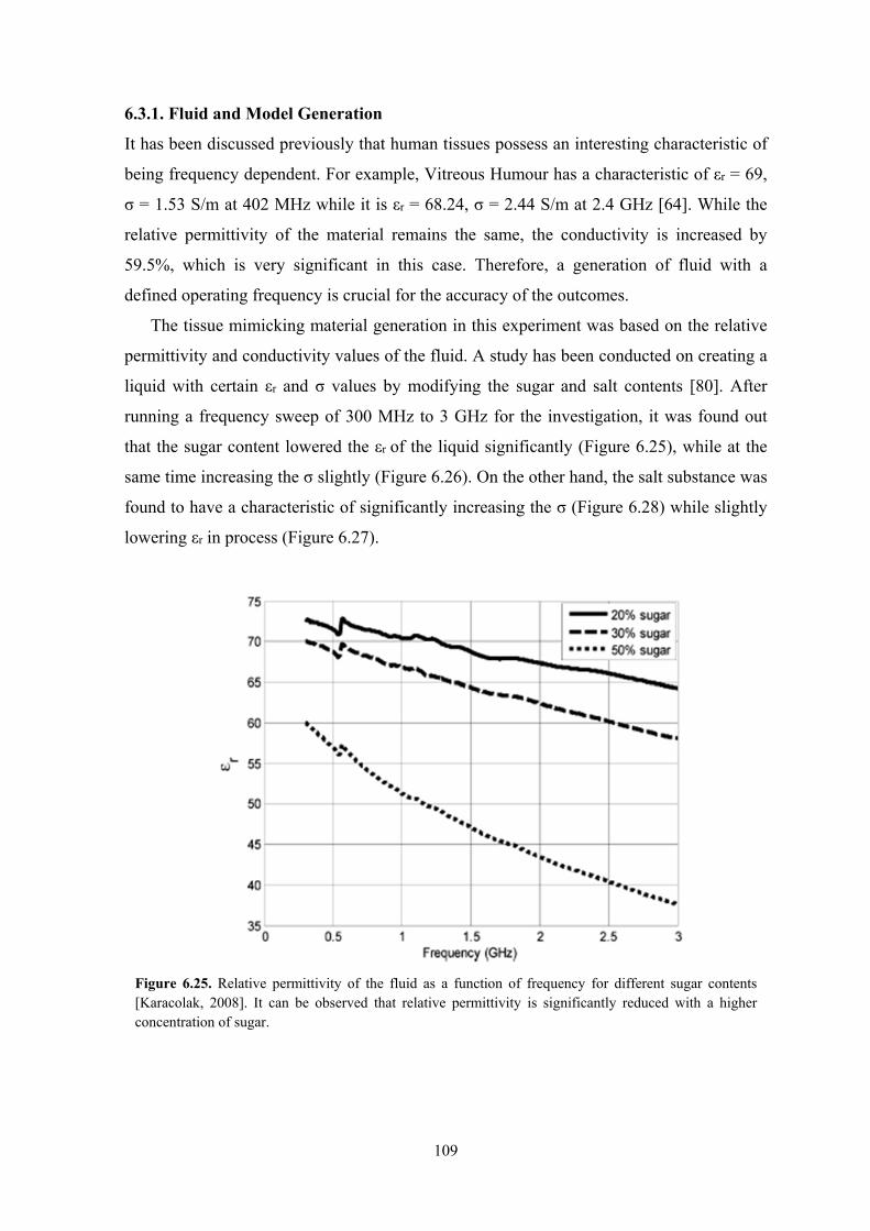
109

6.3.1. Fluid and Model Generation

It has been discussed previously that human tissues possess an interesting characteristic of

being frequency dependent. For example, Vitreous Humour has a characteristic of εr = 69,

σ = 1.53 S/m at 402 MHz while it is εr = 68.24, σ = 2.44 S/m at 2.4 GHz [64]. While the

relative permittivity of the material remains the same, the conductivity is increased by

59.5%, which is very significant in this case. Therefore, a generation of fluid with a

defined operating frequency is crucial for the accuracy of the outcomes.

The tissue mimicking material generation in this experiment was based on the relative

permittivity and conductivity values of the fluid. A study has been conducted on creating a

liquid with certain εr and σ values by modifying the sugar and salt contents [80]. After

running a frequency sweep of 300 MHz to 3 GHz for the investigation, it was found out

that the sugar content lowered the εr of the liquid significantly (Figure 6.25), while at the

same time increasing the σ slightly (Figure 6.26). On the other hand, the salt substance was

found to have a characteristic of significantly increasing the σ (Figure 6.28) while slightly

lowering εr in process (Figure 6.27).

Figure 6.25. Relative permittivity of the fluid as a function of frequency for different sugar contents [Karacolak, 2008]. It can be observed that relative permittivity is significantly reduced with a higher concentration of sugar.

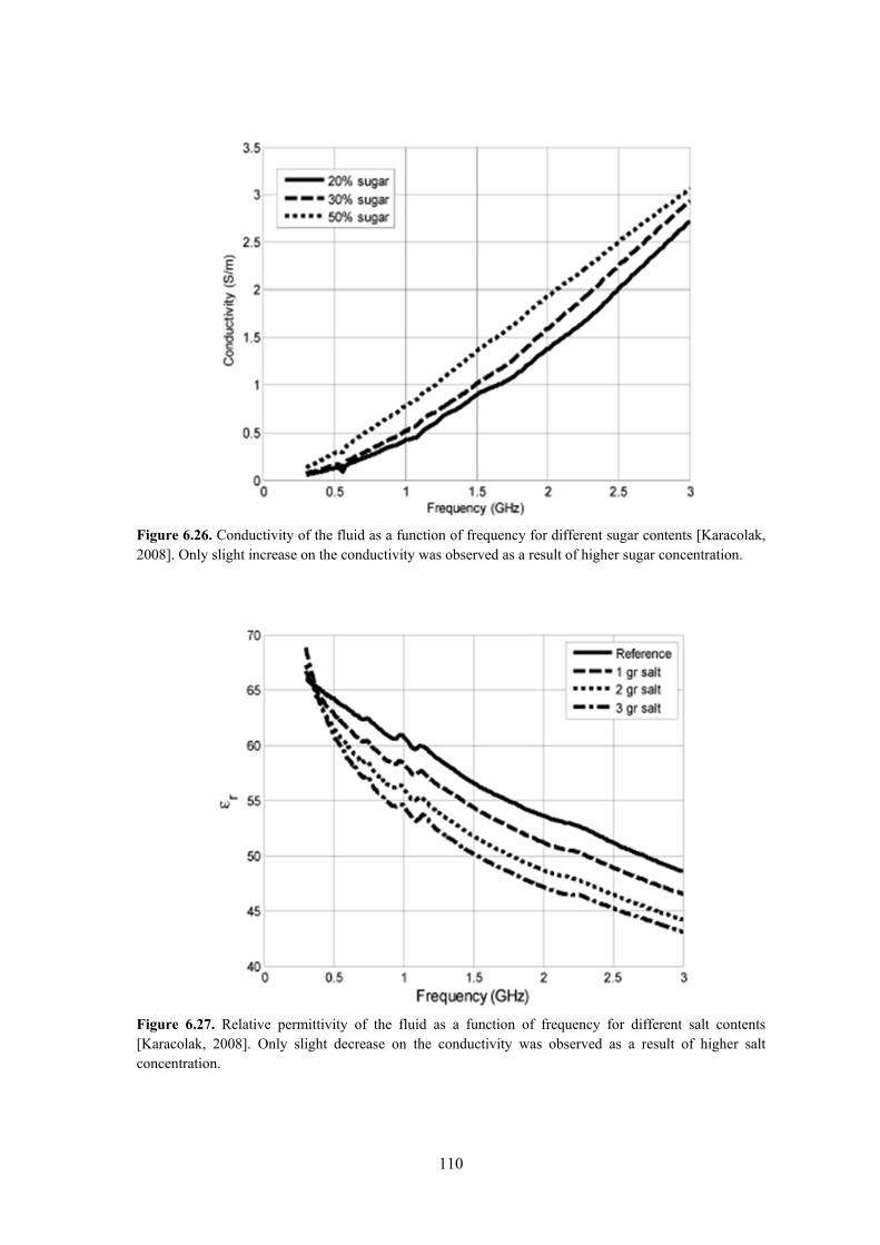
110

Figure 6.26. Conductivity of the fluid as a function of frequency for different sugar contents [Karacolak, 2008]. Only slight increase on the conductivity was observed as a result of higher sugar concentration.

Figure 6.27. Relative permittivity of the fluid as a function of frequency for different salt contents [Karacolak, 2008]. Only slight decrease on the conductivity was observed as a result of higher salt concentration.

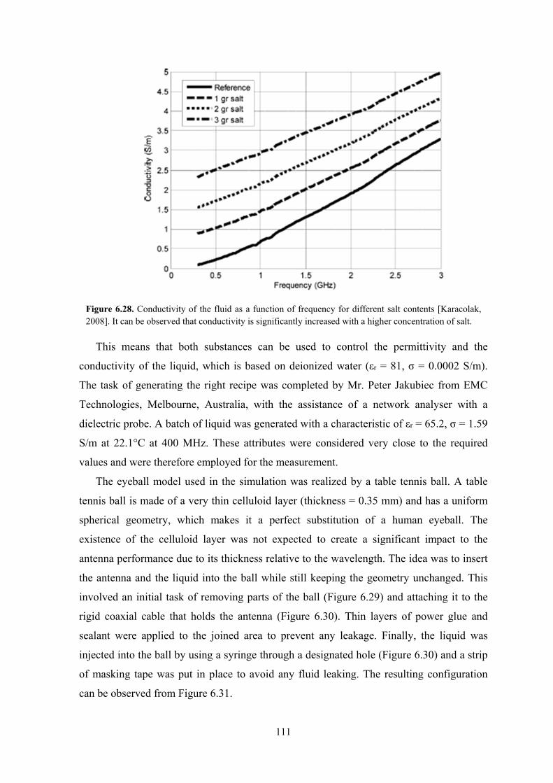
111

This means that both substances can be used to control the permittivity and the

conductivity of the liquid, which is based on deionized water (εr = 81, σ = 0.0002 S/m).

The task of generating the right recipe was completed by Mr. Peter Jakubiec from EMC

Technologies, Melbourne, Australia, with the assistance of a network analyser with a

dielectric probe. A batch of liquid was generated with a characteristic of εr = 65.2, σ = 1.59

S/m at 22.1°C at 400 MHz. These attributes were considered very close to the required

values and were therefore employed for the measurement.

The eyeball model used in the simulation was realized by a table tennis ball. A table

tennis ball is made of a very thin celluloid layer (thickness = 0.35 mm) and has a uniform

spherical geometry, which makes it a perfect substitution of a human eyeball. The

existence of the celluloid layer was not expected to create a significant impact to the

antenna performance due to its thickness relative to the wavelength. The idea was to insert

the antenna and the liquid into the ball while still keeping the geometry unchanged. This

involved an initial task of removing parts of the ball (Figure 6.29) and attaching it to the

rigid coaxial cable that holds the antenna (Figure 6.30). Thin layers of power glue and

sealant were applied to the joined area to prevent any leakage. Finally, the liquid was

injected into the ball by using a syringe through a designated hole (Figure 6.30) and a strip

of masking tape was put in place to avoid any fluid leaking. The resulting configuration

can be observed from Figure 6.31.

Figure 6.28. Conductivity of the fluid as a function of frequency for different salt contents [Karacolak, 2008]. It can be observed that conductivity is significantly increased with a higher concentration of salt.

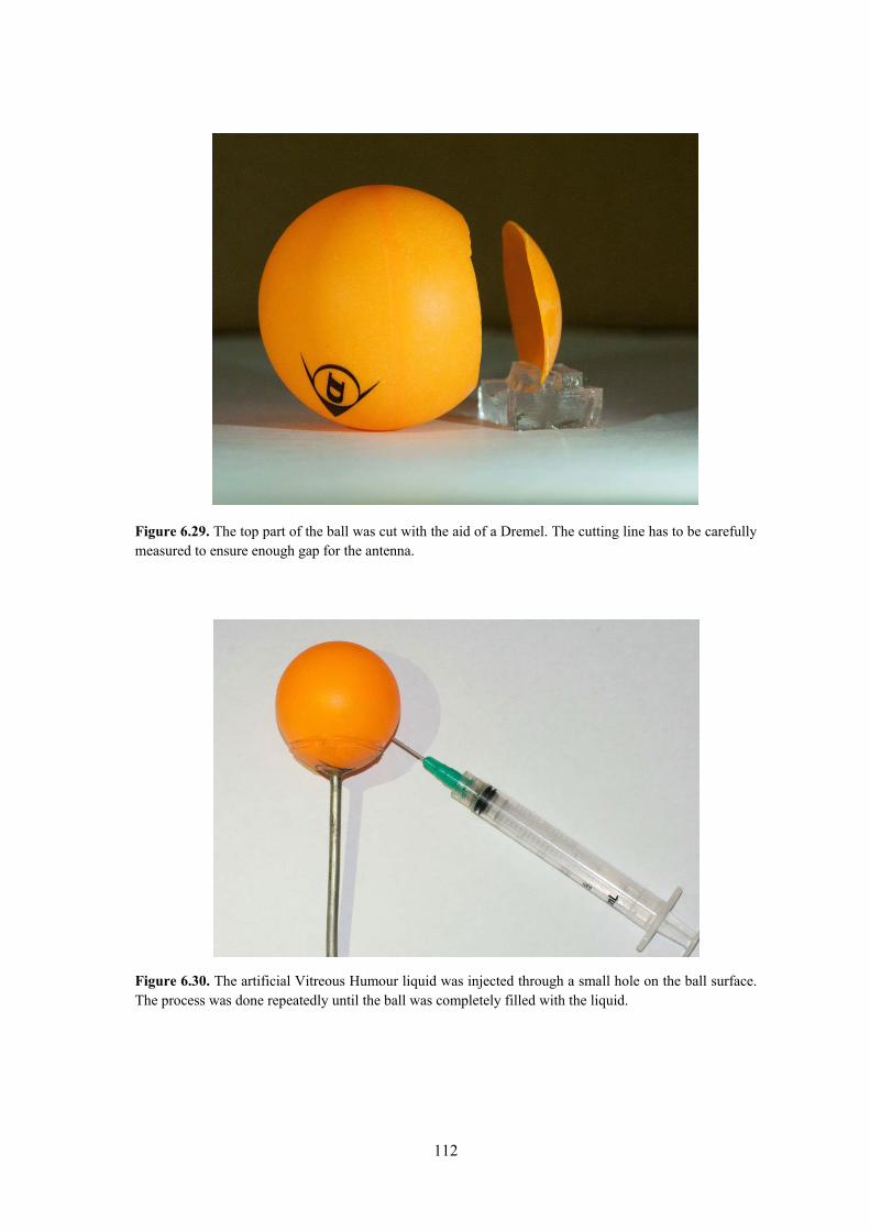
112

Figure 6.29. The top part of the ball was cut with the aid of a Dremel. The cutting line has to be carefully measured to ensure enough gap for the antenna.

Figure 6.30. The artificial Vitreous Humour liquid was injected through a small hole on the ball surface. The process was done repeatedly until the ball was completely filled with the liquid.

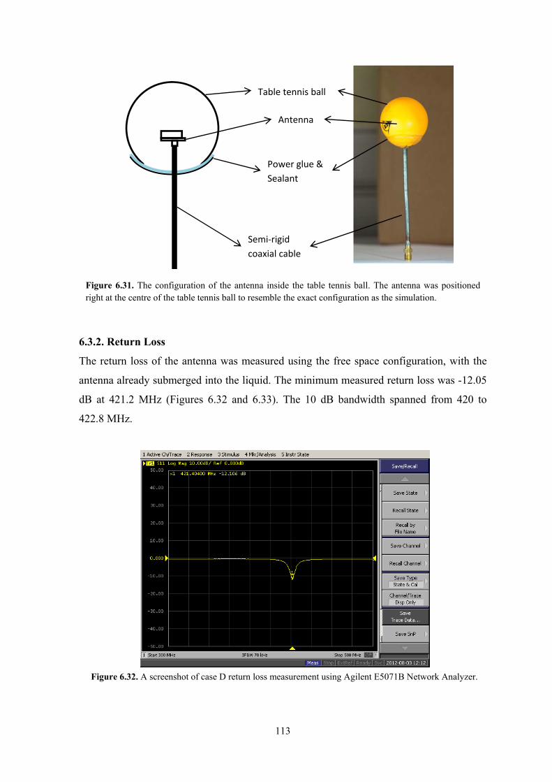
113

6.3.2. Return Loss

The return loss of the antenna was measured using the free space configuration, with the

antenna already submerged into the liquid. The minimum measured return loss was -12.05

dB at 421.2 MHz (Figures 6.32 and 6.33). The 10 dB bandwidth spanned from 420 to

422.8 MHz.

Figure 6.31. The configuration of the antenna inside the table tennis ball. The antenna was positioned right at the centre of the table tennis ball to resemble the exact configuration as the simulation.

Antenna

Semi‐rigid

coaxial cable

Table tennis ball

Power glue &

Sealant

Figure 6.32. A screenshot of case D return loss measurement using Agilent E5071B Network Analyzer.

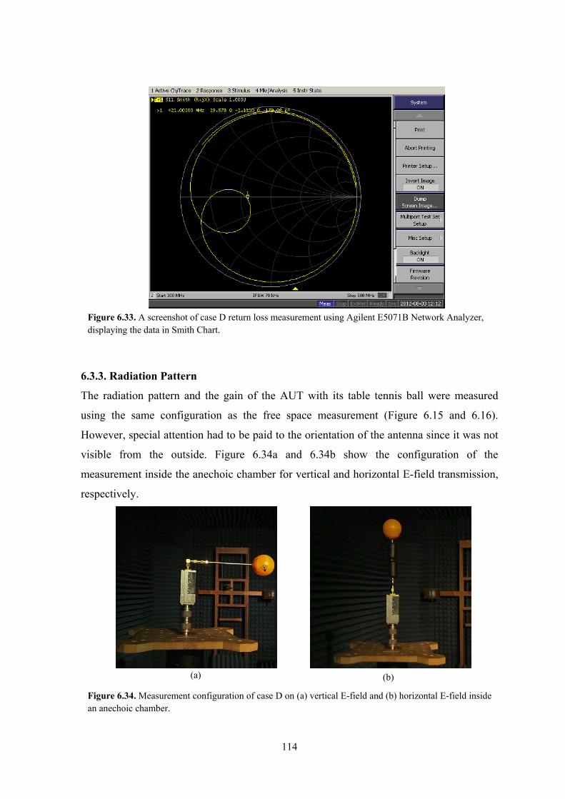
114

6.3.3. Radiation Pattern

The radiation pattern and the gain of the AUT with its table tennis ball were measured

using the same configuration as the free space measurement (Figure 6.15 and 6.16).

However, special attention had to be paid to the orientation of the antenna since it was not

visible from the outside. Figure 6.34a and 6.34b show the configuration of the

measurement inside the anechoic chamber for vertical and horizontal E-field transmission,

respectively.

Figure 6.33. A screenshot of case D return loss measurement using Agilent E5071B Network Analyzer, displaying the data in Smith Chart.

Figure 6.34. Measurement configuration of case D on (a) vertical E-field and (b) horizontal E-field inside an anechoic chamber.

(a) (b)

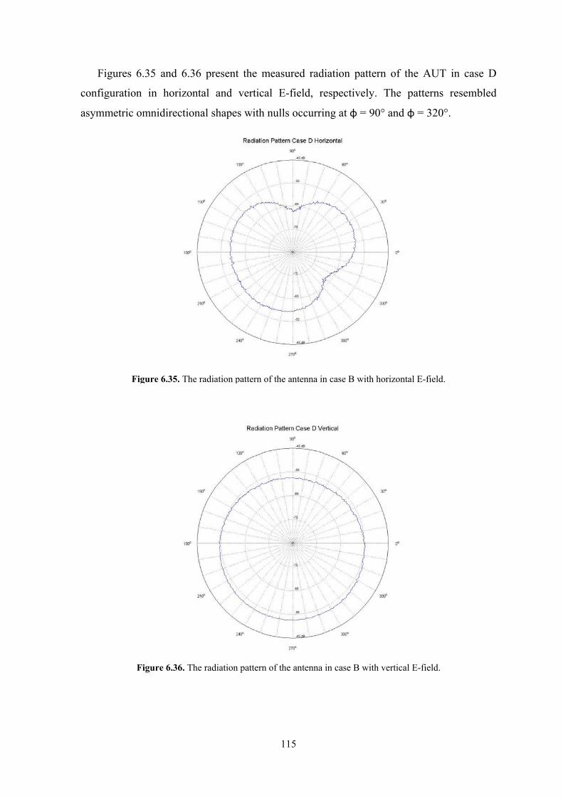
115

Figures 6.35 and 6.36 present the measured radiation pattern of the AUT in case D

configuration in horizontal and vertical E-field, respectively. The patterns resembled

asymmetric omnidirectional shapes with nulls occurring at φ = 90° and φ = 320°.

Figure 6.35. The radiation pattern of the antenna in case B with horizontal E-field.

Figure 6.36. The radiation pattern of the antenna in case B with vertical E-field.

116

6.3.4. Gain

The gain of the AUT was obtained at φ = 0° and φ = 180° of both E-field orientations, and

then the formula 6.2 was applied. For the horizontal E-field, the gain was -39.89 dB and -

39.29 dB for φ = 0° and φ = 180°, respectively. For the vertical E-field set up, it was -

37.89 dB and -37.36 dB, respectively. As expected, the gain values with the Vitreous

Humour surrounding the antenna were lower compared to the free space measurements.

6.4. Summary

In this chapter, the measurement process has been presented. The chapter was initiated by

the antenna fabrication procedure. On the next Section, the measurement configuration of

the antenna in free space was discussed, which included the equipment configuration,

device settings, as well as data analysis process. The antenna performance in terms of

return loss, radiation pattern, and gain, was then presented. The following Section provided

an insight on the measurement inside the Vitreous Humour liquid, started by some

background on the mimicking liquid and the model generation. The measurement

procedure for each parameter was also presented, and this chapter was finalised by the

demonstration of the results on each respective variable. In the next chapter, these results

will be discussed and analysed. The discrepancies between them and the simulation results

will also be explained.

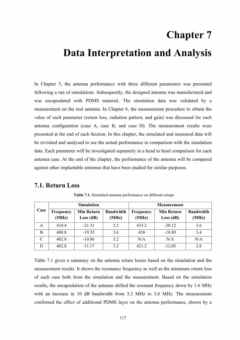
117

Chapter 7

Data Interpretation and Analysis

In Chapter 5, the antenna performance with three different parameters was presented

following a run of simulations. Subsequently, the designed antenna was manufactured and

was encapsulated with PDMS material. The simulation data was validated by a

measurement on the real antenna. In Chapter 6, the measurement procedure to obtain the

value of each parameter (return loss, radiation pattern, and gain) was discussed for each

antenna configuration (case A, case B, and case D). The measurement results were

presented at the end of each Section. In this chapter, the simulated and measured data will

be revisited and analysed to see the actual performance in comparison with the simulation

data. Each parameter will be investigated separately in a head to head comparison for each

antenna case. At the end of the chapter, the performance of the antenna will be compared

against other implantable antennas that have been studied for similar purposes.

7.1. Return Loss

Table 7.1 gives a summary on the antenna return losses based on the simulation and the

measurement results. It shows the resonance frequency as well as the minimum return loss

of each case both from the simulation and the measurement. Based on the simulation

results, the encapsulation of the antenna shifted the resonant frequency down by 1.6 MHz

with an increase in 10 dB bandwidth from 3.2 MHz to 3.6 MHz. The measurement

confirmed the effect of additional PDMS layer on the antenna performance, shown by a

Table 7.1. Simulated antenna performance on different setups

Case Simulation Measurement

Frequency (MHz)


Bandwidth (MHz)

Frequency (MHz)


Bandwidth (MHz)

A 410.4 -21.31 3.2 433.2 -20.12 3.6

B 408.8 -19.35 3.6 430 -18.89 3.4

C 402.8 -10.86 3.2 N/A N/A N/A

D 402.8 -11.17 3.2 421.2 -12.05 2.8

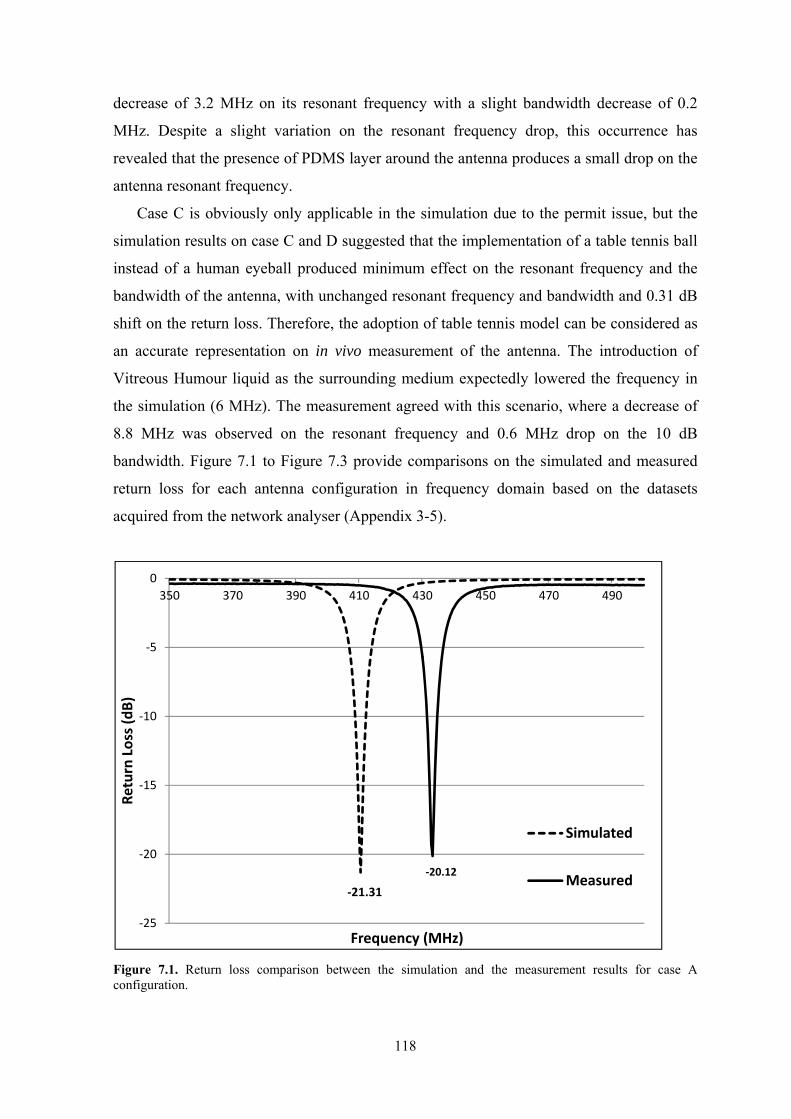
118

decrease of 3.2 MHz on its resonant frequency with a slight bandwidth decrease of 0.2

MHz. Despite a slight variation on the resonant frequency drop, this occurrence has

revealed that the presence of PDMS layer around the antenna produces a small drop on the

antenna resonant frequency.

Case C is obviously only applicable in the simulation due to the permit issue, but the

simulation results on case C and D suggested that the implementation of a table tennis ball

instead of a human eyeball produced minimum effect on the resonant frequency and the

bandwidth of the antenna, with unchanged resonant frequency and bandwidth and 0.31 dB

shift on the return loss. Therefore, the adoption of table tennis model can be considered as

an accurate representation on in vivo measurement of the antenna. The introduction of

Vitreous Humour liquid as the surrounding medium expectedly lowered the frequency in

the simulation (6 MHz). The measurement agreed with this scenario, where a decrease of

8.8 MHz was observed on the resonant frequency and 0.6 MHz drop on the 10 dB

bandwidth. Figure 7.1 to Figure 7.3 provide comparisons on the simulated and measured

return loss for each antenna configuration in frequency domain based on the datasets

acquired from the network analyser (Appendix 3-5).

Figure 7.1. Return loss comparison between the simulation and the measurement results for case Aconfiguration.

‐21.31

‐20.12

‐25

‐20

‐15

‐10

‐5

0

350 370 390 410 430 450 470 490

Return Loss (dB)

Frequency (MHz)

Simulated

Measured

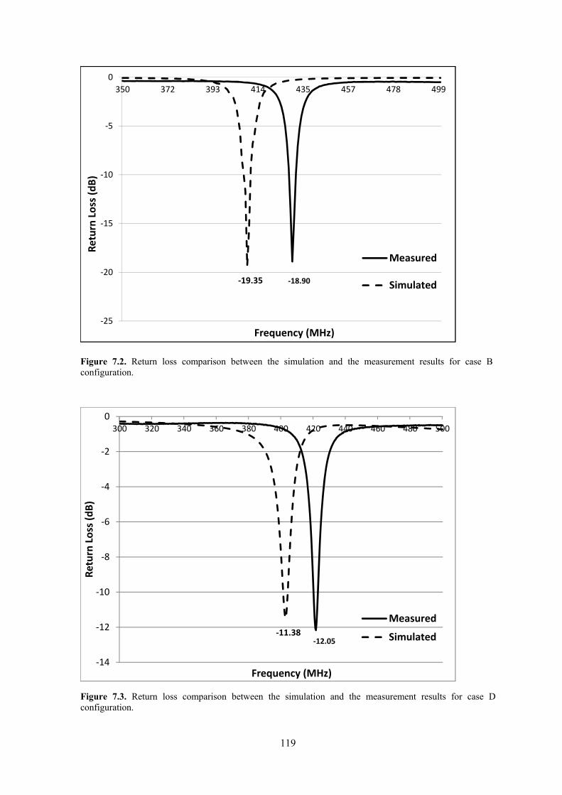
119

Figure 7.2. Return loss comparison between the simulation and the measurement results for case Bconfiguration.

‐18.90‐19.35

‐25

‐20

‐15

‐10

‐5

0

350 372 393 414 435 457 478 499Return Loss (dB)

Frequency (MHz)

Measured

Simulated

Figure 7.3. Return loss comparison between the simulation and the measurement results for case Dconfiguration.

‐12.05‐11.38

‐14

‐12

‐10

‐8

‐6

‐4

‐2

0300 320 340 360 380 400 420 440 460 480 500

Return Loss (dB)

Frequency (MHz)

Measured

Simulated

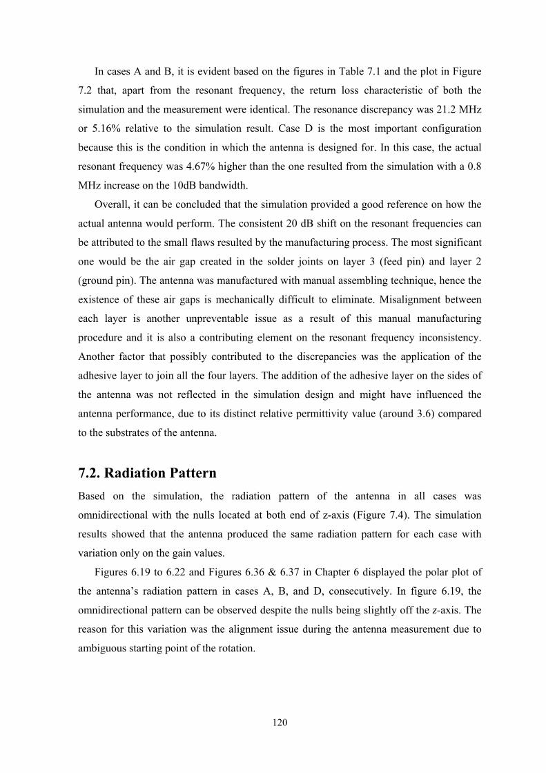
120

In cases A and B, it is evident based on the figures in Table 7.1 and the plot in Figure

7.2 that, apart from the resonant frequency, the return loss characteristic of both the

simulation and the measurement were identical. The resonance discrepancy was 21.2 MHz

or 5.16% relative to the simulation result. Case D is the most important configuration

because this is the condition in which the antenna is designed for. In this case, the actual

resonant frequency was 4.67% higher than the one resulted from the simulation with a 0.8

MHz increase on the 10dB bandwidth.

Overall, it can be concluded that the simulation provided a good reference on how the

actual antenna would perform. The consistent 20 dB shift on the resonant frequencies can

be attributed to the small flaws resulted by the manufacturing process. The most significant

one would be the air gap created in the solder joints on layer 3 (feed pin) and layer 2

(ground pin). The antenna was manufactured with manual assembling technique, hence the

existence of these air gaps is mechanically difficult to eliminate. Misalignment between

each layer is another unpreventable issue as a result of this manual manufacturing

procedure and it is also a contributing element on the resonant frequency inconsistency.

Another factor that possibly contributed to the discrepancies was the application of the

adhesive layer to join all the four layers. The addition of the adhesive layer on the sides of

the antenna was not reflected in the simulation design and might have influenced the

antenna performance, due to its distinct relative permittivity value (around 3.6) compared

to the substrates of the antenna.

7.2. Radiation Pattern

Based on the simulation, the radiation pattern of the antenna in all cases was

omnidirectional with the nulls located at both end of z-axis (Figure 7.4). The simulation

results showed that the antenna produced the same radiation pattern for each case with

variation only on the gain values.

Figures 6.19 to 6.22 and Figures 6.36 & 6.37 in Chapter 6 displayed the polar plot of

the antenna’s radiation pattern in cases A, B, and D, consecutively. In figure 6.19, the

omnidirectional pattern can be observed despite the nulls being slightly off the z-axis. The

reason for this variation was the alignment issue during the antenna measurement due to

ambiguous starting point of the rotation.

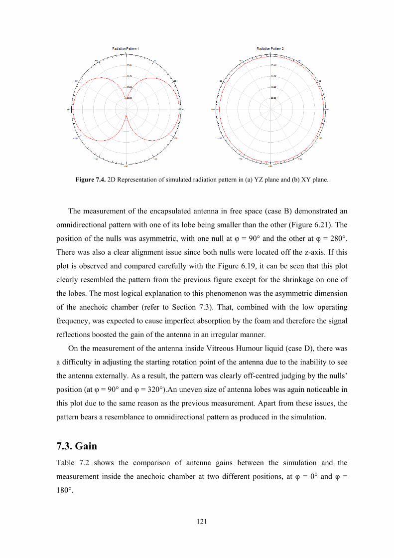
121

The measurement of the encapsulated antenna in free space (case B) demonstrated an

omnidirectional pattern with one of its lobe being smaller than the other (Figure 6.21). The

position of the nulls was asymmetric, with one null at φ = 90° and the other at φ = 280°.

There was also a clear alignment issue since both nulls were located off the z-axis. If this

plot is observed and compared carefully with the Figure 6.19, it can be seen that this plot

clearly resembled the pattern from the previous figure except for the shrinkage on one of

the lobes. The most logical explanation to this phenomenon was the asymmetric dimension

of the anechoic chamber (refer to Section 7.3). That, combined with the low operating

frequency, was expected to cause imperfect absorption by the foam and therefore the signal

reflections boosted the gain of the antenna in an irregular manner.

On the measurement of the antenna inside Vitreous Humour liquid (case D), there was

a difficulty in adjusting the starting rotation point of the antenna due to the inability to see

the antenna externally. As a result, the pattern was clearly off-centred judging by the nulls’

position (at φ = 90° and φ = 320°).An uneven size of antenna lobes was again noticeable in

this plot due to the same reason as the previous measurement. Apart from these issues, the

pattern bears a resemblance to omnidirectional pattern as produced in the simulation.

7.3. Gain

Table 7.2 shows the comparison of antenna gains between the simulation and the

measurement inside the anechoic chamber at two different positions, at φ = 0° and φ =

180°.

Figure 7.4. 2D Representation of simulated radiation pattern in (a) YZ plane and (b) XY plane.

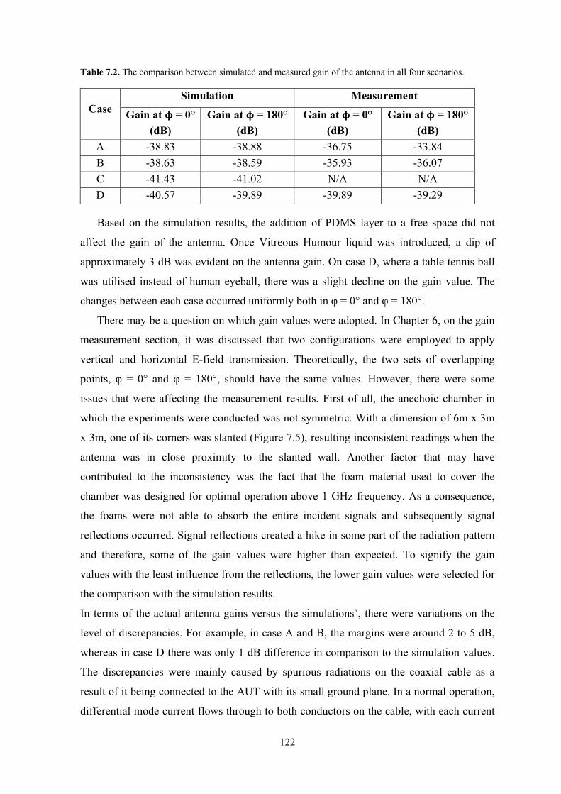
122

Based on the simulation results, the addition of PDMS layer to a free space did not

affect the gain of the antenna. Once Vitreous Humour liquid was introduced, a dip of

approximately 3 dB was evident on the antenna gain. On case D, where a table tennis ball

was utilised instead of human eyeball, there was a slight decline on the gain value. The

changes between each case occurred uniformly both in φ = 0° and φ = 180°.

There may be a question on which gain values were adopted. In Chapter 6, on the gain

measurement section, it was discussed that two configurations were employed to apply

vertical and horizontal E-field transmission. Theoretically, the two sets of overlapping

points, φ = 0° and φ = 180°, should have the same values. However, there were some

issues that were affecting the measurement results. First of all, the anechoic chamber in

which the experiments were conducted was not symmetric. With a dimension of 6m x 3m

x 3m, one of its corners was slanted (Figure 7.5), resulting inconsistent readings when the

antenna was in close proximity to the slanted wall. Another factor that may have

contributed to the inconsistency was the fact that the foam material used to cover the

chamber was designed for optimal operation above 1 GHz frequency. As a consequence,

the foams were not able to absorb the entire incident signals and subsequently signal

reflections occurred. Signal reflections created a hike in some part of the radiation pattern

and therefore, some of the gain values were higher than expected. To signify the gain

values with the least influence from the reflections, the lower gain values were selected for

the comparison with the simulation results.

In terms of the actual antenna gains versus the simulations’, there were variations on the

level of discrepancies. For example, in case A and B, the margins were around 2 to 5 dB,

whereas in case D there was only 1 dB difference in comparison to the simulation values.

The discrepancies were mainly caused by spurious radiations on the coaxial cable as a

result of it being connected to the AUT with its small ground plane. In a normal operation,

differential mode current flows through to both conductors on the cable, with each current

Table 7.2. The comparison between simulated and measured gain of the antenna in all four scenarios.

Case Simulation Measurement

Gain at φ = 0°

(dB)

Gain at φ = 180°

(dB)

Gain at φ = 0°

(dB)

Gain at φ = 180°

(dB)

A -38.83 -38.88 -36.75 -33.84

B -38.63 -38.59 -35.93 -36.07

C -41.43 -41.02 N/A N/A

D -40.57 -39.89 -39.89 -39.29

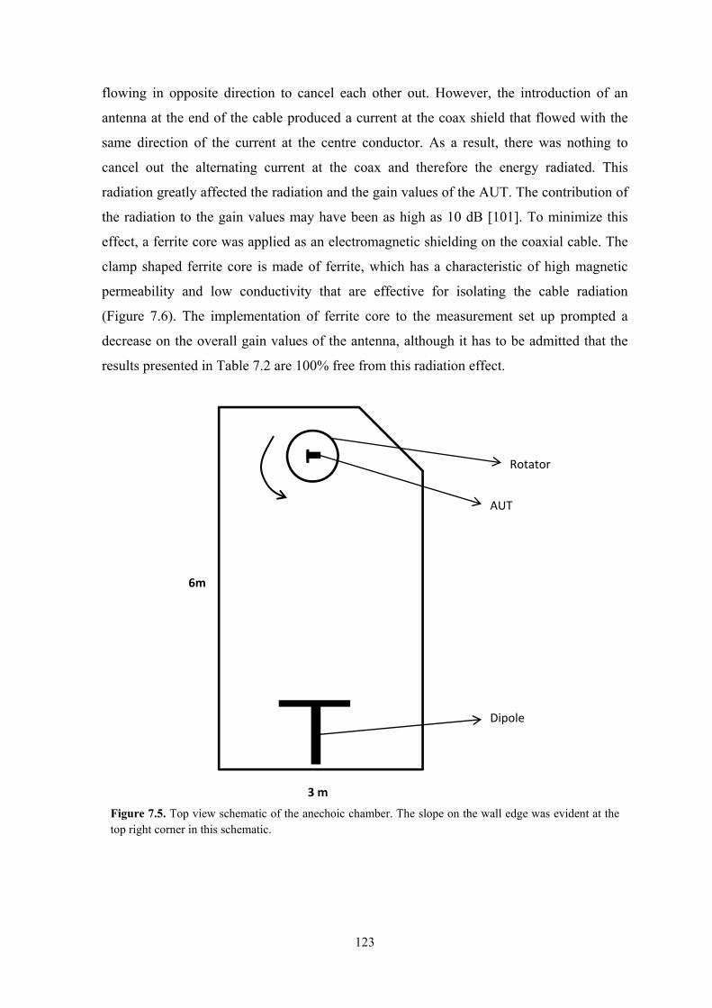
123

flowing in opposite direction to cancel each other out. However, the introduction of an

antenna at the end of the cable produced a current at the coax shield that flowed with the

same direction of the current at the centre conductor. As a result, there was nothing to

cancel out the alternating current at the coax and therefore the energy radiated. This

radiation greatly affected the radiation and the gain values of the AUT. The contribution of

the radiation to the gain values may have been as high as 10 dB [101]. To minimize this

effect, a ferrite core was applied as an electromagnetic shielding on the coaxial cable. The

clamp shaped ferrite core is made of ferrite, which has a characteristic of high magnetic

permeability and low conductivity that are effective for isolating the cable radiation

(Figure 7.6). The implementation of ferrite core to the measurement set up prompted a

decrease on the overall gain values of the antenna, although it has to be admitted that the

results presented in Table 7.2 are 100% free from this radiation effect.

6m

3 m

Rotator

AUT

Dipole

Figure 7.5. Top view schematic of the anechoic chamber. The slope on the wall edge was evident at the top right corner in this schematic.

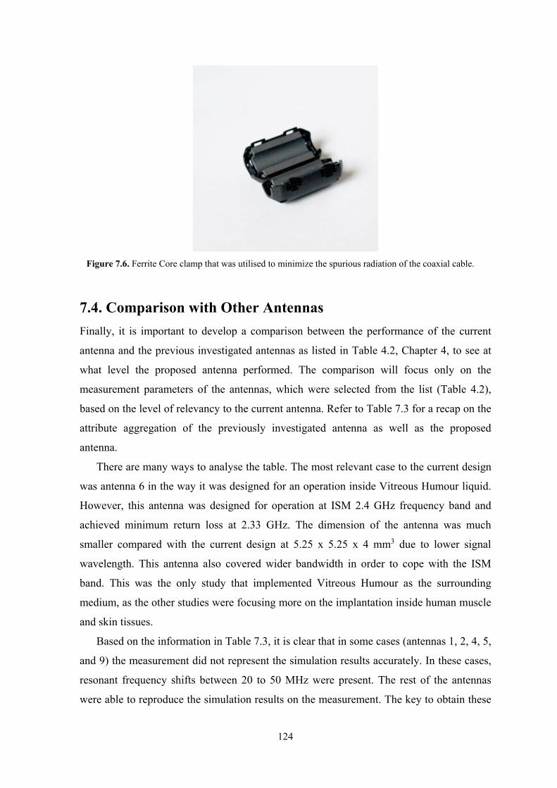
124

7.4. Comparison with Other Antennas

Finally, it is important to develop a comparison between the performance of the current

antenna and the previous investigated antennas as listed in Table 4.2, Chapter 4, to see at

what level the proposed antenna performed. The comparison will focus only on the

measurement parameters of the antennas, which were selected from the list (Table 4.2),

based on the level of relevancy to the current antenna. Refer to Table 7.3 for a recap on the

attribute aggregation of the previously investigated antenna as well as the proposed

antenna.

There are many ways to analyse the table. The most relevant case to the current design

was antenna 6 in the way it was designed for an operation inside Vitreous Humour liquid.

However, this antenna was designed for operation at ISM 2.4 GHz frequency band and

achieved minimum return loss at 2.33 GHz. The dimension of the antenna was much

smaller compared with the current design at 5.25 x 5.25 x 4 mm3 due to lower signal

wavelength. This antenna also covered wider bandwidth in order to cope with the ISM

band. This was the only study that implemented Vitreous Humour as the surrounding

medium, as the other studies were focusing more on the implantation inside human muscle

and skin tissues.

Based on the information in Table 7.3, it is clear that in some cases (antennas 1, 2, 4, 5,

and 9) the measurement did not represent the simulation results accurately. In these cases,

resonant frequency shifts between 20 to 50 MHz were present. The rest of the antennas

were able to reproduce the simulation results on the measurement. The key to obtain these

Figure 7.6. Ferrite Core clamp that was utilised to minimize the spurious radiation of the coaxial cable.

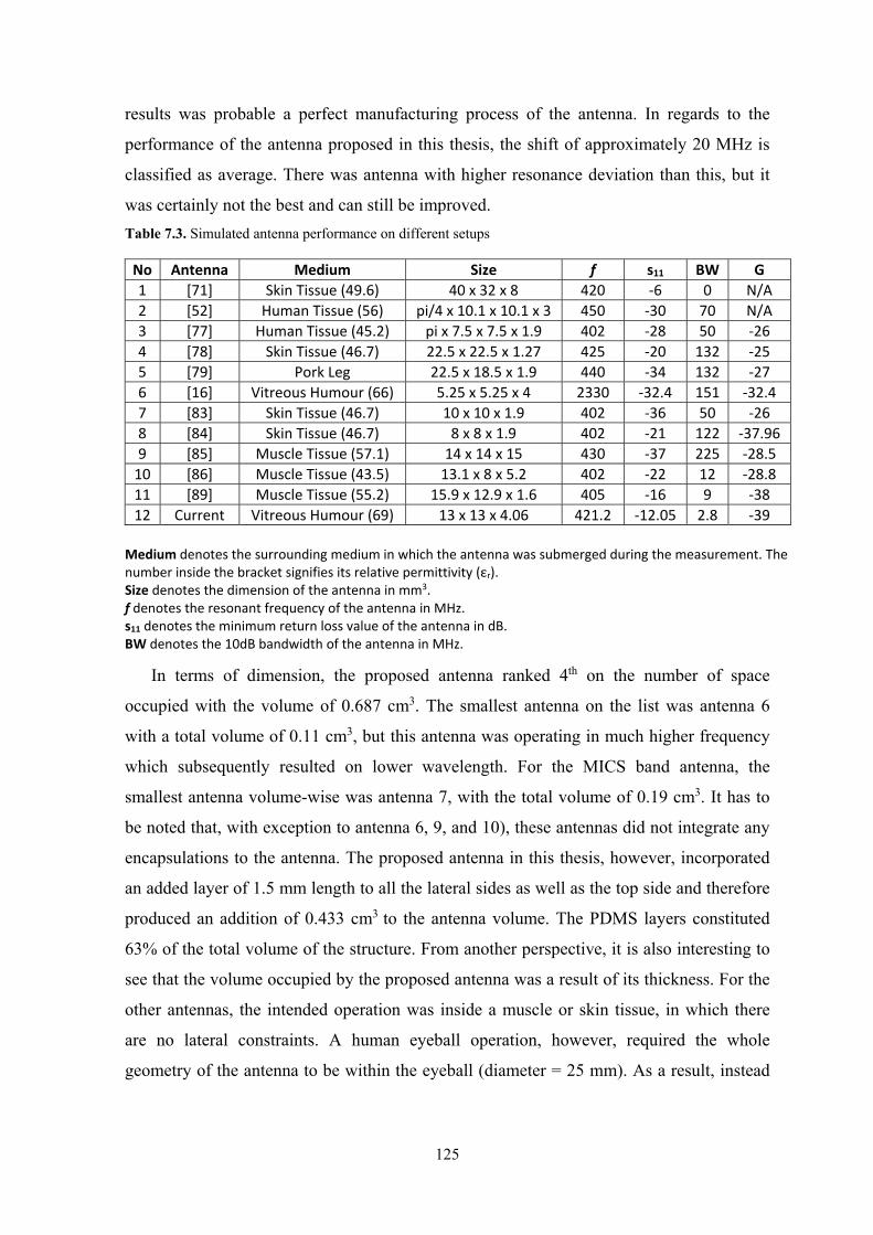
125

results was probable a perfect manufacturing process of the antenna. In regards to the

performance of the antenna proposed in this thesis, the shift of approximately 20 MHz is

classified as average. There was antenna with higher resonance deviation than this, but it

was certainly not the best and can still be improved.

In terms of dimension, the proposed antenna ranked 4th on the number of space

occupied with the volume of 0.687 cm3. The smallest antenna on the list was antenna 6

with a total volume of 0.11 cm3, but this antenna was operating in much higher frequency

which subsequently resulted on lower wavelength. For the MICS band antenna, the

smallest antenna volume-wise was antenna 7, with the total volume of 0.19 cm3. It has to

be noted that, with exception to antenna 6, 9, and 10), these antennas did not integrate any

encapsulations to the antenna. The proposed antenna in this thesis, however, incorporated

an added layer of 1.5 mm length to all the lateral sides as well as the top side and therefore

produced an addition of 0.433 cm3 to the antenna volume. The PDMS layers constituted

63% of the total volume of the structure. From another perspective, it is also interesting to

see that the volume occupied by the proposed antenna was a result of its thickness. For the

other antennas, the intended operation was inside a muscle or skin tissue, in which there

are no lateral constraints. A human eyeball operation, however, required the whole

geometry of the antenna to be within the eyeball (diameter = 25 mm). As a result, instead

Table 7.3. Simulated antenna performance on different setups

No Antenna Medium Size f s11 BW G

1 [71] Skin Tissue (49.6) 40 x 32 x 8 420 ‐6 0 N/A

2 [52] Human Tissue (56) pi/4 x 10.1 x 10.1 x 3 450 ‐30 70 N/A

3 [77] Human Tissue (45.2) pi x 7.5 x 7.5 x 1.9 402 ‐28 50 ‐26

4 [78] Skin Tissue (46.7) 22.5 x 22.5 x 1.27 425 ‐20 132 ‐25

5 [79] Pork Leg 22.5 x 18.5 x 1.9 440 ‐34 132 ‐27

6 [16] Vitreous Humour (66) 5.25 x 5.25 x 4 2330 ‐32.4 151 ‐32.4

7 [83] Skin Tissue (46.7) 10 x 10 x 1.9 402 ‐36 50 ‐26

8 [84] Skin Tissue (46.7) 8 x 8 x 1.9 402 ‐21 122 ‐37.96

9 [85] Muscle Tissue (57.1) 14 x 14 x 15 430 ‐37 225 ‐28.5

10 [86] Muscle Tissue (43.5) 13.1 x 8 x 5.2 402 ‐22 12 ‐28.8

11 [89] Muscle Tissue (55.2) 15.9 x 12.9 x 1.6 405 ‐16 9 ‐38

12 Current Vitreous Humour (69) 13 x 13 x 4.06 421.2 ‐12.05 2.8 ‐39

Medium denotes the surrounding medium in which the antenna was submerged during the measurement. The number inside the bracket signifies its relative permittivity (εr). Size denotes the dimension of the antenna in mm3. f denotes the resonant frequency of the antenna in MHz. s11 denotes the minimum return loss value of the antenna in dB. BW denotes the 10dB bandwidth of the antenna in MHz.

126

of expanding laterally, another substrate was stacked at the top to compensate unfeasible

lateral expansion.

The minimum return loss values do not provide any important information except to

indicate that their return losses are below the typical -10 dB threshold. The bandwidth

parameters are of greater importance to signify the range at which the antenna could

operate. It is clear to see that the proposed antenna has the lowest bandwidth among all

antennas on the list (Table 7.3). Some of the antennas were focused specifically on

achieving a high bandwidth on the design process. The proposed antenna, however, was

intended to operate at MICS band with a maximum bandwidth of 300 kHz. Therefore a

bandwidth of 2.8 MHz was considered adequate for the operation.

Gain is another important parameter that defines the antenna performance. Based on

the information on the list (Table 7.3), the gain of the other antennas was ranging from -25

to -38 dB. Unfortunately, the maximum measured gain of the proposed antenna was -39

dB, which was lower than any of the other antennas. The main reason behind this sub-

optimal performance was the implementation of Vitreous Humour as the surrounding

medium. As stated on previous chapters, Vitreous Humour has a high conductivity (1.53

S/m at 402 MHz [64]), compared to skin (0.69 S/m) or muscle (0.79 S/m). As a

consequence, the absorption rate by the tissue is also higher, which translates to higher loss

to the signal. Even with this disadvantage, the antenna still produced a similar performance

to some of the antennas operating on muscle or skin tissues (antenna 8 and 11) and it

should be considered a satisfying result.

Overall, the antenna has produced satisfying results in relation to the other similar

antennas. Without the PDMS encapsulation, the antenna occupied a comparable amount of

space to the smallest antenna on the list. The addition of the PDMS layer made the antenna

3 times bigger, but the entire structure will still fit inside the human eyeball. The

bandwidth of the antenna was not particularly impressive, but it was still compatible for a

MICS band operation with the right frequency range. The gain performance of the antenna

was comparable with other small size antenna even though more challenging medium was

applied.

127

7.5. Summary

In this chapter, the simulation and measurement data of the antenna have been analysed.

Each parameter was investigated individually to understand how the antenna performed

with respect to the simulated results. The discrepancies were identified and discussed in

order to pursue logical explanation behind them. This step was applied to all three

important parameters of the antenna: return loss, radiation pattern, and gain. Finally, a

comparison was drawn to see the antenna performance level against other antennas

designed for similar purposes. Each attribute of the antenna was analysed and a conclusion

was reached at the end on how the antenna had performed.

128

Chapter 8

Implantable Antenna for Implantable

Body Sensor Network

The implementation of a multilayer microstrip antenna for a retinal prosthesis system has

been discussed in a great detail on the previous chapters. It was clear that the adoption of

multilayer structure produced an enhancement on the antenna performance, which was

very weak due to the lossy surrounding medium. In this chapter, another implantable

antenna for completely different purposed will be presented as part of the derivative study

on the main topic. The antenna was designed to be integrated in an Implantable Body

Sensor Network (IBSN) system. The design will be presented, including the tissue model

and the simulation configuration. The measurement results comprise the performance of

the antenna in terms of return loss, gain, and radiation pattern, as a result of the same

measurement procedure as the previous antenna. A discussion on the result and a summary

will conclude the structure of this chapter.

8.1. Introduction

A decade ago, body sensor network (BSN) technologies started to come into prominence

with the ever increasing demand of higher people life expectancy. With a complex

utilization of multiple micro-sensors, the technology was aimed at introducing a long term

home-based monitoring which would result in more patient freedom as well as healthcare

cost saving. While BSNs are architecturally designed with varying emphasis such as low

power [102] or low cost [103], the main focus is reliable data transmission throughout the

network. This technology has reached its maturity and the focus is now shifted at

implementing the same idea in implantable environments.

The advancement of sensor technology introduces the possibilities of various

implantable sensors for the purpose of measuring and monitoring physiological signals in

vivo. Implantable sensors for measuring SvO2, blood oxygen, blood glucose, neural

activity, as well as internal imaging, have been investigated comprehensively [104-108]. In

129

an implantable body sensor network (IBSN), all the sensors were designed to exchange

data wirelessly by employing master-slave mechanism [54]. To realize this, implantable

communication must be considered at the core design of the architecture.

As in the retinal prosthesis system, the data communication in IBSN involves signal

propagation through human tissues, which leads to similar challenges in the design

process. First of all, the antenna must be capable of complying with the constraints

associated with the implantable environment, such as size and safety constraints. In terms

of the antenna size, there is no freedom in selecting the proper size during the design

process due to the limitation imposed by the surrounding tissues or other body parts. It

would be unlikely to design a traditional λ/2 or λ/4 size antenna for lower frequency bands

to achieve the perfect characteristics. Therefore, miniaturization technique of the antenna

will be enforced in the design process. Another limitation comes from the transmission

power of the antenna in relation to the SAR value. In IBSN, there are a lot of sources that

can produce thermal elevation inside the body, and one of them is the electromagnetic

fields radiated by the telemetry devices [109]. As stated on the early chapter, for a

frequency range of 100 kHz to 10 GHz, the 1g average has a limit of 1.6 W/kg while the

1g average has a threshold of 2 W [110]. These values will dictate the maximum power

that can be applied to the antenna during the transmission, which ultimately means gain

restriction.

Another issue is related to the complex geometry and characteristic of human tissues

on the limbs area. Geometrically, human body is much more than just a simple basic shape

and it consists of heterogeneous parts that would include something as small as blood

vessels. It would be inaccurate to model a human body or a human body part as a plain

model with just a single electrical characteristic value [111, 112]. Electrically, each part of

human body has a certain value of permittivity and conductivity, which are both crucial

components in determining signal propagation characteristic. The value of each part does

not depend on where it is located, makes it difficult to generalize a heterogeneous part into

a homogeneous model. Furthermore, the values are frequency dependent [64]. For those

reasons, the simulation of the implantable antenna necessitates an accurate model of the

surrounding material as well as a specific frequency sweeping.

This brings the next question on what frequency should be used for the antenna

operation. The selection of the band is based on consideration of multiple factors such as

transmission rate, suitability to the network architecture, efficiency, etc. For the purpose of

IBSN, Medical Implant Communication Service (MICS) band of 402-405 MHz was

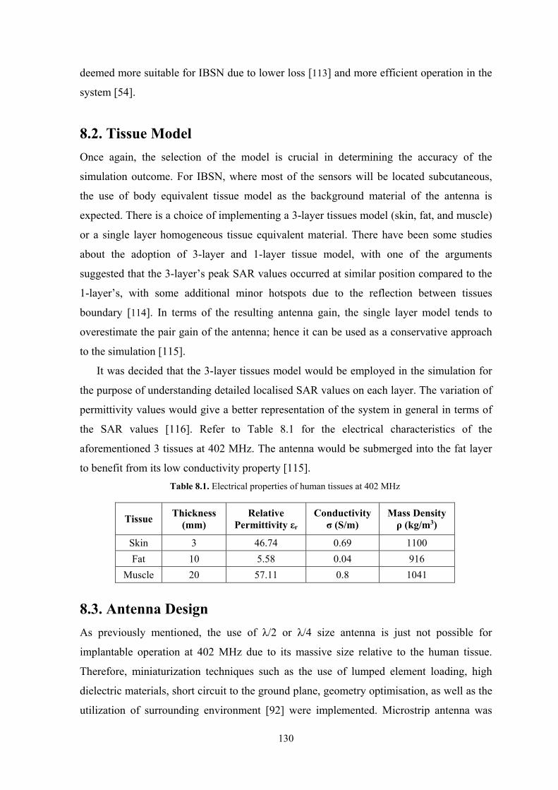
130

deemed more suitable for IBSN due to lower loss [113] and more efficient operation in the

system [54].

8.2. Tissue Model

Once again, the selection of the model is crucial in determining the accuracy of the

simulation outcome. For IBSN, where most of the sensors will be located subcutaneous,

the use of body equivalent tissue model as the background material of the antenna is

expected. There is a choice of implementing a 3-layer tissues model (skin, fat, and muscle)

or a single layer homogeneous tissue equivalent material. There have been some studies

about the adoption of 3-layer and 1-layer tissue model, with one of the arguments

suggested that the 3-layer’s peak SAR values occurred at similar position compared to the

1-layer’s, with some additional minor hotspots due to the reflection between tissues

boundary [114]. In terms of the resulting antenna gain, the single layer model tends to

overestimate the pair gain of the antenna; hence it can be used as a conservative approach

to the simulation [115].

It was decided that the 3-layer tissues model would be employed in the simulation for

the purpose of understanding detailed localised SAR values on each layer. The variation of

permittivity values would give a better representation of the system in general in terms of

the SAR values [116]. Refer to Table 8.1 for the electrical characteristics of the

aforementioned 3 tissues at 402 MHz. The antenna would be submerged into the fat layer

to benefit from its low conductivity property [115].

8.3. Antenna Design

As previously mentioned, the use of λ/2 or λ/4 size antenna is just not possible for

implantable operation at 402 MHz due to its massive size relative to the human tissue.

Therefore, miniaturization techniques such as the use of lumped element loading, high

dielectric materials, short circuit to the ground plane, geometry optimisation, as well as the

utilization of surrounding environment [92] were implemented. Microstrip antenna was

Table 8.1. Electrical properties of human tissues at 402 MHz

Tissue Thickness

(mm) Relative

Permittivity εr Conductivity

σ (S/m) Mass Density ρ (kg/m3)

Skin 3 46.74 0.69 1100

Fat 10 5.58 0.04 916

Muscle 20 57.11 0.8 1041

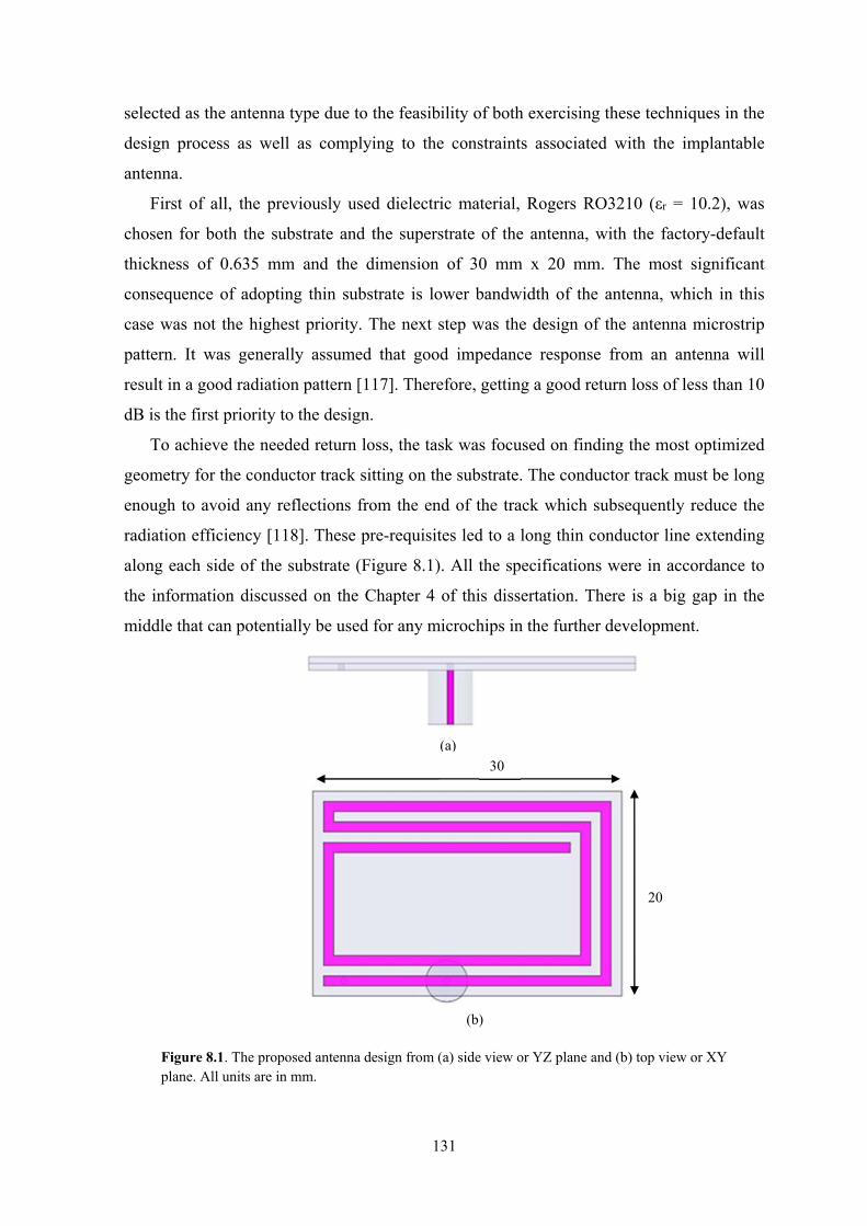
131

selected as the antenna type due to the feasibility of both exercising these techniques in the

design process as well as complying to the constraints associated with the implantable

antenna.

First of all, the previously used dielectric material, Rogers RO3210 (εr = 10.2), was

chosen for both the substrate and the superstrate of the antenna, with the factory-default

thickness of 0.635 mm and the dimension of 30 mm x 20 mm. The most significant

consequence of adopting thin substrate is lower bandwidth of the antenna, which in this

case was not the highest priority. The next step was the design of the antenna microstrip

pattern. It was generally assumed that good impedance response from an antenna will

result in a good radiation pattern [117]. Therefore, getting a good return loss of less than 10

dB is the first priority to the design.

To achieve the needed return loss, the task was focused on finding the most optimized

geometry for the conductor track sitting on the substrate. The conductor track must be long

enough to avoid any reflections from the end of the track which subsequently reduce the

radiation efficiency [118]. These pre-requisites led to a long thin conductor line extending

along each side of the substrate (Figure 8.1). All the specifications were in accordance to

the information discussed on the Chapter 4 of this dissertation. There is a big gap in the

middle that can potentially be used for any microchips in the further development.

(b)

(a)

Figure 8.1. The proposed antenna design from (a) side view or YZ plane and (b) top view or XY plane. All units are in mm.

20

30

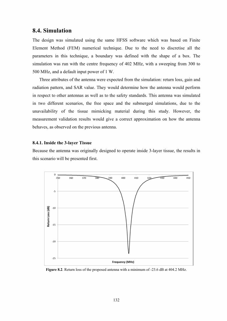
132

8.4. Simulation

The design was simulated using the same HFSS software which was based on Finite

Element Method (FEM) numerical technique. Due to the need to discretise all the

parameters in this technique, a boundary was defined with the shape of a box. The

simulation was run with the centre frequency of 402 MHz, with a sweeping from 300 to

500 MHz, and a default input power of 1 W.

Three attributes of the antenna were expected from the simulation: return loss, gain and

radiation pattern, and SAR value. They would determine how the antenna would perform

in respect to other antennas as well as to the safety standards. This antenna was simulated

in two different scenarios, the free space and the submerged simulations, due to the

unavailability of the tissue mimicking material during this study. However, the

measurement validation results would give a correct approximation on how the antenna

behaves, as observed on the previous antenna.

8.4.1. Inside the 3-layer Tissue

Because the antenna was originally designed to operate inside 3-layer tissue, the results in

this scenario will be presented first.

Figure 8.2. Return loss of the proposed antenna with a minimum of -23.6 dB at 404.2 MHz.

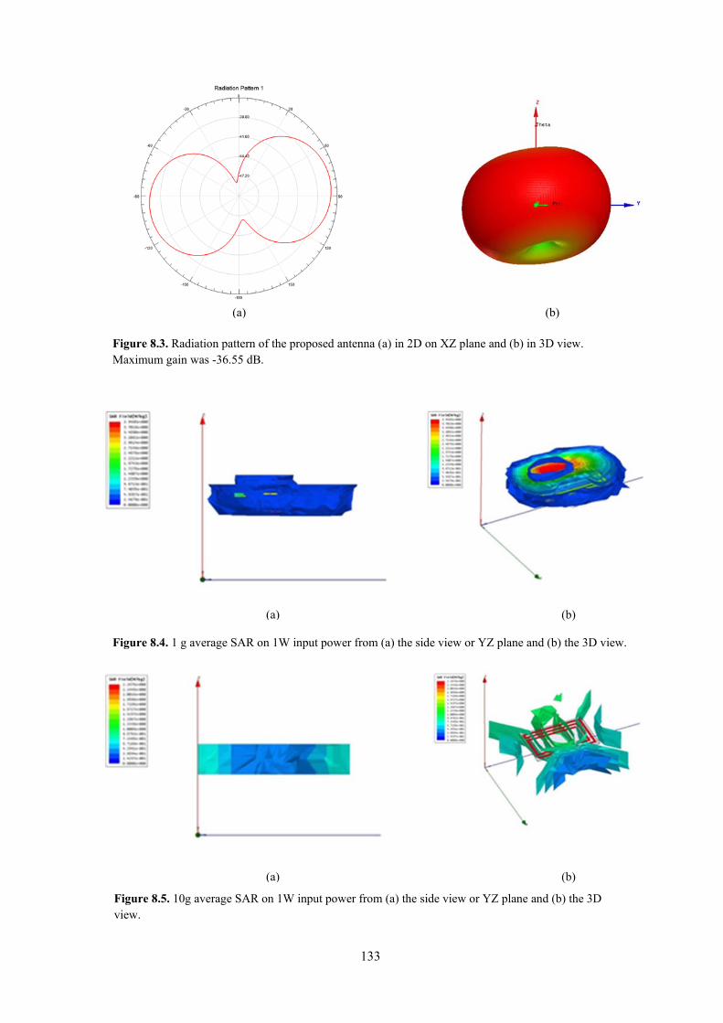
133

(b) (a)

Figure 8.3. Radiation pattern of the proposed antenna (a) in 2D on XZ plane and (b) in 3D view. Maximum gain was -36.55 dB.

(b) (a)

Figure 8.4. 1 g average SAR on 1W input power from (a) the side view or YZ plane and (b) the 3D view.

Figure 8.5. 10g average SAR on 1W input power from (a) the side view or YZ plane and (b) the 3D view.

(b) (a)

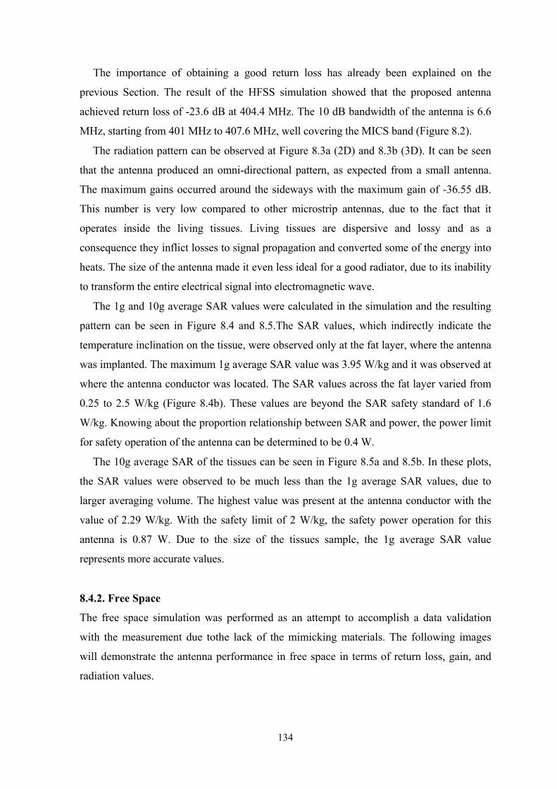
134

The importance of obtaining a good return loss has already been explained on the

previous Section. The result of the HFSS simulation showed that the proposed antenna

achieved return loss of -23.6 dB at 404.4 MHz. The 10 dB bandwidth of the antenna is 6.6

MHz, starting from 401 MHz to 407.6 MHz, well covering the MICS band (Figure 8.2).

The radiation pattern can be observed at Figure 8.3a (2D) and 8.3b (3D). It can be seen

that the antenna produced an omni-directional pattern, as expected from a small antenna.

The maximum gains occurred around the sideways with the maximum gain of -36.55 dB.

This number is very low compared to other microstrip antennas, due to the fact that it

operates inside the living tissues. Living tissues are dispersive and lossy and as a

consequence they inflict losses to signal propagation and converted some of the energy into

heats. The size of the antenna made it even less ideal for a good radiator, due to its inability

to transform the entire electrical signal into electromagnetic wave.

The 1g and 10g average SAR values were calculated in the simulation and the resulting

pattern can be seen in Figure 8.4 and 8.5.The SAR values, which indirectly indicate the

temperature inclination on the tissue, were observed only at the fat layer, where the antenna

was implanted. The maximum 1g average SAR value was 3.95 W/kg and it was observed at

where the antenna conductor was located. The SAR values across the fat layer varied from

0.25 to 2.5 W/kg (Figure 8.4b). These values are beyond the SAR safety standard of 1.6

W/kg. Knowing about the proportion relationship between SAR and power, the power limit

for safety operation of the antenna can be determined to be 0.4 W.

The 10g average SAR of the tissues can be seen in Figure 8.5a and 8.5b. In these plots,

the SAR values were observed to be much less than the 1g average SAR values, due to

larger averaging volume. The highest value was present at the antenna conductor with the

value of 2.29 W/kg. With the safety limit of 2 W/kg, the safety power operation for this

antenna is 0.87 W. Due to the size of the tissues sample, the 1g average SAR value

represents more accurate values.

8.4.2. Free Space

The free space simulation was performed as an attempt to accomplish a data validation

with the measurement due tothe lack of the mimicking materials. The following images

will demonstrate the antenna performance in free space in terms of return loss, gain, and

radiation values.

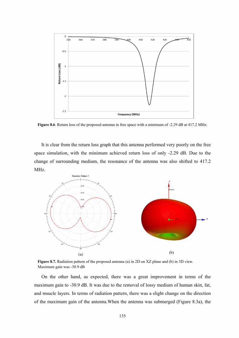
135

It is clear from the return loss graph that this antenna performed very poorly on the free

space simulation, with the minimum achieved return loss of only -2.29 dB. Due to the

change of surrounding medium, the resonance of the antenna was also shifted to 417.2

MHz.

On the other hand, as expected, there was a great improvement in terms of the

maximum gain to -30.9 dB. It was due to the removal of lossy medium of human skin, fat,

and msucle layers. In terms of radiation pattern, there was a slight change on the direction

of the maximum gain of the antenna.When the antenna was submerged (Figure 8.3a), the

Figure 8.6. Return loss of the proposed antenna in free space with a minimum of -2.29 dB at 417.2 MHz.

Figure 8.7. Radiation pattern of the proposed antenna (a) in 2D on XZ plane and (b) in 3D view. Maximum gain was -30.9 dB

(b) (a)

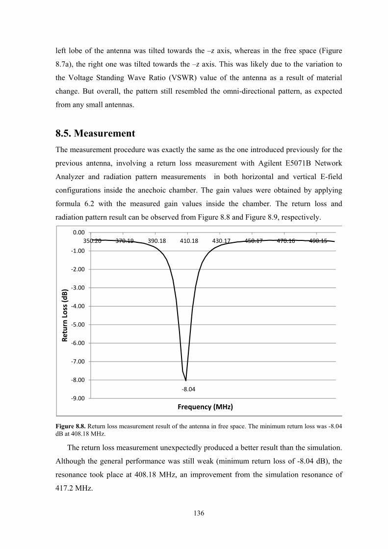
136

left lobe of the antenna was tilted towards the –z axis, whereas in the free space (Figure

8.7a), the right one was tilted towards the –z axis. This was likely due to the variation to

the Voltage Standing Wave Ratio (VSWR) value of the antenna as a result of material

change. But overall, the pattern still resembled the omni-directional pattern, as expected

from any small antennas.

8.5. Measurement

The measurement procedure was exactly the same as the one introduced previously for the

previous antenna, involving a return loss measurement with Agilent E5071B Network

Analyzer and radiation pattern measurements in both horizontal and vertical E-field

configurations inside the anechoic chamber. The gain values were obtained by applying

formula 6.2 with the measured gain values inside the chamber. The return loss and

radiation pattern result can be observed from Figure 8.8 and Figure 8.9, respectively.

The return loss measurement unexpectedly produced a better result than the simulation.

Although the general performance was still weak (minimum return loss of -8.04 dB), the

resonance took place at 408.18 MHz, an improvement from the simulation resonance of

417.2 MHz.

Figure 8.8. Return loss measurement result of the antenna in free space. The minimum return loss was -8.04dB at 408.18 MHz.

‐8.04

‐9.00

‐8.00

‐7.00

‐6.00

‐5.00

‐4.00

‐3.00

‐2.00

‐1.00

0.00

350.20 370.19 390.18 410.18 430.17 450.17 470.16 490.15

Return Loss (dB)

Frequency (MHz)

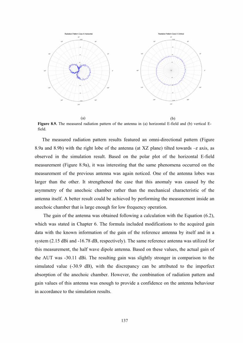
137

The measured radiation pattern results featured an omni-directional pattern (Figure

8.9a and 8.9b) with the right lobe of the antenna (at XZ plane) tilted towards –z axis, as

observed in the simulation result. Based on the polar plot of the horizontal E-field

measurement (Figure 8.9a), it was interesting that the same phenomena occurred on the

measurement of the previous antenna was again noticed. One of the antenna lobes was

larger than the other. It strengthened the case that this anomaly was caused by the

asymmetry of the anechoic chamber rather than the mechanical characteristic of the

antenna itself. A better result could be achieved by performing the measurement inside an

anechoic chamber that is large enough for low frequency operation.

The gain of the antenna was obtained following a calculation with the Equation (6.2),

which was stated in Chapter 6. The formula included modifications to the acquired gain

data with the known information of the gain of the reference antenna by itself and in a

system (2.15 dBi and -16.78 dB, respectively). The same reference antenna was utilized for

this measurement, the half wave dipole antenna. Based on these values, the actual gain of

the AUT was -30.11 dBi. The resulting gain was slightly stronger in comparison to the

simulated value (-30.9 dB), with the discrepancy can be attributed to the imperfect

absorption of the anechoic chamber. However, the combination of radiation pattern and

gain values of this antenna was enough to provide a confidence on the antenna behaviour

in accordance to the simulation results.

(a) (b) Figure 8.9. The measured radiation pattern of the antenna in (a) horizontal E-field and (b) vertical E-field.

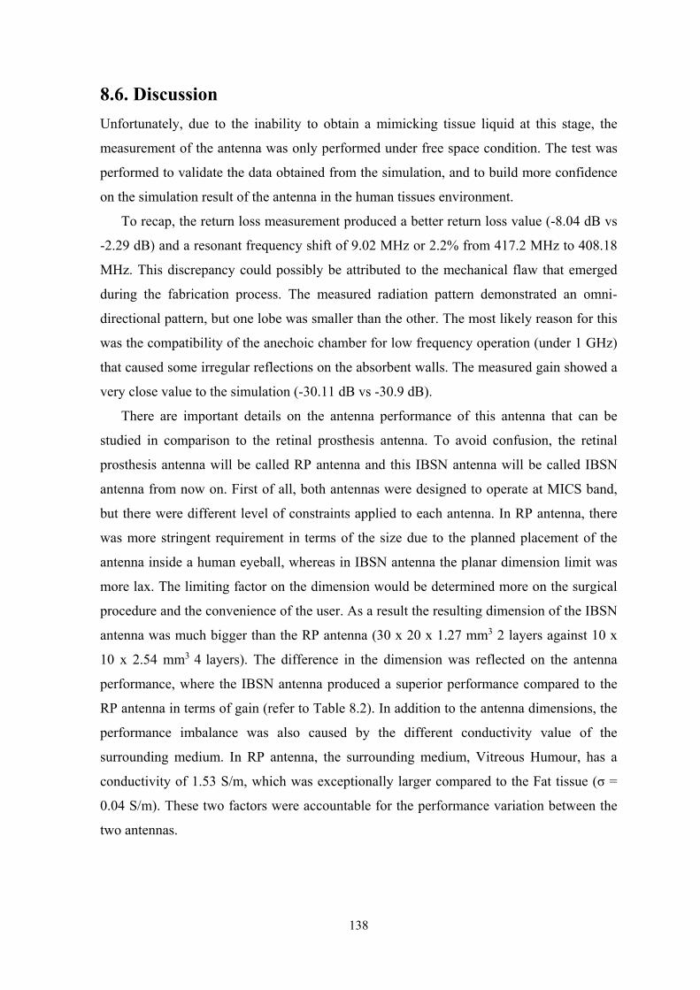
138

8.6. Discussion

Unfortunately, due to the inability to obtain a mimicking tissue liquid at this stage, the

measurement of the antenna was only performed under free space condition. The test was

performed to validate the data obtained from the simulation, and to build more confidence

on the simulation result of the antenna in the human tissues environment.

To recap, the return loss measurement produced a better return loss value (-8.04 dB vs

-2.29 dB) and a resonant frequency shift of 9.02 MHz or 2.2% from 417.2 MHz to 408.18

MHz. This discrepancy could possibly be attributed to the mechanical flaw that emerged

during the fabrication process. The measured radiation pattern demonstrated an omni-

directional pattern, but one lobe was smaller than the other. The most likely reason for this

was the compatibility of the anechoic chamber for low frequency operation (under 1 GHz)

that caused some irregular reflections on the absorbent walls. The measured gain showed a

very close value to the simulation (-30.11 dB vs -30.9 dB).

There are important details on the antenna performance of this antenna that can be

studied in comparison to the retinal prosthesis antenna. To avoid confusion, the retinal

prosthesis antenna will be called RP antenna and this IBSN antenna will be called IBSN

antenna from now on. First of all, both antennas were designed to operate at MICS band,

but there were different level of constraints applied to each antenna. In RP antenna, there

was more stringent requirement in terms of the size due to the planned placement of the

antenna inside a human eyeball, whereas in IBSN antenna the planar dimension limit was

more lax. The limiting factor on the dimension would be determined more on the surgical

procedure and the convenience of the user. As a result the resulting dimension of the IBSN

antenna was much bigger than the RP antenna (30 x 20 x 1.27 mm3 2 layers against 10 x

10 x 2.54 mm3 4 layers). The difference in the dimension was reflected on the antenna

performance, where the IBSN antenna produced a superior performance compared to the

RP antenna in terms of gain (refer to Table 8.2). In addition to the antenna dimensions, the

performance imbalance was also caused by the different conductivity value of the

surrounding medium. In RP antenna, the surrounding medium, Vitreous Humour, has a

conductivity of 1.53 S/m, which was exceptionally larger compared to the Fat tissue (σ =

0.04 S/m). These two factors were accountable for the performance variation between the

two antennas.

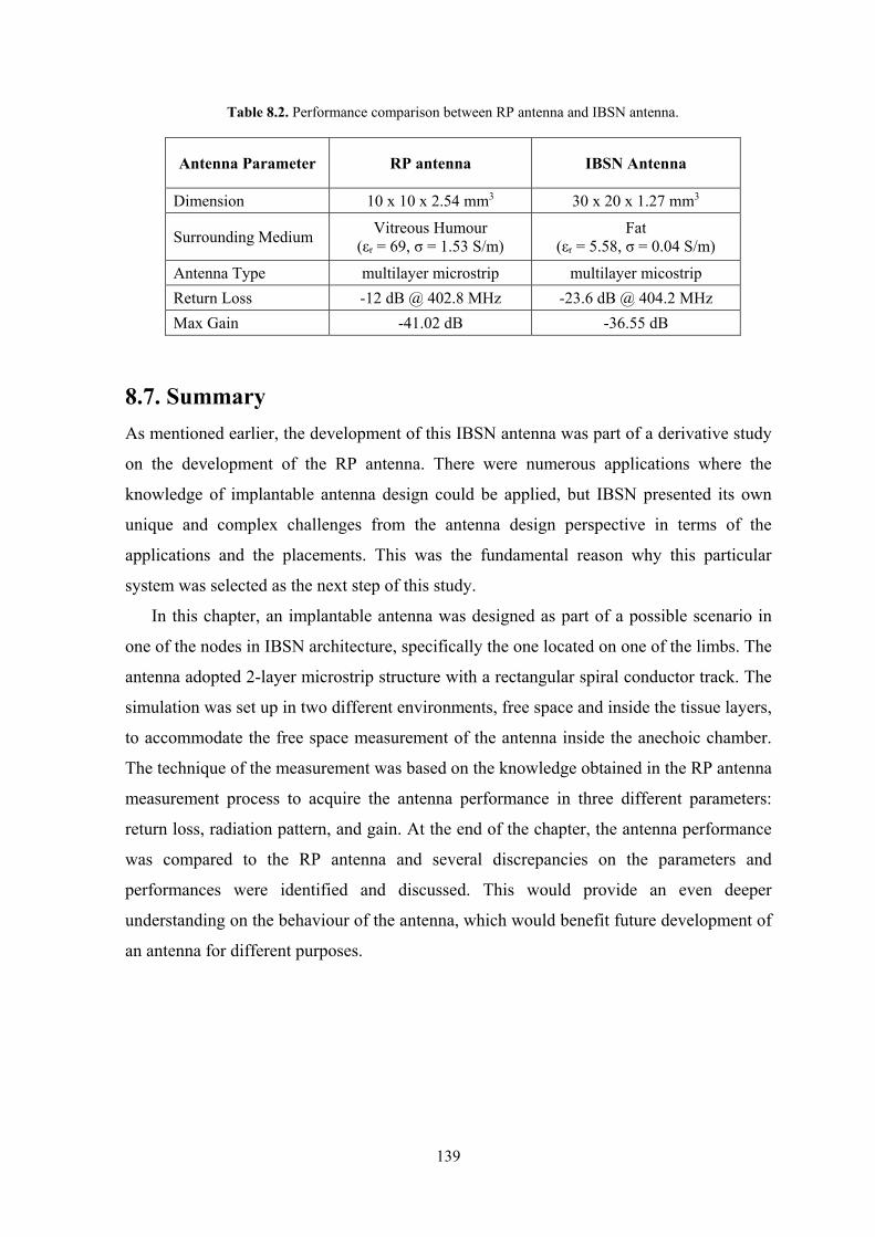
139

8.7. Summary

As mentioned earlier, the development of this IBSN antenna was part of a derivative study

on the development of the RP antenna. There were numerous applications where the

knowledge of implantable antenna design could be applied, but IBSN presented its own

unique and complex challenges from the antenna design perspective in terms of the

applications and the placements. This was the fundamental reason why this particular

system was selected as the next step of this study.

In this chapter, an implantable antenna was designed as part of a possible scenario in

one of the nodes in IBSN architecture, specifically the one located on one of the limbs. The

antenna adopted 2-layer microstrip structure with a rectangular spiral conductor track. The

simulation was set up in two different environments, free space and inside the tissue layers,

to accommodate the free space measurement of the antenna inside the anechoic chamber.

The technique of the measurement was based on the knowledge obtained in the RP antenna

measurement process to acquire the antenna performance in three different parameters:

return loss, radiation pattern, and gain. At the end of the chapter, the antenna performance

was compared to the RP antenna and several discrepancies on the parameters and

performances were identified and discussed. This would provide an even deeper

understanding on the behaviour of the antenna, which would benefit future development of

an antenna for different purposes.

Table 8.2. Performance comparison between RP antenna and IBSN antenna.

Antenna Parameter RP antenna IBSN Antenna

Dimension 10 x 10 x 2.54 mm3 30 x 20 x 1.27 mm3

Surrounding Medium Vitreous Humour

(εr = 69, σ = 1.53 S/m) Fat

(εr = 5.58, σ = 0.04 S/m)

Antenna Type multilayer microstrip multilayer micostrip

Return Loss -12 dB @ 402.8 MHz -23.6 dB @ 404.2 MHz

Max Gain -41.02 dB -36.55 dB

140

Chapter 9

Conclusion The final chapter of this dissertation will be primarily dedicated to highlight the findings

from this study. Initially, a recap in each chapter will be presented sequentially, followed

by the demonstration of important findings from this study. Finally, potential future works

to continue this study will be discussed at the end of the chapter.

9.1. Overview

At the beginning of this dissertation, the background and the rationale of this research was

stated very clearly. In Chapter 2, all aspects about retinal prosthesis system were

explained, starting with the background behind the system, its role in the assistive

integrated system, and the level of technology that is available or currently being research

at this time. In relation to the current technology, a review from 3 major research groups

covering the electrodes, wireless communications, dosimetry analysis, as well as clinical

testing, was also presented. At the end of this chapter, existing implant communication

technologies for various purposes were discussed. In Chapter 3, four frequency bands were

investigated as the first step in the antenna design process. Each band was analysed in

terms of bandwidth, external interference, as well as possible antenna size and SAR values,

in order to find the most suitable band for the proposed antenna. At the end, MICS band

was selected as the operating frequency of the proposed antenna. Comprehensive

explanation about the antenna design was presented in Chapter 4. Initially, the basic

principle as well as the role of an antenna in a wireless communication system was

presented. It also covered the antenna operation inside a medium with high dielectric and

high conductivity property. A list of previous implantable antenna designs from various

researchers worldwide was compiled, highlighting their return loss, gain, and bandwidth

parameters. The last Section of the chapter revealed the proposed antenna design after a

thorough discussion about the constraints and the difficulties of producing an optimized

operation in the specified scenario. Chapter 5 covered the simulation procedure of the

proposed antenna in order to obtain the specified parameters. It was started by a review of

several different numerical techniques to solve Maxwell’s equations, and it has been

141

decided that HFSS with its FEM technique would be employed to perform the computation

on the antenna. A step by step procedure on the simulation process was presented and at

the end of the Section, the simulation results were displayed. The next step was a

manufacturing process of the antenna, which was detailed at the beginning of Chapter 6. A

set of measurements that comprise of two parts, free space and inside Vitreous Humour

Liquid, was conducted with the fabricated antenna to acquire its return loss, radiation

pattern, and gain. The measurement procedure and configuration for both scenarios were

explained in detail and followed by the unveiling of the results in each case. The data was

organized in such a way to allow a clear comparison against the simulation data. Finally, a

discussion on the acquired data, both from the simulation and the measurement, was

disclosed in Chapter 7. The data was analysed to gain an understanding on how the actual

antenna performed in relative to the simulation. Discrepancies on the results were

investigated and possible theories behind these were postulated. To end the chapter, a

compilation of previous implantable antenna performance was created and a comparison

was made against the manufactured antenna to determine the actual performance level of

the antenna. In Chapter 8, a derivative study was also conducted where another

implantable antenna for a purpose other than retinal prosthesis system was designed.

Intended for the implementation in IBSN system, the antenna was developed based on the

knowledge obtained on the previous process. A simulation to acquire the return loss, gain,

and radiation pattern of the antenna was later validated with a free space measurement

inside the anechoic chamber. Finally, the Final Chapter was written to highlight the major

findings of this research, along with possible future works as a continuation of this study.

9.2. Major Findings

There are four major findings that can be reported as a result of this study:

MICS band has been considered as the most suited frequency band for a

retinal prosthesis system

In Chapter 3, four frequency bands have been analysed. Based on the general SAR

values, possible external interferences, as well as the size of the potential antenna,

MICS has been selected as the most suitable candidate for a retinal prosthesis

system.

Microstrip antenna has been determined as the best candidate for an

implantable system

142

After a thorough literature review on the antenna theory as well as the previous

implantable antenna designs, microstrip antenna has been considered as the best

solution for an implantable system due to the following advantages: compact,

simple manufacturing process, as well as possibility of multi-band operation. The

simulation and measurement results of two microstrip antenna designs strengthened

this statement further with their structure and the operating performances in terms

of return loss, radiation pattern, and gain.

A novel configuration to conduct a measurement inside Vitreous Humour

liquid

This was the first time an antenna was measured inside a liquid-filled spherical

container when undertaking a measurement, to mimic an operation inside a human

eyeball. The configuration of the measurement as well as the antenna structure has

been comprehensively disclosed in Chapter 6.

A novel implantable antenna to operate inside Vitreous Humour liquid at

MICS band

This is the ultimate finding of this research. A small multilayer microstrip antenna

with a dimension of 10 x 10 x 2.54 mm3 (without PDMS coating) or 13 x 13 x 4.06

mm3 (with PDMS coating) was designed, simulated, and manufactured. The

measurement results of this antenna generally resembled the simulation data with a

small degree of discrepancies. Compared to other implantable antennas, the

performance of this antenna was at the same level with them despite more

challenging constraints.

9.3. Possible Future Works

There are several ideas on how a new study can be conducted based on the knowledge

acquired from this research:

In vitro and in vivo experiment of the antenna

There is no doubt that both in vitro and in vivo measurement of the antenna are the

obvious next step for this project. It was unfortunately not possible to obtain

permission from the ethics committee to conduct such an experiment during this

project’s lifecycle. In vitro experiment will involve the adoption of bovine’s eyeball

in place of a human eyeball due to the similarity between the two, structurally and

dimensionally. In vivo experiment for only the antenna seems unlikely due to the

143

fact that in normal operation, the antenna will function when it is attached to the

control unit. Integration with a microcontroller unit as well as collaboration with a

medical team would be needed before the in vivo measurement can be materialized

by implanting the whole unit into a living human’s eyeball.

Designing a wireless communication link with an external antenna

A design of wireless communication link that comprises of an extraocular and

intraocular antenna will create a solid topic for a further study. The study will

include investigation of antenna placement as well as different modulation

techniques on the data transmission for optimal data transfer.

Development of an implantable flexible antenna

An introduction of flexible characteristic to an implantable antenna will provide an

immense benefit to the antenna in some situations. When an antenna is bendable, it

is allowed to conform to the contour of the human parts, allowing it to have a larger

aperture. This study will cover an investigation on the most suitable material to be

employed as the substrates and superstrates and eventually the effect of bending

structure to the antenna performance.

144

Bibliography

[1] W. H. Organisation. (2012, 1 October). Prevention of Blindness and Visual Impairment.

Available: http://www.who.int/blindness/causes/priority/en/index.html

[2] D. T. Hartong, E. L. Berson, and T. P. Dryja, "Retinitis pigmentosa," Lancet, vol. 368, pp.

1795-1809, 2006.

[3] E. Margalit and S. R. Sadda, "Retinal and Optic Nerve Diseases," Artificial Organs, vol.

27, pp. 963-974, 2003.

[4] D. B. Rein, P. Zhang, K. E. Wirth, P. P. Lee, T. J. Hoerger, N. McCall, et al., "The

economic burden of major adult visual disorders in the United States," Archives of

Ophthalmology, vol. 124, pp. 1754-1760, 2006.

[5] U. Chakravarthy, T. Y. Wong, A. Fletcher, E. Piault, C. Evans, G. Zlateva, et al., “Clinical

risk factors for age-related macular degeneration: a systematic review and meta-analysis,”

BMC Opthalmology 10: 31, 2010.

[6] L. A. Remington, Clinical Anatomy of the Visual System E-Book, 3rd ed.: Elsevier Health

Sciences, 2004.

[7] N. S. Peachey, "Subretinal implantation of semiconductor-based photodiodes: Progress and

challenges," Journal of Rehabilitation Research and Development, vol. 36, pp. 371-376,

1999.

[8] E. Margalit, M. Maia, J. D. Weiland, R. J. Greenberg, G. Y. Fujii, G. Torres, et al., "Retinal

prosthesis for the blind," Survey of Ophthalmology, vol. 47, pp. 335-356, 2002.

[9] J. S. Hayes, V. T. Yin, D. Piyathaisere, J. D. Weiland, M. S. Humayun, and G. Dagnelie,

"Visually Guided Performance of Simple Tasks Using Simulated Prosthetic Vision,"

Artificial Organs, vol. 27, pp. 1016-1028, 2003.

[10] J. D. Weiland, M. S. Humayun, H. Eckhardt, S. Ufer, L. Laude, B. Basinger, et al., "A

comparison of retinal prosthesis electrode array substrate materials," Conference

proceedings : ... Annual International Conference of the IEEE Engineering in Medicine and

Biology Society. IEEE Engineering in Medicine and Biology Society. Conference, vol.

2009, pp. 4140-4143, 2009.

[11] D. Nanduri, M. S. Humayun, R. J. Greenberg, M. J. McMahon, and J. D. Weiland, "Retinal

prosthesis phosphene shape analysis," Conference proceedings : ... Annual International

Conference of the IEEE Engineering in Medicine and Biology Society. IEEE Engineering

in Medicine and Biology Society. Conference, vol. 2008, pp. 1785-1788, 2008.

[12] V. Singh, A. Roy, R. Castro, K. McClure, R. Dai, R. Agrawal, et al., "On the thermal

elevation of a 60-electrode epiretinal prosthesis for the blind," IEEE Transactions on

Biomedical Circuits and Systems, vol. 2, pp. 289-300, 2008.

145

[13] K. Gosalia, J. Weiland, M. Humayun, and G. Lazzi, "Thermal elevation in the human eye

and head due to the operation of a retinal prosthesis," IEEE Transactions on Biomedical

Engineering, vol. 51, pp. 1469-1477, 2004.

[14] L. Colodetti, J. D. Weiland, S. Colodetti, A. Ray, M. J. Seiler, D. R. Hinton, et al.,

"Pathology of damaging electrical stimulation in the retina," Experimental Eye Research,

vol. 85, pp. 23-33, 2007.

[15] D. V. Piyathaisere, E. Margalit, S. J. Chen, J. S. Shyu, S. A. D'Anna, J. D. Weiland, et al.,

"Heat effects on the retina," Ophthalmic Surgery Lasers and Imaging, vol. 34, pp. 114-120,

2003.

[16] S. Soora, K. Gosalia, M. S. Humayun, and G. Lazzi, "A comparison of two and three

dimensional dipole antennas for an implantable retinal prosthesis," IEEE Transactions on

Antennas and Propagation, vol. 56, pp. 622-629, 2008.

[17] G. Wang, W. Liu, M. Sivaprakasam, M. Zhou, J. D. Weiland, and M. S. Humayun, "A dual

band wireless power and data telemetry for retinal prosthesis," Conference proceedings : ...

Annual International Conference of the IEEE Engineering in Medicine and Biology

Society. IEEE Engineering in Medicine and Biology Society. Conference, vol. 1, pp. 4392-

4395, 2006.

[18] K. Gosalia, G. Lazzi, and M. Humayun, "Investigation of a microwave data telemetry link

for a retinal prosthesis," IEEE Transactions on Microwave Theory and Techniques, vol. 52,

pp. 1925-1933, 2004.

[19] J. D. Weiland, B. Faraji, R. J. Greenberg, M. S. Humayun, and F. G. Shellock,

"Assessment of MRI issues for the Argus II Retinal Prosthesis," Magnetic Resonance

Imaging, vol. 30, pp. 382-389, 2012.

[20] K. Kagawa, K. Isakari, T. Furumiya, A. Uehara, T. Tokuda, J. Ohta, et al., "Pixel design of

pulsed CMOS image sensor for retinal prosthesis with digital photosensitivity control,"

Electronics Letters, vol. 39, pp. 419-421, 2003.

[21] A. Uehara, K. Kagawa, T. Tokuda, J. Ohta, and M. Nunoshita, "Back-illuminated pulse-

frequency-modulated photosensor using silicon-on-sapphire technology developed for use

as epi-retinal prosthesis device," Electronics Letters, vol. 39, pp. 1102-1104, 2003.

[22] T. Tokuda, Y. L. Pan, A. Uehara, K. Kagawa, M. Nunoshita, and J. Ohta, "Flexible and

extendible neural interface device based on cooperative multi-chip CMOS LSI

architecture," Sensors and Actuators, A: Physical, vol. 122, pp. 88-98, 2005.

[23] T. Tokuda, M. Kawada, S. Sugitani, M. Taniyama, A. Uehara, K. Kagawa, et al., "A multi-

chip-architecture based flexible stimulation device for retinal prosthesis with a flip-chip

packaging technique," Conference proceedings : ... Annual International Conference of the

IEEE Engineering in Medicine and Biology Society. IEEE Engineering in Medicine and

Biology Society. Conference, vol. 1, pp. 2920-2923, 2006.

146

[24] T. Tokuda, R. Asano, S. Sugitani, Y. Terasawa, M. Nunoshita, K. Nakauchi, et al., "In vivo

stimulation on rabbit retina using CMOS LSI-based multi-chip flexible stimulator for

retinal prosthesis," Conference proceedings : ... Annual International Conference of the



[25] T. Tokuda, K. Hiyama, S. Sawamura, K. Sasagawa, Y. Terasawa, K. Nishida, et al.,

"CMOS-based multichip networked flexible retinal stimulator designed for image-based

retinal prosthesis," IEEE Transactions on Electron Devices, vol. 56, pp. 2577-2585, 2009.

[26] M. N. Shivdasani, C. D. Luu, R. Cicione, J. B. Fallon, P. J. Allen, J. Leuenberger, et al.,

"Evaluation of stimulus parameters and electrode geometry for an effective suprachoroidal

retinal prosthesis," Journal of Neural Engineering, vol. 7, p. 036008, 2010.

[27] A. C. Bird, "Clinical investigation of retinitis pigmentosa," Australian and New Zealand

Journal of Ophthalmology, vol. 16, pp. 189-198, 1988.

[28] L. S. Lim, P. Mitchell, J. M. Seddon, F. G. Holz, and T. Y. Wong, "Age-related macular

degeneration," The Lancet, vol. 379, pp. 1728-1738, 2012.

[29] R. Klein, B. E. K. Klein, M. D. Knudtson, S. M. Meuer, M. Swift, and R. E. Gangnon,

"Fifteen-Year Cumulative Incidence of Age-Related Macular Degeneration. The Beaver

Dam Eye Study," Ophthalmology, vol. 114, pp. 253-262, 2007.

[30] D. B. Rein, J. S. Wittenborn, X. Zhang, A. A. Honeycutt, S. B. Lesesne, and J. Saaddine,

"Forecasting age-related macular degeneration through the year 2050: The potential impact

of new treatments," Archives of Ophthalmology, vol. 127, pp. 533-540, 2009.

[31] J. D. Weiland, W. Liu, and M. S. Humayun, "Retinal prosthesis," vol. 7, ed, 2005, pp. 361-

401.

[32] C. C. T. Wang and S. Charles, "Microsurgical instrumentation for vitrectomy: Part II,"

Journal of clinical engineering, vol. 9, pp. 63-71, 1984.

[33] A. Santos, M. S. Humayun, E. De Juan Jr, R. J. Greenburg, M. J. Marsh, I. B. Klock, et al.,

"Preservation of the inner retina in retinitis pigmentosa:A morphometric analysis,"

Archives of Ophthalmology, vol. 115, pp. 511-515, 1997.

[34] S. K. Kelly, D. B. Shire, J. Chen, P. Doyle, M. D. Gingerich, W. A. Drohan, et al.,

"Realization of a 15-channel, hermetically-encased wireless subretinal prosthesis for the

blind," 2009, pp. 200-203.

[35] G. J. Suaning and N. H. Lovell, "CMOS neurostimulation ASIC with 100 channels,

scaleable output, and bidirectional radio-frequency telemetry," IEEE Transactions on

Biomedical Engineering, vol. 48, pp. 248-260, 2001.

[36] J. D. Loudin, D. M. Simanovskii, K. Vijayraghavan, C. K. Sramek, A. F. Butterwick, P.

Huie, et al., "Optoelectronic retinal prosthesis: System design and performance," Journal of

Neural Engineering, vol. 4, pp. S72-S84, 2007.

147

[37] M. Schwarz, L. Ewe, N. Hijazi, B. J. Hosticka, J. Huppertz, S. Kolnsberg, et al., "Micro

implantable visual prostheses," in Microtechnologies in Medicine and Biology, 1st Annual

International, Conference On. 2000, 2000, pp. 461-465.

[38] K. Cha, K. Horch, and R. A. Normann, "Simulation of a phosphene-based visual field:

Visual acuity in a pixelized vision system," Annals of Biomedical Engineering, vol. 20, pp.

439-449, 1992.

[39] R. W. Thompson Jr, G. D. Barnett, M. S. Humayun, and G. Dagnelie, "Facial Recognition

Using Simulated Prosthetic Pixelized Vision," Investigative Ophthalmology and Visual

Science, vol. 44, pp. 5035-5042, 2003.

[40] Y. Terasawa, A. Uehara, E. Yonezawa, T. Saitoh, K. Shodo, M. Ozawa, et al., "A visual

prosthesis with 100 electrodes featuring wireless signals and wireless power transmission,"

IEICE Electronics Express, vol. 5, pp. 574-580, 2008.

[41] M. S. Humayun, J. D. Dorn, L. Da Cruz, G. Dagnelie, J. A. Sahel, P. E. Stanga, et al.,

"Interim results from the international trial of second sight's visual prosthesis,"

Ophthalmology, vol. 119, pp. 779-788, 2012.

[42] M. P. Barry and G. Dagnelie, "Use of the Argus II retinal prosthesis to improve visual

guidance of fine hand movements," Investigative Ophthalmology and Visual Science, vol.

53, pp. 5095-5101, 2012.

[43] L. Mertz, "Sight restoration comes into focus: Versions of visual prostheses," IEEE Pulse,

vol. 3, pp. 10-16, 2012.

[44] M. Mahadevappa, J. D. Weiland, D. Yanai, I. Fine, R. J. Greenberg, and M. S. Humayun,

"Perceptual thresholds and electrode impedance in three retinal prosthesis subjects," IEEE

Transactions on Neural Systems and Rehabilitation Engineering, vol. 13, pp. 201-206,

2005.

[45] Y. A. Kerdraon, J. A. Downie, G. J. Suaning, M. R. Capon, M. T. Coroneo, and N. H.

Lovell, "Development and surgical implantation of a vision prosthesis model into the ovine

eye," Clinical and Experimental Ophthalmology, vol. 30, pp. 36-40, 2002.

[46] N. Dommel, Y. T. Wong, P. J. Preston, T. Lehmann, N. H. Lovell, and G. J. Suaning, "The

design and testing of an epi-retinal vision prosthesis neurostimulator capable of concurrent

parallel stimulation," Conference proceedings : ... Annual International Conference of the



[47] Y. T. Wong, N. Dommel, P. J. Preston, T. Lehmann, N. H. Lovell, and G. J. Suaning,

"Microelectronic retinal prosthesis: I. A neurostimulator for the concurrent activation of

multiple electrodes," Conference proceedings : ... Annual International Conference of the



148

[48] Y. T. Wong, L. E. Hallum, S. C. Chen, N. Dommel, S. L. Cloherty, J. W. Morley, et al.,

"Optical imaging of electrically evoked visual signals in cats: I. Responses to corneal and

intravitreal electrical stimulation," Conference proceedings : ... Annual International

Conference of the IEEE Engineering in Medicine and Biology Society. IEEE Engineering

in Medicine and Biology Society. Conference, vol. 2007, pp. 1635-1638, 2007.

[49] Y. T. Wong, S. C. Chen, J. M. Seo, J. W. Morley, N. H. Lovell, and G. J. Suaning, "Focal

activation of the feline retina via a suprachoroidal electrode array," Vision Research, vol.

49, pp. 825-833, 2009.

[50] L. E. Hallum, S. L. Cloherty, and N. H. Lovell, "Image analysis for microelectronic retinal

prosthesis," IEEE Transactions on Biomedical Engineering, vol. 55, pp. 344-346, 2008.

[51] D. Tsai, J. W. Morley, G. J. Suaning, and N. H. Lovell, "A wearable real-time image

processor for a vision prosthesis," Computer Methods and Programs in Biomedicine, vol.

95, pp. 258-269, 2009.

[52] S. I. Kwak, K. Chang, and Y. J. Yoon, "Small spiral antenna for wideband capsule

endoscope system," Electronics Letters, vol. 42, pp. 1328-1329, 2006.

[53] S. H. Lee, J. Lee, Y. J. Yoon, S. Park, C. Cheon, K. Kim, et al., "A wideband spiral antenna

for ingestible capsule endoscope systems: Experimental results in a human phantom and a

pig," IEEE Transactions on Biomedical Engineering, vol. 58, pp. 1734-1741, 2011.

[54] Q. Fang, S. Y. Lee, H. Permana, K. Ghorbani, and I. Cosic, "Developing a wireless

implantable body sensor network in MICS band," IEEE Transactions on Information

Technology in Biomedicine, vol. 15, pp. 567-576, 2011.

[55] D. C. Ng, S. Bai, J. Yang, N. Tran, and E. Skafidas, "Wireless technologies for closed-loop

retinal prostheses," Journal of Neural Engineering, vol. 6, 2009.

[56] L. W. Couch, Digital and analog communication systems: Pearson/Prentice Hall, 2007.

[57] W. Liu, K. Vichienchom, M. Clements, S. C. DeMarco, C. Hughes, E. McGucken, et al.,

"Neuro-stimulus chip with telemetry unit for retinal prosthetic device," IEEE Journal of

Solid-State Circuits, vol. 35, pp. 1487-1497, 2000.

[58] L. S. Theogarajan, "A low-power fully implantable 15-channel retinal stimulator chip,"

IEEE Journal of Solid-State Circuits, vol. 43, pp. 2322-2337, 2008.

[59] C. A. Balanis, Modern Antenna Handbook: Wiley-Interscience, 2008.

[60] A. Ahlbom, U. Bergqvist, J. H. Bernhardt, J. Cesarini, L. Court, M. Grandolfo, et al.,

"Guidelines for limiting exposure to time-varying electric, magnetic, and electromagnetic

fields (up to 300 GHz)," Health Physics, vol. 74, pp. 494-521, 1998.

[61] FCC Policy on Human Exposure to Radiofrequency Electromagnetic Fields, FCC, 2010.

[62] FCC Rules and Regulations, FCC parts 18.301, 2012.

[63] N. Forum. (2012, 16 October). NFC and Interoperability. Available: http://www.nfc-

forum.org/aboutnfc/interop/

149

[64] S. Gabriel, R. W. Lau, and C. Gabriel, "The dielectric properties of biological tissues: II.

Measurements in the frequency range 10 Hz to 20 GHz," Physics in Medicine and Biology,

vol. 41, pp. 2251-2269, 1996.

[65] K. L. Wong, Compact and Broadband Microstrip Antennas: John Wiley & Sons, 2002.

[66] FCC Rules and Regulations, FCC parts 95.627, 2012.

[67] T. Houzen, M. Takahashi, K. Saito, and K. Ito, "Implanted planar inverted F-antenna for

cardiac pacemaker system," 2008, pp. 346-349.

[68] FCC Rules and Regulations, FCC parts 15, 2012.

[69] T. S. Rappaport, Wireless communications: principles and practice: Prentice Hall PTR,

2002.

[70] C. A. Balanis, Antenna Theory, 3rd ed. New Jersey: John Wiley & Sons, Inc., 2005.

[71] P. Soontornpipit, C. M. Furse, and Y. C. Chung, "Design of implantable microstrip antenna

for communication with medical implants," IEEE Transactions on Microwave Theory and

Techniques, vol. 52, pp. 1944-1951, 2004.

[72] J. Kim and Y. Rahmat-Samii, "Implanted antennas inside a human body: Simulations,

designs, and characterizations," IEEE Transactions on Microwave Theory and Techniques,

vol. 52, pp. 1934-1943, 2004.

[73] J. Leithon, "Electromagnetic simulation of a rectangular cavity: A comparison between FIT

and FDTD results," in Electronics, Robotics and Automotive Mechanics Conference

(CERMA) 2008, Cuernavaca, Mexico, October 2008, pp. 169-174.

[74] F. T. Ulaby, Fundamentals of applied electromagnetics: Pearson/Prentice Hall, 2007.

[75] S. J. Orfanidis, Electromagnetic Waves and Antennas Rutgers University, 2010.

[76] M. Z. Azad and M. Ali, "A miniature implanted inverted-F antenna for GPS application,"

IEEE Transactions on Antennas and Propagation, vol. 57, pp. 1854-1858, 2009.

[77] C. M. Lee, T. C. Yo, C. H. Luo, C. H. Tu, and Y. Z. Juang, "Compact broadband stacked

implantable antenna for biotelemetry with medical devices," Electronics Letters, vol. 43,

pp. 660-662, 2007.

[78] C. M. Lee, T. C. Yo, F. J. Huang, and C. H. Luo, "Dual-resonant Π-shape with double L-

strips PIFA for implantable biotelemetry," Electronics Letters, vol. 44, pp. 837-839, 2008.

[79] C. M. Lee, T. C. Yo, F. J. Huang, and C. H. Luo, "Bandwidth enhancement of planar

inverted-f antenna for implantable biotelemetry," Microwave and Optical Technology

Letters, vol. 51, pp. 749-752, 2009.

[80] T. Karacolak, A. Z. Hood, and E. Topsakal, "Design of a dual-band implantable antenna

and development of skin mimicking gels for continuous glucose monitoring," IEEE

Transactions on Microwave Theory and Techniques, vol. 56, pp. 1001-1008, 2008.

150

[81] T. Karacolak, R. Cooper, and E. Topsakal, "Electrical properties of rat skin and design of

implantable antennas for medical wireless telemetry," IEEE Transactions on Antennas and

Propagation, vol. 57, pp. 2806-2812, 2009.

[82] T. Karacolak, R. Cooper, J. Butler, S. Fisher, and E. Topsakal, "In vivo verification of

implantable antennas using rats as model animals," IEEE Antennas and Wireless

Propagation Letters, vol. 9, pp. 334-337, 2010.

[83] W. C. Liu, F. M. Yeh, and M. Ghavami, "Miniaturized implantable broadband antenna for

biotelemetry communication," Microwave and Optical Technology Letters, vol. 50, pp.

2407-2409, 2008.

[84] W. C. Liu, S. H. Chen, and C. M. Wu, "Bandwidth enhancement and size reduction of an

implantable pifa antenna for biotelemetry devices," Microwave and Optical Technology

Letters, vol. 51, pp. 755-757, 2009.

[85] J. Abadia, F. Merli, J. F. Zurcher, J. R. Mosig, and A. K. Skrivervik, "3D-Spiral small

antenna design and realization for biomedical telemetry in the MICS band,"

Radioengineering, vol. 18, pp. 359-367, 2009.

[86] F. Merli, L. Bolomey, J. F. Zürcher, G. Corradini, E. Meurville, and A. K. Skrivervik,

"Design, realization and measurements of a miniature antenna for implantable wireless

communication systems," IEEE Transactions on Antennas and Propagation, vol. 59, pp.

3544-3555, 2011.

[87] T. F. Chien, C. M. Cheng, H. C. Yang, J. W. Jiang, and C. H. Luo, "Development of

nonsuperstrate implantable low-profile CPW-fed ceramic antennas," IEEE Antennas and

Wireless Propagation Letters, vol. 9, pp. 599-602, 2010.

[88] C. J. Sánchez-Fernández, O. Quevedo-Teruel, J. Requena-Carrión, L. Inclán-Sánchez, and

E. Rajo-Iglesias, "Dual-band microstrip patch antenna based on short-circuited ring and

spiral resonators for implantable medical devices," IET Microwaves, Antennas and

Propagation, vol. 4, pp. 1048-1055, 2010.

[89] J. Ha, K. Kwon, and J. Choi, "Compact zeroth-order resonance antenna for implantable

biomedical service applications," Electronics Letters, vol. 47, pp. 1267-1269, 2011.

[90] F. J. Huang, C. M. Lee, C. L. Chang, L. K. Chen, T. C. Yo, and C. H. Luo, "Rectenna

application of miniaturized implantable antenna design for triple-band biotelemetry

communication," IEEE Transactions on Antennas and Propagation, vol. 59, pp. 2646-2653,

2011.

[91] R. Waterhouse, Microstrip Patch Antennas: A Designer's Guide: Springer, 2003.

[92] A. K. Skrivervik, J. F. Zürcher, O. Staub, and J. R. Mosig, "PCS antenna design: The

challenge of miniaturization," IEEE Antennas and Propagation Magazine, vol. 43, pp. 12-

27, 2001.

151

[93] J. W. Hand, "Modelling the interaction of electromagnetic fields (10 MHz-10 GHz) with

the human body: Methods and applications," Physics in Medicine and Biology, vol. 53, pp.

R243-R286, 2008.

[94] Y. Kane, "Numerical solution of initial boundary value problems involving maxwell's

equations in isotropic media," Antennas and Propagation, IEEE Transactions on, vol. 14,

pp. 302-307, 1966.

[95] A. Taflove, Computational electrodynamics: the finite-difference time-domain method:

Artech House, 1995.

[96] R. Marklein, "11. The Finite Integration Technique as a General Tool to Compute

Acoustic, Electromagnetic, Elastodynamic, and Coupled Wave Fields," in Review of Radio

Science: 1999-2002 URSI, W. R. Stone, Ed., ed New York: John Wiley & Sons, 2002, pp.

201-244.

[97] CSGNetwork. (2012, 5 December). Dielectric Constants Of Various Materials Table.

Available: http://www.csgnetwork.com/dieconstantstable.html.

[98] L. V. Blake and M. W. Long, "Antennas - Fundamentals, Design, Measurement (3rd

Edition)," ed: SciTech Publishing, 2009, pp. 371-421.

[99] R. C. Johnson, Antenna Engineering Handbook, 3rd ed. New York: McGraw-Hill, Inc,

1993.

[100] IEEE, "IEEE standard test procedures for antennas," ed: Wiley-Interscience, 1979.

[101] J. F. Zürcher, O. Staub, A. K. Skrivervik, and M. Hermanjat, "Accurate measurement of

the maximum gain of electrically small antennas," Microwave and Optical Technology

Letters, vol. 23, pp. 328-331, 1999.

[102] W. B. Heinzelman, A. P. Chandrakasan, and H. Balakrishnan, "An application-specific

protocol architecture for wireless microsensor networks," IEEE Transactions on Wireless

Communications, vol. 1, pp. 660-670, 2002.

[103] E. Jovanov, A. Milenkovic, C. Otto, and P. C. De Groen, "A wireless body area network of

intelligent motion sensors for computer assisted physical rehabilitation," Journal of

NeuroEngineering and Rehabilitation, vol. 2, 2005.

[104] G. Koley, J. Liu, M. W. Nomani, M. Yim, X. Wen, and T. Y. Hsia, "Miniaturized

implantable pressure and oxygen sensors based on polydimethylsiloxane thin films,"

Materials Science and Engineering C, vol. 29, pp. 685-690, 2009.

[105] B. Kjellström, C. Linde, T. Bennett, A. Ohlsson, and L. Ryden, "Six years follow-up of an

implanted SvO2 sensor in the right ventricle," European Journal of Heart Failure, vol. 6,

pp. 627-634, 2004.

[106] D. A. Gough, L. S. Kumosa, T. L. Routh, J. T. Lin, and J. Y. Lucisano, "Function of an

implanted tissue glucose sensor for more than 1 year in animals," Science Translational

Medicine, vol. 2, 2010.

152

[107] G. Iddan, G. Meron, A. Glukhovsky, and P. Swain, "Wireless capsule endoscopy," Nature,

vol. 405, pp. 417-418, 2000.

[108] M. Han, P. S. Manoonkitiwongsa, C. X. Wang, and D. B. McCreery, "In vivo validation of

custom-designed silicon-based microelectrode arrays for long-term neural recording and

stimulation," IEEE Transactions on Biomedical Engineering, vol. 59, pp. 346-354, 2012.

[109] G. Lazzi, "Thermal effects of bioimplants," IEEE Engineering in Medicine and Biology

Magazine, vol. 24, pp. 75-81, 2005.

[110] "Erratum: International commission on non-ionizing radiation protection (ICNIRP).

Guidelines for limiting exposure to time-varying electric, magnetic, and electromagnetic

fields (Up to 300 GHz) (Health Physics (1998) 74 (494-522))," Health Physics, vol. 75, p.

442, 1998.

[111] C. C. Johnson and A. W. Guy, "Nonionizing electromagnetic wave effects in biological

materials and systems," Proceedings of the IEEE, vol. 60, pp. 692-718, 1972.

[112] K. S. Nikita, M. Cavagnaro, G. Cerri, S. Chiarandini, R. De Leo, and P. Russo, "A study of

uncertainties in modeling antenna performance and power absorption in the head of a

cellular phone user," IEEE Transactions on Microwave Theory and Techniques, vol. 48,

pp. 2676-2685, 2000.

[113] L. C. Chirwa, P. A. Hammond, S. Roy, and D. R. S. Cumming, "Electromagnetic radiation

from ingested sources in the human intestine between 150 MHz and 1.2 GHz," IEEE

Transactions on Biomedical Engineering, vol. 50, pp. 484-492, 2003.

[114] E. Gjonaj, M. Bartsch, M. Clemens, S. Schupp, and T. Weiland, "High-resolution human

anatomy models for advanced electromagnetic field computations," IEEE Transactions on

Magnetics, vol. 38, pp. 357-360, 2002.

[115] J. Gemio, J. Parrón, and J. Soler, "Human body effects on implantable antennas for ism

bands applications: Models comparison and propagation losses study," Progress in

Electromagnetics Research, vol. 110, pp. 437-452, 2010.

[116] P. Gajšek, J. M. Ziriax, W. D. Hurt, T. J. Walters, and P. A. Mason, "Predicted SAR in

Sprague-Dawley rat as a function of permittivity values," Bioelectromagnetics, vol. 22, pp.

384-400, 2001.

[117] W. S. T. Rowe, "Multilayered Patch Antennas," in Printed Antennas for Wireless

Communications, ed: John Wiley & Sons, Ltd, 2007, pp. 37-68.

[118] C.-C. Chen and J. Volakis, "Printed Spiral Antennas," in Printed Antennas for Wireless

Communications, ed: John Wiley & Sons, Ltd, 2007, pp. 103-132.

[119] E. Zrenner, K. U. Bartz-Schmidt, H. Benav, D. Besch, A. Bruckmann, V. Gabel, et al.,

“Subretinal electronic chips allow blind patients to read letters and combine them to

words,” Proceedings of the Royal Society B: Biological Sciences 278 (1711), pp. 1489-

1497, 2011.

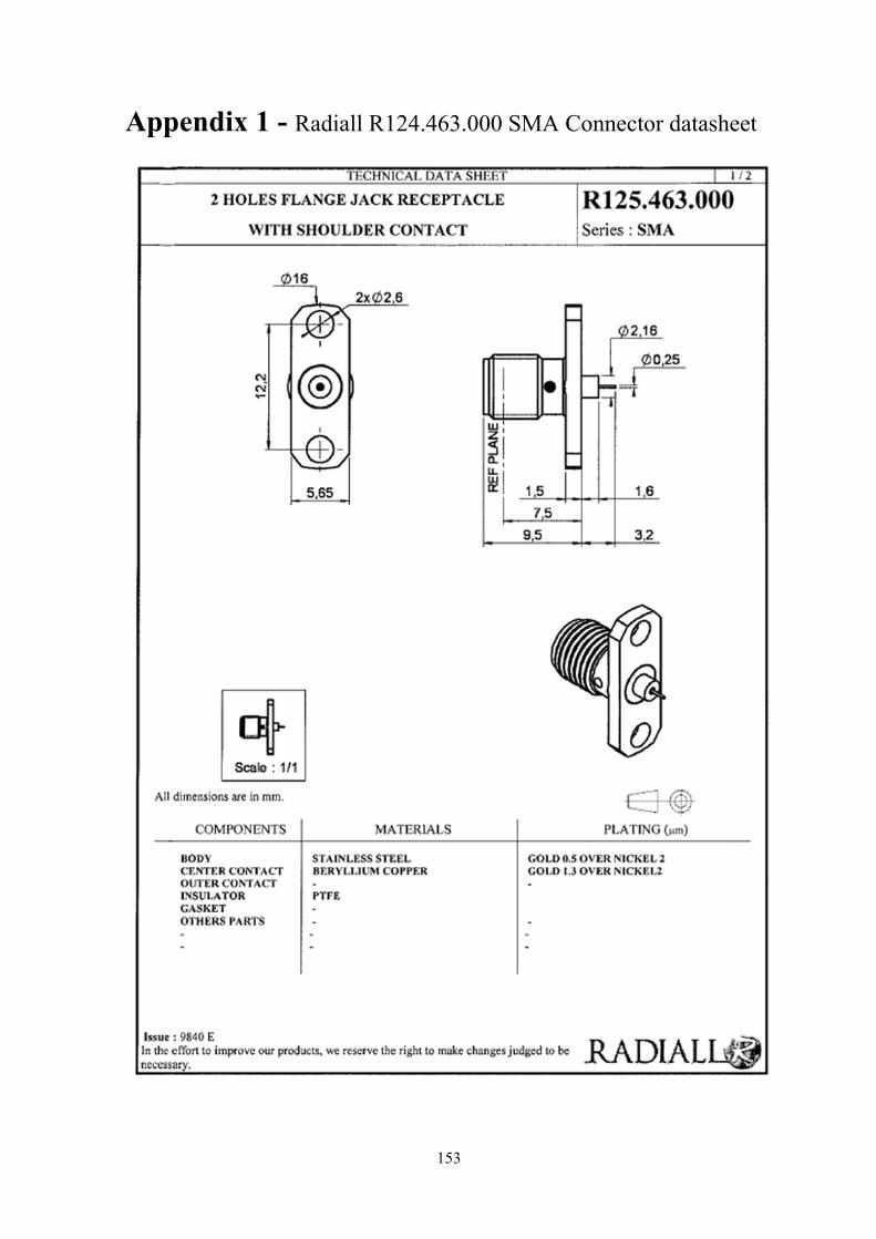
153

Appendix 1 - Radiall R124.463.000 SMA Connector datasheet

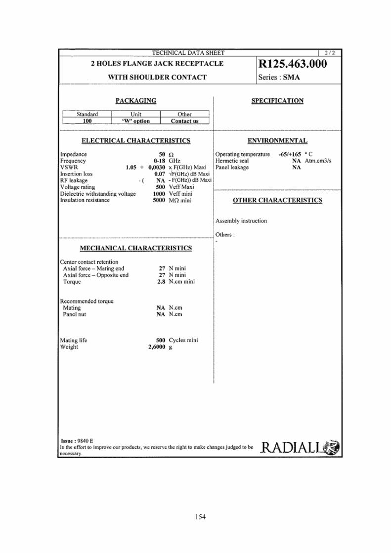
154

155

Appendix 2 - Dow Corning® 184 Silicone Elastomer datasheet

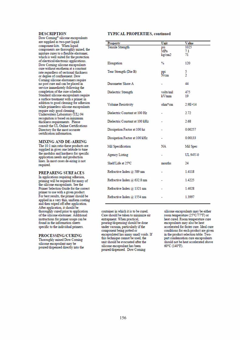
156

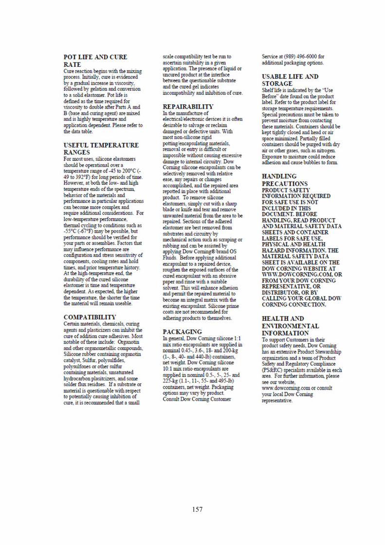
157

158

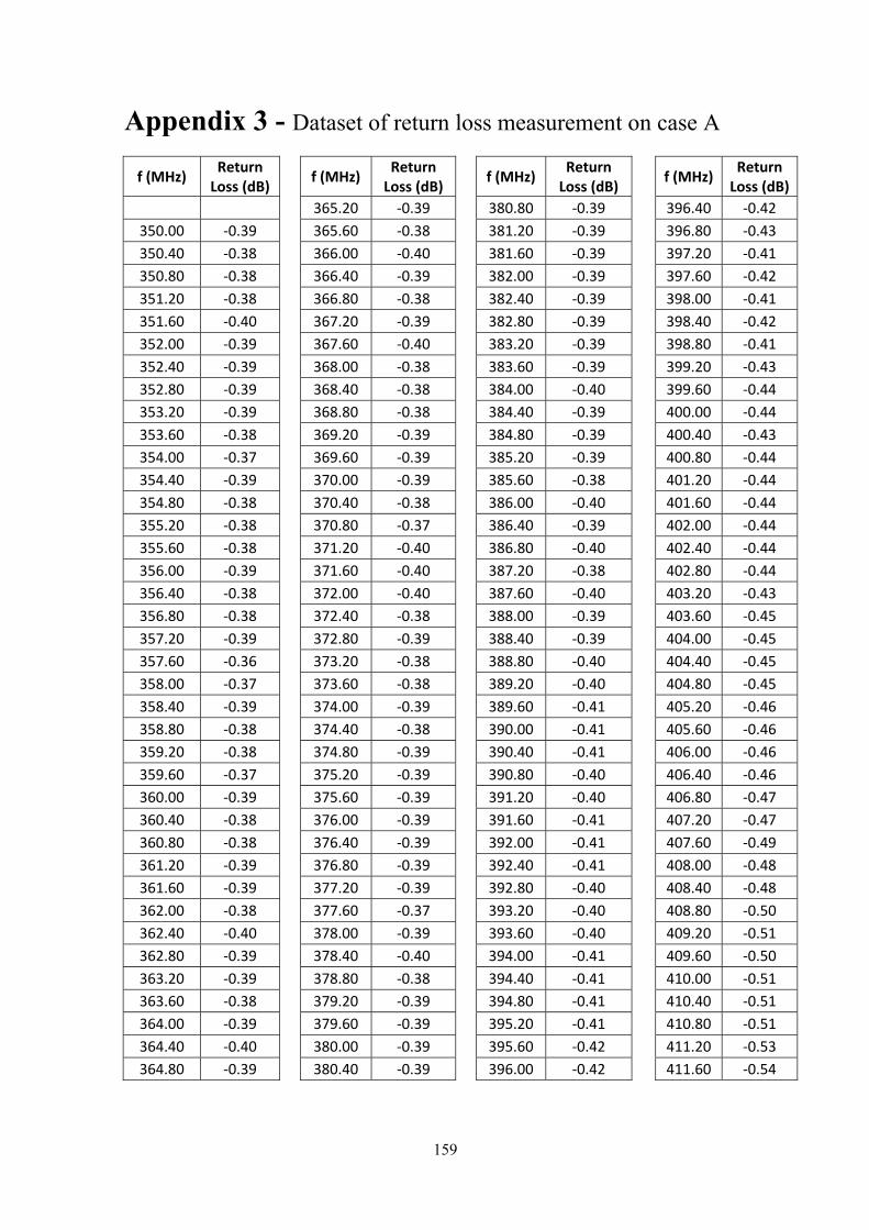
159

Appendix 3 - Dataset of return loss measurement on case A f (MHz)

Return Loss (dB)

f (MHz) Return Loss (dB)



365.20 ‐0.39 380.80 ‐0.39 396.40 ‐0.42

350.00 ‐0.39 365.60 ‐0.38 381.20 ‐0.39 396.80 ‐0.43

350.40 ‐0.38 366.00 ‐0.40 381.60 ‐0.39 397.20 ‐0.41

350.80 ‐0.38 366.40 ‐0.39 382.00 ‐0.39 397.60 ‐0.42

351.20 ‐0.38 366.80 ‐0.38 382.40 ‐0.39 398.00 ‐0.41

351.60 ‐0.40 367.20 ‐0.39 382.80 ‐0.39 398.40 ‐0.42

352.00 ‐0.39 367.60 ‐0.40 383.20 ‐0.39 398.80 ‐0.41

352.40 ‐0.39 368.00 ‐0.38 383.60 ‐0.39 399.20 ‐0.43

352.80 ‐0.39 368.40 ‐0.38 384.00 ‐0.40 399.60 ‐0.44

353.20 ‐0.39 368.80 ‐0.38 384.40 ‐0.39 400.00 ‐0.44

353.60 ‐0.38 369.20 ‐0.39 384.80 ‐0.39 400.40 ‐0.43

354.00 ‐0.37 369.60 ‐0.39 385.20 ‐0.39 400.80 ‐0.44

354.40 ‐0.39 370.00 ‐0.39 385.60 ‐0.38 401.20 ‐0.44

354.80 ‐0.38 370.40 ‐0.38 386.00 ‐0.40 401.60 ‐0.44

355.20 ‐0.38 370.80 ‐0.37 386.40 ‐0.39 402.00 ‐0.44

355.60 ‐0.38 371.20 ‐0.40 386.80 ‐0.40 402.40 ‐0.44

356.00 ‐0.39 371.60 ‐0.40 387.20 ‐0.38 402.80 ‐0.44

356.40 ‐0.38 372.00 ‐0.40 387.60 ‐0.40 403.20 ‐0.43

356.80 ‐0.38 372.40 ‐0.38 388.00 ‐0.39 403.60 ‐0.45

357.20 ‐0.39 372.80 ‐0.39 388.40 ‐0.39 404.00 ‐0.45

357.60 ‐0.36 373.20 ‐0.38 388.80 ‐0.40 404.40 ‐0.45

358.00 ‐0.37 373.60 ‐0.38 389.20 ‐0.40 404.80 ‐0.45

358.40 ‐0.39 374.00 ‐0.39 389.60 ‐0.41 405.20 ‐0.46

358.80 ‐0.38 374.40 ‐0.38 390.00 ‐0.41 405.60 ‐0.46

359.20 ‐0.38 374.80 ‐0.39 390.40 ‐0.41 406.00 ‐0.46

359.60 ‐0.37 375.20 ‐0.39 390.80 ‐0.40 406.40 ‐0.46

360.00 ‐0.39 375.60 ‐0.39 391.20 ‐0.40 406.80 ‐0.47

360.40 ‐0.38 376.00 ‐0.39 391.60 ‐0.41 407.20 ‐0.47

360.80 ‐0.38 376.40 ‐0.39 392.00 ‐0.41 407.60 ‐0.49

361.20 ‐0.39 376.80 ‐0.39 392.40 ‐0.41 408.00 ‐0.48

361.60 ‐0.39 377.20 ‐0.39 392.80 ‐0.40 408.40 ‐0.48

362.00 ‐0.38 377.60 ‐0.37 393.20 ‐0.40 408.80 ‐0.50

362.40 ‐0.40 378.00 ‐0.39 393.60 ‐0.40 409.20 ‐0.51

362.80 ‐0.39 378.40 ‐0.40 394.00 ‐0.41 409.60 ‐0.50

363.20 ‐0.39 378.80 ‐0.38 394.40 ‐0.41 410.00 ‐0.51

363.60 ‐0.38 379.20 ‐0.39 394.80 ‐0.41 410.40 ‐0.51

364.00 ‐0.39 379.60 ‐0.39 395.20 ‐0.41 410.80 ‐0.51

364.40 ‐0.40 380.00 ‐0.39 395.60 ‐0.42 411.20 ‐0.53

364.80 ‐0.39 380.40 ‐0.39 396.00 ‐0.42 411.60 ‐0.54

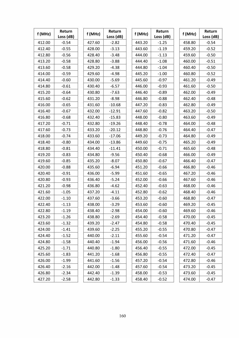
160





412.00 ‐0.54 427.60 ‐2.82 443.20 ‐1.25 458.80 ‐0.54

412.40 ‐0.55 428.00 ‐3.13 443.60 ‐1.19 459.20 ‐0.52

412.80 ‐0.56 428.40 ‐3.48 444.00 ‐1.13 459.60 ‐0.50

413.20 ‐0.58 428.80 ‐3.88 444.40 ‐1.08 460.00 ‐0.51

413.60 ‐0.58 429.20 ‐4.38 444.80 ‐1.04 460.40 ‐0.50

414.00 ‐0.59 429.60 ‐4.98 445.20 ‐1.00 460.80 ‐0.52

414.40 ‐0.60 430.00 ‐5.69 445.60 ‐0.97 461.20 ‐0.49

414.80 ‐0.61 430.40 ‐6.57 446.00 ‐0.93 461.60 ‐0.50

415.20 ‐0.64 430.80 ‐7.63 446.40 ‐0.89 462.00 ‐0.49

415.60 ‐0.62 431.20 ‐8.98 446.80 ‐0.88 462.40 ‐0.48

416.00 ‐0.65 431.60 ‐10.68 447.20 ‐0.83 462.80 ‐0.49

416.40 ‐0.67 432.00 ‐12.91 447.60 ‐0.82 463.20 ‐0.50

416.80 ‐0.68 432.40 ‐15.83 448.00 ‐0.80 463.60 ‐0.49

417.20 ‐0.71 432.80 ‐19.26 448.40 ‐0.78 464.00 ‐0.48

417.60 ‐0.73 433.20 ‐20.12 448.80 ‐0.76 464.40 ‐0.47

418.00 ‐0.74 433.60 ‐17.06 449.20 ‐0.73 464.80 ‐0.49

418.40 ‐0.80 434.00 ‐13.86 449.60 ‐0.75 465.20 ‐0.49

418.80 ‐0.81 434.40 ‐11.41 450.00 ‐0.71 465.60 ‐0.48

419.20 ‐0.83 434.80 ‐9.56 450.40 ‐0.68 466.00 ‐0.49

419.60 ‐0.85 435.20 ‐8.07 450.80 ‐0.67 466.40 ‐0.47

420.00 ‐0.88 435.60 ‐6.94 451.20 ‐0.66 466.80 ‐0.46

420.40 ‐0.91 436.00 ‐5.99 451.60 ‐0.65 467.20 ‐0.46

420.80 ‐0.93 436.40 ‐5.24 452.00 ‐0.66 467.60 ‐0.46

421.20 ‐0.98 436.80 ‐4.62 452.40 ‐0.63 468.00 ‐0.46

421.60 ‐1.05 437.20 ‐4.11 452.80 ‐0.62 468.40 ‐0.46

422.00 ‐1.10 437.60 ‐3.66 453.20 ‐0.60 468.80 ‐0.47

422.40 ‐1.13 438.00 ‐3.29 453.60 ‐0.60 469.20 ‐0.45

422.80 ‐1.19 438.40 ‐2.98 454.00 ‐0.60 469.60 ‐0.46

423.20 ‐1.26 438.80 ‐2.69 454.40 ‐0.58 470.00 ‐0.45

423.60 ‐1.32 439.20 ‐2.47 454.80 ‐0.58 470.40 ‐0.45

424.00 ‐1.41 439.60 ‐2.25 455.20 ‐0.55 470.80 ‐0.47

424.40 ‐1.52 440.00 ‐2.11 455.60 ‐0.54 471.20 ‐0.47

424.80 ‐1.58 440.40 ‐1.94 456.00 ‐0.56 471.60 ‐0.46

425.20 ‐1.71 440.80 ‐1.80 456.40 ‐0.55 472.00 ‐0.45

425.60 ‐1.83 441.20 ‐1.68 456.80 ‐0.55 472.40 ‐0.47

426.00 ‐1.99 441.60 ‐1.56 457.20 ‐0.54 472.80 ‐0.46

426.40 ‐2.16 442.00 ‐1.48 457.60 ‐0.54 473.20 ‐0.45

426.80 ‐2.34 442.40 ‐1.39 458.00 ‐0.53 473.60 ‐0.45

427.20 ‐2.58 442.80 ‐1.33 458.40 ‐0.52 474.00 ‐0.47

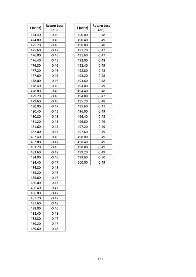
161

f (MHz) Return Loss

(dB) f (MHz)

Return Loss (dB)

474.40 ‐0.46 490.00 ‐0.48

474.80 ‐0.46 490.40 ‐0.49

475.20 ‐0.46 490.80 ‐0.48

475.60 ‐0.47 491.20 ‐0.47

476.00 ‐0.46 491.60 ‐0.47

476.40 ‐0.45 492.00 ‐0.48

476.80 ‐0.46 492.40 ‐0.49

477.20 ‐0.46 492.80 ‐0.48

477.60 ‐0.46 493.20 ‐0.48

478.00 ‐0.46 493.60 ‐0.48

478.40 ‐0.46 494.00 ‐0.49

478.80 ‐0.46 494.40 ‐0.48

479.20 ‐0.46 494.80 ‐0.47

479.60 ‐0.46 495.20 ‐0.48

480.00 ‐0.47 495.60 ‐0.47

480.40 ‐0.45 496.00 ‐0.49

480.80 ‐0.48 496.40 ‐0.48

481.20 ‐0.45 496.80 ‐0.49

481.60 ‐0.45 497.20 ‐0.49

482.00 ‐0.47 497.60 ‐0.49

482.40 ‐0.46 498.00 ‐0.49

482.80 ‐0.47 498.40 ‐0.49

483.20 ‐0.45 498.80 ‐0.49

483.60 ‐0.47 499.20 ‐0.49

484.00 ‐0.46 499.60 ‐0.50

484.40 ‐0.47 500.00 ‐0.49

484.80 ‐0.48

485.20 ‐0.46

485.60 ‐0.47

486.00 ‐0.47

486.40 ‐0.47

486.80 ‐0.47

487.20 ‐0.47

487.60 ‐0.48

488.00 ‐0.46

488.40 ‐0.48

488.80 ‐0.47

489.20 ‐0.47

489.60 ‐0.48

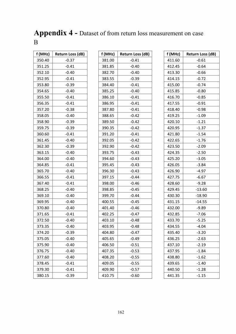
162

Appendix 4 - Dataset of from return loss measurement on case

B

f (MHz) Return Loss (dB) f (MHz) Return Loss (dB) f (MHz) Return Loss (dB)

350.40 ‐0.37 381.00 ‐0.41 411.60 ‐0.61

351.25 ‐0.41 381.85 ‐0.40 412.45 ‐0.64

352.10 ‐0.40 382.70 ‐0.40 413.30 ‐0.66

352.95 ‐0.41 383.55 ‐0.39 414.15 ‐0.72

353.80 ‐0.39 384.40 ‐0.41 415.00 ‐0.74

354.65 ‐0.40 385.25 ‐0.40 415.85 ‐0.80

355.50 ‐0.41 386.10 ‐0.41 416.70 ‐0.85

356.35 ‐0.41 386.95 ‐0.41 417.55 ‐0.91

357.20 ‐0.38 387.80 ‐0.41 418.40 ‐0.98

358.05 ‐0.40 388.65 ‐0.42 419.25 ‐1.09

358.90 ‐0.39 389.50 ‐0.42 420.10 ‐1.21

359.75 ‐0.39 390.35 ‐0.42 420.95 ‐1.37

360.60 ‐0.41 391.20 ‐0.41 421.80 ‐1.54

361.45 ‐0.40 392.05 ‐0.42 422.65 ‐1.76

362.30 ‐0.39 392.90 ‐0.42 423.50 ‐2.09

363.15 ‐0.40 393.75 ‐0.43 424.35 ‐2.50

364.00 ‐0.40 394.60 ‐0.43 425.20 ‐3.05

364.85 ‐0.41 395.45 ‐0.43 426.05 ‐3.84

365.70 ‐0.40 396.30 ‐0.43 426.90 ‐4.97

366.55 ‐0.41 397.15 ‐0.44 427.75 ‐6.67

367.40 ‐0.41 398.00 ‐0.46 428.60 ‐9.28

368.25 ‐0.40 398.85 ‐0.45 429.45 ‐13.60

369.10 ‐0.40 399.70 ‐0.44 430.30 ‐18.90

369.95 ‐0.40 400.55 ‐0.45 431.15 ‐14.55

370.80 ‐0.40 401.40 ‐0.46 432.00 ‐9.89

371.65 ‐0.41 402.25 ‐0.47 432.85 ‐7.06

372.50 ‐0.40 403.10 ‐0.48 433.70 ‐5.25

373.35 ‐0.40 403.95 ‐0.48 434.55 ‐4.04

374.20 ‐0.39 404.80 ‐0.47 435.40 ‐3.20

375.05 ‐0.40 405.65 ‐0.49 436.25 ‐2.63

375.90 ‐0.40 406.50 ‐0.51 437.10 ‐2.19

376.75 ‐0.40 407.35 ‐0.53 437.95 ‐1.84

377.60 ‐0.40 408.20 ‐0.55 438.80 ‐1.62

378.45 ‐0.41 409.05 ‐0.55 439.65 ‐1.40

379.30 ‐0.41 409.90 ‐0.57 440.50 ‐1.28

380.15 ‐0.39 410.75 ‐0.60 441.35 ‐1.15

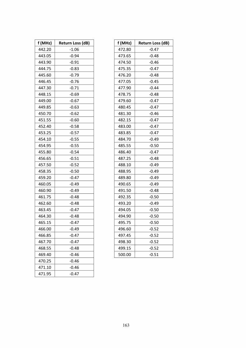
163

f (MHz) Return Loss (dB) f (MHz) Return Loss (dB)

442.20 ‐1.06 472.80 ‐0.47

443.05 ‐0.94 473.65 ‐0.48

443.90 ‐0.91 474.50 ‐0.46

444.75 ‐0.83 475.35 ‐0.47

445.60 ‐0.79 476.20 ‐0.48

446.45 ‐0.76 477.05 ‐0.45

447.30 ‐0.71 477.90 ‐0.44

448.15 ‐0.69 478.75 ‐0.48

449.00 ‐0.67 479.60 ‐0.47

449.85 ‐0.63 480.45 ‐0.47

450.70 ‐0.62 481.30 ‐0.46

451.55 ‐0.60 482.15 ‐0.47

452.40 ‐0.58 483.00 ‐0.47

453.25 ‐0.57 483.85 ‐0.47

454.10 ‐0.55 484.70 ‐0.49

454.95 ‐0.55 485.55 ‐0.50

455.80 ‐0.54 486.40 ‐0.47

456.65 ‐0.51 487.25 ‐0.48

457.50 ‐0.52 488.10 ‐0.49

458.35 ‐0.50 488.95 ‐0.49

459.20 ‐0.47 489.80 ‐0.49

460.05 ‐0.49 490.65 ‐0.49

460.90 ‐0.49 491.50 ‐0.48

461.75 ‐0.48 492.35 ‐0.50

462.60 ‐0.48 493.20 ‐0.49

463.45 ‐0.47 494.05 ‐0.50

464.30 ‐0.48 494.90 ‐0.50

465.15 ‐0.47 495.75 ‐0.50

466.00 ‐0.49 496.60 ‐0.52

466.85 ‐0.47 497.45 ‐0.52

467.70 ‐0.47 498.30 ‐0.52

468.55 ‐0.48 499.15 ‐0.52

469.40 ‐0.46 500.00 ‐0.51

470.25 ‐0.46

471.10 ‐0.46

471.95 ‐0.47

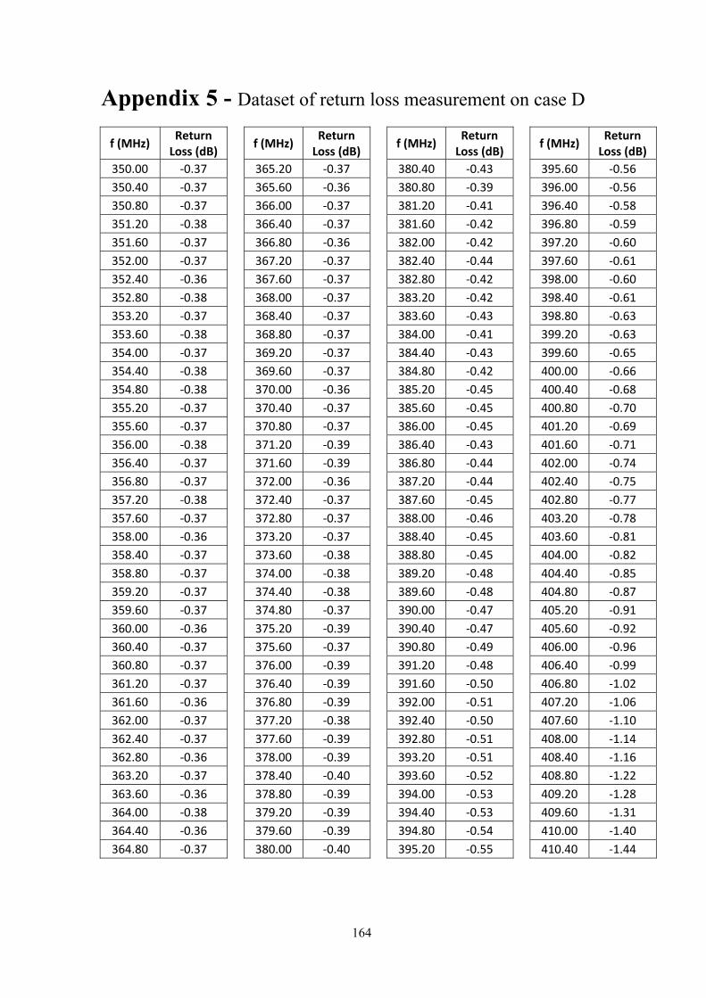
164

Appendix 5 - Dataset of return loss measurement on case D





350.00 ‐0.37 365.20 ‐0.37 380.40 ‐0.43 395.60 ‐0.56

350.40 ‐0.37 365.60 ‐0.36 380.80 ‐0.39 396.00 ‐0.56

350.80 ‐0.37 366.00 ‐0.37 381.20 ‐0.41 396.40 ‐0.58

351.20 ‐0.38 366.40 ‐0.37 381.60 ‐0.42 396.80 ‐0.59

351.60 ‐0.37 366.80 ‐0.36 382.00 ‐0.42 397.20 ‐0.60

352.00 ‐0.37 367.20 ‐0.37 382.40 ‐0.44 397.60 ‐0.61

352.40 ‐0.36 367.60 ‐0.37 382.80 ‐0.42 398.00 ‐0.60

352.80 ‐0.38 368.00 ‐0.37 383.20 ‐0.42 398.40 ‐0.61

353.20 ‐0.37 368.40 ‐0.37 383.60 ‐0.43 398.80 ‐0.63

353.60 ‐0.38 368.80 ‐0.37 384.00 ‐0.41 399.20 ‐0.63

354.00 ‐0.37 369.20 ‐0.37 384.40 ‐0.43 399.60 ‐0.65

354.40 ‐0.38 369.60 ‐0.37 384.80 ‐0.42 400.00 ‐0.66

354.80 ‐0.38 370.00 ‐0.36 385.20 ‐0.45 400.40 ‐0.68

355.20 ‐0.37 370.40 ‐0.37 385.60 ‐0.45 400.80 ‐0.70

355.60 ‐0.37 370.80 ‐0.37 386.00 ‐0.45 401.20 ‐0.69

356.00 ‐0.38 371.20 ‐0.39 386.40 ‐0.43 401.60 ‐0.71

356.40 ‐0.37 371.60 ‐0.39 386.80 ‐0.44 402.00 ‐0.74

356.80 ‐0.37 372.00 ‐0.36 387.20 ‐0.44 402.40 ‐0.75

357.20 ‐0.38 372.40 ‐0.37 387.60 ‐0.45 402.80 ‐0.77

357.60 ‐0.37 372.80 ‐0.37 388.00 ‐0.46 403.20 ‐0.78

358.00 ‐0.36 373.20 ‐0.37 388.40 ‐0.45 403.60 ‐0.81

358.40 ‐0.37 373.60 ‐0.38 388.80 ‐0.45 404.00 ‐0.82

358.80 ‐0.37 374.00 ‐0.38 389.20 ‐0.48 404.40 ‐0.85

359.20 ‐0.37 374.40 ‐0.38 389.60 ‐0.48 404.80 ‐0.87

359.60 ‐0.37 374.80 ‐0.37 390.00 ‐0.47 405.20 ‐0.91

360.00 ‐0.36 375.20 ‐0.39 390.40 ‐0.47 405.60 ‐0.92

360.40 ‐0.37 375.60 ‐0.37 390.80 ‐0.49 406.00 ‐0.96

360.80 ‐0.37 376.00 ‐0.39 391.20 ‐0.48 406.40 ‐0.99

361.20 ‐0.37 376.40 ‐0.39 391.60 ‐0.50 406.80 ‐1.02

361.60 ‐0.36 376.80 ‐0.39 392.00 ‐0.51 407.20 ‐1.06

362.00 ‐0.37 377.20 ‐0.38 392.40 ‐0.50 407.60 ‐1.10

362.40 ‐0.37 377.60 ‐0.39 392.80 ‐0.51 408.00 ‐1.14

362.80 ‐0.36 378.00 ‐0.39 393.20 ‐0.51 408.40 ‐1.16

363.20 ‐0.37 378.40 ‐0.40 393.60 ‐0.52 408.80 ‐1.22

363.60 ‐0.36 378.80 ‐0.39 394.00 ‐0.53 409.20 ‐1.28

364.00 ‐0.38 379.20 ‐0.39 394.40 ‐0.53 409.60 ‐1.31

364.40 ‐0.36 379.60 ‐0.39 394.80 ‐0.54 410.00 ‐1.40

364.80 ‐0.37 380.00 ‐0.40 395.20 ‐0.55 410.40 ‐1.44

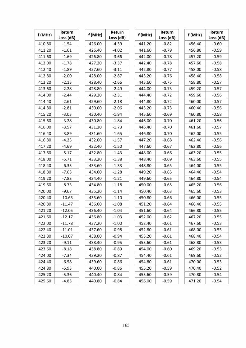
165





410.80 ‐1.54 426.00 ‐4.39 441.20 ‐0.82 456.40 ‐0.60

411.20 ‐1.61 426.40 ‐4.02 441.60 ‐0.79 456.80 ‐0.59

411.60 ‐1.69 426.80 ‐3.66 442.00 ‐0.78 457.20 ‐0.59

412.00 ‐1.78 427.20 ‐3.37 442.40 ‐0.78 457.60 ‐0.58

412.40 ‐1.89 427.60 ‐3.11 442.80 ‐0.77 458.00 ‐0.58

412.80 ‐2.00 428.00 ‐2.87 443.20 ‐0.76 458.40 ‐0.58

413.20 ‐2.13 428.40 ‐2.66 443.60 ‐0.75 458.80 ‐0.57

413.60 ‐2.28 428.80 ‐2.49 444.00 ‐0.73 459.20 ‐0.57

414.00 ‐2.44 429.20 ‐2.31 444.40 ‐0.72 459.60 ‐0.56

414.40 ‐2.61 429.60 ‐2.18 444.80 ‐0.72 460.00 ‐0.57

414.80 ‐2.81 430.00 ‐2.06 445.20 ‐0.73 460.40 ‐0.56

415.20 ‐3.03 430.40 ‐1.94 445.60 ‐0.69 460.80 ‐0.58

415.60 ‐3.28 430.80 ‐1.84 446.00 ‐0.70 461.20 ‐0.56

416.00 ‐3.57 431.20 ‐1.73 446.40 ‐0.70 461.60 ‐0.57

416.40 ‐3.89 431.60 ‐1.65 446.80 ‐0.70 462.00 ‐0.55

416.80 ‐4.25 432.00 ‐1.57 447.20 ‐0.68 462.40 ‐0.56

417.20 ‐4.69 432.40 ‐1.50 447.60 ‐0.67 462.80 ‐0.56

417.60 ‐5.17 432.80 ‐1.43 448.00 ‐0.66 463.20 ‐0.55

418.00 ‐5.71 433.20 ‐1.38 448.40 ‐0.69 463.60 ‐0.55

418.40 ‐6.33 433.60 ‐1.33 448.80 ‐0.65 464.00 ‐0.55

418.80 ‐7.03 434.00 ‐1.28 449.20 ‐0.65 464.40 ‐0.54

419.20 ‐7.83 434.40 ‐1.21 449.60 ‐0.65 464.80 ‐0.54

419.60 ‐8.73 434.80 ‐1.18 450.00 ‐0.65 465.20 ‐0.56

420.00 ‐9.67 435.20 ‐1.14 450.40 ‐0.63 465.60 ‐0.53

420.40 ‐10.63 435.60 ‐1.10 450.80 ‐0.66 466.00 ‐0.55

420.80 ‐11.47 436.00 ‐1.08 451.20 ‐0.64 466.40 ‐0.55

421.20 ‐12.05 436.40 ‐1.04 451.60 ‐0.64 466.80 ‐0.55

421.60 ‐12.17 436.80 ‐1.03 452.00 ‐0.62 467.20 ‐0.55

422.00 ‐11.78 437.20 ‐1.00 452.40 ‐0.61 467.60 ‐0.53

422.40 ‐11.01 437.60 ‐0.98 452.80 ‐0.61 468.00 ‐0.55

422.80 ‐10.07 438.00 ‐0.94 453.20 ‐0.61 468.40 ‐0.54

423.20 ‐9.11 438.40 ‐0.95 453.60 ‐0.61 468.80 ‐0.53

423.60 ‐8.18 438.80 ‐0.89 454.00 ‐0.60 469.20 ‐0.53

424.00 ‐7.34 439.20 ‐0.87 454.40 ‐0.61 469.60 ‐0.52

424.40 ‐6.58 439.60 ‐0.86 454.80 ‐0.61 470.00 ‐0.53

424.80 ‐5.93 440.00 ‐0.86 455.20 ‐0.59 470.40 ‐0.52

425.20 ‐5.36 440.40 ‐0.84 455.60 ‐0.59 470.80 ‐0.54

425.60 ‐4.83 440.80 ‐0.84 456.00 ‐0.59 471.20 ‐0.54

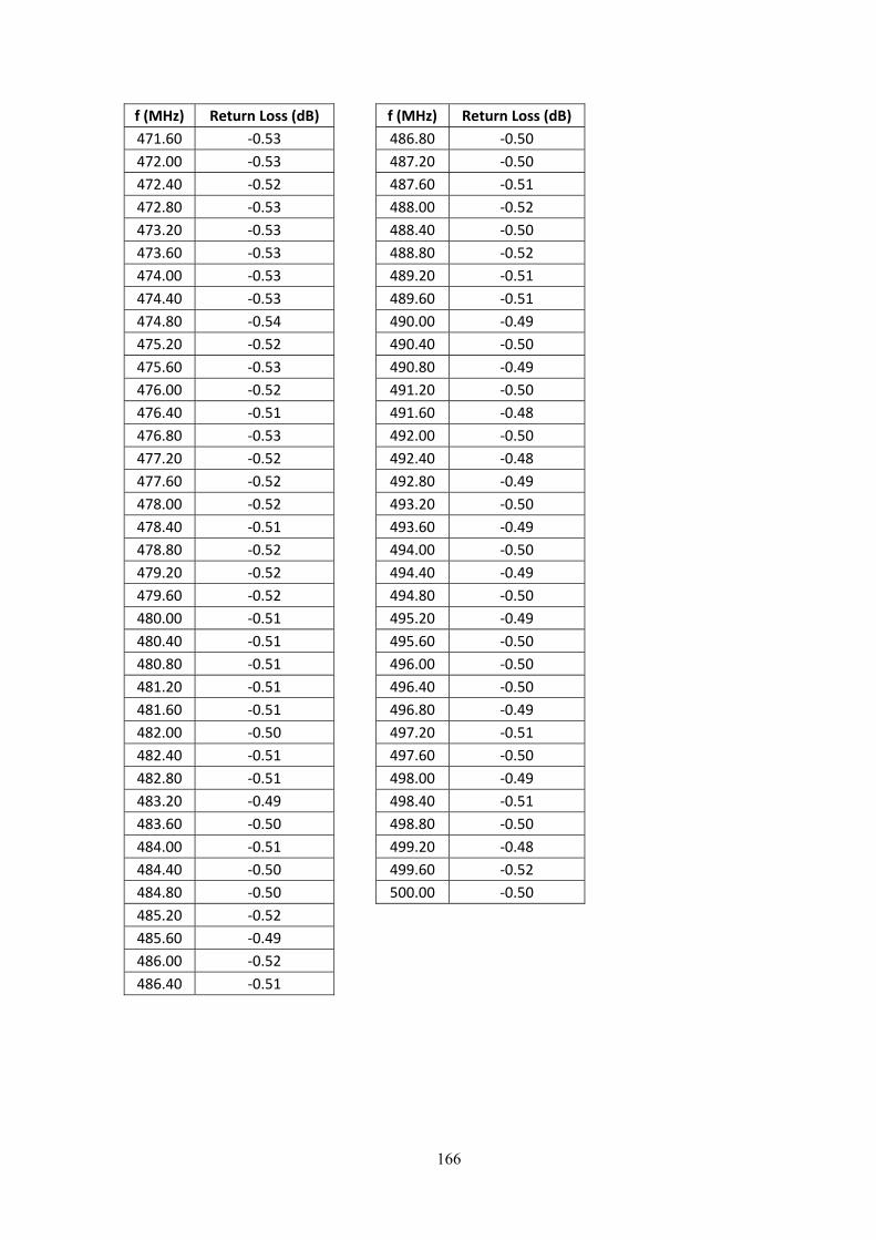
166

f (MHz) Return Loss (dB) f (MHz) Return Loss (dB)

471.60 ‐0.53 486.80 ‐0.50

472.00 ‐0.53 487.20 ‐0.50

472.40 ‐0.52 487.60 ‐0.51

472.80 ‐0.53 488.00 ‐0.52

473.20 ‐0.53 488.40 ‐0.50

473.60 ‐0.53 488.80 ‐0.52

474.00 ‐0.53 489.20 ‐0.51

474.40 ‐0.53 489.60 ‐0.51

474.80 ‐0.54 490.00 ‐0.49

475.20 ‐0.52 490.40 ‐0.50

475.60 ‐0.53 490.80 ‐0.49

476.00 ‐0.52 491.20 ‐0.50

476.40 ‐0.51 491.60 ‐0.48

476.80 ‐0.53 492.00 ‐0.50

477.20 ‐0.52 492.40 ‐0.48

477.60 ‐0.52 492.80 ‐0.49

478.00 ‐0.52 493.20 ‐0.50

478.40 ‐0.51 493.60 ‐0.49

478.80 ‐0.52 494.00 ‐0.50

479.20 ‐0.52 494.40 ‐0.49

479.60 ‐0.52 494.80 ‐0.50

480.00 ‐0.51 495.20 ‐0.49

480.40 ‐0.51 495.60 ‐0.50

480.80 ‐0.51 496.00 ‐0.50

481.20 ‐0.51 496.40 ‐0.50

481.60 ‐0.51 496.80 ‐0.49

482.00 ‐0.50 497.20 ‐0.51

482.40 ‐0.51 497.60 ‐0.50

482.80 ‐0.51 498.00 ‐0.49

483.20 ‐0.49 498.40 ‐0.51

483.60 ‐0.50 498.80 ‐0.50

484.00 ‐0.51 499.20 ‐0.48

484.40 ‐0.50 499.60 ‐0.52

484.80 ‐0.50 500.00 ‐0.50

485.20 ‐0.52

485.60 ‐0.49

486.00 ‐0.52

486.40 ‐0.51

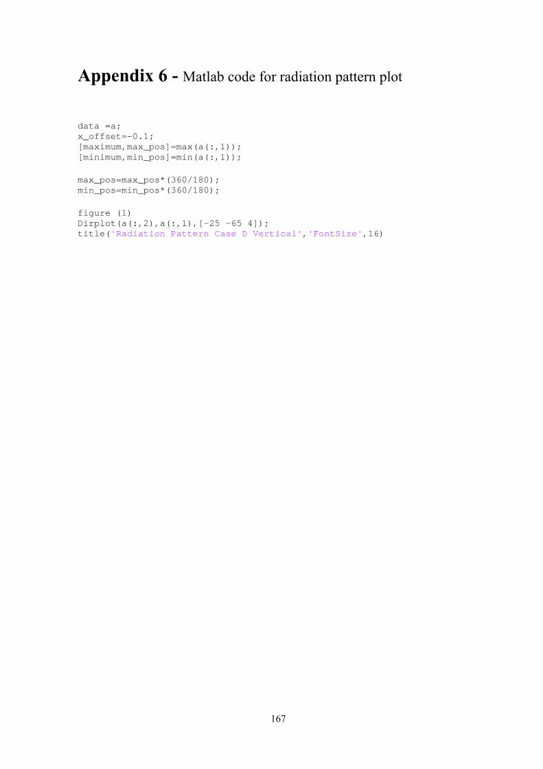
167

Appendix 6 - Matlab code for radiation pattern plot

data =a; x_offset=-0.1; [maximum,max_pos]=max(a(:,1)); [minimum,min_pos]=min(a(:,1)); max_pos=max_pos*(360/180); min_pos=min_pos*(360/180); figure (1) Dirplot(a(:,2),a(:,1),[-25 -65 4]); title('Radiation Pattern Case D Vertical','FontSize',16)

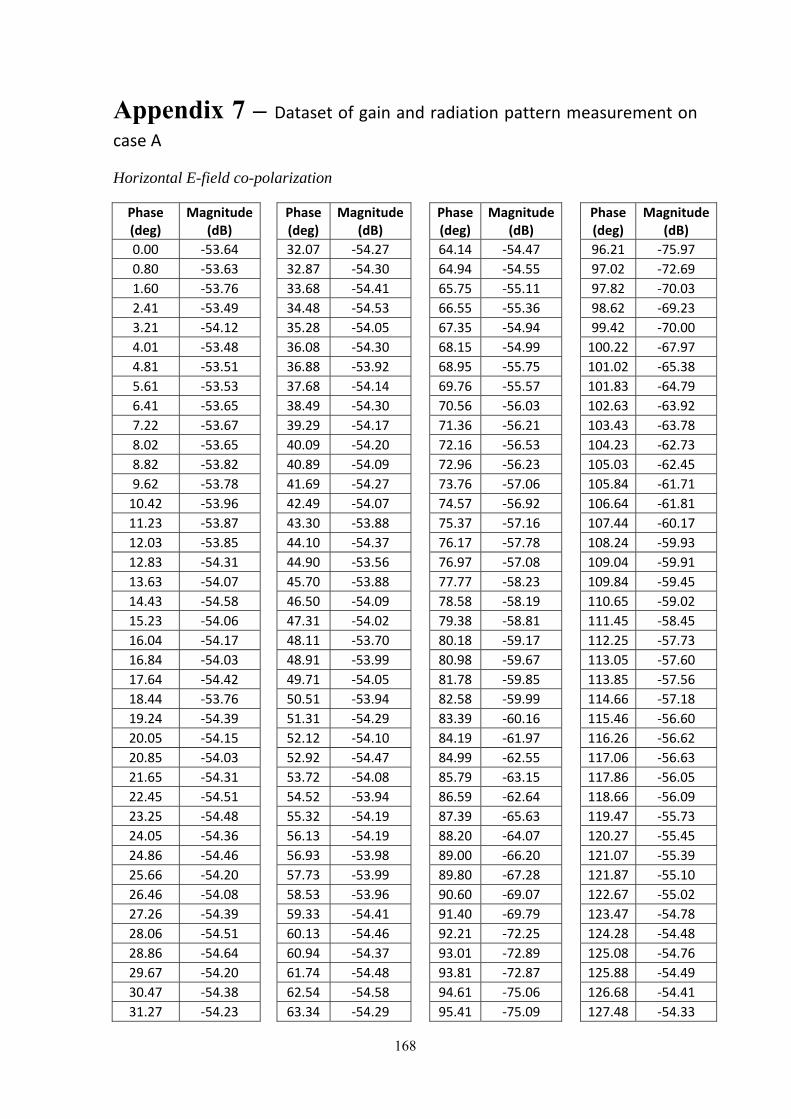
168

Appendix 7 – Dataset of gain and radiation pattern measurement on

case A Horizontal E-field co-polarization

Phase (deg)

Magnitude (dB)

Phase (deg)

Magnitude (dB)

Phase (deg)

Magnitude (dB)

Phase (deg)

Magnitude (dB)

0.00 ‐53.64 32.07 ‐54.27 64.14 ‐54.47 96.21 ‐75.97

0.80 ‐53.63 32.87 ‐54.30 64.94 ‐54.55 97.02 ‐72.69

1.60 ‐53.76 33.68 ‐54.41 65.75 ‐55.11 97.82 ‐70.03

2.41 ‐53.49 34.48 ‐54.53 66.55 ‐55.36 98.62 ‐69.23

3.21 ‐54.12 35.28 ‐54.05 67.35 ‐54.94 99.42 ‐70.00

4.01 ‐53.48 36.08 ‐54.30 68.15 ‐54.99 100.22 ‐67.97

4.81 ‐53.51 36.88 ‐53.92 68.95 ‐55.75 101.02 ‐65.38

5.61 ‐53.53 37.68 ‐54.14 69.76 ‐55.57 101.83 ‐64.79

6.41 ‐53.65 38.49 ‐54.30 70.56 ‐56.03 102.63 ‐63.92

7.22 ‐53.67 39.29 ‐54.17 71.36 ‐56.21 103.43 ‐63.78

8.02 ‐53.65 40.09 ‐54.20 72.16 ‐56.53 104.23 ‐62.73

8.82 ‐53.82 40.89 ‐54.09 72.96 ‐56.23 105.03 ‐62.45

9.62 ‐53.78 41.69 ‐54.27 73.76 ‐57.06 105.84 ‐61.71

10.42 ‐53.96 42.49 ‐54.07 74.57 ‐56.92 106.64 ‐61.81

11.23 ‐53.87 43.30 ‐53.88 75.37 ‐57.16 107.44 ‐60.17

12.03 ‐53.85 44.10 ‐54.37 76.17 ‐57.78 108.24 ‐59.93

12.83 ‐54.31 44.90 ‐53.56 76.97 ‐57.08 109.04 ‐59.91

13.63 ‐54.07 45.70 ‐53.88 77.77 ‐58.23 109.84 ‐59.45

14.43 ‐54.58 46.50 ‐54.09 78.58 ‐58.19 110.65 ‐59.02

15.23 ‐54.06 47.31 ‐54.02 79.38 ‐58.81 111.45 ‐58.45

16.04 ‐54.17 48.11 ‐53.70 80.18 ‐59.17 112.25 ‐57.73

16.84 ‐54.03 48.91 ‐53.99 80.98 ‐59.67 113.05 ‐57.60

17.64 ‐54.42 49.71 ‐54.05 81.78 ‐59.85 113.85 ‐57.56

18.44 ‐53.76 50.51 ‐53.94 82.58 ‐59.99 114.66 ‐57.18

19.24 ‐54.39 51.31 ‐54.29 83.39 ‐60.16 115.46 ‐56.60

20.05 ‐54.15 52.12 ‐54.10 84.19 ‐61.97 116.26 ‐56.62

20.85 ‐54.03 52.92 ‐54.47 84.99 ‐62.55 117.06 ‐56.63

21.65 ‐54.31 53.72 ‐54.08 85.79 ‐63.15 117.86 ‐56.05

22.45 ‐54.51 54.52 ‐53.94 86.59 ‐62.64 118.66 ‐56.09

23.25 ‐54.48 55.32 ‐54.19 87.39 ‐65.63 119.47 ‐55.73

24.05 ‐54.36 56.13 ‐54.19 88.20 ‐64.07 120.27 ‐55.45

24.86 ‐54.46 56.93 ‐53.98 89.00 ‐66.20 121.07 ‐55.39

25.66 ‐54.20 57.73 ‐53.99 89.80 ‐67.28 121.87 ‐55.10

26.46 ‐54.08 58.53 ‐53.96 90.60 ‐69.07 122.67 ‐55.02

27.26 ‐54.39 59.33 ‐54.41 91.40 ‐69.79 123.47 ‐54.78

28.06 ‐54.51 60.13 ‐54.46 92.21 ‐72.25 124.28 ‐54.48

28.86 ‐54.64 60.94 ‐54.37 93.01 ‐72.89 125.08 ‐54.76

29.67 ‐54.20 61.74 ‐54.48 93.81 ‐72.87 125.88 ‐54.49

30.47 ‐54.38 62.54 ‐54.58 94.61 ‐75.06 126.68 ‐54.41

31.27 ‐54.23 63.34 ‐54.29 95.41 ‐75.09 127.48 ‐54.33

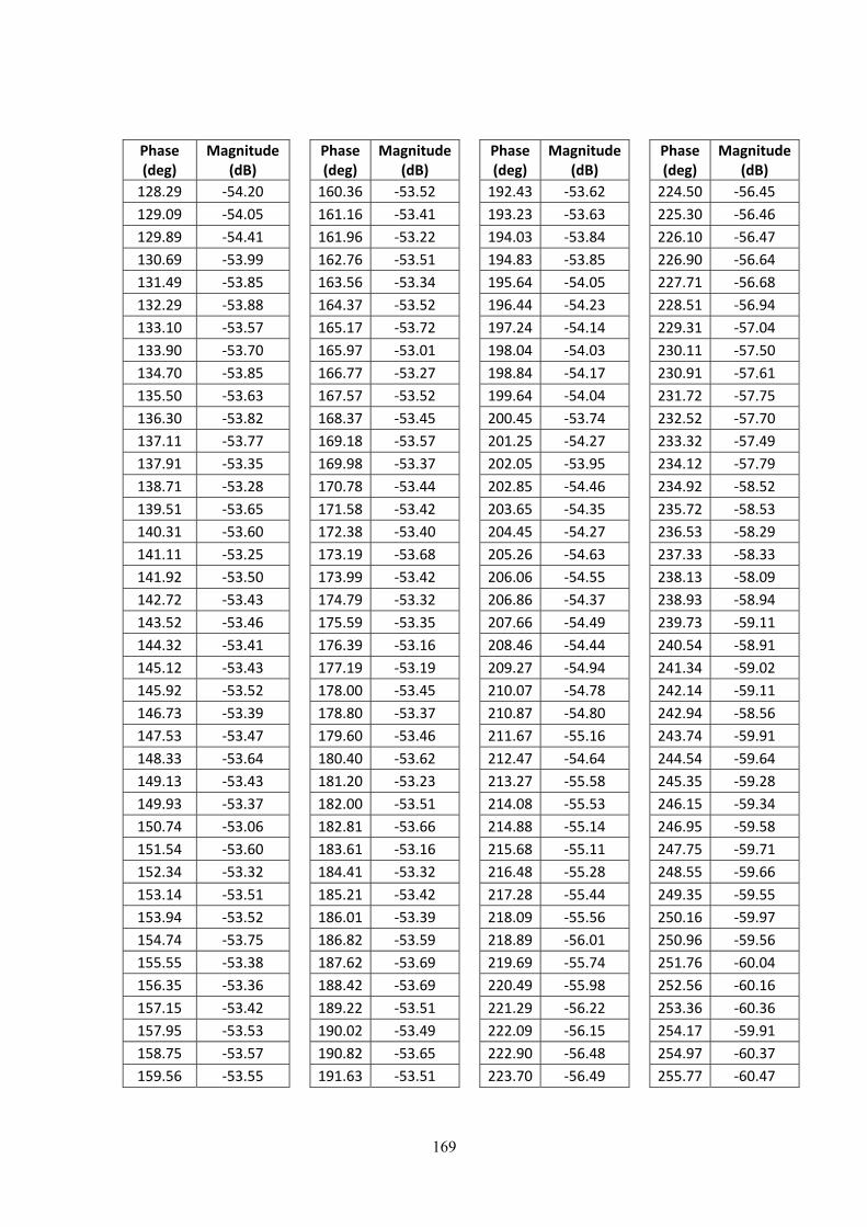
169

Phase (deg)

Magnitude (dB)

Phase (deg)

Magnitude (dB)

Phase (deg)

Magnitude (dB)

Phase (deg)

Magnitude (dB)

128.29 ‐54.20 160.36 ‐53.52 192.43 ‐53.62 224.50 ‐56.45

129.09 ‐54.05 161.16 ‐53.41 193.23 ‐53.63 225.30 ‐56.46

129.89 ‐54.41 161.96 ‐53.22 194.03 ‐53.84 226.10 ‐56.47

130.69 ‐53.99 162.76 ‐53.51 194.83 ‐53.85 226.90 ‐56.64

131.49 ‐53.85 163.56 ‐53.34 195.64 ‐54.05 227.71 ‐56.68

132.29 ‐53.88 164.37 ‐53.52 196.44 ‐54.23 228.51 ‐56.94

133.10 ‐53.57 165.17 ‐53.72 197.24 ‐54.14 229.31 ‐57.04

133.90 ‐53.70 165.97 ‐53.01 198.04 ‐54.03 230.11 ‐57.50

134.70 ‐53.85 166.77 ‐53.27 198.84 ‐54.17 230.91 ‐57.61

135.50 ‐53.63 167.57 ‐53.52 199.64 ‐54.04 231.72 ‐57.75

136.30 ‐53.82 168.37 ‐53.45 200.45 ‐53.74 232.52 ‐57.70

137.11 ‐53.77 169.18 ‐53.57 201.25 ‐54.27 233.32 ‐57.49

137.91 ‐53.35 169.98 ‐53.37 202.05 ‐53.95 234.12 ‐57.79

138.71 ‐53.28 170.78 ‐53.44 202.85 ‐54.46 234.92 ‐58.52

139.51 ‐53.65 171.58 ‐53.42 203.65 ‐54.35 235.72 ‐58.53

140.31 ‐53.60 172.38 ‐53.40 204.45 ‐54.27 236.53 ‐58.29

141.11 ‐53.25 173.19 ‐53.68 205.26 ‐54.63 237.33 ‐58.33

141.92 ‐53.50 173.99 ‐53.42 206.06 ‐54.55 238.13 ‐58.09

142.72 ‐53.43 174.79 ‐53.32 206.86 ‐54.37 238.93 ‐58.94

143.52 ‐53.46 175.59 ‐53.35 207.66 ‐54.49 239.73 ‐59.11

144.32 ‐53.41 176.39 ‐53.16 208.46 ‐54.44 240.54 ‐58.91

145.12 ‐53.43 177.19 ‐53.19 209.27 ‐54.94 241.34 ‐59.02

145.92 ‐53.52 178.00 ‐53.45 210.07 ‐54.78 242.14 ‐59.11

146.73 ‐53.39 178.80 ‐53.37 210.87 ‐54.80 242.94 ‐58.56

147.53 ‐53.47 179.60 ‐53.46 211.67 ‐55.16 243.74 ‐59.91

148.33 ‐53.64 180.40 ‐53.62 212.47 ‐54.64 244.54 ‐59.64

149.13 ‐53.43 181.20 ‐53.23 213.27 ‐55.58 245.35 ‐59.28

149.93 ‐53.37 182.00 ‐53.51 214.08 ‐55.53 246.15 ‐59.34

150.74 ‐53.06 182.81 ‐53.66 214.88 ‐55.14 246.95 ‐59.58

151.54 ‐53.60 183.61 ‐53.16 215.68 ‐55.11 247.75 ‐59.71

152.34 ‐53.32 184.41 ‐53.32 216.48 ‐55.28 248.55 ‐59.66

153.14 ‐53.51 185.21 ‐53.42 217.28 ‐55.44 249.35 ‐59.55

153.94 ‐53.52 186.01 ‐53.39 218.09 ‐55.56 250.16 ‐59.97

154.74 ‐53.75 186.82 ‐53.59 218.89 ‐56.01 250.96 ‐59.56

155.55 ‐53.38 187.62 ‐53.69 219.69 ‐55.74 251.76 ‐60.04

156.35 ‐53.36 188.42 ‐53.69 220.49 ‐55.98 252.56 ‐60.16

157.15 ‐53.42 189.22 ‐53.51 221.29 ‐56.22 253.36 ‐60.36

157.95 ‐53.53 190.02 ‐53.49 222.09 ‐56.15 254.17 ‐59.91

158.75 ‐53.57 190.82 ‐53.65 222.90 ‐56.48 254.97 ‐60.37

159.56 ‐53.55 191.63 ‐53.51 223.70 ‐56.49 255.77 ‐60.47

170

Phase (deg)

Magnitude (dB)

Phase (deg)

Magnitude (dB)

Phase (deg)

Magnitude (dB)

Phase (deg)

Magnitude (dB)

256.57 ‐60.15 288.64 ‐69.24 320.71 ‐58.16 352.78 ‐53.86

257.37 ‐59.83 289.44 ‐68.00 321.51 ‐57.20 353.59 ‐53.37

258.17 ‐60.15 290.25 ‐67.81 322.32 ‐57.14 354.39 ‐53.84

258.98 ‐59.99 291.05 ‐73.08 323.12 ‐56.90 355.19 ‐53.68

259.78 ‐59.96 291.85 ‐75.12 323.92 ‐57.22 355.99 ‐53.47

260.58 ‐60.70 292.65 ‐73.29 324.72 ‐56.94 356.79 ‐53.78

261.38 ‐60.58 293.45 ‐75.17 325.52 ‐56.15 357.60 ‐53.43

262.18 ‐60.17 294.25 ‐76.47 326.33 ‐56.15 358.40 ‐53.77

262.98 ‐60.65 295.06 ‐72.78 327.13 ‐56.66 359.20 ‐53.49

263.79 ‐61.19 295.86 ‐77.04 327.93 ‐56.27 360.00 ‐53.59

264.59 ‐60.26 296.66 ‐75.78 328.73 ‐56.02

265.39 ‐60.27 297.46 ‐72.10 329.53 ‐55.96

266.19 ‐60.31 298.26 ‐75.45 330.33 ‐55.71

266.99 ‐60.88 299.07 ‐72.02 331.14 ‐55.37

267.80 ‐61.18 299.87 ‐68.21 331.94 ‐55.76

268.60 ‐61.54 300.67 ‐69.21 332.74 ‐55.82

269.40 ‐61.54 301.47 ‐67.91 333.54 ‐55.18

270.20 ‐61.83 302.27 ‐67.75 334.34 ‐54.63

271.00 ‐61.36 303.07 ‐67.05 335.15 ‐54.76

271.80 ‐61.59 303.88 ‐67.06 335.95 ‐54.64

272.61 ‐61.32 304.68 ‐64.49 336.75 ‐54.53

273.41 ‐62.64 305.48 ‐64.93 337.55 ‐54.82

274.21 ‐62.74 306.28 ‐64.16 338.35 ‐54.49

275.01 ‐61.98 307.08 ‐64.09 339.15 ‐54.64

275.81 ‐62.75 307.88 ‐63.22 339.96 ‐54.85

276.62 ‐63.59 308.69 ‐63.29 340.76 ‐54.40

277.42 ‐63.98 309.49 ‐61.98 341.56 ‐54.30

278.22 ‐63.64 310.29 ‐61.73 342.36 ‐54.19

279.02 ‐63.57 311.09 ‐62.13 343.16 ‐54.28

279.82 ‐64.08 311.89 ‐60.95 343.96 ‐54.00

280.62 ‐63.81 312.70 ‐60.95 344.77 ‐53.79

281.43 ‐64.92 313.50 ‐60.21 345.57 ‐54.19

282.23 ‐64.92 314.30 ‐60.95 346.37 ‐53.51

283.03 ‐64.83 315.10 ‐60.39 347.17 ‐54.20

283.83 ‐67.39 315.90 ‐59.42 347.97 ‐53.87

284.63 ‐66.86 316.70 ‐59.07 348.78 ‐53.71

285.43 ‐66.84 317.51 ‐58.93 349.58 ‐53.50

286.24 ‐66.17 318.31 ‐58.56 350.38 ‐53.77

287.04 ‐67.63 319.11 ‐58.48 351.18 ‐53.55

287.84 ‐67.40 319.91 ‐58.04 351.98 ‐53.60

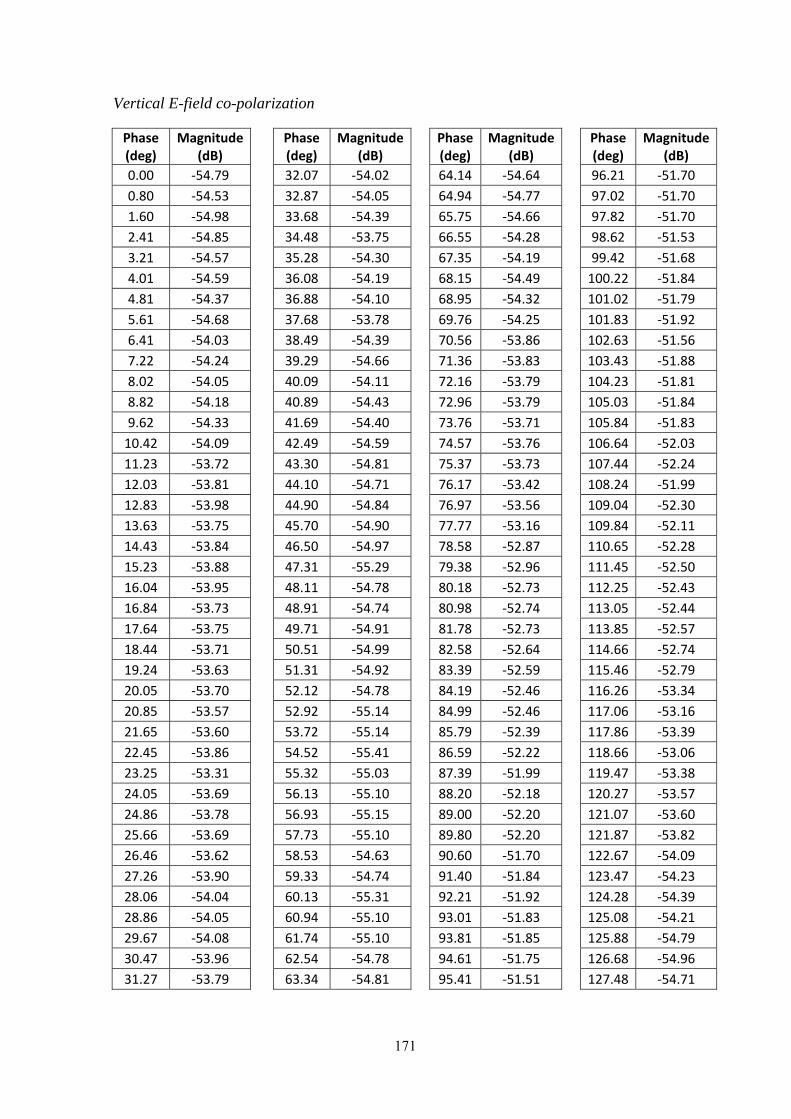
171

Vertical E-field co-polarization

Phase (deg)

Magnitude (dB)

Phase (deg)

Magnitude (dB)

Phase (deg)

Magnitude (dB)

Phase (deg)

Magnitude (dB)

0.00 ‐54.79 32.07 ‐54.02 64.14 ‐54.64 96.21 ‐51.70

0.80 ‐54.53 32.87 ‐54.05 64.94 ‐54.77 97.02 ‐51.70

1.60 ‐54.98 33.68 ‐54.39 65.75 ‐54.66 97.82 ‐51.70

2.41 ‐54.85 34.48 ‐53.75 66.55 ‐54.28 98.62 ‐51.53

3.21 ‐54.57 35.28 ‐54.30 67.35 ‐54.19 99.42 ‐51.68

4.01 ‐54.59 36.08 ‐54.19 68.15 ‐54.49 100.22 ‐51.84

4.81 ‐54.37 36.88 ‐54.10 68.95 ‐54.32 101.02 ‐51.79

5.61 ‐54.68 37.68 ‐53.78 69.76 ‐54.25 101.83 ‐51.92

6.41 ‐54.03 38.49 ‐54.39 70.56 ‐53.86 102.63 ‐51.56

7.22 ‐54.24 39.29 ‐54.66 71.36 ‐53.83 103.43 ‐51.88

8.02 ‐54.05 40.09 ‐54.11 72.16 ‐53.79 104.23 ‐51.81

8.82 ‐54.18 40.89 ‐54.43 72.96 ‐53.79 105.03 ‐51.84

9.62 ‐54.33 41.69 ‐54.40 73.76 ‐53.71 105.84 ‐51.83

10.42 ‐54.09 42.49 ‐54.59 74.57 ‐53.76 106.64 ‐52.03

11.23 ‐53.72 43.30 ‐54.81 75.37 ‐53.73 107.44 ‐52.24

12.03 ‐53.81 44.10 ‐54.71 76.17 ‐53.42 108.24 ‐51.99

12.83 ‐53.98 44.90 ‐54.84 76.97 ‐53.56 109.04 ‐52.30

13.63 ‐53.75 45.70 ‐54.90 77.77 ‐53.16 109.84 ‐52.11

14.43 ‐53.84 46.50 ‐54.97 78.58 ‐52.87 110.65 ‐52.28

15.23 ‐53.88 47.31 ‐55.29 79.38 ‐52.96 111.45 ‐52.50

16.04 ‐53.95 48.11 ‐54.78 80.18 ‐52.73 112.25 ‐52.43

16.84 ‐53.73 48.91 ‐54.74 80.98 ‐52.74 113.05 ‐52.44

17.64 ‐53.75 49.71 ‐54.91 81.78 ‐52.73 113.85 ‐52.57

18.44 ‐53.71 50.51 ‐54.99 82.58 ‐52.64 114.66 ‐52.74

19.24 ‐53.63 51.31 ‐54.92 83.39 ‐52.59 115.46 ‐52.79

20.05 ‐53.70 52.12 ‐54.78 84.19 ‐52.46 116.26 ‐53.34

20.85 ‐53.57 52.92 ‐55.14 84.99 ‐52.46 117.06 ‐53.16

21.65 ‐53.60 53.72 ‐55.14 85.79 ‐52.39 117.86 ‐53.39

22.45 ‐53.86 54.52 ‐55.41 86.59 ‐52.22 118.66 ‐53.06

23.25 ‐53.31 55.32 ‐55.03 87.39 ‐51.99 119.47 ‐53.38

24.05 ‐53.69 56.13 ‐55.10 88.20 ‐52.18 120.27 ‐53.57

24.86 ‐53.78 56.93 ‐55.15 89.00 ‐52.20 121.07 ‐53.60

25.66 ‐53.69 57.73 ‐55.10 89.80 ‐52.20 121.87 ‐53.82

26.46 ‐53.62 58.53 ‐54.63 90.60 ‐51.70 122.67 ‐54.09

27.26 ‐53.90 59.33 ‐54.74 91.40 ‐51.84 123.47 ‐54.23

28.06 ‐54.04 60.13 ‐55.31 92.21 ‐51.92 124.28 ‐54.39

28.86 ‐54.05 60.94 ‐55.10 93.01 ‐51.83 125.08 ‐54.21

29.67 ‐54.08 61.74 ‐55.10 93.81 ‐51.85 125.88 ‐54.79

30.47 ‐53.96 62.54 ‐54.78 94.61 ‐51.75 126.68 ‐54.96

31.27 ‐53.79 63.34 ‐54.81 95.41 ‐51.51 127.48 ‐54.71

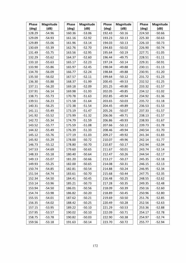
172

Phase (deg)

Magnitude (dB)

Phase (deg)

Magnitude (dB)

Phase (deg)

Magnitude (dB)

Phase (deg)

Magnitude (dB)

128.29 ‐54.96 160.36 ‐53.06 192.43 ‐50.16 224.50 ‐50.66

129.09 ‐54.93 161.16 ‐52.92 193.23 ‐50.13 225.30 ‐50.63

129.89 ‐55.06 161.96 ‐53.14 194.03 ‐50.13 226.10 ‐50.73

130.69 ‐55.39 162.76 ‐52.70 194.83 ‐50.02 226.90 ‐50.74

131.49 ‐55.75 163.56 ‐52.95 195.64 ‐50.19 227.71 ‐51.05

132.29 ‐55.62 164.37 ‐52.60 196.44 ‐49.75 228.51 ‐51.11

133.10 ‐55.63 165.17 ‐52.23 197.24 ‐50.14 229.31 ‐50.91

133.90 ‐55.86 165.97 ‐52.45 198.04 ‐49.88 230.11 ‐51.13

134.70 ‐56.09 166.77 ‐52.24 198.84 ‐49.88 230.91 ‐51.20

135.50 ‐56.02 167.57 ‐52.11 199.64 ‐50.12 231.72 ‐51.23

136.30 ‐55.88 168.37 ‐51.99 200.45 ‐49.53 232.52 ‐51.25

137.11 ‐56.20 169.18 ‐52.09 201.25 ‐49.80 233.32 ‐51.57

137.91 ‐56.14 169.98 ‐51.93 202.05 ‐49.85 234.12 ‐51.02

138.71 ‐55.73 170.78 ‐51.63 202.85 ‐49.94 234.92 ‐51.36

139.51 ‐56.23 171.58 ‐51.64 203.65 ‐50.03 235.72 ‐51.18

140.31 ‐56.25 172.38 ‐51.54 204.45 ‐49.89 236.53 ‐51.53

141.11 ‐55.49 173.19 ‐51.47 205.26 ‐50.07 237.33 ‐51.57

141.92 ‐55.52 173.99 ‐51.32 206.06 ‐49.71 238.13 ‐51.57

142.72 ‐55.34 174.79 ‐51.59 206.86 ‐49.93 238.93 ‐51.67

143.52 ‐55.77 175.59 ‐51.08 207.66 ‐50.12 239.73 ‐51.78

144.32 ‐55.49 176.39 ‐51.33 208.46 ‐49.94 240.54 ‐51.70

145.12 ‐55.76 177.19 ‐51.03 209.27 ‐49.92 241.34 ‐51.83

145.92 ‐55.29 178.00 ‐50.72 210.07 ‐49.96 242.14 ‐51.77

146.73 ‐55.12 178.80 ‐50.70 210.87 ‐50.17 242.94 ‐52.04

147.53 ‐54.69 179.60 ‐50.65 211.67 ‐50.01 243.74 ‐52.14

148.33 ‐55.18 180.40 ‐50.64 212.47 ‐50.26 244.54 ‐52.17

149.13 ‐55.07 181.20 ‐50.66 213.27 ‐50.27 245.35 ‐52.18

149.93 ‐55.25 182.00 ‐50.65 214.08 ‐50.31 246.15 ‐52.13

150.74 ‐54.85 182.81 ‐50.54 214.88 ‐50.24 246.95 ‐52.34

151.54 ‐54.74 183.61 ‐50.70 215.68 ‐50.44 247.75 ‐52.35

152.34 ‐54.50 184.41 ‐50.45 216.48 ‐50.25 248.55 ‐52.62

153.14 ‐53.96 185.21 ‐50.73 217.28 ‐50.35 249.35 ‐52.48

153.94 ‐54.50 186.01 ‐50.56 218.09 ‐50.39 250.16 ‐52.60

154.74 ‐53.98 186.82 ‐50.20 218.89 ‐50.45 250.96 ‐52.80

155.55 ‐54.01 187.62 ‐50.21 219.69 ‐50.50 251.76 ‐52.85

156.35 ‐54.02 188.42 ‐50.25 220.49 ‐50.28 252.56 ‐52.63

157.15 ‐53.95 189.22 ‐50.10 221.29 ‐50.53 253.36 ‐52.88

157.95 ‐53.57 190.02 ‐50.10 222.09 ‐50.71 254.17 ‐52.78

158.75 ‐53.78 190.82 ‐50.03 222.90 ‐50.38 254.97 ‐52.74

159.56 ‐53.18 191.63 ‐50.14 223.70 ‐50.72 255.77 ‐52.94

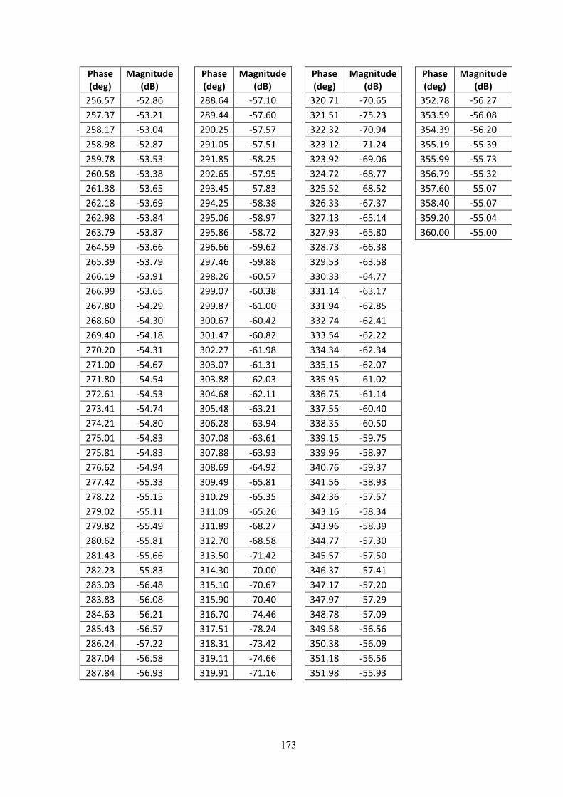
173

Phase (deg)

Magnitude (dB)

Phase (deg)

Magnitude (dB)

Phase (deg)

Magnitude (dB)

Phase (deg)

Magnitude (dB)

256.57 ‐52.86 288.64 ‐57.10 320.71 ‐70.65 352.78 ‐56.27

257.37 ‐53.21 289.44 ‐57.60 321.51 ‐75.23 353.59 ‐56.08

258.17 ‐53.04 290.25 ‐57.57 322.32 ‐70.94 354.39 ‐56.20

258.98 ‐52.87 291.05 ‐57.51 323.12 ‐71.24 355.19 ‐55.39

259.78 ‐53.53 291.85 ‐58.25 323.92 ‐69.06 355.99 ‐55.73

260.58 ‐53.38 292.65 ‐57.95 324.72 ‐68.77 356.79 ‐55.32

261.38 ‐53.65 293.45 ‐57.83 325.52 ‐68.52 357.60 ‐55.07

262.18 ‐53.69 294.25 ‐58.38 326.33 ‐67.37 358.40 ‐55.07

262.98 ‐53.84 295.06 ‐58.97 327.13 ‐65.14 359.20 ‐55.04

263.79 ‐53.87 295.86 ‐58.72 327.93 ‐65.80 360.00 ‐55.00

264.59 ‐53.66 296.66 ‐59.62 328.73 ‐66.38

265.39 ‐53.79 297.46 ‐59.88 329.53 ‐63.58

266.19 ‐53.91 298.26 ‐60.57 330.33 ‐64.77

266.99 ‐53.65 299.07 ‐60.38 331.14 ‐63.17

267.80 ‐54.29 299.87 ‐61.00 331.94 ‐62.85

268.60 ‐54.30 300.67 ‐60.42 332.74 ‐62.41

269.40 ‐54.18 301.47 ‐60.82 333.54 ‐62.22

270.20 ‐54.31 302.27 ‐61.98 334.34 ‐62.34

271.00 ‐54.67 303.07 ‐61.31 335.15 ‐62.07

271.80 ‐54.54 303.88 ‐62.03 335.95 ‐61.02

272.61 ‐54.53 304.68 ‐62.11 336.75 ‐61.14

273.41 ‐54.74 305.48 ‐63.21 337.55 ‐60.40

274.21 ‐54.80 306.28 ‐63.94 338.35 ‐60.50

275.01 ‐54.83 307.08 ‐63.61 339.15 ‐59.75

275.81 ‐54.83 307.88 ‐63.93 339.96 ‐58.97

276.62 ‐54.94 308.69 ‐64.92 340.76 ‐59.37

277.42 ‐55.33 309.49 ‐65.81 341.56 ‐58.93

278.22 ‐55.15 310.29 ‐65.35 342.36 ‐57.57

279.02 ‐55.11 311.09 ‐65.26 343.16 ‐58.34

279.82 ‐55.49 311.89 ‐68.27 343.96 ‐58.39

280.62 ‐55.81 312.70 ‐68.58 344.77 ‐57.30

281.43 ‐55.66 313.50 ‐71.42 345.57 ‐57.50

282.23 ‐55.83 314.30 ‐70.00 346.37 ‐57.41

283.03 ‐56.48 315.10 ‐70.67 347.17 ‐57.20

283.83 ‐56.08 315.90 ‐70.40 347.97 ‐57.29

284.63 ‐56.21 316.70 ‐74.46 348.78 ‐57.09

285.43 ‐56.57 317.51 ‐78.24 349.58 ‐56.56

286.24 ‐57.22 318.31 ‐73.42 350.38 ‐56.09

287.04 ‐56.58 319.11 ‐74.66 351.18 ‐56.56

287.84 ‐56.93 319.91 ‐71.16 351.98 ‐55.93

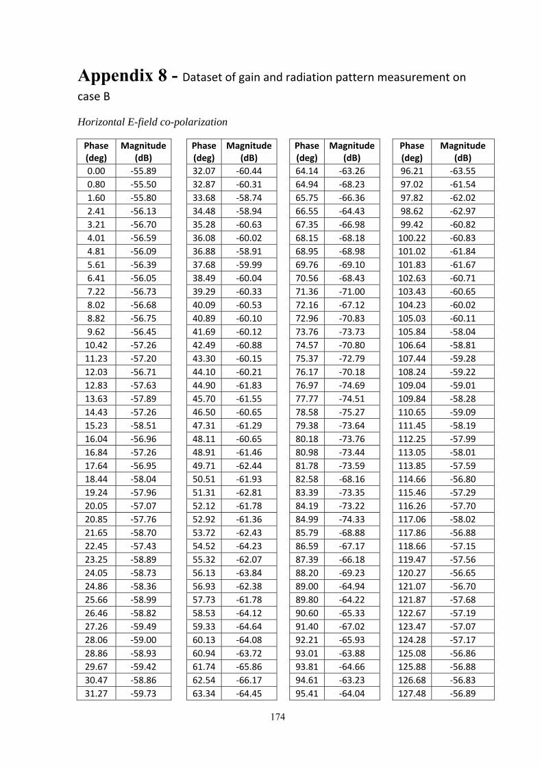
174

Appendix 8 - Dataset of gain and radiation pattern measurement on

case B Horizontal E-field co-polarization

Phase (deg)

Magnitude (dB)

Phase (deg)

Magnitude (dB)

Phase (deg)

Magnitude (dB)

Phase (deg)

Magnitude (dB)

0.00 ‐55.89 32.07 ‐60.44 64.14 ‐63.26 96.21 ‐63.55

0.80 ‐55.50 32.87 ‐60.31 64.94 ‐68.23 97.02 ‐61.54

1.60 ‐55.80 33.68 ‐58.74 65.75 ‐66.36 97.82 ‐62.02

2.41 ‐56.13 34.48 ‐58.94 66.55 ‐64.43 98.62 ‐62.97

3.21 ‐56.70 35.28 ‐60.63 67.35 ‐66.98 99.42 ‐60.82

4.01 ‐56.59 36.08 ‐60.02 68.15 ‐68.18 100.22 ‐60.83

4.81 ‐56.09 36.88 ‐58.91 68.95 ‐68.98 101.02 ‐61.84

5.61 ‐56.39 37.68 ‐59.99 69.76 ‐69.10 101.83 ‐61.67

6.41 ‐56.05 38.49 ‐60.04 70.56 ‐68.43 102.63 ‐60.71

7.22 ‐56.73 39.29 ‐60.33 71.36 ‐71.00 103.43 ‐60.65

8.02 ‐56.68 40.09 ‐60.53 72.16 ‐67.12 104.23 ‐60.02

8.82 ‐56.75 40.89 ‐60.10 72.96 ‐70.83 105.03 ‐60.11

9.62 ‐56.45 41.69 ‐60.12 73.76 ‐73.73 105.84 ‐58.04

10.42 ‐57.26 42.49 ‐60.88 74.57 ‐70.80 106.64 ‐58.81

11.23 ‐57.20 43.30 ‐60.15 75.37 ‐72.79 107.44 ‐59.28

12.03 ‐56.71 44.10 ‐60.21 76.17 ‐70.18 108.24 ‐59.22

12.83 ‐57.63 44.90 ‐61.83 76.97 ‐74.69 109.04 ‐59.01

13.63 ‐57.89 45.70 ‐61.55 77.77 ‐74.51 109.84 ‐58.28

14.43 ‐57.26 46.50 ‐60.65 78.58 ‐75.27 110.65 ‐59.09

15.23 ‐58.51 47.31 ‐61.29 79.38 ‐73.64 111.45 ‐58.19

16.04 ‐56.96 48.11 ‐60.65 80.18 ‐73.76 112.25 ‐57.99

16.84 ‐57.26 48.91 ‐61.46 80.98 ‐73.44 113.05 ‐58.01

17.64 ‐56.95 49.71 ‐62.44 81.78 ‐73.59 113.85 ‐57.59

18.44 ‐58.04 50.51 ‐61.93 82.58 ‐68.16 114.66 ‐56.80

19.24 ‐57.96 51.31 ‐62.81 83.39 ‐73.35 115.46 ‐57.29

20.05 ‐57.07 52.12 ‐61.78 84.19 ‐73.22 116.26 ‐57.70

20.85 ‐57.76 52.92 ‐61.36 84.99 ‐74.33 117.06 ‐58.02

21.65 ‐58.70 53.72 ‐62.43 85.79 ‐68.88 117.86 ‐56.88

22.45 ‐57.43 54.52 ‐64.23 86.59 ‐67.17 118.66 ‐57.15

23.25 ‐58.89 55.32 ‐62.07 87.39 ‐66.18 119.47 ‐57.56

24.05 ‐58.73 56.13 ‐63.84 88.20 ‐69.23 120.27 ‐56.65

24.86 ‐58.36 56.93 ‐62.38 89.00 ‐64.94 121.07 ‐56.70

25.66 ‐58.99 57.73 ‐61.78 89.80 ‐64.22 121.87 ‐57.68

26.46 ‐58.82 58.53 ‐64.12 90.60 ‐65.33 122.67 ‐57.19

27.26 ‐59.49 59.33 ‐64.64 91.40 ‐67.02 123.47 ‐57.07

28.06 ‐59.00 60.13 ‐64.08 92.21 ‐65.93 124.28 ‐57.17

28.86 ‐58.93 60.94 ‐63.72 93.01 ‐63.88 125.08 ‐56.86

29.67 ‐59.42 61.74 ‐65.86 93.81 ‐64.66 125.88 ‐56.88

30.47 ‐58.86 62.54 ‐66.17 94.61 ‐63.23 126.68 ‐56.83

31.27 ‐59.73 63.34 ‐64.45 95.41 ‐64.04 127.48 ‐56.89

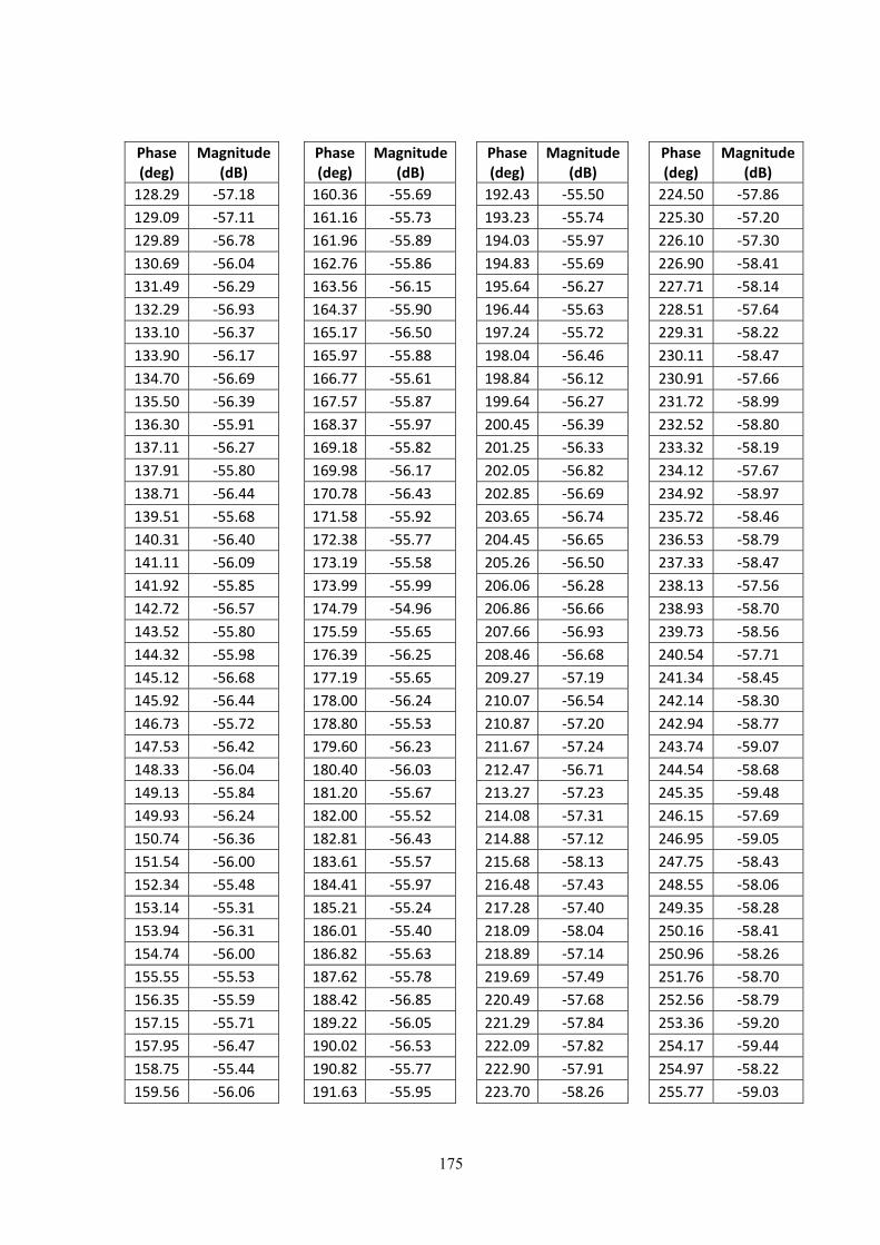
175

Phase (deg)

Magnitude (dB)

Phase (deg)

Magnitude (dB)

Phase (deg)

Magnitude (dB)

Phase (deg)

Magnitude (dB)

128.29 ‐57.18 160.36 ‐55.69 192.43 ‐55.50 224.50 ‐57.86

129.09 ‐57.11 161.16 ‐55.73 193.23 ‐55.74 225.30 ‐57.20

129.89 ‐56.78 161.96 ‐55.89 194.03 ‐55.97 226.10 ‐57.30

130.69 ‐56.04 162.76 ‐55.86 194.83 ‐55.69 226.90 ‐58.41

131.49 ‐56.29 163.56 ‐56.15 195.64 ‐56.27 227.71 ‐58.14

132.29 ‐56.93 164.37 ‐55.90 196.44 ‐55.63 228.51 ‐57.64

133.10 ‐56.37 165.17 ‐56.50 197.24 ‐55.72 229.31 ‐58.22

133.90 ‐56.17 165.97 ‐55.88 198.04 ‐56.46 230.11 ‐58.47

134.70 ‐56.69 166.77 ‐55.61 198.84 ‐56.12 230.91 ‐57.66

135.50 ‐56.39 167.57 ‐55.87 199.64 ‐56.27 231.72 ‐58.99

136.30 ‐55.91 168.37 ‐55.97 200.45 ‐56.39 232.52 ‐58.80

137.11 ‐56.27 169.18 ‐55.82 201.25 ‐56.33 233.32 ‐58.19

137.91 ‐55.80 169.98 ‐56.17 202.05 ‐56.82 234.12 ‐57.67

138.71 ‐56.44 170.78 ‐56.43 202.85 ‐56.69 234.92 ‐58.97

139.51 ‐55.68 171.58 ‐55.92 203.65 ‐56.74 235.72 ‐58.46

140.31 ‐56.40 172.38 ‐55.77 204.45 ‐56.65 236.53 ‐58.79

141.11 ‐56.09 173.19 ‐55.58 205.26 ‐56.50 237.33 ‐58.47

141.92 ‐55.85 173.99 ‐55.99 206.06 ‐56.28 238.13 ‐57.56

142.72 ‐56.57 174.79 ‐54.96 206.86 ‐56.66 238.93 ‐58.70

143.52 ‐55.80 175.59 ‐55.65 207.66 ‐56.93 239.73 ‐58.56

144.32 ‐55.98 176.39 ‐56.25 208.46 ‐56.68 240.54 ‐57.71

145.12 ‐56.68 177.19 ‐55.65 209.27 ‐57.19 241.34 ‐58.45

145.92 ‐56.44 178.00 ‐56.24 210.07 ‐56.54 242.14 ‐58.30

146.73 ‐55.72 178.80 ‐55.53 210.87 ‐57.20 242.94 ‐58.77

147.53 ‐56.42 179.60 ‐56.23 211.67 ‐57.24 243.74 ‐59.07

148.33 ‐56.04 180.40 ‐56.03 212.47 ‐56.71 244.54 ‐58.68

149.13 ‐55.84 181.20 ‐55.67 213.27 ‐57.23 245.35 ‐59.48

149.93 ‐56.24 182.00 ‐55.52 214.08 ‐57.31 246.15 ‐57.69

150.74 ‐56.36 182.81 ‐56.43 214.88 ‐57.12 246.95 ‐59.05

151.54 ‐56.00 183.61 ‐55.57 215.68 ‐58.13 247.75 ‐58.43

152.34 ‐55.48 184.41 ‐55.97 216.48 ‐57.43 248.55 ‐58.06

153.14 ‐55.31 185.21 ‐55.24 217.28 ‐57.40 249.35 ‐58.28

153.94 ‐56.31 186.01 ‐55.40 218.09 ‐58.04 250.16 ‐58.41

154.74 ‐56.00 186.82 ‐55.63 218.89 ‐57.14 250.96 ‐58.26

155.55 ‐55.53 187.62 ‐55.78 219.69 ‐57.49 251.76 ‐58.70

156.35 ‐55.59 188.42 ‐56.85 220.49 ‐57.68 252.56 ‐58.79

157.15 ‐55.71 189.22 ‐56.05 221.29 ‐57.84 253.36 ‐59.20

157.95 ‐56.47 190.02 ‐56.53 222.09 ‐57.82 254.17 ‐59.44

158.75 ‐55.44 190.82 ‐55.77 222.90 ‐57.91 254.97 ‐58.22

159.56 ‐56.06 191.63 ‐55.95 223.70 ‐58.26 255.77 ‐59.03

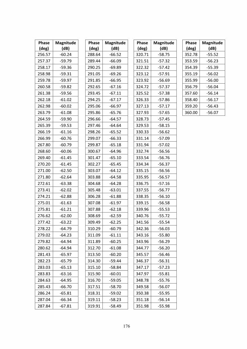
176

Phase (deg)

Magnitude (dB)

Phase (deg)

Magnitude (dB)

Phase (deg)

Magnitude (dB)

Phase (deg)

Magnitude (dB)

256.57 ‐60.24 288.64 ‐66.52 320.71 ‐58.75 352.78 ‐55.52

257.37 ‐59.79 289.44 ‐66.09 321.51 ‐57.32 353.59 ‐56.23

258.17 ‐59.36 290.25 ‐69.89 322.32 ‐57.42 354.39 ‐55.39

258.98 ‐59.31 291.05 ‐69.26 323.12 ‐57.91 355.19 ‐56.02

259.78 ‐59.97 291.85 ‐66.95 323.92 ‐56.69 355.99 ‐56.00

260.58 ‐59.82 292.65 ‐67.16 324.72 ‐57.37 356.79 ‐56.04

261.38 ‐59.56 293.45 ‐67.11 325.52 ‐57.38 357.60 ‐56.14

262.18 ‐61.02 294.25 ‐67.17 326.33 ‐57.86 358.40 ‐56.17

262.98 ‐60.02 295.06 ‐66.97 327.13 ‐57.17 359.20 ‐56.43

263.79 ‐61.08 295.86 ‐65.76 327.93 ‐57.65 360.00 ‐56.07

264.59 ‐59.90 296.66 ‐64.57 328.73 ‐57.45

265.39 ‐59.53 297.46 ‐64.64 329.53 ‐58.15

266.19 ‐61.16 298.26 ‐65.52 330.33 ‐56.62

266.99 ‐60.76 299.07 ‐66.33 331.14 ‐57.09

267.80 ‐60.79 299.87 ‐65.18 331.94 ‐57.02

268.60 ‐60.06 300.67 ‐64.96 332.74 ‐56.56

269.40 ‐61.45 301.47 ‐65.10 333.54 ‐56.76

270.20 ‐61.45 302.27 ‐65.45 334.34 ‐56.37

271.00 ‐62.50 303.07 ‐64.12 335.15 ‐56.56

271.80 ‐62.64 303.88 ‐64.58 335.95 ‐56.57

272.61 ‐63.38 304.68 ‐64.28 336.75 ‐57.16

273.41 ‐62.02 305.48 ‐63.01 337.55 ‐56.77

274.21 ‐62.88 306.28 ‐61.88 338.35 ‐56.10

275.01 ‐61.63 307.08 ‐61.97 339.15 ‐56.58

275.81 ‐61.21 307.88 ‐62.18 339.96 ‐55.53

276.62 ‐62.00 308.69 ‐62.59 340.76 ‐55.72

277.42 ‐63.22 309.49 ‐62.25 341.56 ‐55.54

278.22 ‐64.79 310.29 ‐60.79 342.36 ‐56.03

279.02 ‐64.23 311.09 ‐61.11 343.16 ‐55.80

279.82 ‐64.94 311.89 ‐60.25 343.96 ‐56.29

280.62 ‐64.94 312.70 ‐61.08 344.77 ‐56.20

281.43 ‐65.97 313.50 ‐60.20 345.57 ‐56.46

282.23 ‐65.79 314.30 ‐59.44 346.37 ‐56.31

283.03 ‐65.13 315.10 ‐58.84 347.17 ‐57.23

283.83 ‐63.16 315.90 ‐60.01 347.97 ‐55.81

284.63 ‐64.95 316.70 ‐59.05 348.78 ‐55.76

285.43 ‐66.70 317.51 ‐58.70 349.58 ‐56.07

286.24 ‐65.81 318.31 ‐59.02 350.38 ‐55.95

287.04 ‐66.34 319.11 ‐58.23 351.18 ‐56.14

287.84 ‐67.81 319.91 ‐58.49 351.98 ‐55.98

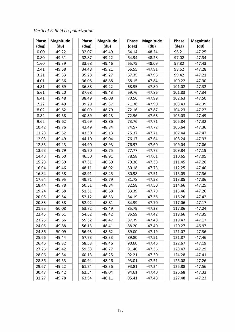
177


Phase (deg)

Magnitude (dB)

Phase (deg)

Magnitude (dB)

Phase (deg)

Magnitude (dB)

Phase (deg)

Magnitude (dB)

0.00 ‐49.22 32.07 ‐49.49 64.14 ‐48.24 96.21 ‐47.25

0.80 ‐49.31 32.87 ‐49.22 64.94 ‐48.28 97.02 ‐47.34

1.60 ‐49.39 33.68 ‐49.46 65.75 ‐48.09 97.82 ‐47.43

2.41 ‐49.58 34.48 ‐49.21 66.55 ‐47.91 98.62 ‐47.28

3.21 ‐49.33 35.28 ‐49.27 67.35 ‐47.96 99.42 ‐47.21

4.01 ‐49.36 36.08 ‐48.88 68.15 ‐47.84 100.22 ‐47.30

4.81 ‐49.69 36.88 ‐49.22 68.95 ‐47.80 101.02 ‐47.32

5.61 ‐49.20 37.68 ‐49.43 69.76 ‐47.86 101.83 ‐47.34

6.41 ‐49.48 38.49 ‐49.08 70.56 ‐47.99 102.63 ‐47.50

7.22 ‐49.49 39.29 ‐49.37 71.36 ‐47.90 103.43 ‐47.35

8.02 ‐49.62 40.09 ‐48.79 72.16 ‐47.87 104.23 ‐47.22

8.82 ‐49.58 40.89 ‐49.23 72.96 ‐47.68 105.03 ‐47.49

9.62 ‐49.62 41.69 ‐48.86 73.76 ‐47.71 105.84 ‐47.32

10.42 ‐49.76 42.49 ‐48.84 74.57 ‐47.72 106.64 ‐47.36

11.23 ‐49.52 43.30 ‐49.13 75.37 ‐47.71 107.44 ‐47.47

12.03 ‐49.49 44.10 ‐49.04 76.17 ‐47.64 108.24 ‐47.33

12.83 ‐49.43 44.90 ‐48.93 76.97 ‐47.60 109.04 ‐47.06

13.63 ‐49.79 45.70 ‐48.75 77.77 ‐47.73 109.84 ‐47.19

14.43 ‐49.60 46.50 ‐48.91 78.58 ‐47.61 110.65 ‐47.05

15.23 ‐49.39 47.31 ‐48.69 79.38 ‐47.38 111.45 ‐47.20

16.04 ‐49.46 48.11 ‐48.92 80.18 ‐47.73 112.25 ‐47.40

16.84 ‐49.58 48.91 ‐48.45 80.98 ‐47.51 113.05 ‐47.36

17.64 ‐49.95 49.71 ‐48.79 81.78 ‐47.58 113.85 ‐47.36

18.44 ‐49.78 50.51 ‐48.84 82.58 ‐47.50 114.66 ‐47.25

19.24 ‐49.68 51.31 ‐48.68 83.39 ‐47.79 115.46 ‐47.26

20.05 ‐49.54 52.12 ‐48.53 84.19 ‐47.38 116.26 ‐47.42

20.85 ‐49.58 52.92 ‐48.81 84.99 ‐47.70 117.06 ‐47.17

21.65 ‐50.08 53.72 ‐48.49 85.79 ‐47.33 117.86 ‐47.24

22.45 ‐49.61 54.52 ‐48.42 86.59 ‐47.42 118.66 ‐47.35

23.25 ‐49.66 55.32 ‐48.47 87.39 ‐47.48 119.47 ‐47.17

24.05 ‐49.88 56.13 ‐48.41 88.20 ‐47.40 120.27 ‐46.97

24.86 ‐50.09 56.93 ‐48.62 89.00 ‐47.19 121.07 ‐47.36

25.66 ‐49.44 57.73 ‐48.33 89.80 ‐47.51 121.87 ‐47.46

26.46 ‐49.32 58.53 ‐48.46 90.60 ‐47.46 122.67 ‐47.19

27.26 ‐49.42 59.33 ‐48.77 91.40 ‐47.36 123.47 ‐47.29

28.06 ‐49.54 60.13 ‐48.25 92.21 ‐47.30 124.28 ‐47.41

28.86 ‐49.53 60.94 ‐48.26 93.01 ‐47.51 125.08 ‐47.26

29.67 ‐49.22 61.74 ‐48.36 93.81 ‐47.24 125.88 ‐47.56

30.47 ‐49.42 62.54 ‐48.04 94.61 ‐47.40 126.68 ‐47.33

31.27 ‐49.78 63.34 ‐48.11 95.41 ‐47.48 127.48 ‐47.23

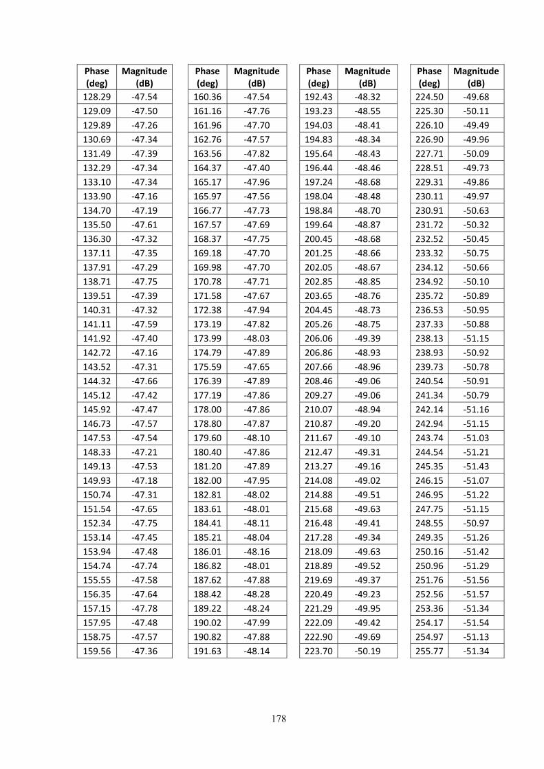
178

Phase (deg)

Magnitude (dB)

Phase (deg)

Magnitude (dB)

Phase (deg)

Magnitude (dB)

Phase (deg)

Magnitude (dB)

128.29 ‐47.54 160.36 ‐47.54 192.43 ‐48.32 224.50 ‐49.68

129.09 ‐47.50 161.16 ‐47.76 193.23 ‐48.55 225.30 ‐50.11

129.89 ‐47.26 161.96 ‐47.70 194.03 ‐48.41 226.10 ‐49.49

130.69 ‐47.34 162.76 ‐47.57 194.83 ‐48.34 226.90 ‐49.96

131.49 ‐47.39 163.56 ‐47.82 195.64 ‐48.43 227.71 ‐50.09

132.29 ‐47.34 164.37 ‐47.40 196.44 ‐48.46 228.51 ‐49.73

133.10 ‐47.34 165.17 ‐47.96 197.24 ‐48.68 229.31 ‐49.86

133.90 ‐47.16 165.97 ‐47.56 198.04 ‐48.48 230.11 ‐49.97

134.70 ‐47.19 166.77 ‐47.73 198.84 ‐48.70 230.91 ‐50.63

135.50 ‐47.61 167.57 ‐47.69 199.64 ‐48.87 231.72 ‐50.32

136.30 ‐47.32 168.37 ‐47.75 200.45 ‐48.68 232.52 ‐50.45

137.11 ‐47.35 169.18 ‐47.70 201.25 ‐48.66 233.32 ‐50.75

137.91 ‐47.29 169.98 ‐47.70 202.05 ‐48.67 234.12 ‐50.66

138.71 ‐47.75 170.78 ‐47.71 202.85 ‐48.85 234.92 ‐50.10

139.51 ‐47.39 171.58 ‐47.67 203.65 ‐48.76 235.72 ‐50.89

140.31 ‐47.32 172.38 ‐47.94 204.45 ‐48.73 236.53 ‐50.95

141.11 ‐47.59 173.19 ‐47.82 205.26 ‐48.75 237.33 ‐50.88

141.92 ‐47.40 173.99 ‐48.03 206.06 ‐49.39 238.13 ‐51.15

142.72 ‐47.16 174.79 ‐47.89 206.86 ‐48.93 238.93 ‐50.92

143.52 ‐47.31 175.59 ‐47.65 207.66 ‐48.96 239.73 ‐50.78

144.32 ‐47.66 176.39 ‐47.89 208.46 ‐49.06 240.54 ‐50.91

145.12 ‐47.42 177.19 ‐47.86 209.27 ‐49.06 241.34 ‐50.79

145.92 ‐47.47 178.00 ‐47.86 210.07 ‐48.94 242.14 ‐51.16

146.73 ‐47.57 178.80 ‐47.87 210.87 ‐49.20 242.94 ‐51.15

147.53 ‐47.54 179.60 ‐48.10 211.67 ‐49.10 243.74 ‐51.03

148.33 ‐47.21 180.40 ‐47.86 212.47 ‐49.31 244.54 ‐51.21

149.13 ‐47.53 181.20 ‐47.89 213.27 ‐49.16 245.35 ‐51.43

149.93 ‐47.18 182.00 ‐47.95 214.08 ‐49.02 246.15 ‐51.07

150.74 ‐47.31 182.81 ‐48.02 214.88 ‐49.51 246.95 ‐51.22

151.54 ‐47.65 183.61 ‐48.01 215.68 ‐49.63 247.75 ‐51.15

152.34 ‐47.75 184.41 ‐48.11 216.48 ‐49.41 248.55 ‐50.97

153.14 ‐47.45 185.21 ‐48.04 217.28 ‐49.34 249.35 ‐51.26

153.94 ‐47.48 186.01 ‐48.16 218.09 ‐49.63 250.16 ‐51.42

154.74 ‐47.74 186.82 ‐48.01 218.89 ‐49.52 250.96 ‐51.29

155.55 ‐47.58 187.62 ‐47.88 219.69 ‐49.37 251.76 ‐51.56

156.35 ‐47.64 188.42 ‐48.28 220.49 ‐49.23 252.56 ‐51.57

157.15 ‐47.78 189.22 ‐48.24 221.29 ‐49.95 253.36 ‐51.34

157.95 ‐47.48 190.02 ‐47.99 222.09 ‐49.42 254.17 ‐51.54

158.75 ‐47.57 190.82 ‐47.88 222.90 ‐49.69 254.97 ‐51.13

159.56 ‐47.36 191.63 ‐48.14 223.70 ‐50.19 255.77 ‐51.34

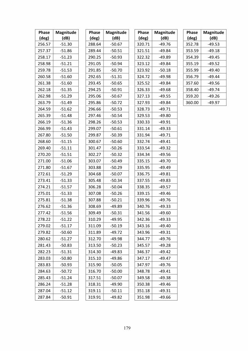
179

Phase (deg)

Magnitude (dB)

Phase (deg)

Magnitude (dB)

Phase (deg)

Magnitude (dB)

Phase (deg)

Magnitude (dB)

256.57 ‐51.30 288.64 ‐50.67 320.71 ‐49.76 352.78 ‐49.53

257.37 ‐51.86 289.44 ‐50.51 321.51 ‐49.84 353.59 ‐49.18

258.17 ‐51.23 290.25 ‐50.93 322.32 ‐49.89 354.39 ‐49.45

258.98 ‐51.21 291.05 ‐50.94 323.12 ‐49.84 355.19 ‐49.52

259.78 ‐51.53 291.85 ‐50.70 323.92 ‐50.18 355.99 ‐49.40

260.58 ‐51.60 292.65 ‐51.31 324.72 ‐49.98 356.79 ‐49.44

261.38 ‐51.60 293.45 ‐50.65 325.52 ‐49.84 357.60 ‐49.56

262.18 ‐51.35 294.25 ‐50.91 326.33 ‐49.68 358.40 ‐49.74

262.98 ‐51.29 295.06 ‐50.67 327.13 ‐49.55 359.20 ‐49.26

263.79 ‐51.49 295.86 ‐50.72 327.93 ‐49.84 360.00 ‐49.97

264.59 ‐51.62 296.66 ‐50.53 328.73 ‐49.71

265.39 ‐51.48 297.46 ‐50.54 329.53 ‐49.80

266.19 ‐51.36 298.26 ‐50.53 330.33 ‐49.91

266.99 ‐51.43 299.07 ‐50.61 331.14 ‐49.33

267.80 ‐51.50 299.87 ‐50.39 331.94 ‐49.71

268.60 ‐51.15 300.67 ‐50.60 332.74 ‐49.41

269.40 ‐51.11 301.47 ‐50.26 333.54 ‐49.32

270.20 ‐51.51 302.27 ‐50.32 334.34 ‐49.56

271.00 ‐51.06 303.07 ‐50.49 335.15 ‐49.70

271.80 ‐51.67 303.88 ‐50.29 335.95 ‐49.49

272.61 ‐51.29 304.68 ‐50.07 336.75 ‐49.81

273.41 ‐51.33 305.48 ‐50.34 337.55 ‐49.83

274.21 ‐51.57 306.28 ‐50.04 338.35 ‐49.57

275.01 ‐51.33 307.08 ‐50.26 339.15 ‐49.46

275.81 ‐51.38 307.88 ‐50.21 339.96 ‐49.76

276.62 ‐51.36 308.69 ‐49.89 340.76 ‐49.33

277.42 ‐51.56 309.49 ‐50.31 341.56 ‐49.60

278.22 ‐51.22 310.29 ‐49.95 342.36 ‐49.33

279.02 ‐51.17 311.09 ‐50.19 343.16 ‐49.40

279.82 ‐50.60 311.89 ‐49.72 343.96 ‐49.31

280.62 ‐51.27 312.70 ‐49.98 344.77 ‐49.76

281.43 ‐50.83 313.50 ‐50.23 345.57 ‐49.28

282.23 ‐51.31 314.30 ‐49.83 346.37 ‐49.42

283.03 ‐50.80 315.10 ‐49.86 347.17 ‐49.47

283.83 ‐50.93 315.90 ‐50.05 347.97 ‐49.76

284.63 ‐50.72 316.70 ‐50.00 348.78 ‐49.41

285.43 ‐51.24 317.51 ‐50.07 349.58 ‐49.38

286.24 ‐51.28 318.31 ‐49.90 350.38 ‐49.46

287.04 ‐51.12 319.11 ‐50.11 351.18 ‐49.31

287.84 ‐50.91 319.91 ‐49.82 351.98 ‐49.66

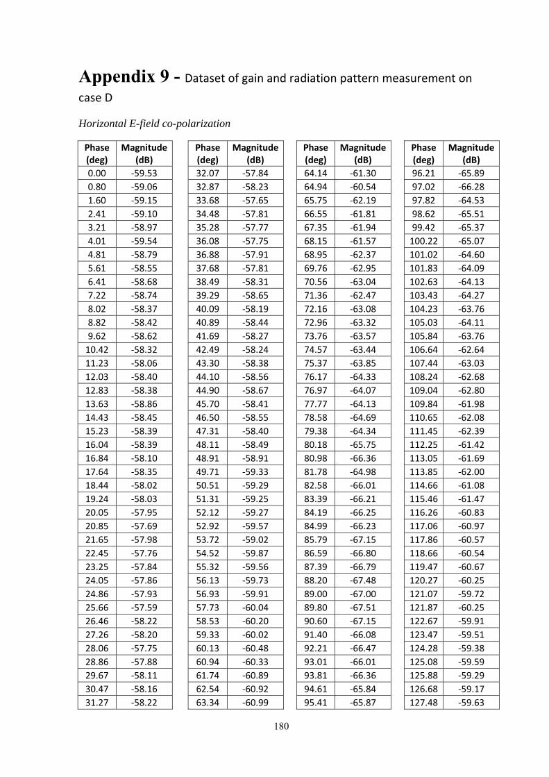
180

Appendix 9 - Dataset of gain and radiation pattern measurement on

case D Horizontal E-field co-polarization

Phase (deg)

Magnitude (dB)

Phase (deg)

Magnitude (dB)

Phase (deg)

Magnitude (dB)

Phase (deg)

Magnitude (dB)

0.00 ‐59.53 32.07 ‐57.84 64.14 ‐61.30 96.21 ‐65.89

0.80 ‐59.06 32.87 ‐58.23 64.94 ‐60.54 97.02 ‐66.28

1.60 ‐59.15 33.68 ‐57.65 65.75 ‐62.19 97.82 ‐64.53

2.41 ‐59.10 34.48 ‐57.81 66.55 ‐61.81 98.62 ‐65.51

3.21 ‐58.97 35.28 ‐57.77 67.35 ‐61.94 99.42 ‐65.37

4.01 ‐59.54 36.08 ‐57.75 68.15 ‐61.57 100.22 ‐65.07

4.81 ‐58.79 36.88 ‐57.91 68.95 ‐62.37 101.02 ‐64.60

5.61 ‐58.55 37.68 ‐57.81 69.76 ‐62.95 101.83 ‐64.09

6.41 ‐58.68 38.49 ‐58.31 70.56 ‐63.04 102.63 ‐64.13

7.22 ‐58.74 39.29 ‐58.65 71.36 ‐62.47 103.43 ‐64.27

8.02 ‐58.37 40.09 ‐58.19 72.16 ‐63.08 104.23 ‐63.76

8.82 ‐58.42 40.89 ‐58.44 72.96 ‐63.32 105.03 ‐64.11

9.62 ‐58.62 41.69 ‐58.27 73.76 ‐63.57 105.84 ‐63.76

10.42 ‐58.32 42.49 ‐58.24 74.57 ‐63.44 106.64 ‐62.64

11.23 ‐58.06 43.30 ‐58.38 75.37 ‐63.85 107.44 ‐63.03

12.03 ‐58.40 44.10 ‐58.56 76.17 ‐64.33 108.24 ‐62.68

12.83 ‐58.38 44.90 ‐58.67 76.97 ‐64.07 109.04 ‐62.80

13.63 ‐58.86 45.70 ‐58.41 77.77 ‐64.13 109.84 ‐61.98

14.43 ‐58.45 46.50 ‐58.55 78.58 ‐64.69 110.65 ‐62.08

15.23 ‐58.39 47.31 ‐58.40 79.38 ‐64.34 111.45 ‐62.39

16.04 ‐58.39 48.11 ‐58.49 80.18 ‐65.75 112.25 ‐61.42

16.84 ‐58.10 48.91 ‐58.91 80.98 ‐66.36 113.05 ‐61.69

17.64 ‐58.35 49.71 ‐59.33 81.78 ‐64.98 113.85 ‐62.00

18.44 ‐58.02 50.51 ‐59.29 82.58 ‐66.01 114.66 ‐61.08

19.24 ‐58.03 51.31 ‐59.25 83.39 ‐66.21 115.46 ‐61.47

20.05 ‐57.95 52.12 ‐59.27 84.19 ‐66.25 116.26 ‐60.83

20.85 ‐57.69 52.92 ‐59.57 84.99 ‐66.23 117.06 ‐60.97

21.65 ‐57.98 53.72 ‐59.02 85.79 ‐67.15 117.86 ‐60.57

22.45 ‐57.76 54.52 ‐59.87 86.59 ‐66.80 118.66 ‐60.54

23.25 ‐57.84 55.32 ‐59.56 87.39 ‐66.79 119.47 ‐60.67

24.05 ‐57.86 56.13 ‐59.73 88.20 ‐67.48 120.27 ‐60.25

24.86 ‐57.93 56.93 ‐59.91 89.00 ‐67.00 121.07 ‐59.72

25.66 ‐57.59 57.73 ‐60.04 89.80 ‐67.51 121.87 ‐60.25

26.46 ‐58.22 58.53 ‐60.20 90.60 ‐67.15 122.67 ‐59.91

27.26 ‐58.20 59.33 ‐60.02 91.40 ‐66.08 123.47 ‐59.51

28.06 ‐57.75 60.13 ‐60.48 92.21 ‐66.47 124.28 ‐59.38

28.86 ‐57.88 60.94 ‐60.33 93.01 ‐66.01 125.08 ‐59.59

29.67 ‐58.11 61.74 ‐60.89 93.81 ‐66.36 125.88 ‐59.29

30.47 ‐58.16 62.54 ‐60.92 94.61 ‐65.84 126.68 ‐59.17

31.27 ‐58.22 63.34 ‐60.99 95.41 ‐65.87 127.48 ‐59.63

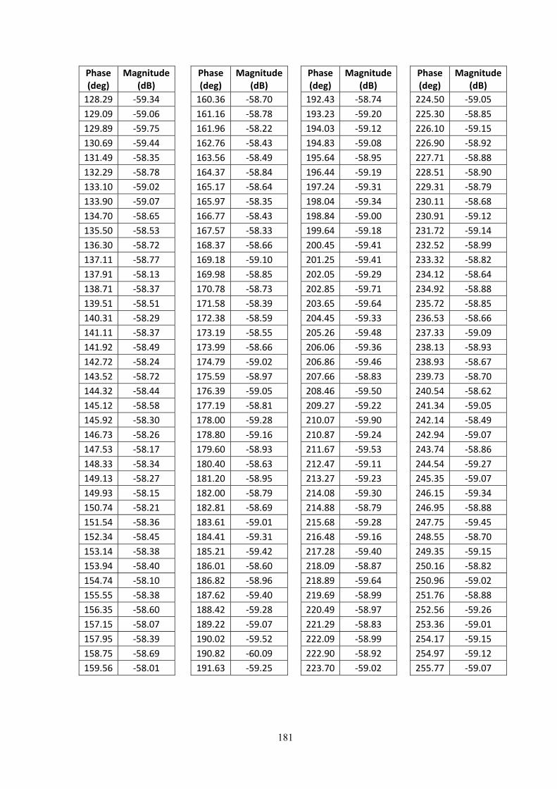
181

Phase (deg)

Magnitude (dB)

Phase (deg)

Magnitude (dB)

Phase (deg)

Magnitude (dB)

Phase (deg)

Magnitude (dB)

128.29 ‐59.34 160.36 ‐58.70 192.43 ‐58.74 224.50 ‐59.05

129.09 ‐59.06 161.16 ‐58.78 193.23 ‐59.20 225.30 ‐58.85

129.89 ‐59.75 161.96 ‐58.22 194.03 ‐59.12 226.10 ‐59.15

130.69 ‐59.44 162.76 ‐58.43 194.83 ‐59.08 226.90 ‐58.92

131.49 ‐58.35 163.56 ‐58.49 195.64 ‐58.95 227.71 ‐58.88

132.29 ‐58.78 164.37 ‐58.84 196.44 ‐59.19 228.51 ‐58.90

133.10 ‐59.02 165.17 ‐58.64 197.24 ‐59.31 229.31 ‐58.79

133.90 ‐59.07 165.97 ‐58.35 198.04 ‐59.34 230.11 ‐58.68

134.70 ‐58.65 166.77 ‐58.43 198.84 ‐59.00 230.91 ‐59.12

135.50 ‐58.53 167.57 ‐58.33 199.64 ‐59.18 231.72 ‐59.14

136.30 ‐58.72 168.37 ‐58.66 200.45 ‐59.41 232.52 ‐58.99

137.11 ‐58.77 169.18 ‐59.10 201.25 ‐59.41 233.32 ‐58.82

137.91 ‐58.13 169.98 ‐58.85 202.05 ‐59.29 234.12 ‐58.64

138.71 ‐58.37 170.78 ‐58.73 202.85 ‐59.71 234.92 ‐58.88

139.51 ‐58.51 171.58 ‐58.39 203.65 ‐59.64 235.72 ‐58.85

140.31 ‐58.29 172.38 ‐58.59 204.45 ‐59.33 236.53 ‐58.66

141.11 ‐58.37 173.19 ‐58.55 205.26 ‐59.48 237.33 ‐59.09

141.92 ‐58.49 173.99 ‐58.66 206.06 ‐59.36 238.13 ‐58.93

142.72 ‐58.24 174.79 ‐59.02 206.86 ‐59.46 238.93 ‐58.67

143.52 ‐58.72 175.59 ‐58.97 207.66 ‐58.83 239.73 ‐58.70

144.32 ‐58.44 176.39 ‐59.05 208.46 ‐59.50 240.54 ‐58.62

145.12 ‐58.58 177.19 ‐58.81 209.27 ‐59.22 241.34 ‐59.05

145.92 ‐58.30 178.00 ‐59.28 210.07 ‐59.90 242.14 ‐58.49

146.73 ‐58.26 178.80 ‐59.16 210.87 ‐59.24 242.94 ‐59.07

147.53 ‐58.17 179.60 ‐58.93 211.67 ‐59.53 243.74 ‐58.86

148.33 ‐58.34 180.40 ‐58.63 212.47 ‐59.11 244.54 ‐59.27

149.13 ‐58.27 181.20 ‐58.95 213.27 ‐59.23 245.35 ‐59.07

149.93 ‐58.15 182.00 ‐58.79 214.08 ‐59.30 246.15 ‐59.34

150.74 ‐58.21 182.81 ‐58.69 214.88 ‐58.79 246.95 ‐58.88

151.54 ‐58.36 183.61 ‐59.01 215.68 ‐59.28 247.75 ‐59.45

152.34 ‐58.45 184.41 ‐59.31 216.48 ‐59.16 248.55 ‐58.70

153.14 ‐58.38 185.21 ‐59.42 217.28 ‐59.40 249.35 ‐59.15

153.94 ‐58.40 186.01 ‐58.60 218.09 ‐58.87 250.16 ‐58.82

154.74 ‐58.10 186.82 ‐58.96 218.89 ‐59.64 250.96 ‐59.02

155.55 ‐58.38 187.62 ‐59.40 219.69 ‐58.99 251.76 ‐58.88

156.35 ‐58.60 188.42 ‐59.28 220.49 ‐58.97 252.56 ‐59.26

157.15 ‐58.07 189.22 ‐59.07 221.29 ‐58.83 253.36 ‐59.01

157.95 ‐58.39 190.02 ‐59.52 222.09 ‐58.99 254.17 ‐59.15

158.75 ‐58.69 190.82 ‐60.09 222.90 ‐58.92 254.97 ‐59.12

159.56 ‐58.01 191.63 ‐59.25 223.70 ‐59.02 255.77 ‐59.07

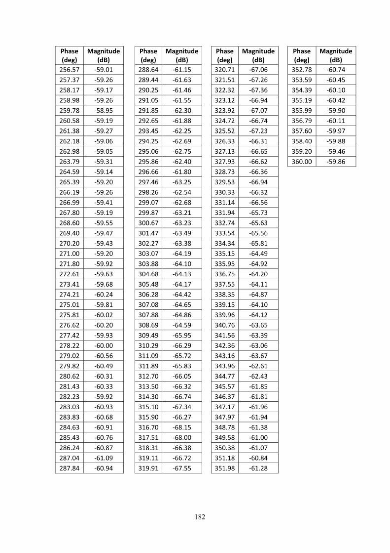
182

Phase (deg)

Magnitude (dB)

Phase (deg)

Magnitude (dB)

Phase (deg)

Magnitude (dB)

Phase (deg)

Magnitude (dB)

256.57 ‐59.01 288.64 ‐61.15 320.71 ‐67.06 352.78 ‐60.74

257.37 ‐59.26 289.44 ‐61.63 321.51 ‐67.26 353.59 ‐60.45

258.17 ‐59.17 290.25 ‐61.46 322.32 ‐67.36 354.39 ‐60.10

258.98 ‐59.26 291.05 ‐61.55 323.12 ‐66.94 355.19 ‐60.42

259.78 ‐58.95 291.85 ‐62.30 323.92 ‐67.07 355.99 ‐59.90

260.58 ‐59.19 292.65 ‐61.88 324.72 ‐66.74 356.79 ‐60.11

261.38 ‐59.27 293.45 ‐62.25 325.52 ‐67.23 357.60 ‐59.97

262.18 ‐59.06 294.25 ‐62.69 326.33 ‐66.31 358.40 ‐59.88

262.98 ‐59.05 295.06 ‐62.75 327.13 ‐66.65 359.20 ‐59.46

263.79 ‐59.31 295.86 ‐62.40 327.93 ‐66.62 360.00 ‐59.86

264.59 ‐59.14 296.66 ‐61.80 328.73 ‐66.36

265.39 ‐59.20 297.46 ‐63.25 329.53 ‐66.94

266.19 ‐59.26 298.26 ‐62.54 330.33 ‐66.32

266.99 ‐59.41 299.07 ‐62.68 331.14 ‐66.56

267.80 ‐59.19 299.87 ‐63.21 331.94 ‐65.73

268.60 ‐59.55 300.67 ‐63.23 332.74 ‐65.63

269.40 ‐59.47 301.47 ‐63.49 333.54 ‐65.56

270.20 ‐59.43 302.27 ‐63.38 334.34 ‐65.81

271.00 ‐59.20 303.07 ‐64.19 335.15 ‐64.49

271.80 ‐59.92 303.88 ‐64.10 335.95 ‐64.92

272.61 ‐59.63 304.68 ‐64.13 336.75 ‐64.20

273.41 ‐59.68 305.48 ‐64.17 337.55 ‐64.11

274.21 ‐60.24 306.28 ‐64.42 338.35 ‐64.87

275.01 ‐59.81 307.08 ‐64.65 339.15 ‐64.10

275.81 ‐60.02 307.88 ‐64.86 339.96 ‐64.12

276.62 ‐60.20 308.69 ‐64.59 340.76 ‐63.65

277.42 ‐59.93 309.49 ‐65.95 341.56 ‐63.39

278.22 ‐60.00 310.29 ‐66.29 342.36 ‐63.06

279.02 ‐60.56 311.09 ‐65.72 343.16 ‐63.67

279.82 ‐60.49 311.89 ‐65.83 343.96 ‐62.61

280.62 ‐60.31 312.70 ‐66.05 344.77 ‐62.43

281.43 ‐60.33 313.50 ‐66.32 345.57 ‐61.85

282.23 ‐59.92 314.30 ‐66.74 346.37 ‐61.81

283.03 ‐60.93 315.10 ‐67.34 347.17 ‐61.96

283.83 ‐60.68 315.90 ‐66.27 347.97 ‐61.94

284.63 ‐60.91 316.70 ‐68.15 348.78 ‐61.38

285.43 ‐60.76 317.51 ‐68.00 349.58 ‐61.00

286.24 ‐60.87 318.31 ‐66.38 350.38 ‐61.07

287.04 ‐61.09 319.11 ‐66.72 351.18 ‐60.84

287.84 ‐60.94 319.91 ‐67.55 351.98 ‐61.28

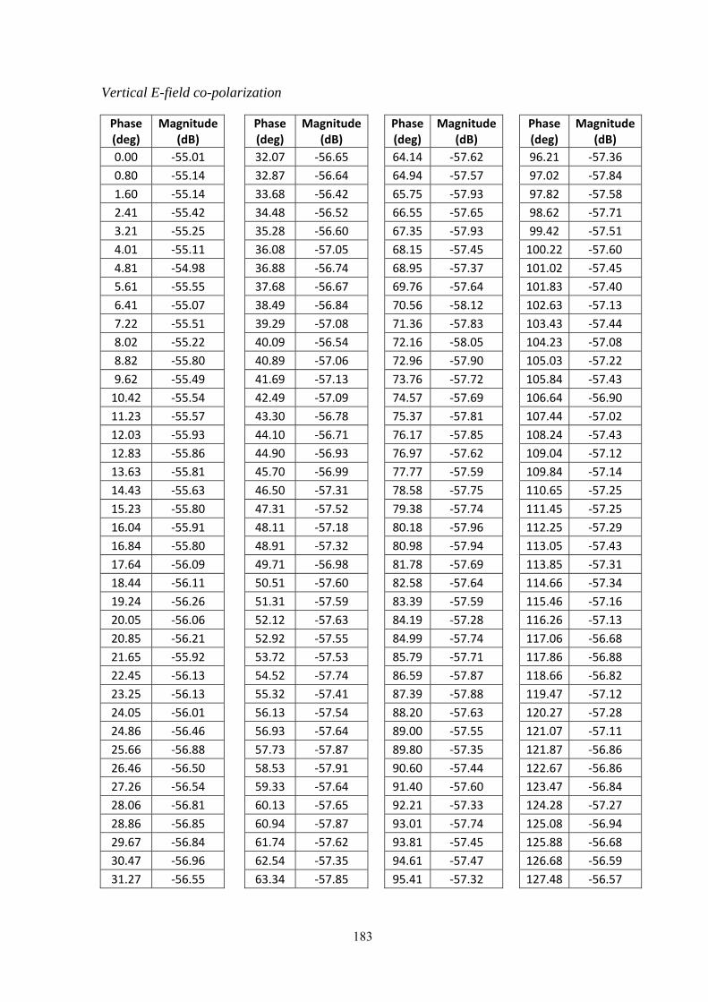
183


Phase (deg)

Magnitude (dB)

Phase (deg)

Magnitude (dB)

Phase (deg)

Magnitude (dB)

Phase (deg)

Magnitude (dB)

0.00 ‐55.01 32.07 ‐56.65 64.14 ‐57.62 96.21 ‐57.36

0.80 ‐55.14 32.87 ‐56.64 64.94 ‐57.57 97.02 ‐57.84

1.60 ‐55.14 33.68 ‐56.42 65.75 ‐57.93 97.82 ‐57.58

2.41 ‐55.42 34.48 ‐56.52 66.55 ‐57.65 98.62 ‐57.71

3.21 ‐55.25 35.28 ‐56.60 67.35 ‐57.93 99.42 ‐57.51

4.01 ‐55.11 36.08 ‐57.05 68.15 ‐57.45 100.22 ‐57.60

4.81 ‐54.98 36.88 ‐56.74 68.95 ‐57.37 101.02 ‐57.45

5.61 ‐55.55 37.68 ‐56.67 69.76 ‐57.64 101.83 ‐57.40

6.41 ‐55.07 38.49 ‐56.84 70.56 ‐58.12 102.63 ‐57.13

7.22 ‐55.51 39.29 ‐57.08 71.36 ‐57.83 103.43 ‐57.44

8.02 ‐55.22 40.09 ‐56.54 72.16 ‐58.05 104.23 ‐57.08

8.82 ‐55.80 40.89 ‐57.06 72.96 ‐57.90 105.03 ‐57.22

9.62 ‐55.49 41.69 ‐57.13 73.76 ‐57.72 105.84 ‐57.43

10.42 ‐55.54 42.49 ‐57.09 74.57 ‐57.69 106.64 ‐56.90

11.23 ‐55.57 43.30 ‐56.78 75.37 ‐57.81 107.44 ‐57.02

12.03 ‐55.93 44.10 ‐56.71 76.17 ‐57.85 108.24 ‐57.43

12.83 ‐55.86 44.90 ‐56.93 76.97 ‐57.62 109.04 ‐57.12

13.63 ‐55.81 45.70 ‐56.99 77.77 ‐57.59 109.84 ‐57.14

14.43 ‐55.63 46.50 ‐57.31 78.58 ‐57.75 110.65 ‐57.25

15.23 ‐55.80 47.31 ‐57.52 79.38 ‐57.74 111.45 ‐57.25

16.04 ‐55.91 48.11 ‐57.18 80.18 ‐57.96 112.25 ‐57.29

16.84 ‐55.80 48.91 ‐57.32 80.98 ‐57.94 113.05 ‐57.43

17.64 ‐56.09 49.71 ‐56.98 81.78 ‐57.69 113.85 ‐57.31

18.44 ‐56.11 50.51 ‐57.60 82.58 ‐57.64 114.66 ‐57.34

19.24 ‐56.26 51.31 ‐57.59 83.39 ‐57.59 115.46 ‐57.16

20.05 ‐56.06 52.12 ‐57.63 84.19 ‐57.28 116.26 ‐57.13

20.85 ‐56.21 52.92 ‐57.55 84.99 ‐57.74 117.06 ‐56.68

21.65 ‐55.92 53.72 ‐57.53 85.79 ‐57.71 117.86 ‐56.88

22.45 ‐56.13 54.52 ‐57.74 86.59 ‐57.87 118.66 ‐56.82

23.25 ‐56.13 55.32 ‐57.41 87.39 ‐57.88 119.47 ‐57.12

24.05 ‐56.01 56.13 ‐57.54 88.20 ‐57.63 120.27 ‐57.28

24.86 ‐56.46 56.93 ‐57.64 89.00 ‐57.55 121.07 ‐57.11

25.66 ‐56.88 57.73 ‐57.87 89.80 ‐57.35 121.87 ‐56.86

26.46 ‐56.50 58.53 ‐57.91 90.60 ‐57.44 122.67 ‐56.86

27.26 ‐56.54 59.33 ‐57.64 91.40 ‐57.60 123.47 ‐56.84

28.06 ‐56.81 60.13 ‐57.65 92.21 ‐57.33 124.28 ‐57.27

28.86 ‐56.85 60.94 ‐57.87 93.01 ‐57.74 125.08 ‐56.94

29.67 ‐56.84 61.74 ‐57.62 93.81 ‐57.45 125.88 ‐56.68

30.47 ‐56.96 62.54 ‐57.35 94.61 ‐57.47 126.68 ‐56.59

31.27 ‐56.55 63.34 ‐57.85 95.41 ‐57.32 127.48 ‐56.57

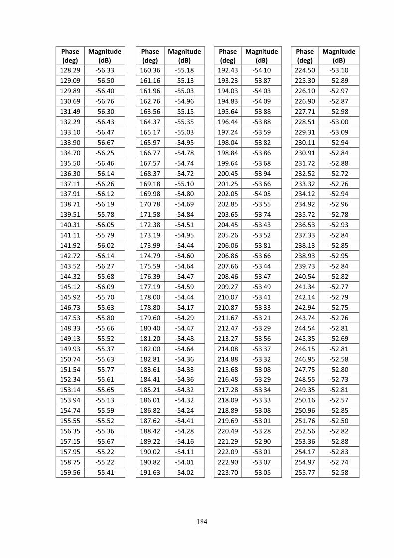
184

Phase (deg)

Magnitude (dB)

Phase (deg)

Magnitude (dB)

Phase (deg)

Magnitude (dB)

Phase (deg)

Magnitude (dB)

128.29 ‐56.33 160.36 ‐55.18 192.43 ‐54.10 224.50 ‐53.10

129.09 ‐56.50 161.16 ‐55.13 193.23 ‐53.87 225.30 ‐52.89

129.89 ‐56.40 161.96 ‐55.03 194.03 ‐54.03 226.10 ‐52.97

130.69 ‐56.76 162.76 ‐54.96 194.83 ‐54.09 226.90 ‐52.87

131.49 ‐56.30 163.56 ‐55.15 195.64 ‐53.88 227.71 ‐52.98

132.29 ‐56.43 164.37 ‐55.35 196.44 ‐53.88 228.51 ‐53.00

133.10 ‐56.47 165.17 ‐55.03 197.24 ‐53.59 229.31 ‐53.09

133.90 ‐56.67 165.97 ‐54.95 198.04 ‐53.82 230.11 ‐52.94

134.70 ‐56.25 166.77 ‐54.78 198.84 ‐53.86 230.91 ‐52.84

135.50 ‐56.46 167.57 ‐54.74 199.64 ‐53.68 231.72 ‐52.88

136.30 ‐56.14 168.37 ‐54.72 200.45 ‐53.94 232.52 ‐52.72

137.11 ‐56.26 169.18 ‐55.10 201.25 ‐53.66 233.32 ‐52.76

137.91 ‐56.12 169.98 ‐54.80 202.05 ‐54.05 234.12 ‐52.94

138.71 ‐56.19 170.78 ‐54.69 202.85 ‐53.55 234.92 ‐52.96

139.51 ‐55.78 171.58 ‐54.84 203.65 ‐53.74 235.72 ‐52.78

140.31 ‐56.05 172.38 ‐54.51 204.45 ‐53.43 236.53 ‐52.93

141.11 ‐55.79 173.19 ‐54.95 205.26 ‐53.52 237.33 ‐52.84

141.92 ‐56.02 173.99 ‐54.44 206.06 ‐53.81 238.13 ‐52.85

142.72 ‐56.14 174.79 ‐54.60 206.86 ‐53.66 238.93 ‐52.95

143.52 ‐56.27 175.59 ‐54.64 207.66 ‐53.44 239.73 ‐52.84

144.32 ‐55.68 176.39 ‐54.47 208.46 ‐53.47 240.54 ‐52.82

145.12 ‐56.09 177.19 ‐54.59 209.27 ‐53.49 241.34 ‐52.77

145.92 ‐55.70 178.00 ‐54.44 210.07 ‐53.41 242.14 ‐52.79

146.73 ‐55.63 178.80 ‐54.17 210.87 ‐53.33 242.94 ‐52.75

147.53 ‐55.80 179.60 ‐54.29 211.67 ‐53.21 243.74 ‐52.76

148.33 ‐55.66 180.40 ‐54.47 212.47 ‐53.29 244.54 ‐52.81

149.13 ‐55.52 181.20 ‐54.48 213.27 ‐53.56 245.35 ‐52.69

149.93 ‐55.37 182.00 ‐54.64 214.08 ‐53.37 246.15 ‐52.81

150.74 ‐55.63 182.81 ‐54.36 214.88 ‐53.32 246.95 ‐52.58

151.54 ‐55.77 183.61 ‐54.33 215.68 ‐53.08 247.75 ‐52.80

152.34 ‐55.61 184.41 ‐54.36 216.48 ‐53.29 248.55 ‐52.73

153.14 ‐55.65 185.21 ‐54.32 217.28 ‐53.34 249.35 ‐52.81

153.94 ‐55.13 186.01 ‐54.32 218.09 ‐53.33 250.16 ‐52.57

154.74 ‐55.59 186.82 ‐54.24 218.89 ‐53.08 250.96 ‐52.85

155.55 ‐55.52 187.62 ‐54.41 219.69 ‐53.01 251.76 ‐52.50

156.35 ‐55.36 188.42 ‐54.28 220.49 ‐53.28 252.56 ‐52.82

157.15 ‐55.67 189.22 ‐54.16 221.29 ‐52.90 253.36 ‐52.88

157.95 ‐55.22 190.02 ‐54.11 222.09 ‐53.01 254.17 ‐52.83

158.75 ‐55.22 190.82 ‐54.01 222.90 ‐53.07 254.97 ‐52.74

159.56 ‐55.41 191.63 ‐54.02 223.70 ‐53.05 255.77 ‐52.58

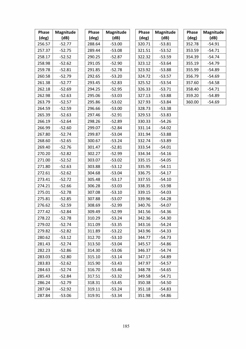
185

Phase (deg)

Magnitude (dB)

Phase (deg)

Magnitude (dB)

Phase (deg)

Magnitude (dB)

Phase (deg)

Magnitude (dB)

256.57 ‐52.77 288.64 ‐53.00 320.71 ‐53.81 352.78 ‐54.91

257.37 ‐52.75 289.44 ‐53.08 321.51 ‐53.52 353.59 ‐54.71

258.17 ‐52.52 290.25 ‐52.87 322.32 ‐53.59 354.39 ‐54.74

258.98 ‐52.62 291.05 ‐52.90 323.12 ‐53.64 355.19 ‐54.79

259.78 ‐52.81 291.85 ‐52.78 323.92 ‐53.88 355.99 ‐54.89

260.58 ‐52.79 292.65 ‐53.20 324.72 ‐53.57 356.79 ‐54.69

261.38 ‐52.77 293.45 ‐52.83 325.52 ‐53.54 357.60 ‐54.58

262.18 ‐52.69 294.25 ‐52.95 326.33 ‐53.71 358.40 ‐54.71

262.98 ‐52.63 295.06 ‐53.03 327.13 ‐53.88 359.20 ‐54.89

263.79 ‐52.57 295.86 ‐53.02 327.93 ‐53.84 360.00 ‐54.69

264.59 ‐52.59 296.66 ‐53.00 328.73 ‐53.38

265.39 ‐52.63 297.46 ‐52.91 329.53 ‐53.83

266.19 ‐52.64 298.26 ‐52.89 330.33 ‐54.26

266.99 ‐52.60 299.07 ‐52.84 331.14 ‐54.02

267.80 ‐52.74 299.87 ‐53.04 331.94 ‐53.88

268.60 ‐52.65 300.67 ‐53.24 332.74 ‐53.89

269.40 ‐52.76 301.47 ‐52.81 333.54 ‐54.01

270.20 ‐52.82 302.27 ‐52.99 334.34 ‐54.16

271.00 ‐52.52 303.07 ‐53.02 335.15 ‐54.05

271.80 ‐52.63 303.88 ‐53.12 335.95 ‐54.11

272.61 ‐52.62 304.68 ‐53.04 336.75 ‐54.17

273.41 ‐52.72 305.48 ‐53.17 337.55 ‐54.10

274.21 ‐52.66 306.28 ‐53.03 338.35 ‐53.98

275.01 ‐52.78 307.08 ‐53.10 339.15 ‐54.03

275.81 ‐52.85 307.88 ‐53.07 339.96 ‐54.28

276.62 ‐52.59 308.69 ‐52.99 340.76 ‐54.07

277.42 ‐52.84 309.49 ‐52.99 341.56 ‐54.36

278.22 ‐52.78 310.29 ‐53.24 342.36 ‐54.30

279.02 ‐52.74 311.09 ‐53.35 343.16 ‐54.24

279.82 ‐52.82 311.89 ‐53.22 343.96 ‐54.33

280.62 ‐53.12 312.70 ‐53.10 344.77 ‐54.73

281.43 ‐52.74 313.50 ‐53.04 345.57 ‐54.86

282.23 ‐52.86 314.30 ‐53.06 346.37 ‐54.74

283.03 ‐52.80 315.10 ‐53.14 347.17 ‐54.89

283.83 ‐52.62 315.90 ‐53.43 347.97 ‐54.57

284.63 ‐52.74 316.70 ‐53.46 348.78 ‐54.65

285.43 ‐52.84 317.51 ‐53.32 349.58 ‐54.71

286.24 ‐52.79 318.31 ‐53.45 350.38 ‐54.50

287.04 ‐52.92 319.11 ‐53.24 351.18 ‐54.83

287.84 ‐53.06 319.91 ‐53.34 351.98 ‐54.86

Documents

Hans Permana - RMIT Research Repository - RMIT University