Embed Size (px)
Citation preview
38 The Open Materials Science Journal, 2010, 4, 38-63
1874-088X/10 2010 Bentham Open
Open Access
Hardness and Case Depth Analysis Through Optimization Techniques in Surface Hardening Processes
K. Palaniradja*, N. Alagumurthi and V. Soundararajan
Department of Mechanical Engineering, Pondicherry Engineering College, Pondicherry – 605 014, India
Abstract: Surface engineering and surface engineered materials find wide applications in engineering industries in recent
years. Inconsistency in hardness and case depth has resulted in the further optimization of the process variables involved
in surface hardening. In the present study, the following operating parameters viz. preheating, carbon potential, holding
position, furnace temperature, carburising time, quenching medium, quenching temperature, quenching time, tempering
temperature and tempering time were taken for optimization using the Taguchi and Factorial design of experiment
concepts. From the experiments and optimization analysis conducted on EN29 and EN34 materials it was observed that
furnace temperature and quenching time had equal influence in obtaining a better surface integrity of the case hardened
components using gas carburizing. Preheating before gas carburizing further enhanced the surface hardness and the depth
of hardness. In the case of induction hardening process, power potential played a vital role in optimizing the surface
hardness and the depth of hardness.
Keywords: Pinion, hardness, case depth, taguchi techniques, optimization, process variables.
1. INTRODUCTION
Changing demands of dynamic market place have improved and increased the commitment to quality consciousness. All over the world, companies are developing quality management systems like ISO 9001-2000 and investing in total quality [1]. One of the critical requirements for the ISO 9001-2000 is adequate control over process parameters. An auditing report of the ISO indicates that the majority of the heat treatment processes in industries present improper application of process variables and inadequate control over the process parameters [2]. Adequate control of process variables is possible if the level at which each of the parameters has to be maintained. Optimization is one of the approaches that help in finding out the right level or value of the parameters that have to be maintained for obtaining quality output. Determination of optimum parameters lies in the proper selection and introduction of suitable design of experiment at the earliest stage of the process and product development cycles so as to result in the quality and productivity improvement with cost effectiveness [3].
Investigations indicate that in surface hardening processes Heat treatment temperature, rate of heating and cooling, heat treatment period, Quenching media and temperature [4], Post heat treatment and pre-heat treatment processes are the major influential parameters, which affect the quality of the part surface hardened. This paper deals with the optimization studies conducted to evaluate the effect of various process variables in Gas Carburizing and Induction Hardening on the attainable Hardness and Case depth [5].
*Address correspondence to this author at the Department of Mechanical
Engineering, Pondicherry Engineering College, Pondicherry-605014, India;
Tel: 91 413 2655281-287, Ext. 252,259; Fax: 91 413 2655101; E-mail:
In this study, Taguchi’s Design of Experiment concept has been used for the optimization of the process variables of Gas Carburizing process and Factorial design of Experiment for the optimization of process variables of Induction Hardening process. Taguchi’s L27 orthogonal array and 3
3
Factorial array have been adopted to conduct experiments in Gas Carburizing and Induction Hardening processes respectively.
Optimum heat treatment conditions have been arrived by employing higher hardness cum case depth are better as the strategies. The secondary objectives of identifying the major influential variables on Hardness and Case depth have also been achieved.
2. GAS CARBURIZING PROCESS VARIABLES OPTIMIZATION USING TAGUCHI’S METHOD
In this study, Taguchi’s L27 orthogonal array of Design of Experiment is used for the optimization of process variables of Gas carburizing process to improve the surface hardness and case depth of a Case hardened component. All these experiments were carried out by Repetition Method. Two different optimization analyses (Response Graph Analysis and Signal to noise Ratio analysis) have been done on the materials selected for the study. The materials used were EN 29 and EN 34. Experiments have been conducted on the machined component pinion of steering wheel assembly.
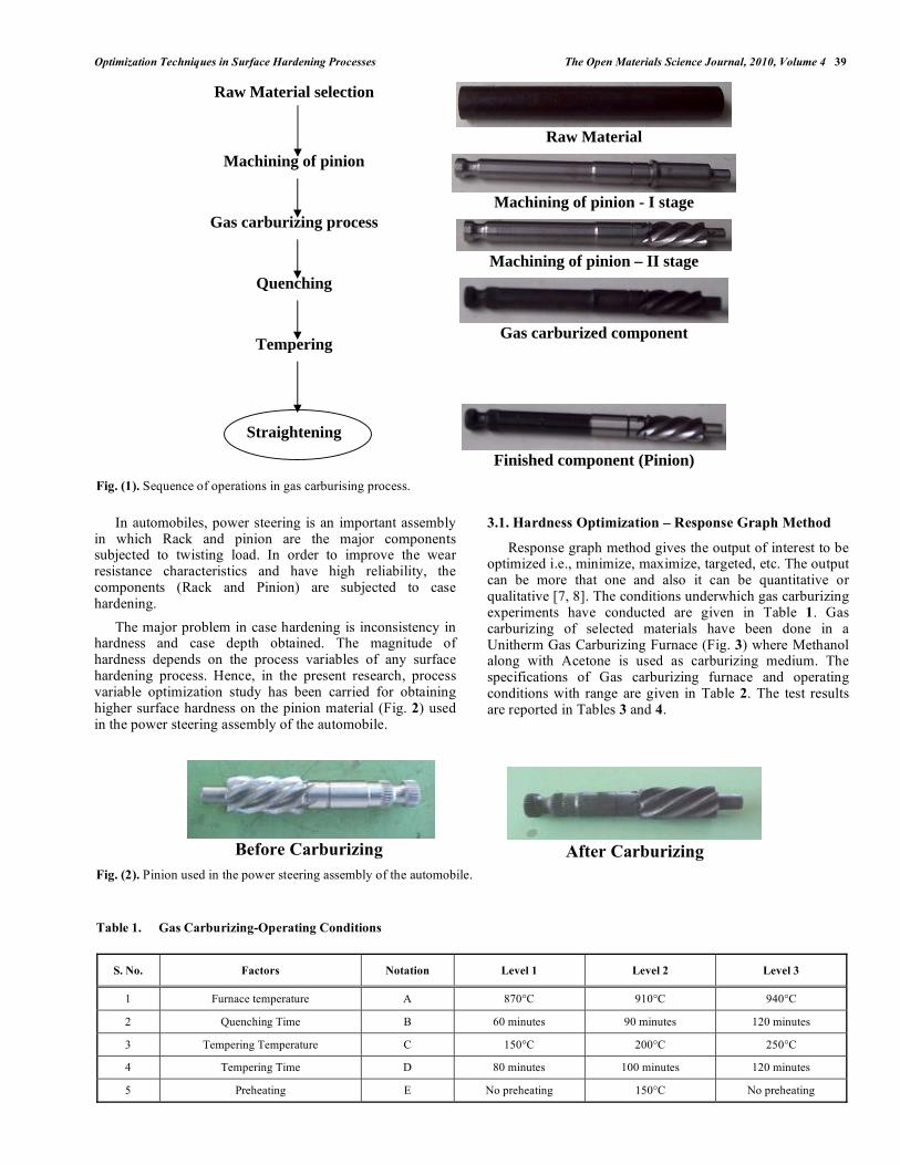
The normal procedure followed in converting the raw material into a finished product is shown in Fig. (1).
3. HARDNESS OF PINION
Hardness of a material is generally defined as resistance to permanent indentation under static or dynamic loads. Engineering materials are subjected to various applications where the load conditions and functional requirements may vary widely [6].
Optimization Techniques in Surface Hardening Processes The Open Materials Science Journal, 2010, Volume 4 39
In automobiles, power steering is an important assembly in which Rack and pinion are the major components subjected to twisting load. In order to improve the wear resistance characteristics and have high reliability, the components (Rack and Pinion) are subjected to case hardening.
The major problem in case hardening is inconsistency in hardness and case depth obtained. The magnitude of hardness depends on the process variables of any surface hardening process. Hence, in the present research, process variable optimization study has been carried for obtaining higher surface hardness on the pinion material (Fig. 2) used in the power steering assembly of the automobile.
3.1. Hardness Optimization – Response Graph Method
Response graph method gives the output of interest to be optimized i.e., minimize, maximize, targeted, etc. The output can be more that one and also it can be quantitative or qualitative [7, 8]. The conditions underwhich gas carburizing experiments have conducted are given in Table 1. Gas carburizing of selected materials have been done in a Unitherm Gas Carburizing Furnace (Fig. 3) where Methanol along with Acetone is used as carburizing medium. The specifications of Gas carburizing furnace and operating conditions with range are given in Table 2. The test results are reported in Tables 3 and 4.
Fig. (1). Sequence of operations in gas carburising process.
Before Carburizing
After Carburizing
Fig. (2). Pinion used in the power steering assembly of the automobile.
Table 1. Gas Carburizing-Operating Conditions
S. No. Factors Notation Level 1 Level 2 Level 3
1 Furnace temperature A 870°C 910°C 940°C
2 Quenching Time B 60 minutes 90 minutes 120 minutes
3 Tempering Temperature C 150°C 200°C 250°C
4 Tempering Time D 80 minutes 100 minutes 120 minutes
5 Preheating E No preheating 150°C No preheating
Raw Material selection
Machining of pinion
Gas carburizing process
Quenching
Tempering
Straightening
Raw Material
Machining of pinion - I stage
Machining of pinion – II stage
Gas carburized component
Finished component (Pinion)

40 The Open Materials Science Journal, 2010, Volume 4 Palaniradja et al.
The experiments have been conducted based on L27 orthogonal array system proposed in Taguchi’s mixed level series DOE with interactions as given below:
i) Furnace Temperature vs Quenching time (AxB)
ii) Furnace Temperature vs Tempering Temperature (AxC)
Table 2. Specifications and Operating Conditions of Gas
Carburizing
Material Used : AISI – Low Carbon steel materials
Diameter : 17.3 mm ; Length : 150 mm
Furnace Details:
Methanol – Acetone Unitherm Gas Carburizing Furnace of 3 m depth
Electrical rating : 130 KW
Temperature: 870 to 940°C.
Operating conditions with range
Furnace Temperature : 870 – 940°C
Quenching Time : 30 – 90 minutes
Tempering Temperature : 150 - 250°C
Tempering Time : 80 - 120 minutes
Preheating : 0-150°C.
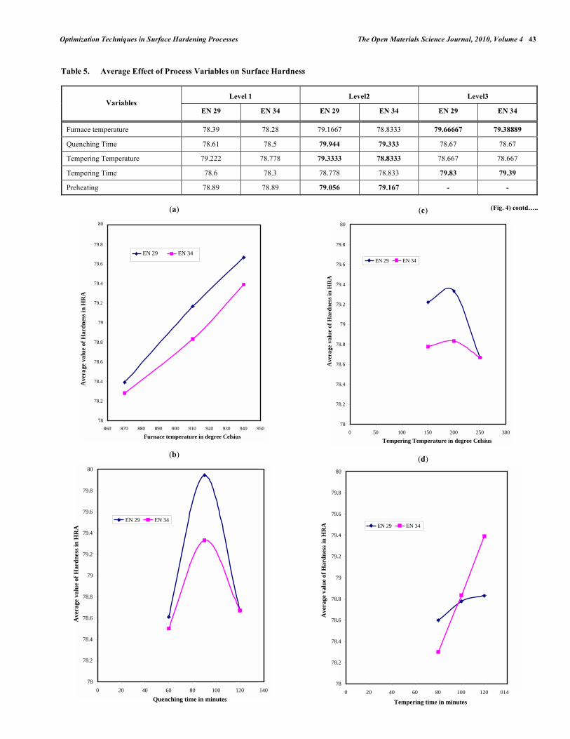
From the experimental result, the average effects of process variables under consideration on the obtainable surface hardness have been calculated and the same are presented in Table 5.
The sample calculation for Average effect of Process variables on surface hardness is given below.
Variable: Furnace temperature, Variable level – Level 1, Material: EN 29 (Table 3).
Average effect = (77+77.5+78.5+79.5+80.5+77+79.5+ 78.5+77.5)/9 = 78.39 HRA
Response graphs shown in Fig. (4a-e) are drawn using the values in Table 5.
3.1.1. Influence of Process Variables on Hardness
ANOVA analysis is carried out to determine the influence of main variables on surface hardness and also to determine the percentage contributions of each variable. Table 6 shows the results of percentage contribution of each variable.
3.1.1.1. Model Calculation for EN 29
Correction factor, C.F = [ yi ] 2
/ Number of Experiments
= [77+77.5+…...79]2 /27 =168823.14
Total sum of squares, = yi 2 – C.F =168866-
SST 168823.14 = 42.85
Sum of Squares of Variables,
Variable A, SSA = [ 1y2 /9+
2y2 /9+ 3y
2/9] – C.F
= [55303.36+56406.25+57121]-C.F
= 168830.61-168823.14
= 7.47
Percentage contribution of
each variable, A = (SSA/SST)*100
Fig. (3). Gas carburizing furnace.
Optimization Techniques in Surface Hardening Processes The Open Materials Science Journal, 2010, Volume 4 41
= (7.47 /42.85) *100 = 17.43%
In the same way the percentage contribution of other
variables are calculated.
Total contribution of variables,
(A+B+C+D+E+AxB+AxC)
= (17.43+18.21+4.34+7.94+10.19+25.43+3.98)
= 87.52%
Error =12.48%
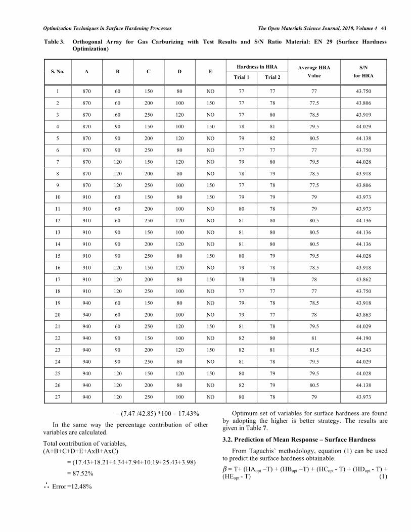
Optimum set of variables for surface hardness are found by adopting the higher is better strategy. The results are given in Table 7.
3.2. Prediction of Mean Response – Surface Hardness
From Taguchis’ methodology, equation (1) can be used to predict the surface hardness obtainable.
= T+ (HAopt –T) + (HBopt –T) + (HCopt - T) + (HDopt - T) + (HEopt - T) (1)
Table 3. Orthogonal Array for Gas Carburizing with Test Results and S/N Ratio Material: EN 29 (Surface Hardness
Optimization)
Hardness in HRA S. No. A B C D E
Trial 1 Trial 2
Average HRA
Value
S/N
for HRA
1 870 60 150 80 NO 77 77 77 43.750
2 870 60 200 100 150 77 78 77.5 43.806
3 870 60 250 120 NO 77 80 78.5 43.919
4 870 90 150 100 150 78 81 79.5 44.029
5 870 90 200 120 NO 79 82 80.5 44.138
6 870 90 250 80 NO 77 77 77 43.750
7 870 120 150 120 NO 79 80 79.5 44.028
8 870 120 200 80 NO 78 79 78.5 43.918
9 870 120 250 100 150 77 78 77.5 43.806
10 910 60 150 80 150 79 79 79 43.973
11 910 60 200 100 NO 80 78 79 43.973
12 910 60 250 120 NO 81 80 80.5 44.136
13 910 90 150 100 NO 81 80 80.5 44.136
14 910 90 200 120 NO 81 80 80.5 44.136
15 910 90 250 80 150 80 79 79.5 44.028
16 910 120 150 120 NO 79 78 78.5 43.918
17 910 120 200 80 150 78 78 78 43.862
18 910 120 250 100 NO 77 77 77 43.750
19 940 60 150 80 NO 79 78 78.5 43.918
20 940 60 200 100 NO 79 77 78 43.863
21 940 60 250 120 150 81 78 79.5 44.029
22 940 90 150 100 NO 82 80 81 44.190
23 940 90 200 120 150 82 81 81.5 44.243
24 940 90 250 80 NO 81 78 79.5 44.029
25 940 120 150 120 150 80 79 79.5 44.028
26 940 120 200 80 NO 82 79 80.5 44.138
27 940 120 250 100 NO 80 78 79 43.973
42 The Open Materials Science Journal, 2010, Volume 4 Palaniradja et al.
where,
-predicted mean response
T-mean of all observed hardness values;
HAopt, HBopt, HCopt HDopt and HEopt – Hardness values obtained at optimum process variable condition.
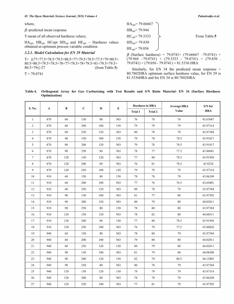
3.2.1. Model Calculation for EN 29 Material
T= {(77+77.5+78.5+79.5+80.5+77+79.5+78.5+77.5+79+80.5+ 80.5+80.5+79.5+78.5+78+77+78.5+78+79.5+81+79.5+79.5+ 80.5+79)}/27 (from Table 3)
T = 79.0741
HAopt= 79.66667
HBopt= 79.944
HCopt= 79.3333 From Table 5
HDopt= 79.830
HEopt= 79.056
(Surface hardness) = 79.0741+ (79.66667 –79.0741) + (79.944 –79.0741) + (79.3333 - 79.0741) + (79.830 - 79.0741) + (79.056 - 79.0741) = 81.5336 HRA
Similarly, for EN 34 the predicted mean response = 80.7802HRA optimum surface hardness value, for EN 29 is 81.5336HRA and for EN 34 is 80.7802HRA.
Table 4. Orthogonal Array for Gas Carburizing with Test Results and S/N Ratio Material: EN 34 (Surface Hardness
Optimization)
Hardness in HRA S. No. A B C D E
Trial 1 Trial 2
Average HRA
Value
S/N for
HRA
1 870 60 150 80 NO 76 76 76 43.63687
2 870 60 200 100 150 79 79 79 43.97314
3 870 60 250 120 NO 80 78 79 43.97384
4 870 90 150 100 150 79 78 78.5 43.91817
5 870 90 200 120 NO 79 78 78.5 43.91817
6 870 90 250 80 NO 78 77 77.5 43.80681
7 870 120 150 120 NO 77 80 78.5 43.91958
8 870 120 200 80 NO 76 81 78.5 43.9224
9 870 120 250 100 150 79 79 79 43.97314
10 910 60 150 80 150 78 78 78 43.86249
11 910 60 200 100 NO 77 76 76.5 43.69401
12 910 60 250 120 NO 80 78 79 43.97384
13 910 90 150 100 NO 81 77 80 43.97592
14 910 90 200 120 NO 80 79 80 44.02811
15 910 90 250 80 150 78 80 80 43.97384
16 910 120 150 120 NO 78 82 80 44.08511
17 910 120 200 80 150 77 80 78.5 43.91958
18 910 120 250 100 NO 76 79 77.5 43.80826
19 940 60 150 80 NO 78 80 79 43.97384
20 940 60 200 100 NO 79 80 80 44.02811
21 940 60 250 120 150 80 79 80 44.02811
22 940 90 150 100 NO 81 79 80 44.08308
23 940 90 200 120 150 82 79 80.5 44.13803
24 940 90 250 80 NO 80 78 79 43.97384
25 940 120 150 120 150 79 79 79 43.97314
26 940 120 200 80 NO 78 78 78 43.86249
27 940 120 250 100 NO 77 81 79 43.97592
Optimization Techniques in Surface Hardening Processes The Open Materials Science Journal, 2010, Volume 4 43
(a)
(b)
(Fig. 4) contd….. (c)
(d)
Table 5. Average Effect of Process Variables on Surface Hardness
Level 1 Level2 Level3 Variables
EN 29 EN 34 EN 29 EN 34 EN 29 EN 34
Furnace temperature 78.39 78.28 79.1667 78.8333 79.66667 79.38889
Quenching Time 78.61 78.5 79.944 79.333 78.67 78.67
Tempering Temperature 79.222 78.778 79.3333 78.8333 78.667 78.667
Tempering Time 78.6 78.3 78.778 78.833 79.83 79.39
Preheating 78.89 78.89 79.056 79.167 - -
78
78.2
78.4
78.6
78.8
79
79.2
79.4
79.6
79.8
80
860 870 880 890 900 910 920 930 940 950 Furnace temperature in degree Celsius
EN 29 EN 34
Ave
rage
val
ue
of H
ard
nes
s in
HR
A
78
78.2
78.4
78.6
78.8
79
79.2
79.4
79.6
79.8
80
0 20 40 60 80 100 120 140 Quenching time in minutes
Ave
rage
val
ue
of H
ard
nes
s in
HR
A
EN 29 EN 34
78
78.2
78.4
78.6
78.8
79
79.2
79.4
79.6
79.8
80
0 50 100 150 200 250 300 Tempering Temperature in degree Celsius
EN 29 EN 34
Ave
rage
val
ue
of H
ard
nes
s in
HR
A
78
78.2
78.4
78.6
78.8
79
79.2
79.4
79.6
79.8
80
0 20 40 60 80 100 120 140 Tempering time in minutes
Ave
rage
val
ue
of H
ard
nes
s in
HR
A
EN 29 EN 34
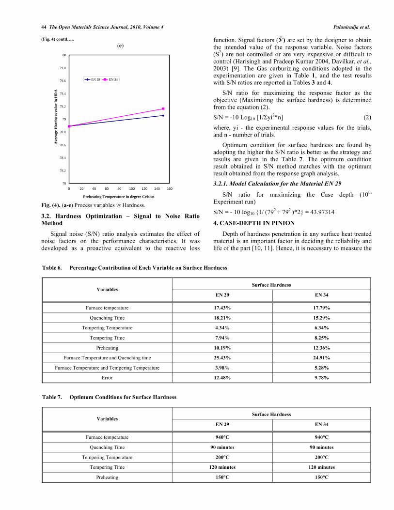
44 The Open Materials Science Journal, 2010, Volume 4 Palaniradja et al.
(Fig. 4) contd…..
(e)
Fig. (4). (a-e) Process variables vs Hardness.
3.2. Hardness Optimization – Signal to Noise Ratio Method
Signal noise (S/N) ratio analysis estimates the effect of noise factors on the performance characteristics. It was developed as a proactive equivalent to the reactive loss
function. Signal factors ( ) are set by the designer to obtain the intended value of the response variable. Noise factors (S
2) are not controlled or are very expensive or difficult to
control (Harisingh and Pradeep Kumar 2004, Davilkar, et al., 2003) [9]. The Gas carburizing conditions adopted in the experimentation are given in Table 1, and the test results with S/N ratios are reported in Tables 3 and 4.
S/N ratio for maximizing the response factor as the objective (Maximizing the surface hardness) is determined from the equation (2).
S/N = -10 Log10 [1/ yi2*n] (2)
where, yi - the experimental response values for the trials, and n - number of trials.
Optimum condition for surface hardness are found by adopting the higher the S/N ratio is better as the strategy and results are given in the Table 7. The optimum condition result obtained in S/N method matches with the optimum result obtained from the response graph analysis.
3.2.1. Model Calculation for the Material EN 29
S/N ratio for maximizing the Case depth (10th
Experiment run)
S/N = - 10 log10 {1/ (792
+ 792
)*2} = 43.97314
4. CASE-DEPTH IN PINION
Depth of hardness penetration in any surface heat treated material is an important factor in deciding the reliability and life of the part [10, 11]. Hence, it is necessary to measure the
Table 6. Percentage Contribution of Each Variable on Surface Hardness
Surface Hardness Variables
EN 29 EN 34
Furnace temperature 17.43% 17.79%
Quenching Time 18.21% 15.29%
Tempering Temperature 4.34% 6.34%
Tempering Time 7.94% 8.25%
Preheating 10.19% 12.36%
Furnace Temperature and Quenching time 25.43% 24.91%
Furnace Temperature and Tempering Temperature 3.98% 5.28%
Error 12.48% 9.78%
Table 7. Optimum Conditions for Surface Hardness
Surface Hardness Variables
EN 29 EN 34
Furnace temperature 940°C 940°C
Quenching Time 90 minutes 90 minutes
Tempering Temperature 200°C 200°C
Tempering Time 120 minutes 120 minutes
Preheating 150°C 150°C
78
78.2
78.4
78.6
78.8
79
79.2
79.4
79.6
79.8
80
0 20 40 60 80 100 120 140 160
Preheating Temperature in degree Celsius
Ave
rage
Har
dne
ss v
alu
e in
HR
A
EN 29 EN 34
Optimization Techniques in Surface Hardening Processes The Open Materials Science Journal, 2010, Volume 4 45
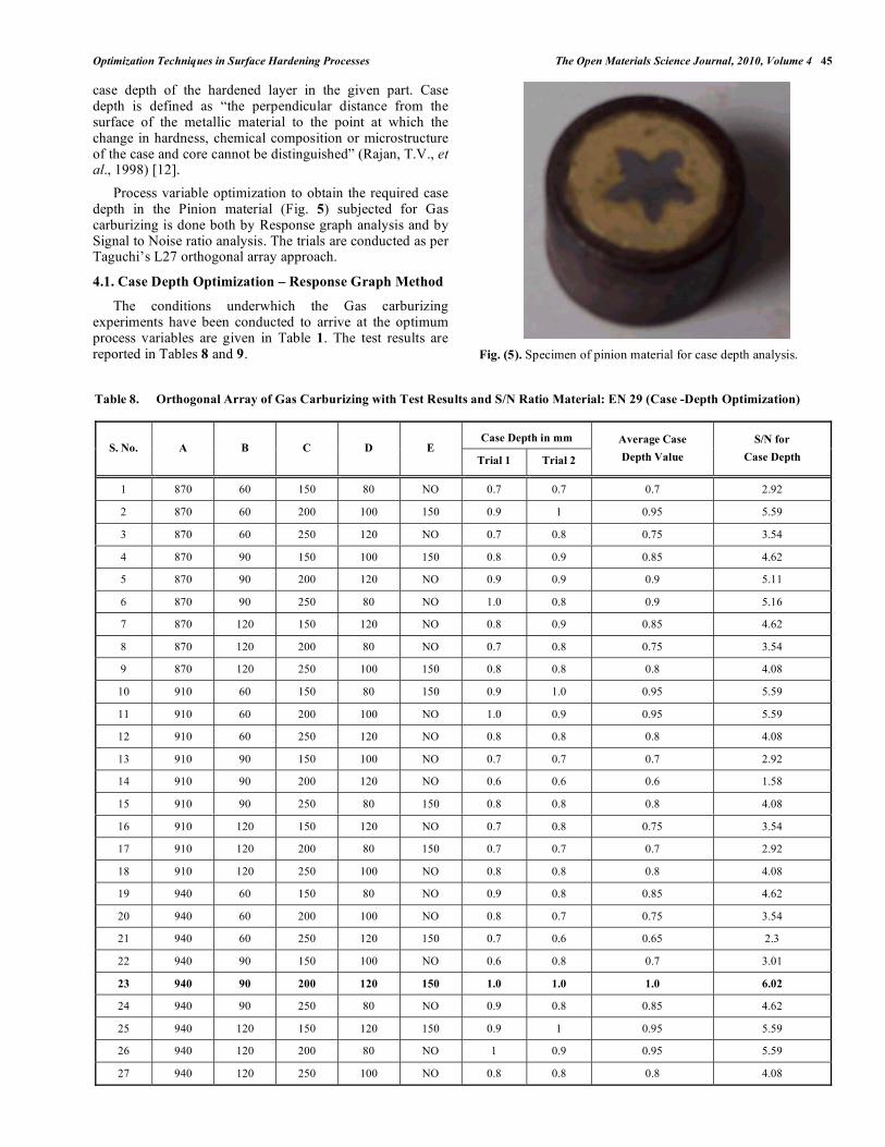
case depth of the hardened layer in the given part. Case depth is defined as “the perpendicular distance from the surface of the metallic material to the point at which the change in hardness, chemical composition or microstructure of the case and core cannot be distinguished” (Rajan, T.V., et al., 1998) [12].
Process variable optimization to obtain the required case depth in the Pinion material (Fig. 5) subjected for Gas carburizing is done both by Response graph analysis and by Signal to Noise ratio analysis. The trials are conducted as per Taguchi’s L27 orthogonal array approach.
4.1. Case Depth Optimization – Response Graph Method
The conditions underwhich the Gas carburizing experiments have been conducted to arrive at the optimum process variables are given in Table 1. The test results are reported in Tables 8 and 9.
Fig. (5). Specimen of pinion material for case depth analysis.
Table 8. Orthogonal Array of Gas Carburizing with Test Results and S/N Ratio Material: EN 29 (Case -Depth Optimization)
Case Depth in mm S. No. A B C D E
Trial 1 Trial 2
Average Case
Depth Value
S/N for
Case Depth
1 870 60 150 80 NO 0.7 0.7 0.7 2.92
2 870 60 200 100 150 0.9 1 0.95 5.59
3 870 60 250 120 NO 0.7 0.8 0.75 3.54
4 870 90 150 100 150 0.8 0.9 0.85 4.62
5 870 90 200 120 NO 0.9 0.9 0.9 5.11
6 870 90 250 80 NO 1.0 0.8 0.9 5.16
7 870 120 150 120 NO 0.8 0.9 0.85 4.62
8 870 120 200 80 NO 0.7 0.8 0.75 3.54
9 870 120 250 100 150 0.8 0.8 0.8 4.08
10 910 60 150 80 150 0.9 1.0 0.95 5.59
11 910 60 200 100 NO 1.0 0.9 0.95 5.59
12 910 60 250 120 NO 0.8 0.8 0.8 4.08
13 910 90 150 100 NO 0.7 0.7 0.7 2.92
14 910 90 200 120 NO 0.6 0.6 0.6 1.58
15 910 90 250 80 150 0.8 0.8 0.8 4.08
16 910 120 150 120 NO 0.7 0.8 0.75 3.54
17 910 120 200 80 150 0.7 0.7 0.7 2.92
18 910 120 250 100 NO 0.8 0.8 0.8 4.08
19 940 60 150 80 NO 0.9 0.8 0.85 4.62
20 940 60 200 100 NO 0.8 0.7 0.75 3.54
21 940 60 250 120 150 0.7 0.6 0.65 2.3
22 940 90 150 100 NO 0.6 0.8 0.7 3.01
23 940 90 200 120 150 1.0 1.0 1.0 6.02
24 940 90 250 80 NO 0.9 0.8 0.85 4.62
25 940 120 150 120 150 0.9 1 0.95 5.59
26 940 120 200 80 NO 1 0.9 0.95 5.59
27 940 120 250 100 NO 0.8 0.8 0.8 4.08

46 The Open Materials Science Journal, 2010, Volume 4 Palaniradja et al.
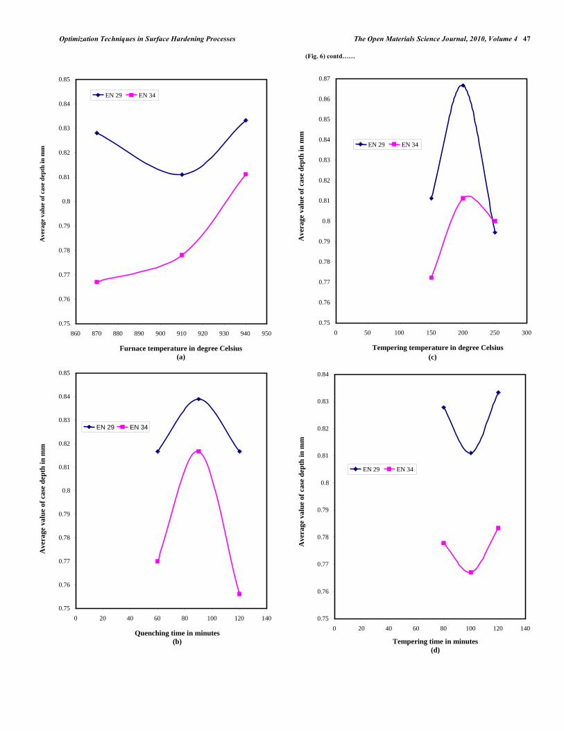
The average effects of main factors on case depth are given in Table 10 for the materials EN 29 and EN 34 respectively.
Response graphs are drawn using Table 10. Fig. (6a-e) (Response graphs) shows the influence of process variables on the case depth for the Materials EN 29 and EN 34.
Table 9. Orthogonal Array of Gas Carburizing with Test Results and S/N Ratio Material: EN 34 (Case-Depth Optimization)
Case Depth in mm S.No. A B C D E
Trial 1 Trial 2
Average Case
Depth Value
S/N for
Case Depth
1 870 60 150 80 NO 0.8 0.6 0.7 3.01
2 870 60 200 100 150 0.7 0.7 0.7 2.92
3 870 60 250 120 NO 0.7 0.7 0.7 2.92
4 870 90 150 100 150 0.8 0.9 0.85 4.62
5 870 90 200 120 NO 0.9 0.8 0.85 4.62
6 870 90 250 80 NO 0.6 0.7 0.65 2.3
7 870 120 150 120 NO 0.7 0.8 0.75 3.54
8 870 120 200 80 NO 0.8 0.9 0.85 4.62
9 870 120 250 100 150 0.8 0.9 0.85 4.62
10 910 60 150 80 150 0.8 0.8 0.8 4.08
11 910 60 200 100 NO 0.8 0.8 0.8 4.08
12 910 60 250 120 NO 0.8 0.8 0.8 4.08
13 910 90 150 100 NO 0.8 0.7 0.75 3.54
14 910 90 200 120 NO 0.9 0.8 0.85 4.62
15 910 90 250 80 150 0.9 0.8 0.85 4.62
16 910 120 150 120 NO 0.8 0.7 0.75 3.54
17 910 120 200 80 150 0.7 0.6 0.65 2.3
18 910 120 250 100 NO 0.7 0.8 0.75 3.54
19 940 60 150 80 NO 0.8 0.8 0.8 4.08
20 940 60 200 100 NO 0.8 0.8 0.8 4.08
21 940 60 250 120 150 0.9 0.8 0.85 4.62
22 940 90 150 100 NO 0.8 0.8 0.8 4.08
23 940 90 200 120 150 1.0 0.90 0.95 5.59
24 940 90 250 80 NO 0.9 0.8 0.85 4.62
25 940 120 150 120 150 0.7 0.8 0.75 3.54
26 940 120 200 80 NO 0.9 0.8 0.85 4.62
27 940 120 250 100 NO 0.6 0.6 0.6 1.58
Table 10. Average Effect of Process Variables on Case Depth
Level 1 Level2 Level3 Variables
EN 29 EN 34 EN 29 EN 34 EN 29 EN 34
Furnace temperature 0.828 0.767 0.811 0.778 0.8333 0.8111
Quenching Time 0.81667 0.77 0.83889 0.8167 0.8167 0.756
Tempering Temperature 0.8111 0.7722 0.86667 0.811111 0.79444 0.8000
Tempering Time 0.8278 0.7778 0.811 0.767 0.8333 0.783333
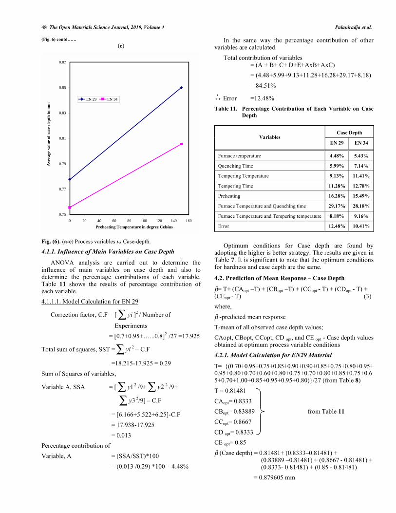
Preheating 0.7778 0.7556 0.85 0.8056 - -
Optimization Techniques in Surface Hardening Processes The Open Materials Science Journal, 2010, Volume 4 47
(Fig. 6) contd……
0.75
0.76
0.77
0.78
0.79
0.8
0.81
0.82
0.83
0.84
0.85
0 20 40 60 80 100 120 140 Quenching time in minutes
(b)
EN 29 EN 34
0.75
0.76
0.77
0.78
0.79
0.8
0.81
0.82
0.83
0.84
0.85
860 870 880 890 900 910 920 930 940 950 Furnace temperature in degree Celsius
(a)
EN 29 EN 34
Ave
rage
val
ue
of c
ase
dep
th in
mm
A
vera
ge v
alue
of
case
dep
th in
mm
0.75
0.76
0.77
0.78
0.79
0.8
0.81
0.82
0.83
0.84
0 20 40 60 80 100 120 140 Tempering time in minutes
(d)
EN 29 EN 34
0.75
0.76
0.77
0.78
0.79
0.8
0.81
0.82
0.83
0.84
0.85
0.86
0.87
0 50 100 150 200 250 300 Tempering temperature in degree Celsius
EN 29 EN 34
A
vera
ge v
alu
e of
cas
e d
epth
in m
mA
vera
ge v
alu
e of
cas
e d
epth
in m
m
(c)
48 The Open Materials Science Journal, 2010, Volume 4 Palaniradja et al.
(Fig. 6) contd……
(e)
Fig. (6). (a-e) Process variables vs Case-depth.
4.1.1. Influence of Main Variables on Case Depth
ANOVA analysis are carried out to determine the influence of main variables on case depth and also to determine the percentage contributions of each variable. Table 11 shows the results of percentage contribution of each variable.
4.1.1.1. Model Calculation for EN 29
Correction factor, C.F = [
yi ]2
/ Number of
Experiments
= [0.7+0.95+…...0.8]2 /27 =17.925
Total sum of squares, SST =
yi2 – C.F
=18.215-17.925 = 0.29
Sum of Squares of variables,
Variable A, SSA = [
y12 /9+
y2
2 /9+
y32/9] – C.F
= [6.166+5.522+6.25]-C.F
= 17.938-17.925
= 0.013
Percentage contribution of
Variable, A = (SSA/SST)*100
= (0.013 /0.29) *100 = 4.48%
In the same way the percentage contribution of other variables are calculated.
Total contribution of variables = (A + B+ C+ D+E+AxB+AxC)
= (4.48+5.99+9.13+11.28+16.28+29.17+8.18)
= 84.51%
Error =12.48%
Table 11. Percentage Contribution of Each Variable on Case
Depth
Case Depth Variables
EN 29 EN 34
Furnace temperature 4.48% 5.43%
Quenching Time 5.99% 7.14%
Tempering Temperature 9.13% 11.41%
Tempering Time 11.28% 12.78%
Preheating 16.28% 15.49%
Furnace Temperature and Quenching time 29.17% 28.18%
Furnace Temperature and Tempering temperature 8.18% 9.16%
Error 12.48% 10.41%
Optimum conditions for Case depth are found by adopting the higher is better strategy. The results are given in Table 7. It is significant to note that the optimum conditions for hardness and case depth are the same.
4.2. Prediction of Mean Response – Case Depth
= T+ (CAopt –T) + (CBopt –T) + (CCopt - T) + (CDopt - T) + (CEopt - T) (3)
where,
-predicted mean response
T-mean of all observed case depth values;
CAopt, CBopt, CCopt, CD opt, and CE opt - Case depth values obtained at optimum process variable conditions
4.2.1. Model Calculation for EN29 Material
T= {(0.70+0.95+0.75+0.85+0.90+0.90+0.85+0.75+0.80+0.95+ 0.95+0.80+0.70+0.60+0.80+0.75+0.70+0.80+0.85+0.75+0.65+0.70+1.00+0.85+0.95+0.95+0.80)}/27 (from Table 8)
T = 0.81481
CAopt= 0.8333
CBopt= 0.83889 from Table 11
CCopt= 0.8667
CD opt= 0.8333
CE opt= 0.85
(Case depth) = 0.81481+ (0.8333–0.81481) + (0.83889 –0.81481) + (0.8667 - 0.81481) + (0.8333- 0.81481) + (0.85 - 0.81481)
= 0.879605 mm
0.75
0.77
0.79
0.81
0.83
0.85
0.87
0 20 40 60 80 100 120 140 160 Preheating Temperature in degree Celsius
EN 29 EN 34
A
vera
ge v
alue
of
case
dep
th in
mm
Optimization Techniques in Surface Hardening Processes The Open Materials Science Journal, 2010, Volume 4 49
Similarly for EN 34 the predicted mean response = 0.96265 mm.
Optimum Case depth value, for EN 29 = 0.96265 mm and for EN 34 = 0.8945 mm.
4.3. Case Depth Optimization – Signal to Noise Ratio Method
Gas carburizing conditions adopted in the experimentation are given in Table 1, and the test results with S/N ratio are given in Tables 8 and 9. Optimum condition for Case depth are found by adopting the higher the S/N ratio is better as the strategy and results are given in the Table 7. The optimum condition result obtained in S/N method matches with the optimum result obtained from the response graph analysis.
4.3.1. Model Calculation for the Material EN 29
S/N ratio for maximizing the Case depth (13th
Experiment run)
S/N = - 10 log10 {1/ (0.72
+ 0.72)*2} = 2.92256
5. INDUCTION HARDENING PROCESS VARIABLES OPTIMIZATION USING FACTORIAL METHOD
In this study 3 3
Factorial Design Matrix is used to optimize the process variables for obtaining improved surface integrity of surface hardened components [13]. The experiments are conducted to study the influence of process variables on Surface hardness and Case depth as per Classical DOE. All these trials have been carried out by Randomization method. ANOVA analysis with F-Test has been carried out to determine the influence of each factor and their interactions. Regression analysis is done to develop a modeling equation to predict the hardness [14]. AISI 4340
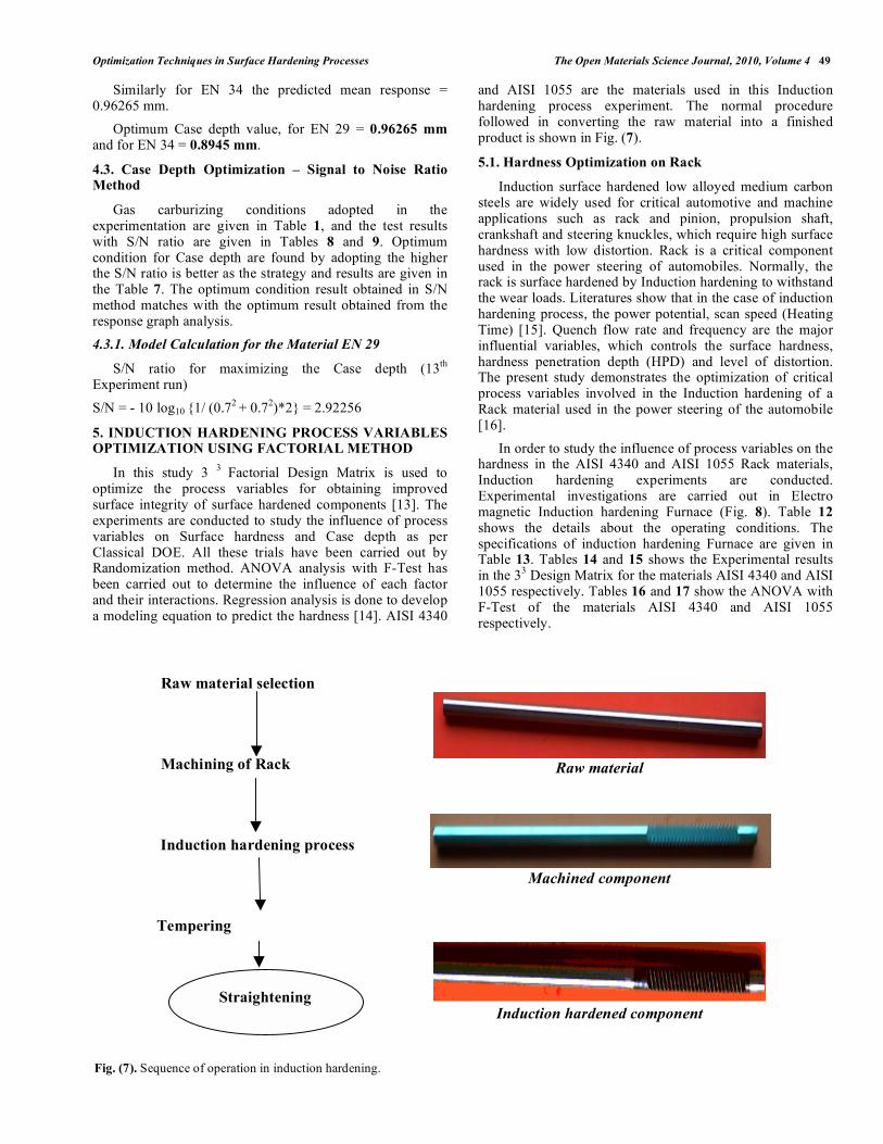
and AISI 1055 are the materials used in this Induction hardening process experiment. The normal procedure followed in converting the raw material into a finished product is shown in Fig. (7).
5.1. Hardness Optimization on Rack
Induction surface hardened low alloyed medium carbon steels are widely used for critical automotive and machine applications such as rack and pinion, propulsion shaft, crankshaft and steering knuckles, which require high surface hardness with low distortion. Rack is a critical component used in the power steering of automobiles. Normally, the rack is surface hardened by Induction hardening to withstand the wear loads. Literatures show that in the case of induction hardening process, the power potential, scan speed (Heating Time) [15]. Quench flow rate and frequency are the major influential variables, which controls the surface hardness, hardness penetration depth (HPD) and level of distortion. The present study demonstrates the optimization of critical process variables involved in the Induction hardening of a Rack material used in the power steering of the automobile [16].
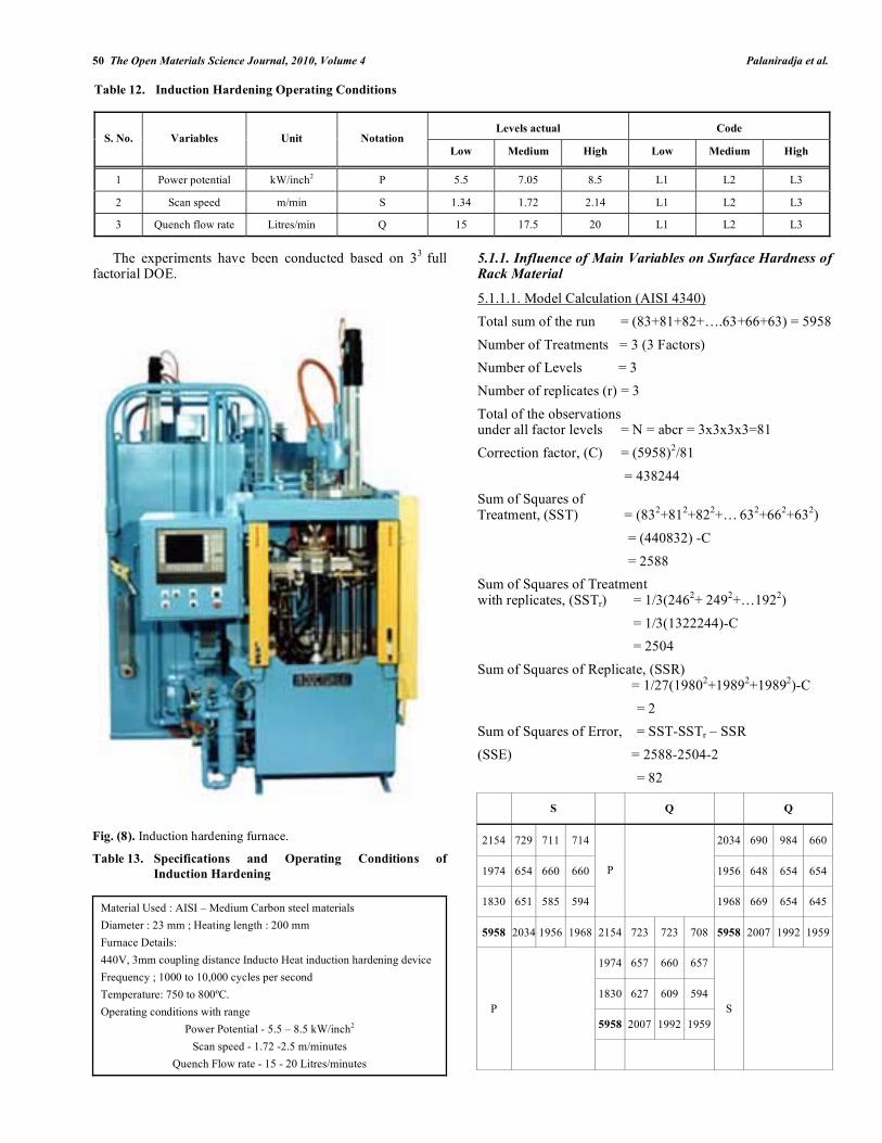
In order to study the influence of process variables on the hardness in the AISI 4340 and AISI 1055 Rack materials, Induction hardening experiments are conducted. Experimental investigations are carried out in Electro magnetic Induction hardening Furnace (Fig. 8). Table 12 shows the details about the operating conditions. The specifications of induction hardening Furnace are given in Table 13. Tables 14 and 15 shows the Experimental results in the 3
3 Design Matrix for the materials AISI 4340 and AISI
1055 respectively. Tables 16 and 17 show the ANOVA with F-Test of the materials AISI 4340 and AISI 1055 respectively.
Raw material selection
Machining of Rack
Induction hardening process
Tempering
Raw material
Machined component
Induction hardened component
Fig. (7). Sequence of operation in induction hardening.
Straightening
50 The Open Materials Science Journal, 2010, Volume 4 Palaniradja et al.
The experiments have been conducted based on 33
full factorial DOE.
Fig. (8). Induction hardening furnace.
Table 13. Specifications and Operating Conditions of
Induction Hardening
Material Used : AISI – Medium Carbon steel materials
Diameter : 23 mm ; Heating length : 200 mm
Furnace Details:
440V, 3mm coupling distance Inducto Heat induction hardening device
Frequency ; 1000 to 10,000 cycles per second
Temperature: 750 to 800ºC.
Operating conditions with range
Power Potential - 5.5 – 8.5 kW/inch2
Scan speed - 1.72 -2.5 m/minutes
Quench Flow rate - 15 - 20 Litres/minutes
5.1.1. Influence of Main Variables on Surface Hardness of Rack Material
5.1.1.1. Model Calculation (AISI 4340)
Total sum of the run = (83+81+82+….63+66+63) = 5958
Number of Treatments = 3 (3 Factors)
Number of Levels = 3
Number of replicates (r) = 3
Total of the observations under all factor levels = N = abcr = 3x3x3x3=81
Correction factor, (C) = (5958)2/81
= 438244
Sum of Squares of Treatment, (SST) = (83
2+81
2+82
2+…
63
2+66
2+63
2)
= (440832) -C
= 2588
Sum of Squares of Treatment with replicates, (SSTr) = 1/3(246
2+ 249
2+…192
2)
= 1/3(1322244)-C
= 2504
Sum of Squares of Replicate, (SSR) = 1/27(1980
2+1989
2+1989
2)-C
= 2
Sum of Squares of Error, = SST-SSTr – SSR
(SSE) = 2588-2504-2
= 82
S Q Q
2154 729 711 714 2034 690 984 660
1974 654 660 660 1956 648 654 654
1830 651 585 594
P
1968 669 654 645
5958 2034 1956 1968 2154 723 723 708 5958 2007 1992 1959
1974 657 660 657
1830 627 609 594
5958 2007 1992 1959
P
S
Table 12. Induction Hardening Operating Conditions
Levels actual Code S. No. Variables Unit Notation
Low Medium High Low Medium High
1 Power potential kW/inch2 P 5.5 7.05 8.5 L1 L2 L3
2 Scan speed m/min S 1.34 1.72 2.14 L1 L2 L3
3 Quench flow rate Litres/min Q 15 17.5 20 L1 L2 L3
Optimization Techniques in Surface Hardening Processes The Open Materials Science Journal, 2010, Volume 4 51
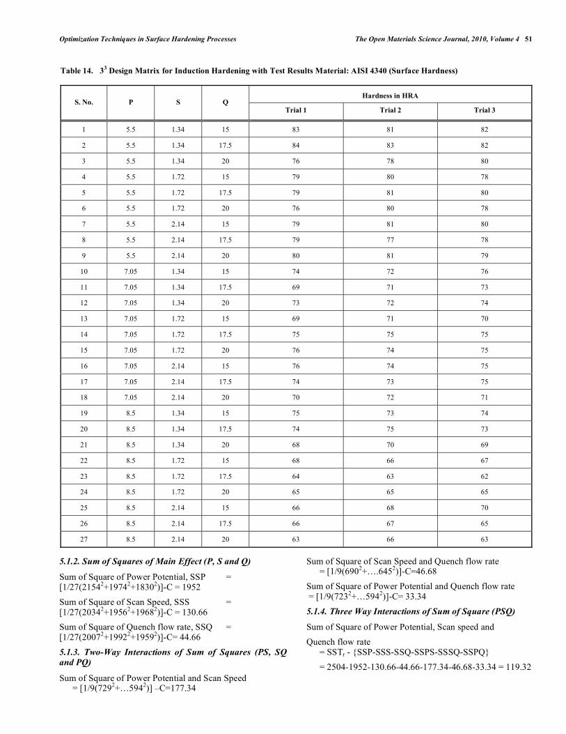
5.1.2. Sum of Squares of Main Effect (P, S and Q)
Sum of Square of Power Potential, SSP = [1/27(2154
2+1974
2+1830
2)]-C = 1952
Sum of Square of Scan Speed, SSS = [1/27(2034
2+1956
2+1968
2)]-C = 130.66
Sum of Square of Quench flow rate, SSQ = [1/27(2007
2+1992
2+1959
2)]-C= 44.66
5.1.3. Two-Way Interactions of Sum of Squares (PS, SQ
and PQ)
Sum of Square of Power Potential and Scan Speed = [1/9(729
2+…594
2)] –C=177.34
Sum of Square of Scan Speed and Quench flow rate = [1/9(690
2+….645
2)]-C=46.68
Sum of Square of Power Potential and Quench flow rate = [1/9(723
2+…594
2)]-C= 33.34
5.1.4. Three Way Interactions of Sum of Square (PSQ)
Sum of Square of Power Potential, Scan speed and
Quench flow rate = SSTr - {SSP-SSS-SSQ-SSPS-SSSQ-SSPQ}
= 2504-1952-130.66-44.66-177.34-46.68-33.34 = 119.32
Table 14. 33 Design Matrix for Induction Hardening with Test Results Material: AISI 4340 (Surface Hardness)
Hardness in HRA S. No. P S Q
Trial 1 Trial 2 Trial 3
1 5.5 1.34 15 83 81 82
2 5.5 1.34 17.5 84 83 82
3 5.5 1.34 20 76 78 80
4 5.5 1.72 15 79 80 78
5 5.5 1.72 17.5 79 81 80
6 5.5 1.72 20 76 80 78
7 5.5 2.14 15 79 81 80
8 5.5 2.14 17.5 79 77 78
9 5.5 2.14 20 80 81 79
10 7.05 1.34 15 74 72 76
11 7.05 1.34 17.5 69 71 73
12 7.05 1.34 20 73 72 74
13 7.05 1.72 15 69 71 70
14 7.05 1.72 17.5 75 75 75
15 7.05 1.72 20 76 74 75
16 7.05 2.14 15 76 74 75
17 7.05 2.14 17.5 74 73 75
18 7.05 2.14 20 70 72 71
19 8.5 1.34 15 75 73 74
20 8.5 1.34 17.5 74 75 73
21 8.5 1.34 20 68 70 69
22 8.5 1.72 15 68 66 67
23 8.5 1.72 17.5 64 63 62
24 8.5 1.72 20 65 65 65
25 8.5 2.14 15 66 68 70
26 8.5 2.14 17.5 66 67 65
27 8.5 2.14 20 63 66 63
52 The Open Materials Science Journal, 2010, Volume 4 Palaniradja et al.
Table 15. 33 Design Matrix for Induction Hardening with Test results Material: AISI 1055 (Surface Hardness)
Hardness in HRA S. No. P S Q
Trial 1 Trial 2 Trial 3
1 5.5 1.34 15 83 84 85
2 5.5 1.34 17.5 82 83 84
3 5.5 1.34 20 83 84 85
4 5.5 1.72 15 78 81 81
5 5.5 1.72 17.5 79 80 81
6 5.5 1.72 20 83 84 85
7 5.5 2.14 15 80 81 82
8 5.5 2.14 17.5 82 83 84
9 5.5 2.14 20 81 82 83
10 7.05 1.34 15 77 78 79
11 7.05 1.34 17.5 77 81 82
12 7.05 1.34 20 77 79 78
13 7.05 1.72 15 69 71 70
14 7.05 1.72 17.5 78 76 77
15 7.05 1.72 20 79 81 80
16 7.05 2.14 15 75 76 74
17 7.05 2.14 17.5 74 72 73
18 7.05 2.14 20 73 74 72
19 8.5 1.34 15 78 77 79
20 8.5 1.34 17.5 71 69 70
21 8.5 1.34 20 69 67 68
22 8.5 1.72 15 69 71 70
23 8.5 1.72 17.5 75 74 73
24 8.5 1.72 20 71 70 69
25 8.5 2.14 15 68 66 67
26 8.5 2.14 17.5 70 69 68
27 8.5 2.14 20 72 71 73
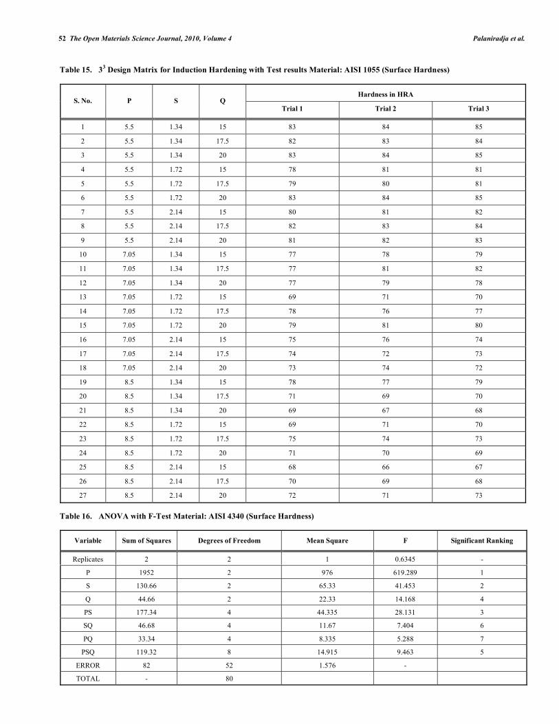
Table 16. ANOVA with F-Test Material: AISI 4340 (Surface Hardness)
Variable Sum of Squares Degrees of Freedom Mean Square F Significant Ranking
Replicates 2 2 1 0.6345 -
P 1952 2 976 619.289 1
S 130.66 2 65.33 41.453 2
Q 44.66 2 22.33 14.168 4
PS 177.34 4 44.335 28.131 3
SQ 46.68 4 11.67 7.404 6
PQ 33.34 4 8.335 5.288 7
PSQ 119.32 8 14.915 9.463 5
ERROR 82 52 1.576 -
TOTAL - 80

Optimization Techniques in Surface Hardening Processes The Open Materials Science Journal, 2010, Volume 4 53
Regression analysis is done using MATLAB and the Regression equations (Equation to predict the hardness of the material AISI 4340) are found and given below.
AISI 4340
Coeff =
1.0000 5.5000 1.3400 15.0000 82
1.0000 5.5000 1.3400 17.5000 83
1.0000 5.5000 1.3400 20.0000 78
1.0000 5.5000 1.7200 15.0000 78
1.0000 5.5000 1.7200 17.5000 80
1.0000 5.5000 1.7200 20.0000 79
1.0000 5.5000 2.1400 15.0000 80
1.0000 5.5000 2.1400 17.5000 77
1.0000 5.5000 2.1400 20.0000 80
1.0000 7.0500 1.3400 15.0000 74
1.0000 7.0500 1.3400 17.5000 72
1.0000 7.0500 1.3400 20.0000 73
1.0000 7.0500 1.7200 15.0000 70
1.0000 7.0500 1.7200 17.5000 75
1.0000 7.0500 1.7200 20.0000 75
1.0000 7.0500 2.1400 15.0000 74
1.0000 7.0500 2.1400 17.5000 72
1.0000 7.0500 2.1400 20.0000 75
1.0000 8.5000 1.3400 15.0000 75
1.0000 8.5000 1.3400 17.5000 69
1.0000 8.5000 1.3400 20.0000 67
1.0000 8.5000 1.7200 15.0000 68
1.0000 8.5000 1.7200 17.5000 63
1.0000 8.5000 1.7200 20.0000 65
1.0000 8.5000 2.1400 15.0000 68
1.0000 8.5000 2.1400 17.5000 66
1.0000 8.5000 2.1400 20.0000 64
The coefficients for the formation of hardness equation are,
111.5611
-4.1474
-2.3059
-0.2889
Equation to Predict the Hardness of the Material AISI 4340
YH = 111.5611-4.1474P-2.3059S-0.2889Q (4)
Similarly, for the material AISI 1055, equation to predict the hardness is given by
YH = 106.7885-3.8179P-3.38671S-0.1778Q (5)
5.2. Case Depth Optimization in Rack
After Induction hardening a steel component is usually hardness/ Case depth tested. And the value obtained is a good indication of the effectiveness of the treatment [17]. The case depth can be measured either by Visual examination or by Hardness measurement. The case depth/Hardness test is carried out by pressing a ball or point with a predetermined force into the surface of the specimen. The hardness figure is function of the size of the indentation for the Brinell (HB) and Vickers (HV), tests and of the depth of the penetration for Rockwell (HRC) test. The above three methods are the most commonly used tests and each has its special range of application and between them they cover almost the whole for the hardness/Case depth field that is of interest of the steel producer and user [18-19].
The present study explains the optimization [20] of critical process variables involved in the Induction hardening of a Rack material (Fig. 10) used in the power steering of the automobile to get higher case depth [21].
In order to study the influence of process variables on the Case depth of the Rack material below the teeth and back of the bar for the AISI 4340 and AISI 1055 Rack materials Induction hardening experiments are conducted.
Table 12 shows the details about the operating conditions.
Table 17. ANOVA with F-Test Material: AISI 1055 (Surface Hardness)
Variable Sum of Squares Degrees of Freedom Mean Square F Significant Ranking
Replicates 6.745 2 3.3725 2.771 -
P 1774.89 2 887.445 729.207 1
S 134.22 2 67.11 55.143 2
Q 11.56 2 5.78 4.749 7
PS 40.45 4 10.1125 8.309 6
SQ 157.78 4 39.445 32.411 3
PQ 53.11 4 13.2775 10.910 5
PSQ 229.55 8 28.69 23.574 4
ERROR 63.295 52 1.217 -
TOTAL - 80
54 The Open Materials Science Journal, 2010, Volume 4 Palaniradja et al.
(a)
(b)
(c)
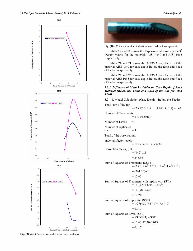
Fig. (9). (a-c) Process variables vs surface hardness.
Fig. (10). Cut section of an induction hardened rack component.
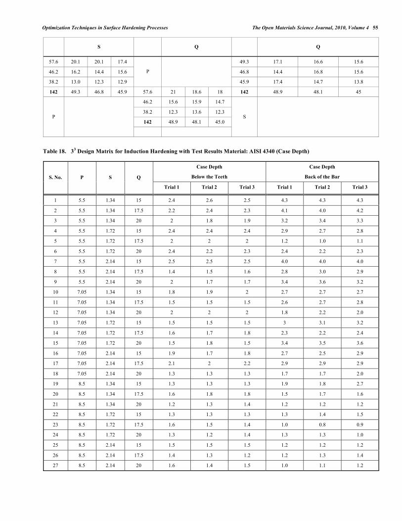
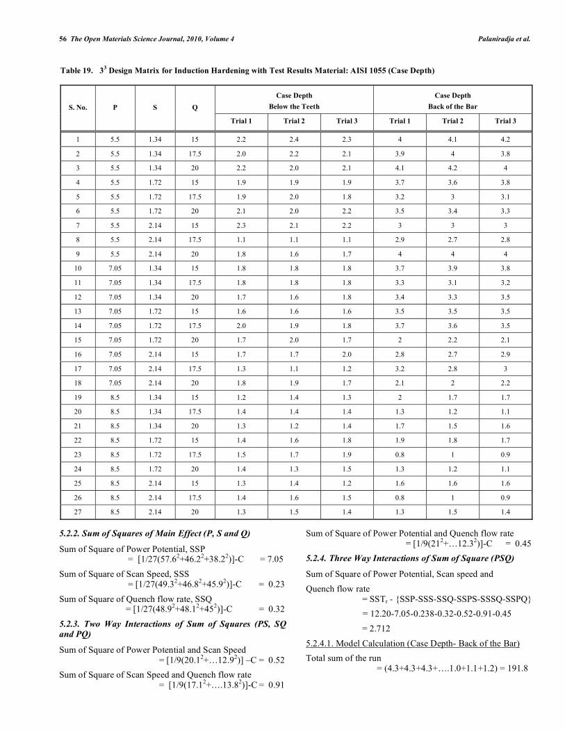
Tables 18 and 19 shows the Experimental results in the 33
Design Matrix for the materials AISI 4340 and AISI 1055 respectively.
Tables 20 and 21 shows the ANOVA with F-Test of the material AISI 4340 for case depth Below the teeth and Back of the bar respectively.
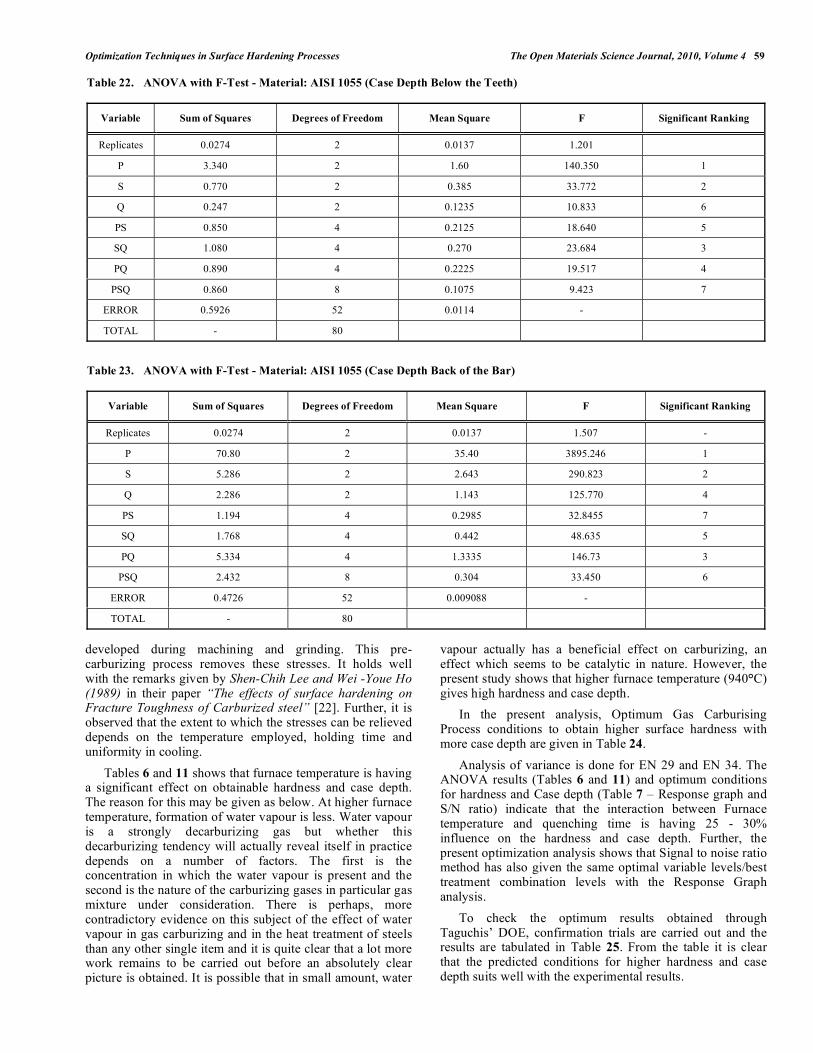
Tables 22 and 23 shows the ANOVA with F-Test of the material AISI 1055 for case depth Below the teeth and Back of the bar respectively.
5.2.1. Influence of Main Variables on Case Depth of Rack
Material (Below the Teeth and Back of the Bar for AISI 4340)
5.2.1.1. Model Calculation (Case Depth – Below the Teeth)
Total sum of the run = (2.4+2.6+2.5+….1.6+1.4+1.5) = 142
Number of Treatments = 3 (3 Factors)
Number of Levels = 3
Number of replicates (r) = 3
Total of the observations
under all factor levels = N = abcr = 3x3x3x3=81
Correction factor, (C) = (142)
2/81
= 248.93
Sum of Squares of Treatment, (SST) = (2.4
2 +2.6
2+2.5
2+
…1.6
2+1.4
2+1.5
2)
= (261.56)-C
= 12.63
Sum of Squares of Treatment with replicates, (SSTr) = 1/3(7.5
2+ 6.9
2+…4.5
2)
= 1/3(783.4)-C
= 12.20
Sum of Squares of Replicate, (SSR) = 1/27(47.3
2+47.1
2+47.6
2)-C
= 0.013
Sum of Squares of Error, (SSE) = SST-SSTr – SSR
= 12.63-12.20-0.013
= 0.417
65
67
69
71
73
75
77
79
81
83
85
0 2 4 6 8 10
Power Potential in kW/sq.inch
AISI 4340 AISI 1055
Ave
rage
val
ue
of H
ard
nes
s in
HR
A
70
71
72
73
74
75
76
77
78
79
0 0.5 1 1.5 2 2.5
Scan speed in m/minutes
AISI 4340 AISI 1055
Ave
rage
val
ue
of H
ard
nes
s in
HR
A
72.5
73
73.5
74
74.5
75
75.5
76
76.5
77
0 5 10 15 20 25
Quench Flow rate in Litres /minutes
AISI 4340 AISI 1055
Ave
rage
val
ue
of H
ard
nes
s in
HR
A
Optimization Techniques in Surface Hardening Processes The Open Materials Science Journal, 2010, Volume 4 55
S Q Q
57.6 20.1 20.1 17.4 49.3 17.1 16.6 15.6
46.2 16.2 14.4 15.6 46.8 14.4 16.8 15.6
38.2 13.0 12.3 12.9
P
45.9 17.4 14.7 13.8
142 49.3 46.8 45.9 57.6 21 18.6 18 142 48.9 48.1 45
46.2 15.6 15.9 14.7
38.2 12.3 13.6 12.3
142 48.9 48.1 45.0 P
S
Table 18. 33 Design Matrix for Induction Hardening with Test Results Material: AISI 4340 (Case Depth)
Case Depth
Below the Teeth
Case Depth
Back of the Bar S. No. P S Q
Trial 1 Trial 2 Trial 3 Trial 1 Trial 2 Trial 3
1 5.5 1.34 15 2.4 2.6 2.5 4.3 4.3 4.3
2 5.5 1.34 17.5 2.2 2.4 2.3 4.1 4.0 4.2
3 5.5 1.34 20 2 1.8 1.9 3.2 3.4 3.3
4 5.5 1.72 15 2.4 2.4 2.4 2.9 2.7 2.8
5 5.5 1.72 17.5 2 2 2 1.2 1.0 1.1
6 5.5 1.72 20 2.4 2.2 2.3 2.4 2.2 2.3
7 5.5 2.14 15 2.5 2.5 2.5 4.0 4.0 4.0
8 5.5 2.14 17.5 1.4 1.5 1.6 2.8 3.0 2.9
9 5.5 2.14 20 2 1.7 1.7 3.4 3.6 3.2
10 7.05 1.34 15 1.8 1.9 2 2.7 2.7 2.7
11 7.05 1.34 17.5 1.5 1.5 1.5 2.6 2.7 2.8
12 7.05 1.34 20 2 2 2 1.8 2.2 2.0
13 7.05 1.72 15 1.5 1.5 1.5 3 3.1 3.2
14 7.05 1.72 17.5 1.6 1.7 1.8 2.3 2.2 2.4
15 7.05 1.72 20 1.5 1.8 1.5 3.4 3.5 3.6
16 7.05 2.14 15 1.9 1.7 1.8 2.7 2.5 2.9
17 7.05 2.14 17.5 2.1 2 2.2 2.9 2.9 2.9
18 7.05 2.14 20 1.3 1.3 1.3 1.7 1.7 2.0
19 8.5 1.34 15 1.3 1.3 1.3 1.9 1.8 2.7
20 8.5 1.34 17.5 1.6 1.8 1.8 1.5 1.7 1.6
21 8.5 1.34 20 1.2 1.3 1.4 1.2 1.2 1.2
22 8.5 1.72 15 1.3 1.3 1.3 1.3 1.4 1.5
23 8.5 1.72 17.5 1.6 1.5 1.4 1.0 0.8 0.9
24 8.5 1.72 20 1.3 1.2 1.4 1.3 1.3 1.0
25 8.5 2.14 15 1.5 1.5 1.5 1.2 1.2 1.2
26 8.5 2.14 17.5 1.4 1.3 1.2 1.2 1.3 1.4
27 8.5 2.14 20 1.6 1.4 1.5 1.0 1.1 1.2
56 The Open Materials Science Journal, 2010, Volume 4 Palaniradja et al.
5.2.2. Sum of Squares of Main Effect (P, S and Q)
Sum of Square of Power Potential, SSP = [1/27(57.6
2+46.2
2+38.2
2)]-C = 7.05
Sum of Square of Scan Speed, SSS = [1/27(49.3
2+46.8
2+45.9
2)]-C = 0.23
Sum of Square of Quench flow rate, SSQ = [1/27(48.9
2+48.1
2+45
2)]-C = 0.32
5.2.3. Two Way Interactions of Sum of Squares (PS, SQ
and PQ)
Sum of Square of Power Potential and Scan Speed = [1/9(20.1
2+…12.9
2)] –C = 0.52
Sum of Square of Scan Speed and Quench flow rate = [1/9(17.1
2+….13.8
2)]-C = 0.91
Sum of Square of Power Potential and Quench flow rate = [1/9(21
2+…12.3
2)]-C = 0.45
5.2.4. Three Way Interactions of Sum of Square (PSQ)
Sum of Square of Power Potential, Scan speed and
Quench flow rate = SSTr - {SSP-SSS-SSQ-SSPS-SSSQ-SSPQ}
= 12.20-7.05-0.238-0.32-0.52-0.91-0.45
= 2.712
5.2.4.1. Model Calculation (Case Depth- Back of the Bar)
Total sum of the run = (4.3+4.3+4.3+….1.0+1.1+1.2) = 191.8
Table 19. 33 Design Matrix for Induction Hardening with Test Results Material: AISI 1055 (Case Depth)
Case Depth
Below the Teeth
Case Depth
Back of the Bar S. No. P S Q
Trial 1 Trial 2 Trial 3 Trial 1 Trial 2 Trial 3
1 5.5 1.34 15 2.2 2.4 2.3 4 4.1 4.2
2 5.5 1.34 17.5 2.0 2.2 2.1 3.9 4 3.8
3 5.5 1.34 20 2.2 2.0 2.1 4.1 4.2 4
4 5.5 1.72 15 1.9 1.9 1.9 3.7 3.6 3.8
5 5.5 1.72 17.5 1.9 2.0 1.8 3.2 3 3.1
6 5.5 1.72 20 2.1 2.0 2.2 3.5 3.4 3.3
7 5.5 2.14 15 2.3 2.1 2.2 3 3 3
8 5.5 2.14 17.5 1.1 1.1 1.1 2.9 2.7 2.8
9 5.5 2.14 20 1.8 1.6 1.7 4 4 4
10 7.05 1.34 15 1.8 1.8 1.8 3.7 3.9 3.8
11 7.05 1.34 17.5 1.8 1.8 1.8 3.3 3.1 3.2
12 7.05 1.34 20 1.7 1.6 1.8 3.4 3.3 3.5
13 7.05 1.72 15 1.6 1.6 1.6 3.5 3.5 3.5
14 7.05 1.72 17.5 2.0 1.9 1.8 3.7 3.6 3.5
15 7.05 1.72 20 1.7 2.0 1.7 2 2.2 2.1
16 7.05 2.14 15 1.7 1.7 2.0 2.8 2.7 2.9
17 7.05 2.14 17.5 1.3 1.1 1.2 3.2 2.8 3
18 7.05 2.14 20 1.8 1.9 1.7 2.1 2 2.2
19 8.5 1.34 15 1.2 1.4 1.3 2 1.7 1.7
20 8.5 1.34 17.5 1.4 1.4 1.4 1.3 1.2 1.1
21 8.5 1.34 20 1.3 1.2 1.4 1.7 1.5 1.6
22 8.5 1.72 15 1.4 1.6 1.8 1.9 1.8 1.7
23 8.5 1.72 17.5 1.5 1.7 1.9 0.8 1 0.9
24 8.5 1.72 20 1.4 1.3 1.5 1.3 1.2 1.1
25 8.5 2.14 15 1.3 1.4 1.2 1.6 1.6 1.6
26 8.5 2.14 17.5 1.4 1.6 1.5 0.8 1 0.9
27 8.5 2.14 20 1.3 1.5 1.4 1.3 1.5 1.4

Optimization Techniques in Surface Hardening Processes The Open Materials Science Journal, 2010, Volume 4 57
Number of Treatments = 3 (3 Factors)
Number of Levels = 3
Number of replicates (r) = 3
Total of the observations
under all factor levels = N = abcr = 3x3x3x3=81
Correction factor, (C) = (191.8)
2/81
= 454.16
Sum of Squares of Treatment, (SST) = (4.3
2 +4.3
2+4.3
2+
…1.0
2+1.1
2+1.2
2)
= (535.93)-C
= 81.8
Sum of Squares of Treatment with replicates, (SSTr) = 1/3(12.9
2+12.3
2+…3.3
2)
= 1/3(1604.44)-C
= 80.65
Sum of Squares of Replicate, (SSR) = 1/27(63
2+63.5
2+65.3
2)-C
= 0.111
Sum of Squares of Error, (SSE) = SST-SSTr – SSR
= 81.8-80.65-0.111
= 1.039
5.3.1. Sum of Squares of Main effect (P, S and Q)
Sum of Square of Power Potential, SSP = [1/27(84.6
2+71.1
2+36.1
2)]-C = 46.417
Sum of Square of Scan Speed, SSS = [1/27(72.1
2+55.8
2+63.9
2)]-C = 4.923
Sum of Square of Quench flow rate, SSQ = [1/27(67.9
2+64.5
2+59.4)]-C =1.359
5.3.2. Two Way Interactions of Sum of Squares (PS, SQ and PQ)
Sum of Square of Power Potential and Scan Speed = [1/9(35.1
2+…10.8
2)] –C =14.19
Sum of Square of Scan Speed and Quench flow rate = [1/9(27.4
2+….18.9
2)]-C = 4.65
S Q Q
84.6 35.1 18.6 30.9 72.1 27.4 25.2 19.5
71.1 22.2 26.7 22.2 55.8 16.8 18.0 21.0
36.1 14.8 10.5 10.8
P
63.9 23.7 21.3 18.9
191.8 72.1 55.8 63.9 84.6 28.2 29.4 27.0 191.8 67.9 64.5 59.4
71.1 25.5 23.7 21.9
36.1 14.2 11.4 10.5
191.8 67.9 64.5 59.4 P
S
Table 20. ANOVA with F-Test Material: AISI 4340 (Case Depth Below the Teeth)
Variable Sum of Squares Degrees of Freedom Mean Square F Significant Ranking
Replicates 0.013 2 0.0065 0.810 -
P 7.05 2 3.525 439.526 1
S 0.238 2 0.119 14.837 6
Q 0.320 2 0.160 19.950 4
PS 0.520 4 0.130 16.209 5
SQ 0.910 4 0.2275 28.366 3
PQ 0.450 4 0.1125 14.027 7
PSQ 2.712 8 0.339 42.269 2
ERROR 0.417 52 0.00802 -
TOTAL - 80
58 The Open Materials Science Journal, 2010, Volume 4 Palaniradja et al.
Sum of Square of Power Potential and Quench flow rate = [1/9(28.2
2+…10.5
2)]-C = 0.508
5.3.3. Three Way Interactions of Sum of Square (PSQ)
Sum of Square of Power Potential, Scan speed and Quench flow rate = SSTr - {SSP-SSS-SSQ-SSPS-SSSQ-SSPQ}
= 80.65-46.417-4.923-1.359-14.19-4.65-0.508
= 8.603
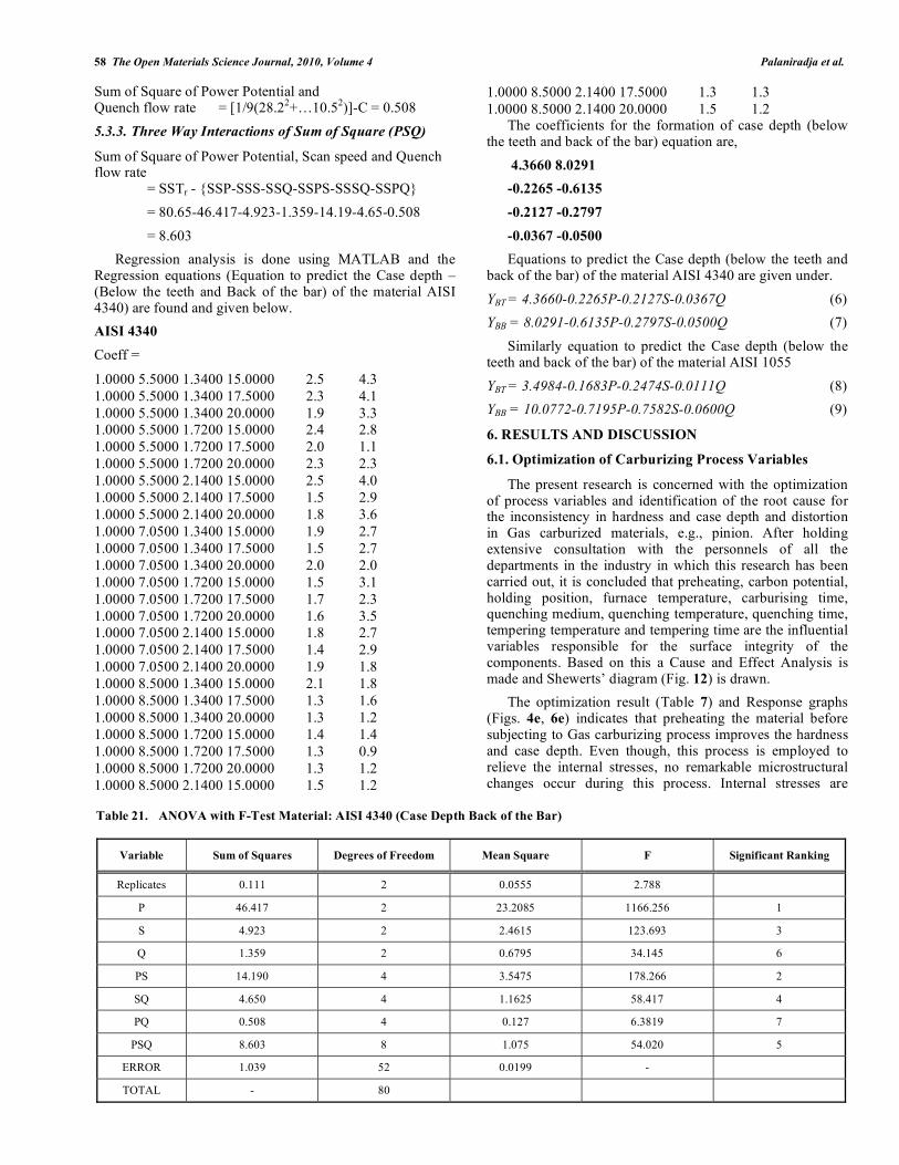
Regression analysis is done using MATLAB and the Regression equations (Equation to predict the Case depth – (Below the teeth and Back of the bar) of the material AISI 4340) are found and given below.
AISI 4340
Coeff =
1.0000 5.5000 1.3400 15.0000 2.5 4.3
1.0000 5.5000 1.3400 17.5000 2.3 4.1
1.0000 5.5000 1.3400 20.0000 1.9 3.3
1.0000 5.5000 1.7200 15.0000 2.4 2.8
1.0000 5.5000 1.7200 17.5000 2.0 1.1
1.0000 5.5000 1.7200 20.0000 2.3 2.3
1.0000 5.5000 2.1400 15.0000 2.5 4.0
1.0000 5.5000 2.1400 17.5000 1.5 2.9
1.0000 5.5000 2.1400 20.0000 1.8 3.6
1.0000 7.0500 1.3400 15.0000 1.9 2.7
1.0000 7.0500 1.3400 17.5000 1.5 2.7
1.0000 7.0500 1.3400 20.0000 2.0 2.0
1.0000 7.0500 1.7200 15.0000 1.5 3.1
1.0000 7.0500 1.7200 17.5000 1.7 2.3
1.0000 7.0500 1.7200 20.0000 1.6 3.5
1.0000 7.0500 2.1400 15.0000 1.8 2.7
1.0000 7.0500 2.1400 17.5000 1.4 2.9
1.0000 7.0500 2.1400 20.0000 1.9 1.8
1.0000 8.5000 1.3400 15.0000 2.1 1.8
1.0000 8.5000 1.3400 17.5000 1.3 1.6
1.0000 8.5000 1.3400 20.0000 1.3 1.2
1.0000 8.5000 1.7200 15.0000 1.4 1.4
1.0000 8.5000 1.7200 17.5000 1.3 0.9
1.0000 8.5000 1.7200 20.0000 1.3 1.2
1.0000 8.5000 2.1400 15.0000 1.5 1.2
1.0000 8.5000 2.1400 17.5000 1.3 1.3
1.0000 8.5000 2.1400 20.0000 1.5 1.2 The coefficients for the formation of case depth (below the teeth and back of the bar) equation are,
4.3660 8.0291
-0.2265 -0.6135
-0.2127 -0.2797
-0.0367 -0.0500
Equations to predict the Case depth (below the teeth and back of the bar) of the material AISI 4340 are given under.
YBT = 4.3660-0.2265P-0.2127S-0.0367Q (6)
YBB = 8.0291-0.6135P-0.2797S-0.0500Q (7)
Similarly equation to predict the Case depth (below the teeth and back of the bar) of the material AISI 1055
YBT = 3.4984-0.1683P-0.2474S-0.0111Q (8)
YBB = 10.0772-0.7195P-0.7582S-0.0600Q (9)
6. RESULTS AND DISCUSSION
6.1. Optimization of Carburizing Process Variables
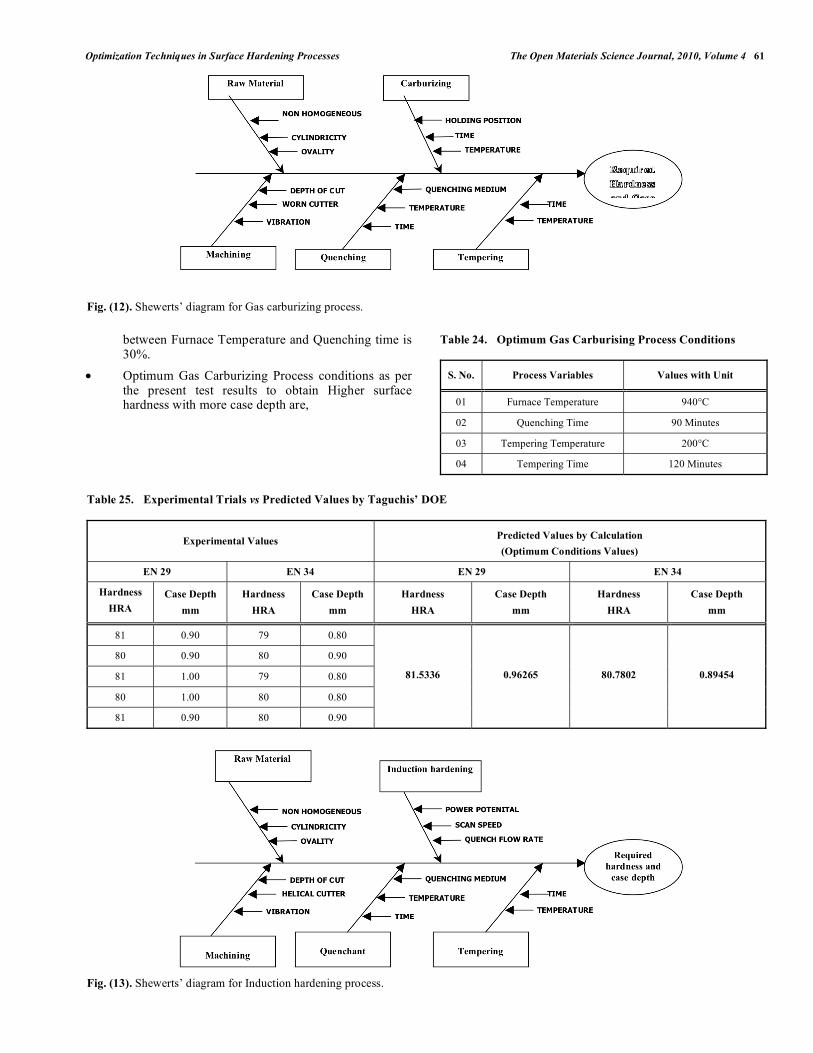
The present research is concerned with the optimization of process variables and identification of the root cause for the inconsistency in hardness and case depth and distortion in Gas carburized materials, e.g., pinion. After holding extensive consultation with the personnels of all the departments in the industry in which this research has been carried out, it is concluded that preheating, carbon potential, holding position, furnace temperature, carburising time, quenching medium, quenching temperature, quenching time, tempering temperature and tempering time are the influential variables responsible for the surface integrity of the components. Based on this a Cause and Effect Analysis is made and Shewerts’ diagram (Fig. 12) is drawn.
The optimization result (Table 7) and Response graphs (Figs. 4e, 6e) indicates that preheating the material before subjecting to Gas carburizing process improves the hardness and case depth. Even though, this process is employed to relieve the internal stresses, no remarkable microstructural changes occur during this process. Internal stresses are
Table 21. ANOVA with F-Test Material: AISI 4340 (Case Depth Back of the Bar)
Variable Sum of Squares Degrees of Freedom Mean Square F Significant Ranking
Replicates 0.111 2 0.0555 2.788
P 46.417 2 23.2085 1166.256 1
S 4.923 2 2.4615 123.693 3
Q 1.359 2 0.6795 34.145 6
PS 14.190 4 3.5475 178.266 2
SQ 4.650 4 1.1625 58.417 4
PQ 0.508 4 0.127 6.3819 7
PSQ 8.603 8 1.075 54.020 5
ERROR 1.039 52 0.0199 -
TOTAL - 80
Optimization Techniques in Surface Hardening Processes The Open Materials Science Journal, 2010, Volume 4 59
developed during machining and grinding. This pre-carburizing process removes these stresses. It holds well with the remarks given by Shen-Chih Lee and Wei -Youe Ho (1989) in their paper “The effects of surface hardening on Fracture Toughness of Carburized steel” [22]. Further, it is observed that the extent to which the stresses can be relieved depends on the temperature employed, holding time and uniformity in cooling.
Tables 6 and 11 shows that furnace temperature is having a significant effect on obtainable hardness and case depth. The reason for this may be given as below. At higher furnace temperature, formation of water vapour is less. Water vapour is a strongly decarburizing gas but whether this decarburizing tendency will actually reveal itself in practice depends on a number of factors. The first is the concentration in which the water vapour is present and the second is the nature of the carburizing gases in particular gas mixture under consideration. There is perhaps, more contradictory evidence on this subject of the effect of water vapour in gas carburizing and in the heat treatment of steels than any other single item and it is quite clear that a lot more work remains to be carried out before an absolutely clear picture is obtained. It is possible that in small amount, water
vapour actually has a beneficial effect on carburizing, an effect which seems to be catalytic in nature. However, the present study shows that higher furnace temperature (940°C) gives high hardness and case depth.
In the present analysis, Optimum Gas Carburising Process conditions to obtain higher surface hardness with more case depth are given in Table 24.
Analysis of variance is done for EN 29 and EN 34. The ANOVA results (Tables 6 and 11) and optimum conditions for hardness and Case depth (Table 7 – Response graph and S/N ratio) indicate that the interaction between Furnace temperature and quenching time is having 25 - 30% influence on the hardness and case depth. Further, the present optimization analysis shows that Signal to noise ratio method has also given the same optimal variable levels/best treatment combination levels with the Response Graph analysis.
To check the optimum results obtained through Taguchis’ DOE, confirmation trials are carried out and the results are tabulated in Table 25. From the table it is clear that the predicted conditions for higher hardness and case depth suits well with the experimental results.
Table 22. ANOVA with F-Test - Material: AISI 1055 (Case Depth Below the Teeth)
Variable Sum of Squares Degrees of Freedom Mean Square F Significant Ranking
Replicates 0.0274 2 0.0137 1.201
P 3.340 2 1.60 140.350 1
S 0.770 2 0.385 33.772 2
Q 0.247 2 0.1235 10.833 6
PS 0.850 4 0.2125 18.640 5
SQ 1.080 4 0.270 23.684 3
PQ 0.890 4 0.2225 19.517 4
PSQ 0.860 8 0.1075 9.423 7
ERROR 0.5926 52 0.0114 -
TOTAL - 80
Table 23. ANOVA with F-Test - Material: AISI 1055 (Case Depth Back of the Bar)
Variable Sum of Squares Degrees of Freedom Mean Square F Significant Ranking
Replicates 0.0274 2 0.0137 1.507 -
P 70.80 2 35.40 3895.246 1
S 5.286 2 2.643 290.823 2
Q 2.286 2 1.143 125.770 4
PS 1.194 4 0.2985 32.8455 7
SQ 1.768 4 0.442 48.635 5
PQ 5.334 4 1.3335 146.73 3
PSQ 2.432 8 0.304 33.450 6
ERROR 0.4726 52 0.009088 -
TOTAL - 80
60 The Open Materials Science Journal, 2010, Volume 4 Palaniradja et al.
(a)
(b)
(c)
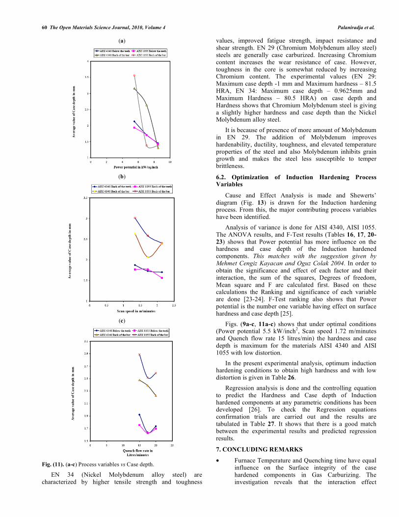
Fig. (11). (a-c) Process variables vs Case depth.
EN 34 (Nickel Molybdenum alloy steel) are characterized by higher tensile strength and toughness
values, improved fatigue strength, impact resistance and shear strength. EN 29 (Chromium Molybdenum alloy steel) steels are generally case carburized. Increasing Chromium content increases the wear resistance of case. However, toughness in the core is somewhat reduced by increasing Chromium content. The experimental values (EN 29: Maximum case depth -1 mm and Maximum hardness – 81.5 HRA, EN 34: Maximum case depth – 0.9625mm and Maximum Hardness – 80.5 HRA) on case depth and Hardness shows that Chromium Molybdenum steel is giving a slightly higher hardness and case depth than the Nickel Molybdenum alloy steel.
It is because of presence of more amount of Molybdenum in EN 29. The addition of Molybdenum improves hardenability, ductility, toughness, and elevated temperature properties of the steel and also Molybdenum inhibits grain growth and makes the steel less susceptible to temper brittleness.
6.2. Optimization of Induction Hardening Process Variables
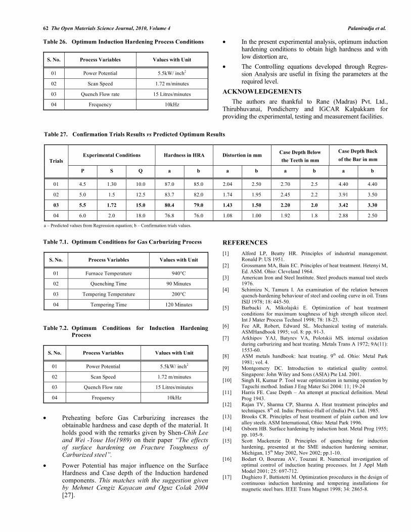
Cause and Effect Analysis is made and Shewerts’ diagram (Fig. 13) is drawn for the Induction hardening process. From this, the major contributing process variables have been identified.
Analysis of variance is done for AISI 4340, AISI 1055. The ANOVA results, and F-Test results (Tables 16, 17, 20-
23) shows that Power potential has more influence on the hardness and case depth of the Induction hardened components. This matches with the suggestion given by Mehmet Cengiz Kayacan and Oguz Colak 2004. In order to obtain the significance and effect of each factor and their interaction, the sum of the squares, Degrees of freedom, Mean square and F are calculated first. Based on these calculations the Ranking and significance of each variable are done [23-24]. F-Test ranking also shows that Power potential is the number one variable having effect on surface hardness and case depth [25].
Figs. (9a-c, 11a-c) shows that under optimal conditions (Power potential 5.5 kW/inch
2, Scan speed 1.72 m/minutes
and Quench flow rate 15 litres/min) the hardness and case depth is maximum for the materials AISI 4340 and AISI 1055 with low distortion.
In the present experimental analysis, optimum induction hardening conditions to obtain high hardness and with low distortion is given in Table 26.
Regression analysis is done and the controlling equation to predict the Hardness and Case depth of Induction hardened components at any parametric conditions has been developed [26]. To check the Regression equations confirmation trials are carried out and the results are tabulated in Table 27. It shows that there is a good match between the experimental results and predicted regression results.
7. CONCLUDING REMARKS
• Furnace Temperature and Quenching time have equal influence on the Surface integrity of the case hardened components in Gas Carburizing. The investigation reveals that the interaction effect
Optimization Techniques in Surface Hardening Processes The Open Materials Science Journal, 2010, Volume 4 61
between Furnace Temperature and Quenching time is 30%.
• Optimum Gas Carburizing Process conditions as per the present test results to obtain Higher surface hardness with more case depth are,
Table 24. Optimum Gas Carburising Process Conditions
S. No. Process Variables Values with Unit
01 Furnace Temperature 940°C
02 Quenching Time 90 Minutes
03 Tempering Temperature 200°C
04 Tempering Time 120 Minutes
Fig. (12). Shewerts’ diagram for Gas carburizing process.
Table 25. Experimental Trials vs Predicted Values by Taguchis’ DOE
Experimental Values Predicted Values by Calculation
(Optimum Conditions Values)
EN 29 EN 34 EN 29 EN 34
Hardness
HRA
Case Depth
mm
Hardness
HRA
Case Depth
mm
Hardness
HRA
Case Depth
mm
Hardness
HRA
Case Depth
mm
81 0.90 79 0.80
80 0.90 80 0.90
81 1.00 79 0.80
80 1.00 80 0.80
81 0.90 80 0.90
81.5336
0.96265
80.7802
0.89454
Fig. (13). Shewerts’ diagram for Induction hardening process.
62 The Open Materials Science Journal, 2010, Volume 4 Palaniradja et al.
Table 26. Optimum Induction Hardening Process Conditions
S. No. Process Variables Values with Unit
01 Power Potential 5.5kW/ inch2
02 Scan Speed 1.72 m/minutes
03 Quench Flow rate 15 Litres/minutes
04 Frequency 10kHz
Table 7.1. Optimum Conditions for Gas Carburizing Process
S. No. Process Variables Values with Unit
01 Furnace Temperature 940°C
02 Quenching Time 90 Minutes
03 Tempering Temperature 200°C
04 Tempering Time 120 Minutes
Table 7.2. Optimum Conditions for Induction Hardening
Process
S. No. Process Variables Values with Unit
01 Power Potential 5.5kW/ inch2
02 Scan Speed 1.72 m/minutes
03 Quench Flow rate 15 Litres/minutes
04 Frequency 10kHz
• Preheating before Gas Carburizing increases the obtainable hardness and case depth of the material. It holds good with the remarks given by Shen-Chih Lee and Wei -Youe Ho(1989) on their paper “The effects of surface hardening on Fracture Toughness of Carburized steel”.
• Power Potential has major influence on the Surface Hardness and Case depth of the Induction hardened components. This matches with the suggestion given by Mehmet Cengiz Kayacan and Oguz Colak 2004 [27].
• In the present experimental analysis, optimum induction hardening conditions to obtain high hardness and with low distortion are,
• The Controlling equations developed through Regres-sion Analysis are useful in fixing the parameters at the required level.
ACKNOWLEDGEMENTS
The authors are thankful to Rane (Madras) Pvt. Ltd., Thirubhuvanai, Pondicherry and IGCAR Kalpakkam for providing the experimental, testing and measurement facilities.
REFERENCES
[1] Alford LP, Beatty HR. Principles of industrial management. Ronald P: US 1951.
[2] Grossmann MA, Bain EC. Principles of heat treatment. Hetenyi M, Ed. ASM. Ohio: Cleveland 1964.
[3] American Iron and Steel Institute. Steel products manual tool steels 1976.
[4] Schimizu N, Tamura I. An examination of the relation between quench-hardening behaviour of steel and cooling curve in oil. Trans
ISIJ 1978; 18: 445-50. [5] Barbacki A, Mikolajski E. Optimization of heat treatment
conditions for maximum toughness of high strength silicon steel. Int J Mater Process Technol 1998; 78: 18-23.
[6] Fee AR, Robert, Edward SL. Mechanical testing of materials. ASMHandbook 1995; vol. 8: pp. 91-3.
[7] Arkhipov YAJ, Batyrev VA, Polotskii MS. internal oxidation during carburizing and heat treating. Metals Trans A 1972; 9A(11):
1553-60. [8] ASM metals handbook: heat treating. 9th ed. Ohio: Metal Park
1981; vol. 4. [9] Montgomery DC. Introduction to statistical quality control.
Singapore: John Wiley and Sons (ASIA) Pte Ltd. 2001. [10] Singh H, Kumar P. Tool wear optimization in turning operation by
Taguchi method. Indian J Eng Mater Sci 2004: 11; 19-24 [11] Harris FE. Case Depth – An attempt at practical definition. Metal
Prog 1943. [12] Rajan TV, Sharma CP, Sharma A. Heat treatment principles and
techniques. 8th ed. India: Prentice-Hall of (India) Pvt. Ltd. 1985. [13] Brooks CR. Principles of heat treatment of plain carbon and low
alloy steels. ASM International, Ohio: Metal Park 1996. [14] Osborn HB. Surface hardening by induction heat. Metal Prog 1955;
pp. 105-9. [15] Scott Mackenzie D. Principles of quenching for induction
hardening, presented at the SME induction hardening seminar, Michigan, 15th May 2002, Nov 2002; pp.1-10.
[16] Bodart O, Boureau AV, Touzani R. Numerical investigation of optimal control of induction heating processes. Int J Appl Math
Model 2001; 25: 697-712. [17] Dughiero F, Battistetti M. Optimization procedures in the design of
continuous induction hardening and tempering installations for magnetic steel bars. IEEE Trans Magnet 1998; 34: 2865-8.
Table 27. Confirmation Trials Results vs Predicted Optimum Results
Experimental Conditions Hardness in HRA Distortion in mm Case Depth Below
the Teeth in mm
Case Depth Back
of the Bar in mm Trials
P S Q a b a b a b a b
01 4.5 1.30 10.0 87.0 85.0 2.04 2.50 2.70 2.5 4.40 4.40
02 5.0 1.5 12.5 83.7 82.0 1.74 1.95 2.45 2.2 3.91 3.50
03 5.5 1.72 15.0 80.4 79.0 1.43 1.50 2.20 2.0 3.42 3.30
04 6.0 2.0 18.0 76.8 76.0 1.08 1.00 1.92 1.8 2.88 2.50
a – Predicted values from Regression equation; b – Confirmation trials values.
Optimization Techniques in Surface Hardening Processes The Open Materials Science Journal, 2010, Volume 4 63
[18] Ashby MF, Easterling KE. The transformation hardening of steel
surfaces by laser beams –I Hypo –eutectoid Steels. Acta Metall 1984; 32(A11): 1935-48.
[19] Averbach BL, Cohen, Fletcher’s. The dimensional stability of steel -part-iii, decomposition of martensite and austenite at room
temperature. Trans ASM 1948; 40: 726-8. [20] Fischer FD. Simplified calculation of temperature filed in heat
treated cylinder using temperature measured at one point. Mater Sci Technol 1992; 1; 468-73.
[21] Iozinskii MG. Industrial application of induction heating. Oxford Pregamon Press Ltd 1969.
[22] Lee SC, Ho WY. The effects of surface hardening on fracture
toughness of carburized steel. Metall Trans A 1989; 20A: 519-24. [23] Matsui K, Hata H, Kadogawa H, Yoshiyuki K. Research on
practical application of dual frequency induction hardening to gears. Int J Soc Automot Eng 1998; 19: 351-71.
[24] Kayacan MC. Design and construction of a set-up for induction hardening, M. Sc., Thesis, University of Gaziantep 1991.
[25] Shary B, Osborn Jr. Surface hardening by induction. Cleveland: Park-Ohio Industries Inc. 1974: 181-3.
[26] Semiatin SL, Stutz DE. Industrial heat treatment of Steel 1986. [27] Kayacan MC, Colak O. A fuzzy approach for induction hardening
parameters selection. Int J Mater Des 2004: 25; 155-61.
Received: October 6, 2009 Revised: October 8, 2009 Accepted: October 27, 2009
© Palaniradja et al.; Licensee Bentham Open.
This is an open access article licensed under the terms of the Creative Commons Attribution Non-Commercial License (http://creativecommons.org/licenses/by-nc/
3.0/) which permits unrestricted, non-commercial use, distribution and reproduction in any medium, provided the work is properly cited.