Embed Size (px)
Citation preview

Faculty of Postgraduate Studies and Scientific Research
German University in Cairo
Hardware Acceleration of High Sensitivity Power-
aware Epileptic Seizure Detection System
A thesis submitted in partial fulfillment of the requirements for the degree of
Master of Science in Electronics
By
Heba Diaaeldeen Fathy Hassan Elhosary
Supervised by
2021
Assoc. Prof. Hassan
Mostafa
Faculty of Engineering
Cairo University
Assoc. Prof. Mohamed
A. Abd El Ghany
Information Engineering and Technology (IET) German university in Cairo (GUC)

Abstract
Epilepsy is a neural disorder that affects approximately 500 million people around the world. Epilepsy is
characterized by seizures that are sudden and recurrent discharges in a group of the brain neurons that
consequently affect the patient’s control over his body muscles. Epileptic patients are usually treated with
a daily medication and in intractable cases, a surgical therapy might be needed. Medications can help most
patients to become completely seizure free within 2-5 years, however up to 30% of the patients do not
respond to the medical treatment. Seizures can be too strong to be controlled by the patients, thus continuous
monitoring to the patient’s EEG signals might be needed which means that the patient needs to be
accompanied by an observer with him/her all the time which is difficult, consequently, automatic seizure
algorithms that is based on the brain signals analysis has evolved.
In this Thesis, a high-sensitivity low-cost power-aware Support Vector Machine (SVM) training and
classification based system is hardware implemented for a neural seizure detection application. The training
accelerator algorithm, adopted in this work, is the sequential minimal optimization (SMO). System blocks
are implemented to achieve the best trade-off between sensitivity and the consumption of area and power.
The proposed seizure detection system achieves 98.38% sensitivity when tested with the implemented
linear kernel classifier. The system is implemented on different platforms: such as Field Programmable
Gate Array (FPGA) Xilinx Virtex-7 board and Application Specific Integrated Circuit (ASIC) using
hardware-calibrated UMC 65nm CMOS technology. A power consumption evaluation is performed on both
the ASIC and FPGA platforms showing that the ASIC power consumption is improved by at least 65%
when compared with the FPGA counterpart. A power-aware system is implemented with FPGAs by the
adoption of the Dynamic Partial Reconfiguration (DPR) technique that allows the dynamic operation of the
system based on power level available to the system at the expense of degradation of the system accuracy.
The proposed system exploits the advantages of DPR technology in FPGAs to switch between two proposed
designs providing a decrease of 64% in power consumption.

Contents
Chapter 1 Introduction ............................................................................................................... 1
1.1 Motivation ........................................................................................................................ 1
1.2 Aim of the project ............................................................................................................ 2
1.3 Contributions .................................................................................................................... 2
1.4 Thesis Organization.......................................................................................................... 3
Chapter 2 State of the art ........................................................................................................... 4
2.1 Epilepsy ............................................................................................................................ 4
2.2 Electroencephalography (EEG) signals ........................................................................... 6
2.3 Machine learning models for seizure detection ................................................................ 7
2.3.1 EEG signal acquisition .............................................................................................. 8
2.3.2 Preprocessing .......................................................................................................... 10
2.3.3 Feature Extraction ................................................................................................... 10
2.3.4 Classification........................................................................................................... 11
2.4 Numbering Encoding and representation ....................................................................... 13
2.5 Elementary arithmetic operations................................................................................... 16
2.6 Advanced function evaluation ........................................................................................ 20
2.7 Timing Analysis ............................................................................................................. 22
2.8 Digital Design flow ........................................................................................................ 24
2.9 FPGA design flow .......................................................................................................... 25

2.10 ASIC design flow ....................................................................................................... 27
2.11 Related Work .............................................................................................................. 28
Chapter 3 My Own Approach ................................................................................................. 31 3.1 Materials and methods ................................................................................................... 31
3.2 Optimizations ................................................................................................................. 37
3.3 Optimized feature extractor ............................................................................................ 43
3.4 Approximate feature extractor ....................................................................................... 46
Chapter 4 ....................................................................................................................................... 49
4.1 Optimized feature extractor ............................................................................................ 49
4.2 Approximate feature extractor ....................................................................................... 55
4.3 SVM Classifier ............................................................................................................... 64
4.4 Dynamic Partial Reconfiguration ................................................................................... 67
4.5 Comparison with Prior work .......................................................................................... 69
Chapter 5 Conclusion .............................................................................................................. 72
References ..................................................................................................................................... 74

List of Figures
Figure 2.1: Seizure and non-seizure segments obtained from different recordings. [18] ............... 5
Figure 2.2: Focal (left) vs. generalized (right) seizure [19] ............................................................ 6
Figure 2.3: EEG sub-bands [22] ..................................................................................................... 7
Figure 2.4: Automatic seizure detection system ............................................................................. 8
Figure 2.5: 10-20 electrode distributing system [22] ...................................................................... 8
Figure 2.6: 4-second epochs [22] .................................................................................................. 11
Figure 2.7: supervised learning [22] ............................................................................................. 12
Figure 2.8: non-supervised algorithms [22] .................................................................................. 13
Figure 2.9: Different numbering representation schemes for a 4-bit number [44] ....................... 15
Figure 2.10: k-stage carry ripple adder [44] ................................................................................. 16
Figure 2.11: 4-bit carry look ahead adder [44] ............................................................................. 17
Figure 2.12: carry network of carry look ahead adder [44] .......................................................... 18
Figure 2.13: Parallel prefix adders [44] ........................................................................................ 18
Figure 2.14: Multiplication in digital systems [44] ...................................................................... 19
Figure 2.15: Squaring as a special case multiplier [44] ................................................................ 19
Figure 2.16: square root hardware implementation [44] ........................................................ 20
Figure 2.17: CORDIC main hardware unit [44] ........................................................................... 21
Figure 2.18: Digital design flow ................................................................................................... 25
Figure 2.19: FPGA internal architecture [56] ............................................................................... 26
Figure 2.20: FPGA design flow [56] ............................................................................................ 27

Figure 2.21: ASIC design flow ..................................................................................................... 28
Figure 3.1: Supervised training and learning structure ................................................................. 32
Figure 3.2: Feature extractor architecture ..................................................................................... 38
Figure 3.5: Hurst Exponent feature ............................................................................................... 42
Figure 3.6: Coastline feature ......................................................................................................... 43
Figure 3.7: Linear scaling of data points through multiplication and division by constants. ....... 44
Figure 3.8: Effect of removing the multiplication by the constant 2 on the curve of ln(x). ......... 45
Figure 3.9: Basic building unit of the hyperbolic CORDIC Architecture. ................................... 46
Figure 3.10: The analogy between Ln function and SQRT function ............................................ 47
Figure 4.1: standard deviation....................................................................................................... 51
Figure 4.2: Hurst Exponent feature ............................................................................................... 51
Figure 4.3: Optimized fractal dimension ...................................................................................... 52
Figure 4.4: Optimized coastline .................................................................................................... 53
Figure 4.5: FPGA implementation of optimized feature extractor ............................................... 54
Figure 4.6: ASIC implementation of the optimized feature extractor .......................................... 55
Figure 4.7: Optimized coastline feature ........................................................................................ 58
Figure 4.8: Optimized fractal dimension feature .......................................................................... 59
Figure 4.9: approximate Hurst exponent feature .......................................................................... 59
Figure 4.10: FPGA implementation of approximate feature extractor ......................................... 60
Figure 4.11: 65-nm ASIC implementation of the approximate feature extractor ........................ 62
Figure 4.12: 130-nm ASIC implementation of the approximate feature extractor. ...................... 63
Figure 4.13: 65-nm ASIC implementation of the SVM classifier. ............................................... 65
Figure 4.14: 130-nm ASIC implementation of the SVM classifier. ............................................. 66
Figure 4.15: Dynamic reconfiguration between Optimized and approximate feature extractor .. 68
Figure 4.16: Dynamic Partial Reconfiguration between optimized and approximate feature
extractor .................................................................................................................... 69

List of Tables
Table 2.1: CORDIC modes of operation [44] ............................................................................... 22
Table 3.1: Optimum Length of Input Vector Simulation Results ................................................. 38
Table 3.2: 〖tanh〗^(-1) vs Sqrt FPGA implementation results .................................................. 47
Table 4.1: The effect of changing the window size on the performance metrics for the optimized
feature extractor. ....................................................................................................... 50
Table 4.2: FPGA Implementation results for different window sizes. ......................................... 54
Table 4.3: ASIC Implementation results of the optimized feature extractor. ............................... 55
Table 4.4: the effect of removing the division by the standard deviation, and replacing each natural
logarithm with a square root ..................................................................................... 56
Table 4.5: Performance metrics obtained from limiting the length of the intermediate signals. .. 57
Table 4.6: Performance metrics with different input window sizes for the approximate feature
extractor. ................................................................................................................... 57
Table 4.7: FPGA implementation results of the approximate feature extractor. .......................... 60
Table 4.8: total power consumption of each feature in frequency range [1KHz-100MHz] ......... 61
Table 4.9: 65-nm ASIC Implementation results of the approximate feature extractor. ............... 61
Table 4.10: 65-nm detailed power consumption........................................................................... 62
Table 4.11: 130-nm ASIC Implementation results of the approximate feature extractor ............ 63
Table 4.12: 130-nm detailed power consumption......................................................................... 64
Table 4.13: classifier FPGA implementation results .................................................................... 64
Table 4.14: 65-nm ASIC Implementation results of the SVM classifier. ..................................... 64
Table 4.15: 65-nm detailed power consumption........................................................................... 65

Table 4.16: 130-nm ASIC Implementation results of the SVM classifier. .................................. 66
Table 4.17: 130-nm detailed power consumption......................................................................... 67
Table 4.18: Dynamic reconfiguration results. ............................................................................... 69
Table 4.19: Proposed Fractal Dimension, Hurst Exponent, and Coastline equations .................. 70
Table 4.20: Comparison with Prior Work..................................................................................... 71

1
Chapter 1
Introduction
In this chapter, the motivation behind this work is stated. Then, the aim of the project is declared.
Afterwards, the contribution of thesis is asserted. Finally, the thesis organization is demonstrated.
1.1 Motivation
Epilepsy is a brain disorder that is accompanied by uncontrolled shaking movements of different
body parts with a chance of losing consciousness. These shaking movements usually happen
because of abnormal electrical discharges in the brain neurons. Epilepsy affects 1% of the
population worldwide [1]. Many epileptic patients are treated with a daily medication. Regardless
of the intensive efforts to develop new pharmacotherapies antiepileptic drugs fail to adequately
treat approximately one-third of the patients with epilepsy [2], and even responsive subjects often
suffer from side effects as medication are experimental and their concentrations are adopted for
each patient individually [3]. Surgical removal of epileptic focus, which is the part of the brain
where the seizure is originated, is an option for some patients with medically resistant epilepsy,
but carries the risk of irreversible functional impairment. Thus, new therapeutic approaches are
needed to overcome the shortages in other mentioned techniques. A promising alternative has
become booming in the last couple of years, which is the intracranial electrical stimulation [4] after
detecting the seizure onset. However, the detection of epileptic seizures is usually done by visual
observation of EEG signals by a trained professional, a process that has several deficiencies. It is
a time-consuming procedure, sensitive to bias and can affect the accuracy of the result,
consequently, automatic seizure detection algorithms have evolved [5]. The need for these

2
automatic detection systems that would alert the patient to take any needed precautions is now of
great importance. An implantable device that can be inserted in the patient’s scalp providing an
electrical stimulation as soon as a seizure occurs can be useful for the patient. Recently, machine-
learning techniques are exploited in automatic seizure detection algorithms as reported in [6-8].
Machine learning is the science of teaching computers how to deal with different situations and to
perform some complicated tasks without being programmed. A supervised machine learning
algorithm SVM (support vector machine) that was first introduced by Vladimir N. Vapnik et al. in
1963 [9] is used in the implemented design. SVM is widely used in statistical classification and
regression analysis generally and as it has produced very promising results in detecting and
predicting seizures onset [10-11]. Learning in SVM is a process in which a hyperplane that
separates two labeled sets of training examples is determined. SVM searches for the hyperplane
that gives the largest margin between the two sets.
1.2 Aim of the project
The aim of the project is to design and implement a seizure detection system that would alert the
patient to take any needed precautions when the seizure onset occurs. The seizure detection system
is an implantable device that can be inserted in the patient’s scalp that provides electrical
stimulation to cancel out the seizure sparks. The proposed system has to fit in the body implants
criteria which implies high sensitivity, low-area, power-aware system.
1.3 Contributions
In this thesis, a hardware implemented automatic seizure detection system using supervised
machine learning that utilizes EEG signals is proposed. The proposed system is consolidated as
follows: First, Features Extraction for training using Sequential Minimal Optimization (SMO)
training accelerators that is used in [12]. Then, Feature extraction for classification through linear

3
Support Vector Machine (SVM) classifier, after that a phase of validation is executed to verify the
quality of the implemented system. The process begins with the training phase in which the data
is inserted through a feature extractor module which extracts important information from the input
signal. These features in addition to the data and corresponding labels are inserted to the training
algorithm. Following that, a classifier is used with the extracted features from the unlabeled testing
examples to detect seizures and to classify these inputs into one of the two classes whether it’s a
seizure or not [13]. A power-aware system is implemented in order to maintain the longevity of
the battery life. This power-aware system is achieved using the new capabilities of Field
Programmable Gate Array (FPGA).
1.4 Thesis Organization
The thesis is organized as follows; the 1st chapter is dedicated for highlighting the motivation
behind this work, the aim of the project, and the actual contribution of the thesis.
Chapter 2 is devoted for the literature review; first, the Epilepsy and EEG signal acquisition are
introduced, then machine-learning models for epilepsy detection are presented. Followed by
demonstrating computer arithmetic techniques. Afterwards, digital design and ASIC flow along
with their challenges are discussed. Finally, previously proposed epileptic seizure detection system
from the literature are reviewed.
In chapter 3, the simulation setup followed in implementing the software model is fully depicted,
then the carried out optimizations in the proposed designs are discussed, afterwards the followed
approach in implementing the two proposed designs is fully covered from both software and
hardware perspective.
The two proposed designs are evaluated on different platforms. Namely, Matlab, FPGA, and
ASIC. The results obtained from the carried out evaluations are listed in Chapter 4. First the
evaluation results are reported for the optimized feature extractor and the approximate feature
extractor. Then, the mentioned evaluations are reported for the SVM classifier. Afterwards, the
Dynamic Partial Reconfiguration results is discussed. Finally, a comparison with previously
proposed systems in the literature is performed.
Finally, the conclusion and future work are depicted in Chapter 5.

4
Chapter 2
State of the art
In this chapter, Epilepsy and its characteristics are demonstrated. Then, machine learning models
exploited in Epilepsy detection are illustrated starting from how EEG signal acquisition is
performed, and passing through the whole Epilepsy detection process which covers a detailed
demonstration of the preprocessing, feature extraction, and classification. Followed by the
hardware implementation background needed to implement the proposed design is discussed; from
numbering representation and up to the detailed hardware implementation of critical computer
arithmetic modules. Afterwards, digital design flow on both FPGA and ASIC platform is depicted.
Finally, the work related to the one done in this thesis is discussed.
2.1 Epilepsy
Epilepsy is a neural disorder that affects approximately 500 million people around the world.
Epilepsy is characterized by seizures that are sudden and recurrent discharges in a group of the
brain neurons that consequently affect the patient’s control over his body muscles [14]. Seizures
vary in strength and frequency. Depending on the Epileptogenic Zone; that is the specific spot in
the brain where the seizures occur. Seizure strength may vary from only simple muscle jerks to
violent convulsions, while seizure frequency may vary from less than one per day to multiple times
per day. Figure 2.1 shows Non-seizure and seizure segments obtained from seven different
recordings [15].

5
Seizures can be categorized into focal and generalized. In focal seizure, the discharges occur in a
specific part of one brain hemisphere. On the contrary, generalized seizures occur in left and right
brain hemisphere. Figure 2.2 illustrates the difference between the two types.
Epileptic patients are usually treated with a daily medication and in intractable cases, a surgical
therapy might be needed. Medications can help most patients to become completely seizure free
within 2-5 years, however up to 30% of the patients do not respond to the medical treatment and
continue to suffer from epileptic seizures as they are experimental and adopted for each case
individually [16].
Seizures can be too strong to be controlled by the patients, thus continuous monitoring to the
patient’s EEG signals might be needed [17]. Continuous monitoring means that the patient needs
to be accompanied by an observer with him/her all the time which is difficult, consequently,
automatic seizure algorithms that is based on the brain signals analysis has evolved.
Figure 2.1: Seizure and non-seizure segments obtained from different recordings. [18]

6
Figure 2.2: Focal (left) vs. generalized (right) seizure [19]
2.2 Electroencephalography (EEG) signals
Electroencephalography (EEG) are electrical signals generated by human brain with voltage
amplitude less than 300 𝜇𝑣 , These signals are generally categorized as delta, theta, alpha, beta and
gamma based on signal frequencies ranges from 0.1 Hz to more than 100 Hz [20]. as depicted in
Figure 2.3, The Delta bands contains signals with frequencies less than 4 Hz, The Theta band
contains signals with frequencies between 4-7 Hz, The Alpha band contains signals with
frequencies between 8-12 Hz, The Beta band contains signals with frequencies between 12-30 Hz,
The Gamma band contains signals with frequencies between 30-100 Hz. [21]
EEG signals are an efficient modality which helps to acquire brain signals that corresponds to
various states from the scalp surface area [15]. These states can be, for example, a transition from
sleep to waking up which is found to be represented by the theta band [22], while a state of
performing any sort of calculations was found to be represented by the alpha band [23]. Further
information can be extracted from the brain EEG signal by analyzing the EEG spikes as it can
indicate neurological disorders such as seizures that are associated with epilepsy, and it can also
represent other human artifacts.

7
Figure 2.3: EEG sub-bands [22]
The fact that an EEG signal is a composite of many sub-bands, and each sub-band can be
representing more than one brain activity makes it challenging to extract accurate origins of the
resulting spikes. Consequently, extra processing might be needed to filter out the unnecessary
information.
2.3 Machine learning models for seizure detection
Machine learning (ML) is the science of making the computers able to learn themselves by their
own from observing large number of examples. Machine learning is not a newly invented science.
ML has been proposed by Arthur Samuel from 1949 through late 1960s [25]. He explicitly defined
ML as it is known today at 1959 [22]. Recently, ML and artificial intelligence (AI) have become
very hot topics for all software and hardware researchers. It plays a significant role in many fields,
such as automatic seizure detection.
In automatic seizure detection, instead of human monitoring, the Electroencephalography (EEG)
signals from the patients’ scalp is used as an input to an algorithm that through processing the input
EEG signals decides whether the input EEG signals correspond to ictal or non-ictal patient.
Automatic seizure detection algorithms are, as depicted in Figure 2.4, a 4-stage algorithm. The
first stage is for EEG signal acquisition from the patient’s scalp. After receiving the EEG signal, a
signal processing is usually done to filter out the noise as the EEG signals does not only contain

8
information about the patient being ictal or not, but also about the whole body functions such as
body movement, artifacts, and thoughts a human being experience. After the preprocessing, each
EEG signal is split into epochs of equal size. The epochs are given as an input to the feature
extraction stage where a discriminating value is derived for every epoch which aids the classifier
to decide whether the epoch represents ictal or non-ictal state.
Figure 2.4: Automatic seizure detection system
2.3.1 EEG signal acquisition
EEG signal acquisition is done through measuring the output voltage of the distributed electrodes
along the space of the patient scalp, the distribution of electrodes follows a certain manner, one of
them s 10-20 distributing system and is depicted in Figure 2.5.
Figure 2.5: 10-20 electrode distributing system [22]
There are two types of EEG acquisition; scalp EEG signal and intra-cranial EEG. In scalp EEG
signal acquisition, the electrodes are distributed on the skull. Scalp EEG signal acquisition undergo

9
a considerable degree of attenuation, and needs careful processing in order to extract useful
information from it. On the other hand, iEEEG is a type of electrophysiological monitoring that
uses electrodes placed directly on the exposed surface of the brain to record electrical activity from
the cerebral cortex, and in this case a surgery is needed which makes it laborious to collect,
however, it is more accurate and record measurement of a smaller scale of neurons [23].
To aid the research being done on the epilepsy detection and prediction, many data sets are made
available for researchers who would like to test their implementations on real data. The most
commonly used data sets in the literature are Bonn data set that is published by the University of
Bonn, Germany. Also, Children Hospital Boston (CHB) data set, and Freiburg data set.
Bonn data consists of 5 subsets marked (A-E) sampled at 173.61 Hz. Each subset is segmented
into 100 windows of 23.6 second intervals. Subsets A and B contain EEG signals that were
recorded from 5 healthy volunteers who were wake with eyes open in case of subset A, and with
eyes closed in case of subset B. subsets (C-E) contained EEG recordings of 5 patients who have
obtained full control over seizure through resection of one of the hippocampal formations that was
diagnosed to be the epileptogenic zone. While subset D was recorded from within the resected
hippocampal formations, subset C was recorded form the hippocampal formation of the opposite
hemisphere. Subsets C and D contain only seizure free epochs, while E contains the epochs of the
seizure activity. [25]
CHB database contains EEG recordings sampled at 256 Hz and collected from 22 patients; five of
them are males aged between 3-22, and 17 females aged between 1.5 -19 at the time of the
recording. The EEG recordings are presented in 23 groups, where the longest average of seizure
periods occur in group 08 and equals to only 183.8 seconds distributed over 20 hours. [26]
Freiburg database contains EEG recordings collected using a Neuro-file NT digital video EEG
system with 128 channels, 256 HZ sampling rate, and a 16-bit analogue-to-digital converter. No
notch or band pass filters have been applied during the EEG recording process. The EEG
recordings are collected from 21 different patients with intractable focal seizure.

10
Bonn and CHB data sets are available free to all researchers; however, Freiburg data set is available
upon purchase.
2.3.2 Preprocessing
EEG signals undergo a considerable amount of noise and attenuation either due to the collection
process or the fact that each EEG signal does not purely represent ictal or non-ictal state, but also
the whole patient state. It is affected by body movements, artifacts, and thoughts. Consequently,
preprocessing is crucial for correct and accurate seizure detection. In the preprocessing stage, the
raw EEG signals are processed such that only the band of interest is kept. Filtering techniques are
applied to remove the artifacts that has a major effect on the EEG signals, while other artifacts are
kept non-filtered as they have minor effect on the EEG signal.
Many filtering techniques are exploited in the literature. In [9], Forth order Butterworth band pass
filter (for removing artifacts), notch filter (for removing unwanted frequencies), forward and
backward filtering (for phase distortion cancellation) is utilized for preprocessing. While in [10],
Band pass filter between 3Hz and 32 Hz is exploited since most seizure activity at ictal state occur
in this range [4,6]. Moreover, zero phase 4th order butter worth filter is exploited.
2.3.3 Feature Extraction
In the feature extraction stage, the EEG signal is divided into epochs of fixed size as depicted in
Figure 2.6, and a discriminating feature is derived from each EEG signal epoch. This is analogous
to conducting an exam to evaluate a set of students, the grade each student get in the conducted
exam is considered to be his/her feature. Same for EEG signal epochs, features are extracted from
each of them which helps the classifier to decide whether this epoch corresponds to an ictal or non-
ictal state, the same way a student grade aids in classifying whether he/she passes the conducted
exam or not, and his/her rank.
Features can be extracted from frequency domain [27], time domain, or even both of them [28]. A
powerful feature extraction stage aids in accurately discriminating between EEG signal epochs,

11
which consequently leads to correct classification results [29] [30]. This is why the feature
extraction stage is usually composed of multiple features from different domains to ensure accurate
evaluation of EEG signals epochs. In some cases, a powerful feature extraction stage can
compensate for not using a preprocessing stage.
When features are extracted from time domain, the feature are applied directly to the EEG epochs,
however, if the extracted features are in the frequency domain, a fast Fourier transform is applied
first to the EEG epochs. In case of applying time-frequency feature extractors, the wavelet
transform is first applied to the EEG epochs.
Figure 2.6: 4-second epochs [22]
2.3.4 Classification
Classification is the procedure of making decisions in machine learning models. Taking decisions
can be done in a supervised or non-supervised manner.
2.3.4.1 Supervised learning
In supervised learning, the machine is trained by giving it labeled input data. In Epilepsy detection
this means that the data set passed to the supervised model must have each of its epochs labeled

12
either seizure or non-seizure. The supervised learning model studies the given labeled inputs well
and correspondingly generates a function that represents the input-output relation as accurate as
possible. Using the generated function, the model decides the output for any new given input. [31]
Figure 2.7 illustrated supervised learning algorithms; class 1 and class 2 are labeled input data that
the machine studies well and accordingly produces a function that it uses later on with any new
input. In Figure 2.7, the input is the unknown class which gets classified into class 1 and 2 based
on the decision of the mapping function produced in the learning phase.
Many decision making techniques fall under the umbrella of the supervised learning models such
as Linear Regression, Logistic Regression, Support Vector Machine, Multi-class Classification,
Decision tree, and Bayesian Logic.
Figure 2.7: supervised learning [22]
2.3.4.2 Non-supervised learning
The supervised learning algorithms, unlike the supervised one, learns from an entirely not labeled
data set. This non-supervised behavior makes it close to the idea of real artificial intelligence,
however producing less accurate results.

13
Figure 2.8: non-supervised algorithms [22]
Figure 2.8 illustrates how non-supervised algorithm takes decision. All data are entered entirely
unlabeled. However, the role of the unsupervised algorithm is to find these labels by analyzing the
data pattern and distribution. Upon finding the labels, the data are grouped accordingly.
The decision making techniques that fall under the umbrella of non-supervised learning algorithms
are Clustering, KNN, and Apriori algorithm.
2.4 Numbering Encoding and representation
Human beings, in order to communicate, had to invent languages. A language is more or less a set
of words that interprets one’s thoughts and ideas. One of the subjects that humans needed to
address frequently is conveying “how many of certain things are there?” either for trade or simply
communicating and explaining issues to one another.
The oldest method for representing numbers witnessed the grouping of sticks and stones, however,
as the numbers needed to be represented were getting larger and comparing magnitudes became
troublesome, different stones and sticks were utilized in representing different magnitudes of 5,10
etc.
The latter method inspired the evolution of the Roman numbers where symbols are exploited to
denote larger units. The units of this system are 1, 5, 10, 50, 100, 500, 1000, 10000, and 100000,

14
denoted by the symbols I, V, X. L, C, D, M, ((I)), and (((I))), respectively. The number is
represented as a string consists of concatenated symbols arranged in descending order of values
from left to right. For example VIIII is the roman representation of 9, which is simplified as VX.
In spite of the progress the Roman numbering representation achieved, it is clear that representing
large number and performing arithmetic operations on them was still troublesome. Afterwards,
positional numbering system was invented by the Chinese. In this representation, the symbol takes
its actual value according to its position relative to other symbols. The conventional numbering
system exploited nowadays is a positional number system. For example, “222” consists of three
duplicates of “2” in different positions. Each symbol takes its actual value according to its position
giving 2 + 20 + 200 which means that the weight of each position is 𝟏𝟎𝒏 where n is a position that
falls in the range of [0, ∞].
The weight of each position defines the radix of the positional numbering system. The
conventional numbering system exploited nowadays is said to be radix 10 because the weights are
𝟏𝟎𝒏. If the weight of each position is given by 𝟐𝒏, it is said to be a radix-2 number (Binary) , while
𝟏𝟔𝒏 weight results in a radix 16 number (Hexadecimal).
The radix defines the range of numbers that can be put in each position. Conventionally, the values
that can be placed in each position must be in the range of [0 – radix -1]. For example, in radix-10
numbers each position can accommodate a value in the range from [0 - 9], and in radix-16 numbers
each position can accommodate a value in the range of [0 - 15] while in radix-2 numbers each
position can accommodate a value in the range of [0 - 1].
In digital systems, numbers are encoded by means of binary digits or bits (Radix-2). This is because
the basic building unit of all digital systems are transistors that accepts either logic ‘1’ or ‘0’. In
the binary numbering representation, the number of bits available define the range of numbers that
can represented. For example, with four available bits, 16 different codes can be generated.
The question now is; what is the range of numbers that can be represented with 16-different codes?
That depends on the nature of numbers that are to be represented. Are they integers? If yes, signed
or unsigned? What if fractions are to be taken into consideration? How many bits are to be

15
dedicated for the fractional part? Figure 2.9 shows some examples of assignment of 4-bit codes to
numbers.
In case of representing unsigned integers, the 16 different codes generated from 4-bits can
represent numbers in the range of [0-15]. However, if representing signed numbers is considered,
the 16 different codes can represent value in the range of [-8, 7].
Figure 2.9: Different numbering representation schemes for a 4-bit number [44]
In digital design, deciding on the numbering representation to be exploited is crucial. The trade-
off between the number of bits and the accuracy must be handled according to the design
specifications. If the speed, area and consequently power are the main issue to handle then
choosing the least possible number of bits that covers the widest possible range of numbers is
mandatory, however, if the accuracy is of main importance, moving to more accurate
representations regardless of the fact that a large number of bits might be still representing a very
narrow range of numbers might be needed.
The next question is; how arithmetic operations are to be carried out? From elementary functions
like Addition, subtraction, multiplication, and divisions, to advanced function evaluation like
trigonometric and hyperbolic functions. In the following sections, arithmetic evaluation techniques
are discussed and compared.

16
2.5 Elementary arithmetic operations
One of the main elementary arithmetic operation is the addition. The basic addition in computer
arithmetic is done using carry ripple adders.
The carry ripple adder consists of a series of full adders with the carry out of each Full adder
connected to the carry-in of the next one. The number of requisite full adders depends on the
number of bits of the operands to be added; addition of two n-bit numbers requires connecting a
series of n full adders.
Carry ripple adders, as its name suggests, keeps propagating the carry from the 1st stage to the last
one in order to produce the correct addition result. However, the sum is produced instantly once
the inputs are placed. As the stages keep progressing, the sum has to wait for the carry produced
from the former stage to produce the correct sum which does mean that the main cause of the carry
ripple adder delay is the carry propagation delay. The higher the number of bits of each operand,
the higher the delay. Figure 2.10 depicts a k stage carry ripple adder. The delay of the carry ripple
adder is governed by Equation 2.1. Extra circuitry is added to indicate overflow, Negative, and
zero conditions. The worst case delay for multi-operand addition using carry ripple adder is
discussed in [29].
Figure 2.10: k-stage carry ripple adder [44]
𝑻𝐫𝐢𝐩𝐩𝐥𝐞−𝐚𝐝𝐝 = 𝑻𝐅𝐀(𝒙, 𝒚𝒄𝐨𝐮𝐭) + (𝒌 – 𝟐)𝑻𝐅𝐀(𝒄𝐢𝐧𝒄𝐨𝐮𝐭) + 𝑻𝐅𝐀(𝒄𝐢𝐧𝒔)
(2.1)
The carry ripple adders display a convenient addition technique, however, the high latency it
suffers opened the door for further latency enhancement. The main component of the carry ripple

17
adder latency is the carry propagation delay. If the carry can be calculated in a faster manner, the
addition can be performed in a faster manner. For any two numbers to be added, x and y. each two
individual bits 𝒙𝒊 and 𝒚𝒊 a carry is said to be generated if both 𝒙𝒊 and 𝒚𝒊 are ones, while a carry
is said to be propagated to the next two bits 𝒙𝒊+𝟏 and 𝒚𝒊+𝟏 if any of them is one, and in the same
manner, the carry is said to be absorbed if both 𝒙𝒊 and 𝒚𝒊 is zeros. This ideology is the base for
constructing the carry network that is considered the essence of fast adders as depicted in Equation
2.2.
𝒈𝒊 = 𝒙𝒊 𝒚𝒊 , 𝒑𝒊 = 𝒙𝒊 𝒚𝒊
(2.2)
The carry look ahead adders deploy the carry networks to perform an addition with an enhanced
latency compared with the carry ripple adder. The carry network deployed for a 4-bit carry look
ahead adder is depicted in Figure 2.11. This network replaces the ripple of the carry technique
creating significantly faster design depicted in Figure 2.12. The delay of the carry look ahead adder
is governed by Equation 2.3.
𝑻𝐂𝐋𝐀−𝐀𝐃𝐃 = 𝟒 𝒍𝒐𝒈𝟒 𝒌 + 𝟏 𝒈𝒂𝒕𝒆 𝒍𝒆𝒗𝒆𝒍𝒔
(2.3)
Figure 2.11: 4-bit carry look ahead adder [44]
The carry look ahead adder achieved a very low latency on the expense of the area utilization
and fan-in. A trade-off between the area utilization and latency encouraged the evolution of the
parallel prefix networks. Parallel prefix adders such as Kogge stone, Brent-kung [33], and
hybrid [34] are depicted in Figure 2.13.

18
Figure 2.12: carry network of carry look ahead adder [44]
Figure 2.13: Parallel prefix adders [44]
The question is, how to decide on the most convenient addition scheme to the digital design?. In
order to answer this question, design specifications must be set. Depending on what is more crucial
to the design, whether it is the latency or the area utilization and consequently the power
consumption.
Multiplication is more or less a multi-operand addition. A hardware multiplier can that multiplies
two n-numbers requires the addition of n-operands. The basic multiplication is depicted in Figure

19
2.14. speeding up the multipliers is crucial to many applications that exploits the multiplication in
its evaluation such as feature extractors, and neural networks.
Speeding up the addition can be done either by speeding up the multi-operand addition itself, or
decreasing the number of operands that are added up. Speeding up the multi-operand addition can
be done through the exploitation of booth encoding [35] or carry save adders trees [38] such as
Dadda [37], Wallace [38], and Binary Trees [39]. Dadda and Wallace Carry save adder trees
enhances the speed of the multiplication, however the VLSI realization of it can be quite
challenging due to their irregularity. Binary Tress, on the other hand, are more regular on the
expense of significantly higher area utilization. Booth encoding can be useful if a long sequence
of one exist, if not, no significant reduction can be achieved.
Figure 2.14: Multiplication in digital systems [44]
Two special cases exist in multiplication that can lead to significantly simpler multipliers. 1- The
multiplication by two which can be performed by merely shifting the number to the left by only
one digit. 2- Squaring of an n-bit number that can be viewed as a special case multiplier. Figure
2.15 depicts how squaring requires significantly less complexity that a regular multiplier.
Figure 2.15: Squaring as a special case multiplier [44]

20
2.6 Advanced function evaluation
Evaluating more advanced mathematical functions such as square root, hyperbolic functions and
trigonometric functions accurately is also crucial to many applications. In addition and
multiplication, when the operands are integers, the result will be an integer as well, however, in
the previously mentioned functions, even when the operands are integers, the result might be a
floating point number which might introduce a range of error to handle. Depending on the output
size, truncating or rounding multiple bits might be needed. The hardware exploited to evaluate the
square root is depicted in Figure 2.16.
Another way to evaluate trigonometric and other function is through the exploitation of the
Coordinate Rotation Digital Computer (CORDIC) technique. The CORDIC method is a
convergence method that applies the idea of rotating a vector with an end point at (x,y) = (1,0) by
the angle z to put its end point at (cos z, sin z).
Figure 2.16: square root hardware implementation [44]
Thanks to the CORDIC convergence method [40] with range expansion [41], many functions such
as trigonometric, hyperbolic and log functions can be evaluated with a latency that is comparable

21
to division or a fairly small multiple of it. Moreover, relatively low complexity and cost as the
hardware design of it consists of just adders and shift registers. Figure 2.17 depicts the basic
hardware unit utilized in the CORDIC convergence method which applies the iterative Equations
2.4 – 2.6.
𝒙(𝒊+𝟏) = 𝒙(𝒊) − 𝒅𝒊 𝒚(𝒊)𝟐−𝒊
(2.4)
𝒚(𝒊+𝟏) = 𝒚(𝒊) − 𝒅𝒊 𝒙(𝒊)𝟐−𝒊
(2.5)
𝒛(𝒊+𝟏) = 𝒛(𝒊) − 𝒅𝒊 𝒕𝒂𝒏−𝟏𝟐−𝒊
(2.6)
Depending on the to-be achieved precision, the width of the look up table is determined. For a k-
bit precision, a width of k-bits is constructed. The CORDIC convergence method has three
different modes of operation; circular, linear, and hyperbolic. In the circular mode, trigonometric
functions can be evaluated as well as the square root. While, in the linear mode, multiplications
and divisions can be evaluated. Finally, in the hyperbolic mode, the hyperbolic functions can be
evaluated. Detailed CORDIC modes of operations are listed in Table 2.1.
Figure 2.17: CORDIC main hardware unit [44]

22
Table 2.1: CORDIC modes of operation [44]
2.7 Timing Analysis
An essential step in the digital design process is the determination and elimination of any possible
timing violations. Timing violations occur when the utilized gates does not hand the necessary
data for the following stages on time. Such a delay can occur depending on multiple factors;
propagation delay within each gate, the number of loads connected to each node, temperature,
voltage, and layout specifications such as wire length and impedance.
Delay is governed by Equation 2.7.
𝑫𝒆𝒍𝒂𝒚 = [𝐓𝐏 + 𝐊𝟏 𝚺𝐍𝐢 + 𝐊𝟐 𝐌𝐋 ]𝑲∗
(2.7)
For cos & sin, set x = 1/K, y = 0
tan z = sin z / cos z
For tan , set x = 1, z = 0
–1
For multiplication, set y = 0
For division, set z = 0
In executing the iterations for = –1, steps 4, 13, 40, 121, . . . , j , 3j + 1, . . .
must be repeated. These repetitions are incorporated in the constant K' below.
For cosh & sinh, set x = 1/K', y = 0
tanh z = sinh z / cosh z
exp(z) = sinh z + cosh z
For tanh , set x = 1, z = 0
–1
w = exp(t ln w)
t
ln w = 2 tanh |(w – 1)/(w + 1)|
–1
Rotation: d = sign(z ),
i
z 0
(i)
(i)
e =
= 1
Circular
tan 2
–i
(i) –1
= –1
Hyperbolic
e =
(i)
tanh 2
–i
–1
Mode Vectoring: d = –sign(x y ),
i
(i)
(i)
y 0
(i)
K(x cos z – y sin z)
K(y cos z + x sin z)
0
x
y
z
C O R D I C
x
y + xz
0
x
y
z
C O R D I C
x
0
z + y/x
x
y
z
C O R D I C
K' (x cosh z – y sinh z)
K' (y cosh z + x sinh z)
0
x
y
z
C O R D I C
0
z + tan (y/x)
–1
x
y
z
C O R D I C
K x + y
2
2
0
z + tanh (y/x)
–1
x
y
z
C O R D I C
K' x – y
2
2
cos w = tan [1 – w / w]
2
–1
–1
sin w = tan [w / 1 – w ]
2
–1
–1
w = (w + 1/4) – (w – 1/4)
2
2
cosh w = ln(w + 1 – w )
–1
2
sinh w = ln(w + 1 + w )
–1
2
Note
e = 2
= 0
Linear
(i)
–i

23
Where TP is the propagation delay within the gate itself in (ns), K1 = fan-out (number of loads
connected to a node) derating factor (ns / fan-out), ΣNi = Sum of input load being driven by the
gate ( Equivalent unit loads), K2 = Metal load derating factor (ns / µm), ML = Metal length being
driven by the output (µm). Finally, K* = Composite derating factor due to process, temperature
and voltage variation.
This delay equation applies to both tplh (propagation time that is necessary for a transition from
low to high to occur) and tphl. (Propagation time that is necessary for a transition from high to low
to occur) and is used to calculate the overall delay of the gate.
Timing analysis is carried out by investigating both combinational timing parameters and
sequential timing parameters. Combinational timing parameters are the timing parameters that are
associated with the gate behaviour itself, while the sequential timing parameters depend on the
steadiness of data with respect to the active clock edge.
For the combinational timing parameters, concluding whether timing violations do exist in a given
circuit or not depends on comparing the required time with the arrival time. The required time is
the time at which a certain gate needs to be handed the input, while the arrival time is the actual
time at which the input signal is handed to the analyzed gate. If an input signal arrives at the input
port of the analyzed gate at the required time or before, no problem occurs which is said to be
positive slack. However, if the needed input signal arrives at the input port of the designated signal
after the required time, then a negative slack occurs. Which means that an incorrect input (old one)
is given as an input to the gate. The slack is calculated according to Equation 2.8
𝑺𝒍𝒂𝒄𝒌 = 𝑹𝒆𝒒𝒖𝒊𝒓𝒆𝒅 𝒕𝒊𝒎𝒆 − 𝒂𝒓𝒓𝒊𝒗𝒂𝒍 𝒕𝒊𝒎𝒆
(2.8)
The sequential timing parameters are setup time, and hold time and any violation that affects any
of them must be corrected before proceeding with digital design flow. Setup time is the minimum
amount of time that data should be held steady before the clock edge, while the hold time is the
amount of time that data must be held steady after the clock event that captures the data.

24
2.8 Digital Design flow
The digital design flow is depicted in Figure 2.18. First the idea that presents a solution to certain
existing issue is conceived. When the idea is there, setting the design specification is mandatory
to set definite design goals. The specifications to be achieved requires constructing an architecture
that meets the set specifications. Afterwards, the desired high-level language is exploited to model
the predetermined architecture.
A careful attention must be devoted to the discussed four steps as elaborating the design afterwards
is both time and resources consuming. If the modelling does not produce the desired output that
meets the design specification, elaborating the architecture and adjusting the model accordingly
can be performed.
When the software model is ensured to be accurately performing the desired functions, moving to
the RTL level can be approved. RTL level is where an HDL language, either Verilog or VHDL, is
exploited to model the design instead of the high-level language exploited in the modelling stage.
The RTL is the hardware equivalent of the software model.
The RTL then passes through validation and verification steps. Validation is the process of making
sure the RTL is working, while the verification is the process of making sure the RTL is working
correctly. The RTL, validation, and verification are usually done on FPGA-based boards.
After verifying the design, the decision of moving to the Application Specific Integrated Circuit
(ASIC) step can be taken. For this purpose, synthesizing the design in order to produce a netlist is
performed. A netlist is a list that specifies which nets are connected to which.
Using the netlist, the design can be placed and then the placed cells are to be routed (physically
connected to one another). Fabricating the design can then be accomplished through any fab like
UMC or TSMC. Finally, the fabricated design can be tested and when accurately meeting the
design specifications can be a product.

25
Figure 2.18: Digital design flow
2.9 FPGA design flow
Field Programmable Gate Arrays (FPGAs) are semiconductor devices that consist of a set of
Configurable Logic Blocks (CLBs) connected together through programmable interconnects and
connected to I/O blocks to enable receiving inputs and delivering outputs from and to external
world. FPGA internal architecture is depicted in Figure 2.19.

26
Figure 2.19: FPGA internal architecture [56]
FPGAs are popular in producing and testing hardware prototypes as it can be reprogrammed
whenever desired. The prototype development passes through many steps in order to be ready for
fabrication. This process is known as FPGA design flow and is depicted in Figure 2.20.
The first step in the FPGA design flow is to write the design in an HDL language, commonly
Verilog or VHDL. The design is then synthesized; translated into its corresponding Register
Transfer Level (RTL). Any error that occurs during the synthesize process indicates a failure in
translating the design into hardware circuitry and must be modified. When the synthesize process
is completed successfully, the design must be verified to be accurately behaving, this is done
through behavioral simulations. If the design is found to be wrongly behaving, the design must be
elaborated, synthesized, and re-simulated. The process is repeated until the design behaves exactly
as expected. Afterwards, implementing the design on the chosen FPGA board is carried out.
Implementing the design on an FPGA board is equivalent to having an actual circuit running in
reality. This step is important in order to make sure that all design constraints are met. The most
important design constraint is having met the timing constraints enforced by the chosen operating
frequency. Successfully implementing the design enables the designer to check the area utilization
and power consumption of the design, also investigate the reported timing analysis of the design
on the selected FPGA board.

27
When the implementation is completed successfully, a bit stream can be generated and with this
bit stream the FPGA can be programmed. This step is called in-circuit verification as the design is
being operated in reality.
The in-circuit verification, when passed successfully, gives the green light for the designer to move
ahead with implementing the Application Specific Integrated Circuit (ASIC).
Figure 2.20: FPGA design flow [56]
2.10 ASIC design flow
The process of converting the FPGA prototype into an actual circuitry is known as ASIC design
flow that is depicted in Figure 2.21. The HDL code is first synthesized on synopsis Design
Compiler (DC) and a netlist is generated. A netlist is a list that specifies which nets are connected
to which ones. This is important because the ASIC implementation used actual transistors and not
CLBs that have their architecture fixed and reconfigured according to the design specs. When the
netlist is generated the ASIC design flow can be started.
The first step is floor planning. In this step, the chip length and width are specified, input and
output ports locations are defined, and locations of the supply voltage is determined. Then, the
design can be placed as a set of standard cells without being connected to one another. Afterwards,

28
the clock tree is synthesized. In this step, the operating frequency is specified and a tree with
branches that connect the main clock to every standard cell should be connected to the clock
according to the netlist is implemented.
After successfully synthesizing the clock tree, the whole design is routed. After the routing step,
all the connections specified in the netlist should be done. Finally, final verification must be carried
out to make sure the design has no connection or timing violations, and behaves as expected.
Usually, checking on the connection and timing violations is carries out between the placement
and clock tree synthesize, and then between the clock tree synthesize and the design routing before
performing the checks in the final verification step.
Figure 2.21: ASIC design flow
2.11 Related Work
Many work in the literature proposed automatic seizure detection systems with various
specifications. In this section, the best performing systems are presented.
The seizure detection system proposed in [45] exploited CHB data set with 1-second- 50%
overlapping epochs as an input to the system, no preprocessing is performed, and the raw EEG
epochs are handed to the feature extraction stage. The feature extraction stage consists of 8
Floor Planning
Design PLcament
Clock Tree Synthesize
(CTS)
Design Routing
Final Verification

29
features, namely, area under the wave, normalized decay, line length, mean energy, average peak
amplitude, average valley amplitude, peak variation, and root mean square. For the classification
stage, four classification techniques are evaluated. The evaluated classification techniques are g k-
nearest neighbor (KNN) with 3, 5, and 7 neighbors, support vector machines (SVM) with linear
and polynomial kernels, logistic regression (LR) and na¨ıve Bayes (NB).
The system sensitivity is reported, where the feature extraction stage is unified, and the
classification technique alternates between the four mention techniques. With KNN (3 neighbors)
the system window sensitivity is 94.44%, with linear kernel SVM the system achieves 95%
sensitivity, moreover, a sensitivity of 95.39% is achieved with SVM classifier of 3rd degree
polynomial RBF kernel. Finally, the system reached 93.65%, and 95.24% sensitivity with na¨ıve
Bayes and logistic regression respectively.
The FPGA implementation results of each design on virtex-5 board are reported. The utilized logic
slices are 3788, 4281, 3629, 2987, 2583, for KNN (3 neighbors), linear kernel SVM, SVM
classifier of 3rd degree polynomial RBF kernel, na¨ıve Bayes and logistic regression based systems
respectively. While the memory utilized in KB are 2916.4, 828.4, 792.4, 0.26, 0.30 for KNN (3
neighbors), linear kernel SVM, SVM classifier of 3rd degree polynomial RBF kernel, na¨ıve Bayes
and logistic regression based systems respectively.
The ASIC implementation results for the proposed feature extractor along with logistic regression
classifier is reported. The design is synthesized and placed and routed in the 65 nm TSMC CMOS
technology and its area is 0.008 mm2
Another FPGA seizure detection system is proposed by [46]. The input EEG signals are provided
from CHB data set. The EEG signals is divided into 4-second half-overlapped windows. The
second stage of the proposed system in [wang] is multi-channel fast Fourier transform and spectral
energy extraction which is considered a mixture between the preprocessing and feature extraction
stage. The classification technique exploited is RBF kernel SVM. The proposed system is written
in high level C++, Vivado HLS is exploited to generate the Verilog HDL that is then used to
program a ZYNQ-7 device. The reported LUTs utilization with loop unrolling factor =1 is 8001,

30
while the total number of utilized DSPs is 31. However, with loop unrolling factor = 4, the
proposed system exploits 11390 LUT, and 35 DSP. The proposed design operates on a maximum
frequency of 100 MHZ. increasing the loop unrolling factor increases the FPGA resource
utilization, however the latency decreases from 1 𝑚𝑠 to 100𝜇𝑠. The highest sensitivity the
proposed system achieved is 98.4%.
In [47] a seizure detection system is proposed, the input EEG signals are collected from 23 patients
(198 seizures in total) with frontal lobe electrodes recordings from CHB data set. The proposed
system is FPGA implemented with a maximum achieved sensitivity and specificity of 92.5% and
80.1%, respectively. A wearable headset is designed for EEG collection and processing, then the
processed EEG signals are handed to the detection stage which is decomposed of feature extraction
and classification. The feature extraction is performed through applying spectral energy feature
extraction. The energy bands exploited are (0-3)Hz, (3-6)Hz, (6-9)Hz, and (9-12)Hz. The
classification is performed through linear kernel SVM.
The FPGA implementation of the proposed design is evaluated on Microsemi Igloo FPGA. The
reported utilization is 1237 logic elements, and 5.56 KB memory. The system reported latency is
2563 cycles.
A seizure detection system is proposed in [48]. the feature extractor is tested on EEG signal from
CHB-MIT data set. The software model of the whole system is developed on MATLAB, while the
hardware model of only the feature extraction is developed on Xilinx XC7Z020- 1CLG400C
FPGA device in Pynq-Z1. The system is composed of three stages; preprocessing, feature
extraction, and classification. In the preprocessing stage, a 0.5Hz High pass filter (64-tap) and a
50Hz notch filter (64-tap) have been implemented to eliminate noise and power line interference,
in addition to, notch filters through a one 64-tap multiband filter. Afterwards, five features are
extracted, namely, discrete wavelet transform (DWT), auto-regression, and cross correlation,
power spectral density, and band energies: delta (1-3 Hz), Theta (4-8 Hz), alpha (8-13 Hz), beta
(13-30 Hz) and gamma (30-60 Hz). The model achieves a sensitivity of 92.9%, and the hardware
implementation of the feature extractor on the FPGA utilizes 17492 LUT, 64 DSP, and 19 RAM
blocks (18KB RAM blocks).

31
Chapter 3
The Proposed Approach
In this Chapter, the simulation setup followed in implementing the MATLAB model is
demonstrated, then the carried out optimizations in the proposed designs are discussed, afterwards
the followed approach in implementing the two proposed designs is fully covered from both
software and hardware perspective.
3.1 Materials and methods
The dataset used was collected at the Children’s Hospital Boston from subjects with intractable
seizures. Recordings were collected from 22 subjects (5 males, and 17 females). The age of the
subjects was from 3 to 22 in males and from 1.5 to 19 in females. The signals were sampled at 256
sample per second with 16-bit resolution. For each subject, 23 channels were recorded from
different electrodes. The dataset comes with labeling on the epileptic sessions for different patients
[26].
The proposed epileptic seizure detection model is constructed as illustrated in Figure 3.1. It is
composed of two main stages: training and testing. In the training stage, the input evoked from the
given data set is fed to the feature extraction block and then the extracted features along with the
data labels (seizure or non-seizures) are used for training. In the testing stage, the input evoked
from the patient’s EEG signals is fed to the feature extraction block along with the trained vector.
Finally, the classifier decides whether the input EEG signals resembles seizure of non-seizure
based on the comparison held between the Extracted features from the patient’s EEG signals and
the trained values.

32
Support Vector Machine (SVM) training and classification are utilized in the proposed model for
its reported high performance in [20] [49] [50]. Linear kernel was chosen as the power
consumption is of major concern to the design specifications [51]. For the feature extraction block
utilized in both training and classification stages, 20 linear and non-linear feature are implemented.
Different combinations of these features are used and tested along with linear kernel SVM. The
performance metrics as shown in Equation 3.1 – 3.3 -sensitivity, specificity and accuracy- are
extracted from each combination and compared. The sensitivity is the true positive rate, and the
specificity is the true negative rate, while accuracy is an average of the two of them.
𝑆𝑒𝑛𝑠𝑖𝑡𝑖𝑣𝑖𝑡𝑦 = 𝑇𝑃
𝑇𝑃 + 𝐹𝑁
(3.1)
𝑆𝑝𝑒𝑐𝑖𝑓𝑖𝑐𝑖𝑡𝑦 = 𝑇𝑁
𝑇𝑁 + 𝐹𝑃
(3.2)
𝐴𝑐𝑐𝑢𝑟𝑎𝑐𝑦 = 𝑇𝑃 + 𝑇𝑁
𝑇𝑃 + 𝑇𝑁 + 𝐹𝑃 + 𝐹𝑁
(3.3)
Figure 3.1: Supervised training and learning structure

33
The combination with the best performance will be chosen for implementing the feature
extractor.
1. Approximate Entropy (ApEn) as depicted in Equation 3.4 – 3.5 is a probabilistic technique
developed by Steve M. Pincs [52]. It evaluates the regularity of the signal, the higher the
output value, the higher the irregularity of the signal. This technique splits the input EEG
signal of length N into overlapping subsequent 𝑖 groups, each subsequent contains 𝑚
values, where 𝑖 takes the values from 0 to𝑁 − 𝑚 + 1. According to a certain input
tolerance 𝑟, the algorithm counts the number of correlated groups that their difference is
less than or equal the specified tolerance. A small number of matched groups indicates
irregularity of the input signal.
𝐴𝑝𝐸𝑛 = ∅𝑚(𝑟) − ∅𝑚+1(𝑟) (3.4)
∅𝑚(𝑟) = 1
𝑁 − 𝑚 + 1 ∑ log (𝐶(𝑟))
𝑁−𝑚+1
𝑖=1
(3.5)
2. Shannon Entropy as shown in Equation 3.6. It is a technique used to quantify the amount
of information stored in the quantized EEG signal by evaluating the number of bits required
to represent each value based on their calculated frequencies.
𝐻(𝑥) = − ∑ 𝑃(𝑥𝑖). log (𝑃(𝑥𝑖)
𝑁
𝑖=1
(3.6)
𝑃(𝑥𝑖) is the probability of the value 𝑥𝑖.
3. Permutation Entropy. A probabilistic technique that measures the regularity of the given
signal. Similar to the approximate Entropy, a low output value indicates regularity while a
low output value indicates that the input EEG signal exhibits an irregular and disordered
behavior. However, instead of counting the number of matched subsequent groups, it
counts the number of groups with a certain permutation.
𝑃(𝜋) = 𝑁𝑢𝑚𝑏𝑒𝑟 𝑜𝑓 𝑤𝑖𝑛𝑑𝑜𝑤𝑠 𝑜𝑓 𝑝𝑒𝑟𝑚𝑢𝑡𝑎𝑡𝑖𝑜𝑛 𝜋
𝑇 − 𝑛 + 1
(3.7)
T is the length of the input EEG signal, and n is the length of each group of the subsequent
groups.

34
𝐻𝑛∗ = − ∑ 𝑃(𝜋). log 𝑃(𝜋)
(3.8)
4. Renyie Entropy. This technique can be considered as the generalized form of Shannon
Entropy.
𝐻(𝑥) = − 1
1−∝ log ( ∑ 𝑃𝑖
∝
𝑁
𝑖=1
)
(3.9)
5. Husrt Exponent [53]. A technique quantifies the meaningfulness of the input signal. If the
output value is in the range from 0.5 to 1 then the input EEG signal contains meaningful
patterns, on the other hand if the output value equals 0.5 it is just noise.
𝐻 = log (
𝑅𝑆)
log(𝑇)
(3.10)
S is the standard deviation, T is the sampling period.
6. Fractal Dimension [54]. It measures the complexity of the input EEG signal over multiple
scales, in other words, it is a measure of how many times a pattern can be found in a signal.
Higuchi’s algorithm with k= 5 is used to calculate the fractal dimension.
𝐿𝑚(𝑘) = {(∑ | 𝑥(𝑚 + 𝑖𝑘) − 𝑥(𝑚 + (𝑖 − 1) ∗ 𝑘)|𝑘𝑖=1 ).
𝑁 − 1𝑀𝐾 }
𝐾⁄
(3.11)
7. Mean Absolute value.
𝑀𝐴𝑉 = 1
𝑁 ∑ |𝑥𝑖|
𝑁
𝑖=1
(3.12)

35
8. Root Mean Square.
𝑅𝑀𝑆 = √1
𝑁∑ 𝑥𝑖
2
𝑁
𝑖=1
(3.13)
9. Standard Deviation.
𝑆𝐷 = √∑ (𝑥𝑖 − 𝑚𝑒𝑎𝑛(𝑥))𝑁
𝑖=1
𝑁 − 1
(3.14)
10. Variance. Standard deviation raised to the power of two.
𝑉𝑎𝑟𝑖𝑎𝑛𝑐𝑒 = ∑ (𝑥𝑖 − 𝑚𝑒𝑎𝑛(𝑥))𝑁
𝑖=1
𝑁 − 1
(3.14)
11. Maximum Absolute value. The technique takes the absolute of all variables of the input
epoch and searches for the maximum value among the calculate absolutes.
12. Minimum Absolute Value. The technique takes the absolute of all variables of the input
epoch and searches for the minimum value among the calculate absolutes.
13. Average Energy. Epileptic seizures are defined by sudden and recurrent discharges in a
group of the brain neurons, consequently the E might be an indication of whether an input
epoch exhibits seizure or not.
𝐸 = ∑ 𝑥𝑖2
𝑁
𝑖=1
(3.15)

36
14. Fluctuation Index [55]. It quantifies the amount of fluctuations in the given epoch.
Seizure is recurrent discharges in brain neurons, which means higher frequency of
Fluctuations than usual.
𝐹𝐼 = ∑ |𝑥𝑖+1 − 𝑥𝑖|
𝑁
𝑖=1
(3.16)
15. Hjorth Parameters: Mobility. It is the square root of the variance of the first derivative
divided over the variance of the signal.
16. Hjorth Parameters: Complexity. It is the change in frequency with respect to a pure sine
wave.
17. Skew. It is a linear measurement of how regular or irregular the given epoch is in the
frequency domain.
𝑆𝑘𝑒𝑤 = 1
𝑁 ∑
(𝑋(𝑤) − 𝜇𝑤))
𝜎𝑤
3𝑁
𝑖=1
(3.17)
18. Kurtosis. Similar to skew, however it is raised to the power of 4 instead of 3.
𝐾𝑢𝑟𝑡𝑜𝑠𝑖𝑠 = 1
𝑁 ∑
(𝑋(𝑤) − 𝜇𝑤))
𝜎𝑤
4𝑁
𝑖=1
(3.18)

37
Based on many work in the literature [7] the features are combined into groups of three. A total of
1140 combinations are tested and compared. Exhaustive search is adopted and Performance
metrics were computed such as accuracy, specificity and sensitivity of classifier.
The best performing features are found to be Fractal dimension, Hurst exponent, and coastline
all together. The sensitivity, specificity, and accuracy obtained when the three features are
exploited along with Linear SVM are 98.39%, 92.60%, and 92.61% respectively. Consequently,
the feature extractor to be utilized in the proposed model will be composed of these three feature
extraction techniques.
3.2 Optimizations
In this section, length of input vector optimization before moving to actual hardware
implementation is discussed. All simulations are carried out on MATLAB2017a. Also, a tolerance
of 2% is introduced; that is the overall optimized design is allowed to have a sensitivity less than
the originally acquired before optimizations by a maximum of 2%.
Moving to the Hardware implementation requires deciding certain design specifications such as
the length of the input vector that represents each sample of the EEG signal, the size of the
intermediate signals from one block to the other, and finally the length of output vector of the
whole module.
For this task, a separate MATLAB function dM2bM2dM was implemented to convert decimal
numbers to approximated binary numbers of desired length (which means chopping all other bits
to the left of the desired number of bits), and again to decimal number. It takes 3 inputs, the matrix
that contains the EEG signal samples, the number of desired bits in the integer part, and number
of bits in the fractional part. To illustrate how the function works, if the input matrix is merely (10)
decimal, and the number of bits in the integer part is only 3. The function approximates 10 to a 3
bit binary number which is in this case (010) instead of (1010), and then back to decimal which
gives 2 as a result. The output matrix of this function is fed to the feature extraction methods.
Originally, when Fractal dimension, Hurst Exponent, and cost line are used to extract the features,
the sensitivity is 98.39%, the specificity is 92.60%, and the accuracy is 92.61%. To decide the
optimum length of the input vector that represent each EEG signal sample, several values were
tested. Table 3.1 shows the values tested, and the sensitivities acquired each test.

38
Total number of
bits
N (Number of
bits in the integer
part)
M (number of bits
in the fractional
part)
Sensitivity Specificity Accuracy
16 10 6 98.387097 92.140990 92.160401
10 10 0 98.387097 91.909694 91.929825
12 8 4 98.387097 91.733709 91.754386
8 8 0 98.387097 91.623089 91.644110
Table 3.1: Optimum Length of Input Vector Simulation Results
It is clear that the fractional part makes no significant contribution to the sensitivity, specificity
and accuracy, thus it is neglected. When the total number of bits is the same as the number of bits
in the integer part equals to 8, the sensitivity remains the same, and the specificity slightly
decreases by 0.5 %.
In both Hurst Exponent and fractal dimension the input is directly fed to accumulate module, where
every new data input is added to the sum of all the previous data inputs. For this reason, choosing
the least possible length for each EEG input sample is mandatory which 8 is bits.
Figure 3.2 shows the architecture of the proposed feature extractor. It consists of three features,
namely, coastline, fractal Dimension, and Hurst Exponent. Since the power consumption, and area
utilization are of great concern for the proposed application, the hardware designs shown below
are first investigated to find where the optimization can take place.
Figure 3.2: Feature extractor architecture

39
Now that the optimum length for input data representation is found. Optimizing the features’
internal architecture is investigated. Below the three best performing features equations are listed.
Fractal Dimension: It is a measurement for the complexity of the input EEG signal over multiple
scales. In other words, it is a measure of how many times a pattern can be found in a signal.
Higuchi’s algorithm with k= 5 is used to calculate the fractal dimension.
𝐿𝑚(𝑘) = ∑ | 𝑥(𝑚 + 𝑖𝑘) − 𝑥(𝑚 + (𝑖 − 1) ∗ 𝑘)|
𝑁−𝑚𝑘
𝑖=1
𝑁∗
1
𝑚𝑘
(3.19)
Where x is a time series that consists of N data points, m is a constant that varies from 1 to k, and
M =𝑛−𝑚
𝑘
𝑁−1.
𝐹𝐷 = ∑ln (𝐿𝑚 (𝑘))
ln (1𝑘
)
𝑘
𝑚=1
(3.20)
Hurst Exponent. It is a technique that quantifies the meaningfulness of the input signal. If the
output value is in the range from 0.5 to 1 then the input EEG signal contains meaningful patterns,
on the other hand if the output value equals 0.5 it is considered noise.
𝑀𝐴𝑉 = 1
𝑁 ∑ |𝑥𝑖|
𝑁
𝑖=1
(3.21)
𝑅 = ||max(𝑥 − 𝑀𝐴𝑉)| − |min (𝑥 − 𝑀𝐴𝑉)||
(3.22)
𝑆 = √∑ (𝑥𝑖 − 𝑚𝑒𝑎𝑛(𝑥))2𝑁
𝑖=1
𝑁 − 1
(3.23)
𝐻 = log (
𝑅𝑆)
log(𝑇)
(3.24)

40
Where x is a time series that consists of N data points, MAV is the mean absolute value, R is the
range of the cumulative deviation from the mean, S is the standard deviation, and T is the sampling
period.
Coastline: It quantifies the amount of fluctuations in the given epoch. Seizures are identified by
recurrent discharges in brain neurons, which means higher frequency of fluctuations than usual.
𝐶𝑜𝑎𝑠𝑡𝑙𝑖𝑛𝑒 = ∑ |𝑥𝑖+1 − 𝑥𝑖|
𝑁
𝑖=1
(3.25)
Where x is a time series that consists of N data points
Figures 3.3-3.4-3.5-3.6. Show the internal architecture of each of the 3 features as its exact
equations suggest. Figure 3.3 depict the standard deviation (STD) internal architecture that is
utilized in the Hurst Exponent (HE) block diagram shown in Figure 3.5. The mean is first
calculated by summing up all the data points within the window and then dividing the summation
result over the number of samples within the window. The mean is then subtracted from each data
point. Afterwards, summing up all squared data points after subtracting the mean from each of
them is performed. Finally, a square root is applied to all the new data points after dividing them
by the total number of points within the window.
Fractal dimension (FD) feature internal architecture is depicted in Figure 3.4; the natural logarithm
is applied to the output of the five accumulate windows sequentially, each is then divided by the
Ln (1/5), the five resulting values are then added up producing the output.
Figure 3.5 shows the block diagram utilized for calculating the Hurst exponent feature as its
equation suggest. It is calculated as follows: 1- the mean absolute value (MAV) of all the points
within the window is first calculated. It is similar to calculating the mean, but in the mean absolute
value the absolute is taken to the result from adding up all data points within the window, this
absolute value is then divided by the number of points within the window
2- The MAV is then subtracted from each data point. Then, finding the minimum and maximum
is done through looping over the new points (resulted from subtracting the MAV from each data
point). If any of them is negative, the absolute is taken. The minimum is then subtracted from the
maximum, and if the result is negative, again absolute the result is taken. afterwards, the natural
logarithm is applied to the absolute the subtraction took place between the minimum and the
maximum divided over the standard deviation calculated for all the data points within the
designated window which is finally divided by the natural logarithm of T which is the period i.e.
window size.

41
Figure 3.3: Standard deviation
Figure 3.4: Fractal dimension feature

42
Figure 3.3: Hurst Exponent feature
The coastline feature is depicted in Figure 3.6. it is calculated by adding up all the values resulted
from taking the absolute for the outcome of the subtraction of each data point from its following
data point.
After investigating the internal architecture of the three selected features, two designs are
proposed: Optimized feature extractor and approximate feature extractor. The approximate feature
extractor considers the power consumption and area utilization more than keeping the sensitivity
as originally obtained from the software simulation. A performance degradation of 1-2% in the
favor of saving power and area is the objective of the approximate design. On the other hand, the
optimized feature extractor main focus is to keep the sensitivity as originally obtained with minor
optimizations to enhance area and power consumption. Finally, partial reconfiguration between
the two designs is implemented.

43
Figure 3.4: Coastline feature
3.3 Optimized feature extractor
As observed in the features’ equations, many stages have a division by a certain constant. For
instance, the division by the constant T in the final stage of calculating the Hurst exponent depicted
in equation (7), or the division by the constant MK in each of the k loops of the fractal dimension
shown in equation (1), and also the division by ln(1
𝑘) in the final stage of calculating the fractal
dimension shown in equation (2). In those cases, removing the division does not affect the
classification result, because it is just scaling all the points by the same amount linearly. Same
concept applies to multiplication by a certain constant; all points are scaled by the same value. In
both division and multiplication by constant removal cases, the classifier shifts the hyper-plane it
draws by the scaling amount correspondingly. Figure 3.7 shows the effect of linearly scaling data
points by removing multiplication or division by a constant.
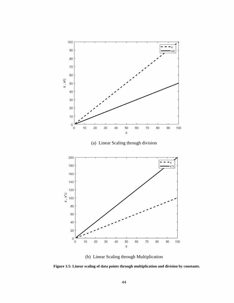
44
(a) Linear Scaling through division
(b) Linear Scaling through Multiplication
Figure 3.5: Linear scaling of data points through multiplication and division by constants.

45
In other stages, the division by the constant N (total number of data points in the designated
window) as in the mean absolute value (MAV) depicted in equation (3) and the mean in standard
deviation (STD) depicted in equation (6) contributes in resulting a shorter vector. Since the output
of both MAV and the mean are fed to other following stages, a shorter output vector creates smaller
and faster design. If the division can be done through shifting, the complexities of division can be
avoided. For this matter, the window size (number of samples in one window) is chosen such that
it is a power of 2.
The only division that cannot be removed, without affecting the sensitivity obtained, is the
division by the standard deviation in the Hurst exponent shown in equation (6). The standard
deviation is not a constant, but rather varying according to the values of the data samples in each
window. However, in order to avoid the complexities of performing a fractional division (as the
length of the vector R is shorter than the length of the vector S), the value of R is multiplied by216.
Linearly scaling the value of R by the constant 216 does not affect the classification results as
previously stated in this subsection.
The natural logarithm in the last stages of both fractal dimension and Hurst exponent is realized
by calculating the inverse hyperbolic tan of the specified value. The adopted identity for
calculating the natural logarithm is ln(𝑥) = 2 ∗ 𝑡𝑎𝑛ℎ−1 ( 𝑥−1
𝑥+1 ). The multiplication by 2 is,
however, not necessarily to be performed as it is only doubling all values and does not affect the
classifier decision. The effect of removing the multiplication by the constant 2 is depicted in Figure
3.8.
Figure 3.6: Effect of removing the multiplication by the constant 2 on the curve of ln(x).

46
The inverse hyperbolic tan is a CORDIC design [40] with range expansion [41]. The CORDIC
approach is an iterative technique that is utilized for evaluating several elementary mathematical
functions that is inverse hyperbolic tan in the proposed design. The technique presents a relatively
low-cost solution for evaluating the function in question as it consists of only LUTs, additions, and
shifts. The basic building unit of the hyperbolic CORDIC design is depicted in Figure 3.9.
Figure 3.7: Basic building unit of the hyperbolic CORDIC Architecture.
3.4 Approximate feature extractor
The approximate feature extractor considers the power consumption and area utilization more
than keeping the sensitivity as originally obtained. A performance degradation of 1-2% in the
favor of saving power and area is the objective of the approximate design. Therefore, all the
scaling techniques performed in the optimized feature extractor are preserved, and in this section
further approximations are adopted.
The CORDIC design of the 𝑡𝑎𝑛ℎ−1 does not only suffer relatively high latency compared to all
other utilized modules, but also has the highest dynamic power consumption in the design.
Taking the natural logarithm of certain value can be considered as non-linearly scaling this value
through a specific manner which is, in this case, 𝑡𝑎𝑛ℎ−1. If there exists a mathematical function
that can perform an approximate scaling to the 𝑡𝑎𝑛ℎ−1, then the 𝑡𝑎𝑛ℎ−1 can be approximated

47
using this mathematical function. The closest curve to the 𝑡𝑎𝑛ℎ−1 is the square root curve.
Figure 3.10 shows that the square root function presents itself as an approximately scaled version
of the hyperbolic tan function.
Figure 3.8: The analogy between Ln function and SQRT function
A comparison between both inverse hyperbolic tan and square root functions in terms of power
consumption, area utilization, and latency when implemented on Virtex-7 FPGA for 24 bit inputs
is depicted in Table 3.2.
𝒕𝒂𝒏𝒉−𝟏 sqrt
Power consumption 27.1 mW 3.7 mW
Area utilization 1314 LUT
451 Register
70 LUT
91 Register
Latency 30 cycles 14 cycles
Table 3.2: 〖tanh〗^(-1) vs Sqrt FPGA implementation results

48
The divider exploited in the Hurst exponent to divide the range of the cumulative deviation from
the mean by the standard deviation is the second highest power consumer in the proposed feature
extractor. Removing this division enhances both occupied area, and power consumption at the
expense of accuracy degradation.

49
Chapter 4 Implementation Results
The implementation results are divided into two sections; Optimized feature extractor results,
and approximate feature extractor results. Each section elucidates Software, and Hardware results
for each design. For the software results, three performance metrics, namely, sensitivity,
specificity, and accuracy are measured for each feature extractor along with Sequential Minimal
Optimization (SMO) training accelerator. While the Hardware results discuss the Area utilization,
and power consumption of each design on both FPGA and ASIC platforms.
4.1 Optimized feature extractor
The sensitivity, specificity, and accuracy originally obtained when the exact features using
floating point arithmetic are exploited along with SMO training and linear SVM classification are
98.39%, 92.60%, and 92.61% respectively.
When the discussed divisions and multiplications by constants are removed, and fixed point
representation is exploited, the sensitivity, specificity, and accuracy are 98.39%, 92.37%, 92.39%,
respectively and correspondingly the metrics degradations due to these approximations are
insignificant.
The performance metrics are not only affected by the feature extraction strategies, training
approaches and classification techniques, but also affected by changing the window size. Window

50
size is the number of samples per single entry; each EEG signal is divided into epochs of either
1024 sample, 512 sample, or 256 sample which corresponds to 4-second windows, 2-second
windows, 1-second windows respectively.
Table 4.1 lists the performance metrics obtained in response to changing the window size. It can
be noted that by increasing the window size, the sensitivity gets improved gradually, while a
specificity degradation occurs.
Window Size Sensitivity Specificity Accuracy
1 second (256 sample) 96.20% 94.04% 94.05%
2 seconds (512 sample) 97.52% 93.66% 93.67%
4 seconds (1024 sample) 98.39% 92.37% 92.39%
Table 4.1: The effect of changing the window size on the performance metrics for the optimized feature
extractor.
The proposed feature extractor is generic; by changing the window size parameter, the whole
design is adjusted to be working with the new window size. The optimized feature extractor is
implemented on Vertix-7 FPGA with 100 MHz clock. The block diagram of the proposed design
is shown in Figures 4.1-4.2-4.3.
Figure 4.1 depict the standard deviation (STD) block diagram utilized in the Hurst Exponent
(HE) block diagram shown in Figure 4.2. the mean is first calculated by summing up all the data
points within the window and then dividing the summation result over the number of samples
within the window. In case of adopting the design scheme with a 4-second second window size,
the number of samples within the window becomes 1024. The division by 1024 (210) is done
through shifting as discussed earlier to avoid the complexities of the normal division. The mean
is then subtracted from each data point. Data points from patient scalp are stored inside 1024
registers each is 16-bit wide. Finally a square root is taken to the summation of all the squared
data points after subtracting the mean from each of them.

51
Figure 4.1: standard deviation
Figure 4.2: Hurst Exponent feature
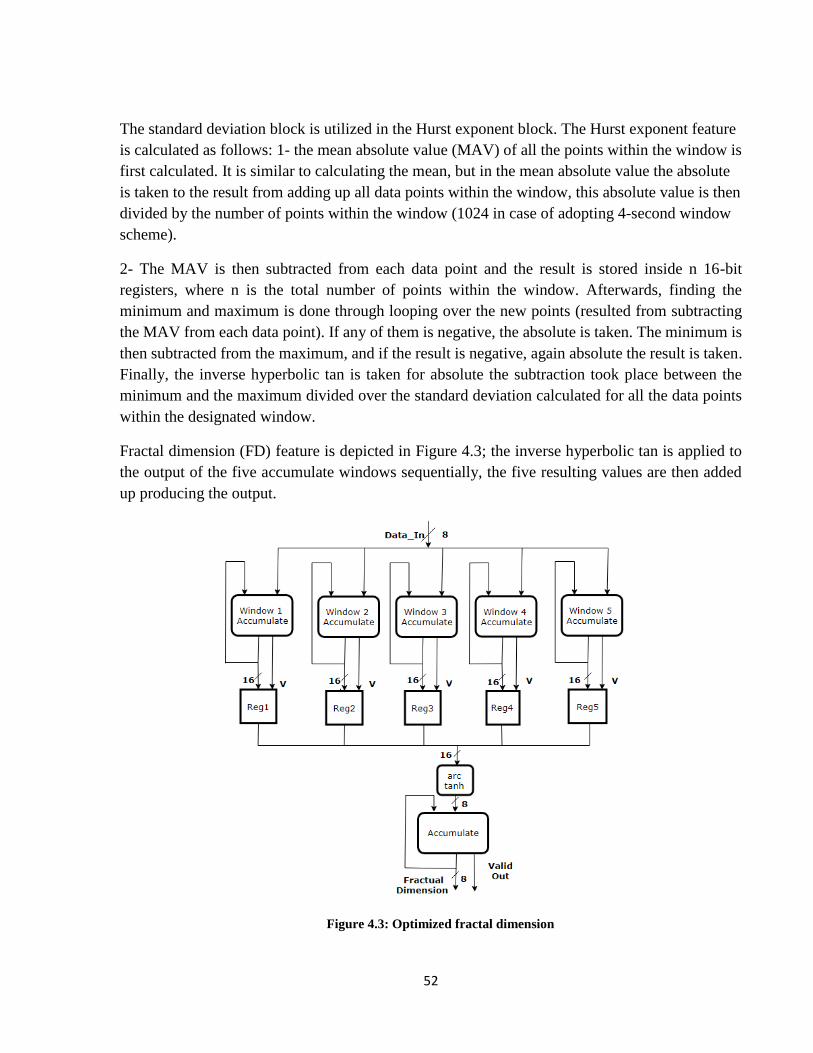
52
The standard deviation block is utilized in the Hurst exponent block. The Hurst exponent feature
is calculated as follows: 1- the mean absolute value (MAV) of all the points within the window is
first calculated. It is similar to calculating the mean, but in the mean absolute value the absolute
is taken to the result from adding up all data points within the window, this absolute value is then
divided by the number of points within the window (1024 in case of adopting 4-second window
scheme).
2- The MAV is then subtracted from each data point and the result is stored inside n 16-bit
registers, where n is the total number of points within the window. Afterwards, finding the
minimum and maximum is done through looping over the new points (resulted from subtracting
the MAV from each data point). If any of them is negative, the absolute is taken. The minimum is
then subtracted from the maximum, and if the result is negative, again absolute the result is taken.
Finally, the inverse hyperbolic tan is taken for absolute the subtraction took place between the
minimum and the maximum divided over the standard deviation calculated for all the data points
within the designated window.
Fractal dimension (FD) feature is depicted in Figure 4.3; the inverse hyperbolic tan is applied to
the output of the five accumulate windows sequentially, the five resulting values are then added
up producing the output.
Figure 4.3: Optimized fractal dimension
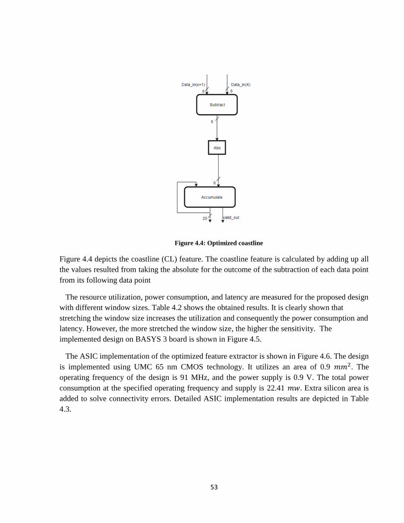
53
Figure 4.4: Optimized coastline
Figure 4.4 depicts the coastline (CL) feature. The coastline feature is calculated by adding up all
the values resulted from taking the absolute for the outcome of the subtraction of each data point
from its following data point
The resource utilization, power consumption, and latency are measured for the proposed design
with different window sizes. Table 4.2 shows the obtained results. It is clearly shown that
stretching the window size increases the utilization and consequently the power consumption and
latency. However, the more stretched the window size, the higher the sensitivity. The
implemented design on BASYS 3 board is shown in Figure 4.5.
The ASIC implementation of the optimized feature extractor is shown in Figure 4.6. The design
is implemented using UMC 65 nm CMOS technology. It utilizes an area of 0.9 𝑚𝑚2. The
operating frequency of the design is 91 MHz, and the power supply is 0.9 V. The total power
consumption at the specified operating frequency and supply is 22.41 𝑚𝑤. Extra silicon area is
added to solve connectivity errors. Detailed ASIC implementation results are depicted in Table
4.3.

54
1-second window
(256 sample)
2- second window
(512 sample)
4-second window
(1024 sample)
Resource
Utilization
5026 LUTs
2319 Slice Registers
5890 LUTs 2320
Slice Registers
7611 LUTS 2342
Slice Registers
Power
Consumption 43.67 mW 47.78 mW 95.822 mW
Latency 8280 ns 15960 ns 31320 ns
Table 4.2: FPGA Implementation results for different window sizes.
Figure 4.5: FPGA implementation of optimized feature extractor

55
Figure 4.6: ASIC implementation of the optimized feature extractor
Block Number of
cells Area (𝒎𝒎𝟐) Power (𝒎𝑾)
Optimized
Feature
Extractor
99051 0.9 22.41
Table 4.3: ASIC Implementation results of the optimized feature extractor.
4.2 Approximate feature extractor
After removing the division by the standard deviation replacing every natural logarithm by square
root, the sensitivity correspondingly drops to 96.77% (a drop by 1.6%).The sensitivity, specificity,
and accuracy obtained when the approximate feature extractor along with linear SVM classifier
and SMO training accelerator are utilized for 4-second windows are 96.77%, 90.41%, and 90.43%
respectively.
As discussed in section 3.3, linearly scaling data points (division by constants) does not affect the
classification result. The standard deviation, however, is not a constant. Thus, removing it does

56
affect the classification result. Also, non-linearly scaling data points, for instance, replacing the
natural logarithm by square root function downgrades the classifier decision. Table 4.4 shows the
effect of removing the division by the standard deviation, and replacing each natural logarithm
with a square root.
Approximation Sensitivity Specificity Accuracy
Before replacing Ln
with sqrt, and
removing the standard
deviation
98.38% 91.62% 91.64%
Removing the division
and replacing Ln by
sqrt (with 8 bit inputs)
96.77% 91.04% 91.05%
Removing the division
by the standard
deviation
96.77%
90.41%
90.43%
Table 4.4: the effect of removing the division by the standard deviation, and replacing each natural
logarithm with a square root
Removing the division by the standard deviation surely has an effect on the sensitivity, but not a
dominating effect. Removing the Ln function has a dominating effect on the sensitivity, while
removing the standard deviation has the dominant effect on the specificity.
If the analysis are reversed; the standard deviation is first removed, then each Ln is replaced by a
Square root. The sensitivity will first drop to approximately 97%, and the specificity drops to
90.41% in response to removing the division by the standard deviation. Then after replacing each
Ln with square root, the sensitivity drops 96.77% and the specificity remains 90.41%
In a similar manner to obtaining the optimum length of the input EEG samples, the optimum length
for each of the intermediate signals was obtained. The output of each mathematical operation was
fed into dM2bM2dM, and the result was again fed into the following mathematical operation.
Table 4.5 shows the obtained sensitivity, specificity, and accuracy from limiting the length of the
intermediate signals.

57
Feature Optimized Vector sensitivity specificity Accuracy
Fractal
Dimension
Limit the output length of the 5
accumulate stages to 8 bits
96.774194 91.041196 91.057546
Mean
Absolute
Value
Limit the output vector length
to 10 bits
96.774194 91.747013 91.761351
Cost Line Limit the length of the output
vector to 20 bits 96.774194 91.765466 91.779751
Table 4.5: Performance metrics obtained from limiting the length of the intermediate signals.
Any smaller value for the intermediate signals length would cause the sensitivity to drop to
approximately 95%.
The effect of changing the window size on the performance metrics is studied by testing the
design with input windows that varies in size from 1 second to 4 seconds. The performance metrics
obtained in response to changing the window size are listed in Table 4.6. The wider the window,
the less the sensitivity. With 4-second window the specificity slightly increases at the expense of
a moderate decrease in the sensitivity.
Window Size Sensitivity Specificity Accuracy
1 second (256 sample) 98.31% 90.11% 90.13%
2 seconds (512
sample) 97.52% 90.97% 90.99%
4 seconds (1024
sample) 96.77% 90.41% 90.43%
Table 4.6: Performance metrics with different input window sizes for the approximate feature extractor.
Similar to the proposed optimized feature extractor, the proposed approximate feature extractor is
generic; by changing the window-Size parameter, the whole design is adapted to be working with

58
any window size. The proposed design is implemented on Vertix-7 FPGA with a clock frequency
of 100 MHz. The block diagram of the proposed feature extractor is shown in Figures 4.7-4.8-4.9.
Figure 4.7 depicts the coastline feature which is calculated in an exactly similar manner to
calculating it in the optimized feature extractor by adding up all the values resulted from taking
the absolute for the outcome of the subtraction of each data point from its following data points.
While, the block diagram of the fractal dimension feature is depicted in Figure 4.7 where the square
root is applied to the output of the five accumulate windows sequentially instead of applying the
inverse hyperbolic tan. The five resulting values are then added up producing the output.
Figure 4.7: Optimized coastline feature
Finally, Figure 4.9 illustrates how the Hurst exponent feature is calculated. The block diagram
makes it clear that the design becomes simpler after removing the standard deviation block. The
Hurst exponent in the approximate feature extractor is calculated as follows: 1- the mean absolute
value (MAV) of all the points within the window is first calculated. 2- The MAV is then subtracted
from each data point and the result is stored inside n 16-bit registers, where n is the total number
of points within the window. Afterwards, finding the minimum and maximum is done through
looping over the new points (resulted from subtracting the MAV from each data point). If any of
them is negative, the absolute is taken. The minimum is then subtracted from the maximum, and
if the result is negative, again absolute the result is taken. Finally, the square root is applied to
absolute the subtraction took place instead of applying the inverse hyperbolic tan.

59
Figure 4.8: Optimized fractal dimension feature
Figure 4.9: approximate Hurst exponent feature
The resource utilization, power consumption, and latency associated with each window size are
shown in Table 4.7. It is clearly shown that increasing the window size increases the utilization
and consequently the power consumption and latency. As opposed to the optimized feature
extractor, the sensitivity increases with smaller window sizes in the approximate feature extractor.
However, the highest specificity is achieved with 2-second window size.

60
1-second
window
(256 sample)
2- second
window
(512 sample)
4-second window
(1024 sample)
Resource
Utilization
1859 LUTs
738 Slice
Registers
2119 LUTs
576 Slice
Registers
3319 LUTs
576 Slice
Registers
Power
Consumpti
on
8.1 mW 9.1 mW 12.3 mW
Latency 7820 ns 15500 ns 30860 ns
Table 4.7: FPGA implementation results of the approximate feature extractor.
For the purpose of testing the design in real life on an available board, the design is also
implemented on BASYS 3 board. The implemented design is shown in Figure 4.10.
Figure 4.10: FPGA implementation of approximate feature extractor
Synopsis Design Compiler (DC) B2008.09 with hardware calibrated UMC65nm CMOS
technology is adopted for testing each feature with different frequencies varying from 1KHz to
100MHz.

61
Feature 1 KHz 10 KHz 100 KHz 1 MHz 10 MHz 100 MHz
Fractal
Dimension 1.27 𝜇𝑊 1.36 𝜇𝑊 2.28 𝜇𝑊 11.4 𝜇𝑊 103 𝜇𝑊 1.017 𝑚𝑊
Hurst
Exponent 319 𝑛𝑊 416 𝑛𝑊 666 𝑛𝑊 3.1 𝜇𝑊 28.1 𝜇𝑊 277 𝜇𝑊
Coastline 82.8 𝑛𝑊 88.8 𝑛𝑊 150 𝑛𝑊 757 𝑛𝑊 6.83 𝜇𝑊 67.3 𝜇𝑊
Table 4.8: total power consumption of each feature in frequency range [1KHz-100MHz]
Table 4.8 shows the total power consumption of each feature with multiple frequencies. It is clearly
shown that the higher the operating frequency, the higher the power consumption. Power
consumption increases gradually in the range of frequencies from 1 KHz to 1 MHZ. at 10 MHz
upward, a significant increase in power consumption can be noted
The proposed feature extractor was implemented using both UMC 65-nm CMOS technology and
UMC 130-nm CMOS technology
The UMC 65-nm CMOS technology ASIC implementation of the approximate feature extractor
is shown in Figure 4.11. The operating frequency of the design is 100 MHz and the power supply
is 0.9V. The total power consumption at the specified operating frequency is 2.5𝑚𝑊. The design
area is 0.057 𝑚𝑚2, and detailed resource utilization and power consumption results are listed in
Table 4.9.
Block Number of
cells Area (𝒎𝒎𝟐) Power (𝒎𝑾)
Approximate
Feature
Extractor
11171 0.057 2.55
Table 4.9: 65-nm ASIC Implementation results of the approximate feature extractor.

62
Figure 4.11: 65-nm ASIC implementation of the approximate feature extractor
Detailed power consumption factors of the 130-nm approximate feature extractor ASIC
implementation is listed in Table 4.10.
Total power Internal power Switching
power
Leakage
power
2.55 mW 1.732 mW 0.817 mW 0.008 mW
Table 4.10: 65-nm detailed power consumption
On the other hand, the UMC 130-nm CMOS technology ASIC implementation of the
approximate feature extractor is shown in Figure 4.12. The operating frequency of the design is
100 MHz and the power supply is 0.9V. The total power consumption at the specified operating
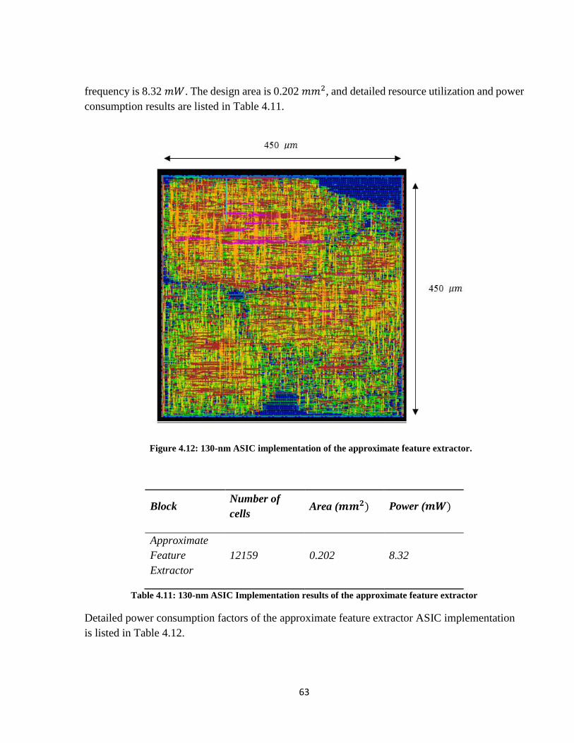
63
frequency is 8.32 𝑚𝑊. The design area is 0.202 𝑚𝑚2, and detailed resource utilization and power
consumption results are listed in Table 4.11.
Figure 4.12: 130-nm ASIC implementation of the approximate feature extractor.
Block Number of
cells Area (𝒎𝒎𝟐) Power (𝒎𝑾)
Approximate
Feature
Extractor
12159 0.202 8.32
Table 4.11: 130-nm ASIC Implementation results of the approximate feature extractor
Detailed power consumption factors of the approximate feature extractor ASIC implementation
is listed in Table 4.12.

64
Total power Internal power Switching
power
Leakage
power
8.322 mW 5.817 mW 2.383 mW 0.128 mW
Table 4.12: 130-nm detailed power consumption
4.3 SVM Classifier
The classifier is implemented on Viretx-7 FPGA with 100 MHz operating frequency. The
implementation results are listed in Table 4.13.
Block LUTS Registers Power
consumption
Classifier 238 137 6 mW
Table 4.13: classifier FPGA implementation results
The classifier is implemented using both UMC 65-nm CMOS technology and UMC 130-nm
CMOS technology
The UMC 65-nm CMOS technology ASIC implementation of the classifier is shown in Figure
4.13. The operating frequency of the design is 100 MHz and the power supply is 0.9V. The total
power consumption at the specified operating frequency is 2.71 𝑚𝑊. The design area is 0.032
𝑚𝑚2, and detailed resource utilization and power consumption results are listed in Table 4.14.
Block Number of
cells Area (𝒎𝒎𝟐) Power (𝒎𝑾)
classifier 8554 0.032 2.71
Table 4.14: 65-nm ASIC Implementation results of the SVM classifier.

65
Figure 4.13: 65-nm ASIC implementation of the SVM classifier.
Detailed power consumption factors of the classifier ASIC implementation is listed in
Table 4.15.
Total power Internal power Switching
power
Leakage
power
2.71 mW 1.01 mW 1.698 mW 0.007 mW
Table 4.15: 65-nm detailed power consumption
On the other hand, the UMC 130-nm CMOS technology ASIC implementation of the
approximate feature extractor is shown in Figure 4.14. The operating frequency of the design is
100 MHz and the power supply is 0.9V. The total power consumption at the specified operating

66
frequency is 8.32 𝑚𝑊. The design area is 0.202 𝑚𝑚2, and detailed resource utilization and power
consumption results are listed in Table 4.16.
Figure 4.14: 130-nm ASIC implementation of the SVM classifier.
Block Number of
cells Area (𝒎𝒎𝟐) Power (𝒎𝑾)
classifier 5270 0.09 6.33
Table 4.16: 130-nm ASIC Implementation results of the SVM classifier.
Detailed power consumption factors of the approximate feature extractor ASIC
implementation is listed in Table 4.17.

67
Total power Internal power Switching
power
Leakage
power
6.33 mW 2.772 mW 3.493 mW 0.068 mW
Table 4.17: 130-nm detailed power consumption
It is clear the 130 nm implementation suffers significantly higher leakage power.
4.4 Dynamic Partial Reconfiguration
The tradeoff between the two proposed designs is sensitivity and specificity achieved versus
area utilization and power consumption of the design. While the approximate design has
significantly less area utilization and power consumption, its specificity suffers a drop by around
2% in comparison with the optimized design.
For maximum advantage the two designs can be exploited, however, When both designs are placed
together the dynamic power consumption is 95 mW and the junction temperature is 125 (junction
temperature exceeded).
The proposed power-aware system is achieved through Dynamic Partial Reconfiguration (DPR).
Dynamic partial reconfiguration is a technique that allows the exploitation of certain FPGA
resources for more than one design at the same time. The two designs can be configured to replace
each other depending on the available power and the criticality of the situation. If the power level
is high or the patient is doing a very critical activity (like driving), the optimized feature extractor
is in control, and when the available power decrease below certain threshold or the patient is doing
a less critical activity, the approximate feature extractor becomes responsible for the operation.
Virtex-7 board is used for testing the proposed prototype; it was found that the most suitable
controller for the implemented design using this board is partial reconfiguration controller (PRC)
based on the comparative study done in [26].

68
Figure 4.15: Dynamic reconfiguration between Optimized and approximate feature extractor
Figure 4.16 shows the implemented dynamic part of the design. The reconfigurable partition can
be reconfigured during run time with the two different reconfigurable modules, the optimized
feature extractor and the approximate feature extractor. The reconfigurable partition size is chosen
to accommodate the optimized feature extractor, or the approximate feature extractor. Resources
utilization and power consumption for each of the two reconfigurable modules are shown in Table
4.18. It is shown that the power consumption drops by around 64%, moreover, the junction
temperature remains within the normal margins.
(a) Black box implementation of RM1 (Optimized FE).

69
(b) Black box implementation of RM2 (Approximate FE).
Figure 4.16: Dynamic Partial Reconfiguration between optimized and approximate feature extractor
Reconfigurable
Module Utilization Dynamic Power
RM1
(Optimized FE)
8236 LUTs 2466
slice Registers 101 𝑚𝑊
RM2
(Approximate
FE)
4132 LUTs 798
slice Registers 36 𝑚𝑊
Table 4.18: Dynamic reconfiguration results.
4.5 Comparison with Prior work
In this work, modified Fractal Dimension, Husrt exponent, and coastline equations are proposed.
The modified equations does not produce the same results as the ones proposed in [54], [53], and
[55] respectively, but they keep the sensitivity of machine learning algorithms either exactly
similar or approximate to the sensitivity obtained from the original equations. Table depicts the
proposed equations.

70
Optimized Feature Extractor Approximated Feature Extractor
Fractal
Dimension
𝐿𝑚(𝑘) = ∑ | 𝑥(𝑚 + 𝑖𝑘)
𝑁−𝑚𝑘
𝑖=1
− 𝑥(𝑚 + (𝑖 − 1) ∗ 𝑘)|
𝐹𝐷 = ∑ 𝑡𝑎𝑛ℎ−1 (𝐿𝑚 (𝑘))
𝑘
𝑚=1
𝐿𝑚(𝑘) = ∑ | 𝑥(𝑚 + 𝑖𝑘)
𝑁−𝑚𝑘
𝑖=1
− 𝑥(𝑚 + (𝑖 − 1) ∗ 𝑘)|
𝐹𝐷 = ∑ sqrt (𝐿𝑚 (𝑘))
𝑘
𝑚=1
Hurst
Exponent
𝑀𝐴𝑉 = 1
𝑁 ∑ |𝑥𝑖|
𝑁
𝑖=1
𝑅 = ||max(𝑥 − 𝑀𝐴𝑉)| − |min (𝑥− 𝑀𝐴𝑉)||
𝑆 = √∑(𝑥𝑖 − 𝑚𝑒𝑎𝑛(𝑥))2
𝑁
𝑖=1
𝐻 = 𝑡𝑎𝑛ℎ−1 (𝑅
𝑆)
𝑀𝐴𝑉 = 1
𝑁 ∑ |𝑥𝑖|
𝑁
𝑖=1
𝑅 = ||max(𝑥 − 𝑀𝐴𝑉)| − |min (𝑥− 𝑀𝐴𝑉)||
𝐻 = sqrt (𝑅)
Coastline 𝐶𝑜𝑎𝑠𝑡𝑙𝑖𝑛𝑒 = ∑ |𝑥𝑖+1 − 𝑥𝑖|
𝑁
𝑖=1
𝐶𝑜𝑎𝑠𝑡𝑙𝑖𝑛𝑒 = ∑ |𝑥𝑖+1 − 𝑥𝑖|
𝑁
𝑖=1
Table 4.19: Proposed Fractal Dimension, Hurst Exponent, and Coastline equations
The two proposed designs achieve a higher sensitivity and specificity then many work in the
literature like [4, 7, 8]. Moreover, an FPGA-system level comparison between the proposed
systems and other seizure detection systems is depicted in Table 4.20.
The highest achieved sensitivity by the proposed designs is higher than that in [43, 44, 20] and
approximately equals to the sensitivity achieved in [44]. No DSPs are utilized in the proposed
design as opposed to [46], and [47]. Moreover, the utilization of the approximate feature extractor
is less than the mentioned previous work [45, 46, 47, 48], while the utilization of the optimized
feature extractor has less utilization than these systems in [45, 46, 48]. The comparison does not

71
include the power consumption because every work has its own operating frequency, thus the
utilization only is compared which gives an insight that the power consumed by the approximate
feature extractor is significantly less than other designs. No work in the literature introduced
power-aware systems for seizure detection where DPR is utilized.
System
blocks FPGA
Latenc
y#cycle
s
Area Performance
LUTs Register
s
DSP
s Sensitivity
Specificit
y
[45]
Feature
Extraction
+
Classificati
on
Virtex - 5 242 2583
0.3KB memory - 95.24% N/R
[46] Feature
Extraction PYNQ-Z1 N/R
1749
2 16685 46 92.9% 96.3%
[48]
Feature
Extraction
+
Classificati
on
Zed-board 20156 8001 8622 31 98.4% N/R
[47]
Feature
Extraction
+
classificati
on
Microsemi
Igloo 2563
1237
5.56 KB memory - 92.51% 80.1%
Proposed
Optimized
system
Feature
Extraction
+
Classificati
on
Virtex - 7 3148 7849 7479 - 98.39% 92.37%
Proposed
Approxim
ate system
Feature
Extraction
+
Classificati
on
Virtex - 7 798 2133 875
-
98.31% 90.11%
Table 4.20: Comparison with Prior Work

72
Chapter 5
Conclusion and Future work
In this chapter, the proposed work is sealed with the conclusion that depicts the main findings
and achievements of this work. Followed by the future work section where the main ideas that
can be implemented in the future are proposed.
5.1 Conclusion
A high sensitivity low cost power-aware seizure detection system that can be exploited in
neural seizure detection applications is implemented on both FPGA and ASIC platforms. Two
designs for the purpose of seizure detection are presented. Optimized design that has
significantly high performance on the expense of area and power consumption, and approximate
design that saves more than 50% the power and area reserved for the optimized design, but
suffers 2% decrease in the specificity achieved.
A power-aware system is achieved through dynamic partial reconfiguration between the two
designs saving around 64% of the power consumption to ensure long battery life time of the
implemented chip while keeping the highest possible performance. The implemented system
exploits fractal dimension, Hurst exponent, and coastline for feature extraction, in addition to
support vector machine training and classification with linear kernel. The system is tested with
SMO training accelerator through a sliding windows varying from 1 to 4 seconds. The maximum
achieved specificity of the proposed system is 92.14%, while the highest achieved sensitivity
obtained is 98.39% at 100 MHz operating frequency.

73
5.2 Future Work
In the future, it is suggested that the proposed work is validated against different data sets other
than Children Hospital Boston (CHB) data set. Multiple human epileptic EEG data sets already
exists in the literature like Bonn and Freiburg. While animal epileptic EEG data sets can be
found in Kaggle data set.
Moreover, the proposed feature extractor can be tested for Epileptics seizure prediction and not
just the detection and find out whether the close sensitivity to the one achieved with the detection
can be achieved.
Furthermore, Dynamic partial reconfiguration can be implemented between Epileptic seizure
detection and prediction systems.

74
References
1. K. Devarajan, S. Bagyaraj, V. Balasampath, E. Jyostna, and K. Jayasri, “EEG-based
epilepsy detection and prediction,” Int. J. Eng. Technol., vol. 6, no. 3, pp. 212–216, 2014.
2. Schmidt DTwo antiepileptic drugs for intractable epilepsy with complex-partial seizures.
Journal of Neurology, Neurosurgery & Psychiatry, 45:1119-1124, 1982.
3. A. Varsavsky, I. Mareels, and M. Cook, Epileptic Seizures and the EEG: Measurement,
Models, Detection and Prediction. Boca Raton, FL, USA: CRC Press, 2016.
4. J. Gotman, “Automatic seizure detection: improvements and evaluation.
Electroencephalography and Clinical Neurophysiology,” 76(4), 317–324, 1990.
5. Kerrigan, J. F., Litt, B., Fisher, R. S., Cranstoun, S., French, J. A., Blum, D. E., Graves, N.,
“Electrical Stimulation of the Anterior Nucleus of the Thalamus for the Treatment of
Intractable Epilepsy,” Epilepsia, 45(4), 346–354, 2004
6. Feng, L., Li, Z., & Wang, Y. VLSI Design of SVM-Based Seizure Detection System With
On-Chip Learning Capability. IEEE Transactions on Biomedical Circuits and Systems,
12(1), 171–181, 2017.
7. Q. Yuan, W. Zhou, S. Li, and D. Cai, “Epileptic eeg classification based on extreme
learning machine and nonlinear features,” Epilepsy research, vol. 96, no. 1-2, pp. 29–38,
2011.
8. S. Li, W. Zhou, Q. Yuan, S. Geng, and D. Cai, “Feature extraction and recognition of ictal
eeg using emd and svm,” Computers in biology and medicine, vol. 43, no. 7, pp. 807–816,
2013.
9. Gammerman and V. Vovk, “Alexey Chervonenkis’s bibliography: Introductory
comments,” J. Mach. Learn. Res., vol. 16, pp. 2051–2066, 2015.
10. Q. Yuan, W. Zhou, S. Li, and D. Cai, “Epileptic eeg classification based on extreme
learning machine and nonlinear features,” Epilepsy research, vol. 96, no. 1-2, pp. 29–38,
2011.
11. Zhang, C., Bin Altaf, M. A., & Yoo, J. Design and Implementation of an On-Chip Patient-
Specific Closed-Loop Seizure Onset and Termination Detection System. IEEE Journal of
Biomedical and Health Informatics, 20(4), 996–1007, 2016.
12. H. Elhosary, M. H. Zakhari, M. A. Elgammal, M. A. E. A. Ghany, K. N. Salama, and H.
Mostafa, “Low-Power Hardware Implementation of a Support Vector Machine Training
and Classification for Neural Seizure Detection”, IEEE Transactions on Biomedical
Circuits and Systems, vol. 13, no. 6, pp. 1324-1337, Dec. 2019

75
13. H. Wang, W. Shi and C. Choy, "Hardware Design of Real Time Epileptic Seizure Detection
Based on STFT and SVM," in IEEE Access, vol. 6, pp. 67277-67290, 2018.
14. F. Mormann, R. G. Andrzejak, C. E. Elger, and K. Lehnertz, “Seizure prediction: The long
and winding road,” Brain, vol. 130, no. 2, pp. 314–333, 2006.
15. KO. Cho, HJ. Jang, “Comparison of different input modalities and network structures for
deep learning-based seizure detection,” Sci Rep 10, 122, 2020.
16. A. Varsavsky, I. Mareels, and M. Cook, Epileptic Seizures and the EEG: Measurement,
Models, Detection and Prediction. Boca Raton, FL, USA:CRC Press, 2016.
17. Y. Liu, W. Zhou, Q. Yuan, and S. Chen, “Automatic seizure detection using wavelet
transform and SVM in long-term intracranial EEG,”IEEE Trans. Neural Syst. Rehabil.
Eng., vol. 20, no. 6, pp. 749–755,Nov. 2012.
18. Cho, KO., Jang, HJ. Comparison of different input modalities and network structures for
deep learning-based seizure detection. Sci Rep 10, 122 (2020).
19. Colucci, Dennis. Cannabis and Hearing Care: Hearing Loss and Tinnitus. The Hearing
Journal. 72. 43. 10, 2019.
20. J. S. Kumar and P. Bhuvaneswari, “Analysis of Electroencephalography (EEG) Signals
and Its Categorization–A Study,”Procedia Engineering,Volume 38, 2012.
21. S. J. van Albada and P. A. Robinson, “Relationships between electroencephalographic
spectral peaks across frequency bands,” Front. Hum. Neurosci., vol. 7, 2013.
22. M. A. Elgammal, "hardware implementation of machine learning techniques for neural
seizure detection," Msc dissertation, Faculty of engineering. Cairo Univ., Cairo, 2018.
23. J. L. Cantero, M. Atienza, R. Stickgold, M. J. Kahana, J. R. Madsen and B. Kocsis, "Sleep-
dependent $\theta$ oscillations in the human hippocampus and neocortex," Journal of
Neuroscience, vol. 23, pp. 10897-10903, 2003.
24. S. Palva and J. M. Palva, "New vistas for α-frequency band oscillations," Trends in
neurosciences, vol. 30, pp. 150-158, 2007.
25. Andrzejak RG, Lehnertz K, Rieke C, Mormann F, David P, Elger CE (2001) Indications
of nonlinear deterministic and finite dimensional structures in time series of brain electrical
activity: Dependence on recording region and brain state, Phys. Rev. E, 64, 061907.
26. A. H. Shoeb, “Application of machine learning to epileptic seizure onset detection and
treatment,” Ph.D. dissertation, Massachusetts Institute of Technology, 2009.
27. B. Boashash, M. Mesbah, and P. Coldtiz, “Time-frequency detection of
EEGabnormalities,” in Time-Frequency Signal Analysis and Processing:A Comprehensive
Reference. Amsterdam, The Netherlands: Elsevier, 2003, ch. 15, pp. 663–670.
28. Y. Liu, W. Zhou, Q. Yuan, and S. Chen, “Automatic seizure detection using wavelet
transform and SVM in long-term intracranial EEG,” IEEE Trans. Neural Syst. Rehabil.
Eng., vol. 20, no. 6, pp. 749–755, Nov. 2012.
29. A. Subasi and M. I. Gursoy, “EEG signal classification using PCA, ICA, LDA and support
vector machines,” Expert Syst. Appl., vol. 37, no. 12, pp. 8659–8666, 2010.
30. K. Helal et al., “Low-power high-accuracy seizure detection algorithms for neural
implantable platforms,” in Proc. IEEE Int. Conf.Microelectron., 2017, pp. 231–234.
31. J. McCarthy and E. A. Feigenbaum, "In memoriam: Arthur samuel: Pioneer in machine
learning," AI Magazine, vol. 11, p. 10, 1990.

76
32. H. C. Hendrickson, "Fast High-Accuracy Binary Parallel Addition," in IRE Transactions
on Electronic Computers, vol. EC-9, no. 4, pp. 465-469, Dec. 1960, doi:
10.1109/TEC.1960.5219886.
33. Brent and Kung, "A Regular Layout for Parallel Adders," in IEEE Transactions on
Computers, vol. C-31, no. 3, pp. 260-264, March 1982, doi: 10.1109/TC.1982.1675982.
34. B. Sugla and D. A. Carlson, "Extreme area-time tradeoffs in VLSI," in IEEE Transactions
on Computers, vol. 39, no. 2, pp. 251-257, Feb. 1990, doi: 10.1109/12.45210.
35. Booth, A. D., “A Signed Binary Multiplication Technique,” Quarterly J. Mechanics and
Applied Mathematics, Vol. 4, Pt. 2, pp.236-240, June 1951.
36. L. Ciminiera and P. Montuschi, "Carry-save multiplication schemes without final
addition," in IEEE Transactions on Computers, vol. 45, no. 9, pp. 1050-1055, Sept. 1996,
doi: 10.1109/12.537128.
37. Dadda, L., “Some Schemes for Parallel Multipliers,” Alta Frequenza, Vol. 34, pp. 349-356,
1956
38. C. S. Wallace, "A Suggestion for a Fast Multiplier," in IEEE Transactions on Electronic
Computers, vol. EC-13, no. 1, pp. 14-17, Feb. 1964, doi: 10.1109/PGEC.1964.263830.
39. C. R. Baugh and B. A. Wooley, "A Two's Complement Parallel Array Multiplication
Algorithm," in IEEE Transactions on Computers, vol. C-22, no. 12, pp. 1045-1047, Dec.
1973, doi: 10.1109/T-C.1973.223648.
40. Walther, John S. A unified algorithm for elementary functions. Proceedings of the May 18-
20, 1971, spring joint computer conference. 1971.
41. Hu, Xiaobo, Ronald G. Harber, and Steven C. Bass. Expanding the range of convergence
of the CORDIC algorithm. IEEE Transactions on computers 1 (1991): 13-21.
42. A. L. Samuel, "Some studies in machine learning using the game of checkers," IBM Journal
of research and development, vol. 3, pp. 210-229, 1959.
43. S. V. Pacia and J. S. Ebersole, "Intracranial EEG substrates of scalp ictal patterns from
temporal lobe foci," Epilepsia, vol. 38, pp. 642-654, 1997.
44. B. Parhami, " Computer arithmetic: algorithms and hardware designs," in Oxford
University Press, Inc., USA., 1999.
45. A. Page, C. Sagedy, E. Smith, N. Attaran, T. Oates and T. Mohsenin, "A Flexible
Multichannel EEG Feature Extractor and Classifier for Seizure Detection," in IEEE
Transactions on Circuits and Systems II: Express Briefs, vol. 62, no. 2, pp. 109-113, Feb.
2015.
46. H. Wang, W. Shi and C. Choy, "Hardware Design of Real Time Epileptic Seizure Detection
Based on STFT and SVM," in IEEE Access, vol. 6, pp. 67277-67290, 2018
47. T. Zhan, S. Z. Fatmi, S. Guraya and H. Kassiri, "A Resource-Optimized VLSI
Implementation of a Patient-Specific Seizure Detection Algorithm on a Custom-Made

77
2.2 cm$^2$ Wireless Device for Ambulatory Epilepsy Diagnostics," in IEEE Transactions
on Biomedical Circuits and Systems, vol. 13, no. 6, pp. 1175-1185, Dec. 2019.
48. D. Serasinghe, D. Piyasena and A. Pasqual, "A Novel Low-Complexity VLSI Architecture
for an EEG Feature Extraction Platform," 21st Euromicro Conference on Digital System
Design (DSD), Prague, 2018, pp. 472-478, 2018.
49. A. Temko, E. Thomas,W.Marnane, G. Lightbody, and G. Boylan, “EEGbased neonatal
seizure detection with support vector machines,” Clin.Neurophysiol., vol. 122, no. 3, 464–
473, 2011.
50. A. Temko, E. Thomas, G. Boylan, W. Marnane, and G. Lightbody, “An SVM-based system
and its performance for detection of seizures in neonates,” in Proc. Annu. Int. Conf. IEEE
Eng. Med. Biol. Soc., 2009, pp. 2643-2646.
51. M. A. Bin Altaf and J. Yoo, “A 1.83 μ J/classification, 8-channel, patientspecific epileptic
seizure classification SoC using a non-linear support vector machine,” IEEE Trans.
Biomed. Circuits Syst., vol. 10, no. 1, pp. 49– 60, Feb. 2016.
52. S. M. Pincus, “Approximate entropy as a measure of system complexity.” Proceedings of
the National Academy of Sciences, vol. 88, no. 6, pp. 2297–2301, 1991.
53. V. Vijith, J. E. Jacob, T. Iype, K. Gopakumar, and D. G. Yohannan, “Epileptic seizure
detection using non linear analysis of EEG,” in Proc.Int. Conf. Inventive Comput. Technol.,
2016, vol. 3, pp. 1–6.
54. T. Higuchi, “Approach to an irregular time series on the basis of the fractal theory,”
Phys.D,Nonlinear Phenomena, vol. 31, no. 2, pp. 277–283, 1988.
55. S. Raghunathan, A. Jaitli, and P. P. Irazoqui, “Multistage seizure detection techniques
optimized for low-power hardware platforms,” Epilepsy Behav., vol. 22, pp. S61–S68,
2011.
56. www.xilinx.com