Hardware-in-the-loop test-bed of an Unmanned Aerial Vehicle usingOrccad

Daniel SimonINRIA Rhone-Alpes

Inovallee, 655 avenue de l’Europe, Montbonnot38334 ST ISMIER Cedex, FRANCE

http://orccad.gforge.inria.fr

Abstract

During the development of control systems, hardware-in-the-loop (HIL) takes place between design level simulationsand costly experiments with the real plant. In this particular experiment the controller is designed under Orccad, as a set ofmulti-rate tasks, allowing for testing weakly hard scheduling schemes. The controller is embedded on a microcontrollersynchronized via a CAN bus to a mini-drone simulator. Observing the simulation traces helps to tune the control design,and avoid crashing down the real system in early testing.

1 From control design to real-time experimentsTo develop effective and safe real-time control for complex applications (e.g. automotive, aerospace...), it is not enough toprovide theoretic control laws and leave programmers and real-time systems engineers just do their best to implement thecontrollers. Complex systems are implemented using digital chips and processors, they are more and more distributed overnetworks, where sensors, actuators and processors are spread over a naturally asynchronous architecture. For efficiencyreasons a given processor is often shared between several computing activities under control of a real-time operatingsystem (RTOS). The control performance and robustness of such system can be very far from expected if implementationinduced disturbances are not taken into account. However the detailed understanding of such complex hybrid systems isup-to-now out of the range of purely theoretic analysis.

Analyzing, prototyping, simulating and guaranteeing the safety of these systems are very challenging topics. Modelsare needed for the mechatronic continuous system, for the discrete controllers and diagnosers, and for network behavior.Real-time properties (task response times) and the network Quality of Service (QoS) influence the controlled systemproperties (Quality of Control, QoC).

Safety critical real-time systems must obey stringent constraints on resource usage such as memory, processing powerand communication, which must all be verified during the design stage. A hard real-time approach is traditionally used be-cause it guarantees that all timing constraints are verified. However, it generally results in oversizing the computing powerand networking bandwidth, which is not always compatible with embedded applications. Thus a soft real-time approachis preferred, since it tolerates timing deviations such as occasionally missed deadlines. However, to keep confidence inthe system safety, the interactions between the computing system and the control system must be carefully designed andobserved whenever the soft real-time approach is used.

Understanding and modeling the influence of an implementation (support system) on the QoC (Quality of control) is achallenging objective in control/computing co-design. Mainly based on case studies several results exist, e.g. [7], to studythe influence of an implementation on the performances of a control system. However real-life size problems, involvingnon-linear systems and uncertain components, still escape from a purely theoretic framework. Hence the design of anembedded real-time control application needs to be progressively developed along the use of several tools ranging fromclassic simulation up-to the implementation of run-time code on the target.

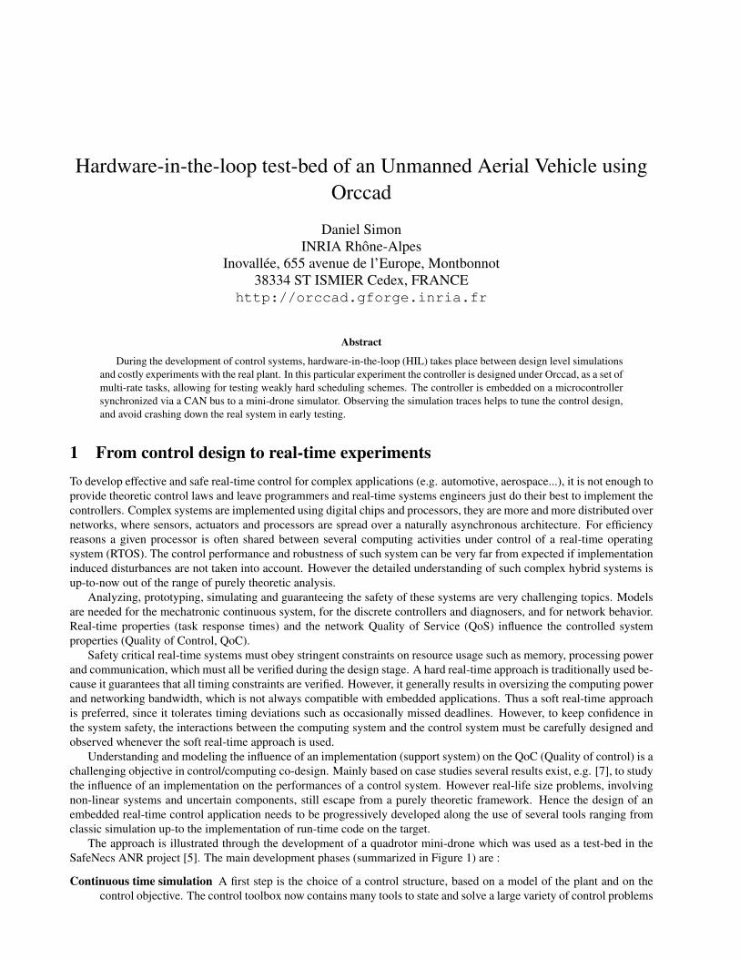
The approach is illustrated through the development of a quadrotor mini-drone which was used as a test-bed in theSafeNecs ANR project [5]. The main development phases (summarized in Figure 1) are :

Continuous time simulation A first step is the choice of a control structure, based on a model of the plant and on thecontrol objective. The control toolbox now contains many tools to state and solve a large variety of control problems

Figure 1: Design flow.

applied to various plants. Besides control theory, preliminary design and tests often rely on simulation tools suchas Matlab/Simulink or Scilab/Scicos. Control design usually needs two different models of the plant. The controlalgorithm design is based on a simplified control design model, which goal is to capture the essential aspects ofthe plant dynamics and behavior. This abstraction must be simple enough to derive a closed-loop controller, e.g.it can be a linearized model of the plant leading to a LQ controller. Then the robustness of the design w.r.t. therealistic plant should be assessed via simulations handling a complete simulation models of the plant, includingits known non-linearities together with a model of the uncertain parameters. The aforementioned simulation toolshandle some modeling capabilities, e.g. the Matlab physical modeling toolbox. These models can also be generatedfrom external tools and languages, e.g. Siconos and Modelica for models of mechanical systems and robotics.

These preliminary simulations are able to rough out the choice of the control algorithm and firstly evaluate itsadequation with the plant structure and control objectives. They are often carried out in the framework of continuoustime, as non-linear control is also often designed in continuous time. When done, the evaluation of digital controland discretization consequences is basic, e.g. modeled via a single numerical loop sampled at a fixed rate.

Simulation including the real-time architecture Further to these preliminary simulation, modeling and simulating theimplementation platform, i.e. the real-time tasks and scheduler inside the control nodes, and the network betweenthe nodes, allows for a new step towards the design and evaluation of the embedded system. Among others theTRUETIME free toolbox is a Matlab/Simulink-based simulator for real-time control systems [11]. TrueTime easesthe co-simulation of controller task execution in real-time kernels, network transmissions, and continuous plantdynamics. With this toolbox the real-time operating system’s and network’s features are handled by high levelabstractions, contrarily to other tools such as SimEvent, or as Opnet [12], which allows users to simulate the networkin a more detailed (and costly) way. TRUETIME allows users to simulate several types of networks (Ethernet, CAN,Round Robin, TDMA, FDMA, Switched Ethernet and WLAN or ZigBee Wireless networks) and new models canbe added.

Hardware-in-the-loop simulation Even with a specialized toolbox like TRUETIME, the previous step remains simu-lations still far from reality. In particular the models of the real-time components (RTOS and network) must bekept simple (high-level) to avoid prohibitive simulation times, and execution or transmission times are based onassumptions and worst cases analysis. Before experiments using the real system a useful next step is to implement

2

the so-called hardware-in-the-loop test-bench. In this case, the plant is still simulated (numerical integration of thenon-linear plant model), but now the control algorithms and real-time software are executed on the embedded targetas real-time tasks communicating through the real network.

Experiments Finally, once the real-time simulations made the designers confident enough in both the control algorithmand its implementation, experiments with the real plant controlled by the embedded hardware and software canbegin while minimizing the risk of early failure. Experiments results can be further used to update the simulationmodels or even to come back on the choice or dimensioning of some of the system’s components.

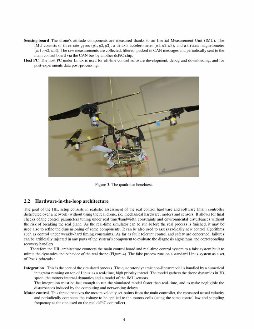
2 Hardware-in-the-loop setupThe utilization of Matlab/Simulink together with TRUETIME remains pure simulation. To provide more realistic resultson the influence of the real-time tasks and network on the system, a hardware-in-the-loop experiment has been set up(Figure 2). In the particular case of the quadrotor, hardware-in-the-loop experiments provide a safe environment for thevalidation of all algorithms and software, prior to any experiments with a real - and very fragile - quadrotor (Figure 3).

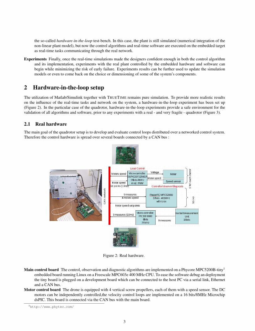
2.1 Real hardwareThe main goal of the quadrotor setup is to develop and evaluate control loops distributed over a networked control system.Therefore the control hardware is spread over several boards connected by a CAN bus :

Figure 2: Real hardware.

Main control board The control, observation and diagnostic algorithms are implemented on a Phycore MPC5200B-tiny1

embedded board running Linux on a Freescale MPC603e 400 MHz CPU. To ease the software debug an deploymentthe tiny board is plugged on a development board which can be connected to the host PC via a serial link, Ethernetand a CAN bus.

Motor control board The drone is equipped with 4 vertical screw propellers, each of them with a speed sensor. The DCmotors can be independently controlled,the velocity control loops are implemented on a 16 bits/8MHz MicrochipdsPIC. This board is connected via the CAN bus with the main board.

1http://www.phytec.com/

3

Sensing board The drone’s attitude components are measured thanks to an Inertial Measurement Unit (IMU). TheIMU consists of three rate gyros (g1, g2, g3), a tri-axis accelerometer (a1, a2, a3), and a tri-axis magnetometer(m1,m2,m3). The raw measurements are collected, filtered, packed in CAN messages and periodically sent to themain control board via the CAN bus by another dsPiC chip.

Host PC The host PC under Linux is used for off-line control software development, debug and downloading, and forpost-experiments data post-processing.

Figure 3: The quadrotor benchtest.

2.2 Hardware-in-the-loop architectureThe goal of the HIL setup consists in realistic assessment of the real control hardware and software (main controllerdistributed over a network) without using the real drone, i.e. mechanical hardware, motors and sensors. It allows for finalchecks of the control parameters tuning under real time/bandwidth constraints and environmental disturbances withoutthe risk of breaking the real plant. As the real-time simulator can be run before the real process is finished, it may beused also to refine the dimensioning of some components. It can be also used to assess radically new control algorithmssuch as control under weakly-hard timing constraints. As far as fault tolerant control and safety are concerned, failurescan be artificially injected in any parts of the system’s component to evaluate the diagnosis algorithms and correspondingrecovery handlers.

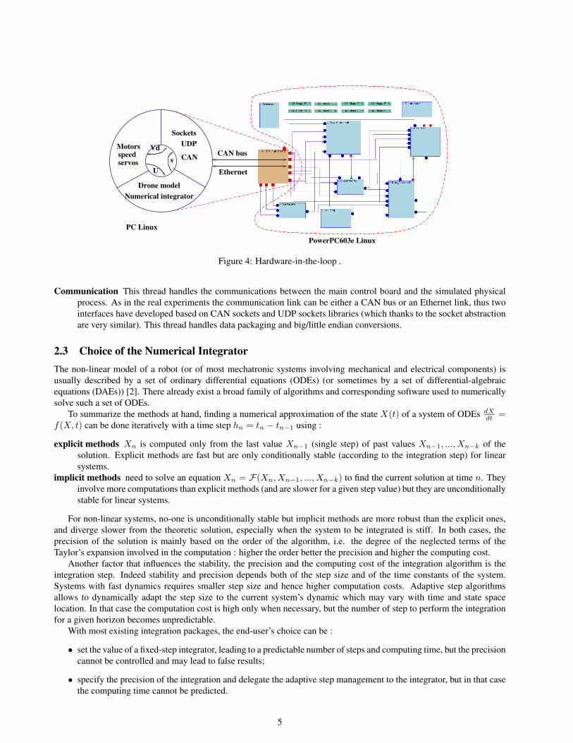
Therefore the HIL architecture connects the main control board and real-time control system to a fake system built tomimic the dynamics and behavior of the real drone (Figure 4). The fake process runs on a standard Linux system as a setof Posix pthreads :

Integration This is the core of the simulated process. The quadrotor dynamic non-linear model is handled by a numericalintegrator running on top of Linux as a real-time, high priority thread. The model gathers the drone dynamics in 3Dspace, the motors internal dynamics and a model of the IMU sensors.The integration must be fast enough to run the simulated model faster than real-time, and to make negligible thedisturbances induced by the computing and networking delays.

Motor control This thread receives the motors velocity set-points from the main controller, the measured actual velocityand periodically computes the voltage to be applied to the motors coils (using the same control law and samplingfrequency as the one used on the real dsPiC controller).

4

Sockets

UDP

CAN

Numerical integrator

Drone model

speedMotors

servos s

U

Vd

PC Linux

PowerPC603e Linux

Ethernet

CAN bus

Figure 4: Hardware-in-the-loop .

Communication This thread handles the communications between the main control board and the simulated physicalprocess. As in the real experiments the communication link can be either a CAN bus or an Ethernet link, thus twointerfaces have developed based on CAN sockets and UDP sockets libraries (which thanks to the socket abstractionare very similar). This thread handles data packaging and big/little endian conversions.

2.3 Choice of the Numerical IntegratorThe non-linear model of a robot (or of most mechatronic systems involving mechanical and electrical components) isusually described by a set of ordinary differential equations (ODEs) (or sometimes by a set of differential-algebraicequations (DAEs)) [2]. There already exist a broad family of algorithms and corresponding software used to numericallysolve such a set of ODEs.

To summarize the methods at hand, finding a numerical approximation of the state X(t) of a system of ODEs dXdt =

f(X, t) can be done iteratively with a time step hn = tn − tn−1 using :

explicit methods Xn is computed only from the last value Xn−1 (single step) of past values Xn−1, ..., Xn−k of thesolution. Explicit methods are fast but are only conditionally stable (according to the integration step) for linearsystems.

implicit methods need to solve an equation Xn = F(Xn, Xn−1, ..., Xn−k) to find the current solution at time n. Theyinvolve more computations than explicit methods (and are slower for a given step value) but they are unconditionallystable for linear systems.

For non-linear systems, no-one is unconditionally stable but implicit methods are more robust than the explicit ones,and diverge slower from the theoretic solution, especially when the system to be integrated is stiff. In both cases, theprecision of the solution is mainly based on the order of the algorithm, i.e. the degree of the neglected terms of theTaylor’s expansion involved in the computation : higher the order better the precision and higher the computing cost.

Another factor that influences the stability, the precision and the computing cost of the integration algorithm is theintegration step. Indeed stability and precision depends both of the step size and of the time constants of the system.Systems with fast dynamics requires smaller step size and hence higher computation costs. Adaptive step algorithmsallows to dynamically adapt the step size to the current system’s dynamic which may vary with time and state spacelocation. In that case the computation cost is high only when necessary, but the number of step to perform the integrationfor a given horizon becomes unpredictable.

With most existing integration packages, the end-user’s choice can be :

• set the value of a fixed-step integrator, leading to a predictable number of steps and computing time, but the precisioncannot be controlled and may lead to false results;

• specify the precision of the integration and delegate the adaptive step management to the integrator, but in that casethe computing time cannot be predicted.

5

A possible way to provide a predictable and safe simulation time would be using a fixed step, implicit method integratorproviding unconditional stability [3]. In that case the integration step should be set at a value small enough to insure therequired accuracy all along the system’s trajectory. Choosing a larger step may lead to poor precision and, for non-linearplants, unstability or convergence towards a false result, e.g. a local minimum far to the real solution.

Conversely, with an adaptive step integration method the controlled variable is the precision (or more exactly theestimate of the integration error). The lsoda package we have elected [1] for the this experiment uses a variable step,variable number of steps algorithm to improve simulation speed and avoid possible numerical unstability.

For a given integration accuracy the simulation speed relies upon the fastest time constant of the model and thesimulation speed cannot be guaranteed to be real-time (but the user is warned in case of deadline miss). The softwareuses two integration methods : an explicit Adams method is used at starting time and when the system is considered tobe non-stiff. The software automatically switches to an implicit (Backward Differentiation Formula) when an on-line testestimates that the system becomes stiff and thus that the implicit integration method becomes faster than the explicit one(and switches back conversely). The variable step method speeds up the integration by increasing the step when possible,e.g when the system exhibits slow transients. Finally the explicit method is chosen when it is faster than the implicitmethod.

Benchmarks and comparisons with renowned methods, e.g. Runge-Kutta 4-5, have shown that despite the complexityof the integration package, the starting overhead is quite small and largely compensated by the efficiency of the method asfar as the integration horizon is large enough. Therefore, we can consider that this software implements a method whichis almost always faster than the potentially predictable fixed step implicit method, and that this choice consists in the besteffort to run the simulation as fast as possible given a required precision.

2.4 Numerical integrator synchronizationThe integration thread is triggered by data requests or arrivals from/to either the network (real system) or the other threadsof the fake system. At each triggering event the integrator is first run from the last event to the current time to update thestate of the drone, then it delivers the new state or accept new inputs.

Therefore even if the integration is always performed late w.r.t. real-time, the whole simulation process is driven bythe events coming from the main real-time controller or by the other real-time threads of the fake system, so that it isglobally synchronized with real time.

The systems works pretty well provided that the computation time needed to integrate from the last event is kept small,and in particular the integration step should be completed before the occurrence of the next request. The distortions fromreality come from the added delay between a state observation request and the answer delayed by the integrator computingtime. This delay depends upon the model’s fastest time constant, on the integration algorithm and on the host computerspeed.

In practice, for the current set-up the simulation very easily runs comfortably faster than real-time, and the bottleneckcomes from the low bandwidth of the CAN bus (which is not simulated, this limitation exists both in the HIL set-up and inthe real system, there is no distortion here). Note that computation times and overruns can be easily checked and reportedto provide information and warnings about the timing behavior and quality of the simulation.

For some cases, it could be interesting (or even necessary) to drive the integrator from events coming from the processmodel itself rather than from external triggers such as real-time clocks. For example, when simulating gas engines, eventsof interest are the ignition instants which are linked to the crank position, i.e. the process state, rather than to time. Thiscould be also the case for incremental encoders for robot arms links. In that case a root finding capability should be usedto cleanly stop the integration at the point of interest. Such capability could be also be used to integrate in advance w.r.treal-time, thus reducing the risk for overruns.

Finally, if real-time simulation cannot be achieved, or if it is wanted that the simulation runs “as fast as possible” with-out reference to real-time, another synchronization scheme could be considered. Rather than synchronize the integratorby the real-time controller, the control software could be triggered by the “end-of-integration” events, thus minimizing theprocessors idle time. However care should be taken to run and synchronize all the simulation components on a coherenttime scale.

6

3 Controller design

3.1 The ORCCAD approachORCCAD is a model-based software environment dedicated to the design, the verification and the implementation of real-time control systems2. In addition to control law design, the specification and validation of complex missions involvingthe logical and temporal cooperation of various controllers along the life of a control application [6, 15] can be achieved.

The ORCCAD methodology is bottom-up, starting from the design of control laws by control engineers, to the designof more complex missions.

The first step in designing a control application is to identify all the necessary elementary tasks involved. Then, foreach of the tasks, various issues are considered, both with an automatic control viewpoint (such as regulation problem def-inition, control law design, choice of relevant events, specification of recovery behaviors, etc.) or with an implementationviewpoint (such as the decomposition of the control law into real-time tasks, and selection of timing parameters). Finally,all the real-time tasks are mapped on a target architecture. During this design, the control engineer may take advantage ofmany degrees of freedom to meet the end-user requirements, and ORCCAD aims at allowing the designer to safely exploitthese degrees of freedom through guided design.

ORCCAD proposes a controller architecture which is naturally open, since the access to every level by different usersis allowed: the application layer is accessed by the end-user (mission specialist), the control layer is used by the controlexpert, and the system layer is accessed by the system engineer. ORCCAD provides formalized control structures, whichare coordinated using the synchronous paradigm, specifically using the Esterel language: while the control laws are oftenperiodic (or more generally cyclic) and programmed using real-time tasks under control of a real-time scheduler, thediscrete-event controller manages the set of control laws and handles exceptions and mode switching. Both activities rununder the control of a real-time operating system (RTOS).

The main entities used in the ORCCAD framework are:

• Algorithmic Modules (MA) which represent functions (e.g. controllers, filters, etc.), encoded as pieces of C code;

• Temporal Constraints (TC), the real-time tasks which implement modules (several modules can be gathered in asingle TC);

• Robot Tasks (RT), the control tasks representing basic control actions encapsulated by a discrete-event controller;

• Robot Procedures (RP), a hierarchical composition of already existing RTs and RPs, to incrementally build morecomplex structures, from elementary executable actions to the full control application.

The RTs characterize continuous-time closed-loop control laws, along with their temporal features and the manage-ment of associated events. From the application perspective, the RT set of signals and associated behavior represent theexternal view of the RTs, hiding all specification and implementation details of the control laws. The RPs, which aremore complex actions, can then be composed from RTs and other RPs in a hierarchical fashion leading to structures ofincreasing complexity. At the top level, RPs are used to describe and implement a full mission specification. At mid-level,they can be used to fulfill a single basic goal through several potential solutions, e.g. a nominal controller supplementedby the recovery substitutions associated with Fault Detection and Diagnosis.

Once a control application has been entirely designed, and for some parts formally verified, a run-time code can beautomatically generated for various real-time operating systems, such as Linux in the present case. It is assumed that theunderlying RTOS supports preemption and fixed priorities, so that the run-time can be fast ported on others Posix systems,and on systems relying on the same abstractions, as already done for Xenomai.

3.2 Quadrotor multi-rate controller3.2.1 Structure

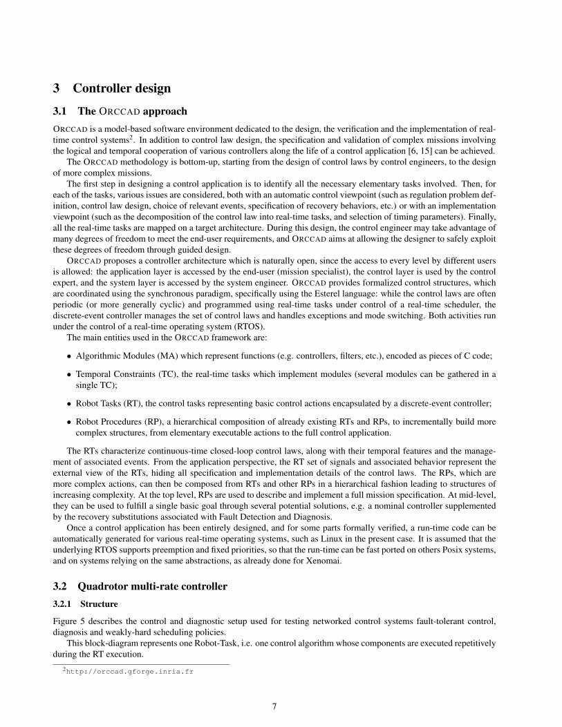
Figure 5 describes the control and diagnostic setup used for testing networked control systems fault-tolerant control,diagnosis and weakly-hard scheduling policies.

This block-diagram represents one Robot-Task, i.e. one control algorithm whose components are executed repetitivelyduring the RT execution.

2http://orccad.gforge.inria.fr

7

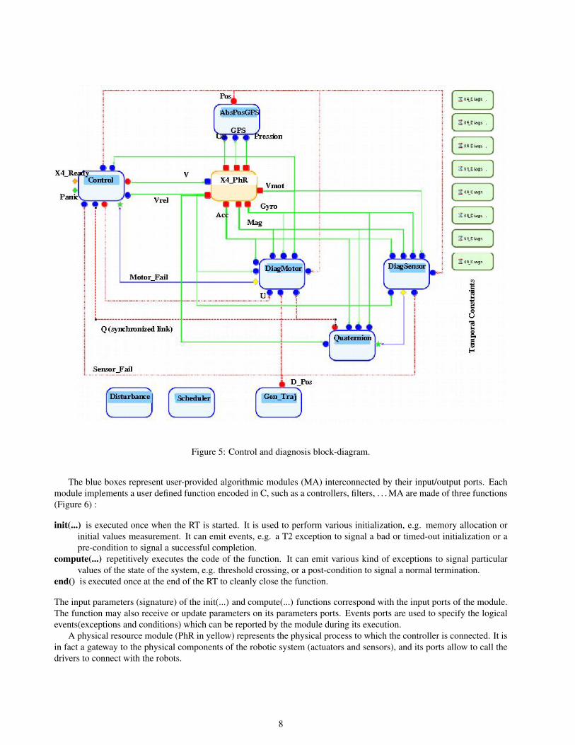
Figure 5: Control and diagnosis block-diagram.

The blue boxes represent user-provided algorithmic modules (MA) interconnected by their input/output ports. Eachmodule implements a user defined function encoded in C, such as a controllers, filters, . . . MA are made of three functions(Figure 6) :

init(...) is executed once when the RT is started. It is used to perform various initialization, e.g. memory allocation orinitial values measurement. It can emit events, e.g. a T2 exception to signal a bad or timed-out initialization or apre-condition to signal a successful completion.

compute(...) repetitively executes the code of the function. It can emit various kind of exceptions to signal particularvalues of the state of the system, e.g. threshold crossing, or a post-condition to signal a normal termination.

end() is executed once at the end of the RT to cleanly close the function.

The input parameters (signature) of the init(...) and compute(...) functions correspond with the input ports of the module.The function may also receive or update parameters on its parameters ports. Events ports are used to specify the logicalevents(exceptions and conditions) which can be reported by the module during its execution.

A physical resource module (PhR in yellow) represents the physical process to which the controller is connected. It isin fact a gateway to the physical components of the robotic system (actuators and sensors), and its ports allow to call thedrivers to connect with the robots.

8

Figure 6: Algorithmic module structure.

3.2.2 Real-time features

From the real-time point of view, each module is own by a TC, i.e. by a real-time thread with a mandatory synchronizationinput. Each TC may have its own programmable clock.

For simple real-time schemes all the MAs of a controller may share a single TC, thus run in sequence at the samerate. In more complex run-time schemes a one-to-one mapping between MAs and TCs allows every module to be runasynchronously at its own (and possibly varying) sampling frequency. For real-time efficiency several MAs, e.g. whichhave a strong dependence, can be gathered in the same TC. Also, besides clock triggering, some TC execution orderingcan be enforced using synchronization between an output port of a TC and the connected input port of the next TC in thecontrol path.

The TC priorities are set according to their relative importance. Data integrity between asynchronous modules isprovided by asynchronous lock-free buffers [14] which are automatically inserted at code generation time.

It is well known that software execution usually show duration variations which are difficult to accurately predict.Moreover systems dimensioned according to worst-cases execution times are over-sized and over-constrained. On theother hand system’s setting based on more realistic average execution times lead to occasional overruns and deadlinesmiss. An Execution Flag is set to every TC to control the behavior of the real-time thread in case of overrun according toa pre-defined exception policy. For example the “SKIP” policy leave the running thread to run to completion but skips itsnext execution.

3.2.3 Control path

The attitude control path starts from the drivers of the quadrotor sensors (accelerometers Acc, rate gyros Gyr and magne-tometers Mag), which are the outputs of the interface module X PhR. The box X4 PhR (where PhR stands for PhysicalResource) is the interface between the controller and the device to control : sending or reading data on its ports actuallycalls the drivers, i.e. the functions used to interface the real-time controller with the real hardware, or with the real-timesimulator.

The raw measurements are used by the Quaternion module Quaternion to estimate the drone attitude using a non-linearobserver [8]. The estimated attitude quaternion Q is forwarded to the Control module to perform the attitude control. Thecomputed motor desired velocities are then sent to the quadrotor via the V driver port.

Provision is given for future enhancements of the sensor set, since a GPS-like position sensor and ultra-sonic sensors

9

were expected to be integrated in an enhanced version. Therefore, a trajectory generator module GEN Traj and a positionestimator module AbsPosGPS are integrated in the control architecture to evaluate position control.

As this control path is critical for the attitude control stability, it is necessary to minimize the loop latency between theraw sensors measurements and the application of the corresponding control to the actuators. Therefore the Quaternionand Control modules are synchronized via the Q data link. In that case both threads have the same priority, and the Controlthread has no real-time clock, it inherits the Quaternion thread execution rate thanks to the synchronization.

3.2.4 Diagnosis and fault tolerant control

To implement diagnosis and fault-tolerant control the drone controller uses the weak exception mechanism (T1) providedby the ORCCAD model to modify the behavior of an algorithmic module (e.g. via a conditional jump in the function code)without switching for a new RT.

The Diag Capteurs module runs the diagnostic algorithm that isolates sensors failures. A failure is signaled by theSensor Fail weak (T1) exception which is forwarded (with a numerical value to precisely identify the failure) to theQuaternion module on a parameter port, so that the quaternion estimation algorithm can be adapted according to thereported failure.

Similarly, the Diag Motors module forwards motor failures signaled by the Motor Fail event to a parameter port ofthe Control module, leading to switch for a pre-defined control degraded mode.

3.2.5 Scheduling controller

The ORCCAD run-time API and library provides some user-level functions to observe and manage on-line the systemscheduling parameters. For example, SetSampleTime() resets on-the-fly the sampling interval of the clocks used to triggerTCs, and MTgetExecTime() records the execution time (cycles) used by a given TC since the RT started3.

Using this API, the Scheduler module performs on-line management of the scheduling policies used to execute thecontroller, for example to implement and test feedback schedulers : it monitors the controller’s real-time activity andmay react by setting on-the-fly the task-scheduling parameters, e.g. their firing intervals. For example, such FeedbackSchedulers can been used to implement a (m,k)-firm dropping policy [9], to dynamically adapt the priorities of messageson the CAN bus [10] or to implement varying sampling control as in [13].

3.2.6 Disturbance daemon

A Disturbance task allows users to generate extra loads with controlled characteristics either on the CPU or on the CANbus, specific data corruption on the CAN or Ethernet drivers, and faulty behavior on the sensors or actuators, e.g. to assessthe effectiveness of the diagnosis and fault isolation capabilities of the control system.

3.2.7 Socket libraries

The embedded and host computers may communicate via a CAN bus or an Ethernet connection. Two interface functionsusing sockets libraries have been implemented, so that the driver ports located in the X4 PhR interface send and receivedata using either the Socket-CAN protocol4 or UDP sockets on Ethernet.

4 Hardware-in-the loop experimentThis set-up has been used by some partners of the Safenecs ANR project, some of the following results are taken from[5].

4.1 Basic scenarioThe attitude control is observed for several networking configurations and real-time control parameters. To minimize theattitude control loop latency the Quaternion and Control modules are synchronized by the Q data link. In both cases the

3the precise semantics and precision of such statement is highly dependent on the underlying RTOS capabilities4http://developer.berlios.de/projects/socketcan/

10

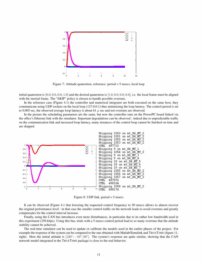
Figure 7: Attitude quaternion, reference: period = 5 msecs, local loop

initial quaternion is [0.0, 0.0, 0.0, 1.0] and the desired quaternion is [1.0, 0.0, 0.0, 0.0], i.e. the local frame must be alignedwith the inertial frame. The “SKIP” policy is chosen to handle possible overruns.

In the reference case (Figure 4.1) the controller and numerical integrator are both executed on the same host, theycommunicate using UDP sockets on the local loop (127.0.0.1) thus minimizing the loop latency. The control period is setto 0.005 sec, the observed average loop latency is about 61 µ sec and not overruns are observed.

In the picture the scheduling parameters are the same, but now the controller runs on the PowerPC board linked viathe office’s Ethernet link with the simulator. Important degradations can be observed : indeed due to unpredictable trafficon the communication link and increased loop latency, many instances of the control loop cannot be finished on time andare skipped.

Figure 8: UDP link, period = 5 msecs

It can be observed (Figure 4.1 that lowering the requested control frequency to 50 msecs allows to almost recoverthe original performance level : in that case the smaller control traffic on the network leads to avoid overruns and greatlycompensates for the control interval increase.

Finally, using the CAN bus introduces even more disturbances, in particular due to its rather low bandwidth used inthis experiment (250 kbps). Using this bus, trials with a 5 msecs control period lead to so many overruns that the attitudestability cannot be achieved.

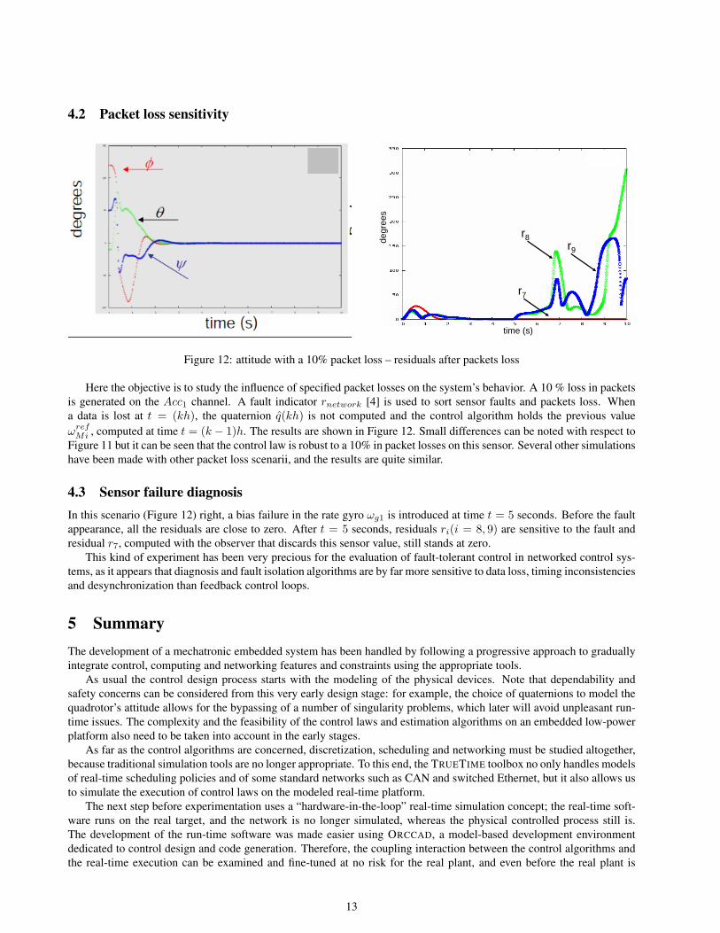
The real-time simulator can be used to update or calibrate the models used in the earlier phases of the project. Forexample the response of the system can be compared to the one obtained with Matlab/Simulink and TRUETIME (figure 11,right). Here the initial attitude is [120◦;−10◦; 50◦]. The system’s response are quite similar, showing that the CANnetwork model integrated in the TRUETIME package is close to the real behavior.

11

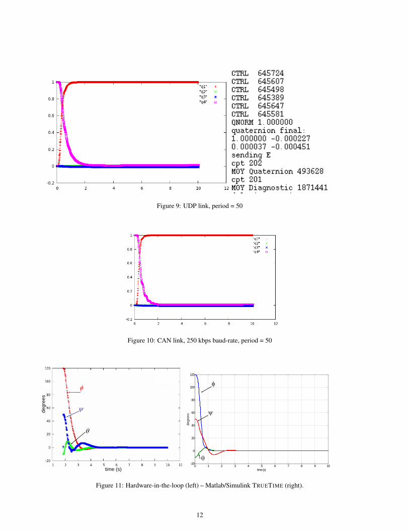
Figure 9: UDP link, period = 50

Figure 10: CAN link, 250 kbps baud-rate, period = 50

φ

ψ

θ

time (s)

degr

ees

0 1 2 3 4 5 6 7 8 9 10-20

0

20

40

60

80

100

120

time (s)

degr

ees

φ

ψ

θ

Figure 11: Hardware-in-the-loop (left) – Matlab/Simulink TRUETIME (right).

12

4.2 Packet loss sensitivity

r7

r8r9

time (s)

degr

ees

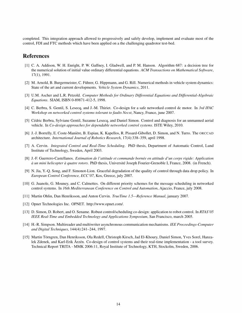
Figure 12: attitude with a 10% packet loss – residuals after packets loss

Here the objective is to study the influence of specified packet losses on the system’s behavior. A 10 % loss in packetsis generated on the Acc1 channel. A fault indicator rnetwork [4] is used to sort sensor faults and packets loss. Whena data is lost at t = (kh), the quaternion q(kh) is not computed and the control algorithm holds the previous valueωref

Mi , computed at time t = (k − 1)h. The results are shown in Figure 12. Small differences can be noted with respect toFigure 11 but it can be seen that the control law is robust to a 10% in packet losses on this sensor. Several other simulationshave been made with other packet loss scenarii, and the results are quite similar.

4.3 Sensor failure diagnosisIn this scenario (Figure 12) right, a bias failure in the rate gyro ωg1 is introduced at time t = 5 seconds. Before the faultappearance, all the residuals are close to zero. After t = 5 seconds, residuals ri(i = 8, 9) are sensitive to the fault andresidual r7, computed with the observer that discards this sensor value, still stands at zero.

This kind of experiment has been very precious for the evaluation of fault-tolerant control in networked control sys-tems, as it appears that diagnosis and fault isolation algorithms are by far more sensitive to data loss, timing inconsistenciesand desynchronization than feedback control loops.

5 SummaryThe development of a mechatronic embedded system has been handled by following a progressive approach to graduallyintegrate control, computing and networking features and constraints using the appropriate tools.

As usual the control design process starts with the modeling of the physical devices. Note that dependability andsafety concerns can be considered from this very early design stage: for example, the choice of quaternions to model thequadrotor’s attitude allows for the bypassing of a number of singularity problems, which later will avoid unpleasant run-time issues. The complexity and the feasibility of the control laws and estimation algorithms on an embedded low-powerplatform also need to be taken into account in the early stages.

As far as the control algorithms are concerned, discretization, scheduling and networking must be studied altogether,because traditional simulation tools are no longer appropriate. To this end, the TRUETIME toolbox no only handles modelsof real-time scheduling policies and of some standard networks such as CAN and switched Ethernet, but it also allows usto simulate the execution of control laws on the modeled real-time platform.

The next step before experimentation uses a “hardware-in-the-loop” real-time simulation concept; the real-time soft-ware runs on the real target, and the network is no longer simulated, whereas the physical controlled process still is.The development of the run-time software was made easier using ORCCAD, a model-based development environmentdedicated to control design and code generation. Therefore, the coupling interaction between the control algorithms andthe real-time execution can be examined and fine-tuned at no risk for the real plant, and even before the real plant is

13

completed. This integration approach allowed to progressively and safely develop, implement and evaluate most of thecontrol, FDI and FTC methods which have been applied on a the challenging quadrotor test-bed.

References[1] C. A. Addison, W. H. Enright, P. W. Gaffney, I. Gladwell, and P. M. Hanson. Algorithm 687: a decision tree for

the numerical solution of initial value ordinary differential equations. ACM Transactions on Mathematical Software,17(1), 1991.

[2] M. Arnold, B. Burgermeister, C. Fuhrer, G. Hippmann, and G. Rill. Numerical methods in vehicle system dynamics:State of the art and current developments. Vehicle System Dynamics, 2011.

[3] U.M. Ascher and L.R. Petzold. Computer Methods for Ordinary Differential Equations and Differential-AlgebraicEquations. SIAM, ISBN 0-89871-412-5, 1998.

[4] C. Berbra, S. Gentil, S. Lesecq, and J.-M. Thiriet. Co-design for a safe networked control dc motor. In 3rd IFACWorkshop on networked control systems tolerant to faults Necst, Nancy, France, june 2007.

[5] Cedric Berbra, Sylviane Gentil, Suzanne Lesecq, and Daniel Simon. Control and diagnosis for an unmanned aerialvehicle. In Co-design approaches for dependable networked control systems. ISTE Wiley, 2010.

[6] J.-J. Borrelly, E. Coste-Maniere, B. Espiau, K. Kapellos, R. Pissard-Gibollet, D. Simon, and N. Turro. The ORCCADarchitecture. International Journal of Robotics Research, 17(4):338–359, april 1998.

[7] A. Cervin. Integrated Control and Real-Time Scheduling. PhD thesis, Department of Automatic Control, LundInstitute of Technology, Sweden, April 2003.

[8] J.-F. Guerrero-Castellanos. Estimation de l’attitude et commande bornee en attitude d’un corps rigide: Applicationa un mini helicopter a quatre rotors. PhD thesis, Universite Joseph Fourier-Grenoble I, France, 2008. (in French).

[9] N. Jia, Y.-Q. Song, and F. Simonot-Lion. Graceful degradation of the quality of control through data drop policy. InEuropean Control Conference, ECC’07, Kos, Greece, july 2007.

[10] G. Juanole, G. Mouney, and C. Calmettes. On different priority schemes for the message scheduling in networkedcontrol systems. In 16th Mediterranean Conference on Control and Automation, Ajaccio, France, july 2008.

[11] Martin Ohlin, Dan Henriksson, and Anton Cervin. TrueTime 1.5—Reference Manual, january 2007.

[12] Opnet Technologies Inc. OPNET. http://www.opnet.com/.

[13] D. Simon, D. Robert, and O. Sename. Robust control/scheduling co-design: application to robot control. In RTAS’05IEEE Real-Time and Embedded Technology and Applications Symposium, San Francisco, march 2005.

[14] H.-R. Simpson. Multireader and multiwriter asynchronous communication mechanisms. IEE Proceedings-Computerand Digital Techniques, 144(4):241–244, 1997.

[15] Martin Torngren, Dan Henriksson, Ola Redell, Christoph Kirsch, Jad El-Khoury, Daniel Simon, Yves Sorel, Hanza-lek Zdenek, and Karl-Erik Arzen. Co-design of control systems and their real-time implementation - a tool survey.Technical Report TRITA - MMK 2006:11, Royal Institute of Technology, KTH, Stockolm, Sweden, 2006.

14