Embed Size (px)
Citation preview
Math. Subject Classifications. Primary 42B30; Secondary 26A46, 46E30.Keywords and Phrases. Fourier transform, Hilbert transform, Riesz transform, Hardy space, Hardy inequality, absolutecontinuity, double Fourier series, conjugate series, conjugate functions, double null sequence of bounded variation,multipliers on L and H.Acknowledgements and Notes. This research was partially supported by the Hungarian National Foundation forScientific Research under Grant T 016 393.
c©1996 CRC Press, Inc.ISSN 1069-5869
The Journal of Fourier Analysis and Applications
Volume 2, Number 5, 1996
Hardy Spaces on the Planeand Double Fourier Transforms
Dang Vu Giang and Ferenc Moricz
ABSTRACT. We provide a direct computational proof of the known inclusion
H.R × R/ ⊆ H.R2/;
where H.R×R/ is the product Hardy space defined for example by R. Fefferman and H.R2/ is theclassical Hardy space used, for example, by E. M. Stein. We introduce a third space J .R × R/ ofHardy type and analyze the interrelations among these spaces. We give simple sufficient conditionsfor a given function of two variables to be the double Fourier transform of a function inL.R2/ andH.R×R/, respectively. In particular, we obtain a broad class of multipliers onL.R2/ and H.R2/,respectively. We also present analogous sufficient conditions in the case of double trigonometricseries and, as a by-product, obtain new multipliers on L.T2/ and H.T2/, respectively.
1. IntroductionFor a complex-valued functionf ∈ L.R2/;R2 := .−∞;∞/×.−∞;∞/, its Fourier transform
f is defined by
f .¾; �/ := 1
4³2
Z ZR2f .x; y/e−i.¾x+�y/ dx dy; .¾; �/ ∈ R2: (1.1)
Here and in the sequel, the sign “:=” means “equal by definition.” It is well known that f iscontinuous (even uniformly) on R2 and
lim|¾ |+|�|→∞
f .¾; �/ = 0: (1.2)
In the sequel, we denote by C0.R2/ the space of all continuous functions on R2 that satisfy (1.2).If f .x; y/ is even in both x and y, denoted
f .x; y/ = f .−x; y/ = f .x;−y/ = f .−x;−y/; x; y ∈ R;
then (1.1) becomes the double cosine Fourier transform of f , denoted
f .¾; �/ = 1
³2
Z ZR2
+
f .x; y/ cos ¾x cos �y dx dy; (1.3)
where R2+ := [0;∞/× [0;∞/.
488 D. Vu Giang and F. Moricz
If f .x; y/ is odd in both x and y, denoted
f .x; y/ = −f .−x; y/ = −f .x;−y/ = f .−x;−y/; x; y ∈ R;
then (1.1) becomes the double sine Fourier transform of f , denoted
f .¾; �/ = 1
³2
Z ZR2
+
f .x; y/ sin ¾x sin �y dx dy (1.4)
(apart from a factor .−1/).If f .x; y/ is even in x and odd in y, denoted
f .x; y/ = f .−x; y/ = −f .x;−y/ = −f .−x;−y/; x; y ∈ R;
then (1.1) becomes the cosine-sine Fourier transform of f , denoted
f .¾; �/ = 1
³2
Z ZR2
+
f .x; y/ cos ¾x sin �y dx dy (1.5)
(apart from a factor .−i/).Finally, if f .x; y/ is odd in x and even in y, denoted
f .x; y/ = −f .−x; y/ = f .x;−y/ = −f .−x;−y/; x; y ∈ R;
then (1.1) becomes the sine-cosine Fourier transform of f , denoted
f .¾; �/ = 1
³2
Z ZR2
+
f .x; y/ sin ¾x cos �y dx dy (1.6)
(apart from a factor .−i/).The next observation will be useful throughout this paper. Given an arbitrary function f on
R2, define
f1.x; y/ := 1
4{f .x; y/+ f .−x; y/+ f .x;−y/+ f .−x;−y/};
f2.x; y/ := 1
4{f .x; y/− f .−x; y/− f .x;−y/+ f .−x;−y/};
f3.x; y/ := 1
4{f .x; y/+ f .−x; y/− f .x;−y/− f .−x;−y/};
f4.x; y/ := 1
4{f .x; y/− f .−x; y/+ f .x;−y/− f .−x;−y/}:
It is plain that
f = f1 + f2 + f3 + f4;
f1.x; y/ is even in both x and y, f2.x; y/ is odd in both x and y, f3.x; y/ is even in x and odd in y,and f4.x; y/ is odd in x and even in y.
The above decomposition of f makes it possible in the sequel to deal with cosine and/or sinetransforms of the forms (1.3)–(1.6) of even and/or odd functions, respectively, instead of the generalcomplex Fourier transform (1.1).
2. Hardy Spaces on the PlaneThe n-dimensional real theory of the classical Hardy spaces H.Rn/ was begun in [14] by
Stein and Weiss (see also [15, Chapter VI, §4]). In their definition they use Riesz transforms as then-dimensional analogues of Hilbert transform. In particular, for n = 2 they set
H.R2/ := {f ∈ L.R2/ : R1f and R2f ∈ L.R2/};
Hardy Spaces 489
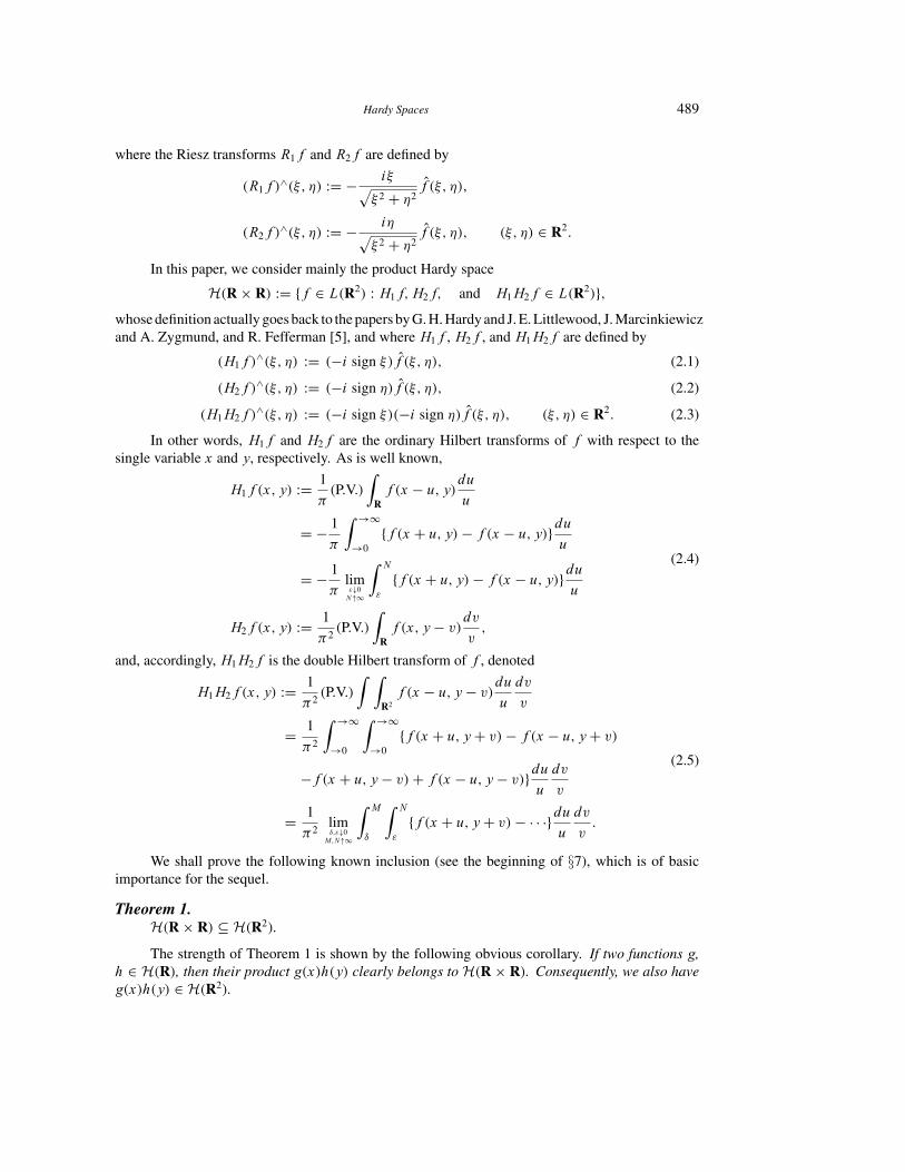
where the Riesz transforms R1f and R2f are defined by
.R1f /∧.¾; �/ := − i¾p
¾ 2 + �2f .¾; �/;
.R2f /∧.¾; �/ := − i�p
¾ 2 + �2f .¾; �/; .¾; �/ ∈ R2:
In this paper, we consider mainly the product Hardy space
H.R × R/ := {f ∈ L.R2/ : H1f;H2f; and H1H2f ∈ L.R2/};whose definition actually goes back to the papers by G. H. Hardy and J. E. Littlewood, J. Marcinkiewiczand A. Zygmund, and R. Fefferman [5], and where H1f , H2f , and H1H2f are defined by
.H1f /∧.¾; �/ := .−i sign ¾/f .¾; �/; (2.1)
.H2f /∧.¾; �/ := .−i sign �/f .¾; �/; (2.2)
.H1H2f /∧.¾; �/ := .−i sign ¾/.−i sign �/f .¾; �/; .¾; �/ ∈ R2: (2.3)
In other words, H1f and H2f are the ordinary Hilbert transforms of f with respect to thesingle variable x and y, respectively. As is well known,
H1f .x; y/ := 1
³.P.V./
ZRf .x − u; y/
du
u
= − 1
³
Z →∞
→0{f .x + u; y/− f .x − u; y/}du
u
= − 1
³lim"↓0N↑∞
Z N
"
{f .x + u; y/− f .x − u; y/}duu
H2f .x; y/ := 1
³2.P.V./
ZRf .x; y − v/
dv
v;
(2.4)
and, accordingly, H1H2f is the double Hilbert transform of f , denoted
H1H2f .x; y/ := 1
³2.P.V./
Z ZR2f .x − u; y − v/
du
u
dv
v
= 1
³2
Z →∞
→0
Z →∞
→0{f .x + u; y + v/− f .x − u; y + v/
−f .x + u; y − v/+ f .x − u; y − v/}duu
dv
v
= 1
³2limŽ;"↓0M;N↑∞
Z M
Ž
Z N
"
{f .x + u; y + v/− · · ·}duu
dv
v:
(2.5)
We shall prove the following known inclusion (see the beginning of §7), which is of basicimportance for the sequel.
Theorem 1.H.R × R/ ⊆ H.R2/.
The strength of Theorem 1 is shown by the following obvious corollary. If two functions g,h ∈ H.R/, then their product g.x/h.y/ clearly belongs to H.R × R/. Consequently, we also haveg.x/h.y/ ∈ H.R2/.
490 D. Vu Giang and F. Moricz
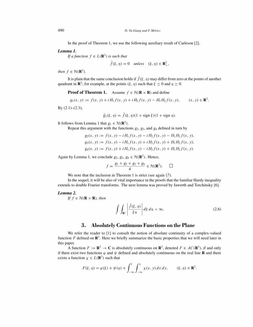
In the proof of Theorem 1, we use the following auxiliary result of Carleson [2].
Lemma 1.If a function f ∈ L.R2/ is such that
f .¾; �/ = 0 unless .¾; �/ ∈ R2+;
then f ∈ H.R2/.
It is plain that the same conclusion holds if f .¾; �/may differ from zero at the points of anotherquadrant in R2; for example, at the points .¾; �/ such that ¾ ≤ 0 and � ≥ 0.
Proof of Theorem 1. Assume f ∈ H.R × R/ and define
g1.x; y/ := f .x; y/+ iH1f .x; y/+ iH2f .x; y/−H1H2f .x; y/; .x; y/ ∈ R2:
By (2.1)–(2.3),
g1.¾; �/ = f .¾; �/.1 + sign ¾/.1 + sign �/:
It follows from Lemma 1 that g1 ∈ H.R2/.Repeat this argument with the functions g2, g3, and g4 defined in turn by
g2.x; y/ := f .x; y/− iH1f .x; y/− iH2f .x; y/−H1H2f .x; y/;
g3.x; y/ := f .x; y/− iH1f .x; y/+ iH2f .x; y/+H1H2f .x; y/;
g4.x; y/ := f .x; y/+ iH1f .x; y/− iH2f .x; y/+H1H2f .x; y/:
Again by Lemma 1, we conclude g2, g3, g4 ∈ H.R2/. Hence,
f = g1 + g2 + g3 + g4
4∈ H.R2/: �
We note that the inclusion in Theorem 1 is strict (see again §7).In the sequel, it will be also of vital importance in the proofs that the familiar Hardy inequality
extends to double Fourier transforms. The next lemma was proved by Jawerth and Torchinsky [6].
Lemma 2.If f ∈ H.R × R/, then
Z ZR2
þþþþþf .¾; �/
¾�
þþþþþ d¾ d� < ∞: (2.6)
3. Absolutely Continuous Functions on the PlaneWe refer the reader to [1] to consult the notion of absolute continuity of a complex-valued
function F defined on R2. Here we briefly summarize the basic properties that we will need later inthis paper.
A function F := R2 → C is absolutely continuous on R2, denoted F ∈ AC.R2/, if and onlyif there exist two functions ' and defined and absolutely continuous on the real line R and thereexists a function � ∈ L.R2/ such that
F.¾; �/ = '.¾/+ .�/+Z ¾
−∞
Z �
−∞�.x; y/ dx dy; .¾; �/ ∈ R2:
Hardy Spaces 491
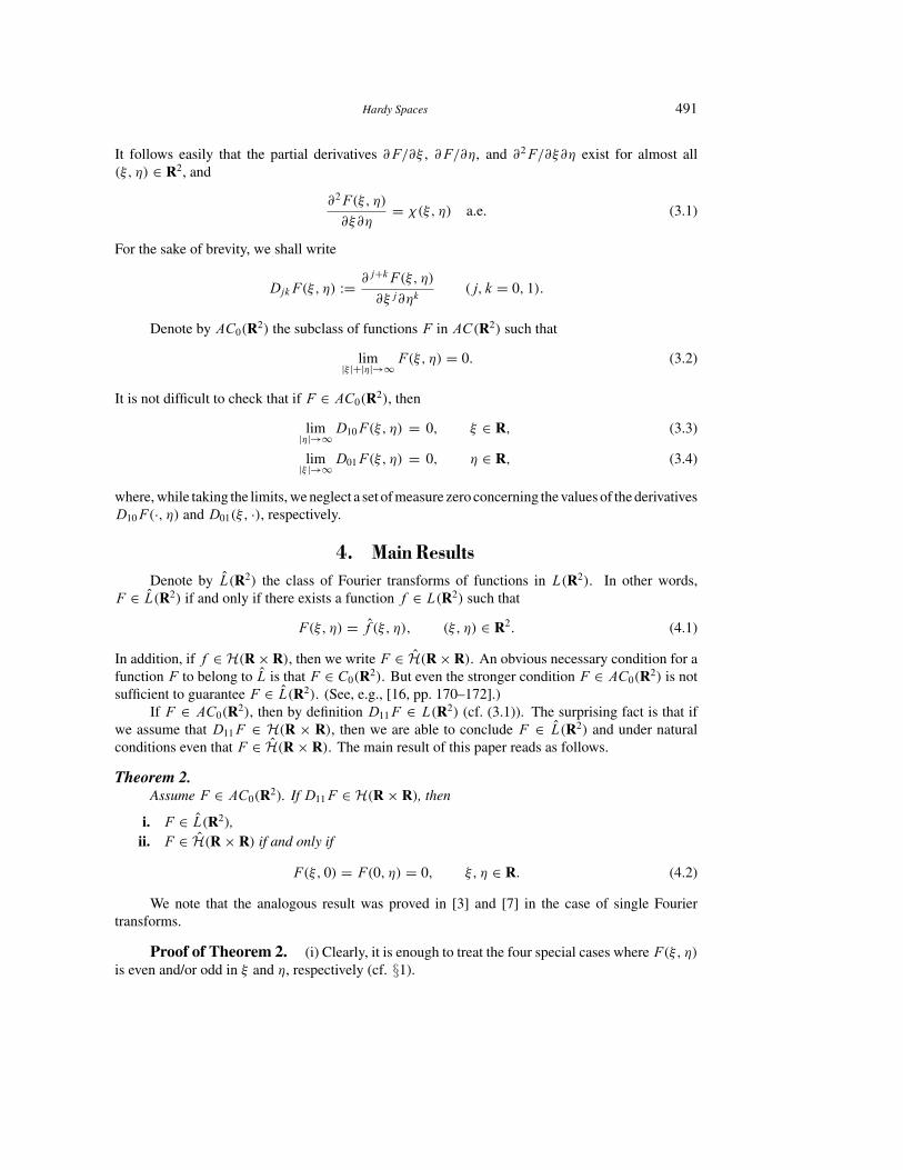
It follows easily that the partial derivatives @F=@¾ , @F=@�, and @2F=@¾@� exist for almost all.¾; �/ ∈ R2, and
@2F.¾; �/
@¾@�= �.¾; �/ a.e. (3.1)
For the sake of brevity, we shall write
DjkF .¾; �/ := @j+kF .¾; �/@¾ j @�k
.j; k = 0; 1/:
Denote by AC0.R2/ the subclass of functions F in AC.R2/ such that
lim|¾ |+|�|→∞
F.¾; �/ = 0: (3.2)
It is not difficult to check that if F ∈ AC0.R2/, then
lim|�|→∞
D10F.¾; �/ = 0; ¾ ∈ R; (3.3)
lim|¾ |→∞
D01F.¾; �/ = 0; � ∈ R; (3.4)
where, while taking the limits, we neglect a set of measure zero concerning the values of the derivativesD10F.·; �/ and D01.¾; ·/, respectively.
4. Main ResultsDenote by L.R2/ the class of Fourier transforms of functions in L.R2/. In other words,
F ∈ L.R2/ if and only if there exists a function f ∈ L.R2/ such that
F.¾; �/ = f .¾; �/; .¾; �/ ∈ R2: (4.1)
In addition, if f ∈ H.R × R/, then we write F ∈ H.R × R/. An obvious necessary condition for afunction F to belong to L is that F ∈ C0.R2/. But even the stronger condition F ∈ AC0.R2/ is notsufficient to guarantee F ∈ L.R2/. (See, e.g., [16, pp. 170–172].)
If F ∈ AC0.R2/, then by definition D11F ∈ L.R2/ (cf. (3.1)). The surprising fact is that ifwe assume that D11F ∈ H.R × R/, then we are able to conclude F ∈ L.R2/ and under naturalconditions even that F ∈ H.R × R/. The main result of this paper reads as follows.
Theorem 2.Assume F ∈ AC0.R2/. If D11F ∈ H.R × R/, then
i. F ∈ L.R2/,ii. F ∈ H.R × R/ if and only if
F.¾; 0/ = F.0; �/ = 0; ¾; � ∈ R: (4.2)
We note that the analogous result was proved in [3] and [7] in the case of single Fouriertransforms.
Proof of Theorem 2. (i) Clearly, it is enough to treat the four special cases where F.¾; �/is even and/or odd in ¾ and �, respectively (cf. §1).
492 D. Vu Giang and F. Moricz
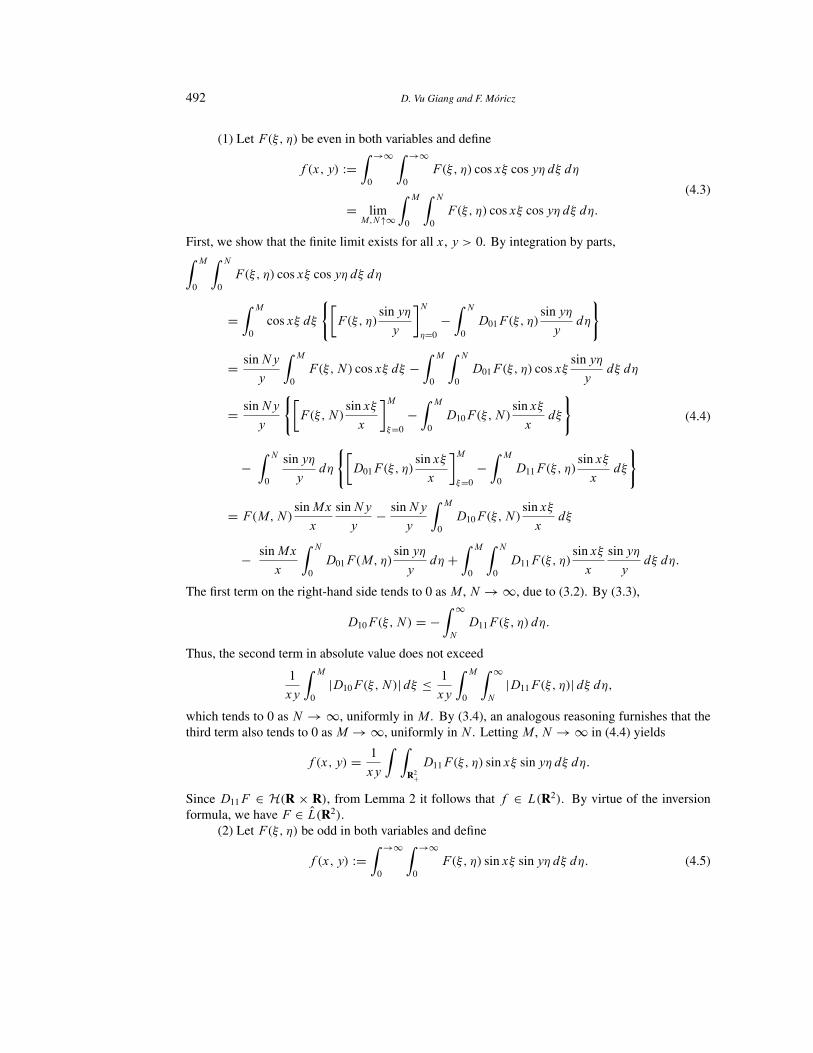
(1) Let F.¾; �/ be even in both variables and define
f .x; y/ :=Z →∞
0
Z →∞
0F.¾; �/ cos x¾ cos y� d¾ d�
= limM;N↑∞
Z M
0
Z N
0F.¾; �/ cos x¾ cos y� d¾ d�:
(4.3)
First, we show that the finite limit exists for all x, y > 0. By integration by parts,Z M
0
Z N
0F.¾; �/ cos x¾ cos y� d¾ d�
=Z M
0cos x¾ d¾
(�F.¾; �/
sin y�
y
½N�=0
−Z N
0D01F.¾; �/
sin y�
yd�
)
= sinNy
y
Z M
0F.¾;N/ cos x¾ d¾ −
Z M
0
Z N
0D01F.¾; �/ cos x¾
sin y�
yd¾ d�
= sinNy
y
(�F.¾;N/
sin x¾
x
½M¾=0
−Z M
0D10F.¾;N/
sin x¾
xd¾
)
−Z N
0
sin y�
yd�
(�D01F.¾; �/
sin x¾
x
½M¾=0
−Z M
0D11F.¾; �/
sin x¾
xd¾
)
= F.M;N/sinMx
x
sinNy
y− sinNy
y
Z M
0D10F.¾;N/
sin x¾
xd¾
− sinMx
x
Z N
0D01F.M; �/
sin y�
yd� +
Z M
0
Z N
0D11F.¾; �/
sin x¾
x
sin y�
yd¾ d�:
(4.4)
The first term on the right-hand side tends to 0 as M , N → ∞, due to (3.2). By (3.3),
D10F.¾;N/ = −Z ∞
N
D11F.¾; �/ d�:
Thus, the second term in absolute value does not exceed
1
xy
Z M
0|D10F.¾;N/| d¾ ≤ 1
xy
Z M
0
Z ∞
N
|D11F.¾; �/| d¾ d�;
which tends to 0 as N → ∞, uniformly in M . By (3.4), an analogous reasoning furnishes that thethird term also tends to 0 as M → ∞, uniformly in N . Letting M , N → ∞ in (4.4) yields
f .x; y/ = 1
xy
Z ZR2
+
D11F.¾; �/ sin x¾ sin y� d¾ d�:
Since D11F ∈ H.R × R/, from Lemma 2 it follows that f ∈ L.R2/. By virtue of the inversionformula, we have F ∈ L.R2/.
(2) Let F.¾; �/ be odd in both variables and define
f .x; y/ :=Z →∞
0
Z →∞
0F.¾; �/ sin x¾ sin y� d¾ d�: (4.5)
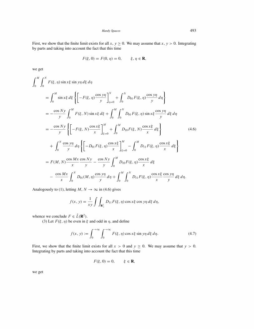
Hardy Spaces 493
First, we show that the finite limit exists for all x, y ≥ 0. We may assume that x, y > 0. Integratingby parts and taking into account the fact that this time
F.¾; 0/ = F.0; �/ = 0; ¾; � ∈ R;
we get
Z M
0
Z N
0F.¾; �/ sin x¾ sin y� d¾ d�
=Z M
0sin x¾ d¾
(�−F.¾; �/cos y�
y
½N�=0
+Z N
0D01F.¾; �/
cos y�
yd�
)
= −cosNy
y
Z M
0F.¾;N/ sin x¾ d¾ +
Z M
0
Z N
0D01F.¾; �/ sin x¾
cos y�
yd¾ d�
= −cosNy
y
(�−F.¾;N/cos x¾
x
½M¾=0
+Z M
0D10F.¾;N/
cos x¾
xd¾
)
+Z N
0
cos y�
yd�
(�−D01F.¾; �/
cos x¾
x
½M¾=0
−Z M
0D11F.¾; �/
cos x¾
xd¾
)
= F.M;N/cosMx
x
cosNy
y− cosNy
y
Z M
0D10F.¾; �/
cos x¾
xd¾
− cosMx
x
Z N
0D01.M; �/
cos y�
yd� +
Z M
0
Z N
0D11F.¾; �/
cos x¾
x
cos y�
yd¾ d�:
(4.6)
Analogously to (1), letting M , N → ∞ in (4.6) gives
f .x; y/ = 1
xy
Z ZR2
+
D11F.¾; �/ cos x¾ cos y� d¾ d�;
whence we conclude F ∈ L.R2/.(3) Let F.¾; �/ be even in ¾ and odd in �, and define
f .x; y/ :=Z →∞
0
Z →∞
0F.¾; �/ cos x¾ sin y� d¾ d�: (4.7)
First, we show that the finite limit exists for all x > 0 and y ≥ 0. We may assume that y > 0.Integrating by parts and taking into account the fact that this time
F.¾; 0/ = 0; ¾ ∈ R;
we get
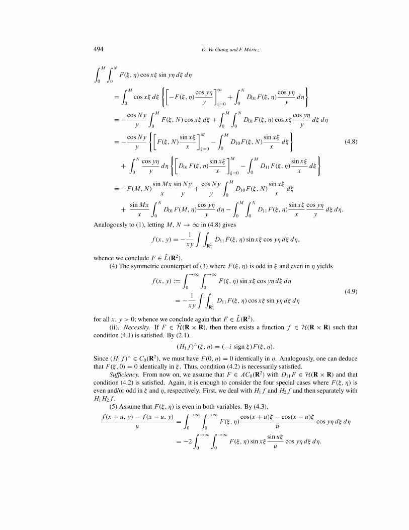
494 D. Vu Giang and F. Moricz
Z M
0
Z N
0F.¾; �/ cos x¾ sin y� d¾ d�
=Z M
0cos x¾ d¾
(�−F.¾; �/cos y�
y
½∞
�=0
+Z N
0D01F.¾; �/
cos y�
yd�
)
= −cosNy
y
Z M
0F.¾;N/ cos x¾ d¾ +
Z M
0
Z N
0D01F.¾; �/ cos x¾
cos y�
yd¾ d�
= −cosNy
y
(�F.¾;N/
sin x¾
x
½M¾=0
−Z M
0D10F.¾;N/
sin x¾
xd¾
)
+Z N
0
cos y�
yd�
(�D01F.¾; �/
sin x¾
x
½M¾=0
−Z M
0D11F.¾; �/
sin x¾
xd¾
)
= −F.M;N/ sinMx
x
sinNy
y+ cosNy
y
Z M
0D10F.¾;N/
sin x¾
xd¾
+ sinMx
x
Z N
0D01F.M; �/
cos y�
yd� −
Z M
0
Z N
0D11F.¾; �/
sin x¾
x
cos y�
yd¾ d�:
(4.8)
Analogously to (1), letting M , N → ∞ in (4.8) gives
f .x; y/ = − 1
xy
Z ZR2
+
D11F.¾; �/ sin x¾ cos y� d¾ d�;
whence we conclude F ∈ L.R2/.(4) The symmetric counterpart of (3) where F.¾; �/ is odd in ¾ and even in � yields
f .x; y/ :=Z →∞
0
Z →∞
0F.¾; �/ sin x¾ cos y� d¾ d�
= − 1
xy
Z ZR2
+
D11F.¾; �/ cos x¾ sin y� d¾ d�(4.9)
for all x, y > 0; whence we conclude again that F ∈ L.R2/.(ii). Necessity. If F ∈ H.R × R/, then there exists a function f ∈ H.R × R/ such that
condition (4.1) is satisfied. By (2.1),
.H1f /∧.¾; �/ = .−i sign ¾/F .¾; �/:
Since .H1f /∧ ∈ C0.R2/, we must have F.0; �/ = 0 identically in �. Analogously, one can deduce
that F.¾; 0/ = 0 identically in ¾ . Thus, condition (4.2) is necessarily satisfied.Sufficiency. From now on, we assume that F ∈ AC0.R2/ with D11F ∈ H.R × R/ and that
condition (4.2) is satisfied. Again, it is enough to consider the four special cases where F.¾; �/ iseven and/or odd in ¾ and �, respectively. First, we deal withH1f andH2f and then separately withH1H2f .
(5) Assume that F.¾; �/ is even in both variables. By (4.3),
f .x + u; y/− f .x − u; y/
u=Z →∞
0
Z →∞
0F.¾; �/
cos.x + u/¾ − cos.x − u/¾
ucos y� d¾ d�
= −2Z →∞
0
Z →∞
0F.¾; �/ sin x¾
sin u¾
ucos y� d¾ d�:
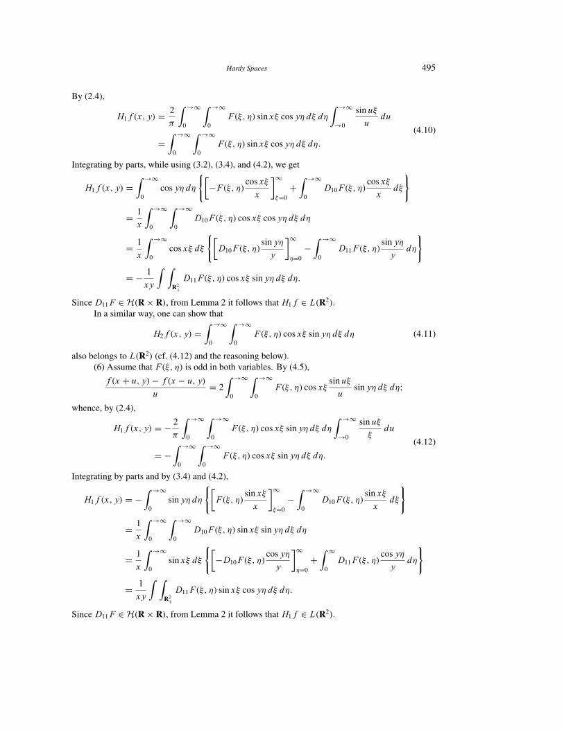
Hardy Spaces 495
By (2.4),
H1f .x; y/ = 2
³
Z →∞
0
Z →∞
0F.¾; �/ sin x¾ cos y� d¾ d�
Z →∞
→0
sin u¾
udu
=Z →∞
0
Z →∞
0F.¾; �/ sin x¾ cos y� d¾ d�:
(4.10)
Integrating by parts, while using (3.2), (3.4), and (4.2), we get
H1f .x; y/ =Z →∞
0cos y� d�
(�−F.¾; �/cos x¾
x
½∞
¾=0
+Z →∞
0D10F.¾; �/
cos x¾
xd¾
)
= 1
x
Z →∞
0
Z →∞
0D10F.¾; �/ cos x¾ cos y� d¾ d�
= 1
x
Z →∞
0cos x¾ d¾
(�D10F.¾; �/
sin y�
y
½∞
�=0
−Z →∞
0D11F.¾; �/
sin y�
yd�
)
= − 1
xy
Z ZR2
+
D11F.¾; �/ cos x¾ sin y� d¾ d�:
Since D11F ∈ H.R × R/, from Lemma 2 it follows that H1f ∈ L.R2/.In a similar way, one can show that
H2f .x; y/ =Z →∞
0
Z →∞
0F.¾; �/ cos x¾ sin y� d¾ d� (4.11)
also belongs to L.R2/ (cf. (4.12) and the reasoning below).(6) Assume that F.¾; �/ is odd in both variables. By (4.5),
f .x + u; y/− f .x − u; y/
u= 2
Z →∞
0
Z →∞
0F.¾; �/ cos x¾
sin u¾
usin y� d¾ d�;
whence, by (2.4),
H1f .x; y/ = − 2
³
Z →∞
0
Z →∞
0F.¾; �/ cos x¾ sin y� d¾ d�
Z →∞
→0
sin u¾
¾du
= −Z →∞
0
Z →∞
0F.¾; �/ cos x¾ sin y� d¾ d�:
(4.12)
Integrating by parts and by (3.4) and (4.2),
H1f .x; y/ = −Z →∞
0sin y� d�
(�F.¾; �/
sin x¾
x
½∞
¾=0
−Z →∞
0D10F.¾; �/
sin x¾
xd¾
)
= 1
x
Z →∞
0
Z →∞
0D10F.¾; �/ sin x¾ sin y� d¾ d�
= 1
x
Z →∞
0sin x¾ d¾
(�−D10F.¾; �/
cos y�
y
½∞
�=0
+Z ∞
0D11F.¾; �/
cos y�
yd�
)
= 1
xy
Z ZR2
+
D11F.¾; �/ sin x¾ cos y� d¾ d�:
Since D11F ∈ H.R × R/, from Lemma 2 it follows that H1f ∈ L.R2/.
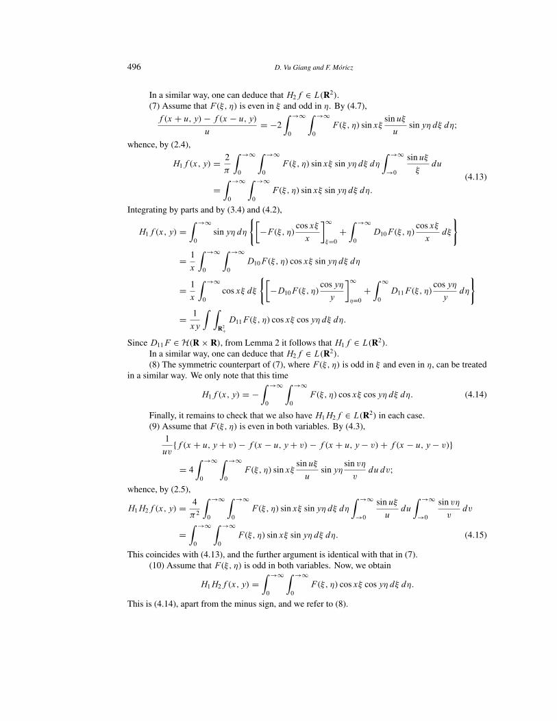
496 D. Vu Giang and F. Moricz
In a similar way, one can deduce that H2f ∈ L.R2/.(7) Assume that F.¾; �/ is even in ¾ and odd in �. By (4.7),
f .x + u; y/− f .x − u; y/
u= −2
Z →∞
0
Z →∞
0F.¾; �/ sin x¾
sin u¾
usin y� d¾ d�;
whence, by (2.4),
H1f .x; y/ = 2
³
Z →∞
0
Z →∞
0F.¾; �/ sin x¾ sin y� d¾ d�
Z →∞
→0
sin u¾
¾du
=Z →∞
0
Z →∞
0F.¾; �/ sin x¾ sin y� d¾ d�:
(4.13)
Integrating by parts and by (3.4) and (4.2),
H1f .x; y/ =Z →∞
0sin y� d�
(�−F.¾; �/cos x¾
x
½∞
¾=0
+Z →∞
0D10F.¾; �/
cos x¾
xd¾
)
= 1
x
Z →∞
0
Z →∞
0D10F.¾; �/ cos x¾ sin y� d¾ d�
= 1
x
Z →∞
0cos x¾ d¾
(�−D10F.¾; �/
cos y�
y
½∞
�=0
+Z ∞
0D11F.¾; �/
cos y�
yd�
)
= 1
xy
Z ZR2
+
D11F.¾; �/ cos x¾ cos y� d¾ d�:
Since D11F ∈ H.R × R/, from Lemma 2 it follows that H1f ∈ L.R2/.In a similar way, one can deduce that H2f ∈ L.R2/.(8) The symmetric counterpart of (7), where F.¾; �/ is odd in ¾ and even in �, can be treated
in a similar way. We only note that this time
H1f .x; y/ = −Z →∞
0
Z →∞
0F.¾; �/ cos x¾ cos y� d¾ d�: (4.14)
Finally, it remains to check that we also have H1H2f ∈ L.R2/ in each case.(9) Assume that F.¾; �/ is even in both variables. By (4.3),
1
uv{f .x + u; y + v/− f .x − u; y + v/− f .x + u; y − v/+ f .x − u; y − v/}
= 4Z →∞
0
Z →∞
0F.¾; �/ sin x¾
sin u¾
usin y�
sin v�
vdu dv;
whence, by (2.5),
H1H2f .x; y/ = 4
³2
Z →∞
0
Z →∞
0F.¾; �/ sin x¾ sin y� d¾ d�
Z →∞
→0
sin u¾
udu
Z →∞
→0
sin v�
vdv
=Z →∞
0
Z →∞
0F.¾; �/ sin x¾ sin y� d¾ d�: .4:15/
This coincides with (4.13), and the further argument is identical with that in (7).(10) Assume that F.¾; �/ is odd in both variables. Now, we obtain
H1H2f .x; y/ =Z →∞
0
Z →∞
0F.¾; �/ cos x¾ cos y� d¾ d�:
This is (4.14), apart from the minus sign, and we refer to (8).
Hardy Spaces 497
(11) Assume that F.¾; �/ is even in ¾ and odd in �. Now, we get
H1H2f .x; y/ = −Z →∞
0
Z →∞
0F.¾; �/ sin x¾ cos y� d¾ d�:
This is (4.10), apart from the minus sign, and we refer to (5).(12) Assume that F.¾; �/ is odd in ¾ and even in �. Now, we get
H1H2f .x; y/ = −Z →∞
0
Z →∞
0F.¾; �/ cos x¾ sin y� d¾ d�:
This is (4.12) and we refer to the corresponding part in (6).The proof of Theorem 2 is complete. �
5. Previous Results ReformulatedIn the light of the proof of Theorem 2, the previous Theorems 1–3 of [4] can be reformulated
as follows.
Lemma 3.If F ∈ AC0.R2/, F.¾; �/ is even in both variables, and for some p > 1 we have
Z ZR2
+
�1
uv
Z 2u
u
Z 2v
v
|D11F.¾; �/|p d¾ d�� 1
p
du dv < ∞; (5.1)
then F ∈ L.R2/.
Lemma 4.If F ∈ AC0.R2/, F.¾; �/ is odd in both variables, and for some p > 1 we have (5.1),
ZR+
d�
�
ZR+
�1
u
Z 2u
u
|D10.¾; �/|p d¾� 1
p
du < ∞; (5.2)
ZR+
d¾
¾
ZR+
�1
v
Z 2v
v
|D01.¾; �/|p d�� 1
p
dv < ∞; (5.3)
then F ∈ L.R2/ if and only ifZ Z
R2
þþþþF.¾; �/¾�
þþþþ d¾ d� < ∞: (5.4)
Lemma 5.If F ∈ AC0.R2/, F.¾; �/ is even in ¾ and odd in �, and for some p > 1 we have (5.1) and
(5.2), then F ∈ L.R2/.
We note that in the symmetric counterpart where F.¾; �/ is odd in ¾ and even in �, conditions(5.1) and (5.3) are sufficient to conclude F ∈ L.R2/.
Making use of the decomposition of an arbitrary function into even and/or odd functionsdescribed at the end of Section 1, and on the basis of Lemmas 3–5 one can give the followingsufficient condition for a function F to belong to L.R2/.
498 D. Vu Giang and F. Moricz
Theorem 3.If F ∈ AC0.R2/ and for some p > 1 we have
Z ZR2
+
�1
uv
Zu<|¾ |<2u
Zv<|�|<2v
|D11F.¾; �/|p d¾ d�� 1
p
du dv < ∞; (5.5)
ZR+
d�
�
ZR+
�1
u
Zu<|¾ |<2u
|D10F.¾; �/−D10F.¾;−�/|p d¾� 1
p
du < ∞; (5.6)
ZR+
d¾
¾
ZR+
�1
v
Zv<|�|<2v
|D01F.¾; �/−D01F.−¾; �/|p d�� 1
p
dv < ∞; (5.7)
then F ∈ L.R2/ if and only ifZ ZR2
+
|F.¾; �/− F.−¾; �/− F.¾;−�/+ F.−¾;−�/| d¾¾
d�
�< ∞: (5.8)
On the other hand, Lemmas 3–5 can be obtained as particular cases of Theorem 3.The following theorem gives a characterization for a function F to belong to H.R × R/.
Theorem 4.If F ∈ AC0.R2/ and for some p > 1 we have condition (5.5),
ZR
d�
|�|Z
R+
�1
u
Zu<|¾ |<2u
|D10F.¾; �/|p d¾� 1
p
du < ∞; (5.9)
ZR
d¾
|¾ |Z
R+
�1
v
Zv<|�|<2v
|D01F.¾; �/|p d�� 1
p
dv < ∞; (5.10)
then F ∈ H .R × R/ if and only if condition (5.4) is satisfied.
Proof of Theorem 4. The necessity part is an immediate consequence of Lemma 2.The sufficiency part hinges on Lemmas 3–5 and the following observation, also extracted from
the proof of Theorem 2. Assume F ∈ AC0.R2/. If F.¾; �/ is even in both variables and f isdefined by (4.3), thenH1f ,H2f , andH1H2f are defined by (4.10), (4.11), and (4.15), respectively.Analogous statements can be made in the particular cases where F.¾; �/ is odd in both variables andf is defined by (4.5), F.¾; �/ is even in ¾ and odd in � and f is defined by (4.7), and F.¾; �/ is oddin ¾ and even in � and f is defined by (4.9), respectively. Now, on the bases of Lemmas 3–5 it isroutine to check that in each case H1f , H2f , and H1H2f all belong to L.R2/. This completes theproof. �
We note that Theorems 2–4 furnish a broad class of multipliers on L.R2/ and H.R2/, respec-tively. Earlier results were obtained, for example, in [10] and [12] under more restricted conditions.More precisely, Peral and Torchinsky [10] found sufficient conditions in terms of directional deriva-tives of F , while Stein [12] (see also [13, p. 232]) gave sufficient conditions in terms of enoughsmoothness and decay at infinity.
Finally, we present two examples to illustrate the applicability of Theorems 3 and 4.
Example 1. Let '.¾/ be an even function on R, convex on R+, and such that
lim¾→0
'.¾/ is finite and lim¾→∞
'.¾/ = 0:
Hardy Spaces 499
For instance,
'.¾/ :=
8><>:
2 − e−1¾ if 0 ≤ ¾ ≤ e;
.ln ¾/−1 if ¾ > e;
'.−¾/ if ¾ < 0
is such a function. Define F.¾; �/ := '.¾/'.�/. Clearly, F ∈ AC0.R2/, conditions (5.6)–(5.8) areautomatically satisfied for any p > 0. It is easy to check that condition (5.5) is also satisfied for anyp > 0. By Theorem 3, we conclude F ∈ L.R2/. On the other hand, condition (5.4) is clearly notsatisfied. By Lemma 2, we conclude that F =∈ H.R × R/. �
Example 2. Let Þ > 0 and Þ.¾/ be defined on R as
Þ.¾/ :=
8><>:¾ if 0 ≤ ¾ ≤ e;
e.ln ¾/−Þ if ¾ > e;
− Þ.−¾/ if ¾ < 0;and let FÞ.¾; �/ := Þ.¾/ Þ.�/. It is not difficult to check that conditions (5.4), (5.5), (5.9), and(5.10) are satisfied for any Þ > 1 and p > 0. By Theorem 4, we conclude that FÞ ∈ H.R × R/ forany Þ > 1. �
6. Extension to Double Fourier SeriesThe majority of the results on Fourier transforms have natural counterparts for Fourier series.
Here, we briefly survey those for double Fourier series that correspond to our results in §§1–5.For a complex-valued function f ∈ L.T2/, periodic in both variables, the double Fourier seriesX X
.j;k/∈ Z2
cjk.f /ei.jx+ky/ (6.1)
of f is defined by
cjk.f / := 1
4³2
Z ZT2f .x; y/e−i.jx+ky/ dx dy; .j; k/ ∈ Z2:
Here and in the sequel
T2 := T × T; T := [−³; ³/;Z2 := Z × Z; Z := {: : : ;−2;−1; 0; 1; 2; : : :}:
It is well known (see, e.g., [15, p. 250]) that
lim|j |+|k|→∞
cjk.f / = 0: (6.2)
If f .x; y/ is even in both variables, then (6.1) becomes a double cosine series; if f .x; y/ isodd in both variables, then (6.1) becomes a double sine series; if f .x; y/ is even in x and odd in y,then (6.1) becomes a cosine-sine series, etc. (cf. §1).
The definition of the three conjugate series (associated with (6.1)) are the following:X X.j;k/∈ Z2
.−i sign j/cjk.f /ei.jx+ky/ (6.3)
(conjugate with respect to x), X X.j;k/∈ Z2
.−i sign k/cjk.f /ei.jx+ky/ (6.4)
500 D. Vu Giang and F. Moricz
(conjugate with respect to y), andX X.j;k/∈ Z2
.−i sign j/.−i sign k/cjk.f /ei.jx+ky/ (6.5)
(conjugate with respect to x and y). The corresponding conjugate functions are
f .1;0/.x; y/ := 1
³.P.V./
ZT
f .x − u; y/
2 tan.u=2/du
(6.6)
= − 1
³lim"↓0
Z ³
"
f .x + u; y/− f .x − u; y/
2 tan.u=2/du;
f .0;1/.x; y/ := 1
³.P.V./
ZT
f .x; y − v/
2 tan.v=2/dv; (6.7)
f .1;1/.x; y/ := 1
³.P.V./
Z ZT2
f .x − u; y − v/
4 tan.u=2/ tan.v=2/du dv
= limŽ↓0"↓0
1
³2
Z ³
Ž
Z ³
"
�f .x + u; y + v/− f .x − u; y + v/
4 tan.u=2/ tan.v=2/(6.8)
− f .x + u; y − v/− f .x − u; y − v/
4 tan.u=2/ tan.v=2/
�du dv:
Now, R. Fefferman [5] defines the Hardy space H.T × T/ as
H.T × T/ := {f ∈ L.T2/ : f .1;0/; f .0;1/; and f .1;1/ ∈ L.T2/}:If f ∈ H.T × T/, then the conjugate series (6.3)–(6.5) are in turn the Fourier series of the corre-sponding conjugate functions (6.6)–(6.8).
The definition of the customary Hardy space H.T2/ uses the notion of the periodic Riesztransforms (see, e.g., [15, p. 283]):
−iX X
.j;k/∈ Z2\{.0;0/}
jpj 2 + k2
cjk.f /ei.jx+ky/; (6.9)
−iX X
.j;k/∈ Z2\{.0;0/}
kpj 2 + k2
cjk.f /ei.jx+ky/: (6.10)
Now, one defines f ∈ H.T2/ if and only if (6.1) is the Fourier series of f ∈ L.T2/ and the Riesztransforms (6.9) and (6.10) are also the Fourier series of some functions in L.T2/.
Analogously to Theorem 1, we also have the following result.
Theorem 1′.H.T × T/ ⊆ H.T2/.
Again, this inclusion is strict (see §7) and we deduce the important corollary that if two functionsg, h ∈ H.T/, then their product g.x/h.y/ belongs to H.T × T/ and, consequently, to H.T2/. Sinceany constant function belongs to H.T/, it follows that if g ∈ H.T/, then g.x/ considered as afunction of .x; y/ belongs to H.T × T/. The latter statement is false if R is substituted for T. Thisis a crucial difference between R and T. In particular, for f ∈ H.T × T/ we may have cjk.f / �= 0for j = 0 or k = 0. Contrarily, for f ∈ H.R × R/ we necessarily have
f .¾; 0/ = f .0; �/ = 0; ¾; � ∈ R
(see the proof of the necessity part of Theorem 2). Furthermore, for f ∈ H.R2/we necessarily havef .0; 0/ = 0 (see Lemma 6 in §7).
The classical Hardy inequality in H.T × T/ (see, e.g., [11, Corollary 1]) reads as follows.
Hardy Spaces 501
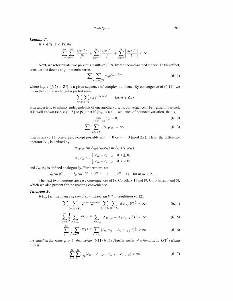
Lemma 2′.If f ∈ H.T × T/, then
∞X|j |=1
∞X|k|=1
þþþþcjk.f /jk
þþþþ+∞X
|j |=1
þþþþcj0.f /
j
þþþþ+∞X
|k|=1
þþþþc0k.f /
k
þþþþ < ∞:
Next, we reformulate two previous results of [8, 9] by the second-named author. To this effect,consider the double trigonometric seriesX X
.j;k/∈ Z2
cjkei.jx+ky/; (6.11)
where {cjk : .j; k/ ∈ Z2} is a given sequence of complex numbers. By convergence of (6.11), wemean that of the rectangular partial sumsX
|j |≤m
X|k|≤n
cjkei.jx+ky/ .m; n ∈ Z+/
asm and n tend to infinity, independently of one another (briefly, convergence in Pringsheim’s sense).It is well known (see, e.g., [8] or [9]) that if {cjk} is a null sequence of bounded variation, that is,
lim|j |+|k|→∞
cjk = 0; (6.12)
X X.j;k/∈ Z2
|111cjk| < ∞; (6.13)
then series (6.11) converges, except possibly at x = 0 or y = 0 (mod 2³ ). Here, the differenceoperator 111 is defined by
111cjk := 110.101cjk/ = 101.110cjk/;
110cjk :=(cjk − cj+1;k if j ≥ 0;
cjk − cj−1;k if j < 0;and 101cjk is defined analogously. Furthermore, set
I0 := {0}; Im := {2m−1; 2m−1 + 1; : : : ; 2m − 1} for m = 1; 2; : : : :
The next two theorems are easy consequences of [8, Corollary 1] and [9, Corollaries 3 and 5],which we also present for the reader’s convenience.
Theorem 3′.If {cjk} is a sequence of complex numbers such that conditions (6.12),X X
.m;n/∈ Z2+
2m+n.2−m−n X|j | ∈ Im
X|k| ∈ In
|111cjk|p/1p < ∞; (6.14)
∞Xk=1
1
k
Xm∈ Z+
2m.2−m X|j | ∈ Im
|110cjk −110cj;−k|p/1p < ∞; (6.15)
∞Xj=1
1
j
Xn∈ Z+
2n.2−n X|k| ∈ In
|101cjk −101c−j;k|p/1p < ∞ (6.16)
are satisfied for some p > 1, then series (6.11) is the Fourier series of a function in L.T2/ if andonly if
∞Xj=1
∞Xk=1
1
jk|cjk − c−j;k − cj;−k + c−j;−k| < ∞: (6.17)
502 D. Vu Giang and F. Moricz
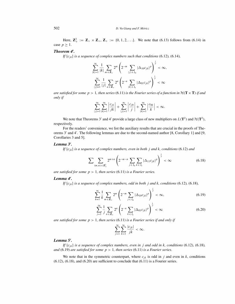
Here, Z2+ := Z+ × Z+, Z+ := {0; 1; 2; : : :}. We note that (6.13) follows from (6.14) in
case p ≥ 1.
Theorem 4′.If {cjk} is a sequence of complex numbers such that conditions (6.12), (6.14),
∞X|k|=1
1
|k|Xm∈ Z+
2m
2−m X|j | ∈ Im
|110cjk|p! 1
p
< ∞;
∞X|j |=1
1
|j |Xn∈ Z+
2n
2−n X|k| ∈ In
|101cjk|p! 1
p
< ∞
are satisfied for some p > 1, then series (6.11) is the Fourier series of a function in H.T × T/ if andonly if
∞X|j |=1
∞X|k|=1
þþþþcjkjkþþþþ+
∞X|j |=1
þþþþcj0
j
þþþþ+∞X
|k|=1
þþþc0k
k
þþþ < ∞:
We note that Theorems 3′ and 4′ provide a large class of new multipliers on L.T2/ and H.T2/,respectively.
For the readers’ convenience, we list the auxiliary results that are crucial in the proofs of The-orems 3′ and 4′. The following lemmas are due to the second-named author [8, Corollary 1] and [9,Corollaries 3 and 5].
Lemma 3′.If {cjk} is a sequence of complex numbers, even in both j and k, conditions (6.12) and
X X.m;n/∈ Z2
+
2m+n
2−m−n Xj ∈ Im
Xk ∈ In
|111cjk|p! 1
p
< ∞ (6.18)
are satisfied for some p > 1, then series (6.11) is a Fourier series.
Lemma 4′.If {cjk} is a sequence of complex numbers, odd in both j and k, conditions (6.12), (6.18),
∞Xk=1
1
k
Xm∈ Z+
2m
2−m Xj ∈ Im
|110cjk|p! 1
p
< ∞; (6.19)
∞Xj=1
1
j
Xn∈ Z+
2n
2−n Xk ∈ In
|101cjk|p! 1
p
< ∞ (6.20)
are satisfied for some p > 1, then series (6.11) is a Fourier series if and only if∞Xj=1
∞Xk=1
|cjk|jk
< ∞:
Lemma 5′.If {cjk} is a sequence of complex numbers, even in j and odd in k, conditions (6.12), (6.18),
and (6.19) are satisfied for some p > 1, then series (6.11) is a Fourier series.
We note that in the symmetric counterpart, where cjk is odd in j and even in k, conditions(6.12), (6.18), and (6.20) are sufficient to conclude that (6.11) is a Fourier series.
Hardy Spaces 503
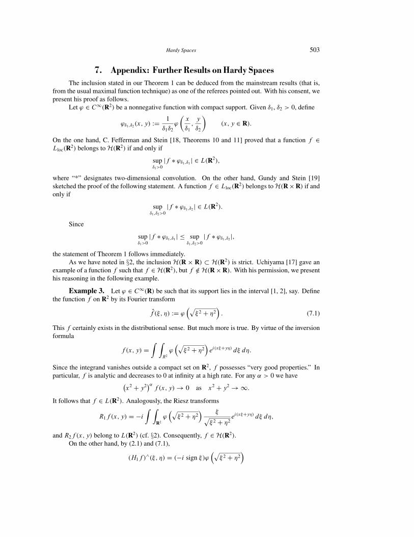
7. Appendix: Further Results on Hardy SpacesThe inclusion stated in our Theorem 1 can be deduced from the mainstream results (that is,
from the usual maximal function technique) as one of the referees pointed out. With his consent, wepresent his proof as follows.
Let ' ∈ C∞.R2/ be a nonnegative function with compact support. Given Ž1, Ž2 > 0, define
'Ž1;Ž2.x; y/ := 1
Ž1Ž2'
�x
Ž1;y
Ž2
�.x; y ∈ R/:
On the one hand, C. Fefferman and Stein [18, Theorems 10 and 11] proved that a function f ∈Lloc.R2/ belongs to H.R2/ if and only if
supŽ1>0
|f ∗ 'Ž1;Ž1 | ∈ L.R2/;
where “*” designates two-dimensional convolution. On the other hand, Gundy and Stein [19]sketched the proof of the following statement. A function f ∈ Lloc.R2/ belongs to H.R × R/ if andonly if
supŽ1;Ž2>0
|f ∗ 'Ž1;Ž2 | ∈ L.R2/:
Since
supŽ1>0
|f ∗ 'Ž1;Ž1 | ≤ supŽ1;Ž2>0
|f ∗ 'Ž1;Ž2 |;
the statement of Theorem 1 follows immediately.As we have noted in §2, the inclusion H.R × R/ ⊂ H.R2/ is strict. Uchiyama [17] gave an
example of a function f such that f ∈ H.R2/, but f =∈ H.R × R/. With his permission, we presenthis reasoning in the following example.
Example 3. Let ' ∈ C∞.R/ be such that its support lies in the interval [1, 2], say. Definethe function f on R2 by its Fourier transform
f .¾; �/ := '�p¾ 2 + �2
�: (7.1)
This f certainly exists in the distributional sense. But much more is true. By virtue of the inversionformula
f .x; y/ =Z Z
R2'�p¾ 2 + �2
�ei.x¾+y�/ d¾ d�:
Since the integrand vanishes outside a compact set on R2, f possesses “very good properties.” Inparticular, f is analytic and decreases to 0 at infinity at a high rate. For any Þ > 0 we have�
x2 + y2ÐÞf .x; y/ → 0 as x2 + y2 → ∞:
It follows that f ∈ L.R2/. Analogously, the Riesz transforms
R1f .x; y/ = −iZ Z
R2'�p¾ 2 + �2
� ¾p¾ 2 + �2
ei.x¾+y�/ d¾ d�;
and R2f .x; y/ belong to L.R2/ (cf. §2). Consequently, f ∈ H.R2/.On the other hand, by (2.1) and (7.1),
.H1f /∧.¾; �/ = .−i sign ¾/'
�p¾ 2 + �2
�
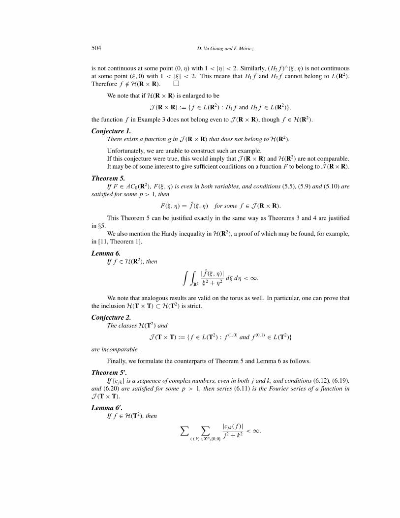
504 D. Vu Giang and F. Moricz
is not continuous at some point .0; �/ with 1 < |�| < 2. Similarly, .H2f /∧.¾; �/ is not continuous
at some point .¾; 0/ with 1 < |¾ | < 2. This means that H1f and H2f cannot belong to L.R2/.Therefore f =∈ H.R × R/. �
We note that if H.R × R/ is enlarged to be
J .R × R/ := {f ∈ L.R2/ : H1f and H2f ∈ L.R2/};the function f in Example 3 does not belong even to J .R × R/, though f ∈ H.R2/.
Conjecture 1.There exists a function g in J .R × R/ that does not belong to H.R2/.
Unfortunately, we are unable to construct such an example.If this conjecture were true, this would imply that J .R × R/ and H.R2/ are not comparable.It may be of some interest to give sufficient conditions on a function F to belong to J .R×R/.
Theorem 5.If F ∈ AC0.R2/, F.¾; �/ is even in both variables, and conditions (5.5), (5.9) and (5.10) are
satisfied for some p > 1, then
F.¾; �/ = f .¾; �/ for some f ∈ J .R × R/:
This Theorem 5 can be justified exactly in the same way as Theorems 3 and 4 are justifiedin §5.
We also mention the Hardy inequality in H.R2/, a proof of which may be found, for example,in [11, Theorem 1].
Lemma 6.If f ∈ H.R2/, then
Z ZR2
|f .¾; �/|¾ 2 + �2
d¾ d� < ∞:
We note that analogous results are valid on the torus as well. In particular, one can prove thatthe inclusion H.T × T/ ⊂ H.T2/ is strict.
Conjecture 2.The classes H.T2/ and
J .T × T/ := {f ∈ L.T2/ : f .1;0/ and f .0;1/ ∈ L.T2/}are incomparable.
Finally, we formulate the counterparts of Theorem 5 and Lemma 6 as follows.
Theorem 5′.If {cjk} is a sequence of complex numbers, even in both j and k, and conditions (6.12), (6.19),
and (6.20) are satisfied for some p > 1, then series (6.11) is the Fourier series of a function inJ .T × T/.
Lemma 6′.If f ∈ H.T2/, then
X X.j;k/∈ Z2\{0;0}
|cjk.f /|j 2 + k2
< ∞:
Hardy Spaces 505
References[1] Berkson, E., and Gillespie, T. A. (1984). Absolutely continuous functions for two variables and well-bounded operators.
J. London Math. Soc. (2) 30, 305–324.
[2] Carleson, L. (1976). Two remarks on H 1 and BMO. Adv. Math. 22, 269–277.
[3] Vu Giang, D., and Moricz, F. (1995). On the L1 theory of Fourier transforms and multipliers. Acta Sci. Math. (Szeged),61, 293–304.
[4] , (1993). Lebesgue intagrability of double Fourier transforms. Acta Sci. Math. (Szeged) 58, 295–324.
[5] Fefferman, R. (1988). Some recent developments in Fourier analysis and Hp theory on product domains II. FunctionSpaces and Applications, Proc. Conf. Lund 1986. Lecture Notes in Math. 1302, 44–51. Springer, Berlin and Heidelberg.
[6] Jawerth, B., and Torchinsky, A. (1986). A note on real interpolation of Hardy spaces in the polydisk. Proc. Amer. Math.Soc. 96, 227–232.
[7] Liflyand, E. R. (1993). On asymptotics of Fourier transform for functions of certain classes. Anal. Math. 19, 151–168.
[8] Moricz, F. (1991). On the integrability and L1-convergence of double trigonometric series. Studia Math. 98, 203–225.
[9] , (1993). Lebesgue integrability of double cosine and sine series. Analysis 13, 321–350.
[10] Peral, J. C., and Torchinsky, A. (1979). Multipliers in Hp.Rn/, 0 < p < ∞. Ark. Mat. 17, 225–235.
[11] Sledd, W. T., and Stagenda, D. A. (1981). An H1 multiplier theorem. Ark. Mat. 19, 265–270.
[12] Stein, E. M. (1966, 1967). Classes Hp , multiplicateurs et fonctions de Littlewood-Paley. C. R. Acad. Sci. Paris Ser. IMath. 263, 716–719; 264, 107–108.
[13] , (1970). Singular Integrals and Differentiability Properties of Functions. Princeton University Press, Prince-ton, N.J.
[14] Stein, E. M., and Weiss, G. (1960). On the theory of harmonic functions of several variables. Acta Math. 103, 26–62.
[15] , (1971). Introduction to Fourier Analysis on Euclidean Spaces. Princeton University Press, Princeton, N.J.
[16] Titchmarsh, E. C. (1937). Introduction to the Theory of Fourier Integrals. Clarendon Press, Oxford.
[17] Uchiyama, A. private communication.
[18] Fefferman, C., and Stein, E. M. (1972). Hp spaces of several variables. Acta Math. 129, 137–193.
[19] Gundy, R. F., and Stein, E. M. (1979). Hp theory for the poly-disc. Proc. Nat. Acad. Sci. U.S.A. 76, 1026–1029.
Received July 11, 1994; in revised form August 9, 1995
Institute of Mathematics, University of Veszprem, Egyetem U. 10, 8201 Veszprem, Hungary
Bolyai Institute, University of Szeged, Aradi Vertanuk Tere 1, 6720 Szeged, Hungary