Harmonic Analysis: from Fourier to Haar

Marıa Cristina Pereyra

Lesley A. Ward

Department of Mathematics and Statistics, MSC03 2150, 1 Univer-sity of New Mexico, Albuquerque, NM 87131-0001, USA

E-mail address: crisp@math.unm.edu

School of Mathematics and Statistics, University of South Aus-tralia, Mawson Lakes SA 5095, Australia

E-mail address: Lesley.Ward@unisa.edu.au

2000 Mathematics Subject Classification. Primary 42-xx

CHAPTER 2

Interlude

In this chapter we describe some useful classes of functions, sets of measurezero, and various ways (known as modes of convergence) in which a sequence offunctions can approximate another function. We then describe situations in whichwe are allowed to interchange limiting operations. Finally we state several densityresults that appear in different guises throughout the book. A leitmotif in analysis,in particular in harmonic analysis, is that often it is easier to prove results for aclass of simpler functions that are dense in a larger class, and then to use limitingprocesses to pass from the approximating simpler functions to the more complicatedlimiting function.

This chapter should be read once to get a glimpse of the variety of functionspaces and modes of convergence that can be considered. It should be revisited asnecessary while the reader gets acquainted with the theory of Fourier series andintegrals, and with the other types of time–frequency decompositions described inthis book.

2.1. Nested classes of functions on bounded intervals

Here we introduce some classes of functions on bounded intervals I (the in-tervals can be open, closed, or neither) and on the unit circle T. In Chapters 7and 8 we introduce analogous function classes on R, and we go beyond functionsand introduce distributions (generalized functions) in Section 8.2.

2.1.1. Riemann-integrable functions. We review the concept of the Rie-mann integral, following the exposition in the book by Terence Tao1 [Tao1, Chap-ter 11]. We highly recommend Tao’s book to our readers.

The development of the Riemann integral is in terms of approximation by stepfunctions. We begin with some definitions.

Definition 2.1. Given a bounded interval I, a partition P of I is a finitecollection of disjoint intervals {Jk}k=1,...,n such that I =

⋃nk=1 Ji. The intervals Ji

are contained in I and are necessarily bounded. ♦

Definition 2.2. The characteristic function χJ(x) of an interval J is definedto be the function that takes the value one if x lies in J , and zero otherwise:

χJ(x) =

{1, if x ∈ J ;0, if x /∈ J .

♦

1Terence Tao (1975–) is an Australian mathematician. He was awarded the Fields Medal in2006.

15

16 2. INTERLUDE

Figure 2.1. Graph of the step function h = 3χ[−1,2) − χ[2,4] +2χ(5,6) in Example 2.4.

The building blocks in the Riemann integration theory are finite linear combi-nations of characteristic functions of disjoint intervals, called step functions.

Definition 2.3. A function h defined on I is a step function if there are apartition P of the interval I, and real numbers {aJ}J∈P , such that

h(x) =∑J∈P

aJχJ(x),

where χJ(x) is the characteristic function of the interval J . ♦

For step functions there is a very natural definition of integral. Let us firstconsider an example.

Example 2.4. The function h = 3χ[−1,2) − χ[2,4] + 2χ(5,6) is a step functiondefined on the interval [−1, 6). Its graph is shown in Figure 2.1. ♦

If we ask the reader to compute the integral of this function over the interval[−1, 6), she will add (with appropriate signs) the areas of the rectangles in thepicture to get (3× 3) + (−1× 2) + (2× 1) = 9. More generally, we can define theintegral of a step function h associated to the partition P over the interval I by

(2.1)∫I

h(x) dx :=∑J∈P

aJ |J |,

where |J | denotes the length of the interval J . A given step function could beassociated to more than one partition, and one can verify that this definition ofthe integral is independent of the partition chosen. Notice that the integral of thecharacteristic function of a subinterval J of I is its length |J |.

Exercise 2.5. Given an interval J ⊂ I, show that∫I

χJ(x) dx = |J |.

♦

Definition 2.6. A function f is bounded on I if there is a constant M > 0such that |f(x)| ≤M for all x ∈ I. If so, we say that f is bounded by M . ♦

Exercise 2.7. Verify that step functions are always bounded functions. ♦

Definition 2.8. A function f : I → R is Riemann integrable if f is boundedon I, and if the supremum of the integrals of all step functions whose graphs liebelow the graph of f is equal to the infimum of the integrals of all step functionswhose graphs lie above that of f . In mathematical notation,

suph1≤f

∫I

h1(x) dx = infh2≥f

∫I

h2(x) dx <∞,

2.1. NESTED CLASSES OF FUNCTIONS ON BOUNDED INTERVALS 17

Figure 2.2. This figure illustrates the approximation of a func-tion f from below and from above by step functions h1 and h2

respectively, as in the definition of the Riemann integral.

where the supremum and infimum are taken over step functions h1(x) ≤ f(x) ≤h2(x) for all x ∈ I. We denote the common value by∫

I

f(x) dx,∫ b

a

f(x) dx, or simply∫I

f,

where a and b (a ≤ b) are the endpoints of the interval I. We denote the classof Riemann-integrable functions on I by R(I). See Figure 2.2 illustrating theapproximation of f from below and from above by step functions. ♦

Riemann integrability is a property preserved under linear transformations,taking maximums and minimums, absolute values, and products. It also preservesorder, meaning that if f and g are Riemann-integrable functions over I and if f < gthen

∫If <

∫Ig. The triangle inequality∣∣∣∣∫

I

f

∣∣∣∣ ≤ ∫I

|f |

holds for Riemann-integrable functions. See [Tao1, Section 11.4].

Exercise 2.9. (The Riemann Integral is Linear) Given two step functions h1

and h2 defined on I, verify that for c, d ∈ R, the linear combination ch1 + dh2 isagain a step function. Also check that∫

I

(ch1(x) + dh2(x)

)dx = c

∫I

h1(x) dx+ d

∫I

h2(x) dx.

Warning: The partitions P1 and P2 associated to the step functions h1 and h2

might be different. Try to find a partition that works for both (a common refine-ment).

Use Definition 2.8 to show that this linearity property is inherited by theRiemann-integrable functions. ♦

One can deduce from Definition 2.8 the following very useful proposition.

Proposition 2.10. A bounded function f is Riemann integrable over I if andonly if for each ε > 0 there are step functions h1 and h2 defined on I below andabove f , that is h1(x) ≤ f(x) ≤ h2(x) for all x ∈ I, such that the integral of theirdifference is bounded by ε. More precisely,

0 ≤∫I

(h2(x)− h1(x)

)dx < ε.

In particular, if f is Riemann-integrable then there exists a step function h suchthat ∫

I

|f(x)− h(x)| dx < ε.

18 2. INTERLUDE

Figure 2.3. The graph illustrates the integral of the difference ofthe two step functions in Figure 2.2.

See Figure 2.3 illustrating the integral of the difference of the two step functionsin Figure 2.2.

Aside 2.11. Readers familiar with the definition of the Riemann integral viaRiemann sums may like to observe that the integral of a step function that is be-low (respectively above) a given function f is always below a corresponding lower(respectively above a corresponding upper) Riemann sum2 for f .

Our first observation is that if f is Riemann integrable on [−π, π), then thezeroth Fourier coefficient of f is well defined:

a0 = f (0) =1

2π

∫ π

−πf(θ) dθ.

We say that a complex-valued function f : I → C is Riemann integrable if itsreal and imaginary parts are Riemann integrable. If f is Riemann integrable, thenthe complex-valued functions f(θ)e−inθ are Riemann integrable for each n ∈ Z, andall the Fourier coefficients an = f (n), n 6= 0, are also well defined.

Exercise 2.12. Verify that if f : [−π, π)→ C is Riemann integrable then thefunction g : [−π, π)→ C defined by g(θ) = f(θ)e−inθ is Riemann integrable. ♦

Here are some examples of familiar functions that are Riemann integrable andfor which we can define Fourier coefficients. See Theorem 2.29 for a completecharacterization of Riemann-integrable functions.

Example 2.13. Uniformly continuous functions on intervals are Riemann in-tegrable. In particular continuous functions on closed intervals are Riemann in-tegrable; see [Tao1, Section 11.5]. Monotone3 bounded functions on intervals areRiemann integrable; see [Tao1, Section 11.6]. ♦

Here is an example of a function that is not Riemann integrable.

Example 2.14. (Dirichlet’s Example) The function

f(x) =

{1, if x ∈ [a, b] ∩Q;0, if x ∈ [a, b] \Q

2A Riemann sum associated to a bounded function f : I → R and to a given partition P ofthe interval I is a real number R(f, P ) defined by R(f, P ) =

PJ∈P f(xJ ) |J |, where xJ is a point

in J for each J ∈ P . The upper (resp. lower) Riemman sum, U(f, P ) (resp. L(f, P ) associatedto f and P is obtained similarly replacing f(xJ ) by supx∈J f(x) (resp. infx∈J f(x)), Note that

since f is bounded both the infimum and supremum over J exist.3A function f : I → R is monotone if it is either increasing on the whole of I, or decreasing

on the whole of I; that is, either for all x, y ∈ I, x ≤ y, we have f(x) ≤ f(y), or for all x, y ∈ I,x ≤ y, we have f(x) ≥ f(y).

2.1. NESTED CLASSES OF FUNCTIONS ON BOUNDED INTERVALS 19

is bounded (by one), but it is not Riemann integrable on [0, 1]. Notice also that itis discontinuous everywhere. ♦

Exercise 2.15. Show that the Dirichlet function is not Riemann integrable. ♦

2.1.2. Lebesgue integrable functions and Lp-spaces. There are othermore general notions of integral; see for example the book by Robert G. Bar-tle [Bart2]. We will consider the Lebesgue integral.

The Lebesgue integral is studied in depth in courses on measure theory. Fora brief introduction see [Tao2, Chapters 18, 19]. For more in-depth presentationsat a level intermediate between advanced undergraduate and graduate studentssee [SS2] or [Bart1]. Classical graduate textbooks include the books by GeraldB. Folland [Fol] and by Halsey L. Royden [Roy].

In this section we simply aim to give some ideas about what the Lebesgueintegral is and what the Lp-spaces are, and we skim over the many subtleties ofmeasure theory.

Every Riemann-integrable function on a bounded interval I is also Lebesgue-integrable on I, and the values of its Riemann and Lebesgue integrals are the same.The Dirichlet function in Example 2.14 is Lebesgue integrable but not Riemannintegrable, with Lebesgue integral equal to zero; see Remark 2.33 at the end ofSection 2.1.4. In practice when you see an integral, it will usually suffice to thinkof Riemann integrals even if sometimes we really mean Lebesgue integrals.

In parallel to the definition of the Riemann integral just presented, we sketchthe definition of the Lebesgue integral over the bounded interval I. We use asscaffolding the so-called simple functions instead of step functions.

Simple functions are finite linear combinations of characteristic functions ofdisjoint measurable sets. The characteristic4 function of a set A ⊂ R is defined,similarly to the characteristic function of an interval, to be

(2.2) χA(x) =

{1, if x ∈ A;0, otherwise.

Intervals are measurable sets, and we can assign to them a measure, namely theirlength. However there are sets that are non-measurable, and we need to excludesuch sets. Once we assign a measure to each measurable set, we can define theLebesgue integral of the characteristic function of a measurable set to be the mea-sure of the set. The Lebesgue integral of a simple function is then defined to bethe corresponding finite linear combination of the measures of the underlying sets,exactly as in (2.1), except that now the sets J are disjoint measurable subsets of themeasurable set I, and the length |J | is replaced by the measure m(J) of the set J .One can then define Lebesgue integrability of a function f : I → R in analogy toDefinition 2.8, replacing the boundedness condition by requiring the function tobe measurable on I, and replacing step functions by simple functions. A functionf : I → R is measurable if the pre-image under f of each measurable subset of R isa measurable subset of I. It all boils down to understanding measurable sets andtheir measures.

4In statistics and probability the characteristic function of a set A is called the indicator func-tion of the set, and denoted IA. The term “characteristic function” refers to the Fourier transform

of a probability density (so-called because it “characterizes” the probability distribution).

20 2. INTERLUDE

In this book we do not define measurable sets, or their measure, except forsets of measure zero in R in Section 2.1.4, and for intervals or countable unions ofdisjoint intervals, whose measure is given, quite naturally, by the sum of the lengthsof the intervals.

A measurable function is said to belong to L1(I) if∫I|f(x)| dx < ∞, where

the integral is in the sense of Lebesgue. In fact, there is a continuum of Lebesguespaces, the Lp-spaces, defined for each real number p such that 1 ≤ p <∞ by

Lp(I) :={f : I → C :

∫I

|f(x)|p dx <∞},

and for p =∞ by

L∞(I) := {f : I → C : f is essentially bounded}.

The L in Lp and L∞ stands for Lebesgue.All the functions involved are assumed to be measurable. In Definition 2.30

we state precisely what essentially bounded means. For now, just think of L∞

functions as bounded functions on I. Let us denote by B(I) the space of boundedfunctions on I:

B(I) := {f : I → C : f is bounded}.There are essentially bounded functions that are not bounded, so B(I) ⊂ L∞(I),but L∞(I) is larger.

These spaces are normed spaces5 (after defining properly what it means for afunction to be zero in Lp, see Remark 2.33) with the Lp-norm defined to be

(2.3) ‖f‖Lp(I) :=(∫

I

|f(x)|p dx)1/p

, 1 ≤ p <∞,

(2.4) ‖f‖L∞(I) := ess supx∈I

|f(x)|, ‖f‖B(I) := supx∈I|f(x)|.

In Definition 2.31 we state precisely what essential supremum of f means.The Lp-metric or Lp-distance dp is the metric induced by the Lp-norm, for

each p with 1 ≤ p ≤ ∞. The Lp-distance between two functions f , g ∈ Lp(I) isgiven by the norm of their difference:

(2.5) dp(f, g) := ‖f − g‖Lp(I).

A property of normed spaces that we use repeatedly is the triangle inequality.In our setting it states that for all f , g ∈ Lp(I), 1 ≤ p ≤ ∞,

(2.6) ‖f + g‖Lp(I) ≤ ‖f‖Lp(I) + ‖g‖Lp(I).

The Riemann-integrable functions are not only contained in all Lp-spaces for1 ≤ p ≤ ∞, but they are also dense in each Lp(I) in its Lp-metric; see Defi-nition 2.62 below. In other words, given any function f ∈ Lp(I) we can find aRiemann-integrable function arbitrarily close to f in the Lp-metric. Furthermore,for each p the space Lp(I) is the completion of R(I) in the Lp-metric. Being thecompletion of R(I) automatically implies that R(I) is dense in Lp(I), but is astronger statement. It also implies that the limit of each convergent sequence in

5See Appendix B for the definition.

2.1. NESTED CLASSES OF FUNCTIONS ON BOUNDED INTERVALS 21

Lp(I) must be a function in Lp(I). Finally, we can think of a Cauchy6 sequence asbeing a sequence that has the right to converge. Every Cauchy sequence in Lp(I)does converge, and its limit is a function in Lp(I).

Informally, the completion Z of a subspace Y of a metric space X in the metricof X is the smallest subspace of X that contains Y and that also contains all limitsof Cauchy sequences in Z.

Aside 2.16. The reader may be familiar with the construction of the realnumbers R as the completion of the rational numbers Q in the Euclidean metricd(x, y) := |x − y|. One can think of R(I) as playing the role of Q and Lp(I) asplaying the role of R. There is a procedure that allows the completion of any metricspace, mirroring the procedure used in the construction of the real numbers. See forexample [Tao2, Exercise 12.4.8].

In fact, we could have defined the Lebesgue spaces Lp(I) as the completionof R(I) in the Lp-metric, instead of attempting to define the Lebesgue integralvia measure theory. The important thing is that both processes lead to the samespaces. This fact is so important that we state it (without proof) as a theorem, forfuture reference.

Theorem 2.17. For each p with 1 ≤ p ≤ ∞, the space Lp(I) is the completionof the Riemann-integrable functions R(I) in the Lp-metric. In particular, everyCauchy sequence in Lp(I) converges to a function in Lp(I).

Therefore the Lp-spaces with the Lp-norms are complete normed spaces. Suchspaces are so common and important that they have a special name, Banach7 spaces.See Appendix B for the definition of a complete normed space, and see Section 2.4for some results about density of one space in another. One learns about Banachspaces in a course on functional analysis. Classical graduate textbooks include [Fol]and the book by Martin Schechter [Sch].

Among the Lp-spaces, both L1 and L∞ play special roles. The space

L2(I) :={f : I → C :

∫I

|f(x)|2 dx <∞}

of square-integrable functions is also very important. The term square-integrableemphasizes that the integral of the square of (the absolute value of) f ∈ L2(I) isfinite. Functions in L2(I) are also said to have finite energy.

The L2-norm is induced by the inner product

(2.7) 〈f, g〉L2(I) :=∫I

f(x)g(x) dx,

meaning that ‖f‖L2(I) =√〈f, f〉L2(I).

The space L2(I) of square-integrable functions over I is a complete inner-product vector space (a Hilbert8 space), and so it has geometric properties verysimilar to those of n-dimensional Euclidean space Rn. In particular the notion

6The idea of a Cauchy sequence is that the terms must get arbitrarily close to each other as

n→∞. In our setting, the sequence {fn} ⊂ Lp(I) is a Cauchy sequence if for each ε > 0 there is

an N > 0 such that for all n, m > N , ‖fn − fm‖Lp(I) < ε. Every convergent sequence is Cauchy,

but the converse does not hold unless the space is complete.7Named after the Polish mathematician Stefan Banach (1892–1945).8Named after the German mathematician David Hilbert (1862–1943).

22 2. INTERLUDE

of orthogonality is very important. See Appendix B for a more detailed descrip-tion of inner-product vector spaces and Hilbert spaces. Another reference is [SS2,Chapters 4, 5].

In Chapter 5 we will be especially interested in the Hilbert space L2(T) ofsquare-integrable functions on T, with the L2-norm

‖f‖L2(T) :=(

12π

∫ π

−π|f(θ)|2 dθ

)1/2

induced by the inner product

〈f, g〉 :=1

2π

∫ π

−πf(θ)g(θ) dθ.

The factor 1/(2π) is just a normalization constant that forces the trigonometricfunctions en(θ) := einθ to have norm one in L2(T).

Exercise 2.18. Verify that

〈en, em〉 = δn,m.

In particular, ‖en‖L2(T) = 1. In the language of Chapter 5, the trigonometricsystem is an orthonormal system. ♦

2.1.3. Ladder of function spaces on T. So far in this chapter, we havebeen concerned with function spaces defined by integrability properties. Earlierwe encountered function spaces defined by differentiability properties. It turns outthat for functions defined on a given closed bounded interval, all these functionspaces are nicely nested. The inclusions are summarized in Figure 2.4 below.

Continuous functions on a closed bounded interval I = [a, b] are Riemann in-tegrable, and hence Lebesgue integrable. The collection of continuous functions onI = [a, b] is denoted by C([a, b]). Next, Ck([a, b]) denotes the collection of k timescontinuously differentiable functions on [a, b], in other words functions whose kth

derivatives exist and are continuous. For convenience we sometimes use the ex-pression ‘f is Ck’ to mean ‘f ∈ Ck’. Finally, C∞([a, b]) denotes the collection offunctions on [a, b] that are differentiable infinitely many times. (At the endpointsa and b, we mean continuous or differentiable from the right and from the leftrespectively.) Notice that there exist functions that are differentiable but not con-tinuously differentiable; the canonical example being f(x) = x2 sin(/x) for x 6= 0,f(0) = 0.

Exercise 2.19. Verify that f(x) = x2 sin(1/x) for x 6= 0, f(0) = 0, is differen-tiable everywhere but its derivative is not continuous at x = 0.

Recall that in Section 1.3.2 we discussed periodic functions on the unit circleT = [−π, π), as well as functions that are continuously differentiable on T. In thatcontext we meant that f : T→ C is Ck if f is k times continuously differentiable onT and if, when f is extended periodically, f (j)(−π) = f (j)(π) for all 0 ≤ j ≤ k. Thisboundary condition implies that when we restrict f to the closed interval [−π, π] itis Ck, in particular it is Riemann integrable on [−π, π).

Define Lp(T) to be Lp([−π, π)).For complex-valued functions defined on T, or on any closed bounded interval

I = [a, b], all these spaces are nicely nested. There is a ladder of function spaces in

2.1. NESTED CLASSES OF FUNCTIONS ON BOUNDED INTERVALS 23

T, running from the small space C∞(T) up to the large space L1(T):

C∞(T) ⊂ Ck(T) ⊂ C2(T) ⊂ C1(T) ⊂ C(T)

⊂ R(T) ⊂ B(T) ⊂ L∞(T) ⊂ Lp1(T) ⊂ Lp2(T) ⊂ L1(T),(2.8)

for integers k ≥ 2 and real numbers p1 and p2 such that p2 < p1. In particular,notice that

L2(T) ⊂ L1(T).

Warning: For functions defined on the real line, the Lp-spaces are no longer nested,nor are the continuous functions necessarily bounded or integrable.

Earlier we encountered a different family of function spaces on T, namely thecollections of 2π-periodic trigonometric polynomials of degree at most N , for N = 0,1, 2, . . . . We denote these spaces by PN (T). More precisely,

PN (T) :={ ∑|n|≤N

aneinθ : an ∈ C, |n| ≤ N

}.

These spaces are clearly nested and increasing as N increases, and they are certainlysubsets of C∞(T). Thus we can extend the above ladder to one starting at P0(T)(the constant functions) and climbing all the way to C∞(T), by including the nestedspaces

P0(T) ⊂ PN1(T) ⊂ PN2(T) ⊂ C∞(T),

for all N1, N2 with 0 ≤ N1 ≤ N2.The step functions defined in Section 2.1.1 are Riemann integrable, although

most of them have discontinuities. Our ladder has a branch:

{ step functions on I} ⊂ R(I).

The simple functions mentioned in Section 2.1.2 are bounded functions that arenot necessarily Riemann integrable. However, they are Lebesgue integrable, and infact simple functions are in Lp(I) for each p such that 1 ≤ p ≤ ∞. Our ladder hasa second branch:

{ simple functions on I} ⊂ B(I).

Exercise 2.20. Compute the Lp-norm of a step function defined on an inter-val I. Compute the Lp-norm of a simple function defined on an interval I. Use thenotation m(A) for the measure of a measurable set A ⊂ I. ♦

We will encounter other classes of functions on T, [a, b], or R, such as functionsthat are piecewise continuous or piecewise smooth, monotone functions, functionsof bounded variation, Lipschitz9 functions, and Holder10-continuous functions. Wedefine what we mean as they appear in the text. As you encounter these spaces,you are encouraged to try to fit them in to the ladder of spaces in Figure 2.4, whichwill start looking more like a tree with branches and leaves.

The results of the following exercises justify some of the inclusions in the ladderof function spaces. Operate with the Lebesgue integrals as you would operate withRiemann integrals. Try to specify which properties of the integral you are using.

9Named after the German mathematician Rudolf Otto Sigismund Lipschitz (1832–1903).10Named after the German mathematician Otto Ludwig Holder (1859–1937).

24 2. INTERLUDE

Exercise 2.21. Let I be a bounded interval. Show that if f : I → C isbounded by M > 0 and f ∈ Lp(I), then f ∈ Lq(I) for all q such that p ≤ q < ∞.Furthermore, ∫

I

|f(x)|q dx ≤Mq−p∫I

|f(x)|p dx <∞,

and so in this situation the Lq-norm is controlled by the Lp-norm. In the languageof norms, the preceding inequality can be written as

‖f‖qLq(I) ≤ ‖f‖q−pL∞(I) ‖f‖

pLp(I),

since ‖f‖L∞(I) is the infimum of the numbers M that bound f . ♦

For the previous exercise you may find Holder’s inequality useful.

Lemma 2.22 (Holder’s Inequality). Suppose I is a bounded interval, 1 ≤ s ≤ ∞,1s

+1t

= 1, f ∈ Ls(I), and g ∈ Lt(I). Then

(2.9)∣∣∣∣∫I

f(x)g(x) dx∣∣∣∣ ≤ ‖f‖Ls(I)‖g‖Lt(I);

in other words the integral of the product of f and g is smaller in absolute valuethan the product of the Ls-norm of f and the Lt-norm of g.

Holder’s inequality reappears in later chapters, and it is discussed and proved,together with other very important inequalities, at the end of the book. The specialcase when s = t = 2 is the celebrated Cauchy–Schwarz11 inequality. Inequalities areinherent to the way of analysis, and we will see them over and over again throughoutthe book.

Exercise 2.23. Let I be a bounded interval. Show that if 1 ≤ p ≤ q <∞ andh ∈ Lq(I) then h ∈ Lp(I). Moreover, show that if h ∈ Lq(I) then

‖h‖Lp(I) ≤ |I|1/p−1/q‖h‖Lq(I).

Thus for those exponents, Lq(I) ⊂ Lp(I). Hint: Apply Holder’s inequality on I,with s = q/p > 1, f = |h|p, g = 1, and h ∈ Lq(I). ♦

2.1.4. Sets of measure zero. For many purposes we often need only thata function has a given property except on an exceptional set of points x. Suchexceptional sets are small. We now introduce the appropriate notion of smallness,given by the concept of a set of measure zero.

Definition 2.24. A set E ⊂ R has measure zero if, for each ε > 0, there areopen intervals Ij such that E is covered by the collection {Ij}j∈N of intervals, andthe total length of the intervals is less than ε:

(i) E ⊂∞⋃j=1

Ij , and (ii)∞∑j=1

|Ij | < ε.

11This inequality is named after the French mathematician Augustin Louis Cauchy (1789–

1857), and the German mathematician Hermann Amandus Schwarz (1843–1921). The Cauchy–

Schwarz inequality was discovered 25 years earlier by the Ukranian mathematician Viktor Yakovle-vich Bunyakovskii (1804–1889), and it is also known as the Cauchy–Bunyakovskii–Schwarz

inequality.

2.1. NESTED CLASSES OF FUNCTIONS ON BOUNDED INTERVALS 25

We say that a given property holds almost everywhere if the set of points where theproperty does not hold has measure zero. We use the abbreviation a.e. for almosteverywhere12. ♦

In particular, every countable set has measure zero. There are uncountable setsthat have measure zero. The most famous example is the Cantor13 set, discussedin Example 2.26.

Exercise 2.25. Show that finite subsets of R have measure zero. Show thatcountable subsets of R have measure zero. In particular the set Q of rationalnumbers has measure zero. ♦

Example 2.26. (The Cantor set) The Cantor set C is obtained from the closedinterval [0, 1] by a sequence of successive deletions of open intervals called the middlethirds, as follows. Remove the middle-third interval (1/3, 2/3) of [0, 1]. We areleft with two closed intervals: [0, 1/3] and [2/3, 1]. Remove the two middle-thirdintervals (1/9, 2/9) and (7/9, 8/9) of the remaining closed intervals. We are leftwith four closed intervals: [0, 1/9], [2/9, 1/3], [2/3, 7/9], and [8/9, 1]. Delete the fourmiddle-third intervals (1/27, 2/27), (7/27, 8/27), (19/27, 20/27), and (25/27, 26/27)of the remaining closed intervals.

Continuing in this way, at the nth stage we are left with 2n disjoint closedintervals each of length 3n−1. Removing the 2n middle-third intervals, each oflength 1/3n, we are left with 2n+1 disjoint closed intervals of length 1/3n. Thisprocess can be continued indefinitely, so that the set A of all points removed fromthe closed interval [0, 1] is the union of a collection of disjoint open intervals. ThusA ⊂ [0, 1] is an open set.

The Cantor set C is defined to be the set of points that remain after A isdeleted: C := [0, 1] \A.

The Cantor set can be seen to coincide with the set of numbers in [0, 1] whoseternary expansion (base three) uses only the digits 0 and 2. Once this identificationis made, one can also verify that C is in a one-to-one correspondence (except forcertain points for which the correspondence is two-to-one) with the interval [0, 1].Therefore C has the same cardinality as R, and so C is an uncountable set. However,C has measure zero, because its complement A has measure one14: the sum of thelengths of the disjoint intervals removed is

m(A) := 1× 13

+ 2× 19

+ 4× 127

+ · · · =∞∑n=1

2n−1

3n= 1.

The last equality holds because we are dealing with a geometric sum with ratior = 2/3 < 1. ♦

Exercise 2.27. Verify that the Cantor set C is closed. Use Definition 2.24 toverify that C has measure zero. ♦

12In probability theory it is used instead a.s. for almost surely, in French p.p. for presquepartout, in Spanish c.s. for casi siempre.

13Named after the German mathematician Georg Ferdinand Ludwig Philipp Cantor (1845–1918).

14Recall that a natural way of defining the length or measure of a subset A of R which is

a countable union of disjoint intervals {Ij} is to declare the measure of A to be the sum of the

lengths of the intervals Ij .

26 2. INTERLUDE

Aside 2.28. We assume that the reader is familiar with basic notions of pointset topology on R, and in particular with the concepts of open and closed sets in R.To review these ideas, see for example [Tao2, Chapter 12].

Here is an important characterization of Riemann-integrable functions; it ap-peared in Lebesgue’s doctoral dissertation. A proof can be found in Stephen Ab-bott’s book [Abb, Section 7.6].

Theorem 2.29 (Lebesgue’s Theorem, 1901). A bounded function f : I → C isRiemann integrable if and only if f is continuous almost everywhere.

We can now define what the terms essentially bounded and essential supremummean.

Definition 2.30. A function f : T→ C is essentially bounded if it is boundedexcept on a set of measure zero. More precisely, there exists a constant M > 0 suchthat |f(x)| ≤M a.e. in I. ♦

Definition 2.31. Let f : I → C be an essentially bounded function. Theessential supremum ess supx∈I |f(x)| of f is defined to be the smallest constant Msuch that |f(x)| ≤M a.e. on the interval I. In other words,

ess supx∈I

|f(x)| := inf{M ≥ 0 : |f(x)| ≤M a.e. in I}.

♦

Exercise 2.32. Verify that if f is bounded on I then f is essentially bounded.In other words, the space B(I) of bounded functions on I is a subset of L∞(I).Show that it is a proper subset. Furthermore, verify that if f is bounded theness supx∈I |f(x)| = supx∈I |f(x)|. ♦

Remark 2.33. For the purposes of Lebesgue integration theory, functions thatare equal almost everywhere are regarded as being the same. To be really precise,one should talk about equivalence classes of Lp-integrable functions: f is equivalentto g if and only if f = g a.e. In that case

∫I|f − g|p = 0, and if f ∈ Lp(I) then

so is g. We say f = g in Lp(I) if f = g a.e. In that case,∫I|f |p =

∫I|g|p. In

particular the Dirichlet function g in Example 2.14 is equal a.e. to the zero function,which is in Lp([0, 1]). Hence the Dirichlet function g is in Lp([0, 1]), its integral inthe Lebesgue sense vanishes, and its Lp-norm is zero for all 1 ≤ p ≤ ∞.

Now that we have given the relevant definitions, we summarize in Figure 2.4the ladder of function spaces discussed in Section 2.1.3. In Figure 2.4, p1 and p2

are real numbers such that 1 < p1 < 2 < p2 < ∞, and N1 and N2 are naturalnumbers such that N1 ≤ N2. The blank box appears because there is no commonlyused symbol for the class of differentiable functions. Notice that as we move downthe ladder into the smaller function classes, the functions become better behaved.For instance, the Lp spaces on T are nested and decreasing as the real number pincreases from 1 to ∞ (Exercise 2.23).

Two warnings are in order. First, when the underlying space is changed fromthe circle T to another space X, the Lp spaces need not be nested: for real numbersp, q with 1 ≤ p ≤ q ≤ ∞, Lp(X) need not contain Lq(X). For example, the Lp

spaces on the real line R are not nested. (By contrast, the Ck classes are alwaysnested: Ck(X) ⊃ Ck+1(X) for all spaces X (in which differentaibility is defined)and for all k ∈ N.) Second, as mentioned above, there are important functionclasses that do not fall into the nested chain of classes shown here.

2.1. NESTED CLASSES OF FUNCTIONS ON BOUNDED INTERVALS 27

6

...

...

...

...∪

∪

∪

∪

∪

∪

∪

∪

∪

∪

∪

∪

∪

∪

∪

∪

∪

∪

∪L1(T)

Lp1(T)

L2(T)

Lp2(T)

L∞(T)

B(T)

R(T)

C(T)

C1(T)

C2(T)

...

Ck(T)

...

C∞(T)

...

PN2(T)

PN1(T)

...

P0(T)

Lebesgue integrable:∫

T |f(x)| dx <∞

∫T |f(x)|p1 dx <∞ , 1 < p1 < 2

square integrable:∫

T |f(x)|2 dx <∞

∫T |f(x)|p2 dx <∞ , 2 < p1 <∞

essentially bounded: ess supx∈T |f(x)| <∞

bounded functions: |f(x)| ≤M for all x ∈ T

Riemann integrable

continuous

differentiable

continuously differentiable:f ′ exists and is continuous

twice continuously differentiable:f , f ′ exist and are continuous

k times continuously differentiable:f , f ′, . . . , f (k) exist and are continuous

infinitely often differentiable:f , f ′, f ′′, . . . , exist and are continuous

trigonometric polynomials of degree N2 > N1

trigonometric polynomials of degree N1 > 0

constant functions

Figure 2.4. Ladder of nested classes of functions f : T→ C.

28 2. INTERLUDE

2.2. Modes of convergence

Given a bounded interval I and functions gn, g : I → C, what does it meanto say that gn → g? In this section we discuss seven different ways in whichthe functions gn could approximate g: pointwise; almost everywhere; uniformly;uniformly outside a set of measure zero; in the sense of convergence in the mean(convergence in L1); in the sense of mean-square convergence (convergence in L2);and in the sense of convergence in Lp. The first four of these modes of convergenceare defined in terms of the behavior of the functions gn and g at individual points x,therefore the itnerval I can be replaced by any subset X of real numbers. The lastthree of these modes are defined in terms of integrals of powers of the difference|gn−g|, in these cases I can be replaced by any set of real numbers X for which theintegral over the set is defined. Some of these modes of convergence are strongerthan others, uniform convergence being the strongest. Figure 2.5 illustrates theinterrelations between five of these modes of convergence.

In Chapter 3, we will be concerned with pointwise and uniform convergenceof Fourier series, and in Chapter 5 we will be concerned with mean-square conver-gence of Fourier series. At the end of the book, we come full circle and show thatconvergence in Lp(T) of Fourier series is a consequence of the boundedness in Lp(T)of the periodic Hilbert transform.

See [Bart1, pp.68–72] for yet more modes of convergence, such as convergencein measure and almost uniform convergence (not to be confused with uniform con-vergence outside a set of measure zero).

We begin with the modes of convergence that are defined in terms of individualpoints x. In what follows X is a subset of the real numbers.

Definition 2.34. A sequence of functions gn : X → C converges pointwise tog : X → C if for each x ∈ X,

limn→∞

gn(x) = g(x).

Equivalently, gn converges pointwise to g if for each ε > 0 and for each x ∈ X thereis an N = N(ε, x) > 0 such that for all n > N ,

|gn(x)− g(x)| < ε.

♦

Almost-everywhere convergence is a little weaker than pointwise convergence.

Definition 2.35. A sequence of functions gn : X → C converges almost ev-erywhere, or pointwise a.e., to g : X → C if it converges pointwise to g except on aset of measure zero:

limn→∞

gn(x) = g(x) a.e. in X.

Equivalently, gn converges a.e. to g if there exists a set E of measure zero, E ⊂ X,such that for each x ∈ X \ E and for each ε > 0 there is an N = N(ε, x) > 0 suchthat for all n > N ,

|gn(x)− g(x)| < ε.

♦

Uniform convergence is stronger than pointwise convergence. Informally, givena fixed ε, for uniform convergence the same N must work for all x, while forpointwise convergence we may use different numbers N for different points x.

2.2. MODES OF CONVERGENCE 29

Uniform convergence:|gn(x)− g(x)| → 0uniformly in x.

For each ε > 0 there is an Nthat works for all x ∈ T.

Pointwise convergence:|gn(x)− g(x)| → 0for all x ∈ T.

For each ε > 0 and each x ∈ Tthere is an N = N(x, ε) that works.

L2 (mean-square) convergence:∫T |gn(x)− g(x)|2 dx→ 0.

Pointwise a.e. convergence:|gn(x)− g(x)| → 0for almost all x ∈ T.

For each ε > 0 and almost every x ∈ Tthere is an N = N(x, ε) that works.

L1 (mean) convergence:∫T |gn(x)− g(x)| dx→ 0.

ww� ww�

=⇒ =⇒

Figure 2.5. Relations between five of the seven modes of conver-gence discussed in Section 2.2, for functions gn, g : T→ C, showingwhich modes imply which other modes. All potential implicationsbetween these five modes other than those shown here are false.

Definition 2.36. A sequence of bounded functions gn : X → C convergesuniformly to g : X → C if given ε > 0 there is an N = N(ε) > 0 such that for alln > N ,

|gn(x)− g(x)| < ε for all x ∈ X.Equivalently, gn converges uniformly to g if

limn→∞

supx∈X|gn(x)− g(x)| = 0.

♦

Here is a slightly weaker version of uniform convergence.

30 2. INTERLUDE

Definition 2.37. A sequence of L∞-functions gn : X → C converges uniformlyoutside a set of measure zero, or in L∞, to g : X → C if

limn→∞

‖gn − g‖L∞(X) = 0.

We write gn → g in L∞(X). ♦

Remark 2.38. If the functions gn and g are continuous and bounded on X ⊂ R,then

‖gn − g‖L∞(X) = supx∈X|gn(x)− g(x)|,

and in this case convergence in L∞(X) and uniform convergence coincide. Thisis why the L∞-norm for continuous functions is often called the uniform norm.The metric space of continuous functions over a closed bounded interval with themetric induced by the uniform norm is a complete metric space (a Banach space),see [Tao2, Section 4.4]. In particular, if the functions gn in Definition 2.36 arecontinuous and converge uniformly, then the limiting function is itself continuous;see Theorem 2.55.

We move to the modes of convergence defined via integrals. The two mostimportant are convergence in L1 and in L2; these are special cases of convergencein Lp.

The integral used in these definitions is the Lebesgue integral, and by integrablewe mean Lebesgue integrable. here we restrict to integrals on bounded intervals I.

Definition 2.39. A sequence of integrable functions gn : I → C converges inthe mean, or in L1(I), to g : I → C if for each ε > 0 there is a number N > 0 suchthat for all n > N ∫

I

|gn(x)− g(x)| dx < ε.

Equivalently, gn converges in L1 to g if limn→∞

‖gn − g‖L1(I) = 0. We write gn → g

in L1(I). ♦

Definition 2.40. A sequence of square-integrable functions gn : I → C con-verges in mean-square, or in L2(I), to g : I → C if for each ε > 0 there is an N > 0such that for all n > N , ∫

I

|gn(x)− g(x)|2 dx < ε.

Equivalently, gn converges in L2 to g if limn→∞

‖gn − g‖L2(I) = 0. We write gn → g

in L2(I). ♦

Convergence in L1(I) and in L2(I) are particular cases of convergence in Lp(I).

Definition 2.41. For p such that 1 ≤ p < ∞, a sequence of Lp-integrablefunctions gn : I → C converges in Lp(I) to g : I → C if given ε > 0 there existsN > 0 such that for all n > N∫

I

|gn(x)− g(x)|p dx < ε.

Equivalently, gn converges in Lp to g if limn→∞

‖gn − g‖Lp(I) = 0. We write gn → g

in Lp(I). ♦

2.2. MODES OF CONVERGENCE 31

We have already noted that the Lp-spaces are complete normed spaces, alsoknown as Banach spaces. Therefore the limit functions in Definition 2.41 have nochoice but to be in Lp(I) themselves. In particular, in Definitions 2.39 and 2.40 thelimit functions must be in L1(I) and L2(I) respectively.

Exercise 2.42. Verify that uniform convergence on a bounded interval I im-plies the other modes of convergence on I. ♦

Exercise 2.43. Show that for 1 ≤ q < p ≤ ∞ convergence in Lp(I) impliesconvergence in Lq(I). Hint: use Holder’s Inequality (2.9). ♦

The following examples show that in Figure 2.5 the implications go only in thedirections indicated. In these examples we work on the unit interval [0, 1].

Example 2.44. (Pointwise but not uniform) The sequence of functions definedby fn(x) = xn for x ∈ [0, 1] converges pointwise to the function f defined byf(x) = 0 for 0 ≤ x < 1 and f(1) = 1, but it does not converge uniformly to f or toany other function. See Figure 2.6. ♦

Figure 2.6. The functions fn(x) = xn converge pointwise, butnot uniformly, on [0, 1] to the function f(x) that is 0 for x ∈ [0, 1)and 1 at x = 1.

Example 2.45. (Pointwise but not in the mean) The sequence of functionsgn : [0, 1]→ R defined by

gn(x) =

{n, if 0 < x < 1/n;0, otherwise,

converges pointwise everywhere to g(x) = 0, but it does not converge in the meanor in L2, nor does it converge uniformly. See Figure 2.7. ♦

Example 2.46. (In the mean but not pointwise) Given a positive integer n, letm, k be the unique non-negative integers such that n = 2k + m and 0 ≤ m < 2k.The sequence of functions hn(x) : [0, 1]→ R defined by

hn(x) =

1, ifm

2k< x <

m+ 12k

;

0, otherwise,

converges in the mean to the zero function, but it does not converge pointwise atany point x ∈ [0, 1]. This sequence of functions is sometimes called the walkingfunction. See Figure 2.8. ♦

Despite these examples, there is a connection between pointwise convergenceand convergence in Lp. For p such that 1 ≤ p <∞, if fn, f ∈ Lp(T), and if fn → fin Lp, then there is a subsequence {fnk

} that converges to f a.e. on T. See [SS2,Corollary 2.2].

Figure 2.7. The functions gn defined in Example 2.45 convergepointwise, but not in the mean, in L2, or uniformly.

32 2. INTERLUDE

Figure 2.8. The functions hn(x) defined in Example 2.46 con-verge in mean, but do not converge pointwise at any x.

Exercise 2.47. Verify that the sequences described in Examples 2.44, 2.45,and 2.46 do have the convergence properties described there. Adapt the sequencesin the examples to have the same convergence properties on the interval [a, b]. ♦

Exercise 2.48. Where would the two missing modes, namely convergence out-side a set of measure zero and Lp convergence for a given p with 1 ≤ p ≤ ∞, fitin Figure 2.4? Prove the implications that involve these two modes, and deviseexamples to show that other potential implications involving these two modes donot hold. ♦

2.3. Interchanging limit operations

Uniform convergence on closed bounded intervals is a very strong form of con-vergence which is amenable to interchange with other limiting operations and prop-erties defined by limits, such as integration, differentiation and continuity. Welist here without proof several results from advanced calculus that will be usedthroughout the book. Some results do involve uniform convergence as one of thelimit operations, some others involve other limit operations (like interchanging twointegrals).

Theorem 2.49 (Interchange of Limits and Integrals). If {fn}n∈N is a sequenceof integrable functions that converges uniformly to f in [a, b] then f is integrable on[a, b] and

limn→∞

∫ b

a

fn =∫ b

a

limn→∞

fn =∫ b

a

f.

In other words,The limit of the integrals of a uniformly convergent sequence offunctions on [a, b] is the integral of the limit function on [a, b].

Notice that the functions in Example 2.45 do not converge uniformly, and theyprovide an example where this interchange fails. In fact,

∫ 1

0gn = 1 for all n and∫ 1

0g = 0, so

limn→∞

∫ 1

0

gn = 1 6= 0 =∫ 1

0

limn→∞

gn =∫ 1

0

g.

Exercise 2.50. Given a closed bounded interval I and integrable functions

gn : I → C, n ∈ N, suppose the partial sumsN∑n=0

gn(x) converge uniformly on I as

N →∞. Show that ∫I

∞∑n=0

gn(x) dx =∞∑n=0

∫I

gn(x) dx.

♦

We can interchange infinite summation and integration providedthe convergence of the partial sums is uniform.

2.3. INTERCHANGING LIMIT OPERATIONS 33

It is therefore important to know when do partial sums converge uniformly totheir series. The Weierstrass M-Test is a very useful technique to deduce uniformconvergence of partial sums of functions.

Theorem 2.51 (Weierstrass M-Test). Let {fn}∞n=1 be a sequence of boundedreal-valued functions on a subset X of the real numbers. Assume there is a sequenceof positive real numbers such that |fn(x)| ≤ an for all x ∈ X, and

∑∞n=1 an < ∞.

Then the series∑∞n=1 fn converges uniformly to a real-valued function on X.

Under certain conditions, involving uniform convergence of a sequence of func-tions and their derivatives, one can exchange differentiation and the limit.

Theorem 2.52 (Interchange of Limits and Derivatives). Let fn : [a, b]→ C bea sequence of C1 functions converging uniformly on [a, b] to the function f . Assumethat the derivatives (fn)′ also converge uniformly on [a, b] to some function g. Thenf is C1, and f ′ = g, that is

limn→∞

(fn)′ =(

limn→∞

fn

)′.

In other words,We can interchange limits and differentiation provided the con-vergence of the functions and the derivatives is uniform.

Exercise 2.53. Show that the hypotheses in Theorem 2.52 are necessary. ♦

Exercise 2.54. What are the necessary hypotheses on a series∞∑n=0

gn(x) so

that it is legal to interchange sum and differentiation? In other words, when canwe guarantee that ( ∞∑

n=0

gn(x)

)′=∞∑n=0

(gn)′(x)?

♦

Here is another classical and useful result in the same vein, already mentionedin Remark 2.38.

Theorem 2.55. The uniform limit of continuous functions on a subset X ofthe real numbers is continuous on X.

Exercise 2.56. Prove Theorem 2.55.

Notice that this is the same as saying that if gn → g uniformly, and the functionsgn are continuous, then for all x0 ∈ X we can interchange the limit as x approachesx0 with the limit as n tend to infinity,

(2.10) limx→x0

limn→∞

gn(x0) = limn→∞

limx→x0

gn(x).

Perhaps inserting a few more equalities will make the above statement clear:

limx→x0

limn→∞

gn(x) = limx→x0

g(x) (gn converges unif. to g)

= g(x0) (g is continuous at x0)= lim

n→∞gn(x0) (gn converges unif. to g)

= limn→∞

limx→x0

gn(x) (gn is continuous at x0).

34 2. INTERLUDE

Example 2.44 shows a sequence of continuous functions on [0, 1] that convergepointwise to a function that is discontinuous (at x = 1). Thus the convergencecannot be uniform.

There is a partial converse, called Dini’s15 Theorem, to Theorem 2.55. It saysthat the pointwise limit of a decreasing sequence of functions is also their uniformlimit.

Theorem 2.57 (Dini’s Theorem). Suppose that f , fn : I → R are continuousfunctions. Assume that (i) fn converges pointwise to f as n → ∞; and (ii) fn isa decreasing sequence, namely fn(x) ≥ fn+1(x) for all x ∈ I. Then fn convergesuniformly to f .

Exercise 2.58. Prove Dini’s Theorem, and show that hypothesis (ii) is es-sential. A continuous version of Example 2.45, where the “steps” are replaced by“tents”, might help. ♦

In Weiertrass’s M-Test, Theorem 2.51, if the functions {fn}∞n=1 being summedup are continuous then the series

∑∞n=1 fn(x) is a continuous function.

Interchanging integrals is another instance of these interchange-of-limit oper-ations. The theorems that allow for such interchange go by the name Fubini’sTheorems16. Here is one such theorem, valid for continuous functions.

Theorem 2.59 (Fubini’s Theorem for Continuous Functions). Let I and J beclosed intervals. Let F : I × J → C be a continuous function. Assume∫∫

I×J|F (x, y)| dA <∞,

where dA denotes the differential of area. Then∫I

∫J

F (x, y) dx dy =∫J

∫I

F (x, y) dy dx =∫∫

I×JF (x, y) dA.

Usually Fubini’s Theorem refers to an L1-version of Theorem 2.59 that is statedand proved in every measure theory book. You can find a two-dimensional versionin [Tao2, Section 19.5].

Interchanging limit operations is a delicate maneuver that cannot always beaccomplished. We illustrate throughout the book settings where this interchangeis allowed and settings where it is illegal, such as the ones just described involvinguniform convergence. If we insist on carrying on the interchange, false conclusionscould be deduced.

Unlike the Riemann integral, the Lebesgue theory allows for the interchange ofa pointwise limit and an integral. There are several landmark theorems that youlearn in a course on measure theory. We state one such result.

Theorem 2.60 (Lebesgue Dominated Convergence Theorem). Consider a se-quence of measurable functions fn defined on the interval I, converging pointwisea.e. to a function f . Suppose there exists a dominating function g ∈ L1(I), meaningthat |fn(x)| ≤ g(x) a.e. for each n > 0. Then

limn→∞

∫I

fn(x) dx =∫I

f(x) dx.

15Ulisse Dini, Italian mathematician (1845–1918).16Named after the Italian mathematician Guido Fubini (1879–1943).

2.4. DENSITY 35

Exercise 2.61. Verify that the functions in Example 2.45 cannot be dominatedby an integrable function g. ♦

2.4. Density

Having different ways to measure convergence of functions to other functionsprovides ways of deciding when we can approximate functions in a given class byfunctions in another class. In particular we can decide when a subset is dense in alarger set of functions.

Definition 2.62. Given a normed space X of functions defined on a boundedinterval I, with norm denoted by ‖ · ‖X , we say that a subset A ⊂ X is dense in Xif given any f ∈ X there exists a sequence of functions fn ∈ A such that

limn→∞

‖fn − f‖X = 0.

Equivalently, A is dense in X if given any f ∈ X and any ε > 0 there exists afunction h ∈ A such that

‖h− f‖X < ε.

♦

One can deduce from the definition of the Riemann-integrable functions on abounded interval I that the step functions (see Definition 2.3) are dense in R(I)with respect to the L1-norm; see Proposition 2.10. We state this result as a theorem,for future reference.

Theorem 2.63. Given a Riemann-integrable function on a bounded interval I,f ∈ R(I), and given ε > 0, there exists a step function h such that

‖h− f‖L1(I) < ε.

Remark 2.64. We can choose the step functions that approximate a givenRiemann-integrable function to lie entirely below the function, or entirely above it.

In Chapter 4 we will learn that

Trigonometric polynomials can approximate uniformly continu-ous functions on T.

This is the celebrated Weierstrass theorem (see Theorem 3.4).In Chapter 9 we will learn that on closed bounded intervals,

Step functions can approximate uniformly continuous functions,despite the fact that step functions are not continuous.

It is not hard to deduce directly from the fact that continuous functions canbe approximated uniformly by step functions that they can also be approximatedin the Lp-norm by step functions.

Step functions can approximate continuous functions in the Lp-norm.

What is perhaps surprising is that

Continuous functions can approximate step functions pointwiseand in the Lp-norm.

36 2. INTERLUDE

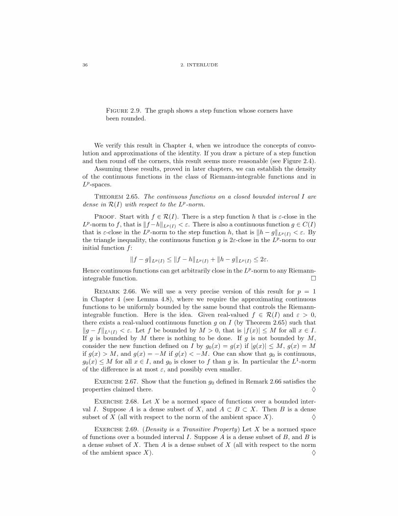
Figure 2.9. The graph shows a step function whose corners havebeen rounded.

We verify this result in Chapter 4, when we introduce the concepts of convo-lution and approximations of the identity. If you draw a picture of a step functionand then round off the corners, this result seems more reasonable (see Figure 2.4).

Assuming these results, proved in later chapters, we can establish the densityof the continuous functions in the class of Riemann-integrable functions and inLp-spaces.

Theorem 2.65. The continuous functions on a closed bounded interval I aredense in R(I) with respect to the Lp-norm.

Proof. Start with f ∈ R(I). There is a step function h that is ε-close in theLp-norm to f , that is ‖f−h‖Lp(I) < ε. There is also a continuous function g ∈ C(I)that is ε-close in the Lp-norm to the step function h, that is ‖h− g‖Lp(I) < ε. Bythe triangle inequality, the continuous function g is 2ε-close in the Lp-norm to ourinitial function f :

‖f − g‖Lp(I) ≤ ‖f − h‖Lp(I) + ‖h− g‖Lp(I) ≤ 2ε.

Hence continuous functions can get arbitrarily close in the Lp-norm to any Riemann-integrable function. �

Remark 2.66. We will use a very precise version of this result for p = 1in Chapter 4 (see Lemma 4.8), where we require the approximating continuousfunctions to be uniformly bounded by the same bound that controls the Riemann-integrable function. Here is the idea. Given real-valued f ∈ R(I) and ε > 0,there exists a real-valued continuous function g on I (by Theorem 2.65) such that‖g − f‖L1(I) < ε. Let f be bounded by M > 0, that is |f(x)| ≤ M for all x ∈ I.If g is bounded by M there is nothing to be done. If g is not bounded by M ,consider the new function defined on I by g0(x) = g(x) if |g(x)| ≤ M , g(x) = Mif g(x) > M , and g(x) = −M if g(x) < −M . One can show that g0 is continuous,g0(x) ≤M for all x ∈ I, and g0 is closer to f than g is. In particular the L1-normof the difference is at most ε, and possibly even smaller.

Exercise 2.67. Show that the function g0 defined in Remark 2.66 satisfies theproperties claimed there. ♦

Exercise 2.68. Let X be a normed space of functions over a bounded inter-val I. Suppose A is a dense subset of X, and A ⊂ B ⊂ X. Then B is a densesubset of X (all with respect to the norm of the ambient space X). ♦

Exercise 2.69. (Density is a Transitive Property) Let X be a normed spaceof functions over a bounded interval I. Suppose A is a dense subset of B, and B isa dense subset of X. Then A is a dense subset of X (all with respect to the normof the ambient space X). ♦

2.4. DENSITY 37

Notice that the notion of density is strongly dependent on the norm or metricof the ambient space. For example, when considering nested Lp-spaces on a closedbounded interval, in Section 2.1 we learned that C(I) ⊂ L2(I) ⊂ L1(I). Supposewe knew that the continuous functions are dense in L2(I) (with respect to the L2-norm), and the square-integrable functions are dense in L1(I) (with respect to theL1-norm). Even so, we could not use transitivity to conclude that the continuousfunctions are dense in L1(I). We need to know more about the relation betweenthe L1- and the L2-norms. In fact, to complete the argument, it suffices to knowthat ‖f‖L1(I) ≤ C‖f‖L2(I) (see Exercise 2.23), because that would imply that if thecontinuous functions are dense in L2(I) (with respect to the L2-norm), then theyare also dense with respect to the L1-norm, and now we can use the transitivity.Such norm inequality is stronger than the statement that L2(I) ⊂ L1(I). It saysthat the identity map or embedding E : L2(I) → L1(I), defined by Ef = f forf ∈ L2(I), is a continuous map or a continuous embedding.

We do not prove the following statements about various subsets of functionsbeing dense in Lp(I), since they rely on Lebesgue integration theory. However, weuse these results in subsequent chapters, for example to show that the trigonometricsystem is a basis for L2(T).

We know that Lp(I) is the completion of R(I) with respect to the Lp-norm;see Theorem 2.17. In particular,

The Riemann-integrable functions are dense in Lp(I) with re-spect to the Lp-norm.

With this fact in mind, we see that any set of functions that is dense in R(I)with respect to the Lp-norm is also dense in Lp(I) with respect to the Lp-norm, bytransitivity. For future reference we state here the specific density of the continuousfunctions in Lp(I).

Theorem 2.70. The continuous functions on a closed bounded interval I aredense in Lp(I), for all p with 1 ≤ p ≤ ∞.

Exercise 2.71. Given f ∈ Lp(I), 1 ≤ p <∞, and ε > 0, and assuming all thetheorems and statements in this section, show that there exists a step function hon I such that

‖h(x)− f(x)‖Lp(I) < ε.

♦