Embed Size (px)
Citation preview

Harmonic Resonance in Power Transmission Systems due to the Addition of Shunt
Capacitors
by
Hardik U. Patil
A Thesis Presented in Partial Fulfillment of the Requirements for the Degree
Master of Science
Approved July 2015 by the Graduate Supervisory Committee:
Gerald Heydt, Chair
George Karady Raja Ayyanar
ARIZONA STATE UNIVERSITY
August 2015

i
ABSTRACT
Shunt capacitors are often added in transmission networks at suitable locations to
improve the voltage profile. In this thesis, the transmission system in Arizona is considered
as a test bed. Many shunt capacitors already exist in the Arizona transmission system and
more are planned to be added. Addition of these shunt capacitors may create resonance
conditions in response to harmonic voltages and currents. Such resonance, if it occurs, may
create problematic issues in the system. It is main objective of this thesis to identify po-
tential problematic effects that could occur after placing new shunt capacitors at selected
buses in the Arizona network. Part of the objective is to create a systematic plan for avoid-
ance of resonance issues.
For this study, a method of capacitance scan is proposed. The bus admittance matrix
is used as a model of the networked transmission system. The calculations on the admit-
tance matrix were done using Matlab. The test bed is the actual transmission system in
Arizona; however, for proprietary reasons, bus names are masked in the thesis copy in-
tended for the public domain. The admittance matrix was obtained from data using the
PowerWorld Simulator after equivalencing the 2016 summer peak load (planning case).
The full Western Electricity Coordinating Council (WECC) system data were used. The
equivalencing procedure retains only the Arizona portion of the WECC.
The capacitor scan results for single capacitor placement and multiple capacitor
placement cases are presented. Problematic cases are identified in the form of ‘forbidden
response. The harmonic voltage impact of known sources of harmonics, mainly large scale
HVDC sources, is also presented.

ii
Specific key results for the study indicated include:
• The forbidden zones obtained as per the IEEE 519 standard indicates the bus 10 to
be the most problematic bus.
• The forbidden zones also indicate that switching values for the switched shunt ca-
pacitor (if used) at bus 3 should be should be considered carefully to avoid reso-
nance condition from existing.
• The highest sensitivity of 0.0033 per unit for HVDC sources of harmonics was ob-
served at bus 7 when all the HVDC sources were active at the same time.

iii
ACKNOWLEDGEMENTS
I would like to express my sincere gratitude to my advisor Dr. Gerald T. Heydt, for
his constant support and encouragement throughout this thesis. Without his patience, mo-
tivation, enthusiasm, positive attitude, incredible wisdom, and guidance the completion of
this thesis would have been difficult. I could not have any better advisor and mentor for
my thesis and I am forever grateful to him. I would also like to thank Dr. George Karady
and Dr. Raja Ayyanar for their time and effort to be a part of my graduate supervisory
committee.
I would also like to thank an industrial sponsor for the financial support they pro-
vided for this thesis. I would also like to thank Messrs. Jeff Loehr and Thomas LaRose for
the engineering advice they provided. I am also thankful to Messrs. Brain Keel and Michael
Chandler for the advice they provided. I am also grateful to Messrs. Ahmed Salloum and
Parag Mitra for guiding me in the software that were used for this thesis.
Finally, and most importantly, I would like to sincerely and gratefully thank my
parents, Mr. Ulhas Patil and Mrs. Milan Patil for their faith, unwavering love, continuous
motivation and support. I would also like to extend my thanks to my friends and colleagues
for their unending love and encouragement.

iv
TABLE OF CONTENTS
Page
LIST OF FIGURES ......................................................................................................... viii
LIST OF TABLES ............................................................................................................ xii
NOMENCLATURE ........................................................................................................ xiii
CHAPTER
1 RESONANCE IN POWER TRANSMISSION SYSTEMS ............................................1
1.1 Objectives and Goals of This Study.......................................................................... 1
1.2 The Phenomenon of Resonance in Electric Power Transmission Systems .............. 2
1.3 The Literature of Resonance in Power Systems ....................................................... 3
1.4 Power System Models at Frequencies Greater than 60 Hz ..................................... 10
1.5 Case studies ............................................................................................................. 14
1.6 Sources of Harmonics ............................................................................................. 18
1.7 Organization of the Thesis ...................................................................................... 19
2 THE CALCULATION AND ANALYSIS OF RESONANCE USING
COMMERCIAL SOFTWARE TOOLS ...................................................................21
2.1 Pertinent Commercial Software Tools .................................................................... 21
2.2 System Data Used ................................................................................................... 21
2.3 The System Impedance and Admittance Matrix from the System Data ................. 22

v
CHAPTER Page
2.4 Calculation of Driving Point Impedance ................................................................ 24
2.5 Frequency Scan ....................................................................................................... 26
2.6 Capacitance Scan .................................................................................................... 26
2.7 Summary ................................................................................................................. 29
3 ANALYSIS USING PLANNING CASE DATA ..........................................................31
3.1 Explanation and Presentation of Results................................................................. 31
3.2 Results for Single Capacitor Placement .................................................................. 31
3.3 Capacitance Scans for the Case of Multiple Shunt Capacitor Placement ............... 59
3.4 Discussion of Results .............................................................................................. 59
4 FORBIDDEN ZONES ...................................................................................................64
4.1 Definition of the Term ‘Forbidden Zone’ as Applied to the Placement of Shunt
Capacitors ............................................................................................................... 64
4.2 Results for the Test Bed System ............................................................................. 65
4.3 Principal Observations on the Forbidden Zones ..................................................... 65
5 IMPACT OF HVDC SOURCES ON THE TEST BED SYSTEM ...............................68
5.1 HVDC Sources in Transmission Systems............................................................... 68
5.2 Results of HVDC Source Impacts for the Test Bed System ................................... 68
5.3 Observations ........................................................................................................... 73
vi
CHAPTER Page
6 CONCLUSIONS AND RECOMMENDATIONS ........................................................74
6.1 Conclusions ............................................................................................................. 74
6.2 Recommendations and Future Work ...................................................................... 75
REFERENCES ..................................................................................................................77
APPENDIX
A FORWARD BACKWARD SUBSTITUTION METHOD FOR THE
CALCULATION OF X IN AX=B ............................................................................82
A.1 Forward/Backward Substitution ............................................................................ 83
A.2 Application in Matlab ............................................................................................ 84
B MATLAB CODE USED FOR THE CREATION OF THE CAPACITANCE
SCANS ......................................................................................................................85
B.1 Matlab Code Used for the Harmonic Assessment of Single Shunt Capacitor
Placement ............................................................................................................... 86
B.2 Matlab Code for Multiple Shunt Capacitor Bank Placement Cases ...................... 88
C SELECTED PHASE ANGLE PLOTS FOR CAPACITANCE SCAN RESULTS ...91
C.1 Selected Phase Angle Plots for Capacitance Scan Results Obtained from
Matlab ........................................................................................................................... 92

vii
APPENDIX Page
D MATLAB CODE FOR EVALUATION OF IMPACT OF HVDC SOURCES .......98
D.1 Matlab Code Used for Evaluation of Impact of HVDC Sources ........................... 99

viii
LIST OF FIGURES
Figure Page
1.1 Three Simple Load Models used for Harmonic Analysis ........................................... 15
2.1 The Original Network and its Equivalenced Network ................................................ 23
2.2 The Flow for Obtaining the System Bus Admittance Matrix ..................................... 27
2.3 A Typical Frequency Scan for Parallel Resonance..................................................... 28
2.4 A Typical Capacitance Scan ....................................................................................... 28
3.1 Capacitance Scan at Bus 1 for Fundamental Frequency ............................................. 34
3.2 Capacitance Scan at Bus 1 for Harmonic Order 5 ...................................................... 34
3.3 Capacitance Scan at Bus 1 for Harmonic Order 7 ...................................................... 35
3.4 Capacitance Scan at Bus 1 for Harmonic Order 11 .................................................... 35
3.5 Capacitance Scan at Bus 1 for Harmonic Order 13 .................................................... 36
3.6 Capacitance Scan at Bus 2 for Fundamental Frequency ............................................. 36
3.7 Capacitance Scan at Bus 2 for Harmonic Order 5 ...................................................... 37
3.8 Capacitance Scan at Bus 2 for Harmonic Order 7 ...................................................... 37
3.9 Capacitance Scan at Bus 2 for Harmonic Order 11 .................................................... 38
3.10 Capacitance Scan at Bus 2 for Harmonic Order 13 .................................................. 38
3.11 Capacitance Scan at Bus 3 for Fundamental Frequency ........................................... 39
3.12 Capacitance Scan at Bus 3 for Harmonic Order 5 .................................................... 39
3.13 Capacitance Scan at Bus 3 for Harmonic Order 7 .................................................... 40
3.14 Capacitance Scan at Bus 3 for Harmonic Order 11 .................................................. 40
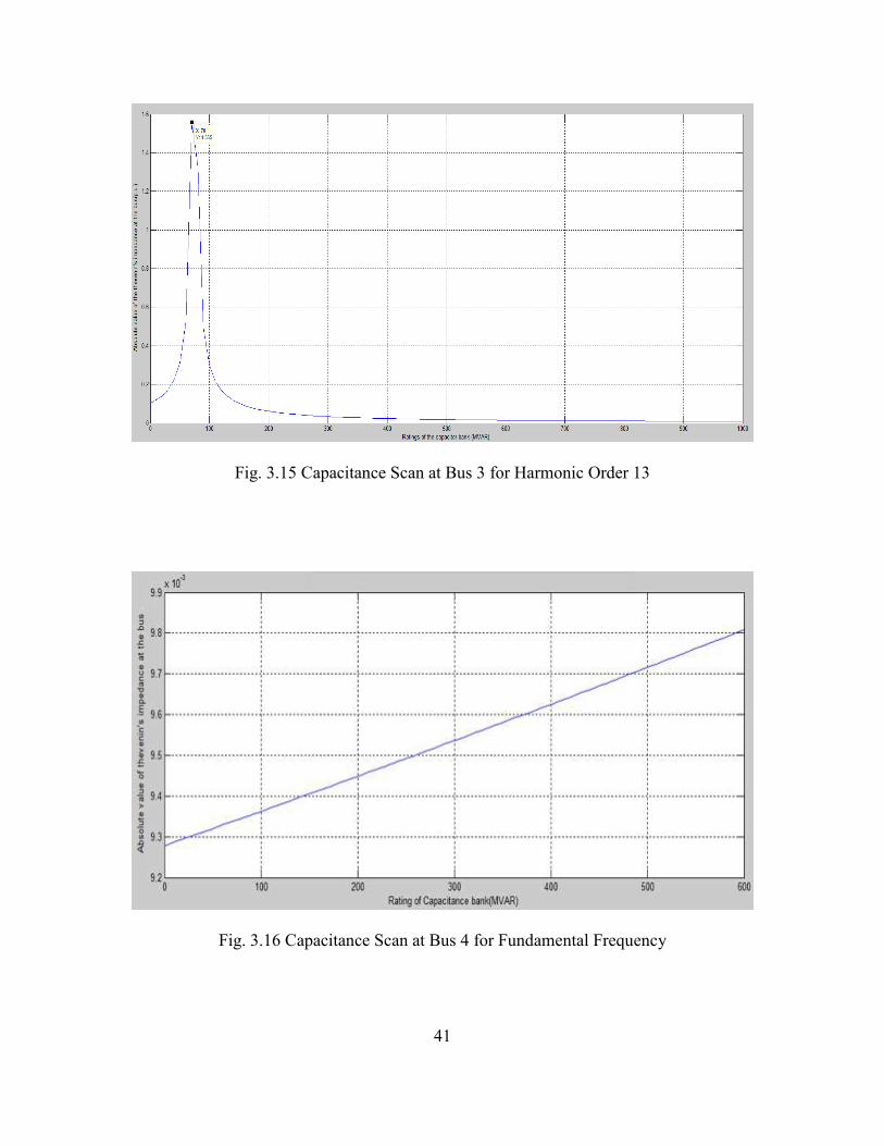
3.15 Capacitance Scan at Bus 3 for Harmonic Order 13 .................................................. 41
3.16 Capacitance Scan at Bus 4 for Fundamental Frequency ........................................... 41

ix
Figure Page
3.17 Capacitance Scan at Bus 4 for Harmonic Order 5 .................................................... 42
3.18 Capacitance Scan at Bus 4 for Harmonic Order 7 .................................................... 42
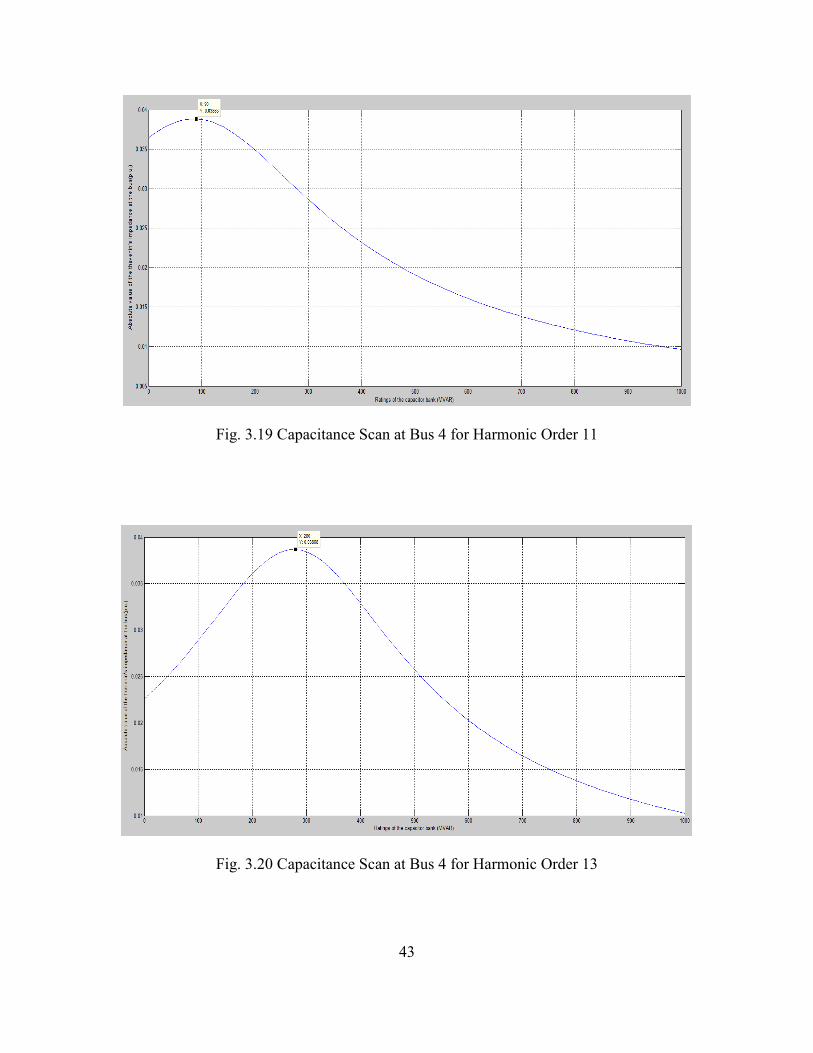
3.19 Capacitance Scan at Bus 4 for Harmonic Order 11 .................................................. 43
3.20 Capacitance Scan at Bus 4 for Harmonic Order 13 .................................................. 43
3.21 Capacitance Scan at Bus 5 for Fundamental Frequency ........................................... 44
3.22 Capacitance Scan at Bus 5 for Harmonic Order 5 .................................................... 44
3.23 Capacitance Scan at Bus 5 for Harmonic Order 7 .................................................... 45
3.24 Capacitance Scan at Bus 5 for Harmonic Order 11 .................................................. 45
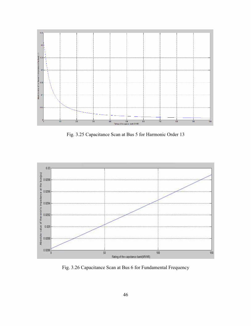
3.25 Capacitance Scan at Bus 5 for Harmonic Order 13 .................................................. 46
3.26 Capacitance Scan at Bus 6 for Fundamental Frequency ........................................... 46
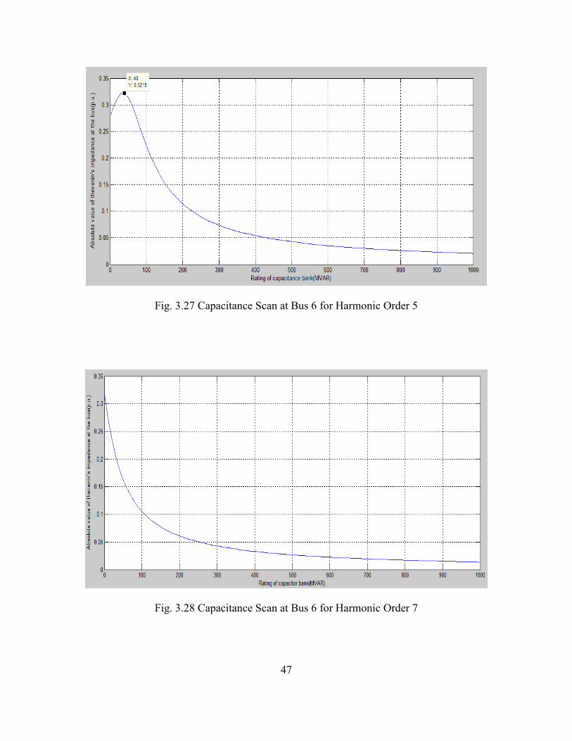
3.27 Capacitance Scan at Bus 6 for Harmonic Order 5 .................................................... 47
3.28 Capacitance Scan at Bus 6 for Harmonic Order 7 .................................................... 47
3.29 Capacitance Scan at Bus 6 for Harmonic Order 11 .................................................. 48
3.30 Capacitance Scan at Bus 6 for Harmonic Order 13 .................................................. 48
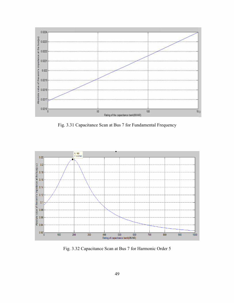
3.31 Capacitance Scan at Bus 7 for Fundamental Frequency ........................................... 49
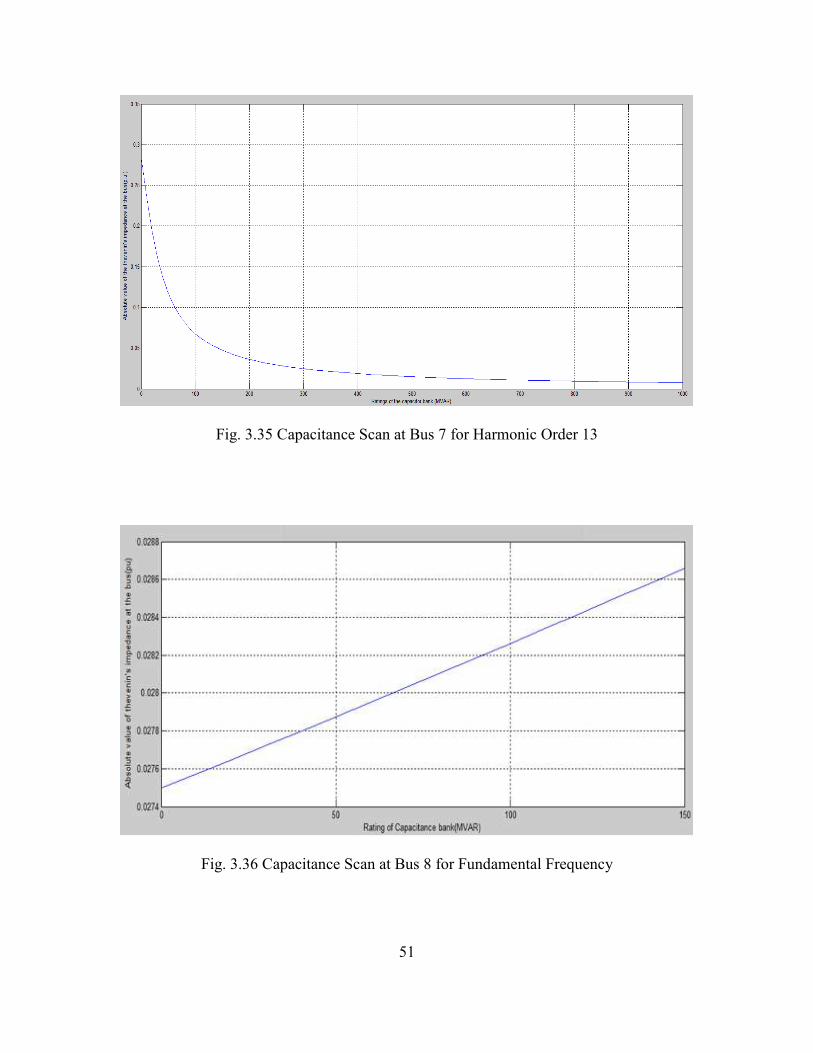
3.32 Capacitance Scan at Bus 7 for Harmonic Order 5 .................................................... 49
3.33 Capacitance Scan at Bus 7 for Harmonic Order 7 .................................................... 50
3.34 Capacitance Scan at Bus 7 for Harmonic Order 11 .................................................. 50
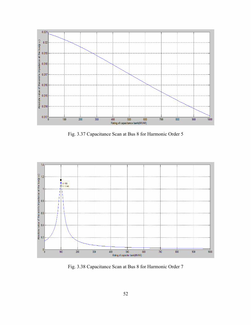
3.35 Capacitance Scan at Bus 7 for Harmonic Order 13 .................................................. 51
3.36 Capacitance Scan at Bus 8 for Fundamental Frequency ........................................... 51
3.37 Capacitance Scan at Bus 8 for Harmonic Order 5 .................................................... 52
3.38 Capacitance Scan at Bus 8 for Harmonic Order 7 .................................................... 52

x
Figure Page
3.39 Capacitance Scan at Bus 8 for Harmonic Order 11 .................................................. 53
3.40 Capacitance Scan at Bus 8 for Harmonic Order 13 .................................................. 53
3.41 Capacitance Scan at Bus 9 for Fundamental Frequency ........................................... 54
3.42 Capacitance Scan at Bus 9 for Harmonic Order 5 .................................................... 54
3.43 Capacitance Scan at Bus 9 for Harmonic Order 7 .................................................... 55
3.44 Capacitance Scan at Bus 9 for Harmonic Order 11 .................................................. 55
3.45 Capacitance Scan at Bus 9 for Harmonic Order 13 .................................................. 56
3.46 Capacitance Scan at Bus 10 for Fundamental Frequency ......................................... 56
3.47 Capacitance Scan at Bus 10 for Harmonic Order 5 .................................................. 57
3.48 Capacitance Scan at Bus 10 for Harmonic Order 7 .................................................. 57
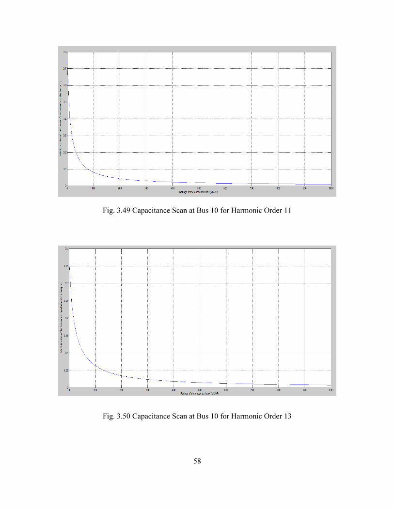
3.49 Capacitance Scan at Bus 10 for Harmonic Order 11 ................................................ 58
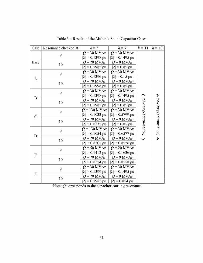
3.50 Capacitance Scan at Bus 10 for Harmonic Order 13 ................................................ 58
4.1 Forbidden Zones for the Test Bed System .................................................................. 66
5.1 The HVDC Sources in the WECC Transmission Network ........................................ 69
C.1 Phase Angle Plot of Capacitance Scan at Bus 1 for Harmonic Order 5..................... 92
C.2 Phase Angle Plot of Capacitance Scan at Bus 2 for Harmonic Order 5..................... 93
C.3 Phase Angle Plot of Capacitance Scan at Bus 3 for Harmonic Order 7..................... 93
C.4 Phase Angle Plot of Capacitance Scan at Bus 4 for Harmonic Order 7..................... 94
C.5 Phase Angle Plot of Capacitance Scan at Bus 5 for Fundamental Frequency ........... 94
C.6 Phase Angle Plot of Capacitance Scan at Bus 6 for Fundamental Frequency ........... 95
C.7 Phase Angle Plot of Capacitance Scan at Bus 7 for Harmonic Order 11................... 95
C.8 Phase Angle Plot of Capacitance Scan at Bus 8 for Harmonic Order 11................... 96

xi
Figure Page
C.9 Phase Angle Plot of Capacitance Scan at Bus 9 for Harmonic Order 13................... 96
C.10 Phase Angle Plot of Capacitance Scan at Bus 10 for Harmonic Order 13............... 97
xii
LIST OF TABLES
Table Page
2.1 Test Bed System Data Description ............................................................................. 22
3.1 Listing of the Results for Figures 3.1 to 3.25 ............................................................. 32
3.2 Listing of the Results for Figures 3.26 to 3.50 ........................................................... 33
3.3 List of the Various Cases Studied ............................................................................... 60
3.4 Results of the Multiple Shunt Capacitor Cases........................................................... 61
4.1 Forbidden Zones for the Test Bed System .................................................................. 66
5.1 Impact of HVDC Sources at Buses 1, 2 and 3 ............................................................ 70
5.2 Impact of HVDC Sources at Buses 4, 5 and 6 ............................................................ 71
5.3 Impact of HVDC Sources at Buses 7, 8, 9 and 10 ...................................................... 72

xiii
NOMENCLATURE
A Equation Formed of Process Matrix H
A Coefficient Matrix for Set of Equations
B Equation Formed of Process Matrix H
B Vector of Constants
b1 First Constant in the Vector of Constants
CIGRÉ International Council on Large Electric Systems
C Capacitance, F
EHV Extra High Voltage
F Frequency, Hz
F Fundamental Fequency, Hz
GE General Electric
HVDC High Voltage Direct Current
H Process Matrix
Hreal Real Component of Process Matrix
Himag Imaginary Component of Process Matrix
h Harmonic Order
h Vector Valued Function of Vector Valued Argument
h� Harmonic Frequency, Hz
IEEE Institute of Electrical and Electronics Engineer
Ibus Column Matrix Showing Current Injection at the Bus
Ikh Current Injection at Bus k for Harmonic Order h
Ih,519max Maximum Current Injection Limit Imposed by IEEE Standard 519 at
Harmonic Order h
∆I Change in Current Brought by Introduction of Shunt Capacitance at the Bus
∆I(f) Fast Fourier Transform of ∆I
xiv
i Bus Number
j √-1
k Bus Number
L Inductance, H
L Lower Left Triangular Matrix
L11 Element in the First Row and First Column of the Lower Left Trian-gular Matrix L
MSCDN Mechanically Switched Capacitor with Damping Network
N Number of Shunt Capacitors in the Network
n Number of Storage Elements
PCC Point of Common Coupling
PDCI Pacific DC Intertie
PSLF Positive Sequence Load Flow
PSS/E Power System Simulator for Engineering
P Active Power Consumption of Load
Q Reactive Power Consumption of Load
Q Size of Shunt Capacitor
Qcap
Size of Shunt Capacitor Bank
RC Resistor-Capacitor
RL Resistor-Inductor
RLC Resistor-Inductor-Capacitor
RMA Resonance Mode Analysis
RDC DC Resistance of Stator
R� Series Resistance in CIGRE Type C Load Model
Rh Generator Resistance at Harmonic Order h
SWIS South West Interconnected System
s Laplace Variable

xv
s Slip of an Induction Motor
U Upper Right Triangular Matrix
Unn Element in the nth Row and nth Column of the Upper Right Triangular Matrix U
V Fundamental Frequency Voltage
Vbus Column Matrix Showing Voltages at the Bus
Vk Voltage at Bus k
Vkh Voltage at Bus k for Harmonic Order h
Vh,519max Maximum Voltage Limit Imposed by IEEE Standard 519 at Harmonic
Order h
V11 11th Harmonic Voltage
V13 13th Harmonic Voltage
∆V Change in Voltage Brought by Introduction of Shunt Capacitance at the Bus
∆V(f) Fast Fourier Transform of ∆V
vreal,i Real Value of Voltage Measured at Bus i
vimag,i Imaginary Value of Voltage Measured at Bus i
WECC Western Electricity Coordinating Council
W Weighing Matrix
W Matrix Product of Upper Right Triangular Matrix U and the Vector of Unknown Elements x
W1 First Element of the Matrix W
W2 Second Element of the Matrix W
Wn nth Element of the Matrix W
X� Series Reactance in CIGRE Type C Load Model
�� Parallel Reactance in CIGRE Type C Load Model
X0 Generator Zero Sequence Reactance at 60 Hz
Xd" Generator Subtransient Reactance at 60 Hz

xvi
X2 Generator Negative Sequence Reactance at 60 Hz
x Vector of Harmonic State
x Vector of Unknown Elements
x1 First Unknown Element of the Vector x
xn nth Unknown Element of the Vector x
Ybus Bus Admittance Matrix
Ycap,k Admittance of Shunt Capacitor Bank at Bus k
Zbus Bus Impedance Matrix
|Zkk| or arg(Zkk)
Absolute Value of Thévenin’s Equivalent Impedance at Bus k
Z(f) Impedance in Fourier Domain
Z0(h) Generator Zero Sequence Impedance at Harmonic Order h
Z1(h) Generator Positive Sequence Impedance at Harmonic Order h
Z2(h) Generator Negative Sequence Impedance at Harmonic Order h
�kkh Thévenin Impedance at Bus K for Harmonic Order h
Zkk,hmax Maximum Value of Thévenin Impedance at Bus k for Harmonic Or-der h
Zkk,hlimit Limiting Value of Thévenin Impedance at Bus k for Harmonic Order
h
z Thévenin Impedance at a Bus
z Vector of Harmonic Measurements
zreal,i Real Value of Impedance Measured at Bus i
zimag,i Imaginary Value of Impedance Measured at Bus i
σ A Complex Root
ω Frequency, Radians
ωr Rotor Speed
ωs Synchronous Speed
η Measurement Error

xvii
Ω Harmonic Set Including Fundamental
(.)T Transpose of a Matrix

1
Chapter 1: Resonance in power transmission systems
1.1 Objectives and goals of this study
The main objectives of this study are the calculations of resonant frequencies in a
large electric power transmission system. The system used is an actual power system in
southwest United States. There are two subgoals of this work:
Study goal A: Evaluate the transmission system network impedance and
determine if there are any areas where resonance conditions could exist
today or where the addition of capacitor banks may create a resonance
condition. This should form the basis of a system wide plan for dealing
with the study of the harmonics when voltage support is added or system
topology changes by identifying possible problem areas.
Study goal B: Evaluate existing harmonic currents on the transmission
system and identify where those harmonic sources are located. Determine
if any identified sources may create problems in relation to Goal A, and if
there are any ways of mitigating those harmonic sources.
The test bed system described in this thesis is a large scale system in Arizona. A
large number of capacitors exist in the Arizona transmission system and more and being
added to improve the voltage profile of the system. The addition of these new capacitors
could create resonance conditions in the system. Also there exist few unidentified sources
of harmonics in the system. These sources could interact with these new capacitors and
cause severe disturbance in the system and may also lead to failure.
2
1.2 The phenomenon of resonance in electric power transmission systems
Resonance is a phenomenon that occurs in AC circuits where the magnitude of the
driving point impedance in the circuit passes through an extremum (i.e., maximum or min-
imum). At the same instant, the phase angle of the driving point impedance also passes
through zero indicating that the driving point impedance is totally resistive in nature. Res-
onance occurs in AC circuits due to the presence of energy storing components: inductors
and capacitors. The resonance in an AC circuit occurs at a certain frequency or at several
frequencies which are governed mainly by the amount of inductance and capacitance pre-
sent in the circuit. For an AC circuit that has n number of storage elements have n/2 reso-
nant frequencies where n is even or (n-1)/2 when n is odd. This observation is consequence
of the fact that an nth order linear ordinary differential equation has an nth order character-
istic equation, and when this characteristic equation has complex conjugate roots, those
roots correspond to resonances. There are two types of resonances commonly observed in
AC circuits the series resonance and parallel resonance. There exist simple methods to
calculate resonant frequency for these simple circuits but for large networked circuits more
complex calculations are needed. Transmission system components create an RLC circuit
which can result in resonance. Shunt capacitor banks are placed in the transmission net-
work to aid the voltage profile of the network. The addition of these capacitor banks affects
the entire network and changes its resonant frequencies.
Many devices in power systems use DC power for its operation such as computers,
communication equipment, some high efficiency lighting and DC motors that are used in
large industrial plants. Rectifiers supply this power requirement. These rectifiers are the

3
main source of harmonics in power systems. In recent times there has been an increasing
use of variable-speed drives which also contribute towards generation of harmonics. Also,
high voltage DC (HVDC) systems may be used in transmission network. These HVDC
converters are another source of harmonics in the system.
1.3 The literature of resonance in power systems
Any linear AC circuit can be represented by resistors, inductors and capacitors as
they are the fundamental passive elements of the power system. Out these three elements,
only an inductor and capacitor are called energy storage devices. An inductor stores its
energy in the magnetic field while the capacitor stores energy as electric field between its
two poles. Both circuit elements vary there impedance with the frequency of the system as
j2πfL and 1
j2πfC where f is the frequency, L is the inductance and C is the capacitance. When
a number of capacitors, inductors, and resistors are combined, the model which describes
this AC circuit is the sinusoidal steady state phasor model. This is equivalent to a high
order differential equation. If the number of energy storage elements is n, the characteristic
equation of that differential is an nth order polynomial in the Laplace variable s,
f�s) = 0. (1.1)
The roots of this characteristic equation are at complex conjugate poles, namely s = σ ± jω.
At these frequencies, the magnitude of the driving point impedance of a given bus in the
circuit passes through extreme values, i.e. either maximum or minimum values. This phe-
nomenon is called as resonance and the frequency at which this occurs is called the resonant

4
frequency of the system. Resonance analysis forms an important part of the process in-
volved in shunt capacitive compensation in power transmission systems as occurrence of
resonance in transmission systems can cause some problematic operating issues to occur.
Resonance can be a reason for malfunctions in the power system and can also lead
to damage / loss of property in some cases [1]. Also the system operation can be affected
by resonance. This makes it important to determine where resonance occurs in the system
with the aim of mitigating resonance while designing the system. Resonance studies are
carried out before making any changes to the system like adding new capacitor banks,
increasing existing capacitor bank sizes or changing overhead transmission to underground
transmission. A few of the methods used for estimation of harmonics and resonant frequen-
cies are described here.
A. Estimation of harmonic resonant frequencies at a bus by using the current source
method
The basic AC model [2] of a power system is
Ibus=YbusVbus (1.2)
Vbus=ZbusIbus. (1.3)
The Zbus and Ybus matrices are the bus impedance and admittance matrices. Normally these
matrices are evaluated at 60 Hz. For studies of resonance, these matrices are evaluated at
other frequencies. References [3, 4, 5, 6, 7] discuss the properties of the bus impedance
and admittance matrices.

5
It is possible to use Zbus and Ybus to evaluate the frequency response of a large scale
interconnected system. This method uses the idea that the diagonal elements of the Zbus are
the Thévenin equivalent impedance at the bus with respect to the ground. In power systems,
the capacitor banks are considered to be connected between the bus and the ground. No
series capacitors are considered at this point. This configuration creates a case of parallel
resonance. Examination of |Zkk| and / or arg�Zkk) gives information about resonance at bus
k. One approach is to allow frequency to 'scan' over a range of values at which the diagonal
entries of Zbus are evaluated. This type of analysis is performed for all the harmonics of
interest and a frequency versus amplitude plot is created. The points where the extreme
values are obtained are the point of resonance. If a maximum value is obtained then parallel
resonance occurs at that frequency. If a minimum value is obtained then series resonance
is observed at that frequency. In this method, the system bus impedance matrix is evaluated
at each frequency. This is done by obtaining the system bus admittance matrix and then
inverting the admittance matrix. The diagonal element that corresponds to the location of
the desired bus in the Zbus matrix is extracted at each frequency and it is stored. The results
at all the desired frequencies are collected for all the desired buses and a subsequent fre-
quency scan is plotted for each bus of interest.
B. Empirical estimation of system parallel resonant frequencies using capacitor switching
transient data
Resonant frequencies can be evaluated by using short circuit impedance of the sys-
tem at the bus where capacitor banks are added [8]. This is not possible for a practical
system which has a large number of capacitor banks. This method uses the capacitor
6
switching transient data which is recorded from various locations in the transmission sys-
tem as it provides accurate estimation of system parallel resonant conditions. The fast Fou-
rier transform is performed on these data to obtain the spectra for transient waveforms of
voltage and current for each phase. By observing the 'bumps' or lobes of same frequencies
in both the current and voltage spectra give us the frequencies at which the system is likely
to resonate.
An improvement over the method to that described above occurs in [9]. It also uses
the capacitor switching transient data in order to estimate the resonant frequencies. In order
to properly extract the transient data from the waveforms, the two sets of voltage and cur-
rent waveforms are taken one when the capacitor is brought into service and other when it
is kept offline. The effective transient data are then obtained by subtracting the offline data
from the online data. This has the benefit of removing any harmonic content that existed
in the waveforms. Fast Fourier transforms are performed on the effective transient data and
the impedance estimation is performed as,
Z�f)=
FFT of ∆V
FFT of ∆I=
∆V�f)∆I�f) .
�1.4)
The terms ∆V�f) and ∆I�f) may contain small values of non-resonant frequencies which
can give large and misleading impedance estimates [8]. This issue is surpassed by setting
such large impedance values to zero for the frequencies which satisfy the condition
∆I�f) < x∆I�60 Hz), where x ranges between 5% and 15%. Another heuristic which uses
voltage is

7
V�f) < xmax[∆V�60 Hz)],
where x ranges between 5% and 25% [9].
C. State estimation of power system harmonics by using synchronized measurements
The harmonic state estimation is formulated as [10],
z=h�x)+η (1.5)
where, z is the vector of harmonic measurements and x is the vector of harmonic state. In
(1.5), η denotes the measurement error and h is a vector valued function of vector valued
argument and h describes the process. The bus voltages are considered as system state. The
phase voltage is expressed as,
Re � ∑ ej�iωt) �vreal,i+jvimag,i
� ; Ω: harmonic set including fundamentaliϵΩ �. (1.6)
Here the terms vreal,i and vimag,i are considered as state variables and one of this set exists
for each harmonic. The measurements are obtained as zreal,i and zimag,i and are expressed in
the form,
Re �∑ ej�iωt) �zreal,i+jzimag,i� ; Ω:harmonic set including fundamentaliϵΩ �. (1.7)
From these measurements, the state variables can be obtained by using the relationship,
8
� A B
-B A� � xreal
ximag� = �Hreal
T Wzreal+HimagT Wzimag
HrealT Wzimag-Himag
T Wzreal
� (1.8)
where, H is the process matrix which models the asymmetric control variables in the trans-
mission system and W is the weight that is applied when the non-diagonal elements are
zero. The elements A and B are given as,
A=HrealT Hreal+Himag
T Himag (1.9)
B=HimagT Hreal-Hreal
T Himag. (1.10)
D. Harmonic current vector method
The harmonic current vector method [11] was devised so as to study the contribu-
tion of utility and the consumers to the harmonics in the system. In this method, the system
to be studied is simplified by creating a Norton equivalent circuit for both the utility side
and the customer side at the point of common coupling (PCC). Thus each side now has its
own equivalent harmonic current source and harmonic impedance for one specific fre-
quency. Thus, the Norton equivalent circuit needs to be recalculated for each and every
frequency of interest. This method can also be used when there are periodically varying
loads on the system and where switching capacitor banks are used. This is done by consid-
ering a constant impedance case and representing the customer side and utility side imped-
ances under this situation as the reference. The variation in the impedance values on any
side of the PCC is represented as change to the current source on that side. The harmonic
9
voltages and currents are measured only at the point of common coupling and the contri-
bution from each side is found out by using the principle of superposition. The contribu-
tions from each side are then projected onto the current flowing through the PCC to obtain
the contribution factors. Depending on the contribution factors, the rates to be imposed in
case of violation of the harmonic limits are decided.
The harmonic current vector method is a very simple method but has one problem
that is the customer and utility side impedances are required. It is easy to get these at power
frequencies but their frequency characteristics are unknown. This can be very easily ex-
plained by considering a case where the customer has an RLC load which is does not have
any harmonic source of its own. This load can simply cause high harmonic current ampli-
fication if supplied from the utility side with a harmonic current that has the same frequency
as its series resonant frequency. The basic harmonic current vector method described above
does not consider this case. This problem is overcome by making use of reference imped-
ances [11, 12]. This replaces the utility side impedance and customer side impedance in
the equivalent circuit with reference impedances on both sides. The difference between the
actual impedance and reference impedance is transferred to an additional harmonic current
source. The reference impedance is defined on the basis of measurements taken at the PCC.
This results in the customer load resistive component to be introduced as the reference
impedance. The customer load is represented as parallel connection of resistance and reac-
tance and only the current through the reactance is transferred to the additional current
source. If needed, the skin effect can also be considered. Thus the customer is treated as
resistive load and any deviation causing harmonic amplification is shown as additional
harmonic source. A similar approach is used when finding the reference impedance for the

10
utility side. The utility side impedance is generally considered as the impedance of the last
transformer before the PCC. Following the later procedures as mentioned in the basic har-
monic current vector method described above will give the rates to be imposed in case of
violation of the harmonic limits.
1.4 Power system models at frequencies greater than 60 Hz
A. Transformers
The transformer model that is used in power flow studies can be used to a certain
extent in harmonic analysis of the system. Though this model fails to consider some of the
effects that occur at higher frequencies, it is generally found to be accurate for analysis up
to 13th harmonic. For higher frequencies, generally more complex models are used. Though
it is not properly known which of the many models available serve the purpose the best,
each of them has its own advantages and drawbacks. The power system transformer model,
consist of both the winding series impedance and the shunt core impedance of the trans-
former coupled to an ideal transformer. The winding impedance on both the sides can be
transferred to either of the two sides and added to the winding impedance on that side to
create the effective series impedance of the transformer. The shunt core loss impedance
can be represented on either of the two sides.
B. Overhead transmission lines
The modeling of overhead transmission lines and transmission lines has been doc-
umented over a wide range of frequencies in the literature. Typically a transmission line is
modeled as a coupled equivalent-pi circuit [13]. But the series impedance per unit length
11
is frequency dependent due to the line inductance and the skin effect of the conductor. The
series impedance values per unit length are calculated by using the physical construction
of the line through established methods [14, 15]. In order to properly account for the fre-
quency dependent components, calculation should be made for each concerned frequency.
Long line effects are also needed to be considered if the line is very long or if the frequency
is very high. It is a general practice to employ long line models if the line length exceeds
150/h miles where h is the harmonic order. It is also observed that for line that have lengths
of 250 km for third harmonic and 150 km for fifth harmonic, transpositions are ineffective
and can cause increased unbalance in the system [16]. The underground cables are also
modeled very similar to an overhead transmission line. But in the case of underground
cables, long line models apply when the length exceeds 90/h miles.
C. Rotating machines
The synchronous and induction machines are the AC rotating machines that are
used in the power industry. The synchronous machines are generally used as generators
while the induction machines finds application as motor. The rotating magnetic field in
these machines has a speed that is significantly higher than rotor due to the stator harmonics
[13]. Thus the machine impedance approaches the negative sequence impedance. In both
these machines, we obtain the inductance in different ways but one fact that is the frequency
dependence of the resistance may be important due to skin effect and eddy current losses.
In cylindrical rotor synchronous machine, a negative current injection of order h in the
stator results in generation of rotor flux having an order of h+1 [17]. This causes an induc-

12
tion of negative sequence voltage of order h in the stator. A similar case results with the
injection of positive sequence current of harmonic order h, the only difference is that the
induced rotor flux has an order of h−1. In salient pole synchronous machines, it is a very
different case. A negative current injection of order h in the stator results in creation of two
counter-rotating rotor fluxes having order of h+1. This causes induction of negative se-
quence voltage of order h and positive sequence voltage of order h+2 in the stator. Similar
observations are made when positive sequence currents of harmonic order h are injected
creates two counter-rotating fluxes of order h−1. This results in generation of positive se-
quence voltage of order h and negative sequence voltage of order h−2 in the stator. This
then again goes on repeating for order of h−2 and higher in the stator. Thus the salient pole
synchronous machine acts as generator of harmonics contrary to popular belief [13]. There
is a very complex model given in reference [17] which describes the process that develops
the model which takes into account the above mentioned harmonic generation phenome-
non. A simple model which can used in harmonic analysis is as follows [18],
Z0�h)=Rh+jhX0 h=3,6, 9… (1.11)
Z1�h)=Rh+jhXd" h=1, 4, 7… (1.12)
Z2�h)=Rh+jhX2 h=2, 5, 8… (1.13)
where, X0, ��" and X2 are the generator zero sequence, subtransient and negative sequence
reactances at fundamental frequency and the resistance at harmonic frequencies is given
as,
13
Rh=RDC �1+0.1 �hf
f 1.5!
(1.14)
where, RDC is the DC resistance of the stator, hf is the harmonic frequency in Hz and f is
the fundamental frequency.
A similar phenomenon is also known to occur in induction machines [18]. But an
induction machine, the rotor speed has a slip s
s=ωs-ωr
ωs
(1.15)
where, ωr is the rotor speed and ωs is the synchronous speed. This slip affects the frequency
of the flux as the multiplier h−1+s times the baseband (60 Hz) frequency for positive se-
quence current injection of harmonic order h. The multiplier h+1−s is applied for negative
sequence current injection of harmonic order h. A simple model used in harmonic analysis
of induction machine is given in reference [18].
D. System loads
The selection of the model for the load that is connected to the transmission system
is very essential for the proper assessment of harmonic resonance magnitude of the system
[13]. But there exist no generally applicable model that can define each and every load.
So if detailed studies are supposed to be conducted then there is need to perform measure-
ments and evaluations for every case. But there are still few simple load models which can
be used for harmonic analysis. One of these simple models is the simple RL and RC circuits

14
as shown in Fig. 1.1 (a) and (b) [18]. The individual components in these two models can
be calculated from the voltage, apparent power and power factor. Another simple model is
the CIGRÉ type C load model as shown in Fig 1.1 (c). This model has been derived exper-
imentally. This model can be used for bulk power loads and is valid between 5th and 30th
harmonics. The parameters in this model can be obtained as,
Rs=
V2
P
(1.15)
Xs=0.073hRs (1.16)
Xp=
hRs
6.7QP
-0.74
(1.17)
where V is the fundamental frequency voltage, P is the real power, h is the harmonic order
and Q is the reactive power.
1.5 Case studies
For the purpose of discussing and illustrating the resonance phenomenon in power
systems, it is useful to examine case studies. References [20] – [23] are a few samples
(taken from the many examples) of case studies that have appeared in the literature. A few
interesting cases are produced here for discussion.
A. Resonance analysis in German transmission system
Resonance analysis for the transmission system in Germany has been carried out

15
Fig. 1.1 Three Simple Load Models used for Harmonic Analysis
(taken directly from [18])
and documented in [20] by the Resonance Mode Analysis (RMA) method at different op-
erating conditions. The extra high voltage (EHV) transmission network used for this anal-
ysis has 268 buses, 244 transmission lines, 8 two-winding and 17 three-winding transform-
ers, 57 linear loads, 35 generators, 9 bus-bar connectors, 9 reactors, and 1 C-type capacitor
bank with damping network (MSCDN). Two loading scenarios were considered. In the
first scenario, system is operated under low load conditions in which most of the loads
exhibit capacitive nature. All the reactors are connected in the network to balance the ca-
pacitive reactive power and the MSCDN is disconnected. In the second scenario, the sys-
tem is operated under high load condition and the behavior of the load is inductive in na-
ture. All the reactors are not needed and are thus turned off. But the MSCDN is turned on
to supply reactive power. Also the switching scenarios (tests) of are different. The fre-
quency scan modal impedance curves are plotted for both the cases for positive and zero
16
sequence components in [20]. The results of the simulations performed reflect that the sys-
tem resonant behavior changes as the load behavior and power system elements switching
conditions change.
B. Harmonic propagation in transmission system with multiple capacitor installations
As an example of published work on harmonics in a power transmission system,
consider a case history from Australia. There has been rapid development in the South
West Interconnected System (SWIS), the main transmission system in Western Australia
in recent years [21]. New capacitor banks were installed to improve voltage profile and
compensate for reactive power. These new capacitor banks created resonance conditions
which then later affected the utility and customer equipment. Harmonic voltage and current
measurements were taken at various buses in the transmission network. The fifth harmonic
voltage at 132 kV Cannington terminal was found to exceed the limit prescribed by the
Western Power technical requirements. Switching on the 132 kV capacitor bank connected
to this bus causes an increased fifth harmonic current to flow in the capacitor banks. At
certain times, it was observed that the capacitor bank was attracting an additional fifth
harmonic current from the low voltage circuit through the substation transformer. Another
bus Mason Road, was found to be the source of distortion caused at Cannington terminal.
The fifth harmonic voltage at 132 kV level and current in the transmission line were found
to exceed the limit specified by Western Power technical requirements.
C. Failure of 13.8 kV switchgear and loss of plant due to harmonic resonance
The Eurocan Pulp and Paper mill located at Kitimat, British Columbia, Canada is
feed by BC Hydro and Alcan by a single 287 kV feeder [22]. This power is then converted
17
to 13.8 kV by using two separate transformers each rated at 50 MVA. The switchgear of
this plant is arranged in such a way that power can be taken from either system inde-
pendently. In order to facilitate this, a 13.8 kV standby incoming tie circuit breaker which
is normally open is used after the transformer which connects BC Hydro system to the
plant. In order to adjust for the plants power factor, a large bank of capacitors is used on
the 13.8 kV bus. BC Hydro and Power Authority had noticed "occasional occurrences" of
fifth harmonic voltage waveforms. The mill itself had 8 MW of paper machine thyristor
DC drives. These drives are the main source of producing 5th, 7th, 11th, 13th, 17th, 19th and
such other harmonics in the system. On 24th June 1986, the standby incoming tie circuit
breaker faced a major failure which resulted in a catastrophic fire that completely destroyed
the mill. An investigation that followed found out that the system was resonating at 4.99
times 60 Hz for a total period of 4 minutes before the catastrophic failure.
D. Failure of 20 kV capacitor bank fuses
In the suburban regions of the city of Shiraz in Iran, exists a sub-transmission 63/20
kV substation [23]. The substation consists of two 40 MVA wye-grounded/delta transform-
ers which are equipped with two 1200 A grounding transformers. On the 20 kV bus of this
substation, four 2.4 MVAr capacitor banks are connected. This substation is feeding a steel
rolling factory. The power authority that is Fars power grid experienced an outage of ca-
pacitor bank in this substation. This outage had occurred due to blowing up of the capacitor
fuse. The investigation that followed into this revealed that the fuse link did not blow due
to a problem with the capacitor bank. It was also observed that a large fifth harmonic dis-
tortion was present on the feeder when the steel rolling mill was operating. Further inves-

18
tigations proved that this caused a very high distorted current of the order of 3.2 times the
fundamental current flowed through the fuse which caused it to melt in 15 seconds.
1.6 Sources of harmonics
Since the very beginning stages of the modern AC power systems, harmonic volt-
ages and currents have been present [24]. The main reason for this is the battle between
AC and DC systems. In the long term, AC systems have largely become standardized
worldwide. The main sources of harmonics are inverters and rectifiers.
One industrial application of rectifiers is for the energization of DC motors. The
main reason for survival of the DC machine is the controllability of the DC motor. Recti-
fiers are used to energize DC machine loads. These power converters use electronic
switches. All harmonics producing devices are found to have one common trait that is they
have a non-linear voltage-current operating relationship [25]. DC motors are mainly used
in paper mills and other special applications where speed control is needed. There are many
other applications which require DC. It is arguable that more than one-third of loads are
electronically controlled, and many of these loads require DC.
A discussion of rectifiers as harmonic sources appears in [17]. Other sources of
harmonics are documented in [27].
It is also found that the traditional electromagnetic devices also produce harmonics.
One such device is the salient pole synchronous machine which is described above as a
source of harmonic. Relating to transformers [25], inrush current that flows on energization
19
contains low order harmonics (e.g., 2nd, 3rd, 4th). Also overexcited transformers exhibit har-
monic voltages. Other industrial devices which result in harmonics are discussed in [28,
29].
1.7 Organization of the thesis
This thesis has been divided into six chapters. Chapter 1 gives a background on
resonance occurring in transmission system. It talks about the various methods used for
evaluating resonance, high frequency models of power system components, case studies
and sources of harmonics. Chapter 2 discusses about the various software tools used for
obtaining steady state AC response of the system. It also describes the test bed system used
for analysis, method used for obtaining system impedance and admittance matrix and the
calculation of driving point impedance at the bus. The discussion on frequency scan and
capacitance scan is also included in this chapter.
In Chapter 3, the results for single capacitor bank placement and multiple capacitor
bank placements cases are shown and discussed. In Chapter 4, the method for calculation
of forbidden zones is described and the forbidden zones thus obtained are discussed. In
Chapter 5, the impact that HVDC sources have on the system was evaluated. The conclu-
sions and recommendations are listed in Chapter 6.
Appendix A describes the forward and backward substitution method in calculation
of the value of x in Ax=b. Appendix B describes the Matlab code developed to perform
harmonic analysis for single capacitor placement and multiple capacitor placement cases.
Appendix C shows a few of the phase angle plots that were used to verify the resonance

20
point observed. Appendix D describes the code developed to evaluate the impact of HVDC
sources on these buses.

21
Chapter 2 The calculation and analysis of resonance using commercial software
tools
2.1 Pertinent commercial software tools
The electric power industry has produced a number of valuable software tools for
the analysis of large scale transmission systems. The effort that has gone into the develop-
ment of these tools is considerable. In these tools, components in the transmission system
are modeled in some detail including such complications as multi-winding transformers,
transmission line long line models, status of series and shunt capacitors, and generator
models and status. Since this research focuses on transmission systems, and on the steady
state AC response of these systems, the software tools that are appropriate include PSS/E
[32], PowerWorld Simulator [33], PSLF [34], and Matlab. Because actual data were used,
and those data were in PSLF format, this software tool was used. Also, the equivalencing
and input / output capabilities of PowerWorld Simulator were used. In this chapter, some
of the analysis details of these software tools are explained and applied to the harmonic
analysis problem. Matlab was used for post-processing of results.
2.2 System data used
The system used here is the complete WECC transmission system. The details of
this system are given in the Table 2.1. But for this thesis, only the transmission network in
Arizona is looked at. Thus the entire WECC transmission network is equivalenced to retain
only the Arizona transmission system. The details of the system after it is equivalenced is
also given in Table 2.1.

22
Table 2.1 Test Bed System Data Description
Bef
ore
eq
uiva
lenc
ing
(f
ull s
yste
m)
Number of buses 21442
Number of lines 17347
Number of generators 3891
Number of areas 21 A
fter
equ
ival
enci
ng Number of buses 2770
Number of lines 2035
Number of generators 272
Number of areas 1
2.3 The system impedance and admittance matrix from the system data
The system data exists in the GE Concorda PSLF software file format '.sav'. This
system data consists of the entire WECC system. This system data contains information
about the buses, generators, transformers, lines, loads, shunts, static var devices, taps,
Qtable, interface, DC bus, DC line, DC converter, branch interface, motors, areas, zones,
owners, interfaces, branch interfaces, transactions, Ztable and line conductors. This com-
plete system data is then converted to '.epc' format by using PSLF software so that Power-
World Simulator V17 can read this data. This system data is then equivalenced in order to
retain the system for Arizona. This is done by inputting the area number of Arizona in the
equivalencing interface of the PowerWorld Simulator V17. The result is that all of the
buses in the WECC system outside Arizona are removed and the equivalent circuit is re-
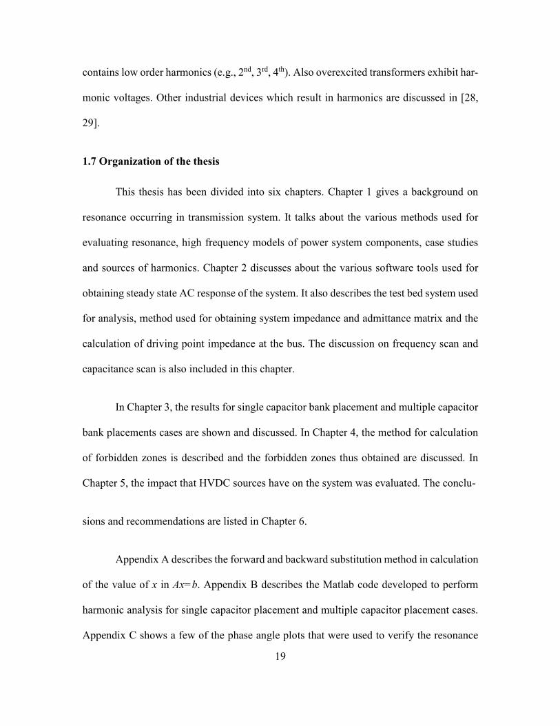
tained as shown in Figure 2.1 [30].
23
(a) Original system (number of buses shown)
(b) Equivalenced system (2770 buses retained)
Fig. 2.1 The Original Network and its Equivalenced Network
Equivalencing a circuit is a reduction of the network external to that under study.
This is not an approximation. Equivalencing is an exact representation of the external por-
tion of the network. However, the external buses are no longer represented in detail in the
model, namely the admittance matrix.
From the equivalenced circuit, the system bus admittance matrix is obtained. The

24
bus admittance matrix being modeled in PowerWorld Simulator V17 consists of only trans-
mission lines, transformers, line shunts, switched shunts and bus shunts [31]. The genera-
tors are modeled as open circuits while the loads are modeled as short circuits to the ground.
This YBUS that is obtained for the equivalent circuit is a sparse matrix and can be exported
to both Microsoft Office Excel and Matlab. Fig. 2.2 shows a pictorial of the approach used.
2.4 Calculation of driving point impedance
The YBUS that was obtained by the above method was exported in to both Microsoft
Office Excel and Matlab. The analysis was done using Matlab but the YBUS was exported
to excel so as to know the position of the required buses in the YBUS. In Matlab, the few
island buses in the system were removed and consequently the same was done in the Excel
copy of YBUS to keep consistency. Then the YBUS was used to find voltages V in Matlab by
forward/backward substitution,
V = Y \ I (2.1)
At bus k, if an injection of 1.0 p.u. current is considered, the corresponding value of Vk at
bus k will give the Zkk at the bus. The Zkk at bus k is the Thévenin equivalent impedance of
the network at bus k.
Shunt capacitor banks are added at certain buses. This modifies the system YBUS at
the diagonal elements that correspond to those buses. The location of these buses in theYBUS
is found from the modified Excel file. In Matlab, the modified YBUS after the removal of
the island buses, is modified at the diagonal elements. The modification of Ykk is accompli-

25
shed by adding the capacitive admittance Ycap,k. The capacitive admittance is,
Ycap,k=
jQcap|Vk|2
. (2.2)
The per unit value of the capcitive admittance is subtracted from the diagonal element of
YBUS to give the modified YBUS which includes the shunt capacitors.
The YBUS obtained is correct for 60 Hz, but analysis is also required to be done for
higher frequencies. This can be done by modifying the elements of the YBUS. Summing the
elements in a row of the YBUS, gives the net admittance tie to ground at the artifact bus; and
the negative of the off diagonal elements are the net admitance between the two buses.
From these YBUS matrix entries, the primitive circuit impedances are obtained and the signs
of their imaginary parts are examined. If the imaginary portion of the primitive circuit
component impedance is positive, that circuit impedance is assessed to be inductive and
therefore the corresponding reactance is the 60 Hz reactance multiplied by the harmonic
order h. If the primitive circuit component reactance is negative, that reactance is assessed
to be capacitive and the conversion to the higher frequency reactance is accomplished by
dividing the 60 Hz value by h. These new impedance values described above are then again
converted to admittance and replaced in the YBUS. While doing so, it is important to note
that off diagonal elements are the negative of admittance between two buses and diagonal
elements are the sum of the admittance between two buses and the net ground tie at that
bus. The YBUS is then inverted to obtain the ZBUS at the required frequency by the method
discussed above.
26
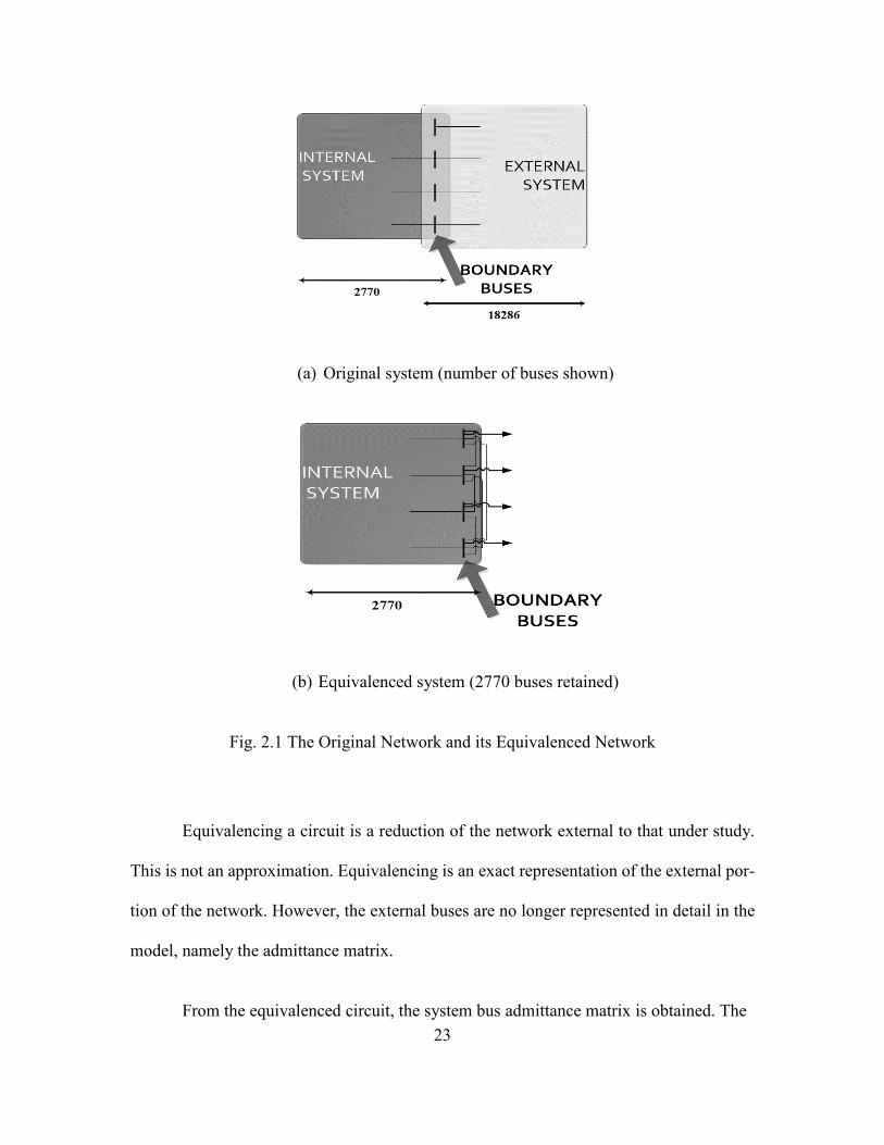
2.5 Frequency scan
Frequency scan is very popular method that is been used to find resonances that
occur in a circuit. A typical frequency scan for a parallel resonance condition is shown in
Figure 2.3. Parallel resonance occurs in the system when the inductors and capacitors are
connected parallel to each other. Under these circumstances, when resonance occurs, the
system impedance reaches a maximum value. If there are multiple such resonant frequen-
cies in the system, there will exist that many maxima each of which corresponds to one
resonant frequency. The frequencies between which half the absolute magnitude of the
Thévenin equivalent at the bus k, that is 1
2|Zkk|, defines the bandwidth as shown in Figure
2.3.
2.6 Capacitance scan
A frequency scan (i.e., a plot of driving point impedance magnitude versus fre-
quency) is a useful method but this tool does not illustrate the impact of variation of the
shunt capacitor value. This is not useful in studying the rating of capacitance bank and a
concomitant assessment of the value that causes resonance. Also frequency scans are done
for all frequencies, while in a power system, only integer multiples of baseband frequency
are injected. Also frequency scans are done for all frequencies, while in a power system,
only integer multiples of baseband frequency are injected. A capacitance scan has been
used here for the purpose of analysis. Instead of keeping the rating of capacitance bank
fixed as done in a frequency scan, frequency is kept fixed and the reactive power rating of
capacitance bank (i.e., Q) is varied from zero to a suitable value. The magnitude of driving
point Thévenin impedance |Zkk| is plotted versus frequency. The reactive power of the

27
F
ig. 2
.2 T
he F
low
for
Obt
aini
ng T
he S
yste
m B
us A
dmit
tanc
e M
atri
x

28
Frequency, f
Imp
ed
an
ce
, Z
Bandwidth
0
Fig. 2.3 A Typical Frequency Scan for Parallel Resonance
Capacitor bank rating,
Imp
ed
ance
, Z
Forbidden Zone
Obtained from IEEE
Standard 519
0
expressed as a positive number for a capacitor
No capacitor
cited at bus k
Fig. 2.4 A Typical Capacitance Scan

29
capacitor bank is expressed as a positive number for the sake of simplicity.
The driving point impedance at the capacitor siting bus is used to assess the result-
ing harmonic voltage magnitude at that bus. From the capacitance scan, the maximum
value of |Zkk| is then multiplied by the maximum per unit value of current permissible as
per the IEEE Standard 519. The resulting value of the ZkkIk is a voltage and this voltage
magnitude is the worst (maximum harmonic voltage) case scenario. This voltage is then
compared to the maximum as per the IEEE Standard 519. Corresponding to the scenarios
that exceed the IEEE 519 harmonic voltage limit, the value of |Zkk| are labeled in a band
of forbidden values on a pictorial range of Q. If more than one frequency is being consid-
ered, similar analysis is needed for those frequencies. It may also be a case that for different
frequencies, these forbidden zones may overlap. Fig. 2.4 shows this concept.
2.7 Summary
In this chapter, a software based method has been outlined for the analysis of a
transmission system for harmonic resonance. The method is suitable for a large scale trans-
mission system. Equivalencing is used to focus on a given area of a large interconnected
system. The software tools PSLF, PowerWorld Simulator and Matlab are used to system
planning data (in PSLF) which is subsequently equivalenced (by PowerWorld Simulator)
and exported to Matlab.
The harmonic resonance analysis is accomplished using a capacitance scan. The
basis of the analysis is the use of IEEE Standard 519 and its harmonic current and voltage

30
limits. Appendix B shows the Matlab code used to modify Ybus, and create the capacitance
scans.

31
Chapter 3 Analysis using planning case data
3.1 Explanation and presentation of results
In this chapter, the test bed described in Chapter 2 is used to assess the harmonic
resonance impact of shunt capacitor placement. The analytical methods described in Chap-
ter 2 are used for this assessment. The results are organized for two cases:
• Single shunt capacitor placement
• Multiple shunt capacitor placement.
3.2 Results for single capacitor placement
Analysis of the system was done by using the algorithm described in Chapter 2
coded in Matlab. The magnitude and phase angle plots were obtained for the driving point
impedance at the buses at which the shunt capacitors are placed. The magnitude plots are
shown here as arranged in Tables 3.1 and 3.2. A sampling of the phase angle plots are
shown in the Appendix C. The phase angle plots were mainly used to verify the location
of the resonance point. In this case, it was considered that the capacitor bank at the bus
under consideration was the only newly added capacitor in the system. Ten buses are con-
sidered. The shunt capacitors other than at the ten artifact buses were considered to be in
service in the base case.
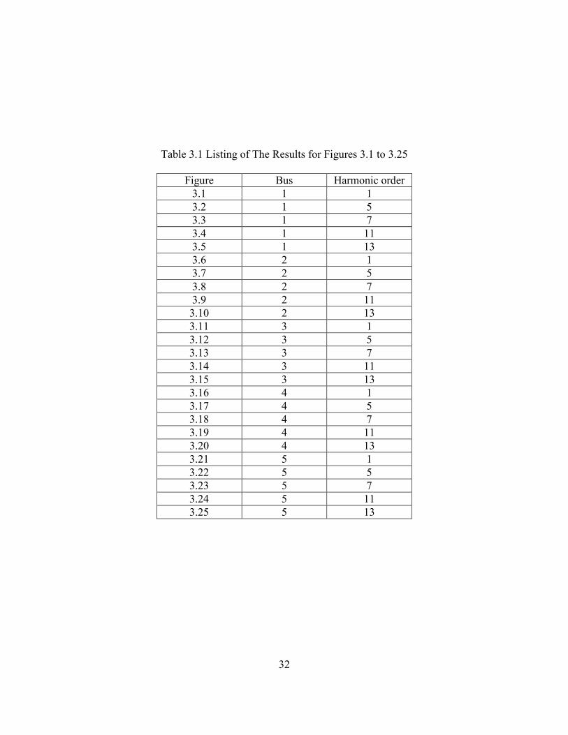
32
Table 3.1 Listing of The Results for Figures 3.1 to 3.25
Figure Bus Harmonic order 3.1 1 1 3.2 1 5 3.3 1 7 3.4 1 11 3.5 1 13 3.6 2 1 3.7 2 5 3.8 2 7 3.9 2 11
3.10 2 13 3.11 3 1 3.12 3 5 3.13 3 7 3.14 3 11 3.15 3 13 3.16 4 1 3.17 4 5 3.18 4 7 3.19 4 11 3.20 4 13 3.21 5 1 3.22 5 5 3.23 5 7 3.24 5 11 3.25 5 13

33
Table 3.2 Listing of The Results for Figures 3.26 to 3.50
Figure Bus Harmonic order 3.26 6 1 3.27 6 5 3.28 6 7 3.29 6 11 3.30 6 13 3.31 7 1 3.32 7 5 3.33 7 7 3.34 7 11 3.35 7 13 3.36 8 1 3.37 8 5 3.38 8 7 3.39 8 11 3.40 8 13 3.41 9 1 3.42 9 5 3.43 9 7 3.44 9 11 3.45 9 13 3.46 10 1 3.47 10 5 3.48 10 7 3.49 10 11 3.50 10 13

34
Fig. 3.1 Capacitance Scan at Bus 1 for Fundamental Frequency
Fig. 3.2 Capacitance Scan at Bus 1 for Harmonic Order 5

35
Fig. 3.3 Capacitance Scan at Bus 1 for Harmonic Order 7
Fig. 3.4 Capacitance Scan at Bus 1 for Harmonic Order 11

36
Fig. 3.5 Capacitance Scan at Bus 1 for Harmonic Order 13
Fig. 3.6 Capacitance Scan at Bus 2 for Fundamental Frequency

37
Fig. 3.7 Capacitance Scan at Bus 2 for Harmonic Order 5
Fig. 3.8 Capacitance Scan at Bus 2 for Harmonic Order 7

38
Fig. 3.9 Capacitance Scan at Bus 2 for Harmonic Order 11
Fig. 3.10 Capacitance Scan at Bus 2 for Harmonic Order 13

39
Fig. 3.11 Capacitance Scan at Bus 3 for Fundamental Frequency
Fig. 3.12 Capacitance Scan at Bus 3 for Harmonic Order 5

40
Fig. 3.13 Capacitance Scan at Bus 3 for Harmonic Order 7
Fig. 3.14 Capacitance Scan at Bus 3 for Harmonic Order 11
41
Fig. 3.15 Capacitance Scan at Bus 3 for Harmonic Order 13
Fig. 3.16 Capacitance Scan at Bus 4 for Fundamental Frequency

42
Fig. 3.17 Capacitance Scan at Bus 4 for Harmonic Order 5
Fig. 3.18 Capacitance Scan at Bus 4 for Harmonic Order 7
43
Fig. 3.19 Capacitance Scan at Bus 4 for Harmonic Order 11
Fig. 3.20 Capacitance Scan at Bus 4 for Harmonic Order 13

44
Fig. 3.21 Capacitance Scan at Bus 5 for Fundamental Frequency
Fig. 3.22 Capacitance Scan at Bus 5 for Harmonic Order 5

45
Fig. 3.23 Capacitance Scan at Bus 5 for Harmonic Order 7
Fig. 3.24 Capacitance Scan at Bus 5 for Harmonic Order 11
46
Fig. 3.25 Capacitance Scan at Bus 5 for Harmonic Order 13
Fig. 3.26 Capacitance Scan at Bus 6 for Fundamental Frequency
47
Fig. 3.27 Capacitance Scan at Bus 6 for Harmonic Order 5
Fig. 3.28 Capacitance Scan at Bus 6 for Harmonic Order 7

48
Fig. 3.29 Capacitance Scan at Bus 6 for Harmonic Order 11
Fig. 3.30 Capacitance Scan at Bus 6 for Harmonic Order 13
49
Fig. 3.31 Capacitance Scan at Bus 7 for Fundamental Frequency
Fig. 3.32 Capacitance Scan at Bus 7 for Harmonic Order 5
0

50
Fig. 3.33 Capacitance Scan at Bus 7 for Harmonic Order 7
Fig. 3.34 Capacitance Scan at Bus 7 for Harmonic Order 11
51
Fig. 3.35 Capacitance Scan at Bus 7 for Harmonic Order 13
Fig. 3.36 Capacitance Scan at Bus 8 for Fundamental Frequency
52
Fig. 3.37 Capacitance Scan at Bus 8 for Harmonic Order 5
Fig. 3.38 Capacitance Scan at Bus 8 for Harmonic Order 7

53
Fig. 3.39 Capacitance Scan at Bus 8 for Harmonic Order 11
Fig. 3.40 Capacitance Scan at Bus 8 for Harmonic Order 13

54
Fig. 3.41 Capacitance Scan at Bus 9 for Fundamental Frequency
Fig. 3.42 Capacitance Scan at Bus 9 for Harmonic Order 5

55
Fig. 3.43 Capacitance Scan at Bus 9 for Harmonic Order 7
Fig. 3.44 Capacitance Scan at Bus 9 for Harmonic Order 11

56
Fig. 3.45 Capacitance Scan at Bus 9 for Harmonic Order 13
Fig. 3.46 Capacitance Scan at Bus 10 for Fundamental Frequency
57
Fig. 3.47 Capacitance Scan at Bus 10 for Harmonic Order 5
Fig. 3.48 Capacitance Scan at Bus 10 for Harmonic Order 7
58
Fig. 3.49 Capacitance Scan at Bus 10 for Harmonic Order 11
Fig. 3.50 Capacitance Scan at Bus 10 for Harmonic Order 13

59
3.3 Capacitance scans for the case of multiple shunt capacitor placement
The system under test has a large number of shunt capacitors. Depending on the
number of shunt capacitor connected in the transmission network, the number of combina-
tions of which capacitors are in service, and which are out of service is of the form 2N. A
few of these cases are considered as shown in the Table 3.3. In Table 3.3, the proposed
shunt capacitor size is given as a single number, a maximum value. In fact, the capacitors
are switched and the shunt capacitor may be smaller than the values shown in Table 3.3.
The capacitor values are shown, as is the usual case in transmission engineering, in mega-
vars (capacitive). In Table 3.3, the notation ‘X’ is used to denote which capacitors are ON.
If the columns at the right contain a blank, then the corresponding capacitor is OFF. Since
the buses 9 and 10 are being studied, in cases C, E and F, they are considered as fixed value
capacitor bank only for case when they are not being studied. It means that for case C when
bus 10 is being studied, bus 9 has a fixed value that is written in the column labeled pro-
posed shunt capacitor. The Q values at bus 10 in this case will vary from 0 to 1000 MVAr.
The notation ‘X1’ is used to denote such cases.
The six cases shown in Table 3.3 are labeled Case A through Case F. The results
of resonances found for these cases are shown in Tables 3.4 and 3.5.
3.4 Discussion of results
By looking at the results of single capacitor placement, it is evident that at the first
four buses that resonance occurs only after addition of the shunt. These four buses have a
rated voltage of 230 kV.

60
Table 3.3 List of the Various Cases Studied
Bus
Bus voltage
Proposed ca-pacitor bank
size
Original case
Case
A
Case
B
Case
C
Case
D
Case
E
Case
F
1 230 kV
150 MVAr
� N
o ot
her
capa
cito
rs s
ited�
X X
2 230 kV
300 MVAr X X X X
3 230 kV
300 MVAr X X X
4 230 kV
300 MVAr X X
5 69 kV 48 MVAr X X X
6 69 kV 48 MVAr X X
7 69 kV 48 MVAr X
8 69 kV 48 MVAr X X
9 69 kV 48 MVAr X1 X1
10 69 kV 24 MVAr X1 X1
X=Shunt capacitor at this bus is ON
X1= Shunt capacitor has values 0 to 1000 MVAr when it is being studied
61
Table 3.4 Results of the Multiple Shunt Capacitor Cases
Case Resonance checked at h = 5 h = 7 h = 11 h = 13
Base
9 Q = 30 MVAr Q = 30 MVAr
� N
o re
sona
nce
obse
rved
�
� N
o re
sona
nce
obse
rved
�
|Z| = 0.1398 pu |Z| = 0.1495 pu
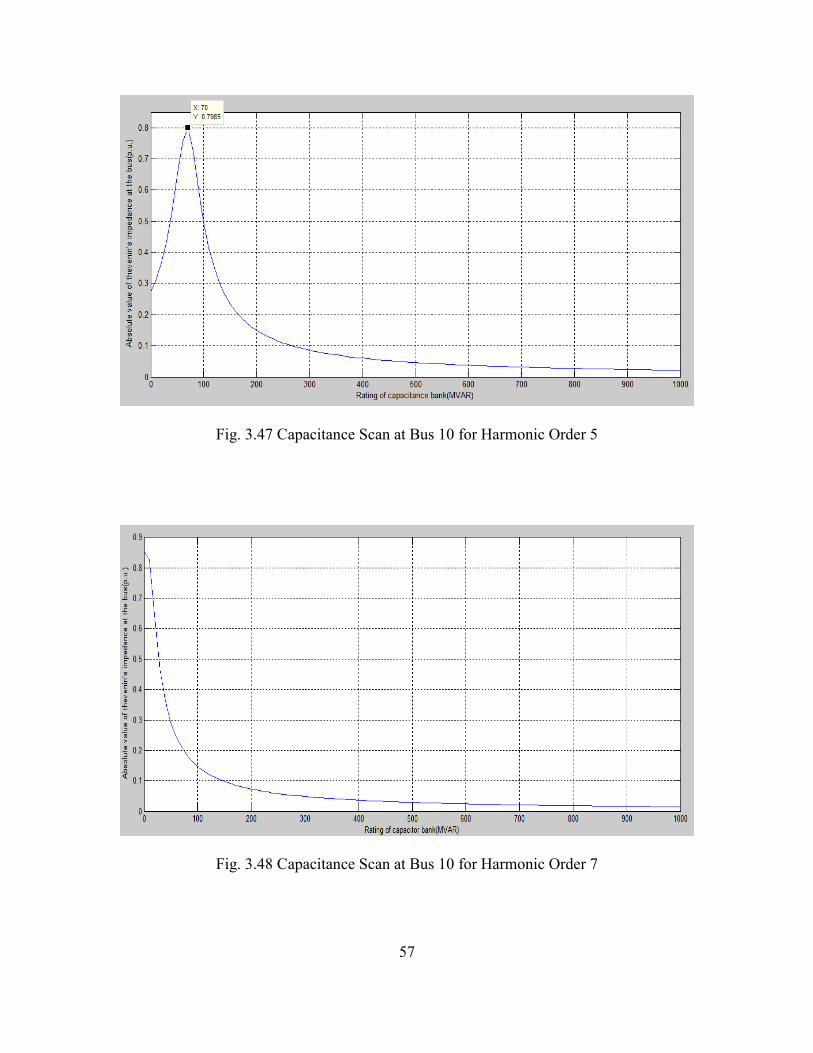
10 Q = 70 MVAr Q = 0 MVAr |Z| = 0.7985 pu |Z| = 0.85 pu
A 9
Q = 30 MVAr Q = 30 MVAr |Z| = 0.1396 pu |Z| = 0.15 pu
10 Q = 70 MVAr Q = 0 MVAr |Z| = 0.7998 pu |Z| = 0.85 pu
B 9
Q = 30 MVAr Q = 30 MVAr |Z| = 0.1398 pu |Z| = 0.1495 pu
10 Q = 70 MVAr Q = 0 MVAr |Z| = 0.7985 pu |Z| = 0.85 pu
C 9
Q = 130 MVAr Q = 30 MVAr |Z| = 0.1032 pu |Z| = 0.5799 pu
10 Q = 70 MVAr Q = 0 MVAr |Z| = 0.8235 pu |Z| = 0.85 pu
D 9
Q = 130 MVAr Q = 30 MVAr |Z| = 0.1054 pu |Z| = 0.6577 pu
10 Q = 70 MVAr Q = 0 MVAr |Z| = 0.8201 pu |Z| = 0.8526 pu
E 9
Q = 50 MVAr Q = 20 MVAr |Z| = 0.1412 pu |Z| = 0.1636 pu
10 Q = 70 MVAr Q = 0 MVAr |Z| = 0.8214 pu |Z| = 0.8558 pu
F 9
Q = 30 MVAr Q = 30 MVAr |Z| = 0.1399 pu |Z| = 0.1495 pu
10 Q = 70 MVAr Q = 0 MVAr |Z| = 0.7985 pu |Z| = 0.854 pu
Note: Q corresponds to the capacitor causing resonance
62
At bus 2, the seventh order resonance occurs off the considered range of Q. The
other buses are all rated 69 kV. At these buses, for harmonic orders 11 and 13, the driving
point impedance has already become capacitive.
Inspection of Figures 3.21-3.50 (for the 69 kV buses studied) indicated the follow-
ing:
• At bus 8, the resonance at seventh harmonic is particularly sharp (low damping)
and the "Zkk7 " is high, thus indicating the potential for high seventh harmonic volt-
ages.
• At bus 10, resonance appears to occur at h=5 and 7, and potentially at h=11.
Inspection of the 69 kV buses in Table 3.4 indicates:
• In cases C, D, and E high values of "Zkk5 " and "Zkk
7 " occur at bus 10. These indicate
the potential for high fifth and seventh harmonic voltages at bus 10. Also in these
cases, the Q value at resonance is significantly different than the base case results.
The common additional capacitors in these cases which are at bus 2 and bus 3 have
very severe effect on the resonance in the system.
In summary, the results in Table 3.4 in combination with the IEEE Standard 519
can be used to identify problematic cases. For both buses 9 and 10, the harmonic current
injection limit is 0.07 per unit at h = 5, 7; and the harmonics voltage limit in 0.03 per unit.
63
Using
"Vkh"="Zkk
h ""Ikh", (3.1)
and
"Vkh"≤0.03 per unit (3.2)
"Ikh"≤0.07 per unit (3.3)
Therefore "Zkkh "≤0.429 per unit. This means that for cases A – F, all cases may result in
high fifth and/or seventh harmonic voltage at bus 10. The identified problematic fifth and
seventh harmonic voltages at bus 10 are consistent with the analysis shown in Chapter 4.

64
Chapter 4 Forbidden zones
4.1 Definition of the term ‘forbidden zone’ as applied to the placement of shunt ca-
pacitors
In Chapter 2, the capacitance scan of a transmission system was described. For such
a capacitance scan, a ‘forbidden zone’ may exist. A forbidden zone is that range of capac-
itor values which causes the harmonic voltage magnitude to equal or exceed the permissi-
ble limits as per the IEEE Standard 519 [35] for an injection of the permissible maximum
harmonic current as per the IEEE Standard 519 at the bus in consideration. The mathemat-
ical approach for finding the forbidden zones proceeds as follows.
Step 1: Determine if the injection of maximum permissible harmonic current as prescribed
in Table 2 of [35] times the maximum value of driving point impedance exceeds or equals
the maximum allowed limit as per Table 1 of [35],
Ih,519max Zkk,hmax≥Vh,519
max . (4.1)
Step 2: If the product obtained in (4.1) equals the maximum permissible value of harmonic
voltage, then the value of shunt capacitor at that point is at the boundary of the forbidden
zone. At the cited boundary,
"Zkk,hlimit"= Vh,519
max
Ih,519max .
(4.2)
Step 3: Find the values of shunt capacitor that corresponds to the limiting value of imped-
65
ance (4.2). The range of values that lies within these two values is the forbidden zone.
Step 4: Forbidden zones should also be calculated by using steps 1 to 3 for other harmonic
orders that are of the interest at the bus. Combining all of these individual forbidden zones
together gives the forbidden zone for the bus.
Since the forbidden zones that are obtained for the individual harmonics are com-
bined together, there may be cases where two such forbidden zones overlap each other.
There can also be cases where there exists a gap between two forbidden zones. The cited
“forbidden zones” are actually ranges of shunt capacitance that are suspect of causing har-
monic resonance. It is quite possible that a shunt capacitor sized in the “forbidden zone”
will not cause difficulty because the specific harmonic in unexcited. Therefore the inter-
pretation of a “forbidden zone” is that this is a range of Q that warrants some scrutiny.
4.2 Results for the test bed system
The forbidden zones for the test bed system described in Chapter 2 were calculated
from the capacitance scans in Chapter 3 by using the above approach. The forbidden zones
thus obtained are shown in Figure 4.1 and in Table 4.1. The forbidden zones only exist for
four out of the ten artifact buses. This is the reason that only four buses are depicted in
Figure 4.1.
4.3 Principal observations on the forbidden zones
The forbidden zones only exist for four buses namely bus 2, bus 3, bus 8 and bus
10 out of the ten artifact buses. For buses 2 and 8, the forbidden zone exists after the pro-

66
Fig. 4.1 Forbidden Zones for the Test Bed System
Table 4.1 Forbidden Zones for the Test Bed System
Bus 5th harmonic 7th harmonic 11th harmonic 13th harmonic
2 No No No 361-391 MVAr
3 No 13-90 MVAr 95-138 MVAr 33-86 MVAr
8 No 66-134 MVAr No No
10 30-110 MVAr 0-31 MVAr 0-9.5 MVAr No
“No” indicates that no forbidden zone was identified

67
posed maximum size of the shunt capacitor. No special attention is needed for these buses.
But care must be taken while considering for future change in sizing as it may causes the
shunt capacitor to be in the forbidden zone.
On bus 3 the forbidden zone lies below the maximum proposed shunt capacitor
size. In this case, care should be taken that no capacitor step lies within the forbidden zone
as it may cause severe resonance issues. Also in bus 3, the forbidden zone overlaps other
forbidden zones and there also exists gaps between two forbidden zones. In bus 10, the
forbidden zone starts right from the zero shunt capacitor added to a value of about 110
MVAr whereas the proposed capacitor bank size is 24 MVAr. On this bus also multiple
forbidden zones overlap.

68
Chapter 5 Impact of HVDC sources on the test bed system
5.1 HVDC sources in transmission systems
Large HVDC installations act as sources of harmonics. These sources consist of
twelve pulse three-phase rectifiers and are thus sources of 11th and 13th harmonics. The
IEEE Standard 519 [35] restricts the harmonic current HVDC installations. Harmonic fil-
ters are used to limit the harmonic current.
In the WECC transmission system there exist six major HVDC installations. They
are as shown in the Figure 5.1. The Pacific DC Intertie which has a line capacity of 3,100
MW [36] and the Intermountain DC Intertie which has capacity of 2400 MW [37] have
comparatively high power ratings as compared to the other four. To assess the impact of
the HVDC facilities, a harmonic current Ih of 1.0 per unit is injected at the appropriate bus.
It must be realized that this is a gross overestimate of impact because Ih will be near zero
at h=5, 7, and also greatly attenuated at h=11, 13 due to the shunt filters at the AC terminals
of the HVDC facility. Here the complete WECC system is considered and is thus not equiv-
alenced so as to consider the effects of HVDC sources which are all outside Arizona.
5.2 Results of HVDC source impacts for the test bed system
For the study purposes, seven cases are considered. The first six cases consider the
effects of these six harmonic sources individually (i.e. only one HVDC source exists) and
in the last case, all the six HVDC sources inject harmonics in the network simultaneously.
The results are shown in the Tables 5.1, 5.2, and 5.3.
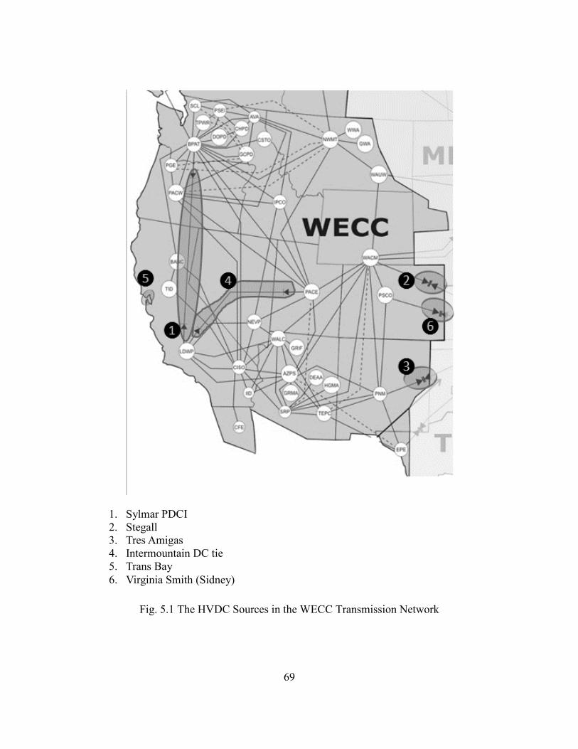
69
Fig. 5.1 The HVDC Sources in the WECC Transmission Network
1. Sylmar PDCI 2. Stegall 3. Tres Amigas 4. Intermountain DC tie 5. Trans Bay 6. Virginia Smith (Sidney)
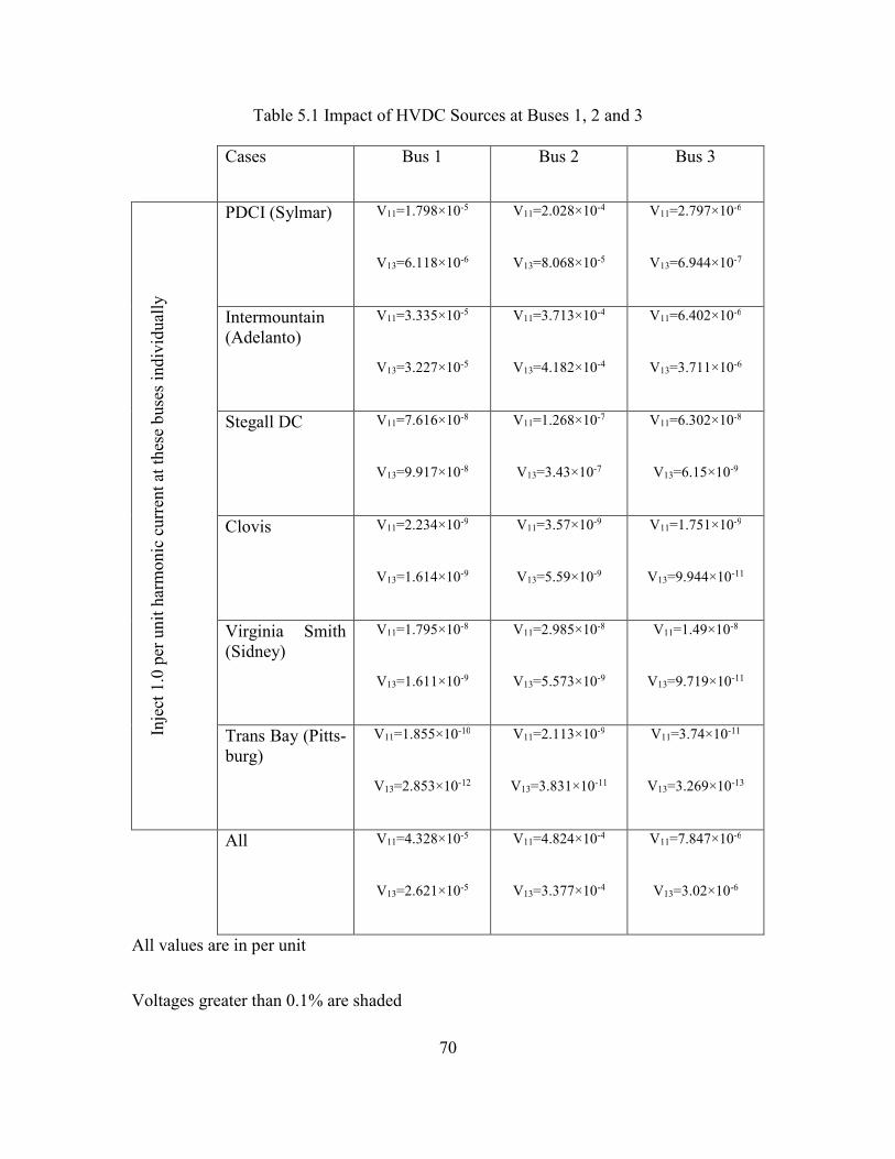
70
Table 5.1 Impact of HVDC Sources at Buses 1, 2 and 3
Cases Bus 1 Bus 2 Bus 3 In
ject
1.0
per
uni
t har
mon
ic c
urre
nt a
t the
se b
uses
indi
vidu
ally
PDCI (Sylmar) V11=1.798×10⁻⁵
V13=6.118×10⁻⁶
V11=2.028×10⁻⁴
V13=8.068×10⁻⁵
V11=2.797×10⁻⁶
V13=6.944×10⁻⁷
Intermountain (Adelanto)
V11=3.335×10⁻⁵
V13=3.227×10⁻⁵
V11=3.713×10⁻⁴
V13=4.182×10⁻⁴
V11=6.402×10⁻⁶
V13=3.711×10⁻⁶
Stegall DC V11=7.616×10⁻⁸
V13=9.917×10⁻⁸
V11=1.268×10⁻⁷
V13=3.43×10⁻⁷
V11=6.302×10⁻⁸
V13=6.15×10⁻⁹
Clovis V11=2.234×10⁻⁹
V13=1.614×10⁻⁹
V11=3.57×10⁻⁹
V13=5.59×10⁻⁹
V11=1.751×10⁻⁹
V13=9.944×10⁻¹¹
Virginia Smith (Sidney)
V11=1.795×10⁻⁸
V13=1.611×10⁻⁹
V11=2.985×10⁻⁸
V13=5.573×10⁻⁹
V11=1.49×10⁻⁸
V13=9.719×10⁻¹¹
Trans Bay (Pitts-burg)
V11=1.855×10⁻¹⁰
V13=2.853×10⁻¹²
V11=2.113×10⁻⁹
V13=3.831×10⁻¹¹
V11=3.74×10⁻¹¹
V13=3.269×10⁻¹³
All V11=4.328×10⁻⁵
V13=2.621×10⁻⁵
V11=4.824×10⁻⁴
V13=3.377×10⁻⁴
V11=7.847×10⁻⁶
V13=3.02×10⁻⁶
All values are in per unit
Voltages greater than 0.1% are shaded

71
Table 5.2 Impact of HVDC Sources at Buses 4, 5 and 6
Cases Bus 4 Bus 5 Bus 6 In
ject
1.0
per
uni
t har
mon
ic c
urre
nt a
t the
se b
uses
indi
vidu
ally
PDCI (Sylmar)
V11=9.719×10⁻⁶
V13=3.387×10⁻⁶
V11=9.337×10⁻⁴
V13=6.732×10⁻⁵
V11=1.875×10⁻⁴
V13=1.885×10⁻⁵
Intermoun-tain (Ade-lanto)
V11=1.836×10⁻⁵
V13=1.781×10⁻⁵
V11=0.0017
V13=3.477×10⁻⁴
V11=3.433×10⁻⁴
V13=9.959×10⁻⁵
Stegall DC V11=1.104×10⁻⁷
V13=6.591×10⁻⁸
V11=5.631×10⁻⁷
V13=3.204×10⁻⁷
V11=1.783×10⁻⁷
V13=1.288×10⁻⁷
Clovis V11=3.262×10⁻⁹
V13=1.072×10⁻⁹
V11=1.555×10⁻⁸
V13=5.213×10⁻⁹
V11=5.066×10⁻⁹
V13=2.094×10⁻⁹
Virginia Smith (Sid-ney)
V11=2.599×10⁻⁸
V13=1.071×10⁻⁹
V11=1.325×10⁻⁷
V13=5.202×10⁻⁹
V11=4.2×10⁻⁸
V13=2.084×10⁻⁹
Trans Bay (Pittsburg)
V11=9.747×10⁻¹¹
V13=1.583×10⁻¹²
V11=9.725×10⁻⁹
V13=3.212×10⁻¹¹
V11=1.952×10⁻⁹
V13=8.873×10⁻¹²
All V11=2.393×10⁻⁵
V13=1.447×10⁻⁵
V11=0.0022
V13=2.807×10⁻⁴
V11=4.473×10⁻⁴
V13=8.065×10⁻⁵
All values are in per unit
Voltages greater than 0.1% are shaded
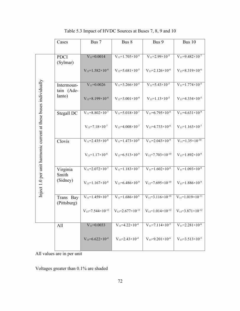
72
Table 5.3 Impact of HVDC Sources at Buses 7, 8, 9 and 10
Cases Bus 7 Bus 8 Bus 9 Bus 10 In
ject
1.0
per
uni
t har
mon
ic c
urre
nt a
t the
se b
uses
indi
vidu
ally
PDCI (Sylmar)
V11=0.0014
V13=1.582×10⁻⁴
V11=1.705×10⁻⁴
V13=5.681×10⁻⁵
V11=2.99×10⁻⁵
V13=2.126×10⁻⁶
V11=9.482×10⁻⁷
V13=8.319×10⁻⁶
Intermoun-tain (Ade-lanto)
V11=0.0026
V13=8.199×10⁻⁴
V11=3.266×10⁻⁴
V13=3.001×10⁻⁴
V11=5.43×10⁻⁵
V13=1.13×10⁻⁵
V11=1.774×10⁻⁵
V13=4.334×10⁻⁵
Stegall DC V11=8.802×10⁻⁷
V13=7.18×10⁻⁷
V11=5.018×10⁻⁷
V13=4.008×10⁻⁷
V11=6.795×10⁻⁸
V13=4.733×10⁻⁸
V11=4.631×10⁻⁹
V13=1.163×10⁻⁷
Clovis V11=2.435×10⁻⁸
V13=1.17×10⁻⁸
V11=1.473×10⁻⁸
V13=6.513×10⁻⁹
V11=2.043×10⁻⁹
V13=7.703×10⁻¹⁰
V11=1.35×10⁻¹⁰
V13=1.892×10⁻⁹
Virginia Smith (Sidney)
V11=2.072×10⁻⁷
V13=1.167×10⁻⁸
V11=1.183×10⁻⁷
V13=6.486×10⁻⁹
V11=1.602×10⁻⁸
V13=7.695×10⁻¹⁰
V11=1.093×10⁻⁹
V13=1.886×10⁻⁹
Trans Bay (Pittsburg)
V11=1.459×10⁻⁹
V13=7.544×10⁻¹²
V11=1.686×10⁻⁹
V13=2.677×10⁻¹¹
V11=3.116×10⁻¹⁰
V13=1.014×10⁻¹²
V11=1.019×10⁻¹¹
V13=3.871×10⁻¹²
All V11=0.0033
V13=6.622×10⁻⁴
V11=4.22×10⁻⁴
V13=2.43×10⁻⁴
V11=7.114×10⁻⁵
V13=9.201×10⁻⁶
V11=2.281×10⁻⁶
V13=3.513×10⁻⁵
All values are in per unit
Voltages greater than 0.1% are shaded

73
5.3 Observations
Tables 5.1, 5.2, and 5.3 are actually a measure of sensitivity of harmonic injection
from the HVDC facility to the ten study buses. At all these buses, sensitivities are very low.
The highest sensitivity of 0.0033 per unit occurs at bus 7 for a 1.0 per unit injection of
harmonic current at all the HVDC sources. This is deemed to be low enough to conclude
that the HVDC impact on harmonics in the Arizona transmission system are negligible.
This conclusion is further supported by noting that Tables 5.1-5.3 are volts for 1.0 per unit
current injection at the HVDC terminals. The actual harmonic current injection at the
HVDC terminals is very small because these are twelve pulse converters, and 11th and 13th
harmonic filters are installed.
74
Chapter 6 Conclusions and recommendations
6.1 Conclusions
Resonance can cause problematic issues with the normal operation of a transmis-
sion network. Addition of capacitors at a bus could create resonance at that bus. The net-
work needs to be examined for resonance conditions that could occur. If these capacitors
can be switched from zero to their maximum rating, it is possible that intermediate values
may create resonance in the system.
Capacitance scans were done for the Arizona transmission system. A capacitance
scan in this context is an evaluation of the driving point impedance at a given bus as the
injected capacitive reactive power is varied (or ‘scanned’). The capacitance scans were
carried at ten buses in consideration for fundamental frequency and 5th, 7th, 11th and 13th
harmonics. The ten buses are the buses identified for the placement of shunt capacitors.
This considers that the harmonics are injected by three-phase rectifiers. The harmonic cur-
rent injection up to 13th harmonic was considered. The study done included ten buses rated
at 230 and 69 kV. Results appear in Figures 3.1-3.20 (for 230 kV buses) and 3.21-3.50 (for
69 kV buses), all showing capacitor scans. The capacitor scans are plots of driving point
impedance "Zkkh " at bus k, and harmonic h, versus the shunt compensation (MVAr) at bus
k. Maxima of "Zkkh " indicates resonance. In Figure 3.10, for bus 2, the highest value of "Zkk
h " is 1.948 per unit at h = 13 for added capacitance of 380 MVAr. This indicates that for 13th
harmonic, bus 2 resonates when a shunt capacitor of 380 MVAr is connected at it.
Also studied were the sensitivities of harmonic current injection at six WECC
HVDC installations. The electrically nearest of these HVDC installations are the Pacific

75
DC Intertie and the Intermountain DC Intertie. The sensitivity studies were done for har-
monics h =11 and h = 13. Both of these frequencies however, are assumed to be highly
attenuated at the HVDC terminals by shunt filters at the HVDC site itself. No significant
impact of 11th or 13th harmonic were observed. The highest voltage sensitivity that was
observed was 0.0033 per unit at bus 7 when all the HVDC sources are active at the same
time.
6.2 Recommendations and future work
The following recommendations are made:
• Problematic cases identified in Figure 4.1 which occurs at buses 2, 3, 8 and 10
should be carefully re-examined.
• In this study, no actual harmonic voltage or current measurements were used. It is
recommended to take sample measurements of h =5, 7, 11, and 13 harmonic volt-
ages and currents at some of the ten buses included in the study. It is recommended
to use voltage and current measurements to obtain impedance at harmonic h �"Zkkh "),
and compare "Zkkh " with the appropriate graphs in Figures 3.1-3.50.
• Any discrepancies between actual measurements and theoretical calculations
should be considered carefully for resolution of differences.
• There was no study of third harmonic voltages or currents. This should be done
including measured data. In particular, the identification of the levels and sources
of third harmonic should be attempted. It is recommended to correlate measured
values of third harmonic currents and voltages with assumed source models. Also,

76
including h =5 and 7 harmonics from the subtransmission and distribution levels is
recommended.
• This study used IEEE 519 maximum harmonic voltage and current values. These
maxima were used to obtain the forbidden zones described in Chapter 4. The use
of these maxima should be reconsidered to obtain less conservative results.
• Reporting main results to IEEE should be considered. For example, [42].

77
REFERENCES
[1] C. Amornvipas, L. Hofmann, "Resonance analysis in transmission systems: experience in Germany," IEEE Power and Energy Society General Meeting, 25-29 July 2010.
[2] S. M. Halpin, P. F. Ribeiro, J. J. Dai, "Frequency-domain harmonic analysis methods," available at:
https://www.calvin.edu/~pribeiro/IEEE/ieee_cd/chapters/CHAP_6/c6toc/c6_text.htm
[3] Anonymous, “Notes on network admittance and impedance matrices,” Indian Institute of Technology, Kanpur, available at:
http://nptel.ac.in/courses/Webcourse-contents/IIT-KANPUR/power-sys-tem/ui/Course_home-3.htm
[4] T. Overbye, R. Baldick, “Notes on power system analysis,” University of Texas at Aus-tin available at:
http://users.ece.utexas.edu/~baldick/classes/369/Lecture_10.ppt
[5] Anonymous, “Notes on power system matrices,” Baylor University available at: http://web.ecs.baylor.edu/faculty/grady/_14_ELC4340_Spring13_Power_System_Matri-
ces.doc
[6] H. Rafik, B. El-Hana, “Notes on power system analysis,” Umm Al-Qura University available at:
https://uqu.edu.sa/files2/tiny_mce/plugins/filemanager/files/4300303/EPS/Electri-cal_Power_System_Analysis_4._The_Impedance_Model_And_Network_Calcula-
tions.pdf
[7] O. Samuelsson, “Notes on power system models,” Lund University, available at: https://www.iea.lth.se/eks/L2_14.pdf
[8] S. Santoso, A. Maitri, "Empirical estimation of system parallel resonant frequencies using capacitor switching transient data," IEEE Transactions on Power Delivery, April 2005, vol. 20, no. 2, pp. 1151-1156.
[9] K. Hur, S. Santoso, "An improved method to empirical estimation of system parallel resonant frequencies using capacitor switching transient data," IEEE Transactions on
Power Delivery, July 2006, vol. 21, no. 3, pp. 1751-1753.

78
[10] A. P. S. Meliopoulos, F. Zhang, S. Zelingher, "Power system harmonic state estima-tion," IEEE Transactions on Power Delivery, July 1994, vol. 9, no. 3, pp. 1701-1709.
[11] W. Xu, Y. Liu, "A method for determining customer and utility harmonic contribu-tions at the point of common coupling," IEEE Transactions on Power Delivery, April 2000, vol. 15, no. 2, pp. 804-811.
[12] B. Blažič, T. Pfajfar, I. Papič, "A modified harmonic current vector method for har-monic contribution determination," IEEE PES Power Systems Conference and Exposition, 2004, pp. 1470-1475.
[13] A. Bonner et al., "Modeling and simulation of the propagation of harmonics in electric power networks - part 1: concepts, models and simulation techniques," IEEE Transactions
on Power Delivery, January 1996, vol. 11, no. 1, pp. 452-465.
[14] R. H. Galloway, W. B. Shorocks, L. M. Wedepohl, "Calculation of electrical param-eters for short and long polyphase transmission lines," Proceedings of the Institution of
Electrical Engineers, December 1964, vol. 111, no. 12, pp. 2051-2059.
[15] P. C. Magnusson, Transmission Lines and Wave Propagation, Allyn and Bacon, Bos-ton, 1965.
[16] J. Arrillaga, E. Acha, T. J. Densem, P. S. Bodger, "Ineffectiveness of transmission line transpositions at harmonic frequencies," Generation, Transmission and Distribution, IEE
Proceedings C, vol. 133, no. 2, pp. 99, March 1986.
[17] J. Arrillaga, B. C. Smith, N. R. Watson, Alan R. Wood, "Power system harmonic analysis," John Wiley & Sons Ltd., Chichester, West Sussex, England, November 2000.
[18] J. C. Das, "Power system harmonics and passive filter designs," IEEE Press, Pisca-taway, NJ, 2015.
[19] S. A. Papathanassiou, M. P. Papadopoulos, "Harmonic analysis in a power system with wind generation," IEEE Transactions on Power Delivery, October 2006, vol. 21, no. 4, pp. 2006-2016.
79
[20] C. Amornvipas, L. Hoffmann, “Resonance Analyses in Transmission Systems: Expe-rience in Germany,” IEEE Power and Energy Society General Meeting, 25-29 July, 2010, pp. 1-8.
[21] D. Tong, V. G. Nikolaenko, N. Ginbey, I. Lau, “ Harmonic propagation in transmis-sion system with multiple capacitor installations,” International Conference on Power Sys-
tem Technology, Dec. 2000, vol. 2, pp. 1007-1012.
[22] G. Lemieux, "Power system harmonic resonance - a documented case," IEEE Trans-
actions on Industry Application, May/June 1990, vol. 26, no. 3, pp. 483-488.
[23] N. Eghtedarpour, M. A. Karimi, M. Tavakoli, "Harmonic resonance in power systems - a documented case," IEEE 16th International Conference on Harmonics and Quality of
Power, 2014, pp. 857-861.
[24] R. Yacamini, "Overview on sources of harmonic distortion," IEE Colloquium on
Sources and Effects of Harmonic Distortion in Power Systems (digest No.: 1997/096), Lon-don, 5th March 1997.
[25] Qual-Tech Engineers, Inc., "Harmonics in industrial power systems," available at: www.qualtecheng.com/docs/harmonics/QT-613.pdf
[26] EPRI / Electrotek Concepts, Inc., “Notes appearing on the subject of sources of har-monics,” available at: www.unge.gq/ftp/biblioteca%20digital/Armonicos/some%20sources%20of%20harmon-
ics%20with%20waveforms.pdf
[27] A. K. Akhani, Engineering Articles, blog on sources of harmonics, available at: top10electrical.blogspot.in/2014/09/sources-of-harmonics.html
[28] Anonymous, “Notes on harmonic sources from industrial loads: part II,” available at: www.idc-online.com/technical_references/pdfs/electrical_engineering/Har-
monic_Sources_from_Industrial _loads_II.pdf
[29] J. Arrillaga, Neville R. Watson, "Power system harmonics," John Wiley & Sons Ltd., 2003.

80
[30] “Introduction to PowerWorld simulator: interface and common tools, I14: Equiva-lents,” PowerWorld Corporation, Champaign, IL, available at:
http://www.powerworld.com/files/I14Equivalents.pdf
[31] PowerWorld Corporation, “Steady-State power system security analysis with Power-World simulator, S1: power system modeling, methods and equations,” Champaign, IL, available at:
http://www.powerworld.com/files/S01SystemModeling.pdf
[32] Anonymous, available at: http://w3.siemens.com/smartgrid/global/en/products-systems-solutions/software-solu-
tions/planning-data-management-software/planning-simulation/pages/pss-e.aspx
[33] Anonymous, available at: http://www.powerworld.com/products/simulator/overview
[34] Anonymous, available at: http://www.geenergyconsulting.com/pslf-re-envisioned
[35] IEEE, “IEEE recommended practice and requirements for harmonic control in electric power systems,” IEEE Standard 519-2014, New York, NY.
[36] Bonneville Power Administration, “Pacific Direct Current Intertie (PDCI) upgrade project,” available at:
http://www.bpa.gov/transmission/Projects/line-projects/Pages/PDCI-Upgrade-Pro-ject.aspx
[37] ABB, “Intermountain Power Project: the second HVDC transmission to Los Angeles,” available at:
http://new.abb.com/systems/hvdc/references/intermountain-power-project
[38] Michigan Technological University, “Solving system of linear equations,” available at: http://www.cs.mtu.edu/~shene/COURSES/cs3621/NOTES/INT-APP/CURVE-linear-sys-
tem.html
[39] Anonymous, Module for forward and backward substitution, available at: http://mathfaculty.fullerton.edu/mathews/n2003/BackSubstitutionMod.html

81
[40] Mathuranathan, Gaussian Waves, Solving a triangular matrix using forward and back-ward substitution, available at: http://www.gaussianwaves.com/2013/05/solving-a-triangular-matrix-using-forward-back-
ward-substitution/
[41] MathWorks, “Matlab Documentation, mldivide, \,” available at: http://www.mathworks.com/help/matlab/ref/mldivide.html
[42] G. T. Heydt, H. U. Patil, J. Loehr, T. LaRose, “Harmonic resonance assessment for transmission class shunt capacitors,” to be submitted to IEEE Transmission and Distribu-
tion Conference and Expo, Dallas, TX, March, 2016.

82
APPENDIX A
FORWARD BACKWARD SUBSTITUTION METHOD FOR THE CALCULATION
OF X IN AX=B

83
A.1 Forward/backward substitution
Forward and backward substitution is used to solve Ax=b for x (given A and b). The
method involves the factorization of A into lower left triangular matrix L and upper right
triangular matrix U,
A=LU.
Then
Ax=b ⇒ LUx=b.
Let Ux=W. Then
LW=b. (A.1)
Matrix L and vector b are given, and (A.1) is easily solved for W1
W1=
b1
L11
.
Then W2-Wn are found by forward substitution. This gives the vector W. Then,
W=Ux. (A.2)
And, in (A.2) xn is found simply by

84
xn=
Wn
Unn
.
And previous (i.e., rows n-1, n-2, and others) rows of x are found by backward substitution.
This method is shown in detail in [38-40].
A.2 Application in Matlab
Matlab uses LU decomposition in solving Ax=b by using “A\b ”. This “\” function
in Matlab also works with sparse matrices. This functionality is useful because the system
admittance matrix is a sparse matrix. The algorithm that Matlab follows to solve Ax=b is
described above and also in [41].

85
APPENDIX B
MATLAB CODE USED FOR THE CREATION OF THE CAPACITANCE SCANS

86
B.1 Matlab code used for the harmonic assessment of single shunt capacitor place-
ment
%Removal of Island Buses from the Ybus p=size(Ybus); q=p(1); m=0; for k=1:1:q if Ybus(k-m,k-m)==0 %B(k-m)=[]; Ybus(k-m,:)=[]; Ybus(:,k-m)=[]; m=m+1; end end %B %x=size(B) %y=size(Ybus) %Extraction of individual components from Bus Admit tance Matrix A=sum(Ybus); h1=1; h=5; %h=7; %h=11; %h=13; for k=1:1:length(A) if imag(A(k))>=0 %Capacitive Z=1/A(k); Ybus(k,k)=Ybus(k,k)-A(k)+(1/(real(Z)+(imag( Z)*h1/h)*i)); end if imag(A(k))<0 %Inductive Z=1/A(k); Ybus(k,k)=Ybus(k,k)-A(k)+(1/(real(Z)+(imag( Z)*h/h1)*i)); end end %Ybus for k=1:1:length(A) for l=k:1:length(A) if k==l else if imag(Ybus(k,l))>0 %Inductive Z=1/-Ybus(k,l); Ybus(k,l)=Ybus(k,l)-Ybus(k,l)-(1/(real(Z)+(imag(Z)*h/h1)*i)); Ybus(l,k)=Ybus(k,l); Ybus(k,k)=Ybus(k,k)-(1/Z)+(1/(real(Z)+(imag(Z)*h/h1)*i)); Ybus(l,l)=Ybus(l,l)-(1/Z)+(1/(real(Z)+(imag(Z)*h/h1)*i)); end if imag(Ybus(k,l))<0 %Capacitive

87
Z=1/-Ybus(k,l); Ybus(k,l)=Ybus(k,l)-Ybus(k,l)-(1/(real(Z)+(imag(Z)*h1/h)*i)); Ybus(l,k)=Ybus(k,l); Ybus(k,k)=Ybus(k,k)-(1/Z)+(1/(real(Z)+(imag(Z)*h1/h)*i)); Ybus(l,l)=Ybus(l,l)-(1/Z)+(1/(real(Z)+(imag(Z)*h1/h)*i)); end end end end %Addition of new capacitor banks at the following b uses:- %Bus 1 - 230 kV - 1 x 150 MVAr %Bus 2 - 230 kV - 2 x 150 MVAr %Bus 3 - 230 kV - 2 x 150 MVAr %Bus 4 - 230 kV - 2 x 150 MVAr %Bus 5 - 69 kV - add one more 48 MVAr to the exis ting %Bus 6 - 69 kV - add one more 48 MVAr to the exis ting %Bus 7 - 69 kV - add one more 48 MVAr to the exis ting %Bus 8 - 69 kV - add one more 48 MVAr to the exis ting %Bus 9 - 69 kV - add one more 48 MVAr to the exis ting %Bus 10 - 69 kV - convert to 48 MVAr from 24 MVAr %For this a matrix will be created which will conta in the position of the %Capacitor bank in the Bus admittance matrix, the v oltage of the con-cerned %bus and the size of the Capacitor bank in MVAr A=[408 230 1000; 417 230 1000; 409 230 1000; 410 230 1000; 693 69 1000; 698 69 1000; 440 69 1000; 688 69 1000; 695 69 1000; 898 69 1000]; p=size(A); for k=4 %k=1:1:p(1) a=zeros(101,2); m=1; k for Q=0:10:A(k,3) m Xc=((A(k,2)*10^3)^2)/((Q*10^6)*h); Zbase=((A(k,2)*10^3)^2)/(100*10^6); Xcpu=Xc/Zbase; Ycpun=1/Xcpu;

88
Ybus(A(k,1),A(k,1))=Ybus(A(k,1),A(k,1))+j*Y cpun; Zbus=Ybus\speye(length(Ybus),length(Ybus)); a(m,1)=Q; a(m,2)=Zbus(A(k,1),A(k,1)); Ybus(A(k,1),A(k,1))=Ybus(A(k,1),A(k,1))-j*Y cpun; m=m+1; end l=0; for m=2:1:101 if a(m-l,1)==0 a(m-l,:)=[]; l=l+1; end end figure(k) plot(a(:,1),abs(a(:,2)), '-b' ) hold on; grid on; figure(k+p(1)) plot(a(:,1),angle(a(:,2))*(180/pi), '-b' ) hold on; grid on; end
B.2 Matlab code for multiple shunt capacitor bank placement cases
%Removal of Island Buses from the Ybus p=size(Ybus); q=p(1); m=0; for k=1:1:q if Ybus(k-m,k-m)==0 %B(k-m)=[]; Ybus(k-m,:)=[]; Ybus(:,k-m)=[]; m=m+1; end end %Extraction of individual components from Bus Admit tance Matrix and change %Ybus to any harmonic order as desired A=sum(Ybus); h1=1; h=5; for k=1:1:length(A) if imag(A(k))>=0 %Capacitive Z=1/A(k); Ybus(k,k)=Ybus(k,k)-A(k)+(1/(real(Z)+(imag( Z)*h1/h)*i)); end if imag(A(k))<0 %Inductive Z=1/A(k); Ybus(k,k)=Ybus(k,k)-A(k)+(1/(real(Z)+(imag( Z)*h/h1)*i)); end

89
end for k=1:1:length(A) for l=k:1:length(A) if k==l else if imag(Ybus(k,l))>0 %Inductive Z=1/-Ybus(k,l); Ybus(k,l)=Ybus(k,l)-Ybus(k,l)-(1/(real(Z)+(imag(Z)*h/h1)*i)); Ybus(l,k)=Ybus(k,l); Ybus(k,k)=Ybus(k,k)-(1/Z)+(1/(real(Z)+(imag(Z)*h/h1)*i)); Ybus(l,l)=Ybus(l,l)-(1/Z)+(1/(real(Z)+(imag(Z)*h/h1)*i)); end if imag(Ybus(k,l))<0 %Capacitive Z=1/-Ybus(k,l); Ybus(k,l)=Ybus(k,l)-Ybus(k,l)-(1/(real(Z)+(imag(Z)*h1/h)*i)); Ybus(l,k)=Ybus(k,l); Ybus(k,k)=Ybus(k,k)-(1/Z)+(1/(real(Z)+(imag(Z)*h1/h)*i)); Ybus(l,l)=Ybus(l,l)-(1/Z)+(1/(real(Z)+(imag(Z)*h1/h)*i)); end end end end %Addition of new capacitor banks at the following b uses:- %Bus 1 - 230 kV - 1 x 150 MVAr %Bus 2 - 230 kV - 2 x 150 MVAr %Bus 3 - 230 kV - 2 x 150 MVAr %Bus 4 - 230 kV - 2 x 150 MVAr %Bus 5 - 69 kV - add one more 48 MVAr to the exis ting %Bus 6 - 69 kV - add one more 48 MVAr to the exis ting %Bus 7 - 69 kV - add one more 48 MVAr to the exis ting %Bus 8 - 69 kV - add one more 48 MVAr to the exis ting %Bus 9 - 69 kV - add one more 48 MVAr to the exis ting %Bus 10 - 69 kV - convert to 48 MVAr from 24 MVAr %For this a matrix will be created which will conta in the position of the %Capacitor bank in the Bus admittance matrix, the v oltage of the con-cerned %bus and the size of the Capacitor bank in MVAr A=[408 230 1000 150; 417 230 1000 300; 409 230 1000 300; 410 230 1000 300; 693 69 1000 48; 698 69 1000 48; 440 69 1000 48; 688 69 1000 48; 695 69 1000 48;
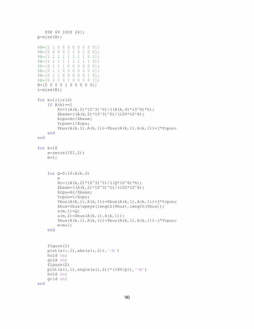
90
898 69 1000 24]; p=size(A); %B=[1 1 0 0 0 0 0 0 0 0]; %B=[0 0 0 0 1 1 0 1 0 0]; %B=[1 1 1 1 1 1 1 1 0 1]; %B=[1 1 1 1 1 1 1 1 1 0]; %B=[0 1 1 1 0 0 0 0 0 0]; %B=[0 1 1 0 0 0 0 0 0 0]; %B=[0 1 1 0 0 0 0 0 1 0]; %B=[0 0 0 0 1 0 0 0 0 1]; B=[0 0 0 0 1 0 0 0 0 0]; r=size(B); for k=1:1:r(2) if B(k)==1 Xc=((A(k,2)*10^3)^2)/((A(k,4)*10^6)*h); Zbase=((A(k,2)*10^3)^2)/(100*10^6); Xcpu=Xc/Zbase; Ycpun=1/Xcpu; Ybus(A(k,1),A(k,1))=Ybus(A(k,1),A(k,1))+j*Y cpun; end end for k=10 a=zeros(101,2); m=1; for Q=0:10:A(k,3) m Xc=((A(k,2)*10^3)^2)/((Q*10^6)*h); Zbase=((A(k,2)*10^3)^2)/(100*10^6); Xcpu=Xc/Zbase; Ycpun=1/Xcpu; Ybus(A(k,1),A(k,1))=Ybus(A(k,1),A(k,1))+j*Y cpun; Zbus=Ybus\speye(length(Ybus),length(Ybus)); a(m,1)=Q; a(m,2)=Zbus(A(k,1),A(k,1)); Ybus(A(k,1),A(k,1))=Ybus(A(k,1),A(k,1))-j*Y cpun; m=m+1; end figure(1) plot(a(:,1),abs(a(:,2)), '-b' ) hold on; grid on; figure(2) plot(a(:,1),angle(a(:,2))*(180/pi), '-b' ) hold on; grid on; end

91
APPENDIX C
SELECTED PHASE ANGLE PLOTS FOR CAPACITANCE SCAN RESULTS

92
C.1 Selected phase angle plots for capacitance scan results obtained from Matlab
The figures C.1-10 show some of the phase angle plots that were taken from the
capacitance scans conducted at the ten buses. These phase angle plots were utilized to ver-
ify the resonance point that was observed on the magnitude plots shown in the Chapter 3.
The plots were plotted by varying the capacitance bank rating in steps of 10 MVAr. The
resonant point was thus chosen based on proximity to zero degrees.
Fig. C.1 Phase Angle Plot of Capacitance Scan at Bus 1 for Harmonic Order 5
Ph
ase
an
gle
of
the
Th
eve
nin
’s im
pe
da
nce
at
the
bu
s(d
eg
)
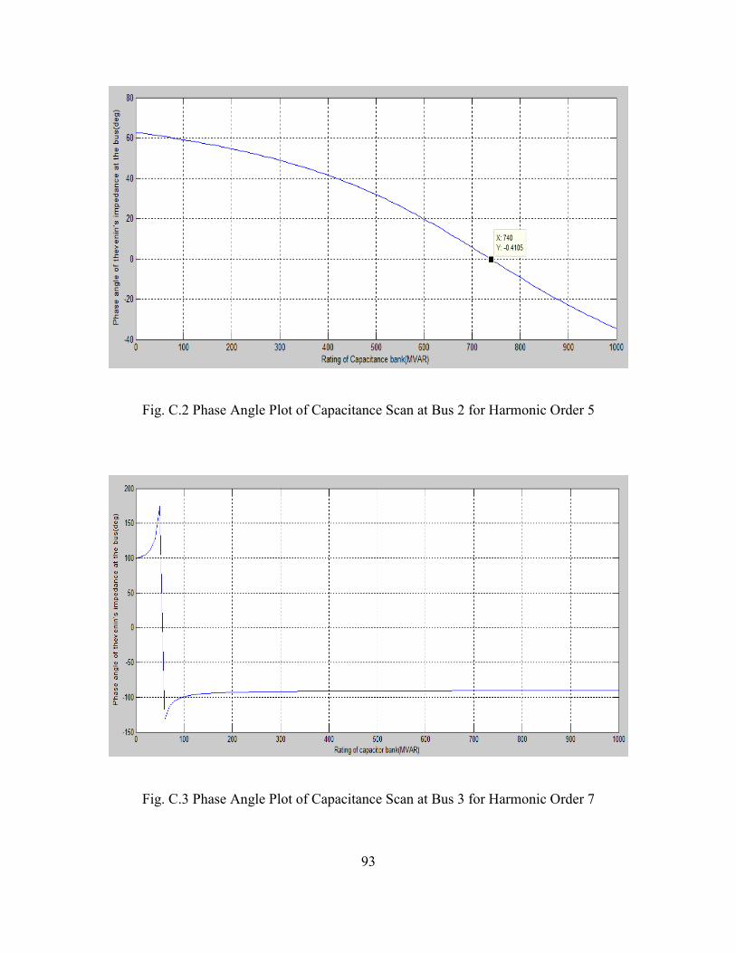
93
Fig. C.2 Phase Angle Plot of Capacitance Scan at Bus 2 for Harmonic Order 5
Fig. C.3 Phase Angle Plot of Capacitance Scan at Bus 3 for Harmonic Order 7

94
Fig. C.4 Phase Angle Plot of Capacitance Scan at Bus 4 for Harmonic Order 7
Fig. C.5 Phase Angle Plot of Capacitance Scan at Bus 5 for Fundamental Frequency
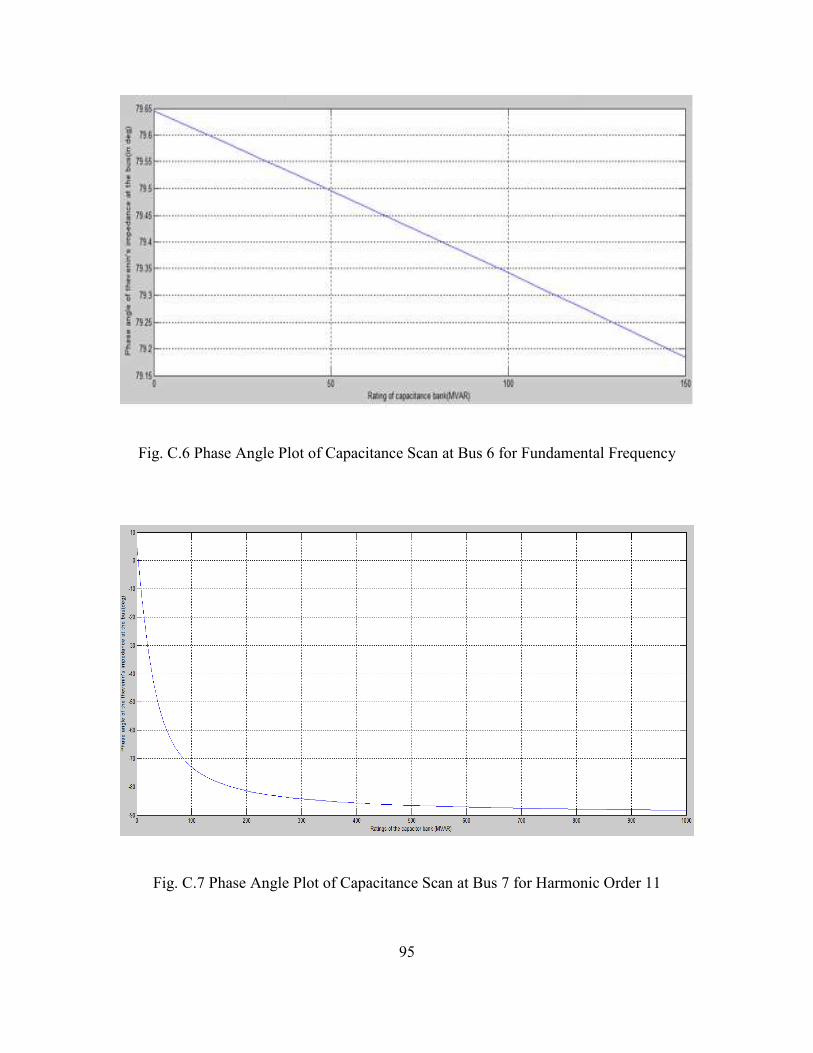
95
Fig. C.6 Phase Angle Plot of Capacitance Scan at Bus 6 for Fundamental Frequency
Fig. C.7 Phase Angle Plot of Capacitance Scan at Bus 7 for Harmonic Order 11
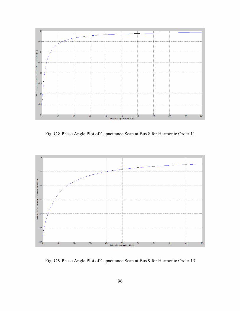
96
Fig. C.8 Phase Angle Plot of Capacitance Scan at Bus 8 for Harmonic Order 11
Fig. C.9 Phase Angle Plot of Capacitance Scan at Bus 9 for Harmonic Order 13
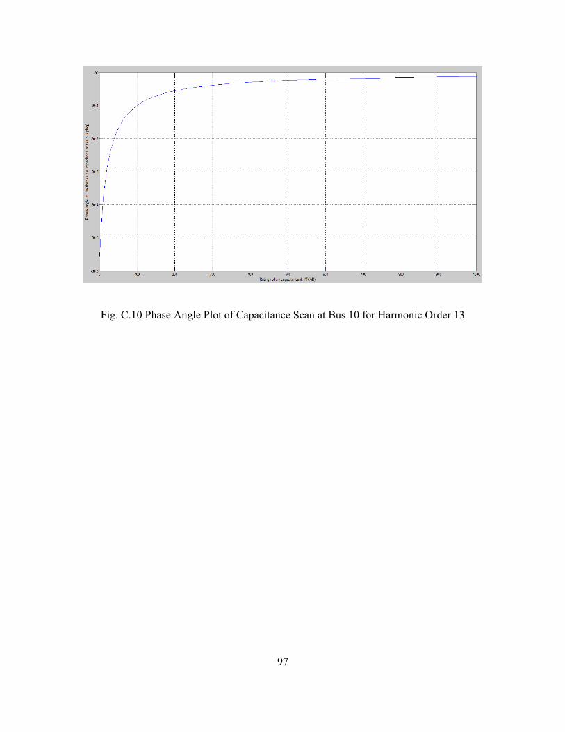
97
Fig. C.10 Phase Angle Plot of Capacitance Scan at Bus 10 for Harmonic Order 13

98
APPENDIX D
MATLAB CODE FOR EVALUATION OF IMPACT OF HVDC SOURCES
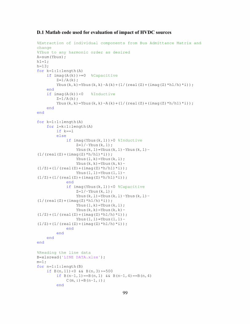
99
D.1 Matlab code used for evaluation of impact of HVDC sources
%Extraction of individual components from Bus Admit tance Matrix and change %Ybus to any harmonic order as desired A=sum(Ybus); h1=1; h=13; for k=1:1:length(A) if imag(A(k))>=0 %Capacitive Z=1/A(k); Ybus(k,k)=Ybus(k,k)-A(k)+(1/(real(Z)+(imag( Z)*h1/h)*i)); end if imag(A(k))<0 %Inductive Z=1/A(k); Ybus(k,k)=Ybus(k,k)-A(k)+(1/(real(Z)+(imag( Z)*h/h1)*i)); end end for k=1:1:length(A) for l=k:1:length(A) if k==l else if imag(Ybus(k,l))>0 %Inductive Z=1/-Ybus(k,l); Ybus(k,l)=Ybus(k,l)-Ybus(k,l)-(1/(real(Z)+(imag(Z)*h/h1)*i)); Ybus(l,k)=Ybus(k,l); Ybus(k,k)=Ybus(k,k)-(1/Z)+(1/(real(Z)+(imag(Z)*h/h1)*i)); Ybus(l,l)=Ybus(l,l)-(1/Z)+(1/(real(Z)+(imag(Z)*h/h1)*i)); end if imag(Ybus(k,l))<0 %Capacitive Z=1/-Ybus(k,l); Ybus(k,l)=Ybus(k,l)-Ybus(k,l)-(1/(real(Z)+(imag(Z)*h1/h)*i)); Ybus(l,k)=Ybus(k,l); Ybus(k,k)=Ybus(k,k)-(1/Z)+(1/(real(Z)+(imag(Z)*h1/h)*i)); Ybus(l,l)=Ybus(l,l)-(1/Z)+(1/(real(Z)+(imag(Z)*h1/h)*i)); end end end end %Reading the line data B=xlsread( 'LINE DATA.xlsx' ); m=1; for n=1:1:length(B) if B(n,11)<0 && B(n,3)>=500 if B(n-1,1)==B(n,1) && B(n-1,4)==B(n,4) C(m,:)=B(n-1,:); end

100
if B(n+1,1)==B(n,1) && B(n+1,4)==B(n,4) C(m,:)=B(n+1,:); end C(m+1,:)=B(n,:); m=m+2; end end xlswrite( 'LINECAPACITANCEDATA.xlsx' ,C); %Locating series capacitor compensated lines in the WECC system Ybus and %modifying the Ybus D=xlsread( 'WECCYbusorder.xlsx' ); x=1; r=0.00001; y=length(Ybus); for n=1:2:length(C) for m=1:1:length(D) if C(n,1)==D(m,1) k=m; end if C(n,4)==D(m,1) l=m; end a=Ybus(k,k) b=Ybus(l,l) c=Ybus(k,l) d=Ybus(l,k) Ybus(k,k)=Ybus(k,k)+Ybus(k,l)+1/(C(n,10)+(j *C(n,11)*h))+1/(r); Ybus(l,l)=Ybus(l,l)+Ybus(k,l)+1/(C(n,10)+(j*C(n,11) *h))+1/(j*(C(n+1,11)/h)); Ybus((y+x),(y+x))=1/(r)+1/(j*(C(n+1,11)/h)) ; Ybus(k,l)=Ybus(k,l)-Ybus(k,l)-1/(C(n,10)+(j *C(n,11)*h)); Ybus(l,k)=Ybus(l,k)-Ybus(l,k)-1/(C(n,10)+(j *C(n,11)*h)); Ybus(k,(y+x))=-1/(r); Ybus(l,(y+x))=-1/(j*C(n+1,11)/h); Ybus((y+x),k)=-1/(r); Ybus((y+x),l)=-1/(j*C(n+1,11)/h); a=Ybus(k,k) b=Ybus(l,l) c=Ybus(k,l) d=Ybus(l,k) x=x+1; end end x %Creation of harmonic current injection vector I=sparse(length(Ybus),1); I(4432)=1; %Sylmar1 bus I(4433)=1; %Sylmar2 bus I(4367)=1; %Adelantx bus
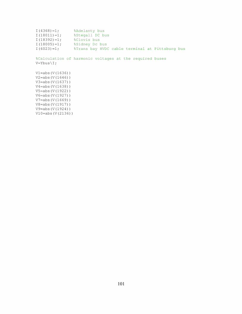
101
I(4368)=1; %Adelanty bus I(18011)=1; %Stegall DC bus I(18392)=1; %Clovis bus I(18005)=1; %Sidney Dc bus I(6023)=1; %Trans bay HVDC cable terminal at Pittsburg bus %Calculation of harmonic voltages at the required b uses V=Ybus\I; V1=abs(V(1636)) V2=abs(V(1646)) V3=abs(V(1637)) V4=abs(V(1638)) V5=abs(V(1922)) V6=abs(V(1927)) V7=abs(V(1669)) V8=abs(V(1917)) V9=abs(V(1924)) V10=abs(V(2136))


![enrollment no :160210119051, hardik ppt[1]](https://img.pdfslide.net/doc/110x75/58f118fa1a28abc52a8b45d5/enrollment-no-160210119051-hardik-ppt1.jpg)