Embed Size (px)
Citation preview
arX
iv:p
hysi
cs/0
6061
79v1
[ph
ysic
s.da
ta-a
n] 2
0 Ju
n 20
06
Probability and Statistical Inference ∗
Harrison B. Prosper
Department of Physics, Florida State University, Tallahassee, Florida 32306, USA
(Dated: March 31, 2007)
Abstract
These lectures introduce key concepts in probability and statistical inference at a level suitable
for graduate students in particle physics. Our goal is to paint as vivid a picture as possible of the
concepts covered.
∗ SERC School in Particle Physics, Chandigarh, India, 7-27 March, 2005
1
Contents
I. Lecture 1 - Probability Theory, Part I 4
A. Historical Note 4
B. Reasoning 7
C. Probability Calculus 9
D. Objective Interpretation 12
E. Subjective Interpretation 13
F. Bayes’ Theorem 13
II. Lecture 2 - Probability Theory, Part II 16
A. Probability Distributions 16
1. Random Variables 16
2. Properties 17
3. Common Densities and Distributions 17
B. The Binomial Distribution 18
C. The Poisson Distribution 22
D. The Gaussian Distribution 23
E. The χ2 Distribution 24
1. A Brief Word on Fitting 25
III. Lecture 3 - Statistical Inference, Part I 26
A. Descriptive Statistics 26
B. Ensemble Averaging 26
C. Estimators 28
D. Loss and Risk 29
E. Risk Minimization 30
F. The Bayesian Approach 31
G. The Likelihood Principle 33
H. Parameter Estimation 33
1. Quadratic Loss 34
2. Absolute Loss 35
3. Uncertainty 35
2
I. Combining Results 36
J. Model Selection 37
K. Optimal Event Selection 38
L. Prior Probabilities 40
M. Counting Experiments 41
IV. Lecture 4 - Statistical Infserence, Part II 44
A. Goodness of Fit 44
B. Confidence Intervals 44
1. Coverage Probability 46
2. The Neyman Construction 47
3. Other Constructions 49
Acknowledgements 51
References 51
3
I. LECTURE 1 - PROBABILITY THEORY, PART I
Sir Harold Jeffreys [1] begins his book, Theory of Probability, with these words
“The fundamental problem of scientific progress, and a fundamental one of ev-
eryday life, is that of learning from experience.”
In everyday life, we learn from experience in a way that is still deeply mysterious. However,
in scientific research the learning is more readily formalized: we collect data in a systematic
way about some aspect of the world and, from these data, infer something of interest using
more or less formal methods. Probability theory is useful at all stages.
Given its central role in statistical inference, we believe it is helpful to have a clear
understanding of what probability is and how that notion arose. Accordingly, these lectures
are divided into two parts: Lectures 1 and 2 cover probability theory, while Lectures 3 and
4 deal with statistical inference. In the first lecture, we begin with a sketch of the history
of probability. This is followed by a discussion of the elements of deductive and inductive
reasoning, ending with a discussion of some elementary aspects of probability theory.
A. Historical Note
The theory of probability arose from the ancient and popular pastime of gambling. One
of the earliest references to chance, and to the woes of gambling, occurs in the cautionary
tale of King Nala from the epic poem Mahabharata [2]. King Nala lost his kingdom in a
gambling contest and was reduced to working for King Bhangasuri as a chariot-driver. One
day, while on a journey with the king, Nala boasted of his mastery of horses. The king did
not take too kindly to such boasting and reminded Nala that no man knows everything. To
make his point, the king made a quick estimate of the number of fruit on a nearby tree,
the extraordinary accuracy of which was verified by Nala, who counted the fruit one by
one. Nala pleaded with the king to divulge the method that yielded such an astonishingly
accurate estimate. The king replied:
“Know that I am a knower of the secret of the dice and therefore adept in the
art of enumeration.”
4
In the end, the king relented and told Nala the secret. It would seem from this tale that some
notions of chance were understood, at least by some, in ancient times. However, probability
theory as a recognizable mathematical discipline was established only centuries later.
In 1654, the French nobleman, Chevalier de Mere, complained to Blaise Pascal that the
rules of arithmetic must be faulty. His reason: the observation that his two methods of
placing bets, using dice, did not work equally well, contrary to his expectation. He would
bet on the basis of obtaining at least one 6 in 4 throws of a single die, or, at least one
double 6 in 24 throws of two dice. Pascal worked out the probabilities and showed that
the first outcome was indeed slightly more probable than the second. Thus was born the
mathematical theory of probability.
By the late 17th century, probability was interpreted in several ways:
• as the fraction of favorable outcomes in a set of outcomes considered equally likely,
• as a measure of uncertain knowledge of outcomes,
• as a physical tendency in things that exhibit chance.
James Bernoulli (1654–1705) labored hard to make sense of these different aspects of proba-
bility, but, dissastisfied with his labors, he chose not to publish his results. Happily, however,
in 1713, his nephew Nicholas Bernoulli published Ars Conjectandi (The Art of Conjecture),
James Bernoulli’s famous treatise on probability. This book contains the proof of an impor-
tant result, namely, the weak law of large numbers, which we discuss later in this lecture.
Some decades later, the English cleric Thomas Bayes (1702–1761) read (via a proxy!) the
following paper before the Royal Society, on 23 December, 1763: An Essay towards solv-
ing a Problem in the Doctrine of Chances. This paper is notable for at least two reasons.
Firstly, in it, a proof is given of a special case of what became known as Bayes’ theorem.
Secondly, this paper makes explicit use of probability as a measure of uncertain knowledge
about something, in this case, uncertain knowledge of the value of a probability! The ideas
of Bayes, and probability theory, in general, were brought to great heights by Pierre Simon
de Laplace (1749–1827) in his book of 1812 entitled: Theorie Analytique des Probabilities.
In it, amongst other things, one finds the general form of Bayes’ theorem. One also finds
results that soon became controversial; indeed, that became the object of ridicule. Laplace
made extensive use of Bayes’ theorem, sometimes in ways that yielded odd results. From
5

one of his results (the law of succession) one would conclude that a 9-year old boy has a
lesser chance of reaching the age of 10 than does a 99-year old man to reach the age of 100.
The logician George Boole was particularly scornful of Laplace’s use of Bayes’ theorem. In
the Bayes-Laplace view of probability, the foundation of the Bayesian approach to sta-
tistical inference, probability is construed as a measure of the plausibility of an assertion.
For example, Bayes and Laplace would have had no difficulty with the assertion “There is
a 60% chance of rain tomorrow”.
For Boole and other mathematicians and philosophers, however, the notion of probability
as a measure of uncertain knowledge, or the plausibility, of the truth of an assertion seemed
metaphysical and therefore unscientific. They therefore sought a different interpretational
foundation for the theory of probability, grounded, as they perceived it, more firmly in
experience. As a result of the critiques of the Bayes-Laplace methods, and the growing
“ideology of the objective” in the natural sciences [3], these methods fell into disfavor.
This was not only because of discomfort with the inherent subjectivity of the probabilities
manipulated by Bayes and Laplace, but because of the seemingly arbitrary manner in which
they assigned certain probabilities. To excise such alleged defects in the theory of probability
a different approach was developed, which, at the start of the 20th century, became the
foundation of what has come to be known as the frequentist approach to statistical
inference. The newer approach, which comprises the body of statistical ideas with which
most physicists are familiar, is closely associated with the names of Sir Ronald Aylmer
Fisher (1890–1962), Jerzy Neyman, Pearson, Cramer, Rao, Mahalanobis, von Mises and
Kolmogorov, to name but a few [4]. The frequentist approach is typically presented as if
it were a single coherent school of thought. In fact, however, within this approach views
differed, sometimes sharply. Indeed, the sharpest disagreements were between Jerzy Neyman
and Ronald Fisher, the two principal architects of the frequentist approach.
Fisher and Neyman, along with the other frequentists, did, however, agree on one crucial
point: probability is to interpreted not as a measure of plausibility, or uncertain knowledge,
or degree of belief, but rather as the relative frequency with which something happens,
or will happen [5]. From the frequentist point of view, statements such as “There is a 60%
chance of rain tomorrow” are devoid of empirical content. Why? Because it is not possible to
repeat the day that is tomorrow and count how often it rained. By contrast, the statement
“There is a 60% chance of rain on days named March 7th” is judged meaningful because
6
such days repeat and we can, therefore, assess by enumeration the relative frequency with
which it rains on days so named.
The frequentist viewpoint took hold in the physical sciences and became the norm in
particle physics [6]. Indeed, that viewpoint is so entrenched in our field that, until fairly
recently, it was hardly recognized that one has a choice about how to conduct statistical
inferences. However, during the latter half of the 20th century the methods of Bayes and
Laplace have undergone a renaissance initiated, in large measure, by Sir Harold Jeffreys [1]
(1891–1989) and vigorously developed by like-minded physicists and mathematicians, no-
tably Cox, de Finetti, Lindley, Savage and Jaynes [7, 8, 9, 10]. Moreover, after a somewhat
slow start, beginning with a few papers in the 1980s [11, 12, 13] a similar renaissance is
underway in particle physics [14].
B. Reasoning
“Probability theory is nothing but common sense reduced to calculation.”
— Laplace, 1819
Aristotle, who lived around 350 BC, was one of the first thinkers to attempt a formalization
of reasoning. He noticed that on those rare occasions when we reason correctly we did so
according to rules that can be reduced to the syllogisms:
modus ponens (ponere=affirm) modus tollens (tollere=deny)
Major premise If A is TRUE, then B is TRUE If A is TRUE, then B is TRUE
Minor premise A is TRUE B is FALSE
Conclusion Therefore, B is TRUE Therefore, A is FALSE
In addition, if the statement A is TRUE then its negation, written as A, is, of necessity,
FALSE. The statement A is said to contradict A. A simple mnemonic for the syllogisms are
the set of symbolic expressions:
7
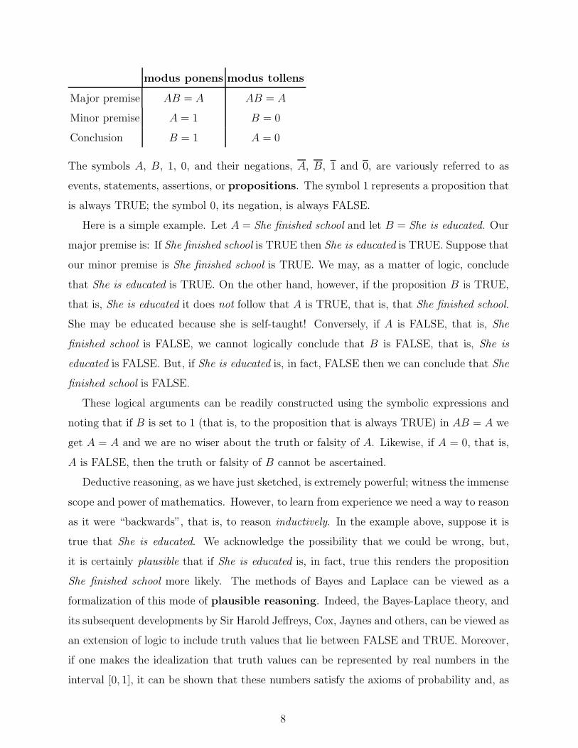
modus ponens modus tollens
Major premise AB = A AB = A
Minor premise A = 1 B = 0
Conclusion B = 1 A = 0
The symbols A, B, 1, 0, and their negations, A, B, 1 and 0, are variously referred to as
events, statements, assertions, or propositions. The symbol 1 represents a proposition that
is always TRUE; the symbol 0, its negation, is always FALSE.
Here is a simple example. Let A = She finished school and let B = She is educated. Our
major premise is: If She finished school is TRUE then She is educated is TRUE. Suppose that
our minor premise is She finished school is TRUE. We may, as a matter of logic, conclude
that She is educated is TRUE. On the other hand, however, if the proposition B is TRUE,
that is, She is educated it does not follow that A is TRUE, that is, that She finished school.
She may be educated because she is self-taught! Conversely, if A is FALSE, that is, She
finished school is FALSE, we cannot logically conclude that B is FALSE, that is, She is
educated is FALSE. But, if She is educated is, in fact, FALSE then we can conclude that She
finished school is FALSE.
These logical arguments can be readily constructed using the symbolic expressions and
noting that if B is set to 1 (that is, to the proposition that is always TRUE) in AB = A we
get A = A and we are no wiser about the truth or falsity of A. Likewise, if A = 0, that is,
A is FALSE, then the truth or falsity of B cannot be ascertained.
Deductive reasoning, as we have just sketched, is extremely powerful; witness the immense
scope and power of mathematics. However, to learn from experience we need a way to reason
as it were “backwards”, that is, to reason inductively. In the example above, suppose it is
true that She is educated. We acknowledge the possibility that we could be wrong, but,
it is certainly plausible that if She is educated is, in fact, true this renders the proposition
She finished school more likely. The methods of Bayes and Laplace can be viewed as a
formalization of this mode of plausible reasoning. Indeed, the Bayes-Laplace theory, and
its subsequent developments by Sir Harold Jeffreys, Cox, Jaynes and others, can be viewed as
an extension of logic to include truth values that lie between FALSE and TRUE. Moreover,
if one makes the idealization that truth values can be represented by real numbers in the
interval [0, 1], it can be shown that these numbers satisfy the axioms of probability and, as
8
such, are a quantitative measure of the plausibility of propositions. These arguments assign
a quantitative meaning to the weaker syllogisms:
Major premise If A is TRUE, then B is TRUE If A is TRUE, then B is TRUE
Minor premise B is TRUE A is FALSE
Conclusion Therefore, A is more plausible Therefore, B is less plausible.
C. Probability Calculus
The theory of probability can be founded in many different ways. One way, is to regard
probability as a function with range [0,1], defined on sets of events or propositions. But in
order speak of sets of propositions, we need to know how they are to be manipulated; that
is, we need an algebra of propositions. The appropriate algebra, Boolean algebra, was
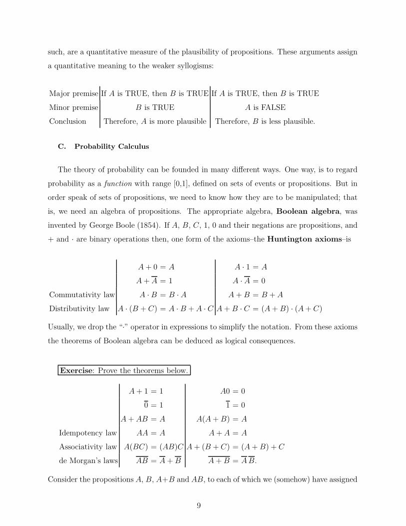
invented by George Boole (1854). If A, B, C, 1, 0 and their negations are propositions, and
+ and · are binary operations then, one form of the axioms–the Huntington axioms–is
A + 0 = A A · 1 = A
A + A = 1 A · A = 0
Commutativity law A · B = B · A A + B = B + A
Distributivity law A · (B + C) = A · B + A · C A + B · C = (A + B) · (A + C)
Usually, we drop the “·” operator in expressions to simplify the notation. From these axioms
the theorems of Boolean algebra can be deduced as logical consequences.
Exercise: Prove the theorems below.
A + 1 = 1 A0 = 0
0 = 1 1 = 0
A + AB = A A(A + B) = A
Idempotency law AA = A A + A = A
Associativity law A(BC) = (AB)C A + (B + C) = (A + B) + C
de Morgan’s laws AB = A + B A + B = A B.
Consider the propositions A, B, A+B and AB, to each of which we (somehow) have assigned
9
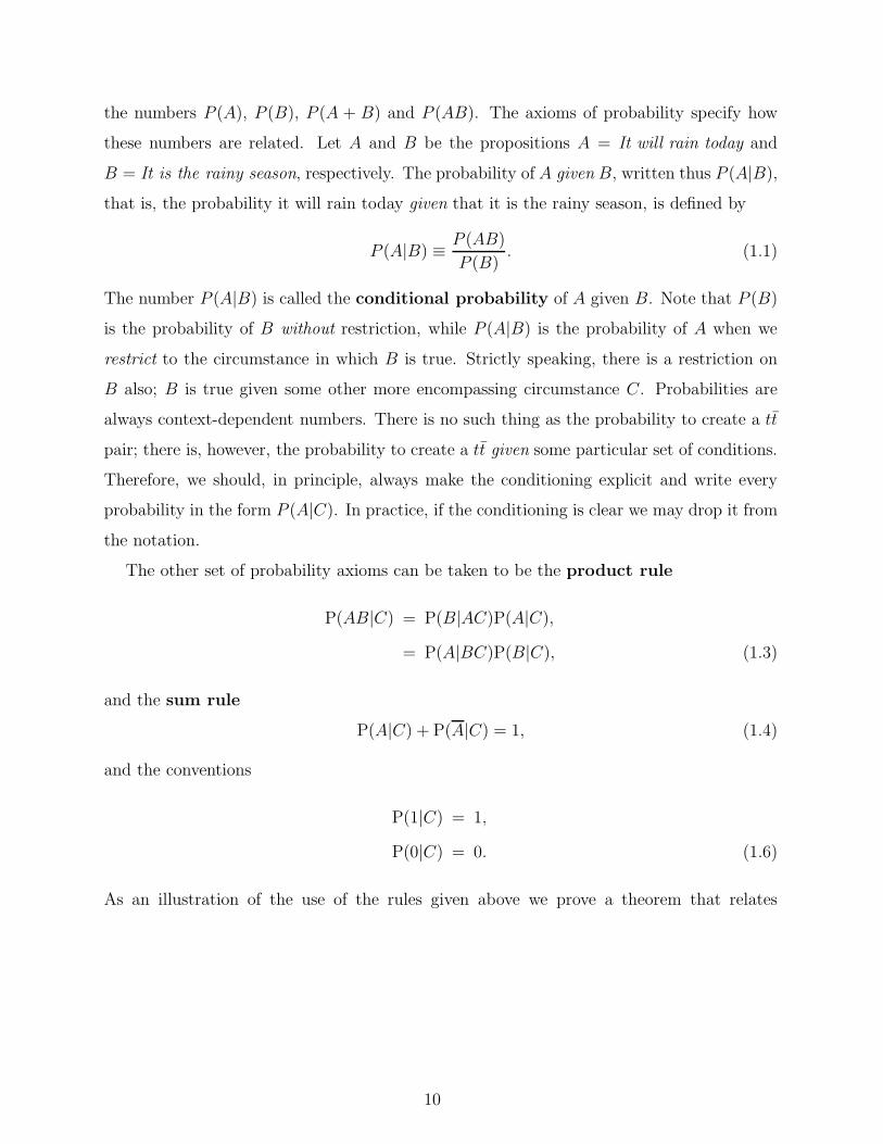
the numbers P (A), P (B), P (A + B) and P (AB). The axioms of probability specify how
these numbers are related. Let A and B be the propositions A = It will rain today and
B = It is the rainy season, respectively. The probability of A given B, written thus P (A|B),
that is, the probability it will rain today given that it is the rainy season, is defined by
P (A|B) ≡ P (AB)
P (B). (1.1)
The number P (A|B) is called the conditional probability of A given B. Note that P (B)
is the probability of B without restriction, while P (A|B) is the probability of A when we
restrict to the circumstance in which B is true. Strictly speaking, there is a restriction on
B also; B is true given some other more encompassing circumstance C. Probabilities are
always context-dependent numbers. There is no such thing as the probability to create a tt
pair; there is, however, the probability to create a tt given some particular set of conditions.
Therefore, we should, in principle, always make the conditioning explicit and write every
probability in the form P (A|C). In practice, if the conditioning is clear we may drop it from
the notation.
The other set of probability axioms can be taken to be the product rule
P(AB|C) = P(B|AC)P(A|C),
= P(A|BC)P(B|C), (1.3)
and the sum rule
P(A|C) + P(A|C) = 1, (1.4)
and the conventions
P(1|C) = 1,
P(0|C) = 0. (1.6)
As an illustration of the use of the rules given above we prove a theorem that relates
10
P(A + B|C) to P(A|C) and P(B|C). We need merely to apply the above rules repeatedly:
P(A + B|C) = 1 − P(A + B|C)
= 1 − P(A B|C)
= 1 − P(B|AC)P(A|C)
= 1 −[
1 − P(B|AC)]
P(A|C)
= 1 − P(A|C) + P(B|AC)P(A|C)
= P(A|C) + P(B|AC)P(A|C)
= P(A|C) + P(AB|C)
= P(A|C) + P(A|BC)P(B|C)
= P(A|C) + [1 − P(A|BC)] P(B|C)
= P(A|C) + P(B|C) − P(A|BC)P(B|C)
P(A + B|C) = P(A|C) + P(B|C) − P(AB|C). (1.8)
The Huntington axioms seem intuitively reasonable, but the product and sum rules,
Eqs. (1.3) and (1.4), seem less so. Remarkably, these rules can be derived from the more
primitive axioms:
• Axiom 1) Plausibilities q can be represented by real numbers.
• Axiom 2) The plausibilities q(B) and q(A|B) of a proposition B and that of another
A given the first determine the plausibility q(AB) of the joint proposition AB; that
is, q(AB) is some function of q(B) and q(A|B).
• Axiom 3) The plausibility q(A) of a proposition A determines the plausibility q(A)
of its converse A.
This was first done by the physicist, R.T. Cox [7], in 1946, who showed that plausibilities
or degrees of belief follow rules that are isomorphic to those of probability and thus provide
a subjective interpretation of the latter. Moreover, well before Cox’s theorem, James
Bernoulli, who, along with his contemporaries, regarded the subjective interpretation of
probability as self-evidently sensible [3], proved a theorem that provides a link between
relative frequency and the abstraction we call probability.
11
D. Objective Interpretation
In the objective interpretation, probability is interpreted as the relative frequency
with which something happens, or could happen. Let n be the number of experiments or
trials; for example, this could be the number of proton-proton collisions at the LHC. Let k
be the number of successes; for example, it could be the count in a given mass bin of Higgs
boson events. The relative frequency of successes is
k
n. (1.9)
It is a matter of experience that as n grows ever larger the relative frequency k/n settles
down to a number, call it p, whose natural interpretion is the probability of a success.
Unfortunately, this interpretation is not quite as straightforward as it seems. Any theory
of probability that defines the latter as the limit of k/n must contend with the following
possibility. It is possible that on every trial we get a success, or a failure, or we alternate
between the two ad infinitum. It is important, therefore, to be precise about what is meant
by the limit of the (rational) number k/n. The correct statement, first noted by James
Bernoulli (1703), is the weak law of large numbers, mentioned briefly above. This
theorem states that
limn→∞
Pr[|kn− p| > ǫ] = 0 , (1.10)
for any real number ǫ > 0. That is, as the number of trials goes to infinity, the probability
Pr[∗], that the relative frequency k/n differs from the probability p by more than ǫ, becomes
vanishingly small.
The implied recursion in this theorem is conceptually problematic. If, indeed, probability
is to be defined as nothing more than the limit of a relative frequency, then the two prob-
abilities that occur in Bernoulli’s theorem must both be limits of relative frequencies. The
second probability p in the theorem may legitimately be viewed as the “limit” of the relative
frequency k/n. However, to define the first probability Pr[∗] requires a second application of
Bernoulli’s theorem. But that second application will specify yet another Pr[∗], which must
itself be defined in terms of a limit, and so it goes. It would seem that we cannot avoid
being ensnared in an infinite hierarchy of infinite sequences of trials. Moreover, never, in
practice, do we ever conduct infinite sequences of trials and therefore the limit, as it true of
all limits, is an abstraction.
12
E. Subjective Interpretation
We can avoid the infinite hierarchy of trials if we are prepared to interprete the first
probability in Bernoulli’s theorem differently from the second. If we interpret the first as
a measure of plausibility then the theorem is a statement about the plausibility of the
proposition limn→∞ k/n = p. Bernoulli’s theorem, as he himself interpreted it, declares that
it is plausible to the point of certainty that k/n → p as the number of trials grows without
limit. The import of this theorem, and Bernoulli’s interpretation of it, is that probability as
relative frequency is a derived notion pertaining to a special class of circumstances, namely,
those in which one can entertain, in principle, performing identically repeated trials in
which the relative frequency converges, in the precise manner of Bernoulli’s theorem, to
some number p, which, because it satisfies the axioms of probability, we are at liberty to
call a probability. The Standard Model is an example of a physical theory that can predict
the limiting numbers p for the kind of identically repeated trials performed in high energy
physics experiments.
The position advocated here is that probability is an abstraction that can be usefully
interpreted in at least two different ways: as the limit of a relative frequency and as a degree
of belief. Moreover, the first is best understood in terms of the second.
F. Bayes’ Theorem
In 1763, Thomas Bayes published a paper in which a special case of a theorem, that bears
his name, appeared. Bayes’ theorem
P(Bk|AC) =P(A|BkC)P(Bk|C)
∑
i P(A|BiC)P(Bi|C), (1.11)
where A, Bk and C are propositions, is a direct consequence of the product rule, Eq. (1.3),
of probability theory. Consider two propositions A and B. They are said to be mutually
exclusive if the truth of one denies the truth of the other, that is: P(AB|C) = 0. In that
case, from the theorem we proved earlier, we conclude that
P(A + B|C) = P(A|C) + P(B|C), (1.12)
which is easily generalized to any number of mutually exclusive propositions. A set of
mutually exclusive propositions Bk is said to be exhaustive if their probabilities sum to
13
unity:∑
k
P(Bk|C) = 1. (1.13)
Let B1 and B2 be exhaustive propopsitions. Consider the propositions AB1 and AB2. From
the product rule, we can write
P (AB1) = P(B1|A)P (A), (1.15)
P (AB2) = P(B2|A)P (A). (1.16)
Now add the two equations
P (AB1) + P (AB2) = [P(B1|A) + P(B2|A)]P (A), (1.18)
= P (A). (1.19)
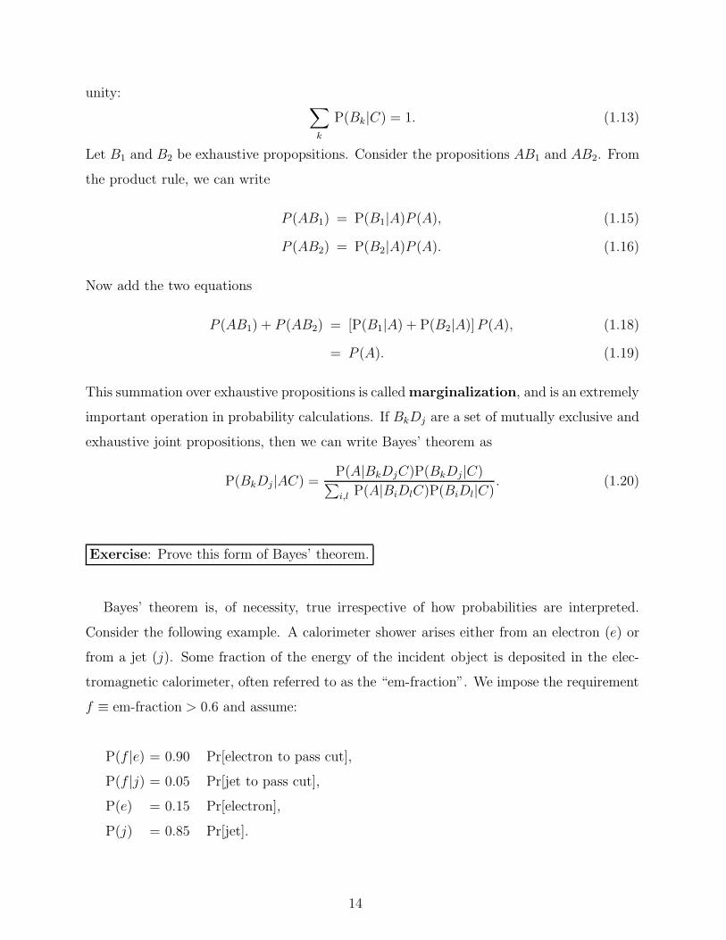
This summation over exhaustive propositions is called marginalization, and is an extremely
important operation in probability calculations. If BkDj are a set of mutually exclusive and
exhaustive joint propositions, then we can write Bayes’ theorem as
P(BkDj|AC) =P(A|BkDjC)P(BkDj|C)
∑
i,l P(A|BiDlC)P(BiDl|C). (1.20)
Exercise: Prove this form of Bayes’ theorem.
Bayes’ theorem is, of necessity, true irrespective of how probabilities are interpreted.
Consider the following example. A calorimeter shower arises either from an electron (e) or
from a jet (j). Some fraction of the energy of the incident object is deposited in the elec-
tromagnetic calorimeter, often referred to as the “em-fraction”. We impose the requirement
f ≡ em-fraction > 0.6 and assume:
P(f |e) = 0.90 Pr[electron to pass cut],
P(f |j) = 0.05 Pr[jet to pass cut],
P(e) = 0.15 Pr[electron],
P(j) = 0.85 Pr[jet].
14
We wish to compute P(e|f), the probability that the shower was caused by an electron,
given that the em-fraction exceeds 0.6. Applying Bayes’ theorem we get
P(e|f) =P(f |e)P(e)
P(f |e)P(e) + P(f |j)P(j),
=0.90 × 0.15
0.9 × 0.15 + 0.05 × 0.85,
= 0.76. (1.22)
We conclude that there is a 76% probability that the shower is caused by an electron. This
calculation is correct whether or not the probabilities are regarded as relative frequencies or
degrees of belief.
15
II. LECTURE 2 - PROBABILITY THEORY, PART II
A. Probability Distributions
1. Random Variables
Statisticians make a distinction between a random variable X and its value x. A
random variable can be thought of as a map X,
X : Ω → R , (2.1)
between a set of possible events or outcomes Ω = ω1, · · · , ωN and the set of reals R.
The map X assigns a real number x = X(ω), called the value of the random variable, to
every outcome ω ∈ Ω. The height of persons who pass you in the street is an example
of a random variable. Its possible events are the people who can pass you and its value
is the height of a person. Since the outcome is random so too is the value of the random
variable. Note, however, that in spite of the name the map X itself is generally not random!
Rather it is the set Ω of possible outcomes that possesses the (rather mysterious) quality
called randomness. One can think of that property as a manifestation of a randomizing
agent whose job it is to pick an outcome from the set of possibilities, according to a rule
that is not readily discernable. The randomizing agent, however, need not be governed by
chance! Consider the set of possible outcomes Ω = 0, . . . , 9 and the function X that
maps this set to the subset 0, . . . , 9 ∈ R. Their exists a random variable X whose value
is the next decimal digit of π, starting, say, from the first. The digits of π do not occur
by chance even though they form an excellent random sequence. The same is true of,
so-called, pseudo-random number generators, which provide sufficiently random sequences
of real numbers—indispensible in Monte Carlo-based calculations, even though, again, the
randomizing agent is not governed by chance; indeed, it is strictly deterministic. Usually, a
random variable is denoted by an upper case symbol, while one of its values is denoted by
the corresponding lower case symbol. Thus, if X is a random variable then x denotes one of
its values. However, for simplicity we shall not use this convention, but refer to both with
the same symbol.
16

2. Properties
In general, we are most interested in propositions involving real numbers of the form
x ∈ (x1, x2). When x is continuous, P (x), is called a probability distribution function,
while its derivative
f(x) =dP (x)
dx, (2.2)
(assuming it exists) is called a probability density function. Notice that probabilities,
being pure numbers, are dimensionless, whereas densities have dimensions x−1. Note, also,
that from the definition, Eq. (2.2),
dP (x) = f(x) dx, (2.3)
and
P (x) =
∫
dP (x), (2.5)
=
∫
f(x) dx. (2.6)
Given a probability distribution function P (x), its moments mr(z) about a value z is
defined by
mr(z) =
∫
(x − z)rdP (x), (2.8)
=
∫
(x − z)rf(x) dx. (2.9)
Of particular importance are the first moment about zero and the second moment about
the first. The first moment about zero, m1(0), is called the mean and is often denoted by
the symbol µ. The second moment about the first, that is about the mean, m2(µ), is called
the variance of the distribution. Its square-root, often denoted by the symbol σ, is the
standard deviation, which is one measure of the width of the distribution. The mode of
a probability density f(x) is the value of x at which the density is a maximum. Finally, the
median of a distribution is the value of x that divides it into two equal parts. The median
is generally most meaningful if x is a 1-dimensional variable. Note, that if the density f(x)
is symmetrical about the mode, its mode, mean and median coincide.
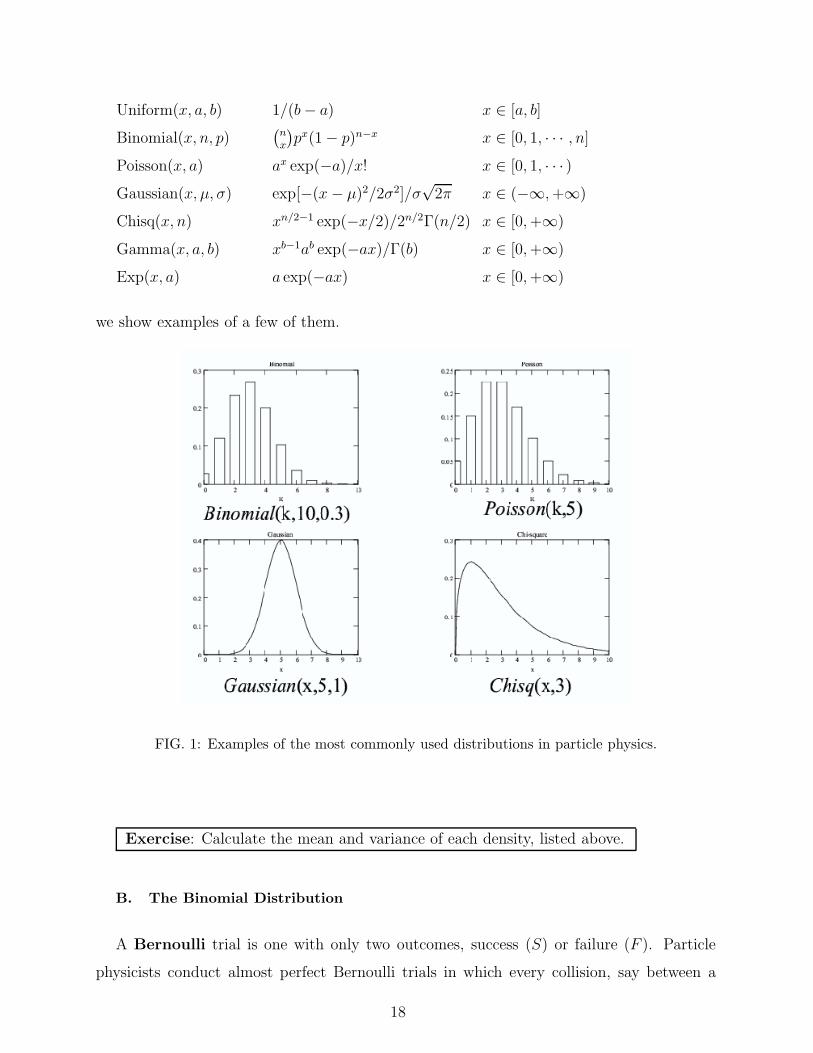
3. Common Densities and Distributions
Below we list the most commonly encountered densities and distributions, while in Fig. 1
17
Uniform(x, a, b) 1/(b − a) x ∈ [a, b]
Binomial(x, n, p)(
nx
)
px(1 − p)n−x x ∈ [0, 1, · · · , n]
Poisson(x, a) ax exp(−a)/x! x ∈ [0, 1, · · · )Gaussian(x, µ, σ) exp[−(x − µ)2/2σ2]/σ
√2π x ∈ (−∞, +∞)
Chisq(x, n) xn/2−1 exp(−x/2)/2n/2Γ(n/2) x ∈ [0, +∞)
Gamma(x, a, b) xb−1ab exp(−ax)/Γ(b) x ∈ [0, +∞)
Exp(x, a) a exp(−ax) x ∈ [0, +∞)
we show examples of a few of them.
FIG. 1: Examples of the most commonly used distributions in particle physics.
Exercise: Calculate the mean and variance of each density, listed above.
B. The Binomial Distribution
A Bernoulli trial is one with only two outcomes, success (S) or failure (F ). Particle
physicists conduct almost perfect Bernoulli trials in which every collision, say between a
18
proton and a proton at the Large Hadron Collider, creates (S), or does not create (F ), an
event of interest. A success could be, for example, the creation of a Higgs boson event.
Typically, we are interested in the probability P(k|n) of k successes given n trials, or some
function thereof. Our task is to calculate this probability, from first principles. Even if one
is of the opinion that relative frequency is the only legitimate scientific way to think about
probability, in practice it is exceedingly difficult, if not impossible, to make headway, from
first principles, using this interpretation alone. Instead, we reproduce here an interesting
result about Bernoulli trials, due Bruno de Finetti [8], following the presentation given by
Heath and Sudderth[15] and Caves [16].
Suppose we have observed a sequence of Bernoulli trials Sk,n = x1, . . . , xn, with k successes
in n trials. We assume that these are the only data of which we have knowledge. We note that
the probability we wish to calculate, P(k|n), makes no reference to the particular sequence
at hand. But, to compute P(k|n), we must, nevertheless, be able to assign a probability to
a sequence of trials, a problem that, in general, is extremely difficult. However, given some
crucial assumptions the problem can be solved.
We assume that the details of the particular sequence observed are unimportant and
that the only thing that matters is the total number of successes k in the n trials we
have conducted. We are therefore led to consider, not just the sequence we have observed,
but the set of all sequences of length n with k successes, of which the one we observed
is a particular instance. Denote by P (Sk,n,j) the probability of the jth sequence Sk,n,j.
de Finetti [8] argues that the probabilities we assign, at this stage, must of necessity be
subjective. They are subjective in that they are based on what we believe to be reasonable
probability assignments, given the objective information at hand, namely, the observed
sequence of trials and their outcomes. The probabilities we assign may be informed by
predictions from, say, the Standard Model or some theory beyond it, but we do not know at
this stage whether or not the predictions are correct. After all, the trials are being conducted
precisely for the purpose of testing these predictions.
What then is the probability of k successes in n trials, regardless of the sequence? The an-
swer, according to the rules of probability theory, is to add up all the probabilities P (Sk,n,j),
P (k|n) =∑
j
P (Sk,n,j), (2.10)
19

that is, to marginalize over all the details that are deemed irrelevant; in this case, proposi-
tions of the form: the jth sequence is x1, . . . , xn. Unfortunately, we can go no further unless
we are prepared to introduce more assumptions. We shall make two more assumptions. The
first is that the order of trials is irrelevant; more precisely, we assume that the probability
of a sequence of trials is symmetric with respect to all permutations of the order of trials.
Each sequence, Sk,n,j, becomes, in effect, indistinguishable. Since they are indistinguishable
we have no reason to favor one sequence over another. In the absence of reasons to do
otherwise it would be rational to assign, to each sequence, the same probability. Since there
are(
nk
)
indistinguishable sequences, the probability of k successes in n trials, regardless of
the sequence, is
P (k|n) =
(
n
k
)
P (Sk,n), (2.11)
where Sk,n can be any one of the sequences Sk,n,j. The second assumption is that the
sequence Sk,n can be embedded in one or more arbitrarily long sequences Sr,m of r successes
in m ≥ n trials in the following way
P (Sk,n) =
m∑
r=0
P (Sk,n|Sr,m) P (Sr,m). (2.12)
Sequences that satisfy both of these assumptions are said to be exchangeable. The prob-
abilities P (Sr,m) must still be freely assigned by us and, at present, there is nothing more
about them that can be said. However, the exchangeability assumption yields a unique
assessment of P (Sk,n|Sr,m), to which we not turn.
By assumption, all successes are indistinguishable, as are all failures. Therefore, the
probability P (Sk,n|Sr,m) of k successes and n − k failures in n trials given that they are
embedded in a a sequence of r successes and m− r failures, in m trials, is akin to drawing,
without replacement, k red balls and n−k white balls out of a box containing r red balls plus
m−r white balls. Since the sequences are indistinguishable, and that consequently the order
of trials is irrelevant, we can consider any convenient sequence to compute P (Sk,n|Sr,m), such
as the one in which we get k successes (red balls) followed by n − k failures (white balls).
Noting that we start with a box containing m balls of which r are red, the probability to
draw k red balls is the product of k fractions
( r
m
)
(
r − 1
m − 1
)
· · ·(
r − (k − 1)
m − (k − 1)
)
=r!
(r − k)!/
m!
(m − k)!, (2.13)
20
while the probability to draw n − k white balls from the remaining m − k balls of which
m − r are white is the product of n − k fractions
(
m − r
m − k
) (
m − r − 1
m − k − 1
)
· · ·(
m − r − (n − k − 1)
m − k − (n − k − 1)
)
=(m − r)!
(m − r − (n − k))!
/(m − k)!
(m − n)!, (2.15)
which yields
P (Sk,n|Sr,m) =r!
(r − k)!
(m − r)!
(m − r − (n − k))!/
m!
(m − n)!. (2.16)
We can write Eq. (2.12) as an integral
P (Sk,n) =
∫ 1
0
P (Sk,n|Szm,m) πm(z) dz , (2.17)
where
πm(z) ≡m
∑
r=0
P (Szm,m)δ(z − r/m), (2.18)
and r/m is the observed relative frequency of success. By assumption, we can make the
sequences Sr,m arbitrarily long. When we do so, P (Sk,n|Szm,m) → zk(1 − z)n−k as m → ∞and the functions πm(z) coalesce into a continuous density π(z). Putting together the pieces
we obtain de Finetti’s Representation Theorem
P (k|n) =
∫ 1
0
Binomial(k, n, z) π(z) dz, (2.19)
for Bernoulli trials. This remarkable result shows that for exchangeable sequences of trials
the probability P (k|n) of k successes in n trials is a binomial distribution weighted by a
density, π(z). What exactly is π(z)? It is simply the probability we have assigned to
every sequence, characterized by the relative frequency z. In other words, π(z) encodes our
assessment of the likely value of the relative frequency in an infinite sequence of trials. If we
knew, or we wished to act as if we knew, or we have a prediction, that the relative frequency
is p, then we would set π(z) = δ(z − p), in which case Eq. (2.19) reduces to the binomial
distribution.
The important point to take away from this is that we have arrived at the binomial
distribution starting with subjective assessments of the probability of sequences of trials and
the powerful assumption of exchangeability.
21
C. The Poisson Distribution
From the discussion above, it would seem that the binomial distribution is the appropriate
one to describe a typical high energy physics counting experiment. However, it is more
usual to take note of the fact that the probability of a success p << 1. Given n trials, the
average number of successes is a = pn. If we write Binomial(k, n, p) in terms of a = pn and
take the limit n → ∞, while keeping a constant, it will tend towards Poisson(k, a). Given
that the probabilities p are typically very small, in practice it is the Poisson distribution that
is used to describe the number of events observed or the count in a given bin of a histogram.
Exercise: Show that Binomial(k, n, p) → Poisson(k, a) in the limit p = a/n → 0.
Another interesting way to understand the Poisson distribution is as the outcome of a
particular stochastic process, which, roughly speaking, is a system that evolves through
random changes of state. Suppose that at time t + ∆t we have recorded k counts. In a
Poisson process one assumes that the probability to get a single count in the short time
interval (t, t+ ∆t) is given by q∆t. Since this probability is small, we can arrive at k counts
at time t + ∆t in at most two ways:
1. we had k counts at time t and recorded none in (t, t + ∆t),
2. we had k − 1 counts at time t and recorded 1 count in (t, t + ∆t).
Let
Pk(t + ∆t) = be the probability that the count is k at time t + ∆t, (2.21)
Pk(t) = be the probability that the count is k at time t, (2.22)
Pk−1(t) = be the probability that the count is k − 1 at time t, (2.23)
q∆t = be the probability of recording a single count in (t, t + ∆t). (2.24)
Given the two possible state changes from time t to time t + ∆t we deduce that the proba-
bilities are related by the finite difference equation
Pk(t + ∆t) = (1 − q∆t) Pk(t) + q∆t Pk−1(t), (2.25)
22
which can be re-expressed as
Pk(t + ∆t) − Pk(t)
∆t= −qPk(t) + qPk−1(t). (2.26)
In the limit ∆t → 0, we obtain the differential equation
dPk(t)
dt= −qPk(t) + qPk−1(t), (2.27)
which is a simple example of a birth - death equation. (See Ref. [17] for another ex-
ample involving Poisson processes.) The first term on the right-hand side describes the
“death” rate, while the second term describes the “birth” rate. Such equations describe the
probability of a given “population” size at time t.
Exercise: Solve Eq. (2.27) and show that Pk(t) = Poisson(k, qt), for q = constant.
Exercise: Repeat the calculation with q(t) = exp(−t/τ)/τ .
D. The Gaussian Distribution
The Gaussian distribution, also known as the normal distribution, is the most impor-
tant distribution in applied probability, principally because of the Central Limit Theo-
rem, which roughly states that
All reasonable distributions become Gaussian in the limit of large numbers.
This is true, in particular, for the Poisson distribution. This is a result of practical impor-
tance in that it is the basis of χ2 methods to fit functions to histograms and in the associated
goodness-of-fit tests (see Lecture 4). To illustrate this theorem, first write Poisson(k, a) as
exp[ln Poisson(a + x, a)], in which we have set k = a + x, and then allow k → ∞. By using
the approximation
lnPoisson(k, a) = k ln a − a − ln k!,
≈ k ln a − a − k ln k + k − ln√
2πk, (2.29)
(2.30)
one can show that the Poisson distribution becomes Gaussian when the counts become large.
23
Exercise: Show that Poisson(k, a) → Gaussian(k, a,√
a).
E. The χ2 Distribution
The χ2 distribution is closely related to the Gaussian. Indeed, if xi ∼ Gaussian(xi, µi, σi),
where µi and σi are known constants, then the quantity z =∑n
i=1(xi − µi)2/σ2
i has a χ2
density with n degrees of freedom [18]. An instructive way to compute the density of z is
to use the intuitively clear formula [19]
f(z) =
∫
δ(z − h(x))dP (x), (2.31)
where h(∗) is some function of x, for example, h(x) =∑n
i=1(xi−µi)2/σ2
i . The formula states
that the density f(z) is given by the sum of the probabilities dP (x) =∏n
i=1 f(xi)dxi over
all values of xi consistent with the constraint z = h(x). By using the integral representation
of the δ-function,
δ(x) =1
2π
∫ ∞
−∞
eiωxdω, (2.32)
we can write f(z) as the Fourier integral
f ′(z) =1
2πi
∫ ∞
−∞
eiωzF (ω)dω, (2.33)
of the complex function
F (ω) = i
∫
e−iωh(x)dP (x). (2.34)
If the exponential function in Eq. (2.34) can be factorized into a product of terms, each
depending on a single variable xi, it may be possible to calculate F (ω) explicitly. This
happens to be the case for the function h(x) =∑n
i=1(xi − µi)2/σ2
i . For this case, we can
write
F (ω) = i
∫
dx1 Gaussian(x1, µ1, σ1) · · ·∫
dxn Gaussian(xn, µn, σn) e−iωh(x), (2.35)
which factorizes into a product of n 1-dimensional integrals, each of the same form. Using
the result∫ ∞
∞exp[−(x − µ)2/2σ2] = σ
√2π, one finds
F (ω) =i
(1 + 2iω)n/2, (2.36)
which, from Eq. (2.33), yields z ∼ Chisq(z, n).
24
Exercise: Give a complete derivation of this result. Hint: use contour integration.
For a more complex example of such a calculation, see Ref. [20].
1. A Brief Word on Fitting
The quadratic form Q =∑n
i=1(xi − µi)2/σ2
i is commonly used to fit a function
µ(θ1, · · · , θP ), with P parameters θk, k = 1, · · · , P , to a histogram of n bins, with count
ki in bin i. If the counts are large enough (say k > 10), and if the variances σ2i are accu-
rately known, then Q ∼ Chisq(Q, n − P ) approximately. However, even if either, or both,
conditions are not met Q can still be used to perform a fit, but its density will not be χ2,
in general. Its actual density, however, can be estimated by Monte Carlo simulation. The
density of Q is typically used to test goodness-of-fit (see Lecture 4).
25

III. LECTURE 3 - STATISTICAL INFERENCE, PART I
A. Descriptive Statistics
One of the very first tasks in the analysis of data is to characterize the data using a few
numerical summaries. A statistic is any function of the data sample x = x1, · · ·xn. They
can be as simple as the sample average,
x =1
n
n∑
i=1
xi, (3.1)
and the mean squared error (MSE),
MSE =1
n
n∑
i=1
(xi − x)2, (3.2)
or as complex as the output of a full-blown analysis program. These summaries provide a
useful compression of the data, making it easier to gain some understanding of the main
features.
B. Ensemble Averaging
In principle, before any serious analysis is undertaken a thorough exploration of the
behaviour of the proposed analysis method should be conducted. This forms part of the
experimental design phase of an experiment. Such studies usually appear in Technical
Design Reports (TDR). The goal, in principle, is to ascertain, a priori, which analysis method
is best, in some agreed upon manner, with the intention of applying the best method to the
data when they are available. In practice, however, such studies are done before, during,
and after analyses of data. And often one decides, after the fact, which of several analyses
merit seeing the light of day. Whatever the motivation, and stage of the analysis, there is
broad agreement that it is crucial to study the behaviour of methods on an ensemble of
artificial data samples, usually created by Monte Carlo simulation. These studies are often
referred to as ensemble tests. As a simple illustration, we discuss the ensemble behaviour
of a few simple statistics.
In general, each sample x = x1, · · · , xn within the ensemble will yield a different value for
the average, Eq. (3.1). Intuitively, we expect these averages to be closer to the mean of the
26

distribution, from which the data have been generated, than the individual data x1, · · · , xn
that comprise each average. Given some measure of “closeness” to the mean it would be
natural to compute its average value over the ensemble; that is, to perform an ensemble
average, denoted by the symbol < · · · >, of the closeness measure. Consider first the
ensemble average of the sample average, Eq. (3.1),
< x > = <1
n
n∑
i=1
xi >,
=1
n
n∑
i=1
< xi >,
=1
nnµ,
= µ. (3.4)
We have assumed that the xi are identically distributed, in which case < xi >= µ, and that
the bias,
b ≡< x > −µ, (3.5)
is zero. Take as our measure of closeness to the mean µ the square of
∆x =1
n
n∑
i=1
∆xi, (3.6)
where the error, ∆xi = xi−µ. Squaring both sides, and taking the ensemble average, yields
< ∆x2 >=1
n2
n∑
i=1
n∑
j=1
Cov(xi, xj), (3.7)
where Cov(xi, xj) ≡< ∆xi∆xj > is called the covariance matrix. If this matrix is diagonal,
the data are said to be uncorrelated. However, this does not necessarily imply that they
are independent; that is, that the probability distribution P (x), generating the samples,
is of the form dP (x) =∏n
i=1 f(xi) dxi. If the xi are independent in this sense then they
are of necessity uncorrelated, but the converse is not true; uncorrelated data may, or may
not, be independent. The diagonal elements Var(xi) ≡< ∆x2i >, which can be written as
Var(xi) =< x2i > − < xi >2, are the variances. Note that the MSE, Eq. (3.2), the bias
and the variance are related as follows
MSE = b2 + Var(x). (3.8)
27
The common practice is to use ensembles whose samples are independent and therefore
uncorrelated. However, for practical reasons it may be necessary to use an ensemble in which
the correlation between samples is not quite zero. This will be the case in an ensemble in
which the samples are generated by a bootstrap method [21]. In a bootstrap method one
draws many samples of size n from a population x1, · · · , xm of size m ≥ n. Each sample
is created by drawing elements xi, one at a time — at random and with replacement, from
the finite population. Since the samples are drawn with replacement, they will in general
have elements xi that are common. Consequently, any statistic calculated from them will
be correlated across the ensemble. In particular, the sample averages will be correlated. In
the following we shall assume this to be the case.
We can re-write < ∆x2 > as follows
< ∆x2 > =1
n2
n∑
i=1
n∑
j=1
< ∆xi∆xj >,
=1
n2
n∑
i=1
< ∆x2i > +
1
n2
n∑
i=1
n∑
j 6=i
< ∆xi∆xj >,
=σ2
n+
1
n2
n∑
i=1
n∑
j 6=i
< ∆xi∆xj >, (3.10)
assuming zero bias and variance σ2 =< ∆x2i >. If the samples are uncorrelated then the
cross-terms in Eq. (3.10) average to zero and we obtain the well-known result that the
variance of the average, x, is smaller by a factor n than the variance of x, confirming that
the average is indeed closer to the mean µ than is x. Suppose, however, that the cross-
terms do not vanish and each is given by < ∆xi∆xj >= ρσ2, where ρ ∈ (−1, +1) is the
correlation coefficient. For this simple case we find
< ∆x2 >=σ2
n[1 + (n − 1)ρ] . (3.11)
As expected, correlated samples yield less precise averages. And, unlike averages from
uncorrelated samples, increasing the sample size n indefinitely does not help since according
to Eq. (3.11) the variance of the average has a lower bound of ρσ.
C. Estimators
As noted in Lecture 1, our goal as scientists is to learn from experience by conducting
carefully controled experiments that yield data from which we can infer something interesting
28
about the system under investigation. Given a data-set x = x1, · · · , xN, a mathematical
model M , characterized by the parameters θ, and the associated probability P(x|θ) we use
statistical inference to decide the best values to assign to the parameters θ. If we have
several models M1, M2 . . . then we may, in addition, wish to decide which one is best. This,
of course, presupposes that we know what we mean by best. The mapping x1, · · · , xN −→θ1, · · · , θM from our data-set to the parameters, or to the set of models, is an example
of a decision function, which will be denoted by the symbol d. Suppose that our model
depends upon a single parameter θ. Denote by θ any estimate thereof. If the decision
function is such that θ = d(x) then the function d is called an estimator for θ. One can
think of the estimator as a program, which when data are entered into it outputs estimates.
The estimator could be as simple as an averaging operation or as complex as several full-scale
analysis program.
D. Loss and Risk
To choose a decision function we need a way to quantify the quality of the associated
decisions. In general, every decision, especially bad ones, entail some loss. The loss can be
quantified with a loss function, L(θ, d), which depends on both the decision function and
the parameter being estimated. The idea of a loss function is useful in both frequentist and
Bayesian analysis. However, the two approaches use the loss function differently:
• Frequentist: In making inferences data we could have observed are as relevant as
data observed.
• Bayesian: In making inferences, only the data observed are relevant.
Accordingly, in the frequentist approach we consider the loss pertaining to every data-set
which could have been observed, as well as the loss pertaining to the data actually obtained.
In the Bayesian theory, on the other hand, all possible hypotheses must be considered in
light of the data-set actually obtained.
In either case, the desire to average the loss function in some way motivates the definition
of a new function
R =< L(θ, d) >∗, (3.12)
29
called the risk function, where the subscript ∗ denotes averaging with respect to either x
or θ. In one case, the averaging is done with respect to all possible data-sets x for fixed
θ (frequentist), while in the other the averaging is done with respect to all possible θ for
fixed x (Bayesian). In the frequentist approach, the risk function is an ordinary function of
the parameter θ but a functional of the decision function d; that is, it depends on the set
of all possible values of d. In the Bayesian approach, the risk function is a functional of θ.
However, it is generally not regarded as a function of x because the data are considered to
be constants.
It should not be construed from the above that Bayesians do not care about data-sets that
could have been observed. On the contrary, it is absolutely essential during the design of an
experiment, or of an analysis, to consider what could be observed in order to conduct the
best possible experiment or the most effective analysis. In the Bayesian approach, however,
when the time comes to make inferences only the data actually acquired are deemed relevant.
E. Risk Minimization
A statistical analysis can be viewed as a procedure that minimizes a risk function in order
to arrive at an optimal decision, usually an optimal decision about the value of a parameter
or a model. In particle physics, one often speaks of “optimizing an analysis”. What we are
doing, without being explicit about it, is minimizing some unstated risk function. If the
risk function is known then, in principle, an optimal decision can be had with respect to
the underlying loss function. However, in many circumstances although the loss function is
known, since we choose it, the risk function is not. In these cases, we must make do with
an estimate of the risk function, the most common of which is given by
Remp =1
n
n∑
i=1
L(θ, f(xi, ω)), (3.13)
where f(xi, ω) is a suitably parameterized function, with parameters ω and data xi, that one
hopes is flexible enough to include a good approximation to the optimal decision function
d, say at the point ω = ω0. The function Remp is called the empirical risk function.
Its minimization, to obtain an approximation to the optimal decision function d, is a widely
used strategy in data analysis, encompassing everything from curve-fitting to the training
of sophisticated learning machines.. The strategy is referred to as empirical risk mini-
30
mization.
The most important mathematical property of empirical risk, and the property that
makes it useful in practice is that the function f(xi, ω0), found by minimizing the empirical
risk, is expected to converge to the optimal decision function d(x) as the sample size n goes
to infinity, provided that the function f(x, ω) is sufficiently flexible and the minimization
algorithm is effective at finding the minimum.
F. The Bayesian Approach
The Bayesian approach to statistical inference is firmly grounded in the subjective inter-
pretation of probability. Whereas the frequentist approach deals only with the distributional
properties of data, that is, with statements of the form
P(Data|Theory) , (3.14)
the Bayesian approach admits, in addition, statements of the form
P(Theory|Data) , (3.15)
that is, the probability that a given Theory is true, in light of evidence provided by Data. This
is precisely the kind of statement that most physicists would wish to make. The connection
between the two probabilities, Eqs. (3.14) and (3.15), is given by Bayes’ theorem, Eq. (1.20),
P(Theory|Data) = P(Data|Theory) P(Theory)/P(Data). (3.16)
The probability P(Theory) is called the prior probability. It encodes what we believe we
know about the Theory independently of the Data. The probability P(Data|Theory) is some-
times referred to, loosely, as the likelihood, while the probability P(Theory|Data) is called
the posterior probability. More correctly, the likelihood is a function ∝ P(Data|Theory).
Viewed this way, it is not a probability.
The power of the Bayesian approach is due in large measure to the fact that one can speak,
meaningfully, of the probability of a theory, or of an hypothesis. Moreover, since Theory
can be anything whatsoever one anticipates that the domain of applicability of Bayesian
reasoning is considerable larger than that of a theory where the notion of the probability of
an hypothesis is absent, as is the case in the frequentist approach. However, this enormous
31

conceptual gain comes at a price. In order to arrive at a posterior probability the price to
be paid is the specification of a prior probability for the Theory, independently of the Data.
There is simply no way around this if one wishes to adhere to the rules of probability theory.
In many applications in high energy physics we are interested in propositions of the form
θ ∈ (a, b), that is, a parameter has a value within some continuous set. Let
P(x|θ, λ) =
∫
Ω
f(z|θ, λ)dz, (3.17)
be the probability assigned to the data-set x, contained in a neighborhood Ω of x, and let
θ and λ be the parameters of the model currently under consideration. Perhaps θ is the
parameter of interest, say the mass of the Higgs boson, while λ represents parameters such as
the mean background rate and the jet energy scale. It could even represent purely theoretical
parameters, such as the renormalization and factorization scales. All such parameters, which
are not of intrinsic interest, are referred to as nuisance parameters.
If P(θ, λ) = π(θ, λ)dθdλ is the prior probability assigned to the proposition that θ and λ
have certain values — where π(θ, λ) is the prior density, we can write Bayes’ theorem as
P(θ, λ|x) =P(x|θ, λ) P(θ, λ)
∫
θ,λP(x|θ, λ) P(θ, λ)
,
= f(θ, λ|x) dθ , (3.19)
which in terms of densities becomes
f(θ, λ|x) =f(x|θ, λ) π(θ, λ)
∫
dθ∫
dλf(x|θ, λ) π(θ, λ). (3.20)
Since the nuisance parameters λ are not of interest we need a way to get rid of them in
order to say something useful about the parameter that is. This is technically difficult in
the frequentist approach, but straightforward in principle in the Bayesian approach: one
“merely” integrates them out of the problem
f(θ|x) =
∫
f(θ, λ|x) dλ. (3.21)
The quotation about the word merely is appropriate because it may be difficult, in practice,
to perform what are often high-dimensional integrals. That being said, the posterior density,
Eq. (3.21), is an elegant encapsulation of all that we know about the parameter θ, given the
data we have acquired and the prior knowledge encoded in the prior density π(θ, λ).
32

G. The Likelihood Principle
The posterior density, f(θ|x) — the final result of our inference about θ, displays a
very important philosophical, and practical, difference between the frequentist and Bayesian
approaches that we have alluded to, namely, that in a Bayesian analysis
an inference depends only on the data observed,
a principle that is referred to as the likelihood principle, not to be confused with the
method of maximum likelihood. Clearly, to base an inference on an ensemble of possible
data-sets is to be sharply at odds with the likelihood principle. Consequently, the principle
is at odds with a host of standard frequentist practice. Since these methods are still firmly
entrenched, one is naturally led to ask: is the likelihood principle sensible? Certainly, this
was Jeffreys [1] opinion. Ironically, even Fisher — a forceful critic of all things Bayesian —
was an advocate of the likelihood principle. Indeed, Fisher was extremely critical of what
he regarded as the “extreme frequentism” advocated by Neyman. A further irony is that,
according to a theorem due to Birnbaum [22], the likelihood principle follows from ideas
that many frequentist statisticians consider unimpeachable.
H. Parameter Estimation
The posterior probability is a complete statement of the results of an inference. However,
particular summaries are often of direct interest. Having finally arrived at a posterior density
for the Higgs boson mass, what we want, of course, is a single mass estimate plus some idea
of how well the mass has been measured. In some circumstances, it may be useful to take
the mean of the posterior density as an estimate of the parameter of interest. However,
the mean is not the only possibility. One way to formalize the construction of estimates
is through loss functions, which we discussed in general terms in Sect. IIID and which we
discuss in more detail below.
In the Bayesian approach it is natural to speak of our knowledge being uncertain, in
particular, our knowledge of the value of a parameter. Moreover, the uncertainy in our
knowledge is measured not by the expected scatter of estimates over an ensemble, as would
be the case in a frequentist analysis, but rather by some measure of the width of the posterior
33
density, which, in accordance with the likelihood principle, depends only on the observed
data.
As noted above, a loss function is a way to measure the quality of a decision. A typical
decision is: given a data-set x decide that the estimate of θ is θ = d(x), where d(x) is a
special kind of decision function called an estimator. To illustrate these ideas, we consider
two commonly used loss functions.
1. Quadratic Loss
The quadratic loss, introduced earlier, is
L(θ, d) = (θ − d)2 . (3.22)
Earlier, we also introduced the average loss, that is, the risk function. In the frequentist
theory, the averaging is done with respect to an ensemble of possible data-sets x. In the
Bayesian theory, one averages over all possible propositions about the value of θ, constrained
by the fact that we have a obtained a specific data-set. Therefore, we are led to consider
the risk function
R(x) = < L(θ, d) >θ,
=
∫
L(θ, d)f(θ|x)dθ, (3.24)
that is,
R(x) =
∫
(θ − d)2f(θ|x)dθ, (3.25)
for the quadratic loss, where f(θ|x) is the posterior density. The best estimator is declared
to be that which minimizes the risk
DdR(x) = Dd
∫
L(θ, d)f(θ|x)dθ,
=
∫
DdL(θ, d)f(θ|x)dθ,
= 0. (3.27)
To simplify the notation, we use the symbol Dd to represent the derivative with respect to
d. (Also, being physicists, we naturally assume that the derivative and integral operators
commute.) After minimization, we obtain the intuitively pleasing result
θ = d(x) =
∫
θ f(θ|x)dθ. (3.28)
34

In words:
The optimal estimate with respect to a quadratic loss is the mean of the posterior
density.
2. Absolute Loss
The absolute loss, defined by
L(θ, d) = |θ − d| , (3.29)
is used when one wishes to be more tolerant of deviations from the mean. Estimates based
on the absolute loss are less sensitive to the tails of the posterior density and in that sense
are more robust than those based on the quadratic loss. As before, we obtain the estimator
d by minimizing the risk
R(x) =
∫
|θ − d| f(θ|x)dθ. (3.30)
Differentiating with respect to the function d yields
DdR(x) = 0
=
∫
Dd|θ − d| f(θ|x)dθ
= −∫
θ − d
|θ − d| f(θ|x)dθ , (3.32)
that is,∫
θ<d
f(θ|x) dθ =
∫
θ>d
f(θ|x) dθ , (3.33)
which shows that the optimal estimator d, using the absolute loss, is the median of the
posterior density.
3. Uncertainty
The uncertainty in our knowledge of a parameter is quantified by some measure of the
width of the posterior density. One such measure is the variance
Var(θ) =< θ2 > − < θ >2 . (3.34)
35
Another is a credible interval, [l(x), u(x)], referred to also as a Bayesian interval, obtained
from the formulae∫
θ≤l(x)
f(θ|x)dθ = αL (3.35)
and∫
θ≥u(x)
f(θ|x)dθ = αR, (3.36)
where αL and αR as chosen so that β = 1−αL−αR, where β is the desired probability, that
is, degree of belief, to be assigned to the specified interval. The interpretation of credible
intervals is direct: β is the probability that the proposition θ ∈ [l(x), u(x)] is true.
I. Combining Results
In the frequentist approach the results from different experiments are combined using a
weighted average. However, more generally, results can be combined using Bayes’ theorem.
Let f(xk|θ, λ, αk) be the likelihood for experiment k, where θ is the parameter of interest
and λ represents any nuisance parameters that are common to all experiments — this could
be, for example, a measured cross section used by all experiments — and αk represents
nuisance parameters specific to experiment k. Ideally, for each experiment the marginal
likelihood,
f(x|θ, λ) =
∫
f(x|θ, λ, αk) π(αk) dαk , (3.37)
would be reported, that is, the likelihood function marginalized with respect to the nuisance
parameters αk specific to the experiment. We do not marginalize, at this stage, with respect
to λ because these parameters are common across experiments. The function π(αk) is the
prior density for αk. In writing Eq. (3.37), we have implicitly factorized the full prior density
π(θ, λ, αk) as follows
π(θ, λ, αk) = π(θ, λ|αk) π(αk). (3.38)
We shall assume that for every experiment, whose results are to be combined, the prior
density π(θ, λ|αk) is independent of αk, in which case we may write
π(θ, λ, αk) = π(θ, λ) π(αk). (3.39)
Given this assumption, each experimental group, if it wishes, can produce an inference about
θ and λ by supplying a prior density π(θ, λ). This observation provides the clue about how
36
to combine results. The prior density π(θ, λ) for a given experiment is simply the posterior
density f(θ, λ|x) from another. Therefore, by recursively combining the results from K
experiments we obtain the overall posterior density
f(θ, λ|x1, . . . ,xK) =f(x1|θ, λ) · · ·f(xK |θ, λ)π(θ, λ)
∫
dθ∫
dλ f(x1|θ, λ) · · ·f(xK |θ, λ)π(θ, λ). (3.40)
This is proportional to the product of the joint likelihood function for the combined results
and a prior density for θ and λ. This method will yield estimates that converge to the
true value as more and more experiments are combined, provided that the result from each
experiment is consistent. By consistent we mean that the estimates from an experiment
would converge to the true value, as more and more data are acquired in that experiment,
with a probability that approaches unity. Note that a consistent estimator need not be
unbiased. However, by definition, its bias vanishes in the limit of large data-sets.
J. Model Selection
Suppose we have a set of competing models M , which may depend upon different sets
of parameters θM and we wish to pick the one that fits the data best. Given some prior
information and a data-set x, how should one make this decision? This is the problem of
hypothesis testing or model selection.
Our first task is to assign a probability density, f(x|θM , M), to our data-set given a
model M and hypotheses about the values of the corresponding parameters θM . We must
also assign a prior density π(θM , M). Then write down Bayes’ theorem
f(θM , M |x) =f(x|θM , M) π(θM , M)
∑
M
∫
f(x|θM , M) π(θM , M) dθM
. (3.41)
The function f(θM , M |x) represents the probability density of the proposition: M is the
true model and it has parameter values θM .
It is very important to understand that the probability densities f(θM , M |x) are condi-
tioned on the set of models considered, so far. “Best model” in this context simply means
the best of the current set. Should another model be added to the set, the probabilities
assigned to different models would, in general, change. Therefore, f(θM , M |x) cannot be
construed as an absolute measure of the validity of a model. But it is a measure of the
conditional validity of a model: it provides a way to compare models within a given set
37
in light of what we know. If a rational thinker had to choose a single model she would
opt for the model with the highest posterior probability. But, should she acquire further
pertinent information, that information, via Bayes’ theorem, could cause her to change her
mind about which model is currently best.
Finally, we can marginalize f(θM , M |x) with respect to θM to obtain P(M |x), the proba-
bility of model M . This is potentially very useful if each model, within the set, are identical,
except for the value of a single parameter α. For example, M could label models that differ
by an assumed value for the mass of the Higgs boson. We then have a way to estimate that
parameter:
α =∑
M
αMP(M |x), (3.42)
and its associated uncertainty
σ2α =
∑
M
(αM − α)2P(M |x). (3.43)
K. Optimal Event Selection
Before we can measure something, we must find a it. Therefore, a basic task of data
analysis is to separate signal from background. Given a set of discriminating variables, the
traditional method combines a judicious use of common sense, physical intuition, and trial
and error to separate signal from background. However, much of the energy devoted to this
can be better spent elsewhere since the task of finding the optimal separation between signal
and background is a well-defined mathematical problem whose solution is known.
It helps to think about the problem geometrically. Suppose we have found n variables that
we consider useful for separating signal from background. The n variables can be thought of
as a point in an n-dimensional space, sometimes referred to as feature space. Presumably,
by construction, the signal tends to cluster in one part of this space while the background
tends to occupy a different region. However, inevitably, there will be some overlap between
the signal and background densities. The problem to be solved is to find the boundary that
separates optimally signal from background. Tradionally, one does the simplest thing: one
constructs a boundary from planes that are perpendicular to the axes, where each plane
corresponds to a cut on a specific variable. However, in general, the optimal boundary
cannot be built from such intersecting planes; in general, it will be a curved surface.
38
The problem of finding this surface, however, is indeterminate until we have specified
what we mean by optimal. A generally accepted definition of an optimal boundary is one
that minimizes the probability to misclassify events. For the moment, we shall suppose
that we know the signal and background densities, f(x|S) and f(x|B), respectively. Let us
further assume that we know the signal and background prior probabilities P (S) and P (B).
These prior probabilities are not controversial: P (S) is just the chance to pick a signal event
without regard to its feature vector x, and likewise for P (B). Since the event must be
either signal or background it must be the case that P (S) + P (B) = 1. The probability to
misclassify a signal event, with feature vector x, is just the probability for signal events to
land on the background side of the optimal boundary, or for a background event to land in
the signal region. For simplicity, we consider a one dimensional problem, with the boundary,
say, at x = x0. The probability ES to misclassify a signal event is
ES(x0) = P (S)
∫
h(x0 − x)f(x|S)dx, (3.44)
where h(z) is the Heaviside step function, defined by h(z) = 1 if z > 0 and zero otherwise.
The probability to misclassify the background is, likewise, the probability for the background
to land on the signal side,
EB(x0) = P (B)
∫
h(x − x0)f(x|B)dx. (3.45)
Hence, the probability to misclassify events, that is, the error rate, regardless of whether
they are signal or background, is the sum
E(x0) = ES(x0) + r EB(x0), (3.46)
where r is a weight that allows for the possibility that we may wish to weight the background
more (or less) than the signal. We now minimize E(x0) with respect to the choice of
boundary, that is, we set Dx0= 0 and obtain
p(S)
∫
δ(x0 − x)f(x|S)dx + P (B)
∫
δ(x − x0)f(x|B)dx = 0. (3.47)
The derivative has conveniently converted the step functions into delta functions, thereby
rendering the integrals trivial, yielding the result
r(x0) =f(x0|S)P (S)
f(x0|B)P (B). (3.48)
39
The function r(∗) is called the Bayes discriminant because of its intimate connection with
Bayes’ theorem,
P (S|x) =r
1 + r=
f(x|S)P (S)
f(x|S)P (S) + f(x|B)P (B). (3.49)
The n-dimensional generalization of this has the same Bayesian form. (See Ref. [23] for
an interesting derivation of this result.) The posterior probability p(S|x) is precisely that
needed for event classification. It is the probability that an event characterized by the vector
x is of the signal class. By using this probability we have succeeded in mapping the original
n-dimensional problem into a more tractable one-dimensional one.
This is all very well, but there is a serious practical problem. Rarely do we have analytical
expressions for the signal and background densities f(x|S) and f(x|B). We seem, alas,
to have achieved a pyrrhic victory! Happily, however, many methods exist that provide
good approximations to the posterior probability. In particular, it has been shown that,
under suitable circumstances, neural networks [24] compute a direct approximation to the
probability p(S|x).
L. Prior Probabilities
So far, we have skirted over a potentially serious difficulty of the Bayesian approach; to
solve an inference problem we must assign two quantities, a prior and a likelihood. There is
broad agreement within physical sciences about the use of a Poisson distributions to model
counting experiments. However, even amongst those who agree that prior probabilities are
necessary, there is disagreement about how to assign them when we have minimal prior
information about the parameters to be estimated, or when we wish to act as if this were
so. The basic problem is to assign a prior that, in some well-defined sense, has as small an
effect as possible on the final inference. In other words, most physicists want a method that
“let’s the data speak for themselves”. At face value, this is the strength of the frequentist
approach where no priors appear. However, this strength is illusory because it forces one
to answer the wrong question, namely, given a particular model M one is forced to answer
the question: what data-sets are possible? But, the question of direct interest is the inverse:
given a particular data-set, namely, the one actually obtained, what models are compatible
with it?
A Bayesian analyst is often faced with the following circumstance: that the only prior
40
information at hand about a parameter θ is that it lies within some set, perhaps the set
θ ∈ [0,∞). What prior probability should we assign to various hypotheses about its value?
Laplace argued that if we know nothing about the value of a parameter then we should
assign a flat prior density to encapsulate this state of knowledge: π(θ) ∝ constant. This
seems reasonable, until we realize that any choice of prior density for a given parameter θ
specifies, implicitly, the prior density for the infinity of parameters that are functions of θ.
Clearly, we have specified a lot more than we bargained for!
For example, suppose we transform from θ to the parameter α = 1/θ. Inferential coher-
ence demands that its prior probability density be π(α) ∝ 1/α2; a form that looks, at best,
non-intuitive. This prior density would be fine were it not for the following question: what
reason do we have to suppose that the prior density is flat in the parameter θ rather than in
the parameter α, or some other parameter, such as τ = ln θ? It seems that the assignment
of prior probabilities for a parameter about which we are almost totally ignorant is, indeed,
arbitrary. This in a nutshell is the core of the controversy about prior probabilities that has
raged for more than 200 years.
The problem of how to assign prior probabilities that, in some sense, have the smallest
effect on inferences has a long, difficult, and polemic history [25]. Here, however, is some
practical advice. Use the prior density that seems most reasonable to you or, better still,
one that has been agreed upon by the community for the given problem. For example,
both the CDF and DØ Collaborations have agreed to use a flat prior for a cross-section.
Then check the robustness of the inferences (that is, see how much they vary) by trying
different reasonable priors. If the answers are unduly sensitive to the choice of prior then
the scientifically honest conclusion should be that the data at hand are inadequate and more
should be acquired.
M. Counting Experiments
We have covered the basic elements of the Bayesian theory. In this section, we illustrate
some of this theory by applying it to a prototypical example in high energy physics: the
analysis of a counting experiment.
Every Bayesian analysis contains at least four ingredients:
• A model
41

• A data-set
• A likelihood
• A prior probability
For a counting experiment the model is
a = s + b, (3.50)
where a is the mean number of events, s the mean signal count and b the mean background
count. Let n be the total number of events observed. As discussed in Lecture 2, the
probability to observe n events may be assumed to be
P(n|s, b) = Poisson(n, s + b). (3.51)
The prior density for s and b can be factorized thus
π(s, b) = π(s|b) π(b),
= π(s) π(b), (3.53)
where we have assumed that the conditional prior density for the signal does not depend on
the value of the background. We have two prior densities to assign. We consider first the
prior for the background, then that for the signal.
Let us suppose that the background has been estimated from a Monte Carlo simulation of
the background process, yielding B background events, with probability given by P(B|λ) =
Poisson(B, λ). Furthermore, we assume that the relationship between b and λ is
b = kλ, (3.54)
where k is a known scale factor, in this example, the ratio of the observed to Monte Carlo
integrated luminosities. Given B, we can compute the posterior density,
f(λ|B) =f(B|λ) π(λ)
∫
f(B|λ) π(λ) dλ, (3.55)
for λ. But, to do so requires specification of the prior density π(λ). We shall suppose that
it is of the form π(λ) = λp, but, for simplicity, we consider p = 0, that is, a flat prior in λ.
The posterior density f(λ|B) contains information about the parameter b, by virtue of the
42

relation b = kλ. It can therefore serve as the prior density for b. From Bayes’ theorem we
obtain the posterior density
f(s, kλ|n) =f(n|s, kλ) π(kλ) π(s)
∫ ∫
f(n|s, kλ) π(kλ) π(s)dλ ds, (3.56)
from which we can eliminate the nuisance parameter λ by marginalization
f(s|n) =
∫
f(s, kλ|n)dλ. (3.57)
The function f(s|n) suggests that it may be convenient to define the marginal likelihood
f(n|s) ≡∫
f(n|s, kλ) π(kλ) dλ, (3.58)
and write Bayes’ theorem as
f(s|n) =f(n|s) π(s)
∫
f(n|s) π(s) ds. (3.59)
For this problem, the marginal likelihood can be calculated. The result is
f(n|s) =1
(1 + k)B+1
n∑
r=0
(
k
1 + k
)n−rΓ(n − r + B + 1)
(n − r)!B!Poisson(r, s). (3.60)
We now turn to the signal prior π(s). Our knowlege of the signal is rather vague: we
know it is positive and finite! It is far from clear how to translate this prior knowledge into
a prior density. We shall simply adopt as a matter of convention the prior π(s) = 1. In
practice, one gets intuitively reasonable results with it; but there are better choices [25].
Putting all pieces together we can compute the posterior density f(s|n), which is the final,
and complete, encoding of our improved knowledge of the possible values of the mean signal
count s.
Exercise: Derive the formulae for f(n|s) and f(s|n).
43
IV. LECTURE 4 - STATISTICAL INFSERENCE, PART II
A. Goodness of Fit
Consider the task of fitting a curve to a histogram of counts. The usual way to do this is
by the method of maximum likelihood. Let f(x, θ) be the curve to be fit by adjusting the
parameters θ. We minimize the sum
∑
i
ln Poisson(ki, f(xi, θ)), (4.1)
which is equivalent to maximizing the joint likelihood of the counts, with respect the pa-
rameters. Having found the best fit parameters, it is considered sound practice to test the
goodness-of-fit. The concept of goodness-of-fit was introduced by Fisher. The basic idea
is simple: one invents a measure of discrepancy D(x) between the fitted curve and the data
such that large values of D would tend to cast doubt on the hypothesis that the curve fits
the data. One calculates the probability density f(D) of the discrepancy D(x), in principle
by the method described in Lecture 2 but in practice by Monte Carlo simulation, and one
computes
p =
∫
D>D0
f(D) dD, (4.2)
the p-value for the observed discrepancy D0. Should that number be judged too small, the
fit is rejected as a bad fit because the discrepancy is correspondingly too large. If on the
other hand p is large, the fit may, or may not, be good! Suppose, for example, that the
discrepancy is defined by the quadratic form
D(x) =∑
i
(ki − f(xi, θ))2/σ2
i , (4.3)
and we find D(x) = 0, and therefore p = 1! This does not necessarily imply a good fit;
goodness-of-fit is a misnomer. These tests should really be called “badness-of-fit” tests!
B. Confidence Intervals
The purpose of this section is to explain as clearly as possible the important frequentist
concept of a confidence interval. Consider the following questions
• What is the mass of the τ neutrino?
44
• What is the mass of the top quark?
• What is the mass of the Higgs boson?
and the following tentative answers
mν < 18.2 MeV,
mt = 175.0 ± 3.1 GeV,
mH > 114.3 GeV. (4.4)
The statements in Eq. (4.4) are unsatisfactory because they fail to indicate how much con-
fidence we should place in them. In the absence of a convention, mt = 175.0 ± 3.1 GeV
conveys no more information than does mt = 100 ± 20 GeV. The statements
mν < 18.2 MeV, with CL = 0.950,
mt = 175.0 ± 3.1 GeV, with CL = 0.683,
mH > 114.3 GeV, with CL = 0.950, (4.5)
are better because they assign probabilities, called confidence levels (CL) that indicate
how seriously the statements should be taken. If the statements, Eq. (4.5), were Bayesian
there is nothing more to be said. The probabilities would be measures of degrees of belief.
However, since we wish to interpret them in a frequentist manner, this involves a bit more
work.
But first we ask the following question: do the three statements in Eq. (4.5) convey
information that is different in kind? As written, the statements look rather different.
However, each can be re-expressed as follows
mν ∈ [0, 18.2] MeV, with CL = 0.950, (4.6)
mt ∈ [169.2, 179.4] GeV, with CL = 0.683, (4.7)
mH ∈ [114.3,∞) GeV, with CL = 0.950, (4.8)
that is, as statements about intervals. Written this way, it is clear that each statement
is conveying the same kind of information, which loosely speaking is this: a parameter of
interest has a true fixed value that has a good chance of being within the specified interval.
The second statement in Eq. (4.5) is an example of the conventional way to state the
45
results of a measurement. The number 3.1, associated with the confidence level of 0.683 (or
equivalently, 68.3%), is referred to as a standard error. Sometimes (this is especially true
in searches for new phenomena) one is interested in only one of the bounds of the interval.
For example, in the first statement in Eq. (4.5) the upper bound, that is, the upper limit,
is of greater interest than the lower one. In the third statement it is the lower bound that
is of interest, that is, the lower limit.
1. Coverage Probability
Imagine a set of ensembles of experiments, each element of which is associated with a
single fixed value θ of the parameter to be measured. We might visualize each ensemble,
within the set, as a huge box filled with experiments, with each box labeled by (that is to
say, associated with) a different value of θ. Each experiment E yields an interval [l(E), u(E)]
for the parameter θ. In each ensemble (that is, box) some fraction of the experiments will
yield intervals that contain the θ value associated with that ensemble. This fraction is
called the coverage probability, which in general will vary from one ensemble to another.
The confidence level is the minimum coverage probability over the set of ensembles. In
terms of our fanciful picture, each box of experiments will have some coverage probability;
obviously, at least one box will have the smallest coverage probability, which, by definition,
is the confidence level of the set of boxes. Now suppose we choose a box and repeatedly, and
randomly, pick an experiment from it. We shall find that the fraction of sampled experiments
that yield intervals containing θ is greater than or equal to the confidence level for our set
of boxes.
The thought experiment we have just described cannot, of course, be carried out in prac-
tice. However, coverage (as Neyman stressed) pertains not only to ensembles of identical
experiments measuring the same thing, but also to ensembles of different experiments mea-
suring different things. If one considers the (finite) ensemble of published intervals there is
no doubt that they have some coverage probability. But it is not clear how useful it is to
know this since we are not privy to the true values of all the different quantities to which
they pertain. And if we were, the experiments would never have been undertaken! The
question remains, in what sense is a confidence level a measure of confidence, as commonly
understood? The basic idea is this: an experiment is imagined selected at random from the
46
ensemble (the box) to which it belongs, presumably the one labeled by a θ whose value is
equal to that dictated by Nature. The probability that our experiment yields an interval
[l(E), u(E)] containing θ is exactly equal to the coverage probability of the ensemble to
which it belongs, which by construction is greater than or equal to the confidence level of
the set of ensembles. A confidence level is a measure of confidence in the sense that the
higher the confidence level the more confident we are invited to be that our interval actually
contains the true value of θ.
We now can state the central problem that must be solved in order to make probabilistic
statements such as those in Eq. (4.5) within the context of a relative frequency interpretation
of probability. The problem is to construct intervals that a priori have a coverage probability
equal to the desired confidence level, or greater, whatever the true value of the parameter
of interest. The qualifying clause is necessary because we do not know what the true value
is. We do not know from which box our experiment has come! If a set of intervals satisfies
the above criterion they are said to cover. Intervals so constructed are called confidence
intervals, a concept introduced by Jerzy Neyman in a seminal paper published in 1937 [26].
Actually, Neyman went further: he required not only that confidence intervals cover for all
possible values of the parameter of interest but also for all possible values of all the other
parameters of the problem, commonly referred to as nuisance parameters. Again, this is
necessary because we generally do not know their true values.
2. The Neyman Construction
In this section, we give the general algorithm for constructing confidence intervals, which
Neyman described in his 1937 paper. For concreteness, we consider the problem of con-
structing confidence intervals for the Poisson distribution with mean count θ.
Happily, the algorithm is conceptually simple. It is illustrated in Fig. 2, which shows a
plot of the parameter θ versus the observed count N . Each point of the parameter space of
θ is associated with an ensemble of experiments, each yielding a count N and an interval
[l(N), u(N)], drawn vertically. The algorithm to construct confidence intervals, when the
probability density of the observations depends on θ only proceeds as follows. For each value
of θ one finds two counts a and b, as indicated in Fig. 2, such that the probability to observe
a count within the set a, . . . , b is ≥ β, where β is the desired confidence level. Figure 2
47

FIG. 2: The plot shows how an observed count N is mapped into an interval [l(N), u(N)], drawn
vertically, in the parameter space of θ. As the count N varies, so do the intervals. Counts that
land in region 2 lead to intervals that bracket the true value of θ, while counts that land in either
region 1 or region 3 exclude θ. But since the true value of θ is unknown we must construct the
curves θ = u(N) and θ = l(N) so that for every value of θ that is possible a priori, that is, for
every box of experiments, the probability to get a count in region 2 is ≥ β. The points a and b,
respectively, define the lower and upper bounds of an interval in N with probability content ≥ β.
shows that, for a given θ, the counts a and b partition the space of observations into three
regions denoted 1, 2 and 3. If an experiment, from the ensemble indexed by θ, yields a count
N that lands in region 2 then the interval [l(N), u(N)] will bracket θ. On the other hand,
for all observations that fall in either regions 1 or 3 the intervals will fail to include θ. By
construction, the relative frequency with which a count falls in region 2 is ≥ β; therefore,
the coverage probability of the confidence intervals [l(N), u(N)] will be exactly equal to the
probability to obtain a count in that region.
48
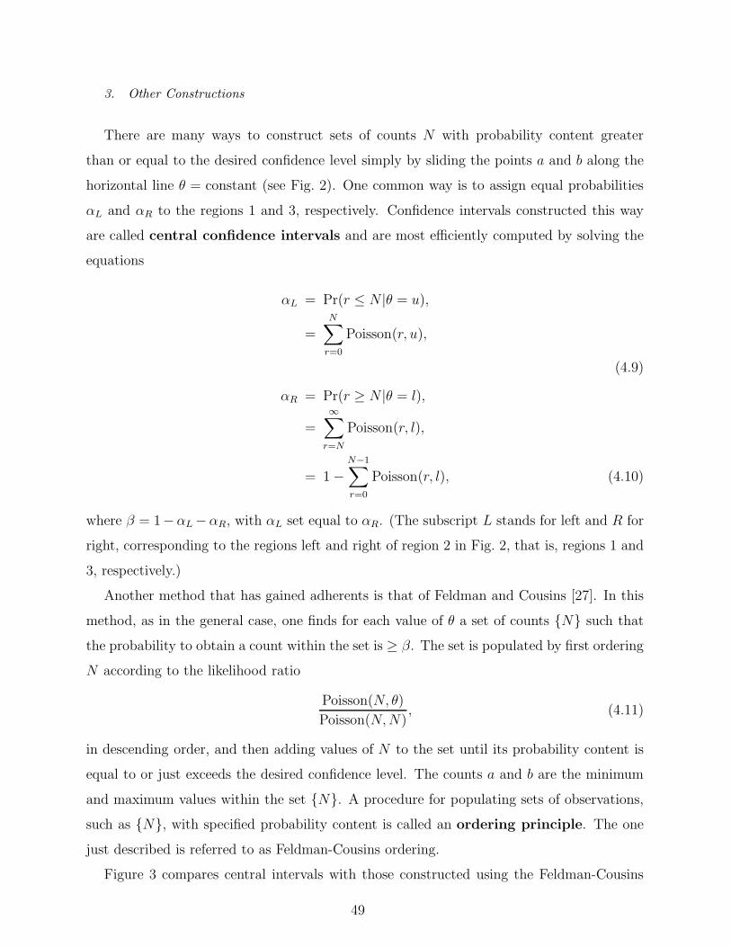
3. Other Constructions
There are many ways to construct sets of counts N with probability content greater
than or equal to the desired confidence level simply by sliding the points a and b along the
horizontal line θ = constant (see Fig. 2). One common way is to assign equal probabilities
αL and αR to the regions 1 and 3, respectively. Confidence intervals constructed this way
are called central confidence intervals and are most efficiently computed by solving the
equations
αL = Pr(r ≤ N |θ = u),
=N
∑
r=0
Poisson(r, u),
(4.9)
αR = Pr(r ≥ N |θ = l),
=∞
∑
r=N
Poisson(r, l),
= 1 −N−1∑
r=0
Poisson(r, l), (4.10)
where β = 1−αL −αR, with αL set equal to αR. (The subscript L stands for left and R for
right, corresponding to the regions left and right of region 2 in Fig. 2, that is, regions 1 and
3, respectively.)
Another method that has gained adherents is that of Feldman and Cousins [27]. In this
method, as in the general case, one finds for each value of θ a set of counts N such that
the probability to obtain a count within the set is ≥ β. The set is populated by first ordering
N according to the likelihood ratio
Poisson(N, θ)
Poisson(N, N), (4.11)
in descending order, and then adding values of N to the set until its probability content is
equal to or just exceeds the desired confidence level. The counts a and b are the minimum
and maximum values within the set N. A procedure for populating sets of observations,
such as N, with specified probability content is called an ordering principle. The one
just described is referred to as Feldman-Cousins ordering.
Figure 3 compares central intervals with those constructed using the Feldman-Cousins
49
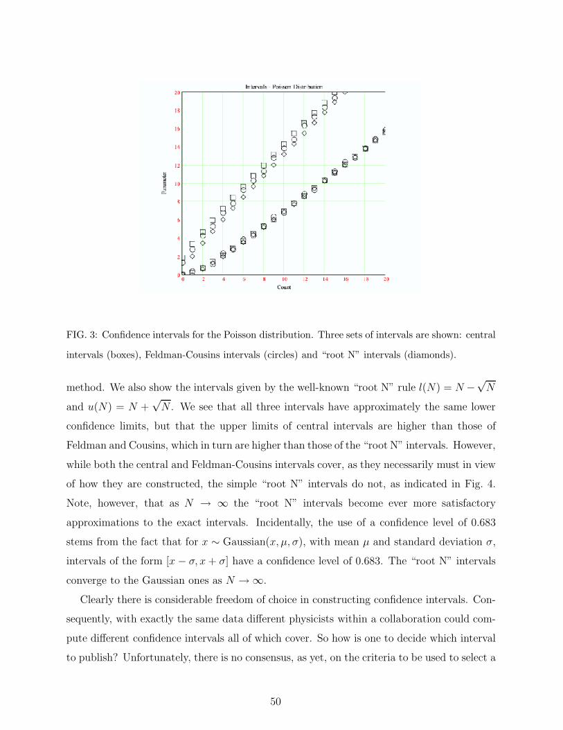
FIG. 3: Confidence intervals for the Poisson distribution. Three sets of intervals are shown: central
intervals (boxes), Feldman-Cousins intervals (circles) and “root N” intervals (diamonds).
method. We also show the intervals given by the well-known “root N” rule l(N) = N −√
N
and u(N) = N +√
N . We see that all three intervals have approximately the same lower
confidence limits, but that the upper limits of central intervals are higher than those of
Feldman and Cousins, which in turn are higher than those of the “root N” intervals. However,
while both the central and Feldman-Cousins intervals cover, as they necessarily must in view
of how they are constructed, the simple “root N” intervals do not, as indicated in Fig. 4.
Note, however, that as N → ∞ the “root N” intervals become ever more satisfactory
approximations to the exact intervals. Incidentally, the use of a confidence level of 0.683
stems from the fact that for x ∼ Gaussian(x, µ, σ), with mean µ and standard deviation σ,
intervals of the form [x − σ, x + σ] have a confidence level of 0.683. The “root N” intervals
converge to the Gaussian ones as N → ∞.
Clearly there is considerable freedom of choice in constructing confidence intervals. Con-
sequently, with exactly the same data different physicists within a collaboration could com-
pute different confidence intervals all of which cover. So how is one to decide which interval
to publish? Unfortunately, there is no consensus, as yet, on the criteria to be used to select a
50

FIG. 4: Coverage probability for three sets of Poisson confidence intervals, central (solid line),
Feldman-Cousins (dashed line) and “root N” (dot-dashed line), as a function of the parameter θ.
By construction the central and Feldman-Cousins intervals cover, whereas the simple “root N”
ones do not.
set of confidence intervals from the (infinite) set of possibilities. The only non-controversial
advice that can be given is this: in a publication explain precisely what you have done!
Acknowledgements
I wish to thank Prof. Suman Beri for hosting such a memorable, and enjoyable, school as
well as all the students who, with their youthful enthusiasm, made it so worthwhile.
[1] H. Jeffreys, Theory of Probability, 3rd edition, Oxford University Press (1961).
[2] S. K. Chatterjee, Statistical Thought: A Perspective and History, Oxford University Press
(2003).
[3] L. Daston, How Probability Came To Be Objective And Subjective, Hist. Math. 21, 330
51

(1994).
[4] S. E. Fienberg and D. V. Hinkley, eds., R.A. Fisher: An Appreciation, Lecture Notes on Statis-
tics, Volume 1, Springer Verlag (1990); W. T. Eadie et al., Statistical Methods in Experimental
Physics, North Holland (1971); G. Cowan, Statistical Data Analysis, Oxford (1998); A. Stuart
and K. Ord, Kendall’s Advanced Theory of Statistics, Volume 1: Distribution Theory, Edward
Arnold (1994); R. J. Barlow, Statistics: A Guide To The Use Of Statistical Methods In The
Physical Sciences, The Manchester Physics Series, John Wiley and Sons, New York (1989).
[5] For a lucid discussion of this point see chapter VII of Ref. [1].
[6] R. D. Cousins, Why Isn’t Every Physicist A Bayesian?, Am. J. Phys. 63, 398 (1995).
[7] R. T. Cox, Probability, Frequency, and Reasonable Expectation, Am. J. Phys. 14, 1 (1946).
[8] B. de Finetti, Theory of Probability, 2 Volumes, translated by A. Machi and A. Smith, Wiley
(1974).
[9] G. E. P. Box and G. C. Tiao, Bayesian Inference In Statistical Analysis, John Wiley and
Sons, New York (1992); A. Gelman et al., Bayesian Data Analysis, Chapman and Hall (1995);
M. Tanner, Tools for Statistical Inference, Springer (1996); A. O’Hagan, Kendall’s Advanced
Theory of Statistics, Volume 2B: Bayesian Inference, Oxford (1994).
[10] E. T. Jaynes and L. Bretthorst, Probability Theory, the Logic of Science, Oxford, 2003;
http://omega.math.albany.edu:8008/JaynesBook.html.
[11] O. Helene, Errors in Experiments With Small Number of Events, Nucl. Instr. and Meth.
A228, 120 (1984).
[12] H.B. Prosper, A Bayesian analysis of experiments with small numbers of events, Nucl. Instr.
and Meth. A241, 236 (1985).
[13] H. B. Prosper, Small Signal Analysis In High-Energy Physics: A Bayesian Approach, Phys.
Rev. D37, 1153 (1988).
[14] M. Whalley, L. Lyons, Proceedings of the Conference on Advanced Statistical Techiques in
Particle Physics, eds., March 18-22, 2002, IPPP/02/39, and
http://www.ippp.dur.ac.uk/Workshops/02/statistics.
[15] D. Heath and W. Sudderth, de Finetti’s Theorem on Exchangeable Variables, Am. Stat. 30
(4), 188 (1976).
[16] C. M. Caves, C. A. Fuchs and R. Schack, The Quantum de Finetti Representation, J. Math.
Phys. 43 (9), 4537 (2002).
52
[17] H. B. Prosper, The Distribution Of The Difference Of Two Poisson Variates, Nucl. Instr.
Meth. A238, 500 (1985).
[18] The symbol “∼” (in this context) means is distributed according to.
[19] D. T. Gillespie, A Theorem For Physicists In The Theory Of Random Variables, Am. J. Phys.
51, 520 (1983).
[20] H. B. Prosper, On Estimating Mean Lifetimes By A Weighted Sum Of Lifetime Measurements,
Phys. Rev. D36, 2047 (1987).
[21] See, for example, Lecture 6 of the SLUO Lectures by Roger Barlow;
http://www.hep.man.ac.uk/u/roger.
[22] A. Birnbaum, On the foundations of statistial inference, J. Amer. Statist. Ass. 65, 402 (1962).
[23] R. Barlow, J. Comp. Phys. 72, 202 (1987).
[24] D. W. Ruck et al., IEEE Trans. Neural Networks 4, 296 (1990); E. A. Wan, IEEE Trans.
Neural Networks 4, 303 (1990); E. K. Blum and L. K. Li, Neural Networks 4, 511 (1991).
[25] R. E. Kass and L. Wasserman, The Selection of Prior Distributions by Formal Rules, J. Amer.
Statist. Ass. 91, 1343 (1996). E. T. Jaynes, Prior Probabilities, IEEE Trans. Syst. Sci. Cybern.
SSC-4, 227 (1968).
[26] J. Neyman, Outline of a Theory of Statistical Estimation Based on the Classical Theory of
Probability, Phil. Trans. R. Soc. London A236, 333 (1937).
[27] G. J. Feldman and R. D. Cousins, Unified approach to the classical statistical analysis of small
signals, Phys. Rev. D57, 3873 (1998).
53


![, R. Ali Vanderveld arXiv:1008.4112v1 [astro-ph.IM] 24 …web.ipac.caltech.edu/staff/fmasci/home/astro_refs/sim_image2010.pdf · Those required rou- ... dition, exploiting the full](https://img.pdfslide.net/doc/110x75/5b84a5487f8b9aec488ca343/-r-ali-vanderveld-arxiv10084112v1-astro-phim-24-webipac-those-required.jpg)