Linear viscoelastic behavior

1. The constitutive equation depends on load history.

2. Diagnostic testing for time dependence.3. Mechanical models.4. Mechanical memory.5. The Boltzmann equation.6. Weeping memory of cartilage.

Harvard-MIT Division of Health Sciences and TechnologyHST.523J: Cell-Matrix MechanicsProf. Ioannis Yannas

1. The constitutive equation depends on the load history.

Time-dependent behavior of tissues

•Weak time dependence of mechanical behavior in tendon, ligaments and bone. Stronger time dependence in skin, and cartilage.

•Can one still use elastic theory anyway or is the predicted behavior going to be grossly wrong?

•Need a diagnostic test for time dependence: Elastic or viscoelastic?

Study of torsional displacement of skin in vivo

Photo removed for copyright reasons.

Barbenel et al.

Stress relaxation of skin: twist skin and measure resulting time-dependent torque

Diagrams removed for copyright reasons.

disc and guard ring

Torque relaxationfrom each displace-ment cycle

Barbenel et al.

Graph “Stress relaxation behavior of skin…”removed for copyright reasons.

Barbenel et al.

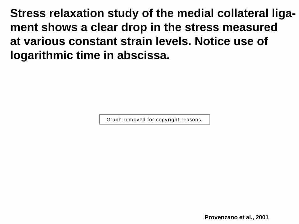
Stress relaxation study of the medial collateral liga-ment shows a clear drop in the stress measured at various constant strain levels. Notice use of logarithmic time in abscissa.

Graph removed for copyright reasons.

Provenzano et al., 2001

Stress relaxation at constant strain

• Test sequence: Suddenly apply a simpledeformation and measure the time-dependent relaxation in the stress.

• Tensor notation typically not required for the simple stress fields used in testing. Below apply εx(t) = ε (t) and measure σx(t) = σ(t.

• Strain applied suddenly to a constant level ε0. Use the Heaviside function to describe “switching on” or “off” of the strain.

H(t) = 0 at t < 0 and H(t) = 1 at t ≥ 0.• Strain “history” shows what happened to

the strain: ε(t) = ε0H(t).

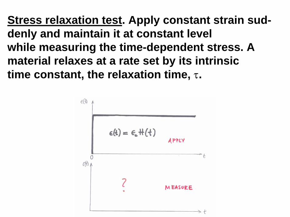
Stress relaxation test. Apply constant strain sud-denly and maintain it at constant level while measuring the time-dependent stress. A material relaxes at a rate set by its intrinsic time constant, the relaxation time, τ.

Three classes of materials described below. Elastic solids “never” relax (τ → ∞). Viscoelastic bodies relax during the (arbitrary) experimental timescale, t (τ = intermed.). Viscous liquids relax “very fast” (τ → 0). Use dimensionless (t/τ) to diagnose “rheological” (flow) state of unknown material.

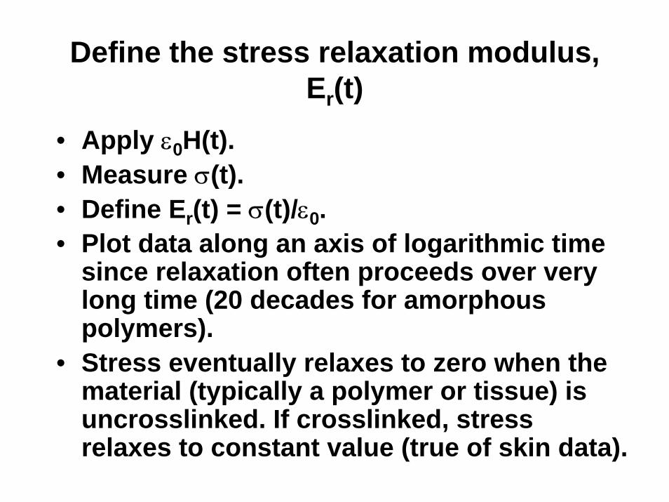
Define the stress relaxation modulus, Er(t)

• Apply ε0H(t).• Measure σ(t).• Define Er(t) = σ(t)/ε0.• Plot data along an axis of logarithmic time

since relaxation often proceeds over very long time (20 decades for amorphous polymers).

• Stress eventually relaxes to zero when the material (typically a polymer or tissue) is uncrosslinked. If crosslinked, stress relaxes to constant value (true of skin data).

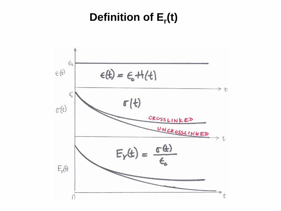
Definition of Er(t)

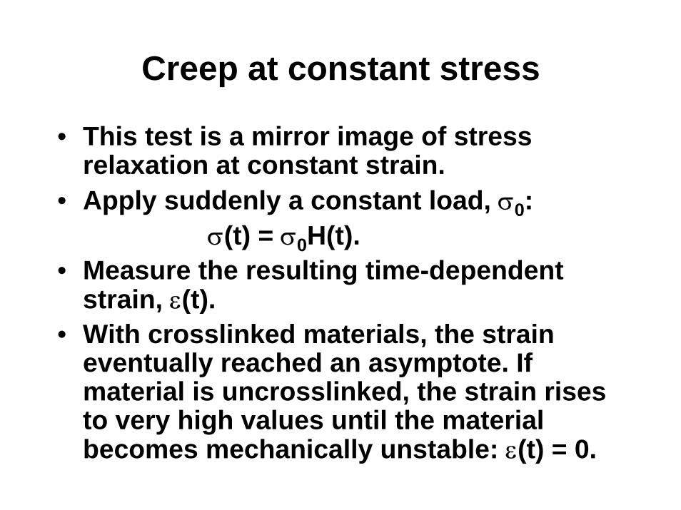
Creep at constant stress

• This test is a mirror image of stress relaxation at constant strain.

• Apply suddenly a constant load, σ0: σ(t) = σ0H(t).

• Measure the resulting time-dependent strain, ε(t).

• With crosslinked materials, the strain eventually reached an asymptote. If material is uncrosslinked, the strain rises to very high values until the material becomes mechanically unstable: ε(t) = 0.

Define the creep compliance: Dc(t) = ε(t)/σ0

σ(t) = σ0H(t)

The uterine cervix before, during and after parturition (childbirth)

• To be born, the fetus must pass through the cervix, a canal made up of rather stiff tissues, that hardly allows easy passage of the head (the largest obstacle to easy passage).

• During parturition, the cervix undergoes a dramatic change in its mechanical behavior, the result of degradation of the stiff collagen fiber network. It changes from a solid to a liquid viscoelastic tissue, similar to that undergone when a crosslinked polymer network becomes degraded.

Uterine cervix. Deformation following application of constant load (rat).During parturition (birth process)cylindricalcervix can deformindefinitely due to reversibleloss of crosslinking

From Harkness and Harkness

deformation

during parturition

Graph removed for copyright reasons.

after

before

time

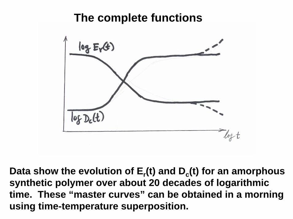
The complete functions

Data show the evolution of Er(t) and Dc(t) for an amorphous synthetic polymer over about 20 decades of logarithmic time. These “master curves” can be obtained in a morning using time-temperature superposition.

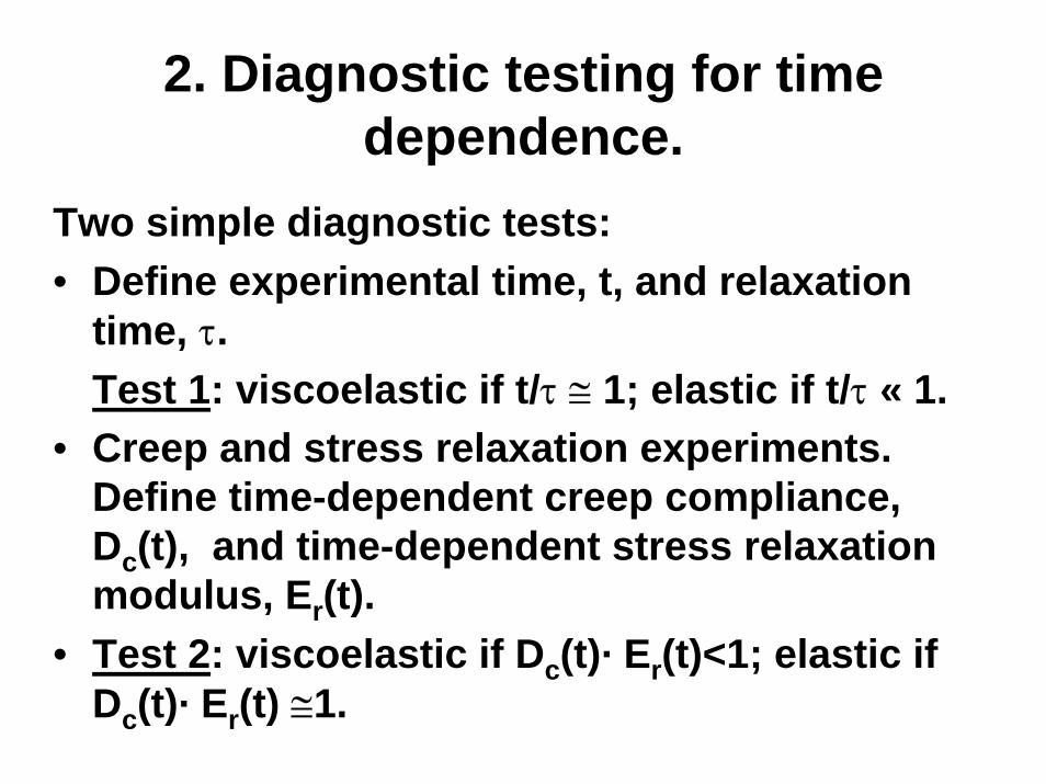
2. Diagnostic testing for time dependence.

Two simple diagnostic tests:• Define experimental time, t, and relaxation

time, τ.Test 1: viscoelastic if t/τ ≅ 1; elastic if t/τ « 1.

• Creep and stress relaxation experiments. Define time-dependent creep compliance, Dc(t), and time-dependent stress relaxation modulus, Er(t).

• Test 2: viscoelastic if Dc(t)· Er(t)<1; elastic if Dc(t)· Er(t) ≅1.

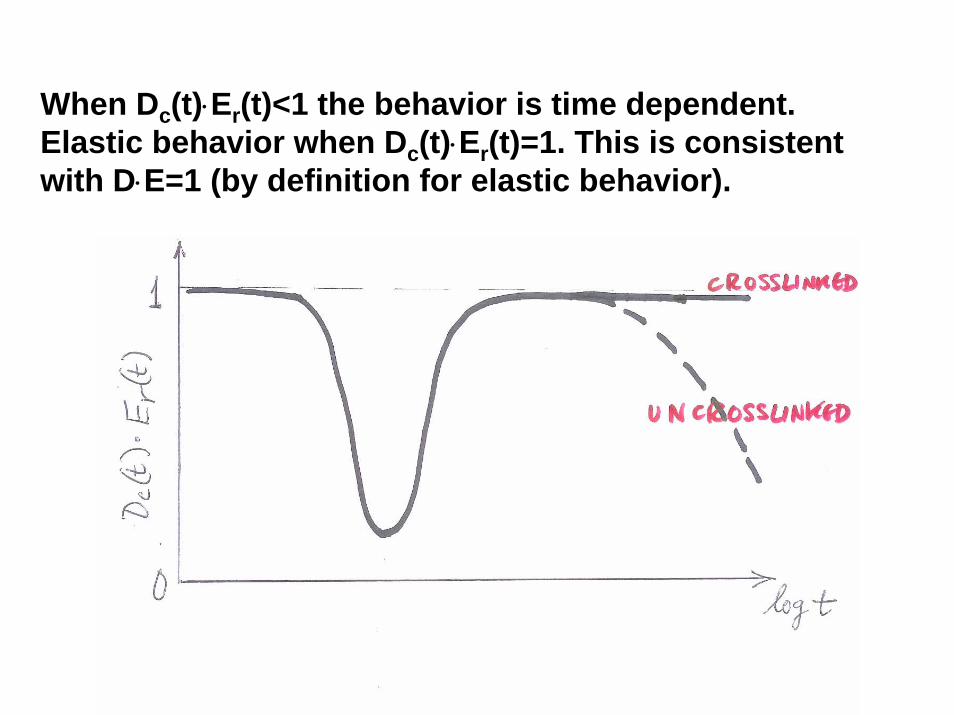
When Dc(t)⋅Er(t)<1 the behavior is time dependent. Elastic behavior when Dc(t)⋅Er(t)=1. This is consistent with D⋅E=1 (by definition for elastic behavior).

3. Mechanical models of viscoelastic behavior.

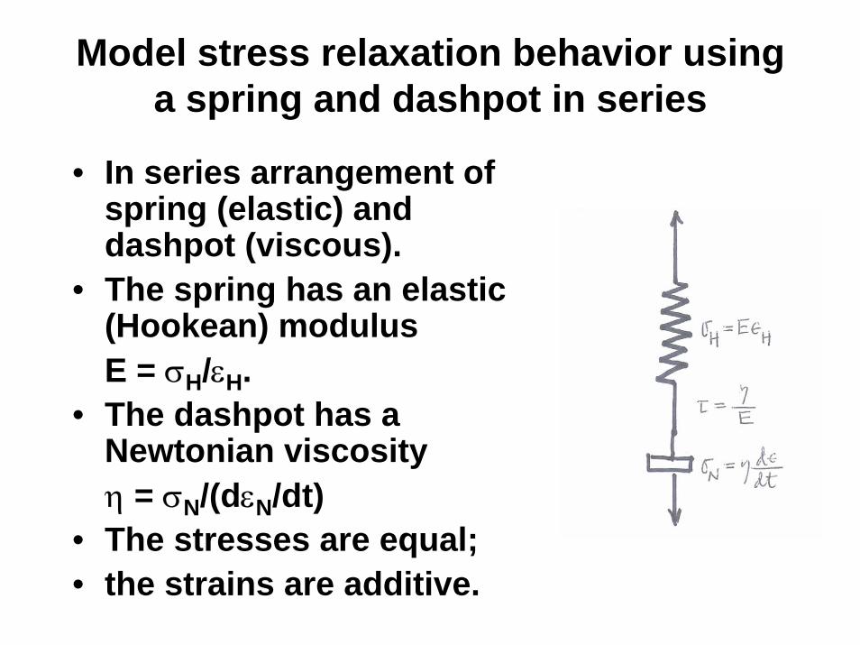
Model stress relaxation behavior using a spring and dashpot in series

• In series arrangement of spring (elastic) and dashpot (viscous).

• The spring has an elastic (Hookean) modulus E = σH/εH.

• The dashpot has a Newtonian viscosity η = σN/(dεN/dt)

• The stresses are equal; • the strains are additive.

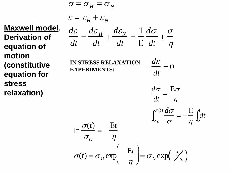
σ = σ H = σ N

ε = εH + εN

dεdt

=dε H

dt+

dεN

dt=

1Ε

dσdt

+ση

Maxwell model.Derivation ofequation of motion (constitutive equation for stress relaxation)

IN STRESS RELAXATION EXPERIMENTS:

dεdt

= 0

dσdt

= Εση

dσσσ O

σ (t )

∫ = −Εη

dto

t

∫ln

σ(t)σO

= −Εtη

σ(t) = σ O exp − Εtη

⎛

⎝ ⎜ ⎜

⎞

⎠ ⎟ ⎟ = σ O exp −t

τ( )

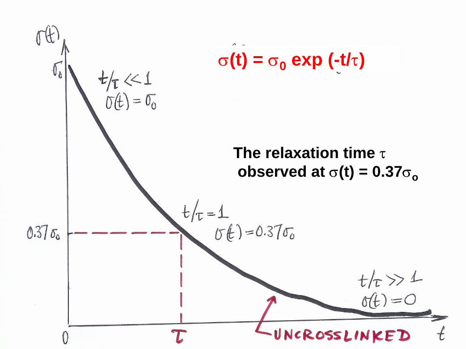
The relaxation time τobserved at σ(t) = 0.37σo

σ(t) = σ0 exp (-t/τ)

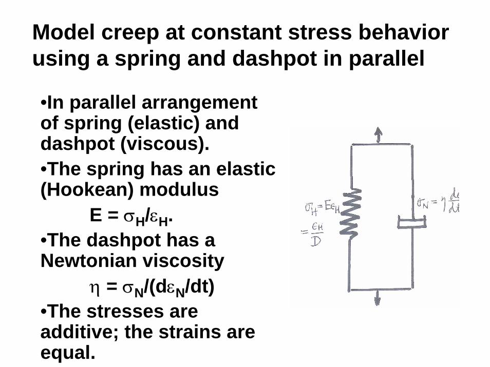
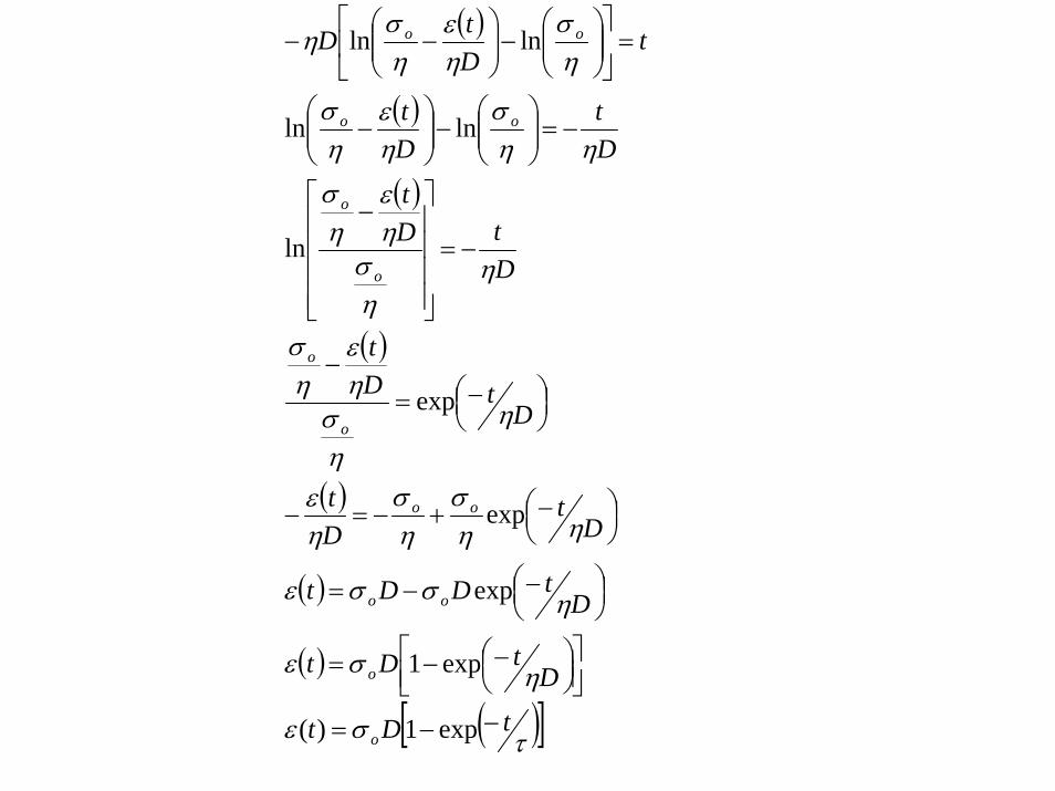
Model creep at constant stress behavior using a spring and dashpot in parallel

•In parallel arrangement of spring (elastic) and dashpot (viscous).•The spring has an elastic (Hookean) modulus

E = σH/εH.•The dashpot has a Newtonian viscosity

η = σN/(dεN/dt)•The stresses are additive; the strains are equal.

σ = σ H + σ N

ε = εH = εN

σ(t) = σ O

σO =εH

D+η

dεΗ

dt=

εD

+ ηdεdt

dεdt

=σO

η−

εηD

dε = σO

ηdt − ε

ηDdt = σO

η− ε

ηD

⎛

⎝ ⎜ ⎜

⎞

⎠ ⎟ ⎟ dt

dεσ O

η− ε

ηD

= dt

dΕ

σO

η− Ε

ηDO

ε ( t )

∫ = dtO

t

∫

INTEGRAL OF FORM

Kelvin-Voigt model.Derivation ofequation of motion (constitutive equation for creep at constantstress)

dxa − bx∫ = −

1b

ln a − bx( )

dxa − bx∫ = −

1b

ln a − bx( )INTEGRAL OF FORM

−ηD ln(σO

η−

εηD

)⎡

⎣ ⎢ ⎢

⎤

⎦ ⎥ ⎥

O

ε t( )

= t[ ]ot

−ηD lnσO

η−

ε(t)ηD

⎛

⎝ ⎜ ⎜

⎞

⎠ ⎟ ⎟ +ηD ln

σ O

η− O

⎛

⎝ ⎜ ⎜

⎞

⎠ ⎟ ⎟ = t

( )

( )

( )

( )

( )

( )

( )

( )[ ]τσε

ησε

ησσε

ηησ

ησ

ηε

ηησ

ηε

ησ

ηησ

ηε

ησ

ηησ

ηε

ησ

ησ

ηε

ηση

tDt

DtDt

DtDDt

Dt

Dt

DtD

t

DtD

t

Dt

Dt

tDtD

o

o

oo

oo

o

o

o

o

oo

oo

−−=

⎥⎦⎤

⎢⎣⎡ ⎟

⎠⎞⎜

⎝⎛−−=

⎟⎠⎞⎜

⎝⎛−−=

⎟⎠⎞⎜

⎝⎛−+−=−

⎟⎠⎞⎜

⎝⎛−=

−

−=

⎥⎥⎥⎥

⎦

⎤

⎢⎢⎢⎢

⎣

⎡ −

−=⎟⎟⎠

⎞⎜⎜⎝

⎛−⎟⎟

⎠

⎞⎜⎜⎝

⎛−

=⎥⎦

⎤⎢⎣

⎡⎟⎟⎠

⎞⎜⎜⎝

⎛−⎟⎟

⎠

⎞⎜⎜⎝

⎛−−

exp1)(

exp1

exp

exp

exp

ln

lnln

lnln

The retardation time τobserved at ε(t) = 0.63σoD

ε(t) = σ0D[1 - exp (-t/τ)]

4. Mechanical memory.

Mechanical memory of tissues• Do tissues recover their original shape when released

from a load? Find out by developing a general criterion for mechanical memory.

• The constitutive equation for a linear viscoelasticbody is written as an nth order, linear differential equation with constant coefficients.

• The related homogeneous equation is obtained by setting the stress and all its derivatives equal to zero, corresponding to sudden release of the load. (Roots of the characteristic equation. Poles.)

• A linear viscoelastic body recovers completely following removal of the load if the general solution of the homogeneous equation approaches zero as time becomes very long.

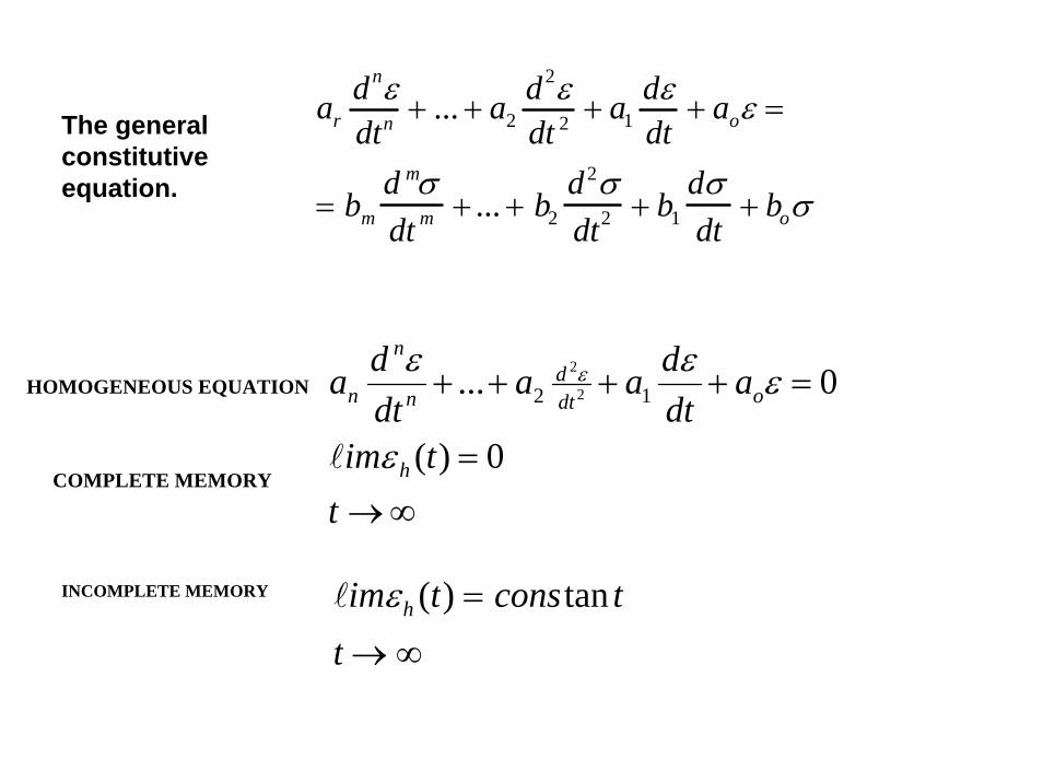
ardnεdtn + ... + a2

d2εdt 2 + a1

dεdt

+ aoε =

= bmd mσdt m + ... + b2

d2σdt2 + b1

dσdt

+ boσ

The general constitutive equation.

HOMOGENEOUS EQUATION

∞→=

=++++

ttim

adtdaa

dtda

h

odtd

n

n

n

0)(

0... 12 2

2

ε

εεε ε

lCOMPLETE MEMORY

limεh (t) = cons tan tt → ∞

INCOMPLETE MEMORY

Diagnostic tests for rheological behavior give information about memory

• Use an imaginary or real Instron machine to identify the rheological nature of an unknown body. Is it a solid? a liquid? How rapidly does it relax?

• Stretch the body at constant extension rate, dε/dt = ε• = constant. For example, the specimen of a rigid plastic may be stretched at 12 inches (1 foot) per sec., about the rate at which we often stretch specimens in our hands.

• The shape of the resulting stress-strain curve gives out the identity of the unknown.

Diagnostic tests for rheological behavior

An elastic solid is a Hookean spring withσ = Eε

A Newtonian viscous liquid with σ = Eε•

NB. Liquid supports only shear stress, τ. Symbol σ used here for uniformity of presentation.

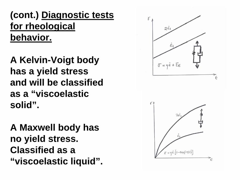
(cont.) Diagnostic tests for rheologicalbehavior.

A Kelvin-Voigt body has a yield stress and will be classified as a “viscoelasticsolid”.

A Maxwell body has no yield stress. Classified as a “viscoelastic liquid”.

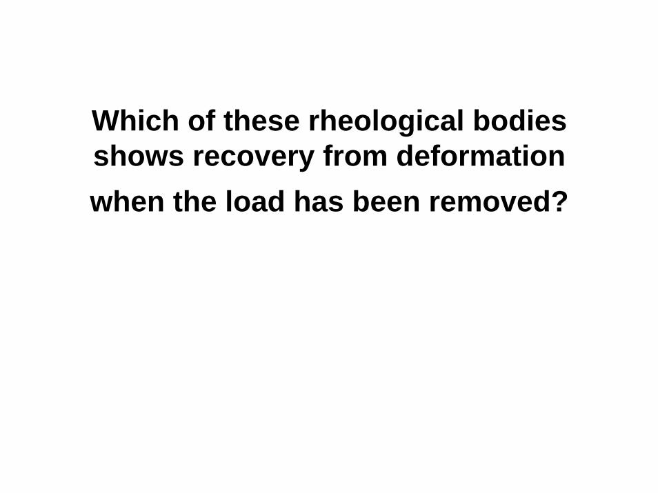
Which of these rheological bodies shows recovery from deformation when the load has been removed?

5. The Boltzmann equation(integral representation of the

constitutive equation)

Integral representation of constitutive equation

The linear differential equation (LDE) representation lacks a ”switching” function (that can turn stress or strain on and off rapidly) which is useful in description of stress and strain histories as well as many testing modes.

To incorporate a switching function use the integral representation (IE) of the constitutive equation. Derivation of the Boltzmann integral follows in 4 steps.

Step 1. Various mathematical switches that depend on use of the Heavisidefunction. These switches can be used to “cut-off” or start a function suddenlyat a desired time.

The Heaviside function

Step 2. Time invariance.

Dc(t) is a function of material structure. It does not vary with time of loading.

“creep and recovery”

Step 3. Additivity.The total strain following addition of a second load is the sum of the strains due to each load.

ε(t) = ε1(t) ± ε 2(t- t1) == σoDc(t) ± σoDc(t- t1) == σoD ± σoDc(t- t1)

Taken together, time invariance and additivitymake up the “linearity” of viscoelastic behavior.

Step 4. Generalizeand integrate.Add several stresses,

σo, σ1, σ2, etc., one after another, at respective times θo, θ1, θ2. Sum upstrains assuming linearity of viscoelasticbehavior (time invariance and additivity).Convert to incremental time intervals between each load addition, then integrate to getBoltzmann integral. This is the new constitutive equation we looked for.

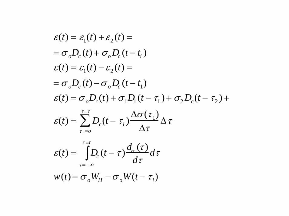
ε(t) = ε1(t) +ε2 (t) =

= σ oDc (t) + σo Dc (t − ti )ε(t) = ε1(t) −ε2 (t) =

= σ oDc (t) −σ o Dc (t − t1)ε(t) = σ oDc(t) +σ1D1 (t − τ1 ) + σ2 Dc(t − τ2 ) +

ε(t) = Dcτ i =o

τ = t

∑ (t − τ i )∆σ (τ1)

∆τ∆τ

ε(t) = Dcτ = −∞

τ =t

∫ (t − τ ) dσ (τ )dτ

dτ

w(t) = σ oWH −σ oW(t − τ i)

Compare the LDE to the IE representation

• Even though differing in its descriptive power from the LDE approach, the new constitutive equation, in the form of an integral equation, provides the same information about the material described as the LDE approach.

• In particular, the material functions are represented in LDE as n constants while being represented in IE as the “kernel” function of the integral, Dc(t).

6. The “weeping memory” of cartilage.

Application: Weeping of joint cartilage modeled in terms of linear

viscoelasticity•Joint (articular) cartilage “weeps” fluid and contracts in volume when loaded in uniaxialcompression (in the form of a specimen cut out of the intact cow tissue).•Following removal of the compressive load, the specimen reswells in the fluid that had been expressed and expands to its original volume. •Analyze data by Edwards and Maroudas et al. using a model of weeping cartilage as if the time-dependent deformation of a viscoelastic body and the mass of fluid expressed by weeping were mathematically identical variables.

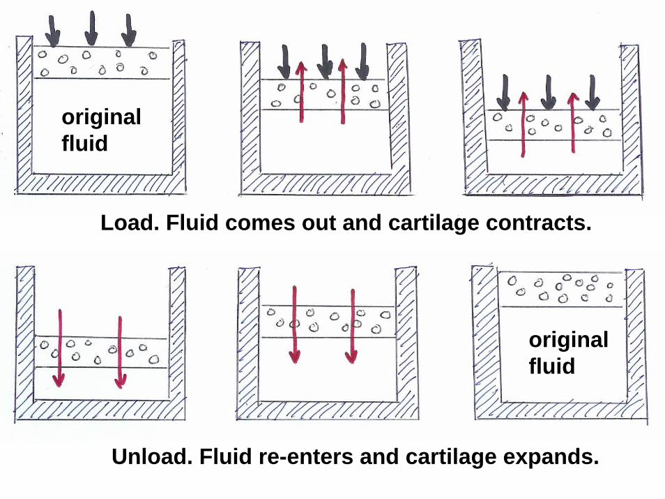
originalfluid

Load. Fluid comes out and cartilage contracts.

original fluid

Unload. Fluid re-enters and cartilage expands.

Analyze cartilage weeping andre-expansion

• The experimental data were obtained in the form of mass of fluid that came out following loading, or re-entered in following unloading, the cartilage specimen.

• Since loading of cartilage was accompanied by loss of mass a simple analysis of cartilage deformation as a linear viscoelastic “body” is not possible.

• Treat the two-step experiment as if it were a creep and recovery cycle. Use the mathematical symbolism of linear visco-elasticity to predict the kinetics of reswellingstep from knowledge of the weeping step.

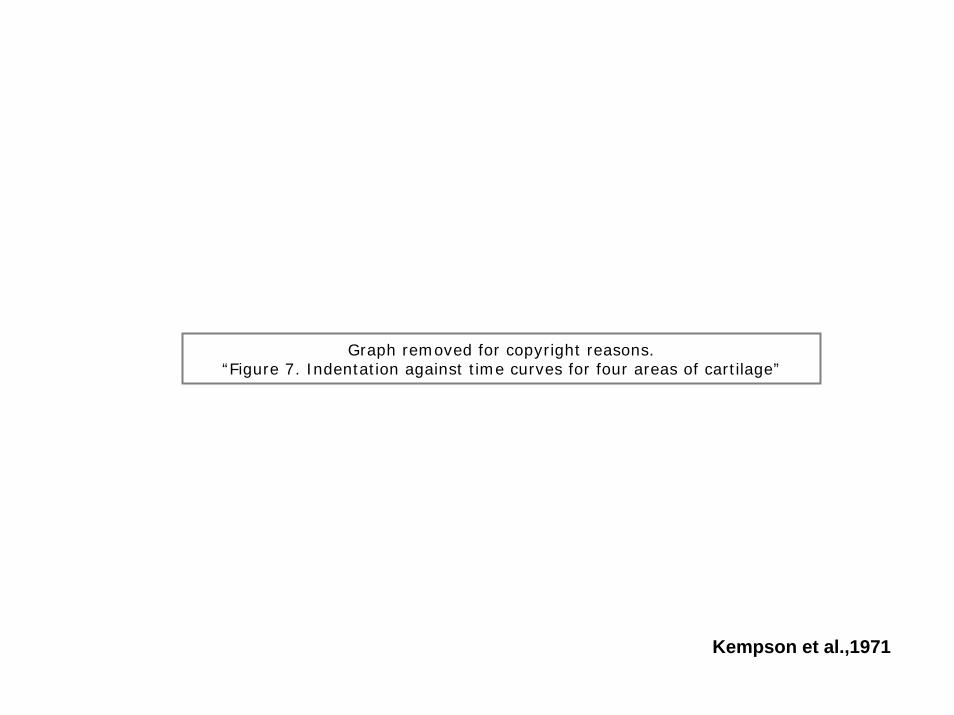
Graph removed for copyright reasons.“Figure 7. Indentation against time curves for four areas of cartilage”

Kempson et al.,1971

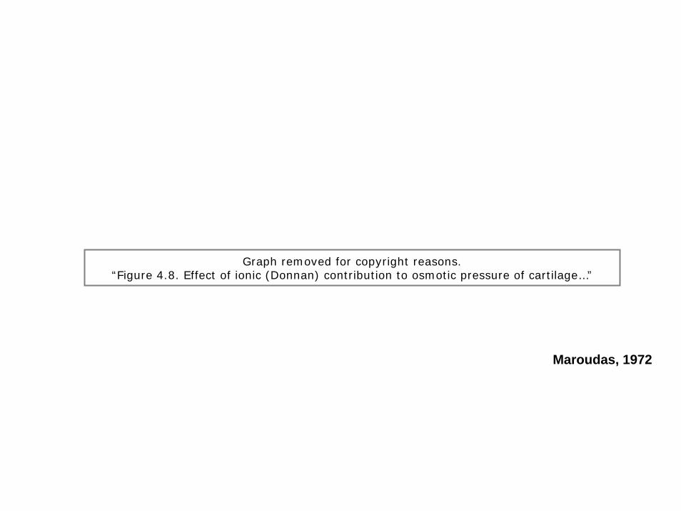
Graph removed for copyright reasons.“Figure 4.8. Effect of ionic (Donnan) contribution to osmotic pressure of cartilage…”

Maroudas, 1972

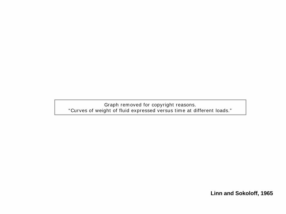
Graph removed for copyright reasons.“Curves of weight of fluid expressed versus time at different loads.”

Linn and Sokoloff, 1965

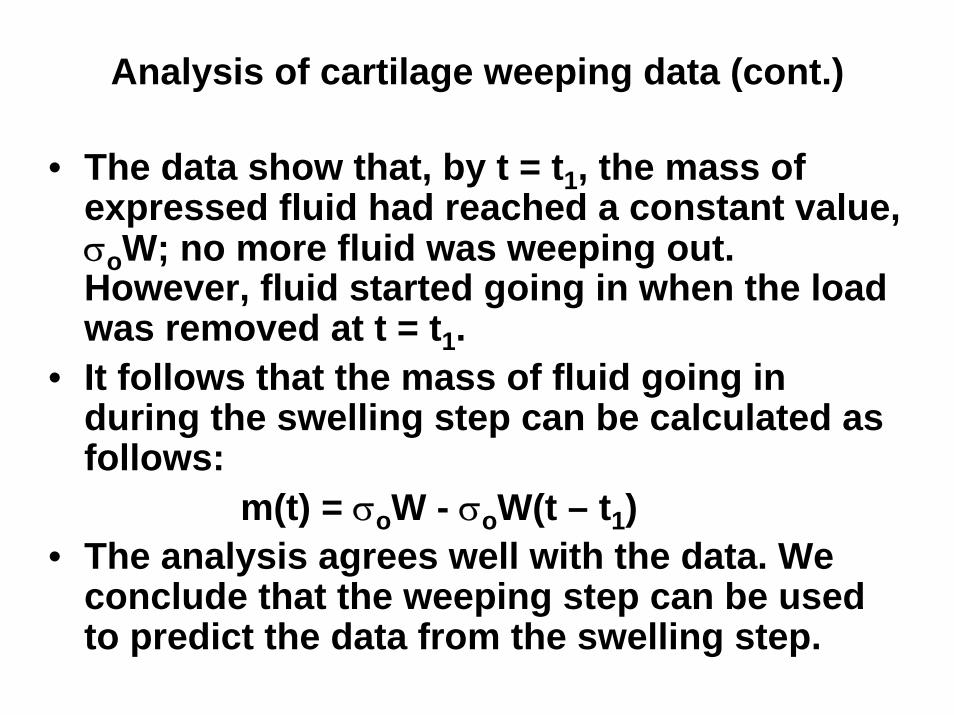
Analysis of cartilage weeping data (cont.)

• Define a new “weeping” function, W(t), as the ratio of time-dependent mass of fluid transferring in or out, m(t), and the constant stress, σo, acting on the specimen.

W(t) = m(t)/σo

• Make the following substitutions : Dc(t) → W(t) ε(t) → m(t)

• Assuming time invariance and additivity hold:m(t) = σoW(t) - σoW(t – t1)

Analysis of cartilage weeping data (cont.)

• The data show that, by t = t1, the mass of expressed fluid had reached a constant value, σoW; no more fluid was weeping out. However, fluid started going in when the load was removed at t = t1.

• It follows that the mass of fluid going in during the swelling step can be calculated as follows:

m(t) = σoW - σoW(t – t1)• The analysis agrees well with the data. We

conclude that the weeping step can be used to predict the data from the swelling step.

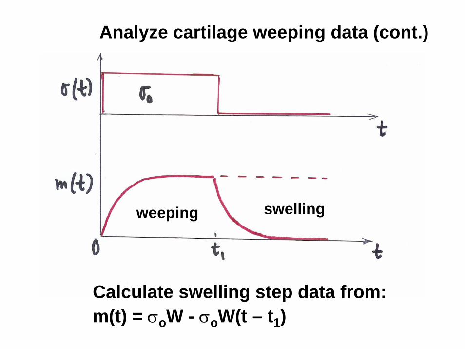
Analyze cartilage weeping data (cont.)

Calculate swelling step data from: m(t) = σoW - σoW(t – t1)

weeping swelling

Summary of linear viscoelastic theory

1. Time dependence is very common during deformation of many tissues. Linear elasticity theory is not useful for lengthy loading experiences. Theory of linear viscoelasticityfocuses on the history of strain or stress.2. Time dependent behavior simulated either using a differential equation or integral equation representation. 3. Viscoelastic behavior is simply modeled using differential equations describing spring-dashpot combinations. Stress relaxation and creep behavior are modeled. Mechanical memory is also modeled in this way.

Summary (cont.)

4. Diagnostic tests for failure of elasticity are developed.

5. Integral equation representation of the constitutive equation (Boltzmann equation) is useful when the stress or strain are being switched on or off suddenly.

6. The weeping behavior of cartilage can be well represented using an integral equation representation.