1

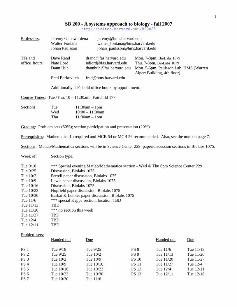
SB 200 - A systems approach to biology - fall 2007 http://isites.harvard.edu/k20028

Professors: Jeremy Gunawardena jeremy@hms.harvard.edu Walter Fontana walter_fontana@hms.harvard.edu Johan Paulsson johan_paulsson@hms.harvard.edu TFs and Dave Rand drand@fas.harvard.edu Mon. 7-8pm, BioLabs 1079 office hours: Nate Lord ndlord@fas.harvard.edu Thu. 7-8pm, BioLabs 1079 Dann Huh dannhuh@fas.harvard.edu Mon. 5-6pm, Paulsson Lab, HMS (Warren

Alpert Building, 4th floor) Fred Berkovitch fred@hms.harvard.edu

Additionally, TFs hold office hours by appointment. Course Times: Tue./Thu. 10 – 11:30am, Fairchild 177. Sections: Tue 11:30am – 1pm Wed 10:00 – 11:30am Thu 11:30am – 1pm Grading: Problem sets (80%); section participation and presentation (20%). Prerequisites: Mathematics 1b required and MCB 54 or MCB 56 recommended. Also, see the note on page 7. Sections: Matlab/Mathematica sections will be in Science Center 229; paper/discussion sections in Biolabs 1075. Week of: Section type:

Tue 9/18 *** Special evening Matlab/Mathematica section - Wed & Thu 6pm Science Center 229 Tue 9/25 Discussion, Biolabs 1075 Tue 10/2 Ferrell paper discussion, Biolabs 1075 Tue 10/9 Lewis paper discussion, Biolabs 1075 Tue 10/16 Discussion, Biolabs 1075 Tue 10/23 Hopfield paper discussion, Biolabs 1075 Tue 10/30 Barkai & Leibler paper discussion, Biolabs 1075 Tue 11/6 *** special Kappa section, location TBD Tue 11/13 TBD Tue 11/20 *** no section this week Tue 11/27 TBD Tue 12/4 TBD Tue 12/11 TBD Problem sets: Handed out Due

Handed out Due

PS 1 Tue 9/18 Tue 9/25 PS 8 Tue 11/6 Tue 11/13 PS 2 Tue 9/25 Tue 10/2 PS 9 Tue 11/13 Tue 11/20 PS 3 Tue 10/2 Tue 10/9 PS 10 Tue 11/20 Tue 11/27 PS 4 Tue 10/9 Tue 10/16 PS 11 Tue 11/27 Tue 12/4 PS 5 Tue 10/16 Tue 10/23 PS 12 Tue 12/4 Tue 12/11 PS 6 Tue 10/23 Tue 10/30 PS 13 Tue 12/11 Tue 12/18 PS 7 Tue 10/30 Tue 11/6

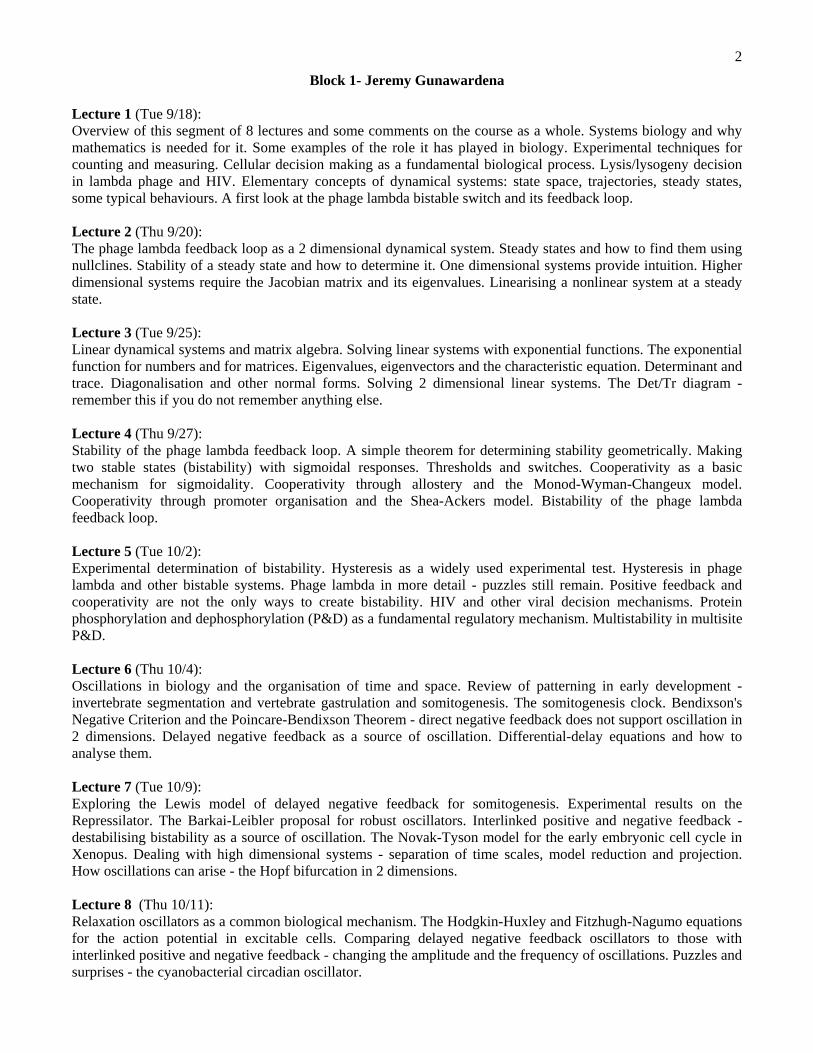
2Block 1- Jeremy Gunawardena

Lecture 1 (Tue 9/18): Overview of this segment of 8 lectures and some comments on the course as a whole. Systems biology and why mathematics is needed for it. Some examples of the role it has played in biology. Experimental techniques for counting and measuring. Cellular decision making as a fundamental biological process. Lysis/lysogeny decision in lambda phage and HIV. Elementary concepts of dynamical systems: state space, trajectories, steady states, some typical behaviours. A first look at the phage lambda bistable switch and its feedback loop. Lecture 2 (Thu 9/20): The phage lambda feedback loop as a 2 dimensional dynamical system. Steady states and how to find them using nullclines. Stability of a steady state and how to determine it. One dimensional systems provide intuition. Higher dimensional systems require the Jacobian matrix and its eigenvalues. Linearising a nonlinear system at a steady state. Lecture 3 (Tue 9/25): Linear dynamical systems and matrix algebra. Solving linear systems with exponential functions. The exponential function for numbers and for matrices. Eigenvalues, eigenvectors and the characteristic equation. Determinant and trace. Diagonalisation and other normal forms. Solving 2 dimensional linear systems. The Det/Tr diagram - remember this if you do not remember anything else. Lecture 4 (Thu 9/27): Stability of the phage lambda feedback loop. A simple theorem for determining stability geometrically. Making two stable states (bistability) with sigmoidal responses. Thresholds and switches. Cooperativity as a basic mechanism for sigmoidality. Cooperativity through allostery and the Monod-Wyman-Changeux model. Cooperativity through promoter organisation and the Shea-Ackers model. Bistability of the phage lambda feedback loop. Lecture 5 (Tue 10/2): Experimental determination of bistability. Hysteresis as a widely used experimental test. Hysteresis in phage lambda and other bistable systems. Phage lambda in more detail - puzzles still remain. Positive feedback and cooperativity are not the only ways to create bistability. HIV and other viral decision mechanisms. Protein phosphorylation and dephosphorylation (P&D) as a fundamental regulatory mechanism. Multistability in multisite P&D. Lecture 6 (Thu 10/4): Oscillations in biology and the organisation of time and space. Review of patterning in early development - invertebrate segmentation and vertebrate gastrulation and somitogenesis. The somitogenesis clock. Bendixson's Negative Criterion and the Poincare-Bendixson Theorem - direct negative feedback does not support oscillation in 2 dimensions. Delayed negative feedback as a source of oscillation. Differential-delay equations and how to analyse them. Lecture 7 (Tue 10/9): Exploring the Lewis model of delayed negative feedback for somitogenesis. Experimental results on the Repressilator. The Barkai-Leibler proposal for robust oscillators. Interlinked positive and negative feedback - destabilising bistability as a source of oscillation. The Novak-Tyson model for the early embryonic cell cycle in Xenopus. Dealing with high dimensional systems - separation of time scales, model reduction and projection. How oscillations can arise - the Hopf bifurcation in 2 dimensions. Lecture 8 (Thu 10/11): Relaxation oscillators as a common biological mechanism. The Hodgkin-Huxley and Fitzhugh-Nagumo equations for the action potential in excitable cells. Comparing delayed negative feedback oscillators to those with interlinked positive and negative feedback - changing the amplitude and the frequency of oscillations. Puzzles and surprises - the cyanobacterial circadian oscillator.

3Block 2 - Walter Fontana

Statement of purpose We will pursue two aspects of intracellular dynamics (wherein we shall be concerned only with temporal – not spatial – aspects). One aspect emphasizes small network chunks – “motifs” – recognized as implementing distinct behaviors that are useful in understanding biological systems. In this view, a motif is akin to what an engineer would call a “device” – a dynamical system whose internal processes are decoupled from the states of the larger context in which the system is embedded. This underscores the modular composition of motifs into larger networks. The other aspect is concerned with large signaling networks characterized by vast numbers of possible states brought about by numerous post-translational modifications and complex formation. In addition, these networks appear oftentimes interwoven with other signaling systems through extensive sharing of components. Both aspects call for different modeling approaches. Jeremy’s prior segment on systems of differential equations will serve us well for the engineering perspective. We will carefully introduce a different approach apt to handle large and complex systems that underlie cellular decision processes. A stochastic element is built into the latter approach and provides a natural transition to Johan’s final segment on the in-depth treatment of stochastic processes. Lecture 9 (Tue 10/16): Thermodynamic primitives:

• The difference between thermodynamic equilibrium and (non-equilibrium) steady-state. • The “value” of an ATP molecule depends on how far from equilibrium its hydrolysis reaction is within a

given system; single molecules versus populations of molecules. • The equilibrium constant is a thermodynamic property, not a kinetic one – although it can be expressed in

terms of ratios of rate constants. Binding equilibria: Many events in biochemistry, molecular signaling, and the regulation of gene expression involve two steps: (1) the reversible binding of substrates or ligands to an enzyme and (2) a subsequent irreversible reaction in which the enzyme modifies the substrate(s). If the binding equilibrium is fast, it will determine the speed of the reaction. Different types of binding equilibria lead to different functional forms for the reaction velocity, such as a hyperbola (Michaelis-Menten), a shifted hyperbola (thresholds), or a sigmoid (Hill-function). Modelers often simplify molecular systems by lumping together several “elementary” reactions into one “overall reaction”, whose velocity as a function of substrate concentration is typically assumed to be one of the types above.

• Understand how to describe ligand (or substrate) binding equilibria • Understand the combinatorics of binding equilibria; the difference between macroscopic and microscopic

rate constants • Understand the different types of saturation functions • Appreciate the assumptions behind these functions and the dangers of using them. • The expressions we derive also apply to steady-states for do/undo loops catalyzed by different enzymes

(such as a kinase and phosphatase), not just bind/unbind equilibria. Though chemically (and thermodynamically) very different, they are mathematically the same thing!

4Lecture 10 (Thu 10/18): Do/Undo loops consist of a modification reaction (such as a phosphorylation) performed on a target substrate T (often itself a protein) by enzyme A and a demodification reaction (such as a dephosphorylation) reaction performed by enzyme B. This simple scheme has several interesting properties, which we shall explore in this lecture on the Goldbeter-Koshland (GK) loop: a “hydrogen atom” of molecular control

• Set up the kinetic rate equations of GK and understand what is the “input” (the ratio of enzyme A to enzyme B) and what the “output” (the fraction of modified target T in steady-state)

• Discuss variations of the scheme throughout cellular processes (GEF/GAP, G proteins, etc.); point to other schemes that we shall build from the GK loop (“in series” (multisite phosphorylation), “in parallel” (MAP kinase cascades), and with feedback (Lisman switch)

• Discuss the analytical solution of GK and point out that the input/output relationship depends critically on the amount of substrate T in the system. Discuss two very differently behaving regimes: both arms unsaturated with T (hyperbolic dependence of output on input) and both arms saturated with T(“switch”-like dependence of output on input)

• The case in which one arm is saturated but not the other leads to a behavior in which the output is independent of the total amount of target substrate T (at steady-state):

o perfect adaptation of the system to concentration changes of T. This is one design principle of chemotaxis.

o Clarify the difference between adaptation and a homeostat. Lecture 11 (Tue 10/23): Introduction to bacterial chemotaxis: a complete small control circuit.

• Characterize physics at low Reynolds numbers • Introduce the molecular parts list and layout of the circuitry • The empirical facts about the behavior of this circuit • What about the circuit behavior needs explaining? The simultaneous

o desensitization to signal background, aka precise adaptation o and maintenance of sensitivity to changes in signal intensity.

• Discuss the Barkai-Leibler (BL) model of precise adaptation. • Convey the gist of the BL model by simplifying it to the GK loop with one-sided saturation (Lecture 2). • Use the BL example to briefly discuss the robustness of a dynamical behavior to changes in parameters.

Address the relationship between “robustness” to parameter variations and “stability” to perturbations in concentration variables.

Step back and point out that chemotaxis of eukaryotic cells is executed in a different manner (“crawling” by cytoskeletal rearrangements). Yet, despite differences in the parts list and the mode of locomotion, the eukaryotic control circuitry seems to implement the same abstract principles as the bacterial case.

5Lecture 12 (Thu 10/25): Decorations of the GK loop Expand the GK loop and transfer the lessons learned in Lecture 1 to steady-states of

• GK “in parallel”: multisite phosphorylation • GK “in series”: cascade architectures

Adding a feedback to the versatile GK loop generates a simple bistable circuit (the Lisman model).

• Review and discuss the concept of bistability in the Lisman model (referring back to Jeremy’s segment). The feed-forward motif

• Strategies for motif detection in networks • Discuss and analyze the

o coherent feed-forward motif (coincidence detection) o incoherent feed-forward motif (acceleration to steady-state)

Lecture 13 (Tue 10/30): The main purpose of this lecture is to make the transition from small networks (motifs) to large networks. It is as much a conceptual as it is a technical transition. Large networks

• Biological significance of signaling: signal processing (e.g. chemotaxis) vs decision-making (e.g. apoptosis)

• Short catalog of experimental techniques in proteomics • Static properties of large networks

o powerlaw statistics o hubs and small worlds

Transition: The changing nature of models (and modeling) from physics to biology

• The challenge of modeling large networks: Two axes of evil - state combinatorics and multiple scales • The need of agent/rule-based approaches: A comparison to ordinary differential equations • Modeling versus encoding

o The dangers of overfitting by using small network motifs and rate constants as a “programming language”

The rule-based representation of molecular interactions with Kappa This will be hands-on, interleaving the presentation of concepts with KappaFactory demos.

� Agents and their interfaces � Elementary interactions: post-translational modifications and binding � Rules as transformation patterns (in complete analogy to chemical reactions in organic chemistry)

o Context-freeness � The “Don’t care, don’t write” principle � Rules as executable knowledge � Rules and events

6Lecture 14 (Thu 11/1): Rule dynamics

� Concrete solutions transformed by repeated application of rules � A brief introduction to stochastic kinetics (Gillespie algorithm). This will be a short forward-pointer to

Johan’s segment. � The meaning of concurrency

o Traces (total order in time) and causality (partial order in time) Hands-on modeling of small networks previously discussed

� Multisite phosphorylation � Cascades

Lecture 15 (Tue 11/6): Connecting mechanism with behavior

� The resource-dependency of complex formation: self-assembly and the “prozone effect” o Scaffolds in signaling

New concepts in the analysis of rule-based representations of large networks

� Contact maps � Causality

o At the level of rules: (low- and high-resolution) influence maps o At the level of events: stories

� The concept of a “story” and the notion of pathway � The superposition of stories and influence maps

Lecture 16 (Thu 11/8): Putting it all together and applying it to a really big network

� EGF signaling o Receptor networks o Scaffolds o Cascades: Ras-Raf-MEK-ERK and PI3K-PIP2/3-PDK1-AKT o Feedback from ERK upstream and oscillations

7Block 3 - Johan Paulsson

The first three lectures in this block will introduce the methods needed to model stochastic kinetics, accompanied by simple toy models for chemical reactions. The following five lectures will then use the techniques to introduce general principles for stochastic cell biology, and illustrate them with specific examples. The last lecture summarizes the course and describes future challenges. Note: Students are expected to know averages, variances, density functions, distribution functions, probability distributions and the law of total probability. If you do not remember these parts, then please consult an introduction to probability or statistics (for an online version, the Wikipedia entries work fine).

Tue. November 13 – last day for graduate students to drop a course

Lecture 17 (Tue 11/13): Stochastic chemical events

• When are stochastic events relevant? • Memory-lacking exponential step • Formulate Markov processes • Formulate average behavior

Lecture 18 (Thu 11/15): Exact simulations and approximate moment equations

• The Doob-Gillespie algorithm • Stochastic-deterministic hybrid methods • Solving linear birth and death process • From Markov processes to moment equations

Lecture 19 (Tue 11/20): Understanding variances

• The Non-equilibrium Fluctuation Dissipation Theorem (FDT) • Sensitivities and lifetimes • FDT in terms of physical observables • Solving the FDT for one-variable processes

Thu. November 22 – Thanksgiving – no class

Lecture 20 (Tue 11/27): Stable dynamics: Disorder in gene expression

• mRNA-protein example • Bursts • Dual reporters • Experiments

8

Lecture 21 (Thu 11/29): Neutrally stable dynamics: Metabolism and microtubules

• Efficiency vs fluctuations in anabolic reactions • Near-critical dynamics and negative correlations • Dynamic instability of microtubules • Near-neutral stochastic processes in biology

Lecture 22 (Tue 12/4): Increasing stability: transcriptional autorepression and replication control

• Direct vs indirect negative feedback • Strategies for sensitivity amplification • Frustration trade-offs • Hard physical limits in nonlinear systems

Lecture 23 (Thu 12/6): Unstable systems: the phage toggle switch and circadian rhythms

• Bistability vs bimodality (genetic toggle switch) • Level-crossing: Bimodality without bistability (chemotaxis) • Noisy limit cycles (circadian rhythms) • Noise in damped oscillations

Lecture 24 (Tue 12/11): Exotic stochastic effects: Replication control and gene expression

• Noise suppression by noise • Noise-induced bistability and limit cycles • Growing and dividing cells • Molecular memory

Lecture 25 (Thu 12/13): Review of stochastic principles and future directions

• Summary of techniques • Summary of concepts • Future theoretical challenges • Future experimental challenges