Embed Size (px)
Citation preview
Harvesting Choices and Timber Supply amongLandowners in the Southern United States
Daowei Zhang,1 Xing Sun,2 Brett J. Butler3 and Jeffrey P. Prestemon4
1Alumni and George Peak Jr. Professor of Forest Economics and Policy, School of Forestryand Wildlife Science, Auburn University, Auburn, AL 36849-5418 (phone: 334-844-1067;
fax: 334-844-1084; e-mail: [email protected]).2Assistant Professor, Institute of Finance and Economics Research, Shanghai University of
Finance and Economics, No. 777 Guoding Road, Shanghai, PR China, 200433(corresponding author: phone: +86 21-6590-3266; e-mail: [email protected]).
3Research Forester, U.S. Forest Service, 160 Holdsworth Way, Amherst, MA 01003 (phone:413-545-1387; e-mail: [email protected]).
4Project Leader, Forest Economics and Policy Research, Southern Research Station, USDAForest Service, PO Box 12254, 3041 Cornwallis Road, Research Triangle Park, NC 27709
(phone: 919-549-4033; fax: 919-549-4047; e-mail: [email protected]).
The recent rise of institutional timberland ownership has led to a significant change in the structure andconduct of the timber industry in the United States. In this study, we apply a two-period harvest model toassess the timber harvesting behavior of various landowners at the stand level by utilizing USDA ForestService Forest Inventory and Analysis data for nine southern states. Forest industry and institutionaltimberland owners were found to be more likely to conduct partial and final harvests than nonindustrialprivate forest landowners. Aggregately, Timberland Investment Management Organizations were foundto be most, and timberland Real Estate Investment Trusts to be least, price-responsive among ownershipgroups.
La hausse recente du nombre de proprietaires institutionnels de terrains forestiers exploitables a modifieconsiderablement la structure et la gestion de l’industrie du bois aux Etats-Unis. Dans le present article,nous avons applique, en utilisant des donnees tirees de la Forest Inventory Analysis (FIA) (Analyse del’inventaire forestier) du Service des forets des Etats-Unis dans neuf Etats du sud, un modele fonde surdeux periodes de recolte pour evaluer le comportement de divers proprietaires selon la periode de recoltedu bois. Selon les resultats de notre etude, l’industrie forestiere et les proprietaires institutionnels deterrains forestiers exploitables sont plus susceptibles d’effectuer des coupes partielles et totales que lesproprietaires non industriels de forets privees. Globalement, parmi les divers groupes de proprietaires,les organismes de gestion des placements dans les terrains forestiers exploitables (TIMO) sont lesplus sensibles aux prix, tandis que les societes de placement immobilier dans le secteur forestier sontles moins sensibles aux prix.
INTRODUCTION
Timberland ownership has changed dramatically in the United States in the two lastdecades (Zhang et al 2012). In particular, institutions now own most of the timberlandspreviously held by vertically integrated forest industry companies. These institutionalinvestors include two broad groups. The first is diverse and generally includes pen-sion funds, endowments, foundations, insurance companies, and family trusts (Binkley
Canadian Journal of Agricultural Economics 00 (2015) 1–21
DOI: 10.1111/cjag.12060
1
2 CANADIAN JOURNAL OF AGRICULTURAL ECONOMICS
et al 1996). This group alone is sometimes referred to institutional timberland owners inthe forestry literature. Often these institutions hire Timberland Investment ManagementOrganizations (TIMOs) to purchase timberlands on behalf of the institutions, managethe timberlands, and sell their timberlands within a specified investment period, usually5 to 15 years. While TIMOs do not legally own the timberlands, this acronym is sometimesused to represent this group of institutional owners.
The other institutional timberland owners are mutual funds which hold the majorityof stocks of publicly traded timberland Real Estate Investment Trusts (REITs). REITs arecorporate entities that make investment in real estate and are required to distribute 90%of their taxable income back to the investors. Unlike traditional industrial timberlandowners, REITs do not pay income taxes at the corporate level; their shareholders paytaxes on dividends they receive as do investors in any other type of publicly tradedcorporation. Also, in contrast with traditional industrial timberland owners whose mainassets are forests products manufacturing facilities, the assets of timberland REITs aremostly timberlands.
The rise of institutional timberland ownerships has altered the structure of timbermarkets and may have triggered a significant change in the conduct of the forest industryin the United States. However, there has been no analysis of timber supply for institutionaltimberland owners, partly because the rapid rise of this ownership class is a recent phe-nomenon and publicly available databases had not previously recorded these ownershipsdistinctly from other corporate ownerships prior to 2003. Since forests owned by institu-tional owners are not directly tied to particular forest products mills, some (e.g., Binkleyet al 1996) hypothesize that institutional owners might be inclined to be more patient(i.e., posting a higher reservation price) in timber harvesting than industrial timberlandowners. Yet, it is unclear if institutional owners differ in their timber supply from otherlandowners.
The purpose of this paper is to estimate the timber harvesting responses of varioustimberland ownership categories—traditional vertically integrated industrial companies,TIMOs, timberland REITs, and other private (that roughly corresponds to the traditionalconcept of nonindustrial private forest [NIPF]) landowners in the U.S. South whereinstitutional timberland ownerships are concentrated. We apply a two-period model tostand-level observations on USDA Forest Service Forest Inventory and Analysis (FIA)plots that have been measured in two consecutive survey cycles in nine southern states.The next section provides a review of literature, followed by methodology and data. Theremaining sections present empirical results and conclusions.
LITERATURE REVIEW
Several scholars (e.g., Rinehart 1985; Zinkhan 1988; Binkley et al 1996; Clutter et al2005; Binkley 2007; Butler and Wear 2013) have discussed the causes of rising insti-tutional timberland ownership and of declining industrial timberland ownership. Theyconclude that policy, institutional, and market factors have raised the opportunity costsfor forest products companies to continue to own large amounts of timberlands, despitethe fact that timberland ownership may enhance the profitability of these companies andlower their levels of risk (Li and Zhang 2014). Other scholars focus either on the demandor supply side of institutional timberland ownership. On the demand side, Rinehart (1985)

HARVESTING CHOICES AND TIMBER SUPPLY 3
and Binkley et al (1996) look into the impacts of timberland investment as part of theportfolio of institutional investors; Sun and Zhang (2001) and Mei and Sun (2008) exam-ine the financial characteristics of timberland investments. On the supply side, Mendellet al (2008) use an event study approach and conclude that REITs are a financially advan-tageous method to hold industrial timberlands rather than traditional C-corporations,which most forest products companies are and which pay corporate taxes and dividendtaxes by their shareholders. Similarly, Sun and Zhang (2011) find that industrial timber-land sales have benefited the shareholders of forest products firms. Zhang et al (2012)identify all timberlands owned by institutions in the U.S. South and document the mag-nitude, forest characteristics, and some management activities of institutional—the sameunderlying data set is basis for the current study.
Most studies of timber supply focus on forest industry or NIPF landowners(Amacher et al 2003). The frameworks used in these studies are either profit maxi-mization, including the Faustmann Model (e.g., Hyde 1980; Newman and Wear 1993), orutility maximization which include the two-period model which will be used in this study(e.g., Prestemon and Wear 2000; Polyakov et al 2010). The choice of analytical frameworkis largely dependent on whether the landowners under study are considered mainly asproducers or consumers. But the empirical results are similar under either framework.For example, industrial forest owners are found to be more responsive to prices thanNIPF landowners (e.g., Newman and Wear 1993; Prestemon and Wear 2000; Liao andZhang 2008), and among NIPF owners, multi-objective landowners have harvested morethan other owners groups such as farmers, recreationists, and investors (Kuuluvainenet al 1996). Further, both forest industry and NIPF landowners exhibit behavior thatis consistent with profit-maximizing motives (Newman and Wear 1993). The empiricalmodels used in these studies have included probit (Boyd 1984; Dennis 1990; Prestemonand Wear 2000), conditional logit (Polyakov et al 2010), tobit (Dennis 1989), and systemof equations approaches (Newman 1987; Liao and Zhang 2008).
Explanatory variables influencing the harvest probability usually include marketfactors, timber stand characteristics, landowner characteristics, and government programs(e.g., cost sharing or technical assistance). The effect of market factors is an importantempirical question and has evolved over time (Binkley 1981; Hultkrantz and Aronsson1989; Hyberg and Holthausen 1989; Dennis 1990; Kuuluvainen et al 1996). Some studies(Binkley 1981; Boyd 1984) find that stumpage prices are significantly and positivelyrelated to harvest behavior. However, Dennis (1989) notes that stumpage price has anambiguous effect on timber harvesting due to the opposing effect of substitution andincome effects in the U.S. North. In their two-period model, Prestemon and Wear (2000)use the Timber Value variable to replace the stumpage price variable; they motivate theirempirical specification on the fact that, according to a Hartman (1976) or Faustmann(1849) decision rule, landowners respond to change in stand value, not to prices per se;stand growth changes are therefore as relevant as timber price changes in the decisionrule. They find that timber harvest probability was positively influenced by present timbervalue and negatively influenced by future timber value for both industrial and NIPFlandowners. Landowners harvest when the rate of change in stand plus bare-land valuefalls below the alternative rate of return. The current study builds on existing literature,especially Prestemon and Wear (2000), and extend it to two new types of ownerships usingplot level data.
4 CANADIAN JOURNAL OF AGRICULTURAL ECONOMICS
METHODOLOGY
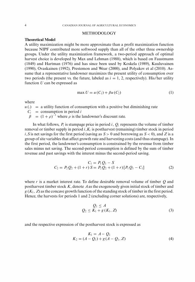
Theoretical ModelA utility maximization might be more approximate than a profit maximization functionbecause NIPF contributed more softwood supply than all of the other three ownershipgroups. Under the utility maximization framework, a two-period approach of optimalharvest choice is developed by Max and Lehman (1988), which is based on Faustmann(1849) and Hartman (1976) and has since been used by Koskela (1989), Kuuluvainen(1990), Ovaskainen (1992), Prestemon and Wear (2000), and Polyakov et al (2010). As-sume that a representative landowner maximizes the present utility of consumption overtwo periods (the present vs. the future, labeled as i = 1, 2, respectively). His/her utilityfunction U can be expressed as
max U = u (C1) + βu (C2) (1)
whereu (.) = a utility function of consumption with a positive but diminishing rate
Ci = consumption in period iβ = (1 + ρ)−1 where ρ is the landowner’s discount rate.
In what follows, Pi is stumpage price in period i , Qi represents the volume of timberremoval or timber supply in period i ,Ki is postharvest (remaining) timber stock in periodi ,S is net savings for the first period (saving as S > 0 and borrowing as S < 0), and Z is agroup of site variables that affect growth rate and harvesting costs (and thus stumpage). Inthe first period, the landowner’s consumption is constrained by the revenue from timbersales minus net saving. The second-period consumption is defined by the sum of timberrevenue and past savings with the interest minus the second-period saving.
C1 = P1 Q1 − SC2 = P2 Q2 + (1 + r ) S = P2 Q2 + (1 + r ) [P1 Q1 − C1] (2)
where r is a market interest rate. To define desirable removal volume of timber Q andpostharvest timber stock K , denote Aas the exogenously given initial stock of timber andg (K1, Z) as the concave growth function of the standing stock of timber in the first period.Hence, the harvests for periods 1 and 2 (excluding corner solutions) are, respectively,
Q1 ≤ AQ2 ≤ K1 + g (K1, Z) (3)
and the respective expression of the postharvest stock is expressed as
K1 = A− Q1
K2 = (A − Q1) + g (A − Q1, Z) (4)

HARVESTING CHOICES AND TIMBER SUPPLY 5
Substituting Equations (2), (3), and (4) into (1), the maximized discounted utility overthe two periods becomes:
maxC1,Q1
U = u (C1) + βu {P2 [(A− Q1) + g (A− Q1, Z)] + (1 + r ) [P1 Q1 − C1]} (5)
The choice variables of this optimization problem are present consumption andharvest. The first-order conditions for present harvest can be written as
UQ1 = βu′(C2){(1 + r ) P1 − [1 + g′ (A− Q1, Z)]P2} = 0 (6)
Because we assume u(.′) > 0, the condition for optimal first-period harvest can besimplified as
P1 = [1 + g′ (A− Q1, Z)]P2/ (1 + r ) (7)
At the optimal point, the left-hand side of Equation (7) represents the marginalrevenue with respect to the present harvest and the right-hand side represents its marginalopportunity cost (the discounted value of the future harvest). Note that, if non timbervalue metrics were incorporated, which are typically associated with timber age or timbervolume, into Equation (2), the optimal condition in Equation (7) will be a little morecomplicated. Nonetheless, the basic identity of marginal revenue and marginal cost holds(Polyakov et al 2010).
Empirical Model for Harvest ChoiceTo link Equation (5), a general utility equation, to a money metric utility equation, whichcan be used in an empirical application of the two-period harvest choice model (Prestemonand Wear 2000) for sampled forest stands along with estimation of timber benefits, theobjective of the discounted utility-maximizing landowner can be expressed as
Y∗ = P1 Q1 + � (Q1, Z) + βE [P2 Q2] + ε = f (ω′x) + ε (8)
where Y∗ is the maximized discounted monetary utility,� (Q1, Z) is the discounted resid-ual value of the harvested stand, E is an expectation operator, and ε is the associatederror term. The variable Y∗ suggests a set of explanatory variables that directly influencethe harvest choice and is denoted as x. The dependent variable (Yi j ) is a set of neutrallyexclusive binary choices (denoting the harvest choice as i and the ownership categoryas j ), and is defined as:
Y1 j = {1 if a partial harvest was conducted, 0 otherwise}
Y2 j = {1 if a final harvest was conducted, 0 otherwise}
and
Y0 j = {1 if no harvest was conducted, 0 otherwise}
6 CANADIAN JOURNAL OF AGRICULTURAL ECONOMICS
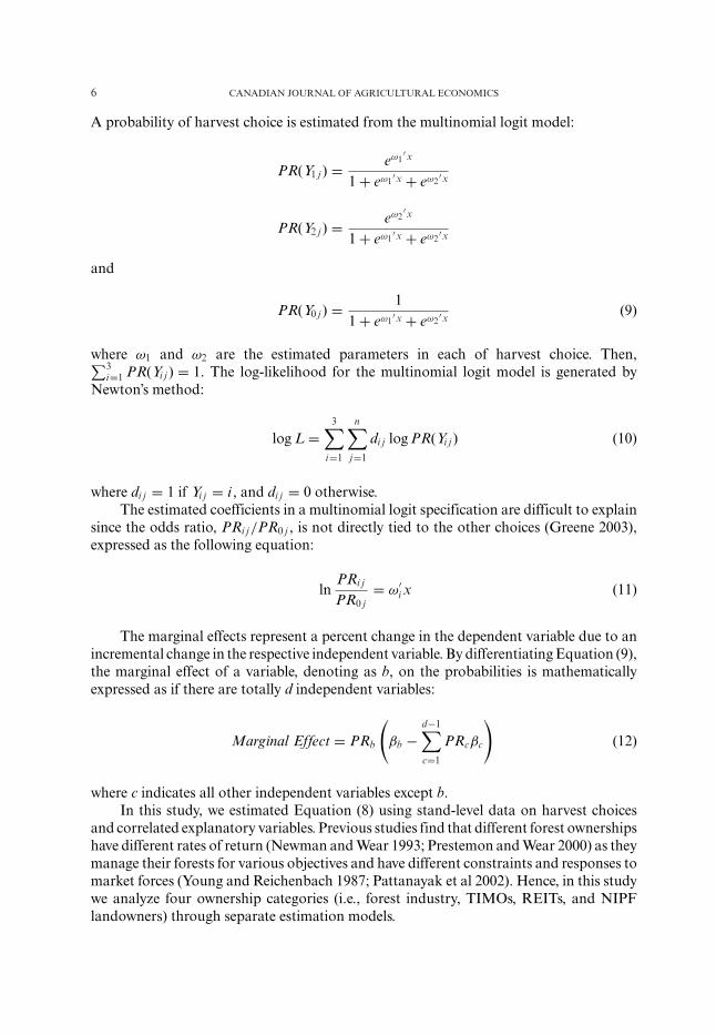
A probability of harvest choice is estimated from the multinomial logit model:
PR(Y1 j ) = eω1′x
1 + eω1′x + eω2
′x
PR(Y2 j ) = eω2′x
1 + eω1′x + eω2
′x
and
PR(Y0 j ) = 11 + eω1
′x + eω2′x (9)
where ω1 and ω2 are the estimated parameters in each of harvest choice. Then,∑3i=1 PR(Yi j ) = 1. The log-likelihood for the multinomial logit model is generated by
Newton’s method:
log L =3∑
i=1
n∑j=1
di j log PR(Yi j ) (10)
where di j = 1 if Yi j = i , and di j = 0 otherwise.The estimated coefficients in a multinomial logit specification are difficult to explain
since the odds ratio, PRi j/PR0 j , is not directly tied to the other choices (Greene 2003),expressed as the following equation:
lnPRi j
PR0 j= ω′
i x (11)
The marginal effects represent a percent change in the dependent variable due to anincremental change in the respective independent variable. By differentiating Equation (9),the marginal effect of a variable, denoting as b, on the probabilities is mathematicallyexpressed as if there are totally d independent variables:
Marginal Effect = PRb
(βb −
d−1∑c=1
PRcβc
)(12)
where c indicates all other independent variables except b.In this study, we estimated Equation (8) using stand-level data on harvest choices
and correlated explanatory variables. Previous studies find that different forest ownershipshave different rates of return (Newman and Wear 1993; Prestemon and Wear 2000) as theymanage their forests for various objectives and have different constraints and responses tomarket forces (Young and Reichenbach 1987; Pattanayak et al 2002). Hence, in this studywe analyze four ownership categories (i.e., forest industry, TIMOs, REITs, and NIPFlandowners) through separate estimation models.
HARVESTING CHOICES AND TIMBER SUPPLY 7
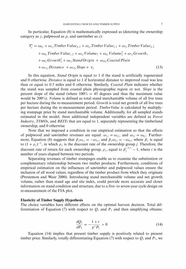
In particular, Equation (8) is mathematically expressed as (denoting the ownershipcategory as j , pulpwood as p, and sawtimber as s):
Y∗j = ω0 j + ω1 j Timber Valuep,1 + ω2 j Timber Values,1 + ω3 j Timber Valuep,2
+ω4 j Timber Values,2 + ω5 j Volume1 + ω6 j Volume21 + ω7 j Growth1
+ω8 j Growth21 + ω9 j Stand Origin + ω10 j Coastal Plain
+ω11 j Distance + ω12j Slope + ∈j (13)
In this equation, Stand Origin is equal to 1 if the stand is artificially regeneratedand 0 otherwise. Distance is equal to 1 if horizontal distance to improved road was lessthan or equal to 0.5 miles and 0 otherwise. Similarly, Coastal Plain indicates whetherthe stand was sampled from coastal plain physiographic region or not. Slope is thepercent slope of the stand (where 100% = 45 degrees and thus the maximum valuewould be 200%). Volume is defined as total stand merchantable volume of all live treesper hectare during the re-measurement period. Growth is total net growth of all live treesper hectare during the re-measurement period. TimberValue is calculated by multiply-ing stumpage price by stand merchantable volume. Additionally, for all sampled standsestimated in the model, three additional independent variables are defined as ForestIndustry, TIMOs, and REITs that are equal to 1, separately representing the timberlandownership, and 0 otherwise.
Note that we imposed a condition in our empirical estimation so that the effectsof pulpwood and sawtimber revenues are equal: ω1 j = ω2 j , and ω3 j = ω4 j . Further-more, Equation (8) suggests that β jω1 j = −ω3 j , and β jω2 j = −ω4 j , where β j is equalto (1 + ρ j )−1, in which ρ j is the discount rate of the ownership group j. Therefore, thediscount rate of return for each ownership group, ρ j , equal to β
−1/tj − 1, where t is the
number of years elapsed between two periods.Separating revenues of timber stumpages enable us to examine the substitution or
complementary relationship between two timber products. Furthermore, conditions ofempirical estimation on the influences of sawtimber and pulpwood values ensure theinclusion of all wood values, regardless of the timber product from which they originate(Prestemon and Wear 2000). Introducing stand merchantable volume and net growthvolume, rather than stand age and site index, could provide more accurate and closerinformation on stand condition and structure, due to a five- to seven-year cycle design onre-measurement of the FIA plot.
Elasticity of Timber Supply HypothesisThe choice variables have different effects on the optimal harvest decision. Total dif-ferentiation of Equation (7) with respect to Q1 and P1 and then simplifying obtains:
dQ1
dP1= −1 + r
g′′ P2> 0 (14)
Equation (14) implies that present timber supply is positively related to presenttimber price. Similarly, totally differentiating Equation (7) with respect to Q1 and P2, we
8 CANADIAN JOURNAL OF AGRICULTURAL ECONOMICS
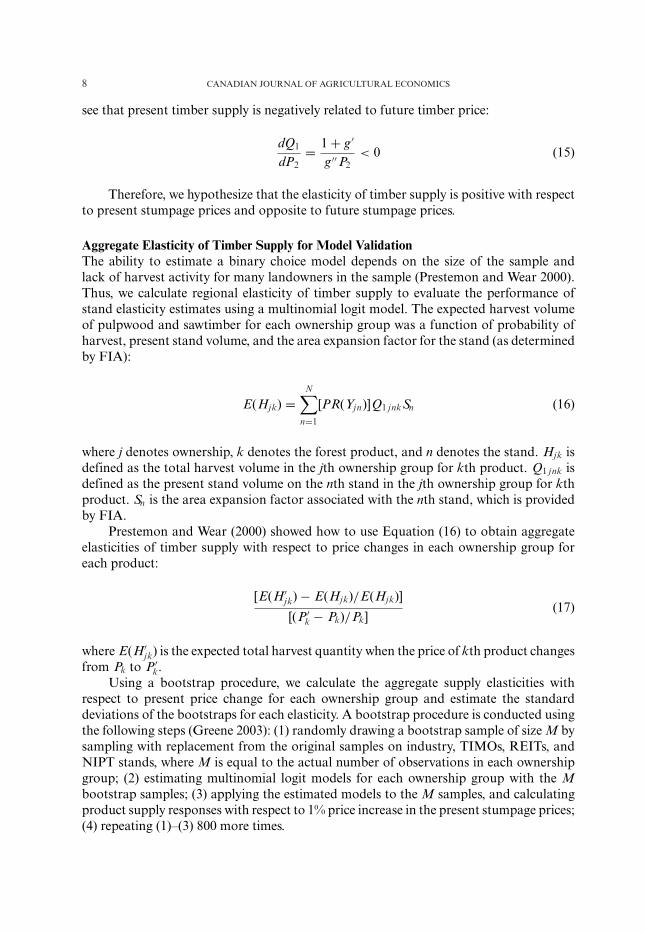
see that present timber supply is negatively related to future timber price:
dQ1
dP2= 1 + g′
g′′ P2< 0 (15)
Therefore, we hypothesize that the elasticity of timber supply is positive with respectto present stumpage prices and opposite to future stumpage prices.
Aggregate Elasticity of Timber Supply for Model ValidationThe ability to estimate a binary choice model depends on the size of the sample andlack of harvest activity for many landowners in the sample (Prestemon and Wear 2000).Thus, we calculate regional elasticity of timber supply to evaluate the performance ofstand elasticity estimates using a multinomial logit model. The expected harvest volumeof pulpwood and sawtimber for each ownership group was a function of probability ofharvest, present stand volume, and the area expansion factor for the stand (as determinedby FIA):
E(Hjk) =N∑
n=1
[PR(Yjn)]Q1 jnkSn (16)
where j denotes ownership, k denotes the forest product, and n denotes the stand. Hjk isdefined as the total harvest volume in the jth ownership group for kth product. Q1 jnk isdefined as the present stand volume on the nth stand in the jth ownership group for kthproduct. Sn is the area expansion factor associated with the nth stand, which is providedby FIA.
Prestemon and Wear (2000) showed how to use Equation (16) to obtain aggregateelasticities of timber supply with respect to price changes in each ownership group foreach product:
[E(H′jk) − E(Hjk)/E(Hjk)]
[(P′k − Pk)/Pk]
(17)
where E(H′jk) is the expected total harvest quantity when the price of kth product changes
from Pk to P′k.
Using a bootstrap procedure, we calculate the aggregate supply elasticities withrespect to present price change for each ownership group and estimate the standarddeviations of the bootstraps for each elasticity. A bootstrap procedure is conducted usingthe following steps (Greene 2003): (1) randomly drawing a bootstrap sample of size M bysampling with replacement from the original samples on industry, TIMOs, REITs, andNIPT stands, where M is equal to the actual number of observations in each ownershipgroup; (2) estimating multinomial logit models for each ownership group with the Mbootstrap samples; (3) applying the estimated models to the M samples, and calculatingproduct supply responses with respect to 1% price increase in the present stumpage prices;(4) repeating (1)–(3) 800 more times.
HARVESTING CHOICES AND TIMBER SUPPLY 9
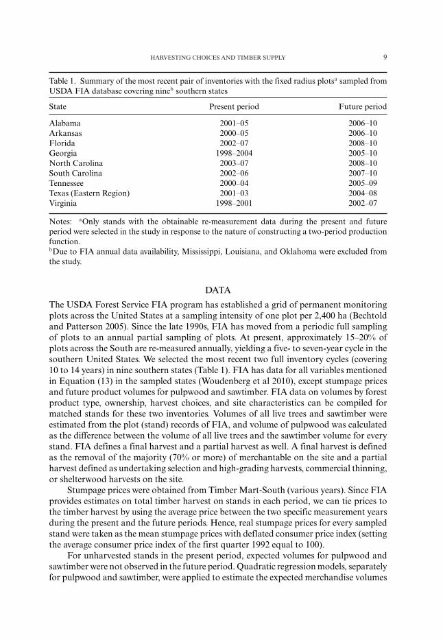
Table 1. Summary of the most recent pair of inventories with the fixed radius plotsa sampled fromUSDA FIA database covering nineb southern states
State Present period Future period
Alabama 2001–05 2006–10Arkansas 2000–05 2006–10Florida 2002–07 2008–10Georgia 1998–2004 2005–10North Carolina 2003–07 2008–10South Carolina 2002–06 2007–10Tennessee 2000–04 2005–09Texas (Eastern Region) 2001–03 2004–08Virginia 1998–2001 2002–07
Notes: aOnly stands with the obtainable re-measurement data during the present and futureperiod were selected in the study in response to the nature of constructing a two-period productionfunction.bDue to FIA annual data availability, Mississippi, Louisiana, and Oklahoma were excluded fromthe study.
DATA
The USDA Forest Service FIA program has established a grid of permanent monitoringplots across the United States at a sampling intensity of one plot per 2,400 ha (Bechtoldand Patterson 2005). Since the late 1990s, FIA has moved from a periodic full samplingof plots to an annual partial sampling of plots. At present, approximately 15–20% ofplots across the South are re-measured annually, yielding a five- to seven-year cycle in thesouthern United States. We selected the most recent two full inventory cycles (covering10 to 14 years) in nine southern states (Table 1). FIA has data for all variables mentionedin Equation (13) in the sampled states (Woudenberg et al 2010), except stumpage pricesand future product volumes for pulpwood and sawtimber. FIA data on volumes by forestproduct type, ownership, harvest choices, and site characteristics can be compiled formatched stands for these two inventories. Volumes of all live trees and sawtimber wereestimated from the plot (stand) records of FIA, and volume of pulpwood was calculatedas the difference between the volume of all live trees and the sawtimber volume for everystand. FIA defines a final harvest and a partial harvest as well. A final harvest is definedas the removal of the majority (70% or more) of merchantable on the site and a partialharvest defined as undertaking selection and high-grading harvests, commercial thinning,or shelterwood harvests on the site.
Stumpage prices were obtained from Timber Mart-South (various years). Since FIAprovides estimates on total timber harvest on stands in each period, we can tie prices tothe timber harvest by using the average price between the two specific measurement yearsduring the present and the future periods. Hence, real stumpage prices for every sampledstand were taken as the mean stumpage prices with deflated consumer price index (settingthe average consumer price index of the first quarter 1992 equal to 100).
For unharvested stands in the present period, expected volumes for pulpwood andsawtimber were not observed in the future period. Quadratic regression models, separatelyfor pulpwood and sawtimber, were applied to estimate the expected merchandise volumes
10 CANADIAN JOURNAL OF AGRICULTURAL ECONOMICS
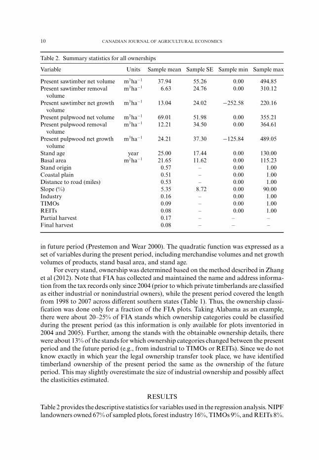
Table 2. Summary statistics for all ownerships
Variable Units Sample mean Sample SE Sample min Sample max
Present sawtimber net volume m3ha−1 37.94 55.26 0.00 494.85Present sawtimber removal
volumem3ha−1 6.63 24.76 0.00 310.12
Present sawtimber net growthvolume
m3ha−1 13.04 24.02 −252.58 220.16
Present pulpwood net volume m3ha−1 69.01 51.98 0.00 355.21Present pulpwood removal
volumem3ha−1 12.21 34.50 0.00 364.61
Present pulpwood net growthvolume
m3ha−1 24.21 37.30 −125.84 489.05
Stand age year 25.00 17.44 0.00 130.00Basal area m2ha−1 21.65 11.62 0.00 115.23Stand origin 0.57 – 0.00 1.00Coastal plain 0.51 – 0.00 1.00Distance to road (miles) 0.53 – 0.00 1.00Slope (%) 5.35 8.72 0.00 90.00Industry 0.16 – 0.00 1.00TIMOs 0.09 – 0.00 1.00REITs 0.08 – 0.00 1.00Partial harvest 0.17 – – –Final harvest 0.08 – – –
in future period (Prestemon and Wear 2000). The quadratic function was expressed as aset of variables during the present period, including merchandise volumes and net growthvolumes of products, stand basal area, and stand age.
For every stand, ownership was determined based on the method described in Zhanget al (2012). Note that FIA has collected and maintained the name and address informa-tion from the tax records only since 2004 (prior to which private timberlands are classifiedas either industrial or nonindustrial owners), while the present period covered the lengthfrom 1998 to 2007 across different southern states (Table 1). Thus, the ownership classi-fication was done only for a fraction of the FIA plots. Taking Alabama as an example,there were about 20–25% of FIA stands which ownership categories could be classifiedduring the present period (as this information is only available for plots inventoried in2004 and 2005). Further, among the stands with the obtainable ownership details, therewere about 13% of the stands for which ownership categories changed between the presentperiod and the future period (e.g., from industrial to TIMOs or REITs). Since we do notknow exactly in which year the legal ownership transfer took place, we have identifiedtimberland ownership of the present period the same as the ownership of the futureperiod. This may slightly overestimate the size of industrial ownership and possibly affectthe elasticities estimated.
RESULTS
Table 2 provides the descriptive statistics for variables used in the regression analysis. NIPFlandowners owned 67% of sampled plots, forest industry 16%, TIMOs 9%, and REITs 8%.
HARVESTING CHOICES AND TIMBER SUPPLY 11
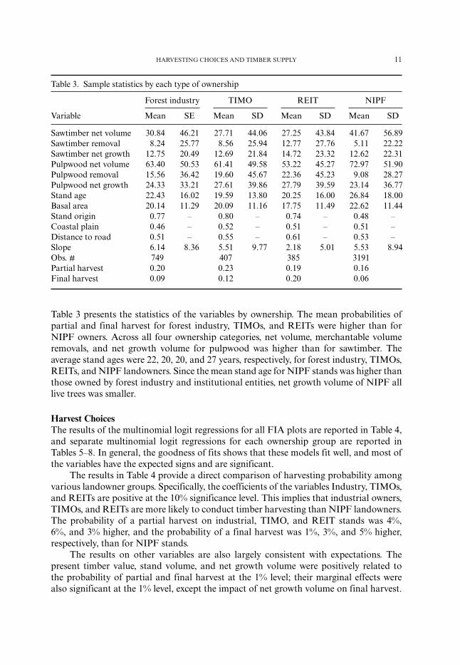
Table 3. Sample statistics by each type of ownership
Forest industry TIMO REIT NIPF
Variable Mean SE Mean SD Mean SD Mean SD
Sawtimber net volume 30.84 46.21 27.71 44.06 27.25 43.84 41.67 56.89Sawtimber removal 8.24 25.77 8.56 25.94 12.77 27.76 5.11 22.22Sawtimber net growth 12.75 20.49 12.69 21.84 14.72 23.32 12.62 22.31Pulpwood net volume 63.40 50.53 61.41 49.58 53.22 45.27 72.97 51.90Pulpwood removal 15.56 36.42 19.60 45.67 22.36 45.23 9.08 28.27Pulpwood net growth 24.33 33.21 27.61 39.86 27.79 39.59 23.14 36.77Stand age 22.43 16.02 19.59 13.80 20.25 16.00 26.84 18.00Basal area 20.14 11.29 20.09 11.16 17.75 11.49 22.62 11.44Stand origin 0.77 – 0.80 – 0.74 – 0.48 –Coastal plain 0.46 – 0.52 – 0.51 – 0.51 –Distance to road 0.51 – 0.55 – 0.61 – 0.53 –Slope 6.14 8.36 5.51 9.77 2.18 5.01 5.53 8.94Obs. # 749 407 385 3191Partial harvest 0.20 0.23 0.19 0.16Final harvest 0.09 0.12 0.20 0.06
Table 3 presents the statistics of the variables by ownership. The mean probabilities ofpartial and final harvest for forest industry, TIMOs, and REITs were higher than forNIPF owners. Across all four ownership categories, net volume, merchantable volumeremovals, and net growth volume for pulpwood was higher than for sawtimber. Theaverage stand ages were 22, 20, 20, and 27 years, respectively, for forest industry, TIMOs,REITs, and NIPF landowners. Since the mean stand age for NIPF stands was higher thanthose owned by forest industry and institutional entities, net growth volume of NIPF alllive trees was smaller.
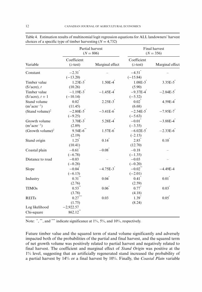
Harvest ChoicesThe results of the multinomial logit regressions for all FIA plots are reported in Table 4,and separate multinomial logit regressions for each ownership group are reported inTables 5–8. In general, the goodness of fits shows that these models fit well, and most ofthe variables have the expected signs and are significant.
The results in Table 4 provide a direct comparison of harvesting probability amongvarious landowner groups. Specifically, the coefficients of the variables Industry, TIMOs,and REITs are positive at the 10% significance level. This implies that industrial owners,TIMOs, and REITs are more likely to conduct timber harvesting than NIPF landowners.The probability of a partial harvest on industrial, TIMO, and REIT stands was 4%,6%, and 3% higher, and the probability of a final harvest was 1%, 3%, and 5% higher,respectively, than for NIPF stands.
The results on other variables are also largely consistent with expectations. Thepresent timber value, stand volume, and net growth volume were positively related tothe probability of partial and final harvest at the 1% level; their marginal effects werealso significant at the 1% level, except the impact of net growth volume on final harvest.
12 CANADIAN JOURNAL OF AGRICULTURAL ECONOMICS
Table 4. Estimation results of multinomial logit regression equations for ALL landowners’ harvestchoices of a specific type of timber harvesting (N = 4,732)
Partial harvest Final harvest(N = 806) (N = 356)
Coefficient CoefficientVariable (z-test) Marginal effect (z-test) Marginal effect
Constant −2.31*
– −4.51*
–(−13.20) (−15.84)
Timber value 1.23E-3*
1.50E-4*
1.08E-3*
3.35E-5*
($/acre), t (10.26) (5.90)Timber value −1.19E-3
* −1.45E-4* −9.37E-4
* −2.84E-5*
($/acre), t + 1 (−10.14) (−5.32)Stand volume 0.02
*2.25E-3
*0.02
*4.59E-4
*
(m3acre−1) (11.45) (6.68)(Stand volume)2 −2.80E-5
* −3.41E-6* −2.54E-5
* −7.95E-7*
(−9.25) (−5.63)Growth volume 3.70E-3
*5.28E-4
* −0.01* −3.88E-4
*
(m3acre−1) (2.89) (−3.35)(Growth volume)2 9.54E-6
**1.57E-6
* −6.02E-5* −2.33E-6
*
(2.19) (–2.15)Stand origin 1.25
*0.14
*2.85
*0.10
*
(10.41) (12.70)Coastal plain −0.61
* −0.08* −0.18 –
(−6.78) (−1.35)Distance to road −0.03 – −0.03 –
(−0.28) (−0.20)Slope −0.04
* −4.75E-3* −0.02
** −4.49E-4(−6.13) (−2.01)
Industry 0.31**
0.04*
0.41*
0.01*
(2.76) (2.59)TIMOs 0.53
**0.06
*0.77
*0.03
*
(3.78) (4.18)REITs 0.27
***0.03 1.39
*0.05
*
(1.75) (8.24)Log likelihood −2,922.57Chi-square 862.12
**
Note: *, **, and *** indicate significance at 1%, 5%, and 10%, respectively.
Future timber value and the squared term of stand volume significantly and adverselyimpacted both of the probabilities of the partial and final harvest, and the squared termof net growth volume was positively related to partial harvest and negatively related tofinal harvest. The coefficient and marginal effect of Stand Origin was positive at the1% level, suggesting that an artificially regenerated stand increased the probability ofa partial harvest by 14% or a final harvest by 10%. Finally, the Coastal Plain variable
HARVESTING CHOICES AND TIMBER SUPPLY 13
Table 5. Estimation results of multinomial logit regression equations for Forest Industry landown-ers’ harvest choices of a specific type of timber harvesting (N = 749)
Partial harvest Final harvest(N = 152) (N = 71)
Coefficient CoefficientVariable (z-test) Marginal effect (z-test) Marginal effect
Constant −2.19*
– −4.29*
–(−4.44) (−5.61)
Timber value 2.27E-3*
2.81E-4*
2.21E-3*
1.09E-4*
($/acre), t (6.01) (4.14)Timber value −2.04E-3
* −2.55E-4* −1.80E-3
* −8.67E-5*
($/acre), t + 1 (−5.72) (−3.58)Stand volume 0.03
*3.85E-3
*0.02
*6.25E-4
***
(m3acre−1) (5.88) (2.78)(Stand volume)2 −6.90E-5
* −8.82E-6* −4.05E-5
* −1.71E-6**
(–5.17) (–3.04)Growth volume 0.01
**1.96E-3
* −0.01 –(m3acre−1) (2.51) (–1.40)(Growth volume)2 −4.87E-5 – −1.27E-5 –
(−1.63) (−0.20)Stand origin 1.43
*0.15
*3.84
*0.21
*
(4.03) (5.34)Coastal plain −1.04
* −0.13* −0.69
** −0.03*
(−4.44) (−2.22)Distance to road 0.15 – 0.35 –
(0.58) (0.98)Slope −0.04
* −0.01* −0.04
*** −1.73E-3(−3.15) (−1.82)
Log likelihood −499.56Chi-square 192.10
*
Note: *, **, and *** indicate significance at 1%, 5%, and 10%, respectively.
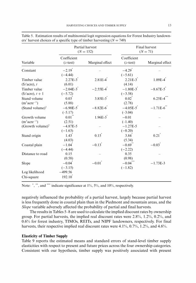
negatively influenced the probability of a partial harvest, largely because partial harvestis less frequently done in coastal plain than in the Piedmont and mountain areas, and theSlope variable adversely affected the probability of partial and final harvests.
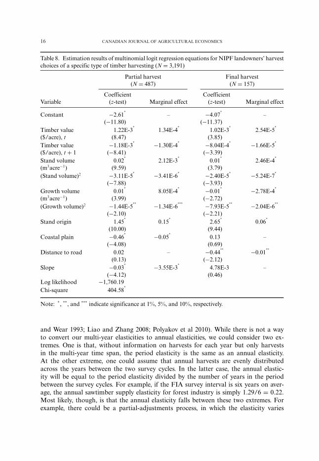
The results in Tables 5–8 are used to calculate the implied discount rates by ownershipgroup. For partial harvests, the implied real discount rates were 2.8%, 1.2%, 0.2%, and0.6% for forest industry, TIMOs, REITs, and NIPF landowners, respectively. For finalharvests, their respective implied real discount rates were 4.1%, 0.7%, 1.2%, and 4.6%.
Elasticity of Timber SupplyTable 9 reports the estimated means and standard errors of stand-level timber supplyelasticities with respect to present and future prices across the four ownership categories.Consistent with our hypothesis, timber supply was positively associated with present
14 CANADIAN JOURNAL OF AGRICULTURAL ECONOMICS
Table 6. Estimation results of multinomial logit regression equations for TIMOs’ harvest choicesof a specific type of timber harvesting (N = 407)
Variable Partial harvest Final harvest(N = 95) (N = 50)
Coefficient Coefficient(z-test) Marginal effect (z-test) Marginal effect
Constant −0.76 – −5.72*
–(−1.30) (−3.97)
Timber value 1.67E-3*
2.62E-4*
2.80E-3*
8.38E-5**
($/acre), t (3.55) (3.88)Timber value −1.57E-4
* −2.46E-4* −2.74E-3
* −8.33E-5**
($/acre), t + 1 (−3.43) (−3.93)Stand volume 0.01
*2.34E-3
*0.02
*6.07E-4
***
(m3acre−1) (2.70) (3.05)(Stand volume)2 −1.33E-5 – 9.92E-6 –
(–1.24) (0.67)Growth volume 0.01
**1.60E-3
**0.01 –
(m3acre−1) (2.06) (1.10)(Growth volume)2 −6.97E-6 – −2.01E-4
*** −6.96E-6*
(−0.39) (−1.73)Stand origin 1.04
**0.13
***5.33
*0.18
**
(2.41) (3.60)Coastal plain −0.47
*** −0.08***
0.15 –(−1.65) (0.38)
Distance to road −0.47 – 0.57 –(−1.38) (1.01)
Slope −0.10* −0.02
* −0.08** −1.99E-3
(−3.66) (−2.20)Log likelihood −293.63Chi-square 129.66
*
Note: *, **, and *** indicate significance at 1%, 5%, and 10%, respectively.
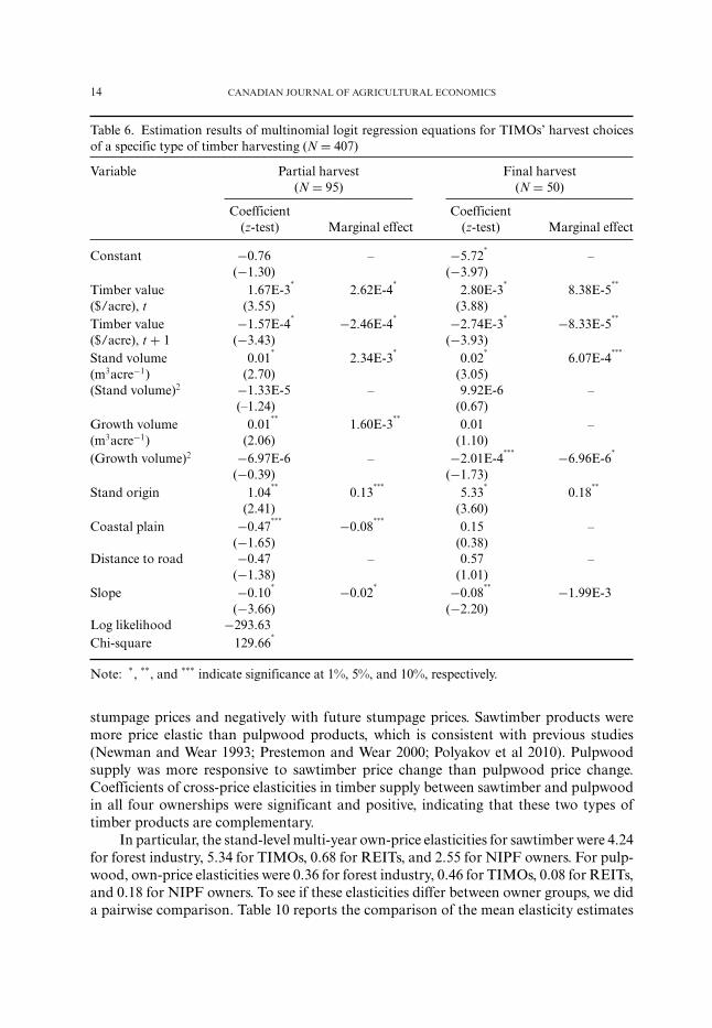
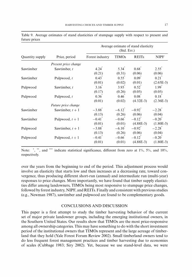
stumpage prices and negatively with future stumpage prices. Sawtimber products weremore price elastic than pulpwood products, which is consistent with previous studies(Newman and Wear 1993; Prestemon and Wear 2000; Polyakov et al 2010). Pulpwoodsupply was more responsive to sawtimber price change than pulpwood price change.Coefficients of cross-price elasticities in timber supply between sawtimber and pulpwoodin all four ownerships were significant and positive, indicating that these two types oftimber products are complementary.
In particular, the stand-level multi-year own-price elasticities for sawtimber were 4.24for forest industry, 5.34 for TIMOs, 0.68 for REITs, and 2.55 for NIPF owners. For pulp-wood, own-price elasticities were 0.36 for forest industry, 0.46 for TIMOs, 0.08 for REITs,and 0.18 for NIPF owners. To see if these elasticities differ between owner groups, we dida pairwise comparison. Table 10 reports the comparison of the mean elasticity estimates
HARVESTING CHOICES AND TIMBER SUPPLY 15
Table 7. Estimation results of multinomial logit regression equations for REITs’ harvest choices ofa specific type of timber harvesting (N = 385)
Partial harvest Final harvest(N = 72) (N = 78)
Coefficient CoefficientVariable (z-test) Marginal effect (z-test) Marginal effect
Constant −2.80*
– −3.59*
–(−3.69) (−4.34)
Timber value 1.44E-3*
1.64E-4**
8.75E-4***
7.40E-5($/acre), t (2.65) (1.62)Timber value −1.43E-4
* −1.63E-4** −8.25E-3 –
($/acre), t + 1 (−2.68) (−1.58)Stand volume 0.03
*3.27E-3
*0.02
*1.93E-3
**
(m3acre−1) (3.55) (3.46)(Stand volume)2 −3.90E-5
** −4.36E-6** −2.76E-5
*** −2.46E-6(−2.04) (−1.73)
Growth volume 0.01 – −0.02 –(m3acre−1) (1.32) (–1.40)(Growth volume)2 −1.89E-5 – −4.52E-5 –
(−0.67) (−0.35)Stand origin 1.08
**0.08 3.01
*0.33
*
(2.40) (4.75)Coastal plain −1.49
* −0.17* −0.99
* −0.09**
(−3.78) (−2.78)Distance to road 0.33 – 0.45 –
(0.70) (0.75)Slope −0.02 – −0.06 –
(−0.65) (−1.51)Log likelihood −285.50Chi-square 151.50
*
Note: *, **, and *** indicate significance at 1%, 5%, and 10%, respectively.
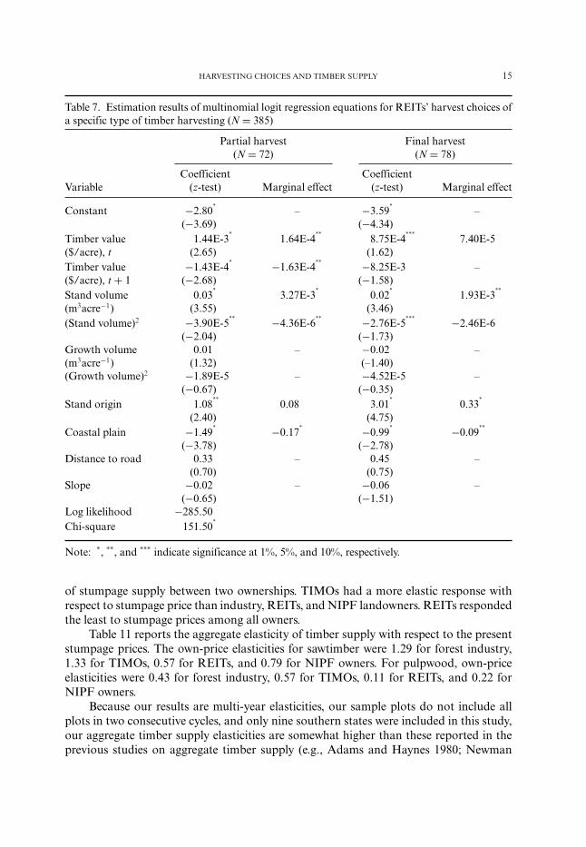
of stumpage supply between two ownerships. TIMOs had a more elastic response withrespect to stumpage price than industry, REITs, and NIPF landowners. REITs respondedthe least to stumpage prices among all owners.
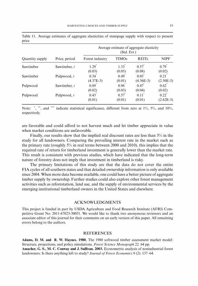
Table 11 reports the aggregate elasticity of timber supply with respect to the presentstumpage prices. The own-price elasticities for sawtimber were 1.29 for forest industry,1.33 for TIMOs, 0.57 for REITs, and 0.79 for NIPF owners. For pulpwood, own-priceelasticities were 0.43 for forest industry, 0.57 for TIMOs, 0.11 for REITs, and 0.22 forNIPF owners.
Because our results are multi-year elasticities, our sample plots do not include allplots in two consecutive cycles, and only nine southern states were included in this study,our aggregate timber supply elasticities are somewhat higher than these reported in theprevious studies on aggregate timber supply (e.g., Adams and Haynes 1980; Newman
16 CANADIAN JOURNAL OF AGRICULTURAL ECONOMICS
Table 8. Estimation results of multinomial logit regression equations for NIPF landowners’ harvestchoices of a specific type of timber harvesting (N = 3,191)
Partial harvest Final harvest(N = 487) (N = 157)
Coefficient CoefficientVariable (z-test) Marginal effect (z-test) Marginal effect
Constant −2.61*
– −4.07*
–(−11.80) (−11.37)
Timber value 1.22E-3*
1.34E-4*
1.02E-3*
2.54E-5*
($/acre), t (8.47) (3.85)Timber value −1.18E-3
* −1.30E-4* −8.04E-4
* −1.66E-5*
($/acre), t + 1 (−8.41) (−3.39)Stand volume 0.02
*2.12E-3
*0.01
*2.46E-4
*
(m3acre−1) (9.59) (3.79)(Stand volume)2 −3.11E-5
* −3.41E-6* −2.40E-5
* −5.24E-7*
(−7.88) (−3.93)Growth volume 0.01
*8.05E-4
* −0.01* −2.78E-4
*
(m3acre−1) (3.99) (−2.72)(Growth volume)2 −1.44E-5
** −1.34E-6*** −7.93E-5
** −2.04E-6**
(−2.10) (−2.21)Stand origin 1.45
*0.15
*2.65
*0.06
*
(10.00) (9.44)Coastal plain −0.46
* −0.05*
0.13 –(−4.08) (0.69)
Distance to road 0.02 – −0.44** −0.01
**
(0.13) (−2.12)Slope −0.03
* −3.55E-3*
4.78E-3 –(−4.12) (0.46)
Log likelihood −1,760.19Chi-square 404.58
*
Note: *, **, and *** indicate significance at 1%, 5%, and 10%, respectively.
and Wear 1993; Liao and Zhang 2008; Polyakov et al 2010). While there is not a wayto convert our multi-year elasticities to annual elasticities, we could consider two ex-tremes. One is that, without information on harvests for each year but only harvestsin the multi-year time span, the period elasticity is the same as an annual elasticity.At the other extreme, one could assume that annual harvests are evenly distributedacross the years between the two survey cycles. In the latter case, the annual elastic-ity will be equal to the period elasticity divided by the number of years in the periodbetween the survey cycles. For example, if the FIA survey interval is six years on aver-age, the annual sawtimber supply elasticity for forest industry is simply 1.29/6 = 0.22.Most likely, though, is that the annual elasticity falls between these two extremes. Forexample, there could be a partial-adjustments process, in which the elasticity varies
HARVESTING CHOICES AND TIMBER SUPPLY 17
Table 9. Average estimates of stand elasticities of stumpage supply with respect to present andfuture prices
Average estimate of stand elasticity(Std. Err.)
Quantity supply Price, period Forest industry TIMOs REITs NIPF
Present price changeSawtimber Sawtimber, t 4.24
*5.34
*0.68
*2.55
*
(0.21) (0.31) (0.06) (0.06)Sawtimber Pulpwood, t 0.43
*0.55
*0.09
*0.21
*
(0.01) (0.02) (0.01) (2.65E-3)Pulpwood Sawtimber, t 3.16
*3.93
*0.52
*1.99
*
(0.17) (0.26) (0.05) (0.05)Pulpwood Pulpwood, t 0.36
*0.46
*0.08
*0.18
*
(0.01) (0.02) (4.32E-3) (2.36E-3)Future price change
Sawtimber Sawtimber, t + 1 −3.88* −6.12
* −0.92* −2.28
*
(0.13) (0.26) (0.06) (0.04)Sawtimber Pulpwood, t + 1 −0.41
* −0.66* −0.12
* −0.20*
(0.01) (0.01) (4.88E-3) (1.80E-3)Pulpwood Sawtimber, t + 1 −3.88
* −6.10* −0.92
* −2.28*
(0.13) (0.26) (0.06) (0.04)Pulpwood Pulpwood, t + 1 −0.41
* −0.66* −0.12
* −0.20*
(0.01) (0.01) (4.88E-3) (1.80E-3)
Note: *, **, and *** indicate statistical significance, different from zero at 1%, 5%, and 10%,respectively.
over the years from the beginning to end of the period. This adjustment process wouldinvolve an elasticity that starts low and then increases at a decreasing rate, toward con-vergence, thus producing different short-run (annual) and intermediate run (multi-year)responses to price changes. More importantly, we have found that timber supply elastici-ties differ among landowners, TIMOs being most responsive to stumpage price changes,followed by forest industry, NIPF, and REITs. Finally and consistent with previous studies(e.g., Newman 1987), sawtimber and pulpwood are found to be complementary goods.
CONCLUSIONS AND DISCUSSION
This paper is a first attempt to study the timber harvesting behavior of the currentset of major private landowner groups, including the emerging institutional owners, inthe Southern United States. Our results show that TIMOs are the most price-responsiveamong all ownership categories. This may have something to do with the short investmentperiod of the institutional owners that TIMOs represent and the large acreage of timber-land that they hold (Yale Forest Forum Review 2002). Small timberland owners tend todo less frequent forest management practices and timber harvesting due to economiesof scales (Cubbage 1983; Siry 2002). Yet, because we use stand-level data, we were
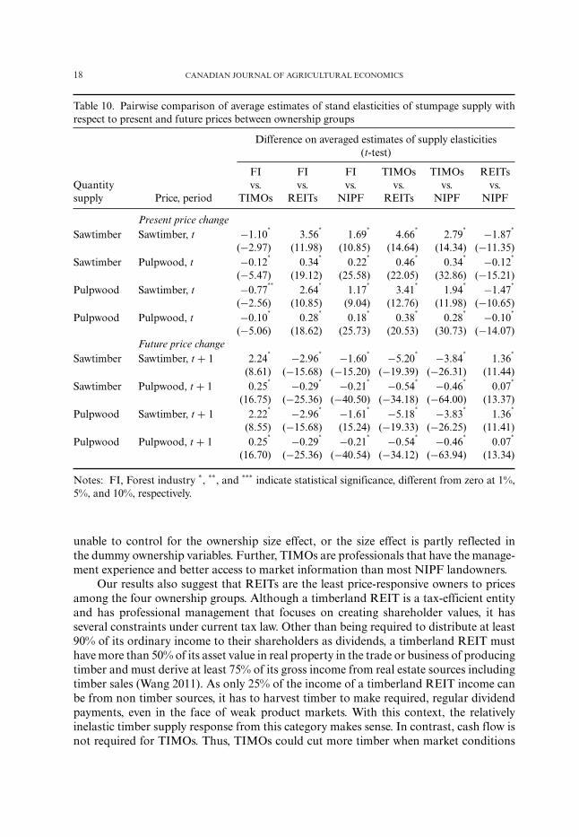
18 CANADIAN JOURNAL OF AGRICULTURAL ECONOMICS
Table 10. Pairwise comparison of average estimates of stand elasticities of stumpage supply withrespect to present and future prices between ownership groups
Difference on averaged estimates of supply elasticities(t-test)
FI FI FI TIMOs TIMOs REITsvs. vs. vs. vs. vs. vs.Quantity
supply Price, period TIMOs REITs NIPF REITs NIPF NIPF
Present price changeSawtimber Sawtimber, t −1.10
*3.56
*1.69
*4.66
*2.79
* −1.87*
(−2.97) (11.98) (10.85) (14.64) (14.34) (−11.35)Sawtimber Pulpwood, t −0.12
*0.34
*0.22
*0.46
*0.34
* −0.12*
(−5.47) (19.12) (25.58) (22.05) (32.86) (−15.21)Pulpwood Sawtimber, t −0.77
**2.64
*1.17
*3.41
*1.94
* −1.47*
(−2.56) (10.85) (9.04) (12.76) (11.98) (−10.65)Pulpwood Pulpwood, t −0.10
*0.28
*0.18
*0.38
*0.28
* −0.10*
(−5.06) (18.62) (25.73) (20.53) (30.73) (−14.07)Future price change
Sawtimber Sawtimber, t + 1 2.24* −2.96
* −1.60* −5.20
* −3.84*
1.36*
(8.61) (−15.68) (−15.20) (−19.39) (−26.31) (11.44)Sawtimber Pulpwood, t + 1 0.25
* −0.29* −0.21
* −0.54* −0.46
*0.07
*
(16.75) (−25.36) (−40.50) (−34.18) (−64.00) (13.37)Pulpwood Sawtimber, t + 1 2.22
* −2.96* −1.61
* −5.18* −3.83
*1.36
*
(8.55) (−15.68) (15.24) (−19.33) (−26.25) (11.41)Pulpwood Pulpwood, t + 1 0.25
* −0.29* −0.21
* −0.54* −0.46
*0.07
*
(16.70) (−25.36) (−40.54) (−34.12) (−63.94) (13.34)
Notes: FI, Forest industry *, **, and *** indicate statistical significance, different from zero at 1%,5%, and 10%, respectively.
unable to control for the ownership size effect, or the size effect is partly reflected inthe dummy ownership variables. Further, TIMOs are professionals that have the manage-ment experience and better access to market information than most NIPF landowners.
Our results also suggest that REITs are the least price-responsive owners to pricesamong the four ownership groups. Although a timberland REIT is a tax-efficient entityand has professional management that focuses on creating shareholder values, it hasseveral constraints under current tax law. Other than being required to distribute at least90% of its ordinary income to their shareholders as dividends, a timberland REIT musthave more than 50% of its asset value in real property in the trade or business of producingtimber and must derive at least 75% of its gross income from real estate sources includingtimber sales (Wang 2011). As only 25% of the income of a timberland REIT income canbe from non timber sources, it has to harvest timber to make required, regular dividendpayments, even in the face of weak product markets. With this context, the relativelyinelastic timber supply response from this category makes sense. In contrast, cash flow isnot required for TIMOs. Thus, TIMOs could cut more timber when market conditions
HARVESTING CHOICES AND TIMBER SUPPLY 19
Table 11. Average estimates of aggregate elasticities of stumpage supply with respect to presentprice
Average estimate of aggregate elasticity(Std. Err.)
Quantity supply Price, period Forest industry TIMOs REITs NIPF
Sawtimber Sawtimber, t 1.29*
1.33*
0.57*
0.79*
(0.03) (0.05) (0.08) (0.02)Sawtimber Pulpwood, t 0.34
*0.49
*0.05
*0.21
*
(4.37E-3) (0.01) (4.36E-3) (2.50E-3)Pulpwood Sawtimber, t 0.89
*0.96
*0.47
*0.62
*
(0.02) (0.03) (0.04) (0.02)Pulpwood Pulpwood, t 0.43
*0.57
*0.11
*0.22
*
(0.01) (0.01) (0.01) (2.62E-3)
Note: *, **, and *** indicate statistical significance, different from zero at 1%, 5%, and 10%,respectively.
are favorable and could afford to not harvest much and let timber appreciate in valuewhen market conditions are unfavorable.
Finally, our results show that the implied real discount rates are less than 5% in thestudy for all landowners. Comparing the prevailing interest rate in the market such asthe primary rate (roughly 5% in real terms between 2000 and 2010), this implies that therequired rate of return for timberland investment is generally lower than the market rate.This result is consistent with previous studies, which have indicated that the long-termnature of forestry does not imply that investment in timberland is risky.
The primary limitations of this study are that the data do not cover the entireFIA cycles of all southern states and that detailed ownership information is only availablesince 2004. When more data become available, one could have a better picture of aggregatetimber supply by ownership. Further studies could also explore other forest managementactivities such as reforestation, land use, and the supply of environmental services by theemerging institutional timberland owners in the United States and elsewhere.
ACKNOWLEDGMENTS
This project is funded in part by USDA Agriculture and Food Research Institute (AFRI) Com-petitive Grant No. 2011-67023-30051. We would like to thank two anonymous reviewers and anassociate editor of this journal for their comments on an early version of this paper. All remainingerrors belong to the authors.
REFERENCES
Adams, D. M. and R. W. Haynes. 1980. The 1980 softwood timber assessment market model:Structure, projections, and policy simulations. Forest Science Monograph 22. 64 pp.Amacher, G. S., M. C. Conway and J. Sullivan. 2003. Econometric analysis of nonindustrial forestlandowners: Is there anything left to study? Journal of Forest Economics 9 (2): 137–64.
20 CANADIAN JOURNAL OF AGRICULTURAL ECONOMICS
Bechtold, W. A. and P. L. Patterson. 2005. The enhanced Forest Inventory and Analysis program -national sampling design and estimation procedures. Gen. Tech. Rep. SRS-80. Asheville, NC: U.S.Department of Agriculture Forest Service, Southern Research Station. 85 pp.Binkley, C. S. 1981. Timber Supply from Private Nonindustrial Forests. New Haven, CT: YaleUniversity School of Forestry and Environmental Studies.Binkley, C. S. 2007. The Rise and Fall of the Timber Investment Management Organizations: Own-ership Changes in US Forestlands. The Pinchot Distinguished Lecture. Washington, DC: PinchotInstitute for Conservation.Binkley, C. S., C. F. Raper and C. L. Washburn. 1996. Institutional ownership of US timberland.Journal of Forestry 94 (9): 21–28.Boyd, R. G. 1984. Government support of non-industrial production: The case of private forests.Southern Economic Journal 51: 89–107.Butler, B. J. and D. N. Wear. 2013. Forest ownership dynamics of southern forests. Chapter 6 inSouthern Forest Futures Project: Technical Report, edited by D. N. Wear and J. G. Greis. Asheville,NC: USDA-Forest Service, Southern Research Station.Clutter, M., B. Mendell, D. Newman and J. Greis. 2005. Strategic Factors Driving Timberland Owner-ship Changes in the U.S. South. www.rothforestry.com/Resources/strategic-factors-and-ownership-v1.pdf (accessed April 22, 2012).Cubbage, F. W. 1983. Economics of forest tract size: Theory and literature. General TechnicalReport 41. U.S. Department of Agriculture, Forest Service.Dennis, D. F. 1989. An economic analysis of harvest behavior: Integrating forest and ownershipcharacteristics. Forest Science 35 (4): 1088–104.Dennis, D. F. 1990. A probit analysis of the harvest decision using pooled time-series and cross-sectional data. Journal of Environmental Economics and Management 18: 176–87.Faustmann, M. 1849. Berechnung des Werthes, welchenWaldbodensowienachnichthaubare Holzbe-standefur die Weldwirtschaftbesitze. AllegemeimeForst und JagdZeitung 25: 441–45.Greene, W. H. 2003. Econometric Analysis. Upper Saddle River, NJ: Pearson Education, Inc.Hartman, R. 1976. The harvesting decision when a standing forest has value. Economic Inquiry 14(1): 52–58.Hultkrantz, L. and T. Aronsson. 1989. Factors affecting the supply and demand of timber fromprivate nonindustrial lands in Sweden. Forest Science 35 (4): 946–61.Hyberg, B. T. and D. M. Holthausen. 1989. The behavior of non-industrial private forest landowners.Canadian Journal of Forest Research 19: 1014–23.Hyde, W. F. 1980. Timber Supply, Land Allocation, and Economic Efficiency. Washington: JohnsHopkins University Press for Resources for the Future.Koskela, E. 1989. Forest taxation and timber supply under price uncertainty: Perfect capital markets.Forest Science 35 (1): 137–59.Kuuluvainen, J. 1990. Virtual price approach to short-term timber supply under credit rationing.Journal of Environmental Economics and Management 19: 109–26.Kuuluvainen, J., H. Karppinen and V. Ovaskainen. 1996. Landowner objectives and nonindustrialprivate timber supply. Forest Science 42 (3): 300–9.Li, Y. and D. Zhang. 2014. Industrial timberland ownership and financial performance of forestproducts companies in the U.S. Forest Science 60 (3): 569–78.Liao, X. and Y. Zhang. 2008. An econometric analysis of softwood production in the U.S. South:A comparison of industrial and nonindustrial forest ownership. Forest Products Journal 58 (11):69–74.Max, W. and D. E. Lehman. 1988. A behavior model of timber supply. Journal of EnvironmentalEconomics and Management 15: 71–86.Mei, B. and C. Sun. 2008. Event analysis of the impact of mergers and acquisitions on the financialperformance of the U.S. forest products industry. Forest Policy and Economics 10 (5): 286–94.
HARVESTING CHOICES AND TIMBER SUPPLY 21
Mendell, B. C., N. Mishra and T. Sydor. 2008. Investor responses to timberlands structured as realestate investment trusts. Journal of Forestry 106 (7): 277–80.Newman, D. H. 1987. An econometric analysis of the southern softwood stumpage market: 1950–1980. Forest Science 33 (4): 932–45.Newman, D. H. and D. N. Wear. 1993. Production economics of private forestry: A comparisonof industrial and nonindustrial forest owners. American Journal of Agricultural Economics 75 (3):674–84.Ovaskainen, V. 1992. Forest taxation, timber supply and economic efficiency. Acta Forest FennicaNo. 233.Pattanayak, S. K., B. C. Murray and R. C. Abt. 2002. How joint is joint forest production? Aneconometric analysis of timber supply conditional on endogenous amenity values. Forest Science48 (3): 479–91.Polyakov, M., D. N. Wear and R. N. Huggett. 2010. Harvest choice and timber supply models forforest forecasting. Forest Science 56 (4): 344–55.Prestemon, J. P. and D. N. Wear. 2000. Linking harvest choices to timber supply. Forest Science 46(3): 377–89.Rinehart, J. A. 1985. Institutional investment in U.S. timberland. Forest Products Journal 35 (5):13–18.Siry, J. 2002. Intensive timber management practices. In Southern Forest Resource Assessment,edited by D. N. Wear and J. G. Greis. Asheville, NC: U.S. Department of Agriculture, ForestService, Southern Research Station. General Technical Report SRS-53.Sun, X. and D. Zhang. 2011. An event analysis of industrial timberland sales on shareholder valuesof major U.S. forest products firms. Forest Policy and Economics 13 (5): 396–401.Wang, L. 2011. Timber REITs and taxation. U.S. Department of Agriculture, For-est Service. General Technical Report August 2011. http://www.fs.fed.us/spf/coop/library/timber_reits_report.pdf (accessed April 26, 2012).Woudenberg, S. W., B. L. Conkling, B. M. O’Connell, E. B. LaPoint, J. A. Turner and K. L. Waddel.2010. The Forest Inventory and Analysis Database: Database Description and Users Manual Version4.0 for Phase 2. Fort Collins, CO: U.S. Department of Agriculture, Forest Service, Rocky MountainResearch Station.Yale Forest Forum Review. 2002. Institutional Timberland Investment: A Summary of a ForumExploring Changing Ownership Patterns and the Implications for Conservation of EnvironmentalValues. New Haven, CT: Global Institute of Sustainable Forestry.Young, R. A. and M. R. Reichenbach. 1987. Factors influencing the timber harvest intentions ofnonindustrial private forest owners. Forest Science 33 (2): 381–93.Zhang, D., B. J. Butler and R. Nagubadi. 2012. Institutional timberland ownership in the U.S. South,magnitude, location, dynamics, and management. Journal of Forestry 110 (7): 355–61.Zinkhan, F. C. 1988. The stock market’s reaction to timberland ownership restructuring announce-ments: A note. Forest Science 34 (3): 815–19.