Applied Energy 101 (2013) 151–160

Contents lists available at SciVerse ScienceDirect

Applied Energy

journal homepage: www.elsevier .com/locate /apenergy

Harvesting high altitude wind energy for power production: The concept basedon Magnus’ effect

Luka Perkovic a,⇑, Pedro Silva b, Marko Ban a, Nenad Kranjcevic c, Neven Duic a

a Department of Energy, Power Engineering and Environment, Faculty of Mechanical Engineering and Naval Architecture, Ivana Lucica 5, 10000 Zagreb, Croatiab Omnidea Lda, Rua Nova da Balsa, Lote D, Loja 5, 3510-007 Viseu, Portugalc Department of Design, Faculty of Mechanical Engineering and Naval Architecture, Ivana Lucica 5, Zagreb, Croatia

h i g h l i g h t s

" High altitude wind energy as a great potential for energy source in the near future." Magnus’ effect can be used for harvesting high altitude winds for energy production." We showed a theoretical feasibility study of Magnus’ effect as a concept for harvesting high altitude winds.

a r t i c l e i n f o

Article history:Received 9 December 2011Received in revised form 10 June 2012Accepted 21 June 2012Available online 20 July 2012

Keywords:Magnus’ effectRenewable energy sourcesHigh altitude wind energyComputational fluid dynamics

0306-2619/$ - see front matter � 2012 Elsevier Ltd. Ahttp://dx.doi.org/10.1016/j.apenergy.2012.06.061

⇑ Corresponding author. Fax: +385 1 6156 940.E-mail addresses: Luka.Perkovic@fsb.hr (L. Perkov

(P. Silva), Marko.Ban@fsb.hr (M. Ban), Nenad.KranjNeven.Duic@fsb.hr (N. Duic).

a b s t r a c t

High altitude winds are considered to be, together with solar energy, the most promising renewableenergy source in the future. The concepts based on kites or airfoils are already under development. In thispaper the concept of transforming kinetic energy of high altitude winds to mechanical energy by exploit-ing Magnus effect on airborne rotating cylinders is presented, together with corresponding two-dimen-sional per-module aerodynamic and process dynamics analysis. The concept is based on a rotatingairborne cylinder connected to the ground station with a tether cable which is used for mechanicalenergy transfer. Performed studies have shown the positive correlation between the wind speed andmechanical energy output. The main conclusion of this work is that the presented concept is feasiblefor power production.

� 2012 Elsevier Ltd. All rights reserved.

1. Introduction

1.1. Motivation and the potential of high altitude winds for powerproduction

The constant need for reduction of emissions and dependencyon oil has made research, development, production and installationof renewable energy sources economically viable during the pastdecades [1–3]. In addition to solar and hydro, one of the most rele-vant renewable energy sources is wind. All feasible concepts forexploiting wind for power production are currently restricted toterrestrial winds. World’s largest wind turbine reaches top heightof little less than 200 m (Enercon E-126 with rated capacity of7.58 MW). Wind power density in these areas is generally underthe influence of relief (mountains, hills, valleys), ground thermic(thermal capacity of different soils and water) and coverage type

ll rights reserved.

ic), Pedro.Silva@omnidea.netcevic@fsb.hr (N. Kranjcevic),

(vegetation) [4]. It is clear that in higher regions wind is less influ-ential by those parameters. They become steadier, more persistentand of higher velocity magnitude [5]. This means that developmentof concepts which aim to harvest winds on these heights may resultin new and powerful category of renewable energy sources. Theseconcepts are called high altitude wind energy (HAWE) or high alti-tude wind power (HAWP) systems. Wind power density whichstands on disposal for power production is a function of air densityand wind velocity. Profile of wind power density with respect toheight, covering average for the entire world as well as some largecities, was assessed for the first time by Archer and Caldeira in 2009[6] for altitudes between 500 and 12,000 m. However, distributionover the Earth’s surface shows significant difference over the longi-tude and latitude, see Fig. 1.

Wind power density in work of Archer and Caldeira [6] is basedon reanalysis data from the National Centers for Environmental Pre-diction (NCEP) and the Department of Energy (DOE) [7]. In this workthe same data for the approximation of wind profile is used. Thesame dataset can be used for estimating wind power on terrestriallevel (example of 10 m above ground level in Hagspiel et al. [8]).

Nomenclature

LatinA cylinder cast surf. (m2)C model coeffi.CFL lift force coeff.(–)CFD drag force coeff.(–)CMZ moment coeff(–)D cylinder diameter (m)E model constant (–)Enet net energy (J)Fc cable force (N)Fg net weight on ABM (N)Fg,c cable weight (N)Fg,ABM ABM weight (N)Fg,EM EM weight (N)Fl net lift on ABM (N)FL,Ar buoyant lift force (N)Fw wind force (N)Fw,D wind force, drag (N)Fw,L wind force, lift (N)g gravitation const. (m/s2)K model constant (N s/m)kp first-node turbulence (m2/s2)L cylinder length (m)Lc cable length (m)Mfr friction moment (N m)Mel moment of el. motor (N m)n freq. of cylinder rot. (1/s)nmax maximum allowable n (1/s)~n normal vector (–)p pressure (N/m2)Pc cable power (W)

PEM EM power (W)Pnet net power (W)qg,c spec. cable weight (N/m)qg,cast spec. cast weight (N/m2)R cylinder radius (m)t time (s)Up first-node velocity (m/s)Uw cylinder wall velocity (m/s)V cylinder volume (m3)v ABM velocity (m/s)~v 0c thresh. velocity (m/s)vrel relative velocity (m/s)vw wind velocity (m/s)vII ABM velocity comp. (m/s)~x ABM horiz. pos. (m)X spin ratio (–)Xopt optimum spin ratio (–)~y ABM vert. pos. (m)y⁄ friction length (–)yp first-node distance (m)

Greeka angle (rad)a0 critical angle (rad)l dynamic viscosity (Pa s)q density (kg/m3)s process time (s)swall,shear wall shear stress (N/m2)x cylinder rotation (1/s)xmax maximum allowable x (1/s)

152 L. Perkovic et al. / Applied Energy 101 (2013) 151–160

1.2. Short overview of HAWE concepts

Bronstein in 2011 made a positive correlation betweenadvancement in development of high altitude wind energy(HAWE) systems to the price of oil [4]. Same author stated thatpresent state of development in concepts for capturing high alti-tude wind power still encounters many technical and policydifficulties. The best proof for this is that, by authors’ knowledge,only the Magenn’s air rotor system [9] is available for orderingon the market. Up to date, all concepts for harvesting high altitudewinds for power production are currently in research and develop-ment stage, with some in the prototype phase. Lansdorp andOckels in 2005 compared laddermill and pumping mill conceptsby weight criteria [10]. Roberts et al. in 2007 presented a 240 kWconcept of tethered rotorcraft [11]. High altitude kites are one ofthe prevailing concepts in the literature. Loyd in 1980 performedcalculations for power production by using the kite concept andvalidated the results against simple analytical models [12]. Argatovet al. in 2009 made an estimation of the mechanical energy output[13] and Argatov and Silvennoinen in 2010 introduced the perfor-mance coefficient [14] for the same concept. Thesis of Fagiano in2009 [15] showed that tethered airfoil concept (KiteGen) can besuccessfully used in power production on almost all locations inthe world with costs lower than fossil energy. Kite concept is alsoexplored by Canale et al. in 2009 [16]. Argatov et al. in 2011 pre-sented analytical model of wind load on a tether constraining apower kite performing a fast crosswind motion [17]. Dirigiblebased rotor (DBR) are also under research, with Magenn air rotorsystem (M.A.R.S.) as most advanced example [9].

1.3. HAWE systems and energy planning

From the energy planning point of view, all HAWE systems areproducing power in discontinuous cycles, having the productionand recovery phase. This gives additional importance to energystorage systems, besides the ones arising from possible intermit-tency of the wind source or limitations of the grid. Krajacic et al.in 2011 related development and use of energy storage systemswith feed-in tariffs [18]. Therefore, in the case of HAWE systemsfeed-in tariffs can play significant role, despite higher energy po-tential from high winds. Since up to date there are no analysesdealing with potential of power production from HAWE systems,it is unknown what would be the impact of incorporating thesesystems into energy systems throughout the world. However,motivation for that could be the increase in fossil fuel price, aswell as CO2 price. Since operating costs of the conventional sys-tems rise with the increase in CO2 price [19], the larger penetra-tion of RES is allowed, possibly also with HAWE systems. HAWEsystems could be used during the planning of electricity and/orintegrated electricity and water supply. For example, they couldbe incorporated into the Renewislands methodology (Chen et al.in 2007 [20], Duic et al. in 2008 [21]), and the widely-usedH2RES and EnergyPLAN models [22–26], by possibly using thesame analogy with terrestrial winds. The difficulties are, though,in finding the real power potential from high winds and unknownresponse of HAWE systems to available wind potential, since thelatter it still known only from modelling and simulation. In thiswork modelling of such response is done for HAWE concept basedon Magnus’ effect.

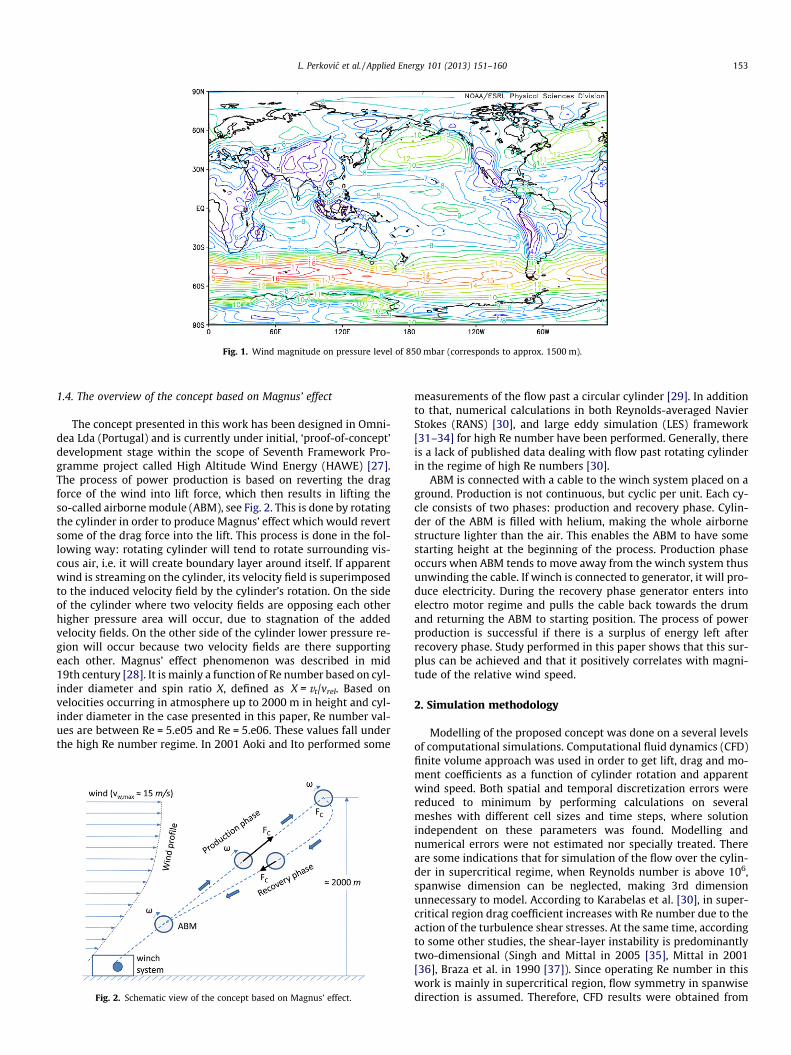
Fig. 1. Wind magnitude on pressure level of 850 mbar (corresponds to approx. 1500 m).

L. Perkovic et al. / Applied Energy 101 (2013) 151–160 153

1.4. The overview of the concept based on Magnus’ effect

The concept presented in this work has been designed in Omni-dea Lda (Portugal) and is currently under initial, ‘proof-of-concept’development stage within the scope of Seventh Framework Pro-gramme project called High Altitude Wind Energy (HAWE) [27].The process of power production is based on reverting the dragforce of the wind into lift force, which then results in lifting theso-called airborne module (ABM), see Fig. 2. This is done by rotatingthe cylinder in order to produce Magnus’ effect which would revertsome of the drag force into the lift. This process is done in the fol-lowing way: rotating cylinder will tend to rotate surrounding vis-cous air, i.e. it will create boundary layer around itself. If apparentwind is streaming on the cylinder, its velocity field is superimposedto the induced velocity field by the cylinder’s rotation. On the sideof the cylinder where two velocity fields are opposing each otherhigher pressure area will occur, due to stagnation of the addedvelocity fields. On the other side of the cylinder lower pressure re-gion will occur because two velocity fields are there supportingeach other. Magnus’ effect phenomenon was described in mid19th century [28]. It is mainly a function of Re number based on cyl-inder diameter and spin ratio X, defined as X = vt/vrel. Based onvelocities occurring in atmosphere up to 2000 m in height and cyl-inder diameter in the case presented in this paper, Re number val-ues are between Re = 5.e05 and Re = 5.e06. These values fall underthe high Re number regime. In 2001 Aoki and Ito performed some

Fig. 2. Schematic view of the concept based on Magnus’ effect.

measurements of the flow past a circular cylinder [29]. In additionto that, numerical calculations in both Reynolds-averaged NavierStokes (RANS) [30], and large eddy simulation (LES) framework[31–34] for high Re number have been performed. Generally, thereis a lack of published data dealing with flow past rotating cylinderin the regime of high Re numbers [30].

ABM is connected with a cable to the winch system placed on aground. Production is not continuous, but cyclic per unit. Each cy-cle consists of two phases: production and recovery phase. Cylin-der of the ABM is filled with helium, making the whole airbornestructure lighter than the air. This enables the ABM to have somestarting height at the beginning of the process. Production phaseoccurs when ABM tends to move away from the winch system thusunwinding the cable. If winch is connected to generator, it will pro-duce electricity. During the recovery phase generator enters intoelectro motor regime and pulls the cable back towards the drumand returning the ABM to starting position. The process of powerproduction is successful if there is a surplus of energy left afterrecovery phase. Study performed in this paper shows that this sur-plus can be achieved and that it positively correlates with magni-tude of the relative wind speed.

2. Simulation methodology

Modelling of the proposed concept was done on a several levelsof computational simulations. Computational fluid dynamics (CFD)finite volume approach was used in order to get lift, drag and mo-ment coefficients as a function of cylinder rotation and apparentwind speed. Both spatial and temporal discretization errors werereduced to minimum by performing calculations on severalmeshes with different cell sizes and time steps, where solutionindependent on these parameters was found. Modelling andnumerical errors were not estimated nor specially treated. Thereare some indications that for simulation of the flow over the cylin-der in supercritical regime, when Reynolds number is above 106,spanwise dimension can be neglected, making 3rd dimensionunnecessary to model. According to Karabelas et al. [30], in super-critical region drag coefficient increases with Re number due to theaction of the turbulence shear stresses. At the same time, accordingto some other studies, the shear-layer instability is predominantlytwo-dimensional (Singh and Mittal in 2005 [35], Mittal in 2001[36], Braza et al. in 1990 [37]). Since operating Re number in thiswork is mainly in supercritical region, flow symmetry in spanwisedirection is assumed. Therefore, CFD results were obtained from

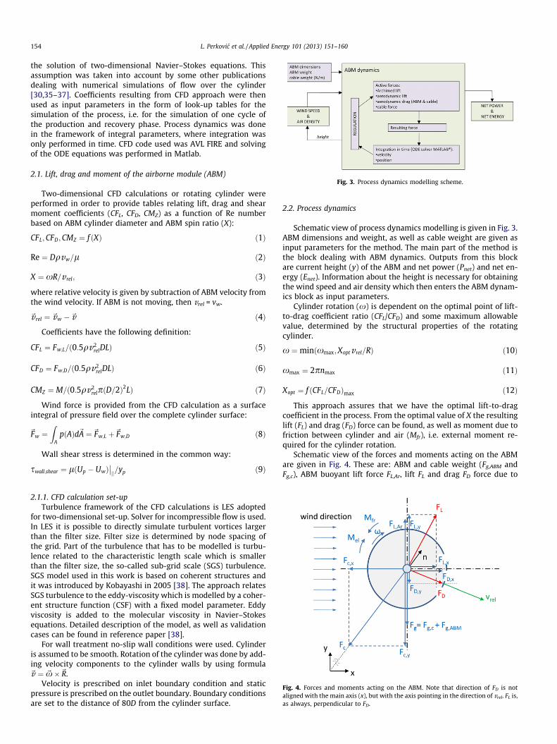
Fig. 3. Process dynamics modelling scheme.

154 L. Perkovic et al. / Applied Energy 101 (2013) 151–160

the solution of two-dimensional Navier–Stokes equations. Thisassumption was taken into account by some other publicationsdealing with numerical simulations of flow over the cylinder[30,35–37]. Coefficients resulting from CFD approach were thenused as input parameters in the form of look-up tables for thesimulation of the process, i.e. for the simulation of one cycle ofthe production and recovery phase. Process dynamics was donein the framework of integral parameters, where integration wasonly performed in time. CFD code used was AVL FIRE and solvingof the ODE equations was performed in Matlab.

2.1. Lift, drag and moment of the airborne module (ABM)

Two-dimensional CFD calculations or rotating cylinder wereperformed in order to provide tables relating lift, drag and shearmoment coefficients (CFL, CFD, CMZ) as a function of Re numberbased on ABM cylinder diameter and ABM spin ratio (X):

CFL;CFD;CMZ ¼ f ðXÞ ð1Þ

Re ¼ Dqvw=l ð2Þ

X ¼ xR=v rel; ð3Þ

where relative velocity is given by subtraction of ABM velocity fromthe wind velocity. If ABM is not moving, then vrel = vw.

~v rel ¼ ~vw �~v ð4Þ

Coefficients have the following definition:

CFL ¼ Fw;L=ð0:5qv2relDLÞ ð5Þ

CFD ¼ Fw;D=ð0:5qv2relDLÞ ð6Þ

CMZ ¼ M=ð0:5qv2relpðD=2Þ2LÞ ð7Þ

Wind force is provided from the CFD calculation as a surfaceintegral of pressure field over the complete cylinder surface:

~Fw ¼Z

ApðAÞd~A ¼~Fw;L þ~Fw;D ð8Þ

Wall shear stress is determined in the common way:

swall;shear ¼ lðUp � UwÞ��jj=yp ð9Þ

Fig. 4. Forces and moments acting on the ABM. Note that direction of FD is notaligned with the main axis (x), but with the axis pointing in the direction of vrel. FL is,as always, perpendicular to FD.

2.1.1. CFD calculation set-upTurbulence framework of the CFD calculations is LES adopted

for two-dimensional set-up. Solver for incompressible flow is used.In LES it is possible to directly simulate turbulent vortices largerthan the filter size. Filter size is determined by node spacing ofthe grid. Part of the turbulence that has to be modelled is turbu-lence related to the characteristic length scale which is smallerthan the filter size, the so-called sub-grid scale (SGS) turbulence.SGS model used in this work is based on coherent structures andit was introduced by Kobayashi in 2005 [38]. The approach relatesSGS turbulence to the eddy-viscosity which is modelled by a coher-ent structure function (CSF) with a fixed model parameter. Eddyviscosity is added to the molecular viscosity in Navier–Stokesequations. Detailed description of the model, as well as validationcases can be found in reference paper [38].

For wall treatment no-slip wall conditions were used. Cylinderis assumed to be smooth. Rotation of the cylinder was done by add-ing velocity components to the cylinder walls by using formula~v ¼ ~x�~R.

Velocity is prescribed on inlet boundary condition and staticpressure is prescribed on the outlet boundary. Boundary conditionsare set to the distance of 80D from the cylinder surface.

2.2. Process dynamics

Schematic view of process dynamics modelling is given in Fig. 3.ABM dimensions and weight, as well as cable weight are given asinput parameters for the method. The main part of the method isthe block dealing with ABM dynamics. Outputs from this blockare current height (y) of the ABM and net power (Pnet) and net en-ergy (Enet). Information about the height is necessary for obtainingthe wind speed and air density which then enters the ABM dynam-ics block as input parameters.

Cylinder rotation (x) is dependent on the optimal point of lift-to-drag coefficient ratio (CFL/CFD) and some maximum allowablevalue, determined by the structural properties of the rotatingcylinder.

x ¼minðxmax;Xoptv rel=RÞ ð10Þ

xmax ¼ 2pnmax ð11Þ

Xopt ¼ f ðCFL=CFDÞmax ð12Þ

This approach assures that we have the optimal lift-to-dragcoefficient in the process. From the optimal value of X the resultinglift (FL) and drag (FD) force can be found, as well as moment due tofriction between cylinder and air (Mfr), i.e. external moment re-quired for the cylinder rotation.

Schematic view of the forces and moments acting on the ABMare given in Fig. 4. These are: ABM and cable weight (Fg,ABM andFg,c), ABM buoyant lift force FL,Ar, lift FL and drag FD force due to

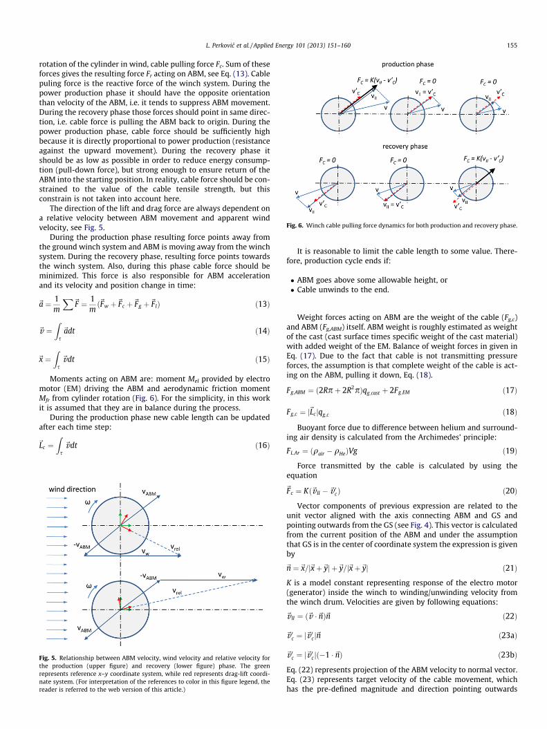
Fig. 6. Winch cable pulling force dynamics for both production and recovery phase.

L. Perkovic et al. / Applied Energy 101 (2013) 151–160 155

rotation of the cylinder in wind, cable pulling force Fc. Sum of theseforces gives the resulting force Fr acting on ABM, see Eq. (13). Cablepuling force is the reactive force of the winch system. During thepower production phase it should have the opposite orientationthan velocity of the ABM, i.e. it tends to suppress ABM movement.During the recovery phase those forces should point in same direc-tion, i.e. cable force is pulling the ABM back to origin. During thepower production phase, cable force should be sufficiently highbecause it is directly proportional to power production (resistanceagainst the upward movement). During the recovery phase itshould be as low as possible in order to reduce energy consump-tion (pull-down force), but strong enough to ensure return of theABM into the starting position. In reality, cable force should be con-strained to the value of the cable tensile strength, but thisconstrain is not taken into account here.

The direction of the lift and drag force are always dependent ona relative velocity between ABM movement and apparent windvelocity, see Fig. 5.

During the production phase resulting force points away fromthe ground winch system and ABM is moving away from the winchsystem. During the recovery phase, resulting force points towardsthe winch system. Also, during this phase cable force should beminimized. This force is also responsible for ABM accelerationand its velocity and position change in time:

~a ¼ 1m

X~F ¼ 1

mð~Fw þ~Fc þ~Fg þ~FlÞ ð13Þ

~v ¼Z

s~adt ð14Þ

~x ¼Z

s~vdt ð15Þ

Moments acting on ABM are: moment Mel provided by electromotor (EM) driving the ABM and aerodynamic friction momentMfr from cylinder rotation (Fig. 6). For the simplicity, in this workit is assumed that they are in balance during the process.

During the production phase new cable length can be updatedafter each time step:

~Lc ¼Z

s~vdt ð16Þ

Fig. 5. Relationship between ABM velocity, wind velocity and relative velocity forthe production (upper figure) and recovery (lower figure) phase. The greenrepresents reference x–y coordinate system, while red represents drag-lift coordi-nate system. (For interpretation of the references to color in this figure legend, thereader is referred to the web version of this article.)

It is reasonable to limit the cable length to some value. There-fore, production cycle ends if:

� ABM goes above some allowable height, or� Cable unwinds to the end.

Weight forces acting on ABM are the weight of the cable (Fg,c)and ABM (Fg,ABM) itself. ABM weight is roughly estimated as weightof the cast (cast surface times specific weight of the cast material)with added weight of the EM. Balance of weight forces in given inEq. (17). Due to the fact that cable is not transmitting pressureforces, the assumption is that complete weight of the cable is act-ing on the ABM, pulling it down, Eq. (18).

Fg;ABM ¼ ð2Rpþ 2R2pÞqg;cast þ 2Fg;EM ð17Þ

Fg;c ¼ j~Lcjqg;c ð18Þ

Buoyant force due to difference between helium and surround-ing air density is calculated from the Archimedes’ principle:

FL;Ar ¼ ðqair � qHeÞVg ð19Þ

Force transmitted by the cable is calculated by using theequation

~Fc ¼ Kð~v II �~v 0cÞ ð20Þ

Vector components of previous expression are related to theunit vector aligned with the axis connecting ABM and GS andpointing outwards from the GS (see Fig. 4). This vector is calculatedfrom the current position of the ABM and under the assumptionthat GS is in the center of coordinate system the expression is givenby

~n ¼~x=j~xþ~yj þ~y=j~xþ~yj ð21Þ

K is a model constant representing response of the electro motor(generator) inside the winch to winding/unwinding velocity fromthe winch drum. Velocities are given by following equations:

~v II ¼ ð~v �~nÞ~n ð22Þ

~v 0c ¼ j~v 0cj~n ð23aÞ

~v 0c ¼ j~v 0cjð�1 �~nÞ ð23bÞ

Eq. (22) represents projection of the ABM velocity to normal vector.Eq. (23) represents target velocity of the cable movement, whichhas the pre-defined magnitude and direction pointing outwards

156 L. Perkovic et al. / Applied Energy 101 (2013) 151–160

or towards the ground station, Eqs. (23a) and (23b), depending ifproduction or recovery phase is occurring. Magnitude of targetvelocity should be set to the values suitable for the unwinding/winding mechanism of the winch system.

Illustration of the principle is given in the following figure:From the known values of the cable force and it’s target velocity

the power transmitted by the cable can be calculated. It has differ-ent form for production and recovery phase, Eqs. (24a) and (24b).

Pc ¼ max½0; ð~Fc �~v 0cÞ� ð24aÞ

Pc ¼ min½0; ð~Fc �~v 0cÞ� ð24bÞ

Power balance consists from power transmitted by the winchcable and losses in the electro motors of the ABM:

Pnet ¼ Pc � PEM ¼ Pc þMfrx ð25Þ

Energy balance is calculated by integrating power balance overtime.

Enet ¼Z

sPnetdt ð26Þ

Special attention has to be given to the recovery phase of thecycle. During the recovery phase lift force should be set to mini-mum in order not to contribute to the forces resisting the down-ward motion. However, lift should be obtained again somewherein the recovery phase, since ABM is not allowed to fall down tothe ground, but has to return to origin. This can be done with incor-porating a simple regulation loop in the system. For instance, inthis work the falling of the ABM to the ground is prevented byemploying the rotation of the cylinder when angle a between theABM, origin of the system and line following the ground falls belowsome critical value. Logistic function, as a smooth approximation ofHeaviside function, is used:

x ¼ 1� 1=ð1þ expð�2Cða� a0ÞÞÞ ð27Þ

In Eq. (27) C represents model constant.

3. Results and discussion

3.1. Overview of simulation parameters and simulation set-up

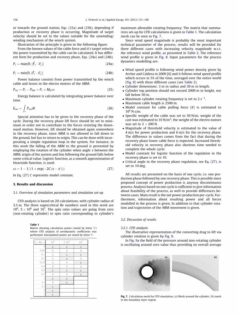
CFD analysis is based on 2D calculations, with cylinder radius of3.5 m. The three supercritical Re numbers used in this work are106, 5 � 106 and 107. The spin ratio values are going from zero(non-rotating cylinder) to spin ratio corresponding to cylinder’s

Table 1Matrix showing calculation points (noted by letter ‘c’)where CFD analysis of aerodynamic coefficients wasperformed. Interpolated points are noted by letter ’i’.

maximum allowable rotating frequency. The matrix that summa-rizes set-up for CFD calculations is given in Table 1. The calculationmesh can be seen in Fig. 7.

Since wind speed magnitude is probably the most importanttechnical parameter of the process, results will be provided forthree different cases with increasing velocity magnitude w.r.t.the reference wind profile, as presented in Table 2. The referencewind profile is given in Fig. 8. Input parameters for the processdynamics modelling are:

� Wind speed profile is following wind power density given byArcher and Caldera in 2009 [6] and it follows wind speed profilewhich occurs in 5% of the time, averaged over the entire world(Fig. 8) with three different cases (see Table 2).� Cylinder dimensions: 3 m in radius and 30 m in length.� Cylinder top position should not exceed 2000 m in height, nor

fall below 50 m.� Maximum cylinder rotating frequency is set to 2 s�1.� Maximum cable length is 2500 m.� Model constant for cable pulling force (K) is estimated to

106 N s/m.� Specific weight of the cable was set to 50 N/m; weight of the

cast was estimated to 10 N/m2; the weight of the electro motorswas set to 2 � 200 N.� Magnitude of threshold velocity is estimated to the value of

4 m/s for power production and 6 m/s for the recovery phase.The difference in values comes from the fact that during therecovery phase lower cable force is expected. Increased thresh-old velocity in recovery phase also shortens time needed tocomplete the whole cycle.� Model constant for logistic function of the regulation in the

recovery phase is set to 10.� Critical angle in the recovery phase regulation, see Eq. (27), is

set to 10 deg.

All results are presented on the basis of one cycle, i.e. one pro-duction phase followed by one recovery phase. This is possible sinceproposed concept of power production is anyway discontinuousprocess. Analysis based on one cycle is sufficient to give informationabout feasibility of the process, as well to provide differences be-tween cases. Main result is the net power production per-cycle. Fur-thermore, information about resulting power and all forcesmodelled in the process is given. In addition to that cylinder rota-tion and trajectories of the ABM movement is given.

3.2. Discussion of results

3.2.1. CFD analysisThe illustrative representation of the converting drag to lift via

cylinder rotation is given by Fig. 9.In Fig. 9a the field of the pressure around non-rotating cylinder

is oscillating around zero value thus providing no overall average

Fig. 7. Calculation mesh for CFD simulation. (a) Mesh around the cylinder; (b) meshin the boundary layer region.

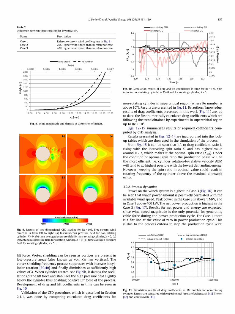
Table 2Difference between three cases under investigation.

Name Description

Case 1 Reference case – wind profile given in Fig. 8Case 2 20% Higher wind speed than in reference caseCase 3 40% Higher wind speed than in reference case

Fig. 8. Wind magnitude and density as a function of height.

Fig. 9. Results of two-dimensional CFD studies for Re = 1e6. Free-stream winddirection is from left to right. (a) Instantaneous pressure field for non-rotatingcylinder, X = 0; (b) time averaged pressure field for non-rotating cylinder, X = 0; (c)instantaneous pressure field for rotating cylinder, X = 5; (d) time averaged pressurefield for rotating cylinder, X = 5.

Fig. 10. Simulation results of drag and lift coefficients in time for Re = 1e6. Spinratio for non-rotating cylinder is X = 0 and for rotating cylinder, X = 5.

Fig. 11. Simulation results of drag coefficients vs. Re number for non-rotatingcylinder. Results are compared with experimental results of Achenbach [41], Tritton[42] and Zdravkovich [43].

L. Perkovic et al. / Applied Energy 101 (2013) 151–160 157

lift force. Vortex shedding can be seen as vortices are present inlow-pressure areas (also known as von Karman vortices). Thevortex shedding frequency process suppresses with increase in cyl-inder rotation [39,40] and finally diminishes at sufficiently highvalues of X. When cylinder rotates, see Fig. 9b, it damps the oscil-lations of the lift force and stabilizes the high pressure field slightlybelow the cylinder thus enabling positive lift force of the process.Development of drag and lift coefficients in time can be seen inFig. 10.

Validation of the CFD procedure, which is described in Section2.1.1, was done by comparing calculated drag coefficients for

non-rotating cylinder in supercritical region (where Re number isabove 106). Results are presented in Fig. 11. By authors’ knowledge,results of drag coefficients presented in this work (Fig. 11) are, upto date, the first numerically calculated drag coefficients which arefollowing the trend obtained by experiments in supercritical regionup to Re = 107.

Figs. 12–15 summarizes results of required coefficients com-puted by CFD analysis.

Results presented in Figs. 12–14 are incorporated into the look-up tables which are then used in the simulation of the process.

From Fig. 15 it can be seen that lift-to drag coefficient ratio isrising with the increasing spin ratio X, and has highest valuearound X = 7, which makes it the optimal spin ratio (Xopt). Underthe condition of optimal spin ratio the production phase will bethe most efficient, i.e. cylinder rotation-to-relative velocity ABMwill tend to go highest possible with the lowest demanding energy.However, keeping the spin ratio in optimal value could result inrotating frequency of the cylinder above the maximal allowablevalue.

3.2.2. Process dynamicsPower on the winch system is highest in Case 3 (Fig. 16). It can

be seen that winch power amount is positively correlated with theavailable wind speed. Peak power in the Case 3 is above 1 MW, andin Case 1 above 400 kW. The net power production is highest in theCase 3 (Fig. 17). Results for net power and energy are expected,since wind speed magnitude is the only potential for generatingcable force during the power production cycle. For Case 1 thereis a flat line at the value of zero in power production cycle. Thisis due to the process criteria to stop the production cycle w.r.t.

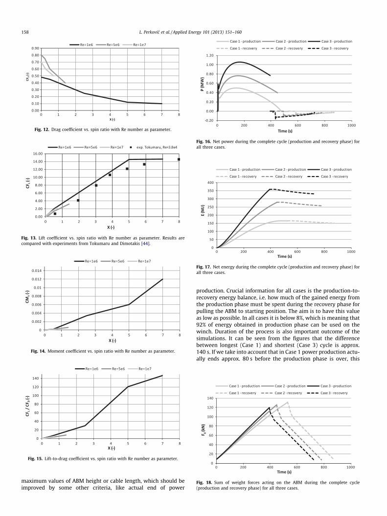
Fig. 12. Drag coefficient vs. spin ratio with Re number as parameter.

Fig. 13. Lift coefficient vs. spin ratio with Re number as parameter. Results arecompared with experiments from Tokumaru and Dimotakis [44].

Fig. 14. Moment coefficient vs. spin ratio with Re number as parameter.

Fig. 15. Lift-to-drag coefficient vs. spin ratio with Re number as parameter.

Fig. 16. Net power during the complete cycle (production and recovery phase) forall three cases.

Fig. 17. Net energy during the complete cycle (production and recovery phase) forall three cases.

Fig. 18. Sum of weight forces acting on the ABM during the complete cycle(production and recovery phase) for all three cases.

158 L. Perkovic et al. / Applied Energy 101 (2013) 151–160

maximum values of ABM height or cable length, which should beimproved by some other criteria, like actual end of power

production. Crucial information for all cases is the production-to-recovery energy balance, i.e. how much of the gained energy fromthe production phase must be spent during the recovery phase forpulling the ABM to starting position. The aim is to have this valueas low as possible. In all cases it is below 8%, which is meaning that92% of energy obtained in production phase can be used on thewinch. Duration of the process is also important outcome of thesimulations. It can be seen from the figures that the differencebetween longest (Case 1) and shortest (Case 3) cycle is approx.140 s. If we take into account that in Case 1 power production actu-ally ends approx. 80 s before the production phase is over, this

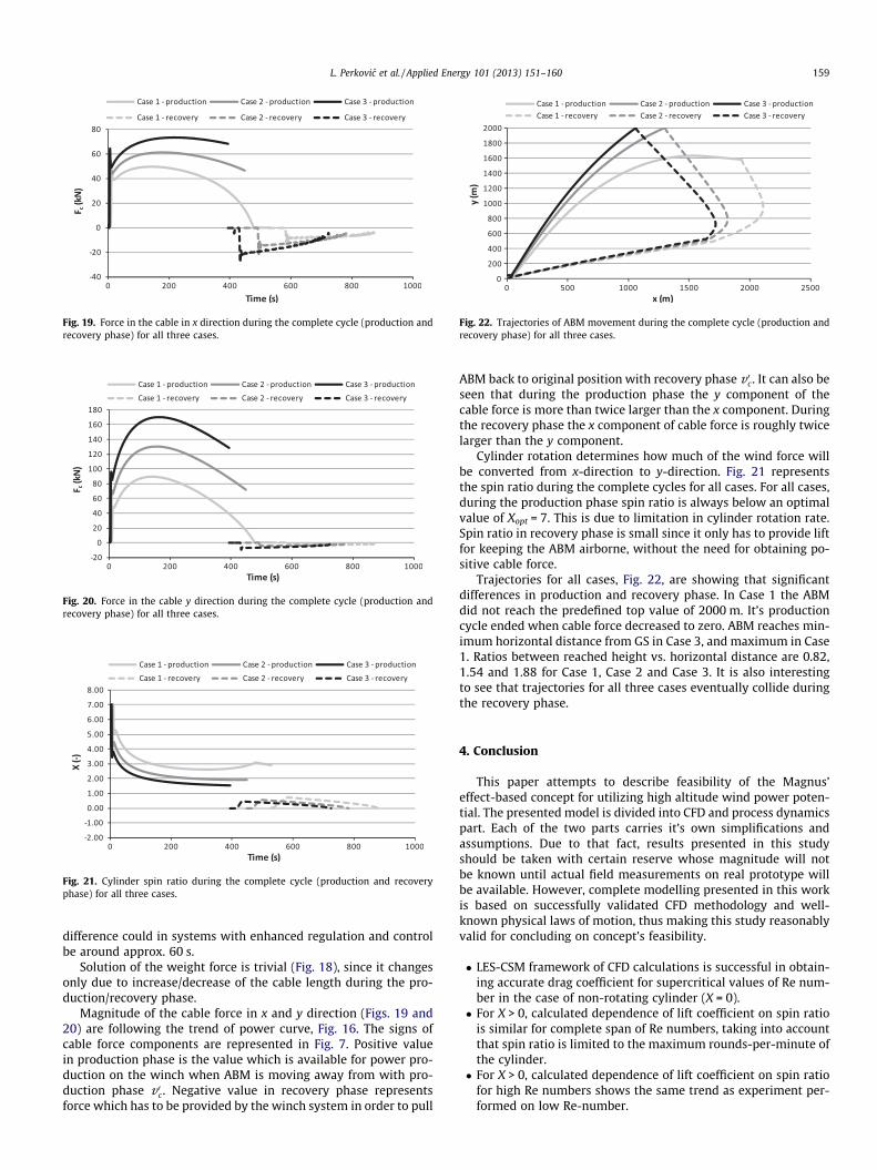
Fig. 19. Force in the cable in x direction during the complete cycle (production andrecovery phase) for all three cases.

Fig. 20. Force in the cable y direction during the complete cycle (production andrecovery phase) for all three cases.

Fig. 21. Cylinder spin ratio during the complete cycle (production and recoveryphase) for all three cases.

Fig. 22. Trajectories of ABM movement during the complete cycle (production andrecovery phase) for all three cases.

L. Perkovic et al. / Applied Energy 101 (2013) 151–160 159

difference could in systems with enhanced regulation and controlbe around approx. 60 s.

Solution of the weight force is trivial (Fig. 18), since it changesonly due to increase/decrease of the cable length during the pro-duction/recovery phase.

Magnitude of the cable force in x and y direction (Figs. 19 and20) are following the trend of power curve, Fig. 16. The signs ofcable force components are represented in Fig. 7. Positive valuein production phase is the value which is available for power pro-duction on the winch when ABM is moving away from with pro-duction phase v 0c. Negative value in recovery phase representsforce which has to be provided by the winch system in order to pull

ABM back to original position with recovery phase v 0c . It can also beseen that during the production phase the y component of thecable force is more than twice larger than the x component. Duringthe recovery phase the x component of cable force is roughly twicelarger than the y component.

Cylinder rotation determines how much of the wind force willbe converted from x-direction to y-direction. Fig. 21 representsthe spin ratio during the complete cycles for all cases. For all cases,during the production phase spin ratio is always below an optimalvalue of Xopt = 7. This is due to limitation in cylinder rotation rate.Spin ratio in recovery phase is small since it only has to provide liftfor keeping the ABM airborne, without the need for obtaining po-sitive cable force.

Trajectories for all cases, Fig. 22, are showing that significantdifferences in production and recovery phase. In Case 1 the ABMdid not reach the predefined top value of 2000 m. It’s productioncycle ended when cable force decreased to zero. ABM reaches min-imum horizontal distance from GS in Case 3, and maximum in Case1. Ratios between reached height vs. horizontal distance are 0.82,1.54 and 1.88 for Case 1, Case 2 and Case 3. It is also interestingto see that trajectories for all three cases eventually collide duringthe recovery phase.

4. Conclusion

This paper attempts to describe feasibility of the Magnus’effect-based concept for utilizing high altitude wind power poten-tial. The presented model is divided into CFD and process dynamicspart. Each of the two parts carries it’s own simplifications andassumptions. Due to that fact, results presented in this studyshould be taken with certain reserve whose magnitude will notbe known until actual field measurements on real prototype willbe available. However, complete modelling presented in this workis based on successfully validated CFD methodology and well-known physical laws of motion, thus making this study reasonablyvalid for concluding on concept’s feasibility.

� LES-CSM framework of CFD calculations is successful in obtain-ing accurate drag coefficient for supercritical values of Re num-ber in the case of non-rotating cylinder (X = 0).� For X > 0, calculated dependence of lift coefficient on spin ratio

is similar for complete span of Re numbers, taking into accountthat spin ratio is limited to the maximum rounds-per-minute ofthe cylinder.� For X > 0, calculated dependence of lift coefficient on spin ratio

for high Re numbers shows the same trend as experiment per-formed on low Re-number.

160 L. Perkovic et al. / Applied Energy 101 (2013) 151–160

Process dynamics is showing that power production and energybalance between production and recovery phase in Magnus’ con-cept depends strongly on wind speed magnitude:

� In all three cases the net energy, given by the sum of energiesfrom the production and recovery phase, is positive thus indi-cating that power production from high altitude winds withthe presented concept is possible.� Increase in wind speed increases net energy and process effi-

ciency, i.e. ratio between energy gained in production vs. energyspent in the recovery phase.� Increase in wind speed shortens time of the production phase

and time of the overall cycle.� On the other hand, increase in wind speed increases force which

should be transmitted by the cable.� With the given wind speed and limitation in cylinder rotation,

spin ratio rapidly decreases just after the start of the productionphase.

The most important improvements, which should be under con-sideration for future studies are: more realistic regulation of theprocess, introduction of third dimension into considerations, andintroduction of the additional model constraints, mainly relatedto winch cable tensile strength limit (which will demand evenmore complicated regulation).

Acknowledgements

This work has been done with the support of Omnidea Lda, Por-tugal, who originally developed the concept. The concept is nowunder the research within the project High Altitude Wind Energy(acronym HAWE), with the financial support of EC’s SeventhFramework Programme (RCN 96067). Also, authors would like tothank the Automotive Mechatronics Group of Faculty of Mechani-cal Engineering and Naval Architecture (University of Zagreb) forproviding useful discussion about the Magnus’ concept.NCEP_Reanalysis 2 data provided by the NOAA/OAR/ESRL PSD,Boulder, Colorado, USA, from their Web site at www.esrl.noaa.-gov/psd/ (last access 5th of April 2012).

References

[1] Chang TH, Huang CM, Lee MC. Threshold effect of the economic growth rate onthe renewable energy development from a change in energy price: evidencefrom OECD countries. Energy Policy 2009;37:5796–802.

[2] Marques AC, Fuinhas JA, Manso JRP. Motivations driving renewable energy inEuropean countries: a panel data approach. Energy Policy 2010;38:6877–85.

[3] Menz FC, Vachon S. The effectiveness of different policy regimes for promotingwind power: experiences from the states. Energy Policy 2006;34:1786–96.

[4] Bronstein MG. Harnessing rivers of wind: a technology and policy assessmentof high altitude wind power in the US. Technol Forecast Soc 2011;78:736–46.

[5] Arya S. Introduction to micrometeorology. New York: Academic press; 1988.[6] Archer CL, Caldeira K. Global assessment of high-altitude wind power. Energies

2009;2:307–19.[7] Kanamitsu M, Ebisuzaki W, Woollen J, Yang SK, Hnilo JJ, Fiorino M, et al. Ncep-

doe amip-ii reanalysis (R-2). Bull Am Meteorol Soc 2002;83:1631–43.[8] Hagspiel S, Papaemannouil A, Schmidt M, Andersson G. Copula-based modeling

of stochastic wind power in Europe and implications for the Swiss power grid.Appl Energy 2011. http://dx.doi.org/10.1016/j.apenergy.2011.10.039.

[9] Magenn Power Inc. <www.magenn.com/technology.php> [accessed 12.04.12].[10] Lansdorp B, Ockels WJ. Comparison of concepts for high-altitude wind energy

generation with ground based generator. In: 2nd China international renewableenergy equipment & technology exhibition and conference. Beijing; 2005.

[11] Roberts BW, Shepard DH, Caldeira K, Cannon ME, Eccles DG, Grenier AJ, et al.Harnessing high-altitude wind power. IEEE Trans Energy Convers 2007;22:136–44.

[12] Loyd ML. Crosswind kite power. J Energy 1980;4:106–11.[13] Argatov I, Rautakorpi P, Silvennoinen R. Estimation of the mechanical energy

output of the kite wind generator. Renew Energy 2009;34:1525–32.[14] Argatov I, Silvennoinen R. Energy conversion efficiency of the pumping kite

wind generator. Renew Energy 2010;35:1052–60.[15] Fagiano L. Control of tethered airfoils for high-altitude wind energy

generation. PhD thesis. Politechnico di Torino; 2009.[16] Canale M, Fagiano L, Milanese M. KiteGen: a revolution in wind energy

generation. Energy 2009;34:7.[17] Argatov I, Rautakorpi P, Silvennoinen R. Apparent wind load effects on the

tether of a kite power generator. J Wind Eng Ind Aerod 2011;99:1079–88.[18] Krajacic G, Duic N, Tsikalakis A, Zoulias M, Caralis G, Panteri E, et al. Feed-in

tariffs for promotion of energy storage technologies. Energy Policy2011;39:1410–25.

[19] Cosic B, Markovska N, Krajacic G, Taseska V, Duic N. Environmental and economicaspects of higher RES penetration into Macedonian power system. Appl ThermEng 2011. http://dx.doi.org/10.1016/j.applthermaleng.2011.10.042.

[20] Chen FZ, Duic N, Alves LM, da Graca Carvalho M. Renewislands – renewableenergy solutions for islands. Renew Sustain Energy Rev 2007;11:1888–902.

[21] Duic N, Krajacic G, Carvalho MD. RenewIslands methodology for sustainableenergy and resource planning for islands. Renew Sustain Energy Rev2008;12:1032–62.

[22] Lund H, Duic N, Krajacic G, Carvalho MD. Two energy system analysis models:a comparison of methodologies and results. Energy 2007;32:948–54.

[23] Busuttil A, Krajacic G, Duic N. Energy scenarios for Malta. Int J HydrogenEnergy 2008;33:4235–46.

[24] Krajacic G, Duic N, Carvalho MD. How to achieve a 100% RES electricity supplyfor Portugal? Appl Energy 2011;88:508–17.

[25] Segurado R, Krajacic G, Duic N, Alves L. Increasing the penetration of renewableenergy resources in S. Vicente, Cape Verde. Appl Energy 2011;88:466–72.

[26] Mathiesen BV, Lund H, Karlsson K. 100% Renewable energy systems, climatemitigation and economic growth. Appl Energy 2011;88:488–501.

[27] European Commission Community Research and Development InformationService (CORDIS). <http://cordis.europa.eu/fetch?CALLER=FP7_PROJ_EN&ACTION=D&DOC=1&CAT=PROJ&RCN=96067> [accessed 15.10.11].

[28] Magnus G. On the deviation of projectiles, and: on a sinking phenomenonamong rotating bodies. Ann Phys 1853;164:29.

[29] Aoki K, Ito T. Flow characteristics around a rotating cylinder. Proc School EngTokai Univ 2001;26:6.

[30] Karabelas SJ, Koumroglou BC, Argyropoulos CD, Markatos NC. High Reynoldsnumber turbulent flow past a rotating cylinder. Appl Math Model2012;36:379–98.

[31] Karabelas SJ. Large Eddy simulation of high-Reynolds number flow past arotating cylinder. Int J Heat Fluid Flow 2010;31:518–27.

[32] Breuer M. A challenging test case for large eddy simulation: high Reynoldsnumber circular cylinder flow. Int J Heat Fluid Flow 2000;21:648–54.

[33] Catalano P, Wang M, Iaccarino G, Moin P. Numerical simulation of the flowaround a circular cylinder at high Reynolds numbers. Int J Heat Fluid Flow2003;24:463–9.

[34] Breuer M. Numerical and modelling influences on large eddy simulations forthe flow past a circular cylinder. Int J Heat Fluid Flow 1998;19:10.

[35] Singh SP, Mittal S. Flow past a cylinder: shear layer instability and drag crisis.Int J Numer Methods Fluids 2005;47:75–98.

[36] Mittal S. Computation of three-dimensional flows past circular cylinder of lowaspect ratio. Phys Fluid 2001;13:177–91.

[37] Braza M, Chassaing P, Minh HH. Prediction of large-scale transition features inthe wake of a circular-cylinder. Phys Fluids A Fluid 1990;2:1461–71.

[38] Kobayashi H. The subgrid-scale models based on coherent structures forrotating homogeneous turbulence and turbulent channel flow. Phys Fluid2005:17.

[39] Lam KM. Vortex shedding flow behind a slowly rotating circular cylinder. JFluids Struct 2009;15:18.

[40] Dol SS, Kopp GA, Martinuzzi RJ. The suppression of periodic vortexshedding from a rotating circular cylinder. J Wind Eng Ind Aerod 2008;96:1164–84.

[41] Achenbach E. Distribution of local pressure and skin friction around a circularcylinder in cross-flow up to Re = 5 � 106. J Fluid Mech 1968;34:625–39.

[42] Tritton DJ. Physical fluid dynamics. 2nd ed. New York: Oxford University PressUSA; 1988.

[43] Zdravkovich MM. Flow around circular cylinders: fundamentals, vol. 1. NewYork: Oxford University Press USA; 1997.

[44] Tokumaru PT, Dimotakis PE. The lift of a cylinder executing rotary motions in auniform-flow. J Fluid Mech 1993;255:1–10.