Embed Size (px)
Citation preview
Harvey Liszt Arecibo July 2009
Reflections on Spectra and Spectra andSpectral Line Work
Harvey S. Liszt
NRAO, CHARLOTTESVILLE

Why spectral lines?
• From profile velocities and widths:– Gas flows in local clouds and the Hubble flow– Galaxy rotation curves and (dark) masses– Cloud dynamics, collapse, turbulence
• From intensities:– Gas temperatures, cloud masses– Chemical composition & chemistry– Atomic/molecular physics
Harvey Liszt Arecibo July 2009

What does it take to see one?
• Medium that isn’t completely transparent– Finite optical depth = photon mean free path– Implies radiative interaction with environment
• Medium that stands out– Its existence must either brighten or dim the radiation
heading in our direction– Background may be the cmb– A medium at the temperature of the cmb is invisible
against the cmb no matter how opaque
Harvey Liszt Arecibo July 2009

Spectral lines
• Spectral lines connect discrete internal states– One, labelled l is lower in energy, u higher
– States are typically degenerate with weights gl , gu
– Radiated energy appears at E = hv (duh)
• For radio hv/k is quite small, 0.048 K/GHz– hv/k isn’t necessarily > 2.73K– More likely (than optical) to be near LTE
– Arbitrarily define “excitation temperature” nu/nl = (gu/gl) e
-hv/kTexc
Harvey Liszt Arecibo July 2009

Radio v. Optical
• By optical standards, radio lines may seem very, very weak; in terms of f-values, – For Lyman- line of H I, f ~ 0.48
– For 21 cm line of H I, f = hv/2mec2 = 5.75.10-12
– Indeed, radio astronomy can only detect relatively large amounts of H I (1018 cm-2 vs 1012 cm-2)
– Nonetheless, RA sees the H I line easily, everywhere in the sky
Harvey Liszt Arecibo July 2009

Radio v. Optical
• And the Einstein Aul are langorous
– For Lyman- line of H I, Aul ~ 109/s
– For 21 cm line of H I, Aul ~ 2.7.10-15/s
• For TK < 500 K, Texc ~ TK
– For CO J=1-0 at 2.6mm, Aul ~ 7.2.10-8/s
• Small Aul + low hv/k result in peculiarities of radiative transfer in the radio
Harvey Liszt Arecibo July 2009

In the optical regime
Harvey Liszt Arecibo July 2009
• How does this difference manifest itself?

Harvey Liszt Arecibo July 2009
• How does this difference manifest itself?
In the optical regime

Harvey Liszt Arecibo July 2009
• How does this difference manifest itself?
In the optical regime

Harvey Liszt Arecibo July 2009
• How does this difference manifest itself?
linear
In the optical regime

Harvey Liszt Arecibo July 2009
• How does this difference manifest itself?
saturated
In the optical regime

Harvey Liszt Arecibo July 2009
• How does this difference manifest itself?
damped
In the optical regime

Harvey Liszt Arecibo July 2009
• How does this difference manifest itself?
In the optical regime

Harvey Liszt Arecibo July 2009
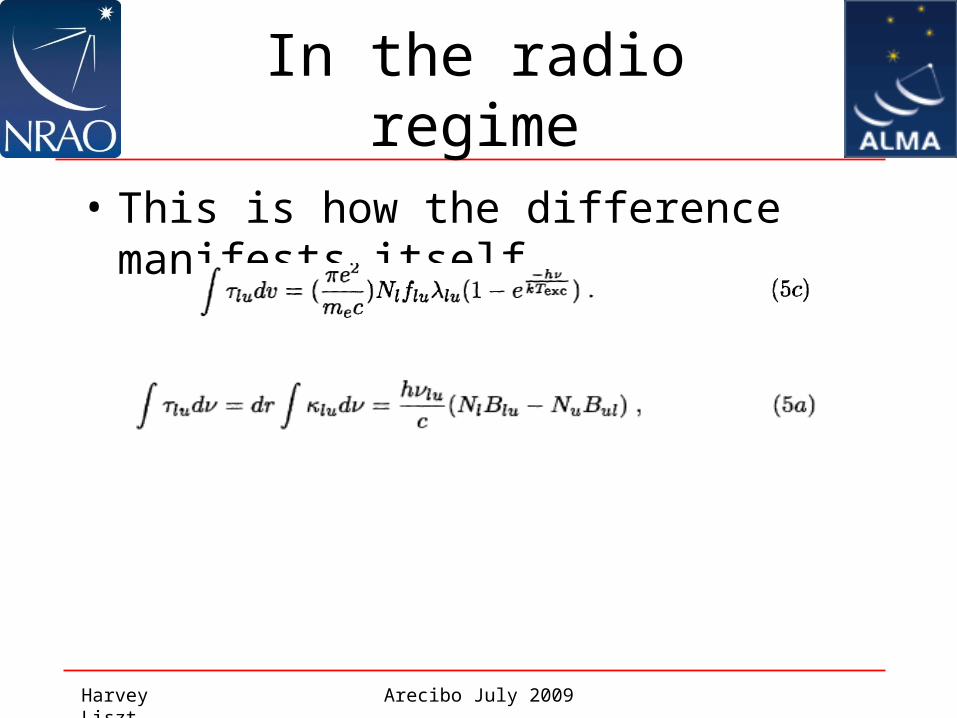
• This is how the difference manifests itself
In the radio regime
Harvey Liszt Arecibo July 2009
• This is how the difference manifests itself
In the radio regime

Harvey Liszt Arecibo July 2009
• This is how the difference manifests itself
In the radio regime

Harvey Liszt Arecibo July 2009
• This is how the difference manifests itself
In the radio regime

Harvey Liszt Arecibo July 2009
• This is how the difference manifests itself
Plug in values for HI and expand for small hv/kTexc
H I & the radio regime

H I optical depth
Harvey Liszt Arecibo July 2009
• This is how the difference manifests itself
(km/s)

Ugh, radiative transfer!
Harvey Liszt Arecibo July 2009
• This is how the difference manifests itself

If the opacity is great
Harvey Liszt Arecibo July 2009
• This is how the difference manifests itself
>> 1, TC small

If opacity is small …
Harvey Liszt Arecibo July 2009
• This is how the difference manifests itself
TC small
>> 1, TC small
Harvey Liszt Tucson December 2007
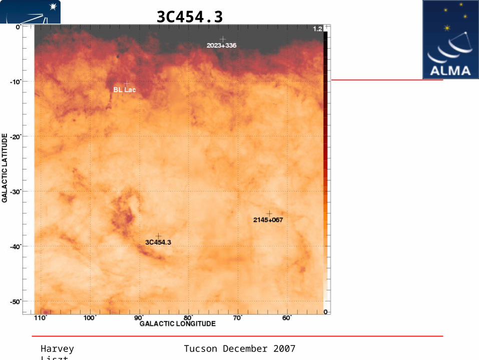
3C454.3

Harvey Liszt Tucson December 2007
3C454.3

Harvey Liszt Tucson December 2007
3C454.3 in H I

H I vs. dust
• Integral of TBdv = 385.5 K km/s
– Equivalent to N(H) = 7.0x1020 cm-2
• E(B-V) = 0.11 mag– From Copernicus, => N(H) ~ 6.4x1020 cm-2
• Most of the extincting material is seen H I
Harvey Liszt Arecibo July 2009

Harvey Liszt Tucson December 2007
3C454.3 in emission

Harvey Liszt Tucson December 2007
3C454.3 in emission and absorption

Harvey Liszt Tucson December 2007
~ 0.3
3C454.3 in emission and absorption
Ratio TB and 1-e-
Harvey Liszt Arecibo July 2005

Ratio TB and 1-e-
Harvey Liszt Arecibo July 2005

Ratio TB and 1-e-
Harvey Liszt Arecibo July 2005

Ratio TB and 1-e-
• Inhomogeneity in TK
• Colder narrow-line “clouds” coexist with a warmer,more diffuse gas, broader- lined gas (inter-cloud medium)
• Two “phase” model cf. Clark (1965)
Harvey Liszt Arecibo July 2005

Harvey Liszt Tucson December 2007
Short Break

Harvey Liszt Tucson December 2007
Short Break

Harvey Liszt Arecibo July 2009
Better epistemolgy through radiometry
• Something (nature?) emits some radiation• Manifested to us as a flux or burst of energy
crossing our telescope• Which we measure through radiometry• By accumulating incident radiation until there
is a detectable amount of energy• Which we relate to some (celestial)
phenomenon by ‘deconvolving’ from the measurement the conditions of making it

Harvey Liszt Arecibo July 2009
Conditions?
• One aspect of ‘conditions’ is physics of spectral line formation in the source– That’s more or less my original book article, which
back in the day was followed by a 2nd lecture
• Another aspect is what happens to these cosmic emanations in our equipment
• And another is how we maul, er, excuse me, manipulate spectra afterward
Harvey Liszt Arecibo July 2009
• E = k T (energy, ergs, Joules)– k = Boltzmann’s constant 10-23 Joules/K– k = k . s-1 . Hz-1
– So Joules = W Hz-1
• That is why we talk about power flux density– Sv (Jy) = 10-26 W m-2 Hz-1
– Accumulate the energy falling across the area of the telescope, over some bandwidth
Energy

Harvey Liszt Arecibo July 2009
• E = k T (energy, ergs, Joules)– k = Boltzmann’s constant 10-23 Joules/K– k = k . Hz-1 s-1
– So Joules = W Hz-1
• That is why we talk about power flux density– Sv (Jy) = 10-26 W m-2 Hz-1
– Accumulate the energy falling across the area of the telescope, over some bandwidth
Area

Harvey Liszt Arecibo July 2009
Area?
• Telescope (effective) area Aeff ~D2/4– D is diameter of the illuminated area– No telescope is perfectly efficient– 75% is very good, 55% is more typical
• Beam solid angle Aeff 2– For a very good antenna ofis in a main
lobe– For an isotropic antenna , Aeff 2/– This is 0 dBi gain, used for RFI calculations

Harvey Liszt Arecibo July 2009
Flux as temperature
• Define antenna temperature Sv = 2 kTA/Aeff – In terms of the effective area of the telescope
• Sv/TA (or TA/Sv) is the gain– 2 Kelvins/Jy at the GBT, 14 K/Jy for ART– Each Jy heats the surface EM field by some K’s– 12m ALMA antennas need ~30 Jy/K but have 1’
beam at 115 GHz (vs 3’-8’ w/Arecibo or GBT H I)

Harvey Liszt Arecibo July 2009
Phooey, noise
• Radiometers have an intrinsic property
• An irreducible rms fluctuation level
• When measuring a source of radiation whose ambient flux is equivalent to that of a black body at temperature T, during a time t, over a bandwidth v
T = T/(v t)1/2

Harvey Liszt Arecibo July 2009
But at what ‘T’?
• What is T in the radiometer equation?
T = (Tsys+ TA)/(v t)1/2
• Where
– Tsys is inherent in the equipment
– TA is what is added by incident flux
– Our signal is usually just additional noise, devoid of character (modulation)

Harvey Liszt Arecibo July 2005
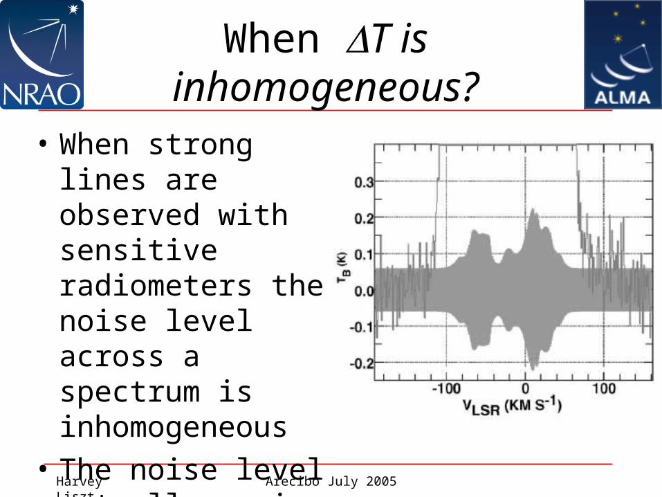
• When strong lines are observed with sensitive radiometers the noise level across a spectrum is inhomogeneous
Assessing your noise

Harvey Liszt Arecibo July 2005
• When strong lines are observed with sensitive radiometers the noise level across a spectrum is inhomogeneous
• This 1990 spectrum of the H I line had Tsys= 36K, now GBT ~ 20 K
How to measure T ?
Harvey Liszt Arecibo July 2005
• When strong lines are observed with sensitive radiometers the noise level across a spectrum is inhomogeneous
• The noise level actually varies by a factor 3.5 over this spectrum!
When T is inhomogeneous?

Harvey Liszt Arecibo July 2005
• Notice how the software you use treats the rms noise … it is probably taken to be homogeneous at the level of the line-free channels … which may be OK if your lines are suitably weak
What’s in it for you?

Harvey Liszt Arecibo July 2005
• The usual assumption is that T is the same across the spectrum
• Notice how the software you use treats the rms noise … it is probably taken to be homogeneous at the level of the line-free channels … which may be OK if your lines are suitably weak
When might business as usual not be OK?

Harvey Liszt Arecibo July 2005
• The usual assumption is that T is the same across the spectrum
• AND that T can be read off the spectrum in signal-free channels
• AND that the rms of an N-channel sum grows as N1/2
• Notice how the software you use treats the rms noise … it is probably taken to be homogeneous at the level of the line-free channels … which may be OK if your lines are suitably weak
When might business as usual not be OK?

Harvey Liszt Arecibo July 2005
When data are smoothed/oversampled!
• When data are oversampled by a factor q>1, the rms of an N-channel sum is q1/2 larger than the naive result, N1/2 x the single-channel rms

Harvey Liszt Arecibo July 2005
When data are smoothed/oversampled!
• When data have q channels/resolution element, the rms of an N-channel sum is asymptotically q1/2 larger than the naive result, N1/2 x the single-channel rms

Harvey Liszt Arecibo July 2009
History
• Since ~1970 when CO was detected at 2.6mm, Tsys for 21cm H I work has fallen from 70 K to 20 K and Tsys for 3mm work has fallen from 5000 K to sub-100 K!
• In terms of the radiometer equation, the ratio (100 GHz/1.42GHz)1/2 now outweighs the higher system temperature at 100 GHz.

Harvey Liszt Arecibo July 2009
What was that?
• The number of km/s in one MHz = mm
– For H I, 1 MHz ~ 211.1 km/s– For CO, 1 MHz = 2.6 km/s– Advantage grows with sqrt(v)
• In terms of the radiometer equation, the ratio (100 GHz/1.42GHz)1/2 now outweighs the higher system temperature at 100 GHz.