Munich Personal RePEc Archive

Has urban economic growth in

Post-Reform India been pro-poor

between 1993-94 and 2009-10?

Tripathi, Sabyasachi

Indian Council for Research on International Economic Relations

December 2013

Online at https://mpra.ub.uni-muenchen.de/52336/

MPRA Paper No. 52336, posted 19 Dec 2013 05:13 UTC

1

Has urban economic growth in Post-Reform India

been pro-poor between 1993-94 and 2009-10?

Sabyasachi Tripathi*

Indian Council for Research on International Economic Relations

New Delhi, India

Email: sabya.tripathi@gmail.com

Abstract:

This paper empirically tests whether urban economic growth has been pro-poor in the post

reform India. The study uses data from the three rounds of quinquennial household survey of

urban monthly per capita consumer expenditure (MPCE) carried out by National Sample Survey

Organization (NSSO) in 1993-94, 2004-05, and 2009-10. To empirically measure the pro-

poorness of urban economic growth, this paper uses the framework developed by Duclos (2004)

and also follows the methodological approach of Araar, Duclos, Audet, and Makdissi (2007,

2009). The study finds strong statistical evidence that India‘s urban economic growth has been absolutely pro-poor but relatively anti-poor between periods 1993-94 - 2004-05, 2004-05 - 2009-

10, and 1993-94 - 2009-10. The results indicate that more effective distributive policies are

urgently required for urban poverty reduction in India.

Key Words: Pro-poor Growth, Poverty, Inequality, Urban India

JEL Classification: D63, D64, R11

* Any opinions expressed here are mine and not necessarily those of the institute. The usual

disclaimer applies.

2

1. Introduction

Economic reforms in India which started on 24 July 1991 have had a significant effect on India‘s

economic growth. For instance, India‘s average gross national product at 2004-05 prices grew at

the impressive annual rate of 6.96 percent from 1992-93 to 20011-12. However, the real

challenge faced by the Indian economy is the equitable distribution of the gains from higher

economic growth to the citizens of India as benefits of growth are not equitably spread across

different income groups and various sections of the society currently. In other words, low income

groups (or lower caste) have benefitted only marginally or not much from the higher economic

growth. For that reason, The Approach Paper to the Twelfth Five-Year Plan (2012-17) has

chosen ‗faster, sustainable and more inclusive growth‘ as its main goal. The thrust in the

Approach Paper is to make growth ‗more inclusive‘ in terms of providing more benefits to those

sections of population, which had hardly benefitted from the higher economic growth achieved

in post-reform India.

India‘s urban economy too is growing and making a sizeable contribution to the country‘s

national income. The latest available Central Statistical Organization (CSO) data shows that in

2004-05, the share of urban NDP was about 52.02 percent in the national NDP, which is quite

higher than the NDP (37.65 per cent) in 1970-71.1 The compound annual growth rate (CAGR) of

urban NDP was about 8.1 per cent from 1993-94 to 2004-05 at constant prices (1999-00). Most

importantly, according to the Mid‐Term Appraisal of the Eleventh Five Year Plan, the urban

share of gross domestic product (GDP) which was about 63 per cent in 2009–2010 is projected to

increase to 75 per cent by 2030. These figures show that the potential contribution of urban

economic growth to national GDP is very high. At the same time, urban consumption inequality

as measured by Gini coefficient increased from 0.34 in 1993-94 to 0.39 in 2009-10 -- an increase

of about 15 per cent. On the other hand, urban poverty as measured by poverty head count ratio

declined from 31.8 in 1993-94 to 20.9 in 2009-10 -- a decline of about 34 per cent. These

inequality and poverty figures suggest that in spite of higher urban economic growth, a large

proportion of urban dwellers are still experiencing inadequate improvement in their standard of

living. In other words, higher urban economic growth is not shared equitably.

1 Net domestic product (NDP) estimated at factor cost and its rural and urban break-up at national level are available

only for the years 1970-71, 1980-81,1993-94, 1999-2000 and 2004-05.

3

Poverty reduction is deemed an important goal of the country‘s urban policy. In India, migration

is not a significant contributing factor in urban population growth; therefore, urban poverty does

not constitute the transfer of rural poverty into urban areas. In the past, several Five Year plans

had adopted several programmes and policies for urban poverty reduction. These include Nehru

Rozgar Yojana (NRY) launched in October 1989 with the objective of providing of employment

to the urban unemployed and underemployed poor; Urban Basic Services for the Poor (UBSP)

implemented in Eight Five Year Plan (1992-97) for community organisation, mobilisation and

empowerment and converence through sustainable support system; Prime Minister's Integrated

Urban Poverty Eradication Programme (PM-IUPEP) launched in November, 1995 for small

towns development and the Swarna Jayanti Shahari Rozgar Yojana (SJSRY) operationalised on

December 1, 1997 for gainful employment to the urban unemployed or underemployed poor by

encouraging the setting up of self-employment ventures or provision of wage employment.

The Twelfth Five Year Plan (2012-17) has its focus on addressing the basic needs of the urban

poor who are largely employed in the informal sector and suffer from multiple deprivations and

vulnerabilities which include lack of access to basic amenities such as water supply, sanitation,

health care, education, social security and affordable housing. Policy interventions like the Rajiv

Awas Yojana (2013-22) proposed in Twelfth Five Year Plan, coupled with policy measures for

augmenting the supply of affordable housing, and expanded access of subsidized healthcare and

education to the urban poor, should result in a significant reduction in the proportion of slum

dwellers as also the geographical spread of slums.2

However, for these interventions to bear fruit, a systematic appraisal of the higher urban

economic growth and the associated distributive effects is imperative. It is important to know

poverty figures as it is one of the essential inputs to design, monitor, and implement anti-poverty

policies. However, little is known about the distributional aspects of this phase of urban

economic growth and how it compares with the previous growth periods in terms of poverty

reduction. Assessing the pro-poorness of growth, and its consequences, has become a general

2 See the following link for more details about the poverty reduction policies and programmes taken in different Five

Year Plans in urban India. Web address:

http://planningcommission.nic.in/plans/planrel/index.php?state=planbody.htm

4

topic of policy discussion in several new development paradigms. It is also important to evaluate

the distributional changes in the post – reform India, as rapid urbanization and urban economic

growth are the main source of sustainable and higher economic growth. Now the question arises

about how India should face the challenges thrown up by the rapid urbanization process, and

what distributive policies need to be taken to ensure distributive justice and harmony in urban

society. It is acknowledged that higher economic growth benefits the poor only when levels of

inequality are lower and the gains of development are equitably distributed through appropriate

redistributive policies.

The main objective of this paper is to empirically assess the pro-poorness of distributive changes

of urban economic growth in post-reform India. In other words, it empirically investigates

whether public policy and public expenditures are pro-poor or not. The study covers the period

1993-94 to 2009-10, and we have used available data from three rounds, i.e., 50th

round for

1993-94, 61st round for 2004-05, and 66

th round for 2009-10, of urban monthly per capita

consumer expenditure (MPCE) data provided by National Sample Survey Organization (NSSO)

for our analysis. For empirically measuring the pro-poorness of urban economic growth, we have

used the framework developed by Duclos (2009) and followed the methodological approach of

Araar et al. (2007, 2009) and Araar (2012). Duclos (2009) presents an axiomatic formulation of

the two different approaches (i.e., relative and absolute) measurement of poverty. Broadly

speaking, in the relative approach, we label a growth process pro-poor if the growth rate of the

poor exceeds some standard (usually the average growth rate – of the median or the mean), e.g.,

are the poor growing at 5 percent? In the absolute approach, we label growth as pro-poor if the

absolute incomes of the poor increase by at least some standard, e.g., have the incomes of the

poor increased by Rs. 100? Araar et al. (2009) illustrate how we can statistically test for pro-poor

growth. The novelty of using these frameworks is that it is based on a new theoretical framework

and analyzes pro-poor growth in a dynamic manner, and has rigorous statistical rationale. The

results are extremely important in the context of the ongoing debate about the distributional

effects of the recent period of rapid urban economic growth experienced in India.

The rest of the paper is structured as follows. Section 2 presents a brief review of literature on

measurement of pro-poor growth in India; Section 3 describes the measurement framework;

Section 4 explains the data used for the empirical analysis and Section 5 highlights the details of

5

estimated results. Summary of findings, major conclusions and implications are provided in

Section 6.

2. Review of literature

There are very few studies which measure the pro-poorness of economic growth in India. Datt

and Ravallion (2009) assess whether the post-reform urban economic growth process has been

more pro-poor than the pre-reform process. They measure pro-poor growth as reduction of

poverty and elasticity of poverty with respect to economic growth.3 Using household

consumption expenditure survey data from National Sample Survey (NSS) for the period 1958-

2006, they have found that a long-run trend of decline in all three of the poverty indicators (i.e.,

Headcount index, Poverty gap index, and Squared poverty gap index), but higher proportionate

rate of progress against poverty after 1991. Post-reform, growth process has become less pro-

poor in the sense that the proportionate rate of poverty reduction from a given rate of growth was

lower than in the pre-reform period. Finally, they find much stronger evidence of a feedback

effect or trickle-down effect, i.e., higher reduction in rural poverty due to urban economic growth

as than in the pre-1991 data.

Liu and Barrett (2013) using 2009-10 National Sample Survey data looks into the patterns of

job-seeking, rationing, and participation under the Mahatma Gandhi National Rural Employment

Guarantee Scheme (MGNREGS). They find that the current administrative rationing of

MGNREGS jobs is not pro-poor (i.e., ―progressive‖ participation profile) but exhibits a sort of

middle-class bias.

Dev (2002) investigates the extent of pro-poor growth by assessing various quantitative and

qualitative aspects of the employment that has been generated, specifically, employment

elasticities of growth, labour productivity and wage rates, job security (casualisation and

multiplicity) and access for the period of 1980 to 2000. He finds that the quality of employment

has declined in all three economic sectors, and particularly in agriculture, and that the acutely

affected are women. Poorer groups are predominantly reliant on casual labour for sustenance.

The rate of growth in employment has been positive over time but it declined between 1994 and

2000.

3 For an overview of the various approaches to defining ―pro-poor growth‖ see Ravallion (2004)

6

For measuring pro-poorness a cross-sectional study by Balasubramanian and Ravindran (2012)

of women beneficiaries under the Muthulakshmi Reddy Maternity Benefit Scheme in five

districts of Tamil Nadu showed that scheduled caste and landless women in the sample were

disadvantaged in receiving benefits. Overall, only one-fourth of the women who delivered first

or second order births in the sample received monetary assistance under the scheme.

Ravallion (2000) finds a number of conditions that determine how much India‘s poor share in

economic growth. He suggested that without higher and more stable agricultural growth, it will

be hard to restore India‘s momentum in poverty reduction. Agriculture, infrastructure and social

spending (especially in lagging rural areas) will have to be prioritized first so as to enable the

poor to participate fully in India‘s post-reform economic growth. The gains to the poor from non-

agricultural growth have varied greatly across states, reflecting the contours of past attainments

in human and physical resource development, especially in rural areas.

Ravallion and Datt (1999) using data from 20 household surveys for India‘s 15 major states for

the period of 1960-94, study how initial conditions and sectoral composition of economic growth

tend to determine the degree of economic growth and reduction in poverty. They find that states

which initially had lower farm productivity, lower rural living standards relative to those in

urban areas, and lower literacy experienced a less pro-poor growth process later. But the

elasticities of poverty to (urban and rural) nonfarm output varied appreciably, and the differences

were quantitatively important to the overall rate of poverty reduction.

The insight provided by the above review of studies clearly indicate that the measurement of pro-

poor growth in the context to urban economic growth is highly neglected filed of research, and

therefore this paper attempt to empirically asses the urban pro-poor growth in context to India.

3. Theoretical framework

3.1 The pro-poor growth

For the measurement of pro-poor growth, this study follows the theoretical framework proposed

by Duclos (2009) and Araar et al., (2007, 2009).4 Absolute pro-poorness refers to a situation

4 We have tried to present the basic theoretical structure and equations which are essential for the empirical analysis

and as they are presented in Araar (2012). The details are given in Duclos (2009), Araar et al., (2007, 2009) and

Araar (2012).

7

where incomes of the poor grow by an absolute amount that is no less than some norm (often set

to zero). Relative pro-poorness requires the increase in the incomes of the poor to be greater than

some norm (often mean income growth).5

For measuring pro-poor growth, the framework of Duclos (2009) has proposed following two

important dimensions: (1) a poverty line to separate the poor from non-poor, and (2) a set of

normative weights to differentiate among the poor. The framework as developed by Duclos

(2009) is described below.

Let 𝒚𝟏 = 𝑦11,𝑦2

1,……… .𝑦𝑛11 ∈ 𝕽+

𝒏𝟏 be a vector of non-negative initial incomes (or

consumption, wealth, or any other welfare indicator of interest) at time 1 of size 𝑛1, and let 𝒚𝟐 = 𝑦12,𝑦2

2,……… .𝑦𝑛12 be an analogues vector of incomes at time 2 of size 𝑛2.

In case of relative standard, which is simply the average growth rate, denoted by 𝑔. Let 𝑊(𝒚𝟏, 𝒚𝟐,𝑔, 𝑧) be the pro-poor evaluation function that we want to use, where 𝑧 > 0 stands as the

poverty line. It is defined as the difference between two evaluation functions 𝜋 (𝒚𝟏, 𝑧) and 𝜋∗ (𝒚𝟐,𝑔, 𝑧), each for time 1 and time 2, respectively, and which are analogous to poverty

indices for each of the two time periods: 𝑊(𝒚𝟏, 𝒚𝟐,𝑔, 𝑧) ≡ 𝜋∗ 𝒚𝟐,𝑔, 𝑧 − 𝜋 (𝒚𝟏, 𝑧) …………… (1)

The change from 𝒚𝟏 to 𝒚2 will be deemed pro-poor if 𝑊(𝒚𝟏, 𝒚𝟐,𝑔, 𝑧) ≤ 0.

The social welfare function of 𝑊 has the following basic axioms. 1) focus axiom, 2) population

invariance axiom, 3) anonymity axiom, 4) normalization axiom, 5) monotonicity axiom, 6)

distribution sensitivity axiom.

3.1.1 Relative pro-poor judgments

Let 𝐹𝑗 (𝑦) be the distribution function of distribution 𝑗. Also define as 𝑄𝑗 (𝑝) the quantile

function for the distribution 𝐹𝑗 . This is formally defined as 𝑄𝑗 𝑝 = inf 𝑠 ≥ 0|𝐹𝑗 𝑠 ≥ 𝑝 for 𝑝 ∈ 0,1 . With a continuous distribution and a strictly positive income density,𝑄 (𝑝) is simply

the inverse of the distribution function, and therefore is the income of the individual at rank 𝑝 in

the distribution. Then the FGT indices are given by: 𝑃𝑗 𝑧;𝛼 = 1 − 𝑄𝑗 𝑝 𝑧 𝛼𝐹𝑗 (𝑧)

0𝑑𝑝. ------- (2)

5 See Araar (2012) for the detailed discussion.

8

𝑃𝑗 𝑧;𝛼 = 0 is the headcount index (and the distribution function) at 𝑧, and 𝑃𝑗 𝑧;𝛼 = 1 is the

average poverty gap.

A movement from 𝒚𝟏 to 𝒚2 will be judged as pro-poor by all such functions if and only if 𝑃2( 1 + 𝑔 𝑧; 𝛼 = 0 ≤ 𝑃1(𝑧;𝛼 = 0) for all 𝑧 ∈ [0, 𝑧+] -------- (3)

A distributional change that satisfies (3) is called first-order relatively pro-poor since all pro-poor

evaluation functions within Ω1 𝑔, 𝑧+ will find that it is pro-poor, and this, for any choice of

poverty line within [0, 𝑧+] and any 𝑊 that obeys the above defines axioms. Verifying (3)

simply involves checking whether—over the range of poverty lines [0, 𝑧+] the headcount index

in the initial distribution is larger than the headcount index in the posterior distribution when that

distribution is normalized by 1 + 𝑔. An alternative and equivalent way of checking whether a

distributional change can be declared first-order relatively pro-poor is to compare the ratio of the

quantiles and (1 + 𝑔), or, if 𝑔 is growth in mean income, to compare the growth in quantiles to

the growth in the mean. That is, we check whether, for all 𝑝 ∈ [0,𝐹1(𝑧+)],

an-GIC 𝑝 = 𝑄2 𝑝 − 𝑄1 𝑝 𝑄1 𝑝 ≥ 𝑔. --------------------- (4)

Using (4) is equivalent to Ravallion and Chen‘s (2003) suggestion to use ―growth incidence

curves‖ to check whether growth is pro-poor. These curves show the growth rates of living

standards at different ranks in the population.

The class Ω2 𝑔, 𝑧+ is a sub set of Ω1 𝑔, 𝑧+ and where the evaluation function obeys to the

distribution sensitivity axiom (sensitive to the situation of the poorer group). First-order pro-poor

judgements can be demanding in expansion periods. A movement from 𝒚𝟏to 𝒚2will be judged

pro-poor by all pro-poor evaluations

Function Ω2 𝑔, 𝑧+ if and only if 𝑃2 1 + 𝑔 𝑧;𝛼 = 1 ≤ 𝑃1 𝑧;𝛼 = 1 for all 𝑧 ∈ [0, 𝑧+] ---------- (5)

Verifying (5) simply involves checking whether the average poverty gap in the initial

distribution is larger than that in the posterior distribution when that distribution is normalized by

(1 + 𝑔) and this, over the range of poverty lines [0, 𝑧+]. An alternative way of checking

condition is by using the Generalized Lorenz curve. A distributional change is second-order

relatively pro-poor if for all 𝑝 ∈ [0,𝐹2(1 + 𝑔) 𝑧+)].

9

𝜆 𝑝 ≡ 𝐶2(𝑝)𝐶1(𝑝)

≥ 1 + 𝑔. ------------------------- (6)

Expression (6) involves computing the growth rates in the cumulative incomes of proportions p

of the poorest, and to compare those growth rates to 𝑔. For 1 + 𝑔 equal to the ratio of mean

income , condition (6) is equivalent to checking whether the Lorenz curve for 𝒚2 is above that of 𝒚1 for the range of 𝑝 ∈ [0,𝐹2(1 + 𝑔) 𝑧+)].

3.1.2 Absolute pro-poor judgments

Absolute pro-poorness can be confirmed by comparing the absolute change in the income of the

poor to some standard, denoted by 𝑎 and usually set to zero. The axiom of absolute pro-poorness

essentially says that 𝜋∗ should be ―translation invariant‖ in 𝒚 and 𝑎 i.e., that the evaluation with

respect to pro-poorness should be neutral whenever the absolute gains of the poor are the same as

the standard 𝑎. This reference point is consistent with the view that a change is good for the poor

if it increases the poor‘s absolute living standards (e.g., Ravallion and Chen, 2003).

Hence, the absolute axiom requires that if 𝒚 + 𝑎 = 𝒚′, then 𝑊(𝒚, 𝒚′,𝑎, 𝒛) = 0.

This allows us to formally define the class of first-order absolute pro-poor evaluation functions

Ω 1 𝑔, 𝑧+ as being comprised of all functions 𝑊(. , . ,𝑎, 𝑧) that satisfy the focus, population,

anonymity, monotonicity, normalization and absolute axioms, and for which 𝑧 ≤ 𝑧+.We will

later set 𝑎 to zero in the empirical section of this paper. It can then be shown that a movement

from 𝒚𝟏 to 𝒚𝟐 is deemed to be first-order absolutely pro-poor (that is, pro-poor by all evaluation

functions 𝑊(. , . ,𝑎, 𝑧) that are members of Ω 1 𝑔, 𝑧+ if and only if 𝑃2 𝑧 + 𝛼;𝛼 = 0 ≤ 𝑃1 𝑧;𝛼 = 0 for all 𝑧 ∈ [0, 𝑧+] --------- (7)

An equivalent way of checking whether a distributional change can be declared to be first-order

absolutely pro-poor is to compare the absolute change in the values of the quantiles for all 𝑝 ∈ [0,𝐹1( 𝑧+): 𝑄2 𝑝 − 𝑄1 𝑝 ≥ 𝑎. ------ (8)

A similar condition holds when evaluating absolute second-order pro-poorness. These

evaluations are based on the Ω 2 𝑎, 𝑧+ class of indices, which is defined similarly to Ω 1 𝑎, 𝑧+

10

but with the additional requirement of distribution sensitivity. A movement from 𝒚𝟏 to 𝒚2 is

then said to be second-order absolutely pro-poor if and only if 𝑧 + 𝑎 𝑃2((𝑧 + 𝑎;𝛼 = 1) ≤ 𝑧𝑃1 𝑧;𝛼 = 1 for all 𝑧 ∈ [0, 𝑧+]. ………………….. (9)

A sufficient condition for (9) is then to verify whether, for all 𝑝 ∈ 0,𝐹2 𝑧+ + 𝑎 , the change

in the average income of the bottom 𝑝 proportion of the population is larger than 𝛼:

𝐶2 𝑝 −𝐶1(𝑝)𝑝 ≥ 𝑎. --------------------------- (10)

5. Data used

Due to non-availability of income data at the individual level, urban monthly per capita consumer

expenditure (MPCE) data from 50th round for 1993-94, 61st round for 2004-05, and 66th round for

2009-10 are used.6, 7 Therefore, we consider the per capita consumption expenditure is the monetary

indicator of wellbeing. The 55th Round for 1999-00 onwards consumption expenditure survey

follows both Uniform Recall Period (URP) and Mixed Recall Period (MRP).8 To ensure comparison

with the other rounds, we have uses information on consumption expenditure based on uniform 30-

day recall period (i.e., URP) for all items of consumption. National Sample Survey follows stratified and

multi-staged sampling method with the final sampling units being households and all their members.

Table 1 shows estimates of all-India urban average MPCEURP from three quinquennial surveys of

consumer expenditure. All consumption expenditures are expressed at 1984-85 prices. For urban

India, real MPCE (measured using a price deflator with base 1987-88) is seen to have grown

6 Less known limited individual level income data are available from National Council of Applied Economic

Research (NCAER). See for more details following link: http://www.ncaer.org/NSHIE-Data-Documentation.pdf. 7 In post-reform India four quinquennial rounds data on MPCE are available from National Sample Survey

Organization (NSSO). However, 55th

round for 1999-2000 cannot be compared with other rounds due to

methodological (recall periods) differences followed in the survey. For more details see the following links:

http://mospi.nic.in/Mospi_New/upload/seminar_61R.pdf. 8 Until 1993-94, information on consumption expenditure collected by National Sample Survey Organisation was

based on a uniform 30-day recall period for all items of consumption. Since 1999-00, NSSO has used a mixed recall

period for collecting information on consumption expenditure from households. The Uniform Recall Period (URP)

refers to consumption expenditure data collected using the 30-day recall or reference period. The Mixed Recall

Period (MRP) refers to consumption expenditure data collected using the one-year recall period for five non-food

items (i.e., clothing, footwear, durable goods, education and institutional medical expenses) and 30-day recall period

for the rest of items.

11

from Rs. 264.92 in 1993-94 to Rs.355.03 in 2009-10.9

The growth in urban MPCE over the 16-

year period since 1993-94 has been about 34%. On the other hand, poverty head count ratio (or

Gini coefficient) has declined (or increased) from 31.8 per cent (or 0.34) in 1993-94 to 20.9 per

cent (or 0.39) in 2009-10.

Table 1: Growth in MPCEURP at current and constant prices since 193-94 to 2009-10, all-India Urban

Year Average

MPCE

URP (Rs.)

Price deflator

for urban sector

#

Average MPCEURP

Urban (Rs.): base

1987-88

Sample

size

(Persons)

Poverty head

count ratio

@

Gini

Coefficient

1993-94 458 173 264.76 208248 31.8 0.34

2004-05 1052 338 311.35 206529 25.7 0.38

2009-10 1786 503 355.03 181412 20.9 0.39 # derived from Consumer Price Index (CPI) for urban non-manual employees with base 1984-85 = 100

@ These poverty estimates are calculated following the new poverty lines as worked out by the Expert Group,

which was set up by the Planning Commission of India in 2009 under the Chairmanship of Prof. Suresh Tendulkar

which uses MPCE based on mixed reference period (MRP). The urban poverty lines as per the Tendulkar

methodology were Rs. 578.8 and Rs. 859.6 in 2004-05 and 2009-10, respectively.

6. Empirical Results

The entire empirical analysis is done using the DASP software package (Araar and Duclos,

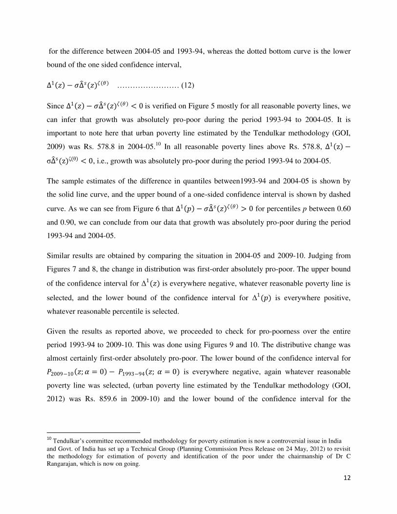
2007) for Stata. We start our investigation by considering the evolution of the density of MPCE

in Figure 1. The distribution of MPCE worsened between 1993-94 and 2004-05 as evidenced by

the shift of the density curves to the left. It however exhibited a quick recovery between 2004-05

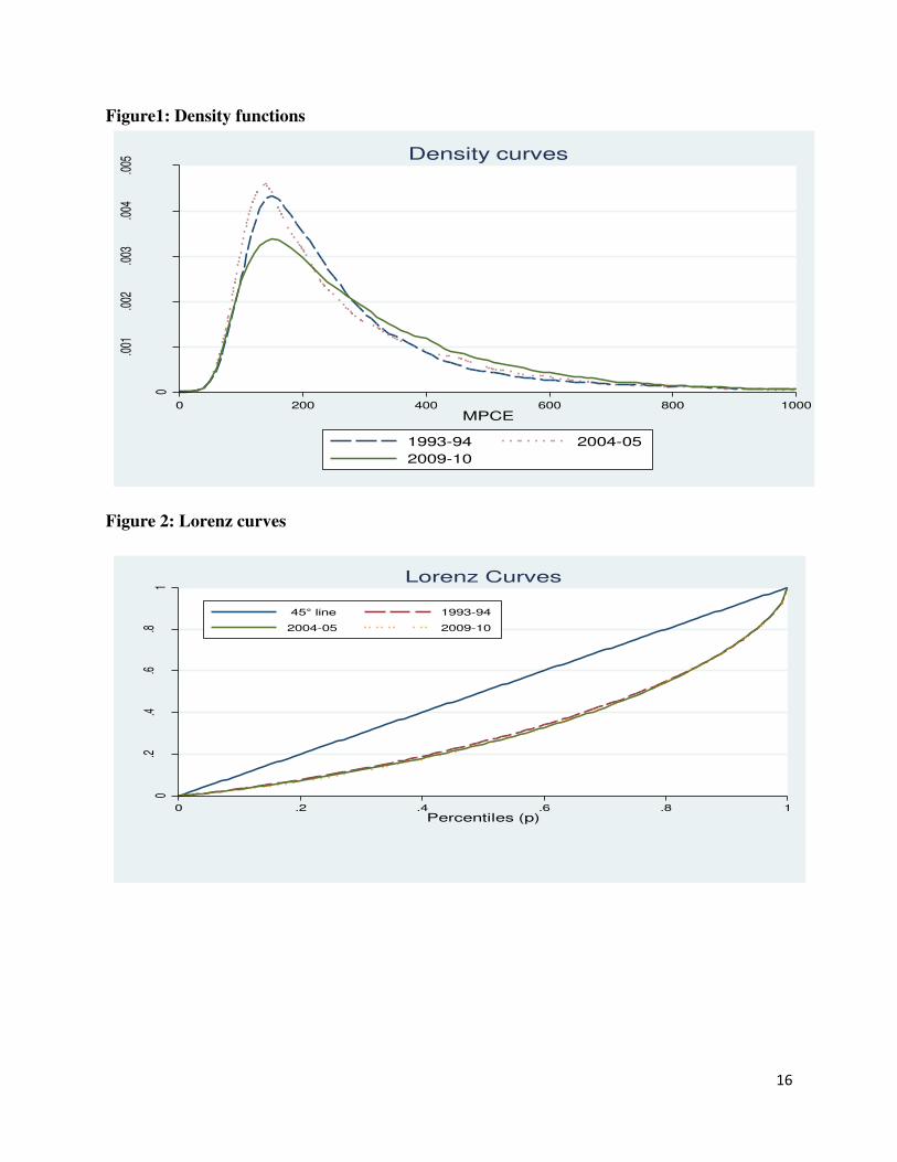
and 2009-10, as shown by the shift of the density curve to the right. The estimates of Lorenz

curves and Gini coefficient presented in Figure 2 and Table 1, suggest that inequality has

increased from 1993-94 to 2009-10. Figures 3 and 4 and the results of Table 1 suggest that

absolute poverty, as measured by the headcount and poverty gap indices, had decreased between

1993-94 to 2009-10.

The statistical testing for first-order absolute pro-poorness of urban India‘s growth can be done

using the information presented in Figure 5 to 10.

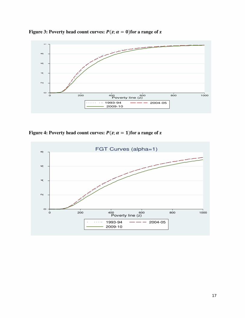
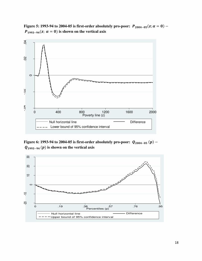
The top line of Figure 5 shows the sample estimates of

∆1 𝑧 = 𝑃2004−05 𝑧;𝛼 = 0 − 𝑃1993−94(𝑧; 𝛼 = 0) ---------------------- (11)

9 Price deflators are reported in the NSSO report entitled ―Key Indicators of Household Consumer Expenditure in

India, 2009-10” available from the following web address; http://mospi.nic.in/Mospi_New/upload/Key_Indicators-

HCE_66th_Rd-Report.pdf

12

for the difference between 2004-05 and 1993-94, whereas the dotted bottom curve is the lower

bound of the one sided confidence interval, ∆1 𝑧 − 𝜎∆ 𝑠(𝑧)𝜁(𝜃) …………………… (12)

Since ∆1 𝑧 − 𝜎∆ 𝑠(𝑧)𝜁(𝜃) < 0 is verified on Figure 5 mostly for all reasonable poverty lines, we

can infer that growth was absolutely pro-poor during the period 1993-94 to 2004-05. It is

important to note here that urban poverty line estimated by the Tendulkar methodology (GOI,

2009) was Rs. 578.8 in 2004-05.10

In all reasonable poverty lines above Rs. 578.8, ∆1 z −σ∆ s(z)ζ(θ) < 0, i.e., growth was absolutely pro-poor during the period 1993-94 to 2004-05.

The sample estimates of the difference in quantiles between1993-94 and 2004-05 is shown by

the solid line curve, and the upper bound of a one-sided confidence interval is shown by dashed

curve. As we can see from Figure 6 that ∆1 𝑝 − 𝜎∆ 𝑠 𝑧 𝜁 𝜃 > 0 for percentiles p between 0.60

and 0.90, we can conclude from our data that growth was absolutely pro-poor during the period

1993-94 and 2004-05.

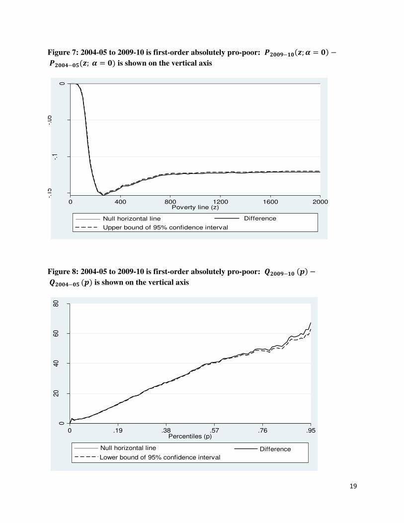
Similar results are obtained by comparing the situation in 2004-05 and 2009-10. Judging from

Figures 7 and 8, the change in distribution was first-order absolutely pro-poor. The upper bound

of the confidence interval for Δ1(𝑧) is everywhere negative, whatever reasonable poverty line is

selected, and the lower bound of the confidence interval for Δ1(𝑝) is everywhere positive,

whatever reasonable percentile is selected.

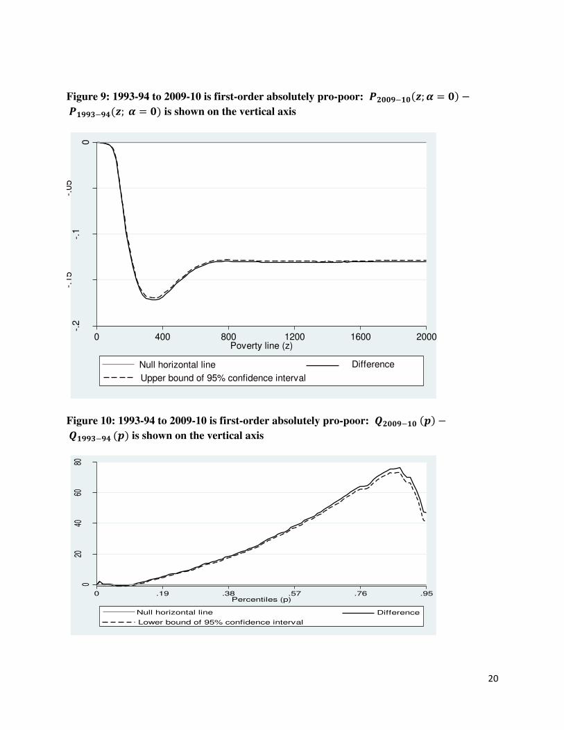
Given the results as reported above, we proceeded to check for pro-poorness over the entire

period 1993-94 to 2009-10. This was done using Figures 9 and 10. The distributive change was

almost certainly first-order absolutely pro-poor. The lower bound of the confidence interval for 𝑃2009−10 𝑧;𝛼 = 0 − 𝑃1993−94(𝑧; 𝛼 = 0) is everywhere negative, again whatever reasonable

poverty line was selected, (urban poverty line estimated by the Tendulkar methodology (GOI,

2012) was Rs. 859.6 in 2009-10) and the lower bound of the confidence interval for the

10

Tendulkar‘s committee recommended methodology for poverty estimation is now a controversial issue in India

and Govt. of India has set up a Technical Group (Planning Commission Press Release on 24 May, 2012) to revisit

the methodology for estimation of poverty and identification of the poor under the chairmanship of Dr C

Rangarajan, which is now on going.

13

difference in quantiles, 𝑄2009−10 𝑝 − 𝑄1993−94 (𝑝), is everywhere positive. Thus, it can be

inferred that the entire period of 1993-94 to 2009-10 was overall first-order absolutely pro-poor.

Given the robust results obtained for first-order pro-poorness, it is not necessary to test for second-

order pro-poorness since first order pro-poorness implies second-order pro-poorness. This can be

seen by noting that 𝑃𝑗 𝑧;𝛼 = 1 = 𝑃𝑗 𝑦;𝛼 = 0 𝑑𝑦𝑧0

. --------- (13)

If first-order pro-poorness is seen at order 1, then by equation (13) second-order pro-poorness also

obtains. The same relation is confirmed by noting from equations (6), (8) and (10) that the

Generalized Lorenz curve is implied by the quantile condition.

Testing for relative pro-poorness can be done using Figures 11 to 19. Figure 11 shows that the

sample estimates of 𝑃2004−05 1 + 𝑔 𝑧; 𝛼 = 0 − 𝑃1993−94 (𝑧;𝛼 = 0) of distributive movement

during the period of 1993-94 to 2004-05 was not first-order relatively pro-poor since the difference

is not always negative in the samples observed. Also the confidence interval around the sample

estimates makes it clear (Figure 11) that the observed differences 𝑃2004−05 1 + 𝑔 𝑧; 𝛼 = 0 −𝑃1993−94 (𝑧;𝛼 = 0) are not statistically significant over a wide range of bottom poverty lines – the

upper bounds of the one-sided confidence intervals extended above zero line for 𝑧 up to around

300 (or between 550 and 1100) rupees and 𝑝 up to around 0.34. Hence, at a conventional level 95

per cent of statistical, the first-order relative pro-poor condition is not satisfied. An analogous

result is obtained (Figure 12) from comparing growth in quantiles to growth in average MPCE.

Again, for a substantial range of percentiles, the one-sided confidence interval lays below zero

line.

This was also the case for the second order of dominance, as shown in Figure 13. However, It

might seem that second-order relative pro-poorness over the period from 1993-94 to 2004-05

certainly cannot be weaker than first-order relative pro-poorness over the same period. This is

because it follows from the fact that statistical uncertainty for first-order comparisons at the bottom

of the distributions builds up at the second-order since second-order conditions are made of

cumulative of first-order statistics. But if one takes into account the effect of sampling variability

14

at the bottom of the distribution, than the evidence for second-order relative pro-poorness is

statistically weaker than that for first-order relative pro-poorness (Araar, 2007).

Testing of first-order relative pro-poorness for the period of 2004-05 to 2009-10 is done using

Figures 14 and 15. The confidence interval around the sample estimates of 𝑃2009−10 1 +𝑔 𝑧; 𝛼 = 0 − 𝑃2004−05 (𝑧;𝛼 = 0) in Figure 14 is below zero only for 𝑧 after around Rs. 500,

which leads to infer that, not very robust first-order relative pro-poorness change was evident

during that period. A similar result is obtained in Figure 15 from comparing growth in quantiles to

growth in average MPCE. For a range of percentiles from 0.28 to 0.7, the lower bound of the

confidence interval lies above the zero line.

Given the above results, it would be interesting to test for second order relative pro-poorness

between 2004-05 and 2009-10. The result is shown in Figure 16. We now get even stronger (and

very strong) evidence of anti relative pro-poorness in that period as the confidence interval is

always below zero for differences in𝐶2009−10(𝑝)/𝐶2004−05 𝑝 − 𝜇2009−10/𝜇2004−05. As

discussed above, if first-order pro-poorness can be verified statistically at order 1, then we can

expect second-order pro-poorness also to be inferred statistically.

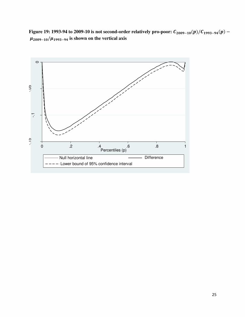
The results of the tests for first order relative pro-poorness over the period 1993-94 to 2009-10 are

presented in Figures 17 and 18. The confidence interval around the sample estimates of 𝑃2009−10 1 + 𝑔 𝑧; 𝛼 = 0 − 𝑃1993−94 (𝑧;𝛼 = 0) in Figure 17 is not always below zero, but

positive between the ranges of Rs. 500 and 1000. The same evidence is confirmed by Figure 18

from the comparison of growth in quantiles to growth in average MPCE between 1993-94 and

2009-10. The low bound of the confidence interval is above the zero line for a range of percentiles

from 0.5 to 0.9. Hence, the incidence of statistically anti relative pro-poorness change in the period

1993-94 to 2009-10 is confirmed by evidence. The robust result of anti relative pro-poorness is

obtained from testing the second order relative pro-poorness, as the confidence interval is always

below zero as seen in Figure 19.

7. Conclusions and policy implications

This paper is devoted to the assessment of pro-poorness of urban economic growth in post

reform India, i.e., for the period of 1993-94 to 2009-10. This paper uses the methodology

15

developed by Duclos (2004) and Araar et al. (2007, 2009). Statistical techniques are used to

derive the sampling distribution of the various estimators and the confidence intervals around the

curves are ranked to conclude whether the change has been robustly pro-poor –or anti-poor.

Due to unavailability of per capita income data, monthly per capita consumer expenditure

(MPCE) data has been used for the study. The statistical exercises are done using the three

rounds of quinquennial household survey data collected by NSSO in 1993-94, 2004-05, and

2009-10, respectively. The empirical results suggest that India‘s urban economic growth has

been absolutely pro-poor but relatively anti-poor between 1993-94 and 2004-05, between 2004-

05 and 2009-10, and between 1993-94 and 2009-10.

The paper argues that there is need for immediate government intervention for the reduction of

effective urban poverty. For this purpose, city specific policies are needed as different size

(measured by population) of cities show different levels of poverty and inequality (Tripathi,

2013). Greater access to and better quality of education, job creation, skill development of the

worker, access of better health, improvement of basic amenities (such as, water, electricity,

roads, sanitation, and housing) are needed for the reduction of urban poverty and more equitable

distribution of the benefits of urbanization and economic development. Above all, what is

required is the political will to adopt meaningful steps to improve the conditions of the poor.

16

Figure1: Density functions

Figure 2: Lorenz curves

0

.001

.002

.003

.004

.005

0 200 400 600 800 1000MPCE

1993-94 2004-05

2009-10

Density curves0

.2.4

.6.8

1

0 .2 .4 .6 .8 1Percentiles (p)

45° line 1993-94

2004-05 2009-10

Lorenz Curves

17

Figure 3: Poverty head count curves: 𝑷(𝒛;𝜶 = 𝟎)for a range of z

Figure 4: Poverty head count curves: 𝑷(𝒛;𝜶 = 𝟏)for a range of z

0.2

.4.6

.81

0 200 400 600 800 1000Poverty line (z)

1993-94 2004-05

2009-10

0.2

.4.6

.8

0 200 400 600 800 1000Poverty line (z)

1993-94 2004-05

2009-10

FGT Curves (alpha=1)

18

Figure 5: 1993-94 to 2004-05 is first-order absolutely pro-poor: 𝑷𝟐𝟎𝟎𝟒−𝟎𝟓 𝒛;𝜶 = 𝟎 − 𝑷𝟏𝟗𝟗𝟑−𝟗𝟒(𝒛; 𝜶 = 𝟎) is shown on the vertical axis

Figure 6: 1993-94 to 2004-05 is first-order absolutely pro-poor: 𝑸𝟐𝟎𝟎𝟒−𝟎𝟓 𝒑 − 𝑸𝟏𝟗𝟗𝟑−𝟗𝟒 (𝒑) is shown on the vertical axis

-.04

-.02

0

.02

.04

0 400 800 1200 1600 2000Poverty line (z)

Difference

Lower bound of 95% confidence interval

Null horizontal line

-20

-10

010

2030

0 .19 .38 .57 .76 .95Percentiles (p)

Difference

Upper bound of 95% confidence interval

Null horizontal line

19

Figure 7: 2004-05 to 2009-10 is first-order absolutely pro-poor: 𝑷𝟐𝟎𝟎𝟗−𝟏𝟎 𝒛;𝜶 = 𝟎 − 𝑷𝟐𝟎𝟎𝟒−𝟎𝟓(𝒛; 𝜶 = 𝟎) is shown on the vertical axis

Figure 8: 2004-05 to 2009-10 is first-order absolutely pro-poor: 𝑸𝟐𝟎𝟎𝟗−𝟏𝟎 𝒑 − 𝑸𝟐𝟎𝟎𝟒−𝟎𝟓 (𝒑) is shown on the vertical axis

-.15

-.1

-.05

0

0 400 800 1200 1600 2000Poverty line (z)

Difference

Upper bound of 95% confidence interval

Null horizontal line

020

40

60

80

0 .19 .38 .57 .76 .95Percentiles (p)

Difference

Lower bound of 95% confidence interval

Null horizontal line

20

Figure 9: 1993-94 to 2009-10 is first-order absolutely pro-poor: 𝑷𝟐𝟎𝟎𝟗−𝟏𝟎 𝒛;𝜶 = 𝟎 − 𝑷𝟏𝟗𝟗𝟑−𝟗𝟒(𝒛; 𝜶 = 𝟎) is shown on the vertical axis

Figure 10: 1993-94 to 2009-10 is first-order absolutely pro-poor: 𝑸𝟐𝟎𝟎𝟗−𝟏𝟎 𝒑 − 𝑸𝟏𝟗𝟗𝟑−𝟗𝟒 (𝒑) is shown on the vertical axis

-.2

-.15

-.1

-.05

0

0 400 800 1200 1600 2000Poverty line (z)

Difference

Upper bound of 95% confidence interval

Null horizontal line

020

4060

80

0 .19 .38 .57 .76 .95Percentiles (p)

Difference

Lower bound of 95% confidence interval

Null horizontal line

21

Figure 11: 1993-94 to 2004-05 is not statistically first-order relatively pro-poor: 𝑷𝟐𝟎𝟎𝟒−𝟎𝟓 𝟏 + 𝒈 𝒛; 𝜶 = 𝟎 − 𝑷𝟏𝟗𝟗𝟑−𝟗𝟒 (𝒛;𝜶 = 𝟎) is shown on the vertical axis

Figure 12: 1993-94 to 2004-05 is not statistically first-order relatively pro-poor: 𝑸𝟐𝟎𝟎𝟒−𝟎𝟓 (𝒑)/𝑸𝟏𝟗𝟗𝟑−𝟗𝟒 (𝒑) − 𝝁𝟐𝟎𝟎𝟒−𝟎𝟓 (𝒑)/𝝁𝟏𝟗𝟗𝟑−𝟗𝟒 (𝒑) is shown on the vertical axis

-.02

0

.02

.04

0 400 800 1200 1600 2000Poverty line (z)

Difference

Upper bound of 95% confidence interval

Null horizontal line

-.1-.0

5

0

.05

0 .19 .38 .57 .76 .95Percentiles (p)

Difference

Lower bound of 95% confidence interval

Null horizontal line

22

Figure 13: 1993-94 to 2004-05 is not statistically second-order relatively pro-poor: 𝑪𝟐𝟎𝟎𝟒−𝟎𝟓(𝒑)/𝑪𝟏𝟗𝟗𝟑−𝟗𝟒 𝒑 − 𝝁𝟐𝟎𝟎𝟒−𝟎𝟓/𝝁𝟏𝟗𝟗𝟑−𝟗𝟒 is shown on the vertical axis

Figure14: 2004-05 to 2009-10 is first-order relatively pro-poor: 𝑷𝟐𝟎𝟎𝟗−𝟏𝟎 𝟏 + 𝒈 𝒛; 𝜶 = 𝟎 −𝑷𝟐𝟎𝟎𝟒−𝟎𝟓 (𝒛;𝜶 = 𝟎) is shown on the vertical axis

-.05

0

.05

0 .19 .38 .57 .76 .95Percentiles (p)

Difference

Lower bound of 95% confidence interval

Null horizontal line

-.05

0

.05

.1

0 400 800 1200 1600 2000Poverty line (z)

Difference

Upper bound of 95% confidence interval

Null horizontal line

23

Figure 15: 2004-05 to 2009-10 is first-order relatively pro-poor: 𝑸𝟐𝟎𝟎𝟗−𝟏𝟎 (𝒑)/𝑸𝟐𝟎𝟎𝟒−𝟎𝟓 (𝒑) −𝝁𝟐𝟎𝟎𝟗−𝟏𝟎 (𝒑)/𝝁𝟐𝟎𝟎𝟒 (𝒑) is shown on the vertical axis

Figure 16: 2004-05 to 2009-10 is not second-order relatively pro-poor: 𝑪𝟐𝟎𝟎𝟗−𝟏𝟎(𝒑)/𝑪𝟐𝟎𝟎𝟒−𝟎𝟓 𝒑 − 𝝁𝟐𝟎𝟎𝟗−𝟏𝟎/𝝁𝟐𝟎𝟎𝟒−𝟎𝟓 is shown on the vertical axis

-.15

-.1

-.05

0

.05

0 .19 .38 .57 .76 .95Percentiles (p)

Difference

Lower bound of 95% confidence interval

Null horizontal line

-.1-.0

8-.0

6-.0

4-.0

2

0

0 .19 .38 .57 .76 .95Percentiles (p)

Difference

Lower bound of 95% confidence interval

Null horizontal line

24

Figure 17: 1993-94 to 2009-10 is not first-order relatively pro-poor: 𝑷𝟐𝟎𝟎𝟗−𝟏𝟎 𝟏 + 𝒈 𝒛; 𝜶 =𝟎 − 𝑷𝟏𝟗𝟗𝟑−𝟗𝟒 (𝒛;𝜶 = 𝟎) is shown on the vertical axis

Figure 18: 1993-94 to 2009-10 is not first-order relatively pro-poor: 𝑸𝟐𝟎𝟎𝟒−𝟎𝟓 (𝒑)/𝑸𝟏𝟗𝟗𝟑−𝟗𝟒 (𝒑) − 𝝁𝟐𝟎𝟎𝟒−𝟎𝟓 (𝒑)/𝝁𝟏𝟗𝟗𝟑−𝟗𝟒 (𝒑) is shown on the vertical axis

-.02

0

.02

.04

.06

0 400 800 1200 1600 2000Poverty line (z)

Difference

Upper bound of 95% confidence interval

Null horizontal line

-.15

-.1

-.05

0

.05

0 .19 .38 .57 .76 .95Percentiles (p)

Difference

Lower bound of 95% confidence interval

Null horizontal line

25

Figure 19: 1993-94 to 2009-10 is not second-order relatively pro-poor: 𝑪𝟐𝟎𝟎𝟗−𝟏𝟎(𝒑)/𝑪𝟏𝟗𝟗𝟑−𝟗𝟒 𝒑 − 𝝁𝟐𝟎𝟎𝟗−𝟏𝟎/𝝁𝟏𝟗𝟗𝟑−𝟗𝟒 is shown on the vertical axis

-.15

-.1

-.05

0

0 .2 .4 .6 .8 1Percentiles (p)

Difference

Lower bound of 95% confidence interval

Null horizontal line

26

References:

Araar, A., ―Pro-Poor Growth in Andean Countries,‖ Working Paper No. 12-25.CIRP EE (2012).

Araar, A. and J.-Y. Duclos, "DASP: Distributive Analysis Stata Package," PEP, World Bank,

UNDP and Université Laval (2007).

Araar, A., J.-Y. Duclos, M. Audet, and P. Makdissi, ―Has Mexican growth been pro-poor?‖ Social Perspectives 9 (2007): 17‐47.

Araar, A., J.-Y. Duclos, M. Audet, and P. Makdissi, ―Testing for Pro-Poorness of Growth, with

an Application to Mexico,‖ Review of Income and Wealth 55 (2009): 853–881.

Balasubramanian, P. and T. K. S. Ravindran, ―Pro-Poor Maternity Benefit Schemes and Rural

Women: Findings from Tamil Nadu,‖ Economic and Political Weekly 47 (2012): 19-22.

Datt, G. and M. Ravallion, ―Has India‘s Economic Growth Become More Pro-Poor in the Wake

of Economic Reforms?‖ Policy Research Working Paper No. 5103, World Bank, Washington DC (2009).

Dev, S. M., ―Pro-Poor Growth in India: What do we know about the Employment Effects of

Growth 1980–2000?‖ Working Paper No. 161.Overseas Development Institute (2002).

Duclos, J.-Y., ―What is Pro-Poor?‖ Social Choice and Welfare, 32 (2009): 37–58.

Liu, Y., and C. B. Barrett, ―Heterogeneous Pro-Poor Targeting in the National Rural

Employment Guarantee Scheme,‖ Economic and Political Weekly 48 (2013), 46-53.

Ravallion, M., ―What Is Needed for a More Pro-Poor Growth Process in India?‖ Economic and

Political Weekly 35 (2000): 1089-1093.

Ravallion, M., ―Pro-Poor Growth: A Primer,‖ Policy Research Working Paper No. 3242, World

Bank, Washington DC (2004).

Ravallion, M., and G. Datt, ―When Is Growth Pro-Poor? Evidence from the Diverse Experience

of India‘s States,‖ Policy Research Working Paper No. 2263, World Bank, Washington DC (1999).

Ravallion, M. And S. Chen, ―Measuring Pro-poor Growth,‖ Economics Letters 78 (2003): 93–99.

Tripathi, S., ―Is Urban Economic Growth Inclusive in India?‖ Margin: The Journal of Applied

Economics Research 7 (2013): 507-539.