Hawaii Solar Integration Study: Final Technical … Solar...Hawaii Solar Integration Study: Final Technical Report for Maui ... Hawaii Solar Integration Study Final Technical Report

Hawaii Solar Integration Study:

Final Technical Report for Maui

Prepared for the

U.S. Department of Energy

Office of Electricity Delivery and Energy Reliability

Under Cooperative Agreement No. DE-FC26-06NT42847

Hawai‘i Distributed Energy Resource Technologies for Energy Security

Subtask 7.1 Deliverable

Prepared by

GE Energy Consulting

Submitted by

Hawai‘i Natural Energy Institute

School of Ocean and Earth Science and Technology

University of Hawai‘i

March 2013

Acknowledgement: This material is based upon work supported by the United States

Department of Energy under Cooperative Agreement Number DE-FC-06NT42847.

Disclaimer: This report was prepared as an account of work sponsored by an agency of the

United States Government. Neither the United States Government nor any agency thereof, nor

any of their employees, makes any warranty, express or implied, or assumes any legal liability

or responsibility for the accuracy, completeness, or usefulness of any information, apparatus,

product, or process disclosed, or represents that its use would not infringe privately owned

rights. Reference here in to any specific commercial product, process, or service by tradename,

trademark, manufacturer, or otherwise does not necessarily constitute or imply its

endorsement, recommendation, or favoring by the United States Government or any agency

thereof. The views and opinions of authors expressed herein do not necessarily state or reflect

those of the United States Government or any agency thereof.

Hawaii Solar Integration Study

Final Technical Report for Maui

Prepared for:

The National Renewable Energy Laboratory Hawaii Natural Energy Institute Hawaii Electric Company Maui Electric Company

Prepared by:

GE Energy Consulting

March 25, 2013

1

Contents 1.0 Introduction ............................................................................................................................................. 3 2.0 Background ............................................................................................................................................. 3 3.0 Study Approach and Objectives .......................................................................................................... 4 4.0 GE Power System Modeling Tools ....................................................................................................... 5

4.1. GE MAPSTM production cost model ......................................................................................................... 7 4.2. GE PSLFTM transient stability model ....................................................................................................... 8 4.3. GE PSLFTM long-term dynamic model .................................................................................................... 8 4.4. GE Interhour screening tool .................................................................................................................... 9 4.5. Statistical analysis of wind, solar and load data ................................................................................. 9 4.6. Modeling limitations and study risks and uncertainties ................................................................. 10

5.0 Study Scenarios ................................................................................................................................... 11 5.1. Solar Site Selection Process ................................................................................................................... 11 5.2. Development of Solar and Wind Datasets ......................................................................................... 13

5.2.1. Analysis of Solar PV and Wind Data ................................................................................................................................. 13 5.2.2. Selection of the Solar and Wind data for the study year ...................................................................................... 17 5.2.3. Variability of Solar and Wind in Different Scenarios ................................................................................................ 18 5.2.4. Solar and Wind Forecast ........................................................................................................................................................ 18 5.2.5. Variability and Statistical Analysis ..................................................................................................................................... 19 5.2.6. Histogram of Ramps ................................................................................................................................................................. 20 5.2.7. ∆P vs. P0 Plots .............................................................................................................................................................................. 22 5.2.8. RMS of Fast Variation ............................................................................................................................................................... 23

5.3. Operating Reserve................................................................................................................................... 24 5.4. Modeling and Assumptions ................................................................................................................... 26

5.4.1. Dynamics (GE PSLFTM Transient Stability and Long-Term Simulations) ......................................................... 26 5.4.2. Production Cost Database .................................................................................................................................................... 32

6.0 Analytical Results ................................................................................................................................ 35 6.1. Production Cost Results ......................................................................................................................... 35

6.1.1. Baseline and Scenario 3 ......................................................................................................................................................... 36 6.1.2. Curtailment Mitigation Strategies ...................................................................................................................................... 43 6.1.3. Additional Energy Storage ..................................................................................................................................................... 53

6.2. Sub-hourly Analysis ................................................................................................................................ 57 6.2.1. Overview of the Critical Events ........................................................................................................................................... 57 6.2.2. Sustained Solar and Wind Power Drops – Short-term ........................................................................................... 58 6.2.3. Sustained Solar and Wind Power Drops in Long-Term .......................................................................................... 67 6.2.4. Sustained increases in wind and solar power ............................................................................................................ 72 6.2.5. High volatility solar and wind power changes............................................................................................................ 75 6.2.6. Loss of load events .................................................................................................................................................................... 88 6.2.7. Sensitivity runs with larger BESS capability in the system ................................................................................ 102 6.2.8. Generation Trip Event ........................................................................................................................................................... 104

7.0 Observations and Conclusions ....................................................................................................... 107 7.1. Under Business as Usual – Without any change to system operating practices ..................... 107

7.1.1. Delivered Energy from Solar and Wind........................................................................................................................ 107 7.1.2. Variables Cost of Operation ............................................................................................................................................... 107 7.1.3. Carbon Emissions .................................................................................................................................................................... 107 7.1.4. Operating Reserves Requirement................................................................................................................................... 107 7.1.5. Non-synchronous Generation Online ........................................................................................................................... 108 7.1.6. Sub-hourly response to Solar and Wind Variability .............................................................................................. 108 7.1.7. Sub-hourly response: Solar and Wind curtailemt .................................................................................................. 108 7.1.8. Sub-hourly response to Loss-of-Load events .......................................................................................................... 108 7.1.9. Sub-hourly response to generation trip events ...................................................................................................... 109

7.2. With Additional Mitigation Strategies in Scenarios 3 ..................................................................... 109

2

7.2.1. Delivered Energy from Solar and Wind........................................................................................................................ 109 7.2.2. Variables Cost of Operation ............................................................................................................................................... 110 7.2.3. Carbon Emissions .................................................................................................................................................................... 110 7.2.4. Non-synchronous Generation Online ........................................................................................................................... 110

7.3. With Additional BESS in Scenario 3 .................................................................................................... 110 8.0 References .......................................................................................................................................... 111 Appendix 1. Power Flow data conversion ........................................................................................... 112 Appendix 2. Dynamic Database (without AGC) ................................................................................. 115 Appendix 3. Under Frequency Load Shedding ................................................................................... 116 Appendix 4. AGC Model .......................................................................................................................... 117 Appendix 5. AGC Dynamic Database .................................................................................................. 119 Appendix 6. AGC data ............................................................................................................................. 120 Appendix 7. Starting conditions for high variability hour ............................................................... 121 Appendix 8. Starting conditions for loss-of-load simulations ........................................................ 122 Appendix 9. Time domain simulation for most volatile hour .......................................................... 125 Appendix 10. Time domain simulation for load rejection ............................................................. 126

3

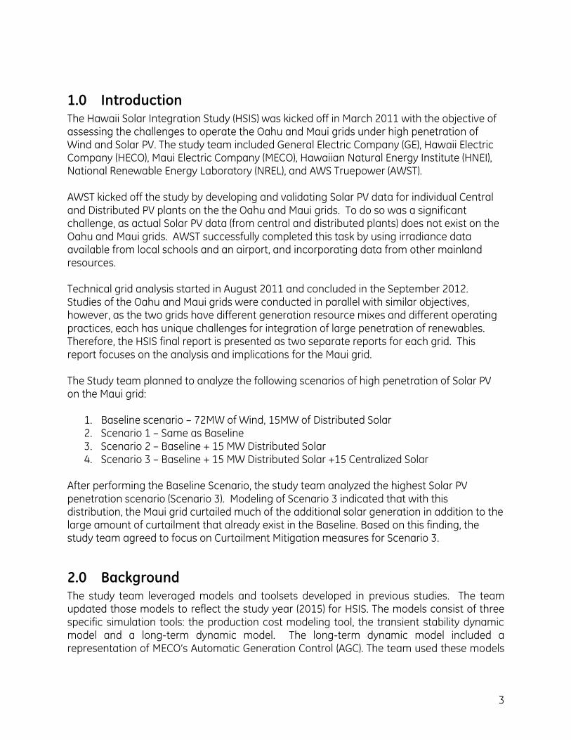
1.0 Introduction The Hawaii Solar Integration Study (HSIS) was kicked off in March 2011 with the objective of assessing the challenges to operate the Oahu and Maui grids under high penetration of Wind and Solar PV. The study team included General Electric Company (GE), Hawaii Electric Company (HECO), Maui Electric Company (MECO), Hawaiian Natural Energy Institute (HNEI), National Renewable Energy Laboratory (NREL), and AWS Truepower (AWST). AWST kicked off the study by developing and validating Solar PV data for individual Central and Distributed PV plants on the the Oahu and Maui grids. To do so was a significant challenge, as actual Solar PV data (from central and distributed plants) does not exist on the Oahu and Maui grids. AWST successfully completed this task by using irradiance data available from local schools and an airport, and incorporating data from other mainland resources. Technical grid analysis started in August 2011 and concluded in the September 2012. Studies of the Oahu and Maui grids were conducted in parallel with similar objectives, however, as the two grids have different generation resource mixes and different operating practices, each has unique challenges for integration of large penetration of renewables. Therefore, the HSIS final report is presented as two separate reports for each grid. This report focuses on the analysis and implications for the Maui grid. The Study team planned to analyze the following scenarios of high penetration of Solar PV on the Maui grid:

1. Baseline scenario – 72MW of Wind, 15MW of Distributed Solar 2. Scenario 1 – Same as Baseline 3. Scenario 2 – Baseline + 15 MW Distributed Solar 4. Scenario 3 – Baseline + 15 MW Distributed Solar +15 Centralized Solar

After performing the Baseline Scenario, the study team analyzed the highest Solar PV penetration scenario (Scenario 3). Modeling of Scenario 3 indicated that with this distribution, the Maui grid curtailed much of the additional solar generation in addition to the large amount of curtailment that already exist in the Baseline. Based on this finding, the study team agreed to focus on Curtailment Mitigation measures for Scenario 3.

2.0 Background The study team leveraged models and toolsets developed in previous studies. The team updated those models to reflect the study year (2015) for HSIS. The models consist of three specific simulation tools: the production cost modeling tool, the transient stability dynamic model and a long-term dynamic model. The long-term dynamic model included a representation of MECO’s Automatic Generation Control (AGC). The team used these models

4

to provide a Baseline measure of power system performance and analyze alternative energy futures for MECO. The production cost model considers the dispatch and constraints of all generation on an hourly basis, and provides outputs such as emissions, electricity production by unit, fossil fuel consumption, and variable cost of production. The transient stability dynamic model considers shorter timescale contingency events (sub-hourly), and characterizes the system’s ability to respond to these events. The long-term dynamic model considers critical wind and solar variability events with one to two hour duration, and characterizes the system’s ability to respond to these types of events. The team also developed additional statistical analysis tools to analyze the variability of Solar PV and Wind resources and to quantify their impact on grid operation.

3.0 Study Approach and Objectives The Hawaii Solar Integration Study looked at two scenarios of the Maui grid build-out, with different central and distributed Solar PV. Study objectives are listed below:

Assess Solar PV and Wind energy delivered to the system

Assess changes in variable operating costs, and reduction in fuel consumption and fossil plant emissions

Assess the dynamic performance of the Maui system in sub-hourly time frames ranging from few seconds to an hour

Identify challenges and the impact on system operation

Identify changes required to facilitate high penetrations of Solar PV and Wind power

Provide recommendations based on study results The study team benchmarked the Baseline scenario and then investigated system operation under Scenario 3, as it includes the highest installed renewable capacity. Detailed hourly and sub-hourly analyses were conducted, with results indicating that a large portion of the renewable enrgy installed was curtailed, The team determined that curtailment mitigations should be the main focus of the balance of the study. The approach for each of the scenarios is summarized as follows:

1. Statistical analysis of Solar PV and Wind energy to determine scenario specific operation reserves

2. Hourly analysis with GE MAPSTM to determine renewable energy delivered, annual operating costs, fuel consumption, emissions, and other production cost metrics

3. Sub-hourly screening analysis using GE’s Interhour toolset to identify hours of high system constraint

4. Sub-hourly dynamic and transient stability simulations using GE PSLF to quantify the impact on system frequency and stability in the hours of high constraint

Results based on analysis of differing Scenarios, using the same tools, provide the bases for conclusions and recommendations. Simulations of the Maui electrical system were

5

performed specifically to provide MECO with knowledge of the potential benefits that can be realized by implementing the recommended strategies. As with any modeling study, additional work is required to assess feasibility, cost/benefit, and develop project plans necessary to implement these projects and strategies.

4.0 GE Power System Modeling Tools The tools used for the study provided a mix of classical utility power system analysis tools (including production cost modeling and transient stability modeling performed by Generation and Transmission Planning teams), and tools developed specifically for this study. The two classical power systems analysis tools used were:

1. GE MAPSTM production cost modeling, used to assess renewable power curtailment, unit heat rates, variable cost of production, fuel consumption, emissions, etc, and

2. GE PSLFTM transient stability modeling, to assess short-timescale planning contingencies associated with high penetration of renewables

An additional tool developed in earlier studies on the Big Island of Hawaii and Maui, and more recently on Oahu (OWITS) was leveraged for use in this project.

3. GE PSLFTM Long-term dynamic simulations to assess sustained and sudden renewable variability events, capturing governor response and representative Automatic Generation Control response of the system

The final two tools were developed and enhanced from previous studies for this project:

4. Statistical Solar PV and Wind power variability assessments, used to quantify operating reserves under different scenarios, and

5. Interhour screening, to identify challenging events that result in system constraint, based on different accounts/performance metrics as defined in the study

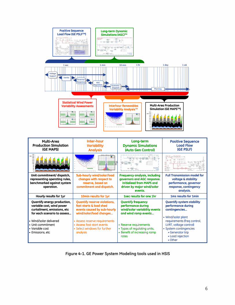
The team performed a variety of simulation tests using these tools to obtain results over a range of timescales of interest to the project team. The range of timescales is shown in Figure 4-1.

6

-50 -40 -30 -20 -10 0 10 20 30 40 500

5

10

15

20

25

30

35

40

45

50

F arm power (MW per interval)F

req

ue

nc

y (

%)

100MW O ahu + 200MW L anai + 200MW Molokai

0.1% percentile (1min) = -12.27


0.1% percentile (10min) = -49.305

Negative most (1min) = -22.479



99.9% percentile (1min) = 11.7685

99.9% percentile (5min) = 33.0615

99.9% percentile (10min) = 54.0865

P ositive most (1min) = 22.5425



Interval = 1min

Interval = 5min

Interval = 10min

1 day1 min 1 hr 1 wk10 min1 sec

Governor

Response

Governor

Response Automatic

Generation

Control

AGC Regulation

Economic

Dispatch

EconomicDispatch

ArbitragePlanning

Governor

ResponseInertiaInertia

Positive Sequence Load Flow (GE PSLFTM)

Interhour Renewables Variability AnalysisTM

Long-term Dynamic Simulations (AGC)TM

Multi-Area Production Simulation (GE MAPSTM)

Governor

ResponseSupport

Voltage

Statistical Wind Power Variability Assessments

-0.25 -0.2 -0.15 -0.1 -0.05 0 0.05 0.1 0.15 0.2 0.250

10

20

30

40

50

P ower ramp (pu per interval)

Fre

qu

en

cy

(%

)

0% percentile (10min) = -0.140% percentile (60min) = -0.450.1% percentile (10min) = -0.090.1% percentile (60min) = -0.27

99.9% percentile (10min) = 0.1099.9% percentile (60min) = 0.31100% percentile (10min) = 0.18100% percentile (60min) = 0.48

Interval = 10min

Interval = 60min

-150 -100 -50 0 50 100 1500

10

20

30

40

50

P ower ramp (MW per interval)

Fre

qu

en

cy

(%

)



Interval = 10min

Interval = 60min

2008

-0.25 -0.2 -0.15 -0.1 -0.05 0 0.05 0.1 0.15 0.2 0.250

10

20

30

40

50

P ower ramp (pu per interval)

Fre

qu

en

cy

(%

)



Interval = 10min

Interval = 60min

-150 -100 -50 0 50 100 1500

10

20

30

40

50

P ower ramp (MW per interval)

Fre

qu

en

cy

(%

)



Interval = 10min

Interval = 60min

2008

Quantify frequency performance during wind/solar variability events and wind ramp events…

• Reserve requirements• Types of regulating units,• Benefit of increasing ramp

rates

1sec results for one 1hr

Frequency analysis, including governors and AGC response.

Initialized from MAPS and driven by major wind/solar

events.

Long-termDynamic Simulations

(Auto Gen Control)

Quantify reserve violations, fast starts & load shed events caused by sub-hourly wind/solar/load changes…

• Assess reserve requirements• Assess fast-start events• Select windows for further

analysis

10min results for 1yr

Sub-hourly wind/solar/load changes with respect to

reserve, based on commitment and dispatch.

Inter-hourVariability Analysis

Quantify energy production, variable cost, wind power curtailment, emissions, etc for each scenario to assess…

• Wind/solar delivered• Unit commitment• Variable cost • Emissions, etc

Hourly results for 1yr

Unit commitment/ dispatch, representing operating rules, benchmarked against system

operation.

Multi-AreaProduction Simulation

(GE MAPS)

Quantify system stability performance during contingencies…

• Wind/solar plant requirements (freq control, LVRT, voltage control)

• System contingencies• Generator trip• Load rejection• Other

Full Transmission model for voltage & stability

performance, governor response, contingency

analysis.

1ms results for 1min

Positive SequenceLoad Flow(GE PSLF)

Quantify frequency performance during wind/solar variability events and wind ramp events…

• Reserve requirements• Types of regulating units,• Benefit of increasing ramp

rates

1sec results for one 1hr

Frequency analysis, including governors and AGC response.

Initialized from MAPS and driven by major wind/solar

events.

Long-termDynamic Simulations

(Auto Gen Control)

Quantify reserve violations, fast starts & load shed events caused by sub-hourly wind/solar/load changes…

• Assess reserve requirements• Assess fast-start events• Select windows for further

analysis

10min results for 1yr

Sub-hourly wind/solar/load changes with respect to

reserve, based on commitment and dispatch.

Inter-hourVariability Analysis

Quantify energy production, variable cost, wind power curtailment, emissions, etc for each scenario to assess…

• Wind/solar delivered• Unit commitment• Variable cost • Emissions, etc

Hourly results for 1yr

Unit commitment/ dispatch, representing operating rules, benchmarked against system

operation.

Multi-AreaProduction Simulation

(GE MAPS)

Quantify system stability performance during contingencies…

• Wind/solar plant requirements (freq control, LVRT, voltage control)

• System contingencies• Generator trip• Load rejection• Other

Full Transmission model for voltage & stability

performance, governor response, contingency

analysis.

1ms results for 1min

Positive SequenceLoad Flow(GE PSLF)

-50 -40 -30 -20 -10 0 10 20 30 40 50

0

5

10

15

20

25

30

35

40

45

50

Farm power (MW per interval)

Fre

quency (

%)

100MW Oahu + 200MW Lanai + 200MW Molokai



0.1% percentile (10min) = -49.305




99.9% percentile (1min) = 11.7685

99.9% percentile (5min) = 33.0615

99.9% percentile (10min) = 54.0865

Positive most (1min) = 22.5425



Interval = 1min

Interval = 5min

Interval = 10min

-50 -40 -30 -20 -10 0 10 20 30 40 50

0

5

10

15

20

25

30

35

40

45

50

-50 -40 -30 -20 -10 0 10 20 30 40 50

0

5

10

15

20

25

30

35

40

45

50

Farm power (MW per interval)

Fre

quency (

%)

100MW Oahu + 200MW Lanai + 200MW Molokai



0.1% percentile (10min) = -49.305




99.9% percentile (1min) = 11.7685

99.9% percentile (5min) = 33.0615

99.9% percentile (10min) = 54.0865




Interval = 1min

Interval = 5min

Interval = 10min

Figure 4-1. GE Power System Modeling tools used in HSIS

7

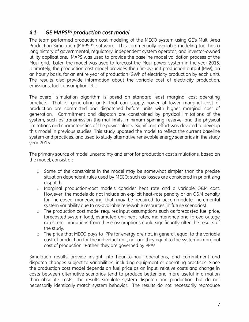
4.1. GE MAPSTM production cost model

The team performed production cost modeling of the MECO system using GE’s Multi Area Production Simulation (MAPSTM) software. This commercially available modeling tool has a long history of governmental, regulatory, independent system operator, and investor-owned utility applications. MAPS was used to provide the baseline model validation process of the Maui grid. Later, the model was used to forecast the Maui power system in the year 2015. Ultimately, the production cost model provides the unit-by-unit production output (MW), on an hourly basis, for an entire year of production (GWh of electricity production by each unit). The results also provide information about the variable cost of electricity production, emissions, fuel consumption, etc. The overall simulation algorithm is based on standard least marginal cost operating practice. That is, generating units that can supply power at lower marginal cost of production are committed and dispatched before units with higher marginal cost of generation. Commitment and dispatch are constrained by physical limitations of the system, such as transmission thermal limits, minimum spinning reserve, and the physical limitations and characteristics of the power plants. Significant effort was devoted to develop this model in previous studies. This study updated the model to reflect the current baseline system and practices, and used to study alternative renewable energy scenarios in the study year 2015. The primary source of model uncertainty and error for production cost simulations, based on the model, consist of:

o Some of the constraints in the model may be somewhat simpler than the precise situation dependent rules used by MECO; such as losses are considered in prioritizing dispatch

o Marginal production-cost models consider heat rate and a variable O&M cost. However, the models do not include an explicit heat-rate penalty or an O&M penalty for increased maneuvering that may be required to accommodate incremental system variability due to as-available renewable resources (in future scenarios).

o The production cost model requires input assumptions such as forecasted fuel price, forecasted system load, estimated unit heat rates, maintenance and forced outage rates, etc. Variations from these assumptions could significantly alter the results of the study.

o The price that MECO pays to IPPs for energy are not, in general, equal to the variable cost of production for the individual unit, nor are they equal to the systemic marginal cost of production. Rather, they are governed by PPAs.

Simulation results provide insight into hour-to-hour operations, and commitment and dispatch changes subject to variabilities, including equipment or operating practices. Since the production cost model depends on fuel price as an input, relative costs and change in costs between alternative scenarios tend to produce better and more useful information than absolute costs. The results simulate system dispatch and production, but do not necessarily identically match system behavior. The results do not necessarily reproduce

8

accurate production costs on a unit-by-unit basis and do not accurately reproduce every aspect of system operation. However, the model reasonably quantifies the incremental changes in marginal cost, emissions, fossil fuel consumption, and other operations metrics that result due to changes, such as higher levels of wind power.

4.2. GE PSLFTM transient stability model

Transient stability simulations were used to estimate system behavior (such as frequency) during system events in the future year of study. This type of modeling indicates the impact of transient operation of generators on system frequency in the timeframe of a second, and is used by utilities to ensure that system frequency remains relatively stable. For example, the simulations can model change based on unanticipated disconnection of a thermal unit from the grid when a large amount of renewable power is generated. PSLF can also model changes in system frequency and power output from committed units change using different assumptions about wind plant performance, thermal unit governor characteristics, etc. The fidelity of short-term dynamics is limited primarily by the quality of governor model database. Short-term dynamic models of the MECO grid were implemented in GE PSLFTM. This tool is widely used for load flow and transient stability analysis. The primary source of model uncertainty and error for short-term dynamic simulations is caused by difficulty quantifying and populating component model parameters of various electric power assets in the MECO grid (primarily generators, load, and governor models).

4.3. GE PSLFTM long-term dynamic model

Long-Term Dynamic Simulations were performed for the Maui grid using GE’s Positive-Sequence Load Flow (PSLFTM) software. Second-by-second load and wind variability was used to drive the full dynamic simulation of the MECO grid for several thousand seconds (approximately for two hours). The model includes all of present day MECO-owned and IPP-owned generation assets, and new plants (thermal, wind and solar) projected for the study year 2015. Long-term dynamic models are two to three orders of magnitude longer (in run-time duration) than typical short-term stability simulations. The long-term simulations were performed with detailed representation of generator rotor flux dynamics and controls, which are typical of short-term dynamics. The models that were modified, or added, to capture long-term dynamics were Automatic Generation Control (AGC), load, and as-available generation variability. One responsibility of the AGC is frequency regulation, which involves managing the balance between supply and demand on the power system and correcting the imbalance by increasing or decreasing power production from a generator. The load and as-available generation are two other independent variables that affect the supply and demand on the short time-scale timescale of interest to the AGC.

9

In contrast to transient stability simulations, the representation of long-term dynamics are of lower fidelity, as it is limited by the accuracy of the governor/power plant models and modeling of AGC, the controller that dispatches generation to maintain system stability. Other phenomena that can affect long-term dynamic behavior, such as long duration power plant time constants (e.g., boiler thermal time constants), slow load dynamics (e.g., thermostatic effects), and human operator interventions (e.g., manual switching of system components) were not included in this model.

The GE PSLFTM simulation outputs include estimations of:

o System frequency fluctuations due to load and wind variability o Voltage throughout the system o Active and reactive power flows o Governor operation o Primary frequency regulation needs, and o Load following regulation needs

4.4. GE Interhour screening tool

The fourth tool used in this study was the GE Interhour tool. This tool was developed specifically for the MECO system and provides, (1) screen results from GE MAPSTM production cost simulations that identify critical hours of interest for further analysis in the GE PSLFTM representation of the Maui Automatic Generation Control, and (2) assess the sub-hourly performance for reserves (up and down) adequacy in different time scales within an hour. The GE interhour screening tool uses the hourly GE MAPS results in sub-hourly increments to observe the impact changes in wind and solar power on system reserves. It respects the ramp rate capability of thermal units and highlights critical hours that warrant further assessment in the second-to-second timeframe using the long-term dynamic simulation tool (GE PSLFTM representation of the Maui Automatic Generation Control). It also highlights critical hours where the system operation may be risky under a contingency event such as generation trip or load rejection. These challenging hours are analyzed in greater detail through the GE PSLF transient stability model.

4.5. Statistical analysis of wind, solar and load data

The Solar PV/Wind power data, Solar PV/Wind forecast data, and load data were analyzed to provide information that shapes operating practices under high penetration of renewable energy. For example, hourly Solar PV and Wind data was analyzed to understand the net variability imposed on the grid, and determine the necessary operating reserves to accommodate the sub-hourly Solar PV and Wind power changes. These reserves were added to the minimum spinning reserve requirement to mitigate wind and solar power variability. This tool was used to provide the team with an understanding of:

10

o Solar/Wind power variability across many timescales (seconds to hours) o Solar/Wind power production correlated to load, time of day, etc, and o Solar/Wind power forecasting accuracy relative to solar/wind power data

4.6. Modeling limitations and study risks and uncertainties

The results of modeling are subject to the accuracy of the assumptions, model inputs and limitations of modeling tools. Contingency events, environment, and specific system conditions may require deviation from operation of the system via the least-cost economic approach used in the model. For example, in the production cost tool there is no knowledge of the inter-hour wind variability. In some cases, MECO operators may commit additional generation due to sudden, unpredictable changes in wind power on timescales shorter than the time steps of the production cost tool (one hour). Further, wind variability also increases the maneuvering of the thermal units. It is believed that the increased maneuvering of thermal units may increase the average heat rate (resulting in lower average thermal efficiency and potentially higher maintenance costs and/or shorter intervals between maintenance). These two factors cannot be in the modeling due to lack of available data to quantify this perceived impact. Further, on some occasions, large frequency excursions may result in MECO operators committing a fast-start unit (typically an EMD unit capable of starting in approximately 10 min) to provide additional regulating reserve. These and other unquantifiable factors may affect the accuracy of the results of this study:

o Wind production data used for the study is from the year 2007, which was a year of unusually high wind production per FW and HECO/MECO

o Production cost estimates do not account for any self-curtailment of wind plants.

o Production cost modeling assumes perfect knowledge of the future load shape (i.e. unit commitment is based on a perfect load forecast)

MECO carries regulating reserve based on an algorithm that increases the amount of up regulating reserve as a function of delivered wind power, therefore, it was necessary to perform iterative production cost simulations. For example, there will be excess regulating reserve when there is wind curtailment, since the regulating reserve calculation was based upon the available and not the delivered wind power. Therefore, after the first production cost simulation was completed, the regulating reserve requirement was recalculated based on the amount of wind power delivered to the system. The new regulating reserve requirement was input to a second GE MAPSTM simulation. Since the requirement was now lower than the requirement in the first simulation, the delivered wind power may be different than earlier simulations. These iterations continued, until the solution converged on a delivered wind shape and a regulating reserve requirement that did not substantially change in further production cost simulations.

11

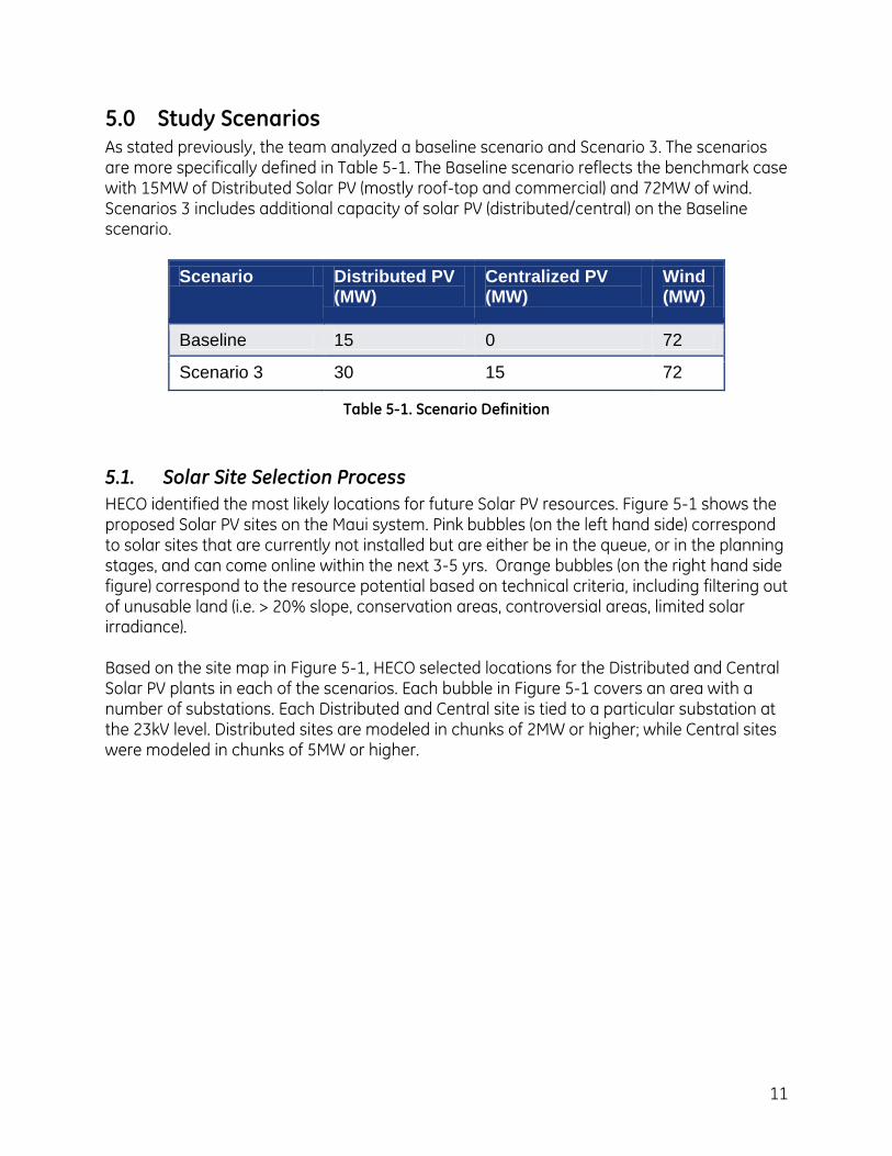
5.0 Study Scenarios As stated previously, the team analyzed a baseline scenario and Scenario 3. The scenarios are more specifically defined in Table 5-1. The Baseline scenario reflects the benchmark case with 15MW of Distributed Solar PV (mostly roof-top and commercial) and 72MW of wind. Scenarios 3 includes additional capacity of solar PV (distributed/central) on the Baseline scenario.

Scenario Distributed PV (MW)

Centralized PV (MW)

Wind (MW)

Baseline 15 0 72

Scenario 3 30 15 72

Table 5-1. Scenario Definition

5.1. Solar Site Selection Process

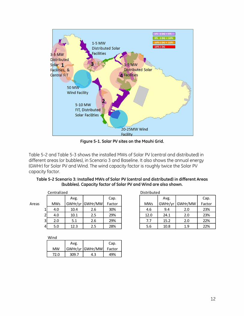
HECO identified the most likely locations for future Solar PV resources. Figure 5-1 shows the proposed Solar PV sites on the Maui system. Pink bubbles (on the left hand side) correspond to solar sites that are currently not installed but are either be in the queue, or in the planning stages, and can come online within the next 3-5 yrs. Orange bubbles (on the right hand side figure) correspond to the resource potential based on technical criteria, including filtering out of unusable land (i.e. > 20% slope, conservation areas, controversial areas, limited solar irradiance). Based on the site map in Figure 5-1, HECO selected locations for the Distributed and Central Solar PV plants in each of the scenarios. Each bubble in Figure 5-1 covers an area with a number of substations. Each Distributed and Central site is tied to a particular substation at the 23kV level. Distributed sites are modeled in chunks of 2MW or higher; while Central sites were modeled in chunks of 5MW or higher.

12

Figure 5-1. Solar PV sites on the Mauhi Grid.

Table 5-2 and Table 5-3 shows the installed MWs of Solar PV (central and distributed) in different areas (or bubbles), in Scenario 3 and Baseline. It also shows the annual energy (GWHr) for Solar PV and Wind. The wind capacity factor is roughly twice the Solar PV capacity factor.

Table 5-2 Scenario 3: Installed MWs of Solar PV (central and distributed) in different Areas (bubbles). Capacity factor of Solar PV and Wind are also shown.

Centralized Distributed

Areas MWs

Avg.

GWHr/yr GWHr/MW

Cap.

Factor MWs

Avg.

GWHr/yr GWHr/MW

Cap.

Factor

1 4.0 10.4 2.6 30% 4.6 9.4 2.0 23%

2 4.0 10.1 2.5 29% 12.0 24.1 2.0 23%

3 2.0 5.1 2.6 29% 7.7 15.2 2.0 22%

4 5.0 12.3 2.5 28% 5.6 10.8 1.9 22%

Wind

MW

Avg.

GWHr/yr GWHr/MW

Cap.

Factor

72.0 309.7 4.3 49%

13

Table 5-3 Baseline scenario: Installed MWs of Solar PV (central and distributed) in different Areas (bubbles). Capacity factor of Solar PV and Wind are also shown.

Centralized Distributed

Areas MWs

Avg.

GWHr/yr GWHr/MW

Cap.

Factor MWs

Avg.

GWHr/yr GWHr/MW

Cap.

Factor

1 - - - - 2.1 4.3 2.0 23%

2 - - - - 3.1 6.3 2.0 23%

3 - - - - 6.4 12.6 2.0 23%

4 - - - - 3.3 6.3 1.9 22%

Wind

MW

Avg.

GWHr/yr GWHr/MW

Cap.

Factor

72.0 309.7 4.3 49%

5.2. Development of Solar and Wind Datasets

In preparation for analyzing the scenarios, AWS Truepower provided time series data for each of the sites in different scenarios listed in Table 5-1. The initial PV production data was provided by AWST at a ten minute resolution, based on 2007-08 data, The frequency of PV ramps over time scales of 10 minutes to several hours captures the spatial variations of PV ramps over the island; however, shorter time scales of several minutes are important to analyze the ramps of central PV plants and other localized cloud phenomena. It was therefore decided by the study team that it is important to model the data in finer time resolution in order to truly capture the impact of solar PV ramps on the grid frequency. As a result, AWS Truepower took the initiative of a cloud simulation that represents the cloud behavior on the island on a 2sec basis for the years 2007-08. The exercise helped to account for precise cloud location and size, varying opacity of clouds, edge effects and other phenomena. It should be noted that the results of the study depend heavily on the quality of data provided, since historical power production data from the solar PV and wind sites does not exist, and models were used to develop the data (wind and solar power).

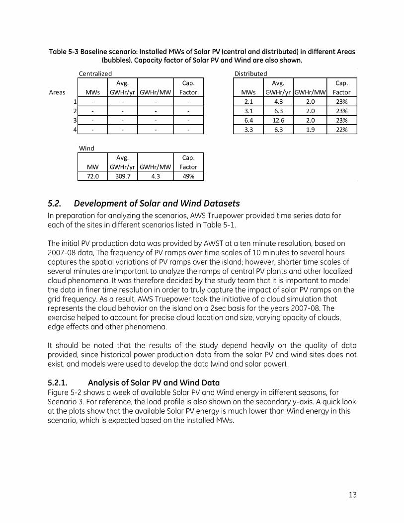
5.2.1. Analysis of Solar PV and Wind Data Figure 5-2 shows a week of available Solar PV and Wind energy in different seasons, for Scenario 3. For reference, the load profile is also shown on the secondary y-axis. A quick look at the plots show that the available Solar PV energy is much lower than Wind energy in this scenario, which is expected based on the installed MWs.

14

Figure 5-2. A week in different seasons in Scenario 3A. This is based on 10-min data.

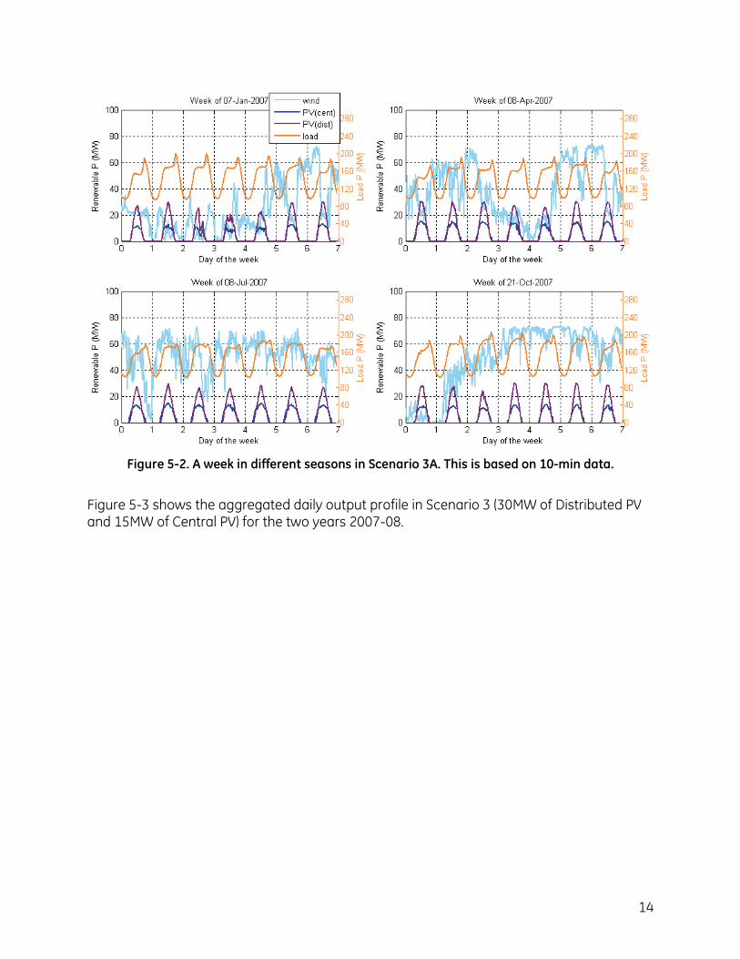
Figure 5-3 shows the aggregated daily output profile in Scenario 3 (30MW of Distributed PV and 15MW of Central PV) for the two years 2007-08.

15

00:00 06:00 12:00 18:00 00:000

5

10

15

20

25

30

35

40

45

Time of day

MW

Solar (cent+dist)

Figure 5-3. Scenario 3A: Daily ouput profiles from Solar PV (central plus distributed) plants for 2007-08

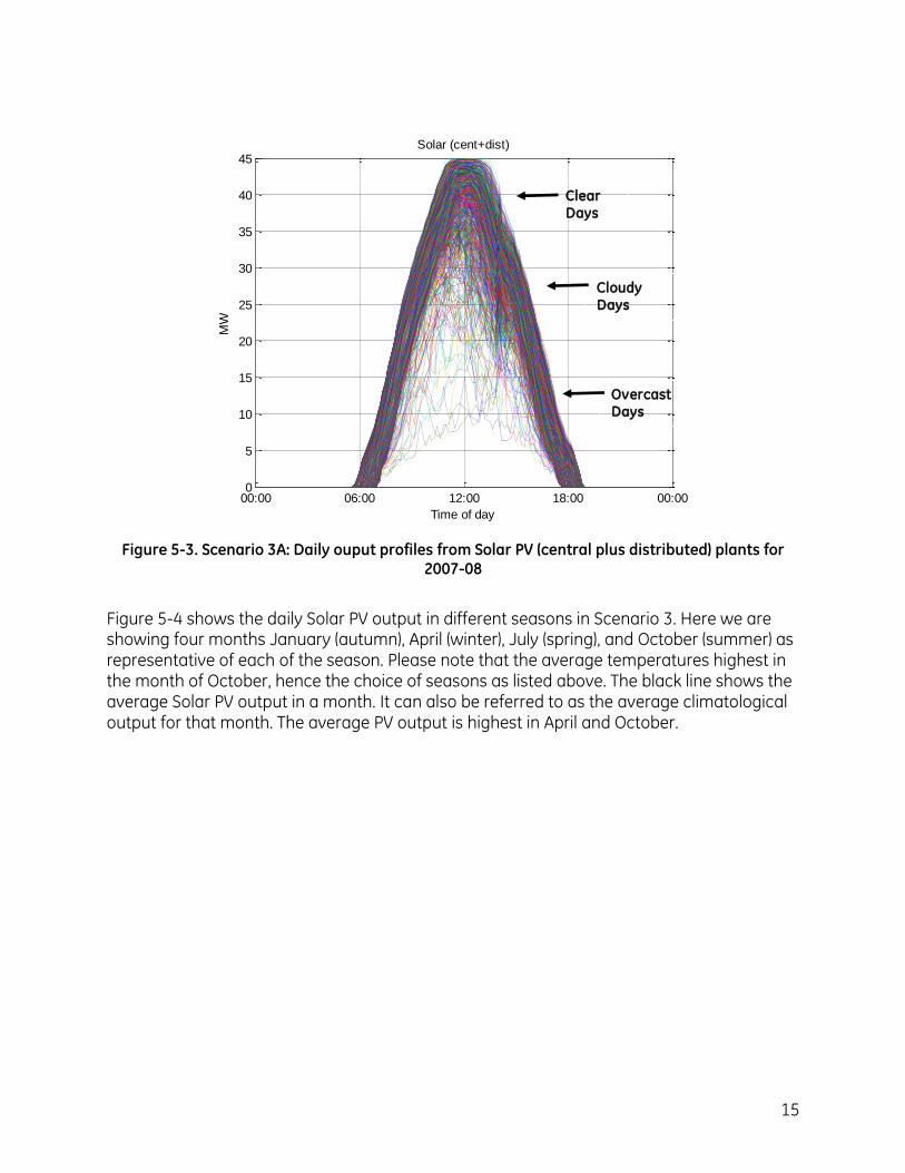
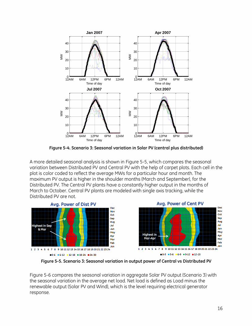
Figure 5-4 shows the daily Solar PV output in different seasons in Scenario 3. Here we are showing four months January (autumn), April (winter), July (spring), and October (summer) as representative of each of the season. Please note that the average temperatures highest in the month of October, hence the choice of seasons as listed above. The black line shows the average Solar PV output in a month. It can also be referred to as the average climatological output for that month. The average PV output is highest in April and October.

Clear Days

Cloudy Days

Overcast Days

16

12AM 6AM 12PM 6PM 12AM0

10

20

30

40

Time of day

MW

Jan 2007


10

20

30

40

Time of day

MW

Apr 2007


10

20

30

40

Time of day

MW

Jul 2007


10

20

30

40

Time of day

MW

Oct 2007

Figure 5-4. Scenario 3: Seasonal variation in Solar PV (central plus distributed)

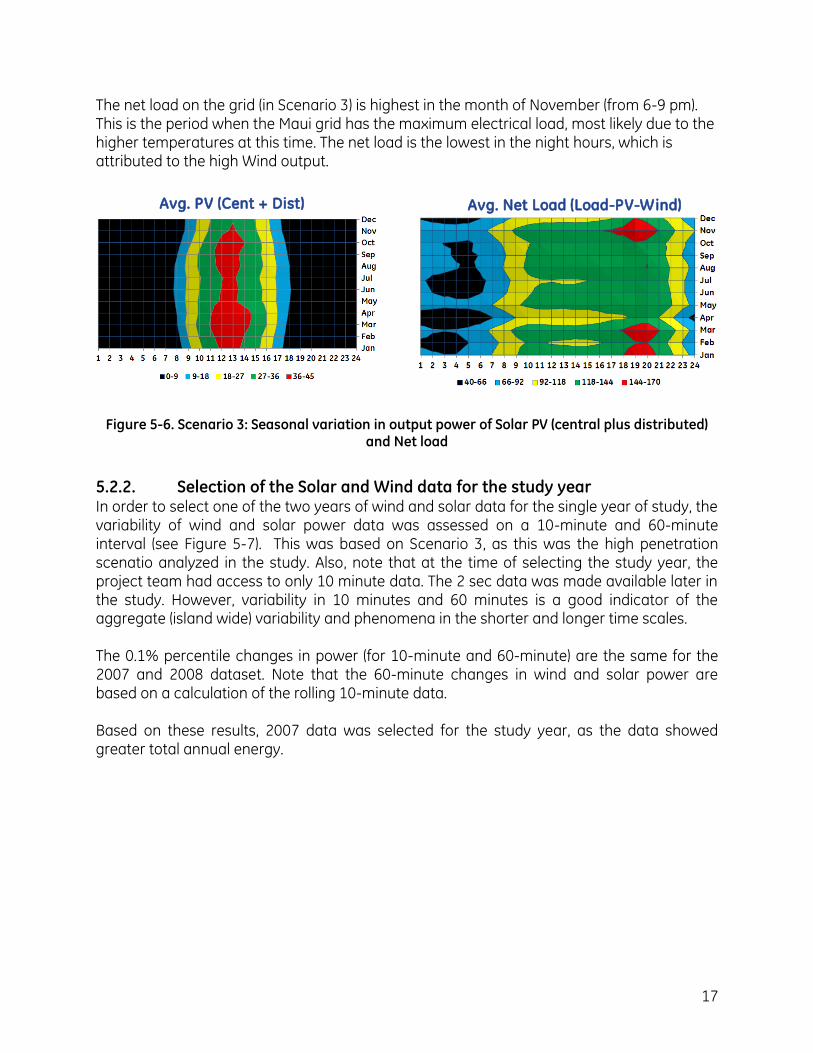
A more detailed seasonal analysis is shown in Figure 5-5, which compares the seasonal variation between Distributed PV and Central PV with the help of carpet plots. Each cell in the plot is color coded to reflect the average MWs for a particular hour and month. The maximum PV output is higher in the shoulder months (March and September), for the Distributed PV. The Central PV plants have a constantly higher output in the months of March to October. Central PV plants are modeled with single axis tracking, while the Distributed PV are not.

Avg. Power of Dist PV Avg. Power of Cent PV

Highest in Mar-Apr

Highest in Sep & Mar

Figure 5-5. Scenario 3: Seasonal variation in output power of Central vs Distributed PV

Figure 5-6 compares the seasonal variation in aggregate Solar PV output (Scenario 3) with the seasonal variation in the average net load. Net load is defined as Load minus the renewable output (Solar PV and Wind), which is the level requiring electrical generator response.

17

The net load on the grid (in Scenario 3) is highest in the month of November (from 6-9 pm). This is the period when the Maui grid has the maximum electrical load, most likely due to the higher temperatures at this time. The net load is the lowest in the night hours, which is attributed to the high Wind output.

Avg. PV (Cent + Dist) Avg. Net Load (Load-PV-Wind)

Figure 5-6. Scenario 3: Seasonal variation in output power of Solar PV (central plus distributed) and Net load

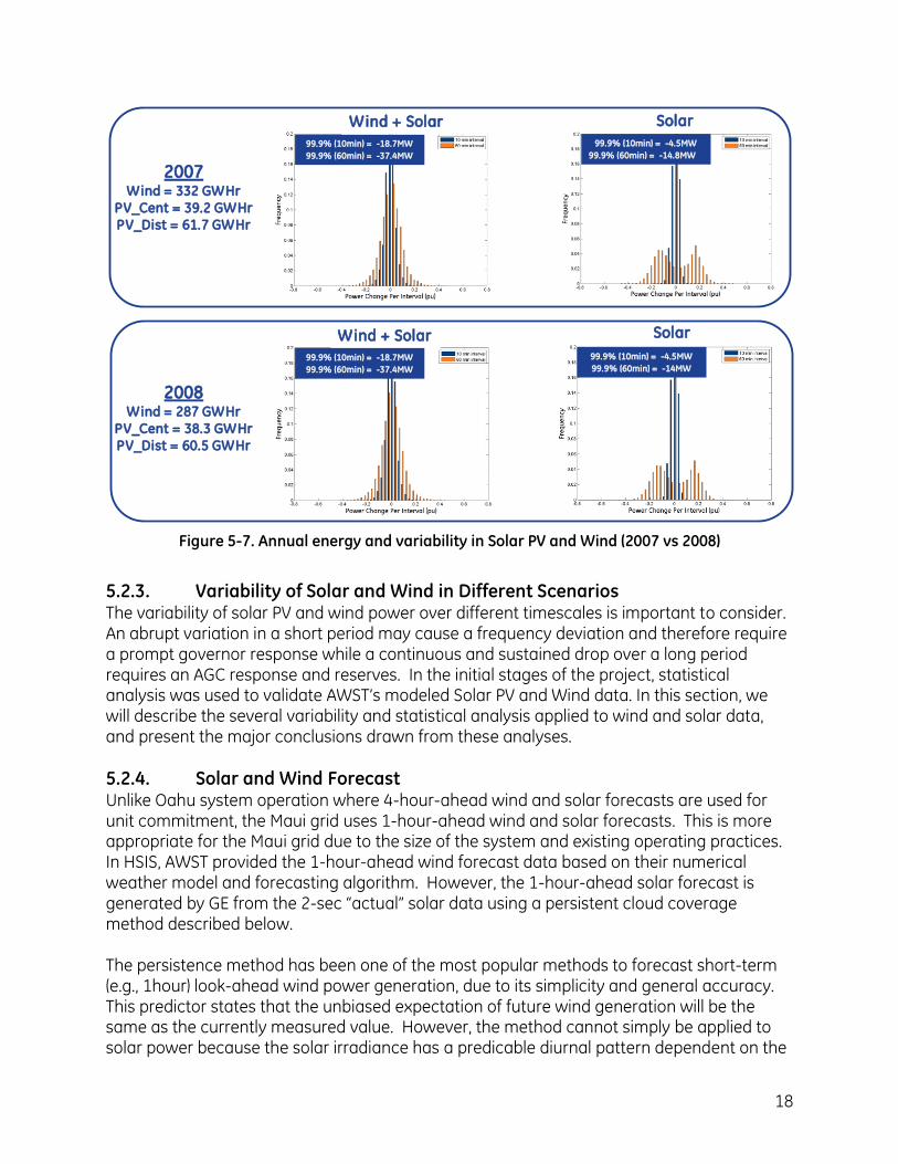
5.2.2. Selection of the Solar and Wind data for the study year In order to select one of the two years of wind and solar data for the single year of study, the variability of wind and solar power data was assessed on a 10-minute and 60-minute interval (see Figure 5-7). This was based on Scenario 3, as this was the high penetration scenatio analyzed in the study. Also, note that at the time of selecting the study year, the project team had access to only 10 minute data. The 2 sec data was made available later in the study. However, variability in 10 minutes and 60 minutes is a good indicator of the aggregate (island wide) variability and phenomena in the shorter and longer time scales. The 0.1% percentile changes in power (for 10-minute and 60-minute) are the same for the 2007 and 2008 dataset. Note that the 60-minute changes in wind and solar power are based on a calculation of the rolling 10-minute data. Based on these results, 2007 data was selected for the study year, as the data showed greater total annual energy.

18

99.9% (10min) = -18.7MW

99.9% (60min) = -37.4MW

Solar

Wind + Solar

Wind + Solar

Solar

99.9% (10min) = -18.7MW

99.9% (60min) = -37.4MW

99.9% (10min) = -4.5MW

99.9% (60min) = -14.8MW

99.9% (10min) = -4.5MW

99.9% (60min) = -14MW

2007Wind = 332 GWHr

PV_Cent = 39.2 GWHr PV_Dist = 61.7 GWHr

2008Wind = 287 GWHr

PV_Cent = 38.3 GWHr PV_Dist = 60.5 GWHr

Figure 5-7. Annual energy and variability in Solar PV and Wind (2007 vs 2008)

5.2.3. Variability of Solar and Wind in Different Scenarios The variability of solar PV and wind power over different timescales is important to consider. An abrupt variation in a short period may cause a frequency deviation and therefore require a prompt governor response while a continuous and sustained drop over a long period requires an AGC response and reserves. In the initial stages of the project, statistical analysis was used to validate AWST’s modeled Solar PV and Wind data. In this section, we will describe the several variability and statistical analysis applied to wind and solar data, and present the major conclusions drawn from these analyses.

5.2.4. Solar and Wind Forecast Unlike Oahu system operation where 4-hour-ahead wind and solar forecasts are used for unit commitment, the Maui grid uses 1-hour-ahead wind and solar forecasts. This is more appropriate for the Maui grid due to the size of the system and existing operating practices. In HSIS, AWST provided the 1-hour-ahead wind forecast data based on their numerical weather model and forecasting algorithm. However, the 1-hour-ahead solar forecast is generated by GE from the 2-sec “actual” solar data using a persistent cloud coverage method described below. The persistence method has been one of the most popular methods to forecast short-term (e.g., 1hour) look-ahead wind power generation, due to its simplicity and general accuracy. This predictor states that the unbiased expectation of future wind generation will be the same as the currently measured value. However, the method cannot simply be applied to solar power because the solar irradiance has a predicable diurnal pattern dependent on the

19

time of day. For this reason, the study incorporated the concept of the persistence method, but assumed variation based on the cloud coverage pattern. Solar power was therefore predicted in the following steps:

From the 2-sec “actual” solar data, the total solar output of the-scenario-under-study for distributed and centralized sites was aggregated. The 2-sec data was re-sampled to obtain the hourly daily solar profile for two years. In HSIS, all centralized PV sites are assumed to be single-axis tracking while all distributed PV sites are assumed to be fix-angled. Separating their forecasting is to take into account of the different solar power profiles.

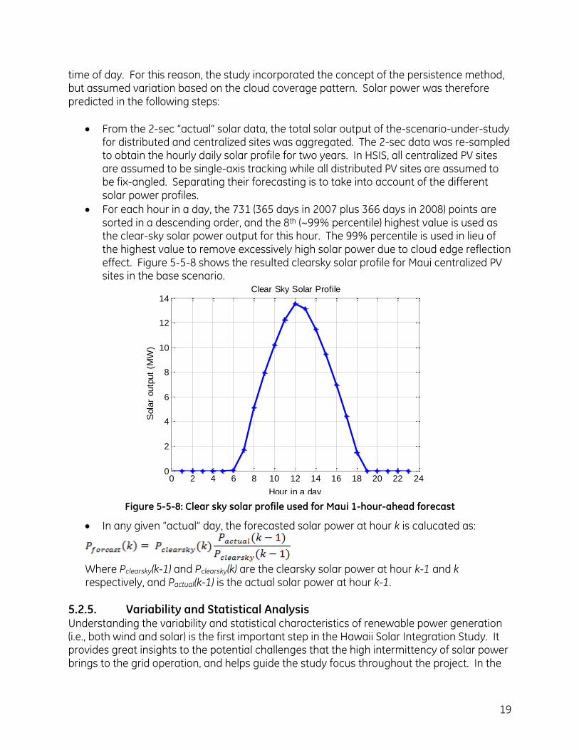
For each hour in a day, the 731 (365 days in 2007 plus 366 days in 2008) points are sorted in a descending order, and the 8th (~99% percentile) highest value is used as the clear-sky solar power output for this hour. The 99% percentile is used in lieu of the highest value to remove excessively high solar power due to cloud edge reflection effect. Figure 5-5-8 shows the resulted clearsky solar profile for Maui centralized PV sites in the base scenario.

0 2 4 6 8 10 12 14 16 18 20 22 240

2

4

6

8

10

12

14

Hour in a day

Sola

r ou

tpu

t (M

W)

Clear Sky Solar Profile

Figure 5-5-8: Clear sky solar profile used for Maui 1-hour-ahead forecast

In any given “actual” day, the forecasted solar power at hour k is calucated as:

Where Pclearsky(k-1) and Pclearsky(k) are the clearsky solar power at hour k-1 and k respectively, and Pactual(k-1) is the actual solar power at hour k-1.

5.2.5. Variability and Statistical Analysis Understanding the variability and statistical characteristics of renewable power generation (i.e., both wind and solar) is the first important step in the Hawaii Solar Integration Study. It provides great insights to the potential challenges that the high intermittency of solar power brings to the grid operation, and helps guide the study focus throughout the project. In the

20

earlier stage of the project, such analyses also served as a sanity check of the validity of AWST high-resolution (i.e., 2-sec intervaled) renewable data. In this section, we will describe the several variability and statistical analyses applied to the AWST two-year-long wind and solar data, and present the major conclusions.

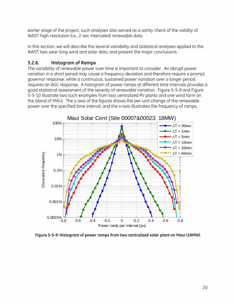
5.2.6. Histogram of Ramps The variability of renewable power over time is important to consider. An abrupt power variation in a short period may cause a frequency deviation and therefore require a prompt governor response, while a continuous, sustained power variation over a longer period requires an AGC response. A histogram of power ramps at different time intervals provides a good statistical assessment of the severity of renewable variation. Figure 5-5-9 and Figure 5-5-10 illustrate two such examples from two centralized PV plants and one wind farm on the island of MAUI. The y-axis of the figures shows the per-unit change of the renewable power over the specified time interval, and the x-axis illustrates the frequency of ramps.

-0.8 -0.6 -0.4 -0.2 0 0.2 0.4 0.6 0.80.0001%

0.001%

0.01%

0.1%

1%

10%

100%

Power ramp per interval (pu)

Occ

ura

nce f

requ

ency

Maui Solar Cent (Site 00007&00023: 18MW)

T = 30sec

T = 1min

T = 5min

T = 10min

T = 20min

T = 60min

Figure 5-5-9: Histogram of power ramps from two centralized solar plant on Maui (18MW)

21

-0.8 -0.6 -0.4 -0.2 0 0.2 0.4 0.6 0.80.0001%

0.001%

0.01%

0.1%

1%

10%

100%


Occ

ura

nce f

requ

ency

Maui Wind (Ulupalakua: 20MW)

T = 30sec

T = 1min

T = 5min

T = 10min

T = 20min

T = 60min

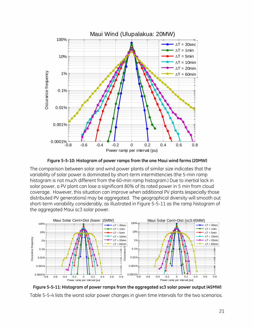
Figure 5-5-10: Histogram of power ramps from the one Maui wind farms (20MW)

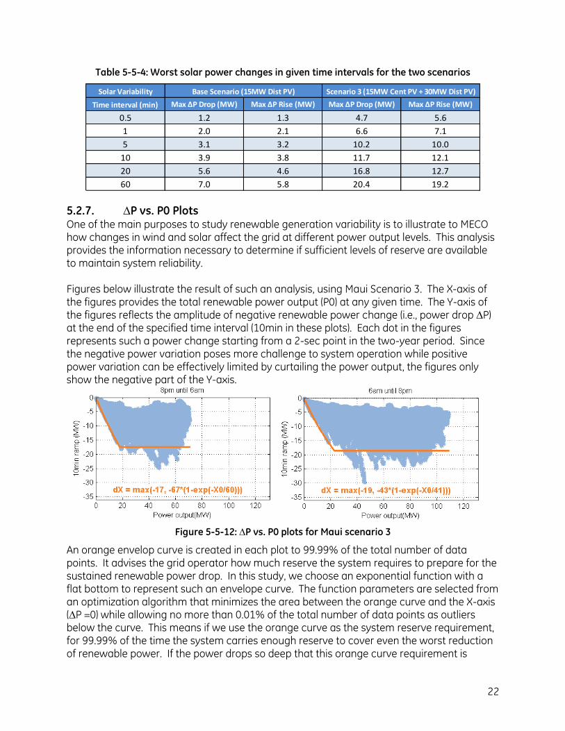
The comparison between solar and wind power plants of similar size indicates that the variability of solar power is dominated by short-term intermittencies (the 5-min ramp histogram is not much different from the 60-min ramp histogram.) Due to inertial lack in solar power, a PV plant can lose a significant 80% of its rated power in 5 min from cloud coverage. However, this situation can improve when additional PV plants (especially those distributed PV generations) may be aggregated. The geographical diversity will smooth out short-term variability considerably, as illustrated in Figure 5-5-11 as the ramp histogram of the aggregated Maui sc3 solar power.

-0.8 -0.6 -0.4 -0.2 0 0.2 0.4 0.6 0.80.0001%

0.001%

0.01%

0.1%

1%

10%

100%


Occ

ura

nce f

requ

ency

Maui Solar Cent+Dist (sc3:45MW)

T = 30sec

T = 1min

T = 5min

T = 10min

T = 20min

T = 60min

-0.8 -0.6 -0.4 -0.2 0 0.2 0.4 0.6 0.80.0001%

0.001%

0.01%

0.1%

1%

10%

100%


Occ

ura

nce f

requ

ency

Maui Solar Cent+Dist (base: 15MW)

T = 30sec

T = 1min

T = 5min

T = 10min

T = 20min

T = 60min

Figure 5-5-11: Histogram of power ramps from the aggregated sc3 solar power output (45MW)

Table 5-5-4 lists the worst solar power changes in given time intervals for the two scenarios.

22

Table 5-5-4: Worst solar power changes in given time intervals for the two scenarios

Solar Variability

Time interval (min) Max ∆P Drop (MW) Max ∆P Rise (MW) Max ∆P Drop (MW) Max ∆P Rise (MW)

0.5 1.2 1.3 4.7 5.6

1 2.0 2.1 6.6 7.1

5 3.1 3.2 10.2 10.0

10 3.9 3.8 11.7 12.1

20 5.6 4.6 16.8 12.7

60 7.0 5.8 20.4 19.2

Base Scenario (15MW Dist PV) Scenario 3 (15MW Cent PV + 30MW Dist PV)

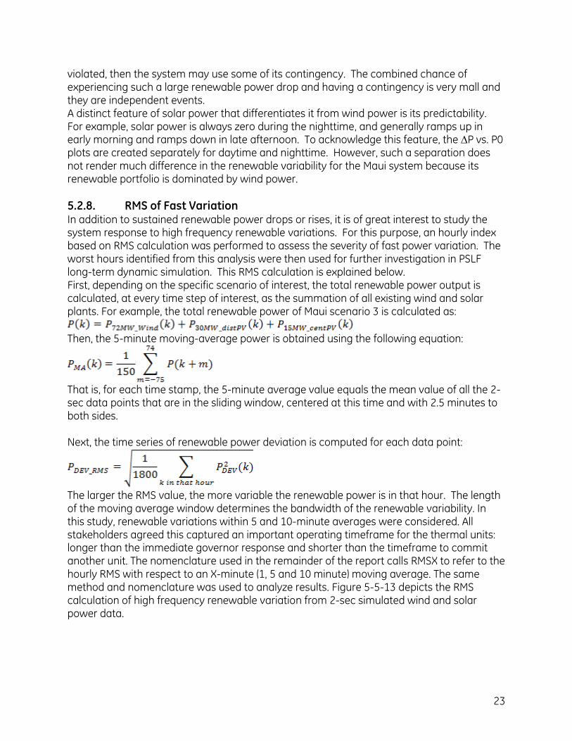
5.2.7. ∆P vs. P0 Plots One of the main purposes to study renewable generation variability is to illustrate to MECO how changes in wind and solar affect the grid at different power output levels. This analysis provides the information necessary to determine if sufficient levels of reserve are available to maintain system reliability. Figures below illustrate the result of such an analysis, using Maui Scenario 3. The X-axis of the figures provides the total renewable power output (P0) at any given time. The Y-axis of the figures reflects the amplitude of negative renewable power change (i.e., power drop ∆P) at the end of the specified time interval (10min in these plots). Each dot in the figures represents such a power change starting from a 2-sec point in the two-year period. Since the negative power variation poses more challenge to system operation while positive power variation can be effectively limited by curtailing the power output, the figures only show the negative part of the Y-axis.

Figure 5-5-12: ∆P vs. P0 plots for Maui scenario 3

An orange envelop curve is created in each plot to 99.99% of the total number of data points. It advises the grid operator how much reserve the system requires to prepare for the sustained renewable power drop. In this study, we choose an exponential function with a flat bottom to represent such an envelope curve. The function parameters are selected from an optimization algorithm that minimizes the area between the orange curve and the X-axis (∆P =0) while allowing no more than 0.01% of the total number of data points as outliers below the curve. This means if we use the orange curve as the system reserve requirement, for 99.99% of the time the system carries enough reserve to cover even the worst reduction of renewable power. If the power drops so deep that this orange curve requirement is

23

violated, then the system may use some of its contingency. The combined chance of experiencing such a large renewable power drop and having a contingency is very mall and they are independent events. A distinct feature of solar power that differentiates it from wind power is its predictability. For example, solar power is always zero during the nighttime, and generally ramps up in early morning and ramps down in late afternoon. To acknowledge this feature, the ∆P vs. P0 plots are created separately for daytime and nighttime. However, such a separation does not render much difference in the renewable variability for the Maui system because its renewable portfolio is dominated by wind power.

5.2.8. RMS of Fast Variation In addition to sustained renewable power drops or rises, it is of great interest to study the system response to high frequency renewable variations. For this purpose, an hourly index based on RMS calculation was performed to assess the severity of fast power variation. The worst hours identified from this analysis were then used for further investigation in PSLF long-term dynamic simulation. This RMS calculation is explained below. First, depending on the specific scenario of interest, the total renewable power output is calculated, at every time step of interest, as the summation of all existing wind and solar plants. For example, the total renewable power of Maui scenario 3 is calculated as:

Then, the 5-minute moving-average power is obtained using the following equation:

That is, for each time stamp, the 5-minute average value equals the mean value of all the 2-sec data points that are in the sliding window, centered at this time and with 2.5 minutes to both sides. Next, the time series of renewable power deviation is computed for each data point:

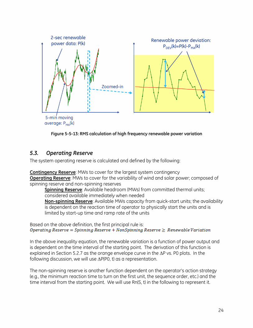
The larger the RMS value, the more variable the renewable power is in that hour. The length of the moving average window determines the bandwidth of the renewable variability. In this study, renewable variations within 5 and 10-minute averages were considered. All stakeholders agreed this captured an important operating timeframe for the thermal units: longer than the immediate governor response and shorter than the timeframe to commit another unit. The nomenclature used in the remainder of the report calls RMSX to refer to the hourly RMS with respect to an X-minute (1, 5 and 10 minute) moving average. The same method and nomenclature was used to analyze results. Figure 5-5-13 depicts the RMS calculation of high frequency renewable variation from 2-sec simulated wind and solar power data.

24

2-sec renewable power data: P(k)

Renewable power deviation:

PDEV(k)=P(k)-PMA(k)

Figure 5-5-13: RMS calculation of high frequency renewable power variation

5.3. Operating Reserve

The system operating reserve is calculated and defined by the following: Contingency Reserve: MWs to cover for the largest system contingency Operating Reserve: MWs to cover for the variability of wind and solar power; composed of spinning reserve and non-spinning reserves

Spinning Reserve: Available headroom (MWs) from committed thermal units; considered available immediately when needed Non-spinning Reserve: Available MWs capacity from quick-start units; the availability is dependent on the reaction time of operator to physically start the units and is limited by start-up time and ramp rate of the units

Based on the above definition, the first principal rule is:

In the above inequality equation, the renewable variation is a function of power output and is dependent on the time interval of the starting point. The derivation of this function is explained in Section 5.2.7 as the orange envelope curve in the ∆P vs. P0 plots. In the following discussion, we will use ∆P(P0, t) as a representation. The non-spinning reserve is another function dependent on the operator’s action strategy (e.g., the minimum reaction time to turn on the first unit, the sequence order, etc.) and the time interval from the starting point. We will use Rn(S, t) in the following to represent it.

25

The spinning reserve is a function of renewable power output but is independent on time. The objective is to determine the minimum value of this system quantity. We will use Rs(P0) in the following for it. The mathematical expression of the above inequality equation is written as: Given an operator’s action strategy, S

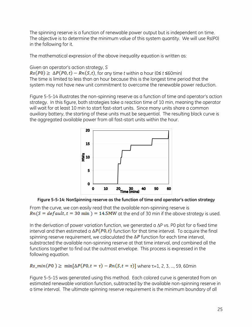
, for any time t within a hour (0≤ t ≤60min) The time is limited to less than an hour because this is the longest time period that the system may not have new unit commitment to overcome the renewable power reduction. Figure 5-5-14 illustrates the non-spinning reserve as a function of time and operator’s action strategy. In this figure, both strategies take a reaction time of 10 min, meaning the operator will wait for at least 10 min to start fast-start units. Since many units share a common auxiliary battery, the starting of these units must be sequential. The resulting black curve is the aggregated available power from all fast-start units within the hour.

0

5

10

15

20

0 10 20 30 40 50 60

MW

s

Time (mins)

Figure 5-5-14: NonSpinning reserve as the function of time and operator’s action strategy

From the curve, we can easily read that the available non-spinning reserve is at the end of 30 min if the above strategy is used.

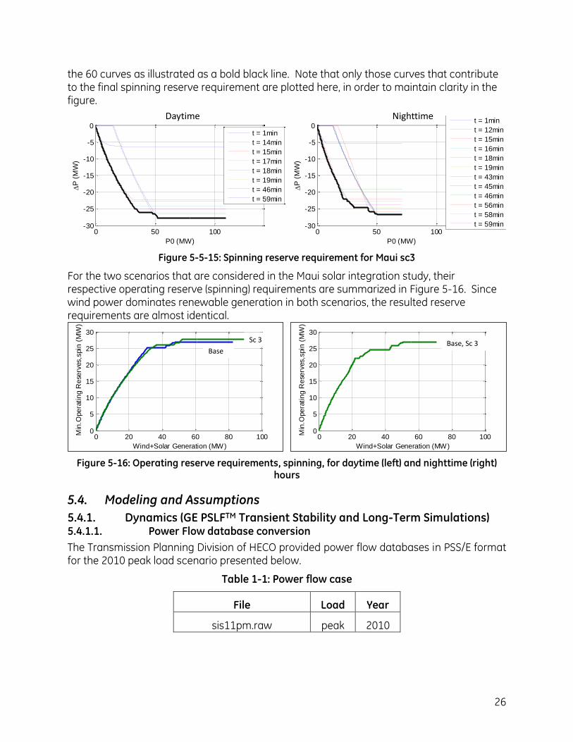
In the derivation of power variation function, we generated a ∆P vs. P0 plot for a fixed time interval and then estimated a function for that time interval. To acquire the final spinning reserve requirement, we calaculated the function for each time interval, substracted the available non-spinning reserve at that time interval, and combined all the functions together to find out the outmost envelope. This process is expressed in the following equation.

where τ=1, 2, 3, …, 59, 60min Figure 5-5-15 was generated using this method. Each colored curve is generated from an estimated renewable variation function, subtracted by the available non-spinning reserve in a time interval. The ultimate spinning reserve requirement is the minimum boundary of all

26

the 60 curves as illustrated as a bold black line. Note that only those curves that contribute to the final spinning reserve requirement are plotted here, in order to maintain clarity in the figure.

0 50 100-30

-25

-20

-15

-10

-5

0

P0 (MW)

P

(M

W)

t = 1min

t = 14min

t = 15min

t = 17min

t = 18min

t = 19min

t = 46min

t = 59min

0 50 100-30

-25

-20

-15

-10

-5

0

P0 (MW)

P

(M

W)

t = 1min

t = 12min

t = 15min

t = 16min

t = 18min

t = 19min

t = 43min

t = 45min

t = 46min

t = 56min

t = 58min

t = 59min

Daytime Nighttime

Figure 5-5-15: Spinning reserve requirement for Maui sc3

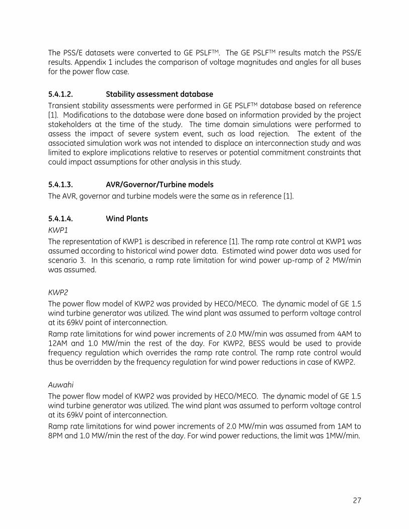
For the two scenarios that are considered in the Maui solar integration study, their respective operating reserve (spinning) requirements are summarized in Figure 5-16. Since wind power dominates renewable generation in both scenarios, the resulted reserve requirements are almost identical.

0 20 40 60 80 1000

5

10

15

20

25

30

Wind+Solar Generation (MW)

Min

.Ope

rati

ng

Re

serv

es,s

pin

(M

W)

Sc 3

Base

0 20 40 60 80 1000

5

10

15

20

25

30

Wind+Solar Generation (MW)

Min

.Ope

rati

ng

Re

serv

es,s

pin

(M

W)

Base, Sc 3

Figure 5-16: Operating reserve requirements, spinning, for daytime (left) and nighttime (right) hours

5.4. Modeling and Assumptions

5.4.1. Dynamics (GE PSLFTM Transient Stability and Long-Term Simulations) 5.4.1.1. Power Flow database conversion

The Transmission Planning Division of HECO provided power flow databases in PSS/E format for the 2010 peak load scenario presented below.

Table 1-1: Power flow case

File Load Year

sis11pm.raw peak 2010

27

The PSS/E datasets were converted to GE PSLFTM. The GE PSLFTM results match the PSS/E results. Appendix 1 includes the comparison of voltage magnitudes and angles for all buses for the power flow case.

5.4.1.2. Stability assessment database

Transient stability assessments were performed in GE PSLFTM database based on reference [1]. Modifications to the database were done based on information provided by the project stakeholders at the time of the study. The time domain simulations were performed to assess the impact of severe system event, such as load rejection. The extent of the associated simulation work was not intended to displace an interconnection study and was limited to explore implications relative to reserves or potential commitment constraints that could impact assumptions for other analysis in this study.

5.4.1.3. AVR/Governor/Turbine models

The AVR, governor and turbine models were the same as in reference [1].

5.4.1.4. Wind Plants

KWP1

The representation of KWP1 is described in reference [1]. The ramp rate control at KWP1 was assumed according to historical wind power data. Estimated wind power data was used for scenario 3. In this scenario, a ramp rate limitation for wind power up-ramp of 2 MW/min was assumed.

KWP2

The power flow model of KWP2 was provided by HECO/MECO. The dynamic model of GE 1.5 wind turbine generator was utilized. The wind plant was assumed to perform voltage control at its 69kV point of interconnection.

Ramp rate limitations for wind power increments of 2.0 MW/min was assumed from 4AM to 12AM and 1.0 MW/min the rest of the day. For KWP2, BESS would be used to provide frequency regulation which overrides the ramp rate control. The ramp rate control would thus be overridden by the frequency regulation for wind power reductions in case of KWP2.

Auwahi

The power flow model of KWP2 was provided by HECO/MECO. The dynamic model of GE 1.5 wind turbine generator was utilized. The wind plant was assumed to perform voltage control at its 69kV point of interconnection.

Ramp rate limitations for wind power increments of 2.0 MW/min was assumed from 1AM to 8PM and 1.0 MW/min the rest of the day. For wind power reductions, the limit was 1MW/min.

28

5.4.1.5. KWP2 BESS Model

The BESS model implemented in GE PSLFTM was used for transient stability and long-term stability. KWP2 BESS was modeled with the power rating of 10MW. The model is based on the functional specification in reference [1] and on inputs from MECO regarding the PPA.

The model was implemented as a current source model. The active current was commanded to fulfill the power request (Pordr) shown in the block diagram in [1]. Different to [1], the frequency regulation function was modeled with ± 0.1 Hz deadband. The frequency error signal was then applied to a lead/lag transfer function of time constants Tld and Tlg and a gain block to create the power request signal. The steady state gain to a frequency error was characterized with the droop setting R, set to 4%. Based on a one-way efficiency parameter, the model also tracks the state-of-charge. The reactive current was assumed to be zero.

The BESS was modeled with high transient gain so as to enable aggressive response to frequency deviation. This aggressive response was characterized by an initial gain of 20 times the gain of a 4% droop. The BESS with aggressive initial response was requested to reduce the down reserve on the CTs required to avoid ST trips during load rejection events (see [1]). This BESS response characteristic also reduces significantly the fast maneuvering required to the thermal units during wind power fluctuations.

The aggressive frequency control and the deadband require particular attention. No information was available regarding the control logic used to reset BESS output when frequency returns within the deadband after an event. It was assumed that the BESS will slowly reduce the power output when the system frequency returns within the deadband to avoid an additional system upset due to BESS sudden power modifications.

Communication between AGC and BESS was considered but not explicitly modeled.. The operation of the BESS due to AGC requests was not expected during conditions simulated in PSLF. Rather, the operation of BESS due to frequency response, explicitly represented in the model, was frequent in the performed simulations.

Reference Frequency +-

+

Magnitude

Limits

Actual Frequency

+

SOC

Pordr

DeadbandTld = 6000Tlg = 300

1sTlg

1sTld

R

1

Figure 5-17: BESS Model

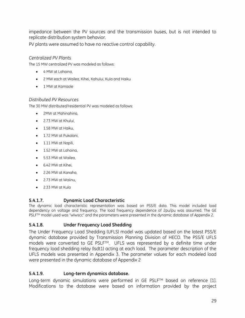
5.4.1.6. PV Plants

The power flow database was updated to include scenario 3 PV allocation consisting of 30MW of distributed PV and 15MW of centralized PV plants. The PV plants have been modeled with aggregated generators connected to equivalent 480 V buses. The generator was connected to a unit transformer of MVA ratings equal to N times the individual device ratings, N being number of converters in the plant. This representation reflects the sizable

29

impedance between the PV sources and the transmission buses, but is not intended to replicate distribution system behavior.

PV plants were assumed to have no reactive control capability.

Centralized PV Plants

The 15 MW centralized PV was modeled as follows:

4 MW at Lahaina,

2 MW each at Wailea, Kihei, Kahului, Kula and Haiku

1 MW at Kamaole

Distributed PV Resources

The 30 MW distributed/residential PV was modeled as follows:

2MW at Mahinahina,

2.73 MW at Khului,

1.58 MW at Haiku,

1.72 MW at Pukalani,

1.11 MW at Napili,

1.52 MW at Lahaina,

5.53 MW at Wailea,

6.42 MW at Kihei,

2.26 MW at Kanaha,

2.73 MW at Waiinu,

2.33 MW at Kula

5.4.1.7. Dynamic Load Characteristic The dynamic load characteristic representation was based on PSS/E data. This model included load dependency on voltage and frequency. The load frequency dependence of 2pu/pu was assumed. The GE PSLFTM model used was “wlwscc” and the parameters were presented in the dynamic database of Appendix 2.

5.4.1.8. Under Frequency Load Shedding

The Under Frequency Load Shedding (UFLS) model was updated based on the latest PSS/E dynamic database provided by Transmission Planning Division of HECO. The PSS/E UFLS models were converted to GE PSLFTM. UFLS was represented by a definite time under frequency load shedding relay (lsdt1) acting at each load. The parameter description of the UFLS models was presented in Appendix 3. The parameter values for each modeled load were presented in the dynamic database of Appendix 2

5.4.1.9. Long-term dynamics database.

Long-term dynamic simulations were performed in GE PSLFTM based on reference [1]. Modifications to the database were based on information provided by the project

30

stakeholders at the time of the study. The Automatic Generation Control (AGC) function at MECO was reflected in a model developed by GE in a prior effort and updated based on the most recent information provided at the time of the study. Economic dispatch calculation was improved. The AGC representation in GE PSLFTM was used to assess dynamic events on the system in timescales longer than transient stability events (less than one minute) and shorter than production cost modeling events (one hour). The longer-term dynamic events assess the impact of system events, primarily related to changes in wind power production that rely upon the action of the AGC to correct for imbalances between the load and generation.

5.4.1.10. AGC model improvement

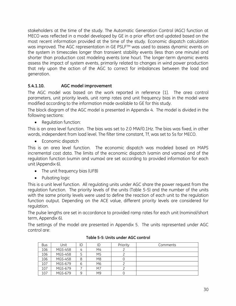
The AGC model was based on the work reported in reference [1]. The area control parameters, unit priority levels, unit ramp rates and unit frequency bias in the model were modified according to the information made available to GE for this study.

The block diagram of the AGC model is presented in Appendix 4. The model is divided in the following sections:

Regulation function:

This is an area level function. The bias was set to 2.0 MW/0.1Hz. The bias was fixed, in other words, independent from load level. The filter time constant, Tf, was set to 5s for MECO.

Economic dispatch

This is an area level function. The economic dispatch was modeled based on MAPS incremental cost data. The limits of the economic dispatch (vamin and vamax) and of the regulation function (vumin and vumax) are set according to provided information for each unit (Appendix 6).

The unit frequency bias (UFB)

Pulsating logic

This is a unit level function. All regulating units under AGC share the power request from the regulation function. The priority levels of the units (Table 5-5) and the number of the units with the same priority levels were used to define the reaction of each unit to the regulation function output. Depending on the ACE value, different priority levels are considered for regulation.

The pulse lengths are set in accordance to provided ramp rates for each unit (nominal/short term, Appendix 6).

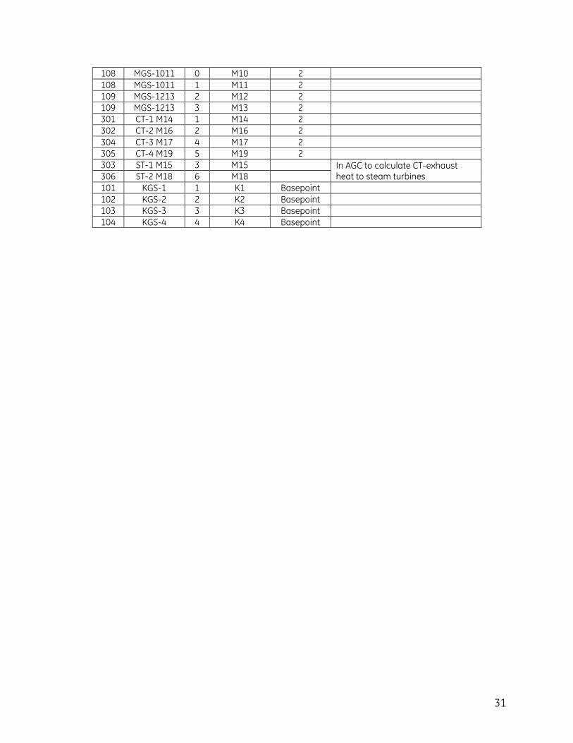
The settings of the model are presented in Appendix 5. The units represented under AGC control are:

Table 5-5: Units under AGC control

Bus Unit ID ID Priority Comments

106 MGS-458 4 M4 2

106 MGS-458 5 M5 2

106 MGS-458 8 M8 0

107 MGS-679 6 M6 2

107 MGS-679 7 M7 2

107 MGS-679 9 M9 0

31

108 MGS-1011 0 M10 2

108 MGS-1011 1 M11 2

109 MGS-1213 2 M12 2

109 MGS-1213 3 M13 2

301 CT-1 M14 1 M14 2

302 CT-2 M16 2 M16 2

304 CT-3 M17 4 M17 2

305 CT-4 M19 5 M19 2

303 ST-1 M15 3 M15 In AGC to calculate CT-exhaust heat to steam turbines 306 ST-2 M18 6 M18

101 KGS-1 1 K1 Basepoint




32

5.4.2. Production Cost Database

The following sub sections address the modeling assumption for the GE MAPSTM Production Cost modeling tool. The starting point was the database of reference [2]. The validation in reference [2] shows good levels of accuracy when compared to actual production. The impact of the further refinements in the database described in this section were verified by MECO operations, based on close examination of hourly dispatch and commitment results.

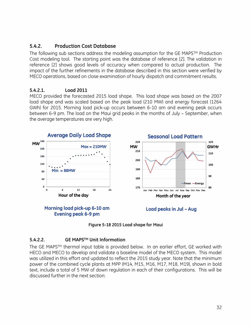
5.4.2.1. Load 2011 MECO provided the forecasted 2015 load shape. This load shape was based on the 2007 load shape and was scaled based on the peak load (210 MW) and energy forecast (1264 GWh) for 2015. Morning load pick-up occurs between 6-10 am and evening peak occurs between 6-9 pm. The load on the Maui grid peaks in the months of July – September, when the average temperatures are very high.

Max = 210MW

Min = 88MW

Hour of the day

MW

Average Daily Load Shape

Month of the year

MW GWHr

Seasonal Load Pattern

Load peaks in Jul – AugMorning load pick-up 6-10 am

Evening peak 6-9 pm

Figure 5-18 2015 Load shape for Maui

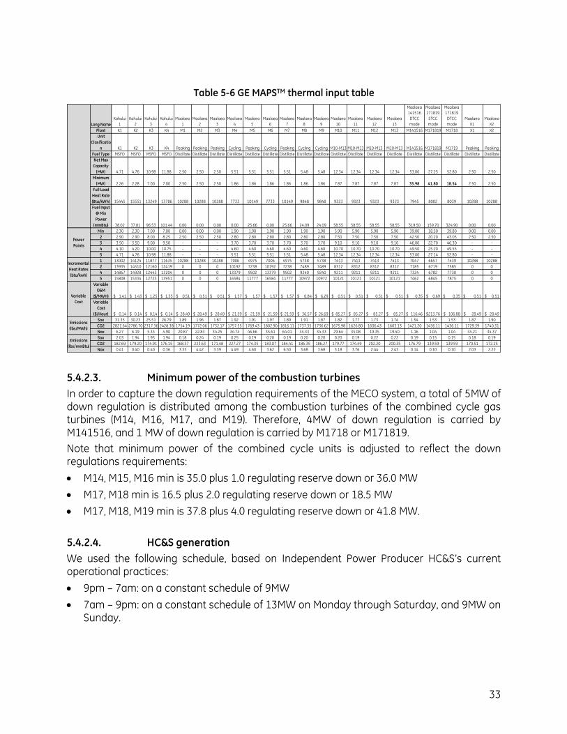
5.4.2.2. GE MAPSTM Unit Information

The GE MAPSTM thermal input table is provided below. In an earlier effort, GE worked with HECO and MECO to develop and validate a baseline model of the MECO system. This model was utilized in this effort and updated to reflect the 2015 study year. Note that the minimum power of the combined cycle plants at MPP (M14, M15, M16, M17, M18, M19), shown in bold text, include a total of 5 MW of down regulation in each of their configurations. This will be discussed further in the next section:

33

Table 5-6 GE MAPSTM thermal input table

Long Name

Kahului

1

Kahului

2

Kahului

3

Kahului

4

Maalaea

1

Maalaea

2

Maalaea

3

Maalaea

4

Maalaea

5

Maalaea

6

Maalaea

7

Maalaea

8

Maalaea

9

Maalaea

10

Maalaea

11

Maalaea

12

Maalaea

13

Maalaea

141516

DTCC

mode

Maalaea

171819

STCC

mode

Maalaea

171819

DTCC

mode

Maalaea

X1

Maalaea

X2

Plant K1 K2 K3 K4 M1 M2 M3 M4 M5 M6 M7 M8 M9 M10 M11 M12 M13 M141516 M171819 M1718 X1 X2

Unit

Clasificatio

n K1 K2 K3 K4 Peaking Peaking Peaking Cycling Peaking Cycling Peaking Cycling Cycling M10-M13 M10-M13 M10-M13 M10-M13 M141516 M171819 M1719 Peaking Peaking

Fuel Type MSFO MSFO MSFO MSFO Distillate Distillate Distillate Distillate Distillate Distillate Distillate Distillate Distillate Distillate Distillate Distillate Distillate Distillate Distillate Distillate Distillate Distillate

Net Max

Capacity

(MW) 4.71 4.76 10.98 11.88 2.50 2.50 2.50 5.51 5.51 5.51 5.51 5.48 5.48 12.34 12.34 12.34 12.34 53.00 27.25 52.80 2.50 2.50

Minimum

(MW) 2.26 2.28 7.00 7.00 2.50 2.50 2.50 1.86 1.86 1.86 1.86 1.86 1.86 7.87 7.87 7.87 7.87 35.98 41.80 18.54 2.50 2.50

Full Load

Heat Rate

(Btu/kWh) 15445 15551 13249 13786 10288 10288 10288 7733 10149 7733 10149 9848 9848 9323 9323 9323 9323 7945 8002 8039 10288 10288

Fuel Input

@ Min

Power

(mmBtu) 38.02 37.81 96.53 101.44 0.00 0.00 0.00 0.00 25.66 0.00 25.66 24.09 24.09 58.55 58.55 58.55 58.55 319.50 159.70 324.90 0.00 0.00

Min 2.30 2.30 7.00 7.00 0.00 0.00 0.00 1.90 1.90 1.90 1.90 1.90 1.90 5.90 5.90 5.90 5.90 39.00 18.50 39.80 0.00 0.00

2 2.90 2.90 8.00 8.25 2.50 2.50 2.50 2.80 2.80 2.80 2.80 2.80 2.80 7.50 7.50 7.50 7.50 42.50 20.20 43.05 2.50 2.50

3 3.50 3.50 9.00 9.50 - - - 3.70 3.70 3.70 3.70 3.70 3.70 9.10 9.10 9.10 9.10 46.00 22.70 46.30 - -

4 4.10 4.20 10.00 10.75 - - - 4.60 4.60 4.60 4.60 4.60 4.60 10.70 10.70 10.70 10.70 49.50 25.20 49.55 - -

5 4.71 4.76 10.98 11.88 - - - 5.51 5.51 5.51 5.51 5.48 5.48 12.34 12.34 12.34 12.34 53.00 27.14 52.80 - -

1 13002 14124 11877 11635 10288 10288 10288 7006 4975 7006 4975 5738 5738 7413 7413 7413 7413 7047 6657 7439 10288 10288

2 13935 14510 12160 12419 0 0 0 10192 7238 10192 7238 7489 7489 8312 8312 8312 8312 7185 6719 7585 0 0

4 14867 14928 12443 13204 0 0 0 13379 9502 13379 9502 9240 9240 9211 9211 9211 9211 7324 6782 7730 0 0

5 15808 15334 12723 13951 0 0 0 16584 11777 16584 11777 10972 10972 10121 10121 10121 10121 7462 6845 7875 0 0

Variable

O&M

($/MWH) 1.41$ 1.43$ 1.25$ 1.35$ 0.51$ 0.51$ 0.51$ 1.57$ 1.57$ 1.57$ 1.57$ 0.84$ 6.29$ 0.51$ 0.51$ 0.51$ 0.51$ 0.35$ 0.69$ 0.35$ 0.51$ 0.51$

Variable

Cost

($/Hour) 0.14$ 0.14$ 0.14$ 0.14$ 28.49$ 28.49$ 28.49$ 21.59$ 21.59$ 21.59$ 21.59$ 36.57$ 26.69$ 85.27$ 85.27$ 85.27$ 85.27$ 116.46$ 213.76$ 106.88$ 28.49$ 28.49$

Sox 31.35 30.23 25.51 26.79 1.89 1.96 1.87 1.92 1.91 1.97 1.89 1.91 1.87 1.82 1.77 1.73 1.74 1.54 1.53 1.53 1.87 1.90

CO2 2821.64 2786.70 2317.36 2428.38 1754.19 1772.06 1732.17 1757.55 1769.43 1802.90 1816.11 1737.35 1736.62 1675.98 1626.80 1606.43 1603.13 1421.20 1436.11 1436.11 1729.39 1740.31

Nox 6.27 6.19 5.33 4.90 20.87 22.83 34.25 34.74 46.66 35.61 64.01 34.33 34.33 29.64 35.08 19.35 19.40 1.16 1.04 1.04 34.21 34.37

Sox 2.03 1.94 1.93 1.94 0.18 0.24 0.19 0.25 0.19 0.20 0.19 0.20 0.20 0.20 0.19 0.22 0.22 0.19 0.15 0.15 0.18 0.19

CO2 182.69 179.20 174.91 176.15 168.37 223.63 171.48 227.27 174.35 183.07 184.41 186.35 186.27 179.77 174.49 202.20 200.35 176.79 139.59 139.59 170.51 172.25

Nox 0.41 0.40 0.40 0.36 3.33 4.42 3.39 4.49 4.60 3.62 6.50 3.68 3.68 3.18 3.76 2.44 2.43 0.14 0.10 0.10 2.03 2.22

Power

Points

Incremental

Heat Rates

(btu/kwh)

Variable

Cost

Emissions

(lbs/MWh)

Emissions

(lbs/mmBtu)

5.4.2.3. Minimum power of the combustion turbines

In order to capture the down regulation requirements of the MECO system, a total of 5MW of down regulation is distributed among the combustion turbines of the combined cycle gas turbines (M14, M16, M17, and M19). Therefore, 4MW of down regulation is carried by M141516, and 1 MW of down regulation is carried by M1718 or M171819.

Note that minimum power of the combined cycle units is adjusted to reflect the down regulations requirements:

M14, M15, M16 min is 35.0 plus 1.0 regulating reserve down or 36.0 MW

M17, M18 min is 16.5 plus 2.0 regulating reserve down or 18.5 MW

M17, M18, M19 min is 37.8 plus 4.0 regulating reserve down or 41.8 MW.

5.4.2.4. HC&S generation

We used the following schedule, based on Independent Power Producer HC&S’s current operational practices:

9pm – 7am: on a constant schedule of 9MW

7am – 9pm: on a constant schedule of 13MW on Monday through Saturday, and 9MW on Sunday.

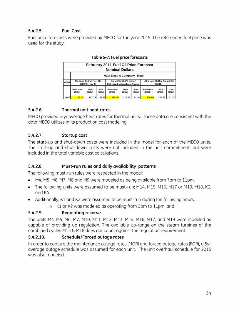
34

5.4.2.5. Fuel Cost

Fuel price forecasts were provided by MECO for the year 2015. The referenced fuel price was used for the study.

Table 5-7: Fuel price forecasts

YEAR

Reference

($/Bbl)

High

($/Bbl)

Low

($/Bbl)

Reference

($/Bbl)

High

($/Bbl)

Low

($/Bbl)

Reference

($/Bbl)

High

($/Bbl)

Low

($/Bbl)

2015 93.32 147.78 46.66 135.30 210.03 71.24 138.05 215.52 71.27

Nominal Dollars

February 2011 Fuel Oil Price Forecast

Ultra Low Sulfur Diesel Oil

(ULSD)

Diesel Oil (0.4% Sulfur)

Delivered to Maalaea Power

Medium Sulfur Fuel Oil

(MSFO - No. 6)

Maui Electric Company - Maui

5.4.2.6. Thermal unit heat rates

MECO provided 5-yr average heat rates for thermal units. These data are consistent with the data MECO utilizes in its production cost modeling.

5.4.2.7. Startup cost

The start-up and shut-down costs were included in the model for each of the MECO units. The start-up and shut-down costs were not included in the unit commitment, but were included in the total variable cost calculations.

5.4.2.8. Must-run rules and daily availability patterns

The following must-run rules were respected in the model:

M4, M5, M6, M7, M8 and M9 were modeled as being available from 7am to 11pm.

The following units were assumed to be must-run: M14, M15, M16, M17 or M19, M18, K3, and K4

Additionally, K1 and K2 were assumed to be must-run during the following hours:

o K1 or K2 was modeled as operating from 2pm to 11pm, and

5.4.2.9. Regulating reserve

The units M4, M5, M6, M7, M10, M11, M12, M13, M14, M16, M17, and M19 were modeled as capable of providing up regulation. The available up-range on the steam turbines of the combined cycles M15 & M18 does not count against the regulation requirement.

5.4.2.10. Schedule/Forced outage rates

In order to capture the maintenance outage rates (MOR) and forced outage rates (FOR), a 5yr average outage schedule was assumed for each unit. The unit overhaul schedule for 2015 was also modeled.

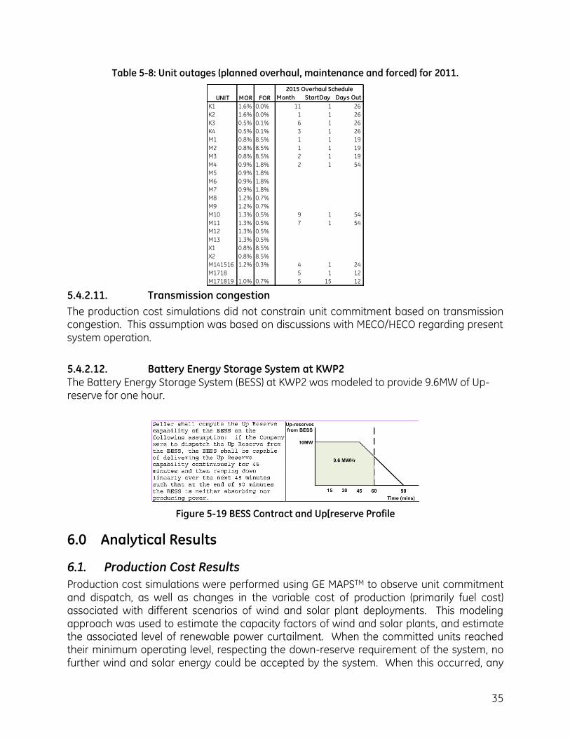
35

Table 5-8: Unit outages (planned overhaul, maintenance and forced) for 2011.

Month StartDay Days Out

K1 1.6% 0.0% 11 1 26

K2 1.6% 0.0% 1 1 26

K3 0.5% 0.1% 6 1 26

K4 0.5% 0.1% 3 1 26

M1 0.8% 8.5% 1 1 19

M2 0.8% 8.5% 1 1 19

M3 0.8% 8.5% 2 1 19

M4 0.9% 1.8% 2 1 54

M5 0.9% 1.8%

M6 0.9% 1.8%

M7 0.9% 1.8%

M8 1.2% 0.7%

M9 1.2% 0.7%

M10 1.3% 0.5% 9 1 54

M11 1.3% 0.5% 7 1 54

M12 1.3% 0.5%

M13 1.3% 0.5%

X1 0.8% 8.5%

X2 0.8% 8.5%

M141516 1.2% 0.3% 4 1 24

M1718 5 1 12

M171819 1.0% 0.7% 5 15 12

UNIT

2015 Overhaul Schedule

MOR FOR

5.4.2.11. Transmission congestion

The production cost simulations did not constrain unit commitment based on transmission congestion. This assumption was based on discussions with MECO/HECO regarding present system operation.

5.4.2.12. Battery Energy Storage System at KWP2 The Battery Energy Storage System (BESS) at KWP2 was modeled to provide 9.6MW of Up-reserve for one hour.

Figure 5-19 BESS Contract and Up[reserve Profile

6.0 Analytical Results

6.1. Production Cost Results

Production cost simulations were performed using GE MAPSTM to observe unit commitment and dispatch, as well as changes in the variable cost of production (primarily fuel cost) associated with different scenarios of wind and solar plant deployments. This modeling approach was used to estimate the capacity factors of wind and solar plants, and estimate the associated level of renewable power curtailment. When the committed units reached their minimum operating level, respecting the down-reserve requirement of the system, no further wind and solar energy could be accepted by the system. When this occurred, any

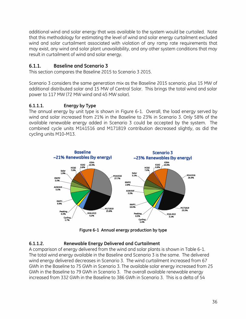
36

additional wind and solar energy that was available to the system would be curtailed. Note that this methodology for estimating the level of wind and solar energy curtailment excluded wind and solar curtailment associated with violation of any ramp rate requirements that may exist, any wind and solar plant unavailability, and any other system conditions that may result in curtailment of wind and solar energy.

6.1.1. Baseline and Scenario 3 This section compares the Baseline 2015 to Scenario 3 2015. Scenario 3 considers the same generation mix as the Baseline 2015 scenario, plus 15 MW of additional distributed solar and 15 MW of Central Solar. This brings the total wind and solar power to 117 MW (72 MW wind and 45 MW solar). 6.1.1.1. Energy by Type The annual energy by unit type is shown in Figure 6-1. Overall, the load energy served by wind and solar increased from 21% in the Baseline to 23% in Scenario 3. Only 58% of the available renewable energy added in Scenario 3 could be accepted by the system. The combined cycle units M141516 and M171819 contribution decreased slightly, as did the cycling units M10-M13.

Scenario 3~23% Renewables (by energy)

Baseline~21% Renewables (by energy)

HC&S7.6%

K1K20.8%

K3K410.9%

M14151627.7%

M17181925.8%

M10-M134.2%

Cycling1.7%

Peaking0.3%

KWP19.9%

AUWAHI5.5%

KWP23.5%

Solar1.9%

HC&S7.6%

K1K20.8%

K3K410.8%

M14151626.9%

M17181925.5%

M10-M133.1%

Cycling1.4%

Peaking0.5%

KWP110.0%

AUWAHI5.5%

KWP22.8%

Solar5.1%

Figure 6-1 Annual energy production by type

6.1.1.2. Renewable Energy Delivered and Curtailment A comparison of energy delivered from the wind and solar plants is shown in Table 6-1. The total wind energy available in the Baseline and Scenario 3 is the same. The delivered wind energy delivered decreases in Scenario 3. The wind curtailment increased from 67 GWh in the Baseline to 75 GWh in Scenario 3. The available solar energy increased from 25 GWh in the Baseline to 79 GWh in Scenario 3. The overall available renewable energy increased from 332 GWh in the Baseline to 386 GWh in Scenario 3. This is a delta of 54

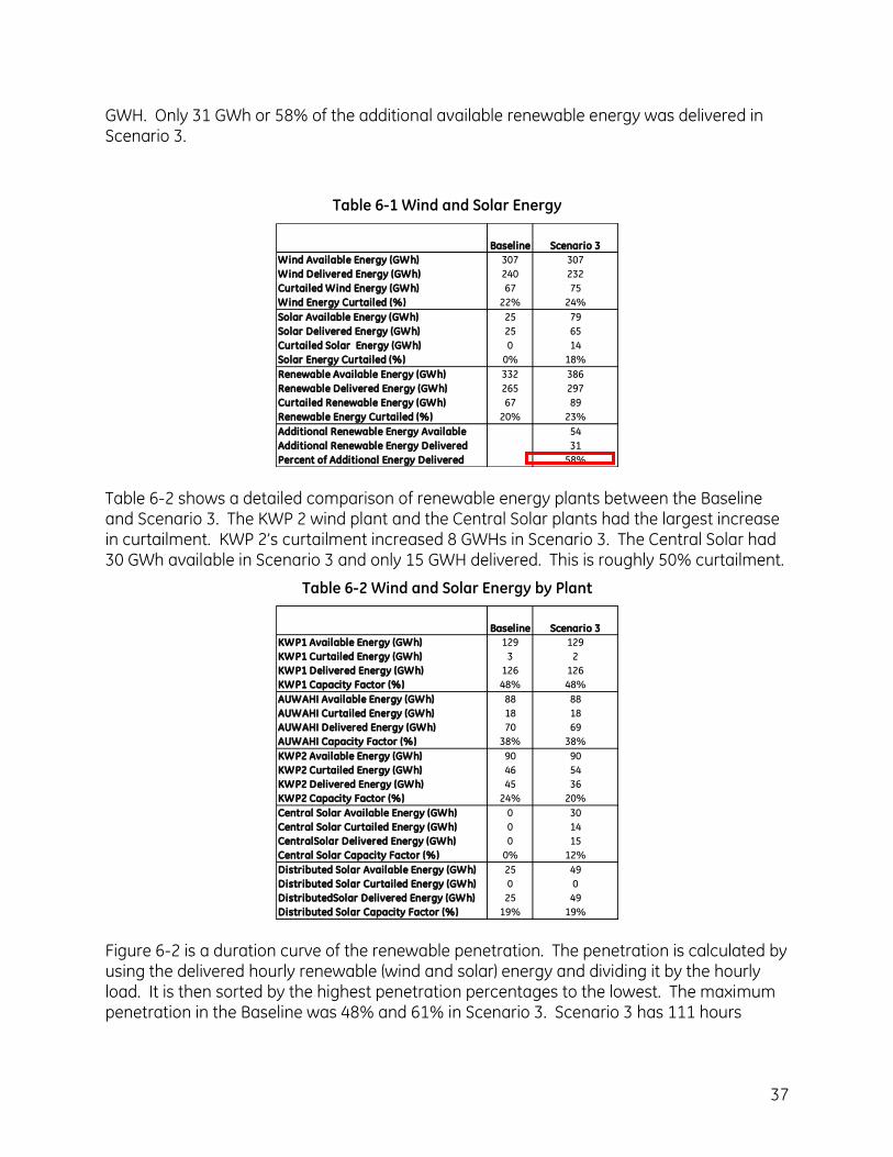
37

GWH. Only 31 GWh or 58% of the additional available renewable energy was delivered in Scenario 3.

Table 6-1 Wind and Solar Energy

Wind Available Energy (GWh) 307 307

Wind Delivered Energy (GWh) 240 232

Curtailed Wind Energy (GWh) 67 75

Wind Energy Curtailed (%) 22% 24%

Solar Available Energy (GWh) 25 79

Solar Delivered Energy (GWh) 25 65

Curtailed Solar Energy (GWh) 0 14

Solar Energy Curtailed (%) 0% 18%

Renewable Available Energy (GWh) 332 386

Renewable Delivered Energy (GWh) 265 297

Curtailed Renewable Energy (GWh) 67 89

Renewable Energy Curtailed (%) 20% 23%

Additional Renewable Energy Available 54

Additional Renewable Energy Delivered 31

Percent of Additional Energy Delivered 58%

Baseline Scenario 3

Table 6-2 shows a detailed comparison of renewable energy plants between the Baseline and Scenario 3. The KWP 2 wind plant and the Central Solar plants had the largest increase in curtailment. KWP 2’s curtailment increased 8 GWHs in Scenario 3. The Central Solar had 30 GWh available in Scenario 3 and only 15 GWH delivered. This is roughly 50% curtailment.

Table 6-2 Wind and Solar Energy by Plant

KWP1 Available Energy (GWh) 129 129

KWP1 Curtailed Energy (GWh) 3 2

KWP1 Delivered Energy (GWh) 126 126

KWP1 Capacity Factor (%) 48% 48%

AUWAHI Available Energy (GWh) 88 88

AUWAHI Curtailed Energy (GWh) 18 18

AUWAHI Delivered Energy (GWh) 70 69

AUWAHI Capacity Factor (%) 38% 38%

KWP2 Available Energy (GWh) 90 90

KWP2 Curtailed Energy (GWh) 46 54

KWP2 Delivered Energy (GWh) 45 36

KWP2 Capacity Factor (%) 24% 20%

Central Solar Available Energy (GWh) 0 30

Central Solar Curtailed Energy (GWh) 0 14

CentralSolar Delivered Energy (GWh) 0 15

Central Solar Capacity Factor (%) 0% 12%

Distributed Solar Available Energy (GWh) 25 49

Distributed Solar Curtailed Energy (GWh) 0 0

DistributedSolar Delivered Energy (GWh) 25 49

Distributed Solar Capacity Factor (%) 19% 19%

Scenario 3Baseline

Figure 6-2 is a duration curve of the renewable penetration. The penetration is calculated by using the delivered hourly renewable (wind and solar) energy and dividing it by the hourly load. It is then sorted by the highest penetration percentages to the lowest. The maximum penetration in the Baseline was 48% and 61% in Scenario 3. Scenario 3 has 111 hours

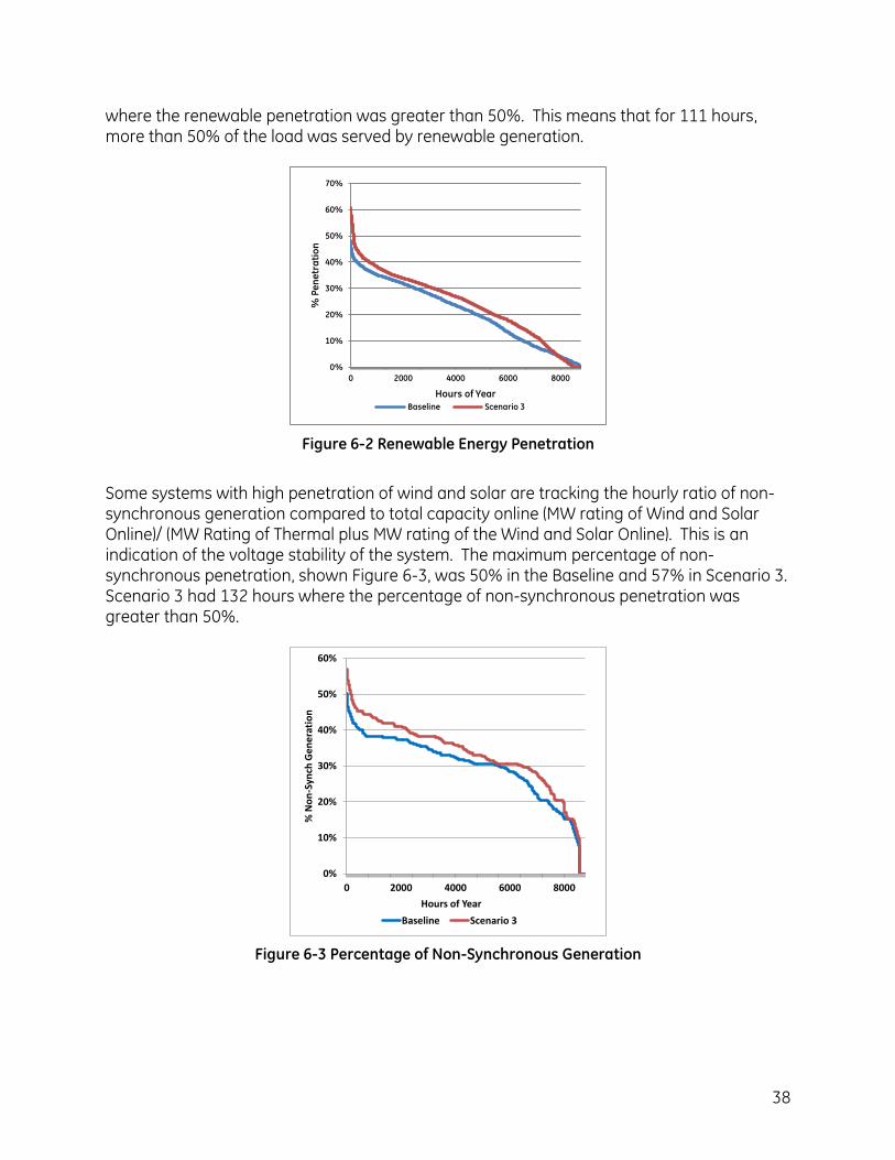
38

where the renewable penetration was greater than 50%. This means that for 111 hours, more than 50% of the load was served by renewable generation.

0%

10%

20%

30%

40%

50%

60%

70%

0 2000 4000 6000 8000

% P

en

etr

ati

on

Hours of Year

Baseline Scenario 3

Figure 6-2 Renewable Energy Penetration

Some systems with high penetration of wind and solar are tracking the hourly ratio of non-synchronous generation compared to total capacity online (MW rating of Wind and Solar Online)/ (MW Rating of Thermal plus MW rating of the Wind and Solar Online). This is an indication of the voltage stability of the system. The maximum percentage of non-synchronous penetration, shown Figure 6-3, was 50% in the Baseline and 57% in Scenario 3. Scenario 3 had 132 hours where the percentage of non-synchronous penetration was greater than 50%.

0%

10%

20%

30%

40%

50%

60%

0 2000 4000 6000 8000

% N

on

-Syn

ch G

en

era

tio

n

Hours of Year

Baseline Scenario 3

Figure 6-3 Percentage of Non-Synchronous Generation

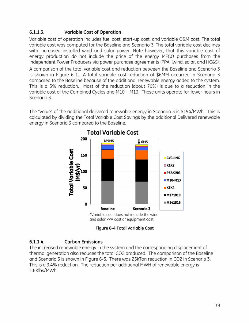
39

6.1.1.3. Variable Cost of Operation

Variable cost of operation includes fuel cost, start-up cost, and variable O&M cost. The total variable cost was computed for the Baseline and Scenario 3. The total variable cost declines with increased installed wind and solar power. Note however, that this variable cost of energy production do not include the price of the energy MECO purchases from the Independent Power Producers via power purchase agreements (PPA) (wind, solar, and HC&S).

A comparison of the total variable cost and reduction between the Baseline and Scenario 3 is shown in Figure 6-1. A total variable cost reduction of $6MM occurred in Scenario 3 compared to the Baseline because of the additional renewable energy added to the system. This is a 3% reduction. Most of the reduction (about 70%) is due to a reduction in the variable cost of the Combined Cycles and M10 – M13. These units operate for fewer hours in Scenario 3.

The “value” of the additional delivered renewable energy in Scenario 3 is $194/MWh. This is calculated by dividing the Total Variable Cost Savings by the additional Delivered renewable energy in Scenario 3 compared to the Baseline.

0

50

100

150

200

Baseline Scenario 3

To

tal

Va

ria

ble

Co

st(M

$/y

r)

CYCLING

K1K2

PEAKING

M10-M13

K3K4

M171819

M141516

6M$

Total Variable Cost

189M$

0

100

200

300

400

500

600

700

800

Wind Wind + PV(Avg. Forecast)

Wind + PV(Perfect Forecast)

To

tal

CO

2E

mis

sio

ns

(kT

on

s/y

r)

CYCLING

K1K2

PEAKING

M10-M13

K3K4

M171819

M141516

Figure 6-4 Total Variable Cost

6.1.1.4. Carbon Emissions The increased renewable energy in the system and the corresponding displacement of thermal generation also reduces the total CO2 produced. The comparison of the Baseline and Scenario 3 is shown in Figure 6-5. There was 25kTon reduction in CO2 in Scenario 3. This is a 3.4% reduction. The reduction per additional MWH of renewable energy is 1.6Klbs/MWh.

*Variable cost does not include the wind and solar PPA cost or equipment cost

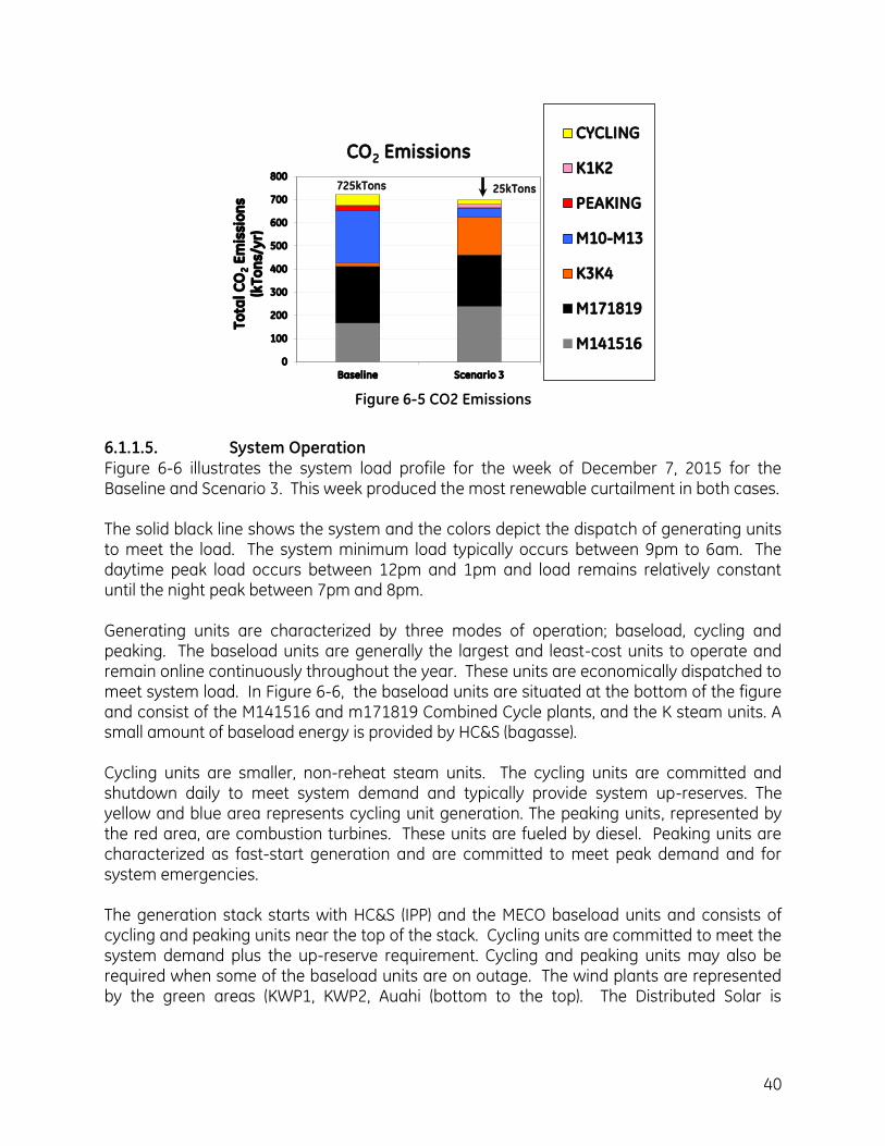
40

0

100

200

300

400

500

600

700

800

Baseline Scenario 3

To

tal

CO

2E

mis

sio

ns

(kT

on

s/y

r)

Solar

K1K2

PEAKING

M10-M13K3K4

M171819

M141516

25kTons

CO2 Emissions

725kTons

0

100

200

300

400

500

600

700

800



To

tal

CO

2E

mis

sio

ns

(kT

on

s/y

r)

CYCLING

K1K2

PEAKING

M10-M13

K3K4

M171819

M141516

Figure 6-5 CO2 Emissions

6.1.1.5. System Operation Figure 6-6 illustrates the system load profile for the week of December 7, 2015 for the Baseline and Scenario 3. This week produced the most renewable curtailment in both cases. The solid black line shows the system and the colors depict the dispatch of generating units to meet the load. The system minimum load typically occurs between 9pm to 6am. The daytime peak load occurs between 12pm and 1pm and load remains relatively constant until the night peak between 7pm and 8pm. Generating units are characterized by three modes of operation; baseload, cycling and peaking. The baseload units are generally the largest and least-cost units to operate and remain online continuously throughout the year. These units are economically dispatched to meet system load. In Figure 6-6, the baseload units are situated at the bottom of the figure and consist of the M141516 and m171819 Combined Cycle plants, and the K steam units. A small amount of baseload energy is provided by HC&S (bagasse). Cycling units are smaller, non-reheat steam units. The cycling units are committed and shutdown daily to meet system demand and typically provide system up-reserves. The yellow and blue area represents cycling unit generation. The peaking units, represented by the red area, are combustion turbines. These units are fueled by diesel. Peaking units are characterized as fast-start generation and are committed to meet peak demand and for system emergencies. The generation stack starts with HC&S (IPP) and the MECO baseload units and consists of cycling and peaking units near the top of the stack. Cycling units are committed to meet the system demand plus the up-reserve requirement. Cycling and peaking units may also be required when some of the baseload units are on outage. The wind plants are represented by the green areas (KWP1, KWP2, Auahi (bottom to the top). The Distributed Solar is

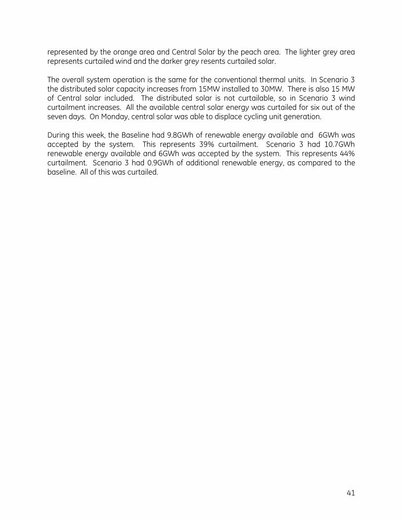
41

represented by the orange area and Central Solar by the peach area. The lighter grey area represents curtailed wind and the darker grey resents curtailed solar. The overall system operation is the same for the conventional thermal units. In Scenario 3 the distributed solar capacity increases from 15MW installed to 30MW. There is also 15 MW of Central solar included. The distributed solar is not curtailable, so in Scenario 3 wind curtailment increases. All the available central solar energy was curtailed for six out of the seven days. On Monday, central solar was able to displace cycling unit generation. During this week, the Baseline had 9.8GWh of renewable energy available and 6GWh was accepted by the system. This represents 39% curtailment. Scenario 3 had 10.7GWh renewable energy available and 6GWh was accepted by the system. This represents 44% curtailment. Scenario 3 had 0.9GWh of additional renewable energy, as compared to the baseline. All of this was curtailed.

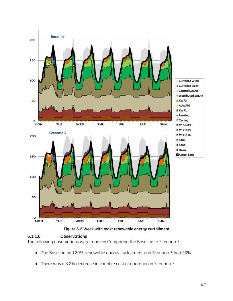
42

0

50

100

150

200

MON TUE WED THU FRI SAT SUN

0

50

100

150

200


Scenario 3

Baseline

0

50

100

150

200


Curtailed Wind

Curtailed Solar

Central SOLAR

Distributed SOLAR

KWP2

AUWAHI

KWP1

Peaking

Cycling

M10-M13

M171819

M141516

K1K2

K3K4

HC&S

Actual Load

Figure 6-6 Week with most renewable energy curtailment

6.1.1.6. Observations The following observations were made in Comparing the Baseline to Scenario 3:

The Baseline had 20% renewable energy curtailment and Scenario 3 had 23%.

There was a 3.2% decrease in variable cost of operation in Scenario 3

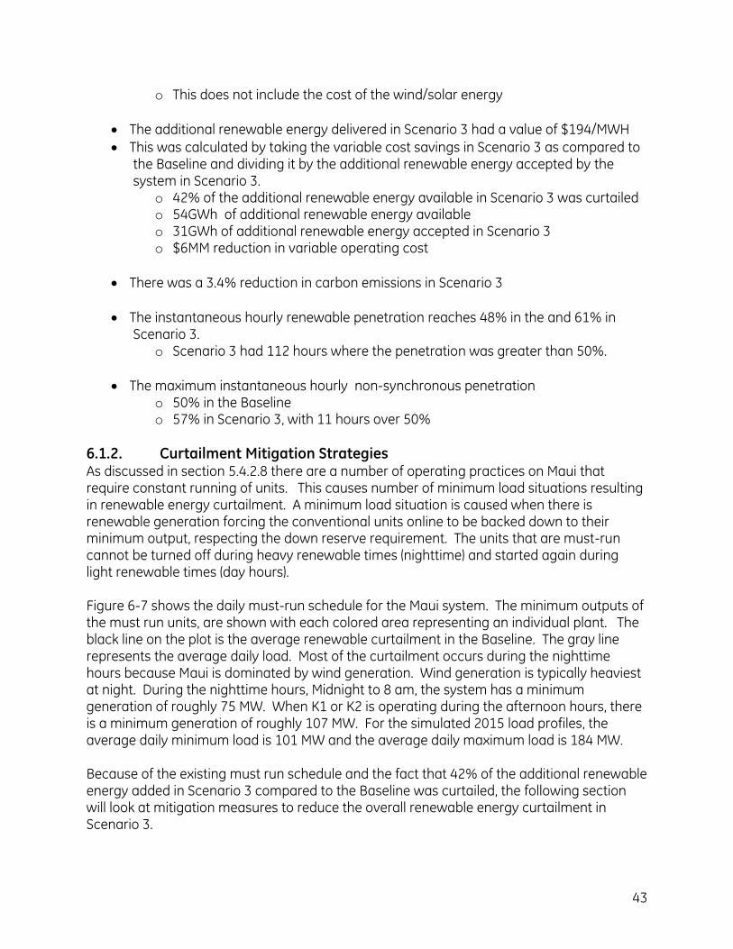
43

o This does not include the cost of the wind/solar energy

The additional renewable energy delivered in Scenario 3 had a value of $194/MWH

This was calculated by taking the variable cost savings in Scenario 3 as compared to the Baseline and dividing it by the additional renewable energy accepted by the system in Scenario 3.

o 42% of the additional renewable energy available in Scenario 3 was curtailed o 54GWh of additional renewable energy available o 31GWh of additional renewable energy accepted in Scenario 3 o $6MM reduction in variable operating cost

There was a 3.4% reduction in carbon emissions in Scenario 3

The instantaneous hourly renewable penetration reaches 48% in the and 61% in Scenario 3.

o Scenario 3 had 112 hours where the penetration was greater than 50%.

The maximum instantaneous hourly non-synchronous penetration o 50% in the Baseline o 57% in Scenario 3, with 11 hours over 50%

6.1.2. Curtailment Mitigation Strategies As discussed in section 5.4.2.8 there are a number of operating practices on Maui that require constant running of units. This causes number of minimum load situations resulting in renewable energy curtailment. A minimum load situation is caused when there is renewable generation forcing the conventional units online to be backed down to their minimum output, respecting the down reserve requirement. The units that are must-run cannot be turned off during heavy renewable times (nighttime) and started again during light renewable times (day hours). Figure 6-7 shows the daily must-run schedule for the Maui system. The minimum outputs of the must run units, are shown with each colored area representing an individual plant. The black line on the plot is the average renewable curtailment in the Baseline. The gray line represents the average daily load. Most of the curtailment occurs during the nighttime hours because Maui is dominated by wind generation. Wind generation is typically heaviest at night. During the nighttime hours, Midnight to 8 am, the system has a minimum generation of roughly 75 MW. When K1 or K2 is operating during the afternoon hours, there is a minimum generation of roughly 107 MW. For the simulated 2015 load profiles, the average daily minimum load is 101 MW and the average daily maximum load is 184 MW. Because of the existing must run schedule and the fact that 42% of the additional renewable energy added in Scenario 3 compared to the Baseline was curtailed, the following section will look at mitigation measures to reduce the overall renewable energy curtailment in Scenario 3.

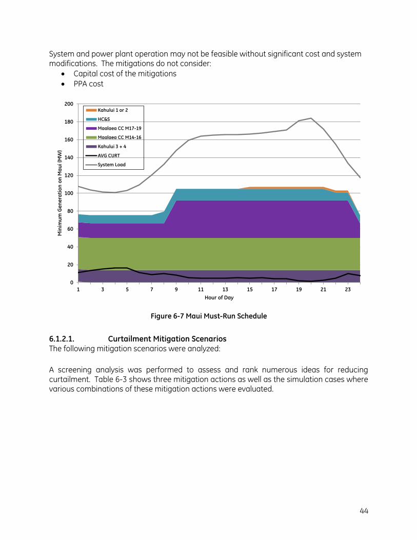
44

System and power plant operation may not be feasible without significant cost and system modifications. The mitigations do not consider:

Capital cost of the mitigations

PPA cost

0

20

40

60

80

100

120

140

160

180

200

1 3 5 7 9 11 13 15 17 19 21 23

Min

imu

m G

en

era

tio

n o

n M

au

i (M

W)

Hour of Day

Kahului 1 or 2

HC&S

Maalaea CC M17-19

Maalaea CC M14-16

Kahului 3 + 4

AVG CURT

System Load

Figure 6-7 Maui Must-Run Schedule

6.1.2.1. Curtailment Mitigation Scenarios The following mitigation scenarios were analyzed:

A screening analysis was performed to assess and rank numerous ideas for reducing curtailment. Table 6-3 shows three mitigation actions as well as the simulation cases where various combinations of these mitigation actions were evaluated.

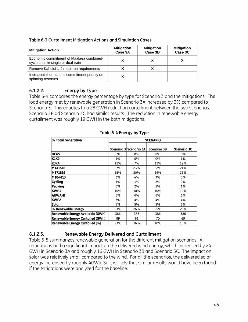
45

Table 6-3 Curtailment Mitigation Actions and Simulation Cases

Mitigation Action Mitigation Case 3A

Mitigation Case 3B

Mitigation Case 3C

Economic commitment of Maalaea combined-cycle units in single or dual train

X X X

Remove Kahului 1-4 must-run requirements X X

Increased thermal unit commitment priority on spinning reserves

X

6.1.2.2. Energy by Type Table 6-4 compares the energy percentage by type for Scenario 3 and the mitigations. The load energy met by renewable generation in Scenario 3A increased by 3% compared to Scenario 3. This equates to a 28 GWH reduction curtailment between the two scenarios. Scenario 3B ad Scenario 3C had similar results. The reduction in renewable energy curtailment was roughly 19 GWH in the both mitigations.

Table 6-4 Energy by Type

% Total Generation

Scenario 3 Scenario 3A Scenario 3B Scenario 3C

HC&S 8% 8% 8% 8%

K1K2 1% 0% 0% 1%

K3K4 11% 7% 11% 12%

M141516 27% 23% 22% 21%

M171819 25% 30% 29% 28%

M10-M13 3% 4% 3% 3%

Cycling 1% 1% 2% 2%

Peaking 0% 2% 1% 1%

KWP1 10% 10% 10% 10%

AUWAHI 5% 6% 6% 6%

KWP2 3% 4% 4% 4%

Solar 5% 5% 5% 5%

% Renewable Energy 23% 26% 25% 25%

Renewable Energy Available (GWh) 386 386 386 386

Renewable Energy Curtailed (GWh) 89 61 70 69

Renewable Energy Curtailed (%) 23% 16% 18% 18%

SCENARIO

6.1.2.3. Renewable Energy Delivered and Curtailment Table 6-5 summarizes renewable generation for the different mitigation scenarios. All mitigations had a significant impact on the delivered wind energy, which increased by 24 GWH in Scenario 3A and roughly 16 GWH in Scenario 3B and Scenario 3C. The impact on solar was relatively small compared to the wind. For all the scenarios, the delivered solar energy increased by roughly 4GWh. So it is likely that similar results would have been found if the Mitigations were analyzed for the baseline.

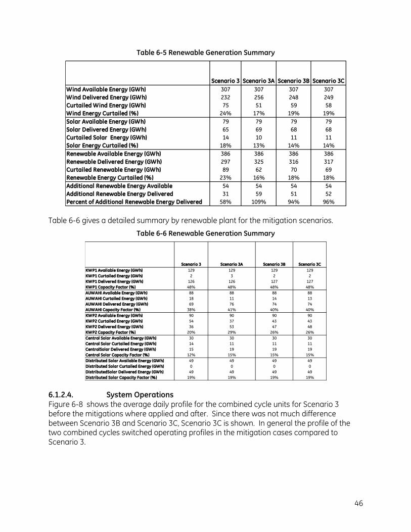
46

Table 6-5 Renewable Generation Summary


Wind Available Energy (GWh) 307 307 307 307

Wind Delivered Energy (GWh) 232 256 248 249

Curtailed Wind Energy (GWh) 75 51 59 58

Wind Energy Curtailed (%) 24% 17% 19% 19%

Solar Available Energy (GWh) 79 79 79 79

Solar Delivered Energy (GWh) 65 69 68 68

Curtailed Solar Energy (GWh) 14 10 11 11

Solar Energy Curtailed (%) 18% 13% 14% 14%

Renewable Available Energy (GWh) 386 386 386 386

Renewable Delivered Energy (GWh) 297 325 316 317

Curtailed Renewable Energy (GWh) 89 62 70 69

Renewable Energy Curtailed (%) 23% 16% 18% 18%

Additional Renewable Energy Available 54 54 54 54

Additional Renewable Energy Delivered 31 59 51 52

Percent of Additional Renewable Energy Delivered 58% 109% 94% 96% Table 6-6 gives a detailed summary by renewable plant for the mitigation scenarios.

Table 6-6 Renewable Generation Summary


KWP1 Available Energy (GWh) 129 129 129 129

KWP1 Curtailed Energy (GWh) 2 3 2 2

KWP1 Delivered Energy (GWh) 126 126 127 127

KWP1 Capacity Factor (%) 48% 48% 48% 48%

AUWAHI Available Energy (GWh) 88 88 88 88

AUWAHI Curtailed Energy (GWh) 18 11 14 13

AUWAHI Delivered Energy (GWh) 69 76 74 74

AUWAHI Capacity Factor (%) 38% 41% 40% 40%

KWP2 Available Energy (GWh) 90 90 90 90

KWP2 Curtailed Energy (GWh) 54 37 43 43

KWP2 Delivered Energy (GWh) 36 53 47 48

KWP2 Capacity Factor (%) 20% 29% 26% 26%

Central Solar Available Energy (GWh) 30 30 30 30

Central Solar Curtailed Energy (GWh) 14 11 11 11

CentralSolar Delivered Energy (GWh) 15 19 19 19

Central Solar Capacity Factor (%) 12% 15% 15% 15%

Distributed Solar Available Energy (GWh) 49 49 49 49

Distributed Solar Curtailed Energy (GWh) 0 0 0 0

DistributedSolar Delivered Energy (GWh) 49 49 49 49

Distributed Solar Capacity Factor (%) 19% 19% 19% 19% 6.1.2.4. System Operations Figure 6-8 shows the average daily profile for the combined cycle units for Scenario 3 before the mitigations where applied and after. Since there was not much difference between Scenario 3B and Scenario 3C, Scenario 3C is shown. In general the profile of the two combined cycles switched operating profiles in the mitigation cases compared to Scenario 3.

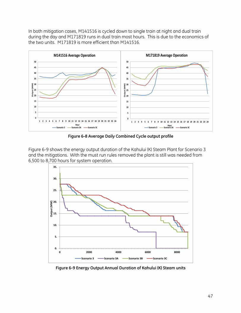
47

In both mitigation cases, M141516 is cycled down to single train at night and dual train during the day and M171819 runs in dual train most hours. This is due to the economics of the two units. M171819 is more efficient than M141516.

0

5

10

15

20

25

30

35

40

45

50

1 2 3 4 5 6 7 8 9 10 11 12 13 14 15 16 17 18 19 20 21 22 23 24

Ou

tpu

t (M

W)

Hour

M141516 Average Operation

Scenario 3 Scenario 3A Scenario 3C

0

5

10

15

20

25

30

35

40

45

50

1 2 3 4 5 6 7 8 9 10 11 12 13 14 15 16 17 18 19 20 21 22 23 24O

utp

ut

(MW

)Hour

M171819 Average Operation

Scenario 3 Scenario 3A Scenario 3C

Figure 6-8 Average Daily Combined Cycle output profile

Figure 6-9 shows the energy output duration of the Kahului (K) Steam Plant for Scenario 3 and the mitigations. With the must run rules removed the plant is still was needed from 6,500 to 8,700 hours for system operation.

0.

5.

10.

15.

20.

25.

30.

35.

0 2000 4000 6000 8000

Ou

tpu

t (M

W)


Figure 6-9 Energy Output Annual Duration of Kahului (K) Steam units

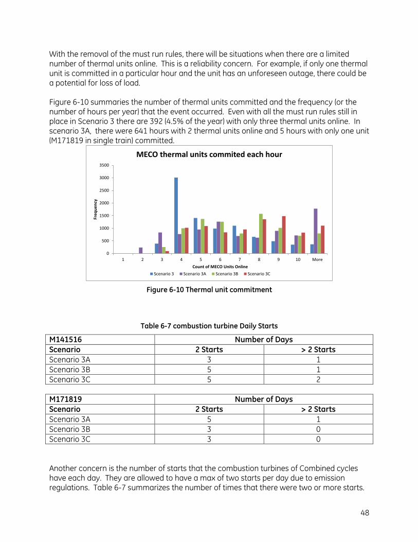
48

With the removal of the must run rules, there will be situations when there are a limited number of thermal units online. This is a reliability concern. For example, if only one thermal unit is committed in a particular hour and the unit has an unforeseen outage, there could be a potential for loss of load. Figure 6-10 summaries the number of thermal units committed and the frequency (or the number of hours per year) that the event occurred. Even with all the must run rules still in place in Scenario 3 there are 392 (4.5% of the year) with only three thermal units online. In scenario 3A, there were 641 hours with 2 thermal units online and 5 hours with only one unit (M171819 in single train) committed.

0

500

1000

1500

2000

2500

3000

3500

1 2 3 4 5 6 7 8 9 10 More

Fre

qu

en

cy

Count of MECO Units Online

MECO thermal units commited each hour


Figure 6-10 Thermal unit commitment

Table 6-7 combustion turbine Daily Starts

M141516 Number of Days

Scenario 2 Starts > 2 Starts

Scenario 3A 3 1

Scenario 3B 5 1

Scenario 3C 5 2

M171819 Number of Days

Scenario 2 Starts > 2 Starts

Scenario 3A 5 1

Scenario 3B 3 0

Scenario 3C 3 0

Another concern is the number of starts that the combustion turbines of Combined cycles have each day. They are allowed to have a max of two starts per day due to emission regulations. Table 6-7 summarizes the number of times that there were two or more starts.

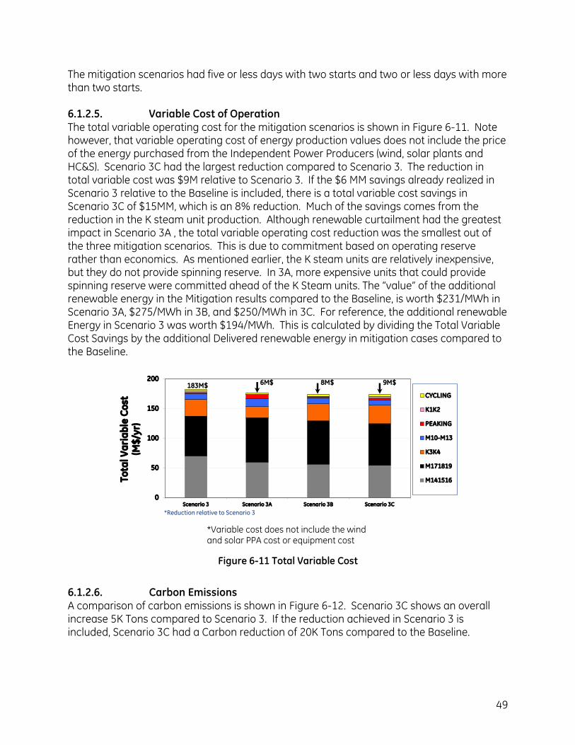
49

The mitigation scenarios had five or less days with two starts and two or less days with more than two starts. 6.1.2.5. Variable Cost of Operation The total variable operating cost for the mitigation scenarios is shown in Figure 6-11. Note however, that variable operating cost of energy production values does not include the price of the energy purchased from the Independent Power Producers (wind, solar plants and HC&S). Scenario 3C had the largest reduction compared to Scenario 3. The reduction in total variable cost was $9M relative to Scenario 3. If the $6 MM savings already realized in Scenario 3 relative to the Baseline is included, there is a total variable cost savings in Scenario 3C of $15MM, which is an 8% reduction. Much of the savings comes from the reduction in the K steam unit production. Although renewable curtailment had the greatest impact in Scenario 3A , the total variable operating cost reduction was the smallest out of the three mitigation scenarios. This is due to commitment based on operating reserve rather than economics. As mentioned earlier, the K steam units are relatively inexpensive, but they do not provide spinning reserve. In 3A, more expensive units that could provide spinning reserve were committed ahead of the K Steam units. The “value” of the additional renewable energy in the Mitigation results compared to the Baseline, is worth $231/MWh in Scenario 3A, $275/MWh in 3B, and $250/MWh in 3C. For reference, the additional renewable Energy in Scenario 3 was worth $194/MWh. This is calculated by dividing the Total Variable Cost Savings by the additional Delivered renewable energy in mitigation cases compared to the Baseline.

0

50

100

150

200


To

tal

Va

ria

ble

Co

st(M

$/y

r)

CYCLING

K1K2

PEAKING

M10-M13

K3K4

M171819

M141516

6M$ 8M$ 9M$183M$

*Reduction relative to Scenario 3

0

100

200

300

400

500

600

700

800



To

tal

CO

2E

mis

sio

ns

(kT

on

s/y

r)

CYCLING

K1K2

PEAKING

M10-M13

K3K4

M171819

M141516

Figure 6-11 Total Variable Cost

6.1.2.6. Carbon Emissions A comparison of carbon emissions is shown in Figure 6-12. Scenario 3C shows an overall increase 5K Tons compared to Scenario 3. If the reduction achieved in Scenario 3 is included, Scenario 3C had a Carbon reduction of 20K Tons compared to the Baseline.


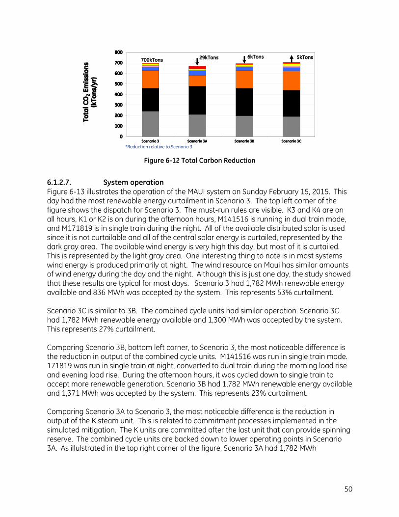
50

0

100

200

300

400

500

600

700

800


To

tal

CO

2E

mis

sio

ns

(kT

on

s/y

r)

PEAKING

CYCLING

K1K2

M10-M13

K3K4

M171819

M141516

*Reduction relative to Scenario 3

5kTons6kTons29kTons700kTons

Figure 6-12 Total Carbon Reduction

6.1.2.7. System operation Figure 6-13 illustrates the operation of the MAUI system on Sunday February 15, 2015. This day had the most renewable energy curtailment in Scenario 3. The top left corner of the figure shows the dispatch for Scenario 3. The must-run rules are visible. K3 and K4 are on all hours, K1 or K2 is on during the afternoon hours, M141516 is running in dual train mode, and M171819 is in single train during the night. All of the available distributed solar is used since it is not curtailable and all of the central solar energy is curtailed, represented by the dark gray area. The available wind energy is very high this day, but most of it is curtailed. This is represented by the light gray area. One interesting thing to note is in most systems wind energy is produced primarily at night. The wind resource on Maui has similar amounts of wind energy during the day and the night. Although this is just one day, the study showed that these results are typical for most days. Scenario 3 had 1,782 MWh renewable energy available and 836 MWh was accepted by the system. This represents 53% curtailment. Scenario 3C is similar to 3B. The combined cycle units had similar operation. Scenario 3C had 1,782 MWh renewable energy available and 1,300 MWh was accepted by the system. This represents 27% curtailment. Comparing Scenario 3B, bottom left corner, to Scenario 3, the most noticeable difference is the reduction in output of the combined cycle units. M141516 was run in single train mode. 171819 was run in single train at night, converted to dual train during the morning load rise and evening load rise. During the afternoon hours, it was cycled down to single train to accept more renewable generation. Scenario 3B had 1,782 MWh renewable energy available and 1,371 MWh was accepted by the system. This represents 23% curtailment. Comparing Scenario 3A to Scenario 3, the most noticeable difference is the reduction in output of the K steam unit. This is related to commitment processes implemented in the simulated mitigation. The K units are committed after the last unit that can provide spinning reserve. The combined cycle units are backed down to lower operating points in Scenario 3A. As illulstrated in the top right corner of the figure, Scenario 3A had 1,782 MWh

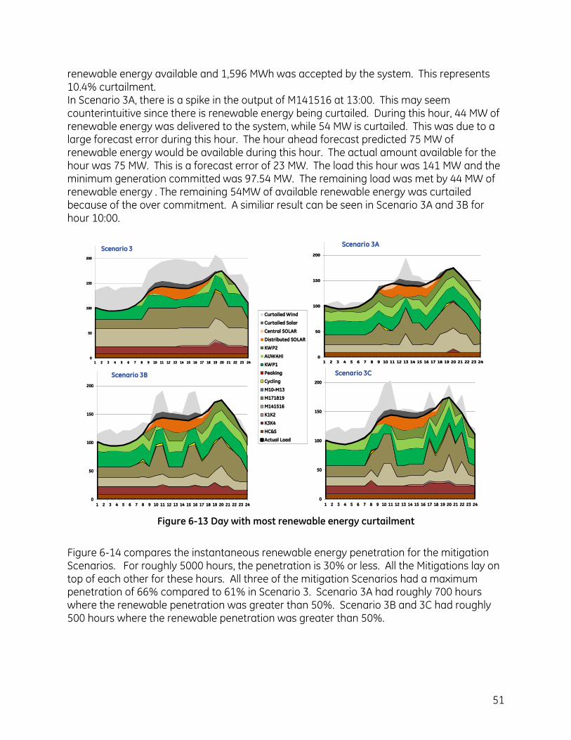
51

renewable energy available and 1,596 MWh was accepted by the system. This represents 10.4% curtailment. In Scenario 3A, there is a spike in the output of M141516 at 13:00. This may seem counterintuitive since there is renewable energy being curtailed. During this hour, 44 MW of renewable energy was delivered to the system, while 54 MW is curtailed. This was due to a large forecast error during this hour. The hour ahead forecast predicted 75 MW of renewable energy would be available during this hour. The actual amount available for the hour was 75 MW. This is a forecast error of 23 MW. The load this hour was 141 MW and the minimum generation committed was 97.54 MW. The remaining load was met by 44 MW of renewable energy . The remaining 54MW of available renewable energy was curtailed because of the over commitment. A similiar result can be seen in Scenario 3A and 3B for hour 10:00.

0

50

100

150

200

1 2 3 4 5 6 7 8 9 10 11 12 13 14 15 16 17 18 19 20 21 22 23 24

Scenario 3

0

50

100

150

200

1 2 3 4 5 6 7 8 9 10 11 12 13 14 15 16 17 18 19 20 21 22 23 24

Scenario 3A

0

50

100

150

200

1 2 3 4 5 6 7 8 9 10 11 12 13 14 15 16 17 18 19 20 21 22 23 24

Scenario 3B

0

50

100

150

200

1 2 3 4 5 6 7 8 9 10 11 12 13 14 15 16 17 18 19 20 21 22 23 24

Scenario 3C

0

50

100

150

200


Curtailed Wind

Curtailed Solar

Central SOLAR

Distributed SOLAR

KWP2

AUWAHI

KWP1

Peaking

Cycling

M10-M13

M171819

M141516

K1K2

K3K4

HC&S

Actual Load

Figure 6-13 Day with most renewable energy curtailment

Figure 6-14 compares the instantaneous renewable energy penetration for the mitigation Scenarios. For roughly 5000 hours, the penetration is 30% or less. All the Mitigations lay on top of each other for these hours. All three of the mitigation Scenarios had a maximum penetration of 66% compared to 61% in Scenario 3. Scenario 3A had roughly 700 hours where the renewable penetration was greater than 50%. Scenario 3B and 3C had roughly 500 hours where the renewable penetration was greater than 50%.

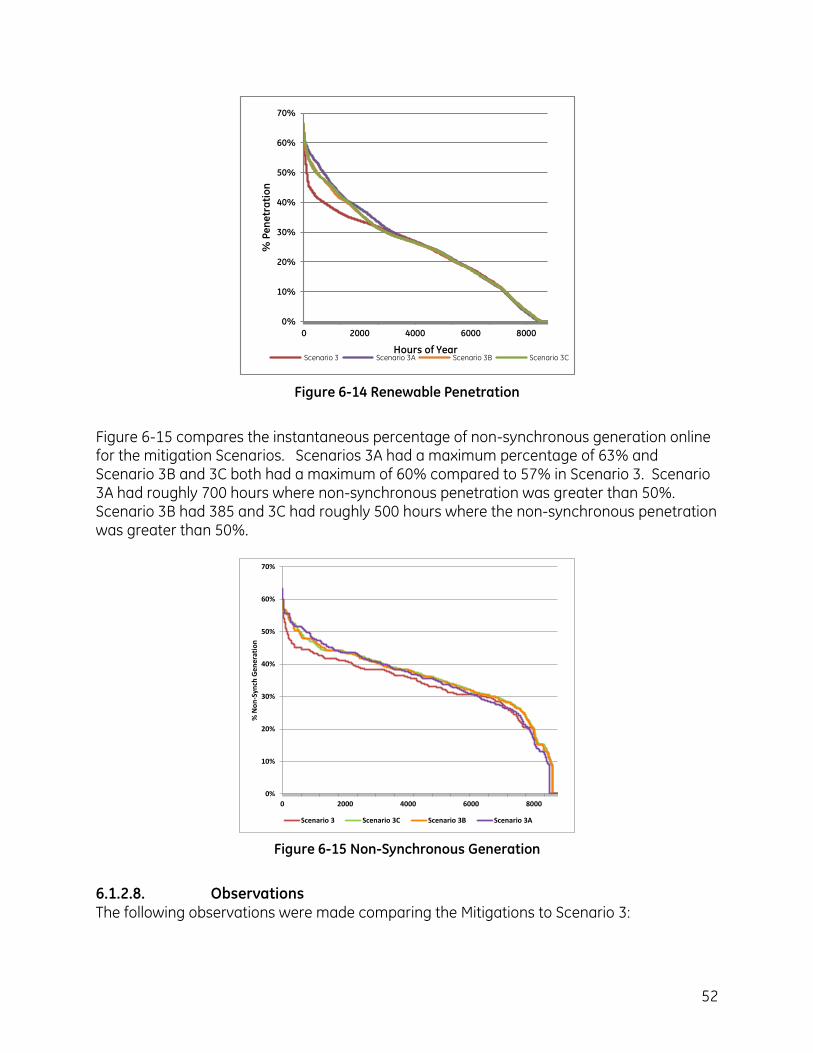
52

0%

10%

20%

30%

40%

50%

60%

70%

0 2000 4000 6000 8000

% P

en

etr

ati

on

Hours of YearScenario 3 Scenario 3A Scenario 3B Scenario 3C

Figure 6-14 Renewable Penetration

Figure 6-15 compares the instantaneous percentage of non-synchronous generation online for the mitigation Scenarios. Scenarios 3A had a maximum percentage of 63% and Scenario 3B and 3C both had a maximum of 60% compared to 57% in Scenario 3. Scenario 3A had roughly 700 hours where non-synchronous penetration was greater than 50%. Scenario 3B had 385 and 3C had roughly 500 hours where the non-synchronous penetration was greater than 50%.

0%

10%

20%

30%

40%

50%

60%

70%

0 2000 4000 6000 8000

% N

on

-Syn

ch G

en

era

tio

n

Scenario 3 Scenario 3C Scenario 3B Scenario 3A

Figure 6-15 Non-Synchronous Generation

6.1.2.8. Observations The following observations were made comparing the Mitigations to Scenario 3:

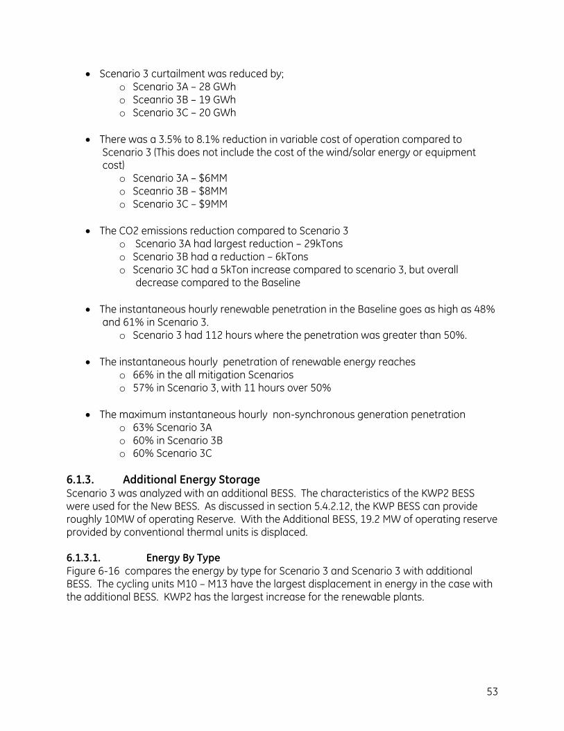
53

Scenario 3 curtailment was reduced by; o Scenario 3A – 28 GWh o Sceanrio 3B – 19 GWh o Scenario 3C – 20 GWh

There was a 3.5% to 8.1% reduction in variable cost of operation compared to Scenario 3 (This does not include the cost of the wind/solar energy or equipment cost)

o Scenario 3A – $6MM o Sceanrio 3B – $8MM o Scenario 3C – $9MM

The CO2 emissions reduction compared to Scenario 3 o Scenario 3A had largest reduction – 29kTons o Scenario 3B had a reduction – 6kTons o Scenario 3C had a 5kTon increase compared to scenario 3, but overall

decrease compared to the Baseline

The instantaneous hourly renewable penetration in the Baseline goes as high as 48% and 61% in Scenario 3.

o Scenario 3 had 112 hours where the penetration was greater than 50%.

The instantaneous hourly penetration of renewable energy reaches o 66% in the all mitigation Scenarios o 57% in Scenario 3, with 11 hours over 50%

The maximum instantaneous hourly non-synchronous generation penetration o 63% Scenario 3A o 60% in Scenario 3B o 60% Scenario 3C

6.1.3. Additional Energy Storage Scenario 3 was analyzed with an additional BESS. The characteristics of the KWP2 BESS were used for the New BESS. As discussed in section 5.4.2.12, the KWP BESS can provide roughly 10MW of operating Reserve. With the Additional BESS, 19.2 MW of operating reserve provided by conventional thermal units is displaced. 6.1.3.1. Energy By Type Figure 6-16 compares the energy by type for Scenario 3 and Scenario 3 with additional BESS. The cycling units M10 – M13 have the largest displacement in energy in the case with the additional BESS. KWP2 has the largest increase for the renewable plants.

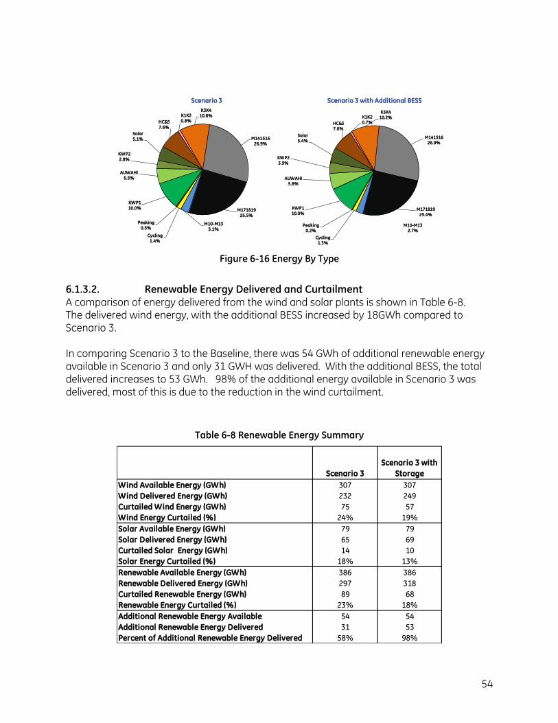
54

HC&S7.6%

K1K20.8%

K3K410.8%

M14151626.9%

M17181925.5%

M10-M133.1%

Cycling1.4%

Peaking0.5%

KWP110.0%

AUWAHI5.5%

KWP22.8%

Solar5.1%

HC&S7.6%

K1K20.7%

K3K410.2%

M14151626.9%

M17181925.4%

M10-M132.7%

Cycling1.3%

Peaking0.2%

KWP110.0%

AUWAHI5.8%

KWP23.9%

Solar5.4%

Scenario 3 Scenario 3 with Additional BESS

Figure 6-16 Energy By Type

6.1.3.2. Renewable Energy Delivered and Curtailment A comparison of energy delivered from the wind and solar plants is shown in Table 6-8. The delivered wind energy, with the additional BESS increased by 18GWh compared to Scenario 3. In comparing Scenario 3 to the Baseline, there was 54 GWh of additional renewable energy available in Scenario 3 and only 31 GWH was delivered. With the additional BESS, the total delivered increases to 53 GWh. 98% of the additional energy available in Scenario 3 was delivered, most of this is due to the reduction in the wind curtailment.

Table 6-8 Renewable Energy Summary

Scenario 3

Scenario 3 with

Storage

Wind Available Energy (GWh) 307 307

Wind Delivered Energy (GWh) 232 249

Curtailed Wind Energy (GWh) 75 57

Wind Energy Curtailed (%) 24% 19%

Solar Available Energy (GWh) 79 79

Solar Delivered Energy (GWh) 65 69

Curtailed Solar Energy (GWh) 14 10

Solar Energy Curtailed (%) 18% 13%

Renewable Available Energy (GWh) 386 386

Renewable Delivered Energy (GWh) 297 318

Curtailed Renewable Energy (GWh) 89 68

Renewable Energy Curtailed (%) 23% 18%

Additional Renewable Energy Available 54 54

Additional Renewable Energy Delivered 31 53

Percent of Additional Renewable Energy Delivered 58% 98%

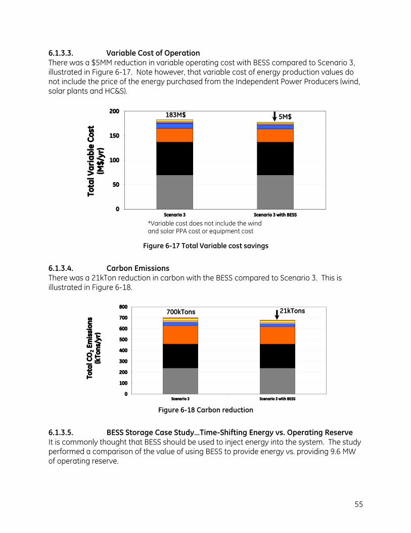
55

6.1.3.3. Variable Cost of Operation There was a $5MM reduction in variable operating cost with BESS compared to Scenario 3, illustrated in Figure 6-17. Note however, that variable cost of energy production values do not include the price of the energy purchased from the Independent Power Producers (wind, solar plants and HC&S).

0

50

100

150

200

Scenario 3 Scenario 3 with BESS

To

tal

Va

ria

ble

Co

st(M

$/y

r)

CYCLING

K1K2

PEAKING

M10-M13

K3K4

M171819

M141516

5M$183M$

Figure 6-17 Total Variable cost savings

6.1.3.4. Carbon Emissions There was a 21kTon reduction in carbon with the BESS compared to Scenario 3. This is illustrated in Figure 6-18.

0

100

200

300

400

500

600

700

800

Scenario 3 Scenario 3 with BESS

To

tal

CO

2E

mis

sio

ns

(kT

on

s/y

r)

PEAKING

CYCLING

K1K2

M10-M13

K3K4

M171819

M141516

21kTons700kTons

Figure 6-18 Carbon reduction

6.1.3.5. BESS Storage Case Study…Time-Shifting Energy vs. Operating Reserve It is commonly thought that BESS should be used to inject energy into the system. The study performed a comparison of the value of using BESS to provide energy vs. providing 9.6 MW of operating reserve.


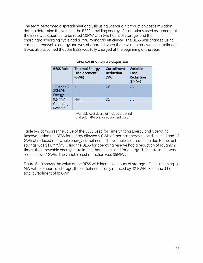
56

The team performed a spreadsheet analysis using Scenario 3 production cost simulation data to determine the value of the BESS providing energy. Assumptions used assumed that the BESS was assumed to be rated 10MW with two hours of storage, and the charging/discharging cycle had a 75% round trip efficiency. The BESS was charged using curtailed renewable energy and was discharged when there was no renewable curtailment. It was also assumed that the BESS was fully charged at the beginning of the year.

Table 6-9 BESS value comparison

BESS Role Thermal Energy Displacement (GWh)

Curtailment Reduction (GWh)

Variable Cost Reduction ($M/yr)

Time-Shift 20MWh Energy

9 12 1.8

9.6 MW Operating Reserve

N/A 21 5.0

Table 6-9 compares the value of the BESS used for Time Shifting Energy and Operating Reserve. Using the BESS for energy allowed 9 GWh of thermal energy to be displaced and 12 GWh of reduced renewable energy curtailment. The variable cost reduction due to the fuel savings was $1.8MM/yr. Using the BESS for operating reserve had a reduction of roughly 2 times the renewable energy curtailment, than being used for energy. The curtailment was reduced by 21GWh. The variable cost reduction was $5MM/yr. Figure 6-19 shows the value of the BESS with increased hours of storage. Even assuming 10 MW with 50 hours of storage, the curtailment is only reduced by 32 GWH. Scenario 3 had a total curtailment of 89GWh.


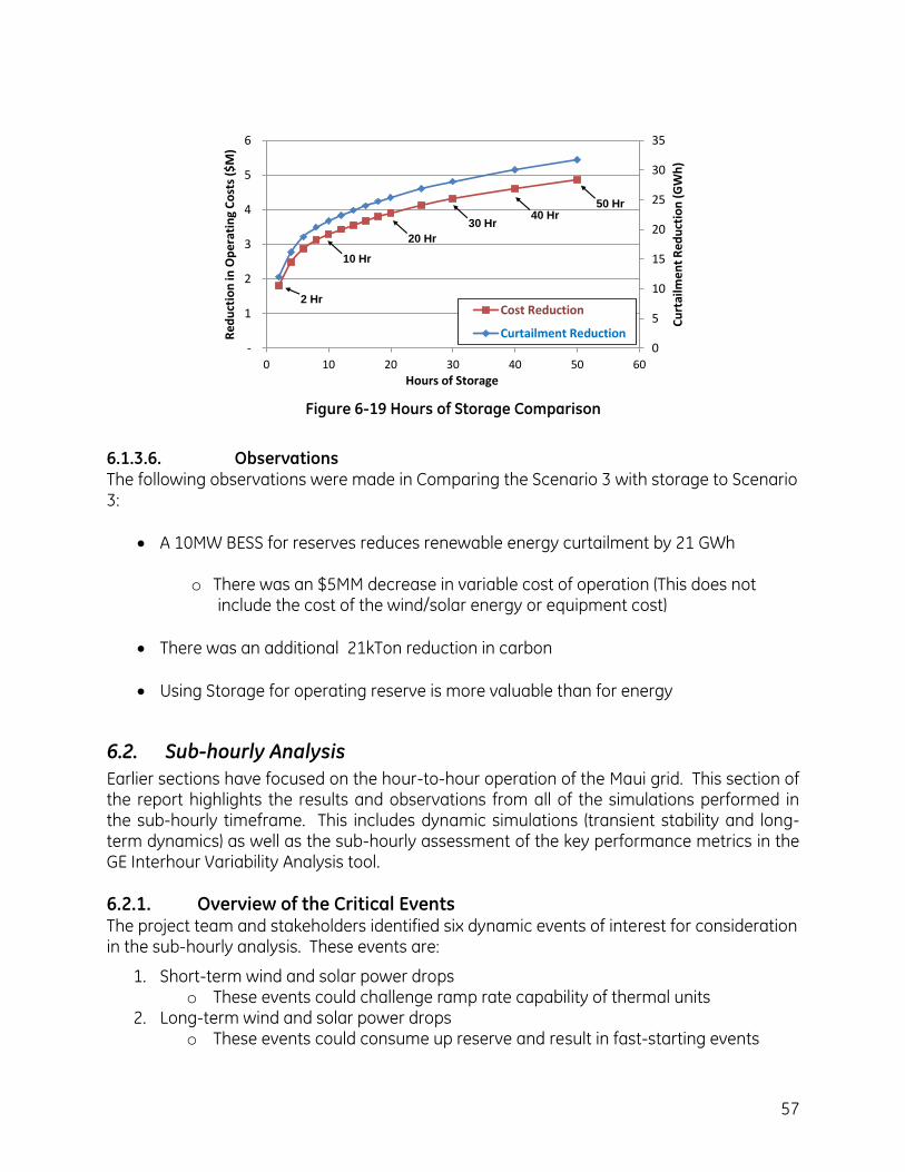
57

0

5

10

15

20

25

30

35

-

1

2

3

4

5

6

0 10 20 30 40 50 60

Cu

rtai

lmen

t R

edu

ctio

n (

GW

h)

Red

uct

ion

in O

per

atin

g C

ost

s ($

M)

Hours of Storage

Cost Reduction

Curtailment Reduction

2 Hr

10 Hr

20 Hr

30 Hr

50 Hr40 Hr

Figure 6-19 Hours of Storage Comparison

6.1.3.6. Observations The following observations were made in Comparing the Scenario 3 with storage to Scenario 3:

A 10MW BESS for reserves reduces renewable energy curtailment by 21 GWh

o There was an $5MM decrease in variable cost of operation (This does not include the cost of the wind/solar energy or equipment cost)

There was an additional 21kTon reduction in carbon

Using Storage for operating reserve is more valuable than for energy

6.2. Sub-hourly Analysis

Earlier sections have focused on the hour-to-hour operation of the Maui grid. This section of the report highlights the results and observations from all of the simulations performed in the sub-hourly timeframe. This includes dynamic simulations (transient stability and long-term dynamics) as well as the sub-hourly assessment of the key performance metrics in the GE Interhour Variability Analysis tool.

6.2.1. Overview of the Critical Events The project team and stakeholders identified six dynamic events of interest for consideration in the sub-hourly analysis. These events are:

1. Short-term wind and solar power drops o These events could challenge ramp rate capability of thermal units

2. Long-term wind and solar power drops o These events could consume up reserve and result in fast-starting events

58

3. Sustained wind and solar power rises when thermal units are near minimal power o These events could challenge down reserve of the system

4. Volatile wind and solar power changes o These events could challenge the system ramp rate and maneuver thermal

units 5. Load rejection contingency event

o These events could push units below stable operating power when already backed down

6.2.2. Sustained Solar and Wind Power Drops – Short-term 6.2.2.1. Overview Wind and solar power can drop quickly within an hour (in time scales of 5-10 minutes), which can challenge the available up-range on the system. Under such a condition, the dispatched thermal generators will have to be ramped up to meet the mismatch in generation. The time is insufficient to commit quick-starting units to reduce the deficit in up-range. The quick drop in wind/solar power can challenge the ramping potential of the system. If the available response rate of regulating units and BESS are compromised, then system frequency drops and in extreme cases load shedding could occur. As a planning exercise, it is therefore essential to screen the system to identify worst-case conditions, and design strategies or operating rules that will help the system to sustain such events.

The GE Interhour Variability Analysis tool was used to screen the Maui grid operation in order to understand the severity and frequency of increased variability in the system due to wind and solar power drops. The tool screens the hourly production results from GE MAPSTM at a sub-hourly time step of 5-minutes. We will refer to the 5-minute screening as Short-term analysis. The objective of the analysis is to identify the hours where a sudden drop in solar and wind power can challenge the ramp rate of the system and completely consume the available (ramp rate constrained) up-range.

The wind and solar data was made available at a time resolution of 2 seconds, and sampled at 5-minute intervals. If a resource was curtailed by GE MAPS™ in the hourly simulation, that resource’s output was not allowed to exceed the curtailed value, but still followed the interhour variability if it fell below the curtailed value..

MAPS production cost simulations have hourly resolution. It is assumed that the interhour load variations can be well predicted by MECO and that units will be committed during an hour to cover for load increase as necessary. On the other hand, it is assumed that the interhour wind and solar power variations are not predicted and therefore the available up-reserve and quick-start units will be used to counteract the wind fluctuations. The additional reserve resulting from the commitment of units during the hour to meet predicted load variations is not available to counteract wind and solar power fluctuations.

6.2.2.2. Screening Methodology The short-term analysis in this section considers the possibility that the unit ramp rates may not enable the full up reserve to be realized over an interval. The calculation of the up-range over short-term intervals follows the equation below:

59

Where, time-interval is 5-minutes Up-reserve is the available headroom on a thermal unit in that hour

Up-range adequacy over short-term intervals is then calculated based on equation (2) below, in order to assess how much up-range is available for each MW of net load rise in the same time interval. The hours with the smallest value of Up-range Adequacy are the most constrained in counteracting the variability.

Up-reserve Adequacytime-interval = Up-reservetime-interval / (wind drop + solar drop + load rise)

(2)

The analysis in this section is based on the following assumptions:

Unit commitment at start of hour is obtained from GE MAPSTM.

Over the 5-minute interval, all wind/solar/load changes are accommodated by the units committed in that hour, triggering quick-start units where necessary

Additional units committed in the following hour in MAPS are not credited to address wind and solar variations in the present hour. In other words, the analysis shows a worst-case scenario.

When the interhour tool determines that operation of quick-start units is necessary, it considers operator decision time and the unit starting time. The specific starting time and generator ratings of the MECO system as shown in Table 6-10.

The availability of these units is determined from the GE MAPS™ output.

Figure 6-20 shows the power output of all quick-start units in the system, in the case that all quick-start units are available and not previously committed. In this tool, the operator starts enough units to compensate for the reserve shortfall, including quick-start units that are in the starting period.

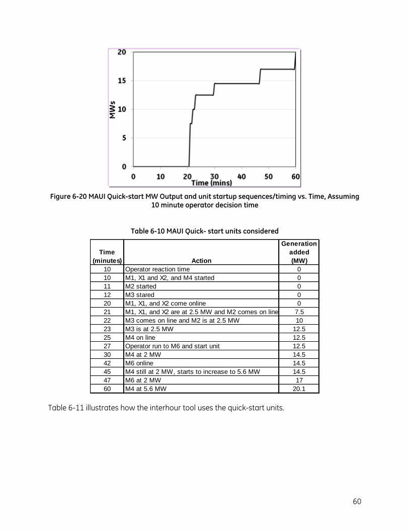
60

Figure 6-20 MAUI Quick-start MW Output and unit startup sequences/timing vs. Time, Assuming 10 minute operator decision time

Table 6-10 MAUI Quick- start units considered

Time

(minutes) Action

Generation

added

(MW)

10 Operator reaction time 0

10 M1, X1 and X2, and M4 started 0

11 M2 started 0

12 M3 stared 0

20 M1, X1, and X2 come online 0

21 M1, X1, and X2 are at 2.5 MW and M2 comes on line 7.5

22 M3 comes on line and M2 is at 2.5 MW 10

23 M3 is at 2.5 MW 12.5

25 M4 on line 12.5

27 Operator run to M6 and start unit 12.5

30 M4 at 2 MW 14.5

42 M6 online 14.5

45 M4 still at 2 MW, starts to increase to 5.6 MW 14.5

47 M6 at 2 MW 17

60 M4 at 5.6 MW 20.1

Table 6-11 illustrates how the interhour tool uses the quick-start units.

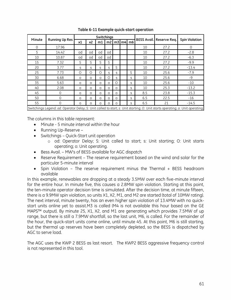
61

Table 6-11 Example quick-start operation

x1 x2 m1 m2 m3 m4 m6

0 17.96 10 27.2 0

5 14.42 od od od od 10 27.2 -2.8

10 10.87 od od od od 10 27.2 -6.3

15 7.32 S S S S 10 27.2 -9.9

20 3.77 s s s s S 10 27.2 -13.4

25 7.73 O O O s s S 10 25.6 -7.9

30 6.68 o o o O s s 10 25.6 -9

35 5.63 o o o o O s 10 25.6 -10

40 2.08 o o o o o s 10 25.3 -13.2

45 0 o o o o o s 8.5 23.8 -15.3

50 0 o o o o o s 6.5 22.5 -16

55 0 o o o o o s 6.5 21 -14.5

Switchings Legend: od: Operator Delay; S: Unit called to start; s: Unit starting; O: Unit starts operating; o: Unit operating.

Spin ViolationReserve Req.BESS Avail.Switchings

Minute Running Up Res

The columns in this table represent:

Minute - 5 minute interval within the hour

Running Up-Reserve –

Switchings – Quick-Start unit operation o od: Operator Delay; S: Unit called to start; s: Unit starting; O: Unit starts

operating; o: Unit operating.

Bess Avail. – MW’s of BESS available for AGC dispatch

Reserve Requirement – The reserve requirement based on the wind and solar for the particular 5-minute interval

Spin Violation – The reserve requirement minus the Thermal + BESS headroom available

In this example, renewables are dropping at a steady 3.5MW over each five-minute interval for the entire hour. In minute five, this causes a 2.8MW spin violation. Starting at this point, the ten-minute operator decision time is simulated. After the decision time, at minute fifteen, there is a 9.9MW spin violation, so units X1, X2, M1, and M2 are started (total of 10MW rating). The next interval, minute twenty, has an even higher spin violation of 13.4MW with no quick-start units online yet to assist.M3 is called (M4 is not available this hour based on the GE MAPS™ output). By minute 25, X1, X2, and M1 are generating which provides 7.5MW of up range, but there is still a 7.9MW shortfall, so the last unit, M6, is called. For the remainder of the hour, the quick-start units come online, until minute 45. At this point, M6 is still starting, but the thermal up reserves have been completely depleted, so the BESS is dispatched by AGC to serve load. The AGC uses the KWP 2 BESS as last resort. The KWP2 BESS aggressive frequency control is not represented in this tool.

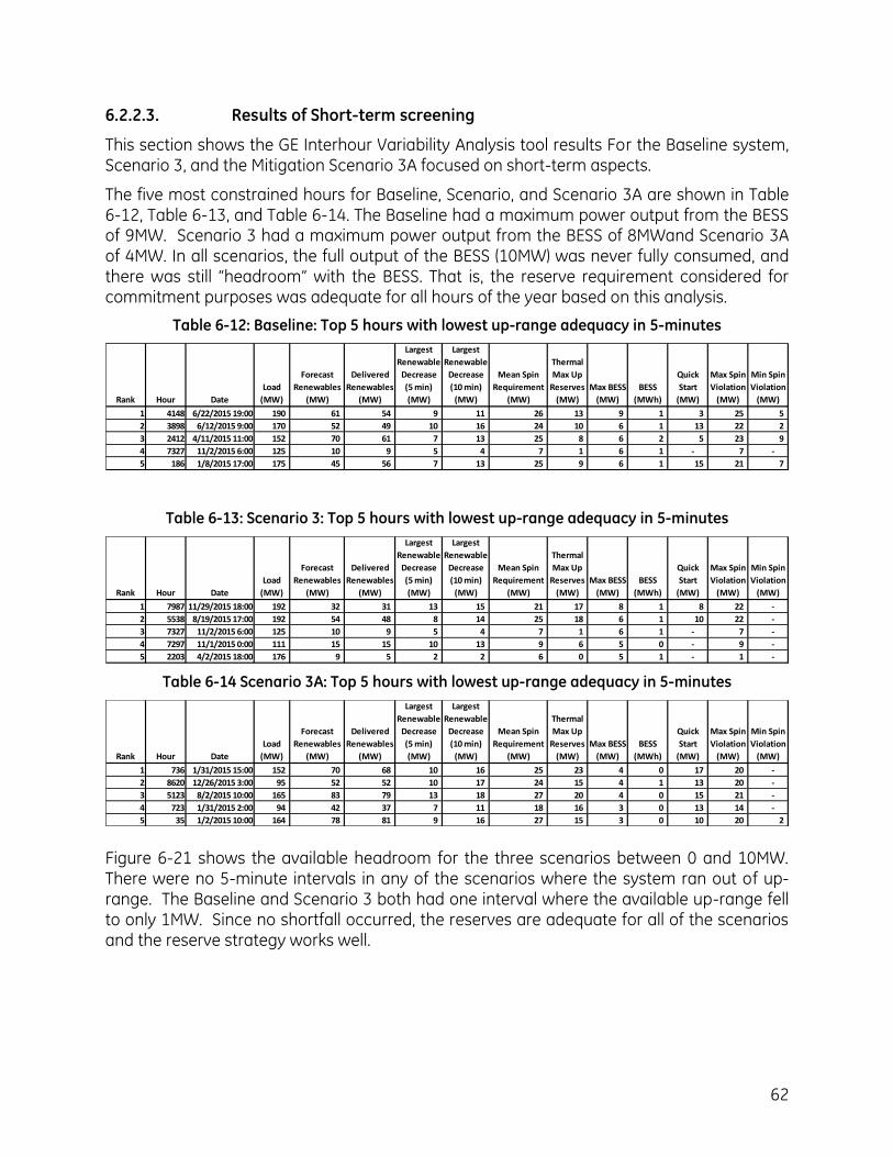
62

6.2.2.3. Results of Short-term screening

This section shows the GE Interhour Variability Analysis tool results For the Baseline system, Scenario 3, and the Mitigation Scenario 3A focused on short-term aspects.

The five most constrained hours for Baseline, Scenario, and Scenario 3A are shown in Table 6-12, Table 6-13, and Table 6-14. The Baseline had a maximum power output from the BESS of 9MW. Scenario 3 had a maximum power output from the BESS of 8MWand Scenario 3A of 4MW. In all scenarios, the full output of the BESS (10MW) was never fully consumed, and there was still “headroom” with the BESS. That is, the reserve requirement considered for commitment purposes was adequate for all hours of the year based on this analysis.

Table 6-12: Baseline: Top 5 hours with lowest up-range adequacy in 5-minutes

Rank Hour Date

Load

(MW)

Forecast

Renewables

(MW)

Delivered

Renewables

(MW)

Largest

Renewable

Decrease

(5 min)

(MW)

Largest

Renewable

Decrease

(10 min)

(MW)

Mean Spin

Requirement

(MW)

Thermal

Max Up

Reserves

(MW)

Max BESS

(MW)

BESS

(MWh)

Quick

Start

(MW)

Max Spin

Violation

(MW)

Min Spin

Violation

(MW)

1 4148 6/22/2015 19:00 190 61 54 9 11 26 13 9 1 3 25 5

2 3898 6/12/2015 9:00 170 52 49 10 16 24 10 6 1 13 22 2

3 2412 4/11/2015 11:00 152 70 61 7 13 25 8 6 2 5 23 9

4 7327 11/2/2015 6:00 125 10 9 5 4 7 1 6 1 - 7 -

5 186 1/8/2015 17:00 175 45 56 7 13 25 9 6 1 15 21 7

Table 6-13: Scenario 3: Top 5 hours with lowest up-range adequacy in 5-minutes

Rank Hour Date

Load

(MW)

Forecast

Renewables

(MW)

Delivered

Renewables

(MW)

Largest

Renewable

Decrease

(5 min)

(MW)

Largest

Renewable

Decrease

(10 min)

(MW)

Mean Spin

Requirement

(MW)

Thermal

Max Up

Reserves

(MW)

Max BESS

(MW)

BESS

(MWh)

Quick

Start

(MW)

Max Spin

Violation

(MW)

Min Spin

Violation

(MW)

1 7987 11/29/2015 18:00 192 32 31 13 15 21 17 8 1 8 22 -

2 5538 8/19/2015 17:00 192 54 48 8 14 25 18 6 1 10 22 -

3 7327 11/2/2015 6:00 125 10 9 5 4 7 1 6 1 - 7 -

4 7297 11/1/2015 0:00 111 15 15 10 13 9 6 5 0 - 9 -

5 2203 4/2/2015 18:00 176 9 5 2 2 6 0 5 1 - 1 -

Table 6-14 Scenario 3A: Top 5 hours with lowest up-range adequacy in 5-minutes

Rank Hour Date

Load

(MW)

Forecast

Renewables

(MW)

Delivered

Renewables

(MW)

Largest

Renewable

Decrease

(5 min)

(MW)

Largest

Renewable

Decrease

(10 min)

(MW)

Mean Spin

Requirement

(MW)

Thermal

Max Up

Reserves

(MW)

Max BESS

(MW)

BESS

(MWh)

Quick

Start

(MW)

Max Spin

Violation

(MW)

Min Spin

Violation

(MW)

1 736 1/31/2015 15:00 152 70 68 10 16 25 23 4 0 17 20 -

2 8620 12/26/2015 3:00 95 52 52 10 17 24 15 4 1 13 20 -

3 5123 8/2/2015 10:00 165 83 79 13 18 27 20 4 0 15 21 -

4 723 1/31/2015 2:00 94 42 37 7 11 18 16 3 0 13 14 -

5 35 1/2/2015 10:00 164 78 81 9 16 27 15 3 0 10 20 2 Figure 6-21 shows the available headroom for the three scenarios between 0 and 10MW. There were no 5-minute intervals in any of the scenarios where the system ran out of up-range. The Baseline and Scenario 3 both had one interval where the available up-range fell to only 1MW. Since no shortfall occurred, the reserves are adequate for all of the scenarios and the reserve strategy works well.

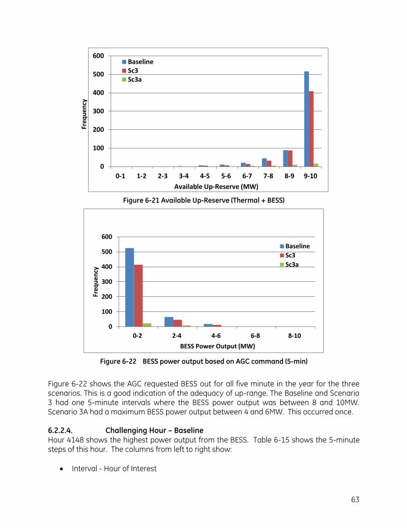
63

0

100

200

300

400

500

600

0-2 2-4 4-6 6-8 8-10

Freq

uen

cy

BESS Power Output (MW)

Baseline

Sc3

Sc3a

0

100

200

300

400

500

600

0-1 1-2 2-3 3-4 4-5 5-6 6-7 7-8 8-9 9-10

Available Up-Reserve (MW)

BaselineSc3Sc3a

Figure 6-21 Available Up-Reserve (Thermal + BESS)

0

100

200

300

400

500

600

0-2 2-4 4-6 6-8 8-10

Freq

uen

cy

BESS Power Output (MW)

Baseline

Sc3

Sc3a

Figure 6-22 BESS power output based on AGC command (5-min)

Figure 6-22 shows the AGC requested BESS out for all five minute in the year for the three scenarios. This is a good indication of the adequacy of up-range. The Baseline and Scenario 3 had one 5-minute intervals where the BESS power output was between 8 and 10MW. Scenario 3A had a maximum BESS power output between 4 and 6MW. This occurred once. 6.2.2.4. Challenging Hour – Baseline Hour 4148 shows the highest power output from the BESS. Table 6-15 shows the 5-minute steps of this hour. The columns from left to right show:

Interval - Hour of Interest

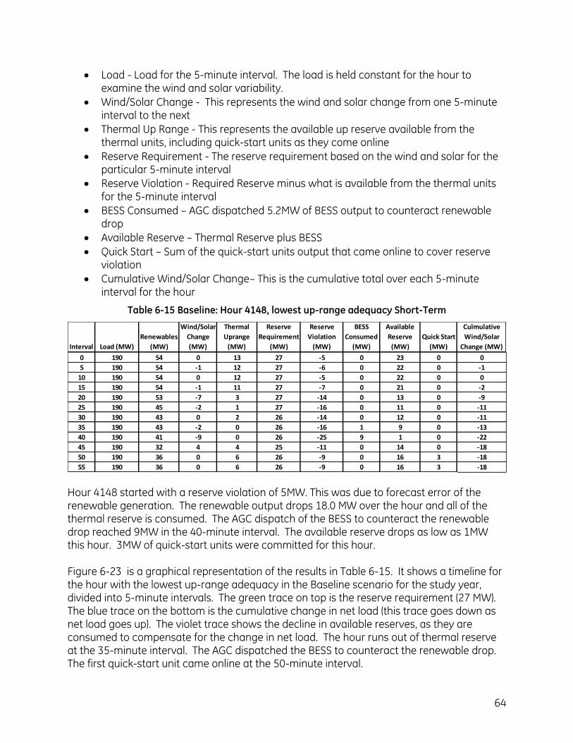
64

Load - Load for the 5-minute interval. The load is held constant for the hour to examine the wind and solar variability.

Wind/Solar Change - This represents the wind and solar change from one 5-minute interval to the next

Thermal Up Range - This represents the available up reserve available from the thermal units, including quick-start units as they come online

Reserve Requirement - The reserve requirement based on the wind and solar for the particular 5-minute interval

Reserve Violation - Required Reserve minus what is available from the thermal units for the 5-minute interval

BESS Consumed – AGC dispatched 5.2MW of BESS output to counteract renewable drop

Available Reserve – Thermal Reserve plus BESS

Quick Start – Sum of the quick-start units output that came online to cover reserve violation

Cumulative Wind/Solar Change– This is the cumulative total over each 5-minute interval for the hour

Table 6-15 Baseline: Hour 4148, lowest up-range adequacy Short-Term

Interval Load (MW)

Renewables

(MW)

Wind/Solar

Change

(MW)

Thermal

Uprange

(MW)

Reserve

Requirement

(MW)

Reserve

Violation

(MW)

BESS

Consumed

(MW)

Available

Reserve

(MW)

Quick Start

(MW)

Culmulative

Wind/Solar

Change (MW)

0 190 54 0 13 27 -5 0 23 0 0

5 190 54 -1 12 27 -6 0 22 0 -1

10 190 54 0 12 27 -5 0 22 0 0

15 190 54 -1 11 27 -7 0 21 0 -2

20 190 53 -7 3 27 -14 0 13 0 -9

25 190 45 -2 1 27 -16 0 11 0 -11

30 190 43 0 2 26 -14 0 12 0 -11

35 190 43 -2 0 26 -16 1 9 0 -13

40 190 41 -9 0 26 -25 9 1 0 -22

45 190 32 4 4 25 -11 0 14 0 -18

50 190 36 0 6 26 -9 0 16 3 -18

55 190 36 0 6 26 -9 0 16 3 -18 Hour 4148 started with a reserve violation of 5MW. This was due to forecast error of the renewable generation. The renewable output drops 18.0 MW over the hour and all of the thermal reserve is consumed. The AGC dispatch of the BESS to counteract the renewable drop reached 9MW in the 40-minute interval. The available reserve drops as low as 1MW this hour. 3MW of quick-start units were committed for this hour. Figure 6-23 is a graphical representation of the results in Table 6-15. It shows a timeline for the hour with the lowest up-range adequacy in the Baseline scenario for the study year, divided into 5-minute intervals. The green trace on top is the reserve requirement (27 MW). The blue trace on the bottom is the cumulative change in net load (this trace goes down as net load goes up). The violet trace shows the decline in available reserves, as they are consumed to compensate for the change in net load. The hour runs out of thermal reserve at the 35-minute interval. The AGC dispatched the BESS to counteract the renewable drop. The first quick-start unit came online at the 50-minute interval.

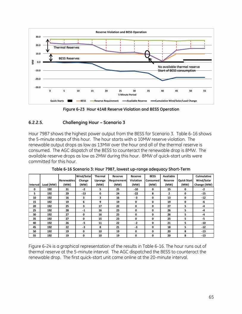
65

-30.0

-20.0

-10.0

0.0

10.0

20.0

30.0

0 5 10 15 20 25 30 35 40 45 50 55

MW

5 Minute Period

Reserve Violation and BESS Operation

Quick Starts BESS Reserve Requirement Available Reserve Cumulative Wind/Solar/Load Change

Figure 6-23 Hour 4148 Reserve Violation and BESS Operation

6.2.2.5. Challenging Hour – Scenario 3 Hour 7987 shows the highest power output from the BESS for Scenario 3. Table 6-16 shows the 5-minute steps of this hour. The hour starts with a 10MW reserve violation. The renewable output drops as low as 13MW over the hour and all of the thermal reserve is consumed. The AGC dispatch of the BESS to counteract the renewable drop is 8MW. The available reserve drops as low as 2MW during this hour. 8MW of quick-start units were committed for this hour.

Table 6-16 Scenario 3: Hour 7987, lowest up-range adequacy Short-Term

Interval Load (MW)

Renewables

(MW)

Wind/Solar

Change

(MW)

Thermal

Uprange

(MW)

Reserve

Requirement

(MW)

Reserve

Violation

(MW)

BESS

Consumed

(MW)

Available

Reserve

(MW)

Quick Start

(MW)

Culmulative

Wind/Solar

Change (MW)

0 192 31 -2 5 25 -10 0 15 0 -2

5 192 29 -13 0 24 -22 8 2 0 -15

10 192 16 3 3 16 -3 0 13 0 -12

15 192 19 6 9 19 0 0 19 0 -6

20 192 25 3 17 22 0 0 27 5 -4

25 192 28 -1 16 23 0 0 26 5 -4

30 192 27 0 16 23 0 0 26 5 -4

35 192 27 0 15 23 0 0 25 5 -5

40 192 26 -5 11 22 -2 0 21 5 -10

45 192 22 -3 8 21 -3 0 18 5 -12

50 192 19 0 10 19 0 0 20 8 -13

55 192 19 0 10 19 0 0 20 8 -13 Figure 6-24 is a graphical representation of the results in Table 6-16. The hour runs out of thermal reserve at the 5-minute interval. The AGC dispatched the BESS to counteract the renewable drop. The first quick-start unit came online at the 20-minute interval.

No available thermal reserve Start of BESS consumption

BESS Reserves

Thermal Reserves

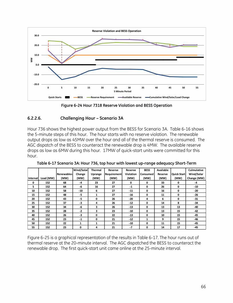
66

-20.0

-10.0

0.0

10.0

20.0

30.0

0 5 10 15 20 25 30 35 40 45 50 55

MW

5 Minute Period




6.2.2.6. Challenging Hour – Scenario 3A Hour 736 shows the highest power output from the BESS for Scenario 3A. Table 6-16 shows the 5-minute steps of this hour. The hour starts with no reserve violation. The renewable output drops as low as 45MW over the hour and all of the thermal reserve is consumed. The AGC dispatch of the BESS to counteract the renewable drop is 4MW. The available reserve drops as low as 6MW during this hour. 17MW of quick-start units were committed for this hour.

Table 6-17 Scenario 3A: Hour 736, top hour with lowest up-range adequacy Short-Term

Interval Load (MW)

Renewables

(MW)

Wind/Solar

Change

(MW)

Thermal

Uprange

(MW)

Reserve

Requirement

(MW)

Reserve

Violation

(MW)

BESS

Consumed

(MW)

Available

Reserve

(MW)

Quick Start

(MW)

Culmulative

Wind/Solar

Change (MW)

0 152 68 -4 23 27 0 0 33 0 -4

5 152 64 -6 16 27 -1 0 26 0 -10

10 152 58 -10 6 27 -11 0 16 0 -20

15 152 48 -5 1 27 -16 0 11 0 -26

20 152 43 -5 0 26 -20 4 6 0 -31

25 152 37 -3 4 26 -12 0 14 8 -34

30 152 34 -6 3 26 -13 0 13 13 -40

35 152 28 -2 3 23 -10 0 13 15 -42

40 152 26 -3 0 22 -13 0 10 15 -45

45 152 23 -1 0 21 -12 1 9 15 -46

50 152 22 1 1 21 -10 0 11 15 -45

55 152 23 0 4 21 -7 0 14 17 -45 Figure 6-25 is a graphical representation of the results in Table 6-17. The hour runs out of thermal reserve at the 20-minute interval. The AGC dispatched the BESS to counteract the renewable drop. The first quick-start unit came online at the 25-minute interval.

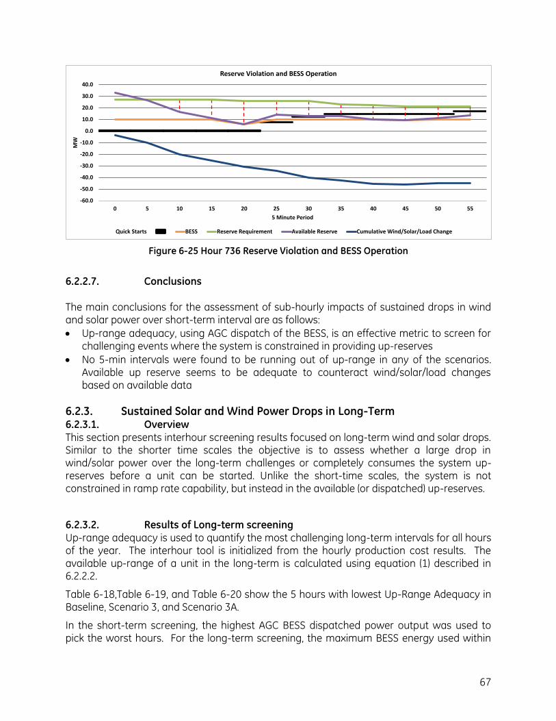
67

-60.0

-50.0

-40.0

-30.0

-20.0

-10.0

0.0

10.0

20.0

30.0

40.0

0 5 10 15 20 25 30 35 40 45 50 55

MW

5 Minute Period




6.2.2.7. Conclusions The main conclusions for the assessment of sub-hourly impacts of sustained drops in wind and solar power over short-term interval are as follows:

Up-range adequacy, using AGC dispatch of the BESS, is an effective metric to screen for challenging events where the system is constrained in providing up-reserves

No 5-min intervals were found to be running out of up-range in any of the scenarios. Available up reserve seems to be adequate to counteract wind/solar/load changes based on available data

6.2.3. Sustained Solar and Wind Power Drops in Long-Term 6.2.3.1. Overview This section presents interhour screening results focused on long-term wind and solar drops. Similar to the shorter time scales the objective is to assess whether a large drop in wind/solar power over the long-term challenges or completely consumes the system up-reserves before a unit can be started. Unlike the short-time scales, the system is not constrained in ramp rate capability, but instead in the available (or dispatched) up-reserves.

6.2.3.2. Results of Long-term screening Up-range adequacy is used to quantify the most challenging long-term intervals for all hours of the year. The interhour tool is initialized from the hourly production cost results. The available up-range of a unit in the long-term is calculated using equation (1) described in 6.2.2.2.

Table 6-18,Table 6-19, and Table 6-20 show the 5 hours with lowest Up-Range Adequacy in Baseline, Scenario 3, and Scenario 3A.

In the short-term screening, the highest AGC BESS dispatched power output was used to pick the worst hours. For the long-term screening, the maximum BESS energy used within

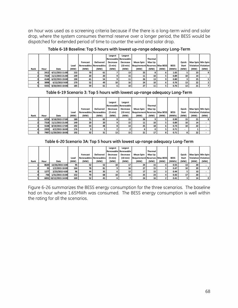
68

an hour was used as a screening criteria because if the there is a long-term wind and solar drop, where the system consumes thermal reserve over a longer period, the BESS would be dispatched for extended period of time to counter the wind and solar drop.

Table 6-18 Baseline: Top 5 hours with lowest up-range adequacy Long-Term

Rank Hour Date

Load

(MW)

Forecast

Renewables

(MW)

Delivered

Renewables

(MW)

Largest

Renewable

Decrease

(5 min)

(MW)

Largest

Renewable

Decrease

(10 min)

(MW)

Mean Spin

Requirement

(MW)

Thermal

Max Up

Reserves

(MW)

Max BESS

(MW)

BESS

(MWh)

Quick

Start

(MW)

Max Spin

Violation

(MW)

Min Spin

Violation

(MW)

1 2412 4/11/2015 11:00 152 70 61 7 13 25 8 6 1.65 5 23 9

2 7318 11/1/2015 21:00 149 20 20 9 15 11 10 5 0.89 10 14 -

3 4148 6/22/2015 19:00 190 61 54 9 11 26 13 9 0.80 3 25 5

4 3898 6/12/2015 9:00 170 52 49 10 16 24 10 6 0.76 13 22 2

5 5555 8/20/2015 10:00 185 59 61 6 10 27 11 5 0.76 13 21 7

Table 6-19 Scenario 3: Top 5 hours with lowest up-range adequacy Long-Term

Rank Hour Date

Load

(MW)

Forecast

Renewables

(MW)

Delivered

Renewables

(MW)

Largest

Renewable

Decrease

(5 min)

(MW)

Largest

Renewable

Decrease

(10 min)

(MW)

Mean Spin

Requirement

(MW)

Thermal

Max Up

Reserves

(MW)

Max BESS

(MW)

BESS

(MWh)

Quick

Start

(MW)

Max Spin

Violation

(MW)

Min Spin

Violation

(MW)

1 6258 9/18/2015 17:00 180 71 65 8 15 26 9 5 0.90 15 21 8

2 7318 11/1/2015 21:00 149 20 20 9 15 11 10 5 0.89 10 14 -

3 5538 8/19/2015 17:00 192 54 48 8 14 25 18 6 0.73 10 22 -

4 2203 4/2/2015 18:00 176 9 5 2 2 6 0 5 0.71 - 1 -

5 7987 11/29/2015 18:00 192 32 31 13 15 21 17 8 0.71 8 22 -

Table 6-20 Scenario 3A: Top 5 hours with lowest up-range adequacy Long-Term

Rank Hour Date

Load

(MW)

Forecast

Renewables

(MW)

Delivered

Renewables

(MW)

Largest

Renewable

Decrease

(5 min)

(MW)

Largest

Renewable

Decrease

(10 min)

(MW)

Mean Spin

Requirement

(MW)

Thermal

Max Up

Reserves

(MW)

Max BESS

(MW)

BESS

(MWh)

Quick

Start

(MW)

Max Spin

Violation

(MW)

Min Spin

Violation

(MW)

1 8620 12/26/2015 3:00 95 52 52 10 17 24 15 4 0.55 13 20 -

2 35 1/2/2015 10:00 164 78 81 9 16 27 15 3 0.47 10 20 2

3 1277 2/23/2015 4:00 96 44 35 6 12 17 15 3 0.44 5 10 -

4 736 1/31/2015 15:00 152 70 68 10 16 25 23 4 0.42 17 20 -

5 6831 10/12/2015 14:00 169 52 45 6 7 24 16 2 0.41 3 14 0

Figure 6-26 summarizes the BESS energy consumption for the three scenarios. The baseline had on hour where 1.65MWh was consumed. The BESS energy consumption is well within the rating for all the scenarios.

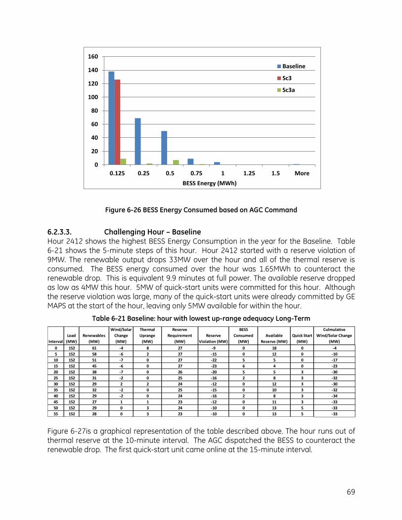
69

0

20

40

60

80

100

120

140

160

0.125 0.25 0.5 0.75 1 1.25 1.5 More

BESS Energy (MWh)

Baseline

Sc3

Sc3a

Figure 6-26 BESS Energy Consumed based on AGC Command

6.2.3.3. Challenging Hour – Baseline Hour 2412 shows the highest BESS Energy Consumption in the year for the Baseline. Table 6-21 shows the 5-minute steps of this hour. Hour 2412 started with a reserve violation of 9MW. The renewable output drops 33MW over the hour and all of the thermal reserve is consumed. The BESS energy consumed over the hour was 1.65MWh to counteract the renewable drop. This is equivalent 9.9 minutes at full power. The available reserve dropped as low as 4MW this hour. 5MW of quick-start units were committed for this hour. Although the reserve violation was large, many of the quick-start units were already committed by GE MAPS at the start of the hour, leaving only 5MW available for within the hour.

Table 6-21 Baseline: hour with lowest up-range adequacy Long-Term

Interval

Load

(MW)

Renewables

(MW)

Wind/Solar

Change

(MW)

Thermal

Uprange

(MW)

Reserve

Requirement

(MW)

Reserve

Violation (MW)

BESS

Consumed

(MW)

Available

Reserve (MW)

Quick Start

(MW)

Culmulative

Wind/Solar Change

(MW)

0 152 61 -4 8 27 -9 0 18 0 -4

5 152 58 -6 2 27 -15 0 12 0 -10

10 152 51 -7 0 27 -22 5 5 0 -17

15 152 45 -6 0 27 -23 6 4 0 -23

20 152 38 -7 0 26 -20 5 5 3 -30

25 152 31 -2 0 25 -16 2 8 3 -32

30 152 29 2 2 24 -12 0 12 3 -30

35 152 32 -2 0 25 -15 0 10 3 -32

40 152 29 -2 0 24 -16 2 8 3 -34

45 152 27 1 1 23 -12 0 11 3 -33

50 152 29 0 3 24 -10 0 13 5 -33

55 152 28 0 3 23 -10 0 13 5 -33 Figure 6-27is a graphical representation of the table described above. The hour runs out of thermal reserve at the 10-minute interval. The AGC dispatched the BESS to counteract the renewable drop. The first quick-start unit came online at the 15-minute interval.

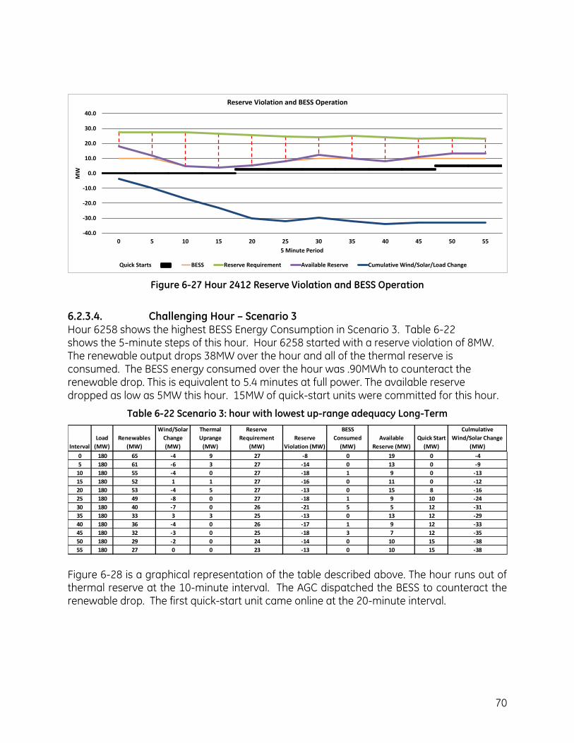
70

-40.0

-30.0

-20.0

-10.0

0.0

10.0

20.0

30.0

40.0

0 5 10 15 20 25 30 35 40 45 50 55

MW

5 Minute Period




6.2.3.4. Challenging Hour – Scenario 3 Hour 6258 shows the highest BESS Energy Consumption in Scenario 3. Table 6-22 shows the 5-minute steps of this hour. Hour 6258 started with a reserve violation of 8MW. The renewable output drops 38MW over the hour and all of the thermal reserve is consumed. The BESS energy consumed over the hour was .90MWh to counteract the renewable drop. This is equivalent to 5.4 minutes at full power. The available reserve dropped as low as 5MW this hour. 15MW of quick-start units were committed for this hour.

Table 6-22 Scenario 3: hour with lowest up-range adequacy Long-Term

Interval

Load

(MW)

Renewables

(MW)

Wind/Solar

Change

(MW)

Thermal

Uprange

(MW)

Reserve

Requirement

(MW)

Reserve

Violation (MW)

BESS

Consumed

(MW)

Available

Reserve (MW)

Quick Start

(MW)

Culmulative

Wind/Solar Change

(MW)

0 180 65 -4 9 27 -8 0 19 0 -4

5 180 61 -6 3 27 -14 0 13 0 -9

10 180 55 -4 0 27 -18 1 9 0 -13

15 180 52 1 1 27 -16 0 11 0 -12

20 180 53 -4 5 27 -13 0 15 8 -16

25 180 49 -8 0 27 -18 1 9 10 -24

30 180 40 -7 0 26 -21 5 5 12 -31

35 180 33 3 3 25 -13 0 13 12 -29

40 180 36 -4 0 26 -17 1 9 12 -33

45 180 32 -3 0 25 -18 3 7 12 -35

50 180 29 -2 0 24 -14 0 10 15 -38

55 180 27 0 0 23 -13 0 10 15 -38 Figure 6-28 is a graphical representation of the table described above. The hour runs out of thermal reserve at the 10-minute interval. The AGC dispatched the BESS to counteract the renewable drop. The first quick-start unit came online at the 20-minute interval.

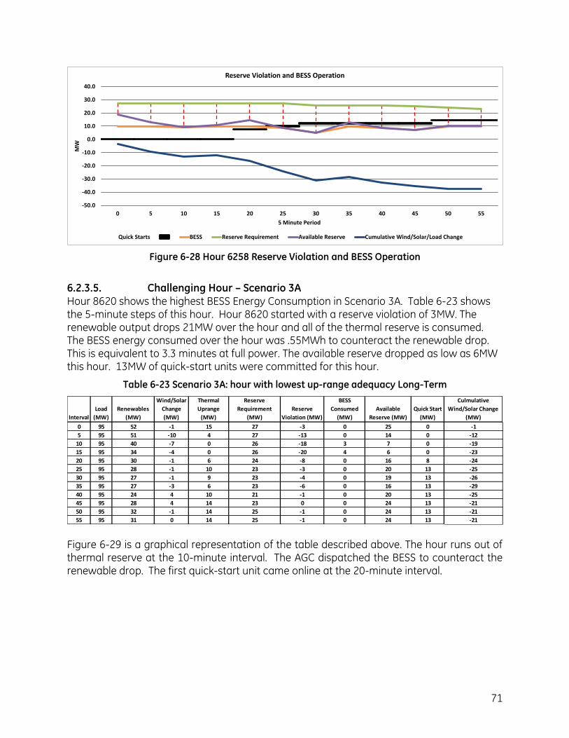
71

-50.0

-40.0

-30.0

-20.0

-10.0

0.0

10.0

20.0

30.0

40.0

0 5 10 15 20 25 30 35 40 45 50 55

MW

5 Minute Period




6.2.3.5. Challenging Hour – Scenario 3A Hour 8620 shows the highest BESS Energy Consumption in Scenario 3A. Table 6-23 shows the 5-minute steps of this hour. Hour 8620 started with a reserve violation of 3MW. The renewable output drops 21MW over the hour and all of the thermal reserve is consumed. The BESS energy consumed over the hour was .55MWh to counteract the renewable drop. This is equivalent to 3.3 minutes at full power. The available reserve dropped as low as 6MW this hour. 13MW of quick-start units were committed for this hour.

Table 6-23 Scenario 3A: hour with lowest up-range adequacy Long-Term

Interval

Load

(MW)

Renewables

(MW)

Wind/Solar

Change

(MW)

Thermal

Uprange

(MW)

Reserve

Requirement

(MW)

Reserve

Violation (MW)

BESS

Consumed

(MW)

Available

Reserve (MW)

Quick Start

(MW)

Culmulative

Wind/Solar Change

(MW)

0 95 52 -1 15 27 -3 0 25 0 -1

5 95 51 -10 4 27 -13 0 14 0 -12

10 95 40 -7 0 26 -18 3 7 0 -19

15 95 34 -4 0 26 -20 4 6 0 -23

20 95 30 -1 6 24 -8 0 16 8 -24

25 95 28 -1 10 23 -3 0 20 13 -25

30 95 27 -1 9 23 -4 0 19 13 -26

35 95 27 -3 6 23 -6 0 16 13 -29

40 95 24 4 10 21 -1 0 20 13 -25

45 95 28 4 14 23 0 0 24 13 -21

50 95 32 -1 14 25 -1 0 24 13 -21

55 95 31 0 14 25 -1 0 24 13 -21 Figure 6-29 is a graphical representation of the table described above. The hour runs out of thermal reserve at the 10-minute interval. The AGC dispatched the BESS to counteract the renewable drop. The first quick-start unit came online at the 20-minute interval.

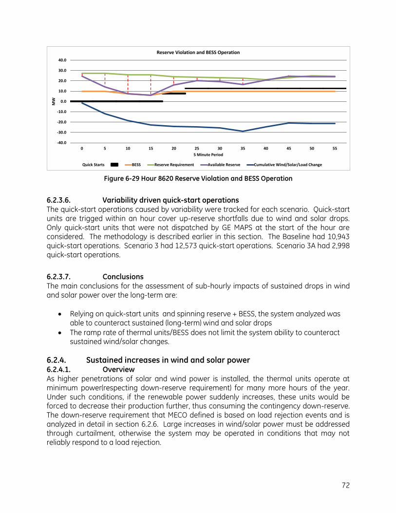
72

-40.0

-30.0

-20.0

-10.0

0.0

10.0

20.0

30.0

40.0

0 5 10 15 20 25 30 35 40 45 50 55

MW

5 Minute Period




6.2.3.6. Variability driven quick-start operations The quick-start operations caused by variability were tracked for each scenario. Quick-start units are trigged within an hour cover up-reserve shortfalls due to wind and solar drops. Only quick-start units that were not dispatched by GE MAPS at the start of the hour are considered. The methodology is described earlier in this section. The Baseline had 10,943 quick-start operations. Scenario 3 had 12,573 quick-start operations. Scenario 3A had 2,998 quick-start operations.

6.2.3.7. Conclusions The main conclusions for the assessment of sub-hourly impacts of sustained drops in wind and solar power over the long-term are:

Relying on quick-start units and spinning reserve + BESS, the system analyzed was able to counteract sustained (long-term) wind and solar drops

The ramp rate of thermal units/BESS does not limit the system ability to counteract sustained wind/solar changes.

6.2.4. Sustained increases in wind and solar power 6.2.4.1. Overview As higher penetrations of solar and wind power is installed, the thermal units operate at minimum power(respecting down-reserve requirement) for many more hours of the year. Under such conditions, if the renewable power suddenly increases, these units would be forced to decrease their production further, thus consuming the contingency down-reserve. The down-reserve requirement that MECO defined is based on load rejection events and is analyzed in detail in section 6.2.6. Large increases in wind/solar power must be addressed through curtailment, otherwise the system may be operated in conditions that may not reliably respond to a load rejection.

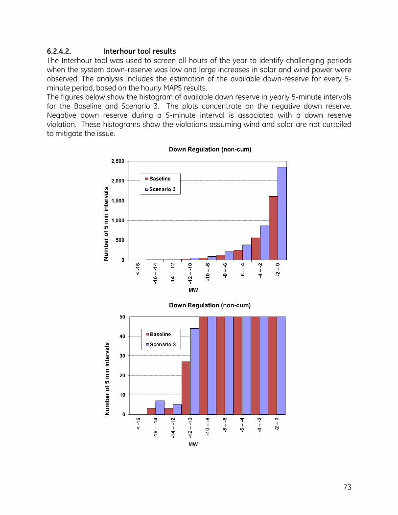
73

6.2.4.2. Interhour tool results The Interhour tool was used to screen all hours of the year to identify challenging periods when the system down-reserve was low and large increases in solar and wind power were observed. The analysis includes the estimation of the available down-reserve for every 5-minute period, based on the hourly MAPS results. The figures below show the histogram of available down reserve in yearly 5-minute intervals for the Baseline and Scenario 3. The plots concentrate on the negative down reserve. Negative down reserve during a 5-minute interval is associated with a down reserve violation. These histograms show the violations assuming wind and solar are not curtailed to mitigate the issue.

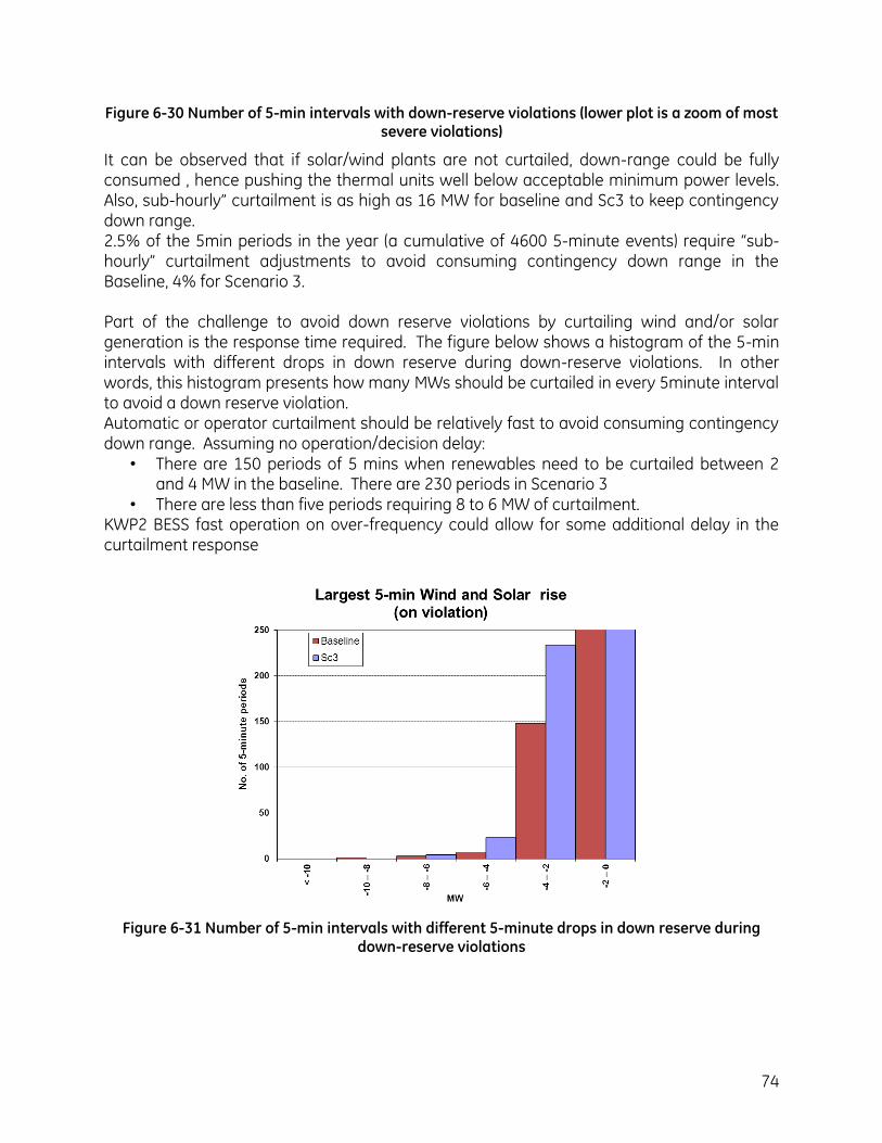
74

Figure 6-30 Number of 5-min intervals with down-reserve violations (lower plot is a zoom of most severe violations)

It can be observed that if solar/wind plants are not curtailed, down-range could be fully consumed , hence pushing the thermal units well below acceptable minimum power levels. Also, sub-hourly” curtailment is as high as 16 MW for baseline and Sc3 to keep contingency down range. 2.5% of the 5min periods in the year (a cumulative of 4600 5-minute events) require “sub-hourly” curtailment adjustments to avoid consuming contingency down range in the Baseline, 4% for Scenario 3. Part of the challenge to avoid down reserve violations by curtailing wind and/or solar generation is the response time required. The figure below shows a histogram of the 5-min intervals with different drops in down reserve during down-reserve violations. In other words, this histogram presents how many MWs should be curtailed in every 5minute interval to avoid a down reserve violation. Automatic or operator curtailment should be relatively fast to avoid consuming contingency down range. Assuming no operation/decision delay:

• There are 150 periods of 5 mins when renewables need to be curtailed between 2 and 4 MW in the baseline. There are 230 periods in Scenario 3

• There are less than five periods requiring 8 to 6 MW of curtailment. KWP2 BESS fast operation on over-frequency could allow for some additional delay in the curtailment response

Figure 6-31 Number of 5-min intervals with different 5-minute drops in down reserve during down-reserve violations

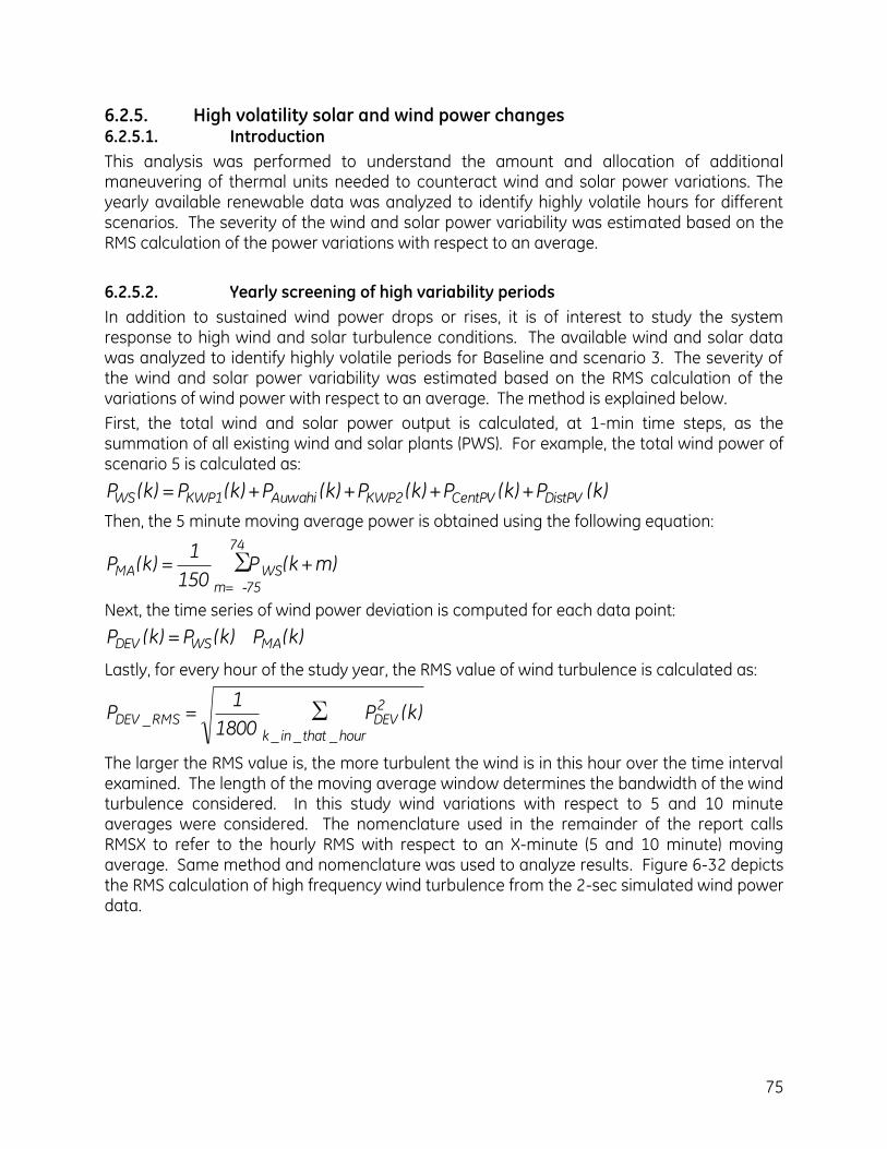
75

6.2.5. High volatility solar and wind power changes 6.2.5.1. Introduction

This analysis was performed to understand the amount and allocation of additional maneuvering of thermal units needed to counteract wind and solar power variations. The yearly available renewable data was analyzed to identify highly volatile hours for different scenarios. The severity of the wind and solar power variability was estimated based on the RMS calculation of the power variations with respect to an average.

6.2.5.2. Yearly screening of high variability periods

In addition to sustained wind power drops or rises, it is of interest to study the system response to high wind and solar turbulence conditions. The available wind and solar data was analyzed to identify highly volatile periods for Baseline and scenario 3. The severity of the wind and solar power variability was estimated based on the RMS calculation of the variations of wind power with respect to an average. The method is explained below.

First, the total wind and solar power output is calculated, at 1-min time steps, as the summation of all existing wind and solar plants (PWS). For example, the total wind power of scenario 5 is calculated as:

)k(P)k(P)k(P)k(P)k(P)k(P DistPVCentPV2KWPAuwahi1KWPWS ++++=

Then, the 5 minute moving average power is obtained using the following equation:

∑-

74

75mWSMA )mk(P

150

1)k(P

=

+=

Next, the time series of wind power deviation is computed for each data point:

)k(P)k(P)k(P MAWSDEV =

Lastly, for every hour of the study year, the RMS value of wind turbulence is calculated as:

∑hour_that_in_k

2DEVRMS_DEV )k(P

1800

1P =

The larger the RMS value is, the more turbulent the wind is in this hour over the time interval examined. The length of the moving average window determines the bandwidth of the wind turbulence considered. In this study wind variations with respect to 5 and 10 minute averages were considered. The nomenclature used in the remainder of the report calls RMSX to refer to the hourly RMS with respect to an X-minute (5 and 10 minute) moving average. Same method and nomenclature was used to analyze results. Figure 6-32 depicts the RMS calculation of high frequency wind turbulence from the 2-sec simulated wind power data.

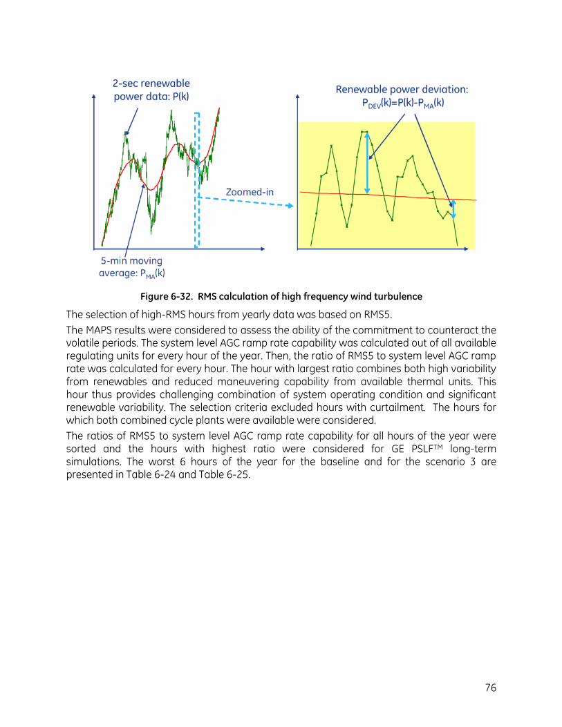
76

2-sec renewable power data: P(k)

Renewable power deviation:

PDEV(k)=P(k)-PMA(k)

Figure 6-32. RMS calculation of high frequency wind turbulence

The selection of high-RMS hours from yearly data was based on RMS5.

The MAPS results were considered to assess the ability of the commitment to counteract the volatile periods. The system level AGC ramp rate capability was calculated out of all available regulating units for every hour of the year. Then, the ratio of RMS5 to system level AGC ramp rate was calculated for every hour. The hour with largest ratio combines both high variability from renewables and reduced maneuvering capability from available thermal units. This hour thus provides challenging combination of system operating condition and significant renewable variability. The selection criteria excluded hours with curtailment. The hours for which both combined cycle plants were available were considered.

The ratios of RMS5 to system level AGC ramp rate capability for all hours of the year were sorted and the hours with highest ratio were considered for GE PSLFTM long-term simulations. The worst 6 hours of the year for the baseline and for the scenario 3 are presented in Table 6-24 and Table 6-25.

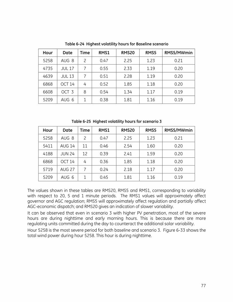
77

Table 6-24 Highest volatility hours for Baseline scenario

Hour Date Time RMS1 RMS20 RMS5 RMS5/MWmin

5258 AUG 8 2 0.47 2.25 1.23 0.21

4735 JUL 17 7 0.55 2.33 1.19 0.20

4639 JUL 13 7 0.51 2.28 1.19 0.20

6868 OCT 14 4 0.52 1.85 1.18 0.20

6608 OCT 3 8 0.54 1.34 1.17 0.19

5209 AUG 6 1 0.38 1.81 1.16 0.19

Table 6-25 Highest volatility hours for scenario 3

Hour Date Time RMS1 RMS20 RMS5 RMS5/MWmin

5258 AUG 8 2 0.47 2.25 1.23 0.21

5411 AUG 14 11 0.46 2.54 1.60 0.20

4188 JUN 24 12 0.39 2.41 1.59 0.20

6868 OCT 14 4 0.36 1.85 1.18 0.20

5719 AUG 27 7 0.24 2.18 1.17 0.20

5209 AUG 6 1 0.45 1.81 1.16 0.19

The values shown in these tables are RMS20, RMS5 and RMS1, corresponding to variability with respect to 20, 5 and 1 minute periods. The RMS1 values will approximately affect governor and AGC regulation; RMS5 will approximately affect regulation and partially affect AGC-economic dispatch; and RMS20 gives an indication of slower variability.

It can be observed that even in scenario 3 with higher PV penetration, most of the severe hours are during nighttime and early morning hours. This is because there are more regulating units committed during the day to counteract the additional solar variability.

Hour 5258 is the most severe period for both baseline and scenario 3. Figure 6-33 shows the total wind power during hour 5258. This hour is during nighttime.

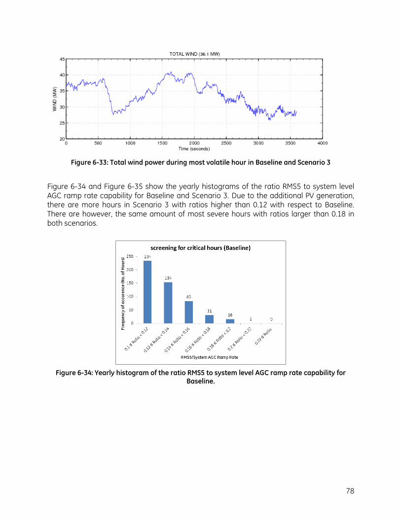
78

Figure 6-33: Total wind power during most volatile hour in Baseline and Scenario 3

Figure 6-34 and Figure 6-35 show the yearly histograms of the ratio RMS5 to system level AGC ramp rate capability for Baseline and Scenario 3. Due to the additional PV generation, there are more hours in Scenario 3 with ratios higher than 0.12 with respect to Baseline. There are however, the same amount of most severe hours with ratios larger than 0.18 in both scenarios.

Figure 6-34: Yearly histogram of the ratio RMS5 to system level AGC ramp rate capability for Baseline.

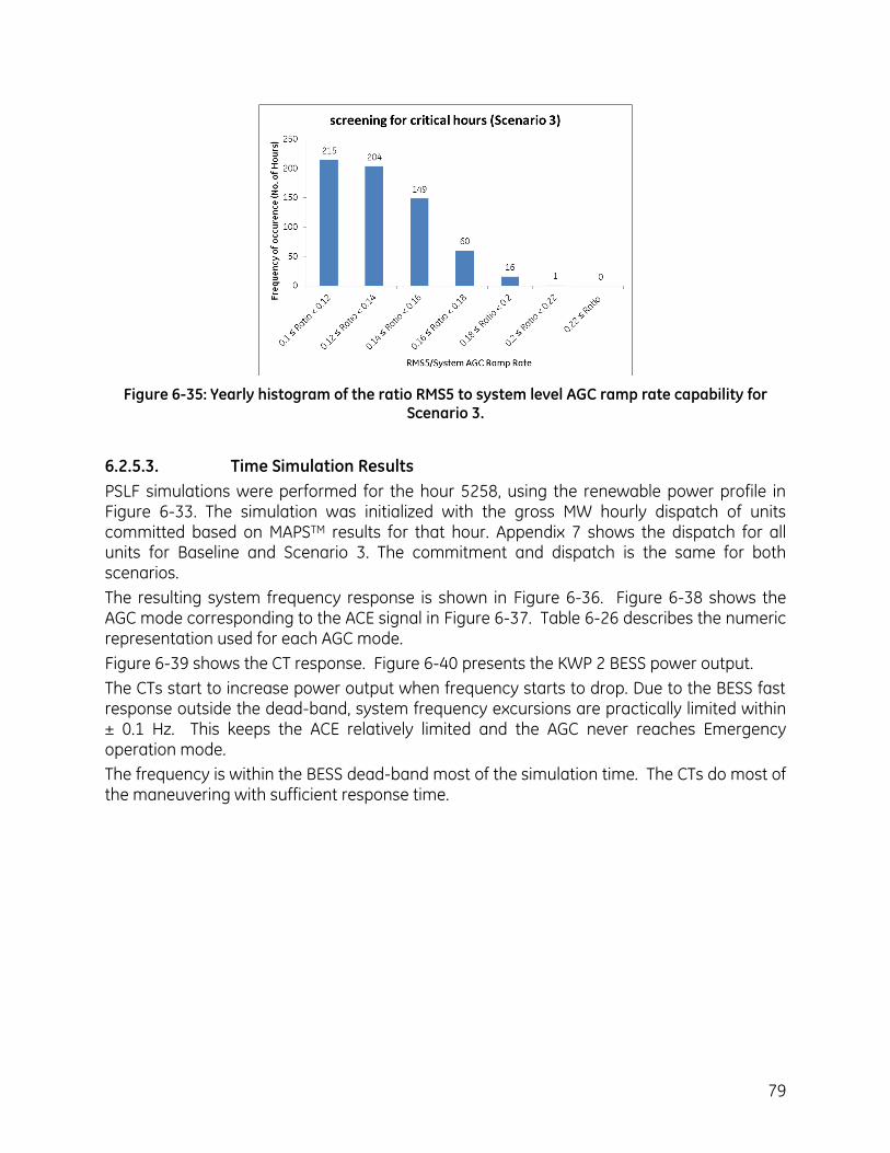
79

Figure 6-35: Yearly histogram of the ratio RMS5 to system level AGC ramp rate capability for Scenario 3.

6.2.5.3. Time Simulation Results

PSLF simulations were performed for the hour 5258, using the renewable power profile in Figure 6-33. The simulation was initialized with the gross MW hourly dispatch of units committed based on MAPSTM results for that hour. Appendix 7 shows the dispatch for all units for Baseline and Scenario 3. The commitment and dispatch is the same for both scenarios.

The resulting system frequency response is shown in Figure 6-36. Figure 6-38 shows the AGC mode corresponding to the ACE signal in Figure 6-37. Table 6-26 describes the numeric representation used for each AGC mode.

Figure 6-39 shows the CT response. Figure 6-40 presents the KWP 2 BESS power output.

The CTs start to increase power output when frequency starts to drop. Due to the BESS fast response outside the dead-band, system frequency excursions are practically limited within ± 0.1 Hz. This keeps the ACE relatively limited and the AGC never reaches Emergency operation mode.

The frequency is within the BESS dead-band most of the simulation time. The CTs do most of the maneuvering with sufficient response time.

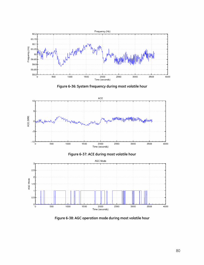
80

Figure 6-36: System frequency during most volatile hour

Figure 6-37: ACE during most volatile hour

Figure 6-38: AGC operation mode during most volatile hour

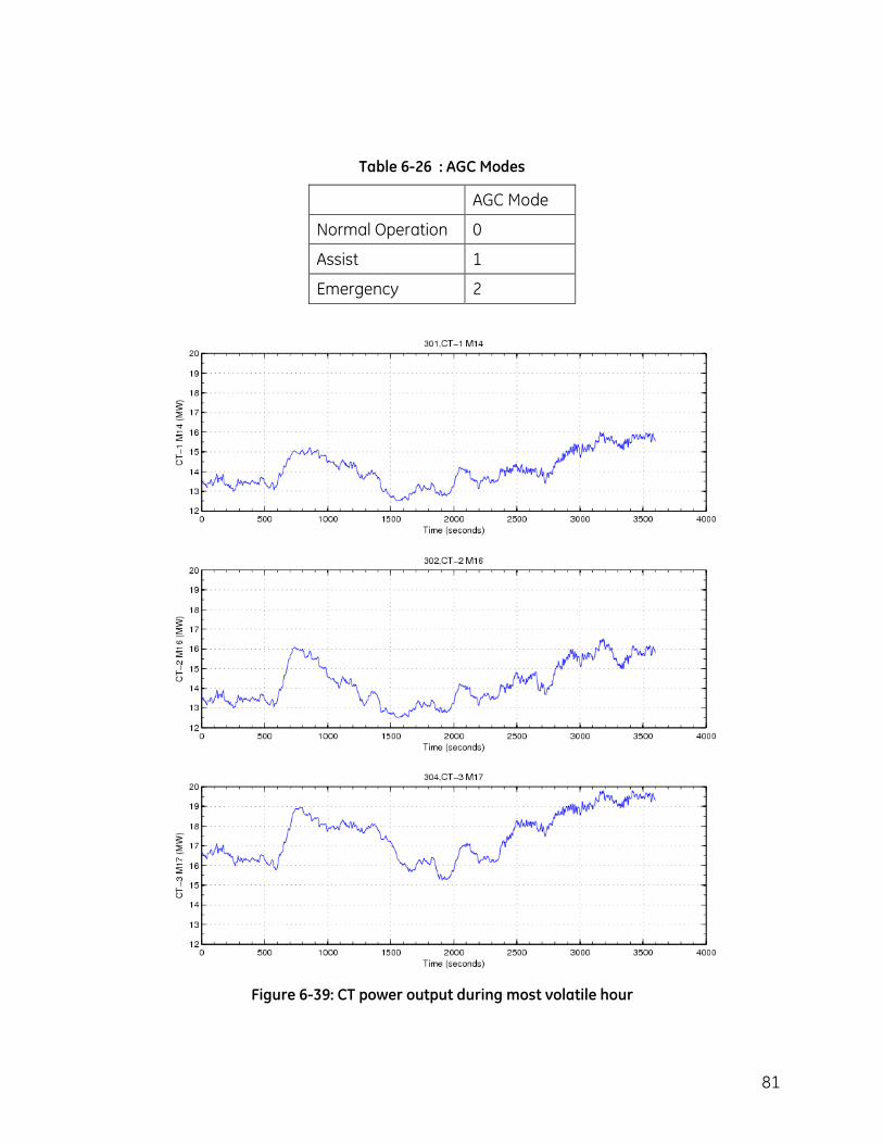
81

Table 6-26 : AGC Modes

AGC Mode

Normal Operation 0

Assist 1

Emergency 2

Figure 6-39: CT power output during most volatile hour

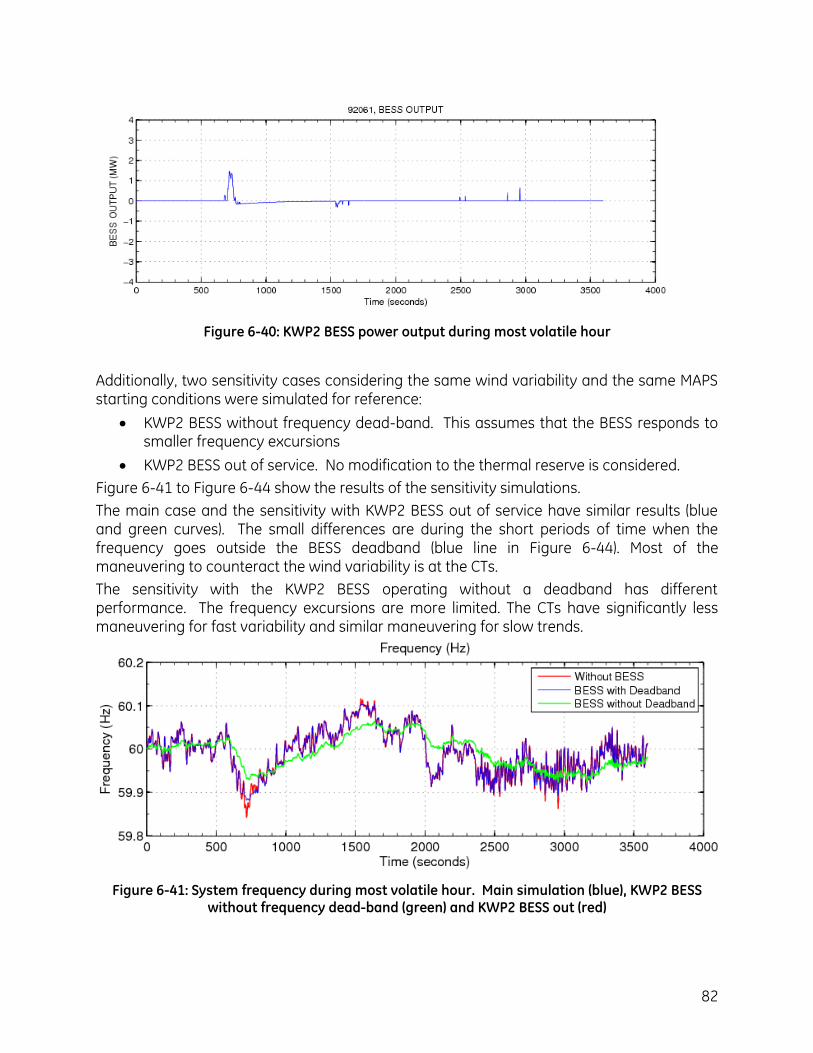
82

Figure 6-40: KWP2 BESS power output during most volatile hour

Additionally, two sensitivity cases considering the same wind variability and the same MAPS starting conditions were simulated for reference:

KWP2 BESS without frequency dead-band. This assumes that the BESS responds to smaller frequency excursions

KWP2 BESS out of service. No modification to the thermal reserve is considered.

Figure 6-41 to Figure 6-44 show the results of the sensitivity simulations.

The main case and the sensitivity with KWP2 BESS out of service have similar results (blue and green curves). The small differences are during the short periods of time when the frequency goes outside the BESS deadband (blue line in Figure 6-44). Most of the maneuvering to counteract the wind variability is at the CTs.

The sensitivity with the KWP2 BESS operating without a deadband has different performance. The frequency excursions are more limited. The CTs have significantly less maneuvering for fast variability and similar maneuvering for slow trends.

Figure 6-41: System frequency during most volatile hour. Main simulation (blue), KWP2 BESS without frequency dead-band (green) and KWP2 BESS out (red)

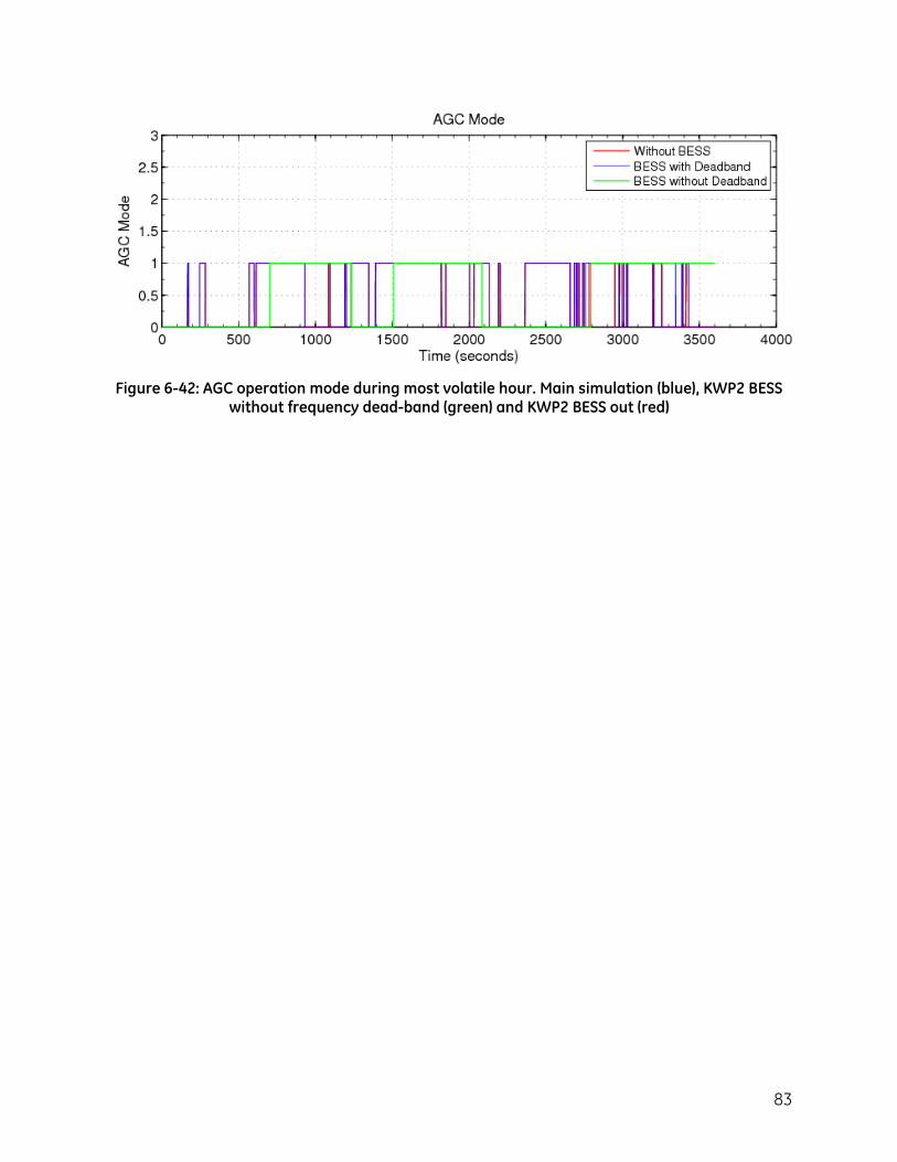
83

Figure 6-42: AGC operation mode during most volatile hour. Main simulation (blue), KWP2 BESS without frequency dead-band (green) and KWP2 BESS out (red)

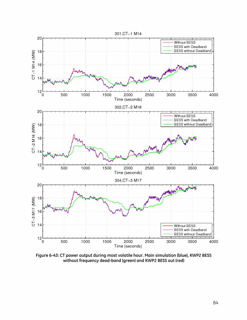
84

Figure 6-43: CT power output during most volatile hour. Main simulation (blue), KWP2 BESS without frequency dead-band (green) and KWP2 BESS out (red)

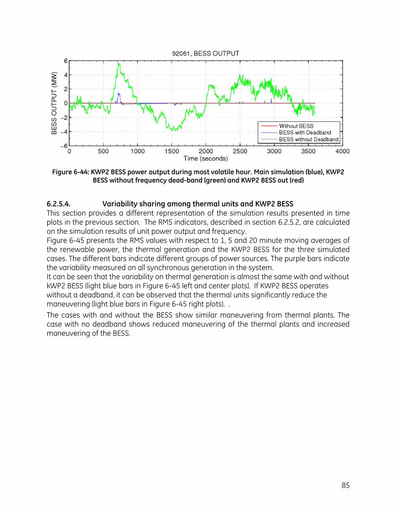
85

Figure 6-44: KWP2 BESS power output during most volatile hour. Main simulation (blue), KWP2 BESS without frequency dead-band (green) and KWP2 BESS out (red)

6.2.5.4. Variability sharing among thermal units and KWP2 BESS This section provides a different representation of the simulation results presented in time plots in the previous section. The RMS indicators, described in section 6.2.5.2, are calculated on the simulation results of unit power output and frequency. Figure 6-45 presents the RMS values with respect to 1, 5 and 20 minute moving averages of the renewable power, the thermal generation and the KWP2 BESS for the three simulated cases. The different bars indicate different groups of power sources. The purple bars indicate the variability measured on all synchronous generation in the system. It can be seen that the variability on thermal generation is almost the same with and without kWP2 BESS (light blue bars in Figure 6-45 left and center plots). If KWP2 BESS operates without a deadband, it can be observed that the thermal units significantly reduce the maneuvering (light blue bars in Figure 6-45 right plots). .

The cases with and without the BESS show similar maneuvering from thermal plants. The case with no deadband shows reduced maneuvering of the thermal plants and increased maneuvering of the BESS.

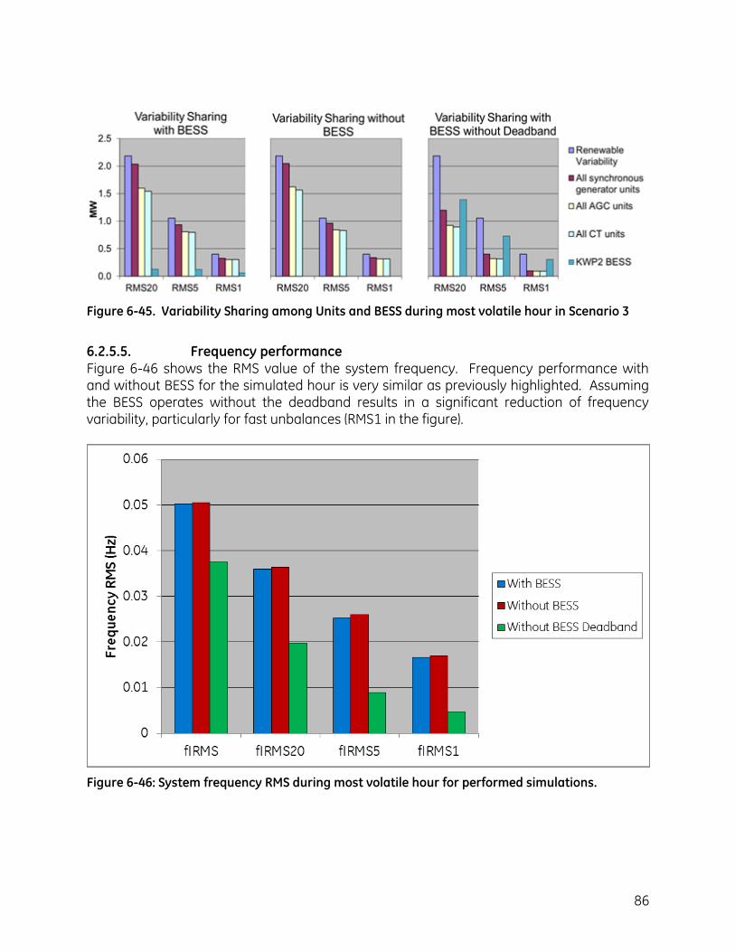
86

Figure 6-45. Variability Sharing among Units and BESS during most volatile hour in Scenario 3

6.2.5.5. Frequency performance Figure 6-46 shows the RMS value of the system frequency. Frequency performance with and without BESS for the simulated hour is very similar as previously highlighted. Assuming the BESS operates without the deadband results in a significant reduction of frequency variability, particularly for fast unbalances (RMS1 in the figure).

Figure 6-46: System frequency RMS during most volatile hour for performed simulations.

87

6.2.5.6. Observations

Based on the available information, the system with the assumed reserve requirement has enough range to counteract most volatile hour

Most challenging hours regarding volatility (as defined in this section) occur during the night. There are normally more regulating units are committed during the day, when the additional PV variability operates.

The ramp rate capability of the units thermal seems adequate for the level of variability observed.

KWP2 BESS is effective in mitigating variations if the frequency is outside the deadband of +/- 0.1 Hz.

The frequency deadband of the BESS reduces the operation of the BESS for frequency excursions below +/-Hz, so all regulating response within that deadband is provided by thermal units.

88

6.2.6. Loss of load events 6.2.6.1. Conceptual discussion

As wind and solar penetration increases, baseload thermal units are required to operate at minimum dispatch power (respecting down-reserves requirement) for many more hours of the year.

The largest anticipated loss-of-load event is 20 MW. Per MECO operating practices, the system carries 5 MW of down-reserves on thermal resources during the day and 3 MW at night. The KWP2 BESS is capable of charging at 10 MW during overfrequency events, thereby contributing 10 MW to down reserves. Another possible source of down-reserves is from wind and solar plants, by curtailing output in response to governor action and/or AGC control. HC&S is not normally counted for down reserve, but is likely to reduce power output in large overfrequency event.

A screening analysis was performed to determine if these three sources of down-reserves could provide enough down-range to compensate for a 20 MW loss-of-load event. The concern in the MECO system has been to avoid trips of the steam turbines in the Maalaea combined cycle plant due to significant mechanical power reduction after the loss-of-load events. This analysis provides insight on the available down-range in the combined cycle plants and other resources in the system during the simulated year of operation. Figure 6-47 shows the results of that analysis.

The green trace represents the worst-case loss of load event, 20 MW.

The blue trace is a duration curve of the thermal plant down-range, calculated from the dispatch for each hour and the minimum power operating limit for each thermal unit. For about 4300 hours, the thermal unit down-range is less than 20 MW and not adequate to cover a 20 MW loss of load event.

The red curve shows the sum of thermal plant down-range plus wind and solar power. This curve is above 20 MW for all but 54 hours of the year.

The purple (top) curve shows the sum of thermal down range, wind+solar power, and the 10 MW charging capacity of the KWP2 BESS. This curve is above 20 MW for all but one hour of the year.

This analysis indicates that if thermal plants, wind plants, central solar plants, and the KWP2 BESS are all equipped with frequency-responsive governors, there is adequate control-range to compensate for a 20 MW loss of load event. Further dynamic modeling analysis would be required to tune the governor controls and ensure that the transient responses do not force thermal units below their minimum power limits, which would introduce the risk of unit trips.

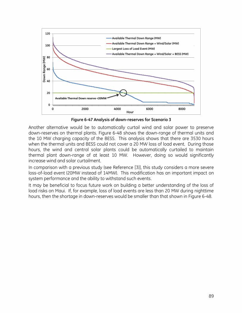
89

0

20

40

60

80

100

120

0 2000 4000 6000 8000

Do

wn

Ra

ng

e (

MW

)

Hour

Available Thermal Down Range (MW)

Available Thermal Down Range + Wind/Solar (MW)

Largest Loss of Load Event (MW)

Available Thermal Down Range + Wind/Solar + BESS (MW)

Available Thermal Down reserve <20MW

Figure 6-47 Analysis of down-reserves for Scenario 3

Another alternative would be to automatically curtail wind and solar power to preserve down-reserves on thermal plants. Figure 6-48 shows the down-range of thermal units and the 10 MW charging capacity of the BESS. This analysis shows that there are 3530 hours when the thermal units and BESS could not cover a 20 MW loss of load event. During those hours, the wind and central solar plants could be automatically curtailed to maintain thermal plant down-range of at least 10 MW. However, doing so would significantly increase wind and solar curtailment.

In comparison with a previous study (see Reference [3)], this study considers a more severe loss-of-load event (20MW instead of 14MW). This modification has an important impact on system performance and the ability to withstand such events.

It may be beneficial to focus future work on building a better understanding of the loss of load risks on Maui. If, for example, loss of load events are less than 20 MW during nighttime hours, then the shortage in down-reserves would be smaller than that shown in Figure 6-48.

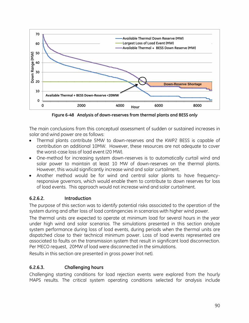
90

0

10

20

30

40

50

60

70

0 2000 4000 6000 8000

Do

wn

Ra

ng

e (

MW

)

Hour

Available Thermal Down Reserve (MW)

Largest Loss of Load Event (MW)

Available Thermal + BESS Down Reserve (MW)

Available Thermal + BESS Down-Reserve <20MW

Down-Reserve Shortage

Figure 6-48 Analysis of down-reserves from thermal plants and BESS only

The main conclusions from this conceptual assessment of sudden or sustained increases in solar and wind power are as follows:

Thermal plants contribute 5MW to down-reserves and the KWP2 BESS is capable of contribution an additional 10MW. However, these resources are not adequate to cover the worst-case loss of load event (20 MW).

One-method for increasing system down-reserves is to automatically curtail wind and solar power to maintain at least 10 MW of down-reserves on the thermal plants. However, this would significantly increase wind and solar curtailment.

Another method would be for wind and central solar plants to have frequency-responsive governors, which would enable them to contribute to down reserves for loss of load events. This approach would not increase wind and solar curtailment.

6.2.6.2. Introduction

The purpose of this section was to identify potential risks associated to the operation of the system during and after loss of load contingencies in scenarios with higher wind power.

The thermal units are expected to operate at minimum load for several hours in the year under high wind and solar scenarios. The simulations presented in this section analyze system performance during loss of load events, during periods when the thermal units are dispatched close to their technical minimum power. Loss of load events represented are associated to faults on the transmission system that result in significant load disconnection. Per MECO request, 20MW of load were disconnected in the simulations.

Results in this section are presented in gross power (not net).

6.2.6.3. Challenging hours

Challenging starting conditions for load rejection events were explored from the hourly MAPS results. The critical system operating conditions selected for analysis include

91

renewable curtailment. If there is curtailment, the thermal units are dispatched at the minimum acceptable level (technical minimum plus minimum down reserve).

Simulations were performed for Baseline and Scenario 3 for two cases as follows:

High load and curtailment condition (Hour 4885, valid for Scenario 3)

Low Load with curtailment condition (Hour 1753, valid for Baseline and Sc3)

These conditions were observed in the production cost simulation on Saturday July 23rd at 1pm (Hour 4885) and on Tuesday March 15 at 1am (Hour 1753). The thermal units were substantially backed down and the system was carrying low down-reserve.

High Load Hour

The units committed during Hour 4885 hour are:

M14, M16 and M15 (dual-train),


K3, K4 and HC&S

Both combined cycle plants were operating at their minimum power level. The power output of KWP1, KWP2 and Auwahi were 26 MW, 19 MW and 18 MW respectively. The total centralized PV power output was 2.3 MW. Total distributed PV power output was 26 MW. The total load was at 195 MW. The total up reserve on thermal generation was 21 MW.

Low Load Hour

The units committed during Hour 1753 hour are:


M17 and M18 (single-train),

K3 and HC&S

Both combined cycle plants were operating at their minimum power level. The power output of KWP1, KWP2 and Auwahi were 28.1 MW, 0 MW and 1.25 MW respectively. Wind plant KWP2 was curtailed and the hour being night time hour, there was no power output from PV plants. The total load was at 99.5 MW. The total up reserve on thermal generation was 16.1 MW.

The unit dispatch levels from MAPS for these hours is presented in Appendix 8.

6.2.6.4. Time Simulations Simulations of 20MW load disconnections were performed considering the starting conditions described in the previous sections.

As discussed in section 6.2.4, reduction of wind and solar plant production may be required to counteract the amount of disconnected load without excessive reduction of thermal plants. This section considers simulations with and without frequency droop response at the wind and solar plants.

In the case with frequency droop response, KWP2 was modeled with 4% droop and 36 mHz deadband, Auwahi Plant was modeled with 4% droop and 0.2 Hz deadband and centralized PV was modeled with 4% droop and 36 mHz deadband. No over-frequency and Hz/sec trips were considered for the simulation. KWP1 was assumed not to provide frequency droop response. These assumptions were based on PPA information provided to GE.

92

6.2.6.5. High Load

Hour 4885 – No droop response from renewable plants

A 20MW load rejection caused a maximum frequency excursion of 60.47 Hz. The mechanical power excursions are summarized in Table 6-27.

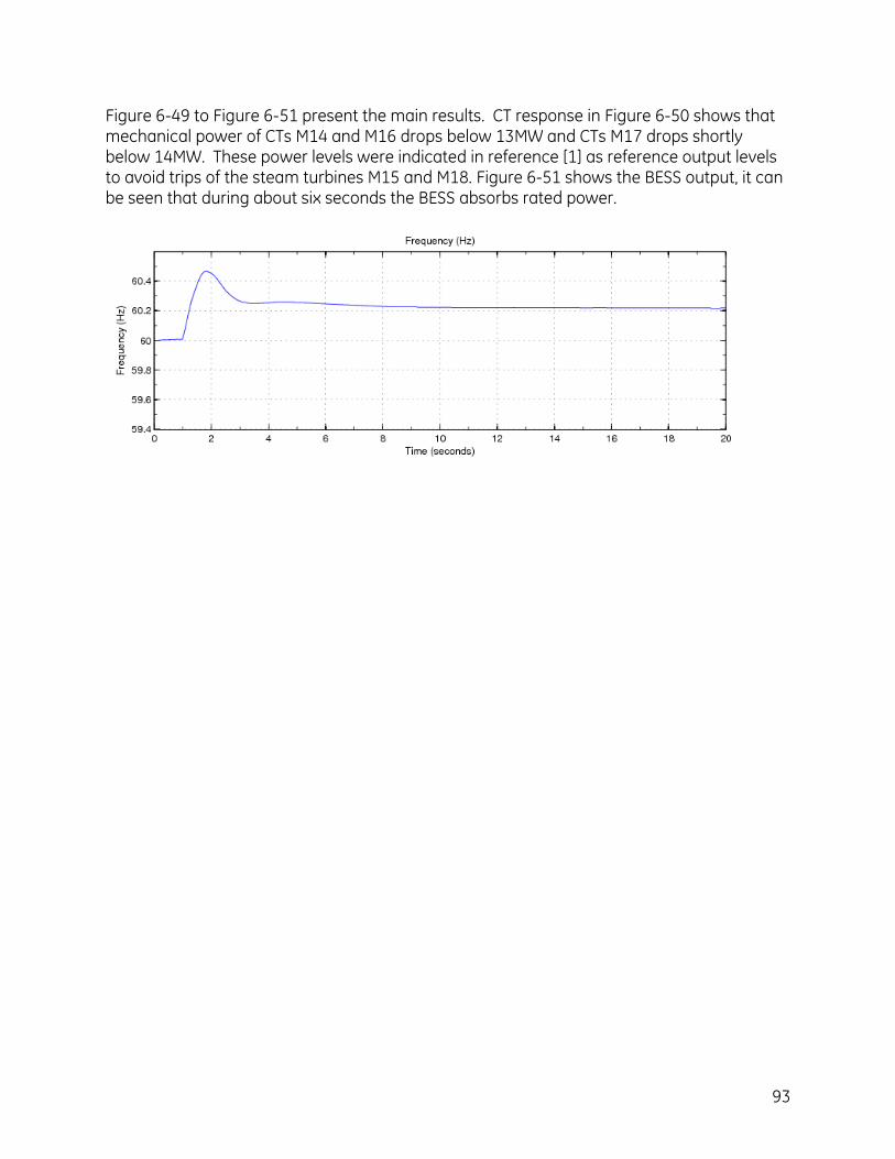
93

Figure 6-49 to Figure 6-51 present the main results. CT response in Figure 6-50 shows that mechanical power of CTs M14 and M16 drops below 13MW and CTs M17 drops shortly below 14MW. These power levels were indicated in reference [1] as reference output levels to avoid trips of the steam turbines M15 and M18. Figure 6-51 shows the BESS output, it can be seen that during about six seconds the BESS absorbs rated power.

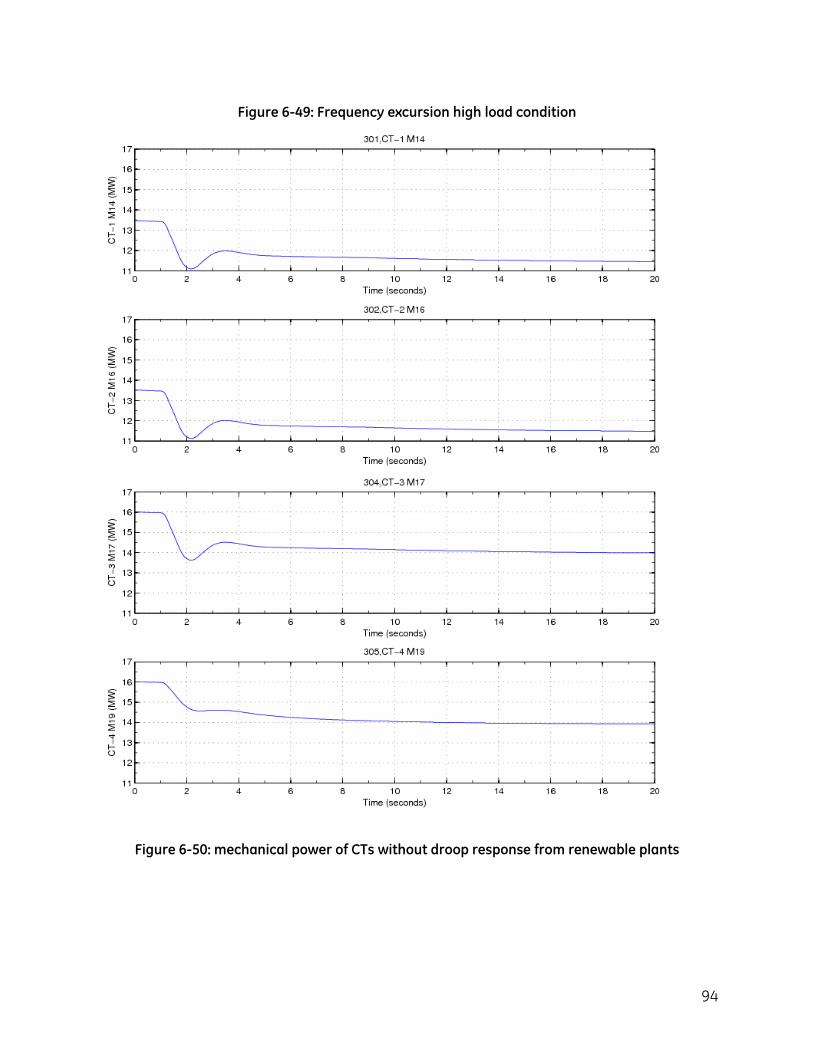
94

Figure 6-49: Frequency excursion high load condition

Figure 6-50: mechanical power of CTs without droop response from renewable plants

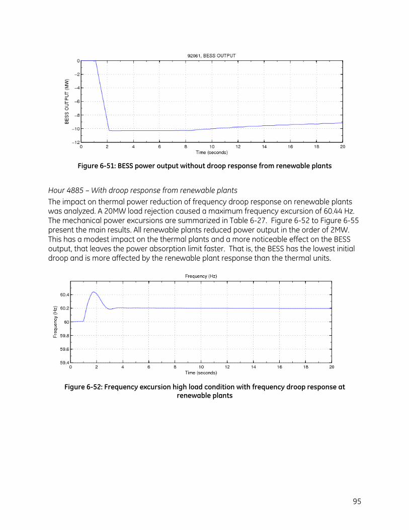
95

Figure 6-51: BESS power output without droop response from renewable plants

Hour 4885 – With droop response from renewable plants

The impact on thermal power reduction of frequency droop response on renewable plants was analyzed. A 20MW load rejection caused a maximum frequency excursion of 60.44 Hz. The mechanical power excursions are summarized in Table 6-27. Figure 6-52 to Figure 6-55 present the main results. All renewable plants reduced power output in the order of 2MW. This has a modest impact on the thermal plants and a more noticeable effect on the BESS output, that leaves the power absorption limit faster. That is, the BESS has the lowest initial droop and is more affected by the renewable plant response than the thermal units.

Figure 6-52: Frequency excursion high load condition with frequency droop response at renewable plants

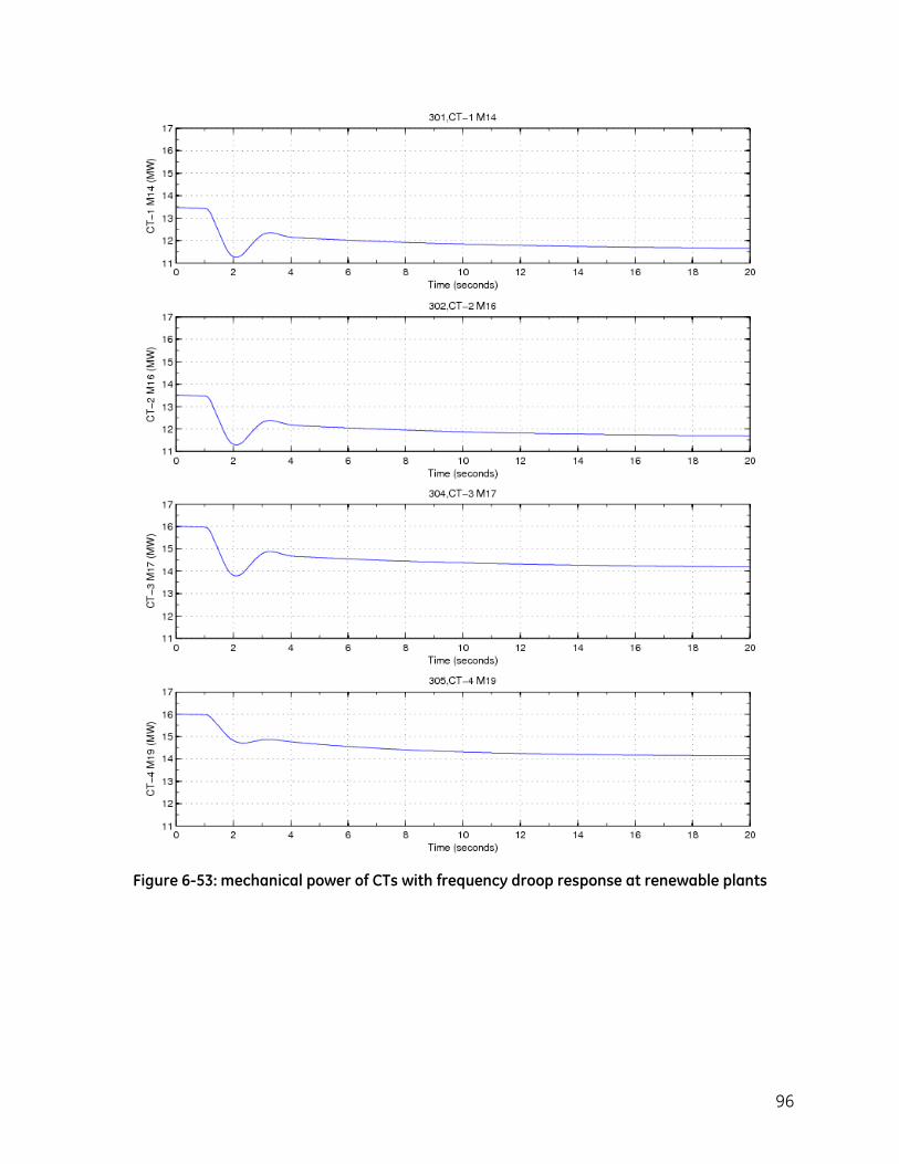
96

Figure 6-53: mechanical power of CTs with frequency droop response at renewable plants

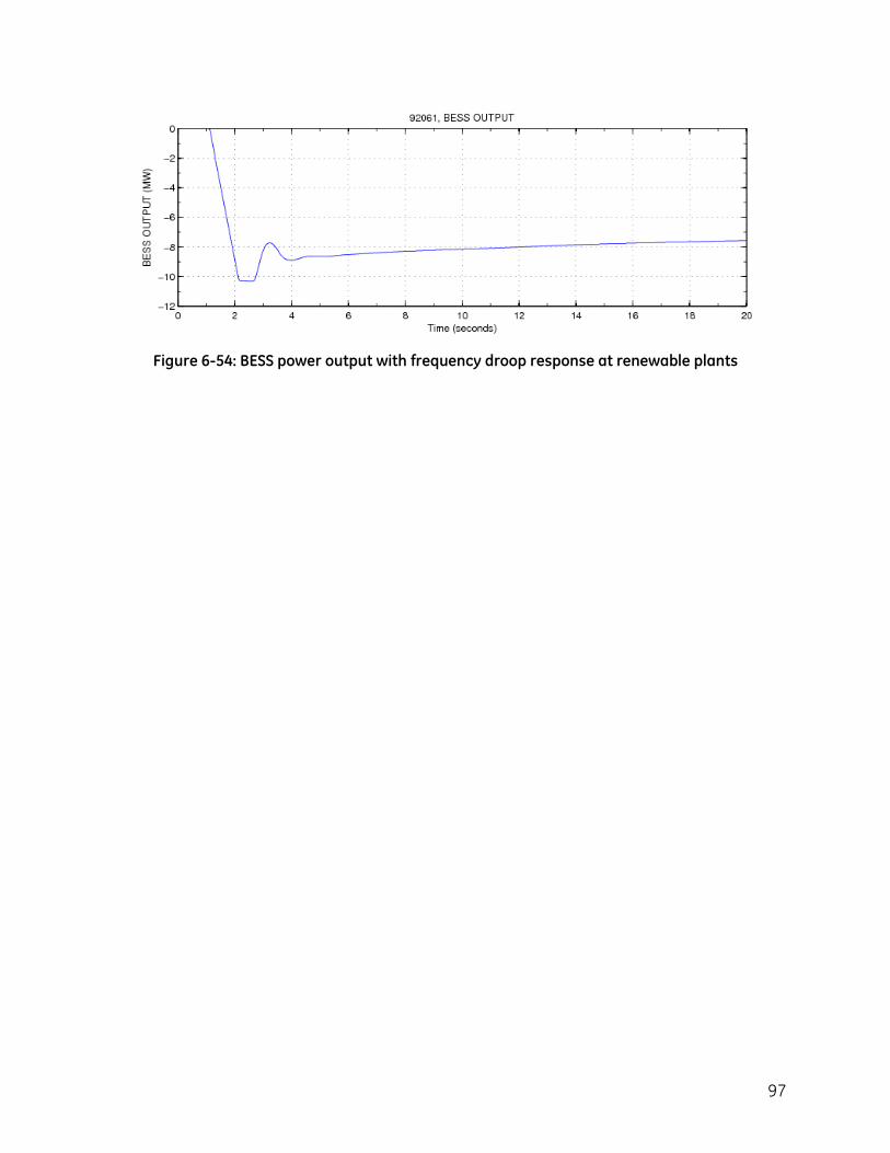
97

Figure 6-54: BESS power output with frequency droop response at renewable plants

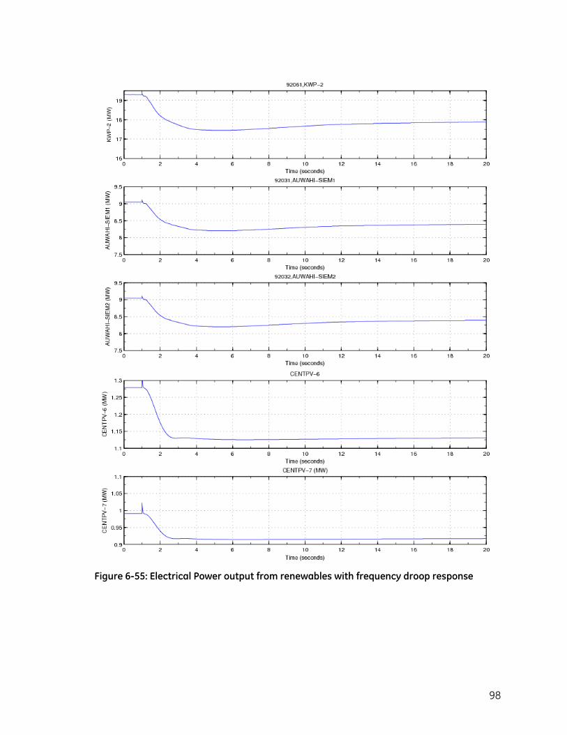
98

Figure 6-55: Electrical Power output from renewables with frequency droop response

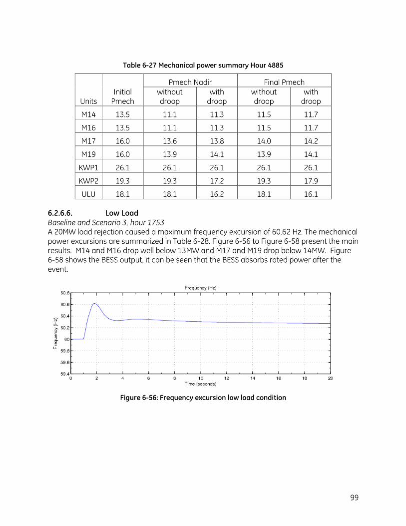
99

Table 6-27 Mechanical power summary Hour 4885

Units Initial

Pmech

Pmech Nadir Final Pmech

without droop

with droop

without droop

with droop

M14 13.5 11.1 11.3 11.5 11.7

M16 13.5 11.1 11.3 11.5 11.7

M17 16.0 13.6 13.8 14.0 14.2

M19 16.0 13.9 14.1 13.9 14.1

KWP1 26.1 26.1 26.1 26.1 26.1

KWP2 19.3 19.3 17.2 19.3 17.9

ULU 18.1 18.1 16.2 18.1 16.1

6.2.6.6. Low Load Baseline and Scenario 3, hour 1753 A 20MW load rejection caused a maximum frequency excursion of 60.62 Hz. The mechanical power excursions are summarized in Table 6-28. Figure 6-56 to Figure 6-58 present the main results. M14 and M16 drop well below 13MW and M17 and M19 drop below 14MW. Figure 6-58 shows the BESS output, it can be seen that the BESS absorbs rated power after the event.

Figure 6-56: Frequency excursion low load condition

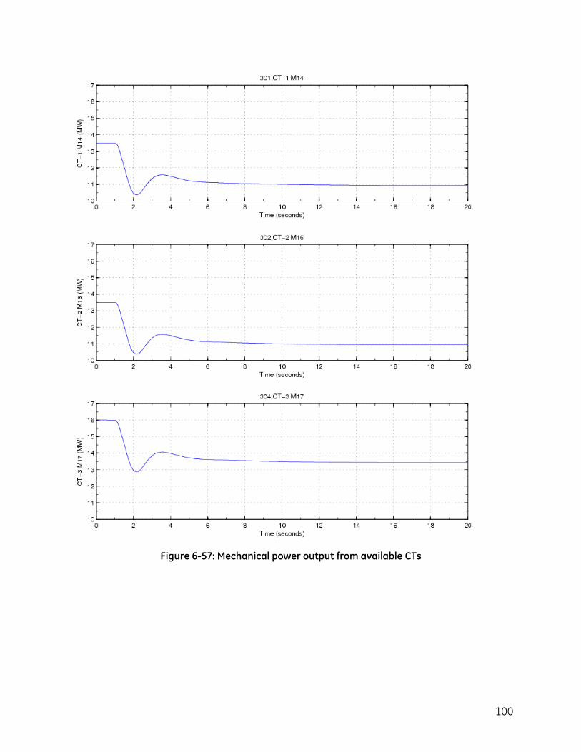
100

Figure 6-57: Mechanical power output from available CTs

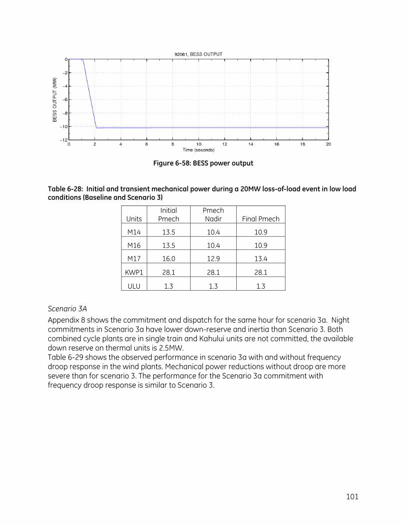
101

Figure 6-58: BESS power output

Table 6-28: Initial and transient mechanical power during a 20MW loss-of-load event in low load conditions (Baseline and Scenario 3)

Units Initial

Pmech Pmech Nadir Final Pmech

M14 13.5 10.4 10.9

M16 13.5 10.4 10.9

M17 16.0 12.9 13.4

KWP1 28.1 28.1 28.1

ULU 1.3 1.3 1.3

Scenario 3A

Appendix 8 shows the commitment and dispatch for the same hour for scenario 3a. Night commitments in Scenario 3a have lower down-reserve and inertia than Scenario 3. Both combined cycle plants are in single train and Kahului units are not committed, the available down reserve on thermal units is 2.5MW. Table 6-29 shows the observed performance in scenario 3a with and without frequency droop response in the wind plants. Mechanical power reductions without droop are more severe than for scenario 3. The performance for the Scenario 3a commitment with frequency droop response is similar to Scenario 3.

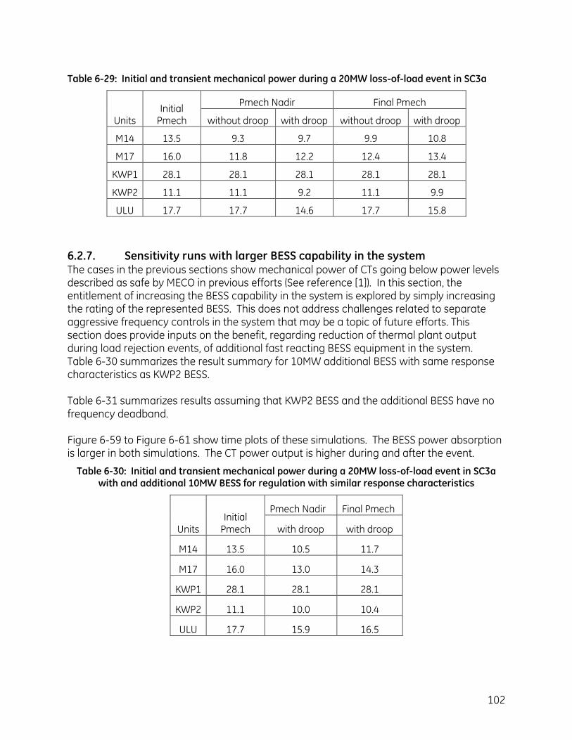
102

Table 6-29: Initial and transient mechanical power during a 20MW loss-of-load event in SC3a

Units Initial

Pmech


without droop with droop without droop with droop

M14 13.5 9.3 9.7 9.9 10.8

M17 16.0 11.8 12.2 12.4 13.4

KWP1 28.1 28.1 28.1 28.1 28.1

KWP2 11.1 11.1 9.2 11.1 9.9

ULU 17.7 17.7 14.6 17.7 15.8

6.2.7. Sensitivity runs with larger BESS capability in the system The cases in the previous sections show mechanical power of CTs going below power levels described as safe by MECO in previous efforts (See reference [1]). In this section, the entitlement of increasing the BESS capability in the system is explored by simply increasing the rating of the represented BESS. This does not address challenges related to separate aggressive frequency controls in the system that may be a topic of future efforts. This section does provide inputs on the benefit, regarding reduction of thermal plant output during load rejection events, of additional fast reacting BESS equipment in the system. Table 6-30 summarizes the result summary for 10MW additional BESS with same response characteristics as KWP2 BESS. Table 6-31 summarizes results assuming that KWP2 BESS and the additional BESS have no frequency deadband. Figure 6-59 to Figure 6-61 show time plots of these simulations. The BESS power absorption is larger in both simulations. The CT power output is higher during and after the event.

Table 6-30: Initial and transient mechanical power during a 20MW loss-of-load event in SC3a with and additional 10MW BESS for regulation with similar response characteristics

Units Initial

Pmech


with droop with droop

M14 13.5 10.5 11.7

M17 16.0 13.0 14.3

KWP1 28.1 28.1 28.1

KWP2 11.1 10.0 10.4

ULU 17.7 15.9 16.5

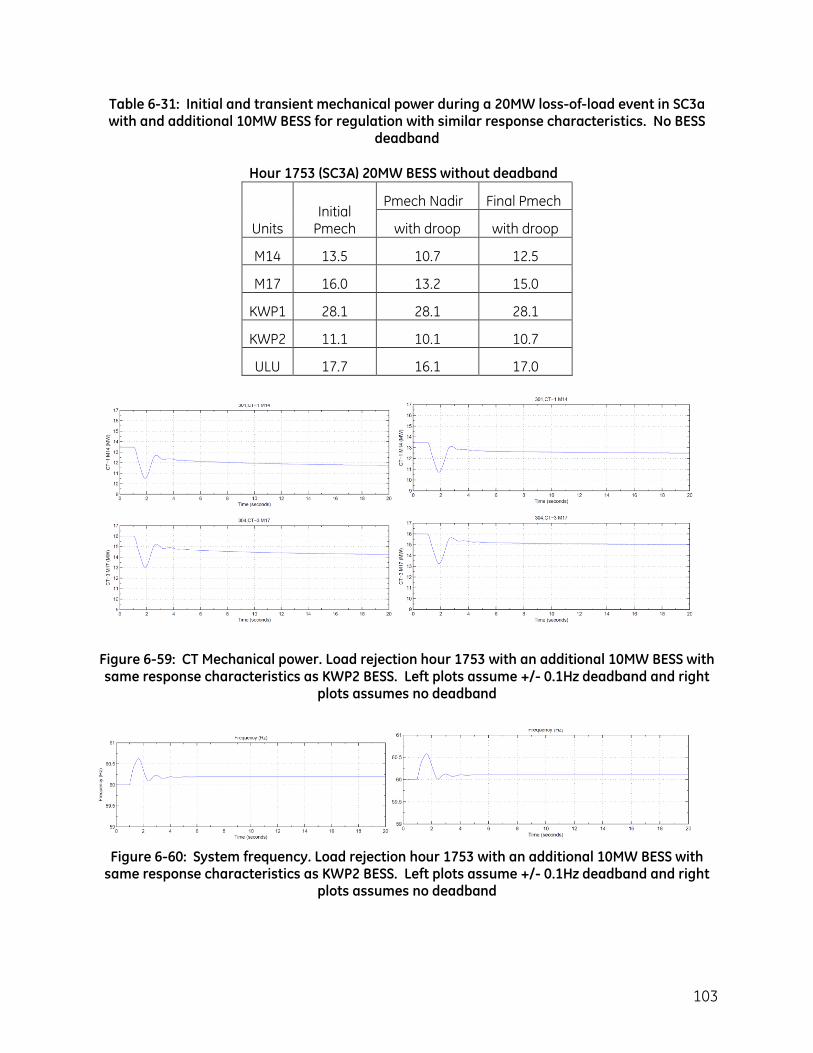
103

Table 6-31: Initial and transient mechanical power during a 20MW loss-of-load event in SC3a with and additional 10MW BESS for regulation with similar response characteristics. No BESS

deadband

Hour 1753 (SC3A) 20MW BESS without deadband

Units Initial

Pmech


with droop with droop

M14 13.5 10.7 12.5

M17 16.0 13.2 15.0

KWP1 28.1 28.1 28.1

KWP2 11.1 10.1 10.7

ULU 17.7 16.1 17.0

Figure 6-59: CT Mechanical power. Load rejection hour 1753 with an additional 10MW BESS with same response characteristics as KWP2 BESS. Left plots assume +/- 0.1Hz deadband and right

plots assumes no deadband

Figure 6-60: System frequency. Load rejection hour 1753 with an additional 10MW BESS with same response characteristics as KWP2 BESS. Left plots assume +/- 0.1Hz deadband and right

plots assumes no deadband

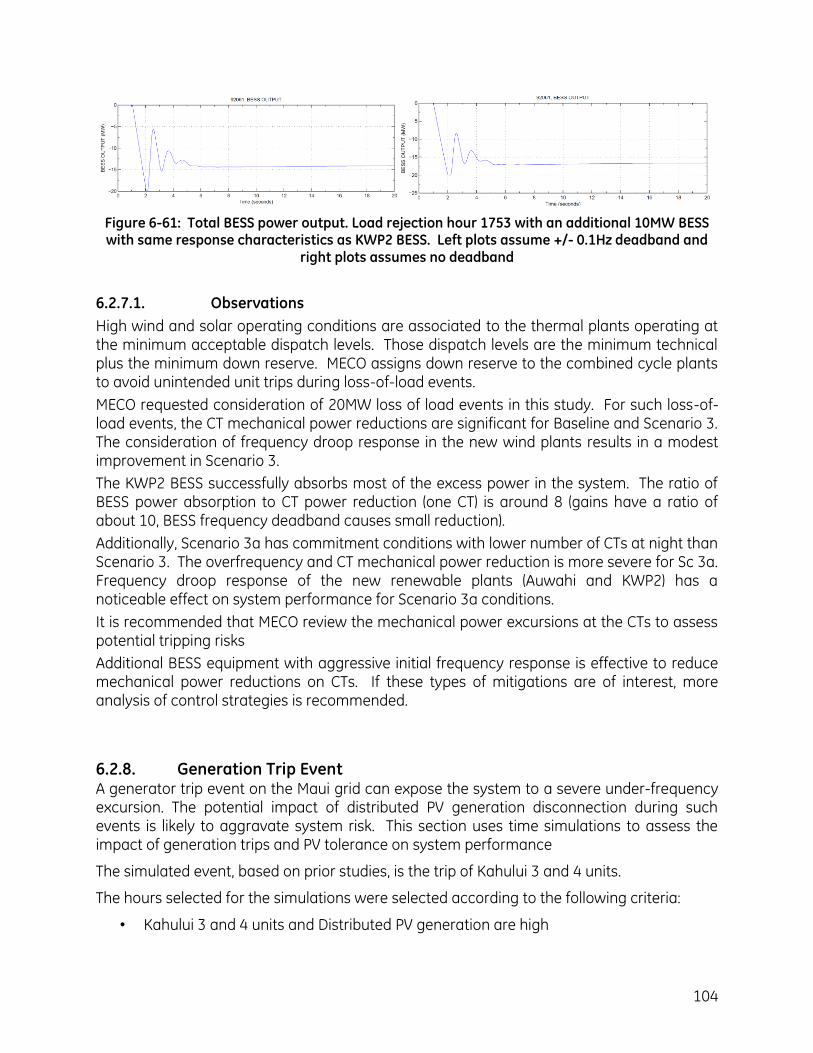
104

Figure 6-61: Total BESS power output. Load rejection hour 1753 with an additional 10MW BESS with same response characteristics as KWP2 BESS. Left plots assume +/- 0.1Hz deadband and

right plots assumes no deadband

6.2.7.1. Observations

High wind and solar operating conditions are associated to the thermal plants operating at the minimum acceptable dispatch levels. Those dispatch levels are the minimum technical plus the minimum down reserve. MECO assigns down reserve to the combined cycle plants to avoid unintended unit trips during loss-of-load events.

MECO requested consideration of 20MW loss of load events in this study. For such loss-of-load events, the CT mechanical power reductions are significant for Baseline and Scenario 3. The consideration of frequency droop response in the new wind plants results in a modest improvement in Scenario 3.

The KWP2 BESS successfully absorbs most of the excess power in the system. The ratio of BESS power absorption to CT power reduction (one CT) is around 8 (gains have a ratio of about 10, BESS frequency deadband causes small reduction).

Additionally, Scenario 3a has commitment conditions with lower number of CTs at night than Scenario 3. The overfrequency and CT mechanical power reduction is more severe for Sc 3a. Frequency droop response of the new renewable plants (Auwahi and KWP2) has a noticeable effect on system performance for Scenario 3a conditions.

It is recommended that MECO review the mechanical power excursions at the CTs to assess potential tripping risks

Additional BESS equipment with aggressive initial frequency response is effective to reduce mechanical power reductions on CTs. If these types of mitigations are of interest, more analysis of control strategies is recommended.

6.2.8. Generation Trip Event A generator trip event on the Maui grid can expose the system to a severe under-frequency excursion. The potential impact of distributed PV generation disconnection during such events is likely to aggravate system risk. This section uses time simulations to assess the impact of generation trips and PV tolerance on system performance

The simulated event, based on prior studies, is the trip of Kahului 3 and 4 units.

The hours selected for the simulations were selected according to the following criteria:

• Kahului 3 and 4 units and Distributed PV generation are high

105

• Up-range of the system is comparatively low

• High renewable generation

The table below presents a summary of the initial conditions considered for the generation trip simulations for Baseline and Scenario 3. In both cases the renewable power production is high and the reserve requirement is at maximum level around 27MW (see Figure 5-16). As expected, there is more distributed PV generation in Sc3. The higher renewable generation in Sc3 results in a lower dispatch level of Kahului 3 and 4. For this reason, the tripped thermal generation is lower in Sc3.

Table 6-32: Initial conditions for generation trip simulations

Scenario Total Ren Dist PV Load

Operating

reserve

Tripped

gen

Baseline 50 11 192 27 23

Sc3 72 22 192 27 14

Based on these intial conditions, time simulations of the Kahului units trip were performed. Table 6-33 shows a summary of the results and Figure 6-62 presents the system frequency and the KWP2 BESS power response.

Cases 4A and 4D (red curves) assume that distributed PV does not trip. As expected from the initial conditions, the frequency response for Scenario 3 was better than for Baseline. In both cases, the increased reserve requirement due to renewable generation (around 27MW) supports the generation trip event and there is no load shedding operation. The BESS power plots show the fast frequency regulation response. In Case 4A the BESS reaches full power output.

Cases 4B and 4E (green curves) assume that distributed PV trips due to the system underfrequency.

In case 4B, the system reaches 59.3Hz before PV trips. The PV trips cause a significant additional frequency excursion that triggers about 11MW of load shedding. In case 4B, the BESS reaches full power output.

In Case 4E the frequency excursion before PV trips is more modest. For purposes of understanding the impact of PV trip, it was assumed that PV would trip around 59.7 Hz. This is rather pessimistic, but useful for the analysis. In this case, the distributed PV generation disconnected was larger than in baseline (22MW in Sc3 and 11MW in baseline). The frequency excursion in case 4E triggers the same UFLS stages as in case 4B. In case 4E, the BESS also reaches full power output.

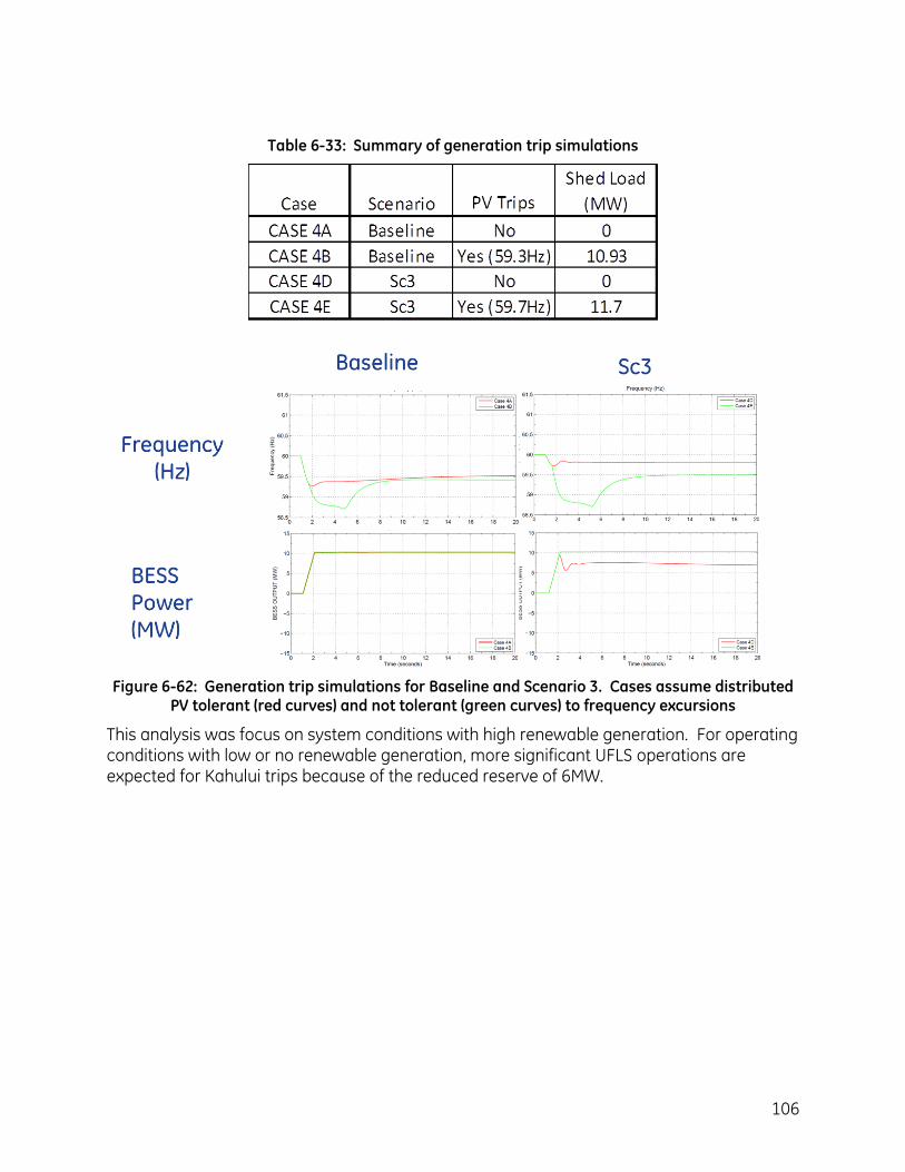
106

Table 6-33: Summary of generation trip simulations

Figure 6-62: Generation trip simulations for Baseline and Scenario 3. Cases assume distributed PV tolerant (red curves) and not tolerant (green curves) to frequency excursions

This analysis was focus on system conditions with high renewable generation. For operating conditions with low or no renewable generation, more significant UFLS operations are expected for Kahului trips because of the reduced reserve of 6MW.

107

7.0 Observations and Conclusions A summary of observations and conclusions of the results is presented below.

7.1. Under Business as Usual – Without any change to system operating practices

7.1.1. Delivered Energy from Solar and Wind The Baseline had 21% of load energy met from wind and solar.

Scenario 3 had 23% of load energy met from wind and solar.

The Baseline had 20% and Scenario 3 had 23% renewable energy curtailment.

42% of the additional renewable energy available in Scenario 3 was curtailed

7.1.2. Variable Cost of Operation There was a 3.2% decrease in variable cost of operation in Scenario 3

o This does not include the cost of the wind/solar energy

7.1.3. Carbon Emissions Scenario 3 had a 3.4% reduction in carbon emissions compared to the baseline.

7.1.4. Operating Reserves Requirement The MECO system is dominated by wind. Therefore, the operating reserve

requirement is practically identical for both the Baseline and Scenario 3. The baseline had a maximum of roughly 26MW and Scenario 3 had a maximum of 27MW. KWP2 BESS reduce the is capable of supplying approximately 10MW of reserves, depending on its state of charge, with the remainder supplied by thermal generation.

This study focused on integrating more solar resources into the Maui grid. The technical analysis assumed that operating reserves would be allocated to cover variability of both wind and solar resources. A new method for calculating reserve requirements was developed, and that method produced reserve requirement curves that are significantly different from those presently used for Maui grid operations.

The reserve requirement developed for this study would generally require more reserves for lower levels of wind and solar contributions and less reserves for higher levels of wind and solar contributions, as compared to the existing reserve requirements for the system. However, it is difficult to compare the two methods since the new reserve requirement also adds reserves for solar power in addition to the wind power where the existing reserve method only carries reserves for the wind power added to the system.

108

Further technical analysis is recommended to quantify curtailment impacts of the reserve requirements used in this study and to explore if and how the existing reserve practices should be changed to cover both wind and solar variability.

7.1.5. Non-synchronous Generation Online As more and more renewables are absorbed into the Maui grid, more thermal

generation is displaced. o In scenario 3, the online non-synchronous generation was as high as 57% of

the total online generation. There were 132 hours or 1.5 % of the year, where the online non-synchronous penetration was greater than 50%

o The maximum hourly load energy served by wind and solar, in Scenario 3, was 61%.

7.1.6. Sub-hourly response to Solar and Wind Variability

Based on the available information and the generation response assumed in the model, the system with the assumed reserve requirement has enough range to counteract most volatile hour of the study year.

Most challenging hours regarding volatility (as defined in this report) occur during the night. There are normally more regulating units committed during the day, when the additional PV variability operates.

The ramp rate capability of the thermal units seems adequate for the level of variability observed.

KWP2 BESS is effective in mitigating renewable power variations if the frequency is outside the deadband of +/- 0.1 Hz.

The frequency deadband of the BESS reduces the operation of the BESS for frequency excursions below +/-0.1Hz, so all regulating response within that deadband is provided by thermal units.

7.1.7. Sub-hourly response: Solar and Wind curtailemt

It is recommended that, automatic or operator curtailment be relatively fast to avoid consuming contingency down range during important number of hours in the year. Assuming no operation/decision delay:

o There are 150 periods of 5 minutes when renewables need to be curtailed between 2 and 4 MW in the baseline. There are 230 periods in Scenario 3.

o There are less than five challenging periods (within 5 minutes) in the year of operation analyzed requiring 8 to 6 MW of curtailment.

The existing BESS operation on overfrequency could allow for some additional delay in the curtailment response

7.1.8. Sub-hourly response to Loss-of-Load events

MECO requested consideration of 20MW loss of load events in this study. For such loss-of-load events, the CT mechanical power reductions are significant for Baseline and Scenario 3.

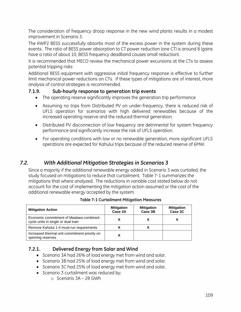
109

The consideration of frequency droop response in the new wind plants results in a modest improvement in Scenario 3.

The KWP2 BESS successfully absorbs most of the excess power in the system during these events. The ratio of BESS power absorption to CT power reduction (one CT) is around 8 (gains have a ratio of about 10, BESS frequency deadband causes small reduction).

It is recommended that MECO review the mechanical power excursions at the CTs to assess potential tripping risks

Additional BESS equipment with aggressive initial frequency response is effective to further limit mechanical power reductions on CTs. If these types of mitigations are of interest, more analysis of control strategies is recommended.

7.1.9. Sub-hourly response to generation trip events The operating reserve significantly improves the generation trip performance

Assuming no trips from Distributed PV on under-frequency, there is reduced risk of UFLS operation for scenarios with high delivered renewables because of the increased operating reserve and the reduced thermal generation.

Distributed PV disconnection of low frequency are detrimental for system frequency performance and significantly increase the risk of UFLS operation.

For operating conditions with low or no renewable generation, more significant UFLS operations are expected for Kahului trips because of the reduced reserve of 6MW.

7.2. With Additional Mitigation Strategies in Scenarios 3

Since a majority if the additional renewable energy added in Scenario 3 was curtailed, the study focused on mitigations to reduce that curtailment. Table 7-1 summarizes the mitigations that where analyzed. The reductions in variable cost stated below do not account for the cost of implementing the mitigation action assumed or the cost of the additional renewable energy accepted by the system.

Table 7-1 Curtailment Mitigation Measures

Mitigation Action Mitigation Case 3A

Mitigation Case 3B

Mitigation Case 3C

Economic commitment of Maalaea combined-cycle units in single or dual train

X X X

Remove Kahului 1-4 must-run requirements X X

Increased thermal unit commitment priority on spinning reserves

X

7.2.1. Delivered Energy from Solar and Wind Scenario 3A had 26% of load energy met from wind and solar.

Scenario 3B had 25% of load energy met from wind and solar.

Scenario 3C had 25% of load energy met from wind and solar.

Scenario 3 curtailment was reduced by; o Scenario 3A – 28 GWh

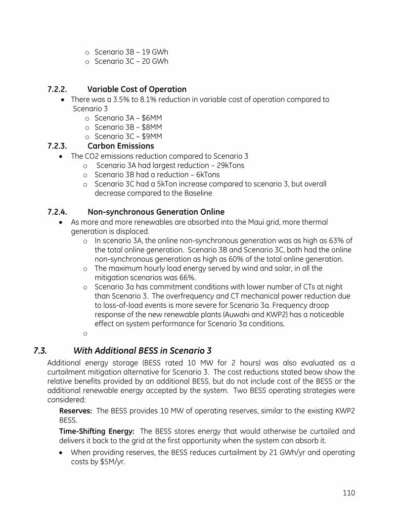
110

o Scenario 3B – 19 GWh o Scenario 3C – 20 GWh

7.2.2. Variable Cost of Operation There was a 3.5% to 8.1% reduction in variable cost of operation compared to

Scenario 3 o Scenario 3A – $6MM o Scenario 3B – $8MM o Scenario 3C – $9MM

7.2.3. Carbon Emissions The CO2 emissions reduction compared to Scenario 3

o Scenario 3A had largest reduction – 29kTons o Scenario 3B had a reduction – 6kTons o Scenario 3C had a 5kTon increase compared to scenario 3, but overall

decrease compared to the Baseline

7.2.4. Non-synchronous Generation Online As more and more renewables are absorbed into the Maui grid, more thermal

generation is displaced. o In scenario 3A, the online non-synchronous generation was as high as 63% of

the total online generation. Scenario 3B and Scenario 3C, both had the online non-synchronous generation as high as 60% of the total online generation.

o The maximum hourly load energy served by wind and solar, in all the mitigation scenarios was 66%.

o Scenario 3a has commitment conditions with lower number of CTs at night than Scenario 3. The overfrequency and CT mechanical power reduction due to loss-of-load events is more severe for Scenario 3a. Frequency droop response of the new renewable plants (Auwahi and KWP2) has a noticeable effect on system performance for Scenario 3a conditions.

o

7.3. With Additional BESS in Scenario 3

Additional energy storage (BESS rated 10 MW for 2 hours) was also evaluated as a curtailment mitigation alternative for Scenario 3. The cost reductions stated beow show the relative benefits provided by an additional BESS, but do not include cost of the BESS or the additional renewable energy accepted by the system. Two BESS operating strategies were considered:

Reserves: The BESS provides 10 MW of operating reserves, similar to the existing KWP2 BESS.

Time-Shifting Energy: The BESS stores energy that would otherwise be curtailed and delivers it back to the grid at the first opportunity when the system can absorb it.

When providing reserves, the BESS reduces curtailment by 21 GWh/yr and operating costs by $5M/yr.

111

o The BESS reduces the amount of spinning reserves required from thermal resources, thereby reducing commitment of thermal generation, which lowers the Pmin of the generation fleet.

When time-shifting energy, the BESS reduces curtailment by 12 GWh/yr and operating costs by $1.8M/yr.

8.0 References [1] KWP2 Wind Integration Study- Final Report. GE June 2010. [2] Deliverable # 3 Maui Electrical System Simulation Model Data and Assumptions. GE

June 2008. [3] GE MAPSTM Manual [4] PSLF Manual

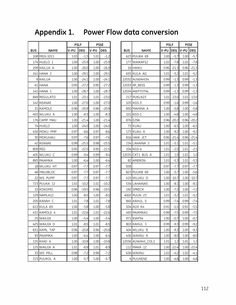
112

Appendix 1. Power Flow data conversion

V-PU DEG V-PU DEG V-PU DEG V-PU DEG

108 MGS-1011 1.03 -1.3 1.01 -1.2 623 PUUKA 69 1.00 -5.7 1.00 -5.7

174 HUELO 1 1.00 -25.9 1.00 -25.9 177 WAIKAP12 1.02 -7.8 1.02 -7.8

209 KAILUA A 1.00 -26.0 1.00 -26.0 16 HAIKU 0.96 -21.3 0.96 -21.3

241 HANA 2 1.00 -29.1 1.00 -29.1 655 KULA AG 1.01 -5.2 1.01 -5.2

9 KAILUA 1.00 -24.1 1.00 -24.1 12032 AUWAHI34 0.99 -1.3 0.99 -1.3

41 HANA 0.95 -27.2 0.95 -27.2 12033 XP_BESS 0.99 -1.3 0.99 -1.3

141 HANA 1 1.00 -28.7 1.00 -28.7 12034 AWFTOTAL 0.99 -1.3 0.99 -1.3

849 REGULATO 1.01 -23.1 1.01 -23.0 217 PUKLN23 1.01 -13.0 1.01 -13.0

142 KEANAE 1.00 -27.0 1.00 -27.0 103 KGS-3 0.99 -1.6 0.99 -1.6

31 KAMOLE 0.96 -20.9 0.96 -20.9 850 MAHINA A 1.00 -5.8 1.00 -5.8

403 WLUKU A 1.00 -8.3 1.00 -8.3 101 KGS-1 1.00 -4.8 1.00 -4.8

176 CAMP MAU 1.00 -21.4 1.00 -21.4 876 E29A 0.96 -20.2 0.96 -20.2

74 HUELO 1.00 -24.0 1.00 -24.0 73 KUAU 1.00 -6.5 1.00 -6.5

430 MOKU PMP 0.97 -8.6 0.97 -8.6 173 KUAU A 1.00 -9.2 1.00 -9.2

30 MOKUHAU 0.97 -7.6 0.97 -7.6 816 HAIK JCT 0.96 -21.4 0.96 -21.4

42 KEANAE 0.99 -25.5 0.98 -25.5 234 LAHAINA 2 1.01 -5.1 1.01 -5.1

809 REG 0.95 -22.5 0.95 -22.5 104 KGS-4 1.01 -2.5 1.01 -2.5

405 WLUKU C 0.99 -9.4 0.99 -9.4 12035 CKT1 BUS A 1.01 1.0 1.01 1.0

893 PAIAMKA 1.00 -6.4 1.00 -6.4 82 AMERON 1.01 -5.3 1.01 -5.3

18 WLUKU HT 0.97 -7.7 0.97 -7.7 838 0.97 -7.7 0.97 -7.7

48 MAUIBLOC 0.97 -7.7 0.97 -7.7 823 PUUKB 69 1.00 -5.7 1.00 -5.6

22 WS PUMP 0.97 -7.7 0.97 -7.7 415 WLUKU D 1.00 -10.7 1.00 -10.7

723 PUUKA 12 1.01 -10.2 1.01 -10.2 534 LAHAINA5 1.00 -8.1 1.00 -8.1

15 KOKOMO 0.96 -19.5 0.96 -19.5 192 SPRECK 1.00 -7.2 1.00 -7.2

129 NAPILA12 1.00 -8.5 1.00 -8.5 4002 PUUN 23 1.01 -5.2 1.01 -5.2

205 KANAH C 1.01 -7.8 1.01 -7.8 845 KAHUL 5 0.99 -7.4 0.99 -7.4

613 KULA 69 1.00 -5.8 1.00 -5.8 504 AUX K4 0.91 -5.5 0.91 -5.5

431 KAMOLE 4 1.01 -22.6 1.01 -22.6 493 PAIAMKA1 0.99 -7.5 0.99 -7.5

25 WAILEA 1.00 -5.4 1.00 -5.4 971 KWP34 1.00 -0.7 1.00 -0.7

425 WAILEA D 1.01 -8.5 1.01 -8.5 803 KAHUL 3 0.99 -9.3 0.99 -9.2

831 KAML TAP 0.96 -20.8 0.96 -20.8 404 WLUKU B 1.00 -9.3 1.00 -9.3

93 PAIAMKA 1.00 -6.4 1.00 -6.4 436 WAIINU A 1.00 -8.0 1.00 -8.0

135 KIHEI A 1.00 -10.8 1.00 -10.8 12036 AUWAHI_COL1 1.01 1.2 1.01 1.2

125 WAILEA A 1.01 -8.9 1.01 -8.9 112 MAKA 12 1.00 -22.4 1.00 -22.4

33 WS MILL 0.98 -7.2 0.98 -7.2 636 WAIINU 1.02 -4.2 1.02 -4.1

223 PUUKOL A 1.00 -5.7 1.00 -5.7 4 PUUNENE 1.00 -4.8 1.00 -4.8

PSLF PSSE

BUS NAME BUS NAME

PSLF PSSE

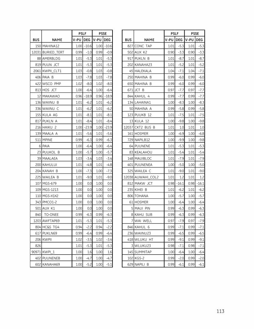
113


150 MAHINA12 1.00 -10.6 1.00 -10.6 827 CONC TAP 1.01 -5.3 1.01 -5.3

12031 BURIED_TERT 0.99 -1.0 0.99 -0.9 502 AUX K2 0.90 -3.3 0.90 -3.3

88 AMERBLDG 1.01 -5.3 1.01 -5.3 917 PUKLN B 1.01 -8.7 1.01 -8.7

819 PUUN JCT 1.01 -5.3 1.01 -5.3 202 KANAHA23 1.01 -5.2 1.01 -5.2

2061 KWPII_CLT1 1.03 -0.8 1.03 -0.8 45 HALEKALA 1.04 -7.1 1.04 -7.1

406 PAIA B 1.03 -7.8 1.03 -7.8 250 MAHINA B 0.99 -6.0 0.99 -6.0

422 WSCO PMP 1.02 -8.0 1.02 -8.0 650 MAHINA B 0.99 -6.0 0.99 -6.0

813 HOS JCT 1.00 -6.4 1.00 -6.4 671 JCT B 0.97 -7.7 0.97 -7.7

12 MAKAWAO 0.96 -18.9 0.96 -18.9 844 KAHUL 4 0.99 -7.7 0.99 -7.7

136 WAIINU B 1.01 -6.2 1.01 -6.2 134 LAHAINA1 1.00 -8.3 1.00 -8.3

336 WAIINU C 1.01 -6.2 1.01 -6.2 50 MAHINA A 0.99 -5.8 0.99 -5.8

155 KULA AG 1.01 -8.1 1.01 -8.1 123 PUUKB 12 1.01 -7.5 1.01 -7.5

817 PUKLN A 1.01 -8.4 1.01 -8.4 13 KULA 12 1.00 -9.8 1.00 -9.8

216 HAIKU 2 1.00 -23.9 1.00 -23.9 12037 CKT2 BUS B 1.01 1.0 1.01 1.0

139 MAALA A 1.01 -5.6 1.01 -5.6 161 HOSMER 1.00 -6.9 1.00 -6.8

511 MPINE 0.99 -6.3 0.99 -6.3 729 NAPILB12 1.00 -9.9 1.00 -9.8

6 PAIA 1.00 -6.4 1.00 -6.4 64 PUUNENE 1.01 -5.3 1.01 -5.3

23 PUUKOL B 1.00 -5.7 1.00 -5.7 83 KEALAHOU 1.01 -5.4 1.01 -5.4

39 MAALAEA 1.03 -3.4 1.03 -3.4 148 MAUIBLOC 1.01 -7.9 1.01 -7.9

200 KAHULUI 1.01 -4.8 1.01 -4.8 401 PUUNENEA 1.00 -5.0 1.00 -5.0

204 KANAH B 1.00 -7.3 1.00 -7.3 325 WAILEA C 1.01 -9.0 1.01 -9.0

225 WAILEA B 1.01 -9.0 1.01 -9.0 12038 AUWAHI_COL2 1.01 1.2 1.01 1.2

107 MGS-679 1.00 0.0 1.00 0.0 812 MAKW JCT 0.98 -16.1 0.98 -16.1

109 MGS-1213 1.00 0.0 1.00 0.0 235 KIHEI B 1.01 -6.2 1.01 -6.2

110 MGS-X1X2 1.00 0.0 1.00 0.0 806 TOHANA 1.00 -5.7 1.00 -5.7

343 PMCO1-2 1.00 0.0 1.00 0.0 61 HOSMER 1.00 -6.4 1.00 -6.4

501 AUX K1 1.00 0.0 1.00 0.0 5 MAUI PIN 0.99 -6.3 0.99 -6.3

840 TO-ONEE 0.99 -6.3 0.99 -6.3 8 KAHU SUB 0.99 -6.3 0.99 -6.3

1203 AWFTAP69 1.01 -5.3 1.01 -5.3 7 WAI WELL 0.97 -7.9 0.97 -7.9

804 HC&S TG4 0.94 -2.2 0.94 -2.2 846 KAHUL 6 0.99 -7.1 0.99 -7.1

617 PUKLN69 0.99 -6.4 0.99 -6.4 236 WAIINU23 0.99 -6.5 0.99 -6.5

206 KWPII 1.02 -3.5 1.02 -3.4 418 WLUKU HT 0.99 -9.1 0.99 -9.1

826 1.01 -5.3 1.01 -5.3 3 WLUKU23 0.98 -7.1 0.98 -7.1

90971 KWPI_1 1.00 1.6 1.00 1.6 145 SUMMITAP 1.00 -6.4 1.00 -6.4

402 PUUNENEB 1.00 -4.7 1.00 -4.7 102 KGS-2 0.99 -2.0 0.99 -2.0

602 KANAHA69 1.00 -5.2 1.00 -5.1 629 NAPILI B 0.99 -6.1 0.99 -6.1

PSSE

BUS NAME

PSLF

BUS NAME

PSLF PSSE

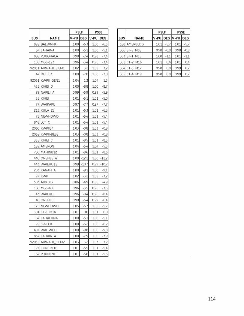
114


892 BALWNPK 1.00 -6.3 1.00 -6.3 188 AMERBLDG 1.01 -5.7 1.01 -5.7

34 LAHAINA 1.00 -5.1 1.00 -5.1 306 ST-2 M18 0.98 -0.8 0.98 -0.8

858 PUUOHALA 0.98 -7.4 0.98 -7.4 303 ST-1 M15 1.00 -1.1 1.01 -1.1

105 MGS-123 0.96 -3.4 0.96 -3.4 302 CT-2 M16 1.01 0.4 1.01 0.4

92031 AUWAHI_SIEM1 1.02 3.2 1.02 3.2 304 CT-3 M17 0.98 0.8 0.99 0.7

44 DET 03 1.00 -7.0 1.00 -7.0 305 CT-4 M19 0.98 0.8 0.99 0.7

92061 KWPII_GEN1 1.04 1.3 1.04 1.3

435 KIHEI D 1.00 -8.8 1.00 -8.7

29 NAPILI A 0.99 -5.9 0.99 -5.9

35 KIHEI 1.01 -5.1 1.01 -5.0

77 WAIKAPU 0.97 -7.7 0.97 -7.7

213 KULA 23 1.01 -6.3 1.01 -6.3

75 NEWHDWD 1.01 -5.4 1.01 -5.4

848 JCT C 1.01 -5.4 1.01 -5.4

2060 KWPII34 1.03 -0.8 1.03 -0.8

2062 KWPII-BESS 1.03 -0.8 1.03 -0.8

335 KIHEI C 1.01 -8.5 1.01 -8.5

182 AMERON 1.04 -5.4 1.04 -5.3

750 MAHINB12 1.01 -8.6 1.01 -8.6

440 ONEHEE 4 1.00 -12.2 1.00 -12.2

443 WAIEHU12 0.99 -10.7 0.99 -10.7

203 KANAH A 1.00 -9.1 1.00 -9.1

97 KWP 1.02 -3.2 1.02 -3.2

503 AUX K3 0.86 -4.9 0.86 -4.9

106 MGS-458 0.96 -3.5 0.96 -3.5

43 WAIEHU 0.96 -8.4 0.96 -8.4

40 ONEHEE 0.99 -6.4 0.99 -6.4

175 NEWHDWD 1.05 -5.7 1.05 -5.7

301 CT-1 M14 1.01 0.0 1.01 0.0

84 LAHALUNA 1.00 -5.1 1.00 -5.1

92 SPRECK 1.00 -6.2 1.00 -6.2

407 WAI WELL 1.00 -9.8 1.00 -9.8

834 LAHAIN 4 1.00 -7.9 1.00 -7.9

92032 AUWAHI_SIEM2 1.03 3.2 1.03 3.2

127 CONCRETE 1.01 -5.5 1.01 -5.4

164 PUUNENE 1.01 -5.6 1.01 -5.6

PSSE

BUS NAME

PSLF PSSE

BUS NAME

PSLF

115

Appendix 2. Dynamic Database (without AGC)

Appendix-2 System Dynamic Database

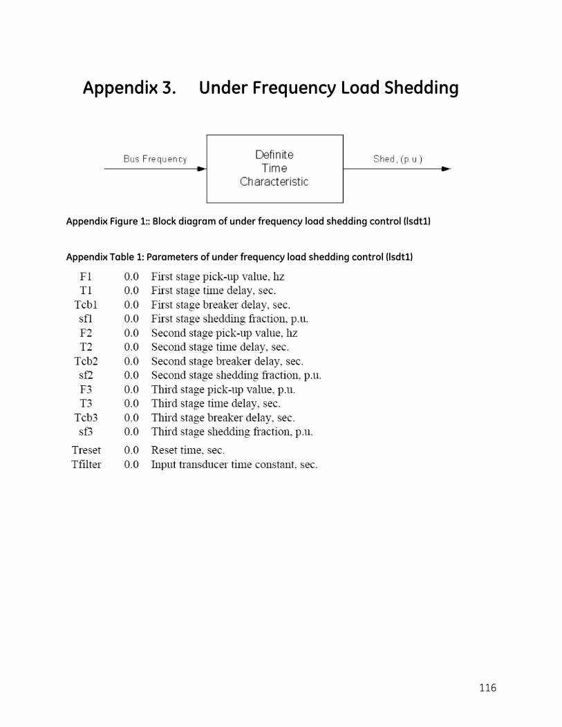
116

Appendix 3. Under Frequency Load Shedding

Appendix Figure 1:: Block diagram of under frequency load shedding control (lsdt1)

Appendix Table 1: Parameters of under frequency load shedding control (lsdt1)

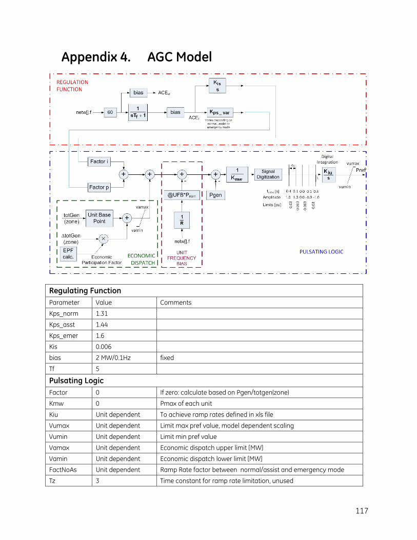
117

Appendix 4. AGC Model

Regulating Function

Parameter Value Comments

Kps_norm 1.31

Kps_asst 1.44

Kps_emer 1.6

Kis 0.006

bias 2 MW/0.1Hz fixed

Tf 5

Pulsating Logic

Factor 0 If zero: calculate based on Pgen/totgen(zone)

Kmw 0 Pmax of each unit

Kiu Unit dependent To achieve ramp rates defined in xls file

Vumax Unit dependent Limit max pref value, model dependent scaling

Vumin Unit dependent Limit min pref value

Vamax Unit dependent Economic dispatch upper limit [MW]

Vamin Unit dependent Economic dispatch lower limit [MW]

FactNoAs Unit dependent Ramp Rate factor between normal/assist and emergency mode

Tz 3 Time constant for ramp rate limitation, unused

118

Cz 0 Ramp rate limitation, unused

Abus 301 Bus number of agc model

AID 11 ID of agc model

119

Appendix 5. AGC Dynamic Database

Appendix-5 AGC Dynamic Database

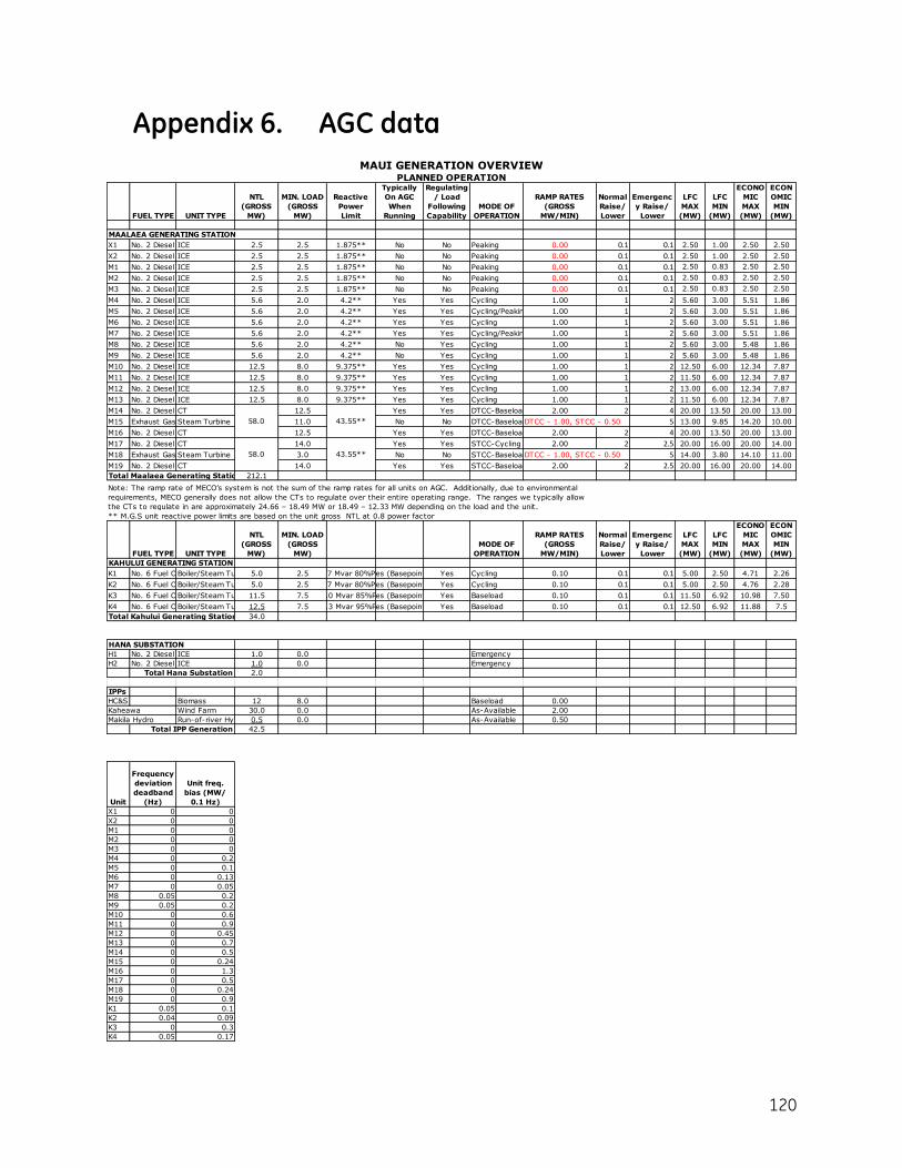
120

Appendix 6. AGC data

FUEL TYPE UNIT TYPE

NTL

(GROSS

MW)

MIN. LOAD

(GROSS

MW)

Reactive

Power

Limit

Typically

On AGC

When

Running

Regulating

/ Load

Following

Capability

MODE OF

OPERATION

RAMP RATES

(GROSS

MW/MIN)

Normal

Raise/

Lower

Emergenc

y Raise/

Lower

LFC

MAX

(MW)

LFC

MIN

(MW)

ECONO

MIC

MAX

(MW)

ECON

OMIC

MIN

(MW)

MAALAEA GENERATING STATION

X1 No. 2 Diesel ICE 2.5 2.5 1.875** No No Peaking 0.00 0.1 0.1 2.50 1.00 2.50 2.50

X2 No. 2 Diesel ICE 2.5 2.5 1.875** No No Peaking 0.00 0.1 0.1 2.50 1.00 2.50 2.50

M1 No. 2 Diesel ICE 2.5 2.5 1.875** No No Peaking 0.00 0.1 0.1 2.50 0.83 2.50 2.50



M4 No. 2 Diesel ICE 5.6 2.0 4.2** Yes Yes Cycling 1.00 1 2 5.60 3.00 5.51 1.86

M5 No. 2 Diesel ICE 5.6 2.0 4.2** Yes Yes Cycling/Peaking 1.00 1 2 5.60 3.00 5.51 1.86


M7 No. 2 Diesel ICE 5.6 2.0 4.2** Yes Yes Cycling/Peaking 1.00 1 2 5.60 3.00 5.51 1.86

M8 No. 2 Diesel ICE 5.6 2.0 4.2** No Yes Cycling 1.00 1 2 5.60 3.00 5.48 1.86

M9 No. 2 Diesel ICE 5.6 2.0 4.2** No Yes Cycling 1.00 1 2 5.60 3.00 5.48 1.86





M14 No. 2 Diesel CT 12.5 Yes Yes DTCC-Baseload 2.00 2 4 20.00 13.50 20.00 13.00

M15 Exhaust Gas Steam Turbine 11.0 No No DTCC-BaseloadDTCC - 1.00, STCC - 0.50 5 13.00 9.85 14.20 10.00

M16 No. 2 Diesel CT 12.5 Yes Yes DTCC-Baseload 2.00 2 4 20.00 13.50 20.00 13.00

M17 No. 2 Diesel CT 14.0 Yes Yes STCC-Cycling 2.00 2 2.5 20.00 16.00 20.00 14.00

M18 Exhaust Gas Steam Turbine 3.0 No No STCC-BaseloadDTCC - 1.00, STCC - 0.50 5 14.00 3.80 14.10 11.00

M19 No. 2 Diesel CT 14.0 Yes Yes STCC-Baseload 2.00 2 2.5 20.00 16.00 20.00 14.00

212.1

** M.G.S unit reactive power limits are based on the unit gross NTL at 0.8 power factor

FUEL TYPE UNIT TYPE

NTL

(GROSS

MW)

MIN. LOAD

(GROSS

MW)

MODE OF

OPERATION

RAMP RATES

(GROSS

MW/MIN)

Normal

Raise/

Lower

Emergenc

y Raise/

Lower

LFC

MAX

(MW)

LFC

MIN

(MW)

ECONO

MIC

MAX

(MW)

ECON

OMIC

MIN

(MW)

KAHULUI GENERATING STATION

K1 No. 6 Fuel OilBoiler/Steam Turbine5.0 2.5 3.7 Mvar 80%PF Yes (Basepoint) Yes Cycling 0.10 0.1 0.1 5.00 2.50 4.71 2.26

K2 No. 6 Fuel OilBoiler/Steam Turbine5.0 2.5 3.7 Mvar 80%PF Yes (Basepoint) Yes Cycling 0.10 0.1 0.1 5.00 2.50 4.76 2.28

K3 No. 6 Fuel OilBoiler/Steam Turbine11.5 7.5 7.0 Mvar 85%PFYes (Basepoint) Yes Baseload 0.10 0.1 0.1 11.50 6.92 10.98 7.50

K4 No. 6 Fuel OilBoiler/Steam Turbine12.5 7.5 9.3 Mvar 95%PFYes (Basepoint) Yes Baseload 0.10 0.1 0.1 12.50 6.92 11.88 7.5

34.0

HANA SUBSTATION

H1 No. 2 Diesel ICE 1.0 0.0 Emergency

H2 No. 2 Diesel ICE 1.0 0.0 Emergency

Total Hana Substation 2.0

IPPs

HC&S Biomass 12 8.0 Baseload 0.00

Kaheawa Wind Farm 30.0 0.0 As-Available 2.00

Makila Hydro Run-of-river Hydro 0.5 0.0 As-Available 0.50

Total IPP Generation 42.5

Unit

Frequency

deviation

deadband

(Hz)

Unit freq.

bias (MW/

0.1 Hz)

X1 0 0

X2 0 0

M1 0 0

M2 0 0

M3 0 0

M4 0 0.2

M5 0 0.1

M6 0 0.13

M7 0 0.05

M8 0.05 0.2

M9 0.05 0.2

M10 0 0.6

M11 0 0.9

M12 0 0.45

M13 0 0.7

M14 0 0.5

M15 0 0.24

M16 0 1.3

M17 0 0.5

M18 0 0.24

M19 0 0.9

K1 0.05 0.1

K2 0.04 0.09

K3 0 0.3

K4 0.05 0.17

Total Kahului Generating Station

Total Maalaea Generating Station

Note: The ramp rate of MECO’s system is not the sum of the ramp rates for all units on AGC. Additionally, due to environmental

requirements, MECO generally does not allow the CTs to regulate over their entire operating range. The ranges we typically allow

the CTs to regulate in are approximately 24.66 – 18.49 MW or 18.49 – 12.33 MW depending on the load and the unit.

58.0

58.0

43.55**

43.55**

MAUI GENERATION OVERVIEWPLANNED OPERATION

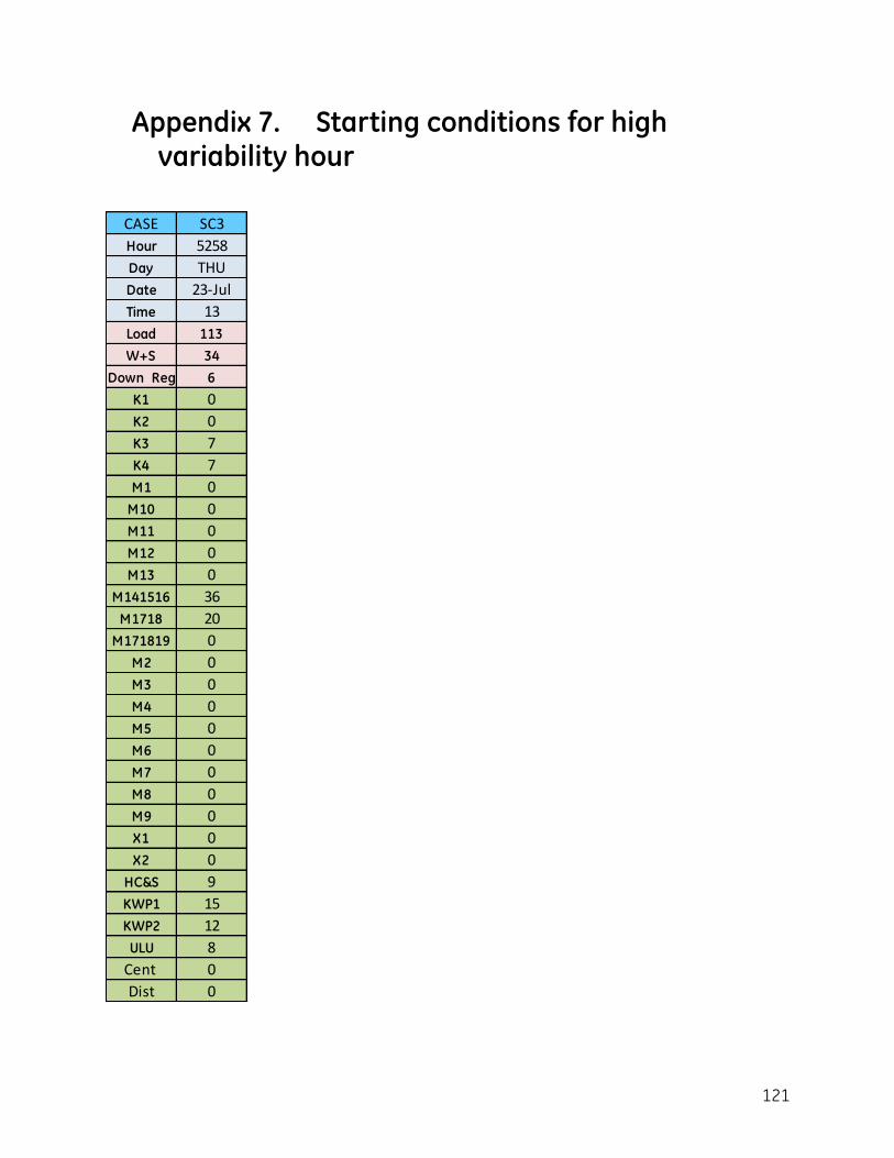
121

Appendix 7. Starting conditions for high variability hour

CASE SC3

Hour 5258

Day THU

Date 23-Jul

Time 13

Load 113

W+S 34

Down Reg 6

K1 0

K2 0

K3 7

K4 7

M1 0

M10 0

M11 0

M12 0

M13 0

M141516 36

M1718 20

M171819 0

M2 0

M3 0

M4 0

M5 0

M6 0

M7 0

M8 0

M9 0

X1 0

X2 0

HC&S 9

KWP1 15

KWP2 12

ULU 8

Cent 0

Dist 0

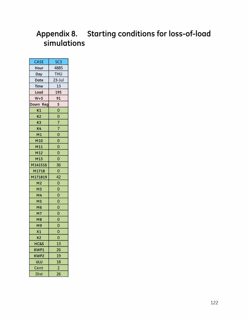
122

Appendix 8. Starting conditions for loss-of-load simulations

CASE SC3

Hour 4885

Day THU

Date 23-Jul

Time 13

Load 195

W+S 91

Down Reg 5

K1 0

K2 0

K3 7

K4 7

M1 0

M10 0

M11 0

M12 0

M13 0

M141516 36

M1718 0

M171819 42

M2 0

M3 0

M4 0

M5 0

M6 0

M7 0

M8 0

M9 0

X1 0

X2 0

HC&S 13

KWP1 26

KWP2 19

ULU 18

Cent 2

Dist 26

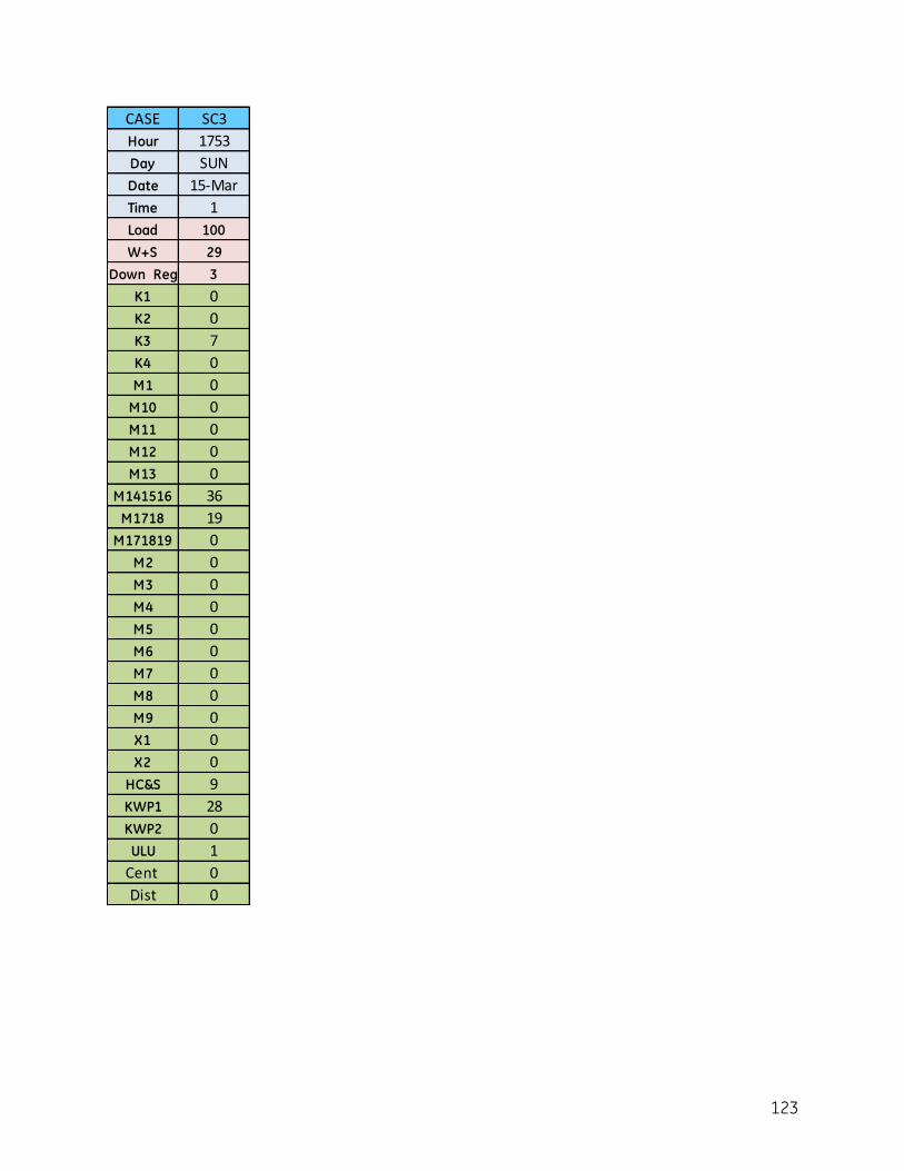
123

CASE SC3

Hour 1753

Day SUN

Date 15-Mar

Time 1

Load 100

W+S 29

Down Reg 3

K1 0

K2 0

K3 7

K4 0

M1 0

M10 0

M11 0

M12 0

M13 0

M141516 36

M1718 19

M171819 0

M2 0

M3 0

M4 0

M5 0

M6 0

M7 0

M8 0

M9 0

X1 0

X2 0

HC&S 9

KWP1 28

KWP2 0

ULU 1

Cent 0

Dist 0

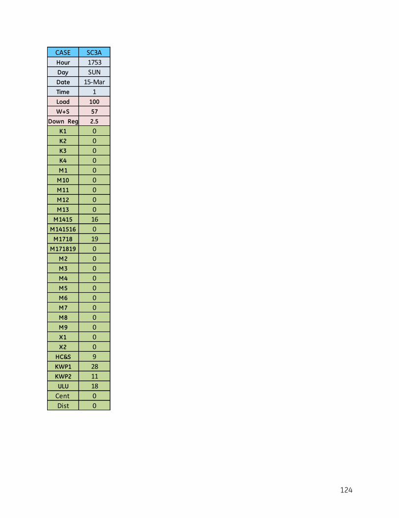
124

CASE SC3A

Hour 1753

Day SUN

Date 15-Mar

Time 1

Load 100

W+S 57

Down Reg 2.5

K1 0

K2 0

K3 0

K4 0

M1 0

M10 0

M11 0

M12 0

M13 0

M1415 16

M141516 0

M1718 19

M171819 0

M2 0

M3 0

M4 0

M5 0

M6 0

M7 0

M8 0

M9 0

X1 0

X2 0

HC&S 9

KWP1 28

KWP2 11

ULU 18

Cent 0

Dist 0

125

Appendix 9. Time domain simulation for most volatile hour

Appendix-9 Time Domain Simulation -Most volatile hour

126

Appendix 10. Time domain simulation for load rejection

Appendix-10 Time Domain Simulation-Load Rejection

Documents

Hawaii Solar Integration Study: Final Technical … Solar...Hawaii Solar Integration Study: Final Technical Report for Maui ... Hawaii Solar Integration Study Final Technical Report