HBST: A Hamming Distance embedding Binary Search Treefor Visual Place Recognition

Dominik Schlegel and Giorgio Grisetti

Abstract— Reliable and efficient Visual Place Recognition isa major building block of modern SLAM systems. Leveragingon our prior work, in this paper we present a HammingDistance embedding Binary Search Tree (HBST) approach forbinary Descriptor Matching and Image Retrieval. HBST allowsfor descriptor Search and Insertion in logarithmic time byexploiting particular properties of binary Feature descriptors.We support the idea behind our search structure with athorough analysis on the exploited descriptor properties andtheir effects on completeness and complexity of search andinsertion. To validate our claims we conducted comparativeexperiments for HBST and several state-of-the-art methods ona broad range of publicly available datasets. HBST is availableas a compact open-source C++ header-only library.

I. INTRODUCTION

Visual Place Recognition (VPR) is a well known problemin Robotics and Computer Vision [1] and represents abuilding block of several applications in Robotics. Theserange from Localization and Navigation to SimultaneousLocalization and Mapping (SLAM). The task of a VPRsystem is to localize an image within a database of placesrepresented by other images. VPR is commonly cast as adata association problem and used in loop closing modulesof SLAM pipelines. A robust VPR system consists of one ormultiple of the following components, which progressivelyimprove the solution accuracy:• Image Retrieval: is the process of retrieving one or more

images from a database that are similar to a query one.• Descriptor Matching: consists of seeking points between

images which look similar. The local appearance of suchpoints is captured by Feature descriptors.

• Geometric Verification: is a common pruning techniquethat removes points obtained from descriptor matching,which are inconsistent with the epipolar geometry.

In the domain of Image Retrieval, common approachescompress entire images in single global descriptors to obtainhigh processing speed [2], [3]. Recently, convolutional neu-ral network methods demonstrated highly accurate results,especially in the field of long-term VPR [4], [5], [6]. Thesemethods, however, might suffer from a high ratio of falsepositives, and thus often require a further stage of local fea-ture Descriptor Matching to reject wrong candidates. Brute-force (BF) and k-d trees [7] are two prominent methods forsolving this task.

Since the introduction of the BRIEF descriptor [8], thecomputer vision community embraced the use of binary

Both authors are with the Dept. of Computer, Control and Man-agement Engineering, Sapienza University of Rome, Rome, Italy{lastname}@diag.uniroma1.it

0.001

0.01

0.1

1

10

100

1000

0 500 1000 1500 2000 2500 3000 3500 4000 4500

Proc

essi

ngtim

et i

(sec

onds

)

Image number i

Runtime: KITTI sequence 00 (BRIEF-256)

BFFLANN-LSH

DBoW2HBST (ours)

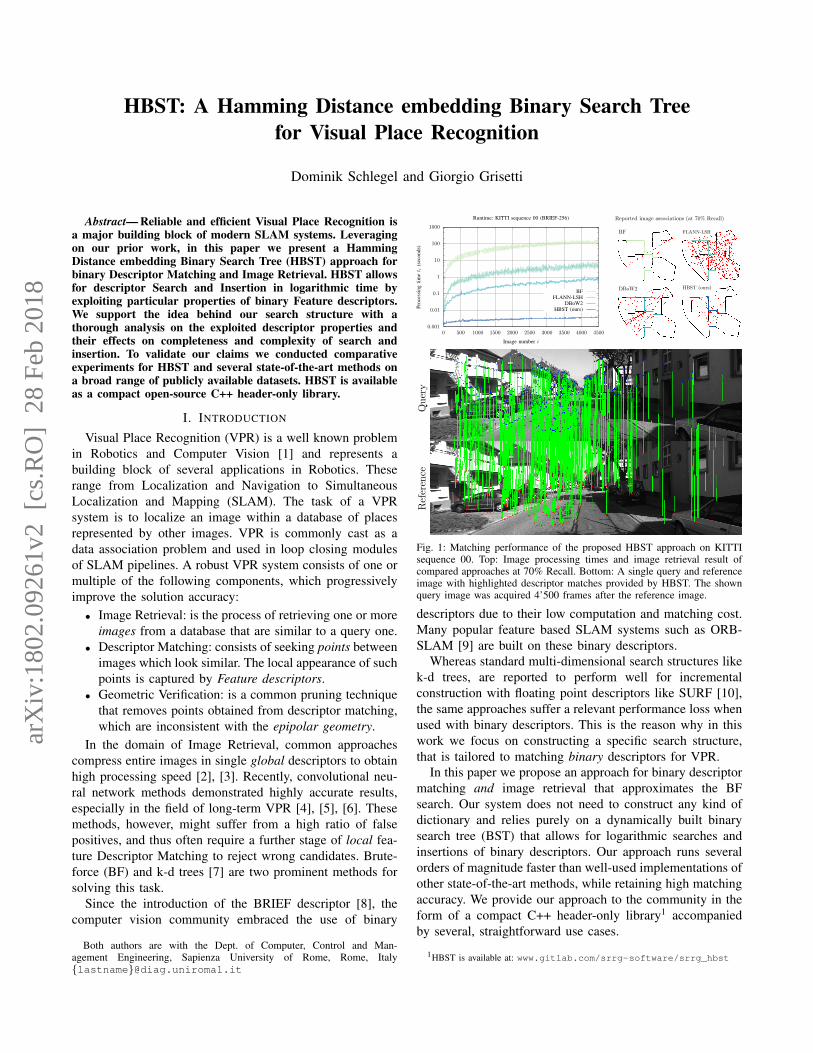
Fig. 1: Matching performance of the proposed HBST approach on KITTIsequence 00. Top: Image processing times and image retrieval result ofcompared approaches at 70% Recall. Bottom: A single query and referenceimage with highlighted descriptor matches provided by HBST. The shownquery image was acquired 4’500 frames after the reference image.

descriptors due to their low computation and matching cost.Many popular feature based SLAM systems such as ORB-SLAM [9] are built on these binary descriptors.

Whereas standard multi-dimensional search structures likek-d trees, are reported to perform well for incrementalconstruction with floating point descriptors like SURF [10],the same approaches suffer a relevant performance loss whenused with binary descriptors. This is the reason why in thiswork we focus on constructing a specific search structure,that is tailored to matching binary descriptors for VPR.

In this paper we propose an approach for binary descriptormatching and image retrieval that approximates the BFsearch. Our system does not need to construct any kind ofdictionary and relies purely on a dynamically built binarysearch tree (BST) that allows for logarithmic searches andinsertions of binary descriptors. Our approach runs severalorders of magnitude faster than well-used implementations ofother state-of-the-art methods, while retaining high matchingaccuracy. We provide our approach to the community in theform of a compact C++ header-only library1 accompaniedby several, straightforward use cases.

1HBST is available at: www.gitlab.com/srrg-software/srrg_hbst

arX

iv:1

802.

0926

1v2

[cs

.RO

] 2

8 Fe

b 20

18

II. IMAGE RETRIEVAL AND DESCRIPTOR MATCHING

In this section we discuss in detail the two fundamentalbuilding blocks of VPR which we address in our approach:Image Retrieval and Descriptor Matching. We present relatedwork directly in context of these two problems.

A. Image Retrieval

A system for image retrieval returns the image I?i con-tained in a database {Ii} that is the most similar to a givenquery image Iq according to a similarity metric eI. The moresimilar two images Ii and Iq , the lower the resulting distancebecomes. More formally, image retrieval consists in solvingthe following problem:

I?i = argminIi

eI(Iq, Ii) : Ii ∈ {Ii}. (1)

Often one is interested in retrieving all images in thedatabase, whose distance to the query image eI is withina certain threshold τI:

{I?i } = {Ii ∈ {Ii} : eI(Iq, Ii) < τI} . (2)

The distance metric itself depends on the target application.A straightforward example of distance between two imagesis the Frobenius norm of the pixel-wise difference:

eI(Iq, Ii) = ‖Iq − Ii‖F . (3)

This measure is not robust to viewpoint or illuminationchanges and its computational cost is proportional to theimage sizes.

Global image descriptors address these issues by com-pressing an entire image into a set of few values. In theremainder we will refer to a global descriptor obtainedfrom an image I as: d(I). GIST of Olvia and Torralba [2]and Histogram of Oriented Gradients (HOG) by Dalal andTriggs [3] are two prominent methods in this class. GISTcomputes a whole image descriptor as the distribution ofdifferent perceptual qualities and semantic classes detectedin an image. Conversely, HOG computes the descriptor as thehistogram of gradient orientations in portions of the image.

When using global descriptors, the distance between im-ages is usually computed as the L2 norm of the differencebetween the corresponding descriptors:

eI(Iq, Ii) = ‖d(Iq)− d(Ii)‖2 . (4)

Milford and Wyeth considered image sequences insteadof single images for place recognition. With SeqSLAM [11]they presented an impressive SLAM system, that computesand processes contrast enhancing image difference vectorsbetween subsequent images. Using this technique, SeqSLAMmanages to recognize places that underwent heavy changesin appearance (e.g. from summer to winter).

In recent years, convolutional neural network approacheshave shown to be very effective in VPR. They are usedto generate powerful descriptors that capture large portionsof the scene at different resolutions. For one, there is theCNN feature boosted SeqSLAM system of Bai et al. [6],accompanied by other off-the-shelf systems such as ConvNet

of Sunderhauf et al. [4] or NetVLAD by Arandjelovic etal. [5]. The large CNN descriptors increase the descriptiongranularity and therefore they are more robust to viewpointchanges than global descriptors. CNN descriptors are addi-tionally resistant to minor appearance changes, making themsuitable for lifelong place recognition applications. One canobtain up to a dozen CNN descriptors per image, whichenable for high-dimensional image distance metrics for eI.

However, if one wants to determine the relative locationat which images have been acquired, which is often the casefor SLAM approaches, additional effort needs to be spent.Furthermore, due to their holistic nature, global descriptorsmight disregard the geometry of the scene and thus are morelikely to provide false positives. Both of these issues can behandled by descriptor matching and a subsequent geometricverification.

B. Descriptor Matching

Given two images Iq and Ii, we are interested in deter-mining which pixel pq ∈ Iq and which pixel pj ∈ Ii, if any,capture the same point in the world. Knowing a set of thesepoint correspondences, allows us to determine the relativeposition of the two images up to a scale using projectivegeometry [12]. To this extent it is common to detect a setof salient points {p} (keypoints) in each image. Amongothers, the Harris corner detector and the FAST detector areprominent approaches for detecting keypoints. Keypoints areusually characterized by a strong local intensity variation.

The local appearance around a keypoint p is captured bya descriptor d(p) which is usually represented as a vector ofeither floating point or boolean values. SURF [10] is a typicalfloating point descriptor, while BRIEF [8], BRISK [13] andORB [14] are well known boolean descriptors. The desiredproperties for local descriptors are the same as for globaldescriptors: light and viewpoint invariance. Descriptors aredesigned such that regions that appear locally similar in theimage result in similar descriptors, according to a certainmetric ed. For floating point descriptors, ed is usuallychosen as the L2-norm. In the case of binary descriptors,the Hamming distance is a common choice. The Hammingdistance between two binary vectors is the number of bitchanges needed to turn one vector into the other, and can beeffectively computed by current processors.

Finding the point p?j ∈ Ii that is the most similar to aquery pq ∈ Iq is resolved by seeking the descriptor d(p?j )with the minimum distance to the query d(pq):

p?j = argminpj

ed(d(pq),d(pj)) : pj ∈ Ii. (5)

If a point pq ∈ Iq is not visible in Ii, Eq. (5) will stillreturn a point p?j ∈ Ii. Unfeasible matches however willhave a high distance, and can be rejected whenever theirdistance ed is greater than a certain matching thresholdτ . The most straightforward way to compute Eq. (5) isthe brute-force (BF) search. BF computes the distance edbetween pq and every pj ∈ Ii. And hence always returnsthe closest match for each query. This unbeatable accuracy

comes with a computational cost proportional to the numberof descriptors Nd = |{d(pj)}|. Assuming Nd is the averagenumber of descriptors extracted for each image, finding thebest correspondence for each keypoint in the query imagewould require O(N2

d) operations. In current applications, Nd

ranges from 100 to 10’000, hence using BF for descriptormatching quickly becomes computationally prohibitive.

To carry on the correspondence search in a more effectiveway it is common to organize the descriptors in search struc-ture, typically a tree. In the case of floating point descrip-tors, FLANN (Fast Approximate Nearest Neighbor SearchLibrary) of Muja and Lowe [15] with k-d tree indexing isa common choice. When working with binary descriptors,the (Multi-Probe) Locality-sensitive hashing (LSH) [16] byLv et al. and hierarchical clustering trees (HCT) of Muja andLowe [17] are popular methods to index the descriptors withFLANN. While LSH allows for database incrementationat a decent computational cost, HCT quickly exceeds real-time constraints. Accordingly, we consider only LSH in ourresult evaluations. The increased speed of FLANN comparedto BF comes at a decreased accuracy of the matches. Inour previous work [18] we presented a binary search treestructure, that resolves Eq. (5) in logarithmic time. However,a tree had to be built for every desired image candidate pair.

C. Image Retrieval based on Descriptor Matching

Assuming to have an efficient method to perform de-scriptor matching as defined in Eq. (5), one could design asimple, yet effective image retrieval system by using a votingscheme. An image Ii will receive at most one vote

⟨pq,p

?i,j

⟩for each keypoint pq ∈ Iq that is successfully matchedwith a keypoint of another image p?i,j ∈ Ii. The distancebetween two images Iq and Ii is then the number of votes∣∣{⟨pq,p?i,j⟩}∣∣ normalized by the number of descriptors inthe query image Nd:

eI(Iq, Ii) =∣∣{⟨pq,p?i,j⟩}∣∣

Nd. (6)

The above procedure allows to gather reasonably goodmatches at a cost proportional to both, the number ofdescriptors in the query image Nd and the cost of retrievingthe most likely descriptor as defined in Eq. (5).

An alternative strategy to enhance the efficiency of imageretrieval, when local descriptors are available, is to computea single image “descriptor” from multiple feature descriptors.Bag-of-visual-Words (BoW) approaches follow this strategyby computing an image descriptor as the histogram ofthe distribution of words appearing in the image. A wordrepresents a group of nearby descriptors, and is learnedby a clustering algorithm such as k-means from a set oftrain descriptors. To compute the histogram, each keypointis converted in a set of weights computed as the distance ofthe descriptors’ keypoint from the centroid of each word inthe dictionary. The histogram is then normalized by the sumof word weights in the scene. Images that present similardistribution of words are likely to be similar. Comparing apair of images can be done in a time linear in the number of

words in the dictionary. This procedure has been shown to beboth robust and efficient, however it does not provide pointcorrespondences, that are required for geometric verification.

Notably the open-source library DBoW2 by Galvez-Lopezand Tardos [19] extends the data structures used in BoW toadd point correspondences to the system. This is done bystoring an Inverted Index from words to descriptors that areclose to a specific word. To retrieve the keypoints p?j that aresimilar to a query p?j one can pick the words in the dictionarythat are best represented by d(p?q) and from them retrieve thedescriptors through the inverted index. In the current versionof DBoW2, Galvez-Lopez and Tardos provide also a DirectIndex descriptor index for correspondence access.

DBoW2 is integrated within the recently published ORB-SLAM2 [9] by Mur-Artal et al. and displays fast and robustperformance for ORB descriptors [14]. Another famous BoWbased approach is FAB-MAP [20] developed by Cummins etal. FAB-MAP allows to quickly retrieve similar images onvery large datasets. FAB-MAP uses costly SURF descrip-tors [10] to maintain a certain level of individuality betweenthe massive number of images described. Typically, BoW isused to determine a preliminary set of good image candi-dates, on which BF, FLANN or BST descriptor matching isperformed. This is a common practice for SLAM systems,that require high numbers of matches for few images.

In this paper, we present a novel approach that:• Allows to perform image retrieval and descriptor match-

ing with correspondences faster than BoW approachesperform image retrieval without correspondences.

• Yields levels of search correctness and completenesscomparable to the one achieved by to state-of-the-artmethods such as FLANN-LSH [16] and DBoW2 [19].

• Allows for incremental insertion of subsequent descrip-tor sets (i.e. images) in a time bounded by the dimensionof the descriptors dim(d).

Furthermore, we provide our approach as a compact C++header-only library, that does not require a vocabulary or anyother pretrained information. The library is accompanied bya set of simple use cases and includes an OpenCV wrapper.

III. OUR APPROACH

We arrange binary feature descriptors {dj} extracted fromeach image Ii of an image sequence {Ii} in a binarytree. This tree allows us to efficiently perform descriptormatching. Additionally, we build a voting scheme on topof this method that enables fast and robust image retrieval.

A. Tree Construction

In our tree, each leaf Li stores a subset {di,j} of theinput descriptors {dj}. The leafs partition the input set suchthat each descriptor dj belongs to a single leaf. Every non-leaf node Ni has exactly two children and stores an indexki ∈ [0, ..,dim(d) − 1]. Where dim(d) is the descriptordimension, corresponding to the number of bits containedin each descriptor. We require that in each path from theroot to a leaf a specific index value ki should appear at mostonce. This limits the depth of the tree h to the dimension of

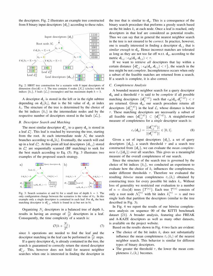
the descriptors. Fig. 2 illustrates an example tree constructedfrom 8 binary input descriptors {dj} according to these rules.

Fig. 2: HBST tree construction for a scenario with 8 input descriptors ofdimension dim(d) = 4. The tree contains 4 nodes {Ni} (circles) with bitindices {ki}, 5 leafs {Li} (rectangles) and has maximum depth h = 3.

A descriptor dj is stored in the left or in the right subtreedepending on dj [ki], that is the bit value of dj at indexki. The structure of the tree is determined by the choice ofthe bit indices {ki} in the intermediate nodes and by therespective number of descriptors stored in the leafs {Li}.

B. Descriptor Search and Matching

The most similar descriptor d?i,j to a query dq is stored ina leaf L?i . This leaf is reached by traversing the tree, startingfrom the root. At each intermediate node Ni the searchbranches according to dq[ki]. Eventually, the search will endup in a leaf L?i . At this point all leaf descriptors {di,j} storedin L?i are sequentially scanned (BF matching) to seek forthe best match according to Eq. (5). Fig. 3 illustrates twoexamples of the proposed search strategy.

Fig. 3: Search scenarios a) and b) for a small tree of depth h = 1. Theonly configuration change between the scenarios is the value of k1. In thisexample only a single descriptor is contained in each leaf. For dq the bestmatching descriptor is d?1,1, which is found in a) but not in b).

Organizing Nj descriptors in a balanced tree of depth h,results in having an average of Nj

2hdescriptors in a leaf.

Consequently, the time complexity of a search is:

O(h+Nj2h

) (7)

since h operations are needed to find the leaf and thedescriptor matching in the leaf can be performed in Nj

2hsteps.

If a query descriptor dq is already contained in the tree, thesearch is guaranteed to correctly return the stored descriptord?i,j . This, however does not hold for nearest neighborsearches when one is interested in finding the descriptor in

the tree that is similar to dq . This is a consequence of thebinary search procedure that preforms a greedy search basedon the bit index ki at each node. Once a leaf is reached, onlydescriptors in that leaf are considered as potential results.Thus we can say that in general the nearest neighbor searchin the tree is not ensured to be correct. In practice, however,one is usually interested in finding a descriptor di,j that issimilar enough to dq . Hence incorrect matches are toleratedas long as they are not too far off w.r.t. dq , according to themetric di,j : ed(dq,di,j) < τ .

If we want to retrieve all descriptors that lay within acertain distance

{d?i,j : ed(dq,di,j) < τ

}, the search in the

tree might be not complete. Incompleteness occurs when onlya subset of the feasible matches are returned from a search.If a search is complete, it is also correct.

C. Completeness Analysis

A bounded nearest neighbor search for a query descriptordq and a threshold τ is said to be complete if all possiblematching descriptors {d(τ,q)

j } such that ed(dq,d(τ,q)j ) < τ

are returned. Given dq , our search procedure returns alldescriptors {d(τ,q)

i,j } in the leaf Li whose distance is belowτ . These matching descriptors are necessarily a subset ofall feasible ones {d(τ,q)

i,j } ⊂ {d(τ,q)j }. A straightforward

measure of completeness for a single descriptor search is:

cτ (dq) =|{d(τ,q)

i,j }|

|{d(τ,q)j }|

∈ [0, 1]. (8)

Given a set of input descriptors {dj}, a set of querydescriptors {dq}, a search threshold τ and a search treeconstructed from {dj}, we can evaluate the mean complete-ness cτ ({dq}) over all searches. This gives us a meaningfulmeasure of the overall completeness of our search.

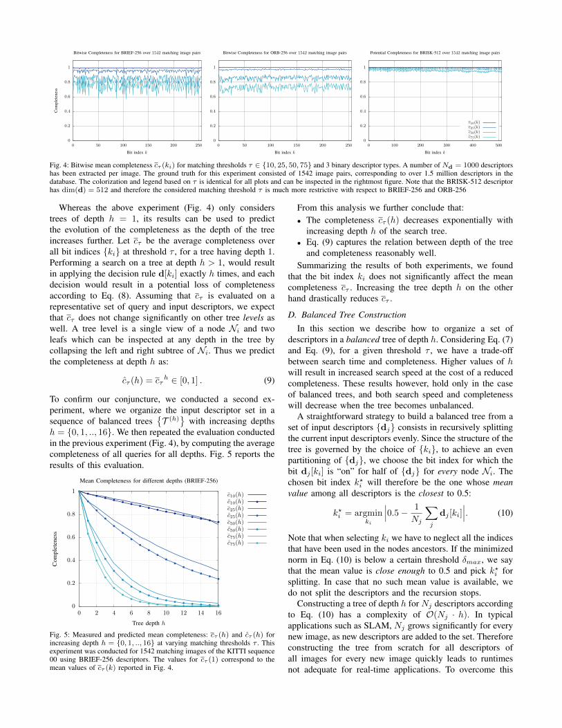
Since the structure of the search tree is governed by thechoice of bit indices {ki}, we conducted an experiment toevaluate how the choice of ki influences the completeness,under different thresholds τ . Therefore we evaluated theresulting bitwise mean completeness cτ (ki) obtained byconstructing trees for every possible bit index ki. Withoutloss of generality we restricted our evaluation to a numberof n = dim(d) trees {T (n)}. Each tree T (n) consists ofonly a root node N (n)

1 with bit index k(n)1 = n and two

single leafs that partition the descriptors (similar to the treedescribed in Fig. 3).

In Fig. 4 we report the results of our bitwise complete-ness analysis on sequence 00 of the KITTI benchmarkdataset [21]. A broader analysis, featuring also FREAKand A-KAZE descriptors as well as many other datasets,is available on the project website.

Based on the results shown in Fig. 4 two facts are evident:• The choice of the bit index ki does not substantially

influence the mean completeness cτ (ki) of the nearestneighbor search. This behavior is similar for differenttypes of binary descriptors.

• The greater the threshold τ , the lower the mean com-pleteness cτ (ki) becomes.

0

0.2

0.4

0.6

0.8

1

0 50 100 150 200 250

Com

plet

enes

s

Bit index k

Bitwise Completeness for BRIEF-256 over 1542 matching image pairs

0

0.2

0.4

0.6

0.8

1

0 50 100 150 200 250

Bit index k

Bitwise Completeness for ORB-256 over 1542 matching image pairs

0

0.2

0.4

0.6

0.8

1

0 100 200 300 400 500

Bit index k

Potential Completeness for BRISK-512 over 1542 matching image pairs

c10(k)c25(k)c50(k)c75(k)

Fig. 4: Bitwise mean completeness cτ (ki) for matching thresholds τ ∈ {10, 25, 50, 75} and 3 binary descriptor types. A number of Nd = 1000 descriptorshas been extracted per image. The ground truth for this experiment consisted of 1542 image pairs, corresponding to over 1.5 million descriptors in thedatabase. The colorization and legend based on τ is identical for all plots and can be inspected in the rightmost figure. Note that the BRISK-512 descriptorhas dim(d) = 512 and therefore the considered matching threshold τ is much more restrictive with respect to BRIEF-256 and ORB-256

Whereas the above experiment (Fig. 4) only considerstrees of depth h = 1, its results can be used to predictthe evolution of the completeness as the depth of the treeincreases further. Let cτ be the average completeness overall bit indices {ki} at threshold τ , for a tree having depth 1.Performing a search on a tree at depth h > 1, would resultin applying the decision rule d[ki] exactly h times, and eachdecision would result in a potential loss of completenessaccording to Eq. (8). Assuming that cτ is evaluated on arepresentative set of query and input descriptors, we expectthat cτ does not change significantly on other tree levels aswell. A tree level is a single view of a node Ni and twoleafs which can be inspected at any depth in the tree bycollapsing the left and right subtree of Ni. Thus we predictthe completeness at depth h as:

cτ (h) = cτh ∈ [0, 1] . (9)

To confirm our conjuncture, we conducted a second ex-periment, where we organize the input descriptor set in asequence of balanced trees

{T (h)

}with increasing depths

h = {0, 1, .., 16}. We then repeated the evaluation conductedin the previous experiment (Fig. 4), by computing the averagecompleteness of all queries for all depths. Fig. 5 reports theresults of this evaluation.

0

0.2

0.4

0.6

0.8

1

0 2 4 6 8 10 12 14 16

Com

plet

enes

s

Tree depth h

Mean Completeness for different depths (BRIEF-256)

c10(h)c10(h)c25(h)c25(h)c50(h)c50(h)c75(h)c75(h)

Fig. 5: Measured and predicted mean completeness: cτ (h) and cτ (h) forincreasing depth h = {0, 1, .., 16} at varying matching thresholds τ . Thisexperiment was conducted for 1542 matching images of the KITTI sequence00 using BRIEF-256 descriptors. The values for cτ (1) correspond to themean values of cτ (k) reported in Fig. 4.

From this analysis we further conclude that:• The completeness cτ (h) decreases exponentially with

increasing depth h of the search tree.• Eq. (9) captures the relation between depth of the tree

and completeness reasonably well.Summarizing the results of both experiments, we found

that the bit index ki does not significantly affect the meancompleteness cτ . Increasing the tree depth h on the otherhand drastically reduces cτ .

D. Balanced Tree Construction

In this section we describe how to organize a set ofdescriptors in a balanced tree of depth h. Considering Eq. (7)and Eq. (9), for a given threshold τ , we have a trade-offbetween search time and completeness. Higher values of hwill result in increased search speed at the cost of a reducedcompleteness. These results however, hold only in the caseof balanced trees, and both search speed and completenesswill decrease when the tree becomes unbalanced.

A straightforward strategy to build a balanced tree from aset of input descriptors {dj} consists in recursively splittingthe current input descriptors evenly. Since the structure of thetree is governed by the choice of {ki}, to achieve an evenpartitioning of {dj}, we choose the bit index for which thebit dj [ki] is “on” for half of {dj} for every node Ni. Thechosen bit index k?i will therefore be the one whose meanvalue among all descriptors is the closest to 0.5:

k?i = argminki

∣∣∣0.5− 1

Nj

∑j

dj [ki]∣∣∣. (10)

Note that when selecting ki we have to neglect all the indicesthat have been used in the nodes ancestors. If the minimizednorm in Eq. (10) is below a certain threshold δmax, we saythat the mean value is close enough to 0.5 and pick k?i forsplitting. In case that no such mean value is available, wedo not split the descriptors and the recursion stops.

Constructing a tree of depth h for Nj descriptors accordingto Eq. (10) has a complexity of O(Nj · h). In typicalapplications such as SLAM, Nj grows significantly for everynew image, as new descriptors are added to the set. Thereforeconstructing the tree from scratch for all descriptors ofall images for every new image quickly leads to runtimesnot adequate for real-time applications. To overcome this

computational limitation we propose an alternative strategyto insert new images (i.e. descriptors) into an existing tree.

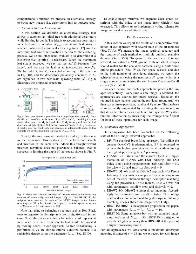
E. Incremental Tree ConstructionIn this section we describe an alternative strategy that

allows to augment an initial tree with additional descriptorswhile limiting its depth. The idea is to accumulate descriptorsin a leaf until a number Nmax (maximum leaf size) isreached. Whereas hierarchical clustering trees [17] use themaximum leaf size as termination criterion for the clusteringprocess, we on the other hand evaluate it to determine if aclustering (i.e. splitting) is necessary. When the maximumleaf size is exceeded, we say that the leaf Li becomes “toolarge”, and we turn the leaf in an intermediate node Ni.The bit index ki for Ni is selected according to the criterionin Eq. (10), and the descriptors previously contained in Liare organized in two new leafs spawning from Ni. Fig. 6illustrates the proposed procedure.

Fig. 6: Descriptor insertion procedure for a single input descriptor dj . Onlythe affected part of the tree is shown. Step 1) The leaf Li containing the mostsimilar descriptor(s) to dj is found. Step 2) dj is integrated into the leafdescriptor set {d4,j}. Step 3) If the leaf becomes “too big”: N4,j > Nmax,it breaks into two child leafs and becomes an intermediate node. In thisexample we set the maximum leaf size to Nmax = 3.

Notably the tree traversal needed to find Li is the sameas for the search. This enables us to perform both searchand insertion at the same time. Albeit this straightforwardinsertion technique does not guarantee a balanced tree, itsucceeds in limiting the depth of the tree as shown in Fig. 7.

0

5

10

15

20

25

0 5000 10000 15000 20000 25000 30000

Tree

dept

hh

Number of inserted images

Tree depths on St. Lucia (BRIEF-256)

Standard deviationMean depth

Fig. 7: Mean and standard deviation of the tree depth h for increasingnumbers of sequentially inserted images. Nd = 1000 BRIEF-256 de-scriptors were extracted for each of the 33’197 images in the dataset(resulting over 30 million inserted descriptors). For this experiment we setτ = 25, δmax = 0.1 and Nmax = 100.

Note that using re-balancing structures such as Red-Blacktrees to organize the descriptors is not straightforward in ourcase. Since the constraint that a bit index would appear atmost once in a path from root to leaf would be violatedby moving nodes. In our approach, no tree re-balancing isperformed as we are able to enforce a desired balance to asatisfiable degree using the parameter δmax (Sec. III-D).

To enable image retrieval, we augment each stored de-scriptor with the index of the image from which it wasextracted. This allows us to implement a voting scheme forimage retrieval at no additional cost.

IV. EXPERIMENTS

In this section we report the results of a comparative eval-uation of our approach with several state-of-the-art methods(Sec. IV-A). We measure the image retrieval accuracy andthe runtime of each method on multiple publicly availabledatasets (Sec. IV-B). To quantify the accuracy of imageretrieval, we extract a VPR ground truth on which imagesshould match for the analyzed datasets, using a brute-forceoffline procedure (Sec. IV-C). For space reasons and dueto the high number of considered datasets, we report theachieved accuracy using the maximum F1 score, which is asingle number summarizing the well known Precision-Recallcurves (Sec. IV-D).

For each dataset and each approach we process the im-ages sequentially. Every time a new image is acquired, theapproaches are queried for image retrieval. Based on thereported image matches and on the provided ground truth wethen can estimate precision, recall and F1 score. The databaseis subsequently augmented by inserting the new image, sothat it can be returned as a match in future queries. We gatherruntime information by measuring the average time t spentfor both of these operations for each image.

A. Compared Approaches

Our comparison has been conducted on the followingstate-of-the-art image retrieval approaches:• BF: The classical brute-force approach. We utilize the

current OpenCV3 implementation. BF is expected toachieve the highest precision and recall, while requiringthe highest processing time t per image.

• FLANN-LSH: We utilize the current OpenCV3 imple-mentation of FLANN with LSH indexing. The LSHindex is built using the parameters: table number = 10,key size = 20 and multi probe level = 0.

• DBoW2-DI: We used the DBoW2 approach with DirectIndexing. Image matches are pruned by decreasing num-ber of matches obtained through descriptor matchingusing the provided DBoW2 indices. DBoW2 was runwith parameters: use di = true and di levels = 2.

• DBoW2-SO: DBoW2 without direct indexing. Accord-ingly the parameters are: use di = false. This config-uration does not report matching descriptors but onlymatching images (based on image Score Only).

• HBST-10: HBST is the approach proposed in this paper,with parameters: δmax = 0.1, Nmax = 10.

• HBST-50: Same as above but with an extended maxi-mum leaf size of Nmax = 50. HBST-50 is designed toprovide a higher accuracy than HBST-10 at the price ofa higher processing time t.

For all approaches we considered a maximum descriptormatching distance of τ = 25 and we extracted for each image

Nd = 1000 BRIEF-256 descriptors. All results were ob-tained on the same machine, running Ubuntu 16.04.3 with anIntel i7-7700K CPU@4.2GHz and 32GB of RAM@4.1GHz.A more extensive evaluation featuring various binary de-scriptor types (e.g. ORB, BRISK, FREAK and A-KAZE)is available on the project website.

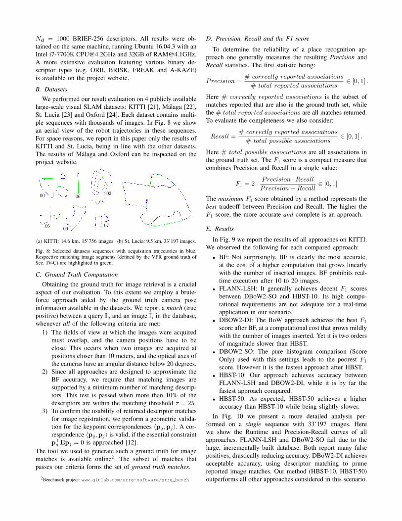
B. DatasetsWe performed our result evaluation on 4 publicly available

large-scale visual SLAM datasets: KITTI [21], Malaga [22],St. Lucia [23] and Oxford [24]. Each dataset contains multi-ple sequences with thousands of images. In Fig. 8 we showan aerial view of the robot trajectories in these sequences.For space reasons, we report in this paper only the results ofKITTI and St. Lucia, being in line with the other datasets.The results of Malaga and Oxford can be inspected on theproject website.

(a) KITTI: 14.6 km, 15’756 images. (b) St. Lucia: 9.5 km, 33’197 images.

Fig. 8: Selected datasets sequences with acquisition trajectories in blue.Respective matching image segments (defined by the VPR ground truth ofSec. IV-C) are highlighted in green.

C. Ground Truth ComputationObtaining the ground truth for image retrieval is a crucial

aspect of our evaluation. To this extent we employ a brute-force approach aided by the ground truth camera poseinformation available in the datasets. We report a match (truepositive) between a query Iq and an image Ii in the database,whenever all of the following criteria are met:

1) The fields of view at which the images were acquiredmust overlap, and the camera positions have to beclose. This occurs when two images are acquired atpositions closer than 10 meters, and the optical axes ofthe cameras have an angular distance below 20 degrees.

2) Since all approaches are designed to approximate theBF accuracy, we require that matching images aresupported by a minimum number of matching descrip-tors. This test is passed when more than 10% of thedescriptors are within the matching threshold τ = 25.

3) To confirm the usability of returned descriptor matchesfor image registration, we perform a geometric valida-tion for the keypoint correspondences 〈pq,pj〉. A cor-respondence 〈pq,pj〉 is valid, if the essential constraintp>q Epj = 0 is approached [12].

The tool we used to generate such a ground truth for imagematches is available online2. The subset of matches thatpasses our criteria forms the set of ground truth matches.

2Benchmark project: www.gitlab.com/srrg-software/srrg_bench

D. Precision, Recall and the F1 score

To determine the reliability of a place recognition ap-proach one generally measures the resulting Precision andRecall statistics. The first statistic being:

Precision =# correctly reported associations

# total reported associations∈ [0, 1] .

Here # correctly reported associations is the subset ofmatches reported that are also in the ground truth set, whilethe # total reported associations are all matches returned.To evaluate the completeness we also consider:

Recall =# correctly reported associations

# total possible associations∈ [0, 1] .

Here # total possible associations are all associations inthe ground truth set. The F1 score is a compact measure thatcombines Precision and Recall in a single value:

F1 = 2 · Precision ·RecallPrecision+Recall

∈ [0, 1]

The maximum F1 score obtained by a method represents thebest tradeoff between Precision and Recall. The higher theF1 score, the more accurate and complete is an approach.

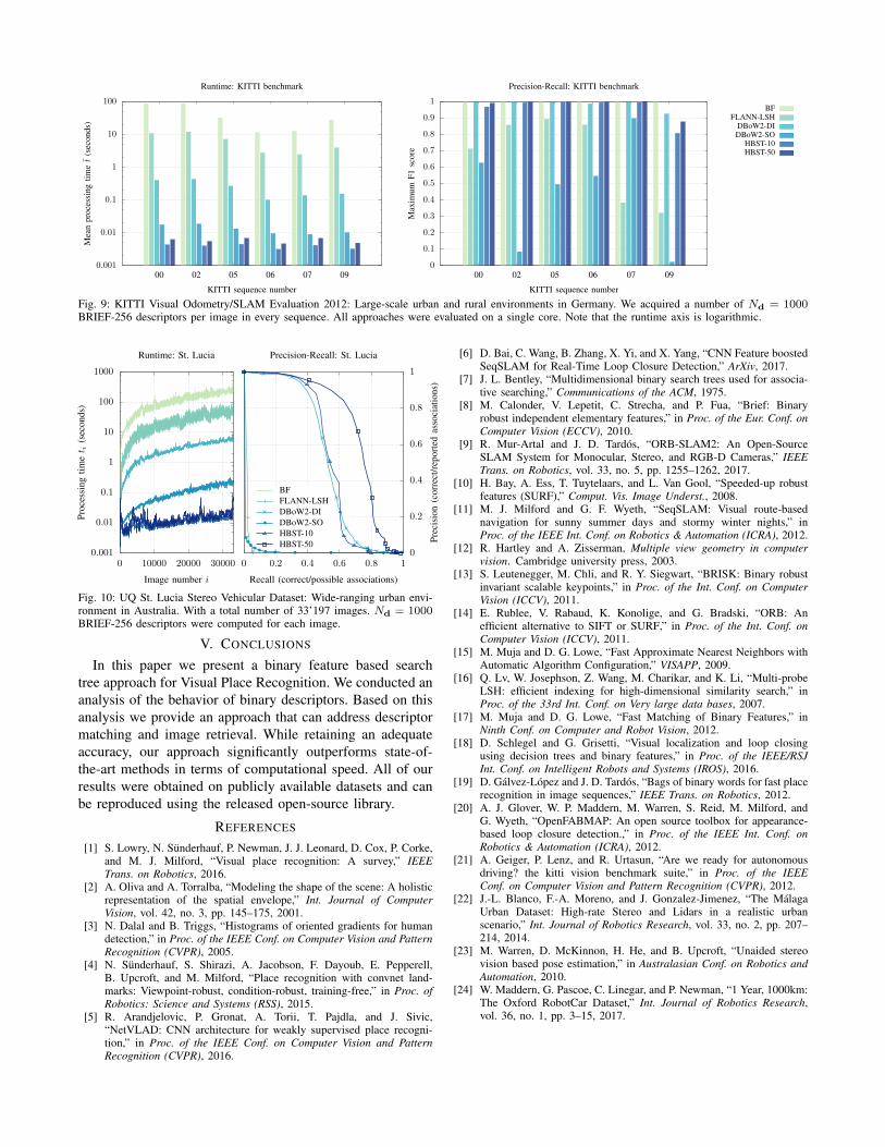
E. Results

In Fig. 9 we report the results of all approaches on KITTI.We observed the following for each compared approach:• BF: Not surprisingly, BF is clearly the most accurate,

at the cost of a higher computation that grows linearlywith the number of inserted images. BF prohibits real-time execution after 10 to 20 images.

• FLANN-LSH: It generally achieves decent F1 scoresbetween DBoW2-SO and HBST-10. Its high compu-tational requirements are not adequate for a real-timeapplication in our scenario.

• DBOW2-DI: The BoW approach achieves the best F1

score after BF, at a computational cost that grows mildlywith the number of images inserted. Yet it is two ordersof magnitude slower than HBST.

• DBOW2-SO: The pure histogram comparison (ScoreOnly) used with this settings leads to the poorest F1

score. However it is the fastest approach after HBST.• HBST-10: Our approach achieves accuracy between

FLANN-LSH and DBOW2-DI, while it is by far thefastest approach compared.

• HBST-50: As expected, HBST-50 achieves a higheraccuracy than HBST-10 while being slightly slower.

In Fig. 10 we present a more detailed analysis per-formed on a single sequence with 33’197 images. Herewe show the Runtime and Precision-Recall curves of allapproaches. FLANN-LSH and DBoW2-SO fail due to thelarge, incrementally built database. Both report many falsepositives, drastically reducing accuracy. DBoW2-DI achievesacceptable accuracy, using descriptor matching to prunereported image matches. Our method (HBST-10, HBST-50)outperforms all other approaches considered in this scenario.

0.001

0.01

0.1

1

10

100

00 02 05 06 07 09

Mea

npr

oces

sing

timet

(sec

onds

)

KITTI sequence number

Runtime: KITTI benchmark

0

0.1

0.2

0.3

0.4

0.5

0.6

0.7

0.8

0.9

1

00 02 05 06 07 09

Max

imum

F1sc

ore

KITTI sequence number

Precision-Recall: KITTI benchmark

BFFLANN-LSH

DBoW2-DIDBoW2-SO

HBST-10HBST-50

Fig. 9: KITTI Visual Odometry/SLAM Evaluation 2012: Large-scale urban and rural environments in Germany. We acquired a number of Nd = 1000BRIEF-256 descriptors per image in every sequence. All approaches were evaluated on a single core. Note that the runtime axis is logarithmic.

0.001

0.01

0.1

1

10

100

1000

0 10000 20000 30000 0 0.2 0.4 0.6 0.8 10

0.2

0.4

0.6

0.8

1

Proc

essi

ngtim

et i

(sec

onds

)

Image number i

Runtime: St. Lucia

Prec

isio

n(c

orre

ct/r

epor

ted

asso

ciat

ions

)

Recall (correct/possible associations)

Precision-Recall: St. Lucia

BFFLANN-LSHDBoW2-DIDBoW2-SOHBST-10HBST-50

Fig. 10: UQ St. Lucia Stereo Vehicular Dataset: Wide-ranging urban envi-ronment in Australia. With a total number of 33’197 images. Nd = 1000BRIEF-256 descriptors were computed for each image.

V. CONCLUSIONS

In this paper we present a binary feature based searchtree approach for Visual Place Recognition. We conducted ananalysis of the behavior of binary descriptors. Based on thisanalysis we provide an approach that can address descriptormatching and image retrieval. While retaining an adequateaccuracy, our approach significantly outperforms state-of-the-art methods in terms of computational speed. All of ourresults were obtained on publicly available datasets and canbe reproduced using the released open-source library.

REFERENCES

[1] S. Lowry, N. Sunderhauf, P. Newman, J. J. Leonard, D. Cox, P. Corke,and M. J. Milford, “Visual place recognition: A survey,” IEEETrans. on Robotics, 2016.

[2] A. Oliva and A. Torralba, “Modeling the shape of the scene: A holisticrepresentation of the spatial envelope,” Int. Journal of ComputerVision, vol. 42, no. 3, pp. 145–175, 2001.

[3] N. Dalal and B. Triggs, “Histograms of oriented gradients for humandetection,” in Proc. of the IEEE Conf. on Computer Vision and PatternRecognition (CVPR), 2005.

[4] N. Sunderhauf, S. Shirazi, A. Jacobson, F. Dayoub, E. Pepperell,B. Upcroft, and M. Milford, “Place recognition with convnet land-marks: Viewpoint-robust, condition-robust, training-free,” in Proc. ofRobotics: Science and Systems (RSS), 2015.

[5] R. Arandjelovic, P. Gronat, A. Torii, T. Pajdla, and J. Sivic,“NetVLAD: CNN architecture for weakly supervised place recogni-tion,” in Proc. of the IEEE Conf. on Computer Vision and PatternRecognition (CVPR), 2016.

[6] D. Bai, C. Wang, B. Zhang, X. Yi, and X. Yang, “CNN Feature boostedSeqSLAM for Real-Time Loop Closure Detection,” ArXiv, 2017.

[7] J. L. Bentley, “Multidimensional binary search trees used for associa-tive searching,” Communications of the ACM, 1975.

[8] M. Calonder, V. Lepetit, C. Strecha, and P. Fua, “Brief: Binaryrobust independent elementary features,” in Proc. of the Eur. Conf. onComputer Vision (ECCV), 2010.

[9] R. Mur-Artal and J. D. Tardos, “ORB-SLAM2: An Open-SourceSLAM System for Monocular, Stereo, and RGB-D Cameras,” IEEETrans. on Robotics, vol. 33, no. 5, pp. 1255–1262, 2017.

[10] H. Bay, A. Ess, T. Tuytelaars, and L. Van Gool, “Speeded-up robustfeatures (SURF),” Comput. Vis. Image Underst., 2008.

[11] M. J. Milford and G. F. Wyeth, “SeqSLAM: Visual route-basednavigation for sunny summer days and stormy winter nights,” inProc. of the IEEE Int. Conf. on Robotics & Automation (ICRA), 2012.

[12] R. Hartley and A. Zisserman, Multiple view geometry in computervision. Cambridge university press, 2003.

[13] S. Leutenegger, M. Chli, and R. Y. Siegwart, “BRISK: Binary robustinvariant scalable keypoints,” in Proc. of the Int. Conf. on ComputerVision (ICCV), 2011.

[14] E. Rublee, V. Rabaud, K. Konolige, and G. Bradski, “ORB: Anefficient alternative to SIFT or SURF,” in Proc. of the Int. Conf. onComputer Vision (ICCV), 2011.

[15] M. Muja and D. G. Lowe, “Fast Approximate Nearest Neighbors withAutomatic Algorithm Configuration,” VISAPP, 2009.

[16] Q. Lv, W. Josephson, Z. Wang, M. Charikar, and K. Li, “Multi-probeLSH: efficient indexing for high-dimensional similarity search,” inProc. of the 33rd Int. Conf. on Very large data bases, 2007.

[17] M. Muja and D. G. Lowe, “Fast Matching of Binary Features,” inNinth Conf. on Computer and Robot Vision, 2012.

[18] D. Schlegel and G. Grisetti, “Visual localization and loop closingusing decision trees and binary features,” in Proc. of the IEEE/RSJInt. Conf. on Intelligent Robots and Systems (IROS), 2016.

[19] D. Galvez-Lopez and J. D. Tardos, “Bags of binary words for fast placerecognition in image sequences,” IEEE Trans. on Robotics, 2012.

[20] A. J. Glover, W. P. Maddern, M. Warren, S. Reid, M. Milford, andG. Wyeth, “OpenFABMAP: An open source toolbox for appearance-based loop closure detection.,” in Proc. of the IEEE Int. Conf. onRobotics & Automation (ICRA), 2012.

[21] A. Geiger, P. Lenz, and R. Urtasun, “Are we ready for autonomousdriving? the kitti vision benchmark suite,” in Proc. of the IEEEConf. on Computer Vision and Pattern Recognition (CVPR), 2012.

[22] J.-L. Blanco, F.-A. Moreno, and J. Gonzalez-Jimenez, “The MalagaUrban Dataset: High-rate Stereo and Lidars in a realistic urbanscenario,” Int. Journal of Robotics Research, vol. 33, no. 2, pp. 207–214, 2014.

[23] M. Warren, D. McKinnon, H. He, and B. Upcroft, “Unaided stereovision based pose estimation,” in Australasian Conf. on Robotics andAutomation, 2010.

[24] W. Maddern, G. Pascoe, C. Linegar, and P. Newman, “1 Year, 1000km:The Oxford RobotCar Dataset,” Int. Journal of Robotics Research,vol. 36, no. 1, pp. 3–15, 2017.